Pattern recognition and lithological interpretation of collocated ...

Originally published as: Bauer, K., Muñoz, G., Moeck, I. (2012): Pattern recognition and lithological interpretation of collocated seismic and magnetotelluric models using self-organizing maps. - Geophysical Journal International, 189, 2, pp. 984—998. DOI: http://doi.org/10.1111/j.1365-246X.2012.05402.x

Geophys. J. Int. (2012) 189, 984–998 doi: 10.1111/j.1365-246X.2012.05402.x

GJI

Sei

smol

ogy

Pattern recognition and lithological interpretation of collocatedseismic and magnetotelluric models using self-organizing maps

K. Bauer, G. Munoz and I. MoeckDeutsches GeoForschungsZentrum GFZ, Telegrafenberg, 14473 Potsdam, Germany. E-mail: [email protected]

Accepted 2012 January 29. Received 2012 January 3; in original form 2011 July 26

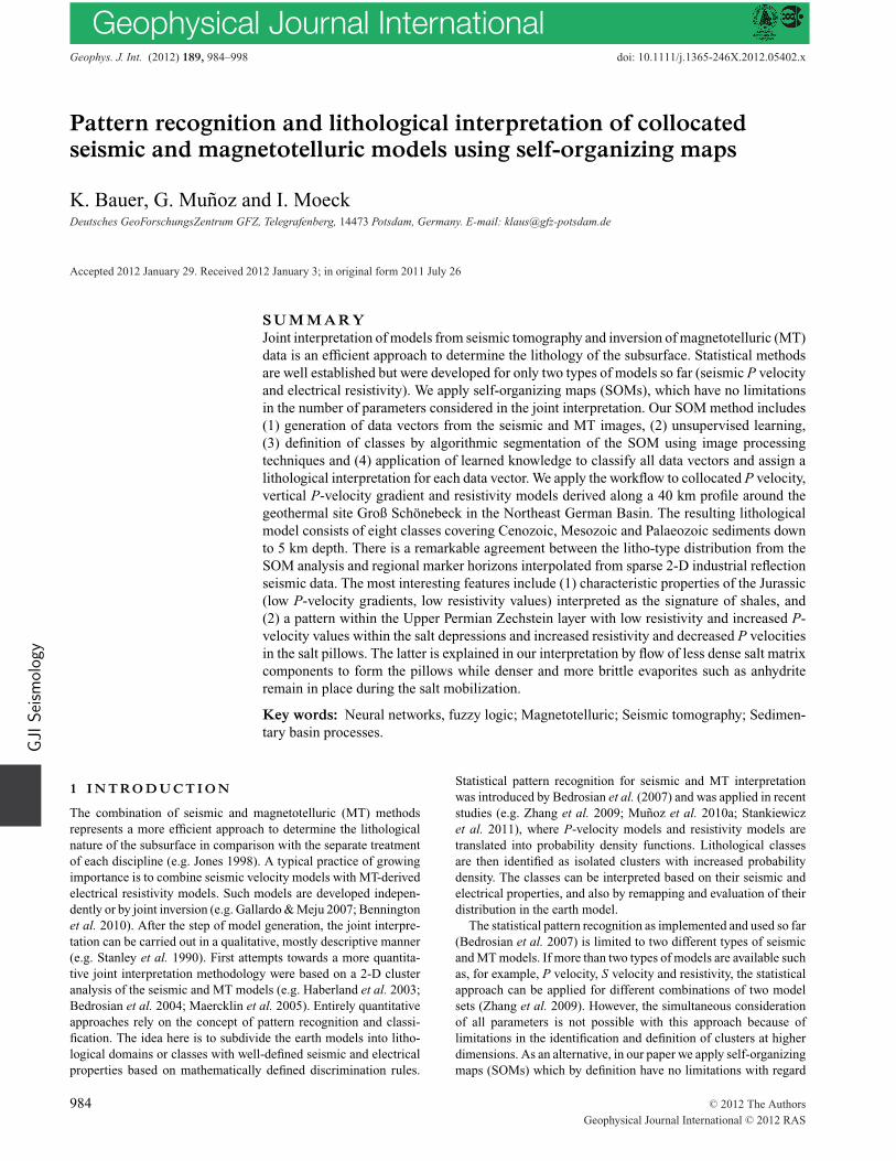
S U M M A R YJoint interpretation of models from seismic tomography and inversion of magnetotelluric (MT)data is an efficient approach to determine the lithology of the subsurface. Statistical methodsare well established but were developed for only two types of models so far (seismic P velocityand electrical resistivity). We apply self-organizing maps (SOMs), which have no limitationsin the number of parameters considered in the joint interpretation. Our SOM method includes(1) generation of data vectors from the seismic and MT images, (2) unsupervised learning,(3) definition of classes by algorithmic segmentation of the SOM using image processingtechniques and (4) application of learned knowledge to classify all data vectors and assign alithological interpretation for each data vector. We apply the workflow to collocated P velocity,vertical P-velocity gradient and resistivity models derived along a 40 km profile around thegeothermal site Groß Schonebeck in the Northeast German Basin. The resulting lithologicalmodel consists of eight classes covering Cenozoic, Mesozoic and Palaeozoic sediments downto 5 km depth. There is a remarkable agreement between the litho-type distribution from theSOM analysis and regional marker horizons interpolated from sparse 2-D industrial reflectionseismic data. The most interesting features include (1) characteristic properties of the Jurassic(low P-velocity gradients, low resistivity values) interpreted as the signature of shales, and(2) a pattern within the Upper Permian Zechstein layer with low resistivity and increased P-velocity values within the salt depressions and increased resistivity and decreased P velocitiesin the salt pillows. The latter is explained in our interpretation by flow of less dense salt matrixcomponents to form the pillows while denser and more brittle evaporites such as anhydriteremain in place during the salt mobilization.

Key words: Neural networks, fuzzy logic; Magnetotelluric; Seismic tomography; Sedimen-tary basin processes.

1 I N T RO D U C T I O N

The combination of seismic and magnetotelluric (MT) methodsrepresents a more efficient approach to determine the lithologicalnature of the subsurface in comparison with the separate treatmentof each discipline (e.g. Jones 1998). A typical practice of growingimportance is to combine seismic velocity models with MT-derivedelectrical resistivity models. Such models are developed indepen-dently or by joint inversion (e.g. Gallardo & Meju 2007; Benningtonet al. 2010). After the step of model generation, the joint interpre-tation can be carried out in a qualitative, mostly descriptive manner(e.g. Stanley et al. 1990). First attempts towards a more quantita-tive joint interpretation methodology were based on a 2-D clusteranalysis of the seismic and MT models (e.g. Haberland et al. 2003;Bedrosian et al. 2004; Maercklin et al. 2005). Entirely quantitativeapproaches rely on the concept of pattern recognition and classi-fication. The idea here is to subdivide the earth models into litho-logical domains or classes with well-defined seismic and electricalproperties based on mathematically defined discrimination rules.

Statistical pattern recognition for seismic and MT interpretationwas introduced by Bedrosian et al. (2007) and was applied in recentstudies (e.g. Zhang et al. 2009; Munoz et al. 2010a; Stankiewiczet al. 2011), where P-velocity models and resistivity models aretranslated into probability density functions. Lithological classesare then identified as isolated clusters with increased probabilitydensity. The classes can be interpreted based on their seismic andelectrical properties, and also by remapping and evaluation of theirdistribution in the earth model.

The statistical pattern recognition as implemented and used so far(Bedrosian et al. 2007) is limited to two different types of seismicand MT models. If more than two types of models are available suchas, for example, P velocity, S velocity and resistivity, the statisticalapproach can be applied for different combinations of two modelsets (Zhang et al. 2009). However, the simultaneous considerationof all parameters is not possible with this approach because oflimitations in the identification and definition of clusters at higherdimensions. As an alternative, in our paper we apply self-organizingmaps (SOMs) which by definition have no limitations with regard

984 C© 2012 The Authors

Geophysical Journal International C© 2012 RAS

Geophysical Journal International

Joint seismic and MT interpretation 985

to the number of models to be classified and interpreted. SOMare neural network techniques which make use of unsupervisedlearning (Kohonen 2001). The motivation to use an unsupervisedpattern recognition method is to investigate the classes which areinherent in the data without introducing a priori information. Inthe following section, we describe by example the methodology ofthe SOM and the modifications used in our technique. The methodis later applied to three different models from collocated seismicand MT experiments in the NE German Basin (Bauer et al. 2010;Munoz et al. 2010b).

2 S O M M E T H O D

Neural networks are simplified mathematical models, which to acertain degree simulate information processing in biological neu-

ral systems. Major principles adopted from nature include paralleland distributed processing, learning and generalization. The ba-sic elements are calculation units called neurons and connectionsto transfer information forming the architecture of the neural net-work. As a whole system, the neural network is used to establisha certain input–output behaviour. The most common applicationis pattern recognition and classification. The input is an objectsuch as a grid block of the earth model, which is described byproperties like seismic velocity and electrical resistivity forming aso-called pattern. The output is the lithological class or rock typedefined by the given petrophysical properties. The input–output be-haviour is established during the learning phase where examplesare presented to the neural network. This can be carried out withspecification of the desired output (supervised learning), or withouta priori information for the output (unsupervised learning). Duringthe subsequent application phase, all available grid blocks with the

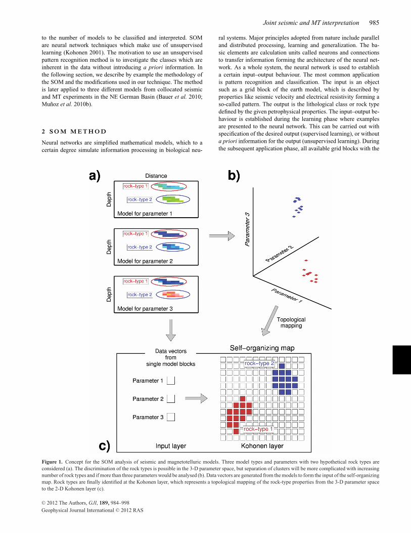
Figure 1. Concept for the SOM analysis of seismic and magnetotelluric models. Three model types and parameters with two hypothetical rock types areconsidered (a). The discrimination of the rock types is possible in the 3-D parameter space, but separation of clusters will be more complicated with increasingnumber of rock types and if more than three parameters would be analysed (b). Data vectors are generated from the models to form the input of the self-organizingmap. Rock types are finally identified at the Kohonen layer, which represents a topological mapping of the rock-type properties from the 3-D parameter spaceto the 2-D Kohonen layer (c).

C© 2012 The Authors, GJI, 189, 984–998


986 K. Bauer, G. Munoz and I. Moeck

given petrophysical properties are presented and classified. Thereare different neural network types, which differ with regard to thearchitecture and the learning algorithm. A broad overview of neu-ral network types and geophysical applications is given in Poulton(2002).

In our investigation we use the SOM neural network type, whichis based on unsupervised learning (Kohonen 2001). We apply amethod with unsupervised learning in our study to reveal the classesinherent in the investigated data sets. Examples for SOM appli-cations to geophysical pattern recognition problems include seis-mic waveform classification (e.g. Essenreiter et al. 2001; Kohleret al. 2010), seismic facies analysis (e.g. Trappe & Hellmich 2001;Matos et al. 2007) and seismic tomography interpretation (e.g.Klose 2006; Tselentis et al. 2007; Bauer et al. 2008; Stankiewiczet al. 2010). To our knowledge, the SOM method is used herefor the first time for the joint interpretation of seismic and MTmodels.

In our application we investigate three types of models: P ve-locity, vertical gradient of P velocity and electrical resistivity. Weconsider here the vertical velocity gradient as additional informa-tion to characterize the lithological nature of the rock types investi-gated. The vertical velocity gradient is sensitive to depth-dependentcompaction effects and changes between mechanical and chemicalcompaction (e.g. Bauer et al. 2010). Other types of models would bepossible as well (Fig. 1a). Each grid block of the collocated modelsis related with a three-component data vector also called pattern. Ifthe models and corresponding data vectors represent specific rocktypes (e.g. two rock types as indicated in Fig. 1a), these would ap-pear as clusters in the 3-D parameter space spanned by the seismicand electrical properties (Fig. 1b). However, in a parameter spacewith more than two dimensions it is difficult to visualize the separa-tion of clusters, particularly if there are more than the two clustersas considered in our example. The SOM method is equivalent witha topological mapping of the multidimensional input space onto a2-D model map where the clusters can be identified and discrimi-nated efficiently (Fig. 1c). The SOM network consists of an inputlayer and a 2-D lattice of neurons also called Kohonen layer. Datavectors (patterns) form the input of the network. The work flow in-cludes preparation of data vectors, unsupervised learning, Kohonenlayer segmentation and clustering, and application of knowledgeincluding classification and remapping (Fig. 2). The details of thework flow are explained by the following synthetic demonstrationexample.

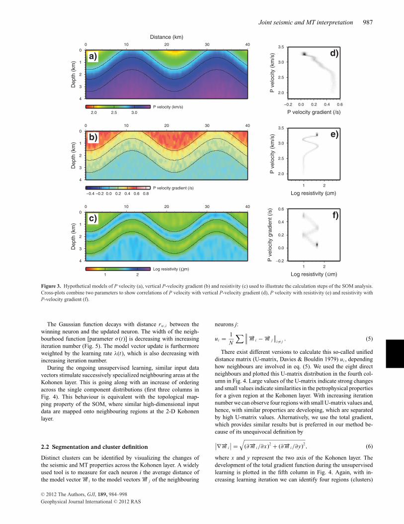
Fig. 3 shows seismic and MT images from a hypothetical exper-iment. The images are generated with the intention to illustrate thesteps to be carried out in the SOM work flow. There is no pretensionto investigate the resolution and model recovery performance of theseismic and MT methods at this point. We defined P velocity, ver-tical P velocity gradient and electrical resistivity distributions for astructure described by four layers (Figs 3a–c). Random noise wasadded to these models to demonstrate the SOM performance undersuch conditions (Figs 3a–c). Different combinations of two mod-els were then considered, and the correlation of the correspondingpetrophysical parameters were visualized in 2-D histogram cross-plots (Figs 3d–f). For the SOM analysis the images are translated toa set of three-component data vectors.

2.1 Unsupervised learning

During the iterative training process (Fig. 4), examples of datavectors are chosen randomly. A data vector at iteration step t is

Figure 2. Schematic workflow of the SOM analysis including (1) generationof data vectors, (2) unsupervised learning, (3) segmentation of the Kohonenlayer and (4) classification of all data vectors.

defined by

−→x (t) =(

vp (t) ,dvp

dz(t) , log ρ (t)

)T

, (1)

where the components of the vector represent the P velocity, thevertical velocity gradient and the decimal logarithm of the electricalresistivity of the chosen grid block, respectively. The data vectoris normalized and then presented to the input layer of the SOMnetwork (upper panel of Fig. 4). At the Kohonen layer, each neuroni is associated with model vector −→m i (t) of the same dimension asthe data vector, in our case 3-D. The single component values of allneurons are plotted in the first columns of the lower panel in Fig. 4.At the first iteration of the learning phase (first row in Fig. 4) themodel vector components are set randomly. The so-called winningneuron w is then determined by finding the model vector −→m w(t)with the smallest Euclidian distance to the data vector −→x (t):

∀i,∥∥−→x (t) − −→m w (t)

∥∥ <∥∥−→x (t) − −→m i (t)

∥∥ . (2)

A learning rule is then applied to all neurons with the principleintention that the model vector of the winning neuron, and to asmaller degree the model vectors of the surrounding neurons arechanged to be more similar to the data vector. The model vectorswith a larger distance to the winning neuron should not be affectedby this operation. This is reached by the following learning function:

−→m i (t + 1) = −→m i (t) + λ (t) nw,i (t) (−→x (t) − −→m i (t)) . (3)

Eq. (3) means that all model vectors are changed into the directionof the data vector, where the actual change is weighted by a Gaussianneighbourhood function centred at the winning neuron:

nw,i (t) = exp(−r 2

w,i/2σ 2 (t)). (4)

C© 2012 The Authors, GJI, 189, 984–998



Figure 3. Hypothetical models of P velocity (a), vertical P-velocity gradient (b) and resistivity (c) used to illustrate the calculation steps of the SOM analysis.Cross-plots combine two parameters to show correlations of P velocity with vertical P-velocity gradient (d), P velocity with resistivity (e) and resistivity withP-velocity gradient (f).

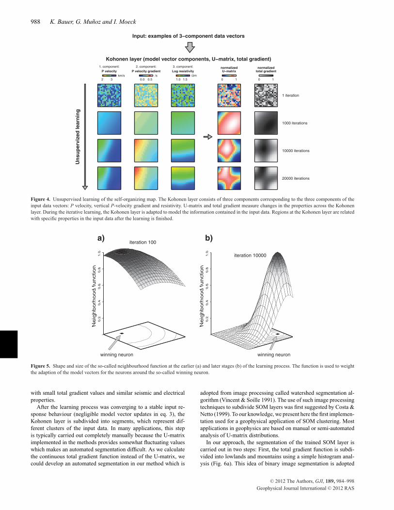
The Gaussian function decays with distance rw,i between thewinning neuron and the updated neuron. The width of the neigh-bourhood function [parameter σ (t)] is decreasing with increasingiteration number (Fig. 5). The model vector update is furthermoreweighted by the learning rate λ(t), which is also decreasing withincreasing iteration number.

During the ongoing unsupervised learning, similar input datavectors stimulate successively specialized neighbouring areas at theKohonen layer. This is going along with an increase of orderingacross the single component distributions (first three columns inFig. 4). This behaviour is equivalent with the topological map-ping property of the SOM, where similar high-dimensional inputdata are mapped onto neighbouring regions at the 2-D Kohonenlayer.

2.2 Segmentation and cluster definition

Distinct clusters can be identified by visualizing the changes ofthe seismic and MT properties across the Kohonen layer. A widelyused tool is to measure for each neuron i the average distance ofthe model vector −→m i to the model vectors −→m j of the neighbouring

neurons j:

ui = 1

N

∑∥∥∥−→m i − −→m j

∥∥i �= j

. (5)

There exist different versions to calculate this so-called unifieddistance matrix (U-matrix, Davies & Bouldin 1979) ui , dependinghow neighbours are involved in eq. (5). We used the eight directneighbours and plotted this U-matrix distribution in the fourth col-umn in Fig. 4. Large values of the U-matrix indicate strong changesand small values indicate similarities in the petrophysical propertiesfor a given region at the Kohonen layer. With increasing iterationnumber we can observe four regions with small U-matrix values and,hence, with similar properties are developing, which are separatedby high U-matrix values. Alternatively, we use the total gradient,which provides similar results but is preferred in our method be-cause of its unequivocal definition by

∣∣∇−→m i

∣∣ =√

(∂−→m i/∂x)2 + (∂−→m i/∂y)2, (6)

where x and y represent the two axis of the Kohonen layer. Thedevelopment of the total gradient function during the unsupervisedlearning is plotted in the fifth column in Fig. 4. Again, with in-creasing learning iteration we can identify four regions (clusters)

C© 2012 The Authors, GJI, 189, 984–998



Figure 4. Unsupervised learning of the self-organizing map. The Kohonen layer consists of three components corresponding to the three components of theinput data vectors: P velocity, vertical P-velocity gradient and resistivity. U-matrix and total gradient measure changes in the properties across the Kohonenlayer. During the iterative learning, the Kohonen layer is adapted to model the information contained in the input data. Regions at the Kohonen layer are relatedwith specific properties in the input data after the learning is finished.

Figure 5. Shape and size of the so-called neighbourhood function at the earlier (a) and later stages (b) of the learning process. The function is used to weightthe adaption of the model vectors for the neurons around the so-called winning neuron.

with small total gradient values and similar seismic and electricalproperties.

After the learning process was converging to a stable input re-sponse behaviour (negligible model vector updates in eq. 3), theKohonen layer is subdivided into segments, which represent dif-ferent clusters of the input data. In many applications, this stepis typically carried out completely manually because the U-matriximplemented in the methods provides somewhat fluctuating valueswhich makes an automated segmentation difficult. As we calculatethe continuous total gradient function instead of the U-matrix, wecould develop an automated segmentation in our method which is

adopted from image processing called watershed segmentation al-gorithm (Vincent & Soille 1991). The use of such image processingtechniques to subdivide SOM layers was first suggested by Costa &Netto (1999). To our knowledge, we present here the first implemen-tation used for a geophysical application of SOM clustering. Mostapplications in geophysics are based on manual or semi-automatedanalysis of U-matrix distributions.

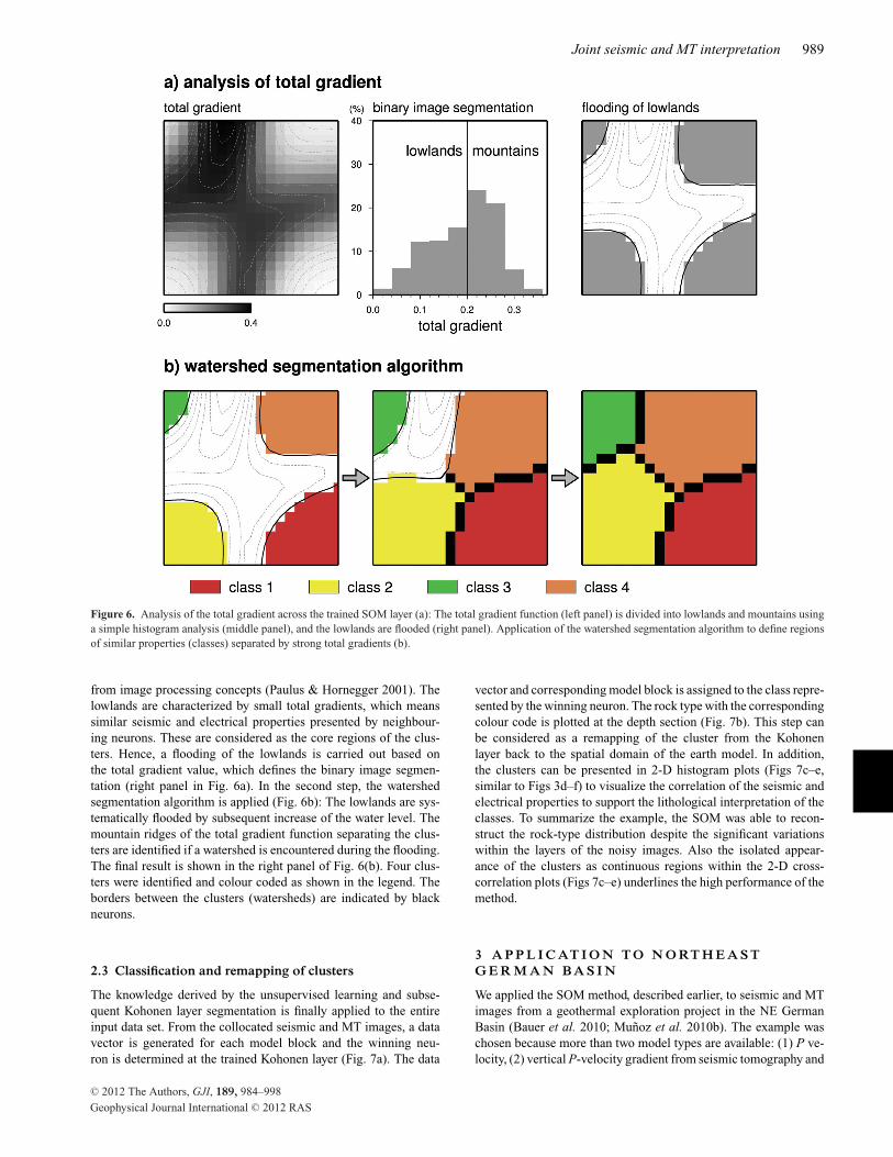
In our approach, the segmentation of the trained SOM layer iscarried out in two steps: First, the total gradient function is subdi-vided into lowlands and mountains using a simple histogram anal-ysis (Fig. 6a). This idea of binary image segmentation is adopted

C© 2012 The Authors, GJI, 189, 984–998



Figure 6. Analysis of the total gradient across the trained SOM layer (a): The total gradient function (left panel) is divided into lowlands and mountains usinga simple histogram analysis (middle panel), and the lowlands are flooded (right panel). Application of the watershed segmentation algorithm to define regionsof similar properties (classes) separated by strong total gradients (b).

from image processing concepts (Paulus & Hornegger 2001). Thelowlands are characterized by small total gradients, which meanssimilar seismic and electrical properties presented by neighbour-ing neurons. These are considered as the core regions of the clus-ters. Hence, a flooding of the lowlands is carried out based onthe total gradient value, which defines the binary image segmen-tation (right panel in Fig. 6a). In the second step, the watershedsegmentation algorithm is applied (Fig. 6b): The lowlands are sys-tematically flooded by subsequent increase of the water level. Themountain ridges of the total gradient function separating the clus-ters are identified if a watershed is encountered during the flooding.The final result is shown in the right panel of Fig. 6(b). Four clus-ters were identified and colour coded as shown in the legend. Theborders between the clusters (watersheds) are indicated by blackneurons.

2.3 Classification and remapping of clusters

The knowledge derived by the unsupervised learning and subse-quent Kohonen layer segmentation is finally applied to the entireinput data set. From the collocated seismic and MT images, a datavector is generated for each model block and the winning neu-ron is determined at the trained Kohonen layer (Fig. 7a). The data

vector and corresponding model block is assigned to the class repre-sented by the winning neuron. The rock type with the correspondingcolour code is plotted at the depth section (Fig. 7b). This step canbe considered as a remapping of the cluster from the Kohonenlayer back to the spatial domain of the earth model. In addition,the clusters can be presented in 2-D histogram plots (Figs 7c–e,similar to Figs 3d–f) to visualize the correlation of the seismic andelectrical properties to support the lithological interpretation of theclasses. To summarize the example, the SOM was able to recon-struct the rock-type distribution despite the significant variationswithin the layers of the noisy images. Also the isolated appear-ance of the clusters as continuous regions within the 2-D cross-correlation plots (Figs 7c–e) underlines the high performance of themethod.

3 A P P L I C AT I O N T O N O RT H E A S TG E R M A N B A S I N

We applied the SOM method, described earlier, to seismic and MTimages from a geothermal exploration project in the NE GermanBasin (Bauer et al. 2010; Munoz et al. 2010b). The example waschosen because more than two model types are available: (1) P ve-locity, (2) vertical P-velocity gradient from seismic tomography and

C© 2012 The Authors, GJI, 189, 984–998



Figure 7. Classification of all data vectors generated from the seismic and magnetotelluric images using the trained and segmented Kohonen layer (a).Remapping of classes to the depth section (b). Cross-plots show correlations between seismic and electrical properties for the individual classes (c–e).

(3) electrical resistivity from MT inversion. Furthermore, we cancompare our results with the statistical pattern recognition anal-ysis applied to two of the mentioned model types (Munoz et al.2010a).

3.1 I-GET project and geophysical experiments

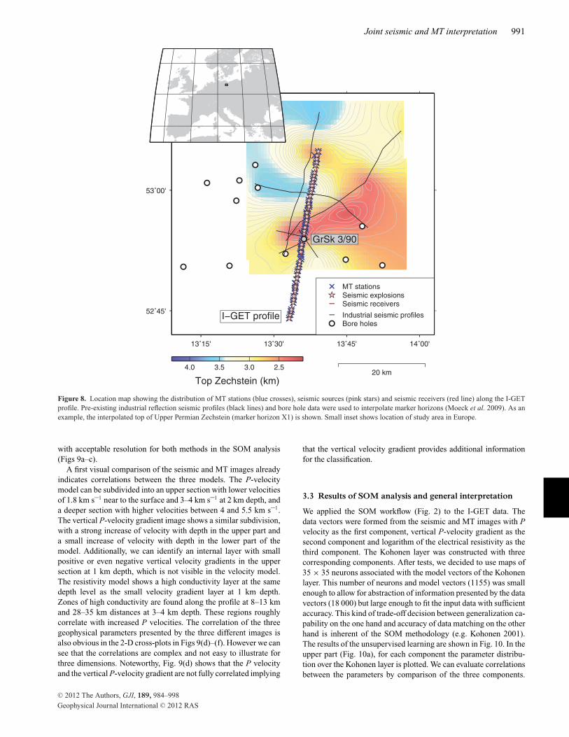
Seismic and MT experiments were carried within the I-GET projectin 2006 (Bauer et al. 2010; Munoz et al. 2010b). The major ob-jective of this European Union funded research initiative was todevelop and apply integrated geophysical exploration techniquesfor geothermal site characterization in different geological settings.One of the studied systems is the geothermal site Groß Schonebecklocated in the eastern part of the Northeast German Basin wherein 4000 m depth a geothermal reservoir of 150 ◦C is developed forexploitation. The NE German Basin is a sub-basin of the South-ern Permian Basin System in Central Europe, and is underlain byDevonian metasediments formed during the Variscan orogeny andunderwent a complex polyphase history since the Lower Permian(Bayer et al. 1999; Scheck & Bayer 1999). A geological model forthe area around Groß Schonebeck was developed by Moeck et al.(2009), based on existing industrial reflection seismic profiles andborehole information (locations are given in Fig. 8). The strati-graphic boundaries interpolated within the geological model can beused to verify our SOM analysis and joint interpretation presentedlater. As an example we plot in Fig. 8 the interpolated top of theZechstein salt layer (marker horizon X1).

The geophysical experiments within I-GET included wide angleseismic and MT measurements along a 40-km-long profile (Fig. 8).

Seismic explosions with 20–30 kg charge size were fired from boreholes with 800 m shot spacings (pink stars in Fig. 8). The shots wererecorded with a constant receiver spread of 190 channels spaced at200 m along the entire profile (red line in Fig. 8). We used 4.5 Hzthree-component geophones and a sampling rate of 5 ms. The MTexperiment was carried out coincident with the seismic measure-ments. We deployed 55 stations with spacings between 400 and 800m (blue crosses in Fig. 8). At each point, horizontal electric andmagnetic field components and the vertical magnetic componentwere measured.

3.2 Seismic and MT models

The data processing and development of 2-D models is describedin detail for the seismic data in Bauer et al. (2010), and for theMT data in Munoz et al. (2010b). From the wide-angle seismicdata, after basic processing the traveltimes of the direct P waveswere picked, and a damped least-squares inversion was carried outto derive a tomographic P-velocity model (Fig. 9a). Additionally,the vertical gradient of the P velocity was determined as shown inFig. 9(b). MT data processing included determination of geomag-netic and electrical impedance tensor transfer functions, remotereference processing and dimensionality analysis. After data rota-tion 2-D inversion was applied to determine the electrical resistivitymodel shown in Fig. 9(c). All three models were interpolated ontothe identical grid (100 m × 100 m node spacings) using the ap-proach of Bedrosian et al. (2007). Extensive uncertainty analysiswas carried out for both data sets (Bauer et al. 2010; Munoz et al.2010b), and the models were clipped to include only grid nodes

C© 2012 The Authors, GJI, 189, 984–998



Figure 8. Location map showing the distribution of MT stations (blue crosses), seismic sources (pink stars) and seismic receivers (red line) along the I-GETprofile. Pre-existing industrial reflection seismic profiles (black lines) and bore hole data were used to interpolate marker horizons (Moeck et al. 2009). As anexample, the interpolated top of Upper Permian Zechstein (marker horizon X1) is shown. Small inset shows location of study area in Europe.

with acceptable resolution for both methods in the SOM analysis(Figs 9a–c).

A first visual comparison of the seismic and MT images alreadyindicates correlations between the three models. The P-velocitymodel can be subdivided into an upper section with lower velocitiesof 1.8 km s–1 near to the surface and 3–4 km s–1 at 2 km depth, anda deeper section with higher velocities between 4 and 5.5 km s–1.The vertical P-velocity gradient image shows a similar subdivision,with a strong increase of velocity with depth in the upper part anda small increase of velocity with depth in the lower part of themodel. Additionally, we can identify an internal layer with smallpositive or even negative vertical velocity gradients in the uppersection at 1 km depth, which is not visible in the velocity model.The resistivity model shows a high conductivity layer at the samedepth level as the small velocity gradient layer at 1 km depth.Zones of high conductivity are found along the profile at 8–13 kmand 28–35 km distances at 3–4 km depth. These regions roughlycorrelate with increased P velocities. The correlation of the threegeophysical parameters presented by the three different images isalso obvious in the 2-D cross-plots in Figs 9(d)–(f). However we cansee that the correlations are complex and not easy to illustrate forthree dimensions. Noteworthy, Fig. 9(d) shows that the P velocityand the vertical P-velocity gradient are not fully correlated implying

that the vertical velocity gradient provides additional informationfor the classification.

3.3 Results of SOM analysis and general interpretation

We applied the SOM workflow (Fig. 2) to the I-GET data. Thedata vectors were formed from the seismic and MT images with Pvelocity as the first component, vertical P-velocity gradient as thesecond component and logarithm of the electrical resistivity as thethird component. The Kohonen layer was constructed with threecorresponding components. After tests, we decided to use maps of35 × 35 neurons associated with the model vectors of the Kohonenlayer. This number of neurons and model vectors (1155) was smallenough to allow for abstraction of information presented by the datavectors (18 000) but large enough to fit the input data with sufficientaccuracy. This kind of trade-off decision between generalization ca-pability on the one hand and accuracy of data matching on the otherhand is inherent of the SOM methodology (e.g. Kohonen 2001).The results of the unsupervised learning are shown in Fig. 10. In theupper part (Fig. 10a), for each component the parameter distribu-tion over the Kohonen layer is plotted. We can evaluate correlationsbetween the parameters by comparison of the three components.

C© 2012 The Authors, GJI, 189, 984–998



Ω

Ω

Figure 9. Images of seismic P velocity (a), vertical P-velocity gradient (b) and electrical resistivity (c) derived in previous studies (Bauer et al. 2010; Munozet al. 2010b), which are combined and analysed with SOM in this paper. Cross-plots are showing correlation between P velocity and vertical P-velocity gradient(d), P velocity and resistivity (e) and resistivity with vertical P velocity gradient (f).

For instance, the lower right region of the Kohonen layer corre-sponds to high P velocities, low vertical P-velocity gradients andhigh resistivity values in the input data. Fig. 10(b) illustrates theanalysis of the total gradient function across the trained Kohonenlayer including histogram analysis, binary image segmentation andflooding of the lowlands. The subsequent application of the water-shed segmentation algorithm finally reveals eight separated classesacross the Kohonen layer (Fig. 10c). Colour-coded neurons repre-sent distinct members of the identified classes. The borders betweenthe classes are indicated by black neurons and are not assigned to aspecific class.

The classification of all available data vectors and remapping inthe depth section is shown in Fig. 11(a). Cross-plots are used toillustrate the signature of each class and to visualize characteristiccross-correlations between the seismic and electrical properties ofdistinct classes (Figs 11b–e). The cross-plot between resistivity andP velocity is shown not only for the SOM clustering (Fig. 11b) butalso for the results derived by Munoz et al. (2010a) using a statis-tical analysis of P velocity and electrical resistivity (Fig. 11c). Thecomparison of both methods is discussed in the conclusions. Forthe purpose of interpretation we compare the SOM classificationand remapping results with the distribution of pre-existing marker

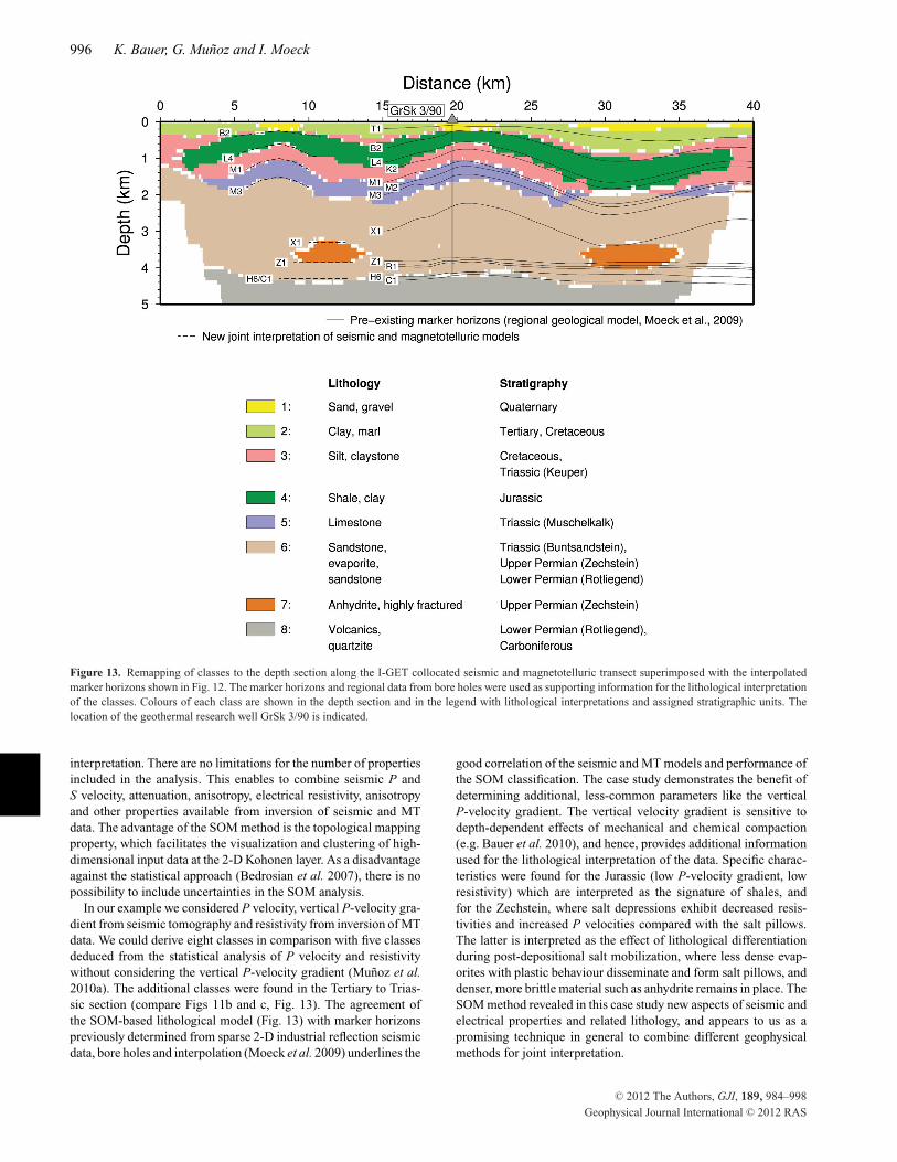
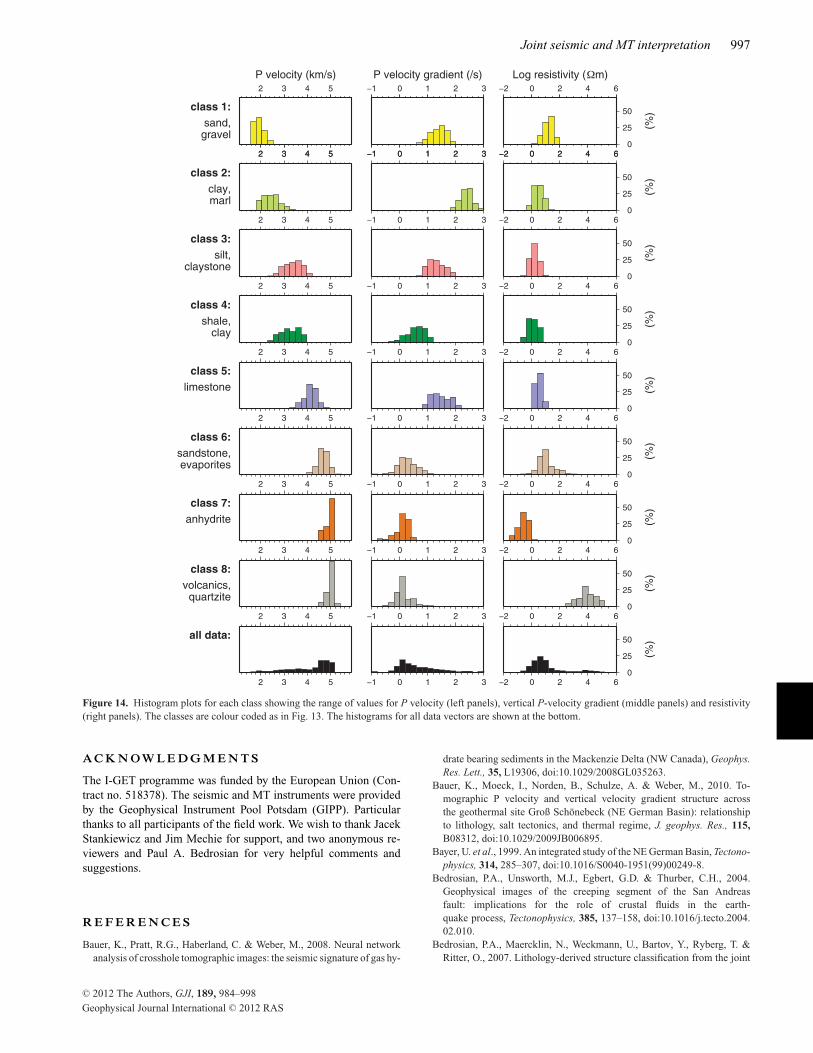
horizons (Fig. 12). These marker horizons were determined alongthe industrial reflection seismic lines shown in Fig. 8, and were in-terpolated based on additional information from bore holes (Moecket al. 2009). The final interpretation of the depth section is shownin Fig. 13. The remapping of the classes is superimposed with theinterpolated marker horizons to support the interpretation of theclasses. Additionally, histograms for each class and each parameterare plotted in Fig. 14. These can be used to identify the range ofseismic and electrical properties of distinct classes, which allowsa lithological interpretation based on comparison with availablepetrophysical data.

We interpret the eight classes as different litho-types, whichcan also be related to particular stratigraphic units (see legend inFig. 13). The class index in most cases was defined with increasingnumbering with depth. The P velocity is generally increasing withdepth (left panels in Fig. 14). The vertical gradient of the P veloc-ity is generally larger for the upper five classes with exception ofclass 4, and shows lower values for classes 6–8 (middle panels inFig. 14). This was interpreted by Bauer et al. (2010) as the effectof predominantly mechanical compaction down to 2 km depth anda change to predominantly chemical compaction and cementationbelow 2 km depth. The electrical resistivity starts with moderate

C© 2012 The Authors, GJI, 189, 984–998



Figure 10. SOM analysis of the models from the I-GET experiment shown in Fig. 9. Kohonen layer components after training (a). Analysis of the total gradientfunction including histogram analysis, binary image segmentation and flooding of lowlands (b). Application of the watershed segmentation algorithm resultingin eight classes (c).

values near to the surface, shows a tendency to lower resistivityvalues for classes 2–5 (depth range 0.5–2 km) and again increas-ing resistivity values for the deeper section, with the exception ofclass 7 (right panels in Fig. 14). This pattern of decreased resistiv-ity values in the upper 0.5–2 km is also reported from MT studiesin other regions in the North German Basin (e.g. Hoffmann et al.2001).

3.4 Detailed interpretation of classes

We assign each class with a lithology and stratigraphic unit based oncomparison with the interpolated reflection seismic marker horizons

(Fig. 13) and information from bore holes used for the regional ge-ological model of Moeck et al. (2009). This assignment is driven bythe very good agreement between the classification results and themarker horizons. This agreement is underlined by the topographyof the marker horizons B2, L4, K2, M1, M2, M3 and X1 (Fig. 13),which is related with the salt tectonic movements and generation ofsalt pillows since the Late Jurassic and Early Cretaceous (Kossowet al. 2000).

Class 1 shows the lowest P velocities and is remapped near to thesurface where Quaternary sands and gravels are found in bore holes(Moeck et al. 2009). Class 2 is assigned to clay and marls of theTertiary and Upper Cretaceous. Compared with class 1 it has slightlyhigher P velocities but particularly differs by much higher vertical

C© 2012 The Authors, GJI, 189, 984–998



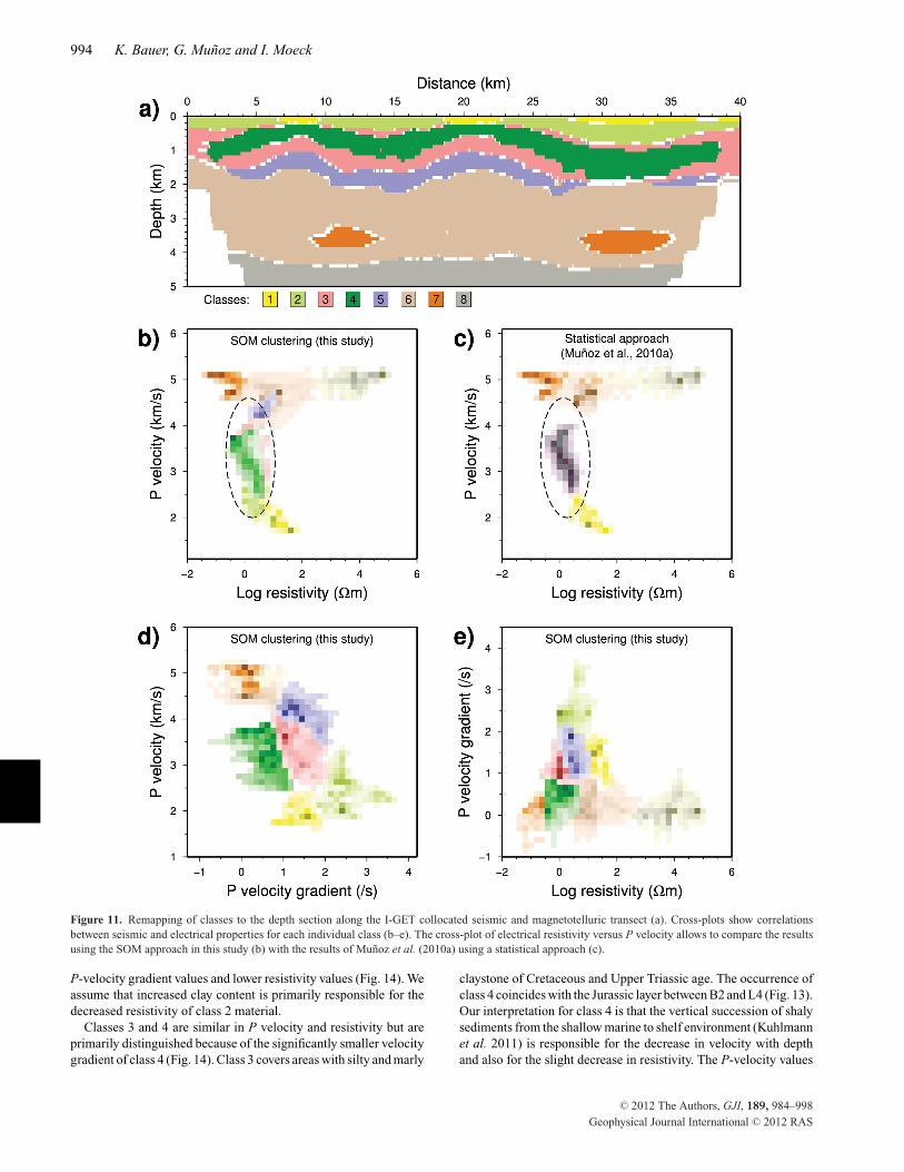
Figure 11. Remapping of classes to the depth section along the I-GET collocated seismic and magnetotelluric transect (a). Cross-plots show correlationsbetween seismic and electrical properties for each individual class (b–e). The cross-plot of electrical resistivity versus P velocity allows to compare the resultsusing the SOM approach in this study (b) with the results of Munoz et al. (2010a) using a statistical approach (c).

P-velocity gradient values and lower resistivity values (Fig. 14). Weassume that increased clay content is primarily responsible for thedecreased resistivity of class 2 material.

Classes 3 and 4 are similar in P velocity and resistivity but areprimarily distinguished because of the significantly smaller velocitygradient of class 4 (Fig. 14). Class 3 covers areas with silty and marly

claystone of Cretaceous and Upper Triassic age. The occurrence ofclass 4 coincides with the Jurassic layer between B2 and L4 (Fig. 13).Our interpretation for class 4 is that the vertical succession of shalysediments from the shallow marine to shelf environment (Kuhlmannet al. 2011) is responsible for the decrease in velocity with depthand also for the slight decrease in resistivity. The P-velocity values

C© 2012 The Authors, GJI, 189, 984–998



Figure 12. Geological model after Moeck et al. (2009) showing marker horizons interpreted along pre-existing industrial reflection seismic profiles, bore holelocations and interpolated marker horizons along the I-GET collocated seismic and magnetotelluric transect.

of 2.5–3.8 km s–1 and resistivity values of 0.1–10 �m determinedfor class 4 are typical values for shales (e.g. Johnston 1987). Shalesare generally known for low resistivity and decreasing P velocitywith increasing content of organic material (Johnston 1987). Class 5agrees with the Middle Triassic (Muschelkalk) succession betweenmarker horizons M1 and M3 (Fig. 13). The dominant lithologyfor Muschelkalk in the Northeast German Basin is limestone. Ourvelocity values of 3.8–4.5 km s–1 for class 5 are in agreementwith laboratory measurements in limestones (Remy et al. 1994).The small resistivity values of 1–20 �m can be explained by thepresence of fluids in the typically porous limestones.

Class 6 covers the sandstones of the Lower Triassic (Buntsand-stein) between M3 and X1, the evaporites of the Upper Permian(Zechstein) between X1 and Z1 and the sandstones of the LowerPermian (Rotliegend) between Z1 and H6 (Fig. 13). Surprisinglyit is not possible to distinguish these two lithologies because oftheir similarity in seismic and electrical properties. This was alsoobserved by Munoz et al. (2010a) in their joint interpretation ofthe seismic P velocity and electrical resistivity models using thestatistical classification approach of Bedrosian et al. (2007). Class7 is found within the Zechstein layer between X1 and Z1 at thelocations of reduced Zechstein thickness (Fig. 13). This materialis characterized by low resistivity (0.01–1 �m) and slightly in-creased P-velocity values (4.6–5 km s–1) compared with class 6.Considering possible lithologies to be expected within the Zechsteinsuccession and petrophysical data (e.g. Schon 1996) class 7 is inter-preted as anhydrite with brittle behaviour. We assume that the brittle

material is highly fractured and is bearing saline fluids, which cansignificantly reduce the electrical resistivity (Munoz et al. 2010a).Furthermore, gypsum and clay compounds in the regions of saltdepression (Hoth et al. 1993) could be responsible for a decreasein resistivity for this material. Our interpretation is that less denseplastic salt was mobilized to form salt pillows while denser mate-rial like anhydrite remained in place at the locations of the reducedZechstein thickness (Bauer et al. 2010; Munoz et al. 2010a). Thepattern of increased P velocity within the Zechstein between X1and Z1 at the salt depressions and decreased P velocity at the saltpillows was also proved by average sonic log P velocities from boreholes (Bauer et al. 2010).

Class 8 is found below marker horizons H6/C1 (Fig 13) and showsP velocities of 5 km s–1 and resistivities of 1000–30 000 �m. Theinterpretation as volcanics of the Lower Permian (Rotliegend) andflysch sediments and quartzites of the Carboniferous is in agree-ment with seismic and electrical properties to be expected for theselithologies (e.g. Hoffmann et al. 2001).

4 C O N C LU S I O N S

Pattern recognition and classification methods translate a set ofcontinuous geophysical parameter distributions into a depth sec-tion that shows a distribution of classes, which are interpretedas different rock types. The use of SOMs allows us to com-bine more than two model types for the classification and joint

C© 2012 The Authors, GJI, 189, 984–998



Figure 13. Remapping of classes to the depth section along the I-GET collocated seismic and magnetotelluric transect superimposed with the interpolatedmarker horizons shown in Fig. 12. The marker horizons and regional data from bore holes were used as supporting information for the lithological interpretationof the classes. Colours of each class are shown in the depth section and in the legend with lithological interpretations and assigned stratigraphic units. Thelocation of the geothermal research well GrSk 3/90 is indicated.

interpretation. There are no limitations for the number of propertiesincluded in the analysis. This enables to combine seismic P andS velocity, attenuation, anisotropy, electrical resistivity, anisotropyand other properties available from inversion of seismic and MTdata. The advantage of the SOM method is the topological mappingproperty, which facilitates the visualization and clustering of high-dimensional input data at the 2-D Kohonen layer. As a disadvantageagainst the statistical approach (Bedrosian et al. 2007), there is nopossibility to include uncertainties in the SOM analysis.

In our example we considered P velocity, vertical P-velocity gra-dient from seismic tomography and resistivity from inversion of MTdata. We could derive eight classes in comparison with five classesdeduced from the statistical analysis of P velocity and resistivitywithout considering the vertical P-velocity gradient (Munoz et al.2010a). The additional classes were found in the Tertiary to Trias-sic section (compare Figs 11b and c, Fig. 13). The agreement ofthe SOM-based lithological model (Fig. 13) with marker horizonspreviously determined from sparse 2-D industrial reflection seismicdata, bore holes and interpolation (Moeck et al. 2009) underlines the

good correlation of the seismic and MT models and performance ofthe SOM classification. The case study demonstrates the benefit ofdetermining additional, less-common parameters like the verticalP-velocity gradient. The vertical velocity gradient is sensitive todepth-dependent effects of mechanical and chemical compaction(e.g. Bauer et al. 2010), and hence, provides additional informationused for the lithological interpretation of the data. Specific charac-teristics were found for the Jurassic (low P-velocity gradient, lowresistivity) which are interpreted as the signature of shales, andfor the Zechstein, where salt depressions exhibit decreased resis-tivities and increased P velocities compared with the salt pillows.The latter is interpreted as the effect of lithological differentiationduring post-depositional salt mobilization, where less dense evap-orites with plastic behaviour disseminate and form salt pillows, anddenser, more brittle material such as anhydrite remains in place. TheSOM method revealed in this case study new aspects of seismic andelectrical properties and related lithology, and appears to us as apromising technique in general to combine different geophysicalmethods for joint interpretation.

C© 2012 The Authors, GJI, 189, 984–998



Figure 14. Histogram plots for each class showing the range of values for P velocity (left panels), vertical P-velocity gradient (middle panels) and resistivity(right panels). The classes are colour coded as in Fig. 13. The histograms for all data vectors are shown at the bottom.

A C K N OW L E D G M E N T S

The I-GET programme was funded by the European Union (Con-tract no. 518378). The seismic and MT instruments were providedby the Geophysical Instrument Pool Potsdam (GIPP). Particularthanks to all participants of the field work. We wish to thank JacekStankiewicz and Jim Mechie for support, and two anonymous re-viewers and Paul A. Bedrosian for very helpful comments andsuggestions.

R E F E R E N C E S

Bauer, K., Pratt, R.G., Haberland, C. & Weber, M., 2008. Neural networkanalysis of crosshole tomographic images: the seismic signature of gas hy-

drate bearing sediments in the Mackenzie Delta (NW Canada), Geophys.Res. Lett., 35, L19306, doi:10.1029/2008GL035263.

Bauer, K., Moeck, I., Norden, B., Schulze, A. & Weber, M., 2010. To-mographic P velocity and vertical velocity gradient structure acrossthe geothermal site Groß Schonebeck (NE German Basin): relationshipto lithology, salt tectonics, and thermal regime, J. geophys. Res., 115,B08312, doi:10.1029/2009JB006895.

Bayer, U. et al., 1999. An integrated study of the NE German Basin, Tectono-physics, 314, 285–307, doi:10.1016/S0040-1951(99)00249-8.

Bedrosian, P.A., Unsworth, M.J., Egbert, G.D. & Thurber, C.H., 2004.Geophysical images of the creeping segment of the San Andreasfault: implications for the role of crustal fluids in the earth-quake process, Tectonophysics, 385, 137–158, doi:10.1016/j.tecto.2004.02.010.

Bedrosian, P.A., Maercklin, N., Weckmann, U., Bartov, Y., Ryberg, T. &Ritter, O., 2007. Lithology-derived structure classification from the joint

C© 2012 The Authors, GJI, 189, 984–998



interpretation of magnetotelluric and seismic models, Geophys. J. Int.,170, 737–748, doi:10.1111/j.1365-246X.2007.03440.x.

Bennington, N.L., Zhang, H., Thurber, C.H. & Bedrosian, P.A., 2010. Jointinversion of Vp, Vs, and resistivity at SAFOD, EOS, Trans. Am. geophys.Union, 91, Fall. Meet. Suppl., T41A–2084.

Costa, J.A.F. & Netto, M.L.A., 1999. Cluster analysis using self-organizing maps and image processing techniques, in Systems, Man,and Cybernetics, IEEE SMC 99 Conf. Proc. Vol. 5, pp. 367–372, Tokyo, doi:10.1109/ICSMC.1999.815577.

Davies, D.L. & Bouldin, W., 1979. A cluster separation measure, IEEETrans. Pattern Anal. Mach. Intel., 1, 224–227.

Essenreiter, R., Karrenbach, M. & Treitel, S., 2001. Identification and clas-sification of multiple reflections with self-organizing maps, Geophys.Prospect., 49, 341–352.

Gallardo, L.A. & Meju, A., 2007. Joint two-dimensional cross-gradientimaging of magnetotelluric and seismic traveltime data for structural andlithological classification, Geophys. J. Int., 169, 1261–1272.

Haberland, C., Rietbrock, A., Schurr, B. & Brasse, H., 2003. Coinci-dent anomalies of seismic attenuation and electrical resistivity beneaththe southern Bolivian Altiplano plateau, Geophys. Res. Lett., 30, 1923,doi:10.1029/2003GL017492.

Hoffmann, N., Jodicke, H. & Gerling, P., 2001. The distribution of Pre-Westphalian source rocks in the North German Basin: evidence frommagnetotelluric and geochemical data, Netherlands J. Geosci., 81, 71–84.

Hoth, K., Rusbult, J., Zagora, K., Beer, H., Hartmann, O. & Schretzen-mayr, S., 1993. Die tiefen Bohrungen im Zentralabschnitt der Mit-teleuropaischen Senke. Dokumentation fur den Zeitabschnitt 1962–1990,Schriftenreihe fur Geowissenschaften, Berlin.

Johnston, D.H., 1987. Physical properties of shale at temperature and pres-sure, Geophysics, 52, 1391–1401, doi:10.1190/1.1442251.

Jones, A., 1998. Waves of the future: superior inferences from collocatedseismic and electromagnetic experiments, Tectonophysics, 286, 273–298.

Klose, C., 2006. Self-organizing maps for geoscientific data analysis: ge-ological interpretation of multidimensional geophysical data, Comput.Geosci., 10, 265–277, doi:10.1007/s10596-006-9022-x.

Kohler, A., Ohrnberger, M. & Scherbaum, F., 2010. Unsupervised pat-tern recognition in continuous seismic wavefield records using self-organizing maps, Geophys. J. Int., 182, 1619–1630, doi:10.1111/j.1365-246x.2010.04709.x.

Kohonen, T., 2001. Self-Organizing Maps, Information Sciences, 3rd edn,Vol. 30, Springer, Berlin, 501pp.

Kossow, D., Krawczyk, C., MacCann, T., Strecker, M. & Negendank, J.,2000. Style and evolution of salt pillows and related structures in the north-ern part of the Northeast German Basin, Int. J. Earth Sci., 89, 652–664,doi:10.1007/s005310000116.

Kuhlmann, G., Gast, S. & Wirth, H., 2011. Characteristics of Lower Triassicand Jurassic reservoir and seal formations as depicted from boreholeevidence in the eastern part of the North German Basin with regard toCO2 storage, Geophys. Res. Abstr., 13, EGU2011-11020.

Maercklin, N., Bedrosian P.A., Haberland, C., Ritter, O., Ryberg, T. & Weber,M., 2005. Characterizing a large shear-zone with seismic and magnetotel-

luric methods: the case of the Dead Sea Transform, Geophys. Res. Lett.,32, L15303, doi:10.1029/2005GL022724.

Matos, M.C., Osorio, P.L.M. & Johann, P.R.S., 2007. Unsupervised seis-mic facies analysis using wavelet transform and self-organizing maps,Geophysics, 72, P9–P21, doi:10.1190/1.2392789.

Moeck, I., Schandelmeier, H. & Holl, H.G., 2009. The stress regime in aRotliegend reservoir of the Northeast German Basin, Int. J. Earth Sci.,98, 1643–1654, doi:10.1007/s00531-008-0316-1.

Munoz, G., Bauer, K., Moeck, I., Schulze, A. & Ritter, O., 2010a. Explor-ing the Groß Schonebeck (Germany) geothermal site using a statisticaljoint interpretation of magnetotelluric and seismic tomography models,Geothermics, 39, 35–45.

Munoz, G., Ritter, O. & Moeck, I., 2010b. A target-oriented magnetotelluricinversion approach for characterizing the low enthalpy Groß Schonebeckgeothermal reservoir, Geophys. J. Int., 183, 1199–1215.

Paulus, D.W.R. & Hornegger, J., 2001. Applied Pattern Recognition, Vieweg,Wiesbaden.

Poulton, M.M., 2002. Neural networks as an intelligence amplification tool: areview of applications, Geophysics, 67, 979–993, doi:10.1190/1.1484539.

Remy, J.-M., Bellanger, M. & Homand-Etienne, F., 1994. Laboratory veloc-ities and attenuation of P-waves in limestones during freeze-thaw cycles,Geophysics, 59, 245–251, doi:10.1190/1.1443586.

Scheck, M. & Bayer, U., 1999. Evolution of the Northeast German Basin:inference from structural model and subsidence analysis, Tectonophysics,313, 145–169, doi:10.1016/S0040-1951(99)00194-8.

Schon, J.H., 1996. Physical Properties of Rocks: Fundamentals and Prin-ciples of Petrophysics, Handbook of Geophysical Exploration; SeismicExploration, Vol. 18, Pergamon, New York, NY, 600pp.

Stankiewicz, J., Bauer, K. & Ryberg, T., 2010. Lithology classification fromseismic tomography: additional constraints from surface waves, J. Afr.Earth Sci., 58, 547–552, doi:10.1016/j.jafrearsci.2010.05.012.

Stankiewicz, J., Munoz, G., Ritter, O., Bedrosian, P., Ryberg, T., Weckmann,U. & Weber, M., 2011. Shallow lithological structure across the Dead Seatransform derived from geophysical experiments, Geochem. Geophys.Geosyst., 12, Q07019, doi:10.1029/2011GC003678.

Stanley, W.D., Mooney, W.D. & Fuis, G.S., 1990. Deep crustal struc-ture of the Cascade Range and surrounding regions from seismic re-fraction and magnetotelluric data, J. geophys. Res., 95, 19 419–19 438,doi:10.1029/JB095iB12p19419.

Trappe, H. & Hellmich, C., 2001. Using neural networks to predict porositythickness from 3D seismic, First Break, 18, 377–384, doi:10.1046/j.1365-2397.2000.00091.x.

Tselentis, G.-A., Serpetsidaki, A., Martakis, N., Sokos, E., Paraskevopoulos,P. & Kapotas, S., 2007. Local high-resolution passive seismic tomogra-phy and Kohonen neural networks: application at the Rio-Antririo Strait,central Greece, Geophysics, 72, B93–B106, doi:10.1190/1.2729473.

Vincent, L. & Soille, P., 1991. Watersheds in digital spaces: an efficientalgorithm based on immersion simulation, IEEE Trans. Pattern Anal.Mach. Intel., 13, 583–598.

Zhang, H., Thurber, C. & Bedrosian, P., 2009. Joint inversion for Vp, Vs, andVp/Vs at SAFOD, Parkfield, California, Geochem. Geophys. Geosyst., 10,Q11002, doi:10.1029/2009GC002709.

C© 2012 The Authors, GJI, 189, 984–998


Pattern recognition and lithological interpretation of collocated ...

Documents

Transcript of Pattern recognition and lithological interpretation of collocated ...