PASSIVITY ENFORCEMENT VIA RESIDUES PERTURBATION FOR ADMITTANCE REPRESENTATION OF POWER SYSTEM...

Iranian Journal of Science & Technology, Transaction B, Engineering, Vol. 31, No. B3, pp 273-288 Printed in The Islamic Republic of Iran, 2007 © Shiraz University

PASSIVITY ENFORCEMENT VIA RESIDUES PERTURBATION FOR ADMITTANCE REPRESENTATION OF

POWER SYSTEM COMPONENTS*

B. PORKAR1, M. VAKILIAN1**, S. M. SHAHRTASH 2 AND M. R. IRAVANI3 1 Dept. of Electrical Eng., Sharif University of Technology, Tehran, I. R. of Iran

Email: [email protected] 2 Dept. of Electrical Eng., Iran University of Science & Technology, Tehran, I. R. of Iran 3Electrical and Computer Eng. Dept., University of Toronto, ON, M5S 3G4, Canada

Abstract– Employing an admittance representation in the form of a black box model approximated by rational functions for linear power system components or network equivalents to be included in electromagnetic transient studies is a well-known method which improves calculation efficiency. All of the methods that have been proposed to solve the rational approximation problem have made efforts to overcome the problem of preserving the passivity of the final model. Passivity is a vital property, since a non-passive model may lead to an unstable transient simulation in the time domain. In this paper a post-processing technique for passivity enforcement through an iterative process for the detection and compensation of passivity violations is presented. The passivity violation regions are detected via a purely algebraic approach based on the existence of purely imaginary eigenvalues in the Hamiltonian matrix. Then a compensation technique via the perturbation of residues of the rational function is applied. Some examples are used to illustrate the characteristics of the proposed technique in terms of accuracy and efficiency by comparison with the Quadratic Programming (QP) method.

Keywords– Residues perturbation, Hamiltonian matrix, passivity enforcement

1. INTRODUCTION

The application of network equivalents for external systems in the well-known time domain programs such as EMTPs (Electro_Magnetic Transient Programs) has valuable merits in saving the CPU memory and the run time. Several approaches have been developed for the construction of network equivalent which can be categorized into two main groups, the time domain equivalent and the frequency domain equivalent. The solution in the frequency domain is essentially aimed at the identification of rational functions that approximate the admittance matrix of the external system seen from boundary bus(es). Among the various methods of fitting, the Vector Fitting (VF) has proved its efficiency and accuracy in different applications [1-6]. Although VF can lead to a stable and precise approximation, the model may not be passive. A stable, however nonpassive network in addition to some passive networks or loads may lead to an unstable general system. Therefore passivity is an important property for a model, although its enforcement is a difficult task. In [7], a post-processing algorithm based on Quadratic Programming (QP) is employed to ensure the local passivity. The regions of passivity violation are searched by a frequency scan. The drawbacks of this detection method are: 1) The passivity violation regions may be outside of the considered frequency spectrum when examined by a frequency sweep. On the other hand, the method needs a frequency sweep from 0 to ∞ to detect the nonpassive regions. 2) The accurate detection of ∗Received by the editors November 25, 2006; final revised form April 10, 2007. ∗∗Corresponding author

B. Porkar / et al.

Iranian Journal of Science & Technology, Volume 31, Number B3 June 2007

274

regions of passivity violation depends on the fineness of the frequency sweep, where undoubtedly a higher fineness is more time-consuming. In this paper a purely algebraic method for the detection of nonpassive regions is presented that can overcome the above drawbacks. For the cases where the passivity violation is very large, (in comparison with having very small eigenvalues), the QP algorithm used, [7], ensures the passivity by perturbation of residues in the other diagonal bands besides the main diagonal elements. In these cases the computation time may be significant. In the proposed method, the perturbation is applied only on the main diagonal elements of the admittance matrix; meanwhile the method is shown to be efficient and accurate.

2. PROBLEM FORMULATION In this section, the definition and criterion of the passivity of multiport systems represented by the admittance matrix is set. In the following section, the techniques needed to detect passivity violation regions and to compensate the violations are presented. a) State-space representation of system

The admittance matrix of a multiport system can be approximated in terms of pole-residue form as follows:

∑=

−+==

N

m m

mjiji as

cdYY

1,, ;][Y (1)

where the direct coupling constant (d) is real, the poles (am) and the residues (cm) can be real or complex conjugate pairs and N is the total number of poles. The linear time-invariant multiport system can be converted into state-space form as follows:

)()()()()()(

tutxtytutxtx

DCBA

+=

+=& (2)

where the dot denotes time differentiation. The number of ports and the dynamic order of the function in the approximation are p and n respectively. Then the state vector ntx ℜ∈)( , the input and out-put vectors

pyx ℜ∈, , nn×ℜ∈A , pn×ℜ∈B , np×ℜ∈C and pp×ℜ∈D . The poles and residues of the system are included in the matrices A and C respectively. The input-output transfer function matrix of the system can be obtained from (2) as follows:

DBAICY +−= −1)()( ss (3) where s is the Laplace operator. Methods such as Vector Fitting can provide the accurate approximation of matrix (3) in a pole/residue form, however the passivity of the model is not guaranteed. b) Passivity

The concept of "passivity" was first used in the circuit theory [8], where a network consisting of only resistors, capacitors and inductors is said to be passive, as this network will not deliver energy. In general, one can say that a linear or non-linear system is “strictly passive” if it consumes energy, and is just “passive” if it does not deliver energy [8]. In this paper only time-invariant linear systems are considered. In these systems, the passivity of the system is equivalent to the positive realness of the systems transfer function. Passivity is the key to ensure stable transient simulation responses. A stable but nonpassive subsystem may lead to an unstable system when it is terminated with some passive loads. However if a

Passivity enforcement via residues perturbation for…

June 2007 Iranian Journal of Science & Technology, Volume 31, Number B3

275

subsystem is passive and terminated with any arbitrary passive load, the stability of the overall resulting network will be always guaranteed.

3. IDENTIFICATION OF PASSIVITY VIOLATION REGIONS A pure algebraic method for the detection of the passivity violation regions can be introduced. The system (2), assuming the initial condition as follows:

0)0( =x would be passive, i.e., it satisfies the following constraint [9]:

∫ ≥T

T dttytu0

0)()( for: all the solutions, all values of u, and for 0≥T .

The passivity constraint in terms of the transfer matrix (3) is equivalent to being Positive-Real (PR) which means that [9]:

0)()( ≥+ ∗ss YY (for all values of s if 0>ℜ se ) (4) where ∗ denotes complex conjugate. This constraint can be verified by ensuring that all the eigenvalues of the real section of the admittance matrix are nonnegative in the whole region of frequency.

ωωλωλωλ ∀∧∈∀≥ )))(()(0)( jjj ii G (5) where: ))(()( ωω jealj YG ℜ= However, satisfying this constraint is a difficult task. On the other hand, if the passivity condition is satisfied, the following Linear Matrix Inequality (LMI) is feasible if P>0 and vice versa [9].

0)(≤

+−−−+

TT

TT

DDCPBCPBPAPA (6)

where: nnT ×∈= RPP . This means that satisfying the passivity is equivalent to satisfying the LMI (6). If 0>+ TDD , the LMI (6) is equivalent to the following Algebraic Riccati Equation (ARE).

0)())(( 1 =−+−++ − TTTTT CPBDDCPBPAPA (7) To solve the ARE (7), first the associated Hamiltonian matrix should be built:

−−

−−

++−+−++−

= TTTTTT

TTT

BDDCACDDCBDDBCDDBAM 11

11

)()()()( (8)

The system (8) is passive, or equivalently, the LMI (7) is satisfied, if and only if M has no pure

imaginary eigenvalues. On the other hand, pure imaginary eigenvalues of matrix M correspond to the exact locations where the real part of the symmetric admittance matrix becomes singular [9]. The powerful merit of the above technique (based on Hamiltonian Matrix) is independent of the frequency. This pure algebraic method overcomes the above mentioned drawbacks of the frequency sweep method. Although due to numerical noise the detection of imaginary eigenvalues of matrix M is difficult, by employing the special properties of the eigenvalues of Hamiltonian matrix M, this problem can be solved.

The eigenvalues of M are symmetrical with respect to the real and imaginary axes. On the other hand, ifλ is an eigenvalue of M, then λ− , ∗λ and ∗− λ would be the other eigenvalues of M. Hence, for an imaginary eigenvalue ofλ there is only just one other eigenvalue, ∗λ . Although based on the properties of

B. Porkar / et al.


276

the eigenvalues, the precise locations of the singular values of )( ωjG are known, this does not contain any information about passivity violation regions. For this purpose a method based on the slope of the eigenvalues of )( ωjG at its singular locations is employed. If λ is an eigenvalue of )( ωjG and tv is the corresponding left eigenvector, then:

0))(( =− Ijvt λωG (9) Differentiating this equation with respect to the angular frequencyω results in:

0))(())(( =−+− Idd

jdd

vIjddv t

t

ωλ

ωω

λωω

GG (10)

Multiplying (10) by the corresponding right eigenvector u results in:

0)(

0

))(( =−+

=

− udd

vujdd

vuIjddv tt

t

ωλ

ωω

λωω

GG 4434421 (11)

The right-hand side of (11) is zero by the definition of the right eigenvector. Therefore (11) can be rewritten as:

ujdd

vudd

v tt )( ωωω

λG= (12)

or

uv

ujddv

dd

t

t )( ωω

ωλ G= (13)

In (13), the derivative of )( ωjG with respect to ω can be obtained from:

BAICAG ωωωω

2)()( 222 −+=jdd

(14) Substituting (14) into (13) results in:

uv

uvdd

t

t )2)(( 222 BAICA ωωωλ −+= (15)

Using (15), the slope of eigenvalues of )( ωjG at singular locations can be determined. The singular frequencies in a vector ],,,[ 21 hW ωωω K= where hωωω <<< K21 are found. Starting from the highest frequency, hω , and counting the positive and the negative slopes in the specified frequencies, then in any frequency where the number of positive and negative slopes equate there is an indication of a local nonpassive region. The slope of hω is always positive since 0>+ TDD . In the next section a new algorithm for the compensation of residues of )( ωjY is employed to enforce the passivity in those violation regions.

4. PASSIVITY ENFORCEMENT The flowchart shown in Fig.1 describes the proposed passivity enforcement algorithm. This algorithm first identifies the passivity violation regions and then compensates the violations. To detect the magnitude of the maximum violation in any nonpassive region, a frequency sweep method can be used. However by using the frequency sweep, there would be no guarantee of detecting the maximum violation. This difficulty is overcome by employing an efficient method based on the H∞-norm approximation.

Let first consider the minimum dissipation, diss(H), of a transfer matrix defined by:



277

Start

Stop

Identification of passivity violation regions

Consider the region where the magnitude of its maximum violation is the most negative.

Find the magnitude of the maximum violation in any nonpassive region

Enforce passivity

Is there any nonpassive region?

)2/))()(((inf)(0Re

min>

∗+=s

sHsHHdiss λ (16) Then consider the following theorem [10]. Theorem: Let A be stable and )2/)((min

TDD +< λδ . Then δ≤)(Hdiss if and only if δN has imaginary eigenvalues.

The above theorem suggests a bisection algorithm for the computation of diss(H). Let lbγ and ubγ be the lower and upper bounds of diss(H), respectively. In a nonpasssive region the upper bound will be zero. For the lower bound, one can use a modification of Enns and Glover bounds [11, 12] used for H∞-norm approximation:

)}2/)((),2/)((min{ minminT

lb DDLL ++= ∗ λλγ (17) Where, co LLL =

oL and cL can be computed by solving the observability and controllability Grammian Lyapunov equations as follows:

0

0

=++

=++

CCALLA

BBALALT

ooT

TTcc (18)

Then a bisection algorithm [10] can be used to detect the maximum violation in any nonpassive region.

The nonpassive region where the magnitude of its maximum passivity is the most negative, among the other passivity violation regions is selected to enforce the passivity. In other words the region with the worst passivity violation is selected to enforce the passivity. Then, based on the compensation of residues of )( ωjY the passivity is ensured. No Yes

Fig. 1. Flowchart of passivity enforcement

B. Porkar / et al.


278

To address this issue, let 1λ be a simple eigenvalue of G and the corresponding characteristic equation is as follows:

0)det( 02

21

1 =++++=− −−

−− cccI n

nn

nn Lλλλλ G (19)

Let us consider for a sufficiently smallε , FG ε=∆ which is the perturbation of matrix G where F is an arbitrary matrix. Then the characteristic equation for the matrix of FG ε+ is given by:

0)()()(

)det(

02

21

1 =++++

=−−−

−−

− ελελελ

ελ

ccc

In

nn

nn L

FG (20)

where )(εrc is a polynomial of degree (n-r) of ε , as:

rnrnrrrrr ccccc −

−++++= εεεε ,2

21)( L

and rr cc =)0( , Let 1λ be a simple root of Eq. (19), then based on the theory of algebraic functions [13], for sufficiently small ε there is a simple root )(1 ελ for (20) as follows:

L+++= 22111 )( εελελ kk (21)

Clearly 11 )( λελ → as 0→ε , if )()( 11 ελελ Ο=− . Also for the corresponding eigenvector it may be written as:

nnn xtt

xttxx

][

][)(

22

1

2222

2111

LL

L

+++

++++=

εε

εεε (22)

where the expressions in brackets are the convergent power series of sufficiently small ε . Also it can be written:

)()()()( 111 εελεε xx =+ FG (23) Substituting from (21) and (22) in (23) and keeping only first-order terms of ε in the result (first-order perturbation of eigenvalues) gives:

112 1112 1 xkxtxxtn

i iin

i ii +∑=+∑

==λFG (24)

or

( ) 1112 11 xkxxtn

i iii =+∑ −=

Fλλ (25) Pre-multiplying this by ty1 and considering that 01 =i

t xy , )1( ≠i results in [13-15]:

11

111 xy

xyk

t

t F= (26)

The higher-order perturbation of eigenvalues may be applied by equating the coefficients of the

higher powers of ε related terms in Eq. (23). Equating the coefficients of 2ε results in:

)()()()(2

212

11122

12

2 ∑∑∑∑====

++=+n

iii

n

iii

n

iii

n

iii xtxtkxkxtFxtG λ (27)

or



279

)()()(2

11122

112

2 ∑∑∑===

+=+−n

iii

n

iiii

n

iii xtkxkxtFxt λλ (28)

Pre-multiplication by ty1 gives

∑=

=n

iii skt

21211β (29)

where i

tii xys = and i

tiij xy F=β for ),,2,1( ni K= .

Per-multiplying (25) by t

iy results in: ),,3,2(0)( 111 nist iiii K==+− βλλ (30)

Then from (29) and (30), the following can be derived:

( )∑= −

=n

i ii

ii

ssk

2 1

11

12

1λλ

ββ (31)

In the same way, the higher order terms in the perturbation process can be obtained.

Since the first-order perturbation of eigenvalues is employed, ελ11 k=∆ , and (26) may be rewritten

as:

11

111

xy

xy

t

t G∆=∆λ (32)

For an n-port system, applying the perturbation only on the diagonal elements results in:

∆

∆∆

=∆

)(

)()(

22

11

ω

ωω

nnG

GG

OG (33)

Using the eigenvalue perturbation theory, it may be written as:

],,[],,,[,11 nnt

tyyyxxx

xy

xyKK ==

∆=∆

Gλ (34)

where y and x are left and right eigenvectors of G. Then based on (33), it can be written as:

222

21

22222

2111 )()()(

n

nnn

xxx

xGxGxG

+++

∆++∆+∆=∆

L

L ωωωλ (35)

Considering that GGGG nn ∆=∆==∆=∆ )()()( 2211 ωωω L , Eq. (35) can be written in the form of

G∆=∆λ . Based on (31) and considering that 0,0 11 == xyxy ttii , )1( ≠i , the second and higher

perturbation expressions are deleted. Therefore only the first-order perturbation of eigenvalues will exist and this term is almost exact. The perturbation is enforced only on the diagonal elements of matrix C at the maximum passivity violation location of the nonpassive region. As a result of perturbation, there will be some error introduced in the time and frequency domain responses. The goal of the perturbation theory is the minimization of this error. The criterion for the selection of appropriate residues for perturbation is

B. Porkar / et al.


280

the minimum Root Means Square (RMS) error. On the other hand, a residue corresponding to the pole is chosen which satisfies the passivity violation at the maximum passivity violation location and minimizes the RMS error. Our experience shows that the selection of complex pole pairs compared to the real pole can be more efficient in ensuring the above conditions. To clarify the method, let the complex pole pairs of pjp ′′±′ with the corresponding residues of rjr ′′±′ are to perturb the diagonal element of Y(s) in the following form:

pjpsrjr

pjpsrjr

sy′′+′+

′′−′+′′−′+

′′+′=)( (36)

The real and imaginary parts of y(s) can be found in the following forms.

2222

222222

4)()(2)(2

))((ωω

ωωω

pppppprpppr

jye′+−′′+′

−′′+′′′′′−+′′+′′′=ℜ (37)

2222

222

4)()(2)4)((

))(Im(ωω

ωωωppp

pprpprprsy

′+−′′+′

−′′+′′+′−′′′′−′′= (38)

As seen from (37), the real part of the frequency response of a pole is a linear function of the real part

of its residue. As mentioned before, it is considered here that the diagonal elements of G are to be perturbed equally as shown.

2222

222

4)()(2

))((ωω

ωωλ

ppppppr

jyeg′+−′′+′

+′′+′′′∆=ℜ∆=∆=∆ (39)

or

)(24)(222

2222

ωωωλ

+′′+′′

′+−′′+′∆==′∆

pppppp

r (40)

5. A FAST TEST METHOD TO CHECK PASSIVITY

In some cases the network equivalent is inherently passive and enforcement for passivity is not necessary. In these cases it is sufficient just to check the passivity. Hence a fast test method to check the existence of the purely imaginary eigenvalues of associated Hamiltonian matrices (without direct calculation of eigenvalues) enhances the efficiency of calculation.

Since M is Hamiltonian, the characteristic polynomial of M, in )det()( Mssa −= I , is a polynomial of 2s ; )()( 2spsa −= . Therefore M has imaginary eigenvalues if and only if p has real nonnegative roots.

The coefficients of polynomial p could be computed from M by the Leverrier-Feddeva algorithm [8]. Also a Sturm method can be used to test whether p has real nonnegative roots [16]. Consider two polynomials with real coefficients as shown below [17]:

0,)(0,)(

01

10

01

10

≠+++=

≠+++=−

−

βββββααααα

mmm

mmm

xxxxxx

L

L (41)

The Strum sequence associated with )(xα and )(xβ is a set of polynomials )}({ xfk ii where ik are arbitrary positive constants, and:

K,2,1,0)()()()()()()()(

21

1

0

=−===

++ ixfxqxfxfxxfxxf

iiii

βα

(42)



281

Equations (42) represent Euclid’s algorithm applied to )(xα and )(xβ , while the signs of the reminders are reversed. A second fundamental tool in the qualitative study of polynomials is the Cauchy index

)(xI baγ , where )()()( xxx αβγ = , and it is known that:

)()()( bVaVxI b

a −=γ (43) where V(x0) denotes the number of variations in the sign of the sequence of f0(x), f1(x), f2(x),….

The algorithm of Routh, presented first by British mathematician, E. J. Routh, enables the Strum sequence to be constructed without explicitly carrying out the polynomial divisions in (42). Specifically, the Routh array (rij) is a set of rows as follows:

LLLLL

L

L

L

232221

1131211

1,00030201

rrrrrrr

rrrrr

m

mm +

(44)

where

K,3,2,1,, 1110 === −− jrr jjjj βα (45) and

K,4,3,2,11,11,1

1,21,2

1,1

=−

=+−−

+−−

−

irrrr

rr

jii

jii

iij (46)

It is assumed that the array is in a regular form, i.e., all 01 ≠ir .

The problem, resolved by Routh [18], is to determine when a given polynomial with real coefficients as:

0,)( 01

10 >+++= − αααα nnn xxxf L (47)

is the characteristic polynomial of an asymptotically stable linear system. This requires that all the zeros of (47) have negative real parts. In this case, the required and sufficient condition is:

0),,,( 211101 =Krrrv (48)

In other words, all the first column elements in the Routh array generated by (46) should be positive. The Routh algorithm can readily be modified to determine the number of real zeroes of a real polynomial f(x). The modified Routh array )~( ijr is formed starting with the first two rows as:

[ ][ ]11

101

111

00

,,)1()1(,)1()~(

,,,)1(,)1()~(

−−

−−

−−−−=

−−−=

nnn

j

nnnn

j

aannar

aaaar

K

K (49)

The rows are formed by the coefficients of the polynomials )( xf − and dxxdfxf /)()( −=−′ . Computing the modified Routh array )~( ijr , (46), the parameter kp, the number of positive real zeros can be computed as follows:

),~,~,~( 211101 Krrrvnk p −= (50)

6. COMPUTED RESULTS In this section three examples will be presented to demonstrate the accuracy and efficiency of the passivity check and compensation algorithm. Example 1: This is a 3 port example [19] which has been fitted with 28 poles in a frequency range of 10

B. Porkar / et al.


282

Hz to 10 kHz. In Fig. 2a three eigenvalues of )( ωjG are shown. Fig. 2b shows an expanded view of two nonpassive regions; [11.810 12.780] and [14.440 19.784] kHz, obtained by Hamiltonian matrix theory.

Fig. 2. a) Frequency spectrum of eigenvalues.

The magnitude of maximum passivity violation in these two regions is -3.5167e-4 at a frequency of 14.801 kHz. After the 1st iteration of perturbation, there is only one nonpassive region, [14.801 19.161] kHz, and the passivity violation is mitigated. For passivity enforcement only four iterations is sufficient. It is considered that the residue corresponds to the poles with minimum RMS error to be perturbed. Since the detection and the compensation processes of the proposed method are not time-consuming, the iterations can be done quickly. To increase the calculation efficiency, the residue of the appropriate pole in the first iteration is considered for the other iterations. Table 1 shows the details of the calculation in each stage of iterations. An expanded view of violations mitigation, in each stage of iteration, is shown in Fig. 2c.

Fig. 2. b) Expanded view

0 5 10 15 20 25 30-0.5

0

0.5

1

1.5

2

2.5

3 x 10 -3

Frequency [kHz]

Eige

nval

ues

of R

e(Y)

8 10 12 14 16 18 20 22 24 -5

-4

-3

-2

-1

0

1

2

3

4

5

x 10 -4

Frequency [kHz]

Eige

nval

ues

of R

e(Y)

19.784 kHz

14.440 kHz

11.810 kHz

12.780 kHz



283

Table 1. The details of calculation of proposed method

In a similar example, this time enforcement is done through the QP method. In this example, if only

the diagonal elements of residue matrix C, and the constant term matrix, D, are perturbed, the RMS error would be 5.6234e-007 and if the perturbation is applied on all of the matrix elements of C and D matrices, the computing efficiency decreases significantly, and the RMS error would be 1.7682e-007 as shown in Fig. 3. The RMS error of the proposed method is 1.0959e-007 which is less than that obtained by the QP method in addition to its higher calculation efficiency. 300 frequency samples were considered to calculate RMS errors in this and the following examples.

Fig. 2. c) Mitigation of violations during iterations

Fig. 3. Passivity enforcement by QP method

Example 2: This is a 6 port case [19], which has been fitted with 30 poles in a frequency range of 10 Hz to

The freq. of max. violation passivity [kHz]

The mag. of max. violation passivity [PU]

Passivity violation regions [kHz]

Number of iterations

14.801

-3.5167e-4

[11.810, 12.780] [14.440, 19.784]

Original Case

15.300 -1.3941e-4 [14.801, 19.161] 1st iteration 16.000 -4.7429e-5 [15.300, 18.395] 2nd iteration 16.500 -8.3963e-6 [16.000, 17.484] 3rd iteration

11 12 13 14 15 16 17 18

-4

-2

0

2

4

6

x 10 -4

Frequency [kHz]

Eig

enva

lues

of R

e(Y

)

Original

1st iter.

2nd iter.

3rd iter.

0 5 10 15 20 25 30-0.5

0

0.5

1

1.5

2

2.5

3 x 10 -3

Frequency [kHz]

Eig

enva

lues

of R

e(Y

)

B. Porkar / et al.


284

10 kHz. The resulting model has large passivity violations at frequencies above 10 kHz. The nonpassive region, [11.498, 14.188] kHz, obtained by imaginary eigenvalues of the Hamiltonian matrix and the proposed method of related slopes is shown in Fig. 4a. Fig. 4b shows the resulted mitigations due to the proposed compensation algorithm during three iterations to guarantee the passivity. Table 2 illustrates the details of the passivity violation mitigation during each stage of iterations. The results of the application of the QP method on a similar example considering only the diagonal elements of C and D matrices will still have some passivity violations.

Fig. 4. a) Expanded view of Frequency spectrum of eigenvalues


The frequency of max.

violation passivity [kHz] The magnitude of max.

violation passivity [P.U.] Passivity violation

regions [kHz] Number of iterations

11.991 -0.0053 [11.498, 14.188] Original 12.081 -0.0013 [11.991, 14.186] 1st iter. 13. 901 -1.8061e-4 [13.691, 14.057] 2nd iter.

The RMS error in this case which is named QP.1 will be 0.4301. In order to improve the accuracy of

the above perturbation, in another case named QP.2, all the elements of matrices C and D are used as free variables to be perturbed. However in QP.2 the passivity has not been ensured yet.

Fig. 4. b) Mitigation of violations during iterations

11 11.5 12 12.5 13 13.5 14 14.5

-5

-4

-3

-2

-1

0

1 x 10 -3

Frequency [kHz]

Eig

enva

lues

of R

e(Y

)

11.498 kHz

14.188 kHz

10 10.5 11 11.5 12 12.5 13 13.5 14 14.5 15-6

-5

-4

-3

-2

-1

0

1 x 10 -3

Frequency [kHz]

Eig

enva

lues

of R

e(Y

)

Original

1st iter.

2nd iter.

3rd iter.



285

Therefore, to further improve the accuracy, a weighting scheme is employed such that all the elements

of Y are weighted with the inverse of their magnitude, thus placing more weight on small elements, and it is named QP.3. This provides a strong improvement in accuracy. Yet passivity violations still exist in the system. Applying the iterative scheme on the QP method, a satisfactory result is achieved as shown in Fig. 5. This is named QP.4.

The total computation time in QP.4 is extremely significant compared to the proposed method of this paper. It should be mentioned that the illustrated method uses only diagonal elements of C matrix to perturb, which is more efficient than employing perturbation on all the elements of both C and D matrices. This fact is more important in systems with numerous ports or phases such as the network equivalent of multiport multiphase power systems. Table 3 compares the RMS error of the different QPs versus this paper proposed method.

Table 3. Comparison of RMS error from different methods

Type of method RMS error QP method (QP.1) 0.4301 QP method (QP.2) 0.4300 QP method (QP.3) 2.9245e-6 QP method (QP.4) 1.5804e-6 Proposed method 1.6951e-5

Fig. 5. Passivity enforcement by QP method (QP.4)

Example 3: In this example the proposed method is examined on a sample distribution network where the passivity enforcement of the terminal admittance matrix of this system is looked for. The information of this network is provided by [20]. The distribution system has two 3-phase buses as terminals (A, B) shown in Fig.6. The 6×6 admittance matrix Y is calculated for this system in a frequency range of 10 Hz–100 kHz. To increase the calculation efficiency all the elements of Y are fitted with a common pole set. To fit, 50 complex pair poles are selected as initial poles.

Fig. 6. Power system distribution system

11.5 12 12.5 13 13.5 14 14.5

-5

-4

-3

-2

-1

0

1 x 10 -3

Frequency [kHz]

Eig

enva

lues

of R

e(Y

)

B. Porkar / et al.


286

Figures 7 and 8 show fitting the magnitude and phase angle of 6×6 admittance matrix Y through an

improved version of VF named vfit2 [20]. Figure 9a shows the frequency spectrum of the six eigenvalues of the admittance matrix. As shown in Fig. 9a, the passivity violations occur in frequencies of about 3kHz.

Fig. 7. Fitting of the magnitude by VF

Fig. 8. Fitting of the phase angle by VF

0 1 2 3 4 5 6 7 8 9 10

x 104

-5

0

5

10x 10-4

Frequency [Hz]

Eigenvalues of ReY(s)]

Fig. 9. a) Frequency spectrum of eigenvalues

1 2 3 4 5 6 7 8 9 10

x 104

10 -7

10 -6

10 -5

10 -4

10 -3

10 -2

10 -1

10 0

10 1

Frequency [Hz]

Mag

nitu

de [p

.u.]

OriginalVFDeviation

Approximation of f

1 2 3 4 5 6 7 8 9 10

x 104

-2500

-2000

-1500

-1000

-500

0

500

Frequency [Hz]

Phas

e an

gle

[deg

]

Approximation of f

OriginalVF



287

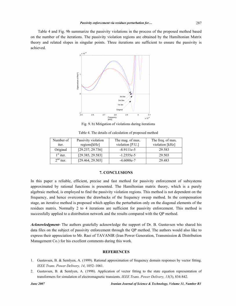
Table 4 and Fig. 9b summarize the passivity violations in the process of the proposed method based on the number of the iterations. The passivity violation regions are obtained by the Hamiltonian Matrix theory and related slopes in singular points. Three iterations are sufficient to ensure the passivity is achieved.

Fig. 9. b) Mitigation of violations during iterations


The freq. of max. violation [kHz]

The mag. of max. violation [P.U.]

Passivity violation regions[kHz]

Number of iter.

29.583 -8.9111e-5 [29.237, 29.736] Original 29.503 -1.2555e-5 [29.385, 29.583] 1st iter. 29.483 -4.6088e-7 [29.464, 29.503] 2nd iter.

7. CONCLUSIONS

In this paper a reliable, efficient, precise and fast method for passivity enforcement of subsystems approximated by rational functions is presented. The Hamiltonian matrix theory, which is a purely algebraic method, is employed to find the passivity violation regions. This method is not dependent on the frequency, and hence overcomes the drawbacks of the frequency sweep method. In the compensation stage, an iterative method is proposed which applies the perturbation only on the diagonal elements of the residues matrix. Normally 2 to 4 iterations are sufficient for passivity enforcement. This method is successfully applied to a distribution network and the results compared with the QP method. Acknowledgment- The authors gratefully acknowledge the support of Dr. B. Gustavsen who shared his data files on the subject of passivity enforcement through the QP method. The authors would also like to express their appreciation to Mr. Raei of TAVANIR (Iran Power Generation, Transmission & Distribution Management Co.) for his excellent comments during this work.

REFERENCES 1. Gustavsen, B. & Semlyen, A. (1999). Rational approximation of frequency domain responses by vector fitting.

IEEE Trans. Power Delivery, 14, 1052–1061. 2. Gustavsen, B. & Semlyen, A. (1998). Application of vector fitting to the state equation representation of

transformers for simulation of electromagnetic transients. IEEE Trans. Power Delivery, 13(3), 834-842.

2.5 2.6 2.7 2.8 2.9 3 3.1

x 10 4

-1

0

1

2 x 10 -4

Frequency [kHz]

Eig

enva

lues

of R

e(Y

)

Original

1st iter.

2nd iter.

3rd iter.

B. Porkar / et al.


288

3. Morched, A., Gustavsen, B. & Tartibi, M. (1999). A universal model for accurate calculation of electromagnetic transients on overhead lines and underground cables. IEEE Trans. Power Delivery, 14(3), 1032-1038.

4. Abdel-Rahman, M., Semlyen, A. & Iravani, M. R. (2003). Two-layer network equivalent for electromagnetic transients. IEEE Trans. on Power Delivery, 18(4), 1328-1335.

5. Gustavsen, B. (2004). Wide band modeling of power transformers. IEEE Trans. on Power Delivery, 19(1), 414-422.

6. Ramirez, A., Naredo, J. L. & Moreno, P. (2005). Full frequency-dependent line model for electromagnetic transient simulation including lumped and distributed sources. IEEE Trans. Power Delivery, 20(1), 292-299.

7. Gustavsen, B. & Semlyen, A. (2001). Enforcing passivity for admittance matrices approximated by rational functions. IEEE Trans. Power Syst., 16(1), 97–104.

8. Kailath, T. (1980). Linear systems. Englewood Cliffs, NJ: Prentice-Hall. 9. Boyd, S., Ghaoui, L. E., Feron, E. & Balakrishnan, V. (1994). Linear matrix inequalities in system and control

theory. Philadelphia, PA: SIAM, Vol. 15. 10. Boyd, S., Balakrishnan, V. & Kabamba, P. (1989). A bisection method for computing the H_infinity-norm of a

transfer matrix and related problems. Mathematics of control, signals, and systems, 2(3), 207-219. 11. Glover, K. (1984). All optimal Hankel-norm approximation of linear multivariable systems and their L∞-erroe

bounds. Internat. J. Control, 39. 12. Enns, D. F. (1984). Model Reduction with balanced realization: an error bound and a frequency weighted

generation. Proceedings of the 23rd IEEE Conference on Decision and Control, Las Vegas, NV, 172-132. 13. Wilkinson, J. H. (1965). The algebraic eigenvalue problem. Oxford, U.K.: Oxford Univ. Press. 14. Stewart, G. W. & Sun, J. (1990). Matrix perturbation theory. Boston, MA: Academic. 15. Watkins, D. S. (2002). Fundamentals of matrix computations. Second Edition, New York: Wiley. 16. Henrici, P. (1974). Applied and computational complex Analysis. John Wiley. 17. Barnett, S. & Siljak, D. D. (1977). Routh’s algorithm: a centennial survey. SIAM Review, 19(3), 472-489. 18. Routh, E. J. (1877). A treatise on the stability of a given state of motion. Macmillan, London. 19. QPpassive.zip [Online]. Available: http://www.energy.sintef.no/Produkt/VECTFIT/index.asp 20. vfit2.zip [Online]. Available: http://www.energy.sintef.no/Produkt/VECTFIT/index.asp

PASSIVITY ENFORCEMENT VIA RESIDUES PERTURBATION FOR ADMITTANCE REPRESENTATION OF POWER SYSTEM...

Documents

Transcript of PASSIVITY ENFORCEMENT VIA RESIDUES PERTURBATION FOR ADMITTANCE REPRESENTATION OF POWER SYSTEM...