Particle Swarm Optimization Method for Image Clustering

M Omrana, AP Engelbrechta, A Salmanb

aDepartment of Computer Science, University of Pretoria, South Africa

mjomran@engineer.com, engel@driesie.cs.up.ac.za

bComputer Engineering Department, Kuwait University, Kuwait

ayed@eng.kuniv.edu.kw

Abbreviated title: PSO for Image Clustering

Abstract

An image clustering method that is based on the particle swarm optimizer (PSO) is developed in this paper.

The algorithm finds the centroids of a user specified number of clusters, where each cluster groups together similar

image primitives. To illustrate its wide applicability, the proposed image classifier has been applied to synthetic,

MRI and satellite images. Experimental results show that the PSO image classifier performs better than state-

of-the-art image classifiers (namely, K-means, Fuzzy C-means, K-Harmonic means and Genetic Algorithms) in all

measured criteria. The influence of different values of PSO control parameters on performance is also illustrated.

Keywords: Image Clustering, Particle Swarm Optimization, Pattern Recognition, Remote Sensing, Spectral Domain

1 Introduction

Image classification is the process of identifying groups of similar image primitives [38]. These image primitives can

be pixels, regions, line elements, etc. depending on the problem encountered. Many basic image processing techniques

such as quantization, segmentation and coarsening can be viewed as different instances of the clustering problem [38].

There are two main approaches to image classification: supervised and unsupervised. In the supervised approach,

the number and the numerical characteristics (e.g. mean and variance) of the classes in the image are known in advance

(by the analyst) and used in the training step, which is followed by a classification step. There are several popular

supervised algorithms such as the minimum-distance-to-mean, parallelepiped and the Gaussian maximum likelihood

classifiers [46]. For unsupervised approaches, classes are unknown and the approach starts by partitioning the image

data into groups (or clusters), according to a similarity measure, which can be compared by an analyst to available

1

reference data [29]. Therefore, unsupervised classification is also referred to as a clustering problem. In general, the

unsupervised approach has several advantages over the supervised approach [10], namely

• For unsupervised approaches, there is no need for an analyst to specify in advance all the classes in the image

data set. The clustering algorithm will automatically find distinct classes, which dramatically reduce the work

of the analyst.

• The characteristics of the objects being classified can vary with time; the unsupervised approach is an excellent

way to monitor these changes.

• Some characteristics of objects may not be known in advance. Unsupervised approaches will automatically flag

these characteristics.

The focus in this paper is on the unsupervised approach (i.e. image clustering). There are several algorithms that

belong to this class of algorithms. These algorithms can be categorized into two groups: hierarchical and partitional

[15, 28]. For hierarchical clustering, the output is a tree showing a sequence of clustering with each cluster being a

partition of the data set [28]. These type of algorithms have the following advantages:

• The number of clusters need not be specified a priori.

• They are independent of the initial condition.

However, they suffer from the following drawbacks:

• They are static, i.e. pixels assigned to a cluster can not move to another cluster.

• They may fail to separate overlapping clusters due to lack of information about the global shape or size of the

clusters [15].

On the other hand, partitional clustering algorithms partition the data set into a specified number of clusters. These

algorithms try to minimize certain criteria (e.g. a squared error function). Therefore, they can be treated as an

optimization problem. The advantages of the hierarchical algorithms are the disadvantages of the partitional algorithms

and vice versa.

The most widely used partitional algorithm is the iterative K-means approach. For K-means clustering, the

algorithm starts with K cluster centers or centroids (initial values for the centroids are randomly selected or derived

from a priori information). Then, each pixel in the image is assigned to the closest cluster (i.e. closest centroid).

Finally, the centroids are recalculated according to the associated pixels. This process is repeated until convergence

[14]. There are three drawbacks of this algorithm, namely

• the algorithm is data-dependent;

2

• it is a greedy algorithm that depends on the initial condition, which may cause the algorithm to converge to

suboptimal solutions; and

• the user needs to specify the number of classes in advance [10].

ISODATA is an enhancement proposed by Ball and Hall [4] that operates on the same concept of the K-means algorithm

with the addition of the possibility of merging classes and splitting elongated classes. A recent alternative approach

to ISODATA is SYNERACT [20]. This approach combines both K-means and hierarchical descending approaches to

overcome the three drawbacks mentioned above. Three concepts are used by SYNERACT:

• a hyperplane to split a cluster into two smaller clusters and compute their centroids,

• iterative clustering to assign the pixels into the available clusters, and

• a binary tree to store the clusters generated from the splitting process.

According to Huang [20], SYNERACT is faster than ISODATA, and almost as accurate as ISODATA. Furthermore,

it does not require the user to specify the number of clusters and initial location of the centroids in advance. Another

improvement to the K-means algorithm is proposed by Rosenberger and Chehdi [41], which automatically finds the

number of clusters in the image set by using intermediate results.

A fuzzy version of K-means, called Fuzzy C-means (FCM), was proposed by Bezdek [28, 5]. FCM is based on a

fuzzy extension of the least-square error criterion. The advantage of FCM over K-means is that, while in K-means

the pixels are assigned to one and only one cluster (i.e. hard or crisp clustering), in FCM each pixel belongs to each

cluster with some degree of membership (i.e. fuzzy clustering). This is more suitable for real applications where there

are some overlap between the clusters in the data set. Gath and Geva proposed an algorithm based on a combination

of fuzzy C-means and fuzzy maximum likelihood estimation [16]. Based on fuzzy clustering, Lorette et al optimizes

an objective function which takes into consideration the entropy of the image partition using an iterative schema [30].

These approaches developed by Gath et al and Lorette et al do not require the user to specify the number of clusters

in advance – they are fully unsupervised.

Another popular clustering algorithm is the Expectation-Maximization (EM) [7, 34, 40]. EM is a general algorithm

for parameter estimation in the presence of some unknown data [17]. EM partitions the data set into clusters by

determining a mixture of Gaussians to fit the data set. Each Gaussian has a mean and covariance matrix [1]. Zhang et

al [51] used EM along with a hidden Markov random field (HMRF) for the segmentation of brain magnetic resonance

(MR) images.

Results from [17, 18] showed that K-means performs comparably to EM. Furthermore, Aldrin et al [1] stated that

EM fails on high-dimensional data sets due to numerical precision problems. They also observed that Gaussians often

3

collapsed to delta functions [1].

Recently, Zhang et al [50, 49] proposed a novel algorithm called K-harmonic means (KHM) with promising results.

In KHM, the harmonic mean of the distance of each cluster center to every data point is computed. The cluster

centers are then updated accordingly. KHM is less sensitive to initial conditions (contrary to K-means) and does not

have the problem of collapsing Gaussians exhibited by EM [1]. Experiments conducted by Zhang et al [50, 49] and

Hamerly el al [17, 18] showed that KHM outperforms K-means, FCM (according to Hamerly [17]) and EM. Hamerly

et al [17, 18] proposed a variation of KHM, called Hybrid 2 (H2), which uses the soft membership function of KHM

and the constant weight function of K-means (refer to section 3.2.1) with encouraging results.

Another category of unsupervised partitional algorithms includes the non-iterative algorithms. The most widely

used non-iterative algorithm is MacQueen’s K-means algorithm [31]. This algorithm works in two phases as follows:

the first phase finds the centroids of the classes, and the second classifies the image pixels. Competitive Learning (CL)

updates the centroids sequentially by moving the closest centroid toward the pixel being classified [42]. These algo-

rithms suffer the drawback of being dependent on the order in which the data points are presented. To overcome this

problem, data points are presented in a random order [10]. Another common non-iterative approach for unsupervised

clustering depends on image texture. These algorithms work by moving a window (e.g. 3× 3 window) over the image,

calculating the variance of the pixels within this window. If the variance is less than a pre-specified threshold, the

mean of the pixels within this window is considered as a new centroid. This process is repeated until a pre-specified

maximum number of classes is reached. The closest centroids are then merged until the entire image is analyzed.

The final centroids resulting from this algorithm are used to classify the image [29]. In general, iterative algorithms

are more effective than non-iterative algorithms, since they are less dependent on the order in which data points are

presented.

Furthermore, Artificial Neural Networks (ANN) have been successfully applied to image clustering [32, 36]. Self-

Organizing Maps (SOM) [27] has been used by Evangelou et al as a data mining tool in image clustering [12]. Different

data mining techniques have been used by Antonie et al to detect tumors in digital mammography [2]. On the other

hand, due to its ability to handle large search spaces with minimum information about the objective function, GAs

have been used to develop GA-based clustering algorithms [13, 33]. Ramos and Muge used K-means clustering as

a guide for a GA to search for the most appropriate clusters [39]. Furthermore, Scheunders proposed a GA-based

K-means clustering algorithm for color quantization [42]. Vafaie et al and Bala et al used GAs for image feature

selection. Recently, an approach to simulate the human visual system by modeling the blurring effect of lateral retinal

interconnections based on scale space theory has been proposed by [28]. Finally, an approach that performs grouping

directly on the histogram data without requiring data re-representation was proposed in [38].

4

Omran et al introduced a new PSO-based image clustering algorithm in [35]. This paper explores this algorithm in

more detail, and presents an improved fitness function. A second PSO-based algorithm is implemented and compared

with the standard PSO approach. The influence of PSO control parameters on performance is illustrated. It is

shown in the paper that the PSO-based image clustering approaches perform better than state-of-the-art clustering

approaches.

The rest of the paper is organized as follows: An overview of different PSO variations is presented in section 2.

A detailed description of the algorithms used in the study is presented in section 3. Section 4 presents experimental

results to illustrate the efficiency of the algorithm and studies the effects of the user defined parameters on the final

product. Section 5 concludes the paper, and outlines future research.

2 Particle Swarm Optimization

Particle swarm optimizers (PSO) are population-based optimization algorithms modeled after the simulation of social

behavior of birds in a flock [21, 25]. The PSO maintains a swarm of candidate solutions to the optimization problem

under consideration. Each candidate solution is referred to as a particle. If the optimization problem has n variables,

then each particle represents an n-dimensional point in the search space. The quality, or fitness, of a particle is

measured using a fitness function. The fitness function quantifies how close a particle is to the optimal solution.

Each particle is flown through the search space, having its position adjusted based on its distance from its own

personal best position and the distance from the best particle of the swarm [44]. The performance of each particle,

i.e. how close the particle is from the global optimum, is measured using a fitness function which depends on the

optimization problem.

Each particle i maintains the following information:

• xi, the current position of the particle;

• vi, the current velocity of the particle; and

• yi, the personal best position of the particle.

The personal best position associated with a particle i is the best position that the particle has visited so far, i.e. a

position that yielded the highest fitness value for that particle. The personal best position therefor serves as a kind of

memory. If f denotes the objective function, then the personal best of a particle at a time step t is updated as:

yi(t+ 1) =

yi(t) if f(xi(t+ 1)) ≥ f(yi(t))

xi(t+ 1) if f(xi(t+ 1)) < f(yi(t))

(1)

5

One of the unique principles of PSO is that of information exchange between members of a swarm. This information

exchange is used to determine the best particle(s), or position(s), in the swarm so that other particles can adjust their

position toward the best ones. The first social topologies that were developed are the star and ring topologies [24].

The star topology allows each particle to communicate with every other particle. The effect of the star topology

is that the best particle in the swarm is determined, and all particles move towards this global best particle. The

resulting algorithm is generally referred to as the gbest PSO. The ring topology, on the other hand, defines overlapping

neighborhoods of particles. Particles in a neighborhood communicate to identify the best in that neighborhood. All

particles in a neighborhood then adjust toward to neighborhood best, or local best particle. The resulting algorithm is

generally referred to as the lbest PSO. Recently, Kennedy and Mendes [26] investigated more complex social topologies,

of which the Von Neumann topology showed to be an efficient alternative [37]. For the Von Neumann topology,

neighborhoods are formed on a 2-dimensional lattice.

For the gbest PSO model, where the best particle is determined from the entire swarm, the best particle is

y(t) ∈ {y0,y1, . . . ,ys} = min{f(y0(t)), f(y1(t)), . . . , f(ys(t))} (2)

where s is the total number of particles in the swarm. For the lbest PSO model, neighborhoods are defined as

Nj = {yi−l(t),yi−l+1(t), . . . ,yi−1(t),yi(t),yi+1(t), . . . ,yi+l−1(t),yi+1(t)} (3)

and the best particle in neighborhood Nj is

yj(t+ 1) ∈ Nj | f(yj(t+ 1)) = min{f(yi)}, ∀yi ∈ Nj (4)

Neighborhoods are usually determined using particle indices [24], although topological neighborhoods have also been

used [45]. The gbest PSO is simply a special case of lbest with l = s; that is, the neighborhood is the entire swarm.

While the lbest PSO has larger diversity than the gbest PSO, it is slower than gbest PSO. The rest of this paper

concentrates on the faster gbest PSO.

For each iteration of a gbest PSO algorithm, vi and xi are updated as follows:

vi(t+ 1) = wvi(t) + c1r1(t)(yi(t)− xi(t)) + c2r2(t)(y(t)− xi(t)) (5)

xi(t+ 1) = xi(t) + vi(t+ 1) (6)

where w is the inertia weight [43], c1 and c2 are the acceleration constants and r1(t), r2(t) are vectors with their

elements sampled from a uniform distribution, U(0, 1). Equation (5) consists of three components, namely:

• The inertia term, which serves as a memory of previous velocities. The inertia weight controls the impact of the

previous velocity: a large inertia weight favors exploration, while a small inertia weight favors exploitation [44].

6

• The cognitive component, yi(t)−xi, which represents the particle’s own experience as to where the best solution

is. The cognitive component serves as a memory of previous best positions for each particle.

• The social component, y(t)− xi(t), which represents the belief of the entire swarm as to where the best solution

is.

The performance of the PSO is sensitive to the values of the parameters w, c1 and c2. While several suggestions

(based on empirical studies) for good values can be found in the literature, theoretical studies have been done to

provide bounds on these values. For example, Van den Bergh et al showed that, if

w >1

2(c1 + c2), w < 1 (7)

then the PSO exhibits convergent behavior [47, 48]. If the above condition is not satisfied, the PSO exhibit cyclic or

divergent behavior.

To ensure that adjustments to particle velocities are not too large (which may cause the particles to leave the

confines of the search space), velocity updates are usually clamped. Velocity clamping is, however, problem dependent.

The PSO algorithm performs repeated applications of the update equations above until a specified number of

iterations has been exceeded, or until velocity updates are close to zero. The quality of particles is measured using a

fitness function which reflects the optimality of the corresponding solution.

The original versions of PSO as given above, suffer when xi = yi = y, since the velocity update equation will

depend only on the term wvi(t). If this condition persists for a number of iterations, wvi(t) → 0, which means that

the global best particle stagnates. As a result, all particles converge on this global best position, with no guarantee

that it is an optimum [47]. To overcome this problem, a new version of PSO with guaranteed local convergence was

introduced by Van den Bergh et al, namely GCPSO [48, 47]. In GCPSO, the global best particle with index τ is

updated using a different velocity update, namely

vτ,j(t+ 1) = −xτ,j(t) + yj(t) + wvτ,j(t) + ρ(t)(1− 2r2,j(t)) (8)

which results in a position update of

xτ,j(t+ 1) = yj(t) + wvτ,j(t) + ρ(t)(1− 2r2,j(t)) (9)

The term −xτ ‘resets’ the particle’s position to the global best position y, wvτ signifies a search direction, and

ρ(t)(1 − 2r2(t))) adds a random search term to the equation. The constant ρ(t) defines the area in which a better

solution is searched.

7

The value of ρ(0) is initialized to 1.0, with ρ(t+ 1) defined as

ρ(t+ 1) =

2ρ(t) if #successes > sc

0.5ρ(t) if #failures > fc

ρ(t) otherwise

(10)

A ‘failure’ occurs when f(y(t)) ≥ f(y(t−1)) (in the case of a minimization problem) and the variable #failures is

subsequently incremented (i.e. no apparent progress has been made). A success then occurs when f(y(t)) < f(y(t−1)).

Van den Bergh et al suggest learning the control threshold values fc and sc dynamically [48, 47]. That is,

sc(t+ 1) =

sc(t) + 1 if #failures(t+ 1) > fc

sc(t) otherwise

(11)

fc(t+ 1) =

fc(t) + 1 if #successes(t+ 1) > sc

fc(t) otherwise

(12)

This arrangement ensures that it is harder to reach a success state when multiple failures have been encountered,

and likewise, when the algorithm starts to exhibit overly confident convergent behavior, it is forced to randomly search

a smaller region of the search space surrounding the global best position. For equation (10) to be well defined, the

following rules should be implemented:

#successes(t+ 1) > #successes(t)⇒ #failures(t+ 1) = 0

#failures(t+ 1) > #failures(t)⇒ #successes(t+ 1) = 0

Van den Bergh et al suggest repeating the algorithm until ρ becomes sufficiently small, or until stopping criteria are

met. Stopping the algorithm once ρ reaches a lower bound is not advised, as it does not necessarily indicate that all

particles have converged – other particles may still be exploring different parts of the search space.

It is important to note that, for the GCPSO algorithm, all particles except for the global best particle, still follow

equations (5) and (6). Only the global best particle follows the new velocity and position update equations.

PSO is generally considered as an evolutionary algorithm, such as genetic algorithms (GA) and evolutionary

programs (EP) [11]. In the terminology of evolutionary algorithms, a swarm is equivalent to a population, and a

particle is the same as an individual (chromosome). However, the PSO differs from evolutionary algorithms in that no

reproduction occurs, and that particles have a memory of previously found best solutions. Furthermore, changes in

particle positions are based on the exchange of socially acquired information as dictated by the social topology used.

8

3 Image Clustering

This section defines the terminology used throughout the rest of the paper. A measure is given to quantify the

quality of image clustering algorithms, after which an overview of the clustering algorithms used in the paper (namely,

K-means, FCM, KHM and H2) is presented. The PSO-based image clustering algorithms are then introduced.

For the purpose of this paper, let

• Nb denote the number of spectral bands of the image set

• Np denote the number of image pixels

• Nc denote the number of spectral classes (as provided by the user)

• zp denote the Nb components of pixel p

• mj denote the mean of cluster j

For the rest of this paper, image clustering is with regard to the spectral domain (i.e. pixel values).

3.1 Measure of Quality

Different measures can be used to express the quality of image clustering algorithms. The most general measure of

performance is the quantization error, defined as

Je =

∑Ncj=1[

∑∀zp∈Cj d(zp,mj)]/|Cj |

Nc(13)

where

d(zp,mj) =

√√√√Nb∑

k=1

(zpk −mjk)2 (14)

3.2 General Iterative Clustering

Using the general form of iterative clustering used by Hamerly el al [17, 18], the steps of a clustering algorithm are:

1. Randomly initialize the Nc cluster means

2. Repeat

(a) for each pixel, zp, in the image, compute its membership u(mj |zp) to each centroid mj and its weight w(zp)

(i.e. how much influence pixel zp has in recomputing the centroids in the next iteration; w(zp) > 0 [18]).

(b) recalculate the Nc cluster means, using

mj =

∑∀zp u(mj |zp)w(zp)zp∑∀zp u(mj |zp)w(zp)

for j = 1, · · · , Nc (15)

9

until a stopping criterion is satisfied.

Different stopping criteria can be used, for example:

• stop when the change in centroid values are smaller than a user-specified value

• stop when the quantization error is small enough

• stop when a maximum number of iterations has been exceeded.

This paper terminates the clustering process after a fixed number of iterations have been reached to allow for a fair

comparison of clustering algorithms.

In the next subsections, specific iterative clustering algorithms are described by defining the membership and

weight functions in equation (15).

3.2.1 The K-means algorithm

The membership and weight functions for K-means are defined as

u(mj |zp) =

1 if arg minj ‖zp −mj‖2

0 otherwise

(16)

and

w(zp) = 1 (17)

3.2.2 The FCM algorithm

The membership and weight functions for FCM are defined as

u(mj |zp) =||zp −mj ||−2/(q−1)

∑Ncj=1 ||zp −mj ||−2/(q−1)

(18)

and

w(zp) = 1 (19)

where q is the fuzziness exponent and q ≥ 1.

3.2.3 The KHM algorithm

The membership and weight functions for KHM are defined as

u(mj |zp) =||zp −mj ||−p−2

∑Ncj=1 ||zp −mj ||−p−2

(20)

10

and

w(zp) =

∑Ncj=1 ||zp −mj ||−p−2

(∑Nc

j=1 ||zp −mj ||−p)2(21)

where p is an input parameter; typically p ≥ 2.

3.2.4 The H2 algorithm

The membership and weight functions for H2 are defined as

u(mj |zp) =||zp −mj ||−p−2

∑Ncj=1 ||zp −mj ||−p−2

(22)

and

w(zp) = 1 (23)

where p is an input parameter; typically p ≥ 2.

The iterative nature of K-means, FCM, KHM and H2 algorithms makes them computationally expensive. Also,

due to the greedy nature of K-means and FCM, these algorithms are susceptible to local minima (refer to section 4

for an illustration of this).

3.3 PSO-Based Image Clustering

In the context of image clustering, a single particle represents the Nc cluster means. That is, each particle xi is

constructed as xi = (mi1, · · · ,mij , · · · ,miNc) where mij refers to the j-th cluster centroid vector of the i-th particle.

Therefore, a swarm represents a number of candidate image clusterings.

Omran et al introduced a gbest PSO image clustering algorithm in [35], where the quality of each particle is

measured using

f(xi,Zi) = w1dmax(Zi,xi) + w2(zmax − dmin(xi)) (24)

where zmax is the maximum pixel value in the image set (i.e. zmax = 2b − 1 for an b-bit image); Zi is a matrix

representing the assignment of pixels to clusters of particle i. Each element zijp indicates if pixel zp belongs to cluster

Cij of particle i. The constants w1 and w2 are user defined constants. Also,

dmax(Zi,xi) = maxj=1,···,Nc

{∑

∀zp∈Cijd(zp,mij)/|Cij |}

is the maximum average Euclidean distance of particles to their associated classes, and

dmin(xi) = min∀j1,j2,j1 6=j2

{d(mij1 ,mij2)}

is the minimum Euclidean distance between any pair of clusters. In the above, |Cij | is the cardinality of the set Cij .

This fitness function has as objective to simultaneously

11

• minimize the intra-distance between pixels and their cluster means, as quantified by dmax(Zi,xi), and

• maximize the inter-distance between any pair of clusters, as quantified by dmin(xi).

The fitness function is thus a multi-objective problem. Approaches to solve multi-objective problems have been

developed mostly for evolutionary computation approaches [8]. Recently, an approach to multi-objective optimization

using PSO has been developed [9]. Since the focus of this paper is to illustrate the applicability of PSO to image

clustering, and not on multi-objective optimization, this paper uses a simple approach to cope with multiple objectives.

Different priorities are assigned to the sub-objectives through appropriate initialization of the values of w1 and w2.

Experimental results in [35] have shown the PSO image classifier to improve on the performance of the K-means

algorithm. This paper proposes a different fitness function, i.e.

f(xi,Zi) = w1dmax(Zi,xi) + w2(zmax − dmin(xi)) + w3Je,i (25)

which simply adds to the fitness function an additional sub-objective to also minimize the quantization error.

The PSO image clustering algorithm is summarized below:

1. Initialize each particle to contain Nc randomly selected cluster means

2. For t = 1 to tmax

(a) For each particle i

i. For each pixel zp

• calculate d(zp,mij) for all clusters Cij

• assign zp to Cij where

d(zp,mij) = min∀c=1,···,Nc{d(zp,mic)}

ii. Calculate the fitness, f(xi(t),Zi)

(b) Find the global best solution y(t)

(c) Update the cluster centroids using equations (5) and (6)

In addition to the new fitness function, this paper also investigates the performance of the GCPSO for image

clustering to see if any improvement can be obtained, and adds comparisons with K-means, FCM, KHM, H2 and a

GA clustering algorithm. For comparison reasons, another population-based approach has been used, namely GA.

The above algorithm of PSO has been used for a GA-based image classifier except for step (c) which has been replaced

by the GA operators: elitism, tournament selection, uniform crossover and random mutation.

12

Figure 1: Synthesized Image

Figure 2: MRI Image of Human Brain

An advantage of using PSO is that a parallel search for an optimal clustering is performed. This population-based

search approach reduces the effect of initial conditions, compared to K-means (especially for relatively large swarm

sizes).

4 Experimental Results

The PSO-based image clustering algorithms have been applied to three types of imagery data, namely synthesized,

MRI and LANDSAT 5 MSS (79 m GSD) images. These data sets have been selected to test the algorithm, and to

compare it with other algorithms, on a range of problem types, as listed below:

• Synthesized Image: Figure 1 shows a 100× 100 8-bit gray scale image created to specifically show that the

PSO algorithm does not get trapped in the local minimum. The image was created using two types of brushes,

Figure 3: Band 4 of the Landsat MSS test image of Lake Tahoe

13

one brighter than the other.

• MRI Image: Figure 2 shows a 300× 300 8-bit gray scale image of a human brain, intensionally chosen for its

importance in medical image processing.

• Remotely Sensed Imagery Data: Figure 3 shows band 4 of the four-channel multi-spectral test image set

of the Lake Tahoe region of the US. Each channel comprises of a 300× 300 8-bit per pixel (remapped from the

original 6-bit) image. The test data are one of the North America Landscape Characterization (NALC) Landsat

multi-spectral scanner data sets obtained from the US Geological Survey (USGS).

The rest of this section is organized as follows: Section 4.1 illustrates that the basic PSO can be used successfully as

image classifier, using the original fitness function as defined in equation (24). Section 4.2 illustrates the performance

under the new fitness function. Results of the gbest PSO are compared with that of GCPSO in section 4.3, using the

new fitness function. Section 4.4 investigates the influence of the different PSO control parameters. The performance

of PSO using the new fitness function is compared with state-of-the-art clustering approaches in Section 4.5.

The results reported in this section are averages and standard deviations over 20 simulations. All comparisons are

made with reference to Je, dmax and dmin.

4.1 gbest PSO versus K-Means

This section presents a short graphic summary of the results in [35] to illustrate the applicability of PSO to image

clustering. Figure 4(a) illustrates the thematic map image of the synthesized image for K-means, while figure 4(b)

illustrates the thematic map obtained from the PSO algorithm. These figures clearly illustrates that K-means was

trapped in a local minimum, and could not classify the clusters correctly. PSO, on the other hand, was not trapped in

this local minimum. The thematic maps for the MRI and Tahoe images are given in figures 5 and 6. Table 1 presents

a summary of the results using 10 particles, w1 = w2 = 0.5, c1 = c2 = 1.49 and w = 0.72 (these values were found to

ensure good convergence [48]). Velocities were clamped at Vmax = 4.

4.2 Improved Fitness Function

This section compares the results of the gbest PSO above with results using the new fitness function as defined in

equation (25). For this purpose, 50 particles were trained for 100 iterations, Vmax = 5, w = 0.72 and c1 = c2 = 1.49.

For fitness function (24), w1 = w2 = 0.5 and for fitness function (25), w1 = w2 = 0.3, w3 = 0.4 were used for the

synthetic image, w1 = 0.2, w2 = 0.5, w3 = 0.3 were used for the MRI image and w1 = w2 = w3 = 0.333 were used for

the Tahoe image. A total number of clusters of 3, 8 and 4 was used respectively for the synthetic, MRI and Tahoe

images.

14

(a) K-means (b) PSO

Figure 4: Thematic Maps for the Synthesized Image

(a) K-means (b) PSO

Figure 5: Thematic Maps for the MRI Image

(a) K-means (b) PSO

Figure 6: Thematic Maps for the Lake Tahoe Image

15

Table 1: Comparison between K-means and PSO

Image Je dmax dmin Function Evaluations

Synthesized K-means 20.466 28.676 77.146 10000

PSO 24.413 27.156 98.680 10000

MRI K-means 7.370 13.214 9.934 5000

PSO 11.030 12.777 37.466 5000

Tahoe K-means 7.281 11.877 17.674 1000

PSO 12.344 13.760 27.920 1000

Table 2: 2-Component versus 3-Component Fitness Function

2-Component Fitness Function 3-Component Fitness Function

Problem Je dmax dmin Je dmax dmin

Synthetic 24.452958 ± 27.157489 ± 98.678918 ± 17.112672 ± 24.781384 ± 92.767925 ±

0.209681 0.017690 0.023706 0.548096 0.270409 4.043086

MRI 8.535903 ± 10.129168 ± 28.744714 ± 7.225384 ± 12.205947 ± 22.935685 ±

0.584300 1.261646 2.948953 0.552381 2.506827 8.310654

Tahoe 7.214660 ± 9.035649 ± 25.777255 ± 3.556281 ± 4.688270 ± 14.986923 ±

2.392860 3.362867 9.601882 0.139881 0.259919 0.425077

Table 2 compares the results for the two fitness functions. The new fitness function succeeded in significant

improvements in the quantization error, Je. The new fitness function also achieved significant improvement in min-

imizing the intra-cluster distances for the synthetic and Tahoe images, thus resulting in more compact clusters, and

only marginally worse for the MRI image. These improvements were at the cost of loosing on maximization of the

inter-cluster distances.

Due to the improved performance on the quantization error and intra-cluster distances, the rest of this paper uses

the 3-component fitness function as defined in equation (25).

4.3 gbest PSO versus GCPSO

This section compares the performance of the gbest PSO with the GCPSO. This is done for a low Vmax = 5 and a high

Vmax = 255. All other parameters are as for section 4.2. Table 3 shows no significant difference in the performance

between PSO and GCPSO. It is, however, important to note that too much clamping of the velocity updates have a

16

Table 3: PSO versus GCPSO

Problem PSO GCPSO

Vmax = 5 Je dmax dmin Je dmax dmin

Synthetic 17.112672 ± 24.781384 ± 92.767925 ± 17.116036 ± 24.826868 ± 92.845323 ±

0.548096 0.270409 4.043086 0.547317 0.237154 4.056681

MRI 7.225384 ± 12.205947 ± 22.935786 ± 7.239264 ± 12.438016 ± 23.377287 ±

0.552381 2.506827 8.310654 0.475250 2.437064 6.722787

Tahoe 3.556281 ± 4.688270 ± 14.986923 ± 3.542732 ± 4.672483 ± 15.007491 ±

0.139881 0.259919 0.425077 0.109415 0.129913 0.621020

Vmax = 255

Synthetic 17.004993 ± 24.615665 ± 93.478081 ± 17.000393 ± 24.672107 ± 93.588530 ±

0.086698 0.143658 0.276109 0.022893 0.174457 0.400137

MRI 7.640622 ± 10.621452 ± 24.948486 ± 7.694498 ± 10.543233 ± 25.355967 ±

0.514184 1.284735 3.446673 0.591383 1.038114 3.945929

Tahoe 3.523967 ± 4.681492 ± 14.664859 ± 3.609807 ± 4.757948 ± 15.282949 ±

0.172424 0.110739 1.177861 0.188862 0.227090 1.018218

negative influence on performance. Better results were obtained, for both the PSO and GCPSO, with a large value of

Vmax.

4.4 Influence of PSO parameters

The PSO have a number of parameters that have an influence on the performance of the algorithm. These parameters

include Vmax, the number of particles, the inertia weight and the acceleration constants. Additionally, the PSO-based

image classifier adds a weight to each sub-objective. This section investigates the influence of different values of these

parameters.

Velocity Clamping

Table 3 shows that less clamping of velocity updates is more beneficial. This allows larger jumps of particles in the

search space.

17

(a) Quantization Error (b) Intra-cluster Distances

(c) Inter-cluster Distances

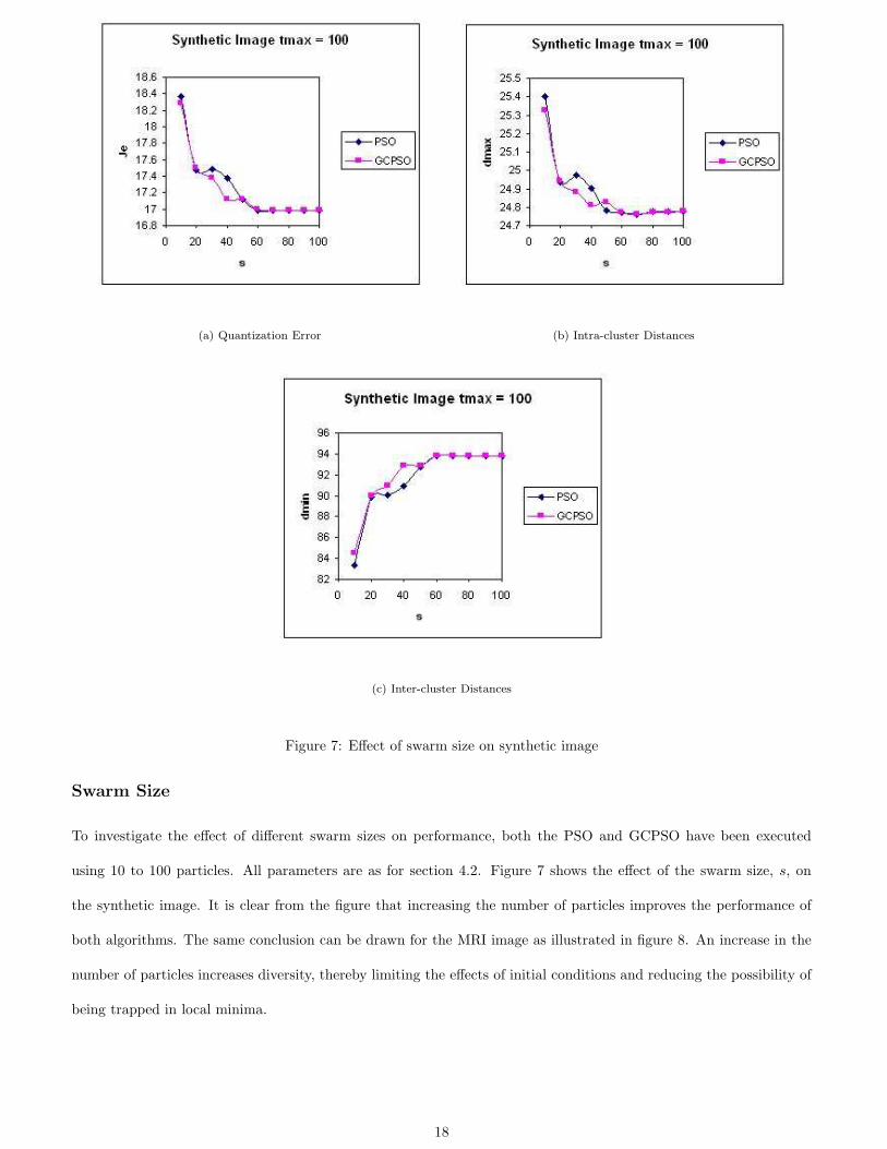
Figure 7: Effect of swarm size on synthetic image

Swarm Size

To investigate the effect of different swarm sizes on performance, both the PSO and GCPSO have been executed

using 10 to 100 particles. All parameters are as for section 4.2. Figure 7 shows the effect of the swarm size, s, on

the synthetic image. It is clear from the figure that increasing the number of particles improves the performance of

both algorithms. The same conclusion can be drawn for the MRI image as illustrated in figure 8. An increase in the

number of particles increases diversity, thereby limiting the effects of initial conditions and reducing the possibility of

being trapped in local minima.

18

(a) Quantization Error (b) Intra-cluster Distances

(c) Inter-cluster Distances

Figure 8: Effect of swarm size on MRI image

19

Table 4: Effect of inertia weight on the synthetic image

PSO GCPSO

w Je dmax dmin Je dmax dmin

0.0 16.983429 ± 24.581799 ± 93.435221 ± 16.986386 ± 24.649368 ± 93.559275 ±

0.017011 0.165103 0.308601 0.016265 0.138223 0.254670

0.1 16.982362 ± 24.645884 ± 93.543795 ± 16.985079 ± 24.637893 ± 93.538635 ±

0.016074 0.137442 0.256700 0.016995 0.138894 0.257167

0.5 16.985826 ± 24.664421 ± 93.595394 ± 16.987470 ± 24.662973 ± 93.581237 ±

0.014711 0.144252 0.246110 0.028402 0.163768 0.281366

0.72 16.992102 ± 24.670338 ± 93.606400 ± 16.995967 ± 24.722414 ± 93.680765 ±

0.021756 0.150542 0.258548 0.039686 0.144572 0.253954

0.9 16.993759 ± 24.650337 ± 93.569595 ± 17.040990 ± 24.633802 ± 93.495340 ±

0.014680 0.140005 0.252781 0.168017 0.352785 0.584424

1.4 to 17.824495 ± 24.433770 ± 92.625088 ± 17.481146 ± 24.684407 ± 93.223498 ±

0.8 0.594291 1.558219 2.031224 0.504740 1.010815 1.490217

Inertia Weight

Given that all parameters are fixed at the values given in section 4.2, the inertia weight w was set to different values

for both PSO and GCPSO. In addition, a dynamic inertia weight was used with an initial w = 1.4, which linearly

decreased to 0.8. The initial large value of w favors exploration in the early stages, and exploitation in the later

stages. Tables 4 and 5 summarize the results for the synthetic and MRI images respectively. The results illustrate

no significant difference in performance, meaning that for the two images, the PSO-based clustering algorithms are

insensitive to the value of the inertia weight (provided that c1 and c2 are selected such that equation (7) is not violated).

Acceleration Coefficients

Given that all parameters are fixed at the values given in section 4.2, the influence of different values for the acceleration

coefficients, c1 and c2, were evaluated for the synthetic and MRI images. Tables 6 and 7 summarize these results. For

these choices of the acceleration coefficients, no single choice is superior to the others. While these tables indicate

an independence to the value of the acceleration coefficients, it is important to note that convergence depends on the

relationship between the inertia weight and the acceleration coefficients, as derived in [48, 47] (also refer to equation

(7).

20

Table 5: Effect of inertia weight on the MRI image

PSO GCPSO

w Je dmax dmin Je dmax dmin

0.0 7.538669 ± 9.824915 ± 28.212823 ± 7.497944 ± 9.731746 ± 28.365827 ±

0.312044 0.696940 2.300930 0.262656 0.608752 1.882164

0.1 7.511522 ± 10.307791 ± 27.150801 ± 7.309289 ± 10.228958 ± 26.362349 ±

0.281967 1.624499 3.227550 0.452103 1.354945 3.238452

0.5 7.612079 ± 10.515242 ± 26.996556 ± 7.466388 ± 10.348044 ± 26.790056 ±

0.524669 1.103493 2.161969 0.492750 1.454050 2.830860

0.72 7.574454 ± 10.150214 ± 27.393498 ± 7.467591 ± 10.184191 ± 26.596493 ±

0.382172 1.123441 3.260418 0.396310 0.955129 3.208689

0.9 7.847689 ± 10.779765 ± 26.268057 ± 7.598518 ± 10.916945 ± 25.417859 ±

0.529134 1.134843 3.595596 0.516938 1.534848 3.174232

1.4 to 8.354957 ± 13.593536 ± 21.625623 ± 8.168068 ± 12.722139 ± 21.169304 ±

0.8 0.686190 2.035889 4.507230 0.709875 1.850957 4.732452

Table 6: Effect of acceleration coefficients on the synthetic image

PSO GCPSO

w Je dmax dmin Je dmax dmin

c1 = 0.7 16.989197 ± 24.726716 ± 93.698591 ± 16.989355 ± 24.708151 ± 93.667144 ±

c2 = 1.4 0.011786 0.101239 0.184244 0.012473 0.120168 0.207355

c1 = 1.4 16.991884 ± 24.700627 ± 93.658673 ± 16.993095 ± 24.685461 ± 93.619162 ±

c2 = 0.7 0.016970 0.125603 0.208500 0.040042 0.165669 0.279258

c1 = 1.49 16.987582 ± 24.710933 ± 93.672792± 16.995967 ± 24.722414 ± 93.680765 ±

c2 = 1.49 0.009272 0.122622 0.206395 0.039686 0.144572 0.253954

21

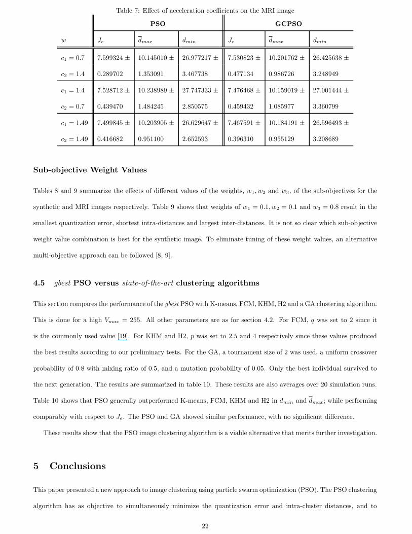
Table 7: Effect of acceleration coefficients on the MRI image

PSO GCPSO

w Je dmax dmin Je dmax dmin

c1 = 0.7 7.599324 ± 10.145010 ± 26.977217 ± 7.530823 ± 10.201762 ± 26.425638 ±

c2 = 1.4 0.289702 1.353091 3.467738 0.477134 0.986726 3.248949

c1 = 1.4 7.528712 ± 10.238989 ± 27.747333 ± 7.476468 ± 10.159019 ± 27.001444 ±

c2 = 0.7 0.439470 1.484245 2.850575 0.459432 1.085977 3.360799

c1 = 1.49 7.499845 ± 10.203905 ± 26.629647 ± 7.467591 ± 10.184191 ± 26.596493 ±

c2 = 1.49 0.416682 0.951100 2.652593 0.396310 0.955129 3.208689

Sub-objective Weight Values

Tables 8 and 9 summarize the effects of different values of the weights, w1, w2 and w3, of the sub-objectives for the

synthetic and MRI images respectively. Table 9 shows that weights of w1 = 0.1, w2 = 0.1 and w3 = 0.8 result in the

smallest quantization error, shortest intra-distances and largest inter-distances. It is not so clear which sub-objective

weight value combination is best for the synthetic image. To eliminate tuning of these weight values, an alternative

multi-objective approach can be followed [8, 9].

4.5 gbest PSO versus state-of-the-art clustering algorithms

This section compares the performance of the gbest PSO with K-means, FCM, KHM, H2 and a GA clustering algorithm.

This is done for a high Vmax = 255. All other parameters are as for section 4.2. For FCM, q was set to 2 since it

is the commonly used value [19]. For KHM and H2, p was set to 2.5 and 4 respectively since these values produced

the best results according to our preliminary tests. For the GA, a tournament size of 2 was used, a uniform crossover

probability of 0.8 with mixing ratio of 0.5, and a mutation probability of 0.05. Only the best individual survived to

the next generation. The results are summarized in table 10. These results are also averages over 20 simulation runs.

Table 10 shows that PSO generally outperformed K-means, FCM, KHM and H2 in dmin and dmax; while performing

comparably with respect to Je. The PSO and GA showed similar performance, with no significant difference.

These results show that the PSO image clustering algorithm is a viable alternative that merits further investigation.

5 Conclusions

This paper presented a new approach to image clustering using particle swarm optimization (PSO). The PSO clustering

algorithm has as objective to simultaneously minimize the quantization error and intra-cluster distances, and to

22

Table 8: Effect of sub-objective weight values on synthetic image

PSO GCPSO

w1 w2 w3 Je dmax dmin Je dmax dmin

0.3 0.3 0.3 17.068816 ± 24.672006 ± 93.594977 ± 17.010279 ± 24.742272 ± 93.711385 ±

0.157375 0.572276 0.984724 0.059817 0.258118 0.437418

0.8 0.1 0.1 17.590421 ± 21.766287 ± 88.892284 ± 17.514336 ± 21.724623 ± 88.879342 ±

0.353375 0.127098 0.143159 0.025242 0.018983 0.062452

0.1 0.8 0.1 18.827495 ± 27.623976 ± 97.719446 ± 18.827120 ± 27.522388 ± 97.768398 ±

0.558357 0.427120 0.202744 0.688529 0.282601 0.266885

0.1 0.1 0.8 16.962755 ± 24.495742 ± 93.228826 ± 16.983721 ± 24.546881 ± 92.576271 ±

0.003149 0.089611 0.135893 0.122501 0.434417 4.357444

0.1 0.45 0.45 17.550448 ± 26.707924 ± 96.020559 ± 17.557817 ± 26.598435 ± 95.888089 ±

0.184982 0.692239 0.757185 0.226305 0.907974 1.152158

0.45 0.45 0.1 18.134349 ± 26.489043 ± 96.461779 ± 18.294904 ± 26.795286 ± 96.922471 ±

0.669151 0.982256 1.495491 0.525467 0.800436 1.225336

0.45 0.1 0.45 17.219807 ± 22.631958 ± 90.152811 ± 17.201690 ± 22.701159 ± 90.289690 ±

0.110357 0.522369 0.887423 0.093969 0.469470 0.828522

23

Table 9: Effect of sub-objective weight values on MRI image

PSO GCPSO

w1 w2 w3 Je dmax dmin Je dmax dmin

0.3 0.3 0.3 7.239181 ± 10.235431 ± 24.705469 ± 7.194243 ± 10.403608 ± 23.814072 ±

0.576141 1.201349 3.364803 0.573013 1.290794 3.748753

0.8 0.1 0.1 7.364818 ± 9.683816 ± 24.021787 ± 7.248268 ± 9.327774 ± 23.103375 ±

0.667141 0.865521 3.136552 0.474639 0.654454 4.970816

0.1 0.8 0.1 8.336001 ± 11.256763 ± 31.106734 ± 8.468620 ± 11.430190 ± 30.712733 ±

0.599431 1.908606 1.009284 0.626883 1.901736 1.336578

0.1 0.1 0.8 6.160486 ± 15.282308 ± 2.342706 ± 6.088302 ± 15.571290 ± 1.659674 ±

0.241060 2.300023 5.062570 0.328147 2.410393 4.381048

0.1 0.45 0.45 7.359711 10.826327 24.536828 ± 7.303304 ± 11.602263 ± 22.939088 ±

0.423120 1.229358 3.934388 0.439635 1.975870 3.614108

0.45 0.45 0.1 8.001817 ± 9.885342 ± 28.057459 ± 7.901145 ± 9.657340 ± 29.236420 ±

0.391616 0.803478 1.947362 0.420714 0.947210 1.741987

0.45 0.1 0.45 6.498429 ± 11.392347 ± 12.119429 ± 6.402205 ± 10.939902 ± 14.422413 ±

0.277205 2.178743 8.274427 0.363938 2.301587 6.916785

24

Table 10: Comparison between K-means, FCM, KHM, H2, GA and PSO

Function

Image Je dmax dmin Evaluations

Synthesized K-means 20.21225 ± 0.937836 28.04049 ± 2.777938 78.4975 ± 7.062871 5000

FCM 20.73192 ± 0.650023 28.55921 ± 2.221067 82.4341 ± 4.404686 5000

KHM 20.16857 ± 0.0 23.36242 ± 0.0 86.3076 ± 0.000008 5000

H2 20.13642 ± 0.793973 26.68694 ± 3.011022 81.8341 ± 6.022036 5000

GA 17.00400 ± 0.035146 24.60302 ± 0.11527 93.4922 ± 0.2567 5000

PSO 16.98891 ± 0.023937 24.69606 ± 0.130334 93.6322 ± 0.248234 5000

MRI K-means 7.3703 ± 0.042809 13.21437 ± 0.761599 9.9343 ± 7.30853 5000

FCM 7.205987 ± 0.166418 10.85174 ± 0.960273 19.5178 ± 2.014138 5000

KHM 7.53071 ± 0.129073 10.65599 ± 0.295526 24.2708 ± 2.04944 5000

H2 7.264114 ± 0.149919 10.92659 ± 0.737545 20.5435 ± 1.871984 5000

GA 7.038909 ± 0.508953 9.811888 ± 0.419176 25.9542 ± 2.993480 5000

PSO 7.594520 ± 0.449454 10.18609 ± 1.237529 26.7059 ± 3.008073 5000

Tahoe K-means 3.280730 ± 0.095188 5.234911 ± 0.312988 9.40262 ± 2.823284 5000

FCM 3.164670 ± 0.000004 4.999294 ± 0.000009 10.9706 ± 0.000015 5000

KHM 3.830761 ± 0.000001 6.141770 ± 0.0 13.7684 ± 0.000002 5000

H2 3.197610 ± 0.000003 5.058015 ± 0.000007 11.0529 ± 0.000012 5000

GA 3.472897 ± 0.151868 4.645980 ± 0.105467 14.4469 ± 0.857770 5000

PSO 3.523967 ± 0.172424 4.681492 ± 0.110739 14.6649 ± 1.177861 5000

25

maximize the inter-cluster distances. Both a gbest PSO and GCPSO algorithm have been evaluated. The gbest

PSO clustering algorithm was further compared against K-means, FCM, KHM, H2 and a GA. In general, the PSO

algorithm produced better results with reference to inter- and intra-cluster distances, while having quantization errors

comparable to the other algorithms.

Although the fitness function used by the PSO-approach contains multiple objectives, no special multi-objective

optimization techniques have been used. Further research will investigate the use of a PSO multi-objective approach,

which may produce better results. A strategy will also be developed to dynamically determine the optimal number of

clusters.

6 Acknowledgments

We are grateful to G. Hamerly and C. Elkan for providing us with MATLAB code for KHM.

References

[1] N. Alldrin, A. Smith, D. Turnbull, “Clustering with EM and K-means,” Unpublished Manuscript,

http://louis.ucsd.edu/ nalldrin/research/cse253 wi03.pdf, 15 Nov 2003.

[2] M. Antonie, O. Zaiane, A. Coman, “Application of Data Mining Techniques for Medical Image Classification,”

Proceedings of the 2nd International Workshop on Multimedia Mining, San Francisco, USA, pp. 94-101, 2001.

[3] J. Bala, J. Juang, H. Vafaie, K. DeJong, W. Wechsler, “Hybrid Learning Using Genetic Algorithms and Decision

Trees for Pattern Classification,” International Joint Conference on Artificial Intelligence, Montreal, August, 1995.

[4] G. Ball, D. Hall, “A Clustering Technique for Summarizing Multivariate Data,” Behavioral Science, vol. 12, pp.

153-155, 1967.

[5] J. Bezdek, “A Convergence Theorem for the fuzzy ISODATA Clustering Algorithms,” IEEE Transactions on

Pattern Analysis and Machine Intelligence, vol. 2, pp. 1-8, 1980.

[6] J. Bezdek, Pattern Recognition with Fuzzy Objective Function Algorithms, Plenum Press, 1981.

[7] C. Bishop, Neural Networks for Pattern Recognition, Clarendon Press, Oxford, 1995.

[8] C.A. Coello-Coello, “An Empirical Study of Evolutionary Techniques for Multiobjective Optimization in Engi-

neering Design”, PhD Thesis, Tulane University, 1996.

26

[9] C.A. Coello-Coello, M.S. Lechuga, “MOPSO: A Proposal for Multiple Objective Particle Swarm Optimization”,

IEEE Congress on Evolutionary Computation, Vol. 2, pp. 1051-1056, 2002.

[10] E. Davies, Machine Vision: Theory, Algorithms, Practicalities, Academic Press, 2nd Edition, 1997.

[11] A.P. Engelbrecht, “Computational Intelligence: An Introduction,” John Wiley, 2002.

[12] I. Evangelou, D. Hadjimitsis, A. Lazakidou, C. Clayton, “Data Mining and Knowledge Discovery in Complex Im-

age Data using Artificial Neural Networks,” Proceedings of the Workshop on Complex Reasoning on Geographical

Data (CRGD), 7th International Conference on Logic Programming - ICLP’01 and 7th International Conference

on Principles and Practice of Constraint Programming - CP’01, Paphos, Cyprus, pp. 39-48, 2001.

[13] E. Falkenauer, Genetic Algorithms and Grouping Problems, John Wiley & Sons Publishing, 1998.

[14] E. Forgy, “Cluster Analysis of Multivariate Data: Efficiency versus Interpretability of Classification,” Biometrics,

vol. 21, pp. 768-769, 1965.

[15] H. Frigui, R. Krishnapuram, “A Robust Competitive Clustering Algorithm with Applications in Computer Vi-

sion,” IEEE Transactions on Pattern Analysis and Machine Intelligence, vol. 21, no. 5, pp. 450-465, 1999.

[16] I. Gath, A. Geva, “Unsupervised Optimal Fuzzy Clustering,” IEEE Transactions on Pattern Analysis and Machine

Intelligence, vol. 11, no. 7, pp. 773-781, 1989.

[17] G. Hamerly, Learning structure and concepts in data using data clustering, PhD Thesis, University of California,

San Diego, 2003.

[18] G. Hamerly, C. Elkan, “Alternatives to the K-means algorithm that find better clusterings,” Proceedings of the

ACM Conference on Information and Knowledge Management, pp.600-607, 2002.

[19] F. Hoppner, F. Klawonn, R. Kruse, T. Runkler, Fuzzy Cluster Analysis, Methods for Classification, Data Analysis

and Image Recognition. John Wiley & Sons Ltd, 1999.

[20] K. Huang, “A Synergistic Automatic Clustering Technique (Syneract) for Multispectral Image Analysis,” Pho-

togrammetric Engineering and Remote Sensing, vol. 1, no. 1, pp. 33-40, 2002.

[21] J. Kennedy, R. Eberhart, “Particle Swarm Optimization,” Proceedings of IEEE International Conference on

Neural Networks, vol. 4, pp. 1942-1948, Perth, Australia, 1995.

[22] J. Kennedy, R. Eberhart, “A Discrete Binary Version of the Particle Swarm Algorithm,” Proceedings of the

Conference on Systems, Man, and Cybernetics, pp. 4104-4109, 1997.

27

[23] J. Kennedy, W. Spears, “Matching Algorithms to Problems: An Experimental Test of the Particle Swarm and

Some Genetic Algorithms on the Multimodal Problem Generator,” Proceedings of the International Conference

on Evolutionary Computation, pp. 78-83, Anchorage, Alaska, 1998.

[24] J. Kennedy, “Small Worlds and Mega-Minds: Effects of Neighborhood Topology on Particle Swarm Performance,”

Proceedings of the Congress on Evolutionary Computation, pp. 1931-1938, 1999.

[25] J. Kennedy, R. Eberhart, Swarm Intelligence, Morgan Kaufmann, 2001.

[26] J. Kennedy, R. Mendes, “Population Structure and Particle Performance,” Proceedings of the IEEE Congress on

Evolutionary Computation, Honolulu, Hawaii, 2002.

[27] T. Kohonen, Self-Organizing Maps, Springer Series in Information Sciences, Vol. 30, Springer-Verlag, 1995.

[28] Y. Leung, J. Zhang, Z. Xu, “Clustering by Space-Space Filtering,” IEEE Transactions on Pattern Analysis and

Machine Intelligence, vol. 22, no. 12, pp. 1396-1410, 2000.

[29] T. Lillesand, R. Kiefer, Remote Sensing and Image Interpretation, John Wiley & Sons Publishing, 1994.

[30] A. Lorette, X. Descombes, J. Zerubia, “Fully Unsupervised Fuzzy Clustering with Entropy Criterion,” IEEE

Proceedings of the International Conference on Pattern Recognition, pp. 986-989, 2000.

[31] J. MacQueen, “Some Methods for Classification and Analysis of Multivariate Observations,” Proceedings 5th

Berkeley Symposium on Mathematics, Statistics and Probability, vol. 1, pp. 281-297, 1967.

[32] P. Mather, Computer Processing of Remotely Sensed Images, John Wiley & Sons Publishing, 1999.

[33] U. Maulik, S. Bandyopadhyay, “Genetic Algorithm-Based Clustering Technique,” Pattern Recognition, vol. 33,

pp. 1455-1465, 2000.

[34] G. McLachlan, T. Krishnan, The EM algorithm and Extensions, John Wiley & Sons, Inc., 1997.

[35] M. Omran, A. Salman, A.P. Engelbrecht, “Image Classification using Particle Swarm Optimization,” Proceedings

of the 4th Asia-Pacific Conference on Simulated Evolution and Learning, Singapore, 2002.

[36] D. Paola, R. Schowenderdt, “A Review and Analysis of Back Propagation Neural Networks for Classification of

Remotely Sensed Multi-Spectral Imagery,” International Journal of Remote Sensing, vol. 16, pp. 3033-3058, 1995.

[37] E.S. Peer, F. van den Bergh, A.P. Engelbrecht, “Using Neighborhoods with the Guaranteed Convergence PSO,”

Proceedings of the IEEE Swarm Intelligence Symposium, Indianapolis, pp. 235-242, 2003.

28

[38] J. Puzicha, T. Hofmann, J.M. Buhmann, “Histogram Clustering for Unsupervised Image Segmentation,” IEEE

Proceedings of the Computer Vision and Pattern Recognition, pp. 602-608, 2000.

[39] V. Ramos, F. Muge, “Map Segmentation by Colour Cube Genetic K-Mean Clustering,” Proceedings of the 4th

European Conference on Research and Advanced Technology for Digital Libraries, Lecture Notes in Computer

Science, Vol. 1923, pp. 319-323, Springer-Verlag, Lisbon, Portugal, September 2000.

[40] R. Rendner, H. Walker, “Mixture Densities, Maximum Likelihood and The EM Algorithm,” SIAM Review, Vol.

26, No. 2, 1984.

[41] C. Rosenberger, K. Chehdi, “Unsupervised Clustering Method with Optimal Estimation of the Number of Clus-

ters: Application to Image Segmentation,” IEEE Proceedings of the International Conference on Pattern Recog-

nition, pp. 656-659, 2000.

[42] P. Scheunders, “A Genetic C-means Clustering Algorithm Applied to Image Quantization,” Pattern Recognition,

vol. 30, no. 6, 1997.

[43] Y. Shi, R. Eberhart, “A Modified Particle Swarm Optimizer,” IEEE International Conference of Evolutionary

Computation, Anchorage, Alaska, May 1998.

[44] Y. Shi, R. Eberhart, “Parameter Selection in Particle Swarm Optimization,” Evolutionary Programming VII:

Proceedings of EP 98, pp. 591-600, 1998.

[45] P. Suganthan, “Particle Swarm Optimizer with Neighborhood Optimizer,” Proceedings of the Congress on Evo-

lutionary Computation, pp. 1958-1962, 1999.

[46] H Vafaie, K. De Jong, “Genetic Algorithms as a Tool for Feature Selection in Machine Learning,” Fourth In-

ternational Conference on Tools with Artificial Intelligence (ICTAI ’92), Arlington, Virginia, USA, pp. 200-203,

1992.

[47] F. van den Bergh, A.P. Engelbrecht, “A New Locally Convergent Particle Swarm Optimizer,” Proceedings of the

IEEE Conference on Systems, Man, and Cybernetics, Hammamet, Tunisia, 2002.

[48] F. van den Bergh, An Analysis of Particle Swarm Optimizers, PhD Thesis, University of Pretoria, 2002.

[49] B. Zhang, “Generalized K-Harmonic Means - Boosting in Unsupervised Learning,” Technical Report HPL-2000-

137). Hewlett-Packard Labs, 2000.

[50] B. Zhang, M. Hsu, U. Dayal, “K-Harmonic Means - A Data Clustering Algorithm,” Technical Report HPL-1999-

124). Hewlett-Packard Labs, 1999.

29

[51] Y. Zhang, M. Brady, S. Smith, “Segmentation of Brain MR Images Through a Hidden Markov Random Field

Model and the Expectation-Maximization Algorithm,” IEEE Transactions on Medical Imaging, vol. 20, no. 1, pp.

45-57, 2001.

30