Particle Swarm Optimization for the Minimum Energy Broadcast Problem in Wireless Ad-Hoc

Networks

Ping-Che Hsiao Dept. of Computer Science and

Information Engineering, National Taiwan University,

Taipei, Taiwan, R.O.C. r99922111@ntu.edu.tw

Tsung-Che Chiang Dept. of Computer Science and

Information Engineering, National Taiwan Normal

University, Taipei, Taiwan, R.O.C.

tcchiang@ieee.org

Li-Chen Fu Dept. of Electrical Engineering and

Dept. of Computer Science and Information Engineering,

National Taiwan University, Taipei, Taiwan, R.O.C.

lichen@ntu.edu.tw

Abstract—In this paper, we propose a novel approach based on particle swarm optimization (PSO) for solving the minimum energy broadcast (MEB) problem, which has been proven to be NP-complete. Wireless sensor networks (WSNs) have attracted large intention in recent years due to its powerful ability. One crucial issue in WSN is energy saving because of the limited battery resource. The MEB problem is one of the important scenarios in WSN, where a node needs to broadcast packets to all other nodes in the network. The objective is to minimize power consumption of all nodes in the network. Here we take advantage of fast and guided convergence characteristics of PSO to solve the MEB problem. For applying PSO to the MEB problem, we use the power degree to define the particle position. We go a step further to analyze one well-known local search mechanism: r-shrink and propose an improved version. The experimental results show that the proposed approach is able to compete and even outperform state-of-the-art works.

Keywords-Particle Swarm Optimizatioin; Minimum Energy Broadcast Problem; Minimum Power Broadcast Problem; Wireless Ad-Hoc Networks; Wireless Sensor Networks; Network Routing

I. INTRODUCTION

Recent years, researches in WSN have attracted significant attentions due to its powerful sensing ability and convenient deployment. WSNs consist of a large number of sensor nodes, which are equipped with sensing, communication and computing abilities. Each sensor node can measure parameters such as temperature, and vibration, perform the simple computations and communicate with neighbors or the base station [1]. WSN have already been applied broadly on several civil and military applications including forest surveillance, disaster monitoring, factory automation, border protection, battlefield surveillance, and animal tracking [2-4].

Usually, each node has limited energy resource (usually a battery or an embedded form of energy resource), which is in some cases completely non-renewable. This implies that the sensor nodes are expected to perform sensing and communication for a long time without maintenance or reorganization [1, 5]. One of the main issues to be solved in WSNs is the routing problems. The utmost purposes of the

routing problems in WSN are to minimize the total power consumption of the sensor nodes and prevent the network from loss of connectivity. Compared with traditional link-based networks, wireless networks can be deployed in shorter time and less cost; however, the routing mechanism in link-based networks cannot be forthright applied to wireless networks due to their difference in innate transmission properties [6].

MEB is a routing problem in a scenario where the same packets need to be disseminated to all other nodes in the network, and the MEB problem has been proven to be NP-complete [7]. In link-based networks, there is usually only one receiver in a single transmission from the sender. However, in networks in wireless fashion, several nodes can receive the same piece of information as long as they are in the transmission range from the sender. This evident difference is also called Wireless Multicast Advantage (WMA) [8]. If a node sends a packet with a power level P = ξ × dα, then all nodes located within the distance d and power threshold ξ are able to receive this packet [9]. The variable α is the path loss exponent ranging between 2 and 4. Without loss of generality, the transmission power level required for a sensor node i to

transmit a packet to another node j can be reduced to ij ijP d ,

where dij represents the distance from node i to node j. Then the total power consumption f(T) for a broadcast tree T = (V, E) in the MEB problem can be formulated as:

{ | }

( ) maxij

ijj e E

i V

f T d

(1)

where V is the set of sensor nodes in T, E is the set of directed edges in T, eij is the directed edge from node i to node j, representing that node j can receive broadcast messages from node i. The routing paths can be expressed by a broadcast tree rooted at the source node s, and all other nodes in V are descendant nodes of s. The objective of this problem, therefore, is to minimize the total power consumption in (1).

The transmission power level of a sensor node hinges on the distance from the farthest child node, which is usually referred to the critical child [10]. Also, a broadcast tree may

U.S. Government work not protected by U.S. copyright

WCCI 2012 IEEE World Congress on Computational Intelligence June, 10-15, 2012 - Brisbane, Australia IEEE CEC

contain several leaf nodes, which do not have any transmission power consumption [11]. Often, in wireless framework the power consumption in transmission can be further reduced by using one or more intermediate nodes instead of transmitting directly [12]. Nevertheless, sometimes long-distance transmissions may be preferred due to the WMA characteristic in the broadcast scenario. Therefore, the MEB problem cannot be solved by an ordinary single-path routing algorithm.

The outline of this paper is as follows. In Section II, we introduce the background literature on the MEB problem, including simple heuristics, local search, and meta-heuristic algorithms. Then we introduce the proposed algorithm in Section III. Section IV presents the experimental results for instances with 50 nodes and 100 nodes. Finally, conclusions and plans for future work are given in Section V.

II. LITERATURE REVIEW

A. Simple Constructive Heuristics

Various simple constructive heuristics for the MEB problem have been proposed since early 2000s, such as Embedded Wireless Multicast Advantage (EWMA) [7], Greedy Perimeter Broadcast Efficiency (GPBE) [13], Adaptive Broadcast Consumption (ABC) [14] and Minimum Weight Incremental Arborescence (MWIA) [15]. One of the best-known algorithms is Broadcast Incremental Power (BIP) [16], which constructs a broadcast tree starting by a source node and then iteratively adding an uncovered node with the minimum incremental power. Most of these works are based on the minimum weighted spanning tree (MST) [16] and iteratively join nodes with specific greedy methodologies. The approximation ratio in MST is between 6 and 12, and BIP is between 13/3 and 12. The approximation ratio of several algorithms are investigated in [6].

B. Local Search Algorithms

Simple heuristics can build a broadcast tree in a short time, but the results are still improvable. In order to make up for the performance, many simple heuristics are paired with local search mechanisms after a broadcast tree is constructed. Examples of typical local search examples include Sweep [16], r-shrink [17], Broadcast Incremental-Decremental Power (BIDP) [18] and Largest Expanding Sweep Search (LESS) [19]. Among these algorithms, Sweep and r-shrink are the most widely used owing to their intuitive concept.

Sweep was firstly presented by Wieselthier et al. in [16]. For all non-leaf nodes, it checks if its critical child can be covered by other nodes which are the foster parent of the critical child. If node i is the critical child of node j, then the foster parent of node i refers to each node in the broadcast tree excluding node j and descendant nodes of node i. In the framework of Sweep, no node is allowed to increase its transmission power level; therefore, the improvement is limited.

The r-shrink procedure also checks all non-leaf nodes and then reassigns the farthest r children to other foster-parent nodes which produce minimum incremental cost. If the power consumption becomes higher than the earlier one, it returns to the previous status. Both Sweep and r-shrink can be applied

iteratively. The performance of r-shrink is much better than Sweep because of the allowance of increasing the power level of an individual node but reducing the total power consumption. One can observe that most of the state-of-the-art works are cooperated with r-shrink. Several works applied r-shrink within Variable Neighborhood Descent (VND) [20] procedure, which starts with r = 1 and gradually increase the value of r until reaching the maximum value rmax. Once the solution gets improved, the search will start again with r = 1.

C. Meta-heuristic Algorithms

Over the years, several meta-heuristic algorithms for the MEB problem have also been proposed, e.g. Genetic Algorithm (GA) [11], Evolutionary Local Search (ELS) [21], Iterated Local Search (ILS) [22], Hybrid Genetic Algorithm (HGA) [23], and Ant Colony Optimization (ACO) [24, 25].

ELS [21] is based on the evolutionary algorithm and local search. It is similar to iterated local search, but more than one offspring solution is used. The authors used modified r-shrink as the local search procedure. Modified r-shrink becomes much more complex, but it yielded better results. As the fact that the search progress is stuck in the local optima rapidly, a mutation is applied to solutions after local search. The mutation increases the transmission power level of randomly chosen nodes to a random level. The experimental results showed that ELS sometimes fails to find the optimum solution when it comes to instances with 50 nodes.

HGA [23] used the permutation encoding proposed by Xiang et al. [11]. It is a steady-state GA and again takes r-shrink as the local search procedure. The encoding is composed of a permutation of node ID. When it decodes the chromosome to a broadcast tree, it starts with the source node and adds the rest of nodes according to the order of encoding. When a node is going to be added to the tree, they use BIP to decide which of the node in the tree is about to be the parent. Although GA is a strengthful search algorithm, the permutation encoding has two undesirable features. First, the search space of the permutation encoding cannot present all solutions. Furthermore, it is not proven that the search space of the permutation encoding contains the optimal solution. Second, the permutation encoding contains redundant solutions leading to the same broadcast tree. It makes search more time-consuming and more arduous.

ACO [24] utilized the concept of seeking a path by ants to deal with the MEB problem. Any pair of two sensor nodes maintains a pheromone value. In construction of a broadcast tree, it starts with the source node and then iteratively adds one node to the tree in a probability based on the incremental power and pheromone value. In order to improve the performance for large-scale instances, they used the Min-Max Ant System (MMAS) to first conditionally select several candidates and proceed to select the final link from these candidates to be added. After constructing the broadcast tree, they applied r-shrink within the VND procedure to get to the local optima. Several broadcast trees are constructed in an iteration and then the iteration-best-solution, restart-best-solution and best-solution-so-far are updated. These best solutions are used to

update the pheromone values between nodes. The experimental results of ACO are acceptable for large-scale instances.

III. PROPOSED ALGORITHM

Our proposed algorithm is based on particle swarm optimization, and it cooperates with an improved version of r-shrink. This section firstly gives a brief review of particle swarm optimization, and proceeds to our proposed algorithm for the MEB problem. Finally we will introduce our improved version of r-shrink.

A. Particle Swarm Optimization

Particle swarm optimization (PSO) was originally proposed by Kennedy and Eberhart [26], and it was intended to simulate the movement in a bird flock or fish school. A PSO algorithm maintains a group of solutions, called particles. These particles flying around in the search space aims to find the global optimum. The movement of a particle is decided by the velocity, which guides the particle toward its own best-known position and the best-known position from all particles. Assume particles are able to communicate and share the solution information between one another. Then, the velocity of particle i can be calculated by

1 1 2 2( ) ( )pb gbi i i i iv wv r c x x r c x x (2)

and the new position of ith particle can be then updated by vi'

i i ix x v (3)

where vi' and vi are the new and original velocity vectors, respectively. The variable pb

ix represents the previous best-known position of particle i, also called pbest; xgb represents the previous best-known position among all particles, also called gbest; w is an inertia weight for the original velocity; c1 and c2 are weights for acceleration towards pbest and gbest; xi' and xi are the new and original positions of particle i, respectively; r1 and r2 are random numbers between 0 and 1.

B. Power Degree Encoding

There exist several solution encoding schemes for routing in WSN. With the permutation encoding [11, 23], they use a heuristic to decode the permutation sequence into a broadcast tree. Nevertheless, a broadcast tree cannot be reversely encoded to a permutation sequence. Some works in other WSN routing problem encoded exact power level of each node [9], but the transmission power level is usually oversized when the power level reaches farther than its critical child. Although we could reduce the transmission power level to the range to the critical child afterwards, there still exists the shortcoming of redundant search space. Plentiful of broadcast trees will be the same after reducing the oversized transmission power level.

Here, we present a power degree encoding, and we take the power degree as the particle position in the search space. Before starting the search, we have to build a power degree table. Each node firstly constructs a sequence of node ID excluding the source node in an ascending ordering of the distance. In Fig. 1, for node 1, the nodes from near to distant are 3, 2, 4, and 5, respectively. Node 4 is omitted from the sequence since it is the source node. Therefore, the sequence of node 1 is 3, 2, and 5. The sequence of other nodes can be constructed in a similar way.

After constructing a power degree table, we then can show the position of a particle. There is a broadcast tree in Fig. 2, and the distances between nodes are the same as in Fig. 1. The particle of this broadcast tree is [0, 1, 2, 2, 0], the power degree of each node. The power degree of a node is determined by its critical child, e.g., the critical child of node 3 is node 1, and the corresponding power degree is 2. The power degree encoding reflects the required transmission power level of each node. The information of power adjustment, i.e. the velocity, can be further inferred by the difference of the power degree between two particles. The velocity implies how much transmission power the node has to increase (reduce) in order to get closer to the best solutions.

C. Position Update

In our PSO, the velocity is formulated as follows:

1 2( ) ( )pb nbi i i i i iv wv r x x r x x (4)

where nbix is the best-known position within all neighborhood

particles of particle i, which is also called nbest. The neighborhood is defined by the K nearest pbest solutions of other particles. The distance between two particles is

1

( , )n

i j ik jkk

d x x x x

(5)

where xik is the power degree of node k in particle i. To make the implementation plainer, the weights c1 and c2 for acceleration towards best solutions are pruned away. The values in the velocity vector are limited in the range [−vmax, vmax], which can prevent the particles from incurring extreme perturbation. In order to maintain enough diversity and variation in the system, there is a probability pc in which one value in the velocity vector will become a random number in [−vmax, vmax]. This mutation-like procedure is called craziness in

Node Deg 1 Deg 2 Deg 3 Deg 4Node 1 3 2 5Node 2 3 1 5Node 3 2 1 5Node 4 5 2 3 1Node 5 2 3 1

Figure 1. The power degree table: the degree sequence is in ascending ordering of distance to all other nodes except source node. Gray node

represents the source node.

Node 1 Node 2 Node 3 Node 4 Node 5Degree 0 1 2 2 0

Figure 2. The power degree encoding for a specific broadcast tree. In this figure, the corresponding chromosome is [0, 1, 2, 2, 0].

PSO. The original authors [26] used craziness as a simulation of the life-like interesting movement in a bird flock or other animal groups.

Each node obtains its own new power degree by (3). If the new power degree of a node gets larger, this node will become the new parent of nodes in the extended region of the increased power. Let a and b be the original power degree and the new power degree, then

, ( )

( ) , ijij ij ij

a j b ascendant ipa i

j b

(6)

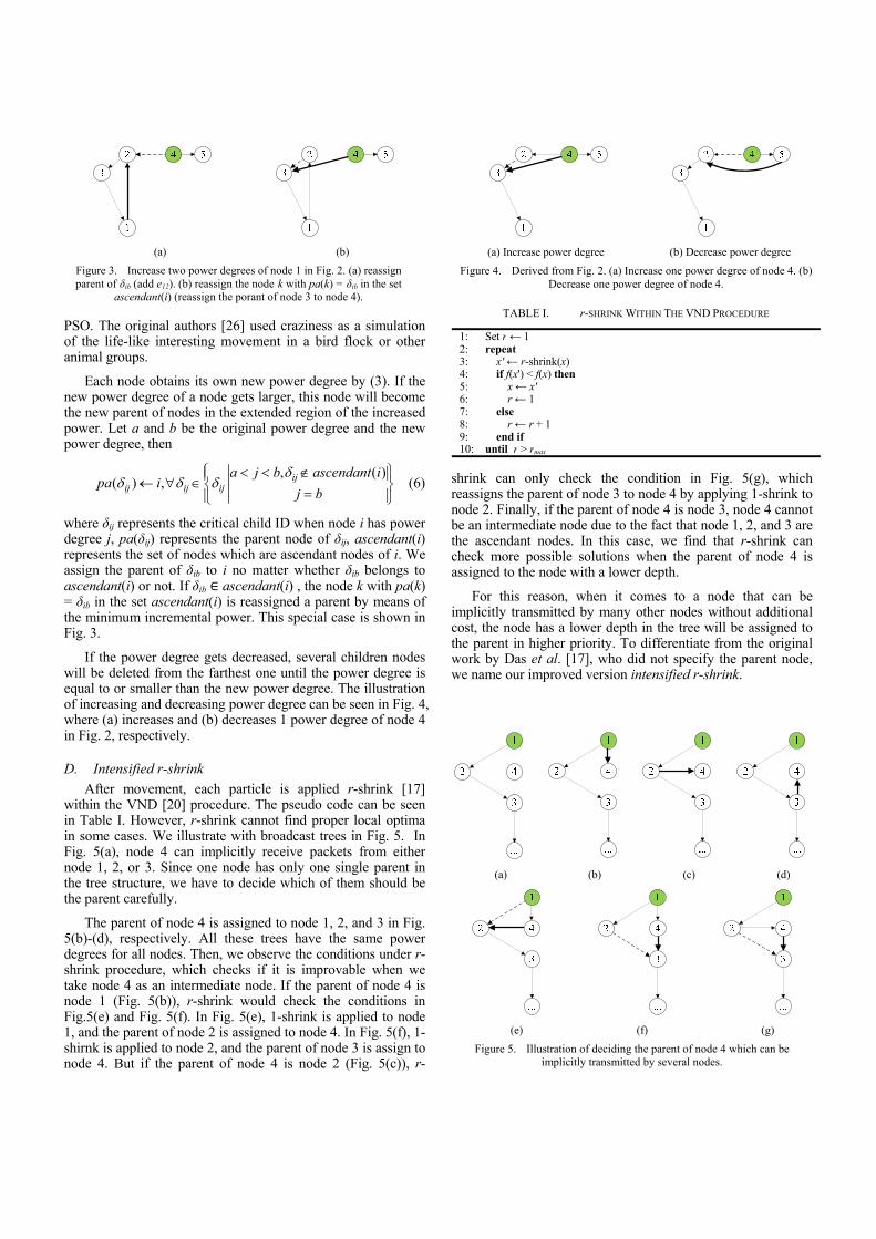
where δij represents the critical child ID when node i has power degree j, pa(δij) represents the parent node of δij, ascendant(i) represents the set of nodes which are ascendant nodes of i. We assign the parent of δib to i no matter whether δib belongs to ascendant(i) or not. If δib ∈ ascendant(i) , the node k with pa(k) = δib in the set ascendant(i) is reassigned a parent by means of the minimum incremental power. This special case is shown in Fig. 3.

If the power degree gets decreased, several children nodes will be deleted from the farthest one until the power degree is equal to or smaller than the new power degree. The illustration of increasing and decreasing power degree can be seen in Fig. 4, where (a) increases and (b) decreases 1 power degree of node 4 in Fig. 2, respectively.

D. Intensified r-shrink

After movement, each particle is applied r-shrink [17] within the VND [20] procedure. The pseudo code can be seen in Table I. However, r-shrink cannot find proper local optima in some cases. We illustrate with broadcast trees in Fig. 5. In Fig. 5(a), node 4 can implicitly receive packets from either node 1, 2, or 3. Since one node has only one single parent in the tree structure, we have to decide which of them should be the parent carefully.

The parent of node 4 is assigned to node 1, 2, and 3 in Fig. 5(b)-(d), respectively. All these trees have the same power degrees for all nodes. Then, we observe the conditions under r-shrink procedure, which checks if it is improvable when we take node 4 as an intermediate node. If the parent of node 4 is node 1 (Fig. 5(b)), r-shrink would check the conditions in Fig.5(e) and Fig. 5(f). In Fig. 5(e), 1-shrink is applied to node 1, and the parent of node 2 is assigned to node 4. In Fig. 5(f), 1-shirnk is applied to node 2, and the parent of node 3 is assign to node 4. But if the parent of node 4 is node 2 (Fig. 5(c)), r-

shrink can only check the condition in Fig. 5(g), which reassigns the parent of node 3 to node 4 by applying 1-shrink to node 2. Finally, if the parent of node 4 is node 3, node 4 cannot be an intermediate node due to the fact that node 1, 2, and 3 are the ascendant nodes. In this case, we find that r-shrink can check more possible solutions when the parent of node 4 is assigned to the node with a lower depth.

For this reason, when it comes to a node that can be implicitly transmitted by many other nodes without additional cost, the node has a lower depth in the tree will be assigned to the parent in higher priority. To differentiate from the original work by Das et al. [17], who did not specify the parent node, we name our improved version intensified r-shrink.

(a) (b)

Figure 3. Increase two power degrees of node 1 in Fig. 2. (a) reassign parent ofδib (add e12). (b) reassign the node k with pa(k) = δib in the set

ascendant(i) (reassign the porant of node 3 to node 4).

(a) Increase power degree (b) Decrease power degree

Figure 4. Derived from Fig. 2. (a) Increase one power degree of node 4. (b) Decrease one power degree of node 4.

TABLE I. r-SHRINK WITHIN THE VND PROCEDURE

1: Set r ← 12: repeat 3: x' ← r-shrink(x) 4: if f(x') < f(x) then 5: x ← x' 6: r ← 1 7: else 8: r ← r + 1 9: end if 10: until r > rmax

(a) (b) (c) (d)

(e) (f) (g)

Figure 5. Illustration of deciding the parent of node 4 which can be implicitly transmitted by several nodes.

E. The Proposed PSO Algorithm

A population of μ particles x1, x2, …,xμ. A set of μ velocity vectors v1, v2, …,vμ. The particle and neighborhood best-known solutions

1 2, ,...,pb pb pbx x x and 1 2, ,...,nb nb nbx x x .

The algorithm works as follows:

Step 1 Initialization

1.1 For i = 1…µ, randomly build a broadcast tree for xi, and then apply the intensified r-shrink within the VND for xi.

1.2 For i = 1…µ, pbi ix x .

1.3 For i = 1…µ, assign random values between [−vmax, vmax] for all values in vi.

Step 2 Landing

2.1 Repeat 2.1.1 and 2.1.2 for i = 1… µ. 2.1.1 Calculate the new power degree by vi. 2.1.2 For j = 1…n, increase (decrease) the power

degree of node j in xi by (3). 2.2 For i = 1…µ, update neighbors according to the

distance between xi and pbjx j i .

2.3 Update nbix by choosing the best solution from K

neighbors. Step 3 Acceleration, Craziness and Local Search

3.1 Acceleration: For i = 1…µ, calculate velocity vi for the next iteration by (4). Then, confine velocity values by

max( , min( , ))i max max iv v v v (7) 3.2 Craziness: For i = 1…µ, assign random values in

[−vmax, vmax] for each value in vi with probability pc. 3.3 Local Search: For i = 1…µ, apply the intensified r-

shrink within the VND procedure for xi.

Step 4 Update

4.1 For i = 1…µ, update pbi ix x if ( ) ( )pb

i if x f x . 4.2 For 1...i , if pb pb

i jx x i j , randomly initialize

xi and update pbi ix x .

4.3 If the stopping criterion is met, then terminate the search. Otherwise, return to Step 2.

Note that in 4.2, the identical particle best-known solution is reinitialized for maintaining diversity.

IV. EXPERIMENTAL RESULTS

A. Benchmark Instances

The benchmark instances was proposed by Al-Shihabi et al. in [27]. There are n sensor nodes randomly deployed in a 1000 × 1000 square plain, and the loss exponent α is 2. There are 30 instances for n = 20 and 30 instances for n = 50. In each instance, one node is specified to be the source node. We do not show the results about 20-node instances because these can be easily solved in a very short time. We take another 30 instances with n = 100 proposed by Hernández and Blum in

[24]. For instances with 50 nodes, they acquired half the optimal solutions by a linear programming solver. Since the MEB problem is NP-complete, they stopped searching after 24 hours for the rest of instances. We compare our proposed PSO algorithm with three state-of-the-art algorithms, ELS [21], HGA [23], and ACO[24]. Literatures have shown that they are among the best algorithms for the MEB problem.

B. Experiment Setting

Our PSO algorithm contains six parameters. The following parameters are fine-tuned by hand. The population size μ is 40, inertia weight for the preceding velocity w is 0.8, maximum value of velocity vmax is n/4, crazy rate pc is 0.05, neighborhood size K is 4, and the maximum r value for r-shrink with the VND procedure rmax is (n–2). The algorithm was coded in C programming language and run on a personal computer with Intel 3.2 GHz CPU and 2GB RAM. We follow the stopping criterion in [24] and set the CPU time limit accordingly, which is given in Table II. The parameter settings of the benchmark algorithms are identical to those in the original papers. Each algorithm was applied 30 times to each instance.

(a) BIP + r-shrink (VND)

(b) PSO

Figure 6. The broadcast tree built by (a) BIP + r-shrink (VND) and (b) PSO for instance p50.02.

TA

BL

E I

I.

TIM

E L

IMIT

S I

N E

XPE

RIM

EN

TS

TA

BL

E I

II.

EX

PER

IME

NT

AL

RE

SU

LT

S I

N IN

ST

AN

CE

S W

ITH

50

NO

DE

S

na

50

10

0

Tim

e L

imit

s (s

)

20

100

a. T

he n

umbe

r of

nod

es.

Inst

ance

a

Opt

imu

m [

21]

E

LS

[21

]

HG

A [

23]

A

CO

[24]

PSO

E

xces

s F

ound

T

ime(

s)

E

xces

s F

ound

T

ime(

s)

E

xces

s Fo

und

Tim

e(s)

A

vera

ge

Std

.dev

.

Exc

ess

Fou

nd

Tim

e(s)

b A

vera

ge

Std.

dev.

p5

0.00

3990

74.6

4

0.41

%

15/3

0 57

0.88

%

6/30

12

.82

–

30/3

0 0.

52

3990

74.6

4 0.

00

–

30/3

0 0.

81

3990

74.6

4 0.

00

p50.

01

37

3565

.15

0.

16%

5/

30

47

0.

36%

9/

30

20.1

8

– 30

/30

1.97

37

3565

.15

0.00

– 30

/30

6.75

37

3565

.15

0.00

p5

0.02

3936

41.0

9

0.28

%

13/3

0 46

– 30

/30

9.76

– 30

/30

2.84

39

3641

.09

0.00

– 30

/30

2.23

39

3641

.09

0.00

p5

0.03

3168

01.0

9

1.71

%

11/3

0 57

– 30

/30

15.2

8

– 30

/30

0.36

31

6801

.09

0.00

– 30

/30

0.96

31

6801

.09

0.00

p5

0.04

3257

74.2

2

0.30

%

25/3

0 40

0.40

%

8/30

13

.15

–

30/3

0 1.

89

3257

74.2

2 0.

00

–

30/3

0 1.

31

3257

74.2

2 0.

00

p50.

05

38

2235

.90

0.

83%

16

/30

31

–

30/3

0 9.

61

–

30/3

0 3.

42

3822

35.9

0 0.

00

–

30/3

0 1.

11

3822

35.9

0 0.

00

p50.

06

38

4438

.46

–

30/3

0 29

– 30

/30

9.20

– 30

/30

3.54

38

4438

.46

0.00

– 30

/30

1.63

38

4438

.46

0.00

p5

0.07

4018

36.8

5

0.54

%

24/3

0 64

1.46

%

1/30

13

.24

–

30/3

0 0.

54

4018

36.8

5 0.

00

–

30/3

0 0.

79

4018

36.8

5 0.

00

p50.

08

33

4418

.45

–

30/3

0 29

– 30

/30

6.71

– 30

/30

0.73

33

4418

.45

0.00

– 30

/30

1.26

33

4418

.45

0.00

p5

0.09

3467

32.0

5

3.29

%

0/30

10

2

1.24

%

17/3

0 21

.84

–

30/3

0 1.

88

3467

32.0

5 0.

00

–

30/3

0 1.

65

3467

32.0

5 0.

00

p50.

10

41

6783

.45

1.

16%

13

/30

40

–

30/3

0 14

.14

–

30/3

0 0.

85

4167

83.4

5 0.

00

–

30/3

0 1.

50

4167

83.4

5 0.

00

p50.

11

36

9869

.41

2.

87%

1/

30

28

0.

32%

25

/30

15.0

5

– 30

/30

4.47

36

9869

.41

0.00

– 30

/30

1.22

36

9869

.41

0.00

p5

0.12

3923

26.0

1

0.57

%

7/30

66

0.90

%

20/3

0 18

.57

–

30/3

0 0.

42

3923

26.0

1 0.

00

–

30/3

0 0.

64

3923

26.0

1 0.

00

p50.

13

40

0563

.83

0.

04%

29

/30

74

0.

09%

11

/30

25.5

5

– 30

/30

1.38

40

0563

.83

0.00

– 30

/30

1.69

40

0563

.83

0.00

p5

0.14

3887

14.9

1

0.34

%

3/30

11

– 30

/30

4.12

0.00

%

29/3

0 2.

26

3887

63.1

3 26

4.14

0.00

%

28/3

0 2.

00

3905

32.5

1 69

17.0

9 p5

0.15

3716

94.6

5

0.20

%

5/30

35

– 30

/30

13.0

9

– 30

/30

1.12

37

1694

.65

0.00

– 30

/30

0.86

37

1694

.65

0.00

p5

0.16

4145

87.4

2

0.30

%

26/3

0 81

1.24

%

1/30

30

.19

–

30/3

0 0.

48

4145

87.4

2 0.

00

–

30/3

0 1.

61

4145

87.4

2 0.

00

p50.

17

35

5937

.07

1.

88%

17

/30

33

0.

03%

28

/30

14.3

7

– 30

/30

0.38

35

5937

.07

0.00

– 30

/30

1.19

35

5937

.07

0.00

p5

0.18

3766

17.3

3

0.24

%

8/30

65

0.00

%

24/3

0 16

.17

–

30/3

0 0.

55

3766

17.3

3 0.

00

0.

00%

29

/30

1.00

37

6619

.01

9.19

p5

0.19

3350

59.7

2

– 30

/30

28

–

30/3

0 10

.57

–

30/3

0 0.

39

3350

59.7

2 0.

00

–

30/3

0 0.

56

3350

59.7

2 0.

00

p50.

20

41

4768

.96

0.

15%

0/

30

35

0.

13%

4/

30

10.2

9

0.00

%

21/3

0 5.

85

4149

52.3

6 28

4.94

– 30

/30

0.95

41

4768

.96

0.00

p5

0.21

3613

54.2

7

– 30

/30

41

–

30/3

0 10

.61

–

30/3

0 0.

29

3613

54.2

7 0.

00

–

30/3

0 1.

25

3613

54.2

7 0.

00

p50.

22

32

9043

.51

–

30/3

0 14

– 30

/30

8.32

– 30

/30

0.74

32

9043

.51

0.00

– 30

/30

0.77

32

9043

.51

0.00

p5

0.23

3833

21.0

4

– 30

/30

109

–

30/3

0 12

.49

–

30/3

0 1.

06

3833

21.0

4 0.

00

–

30/3

0 2.

99

3833

21.0

4 0.

00

p50.

24

40

4855

.92

0.

07%

17

/30

37

–

30/3

0 12

.82

–

30/3

0 0.

53

4048

55.9

2 0.

00

–

30/3

0 0.

87

4048

55.9

2 0.

00

p50.

25

36

3200

.32

–

30/3

0 7

–

30/3

0 6.

37

–

30/3

0 0.

45

3632

00.3

2 0.

00

–

30/3

0 0.

28

3632

00.3

2 0.

00

p50.

26

40

6631

.51

2.

17%

2/

30

60

0.

30%

27

/30

15.2

6

– 30

/30

2.16

40

6631

.51

0.00

– 30

/30

1.77

40

6631

.51

0.00

p5

0.27

4510

59.6

2

0.18

%

22/3

0 40

0.01

%

29/3

0 9.

85

–

30/3

0 1.

50

4510

59.6

2 0.

00

–

30/3

0 1.

40

4510

59.6

2 0.

00

p50.

28

41

5832

.44

0.

47%

23

/30

78

0.

16%

27

/30

23.6

9

– 30

/30

0.38

41

5832

.44

0.00

– 30

/30

0.91

41

5832

.44

0.00

p5

0.29

3804

92.7

7

0.08

%

27/3

0 18

– 30

/30

8.10

– 30

/30

1.92

38

0492

.77

0.00

– 30

/30

1.61

38

0492

.77

0.00

A

vera

ge

0.

61%

17

.3/3

0 46

0.25

%

22.9

/30

13.7

1

0.00

%

29.7

/30

1.51

37

9715

.46

18.3

0  

18.30 

29.9

/30

1.45

37

9768

.38

230.

88

a. T

he in

stan

ces

wit

h 50

nod

es c

an b

e ob

tain

ed a

t htt

p://

dag.

info

rmat

ik.u

ni-k

l.de/

rese

arch

/meb

/

b. T

he c

ompu

tatio

n tim

e re

fers

to th

e av

erag

e tim

e re

quir

ed to

fin

d th

e op

tim

al s

olut

ions

, and

the

tria

ls w

hich

fai

l to

find

the

opti

mum

are

not

incl

uded

.

C. Instances with 50 nodes

We firstly present the broadcast trees built by BIP + r-shrink within the VND procedure and PSO. Fig. 6 shows that these two algorithms result in very different structures in the instance p50.02. BIP tends to transmit packets in multiple short hops, but PSO can find more inexpensive way, which transmits packets with large transmission power level by few points. The detailed experimental results for instances with 50 nodes are shown in Table III. There are 30 instances, and the values of the optimum solutions are obtained from [21]. For each algorithm we present the average excess percentage over the optimum, the number of optimal solutions found among 30 runs, and the average computation time required for finding the optimal solutions. We also show the average total power consumption and standard deviation of ACO and PSO. Among the four algorithms, ELS performs the worst in terms of both the solution quality and computation time. HGA performs slightly better than ELS, but there is still a gap from PSO. HGA spends 13.71 seconds on average to find the optimal solutions, but PSO only needs 1.45 seconds. The weakness of HGA is the permutation encoding, which can only reflect the solutions before local search. The broadcast tree after local search cannot be encoded back to the permutation encoding. Finally, both ACO and our PSO can find most of the optimal solutions for instances with 50 nodes, and the computation times are quite close. Next, we test them with instances of larger scale.

D. Instances with 100 nodes

The previous experiment shows that only ACO matches PSO in instances with 50 nodes. Therefore, we compared our proposed algorithm with ACO in instances with 100 nodes, and the results are shown in Table IV. Because it takes tremendous computation time for obtaining the optimal solutions by the linear programming solver, only the best-known solutions are presented. We analyze the effectiveness of intensified r-shrink and our proposed PSO individually. Table IV first presents some results for BIP with two different r-shrink within the VND procedure. The results show that we can obtain better solutions in half cases by our intensified r-shrink. The experiment also shows that PSO can find better solutions than ACO on average. The power consumption of solutions found by ACO exceeds that of the best-known solutions 0.21% on average, but our PSO exceeds only by 0.07%. In terms of the average solution quality, PSO is better than ACO for 16 instances, and is slightly worse for 8 instances. The intensified r-shrink helps PSO to find solutions with better quality in half instances. The intensified r-shrink performs better than original r-shrink, but it also takes more time because that more solutions are examined in one trial of the local search.

V. CONCLUSIONS

In this paper, we proposed an algorithm based on particle swarm optimization for solving the minimum energy broadcast

TABLE IV. EXPERIMENTAL RESULTS IN INSTANCES WITH 100 NODES

Instancea Best

Known [24]

BIP +

r-shrink

BIP + intensified r-shrink

ACO [24] Proposed PSO

Obj. value Time(s) Obj. value Time(s) Excess Average Std.dev. Time(s) Excess Average Std.dev. Found Time(s)

p100.00 340869.27 392882.19 0.002 392882.19 0.003 0.01% 340909.39 122.41 26.50 − 340869.27b 0.00 30/30 20.38 p100.01 355284.77 386024.28 0.002 386024.28 0.004 0.09% 355619.98 256.40 38.98 0.01% 355320.76 129.60 27/30 41.75 p100.02 377145.59 421535.77 0.003 419694.61b 0.003 − 377145.59 0.00 6.80 − 377145.59 0.00 30/30 11.69 p100.03 356942.53 380582.22 0.002 380582.22 0.003 0.09% 357246.73 186.58 23.78 0.09% 357246.75 149.47 1/30 57.31 p100.04 384446.36 421756.05 0.002 421394.03 0.002 0.09% 384781.20 170.28 21.10 − 384446.36 0.00 30/30 36.99 p100.05 416758.58 461204.71 0.002 461204.71 0.002 − 416758.58 0.00 19.21 − 416758.58 0.00 30/30 30.38 p100.06 376408.49 408560.85 0.002 408560.85 0.004 0.76% 379266.65 1603.74 34.61 − 376408.49 0.00 30/30 19.21 p100.07 343798.46 401831.14 0.002 401831.14 0.003 − 343798.46 0.00 10.95 0.11% 344181.03 1455.91 28/30 31.63 p100.08 372254.06 414736.54 0.003 413375.82 0.003 0.44% 373888.96 743.65 31.35 0.09% 372594.12 458.91 19/30 62.69 p100.09 366993.89 435568.18 0.002 433518.49 0.004 − 366993.89 0.00 10.38 − 366993.89 0.00 30/30 23.50 p100.10 334579.00 381011.32 0.002 381011.32 0.002 − 334579.00 0.00 3.80 − 334579.00 0.00 30/30 17.35 p100.11 356219.14 398282.08 0.002 397222.37 0.002 − 356219.14 0.00 12.28 − 356219.14 0.00 30/30 36.23 p100.12 393854.17 436048.36 0.002 436048.36 0.002 0.11% 394305.00 618.38 33.81 0.06% 394095.59 357.55 6/30 43.16 p100.13 331270.37 399381.12 0.001 399381.12 0.003 − 331270.37 0.00 11.89 0.07% 331515.93 777.92 27/30 48.89 p100.14 344175.57 376032.03 0.002 374006.99 0.003 0.21% 344883.10 1013.85 29.09 − 344175.57 0.00 30/30 27.07 p100.15 352884.55 379065.52 0.002 379065.52 0.002 0.01% 352930.55 76.34 40.42 0.00% 352897.81 34.38 26/30 49.88 p100.16 338713.69 372898.29 0.002 372898.29 0.003 0.37% 339968.85 1007.75 43.65 0.06% 338925.05 540.78 20/30 55.00 p100.17 374059.25 406460.51 0.002 405098.58 0.002 1.11% 378223.85 3362.87 41.84 0.40% 375549.92 1611.15 15/30 46.13 p100.18 331926.13 368321.6 0.002 356526.16 0.004 1.56% 337088.24 2625.18 23.70 − 331926.13 0.00 30/30 37.47 p100.19 365078.37 430701.95 0.002 429884.32 0.004 − 365078.37 0.00 13.18 − 365078.37 0.00 30/30 12.23 p100.20 355078.27 387253.06 0.002 387253.06 0.002 0.22% 355874.33 1538.21 46.43 0.53% 356963.57 1928.98 13/30 40.89 p100.21 362204.29 403978.35 0.002 400308.56 0.002 0.01% 362251.54 179.82 22.39 0.02% 362267.30 271.90 28/30 59.59 p100.22 366125.96 415337.68 0.002 415337.68 0.003 − 366125.96 0.00 39.12 0.01% 366146.09 90.65 27/30 51.98 p100.23 409062.55 454805.00 0.002 454454.01 0.003 0.13% 409614.57 1144.29 42.10 0.04% 409228.64 309.21 22/30 59.27 p100.24 357772.11 389233.09 0.002 389233.09 0.003 0.24% 358616.47 827.94 36.93 0.05% 357955.48 418.80 25/30 57.70 p100.25 357191.63 389124.06 0.002 380240.03 0.002 0.27% 358138.87 708.06 54.25 0.06% 357396.28 357.01 16/30 58.17 p100.26 352148.02 415937.61 0.002 414277.11 0.002 − 352148.02 0.00 28.37 0.06% 352366.35 667.84 27/30 36.56 p100.27 370033.07 405906.76 0.002 405906.76 0.003 0.32% 371208.73 991.17 47.63 0.21% 370820.22 790.17 13/30 60.49 p100.28 348889.36 378727.93 0.002 378482.93 0.004 0.20% 349602.54 1085.17 35.84 − 348889.36 0.00 30/30 16.51 p100.29 357595.04 417051.09 0.003 416836.71 0.004 0.07% 357862.43 420.10 30.67 0.16% 358165.04 487.32 10/30 62.19

Average 404341.31 0.00207 403084.71 0.00287 0.21% 362413.31 622.74 28.70 0.07% 361904.19 361.25 23.67/30 40.41 a. The instances with 100 nodes can be obtained at http://www.lsi.upc.edu/~hhernandez/mem

b. The data in the bold represents BIP + intensified r-shrink outperforms BIP + r-shrink or PSO outperforms ACO.

problem in the wireless ad-hoc network. We presented a power degree encoding, which avoids the disadvantages of existing encoding schemes. In our algorithm, the search process is guided by the velocities toward personal best solutions and neighborhood best solutions. We also proposed an improved r-shrink as local search. It assigns the node with the lowest depth in the tree as a parent when a node can receive the packets from more than one sensor node. Doing in this way can generate more solutions during the node re-assignment. The experiments show that our proposed algorithm outperforms three algorithms for 60 instances with 50 nodes and 100 nodes.

The proposed algorithm can be utilized in different WSN routing problems. Our current research is based on the environment with omni-directional antennas and static deployment. We plan to extend our work in more realistic requirements with directional antennas and dynamic deployment.

ACKNOWLEDGMENT

The authors are grateful to the anonymous referees for their insightful comments. This research was sponsored by the National Science Council of Republic of China under research grant with No. 100-2221-E-002-082-MY3.

REFERENCES [1] S. Okdem, D. Karaboga, and C. Ozturk, "An application of Wireless

Sensor Network routing based on Artificial Bee Colony Algorithm," in Proceedings of IEEE Congress on Evolutionary Computation, 2011, pp. 326-330.

[2] X. M. Hu, J. Zhang, Y. Yu, H. S. H. Chung, Y. L. Li, Y. H. Shi, and X. N. Luo, "Hybrid genetic algorithm using a forward encoding scheme for lifetime maximization of wireless sensor networks," IEEE Transactions on Evolutionary Computation, vol. 14, pp. 766-781, 2010.

[3] C.-C. Lai, C.-K. Ting, and R.-S. Ko, "An effective genetic algorithm to improve wireless sensor network lifetime for large-scale surveillance applications," in Proceedings of IEEE Congress on Evolutionary Computation, 2007, pp. 3531-3538.

[4] M. Younis and K. Akkaya, "Strategies and techniques for node placement in wireless sensor networks: A survey," Ad Hoc Networks, vol. 6, pp. 621-655, 2008.

[5] S. Guo and O. W. W. Yang, "Energy-aware multicasting in wireless ad hoc networks: A survey and discussion," Computer Communications, vol. 30, pp. 2129-2148, 2007.

[6] P. J. Wan, G. Călinescu, X. Y. Li, and O. Frieder, "Minimum-energy broadcasting in static ad hoc wireless networks," Wireless Networks, vol. 8, pp. 607-617, 2002.

[7] M. Čagalj, J.-P. Hubaux, and C. Enz, "Minimum-energy broadcast in all-wireless networks: NP-completeness and distribution issues," in Proceedings of the 8th Annual International Conference on Mobile Computing and Networking, 2002, pp. 172-182.

[8] C. Miller and C. Poellabauer, "A decentralized approach to minimum-energy broadcasting in static ad hoc networks," Ad-Hoc, Mobile and Wireless Networks, vol. 5793, pp. 298-311, 2009.

[9] A. Konstantinidis, K. Yang, H.-H. Chen, and Q. Zhang, "Energy-aware topology control for wireless sensor networks using memetic algorithms," Computer Communications, vol. 30, pp. 2753-2764, 2007.

[10] J. Bauer, D. Haugland, and D. Yuan, "A fast local search method for minimum energy broadcast in wireless ad hoc networks," Operations Research Letters, vol. 37, pp. 75-79, 2009.

[11] W. Xiang, W. Xinheng, and L. Rui, "Solving minimum power broadcast problem in wireless ad-hoc networks using genetic algorithm," in Proceedings of Communication Networks and Services Research Conference, 2008, pp. 203-207.

[12] M. Cardei and J. Wu, "Energy-efficient coverage problems in wireless ad-hoc sensor networks," Computer Communications, vol. 29, pp. 413-420, 2006.

[13] K. Intae and R. Poovendran, "A novel power-efficient broadcast routing algorithm exploiting broadcast efficiency," in Proceedings of IEEE Vehicular Technology Conference, 2003, pp. 2926-2930.

[14] R. Klasing, A. Navarra, A. Papadopoulos, and S. Pérennes, "Adaptive Broadcast Consumption (ABC), a new heuristic and new bounds for the minimum energy broadcast routing problem," in Networking 2004, Lecture Notes in Computer Science. vol. 3042, N. Mitrou, K. Kontovasilis, G. Rouskas, I. Iliadis, and L. Merakos, Eds.: Springer Berlin / Heidelberg, 2004, pp. 866-877.

[15] M. X. Cheng, J. Sun, M. Min, Y. Li, and W. Wu, "Energy-efficient broadcast and multicast routing in multihop ad hoc wireless networks," Wireless Communications and Mobile Computing, vol. 6, pp. 213-223, 2006.

[16] J. E. Wieselthier, G. D. Nguyen, and A. Ephremides, "On the construction of energy-efficient broadcast and multicast trees in wireless networks," in Proceedings of IEEE International Conference on Computer Communications, 2000, pp. 585-594.

[17] A. K. Das, R. J. Marks, M. El-Sharkawi, P. Arabshahi, and A. Gray, "r-shrink: a heuristic for improving minimum power broadcast trees in wireless networks," in Proceedings of IEEE Global Telecommunications Conference, 2003, pp. 523-527.

[18] G. Song and O. Yang, "A dynamic multicast tree reconstruction algorithm for minimum-energy multicasting in wireless ad hoc networks," in Proceedings of IEEE International Conference on Performance, Computing, and Communications, 2004, pp. 637-642.

[19] I. Kang and R. Poovendran, "Broadcast with heterogeneous node capability," in Proceedings of IEEE Global Telecommunications Conference, 2004, pp. 4114-4119.

[20] P. Hansen and N. Mladenović "Variable neighborhood search," Handbook of Metaheuristics, pp. 145-184, 2003.

[21] S. Wolf and P. Merz, "Evolutionary local search for the minimum energy broadcast problem," in Proceedings of the 8th European Conference on Evolutionary Computation in Combinatorial Optimisation, Lecture Notes in Computer Science. vol. 4972, J. van Hemert and C. Cotta, Eds.: Springer Berlin / Heidelberg, 2008, pp. 61-72.

[22] K. Intae and R. Poovendran, "Iterated local optimization for minimum energy broadcast," in Proceedings of International Symposium on Modeling and Optimization in Mobile, Ad Hoc, and Wireless Networks, 2005, pp. 332-341.

[23] A. Singh and W. N. Bhukya, "A hybrid genetic algorithm for the minimum energy broadcast problem in wireless ad hoc networks," Applied Soft Computing, vol. 11, pp. 667-674, 2011.

[24] H. Hernández and C. Blum, "Ant colony optimization for multicasting in static wireless ad-hoc networks," Swarm Intelligence, vol. 3, pp. 125-148, 2009.

[25] H. Hernández and C. Blum, "Minimum energy broadcasting in wireless sensor networks: An ant colony optimization approach for a realistic antenna model," Applied Soft Computing, vol. 11, pp. 5684-5694, 2011.

[26] J. Kennedy and R. C. Eberhart, "Particle swarm optimization," in Proceedings of IEEE International Conference on Networks, 1995, pp. 1942-1948.

[27] S. Al-Shihabi, P. Merz, and S. Wolf, "Nested partitioning for the minimum energy broadcast problem," in Proceedings of Learning and Intelligent Optimization, Lecture Notes in Computer Science. vol. 5313, V. Maniezzo, R. Battiti, and J.-P. Watson, Eds.: Springer Berlin / Heidelberg, 2008, pp. 1-11.