PART EIGHTPART EIGHT

cha1873X_p08.qxd 5/2/05 3:59 PM Page 812

PT8.1 MOTIVATION

Given a function u that depends on both x and y, the partial derivative of u with respect tox at an arbitrary point (x, y) is defined as

∂u

∂x= lim

�x→0

u(x + �x, y) − u(x, y)

�x(PT8.1)

Similarly, the partial derivative with respect to y is defined as

∂u

∂y= lim

�y→0

u(x, y + �y) − u(x, y)

�y(PT8.2)

An equation involving partial derivatives of an unknown function of two or more indepen-dent variables is called a partial differential equation, or PDE. For example,

∂2u

∂x2+ 2xy

∂2u

∂y2+ u = 1 (PT8.3)

∂3u

∂x2∂y+ x

∂2u

∂y2+ 8u = 5y (PT8.4)

(∂2u

∂x2

)3

+ 6∂3u

∂x∂y2= x (PT8.5)

∂2u

∂x2+ xu

∂u

∂y= x (PT8.6)

The order of a PDE is that of the highest-order partial derivative appearing in the equation.For example, Eqs. (PT8.3) and (PT8.4) are second- and third-order, respectively.

A partial differential equation is said to be linear if it is linear in the unknown functionand all its derivatives, with coefficients depending only on the independent variables. Forexample, Eqs. (PT8.3) and (PT8.4) are linear, whereas Eqs. (PT8.5) and (PT8.6) are not.

Because of their widespread application in engineering, our treatment of PDEs willfocus on linear, second-order equations. For two independent variables, such equations canbe expressed in the following general form:

A∂2u

∂x2+ B

∂2u

∂x∂y+ C

∂2u

∂y2+ D = 0 (PT8.7)

where A, B, and C are functions of x and y and D is a function of x, y, u, ∂u/∂x , and ∂u/∂y.Depending on the values of the coefficients of the second-derivative terms—A, B, C—

PARTIAL DIFFERENTIALEQUATIONS

813

cha1873X_p08.qxd 5/2/05 3:59 PM Page 813

Eq. (PT8.7) can be classified into one of three categories (Table PT8.1). This classification,which is based on the method of characteristics (for example, see Vichnevetsky, 1981, orLapidus and Pinder, 1981), is useful because each category relates to specific and distinctengineering problem contexts that demand special solution techniques. It should be notedthat for cases where A, B, and C depend on x and y, the equation may actually fall into a dif-ferent category, depending on the location in the domain for which the equation holds. Forsimplicity, we will limit the present discussion to PDEs that remain exclusively in one ofthe categories.

PT8.1.1 PDEs and Engineering Practice

Each of the categories of partial differential equations in Table PT8.1 conforms to specifickinds of engineering problems. The initial sections of the following chapters will be de-voted to deriving each type of equation for a particular engineering problem context. Forthe time being, we will discuss their general properties and applications and show how theycan be employed in different physical contexts.

Elliptic equations are typically used to characterize steady-state systems. As in theLaplace equation in Table PT8.1, this is indicated by the absence of a time derivative.Thus, these equations are typically employed to determine the steady-state distribution ofan unknown in two spatial dimensions.

A simple example is the heated plate in Fig. PT8.1a. For this case, the boundaries ofthe plate are held at different temperatures. Because heat flows from regions of high to lowtemperature, the boundary conditions set up a potential that leads to heat flow from the hotto the cool boundaries. If sufficient time elapses, such a system will eventually reach thestable or steady-state distribution of temperature depicted in Fig. PT8.1a. The Laplaceequation, along with appropriate boundary conditions, provides a means to determine thisdistribution. By analogy, the same approach can be employed to tackle other problems in-volving potentials, such as seepage of water under a dam (Fig. PT8.1b) or the distributionof an electric field (Fig. PT8.1c).

814 PARTIAL DIFFERENTIAL EQUATIONS

TABLE PT8.1 Categories into which linear, second-order partial differential equations intwo variables can be classified.

B2 � 4AC Category Example

< 0 Elliptic Laplace equation (steady state with two spatial dimensions)

+ = 0

= 0 Parabolic Heat conduction equation (time variable with one spatialdimension)

= k′

> 0 Hyperbolic Wave equation (time variable with one spatial dimension)

= ∂2y�∂t2

1�c2

∂2y�∂x2

∂2T�∂x2

∂T�∂t

∂2T�∂y2

∂2T�∂x2

cha1873X_p08.qxd 5/2/05 3:59 PM Page 814

In contrast to the elliptic category, parabolic equations determine how an unknownvaries in both space and time. This is manifested by the presence of both spatial andtemporal derivatives in the heat conduction equation from Table PT8.1. Such cases arereferred to as propagation problems because the solution “propagates,’’ or changes, intime.

A simple example is a long, thin rod that is insulated everywhere except at its end(Fig. PT8.2a). The insulation is employed to avoid complications due to heat loss along the

PT8.1 MOTIVATION 815

Conductor

Dam

Flow line

Impermeable rock

Equipotentialline

Hot

Cool

CoolHot

(a) (b) (c)

FIGURE PT8.1Three steady-state distribution problems that can be characterized by elliptic PDEs. (a) Tempera-ture distribution on a heated plate, (b) seepage of water under a dam, and (c) the electricfield near the point of a conductor.

T

x

(a)

(b)

CoolHot

t = 3�t

t = 2�tt = �tt = 0

FIGURE PT8.2(a) A long, thin rod that isinsulated everywhere but at itsend. The dynamics of the one-dimensional distribution oftemperature along the rod’slength can be described by aparabolic PDE. (b) The solution,consisting of distributionscorresponding to the state of therod at various times.

cha1873X_p08.qxd 5/2/05 3:59 PM Page 815

rod’s length. As was the case for the heated plate in Fig. PT8.1a, the ends of the rod are setat fixed temperatures. However, in contrast to Fig. PT8.1a, the rod’s thinness allows us toassume that heat is distributed evenly over its cross section—that is, laterally. Consequently,lateral heat flow is not an issue, and the problem reduces to studying the conduction of heatalong the rod’s longitudinal axis. Rather than focusing on the steady-state distribution intwo spatial dimensions, the problem shifts to determining how the one-dimensional spatialdistribution changes as a function of time (Fig. PT8.2b). Thus, the solution consists of aseries of spatial distributions corresponding to the state of the rod at various times. Using ananalogy from photography, the elliptic case yields a portrait of a system’s stable state,whereas the parabolic case provides a motion picture of how it changes from one state to an-other. As with the other types of PDEs described herein, parabolic equations can be used tocharacterize a wide variety of other engineering problem contexts by analogy.

The final class of PDEs, the hyperbolic category, also deals with propagation prob-lems. However, an important distinction manifested by the wave equation in Table PT8.1 isthat the unknown is characterized by a second derivative with respect to time. As a conse-quence, the solution oscillates.

The vibrating string in Fig. PT8.3 is a simple physical model that can be describedwith the wave equation. The solution consists of a number of characteristic states withwhich the string oscillates. A variety of engineering systems such as vibrations of rods andbeams, motion of fluid waves, and transmission of sound and electrical signals can be char-acterized by this model.

PT8.1.2 Precomputer Methods for Solving PDEs

Prior to the advent of digital computers, engineers relied on analytical or exact solutions ofpartial differential equations. Aside from the simplest cases, these solutions often requireda great deal of effort and mathematical sophistication. In addition, many physical systemscould not be solved directly but had to be simplified using linearizations, simple geomet-ric representations, and other idealizations. Although these solutions are elegant andyield insight, they are limited with respect to how faithfully they represent real systems—especially those that are highly nonlinear and irregularly shaped.

PT8.2 ORIENTATION

Before we proceed to the numerical methods for solving partial differential equations,some orientation might be helpful. The following material is intended to provide you withan overview of the material discussed in Part Eight. In addition, we have formulated ob-jectives to focus your studies in the subject area.

816 PARTIAL DIFFERENTIAL EQUATIONS

FIGURE PT8.3A taut string vibrating at a lowamplitude is a simple physicalsystem that can be character-ized by a hyperbolic PDE.

cha1873X_p08.qxd 5/2/05 3:59 PM Page 816

PT8.2.1 Scope and Preview

Figure PT8.4 provides an overview of Part Eight. Two broad categories of numerical meth-ods will be discussed in this part of this book. Finite-difference approaches, which are cov-ered in Chaps. 29 and 30, are based on approximating the solution at a finite number ofpoints. In contrast, finite-element methods, which are covered in Chap. 31, approximate

PT8.2 ORIENTATION 817

CHAPTER 29Finite Difference:

EllipticEquations

PART EIGHTPartial

DifferentialEquations

CHAPTER 30Finite Difference:

ParabolicEquations

CHAPTER 31Finite-Element

Method

CHAPTER 32Case Studies

EPILOGUE

30.4Crank-

Nicolson

30.3Simple implicit

methods

30.2Explicit

methods

30.1Heat-conduction

equation

PT 8.5Advancedmethods

PT 8.4Importantformulas

32.4Mechanicalengineering

32.3Electrical

engineering

32.2Civil

engineering32.1

Chemicalengineering

31.4Libraries and

packages

31.1General

approach

31.3Two-dimensional

analysis

31.2One-dimensional

analysis

PT 8.3Trade-offs

PT 8.2Orientation

PT 8.1Motivation

29.2Finite-difference

solution

29.3Boundaryconditions

29.4Control-volume

approach

29.5Computeralgorithms

29.1Laplaceequation

30.5ADI

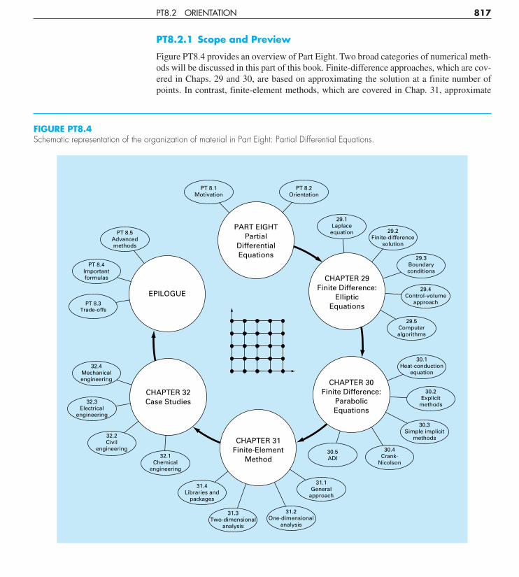
FIGURE PT8.4Schematic representation of the organization of material in Part Eight: Partial Differential Equations.

cha1873X_p08.qxd 5/2/05 3:59 PM Page 817

the solution in pieces, or “elements.” Various parameters are adjusted until these approxi-mations conform to the underlying differential equation in an optimal sense.

Chapter 29 is devoted to finite-difference solutions of elliptic equations. Beforelaunching into the methods, we derive the Laplace equation for the physical problem con-text of the temperature distribution for a heated plate. Then, a standard solution approach,the Liebmann method, is described. We will illustrate how this approach is used to computethe distribution of the primary scalar variable, temperature, as well as a secondary vectorvariable, heat flux. The final section of the chapter deals with boundary conditions. Thismaterial includes procedures to handle different types of conditions as well as irregularboundaries.

In Chap. 30, we turn to finite-difference solutions of parabolic equations. As with thediscussion of elliptic equations, we first provide an introduction to a physical problem con-text, the heat-conduction equation for a one-dimensional rod. Then we introduce both ex-plicit and implicit algorithms for solving this equation. This is followed by an efficient andreliable implicit method—the Crank-Nicolson technique. Finally, we describe a particu-larly effective approach for solving two-dimensional parabolic equations—the alternating-direction implicit, or ADI, method.

Note that, because they are somewhat beyond the scope of this book, we have chosento omit hyperbolic equations. The epilogue of this part of the book contains references re-lated to this type of PDE.

In Chap. 31, we turn to the other major approach for solving PDEs—the finite-elementmethod. Because it is so fundamentally different from the finite-difference approach, wedevote the initial section of the chapter to a general overview. Then we show how thefinite-element method is used to compute the steady-state temperature distribution of aheated rod. Finally, we provide an introduction to some of the issues involved in extendingsuch an analysis to two-dimensional problem contexts.

Chapter 32 is devoted to applications from all fields of engineering. Finally, a short re-view section is included at the end of Part Eight. This epilogue summarizes important in-formation related to PDEs. This material includes a discussion of trade-offs that are rele-vant to their implementation in engineering practice. The epilogue also includes referencesfor advanced topics.

PT8.2.2 Goals and Objectives

Study Objectives. After completing Part Eight, you should have greatly enhanced yourcapability to confront and solve partial differential equations. General study goals shouldinclude mastering the techniques, having the capability to assess the reliability of the an-swers, and being able to choose the “best’’ method (or methods) for any particular problem.In addition to these general objectives, the specific study objectives in Table PT8.2 shouldbe mastered.

Computer Objectives. Computer algorithms can be developed for many of the methodsin Part Eight. For example, you may find it instructive to develop a general program to sim-ulate the steady-state distribution of temperature on a heated plate. Further, you might wantto develop programs to implement both the simple explicit and the Crank-Nicolson meth-ods for solving parabolic PDEs in one spatial dimension.

818 PARTIAL DIFFERENTIAL EQUATIONS

cha1873X_p08.qxd 5/2/05 3:59 PM Page 818

PT8.2 ORIENTATION 819

TABLE PT8.2 Specific study objectives for Part Eight.

1. Recognize the difference between elliptic, parabolic, and hyperbolic PDEs.2. Understand the fundamental difference between finite-difference and finite-element approaches.3. Recognize that the Liebmann method is equivalent to the Gauss-Seidel approach for solving

simultaneous linear algebraic equations.4. Know how to determine secondary variables for two-dimensional field problems.5. Recognize the distinction between Dirichlet and derivative boundary conditions.6. Understand how to use weighting factors to incorporate irregular boundaries into a finite-difference

scheme for PDEs.7. Understand how to implement the control-volume approach for implementing numerical solutions

of PDEs.8. Know the difference between convergence and stability of parabolic PDEs.9. Understand the difference between explicit and implicit schemes for solving parabolic PDEs.

10. Recognize how the stability criteria for explicit methods detract from their utility for solvingparabolic PDEs.

11. Know how to interpret computational molecules.12. Recognize how the ADI approach achieves high efficiency in solving parabolic equations in two

spatial dimensions.13. Understand the difference between the direct method and the method of weighted residuals for deriving

element equations.14. Know how to implement Galerkin’s method.15. Understand the benefits of integration by parts during the derivation of element equations; in particular,

recognize the implications of lowering the highest derivative from a second to a first derivative.

Finally, one of your most important goals should be to master several of the general-purpose software packages that are widely available. In particular, you should becomeadept at using these tools to implement numerical methods for engineering problemsolving.

cha1873X_p08.qxd 5/2/05 3:59 PM Page 819