Parallelization Schemes for Memory Optimization on theCell Processor : A Case Study on the Harris Corner

Detector

Tarik Saidani, Lionel Lacassagne, Joel Falcou, Claude Tadonki, and Samir Bouaziz

Institut d’Electronique FondamentaleUniversite de Paris Sud

91405 Orsay CedexFrance

Abstract. The Cell processor is a typical example of a heterogeneous multiprocessor on-chip architecture that uses several levels of parallelism to deliver high performance. Reducingthe gap between peak performance and effective performance is the challenge for softwaretool developers and the application developers. Image processing and media applications aretypical “main stream” applications. We use the Harris algorithm for the detection of interestpoints in an image as a benchmark to compare the performance of several parallel schemeson a Cell processor. The impact of the DMA controlled data transfers and the synchro-nizations between SPEs explains the differences between the performance of the differentparallelization schemes. The scalability of the architecture is modeled and evaluated.

1 Introduction

Image processing applications are generally composed of a set of basic operators. These com-ponents can be point to point operators or convolution kernels. Due to both computation andmemory complexity, real-time execution of image processing algorithms has historically not beeneasily done efficiently. Multi-core processors family appeared to respond to an increasing demandof processing power that single-task scalar systems, which raised computing and energy efficiencyproblems, could not satisfy. Furthermore, computing and transfer workloads can be distributedon the multiple processing units to reduce the processing time, in particular for media process-ing application which are well suited for the multiple levels of parallelism provided by parallelarchitectures.

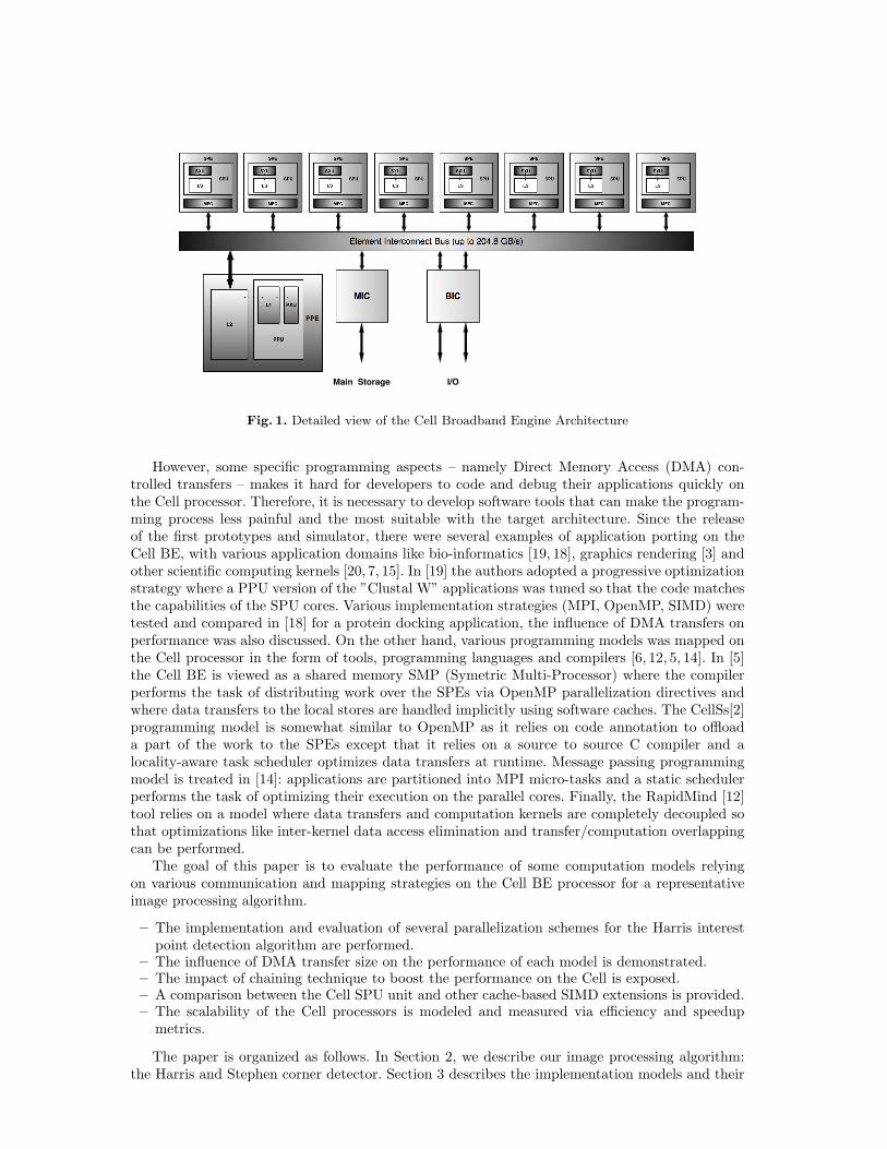
The Cell processor [16] is a good example of a heterogeneous multi-processor (Fig. 1). Com-posed of a 64-bit power processor element (PPE), eight specialized units called synergistic proces-sors (SPE) and a high bandwidth bus called Element Interconnect Bus (EIB), that allows com-munications between the different components [9], The Cell is a heterogeneous, multi-core chipcontaining several levels of parallelism that can be exploited to reach high peak performances.Assuming a clock speed of 3.2 Ghz, the Cell processor has a theoretical peak performance of 204.8GFlops/s in single precision. The EIB is composed of four 128-bit rings, each ring can handle upto three concurrent transfers. The theoretical peak bandwidth of the bus is 204.8 GBytes/s forinternal transfers, when performing 8 simultaneous non-colliding 25.6 GB/s transfers (the Cellnetwork topology allows only 8 transfers to be done in parallel without collision). The PPE unit isa traditional 64-bit PowerPC Processor with a vector multimedia extension (VMX aka Altivec).This Cell’s main processor is in charge of running the OS, and coordinating the SPEs. Each SPEconsists in a synergistic processor unit (SPU) and a Memory Flow Controller (MFC). The SPEholds a local storage (LS) of 256 KB, and a 128-bit SWAR (very close to Altivec) unit dedicatedto high-performance data-intensive computation. The MFC holds a 1D DMA controller, that is incharge of transferring data from external devices to the local store, or writing back computationresults to main memory. One of the main characteristics of the Cell processor is its distributedmemory hierarchy. The main drawback of this kind of memory, is that the software must handlethe limited size of the LS of each SPE, by issuing DMA transfers from or toward main storage(MS).

L2

MIC BIC

Main Storage I/O

PPE

Element Interconnect Bus (up to 204.8 GB/s)

Fig. 1. Detailed view of the Cell Broadband Engine Architecture

However, some specific programming aspects – namely Direct Memory Access (DMA) con-trolled transfers – makes it hard for developers to code and debug their applications quickly onthe Cell processor. Therefore, it is necessary to develop software tools that can make the program-ming process less painful and the most suitable with the target architecture. Since the releaseof the first prototypes and simulator, there were several examples of application porting on theCell BE, with various application domains like bio-informatics [19, 18], graphics rendering [3] andother scientific computing kernels [20, 7, 15]. In [19] the authors adopted a progressive optimizationstrategy where a PPU version of the ”Clustal W” applications was tuned so that the code matchesthe capabilities of the SPU cores. Various implementation strategies (MPI, OpenMP, SIMD) weretested and compared in [18] for a protein docking application, the influence of DMA transfers onperformance was also discussed. On the other hand, various programming models was mapped onthe Cell processor in the form of tools, programming languages and compilers [6, 12, 5, 14]. In [5]the Cell BE is viewed as a shared memory SMP (Symetric Multi-Processor) where the compilerperforms the task of distributing work over the SPEs via OpenMP parallelization directives andwhere data transfers to the local stores are handled implicitly using software caches. The CellSs[2]programming model is somewhat similar to OpenMP as it relies on code annotation to offloada part of the work to the SPEs except that it relies on a source to source C compiler and alocality-aware task scheduler optimizes data transfers at runtime. Message passing programmingmodel is treated in [14]: applications are partitioned into MPI micro-tasks and a static schedulerperforms the task of optimizing their execution on the parallel cores. Finally, the RapidMind [12]tool relies on a model where data transfers and computation kernels are completely decoupled sothat optimizations like inter-kernel data access elimination and transfer/computation overlappingcan be performed.

The goal of this paper is to evaluate the performance of some computation models relyingon various communication and mapping strategies on the Cell BE processor for a representativeimage processing algorithm.

– The implementation and evaluation of several parallelization schemes for the Harris interestpoint detection algorithm are performed.

– The influence of DMA transfer size on the performance of each model is demonstrated.– The impact of chaining technique to boost the performance on the Cell is exposed.– A comparison between the Cell SPU unit and other cache-based SIMD extensions is provided.– The scalability of the Cell processors is modeled and measured via efficiency and speedup

metrics.

The paper is organized as follows. In Section 2, we describe our image processing algorithm:the Harris and Stephen corner detector. Section 3 describes the implementation models and their

comparative performances. In Section 4 we model and evaluate the Cell scalability. Finally, wesum up our main contributions and discuss future work in Section 5.

2 The Harris Interest Point Detection Algorithm

Harris and Stephen [8] interest point detection algorithm is used in computer vision systems forfeature extraction like motion detection, image matching, tracking, 3D reconstruction and objectrecognition. This algorithm was proposed to address the limitations of the Moravec corner detector[13] which was sensitive to noise and not rotationally invariant. A corner can be defined as theintersection of two edges when an interest point can be defined as a point which has a well definedposition and can be robustly detected. Hence, the interest point can be a corner but also anisolated point of local intensity maximum or minimum, a line ending, or a point on a curve wherethe curvature is locally maximal.

2.1 Algorithm description

Assuming image patches of dimensions u×v (in our case 3×3) in a grayscale 2-dimensional imageI and shifting it by (x, y), the Harris operator is based on the estimation of local autocorrelationS for which the expression is:

S(x, y) =∑

u

∑v

w(u, v) (I(u, v)− I(u− x, v − y))2 (1)

By approximating S with a second order Taylor series expansion the Harris matrix M is given by:

M =∑

u

∑v

w(u, v)[I2x IxIy

IxIy I2y

](2)

An interest point is characterized by a large variation of S in all directions of the vector (x, y). Byanalyzing the eigenvalues of M , this characterization can be expressed in the following way. Letλ1, λ2 be the eigenvalues on the matrix M :

1. If λ1 ≈ 0 and λ2 ≈ 0 then there are no features of interest at this pixel (x, y).2. If λ1 ≈ 0 and λ2 is some large positive value, then an edge is found.3. If λ1 and λ2 are both large, distinct positive values, then a corner is found.

Harris and Stephens note that eigenvalues computation is expensive, since it requires the compu-tation of a square root, and instead suggest the following algorithm:

1. For each pixel (x, y) in the image compute the autocorrelation matrix M :

M =[Sxx Sxy

Sxy Syy

]; where:Sxx =

(∂I

∂x

)2

⊗ w, Syy =(∂I

∂y

)2

⊗ w, Sxy =(∂I

∂x

∂I

∂y

)⊗ w (3)

Where ⊗ is the convolution operator and w a Gaussian kernel.

2. Construct the coarsity map by calculating the coarsity measure C(x, y) for each pixel (x, y),with k being a empirically determined constant:

C(x, y) = det(M)− k(trace(M))2

det(M) = Sxx · Syy − S2xy

trace(M) = Sxx + Syy

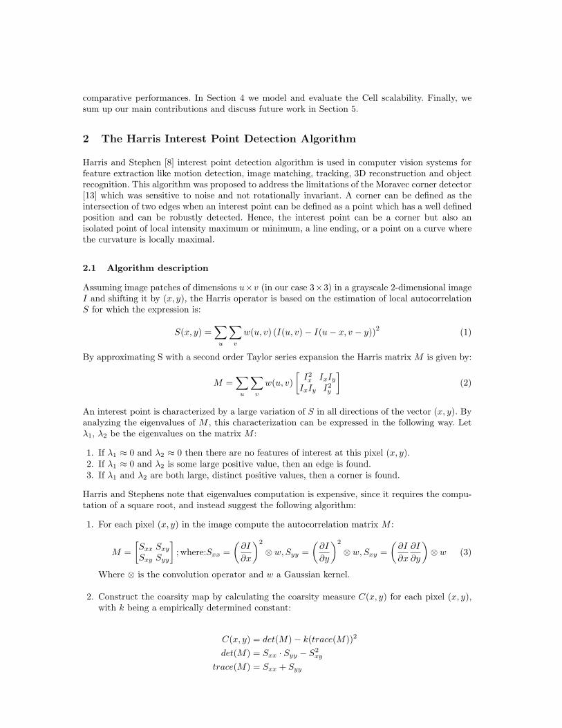
An illustration of an input 512×512 grayscale image and a interest point detection on it aregiven in Fig. 2. To obtain this result, two additional steps are performed in order to extract visuallyappealing information from the dense coarsity matrix1. Those steps are:

1. Threshold the interest map by setting all C(x, y) below a given threshold T to zero.2. Local maxima are then extracted by filtering points which are greater than all the points in a

3× 3 neighborhood.

Fig. 2. Illustration of the interest point detection on a grayscale 512×512 image

2.2 Implementation Details

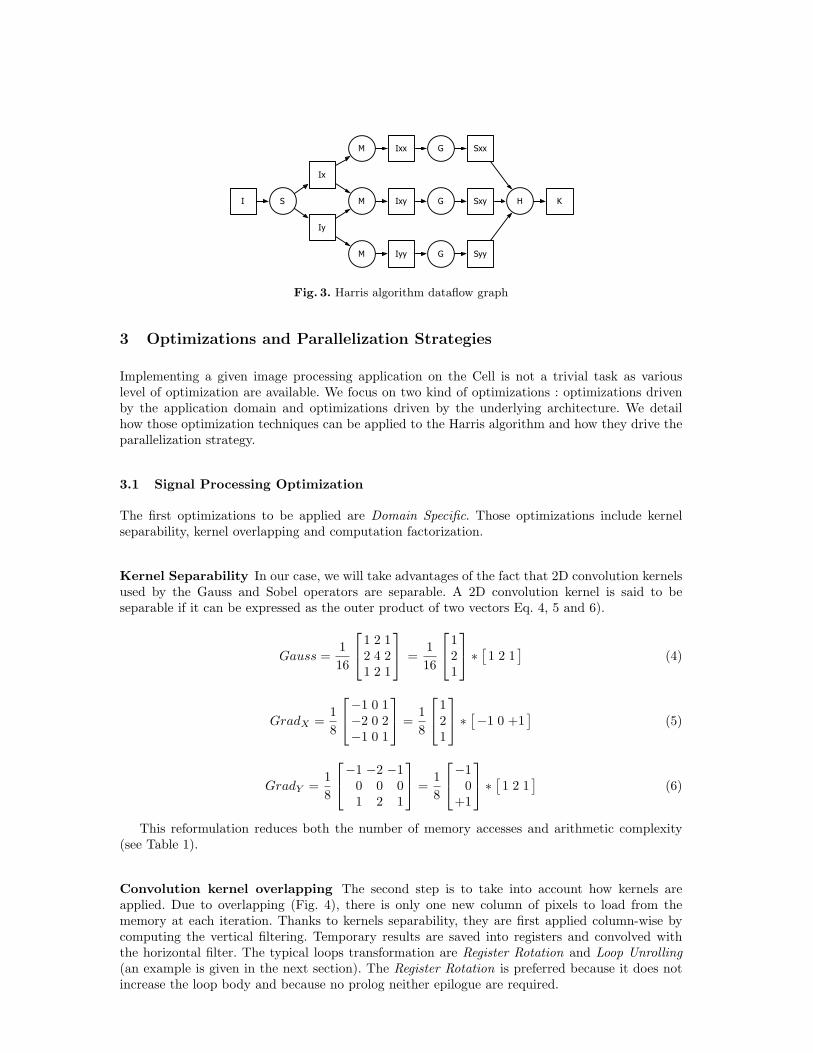
Grayscale 2-dimensional image pixels are typically 8-bit unsigned integers and the Harris algorithmoutput is in this case a 32-bit signed integer. However, because of the limitations of the Cell SPUISA, and in order to guarantee a fair comparison between Altivec, SSE and Cell SPU, we chose thesingle precision floating point format for both input pixels and the output of the Harris operator.In our implementation of the Harris operator we divided the algorithm into four computationkernels: a Sobel operator representing the derivative in the horizontal and vertical directions,a multiplication operator, a Gaussian smoothing operator (w in Eq. 2) followed by a coarsitycomputation. In our implementation the k constant in Eq. 4 is fixed to 0 as it does not changethe qualitative results. This leads to the data flow graph given in Fig. 3 which is representative oftypical image processing algorithms as it includes convolution kernels and point to point operatorsand in which the Sobel operator convolution kernels (one for horizontal gradient (GradX) andone for the vertical gradient (GradY )) and the Gauss smoothing kernel Gauss are defined by :

GradX =18

−1 0 1−2 0 2−1 0 1

;GradY =18

−1 −2 −10 0 01 2 1

;Gauss =116

1 2 12 4 21 2 1

The convolution kernels computation consist in centering the kernel on a pixel and computing

the cumulated sum of the point to point product of the kernel elements with the image patchsurrounding the central pixel. Hence, the Harris algorithm can be considered as a memory boundedproblem since this kind of operators are great bandwidth consumers as they consume more elementsthan they produce. For this reason we chose to perform memory access optimizations at severallevels of the Cell processor memory hierarchy.1 As those steps are merely cosmetic, we will not consider them as part of the algorithmic chain.

I S

Iy

Ix

M

M

M

Sxx

Sxy

Syy

H K

Ixx

Ixy

Iyy

G

G

G

Fig. 3. Harris algorithm dataflow graph

3 Optimizations and Parallelization Strategies

Implementing a given image processing application on the Cell is not a trivial task as variouslevel of optimization are available. We focus on two kind of optimizations : optimizations drivenby the application domain and optimizations driven by the underlying architecture. We detailhow those optimization techniques can be applied to the Harris algorithm and how they drive theparallelization strategy.

3.1 Signal Processing Optimization

The first optimizations to be applied are Domain Specific. Those optimizations include kernelseparability, kernel overlapping and computation factorization.

Kernel Separability In our case, we will take advantages of the fact that 2D convolution kernelsused by the Gauss and Sobel operators are separable. A 2D convolution kernel is said to beseparable if it can be expressed as the outer product of two vectors Eq. 4, 5 and 6).

Gauss =116

1 2 12 4 21 2 1

=116

121

∗ [1 2 1]

(4)

GradX =18

−1 0 1−2 0 2−1 0 1

=18

121

∗ [−1 0 +1]

(5)

GradY =18

−1 −2 −10 0 01 2 1

=18

−10

+1

∗ [1 2 1]

(6)

This reformulation reduces both the number of memory accesses and arithmetic complexity(see Table 1).

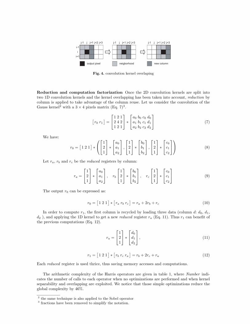
Convolution kernel overlapping The second step is to take into account how kernels areapplied. Due to overlapping (Fig. 4), there is only one new column of pixels to load from thememory at each iteration. Thanks to kernels separability, they are first applied column-wise bycomputing the vertical filtering. Temporary results are saved into registers and convolved withthe horizontal filter. The typical loops transformation are Register Rotation and Loop Unrolling(an example is given in the next section). The Register Rotation is preferred because it does notincrease the loop body and because no prolog neither epilogue are required.

jj-1 j+1 j+2 j+3

i

i-1

i+1

jj-1 j+1 j+2 j+3 jj-1 j+1 j+2 j+3

output pixel neigborhood new column

Fig. 4. convolution kernel overlaping

Reduction and computation factorization Once the 2D convolution kernels are split intotwo 1D convolution kernels and the kernel overlapping has been taken into account, reduction bycolumn is applied to take advantage of the column reuse. Let us consider the convolution of theGauss kernel2 with a 3× 4 pixels matrix (Eq. 7)3.

[r0 r1

]=

1 2 12 4 21 2 1

∗a0 b0 c0 d0

a1 b1 c1 d1

a2 b2 c2 d2

(7)

We have:

r0 =[

1 2 1]∗

121

∗a0

a1

a2

,1

21

∗ b0b1b2

,1

21

∗ c0c1c2

(8)

Let ra, rb and rc be the reduced registers by column:

ra =

121

∗a0

a1

a2

, rb

121

∗ b0b1b2

, rc

121

∗ c0c1c2

(9)

The output r0 can be expressed as:

r0 =[

1 2 1]∗[ra rb rc

]= ra + 2rb + rc (10)

In order to compute r1, the first column is recycled by loading three data (column d: d0, d1,d2 ), and applying the 1D kernel to get a new reduced register ra (Eq. 11). Thus r1 can benefit ofthe previous computations (Eq. 12).

ra =

121

∗d0

d1

d2

, (11)

r1 =[

1 2 1]∗[rb rc ra

]= rb + 2rc + ra (12)

Each reduced register is used thrice, thus saving memory accesses and computations.

The arithmetic complexity of the Harris operators are given in table 1, where Number indi-cates the number of calls to each operator when no optimizations are performed and when kernelseparability and overlapping are exploited. We notice that those simple optimizations reduce theglobal complexity by 46%.

2 the same technique is also applied to the Sobel operator3 fractions have been removed to simplify the notation.

Operator Number MUL ADD Total

Complexity without optimization

Sobel 2 3 5 16

Mul 3 1 0 3

Gauss 3 6 8 42

Coarsity 1 2 1 3

Total - 29 35 64

Complexity with optimizations

Sobel 2 0 5 10

Mul 3 1 0 3

Gauss 3 0 6 18

Coarsity 1 2 1 3

Total - 4 30 34

Table 1. arithmetic operator complexity with/without optmizations

Temporal Pipelining In a producer-consumer point of view, there are actually two kind ofoperators in the Harris operator, each having a specific memory access pattern:

– point to point operators, like the Multiplication and the Coarsity operators, that consume a1× 1 data to produce a 1× 1 data.

– 3×3 convolution kernels, like the Sobel gradients (GradX and GradY ) and the Gauss smootherthat consumes 3× 3 data and produces a 1× 1 data (Fig. 5)

A B(1x1) (1x1)

(3x3)(1x1)

: data

: operator

point to point operator convolution kernel

Fig. 5. producer-consumer model: memory access pattern for point operator and convolution kernel

The Temporal pipelining optimization consists in chaining operators together by adapting theirmemory access patterns in order to remove the intermediate LOAD/STORE instructions.

Figure 6 sums up the various pipelining rules. In rule 1, the output pattern of the first operatoralready fit the input pattern. No pattern adaptation is required before removing the intermediatememory access. For rule 2 : there is nothing to do for pipelining a 3 × 3 convolution kernel witha point operator. But permuting point operator and convolution kernel (rule 3) requires unrollingthe first operator in order to adapt the pattern. In that case the first operator should be unrolledthrice in both dimensions. The last rule is the pipelining of two 3× 3 convolution kernels (rule 4).As for the third rule, the first operator should be unrolled 3× 3 times. The big difference in thatcase is that the new input pattern is 5× 5, that requires 25 registers just to hold the loaded data.One possible drawback of this pipelining is spill code if the compiler runs out of register. The lastpoint about pipelining is to see the Sobel gradient operator as one operator instead of two: 3× 3points are loaded only one time but consumed twice to produce two points, one for GradX andone for GradY .

Benefits of Domain Specific Optimizations The leading idea of all those optimizations is toreduce complexity. This can be done by both the reduction of the number of computations per

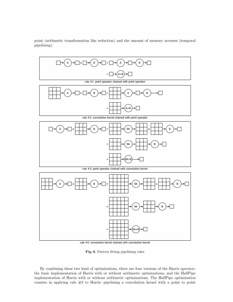
point (arithmetic transformation like reduction) and the amount of memory accesses (temporalpipelining).

A o B = A B

= A+B

A o B = BA

= A+B

BoA = 9A Bo

= 9A B

= 9A+B

BoA = 9A Bo

= 9A B

= 9A+B

rule #1: point operator chained with point operator

rule #2: convolution kernel chained with point operator

rule #3: point operator chained with convolution kernel

rule #4: convolution kernel chained with convolution kernel

Fig. 6. Pattern fitting pipelining rules

By combining these two kind of optimizations, there are four versions of the Harris operator:the basic implementation of Harris with or without arithmetic optimizations, and the HalfPipeimplementation of Harris with or without arithmetic optimizations. The HalfPipe optimizationconsists in applying rule #2 to Harris: pipelining a convolution kernel with a point to point

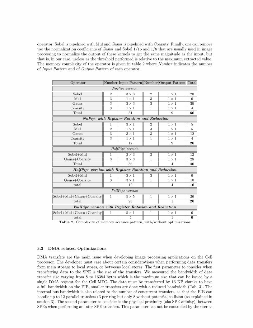
operator: Sobel is pipelined with Mul and Gauss is pipelined with Coarsity. Finally, one can removetoo the normalization coefficients of Gauss and Sobel 1/16 and 1/8 that are usually used in imageprocessing to normalize the output of these kernels to get the same magnitude as the input, butthat is, in our case, useless as the threshold performed is relative to the maximum extracted value.The memory complexity of the operator is given in table 2 where Number indicates the numberof Input Pattern and of Output Pattern of each operator.

Operator Number Input Pattern Number Output Pattern Total

NoPipe version

Sobel 2 3× 3 2 1× 1 20

Mul 3 1× 1 3 1× 1 6

Gauss 3 3× 3 3 1× 1 30

Coarsity 3 1× 1 1 1× 1 4

Total 51 9 60

NoPipe with Register Rotation and Reduction

Sobel 1 3× 1 2 1× 1 5

Mul 2 1× 1 3 1× 1 5

Gauss 3 3× 1 3 1× 1 12

Coarsity 3 1× 1 1 1× 1 4

Total 17 9 26

HalfPipe version

Sobel+Mul 1 3× 3 3 1× 1 12

Gauss+Coarsity 3 3× 3 1 1× 1 28

Total 36 4 40

HalfPipe version with Register Rotation and Reduction

Sobel+Mul 1 3× 1 3 1× 1 6

Gauss+Coarsity 3 3× 1 1 1× 1 10

total 12 4 16

FullPipe version

Sobel+Mul+Gauss+Coarsity 1 5× 5 1 1× 1 26

total 25 1 26

FullPipe version with Register Rotation and Reduction

Sobel+Mul+Gauss+Coarsity 1 5× 1 1 1× 1 6

total 5 1 6

Table 2. Complexity of memory accesses pattern, with/without optimizations

3.2 DMA related Optimizations

DMA transfers are the main issue when developing image processing applications on the Cellprocessor. The developer must care about certain considerations when performing data transfersfrom main storage to local stores, or betweens local stores. The first parameter to consider whentransferring data to the SPE is the size of the transfers. We measured the bandwidth of datatransfer size varying from 8 to 16384 bytes which is the maximum size that can be issued by asingle DMA request for the Cell MFC. The data must be transferred by 16 KB chunks to havea full bandwidth on the EIB, smaller transfers are done with a reduced bandwidth (Tab. 3). Theinternal bus bandwidth is also related to the number of concurrent transfers, as that the EIB canhandle up to 12 parallel transfers (3 per ring but only 8 without potential collision (as explained insection 3). The second parameter to consider is the physical proximity (aka SPE affinity), betweenSPEs when performing an inter-SPE transfers. This parameter can not be controlled by the user as

the task of scheduling tasks on SPEs is done by the kernel scheduler. Finally, data being transferedmust be contiguous in memory4. Those limitations have a big impact on the tiling strategy. Aslocal store has only 256 KB to hold both code and data, large amounts of data being processedhave to be split into tiles which size is compatible with the memory available on the SPEs andcompatible with the maximal size of a DMA transfer.

Size (B) Agg BW (GB/s) Size (B) Agg BW (GB/s)

8 0.92 512 47.92

16 1.86 1024 72.57

32 3.72 2048 86.48

64 7.42 4096 94.09

128 14.87 8192 97.72

256 27.37 16384 104.10

Table 3. Aggregate bandwidth for inter-SPE DMA transfers with 8 SPE transferring concurrently on aQS20 Blade

3.3 Parallel Implementations

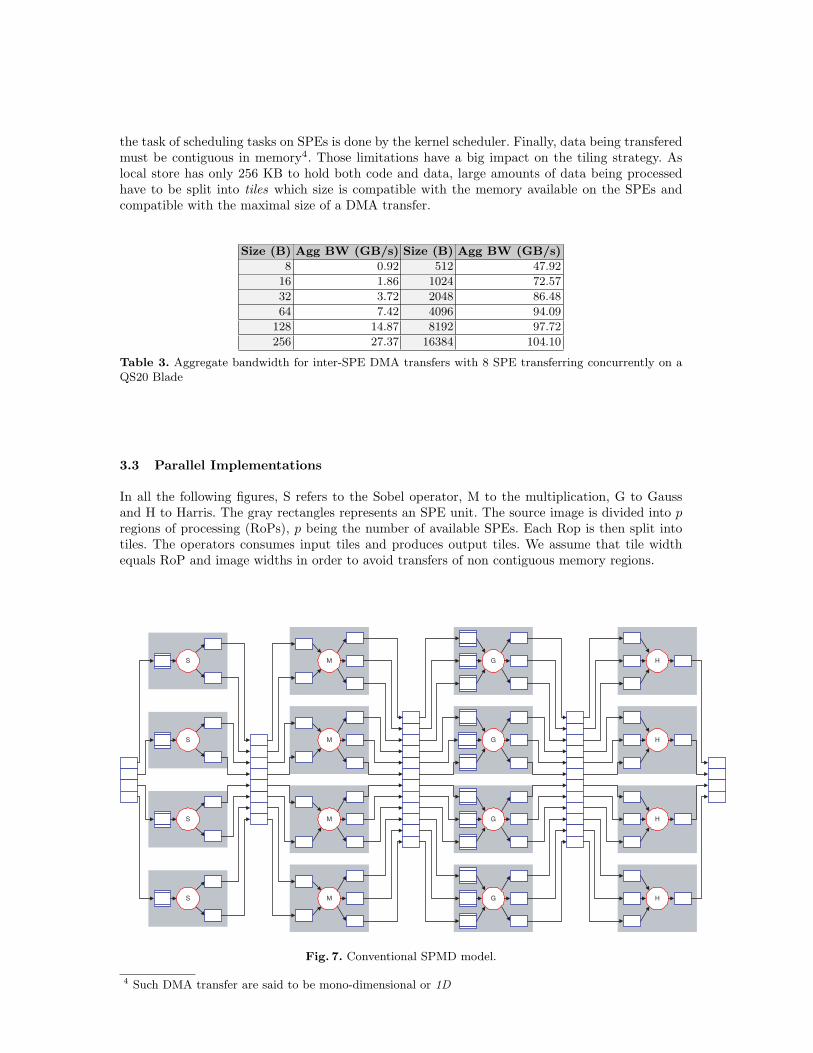
In all the following figures, S refers to the Sobel operator, M to the multiplication, G to Gaussand H to Harris. The gray rectangles represents an SPE unit. The source image is divided into pregions of processing (RoPs), p being the number of available SPEs. Each Rop is then split intotiles. The operators consumes input tiles and produces output tiles. We assume that tile widthequals RoP and image widths in order to avoid transfers of non contiguous memory regions.

MS HG

MS HG

MS HG

MS HG

Fig. 7. Conventional SPMD model.

4 Such DMA transfer are said to be mono-dimensional or 1D

Conventional SPMD The conventional SPMD programming model (Fig. 7) equally dividesthe image into 8 RoPs, mapped on the SPEs (in the figure, only 4 SPEs are drawn to get asmaller figure, but 8 SPEs are actually used). All SPUs execute the same program/code.The PPUlets the SPUs run one operator on the whole image before proceeding with the next operator. Forexample, it will not issue the command for Multiplication operator until all the SPEs have finishedperforming the Sobel operator and the whole of the image has been transfered back into the MS.

I

Ix

Iy

S

G SxxIxx

tile

Ix

Ix

M Ixx

Ix

Iy

M Ixy

Iy

Iy

M Iyy

G SxxIxx

G SxxIxx

Sxx

Syy

H KSxy tile

stage 1 stage 2 stage 3 stage 4

SPE #0

SPE #1

SPE #2

SPE #3

SPE #4

SPE #5

SPE #6

SPE #7

Fig. 8. Conventional pipeline model.

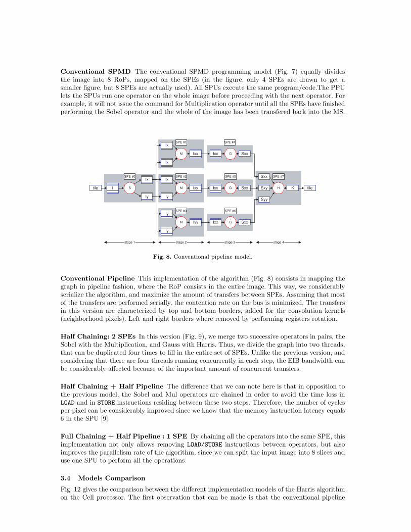
Conventional Pipeline This implementation of the algorithm (Fig. 8) consists in mapping thegraph in pipeline fashion, where the RoP consists in the entire image. This way, we considerablyserialize the algorithm, and maximize the amount of transfers between SPEs. Assuming that mostof the transfers are performed serially, the contention rate on the bus is minimized. The transfersin this version are characterized by top and bottom borders, added for the convolution kernels(neighborhood pixels). Left and right borders where removed by performing registers rotation.

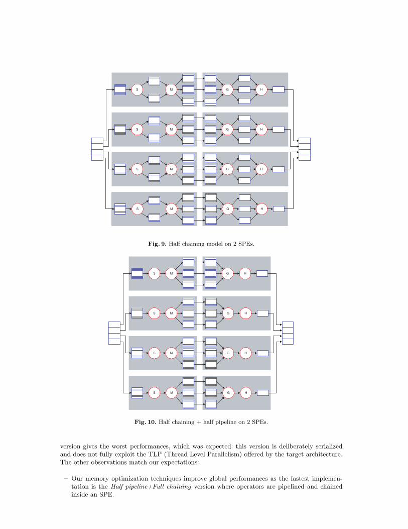
Half Chaining: 2 SPEs In this version (Fig. 9), we merge two successive operators in pairs, theSobel with the Multiplication, and Gauss with Harris. Thus, we divide the graph into two threads,that can be duplicated four times to fill in the entire set of SPEs. Unlike the previous version, andconsidering that there are four threads running concurrently in each step, the EIB bandwidth canbe considerably affected because of the important amount of concurrent transfers.

Half Chaining + Half Pipeline The difference that we can note here is that in opposition tothe previous model, the Sobel and Mul operators are chained in order to avoid the time loss inLOAD and in STORE instructions residing between these two steps. Therefore, the number of cyclesper pixel can be considerably improved since we know that the memory instruction latency equals6 in the SPU [9].

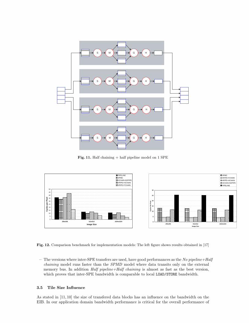
Full Chaining + Half Pipeline : 1 SPE By chaining all the operators into the same SPE, thisimplementation not only allows removing LOAD/STORE instructions between operators, but alsoimproves the parallelism rate of the algorithm, since we can split the input image into 8 slices anduse one SPU to perform all the operations.

3.4 Models Comparison

Fig. 12 gives the comparison between the different implementation models of the Harris algorithmon the Cell processor. The first observation that can be made is that the conventional pipeline

MS HG

MS HG

MS HG

MS HG

Fig. 9. Half chaining model on 2 SPEs.

MS HG

MS HG

MS HG

MS HG

Fig. 10. Half chaining + half pipeline on 2 SPEs.

version gives the worst performances, which was expected: this version is deliberately serializedand does not fully exploit the TLP (Thread Level Parallelism) offered by the target architecture.The other observations match our expectations:

– Our memory optimization techniques improve global performances as the fastest implemen-tation is the Half pipeline+Full chaining version where operators are pipelined and chainedinside an SPE.

MS HG

MS HG

MS HG

MS HG

Fig. 11. Half chaining + half pipeline model on 1 SPE

0

5

10

15

20

25

30

35

40

45

50

256x256 512x512 1024x1024

Image Size

Cyc

les

per

Pix

el

PIPELINESPMDHCHAIN-NOPIPEHPIPE+HCHAINHPIPE+FCHAIN

0

5

10

15

20

25

30

256x256 512x512 1024x1024

Image Size

Cyc

les

Per

Pix

el

SPMD

HPIPE+FCHAIN

HPIPE+HCHAIN

HCHAIN-NOPIPE

PIPELINE

Fig. 12. Comparison benchmark for implementation models: The left figure shows results obtained in [17]

– The versions where inter-SPE transfers are used, have good performances as the No pipeline+Halfchaining model runs faster than the SPMD model where data transits only on the externalmemory bus. In addition Half pipeline+Half chaining is almost as fast as the best version,which proves that inter-SPE bandwidth is comparable to local LOAD/STORE bandwidth.

3.5 Tile Size Influence

As stated in [11, 10] the size of transfered data blocks has an influence on the bandwidth on theEIB. In our application domain bandwidth performance is critical for the overall performance of

16KB 16KB 16KB8KB 8KB 8KB

4KB 4KB 4KB

2KB 2KB 2KB

0

2

4

6

8

10

12

14

16

18

256x256 512x512 1024x1024Image Size

Cyc

les

per

Pix

el

16K

16K

16K

8K

8K

8K

4K

4K

4K

0

5

10

15

20

25

30

35

40

256x256 512x512 1024x1024

Image Size

Cyc

les

Per

Pix

el

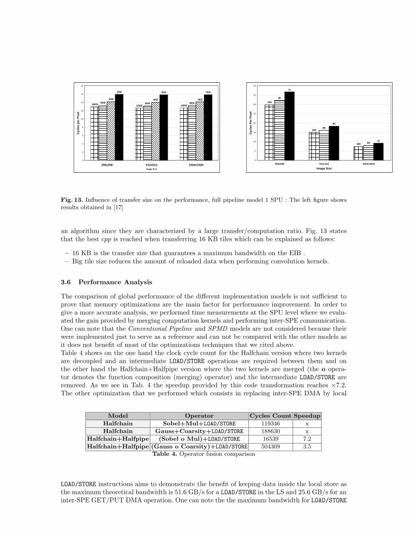
Fig. 13. Influence of transfer size on the performance, full pipeline model 1 SPU : The left figure showsresults obtained in [17]

an algorithm since they are characterized by a large transfer/computation ratio. Fig. 13 statesthat the best cpp is reached when transferring 16 KB tiles which can be explained as follows:

– 16 KB is the transfer size that guarantees a maximum bandwidth on the EIB .– Big tile size reduces the amount of reloaded data when performing convolution kernels.

3.6 Performance Analysis

The comparison of global performance of the different implementation models is not sufficient toprove that memory optimizations are the main factor for performance improvement. In order togive a more accurate analysis, we performed time measurements at the SPU level where we evalu-ated the gain provided by merging computation kernels and performing inter-SPE communication.One can note that the Conventional Pipeline and SPMD models are not considered because theirwere implemented just to serve as a reference and can not be compared with the other models asit does not benefit of most of the optimizations techniques that we cited above.Table 4 shows on the one hand the clock cycle count for the Halfchain version where two kernelsare decoupled and an intermediate LOAD/STORE operations are required between them and onthe other hand the Halfchain+Halfpipe version where the two kernels are merged (the o opera-tor denotes the function composition (merging) operator) and the intermediate LOAD/STORE areremoved. As we see in Tab. 4 the speedup provided by this code transformation reaches ×7.2.The other optimization that we performed which consists in replacing inter-SPE DMA by local

Model Operator Cycles Count Speedup

Halfchain Sobel+Mul+LOAD/STORE 119346 x

Halfchain Gauss+Coarsity+LOAD/STORE 188630 x

Halfchain+Halfpipe (Sobel o Mul)+LOAD/STORE 16539 7.2

Halfchain+Halfpipe (Gauss o Coarsity)+LOAD/STORE 504309 3.5Table 4. Operator fusion comparison

LOAD/STORE instructions aims to demonstrate the benefit of keeping data inside the local store asthe maximum theoretical bandwidth is 51.6 GB/s for a LOAD/STORE in the LS and 25.6 GB/s for aninter-SPE GET/PUT DMA operation. One can note the the maximum bandwidth for LOAD/STORE

in Tab. 5 computed assuming that there is 1 instruction issued each cycle (pipelined execution)for a clock frequency of 3.2 Ghz. The same assumption was made in [10] for the LS bandwidthmeasurement. On the other hand, we used the IBM Performance Debugging Tool (PDT) to mea-sure the average effective DMA bandwidth the result is given in Tab. 5. We observe that thereis an order of magnitude between the two transfer rates which explains the difference in globalperformance between Halfchain and Fullchain versions. The measurements that we performed give

Model Communication Type Average Bandwidth GB/s

Halfchain inter-SPE DMA 6.95

Halfchain+Halfpipe LOAD/STORE 51.6Table 5. average bandwidth comparison between models

a more precise view of the factors that influence the global performance of the different implemen-tations. Merging computation kernels, reduces the memory complexity by maximizing the reuseof register to perform intermediate computations. However, this optimization should be used withcare as there is a limited amount of available register to store intermediate results (128 for theSPU). On the other hand, keeping data in the local store whenever it is possible is a good practiceas the LOAD/STORE bandwidth is higher than inter-SPE DMA bandwidth. This last optimizationincreases data locality and thus global performance but is limited by the available memory space(256 KB for the SPE local store).

3.7 Comparison between the SPU and General Purpose Processors (GPP) withSIMD extensions

0

5

10

15

20

25

30

35

40

45

256x256 512x512 1024x1024

Image Size

Cyc

les

per

Pix

el

Cell SPU PowerPC 970 Intel Xeon

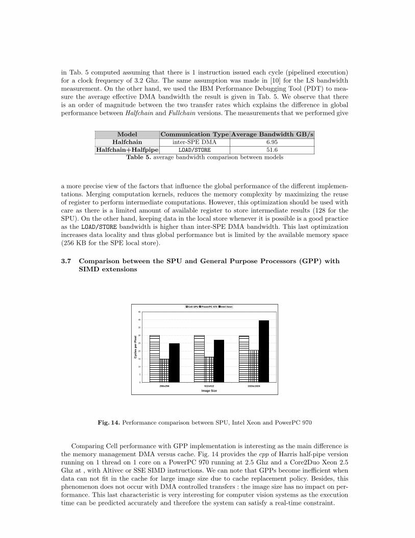
Fig. 14. Performance comparison between SPU, Intel Xeon and PowerPC 970

Comparing Cell performance with GPP implementation is interesting as the main difference isthe memory management DMA versus cache. Fig. 14 provides the cpp of Harris half-pipe versionrunning on 1 thread on 1 core on a PowerPC 970 running at 2.5 Ghz and a Core2Duo Xeon 2.5Ghz at , with Altivec or SSE SIMD instructions. We can note that GPPs become inefficient whendata can not fit in the cache for large image size due to cache replacement policy. Besides, thisphenomenon does not occur with DMA controlled transfers : the image size has no impact on per-formance. This last characteristic is very interesting for computer vision systems as the executiontime can be predicted accurately and therefore the system can satisfy a real-time constraint.

3.8 Discussion on Benchmarking Methodology

There are several reasons that justify the difference in performance results obtained above andthose in [17]:

1. Since we adopted a separated source compilation (one source for the PPU and one for theSPU), we were forced to change the compiler from IBM XLC (ppu-xlc, spu-xlc) to GCC (ppu-gcc, spu-gcc) as in the last release of the Cell SDK (3.0), the XLC compiler became exclusivelysingle-source. This first point can explain the difference in global performance as some compileroptimizations can be performed by XLC and not by GCC and vice versa.

2. The second reason concerns measurement methodology. In the [17] we measured the cyclescount in the PPE using the time base counter, with two versions of the code: the first oneincluding computation and the overhead related to thread creation and synchronization andthe other one without computation. Then we subtracted the second from the first to get thecomputation duration. These measures were performed over several runs, and the mean valuewas taken. However, data presented a great sensitivity to image size. In this paper we took amore representative case were we consider the input data coming from a continuous streamand we make the measure on the PPE with an additional outer loop in the SPEs to processmore than one image. This leads to a thread overhead becoming negligible when compared tothe pure processing time. As this time was subject to big variation in the [17] we chose thismethod to attenuate its effect.

3. The last reason is about the computation tiles. In [17], the tile size is fixed to 16K and its widthw always equals the image width W but its height h varies with W , typically h = 16K

w . Asstated in [1] h has an influence on the amount of reloaded data for a tile (when h increases thisamount decreases), we decided to adopt a new measurement methodology where we considera 16K tile with h and and w being constants (in our case h = 16 and w = 256) in orderto eliminate this perturbation. Hence, the cpp is less sensitive to image size, which is morecoherent as the tile size is a constant whatever the image size is. Table 6 gives the percentagesof reloaded data with different couples of (h,w). From these values, we conclude that theamount of reloaded data explains the great sensitivity to image size for the left histograms inFig. 12 and Fig. 13.

Image Size H ×W Tile Size h× w Total Reload Ratio %

256× 256 16× 256 11

512× 512 8× 512 20

1024× 1024 4× 1024 33Table 6. Illustration of the difference of the amount of reloaded data depending on the tile height for theHalfpipe+Halfchain model

4 Scalability Measure on the Cell Processor

In this section, we evaluate the scalability of the Cell processor by both measuring and modelingSpeedup and Efficiency metrics. The measurements provide informations on how the Cell archi-tecture scales to the Harris algorithms when varying the number of used SPUs. Modeling thosemetrics allows the prediction of scalability when considering future Cell generations with moreaccelerator units (SPUs).

Amdahl’s Law In the basic formulation of the Amdahl’s law the execution time of any algorithmon a sequential machine is divided into two parts: the time to execute the pure sequential part

of the code Seq0 and the time to execute the part of the code that is parallelizable Par0. For amachine containing p processors the execution time will have the following expression:

T (p) = Seq0 +Par0p

(13)

Driscoll and Daasch Reformulation The last formulation is not appropriate to predict per-formance on the Cell processor. The sequential portion of the code consisting in the cost of thethread creation, communications and synchronization of the threads. These parameters dependon the number of processors, namely they increase when the number of processors increases. Theparallel portion of the code is also a function of p. These assumptions was made in [4] by Driscollet al. We concluded after measurements that :

Seq(p) = asp+ bs (14)

andPar(p) = app+ bp (15)

Where as, bs, ap, bp are constants that we measured in our experiments. This leads to the followingexpression of the execution time:

T (p) = asp+ bs +app+ bp

p= asp+ bs + ap +

bpp

(16)

One of the main characteristics of parallel architectures that reflect there performance is theirscalability. Scalability metrics show how the system adapt to a certain workload when increasingthe number of processing units. Efficiency and Speedup are one of the basic metrics of scalability,they are defined by the following expressions:

E =Ts

pTp(17)

S =Ts

Tp(18)

Where Ts is the execution time on one processor , p the number of processors and Tp is theexecution time on p processors. If we replace Tp and Ts by the expression in Eq. 16 we find thefollowing expression of the efficiency:

E =as + bs + ap + bp

asp2 + (as + ap)p+ bp(19)

This leads to an efficiency decreasing when p increases. The expression of the speedup is of theform :

S =(as + bs + ap + bp)pasp2 + (as + ap)p+ bp

(20)

Which is also a decreasing function of p. One must know that that the expressions above wasevaluated when considering one input image for the algorithm.When processing an image stream which is typically captured by a video camera, we can considerthe cost of thread creation and synchronization (Seq(p) in the formulas) negligible comparing tothe parallel time (computation). We derive equations 21, 22 and 23 assuming that Seq(p) = 0

T (p) =Par(p)p

= ap +bpp

(21)

E =ap + bpapp+ bp

(22)

Speedup

0

1

2

3

4

5

6

7

8

9

0 2 4 6 8 10

P

S

Measured

Model

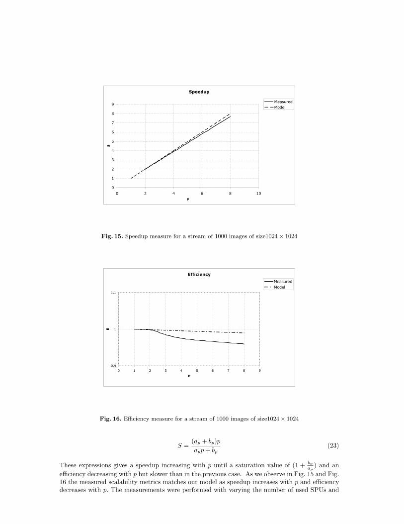
Fig. 15. Speedup measure for a stream of 1000 images of size1024× 1024

Efficiency

0,9

1

1,1

0 1 2 3 4 5 6 7 8 9

P

E

Measured

Model

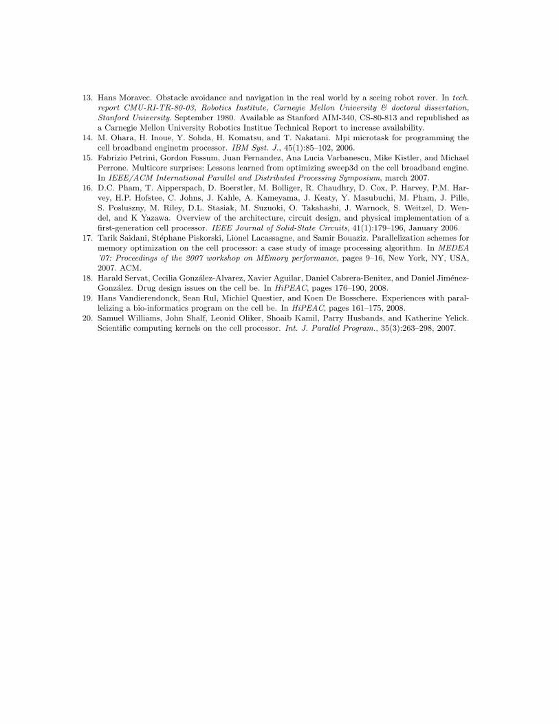
Fig. 16. Efficiency measure for a stream of 1000 images of size1024× 1024

S =(ap + bp)papp+ bp

(23)

These expressions gives a speedup increasing with p until a saturation value of (1 + bp

ap) and an

efficiency decreasing with p but slower than in the previous case. As we observe in Fig. 15 and Fig.16 the measured scalability metrics matches our model as speedup increases with p and efficiencydecreases with p. The measurements were performed with varying the number of used SPUs and

the execution time one SPU served as the sequential time Ts (T (p = 1)).From the experiments above we can conclude on how the Cell processor scales to our applicationwhich is a data-parallel/memory-bounded problem by making this two assertions:

– The current Cell processor with eight SPUs has a good scalability as the Speedup is close tothe number of the working SPUs and Efficiency is close to 1.

– In the future releases of the Cell where there would be more SPUs, scalability will not be asgood as we measured because an increasing number of cores leads to the decrease of Efficiencyand thus to a saturating Speedup.

5 Conclusion and Future Work

In this paper, we investigated how a sample image processing algorithm - the Harris corner detector- can be efficiently implemented while taking into account the various architectural particularitiesof this processor. We explore, contrary to previous works, other models than the simple SPMDparallelization technique. We explored a variety of parallelization schemes that took advantageof the main architectural features of the Cell: a DMA based, distributed memory. The differentoptimization techniques, Domain Specific or those related to the Cell architectures were analyzed.By combining each step of our algorithm in various manners, we demonstrated that chaining andpipelining operators had a large impact on global performance of the application. Our schemes werebenchmarked on the Harris corner detector because it features both point-to-point and convolutionoperations, making it a realistic sample of more complex image processing library. We also proposeda model of efficiency and scalability for the Cell processor in order to be able to predict performanceof future releases of the machine with a greater number of SPEs. Future works includes : a deeperanalysis of the relation between tiles shape and size and the overall algorithm performance. Otheroptimization techniques such as multi-buffering will be explored in the future.

References

1. 12th IEEE Real-Time and Embedded Technology and Applications Symposium (RTAS 2006), 4-7 April2006, San Jose, California, USA. IEEE Computer Society, 2006.

2. P. Bellens, J.M. Perez, , R.M. Badia, and J. Labarta. Cellss: a programming model for the cell bearchitecture. In in Proceedings of the ACM/IEEE Supercomputing Conference, 2006.

3. Carsten Benthin, Ingo Wald, Michael Scherbaum, and Heiko Friedrich. Ray tracing on the cell pro-cessor. In IEEE Symposium on Interactive Ray Tracing, 2006.

4. Michael A. Driscoll and W. Robert Daasch. Accurate predictions of parallel program execution time.J. Parallel Distrib. Comput., 25(1):16–30, 1995.

5. A. E. Eichenberger, J. K. O’Brien, K. M. O’Brien, P. Wu, T. Chen, P. H. Oden, D. A. Prener, J. C.Shepherd, B. So, Z. Sura, A. Wang, T. Zhang, P. Zhao, M. K. Gschwind, R. Archambault, Y. Gao,and R. Koo. Using advanced compiler technology to exploit the performance of the cell broadbandengineTM architecture. IBM Syst. J., 45(1):59–84, 2006.

6. Kayvon Fatahalian, Timothy J. Knight, and Mike Houston. Sequoia: Programming the memoryhierarchy. In Proceedings of the 2006 ACM/IEEE Conference on Supercomputing, 2006.

7. J. Greene and R Cooper. A parallel 64k complex fft algorithm for the ibm/sony/toshiba cell broadbandengine processor. In Global Signal Processing Expo, 2005.

8. C. Harris and M. Stephens. A combined corner and edge detector. In 4th ALVEY Vision Conference,1988.

9. IBM. Cell Broadband Engine Programming Handbook. IBM, version 1.0 edition, 2006.10. X. Ramirez A. Jimenez-Gonzalez, D. Martorell. Performance analysis of cell broadband engine for

high memory bandwidth applications. In in Proceedings of the IEEE International Symposium onPerformance Analysis of Systems & Software, 2007.

11. Michael Kistler, Michael Perrone, and Fabrizio Petrini. Cell multiprocessor communication network:Built for Speed. IEEE Micro, 26(3):10–23, 2006.

12. Michael D. McCool. Data-parallel programming on the cell be and the gpu using the rapidminddevelopment platform. In GSPx Multicore Applications Conference, 2006.

13. Hans Moravec. Obstacle avoidance and navigation in the real world by a seeing robot rover. In tech.report CMU-RI-TR-80-03, Robotics Institute, Carnegie Mellon University & doctoral dissertation,Stanford University. September 1980. Available as Stanford AIM-340, CS-80-813 and republished asa Carnegie Mellon University Robotics Institue Technical Report to increase availability.

14. M. Ohara, H. Inoue, Y. Sohda, H. Komatsu, and T. Nakatani. Mpi microtask for programming thecell broadband enginetm processor. IBM Syst. J., 45(1):85–102, 2006.

15. Fabrizio Petrini, Gordon Fossum, Juan Fernandez, Ana Lucia Varbanescu, Mike Kistler, and MichaelPerrone. Multicore surprises: Lessons learned from optimizing sweep3d on the cell broadband engine.In IEEE/ACM International Parallel and Distributed Processing Symposium, march 2007.

16. D.C. Pham, T. Aipperspach, D. Boerstler, M. Bolliger, R. Chaudhry, D. Cox, P. Harvey, P.M. Har-vey, H.P. Hofstee, C. Johns, J. Kahle, A. Kameyama, J. Keaty, Y. Masubuchi, M. Pham, J. Pille,S. Posluszny, M. Riley, D.L. Stasiak, M. Suzuoki, O. Takahashi, J. Warnock, S. Weitzel, D. Wen-del, and K Yazawa. Overview of the architecture, circuit design, and physical implementation of afirst-generation cell processor. IEEE Journal of Solid-State Circuits, 41(1):179–196, January 2006.

17. Tarik Saidani, Stephane Piskorski, Lionel Lacassagne, and Samir Bouaziz. Parallelization schemes formemory optimization on the cell processor: a case study of image processing algorithm. In MEDEA’07: Proceedings of the 2007 workshop on MEmory performance, pages 9–16, New York, NY, USA,2007. ACM.

18. Harald Servat, Cecilia Gonzalez-Alvarez, Xavier Aguilar, Daniel Cabrera-Benitez, and Daniel Jimenez-Gonzalez. Drug design issues on the cell be. In HiPEAC, pages 176–190, 2008.

19. Hans Vandierendonck, Sean Rul, Michiel Questier, and Koen De Bosschere. Experiences with paral-lelizing a bio-informatics program on the cell be. In HiPEAC, pages 161–175, 2008.

20. Samuel Williams, John Shalf, Leonid Oliker, Shoaib Kamil, Parry Husbands, and Katherine Yelick.Scientific computing kernels on the cell processor. Int. J. Parallel Program., 35(3):263–298, 2007.