Object-oriented parallelization of explicit structuraldynamics with PVMPetr Krysl�and Ted BelytschkoyMay 20, 1997AbstractExplicit �nite element programs for non-linear dynamics are of rather sim-ple logical structure. If the inherent characteristics of this logic are exploitedin the design and implementation of a parallel computer program, the resultcan be a lucid, extendible, and maintainable code. The design of an explicit,�nite element, structural dynamics program is discussed to some detail, and itis demonstrated that the program lends itself easily to parallelization for het-erogeneous workstation clusters, or massively parallel computers, running thePVM software. The design is documented by C-language fragments.Keywords: �nite element method, explicit dynamics, parallelization, PVMIntroductionAs users of �nite element programs try to obtain solutions to larger and larger prob-lems, they encounter major technical barriers; limitations in memory or in CPUspeed, or both. One of the remedies is parallelization [13]. Conversion of an existingprogram to run on a network of workstations is in many cases the least expensivesolution (compare with Baugh and Sharma [2]).In the present paper, we deal with a non-linear �nite element program for explicittime integration of the momentum equations in structural dynamics. The programcan be run on a heterogeneous cluster of workstations, and/or nodes of multiprocessormachines, or on massively parallel machines such as the SP-2 or Paragon. We applythe usual message-passing parallelization technique based in our case on the message-passing library PVM, Parallel Virtual Machine; see Geist et al. [17]. One of thereasons for this choice was that PVM is becoming a de facto standard among message-passing libraries due to its widespread usage and its support by many major computervendors.�Research Associate, Civil Engineering, Northwestern UniversityyWalter P. Murphy Professor of Civil and Mechanical Engineering, Northwestern University1

A network of workstations can be viewed as an MIMD (multiple-instruction,multiple-data) machine with distributed memory. Parallelization of serial programsfor this type of parallel machine is notoriously di�cult. One of the reasons is thatthe parallelization is mostly done manually, by augmenting the serial program con-trol by message-passing directives. Automatic parallelization tools are currently notavailable [13].In order to preserve the investments in the serial �nite element program, it isclearly desirable to parallelize the existing code, at the smallest possible cost, and insuch a way that it is possible to maintain both the serial and the parallel versionsof the program. The serial �nite element code parallelized in the present e�ort waswritten by the �rst author in an \object-oriented" programming style [10]. We wishto show how this can lead to a clean implementation of the parallel version of thisprogram.The outline of the paper is as follows. First, we review the related research in Sec-tion 1. We brie y discuss domain decomposition and the characteristics of computernetworks with respect to parallelization. Next, in Section 2, we show how the abstractalgorithm of an explicit time-stepping scheme can be transformed into a high-levelrepresentation in terms of programming design and implementation. We construct anintegrator object, which provides the appropriate behavior, while encapsulating the\knowledge" corresponding to the mathematical algorithm. The implementation ofthe serial time-stepping driver is described in Section 3. The parallel time-steppingalgorithm is then formulated in Section 4. It is shown that the star-shaped con�gura-tion of a central \master" program communicating with a number of \workers" is wellsuited to the parallel formulation in the target hardware and software environment.The implementation of the parallel integrator is then described. It is demonstratedthat the master-worker distinction is cleanly re ected in two di�erent implementa-tions of the integrator, which correspond either to the master (Section 5), or to theworker (Section 6). Section 7 discusses two algorithms for the computation of theinertial properties of the structural system, the ghost elements and the exchange al-gorithm. Since maintainability is considered vital, we implement the parallel versionby minimal modi�cations of the serial program. This is achieved by using the macro-facilities of the C-language. It is shown that as a result only a single source codeneeds to be maintained.1 Related research1.1 Domain decompositionThe underlying concept of parallelization in the form considered here, i.e., data decom-position, is currently a subject of lively research. Data decomposition is representedby a splitting of the �nite element mesh. The decomposition, or partitioning, canbe dynamic, i.e., it may change during the computation, or it can be static. Sincewe are dealing with non-linear problems, it would be advantageous to use dynamic2

partitioning; the e�ort to compute the internal forces may change dramatically dur-ing the computation, e.g., because of inelastic constitutive laws. However, dynamicload balancing is a rather complicated and an evolving issue, for which no simplesolutions exist; see, e.g., Farhat and Lesoinne [16], Ecer et al. [14], Chien et al. [9],and �Ozturan et al. [26], and Vanderstraeten and Keunings [29]. Moreover, it is notessential with respect to the goals of the present paper. Therefore, we restrict ourpresentation to static domain decomposition.1.2 Parallelization for computer networksLet us �rst note that local area networks, which are assumed to be used for executionof the present program, have certain properties with respect to communication. Thesecharacteristics should be taken into account to devise an e�cient algorithm [2, 13].The time to send a message through the network can be approximately written as alinear function [see, e.g., Abeysundara and Kamal [1]]Tm = Tl + �TbB ; (1)where Tm is the time needed to communicate a message of B bytes, Tl is the networklatency time (usually several milliseconds), and �Tb is the time needed to transfer onebyte of data. For Ethernet networks, which are the most frequently used networktype for connecting engineering workstations, Tl � 1000 � �Tb. Thus, the larger thedata packets, the better the e�ciency achieved (the goal is to \eliminate" the e�ectof network latency).While some researchers have opted for RPC (remote procedure call) based mes-sage passing [18], or even for direct use of the TCP/IP communications level [2],we are of the opinion that the programming e�ort is much smaller with a higher-level communication library. Also, ease of maintenance and portability are enhanced.The parallelization in our case was supported by the PVM library. The underlyingmechanisms of PVM are described in Geist et al. [17]. PVM enables a collectionof workstations and/or nodes of multiprocessor machines to act as a single parallelcomputer. It is a library, which handles the message-passing, data conversions, andtask scheduling. The applications are decomposed into a set of tasks, which executein parallel (with occasional synchronization). The programmer has to write the \pro-totypes" of the tasks as serial programs. The tasks are instantiated on the machinesto be included in the parallel virtual machine by starting up the prototypes. Dataexchanges and communication are explicitly programmed.Although e�orts to parallelize linear static �nite element analysis have ratherlittle in common with the present work (the main concern is the solution of largesystems of linear equations), they are of conceptual interest. Hudli and Pidaparti [18]have dealt with distributed linear static �nite element analysis using the client-servermodel. They have used the RPC library together with (non-portable) lightweightprocesses to implement their algorithms. The performance issues of the network-based parallel programs were discussed in Baugh and Sharma [2] on the example3

of linear statics computation. In order to isolate e�ects, they implemented theirparallel algorithm directly on the TCP/IP layer. They conclude that (as expected)the parallelization on local area networks should be rather coarse grained, because ofthe large communication overhead associated with the relatively slow networks. Also,they note di�culties associated with dynamic load balancing, because of the widelydi�ering characteristics of the participating computers.1.3 Non-linear parallel dynamicsFor a comprehensive account of parallel non-linear dynamics, the reader is referredto the review by Fahmy and Namini [15]. Due to the fundamental di�erences inhardware characteristics, we choose not to discuss implementations of parallel �niteelement algorithms on vector, or shared-memory machines.Yagawa et al. [30] have investigated non-linear implicit dynamics with domaindecomposition on a network of engineering workstations or supercomputers. Althoughaimed at implicit structural dynamics, this paper is of interest here, as it illustratesthe fundamental di�erences between data structures, and algorithms used in implicitand explicit analysis. The authors have also addressed the issues of dynamic loadbalancing through a special processor management.Namburu et al. [24] have investigated explicit dynamics on a massively parallelmachine. They have used their own variant of an explicit algorithm.Malone and Johnson [20, 21] have dealt with explicit dynamics of shells on mas-sively parallel machines (IPSC/i860). They have concentrated on the formulation ofa contact algorithm. The mesh is in their algorithm split between processors, and theindividual interface nodes are assigned uniquely to processors. Thus it is the respon-sibility of the processors to keep track of which data to send to which processor, and,more importantly, many small messages need to be sent.Chandra et al. [8] have investigated an object-oriented methodology as appliedto transient dynamics. They show how to �nd inherent parallelism in the interactionof a large number of particles, and they establish an object-oriented data structurefor this kind of computation.2 Explicit integration in timeIn this section, we inspect the general properties of the (explicit) central di�erenceformula. We construct an abstraction, which cleanly translates the mathematicaldesign into the programming language implementation. The resulting serial time-stepping driver, the integrator, is then reformulated to incorporate parallelism.Interestingly, there are several alternative formulations of the explicit central dif-ference integration; see, for instance, Belytschko [3], Hughes and Belytschko [19], Ouand Fulton [25], Belytschko et al. [4], Dokainish and Subbaraj [12], Simo et al. [28],and Chung and Lee [11]. In order to be able to exploit fully the potential of theexplicit time stepping scheme, matrix inversions must be avoided. Thus the goal is4

to obtain the primary unknowns by solving a system with a diagonal system matrix.When we consider a general damping, the above goal can be achieved only if thedamping terms are not present on the left-hand side. If damping is not present (or ifit is expressed by a diagonal matrix), more specialized forms of the central di�erencealgorithm can be used. The di�culty of the coupling due to the presence of both thevelocity and the acceleration in the equations of motion is then avoided ab initio.2.1 Central di�erence formulasThe symbols in the below formulas are: M the mass matrix (constant, and diagonalin all cases), C the damping matrix, which can be in general function of the velocities,u� , _u� , �u� , the vectors of displacements, velocities, and accelerations, respectively,f ext� the external loads, and f intt the nodal forces corresponding to the stresses, all atthe time � .The �rst variant of the central di�erence scheme can be obtained from the New-mark � implicit algorithm by inserting limit values of the parameters[28]. The New-mark algorithm is summarized in equations (2){(3).ut+�t = ut +�t _ut +�t2 ��12 � �� �ut + � �ut+�t� ; (2)_ut+�t = _ut +�t [(1 � )�ut + �ut+�t] : (3)The algorithm becomes explicit (central di�erence scheme) for = 12 and � = 0. Itscentral di�erence variant can then be written as in equations (4) to (9).Variant 1 (Newmark):1. Calculate velocities at time t:_ut = _ut��t + �t2 (�ut + �ut��t) : (4)2. Calculate displacements at time t+�t:ut+�t = ut +�t _ut + �t22 �ut (5)3. Calculate e�ective loads:bf t+�t = f extt+�t � f intt+�t �C _upt+�t ; (6)with either _upt+�t = _ut +�t�ut ; (7)or _upt+�t = (ut+�t � ut)=�t (8)5

4. Solve for accelerations at time t+�t from:M �ut+�t = bf t+�t : (9)The second time-stepping formula is the central di�erence algorithm in the formas presented for example by Park and Underwood [27]. The formulas correspondto an iterative correction of the velocity present in the equations of motion. Theparameters � and are integration constants, and � is an averaging factor (� = 1,� = 1, = 0 for a lightly damped structure, � = 1=2, � = 1, = 0 for a heavilydamped structure).Variant 2:1. Predict velocity _ut as _ut = � _uct + (1 � �) _upt ; (10)with _uct = _ut��t=2 + �t2 [� �upt � (1� �)�ut��t] ; (11)and _upt = _ut��t=2 + �t�ut��t (12)M �upt = f extt � f intt �C _upt ) �upt : (13)Then compute the e�ective loads at time t:bf t = f extt � f intt �C _ut : (14)2. Solve for accelerations at time t from:M �ut = bf t : (15)3. Evaluate velocities at time t+�t=2, and displacements at time t+�t:_ut+�t=2 = _ut��t=2 +�t�ut (16)ut+�t = ut +�t _ut+�t=2 : (17)The third variant, used for example by Warburton [22], can be obtained by usinga backward di�erence stencil for the velocities _ut = �t�1(ut � ut��t); see equations(18) to (21).Variant 3:1. Calculate e�ective loads at time t:bf t = f extt � f intt �C _ut : (18)2. Solve for accelerations at time t from:M �ut = bf t : (19)3. Evaluate displacements and velocities at time t+�t:ut+�t = �ut��t + 2ut +�t2�ut ; (20)_ut+�t = �t�1(ut+�t � ut) : (21)6

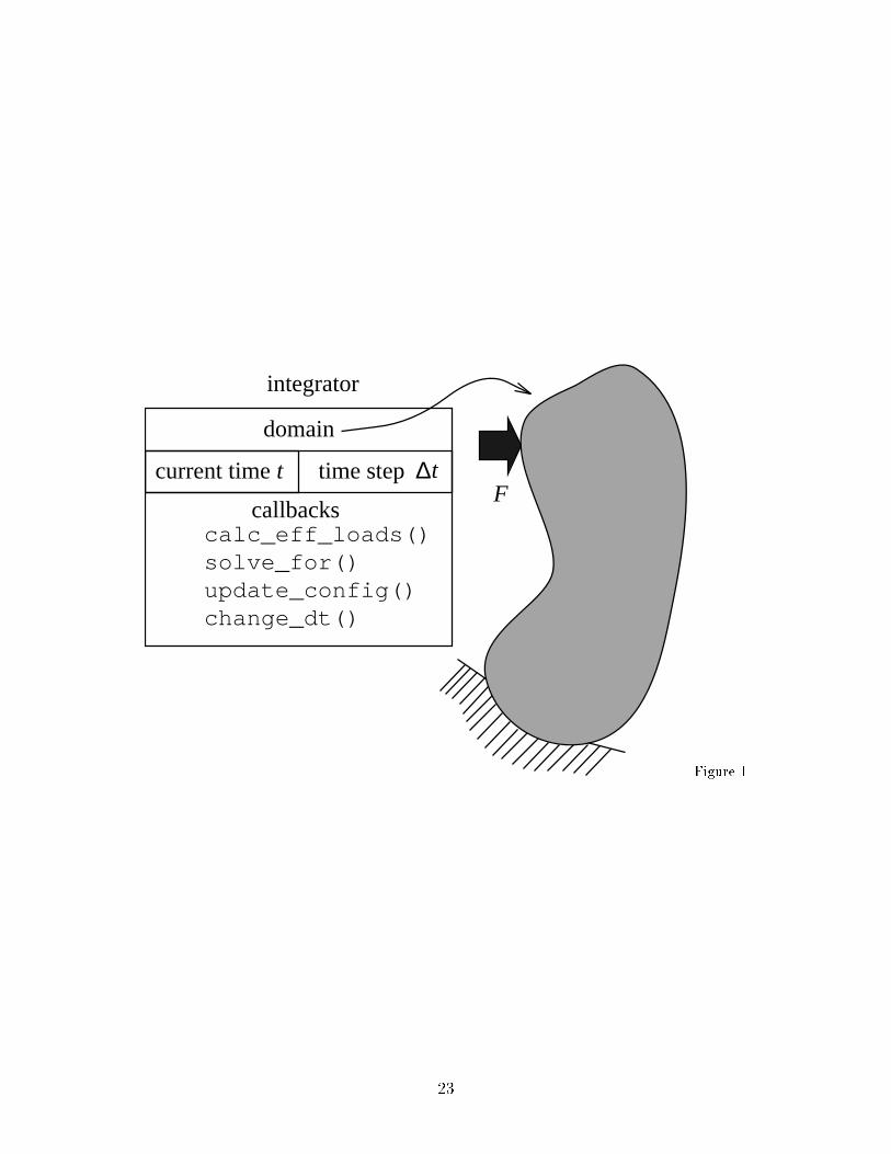
2.2 IntegratorNote that the algorithms in equations (4) to (21) were speci�ed without explicitlyde�ning the structure of the vectors of displacements, internal and external forces(loads), and the mass (damping) matrices of the structure. These objects were de-�ned by their abstract properties, e.g., the vector of internal forces represents thestresses within the structure without any mention of �nite element nodes, numericalintegration etc. Further, the algorithms were formulated with a physical domain inmind, or rather a discrete model of a physical domain. It is therefore possible toencapsulate the time-stepping algorithms by formulating them at the logical levelof (10) to (9). The algorithms thus \operate" only on the physical domain, andall representational details concerning the objects f , u etc. are left to the domain.The domain is free to choose the representation of the mathematical, or computa-tional objects involved. For instance, the domain may use for the storage of �ut andbf t either two vectors, or only a single vector. There is even wider freedom in theirimplementation (single or double precision, static or global, private or public accessetc.).We are now in a position to describe the integrator object; compare with Fig. 1.The integrator is created by the model of the physical domain, and consists of dataand callback procedures. The concept of a callback procedure is best explained by anexample from the everyday life1: Person A calls a person B and leaves their phonenumber. This enables the person B to call person A when needed, with the purpose ofobtaining or supplying information. A callback procedure is equivalent to the phonenumber person A left with person B.An integrator refers to the model of the physical domain. It also maintains thecurrent time t and the time step �t. The behavior of the integrator manifests itselfthrough callback procedures. Note that the callback procedures are not de�ned bythe integrator. Rather, the model of the physical domain de�nes these procedures,and they re ect all the peculiarities of a given domain model. The model allowsthe integrator to invoke the callbacks on the domain, i.e., the integrator activatesthe callback procedure and passes the reference to the domain as an argument. Thecallback procedures required are:(a) calc_eff_loads(), to compute the e�ective loads,(b) solve_for(), to solve for the primary unknowns,(c) update_config(), to update the con�guration (displacements, velocities etc.),and(d) change_dt(), to change the time step �t during the time integration.1The On-line Computing Dictionary (URL http://wombat.doc.ic.ac.uk) de�nes a callbackas \A scheme used in event-driven programs where the program registers a callback handler for acertain event. The program does not call the handler directly but when the event occurs, the handleris called, possibly with arguments describing the event."7

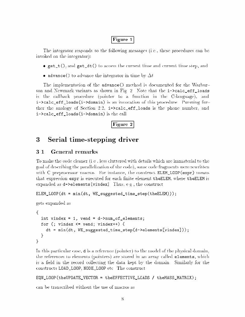
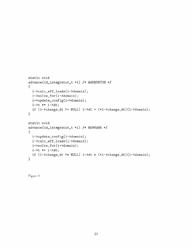
Figure 1The integrator responds to the following messages (i.e., these procedures can beinvoked on the integrator):� get_t(), and get_dt() to access the current time and current time step, and� advance() to advance the integrator in time by �t.The implementation of the advance() method is documented for the Warbur-ton and Newmark variants as shown in Fig. 2. Note that the i->calc_eff_loadsis the callback procedure (pointer to a function in the C-language), andi->calc_eff_loads(i->domain) is an invocation of this procedure. Pursuing fur-ther the analogy of Section 2.2, i->calc_eff_loads is the phone number, andi->calc_eff_loads(i->domain) is the call.Figure 23 Serial time-stepping driver3.1 General remarksTo make the code cleaner (i.e., less cluttered with details which are immaterial to thegoal of describing the parallelization of the code), some code fragments were rewrittenwith C preprocessor macros. For instance, the construct ELEM_LOOP(expr) meansthat expression expr is executed for each �nite element theELEM, where theELEM isexpanded as d->elements[vindex]. Thus, e.g., the constructELEM_LOOP(dt = min(dt, WE_suggested_time_step(theELEM)));gets expanded as{ int vindex = 1, vend = d->num_of_elements;for (; vindex <= vend; vindex++) {dt = min(dt, WE_suggested_time_step(d->elements[vindex]));}}In this particular case, d is a reference (pointer) to the model of the physical domain,the references to elements (pointers) are stored in an array called elements, whichis a �eld in the record collecting the data kept by the domain. Similarly for theconstructs LOAD_LOOP, NODE_LOOP etc. The constructEQN_LOOP(theUPDATE_VECTOR = theEFFECTIVE_LOADS / theMASS_MATRIX);can be transcribed without the use of macros as8

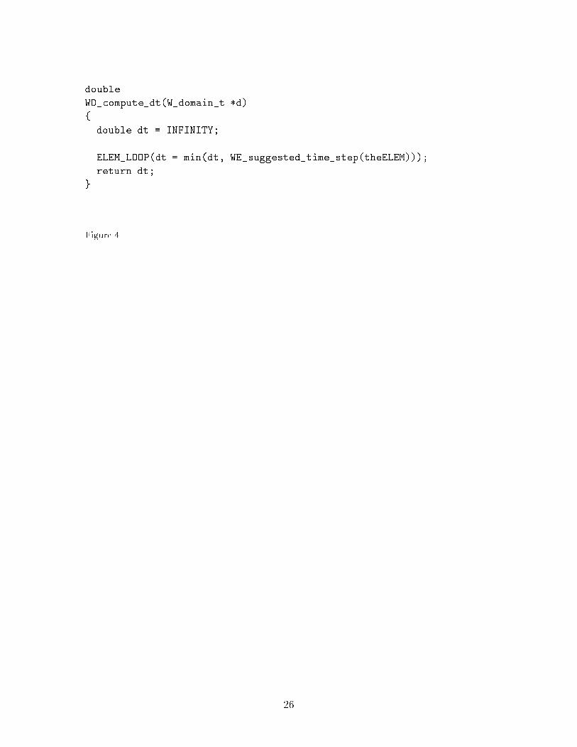
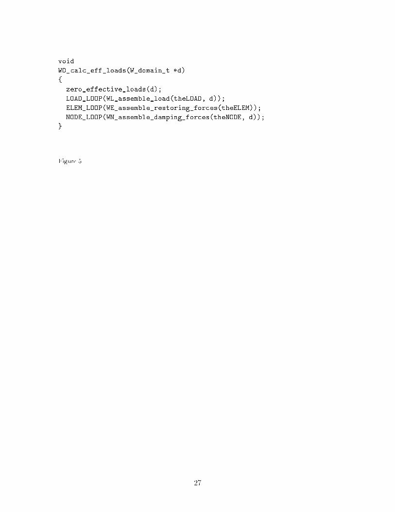
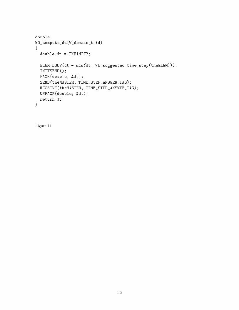
for (i = 1; i <= number_of_equations; i++)update_vector[i] = effective_loads[i] / mass_matrix[i];with the pointers update_vector etc. being initialized to point at appropriate mem-ory locations.3.2 Callbacks3.2.1 WD integrateThe actual computation is carried out by the domain when the procedureWD_integrate() is invoked on it. This routine creates the appropriate integrator(the Newmark integrator has been hardwired into the code in Fig. 3 for simplicity),and sets up the initial conditions (and other data structures, if necessary). Thenthe integrator is advanced in time until the target time is reached. Note, that theprocedure to change the time step, change_dt(), has not been speci�ed (it has beenset to NULL meaning \not de�ned"). To simplify matters, it is not discussed here.Figure 33.2.2 WD compute dtThe initial time increment is computed from the shortest time a wave needs to travelbetween two �nite element nodes. The usual estimate based on the highest eigenvi-bration frequencies of individual elements is used. The function WD_compute_dt()returning the estimated time step computed element-by-element is given in Fig. 4.Here, WE_suggested_time_step() is a function invoked for each element to get anestimate of �t computed on the isolated element.Figure 43.2.3 WD calc e� loadsThe routine WD_calc_eff_loads() is the �rst of the procedures used by the integratorto communicate with the model of the physical domain. It loops over active loads,elements and nodes to assemble external loads, restoring (internal) and dampingforces, respectively, into the vector of e�ective loads; cf. Fig. 5.Figure 53.2.4 WD solve forThe routine WD_solve_for() of Fig. 6 is very simple: It consists of a single loop overall the equations, solving for the global unknowns. Note that it is the same for allvariants of the integrator. However, the order in which it is invoked di�ers (cf. Fig. 2).Figure 69

3.2.5 WD update con�g xxxThe physical domain has to de�ne a procedure to update the con�guration for eachvariant of the integrator. The procedures in our case delegate the task to the �niteelement nodes, since the nodes maintain the displacement (velocity) data; comparewith Fig. 7. Figure 74 Parallel time-stepping algorithmThe parallelization by data decomposition requires a partitioning of the structure,which is here assumed to be static. In other words, we assume that a decompositionof the �nite element mesh is available, and we do not allow it to change during thecomputation. This assumption is not necessary (our design remains valid conceptu-ally), but it simpli�es the discussion by separating issues.4.1 Parallel algorithm with neighbor-to-neighbor communi-cationThe partitions are assigned to processors, which operate on them, exchanging infor-mation with other processors as necessary. The most commonly employed schemeuses a communication of the forces on the contacts between two partitions directlybetween the processors responsible for the two partitions. Such an algorithm hasbeen reported by Belytschko et al. [7], and Belytschko and Plaskacz [6] for explicitdynamics on SIMD machines. The communication between neighbors on this type ofmachine is rather e�cient, and the message size can be much smaller due to relativelylow overhead latency per message.Malone and Johnson [20, 21] have used similar communication pattern in theirparallel algorithm for massively parallel machines, i.e., the internal forces at nodesat the interfaces are exchanged directly between the processors sharing the node.Again, the hardware targeted by these researchers provides very fast communicationchannels.Let us summarize the characteristics of the described scheme:� The communication consists of a large number of small-grain messages (typicallyonly several oating point numbers).� The processors must do the book-keeping necessary to keep track of which pro-cessor is responsible for which interface node. Also, note that the number ofprocessors interested in a given node varies. For example, in a regular hexahe-dral mesh, an interface node may belong to up to eight di�erent partitions.10

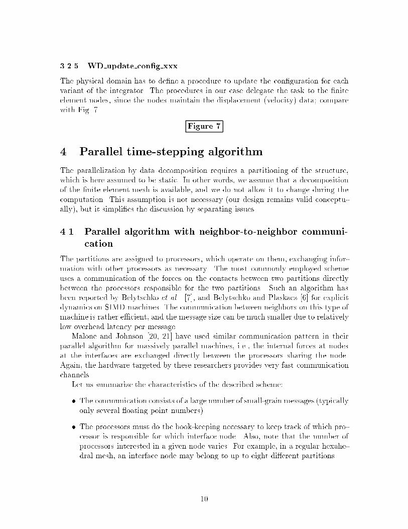
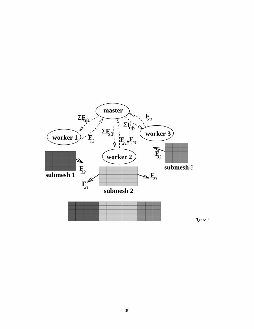
� The communication of the information between the neighbors can proceed insome cases concurrently, which requires independent communication paths be-tween di�erent processors.4.2 Parallel algorithm with master-worker communicationAs discussed in the Section 1.2, parallelization for computer networks requires muchlarger messages to ameliorate the e�ects of large latencies. Also parallel communica-tion between several workstations on the network is not possible (the communicationpaths are shared). Thus we chose an alternative communication pattern, which isbased on a star-shaped con�guration of workers, synchronized by a master processor;see Fig. 8. Figure 84.2.1 Variants with superelementsOne possible way to achieve parallelism with the master-worker communication pat-tern is based on the concept of a superelement with internal degrees of freedom. Thepartitions become the superelements, and the nodes which are common to the par-titions are the only global nodes in the mesh. The nodes which belong to only onepartition are internal to this partition. The global nodes interface nodes are handledas the only global �nite element nodes present in the mesh. Thus the \master" worksonly with these global nodes, and no \regular" �nite elements, only the superele-ments. The worker operates on the �nite elements of its partition, and communicatesthe computed results to the master. While this may seem a natural solution (it isin fact a pure example of the server-client architecture), it has serious drawbacks: Itmakes the coexistence of the serial and the parallel version more di�cult, becausethe parallel version requires the implementation of a special \internal" node, and ofa special remote superelement. Additionally, the operations on the interface nodescreate a considerable amount of small-grain communication (recall that the opera-tions on the global nodes have to be done \remotely", i.e., on the master). For thesereasons this variant is not suitable for a program meeting our speci�cations, and wasnot considered further.4.2.2 Master-workers variantThe basic idea is that the parallel algorithm is (i) synchronized at each time stepby assembling the interface forces, and (ii) dependent on the presence of a drivingprogram which mediates in the necessary communication. Therefore, it is quite nat-ural to consider a \star" con�guration of a master program at the center and a setof worker programs. The master is responsible for starting up the workers, and forthe assembly and distribution of the interface forces. The workers manipulate thepartitions as if they were ordinary serial programs, hiding the few points at which acommunication with the master is necessary in well-protected \parallel" interfaces.11

The algorithm can be speci�ed as:� Split the original �nite element mesh and assign the partitions to di�erent pro-cessors. De�ne interfaces between the partitions as such nodes that are sharedby two or more partitions.� For each time step:{ Compute the solution for the partitions in parallel as if they were individualmodels.{ For the nodes at the interfaces, assemble the nodal forces globally on themaster, i.e., sum the forces by which the partitions act on the interfacenodes.{ Distribute the forces assembled by the master for the interface nodes topartitions. Note that the interface nodal forces at the workers are over-written by the forces received from the master.The implementation of the above parallel algorithm can be done in a very cleanand concise manner based on the preceding high-level description of the serial timeintegration. The idea is to create the prototypes of the master and of the workersby modifying the integrator callbacks to account for the distributed character of theconcurrent computation.4.2.3 Possible extensionsOne further issue deserves mention at this point. All the workers integrate the equa-tions of motion with the same time step. To achieve a more e�cient algorithm, itis possible to use di�erent time steps on di�erent partitions; see, e.g., Hughes andBelytschko [19], Belytschko et al. [4, 5], or Chandra et al. [8]. The synchronizationand communication pattern is not really a�ected, and the design principles presentedhere remain valid.4.3 Implementation remarksSince one of our goals was to preserve both the serial and the parallel program, and tohave only one code to maintain, the implementation of the parallel version modi�esthe serial code by inserting conditional compilation units. Conditional compilationis achieved by de�ning preprocessor directives. Thus we are able to generate threedi�erent programs from a single source code: The serial program, and the master'sand the worker's versions of the parallel program.Code valid for the master is embedded between the directives#if defined(PVM_WASP_MASTER)...#endif 12

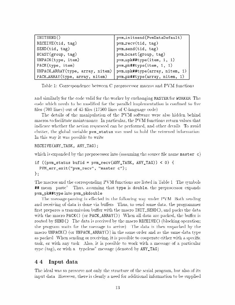
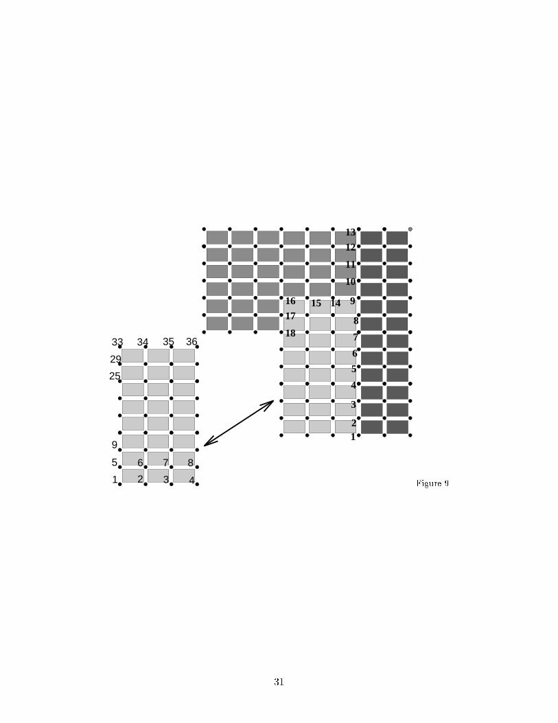
INITSEND() pvm initsend(PvmDataDefault)RECEIVE(tid, tag) pvm recv(tid, tag)SEND(tid, tag) pvm send(tid, tag)BCAST(group, tag) pvm bcast(group, tag)UNPACK(type, item) pvm upk##type(item, 1, 1)PACK(type, item) pvm pk##type(item, 1, 1)UNPACK ARRAY(type, array, nitem) pvm upk##type(array, nitem, 1)PACK ARRAY(type, array, nitem) pvm pk##type(array, nitem, 1)Table 1: Correspondence between C preprocessor macros and PVM functionsand similarly for the code valid for the worker by exchanging MASTER for WORKER. Thecode which needs to be modi�ed for the parallel implementation is con�ned to �ve�les (700 lines) out of 45 �les (17500 lines of C-language code).The details of the manipulation of the PVM software were also hidden behindmacros to facilitate maintenance. In particular, the PVM functions return values thatindicate whether the action requested can be performed, and other details. To avoidclutter, the global variable pvm_status was used to hold the returned information.In this way it was possible to writeRECEIVE(ANY_TASK, ANY_TAG);which is expanded by the preprocessor into (assuming the source �le name master.c)if ((pvm_status.bufid = pvm_recv(ANY_TASK, ANY_TAG)) < 0) {PVM_err_exit("pvm_recv", "master.c");};The macros and the corresponding PVM functions are listed in Table 1. The symbols## mean \paste". Thus, assuming that type is double, the preprocessor expandspvm_pk##type into pvm_pkdouble.The message-passing is e�ected in the following way under PVM. Both sendingand receiving of data is done via bu�ers. Thus, to send some data, the programmer�rst prepares a transmission bu�er with the macro INIT_SEND(), and packs the datawith the macro PACK() (or PACK_ARRAY()). When all data are packed, the bu�er isrouted by SEND(). The data is received by the macro RECEIVE() (blocking operation;the program waits for the message to arrive). The data is then unpacked by themacro UNPACK() (or UNPACK_ARRAY()) in the same order and as the same data typeas packed. When sending or receiving, it is possible to cooperate either with a speci�ctask, or with any task. Also, it is possible to work with a message of a particulartype (tag), or with a \typeless" message (denoted by ANY_TAG).4.4 Input dataThe ideal was to preserve not only the structure of the serial program, but also of itsinput data. However, there is clearly a need for additional information to be supplied13

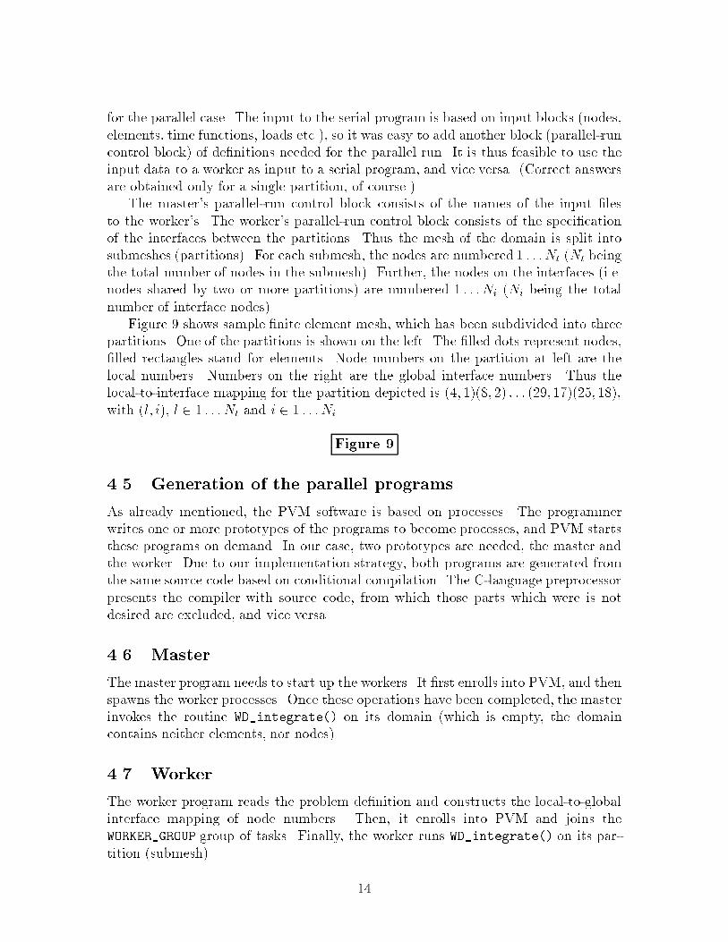
for the parallel case. The input to the serial program is based on input blocks (nodes,elements, time functions, loads etc.), so it was easy to add another block (parallel-runcontrol block) of de�nitions needed for the parallel run. It is thus feasible to use theinput data to a worker as input to a serial program, and vice versa. (Correct answersare obtained only for a single partition, of course.)The master's parallel-run control block consists of the names of the input �lesto the worker's. The worker's parallel-run control block consists of the speci�cationof the interfaces between the partitions. Thus the mesh of the domain is split intosubmeshes (partitions). For each submesh, the nodes are numbered 1 : : : Nt (Nt beingthe total number of nodes in the submesh). Further, the nodes on the interfaces (i.e.nodes shared by two or more partitions) are numbered 1 : : : Ni (Ni being the totalnumber of interface nodes).Figure 9 shows sample �nite element mesh, which has been subdivided into threepartitions. One of the partitions is shown on the left. The �lled dots represent nodes,�lled rectangles stand for elements. Node numbers on the partition at left are thelocal numbers. Numbers on the right are the global interface numbers. Thus thelocal-to-interface mapping for the partition depicted is (4; 1)(8; 2) : : : (29; 17)(25; 18),with (l; i), l 2 1 : : : Nt and i 2 1 : : : Ni.Figure 94.5 Generation of the parallel programsAs already mentioned, the PVM software is based on processes. The programmerwrites one or more prototypes of the programs to become processes, and PVM startsthese programs on demand. In our case, two prototypes are needed, the master andthe worker. Due to our implementation strategy, both programs are generated fromthe same source code based on conditional compilation. The C-language preprocessorpresents the compiler with source code, from which those parts which were is notdesired are excluded, and vice versa.4.6 MasterThe master program needs to start up the workers. It �rst enrolls into PVM, and thenspawns the worker processes. Once these operations have been completed, the masterinvokes the routine WD_integrate() on its domain (which is empty, the domaincontains neither elements, nor nodes).4.7 WorkerThe worker program reads the problem de�nition and constructs the local-to-globalinterface mapping of node numbers. Then, it enrolls into PVM and joins theWORKER_GROUP group of tasks. Finally, the worker runs WD_integrate() on its par-tition (submesh). 14

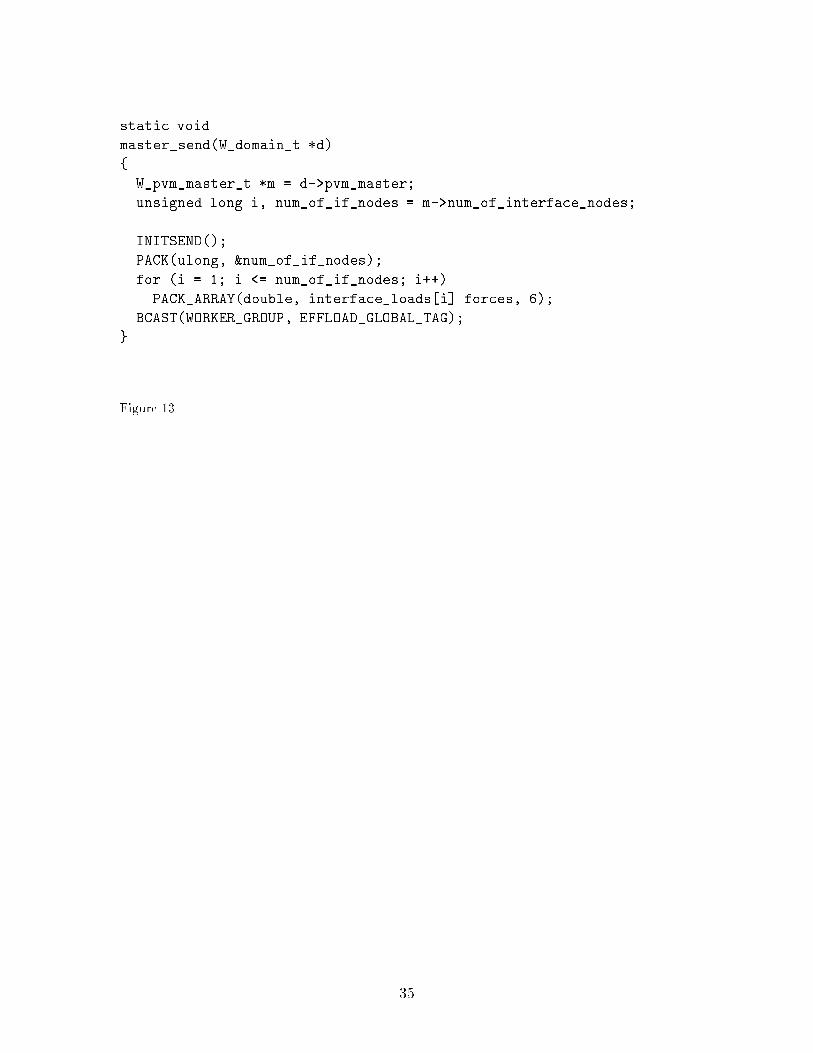
Note that both master and the workers invoke routines of the same name, andin the same order. The e�ects di�er, however, as the actions are coded di�erently.In particular, both master and workers invoke advance() on their integrators. Theintegrators are, however, parameterized with di�erent callbacks. This polymorphismseems to contribute to the readability of the source code, as the necessary paralleliza-tion constructs are well localized.5 Master's modi�cationsThe master's version of the function computing the time step is given in Fig. 10. Themaster broadcasts a request to compute the time step to all workers (they all joinedthe group WORKER_GROUP). The master then waits for the responses, and computesthe globally shortest time step. This value is then broadcast to the workers.Figure 10The master's version of the routine WD_calc_eff_loads() only consists of twolines; cf. Fig. 11. The routine master_recv() is shown in Fig. 12. It receives for eachworker the number of the interface nodes on the worker's partition and the e�ectiveload contributions. These are assembled into the master's bu�er interface_loads.After the e�ective load contributions have been received from all the workers, themaster sends out the assembled forces in master_send(). For e�ciency reasons, themaster is not required to keep track of which forces to send to which worker, and themaster sends the forces for all the interface nodes to all the workers.Figure 11Figure 12Figure 13Both the routines WD_solve_for() and WD_update_config() are de�ned asempty (doing nothing) for the master.6 Worker's modi�cationsThe worker's version of the function computing the time step is given in Fig. 14. Itdi�ers from the serial version of Fig. 4 in that the computed time step is sent to themaster and the globally shortest time step is received from it, which is then returned.Figure 14The worker's version of the WD_calc_eff_loads() routine is derived from theserial one by appending at the end the two lines15

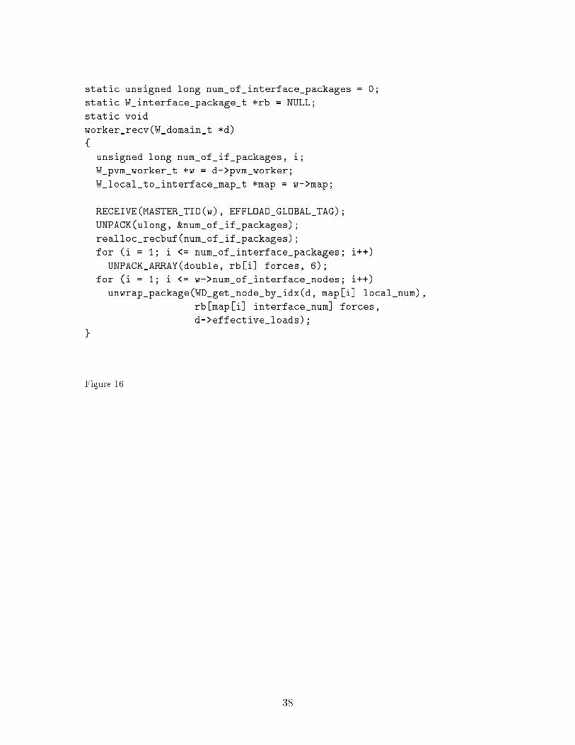
worker_send(d);worker_recv(d);The �rst procedure, worker_send(), packs and sends the global numbers of theinterface nodes, and the e�ective nodal loads. The e�ective nodal loads are packedinto arrays of six elements (three components of a 3D force and three components of a3D moment). Finally, the whole package is sent to the master. When the master hasassembled the e�ective loads from all partitions, it sends them out to the workers,and this package is received in the worker by worker_recv(). The worker has toaccept the package of all the interface nodes in the whole structure. Therefore, it �rst(re)allocates a bu�er rb to hold them by realloc_recbuf(). Then it unpacks theinterface e�ective loads (again in 6-element arrays) into the bu�er and then loops overall interface nodes on its partition and overwrites the entries in the local vector ofe�ective loads by the entries received into the bu�er. The function constr_package()collects the entries of the vector effective_loads into the vector forces, and thefunction unwrap_package() overwrites the entries of the vector effective_loads byentries of the bu�er array rb[map[i].interface_num].forces. These functions arede�ned for a node. The reason for this is that only the node (as an \object") hasaccess to the equation numbers (these are needed to address the entries of the systemvectors). Figure 15Figure 16The worker uses the serial versions of WD_solve_for() and WD_update_config()without any changes.7 Mass propertiesThe partitioning of the original domain leads to the creation of interface nodes. Thesenodes are by de�nition connected to several partitions at once. But the workers\know" only their own partition, so that the lumped mass properties computed forthe interface nodes from only the single partition elements would not be correct. Con-sequently, the inertial properties of the interface nodes must be computed in a globalmanner, similarly to the interface forces. However, if it is assumed that the mass dis-tribution does not change during the computation (as is often the case), this globalcomputation needs to be done only once. There are at least two ways to compute theinertial properties of the interface nodes. The �rst approach is based on a commu-nication of the local inertial properties, so it is called the exchange algorithm. Thesecond approach uses duplication of elements which reference the interface nodes inappropriate workers. This is called the ghost element algorithm. A similar algorithmwas used for slightly di�erent purpose by McGlaun et al. [23].16

7.1 Exchange algorithmThis algorithm computes the inertial properties locally on the workers using the par-tition elements. Then a gather is performed to assemble the local information intothe global inertial properties at the master. The global information is then broadcastto the workers. The advantage of this approach is that no information needs to beduplicated; the communication becomes more complicated, however. Consider, forexample, the case of structures with rotational degrees of freedom. In order to diago-nalize the mass matrix, the mass matrix assembly �rst collects the rotational inertiasassociated with the nodes in an element-by-element fashion. This is then followed bya node-by-node computation of the principal directions of the nodal tensor of iner-tia. Under these circumstances it is clear that additional synchronization is needed,which rather complicates the program logic, and also requires the data formats to beextended.7.2 Ghost-element algorithmThe elements which are connected at the interface nodes of a given partition are allincluded in the partition de�nition. However, the elements inside the partition arethe regular elements (which are used in all computations), while the elements that areoutside the partition are the ghost elements, which are used in the computation of themass properties, and are ignored otherwise. This approach duplicates information forall the ghost elements. However, additional communication (and computation on themaster) is totally avoided. Given both the advantages and disadvantages, it seemedthat the ghost-element approach was preferable. However, no rigorous evaluation wasconducted.8 Additional data exchangesExplicit �nite element programs need to compute additional information. For in-stance, the energy balance is a very important indicator of the solution quality. Con-sequently, a parallel program needs to include additional communication mechanismto gather this information from the workers at appropriate time instants (it does notneed to be computed every time step).9 PerformanceThe performance of any parallel implementation needs to be evaluated with respectto its scalability, i.e., the dependence of the obtained speed up on the number ofprocessors used. This is especially true for programs based on message passing, sincethe connecting link tends to be slow. However, a thourough scalability evaluation isoutside the scope of this paper, and will not be pursued here. Nevertheless, we feelit important to verify the basic concept by some timings.17

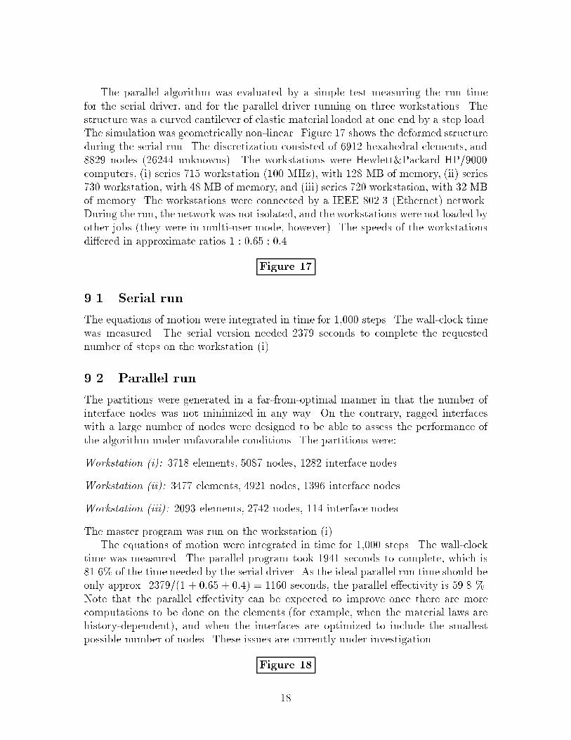
The parallel algorithm was evaluated by a simple test measuring the run timefor the serial driver, and for the parallel driver running on three workstations. Thestructure was a curved cantilever of elastic material loaded at one end by a step load.The simulation was geometrically non-linear. Figure 17 shows the deformed structureduring the serial run. The discretization consisted of 6912 hexahedral elements, and8829 nodes (26244 unknowns). The workstations were Hewlett&Packard HP/9000computers, (i) series 715 workstation (100 MHz), with 128 MB of memory, (ii) series730 workstation, with 48 MB of memory, and (iii) series 720 workstation, with 32 MBof memory. The workstations were connected by a IEEE 802.3 (Ethernet) network.During the run, the network was not isolated, and the workstations were not loaded byother jobs (they were in multi-user mode, however). The speeds of the workstationsdi�ered in approximate ratios 1 : 0:65 : 0:4.Figure 179.1 Serial runThe equations of motion were integrated in time for 1,000 steps. The wall-clock timewas measured. The serial version needed 2379 seconds to complete the requestednumber of steps on the workstation (i).9.2 Parallel runThe partitions were generated in a far-from-optimal manner in that the number ofinterface nodes was not minimized in any way. On the contrary, ragged interfaceswith a large number of nodes were designed to be able to assess the performance ofthe algorithm under unfavorable conditions. The partitions were:Workstation (i): 3718 elements, 5087 nodes, 1282 interface nodes.Workstation (ii): 3477 elements, 4921 nodes, 1396 interface nodes.Workstation (iii): 2093 elements, 2742 nodes, 114 interface nodes.The master program was run on the workstation (i).The equations of motion were integrated in time for 1,000 steps. The wall-clocktime was measured. The parallel program took 1941 seconds to complete, which is81.6% of the time needed by the serial driver. As the ideal parallel run time should beonly approx. 2379=(1 + 0:65 + 0:4) = 1160 seconds, the parallel e�ectivity is 59.8 %.Note that the parallel e�ectivity can be expected to improve once there are morecomputations to be done on the elements (for example, when the material laws arehistory-dependent), and when the interfaces are optimized to include the smallestpossible number of nodes. These issues are currently under investigation.Figure 1818

ConclusionsCareful design of the data structures and of the logic of an explicit �nite element pro-gram for non-linear dynamics can lead to a remarkably clean parallelization. We hadmade this experience when parallelizing a serial �nite element program of \object-oriented" design (implemented in the C-language) for heterogeneous workstation clus-ters running the PVM software.The resulting source code of the parallel program was obtained by an almost trivialmodi�cation of the serial version (the C-language fragments presented above cover,with the exception of the setup of the PVM software, all the necessary modi�cations).It is extendible, and maintainable. In case the code needs to be modi�ed, it isnecessary to maintain only one version of the source code, from which both the serialand the parallel programs can be generated.Dynamic load balancing, and integration with time step varying across the meshpartitions were not addressed here. These issues, and their e�ect on the design andimplementation, will be covered by subsequent research.AcknowledgmentsThe support of the National Science Foundation, and of the Army Research O�ce isgratefully acknowledged.References[1] B. W. Abeysundara and A. E. Kamal. High-speed local area networks and theirperformance: A survey. ACM Computing Surveys, 21:261{322, 1991.[2] J. W. Baugh and S. K. Sharma. Evaluation of distributed �nite element algo-rithms on a workstation. Engineering with Computers, 10:45{62, 1995.[3] T. Belytschko. A survey of numerical methods and computer programs for dy-namic structural analysis. Nucl. Engng. Design, 37(1):23{34, 1976.[4] T. Belytschko, B. Engelmann, and W. K. Liu. A review of recent developmentsin time integration. In A. K. Noor and J. T. Oden, editors, State-of-the-artsurveys of computational mechanics, New York, 1989. ASME.[5] T. Belytschko and N. D. Gilbertsen. Implementation of mixed time integrationtechniques on a vectorized computer with shared memory. International Journalof Numerical Methods in Engineering, 35:1803{1828, 1992.[6] T. Belytschko and E. J. Plaskacz. SIMD implementation of a non-linear tran-sient shell program with partially structured meshes. International Journal ofNumerical Methods in Engineering, 33:997{1026, 1992.19

[7] T. Belytschko, E. J. Plaskacz, and H. Y. Chiang. Explicit �nite element methodwith contact - impact on SIMD computers. Computer Systems in Engineering,2:269{276, 1991.[8] S. Chandra, N. J. Woodman, and D. I. Blockley. An object-oriented structure fortransient dynamics on concurrent computers. Comput. & Structures, 51:437{452,1994.[9] Y. P. Chien, A. Ecer, H. U. Akay, F. Carpenter, and R. A. Blech. Dynamic loadbalancing on a network of workstations. Computer Methods in Applied Mechanicsand Engineering, 119:17{33, 1994.[10] R. Chudoba and P. Krysl. Explicit �nite element computations: Object-orientedapproach. In P.J. Pahl and H. Werner, editors, Proc. of the 6th InternationalConf. on Computing in Civil and Building Engineering, pages 139{145, Berlin,1995. Balkema, Rotterdam.[11] J. Chung and J. M. Lee. A new family of explicit time integration methods forlinear and non-linear structural dynamics. International Journal of NumericalMethods in Engineering, 37:3961{3976, 1994.[12] M. A. Dokainish and K. Subbaraj. A survey of direct time integration methods incomputational structural dynamics - i. explicit methods. Comput. & Structures,32:1371{1386, 1989.[13] K. Dowd. High performance computing. O'Reilly & Associates, Sebastopol, CA,1994.[14] A. Ecer, H. U. Akay, W. B. Kemle, H. Wang, D. Ercoskun, and E. J. Hall.Parallel computation of uid dynamics problems. Computer Methods in AppliedMechanics and Engineering, 112:91{108, 1994.[15] M. W. Fahmy and A. H. Namini. A survey of parallel non-linear dynamic analysismethodologies. Comput. & Structures, 53:1033{1043, 1994.[16] C. Farhat and M. Lesoinne. Automatic partitioning of unstructured meshesfor the parallel solution of problems in computational mechanics. InternationalJournal of Numerical Methods in Engineering, 36:745{764, 1993.[17] A. Geist, A. Beguelin, J. Dongarra, W. Jiang, R. Manchek, and V. Sunderam.PVM: Parallel Virtual Machine: A users' guide and tutorial for networked par-allel computing. MIT Press, Cambridge, Mass., 1994.[18] A. V. Hudli and R. M. V. Pidaparti. Distributed �nite element structural analysisusing the client-server model. Comm. Numer. Meth. Engineering, 11, 1995.[19] T. J. R. Hughes and T. Belytschko. A pr�ecis of developments in computationalmethods for transient analysis. J. Appl. Mech., 50:1033{1041, 1983.20

[20] J. G. Malone and N. L. Johnson. A parallel �nite element contact/impact algo-rithm for non-linear explicit transient analysis. Part I. The search algorithm andcontact mechanics. International Journal of Numerical Methods in Engineering,37:559{590, 1994.[21] J. G. Malone and N. L. Johnson. A parallel �nite element contact/impact algo-rithm for non-linear explicit transient analysis. Part II. Parallel implementation.International Journal of Numerical Methods in Engineering, 37:591{539, 1994.[22] M. McGlaun, A. Robinson, and J. Peery. Some recent advances in structuralvibrations. In C. A. et al. Brebbia, editor, Vibrations of engineering structures,Berlin, New York, 1985. Springer-Verlag.[23] M. McGlaun, A. Robinson, and J. Peery. The development and applicationof massively parallel solid mechanics codes. In S. N. Atluri, G. Yagawa, andT. A. Cruse, editors, Computational mechanics '95, Int. Conf. on ComputationalEngineering Science, New York, 1995. Springer.[24] R. R. Namburu, D. Turner, and K. K. Tamma. An e�ective data parallel self-starting explicit methodology for computational structural dynamics on the Con-nection Machine CM-5. International Journal of Numerical Methods in Engineer-ing, 38:3211{3226, 1995.[25] R. Ou and R. Fulton. An investigation of parallel integration methods for non-linear dynamics. Comput. & Structures, 30:403{409, 1988.[26] C. �Ozturan, H. L. deCougny, M. S. Shephard, and J. E. Flaherty. Paralleladaptive mesh re�nement and redistribution on distributed memory computers.Computer Methods in Applied Mechanics and Engineering, 119:123{137, 1994.[27] K. C. Park and P. G. Underwood. A variable-step central di�erence method forstructural dynamics analysis. Part I. Theoretical aspects. Computer Methods inApplied Mechanics and Engineering, 22:241{258, 1980.[28] J. C. Simo, N. Tarnow, and K. K. Wong. Exact energy-momentum conservingalgorithms and symplectic schemes for nonlinear dynamics. Computer Methodsin Applied Mechanics and Engineering, 100:63{116, 1992.[29] D. Vanderstraeten and R. Keunings. Optimized partitioning of unstructured�nite element meshes. International Journal of Numerical Methods in Engineer-ing, 38:433{450, 1995.[30] G. and Yagawa. A parallel �nite element analysis with supercomputer network.Comput. & Structures, 47:407{418, 1993.21

Figure 1: The explicit integrator object in graphic formFigure 2: Implementation of the advance() methodFigure 3: Central di�erence driver on the highest level (a method de�ned on thephysical domain)Figure 4: Function WD compute dt() to compute the initial time stepFigure 5: Function WD calc eff loads() to compute the e�ective loadsFigure 6: Function WD solve for() to compute the primary unknownsFigure 7: Function to update the geometric con�guration for the Newmark integratorFigure 8: The con�guration of the master and the workers in a \star"Figure 9: Sample partition of a �nite element meshFigure 10: Modi�cation of WD compute dt() for the master versionFigure 11: Modi�cation of WD calc eff loads() for the masterFigure 12: Routine master recv()Figure 13: Routine master send()Figure 14: Modi�cation of WD compute dt() for the workerFigure 15: Function worker send()Figure 16: Function worker recv()Figure 17: Deformed structure. Serial modelFigure 18: Parallel model. Partitions22

F

integrator

calc_eff_loads()solve_for()update_config()change_dt()

current time t time step ∆t

callbacks

domain

Figure 123

static voidadvance(cd_integrator_t *i) /* WARBURTON */{ i->calc_eff_loads(i->domain);i->solve_for(i->domain);i->update_config(i->domain);i->t += i->dt;if (i->change_dt != NULL) i->dt = (*i->change_dt)(i->domain);}static voidadvance(cd_integrator_t *i) /* NEWMARK */{ i->update_config(i->domain);i->calc_eff_loads(i->domain);i->solve_for(i->domain);i->t += i->dt;if (i->change_dt != NULL) i->dt = (*i->change_dt)(i->domain);}Figure 224

voidWD_integrate(W_domain_t *d, double start_time, double target_time){ d->integrator = create_Newmark_integrator(d, /* domain */start_time, WD_compute_dt(d), /* t and dt */WD_calc_eff_loads, /* procedure: (a) */WD_solve_for, /* (b) */WD_update_config_Newmark, /* (c) */NULL /* (d) */);setup_initial_conditions(d);do {integrator_advance(d->integrator);} while (integrator_t(d->integrator) < target_time);}Figure 3

25

doubleWD_compute_dt(W_domain_t *d){ double dt = INFINITY;ELEM_LOOP(dt = min(dt, WE_suggested_time_step(theELEM)));return dt;}Figure 4

26

voidWD_calc_eff_loads(W_domain_t *d){ zero_effective_loads(d);LOAD_LOOP(WL_assemble_load(theLOAD, d));ELEM_LOOP(WE_assemble_restoring_forces(theELEM));NODE_LOOP(WN_assemble_damping_forces(theNODE, d));}Figure 5

27

voidWD_solve_for(W_domain_t *d){ EQN_LOOP(theUPDATE_VECTOR = theEFFECTIVE_LOADS / theMASS_MATRIX);}Figure 6

28

voidWD_update_config_Newmark(W_domain_t *d){ NODE_LOOP(WN_update_config_Newmark(theNODE, d));}Figure 7

29

12

21F

F32

23F

F32

21F 23

F,αβFΣ

F12

αβFΣ

αβFΣ

F

master

worker 1

worker 2

worker 3

submesh 2

submesh 3submesh 1 Figure 8

30

25

12

3

4

5

6

7

8

33 34 35 36

29

9

5

1 2

6 7 8

43

18

17

16 15 14

13

12

11

10

9

Figure 931

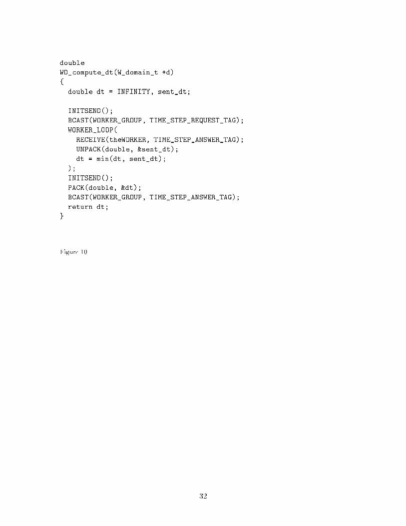
doubleWD_compute_dt(W_domain_t *d){ double dt = INFINITY, sent_dt;INITSEND();BCAST(WORKER_GROUP, TIME_STEP_REQUEST_TAG);WORKER_LOOP(RECEIVE(theWORKER, TIME_STEP_ANSWER_TAG);UNPACK(double, &sent_dt);dt = min(dt, sent_dt););INITSEND();PACK(double, &dt);BCAST(WORKER_GROUP, TIME_STEP_ANSWER_TAG);return dt;}Figure 10

32

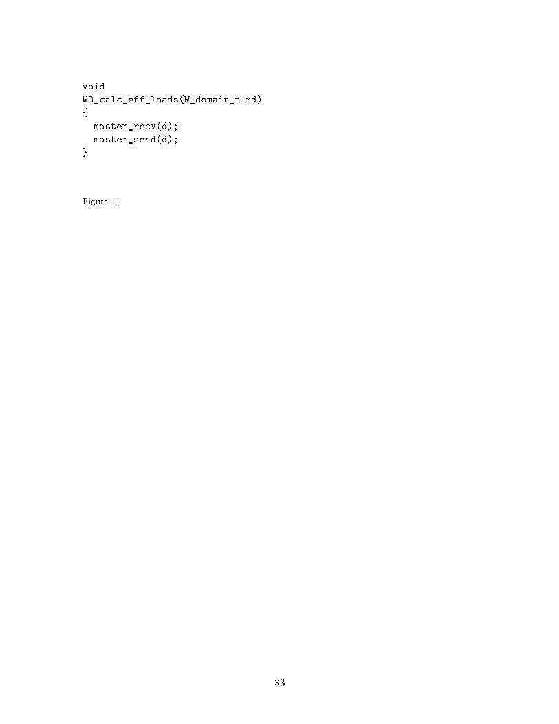
voidWD_calc_eff_loads(W_domain_t *d){ master_recv(d);master_send(d);}Figure 11

33

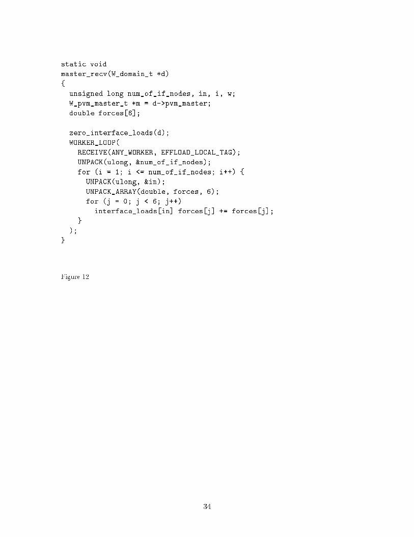
static voidmaster_recv(W_domain_t *d){ unsigned long num_of_if_nodes, in, i, w;W_pvm_master_t *m = d->pvm_master;double forces[6];zero_interface_loads(d);WORKER_LOOP(RECEIVE(ANY_WORKER, EFFLOAD_LOCAL_TAG);UNPACK(ulong, &num_of_if_nodes);for (i = 1; i <= num_of_if_nodes; i++) {UNPACK(ulong, &in);UNPACK_ARRAY(double, forces, 6);for (j = 0; j < 6; j++)interface_loads[in].forces[j] += forces[j];});}Figure 12

34

static voidmaster_send(W_domain_t *d){ W_pvm_master_t *m = d->pvm_master;unsigned long i, num_of_if_nodes = m->num_of_interface_nodes;INITSEND();PACK(ulong, &num_of_if_nodes);for (i = 1; i <= num_of_if_nodes; i++)PACK_ARRAY(double, interface_loads[i].forces, 6);BCAST(WORKER_GROUP, EFFLOAD_GLOBAL_TAG);}Figure 13

35

doubleWD_compute_dt(W_domain_t *d){ double dt = INFINITY;ELEM_LOOP(dt = min(dt, WE_suggested_time_step(theELEM)));INITSEND();PACK(double, &dt);SEND(theMASTER, TIME_STEP_ANSWER_TAG);RECEIVE(theMASTER, TIME_STEP_ANSWER_TAG);UNPACK(double, &dt);return dt;}Figure 14

36

static voidworker_send(W_domain_t *d){ W_pvm_worker_t *w = d->pvm_worker;unsigned long i, num_of_if_nodes = w->num_of_interface_nodesW_local_to_interface_map_t *map = w->map;double forces[6];INITSEND();PACK(ulong, &num_of_if_nodes);for (i = 1; i <= num_of_if_nodes; i++) {PACK(ulong, &map[i].interface_num);constr_package(WD_get_node_by_idx(d, map[i].local_num),d->effective_loads, forces);PACK_ARRAY(double, forces, 6);}SEND(theMASTER, EFFLOAD_LOCAL_TAG);}Figure 15

37

static unsigned long num_of_interface_packages = 0;static W_interface_package_t *rb = NULL;static voidworker_recv(W_domain_t *d){ unsigned long num_of_if_packages, i;W_pvm_worker_t *w = d->pvm_worker;W_local_to_interface_map_t *map = w->map;RECEIVE(MASTER_TID(w), EFFLOAD_GLOBAL_TAG);UNPACK(ulong, &num_of_if_packages);realloc_recbuf(num_of_if_packages);for (i = 1; i <= num_of_interface_packages; i++)UNPACK_ARRAY(double, rb[i].forces, 6);for (i = 1; i <= w->num_of_interface_nodes; i++)unwrap_package(WD_get_node_by_idx(d, map[i].local_num),rb[map[i].interface_num].forces,d->effective_loads);}Figure 16

38

Figure 1739

Figure 1840