Conserved quantities, optimal systems and explicit solutions ...
229
Conserved quantities, optimal systems and explicit solutions of certain partial differential equations I Simbanefayi orcid.org / 0000-0001-7420-1911 Thesis accepted for the degree Doctor of Philosophy in Science with Applied Mathematics at the North-West University Promoter: Prof CM Khalique Graduation: May 2021 Student number: 24536849
-
Upload
khangminh22 -
Category
Documents
-
view
2 -
download
0
Transcript of Conserved quantities, optimal systems and explicit solutions ...

Conserved quantities, optimal systems and explicit solutions of certain
partial differential equations
I Simbanefayi
orcid.org / 0000-0001-7420-1911
Thesis accepted for the degree Doctor of Philosophy in Science with Applied Mathematics at the North-West University
Promoter: Prof CM Khalique
Graduation: May 2021
Student number: 24536849

CONSERVED QUANTITIES,
OPTIMAL SYSTEMS AND EXPLICIT
SOLUTIONS OF CERTAIN PARTIAL
DIFFERENTIAL EQUATIONS
by
Innocent Simbanefayi (24536849)
Thesis submitted for the degree of Doctor of Philosophy in Applied
Mathematics at the Mafikeng Campus of the North-West University
November 2020
Supervisor: Professor C M Khalique

Contents
Declaration . . . . . . . . . . . . . . . . . . . . . . . . . . . . . . . . . . viii
Declaration of Publications . . . . . . . . . . . . . . . . . . . . . . . . . ix
Dedication . . . . . . . . . . . . . . . . . . . . . . . . . . . . . . . . . . . xi
Acknowledgements . . . . . . . . . . . . . . . . . . . . . . . . . . . . . . xii
Abstract . . . . . . . . . . . . . . . . . . . . . . . . . . . . . . . . . . . . xiii
Introduction 1
1 Preliminaries 5
1.1 One-parameter group of continuous transformations . . . . . . . . . 5
1.2 Prolongations . . . . . . . . . . . . . . . . . . . . . . . . . . . . . . 6
1.2.1 Prolonged or extended groups . . . . . . . . . . . . . . . . . 7
1.2.1.1 Prolonged generators . . . . . . . . . . . . . . . . . 9
1.3 Group admitted by a partial differential equations . . . . . . . . . . 10
1.4 Infinitesimal criterion of invariance . . . . . . . . . . . . . . . . . . 11
1.5 Conservation laws . . . . . . . . . . . . . . . . . . . . . . . . . . . . 12
1.5.1 Fundamental operators and their relationship . . . . . . . . 12
i
1.5.2 Noether Approach . . . . . . . . . . . . . . . . . . . . . . . 13
1.5.3 Ibragimov’s method for finding conservation laws . . . . . . 15
1.5.4 Multiplier method . . . . . . . . . . . . . . . . . . . . . . . 17
1.6 Exact solutions . . . . . . . . . . . . . . . . . . . . . . . . . . . . . 18
1.6.1 Multiple exp-function method . . . . . . . . . . . . . . . . . 18
1.6.2 The extended Jacobi elliptic function method . . . . . . . . 19
1.6.3 Synopsis of (G′/G)−expansion method . . . . . . . . . . . . 20
1.6.4 Power series solution method . . . . . . . . . . . . . . . . . 21
1.7 Concluding remarks . . . . . . . . . . . . . . . . . . . . . . . . . . . 21
2 Cnoidal and snoidal waves and conservation laws for physical
space-time (3+1)-dimensional modified KdV models 23
2.1 Introduction . . . . . . . . . . . . . . . . . . . . . . . . . . . . . . . 23
2.2 Solutions and conservation laws of (2.1) . . . . . . . . . . . . . . . . 24
2.2.1 Lie point symmetries . . . . . . . . . . . . . . . . . . . . . . 24
2.2.2 Exact solutions by using Lie point symmetries and direct
integration . . . . . . . . . . . . . . . . . . . . . . . . . . . . 27
2.2.3 Exact solutions using the extended Jacobi elliptic function
expansion method . . . . . . . . . . . . . . . . . . . . . . . . 29
2.2.3.1 Cnoidal wave solutions . . . . . . . . . . . . . . . . 29
2.2.3.2 Snoidal wave solutions . . . . . . . . . . . . . . . . 30
2.2.4 Conservation laws . . . . . . . . . . . . . . . . . . . . . . . . 31
2.3 Exact solutions and conservation laws of (2.2) . . . . . . . . . . . . 32
ii
2.4 Exact solutions and conservation laws of (2.3) . . . . . . . . . . . . 33
2.5 Concluding remarks . . . . . . . . . . . . . . . . . . . . . . . . . . . 35
3 A symbolic computational approach to finding solutions and con-
servation laws for (3+1)- dimensional modified BBM models 36
3.1 Introduction . . . . . . . . . . . . . . . . . . . . . . . . . . . . . . . 36
3.2 Conservation laws and analytic solutions . . . . . . . . . . . . . . . 37
3.2.1 Conservation laws . . . . . . . . . . . . . . . . . . . . . . . . 37
3.2.2 Closed form solutions . . . . . . . . . . . . . . . . . . . . . . 45
3.2.2.1 Soliton solution . . . . . . . . . . . . . . . . . . . . 46
3.2.2.2 Exact solutions using the simplest equation method 48
3.3 Conservation laws and exact solutions of (3.3) . . . . . . . . . . . . 53
3.4 Conservation laws and exact solutions of (3.4) . . . . . . . . . . . . 56
3.5 Concluding remarks . . . . . . . . . . . . . . . . . . . . . . . . . . . 59
4 Conserved quantities, optimal system and explicit solutions of a
(1+1)-dimensional generalised coupled mKdV-type system 60
4.1 Introduction . . . . . . . . . . . . . . . . . . . . . . . . . . . . . . . 60
4.2 Conserved quantities . . . . . . . . . . . . . . . . . . . . . . . . . . 61
4.3 analytic solutions of (4.2) . . . . . . . . . . . . . . . . . . . . . . . 64
4.3.1 Optimal system of one-dimensional subalgebras for (4.2) . . 64
4.3.2 Symmetry reductions and explicit solutions of (4.2) . . . . . 66
4.3.2.1 Symmetry reductions . . . . . . . . . . . . . . . . . 66
iii

4.3.2.2 Explicit solutions of (4.2) . . . . . . . . . . . . . . 68
4.4 Concluding remarks . . . . . . . . . . . . . . . . . . . . . . . . . . . 76
5 Group invariant solutions and conserved quantities of a (3+1)-
dimensional generalized Kadomtsev–Petviashvili equation 78
5.1 Introduction . . . . . . . . . . . . . . . . . . . . . . . . . . . . . . . 78
5.2 Exact Solutions of the (3+1)-D gKPe . . . . . . . . . . . . . . . . . 80
5.2.1 Invariant Solutions under the Symmetries X1, · · · , X4 . . . . 81
5.2.2 Invariant Solution under the Symmetry X5 . . . . . . . . . . 83
5.2.3 Invariant Solution under the Symmetry X6 . . . . . . . . . . 84
5.3 Conserved Quantities of the (3+1)-D gKPe . . . . . . . . . . . . . . 85
5.3.1 Application of the Method . . . . . . . . . . . . . . . . . . . 85
5.3.2 Ibragimov’s Approach . . . . . . . . . . . . . . . . . . . . . 87
5.3.2.1 Application of the Method . . . . . . . . . . . . . . 87
5.4 Concluding remarks . . . . . . . . . . . . . . . . . . . . . . . . . . . 96
6 Travelling wave solutions and conservation laws of the (2+1)- di-
mensional Broer-Kaup- Kupershmidt equations 98
6.1 Introduction . . . . . . . . . . . . . . . . . . . . . . . . . . . . . . . 98
6.2 Bounded travelling wave solutions of the BKK equations (1) . . . . 100
6.3 Conservation laws of the BKK equations (1.1) . . . . . . . . . . . . 104
6.4 Concluding remarks . . . . . . . . . . . . . . . . . . . . . . . . . . . 108
7 An optimal system of group- invariant solutions and conserved
iv

quantities of a nonlinear fifth-order integrable equation 110
7.1 Introduction . . . . . . . . . . . . . . . . . . . . . . . . . . . . . . . 110
7.2 Lie group analysis of (7.2) . . . . . . . . . . . . . . . . . . . . . . . 112
7.2.1 Infinitesimal generators . . . . . . . . . . . . . . . . . . . . . 112
7.2.2 Group transformations of known solutions . . . . . . . . . . 113
7.2.3 Optimal system of one-parameter group invariant solutions . 114
7.2.3.1 Cases X1, X2 and X2 ±X4 . . . . . . . . . . . . . 115
7.2.3.2 Case X1 +X2 . . . . . . . . . . . . . . . . . . . . . 116
7.2.3.3 Case X3 . . . . . . . . . . . . . . . . . . . . . . . . 121
7.3 Conserved quantities of (7.2) . . . . . . . . . . . . . . . . . . . . . . 126
7.3.1 Noether’s approach . . . . . . . . . . . . . . . . . . . . . . . 126
7.3.2 Multiplier approach . . . . . . . . . . . . . . . . . . . . . . . 129
7.4 Concluding remarks . . . . . . . . . . . . . . . . . . . . . . . . . . . 131
8 Analytic solutions and conserved quantities of the coupled com-
plex modified Korteweg-de Vries equations of plasma physics 132
8.1 Introduction . . . . . . . . . . . . . . . . . . . . . . . . . . . . . . . 132
8.2 Lie algebra and one-parameter group transformations . . . . . . . . 134
8.3 Analytic solutions . . . . . . . . . . . . . . . . . . . . . . . . . . . . 136
8.3.1 Case X1 + cX2 . . . . . . . . . . . . . . . . . . . . . . . . . 137
8.3.1.1 Elliptic cosine solutions . . . . . . . . . . . . . . . 138
8.3.1.2 Elliptic sine solutions . . . . . . . . . . . . . . . . . 142
v
8.3.1.3 Delta amplitude solutions . . . . . . . . . . . . . . 146
8.3.2 Case X3 . . . . . . . . . . . . . . . . . . . . . . . . . . . . . 148
8.4 Conserved currents . . . . . . . . . . . . . . . . . . . . . . . . . . . 153
8.5 Concluding remarks . . . . . . . . . . . . . . . . . . . . . . . . . . . 159
9 Conservation laws and symmetry reductions for a generalized hyperelastic-
rod wave equation 161
9.1 Introduction . . . . . . . . . . . . . . . . . . . . . . . . . . . . . . . 161
9.2 Conserved quantities . . . . . . . . . . . . . . . . . . . . . . . . . . 163
9.3 Exact solutions . . . . . . . . . . . . . . . . . . . . . . . . . . . . . 166
9.3.1 Quadratic function case . . . . . . . . . . . . . . . . . . . . 167
9.3.2 Power law nonlinearity case . . . . . . . . . . . . . . . . . . 170
9.3.3 Exponential function case. . . . . . . . . . . . . . . . . . . . 171
9.3.4 Logarithmic function case. . . . . . . . . . . . . . . . . . . . 172
9.4 Concluding remarks . . . . . . . . . . . . . . . . . . . . . . . . . . . 173
10 Lie symmetry analysis and conserved quantities of a (1+1)- di-
mensional fifth-order integrable equation 174
10.1 Introduction . . . . . . . . . . . . . . . . . . . . . . . . . . . . . . . 174
10.2 Lie group analysis . . . . . . . . . . . . . . . . . . . . . . . . . . . . 175
10.2.1 Classical symmetries . . . . . . . . . . . . . . . . . . . . . . 175
10.2.2 Optimal system of one dimensional subalgebras . . . . . . . 176
10.3 Group Invariant solutions . . . . . . . . . . . . . . . . . . . . . . . 177
vi

10.3.1 Case X1 + kX2 . . . . . . . . . . . . . . . . . . . . . . . . . 177
10.3.1.1 Elliptic integral solutions . . . . . . . . . . . . . . 178
10.3.1.2 Rational and hyperbolic solutions . . . . . . . . . . 179
10.3.2 Case X2 . . . . . . . . . . . . . . . . . . . . . . . . . . . . . 183
10.3.3 Case X1 +X4 . . . . . . . . . . . . . . . . . . . . . . . . . . 183
10.3.4 Case X3 . . . . . . . . . . . . . . . . . . . . . . . . . . . . . 183
10.4 One and two-wave solutions . . . . . . . . . . . . . . . . . . . . . . 186
10.4.1 One-soliton solutions . . . . . . . . . . . . . . . . . . . . . . 186
10.4.2 Two-soliton solutions . . . . . . . . . . . . . . . . . . . . . . 188
10.5 Conservation laws of (10.1) . . . . . . . . . . . . . . . . . . . . . . . 193
10.6 Concluding remarks . . . . . . . . . . . . . . . . . . . . . . . . . . . 195
11 Conclusions and future work 196
vii


Declaration of Publications
Details of contribution to publications that form part of this thesis.
Chapter 2
I. Simbanefayi, C.M. Khalique, Cnoidal and snoidal waves and conservation laws
for physical space-time (3+1)-dimensional modified KdV models, Results Phys.,
10 (2018) 975–979.
Chapter 3
I. Simbanefayi, C.M. Khalique, A symbolic computational approach to finding
solutions and conservation laws for (3+1)-dimensional modified BBM models, Alex.
Eng. J., 59 (2020) 1799–1809.
Chapter 4
I. Simbanefayi, C.M. Khalique, Conserved quantities, optimal system and explicit
solutions of a (1+1)-dimensional generalised coupled mKdV-type system, J. Adv.
Res., in press. https://doi.org/10.1016/j.jare.2020.10.002.
Chapter 5
I. Simbanefayi, C.M. Khalique, Group invariant solutions and conserved quantities
of a (3+1)-dimensional generalized Kadomtsev-Petviashvili equation, Mathemat-
ics, 8 (2020) 1012; doi:10.3390/math8061012.
Chapter 6
L. Zhang, I. Simbanefayi, C.M. Khalique, Travelling wave solutions and conserva-
tion laws of the (2+1)-dimensional Broer-Kaup-Kupershmidt equation, submitted
to Iran. J. Sci. Technol. Trans. A Sci.
Chapter 7
I. Simbanefayi, C.M. Khalique, An optimal system of group-invariant solutions and
conserved quantities of a nonlinear fifth-order integrable equation, Open Phys., in
ix

press.
Chapter 8
I. Simbanefayi, C.M. Khalique, Analytic solutions and conserved quantities of the
coupled complex modified Korteweg-de Vries equations, submitted to Physica D.
Chapter 9
L. Zhang, I. Simbanefayi, C.M. Khalique, Conservation laws and symmetry reduc-
tions for a generalized hyperelastic-rodwave equation, submitted to Chaos Soliton.
Fract.
Chapter 10
I. Simbanefayi, C.M. Khalique, Conservation laws, classical symmetries and ex-
act solutions of a (1+1)-dimensional fifth-order integrable equation, submitted to
Phys. Scr.
x

Dedication
For my dear wife Simiso, my lovely daughter Nomthandazo and my beloved sons
Phakade & Uphakeme.
xi

Acknowledgements
My heartfelt gratitude goes to my supervisor Professor CM Khalique for his con-
sistent guidance and support throughout this research work. I would also like to
thank Professor Lijun Zhang and Professor Maria Luz Gandarias for the collabo-
rative work in two of the problems studied in this research. I greatly appreciate
the financial support from the North-West University, Mafikeng Campus, through
the postgraduate bursary scheme. Last but not least, I would like to thank my
wife Mimie, my daughter Nomthie and my two boys Phakae and Phake for their
patience while l slaved on without end. Finally, my deepest gratitude goes to God,
my sustainer and enabler.
xii

Abstract
In this thesis we study nine nonlinear partial differential equations (NLPDEs)
from the point of view of classical Lie point symmetries and conserved quantities.
These equations of choice have real world applications, primarily in the field of
fluid dynamics and plasma physics. One equation models wave propagation in a
hyperelastic-rod. Several (3+1)-dimensional equations are studied in detail, these
are the modified Korteweg-de Vries (mKdV) and Benjamin-Bona-Mahony (BBM)
equations. We also study a (3+1)-dimensional generalised Kadomtsev-Petviashvili
(KP) equation. Higher dimensional equations tend to be more apt models of
nonlinear interrelations between physical quantities. Moreover, we study three
systems, that is, the generalised coupled mKdV, Broer-Kaup-Kupershmidt (BKK)
and coupled complex mKdV systems. We also explore two fifth-order nonlinear
integrable models.
Using Lie algebras, we obtain group invariant solutions, optimal systems of one di-
mensional subalgebras and their corresponding reductions. Techniques such as the
extended Jacobi elliptic function, (G′/G)-expansion, power series solution, multiple
exp-function methods are used in this work. Furthermore, we derive conservation
laws for the underlying equations. Three and two dimensional renderings of se-
lected solutions are provided. Techniques such as Noether’s approach, multiplier
method and Ibragimov’s conservation theorem are used. In several instances we
demonstrate explicitly the use of the first homotopy integral formula from varia-
tional calculus, which is sometimes attached to the multiplier method.
xiii

Introduction
Nonlinear partial differential equations (NLPDEs) have rapidly become indispens-
able in the quest to conceptualise the world around us. It is against this backdrop
that countless research papers today explore various aspects of NLPDEs. The
value attached to seeking exact solutions of NLPDEs is thus immense. However,
compared to linear partial differential equations, there is no systematic way to
obtain exact solutions of NLPDEs due to their complexity. Nonetheless, many ad
hoc methods of finding exact solutions of NLPDEs have been developed, for ex-
ample, the improved tanh method [1] the Riccati-Bernoulli sub-ODE method [2],
the homogeneous balance of undetermined coefficients method [3–6], the first inte-
gral method [7], the bifurcation technique [8], the generalised unified method [9],
the multiple exp-function method [10–13], dynamical system approach [14–16],
simplified Hirota’s method [17, 18], the (G′/G)-expansion function method [19],
Kudryashov’s method [20], Jacobi elliptic function expansion technique [21–24],
the power series technique [25–27], and Lie group analysis approach [28–32].
Lie group theory is one of the most proficient methods for treatment of differential
equations (DEs). Marius Sophus Lie (1842–99) is credited for this quintessential
body of knowledge. He understood that the myriad of apparently different methods
for obtaining analytic solutions of DEs were, in essence, all special cases of a broad
integration approach; the theory of transformation groups. This theory is an analog
of Galois theory and continues to impact mathematics and mathematical physics to
1

this day. It is easy to view Lie group theory as one of the most eminent techniques
to derive analytic solutions of DEs.
Conservation laws are crucial for determining the extent of integrability of DEs,
development of numerical schemes, reduction and solutions of partial differential
equations (PDEs) amongst others. Methods for finding conservation laws include
the celebrated Noether’s theorem [33–35] for determining conserved vectors of sys-
tems of PDEs with a variational principle. In order to sidestep the requirement
for a variational principle imposed by Noether’s theorem, a modern form has been
developed [36–50]. For example, the aptly named multiplier approach [45]. An-
other such method is the conservation theorem by Ibragimov [39,40] whose method
associates every infinitesimal vector with a conservation law. Moreover, there is
the partial Noether approach, which works like the Noether approach for the DEs
with or without a Lagrangian [51,52].
We give a few recent studies of NLPDEs presented in the literature. For instance,
Kadomtsev-Petviashvili-Benjamin-Bona-Mahony (KP-BBM) equation was investi-
gated in [53] and exact solutions were constructed. In [54], the (2+1)-dimensional
B-type KP equation of fluid mechanics was studied and soliton molecules and
some novel interaction solutions were discussed. The (2+1)-dimensional modified
dispersive water-wave system was considered in [55] and variable separation so-
lutions were obtained. The authors of [56] examined the KP-BBM equation and
constructed periodic, multi wave, cross-kink wave and breather wave solutions.
The Boiti-Leon-Manna-Pempinelli equation was studied using the Hirota bilinear
form and rational wave solutions were obtained in [57]. Lie symmetry analysis was
carried out on a generalized (2+1)-dimensional KP equation [58] and in [59], the
(2+1)-dimensional dispersive long wave equation was investigated via the trun-
cated Painleve series method. A new method was introduced in [60] to find exact
solutions for NLPDEs of mathematical physics.
2
This thesis is structured as follows.
In Chapter one, we provide a synopsis of pertinent concepts in Lie group theory
that will be used throughout this thesis. We also outline the methods of exact
solutions and conserved quantities that we will utilise.
Chapter two is a study of three (3+1)-dimensional mKdV equations. Similarity
reductions along with extended Jacobi elliptic method are used to obtain exact
solutions. Conserved quantities are obtained via the direct method.
In Chapter three, we explore three (3+1)-dimensional BBM equations and obtain
exact solutions via symmetry reductions and simplest equation method. Noether’s
theorem is used to derive conservation laws.
Chapter four studies a (1+1)-dimensional mKdV system. We use elements of the
optimal system of one-dimensional subalgebras to reduce the system. The power
series method is used to solve the resultant ODEs. We obtain conservation laws
using a homotopy integral approach.
Chapter five deals with group invariant solutions of a (3+1)-dimensional gener-
alised KP equation. The multiplier approach and Ibragimov’s conservation theo-
rem are applied successfully to obtained local conservation laws.
Chapter six investigates the bounded travelling wave solutions of a (2+1)-dimensional
BKK system using bifurcation analysis. The first homotopy integral approach is
used to obtain conserved vectors.
In Chapter seven, we investigate the optimal system of group invariant solutions
of a new integrable fifth-order nonlinear partial differential equation. We analyse
the equation for a variational principle and in turn apply Noether’s theorem and
the multiplier method to get conservation laws.
In Chapter eight, we examine a (1+1)-dimensional coupled complex mKdV system.
3

We derive group transformations using the nine-dimensional Lie algebra of this
equation. Exact solutions are obtained and conserved quantities are computed.
Chapter nine is an application of symmetry reductions on a generalized hyperelastic-
rod wave equation. Using the travelling wave variable, we perform a triple reduc-
tion on the conserved vectors of the equation.
In Chapter ten, we study a (1+1)-dimensional fifth-order equation. Using the
optimal systems of Lie algebras we obtain exact solutions. We also use the multiple
exp-function method to obtain one and two wave solutions. Conservation are
derived at the end of the chapter.
Chapter eleven provides a summary of the results in the thesis and future work is
contemplated.
Bibliography is given at the end.
4

Chapter 1
Preliminaries
This chapter presents some preliminaries on Lie symmetry analysis and conserva-
tion laws of differential equations, which are used throughout this work. Selected
methods of obtaining analytic solutions and conserved quantities of differential
equations are also outlined.
1.1 One-parameter group of continuous transfor-
mations
Let x = (x1, ..., xn) be the independent variables with coordinates xi and u =
(u1, ..., um) be the dependent variables with coordinates uα (n and m finite). Con-
sider a change of the variables x and u involving a real parameter a:
Ta : xi = f i(x, u, a), uα = φα(x, u, a), (1.1)
where a continuously ranges in values from a neighborhood D′ ⊂ D ⊂ R of a = 0,
and f i and φα are differentiable functions.
5

Definition 1.1 (Lie group) A set G of transformations (1.1) is called a contin-
uous one-parameter (local) Lie group of transformations in the space of variables
x and u if
(i) For Ta, Tb ∈ G where a, b ∈ D′ ⊂ D then Tb Ta = Tc ∈ G, c = φ(a, b) ∈ D
(Closure)
(ii) T0 ∈ G if and only if a = 0 such that T0 Ta = Ta T0 = Ta (Identity)
(iii) For Ta ∈ G, a ∈ D′ ⊂ D, T−1a = Ta−1 ∈ G, a−1 ∈ D such that
Ta Ta−1 = Ta−1 Ta = T0 (Inverse)
We note that the associativity property follows from (i). The group property (i)
can be written as
¯xi ≡ f i(x, u, b) = f i(x, u, φ(a, b)),
¯uα ≡ φα(x, u, b) = φα(x, u, φ(a, b)) (1.2)
and the function φ is called the group composition law. A group parameter a is
called canonical if φ(a, b) = a+ b.
Theorem 1.1 For any φ(a, b), there exists the canonical parameter a defined by
a =
∫ a
0
ds
w(s), where w(s) =
∂ φ(s, b)
∂b
∣∣∣∣b=0
.
1.2 Prolongations
The derivatives of u with respect to x are defined as
uαi = Di(uα), uαij = DjDi(ui), · · · , (1.3)
6

where
Di =∂
∂xi+ uαi
∂
∂uα+ uαij
∂
∂uαj+ · · · , i = 1, ..., n (1.4)
is the operator of total differentiation. The collection of all first derivatives uαi is
denoted by u(1), i.e.,
u(1) = uαi α = 1, ...,m, i = 1, ..., n.
Similarly
u(2) = uαij α = 1, ...,m, i, j = 1, ..., n
and u(3) = uαijk and likewise u(4) etc. Since uαij = uαji, u(2) contains only uαij for
i ≤ j. In the same manner u(3) has only terms for i ≤ j ≤ k. There is natural
ordering in u(4), u(5) · · · .
In group analysis all variables x, u, u(1) · · · are considered functionally independent
variables connected only by the differential relations (1.3). Thus the uαs are called
differential variables [31,65].
Now let us consider a pth-order system of PDEs of n independent variables x =
(x1, x2, · · · , xn) and m dependent variables u = (u1, u2, · · · , um) given by
Eα(x, u, u(1), · · · , u(p)) = 0, α = 1, · · · ,m. (1.5)
Here u(1), u(2), . . . , u(p) represent the collections of all first, second, . . ., pth-order
partial derivatives, that is, uαi = Di(uα), uαij = DjDi(u
α), . . ., respectively, and the
total derivative operator Di given by (1.4).
1.2.1 Prolonged or extended groups
If z = (x, u), one-parameter group of transformations G is
xi = f i(x, u, a), f i|a=0 = xi,
7

uα = φα(x, u, a), φα|a=0 = uα. (1.6)
According to the Lie’s theory, the construction of the symmetry group G is equiv-
alent to the determination of the corresponding infinitesimal transformations :
xi ≈ xi + a ξi(x, u), uα ≈ uα + a ηα(x, u) (1.7)
obtained from (1.1) by expanding the functions f i and φα into Taylor series in a,
about a = 0 and also taking into account the initial conditions
f i∣∣a=0
= xi, φα|a=0 = uα.
Thus, we have
ξi(x, u) =∂f i
∂a
∣∣∣∣a=0
, ηα(x, u) =∂φα
∂a
∣∣∣∣a=0
. (1.8)
One can now introduce the symbol of the infinitesimal transformations by writing
(1.7) as
xi ≈ (1 + aX)x, uα ≈ (1 + aX)u,
where
X = ξi(x, u)∂
∂xi+ ηα(x, u)
∂
∂uα. (1.9)
This differential operator X is known as the infinitesimal operator or generator of
the group G. If the group G is admitted by (1.5), we say that X is an admitted
operator of (1.5) or X is an infinitesimal symmetry of equation (1.5).
We now see how the derivatives are transformed.
The Di transforms as
Di = Di(fj)Dj, (1.10)
where Dj is the total differentiation in transformed variables xi. So
uαi = Dj(uα), uαij = Dj(u
αi ) = Di(u
αj ), · · · .
8

Now let us apply (1.6) and (1.10) as follows:
Di(φα) = Di(f
j)Dj(uα)
= Di(fj)uαj . (1.11)
Thus (∂f j
∂xi+ uβi
∂f j
∂uβ
)uαj =
∂φα
∂xi+ uβi
∂φα
∂uβ. (1.12)
The quantities uαj can be represented as functions of x, u, u(i), a for small a, i.e.,
(1.12) is locally invertible:
uαi = ψαi (x, u, u(1), a), ψα|a=0 = uαi . (1.13)
The transformations in x, u, u(1) space given by (1.6) and (1.13) form a one-
parameter group (one can prove this but we do not consider the proof) called
the first prolongation or just extension of the group G and denoted by G[1].
We let
uαi ≈ uαi + aζαi (1.14)
be the infinitesimal transformation of the first derivatives so that the infinitesimal
transformation of the group G[1] is (1.7) and (1.14).
Higher-order prolongations of G, viz. G[2], G[3] can be obtained by derivatives of
(1.11).
1.2.1.1 Prolonged generators
Using (1.11) together with (1.7) and (1.14) we get
Di(fj)(uαj ) = Di(φ
α)
Di(xj + aξj)(uαj + aζαj ) = Di(u
α + aηα)
9

(δji + aDiξj)(uαj + aζαj ) = uαi + aDiη
α
uαi + aζαi + auαjDiξj = uαi + aDiη
α
ζαi = Di(ηα)− uαjDi(ξ
j), (sum on j). (1.15)
This is called the first prolongation formula. Likewise, one can obtain the second
prolongation, viz.,
ζαij = Dj(ηαi )− uαikDj(ξ
k), (sum on k). (1.16)
By induction (recursively)
ζαi1,i2,...,ip = Dip(ζαi1,i2,...,ip−1
)− uαi1,i2,...,ip−1 jDip(ξ
j), (sum on j). (1.17)
The first and higher prolongations of the group G form a group denoted by
G[1], · · · , G[p]. The corresponding prolonged generators are
X [1] = X + ζαi∂
∂uαi(sum on i, α),
...
X [p] = X [p−1] + ζαi1,...,ip∂
∂uαi1,...,ipp ≥ 1,
where
X = ξi(x, u)∂
∂xi+ ηα(x, u)
∂
∂uα.
1.3 Group admitted by a partial differential equa-
tions
Definition 1.2 (Point symmetry) The vector field
X = ξi(x, u)∂
∂xi+ ηα(x, u)
∂
∂uα, (1.18)
10
is a point symmetry of the pth-order partial differential equations (1.5), if
X [p](Eα) = 0 (1.19)
whenever Eα = 0. This can also be written as
X [p] Eα∣∣Eα=0
= 0, (1.20)
where the symbol |Eα=0 means evaluated on the equation Eα = 0.
Definition 1.3 (Determining equation) Equation (1.19) is called the deter-
mining equation of (1.5) because it determines all the infinitesimal symmetries
of (1.5).
Definition 1.4 (Symmetry group) A one-parameter group G of transforma-
tions (1.1) is called a symmetry group of equation (1.5) if (1.5) is form-invariant
(has the same form) in the new variables x and u, i.e.,
Eα(x, u, ¯u(1), · · · , ¯u(p)) = 0, (1.21)
where the function Eα is the same as in equation (1.5).
1.4 Infinitesimal criterion of invariance
Definition 1.5 (Invariant) A function F (x, u) is called an invariant of the
group of transformation (1.1) if
F (x, u) ≡ F (f i(x, u, a), φα(x, u, a)) = F (x, u), (1.22)
identically in x, u and a.
11

Theorem 1.2 (Infinitesimal criterion of invariance) A necessary and suffi-
cient condition for a function F (x, u) to be an invariant is that
X F ≡ ξi(x, u)∂F
∂xi+ ηα(x, u)
∂F
∂uα= 0 . (1.23)
It follows from the above theorem that every one-parameter group of point trans-
formations (1.1) has n−1 functionally independent invariants, which can be taken
to be the left-hand side of any first integrals
J1(x, u) = c1, · · · , Jn−1(x, u) = cn
of the characteristic equations
dx1
ξ1(x, u)= · · · = dxn
ξn(x, u)=
du1
η1(x, u)= · · · = dun
ηn(x, u).
Theorem 1.3 (Lie equations) If the infinitesimal transformation (1.7) or its
symbol X is given, then the corresponding one-parameter group G is obtained
by solving the Lie equations
dxi
da= ξi(x, u),
duα
da= ηα(x, u) (1.24)
subject to the initial conditions
xi∣∣a=0
= x, uα|a=0 = u .
1.5 Conservation laws
1.5.1 Fundamental operators and their relationship
Definition 1.6 (Euler-Lagrange operator) The Euler-Lagrange operator, for
each α, is defined by
δ
δuα=
∂
∂uα+∑s≥1
(−1)sDi1 . . . Dis
∂
∂uαi1i2...is, α = 1, . . . ,m. (1.25)
12

Definition 1.7 (Lie-Backlund operator) The Lie-Backlund operator is given
by
X = ξi∂
∂xi+ ηα
∂
∂uα, ξi, ηα ∈ A, (1.26)
where A is the space of differential functions [31]. The generator (1.26) can be
prolonged to some arbitrary order using the infinite formal sum
X = ξi∂
∂xi+ ηα
∂
∂uα+∑s≥1
ζαi1i2...is∂
∂uαi1i2...is, (1.27)
where the prolongation coefficients are obtained by the following formulae:
ζαi = Di(Wα) + ξjuαij
ζαi1...is = Di1 . . . Dis(Wα) + ξjuαji1...is , s > 1, (1.28)
with Lie characteristic function Wα given by
Wα = ηα − ξiuαj . (1.29)
The characteristic form of (1.27) is
X = ξiDi +Wα ∂
∂uα+∑s≥1
Di1 . . . Dis(Wα)
∂
∂uαi1i2...is. (1.30)
Definition 1.8 (Conservation law) The n-tuple vector T = (T 1, T 2, . . . , T n), T j ∈
A, j = 1, . . . , n, is a conserved vector of (1.5) if T i satisfies
DiTi|(1.5) = 0. (1.31)
The equation (1.31) defines a local conservation law of system (1.5).
1.5.2 Noether Approach
In this section, we recall certain salient features of the Noether approach [33] to
finding conserved quantities.
13

Definition 1.9 (Lagrangian) If there exists a function
L = L(x, u, u(1), u(2), · · · , u(s)) , s ≤ p, p being the order of equation (1.5), such
thatδLδuα
= 0 α = 1, · · · ,m, (1.32)
then L is called a Lagrangian of equation (1.5). Equation (1.32) is known as the
Euler-Lagrange equation.
The vector T = (T 1, T 2, · · · , T n), T j ∈ A, j = 1, · · · , n, is said to be a conserved
vector of (1.5) provided T i satisfies the equation
DiTi|(1.5) = 0. (1.33)
This defines a local conservation law of (1.5).
The Noether operators associated with a Lie-Backlund symmetry operator (1.26)
X are
N i = ξi +Wα δ
δuαi+∑s≥1
Di1 · · ·Dis(Wα)
δ
δuαii1i2···is, i = 1, · · · , n, (1.34)
where the Euler-Lagrange operators with respect to derivatives of uα are obtained
from (1.25) by replacing uα with the corresponding derivatives. For example,
δ
δuαi=
∂
∂uαi+∑s≥1
(−1)sDj1 · · ·Djs
∂
∂uαij1j2···js, i = 1, · · · , n, α = 1, · · · ,m, (1.35)
and the Euler-Lagrange, Lie-Backlund and Noether operators are linked by the
operator identity [31,32]
X +Di(ξi) = Wα δ
δuα+DiN
i. (1.36)
A Lie-Backlund operator (1.27) X is called a Noether symmetry corresponding to
a Lagrangian L ∈ A, if
X(L) + LDi(ξi) = Di(B
i), (1.37)
where Bi = (B1, · · · , Bn), Bi ∈ A are known as gauge functions.
14

Theorem 1.4 (Noether’s Theorem) For any Noether symmetry generator X
connected to a Lagrangian L ∈ A, there correlates a vector T = (T 1, · · · , T n),
T i ∈ A, given by
T i = N i(L)−Bi, i = 1, · · · , n, (1.38)
which is a conserved vector of the Euler-Lagrange DEs (1.32).
In using this method, it is imperative to begin by seeking for the unique Lagrangian
associated with system (1.5), this is followed by determining the variational sym-
metries by using the determining condition (1.37). Finally, from (1.38) we obtain
conserved quantities of system (1.5).
1.5.3 Ibragimov’s method for finding conservation laws
The gist of Ibragimov’s method [39, 40] is that every infinitesimal generator is
associated with a conserved quantity, notwithstanding the absence of traditional
Lagrangians which are envisaged in Noether’s theorem [33]. Below we provide a
synopsis of the method.
Consider the system of NLPDEs (1.5) and its adjoint equations system given by
E∗α(x, u, v, · · · , u(p), v(p)) =δ
δuα(vEβ), α = 1, · · · ,m, (1.39)
where δ/δvα is the Euler–Lagrange operator (1.25) and where v = (v1, . . . , vm) are
m novel field variables .
Theorem 1.5 Consider a system of m Equations (1.5). The adjoint system given
by (1.39), inherits the symmetries of the system (1.5). Namely, if the system (1.5)
admits a point transformation group with a generator X = ξi∂/∂t+ η∂/∂uα, then
the adjoint system (1.39) admits the operator X extended to the variables vα by
15

the formula
Y = ξi∂
∂xi+ ηα
∂
∂uα+ ηα∗
∂
∂vα(1.40)
with appropriately chosen ηα∗ = ηα∗ (x, u, v).
The functions ξi and ηα are infinitiesimal generator coefficients dependent on x
and u. In [39], the coefficients ηα∗ in (1.40) are given by
ηα∗ = −[λαβ +Di(ξ
i)]v, (1.41)
where λαβ is a constant and can be computed by utilising the equation
X(Eα) = λβαEβ. (1.42)
We can obtain a conserved vector, for instance, for a third-order Lagrangian by
applying the formula
Ci = ξiL+Wα
[∂L∂uαi−Dj
∂L∂uαij
+DjDk
(∂L∂uαijk
)+ · · ·
]
+Dj(Wα)
[∂L∂uαij
−Dk∂L∂uαijk
+ . . .
]+DjDk(W
α)∂L∂uijk
+ · · · , (1.43)
where L is the Lagrangian of the system E andE∗ that is defined as
L = vαEα (1.44)
and Wα is the Lie characteristic function given by
Wα = ηα − ξjuαj , α = 1, . . . ,m. (1.45)
The reader is referred to [39,40] for a more comprehensive discussion of this method.
16

1.5.4 Multiplier method
The multiplier method is one of the most robust and preferred methods for deriving
conserved quantities of DEs [30,43,46,47,61–63]. This method attempts to mitigate
the shortcomings of Noether’s theorem [33], which requires amongst other things,
the existence of a variational principle or a Lagrangian before the theorem can be
applied. We begin by providing a concise basis of the method.
Consider system E (1.5) of m PDEs of order p. A local conserved quantity
T i(x, u, u(1), u(2), · · · , u(l)) of system (1.5) is a continuity equation (1.33) valid for
the solution space ε of system (1.5).
In general, local nontrivial conserved quantities emanate from the divergence iden-
tity
Dx1T1 +Dx2T
2 + · · ·+DxnTn = Λα(x, u, u(1), u(2), · · · , u(r))E. (1.46)
Here, Λα(x, u, u(1), u(2), · · · , u(r)) is a series of conservation law multipiers which
are dependent on x, u and the derivatives of u, up to some arbitrary order r <
k. The relationship (1.46) brings to light the pre-eminent interrelation between
conserved quantities T i and multipliers Λα. A determining condition to derive a
set of multipliers Λα(x, u, u(1), u(2), · · · , u(r)) for system (1.5) is that
δ
δuα(ΛαE) = 0, α = 1, · · · ,m, (1.47)
where δ/δuα is the Euler–Lagrange operator (1.25).
The condition (1.47) is requisite and adequate for Λ to be a multiplier. In this
research work, we will explore the lesser known first homotopy integral formula [43]
Φ =
∫ 1
0
p∑j=1
∂λ∂j−1uα(λ)
(p∑l=j
(−D)l−j ·(∂EαΛα
∂u
) ∣∣∣uα=uα(λ)
)dλ, (1.48)
where α = 1, · · · ,m, and m is the number of dependent variables. Also, Φ = (T,X)
is a conserved quantity composed of conserved density T and spatial fluxX. A more
17

rigorous and detailed treatment of the theoretical justification of the multiplier
approach including proofs of the formulas utilised in this section can be found
in [45].
1.6 Exact solutions
We now review some of the methods used in this work to find analytic solutions
differential equations.
1.6.1 Multiple exp-function method
In order to obtain multiple wave solutions of equation (1.5) we will use the multiple
exponential function method [10–13]. Here we provide a brief outline of the method.
First we define the auxillary first-order PDEs
θi,t = −ωiθi, θi,x = kiθi, (1.49)
for some constants ωi and ki, where 1 ≤ i ≤ m. Equations (1.49) have the exact
solutions
θi = qieξi ξi = kit− ωix, (1.50)
where qi represents arbitrary constants. Now suppose that NLPDE (1.5) admits
the solution
u(t, x) =p(θi)
g(θi), (1.51)
where
p =n∑
r,s=1
N∑i,j=0
prs,ijθirθjs
and
g =n∑
r,s=1
N∑i,j=0
grs,ijθirθjs.
18
We seek to determine values of the arbitrary constants prs,ij and grs,ij. By taking all
derivatives of (1.51) and substituting in equation (1.5) we obtain the determining
equation
W (t, x, θ1, θ2, · · · , θn). (1.52)
Collecting coefficients of θi in equation (1.52) results in an overdetermined system of
algebraic equations. The use of computer software such as Maple or Mathematica
proves indispensable in executing this algorithm, culminating in the solutions of
polynomials p and g. In essence, the multiple wave solutions of equation (1.5) are
given by
u(t, x) =p(q1e
k1x−ω1t, · · · , · · · , qneknx−ωnt)
g (q1ek1x−ω1t, · · · , · · · , qneknx−ωnt). (1.53)
1.6.2 The extended Jacobi elliptic function method
This method was first used in [21]. It has however undergone minor modifications
over time, see for example [22–24]. The space-time group invariant
u(t, x) = φ(ξ), ξ = x− νt, (1.54)
transforms NLPDE (1.5) into a NLODE, say,
F (φ, φ′, φ′′, · · · , φ(p)). (1.55)
Now suppose φ(ξ) can be expressed as
φ(ξ) =M∑
i=−M
AiH(ξ)i, (1.56)
where M is a positive integer obtained by the balancing procedure [64]. Here H(ξ)
satisfies the first-order ODE
H ′(ξ) = −√
(1−H2(ξ))(1− ω + ωH2(ξ)) (1.57)
19

or
H ′(ξ) =√
(1−H2(ξ))(1− ωH2(ξ)). (1.58)
We recall that
H(ξ) = cn(ξ|ω), (1.59)
the Jacobi cosine-amplitude function, is a solution to (1.57), whereas the Jacobi
sine-amplitude function
H(ξ) = sn(ξ|w) (1.60)
is a solution to (1.58). Here ω is a parameter such that 0 ≤ ω ≤ 1 [66,67].
The third step of our procedure entails substituting (1.56) subject to (1.57) or
(1.58) into the ODE mentioned earlier. This produces an equation in powers of
H(ξ). Finally separating coefficients with respect to like powers of H(ξ) yields
an algebraic system of equations which we solve for potential values of Ai, i =
0,±1, · · · ±M .
We note that when ω → 1, then cn(ξ|ω) → sech(ξ) and sn(ξ|ω) → tanh(ξ). Also,
when ω → 0, then cn(ξ|ω) → cos(ξ) and sn(ξ|ω) → sin(ξ).
Delta amplitude dn(ξ|ω) solutions can be obtained by using the ODE
H(ξ) = −
(1−H2(ξ))(H2(ξ) + ω − 1)1/2
. (1.61)
This would complete the copolar trio, see [66].
1.6.3 Synopsis of (G′/G)−expansion method
Suppose that the solution(s) of NLODE (1.55) take the following series form [19]:
φ(ξ) =M∑i=0
Ai
(G′(ξ)
G(ξ)
)i, (1.62)
20

where G = G(ξ) satisfies the second-order linear ODE
G′′(ξ) + λG′(ξ) + µG(ξ) = 0. (1.63)
Here λ and µ take arbitrary real values. The integer M is found by considering
the homogenous balance between the highest order derivatives and nonlinear terms
appearing in ODE (1.55). The next step entails substituting equation (1.62) along
with ODE (1.63) into equation (1.55) yielding an algebraic equation in powers of
(G′/G). Collecting all terms with same order of (G′/G) together gives an overde-
termined system of algebraic equations whose solutions are the desired values of
Ai. Finally, ODE (1.63) has three types of well known general solutions, namely,
hyperbolic, trigonometric and rational. These are substituted along with computed
parameter values of Ai’s into equation (1.62) to give three types of solutions of the
ODE (1.55). These are by extension, solutions of NLPDE (1.5).
1.6.4 Power series solution method
The power series solution method for DEs [25–27] will also be utilised in this work.
This method entails using the infinite series
φ(ξ) =∞∑z=0
gzξz
and its respective derivatives, which are then substituted into equation (1.55). This
method will be outlined in full in Chapter 4.
1.7 Concluding remarks
In this chapter, we provided a concise outline of some notable aspects of Lie group
analysis which provide a basis for this research work. We outlined several conserved
21

quantity methods which will be implemented throughout our work. Finally, we
presented the methods for determining exact solutions of DEs that will be utilised
in this thesis.
22

Chapter 2
Cnoidal and snoidal waves and
conservation laws for physical
space-time (3+1)-dimensional
modified KdV models
2.1 Introduction
The nonlinear space-time (3+1)-dimensional modified Korteweg-de Vries (KdV)
model given by
ut + 6u2ux + uxyz = 0 (2.1)
was studied by Wazwaz [68], which was proposed by Hereman [69,70]. A variety of
exact solutions that contained soliton, kink and periodic solutions were obtained in
[68]. Also, two new nonlinear (3+1) dimensional modified KdV equations, namely,
ut + 6u2uy + uxyz = 0 (2.2)
23

and
ut + 6u2uz + uxyz = 0 (2.3)
were introduced in [68] and soliton, kink and periodic solutions were presented
along with the constraints that guarantee their existence. The importance of
studying the (3+1)-dimensional equations has been given in [68]. For example,
Wazwaz [71] studied an extended (3+1)-dimensional nonlinear evolution equation
and found multiple soliton solutions with the aid of the simplified Hirota’s method.
Furthermore, the linear superposition principle was applied to a (3+1)-dimensional
nonlinear evolution equation and two sets of the resonant multiple wave solutions
were presented in [72].
In this chapter, we study the three nonlinear (3+1)-dimensional modified KdV
equations (2.1)–(2.3). Firstly using the Lie symmetry method along with the ex-
tended Jacobi elliptic function expansion method we obtain their soliton, cnoidal
and snoidal wave solutions. Furthermore, we construct conservation laws using the
direct method.
The work done in this chapter has been published in [24].
2.2 Solutions and conservation laws of (2.1)
2.2.1 Lie point symmetries
We begin the solution of (2.1) by first determining its Lie point symmetries. The
vector field
X = ξ1(t, x, y, z, u)∂
∂t+ ξ2(t, x, y, z, u)
∂
∂x+ ξ3(t, x, y, z, u)
∂
∂y+ ξ4(t, x, y, z, u)
∂
∂z
+ η(t, x, y, z, u)∂
∂u, (2.4)
24

where ξi, i = 1, 2, · · · , 4 and η depend on t, x, y, z and u, is a Lie point symmetry
of (2.1) provided
pr(3)X(ut + 6u2ux + uxyz)|ut+6u2ux+uxyz=0 = 0. (2.5)
Here pr(3)X is the third prolongation [30] of X and is defined by
X [3] = X + ζt∂
∂ut+ ζx
∂
∂ux+ ζxyz
∂
∂uxyz, (2.6)
where ζt, ζx, and ζxyz are determined as follows:
ζt = Dt(η)− utDt(ξ1)− uxDt(ξ
2)− uyDt(ξ3)− uzDt(ξ
4),
ζx = Dx(η)− utDx(ξ1)− uxDx(ξ
2)− uyDx(ξ3)− uzDx(ξ
4),
ζy = Dy(η)− utDy(ξ1)− uxDy(ξ
2)− uyDy(ξ3)− uzDy(ξ
4),
ζxy = Dx(ζy)− uxtDx(ξ1)− uxxDx(ξ
2)− uxyDx(ξ3)− uxzDx(ξ
4),
ζxyz = Dz(ζxy)− uxytDz(ξ1)− uxyxDz(ξ
2)− uxyyDz(ξ3)− uxyzDz(ξ
4)
with the total derivatives Dt, Dx, Dy and Dz given by
Dt =∂
∂t+ ut
∂
∂u+ utt
∂
∂ut+ utx
∂
∂ux+ uty
∂
∂uy+ utz
∂
∂uz+ · · · ,
Dx =∂
∂x+ ux
∂
∂u+ uxx
∂
∂ux+ uxt
∂
∂ut+ uxy
∂
∂uy+ uxz
∂
∂uz+ · · · ,
Dy =∂
∂y+ uy
∂
∂u+ uyy
∂
∂uy+ uyt
∂
∂ut+ uyx
∂
∂ux+ uyz
∂
∂uz+ · · · ,
Dz =∂
∂z+ uz
∂
∂u+ uzz
∂
∂uz+ uzt
∂
∂ut+ uzy
∂
∂uy+ uzx
∂
∂ux+ · · · .
(2.7)
Expanding (2.5) and separating the resultant determining equation with respect
to the derivatives of u, yields the system of twenty two linear partial differential
equations
ξ1x = 0, ξ1
y = 0, ξ1z = 0, ξ1
u = 0, ξ2y = 0, ξ2
u = 0, ξ2z = 0, ξ3
t = 0, ξ3z = 0,
ξ3x = 0, ξ3
u = 0, ξ4x = 0, ξ4
t = 0, ξ4u = 0, ξ4
y = 0, ηyu = 0, ηzu = 0,
25

ηuu = 0, ηxu = 0, ηt + 6u2ηx + ηxyz = 0, ξ2x + ξ3
y + ξ4z − ξ1
t = 0,
ξ2t − 12uη − 6u2ξ1
t + 6u2ξ2x = 0.
On solving the above system of PDEs for ξ1, ξ2, ξ3, ξ4 and η we obtain
ξ1 = C2 + C3t,
ξ2 = C1 + (C3 − C5 − C7)x,
ξ3 = C4 + C5y,
ξ4 = C6 + C7z,
η = −1
2(C5 + C7)u,
where Ci, i = 1, 2, · · · , 7 are arbitrary constants. The symmetry algebra is thus
generated by the operators
X1 =∂
∂t,
X2 =∂
∂x,
X3 =∂
∂y,
X4 =∂
∂z,
X5 = t∂
∂t+ x
∂
∂x,
X6 = 2x∂
∂x− 2y
∂
∂y+ u
∂
∂u,
X7 = 2x∂
∂x− 2z
∂
∂z+ u
∂
∂u.
We remark here that the groups corresponding to X1, X2, X3 and X4 demonstrate
the time- and space-invariance of the equation, while the groups corresponding to
X5, X6 and X7 represent scaling symmetries.
26

2.2.2 Exact solutions by using Lie point symmetries and
direct integration
In this section we find exact closed form solutions of the (3+1)-dimensional mod-
ified KdV equation (2.1). We first use the Lie symmetry method to convert the
NLPDE (2.1) to a nonlinear ordinary differential equation (NLODE). We consider
a linear combination of the four translation symmetries X1, X2, X3 and X4, namely
X = X1 + αX2 +X3 +X4, (2.8)
where α is a constant. Solving the associated Lagrange equations of (2.8), we
obtain three invariants f = αt − x, g = x − αy and h = y − z and consequently
the group invariant solution
u (t, x, y, z) = θ (f, g, h) (2.9)
of (2.1). Using the above invariants, equation (2.1) is transformed into the NLPDE
αθf − 6θ2θf + 6αθ2θg − αθhgf + θhhf + αθhgg − θhhg = 0 (2.10)
with three independent variables f , g and h. The Lie point symmetries of (2.10)
are
Γ1 =∂
∂f, Γ2 =
∂
∂g, Γ3 =
∂
∂h. (2.11)
Again, by taking a linear combination of (2.11), i.e., Γ = Γ1 + βΓ2 + Γ3, β is an
arbitrary constant, we obtain two invariants r = f − h and s = g− βh. Hence the
group invariant θ(f, g, h) = φ(r, s) satisfies the NLPDE
αφr − 6φ2φr + 6φ2φs + αφsrr + αβφssr + φrrr + 2βφsrr + β2φssr
− αφssr − αβφsss − αβφsrr − 2βφssr − β2φssr = 0 (2.12)
with two independent variables r and s. Equation (2.12) has two infinitesimal
symmetry generators
Σ1 =∂
∂r, Σ2 =
∂
∂s(2.13)
27

and as before, the linear combination Σ1 + νΣ2 (ν an arbitrary constant) yields
the group invariant solution
φ(r, s) = ψ(ξ), (2.14)
where ξ = s − νr as a solution of (2.1). Using (2.14), equation (2.12) is trans-
formed into the third-order NLODE
aψ′′′(ξ) + 6bψ2(ξ)ψ′(ξ)− cψ′(ξ) = 0, (2.15)
where a = (ν + 1)(β − ν) (α + β − ν), b = ν + 1 and c = αν. Integrating (2.15)
twice with respect to ξ while setting the constants of integration to zero (since we
are seeking a soliton solution) gives
ψ′(ξ)2 = Aψ(ξ)2 −Bψ(ξ)4, (2.16)
where A = c/a and B = b/a. Basic manipulation of (2.16) gives
d
dξψ (ξ) = ±
√Bψ (ξ)
√K2 − ψ(ξ)2, (2.17)
where K2 = A/B. Evidently (2.17) is a variables-separable ODE. Thus separating
the variables and integrating yields
sech−1
(ψ
K
)= ±√Bξ + C, (2.18)
where C is an arbitrary constant of integration. Solving for ψ and reverting to
original variables we get
u(t, x, y, z) = ±√
αν
ν + 1sech
(C ±
√1
(β − ν) (α + β − ν)ξ
), (2.19)
where ξ = (ν + 1)x + (ν − α− β) y + (β − ν) z − α ν t, as a solution of (2.1). It
should be noted that this bell shaped soliton solution (2.19) was obtained in [68]
by ansatz method.
28

2.2.3 Exact solutions using the extended Jacobi elliptic
function expansion method
In this subsection we use the extended Jacobi elliptic function expansion method
[22] to obtain more closed form solutions of (2.1).
2.2.3.1 Cnoidal wave solutions
Considering the NLODE (2.15), the balancing procedure yields M = 1, thus (1.56)
is
ψ(ξ) = A−1H−1(ξ) + A0 + A1H(ξ). (2.20)
We now substitute the value of ψ from (2.20) into (2.15) and utilise (1.57) to obtain
6aA1ωH(ξ)6 − 2aA1ωH(ξ)4 + 2aA−1ωH(ξ)2 + aA1H(ξ)4 − aA−1H(ξ)2
− 6aA−1ω + 6aA−1 − 6A31bH(ξ)6 − 12A0A
21bH(ξ)5 − 6A−1A
21bH(ξ)4
+ 6A−1A20bH(ξ)2 − 6A2
0A1bH(ξ)4 + 6A2−1A1bH(ξ)2 + 12A2
−1A0bH(ξ)
+ 6A3−1b+ A1cH(ξ)4 − A−1cH(ξ)2 = 0. (2.21)
Equation (2.21) can be separated on like powers of H(ξ) to obtain an overdeter-
mined system of four algebraic equations
aω − bA21 = 0
aωA−1 − aA−1 + bA3−1 = 0,
aA1 − 2ωaA1 − 6bA1A20 − 6bA−1A
21 + cA1 = 0,
2aωA−1 − aA−1 + 6bA1A2−1 + 6bA2
0A−1 − cA−1 = 0.
Solving the above system gives
ω =a+ αν
2a, A−1 = A0 = 0, A1 = ±
√a+ αν
2(ν + 1).
29

Therefore the solution to equation (2.1) is
u(t, x, y, z) = ±√
a+ αν
2(ν + 1)cn
(ξ
∣∣∣∣a+ αν
2a
),
where ξ = (ν + 1)x + (ν − α− β) y + (β − ν) z − α ν t and a = (ν + 1)(β −
ν) (α + β − ν).
2.2.3.2 Snoidal wave solutions
In this subsection we obtain snoidal wave solutions for the equation (2.1). We
recall that the balancing procedure yields M = 1, thus substituting the value of ψ
from (2.20) into (2.15) and making use of (1.58) we obtain
6aA1ωH(ξ)6 − aA1ωH(ξ)4 + aA−1ωH(ξ)2 − aA1H(ξ)4 + aA−1H(ξ)2
− 6aA−1 + 6A31bH(ξ)6 + 12A0A
21bH(ξ)5 + 6A−1A
21bH(ξ)4 + 6A2
0A1bH(ξ)4
− 6A−1A20bH(ξ)2 − 6A2
−1A1bH(ξ)2 − 12A2−1A0bH(ξ)− 6A3
−1b− A1cH(ξ)4
+ A−1cH(ξ)2 = 0,
which splits into the four algebraic system of equations
aω + bA21 = 0,
aA−1 + bA3−1 = 0,
6bA1A20 − aωA1 − aA1 + 6bA−1A
21 − cA1 = 0,
aA−1ω + aA−1 − 6bA1A2−1 − 6bA2
0A−1 + cA−1 = 0.
One possible solution of the above system is
a = − αν
ω + 6√ω + 1
, A−1 =
√αν(ν + 1)
ω + 6√ω + 1
, A0 = 0,
A1 = − 1
ν + 1
√αν(ν + 1)ω
ω + 6√ω + 1
.
30

Consequently, the solution to (2.1) is
u(t, x, y, z) =
√αν(ν + 1)
ω + 6√ω + 1
(ns(ξ|ω)− 1
ν + 1
√ω sn(ξ|ω)
),
where ξ = (ν + 1)x+(ν − α− β) y+(β − ν) z−α ν t, a = (ν+1)(β−ν) (α + β − ν),
ns(ξ|ω) = 1/sn(ξ|ω) and 0 ≤ ω ≤ 1.
2.2.4 Conservation laws
In this subsection we apply the direct approach to determine the conservation laws
for equation (2.1). We begin by computing the zeroth-order multiplier using
δ
δu
[Λ(t, x, y, z, u)(ut + 6u2ux + uxyz)
]= 0, (2.22)
where δ/δu is the Euler-Lagrange operator which in this case is given by
δ
δu=
∂
∂u−Dt
∂
∂ut−Dx
∂
∂ux−DxDyDz
∂
∂uxyz, (2.23)
and Dt, Dx, Dy and Dz are the total derivatives as in (2.7). Expanding (2.22) and
splitting the resultant equation with respect to derivatives of u yields the twelve
determining equations
Λyu = 0, Λxu = 0, Λuu = 0, Λzu = 0, Λuuu = 0, Λxuu = 0, Λyuu = 0,
Λzuu = 0,Λxyu = 0, Λxzu = 0, Λyzu = 0, 6u2Λx + Λt + Λxyz = 0.
We solve the above system of equations for Λ and obtain
Λ (t, x, y, z, u) = C1u+ F2 (y, z) , (2.24)
where C1 is an arbitrary constant and F2 is an arbitrary function of y and z. Thus
the conserved vectors corresponding to (2.24) are [73,74]
T1t =
1
2u2,
31

T1x =
3
2u4 +
1
3uuyz −
1
6uyuz,
T1y =
1
3uuxz −
1
6uxuz,
T1z =
1
3uuxy −
1
6uxuy;
T2t = uF (y, z),
T2x = 2u3F (y, z) +
1
3uFyz (y, z)− 1
6uz Fy (y, z)− 1
6uyFz (y, z) +
1
3uyzF (y, z) ,
T2y =
1
3uxzF (y, z)− 1
6uxFz (y, z) ,
T2z =
1
3uxyF (y, z)− 1
6uxFy (y, z) .
2.3 Exact solutions and conservation laws of (2.2)
In this section we study the second (3+1)-dimensional modified KdV equation,
namely
ut + 6u2uy + uxyz = 0.
Using the Lie symmetry method together with direct integration, as in Section 2.2,
we obtain the 1-soliton solution
u(t, x, y, z) = ±√
αν
ν − α− βsech
(C ±
√1
(β − ν) (ν + 1)ξ
), (2.25)
where ξ = (ν + 1)x + (ν − α− β) y + (β − ν) z − α ν t. We have recovered the
solution obtained in [68] by ansatz method. Furthermore using the extended Jacobi
elliptic function expansion method we obtain the cnoidal and snoidal wave solutions
of (2.2) in the form
u(t, x, y, z) = ±√
a+ αν
2(ν − α− β)cn
(ξ
∣∣∣∣ a+ αν
2a
),
u(t, x, y, z) = ±
√αν(ν − α− β)
ω + 6√ω + 1
(ns(ξ|ω)− 1
(ν − α− β)
√ω sn(ξ|ω)
),
32
respectively. Here ξ = (ν + 1)x + (ν − α− β) y + (β − ν) z − α ν t and a = (ν +
1)(β − ν) (α + β − ν).
Following the method outlined in the previous section, we obtain the zeroth-order
multiplier as
Λ (t, x, y, z, u) = C1u+ F2 (x, z) , (2.26)
where C1 is an arbitrary constant and F2 is an arbitrary function of x and z and
the corresponding conserved vectors of (2.2) are
T1t =
1
2u2,
T1x = −1
6uz uy +
1
3uuyz,
T1y =
3
2u4 +
1
3uuxz −
1
6uxuz
T1z = −1
6uxuy +
1
3uuxy;
T2t = uF (x, z),
T2x =
1
3F (x, z)uyz −
1
6Fz (x, z)uy,
T2y = (2u3 +
1
3uxz)F (x, z) +
1
3uFxz (x, z)− 1
6Fx (x, z)uz −
1
6Fz (x, z)ux,
T2z =
1
3F (x, z)uxy −
1
6Fx (x, z)uy.
2.4 Exact solutions and conservation laws of (2.3)
Finally we consider the third (3+1)-dimensional modified KdV equation
ut + 6u2uz + uxyz = 0.
Proceeding as in Section 3, we obtain the soliton solution
u(t, x, y, z) = ±√
αν
β − νsech
(C ±
√1
(α + β − ν)(ν + 1)ξ
),
33
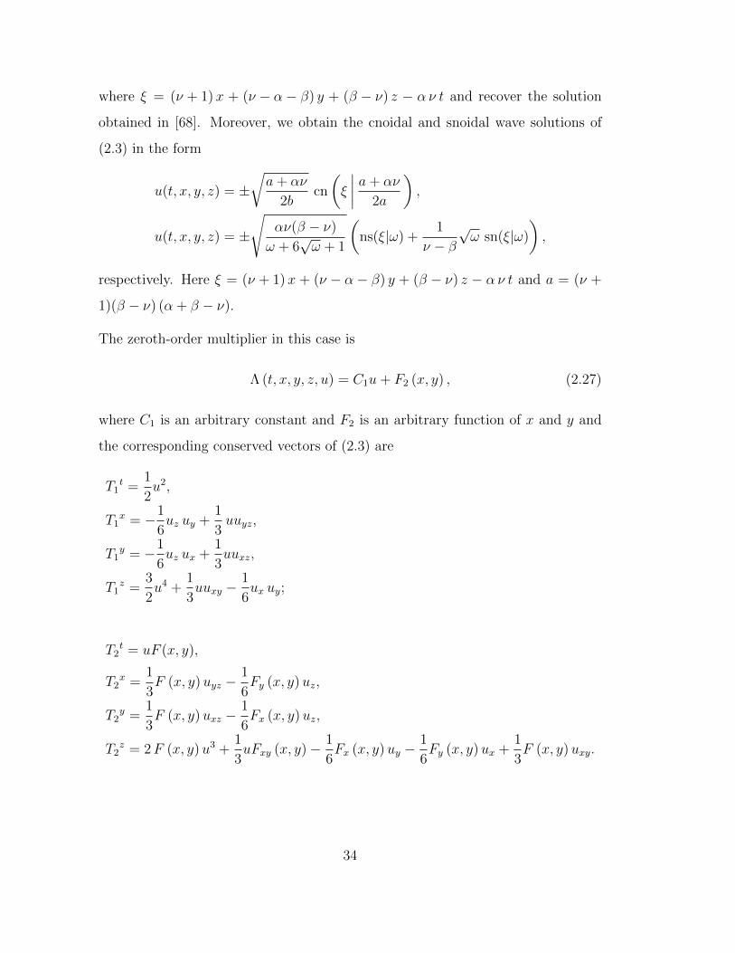
where ξ = (ν + 1)x + (ν − α− β) y + (β − ν) z − α ν t and recover the solution
obtained in [68]. Moreover, we obtain the cnoidal and snoidal wave solutions of
(2.3) in the form
u(t, x, y, z) = ±√a+ αν
2bcn
(ξ
∣∣∣∣ a+ αν
2a
),
u(t, x, y, z) = ±
√αν(β − ν)
ω + 6√ω + 1
(ns(ξ|ω) +
1
ν − β√ω sn(ξ|ω)
),
respectively. Here ξ = (ν + 1)x + (ν − α− β) y + (β − ν) z − α ν t and a = (ν +
1)(β − ν) (α + β − ν).
The zeroth-order multiplier in this case is
Λ (t, x, y, z, u) = C1u+ F2 (x, y) , (2.27)
where C1 is an arbitrary constant and F2 is an arbitrary function of x and y and
the corresponding conserved vectors of (2.3) are
T1t =
1
2u2,
T1x = −1
6uz uy +
1
3uuyz,
T1y = −1
6uz ux +
1
3uuxz,
T1z =
3
2u4 +
1
3uuxy −
1
6ux uy;
T2t = uF (x, y),
T2x =
1
3F (x, y)uyz −
1
6Fy (x, y)uz,
T2y =
1
3F (x, y)uxz −
1
6Fx (x, y)uz,
T2z = 2F (x, y)u3 +
1
3uFxy (x, y)− 1
6Fx (x, y)uy −
1
6Fy (x, y)ux +
1
3F (x, y)uxy.
34
2.5 Concluding remarks
In this chapter we studied three space-time (3+1)-dimensional modified Korteweg-
de Vries equations. Such partial differential equations model many realistic prob-
lems in engineering, wave propagation, fluids, etc. The closed form exact solutions
for the three equations (2.1)–(2.3) were obtained using Lie symmetry method along
with the extended Jacobi elliptic expansion method. Soliton, cnoidal and snoidal
waves solutions were derived. Moreover, conservation laws for the three equations
(2.1)–(2.3) were obtained by the application of direct method.
35
Chapter 3
A symbolic computational
approach to finding solutions and
conservation laws for (3+1)-
dimensional modified BBM
models
3.1 Introduction
The regularized long-wave (RLW) equation
ut + ux + uux − uxxt = 0 (3.1)
is a (1+1)-dimensional equation and is an evolution equation. In equation (3.1), ut
represents time evolution, whereas uux is nonlinear term that describes the rising
or falling of a wave sharply. The mixed derivative term −uxxt is a result of a
36

bounded dispersion relation. Since the (3+1)-dimensional nonlinear differential
equations are considered to be more realistic compared to the (1+1) and (2+1)-
dimensional equations, Wazwaz [68] recently introduced a set of three equations,
viz., (3+1)-dimensional modified Benjamin-Bona-Mahony (D mBBM) equations
that read
ut + ux + u2uy − utxz = 0, (3.2)
ut + uz + u2ux − uxyt = 0 (3.3)
and
ut + uy + u2uz − uxxt = 0. (3.4)
Using a variety of ansatz, exact solutions to (3.2)–(3.4) were derived that described
distinct physical structures of solutions along with some constraints. In this work,
we study three (3+1)-D mBBM equations (3.2)–(3.4). By employing Noether’s ap-
proach [34,46] we construct the conservation laws of these three equations. There-
after, we construct soliton and Jacobi elliptic function solutions of (3.2)–(3.4) by
using Lie group techniques with the aid of the simplest equation technique.
The work presented in this chapter has been published in [75].
3.2 Conservation laws and analytic solutions
3.2.1 Conservation laws
Here conservation laws of the (3+1)-D mBBM equation (3.2) are constructed by
employing Noether’s approach. To utilise Noether’s theorem one needs to have a
Lagrangian for the corresponding Euler-Lagrange equation. Since equation (3.2)
is of order three, its Lagrangian does not exist. However, to implement Noether’s
theorem we raise the order of (3.2) to the fourth-order by letting u = vy. Thus
37

(3.2) becomes
vty + vxy + v2yvyy − vtxyz = 0. (3.5)
It can easily be verified that equation (3.5) has a Lagrangian
L = −1
2vtvy −
1
2vxvy −
1
12v4y −
1
2vtyvxz (3.6)
as δL/δv = 0, where in our case
δLδv
= −Dt∂L∂vt−Dx
∂L∂vx−Dy
∂L∂vy
+DtDy∂L∂vty
+DxDz∂L∂vxz
.
Noether symmetries for (3.5) of the form
X = ξ1(t, x, y, z, v)∂
∂t+ ξ2(t, x, y, z, v)
∂
∂x+ ξ3(t, x, y, z, v)
∂
∂y+ ξ4(t, x, y, z, v)
∂
∂z
+ η(t, x, y, z, v)∂
∂v,
corresponding to Lagrangian (3.6) may be obtained by solving the determining
equation
X [2]L+Dt(ξ1)+Dx(ξ
2)+Dy(ξ3)+Dz(ξ
4)L = Dt(B1)+Dx(B
2)+Dy(B3)+Dz(B
4),
(3.7)
where X [2], the second prolongation of X, is given by [32]
X [2] = ξ1 ∂
∂t+ ξ2 ∂
∂x+ ξ3 ∂
∂y+ ξ4 ∂
∂z+ η
∂
∂v+ ζt
∂
∂vt+ ζx
∂
∂vx+ ζy
∂
∂vy
+ ζty∂
∂vty+ ζxz
∂
∂vxz,
and Bi(t, x, y, z, v), (i = 1, · · · , 4) are gauge functions. Now expanding (3.7), we
have
1
2vxzvy
2ξ3tv −
1
2vtvyξ
4z −
1
2vxvyξ
4z −
1
2vxzvyηtv −
1
2vtyvzηxv −
1
2vxzvtηyv −
1
2vtyvxηvv
+1
2vtyvz
2ξ4xv +
1
2vxzvt
2ξ1yv +
1
2vtyvx
2ξ2zv +
1
2vxzvtξ
tty +
1
2vxzvxξ
2ty +
1
2vxzvyξ
3ty
+1
2vxzvzξ
4ty +
1
2vtyvtξ
1xz +
1
2vtyvxξ
2xz +
1
2vtyvyξ
3xz +
1
2vtyvzξ
4xz − vyvxηv − vyvtηv
38

− vxzvtyηv +1
2vyvt
2ξ1v +
1
4vy
4vtξ1v +
1
2vyvx
2ξ2v +
1
4vy
4vxξ2v +
1
2vy
2vtξ3v +
1
2vy
2vxξ3v
+1
4vy
4vzξ4v −
1
2vxvyξ
1t +
1
2vyvxξ
2t +
1
2vxzvxyξ
2t +
1
2vxzvyyξ
3t +
1
2vxzvyzξ
4t +
1
2vyvzξ
4t
+1
2vyvtξ
1x +
1
2vtyvtzξ
1x −
1
2vtvyξ
2x +
1
2vtyvyzξ
3x +
1
2vyvzξ
4x +
1
2vtyvzzξ
4x +
1
2vtvxξ
1y
+1
3vtvy
3ξ1y +
1
2vxzvttξ
1y +
1
2vxξ
2yvt +
1
3vxvy
3ξ2y +
1
2vxzvtxξ
2y +
1
2vzvtξ
4y +
1
2vzvxξ
4y
+1
3vzvy
3ξ4y +
1
2vxzvtzξ
4y +
1
2vtyvtxξ
1z +
1
2vtyvxxξ
2z +
1
2vtyvxyξ
3z +
1
2vxzvt
2vyξ1vv
+1
2vtyvx
2vzξ2vv +
1
2vxzvy
2vtξ3vv +
1
2vtyvz
2vxξ4vv +
1
2vxzvtvyξ
1tv +
1
2vxzvxvyξ
2tv
+1
2vxzvzvyξ
4tv +
1
2vtyvtvzξ
1xv +
1
2vtyvxvzξ
2xv +
1
2vtyvyvzξ
3xv +
1
2vxzvxvtξ
2yv +
1
2vxzvyvtξ
3yv
+1
2vxzvzvtξ
4yv +
1
2vtyvtvxξ
1zv +
1
2vtyvyvxξ
3vz +
1
2vtyvzvxξ
4vz +
1
2vxvyvtξ
1v + vxzvtvtyξ
1v
+1
2vxzvttvyξ
1v +
1
2vtyvtzvxξ
1v +
1
2vtyvtxvzξ
1v +
1
2vtvyvxξ
2v + vxzvxvtyξ
2v +
1
2vxzvxyvtξ
2v
+1
2vxzvtxvyξ
2v +
1
2vtyvxxvzξ
2v + vxzvyvtyξ
3v +
1
2vxzvyyvtξ
3v +
1
2vtyvxyvzξ
3v +
1
2vtyvyzvxξ
3v
+1
2vtvyvzξ
4v +
1
2vxvyvzξ
4v +
1
2vxzvtzvyξ
4v + vxzvzvtyξ
4v +
1
2vxzvyzξ
4vvt +
1
2vtyvzzvxξ
4v
− 1
2vtyvxvzηvv +
1
2vtyvtvxvzξ
1vv +
1
2vxzvxvtvyξ
2vv +
1
2vtyvyvxvzξ
3vv +
1
2vxzvzvtvyξ
4vv
− 1
2vxzvtvyηvv −B2
x −B3y −B4
z −B1t −
1
3vy
4ηv +1
4vy
5ξ3v −
1
2vyηt −
1
2vyηx −
1
2vtηy
− 1
2vxηy −
1
3vy
3ηy −1
12vy
4ξ1t +
1
2vy
2ξ3t −
1
12vy
4ξ2x +
1
2vy
2ξ3x +
1
2vt
2ξ1y +
1
2vx
2ξ2y
+1
4vy
4ξ3y −
1
12vy
4ξ4z − vtB1
v − vxB2v − vyB3
v − vzB4v −
1
2vxzηty −
1
2vtyηxz = 0.
The above equation now splits on derivatives of v yielding twenty seven homoge-
neous linear partial differential equations (PDEs)
ξ1x = 0, ξ1
y = 0, ξ1z = 0, ξ1
v = 0,
ξ2t = 0, ξ2
y = 0, ξ2z = 0, ξ2
v = 0,
ξ3t = 0, ξ3
x = 0, ξ3z = 0, ξ3
v = 0,
ξ4t = 0, ξ4
x = 0, ξ4y = 0, ξ4
v = 0,
ξ2x + ξ4
z = 0, ξ1t + ξ4
z = 0,
39

ξ1t + ξ2
x + ξ4z − 3ξ3
y = 0, ηxz = 0,
ηv = 0, ηy = 0, ηxz = 0,
B1v = 0, B2
v = 0, B4v = 0,
B3v = −1
2(ηt + ηx) ,
B1t +B2
x +B3y +B4
z = 0.
Solving the above PDEs, albeit easy calculations, we obtain
ξ1 = C1t+ C4,
ξ2 = C1x+ C2,
ξ3 =1
3C1y + C5,
ξ4 = −C1z + C3,
η = F 4(t, x) + F 5(t, z),
B1 = F 1 (t, x, y, z) ,
B2 = F 2 (t, x, y, z) ,
B3 = F 6(t, x, y, z)− 1
2
(F 4t + F 4
x + F 5t
)v,
B4 = F 3 (t, x, y, z) .
Thus, Noether symmetries and their corresponding gauge functions are
X1 =∂
∂t, Bi = 0, (i = 1, · · · , 4),
X2 =∂
∂x, Bi = 0, (i = 1, · · · , 4),
X3 =∂
∂y, Bi = 0, (i = 1, · · · , 4),
X4 =∂
∂z, Bi = 0, (i = 1, · · · , 4),
X5 = 3t∂
∂t+ 3x
∂
∂x+ y
∂
∂y− 3z
∂
∂z, Bi = 0, (i = 1, · · · , 4),
XF 4 = F 4(t, x)∂
∂v, B1 = B2 = B4 = 0, B3 = −1
2(F 4
t + F 4x )v
40

XF 5 = F 5(t, z)∂
∂v, B1 = B2 = B4 = 0, B3 = −1
2F 5t v.
The conserved vector components corresponding to the above Noether point sym-
metries can be obtained by using [34]
T k = Lξk+(ηα − uαxjξj
)( ∂L∂uα
xk
−k∑l=1
Dxl
(∂L
∂uαxlxk
))+
n∑l=k
(ζαl − uαxlxjξ
j) ∂L∂uα
xkxl
−Bk.
(3.8)
Thus, in our case the conserved vectors corresponding to the Noether point sym-
metries X1, · · · , X5, XF 4 and XF 5 are
T t1 = − 1
2vxvy −
1
12v4y ,
T x1 =1
2vtvy +
1
2vtzvty,
T y1 =1
2v2t +
1
2vtvx +
1
3vtv
3y −
1
2vtvtxz,
T z1 =− 1
2vtvtxy;
T t2 =1
2vxvy +
1
2vxyvxz,
T x2 = − 1
2vtvy −
1
12v4y,
T y2 =1
2v2x +
1
2vtvx +
1
3vxv
3y −
1
2vxvtxz,
T z2 = − 1
2vxvtxy;
T t3 =1
2v2y +
1
2vyyvxz,
T x3 =1
2v2y +
1
2vtyvyz,
T y3 =1
4v4y −
1
2vtyvxz −
1
2vyvtxz,
T z3 = − 1
2vyvtxy;
41

T t4 =1
2vyvz +
1
2vyzvxz,
T x4 =1
2vyvz +
1
2vtyvzz,
T y4 =1
2vtvz +
1
2vxvz +
1
3vzv
3y −
1
2vzvtxz,
T z4 = − 1
2vtvy −
1
2vxvy −
1
12v4y −
1
2vxzvty − vzvtxy;
T t5 = − 3
2tvxvy −
1
4tv4y +
3
2xvxvy +
1
2yv2
y −3
2zvyvz +
1
2vyvxz +
3
2xvxyvxz +
1
2yvxzvyy
− 3
2zvxzuz,
T x5 = − 3
2xvtvy −
1
4xv4
y +3
2tvtvy +
1
2yv2
y −3
2zvyvz −
3
2vzvty +
3
2tvtyvtz +
1
2yvtyuz
− 3
2zvtyvzz,
T y5 = − 1
4yv4
y −1
2yvxzvty +
3
2tv2t +
3
2vtvx + vtv
3y −
3
2vtvtxz +
3
2vtvx +
3
2xv2
x + xvxv3y
− 3
2xvxvtxz −
1
2yvyvtxz −
3
2zvzvt −
3
2zvxvz − zvzv3
y +3
2zvzvtxz,
T z5 =3
2zvtvy +
3
2zvxvy +
1
4zv4
y +3
2zvxzvty −
3
2tvtvtxy −
3
2xvxvtxy −
1
2yvyvtxy
+3
2zvzvtxy;
T tF 4 = − 1
2vyF
4(t, x),
T xF 4 = − 1
2vyF
4(t, x),
T yF 4 =
(−1
2vt −
1
2vx −
1
3v3y +
1
2vtxz
)F 4(t, x) +
1
2vF 4
t +1
2vF 4
x ,
T zF 4 =1
2F 4(t, x)vtxy;
T tF 5 = − 1
2vyF
5(t, z),
T xF 5 = − 1
2vyF
5(t, z)− 1
2vtyF
5z (t, z),
42

T yF 5 = − 1
2vtF
5(t, z)− 1
2vxF
5(t, z)− 1
3v3yF
5(t, z) +1
2vtxzF
5(t, z) +1
2vF 5
t ,
T zF 5 =1
2vtxyF
5(t, z).
Now reverting to variable u, we get nonlocal conservation laws of (3.2) as
T t1 = − 1
2u
∫uxdy −
1
12u4,
T x1 =1
2u
∫utdy +
1
2ut
∫utzdy,
T y1 =1
2
(∫utdy
)2
+1
2
∫utdy
∫uxdy +
1
3u3
∫utdy −
1
2
∫utdy
∫utxzdy,
T z1 =− 1
2utx
∫utdy;
T t2 =1
2u
∫uxdy +
1
2ux
∫uxzdy,
T x2 = − 1
2u
∫utdy −
1
12u4,
T y2 =1
2
(∫uxdy
)2
+1
2
∫utdy
∫uxdy +
1
3u3
∫uxdy −
1
2
∫uxdy
∫utxzdy,
T z2 = − 1
2utx
∫uxdy;
T t3 =1
2u2 +
1
2uy
∫uxzdy,
T x3 =1
2u2 +
1
2utuz,
T y3 =1
4u4 − 1
2ut
∫uxzdy −
1
2u
∫utxzdy,
T z3 = − 1
2uutx;
T t4 =1
2u
∫uzdy +
1
2uz
∫uxzdy,
T x4 =1
2u
∫uzdy +
1
2ut
∫uzzdy,
43

T y4 =1
2
∫utdy
∫uzdy +
1
2
∫uxdy
∫uzdy +
1
3u3
∫uzdy −
1
2
∫uzdy
∫utxzdy,
T z4 = − 1
2u
∫utdy −
1
2u
∫uxdy −
1
12u4 − 1
2ut
∫uxzdy − utx
∫uzdy;
T t5 = − 3
2tu
∫uxdy −
1
4tu4 +
3
2xu
∫uxdy +
1
2yu2 − 3
2zu
∫uzdy +
1
2u
∫uxzdy
+3
2xux
∫uxzdy +
1
2yuy
∫uxzdy −
3
2zuz
∫uxzdy,
T x5 = − 3
2xu
∫utdy −
1
4xu4 +
3
2tu
∫utdy +
1
2yu2 − 3
2zu
∫uzdy −
3
2ut
∫uzdy
+3
2tut
∫utzdy +
1
2yutuz −
3
2zut
∫uzzdy,
T y5 = − 1
4yu4 − 1
2yut
∫uxzdy +
3
2t
(∫utdy
)2
+3
2
∫utdy
∫uxdy + u3
∫utdy
− 3
2
∫utdy
∫utxzdy +
3
2
∫utdy
∫uxdy +
3
2x
(∫uxdy
)2
+ xu3
∫uxdy
− 3
2x
∫uxdy
∫utxzdy −
1
2yu
∫utxzdy −
3
2z
∫uzdy
∫utdy
− 3
2z
∫uxdy
∫uzdy − zu3
∫uzdy +
3
2z
∫uzdy
∫utxzdy,
T z5 =3
2zu
∫utdy +
3
2zu
∫uxdy +
1
4zu4 +
3
2zut
∫uxzdy −
3
2t
∫utdyutx
− 3
2xutx
∫uxdy −
1
2yuutx +
3
2zutx
∫uzdy;
T tF 4 = − 1
2uF 4(t, x),
T xF 4 = − 1
2uF 4(t, x),
T yF 4 = − 1
2F 4(t, x)
∫utdy −
1
2F 4(t, x)
∫uxdy −
1
3u3F 4(t, x) +
1
2F 4(t, x)
∫utxzdy
+1
2F 4t
∫udy +
1
2F 4x
∫udy,
T zF 4 =1
2utxF
4(t, x);
44

T tF 5 = − 1
2uF 5(t, z),
T xF 5 = − 1
2uF 5(t, z)− 1
2utF
5z ,
T yF 5 = − 1
2F 5(t, z)
∫utdy −
1
2F 5(t, z)
∫uxdy −
1
3u3F 5(t, z) +
1
2F 5(t, z)
∫utxzdy
+1
2F 5t
∫udy,
T zF 5 =1
2utxF
5(t, z).
3.2.2 Closed form solutions
In this section, we compute soliton and Jacobi elliptic function solutions of the
(3+1)-D mBBM equation (3.2) by invoking Lie point symmetry and simplest equa-
tion techniques.
Lie symmetries
The vector field (2.4) is a Lie symmetry of (3.2) if
X [3](ut + ux + u2uy − utxz)|(3.2) = 0, (3.9)
where X [3], the third prolongation of X, is given by [32]
X [3] = X + ζt∂
∂ut+ ζx
∂
∂ux+ ζy
∂
∂uy+ ζtxz
∂
∂utxz(3.10)
with ζt, ζx, ζx, ζtx and ζtxz being defined as
ζt = Dt(η)− utDt(ξ1)− uxDt(ξ
2)− uyDt(ξ3)− uzDt(ξ
4),
ζx = Dx(η)− utDx(ξ1)− uxDx(ξ
2)− uyDx(ξ3)− uzDx(ξ
4),
ζy = Dy(η)− utDy(ξ1)− uxDy(ξ
2)− uyDy(ξ3)− uzDy(ξ
4),
ζtx = Dx(ζt)− uttDx(ξ1)− utxDx(ξ
2)− utyDx(ξ3)− utzDx(ξ
4),
ζtxz = Dz(ζtx)− utxtDz(ξ1)− utxxDz(ξ
2)− utxyDz(ξ3)− utxzDz(ξ
4).
45

The total differential operators Dt, Dx, Dy, and Dz are given by (2.7). Equation
(3.9) now splits on derivatives of v yielding twenty one homogeneous linear PDEs
ξ4t = 0, ξ3
t = 0, ξ2t = 0, ξ1
tt = 0, ξ4x = 0, ξ3
x = 0, ξ1x = 0, ξ1
y = 0, ξ2y = 0, ξ3
yy = 0,
ξ4y = 0, ξ3
z = 0, ξ2z = 0, ξ1
z = 0, ξ4u = 0, ξ3
u = 0, ξ2u = 0, ξ1
u = 0, ξ1t − ξ2
x = 0,
ξ1t − ξ4
z = 0, 2η + u(ξ1t − ξ3
y
)= 0.
After some simple calculations, one obtains the following values of ξ1, ξ2, ξ3, ξ4 and
η:
ξ1 = C4 + C6t,
ξ2 = C5 + C6x,
ξ3 = C1 + C2y,
ξ4 = C3 − C6z,
η =1
2u(C2 − C6),
where Ci, (i = 1, 2, · · · , 6) are constants. Thus, Lie symmetries of (3.2) are
X1 =∂
∂t, X2 =
∂
∂x, X3 =
∂
∂y, X4 =
∂
∂z, X5 = 2y
∂
∂y+ u
∂
∂u,
X6 = 2t∂
∂t+ 2x
∂
∂x− 2z
∂
∂z− u ∂
∂u,
which includes four translation and two scaling operators.
3.2.2.1 Soliton solution
We first perform symmetry reductions and transform the (3+1)-D mBBM equation
(3.2) to a third-order nonlinear ODE. Consider the four translation symmetries X1,
X2, X3 and X4. Taking a linear combination of the aforementioned generators,
viz., X = X1 + αX2 +X3 +X4, (α a constant) yields the invariants f = −x+ αt,
46

g = −αy + x and h = −z + y. Using these invariants, the invariant solution
u = θ (f, g, h) satisfies
θg − (1− α)θf + θ2(θh − αθg)− α(θffh − θfgh) = 0. (3.11)
Likewise, making use of the linear combination Γ = Γ1 + βΓ2 + Γ3 of the Lie point
symmetries
Γ1 =∂
∂f, Γ2 =
∂
∂g, Γ3 =
∂
∂h(3.12)
of (3.11) gives r = −h + f and s = −βh + g as two invariants. Hence θ = φ(r, s)
solves
φs − (1− α)φr − φ2(αφs + φr + βφs)− α(1− β)φrrs + αφrrr − αβφsrs = 0.
(3.13)
As before, we now utilise the two infinitesimal symmetry generators of (3.13),
namely Σ1 = ∂/∂r and Σ2 = ∂/∂s. The symmetry Σ = Σ1 + νΣ2 provides us
with the invariant solution φ(r, s) = ψ(ξ) with ξ = s − νr. Thus, equation (3.13)
transforms to
aψ′′′ + bψ2ψ′ − cψ′ = 0, (3.14)
with a = να(ν + 1)(ν − β), b = α− ν + β and c = ν − αν + 1. Double integration
of (3.14) with integration constants zero (as we are looking for a soliton solution)
yields
ψ′2 = Aψ2 −Bψ4, (3.15)
where A = c/a and B = b/(6a). Integration of equation (3.15) yields
sech−1
(ψ
K
)= ±√Bξ + C∗, (3.16)
where K2 = A/B and C∗ is a constant. Equation (3.16) gives the value of ψ and
hence we have
u = ±
√6(ν − αν + 1)
α− ν + βsech
(C∗ ±
√α− ν + β
6να(ν + 1)(ν − β)ξ
), (3.17)
47

where ξ = −α ν t+ (1 + ν)x− (α + β − ν) y − (ν − β) z. Thus, we recuperate the
bell-shaped soliton solution (3.17), which was derived in [68] by using an ad hoc
method. The beauty of the above method is that the form of the solution was not
chosen in advance. See the graphical representation below which has been drawn
using suitable parameter values of solution (3.17).
50 100 150 200z
2
4
6
8
Figure 3.1: Profile of soliton solution (3.17).
3.2.2.2 Exact solutions using the simplest equation method
We now construct exact explicit solutions of the (3+1)-D mBBM equation (3.2) in
terms of Jacobi elliptic functions following the method of Section 1.6.2. We apply
this method to ODE (3.14).
Solutions of (3.14) using (1.57) as the simplest equation
We note that for the equation (3.14), using the balancing procedure, we get M = 1.
Thus, (1.56) is
ψ(ξ) = A−1H−1(ξ) + A0 + A1H(ξ). (3.18)
Using this value of ψ in (3.14) along with (1.57) we obtain eleven algebraic equa-
tions:
αA0A12 + β A0A1
2 − ν A0A12 = 0,
αA−12A0 − αω A−1
2A0 − β ω A−12A0 + ν ω A−1
2A0 + β A−12A0
48

− ν A−12A0 = 0,
2αω A−12A0 − 2ν ω A−1
2A0 − αA−12A0 − β A−1
2A0 + ν A−12A0 = 0,
2 ν ω A0A12 − 2αω A0A1
2 − 2 β ω A0A12 + αA0A1
2 + β A0A12 − ν A0A1
2 = 0,
6αβ ν2ω A1 − 6α ν3ω A1 + 6αβ ν ω A1 − 6α ν2ω A1 + αA13 + β A1
3
− ν A13 = 0,
α ω A0A12 − αω A−1
2A0 − β ω A−12A0 + β ω A0A1
2 + ν ω A−12A0 − ν ω A0A1
2
+ ν A0A12 − αA0A1
2 − β A0A12 = 0,
6α ν3ω2A−1 − 6αβ ν2ω2A−1 + 12αβ ν2ω A−1 − 6αβ ν ω2A−1 − 12α ν3ω A−1
+ 6α ν2ω2A−1 − 6αβ ν2A−1 + 12αβ ν ω A−1 + 6α ν3A−1 − 12α ν2ω A−1 − αω A−13
+ ν ω A−13 − β ω A−1
3 − 6αβ ν A−1 + 6α ν2A−1 + αA−13 + β A−1
3 − ν A−13 = 0,
14α ν3ω2A1 − 14αβ ν2ω2A1 + 7αβ ν2ω A1 − 14αβ ν ω2A1 − 7α ν3ω A1 + 14α ν2ω2A1
+ 7αβ ν ω A1 − 7α ν2ω A1 + αω A−1A12 + αω A0
2A1 − 2αω A13 + β ω A−1A1
2
+ β ω A02A1 − 2 β ω A1
3 − ν ω A−1A12 − ν ω A0
2A1 + 2 ν ω A13 + α ν ω A1 + αA1
3
+ β A13 − ν A1
3 − ν ω A1 − ω A1 = 0,
14αβ ν2ω2A−1 − 14α ν3ω2A−1 − 21αβ ν2ω A−1 + 14αβ ν ω2A−1
+ 21α ν3ω A−1 − 14α ν2ω2A−1 + 7αβ ν2A−1 − 21αβ ν ω A−1
− 7α ν3A−1 + 21α ν2ω A−1 + 2αω A−13 − αω A−1
2A1 − αω A−1A02 + 2 β ω A−1
3
− β ω A−12A1 − β ω A−1A0
2 − 2 ν ω A−13 + ν ω A−1
2A1 + ν ω A−1A02 + 7αβ ν A−1
+ αA−1A02 − 7α ν2A−1 − α ν ω A−1 − αA−1
3 + αA−12A1 − β A−1
3 + β A−12A1 + ν A−1
3
+ β A−1A02 − ν A−1
2A1 − ν A−1A02 + α ν A−1 + ν ω A−1 − ν A−1 + ω A−1 − A−1 = 0,
2αβ ν2ω2A−1 + 10αβ ν2ω2A1 − 2α ν3ω2A−1 − 10α ν3ω2A1 − αβ ν2ω A−1 − 10αβ ν2ω A1
+ 2αβ ν ω2A−1 + 10αβ ν ω2A1 + α ν3ω A−1 + 10α ν3ω A1 − 2α ν2ω2A−1 − 10α ν2ω2A1
+ αβ ν2A1 − αβ ν ω A−1 − 10αβ ν ω A1 − α ν3A1 + α ν2ω A−1 + 10α ν2ω A1
− αω A−12A1 − αω A−1A0
2 − 2αω A−1A12 − 2αω A0
2A1 + αω A13 − β ω A−1
2A1
49

− β ω A−1A02 − 2 β ω A−1A1
2 − 2 β ω A02A1 + β ω A1
3 + ν ω A−12A1 + ν ω A−1A0
2
+ 2 ν ω A−1A12 + 2 ν ω A0
2A1 − ν ω A13 + αβ ν A1 − α ν2A1 − α ν ω A−1 − 2α ν ω A1
+ αA−1A12 + αA0
2A1 − αA13 + β A−1A1
2 + β A02A1 − β A1
3 − ν A−1A12
− ν A02A1 + ν A1
3 + α ν A1 + ν ω A−1 + 2 ν ω A1 − ν A1 + ω A−1 + 2ω A1 − A1 = 0,
− 10αβ ν2ω2A−1 − 2αβ ν2ω2A1 + 10α ν3ω2A−1 + 2α ν3ω2A1 + 10αβ ν2ω A−1
+ 3αβ ν2ω A1 − 10αβ ν ω2A−1 − 2αβ ν ω2A1 − 10α ν3ω A−1 − 3α ν3ω A1
+ 10α ν2ω2A−1 + 2α ν2ω2A1 − αβ ν2A−1 − αβ ν2A1 + 10αβ ν ω A−1 + 3αβ ν ω A1
+ α ν3A−1 + α ν3A1 − 10α ν2ω A−1 − 3α ν2ω A1 − αω A−13 + 2αω A−1
2A1
+ 2αω A−1A02 + αω A−1A1
2 + αω A02A1 − β ω A−1
3 + 2 β ω A−12A1
+ 2 β ω A−1A02 + β ω A−1A1
2 + β ω A02A1 + ν ω A−1
3 − 2 ν ω A−12A1
− 2 ν ω A−1A02 − ν ω A−1A1
2 − ν ω A02A1 − αβ ν A−1 − αβ ν A1 + α ν2A−1
+ α ν2A1 + 2α ν ω A−1 + α ν ω A1 − αA−12A1 − αA−1A0
2 − αA−1A12 − αA0
2A1
− β A−12A1 − β A−1A0
2 − β A−1A12 − β A0
2A1 + ν A−12A1 + ν A−1A0
2
+ ν A−1A12 + ν A0
2A1 − α ν A−1 − α ν A1 − 2 ν ω A−1 − ν ω A1 + ν A−1 + ν A1
− 2ω A−1 − ω A1 + A−1 + A1 = 0.
Solving the above system, using Maple, we obtain
ν = −α2 − α + 1 +
√α4 − 2α3 − α2 − 2α + 1
2α2 ,
β =ν(2 ω − 1) + α
2ω − 1, A−1 = A0 = 0, A1 = ±
√3(ν(1− α) + 1)
α,
α 6= 0, α 6= 1, ν 6= β.
Therefore the solution to (3.2) is
u(t, x, y, z) = ±√
3(ν(1− α) + 1)
αcn (ξ |ω ) , (3.19)
where α 6= 0, α 6= 1,, ν 6= β, and ξ = −α ν t+(1 + ν)x−(α + β − ν) y−(ν − β) z.
We note that the solution (3.17) obtained by direct integration can be derived from
50

solution (3.19), since cn(ξ|ω)→ sech(ξ) when ω → 1. However, solutions (3.19) are
periodic in nature, consistent with Jacobi amplitude functions. See a 3D rendering
of one of the solutions in Figure 3.2. Here we utilise suitable values for parameters
α and ω.
-20 -10 10 20
-6
-4
-2
2
4
6
Figure 3.2: Profile of cnoidal wave solution (3.19)
Solutions of (3.14) using (1.58) as the simplest equation
Substituting (3.18) along with (1.58) into (3.14), we obtain an algebraic equation,
which splits into the following eleven algebraic equations:
αA−12A0 + β A−1
2A0 − ν A−12A0 = 0,
ν A0A12 − αA0A1
2 − β A0A12 = 0,
ν A−12A0 − αω A−1
2A0 − β ω A−12A0 + ν ω A−1
2A0 − αA−12A0
− β A−12A0 = 0,
α ω A0A12 + β ω A0A1
2 − ν ω A0A12 + αA0A1
2 + β A0A12 − ν A0A1
2 = 0,
α ω A−12A0 + β ω A−1
2A0 − ν ω A−12A0 − αA0A1
2 − β A0A12
+ ν A0A12 = 0,
6α ν3A−1 − 6αβ ν2A−1 − 6αβ ν A−1 + 6α ν2A−1 + αA−13 + β A−1
3 − ν A−13 = 0,
6αβ ν2ω A1 − 6α ν3ω A1 + 6αβ ν ω A1 − 6α ν2ω A1 − αA13 − β A1
3
+ ν A13 = 0,
51

7αβ ν2ω A−1 − 7α ν3ω A−1 + 7αβ ν2A−1 + 7αβ ν ω A−1 − 7α ν3A−1 − 7α ν2ω A−1
− αω A−13 − β ω A−1
3 + ν ω A−13 + 7αβ ν A−1 − 7α ν2A−1 − αA−1
3 + αA−12A1
+ αA−1A02 − β A−1
3 + β A−12A1 + β A−1A0
2 + ν A−13 − ν A−1
2A1 − ν A−1A02
+ α ν A−1 − ν A−1 − A−1 = 0,
7α ν3ω2A1 − 7αβ ν2ω2A1 − 7αβ ν2ω A1 − 7αβ ν ω2A1 + 7α ν3ω A1 + 7α ν2ω2A1
+ 7α ν2ω A1 − 7αβ ν ω A1 − αω A−1A12 − αω A0
2A1 + αω A13 − β ω A−1A1
2
+ β ω A13 − β ω A0
2A1 + ν ω A−1A12 + ν ω A0
2A1 − ν ω A13 − α ν ω A1 + αA1
3
+ β A13 − ν A1
3 + ν ω A1 + ω A1 = 0,
α ν3ω2A−1 − αβ ν2ω2A−1 − 8αβ ν2ω A−1 − αβ ν2ω A1 − αβ ν ω2A−1 + 8α ν3ω A−1
+ α ν3ω A1 + α ν2ω2A−1 − αβ ν2A−1 − αβ ν2A1 − 8αβ ν ω A−1 − αβ ν ω A1
+ α ν3A−1 + α ν3A1 + 8α ν2ω A−1 + α ν2ω A1 + αω A−13 − αω A−1
2A1 − αω A−1A02
+ β ω A−13 − β ω A−1
2A1 − β ω A−1A02 − ν ω A−1
3 + ν ω A−12A1 + ν ω A−1A0
2
− αβ ν A−1 − αβ ν A1 + α ν2A−1 + α ν2A1 − α ν ω A−1 − αA−12A1 − αA−1A0
2
− αA−1A12 − αA0
2A1 − β A−12A1 − β A−1A0
2 − β A−1A12 − β A0
2A1 + ν A−12A1
+ ν A−1A02 + ν A−1A1
2 + ν A02A1 − α ν A−1 − α ν A1 + ν ω A−1 + ν A−1 + ν A1
+ ω A−1 + A−1 + A1 = 0,
α β ν2ω2A−1 + αβ ν2ω2A1 − α ν3ω2A−1 − α ν3ω2A1 + αβ ν2ω A−1 + 8αβ ν2ω A1
+ αβ ν ω2A−1 + αβ ν ω2A1 − α ν3ω A−1 − 8α ν3ω A1 − α ν2ω2A−1 − α ν2ω2A1
+ αβ ν2A1 + αβ ν ω A−1 + 8αβ ν ω A1 − α ν3A1 − α ν2ω A−1 − 8α ν2ω A1
+ αω A−12A1 + αω A−1A0
2 + αω A−1A12 + αω A0
2A1 + β ω A−12A1 + β ω A−1A0
2
+ β ω A−1A12 + β ω A0
2A1 − ν ω A−12A1 − ν ω A−1A0
2 − ν ω A−1A12 − ν ω A0
2A1
+ αβ ν A1 − α ν2A1 + α ν ω A−1 + α ν ω A1 + αA−1A12 + αA0
2A1 − αA13
+ β A−1A12 + β A0
2A1 − β A13 − ν A−1A1
2 − ν A02A1 + ν A1
3 + α ν A1
− ν ω A−1 − ν ω A1 − ν A1 − ω A−1 − ω A1 − A1 = 0.
52

A solution of the above system, using Maple, is
ν = −α2 − α + 1 +
√α4 − 2α3 − α2 − 2α + 1
2α2 ,
β =ν (ω + 1)− α
ω + 1, A−1 = A0 = 0, A1 = ±
√6(ν(1− α) + 1)
α,
α 6= 0, α 6= 1, ν 6= β.
Therefore a solution to (3.2) becomes
u(t, x, y, z) = ±√
6(ν(1− α) + 1)
αsn (ξ |ω ) , (3.20)
where 0 ≤ ω ≤ 1 and ξ = −α ν t + (1 + ν)x − (α + β − ν) y − (ν − β) z. See the
profile of solution (3.20) in Figure 3.3.
-20 -10 10 20
-6
-4
-2
2
4
6
Figure 3.3: Profile of snoidal wave solution (3.20).
3.3 Conservation laws and exact solutions of (3.3)
Following the procedure of the previous section, we have the following nonlocal
conservation laws of the (3+1)-D mBBM equation (3.3):
T t1 = − 1
2u
∫uzdx−
1
12u4,
T x1 =1
2
(∫utdx
)2
+1
2
∫utdx
∫uzdx+
1
3u3
∫utdx−
1
2uty
∫utdx+
1
2ut
∫utydx,
53
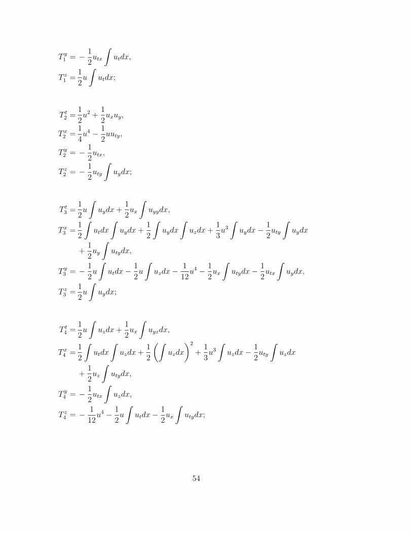
T y1 = − 1
2utx
∫utdx,
T z1 =1
2u
∫utdx;
T t2 =1
2u2 +
1
2uxuy,
T x2 =1
4u4 − 1
2uuty,
T y2 = − 1
2utx,
T z2 = − 1
2uty
∫uydx;
T t3 =1
2u
∫uydx+
1
2ux
∫uyydx,
T x3 =1
2
∫utdx
∫uydx+
1
2
∫uydx
∫uzdx+
1
3u3
∫uydx−
1
2uty
∫uydx
+1
2uy
∫utydx,
T y3 = − 1
2u
∫utdx−
1
2u
∫uzdx−
1
12u4 − 1
2ux
∫utydx−
1
2utx
∫uydx,
T z3 =1
2u
∫uydx;
T t4 =1
2u
∫uzdx+
1
2ux
∫uyzdx,
T x4 =1
2
∫utdx
∫uzdx+
1
2
(∫uzdx
)2
+1
3u3
∫uzdx−
1
2uty
∫uzdx
+1
2uz
∫utydx,
T y4 = − 1
2utx
∫uzdx,
T z4 = − 1
12u4 − 1
2u
∫utdx−
1
2ux
∫utydx;
54

T t5 =1
2tu
∫uzdx−
1
2zu
∫uzdx−
1
12zu4 +
1
12tu4 +
1
2yu
∫uydx+
1
2ux
∫uydx
+1
2yux
∫uyydx,
T x5 =1
2
∫udx
∫utdx+
1
2
∫udx
∫uzdx+
1
3u3
∫udx− 1
2uty
∫udx
+ t
(∫utdx
)2
+ t
∫utdx
∫uzdx+
2
3tu3
∫utdx− tuty
∫utdx
+ z
∫utdx
∫uzdx+ z
(∫uzdx
)2
+2
3zu3
∫uzdx− zuty
∫uzdx
+1
2u
∫utydx+ tut
∫utydx+ zuz
∫utydx,
T y5 = − 1
2utx
∫udx− tutx
∫utdx− zutx
∫uzdx,
T z5 =u
∫utdx− zu
∫utdx−
1
6zu4 − zux
∫utydx+
1
2u
∫udx;
T tF 1 = − 1
2uF 1(y, z)− 1
2uxF
1y ,
T xF 1 = − 1
2F 1(y, z)
∫utdx−
1
2F 1(y, z)
∫uzdx−
1
3u3F 1(y, z) +
1
2utyF
1(y, z)
+1
2F 1z
∫udx,
T yF 1 =1
2utxF
1(y, z),
T zF 1 = − 1
2uF 1(y, z);
T tF 2 = − 1
2uF 2(t, z),
T xF 2 = − 1
2F 2(t, z)
∫utdx−
1
2F 2(t, z)
∫uzdx−
1
3u3F 2(t, z) +
1
2utyF
2(t, z)
+1
2F 2t
∫udx+
1
2F 2z
∫udx,
T yF 2 = − 1
2uF 2(t, z)− 1
2F 2z
∫utydx,
T zF 2 = − 1
2uF 2(t, z).
55

The Lie symmetry technique and direct integration yields the soliton solution
u = ±√
6(αν + ν − β)
ν + 1sech
(C ±
√ν + 1
6αν(ν − α + β)(ν + 1)ξ
)
of (3.3), where ξ = −α ν t+(1 + ν)x−(α + β − ν) y−(ν − β) z and C is a constant.
As before, we have retrieved the bell shaped soliton solution of [68]. Moreover, the
cnoidal and snoidal wave solutions of (3.3) are
u(t, x, y, z) = ±√
3α cn (ξ |ω ) , α > 0. (3.21)
u(t, x, y, z) = ±√
6α sn (ξ |ω ) , α > 0, (3.22)
respectively, with ξ = −α ν t+ (1 + ν)x− (α + β − ν) y − (ν − β) z.
3.4 Conservation laws and exact solutions of (3.4)
For the third (3+1)-D mBBM equation (3.4), we have the following nonlocal con-
servation laws:
T t1 = − 1
2u
∫uydz −
1
12u4,
T x1 = − 1
2utx
∫utdz +
1
2ut
∫utxdz,
T y1 = − 1
2u
∫utdz,
T z1 =1
2
(∫utdz
)2
+1
2
∫utdz
∫uydz +
1
2u3
∫utdz −
1
2
∫utdz
∫utxxdz;
T t2 =1
2u
∫uxdz +
1
2ux
∫uxxdz,
T x2 = − 1
2u
∫utdz −
1
2u
∫uydz −
1
12u4 − 1
2utx
∫uxdz,
T y2 =1
2u
∫uxdz,
56

T z2 =1
2
∫utdz
∫uxdz +
1
2
∫uxdz
∫uydz +
1
2u3
∫uxdz −
1
2
∫uxdz
∫utxxdz;
T t3 =1
2u
∫uydz +
1
2uy
∫uxxdz,
T x3 = − 1
2utx
∫uydz +
1
2ut
∫uxydz,
T y3 = − 1
2u
∫utdz −
1
12u4 − 1
2ut
∫uxxdz,
T z3 =1
2
∫utdz
∫uydz +
1
2
(∫uydz
)2
+1
3u3
∫uydz −
1
2
∫uydz
∫utxxdz;
T t4 =1
2u2 +
1
2uz
∫uxxdz,
T x4 = − 1
2uutx +
1
2utux,
T y4 =1
2u2,
T z4 =1
4u4 − 1
2ut
∫uxxdz −
1
2u
∫utxxdz;
T t5 = − tu∫uydz −
1
6tu4 +
1
2u
∫udz + yu
∫uydz +
1
2uz
∫uxxdz + yuy
∫uxxdz,
T x5 = − 1
2utx
∫udz − tutx
∫utdz − yutx
∫uydz +
1
2ut
∫uxdz + tut
∫utxdz
+ yut
∫uxydz,
T y5 = − yu∫utdz −
1
6yu4 − yut
∫uxxdz +
1
2u
∫udz + tu
∫utdz,
T z5 =1
2
∫udz
∫utdz +
1
2
∫udz
∫uydz +
1
3u3
∫udz − 1
2
∫udz
∫utxxdz
+ t
(∫utdz
)2
+ t
∫utdz
∫uydz +
2
3tu3
∫utdz − t
∫utdz
∫utxxdz
+ y
∫utdz
∫uydz + y
(∫uydz
)2
+2
3yu3
∫uydz − y
∫uydz
∫utxxdz;
57

T t6 = − 6yu
∫uydz + 6tu
∫uydz − yu4 + tu4 − 3
2u
∫udz + zu2 − 1
2u
∫uxxdz
+ 3x
∫uxxdzux + zuz
∫uxxdz,
T x6 = − 3xu
∫utdz − 3xu
∫uydz −
1
2xu4 +
3
2utx
∫udz − 6yutx
∫utdz
+ 6tutx
∫utdz − 3xutx
∫uxdz − zuutx +
3
2ut
∫uxdz + 6yut
∫utxdz
− 6tut
∫utxdz + zutux,
T y6 = 6yu
∫utdz −
3
2u
∫udz − 6tu
∫utdz + 3xu
∫uxdz
∫udz + zu2,
T z6 =1
2
∫udz
∫utdz +
1
2
∫udz
∫uydz +
1
3u3
∫udz − 1
2
∫udz
∫utxxdz
+ t
(∫utdz
)2
+ t
∫utdz
∫uydz +
2
3tu3
∫utdz − t
∫utdz
∫utxxdz
+ y
∫utdz
∫uydz + y
(∫uydz
)2
+2
3yu3
∫uydz − y
∫uydz
∫utxxdz;
T tF 1 = − 1
2xuF 1(t, y),
T xF 1 =1
2xutxF
1(t, y)− 1
2utF
1(t, y),
T yF 1 = − 1
2xuF 1(t, y),
T zF 1 = − 1
2xF 1(t, y)
∫utdz −
1
2xF 1(t, y)
∫uydz −
1
3xu3F 1(t, y)
+1
2xF 1(t, y)
∫utxxdz +
1
2F 1t
∫udz +
1
2F 1x
∫udz;
T tF 2 = − 1
2uF 2(t, y),
T xF 2 =1
2utxF
2(t, y),
T yF 2 = − 1
2uF 2(t, y),
T zF 2 = − 1
2F 2(t, y)
∫utdz −
1
2F 2(t, y)
∫uydz −
1
3u3F 2(t, y) +
1
2F 2(t, y)
∫utxxdz
58

+1
2F 2t
∫udz +
1
2F 2y
∫udz.
The one-soliton solution of (3.4) is
u = ±
√6(α + β + αν − ν)
β − νsech
(C ±
√β − ν
6αν(ν + 1)2ξ
), (3.23)
α 6= 0, ν 6= 0, β 6= ν, ν 6= 1, (3.24)
and the cnoidal and snoidal wave solutions of (3.4) are
u =±√
6ν ω (ν + 1) (2 ν2ω − ν2 + 2 ν ω − ν − 1)
2 ν2ω − ν2 + 2 ν ω − ν − 1cn (ξ |ω ) , (3.25)
u = ±√
6α cn (ξ |ω ) , α > 0, (3.26)
respectively, with ξ = −α ν t+ (1 + ν)x− (α + β − ν) y − (ν − β) z.
3.5 Concluding remarks
In this chapter, we studied the three (3+1)-D mBBM equations, which were intro-
duced in [68]. We obtained soliton solutions for each equation without any fore-
going assumptions about the form of the solutions. Furthermore, we constructed
Jacobi elliptic function solutions of the three equations with the aid of the sim-
plest equation method. Jacobi elliptic solutions are more general as they contain
trigonometric and hyperbolic functions depending on the behaviour of the param-
eter ω. The obtained solutions are presented graphically. Finally, we successfully
derived nonlocal conservation laws for each (3+1)-D mBBM equation by enlisting
the famous Noether’s theorem.
59

Chapter 4
Conserved quantities, optimal
system and explicit solutions of a
(1+1)-dimensional generalised
coupled mKdV-type system
4.1 Introduction
In [76], Foursov performed a classification of coupled potential KdV-type and mod-
ified KdV-type equations that possess higher symmetries, and eleven new systems
were presented for which Hamiltonian and bi-Hamiltonian formulations were pro-
vided for some of the equations. His work focused on coupled and symmetric
systems of type ut = F [u, v] and vt = F [v, u]. It is against this backdrop that the
following previously unknown coupled system was obtained in [76]:
ut − u2vx − 3uvux − uxxx = 0,
vt − v2ux − 3uvvx − vxxx = 0.(4.1)
60

In this chapter, however, we investigate the generalised coupled mKdV-type system
E1 ≡ ut − u2vx − αuvux − uxxx = 0,
E2 ≡ vt − v2ux − αuvvx − vxxx = 0(4.2)
with α a constant. System (4.1) is interesting in that it is non-decouplable and
possesses higher generalised symmetries. To the best of our knowledge, the above
system (4.2) is studied extensively for the first time in this chapter and the results
are therefore new. With the application of Lie symmetry analysis we seek to
derive conserved quantities and exact solutions for the system (4.2). For this we
shall utilise multiplier approach via the homotopy integral and Lie group analysis
along with power series solution method.
The work presented in this chapter has been published in [77].
4.2 Conserved quantities
For the generalised coupled mKdV-type system (4.2) with multipliers Λ1 and Λ2 we
determine the corresponding conserved quantities by using the homotopy integral
method, but first we find the multipliers.
To compute all multipliers of (4.2), we use the determining condition
δ
δu
[Λ1E1 + Λ2E2
]= 0,
δ
δv
[Λ1E1 + Λ2E2
]= 0. (4.3)
Here the operators δ/δu and δ/δv are the well known Euler operators (1.25), which
in this instance are specified as
δ
δu=
∂
∂u−Dt
∂
∂ut−Dx
∂
∂ux+D2
x
∂
∂uxx−D3
x
∂
∂uxxx,
δ
δv=
∂
∂v−Dt
∂
∂vt−Dx
∂
∂vx+D2
x
∂
∂vxx−D3
x
∂
∂vxxx
(4.4)
with Dt and Dx being the total derivatives (1.4) explicitly given by
Dt =∂
∂t+ ut
∂
∂u+ vt
∂
∂v+ utt
∂
∂ut+ vtt
∂
∂vt+ utx
∂
∂ux+ vtx
∂
∂vx+ · · · ,
61

Dx =∂
∂x+ ux
∂
∂u+ vx
∂
∂v+ uxx
∂
∂ux+ vxx
∂
∂vx+ uxt
∂
∂ut+ vxt
∂
∂vt+ · · · .
Here we seek to compute second order multipliers
Λm = Λm(t, x, u, v, ux, vx, uxx, vxx), m = 1, 2.
Expanding (4.3) and comparing powers of derivatives of u, v, we acquire a system
of thirty six PDEs. The solution to this system of PDEs is akin to the algorithm
for obtaining Lie point symmetries. Solving this system of PDEs gives
Λ1 =C1
[(α + 1)tuv2 + xv + 3 tvxx
]+
1
α + 1[C2(α + 1)uv2 + 3 vxx+ C3 (α + 1) v], α 6= −1,
Λ2 =C1
[xu+
(α + 1) vu2 + 3uxx
t]
+1
α + 1[C2
((α + 1)u2v + 3uxx
)] + C3 u, α 6= −1
(4.5)
with C1, C2 andC3 constants. Thus, we obtain three multipliers given by
Λ11 = (α + 1) tuv2 + xv + 3 tvxx, Λ2
1 = xu+((α + 1) vu2 + 3uxx
)t;
Λ12 =
1
α + 1
(α + 1)uv2 + 3 vxx
, Λ2
2 =1
α + 1
(α + 1)u2v + 3uxx
;
Λ13 = v, Λ2
3 = u.
(4.6)
From these three sets of multipliers, conserved densities T i and spatial fluxes X i
for i = 1, 2, 3 can be obtained in several ways [43]. In this work, we use the first
62

homotopy integral (1.48), here given explicitly by
T =
∫ 1
0
(u
(∂E1Λ1
∂ut
) ∣∣∣u=u(λ) + v∂E2Λ2
∂vt
∣∣∣v=v(λ)
)dλ,
X =
∫ 1
0
[u
(∂E1Λ1
∂ux
) ∣∣∣u=u(λ) −Dx
(∂E1Λ1
∂uxx
) ∣∣∣u=u(λ) +D2x
(∂E1Λ1
∂uxxx
) ∣∣∣u=u(λ)
+ux
(∂E1Λ1
∂uxx
) ∣∣∣u=u(λ) +D2x
(∂E1Λ1
∂uxx
) ∣∣∣u=u(λ)
+ uxx
(∂E1Λ1
∂uxxx
) ∣∣∣u=u(λ)
+u
(∂E2Λ2
∂ux
) ∣∣∣u=u(λ) −Dx
(∂E2Λ2
∂uxx
) ∣∣∣u=u(λ) +D2x
(∂E2Λ2
∂uxxx
) ∣∣∣u=u(λ)
+ux
(∂E2Λ2
∂uxx
) ∣∣∣u=u(λ) +D2x
(∂E2Λ2
∂uxx
) ∣∣∣u=u(λ)
+ uxx
(∂E2Λ2
∂uxxx
) ∣∣∣u=u(λ)
+v
(∂E1Λ1
∂vx
) ∣∣∣v=v(λ) −Dx
(∂E1Λ1
∂vxx
) ∣∣∣v=v(λ) +D2x
(∂E1Λ1
∂vxxx
) ∣∣∣v=v(λ)
+vx
(∂E1Λ1
∂vxx
) ∣∣∣v=v(λ) +D2x
(∂E1Λ1
∂vxx
) ∣∣∣v=v(λ)
+ vxx
(∂E1Λ1
∂vxxx
) ∣∣∣v=v(λ)
v
(∂E2Λ2
∂vx
) ∣∣∣v=v(λ) −Dx
(∂E2Λ2
∂vxx
) ∣∣∣v=v(λ) +D2x
(∂E2Λ2
∂vxxx
) ∣∣∣v=v(λ)
+vx
(∂E2Λ2
∂vxx
) ∣∣∣v=v(λ) +D2x
(∂E2Λ2
∂vxx
) ∣∣∣v=v(λ)
+ vxx
(∂E2Λ2
∂vxxx
) ∣∣∣v=v(λ)
]dλ.
(4.7)
Choosing the homotopy u(λ) = λu, for Λ11 and Λ2
1 we have
T 1 =
∫ 1
0
(2u2λ3tv2α + 2u2λ3v2t+ 2λuvx+ 3λuvxxt+ 3tvλuxx
)dλ
=1
2αtv2u2 +
1
2tv2u2 + xvu+
3
2tuvxx +
3
2tvuxx
and
X1 =
∫ 1
0
(−vxλu− λ vux − 4αλ3tvuvxux − 2αxu2λ3v2 − 2λ5α2tv3u3 − 4λ5αtu3v3
−6λtvxxuxx − 2λxuxxv − 3λtvuxt − 2λ5tu3v3 − 3λt uvtx − 2λuxvxx − 4λ3tv2u2x
−4λ3tv2xu
2 + 2λxvxux + 3λtuxvt + 3λtutvx + 2λ3α tu2v2x − 4 v2tλ3uuxx
+2αλ3tv2u2x − 4 vxxtλ
3v (u)2 − 2u2λ3v2x+ 8 vλ3uvxuxt− 4 v2αλ3tuuxx
−4λ3αtvu2vxx)
dλ
= − 1
2αxu2v2 +
1
2α tu2
xv2 − 1
3α2tu3v3 +
1
2α tu2v2
x −2
3α tαv3u3 − tuxxuv2
63

− t vu2vxx − α tuux vvx − α tuuxx v2 + 2 tuux vvx − α tu2vvxx −1
2vux −
1
2uvx
− 3
2t vutx − tu2
xv2 − 1
2xu2v2 − 1
3t u3v3 +
3
2tux vt − xuvxx + xux vx − xvuxx
− 3 tuxx vxx +3
2tut vx − tu2v2
x −3
2tuvtx.
In a similar manner, we obtain two more conserved quantities of (4.2) associated
with the two multipliers (Λ12,Λ
22) and (Λ1
3,Λ23). These are
T 2 =1
2(α + 1)
αu2v2 + v2u2 + 3uvxx + 3uxx v
,
X2 =− 1
6(α + 1)
2α2u3v3 + 4αu3v3 + 2u3v3 + 6αu2vvxx − 3αu2v2
x + 6αuux vvx
+6αuuxx v2 − 3αux
2v2 + 6 vxx vu2 + 6u2v2
x − 12uux vvx + 6uuxx v2 + 6ux
2v2
+9uvtx − 9ut vx + 9utx v − 9ux vt + 18uxx vxx ;
T 3 =uv,
X3 =vx ux − uvxx − uxx v −1
2(α + 1)u2v2.
4.3 analytic solutions of (4.2)
Here we utilise point symmetries of the generalised coupled mKdV-type system
(4.2) and build up an optimal system of one-dimensional subalgebras in order to
achieve symmetry reductions as well as symmetry invariant solutions.
4.3.1 Optimal system of one-dimensional subalgebras for
(4.2)
The symmetry group of (4.2) can be obtained using Maple and it consists of
X1 =∂
∂x, X2 =
∂
∂t, X3 = u
∂
∂u− v ∂
∂v, X4 = 3 t
∂
∂t+ x
∂
∂x− 2u
∂
∂u,
64

which are space and time translations and scaling symmetries, respectively. We
now seek to exploit one elementary facet of Lie algebras, that is, the bilinear
product property. The commutators of these Lie symmetries are tabulated in
Table 4.3.1, where the entry at the intersection of ith row with jth column is a
reckoning of Lie bracket [Xi, Xj] [30, 31].
Table 4.31. Commutation relations of 4-dimensional Lie algebra of (4.2)
[ , ] X1 X2 X3 X4
X1 0 0 0 X1
X2 0 0 0 3X2
X3 0 0 0 0
X4 −X1 −3X2 0 0
We now enlist Lie series [30]
Ad(exp(εXi))Xj =∞∑
n=0
εn
n!(ad Xi)
n(Xj),
together with bilinear products in Table 4.31 to obtain adjoint representations.
The results are tabulated in Table 4.32.
Table 4.32. Adjoint table of Lie algebra of (4.2)
Ad X1 X2 X3 X4
X1 X1 X2 X3 X4 − εX1
X2 X1 X2 X3 X4 − 3εX2
X3 X1 X2 X3 X4
X4 eεX1 e3εX2 X3 X4
65

With the aid of Table 4.31 and Table 4.32 and by prudently applying adjoint
maps, see for instance [30,42,78] we see that the optimal system of 1-dimensional
subalgebras is spanned by
X1 =∂
∂x,
X2 =∂
∂t,
X1 +X2 =∂
∂x+∂
∂t,
X2 −X1 =∂
∂t− ∂
∂x
cX3 +X4 =x∂
∂x+ 3t
∂
∂t+ (c− 2)u
∂
∂u− cv ∂
∂v,
aX1 + bX2 +X3 =a∂
∂x+ b
∂
∂x+ u
∂
∂u− v ∂
∂v
with a, b, c constants. The symmetry (x, t, u, v) 7→ (−x, t, u, v) is discrete and
maps X2−X1 onto X1 +X2, thus reducing our optimal system to five inequivalent
subgroups, viz.,
X1, X2, X1 +X2, cX3 +X4, aX1 + bX2 + cX3 . (4.8)
4.3.2 Symmetry reductions and explicit solutions of (4.2)
We now present symmetry reductions and some explicit solutions of (4.2) according
to the optimal system (4.8).
4.3.2.1 Symmetry reductions
We proceed to compute the invariant solutions of each of the five cases presented
in (4.8). Firstly we transform the NLPDE system (4.2) into several systems of
nonlinear ordinary differential equations (NLODEs). Furthermore, we present the
solutions for (4.2).
66
Case 1. X1
For vector field X1, we obtain the invariant ξ = x and the group invariant solutions
u(t, x) = U(ξ) and v(t, x) = V (ξ). Substitution of these values of u, v in (4.2) gives
the NLODEs
U ′′′ + 3UV U ′ + V ′U2 = 0,
V ′′′ + 3V UV ′ + V 2U ′ = 0.(4.9)
Case 2. X2
Without giving detail, it can be readily seen that this case leads to the obvious
constant solutions
U = k1, V = k2 (4.10)
with k1, k2 constants.
Case 3. X1 +X2
The third member of (4.8), namely X1 +X2 provides us with the invariant ξ = x−t
and group invariant solutions u = U(ξ) and v = V (ξ). Consequently, U and V
satisfy
U ′′′ + αUU ′V + V ′U2 + U ′ = 0,
V ′′′ + αV UV ′ + U ′V 2 + V ′ = 0.(4.11)
Case 4. cX3 +X4
In this case, the invariants ξ = xt1/3, u = t(c−2)/3U(ξ) and v = tc/3V (ξ) are
apparent, with functions U , V conforming to the system
3U ′′′ + 3αUV U ′ + 3U2V ′ + ξU ′ − (c− 2)U = 0,
3V ′′′ + 3αUV V ′ + 3V 2U ′ + ξV ′ + cV = 0.(4.12)
Case 5. aX1 + bX2 +X3
In this final instance, we obtain the invariants ξ = bx − at, u = et/bU(ξ) and
v = e−t/bV (ξ). By substituting these invariant solutions into system (4.2) we find
67

the following system of nonlinear ODEs:
b2U2V ′ + α b2UV U ′ + b4U ′′′ + abU ′ − U = 0,
b2V 2U ′ + α b2UV V ′ + b4V ′′′ + abV ′ + V = 0.(4.13)
4.3.2.2 Explicit solutions of (4.2)
In this subsection, we determine exact power series solutions [25–27] for the ODEs
(4.9) and (4.11–4.13). For the ODE (4.9), we have the power series form
U(ξ) =∞∑j=0
pjξj and V (ξ) =
∞∑j=0
qjξj, (4.14)
where pj and qj for j = 1, 2, · · · are undetermined constants. From (4.14), we
obtain
U ′(ξ) =∞∑j=0
(j + 1)pj+1ξj, V ′(ξ) =
∞∑j=0
(j + 1)qj+1ξj,
U ′′(ξ) =∞∑j=0
(j + 1)(j + 2)pj+2ξj, V ′′(ξ) =
∞∑j=0
(j + 1)(j + 2)qj+2ξj,
U ′′′(ξ) =∞∑j=0
(j + 1)(j + 2)(j + 3)pj+3ξj,
V ′′′(ξ) =∞∑j=0
(j + 1)(j + 2)(j + 3)qj+3ξj.
(4.15)
Substituting (4.14) and (4.15) into (4.9) we have
∞∑j=0
(j + 1)(j + 2)(j + 3)pj+3ξj + 3
(∞∑j=0
pjξj
)(∞∑j=0
qjξj
)(∞∑j=0
(j + 1)pj+1ξj
)
+
(∞∑j=0
pjξj
)2( ∞∑j=0
(j + 1)qj+1ξj
)= 0,
∞∑j=0
(j + 1)(j + 2)(j + 3)qj+3ξj + 3
(∞∑j=0
pjξj
)(∞∑j=0
qjξj
)(∞∑j=0
(j + 1)qj+1ξj
)
68

+
(∞∑j=0
qjξj
)2( ∞∑j=0
(j + 1)pj+1ξj
)= 0,
which simplifies to
∞∑j=0
(j + 1)(j + 2)(j + 3)pj+3ξj + 3
∞∑j=0
j∑k=0
k∑i=0
(j − k + 1)piqk−ipj−k+1ξj
+∞∑j=0
j∑k=0
k∑i=0
(j − k + 1)pipk−iqj−k+1ξj = 0,
∞∑j=0
(j + 1)(j + 2)(j + 3)qj+3ξj + 3
∞∑j=0
j∑k=0
k∑i=0
(j − k + 1)piqk−iqj−k+1ξj
+∞∑j=0
j∑k=0
k∑i=0
(j − k + 1)qiqk−ipj−k+1ξj = 0.
(4.16)
From (4.16) the following recursion formulae are understood:
pj+3 = − 1
(j + 1)(j + 2)(j + 3)
(3
j∑k=0
k∑i=0
(j − k + 1)piqk−ipj−k+1
+
j∑k=0
k∑i=0
(j − k + 1)pipk−iqj−k+1
),
qj+3 = − 1
(j + 1)(j + 2)(j + 3)
(3
j∑k=0
k∑i=0
(j − k + 1)piqk−iqj−k+1
+
j∑k=0
k∑i=0
(j − k + 1)qiqk−ipj−k+1
),
(4.17)
for j = 0, 1, 2, · · · . Thus, by choosing the constants pm and qm, m = 0, 1, 2, suc-
cessive coefficients can be obtained, uniquely, from (4.17). We have, for instance,
p3 = − 1
6p2
0q1 −1
2p0q0p1,
q3 = − 1
6q2
0p1 −1
2p0q0q1;
p4 = − 1
12p2
0q2 −1
4p2p0q0 −
5
24p1p0q1 −
1
8p2
1q0,
q4 = − 1
12p2q
20 −
1
4p0q2q0 −
5
24p1q1q0 −
1
8p0q
21;
69

p5 =1
20p3
0q0q1 +1
12p1p
20q
20 −
2
15p2p0q1 −
7
60p1p0q2 −
3
20p1p2q0 −
1
15p2
1q1,
q5 =1
20p0p1q
30 +
1
12p2
0q1q20 −
7
60p2q1q0 −
2
15p1q2q0 −
1
15p1q
21 −
3
20p0q1q2;
and so on. Consequently, the exact power series solution of (4.9) or in fact (4.2),
is given by
u(t, x) =p0 + p1ξ + p2ξ2 −
(1
6p2
0q1 +1
2p0q0p1
)ξ3 −
(1
12p2
0q2 +1
4p2p0q0
+5
24p1p0q1 +
1
8p2
1q0
)ξ4 +
(1
20p3
0q0q1 +1
12p1p
20q
20 −
2
15p2p0q1 −
7
60p1p0q2
− 3
20p1p2q0 −
1
15p2
1q1
)ξ5 −
∞∑j=3
j!
(j − 3)!
(3
j∑k=0
k∑i=0
(j − k + 1)piqk−ipj−k+1
+
j∑k=0
k∑i=0
(j − k + 1)pipk−iqj−k+1
)ξj+3, (4.18)
v(t, x) =q0 + q1ξ + q2ξ2 −
(1
6q2
0p1 +1
2p0q0q1
)ξ3 −
(1
12p2q
20 +
1
4p0q2q0 +
5
24p1q1q0
+1
8p0q
21
)ξ4 +
(1
20p0p1q
30 +
1
12p2
0q1q20 −
7
60p2q1q0 −
2
15p1q2q0 −
1
15p1q
21
− 3
20p0q1q2
)ξ5 −
∞∑j=3
j!
(j − 3)!
(3
j∑k=0
k∑i=0
(j − k + 1)piqk−iqj−k+1
+
j∑k=0
k∑i=0
(j − k + 1)qiqk−ipj−k+1
)ξj+3. (4.19)
70

Figure 4.1: Profiles of even partial sums for solution (4.18).
71

Figure 4.2: Profiles of odd partial sums for solution (4.18).
Indications from Figure 4.1 and Figure 4.2 are that solution (4.18) is convergent.
Figure 4.3 is a consolidation of the above solution profiles.
Figure 4.3: Consolidated profiles of partial sums T0 · · · T10 for solution (4.18).
We now employ the same procedure to solve system (4.12). Substituting (4.15)
72

into (4.12), we have
3∞∑j=0
(j + 1)(j + 2)(j + 3)pj+3ξj + 3α
(∞∑j=0
pjξj
)(∞∑j=0
qjξj
)(∞∑j=0
(j + 1)pj+1ξj
)
+ 3
(∞∑j=0
pjξj
)2( ∞∑j=0
(j + 1)qj+1ξj
)+ ξ
(∞∑j=0
(j + 1)qj+1ξj
)− (c− 2)
(∞∑j=0
pjξj
)= 0,
3∞∑j=0
(j + 1)(j + 2)(j + 3)qj+3ξj + 3α
(∞∑j=0
pjξj
)(∞∑j=0
qjξj
)(∞∑j=0
(j + 1)qj+1ξj
)
+ 3
(∞∑j=0
qjξj
)2( ∞∑j=0
(j + 1)pjξj
)+ ξ
(∞∑j=0
(j + 1)qj+1ξj
)+ c
(∞∑j=0
qjξj
)= 0.
Simplifying the above system we now have
3∞∑j=0
(j + 1)(j + 2)(j + 3)pj+3ξj + 3α
∞∑j=0
j∑k=0
k∑i=0
(j − k + 1)piqk−ipj−k+1ξj
+∞∑j=0
j∑k=0
k∑i=0
(j − k + 1)pipk−iqj−k+1ξj +
∞∑j=0
(j − c+ 2)pjξj = 0,
3∞∑j=0
(j + 1)(j + 2)(j + 3)qj+3ξj + 3α
∞∑j=0
j∑k=0
k∑i=0
(j − k + 1)piqk−iqj−k+1ξj
+∞∑j=0
j∑k=0
k∑i=0
(j − k + 1)qiqk−ipj−k+1ξj +
∞∑j=0
(j + c)qjξj = 0.
(4.20)
The system (4.20) is true if the coefficients of ξj, j ∈ Z+ are equal to 0:
pj+3 = − 1
3(j + 1)(j + 2)(j + 3)
(3α
j∑k=0
k∑i=0
(j − k + 1)piqk−ipj−k+1
+
j∑k=0
k∑i=0
(j − k + 1)pipk−iqj−k+1 + j − c+ 2
)
qj+3 = − 1
3(j + 1)(j + 2)(j + 3)
(3α
j∑k=0
k∑i=0
(j − k + 1)piqk−iqj−k+1
+
j∑k=0
k∑i=0
(j − k + 1)qiqk−ipj−k+1 + j + c
)(4.21)
73

for j = 0, 1, 2, · · · . Thus, for arbitrary constants pm and qm, m = 0, 1, 2, we have
p3 = − 1
6α p0 q0 p1 −
1
18p0
2q1 +1
18c− 1
9,
q3 = − 1
6α p0 q0 q1 −
1
18q0
2p1 −1
18c;
p4 = − 1
12α p0 q0 p2 −
1
36p0
2q2 −1
72(3α + 2) p0 q1 p1 −
1
24α p1
2q0 +1
72c− 1
24,
q4 = − 1
12α p0 q0 q2 −
1
36q0
2p2 −1
72(3α + 2) q0 q1 p1 −
1
24α q1
2p0 −1
72c− 1
72;
p5 =1
120α2p0
2q02p1 +
1
180α p0
3q0 q1 −1
360αc p0 q0 +
1
180α p0 q0 +
1
1080p0
2q02p1
+1
1080p0
2c− 1
30p0 q1 p2 α−
1
90p0 q1 p2 −
1
60p0 p1 q2 α−
1
45p0 p1 q2
− 1
20α p1 q0 p2 −
1
60αp1
2q1 −1
180p1
2q1 +1
180c− 1
45,
q5 =1
120α2p0
2q02q1 +
1
180α p0 q0
3p1 +1
360α cp0 q0 +
1
1080q0
2p02q1 −
1
1080cq0
2
+1
540q0
2 − 1
30q0 p1 q2 α−
1
90q0 p1 q2 −
1
60q0 q1 p2 α−
1
45q0 q1 p2
− 1
20α p0 q1 q2 −
1
60q1
2p1 α−1
180q1
2p1 +1
180c− 1
90.
(4.22)
Hence the exact power series solution to (4.12) is
u(t, x) = t(c−2)/3
p0 + p1ξ + p2ξ
2 −(
1
6α p0 q0 p1 +
1
18p0
2q1 −1
18c+
1
9
)ξ3
−(
1
12α p0 q0 p2 +
1
36p0
2q2 +1
72(3α + 2) p0 q1 p1 +
1
24α p1
2q0
− 1
72c+
1
24
)ξ4 +
(1
120α2p0
2q02p1 +
1
180α p0
3q0 q1 −1
360αc p0 q0
+1
180α p0 q0 +
1
1080p0
2q02p1 +
1
1080cp0
2 − 1
30p0 q1 p2 α−
1
90p0 q1 p2
− 1
60p0 p1 q2 α−
1
45p0 p1 q2 −
1
20α p1 q0 p2 −
1
60αp1
2q1 −1
180p1
2q1
+1
180c− 1
45
)ξ5 +
∞∑n=3
3n!
(n− 3)!
(3α
n∑k=0
k∑i=0
(n− k + 1)piqk−ipn−k+1
74

+n∑k=0
k∑i=0
(n− k + 1)pipk−iqn−k+1 + n− c+ 2
)ξn+3
, (4.23)
v(t, x) = tc/3q0 + q1ξ + q2ξ
2 −(
1
6α p0 q0 q1 +
1
18q0
2p1 +1
18c
)ξ3 −
(1
12α p0 q0 q2
+1
36q0
2p2 +1
72(3α + 2) q0 q1 p1 +
1
24α q1
2p0 +1
72c+
1
72
)ξ4
+
(1
120α2p0
2q02q1 +
1
180α p0 q0
3p1 +1
360α cp0 q0 +
1
1080q0
2p02q1
− 1
1080cq0
2 +1
540q0
2 − 1
30q0 p1 q2 α−
1
90q0 p1 q2 −
1
60q0 q1 p2 α
− 1
45q0 q1 p2 −
1
20α p0 q1 q2 −
1
60q1
2p1 α−1
180q1
2p1 +1
180c− 1
90
)ξ5
−∞∑n=3
3n!
(n− 3)!
(3α
n∑k=0
k∑i=0
(n− k + 1)piqk−iqn−k+1
+n∑k=0
k∑i=0
(n− k + 1)qiqk−ipn−k+1 + n+ c
)ξn+3
. (4.24)
We now provide 3D renderings of (4.23) and (4.24) for n = 0, 1, 2 and for arbitrary
values of p0, q0, p1, q1, p2, q2 and c in Figures 4.4, 4.5 and 4.6.
-100 -50 50 100x
-4×10¹¹
-3×10¹¹
-2×10¹¹
-1×10¹¹
1×10¹¹
2×10¹¹
3×10¹¹
Figure 4.4: Profiles of solution (4.23)
75

Figure 4.5: Profiles of solution (4.24)
Figure 4.6: Profiles of (4.24) from different vantage points
4.4 Concluding remarks
In this chapter, we considered a (1+1)-dimensional generalised coupled mKdV-type
system. It has no variational principle and as such, we employed the multiplier
method and used a homotopy integral formula to derive the conserved quantities
to which it conforms. As already seen, the homotopy integral approach is relatively
simple, concise and elegant compared to other traditional avenues of computing
conserved quantities. In this work, we provided a step-by-step illustrative example
of this algorithm with the aid of a system which has not been previously studied.
Again we sought the optimal system of one-dimensional algebras for this system
by invoking its four-dimensional Lie algebras. This enabled us to transform the
76

system into several systems of NLODEs. With the aid of the power series solution
method, we solved some of the systems of NLODEs and obtained its exact solutions
which are by extension also solutions of system (4.2).
77
Chapter 5
Group invariant solutions and
conserved quantities of a (3+1)-
dimensional generalized
Kadomtsev–Petviashvili equation
5.1 Introduction
The (3+1)-dimensional Kadomtsev–Petviashvili (KP) equations [79]
(ut + 6uux + uxxx)x ± 3uyy ± 3uzz = 0 (5.1)
have their origins in the classic 1970 work of two Soviet physicists Kadomtsev and
Petviashvili [80]. It models waves in scenarios where the ratio between the depth of
water and the wavelength is very small coupled with insubstantial nonlinear restor-
ing forces. It is also a generalisation of the Korteweg–de Vries (KdV) equation,
named after the Dutch mathematicians Korteweg and de Vries [81]. The high-
est order term uxxx caters for weak dispersion, while the term uux describes the
78

nonlinearity aspect of a wave and the last two terms of (5.1) describe diffractive
divergence [82]. The sign “±” in the last two terms corresponds to either posi-
tive or negative dispersion. Since then, several researchers have studied equations
of the form (5.1), see for instance [83–88]. Investigations into (5.1) have ranged
from establishing the stability of their solitons [85], determining their integrabil-
ity properties [86], Painleve analysis [87] and deriving their exact multiple wave
solutions [88]. The (3+1)-dimensional generalised KP equation
utx + uty + 3uxuxy + 3uxxuy + uxxxy − uzz = 0 (5.2)
to the best of our knowledge was introduced in [89], where the Plucker relation for
determinants was used to obtain one Wronskian solution. Furthermore, in the same
work, the Jacobi identity for determinants was used to establish a Grammian so-
lution for (5.2). Multiple solitons and multiple singular solitons for Equation (5.2)
were derived in [90] using a simplified form of Hirota’s method. In their work,
the researchers in [90] contrast their results with those obtained in [89] in terms of
the spatial variable z. Later in [91], an extra term utz, was added to (5.2), thus
introducing a new form of the (3+1)-dimensional generalised KP equation, which
we denote here by (3+1)-D gKPe, and it reads
utx + uty + utz + 3uxuxy + 3uxxuy + uxxxy − uzz = 0. (5.3)
In their work [91], the authors showed that addition of the new term affects the
dispersion relations significantly. Furthermore, they applied Hirota’s direct method
to determine the multiple soliton solutions of (5.3). In [92], the Equation (5.3) was
studied and exact solutions were obtained through the use of Hirota’s bilinear
method and an extended homoclinic test approach.
In this chapter, we seek to derive the exact solutions of the (3+1)-D gKPe (5.3) by
making use of its Lie point symmetries and direct integration. We will not employ
79

ad hoc methods as often is the case when treating NLPDEs of this nature. Further-
more, we will for the first time derive the conserved quantities of Equation (5.3)
by using two approaches.
We want to reiterate here that a study of higher dimensional NLPDEs is critical
to our understanding of the world around us since they are more realistic models
of natural and man-made phenomena [68].
The work presented in this chapter has been published in [93].
5.2 Exact Solutions of the (3+1)-D gKPe
In this section, we determine the exact solutions of the (3+1)-D gKPe (5.3) by
utilising its Lie point symmetries and direct integration. Roughly speaking, a Lie
point symmetry of a PDE is a local group of transformations acting on the inde-
pendent and dependent variables of the PDE that maps every solution of the PDE
to another solution of the same PDE. That is to say, it maps the solution set of
the PDE to itself. It can be seen, using for example, MathLie package [94], that
equation (5.3) has a finite-dimensional Lie subalgebra L6, which is generated by
the vector fields
X1 =∂
∂t, X2 =
∂
∂x, X3 =
∂
∂y, X4 =
∂
∂z,
X5 = − t ∂∂t
+ z∂
∂x+ z
∂
∂y+ (2t+ z)
∂
∂z,
X6 = 15t∂
∂t+ 3(4t+ x)
∂
∂x+ 3(3y − 2z)
∂
∂y− 3(4t− z)
∂
∂z
+ (4x+ 4y − 3u)∂
∂u,
(5.4)
and the two infinite-dimensional subalgebras generated by
XF1 = F1(t)∂
∂u, XF2 = F2(t+ z)
∂
∂u, (5.5)
80

where F1 and F2 are arbitrary functions of their arguments.
5.2.1 Invariant Solutions under the Symmetries X1, · · · , X4
Firstly, we utilise the translation symmetries and reduce the (3+1)-D gKPe (5.3)
to a fourth-order ODE. Thus, using the four translation symmetries X1, X2, X3
and X4 of equation (5.3), we can obtain the following invariant solution:
u(t, x, y, z) = U(p), p = γx+ αy + βz − νt, (5.6)
where γ, α, β and ν are constants. This reduces equation (5.3) to
αγ3U ′′′′ + 6αγ2U ′U ′′ − (αν + β2 + βν + γν)U ′′ = 0. (5.7)
Integrating (5.7) once with respect to p yields
αγ3U ′′′ + 3αγ2U ′2 − (αν + β2 + βν + γν)U ′ +K0 = 0 (5.8)
with K0 a constant. Now letting
U ′(p) = γ φ(p), ω = −αν + β2 + βν + γν
αγ3and K1 =
K0
αγ4,
Equation (5.8) becomes
φ′′ + 3φ2 − ωφ+K1 = 0. (5.9)
This ODE can be integrated easily. Multiplying (5.9) by φ′ and integrating once
with respect to p gives
φ′2 = −(2φ3 − ωφ2 + 2K1φ+ 2K2) (5.10)
with K2 an integration constant. If the algebraic equation φ3− 12ωφ2+K1φ+K2 = 0
has the roots λ1 ≥ λ2 ≥ λ3, then we have
φ′2 = −2(φ− λ1)(φ− λ2)(φ− λ3). (5.11)
81

Equation (5.11) has the well-known solution expressed in terms of the Jacobi elliptic
function, that is,
φ(p) = λ2 + (λ1 − λ2)cn2
(√λ1 − λ3
2p∣∣M2
), M2 =
λ1 − λ2
λ1 − λ3
. (5.12)
Here cn(p|M2) is the Jacobi elliptic cosine function. Furthermore, pertinent to note
is that when M2→ 1, cn( p|M2)→ sech (p) and when M2→ 0, cn(p|M2)→ cos (p)
[66]. A comparison of Equations (5.9) and (5.10) reveals that
ω = 2(λ1 + λ2 + λ3), K1 = λ1λ2 + λ2λ3 + λ1λ3, K2 = −λ1λ2λ3.
Reverting to original variables, the solution of the (3+1)-D gKPe (5.3) is thus
u(t, x, y, z) =λ2 − (1−M2)λ1γp
M2+
(λ1 − λ2) γdn (Ap|M2)E (am (Ap|M2) |M2)
AM2√
dn (Ap|M2) 2,
(5.13)
where E(p|M2) is the elliptic integral of the second kind, am(p|M2) is the amplitude
function, dn(p|M2) is the delta amplitude function, cn(p|M2) is the Jacobi cosine
function and A =√
(λ1 − λ3)/2 [66, 95]. Figure 5.1 depicts the profile of solution
(5.13) for suitable parameter values.
Figure 5.1: Profiles of solution (5.13).
Figure 5.1 depicts the coexistence of bright and dark solitons. It is well-known that
bright soliton profile are characterized by hyperbolic secant. The bright soliton
82

solution usually takes a bell-shaped figure and propagates undistorted without any
change in shape for arbitrarily long distances. However, dark soliton solutions,
configured also as topological optical solitons, are given by hyperbolic tangent.
Important to note is that Equation (5.10) is reminiscent of the ODE obtained in
the quintessential work of Korteweg and de Vries in [96]. This ODE is associated
with long waves propagating along a rectangular canal. The ODE (5.10) describes
stationary waves and by imposing certain constraints such as having the fluid
undisturbed at infinity, Korteweg and de Vries obtained negative and positive
solitary waves as well as cnoidal wave solutions [96,97].
5.2.2 Invariant Solution under the Symmetry X5
We now turn our attention to the point symmetry X5. The usual computations
yield the group invariant solution u(t, x, y, z) = U(ξ), where ξ = t(t + z). This,
substituted into (5.3) gives the ODE
ξU ′′ + U ′ = 0, (5.14)
whose solution is U(ξ) = C1 + C2 ln(ξ), and hence the group invariant solution of
the (3+1)-D gKPe (5.3) under the symmetry X5 is
u(t, x, y, z) = C1 + C2 ln t(t+ z) (5.15)
with C1, C2 integration constants. The corresponding graphical representation of
solution (5.15) is given in Figure 5.2.
83

Figure 5.2: Profiles of solution (5.15).
The profiles portrayed in Figure 5.2 are typical of a grey singular soliton solution,
more so the distinctive asymptotic form observable for limt→0 u(t, x, y, z) = −∞.
5.2.3 Invariant Solution under the Symmetry X6
Finally, we compute the group invariant solution under X6. By following the usual
procedure we obtain the group invariant solution
u(t, x, y, z) = t−15U(ξ)− 2
9t+
2
3x+
1
3y +
1
3z, (5.16)
where ξ = t−1/5(x − t). Substituting (5.16) into (5.3) and simplifying ultimately
yields the second-order ODE
ξU ′′ + 2U ′ = 0. (5.17)
Equation (5.17) can be solved much like Equation (5.14), which in turn gives the
invariant solution of the (3+1)-D gKPe (5.3) under the group generated by X6:
u(t, x, y, z) = C1 + C2 t1/5(x− t)−1 (5.18)
with C1, C2 integration constants. In Figure 5.3, solution (5.18) is depicted.
84
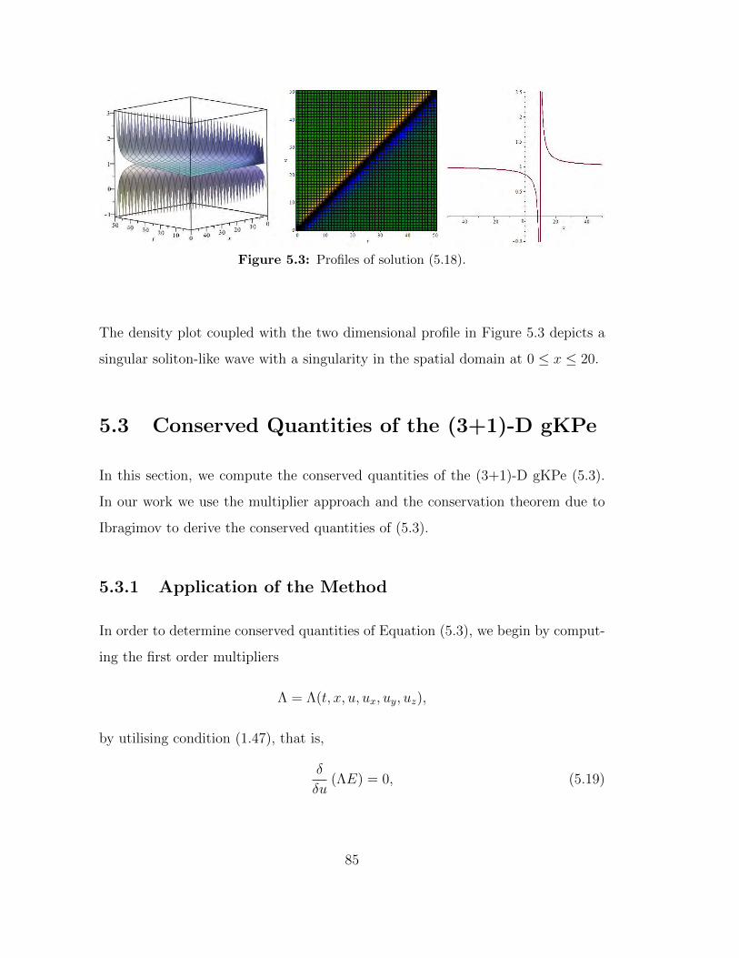
Figure 5.3: Profiles of solution (5.18).
The density plot coupled with the two dimensional profile in Figure 5.3 depicts a
singular soliton-like wave with a singularity in the spatial domain at 0 ≤ x ≤ 20.
5.3 Conserved Quantities of the (3+1)-D gKPe
In this section, we compute the conserved quantities of the (3+1)-D gKPe (5.3).
In our work we use the multiplier approach and the conservation theorem due to
Ibragimov to derive the conserved quantities of (5.3).
5.3.1 Application of the Method
In order to determine conserved quantities of Equation (5.3), we begin by comput-
ing the first order multipliers
Λ = Λ(t, x, u, ux, uy, uz),
by utilising condition (1.47), that is,
δ
δu(ΛE) = 0, (5.19)
85

where
E ≡ utx + uty + utz + 3uxuxy + 3uxxuy + uxxxy − uzz = 0.
The Euler operator is given by (1.25).
δ
δu=
∂
∂u−Dx
∂
∂ux−Dy
∂
∂uy+DtDx
∂
∂utx+DtDy
∂
∂uty+DtDz
∂
∂utz
+D2x
∂
∂uxx+DxDy
∂
∂uxy+D2
z
∂
∂uzz+D3
xDy∂
∂uxxxy
and Dt, Dx, Dy and Dz are total derivative operators (1.4). Expanding (5.19)
and splitting on derivatives of u, we obtain the following system of nine multiplier
determining equations:
Λty + Λtz − Λzz = 0, Λtux = 0, Λyux = 0, Λzux = 0, Λuxux = 0,
Λx = 0, Λu = 0, Λuy = 0, Λuz = 0. (5.20)
The solution algorithm of system (5.20) is similar to that of obtaining Lie point
symmetries. However, with the aid of Gem, a Maple based package [73], this can
be expedited. We thus have the multiplier
Λ = Cux (5.21)
with C an integration constant. The conserved quantities of (5.3) are obtained via
the divergence identity
DtTt +DxT
x +DyTy +DzT
z = EΛ,
where T t is a conserved density and T x, T y, T z are spatial fluxes [43]. Thus, af-
ter some calculations, we obtain the following conservation law:
T t =1
2ux
2 +1
2uy ux +
1
2uz ux,
T x =uux uxy + 2ux2uy +
1
2uy uxxx −
1
2uxy uxx +
1
2uxxy ux +
1
2uuty +
1
2uutz
+1
2uuxxxy −
1
2uuzz,
86
T y = − uux uxx −1
2uutx −
1
2uuxxxx,
T z = − 1
2uutx +
1
2uuxz −
1
2uz ux.
Since the derivatives of u in the multiplier (5.21) are of a lower order than both
leading derivatives of equation (5.3), that is, utx and uxxxy, the conserved quantities
derived here are low-order conservation laws [43].
5.3.2 Ibragimov’s Approach
We now determine the conservation laws of (5.3) by applying a theorem due to
Ibragimov [39, 40]. As in the case of multiplier method, this theorem does not
demand availability of a Lagrangian and is established on a concept of an adjoint
equation. Thus, it applies to an arbitrary differential equation, irrespective of
whether or not it comes from a variational principle.
5.3.2.1 Application of the Method
To begin, we define the adjoint equation of (5.3) as [39]
F ∗ =δ
δuv(utx + uty + utz + 3uxuxy + 3uxxuy + uxxxy − uzz)
=
(∂
∂u−Dx
∂
∂ux−Dy
∂
∂uy+DtDx
∂
∂utx+DtDy
∂
∂uty+DtDz
∂
∂utz
+D2x
∂
∂uxx+DxDy
∂
∂uxy+D2
z
∂
∂uzz+D3
xDy∂
∂uxxxy
)v (utx + uty
+utz + 3uxuxy + 3uxxuy + uxxxy − uzz)
= vtx + vty + vtz + 6vxuxy + 3uxvxy + 3uyvxx + vxxxy − vzz = 0. (5.22)
We have introduced a new variable v = v(t, x, y, z). According to [39], the Equa-
tion (5.3) considered together with its adjoint (5.22) has a Lagrangian L, given
87
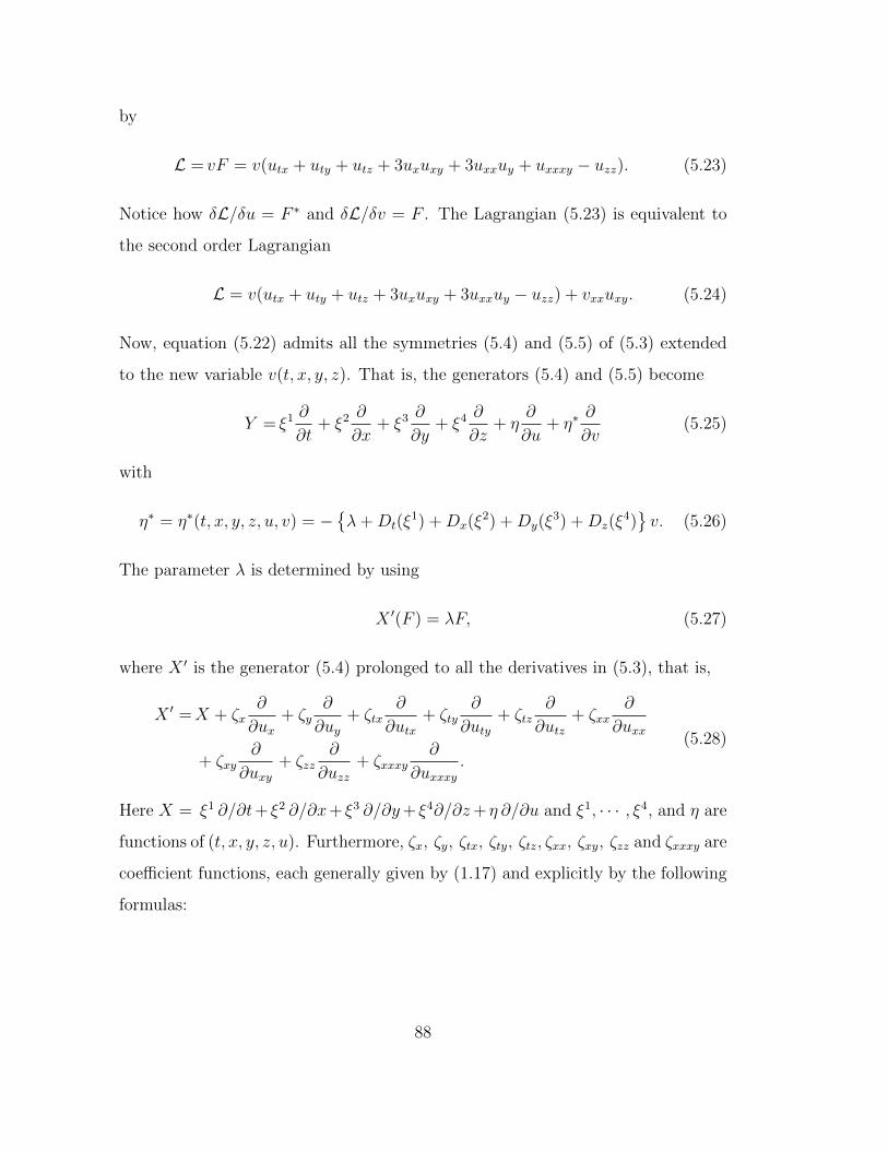
by
L = vF = v(utx + uty + utz + 3uxuxy + 3uxxuy + uxxxy − uzz). (5.23)
Notice how δL/δu = F ∗ and δL/δv = F . The Lagrangian (5.23) is equivalent to
the second order Lagrangian
L = v(utx + uty + utz + 3uxuxy + 3uxxuy − uzz) + vxxuxy. (5.24)
Now, equation (5.22) admits all the symmetries (5.4) and (5.5) of (5.3) extended
to the new variable v(t, x, y, z). That is, the generators (5.4) and (5.5) become
Y = ξ1 ∂
∂t+ ξ2 ∂
∂x+ ξ3 ∂
∂y+ ξ4 ∂
∂z+ η
∂
∂u+ η∗
∂
∂v(5.25)
with
η∗ = η∗(t, x, y, z, u, v) = −λ+Dt(ξ
1) +Dx(ξ2) +Dy(ξ
3) +Dz(ξ4)v. (5.26)
The parameter λ is determined by using
X ′(F ) = λF, (5.27)
where X ′ is the generator (5.4) prolonged to all the derivatives in (5.3), that is,
X ′ =X + ζx∂
∂ux+ ζy
∂
∂uy+ ζtx
∂
∂utx+ ζty
∂
∂uty+ ζtz
∂
∂utz+ ζxx
∂
∂uxx
+ ζxy∂
∂uxy+ ζzz
∂
∂uzz+ ζxxxy
∂
∂uxxxy.
(5.28)
Here X = ξ1 ∂/∂t+ ξ2 ∂/∂x+ ξ3 ∂/∂y+ ξ4∂/∂z+ η ∂/∂u and ξ1, · · · , ξ4, and η are
functions of (t, x, y, z, u). Furthermore, ζx, ζy, ζtx, ζty, ζtz, ζxx, ζxy, ζzz and ζxxxy are
coefficient functions, each generally given by (1.17) and explicitly by the following
formulas:
88
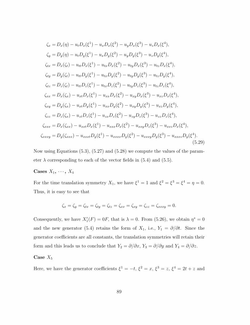
ζx =Dx(η)− utDx(ξ1)− uxDx(ξ
2)− uyDx(ξ3)− uzDx(ξ
4),
ζy =Dy(η)− utDy(ξ1)− uxDy(ξ
2)− uyDy(ξ3)− uzDy(ξ
4),
ζtx =Dx(ζt)− uttDx(ξ1)− utxDx(ξ
2)− utyDx(ξ3)− utzDx(ξ
4),
ζty =Dy(ζt)− uttDy(ξ1)− utxDy(ξ
2)− utyDy(ξ3)− utzDy(ξ
4),
ζtz =Dz(ζt)− uttDz(ξ1)− utxDz(ξ
2)− utyDz(ξ3)− utzDz(ξ
4),
ζxx =Dx(ζx)− uxtDx(ξ1)− uxxDx(ξ
2)− uxyDx(ξ3)− uxzDx(ξ
4),
ζxy =Dy(ζx)− uxtDy(ξ1)− uxxDy(ξ
2)− uxyDy(ξ3)− uxzDy(ξ
4),
ζzz =Dz(ζx)− uztDz(ξ1)− uzxDz(ξ
2)− uzyDz(ξ3)− uzzDz(ξ
4),
ζxxx =Dx(ζxx)− uxxtDx(ξ1)− uxxxDx(ξ
2)− uxxyDz(ξ3)− uxxzDx(ξ
4),
ζxxxy =Dy(ζxxx)− uxxxtDy(ξ1)− uxxxxDy(ξ
2)− uxxxyDy(ξ3)− uxxxzDy(ξ
4).
(5.29)
Now using Equations (5.3), (5.27) and (5.28) we compute the values of the param-
eter λ corresponding to each of the vector fields in (5.4) and (5.5).
Cases X1, · · · , X4
For the time translation symmetry X1, we have ξ1 = 1 and ξ2 = ξ3 = ξ4 = η = 0.
Thus, it is easy to see that
ζx = ζy = ζtx = ζty = ζtz = ζxx = ζxy = ζzz = ζxxxy = 0.
Consequently, we have X ′1(F ) = 0F, that is λ = 0. From (5.26), we obtain η∗ = 0
and the new generator (5.4) retains the form of X1, i.e., Y1 = ∂/∂t. Since the
generator coefficients are all constants, the translation symmetries will retain their
form and this leads us to conclude that Y2 = ∂/∂x, Y3 = ∂/∂y and Y4 = ∂/∂z.
Case X5
Here, we have the generator coefficients ξ1 = −t, ξ2 = x, ξ3 = z, ξ4 = 2t + z and
89
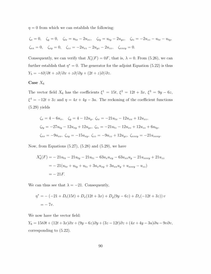
η = 0 from which we can establish the following:
ζx = 0, ζy = 0, ζtx = utx − 2uxz, ζty = uty − 2uyz, ζtz = −2uzz − utx − uty,
ζxx = 0, ζxy = 0, ζzz = −2uxz − 2uyz − 2uzz, ζxxxy = 0.
Consequently, we can verify that X ′5(F ) = 0F , that is, λ = 0. From (5.26), we can
further establish that η∗ = 0. The generator for the adjoint Equation (5.22) is thus
Y5 = −t∂/∂t+ z∂/∂x+ z∂/∂y + (2t+ z)∂/∂z.
Case X6
The vector field X6 has the coefficients ξ1 = 15t, ξ2 = 12t + 3x, ξ3 = 9y − 6z,
ξ4 = −12t + 3z and η = 4x + 4y − 3u. The reckoning of the coefficient functions
(5.29) yields
ζx = 4− 6ux, ζy = 4− 12uy, ζtx = −21utx − 12uxx + 12uxz,
ζty = −27uty − 12uxy + 12uyz, ζtz = −21utz − 12uxz + 12uzz + 6uty,
ζxx = −9uxx, ζxy = −15uxy, ζzz = −9uzz + 12uyz, ζxxxy = −21uxxxy.
Now, from Equations (5.27), (5.28) and (5.29), we have
X ′6(F ) =− 21utx − 21uty − 21utz − 63uxuxy − 63uxxuy − 21uxxxy + 21uzz
=− 21(utx + uty + utz + 3uxuxy + 3uxxuy + uxxxy − uzz)
=− 21F.
We can thus see that λ = −21. Consequently,
η∗ =− (−21 +Dt(15t) +Dx(12t+ 3x) +Dy(9y − 6z) +Dz(−12t+ 3z)) v
=− 7v.
We now have the vector field:
Y6 = 15t∂t+ (12t+ 3x)∂x+ (9y− 6z)∂y+ (3z− 12t)∂z+ (4x+ 4y− 3u)∂u− 9v∂v,
corresponding to (5.22).
90

Cases X7, X8
Finally, considering the infinite-dimensional vector fields X7 and X8 we have,
for (5.22), Y7 = F (t)∂u and Y8 = F (t+ z)∂u, respectively.
To compute the conservation laws of (5.3), we utilise the formula [39]
Ci =ξiL+Wα
(∂L∂uαi−Dk
∂L∂uαik
)+Dk(W
α)∂L∂uαik
, (5.30)
where Wα is the Lie characteristic function given by Wα = ηα − ξjuαj . The reck-
oning of (5.30) gives the following conserved quantities:
T1 = − vuzz + 3vuxuxy + 3vuyuxx + vuxxxy +1
2vzut +
1
2vyut +
1
2vxut +
1
2vutz
+1
2vuty +
1
2vutx,
X1 =3
2vyuxut + 3uyvxut +
3
2vuxyut +
3
4vxxyut +
1
2vtut −
3
2vuxuty −
1
4vxxuty
− 3vuyutx −1
2vxyutx +
1
2vxutxy +
1
4vyutxx −
3
4vutxxy −
1
2vutt,
Y1 =3
2uxvxut −
3
2vuxxut +
1
4vxxxut +
1
2vtut −
3
2vuxutx −
1
4vxxutx +
1
4vxutxx
− 1
4vutxxx −
1
2vutt,
Z1 = − vzut +1
2vtut + vutz −
1
2vutt;
T2 = − 1
2uxzv −
1
2uxyv −
1
2uxxv +
1
2uxvy +
1
2uxvz +
1
2uxvx,
X2 = 3uxuxyv − uzzv +1
4uxxxyv + utzv + utyv +
1
2utxv +
1
2vtux +
3
2u2xvy + 3uxuyvx
+3
4uxvxxy −
1
2uxxvxy −
1
4vxxuxy +
1
2vxuxxy +
1
4uxxxvy,
Y2 = − 3uxxuxv −1
4uxxxxv −
1
2utxv +
1
2vtux +
3
2u2xvx +
1
4uxvxxx −
1
4uxxvxx
+1
4uxxxvx,
Z2 =uxzv −1
2utxv +
1
2vtux − uxvz;
91
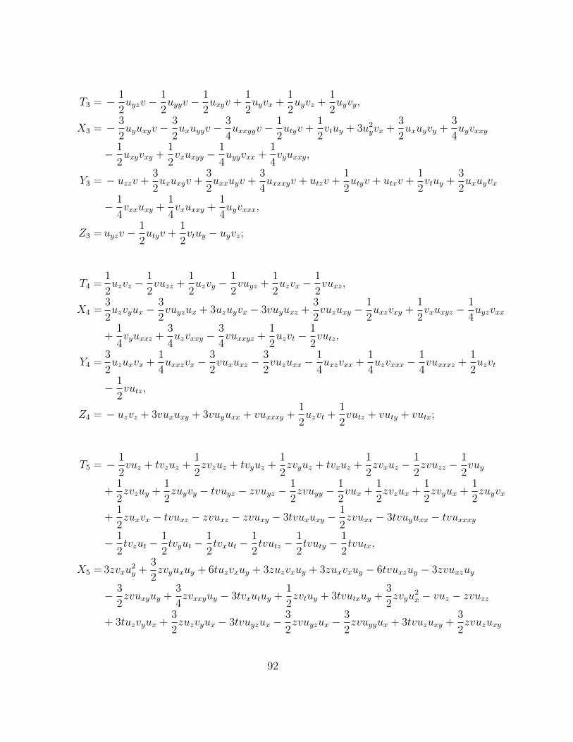
T3 = − 1
2uyzv −
1
2uyyv −
1
2uxyv +
1
2uyvx +
1
2uyvz +
1
2uyvy,
X3 = − 3
2uyuxyv −
3
2uxuyyv −
3
4uxxyyv −
1
2utyv +
1
2vtuy + 3u2
yvx +3
2uxuyvy +
3
4uyvxxy
− 1
2uxyvxy +
1
2vxuxyy −
1
4uyyvxx +
1
4vyuxxy,
Y3 = − uzzv +3
2uxuxyv +
3
2uxxuyv +
3
4uxxxyv + utzv +
1
2utyv + utxv +
1
2vtuy +
3
2uxuyvx
− 1
4vxxuxy +
1
4vxuxxy +
1
4uyvxxx,
Z3 =uyzv −1
2utyv +
1
2vtuy − uyvz;
T4 =1
2uzvz −
1
2vuzz +
1
2uzvy −
1
2vuyz +
1
2uzvx −
1
2vuxz,
X4 =3
2uzvyux −
3
2vuyzux + 3uzuyvx − 3vuyuxz +
3
2vuzuxy −
1
2uxzvxy +
1
2vxuxyz −
1
4uyzvxx
+1
4vyuxxz +
3
4uzvxxy −
3
4vuxxyz +
1
2uzvt −
1
2vutz,
Y4 =3
2uzuxvx +
1
4uxxzvx −
3
2vuxuxz −
3
2vuzuxx −
1
4uxzvxx +
1
4uzvxxx −
1
4vuxxxz +
1
2uzvt
− 1
2vutz,
Z4 = − uzvz + 3vuxuxy + 3vuyuxx + vuxxxy +1
2uzvt +
1
2vutz + vuty + vutx;
T5 = − 1
2vuz + tvzuz +
1
2zvzuz + tvyuz +
1
2zvyuz + tvxuz +
1
2zvxuz −
1
2zvuzz −
1
2vuy
+1
2zvzuy +
1
2zuyvy − tvuyz − zvuyz −
1
2zvuyy −
1
2vux +
1
2zvzux +
1
2zvyux +
1
2zuyvx
+1
2zuxvx − tvuxz − zvuxz − zvuxy − 3tvuxuxy −
1
2zvuxx − 3tvuyuxx − tvuxxxy
− 1
2tvzut −
1
2tvyut −
1
2tvxut −
1
2tvutz −
1
2tvuty −
1
2tvutx,
X5 = 3zvxu2y +
3
2zvyuxuy + 6tuzvxuy + 3zuzvxuy + 3zuxvxuy − 6tvuxzuy − 3zvuxzuy
− 3
2zvuxyuy +
3
4zvxxyuy − 3tvxutuy +
1
2zvtuy + 3tvutxuy +
3
2zvyu
2x − vuz − zvuzz
+ 3tuzvyux +3
2zuzvyux − 3tvuyzux −
3
2zvuyzux −
3
2zvuyyux + 3tvuzuxy +
3
2zvuzuxy
92
+ 3zvuxuxy − tuxzvxy −1
2zuxzvxy −
1
2zuxyvxy + tvxuxyz +
1
2zvxuxyz +
1
2zvxuxyy
− 1
2zvxyuxx −
1
2tuyzvxx −
1
4zuyzvxx −
1
4zuyyvxx −
1
4zuxyvxx +
1
2tvyuxxz
+1
4zvyuxxz +
1
4zvyuxxy +
1
2zvxuxxy +
3
2tuzvxxy +
3
4zuzvxxy +
3
4zuxvxxy −
3
2tvuxxyz
− 3
4zvuxxyz −
3
4zvuxxyy +
1
4zvyuxxx +
1
4zvuxxxy +
1
2vut −
3
2tvyuxut −
3
2tvuxyut
− 3
4tvxxyut + tuzvt +
1
2zuzvt +
1
2zuxvt −
1
2tutvt − tvutz +
1
2zvutz +
1
2zvuty
+3
2tvuxuty +
1
4tvxxuty +
1
2zvutx +
1
2tvxyutx −
1
2tvxutxy −
1
4tvyutxx +
3
4tvutxxy +
1
2tvutt;
Y5 =3
2zvxu
2x + 3tuzvxux +
3
2zuzvxux +
3
2zuyvxux − 3tvuxzux −
3
2zvuxzux
+3
2zvuxyux − 3zvuxxux +
1
4zvxxxux −
3
2tvxutux +
1
2zvtux +
3
2tvutxux
− vuz − zvuzz − 3tvuzuxx −3
2zvuzuxx +
3
2zvuyuxx −
1
2tuxzvxx −
1
4zuxzvxx
− 1
4zuxyvxx −
1
4zuxxvxx +
1
2tvxuxxz +
1
4zvxuxxz +
1
4zvxuxxy +
1
4zvxuxxx
+1
2tuzvxxx +
1
4zuzvxxx +
1
4zuyvxxx −
1
2tvuxxxz −
1
4zvuxxxz +
3
4zvuxxxy
− 1
4zvuxxxx +
1
2vut +
3
2tvuxxut −
1
4tvxxxut + tuzvt +
1
2zuzvt +
1
2zuyvt
− 1
2tutvt − tvutz +
1
2zvutz +
1
2zvuty +
1
2zvutx +
1
4tvxxutx −
1
4tvxutxx
+1
4tvutxxx +
1
2tvutt,
Z5 = − 2tuzvz − zuzvz − zuyvz − zuxvz + tutvz + vuy + zvuyz + vux + zvuxz
+ 6tvuxuxy + 3zvuxuxy + 6tvuyuxx + 3zvuyuxx + 2tvuxxxy + zvuxxxy
+1
2vut + tuzvt +
1
2zuzvt +
1
2zuyvt +
1
2zuxvt −
1
2tutvt +
1
2zvutz + 2tvuty
+1
2zvuty + 2tvutx +
1
2zvutx +
1
2tvutt;
T6 = − 3vuz − 9tuzzv −3
2zuzzv − 3uyv + 6tuyzv −
9
2yuyzv +
3
2zuyzv −
9
2yuyyv
93

+ 3zvuyy − 3uxv −3
2xuxzv −
3
2zuxzv − 6tuxyv −
3
2xuxyv −
9
2yuxyv + 3zuxyv
+ 45tuxuxyv − 6tuxxv −3
2xuxxv + 45tuyuxxv + 15tuxxxyv +
15
2tutzv +
15
2tutyv
+15
2tvutx + 4v − 2xvz − 2yvz +
3
2uvz − 6tuzvz +
3
2zuzvz +
9
2yvzuy − 3zvzuy
− 2xvy − 2yvy +3
2uvy − 6tuzvy +
3
2zuzvy +
9
2yuyvy − 3zuyvy + 6tvzux
+3
2xvzux + 6tvyux +
3
2xvyux − 2xvx − 2yvx +
3
2uvx − 6tuzvx +
3
2zuzvx
+9
2yuyvx − 3zuyvx + 6tuxvx +
3
2xuxvx +
15
2tvzut +
15
2tvyut +
15
2tvxut,
X6 = 27yvxu2y − 18zvxu
2y + 12vuy − 36vuxuy +
27
2yvyuxuy − 9zvyuxuy − 12xvxuy
− 12yvxuy + 9uvxuy − 36tuzvxuy + 9zuzvxuy + 36tuxvxuy + 9xuxvxuy
+ 36tvuxzuy − 9zvuxzuy −27
2yvuxyuy + 9zvuxyuy − 3vxxuy +
27
4yvxxyuy
− 9
2zvxxyuy + 45tvxutuy +
9
2yvtuy − 3zvtuy − 45tvutxuy + 18tvyu
2x +
9
2xvyu
2x
+ 6vuz − 12tvuzz − 3xvuzz − 6xvyux − 6yvyux +9
2uvyux − 18tuzvyux
+9
2zuzvyux + 18tvuyzux −
9
2zvuyzux −
27
2yvuyyux + 9zvuyyux − 6xvuxy
− 6yvuxy +9
2uvuxy − 18tvuzuxy +
9
2zvuzuxy + 36tvuxuxy + 9xvuxuxy
+15
2vxuxy − 3uxvxy + 6tuxzvxy −
3
2zuxzvxy −
9
2yuxyvxy + 3zuxyvxy + 2vxy
− 6tvxuxyz +3
2zvxuxyz +
9
2yvxuxyy − 3zvxuxyy +
9
4vyuxx − 6tvxyuxx −
3
2xvxyuxx
+ 3tuyzvxx −3
4zuyzvxx −
9
4yuyyvxx +
3
2zuyyvxx − 3tuxyvxx −
3
4xuxyvxx + vxx
− 3tvyuxxz +3
4zvyuxxz −
27
2vuxxy +
9
4yvyuxxy −
3
2zvyuxxy + 6tvxuxxy
+3
2xvxuxxy − 3xvxxy − 3yvxxy +
9
4uvxxy − 9tuzvxxy +
9
4zuzvxxy + 9tuxvxxy
+9
4xuxvxxy + 9tvuxxyz −
9
4zvuxxyz −
27
4yvuxxyy +
9
2zvuxxyy + 3tvyuxxx
+3
4xvyuxxx + 3tvuxxxy +
3
4xvuxxxy − 9vut +
45
2tvyuxut +
45
2tvuxyut +
45
4tvxxyut
− 2xvt − 2yvt +3
2uvt − 6tuzvt +
3
2zuzvt + 6tuxvt +
3
2xuxvt +
15
2tutvt + 18tvutz
94
+ 3xvutz −3
2zvutz + 12tvuty + 3xvuty −
9
2yvuty + 3zvuty −
45
2tvuxuty
− 15
4tvxxuty + 6tvutx +
3
2xvutx −
15
2tvxyutx +
15
2tvxutxy +
15
4tvyutxx
− 45
4tvutxxy −
15
2tvutt,
Y6 = − 9vu2x + 18tvxu
2x +
9
2xvxu
2x − 6xvxux − 6yvxux +
9
2uvxux − 18tuzvxux
+9
2zuzvxux +
27
2yuyvxux − 9zuyvxux + 18tvuxzux −
9
2zvuxzux +
27
2yvuxyux
− 9zvuxyux − 36tvuxxux − 9xvuxxux −3
2vxxux + 3tvxxxux +
3
4xvxxxux
+45
2tvxutux + 6tvtux +
3
2xvtux −
45
2tvutxux + 6vuz − 9yvuzz + 6zvuzz
+ 6xvuxx + 6yvuxx −9
2uvuxx + 18tvuzuxx −
9
2zvuzuxx +
27
2yvuyuxx
− 9zvuyuxx +9
4vxuxx + 3tuxzvxx −
3
4zuxzvxx −
9
4yuxyvxx +
3
2zuxyvxx
− 3tuxxvxx −3
4xuxxvxx + vxx − 3tvxuxxz +
3
4zvxuxxz +
9
4yvxuxxy −
3
2zvxuxxy
− 3vuxxx + 3tvxuxxx +3
4xvxuxxx − xvxxx − yvxxx +
3
4uvxxx − 3tuzvxxx
+3
4zuzvxxx +
9
4yuyvxxx −
3
2zuyvxxx + 3tvuxxxz −
3
4zvuxxxz +
27
4yvuxxxy
− 9
2zvuxxxy − 3tvuxxxx −
3
4xvuxxxx − 9vut −
45
2tvuxxut +
15
4tvxxxut − 2xvt
− 2yvt +3
2uvt − 6tuzvt +
3
2zuzvt +
9
2yuyvt − 3zuyvt +
15
2tutvt + 6tvutz
+ 9yvutz −15
2zvutz +
9
2yvuty − 3zvuty − 6tvutx −
3
2xvutx + 9yvutx
− 6zvutx −15
4tvxxutx +
15
4tvxutxx
− 15
4tvutxxx −
15
2tvutt,
Z6 = 12vuz + 12tvzuz − 3zvzuz − 6tvtuz +3
2zvtuz + 4xvz + 4yvz − 3uvz
− 6vuy − 9yvzuy + 6zvzuy + 9yvuyz − 6zvuyz − 6vux − 12tvzux
− 3xvzux + 12tvuxz + 3xvuxz − 36tvuxuxy + 9zvuxuxy − 36tvuyuxx
95

+ 9zvuyuxx − 12tvuxxxy + 3zvuxxxy − 9vut − 15tvzut − 2xvt − 2yvt
+3
2uvt +
9
2yuyvt − 3zuyvt + 6tuxvt +
3
2xuxvt +
15
2tutvt + 9tvutz +
3
2zvutz
− 12tvuty −9
2yvuty + 6zvuty − 18tvutx −
3
2xvutx + 3zvutx −
15
2tvutt;
TF1 =1
2F1(t)vx −
1
2F1(t)vy −
1
2F1(t)vz,
XF1 = − 3
2F1(t)uxyv +
1
2F ′1v −
3
2F1(t)uxvy − 3F1(t)uyvx −
3
4F1(t)vxxy −
1
2F1(t)vt,
YF1 =3
2F1(t)uxxv +
1
2F ′1v −
3
2F1(t)uxvx −
1
4F1(t)vxxx −
1
2F1(t)vt,
ZF1 =1
2F ′1v + F1(t)vz −
1
2F1(t)vt;
TF2 =1
2F ′2v −
1
2vxF2(t+ z)− 1
2vyF2(t+ z)− 1
2vzF2(t+ z),
XF2 = − 3
2F2(t+ z)uxyv +
1
2F ′2v −
3
2uxvyF2(t+ z)− 3uyvxF2(t+ z)
− 3
4F2(t+ z)vxxy −
1
2vtF2(t+ z),
YF2 =3
2uxxF2(t+ z)v +
1
2F ′2v −
3
2uxvxF2(t+ z)− 1
4vxxxF2(t+ z)− 1
2vtF2(t+ z),
ZF2 = − 1
2F ′2v + vzF2(t+ z)− 1
2vtF2(t+ z).
5.4 Concluding remarks
In this chapter, we used Lie symmetry methods to obtain analytic solutions of the
(3+1)-dimensional generalised KP equation (5.3). The first solution contains an
elliptic integral of the second kind, an amplitude function, a delta amplitude func-
tion and a Jacobi cosine function. It is common knowledge that these functions
degenerate to trigonometric or hyperbolic functions depending on the behaviour
of the parameter M2. Thus, the solution (5.13) is to our knowledge the most
96
general solution of (5.3) that has been obtained to date. Some of the solutions
obtained were presented graphically. Furthermore, we obtained logarithmic and
rational solutions. Finally, we computed the conserved quantities of equation (5.3)
using the multiplier method as well as Ibragimov’s conservation theorem. The for-
mer method yielded a local low-order conserved quantity, while the later method
yielded eight conservation laws with each conserved vector corresponding to an
infinitesimal generator.
97

Chapter 6
Travelling wave solutions and
conservation laws of the (2+1)-
dimensional Broer-Kaup-
Kupershmidt equations
6.1 Introduction
The Broer-Kaup-Kupershmidt (BKK) system of equations
E1 ≡ uty − uxxy + 2(uux)y + 2vxx = 0,
E2 ≡ vt + vxx + 2(uv)x = 0.
(6.1)
is one of the most popular system of NLPDEs to emerge in the past few decades.
This is evidenced by the vast array of scholars who have researched various aspects
of the system. It has applications in fluid dynamics where it models dispersive
shallow water waves travelling in equal depth. By using a convenient scaling trans-
98

formation, it has been shown in [98, 99] that the (2+1)-dimensional asymmetric
Davey-Stewartson system [100]
qt +qxx2
+ 2q∂−1y (qr)x = 0, rt +
rxx2
+ 2r∂−1y (qr)x = 0,
transforms into (6.1) under the transformation
q = exp
(−∫ x
udx
), r = −v exp
(∫ x
udx
).
Solitoff and dromion solutions are obtained in the same work [98]. Also, the
Kadomtsev-Petviashvili equation transforms into the BKK equation under a sym-
metry constraint, see for example, [100, 101]. In [101] the modified extended Fan
sub-equation method is used to obtain soliton-like and Jacobi elliptic wave function-
like solutions of (6.1). In [102], Backlund transformation and variable separation
approach was used to obtain dromions, lumps and peakons through the introduc-
tion of an arbitrary function. Again, in [103, 104] an auxiliary equation method
was utilised to obtain its exact travelling wave solutions. He’s semi-inverse method
was applied in [105] to establish a variational principle of the BKK system. Sev-
eral other researchers have utilised different ad hoc methods to establish different
solutions of (6.1). Kassem and Rashed [106] came up with closed form solutions of
(6.1) by using hidden symmetries of its Lie optimal systems. The most recent work
on the BKK system was by Tang et al. [107] who presented the double Wronskian
solutions by using Hirota’s method and binary bell polynomials.
Due to its undeniably vast applicability, continued study of the BKK system re-
mains necessary. In this chapter, we further explore the (2+1)-dimensional BKK
system (6.1). Unlike most of the previous research on this system, we do not em-
ploy ad hoc methods to obtain its analytic solutions, but utilise a standard Lie
based integration method [30]. Here we provide a detailed outline of the derivation
of the bounded travelling wave solutions, which include kink and anti-kink profiles.
We also outline how periodic solutions of a snoidal nature are obtained. Moreover,
99

the homotopy integral approach to finding conservation laws is explored in detail.
To the best of our knowledge, the literature is devoid of explicit applications of
this approach, more so for NLPDEs with mixed derivatives, our work is novel in
this regard.
The work presented in this chapter has been submitted for possible publication.
See [108].
6.2 Bounded travelling wave solutions of the BKK
equations (1)
Let ξ = x+ by + ct, then the BKK equations (6.1) becomes
bcu′′ − bu′′′ + 2b(uu′)′ + 2v′′ = 0,
cv′ + v′′ + 2(uv)′ = 0.
(6.2)
Integrating (6.2) once with respect to ξ and letting the constants of integration be
zero, one gets
bcu′ − bu′′ + 2buu′ + 2v′ = 0,
(2u+ c)v + v′ = 0.
(6.3)
Integrating the first equation of (6.3) once again and then solving for v gives
v =1
2(bu′ − bu2 − bcu+ g), (6.4)
where g is a constant of integration. Substituting the expression of v from (6.4)
into the second equation of system (6.3), we have for the case when b 6= 0, that
u′′ = (2u+ c)(u2 + cu− g
b
)+g2
b. (6.5)
100

Let u′ = y, then equation (6.5) is equivalent to the following planar dynamical
system:
u′ = y, y′ = (2u+ c)(u2 + cu− g
b
). (6.6)
Suppose u0 > − c2
satisfies g = bu0(c+u0), then system (6.6) has three equilibrium
points E1(−c − u0, 0), E2(− c2, 0) and E3(u0, 0), where −c − u0 < − c
2< u0. By
determining the Jacobian determinant, we know that E1 and E3 are saddle points
and E2 is a center. Clearly, system (6.6) is a Hamiltonian system with Hamiltonian
H(u, y) =y2
2− 1
2u4 − cu3 − 1
2
(c2 − 2
g
b
)u2 +
gc
bu. (6.7)
Hence H(E2) = h2 and H(E1) = H(E3) = h0, where h1 = 12u2
0(u0 + c)2 and
h2 = − 132c2(c2 + 8cu0 + 8u2
0). Therefore, we have the phase portrait of (6.6) (see
Figure 1). It shows that there are two heteroclinic orbits connecting the two
saddle points E1 and E3 which consist of the boundary of a family of periodic
orbits. As is well-known, the two heteroclinic orbits of (6.6) which are determined
by H(u, y) = h1 correspond to a kink and an anti-kink for u of (6.1) respectively
and the periodic orbits given by H(u, y) = h with h2 < h < h1 correspond to
periodic travelling wave solutions. Hence, one sees easily from Figure 1 that there
are a family of periodic wave solutions and a kink and an anti-kink for u of (6.1).
Note that v is determined by (6.4) which is equivalent to
v =b
2(u′ − u2 − cu+ u0(c+ u0)), (6.8)
so (u, v) is a periodic travelling wave solution of (6.1) if u is periodic.
To derive the kink and anti-kink, we integrate along the heteroclinic orbitsH(u, y) =
h1, that is,
y± = ±(u− u0)(u+ c+ u0).
Substituting the above equation into the first equation of (6.6) and then integrating
101

the resulting differential equation yields
u±(ξ) = − c2± 1
2(c+ 2u0) tanh
(1
2(c+ 2u0)(ξ − ξ0)
), (6.9)
where ξ0 is a constant of integration. It implies that for arbitrary constants ξ0, c
and u0 > − c2, (6.9) determine a kink and an anti-kink for u of (6.1) respectively.
Taking account of (6.8), we have the corresponding
v+(ξ) =b
4(c+ 2x0)2sech2
(1
2(c+ 2u0)(ξ − ξ0)
)(6.10)
and
v−(ξ) = 0,
that is to say, (u+(ξ), v+(ξ)) and (u−(ξ), v−(ξ)) are two travelling wave solutions
to (6.1).
Figure 6.1: Phase orbit of (6.6) and the corresponding bounded travelling wave
solutions.
For the periodic orbits determined by H(u, y) = h with h2 < h < h1, we know
from (6.7) that the periodic orbit passing through (u2, 0), for arbitrary u2 ∈ (−c−
u0,− c2), is determined by
y = ±√
(u− u1)(u− u2)(u3 − u)(u4 − u) (u2 ≤ u ≤ u3), (6.11)
where u1, u3 and u4 satisfying u1 < −c− u0 and − c2< u3 < u0 < u4 are three real
roots of the following cubic algebraic equation:
u3 +(2c+u2)u2 +((c+ u2)2 − 2u0(c+ u0)
)u+u2(c+u2)2−2u0(c+u0)(c+u2) = 0.
102

Inserting equation (6.11) into the first equation of (6.6) and then integrating the
resulting differential equation yields
u(ξ) = u1 +(u2 − u1)(u3 − u1)
(u3 − u1)− (u3 − u2)sn2(Ωξ, q), (6.12)
where Ω = 12
√(u4 − u2)(u3 − u1) and q =
√(u3−u2)(u4−u1)(u3−u1)(u4−u2)
. Therefore, we derive
a family of periodic travelling wave solutions u(ξ), v(ξ) to (6.1), where u(ξ) is
given by (6.12) and the associated v(ξ) is derived by inserting (6.12) into (6.8) for
arbitrary u2 ∈ (−c− u0,− c2).
(1) u = u+(ξ) (2) v = v+(ξ) with b = 1 (3) v = v+(ξ) with b = −2
Figure 6.2: Bounded travelling wave solutions with c = −2 and u0 = 3.
Theorem 6.1 For arbitrary real numbers b, c and u0 > − c2, let ξ = x + by + ct.
Then the (2+1)-dimensional BKK system (6.1) has the following bounded travelling
wave solutions:
(1) two families of travelling wave solutions (u+(ξ), v+(ξ)) and (u−(ξ), v−(ξ)),
where u+(ξ) is of kink shape but the associated v+(ξ) is of solitary shape whose
103

(1) u = u(ξ) (2) v = v(ξ) with b = 1 (3) v = v(ξ) with b = −2
Figure 6.3: Periodic travelling wave solutions with c = −2, u0 = 3 and u2 = 0.
amplitude is determined by b (See Figure 6.2). However, u−(ξ) is of anti-kink
shape and u−(ξ) = 0;
(2) a family of periodic travelling wave solutions (u(ξ), v(ξ)) given by (6.12) and
the associated v(ξ) is determined by (6.8) for arbitrary u2 ∈ (−c − u0,− c2) (See
Figure 6.3).
6.3 Conservation laws of the BKK equations (1.1)
A conservation law is a divergence expression DtT + DxX + DyY = 0 subject to
solutions of the BKK system (6.1). The conserved density T and the spatial flux
(X, Y ) are functions of t, x, y, u, v and the derivatives of u and v. The BKK system
(6.1) does not possess a variational principle as it does not satisfy the Helmholtz
conditions [43]. However, conserved quantities may be obtained using a more
104

direct approach which does not require the existence of a variational principle. In
this work we employ the multiplier approach to compute conservation laws. This
approach capitalises on the well known correspondence between multipliers and
conservation laws [43]. Furthermore, we will employ the first homotopy integral
formula to compute conserved quantities. To date, the authors have not come
across an explicit application of this formula to a system with mixed derivatives.
This work will thus serve as an illustrative example, amongst other things. A
determining condition to find multipliers of the BKK system (6.1) is
δ
δu
[Λ1E1 + Λ2E2
]= 0,
δ
δv
[Λ1E1 + Λ2E2
]= 0,
(6.13)
where δ/δu and δ/δv are Euler-Lagrange operators (1.25), here given by
δ
δu=
∂
∂u−Dx
∂
∂ux−Dy
∂
∂uy+DtDy
∂
∂uty+DxDy
∂
∂uxy−D2
xDy∂
∂uxxy,
δ
δv=
∂
∂v−Dt
∂
∂vt−Dx
∂
∂vx+D2
x
∂
∂vxx.
(6.14)
Furthermore, Dt, Dx and Dy are total derivatives (1.4) given by
Dt =∂
∂t+ ut
∂
∂u+ vt
∂
∂v+ utt
∂
∂ut+ vtt
∂
∂vt+ utx
∂
∂ux+ vtx
∂
∂vx+ · · · ,
Dx =∂
∂x+ ux
∂
∂u+ vx
∂
∂v+ uxx
∂
∂ux+ vxx
∂
∂vx+ uxt
∂
∂ut+ vxt
∂
∂vt+ · · · ,
Dy =∂
∂y+ uy
∂
∂u+ vy
∂
∂v+ uyy
∂
∂uy+ vyy
∂
∂vy+ uyt
∂
∂ut+ vyt
∂
∂vt+ · · · .
Here we seek to compute first order conservation law multipliers
Λα = Λα(t, x, u, v, ux, vx, uy, vy), α = 1, 2.
Expanding (6.13) and splitting on derivatives of u and v, we obtain the following
system of multiplier determining equations:
Λ1ty = 0, Λ2
ty = 0, 2Λ1xx − Λ2
t = 0, Λ1xy = 0, Λ2
x = 0, Λ1u = 0, Λ2
u = 0, Λ2ux = 0,
105

Λ1v = 0, Λ2
v = 0, Λ2v = 0, Λ1
ux = 0, Λ2ux = 0,
Λ1vx = 0, Λ2
vx = 0, Λ1uy = 0, Λ2
uy = 0.
Solving the above system for Λ1 and Λ2, we obtain
Λ1 =1
4F ′2 (t)x2 + F3 (t)x+ F4 (y) + F5 (t) ,
Λ2 =F1 (y) + F2 (t) ,
(6.15)
where Fi, i = 1, · · · , 5 are arbitrary functions of their respective arguments. We
thus have the following five multipliers
Λ11 = 0, Λ2
1 = F1(y);
Λ12 =
1
4F ′2(t)x2, Λ2
2 = F2(t);
Λ13 = F3(t)x, Λ2
3 = 0;
Λ14 = F4(y), Λ2
4 = 0;
Λ15 = F5(t), Λ2
5 = 0.
(6.16)
The homotopy integral formula [43] is a revolutionary approach for computing
conserved vectors and is given by (1.48). In accordance with system (6.1) and
106

multipliers (6.15) we give formula (1.48) in explicit form as
T =
∫ 1
0
(uDy
(∂E1Λ1
∂uty
) ∣∣∣u=u(λ) + v
(∂E2Λ2
∂vt
) ∣∣∣v=v(λ)
)dλ,
X =
∫ 1
0
u
(∂E1Λ1
∂ux
) ∣∣∣u=u(λ) +
(∂E2Λ2
∂ux
) ∣∣∣u=u(λ) −Dy
(∂E1Λ1
∂uxy
) ∣∣∣u=u(λ)
+DxDy
(∂E1Λ1
∂uxxy
) ∣∣∣u=u(λ)
− uxDy
(∂E1Λ1
∂uxxy
) ∣∣∣u=u(λ)
+v
(∂E2Λ2
∂vx
) ∣∣∣v=v(λ) −Dx
(∂E1Λ1
∂vxx
) ∣∣∣v=v(λ) −Dx
(∂E2Λ2
∂vxx
) ∣∣∣v=v(λ)
+vx
(∂E2Λ2
∂vxx
) ∣∣∣v=v(λ)
dλ,
Y =
∫ 1
0
u
(∂E1Λ1
∂uy
) ∣∣∣u=u(λ) + ut
(∂E1Λ1
∂uty
) ∣∣∣u=u(λ) + ux
(∂E1Λ1
∂uxy
) ∣∣∣u=u(λ)
+uxx
(∂E1Λ1
∂uxxy
) ∣∣∣u=u(λ)
dλ.
(6.17)
Choosing the homotopy u(λ) = λu, and v(λ) = λv as is usually the case, we have
for Λ11 and Λ2
1
T1 =
∫ 1
0
vF1dλ
= vF1,
X1 =
∫ 1
0
(4λuvF1 + vxF1) dλ
= 2uvF1 + vxF1,
Y1 = 0.
T1 = vF1 is mass density, and X1 = 2uv + vxF1 is mass flux or momentum.
Similarly, the complete set of flux densities and spatial fluxes are derived to obtain
T2 =1
4x2uyF
′2 + vF2,
107

X2 =1
2uuyF
′2x
2 + 2uvF2 +1
2xuyF
′2 −
1
4x2uxyF
′2 − xvF ′2 +
1
2x2vxF
′2 + vxF2,
Y2 =− 1
4u(x2F ′′2 + 2xuF ′2 + 2F ′2
);
T3 = = xuy F3,
X3 = 2xuuyF3 + uy F3 − uxyF3x− 2 vF3 + 2xvx F3,
Y3 = − xuF ′3 + uF3;
T4 =uy F4,
X4 = = 2uuyF4 − uxyF4 + 2 vx F4,
Y4 = 0;
T5 =uy F5,
X5 = 2uF5uy − uxy F5 + 2 vx F5,
Y5 = − uF ′5.
The conservation laws obtained here are local and infinitely many because of the
presence of arbitrary functions. Due to the order of the dependencies of the adjoint
symmetries being of a lower order than the leading derivatives of the underlying
system, the conserved quantities are low-order.
6.4 Concluding remarks
In this chapter we carried out a bifurcation analysis of the (2+1)-dimensional BKK
system (6.1). We obtained bounded travelling wave solutions in the form of kink,
bright and dark solitons as well as periodic waves. We also provided the parametric
conditions for which these solutions hold. Finally, using the first homotopy integral
108

approach we successfully derived conservation laws for the BKK system. Due to
the presence of arbitrary functions in the multipliers, we obtained infinitely many
conserved vectors.
109

Chapter 7
An optimal system of group-
invariant solutions and conserved
quantities of a nonlinear
fifth-order integrable equation
7.1 Introduction
The most general form of a fifth-order KdV equation reads [109]
ut + αu2ux + νuxuxx + γuuxxx + uxxxxx = 0 (7.1)
with arbitrary real constants α, ν and γ. Equation (7.1) models long waves prop-
agating in shallow water and in the presence of gravity. Several famous fifth-order
KdV equations emanate from equation (7.1), for instance, the fifth-order Sawada-
Kotera equation [110]
ut + 45u2ux + 15uxuxx + 15uuxxx + uxxxxx = 0
110

occurs when α = 3ν, ν = γ and γ = 15. On the other hand, when α = 5/2ν, ν =
5/4γ and γ = 20, we have the nonlinear fifth-order Kaup-Kupershmidt equation
[111]
ut + 20u2ux + 25uxuxx + 10uuxxx + uxxxxx = 0.
In this chapter, we study a newly formulated integrable fifth-order equation
F ≡ βuxxx − 4utuxxx − 12uxxutx − 8uxutxx − utxxxx + uttt = 0, β 6= 0. (7.2)
Equation (7.2) was developed in [112], where the researchers performed a Painleve
test to prove its integrability. The authors went further to find different types of
soliton solutions of (7.2) using Hirota’s method. In a sense, equation (7.2) is a
second generation hybrid between the fifth-order Kawahara equation [113]
ut + αuux + νuxxx + γuxxxxx (7.3)
and another fifth-order equation [114]
uxxx − 4utuxxx − 12uxxutx − 8uxutxx − utxxxx + uttt = 0. (7.4)
In other words, equation (7.2) is a progression from equation (7.4) due to the ad-
dition of a second dispersive term (uxxx), by lending credence from the Kawahara
equation, which also has the two dispersive terms (uxxx) and (utxxxx). Notwith-
standing this backdrop, integrable models are of great interest to mathematicans
and physicists for the plethora of information they possess. The integrability of
equation (7.2), which has been proven in [112], makes it a significant model and
worth studying. In this chapter, we seek to obtain a more comprehensive set of
solutions with the aid of an optimal system of one-dimensional subalgebras. Also,
we will derive a group of transformations corresponding to the symmetry algebra
of (7.2).
Although the solutions given in [112] are extensive, it will be seen that our solutions
subsume those in [112] since we obtain hyperbolic, parabolic, elliptic and power
111

series solutions. We will go a step further to determine the conserved vectors
attributable to this equation.
The work presented in this chapter has been published in [115].
7.2 Lie group analysis of (7.2)
7.2.1 Infinitesimal generators
For a one-parameter group of transformations
t→ t+ aξ1(t, x, u), x→ x+ aξ2(t, x, u), u→ u+ aη(t, x, u)
with a small parameter a, we have the corresponding infinitesimal generator
X = ξ1(t, x, u)∂
∂t+ ξ2(t, x, u)
∂
∂x+ η(t, x, u)
∂
∂u. (7.5)
The vector field (7.5) in conjunction with (7.2) satisfies the invariance condition
pr(5)X(βuxxx − 4utuxxx − 12uxxutx − 8uxutxx − utxxxx + uttt)|F=0 = 0. (7.6)
Here, pr(5)X is the fifth-order extension of (7.5) given by [30]
pr(5)X =X + ζt∂
∂ut+ ζx
∂
∂ux+ ζtx
∂
∂utx+ ζxx
∂
∂uxx+ ζttt
∂
∂uttt+ ζtxx
∂
∂utxx
+ ζxxx∂
∂uxxx+ ζtxxxx
∂
∂utxxxx
and ζt, ζx, ζtx, ζxx, ζttt, ζtxx, ζxxx, ζtxxxx are prolongation coefficient functions which
can be obtained from (1.16) and (1.17). From (7.6), we obtain the following system
of twelve linear homogeneous PDEs:
ξ1x = 0, ξ1
u = 0, ξ1tt = 0, ξ1
tx = 0, ξ1tu = 0, ξ2
t = 0, ξ2u = 0,
2ξ2x − ξ1
t = 0, ηttt = 0, ηx = 0, ξ1t + 2ηu = 0, 8ηt − 3βξ1
t = 0.(7.7)
112

Solving system (7.7) yields the generator coefficients
ξ1 =8C2
3βt+ C1, ξ
2 =4C2
3βx+ C4, η = −4C2
3βu+ C2t+ C3 (7.8)
and ultimately we obtain a four-dimensional Lie algebra L4, spanned by the gen-
erators
X1 =∂
∂t, X2 =
∂
∂x, X3 = 8t
∂
∂t+ 4x
∂
∂x+ (3βt− 4u)
∂
∂u, X4 =
∂
∂u. (7.9)
7.2.2 Group transformations of known solutions
The one-parameter groups Gi of transformations generated by the four-dimensional
Lie algebra (7.9) can be obtained by solving the Lie equations [31] and these are
G1 : (t, x, u)→ (t+ a, x, u),
G2 : (t, x, u)→ (t, x+ a, u),
G3 : (t, x, u)→(te8a, xe4a, ue−4a +
1
4βte−4a
(e12a − 1
)),
G4 : (t, x, u)→ (t, x, u+ a).
Thus, we have the following theorem.
Theorem 7.1 If u = m(t, x) is a solution of the PDE (7.2), then so are the
functions
G1 : u(1) = m(t− a, x),
G2 : u(2) = m(t, x− a),
G3 : u(3) = e−4am(te−8a, xe−4a) +1
4βt(1− e−12a
),
G4 : u(4) = m(t, x) + a.
This means that from any known solution of (7.2) one can obtain infinitely many
new exact solutions of (7.2) by the repeated use of the above family of solutions.
113
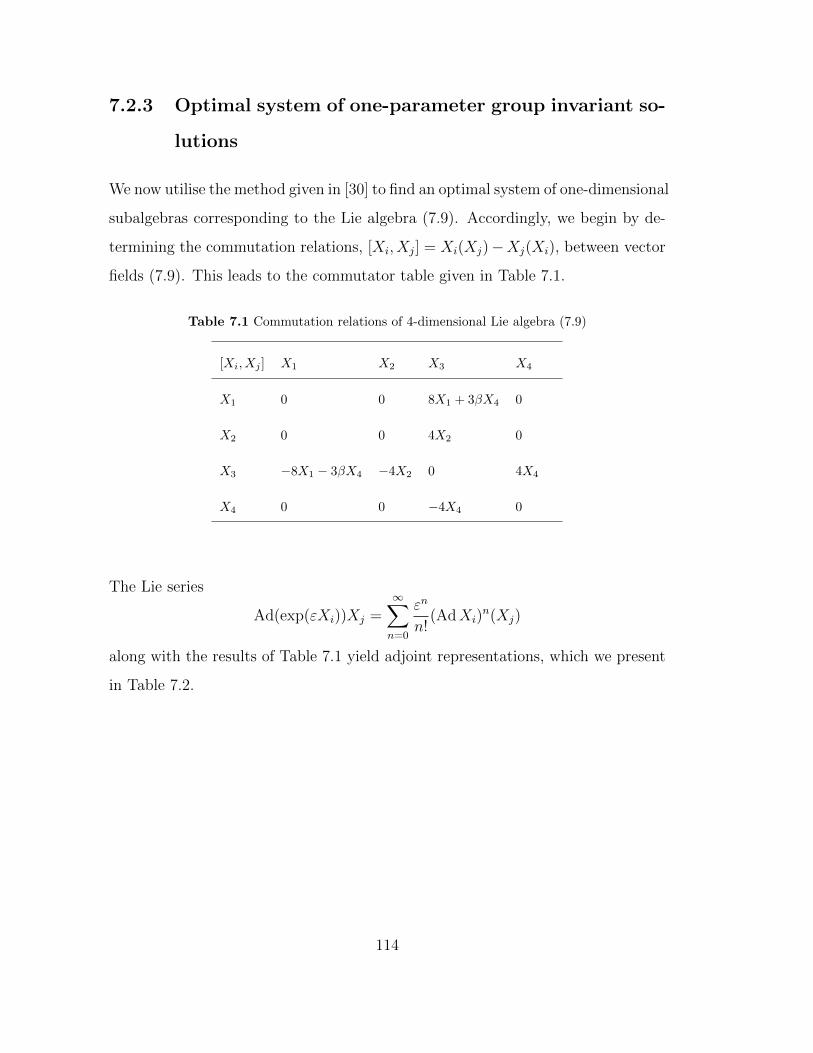
7.2.3 Optimal system of one-parameter group invariant so-
lutions
We now utilise the method given in [30] to find an optimal system of one-dimensional
subalgebras corresponding to the Lie algebra (7.9). Accordingly, we begin by de-
termining the commutation relations, [Xi, Xj] = Xi(Xj)−Xj(Xi), between vector
fields (7.9). This leads to the commutator table given in Table 7.1.
Table 7.1 Commutation relations of 4-dimensional Lie algebra (7.9)
[Xi, Xj ] X1 X2 X3 X4
X1 0 0 8X1 + 3βX4 0
X2 0 0 4X2 0
X3 −8X1 − 3βX4 −4X2 0 4X4
X4 0 0 −4X4 0
The Lie series
Ad(exp(εXi))Xj =∞∑n=0
εn
n!(AdXi)
n(Xj)
along with the results of Table 7.1 yield adjoint representations, which we present
in Table 7.2.
114

Table 7.2 Adjoint table of Lie algebra (7.9)
Ad X1 X2 X3 X4
X1 X1 X2 −8εX1 +X3 − 3βεX4 X4
X2 X1 X2 −4εX2 +X3 X4
X3 e8εX1 + 14βe
−4ε(e12ε − 1
)e4εX2 X3 e−4εX4
X4 X1 X2 X3 + 4εX4 X4
Using the Tables 7.1 and 7.2, and the procedure given in [30,78], we obtain an op-
timal system of one-dimensional subalgebras spanned by X1, X2, X3, X1±X2, X2±
X4. However, we note that the vector field X1 − X2 can be mapped to the vec-
tor field X1 + X2 by the discrete symmetry (t, x, u) 7−→ (t,−x, u). This leaves us
with the following optimal system of one-dimensional subalgebras of (7.2) that is
spanned by
X1, X2, X3, X1 +X2, X2 ±X4. (7.10)
We now determine an optimal system of group invariant solutions corresponding
to (7.10). This will give us closed-form solutions of (7.2).
7.2.3.1 Cases X1, X2 and X2 ±X4
From the generators X1, X2 and X2±X4, we obtain the group invariant solutions:
u(t, x) = φ1(ξ), ξ = x, (7.11)
u(t, x) = φ2(ξ), ξ = t, (7.12)
u(t, x) = φ3(ξ)± x, ξ = t, (7.13)
respectively. Each of the group invariant solutions in (7.11)–(7.13) transform equa-
tion (7.2) into the ODE φ′′′j (ξ) = 0, j = 1, 2, 3. This is easily solved to give the
115

solution
φj(ξ) =1
2C1ξ
2 + C2ξ + C3, j = 1, 2, 3, (7.14)
with C1, C2, C3 integration constants. Thus,
u1 =1
2C1x
2 + C2x+ C3, (7.15)
u2 =1
2C1t
2 + C2t+ C3, (7.16)
u3 =1
2C1t
2 + C2t+ C3 ± x (7.17)
are the group invariant solutions of (7.2) under the optimal system elements X1,
X2 and X2 ±X4, respectively.
7.2.3.2 Case X1 +X2
We now focus on the optimal system element X1 +X2. Using the usual Lie theory,
we obtain the group invariant solution u(t, x) = φ(ξ), ξ = x− t, which transforms
equation (7.2) into the nonlinear ordinary differential equation (NLODE)
φ′′′′′ + (β − 1)φ′′′ + 12(φ′′′φ′ + φ′′2) = 0. (7.18)
(a) Solutions of (7.2) by direct integration of (7.18)
Integrating (7.18) twice with respect to ξ gives
φ′′′ + 6φ′2 + (β − 1)φ′ + C1ξ + C2 = 0 (7.19)
with integration constants C1 and C2. Equation (7.19) cannot be solved to produce
solutions in terms of classical functions, see for example [116–118]. At this point we
are compelled to explore two interesting cases which lead to elliptic and hyperbolic
solutions.
(i) The Jacobi elliptic function solutions of (7.2)
116

Consider the NLODE (7.19) with C1 = 0 and let φ′(ξ) = (1/2) Θ(ξ). Then
equation (7.19) becomes
Θ′′ + 3Θ2 − ρΘ + C4 = 0, (7.20)
where ρ = 1−β and C4 = 2C2. The solution for equation (7.2) will thus take
the form u(t, x) = 1/2∫θ(ξ)dξ. The NLODE (7.20) is a principal equation
and arises from many famous NLPDEs. See for example [116]. Multiplying
(7.20) by Θ′ and integrating with respect to ξ yields
Θ′2 + 2Θ3 − ρΘ2 + 2C4Θ + 2C5 = 0. (7.21)
Equation (7.21) leads us to the well-known Jacobi elliptic cosine function
solution of (7.20), namely [66,95]
Θ(ξ) = µ2 + (µ1 − µ2) cn2
√µ1 − µ3
2ξ,M2
, M2 =
µ1 − µ2
µ1 − µ3
. (7.22)
Here µ1, µ2 and µ3 (with µ1 ≥ µ2 ≥ µ3, 0 ≤ M2 ≤ 1) are roots of the
algebraic equation
Θ3 − 1
2ρΘ2 + C4Θ + C5 = 0
and thus satisfy the differential equation
Θ′2 = −2(Θ− µ1)(Θ− µ2)(Θ− µ3).
Moreover, C4 = 2C2 = µ1µ2 + µ2µ3 + µ1µ3 and C5 = µ1µ2µ3. Finally, we
recuperate the variable u to obtain the solution of (7.2) as
u(t, x) =(µ1 − µ2) sn (Aξ|M2) cos−1 dn(Aξ|M2)
2A√
1− dn (Aξ|M2)2+ 1/2µ2ξ, (7.23)
where A =√µ1 − µ3/
√2, β = 1− 2(µ1 + µ2 + µ3) and ξ = x− t.
The analytic solution (7.23) is periodic in nature, and its profile is sketched
in Figure 7.1.
117

t=0 t=1
t=2
-4 -2 2 4 6 8 10
-30
-20
-10
10
20
30
408Case X2 + X1<
Figure 7.1: Profile of periodic solution (7.23).
(ii) The hyperbolic solutions of (7.2)
By letting the integration constants C1 and C2 equal to zero and φ′(ξ) = ψ(ξ)
in (7.19), equation (7.19) becomes
ψ′′ + (β − 1)ψ + 6ψ2 = 0. (7.24)
Multiplying by ψ′ and integrating with respect to ξ leads us to
ψ′2 + 4ψ3 + (β − 1)ψ2 = 0, (7.25)
where once again, the integration constant is taken as zero. The solution of
equation (7.25) is
ψ(ξ) = −1
4(β − 1)
[1− tanh2
1
2
(±√
1− βC3 −√
1− βξ)]
(7.26)
118
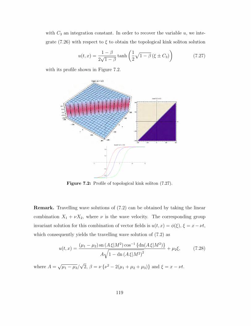
with C3 an integration constant. In order to recover the variable u, we inte-
grate (7.26) with respect to ξ to obtain the topological kink soliton solution
u(t, x) =1− β
2√
1− βtanh
(1
2
√1− β (ξ ± C3)
)(7.27)
with its profile shown in Figure 7.2.
-5 5 10 15
-0.4
-0.2
0.2
0.4
8case1 x2 + x1<
Figure 7.2: Profile of topological kink soliton (7.27).
Remark. Travelling wave solutions of (7.2) can be obtained by taking the linear
combination X1 + νX2, where ν is the wave velocity. The corresponding group
invariant solution for this combination of vector fields is u(t, x) = φ(ξ), ξ = x− νt,
which consequently yields the travelling wave solution of (7.2) as
u(t, x) =(µ1 − µ2) sn (Aξ|M2) cos−1 dn(Aξ|M2)
A√
1− dn (Aξ|M2)2+ µ2ξ, (7.28)
where A =√µ1 − µ3/
√2, β = ν ν2 − 2(µ1 + µ2 + µ3) and ξ = x− νt.
119
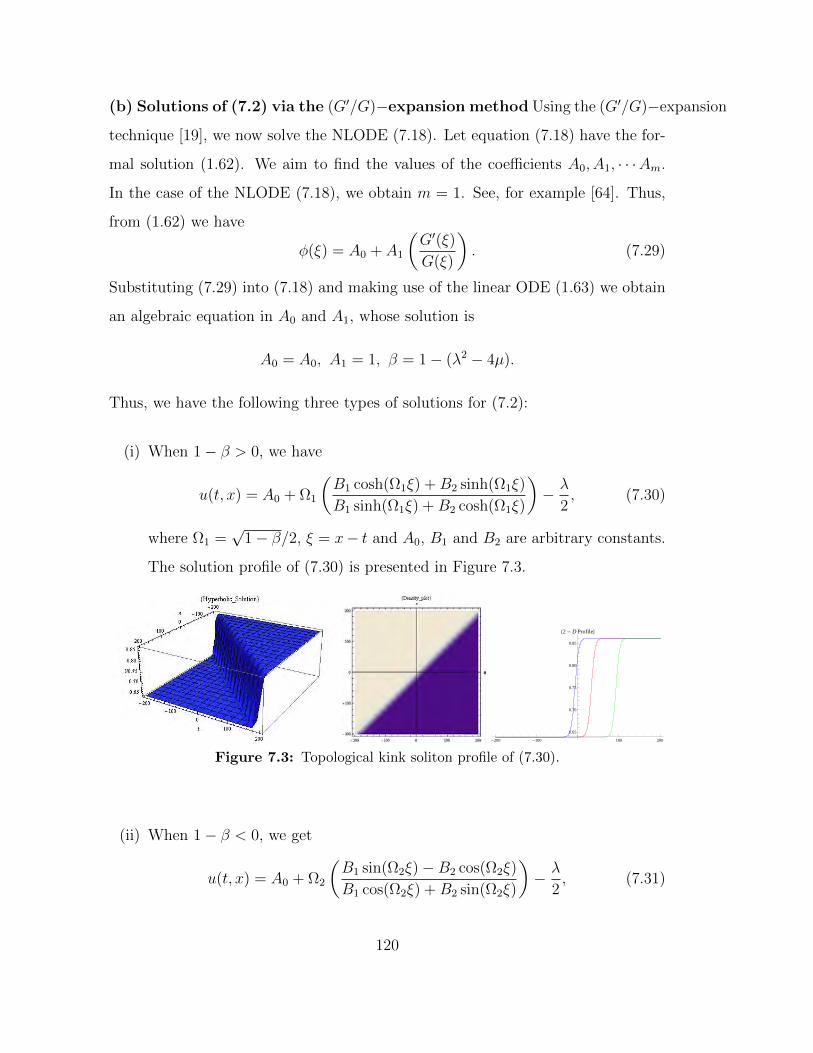
(b) Solutions of (7.2) via the (G′/G)−expansion method Using the (G′/G)−expansion
technique [19], we now solve the NLODE (7.18). Let equation (7.18) have the for-
mal solution (1.62). We aim to find the values of the coefficients A0, A1, · · ·Am.
In the case of the NLODE (7.18), we obtain m = 1. See, for example [64]. Thus,
from (1.62) we have
φ(ξ) = A0 + A1
(G′(ξ)
G(ξ)
). (7.29)
Substituting (7.29) into (7.18) and making use of the linear ODE (1.63) we obtain
an algebraic equation in A0 and A1, whose solution is
A0 = A0, A1 = 1, β = 1− (λ2 − 4µ).
Thus, we have the following three types of solutions for (7.2):
(i) When 1− β > 0, we have
u(t, x) = A0 + Ω1
(B1 cosh(Ω1ξ) +B2 sinh(Ω1ξ)
B1 sinh(Ω1ξ) +B2 cosh(Ω1ξ)
)− λ
2, (7.30)
where Ω1 =√
1− β/2, ξ = x− t and A0, B1 and B2 are arbitrary constants.
The solution profile of (7.30) is presented in Figure 7.3.
-200 -100 100 200
0.65
0.70
0.75
0.80
0.85
82 - D Profile<
Figure 7.3: Topological kink soliton profile of (7.30).
(ii) When 1− β < 0, we get
u(t, x) = A0 + Ω2
(B1 sin(Ω2ξ)−B2 cos(Ω2ξ)
B1 cos(Ω2ξ) +B2 sin(Ω2ξ)
)− λ
2, (7.31)
120

where Ω2 =√β − 1/2, ξ = x− t and A0, B1 and B2 are arbitrary constants.
The solution profile of (7.31) is sketched in Figure 7.4.
Figure 7.4: Periodic behaviour with singularities for (7.31).
(iii) When β = 1, we obtain
u(t, x) = A0 +B2
B2ξ +B1
− λ
2, (7.32)
where ξ = x − t and A0, B1 and B2 are arbitrary constants. The profile of
solution (7.32) is given in Figure 7.5.
-5 5 10 15
-600
-400
-200
200
40082 - D Profile<
Figure 7.5: Bright and dark soliton (7.32) with a singularity.
7.2.3.3 Case X3
Finally, we consider the optimal system element X3, which culminates in the group
invariant solution u(t, x) = (1/√t)φ(ξ) + 1/4 βt, ξ = x/
√t. Thus, equation (7.2)
121

is transformed into the NLODE
4ξφ(5) + 20φ(4) + 48ξφ′φ′′′ − ξ3φ′′′ + 96ξφ′2
+ 96ξφφ′′ + 16φφ′′′ + 192φ′φ′′
− 33ξφ′ − 12ξ2φ′′ − 15φ = 0. (7.33)
The power series solution method is ideal for solving such complicated nonlinear
differential equations (7.33). See, for example [25–27]. To begin, let the solution
of (7.33) take the form
φ(ξ) =∞∑z=0
gzξz (7.34)
with constants gz, z = 0, 1, 2, · · · , to be determined. The various derivatives of
(7.34) are thus
φ′(ξ) =∞∑z=0
(z + 1)gz+1ξz,
φ′′(ξ) =∞∑z=0
(z + 1)(z + 2)gz+2ξz,
φ′′′(ξ) =∞∑z=0
(z + 1)(z + 2)(z + 3)gz+3ξz,
φ(4)(ξ) =∞∑z=0
(z + 1)(z + 2)(z + 3)(z + 4)gz+4ξz,
φ(5)(ξ) =∞∑z=0
(z + 1)(z + 2)(z + 3)(z + 4)(z + 5)gz+5ξz.
(7.35)
Substituting the results of (7.35) into (7.33) gives
4∞∑z=1
z(z + 1)(z + 2)(z + 3)(z + 4)gz+4ξz + 20
∞∑z=0
(z + 1)(z + 2)(z + 3)
(z + 4)gz+4ξz + 48
∞∑z=1
z−1∑j=0
(j + 1)(z − j)(z + 1− j)(z + 2− j)gj+1gz+2−jξz
−∞∑z=3
(z − 2)(z − 1)zgzξz + 96
∞∑z=1
z−1∑j=0
(j + 1)(z − j)gj+1gz−jξz
+ 96∞∑z=1
z−1∑j=0
(z − j)(z + 1− j)gjgz+1−jξz + 16
∞∑z=0
z∑j=0
(z + 1− j) (7.36)
122

(z + 2− j)(z + 3− j)gjgz+3−jξz + 192
∞∑z=0
z∑j=0
(j + 1)(z + 1− j)
(z + 2− j)gj+1gz+2−jξz − 33
∞∑z=1
zgzξz − 12
∞∑z=2
(z − 1)zgzξz
− 15∞∑z=0
gzξz = 0.
Equation (7.36) leads to
480g5ξ + 2880g6ξ2 + 4
∞∑z=3
z(z + 1)(z + 2)(z + 3)(z + 4)gz+4ξz + 480g4
+ 2400g5ξ + 7200g6ξ2 + 20
∞∑z=3
(z + 1)(z + 2)(z + 3)(z + 4)gz+4ξz
+ 288g1g3ξ + 1152g1g4ξ2 + 48
∞∑z=3
z−1∑j=0
(j + 1)(z − j)(z + 1− j)(z + 2− j)
gj+1gz+2−jξz −
∞∑z=3
(z − 2)(z − 1)zgzξz + 96g2
1ξ + 192g1g2ξ2
+ 96∞∑z=3
z−1∑j=0
(j + 1)(z − j)gj+1gz−jξz + 192g0g2ξ + 576g0g3ξ
2 (7.37)
+ 96∞∑z=3
z−1∑j=0
(z − j)(z + 1− j)gjgz+1−jξz + 96g0g3 + 384g0g4ξ
+ 960g0g5ξ2 + 16
∞∑z=3
z∑j=0
(z + 1− j)(z + 2− j)(z + 3− j)gjgz+3−jξz
+ 384g1g2 + 1152g1g3ξ + 2304g1g4ξ2 + 192
∞∑z=3
z∑j=0
(j + 1)(z + 1− j)
(z + 2− j)gj+1gz+2−jξz − 33g1ξ − 66g2ξ
2 − 33∞∑z=3
zgzξz − 12g2ξ
2
− 12∞∑z=3
(z − 1)zgzξz − 15g0 − 15g1ξ − 15g2ξ
2 − 15∞∑z=3
gzξz = 0.
Now comparing coefficients of ξ in equation (7.37) we have, for z = 0, 1, 2:
96g0g3 + 384g1g2 − 15g0 + 480g4 = 0, (7.38)
123
192g0g2 + 384g0g4 + 96g12 + 1440g1g3 − 48g1 + 2880g5 = 0, (7.39)
576g0g3 + 960g0g5 + 192g1g2 + 3456g1g4 − 93g2 + 10080g6 = 0 (7.40)
and generally for z ≥ 3 we have the recurrence relation
gz+4 =− 1
(4z + 20)(z + 1)(z + 2)(z + 3)(z + 4)
48
z−1∑j=0
(j + 1)(z − j)
(z + 1− j)(z + 2− j)gj+1gz+2−j − 33zgz − 12(z − 1)zgz − 15gm
+96z−1∑j=0
(j + 1)(z − j)gj+1gz−j + 96z−1∑j=0
(z − j)(z + 1− j)gjgz+1−j
+16m∑j=0
(z + 1− j)(z + 2− j)(z + 3− j)gjgz+3−j − (z − 2)(z − 1)zgz
+192m∑j=0
(j + 1)(z + 1− j)(z + 2− j)gj+1gz+2−j
.
(7.41)
From equations (7.38)–(7.40) and for arbitrary g0, · · · , g3, we have the following:
g4 =1
32g0 −
1
5g0 g3 −
4
5g1 g2,
g5 =2
75g0
2g3 −1
15g0 g2 +
8
75g0 g1 g2 −
1
240g0
2 − 1
30g1
2 − 1
2g1 g3 +
1
60g1,
g6 =1
2520g3
0 −4
1575g3g
30 −
16
1575g1g2g
20 +
2
315g2g
20 +
1
315g2
1g0 −31
2520g1g0
+61
525g1g3g0 −
2
35g3g0 +
48
175g2
1g2 −2
105g1g2 +
31
3360g2.
(7.42)
Using the recursion formula (7.41), successive terms gm, m = 7, 8, · · · , can be
124

determined uniquely. Thus, the power series solution of (7.33) can be written as
φ(ξ) =g0 + g1ξ + g2ξ2 + g3ξ
3 +
(1
32g0 −
1
5g0 g3 −
4
5g1 g2
)ξ4 +
(2
75g0
2g3
− 1
15g0 g2 +
8
75g0 g1 g2 −
1
240g0
2 − 1
30g1
2 − 1
2g1 g3 +
1
60g1
)ξ5
+
(1
2520g3
0 −4
1575g3g
30 −
16
1575g1g2g
20 +
2
315g2g
20 +
1
315g2
1g0 −31
2520g1g0
+61
525g1g3g0 −
2
35g3g0 +
48
175g2
1g2 −2
105g1g2 +
31
3360g2
)ξ6 +
∞∑z=3
gz+4ξz+4.
(7.43)
Finally, the solution of (7.2) is
u(t, x) =g0 + g1x√t
+ g2x2
t+ g3
x3
t3/2+
(1
32g0 −
1
5g0 g3 −
4
5g1 g2
)x4
t2+
(2
75g0
2g3
− 1
15g0 g2 +
8
75g0 g1 g2 −
1
240g0
2 − 1
30g1
2 − 1
2g1 g3 +
1
60g1
)x5
t5/2
+
(1
2520g3
0 −4
1575g3g
30 −
16
1575g1g2g
20 +
2
315g2g
20 +
1
315g2
1g0 −31
2520g1g0
+61
525g1g3g0 −
2
35g3g0 +
48
175g2
1g2 −2
105g1g2 +
31
3360g2
)x6
t3
−∞∑z=3
(z + 4)!
(4z + 20)z!
(48
z−1∑j=0
(j + 1)(z − j)(z + 1− j)(z + 2− j) (7.44)
gj+1gz+2−j − 33zgz − 12(z − 1)zgz − 15gz + 96z−1∑j=0
(j + 1)(z − j)
gj+1gz−j + 96z−1∑j=0
(z − j)(z + 1− j)gjgz+1−j + 16z∑j=0
(z + 1− j)
(z + 2− j)(z + 3− j)gjgz+3−j − (z − 2)(z − 1)zgz
+192z∑j=0
(j + 1)(z + 1− j)(z + 2− j)gj+1gz+2−j
)(x√t
)z+4
.
The graphical depiction of the behavioural pattern of solution (7.44) is given in
Figure 7.6.
125
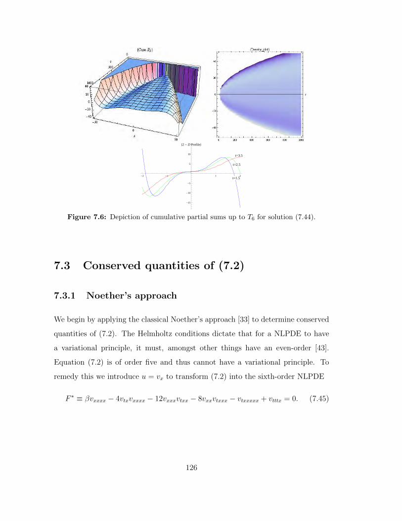
t=3.5
t=2.5
t=1.5-2 -1 1 2
-15
-10
-5
5
10
82 - D Profile<
Figure 7.6: Depiction of cumulative partial sums up to T6 for solution (7.44).
7.3 Conserved quantities of (7.2)
7.3.1 Noether’s approach
We begin by applying the classical Noether’s approach [33] to determine conserved
quantities of (7.2). The Helmholtz conditions dictate that for a NLPDE to have
a variational principle, it must, amongst other things have an even-order [43].
Equation (7.2) is of order five and thus cannot have a variational principle. To
remedy this we introduce u = vx to transform (7.2) into the sixth-order NLPDE
F ∗ ≡ βvxxxx − 4vtxvxxxx − 12vxxxvtxx − 8vxxvtxxx − vtxxxxx + vtttx = 0. (7.45)
126

For the transformed equation (7.45) to have a variational principle, it must indeed
satisfy the Helmholtz conditions
∂F ∗
∂(∂qv)= (−1)q(Eq
v(F∗))t. (7.46)
Here q = 1, · · · , Q, where Q is the order of equation (7.45). Due to the presence of
the transpose t, generally the number of field variables v should equal the number of
components in system F ∗, else the Helmholtz conditions do not hold and extension
F ∗ would not possess a variational principle. Also, Eqv represents higher Euler
operators, which are given by
E(r)v (F ∗) =
∂F ∗
∂(∂rv)−(r + 1
r
)D · ∂F ∗
∂(∂r+1v)+ · · ·+
(q
r
)(−D)q−r · ∂F ∗
∂(∂rv)(7.47)
with r = 1 · · · q and D represents the total derivatives D = (Dt, Dx). It can be
shown with relative ease that a reckoning of (7.46) will confirm that equation (7.45)
indeed has a variational principle. A Lagrangian can thus be recovered for (7.45)
as
L =8
3vtxx (vvxxx + vxvxx) +
4
3vxxx (vvtxx + vxvtx) +
1
2βvxx
2
+1
2vxxxvtxx +
1
2vttvtx − 4vxxxvvtxx. (7.48)
The Lagrangian (7.48) conforms with condition δL/δv = F ∗ = 0, as expected.
In order to obtain the variational symmetries Y = ξ1∂/∂t + ξ2∂/∂x + η∂/∂v cor-
responding to Lagrangian (7.48), we shall use the invariance condition
pr(3)Y (L) + LDtξ1 +Dxξ
2 = DtB1 +DxB
2, (7.49)
where pr(3)Y is the third prolongation of Y obtainable from
pr(3)Y = Y + ζx∂
∂vx+ ζtt
∂
∂vtt+ ζtx
∂
∂vtx+ ζxx
∂
∂vxx+ ζtxx
∂
∂vtxx+ ζxxx
∂
∂vxxx.
127

Note that in (7.49), ξ1, ξ2, η, B1 and B2 are functions of (t, x, v). The invariance
condition (7.49) yields the following system of twelve linear PDEs:
ξ1t = 0, ξ1
x = 0, ξ1v = 0, ξ2
t = 0, ξ2x = 0, ξ2
v = 0,
ηtt = 0, ηx = 0, ηv = 0, B1v = 0, B2
v = 0, B1t +B2
x = 0.(7.50)
From system (7.50) we can readily infer without any tedious calculations that
ξ1 = C1, ξ2 = C2, η = C3t+ C4, B
1 = F (t, x), B2 = H(t, x) + P (t)
with H(t, x) = −∫Ft(t, x)dx. The above generator coefficients lead us to the
variational symmetries
Y1 =∂
∂t, B1 = B2 = 0,
Y2 =∂
∂x, B1 = B2 = 0,
Y3 = t∂
∂v, B1 = B2 = 0,
Y4 =∂
∂v, B1 = B2 = 0.
(7.51)
Following the algorithm outlined in Section 1.5.2 we obtain the following nonlocal
conserved quantities of equation (7.2):
T t1 =1
36
2 (16ut + 9β)u2
x + 8
(8uutx − 9uxx
(∫utdx
))ux − 8
(uxxx
∫utdx
−7utuxx)u+ 3
(4uxxutx +
(2uxxx − 3
∫uttdx
)ut + (9utt − 2uxxx)
∫utdx
),
T x1 =1
36
4
((9β − 34ut)uxx
∫utdx+ 2u
∫uttdx− 3utt
)+ 32u2
x
∫uttdx− 18utx
2
−4
(9βut − 20ut
2 + 56utx
∫utdx+ 16uutt
)ux − 64uututx + 8uutxx
∫utdx
+24ututxx − 30utxxx
∫utdx+ 6uxxx
∫uttdx− 9
(∫uttdx
)2
+9
(∫utdx
)(∫utttdx
);
128
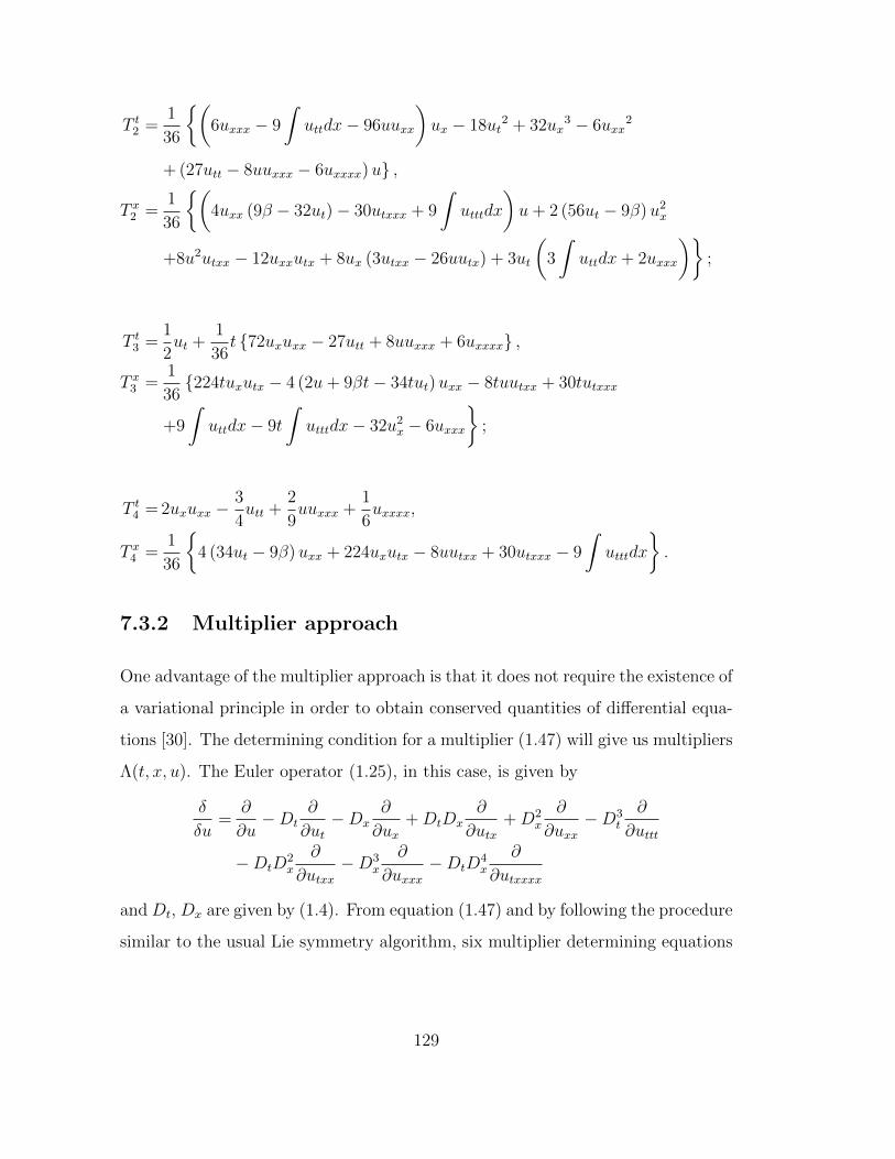
T t2 =1
36
(6uxxx − 9
∫uttdx− 96uuxx
)ux − 18ut
2 + 32ux3 − 6uxx
2
+ (27utt − 8uuxxx − 6uxxxx)u ,
T x2 =1
36
(4uxx (9β − 32ut)− 30utxxx + 9
∫utttdx
)u+ 2 (56ut − 9β)u2
x
+8u2utxx − 12uxxutx + 8ux (3utxx − 26uutx) + 3ut
(3
∫uttdx+ 2uxxx
);
T t3 =1
2ut +
1
36t 72uxuxx − 27utt + 8uuxxx + 6uxxxx ,
T x3 =1
36224tuxutx − 4 (2u+ 9βt− 34tut)uxx − 8tuutxx + 30tutxxx
+9
∫uttdx− 9t
∫utttdx− 32u2
x − 6uxxx
;
T t4 = 2uxuxx −3
4utt +
2
9uuxxx +
1
6uxxxx,
T x4 =1
36
4 (34ut − 9β)uxx + 224uxutx − 8uutxx + 30utxxx − 9
∫utttdx
.
7.3.2 Multiplier approach
One advantage of the multiplier approach is that it does not require the existence of
a variational principle in order to obtain conserved quantities of differential equa-
tions [30]. The determining condition for a multiplier (1.47) will give us multipliers
Λ(t, x, u). The Euler operator (1.25), in this case, is given by
δ
δu=
∂
∂u−Dt
∂
∂ut−Dx
∂
∂ux+DtDx
∂
∂utx+D2
x
∂
∂uxx−D3
t
∂
∂uttt
−DtD2x
∂
∂utxx−D3
x
∂
∂uxxx−DtD
4x
∂
∂utxxxx
and Dt, Dx are given by (1.4). From equation (1.47) and by following the procedure
similar to the usual Lie symmetry algorithm, six multiplier determining equations
129

are realised, which are
Λuu = 0, Λxu = 0, Λxx = 0, Λtu = 0, Λtx = 0, Λttt = 0. (7.52)
Solving equations (7.52) one obtains the multipliers corresponding to equation (7.2)
as
Λ = C1u+ C2x+1
2C3t
2 + C4t+ C5, (7.53)
where C1,. . . ,C5 are constants. We now employ the first homotopy integral formula
(1.48) with equation (7.2) along with multipliers (7.53). We obtain
T =C2uutt − 2C1uuxx − 4C2uuxuxx + C3u−1
2C2uuxxxx −
1
2C2u
2t − C3tut − utC4
+ C1xutt +1
2C3t
2utt + C4tutt + C5utt
and
X =C5βuxx − C1xutxxx − C4tutxxx − C1βux −1
2C3t
2utxxx + C1βxuxx +1
2C3βt
2uxx
+ C4βtuxx −1
2C2uutxxx − 8C5uxutx + 6C1utux −
1
2C2utxuxx − 4C5utuxx
+1
2utxxC2ux + 2uutxC1 + 4utC2u
2x +
1
2C2utuxxx −
1
2C2βu
2x − C5utxxx + C1utxx
− 4C2uuxxut − 4C1xutuxx − 2C3t2utuxx − 4C4tutuxx − 8C1xuxutx − 4C3t
2uxutx
+ C2βuuxx − 8C4tuxutx − 4C2uutxux
and consequently, we have the following five conserved quantities of (7.2):
T t1 =xutt − 2uuxx,
T x1 =utxx + βxuxx − 8xuxutx − 4xutuxx + 2uutx − βux + 6utux − xutxxx;
T t2 =uutt −1
2uuxxxx − 4uuxuxx −
1
2u2t ,
T x2 = 4utux2 − 1
2uutxxx +
1
2uxutxx −
1
2uxxutx +
1
2utuxxx − 4uuxutx + βuuxx − 4uutuxx
− 1
2βux
2;
130

T t3 =1
2t2utt + u− tut,
T x3 =1
2βt2uxx −
1
2t2utxxx − 2t2utuxx − 4t2uxutx;
T t4 = tutt − ut,
T x4 = βtuxx − 8tuxutx − 4tutuxx − tutxxx;
T t5 =utt,
T x5 = βuxx − 4utuxx − 8uxutx − utxxx.
Remarks As can be seen, the conserved vectors obtained here are first integrals
of equation (7.2).
7.4 Concluding remarks
In this chapter, we performed an extensive study of a fifth-order integrable NLPDE
(7.2), which was lately established in the literature and consisted of two dispersive
terms. We obtained group transformations under which the equation (its solu-
tions) remained invariant. Furthermore, we deduced an optimal system of one-
dimensional subalgebras culminating in several group invariant solutions. This
resulted in parabolic, trigonometric, hyperbolic, elliptic and power series solutions.
The corresponding solution profiles depict topological kink soliton and periodic
behaviour. Moreover, we investigated the existence of a variational principle in
relation to Helmholtz conditions and went on to derive nonlocal conserved vectors
corresponding to the variational principle obtained. Local and low-order conserved
quantities were computed using a homotopy integral formula and multipliers.
131

Chapter 8
Analytic solutions and conserved
quantities of the coupled complex
modified Korteweg-de Vries
equations of plasma physics
8.1 Introduction
The complex modified Korteweg-de Vries (cmKdV) equation [118] is given by
ut + 6ε|u|2ux + uxxx = 0, ε± 1. (8.1)
This equation is a model for weakly dispersive shallow water waves. Equation (8.1)
is integrable and belongs to a hierarchy of nonlinear Schrodinger (NLS) equations.
Several researchers have explored various aspects of the cmKdV equation. For
instance, in [119] researchers managed to show that equation (8.1) is gauge equiv-
alent to a spin equation by utilising gauge transformations. They also found exact
soliton and periodic solutions via Darboux transformation. In [120], the existence
132

and orbital stability of travelling wave solutions of (8.1) was determined. Further-
more, breathers and localised solitons of the cmKdV equation were found in [121].
Of note however is that the cmKdV equation (8.1) was extended to the coupled
cmKdV system (ccmKdV)
ut + uxxx + 6(|u|2 + |v|2)ux = 0,
vt + vxxx + 6(|u|2 + |v|2)vx = 0,(8.2)
which was seen for the first time in [122]. System (8.2) has been put forward
as a nonlinear model for the propagation of plasma waves as well as transverse
waves in a molecular chain model. The authors of [122] gave a binary Darboux
transformation for the ccmKdV system (8.2). Furthermore, the authors manage to
obtain several types of solutions which are in terms of trigonometric, hyperbolic,
exponential and rational functions. The solution profiles, as expected are differ-
ent forms of solitons. By introducing transformations u(t, x) = p(t, x) + iq(t, x),
v(t, x) = r(t, x) + is(t, x) and a parameter generalisation, system (8.2) becomes a
(1+1)-dimensional generalised coupled mKdV ((1+1)-dgcmKdV) system
E1 ≡ pt + pxxx + α(p2 + q2 + r2 + s2)px = 0,
E2 ≡ qt + qxxx + α(p2 + q2 + r2 + s2)qx = 0,
E3 ≡ rt + rxxx + α(p2 + q2 + r2 + s2)rx = 0,
E4 ≡ st + sxxx + α(p2 + q2 + r2 + s2)sx = 0,
(8.3)
where α is a non-zero real constant. In this chapter, we study the (1+1)-dgcmKdV
system (8.3). Firstly, using Lie symmetry analysis, we establish a one-parameter
group of transformations of the solutions of this system. Moreover, we find group
invariant solutions and utilise a simplest equation approach along with three dif-
ferential equations, each satisfied by the copolar trio of elliptic functions cn, sn
and dn to obtain analytic solutions. Furthermore, using the power series solution
method we secure an extensive and unique set of solutions of the system under
133

study. Finally, we determine conserved quantities to which system (8.3) conforms
by using the multiplier approach and provide an explicit form of the first homotopy
integral formula.
The work presented in this chapter has been submitted for possible publication
[123].
8.2 Lie algebra and one-parameter group trans-
formations
The infinitesimal transformations corresponding to system (8.3) are given by [25]
t ≈ t+ aξ1(t, x, p, q, r, s), x ≈ x+ aξ2(t, x, p, q, r, s),
p ≈ p+ aη1(t, x, p, q, r, s), q ≈ q + aη2(t, x, p, q, r, s),
r ≈ r + aη3(t, x, p, q, r, s), s ≈ s+ aη4(t, x, p, q, r, s)
(8.4)
with a 1.
An infinitesimal vector field of transformations (8.4) is given by
X = ξ1(t, x, p, q, r, s)∂
∂t+ ξ2(t, x, p, q, r, s)
∂
∂x+ η1(t, x, p, q, r, s)
∂
∂p
+ η2(t, x, p, q, r, s)∂
∂q+ η3(t, x, p, q, r, s)
∂
∂r+ η4(t, x, p, q, r, s)
∂
∂s.
(8.5)
The third prolongation of vector field (8.5)
pr(3)X =X + ζ1t
∂
∂pt+ ζ1
x
∂
∂px+ ζ1
xxx
∂
∂pxxx+ ζ2
t
∂
∂qt+ ζ2
x
∂
∂qx+ ζ2
xxx
∂
∂qxxx
+ ζ3t
∂
∂rt+ ζ3
x
∂
∂rx+ ζ3
xxx
∂
∂rxxx+ ζ4
t
∂
∂st+ ζ4
x
∂
∂sx+ ζ4
xxx
∂
∂sxxx
(8.6)
with prolongation coefficients (1.16) and (1.17). Equation (8.6) gives the deter-
mining equation for obtaining an r-dimensional Lie algebra associated with system
134

(8.3). Using Maple the following nine-dimensional Lie algebra L9 is obtained:
X1 =∂
∂t, X2 =
∂
∂x, X3 = 3t
∂
∂t+ x
∂
∂x− p ∂
∂p− q ∂
∂q− r ∂
∂r− s ∂
∂s,
X4 = p∂
∂q− q ∂
∂p, X5 = q
∂
∂s− s ∂
∂q, X6 = p
∂
∂s− s ∂
∂p,
X7 = q∂
∂r− r ∂
∂q, X8 = p
∂
∂r− r ∂
∂p, X9 = r
∂
∂s− s ∂
∂r.
(8.7)
We now construct one-parameter group of transformations G1, . . . , G9 generated
by L9 (8.7) by solving the Lie equations
dt
da= ξ1(t, x, p, q, r, s), t|a=0 = t,
dx
da= ξ2(t, x, p, q, r, s), x|a=0 = x,
dp
da= η1(t, x, p, q, r, s), p|a=0 = p,
dq
da= η2(t, x, p, q, r, s), q|a=0 = q,
dr
da= η3(t, x, p, q, r, s), r|a=0 = r,
ds
da= η4(t, x, p, q, r, s), s|a=0 = s.
(8.8)
Thus, we obtain
G1 : (t, x, p, q, r, s)→ (t+ a1, x, p, q, r, s),
G2 : (t, x, p, q, r, s)→ (t, x+ a2, p, q, r, s),
G3 : (t, x, p, q, r, s)→ (te3a3 , xea3 , pe−a3 , qe−a3 , re−a3 , se−a3),
G4 : (t, x, p, q, r, s)→ (t, x, p cos a4 − q sin a4, p sin a4 + q cos a4, r, s),
G5 : (t, x, p, q, r, s)→ (t, x, p, q cos a5 − s sin a5, r, q sin a5 + s cos a5),
G6 : (t, x, p, q, r, s)→ (t, x, p cos a6 − s sin a6, q, r, p sin a6 + s cos a6),
G7 : (t, x, p, q, r, s)→ (t, x, p, q cos a7 − r sin a7, q sin a7 + r cos a7, s),
G8 : (t, x, p, q, r, s)→ (t, x, p cos a8 − r sin a8, q, p sin a8 + r cos a8, s),
G9 : (t, x, p, q, r, s)→ (t, x, p, q, r cos a9 − s sin a9, r sin a9 + s cos a9).
Using the above results, we can now state the following theorem:
Theorem 8.1 If p = f(t, x), q = g(t, x), r = h(t, x) and s = w(t, x) is a solution
of (8.3), then the one-parameter family of solutions generated by group G1, . . . , G9
135

are:
Ga1 : p = f(t+ a1, x), q = g(t+ a1, x), r = h(t+ a1, x), s = w(t+ a1, x);
Ga2 : p = f(t, x+ a2), q = g(t, x+ a2), r = h(t, x+ a2), s = w(t, x+ a2);
Ga3 : p = f(te3a3 , xea3)ea3 , q = g(te3a3 , xea3)ea3 ,
Ga3 : r = h(te3a3 , xea3)ea3 , s) = w(te3a3 , xea3)ea3 ;
Ga4 : p = f(t, x) sec a4 + g(t, x) tan a4, q = g(t, x) sec a4 − f(t, x) tan a4,
Ga4 : r = h(t, x), s = w(t, x);
Ga5 : p = f(t, x), q(t, x) = g(t, x) sec a5 + w(t, x) tan a5,
Ga5 : r = h(t, x), s(t, x) = w(t, x) sec a5 − g(t, x) tan a5;
Ga6 : p = f(t, x) sec a6 + w(t, x) tan a6, q = g(t, x),
Ga6 : r = h(t, x), s = w(t, x) sec a6 − f(t, x) tan a6;
Ga7 : p = f(t, x), q = g(t, x) sec a7 + h(t, x) tan a7,
Ga7 : r = h(t, x) sec a7 − g(t, x) tan a7, s = w(t, x);
Ga8 : p = f(t, x) sec a8 + h(t, x) tan a8, q = g(t, x),
Ga8 : r = h(t, x) sec a8 − f(t, x) tan a8, s = w(t, x);
Ga9 : p = f(t, x), q = g(t, x),
Ga9 : r = h(t, x) sec a9 + s(t, x) tan a9, s = s(t, x) sec a9 − h(t, x) tan a9.
8.3 Analytic solutions
We now seek to derive exact solutions of system (8.3) by making use of the time
translation symmetry X1, space translation symmetry X2 and scaling symmetry
X3. Group invariant solutions [93] for the rotation symmetries X4, . . . , X9 cannot
be recovered unless perhaps by taking linear combinations of X1 and/or X2 with
any of X4, . . . , X9. In this work, we will only explore exact solutions emanating
136

from symmetries X1, X2 and X3 as already alluded to.
8.3.1 Case X1 + cX2
Using Lie theory this linear combination gives the group invariant (travelling wave)
solutions
p = w(ξ), q = h(ξ), r = g(ξ), s = f(ξ), ξ = x− ct, (8.9)
where c is the speed of the wave. With (8.9) we transform system (8.3) into the
system of nonlinear ordinary differential equations (NLODEs)
w′′′ − cw′ + α(w2 + h2 + g2 + f 2)w′ = 0,
h′′′ − ch′ + α(w2 + h2 + g2 + f 2)h′ = 0,
g′′′ − cg′ + α(w2 + h2 + g2 + f 2)g′ = 0,
f ′′′ − cf ′ + α(w2 + h2 + g2 + f 2)f ′ = 0.
(8.10)
We seek to obtain solutions of system (8.10) in terms of the main copolar trio of
Jacobian elliptic functions, that is, elliptic cosine cn(ξ|ω), elliptic sine sn(ξ|ω) and
delta amplitude dn(ξ|ω). Here ω represents a parameter such that 0 ≤ ω ≤ 1. All
remaining nine Jacobian functions can be written in terms of at least one of the
elliptic functions in this copolar trio. See for example [66,67]. What makes Jacobi
elliptic functions interesting is that they degenerate to trigonometric, hyperbolic
and by extension exponential functions depending on the value of parameter ω, see
Table 8.3.1.
137

Table 8.3.1. Copolar trio for ω = 0 and ω = 1
ω = 0 ω = 1
sn(ξ|ω) sinω tanhω
cn(ξ|ω) cosω sechω
dn(ξ|ω) 1 sechω
The elliptic functions cn(ξ|ω), sn(ξ|ω) and dn(ξ|ω) are solutions of the following
NLODEs:
φ(ξ) = −
(1− φ2(ξ))(1− ω + ωφ2(ξ))1/2
, (8.11)
φ(ξ) =
(1− φ2(ξ))(1− ωφ2(ξ))1/2
, (8.12)
φ(ξ) = −
(1− φ2(ξ))(φ2(ξ) + ω − 1)1/2
, (8.13)
respectively. Suppose system (8.3) has solutions of the form
f(ξ) =M∑i=0
Aiφ(ξ), g(ξ) =M∑i=0
Biφ(ξ), h(ξ) =M∑i=0
Ciφ(ξ), w(ξ) =M∑i=0
Diφ(ξ).
(8.14)
Here Ai, Bi, Ci and Di are constants to be determined. For system (8.10), M = 1
and is determined by the balancing procedure. Thus, (8.14) becomes
f(ξ) =A0 + A1φ(ξ), g(ξ) = B0 +B1φ(ξ),
h(ξ) =C0 + C1φ(ξ), w(ξ) = D0 +D1φ(ξ).(8.15)
8.3.1.1 Elliptic cosine solutions
Periodic solutions
Substituting (8.15) along with (8.11) into NLODE system (8.10), we get a system
138

of four algebraic equations in terms of φ(ξ). We can further split this system by
collecting coefficients of powers of φ(ξ) leading to a system of twenty one equations
in terms of parameters Ai, Bi, Ci Di, c, α and ω. Using Maple we get the following
solution
c =1
3A02
(3αA0
4 + 3αB02A0
2 + αB12A0
2 + 3αC02A0
2 + αC12A0
2 + 3αD02A0
2
+αD12A0
2 + αB02B1
2 + 2αB0B1C0C1 + 2αB0B1D0D1 + αC02C1
2 − 3A02
+2αC0C1D0D1 + αD02D1
2),
ω =1
6α(A1
2 +B12 + C1
2 +D12), A1 = − 1
A0
(B0B1 + C0C1 +D0D1) ,
α =α, A0 = A0, B0 = B0, B1 = B1, C0 = C0, C1 = C1, D0 = D0, D1 = D1.
Thus for φ(ξ) = cn(ξ|ω) we have the solution
p(t, x) =D0 +D1cn
(x− c t
∣∣∣∣16 α (A12 +B1
2 + C12 +D1
2))
, (8.16)
q(t, x) =C0 + C1cn
(x− c t
∣∣∣∣16 α (A12 +B1
2 + C12 +D1
2))
, (8.17)
r(t, x) =B0 +B1cn
(x− c t
∣∣∣∣16 α (A12 +B1
2 + C12 +D1
2))
, (8.18)
s(t, x) =1
A0
A2
0 − (B0B1 + C0C1 +D0D1) cn
(x− c t
∣∣∣∣16 α (A12 +B1
2 + C12 +D1
2))
,
(8.19)
For brevity we will only pay attention to the graphical depiction of solution (8.19),
which is provided in Figure 8.1.
139

Figure 8.1: Periodic wave, a depiction of solution (8.19) with parameter values
A0 = 1, B0 = 1, B1 = 1, C0 = 1, C1 = 1, α = 0.2, D0 = 1, D1 = 1.
.
The periodic nature of solution (8.19) is aptly depicted in Figure 8.1 and is typical
behaviour of an elliptic cosine function. In this instance, the resultant value of
ω corresponding to the selected parameter values is ω = 0.4. As evidenced by
the two-dimensional profile in Figure 8.1, taken at t = 0, t = 10 and t = 20, the
periodic transverse wave propagates with constant amplitude and frequency.
Bell-shaped dark solitons
Maintaining the parameter values in Figure 8.1 but replacing α = 0.2 with α = 0.5
leads to ω = 1 and solutions (8.16)–(8.19) degenerate to
p(t, x) =D0 +D1sech(x− ct), (8.20)
q(t, x) =C0 + C1sech(x− ct), (8.21)
r(t, x) =B0 +B1sech(x− ct), (8.22)
s(t, x) =1
A0
A2
0 − (B0B1 + C0C1 +D0D1) sech(x− ct). (8.23)
A bell-shaped dark soliton profile of solution (8.23), typical of the hyperbolic secant
is observed in Figure 8.2.
140

Figure 8.2: A depiction of dark soliton solution (8.23) with parameter values
A0 = 1, B0 = 1, B1 = 1, C0 = 1, C1 = 1, α = 0.5, D0 = 1, D1 = 1.
.
Periodic sine wave solutions
Although α 6= 0, it should be noted that as α → 0 then ω → 0 and solutions
(8.16)–(8.19) begin to exhibit an increasingly sinusoidal behaviour, that is,
p(t, x) =D0 +D1 sin(x− ct), (8.24)
q(t, x) =C0 + C1 sin(x− ct), (8.25)
r(t, x) =B0 +B1 sin(x− ct), (8.26)
s(t, x) =1
A0
A2
0 − (B0B1 + C0C1 +D0D1) sin(x− ct), (8.27)
with a typical sine wave-like deportment as shown in Figure 8.3.
141

Figure 8.3: Periodic wave solution (8.27) with parameter values
A0 = 1, B0 = 1, B1 = 1, C0 = 1, C1 = 1, α→ 0, D0 = 1, D1 = 1.
.
8.3.1.2 Elliptic sine solutions
Periodic wave solutions
Elliptic sine solutions can be obtained by substituting equations (8.15) along with
NLODE (8.12) into (8.10). The resultant parameter values are
c =1
6A20
(6αA0
4 + 6αA02B0
2 + αA02B1
2 + 6αA02C0
2 + αA02C1
2 + 6αA02D0
2
+αA02D1
2 + αB02B1
2 + 2αB0B1C0C1 + 2αB0B1D0D1 + αC02C1
2
+2αC0C1D0D1 + αD02D1
2 − 6A02),
ω =− 1
6α(A1
2 +B12 + C1
2 +D12), A1 = − 1
A0
(B0B1 + C0C1 +D0D1) ,
α =α, A0 = A0, B0 = B0, B1 = B1, C0 = C0, C1 = C1, D0 = D0, D1 = D1,
and consequently the set of solutions satisfying system (8.3) are given by
p(t, x) =D0 +D1sn
(x− c t
∣∣∣∣−1
6α(A1
2 +B12 + C1
2 +D12))
, (8.28)
q(t, x) =C0 + C1sn
(x− c t
∣∣∣∣−1
6α(A1
2 +B12 + C1
2 +D12))
, (8.29)
142

r(t, x) =B0 +B1sn
(x− c t
∣∣∣∣−1
6α(A1
2 +B12 + C1
2 +D12))
, (8.30)
s(t, x) =1
A0
A2
0 − (B0B1 + C0C1 +D0D1)
× sn
(x− c t
∣∣∣∣−1
6α(A1
2 +B12 + C1
2 +D12))
. (8.31)
Obviously the restriction α < 0 is necessary for solutions (8.28)–(8.31) to hold.
For brevity we will only explore various aspects of (8.31).
Figure 8.4: Periodic wave solution (8.31) with parameter values
A0 = 1, B0 = 1, B1 = 1, C0 = 1, C1 = 1, α = −0.2, D0 = 1, D1 = 1.
.
Figure 8.4 depicts a periodic profile of the elliptic sine solution (8.31). Variation
of parameter D0 for 0 ≤ D0 ≤ 1 directly leads to vertical translation as seen in
the two-dimensional profile of Figure 10.4. In this instance the value of parameter
ω = 0.4.
Topological kink and anti-kink solitons
Hyperbolic tangent soliton solutions are recovered when α = −0.5 since this leads
to ω = 1 provided the parameter values given in Figure 10.4 remain unchanged.
Thus, solutions (8.28) –(8.31) become
p(t, x) =D0 +D1tanh(x− c t), (8.32)
143

q(t, x) =C0 + C1tanh(x− c t), (8.33)
r(t, x) =B0 +B1tanh(x− c t), (8.34)
s(t, x) =1
A0
A2
0 − (B0B1 + C0C1 +D0D1) tanh(x− c t). (8.35)
The corresponding solution profiles for (8.35) are provided in Figure 8.5.
Figure 8.5: Topological kink and anti-kink soliton profiles of (8.31) with parameter
values A0 = ±1, B0 = 1, B1 = 1, C0 = 1, C1 = 1, α = −0.5, D0 = 1, D1 = 1.
.
A topological kink soliton profile is observable, for instance, when A0 = 1 while an
anti-kink profile can be seen when A0 = −1.
144

Periodic cosine solutions
Periodic cosine solutions can be recovered by considering the case α→ 0 resulting
in the trigonometric solution
p(t, x) =D0 +D1cos(x− c t), (8.36)
q(t, x) =C0 + C1cos(x− c t), (8.37)
r(t, x) =B0 +B1cos(x− c t), (8.38)
s(t, x) =1
A0
A2
0 − (B0B1 + C0C1 +D0D1) cos(x− c t). (8.39)
The resultant solution profile is depicted by the Figure 8.6.
Figure 8.6: Periodic wave profiles of (8.35) with parameter values A0 = 1, B0 =
1, B1 = 1, C0 = 1, C1 = 1, α = −0.5, D0 ∈ (1, 2, 4), D1 = 1.
.
As can be seen in Figure 8.6, an increase in at least one of the parameters Ai,
. . . , Di leads to a commensurate increase in wave amplitude, while period and
frequency remain unchanged.
145

8.3.1.3 Delta amplitude solutions
Periodic wave solutions
Likewise, we obtain delta amplitude solutions of system (8.3) by utilising (8.15)
together with (8.13) and obtain parameter values
ω =α(A2
0 +B20 + C2
0 +D20
)− c+ 2,
α =α, c = c, A0 = A0, B0 = B0, C0 = C0, C1 = C1, D0 = D0, D1 = D1,
A1 =− α(A20 +B2
0)(C0C1 +D0D1)−B0(αB0C0C1 + αB0D0D1 −√
∆)
αA0(A20 +B2
0),
B1 =− B0
αA0(A20 +B2
0)
(αB0C0C1 + αB0D0D1 −
√∆),
∆ = 6αA02(A0
2 +B02)− α2A0
4C12 − α2A0
4D12 − α2A0
2B02C1
2 − α2A02B0
2D12
− α2A02C0
2C12 − 2α2A0
2C0C1D0D1 − α2A02D0
2D12.
For certain α such that 0 < α < 1, we can ensure that the parameter values hold.
Consequently, we have the delta amplitude solutions
p(t, x) =D0 +D1dn(x− c t
∣∣α (A20 +B2
0 + C20 +D2
0
)− c+ 2
), (8.40)
q(t, x) =C0 + C1dn(x− c t
∣∣α (A20 +B2
0 + C20 +D2
0
)− c+ 2
), (8.41)
r(t, x) =B0
1− 1
αA0(A20 +B2
0)
(αB0C0C1 + αB0D0D1 −
√∆)
×dn(x− c t
∣∣α (A20 +B2
0 + C20 +D2
0
)− c+ 2
), (8.42)
s(t, x) =1
A0
A2
0 −α (A2
0 +B20) (C0C1 +D0D1)−B0 (αB0C0C1 + αB0D0D1)
α(A20 +B2
0)
+B0
α(A20 +B2
0)
√∆
× dn
(x− c t
∣∣α (A20 +B2
0 + C20 +D2
0
)− c+ 2
).
(8.43)
Not surprisingly, solutions (8.40)–(8.43) are periodic in nature. Let us explore, say,
solution (8.42). For example, when α = 0.5, c = 3.5, A0 = 1, B0 = 1, B1 = 1, C0 =
1, C1 = 1, D0 = 1, D1 = 1, we have the periodic wave profile shown in Figure 8.7.
146

Figure 8.7: Periodic wave profiles of (8.43) with parameter values α = 0.5, c =
3.5, A0 = 1, B0 = 1, B1 = 1, C0 = 1, C1 = 1, D0 = 1, D1 = 1.
.
Bell-shaped bright solitons
If we take the wave speed, say c = 3, we have hyperbolic secant solutions akin to
(8.40)–(8.43). For example, solution (8.42) becomes
r(t, x) =B0
1− 1
αA0(A20 +B2
0)
(αB0C0C1 + αB0D0D1 −
√∆)
sech (x− c t)
(8.44)
and is depicted in Figure 8.8.
147

Figure 8.8: Bell-shaped bright soliton profile of (8.44) with parameter values α =
0.5, c = 3, A0 = 1, B0 = 1, B1 = 1, C0 = 1, C1 = 1, D0 = 1, D1 = 1.
Constant solution
A constant is often part of the set of solutions of a system of NLPDEs and system
(8.3) is not an exception. Of interest, however, is that solutions (8.40)–(8.43)
degenerate to arbitrary constants for the non-unique instance c = 4 and α =
0.5, c = 4, A0 = 1, B0 = 1, B1 = 1, C0 = 1, C1 = 1, D0 = 1, D1 = 1, which gives
ω = 0. See Table 8.3.1.
8.3.2 Case X3
From the symmetry generator X3, we have the group invariant solution
p = t−1/3w(ξ), q = t−1/3h(ξ), r = t−1/3g(ξ), s = t−1/3f(ξ), ξ =x
t1/3, (8.45)
which transforms system (8.3) into
3αf 2f ′ + 3αw2f ′ + 3αh2f ′ + 3αg2f ′ − f − ξf ′ + 3f ′′′ = 0,
3αf 2g′ + 3αw2g′ + 3αh2g′ + 3αg2g′ − g − ξg′ + 3g′′′ = 0,
3αf 2h′ + 3αw2h′ + 3αh2h′ + 3αg2h′ − h− ξh′ + 3h′′′ = 0,
3αf 2w′ + 3αw2w′ + 3αh2w′ + 3αg2w′ − w − ξw′ + 3w′′′ = 0.
(8.46)
148

We now use the power series method [77] to obtain analytic solutions of NLODE
system (8.46). Let the solutions of system (8.46) take the form
f(ξ) =∞∑z=0
azξz, g(ξ) =
∞∑z=0
bzξz,
h(ξ) =∞∑z=0
czξz, w(ξ) =
∞∑z=0
dzξz
(8.47)
with constants az, bz, cz, dz, z = 0, 1, 2, . . . to be determined. Substituting (8.47)
into (8.46), we have
3α(a20a1 + b2
0a1 + c20a1 + d2
0a1)− a0 + 18a3 + 3∞∑z=1
(z + 1)(z + 2)(z + 3)bz+3ξz
+ 3α
(∞∑z=1
z∑k=0
k∑i=0
(z − k + 1)aiak−iaz−k+1 +∞∑z=1
z∑k=0
k∑i=0
(z − k + 1)bibk−iaz−k+1
+∞∑z=1
z∑k=0
k∑i=0
(z − k + 1)cick−iaz−k+1 +∞∑z=1
z∑k=0
k∑i=0
(z − k + 1)didk−iaz−k+1
)ξz
−∞∑z=1
zazξz −
∞∑z=1
azξz = 0, (8.48)
3α(a20b1 + b2
0b1 + c20b1 + d2
0d1)− b0 + 18b3 + 3∞∑z=1
(z + 1)(z + 2)(z + 3)bz+3ξz
+ 3α
(∞∑z=1
z∑k=0
k∑i=0
(z − k + 1)aiak−ibz−k+1 +∞∑z=1
z∑k=0
k∑i=0
(z − k + 1)bibk−ibz−k+1
+∞∑z=1
z∑k=0
k∑i=0
(z − k + 1)cick−ibz−k+1 +∞∑z=1
z∑k=0
k∑i=0
(z − k + 1)didk−ibz−k+1
)ξz
−∞∑z=1
zbzξz −
∞∑z=1
bzξz = 0, (8.49)
3α(a20c1 + b2
0c1 + c20c1 + d2
0c1)− c0 + 18c3 + 3∞∑z=1
(z + 1)(z + 2)(z + 3)cz+3ξz
+ 3α
(∞∑z=1
z∑k=0
k∑i=0
(z − k + 1)aiak−icz−k+1 +∞∑z=1
z∑k=0
k∑i=0
(z − k + 1)bibk−icz−k+1
+∞∑z=1
z∑k=0
k∑i=0
(z − k + 1)cick−icz−k+1 +∞∑z=1
z∑k=0
k∑i=0
(z − k + 1)didk−icz−k+1
)ξz
149

−∞∑z=1
zczξz −
∞∑z=1
czξz = 0, (8.50)
3α(a20d1 + b2
0d1 + c20d1 + d2
0d1)− d0 + 18d3 + 3∞∑z=1
(z + 1)(z + 2)(z + 3)dz+3ξz
+ 3α
(∞∑z=1
z∑k=0
k∑i=0
(z − k + 1)aiak−idz−k+1 +∞∑z=1
z∑k=0
k∑i=0
(z − k + 1)bibk−idz−k+1
+∞∑z=1
z∑k=0
k∑i=0
(z − k + 1)cick−idz−k+1 +∞∑z=1
z∑k=0
k∑i=0
(z − k + 1)didk−idz−k+1
)ξz
−∞∑z=1
zdzξz −
∞∑z=1
dzξz = 0. (8.51)
From equations (8.48)–(8.51) and for arbitrary ai, bi, ci, di, i = 0, 1, 2, we have
a3 =1
18
(a0 − 3α(a2
0a1 + b20a1 + c2
0a1 + d20a1)
),
b3 =1
18
(b0 − 3α(a2
0b1 + b20b1 + c2
0b1 + d20b1)
),
c3 =1
18
(c0 − 3α(a2
0c1 + b20c1 + c2
0c1 + d20c1)
),
d3 =1
18
(d0 − 3α(a2
0d1 + b20d1 + c2
0d1 + d20d1)
),
150

respectively, and the following recursion formulae:
az+3 =1
3(z + 1)(z + 2)(z + 3)
az(z + 1)− 3α
(z∑
k=0
k∑i=0
(z − k + 1)aiak−iaz−k+1
+z∑
k=0
k∑i=0
(z − k + 1)bibk−iaz−k+1 +z∑
k=0
k∑i=0
(z − k + 1)cick−iaz−k+1
+z∑
k=0
k∑i=0
(z − k + 1)didk−iaz−k+1
),
bz+3 =1
3(z + 1)(z + 2)(z + 3)
bz(z + 1)− 3α
(z∑
k=0
k∑i=0
(z − k + 1)aiak−ibz−k+1
+z∑
k=0
k∑i=0
(z − k + 1)bibk−ibz−k+1 +z∑
k=0
k∑i=0
(z − k + 1)cick−ibz−k+1
+z∑
k=0
k∑i=0
(z − k + 1)didk−ibz−k+1
),
cz+3 =1
3(z + 1)(z + 2)(z + 3)
cz(z + 1)− 3α
(z∑
k=0
k∑i=0
(z − k + 1)aiak−icz−k+1
+z∑
k=0
k∑i=0
(z − k + 1)bibk−icz−k+1 +z∑
k=0
k∑i=0
(z − k + 1)cick−icz−k+1
+z∑
k=0
k∑i=0
(z − k + 1)didk−icz−k+1
),
dz+3 =1
3(z + 1)(z + 2)(z + 3)
dz(z + 1)− 3α
(z∑
k=0
k∑i=0
(z − k + 1)aiak−idz−k+1
+z∑
k=0
k∑i=0
(z − k + 1)bibk−idz−k+1 +z∑
k=0
k∑i=0
(z − k + 1)cick−idz−k+1
+z∑
k=0
k∑i=0
(z − k + 1)didk−idz−k+1
),
for z = 1, 2, . . . . Therefore, the explicit power series solution of system (8.56)
under the action of infinitesimal vector field X3 is
p(t, x) = a0 + a1
( x
t1/3
)+ a2
(x2
t2/3
)+
1
18
(a0 − 3α(a2
0a1 + b20a1 + c2
0a1 + d20a1)
)(x3
t
)
151

+1
3
∞∑z=1
z!
(z + 3)!
az(z + 1)− 3α
(z∑
k=0
k∑i=0
(z − k + 1)aiak−iaz−k+1
+z∑
k=0
k∑i=0
(z − k + 1)bibk−iaz−k+1 +z∑
k=0
k∑i=0
(z − k + 1)cick−iaz−k+1
+z∑
k=0
k∑i=0
(z − k + 1)didk−iaz−k+1
)( x
t1/3
)z+3
, (8.52)
q(t, x) = b0 + b1
( x
t1/3
)+ b2
(x2
t2/3
)+
1
18
(b0 − 3α(a2
0b1 + b20b1 + c2
0b1 + d20b1)
)(x3
t
)+
1
3
∞∑z=1
z!
(z + 3)!
bz(z + 1)− 3α
(z∑
k=0
k∑i=0
(z − k + 1)aiak−ibz−k+1
+z∑
k=0
k∑i=0
(z − k + 1)bibk−ibz−k+1 +z∑
k=0
k∑i=0
(z − k + 1)cick−ibz−k+1
+z∑
k=0
k∑i=0
(z − k + 1)didk−ibz−k+1
)( x
t1/3
)z+3
(8.53)
r(t, x) = c0 + c1
( x
t1/3
)+ c2
(x2
t2/3
)+
1
18
(c0 − 3α(a2
0c1 + b20c1 + c2
0c1 + d20c1)
)(x3
t
)+
1
3
∞∑z=1
z!
(z + 3)!
cz(z + 1)− 3α
(z∑
k=0
k∑i=0
(z − k + 1)aiak−icz−k+1
+z∑
k=0
k∑i=0
(z − k + 1)bibk−icz−k+1 +z∑
k=0
k∑i=0
(z − k + 1)cick−icz−k+1
+z∑
k=0
k∑i=0
(z − k + 1)didk−icz−k+1
)( x
t1/3
)z+3
(8.54)
s(t, x) = d0 + d1
( x
t1/3
)+ d2
(x2
t2/3
)+
1
18
(d0 − 3α(a2
0d1 + b20d1 + c2
0d1 + d20d1)
)(x3
t
)+
1
3
∞∑z=1
z!
(z + 3)!
dz(z + 1)− 3α
(z∑
k=0
k∑i=0
(z − k + 1)aiak−idz−k+1
+z∑
k=0
k∑i=0
(z − k + 1)bibk−idz−k+1 +z∑
k=0
k∑i=0
(z − k + 1)cick−idz−k+1
+z∑
k=0
k∑i=0
(z − k + 1)didk−idz−k+1
)( x
t1/3
)z+3
. (8.55)
152

Figure 8.9 is a depiction of solution (8.52) and solutions (8.53)–(8.55) have analo-
gous profiles.
-2 -1 1 2 3
-1
1
2
3
4
82<
Figure 8.9: Cumulative partial sums of solution (8.52) up to T5 with parameter
values a0 = 1, a1 = 1, a2 = 0.5, b0 = 2, b1 = 2, b2 = 2, c0 = 2, c1 = 1, c2 = 1, d0 =
1, d1 = 0.9, d2 = 3, α = 0.29.
8.4 Conserved currents
In this Section, we employ the first homotopy integral formula [43] explicitly to
obtain nine local and low-order conserved quantities of the (1+1)-dgcmKdV system
(8.3). The reckoning of
δ
δp
[Λ1E1 + Λ2E2 + Λ3E3 + Λ4E4
]= 0,
δ
δq
[Λ1E1 + Λ2E2 + Λ3E3 + Λ4E4
]= 0,
δ
δr
[Λ1E1 + Λ2E2 + Λ3E3 + Λ4E4
]= 0,
δ
δs
[Λ1E1 + Λ2E2 + Λ3E3 + Λ4E4
]= 0,
(8.56)
indeed yields all multipliers of system (8.3). The well-known Euler operator δ/δp
is given by [45]
δ
δp=
∂
∂p−Dt
∂
∂pt−Dx
∂
∂px+D2
x
∂
∂pxx−D3
x
∂
∂pxxx(8.57)
153
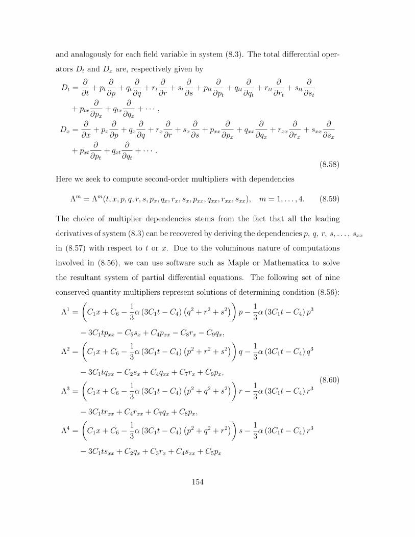
and analogously for each field variable in system (8.3). The total differential oper-
ators Dt and Dx are, respectively given by
Dt =∂
∂t+ pt
∂
∂p+ qt
∂
∂q+ rt
∂
∂r+ st
∂
∂s+ ptt
∂
∂pt+ qtt
∂
∂qt+ rtt
∂
∂rt+ stt
∂
∂st
+ ptx∂
∂px+ qtx
∂
∂qx+ · · · ,
Dx =∂
∂x+ px
∂
∂p+ qx
∂
∂q+ rx
∂
∂r+ sx
∂
∂s+ pxx
∂
∂px+ qxx
∂
∂qx+ rxx
∂
∂rx+ sxx
∂
∂sx
+ pxt∂
∂pt+ qxt
∂
∂qt+ · · · .
(8.58)
Here we seek to compute second-order multipliers with dependencies
Λm = Λm(t, x, p, q, r, s, px, qx, rx, sx, pxx, qxx, rxx, sxx), m = 1, . . . , 4. (8.59)
The choice of multiplier dependencies stems from the fact that all the leading
derivatives of system (8.3) can be recovered by deriving the dependencies p, q, r, s, . . . , sxx
in (8.57) with respect to t or x. Due to the voluminous nature of computations
involved in (8.56), we can use software such as Maple or Mathematica to solve
the resultant system of partial differential equations. The following set of nine
conserved quantity multipliers represent solutions of determining condition (8.56):
Λ1 =
(C1x+ C6 −
1
3α (3C1t− C4)
(q2 + r2 + s2
))p− 1
3α (3C1t− C4) p3
− 3C1tpxx − C5sx + C4pxx − C8rx − C9qx,
Λ2 =
(C1x+ C6 −
1
3α (3C1t− C4)
(p2 + r2 + s2
))q − 1
3α (3C1t− C4) q3
− 3C1tqxx − C2sx + C4qxx + C7rx + C9px,
Λ3 =
(C1x+ C6 −
1
3α (3C1t− C4)
(p2 + q2 + s2
))r − 1
3α (3C1t− C4) r3
− 3C1trxx + C4rxx + C7qx + C8px,
Λ4 =
(C1x+ C6 −
1
3α (3C1t− C4)
(p2 + q2 + r2
))s− 1
3α (3C1t− C4) r3
− 3C1tsxx + C2qx + C3rx + C4sxx + C5px
(8.60)
154

with C1, . . . , C9 as free constants. Conserved densities T i and spatial fluxes X i for
i = 1, . . . , 9 can be obtained by using the first homotopy integral formula (1.48),
see also [77]. Thus, for (8.3) and (8.60), formula (1.48) is explicitly given by
T =
∫ 1
0
(p
(∂EmΛm
∂pt
)|p=pλ + q
(∂EmΛm
∂qt
)|q=qλ + r
(∂EmΛm
∂rt
)|r=rλ
+s
(∂EmΛm
∂st
)|s=sλ
)dλ,
X =
∫ 1
0
p
(∂EmΛm
∂px
)|p=pλ −Dx
(∂EmΛm
∂pxx
)|p=pλ +D2
x
(∂EmΛm
∂pxxx
)|p=pλ
+px
(∂EmΛm
∂pxx
)|p=pλ +D2
x
(∂EmΛm
∂pxx
)|p=pλ
+ pxx
(∂EmΛm
∂pxxx
)|p=pλ
+q
(∂EmΛm
∂qx
)|q=qλ −Dx
(∂EmΛm
∂qxx
)|q=qλ +D2
x
(∂EmΛm
∂qxxx
)|q=qλ
+qx
(∂EmΛm
∂qxx
)|q=qλ +D2
x
(EmΛm
∂qxx
)|q=qλ
+ qxx
(∂EmΛm
∂qxxx
)|q=qλ
r
(∂EmΛm
∂rx
)|r=rλ −Dx
(∂EmΛm
∂rxx
)|r=rλ +D2
x
(∂EmΛm
∂rxxx
)|r=rλ
+rx
(∂EmΛm
∂rxx
)|r=rλ +D2
x
(∂EmΛm
∂rxx
)|r=rλ
+ rxx
(∂E2Λ2
∂rxxx
)|r=rλ
+s
(∂EmΛm
∂sx
)|s=sλ −Dx
(∂EmΛm
∂sxx
)|s=sλ +D2
x
(∂EmΛm
∂sxxx
)|s=sλ
+sx
(∂EmΛm
∂sxx
)|s=sλ +D2
x
(∂EmΛm
∂sxx
)|s=sλ
+ sxx
(∂EmΛm
∂sxxx
)|s=sλ
dλ.
(8.61)
Now considering the case
Λ11 =xp− α tp3 − αtpq2 − αtpr2 − αtps2 − 3tpxx,
Λ21 =xq − αtp2q − αtq3 − αtqr2 − αtqs2 − 3tqxx,
Λ31 =xr − αtp2r − αtq2r − αtr3 − αtrs2 − 3trxx,
Λ41 =xs− αtp2s− αtq2s− αtr2s− αts3 − 3tsxx,
we have
T 1 =
∫ 1
0
(λxp2 − αtλ3p4 − 2αtλ3p2q2 − 2αtλ3p2r2 − 2αtλ3p2s2 − 3λtppxx
155

−αtλ3q4 − 2λ3αtq2r2 − 2λ3αtq2s2 + λxq2 − 3λtqqxx − αtλ3r4
−2λ3αtr2s2 + λxr2 − 3λtrrxx − λ3αts4 + λxs2 − 3λtssxx)
dλ
=1
2xp2 − 1
4αtp4 − 1
2αtp2q2 − 1
2αtp2r2 − 1
2αtp2s2 − 3
2tppxx
− 1
4αtq4 − 1
2αtq2r2 − 1
2αtq2s2 +
1
2xq2 − 3
2tqqxx −
1
4αtr4
− 1
2αtr2s2 +
1
2xr2 − 3
2trrxx −
1
4αts4 +
1
2xs2 − 3
2tssxx
and
X1 =
∫ 1
0
(2λxqqxx − 3λtqxqt − λxq2
x − 3λtq2xx + 3λtqtx − λxp2
x + 2λxppxx
−3λtp2xx + 3λtpptx − 3λtptpx + 3λtsstx + 2λxssxx − 3λtsxst − λxs2
x
−3λts2xx + 3λtrrtx + 2λxrrxx − 3λtrtrx − λxr2
x − 3λtr2xx − 6λ5α2tp2q2s2
−6λ5α2tp2r2s2 − 6λ5α2ts2q2r2 + 8λ3αtpssxpx + 8λ3αtqssxqx + 8λ3αtrssxrx
+8λ3αtppxqqx + 8αλ3tprpxrx − 6λ5α2tp2q2r2 + 8λ3αtrqqxrx + λ3αxp4
+λ3αxs4 − λ5α2ts6 − 4λ3ts3αsxx − λ5α2tr6 + λ3αxr4 − 4αλ3tr3rxx + λ3αxq4
−4λ3αtq3qxx − λ5α2tq6 − λ5α2tp6 − 4λ3αtp3pxx − 4λ3αts2p2x − 4λ3αts2q2
x
−4λ3αtp2s2x − 4λ3αtq2s2
x − 4λ3αtr2s2x − 4λ3αtsp2sxx − 4λ3αtsq2sxx
−4λ3αtsr2sxx − 4αλ3ts2r2x + 2αλ3xs2p2 + 2λ3αxs2q2 + 2αλ3r2x− 3λ5α2ts2p4
−3λ5α2ts2s4q2 − 3λ5α2tq4s2 − 3λ5r2s4α2t− 3λ5α2tr4s2 − 3λ5α2ts4p2
+2λ3αxr2q2 − 4λ3αrq2rxxt− 4λ3αrs2rxxt− 4λ3αr2p2xt− 4λ3αr2q2
xt
−4λ3αtp2r2x − 4λ3αtq2r2
x − 4λ3rαtp2rxx − 3λ5α2tr4p2 − 3λ5α2tp4r2
−3λ5α2tq2r4 − 3λ5α2tq4r2 + 2αλ3xp2r2 + 2αλ3xp2q2 − 4λ3αqp2tqxx
−4λ3αtqr2qxx − 4αλ3tqs2qxx − 4λ3αtq2p2x − 4λ3αtq2
xp2 − 4λ3pαtr2pxx
−4λ3αts2ppxx − 3λ5α2tp2q4 − 3q2λ5α2tp4 − 4λ3αtpq2pxx + λppx + λssx
+λrrx + λqqx) dλ
=xqqxx −3
2tqxqt −
1
2xq2
x −3
2tq2xx +
3
2tqtx −
1
2xp2
x + xppxx
156

− 3
2tp2xx +
3
2tpptx −
3
2tptpx +
3
2tsstx + xssxx −
3
2tsxst −
1
2xs2
x
− 3
2ts2xx +
3
2trrtx + xrrxx −
3
2trtrx −
1
2xr2
x −3
2tr2xx − α2tp2q2s2
− α2tp2r2s2 − α2ts2q2r2 + 2αtpssxpx + 2αtqssxqx + 2αtrssxrx
+ 2αtppxqqx + 2αtprpxrx − α2tp2q2r2 + 2αtrqqxrx +1
4αxp4
+1
4αxs4 − 1
6α2ts6 − ts3αsxx −
1
6α2tr6 +
1
4αxr4 − αtr3rxx +
1
4αxq4
− αtq3qxx −1
6α2tq6 − 1
6α2tp6 − αtp3pxx − αts2p2
x − αts2q2x
− αtp2s2x − αtq2s2
x − αtr2s2x − αtsp2sxx − αtsq2sxx
− αtsr2sxx − αts2r2x +
1
2αxs2p2 +
1
2xαs2q2 +
1
2αxr2 − 1
2α2ts2p4
− 1
2α2ts2s4q2 − 1
2α2tq4s2 − 1
2r2s4α2t− 1
2α2tr4s2 − 1
2α2ts4p2
+1
2αxr2q2 − αrq2rxxt− αrs2rxxt− αr2p2
xt− αr2q2xt
− αtp2r2x − αtq2r2
x − rαtp2rxx −1
2α2tr4p2 − 1
2α2tp4r2
− 1
2α2tq2r4 − 1
2α2tq4r2 +
1
2αxp2r2 +
1
2αxp2q2 − αqp2tqxx
− αtqr2qxx − αtqs2qxx − αtq2p2x − αtq2
xp2 − pαtr2pxx
− αts2ppxx −1
2α2tp2q4 − 1
2q2α2tp4 − αtpq2pxx +
1
2ppx +
1
2ssx
+1
2rrx +
1
2qqx.
Likewise, conserved quantities corresponding to the different sets of multipliers
Λ12 . . .Λ
42; Λ1
3 . . .Λ43; . . . ; Λ1
9 . . .Λ49 are computed to give the following conservation
laws:
T 2 =1
2sqx −
1
2qsx,
X2 =1
2qst + qxsxx − sxqxx −
1
2sqt;
T 3 =1
2srx −
1
2rsx,
157
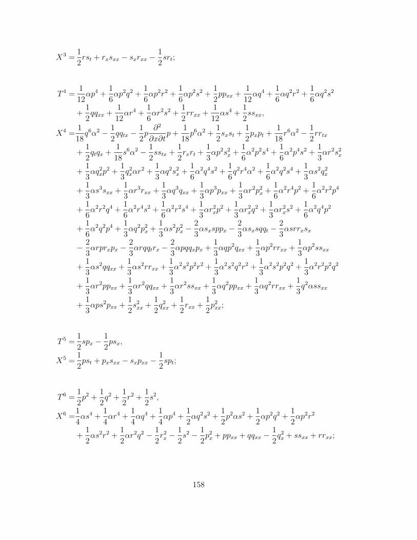
X3 =1
2rst + rxsxx − sxrxx −
1
2srt;
T 4 =1
12αp4 +
1
6αp2q2 +
1
6αp2r2 +
1
6αp2s2 +
1
2ppxx +
1
12αq4 +
1
6αq2r2 +
1
6αq2s2
+1
2qqxx +
1
12αr4 +
1
6αr2s2 +
1
2rrxx +
1
12αs4 +
1
2ssxx,
X4 =1
18q6α2 − 1
2qqtx −
1
2p∂2
∂x∂tp+
1
18p6α2 +
1
2sxst +
1
2pxpt +
1
18r6α2 − 1
2rrtx
+1
2qtqx +
1
18s6α2 − 1
2sstx +
1
2rxrt +
1
3αp2s2
x +1
6α2p2s4 +
1
6α2p4s2 +
1
3αr2s2
x
+1
3αq2
xp2 +
1
3q2xαr
2 +1
3αq2s2
x +1
6α2q4s2 +
1
6q2r4α2 +
1
6α2q2s4 +
1
3αs2q2
x
+1
3αs3sxx +
1
3αr3rxx +
1
3αq3qxx +
1
3αp3pxx +
1
3αr2p2
x +1
6α2r4p2 +
1
6α2r2p4
+1
6α2r2q4 +
1
6α2r4s2 +
1
6α2r2s4 +
1
3αr2
xp2 +
1
3αr2
xq2 +
1
3αr2
xs2 +
1
6α2q4p2
+1
6α2q2p4 +
1
3αq2p2
x +1
3αs2p2
x −2
3αsxsppx −
2
3αsxsqqt −
2
3αsrrxsx
− 2
3αrprxpx −
2
3αrqqtrx −
2
3αpqqxpx +
1
3αqp2qxx +
1
3αp2rrxx +
1
3αp2ssxx
+1
3αs2qqxx +
1
3αs2rrxx +
1
3α2s2p2r2 +
1
3α2s2q2r2 +
1
3α2s2p2q2 +
1
3α2r2p2q2
+1
3αr2ppxx +
1
3αr2qqxx +
1
3αr2ssxx +
1
3αq2ppxx +
1
3αq2rrxx +
1
3q2αssxx
+1
3αps2pxx +
1
2s2xx +
1
2q2xx +
1
2rxx +
1
2p2xx;
T 5 =1
2spx −
1
2psx,
X5 =1
2pst + pxsxx − sxpxx −
1
2spt;
T 6 =1
2p2 +
1
2q2 +
1
2r2 +
1
2s2,
X6 =1
4αs4 +
1
4αr4 +
1
4αq4 +
1
4αp4 +
1
2αq2s2 +
1
2p2αs2 +
1
2αp2q2 +
1
2αp2r2
+1
2αs2r2 +
1
2αr2q2 − 1
2r2x −
1
2s2 − 1
2p2x + ppxx + qqxx −
1
2q2x + ssxx + rrxx;
158

T 7 =1
2qrt −
1
2qrx,
X7 =1
2qrt + qxrxx − rxqxx −
1
2rqt;
T 8 =1
2rpx −
1
2prx,
X8 =1
2prt + pxrxx − rxpxx −
1
2rpt;
T 9 =1
2qpx −
1
2pqx,
X9 =1
2pqt + pxqxx − qxpxx −
1
2qpt.
A casual glance at these results reveals that the conserved quantities are local and
low-order. They are also non-trivial first integrals of system (8.3). The multiplier
approach via the first homotopy integral formula proves to be a reliable method
for determining local conservation laws of a system of differential equations. Sys-
tem (8.3) does not possess a variational principle. This is where the classical
Noether’s approach falters as the conservation laws for this system cannot be re-
trieved. However, with the multiplier method, we could obtain local non-trivial
conserved vectors with relative ease.
8.5 Concluding remarks
In this work, we studied the (1+1)-dimensional generalised coupled mKdV sys-
tem (8.3) of four equations, which was derived from the extended complex cou-
pled cmKdV system (8.2), using the transformations u(t, x) = p(t, x) + iq(t, x),
v(t, x) = r(t, x) + is(t, x). We obtained a nine-dimensional Lie algebra for sys-
tem (8.3). A one-parameter group of transformations for the solutions of (8.3)
159

were determined. These were the most general solutions of system (8.3). Using
infinitesimal vector fields X1, X2 and X3 we obtained group invariant solutions.
With the aid of the main copolar trio elliptic functions along with simplest equation
method, we obtained elliptic cosine and sine solutions as well as delta amplitude
function solutions. Also, we gave parameter conditions suitable for degeneration
of the elliptic functions into trigonometric, hyperbolic and constant solutions. As
evidenced in the graphical depictions, solutions of system (8.3) obtained here are
periodic, bell-shaped bright and dark solitons, topological kink and anti-kink soli-
tons. Furthermore, by using the multiplier method coupled with the first homotopy
integral formula, we computed nine local and low-order conserved quantities. The
multiplier approach coupled with the first homotopy integral formula is one of the
most effective, efficient and reliable methods for determining conserved quantities.
160

Chapter 9
Conservation laws and symmetry
reductions for a generalized
hyperelastic-rod wave equation
9.1 Introduction
The generalized hyperelastic-rod wave (gHRW) equation
E ≡ ut − uxxt +1
2g(u)x − α(2uxuxx + uuxxx) = 0, g(u)′ 6= 0, (9.1)
was seen for the first time in [124], where the authors proved the existence of a
strongly continuous semigroup of global weak solutions for t > 0 and x ∈ <. This
equation describes dispersive waves propagating in hyperelastic-rods. By using the
transformation g(u) = 2κu+3u2, equation (9.1) becomes the well known Camassa-
Holm equation [125]
ut + 2κux − uxxt + 3uux − 2uxuxx − uuxxx = 0. (9.2)
161

For κ > 0, equation (9.2) represents the one directional motion of shallow waves.
The time and spatial dimensions are represented by t and x, while the wave velocity
is given by u(t, x). For the case g(u) = 3u2 we obtain the equation
ut − uxxt + 3uux − 2uxuxx − uuxxx = 0, (9.3)
which made its debut appearance in [126], where the authors found its unbounded
travelling wave solutions. It is in the work of Dai [126] that we find the name
hyperelastic-rod wave equation. Equation (9.3) can be obtained from the Camassa-
Holm equation by taking κ = 0. While the hyperelastic-rod equation appears to
be a variation of the Camassa-Holm equation (9.2), its physical significance is
different because it was derived independently of equation (9.2) by Dai, see for
example [126,127].
The gHRW equation (9.1) along with other nonlinear dispersive equations made
another appearance in [128] where their geometric integrators were presented. In
this present work we seek to explore the gHRW equation further. We derive the low-
order conservation laws of the gHRW equation. We will make use of conservation
laws to obtain a multi-reduction of the gHRW equation to a first-order ordinary
differential equation (ODE), without having to do successive single reductions.
Furthermore, we study several plausible cases of the arbitrary function g(u) with
the aim of utilising Lie group analysis to obtain symmetry reductions to first or
second-order ODEs and where possible, to obtain exact solutions.
The work presented in this chapter has been submitted for possible publication
[129].
162
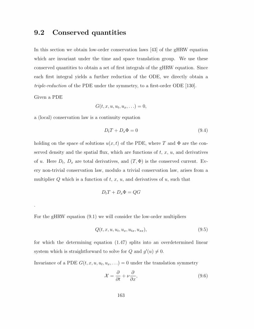
9.2 Conserved quantities
In this section we obtain low-order conservation laws [43] of the gHRW equation
which are invariant under the time and space translation group. We use these
conserved quantities to obtain a set of first integrals of the gHRW equation. Since
each first integral yields a further reduction of the ODE, we directly obtain a
triple-reduction of the PDE under the symmetry, to a first-order ODE [130].
Given a PDE
G(t, x, u, ut, ux, . . .) = 0,
a (local) conservation law is a continuity equation
DtT +DxΦ = 0 (9.4)
holding on the space of solutions u(x, t) of the PDE, where T and Φ are the con-
served density and the spatial flux, which are functions of t, x, u, and derivatives
of u. Here Dt, Dx are total derivatives, and (T,Φ) is the conserved current. Ev-
ery non-trivial conservation law, modulo a trivial conservation law, arises from a
multiplier Q which is a function of t, x, u, and derivatives of u, such that
DtT +DxΦ = QG
.
For the gHRW equation (9.1) we will consider the low-order multipliers
Q(t, x, u, ut, ux, utx, uxx), (9.5)
for which the determining equation (1.47) splits into an overdetermined linear
system which is straightforward to solve for Q and g′(u) 6= 0.
Invariance of a PDE G(t, x, u, ut, ux, . . .) = 0 under the translation symmetry
X =∂
∂t+ ν
∂
∂x, (9.6)
163

gives rise to travelling wave solutions, with u = U and ξ = x − νt being the
invariants.
Proposition 9.1 All low-order multipliers (9.5) admitted by the gHRW equation
(9.1) with g′(u) 6= 0, give rise to conservation laws which are invariant under the
translation group and they are given by
(i) g(u) arbitrary:
Q1a = 1, (9.7)
Q1b = u, (9.8)
Q1c =1
2α(α(2uuxx + u2
x) + 2utx − g(u)). (9.9)
(ii) g(u) = 3αu2 + au+ b:
Q2 = − 1
2α√
4α(uxx − u)− a. (9.10)
These multipliers yield non-trivial conservation laws of low-order, summarized as
follows.
Theorem 9.1 (i) The conservation laws admitted by the gRHW equation (9.1) for
g′(u) 6= 0 are given by:
Case 1a: g(u) arbitrary
T1a =u,
X1a =− αuuxx − utx −1
2αu2
x +1
2g(u).
(9.11)
Case 1b: g(u) arbitrary
T1b =1
2u2x +
1
2u2,
X1b =− αu2uxx − uutx +1
2
∫ug(u)du.
(9.12)
164

Case 1c: g(u) arbitrary
T1c =− 1
2uu2
x −1
2α
∫gdu,
X1c =1
2αu2t + uutux −
1
2αu2u2
xx
+1
2uxx(ug(u)− αu2
x − 2utx)−1
8α(g(u)2 − αu2
x − 2utx).
(9.13)
Case 2: g(u) = 3αu2 + c1u+ a
T2 =1
4α2
√4αuxx − 4αu− a,
X2 =1
4α2
√4αuxx − 4αu− au.
(9.14)
Substituting the group invariant
u(t, x) = U(x− νt) (9.15)
into equation (9.1), with g(u) = up yields the nonlinear third-order ODE
2(αU − ν)U ′′′ − (pUp−1 − 4αU ′′ − 2ν)U ′ = 0. (9.16)
First integrals of the travelling wave ODE (9.16) can be found by symmetry reduc-
tions of all conservation laws that are invariant under the travelling wave symmetry
(9.6) of the PDE. The reduction can be understood through considering the action
of (9.6) on a conservation law expressed in terms of the canonical variables.
On travelling wave solutions u = U(ξ), a symmetry-invariant conservation law
DtT + Dxφ = 0 reduces to the form Dξ(φ − νT ) = 0. This yields a first integral
ψ = φ− νT = C(const.) of the travelling wave ODE [130].
By using the conservation laws (9.11), (9.12), (9.13) we get three first integrals,
that is,
Ψ1 = (αU − ν)U ′′ + νU + 1/2(αU ′2 − Up) = C1, (9.17)
165

Ψ2 = (αU2 − νU)U ′′ +ν
2(U ′2 + U2)− p
2(p+ 1)Up+1 = C2, (9.18)
Ψ3 =
(α
2U2 − νU +
ν2
2a
)U ′′2 +
(1
2(αU − ν)U ′2 − 1
2α(νUp − αUp+1)
)U ′′
+α
8U ′4 +
(ν
2U − 1
4α(αUp + 2ν2)
)U ′2 (9.19)
− 1
8α(p+ 1)(4νUp+1 − (p+ 1)U2p) = C3.
By combining the two first integrals (9.17) and (9.18) we obtain a triple reduction
to a first-order autonomous equation
U ′2 +1
(p+ 1)(αU − ν)(Up+1−ν(p+1)U2 +2(p+1)C1U −2(p+1))C2 = 0. (9.20)
The third first integral is not functionally independent. The remaining conservation
laws are also invariant under the translation group yielding first integrals.
9.3 Exact solutions
In this section we perform a symmetry classification of equation (9.1). An infinites-
imal vector field is given by
X = ξ1(t, x, u)∂
∂t+ ξ2(t, x, u)
∂
∂x+ η(t, x, u)
∂
∂u, (9.21)
for some generator coefficient functions ξ1, ξ2 and η to be determined. The invari-
ance condition
pr(3)X(∆)|∆=0 = 0 (9.22)
yields the determining equation for the generator coefficients. Here, pr(3)X is a
third order extension of generator (9.21). Taking into consideration determining
condition (9.22) we now consider different cases for the coefficient function g(u).
166

9.3.1 Quadratic function case
In this subsection we consider the case
g(u) = 3αu2 + au+ b (9.23)
where a and b are free constants. Thus equation (9.1) is now
ut − uxxt + 3αuux +1
2aux − α(2uxuxx + uuxxx) = 0 (9.24)
and admits the following 3-dimensional Lie algebra:
X1 =∂
∂t, X2 =
∂
∂x, X3 = 4αt
∂
∂t− aαt ∂
∂x− (a+ 4αu)
∂
∂u. (9.25)
(i) Travelling wave reduction
The linear combination X1+νX2 gives the group invariant u(t, x) = φ(ξ) with
ξ = x−νt which transforms nonlinear partial differential equation (NLPDE)
(9.24) into the nonlinear ordinary differential equation (NLODE)
νφ′′′ − αφφ′′′ − 2αφ′φ′′ + 3αφφ′ +1
2(a− ν)φ′ = 0. (9.26)
Integrating equation (9.26) once with respect to ξ gives
νφ′′ − αφφ′′ + 3
2αφ2 − 1
2αφ′2 +
1
2aφ− aφ′2 − νφ+ C1 = 0 (9.27)
with integration constant C1. Equation (9.27) admits the Lie point symmetry
X = ∂/∂ξ with first-order invariants z = φ(ξ) and ψ(z) = φ′ which reduce
NLODE (9.27) into the first-order Bernoulli differential equation (DE)
dψ
dz+
α
2(αz − ν)ψ =
3αz2 − (2ν − a)z + 2C1
2(αz − ν)ψ−1, (9.28)
Letting w(z) = ψ2 we have a first-order linear differential equation given by
w′ +α
αz − ν=
3αz2 + az − 2νz + 2C1
αz − ν. (9.29)
167

Equation (9.29) has solution
w (z) =2αz3 + z2a− 2νz2 + 4C1z + 2C2
2(α z − ν), (9.30)
where C2 is a constant of integration. Reverting to original variables we have
u(t, x) = φ = ±√
2
2
∫ √2αφ3 + (a− 2ν)φ2 + 4C1φ+ 2C2
αφ− νdξ + C3, (9.31)
where C3 is an integration constant.
(ii) Symmetry reduction using vector field X3
From infinitesimal generator X3 in (9.25) we have the group invariant solution
u (t, x) =4αφ(ξ)− at
4αtwith ξ =
1
4at+ x,
such that equation (9.24) is transformed into the NLODE
αφφ′′′ + 2αφ′φ′′ − φ′′ − 3αφφ′ + φ = 0. (9.32)
Equation (9.32) has the symmetry X = ∂/∂ξ with differential invariants
z = φ(ξ) and f(z) = φ′. Using these invariants, equation (9.32) is reduced
to the second-order NLODE
α zf 2f ′′ + α zff ′2 + 2αf 2f ′ − 3αzf − ff ′ + z = 0. (9.33)
We have thus obtained a reduced form of equation (9.24).
(iii) Special case g(u) = 3αu2
By taking a = b = 0 in (9.23), equation (9.24) becomes
ut − uxxt + 3αuux − α(2uxuxx + uuxxx) = 0. (9.34)
Equation (9.34) admits the Lie algebra
X1 =∂
∂t, X2 =
∂
∂x, X3 = t
∂
∂t− u ∂
∂u. (9.35)
168

Travelling wave reduction and solutions
As before, a linear combination of Lie point symmetriesX1 andX2 transforms
equation (9.35) into the NLODE
νφ′′′ − αφφ′′′ − 2αφ′φ′′ + 3αφφ′ − νφ′ = 0. (9.36)
Integrating (9.36) with respect to ξ gives the second order ODE
νφ′′ − αφφ′′ + 3
2αφ2 − 1
2αφ′2 − νφ+ C1 = 0, (9.37)
where C1 is an integration constant. Equation (9.37) can be reduced to the
first-order DE
dψ
dz+
α
2(αz − ν)ψ =
3αz2 − 2νz + 2C1
2(αz − ν)ψ−1, (9.38)
by using generator X = ∂/∂ξ. Solving (9.38) and reverting to original vari-
ables gives
φ′2 =αφ3 − ν φ2 + 2C1φ+ C2
αφ− ν. (9.39)
Thus for arbitrary α and ν the integral equation
u(t, x) = φ(ξ) = ±
∫ √φ2 +
2C1φ+ C2
αφ− νdξ + C3. (9.40)
is understood. For the special instance α = 2C1 and ν = −C2 we have the
solutions
u(t, x) = ± sinh(C4 + ξ) (9.41)
with the following profile:
169

Figure 9.1: Depiction of solution (9.41) with parameter values C4 = −0.05, ν =
0.08.
.
Alternatively, taking the constants of integration C1 = C2 = 0 we have the
solution
u(t, x) = C5e±ξ, (9.42)
Symmetry reduction using generator X3
Using the usual Lie theory, vector field X3 yields the group invariant solution
u(t, x) = φ(ξ)/t, ξ = x. Accordingly, equation (9.34) is transformed into the
NLODE
αφφ′′′ + 2αφ′φ′′ − φ′′ − 3αφφ′ + φ = 0, (9.43)
which is identical to (9.32) and thus the reduced equation (9.33) follows.
9.3.2 Power law nonlinearity case
For the case g(u) = up, we have NLPDE
ut − uxxt +1
2pup−1ux − α(2uxuxx + uuxxx) = 0, (9.44)
170

which admits time and space translation symmetries X1 = ∂/∂t and X2 = ∂/∂x
respectively. Hence (9.44) becomes
νφ′′′ − αφφ′′′ + 1
2pφp−1φ′ − 2αφ′φ′′ − νφ′ = 0. (9.45)
Integrating (9.45) once with respect to ξ we get NLODE
νφ′′ − αφφ′′ − 1
2αφ′2 +
1
2φp − νφ+ C1 = 0, (9.46)
which admits the Lie point symmetry X = ∂/∂ξ with differential invariants ψ(z) =
φ′(ξ) and z = φ(ξ). Using these invariants, the differential order of equation (9.46)
is reduced by one to give the first-order DE
dψ
dz+
α
2(αz − ν)ψ =
zp − 2νz + 2C1
2(αz − ν)ψ−1. (9.47)
Solving (9.47) and reintroducing the native variables we have
φ′2 − φp+1 − (p+ 1)(νφ2 − 2C1φ− C2)
(αφ− ν)(p+ 1)= 0
with constant of integration C2. Thus we have managed to perform a double
symmetry reduction of equation (9.44). Interesting to note is the convergence of
two different approaches for reduction of order of differential equations, that is, the
reduced equation (9.20) obtained by making use of conservation laws is similar to
the equation obtained via symmetry reduction.
9.3.3 Exponential function case.
Suppose g(u) = AeBu, then equation (9.1) becomes
ut − uxxt +1
2ABuxe
Bu − α(2uxuxx + uuxxx) = 0 (9.48)
with free constants A and B. Equation (9.48) only admits translation symmetries,
that is, X1 = ∂/∂t and X1 = ∂/∂x. Thus symmetry reduction via the travelling
171

wave variable is appropriate as in the previous sections. This gives the third-order
NLODE
νφ′′′ − αφφ′′′ + 1
2ABφ′eBφ − 2αφ′φ′′ − νφ′ = 0. (9.49)
The second-order DE
νφ′′ − αφφ′′ + 1
2AeBφ − 1
2αφ′2 − νφ+ C1 = 0, (9.50)
is a first integral of (9.49) with respect to ξ. As in previous sections, equation (9.50)
can be written in terms of the differential invariants z = φ(ξ) and ψ(z) = φ′(ξ) to
getdψ
dz+
α
2(αz − ν)ψ =
AeBz − 2νz + 2C1
2(αz − ν)ψ. (9.51)
Making the substitution w(z) = ψ2, equation (9.51) is transformed into
w′ +α
α z − νw =
AeBz − 2 ν z + 2C1
α z − ν(9.52)
which is a linear DE with integrating factor
µ(z) =exp
(∫α
α z − νdz
)=αz − ν.
Multiplying (9.52) with µ(z) and integrating the resultant variables separable DE
we finally have
u(t, x) = φ(ξ) =± 1
B
∫ A (Bαφ− (Bν + α)) eBφ −B2
(2/3ναφ3 −
(C1α + ν2
)φ2
+2νC1φ− C2)1/2 dξ + C3
where C3 is a constant of integration.
9.3.4 Logarithmic function case.
Finally, for the case g(u) = ln(u), we have
ut − uxxt +1
2u−1ux − α(2uxuxx + uuxxx) = 0, (9.53)
172

and following the method of the previous section we finally have
u(t, x) = φ(ξ) =± 1
6
∫ 18(α− 2ν)φ lnφ− 24ανφ3 − 9(α− 4C1α− 4ν2)φ2
+36ν(1− 2C1)φ+ 36C21/2 dξ + C3
9.4 Concluding remarks
In this paper we reduced the third-order gHRW equation into a first-order au-
tonomous ODE. By making use of the time and space translation group, conser-
vation laws were reduced into first integrals, which in turn led to the reduced form
of the gHRW equation . We went further to perform several symmetry reductions
of the gHRW equation for different cases of the arbitrary function g(u). For the
case g(u) = up, we applied the travelling wave variable directly onto our equation
(9.1) and managed to recover the reduced form of the gHRW equation obtained
via triple reduction using conservation laws. Lie point symmetries are an efficient
way of transforming a NLPDE into an ODE of a lower-order. For special values of
the free constants we managed to obtain hyperbolic sine and exponential solutions
for the instance g(u) = 3αu2.
173

Chapter 10
Lie symmetry analysis and
conserved quantities of a (1+1)-
dimensional fifth-order integrable
equation
10.1 Introduction
In this chapter, we study a newly formulated integrable fifth-order equation
E ≡ uttt − autxxxx − butxx − c(2utxuxx + utuxxx + uxutxx)− d(utxuxx + uxutxx) = 0,
(10.1)
where a, b, c, d are nonzero constants. Equation (10.1) can be used as a model for
bidirectional water waves propagating in a shallow medium. This is a new equation
first seen in [131] where its integrability was demonstrated by using a singularity
manifold analysis. Several methods, including the simplified Hirota approach and
a form of Riccati expansion method, are used to obtain various types of solutions
174

of equation (10.1). Some solutions obtained include multiple solitons, kink and
periodic waves. By taking a = 1, b = 0, c = d = 4, equation (10.1) becomes the
fifth-order integrable equation
F ≡ βuxxx − 4utuxxx − 12uxxutx − 8uxutxx − utxxxx + uttt = 0, β 6= 0, (10.2)
which has been studied extensively in [112,115].
In our work we seek to use the classical Lie Group approach to derive analytic
solutions of equation (10.1). We begin by deriving elements of a one dimensional
optimal system of subalgebras and obtain the corresponding similarity reductions.
As such, the group invariant solutions take rational, hyperbolic, Jacobian elliptic
and elliptic integral of the second kind forms. Furthermore, power series solutions
are obtained for the highly nonlinear transformed equation in one of the cases.
One and two wave solutions are also obtained via a multiple exponential function
method. Finally, five low-order conserved quantities are obtained via the multiplier
approach.
The work presented in this chapter has been submitted for possible publication
[132].
10.2 Lie group analysis
We shall now perform Lie group analysis on the underlying equation (10.1).
10.2.1 Classical symmetries
The one-parameter group of transformations
t→ t+ aξ1(t, x, u), x→ x+ aξ2(t, x, u), u→ u+ aη(t, x, u)
175
with a small parameter a, correspond to vector field
X = ξ1(t, x, u)∂
∂t+ ξ2(t, x, u)
∂
∂x+ η(t, x, u)
∂
∂u. (10.3)
The vector field (10.3) in conjunction with (10.1) conforms to condition
pr(5)X(uttt−autxxxx−butxx−c(2utxuxx+utuxxx+uxutxx)−d(utxuxx+uxutxx))|E=0 = 0.
(10.4)
Here, pr(5)X is a fifth-order extension of (10.3), see for example [30] and the refer-
ences therein. Following the usual Lie theory and using Maple it is easy to see that
equation (10.1) has a four-dimensional Lie algebra L4, spanned by the generators
X1 =∂
∂t, X2 =
∂
∂x, X3 = 2t
∂
∂t+ x
∂
∂x−(
2bx
c+ d+ u
)∂
∂u, X4 =
∂
∂u. (10.5)
10.2.2 Optimal system of one dimensional subalgebras
The optimal system of one-dimensional subalgebras for the Lie algebra (10.5) can
be obtained by using the commutation relations and the adjoint representations
given in Tables 10.1 and 10.2, respectively [30,78,133].
Table 10.1. Commutation relations of 4-dimensional Lie algebra (10.5)
[Xi, Xj ] X1 X2 X3 X4
X1 0 0 2X1 0
X2 0 0 X2 − 2bc+dX4 0
X3 −2X1 −X2 + 2bc+dX4 0 X4
X4 0 0 −X4 0
Table 10.2. Adjoint table of Lie algebra (10.5)
176

Ad X1 X2 X3 X4
X1 X1 X2 −2εX1 +X3 X4
X2 X1 X2 −εX2 +X3 + 2bc+dεX4 X4
X3 e2εX1 eεX2 − bc+de
−ε(−1 + e2ε) X3 e−εX4
X4 X1 X2 X3 + εX4 X4
Using Table 10.2 and following the method detailed in, for example [30, 78, 133],
we obtain the following set of elements of the optimal system:
X2, X3, X1 +X2, X1 +X4 . (10.6)
10.3 Group Invariant solutions
Using results of the previous section we will now proceed to construct an optimal
system of group invariant solutions through symmetry reductions [30,133].
10.3.1 Case X1 + kX2
In this section we seek to obtain group invariant solutions corresponding to the
travelling wave variable. The linear combination X1 + kX2, with k a constant,
gives the invariant solution u = U(ξ), ξ = x− kt leading to the nonlinear ordinary
differential equation (NLODE)
aU ′′′′′ + (b− k2)U ′′′ + (2c+ d)U ′U ′′′ + (2c+ d)U ′′2 = 0. (10.7)
Integrating (10.7) twice with respect to ξ we obtain the third-order NLODE
aU ′′′ +1
2(2c+ d)U ′2 + (b− k2)U ′ + C1ξ + C2 = 0 (10.8)
for some arbitrary constants of integration C1 and C2.
177

10.3.1.1 Elliptic integral solutions
Suppose we take C1 = 0 and let
U ′ =6a
2c+ dV (ξ),
then from equation (10.8) we have
V ′′ + 3V 2 − ωV + C3 = 0. (10.9)
Here, ω = 6(k2 − b)/(2c + d) and C3 = C2(2c + d)/6. The solution of NLODE
(10.7) is thus given by
U(ξ) =6a
2c+ d
∫V (ξ)dξ. (10.10)
Many NLPDEs can be reduced to equation (10.9), see for example [20, 93]. Mul-
tiplying equation (10.9) by V ′ and integrating with respect to ξ we have the first-
order ODE
V ′2 + 2V 3 − ωV 2 + 2C3V + 2C4 = 0, (10.11)
which we can write as
V ′2 = −2(V − α1)(V − α2)(V − α3). (10.12)
Here α1, α2 and α3 are some roots of the equation V 3 − ωV 2/2 + C3V + C4 = 0,
with α1 > α2 > α3. According to [95] and taking into account equation (10.10), we
have the elliptic solution
u(t, x) =6a
(α1 − α3)2 E (sn (∆ξ,M2) ,M2)−∆ ((α2 − 2α3)α1 + α32) ξ
∆ (2c+ d) (α1 − α2)
(10.13)
with
M2 =α1 − α2
α1 − α3
, ∆ =
√α1 − α3
2.
Here, E is the incomplete elliptic integral of the second kind, which is given by
E(z, k) =
∫ z
0
√1− k2t2
1− t2dt,
178
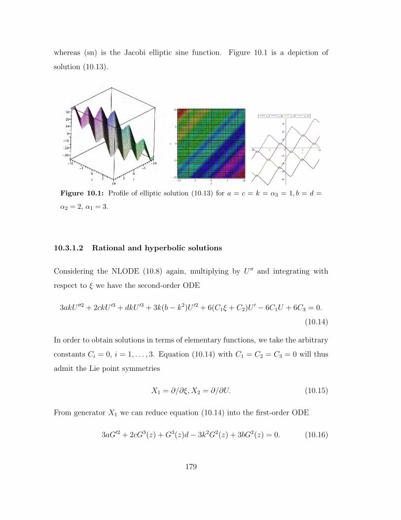
whereas (sn) is the Jacobi elliptic sine function. Figure 10.1 is a depiction of
solution (10.13).
Figure 10.1: Profile of elliptic solution (10.13) for a = c = k = α3 = 1, b = d =
α2 = 2, α1 = 3.
10.3.1.2 Rational and hyperbolic solutions
Considering the NLODE (10.8) again, multiplying by U ′′ and integrating with
respect to ξ we have the second-order ODE
3akU ′′2 + 2ckU ′3 + dkU ′3 + 3k(b− k2)U ′2 + 6(C1ξ + C2)U ′ − 6C1U + 6C3 = 0.
(10.14)
In order to obtain solutions in terms of elementary functions, we take the arbitrary
constants Ci = 0, i = 1, . . . , 3. Equation (10.14) with C1 = C2 = C3 = 0 will thus
admit the Lie point symmetries
X1 = ∂/∂ξ,X2 = ∂/∂U. (10.15)
From generator X1 we can reduce equation (10.14) into the first-order ODE
3aG′2 + 2cG3(z) +G3(z)d− 3k2G2(z) + 3bG2(z) = 0. (10.16)
179

The reader should note the use of appropriate invariants z = ξ and G(z) = U ′ cul-
minating in (10.16). Solving (10.16) with the aid of Maple and reverting to native
variables we have the following rational and hyperbolic solutions respectively:
u(t, x) = C4 +3 (k2 − b)
2 c+ d(x− kt) (10.17)
u(t, x) = C5 +6a (k2 − b)
(2 c+ d)√a (k2 − b)
tanh
[√a (k2 − b) (x− kt− C4)
2a
], (10.18)
where C4 and C5 are integration constants. Profile of solution (10.18) is given in
Figure 10.2.
180

Figure 10.2: Profile of singular soliton solution (10.18) for a = b = c = C5 = 1, d =
5, k = 0.5, C4 =3.
Likewise, using symmetry generator X2, equation (10.14) is reduced to the first-
order ODE
3aG′ + (2c+ d)G(z) + 3(b− k2) = 0. (10.19)
From (10.19) we recover the rational solution (10.17) as is, and the hyperbolic
solution
u(t, x) =6√a(k2 − b)2 c+ d
tanh
[√a (k2 − b) (C7 + x− kt)
2a
]+ C6 (10.20)
181

with integration constants C6 and C7. Taking the same parameter values as in
Figure 10.2, the one soliton profile of solution (10.20) is given in Figure 10.3.
Figure 10.3: Profile of singular soliton solution (10.20) for a = b = c = C5 = 1, d =
5, k = 0.5, C4 = 3.
182

10.3.2 Case X2
Using optimal system element X2 we have the invariant u = U(t), which in turn
gives us the ODE U ′′′ = 0 and thus we obtain
u(t, x) =1
2C1t
2 + C2t+ C3
as a solution of (10.1), where C1, C2 and C3 are arbitrary constants.
10.3.3 Case X1 +X4
The optimal system element X1 +X4 provides the invariant solution u = t+U(x)
that leads us to the solution
u(t, x) =1
2C1x
2 + C2x+ C3
of (10.1). Here C1, C2 and C3 are arbitrary constants.
10.3.4 Case X3
The group invariant solution corresponding to vector X3 is u(t, x) = 1/t1/2U(ξ)−
b/(c + d)x, where ξ = x/t1/2. Accordingly, the NLPDE (10.1) is transformed into
the fifth-order highly nonlinear ODE
4aξU (5) + 20aU (4) + 4ξ(2c+ d)U ′U ′′′ + 4cUU ′′′ − ξ3U ′′′ − 12ξ2U ′′
+ 4(7c+ 5d)U ′U ′′ + 4ξ(d+ 2c)U ′′2 − 33ξU ′ − 15U = 0.(10.21)
Equation (10.21) can be integrated once with respect to ξ, giving
4aU (4) + 16aU ′′′ + 4cUU ′′ − ξ3U ′′ + 4ξ(d+ 2c)U ′U ′′ − 9ξ2U ′ + 8(d+ c)U ′2
− 15ξU + C1 = 0,
(10.22)
183

where C1 is a constant of integration. We will use the power series solution method
[25,27,77] to solve equation (10.22). If we let
U(ξ) =∞∑z=0
gzξz, (10.23)
where gz, z = 0, 1, . . . , are constants to be determined, then the various derivatives
of (10.22) are
U ′(ξ) =∞∑z=0
(z + 1)gz+1ξz,
U ′′(ξ) =∞∑z=0
(z + 1)(z + 2)gz+2ξz,
U ′′′(ξ) =∞∑z=0
(z + 1)(z + 2)(z + 3)gz+3ξz,
U (4)(ξ) =∞∑z=0
(z + 1)(z + 2)(z + 3)(z + 4)gz+4ξz.
(10.24)
By taking into account the derivatives (10.24), equation (10.22) is transformed into
96ag4 + 480ag5ξ + 1440ag6ξ2 + 4a
∞∑z=3
(z + 1)(z + 2)(z + 3)(z + 4)gz+4ξz
96ag3 + 384ag4ξ + 960ag5ξ2 + 16a
∞∑z=3
(z + 1)(z + 2)(z + 3)gz+3ξz
8cg0g2 + 24cg0g3ξ + 48cg0g4ξ2 + 4c
∞∑z=3
z∑j=0
(z + 1− j)(z + 2− j)gjgz+2−jξz
−∞∑z=3
(z − 2)(z − 1)gz−1ξz + 4(d+ 2c)
(2g1g2ξ + 6g1g3ξ
2)
+ 4(d+ 2c) (10.25)
×∞∑z=3
z−1∑j=0
(j + 1)(z − j)(z + 1− j)gj+1gz+1−jξz − 9
(g1 + g2ξ + g3ξ
2)
− 9∞∑z=3
(z + 1)gz+1ξz + 8(d+ c)g2
1ξ2 + 8(d+ c)
∞∑z=3
z−2∑j=0
(j + 1)(z − 1− j)
× gj+1gz−1−jξz − 15g1ξ − 15g2ξ
2 − 15∞∑z=3
gzξz + C1 = 0.
184

For more details, see [25, 77] and the references therein. Now splitting equation
(10.25) with respect to powers of ξ, we have
ξ0 : 8 cg0 g2 + 96 ag3 + 96 ag4 + C1 − 9 g1 = 0, (10.26)
ξ1 : 24 cg0 g3 + 16 cg1 g2 + 8 dg1 g2 + 384 ag4 + 480 ag5 − 15 g1 − 9 g2 = 0,
(10.27)
ξ2 : 48 cg0 g4 + 8 cg12 + 48 cg1 g3 + 8 dg1
2 + 24 dg1 g3 + 960 ag5 + 1440 ag6
− 15 g2 − 9 g3 = 0, (10.28)
and generally for z ≥ 3 we have the recurrence relation
gz+4 =− 1
4a(z + 1)(z + 2)(z + 3)(z + 4)
4c
z∑j=0
(z + 1− j)(z + 2− j)gjgz+2−j
−(z − 2)(z − 1)gz−1 + 16a(z + 1)(z + 2)(z + 3)gz+3
+4(d+ 2c)z−1∑j=0
(j + 1)(z − j)(z + 1− j)gj+1gz+1−j − 9(z + 1)gz+1
+8(d+ c)z−2∑j=0
(j + 1)(z − 1− j)gj+1gz−1−j − 15gz
.
(10.29)
Taking gi, i = 0, . . . , 3 arbitrary, we can determine explicit values for g4, g5 and g6.
From equations (10.26)–(10.28), we have the following:
g4 =1
96a(9g1 − 8cg0g2 − 96ag3 − C1) ,
g5 =1
480a((−16c− 8d) g1 + 32cg0 + 9) g2 − 24cg0g3 + 384ag3 + 4C1 − 21g1 ,
g6 =1
2880a2
(−1536a2g3 +
((−16c− 16d) g1
2 + ((64g2 − 96g3) c+ 32dg2 (10.30)
−48dg3 + 84) g1 − 128g0 (g2 − 3/2g3) c− 16C1 − 6g2 + 18g3) a
+cg0 (8cg0g2 + C1 − 9g1)) .
185

Likewise, from (10.29) we can deduce exact values of successive terms gm, m =
7, 8, . . . . Thus, the power series solution of (10.1) can be written as
u(t, x) = g0 + g1ξ + g2ξ2 + g3ξ
3 +1
96a(9g1 − 8cg0g2 − 96ag3 − C1) ξ4
1
480a((−16c− 8d) g1 + 32cg0 + 9) g2 − 24cg0g3 + 384ag3 + 4C1 − 21g1 ξ5
+1
2880a2
(−1536a2g3 +
((−16c− 16d) g1
2 + ((64g2 − 96g3) c+ 32dg2
−48dg3 + 84) g1 − 128g0 (g2 − 3/2g3) c− 16C1 − 6g2 + 18g3) a
+cg0 (8cg0g2 + C1 − 9g1)) ξ6
− 1
4a
∞∑z=3
z!
(z + 4)!
4c
z∑j=0
(z + 1− j)(z + 2− j)gjgz+2−j
−(z − 2)(z − 1)gz−1 + 16a(z + 1)(z + 2)(z + 3)gz+3
+4(d+ 2c)z−1∑j=0
(j + 1)(z − j)(z + 1− j)gj+1gz+1−j − 9(z + 1)gz+1
+8(d+ c)z−2∑j=0
(j + 1)(z − 1− j)gj+1gz−1−j − 15gz
ξz+4.
10.4 One and two-wave solutions
In this section we seek multiple-wave solutions of equation (10.1) using the multiple
exponential function method [10].
10.4.1 One-soliton solutions
In order to obtain one-wave solutions we take p(θ1) = A0 + A1θ1 and g(θ1) =
B0 +B1θ1. Following the steps alluded to in Section 1.6.1, we obtain the following
two sets of dispersion relations:
186

(i) Case 1.
A1 =(12B0 ak1 + 2A0 c+ A0 d)B1
B0 (2 c+ d), ω1 =
√ak1
2 + bk1. (10.31)
(ii) Case 2.
A1 =A0B1
B0
, ω1 = ω1. (10.32)
In both cases A0, B0 and B1 are arbitrary constants. Thus, the one-wave solutions
corresponding to (10.31) and (10.32) are given by
u(t, x) =A0 + A1e
k1x−ω1t
B0 +B1ek1x−ω1t(10.33)
and the one-soliton profile of (10.32) is depicted in Figure 10.4.
187

Figure 10.4: Profile of kink soliton (10.20) for a = A0 = B1 = 1, c = B0 = 0.1,
k1 = 3 b = d = 0.5.
10.4.2 Two-soliton solutions
As outlined in Section 1.6.1, two-wave solutions are obtained by taking u = p/g,
where
p(θ1, θ2) = 2(k1θ1 + k2θ2 + A12(k1 + k2)θ1θ2), g(θ1, θ2) = (1 + θ1 + θ2 + A12θ1θ2)
188

and θi = ekix−ωit. Also, A12 is a constant to be determined. Consequently, we have
the following parameter relations:
(i) Case 1.
ω1 =
(ak1
3 + bk1 +√(
ak22 + b
) (ak1
2 + b)k2
)k1√
ak14 + ak2
4 + bk12 + bk2
2 + 2 k1 k2
√(ak2
2 + b) (ak1
2 + b) ,
ω2 = −
(ak2
3 + bk2 +√(
ak22 + b
) (ak1
2 + b)k1
)k2√
ak14 + ak2
4 + bk12 + bk2
2 + 2 k1 k2
√(ak2
2 + b) (ak1
2 + b) ,
(10.34)
A12 =ak1
4 + ak24 + bk1
2 + bk22 + 2
√k1
2k22(ak2
2 + b) (ak1
2 + b)
(k1 + k2)2 (ak12 + ak2
2 + b) ,
c = d = 2a.
(ii) Case 2.
ω1 =k1 k2
(k1
2 − 2 k22)√
a (k1 − 2 k2)(2 k2
3−k13 + k2
2k1
)(k1 − 2 k2)
(k1
3 − k1 k22 − 2 k2
3) ,
ω2 =k1 k2
(k1
2 − k1 k2 − k22)√
a (k1 − 2 k2)(2 k2
3−k13 + k2
2k1
)(k1 − 2 k2)
(k1
3 − k1 k22 − 2 k2
3) , (10.35)
A12 =2 k1 − 3 k2
k2
, b = −a(k1
6 − 2 k15k2 + 4 k2
6)
(k1 − 2 k2)(k1
3 − k1 k22 − 2 k2
3) , c = d = 2a.
(iii) Case 3.
ω1 = ω2 =√ak1
2 + bk1, A12 =(2a+ d)k1
2 + 2 b
2(ak12 + b)
,
c = 3a− 1
2d, k2 = −k1.
(10.36)
The profiles of solutions (10.34)–(10.36) are given in Figures 10.5–10.7.
189

Figure 10.5: Interaction of kink and anti-kink solitons. Solution (10.34) for a =
b = k1 = 1 and k2 = 2.
190
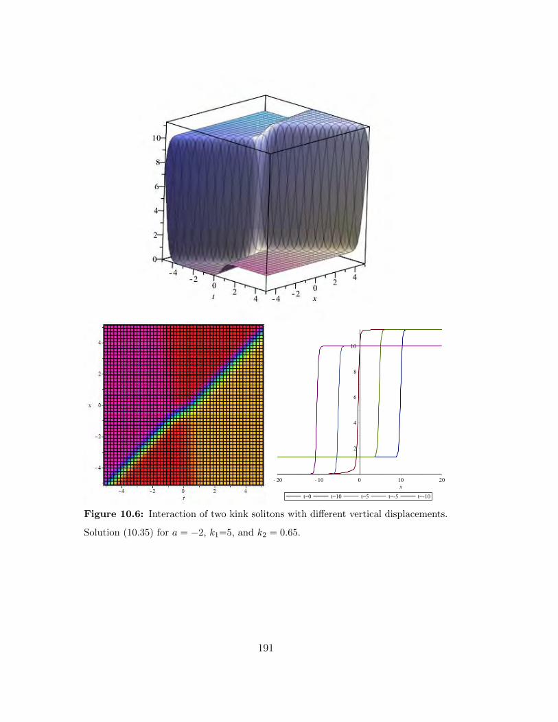
Figure 10.6: Interaction of two kink solitons with different vertical displacements.
Solution (10.35) for a = −2, k1=5, and k2 = 0.65.
191

Figure 10.7: Interaction of dark and bright solitons. Solution (10.36) for a = b =
d = k1 = 1.
192

10.5 Conservation laws of (10.1)
Using the multiplier approach [45, 77, 134], we determine local low-order conser-
vation laws of equation (10.1). This method is a modern form of the classical
Noether’s approach, see for example [43].
Multipliers (Λ) can be determined via the determining condition
δ
δu(ΛE) = 0 (10.37)
with E given by equation (10.1) and where δ/δu is the Euler operator as given
in [115]. Multiplier determining condition (10.37) gives the following six linear
PDEs:
Λuu = 0, Λxu = 0, Λxx = 0, Λtu = 0, Λtx = 0, Λttt = 0. (10.38)
The solution algorithm of (10.38) is analogous to that of obtaining Lie point sym-
metries. In this instance we obtain the zeroth-order multipliers Λ(t, x, u)
Λ = C1x+ C2u+1
2C3t
2 + C4t+ C5, (10.39)
where C1,. . . ,C5 are constants. For the case (10.1) and (10.39), formula (1.48)
takes the form
193

T =
∫ 1
0
u
((∂EΛ
∂ut
) ∣∣∣u=u(λ) −Dx
(∂EΛ
∂utx
) ∣∣∣u=u(λ) +D2t
(∂EΛ
∂uttt
) ∣∣∣u=u(λ)
+D2x
(∂EΛ
∂utxx
) ∣∣∣u=u(λ) +D4x
(∂EΛ
∂utxxxx
) ∣∣∣u=u(λ)
)+ ut
(−Dt
(∂EΛ
∂uttt
) ∣∣∣u=u(λ)
)+utt
(∂EΛ
∂uttt
) ∣∣∣u=u(λ)
dλ,
X =
∫ 1
0
u
((∂EΛ
∂ux
) ∣∣∣u=u(λ) −Dx
(∂EΛ
∂uxx
) ∣∣∣u=u(λ) +D2x
(∂EΛ
∂uxxx
) ∣∣∣u=u(λ)
)+ut
((∂EΛ
∂utx
) ∣∣∣u=u(λ) −Dx
(∂EΛ
∂utxx
) ∣∣∣u=u(λ) −D3x
(∂EΛ
∂utxxxx
) ∣∣∣u=u(λ)
)+ux
((∂EΛ
∂uxx
) ∣∣∣u=u(λ) −Dx
(∂EΛ
∂uxxx
) ∣∣∣u=u(λ)
)+ utx
((∂EΛ
∂utxx
) ∣∣∣u=u(λ)
+D2x
(∂EΛ
∂utxxxx
) ∣∣∣u=u(λ)
)+ uxx
((∂EΛ
∂uxxx
) ∣∣∣u=u(λ)
)+utxx
(−Dx
(∂EΛ
∂utxxxx
) ∣∣∣u=u(λ)
)+ utxxx
((∂EΛ
∂utxxxx
) ∣∣∣u=u(λ)
)dλ.
(10.40)
Thus the conserved quantities of equation (10.1) are
T t1 = − 1
2cxuuxxx −
3
2cxuxuxx − dxuxuxx + xutt − bxuxx − axuxxxx,
T x1 =1
2cxuutxx −
1
2cuutx +
1
2cutux −
1
2cxuxxut;
T t2 = − 1
3cu2uxxx − cuuxuxx −
2
3duuxuxx + uutt −
1
2ut
2 − 1
2buuxx −
1
2auuxxxx,
T x2 =1
3cu2utxx +
2
3cutux
2 +1
3dutux
2 +1
2buxut −
1
2buutx −
1
2auutxxx +
1
2auxutxx
− 1
2auxxutx +
1
2auxxxut −
2
3cuutxux −
1
3duutxux −
1
3cuxxuut;
T t3 = − 1
4cut2uxxx −
3
4uxuxxt
2 − 1
2dt2uxuxx + u− tut +
1
2t2utt −
1
2bt2uxx −
1
2at2uxxxx,
T x3 =1
4cut2utxx +
1
2ctuuxx +
1
2ctu2
x +1
2dtux
2 − 1
4ct2utuxx + btux + atuxxx;
194

T t4 = − 1
2ctuuxxx −
3
2ctuxuxx − dtuxuxx − ut + tutt − btuxx − atuxxxx,
T x4 =1
2ctuutxx +
1
2cuuxx +
1
2cu2
x +1
2dux
2 − 1
2ctuxxut + bux + auxxx;
T t5 = − 1
2cuuxxx −
3
2cuxuxx − duxuxx + utt − buxx − auxxxx,
T x5 =1
2cuutxx −
1
2cutuxx.
Remark: These conserved vectors are local and low-order conserved vectors.
10.6 Concluding remarks
In this chapter we studied the new fifth-order integrable equation (10.1) from the
point of view of Lie symmetries. We obtained an optimal system of group invariant
solutions which culminated in various types of exact solutions, namely, rational,
quadratic, hyperbolic, incomplete elliptic integral of the second kind solutions. The
solution profiles depicted one singular soliton and periodic waves. Furthermore,
with the aid of the multiple exponential method we constructed one and two soliton
solutions. Kink, anti-kink, dark and bright soliton were observed. Five low-order
conservation laws were obtained by utilising the multiplier method.
195

Chapter 11
Conclusions and future work
The aim of this work was to derive closed form solutions of selected nonlinear
partial differential equations (NLPDEs) and to determine their conservation laws.
We did this from the point of view of Lie group analysis.
In Chapter one we gave a brief theoretical justification of ideas that are pertinent
to this thesis. This, amongst other things included definitions and theorems of
certain concepts in Lie symmetry analysis, conserved quantities and other selected
ad hoc methods for obtaining analytic solutions of NLPDEs.
Chapter two presented local conservation laws of three mKdV models. Through
similarity reductions and direct integration we also obtained one-soliton solutions
of each equation. Periodic solutions were obtained via the extended Jacobi elliptic
function method.
In Chapter three we derived the variational symmetries of three (3+1)-D mBBM
equations by using the Noether condition. Thereafter, nonlocal conserved vectors
for the underlying equations were obtained. By taking a linear combination of
the space-time Lie point symmetries we performed successive similarity reductions
culminating in a bright one-soliton solution and periodic solutions from the Jacobi
196
elliptic function method.
Chapter four outlined an in-depth study of the four-dimensional Lie algebras of
a coupled mKdV system. Five inequivalent subgroups were constructed and were
used to obtain systems of ODEs. The power series solution method was used to
solve some of these ODEs. We also introduced and utilised the first homotopy
integral formula here to obtain three local conservation laws.
In Chapter five we obtained an eight-dimensional Lie algebra for (3+1)-dimensional
generalised KP equation. Two of these were infinite dimensional symmetries. We
thus obtained group invariant solutions from the remaining six vector fields. We
obtained elliptic, logarithmic and rational solutions. Conserved quantities of this
equation were computed using the multiplier method as well as Ibragimov’s con-
servation theorem.
In Chapter six we performed a bifurcation analysis of a (2+1)-dimensional BKK
system. We managed to decouple the system and consequently obtained a second-
order ODE which coincided with a Hamiltonian planar dynamical system with
three arbitrary constants. Ultimately, bounded travelling wave solutions were ob-
tained and these included kink, anti-kink and periodic waves. By employing a
homotopy integral approach, we derived five local conserved quantities of the BKK
system.
Chapter seven is an extensive study of a fifth-order integrable NLPDE. A one pa-
rameter group of transformations corresponding to the four-dimensional Lie algebra
was derived. An optimal system of group invariant solutions were obtained. Using
Helmholtz conditions, the fifth-order integrable was proven to have a variational
principle after increasing the order by one, thus we derived nonlocal conserved
vectors using Noether’s theorem. Finally, local and low-order conserved quantities
were computed using a homotopy integral formula.
197

In Chapter eight we presented group transformations of a nine-dimensional Lie
algebra for the (1+1)-dimensional generalised coupled mKdV system of four equa-
tions. One-parameter group of transformations for the nine-dimensional Lie alge-
bra was derived. Using the copolar trio along with the simplest equation method,
we obtained various kinds of analytic solutions. Nine local conservation laws of the
system were also derived.
Chapter nine gave a triple-reduction of a third-order generalized hyperelastic-
rod wave equation into a first-order autonomous ODE. Using the transformation
u(t, x) = U(x− ct), conserved quantities were reduced into first integrals. We also
performed symmetry reductions of the equation for various possible cases of the
arbitrary coefficient function.
In Chapter ten we investigated various types of solutions of a fifth-order NLPDE.
Using an optimal system we obtained several varieties of group invariant solutions.
We also computed one and two-wave solutions with the aid of the multiple exp-
function method. Kink, anti-kink, interactions of dark and bright soliton were
observed. Five low-order conservation laws were obtained by utilising the multiplier
method.
For future work we plan to use the conservation laws derived here to obtain exact
solutions of the nonlinear partial differential equations studied in this thesis.
198
Bibliography
[1] T. Ozer, Symmetry group analysis and similarity solutions of variant nonlinear
longwave equations, Chaos Soliton. Fract., 33 (2008) 722–730.
[2] X. Yang, Z. Deng, Y. Wei, A Riccati-Bernoulli sub-ODE method for nonlinear
partial differential equations and its application, Adv. Differ. Equ., 117 (2015)
17pages.
[3] X. Yang, Z. Deng, Q. Li, Y. Wei, Exact combined traveling wave solutions and
multi-symplectic structure of the variant Boussinesq-Whitham-Broer-Kaup
type equations, Commun. Nonlinear. Sci. Numer. Simulat., 36 (2016) 1–13.
[4] Y. Wei, X. He, X. Yang, The homogeneous balance of undetermined coeffi-
cients method and its application, Open Math., 14 (2016) 816–826.
[5] X. Yang, Z. Deng, Q. Li, Exact solutions and multi-symplectic structure of
the generalized KdV-type equation, Adv. Differ. Equ., 271 (2015) 15pages.
[6] Y. Wei, X. Yang, Bilinear equation of nonlinear partial differential equations
and its application, J. Funct. Spaces, 2020, Article ID 4912159, 14pages.
[7] N. Taghizadeh, M. Mirzazadeh, A.S. Paghaleh, The first integral method to
nonlinear partial differential equations, Appl. Math., 7 (2012) 117–132.
199

[8] L. Zhang, C.M. Khalique, Classification and bifurcation of a class of second-
order ODEs and its application to nonlinear PDEs, Discrete Cont. Dyn-S, 11
(4) (2018) 777–790.
[9] D. Baleanu, A.R. Adem, K. Hosseini, M. Mirzazadeh, M. Eslami, Double-
wave solutions and Lie symmetry analysis to the (2+1)-dimensional coupled
Burgers equations, Chinese J. Phys., 63 (2020) 122–129.
[10] W.X. Ma, T. Huang, Y. Zhang, A multiple exp-function method for nonlinear
differential equations and its application, Phys. Scr., 82 (2010) 065003 8pages.
[11] Y. Yildirim, E. Yasar, A.R. Adem, A multiple exp-function method for the
three model equations of shallow water waves, Nonlinear Dyn., 89 (2017)
2291–2297.
[12] A.R. Adem, Y. Yildirim, E. Yasar, Complexiton solutions and soliton solu-
tions: (2 + 1)-dimensional Date-Jimbo-Kashiwara-Miwa equation, Pramana-
J. Phys., 92 (2019) 36–43.
[13] P. Wan, J. Manafian , H.F. Ismael, S.A. Mohammed, Investigating one-, two-,
and triple-wave solutions via multiple exp-function method arising in engi-
neering sciences, Adv. Math. Phys., 2020, 18pages.
[14] M. Han, L. Zhang, Y. Wang, C.M. Khalique, The effects of the singular lines
on the traveling wave solutions of modified dispersive water wave equations,
Nonlinear Analysis: Real World Applications, 47 (2019) 236–250.
[15] L. Zhang, Y. Wang, C.M. Khalique, Y. Bai, Peakon and cuspon solutions
of a generalized Camassa-Holm-Novikov equation, J. Appl. Anal. Comput., 8
(2018) 1938–1958.
200

[16] M. Han, L. Zhang, Y. Wang, C.M. Khalique, The effects of the singular lines
on the traveling wave solutions of modified dispersive water wave equations,
Nonlinear Anal. Real World Appl., 47 (2019) 236–250.
[17] K. Hosseini, M. Samavat, M. Mirzazadeh, W. Ma, Z. Hammouch, A new
(3+1)-dimensional Hirota bilinear equation: its Bcklund transformation and
rational-type solutions, Regul. Chaotic Dyn., 25 (2020) 383–391.
[18] J. Yu, F. Wang, W.X. Ma, Y. Sun, C.M. Khalique, Multiple-soliton solutions
and lumps of a (3+1)-dimensional generalized KP equation, Nonlinear Dyn.,
95 (2019) 1687–1692.
[19] C.M. Khalique, I. Simbanefayi, Exact solutions and conservation laws for the
modified equal width-Burgers equation, Open Phys., 16 (2018) 795–800.
[20] N.A. Kudryashov, One method for finding exact solutions of nonlinear differ-
ential equations, Commun. Nonlinear Sci. Numer. Simulat., 17 (2012) 2248–
2253.
[21] Z. Zhang, Jacobi elliptic function expansion method for the modified
Korteweg-de Vries-Zakharov-Kuznetsov and the Hirota equations, Phys. Lett.
A, 289 (2001) 69–74.
[22] T. Motsepa, C.M. Khalique, Cnoidal and snoidal waves solutions and conser-
vation laws of a generalized (2+1)-dimensional KdV equation, Mathematical
Physics - Proceedings Of The 14th Regional Conference, World Scientific Pub-
lishing, Singapore, 2018, 320 pages.
[23] H. Zhang, Extended Jacobi elliptic function expansion method and its appli-
cations, Commun. Nonlinear Sci. Numer. Simul., 12 (2007) 627–635.
201

[24] I. Simbanefayi, C.M. Khalique, Travelling wave solutions and conserva-
tion laws for the Korteweg-de Vries-Bejamin-Bona-Mahony equation, Results
Phys., 8 (2018) 57–63.
[25] L. Feng, S. Tian, T. Zhang, J. Zhou, Lie symmetries, conservation laws and
analytical solutions for two-component integrable equations, Chinese J. Phys.
55 (2017) 996–1010.
[26] Q. Zhou, A. Pana, S.M. Alizamini, M. Mirzazadeh, W. Liud, A. Biswas, Group
analysis and exact soliton solutions to a new (3+1)-dimensional generalized
KadomtsevPetviashvili equation in fluid mechanics, Acta Phys. Polon. A, 134
(2018) 564–569.
[27] T. Jian-Min, T. Shou-Fu, X. Mei-Juan, Z. Tian-Tian, On Lie symmetries,
optimal systems and explicit solutions to the Kudryashov-Sinelshchikov equa-
tion, Appl. Math. Comput., 275 (2016) 345–352.
[28] L.V. Ovsiannikov, Group Analysis of Differential Equations, Academic Press,
New York, 1982.
[29] G.W. Bluman, S. Kumei, Symmetries and Differential Equations, Springer-
Verlag, New York, 1989.
[30] P.J. Olver, Applications of Lie Groups to Differential Equations, second ed.,
Springer-Verlag, Berlin, 1993.
[31] N.H. Ibragimov, CRC Handbook of Lie Group Analysis of Differential Equa-
tions, Vols 1–3, CRC Press, Boca Raton, Florida, 1994–1996.
[32] N.H. Ibragimov, Elementary Lie Group Analysis and Ordinary Differential
Equations, John Wiley & Sons, Chichester, NY, 1999.
202

[33] E. Noether, Invariante variations probleme, Nachr. d. Konig. Gesellsch. d.
Wiss. zu Gottingen, Math-phys. Klasse, 2 (1918) 235–257.
[34] W. Sarlet, Comment on Conservation laws of higher order nonlinear PDEs
and the variational conservation laws in the class with mixed derivatives, J.
Phys. A: Math. Theor., 43 (2010) 458001.
[35] O. Orhan, T. 0zer, New conservation forms and Lie algebras of Ermakov-
Pinney equation, Discrete Cont Dyn-S., 11 (2018) 735–746.
[36] S.C. Anco, Symmetry properties of conservation laws, Internat. J. Modern
Phys. B, 30 (2016), 1640003.
[37] S.C. Anco and A. Kara, Symmetry invariance of conservation laws, Euro. J.
Appl. Math., 29 (2018), 78–117.
[38] A.H. Kara, On the relationship between the invariance and conservation laws
of differential equations, J. Math., (2018) 2952583 5pages.
[39] N.H. Ibragimov, A new conservation theorem, J. Math. Anal. Appl., 333
(2007) 311–328.
[40] N.H. Ibragimov, Integrating factors, adjoint equations and Lagrangians, J.
Math. Anal. Appl., 318 (2006) 742–757.
[41] A. Sjoberg, On double reductions from symmetries and conservation laws,
Nonlinear Anal. Real World Appl., 10 (2009) 3472–3477.
[42] E. Yasar, T. Ozer, On symmetries, conservations laws and similarity solutions
of foam drainage equation, Int. J. Nonlin. Mech., 46 (2011) 357–362.
[43] S.C. Anco, Generalization of Noethers theorem in modern form to non-
variational partial differential equations. In: Recent progress and Modern
203

Challenges in Applied Mathematics, Modeling and Computational Science,
119–182, Fields Institute Communications 79, 2017.
[44] G.G. Polat, O. Orhan, T. Ozer, On new conservation laws of fin equation,
Adv. Math. Phys., Article ID 695408, (2014) 16 pages.
[45] G.W. Bluman, A.F. Cheviakov, S.C. Anco, Applications of Symmetry Meth-
ods to Partial Differential Equations, Springer, New York, 2010.
[46] T. Motsepa, M. Abudiab, C.M. Khalique, A Study of an extended general-
ized (2+1)-dimensional JaulentMiodek equation, Int. J. Nonlin. Sci. Num., 19
(2018) 391–395.
[47] M.S. Bruzon, M.L. Gandarias, Traveling wave solutions of the K(m,n) equa-
tion with generalized evolution, Math. Meth. Appl. Sci., 41 (2018) 5851–5857.
[48] R. Naz, F.M. Mahomed, A complex Noether approach for variational partial
differential Equations, Commun. Nonlinear Sci. Numer. Simulat., 27 (2015)
120–135.
[49] R. Naz, D.P. Mason, F.M. Mahomed, Conservation laws and conserved quan-
tities for laminar two-dimensional and radial jets, Nonlinear Anal. Real World
Appl., 10 (2009) 2641–2651.
[50] R. Naz, F.M. Mahomed, D.P. Mason, Conservation laws via the partial La-
grangian and group invariant solutions for radial and two-dimensional free
jets, Nonlinear Anal. Real World Appl., 10 (2009) 3457–3465.
[51] A.H. Kara, F.M. Mahomed, Noether-type symmetries and conservation laws
via partial Lagrangians, Nonlinear Dynam., 45 (2006) 367–383.
204
[52] R. Naz, I. Naeem, F.M. Mahomed, A Partial Lagrangian Approach to Mathe-
matical Models of Epidemiology, Mathematical problems in Engineering, Vol-
ume 2015 (2015), Article ID 602915, 11pages.
[53] D.V. Tanwar, A.M. Wazwaz, Lie symmetries, optimal system and dynamics of
exact solutions of (2+1)-dimensional KP-BBM equation, Phys. Scr., 95 (2020)
065220.
[54] X. Yang, R. Fan, B. Li, Soliton molecules and some novel interaction solutions
to the (2+1)-dimensional B-type Kadomtsev-Petviashvili equation, Phys. Scr.,
95 (2020) 045213.
[55] Y.X. Chen, Soliton exotic collision of the (2+1)-dimensional modified disper-
sive water-wave system in fluid mechanics, Phys. Scr., 95 (2020) 055205.
[56] J. Manafian, O.A. Ilhan, A. Alizadeh, Periodic wave solutions and stability
analysis for the KP-BBM equation with abundant novel interaction solutions,
Phys. Scr., 95 (2020) 065203.
[57] K. Hosseini, W.X. Ma, R. Ansari, M. Mirzazadeh, R. Pouyanmehr, F.
Samadani, Evolutionary behavior of rational wave solutions to the (4+1)-
dimensional Boiti-Leon-Manna-Pempinelli equation, Phys. Scr., 95 (2020)
065208.
[58] A. Paliathanasis, Lie symmetry analysis and one-dimensional optimal sys-
tem for the generalized 2+1 Kadomtsev-Petviashvili equation, Phys. Scr., 95
(2020) 055223.
[59] H.Y. Zhang, Y.F. Zhang, Rational solutions and their interaction solutions for
the (2+1)-dimensional dispersive long wave equation, Phys. Scr., 95 (2020)
045208.
205

[60] A.A. Hyder, M.A. Barakat, General improved Kudryashov method for exact
solutions of nonlinear evolution equations in mathematical physics, Phys. Scr.,
95 (2020) 045212.
[61] A.G. Johnpillai, C.M. Khalique, F.M. Mahomed, Travelling wave group-
invariant solutions and conservation laws for θ−equation, Malays. J. Math.
Sci., 13 (2019) 13–29.
[62] C.M. Khalique, S.A. Abdallah, Coupled Burgers equations governing poly-
dispersive sedimentation; a Lie symmetry approach, Results Phys., 16 (2020)
102967.
[63] T. Motsepa, C.M. Khalique, Closed-form solutions and conserved vectors of
the (3+1)-dimensional negative-order KdV equation, Advanced Mathematical
Models & Applications, 5, (2020) 7–18.
[64] M. Wang, Y. Zhou, Z. Li, Application of a homogeneous balance method to
exact solutions of nonlinear equations in mathematical physics, Phys. Lett. A,
216 (1996) 67–75.
[65] P.E. Hydon, Symmetry methods for differential equations; a beginner’s guide,
Cambridge University Press, Cambridge, 2000.
[66] I.S. Gradshteyn, I.M. Ryzhik, Table of Integrals, Series, and Products, 7th
edn. Academic Press, New York, 2007.
[67] M. Abramowitz, I.A. Stegun, Handbook of Mathematical Functions with
Formulas, Graphs and Mathematical Tables, volume 55 of National Bureau
of Standards Applied Mathematics Series, U.S. Government Printing Office,
Washington, D.C., 1964.
206

[68] A.M. Wazwaz, Exact soliton and kink solutions for new (3+1)-dimensional
nonlinear modified equations of wave propagation, Open Eng., 7 (2017)
169174.
[69] W. Hereman, Exact Solutions of Nonlinear Partial Differential Equations The
Tanh/Sech Method, Wolfram Research Academic Intern Program Inc., Cham-
paign, Illinois, (2000) 1–14.
[70] W. Hereman, Shallow water waves and solitary waves, Encyclopedia of Com-
plexity and Systems Science, Ed.: R.A. Meyers, Springer Verlag, Heibelberg,
Germany, 2009, 1620–1536.
[71] A.M. Wazwaz, New (3+1)-dimensional nonlinear evolution equation: multiple
soliton solutions, Cent. Eur. J. Eng., 4 (2014) 352–356.
[72] H.Q. Zhang, W.X. Ma, Resonant multiple wave solutions for a (3+1)-
dimensional nonlinear evolution equation by linear superposition principle,
Comput. Math. with Appl., 73 (2017) 2339–2343.
[73] A. Cheviakov, Computation of fluxes of conservation laws, J. Engrg. Math.,
66 (2010) 153–173.
[74] A. Cheviakov, Symbolic computation of local symmetries of nonlinear and
linear partial and ordinary differential equations, Math. Comput. Sci., 4 (2010)
203–222.
[75] C.M. Khalique, I. Simbanefayi, A symbolic computational approach to finding
solutions and conservation laws for (3+1)-dimensional modified BBM models,
Alex. Eng. J., 59 (2020) 1799–1809.
[76] M.V. Foursov, Classification of certain integrable coupled potential KdV and
modified KdV-type equations, J. Math. Phys., 41 (2000) 6173–6185.
207

[77] I. Simbanefayi, C.M. Khalique, Conserved quantities, optimal system and
explicit solutions of a (1+1)-dimensional generalised coupled mKdV-type sys-
tem, J. Adv. Res., in press. https://doi.org/10.1016/j.jare.2020.10.002.
[78] X. Hu, Y. Li, Y. Chen, A direct algorithm of one-dimensional optimal system
for the group invariant solutions, J. Math. Phys., 56 (2015) 053504.
[79] W.X. Ma, Comment on the (3+1)-dimensional Kadomtsev-Petviashvili equa-
tions, Commun. Nonlinear Sci. Numer. Simulat., 16 (2011) 2663–2666.
[80] B.B. Kadomtsev, V.I. Petviashvili, On the stability of solitary waves in weakly
dispersing media, Sov. Phys. Dokl., 192 (1970) 753–756.
[81] F. You, T. Xia, D. Chen, Decomposition of the generalized KP, cKP and mKP
and their exact solutions, Phys. Lett. A, 372 (2008) 3184–3194
[82] E.A. Kuznetsov, S.K. Turitsyn, Two- and three-dimensional solitons in weakly
dispersive media, Zh. Ebp. Teor. Fa., 82 (1982) 1457–1463.
[83] M.J. Ablowitz, H. Segur, On the evolution of packets of water waves, J. Fluid
Mech., 92 (1979) 691–715.
[84] E. Infeld, G. Rowlands, Three-dimensional stability of Korteweg-de Vries
waves and solitons II, Acta Phys. Polon. A, 56 (1979) 329–332.
[85] A. Senatorski, E. Infeld, Simulations of two-dimensional Kadomtsev-
Petviashvili soliton dynamics in three-dimensional space, Phys. Rev. Lett.,
77 (1996) 2855–2858.
[86] T. Alagesan, A. Uthayakumar, K. Porsezian, Painleve analysis and Backlund
transformation for a three-dimensional Kadomtsev-Petviashvili equation,
Chaos Soliton. Fract., 8 (1997) 893–895.
208
[87] G. Xu, Z. Li, Symbolic computation of the Painleve test for nonlinear partial
differential equations using Maple, Comput. Phys. Commun., 161 (2004) 65–
75.
[88] W.X. Ma, E. Fan, Linear superposition principle applying to Hirota bilinear
equations, Comput. Math. Appl., 61 (2011) 950–959.
[89] W.X. Ma, A. Abdeljabbar, M. G. Asaad, Wronskian and Grammian solutions
to a (3+1)-dimensional generalized KP equation, Appl. Math. Comput., 217
(2011) 10016–10023.
[90] A.M. Wazwaz, Multiple-soliton solutions for a (3 +1)-dimensional generalized
KP equation, Commun. Nonlinear Sci. Numer. Simulat., 17 (2012) 491–495.
[91] A.M. Wazwaz, S.A. El-Tantawy, A new (3+1)-dimensional generalized
Kadomtsev-Petviashvili equation, Nonlinear Dyn., 84 (2016) 1107–1112.
[92] J.G. Liu, Y. Tian, Z.F. Zeng, New exact periodic solitary-wave solutions for
the new (3+1)-dimensional generalized Kadomtsev-Petviashvili equation in
multi-temperature electron plasmas, AIP Adv., 7 (2017) 2158–3226.
[93] I. Simbanefayi, C.M. Khalique, Group invariant solutions and conserved quan-
tities of a (3+1)-dimensional generalized Kadomtsev-Petviashvili equation,
Mathematics, 8 (2020) 1012; doi:10.3390/math8061012.
[94] G. Baumann, Symmetry Analysis of Differential Equations with Mathematica,
Springer-Verlag, New York, 2000.
[95] J. Billingham, A.C. King, Wave motion. Cambridge University Press, Cam-
bridge, 2000.
209
[96] D.J. Korteweg, G. de Vries, On the change of form of long waves advancing
in a rectangular canal, and on a new type of long stationary waves, Phil Mag
series 5, 39 (1895) 422–443.
[97] P.G. Drazin, R.S. Johnson, Soliton: An Introduction, Cambridge University
Press, Cambridge, 1989.
[98] C.L. Chen, Y.S. Li, The exact solutions of Some (2+1)-dimensional integrable
systems, Commun. Theor. Phys., 38 (2002) 129–132.
[99] T.Y. Wu, J.E. Zhang, On modeling nonlinear long wave, in Mathematics Is for
Solving Problems, eds. L.P. Look, V. Rogthurd, and M. Tulin, SIAM, (1996)
233–236.
[100] S.Y. Lou, X.B. Hu, Infinitely many Lax pairs and symmetry constraints of
the KP equation, J. Math. Phys., 38 (1997), 6401–6427.
[101] E. Yomba, The modified extended Fan sub-equation method and its appli-
cation to the (2+1)-dimensional Broer-Kaup-Kupershmidt equation, Chaos
Soliton. Fract., 27 (2006) 187–196.
[102] H.M. Li, Rich localized coherent structures of the (2+1)-dimensional Broer-
Kaup-Kupershmidt equation, Commun. Theor. Phys., 39 (2003) 513–518.
[103] G. Xu, Z. Li, Exact travelling wave solutions of the Whitham-Broer-Kaup
and Broer-Kaup-Kupershmidt equations, Chaos Soliton. Fract., 24 (2005)
549–556.
[104] X.L. Yang, J.S. Tang, New travelling wave solutions fro combined KdV-
mKdV equation and (2+1)-dimensional Broer-kaup-Kupershmidt system,
Chinese J. Phys., 16 (2007) 310-318.
210

[105] X.W. Zhou, Variational approach to the Broer-Kaup-Kupershmidt equation,
Phys. Lett. A, 363 (2007) 108–109.
[106] M.M. Kassem, A. S. Rashed, N-solitons and cuspon waves solutions of (2+1)-
dimensional Broer-Kaup-Kaupershmidt equations via hidden symmetries of
Lie optimal system, Chinese J. Phys., 57 (2019) 90–104.
[107] Y. Tang, W. Yuen, L. Zhang, Double Wronskian solutions to the (2+1)-
dimensional Broer-Kaup-Kupershmidt equation, Appl. Math. Lett., 105
(2020) 106285.
[108] L. Zhang, I. Simbanefayi, C.M. Khalique, Travelling wave solutions and con-
servation laws of the (2+1)-dimensional Broer-Kaup-Kupershmidt equation,
submitted to Iran. J. Sci. Technol. Trans. A Sci.
[109] C.T. Lee, Some remarks on the fifth-order KdV equations, J. Math. Anal.
Appl., 425 (2015) 281–294.
[110] C. Liu, Z. Dai, Exact soliton solutions for the fifth-order Sawada-Kotera
equation, Appl. Math. Comput., 206 (2008) 272–275.
[111] P. Wang, S.H. Xiao, Soliton solutions for the fifth-order Kaup-Kupershmidt
equation, Phys. Scr., 93 (2018) 105201.
[112] A.M. Wazwaz, L. Kaur, A new nonlinear integrable fifth-order equation:
multiple soliton solutions with unusual phase shifts, Phys. Scr., 93 (2018)
115201 5pages.
[113] N. Sirendaoreji, New exact travelling wave solutions for the Kawahara and
modified Kawahara equations, Chaos Soliton. Fract., 19 (2004) 147–150.
[114] A.M. Wazwaz, A new fifth-order nonlinear integrable equation: multiple
soliton solutions, Phys. Scr., 83 (2011) 015012.
211

[115] I. Simbanefayi, C.M. Khalique, An optimal system of group-invariant solu-
tions and conserved quantities of a nonlinear fifth-order integrable equation,
Open Phys., article in press.
[116] N.A. Kudryashov, On new travelling wave solutions of the KdV and the
KdV-Burgers equations, Commun. Nonlinear Sci. Numer. Simulat., 14 (2009)
1891–1900.
[117] N.A. Kudryashov, Analytical theory of nonlinear differential equations,
Moskow Igevsk. Inst Comput Investigat., 2004.
[118] M.J. Ablowitz, P.A. Clarkson, Solitons, Nonlinear Evolution Equations and
Inverse Scattering, Cambridge University Press, Cambridge, 1991.
[119] L. Ma, S. Shen, Z. Zhu, Soliton solution and gauge equivalence for an inte-
grable nonlocal complex modified Korteweg-de Vries equation, J. Math. Phys.,
58 (2017) 103501.
[120] S. Hakkaev, I.D. Iliev, K. Kirchev, Stability of periodic traveling waves for
complex modified Korteweg-de Vries equation, J. Differential Equations, 248
(2010) 2608–2627.
[121] Y. Liu, R. Guo, H. Li, Breathers and localized solutions of complex modified
Korteweg de Vries equation, Modern Phys. Lett. B, 29 (2015) 1550129 11pages.
[122] Y. Zhang, R. Ye, W.X. Ma, Binary Darboux transformation and soliton so-
lutions for the coupled complex modified Korteweg-de Vries equations, Math.
Meth. Appl. Sci., 43 (2020) 613–627.
[123] I. Simbanefayi, C.M. Khalique, Analytic solutions and conserved quantities
of the coupled complex modified Korteweg-de Vries equations, submitted to
Physica D.
212
[124] G.M. Coclite, H. Holden, K.H. Karlsen, Global weak solutions to a general-
ized hyperelastic-rod wave equation, SIAM J. Math. Anal., 37 (2005) 1044–
1069.
[125] R. Camassa, D.D. Holm, An integrable shallow water equation with peaked
solitons, Phys. Rev. Lett., 71 (1993) 1661–1664.
[126] H.H. Dai, Exact travelling-wave solutions of an integrable equation arising
in hyperelastic rods, Wave Motion, 28 ( 1998) 367–381.
[127] H.H. Dai, Model equations for nonlinear dispersive waves in a compressible
Mooney-Rivlin rod, Acta Mech., 127 (1998) 193–207.
[128] D. Cohen, X. Raynaud, Geometric finite difference schemes for the gener-
alized hyperelastic-rod wave equation, J. Comput. Appl. Math., 235 (2011)
1925–1940.
[129] I. Simbanefayi, C.M. Khalique, M.L. Gandarias, Conservation laws and sym-
metry reductions for a generalized hyperelastic-rodwave equation, submitted
to Chaos Soliton. Fract.
[130] S.C. Anco, M.L. Gandarias, Multi-reduction theory for PDEs with conserva-
tion laws, Commun. Nonlinear Sci., 91 (2020) 105349.
[131] G. Xu, A.M. Wazwaz, Bidirectional solitons and interaction solutions for a
new integrable fifth-order nonlinear equation with temporal and spatial dis-
persion, Nonlinear Dyn., 101 (2020) 581–595.
[132] I. Simbanefayi, C.M. Khalique, Conservation laws, classical symmetries and
exact solutions of a (1+1)-dimensional fifth-order integrable equation, submit-
ted to Phys. Scr.
213

[133] N. Benoudina, Y. Zhang, C.M. Khalique, Lie symmetry analysis, optimal
system, new solitary wave solutions and conservation laws of the Pavlov equa-
tion, Commun. Nonlinear Sci. Numer. Simulat., 94 (2021) 105560.
[134] Y. Yildirim, E. Yasar, An extended Korteweg-de Vries equation: multi-
soliton solutions and conservation laws, Nonlinear Dyn., 90 (2017) 1571–1579.
214