Parallel Morphological/Neural Classification of Remote Sensing Images UsingFully Heterogeneous and Homogeneous Commodity Clusters

Javier Plaza, Rosa Perez, Antonio Plaza, Pablo Martınez and David ValenciaNeural Networks & Signal Processing Group (GRNPS)

Computer Science department, University of ExtremaduraAvda. de la Universidad s/n, E-10071 Caceres, Spain

Contact e-mail: jplaza@unex.es

Abstract

The wealth spatial and spectral information availablefrom last-generation Earth observation instruments hasintroduced extremely high computational requirements inmany applications. Most currently available parallel tech-niques treat remotely sensed data not as images, but asunordered listings of spectral measurements with no spa-tial arrangement. In thematic classification applications,however, the integration of spatial and spectral informa-tion can be greatly beneficial. Although such integrated ap-proaches can be efficiently mapped in homogeneous com-modity clusters, low-cost heterogeneous networks of com-puters (HNOCs) have soon become a standard tool ofchoice in Earth and planetary missions. In this paper, wedevelop a new morphological/neural parallel algorithm forcommodity cluster-based analysis of high-dimensional re-motely sensed image data sets. The algorithms accuracyand parallel performance are tested (in the context of a realprecision agriculture application) using two parallel plat-forms: a fully heterogeneous cluster made up of 16 work-stations at University of Maryland, and a massively parallelBeowulf cluster at NASA’s Goddard Space Flight Center.

1. Introduction

Many international agencies and research organizationsare currently devoted to the analysis and interpretation ofhigh-dimensional image data collected over the surface ofthe Earth [2]. For instance, NASA is continuously gather-ing hyperspectral images using Jet Propulsion Laboratory’sAirborne Visible-Infrared Imaging Spectrometer (AVIRIS)[5], which measures reflected radiation in the wavelengthrange from 0.4 to 2.5 µm using 224 spectral channels atspectral resolution of 10 nm (see Fig. 1). The incor-poration of hyperspectral instruments aboard satellite plat-

forms is now producing a nearly continual stream of high-dimensional remotely sensed data, and cost-effective tech-niques for information extraction and mining from mas-sively large hyperspectral data repositories are highly re-quired [1]. In particular, although it is estimated that sev-eral Terabytes of hyperspectral data are collected every day,about 70% of the collected data are never processed, mainlydue to extremely high computational requirements.

Several challenges still remain open in the developmentof efficient data processing techniques for hyperspectral im-agery [2]. For instance, previous research has demonstratedthat the high-dimensional data space spanned by hyperspec-tral data sets is usually empty, indicating that the data struc-ture involved exists primarily in a subspace. A commonlyused approach to reduce the dimensionality of the data is theprincipal component transform (PCT). However, this ap-proach is characterized by its global nature and cannot pre-serve subtle spectral differences required to obtain a gooddiscrimination of classes [4]. Further, this approach relieson spectral properties of the data alone, thus neglecting theinformation related to the spatial arrangement of the pixelsin the scene. As a result, there is a need for feature ex-traction techniques able to integrate the spatial and spectralinformation available from the data simultaneously [8].

While such integrated spatial/spectral developments holdgreat promise in the field of remote sensing data analy-sis, they introduce new processing challenges [9, 15]. Theconcept of Beowulf cluster was developed, in part, to ad-dress such challenges [13, 3]. The goal was to create par-allel computing systems from commodity components tosatisfy specific requirements for the Earth and space sci-ences community. Although most dedicated parallel ma-chines employed by NASA and other institutions during thelast decade have been chiefly homogeneous in nature, a cur-rent trend is to utilize heterogeneous clusters of computers[6]. In particular, computing on heterogeneous networksof computers (HNOCs) is an economical alternative which

1-4244-0328-6/06/$20.00 c©2006 IEEE.

Figure 1. Concept of hyperspectral imaging using NASA Jet Propulsion Laboratory’s AVIRIS system.

can benefit from local (user) computing resources while, atthe same time, achieve high communication speed at lowerprices. The properties above have led HNOCs to become astandard tool for high-performance computing in many on-going and planned remote sensing missions [1, 6].

To address the need for cost-effective and innovative al-gorithms in this emerging new area, this paper developsa new parallel algorithm for classification of hyperspec-tral imagery. The algorithm is inspired by previous workon morphological neural networks, such as autoassociativemorphological memories and morphological perceptrons[11], although it is based on different concepts. Most im-portantly, it can be tuned for very efficient execution on bothHNOCs and massively parallel, Beowulf-type commodityclusters. The remainder of the paper is structured as fol-lows. Section 2 describes the heterogeneous parallel algo-rithm, which consists of two main processing steps: 1) par-allel morphological feature extraction taking into accountthe spatial and spectral information, and 2) robust classifica-tion using a parallel multi-layer neural network with back-propagation learning. Section 3 describes the algorithm’saccuracy and parallel performance. Classification accuracyis first discussed in the context of a real precision agricul-ture application, based on hyperspectral data collected byNASA/JPL AVIRIS sensor over the valley of Salinas in Cal-ifornia. Parallel performance is then assessed by compar-ing the efficiency achieved by the heterogeneous version ofthe algorithm, executed on a fully heterogeneous HNOC,with the efficiency achieved by its equivalent homogeneousversion, executed on a fully homogeneous HNOC with thesame aggregate performance as the heterogeneous one. Forcomparative purposes, performance data on Thunderhead,

a massively parallel Beowulf cluster at NASA’s GoddardSpace Flight Center, are also given. Section 4 concludeswith some remarks and hints at future research.

2. Parallel algorithm

This section describes a new parallel algorithm for anal-ysis of remotely sensed hyperspectral images. Before de-scribing the two main steps of the algorithm, we first for-mulate a general optimization problem in the context ofHNOCs, composed of different-speed processors that com-municate through links at different capacities [6]. Thistype of platform can be modeled as a complete graph G =(P,E) where each node models a computing resource pi

weighted by its relative cycle-time wi . Each edge in thegraph models a communication link weighted by its rela-tive capacity, where cij denotes the maximum capacity ofthe slowest link in the path of physical communication linksfrom pi to pj . We also assume that the system has sym-metric costs, i.e., cij = cji. Under the above assumptions,processor pi will accomplish a share of αi × W of the totalworkload W , with αi ≥ 0 for 1 ≤ i ≤ P and

∑Pi=1 αi = 1.

With the above assumptions in mind, an abstract view ofour problem can be simply stated in the form of a client-server architecture, in which the server is responsible forthe efficient distribution of work among the P nodes, andthe clients operate with the spatial and spectral informationcontained in a local partition. The partitions are then up-dated locally and the resulting calculations may also be ex-changed between the clients, or between the server and theclients. Below, we describe the two steps of our parallelalgorithm.

2.1 Parallel morphological processing

This section develops a parallel morphological featureextraction algorithm for hyperspectral image analysis. First,we briefly introduce the concept of spectral matching.Then, we describe the morphological algorithm and its par-allel implementation for HNOCs.

2.1.1 Spectral matching in hyperspectral imaging

Let us first denote by f a hyperspectral image defined onan N-dimensional (N-D) space, where N is the number ofchannels or spectral bands in the image. A widely usedtechnique to measure the similarity between spectral signa-tures in the input data is spectral matching [2], which eval-uates the amount of correlation between the signatures. Forinstance, a widely used distance in hyperspectral analysisis the spectral angle mapper (SAM), which can be used tomeasure the spectral similarity between two pixels, f(x, y)and f(i, j), i.e., two N-D vectors at discrete spatial coordi-nates (x, y) and (i, j) ∈ Z2, as follows:

SAM(f(x, y), f(i, j)) = cos−1 f(x, y) · f(i, j)‖f(x, y)‖ · ‖f(i, j)‖ (1)

2.1.2 Morphological feature extraction algorithm

The proposed feature extraction method is based on math-ematical morphology [12] and spectral matching concepts.The goal is to impose an ordering relation (in terms of spec-tral purity) in the set of pixel vectors lying within a spatialsearch window (called structuring element) designed by B[8]. This is done by defining a cumulative distance betweena pixel vector f(x, y) and all the pixel vectors in the spa-tial neighborhood given by B (B-neighborhood) as follows:DB [f(x, y)] =

∑i

∑j SAM[f(x, y), f(i, j)], where (x, y)

refers to spatial coordinates in the B-neighborhood. Fromthe above definitions, two standard morphological opera-tions called erosion and dilation can be respectively definedas follows:

(f ⊗ B)(x, y) =

argmin(s,t)∈Z2(B)

∑

s

∑

t

SAM(f(x, y), f(x+s, y+t))

(2)

(f ⊕ B)(x, y) =

argmax(s,t)∈Z2(B)

∑

s

∑

t

SAM(f(x, y), f(x−s, y−t))

(3)

Using the above operations, the opening filter is definedas (f ◦ B)(x, y) = [(f ⊗ C) ⊕ B](x, y) (erosion fol-lowed by dilation), while the closing filter is defined as

(f • B)(x, y) = [(f ⊕ C) ⊗ B](x, y) (dilation followedby erosion). The composition of opening and closing op-erations is called a spatial/spectral profile, which is de-fined as a vector which stores the relative spectral varia-tion for every step of an increasing series. Let us denoteby {(f ◦B)λ(x, y)}, λ = {0, 1, ..., k}, the opening series atf(x, y), meaning that several consecutive opening filters areapplied using the same window B. Similarly, let us denoteby {(f • B)λ(x, y)}, λ = {0, 1, ..., k}, the closing series atf(x, y). Then, the spatial/spectral profile at f(x, y) is givenby the following vector:

p(x, y) = {SAM((f ◦ B)λ(x, y), (f ◦ B)λ−1(x, y))}∪ {SAM((f • B)λ(x, y), (f • B)λ−1(x, y))} (4)

Here, the step of the opening/closing series iteration atwhich the spatial/spectral profile provides a maximum valuegives an intuitive idea of both the spectral and spatial dis-tribution in the B-neighborhood [8]. As a result, the profilecan be used as a feature vector on which the classificationis performed using a spatial/spectral criterion.

2.1.3 Parallel implementation

Two types of partitioning can be exploited in the paralleliza-tion of spatial/spectral algorithms such as the one addressedabove [9]. Spectral-domain partitioning subdivides the vol-ume into small cells or sub-volumes made up of contigu-ous spectral bands, and assigns one or more sub-volumesto each processor. With this model, each pixel vector issplit amongst several processors, which breaks the spectralidentity of the data because the calculations for each pixelvector (e.g., for the SAM calculation) need to originatefrom several different processing units. On the other hand,spatial-domain partitioning provides data chunks in whichthe same pixel vector is never partitioned among severalprocessors. In this work, we adopt a spatial-domain par-titioning approach due to several reasons. First, the appli-cation of spatial-domain partitioning is a natural approachfor morphological image processing, as many operations re-quire the same function to be applied to a small set of ele-ments around each data element present in the image datastructure, as indicated in the previous subsection. A secondreason has to do with the cost of inter-processor communi-cation. In spectral-domain partitioning, the window-basedcalculations made for each hyperspectral pixel need to orig-inate from several processing elements, in particular, whensuch elements are located at the border of the local data par-titions (see Fig. 2), thus requiring intensive inter-processorcommunication.

However, if redundant information such as an overlapborder is added to each of the adjacent partitions to avoidaccesses outside the image domain, then boundary data tobe communicated between neighboring processors can be

Figure 2. Communication framework for themorphological feature extraction algorithm.

greatly minimized. Such an overlapping scatter would ob-viously introduce redundant computations, since the inter-section between partitions would be non-empty. Our im-plementation makes use of a constant structuring element B(with size of 3 × 3 pixels) which is repeatedly iterated toincrease the spatial context, and the total amount of redun-dant information is minimized. To do so, we have imple-mented a special ‘overlapping scatter’ operation that alsosends out the overlap border data as part of the scatter op-eration itself (i.e., redundant computations replace commu-nications). Here, we make use of MPI derived datatypes todirectly scatter hyperspectral data structures, which may bestored non-contiguously in memory, in a single communica-tion step. A comparison between the associative costs of re-dundant computations in overlap with the overlapping scat-ter approach, versus the communications costs of accessingneighboring cell elements outside of the image domain hasbeen presented and discussed in previous work [9].

A pseudo-code of the proposed parallel algorithm,specifically tuned for HNOCs, is given below.

HeteroMORPH algorithm:

Inputs: N-dimensional cube f , Structuring element B.

Output: Set of morphological profiles for each pixel.

1. Obtain information about the heterogeneous system,including the number of processors, P , each pro-cessors identification number, {pi}P

i=1, and processorcycle-times, {wi}P

i=1.

2. Using B and the information obtained in step 1, de-termine the total volume of information, R, that needsto be replicated from the original data volume, V , ac-cording to the data communication strategies outlinedabove, and let the total workload W to be handled bythe algorithm be given by W = V + R.

3. Set αi = (P/wi)∑ Pi=1(1/wi)

� for all i ∈ {1, ..., P}.

4. For m =∑P

i=1 αi to (V + R), find k ∈ {1, .., P} sothat wk · (αk + 1) = min{wi · (αi + 1)}P

i=1 and setαk = αk + 1.

5. Use the resulting {αi}Pi=1 to obtain a set of P spatial-

domain heterogeneous partitions (with overlap bor-ders) of W , and send each partition to processor pi,along with B.

6. Calculate the morphological profiles p(x, y) for thepixels in the local data partitions (in parallel) at eachheterogeneous processor.

7. Collect all the individual results and merge them to-gether to produce the final output.

A homogeneous version of the HeteroMORPH algo-rithm above can be simply obtained by replacing step 4 withαi = P/wi for all i ∈ {1, ..., P}, where wi is the commu-nication speed between processor pairs in the cluster, whichis assumed to be homogeneous.

2.2. Parallel neural network processing

In this section, we describe a supervised parallel clas-sifier based on a multi-layer perceptron (MLP) neural net-work with back-propagation learning. This approach hasbeen shown in previous work to be very robust for classifi-cation of hyperspectral imagery [10]. However, the consid-ered neural architecture and back-propagation-type learn-ing algorithm introduce additional considerations for paral-lel implementation on HNOCs.

Figure 3. MLP neural network topology.

2.2.1 Network architecture and learning

The architecture adopted for the proposed MLP-based neu-ral network classifier is shown in Fig. 3. As shown by thefigure, the number of input neurons equals the number of

spectral bands acquired by the sensor. In the case of PCT-based pre-processing or morphological feature extractioncommonly adopted in hyperspectral analysis, the numberof neurons at the input layer equals the dimensionality offeature vectors used for classification. The second layer isthe hidden layer, where the number of nodes, M , is usuallyestimated empirically. Finally, the number of neurons at theoutput layer, C, equals the number of distinct classes to beidentified in the input data. With the above architecture inmind, the standard back-propagation learning algorithm canbe outlined by the following steps:

1. Forward phase. Let the individual components ofan input pattern be denoted by fj(x, y), with j =1, 2, ..., N . The output of the neurons at the hiddenlayer are obtained as: Hi = ϕ(

∑Nj=1 ωij · fj(x, y))

with i = 1, 2, ...,M , where ϕ(·) is the activation func-tion and ωij is the weight associated to the connec-tion between the i-th input node and the j-th hiddennode. The outputs of the MLP are obtained usingOk = ϕ(

∑Mi=1 ωki · Hi), with k = 1, 2, ..., C. Here,

ωki is the weight associated to the connection betweenthe i-th hidden node and the k-th output node.

2. Error back-propagation. In this stage, the differencesbetween the desired and obtained network outputs arecalculated and back-propagated. The delta terms forevery node in the output layer are calculated usingδok = (Ok−dk)·ϕ′

(·), with i = 1, 2, ..., C. Here, ϕ′(·)

is the first derivative of the activation function. Simi-larly, delta terms for the hidden nodes are obtained us-ing δh

i =∑C

k=1(ωki · δoi ) · ϕ(·)), with i = 1, 2, ...,M .

3. Weight update. After the back-propagation step, all theweights of the network need to be updated accordingto the delta terms and to η, a learning rate parameter.This is done using ωij = ωij + η · δh

i · fj(x, y) andωki = ωki+η·δo

k ·Hi. Once this stage is accomplished,another training pattern is presented to the network andthe procedure is repeated for all incoming training pat-terns.

Once the back-propagation learning algorithm is finalized, aclassification stage follows, in which each input pixel vectoris classified using the weights is obtained by the networkduring the training stage [10].

2.2.2 Parallel multi-layer perceptron classifier

The parallel classifier presented in this work is based ona hybrid partitioning scheme, in which the hidden layer ispartitioned using neuronal level parallelism and weight con-nections are partitioned on the basis of synaptic level par-allelism [14]. As a result, the input and output neuronsare common to all processors, while the hidden layer is

partitioned so that each heterogeneous processor receivesa number of hidden neurons which depends on its relativespeed. Each processor stores the weight connections be-tween the neurons local to the processor. Since the fullyconnected MLP network is partitioned into P partitions andthen mapped onto P heterogeneous processors using theabove framework, each processor is required to communi-cate with every other processor to simulate the completenetwork. For this purpose, each of the processors in thenetwork executes the three phases of the back-propagationlearning algorithm described above.

HeteroNEURAL algorithm:

Inputs: N-dimensional cube f , Training patterns fj(x, y).

Output: Set of classification labels for each image pixel.

1. Use steps 1-4 of HeteroMORPH algorithm to obtain aset of values (αi)P

i=1 which will determine the shareof the workload to be accomplished by each heteroge-neous processor.

2. Use the resulting (αi)Pi=1 to obtain a set of P heteroge-

neous partitions of the hidden layer and map the result-ing partitions among the P heterogeneous processors(which also store the full input and output layers alongwith all connections involving local neurons).

3. Parallel training. For each considered training pattern,the following three parallel steps are executed:

(a) Parallel forward phase. In this phase, the activa-tion value of the hidden neurons local to the pro-cessors are calculated. For each input pattern, theactivation value for the hidden neurons is calcu-lated using HP

i = ϕ(∑N

j=1 ωij · fj(x, y)). Here,the activation values and weight connections ofneurons present in other processors are requiredto calculate the activation values of output neu-rons according to OP

k = ϕ(∑M/P

i=1 ωPki · HP

i ),with k = 1, 2, ..., C. In our implementation,broadcasting the weights and activation values iscircumvented by calculating the partial sum ofthe activation values of the output neurons.

(b) Parallel error back-propagation. In this phase,each processor calculates the error terms for thelocal hidden neurons. To do so, delta termsfor the output neurons are first calculated using(δo

k)P = (Ok − dk)P ·ϕ′(·), with i = 1, 2, ..., C.

Then, error terms for the hidden layer are com-puted using (δh

i )P =∑P

k=1(ωPki · (δo

k)P ) · ϕ′(·),

with i = 1, 2, ..., N .

(c) Parallel weight update. In this phase, the weightconnections between the input and hidden layersare updated by ωij = ωij + ηP · (δh

i )P · fj(x, y).Similarly, the weight connections between thehidden and output layers are updated using theexpression: ωP

ki = ωPki + ηP · (δo

k)P · HPi .

4. Classification. For each pixel vector in the input datacube f , calculate (in parallel)

∑Pj=1 Oj

k, with k =1, 2, ..., C. A classification label for each pixel canbe obtained using the winner-take-all criterion com-monly used in neural networks by finding the cumu-lative sum with maximum value, say

∑Pj=1 Oj

k∗ , with

k∗ = arg{max1≤k≤C

∑Pj=1 Oj

k}.

3. Experimental results

This section provides an assessment of the effectivenessof the parallel algorithms described in section 2. The sec-tion is organized as follows. First, we describe a frame-work for assessment of heterogeneous algorithms and pro-vide an overview of the heterogeneous and homogeneousclusters used in this work for evaluation purposes. Second,we briefly describe the hyperspectral data set used in exper-iments. Performance data are given in the last subsection.

3.1. Network description

Following a recent study [7], we assess the proposed het-erogeneous algorithms using the basic postulate that theycannot be executed on a heterogeneous cluster faster thanits homogeneous prototype on the equivalent homogeneouscluster. Let us assume that a heterogeneous cluster consistsof {pi}P

i heterogeneous workstations with different cycle-times wi, which span m communication segments {sj}m

j=1,where c(j) denotes the communication speed of segment sj .Similarly, let p(j) be the number of processors that belongto sj , and let w

(j)t be the speed of the t-th processor con-

nected to sj , where t = 1, ..., p(j). Finally, let c(j,k) be thespeed of the communication link between segments sj andsk, with j, k = 1, ...,m. According to [7], the above clustercan be considered equivalent to a homogeneous one madeup of {qi}P

i=1processors with constant cycle-time and inter-connected through a homogeneous communication networkwith speed c if, and only if the following expressions aresatisfied:

c =

∑mj=1 c(j) · [p(j)(p(j)−1)

2 ]P (P−1)

2

+ · · ·

· · · +∑m

j=1

∑mk=j+1 p(j) · p(k) · c(j,k)

P (P−1)2

(5)

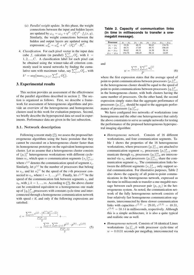
Table 2. Capacity of communication links(in time in milliseconds to transfer a one-megabit message).

Processor p1 − p4 p5 − p8 p9 − p10 p11 − p16p1 − p4 19.26 48.31 96.62 154.76p5 − p8 48.31 17.65 48.31 106.45p9 − p10 96.62 48.31 16.38 58.14p11 − p16 154.76 106.45 58.14 14.05

and

w =

∑mj=1

∑p(j)

t=1 w(j)t

P(6)

where the first expression states that the average speed ofpoint-to-point communications between processors {pi}P

i=1

in the heterogeneous cluster should be equal to the speed ofpoint-to-point communications between processors {qi}P

i=1

in the homogeneous cluster, with both clusters having thesame number of processors. On the other hand, the secondexpression simply states that the aggregate performance ofprocessors {pi}P

i=1 should be equal to the aggregate perfor-mance of processors {qi}P

i=1.We have configured two networks of workstations (one

homogeneous and the other one heterogeneous) that satisfythe above constraints to serve as sample networks for testingthe performance of the proposed heterogeneous hyperspec-tral imaging algorithm:

• Heterogeneous network. Consists of 16 differentworkstations, and four communication segments. Ta-ble 1 shows the properties of the 16 heterogeneousworkstations, where processors {pi}4

i=1 are attached tocommunication segment s1, processors {pi}8

i=5 com-municate through s2, processors {pi}10

i=9 are intercon-nected via s3, and processors {pi}16

i=11 share the com-munication segment s4. The communication links be-tween the different segments {sj}4

j=1 only support se-rial communication. For illustrative purposes, Table 2also shows the capacity of all point-to-point commu-nications in the heterogeneous network, expressed asthe time in milliseconds to transfer a one-megabit mes-sage between each processor pair (pi, pj) in the het-erogeneous system. As noted, the communication net-work of the fully heterogeneous network consists offour relatively fast homogeneous communication seg-ments, interconnected by three slower communicationlinks with capacities c(1,2) = 29.05, c(2,3) = 48.31,c(3,4) = 58.14 in milliseconds, respectively. Althoughthis is a simple architecture, it is also a quite typicaland realistic one as well.

• Homogeneous network. Consists of 16 identical Linuxworkstations {qi}1

i=16 with processor cycle-time ofw = 0.0131 seconds per megaflop, interconnected via

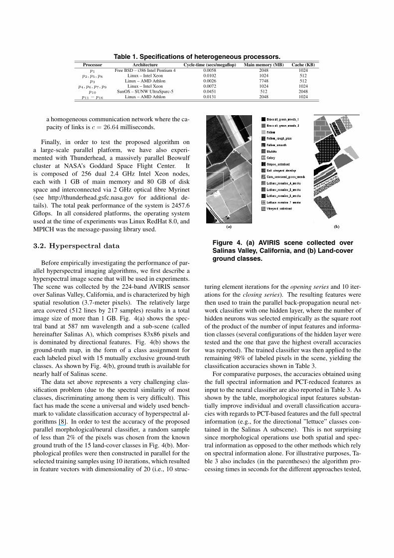
Table 1. Specifications of heterogeneous processors.Processor Architecture Cycle-time (secs/megaflop) Main memory (MB) Cache (KB)

p1 Free BSD – i386 Intel Pentium 4 0.0058 2048 1024p2, p5, p8 Linux – Intel Xeon 0.0102 1024 512

p3 Linux – AMD Athlon 0.0026 7748 512p4, p6, p7, p9 Linux – Intel Xeon 0.0072 1024 1024

p10 SunOS – SUNW UltraSparc-5 0.0451 512 2048p11 − p16 Linux – AMD Athlon 0.0131 2048 1024

a homogeneous communication network where the ca-pacity of links is c = 26.64 milliseconds.

Finally, in order to test the proposed algorithm ona large-scale parallel platform, we have also experi-mented with Thunderhead, a massively parallel Beowulfcluster at NASA’s Goddard Space Flight Center. Itis composed of 256 dual 2.4 GHz Intel Xeon nodes,each with 1 GB of main memory and 80 GB of diskspace and interconnected via 2 GHz optical fibre Myrinet(see http://thunderhead.gsfc.nasa.gov for additional de-tails). The total peak performance of the system is 2457.6Gflops. In all considered platforms, the operating systemused at the time of experiments was Linux RedHat 8.0, andMPICH was the message-passing library used.

3.2. Hyperspectral data

Before empirically investigating the performance of par-allel hyperspectral imaging algorithms, we first describe ahyperspectral image scene that will be used in experiments.The scene was collected by the 224-band AVIRIS sensorover Salinas Valley, California, and is characterized by highspatial resolution (3.7-meter pixels). The relatively largearea covered (512 lines by 217 samples) results in a totalimage size of more than 1 GB. Fig. 4(a) shows the spec-tral band at 587 nm wavelength and a sub-scene (calledhereinafter Salinas A), which comprises 83x86 pixels andis dominated by directional features. Fig. 4(b) shows theground-truth map, in the form of a class assignment foreach labeled pixel with 15 mutually exclusive ground-truthclasses. As shown by Fig. 4(b), ground truth is available fornearly half of Salinas scene.

The data set above represents a very challenging clas-sification problem (due to the spectral similarity of mostclasses, discriminating among them is very difficult). Thisfact has made the scene a universal and widely used bench-mark to validate classification accuracy of hyperspectral al-gorithms [8]. In order to test the accuracy of the proposedparallel morphological/neural classifier, a random sampleof less than 2% of the pixels was chosen from the knownground truth of the 15 land-cover classes in Fig. 4(b). Mor-phological profiles were then constructed in parallel for theselected training samples using 10 iterations, which resultedin feature vectors with dimensionality of 20 (i.e., 10 struc-

Figure 4. (a) AVIRIS scene collected overSalinas Valley, California, and (b) Land-coverground classes.

turing element iterations for the opening series and 10 iter-ations for the closing series). The resulting features werethen used to train the parallel back-propagation neural net-work classifier with one hidden layer, where the number ofhidden neurons was selected empirically as the square rootof the product of the number of input features and informa-tion classes (several configurations of the hidden layer weretested and the one that gave the highest overall accuracieswas reported). The trained classifier was then applied to theremaining 98% of labeled pixels in the scene, yielding theclassification accuracies shown in Table 3.

For comparative purposes, the accuracies obtained usingthe full spectral information and PCT-reduced features asinput to the neural classifier are also reported in Table 3. Asshown by the table, morphological input features substan-tially improve individual and overall classification accura-cies with regards to PCT-based features and the full spectralinformation (e.g., for the directional ”lettuce” classes con-tained in the Salinas A subscene). This is not surprisingsince morphological operations use both spatial and spec-tral information as opposed to the other methods which relyon spectral information alone. For illustrative purposes, Ta-ble 3 also includes (in the parentheses) the algorithm pro-cessing times in seconds for the different approaches tested,

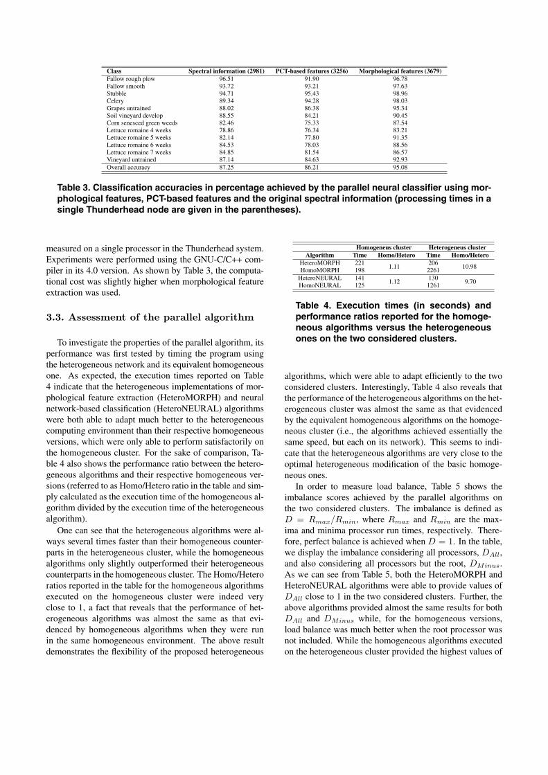
Class Spectral information (2981) PCT-based features (3256) Morphological features (3679)Fallow rough plow 96.51 91.90 96.78Fallow smooth 93.72 93.21 97.63Stubble 94.71 95.43 98.96Celery 89.34 94.28 98.03Grapes untrained 88.02 86.38 95.34Soil vineyard develop 88.55 84.21 90.45Corn senesced green weeds 82.46 75.33 87.54Lettuce romaine 4 weeks 78.86 76.34 83.21Lettuce romaine 5 weeks 82.14 77.80 91.35Lettuce romaine 6 weeks 84.53 78.03 88.56Lettuce romaine 7 weeks 84.85 81.54 86.57Vineyard untrained 87.14 84.63 92.93Overall accuracy 87.25 86.21 95.08

Table 3. Classification accuracies in percentage achieved by the parallel neural classifier using mor-phological features, PCT-based features and the original spectral information (processing times in asingle Thunderhead node are given in the parentheses).

measured on a single processor in the Thunderhead system.Experiments were performed using the GNU-C/C++ com-piler in its 4.0 version. As shown by Table 3, the computa-tional cost was slightly higher when morphological featureextraction was used.

3.3. Assessment of the parallel algorithm

To investigate the properties of the parallel algorithm, itsperformance was first tested by timing the program usingthe heterogeneous network and its equivalent homogeneousone. As expected, the execution times reported on Table4 indicate that the heterogeneous implementations of mor-phological feature extraction (HeteroMORPH) and neuralnetwork-based classification (HeteroNEURAL) algorithmswere both able to adapt much better to the heterogeneouscomputing environment than their respective homogeneousversions, which were only able to perform satisfactorily onthe homogeneous cluster. For the sake of comparison, Ta-ble 4 also shows the performance ratio between the hetero-geneous algorithms and their respective homogeneous ver-sions (referred to as Homo/Hetero ratio in the table and sim-ply calculated as the execution time of the homogeneous al-gorithm divided by the execution time of the heterogeneousalgorithm).

One can see that the heterogeneous algorithms were al-ways several times faster than their homogeneous counter-parts in the heterogeneous cluster, while the homogeneousalgorithms only slightly outperformed their heterogeneouscounterparts in the homogeneous cluster. The Homo/Heteroratios reported in the table for the homogeneous algorithmsexecuted on the homogeneous cluster were indeed veryclose to 1, a fact that reveals that the performance of het-erogeneous algorithms was almost the same as that evi-denced by homogeneous algorithms when they were runin the same homogeneous environment. The above resultdemonstrates the flexibility of the proposed heterogeneous

Homogeneus cluster Heterogeneus clusterAlgorithm Time Homo/Hetero Time Homo/Hetero

HeteroMORPH 2211.11

20610.98

HomoMORPH 198 2261HeteroNEURAL 141

1.12130

9.70HomoNEURAL 125 1261

Table 4. Execution times (in seconds) andperformance ratios reported for the homoge-neous algorithms versus the heterogeneousones on the two considered clusters.

algorithms, which were able to adapt efficiently to the twoconsidered clusters. Interestingly, Table 4 also reveals thatthe performance of the heterogeneous algorithms on the het-erogeneous cluster was almost the same as that evidencedby the equivalent homogeneous algorithms on the homoge-neous cluster (i.e., the algorithms achieved essentially thesame speed, but each on its network). This seems to indi-cate that the heterogeneous algorithms are very close to theoptimal heterogeneous modification of the basic homoge-neous ones.

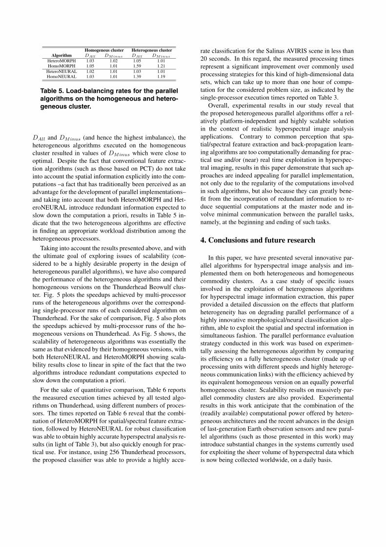
In order to measure load balance, Table 5 shows theimbalance scores achieved by the parallel algorithms onthe two considered clusters. The imbalance is defined asD = Rmax/Rmin, where Rmax and Rmin are the max-ima and minima processor run times, respectively. There-fore, perfect balance is achieved when D = 1. In the table,we display the imbalance considering all processors, DAll,and also considering all processors but the root, DMinus.As we can see from Table 5, both the HeteroMORPH andHeteroNEURAL algorithms were able to provide values ofDAll close to 1 in the two considered clusters. Further, theabove algorithms provided almost the same results for bothDAll and DMinus while, for the homogeneous versions,load balance was much better when the root processor wasnot included. While the homogeneous algorithms executedon the heterogeneous cluster provided the highest values of

Homogeneus cluster Heterogeneus clusterAlgorithm DAll DMinus DAll DMinus

HeteroMORPH 1.03 1.02 1.05 1.01HomoMORPH 1.05 1.01 1.59 1.21

HeteroNEURAL 1.02 1.01 1.03 1.01HomoNEURAL 1.03 1.01 1.39 1.19

Table 5. Load-balancing rates for the parallelalgorithms on the homogeneous and hetero-geneous cluster.

DAll and DMinus (and hence the highest imbalance), theheterogeneous algorithms executed on the homogeneouscluster resulted in values of DMinus which were close tooptimal. Despite the fact that conventional feature extrac-tion algorithms (such as those based on PCT) do not takeinto account the spatial information explicitly into the com-putations –a fact that has traditionally been perceived as anadvantage for the development of parallel implementations–and taking into account that both HeteroMORPH and Het-eroNEURAL introduce redundant information expected toslow down the computation a priori, results in Table 5 in-dicate that the two heterogeneous algorithms are effectivein finding an appropriate workload distribution among theheterogeneous processors.

Taking into account the results presented above, and withthe ultimate goal of exploring issues of scalability (con-sidered to be a highly desirable property in the design ofheterogeneous parallel algorithms), we have also comparedthe performance of the heterogeneous algorithms and theirhomogeneous versions on the Thunderhead Beowulf clus-ter. Fig. 5 plots the speedups achieved by multi-processorruns of the heterogeneous algorithms over the correspond-ing single-processor runs of each considered algorithm onThunderhead. For the sake of comparison, Fig. 5 also plotsthe speedups achieved by multi-processor runs of the ho-mogeneous versions on Thunderhead. As Fig. 5 shows, thescalability of heterogeneous algorithms was essentially thesame as that evidenced by their homogeneous versions, withboth HeteroNEURAL and HeteroMORPH showing scala-bility results close to linear in spite of the fact that the twoalgorithms introduce redundant computations expected toslow down the computation a priori.

For the sake of quantitative comparison, Table 6 reportsthe measured execution times achieved by all tested algo-rithms on Thunderhead, using different numbers of proces-sors. The times reported on Table 6 reveal that the combi-nation of HeteroMORPH for spatial/spectral feature extrac-tion, followed by HeteroNEURAL for robust classificationwas able to obtain highly accurate hyperspectral analysis re-sults (in light of Table 3), but also quickly enough for prac-tical use. For instance, using 256 Thunderhead processors,the proposed classifier was able to provide a highly accu-

rate classification for the Salinas AVIRIS scene in less than20 seconds. In this regard, the measured processing timesrepresent a significant improvement over commonly usedprocessing strategies for this kind of high-dimensional datasets, which can take up to more than one hour of compu-tation for the considered problem size, as indicated by thesingle-processor execution times reported on Table 3.

Overall, experimental results in our study reveal thatthe proposed heterogeneous parallel algorithms offer a rel-atively platform-independent and highly scalable solutionin the context of realistic hyperspectral image analysisapplications. Contrary to common perception that spa-tial/spectral feature extraction and back-propagation learn-ing algorithms are too computationally demanding for prac-tical use and/or (near) real time exploitation in hyperspec-tral imaging, results in this paper demonstrate that such ap-proaches are indeed appealing for parallel implementation,not only due to the regularity of the computations involvedin such algorithms, but also because they can greatly bene-fit from the incorporation of redundant information to re-duce sequential computations at the master node and in-volve minimal communication between the parallel tasks,namely, at the beginning and ending of such tasks.

4. Conclusions and future research

In this paper, we have presented several innovative par-allel algorithms for hyperspectral image analysis and im-plemented them on both heterogeneous and homogeneouscommodity clusters. As a case study of specific issuesinvolved in the exploitation of heterogeneous algorithmsfor hyperspectral image information extraction, this paperprovided a detailed discussion on the effects that platformheterogeneity has on degrading parallel performance of ahighly innovative morphological/neural classification algo-rithm, able to exploit the spatial and spectral information insimultaneous fashion. The parallel performance evaluationstrategy conducted in this work was based on experimen-tally assessing the heterogeneous algorithm by comparingits efficiency on a fully heterogeneous cluster (made up ofprocessing units with different speeds and highly heteroge-neous communication links) with the efficiency achieved byits equivalent homogeneous version on an equally powerfulhomogeneous cluster. Scalability results on massively par-allel commodity clusters are also provided. Experimentalresults in this work anticipate that the combination of the(readily available) computational power offered by hetero-geneous architectures and the recent advances in the designof last-generation Earth observation sensors and new paral-lel algorithms (such as those presented in this work) mayintroduce substantial changes in the systems currently usedfor exploiting the sheer volume of hyperspectral data whichis now being collected worldwide, on a daily basis.

(a) (b)

Figure 5. Scalability of morphological feature extraction (a) and neural network-based (b) parallelalgorithms on Thunderhead.

Processors: 1 4 16 36 64 100 144 196 256HeteroMORPH

2041797 203 79 39 23 17 13 10

HomoMORPH 753 170 70 36 22 16 12 9Processors: 1 2 4 8 16 32 64 128 256

HeteroNEURAL1638

985 468 239 122 61 30 18 9HomoNEURAL 973 458 222 114 55 27 15 7

Table 6. Processing times (in seconds) achieved by multi-processor runs of the considered parallelalgorithms on Thunderhead.

5 Acknowledgement

The authors would like to thank Drs. John Dorband,James C. Tilton and Anthony Gualtieri for their with exper-iments on NASA’s Thunderhead system and also for manyhelpful discussions. They also state their appreciation forProfs. Mateo Valero and Francisco Tirado.

References

[1] G. Aloisio and M. Cafaro. A dynamic earth observation sys-tem. Parallel Computing, 29:1357–1362, 2003.

[2] C.-I. Chang. Hyperspectral imaging: Techniques for spec-tral detection and classification. Kluwer: New York, 2003.

[3] J. Dorband, J. Palencia, and U. Ranawake. Commodity clus-ters at Goddard Space Flight Center. Journal of Space Com-munication, 3:227–248, 2003.

[4] T. El-Ghazawi, S. Kaewpijit, and J. L. Moigne. Parallel andadaptive reduction of hyperspectral data to intrinsic dimen-sionality. Cluster Computing, pages 102–110, 2001.

[5] R. O. Green. Imaging spectroscopy and the airborne visi-ble/infrared imaging spectrometer (AVIRIS). Remote Sens-ing of Environment, 65:227–248, 1998.

[6] A. Lastovetsky. Parallel computing on heterogeneous net-works. Wiley-Interscience: Hoboken, NJ, 2003.

[7] A. Lastovetsky and R. Reddy. On performance analysisof heterogeneous parallel algorithms. Parallel Computing,30:1195–1216, 2004.

[8] A. Plaza, P. Martinez, J. Plaza, and R. Perez. Dimen-sionality reduction and classification of hyperspectral im-age data using sequences of extended morphological trans-formations. IEEE Transactions on Geoscience and RemoteSensing, 43:466–479, 2005.

[9] A. Plaza, D. Valencia, J. Plaza, and P. Martinez. Commoditycluster-based parallel processing of hyperspectral imagery.Journal of Parallel and Distributed Computing, 66:345–358, 2006.

[10] J. Plaza, A. Plaza, R. Perez, and P. Martinez. Automatedgeneration of semi-labeled training samples for nonlinearneural network-based abundance estimation in hyperspec-tral data. Proceedings IEEE International Geoscience andRemote Sensing Symposium, pages 345–350, 2005.

[11] G. X. Ritter, P. Sussner, and J. L. Diaz. Morphological asso-ciative memories. IEEE Transactions on Neural Networks,9:281–293, 2004.

[12] P. Soille. Morphological image analysis: Principles andapplications. Springer: Berlin, 2003.

[13] T. Sterling. Cluster computing. Encyclopedia of PhysicalScience and Technology, 3, 2002.

[14] S. Suresh, S. N. Omkar, and V. Mani. Parallel implementa-tion of back-propagation algorithm in networks of worksta-tions. IEEE Transactions on Parallel and Distributed Sys-tems, 16:24–34, 2005.

[15] P. Wang, K. Y. Liu, T. Cwik, and R. Green. MODTRAN onsupercomputers and parallel computers. Parallel Comput-ing, 28:53–64, 2002.