Paper title for the 2011 AIVC-TIGHTVENT conference

Poznań, Poland

Andersia Hotel

24–25 September 2014

35th AIVC Conference

4th TightVent Conference

2nd venticool Conference

Ventilation and airtightness in

transforming the building stock to

high performance

PROCEEDINGS

In cooperation with:

Acknowledgments

The conference organisers gratefully acknowledge the support from:

AIVC with its member countries : Belgium, Czech Republic, Denmark, Finland, France,

Germany, Greece, Italy, Japan, the Netherlands, New Zealand, Norway, Poland, Republic of

Korea, Sweden and USA.

Since 1980, the annual AIVC conferences have been the meeting point for presenting and

discussing major developments and results regarding infiltration and ventilation in buildings.

AIVC contributes to the programme development, selection of speakers and dissemination of

the results. pdf files of the papers of older conferences can be found in AIRBASE. See

www.aivc.org.

TightVent Europe The TightVent Europe ‘Building and Ductwork Airtightness Platform’ was launched in

January 2011.

It aims at facilitating exchanges and progress on building and ductwork airtightness issues,

including the production and dissemination of policy oriented reference documents and the

organization of conferences, workshops, webinars, etc. The platform has been initiated by

INIVE EEIG (International Network for Information on Ventilation and Energy Performance)

and receives active support from the following organisations: Aeroseal, Buildings

Performance Institute Europe, BlowerDoor GmbH, European Climate Foundation, Eurima,

Lindab, Retrotec, Soudal, Tremco illbruck, and Wienerberger. More information can be found

on www.tightvent.eu.

venticool The international ventilative cooling platform, venticool (venticool.eu) was launched in

October 2012 to accelerate the uptake of ventilative cooling by raising awareness, sharing

experience and steering research and development efforts in the field of ventilative cooling.

The platform supports better guidance for the appropriate implementation of ventilative

cooling strategies as well as adequate credit for such strategies in building regulations. The

platform philosophy is pull resources together and to avoid duplicating efforts to maximize

the impact of existing and new initiatives. venticool will join forces with organizations with

significant experience and/or well identified in the field of ventilation and thermal comfort

like AIVC (www.aivc.org) and REHVA (www.rehva.eu). Venticool has been initiated by

INIVE EEIG (International Network for Information on Ventilation and Energy Performance)

with the financial and/or technical support of the following partners: Agoria-NAVENTA, ES-

SO, Velux, Wienerberger and WindowMaster

Poznań University of Technology Poznań University of Technology (PUT, www.put.edu.pl) was established in 1919 and

currently, with over 20 thousand students and more than 1 000 academic staff, is one of the

leading technical universities in Poland.

10 Faculties cover wide range of technical knowledge: Architecture, Chemical Technology,

Civil and Environmental Engineering, Computing, Engineering Management, Electrical

Engineering, Electronics and Telecommunications, Mechanical Engineering and

Management, Technical Physics, Machines and Transportation. PUT offers Bachelor, Master

and Doctorate courses in Polish and English. European Credit Transfer System (ECTS) is

implemented, many foreign students study in the Erasmus program. PUT participates in

Polish and international scientific projects and is involved in cooperation with industry.

INIVE EEIG (International Network for Information on

Ventilation and Energy performance)

INIVE was founded in 2001.

INIVE is a registered European Economic Interest Grouping (EEIG), whereby from a legal viewpoint its

full members act together as a single organisation and bring together the best available knowledge from its

member organisations. The present full members are all leading organisations in the building sector, with

expertise in building technology, human sciences and dissemination/publishing of information. They also

actively conduct research in this field - the development of new knowledge will always be important for

INIVE members.

INIVE has multiple aims, including the collection and efficient storage of relevant information, providing

guidance and identifying major trends, developing intelligent systems to provide the world of construction

with useful knowledge in the area of energy efficiency, indoor climate and ventilation. Building energy-

performance regulations are another major area of interest for the INIVE members, especially the

implementation of the European Energy Performance of Buildings Directive.

With respect to the dissemination of information, INIVE EEIG aims for the widest possible distribution of

information.

The following organisations are members of INIVE EEIG (www.inive.org):

BBRI - Belgian Building Research Institute - Belgium

CETIAT - Centre Technique des Industries Aérauliques et Thermiques - France

CSTB - Centre Scientifique et Technique du Bâtiment - France

IBP - Fraunhofer Institute for Building Physics - Germany

SINTEF - SINTEF Building and Infrastructure - Norway

NKUA - National & Kapodistrian University of Athens - Greece

TNO - TNO Built Environment and Geosciences, business unit Building and Construction -

Netherlands

The following organisations are associated members.

CIMNE - International Center for Numerical Methods in Engineering, Barcelona, Spain

eERG - End-use Efficiency Research Group, Politecnico di Milano, Italy

ENTPE - Ecole Nationale des Travaux Publics de l'Etat, Vaulx en Velin, France

TMT US - Grupo Termotecnia, Universidad de Sevilla, Spain

Table of Contents

PROPOSED CHANGE IN SPANISH REGULATIONS RELATING TO INDOOR AIR QUALITY WITH

THE AIM OF REDUCING ENERGY CONSUMPTION OF VENTILATION SYSTEMS ......................... 1

DURABLE AIRTIGHTNESS IN SINGLE-FAMILY DWELLINGS: FIELD MEASUREMENTS AND

ANALYSIS ..................................................................................................................................................... 7

IMPACT OF A PHOTOCATALYTIC OXIDATION LAYER COVERING THE INTERIOR SURFACES

OF A REAL TEST ROOM: VOLATILE ORGANIC COMPOUND MINERALISATION, RISK

ASSESSMENT OF BY-PRODUCT AND NANOPARTICLE EMISSIONS. ............................................. 16

THE ENERGY IMPACT OF ENVELOPE LEAKAGE. THE CHILEAN CASE ....................................... 25

AIRTIGHTNESS IMPROVEMENT OF STRUCTURES TO IMPROVE INDOOR AIR QUALITY ....... 36

DEMAND CONTROLLED VENTILATION IN RENOVATED BUILDINGS WITH REUSE OF

EXISTING DUCTWORK ............................................................................................................................ 46

REQUIREMENTS AND HAND-OVER DOCUMENTATION FOR ENERGY-OPTIMAL DEMAND-

CONTROLLED VENTILATION ................................................................................................................ 53

MONITORING RESULTS AND OPTIMIZATION OF A FAÇADE INTEGRATED VENTILATION

CONCEPT FOR BUILDING RETROFIT ....................................................................................................61

USE OF DCV FOR HEATING AND THE INFLUENCE ON IAQ IN PASSIVE HOUSE BUILDINGS . 71

THE EFFECT OF ENTHALPY RECOVERY VENTILATION ON THE RESIDENTIAL INDOOR

CLIMATE ..................................................................................................................................................... 78

AIR RENEWAL EFFECTIVENESS OF DECENTRALIZED VENTILATION DEVICES WITH HEAT

RECOVERY ................................................................................................................................................. 83

PERCEPTION OF A COOLING JET FROM CEILING - A LABORATORY STUDY............................. 94

PROMEVENT: IMPROVEMENT OF PROTOCOLS MEASUREMENTS USED TO CHARACTERIZE

VENTILATION SYSTEMS PERFORMANCE ...........................................................................................100

IMPACT OF A POOR QUALITY OF VENTILATION SYSTEMS ON THE ENERGY EFFICIENCY

FOR ENERGY-EFFICIENT HOUSES ...................................................................................................... 108

DEMAND-CONTROLLED VENTILATION 20 YEARS OF IN-SITU MONITORING IN THE

RESIDENTIAL FIELD ............................................................................................................................... 119

SUMMER PERFORMANCE OF RESIDENTIAL HEAT RECOVERY VENTILATION WITH AN AIR-

TO-AIR HEAT PUMP COOLING SYSTEM ............................................................................................ 130

HEATING "PASSIVE HOUSE" OFFICES IN COLD CLIMATE USING ONLY THE VENTILATION

SYSTEM – COMPARISON OF TWO VENTILATION STRATEGIES .................................................. 137

MONITORING OF AN INNOVATIVE ROOM-BY-ROOM DEMAND CONTROLLED HEAT

RECOVERY SYSTEM ON FOUR LOCATIONS ..................................................................................... 142

CLEANLINESS OF AIR FILTERS IN THE EXPERIMENTAL PASSIVE HOUSE............................... 154

COMPARISON OF TWO VENTILATION CONTROL STRATEGIES IN THE FIRST NORWEGIAN

SCHOOL WITH PASSIVE HOUSE STANDARD ................................................................................... 163

SELF-EVALUATED THERMAL COMFORT COMPARED TO MEASURED TEMPERATURES

DURING SUMMER IN THREE ACTIVE HOUSES WHERE VENTILATIVE COOLING IS APPLIED

..................................................................................................................................................................... 171

EXPERIENCES WITH VENTILATIVE COOLING IN PRACTICAL APPLICATION BASED ON

EXPERIENCES WITH COMPLETED ACTIVE HOUSES ...................................................................... 180

INDOOR CLIMATE IN A DANISH KINDERGARTEN BUILT ACCORDING TO ACTIVE HOUSE

PRINCIPLES: MEASURED THERMAL COMFORT AND USE OF ELECTRICAL LIGHT ............... 188

AIR HEATING OF PASSIVE HOUSE OFFICE BUILDINGS IN COLD CLIMATES – HOW HIGH

SUPPLY TEMPERATURE IS ACCEPTABLE? ....................................................................................... 198

ENERGY-OPTIMAL VENTILATION STRATEGY OUTSIDE OF THE OPERATING TIME FOR

PASSIVE HOUSE OFFICE BUILDINGS IN COLD CLIMATES ........................................................... 207

CAN AIR HEATING ALONE BE USED IN PASSIVE HOUSE OFFICE BUILDING IN COLD

CLIMATES? REVIEW OF THE OBTAINED RESULTS ........................................................................ 217

IMPACT OF THE USE OF A FRONT DOOR ON THERMAL COMFORT IN A CLASSROOM IN A

PASSIVE SCHOOL .................................................................................................................................... 226

A NOZZLE PULSE PRESSURISATION TECHNIQUE FOR MEASUREMENT OF BUILDING

LEAKAGE AT LOW PRESSURE ............................................................................................................. 236

EXERGY EVALUATION OF MECHANICAL VENTILATION SYSTEMS.......................................... 245

STRATEGIES FOR EXPLOITING CLIMATE POTENTIAL THROUGH VENTILATIVE COOLING IN

A RENOVATED HISTORIC MARKET ................................................................................................... 257

DURABILITY OF AIR TIGHTNESS SOLUTIONS FOR BUILDINGS.................................................. 268

MULTI-PIPE EARTH-TO-AIR HEAT EXCHANGER (EAHE) GEOMETRY INFLUENCE ON THE

SPECIFIC FAN POWER (SFP) AND FAN ENERGY DEMAND IN MECHANICAL VENTILATION

SYSTEMS ................................................................................................................................................... 279

AIRFLOW MODELLING SOFTWARE DEVELOPMENT FOR NATURAL VENTILATION DESIGN

..................................................................................................................................................................... 287

REDUCING COOLING ENERGY NEEDS THROUGH AN INNOVATIVE DAILY STORAGE BASED

FACADE SOLUTION ................................................................................................................................ 297

SIMULATION OF STATIC PRESSURE RESET CONTROL IN COMFORT VENTILATION ............ 305

A PROTOCOL FOR ASSESSING INDOOR AIR QUALITY IN RETROFITTED ENERGY EFFICIENT

HOMES IN IRELAND ............................................................................................................................... 315

TESTING FOR BUILDING COMPONENTS CONTRIBUTION TO AIRTIGHTNESS ASSESSMENT

..................................................................................................................................................................... 322

IMPLEMENTATION AND PERFORMANCE OF VENTILATION SYSTEMS: FIRST REVIEW OF

VOLUNTARY CERTIFICATION CONTROLS IN FRANCE ................................................................. 331

AIR LEAKAGES IN A RETROFITTED BUILDING FROM 1930: MEASUREMENTS AND

NUMERICAL SIMULATIONS ................................................................................................................. 341

INDOOR ENVIRONMENTAL QUALITY-GLOBAL ALLIANCE: THE VALUE CHAIN OF IEQ ..... 350

DO EXISTING INTERNATIONAL STANDARDS SUPPORT VENTILATIVE COOLING? ............... 351

THE INFLUENCE OF TRAFFIC EMISSION ON IAQ ESPECIALLY IN STREET CANYONS .......... 352

SIMULATION OF NIGHT VENTILATION PERFORMANCE AS A SUPPORT FOR AN

INTEGRATED DESIGN OF BUILDINGS ............................................................................................... 361

ESTIMATING THE IMPACT OF INCOMPLETE TRACER GAS MIXING ON INFILTRATION RATE

MEASUREMENTS .................................................................................................................................... 371

VENTILATIVE COOLING IN NATIONAL ENERGY PERFORMANCE REGULATIONS:

REQUIREMENTS AND SENSITIVITY ANALYSIS .............................................................................. 378

THE 10 STEPS TO CONCEIVE AND BUILD AIRTIGHT BUILDINGS ............................................... 398

BELGIAN FRAMEWORK FOR RELIABLE FAN PRESSURIZATION TESTS FOR BUILDINGS .... 406

CO-HEATING TEST AND COMFORT ASSESSMENT OF A COUPLED SYSTEM MADE BY A

VENTILATED WINDOW AND A HEAT RECOVERY UNIT ............................................................... 417

DERIVATION OF EQUATION FOR PERSONAL CARBON DIOXIDE IN EXHALED BREATH

INTENDED TO ESTIMATION OF BUILDING VENTILATION ........................................................... 427

PASSIVE COOLING THROUGH VENTILATION SHAFTS IN HIGH-DENSITY ZERO ENERGY

BUILDINGS: A DESIGN STRATEGY TO INTEGRATE NATURAL AND MECHANICAL

VENTILATION IN TEMPERATE CLIMATES. ...................................................................................... 436

ENERGY SAVING AND THERMAL COMFORT IN RESIDENTIAL BUILDINGS WITH DYNAMIC

INSULATION WINDOWS ........................................................................................................................ 447

EXPERIENCES IN THE AIRTIGHTNESS OF RENOVATED TERTIARY EXEMPLARY BUILDINGS

IN THE BRUSSELS CAPITAL REGION ................................................................................................. 457

MONITORING THE ENERGY- & IAQ PERFORMANCE OF VENTILATION SYSTEMS IN DUTCH

RESIDENTIAL DWELLINGS ................................................................................................................... 467

DUCTWORK AIRTIGHTNESS: RELIABILITY OF MEASUREMENTS AND IMPACT ON

VENTILATION FLOWRATE AND FAN ENERGY CONSUMPTION .................................................. 478

AIRTIGHTNESS OF BUILDING PENETRATIONS: AIR SEALING SOLUTIONS, DURABILITY

EFFECTS AND MEASUREMENT UNCERTAINTY .............................................................................. 488

COMPARISON OF BUILDING PREPARATION RULES FOR AIRTIGHTNESS TESTING IN 11

EUROPEAN COUNTRIES ........................................................................................................................ 501

THE IMPACT OF AIR-TIGHTNESS IN THE RETROFITTING PRACTICE OF LOW TEMPERATURE

HEATING ................................................................................................................................................... 511

THE USE OF A ZONAL MODEL TO CALCULATE THE STRATIFICATION IN A LARGE

BUILDING ................................................................................................................................................. 522

RECENT ADVANCES ON FACTORS INFLUENCING HUMAN RESPONSES AND PERFORMANCE

IN BUILDINGS AND POTENTIAL IMPACTS ON VENTILATION REQUIREMENTS ..................... 532

STRATEGIES FOR EFFICIENT KITCHEN VENTILATION ................................................................. 534

COUPLING HYGROTHERMAL WHOLE BUILDING SIMULATION AND AIR-FLOW MODELLING

TO DETERMINE STRATEGIES FOR OPTIMIZED NATURAL VENTILATION ................................ 537

EXPERIMENTAL CHARACTERISATION OF DOMINANT DRIVING FORCES AND

FLUCTUATING VENTILATION RATES FOR A SINGLE SIDED SLOT LOUVER VENTILATION

SYSTEM ..................................................................................................................................................... 547

A STUDY OF CARBON DIOXIDE CONCENTRATIONS IN ELEMENTARY SCHOOLS ................. 557

MEASUREMENT OF INFILTRATION RATES FROM DAILY CYCLE OF AMBIENT CO2 ............. 568

PREDICTING THE OPTIMUM AIR PERMABILIY OF A STOCK OF DETACHED ENGLISH

DWELLINGS ............................................................................................................................................. 575

DEVELOPMENT OF AN EVALUATION METHODOLOGY TO QUANTIFY THE ENERGY

POTENTIAL OF DEMAND CONTROLLED VENTILATION STRATEGIES ...................................... 587

SYSTEM FOR CONTROLLING VARIABLE AMOUNT OF AIR ENSURING APPROPRIATE

INDOOR AIR QUALITY IN LOW-ENERGY AND PASSIVE BUILDINGS ......................................... 597

MULTI-ZONE DEMAND-CONTROLLED VENTILATION IN RESIDENTIAL BUILDINGS: AN

EXPERIMENTAL CASE STUDY ............................................................................................................. 614

SEASONAL VARIATION IN AIRTIGHTNESS ...................................................................................... 621

OPTIMIZATION OF DATA CENTER CHILLED WATER COOLING SYSTEM ACCORDING TO

ANNUAL POWER CONSUMPTION CRITERION ................................................................................. 629

NUMERICAL SIMULATION OF INDOOR AIR QUALITY - MECHANICAL VENTILATION

SYSTEM SUPPLIED PERIODICALLY VS. NATURAL VENTILATION. ............................................ 638

DEVELOPMENT OF A DECENTRALIZED AND COMPACT COMFORT VENTILATION SYSTEM

WITH HIGHLY EFFICIENT HEAT RECOVERY FOR THE MINIMAL INVASIVE

REFURBISHMENT OF BUILDINGS ....................................................................................................... 648

CFD SIMULATION OF AN OFFICE HEATED BY A CEILING MOUNTED DIFFUSER ................... 655

OPTIMAL POSITIONING OF AIR-EXHAUST OPENINGS IN AN OPERATING ROOM BASED ON

RECOVERY TEST: A NUMERICAL STUDY ......................................................................................... 665

STRATEGIES FOR THE PLANNING AND IMPLEMENTATION OF AIRTIGHTNESS ON EXISTING

SLOPED ROOFS ........................................................................................................................................ 671

ACH AND AIR TIGHTNESS TEST RESULTS IN THE CROATIAN AND HUNGARIAN BORDER

REGION ...................................................................................................................................................... 680

MEASURED MOISTURE BUFFERING AND LATENT HEAT CAPACITIES IN CLT TEST HOUSES

..................................................................................................................................................................... 691

BREATHING FEATURES ASSESSMENT OF POROUS WALL UNUITS IN RELATION TO INDOOR

AIR QUALITY ........................................................................................................................................... 703

LARGE BUILDINGS AIRTIGHTNESS MEASUREMENTS USING VENTILATION SYSTEMS ...... 712

SIMULATION ANALYSIS FOR INDOOR TEMPERATURE INCREASE AND REDUCTION OF

HEATING LOAD IN THE DETACHED HOUSE WITH BUOYANCY VENTILATED WALL IN

WINTER ..................................................................................................................................................... 721

DEVELOPMENT OF A UNIQUE THERMAL AND INDOOR AIR QUALITY PROBABILISTIC

MODELLING TOOL FOR ASSESSING THE IMPACT OF LOWERING BUILDING VENTILATION

RATES. ....................................................................................................................................................... 730

ASSESSMENT OF THE DURABILITY OF THE AIRTIGHTNESS OF BUILDING ELEMENTS VIA

LABORATORY TESTS. ............................................................................................................................ 738

CONTROL OF INDOOR CLIMATE SYSTEMS IN ACTIVE HOUSES ................................................. 747

TIPS FOR IMPROVING REPEATABILITY OF AIR LEAKAGE TESTS TO EN AND ISO

STANDARDS. ............................................................................................................................................ 758

THE INDOOR AIR QUALITY OBSERVATORY - OUTCOMES OF A DECADE OF RESEARCH AND

PERSPECTIVES. ........................................................................................................................................ 760

MODEL ERROR DUE TO STEADY WIND IN BUILDING PRESSURIZATION TESTS .................... 770

TEMPERATURE AND PRESSURE CORRECTIONS FOR POWER-LAW COEFFICIENTS OF

AIRFLOW THROUGH VENTILATION SYSTEM COMPONENTS AND LEAKS .............................. 778

TOPICAL SESSION: STATUS OF THE REVISION OF EN VENTILATION STANDARDS

SUPPORTING THE EPBD RECAST. ....................................................................................................... 786

INTEGRATED APPROACH AS A PREREQUISITE FOR NEARLY ZERO ENERGY SCHOOLS IN

MEDITERRANEAN REGION-ZEMEDS PROJECT. .............................................................................. 788

1 | P a g e

PROPOSED CHANGE IN SPANISH REGULATIONS

RELATING TO INDOOR AIR QUALITY WITH THE

AIM OF REDUCING ENERGY CONSUMPTION OF

VENTILATION SYSTEMS

Linares, Pilar*

1, García, Sonia

1, Sotorrío, Guillermo

1, Tenorio, José A

1

1 Eduardo Torroja Institute for construction sciences-

CSIC

4, Serrano Galvache St.

Madrid, Spain

*Corresponding author: [email protected]

ABSTRACT

The ventilation required in order to maintain acceptable indoor hygiene standards results in a significant

consumption of energy. Currently the Spanish regulations on indoor air quality (IAQ) require minimum rates for

delivery-to and extraction-from the habitable rooms of residential buildings. These rates are not adjustable, so

ventilation systems based on variable ventilation rates, are not normally deemed acceptable unless a

comprehensive statement of compliance is provided, justifying the proposed ventilation solution. However the

use of variable ventilation systems is desirable, as it would almost certainly produce a reduction of the overall

ventilation rate and, consequently, a reduction in the heating and cooling energy demand while maintaining a

good level of air quality.

This paper presents part of the ongoing research towards the modification of the Spanish regulations in order to

adapt required ventilation rates to real needs. This would mean allowing reduction in ventilation rates and energy

demand but without any impact on indoor air quality.

The objective behind this research is to propose to the Spanish Government the substitution of the current

required constant ventilation rates by maximum values of CO2 concentration as an indicator of air quality. By

establishing maximum values, the implementation of ventilation systems based on variable ventilation rates will

be enabled because the justification will be more easily provided.

KEYWORDS

Ventilation, IAQ, regulations, energy efficiency

1 INTRODUCTION

The current Spanish Building Code was enforced in 2006 including IAQ provisions for

dwellings which represented a big regulatory step. However the provisions are not as

performance-oriented as was initially anticipated, requiring minimum rates for delivery-to

and extraction-from the habitable rooms. These rates are not adjustable, so ventilation systems

based on variable ventilation rates are not normally deemed acceptable, unless a

comprehensive statement of compliance is provided, justifying the proposed ventilation

solution.

In 2010 with the adoption of the recast EPBD, EU Member States faced new challenges. The

new goal is to increase the level of performance towards nearly-zero energy buildings by

2020. In order to achieve this goal in Spain, a deep review of the energy requirements has

been made in 2013 increasing the energy efficiency of buildings. However, this is not enough,

energy efficiency in buildings is affected as well by ventilation systems.

2 | P a g e

Therefore the use of variable ventilation systems is desirable, as it would almost certainly

produce a reduction of the global ventilation rate and, consequently, a reduction of the heating

and cooling energy demand, while maintaining a good air quality level.

As a consequence research is in progress to modify the Spanish regulations to allow the use of

more efficient systems, adapting required ventilation rates to real needs. This would mean a

reduction in ventilation rates and energy demand but without impact on indoor air quality.

The goal of this research is to update the regulations which should require an IAQ level that

shall be provided. Equally, the goal is to provide a simplified verification method that

facilitates the fulfilment of this IAQ level.

2 CURRENT IAQ REQUIREMENT

The current IAQ requirement establishes minimum ventilation rates (see Table 1) for

delivery-to and extraction-from the habitable rooms. These rates have to be provided in a

continuous way. Table 1. Minimum ventilation rates

Rooms Per person Per usable floor

area m2

Per room

Bedrooms 5 l/s

Living and dining rooms 3 l/s

WC and bathrooms 15 l/s

Kitchens 2 l/s

3 PROPOSED IAQ REQUIREMENT

IAQ level is usually characterized by a maximum level of pollutants that may affect people´s

health and comfort and that could be achieved by different ventilation systems.

However, common pollutants are not easy to assess, so generally an indicator is used to model

the state of the rest of the pollutants. Among the possible pollutants that are commonly

produced indoors, CO2 is the most commonplace and closest related to human activity. In

spite not supposing a health risk in the usual concentrations that is found in dwellings, CO2 is

a very good indicator of the ventilation rate. This way is the most common indicator used in

regulations and guides.

The required CO2 concentration is limited in two ways:

- 900 ppm maximum yearly average;

- 500.000 ppm per hour maximum yearly accumulated above 1.600 ppm. This parameter

shows the relationship between the CO2 concentrations reached above a limit value and

their duration over a year. It can be calculated as the sum of the areas (in ppm•h) within the

representation of the CO2 concentration as a time function and the limit value (See Fig. 1).

Fig. 1. CO2 concentration over time

These required concentration levels shall be achieved under certain design conditions (such as

occupancy scenarios, CO2 production rate, yearly average outdoor CO2 concentration, etc.)

Time

CO2 ppm per hour accumulated

Limit value

3 | P a g e

that should be set in the regulation. This means it is a design performance because it would

only be measurable in situ under these conditions.

These values have been chosen based on the specified values in the RITE taking into account

an outdoor CO2 concentration of 400 ppm: the value corresponding to IAQ 2 for the

maximum yearly average concentration and the IAQ 4 value for the base over which to

calculate the maximum yearly accumulated. (See Table 2)

Table 2. IAQ classes according to RITE

IAQ Classification CO2 concentration

(ppm)

1 Best quality indoor air 750

2 Good quality indoor air 900

3 Medium quality indoor air 1.200

4 Low quality indoor air 1.600

4 PROPOSED VERIFICATION METHOD

The fulfilment of the requirement can be achieved by the use of expertise methods (like

specialized software), but it is convenient as well that at least a simplified verification method

is provided by the regulations for designers to use. This simplified method shall be easy to use

by non-expert practitioners and will consist of different ventilation rates (continuous and

variable) that will provide fulfilment of the requirement.

These ventilation rates are obtained from the results of an analysis of the IAQ of different

dwelling types (case studies) assessed with pollutants distribution software CONTAM. The

analysis consists of simulating these dwellings (with an occupancy scenario) with different

ventilation rates in order to optimize them achieving the required IAQ.

By using CONTAM we have obtained for each dwelling CO2 concentrations for certain

ventilation flows in each room. (See Fig. 2).

Fig. 2. Results for a week for dwelling 2 with variable ventilation flow:5-14 l/s. CONTAM.

4 | P a g e

From these data we can derive the yearly average and the yearly accumulated over 1.600 ppm,

and compare them with the IAQ requirements. These ventilation flows are optimized,

choosing the minimum ones that allow fulfilling the IAQ requirement.

Several dwelling types have been chosen for the analysis taking into account their bedroom

and bathroom counts (See Table 3). They are real dwellings representative of the dwellings

that have been built recently (the Spanish population and dwelling census has been used). The

results for each of these dwellings can be extended to the rest of cases of the same type.

Table 3. Dwelling types

Kind and composition of dwelling Type

Flat: Living/Kitchen+1 Bedroom+1 Bathroom 1

Flat: Living+Kitchen+2 Bedrooms+2 Bathrooms 2



Terrace house: Living+Kitchen+4 Bedrooms+2

Bathrooms 5

The occupancy scenario allows setting the CO2 production for each room at any time. The

number of occupants in each dwelling has been determined depending on the number of

bedrooms. (See Table 4) based on the Spanish population and dwellings census.

Table 4. Dwellings occupancy

Bedroom number Occupants

≤ 1 2

2 3

≥ 3 4

The scenario shall specify for each occupant: sleeping hours, number and duration of each

stay in every room and times when the occupants are out from home. (See Table 5).

Table 5. Occupancy scenario for one person

Room Monday to

Friday

Room Saturday and

Sunday

Bedroom 1 0:00-8:00

Bedroom 1 0:00-8:00

Kitchen 8:00-8:30

Kitchen 8:00-8:30

Bathroom 1 8:30-9:00

Bathroom 1 8:30-9:00

----------------

Living room 9:00-10:00


----------------

Bathroom 1 18:00-18:05



Kitchen 13:00-14:00

Kitchen 20:00-21:00


Bathroom 1 21:00-21:05

Bathroom 1 15:30-15:35



----------------

Kitchen 20:30-21:30

Bathroom 1 21:30-21:35


5 | P a g e

5 RESULTS

Table 6 shows the continuous flow values for the different dwelling types.

Table 6. Results with continuous flow

Dwelling type Continous flow

(1) (l/s)

Total continous

flow (l/s) Yearly average CO2

concentration (ppm)

Yearly accumulated over

1.600 ppm (ppm·h)

1 6 12 898 11.700

2 7 21 875 417.040

3 12 36 828 437.840

4 13 39 870 497.380

5 9 27 844 441.220

(1) In kitchen and each bathroom

Table 7 shows the possible variable flow values for the different dwelling types.

Table 7. Results with variable flow

Dwelling type

Variable flow (1) Yearly average CO2

concentration (ppm)

Yearly accumulated over

1.600 ppm (ppm·h) MAX (during

occupation) (l/s)

MIN (during no

occupation) (l/s)

1 7 5 901 0

10 4 883 0

2

11 6 862 261.560

14 5 892 244.660

21 4 898 106.340

3

14 11 844 421.720

18 9 880 380.900

33 6 897 185.640

4

22 12 874 264.420

30 10 884 235.820

47 8 897 127.920

5 14 7 864 398.840

34 4 878 307.320

(1) In kitchen and each bathroom

5 CONCLUSIONS

Results show how it should be possible to achieve target IAQ requirements based on variable

ventilation rates and lower continuous ventilation rates than the ones that are currently

required, thus saving energy for heating and cooling without impacting air quality.

Ongoing research will quantify the saved energy in each case study.

6 REFERENCES

Código Técnico de la Edificación (Building Code). RD 314/2006.

Documento Básico sobre Ahorro energético (Basic procedure for Building Energy

Efficiency). RD 235/2013

RITE. Reglamento de Instalaciones Térmicas en los Edificios. RD 238/2013.

6 | P a g e

Gavira, M, Linares, P et al (2005). Comportamiento higrotérmico de la envolvente del edificio

según el CTE. … Soluciones alternativas: sistemas de ventilación por caudal variable

(Hygrothermal behaviour of the building envelope according to CTE…Alternative solutions:

variable flow ventilation systems). I Jornadas de investigación, 2, 739-756.

EPBD. Directive 2010/31/EU of the European parliament and of the council on the energy

performance of buildings (recast).

Spengler, J., Samet, J.M., Mc Carthy, J. Indoor Air Quality Handbook. McGraw Hill. 2000.

UNE-CEN/TR 14788:2007 In Ventilation for buildings - Design and dimensioning of

residential ventilation systems.

CONTAM Multizone Airflow and Contaminant Transport Analysis Software. National

Institute of Standards and Technology (NIST)

Censo de Población y Viviendas (Population and dwellings census) 2001, INE

•Réglementation aération des logements. Arrệtés du 24.03.82 et 28.10.83.

7 | P a g e

DURABLE AIRTIGHTNESS IN SINGLE-FAMILY

DWELLINGS: FIELD MEASUREMENTS AND

ANALYSIS

Wanyu Rengie Chan

* and Max H. Sherman

Lawrence Berkeley National Laboratory

1 Cyclotron Road, Mail Stop 90R3058

Berkeley, CA 94720, USA

*Corresponding author: [email protected].

ABSTRACT

This study presents a comparison of air leakage measurements collected recently (November 2013 to March

2014) with two sets of prior data collected between 2001-2003 from 17 new homes located near Atlanta, GA,

and 17 homes near Boise, ID that were weatherized in 2007-2008. The purpose of the comparison is to

determine if there are changes to the airtightness of building envelopes over time. Durability of building

envelope is important to new homes that are increasingly built with improved levels of airtightness. It is also

important to weatherized homes such that energy savings from retrofit measures, such as air sealing, are

persistent. Analysis of the multi-point depressurization data shows that the blower tests characterized the air

leakage at 50 Pa pressure difference well. This is shown by good agreement between air changes per hour at 50

Pa (ACH50 or n50) as measured, and as estimated from the fitted values of leakage coefficients and pressure

exponents to the multi-point depressurization data. We used Student’s t-test to compare the current two sets of

air leakage measurements with their respective prior data. Results suggest that the mean of 6.5 ACH50 measured

recently from the new homes was higher than the mean of 5.6 measured previously in 2001-2003. Calculations

of the percentage change with respect to the prior ACH50 show that all but one new home show increases in

ACH50. The median percentage increase in ACH50 is about 20% for new homes, but it is nearly zero for the

weatherized homes. We performed a regression analysis to describe the relationship between prior and current

measurements of ACH50. For the new homes, best estimate of the slope factor is approximately 1.15, meaning

that the regression model predicts a 15% increase in ACH50 over ten years. On the other hand, analysis of the

weatherized homes suggests no significant increase (slope factor near 1). Further analysis of the data is

underway that will characterize the potential increase in air leakage among new homes using data from ResDB

(LBNL’s Residential Diagnostic Database). More understanding of the factors associated with building envelope

durability will eventually lead to improvements in building materials and practices that are better at sustaining

airtightness in the long run.

KEYWORDS

Blower door, fan pressurization measurements, air leakage, new construction, weatherization

1 INTRODUCTION

The building industry has made great progress over the past 30 years in building homes with

improved airtightness. Most homes have demonstrated improved levels of airtightness

through testing shortly after construction, however, little is known about how the airtightness

changes with time as houses age. This is also a concern in retrofitted homes, where the energy

savings from air sealing might be short-lived if the airtightness improvements are not durable.

8 | P a g e

Analysis of the LBNL Residential Diagnostic Database (ResDB, Chan et al. 2012) suggests

that the air leakage of new US single-family detached homes improves at a rate of roughly 1%

per year, such that the airtightness testing results when the homes are new shows that recently

constructed homes are about 10% tighter than homes built ten years ago. The database has

limited test results available from homes that were built in the same year, but tested at

different times after construction. Analysis of these tests also showed that for homes all built

within a given year, there is an increase in air leakage at about 1% per year with respect to the

age of the home when the blower door test was performed. However, this result is uncertain

because there are many external factors that the regression analysis cannot account for.

To better address the question of air leakage changes with time, this study performed air

leakage testing in homes where a blower door test was performed approximately five to ten

years ago. This study targeted two types of homes. The first category of homes were built

between 2001 and 2003, and with the blower door test performed prior to occupancy. These

data will reflect a potential change in air leakage after approximately ten years. Homes to be

recruited in this category had not had had any major renovations. The second category of

homes had undergone retrofits, with the air-sealing work and blower door test performed

between 2007 and 2008.

2 METHODS

We collaborated with two subcontractors to collect air leakage measurements of single-family

homes on this project: Southface Energy Institute in Atlanta, GA, and Community Action

Partnership of Idaho (CAPAI) in Boise. These organizations were selected because they had

access to homes in the above two categories, i.e., (i) homes built between 2001 and 2003 that

were tested for air leakage when new; (ii) homes that were weatherized between 2007 and

2008. Both Southface and CAPAI were very knowledgeable about the characteristics of the

homes in their area because they worked closely with builders and homeowners in their

communities. Their field technicians routinely conduct blower door tests, and are comfortable

with performing variations of the blower door test besides the typical single-point

measurement at 50 Pa depressurization. In this study, both pressurization and depressurization

tests were performed at multiple pressure points as a way to evaluate the extent to which

testing conditions may influence the air leakage results.

Southface tested 17 homes that were built between 2001 and 2003 from Atlanta and its

surrounding neighborhoods of Alpharetta, Cumming, and Decatur. CAPAI also tested 17

homes that participated in low-income weatherization program between 2007 and 2008 from

Boise, Caldwell, Nampa, and Notus. Southface and CAPAI reached out to potential

homeowners by phone and by using mailing materials. The recruitment materials and phone

scripts were prepared by LBNL and approved by LBNL’s Institution Review Board (IRB) for

protection of human subjects. Each participant signed a consent form, and received a small

financial incentive for completing the blower door test. Personal identifiable information,

such as homeowner names, full street address, and phone number, were treated as secured

data by Southface and CAPAI. This information is not shared with LBNL or included in any

of our reporting or analyses.

Southface and CAPAI recruited homes and conducted blower door tests between November

2013 and March 2014. In addition to the blower door test, other basic information about the

homes was also collected, including floor area, number of stories, number of bedrooms, year

built, foundation type, presence of an attached garage, and the type of heating and cooling

equipment. General descriptions about the air barrier if presence, caulking, weatherstripping,

9 | P a g e

use of spray foam and mastic at the different building components were also noted in some of

the homes.

3 RESULTS

3.1 Descriptions of Sampled Homes

All the 2001-2003 new homes belonged to an energy efficiency program. Table 1 shows the

basic characteristics of the 17 homes recruited for this study. They are typically 275 m2 (3000

ft2) in floor area, ranging between 170 m

2 and 400 m

2. Most of the homes (14 of 17) are two-

stories. Many of them (9 of 17) have a basement. The number of homes with finished (5

homes) and unfinished basement (4 homes) is about equal. The remaining homes are either

built on slab (4 homes) or have a crawlspace (4 homes). Most of the homes (15 of 17) are

heated by forced-air furnace and cooled by centralized air-conditioning. Only two homes are

the exceptions, where heat pumps are used instead for heating and cooling. Due to the large

size of these homes, many of them (9 of 17) have two heating and cooling systems, where one

of them is in the attic, and the other is in the basement.

Table 1: House characteristics of new homes built between 2001 and 2003.

ID City Year

Built

Floor

Area

(m2)

Ceiling

Height

(m)

Stories N

Bed-

room

Foundation Heating/Cooling

(x2 = two

systems)

N1 Cumming 2001 256 3.7 2.5 4 Crawlspace (unvent) Heat pump

N2 Cumming 2001 243 2.7 2 4 Crawlspace (unvent) Furnace/AC

N3 Cumming 2003 305 3.0 2.5 5 Basement (cond) Furnace/AC

N4 Cumming 2003 191 3.0 2.5 5 Slab Furnace/AC (x2)

N5 Alpharetta 2002 287 3.0 2 4 Basement (cond) Furnace/AC (x2)

N6 Alpharetta 2003 305 3.7 2.5 2 Basement (cond) Furnace/AC (x2)

N7 Cumming 2001 277 3.0 2.5 4 Basement (cond) Furnace/AC (x2)

N8 Cumming 2001 336 3.0 2 5 Basement (cond) Furnace/AC (x2)

N9 Cumming 2002 203 3.2 2.5 5 Basement (uncond) Furnace/AC (x2)

N10 Cumming 2003 281 3.0 2.5 3 Slab Furnace/AC

N11 Alpharetta 2001 330 3.0 2 3 Basement (uncond) Furnace/AC (x2)

N12 Atlanta 2001 405 3.7 1 2 Slab Heat pump (x2)

N13 Decatur 2002 170 2.6 1 2 Crawlspace (vent) Furnace/AC

N14 Decatur 2002 202 3.0 1 3 Slab Furnace/AC

N15 Decatur 2002 289 2.6 2 3 Crawlspace (vent) Furnace/AC (x2)

N16 Cumming 2002 296 3.0 2 3 Basement (uncond) Furnace/AC

N17 Cumming 2002 281 3.0 2 4 Basement (uncond) Furnace/AC

Table 2 shows the characteristics of the homes sampled by CAPAI. The homes were smaller

in size, with a mean floor area of 130 m2 (about 1400 ft

2), and all of them are single-story.

The common foundation types are crawlspace (11 homes) and basement (6 homes). Most

crawlspaces are vented (10 of 11). There are homes with conditioned basement (4 homes) and

unconditioned basement (2 homes) in the dataset. Most of the houses (13 of 17) are heated by

a forced-air furnace. Three of the homes use electric baseboard as the main heating

equipment, and one uses a wood pellet stove. A wide range of cooling equipment was used in

these homes, including centralized AC, wall AC, window AC, or an evaporative cooler

(swamp cooler). There were also three homes that currently do not have a cooling system.

It was noted by the field technician that weatherization work in these homes typically include

doors/windows upgrade (14 homes received doors/windows replacement or air sealing around

them), insulation of floor (11 homes) or ceiling (7 homes), and duct sealing and/or insulation

(9 homes).

10 | P a g e

Table 2: House characteristics of homes weatherized between 2006 and 2008.

ID City Year

Built

Floor

Area

(m2)

Ceiling

Height

(m)

Stories N

Bed-

room

Foundation Heating/Cooling

W1 Caldwell 1959 87 2.4 1 3 Crawlspace (vent) Furnace/Wall AC

W2 Boise 1978 103 2.3 1 2 Crawlspace (vent) Furnace/Evap Cool

W3 Boise 1930s 151 2.7 1 3 Crawlspace (unvent) Furnace/AC

W4 Boise 1977 94 2.3 1 3 Crawlspace (vent) Furnace/AC

W5 Caldwell 1960s 101 2.4 1.5 3 Crawlspace (vent) Furnace/AC

W6 Caldwell 1951 234 2.4 1 4 Basement (cond) Furnace/Evap Cool

W7 Caldwell 1970s 102 2.4 1 3 Crawlspace (vent) Furnace/Widw AC

W8 Boise 1970s 99 2.3 1 2 Crawlspace (vent) Furnace/(none)

W9 Caldwell 1967 89 2.3 1 2 Crawlspace (vent) Elec. /(none)

W10 Caldwell 1979 116 2.3 1 2 Crawlspace (vent) Furnace/AC

W11 Nampa 1948 114 2.2 1 2 Basement (uncond) Furnace/Evap Cool

W12 Notus 1974 125 2.3 1 3 Basement (cond) Elec. /Evap Cool

W13 Nampa 1927 204 2.4 1 4 Basement (cond) Furnace/AC

W14 Boise 1900s 117 2.7 1 2 Basement (uncond) Elec./Wall AC

W15 Boise 1968 188 2.4 1 4 Basement (cond) Furnace/Evap Cool

W16 Boise 1960s 122 2.5 1 3 Crawlspace (vent) Furnace/(none)

W17 Nampa 1967 181 2.3 1 4 Crawlspace (vent) Wood/Evap Cool

3.2 Air Leakage Measurements

All prior measurements of air leakage were collected from single-point depressurization test

at a pressure difference of 50 Pa. The new homes were tested following RESNET test

protocol, and the weatherized homes were tested post-weatherization following testing

procedure specified by the Weatherization Assistance Program. The air change rates at 50 Pa,

n50 orACH50 (h-1

), were computed from the reported airflow rates at 50 Pa divided by the

house volume (Equation (1)). House volume, V (m3), is estimated by multiplying the floor

area by the ceiling height.

ACH50 = Q50Pa/V (1)

Both depressurization and pressurization measurements were collected from the two sets of

homes, with differential pressures ranging between ±30 to ±60 Pa. The leakage coefficient, C

(m3/s-Pa

n) and pressure exponent, n (-), were fitted from the depressurization test results using

Equation (2).

Q = C x Pn (2)

where Q (m3

P (Pa).

Estimated C for new homes has a mean of 0.10 m3/s-Pa

n (std. dev. = 0.041). For weatherized

homes, C has a mean of 0.065 m3/s-Pa

n (std. dev. = 0.019). Estimates of n for the new homes

and weatherized homes have a similar mean values of 0.68 (std. dev. = 0.074) and 0.66 (std.

dev. = 0.043), respectively.

The new homes have larger leakage coefficients partly because they are larger in size than the

weatherized homes. Using the fitted values of C and n, estimates of ACH50 for new homes

has a mean of 6.5 (std. dev. = 2.4). For weatherized homes, the estimated mean of ACH50 is

10.2 (std. dev. = 3.6). ACH50 estimated from the fitted values of C and n are essentially the

same as the ACH50 calculated from the single point measurement at 50 Pa, as shown in

11 | P a g e

Figure 1. The remaindering of this analysis will use the ACH50 measured at a single point of

50 Pa depressurization, which is closer to the test protocol used to collect the prior

measurements.

Figure 1: Comparison of the air changes per hour at 50 Pa (ACH50) in two groups of homes, calculated using a

single-point measurement at 50 Pa depressurization (x-axis), and by using fitted values of C and n (y-axis).

3.3 Changes in Air Leakage

Figure 2 compares the ACH50 measured previously with the current measurements. Results

from the t-test (Table 3) suggest that there is a change in ACH50 among the 2001-2003 at a

75% confidence interval (from p-value = 0.248). The confidence level improves when the

ACH50 data is log-transformed that there is an increase in ACH50. On the other hand, the t-

test results show no change in mean ACH50 for the weatherized homes in 2007-2008. The

log-transformation has little impact on the analysis for this group of homes.

Figure 2: Comparison of the air changes per hour at 50 Pa (ACH50) in two groups of homes, where air leakage

were measured previously and were repeated again recently. The boxplot shows interquartile range (25th

to 75th

percentile), and the median. The whiskers extend to 5th

and 95th

percentiles. The solid triangle shows the mean

ACH50.

12 | P a g e

Table 3: Summary statistics of Student’s t-test results

Dataset Parameter Prior Test

Mean ACH50

Current Test

Mean ACH50

t-Test: Difference b/w Prior and

Current Mean Values

p-value 95% Conf.

Interval

New Homes ACH50 5.56 6.54 0.248 -0.71 to 2.66

New Homes log (ACH50) 1.62 1.82 0.180 -0.10 to 0.49

Weatherized Homes ACH50 10.21 9.40 0.460 -1.41 to 3.03

Weatherized Homes log (ACH50) 2.27 2.20 0.577 -0.16 to 0.29

Figure 3 shows the change in ACH50 calculated from the current tests with respect to the

prior tests measured in 2001-2003 for the new homes, and 2007-2008 for the weatherized

homes. All but one of the new homes show an increase in ACH50. The median change is

about 20%. On the other hand, there are roughly equal numbers of weatherized homes that

show positive and negative changes in ACH50. The median change is nearly zero.

Figure 3: Percentage change in ACH50 calculated with respect to the prior values measured in 2001-2003 for the

new homes, and 2007-2008 for the weatherized homes. The horizontal line indicates the median % change.

3.4 Regression Analysis

A regression analysis was preformed to describe the relationship between the ACH50

measured from the prior air leakage tests and now. The intercept was set to zero in the linear

regression, as follows:

ACH50current = a x ACH50prior (3)

Figure 2 compares the ACH50 measured with results from the prior tests plotted on the x-

axis, and results from the current tests on the y-axis. Overlaid on these figures are the results

from the linear regression. Solid blue line shows the model-fit from least square estimate. The

dotted blue lines shows the 95% confidence interval from the predictions. The regression

results are summarized in Table 4.

For the 2001-2003 new homes, three of homes (N9, N12, and N14) indicated in Figure 4 by

the “X” symbol appear to be outliners, suggesting possible abnormality with the blower door

tests. If these three homes were excluded, the slope of the regression line would increase but

only by a small amount. This is illustrated by the solid orange line in Figure 4. Field

technicians reported problems with keeping the attic hatch door closed during the blower door

test in one of these three homes (N14). N9 and N12 had the highest and lowest ACH50

estimated for this group of homes tested when new. This is perhaps an indication that their

13 | P a g e

construction was unique in some ways from the rest of the group, or perhaps the data is

inaccurate for some reason. Unfortunately, the prior test reports on N9 and N12 did not record

any detailed information that could explain their extreme values. Excluding these three homes

resulted in a slightly higher slope estimate of 1.18, instead of 1.12 (see Table 4). Based on

these two estimates of the slope factor, the increase in ACH50 is about 1.15, i.e. 15% increase

over ten years for these new homes.

For the weatherized homes, there was one home that showed substantial increase (W13) in

ACH50, and another home that showed substantial decrease (W12) in ACH50. Table 4 shows

that these two data points have negligible effect on the slope estimate. The slope estimates do

not preclude zero at the 95% confidence interval. Based on this analysis, which is in

agreement with the percentage change calculations presented above, we concluded that there

is no significant change in the air leakage of homes that were weatherized in 2007-2008.

Figure 4: Comparison of the air changes per hour at 50 Pa (ACH50) in two groups of homes, where air leakage

were measured previously and were repeated again recently. The boxplot shows interquartile range (25th

to 75th

percentile), and the median. The whiskers extend to 5th

and 95th

percentiles. The solid triangle shows the mean

ACH50.

Table 4: Results of linear regressison.

Dataset

(see Figure 4 for data excluded)

Estimate

of a

Std.

Error

p-value 95% Conf.

Interval

R2

New Homes 1.12 0.066 1.17e-11 0.98 to 1.26 0.944

New Homes (excl. 3 data points) 1.18 0.031 9.60e-15 1.12 to 1.25 0.991

Weatherized Homes 1.05 0.090 2.84e-9 0.86 to 1.24 0.889

Weatherized Homes (excl. 2 data points) 1.06 0.091 1.36e-8 0.87 to 1.26 0.900

14 | P a g e

4 CONCLUSIONS

Blower door measurements in homes built between 2001 and 2003 show an increase in air

leakage of about 15% in ten years. The rate of increase in air leakage observed in this study is

about the same as previously analyzed in ResDB (approximately 10%), thus confirming our

hypothesis that aging of the building envelope is the cause. On the other hand, effectively no

increase in air leakage was observed in homes that were weatherized about six or seven years

ago between 2007 and 2008. This suggests that the improvements made from weatherization

were still effective. Moreover, aging appears not to occur in this later group of homes that

were all built prior to 1970s.

The vastly different results from these two groups of homes suggest that the leakage sites may

be different. For the weatherized homes, the joints between building components that were

sealed, such as by caulking and weatherstripping around windows and doors, do not change

their leakage characteristics with time. On the other hand, in new homes, the new and moist

wood materials can shrink over the first several years, potentially causing leaks in the

building envelope. The effect of this drying process may be similar to the relationship

between air leakage and indoor humidity observed by Kim and Shaw (1986). In addition, past

work by Proskiw (1998) measured the airtightness of 17 Canadian homes over an 11-year

period and found leakage occurring at the floor drains, around duct penetrations and windows,

even though the air barrier remained effective. The drying of wood frames leading to

shrinkage and therefore gaps between building components may be one reason that could

explain the leaks that were found.

Since the finding of this study is based on a small set of data from two groups of homes

located near Atlanta, GA and Boise, ID. More data is needed to determine if aging of the

building envelope leading to increase in air leakage is a widespread issue in the US housing

stock. We plan to incorporate the measurements collected from this study with the air leakage

model developed using data from ResDB. If further analysis also suggests that there is an

increase in air leakage over time, then there is an opportunity for improvements in building

materials and practices that can better sustain airtightness and realize the energy savings.

While the change in air leakage is only about 15% over ten years based on this study, some

homes experienced rather substantial increases in ACH50 (>30%). Future work to identify

factors that are associated with durability issues would provide valuable information on how

to improve airtightness not just test-when-new, but also in the long run.

5 ACKNOWLEDGEMENTS

Support for this work was provided by the U.S. Dept. of Energy Building America Program,

Office of Energy Efficiency and Renewable Energy under DOE Contract DE-AC02-

05CH11231; by the U.S. Dept. of Housing and Urban Development, Office of Healthy

Homes and Lead Hazard Control through Interagency Agreement I-PHI-01070; by the U.S.

Environmental Protection Agency Indoor Environments Division through Interagency

Agreement DW-89-92322201-0; and by the California Energy Commission through Contract

500-09-042.

We want to thank all the homeowners who participated in this study for their time and

cooperation. We also want to acknowledge the field team who performed this work, led by

Eyu-Jin Kim at Southface Energy Institute, and Hans Berg at Community Action Partnership

of Idaho (CAPAI).

15 | P a g e

6 REFERENCES

ASTM (2010). E779-10 Standard Test Method for Determining Air Leakage Rate by Fan

Pressurization. ASTM International, Conshohocken, PA.

Chan W.R., Joh J., and Sherman M.H. (2012) Analysis of Air Leakage Measurements from

Residential Diagnostics Database. LBNL Report 5967E. Lawrence Berkeley National

Laboratory, Berkeley, CA.

Kim A.K. and Shaw C.Y. (1986) Seasonal variation in airtightness of two detached houses.

Measured Air Leakage of Buildings: A Symposium, Issue 904. American Society for

Testing and Materials, p.17-32.

Proskiw G. (1998) The variation of airtightness of wood-frame houses over an 11-year period.

Thermal Performance of The Exterior Envelopes of Buildings VII Conference

Proceedings. December 6-10, Clearwater Beach, FL.

16 | P a g e

IMPACT OF A PHOTOCATALYTIC OXIDATION

LAYER COVERING THE INTERIOR SURFACES OF A

REAL TEST ROOM: VOLATILE ORGANIC

COMPOUND MINERALISATION, RISK ASSESSMENT

OF BY-PRODUCT AND NANOPARTICLE EMISSIONS.

Franck Alessi*1, Didier Therme

1

1 CEA, INES, SBST, LGEB,

50 avenue du lac Léman (bâtiment HELIOS)

F-73377 Le Bourget-du-lac, France.

* [email protected]

ABSTRACT

Many studies about photocatalytic oxidation (PCO) have been carried out in laboratories. They use an inert test

chamber with ideal indoor conditions: a low volume, a controlled temperature and humidity, and a constant

injection of one to five specific gases. The principal aim of this study was to implement, in a real test room (TR)

of an experimental house, a titanium dioxide (TiO2) layer to quantify its efficiency. This layer, directly in contact

with the indoor air (IA), was one of the four layers embedded in a passive system (PS) specifically designed to

improve the indoor air quality (IAQ) and the thermal comfort. A specific monitoring in the TR assessed the

removal rate of the volatile organic compounds (VOCs), as well as formaldehyde (HCHO) as a possible

intermediate, and the nanoparticle (NP) emissions. In addition, a comparison was made with a reference room

(RR) which was not equipped with the PS.

KEYWORDS

Photocatalytic oxidation, Indoor air quality, Volatile organic compounds, Nanoparticles, Real test room.

1 INTRODUCTION

The photocatalytic oxidation may be divided into six elemental mass transfer processes

occurring in series (Zhong et al., 2010): 1) Advection (pollutants are carried by airflows), 2)

External diffusion of reagent species through the boundary layer (BL) surrounding the

catalyst or catalyst pellet, 3) Adsorption onto the catalyst surface, 4) Chemical reaction at the

catalyst surface, 5) Desorption of reaction product(s), 6) Boundary layer diffusion of

product(s) to the main airflow.

One of the most common choices of photocatalyst is titanium dioxide. This TiO2 has two

crystal forms: Anatase and Rutile with respectively an energy band-gap of 3.23eV and

3.02eV. When the TiO2 semiconductor is illuminated by photons, an electron in an electron-

filled valence band (VB) is excited by photoirradiation (the energy hv must be equal or greater

than the band-gap energy) toward a vacant conduction band (CB), leaving a positive hole in

the VB (Mo et al., 2009). The key step in photocatalysis is the formation of hole-electron

pairs on irradiation with UV-light. The energy of UVA [320 )(nm 400], UVB [280

)(nm 320], UVC [100 )(nm 280], are widely used because it is equal or greater than

the 3.2eV band-gap energy of TiO2 (Zhong et al., 2010).

17 | P a g e

These electrons and positive holes drive reduction and oxidation, respectively, of compounds

adsorbed on the surface of a photocatalyst such as oxygen ‘O2’, water vapor ‘H2O’, ‘VOCs’

(Ginestet et al., 2005; Auvinen et al., 2008; Zhong et al., 2010; Mo et al., 2009).

The activation equation can be written as:

ehhTiO 2 (1)

In this reaction, h+ and e

- are powerful oxidizing and reducing agents, respectively. The

oxidation (2) and reduction (3) reactions can be expressed as:

OHOHh (2)

adsads OOe 22 (3)

Where O2- is a superoxide anion. When organic compounds are chemically transformed by a

PCO, it is the hydroxyl radical (OH ), derived from the oxidation of adsorbed water or

adsorbed hydroxide ion (OH ), that is the dominant strong oxidant. Its net reaction with a

VOC can be expressed as (Mo et al., 2009):

0222 mHnCOOVOCOH

(4)

Some reactants will generate partial oxidation products (intermediates) which are relatively

more harmful to people’s health (Mo J, Zhang Y et al., 2009). The oxidation process

sometimes stops along the way yielding aldehydes, ketones and organics acids (Mo et al.,

2009). For example, formaldehyde is frequently quoted as one of the main intermediates

(Ginestet et al., 2005; Auvinen J et al., 2008; Kolarik J et al., 2010).

Furthermore, the photocatalyst may potentially emit some nanoparticles of TiO2 in the indoor

air. The TiO2 dust, when inhaled, has been classified as possibly carcinogenic to humans

(Group 2B) WHO (2010). The size of these nanoparticles may vary from 10 to 50nm INRS

(2012).

A lot of studies use the PCO in a laboratory test chamber. Their volumes are very small (often

less than 1m3) and most of the time the tests are carried out at constant air temperature (e.g.

20°C) and relative humidity (e.g. 50%), coupled with a constant injection of one to five

different gases able to represent, partially, the indoor air.

In this study, a PS was developed embedding 4 layers with a total thickness of 5.5cm: an

adhesive layer (0.3cm), a thermal insulation layer (3cm), a thermal storage layer (2cm), and a

photocatalytic layer (0.2cm, directly in contact with the IA). This photocatalyst contained 5%

of TiO2 doped with carbon. Consequently, only 2.32 eV has to be transferred into this layer

instead of 3.23 eV for the pure anatase. This study focuses only on the PCO impact on the

indoor air quality of a room equipped with the PS (TR) and without the PS (RR).

2 METHODOLOGIES

2.1 Location of the tests

The tests were carried out in two rooms (the test room -TR- and the reference room -RR-) of

an experimental test house located on the INCAS platform of the French National Institute of

18 | P a g e

Solar Energy (INES). To compare the TR and the RR, each room was covered with an

identical sarcophagus (SG) on the walls and the ceiling. This SG was made of plasterboard

and was covered with 2 layers of white paint. After the SG installation, the TR and the RR

had the same volume 3.62 x 3.10 x 2.34 m3 and identical building materials, insulation, and

paint. The rooms were south facing and they were juxtaposed on the first floor as shown in

Figure 1.

To understand the PCO impact on the indoor air, the TR was equipped with the passive

system (PS) and the RR was without the PS. No furniture was added in the TR and the RR.

There was no air exchange rate to avoid new pollutants entering from the outside, and the

doors and the windows remained closed. The sources of pollution mainly came from the PS in

the TR and from the SG in the RR. The floors of the TR and the RR were covered with

identical linoleum 4 years ago.

Figure 1 From the left to the right: illustration of the experimental test house, and localization of the test room

(TR) and the reference room (RR)

2.2 Measurement campaigns

Four measurement campaigns were carried out to quantify the impact of the PS on the IA.

Figure 2 Four different steps, from January to May, to quantify the impact of the PS on the indoor air

The steps T0 and T1 were an “IAQ blank test” focused only on the TR. T0 corresponded to

the room in its original state whereas T1 was equipped with the SG, see Figure 2. The

parameters monitored and their positioning are indicated in the Table 1.

The step T1 monitored, directly after the installation of the SG, the same parameters as the

previous step T0. In addition, the HCHO concentration was monitored to assess the SG

TR RR

19 | P a g e

emission and to compare this result with the HCHO concentration coming from the PS in the

next step T2.

The step T2 was done right after the PS installation both in the TR and the RR. To highlight

the PCO efficiency (T2) and to compare the results with the RR and the previous steps (T0

and T1), the tests were carried out without interference: no occupants, no intrusions, no

furniture, doors and windows closed, mechanical ventilation system (MVS) was off, and the

roller blind remained open.

In the final step T3PCO, the difference with T2 came from the use of specific actuators to

modify the indoor environment modifying the behaviour of the PCO. The TR and the RR

were equipped with identical resistances to make a ramp of temperature, visible lamps and

UVA lamps (only in the TR) to activate the PCO, fans to mix the IA and improve the contact

time with the TiO2, roller blinds opened or closed to show the impact of the natural light on

the PCO, and finally the MVS turned ‘on’ coupled with the opening of the door or the

window to compare the PCO efficiency and the ventilation on the IAQ.

2.3 Parameters monitored

For the main parameters (Table 5), the monitoring was principally focused on the TR where

the passive system was installed. To highlight the PCO effects, the measurements were made

before and after the PS installation, and in comparison with the reference room (RR) when

possible. The air temperature (Ta) and the relative humidity (RH) were monitored at each step

in the TR, then in the two rooms after the PS installation. These parameters are some key

factors for the PCO efficiency as well as the pollutant concentration, the type of photocatalyst

and its quantity, the type of lighting and so on (Mo et al., 2009; Juan et al., 2003). As the

photocatalyst layer should remove the VOCs and give off some carbon dioxide (CO2), the

total volatile organic compounds (TVOC) and the CO2 were monitored. The formaldehyde

(HCHO) was also measured as one possible intermediate as well as the number and the

diameter of the nanoparticles (NP) to highlight a possible release of TiO2 in the indoor air.

The TVOC, CO2, HCHO, NP were monitored before and after the PS installation and

compared with the RR when it was possible (for more details, cf. Table 1).

Table 1. Information about the sensors used

Parameters Sensor

model

Type of

sampling

Rooms

monitored

Steps

Probe

positioning

Duration

(Days)

Time

step

CO2

(ppm)

VAISALA MI70 & GMP70

Continuous TR

T0/T1

T2/T3PCO

CR

H: 125cm 7 5

min

NP

(p/l & Ø:nm)

GRIMM

NanoCheck model 1.365

Continuous TR

T0/T1

T2/T3PCO

CR

H: 125cm 7 10 s

HCHO

(ppb)

ETHERA

Profil'air®

Dynamic Kit

Integrated

measurement (every 2h

from 9am to 5pm)

TR T1/T2

T3PCO

CR

H: 125cm 5 4

S/D

TVOC

(mg/m3)

INNOVA 1412i & 1303

Continuous TR & RR

T0/T1

T2/T3PCO

CR

H: 125cm 7 5

min

Ta (°C)

RH (%)

VAISALA HMP 110

Continuous TR

TR & RR

T0/T1

T2/T3PCO

CR

H: 125cm 7 1

min CR: Centre of the room; S/D: sample per day; p/l: Number of nanoparticles per litre; Ø: diameter of nanoparticles (nm).

3 RESULTS AND DISCUSSION

The Table 2 shows a normal carbon dioxide concentration which fluctuated, for T0 and T1,

around the ambient CO2 concentration of 400ppm ASHRAE (2007). For T2 and T3PCO, the

CO2 concentration was very low (+/-40ppm) and ≈10 times less than the ambient CO2

20 | P a g e

concentration (Cf. Table 2). These results didn’t come from a measurement mistake or a CO2

stratification because additional measurements were made to invalidate these hypotheses.

This low concentration was due to a sink effect between the CO2 and the calcium hydroxide

Ca(OH)2 embedded in the PS to form calcium carbonate (CaCO3) and water. The equation

can be written as:

Ca(OH)2 + CO2 → CaCO3 + H2O (5)

After the PS installation there was not a significant difference? of air temperature between the

TR and the RR. The main difference concerned the relative humidity parameter with a higher

level in the TR (almost twice as high) than in the RR especially during the step T2. This high

concentration in the TR came from the PS containing 80% of water in its structure.

For the step T1, the sarcophagus multiplied the TVOC concentration by 7.5, inside the TR in

comparison with T0 (cf. Table 2).

Table 2. Average values of all parameters monitored from the steps T0 to T3PCO

Steps T0 SG

C*

T1 PS

C*

T2 T3PCO

Date

(year 2013)

28/0104/02

14/0

2 18/0225/02

06/0

3 18/0326/03 19/0402/05

Rooms TR RR

SG

in

TR

an

d R

R TR RR

PS

on

ly i

n T

R

TR RR TR RR

CO2 (ppm) 392 / 440 / 36 / 53 /

TVOC (mg/m3) 4.23 / 30.6 / 212.9 15.5 53.2 20.7

HCHO (ppb) / / 175.3 / 22.9 / 137.6 /

NP p/l 2.04x106 / 9.61x10

5 / 3.66x10

6 / 7.2x10

7 /

Ø (nm) 47 / 67 / 45 / 25 /

Ta (°C) 16.0 / 20.6 / 14.2 14.4 27.7 25.2

RH (%) 36.6 / 40.7 / 87.3 52.2 64.1 43.4 SG: Sarcophagus; PS: Passive system; C*: Construction; p/l: Number of nanoparticles per litre;

Compared to the step T1, the HCHO concentration decreased and was reduced by a factor of

9 after the installation of the PS (step T2), whereas at the same time, the TVOC concentration

increased strongly by a factor of 7.

The decrease of the HCHO concentration is likely due to the high RH inside the TR (around

87%, Table 6) because the formaldehyde has a good solubility in the water INRS (2011). The

HCHO was probably dissolved in the adsorbed water or condensed water (Pei et al., 2011) on

the windows. Furthermore, a high water vapour concentration saturates the photocatalyst

surface (Mo et al., 2009; Wang et al., 2007; Juan et al., 2003; Gaya et al., 2008). An excessive

water vapour competes with pollutants such as VOCs for an adsorption site on the

photocatalyst, thus reducing the pollutant removal rate. This is the “competitive adsorption”

between the water vapour and the pollutants (Zhong et al., 2010; Mo et al., 2009; Wang et al.,

2007). This phenomenon could explain the high TVOC concentration for the step T2.

Compared to T2, the step T3PCO had a TVOC concentration divided by 4 whereas the

HCHO concentration increased and was multiplied by 6. Even if the TVOC concentration

decreased, the value was still high (>50mg/m3) compared with the RR (Table 2). The decrease

of the TVOC concentration can be explained by a long period between T2 and T3PCO (23

days), a natural decrease of the VOCs emissions in the time coming from the PS, and a lower

RH (64%) in the TR limiting the “competitive adsorption” phenomenon.

21 | P a g e

3.1 Impact of the actuators on the PCO efficiency

At the beginning of T3PCO, the Error! Reference source not found. shows an increase of

the TVOC concentration in the TR and the RR. The doors and the windows were just closed

and the MVS was turned off. The previous days before T3PCO, the doors were opened and

the MVS was turned on to dry out the room and reduce the RH.

Figure 3. HCHO and TVOC concentrations for the step T3PCO

Every night, the Figure 3 shows a decrease or a stabilization of the TVOC and HCHO

concentrations. Every night there was no heating system (Figure 3). Consequently the air

temperature naturally decreased and an adsorption phenomenon of the pollutants occurred

(Zhong et al., 2010).

Figure 3 shows the ramp of temperature from 9am to 1pm on the 30th

April. It raised the

TVOC concentration by +8mg/m3 and the HCHO concentration by +19.1ppb. In the afternoon

the UVA lamps were added to the heating system. The impact on the TVOC concentration is

significant (+16.9 mg/m3) as well as for the HCHO concentration (+89.9ppb). When the UVA

lamps were turned on the TVOC increased as well as the HCHO (Auvinen et al., 2008;

ADEME, 2013). The UVA activates the HCHO emission as an intermediate.

From 30th

April 5:00pm to 2nd

May 9:00am, a long test period was made with only the UVA

lamps turned on to test the impact on the PCO. The results showed a ‘linear’ increase of

TVOC. There was no PCO effect.

The fans coupled with the UVA lamps seem to stabilize or slightly reduce the HCHO

emissions (Cf. 23rd

, 25th

, 26th

April of the Figure 3). This is probably due to better air

recirculation on the photocatalyst surface as well as a better contact time ADEME (2013).

D

A

T

A

L

O

S

T ACTUATORS USED ACTUATORS USED

UVA

NO ACTUATORS NO ACTUATORS

FAN

UVA

RESISTANCE

22 | P a g e

The last day (2nd

May at 9am), the MVS was turned on for 2 hours in the TR and the RR, then

the door was also added for 2 hours, as well as the windows for the following 2 hours. The

TVOC and the HCHO concentrations were almost divided by 4 in 6 hours. At the end, the

TVOC concentrations were equivalent and slightly inferior to 10mg/m3

for the TR and the

RR.

3.2 Nanoparticles results and discussion

The bar graph shows (Figure 4.) a lower number of NP coupled with a higher diameter than

before the installation of the PS (steps T0 and T1). After the PS installation, the Figure 4.

shows an increase of the number of NP coupled with a decrease of their diameter (Table 2).

Under UVA radiation, the bar graph shows a huge increase of TiO2 nanoparticles (the number

of NP per litre was multiplied by 19.5 for T3PCO in comparison to T2).The reference OQAI

(2012) speaks about an increase of TiO2 nanoparticles <200nm under a UV radiation. To

finish, the diameter of the NP measured in the step T3PCO (Ø: 25nm) tended toward the

crystalline size of the TiO2 used in the photocatalyst layer (Ø: 15nm for the step T3PCO).

Figure 4.Nanoparticles measured in the TR, from the steps T0 to T3PCO

(IR: Initial Room; SG: Sarcophagus; PS: Passive system)

4 CONCLUSIONS

In this study, the efficiency of the PS generated some disappointing results in a real indoor

environment. This PS was embedded with 3 different layers plus a specific TiO2 layer to

improve the IAQ. The PS was applied onto the walls and the ceiling of the TR and was

compared to a RR without anything added. There are several key factors to enhance the PCO

efficiency: the temperature (Zhong et al., 2010; Mo et al., 2009), the water vapour

concentration (Whang et al., 2007), the contaminant mixture (Ao et al., 2004), the quantity of

photocatalyst substrate OQAI (2012), the amount of UVA lamps (Juan et al., 2003), etc.

For the step T2, immediately after the installation of the passive system, there was a high

emission of VOCs in comparison to the RR and to the previous steps T1 and T0.

The high amount of water embedded in the PS (80%) increased the RH up to 90% in the TR,

for the step T2. A high RH is responsible for a competitive adsorption between the water

23 | P a g e

vapour and the pollutants onto the photocatalyst surface thus reducing the PCO process. This

could explain the high TVOC concentration for the step T2, as well as the low HCHO

concentration compared to T1. The HCHO is extremely soluble in water and there was

probably a dissolution of this pollutant in the water vapour which was preferentially adsorbed

by the photocatalyst surface rather than the TVOC pollutants.

For the step T3PCO, the results were not better with the use of actuators, especially the UVA-

lamps. In the TR and the RR, there was a low UV light intensity because the window filtered

the UV wavelengths. This lack of UV was compensated by the UVA lamps. When they were

turned on for a long time (≈48h), the UVA lamps did not enhance the PCO process but

increased the TVOC and the HCHO emissions (intermediate).

Moreover, the results showed an increase of the air temperature due to the heating system and

the UVA lamps. These 2 actuators were responsible for raising the TVOC and HCHO

concentration. But the UVA raised the TVOC and the HCHO concentration more than the

heating system. The combination of the opening of the door, window, and MVS showed a

good improvement of the IAQ during the last day of the step T3PCO.

Finally, immediately after the PS installation (T2), there was an increase of NP and especially

during the step T3PCO under UVA radiations. Without laboratory analysis, it is difficult to

conclude formally about their origins even if their diameter (Ø: 25nm for T3PCO) tended

toward the crystalline size of the TiO2 nanoparticles used in the PS (Ø: 15nm).

The next step of further studies will consist of improving the efficiency of the PCO layer by

dispersion of TiO2 on a specific perlite substrate. This new PCO layer will be tested alone

then with the PS.

ACKNOWLEDGEMENTS

The work described in this paper was supported by an FP7 research project funded by the

European Commission: CETIEB (FP7 Grant Agreement No. 285623). I wish to thank my

Work Package 5 partners and Jay Stuart.

REFERENCES

Zhong L et al (2010) Modelling and physical interpretation of photocatalytic oxidation

efficiency in indoor air applications. Building and environment, 45, 2689–2697.

Mo J et al (2009) Photocatalytic purification of volatile organic compounds in indoor air : A

literature review. Atmospheric Environment, 43, 2229–2246.

Ginestet et al (2005) Development of a new photocatalytic oxidation air filter for aircraft

cabin. Indoor Air, 15, 326–334.

Auvinen J et al (2008) The influence of photocatalytic interior paints on indoor air quality.

Atmospheric Environment, 42, 4101–4112.

Mo J, Zhang Y et al (2009) Determination and risk assessment of by-products resulting from

photocatalytic oxidation of toluene. Applied Catalysis B: environmental, 89, 570–576.

INRS (2012) Préconisation en matière de caractérisation des potentiels d’émission et

d’exposition professionnelle aux aérosols lors d’opérations mettant en œuvre des

nanomatériaux. Institut National de Recherche et de Sécurité, (HST ND2355-226-12).

WHO (2010) World Health Organization, International Agency for Research on Cancer,

Monographs on the Evaluation of carcinogenic Risks to Humans, Volume 93, Carbon

black, Titanium Dioxide, and talc, Lyon France.

Kolarik J, Wargocki P (2010) Can a photocatalytic air purifier be used to improve the

perceived air quality indoors. Indoor Air, 20, 255-262.

Juan Z, Xudong Y (2003) Photocatalytic oxidation for indoor air purification: a literature

review. Building and Environment, 38, 645–654.

24 | P a g e

ASHRAE (2007) Ventilation for acceptable indoor air quality, ASHRAE standard 62.1-2007,

American Society of Heating, Refrigerating and Air–Conditioning Engineers, Inc.,

Atlanta, GA.

Wang S et al (2007) Volatile organic compounds in indoor environment and photocatalytic

oxidation: State of the art. Environment International, 33, 694–705.

Gaya UI, Abdullah AH (2008) Heterogeneous photocatalytic degradation of organic

contaminants over titanium dioxide: A review of fundamentals, progress and

problems. Journal of Photochemistry and Photobiology C: Photochemistry Reviews,

9, 1–12.

INRS (2011) Fiche toxicologique aldehydes formiques et solutions aqueuses, Institut National

de Recherche et de Sécurité, FT7.

Pei J, Jianshun S et al (2011) An experimental study of relative humidity effect on VOCs’

effective diffusion coefficient and partition coefficient in a porous medium. Chemical

Engineering Journal, 167, 59–66.

ADEME (2013) Fiche technique de l’ADEME, Epuration de l’air par photocatalyse. Agence

de l’Environnement et de la Maitrise de l’Energie.

OQAI (2012) Journée technique OQAI, RECUEIL DES RESUMES, L’épuration de l’air

intérieur par les procédés photocatalytiques : efficacité et innocuité, Observatoire de la

Qualité de l’Air Intérieur, Paris, France.

Ao CH, Lee SC (2004) Photodegradation of formaldehyde by photocatalyst TiO2: effects on

the presences of NO, SO2 and VOCs, Applied Catalysis B: Environmental, 54, 41–50.

25 | P a g e

THE ENERGY IMPACT OF ENVELOPE LEAKAGE.

THE CHILEAN CASE

Ariel Bobadilla1,3

, Felipe Ossio*2,3

, Rodrigo Figueroa1,

Alex González1, Muriel Díaz

1, and Roberto Arriagada

1

1 CITEC UBB, Universidad del Bío Bío.

Av. Collao 1202, Concepción, Chile

2 Escuela de Construcción Civil, Pontificia

Universidad Católica de Chile.

Av. Vicuña Mackenna 4860, Santiago, Chile


3 Architecture et Climat, Université

catholique de Louvain

Place du Levant 1, Louvain-la-Neuve, Belgium

ABSTRACT

Improving the airtightness of housing is an issue that concerns the Chilean state. Building ordinances do not

currently include any requirement to limit infiltration and its associated energy loads. This situation affects the

energy and environmental performance of housing, and has economic and social consequences of great

importance for inhabitants and the State. This text presents part of a research project commissioned by the

Chilean Ministry of Housing and Public Works, with the aim of defining acceptable airtightness standards for

buildings by territorial zone in Chile. The results are presented of a baseline study intended to measure the

impact of infiltration on the energy demand for the thermal conditioning of dwellings in Chile.

Using pressurization techniques, air tightness was measured in a sample of 185 dwellings built in 2007 and

2010, which is representative of more than 95% of the construction carried out in those years in the 54 provincial

capitals of Chile. The LBL model was used to link airtightness properties of dwellings with climate variables in

each of the provinces to obtain standardized coefficients of infiltration. Finally, with the dynamic simulation

software TAS, energy loads due to infiltration and total energy demand were measured by building type and

province.

It was concluded that the energy loads caused by infiltration in Chile vary significantly and have different effects

depending on the type of energy demand. In particular, in the sectors with predominant heating needs, air

infiltration generates demands of between 23 and 203 kWh/m².year, and can represent between 20 and 50% of

the total energy demand for thermal conditioning. Also, it was confirmed that in the country's current state of

development, an important step in the energy improvement of the building stock necessarily lies in the

improvement of its airtightness characteristics.

KEYWORDS

Air infiltration; Airtightness; Energy efficiency of buildings

1 INTRODUCTION

Through an agreement signed by the National Commission for Scientific and Technological

Research CONICYT, the University of the Bío‐Bío and the Pontifical Catholic University of

26 | P a g e

Chile, it was agreed to carry out FONDEF project D10R1025, "Establishment of acceptable

kinds of building infiltration for Chile", with an implementation deadline of 30 months

starting in December 2011. This work was commissioned by the Chilean Ministries of

Housing and Urban Development and Public Works.

The project was submitted to the XVIII FONDEF Projects Competition by a technology

consortium, under the mandate of the Chilean Ministries of Housing and Urban Development,

and Public Works. The technology consortium in charge of its execution and transfer is

comprised of: the Technical Division of Housing Development and Study (DITEC) at the

Ministry of Housing and Urban Development; the Directorate of Architecture at the Ministry

of Public Works; the Chilean Energy Efficiency Agency at the Ministry of Energy; the School

of Civil Construction at the Pontifical Catholic University of Chile and its Directorate of

Outreach in Construction (DECON UC); the Center for Research in Construction

Technologies at the University of the Bío-Bío (CITEC UBB); the Catholic University of

Louvain in Belgium; the Technology Resource Center in France (NOBATEK); and the

Pocuro S.A., Venteko S.A., Indalum S.A., Alcorp S.A. and Wintec S.A. construction

companies.

The Fondef Project proposed the development of standards for airtightness and acceptable

kinds of building infiltration by territorial zone in Chile, with the aim of reducing to

acceptable limits the impact of air infiltration on energy demand and consumption in the

building industry. In addition, it involved the development of knowledge and technological

solutions to support the design, implementation and quality control of projects, in order to

obtain buildings with airtightness levels adjusted to minimum optimum energy use needs

throughout the nation (CITEC UBB & DECON UC, 2010).

This report, part of Fondef Project D10I1025, presents the results of a baseline study designed

to measure the current impact of air infiltration on the energy demand for the thermal

conditioning of dwellings in each of the 54 provinces of Chile. This knowledge is necessary

to define criteria to establish kinds of airtightness and to understand gaps in quality by

building type and Chilean province.

2 DESCRIPTION OF THE PROBLEM

Air infiltration, is defined as the passage of uncontrolled air through hidden cracks and

unplanned openings in the envelope. It generates thermal loads, due to cold or heat depending

on the season, which affect a building's energy performance, and also transport noise and air

pollutants that affect environmental comfort (Liddament, 1996). It is produced by pressure

differences that induce flow through the envelope. These are caused by wind action, indoor-

outdoor temperature differences, or by the operation of mechanical ventilation equipment.

Chile is located between 17°30' south and the South Pole, primarily in the temperate and polar

zones of the southern hemisphere. Because of its size, location and geographical

configuration, it has a great variety of climates and micro-climates. More than 80% of the

population is located in the central and southern parts of the country where the energy

demands for the thermal conditioning of buildings are mainly for heating.

Thermal regulations, which are intended to establish energy savings objectives and

requirements for residential buildings in Chile, are under construction. Newly created in the

year 2000, the regulations establish seven thermal zones differentiated by heating degree

days, and for each, set only thermal insulation requirements. At present, different activities

27 | P a g e

are being carried out including the Fondef project mentioned above, which aim to define the

requirements necessary to regulate other important matters, such as airtightness and

ventilation, with the purpose of improving the construction ordinance in the areas of energy

and environment. This is nowadays esteemed to be essential in reducing the energy demand

of buildings in Chile to acceptable limits (Bobadilla, 2014).

In the last decade, regulations have been able to limit transmission losses through building

envelopes, but have not produced significant results in the energy improvement of buildings,

as demonstrated by several recent studies (Damico et al., 2012; Escorcia et al., 2012). The

most consistent explanation attributes this fact to the reduced ability of buildings in Chile to

resist air infiltration.

A baseline study of air infiltration, also carried out in the context of Fondef Project D10I1025,

found that the average airtightness of the new housing stock in Chile, its n50 value, is located

at the level 12.9 1/h (Bobadilla et al., 2014; Figueroa et al., 2013). Average values for stock

are expected to be in the range of between 11.1 and 14.7, at 95% confidence level. These

indicators are enlightening in regards to the degree of airtightness in buildings in Chile and

the current state of development of design and building techniques. However, they are also

indicators of the energy efficiency of the stock. Less than 5% of stock meets the 3.0 1/h

standard reference limit of airtightness that is in effect in several European countries.

Particularly critical is the standard in timber construction, which presently exhibits

airtightness indices around 24.6 1/h. All of these indicate the absence or deficient use of

sealing techniques, as well as poor implementation quality, which should be improved to

ensure the acceptable energy performance of the building stock in Chile.

Alternately, case studies showed that air infiltration can come to represent 60% of energy

demand in some areas (Ossio et al., 2012). This situation plays a key role in the energy and

environmental performance of dwellings, in the quality of life of the population and, to a

significant degree, in energy costs, which have economic and social consequences of great

importance for the population, industry and State of Chile.

The acceptable type of airtightness defines in practice what society accepts as the maximum

permissible heat loss in an area or country due to air infiltration. In accordance with

international practice, the standard is set by attempting to successfully combine at least two

criteria: that the type is such that at least a percentage of the building stock complies and; that

energy demand attributed to infiltration does not exceed a certain value (ASHRAE, 2004). It

is this context that justified this investigation, which aimed to establish the energy impact of

air infiltration on new building stock in Chile. The results are presented in this report.

3 METHODOLOGY

For research purposes, the target population was defined as all dwellings with building

permits requested in 2011, distributed throughout the 54 provinces of Chile. The universe

included 151,071 housing units, which have a combined floor area of 10,431,888 m². From

this universe, a sample of 185 dwellings was selected. This was representative of more than

95% of the construction undertaken that year in Chile and had a sampling error of 10%. The

sample was defined considering features of interest, such as the predominant material in walls

(concrete; brickwork; brickwork plus lightweight structure; timber; other materials) and the

type of grouping (detached, semi-detached and row houses). In this way, 20 distinct building

types were obtained in the 54 provinces, which are detailed in Table 1.

28 | P a g e

The investigation involved the following activities:

Measurement of the sample

Dynamic Simulation

Table: 1 Housing types that make up the sample. Source: CITEC UBB & DECON UC, 2013.

Code Description Surface

(m²)

T1 House - brickwork - one floor - detached 67

T2 House - brickwork - one floor - row houses 67

T3 House - brickwork - two floors - detached 75

T4 House - brickwork - two floors - row houses 75

T5 House - concrete - one floor - detached 66

T6 House - concrete - two floors - detached 66

T7 Apartment building - brickwork and/or concrete 46

T8 House - concrete blocks - one floor - detached 50

T9 House - concrete blocks - two floors - detached 75

T10 House - concrete blocks - two floors - row houses 75

T11 House - timber - one floor - detached 50

T12 House - timber - one floor - row houses 50

T13 House - timber - two floors - detached 80

T14 House - timber - two floors - row houses 80

T15 House - SIP - one floor - detached 66

T16 House - other materials - one floor - detached 66

T17 House - other materials - two floors - detached 75

T18 House - other materials - two floors - row houses 75

T19 House - brickwork plus lightweight structure - two floors - detached 75

T20 House - brickwork plus lightweight structure - two floors - row houses 75

3.1 Measurement of the sample

The Blower Door pressurization technique was used as described in the standard UNE -IN

13829 "Thermal performance of buildings -- Determination of air permeability of building --

Fan pressurization method", to measure air permeability, and with it the airtightness of the

housing sample. This physical property was synthesized with the indicator air changes per

hour, 1/h, measured at 50 pascals of pressure difference.

Table 2 shows the results obtained. A considerable difference was observed in airtightness

properties when the different materials categories were compared; the average n50 value of

the sample was determined to be 12.9 1/h, with minimum values of 2.6 1/h and a maximum of

49.8 1/h.

29 | P a g e

Table: 2. Summary of Study Results, Method A. Source: Figueroa et ál, 2013. Predominant Material in Walls Minimum n50

value (1/H)

Maximum n50

value (1/h)

Average

n50 value (1/h)

Concrete 2.6 28.6 9.0

Brickwork 4.3 19.6 11.8

Brickwork plus Lightweight Structure 2.3 49.2 15.0

Timber 4.5 49.8 24.6

Other materials 3.3 15.7 10.2

3.2 Dynamic Simulation

The energy modeling software TAS version 9.2.1.4 was used to determine energy loads from

infiltration and the total demand of dwellings, including the distinct building types present in

the 54 provinces of Chile.

It was necessary to create new meteorological databases to cover the entire nation and make

improvements to the existing databases. The new databases include time information for

weather variables in the 54 provincial capitals of Chile and were obtained through a process

of adaptation and validation of the databases that the software Meteonorm 6 generates. The

adjustment method used at the University of Southampton (Hampton et al., 2013), originally

applied to correct the effects of global warming on weather databases, was employed in the

correction and adaptation of data. This methodology made it possible to modify the time data

of the Meteonorm databases, so as to coincide with official monthly information and other

specific local sources (Gonzalez et al., 2013).

The thermal properties of the dwellings were deduced from the plans and technical

specifications for the housing projects. To consider air infiltration, standard coefficients of

infiltration were determined for the distinct dwellings in each of the provinces using the LBL

model developed at the Lawrence Berkeley Laboratory (Sherman & Modera, 1986). These

coefficients of infiltration linked the typical airtightness properties of the envelope of each

building type (determined in 3.1) with local climate variables. This was used to measure the

energy load from air infiltration with the energy simulation program TAS.

4 RESULTS

4.1 . Standardized coefficients of infiltration

In 14 of the 54 provinces, the standardized coefficients of infiltration are less than or equal to

1 1/h, within the range 0.7 -1.0 1/h. They are associated with inland locations, mainly in the

north central area of the country, some of which have micro-climates, average wind speeds

under 2.5 m/s and several months officially designated as calm weather (less than 2.0 m/s).

These localities are also compatible, in some cases, with relatively high average exterior

temperatures, which minimize the effects of thermal draft. The greatest weighted provincial

values are in the range of 1 and 2.9 1/h and are associated with coastal localities, mainly in the

southern and austral areas, with annual average speeds greater than 2.5 m/s and/or low

average temperatures. Variations in standardized infiltration by building type and province are

quite a bit larger. They range from 0.4 1/h for a detached, 1-floor, block concrete dwelling in

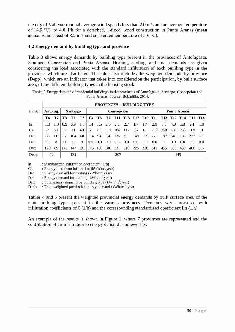
30 | P a g e

the city of Vallenar (annual average wind speeds less than 2.0 m/s and an average temperature

of 14.9 ºC), to 4.0 1/h for a detached, 1-floor, wood construction in Punta Arenas (mean

annual wind speed of 8.2 m/s and an average temperature of 5.9 °C).

4.2 Energy demand by building type and province

Table 3 shows energy demands by building type present in the provinces of Antofagasta,

Santiago, Concepción and Punta Arenas. Heating, cooling, and total demands are given

considering the load associated with the standard infiltration of each building type in the

province, which are also listed. The table also includes the weighted demands by province

(Depp), which are an indicator that takes into consideration the participation, by built surface

area, of the different building types in the housing stock.

Table: 3 Energy demand of residential buildings in the provinces of Antofagasta, Santiago, Concepción and

Punta Arenas. Source: Bobadilla, 2014.

Parám.

PROVINCES - BUILDING TYPE

Antofag. Santiago Concepción Punta Arenas

T6 T7 T3 T6 T7 T3 T6 T7 T11 T13 T17 T19 T11 T13 T12 T14 T17 T18

ln 1.3 1.0 0.9 0.9 1.6 1.4 1.5 2.6 2.3 2.7 1.7 1.4 2.9 3.3 4.0 3.3 2.1 1.0

Cei 24 22 37 31 63 61 66 112 106 117 75 61 238 258 336 256 169 81

Dec 86 60 97 104 60 114 94 74 125 93 149 175 273 197 248 183 237 226

Der 9 8 11 12 9 0.0 0.0 0.0 0.0 0.0 0.0 0.0 0.0 0.0 0.0 0.0 0.0 0.0

Dett 120 89 145 147 131 175 160 186 231 210 225 236 511 455 585 439 406 307

Depp 92 134 207 449

ln : Standardized infiltration coefficient (1/h)

Cei : Energy load from infiltration (kWh/m2.year)

Dec : Energy demand for heating (kWh/m2.year)

Der : Energy demand for cooling (kWh/m2.year)

Dett : Total energy demand by building type (kWh/m2.year)

Depp : Total weighted provincial energy demand (kWh/m 2.year)

Tables 4 and 5 present the weighted provincial energy demands by built surface area, of the

main building types present in the various provinces. Demands were measured with

infiltration coefficients of 0 (1/h) and the corresponding standardized coefficient Ln (1/h).

An example of the results is shown in Figure 1, where 7 provinces are represented and the

contribution of air infiltration to energy demand is noteworthy.

31 | P a g e

Figure: 1 Weighted energy demands by provincial capital with energy load from infiltration.

Source: Bobadilla, 2014.

Cei : Energy load from infiltration (kWh/m

2.year)

These tables were used to create the provincial map of energy demands for the thermal

conditioning of housing stock with 2011 building permits in Chile. At this level, the

predominance of heating needs in residential buildings in Chile can be observed. In 21 of the

54 provinces only heating needs are reported. 31 provinces present combined heating and

cooling demands. In 18 of these, cooling demands do not exceed 15 kWh/m². year; in 2 they

do not exceed 28 kWh/m².year; and in 2 there are only cooling requirements. These are

mostly concentrated in the provinces in the north and some in the center of the country,

including Santiago.

Heating requirements are present in virtually the entire nation, mainly in the Andean area and

center south of the country. In 45 of the 54 provinces, the demand exceeds 100 kWh/m².year;

in 15 provinces it exceeds 200 kWh/m².year; and in 4 provinces it exceeds 400 kWh/m².year.

These are all indicators that reflect a low level of energy quality in the new building stock in

Chile.

The energy load due to air infiltration varies significantly and has a different impact

depending on the type of energy demand. In the provinces with predominant heating needs

(Only heating is required or cooling demand does not exceed 10% of heating.), infiltration

means demands of between 23 and 203 kWh/m².year, which may represent between 20 and

50% of the total energy demand for thermal conditioning.

32 | P a g e

Table: 4 Weighted energy demands by provincial capital - North and Center. Source: Bobadilla, 2014.

Zone Province Deto ln Detp Decp Derp Cei

17°35’S

N

O

R

T

H

31°46’S

Arica 19 1,3 21 0 21 -3

Putre 135 1.5 209 209 0 74

Iquique 21 1.2 28 20 9 7

Pozo Almonte 297 1.5 378 367 10 81

Tocopilla 12 0.9 11 0 11 -1

Calama 137 2.8 269 259 9 132

Antofagasta 70 1.0 93 79 14 23

Chañaral 54 1.0 60 49 11 6

Copiapó 75 1.7 104 76 28 29

Vallenar 74 0.7 92 81 11 18

Coquimbo 91 1.4 133 122 11 42

Ovalle 79 1.5 113 93 20 34

Illapel 127 0.7 168 143 26 41

32°15’S

C

E

N

T

E

R

38°20’S

La Ligua 90 1.1 124 100 23 34

Los Andes 74 1.9 138 116 22 64

San Felipe 109 1.3 152 119 33 43

Quillota 113 0.9 151 133 18 38

Valparaíso 53 2.2 111 111 0 58

San Antonio 73 2.1 119 119 0 46

Hanga Roa 34 1.0 35 1 33 1

Quilpué 51 1.5 110 110 0 59

Colina 106 0.9 140 124 16 34

Santiago 77 1.5 133 119 14 56

Puente Alto 103 0.8 134 117 17 31

San Bernardo 98 0.9 148 134 14 50

Melipilla 109 0.9 130 109 21 21

Talagante 114 1.1 160 149 10 46

Rancagua 92 0.9 113 103 10 80

San Fernando 109 0.9 137 126 11 94

Pichilemu 78 1.0 96 96 0 23

Curicó 106 1.0 141 132 9 33

Talca 87 1.1 129 112 17 131

Linares 111 0.7 133 123 9 22

Cauquenes 99 1.6 159 143 16 60

Chillán 89 1.3 142 133 9 53

Los Ángeles 91 1.2 150 136 14 59

Concepción 73 1.7 180 180 0 107

Lebu 79 2.3 197 197 0 118

Det0 : Total provincial energy demand without infiltration (kWh/m 2.year)


Detp : Total energy demand with standardized provincial infiltration (kWh/m 2.year)

Decp : Provincial energy demand for heating (kWh/m2.year)

Derp : Provincial energy demand for cooling (kWh/m2.year)

Cei : Energy load from Infiltration (kWh/m2.year)

33 | P a g e

Table: 5 Table: 6 Weighted energy demands by provincial capital - South and Austral. Source: Bobadilla, 2014.

Zone Province Deto In Detp Decp Derp Cei

37°40’S

S

O

U

T

H

43°37’S

Angol 75 1.2 110 104 6 35

Temuco 155 0.8 202 202 0 47

Valdivia 117 1.0 171 170 0 54

La Unión 108 1.0 154 154 0 46

Osorno 137 1.1 195 195 0 58

Puerto Montt 137 1.3 192 192 0 55

Castro 145 1.2 207 199 7 62

Chaitén 155 1.0 201 201 0 46

44°45’S

A

U

S

T

R

A

L

54°56’S

Coyhaique 181 1.5 264 264 0 83

Puerto Aysén 161 1.6 260 260 0 99

Chile Chico 187 2.9 364 364 0 177

Cochrane 117 2.7 227 227 0 110

Puerto Natales 221 1.7 325 325 0 104

Punta Arenas 213 2.8 446 446 0 233

Porvenir 199 1.2 277 277 0 78

Puerto

Williams 281 2.1 484 484 0 203

Det0 : Total provincial energy demand without infiltration (kWh/m 2.year)


Detp : Total energy demand with standardized provincial infiltration (kWh/m2.year)

Decp : Provincial energy demand for heating (kWh/m2.year)

Derp : Provincial energy demand for cooling (kWh/m2.year)

Cei : Energy load from infiltration (kWh/m2.year)

An analysis at the level of building type by province shows more significant differences,

given that the average values hide the marked dispersions observed in those provinces where

construction systems with very different airtightness properties coexist.

The localities that demand the most energy are: Puerto Williams, Punta Arenas, Puerto

Natales, Chile Chico and Pozo Almonte, all of which have weighted provincial demands

greater than 325 kWh/m².year. In contrast, the localities with the least energy demand are:

Arica, Iquique and Tocopilla, with values below 28 kWh/m².year, corresponding to only

cooling demands. In the provinces where cooling needs predominate (Only cooling is

required or heating demand does not exceed 10% of cooling.), in 4 of the 54 provinces of

Chile, infiltration helps to reduce energy use.

Dwellings located in localities in the Andean zone, which runs from the north to the south of

the country, present demands above 200 kWh/m².year. These are high but expected

considering the harsh climate of this area and the typically low levels of thermal protection in

the buildings in this territory. From north to south in inland areas, progressive demands can be

observed in general terms, ranging from a bit more than 10 KWh/m².year in Arica and

Tocopilla (cooling), up to more than 400 KWh/m².year in Punta Arenas and Puerto Williams

(heating), which are explained in the same way.

5 CONCLUSIONS

Improving the airtightness of housing is an issue that concerns the Chilean state. Building

ordinances do not currently include any requirement to limit infiltration and its associated

energy loads. This situation affects the energy and environmental performance of housing,

and has economic and social consequences of great importance for inhabitants and the State.

34 | P a g e

In the current state of development, an important step in the energy improvement of the

building stock in Chile is, necessarily, to improve its airtightness characteristics. The baseline

of airtightness in buildings completed between the years 2007 and 2010 is 12.9 1/h, with

expected values between 11.1 and 14.7 1/h with 95% confidence. This is an overall measure

of the current techniques used and quality associated with sealing and airtightness of

residential buildings in Chile. Especially critical is the standard of airtightness in timber

construction, which has indices around 24.6 1/h. All of these indicate the absence or deficient

use of sealing techniques, as well as poor implementation quality, which should be improved

in Chile to ensure the acceptable energy performance of all building types constructed in

Chile.

The standardized coefficients of infiltration range from 0.7 to 2.9 1/h throughout the nation.

The lowest values are associated with inland locations, mainly in the north central area of the

country, some of which have micro-climates, that are compatible with low average wind

speeds and/or relatively high average exterior temperatures. Meanwhile, the highest

standardized coefficients of infiltration are associated with coastal localities, mainly in the

southern and austral areas, with wind speeds over 2.5 m/s and/or low average exterior

temperatures.

The results of the dynamic simulations show that energy loads due to infiltration in Chile vary

significantly and impact in different ways depending on the type of energy demand. In

particular, in the sectors with predominant heating needs, air infiltration generates demands of

between 23 and 203 kWh/m².year, and can represent between 20 and 50% of the total energy

demand for heating and cooling.

All regulation that seeks to organize and regulate construction should be based on actual

physical data so that its dictates are effectively feasible. For these purposes, this research

delivers important references in order to understand and reduce gaps in quality in terms of

sealing and airtightness of buildings in Chile, and criteria for the establishment of airtightness

requirements, an undertaking that is currently in progress in Chile.

6 ACKNOWLEDGMENTS

The authors wish to thank CONICYT for funding this initiative, and the entities DITEC, the

Department of Architecture at the Chilean Ministry of Public Works, the Chilean Energy

Efficiency Agency at the Ministry of Energy; and the companies Pocuro S.A., Venteko S.A.,

Indalum S.A., Alcorp S.A., and Wintec S.A. for their support and cooperation.

7 REFERENCES

CITEC UBB & DECON UC (2010). FONDEF D10I1025 Establecimiento de clases de

infiltración aceptable de edificios para Chile. XVIII Concurso de Proyectos de

Investigación y Desarrollo. Santiago, Chile.

Liddament, M. (1996). A Guide to Energy Efficient Ventilation. Brussels, Belgium: Air

Infiltration and Ventilation Center.

35 | P a g e

Bobadilla, A. (2014). Energy and Indoor Environmental Quality of Residential Construction

in Chile. Analysis of the trends, achievements and pending challenges. Université

catholique de Louvain, Louvain-la-Neuve, Belgium.

Damico, F. C., Alvarado, R. G., Bruscato, U., Kelly, M. T., Oyola, O. E., & Diaz, M. (2012).

Análisis energético de las viviendas del centro-sur de Chile. Arquitetura Revista, 8(1),

62–75. doi:10.4013/arq.2012.81.07.

Escorcia, O., García, R., Trebilcock, M., Celis, F., & Miotto, U. (2012). Mejoramientos de

envolvente para la eficiencia energética de viviendas en el centro-sur de Chile.

Informes de la Construcción, 64(000). doi:10.3989/ic.11.143.

Bobadilla, A., Figueroa, R., Díaz, M., Vargas, G., Arriagada, R., Espinoza, R. (in press)

(2014). Establecimiento de línea base de infiltraciones de aire para la limitación de la

demanda energética en edificios residenciales existentes. El caso de Chile. Informes

de la Construcción.

Figueroa, R., Bobadilla, A., Besser, D., Días, M., Arriegada, R., & Espinoza, R. (2013) Air

infiltration in Chilean housing: A baseline determination. 29th Conference,

Sustainable Architecture for a Renewable Future PLEA2013, Munich, Germany.

Ossio, F, De Herde, A, & Veas, L. (2012). Exigencias europeas para infiltraciones de aire:

Lecciones para Chile. Revista de la Construcción, 11(1), 54-63.

ASHRAE. (2004). Air Leakage performance for Detached Single‐Family Residential

Buildings. ANSI/ASHRAE Standard 119‐1988 (RA 2004). Atlanta, USA.

CITEC UBB & DECON UC. (2013). Informe Hito 3: Clases de infiltraciones aceptables.

FONDEF D10I1025 “Establecimiento de clases de infiltración aceptable de edificios

para Chile”. CONICYT, Chile

Comité Europeo de Normalización, (2010). UNE-EN 13829: Aislamiento térmico.

Determinación de la estanquidad al aire en edificios. Método de presurización por

medio de ventilador. Madrid, España.

Hampton Jentsch M.F., James P.A.B., Bourikas L. and Bahaj A.S. (2013) Transforming

existing weather data for worldwide locations to enable energy and building

performance simulation under future climates, Renewable Energy, Volume 55, pp

514-524.

González, A., & Díaz, M. (2013). Función e impacto del archivo climático sobre las

simulaciones de demanda energética. Hábitat Sustentable, 3(2), 75–85.

Sherman, M., & Modera, M. (1986). Comparison of measured and predicted infiltration using

the lbl infiltration model. Measured Air Leakage of Buildings, ASTM STP 904 (págs.

325-347). Philadelphia: American Society for Testing and Materials.

36 | P a g e

AIRTIGHTNESS IMPROVEMENT OF STRUCTURES

TO IMPROVE INDOOR AIR QUALITY

Katariina Laine *2

2 Vahanen Oy

Building Physics Specialist Services

Linnoitustie 5

02600 Espoo, Finland


ABSTRACT

The aim of improving air tightness of structures is to prevent the uncontrolled air leakages through structures. Built environments contain microbes, particulate and gaseous impurities but removing them is not always

necessary. For example, an ageing building envelope commonly contains microbial impurities even when there

is no obvious moisture damage. Air leaks convey impurities to indoors where they can lead to poor indoor air

quality and associated health problems. Air leaks have also negative impact to energy efficiency and living

comfort.

An air tight building envelope prevents air leaks through the envelope structure. Common air leakage places are

the joints of structures, i.e. the joint of ground slab and external wall and untight inlets of the envelope. The

joints of the structures are typically not air tight without detailed planning. In Finland an air tight building

envelope is taken into account in the building regulations and therefore airtightness is relatively good in the new

construction. In the existing buildings improving airtightness of structures is a relatively new concept. It can be

used in a combination with other renovation methods to solve indoor air quality problems in buildings. In

Finland several techniques have been implemented in order to prevent uncontrolled air flux through the

structures since 1980’s. In practise the air tightness renovation method has been successful in indoor air quality

problems in buildings.

The main principle of moisture or microbial damage renovation is that before installing new building materials

all moisture or microbially damaged materials are removed and the source of the problem is identified and fixed.

However, in practise it is often impossible to remove all impurities and therefore improving airtightness of the

new structure has an important role in completing a successful renovation. Improving of airtightness must be

applied on to the whole building envelope. Air tightening renovation is never a single renovation action but

always a part of other action. The air tightening material must be elastic, safe and long lasting and tested for its

purpose. Improving airtightness requires planning, accurate execution on the construction site and supervision.

Quality control measurements are in a key role to success. Quality control measurements are done visually and

with the trace-gas leak test. It is very important always adjust the ventilation system to match the changed

pressure difference.

In Finland there are no guidelines for planning, execution or supervising air tightness renovation method. It is

planned to start certification training and publish first guideline in 2014.

KEYWORDS

Improving air tightness, air leakages, microbial damages, indoor air quality, repair method

37 | P a g e

1 INTRODUCTION

Poor indoor air quality associated problems can have a major impact on occupant health and

comfort. Indoor air quality problems in western countries in homes, schools and offices are

often caused by complex, inter-related issues. The problems can be caused i.e. by moisture

damages, microbial damages, harmful substances, radon or other impurities. In external

envelope structures and in the soil under building’s ground slab there are almost always some

microbial based impurities and radon which can affect negatively to the indoor air quality

when transported with the air flux into the room.

Structure’s joints are not automatically completely tight and therefore their implementation

requires detailed planning. Common air leakage places are the joints of structures, i.e. the

joint of ground slab and external wall and untight inlets of the envelope. There is usually air

flow from outside to inside the building caused by the building’s pressure ratio. The

building’s pressure ratio is determined by interaction of wind, chimney effect and ventilation

as well as the usage of the premises. The pressure ratio will vary and can change very fast and

strongly. As a result the air flows from one room to another, between floors or through

envelope structures. The air flow conveys heat, moisture and impurities such as particles,

mineral wool fibres, microbial and gaseous impurities, radon and other harmful substances.

The aim to improve air tightness of structures is to prevent the uncontrolled air leakages

through structures. Methods used to improve the air tightness in structural renovation are

called air tightness renovation. Using air tightness renovation energy consumption can be

decreased, moisture convection can be prevented and uncontrolled air leakages through

structures, junctions and inlets are cut off. The poor indoor air quality associated problems

can be decreased and prevented with airtight structures. In Finland, improving airtightness of

structures has long been a stabilized renovation method for prevention of radon. In practise air

tightness renovation method as part of a larger entity has successfully solved the indoor air

quality problems in buildings.

Air tightness factor has been taken into consideration in the National Building Code of

Finland and in the regulations of new building. In the existing buildings improving

airtightness of structures is a relatively new concept. Practice has shown that the air tightness

renovation as its own is not sufficient but requires other actions to solve the problems. An air

tightness renovation can fail due inadequate planning, careless implementation or lack of

quality control at the construction site. Additionally some structures might have been air

tightened where it is not a suitable method. Lack of understanding structures building physical

functionality has even caused further damages. In Finland the experts working with the indoor

air quality problems have different opinions regarding using the air tightness renovation

method, its effect in the indoor air quality, its durability and its effect to the life cycle costs for

buildings. Therefore several projects have been started to develop common procedures and

guidelines this year.

Demolishing and building new is one option to solve an indoor air quality problem, when the

structure is at the end of its lifecycle. In some cases demolishing and building new might be

economically better option than renovating old. Demolishing and building new is not always

possible for economic reasons. In old protected buildings demolishing is often not permitted.

In some cases to remove a small quantity of impurities would require unreasonable

demolishing actions. In old buildings it is not possible to remove all risk structures or

contaminated materials. It is a fact, that built environments contain microbes, particulate and

gaseous impurities but removing them is not always necessary. For example, an ageing

38 | P a g e

building envelope commonly contains microbial impurities even when there is no obvious

moisture damage. The impurities are simply conveyed from outdoor and from soil under the

building. As it is not always possible to demolish and build new structures, optional

renovation methods are needed, i.e. air tightness renovation. There is also need for more

solutions to solve indoor air quality problems.

2 AIR TIGHTNESS OF STRUCTURES IN RADON PREVENTION

Radon is odourless, colourless, harmful and dangerous gas. Harmful quantities should not be

released into living spaces. In the National Building Code of Finland it is stated that tight

uniform slab solution is safe in respect of radon. Air tightening of the joint between a ground-

supported slab and the enclosure wall is necessary, when the enclosure walls are constructed

separately. Additionally tightening of lead-ins is extremely important in all structural

solutions. A tight concrete structure not susceptible to cracking prevents the penetration of

radon through the structure. (Ministry of the Environment, 2004)

Radon prevention methods are e.g. air tightening of the ground slab and enclosure wall and

under pressure solutions of soil under the ground slab. In Finland, the air tightening method to

prevent radon has been used for decades and it is an established renovation method. The

oldest radon renovations with air tightness solutions have been done in the 1980’s. Radon is a

good indicator for successful air tightness renovation i.e. how much soil-borne air containing

radon leaks into the room spaces. Therefore radon measurements before and after the

renovation can be used in evaluating the success of the air tightness renovation in radon areas.

(Kettunen et. al, 1991)

The essential requirement for preventing radon by air tightening structures is that the air flow

paths are cut off totally not only partly. The implementation of air tightening has to be done

carefully. When the renovation has been planned, the work has been performed carefully with

quality controlling, can the radon containing air leaks into indoor air cut off totally. When the

air leakages are cut off, the only way radon can be conveyed through structure is by diffusion.

The impact of diffusion is irrelevant for indoor air quality. (Kettunen et. al, 1991)

2.1 Air tightness of external envelope structures in new buildings

The National Building Code of Finland for new buildings requires air tightness for external

envelope structures. The air tightness is usually done with vapour barrier which functions at

the same time as an air barrier. A massive concrete or brick structure can also function as a

vapour and air barrier structure. In an air tight building the supply air is not taken through air

leakage but controlled through supply air valves or through mechanical ventilation.

(Ympäristöministeriö, 1998, 2010, 2012a, 2012b)

According the National Building Code of Finland, in respect of functioning of the ventilation

system, moisture technical functionality, good indoor air quality and energy efficiency

reasons the air leakage value q50 for envelopes in new buildings should be not more than

1 m3/(h·m

2). However, it is allowed to be up to 4 m

3/(h·m

2), in some special cases even

higher. However a low air tightness value measured from the building does not guarantee

completely air tightness of the envelope structures. There can still be locally significant air

leakage points. Therefore careful tightening of joints and inlets is very important.

(Ympäristöministeriö, 2012b; RIL 107-2012)

39 | P a g e

Structure’s joints are not automatically completely tight and therefore the implementation

requires detailed planning. E.g. for ground floor concrete slab it is typical that after casting,

cracks will occur at the edges of the new concrete slab due shrinkage which is associated with

drying of concrete. Also cracks can occur at the corners and around pillars due to drying

shrinkage. Therefore in concrete structures’ joints there are without exception discontinuity

points for air leakage if the air tightness is not specifically planned. There is an example of air

tightening principle for the ground floor concrete slab in figure 1. The same principal is also

used in preventing radon.

Figure 1: Principal solutions for ground floor concrete slab and concrete wall or pillar joint air tightness

renovation with waterproofing mass system. Extract from a plan and photos from impletion at the site.

3 AIM FOR AIR TIGHTNESS OF STRUCTURES

3.1 Effects of air tightness on structure’s functionality Improving air tightness of envelope structure has a positive effect on the following factors:

1. Reduction of energy consumption

2. Prevention of moisture convection

3. Prevention of impurities entering through air leakage flows

Additionally an air tight envelope is a fundamental condition for a reliable and energy

efficient mechanical ventilation system. By improving air tightness the living comfort can be

improved as the feeling of draft is decreased and the temperatures of inner surface will

increase. (Vinha, 2014)

Improving air tightness of envelope structure has a negative effect on the following factors:

1. Air flows drying the envelope structure will decrease

2. The natural moisture of new construction materials e.g. concrete dries more slowly.

However not all air flows through structures have a drying effect. The relative moisture

content of soil’s porosity is almost 100 % RH and therefore the air flows through ground slab

do not dry the structures. In general, the structures should not be tightened without survey,

planning and supervision. The building physical behaviour of the tightened structure must

always be evaluated prior to the actual renovation.

New low energy construction concepts are challenging especially regarding thick insulation

layers and drying of structures. The significance of water vapour and air tightness of inner

surface of external envelope will increase. The moisture obtained during construction time

dries out more slowly in thicker insulation layers in the absence of air flows through

40 | P a g e

structures. This sets tighter requirements for the site moisture management and weather

protection. In some cases the structures need to be dried during installation.

Reduction of energy consumption. The actual effect of air leaks on energy consumption

depends on e.g. air leak distribution and pressure differential over the envelope structure. Air

flow through structures reduces thermal insulation and cools the structures. Improving air

tightness with current heat insulation material thicknesses is a one of the most significant and

inexpensive means to reduce energy consumption in modern, already energy efficient

buildings. However, the usage of buildings and the habits of the residents have an effect on

energy consumption. E.g. window ventilation can increase significantly the need for heating

energy in otherwise air tight building. (Vinha, 2014)

Prevention of moisture convection. Air leakages may carry significant amount of water

vapour into the building envelope. Moisture damages can occur, when the moisture

condensates on the cool surfaces. Moisture provides favourable condition for local microbial

growth inside the structures. Harmful moisture convection will decrease when the inner layer

of the envelope structures are air tight. Also cooling of the surfaces due to cold air leaks will

cause condensation risk which can be controlled by preventing air flows through structures.

Prevention of flow of impurities and its effect on the indoor air quality. There are several

factors influencing the indoor air quality. Physical factors, chemical and microbiological

impurities, concentration of particles and fibres can be examined using different measurement

methods and results can be verified against guidelines in the literature in order to get objective

results. Indoor air quality is experienced by each individual subjectively and is affected by

individual differences and physiological factors. (Sosiaali- ja terveysministeriö, 2003)

The impurities have a negative effect on the indoor air quality. With air flow through leakages

microbial impurities, particles, radon and chemical impurities or other harmful substances can

be conveyed into indoor air. Also noise and smell from smoke or food can enter indoor. By

air tightness renovation, the inner surface of the structures is made airtight so that the air

leakages are cut off. The air tightness of structures will also improve fire safety by slowing

the spreading of flue gases. In general, air tightness of inner shell structure has a positive

effect to indoor air quality. (Sosiaali- ja terveysministeriö, 2003)

Studies related to air tightness renovation has been done relatively few. In general it is known

that with air tightness renovation the impurities entering through air leakages can be

prevented and the flow of gaseous impurities will be slowed down. It is not known, what kind

of concentration of impurities can be conveyed with air flow. The speed and significance of

microbial transportation through materials with diffusion is also unknown. There are no

health based limits to evaluate the significance of microbial based exposure. Generally it can

be estimated that air leakages convey more significant concentration of impurities than

diffusion. The importance of the air tightness of the structures of the indoor air quality is not

specific determined. There is a need for some research.

4 PLANNING OF AIR TIGHTNESS RENOVATION

4.1 Air tightness testing methods in existing buildings

Before planning for air tightness renovation and implementation on site, the required actual

data has to be collected. The locations of the air leaks in structures can be clarified accurately

with tracer-gas leak testing method. In the test the tracer gas is led into the tested structure

41 | P a g e

from where gas leaks along with the air flux into the direction of under pressurized room. In

the room the trace gas is detected and the leakage points are located with tracer gas analyser.

The air tightness of building envelope structures can be evaluated from architectural and

structural drawings showing the implementation method and materials used. The

discontinuity points in structure such as gaps and cracks can be found by visual inspection

during site inspection. by opening structures e.g. by removing skirting and window trims, the

implementation method of joints can be evaluated. Air movement near joints can be observed

by sensory smoke gas. Thermal leakages and some air leakages can be detected with an infra-

red camera.

4.2 Principles in planning improving air tightness renovation

When renovating an existing building the aim is principally to achieve the same air tightness

as it should have had originally. Renovations are always compromises between technical and

building history point of view and e.g. the protection degree of the building may have an

effect on the renovation method. When planning an air tightness renovation, the air tightness

of the whole envelope structure should be taken into consideration. Air tightness renovations

implemented on individual structures or premises do neither significantly improve the air

tightness of the building nor decrease the impurities in the indoor air.

Air tightness renovations are not suitable for all structures. In general, the structures

should not be tightened without survey, planning, supervision of renovation and control. The

building physical behaviour of the tightened structure must always be evaluated prior to the

actual renovation. Structures with microbial or moisture damage should not be tightened.

Damage is removed from the structure and the cause of the damage is fixed.

Improving air tightness is not a sufficient method for blocking all harmful substances from

entering indoor air. E.g. for petroleum hydrocarbons other actions need to be used. When

removing of harmful substances is not possible, encapsulation renovation can be used.

Encapsulation is a renovation method that aims at preventing the entrance of harmful

substances or other impurities from entering into the indoor air both with convection and

diffusion. Products used in encapsulation of harmful substances prevent or slow the diffusion

of gases.

Air tightness renovation requires structural engineering designing. The designing of air

tightness renovation is always done case by case and should not be applied directly on other

sites. The renovation designing requires expertise and knowledge of material and methods

used. Building’s thermal and moisture technical functionality, which can change after

implementation of renovation, has to be taken into consideration. If there is a danger that after

tightening the moisture content might increase detrimentally in moisture sensitive structures,

tightening should not be done. The drying ability of the structure should be taken into

consideration in renovation especially for external wall structures so that there is a functional

ventilation gap.

Air tightening renovation should never be the only renovation action but always a part

of a larger entity. When improving air tightness, at least the ventilation system should be

inspected and when required adjusted to correspond the changed pressure conditions. The

optimal pressure difference over the external envelope is after the indoor air renovation close

to 0 Pa. Controlled supply air should be taken into consideration. In moisture and microbe

damage renovation, the damaged materials are removed, problem is identified and fixed. The

42 | P a g e

structures are renovated so that they building physics properties stay correct. Implementation

should be long-lasting and reliable. (Ympäristöministeriö, 1997)

The methods and materials used in air tightness renovation are determined by

structural designer. The materials or methods determined in the designs cannot be changed

without prior approval from the designer. The expected life expectation of the structure is

stated in the designs. The structural engineering designs consist of work plans and required

drawing with necessary details of implementation method of the renovation. The extension of

dismantling, its implementation and preparation of the surface is determined in the designs.

Preparation of the surface requires typically the removal of the surface material because old

finishes seldom provide a solid enough surface for a good attachment of the sealing material.

The surface should be even enough, strong and clean from any dirt or dust or any other factors

reducing adhering.

5 MATERIALS USED IN AIR TIGHTNESS RENOVATION

In Finland, there are presently no requirements by the authorities for the materials used in air

tightness renovation. The materials used should however, fill several requirements for the

purpose. The products should have sufficient adhesive and elasticity, long-term durability and

airtightness for the purposed use. When large surfaces are treated, the designer should pay

special attention on material emissions and on their effect on indoor air quality. In Finland,

building materials with air permeability max 1·10-6

m3/(m

2·s·Pa) are considered as air

barriers. E.g. sealing strip, sealant, polyurethane foams, butyl or other special tape or special

adhesive tape can be used for improving the air tightness of structures. When using a sealant,

polyurethane foam or special tape it should be verified that the tightening is made using a

broad enough adhesive area. The air tightness of the structure can also be improved with

material combinations. A common method is to use a liquid spreadable waterproof mass

system. Liquid waterproofing barriers have an estimated life span of 40 years. An air tight

system installed onto brickwork consists of tight filler, glass fibre mesh and a surface

treatment e.g. special paint. Air tight building materials include also several coatings and

epoxy primers. Also tight building boards such as gypsum board with carefully sealed seams

can function as a part of air barrier in the structure.

6 IMPLEMENTATION OF AIR TIGHTNESS RENOVATION ON SITE

Careful implementation of the work is detrimental for the success of renovation. The technical

implementation of the air tightness renovation is confirmed on site with appropriate quality

control methods. Quality control methods for the assessment of the technical implementation

of renovation are determined in the design documents. Control methods include supervision,

implementation and evaluation of models and measuring the air tightness with tracer-gas leak

test. Model works of different structures to be tightened are important for the success of the

implementation. The quality control of air tightness renovation is done on site before

installing the surface structures. The quality control investigation is documented. At the

moment there are no official qualification requirements for the workers or for the quality

controlling. Certification training in planned to for people doing renovation work and

supervision in autumn 2014.

6.1 Quality control with tracer-gas leak testing method

In the trace-gas leak testing method the tracer gas is led into the tested structure from where

gas leaks along with the air flux into the direction of under pressurized room. In the room the

trace gas is detected and the leaking points are located with tracer gas analyser. A constant

43 | P a g e

negative pressure of 10…15 Pa over the examined structure should be maintained (in the

testing room) to obtain comparable results. The negative pressure condition is implemented

with a mechanical exhaust ventilator machine. Prior to testing the pressure differences of

structure to the room should be verified by measurement. The stability of the prevailing under

pressure is recommended to be verified by repeated measurement during the tracer gas

testing.

Leakage points are detected with tracer gas analyser and the results are interpreted

qualitatively. The conclusion is simple: there is ‘’either leakage’’ or ‘’no leakage’’. The

concentration of tracer gas in the structure is not known. Therefore the qualification of the

investigator is very important. The detected leak points are marked and the tightness is

improved with a suitable method. The tracer-gas leak test should be repeated until all leak

points have been eliminated. A quality control report should be issued where the detected leak

points are marked e.g. to the layout. Figure 2 explains the quality control assessment of air

tightness renovation using tracer-gas leak test.

Figure 2: Air tightness renovation of concrete ground slab is done with waterproofing mass system. The tracer-

gas leak test is done as part of quality control. In the picture on the right hand, in the test found leakages are

marked with an orange tape, so they can be fixed.

7 SUCCESS OF AIR TIGHTNESS RENOVATION AND ITS DURABILITY

7.1 Evaluating the success of the (air tightness) renovation

The evaluation of the success of the renovation is based on user’s subjective experience of

condition in the premises and objective measurements to evaluate the technical success of

renovation. The success is evaluated by visual inspection, different types of measurements as

well as with user questionnaires. The process is defined in the quality control plan. The

measurements are verified against guidelines in the literature in order to get objective results.

Because air tightness renovation should never be the only renovation action but always a part

of other action, the success of the whole renovation should be evaluated. For example, if the

air tightness is done well but the final cleaning has been neglected or the ventilation system

does not work as planned, it is obvious that the user experiences that indoor air quality

problem is not solved. Feedback is often a good measure for evaluating the success of

renovation.

The most important evaluation methods are:

44 | P a g e

feedback from users and user questionnaires prior and after renovation

control measurements of structure’s air tightness (trace-gas leak test)

inspection of ventilation system’s functionality

inspection of cleaning level

measurement of indoor air factors (temperature, humidity, carbon dioxide, pressure)

measurements of indoor air’s chemical and microbiology concentration, if needed.

In practise evaluations after renovation have been done in individual buildings and the

structures have been found as air tight as during quality control on-site. However, practise has

also shown, that even the most carefully executed renovation and mould dust cleaning is not

enough for the most sensitive people and their symptoms return after returning to the

premises.

8 CONCLUSIONS

The National Building Code of Finland for new buildings requires air tightness for external

envelope structures. The air tightness is done with vapour barrier or with an air barrier.

Structure’s joints are not automatically completely tight and therefore the implementation

requires detailed planning. In external envelope structures and in the soil under building’s

ground slab there are almost always some microbial based impurities and radon which can

affect negatively to the indoor air quality when transported with the air flux into the room.

The impurities can lead to poor indoor air quality associated problems. The aim to improve air

tightness of structures is to prevent the uncontrolled air leakages through structures. It is a

relatively new renovation method and therefore renovation designing requires expertise and

knowledge of material and methods used. Research studies related to air tightness renovation

has been done relatively few. Some research still needs to be done.

Air tightness renovation is not suitable for all structures. In general, structures should never be

tightened without inspection, planning and supervision. Structures with microbial or moisture

damage should not be tightened. Air tightening renovation should never be the only

renovation action but always a part of a lager entity. When improving air tightness, at least the

ventilation system should be inspected and when required adjusted to correspond the changed

pressure conditions. Careful implementation of the work is detrimental to the success of

renovation. The essential requirement for preventing air leakages is that the air flow paths are

cut off totally not only partly. The technical implementation of the air tightness renovation is

confirmed on site with appropriate quality control methods i.e. addition to visual inspection

the tightness is tested with tracer-gas leak testing method.

In practise air tightness renovation as part of a larger entity has successfully solved the indoor

air quality problems in buildings. In Finland the air tightness renovation method to prevent

radon is an established renovation method and it has been used for decades. Air tightness

renovation has been used to solve microbial based indoor air quality problems about 15 years.

The materials used should fill several requirements for the purpose. In practise evaluations

after renovation have been done in individual buildings and the structures have been found as

air tight as during quality control on-site. The air tightness renovation can be one solution to

solve poor indoor air quality problems.

45 | P a g e

9 REFERENCES

Kettunen, A-V., Slunga E., Viljanen, M. (1991). Radonin merkitys talonrakennustekniikassa.

Radonsuunnitteluohje normaalin radonluokan alueille. Julkaisu/Report 114. Teknillinen

korkeakoulu, Rakennetekniikan laitos. 1991. Espoo.

Ministry of the Environment (2004). National Building Code of Finland. B3 Foundations.

Regulations and Guidelines 2004. Helsinki.

Rakennusinsinöörien Liitto RIL ry. (2012). RIL 107-2012 Rakennusten veden- ja

kosteudeneristysohjeet. Helsinki.

Sosiaali- ja terveysministeriö. (2003). Asumisterveysohje 2003:1. Asuntojen ja muiden

oleskelutilojen fysikaaliset, kemialliset ja mikrobiologiset tekijät. Sosiaali- ja

terveysministeriön oppaita.

Vinha, J. (2014). Rakennusten rakennusfysikaalisen suunnittelun ja toteutuksen periaatteet.

Tampereen Teknillinen yliopisto, Rakennustekniikan laitos. Rakentajain kalenteri 2014.

s.351-373.

Ympäristöministeriö. (1997). Ympäristöopas 29. Kosteus- ja homevaurioituneen rakennuksen

korjaus. Tampere.

Ympäristöministeriö. (1998). Suomen Rakentamismääräyskokoelma, osa C2 Kosteus,

määräykset ja ohjeet 1998. Helsinki.

Ympäristöministeriö. (2010). Suomen Rakentamismääräyskokoelma, osa C3, Rakennusten

lämmöneristys 2010, Määräykset. Helsinki.

Ympäristöministeriö. (2012a). Suomen Rakentamismääräyskokoelma, osa D2, Rakennusten

sisäilmasto ja ilmanvaihto. Määräykset ja ohjeet 2012. Helsinki.

Ympäristöministeriö. (2012b). Suomen Rakentamismääräyskokoelma, osa D3, Rakennusten

energiatehokkuus. Määräykset ja ohjeet 2012.Helsinki.

46 | P a g e

DEMAND CONTROLLED VENTILATION IN

RENOVATED BUILDINGS WITH REUSE OF

EXISTING DUCTWORK Mads Mysen

*1, Kari Sørnes

1

1 SINTEF Building and Infrastructure

Forskningsveien 3B

NO-0314, Oslo, NORWAY


ABSTRACT

Most existing non-residential buildings have Constant Air Volume (CAV) ventilation leading to over-ventilation

in periods with low or no occupancy. Demand controlled ventilation (DCV) can considerably reduce the

ventilation airflow rate and energy use for fans, heating and cooling compared to constant air volume (CAV)

ventilation. There is a potentially enormous upcoming marked for converting from CAV to efficient DCV in

existing commercial buildings.

Conversion from CAV to DCV with reuse of existing ductworks, was one of several energy measures carried out

in Solbraaveien 23, a Norwegian office building. The building was originally built in the early eighties and is

considered to be representative for a large number of buildings in need for an upgrade. Total delivered energy

use was reduced from 250 kWh/m2 to 80 kWh/m

2, and the indoor environment was improved.

Reuse of existing ductworks was very profitable. The ductwork cost in Solbraaveien 23 was roughly cut in half

compared to the alternative which was demolition and new ductwork installation.

Based on the experiences from Solbraaveien 23, it is specified a step by step procedure for reuse of existing

ductwork that can be used in all projects where such reuse is considered.

The following success criteria are identified for the successful conversion from CAV to DCV with reuse of

existing ductwork:

• Can the original system partition be reused?

• Do shafts have sufficient capacity and availability?

• Does the ductwork have sufficient access and quality?

• Are there any visible corrosion?

• Are there risks for any duct parts with asbestos?

• Is the ductwork sufficiently airtight?

• Are the drawings up to date and easily accessible?

KEYWORDS

CAV, DCV, Reuse, Ductwork, Energy

1 INTRODUCTION

IEA reports that CO2 emissions from buildings must be reduced from 50 MtCO2 in 2010 to 5

MtCO2 in 2050 in the Nordic countries to avoid severe problems of global warming (IEA &

Nordic energy research, 2013). A consequence for the building sector is that a widespread

47 | P a g e

conversion of buildings to very low energy consumption and even zero energy buildings is

necessary.

Demand controlled ventilation (DCV) can considerably reduce the ventilation airflow rate and

energy use for fans, heating and cooling compared to constant air volume (CAV) ventilation

(Maripuu, 2009) due to relatively low simultaneous occupancy in office buildings

(Halvarsson, 2012). The central ductwork-components will probably have more capacity in a

DCV-system than in a CAV-system because of limited simultaneous use. Hence, conversion

from CAV to DCV with reuse of existing ductwork could increase the system capacity and

actually solve a former capacity problem. There is a potentially huge upcoming marked for

converting from CAV to efficient DCV in existing commercial buildings (Mysen et. al.,

2011).

A Norwegian office building has been upgraded from CAV to DCV with reuse of existing

ductwork. This paper presents this upgrading to modern DCV (Mysen et. al., 2014)

2 DESCRIPTION OF SOLBRAAVEIEN 23

Solbraaveien (Figure 1) is an office building built early in the eighties. It is situated in the

municipality of Asker, close to Oslo.

Figure 1. Solbraaveien 23 before and after refurbishment.

It was originally built with CAV-ventilation with reports of annoying noise from the

ventilation system. The air inlet was below the windows, blowing upwards with room air

induction. Such air inlets are space consuming (Figure 2).

Figure 2. Left: Before retrofitting, the old air-inlets were space consuming. Right: After retrofitting.

48 | P a g e

The following main retrofit measures were carried out:

New air-handling-units

Conversion from CAV to DCV

The windows were changed, new U-value of 0,8 W/m2K

Additional insulation on walls and roof

Reduced leakage

Air-water heat pump

Total delivered energy use was reduced from 250 kWh/m2 before retrofitting to 80 kWh/m

2

after retrofitting and the indoor environment was improved (Mysen et. al., 2014).

3 RESULTS

3.1 Premises and procedure for re-use of existing ductwork

The procedure for re-use is developed by the entrepreneur (GK AS) and SINTEF in the R&D-

project UPGRADE Solutions (Mysen et. al., 2014). It is existing ductwork at the "user-side"

of the air-handling-unit that is of interest to re-use in upgraded DCV.

49 | P a g e

Not suitable

No

Suitable

No

A stepwise procedure is developed and shown in figure 3.

Figure 3. Stepwise procedure for re-use of duct-work.

3.2 DCV system solution

The ventilation system is upgraded with the use of variable supply air diffusers (VSAD). The

DCV-units (same as VAV-damper) are integrated in the air diffusers, making it espcially

suitable for upgrading to DCV. Figure 4 shows a schematic diagram where variable supply air

diffusers are regulated by a controller, and communication is performed via bus.

1. Collect drawings, leakage- and balancing

reports

2. Examine drawings. Might the

ductwork be suitable?

3. Explore in field. Might parts of the

ductwork be suitable for reuse?

Demolish

4. Outline the new ventilation system

Yes

5. Examine duct sizes. Are the existing

sizes OK?

6. Design of new ventilation system

7. Fitting of new ventilation ducts. Demolish not suitable parts.

10. Cleaning

8. Leakage test 9. Leakage sealing

Not passed

11. Commissioning

Passed

50 | P a g e

Figure 4.Schematic diagram with VASD regulated by a main controller.

The controller records the required airflow rate, the supplied airflow rate and the damper

angle for all the DVC-dampers, and regulates the fan speed such that one of the VSAD is in a

maximum open position opened on the supply side, and such that one of the DVC-damper is

in a maximum open position on the exhaust side. The integrated motor-driven damper makes

sure that the pressure remains in the working range of the VSADs. This damper should

normally remain in a maximum open position and only throttle if the pressure in the duct

becomes too high relatively to the working range of the VSADs. Such a situation can happen

in the branches closest to the fan in large ventilation systems.

VSAD is combined with overflowing arrangement from the offices to corridors and outlets

controlled by traditional VAV-dampers.

Table 1. New and re-used parts of the ventilation system after retrofitting.

Ductwork 90-95% is re-used

Air inlets New VSAD

Air outlets New, controlled by new

VAV-dampers

Air-handling-units (AHU) New

All ventilation-parts between

outside air and AHU (main

building air-intake and air

exhaust)

New

3.3 Investment costs for re-use versus new ductwork

Table 2 shows the estimated costs in Solbraaveien 23 compared with a new ductwork-

solution. Additional costs related to demolishing or fitting of new duct-work is roughly

estimated based on Norwegian prices and experiences from Solbraaveien which has a total net

area of 10.000 m2.

51 | P a g e

Table 2. Costs with reuse of ductwork compared with new ductwork.

Activity Total cost in

Solbraaveien (with

reuse)

[Euro/10.000 m2]

Total costs with new

ducts (traditional

solution)

[Euro/10.000 m2]

1. Collect drawings, leakage-

and balancing reports

1 250,-

2. Examine drawing. Might the

ductwork be suitable?

1 250,-

3. Explore in field. Might parts of the

ductwork be suitable for reuse?

1 250-13 000,-

4. Outline the new ventilation system No difference

5. Examine duct sizes. Are the existing

sizes OK?

2.500 – 6.000

6. Design of new ventilation system 0

7a. Demolish not suitable parts. 19 000,- 150 000 – 200 000,-

7b. Fitting of new ventilation ducts 50.000-62.500,- 400 000 - 500 000,-

8. Leakage test No difference

9. Leakage sealing 6.250

10. Cleaning 112.500 -225.000

11. Commissioning 0

12. Unforeseen costs

SUM 194 000 – 328 000 550 000 – 700 000

This rough estimate shows that reuse was a very profitable alternative to new ventilation

ductwork in Solbraaveien 23. Maximum additional cost for reuse was estimated to 40

Euro/m2, while the minimum alternative cost for demolishing and installation of new

ductwork was estimated to 70 Euro/m2. Reduction of the demolishing costs is an important

cause of the profitability.

4 DISCUSSION AND CONCLUSIONS

Conversion from CAV to DCV was one of several energy measures carried out in

Solbraaveien 23. Total delivered energy use was reduced from 250 kWh/m2 to 80 kWh/m

2,

and the indoor environment was improved.

Reuse of existing ductwork might require some compromises when it comes to normal

requirements for specific fan power, maximum air velocity, noise generation and leakage.

Before considering ductwork reuse, one has to clarify that the builder owner has a pragmatic

attitude towards such normal requirements.

Furthermore, one must clarify if the ductwork is suitable for reuse as early as possible in the

process. Based on the experiences from Solbraaveien 23, it is specified a step by step

procedure for reuse of existing ductwork that can be used in all projects where such reuse is

considered (Figure 3).

52 | P a g e

The following success criteria are identified for the successful conversion from CAV to DCV

with reuse of existing ductwork:

• Can the original system partition be reused?

• Do shafts have sufficient capacity and availability?

• Does the ductwork have sufficient access and quality?

• Are there any visible corrosion?

• Are there risks for any duct parts with asbestos?

• Is the ductwork sufficiently airtight?

• Are the drawings up to date and easily accessible?

Reuse of existing ductworks was very profitable in Solbraaveien 23. The ductwork cost was

roughly cut in half compared to the alternative which was demolition and new ductwork

installation. Reuse of the existing ductwork can potentially reduce the refurbishment period

and therefore reduce loss of rental income. This is not included in the economical

consideration.

5 ACKNOWLEDGEMENTS

This paper is funded by contributions from industry partners and public funding from the

Norwegian Research Council as part of the project “UPGRADE Solutions”.

6 REFERENCES

IEA & Nordic energy research (2013). Nordic Energy Technology Perspective. Paris/France,

OECD/IEA. www.IEA.org.

Maripuu, M.-L. (2009). Demand controlled Ventilation (DCV) systems in commercial

buildings: functional requirements on systems and components. Goteborg/Sweden.

School of Electrical and Computer Engineering. Chalmers tekniska högskola.

Halvarsson, J. (2012). Occupancy Pattern in Office Buildings - Consequences for HVAC

system design and operation. Trondheim/Norway. Doctoral Thesis, NTNU.

Mysen, M. Schild, P. Drangsholt, F. Larsen, B.T. (2011) Convertion from CAV to VAV - a

key to upgrade ventilation and reach energy targets in the existing building Stock.

Proceedings Roomvent 2011, Paper 142, ISBN: 978-82-519-2812-0, June 2011,

Trondheim/NORWAY.

Mysen, M. Aronsen, E. Johansen, B.S. (2014) Conversion to DCV with reuse of ductwork (In

Norwegian). Oslo/Norway. SINTEF Fag 15. SINTEF akademiske forlag. ISBN: 978-

82-536-1377-2.

53 | P a g e

REQUIREMENTS AND HAND-OVER

DOCUMENTATION FOR ENERGY-OPTIMAL

DEMAND-CONTROLLED VENTILATION

Mads Mysen*1, Axel Cablé

1, Peter G. Schild

1, and Kari Thunshelle

1


Forskningsveien 3B

NO-0314, Oslo, NORWAY


ABSTRACT

Demand controlled ventilation (DCV) considerably reduce the ventilation airflow rates and energy use compared

to Constant Air Volume (CAV) systems. DCV in commercial buildings is probably a prerequisite to achieve

ambitious energy-goal. However, evaluation of real energy use demonstrates that the energy saving potential is

seldom met. DCV-based ventilation systems must become more reliable to close the gap between theoretical and

real energy-performance. These unfortunate experiences with DCV have many causes, including: inadequate

specifications and hand-over documentation, balancing report not suitable for DCV, communication errors and

lack of knowledge about DCV-systems among decision makers.

There is also a significant difference in performance between DCV-systems and simpler systems that, for

example, vary the airflow rate with pre-set air damper positions, or that use a single sensor for several rooms. In

order to verify that a DCV system fulfils the expectations in terms of indoor climate and energy use, one must

specify measureable objectives of performance.

In this paper, the most important control points during commissioning of a DCV system are described.

Measureable objectives of performance should be specified. In particular, recommendations are given in terms

of:

control and measurement of Specific Fan Power

balancing procedures and control of airflow rates

requirements for sensors and dampers

hand-over documentation

deviations during commissioning and corrective procedures.

KEYWORDS

Energy use, Demand controlled ventilation, Specific fan power

1 INTRODUCTION

Demand controlled ventilation (DCV) considerably reduces the ventilation airflow rates and

energy use compared to Constant Air Volume (CAV) systems. DCV in commercial buildings

is probably a prerequisite to achieve Nordic and European energy-goal (IEA and Nordic

Energy Research, 2014).

When correctly implemented, DCV can reduce the energy consumption of ventilation by

more than 50 % (Maripuu, 2009). However, evaluation of real energy use demonstrates that

the energy saving potential is seldom met (Mysen et al., 2010). DCV-based ventilation

54 | P a g e

systems must become more reliable to close the gap between theoretical and real energy-

performance. These unfortunate experiences with DCV have many causes, including:

inadequate specifications and hand-over documentation, balancing report not suitable for

DCV, communication errors and lack of knowledge about DCV-systems among decision

makers. Based on this experience from case-studies, an expert group has developed new

requirements and hand-over documentation (Mysen and Schild, 2013). The work is carried

out in the Norwegian R&D-project reDuCeVentilation

(http://www.sintef.no/Projectweb/reDuCeVentilation/).

DCV systems are ventilation systems in which the air flow is controlled automatically

according to a measured demand at room level. This means that DCV-systems must have a

sensor in the room giving a continuous measurement of the indoor air quality. This signal is

then used to control the airflow rate according to the desired indoor air quality level.

VAV stands for Variable Air Volume. It is a broader term than DCV, as it encompasses all

systems with variable airflow rate, irrespective of type of control. Only VAV-systems that

control the airflow rate according to a measured demand in the room, and not according to a

preset value, are considered as DCV in this paper. Normal VAV-dampers in DCV systems are

denoted DCV-damper in this paper.

The commissioning, balancing, and control of a DCV-system consist of the following work

steps:

Figure 1. Recommended work steps subsequent to the mounting of the ventilation system.

This paper addresses only requirements and the balancing, control- and hand-over steps.

2 DCV- PRINCIPLES AND BALANCING PROCEDURE

2.1 General

There are several DCV-systems, but they can roughly be divided into the following

principles:

“Pressure Controlled DCV”, “Static Pressure Reset DCV”, “Damper optimized DCV" and

"Variable Air Supply Diffusor DCV”. These principles are defined and described by Mysen

(Mysen and Schild, 2011). Some of the DCV-principles require special balancing procedure

and this paper address "Pressure Controlled DCV” and “Damper optimized DCV". Balancing

procedure for “Static Pressure Reset DCV” is similar to "Pressure Controlled DCV".

Balancing procedure for "Variable Air Supply Diffusor DCV" is similar to “Damper

optimized DCV".

Mouting completed

(ductwork & automatic)

Physical control (hatches, tightness)

Addressing in the bus-system

Balancing Control of the

performance of the system

Handover documentation

Operational phase

55 | P a g e

2.2 Pressure controlled DCV

Pressure Controlled DCV (PC-DCV) is the traditional DCV systems (Figure 2). The purpose

of static pressure control is to indirectly control the airflows by controlling the pressure in a

strategic duct position. PC-DCV requires installation of active DCV-units, or known as VAV-

units, controlling supply and exhaust air flows to each DCV-room/zone. Controlling fan speed

to maintain a constant static fan pressure rise, will result in unnecessary throttling along the

critical path during most of the air-handling-units (ahu's) operating time, and therefore

unnecessary fan energy use. The duct path with the greatest flow resistance from the ahu to

any terminal, is called the ‘critical path’ dimensioning necessary fan pressure rise.

One unfortunate experience of pressure controlled DCV system is that minor changes in room

demand just redistribute airflow in the duct system with the airflow in the AHU being more or

less constant. The consequence is that no energy saving is achieved, or the supply air is

insufficient. This is normally caused by inadequate precision or wrong placement of the

pressure sensor.

Figure 2. Pressure controlled DCV system. The fan speed is controlled so as to keep constant static pressure in

the main ventilation duct, at the location of the pressure tap.

The main purposes of balancing a pressure controlled DCV system are:

controlling the placement of the pressure sensor

setting the right pressure set point

In addition, the balancing will reveal connection and communication errors.

56 | P a g e

Balancing of a pressure controlled DCV-system consists of the following steps:

Control that all the DCV-units have supply voltage and no polarity error

Control that the pressure sensor is mounted on a location with stable static pressure or

uniform velocity profile, by performing measurements over the duct cross section with

a Pitot-tube or a hot-wire anemometer.

Select a pressure set point which is slightly higher than necessary. This can be

deduced from pressure drop calculations or empirically.

Program the actual maximum and minimum airflow rates values (Vmax and Vmin) on

each DCV-damper and set the dampers to automatic mode. Control that all the DCV-

dampers get the maximum airflow rate, and read the degree of opening. Find the index

damper, which is the damper with the highest degree of opening.

Adjust the pressure set point until the index DCV-damper gets the maximum airflow

rate without throttling (about 80 % degree of opening). You have then found the

energy optimal pressure set point, which is the lowest pressure set point which

provides the right airflow rates according to the designed values.

Complete the VAV control form. The completed control form should be included in

the documentation of the ventilation system.

2.3 Damper optimized DCV

Damper optimized DCV consists in controlling the airflow rate in the main duct according to

the position of the dampers, such that at least one of the dampers is in a maximum open

position (Figure 3). The purpose is to ensure minimum fan energy consumption by looking

for a minimum pressure rise over the fan. This is achieved if one duct path (critical path) is

always open. With damper-optimized DCV, the required airflow rate, the supplied airflow

rate as well as the damper angle are recorded for all the DCV-dampers. This information is

sent to a controller which regulates the fan speed.

Balancing of DCV-units in damper-optimized systems is very simple, and consists in

specifying minimum and maximum design airflow rate for each DCV-unit. This can be done

either through the bus-system or by connecting a programming device directly on the DCV-

units. Various programming devices are used by the different suppliers.

Balancing of a Damper optimized DCV -system consists of the following steps:

Control that all the DCV-units, room sensors/ room regulators etc. have supply voltage

and no polarity error

Program the actual maximum and minimum airflow rates values (Vmax and Vmin) on

each DCV-damper and set the dampers to automatic mode.

If the DCV-units do not give the expected response, check the polarity on the supply

voltage.

Complete the VAV control form. The completed control form should be included in

the documentation of the ventilation system.

57 | P a g e

Figure 3. Damper-optimized DCV-system.

3 REQUIREMENTS

It must be possible to control the specified requirements. Specific Fan Power (SFP) is

normally required and controlled at maximum air flow. However a DCV system will typically

have air flow rates between 30 and 80% of maximum air flow, depending mainly on diversity

factor for dimensioning and base ventilation level. At maximum airflow, there are only small

differences between the system’s SFP (Figure 4, r=1), but at lower airflow rates there are

major differences depending on the control strategy. It is important to require maximum SFP-

value for two operating scenarios, maximum airflow and reduced airflow rate, to ensure an

energy efficient control strategy (Figure 4).

Fitting a DCV-system, typically involves several contracts including BMS (Building

Management System), Ventilation system and Electrical Equipment. However, the overall

responsibility for the system functionality should be clearly defined and placed in one

contract.

Adequate specifications, hand-over documentation and balancing report suitable for DCV-

systems must be used.

Critical components, such as sensors, must have proper functionality and acceptable

measurement uncertainty throughout their predicted life expectancy, for instance:

CO2-sensors +/- 50 ppm

Temperature sensors +/- 0.5 oC

58 | P a g e

Some of the critical components like CO2-sensors should be controlled at site. One control

point for CO2-sensors is to check if they all give the same ppm-results when the building is

empty during evening/night.

An airflow change in any room should give approximately the same change of the total

airflow through the air-handling-unit (ahu). This test will reveal pressure controlled DCV

system that redistributes parto of the airflow caused by inadequate precision or wrong

placement of the pressure sensor.

A DCV is a dynamic system and should be tested and tuned in for both summer and winter

conditions. There should be an inspection, function test and review of the DCV- system after

a period of normal operation, e.g. 1 year.

The most important control points are presented in figure 4.

Figure 4. The most important control points. Measurement of SFP with partial load, control of the compliance

between airflow rate at room level and total airflow rate, and control that there is always a DCV-damper in max

open position with the help of the BMS (Schild&Mysen, 2009).

SFP shall be measured such that power losses in Variable Speed Drives are included,

preferably using a suitable 3-phase energy analyzer, or read directly on the AHU.

Deviations during commissioning are normal and should be expected. Therefore, it is

important to either forecast time to improve the system, or to create a model for economic

compensation to take into account the deviations from the requirements which affect the

energy consumption.

Furthermore, new discrepancies will occur during the operational life. It is essential that the

automatic controls and the Building Management System (BMS) make it easy to detect faults.

It is also important that the control components are accessible for inspection, service and

replacement. DCV- dampers in exhaust ducts are especially exposed for dust and must be

accessible for inspection and cleaning.

59 | P a g e

4 HAND-OVER DOCUMENTATION

4.1 VAV-control form

Problems during operation occur most often at maximum or minimum airflow rates. Tests

should therefore be carried out for these two operating situations. For each of these situations,

it is necessary to consider each DCV-unit and override the control signal from the roomsensor

(eg. temperature) in order to force the DCV-unit to respectively max and min airflow rate, and

document both airflow rate and degree of opening. The degree of opening tells whether the

DCV-units work in a favorable range (40 to 80%) and whether the pressure set point is

balanced.

This requires four control measurements per DCV-unit. Such a control procedure is

particularly relevant for DCV-systems with pressure control and limited control possibilities

from the BMS.

A special VAV-control form is designed for this purpose (Figure 5).

Figure 5. Recommended VAV-form (http://www.sintef.no/Projectweb/reDuCeVentilation/)

There are developed procedures for load tests at maximum and minimum loads/airflow rates

(Mysen and Schild, 2013).

4.2 Automated load test

Manual load test are time consuming, and it has proven to be very difficult to override DCV-

units in a load test. One should therefore strive to automate the load test completely by

programming it in the control panel or in the BMS. This has several advantages: it can be a

60 | P a g e

complete test (not spot-checking) with all combinations of overriding, it reduces costs

significantly, and can be repeated as often as needed (one time per year during normal

operation, or after changes in the system).

5 REFERENCE

IEA & NORDIC ENERGY RESEARCH (2014). Nordic Energy Technology Perspective,

Pathways to a Carbon Neutral Energy Future. OECD/IEA France.

MARIPUU, M.-L. (2009). Demand controlled Ventilation (DCV) systems in commercial

buildings: functional requirements on systems and components, Göteborg, School of

Electrical and Computer Engineering, Chalmers tekniska högskola.

MYSEN, M. & SCHILD, P. G. (2013). DCV- Requirements and hand-over documentation

(In Norwegian). SINTEF Fag 11. ISBN: 978-82-536-1369-7 (71 s)

MYSEN, M. & SCHILD, P. G. 2011. Requirements for well functioning Demand Controlled

Ventilation. REHVA European HVAC Journal, 48, 14-19.

MYSEN, M., SCHILD, P. G. & DRANGSHOLT, F. 2010. Robustness and True Performance

of Demand Controlled Ventilation in Educational Buildings – Review and Needs for

Future Development. 31st Air Infiltration and Ventilation Centre Conference 2010 :

(AIVC 2010) : low energy and sustainable ventilation technologies for green buildings

: Seoul, South Korea, 26-28 October 2010. Seoul: International Network for

Information on Ventilation and Energy Performance.

61 | P a g e

MONITORING RESULTS AND OPTIMIZATION OF

A FAÇADE INTEGRATED VENTILATION CONCEPT

FOR BUILDING RETROFIT

Fabien Coydon, Maxime Duran, Arnulf Dinkel, Sebastian Herkel

Fraunhofer Institute for Solar Energy Systems ISE

Heidenhofstrasse 2

79110 Freiburg, Germany

[email protected]

ABSTRACT

An office building of the Fraunhofer Institute for Solar Energy systems (Fraunhofer ISE) in Freiburg was

retrofitted in 2012 with an innovative concept based on technology integration in the façade. Prefabricated

window modules integrating air inlets and outlets, façade integrated air ducts and a heat and moisture recovery

ventilation device were implemented. A long term monitoring was set up including energy, temperature, CO2

and humidity measurements. The results of this monitoring and an analysis of the system are presented,

focussing on the influence of façade integrated air ducts on the energy performance of the whole system and on

the thermal comfort.

A specific definition of the global energy efficiency of façade integrated ventilation systems is proposed and

used to evaluate the performance of the system.

On the basis of the monitoring results, a simulation model could be defined and used to optimize the integration

concept by testing different geometries and materials. The last developments of the integration system are

presented such as the next step of this work: the implementation of the system on the façade of a multifamily

home in Frankfurt.

KEYWORDS

Central ventilation, Façade integration, Heat recovery, Building retrofit, Energy efficiency

1 INNOVATIVE FAÇADE RETROFIT WITH INTEGRATED AIR DUCTS

1.1 Advantages and risks of façade integration

In order to reach the goals for the reduction of CO2 emissions set by the European Union, the

rate of energy retrofit has to be multiplied by 2 or 3. The main difficulties are the costs which

are often high because of the multiplicity of tasks to be realized. Walls, roof and floor must be

insulated, windows and heating device must be replaced and a ventilation system must be

installed. The dwellings are mostly unfit for habitation during a few weeks, a few months or

sometimes for the whole duration of the retrofit. In some European countries, the installation

of ventilation is mandatory in retrofitted buildings, as for example in Germany where the DIN

norm 1946-6 (DIN 2009) imposes since 2009 to install a ventilation system as soon as a third

of the windows are replaced.

Integrating the ventilation system in the façade can represent a good solution (Coydon, Dinkel

et al. 2013) since it avoids cumbersome air ducts inside the dwellings, simplifies the retrofit

62 | P a g e

work by avoiding core holes and allows to let the tenants inside the dwellings during the

work.

The main risk of integrating air ducts into an external wall is the heat loss leading to a

reduction of the heat recovery potential which was already investigated by the Fraunhofer IBP

for a similar integration concept (Ziegler, Krause et al. 2012). This study presents an analysis

of this risk.

1.2 Demonstration building and its retrofit concept

A new façade concept was tested in 2012 for the energy retrofit of an office building

belonging to the Fraunhofer ISE (Figure 1):

Figure 1 Retrofitted façade of the demonstration building and retrofit concept

This retrofit concept is based on insulation boards (standard EPS material) in which air ducts

can easily be clipped-in. These insulation boards are fixed on the façade after what the air

ducts can be installed and covered by a second layer of insulation boards. Thanks to these

systems, air ducts are integrated in a structured manner allowing fast and replicable work.

This layer allows clipping-in the pipes horizontally or vertically into the prepared channels.

Prefabricated window modules are including roller shutters and air inlets so that the windows

openings can be directly used for penetrating into the building and no core hole is necessary.

The panels cover the wall of 6 offices situated on the second floor (see Figure 2). In that case,

the air handling unit is placed outside on a separate roof in a container.

Air inlet

63 | P a g e

Figure 2 Renovated façade with air ducts paths

2 ANALYSIS OF THE SYSTEM

2.1 Monitoring concept

The measurements include temperature and humidity sensors at each strategic point of the

system (inlets and outlets of the ventilation device and of each air duct) but also sensors for

airflows and electrical consumptions (Figure 3).

Figure 3 Setup of the monitoring concept

64 | P a g e

2.2 Energy efficiency of the ventilation system: definitions

The norm DIN EN308 (DIN 1997) defines the heat recovery rate of a ventilation system with

a simple ratio of temperature differences. This definition is based on the comparison between

a ventilation device and a theoretical reference case which is a ventilation system without heat

recovery providing the same airflow. The temperatures taken into account are directly

measured at the inlets and outlets of the ventilation device:

(1)

In order to describe the energy performance of the system, the electrical power of the fans

must be taken into account. For the theoretical reference case, the electrical power is supposed

to be equal to zero:

(2)

The main issue of façade integrated air ducts is their heat losses. Therefore, we used the

supply and exhaust temperatures inside the rooms instead of the temperatures at the interface

between façade integrated ducts and device:

(3)

In order to respect the heat balance with the new boundaries, we had to take the influence of

the air ducts on the building envelope insulation into account:

(4)

With:

HL: Heat Losses through the wall of the reference case

HL’: Heat Loss through the wall with façade integrated air ducts

Figure 4 Thermal balances of the analysed system (left) and reference case (right)

Heat balance boundary

WALL

HL HL‘

Toutside

WALL

Texhaust-1

Tsupply-1

Tsupply-2

Texhaust-2

Tstale

Heat balance boundary

Pelec

Toutside Toutside

Texhaust Texhaust

65 | P a g e

2.3 Energy efficiency of the ventilation system: results

In order to distinguish the influence of heat losses of the air ducts and of the external wall, we

compared the results obtained by equations (2), (3) and (4) and represented the results on

Figure 5.

As the boundary of the heat balance is set on the inner surface of the wall, the presence of air

ducts in the façade is reducing the heat losses coming from the inside air. In the relevant

domain (Text < 14°C), the efficiency of the device itself, taking the electrical power into

account is around 85 %.

This efficiency is reduced to around 65 % by the heat losses in the air ducts but a part of these

heat losses is regained by the reduction of losses through the wall. Thus the global efficiency

of the system is around 75 %.

Figure 5 Energy efficiency of the ventilation system according to 3 different definitions

In order to improve this result and reduce the influence of the heat losses in the ducts, a

numerical model was developed at the Fraunhofer ISE, so that modifications in the system

could be simulated.

3 NUMERICAL MODEL

3.1 Description of the model

The model aims to optimize the panels by calculating the heat losses of the air ducts and

through the wall according to several contexts.

66 | P a g e

The mesh size for the model is 5 mm x 5mm in a vertical section of the wall and around 1 m

for the dimension parallel to the air ducts. The model allows a combination of exhaust and

supply airs and can only analyse steady states.

Figure 6 Description of the numerical model

1.1 Validation of the model

Figure 7 Results difference between the model and measurements

L/6

L/6

L/6

L/6

L/6

T outlet

Exhaust air

T inlet

Exhaust air

T outlet

Supply air

T inlet

Supply air

Results of the simulations (exhaust-1)

Temperature used for the simulation (exhaust-2 and outside)

67 | P a g e

Figure 7 presents the results of the validation tests for the longest exhaust air duct (duct where

the heat losses are the highest). Only the heat losses of the air ducts could be validated

whereas the model is also calculating the heat losses of the wall but this point seems to be less

critical.

The same validation tests were done for the other air ducts and for different airflows and gave

all acceptable results.

4 OPTIMISATION OF THE INTEGRATION SYSTEM

4.1 Context of the work

Within a European project (Retrokit) focusing on prefabrication for building retrofit, a

demonstration building will be renovated in 2015 in Frankfurt (Germany) with façade

integrated HVAC networks. This demonstration building is a multifamily home (20

dwellings) where the external walls will be insulated, the windows and the heating system

will be replaced and a new façade integrated ventilation system will be installed.

Figure 8 shows the design phase on one façade of the building with air ducts and heating

pipes. Figure 9 shows the foreseen integration concept.

Figure 8 Networks layout on one of the façades

As the new developments are done for a multifamily home, a special focus had to be set on

the fire protection. This issue had a strong influence on the choice of the materials:

- the insulation boards will be made of mineral wool,

- the air ducts will be either PVC or Aluminium ducts.

68 | P a g e

Figure 9 Picture and 3D view of the new foreseen integration concept

4.2 Optimisation

The main parameter used for the optimization was the thickness of both insulation layers

(Figure 10). The total thickness of the insulation is 160 mm (fixed by the building owner).

The energy point of view is playing a key role in the choice of these thicknesses but the

stability of the insulation boards (which has to resist to the working conditions of construction

sites) is also an important point. Different geometries of air ducts were also investigated

regarding their heat losses but also other issues like their simplicity to be cleaned.

Figure 10 Two different configurations of the insulation layers thickness

Figure 11 is showing the temperature difference between inlet and outlet of the longest air

duct planned for the demonstration building presented in 4.1.

Demonstrator

Bürogebäude – Fraunhofer ISE

60 50 50 mm

20 °C

0 °C

20 °C

16 °C

20 80 60 mm

20 °C

0 °C

20 °C

16 °C

100 80 mm mm Total thickness of the

first insulation layer

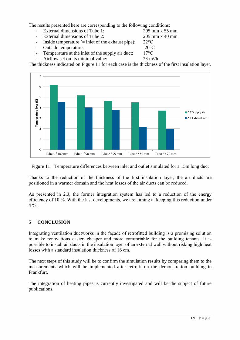
69 | P a g e

The results presented here are corresponding to the following conditions:

- External dimensions of Tube 1: 205 mm x 55 mm

- External dimensions of Tube 2: 205 mm x 40 mm

- Inside temperature (= inlet of the exhaust pipe): 22°C

- Outside temperature: -20°C

- Temperature at the inlet of the supply air duct: 17°C

- Airflow set on its minimal value: 23 m³/h

The thickness indicated on Figure 11 for each case is the thickness of the first insulation layer.

Figure 11 Temperature differences between inlet and outlet simulated for a 15m long duct

Thanks to the reduction of the thickness of the first insulation layer, the air ducts are

positioned in a warmer domain and the heat losses of the air ducts can be reduced.

As presented in 2.3, the former integration system has led to a reduction of the energy

efficiency of 10 %. With the last developments, we are aiming at keeping this reduction under

4 %.

5 CONCLUSION

Integrating ventilation ductworks in the façade of retrofitted building is a promising solution

to make renovations easier, cheaper and more comfortable for the building tenants. It is

possible to install air ducts in the insulation layer of an external wall without risking high heat

losses with a standard insulation thickness of 16 cm.

The next steps of this study will be to confirm the simulation results by comparing them to the

measurements which will be implemented after retrofit on the demonstration building in

Frankfurt.

The integration of heating pipes is currently investigated and will be the subject of future

publications.

70 | P a g e

6 ACKNOWLEDGEMENTS

Part of the work presented was funded by the German Ministry of Economics and Labour

BMWi under the reference 03ET1035A and 0327400 P. Other parts were funded by the

European Commission under the contract number 314229 – RETROKIT in the FP7

Programme.

7 REFERENCES

Coydon, F., A. Dinkel, et al. (2013). Rapid Retrofit Solutions Integrating HVAC into

Prefabricated EWIS Systems. CLIMA 2013: 11th REHVA World Congress & 8th

International Conference on IAQVEC. Prague.

DIN (1997). DIN EN 308. Wärmeaustauscher - Prüfverfahren zur Bestimmung der

Leistungskriterien von Luft/Luft- und Luft/Abgas-Wärmerückgewinnungsanlagen.

Berlin, Deutsches Institut für Normung e.V. DIN EN 308.

DIN (2009). DIN 1946-6. Raumlufttechnik - Teil 6: Lüftung von Wohnungen - Allgemeine

Anforderungen, Anforderungen zur Bemessung, Ausführung und Kennzeichnung,

Übergabe/Übernahme (Abnahme) und Instandhaltung

Germany, Deutsches Institut für Normung e.V. DIN 1946-6:.

Ziegler, M., M. Krause, et al. (2012). Thermische und strömungstechnische Simulation einer

Fassadendäammung mit integrierter Luftführung für die Bestandssanierung. BauSIM

2012. IBPSA. Berlin, IBPSA.

71 | P a g e

USE OF DCV FOR HEATING AND THE INFLUENCE

ON IAQ IN PASSIVE HOUSE BUILDINGS Vegard Aslaksen

1

1 Norconsult AS

Vestfjordgaten 4

1338 Sandvika,Norway

ABSTRACT

Measurements were performed in a test room at SINTEF building and infrastructure, Oslo. The test room is 16

m2 and built according to NS-EN 442-2. Measurements of various air flow rates (9 l/s, 18 l/s, 34 l/s and 50 l/s)

and different supply air temperatures (2, 4, 6 and 10 degrees over room temperature) were performed. Tracer gas

(SF6) measurements were performed to evaluate ventilation effectiveness and age of air in occupied zone.

These tests were performed with 2 different exhaust positions (down by the floor and up under the ceiling) to

check if the position of the exhaust influence the ventilation efficiency and age of air in the occupied zone.

The test room used an Active supply air diffuser from Lindinvent, (http://www.lindinvent.com/products/air-

diffusers/ttc/) designed to keep a constant air velocity with various air flow rate.

The results show variable local air change index in the breathing zone based on air flow rate and the difference

between room temperature and supply air temperature. The heating demand that’s needed can be delivered

without influencing the IAQ in passive house buildings.

Results show the different local air change index in the breathing zone for the different exhaust positions.

There are preformed measurements with heat sources, and they appear to increase mixing, and measurements

done without heat sources are a worst case scenario.

KEYWORDS

Air heating, indoor climate, Tracer gas, passive housing, cold climate

1 INTRODUCTION

The Norwegian government are implementing new and stricter regulations for new buildings.

The new regulations in TEK15 mean that new buildings after 2015 will have to meet passive

house requirements. New requirements for isolation and airtightness will reduce the heating

demand. And due to energy regulations, new buildings often use ventilations systems with

variable air volume (VAV) as opposed to constant air volume (CAV).

This project is part of the research project “For Klima”. “For Klima” is a research project

which is researching the possibility to simplify the solutions for heating, while maintaining a

good indoor climate.

This project has been focused on the possibility of using the ventilation system to supply

heating. If the ventilation system can be used, this will reduce both investment- and operating

costs.

72 | P a g e

The heating demand in passive house buildings has been calculated, and the data has been

used to estimate how frequent heating is used. There is also been built a test room to measure

the local air change index with different heating demands covered by using heated supply air

and with varying air flows.

2 METHOD

2.1 Heating demand and occurrence

The testing plan for the tracer gas measurements are based on the calculated heating demand.

The calculated heat deamand is based on heat loss and internal loads from “Prosjektrapport

42” (Mads Mysen 2009) from SINTEF building and infrastructure.

Table 1: Test plan for tracer gas measurements. It will be done with two different placements of the exhaust.

Test plan

Air Flow: 50 l/s

ΔT 2 4 6 10 Isothermal

Air Flow: 34 l/s


Air Flow: 18 l/s


Air Flow: 9 l/s


The test plan consists of four different airflows, where 18 l/s is air flow equivalent to

requirements set by TEK10(DIBK). The test plan is carried out twice, with exhaust located

both in the ceiling and by the floor. This is done to examine how exhaust location affect local

air change index.

Heating demand is used in combination with metrological data to estimate the occurrence of

outdoor temperatures that leads to a heating demand in passive house buildings.

2.2 Tracer gas measurements

The test room used in tracer gas measurements is 16 m2 room built according to NS-EN 442-

2(Norge 1996) and is used to simulate an office. To simulate a heating demand in the room,

it’s possible to regulate the temperatures of the walls. This is done by pumping water trough

pipes in the walls. Only one wall was cooled down during testing, this was done to simulate

an office with one outer wall. The test room is built with a separate air supply connected to a

active supply air diffuser from Lindinvent (http://www.lindinvent.com/products/air-

diffusers/ttc/) for easy regulation of the air flow. Heating of the supply air is done with a heat

coil. Temperature measurements during testing includes: Surface temperatures in the room,

supply air temperature and room temperatures. These measurements are used to make sure

there are stable conditions during the tracer gas measurements.

73 | P a g e

The tracer gas measurements are analysed using both a step up and step down analysis to

determine local air change efficiency in the breathing zone. The analysis is done by using a

analysis-tool developed by Peter Schild, SINTEF Building and infrastructure / HiOA.

3 RESULTS

3.1 Heating demand

Figur 1: The temperature difference between supply air and room temperature necessary to cover the heating

demand at different outside temperatures with different air flows.

Figure 1 shows the increasing difference between the supply air temperature and the room

temperature necessary to cover the heating demand at different outside temperatures. The

result shows that passive house buildings don’t have a heating demand until the outside

temperatures reach as low as -8 °C, and that the air flow has a significant impact on the

necessary difference between supply and room temperatures.

The necessary difference between air supply and room temperature at an outside temperature

of -22 °C varies between 2 °C and 10 °C based on the size of the air flow.

Air flow according to TEK10 (18 l/s) gives a necessary difference between supply air and

room temperature at 5 °C at an outside temperature at -22 °C.

Table 2: The occurrence of days with temperatures below a set point. Data from the last 10 years collected at

Blindern, Oslo. From eklima, Metrologiske institutt.

Measuring station Oslo-Blindern

Results from 2004-2013 (10 years)

Jan Feb Mar Nov Des Tot Snitt pr.

år

Days with -8 °C 85 78 45 8 74 290 29

Days with -14 °C 18 16 6 0 17 57 5,7

Days with -20 °C 2 0 0 0 0 2 0,2

Table 2 shows the number of days with occurrence of temperatures below -8, -14 and -20 ° C.

-8 ° C is the highest outside temperature resulting in a heating demand in passive house

buildings. While -14 ° C is the outdoor temperature that will require a difference between the

supply and room temperature of 2 ° C when using air flow based on the requirements in

74 | P a g e

TEK10. These figures will vary depending on your location and altitude, these figures

represent the situation in Oslo, Norway.

The figures indicate the occurrence of the given temperature or below during a 24 hour

period, so the occurrence during working hours is lower than the number given, since the

coldest periods of the day often occurs outside working hours.

The incidence of days that requires heating is low and very rarely is there a need that exceeds

2 ° C difference between the air supply and room temperature, when using air flow based on

requirements in TEK10.

3.2 Tracer gas measurements

Tracer gas measurements to find the local air change index in the breathing zone were

conducted at isothermal conditions. Measurements were then performed according to the test

plan, with the corresponding variations in air flow, temperature difference between supply air

and room temperature and exhaust position. The results are then presented by comparing local

air change index in the breathing zone with the corresponding result from the measurements

done under isothermal conditions. The results therefore shows how the temperature difference

between supply air and room temperature affects local air change index in the breathing zone

compared to isothermal conditions.

Figure 2: Development of local air change index for different air flows with increasing temperature difference

between supply air and room temperature. Graphs for both exhaust positions.

75 | P a g e

Figure 2 shows the development of local air change index in the breathing zone with

increasing temperature difference between the supply air and the room temperature with

exhaust placed both in the ceiling and down by the floor and with different air flows.

Local air change index in the breathing zone is affected by both the exhaust location and the

difference between the supply air and room temperature. The results shows that placing the

exhaust down by the floor, provides a consistently higher local air exchange index in the

breathing zone than the exhaust positioned at the ceiling. Local air change index will also

decrease with increasing difference between supply air and room temperature. While placing

the exhaust down by the floor, gives the same trend, the local air change index decreases

slower and at lower air flow rates (9 l / s and 18 l / s) the curve is flat, and you keep a constant

local air change index in the breathing zone.

Figur 3Local air change index with a temperature difference between supply air and room temperature that

covers the heating demand at an outside temperature at -22 °C. Compares different air flows and exhaust

position

Figure 3 shows the local air change index in the breathing zone for different airflows with a

difference in supply air and room temperature that corresponds to a heating demand with an

outside temperature at -22 °C. It also shows how the location of the exhaust affects the results

under these circumstances.

The figure shows that the exhaust location is less important at the above temperatures, when

you use an airflow corresponding to the requirements in Norway or higher (18 l/s or higher).

Exhaust placement is of greater importance when the difference between supply air and room

temperature are higher, which corresponds to greater heating demands than passive house

buildings, or a lower airflow.

3.3 Heat sources

Trace gas measurements conducted and presented in the results are done without heat sources

in the room. A room without heat sources is thought to be a worst case scenario, and

introducing heat sources in the room will increase mixing and increase the local air change

76 | P a g e

index in the breathing zone. To test this assumption, two tests were conducted with heat

sources in the room and compared to the same test done without heat sources. The heat

sources that were introduced were a dummy to simulate a human working by the desk and a

lamp placed at the desk.

Table 3: The effect of heats sources in the room.

Effect of heat sources

Air flow: 34 l/s

Exhaust by the floor Exhaust in the ceiling

Temperature

difference

(ΔT)

Local air change

index(%)

Temperature

difference (ΔT)

Local air change

index(%)

Without

heat

sources

9,9 72 4,1 86

With heat

sources

10,2 90 5,1 97

Table 3 shows the results of the tests. In both cases, the temperature difference is slightly

higher with the introduction of heat sources than without. Introduction of heat sources

increased local air change index by 18% with exhaust located by the floor, and 11% with the

exhaust located in the ceiling. This is a good indication that the assumption was correct, and

heat sources increases the mixing and therefore the local air change index in the breathing

zone.

4 CONCLUSION

The results for the calculation of heating demands and use of meteorological data shows that

buildings on passive house level, rarely needs a temperature difference between supply air

and room temperature that exceeds 2 °C when using air flows according to TEK10. At this

temperature difference the exhaust position has a negligible effect and the results for local air

change index in the breathing zone shows that it’s possible to maintain a good IAQ.

The results show that even on the coldest days of winter (-22 °C) it’s possible to maintain a

high local air change index and the position of exhaust is negligible when using air flow

according to TEK10. This means that you can maintain a good IAQ even on the coldest days

of winter.

This means that the use of the ventilation system for heating buildings at passive house level

can be performed while maintaining good air quality in the breathing zone on even the coldest

days of the year.

5 REFERENCES

DIBK. "TEK10." from http://www.dibk.no/no/BYGGEREGLER/TEK10-Forskrift-om-

tekniske-krav-til-byggverk-med-veiledning/.

77 | P a g e

Mads Mysen, M. K., Matthias Haase, Tor Helge Dokka (2009). "Kriterier for passivhus- og

lavenergibygg- Yrkesbygg, Prosjektrapport 42."

Norge, S. (1996). NS-EN 442-2 Radiatorer og konvektorer. Standard.no, Standard Norge.

78 | P a g e

THE EFFECT OF ENTHALPY RECOVERY

VENTILATION ON THE RESIDENTIAL INDOOR

CLIMATE

Bart Cremers

Zehnder Group Nederland

Lingenstraat 2

8028 PM Zwolle, The Netherlands

[email protected]

ABSTRACT

The indoor climate in residential buildings is affected by the people that live in the house and their activities.

One of the goals of a ventilation system is to prevent excess humidity in the house by removing part of the

moisture. The moisture balance can however be distorted in winter with a low humidity in the house as a result.

An enthalpy exchanger can be used in a recovery ventilation system to reduce the risk of very low indoor

humidity levels in winter. While heat recovery ventilation (HRV) is recovering energy in terms of temperature,

enthalpy recovery ventilation (ERV) is recovering energy in terms of both temperature and moisture.

In a house in Rotterdam, The Netherlands, the temperatures and humidities of the air streams in a recovery

ventilation system were monitored. Eight day periods with HRV and ERV are compared with each other during

mild outdoor conditions.

In the monitored house, the measured recovered amount of absolute humidity with ERV is about 1-2 g/kg with

an average humidity recovery efficiency of 65%. In the monitored house, ERV brings the indoor relative

humidity up to 10 percentage point higher than HRV.

The measured average thermal efficiency and humidity efficiency correspond well with the laboratory values

from the specifications.

KEYWORDS

Enthalpy recovery, residential ventilation, indoor air quality, moisture balance

1 INTRODUCTION

The indoor climate in residential buildings is affected by the people that live in the house. The

presence of people and their activities (like cooking and showering) and the presence of plants

make the indoor climate rise in humidity. One of the goals of a ventilation system is to

prevent excess humidity in the house by removing part of the moisture. The indoor air is

replaced by winter outdoor air, which usually has a lower moisture content than the indoor

air.

The moisture balance can however be distorted in winter (e.g. with high ventilation rate and

very low outdoor air humidity) with a low humidity in the house as a result. An indoor

relative humidity lower than 30% can affect our well-being as it causes dry throat or nose, and

it can affect construction of the house or the (wooden) carpets or furniture.

79 | P a g e

An enthalpy exchanger can be used in a recovery ventilation system to reduce the risk of very

low indoor humidity levels in winter. While heat recovery ventilation (HRV) is recovering

energy in terms of temperature, enthalpy recovery ventilation (ERV) is recovering energy in

terms of both temperature and moisture.

The effect of ERV can only be seen in houses that are air tight, and when there are moisture

sources (cooking, showering, plants) in the house. Without any moisture sources there is

nothing to recover, and there is no difference between ERV and HRV.

2 THE MONITORING SET-UP

Figure 1: The monitored house in Rotterdam

A house (fig. 1) in Rotterdam, The Netherlands, is ventilated with a balanced ventilation

system. The air distribution system is a flexible circular duct system with separate channels

leading to the rooms in the house. The ventilation unit is controlled by a main CO2 control in

the living room. The air flow rate is set to a minimum of 210 m3/h and is increased

automatically when the CO2 level in the living room rises or as a result of a humidity sensor

in the bath room.

In the winter of 2012 the ventilation unit was equipped alternately with a heat exchanger and

an enthalpy exchanger. Unfortunately, the winter was a very short one with only two week

period of cold sub-zero temperatures. In the cold period, the heat exchanger was used, but

after placement of the enthalpy exchanger, the very low outside temperatures have not

returned!

In order to compare the indoor climate for similar outdoor conditions, two periods of eight

days were compared. These days had similar outdoor conditions with temperature between 5

and 10 °C and absolute humidity between 4 and 6 g/kg. During these periods, the air

temperatures and humidities were monitored for each of the four air streams: outdoor air,

supply air, extract air and exhaust air.

80 | P a g e

3 ENTHALPY RECOVERY

A heat exchanger is transferring heat between two air streams and therefore in winter the

supply air stream is increased in temperature. An enthalpy exchanger is transferring heat

between two air streams and also transferring moisture between two air streams. Therefore the

supply air stream in winter is not only increased in temperature, but also increased in

humidity.

a) b)

Figure 2: The effect of heat recovery (a) and enthalpy recovery (b) on the humidity of the supply air.

In fig. 2 the effect of heat exchanger (HRV) and enthalpy exchanger (ERV) on the supply air

humidity is shown by hourly averaged values in the 8-day period. The absolute humidity of

the outdoor air is shown on the horizontal axis and the absolute humidity of the supply air is

shown on the vertical axis. HRV (fig. 2a) has no effect on the humidity of the supply air, but

for ERV (fig. 2b) it is apparent that the supply air is increased in humidity. This humidity is

recovered from the extract air, and thus from the humidity in the house.

The average increase of absolute humidity in the supply air is about 1 – 2 g/kg. For a typical

ventilation air flow of 150 m3/h this means a recovery of 4 – 8 liter of water per day.

4 THE INDOOR CLIMATE

In fig. 3 the hourly values of temperature and humidity levels are shown in Mollier diagrams

for the 8-day periods with heat exchanger (fig. 3a) and with enthalpy exchanger (fig. 3b).

Focusing first on the supply air stream, the air coming from outside is expressed with green

dots and the supply air just after the exchanger is expressed with red dots. Fig. 3 shows that

for HRV the temperature is increased by heat recovery to a level of 20 °C, almost the indoor

temperature. For ERV, the same is happening for the temperature, but also the moisture level

is increased as indicated by the black arrow that is slanted to the right.

In fig. 3 the extract air from the house is expressed with yellow dots, and it is shown that for

the same outdoor conditions, the indoor humidity is higher when the enthalpy exchanger is

used. For HRV, the indoor relative humidity varies in this (relatively mild) period between

35% and 45%, while for ERV the indoor relative humidity varies between 45% and 50%.

81 | P a g e

From this we can conclude that the use of ERV increases the indoor relative humidity in

winter up to 10 percentage point, with HRV as reference.

a) b)

Figure 3: The effect of a heat exchanger (a) and an enthalpy exchanger (b) on the supply air and the indoor air.

5 RECOVERY EFFICIENCY

For the whole monitored winter the efficiencies are summarized in table 1. The thermal

efficiency th can be calculated from the temperatures T and the humidity efficiency (or latent

efficiency) hum can be calculated from the absolute humidities x according to the following

formulas.

( )

( ) (4)

( )

( ) (5)

For the heat exchanger, the average thermal efficiency is 89% for mild outdoor temperatures.

With cold outdoor air, condensation in the return air of the exchanger may be formed and the

flow of return air maybe partly blocked, with the effect that the thermal efficiency drops to

70% in condensing states. As the heat exchanger does not transfer moisture, the humidity

efficiency is zero.

For the enthalpy exchanger, the measured thermal efficiency has an average value of 88%,

while the humidity efficiency is averaged to 65%. These values correspond well with the

values in the specifications.

Table 11: Thermal efficiency and humidity efficiency of the two exchanger types.

Exchanger type Thermal efficiency Humidity efficiency

Heat exchanger 89% (non-condensing)

70% (condensing)

0%

Enthalpy exchanger 88% 65%

82 | P a g e

6 CONCLUSIONS

Ventilation removes stale air, and therefore also humidity from the indoor climate of a house.

In winter, the moisture balance may be distorted causing relatively dry indoor climate,

because dry outdoor air is entering the indoor climate. An enthalpy exchanger recovers a part

of the humidity from the extract air to the supply air, helping to maintain the moisture

balance.

In the monitored house, the recovered amount of absolute humidity is about 1-2 g/kg.

Therefore, the use of enthalpy recovery brings the indoor relative humidity up to 10

percentage point higher than the use of heat recovery (for instance from 35% to 45%). In the

monitored house, the thermal efficiency and the humidity efficiency correspond well with the

values from the specifications.

83 | P a g e

AIR RENEWAL EFFECTIVENESS OF

DECENTRALIZED VENTILATION DEVICES WITH

HEAT RECOVERY

Fabien Coydon1, Jens Pfafferott

2

1 Fraunhofer Institute for Solar Energy Systems ISE

Heidenhofstrasse 2

79110 Freiburg, Germany

[email protected]

2 University of Applied Sciences Offenburg

Badstraße 24a

77652 Offenburg, Germany

[email protected]

ABSTRACT

Central ventilation systems with heat recovery have shown their limits especially within the context of building

energy retrofit. The difficulties to install these systems in existing buildings, to find available space for devices,

air ducts, silencers and fire dampers and to independently control the air flow in each room according to the real

ventilation needs have led to an increasing market for decentralized ventilation devices.

A frequent criticism of decentralized devices is the poor ventilation effectiveness due to a high short-circuiting

risk. Therefore, the University of Applied Sciences of Offenburg and the Frauhofer Institute for Solar Energy

Systems are evaluating together the inside air quality reached with decentralized ventilation systems.

The tests described in this paper were performed in a test lab representing a single room were a decentralized

ventilation system with heat recovery, heating and cooling functions was implemented. In a first part of the

evaluation process, tests are realized to characterize the air distribution provided by the decentralized device by

smoke visualization. The results are showing interesting differences between isothermal, heating and cooling

cases.

The characterization of air distribution in the volume of the room is not enough to evaluate the capacity of a

ventilation system to provide a good inside air quality. Therefore, a second series of tests was performed with

CO2 as a tracer gas, enabling a more precise quantification of the ventilation effectiveness. The results show the

CO2 concentrations over time in zones with different air renewal levels for each of the 3 modes.

KEYWORDS

Decentralized ventilation, Ventilation effectiveness, Heat recovery, Inside air quality

1 INTRODUCTION

The work presented in this paper is included in a research program aiming at evaluating

ventilation concepts for the energy retrofit of residential buildings. Central and decentralized

ventilation are compared on the basis of a full list of criteria including their energy

performances, comfort, acceptance and life cycle costs.

As a part of this work, an analysis of the inside air quality provided by decentralized

ventilation systems will be detailed here.

As no ductwork is necessary, decentralized ventilation systems are a very interesting solution

to provide fresh air in retrofitted buildings where place is rarely available to install

voluminous equipment. A frequent criticism against decentralized devices is their low

84 | P a g e

ventilation effectiveness since the air inlets and outlets are often very close to each other

risking a short-circuit inside the ventilated room as well as outside.

Decentralized ventilation systems have already been evaluated (Mahler, Himmler et al. 2008;

Haase and Gruner 2013) but only a few studies have a specific focus on the ventilation

effectiveness of these systems (Ender, Gritzki et al. 2004; Ajaji and André 2013). At the

Wuppertal University, the microclimatic influence of the external side of the façade was

investigated (Voß and Voss 2012) but not the short-circuiting risk.

At last, the combination of heating by warm air and ventilation was investigated by the

Technical University of Denmark and the Slovak University of Technology but in a context of

central ventilation (Krajčík, Simone et al. 2012).

The main goal of the study presented here is to evaluate a decentralized ventilation system

including heating and cooling functions in different running modes.

In order to describe the capacity of decentralized ventilation to provide a good inside air

quality, one parameter, the ventilation effectiveness, is often used with different definitions. A

first possibility, related to smoke visualisation of the ventilation air movements, is based on

time measurements describing how long the fresh air needs to reach each point of a room. A

second definition, related to tracer gas evaluations, is based on concentration measurements in

different points of the room and in the fresh and exhaust air (Mats 1981; Recknagel, Sprenger

et al. 2007/2008).

2 DESCRIPTION OF THE TESTS AND EVALUATION METHODS

2.1 Ventilation device

The decentralized ventilation system tested here and shown on Figure 1 is foreseen to provide

fresh air, to heat and to cool office rooms until 6m deepness. It includes 2 fans, 1 heat

exchanger, 1 heating/cooling coil, 2 filters and can run with 3 different airflows.

Figure 1 Tested decentralized ventilation device

2.2 Test room

The decentralized ventilation device was evaluated in the test facilities of the University of

Applied Sciences Offenburg. The room dimensions are 5,2 x 3,8 x 3 m³. Two walls are

producing heating or cooling loads.

85 | P a g e

Figure 2 3D view of the test room and positions of the CO2 sensors

2.3 Smoke visualisation

The first series of tests was done with smoke visualisation. We focussed on two dimensions in

the area directly placed in front of the device. The first dimension was the deepness of the

room so that we could verify that the device was able to treat a 5m deep room. The second

dimension was the height which allows describing an eventual stratification of the fresh air

provided by the ventilation device.

Figure 3 View of a smoke visualization test

In many test cases, the smoke was not visible any more before it filled the entirety of the

room volume and in particular before it reached all of the four points were CO2 sensors were

placed. This phenomenon made it impossible to determine a ventilation effectiveness based

on time measurements and could lead to the conclusion that the ventilation device is not able

to treat the air in the whole room volume.

2.4 CO2 measurements

The second series of tests was done with a tracer gas. As the main pollutants removed by

ventilation systems are humidity and CO2, we choosed CO2 as a tracer gas. The choice of

another tracer gas could have led to errors in the evaluation due to different behaviors of gases

Decentralized

ventilation

device

Walls providing

heating and

cooling loads

CO2 sensors

86 | P a g e

regarding the diffusion and mixing phenomenons in the air. To compare the results with the

smoke visualisation, we used 4 CO2 sensors placed in front of the ventilation device at

horizontal distances of 1,5 m and 4 m and at 2 different heights (“Down”: 0,5 m and

“Up”: 1,8m).

The room was filled with CO2 and the analysis began after homogenisation of the 4 measured

CO2 concentrations as shown on Figure 4.

Figure 4 Example of CO2 measurements including filling and homogenisation periods

Isothermal mode (60 m³/h)

Figure 5 CO2 homogenisation period without ventilation

A first conclusion can be drawn from the measurement of the homogenisation period which is

the period where the CO2 concentrations dynamyc is still due to the initial concentration

differences. In order to define this homogenisation period, we used the theoretical evolution

of each CO2 concentration, having an exponential form (cCO2 = c0 + A.e-b.t

). After the

homogenisetion period, the measured concentration is actually close to the theoretical one.

87 | P a g e

We considered that the end of the homogenisation period occurred as the difference between

theoretical and measured CO2 concentrations were lower than 5% of the initial difference.

We compared 2 different cases:

- ventilation off – corresponding to Figure 5

- ventilation on – minimal airflow (around 60 m³/h) – corresponding to Figure 4

The first one lasted around 3480 s, whereas the second one lasted only 880 s. This means that

even set on its minimal airflow, the device is able to homogenise pollutant concentrations in

the room which reduces short-circuiting risks.

In order to compared the diferent cases, we used the definition of the ventilation effectiveness

proposed by Mats and Recknagel (Mats 1981; Recknagel, Sprenger et al. 2007/2008):

(1)

Where:

- η: ventilation effectiveness

- cexhaust: CO2 concentration in the exhaust air

- cfresh: CO2 concentration in the fresh air

- caverage: average CO2 concentration of the 4 measured points

In our case, this effectiveness does not describe the capacity of the device to ventilate the

whole volume of the room, but only the vertical plane situated in front of the ventilation

device.

3 ANALYSIS OF ISOTHERMAL, HEATING AND COOLING MODES

An important part of the work is to compare isothermal, heating and cooling modes with both

evaluation methods. The results presented here were obtained with a middle airflow (around

80 m³/h) with following temperatures:

- isothermal mode: Tsupply air = 22 °C Troom inside = 22 °C

- heating mode: Tsupply air = 40 °C Troom inside = 23 °C

- cooling mode: Tsupply air = 12 °C Troom inside = 24 °C


Figure 6 is presenting the results of the smoke visualisation tests. As mentioned in 2.3, the

measurement of the time needed by the fresh air to reach each of the 4 points corresponding

to the CO2 sensors was not possible especially for the cooling mode. These pictures are

showing important differences between each case. The repartition in the room of the fresh air

provided by the ventilation device is good in the isothermal mode but in the cooling mode, the

fresh air is only filling the lower part of the room and in the heating mode, only the upper

part.

88 | P a g e

Isothermal mode

Cooling mode

Heating mode

Figure 6 Smoke visualisations after 5, 10, 15, 20, 30 and 50 s for the 3 different modes

A purely qualitative analysis of these pictures leads to the conclusion that only one of these

cases presents an acceptable air distribution.


In order to quantitatively verify these results, 0, 0 and 0 are presenting the CO2 measurements

obtained for the same cases.

A first observation can be done regarding the differences between the 4 sensors:

- Isothermal mode:

The lowest CO2 concentrations after homogenisation were obtained at the 2 points

situated near the device. No stratification of the CO2 concentration is appearing for

this case (no difference between the upper and the lower sensors for both locations).

The differences between the 4 measured concentrations and their average value

remains under 15 %.

- Heating mode:

The lowest CO2 concentration after homogenisation was obtained at the upper point

situated near the device. A vertical stratification of the CO2 concentration only appears

at the nearest location.

The differences between the 4 measured concentrations and their average value also

remains under 15 %.

- Cooling mode:

The lowest CO2 concentration after homogenisation was obtained at the lower point

situated at 4 m from the device. A vertical stratification of the CO2 concentration only

appears at this location but not at 1,5 m from the device.

89 | P a g e

The differences between the 4 measured concentrations and their average value are

reaching 40 %.

Figure 7 CO2 measurements in isothermal mode (80 m³/h)

Figure 8 CO2 measurements in heating mode (80 m³/h)

90 | P a g e

Figure 9 CO2 measurements in cooling mode (80 m³/h)

The ventilation effectiveness was calculated for each measurement and is represented on

Figure 10. On this figure we can see that the values obtained during the homogenisation

period are not relevant.

Figure 10 Comparison of ventilation effectiveness in isothermal, heating and cooling modes

For all 3 modes, values above 1 can be found on the chart. This is due to the position of the

CO2 sensors used for the determination of the average concentration in the room. As they are

positioned in the vertical plane directly aligned with the fresh air direction, they are in the best

ventilated part of the room. This means that no conclusion can be drawn from the absolute

values but only comparisons between the 3 cases.

The average values of the ventilation effectiveness are:

- isothermal mode: 1,6

- heating mode: 1,5

- cooling mode: 1,1

91 | P a g e

These results confirm that the best air distribution is obtained for the isothermal mode and the

worst for the cooling mode. They show that the air distribution obtained for the heating mode

is quite similar to the isothermal mode.

4 INFLUENCE OF THE AIR FLOW RATE

The same investigations were made to analyse the influence of the airflow rate on the

ventilation effectiveness. These investigations are presented here for the isothermal mode.


Figure 11 presents the results of the smoke visualisations for the 3 different airflows. On these

pictures, we can see that the air speed allows a faster penetration of the smoke in the room

after 5 seconds, but no real difference can be seen in the repartition of the smoke in the room

volume between the 3 cases after 20, 30 or 50 seconds.

Isothermal mode – Airflow 60 m³/h



Figure 11 Smoke visualisations after 5, 10, 15, 20, 30 and 50 s for the 3 different airflows


The CO2 measurements can be seen on Figure 4 (60 m³/h), Figure 7 (80 m³/h) and Figure 12

(100 m³/h). The repartition is by each case identical: no vertical stratification of the CO2

concentrations and a notable difference between both locations (1,5 m and 4 m).

92 | P a g e

Figure 12 CO2 measurements in isothermal mode (100 m³/h)

The average values of the ventilation effectiveness obtained with each airflow are:

- 60 m³/h: 2,0

- 80 m³/h: 1,6

- 100 m³/h: 1,3

The results are showing a higher effectiveness for the lowest airflow. We suppose that there is

an optimal airflow for which this effectiveness would be the highest. It would be interesting to

test airflows lower as 60 m³/h in order to verify that this optimum exists. We also suppose that

the results would be different if the effectiveness had been determine using sensors in the

whole volume of the room.

5 CONCLUSIONS

The main goal of a ventilation system is to remove pollutants like CO2 from a room. In order

to quantify its capacity to reach this goal, smoke visualisation is not the right tool. Indeed, we

have seen for the heating mode that the smoke seems to stay in the highest layers of the air

volume but the CO2 concentrations are still reduced at each measured point with a similar

speed.

One important conclusion is about the cooling mode for which the ventilation effectiveness

was the lowest obtained in our tests. It might be interesting to equip the air inlet of such a

reversible device with a system adapting the speed and direction of the airflow to the inlet

temperature of the air.

6 ACKNOWLEDGEMENTS

Part of the work presented was funded by the German Ministry of Economics and Labour

BMWi under the reference 03ET1035A and 0327400 P. Other parts were funded by the

European Commission under the contract number 314229 – RETROKIT in the FP7

Programme.

93 | P a g e

7 REFERENCES

Ajaji, Y. and P. André (2013). A Decentralized Mechanical Ventilation System with Heat

Recovery: Experimental Assessment of Thermal Comfort and Pollutant Removal

Ability. Clima 2013. Prague.

Ender, T., R. Gritzki, et al. (2004). Bewertung von dezentralen, raumweisen Lüftungsgeräten

für Wohngebäude sowie Bestimmung von Aufwandszahlen für die Wärmeübergabe

im Raum infolge Sanierungsmaßnahmen. [Abschlußbericht]. Stuttgart, Fraunhofer-

IRB-Verl.

Haase, M. and M. Gruner (2013). Evaluation of Decentralized Façade-Integrated Ventilation

Systems in Nordic Climate. Clima 2013. Prague.

Krajčík, M., A. Simone, et al. (2012). "Air distribution and ventilation effectiveness in an

occupied room heated by warm air." Energy and Buildings 55: 94-101.

Mahler, B., R. Himmler, et al. (2008). DeAL - Evaluierung dezentraler außenwandintegrierter

Lüftungssysteme - Abschlußbericht. Stuttgart, Steinbeis-Transferzentrum und

Steinbeis Forschungszentrum Energie-, Gebäude- und Solartechnik.

Mats, S. (1981). "What is Ventilation Efficiency." Building and Environment 16(2): 123-135.

Recknagel, H., E. Sprenger, et al. (2007/2008). Taschenbuch für Heizung und Klimatechnik,

Oldenbourg Industrieverlag, München.

Voß, T. and K. Voss (2012). Mikroklimatische und baukonstruktive Einflüsse bei dezentraler

Lüftung. BauSIM 2012. IBPSA. Berlin, IBPSA.

94 | P a g e

PERCEPTION OF A COOLING JET FROM CEILING -

A LABORATORY STUDY

Henna Maula*, Hannu Koskela, Annu Haapakangas and Valtteri Hongisto

Finnish Institute of Occupational Health

Lemminkäisenkatu 14-18 B

20520 Turku, Finland


ABSTRACT

The effect of a cooling jet from ceiling on thermal comfort, perception and subjective performance in warm

office environment (29.5 °C) was studied. Altogether, 29 participants (13 male and 16 female) participated. All

participants were tested in both thermal conditions and the order of the thermal conditions was counterbalanced

between the participants. During the experiment, participants filled questionnaires and performed computerised

tasks. Using the cooling jet significantly improved the whole body and local thermal comfort. It also improved

the perception of the whole working environment. The indoor air was perceived fresher when the cooling jet was

provided. Fatigue increased in time significantly only when the cooling jet was not provided. Eye symptoms

increased in time only with the cooling jet. The cooling jet increased the sensation of draught, but still the warm

room air temperature was perceived to impair the performance more than draught. The room air temperature was

perceived to be better for working effectively for a long period of time with the cooling jet.

KEYWORDS

Thermal comfort, cooling jet, perception, symptoms, self-rated performance

1 INTRODUCTION

Room temperature is an important part of the indoor environment. Too warm room air affects

negatively occupant’s thermal comfort and performance (Häggblom et al. 2011). Local

cooling can be produced by increasing the air movement (Melikov et al. 2013).

Table fans are commonly used in offices during warm summer periods. Huang et al. (2013)

studied the user requirements for air movement with an online survey in China and a series of

climate chamber experiments. They concluded that the flow generated by electric fans can be

used as an effective cooling method to maintain a comfortable environment at 28 °C-32 °C.

However, in open-plan offices with high density of workstations the fans also increase

substantially the thermal load of the office increasing the need of cooling and the energy

consumption. Supplying an air jet from the ceiling can be integrated to the air conditioning

system thus removing the need for a local fan.

Toftum (2014) summarized the factors influencing the perception of air movement.

According to the summary, occupants feeling warmer than neutral do not feel draught at air

velocities up to 0.4 m/s. In the high temperature range up to 30 °C, very high air velocities,

such as 1.6 m/s, were found to be acceptable. However, they concluded that very high air

movement should be under the control of the exposed occupant.

95 | P a g e

ASHRAE 55(2010) and ISO 7730 (2005) standards allow elevated air speed to be used to

increase the maximum operative temperature for acceptability under certain conditions.

According to the ASHRAE standard, if sedentary office occupants don’t have control over the

local air speed in their space, the upper limit to air speed should be 0.8 m/s for operative

temperatures above 25.5 °C.

The aim of this study was to investigate how the cooling jet from ceiling is perceived and how

it affects the thermal comfort and subjective work performance.

2 METHODS

The study was carried out in the open-plan office laboratory (82 m2) of FIOH in spring 2013.

The room had twelve workstations and was designed to resemble a neutral clerical office.

Four workstations out of the twelve were used in this study (Figure 1). The HVAC of the

office laboratory was adjusted to room air temperature 29.5 °C, relative humidity 20 % and

supply air flow rate 280 l/s. Supply air was blown with five terminal units and with one

cooling jet. The cooling jet was produced with seven adjustable nozzles installed

symmetrically into the end of one of the inlet ducts (Figure 3). Noise level and lighting

conditions met current recommendations.

Figure 1: Layout of the open-plan office laboratory.

96 | P a g e

Figure 2: Seven nozzles installed symmetrically into the end of one of the inlet ducts to produce the cooling jet.

Two thermal conditions were tested; (1) no cooling jet and (2) cooling jet with fresh supply

air (T = -3.5 °C and target velocity 0.8 m/s). Air velocity was measured in the occupied zone

with hot-sphere anemometers while the dummy subjects (heat load 90 W/dummy) were

present to simulate a sitting person (Zukowska-Tejsen et al., 2012). The cooling jet in

thermal condition 2 was located in front of the occupant in the suspended ceiling (height 2.55

m). The angle of the cooling jet was 45° from the vertical axis. Target velocity of the cooling

jet was set to upper limit of acceptable air speed without personal control according to

ASHRAE standard 55 (2010) and ISO standard 7730 (2005). Both thermal conditions were

tested simultaneously in the open-plan office laboratory.

Altogether, 29 participants (13 male and 16 female) were recruited. The participants were

native Finnish speakers and aged between 20 and 33 years (average = 24). The study had a

repeated measures design. All participants were tested in both thermal conditions two at a

time. The order of thermal conditions was counterbalanced between participants. Clothing

insulation and activity level were controlled. The participants were advised to wear trousers,

short sleeve shirt, socks and ankle-length shoes. The estimated clothing insulation including

office chair (0.1 clo) was 0.71 clo. The main activity of the participants during the study was

typing. The estimated activity level was 1.1 met.

The experiment day started with 30 minutes acclimatization (Figure 3). Workstations meant

for acclimatization didn’t differ from the thermal condition without the cooling jet. The

purpose of the acclimatization was to secure that each participant had similar acclimatization

despite of in which thermal condition they took part in first. During acclimatization the

participants filled questionnaires and computerised performance tasks were introduced to

them. After the acclimatization, participants moved to the experimental workstation and the

first session started with questionnaires. After the questionnaires the participants performed

computerised tasks followed by questionnaires at the end of the session. The session in both

thermal conditions lasted for 40 minutes. After the first session the participants changed

places with each other and the second session in different thermal condition but with an

identical procedure started immediately. There were no breaks in between the two sessions.

97 | P a g e

Figure 3: Test procedure

Whole body thermal comfort, local thermal comfort, symptoms, subjective performance

ratings and overall experience of the environment were assessed with questionnaires, which

were repeated throughout the session. Thermal comfort was evaluated using a seven-point

thermal sensation scale. Fatigue was measured with a modified version of the Swedish

Occupational Fatigue Inventory (SOFI; Åhsberg et al., 1995, Åhsberg et al., 1998) including

three factors which were sum variables of three items (tiredness: sleepy, yawning, drowsy;

lack of energy: worn out, exhausted, drained; lack of motivation: uninterested, indifferent,

passive).

Statistical analyses were conducted with SPSS Statistics 20 with a confidence interval of

95 %. The normality of the data was tested with Shapiro-Wilk. A repeated measures ANOVA

was used when data was normally distributed or when distributions were similarly skewed.

Whenever parametric methods were used, the results were also checked with the

nonparametric Wilcoxon test. When an interaction effect was found, paired comparisons

between conditions were performed using t-test or Wilcoxon. Benjamini-Hochberg procedure

was used in paired comparisons.


Table 1 shows the percentage of participants experiencing the cooling jet to be pleasant or

unpleasant in certain body parts. The perception of the cooling jet was contradictory. Over

50 % of the participants reported the cooling jet to be pleasant in the arms, face or at the top

of the head. Respectively the face and the top of the head received most votes of the airflow

being unpleasant. On the open questionnaires some participants reported the airflow to be

unpleasant in the eyes but to be pleasant everywhere else in the face. Those answers are

included in both pleasantness categories. Also the intensity of the cooling jet distributed the

opinions. Some of the participants would have preferred more air flow and some less.

Table 1: The percentage of participants reporting airflow pleasant or unpleasant in certain body parts.

Top of

the head

Face Neck Front

neck

Torso Arms Hands

Pleasant 52 66 7 38 45 72 31

Unpleasant 21 41 10 10 0 10 0

The differences in thermal comfort were statistically significant (p<.01, Figure 4). 67 % of the

participants considered the thermal conditions to be acceptable with the cooling jet, while

only 28 % considered them to be acceptable without the cooling jet. No gender differences

were found. The improvement of thermal comfort under the influence of the cooling jet was

98 | P a g e

statistically significant in each body part except the thighs. However, a trend of the cooling jet

improving thermal comfort in thighs was found (p=.068). Thermal comfort was significantly

better with the cooling jet even in legs and feet, although they were not under direct influence

of the airflow.

The occurrence of fatigue was minor. Fatigue increased in one measured factor, tiredness,

toward the end in both thermal conditions, but the increment of fatigue was significant only in

the condition without the cooling jet (p<.01; Figure 5). Eye symptoms increased in time only

in the condition with the cooling jet (p<.001), but the intensity of eye symptoms was minor

even at the end of the session.

Figure 4: Thermal sensation votes

Figure 5: Fatigue, factor tiredness

The indoor air was perceived fresher when the cooling jet was provided (p<.01). Under the

cooling jet the air temperature was perceived better (p<.001) but there was more sensation of

draught (p<.001). The whole working environment was perceived better in the thermal

condition with the cooling jet (p<.05).

There was a trend that the subjective performance was better when working under the

influence of the cooling jet, but the difference between the conditions was not statistically

significant (p=.064). However, the participants were more frustrated during the most difficult

task in the condition with no cooling jet (p<.05). The stuffiness of the room air was perceived

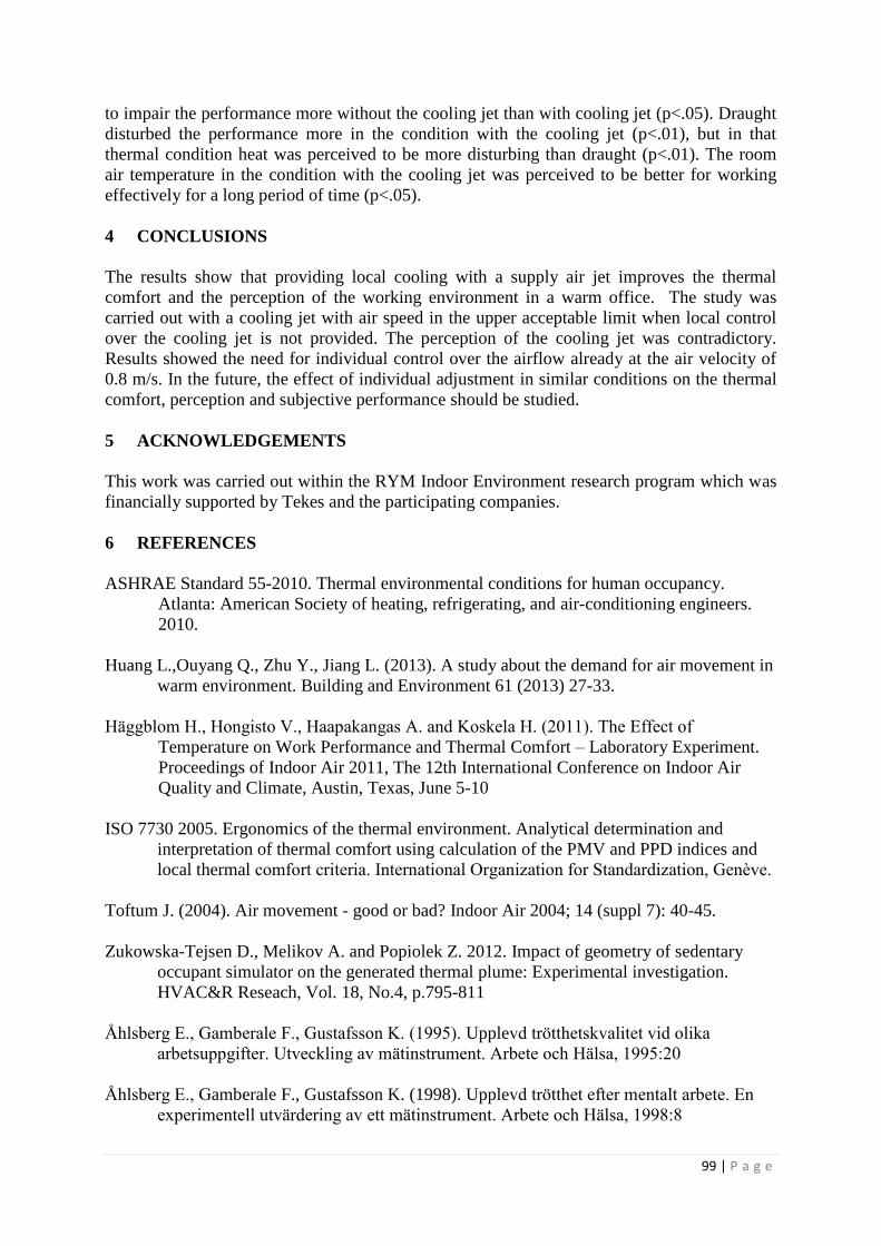
99 | P a g e

to impair the performance more without the cooling jet than with cooling jet (p<.05). Draught

disturbed the performance more in the condition with the cooling jet (p<.01), but in that

thermal condition heat was perceived to be more disturbing than draught (p<.01). The room

air temperature in the condition with the cooling jet was perceived to be better for working

effectively for a long period of time (p<.05).

4 CONCLUSIONS

The results show that providing local cooling with a supply air jet improves the thermal

comfort and the perception of the working environment in a warm office. The study was

carried out with a cooling jet with air speed in the upper acceptable limit when local control

over the cooling jet is not provided. The perception of the cooling jet was contradictory.

Results showed the need for individual control over the airflow already at the air velocity of

0.8 m/s. In the future, the effect of individual adjustment in similar conditions on the thermal

comfort, perception and subjective performance should be studied.

5 ACKNOWLEDGEMENTS

This work was carried out within the RYM Indoor Environment research program which was

financially supported by Tekes and the participating companies.

6 REFERENCES

ASHRAE Standard 55-2010. Thermal environmental conditions for human occupancy.

Atlanta: American Society of heating, refrigerating, and air-conditioning engineers.

2010.

Huang L.,Ouyang Q., Zhu Y., Jiang L. (2013). A study about the demand for air movement in

warm environment. Building and Environment 61 (2013) 27-33.

Häggblom H., Hongisto V., Haapakangas A. and Koskela H. (2011). The Effect of

Temperature on Work Performance and Thermal Comfort – Laboratory Experiment.

Proceedings of Indoor Air 2011, The 12th International Conference on Indoor Air

Quality and Climate, Austin, Texas, June 5-10

ISO 7730 2005. Ergonomics of the thermal environment. Analytical determination and

interpretation of thermal comfort using calculation of the PMV and PPD indices and

local thermal comfort criteria. International Organization for Standardization, Genève.

Toftum J. (2004). Air movement - good or bad? Indoor Air 2004; 14 (suppl 7): 40-45.

Zukowska-Tejsen D., Melikov A. and Popiolek Z. 2012. Impact of geometry of sedentary

occupant simulator on the generated thermal plume: Experimental investigation.

HVAC&R Reseach, Vol. 18, No.4, p.795-811

Åhlsberg E., Gamberale F., Gustafsson K. (1995). Upplevd trötthetskvalitet vid olika

arbetsuppgifter. Utveckling av mätinstrument. Arbete och Hälsa, 1995:20

Åhlsberg E., Gamberale F., Gustafsson K. (1998). Upplevd trötthet efter mentalt arbete. En

experimentell utvärdering av ett mätinstrument. Arbete och Hälsa, 1998:8

100 | P a g e

PROMEVENT: IMPROVEMENT OF PROTOCOLS

MEASUREMENTS USED TO CHARACTERIZE

VENTILATION SYSTEMS PERFORMANCE

Adeline Bailly*1, Cedric Lentillon

1

1 Cerema

Direction Territoriale Centre-Est 46 rue Saint-Théobald

38081 l'Isle d'Abeau, FRANCE


ABSTRACT

For the coming energy-efficient buildings, the guarantee of energy performance becomes a major challenge. It is

therefore crucial to implement accurate and reliable measurements, in order to ensure this performance. The in-

force French EP-regulation RT2012 already imposes compulsory justification of envelope airtightness.

Moreover, the Effinergie+ label requires ventilation systems control and ductwork airleakage performance.

These requirements, ventilation controls for IAQ concern and regulatory compulsory controls of buildings need

reliable diagnostic protocols.

In 2014, several French partners, led by the Cerema1, proposed a new project, PROMEVENT, which main

objective is to improve ventilation systems measurements protocols. It aims to deal with different phases of a

diagnostic:

1) Visual control

2) Airflow measurements and pressure differences measurements at air vents

3) Ventilation ductwork airleakage measurements.

Several points will be tested through repeatability and reproducibility assessments. Then measurements will be

performed on laboratory benches, and on ventilation systems of single-family and multi-family dwellings. By the

end of the PROMEVENT project, recommendations and a first version of a protocol for the measurement of

residential buildings ventilation systems will be proposed. Moreover, one of the main objective is to produce a

more reliable and optimised protocol which will be written as a proposed draft standard.

This paper presents the context in which the PROMEVENT project has been defined, and describes its different

steps.

KEYWORDS

Ventilation – Measurements – Airtightness – Airflow - Improvement

1 CONTEXT AND OBJECTIVES

The recent French energy performance regulations and labels have resulted in a new buildings

generation. Since 2000, airtightness requirements have been gradually implemented in French

1 A new public scientific organism born from the merging of 11 scientific institutes (including the CETE de

Lyon) of the French ministry for ecology, sustainable development and energy (MEDDE).

101 | P a g e

regulations, leading to a reinforcement of air renewal systems and a need to ensure their

reliability. First labels and mostly Effinergie-BBC label have imposed a requirement on

building envelope airtightness for residential building. Since January, 2013, the in-force EP-

regulation RT2012 imposes airtightness requirements for all new residential buildings.

Figure 1: Evolution of French Thermal Regulations

These highly airtight buildings create an issue for both comfort and indoor air quality. Indeed,

in these dwellings, air change rates are provided by ventilation system, which have to be

efficient to ensure good indoor air quality, while limiting heat losses due to air change.

Several recent studies illustrate this concern. The OQAI (French indoor air quality

observatory) performed a national IAQ campaign from 2003 to 2005 (Kirchner, 2008). 567

dwellings (chosen in order to represent the national housing stock) have been investigated

through ventilation systems diagnostics and indoor air quality measurements. This national

study has concluded that the air change rate and the duration windows are opened are the

most important factors of the indoor air quality. Moreover, calculations analysis which have

been performed during the project QUAD-BBC have shown some typical evolution of

pollutants in highly airtight low consumption buildings (Boulanger, 2012).

The French in-force regulation concerning ventilation requires a general and permanent

ventilation for residential buildings. It also imposes minimal airflow of exhaust air. So as to

meet those two seemingly divergent objectives, technically advanced mechanical ventilation

systems have been developed. Nevertheless, high quality and technical skills are required

during design phase, implementation and maintenance, which are often neglected. Ventilation

systems have an influence on the sanitary aspects of the supplied and indoor air, through

moisture development for example (Van Herreweghe, 2013). Moreover, inhabitants may have

not understood the functioning of new mechanical systems, especially for balanced

ventilation, and might decide to take it down. The OQAI has recently carried out a field

survey in seven new built energy-efficient houses in France (Derbez, 2014). All inhabitants

have experienced some difficulties with their Mechanical Ventilation with Heat-Recovery

102 | P a g e

systems, because they are difficult to use, the user’s manual is complex, high noise levels can

be produced or they cause a lack of comfort. But if MVHR systems are turned out or

voluntary degraded (airvents closed for example), indoor air quality can become poor and

present a risk to human health.

Therefore, in many countries, several studies have been launched to realize a state of the art of

ventilation systems in dwellings. In France, a survey (Jobert, 2013) has been carried out

through control reports performed between 2008 and 2011 concerning 1287 dwellings (88%

are multi-family dwellings). Almost all buildings are equipped by simple exhaust ventilation

systems.

Figure 1: Ventilation system repartition in the analysed sample (Jobert, 2013)

47% of the sample do not comply with the airing regulation, which means that they present at

least one non-compliance remark (68% for single-family dwellings, and 44% for multi-family

dwellings). Those non-compliances are generally related to design errors, poor

implementation and lack of maintenance. Same issues have been observed in many European

and American countries (Van Den Bossche, 2013). Two practices could improve the quality

of ventilation systems. On one hand, a quality approach could be set up. In France, such

approaches have been successfully adopted for building envelope airtightness (Charrier, 2013).

Moreover, the VIA-Qualité project is testing the feasibility of such approach for ventilation

systems and IAQ (Jobert, 2013). In a second hand, as the French thermal regulation imposed

the airtightness level justification, the ventilation system performance could also be

controlled, what is already compulsory with a recent label, “Effinergie +”. Those controls are

in accordance with new approaches, which impose that standards and regulations compliance

is ensured by on-site verifications. Those approaches might lead to financial or organizational

consequences. Currently, ventilation systems controls are generally performed in France in

three cases:

For buildings applying for new Effinergie label (Effinergie +)

During regulatory compulsory control (by the technical civil servants network of the

Ministry in charge of the Construction’s sector)

When IAQ issues have been set out for a building.

Therefore, control protocols have to be unquestionable. In these cases, several diagnostic

protocols are used: either labels reference documents or good practice guide, such as the

Effinergie protocol, the DIAGVENT method and the European standard EN12599. The

reliability of these protocols may be not sufficient. The PROMEVENT project proposes to

test repeatability, reproducibility and feasibility of these protocols in order to define a more

reliable protocol for ventilation system controls.

103 | P a g e

This project may have to deal with such issues as: how can it be representative of all different

situations? How can it characterize the equipment use impact? How will it overcome airflow

measurement difficulties? The PROMEVENT established program is described in the second

part of this paper.

2 PROMEVENT PROGRAM

PROMEVENT is an 8 organizations project whose main objective is to improve the quality of

ventilation system controls. More precisely, it aims to ensure the reliability of ventilation

measurement protocols concerning pressure and airflow differences at air vents, and ductwork

airleakage. This program will focus on residential buildings. According to current practices in

new constructions, two “dwelling/ventilation systems” associations will be studied:

Single-family dwellings equipped with balanced ventilation

Multi-family dwellings equipped with single humidity demand-controlled ventilation.

This project includes three workpackages. The first one consists in a characterization of existing

protocols in order to evaluate their reliability, through experimental campaigns. The second one is

the elaboration of a new protocol which must ensure controls reliability. The last one will lead to a

verification of the new protocol feasibility, reliability and relevancy, through on-site tests.

The PROMEVENT project has been proposed to a call for proposals launched by ADEME within

the subject “toward responsible buildings in 2020”. The Consortium is constituted of 8 French

partners, both private and public sectors: a public institution (Cerema2 - ex CETE de Lyon), a

laboratory (CETIAT), 5 consultancies (ALLIE’AIR, ICEE, PLEIAQ, CETii, PBC) and an

association (Effinergie). They are quite complementary on scientific and operational dimensions.

The Consortium, thus formed should be able to defend the importance of a unique and

standardized protocol which will have to take into account uncertainty requirements and

implementation concerns. It should also convey its discourse to all relevant professionals.

2.1 Existing protocols reliability

Several protocols are used in France and abroad to control ventilation systems performance,

including visual diagnostic, proper functioning at air vents control and ductwork airtightness

measurement. There are described in label reference documents, campaign protocols,

standards or good practice guides. EN12599, DIAGVENT method, Effinergie protocol or

OQAI protocol are some of them. In a first step, an inventory is being taken to compare the

different protocols considering risks and sources of uncertainty, investigated components and

technical feasibility. Moreover, different technologies and equipment used to perform

measurements (concerning airflow, pressure difference and ductwork airtightness) are being

listed and studied to describe their field of application and product liability according to their

manufacturers. This review is also including a state of the art of international projects and

studies dealings with this topic, in order to be able to integrate current evolutions.

This first step is preparing the second one: experimental campaigns. A methodology will be

established to evaluate feasibility, relevancy and reliability of existing protocols. Two

2 Centre for expertise and engineering on risks, environment, mobility, urban and country planning

104 | P a g e

campaigns will be performed in order to conduct repeatability and reproducibility evaluations

from 2014 to 2015.

One campaign will be carried out in laboratory. It will study measurement equipment

performance and calibration in different configurations: proper functioning without, then with

components which might disrupt the flow. Thanks to a ventilation system assembled in

laboratory, the impact of some specific configurations will be evaluated without risking a

building deterioration.

A second campaign will be performed in situ on:

10 single-family dwellings equipped with balanced ventilation;

2 multi-family dwellings equipped with single humidity demand-controlled

ventilation. 4 operating-teams will contribute to this campaign. Roles are defined in the following table.

Table 1: First in-situ campaign program

Team 1 Team 2 Team 3 Team 4

2 multi-family

dwellings

Building 1: airflow, pressure difference

at airvents and ductwork airtightness B1 B1

Building 2: airflow and pressure

difference at airvents B2 B2

10 single-family

dwellings

House 1: airflow, pressure difference at

airvents, and ductwork airtightness H1 H1 H1

House 2: airflow and pressure

difference at airvents H2 H2

House 3 to 10: airflow and pressure

difference at airvents H3 ; H4 H5 ; H6 H7 ; H8 H9 ; H10

This dwellings repartition has been defined to optimise repeatability and reproducibility

evaluation regarding to geographical, financial and temporal limits. Several measurements (as

much as possible) will be performed in each dwellings (for repeatability and equipment

reproducibility evaluation). Ventilation systems of 4 buildings (B1, B2, H1 and H2) will be

controlled by 2 or 3 different teams (reproducibility evaluation).

2.2 New protocol formulation

The results of the two campaigns and the review will be analysed to determine which points of

currently used protocols are unreliable, to what extent and why.

The laboratory campaign analysis will help to determine measurement uncertainty of each

equipment depending on the application, and the need of calibration. Impact of air vents type or

non-alignment measurement will be assessed. It is also expected to detect the impact of some

specific issues related to ventilation ductwork through tests performed on the ventilation system

assembled in laboratory.

The in-situ campaign results will be analysed through several aspects:

Repeatability of tested protocols

Reproducibility concerning equipment impact

Reproducibility concerning operator impact

“Out of hand” in-situ conditions impact.

105 | P a g e

Main objectives are to evaluate uncertainty of the tested protocols and to specify uncertainties

sources. According to those results, the Consortium will formulate a new protocol. At this step, a group of

relevant professionals will be consulted. It could be composed of ventilation experts and

industrials, controllers, control equipment manufacturers, architects, certification organisms.

Discussions on new protocols will focus on several points:

Ensure sufficient reliability

Ensure technical and financial feasibility

Define self-checking equipment conditions

Define needs and organisation of operators training, qualification and control.

2.3 New protocol validation

The last milestone of this project consists on the new protocol validation. It will be based on a

second in-situ campaign results. According to geographical and financial limits and buildings

availability, fewer buildings will be tested. Each team will perform several measurements (as

many as possible), with different equipment. The following table presents the second in-situ

campaign program.

Table 2: Second in-situ campaign program

Team 5 Team 6 Team 7 Team 8

1 multi-family

dwellings

Building 3: airflow, pressure difference

at airvents and ductwork airtightness B3 B3 B3

4 single-family

dwellings

House 11: airflow, pressure difference

at airvents and ductwork airtightness H11 H11

House 12: airflow, pressure difference

at airvents and ductwork airtightness H12 H12

House 13 & 14: airflow, pressure

difference at airvents and ductwork

airtightness

H13 ;

H14

In order to evaluate the technical feasibility and the relevancy of the protocol, new teams will be

composed with new operators: they will not have been part of the project before this step. Each

team will be accompanied by an operator of team 1 to 4 (first campaign and all project) whose

role will be to assist, to guide and to audit new operators. It will lead to evaluate of the

understanding of the protocol. It will also ensure that diagnostics have been performed properly to

evaluate repeatability and reproducibility of the new protocol.

Experimental results will be analysed to evaluate:

New protocol relevancy: improvement of reliability

Implantation ease, understanding and appropriation by new operator

Financial feasibility: difference between costs of current used protocols and new

protocol

The self-checking relevancy.

106 | P a g e

Those evaluations will lead to a final protocol that will be drawn up as a proposed draft

standard. It will also lead to a guide intended to ventilation operators. This guide will explain

and illustrate each step of this ventilation system diagnostic protocol. It will be available and

free for download.

3. CONCLUSIONS

The PROMEVENT project objective is to define a new protocol for controls of ventilation

systems performance. This protocol will be established based on many existing protocols

currently used. Several laboratory and in-situ campaigns will be carried in order to test

repeatability, reproducibility and feasibility of those protocols, including the equipment choice

impact. It is expected that conclusions of this project will lead to a new standard which will be

imposed in new buildings regulation, in order to impose compulsory check of ventilation systems

performance. At the end of this project, training and recommendations will be provided to

operators through a practical guide, which may be useful for measurements performed for label.

4. ACKNOWLEDGEMENTS

The “PROMEVENT” project receives funding from the French Environment and Energy

Management Agency. The contribution of Cerema is funded by the French ministry for

ecology, sustainable development, and energy (MEDDE).

The sole responsibility for the content of this publication lies with the authors.

5 REFERENCES

S. Kirchner, M. Derbez, C. Duboudin, P. Elias, A. Gregoire, J-P. Lucas, N. Pasquier, O.

Ramalho, N. Weiss. Indoor air quality in French dwellings. Indoor Air 2008. Copenhagen,

Denmark - Paper ID: 574. 2008

X. Boulanger, L. Mouradian, C. Pele, Y-M. Pamart, A-M. Bernard. Lessons learned on

ventilation systems from the IAQ calculations on tight energy performant buildings. 33rd

AIVC Conference. Copenhagen, Denmark. 2012.

J. Van Herreweghe, S. Caillou, M. Roger, K. Dinne. Sanitary aspects of domestic ventilation

systems: an in situ study. 34th AIVC Conference. Athens, Greece. 2013.

Jobert, R., Guyot, G. Detailed analysis of regulatory compliance controls of 1287 dwellings

ventilation systems. 34th AIVC Conference. Athens, Greece. 2013.

M. Derbez, B. Berthineau, V. Cochet, M. Lethrosne, C. Pignon, J. Riberon, S. Kirchner.

Indoor air quality and comfort in seven newly built, energy-efficient houses in France.

Building and Environment. N°72, p. 173-187. 2014.

P. Van Den Bossche, A. Janssens, D. Saelens. Securing the quality of ventilation systems in

residential buildings: existing approaches in various countries. 34th AIVC Conference.

Athens, Greece. 2013.

107 | P a g e

S. Charrier, J. Ponthieux, A. Huet. Airtightness quality management scheme in France:

assessment after 5 years operation. 34th AIVC Conference. Athens, Greece. 2013.

108 | P a g e

IMPACT OF A POOR QUALITY OF VENTILATION

SYSTEMS ON THE ENERGY EFFICIENCY FOR

ENERGY-EFFICIENT HOUSES

Adeline Bailly*1

, Franck Duboscq1, Romuald Jobert

1

1 CEREMA

Direction Territoriale Centre-Est

46 rue Saint-Théobald

38081 l'Isle d'Abeau, France

Corresponding author: [email protected]

ABSTRACT

The “VIA-Qualité” project (2013-2016) focuses on low energy, single-family dwellings. It proposes the

development of quality management approaches (ISO 9001) which aim to increase both on-site ventilation and

indoor air quality. One of the main benefits of those approaches is the improvement of ventilation system

performance, especially thanks to a rigorous follow-up from design to installation. Efficient ventilation system

performance is rewarded in the French EP-calculation, through a primary energy consumption estimation. In

order to evaluate the energy impact of the proposed quality approaches, some sensitivity studies have been

carried out for single humidity-controlled ventilation system. The primary energy consumption of typical single-

family dwellings has been estimated along various parameters, such as:

• Ductwork airleakage

• Exhaust and incoming airflow

• Electrical fan power

• System localization (to take into account leakages in and out of heated volume).

This paper presents variations of the estimated dwellings energy consumptions as an indicator of the impact of

several typical dysfunctions of ventilation systems which have been observed during different campaigns and

controls.

KEYWORDS

Ventilations systems – Dysfunctions – Energy impact – Single-family house

1 INTRODUCTION

In France, the energy performance regulation (RT2012) generalizes requirements of the BBC-

Effinergie label, in particular regarding the envelope airtightness. For a single family

dwelling, the requirement is Q4Pa-Surf 1≤ 0.6 m

3.h

-1.m

-2 (around n50≤ 2.3 h

-1). In those airtight

dwellings, the air change rates have to be adequate to insure a good indoor air quality, and at

the same time they have to induce low thermal losses in order to comply with requirements of

the regulation. Nevertheless, the RT2012 does not include any new requirement on ventilation

rates, which are provided by another 30-years-old regulation (JO, 1983). Therefore, without

1 Air permeability at 4 PA divided by the loss surfaces area excluding basement floor

109 | P a g e

compulsory check of the proper functioning of ventilation systems, how inhabitants can be

sure that the air renewal of their houses is adequate to ensure a good indoor air quality? In

addition, in the current energy context, mechanical ventilation systems are spreading,

including high technical systems such as single humidity-controlled ventilation systems and

balanced ventilation systems. These systems require knowledge and skills from each of the

three main actors: designers, installers and inhabitants, who in most cases are not even aware

of the ventilation principles. Indeed, various campaigns (Paul Van Den Bossche, 2013) in

different countries have brought forward the poor quality of ventilation systems, mainly

related to a poor design or installation and a lack of maintenance. In France, a study (Romuald

Jobert, 2013) has been carried out from regulatory compliance control reports of almost 1300

dwellings. This survey confirms that ventilation system dysfunctions are very frequently

observed in dwellings, and it gives clear information about their localization and qualification.

Therefore, we need solutions to prevent those dysfunctions and ensure a good indoor air

quality. Various countries (Paul Van Den Bossche, 2013) are developing different schemes to

secure the quality of ventilation systems through actions during all steps of the process of a

building construction. Such a system is already in place since 5 years in France regarding the

envelope airtightness. The good experience of this quality approach (Sandrine Charrier, 2013)

and the current ventilation systems quality assessment have motivated the “VIA-Qualité”

project. Started in 2013, this 3-years French project proposes to develop quality management

(QM) approaches (ISO 9001) with the goal of increasing both on-site ventilation and indoor

air quality (IAQ). It focuses on low energy, single-family dwellings, which mainly concerns

in France the individual homebuilders sector. The benefits would be to: 1- Improve

ventilation system performance, especially thanks to rigorous monitoring from design to

installation; 2- Limit indoor internal pollution sources, monitoring materials selection

(Wargocki P, 2012); 3- Increase final users’ awareness and understanding. An assess of the

effectiveness of these QM approaches will be carried out, through ventilation measurements

and IAQ measurements in 8 test houses. Moreover, in order to ensure the reproducibility of

this kind of operation, the economic and energetic interests of these QM approaches have to

be evaluated. This analysis will be carried out in two steps: 1- evaluation of the impact of

ventilation system performance on energy consumptions; 2- crossed analysis between the

energy-savings and the additional costs due to materials, studies, controls... This paper

presents an analysis of impacts of ventilation system dysfunctions on the regulatory energy

performance calculations (RT2012) for the three first single-family houses of the VIA-Qualité

project.

2 VENTILATION PARAMETERS IN THE FRENCH EP-CALCULATION

The in-force French EP-regulation (RT2012) is mainly based on 3 kind of performance

requirements: 1- energy efficiency (independent of systems); 2- primary energy consumption

[Cpe2] and 3- summer comfort (for buildings without air-conditioning). In this study, the

variations of the energy consumptions have been calculated as an indicator of the energy cost

of several ventilation systems dysfunctions.

2 In France, it is noted Cep

110 | P a g e

The EP-calculation is run with XML data which define the values of various input parameters.

The following part briefly explains how ventilation is taken into account in the EP-calculation

for a classic single-family house, with a single humidity-controlled ventilation system.

Concerning ventilation system, the input parameters used in this study are listed in table 1.

Table 1: Income parameters concerning ventilation systems in the French EP-calculation

Income parameter Definition Possible values

Air inlet module (m3.h

-1) Coefficient which is used to estimate

the total airflow incoming through all

air inlets

From 0 to ∞

Qext (m3.h

-1) Total extraction airflow From 0 to ∞

Type_air_intake (-) Two types of air intake are identified in

the EP-calculation: humidity &

pressure controlled air intake or

pressure controlled air intake

0: humidity & pressure controlled air intake

1: pressure controlled air intake

Engine_Power (W) Engine power of the fan From 0 to ∞

Cdep (-) Coefficient of design quality From 1 to ∞

Ratfuitevc (-) Ratio of leaks to heated volume From 0 to 1

Cletres Airtightness class of the ductwork

(A,B,C,D): defined the value of the

ductwork leakage coefficient Kres

C: Kres = 0,003.10-3

m3.s

-1.m

-2

B: Kres = 0,009.10-3

m3.s

-1.m

-2

A: Kres = 0,027.10-3

m3.s

-1.m

-2

Default (2.5A): Kres = 0,0675.10-3

m3.s

-1.m

-2

2.1 Some equations of the EP-calculation concerning ventilation systems

The following equations and fixed values of some coefficients are defined in the EP-

calculation method.

Exhaust airflow model

For a single-family house, the regulated exhaust airflow is defined with two indicators: Qext,

min which represents the base flow, and Qext, max which represents the flow at full load. The

values of these two airflows have to be consistent with the French ventilation regulation (JO,

1983). The average flow Qext, regul is calculated according to equation 1:

( )

(1)

Dugd [hour/week] is the duration of use at full load expressed in h/week. For a single-

family house, Dugd = 7 hours per week.

Then, the EP-calculation introduces the coefficient Cdep in order to take into account some

dysfunctions of the system due to design. Therefore, the extraction flow becomes Qext, dep:

(2)

The default value of Cdep is 1.25, and in most cases Cdep=1.1 (justification with a

certified document).

111 | P a g e

The following equation defines the leakage rate through all duct leaks Qext, leaks for a pressure

difference ΔP:

(3)

Kres [m3.s

-1.m²] depends on the leaktightness class of the network

Aduct, ext [m²] is the surface of the air duct, which can be estimated as a percentage of

the floor area (the uncertainty of this parameter value is not analysed in this study).

The final extraction flow is calculated according to equation 4:

(4)

Khv [-] describes the part of the exhaust duct in the heated volume (from 0 to 1).

Intake airflow model

In a single humidity-controlled ventilation system, the characteristic curve which represents

the air inlets performance has a straight line format. The following equation corresponds with

the principal part, which is used when the pressure difference at the air inlet is under 20 Pa.

( ) (

)

(

| |)

(5)

QAI [m3.h

-1] is the airflow which enters through the air inlets.

Cd [-] is the coefficient of discharge. Its value is 0.68.

ρref [kg.m-3

] is the air density at 19°C. Its value is 1.2 kg.m-3

.

M is the sum of the air inlet modules.

ΔPref [Pa] is the pressure difference for which the module is defined. Its value is 20

Pa.

The two airflows Qext and QAI are then used to estimate the indoor temperature for each time

step. The difference between the indoor temperature and the setpoint temperature is an input

for evaluating the heating needs. With those needs and the performance of the house systems,

the EP-calculation establishes the regulatory primary energy consumptions for 1 year and for

1 square meter of a specific floor area named SHONRT (without some parts like non-heated

places, balcony...): Cpe [kWhpe.m-2

.year-1

]. In order to respect the EP-regulation (R2012), the

Cpe of a house have to be lower a limit value Cpe max, which depends on various parameters

including climate zone and altitude. The average limit value is 50 kWhpe.m-2

.year-1

.

2.2 Definition of dysfunction scenarios

A list of dysfunctions of ventilation systems has been established based on the analysis of

Jobert, 2013, and supplemented with results of a 20 houses campaign realised during the first

step of the VIA-Qualité project. In this list, dysfunctions which could have an impact on

energy consumption of the house have been identified. For each of them, related parameters

of the EP- calculation and the appropriate variation range have been identified. Those criteria

have been introduced into six scenarios which correspond to different common situations in

low-energy houses. Table 2 presents those scenarios.

112 | P a g e

Table 2: Various scenarios representing common ventilation system dysfunctions Scenario Characteristic Concerned parameters

1: Lack of humidity-

control

In this scenario, the installer has put in place

the wrong air inlets: they are not humidity-

controlled, but just pressure-controlled

Type_air_intake

Air inlet module [74.9 m3.h

-1 ;

186 m3.h

-1]

2: Excessive number of air

inlets

This scenario corresponds with a common

situation where 1 additional air inlet has been

installed in a room

Air inlet module [74.9 m3.h

-1 ;

115 m3.h

-1]

3: Low battery in toilets air

outlets

Most of the air outlets which are installed in

the toilet fitted out with a presence sensor. In

most cases, the sensor runs with batteries.

This scenario represents the impact of low

batteries, which impact on the exhaust

airflow.

Qext [59 m3.h

-1 ; 110.1 m

3.h

-1]

4: Duct leakage In this scenario, various configurations are

texted, which correspond with different

airtightness classes of the ductwork and

different duct positions in the heated volume

Airtightness class of the

ductwork [2.5A ; C]

Khv [0.25 ; 1]

5: Over ventilation In some cases, fans are wrongly adjusted,

which induces an over ventilation of the

house. In this scenario, various level of over

ventilation are simulated.

Qext [59 m3.h

-1 ; 100 m

3.h

-1]

2: Fan performance In this scenario, various fan with different

performance are tested. Engine_Power [8W ; 45 W]

2.3 Houses presentation

Those scenarios have been modelled with the EP-calculation for three low-energy houses.

Each of them are equipped with a single humidity-controlled ventilation system, which equips

most of new single-family houses. Table 3 describes some characteristics of those houses. A

first simulation in normal situation (no modification of the project input data) has been

performed for each house. The calculated value of the Cpe [Consumption calculated in

primary energy3] is then used as the reference value for the six previously described scenarios.

Table 3: Houses presentation

House Type Heating system Cpe (total) / Cpe max

[kWhpe.m-2

.year-1

] Cpe

(heating consumption)

[kWhpe.m-2

.year-1

]

House 1 Two-storey house

Floor area: 97 m²

Heat pomp 51.3 / 60 24.4

House 2 Single-storey house

Floor area: 84 m²

Heat pomp 55.2 / 64.6 26.9

House 3 Single-storey house

Floor area: 90 m²

Condensing boiler 57.2 / 73.2 39.9

3 Consumptions are presented in energy primary: for electrical source, a multiplier factor equal to 2.58 is applied.

113 | P a g e

3 RESULTS

Each of the 6 scenarios has been simulated for the three test houses with the EP-calculation.

In this study, every consumption is expressed in primary energy: electrical source is penalised

(1 kWh of final energy = 2.58 kWh en primary energy4). Houses 1 and 2 use only electrical

source for all energy consumers (heating, cooling, lighting, domestic hot water, ventilation

fans and distribution systems). House 3 uses gas source for heating and a part of the domestic

hot water.

Except for scenario 6, the analysed dysfunctions only impact on the heating consumptions.

The following part presents those impacts and gives some explanations of those results.

Results of scenario 6 are presented in a second time, as the impact of the studied dysfunctions

does not concern the heating consumption.

3.1 Impact of several ventilation dysfunctions on regulatory heating consumption

As the relative impacts on the heating consumption of each dysfunctions are almost the same

for the three houses, figure 1 introduces the average impact for each scenario (except scenario

6). Table 4 gives results for each house.

Figure 1: Impact of several ventilation dysfunctions on the regulatory heating consumptions [in primary energy]

4 This coefficient is defined in the French regulation

114 | P a g e

Whereas different kinds of heating systems with a 2.58-coefficient for electrical source, the

standard deviations of the impacts of these dysfunctions are small. Indeed, house 3 (which

uses gas-source) has been built in a colder climate, so even with a 1-coefficient for primary

energy consumption, the part of heating consumption is almost the same than for the two

other houses. It will be interesting to perform the same study with a gas-source house built in

a “hot” climate, for which the part of heating consumption should be significantly lower.

Table 4: Impact of several ventilation dysfunctions on the regulatory heating consumption depending on the test

house (in primary energy)

Relative impact on the regulatory heating consumption (primary energy)

Scenario 1: Scenario 2: Scenario 3: Scenario4: Scenario 6 :

Non-

humidity-

controlled air

inlets

One excessive

air inlet

Low

batteries in

toilets air

outlets

All duct

leakage in

heating

volume

Good

ductwork

airtightness

60% of over

ventilation

House 1 +7.4% +2.9% +22.5% +13.9% -3.7% +16%

House 2 +5.6% +3.3% +23.4% +12.6% -3.7% +16%

House 3 +5.5% +2.0% +23.6% +14.0% -4.0% +18%

Average +6.2% +2.7% +23.2% +13.5% -3.8% +16%

Standard

deviation 0.9% 0.6% 0.5% 0.6% 0.1% 1.2%

According to (Jobert, 2013), among the key elements of a ventilation system, air inlet is one

of the worse installed. Within those dysfunctions, 18% concern the non-compliance with

prescribed rules and regulations and 18% concern the presence of an additional air inlet.

Figure 2: Number of non-compliance or dysfunctions items per category (Jobert, 2013)

115 | P a g e

Scenario 1 corresponds with an installation of wrong air inlets. Indeed, in France, there are

two types of single-flow humidity-controlled ventilation systems called A and B. For the A

system, air outlets are humidity and pressure controlled, but air inlets are pressure-controlled

only. On the contrary, for the B system, outlets and inlets are humidity and pressure

controlled. In most houses, the B system is installed, which induces a lower total incoming

airflow than the A systems. Figure 1 shows that this error could increase the heating

consumption of about 6%.

Scenario 2 also corresponds with an air inlet dysfunction: it models the implementation of one

excess air inlet somewhere in the house. The model of the EP-calculation does not let to

precise in which room (utility room or main room) the air inlet is installed. The only effect

considered in this study is the increase of the total airflow incoming. With this hypothesis, the

excess air inlet induces an overconsumption of almost 3%. This result is not really significant.

Nevertheless, depending of the localisation of the excess air inlet, it could induce a short

circuit of the house sweep and therefore be responsible of a poor air renewal in some rooms.

This energy impact should be supplemented with sanitary impact.

Air outlets are also often affected by dysfunctions (22% of cases). Indeed, in a single

humidity- controlled ventilation system, outlet in the toilet are equipped with a system which

momentarily increases airflow when someone uses the toilet. In most new houses, the system

is a presence sensor running on batteries. The lack of battery is a common dysfunction: it

represents 15% of dysfunctions concerning outlets (people often did not know they have to

replace them). In this case, the outlet stays in the position where it was when the batteries

have stopped: it could be either the lower airflow or the big airflow. Scenario 3 corresponds

with the “worst” situation: the batteries of the two toilets outlets are fallen out of order when

the outlets were in the big airflow position (it could happen!). In this case, the total exhaust

airflow is more important than the predicted one. The impact of this dysfunction is significant:

about 23% of over consumption for heating. It could induce an additional cost of more than

60 € each year, while batteries for 2 outlets cost about 10€. This situation is the “worst”, but

in the other one, when the airflow is blocked in the lower position, the air renewal in the

toilets will be insufficient. So, a lack of batteries will either induce an important additional

cost each year, or lead to a moisture development in toilets. Therefore, it should probably be

more relevant to pay 10€ and change the batteries.

The previous dysfunctions concern an over energy cost when the exhaust airflow is blocked at

a high value. Nevertheless, is some cases, the poor quality of the ductwork prevents the

airflow from reaching this value. The EP-calculation takes into account this quality with 4

different ductwork airtightness classes. Without any measurement, the worse class has to be

used in the calculation. Scenario 4 includes several configuration, with classes varying for

different positions of the ductwork leaks (in or out the heated volume). Figure 1 shows that a

good ductwork airtightness should induce almost 4% of energy consumption gain. This gain

is estimated with the hypothesis of a fixed exhaust airflow at the outlet (independent of the

airtightness class). Therefore, with more leaks, there is an additional exhaust airflow through

those leaks. With this hypothesis, the impact of the localisation of the leaks compared to the

heated volume is significant: for a bad airtightness (class 2.5A) and a duct entirely in the

heated volume, the overheating energy consumption could raise more than 13%. The EP-

calculation do not estimate the over consumption of the fan needed to secure the airflow at the

outlet, so this dysfunction impact might be higher. In practice, the exhaust airflow at the

outlets is often not secured, and in this case, the impact of this dysfunction is a sanitary impact

116 | P a g e

with a possible very low exhaust flow. Therefore, a bad ductwork could induce either an

important energy consumption or a sanitary issue, or both.

Then, scenario 5, frequent for balanced ventilation system, is less frequent for single-flow

ventilation systems: it deals with over ventilation. This dysfunction happens if the fan has not

be well set. Various total exhaust airflow have been tested, the most important is a 60% of

over ventilation. For this value, the ventilation may be responsible of a 16% increase of the

energy consumption for heating, hence the importance of the fan setting.

3.2 How initial financial savings could induce significant losses

Some dysfunctions are due to design and installation, others to maintenance. The following

part concerns dysfunctions due to initial financial savings. Indeed, fans and ventilation

terminals are available in various models, at various prices. Scenario 6 is related to fan. For

each of the three test houses, the fan which is foretold in their thermal study is a high-

performance fan: the nominal power is 8 W. Some other lower performance fans exist for this

type of ventilation system, for the same delivered airflow. For financial reasons (up to a 100

€-difference between fan prices for an initial 200€-price), it is possible than one of this fan is

finally installed instead of the 8 W fan. Table 5 presents the impact of the fan choice on the

total energy consumption Cpe compared with the initial Cpe (with an 8W-fan).

Table 5: Impact of a bad performance-fan on the total energy consumption (primary energy)

Fan Nominal

power

Impact on the Cpe (heating consumption)

[kWhpe.m-2

.year-1

]

House 1 House 2 House 3

12 W 1% 2% 2%

30 W 8% 9% 8%

45 W 13% 15% 14%

Those results prove the importance of the fan choice. Indeed, with a low-performance fan (45

W), the regulatory energy consumption can significantly increase (until 15% for the house 2).

In practice, the impact on the energy bill is less important: until 11% (above 45€).

Nevertheless, this additional cost for a 8W-fan is low enough to be quickly paid off: 2 years

and 3 months only!

Moreover, the impact on the Cpe could be critical: for house 2, with a 45W-fan, the

recalculated Cpe is almost equal to the limit value Cpe max. If an other dysfunction exists, the

Cpe max could therefore be overtaken. Then, the house would not respect the RT2012.

On this point, air inlet are also affected by financial choice. For example, scenario 2

corresponds with an initial 30% saving. In order to evaluate the energy and final economic

impact of a first price installation, a combination of scenario 1 and 2 have be modeled (non-

humidity controlled air inlet and a 45W-fan). Moreover, a dysfunctions combination is a

current situation: according to Jobert, among all controlled dwellings, 29% get two non-

compliances or more. Figure 3 presents results of this particular combination.

117 | P a g e

Figure 3: Regulatory energy consumption (primary energy) of 3 houses depending on the ventilation fan

performances

In this probable situation, the regulatory Cpe recalculated with the real equipment will exceed

the limit value Cpe max for two houses (1 and 2). In a first hand, energy consumptions would

be significantly higher than the predicted ones, and in the other hand, the house would not

respect the EP-regulation RT2012! Therefore, make some initial financial savings should

rapidly induce many issues, including energy losses and poor indoor air quality.

4 CONCLUSIONS

Ventilation has to be understood as a principle and not just a system. A dysfunction of one

element impact the whole buildings, and may increase the total primary energy consumption

[Cep] by about 16% (22% of the heating consumption). Not only the energy bill may be

significantly increased, but also the house might not respect the EP-regulation requirements.

As ventilation systems dysfunctions are a main issue for single-family houses, a scheme as a

quality management approach may increase ventilation quality. To that end, the VIA-Qualité

project develop tools for each of the three main actors (designer, installers and inhabitants) in

order raise awareness among them about the ductwork, products and maintenance quality.

5 ACKNOWLEDGEMENTS

The “VIA-Qualité” project has received funding from the French Environment and Energy

Management Agency under the contract ADEME/1304CO014 and from the Rhône-Alpes

118 | P a g e

region. The contribution of CEREMA is funded by the French ministry for ecology,

sustainable development, and energy (MEDDE).

The sole responsibility for the content of this publication lies with the authors.

6 REFERENCES

JO. (1983). Arrêté du 24 mars 1982 consolidé relatif à l'aération des logements : aération

générale ou permanente. JO du 15 novembre 1983.

Paul Van Den Bossche, A. J. (2013, Septembre 25-26). Securing the quality of ventilation

systems in residential buildings: existing approaches in various countries. 34th AIVC

Conference, Athens, Greece, pp. 70-72.

Romuald Jobert, G. G. (2013, September 25-26). Detailes analysis of regulatory compliance

controls of 1287 dwellings ventilation systems. 34th AIVC Conference, Athens,

Greece, pp. 74-76.

Sandrine Charrier, J. P. (2013, September 25-26). Airtightness quality management scheme in

France: assessment after 5 years operation. 34th AIVC Conference, Athens, Greece,

pp. 42-44.

Wargocki P, H. T. (2012, October 11-12). Health-Based ventilation Guidelines for Europe -

HealthVent project. 33th AIVC Conference, Copenhagen, Denmark.

119 | P a g e

DEMAND-CONTROLLED VENTILATION

20 YEARS OF IN-SITU MONITORING IN THE

RESIDENTIAL FIELD

Jean-Luc Savin1, Stéphane Berthin

1 and Marc Jardinier

1

1 Aereco

62 rue de Lamirault

Collégien

77615 Marne la Vallée cedex3

France

ABSTRACT

Is Demand-controlled ventilation a relevant answer to face the new challenges of the Building sector, which

requires everyday higher energy efficiency and better indoor air quality? Can Demand-controlled ventilation be

considered as an alternative to heat recovery ventilation, through an affordable and low maintenance solution?

Since the take off of the DCV in the early 80’s, these questions have been considered many times. Following the

expansion of the technology over the world (more than 4.5 million dwellings are already equipped today, only

considering humidity controlled ventilation), numerous in-situ monitoring have been conducted to try to better

understand the behaviour and the performance of the DCV. Precursor in the field as inventor of humidity

controlled ventilation in 1983, Aereco has carried out numbers of monitoring on different ventilation types, in

various countries and on specific buildings, measuring in total hundreds of dwellings. With a first large-scale

study based on natural ventilation in multi-storey buildings realised in 1993, the research has been completed

with experiments on hybrid ventilation and on mechanical exhaust ventilation, individually or collectively

managed, to recently lead to the follow-up of on an innovative full room-by-room DCV balanced system with

heat recovery.

This proceeding will specially focus on four major monitoring: demonstration project “EE/166/87” (natural

ventilation, France, Belgium and Netherlands, 1991-1993), “HR-VENT” (hybrid ventilation, 55 dwellings,

France, 2004-2005), “Performance” (collective MEV, 29 dwellings, France, 2008-2009) and the last monitoring

that concerns several houses in Germany and France equipped with a full DCV heat recovery (started in 2013).

In parallel to the ventilation systems evolution, the one of the measurements methods and instruments has been

remarkable since the first monitoring. From tracer gas to collect the airflows at the first monitoring, we have

reached today a level of technology that enables more reliable and more precise multi-parameters measurements

through electronic sensors, sending data via internet.

Whatever the ventilation technique it is associated with, the automatic control of the airflows according to the

demand has demonstrated benefits at various levels. The first monitoring highlighted the correlation between

CO2 and humidity, even in the technical rooms, conferring relevancy to humidity controlled at the exhaust. On

all monitoring, the seasonal behaviour of the system when humidity controlled has been found out: following the

lower absolute humidity level in winter, the airflows are reduced when the dwellings are unoccupied, leading to

energy savings on both the heating and on the fan electrical consumption. On the indoor air quality side, we have

checked that the automatic control to the demand enables to optimise it: the system improves the repartition of

the airflows among the rooms according to their specific needs, increasing the air renewal in the most occupied

and polluted rooms. In addition, DCV monitoring have shown specific phenomena such as the ability to optimise

the available pressure through a time-repartition of the exhaust demand dwelling-to-dwelling, when connected to

120 | P a g e

a collective duct. Besides parameters measurements and data collection we brought specific care on occupant’s

acceptance, making surveys every time it was possible. The results have shown that the system was in general

very well accepted, highlighting the relevancy of non intrusive and low maintenance systems.

KEYWORDS

Monitoring, Demand-controlled Ventilation, Humidity controlled, Indoor Air Quality, Energy Savings.

1. INTRODUCTION

Since the take off of the Demand-controlled Ventilation in the early 80’s, the question of its

performance and of its ability to position as an alternative to the heat recovery ventilation has

been considered many times. Following the expansion of the technology over the world -more

than 7 million dwellings are already equipped today only considering humidity controlled

ventilation-, numerous in-situ monitoring have been conducted to better understand the

behaviour and the performance of the DCV. Precursor in the field as inventor of humidity

controlled ventilation in 1983, Aereco has carried out numbers of monitoring in residential

buildings on different ventilation types, in various countries, measuring in total hundreds of

dwellings. This paper aims at giving a global overview of the major monitoring that have

been hold on Demand-controlled ventilation systems in residential application, dealing with

different topics such as indoor air quality, energy efficiency and evolution of measurement

instruments

2. 20 YEARS OF MONITORING

Monitoring one or several dwellings to assess the performance of a specific building

equipment always raises the question of the significance and of the relevancy of the study:

how to be sure that these dwellings are representative, so that we can approach the statistical

and average behaviour of a system through the follow up of a limited set of dwellings? The

multiplication of monitoring campaigns as well as the quantity of monitored dwellings is the

only way to evaluate as best the performance of a ventilation system. As application of this

principle, Aereco has conducted numerous in-situ experiments on various places testing its

Demand-controlled ventilation systems in the residential field, as presented on Figure 1.

Figure 1: Historic presentation of Aereco major monitoring campaigns on ventilation (Starting dates).

121 | P a g e

Figure 2: One of the five buildings monitored in “HR-VENT” project (left); One of the two buildings monitored

in “Performance” project (right)

3. EVOLUTION OF MEASUREMENT METHODS AND MEANS

The precision and the quality of results of in-situ experiments are very dependent from the

sensors and the methodology used. Since our first monitoring of DCV realised in 1993 up to

now in 2014, the evolution of the means has been continuous and strong, improving the

accuracy of the measurements and enlarging the spectrum of measurable parameters.

From tracer gases used in 1993 in “Les Ulis” monitoring giving punctual measurements up to

electronic sensors generalised in the latest monitoring, the airflow measurements have

become much more precise and reliable, offering possibilities of a permanent follow up that

can be applied to a large set of dwellings.

The data collection has also been considerably eased with the development of WiFi and

internet: a recent in-situ experiment applied on a new Demand-controlled heat recovery

ventilation system now includes climatic sensors that are directly connected to the local WiFi,

sending the data through internet.

4. DEMAND-CONTROLLED VENTILATION SYSTEMS

The typical system measured during the various monitoring we are talking about in this paper

is an unbalanced system with humidity controlled air inlets (Figure 3) in the bedroom and

living room, humidity and / or presence detection exhaust units (Figure 4) in the wet rooms,

and a centralised fan connected to these units. These systems are presented on the following

schemes for hybrid ventilation (Figure 5) or for mechanical exhaust ventilation (Figure 6). In

these systems, the fan has the singularity to provide a constant pressure for a varying airflow.

122 | P a g e

Figure 3: Humidity controlled air inlet

Figure 4: Demand-controlled exhaust unit (MEV)

Figure 5: System scheme in hybrid ventilation

Figure 6: System scheme in mechanical exhaust

ventilation (MEV)

5. IN-SITU WORKING OF DEMAND-CONTROLLED VENTILATION SYSTEMS

5.1 Instantaneous behavior

One of the first objectives of a monitoring on ventilation is to check that the system in-situ

working conforms to the laboratory measurements. The dynamic working of the Demand-

controlled ventilation, with its airflows constantly moving according to the humidity or to the

presence1 has been measured in most of the experiments as a key result.

1for the majority of the products in Aereco’s range

123 | P a g e

HR-VENT monitoring (humidity controlled system with hybrid ventilation) has given the

opportunity to check the working of the extract grilles. Figure 7 presents the day variation of

the aperture according to the relative humidity for a humidity sensitive extract grille located in

a bathroom. We can see that the variations of aperture –so the airflow for a given pressure-

follow well the evolution of the relative humidity, with a high reactivity.

0

20

40

60

80

100

120

02/06/2005

00:00

02/06/2005

02:24

02/06/2005

04:48

02/06/2005

07:12

02/06/2005

09:36

02/06/2005

12:00

02/06/2005

14:24

02/06/2005

16:48

02/06/2005

19:12

02/06/2005

21:36

03/06/2005

00:00

Relative humidity in %

Aperture in cm²

Figure 7 : Aperture vs. relative humidity of a humidity sensitive extract grille in the bathroom. “HR-VENT”

project.

The working of the system has also been observed at the level of the air inlets during the

“Performance” monitoring (humidity controlled system in mechanical exhaust ventilation).

The scheme Figure 8 shows that the airflow at 10 Pa (noted “Qea 10 Pa”) of the humidity

controlled air inlet follows quite well the variations of the relative humidity (RH) in a

bedroom.

Figure 8 : Airflow @ 10 Pa (“Qea 10 Pa”), Relative humidity (“HR”), CO2 and Temperature in a bedroom

equipped with a humidity controlled air inlet during one week. “Performance” project.

124 | P a g e

Microscopic and macroscopic behavior

Long term monitoring campaigns enable to highlight a major phenomenon inherent to the

humidity controlled ventilation: its statistical seasonal behavior. On the chart Figure 9 we can

compare a microscopic view and a macroscopic view of the aperture of the humidity

controlled extract grille for different climatic seasons. Due to the evolution of the average

indoor relative humidity along the year, the grille is mainly closed in cold season; in hot

season the grille aperture opens wider. In parallel to this statistical behavior, the charts on the

left column remain that the humidity controlled extract grille always reacts to the humidity

giving punctually a high airflow when needed, in cold as in hot season. Only the average

aperture varies according to the thermal season during the year. This lower airflow level

during the cold season allows to save energy on thermal losses due to ventilation.

Instantaneous / punctual behavior (on day) Statistical behavior (two months)

0

20

40

60

80

100

120

02/06/2005

00:00

02/06/2005

02:24

02/06/2005

04:48

02/06/2005

07:12

02/06/2005

09:36

02/06/2005

12:00

02/06/2005

14:24

02/06/2005

16:48

02/06/2005

19:12

02/06/2005

21:36

03/06/2005

00:00


Aperture in cm²

0

20

40

60

80

100

120

00/01/1900 00:00 18/07/1900 00:00 03/02/1901 00:00 22/08/1901 00:00 10/03/1902 00:00 26/09/1902 00:00 14/04/1903 00:00 31/10/1903 00:00


Aperture in cm²

Figure 9 : Microscopic day-view and macroscopic monthly view of the variation of Aperture Vs Relative

humidity of a humidity sensitive extract grille in a bathroom. HR-VENT project.

June

February February

June

125 | P a g e

6. INDOOR AIR QUALITY

6.1 IAQ in the technical rooms

From 1993, a first monitoring (“Les Ulis”, humidity controlled passive stack ventilation) gave

the evidence that CO2 elevations are correlated with H2O ones in the technical rooms. Either

humidity and CO2 evolve through a linear –or close to- scheme (case of the toilets – see

Figure 10), or H2O increases more than CO2 (in the bathroom or in the kitchen – see Figure 11

and Figure 12). Considering this phenomenon, driving the exhausted airflow according to

humidity offers a guarantee of well reacting to potential elevations of CO2, whatever the

technical room, giving full consistency to the humidity controlled extract grilles.

Figure 10 : Correlation between elevations of CO2 and absolute humidity in the toilets

Figure 11 : Correlation between elevations of CO2 and absolute humidity in the bathroom

126 | P a g e

Figure 12 : Correlation between elevations of CO2 and absolute humidity in the kitchen

6.2 IAQ in the main rooms

“Performance” project has given complementary results at the level of the humidity controlled

air inlets. The measurements of CO2 in two different bedrooms equipped with humidity

controlled air inlets during one year show that the indoor air quality can be ensured in a low

occupied bedroom (with one adult) as well as in a high occupied one (with four adults) as

presented Figure 13. The peak of CO2 concentration has shifted from 700 ppm in the low

occupied bedroom to 950 ppm in the highly occupied one, but even in that case, the 1500 ppm

level is not exceeded more than a very few hours.

0

200

400

600

800

1000

400 500 600 700 800 900 1000 1100 1200 1300 1400 1500 1600 1700 1800 1900 2000

CO2 ppm concentrations

Number of

hoursB43 T3 Room n.2 4 adult

B32 T2 Room n.1 1 adult

Figure 13 : CO2 concentrations (absolute) in two bedrooms with different occupations (blue - square: 1 adult, red

triangle: 4 adults).

127 | P a g e

7. ENERGY PERFORMANCE

7.1 Energy losses due to the air renewal

The Figure 14 presents the average measured equivalent airflow for energy1 per dwelling

during a complete heating season.

0

10

20

30

40

50

60

70

80

90

100

110

120

130

140

150

160

30

Fixed

(reg

.) 14 12 26 22 20 16 18 24 25

Fixed

(reg

.) 27 13 21 23 15 29 17 19

Fixed

(reg

.) 28

Fixed

(reg

.)

Air

flo

ws

(e

qu

iva

len

t fo

r e

ne

rgy

) (

m3/h

)

Figure 14 : Statistical equivalent airflows for energy per dwelling on Paris site. Rated by dwelling types.

Comparison with French regulatory constant airflow (grey squares). 2007-2008 heating period.

The disparity of the measured equivalent airflows results from the adaptation of the

ventilation system to various occupations, activities, occupant behaviours and dwelling sizes.

The comparison with the French regulatory reference (fixed airflow, grey triangles bar) shows

the statistical airflow reduction –thus the heating energy savings- given by the DCV system.

The measured savings on the airflow for this project have been evaluated at 30% in average

(55% if extrapolating to the statistical average occupancy in France). It is important to

understand that this statistical airflow reduction does not affect the IAQ as the system still

reacts to punctual high needs with high airflows, as discussed before in the paper.

7.2 Fan consumption

An additional advantage of the Demand-controlled ventilation is to reduce the average power

consumption of the fans by reducing the average global exhaust airflow. Through

“Performance” project, the measurements have shown that the energy consumption of the fan

has been reduced between 35% to 50% in comparison with the French reference for a constant

airflow ventilation system.

1 The equivalent airflow for energy corresponds to the fix equivalent airflow in terms of heat losses through ventilation. It

takes into account the indoor-outdoor temperature difference.

128 | P a g e

8 CONCLUSIONS

As a specialist of demand-controlled ventilation, Aereco has carried out numerous in-situ

monitoring in the residential field to evaluate the performance and the behaviour of its

ventilation systems since 1993. The evolution of the technology for measurements devices has

offered new opportunities in the experiment field for larger, more accurate and multi-

parameters monitoring. The working of the demand-controlled ventilation systems has been

validated in real occupancy conditions, notably the one of the humidity controlled ventilation,

at the level of the air inlets as well as for the exhaust units.

Long term monitoring campaigns enable to observe a major phenomenon inherent to the

humidity controlled ventilation: its statistical seasonal behavior. Giving naturally an average

airflow lower in winter than in summer, the humidity controlled ventilation saves energy on

heat losses, from 30% to 55% in the measured dwellings. The monitoring campaigns have

also demonstrated that the instantaneous airflow can be very high when needed with this

system, even in winter where the average airflow is low. The indoor air quality is then

optimized at every moment. A complementary advantage of the demand-controlled

ventilation is to reduce the average fan power consumption, as a consequence of the low

statistical airflow induced by the system. The very positive results from the numerous

monitoring conducted allow to consider the demand-controlled ventilation as a real alternative

to the heat recovery ventilation systems in the residential field.

In-situ monitoring are and will always be the most effective way to assess and to validate the

real performance of ventilation systems, moreover when they are innovative: the occupants

behavior and the dwelling configuration can hardly be strictly repeated in laboratory.

9 REFERENCES

Air.H. (2009). "Performance de la ventilation et du bâti" Final report (2009). Ademe

convention n.0504C0114.

Jardinier, M. (2006). “Demand controlled ventilation : conciliating IAQ and energy savings.”

Moscow, Cold Climate 2006 conference.

Savin J.L., Berthin S. and Jardinier M. (2005). “Assessment of improvements brought by

humidity sensitive and hybrid ventilation/ HR-Vent project”. 26th AIVC conference,

Brussels.

Savin, J.L., Jardinier, M. and Siret, F. (2004). "In-situ performances measurement of an

innovative hybrid ventilation system in collective social housing retrofitting". 25th AIVC

conference.

Savin J.L and Bernard A.M., 2009. “Performance” project: Improvement of the ventilation

and building air tightness performance by implementing a quality approach when building

and monitoring of results in occupied dwellings in France. AIVC Conference 2009.

Siret, F., Savin, J.L., Jardinier, M. and Berthin, S. (2004). " Monitoring on hybrid ventilation

project - first results." 25th AIVC conference.

Siret, F. and Jardinier, M. (2004). "High accuracy manometer for very low pressure." 25th

AIVC conference.

129 | P a g e

Wouters, P., Geerinckx, B, L'Heureux, D., Simonnot, J. and Phaff, J. (1993). "Passive

humidity controlled ventilation for existing dwellings" - Demonstration project EE/166/87.

December 1993

130 | P a g e

SUMMER PERFORMANCE OF RESIDENTIAL HEAT

RECOVERY VENTILATION WITH AN AIR-TO-AIR

HEAT PUMP COOLING SYSTEM

Bart Cremers

Zehnder Group Nederland

Lingenstraat 2

8028 PM Zwolle, The Netherlands

[email protected]

ABSTRACT

Increasing airtightness and isolation of residential buildings in today’s climates cause challenging situations for

the summer indoor climate. In combination with ventilation for fresh air, it calls for intelligent control of passive

cooling when available, and active cooling when needed.

The combination of heat recovery ventilation and an air-to-air heat pump cooling system is a solution to these

challenging situations. With the exhaust air heat pump cooling system, heat is transferred from the supply air

(which is getting colder) to the exhaust air (which is getting warmer).

Such a ventilation system is monitored throughout the summer for an actual installation in The Netherlands. The

control of such a system depending on the actual indoor and outdoor conditions is explained in a control

diagram.

Correlation diagrams show how the ventilation supply air temperature and humidity varies with outdoor

temperature in accordance with the passive or active cooling mechanism. It has been shown that the sensible

cooling can be doubled with active cooling when compared to passive cooling. The total (sensible + latent)

cooling of the air-to-air heat pump amounts up to 1100 W with 150 m3/h and up to 1700 W with 270 m

3/h.

Limitations of the technology are explained with diagrams for conditions where the condenser gets too hot. For

these situations the ventilation air flow rate is first automatically increased to allow the condenser to cool. If

necessary, the heat pump is shut off intermittently to prevent damage to the condenser.

KEYWORDS

Residential ventilation, indoor air quality, ventilative cooling, air-to-air heat pump

1. INTRODUCTION

Increasing airtightness and isolation of residential buildings in today’s climates cause

challenging situations for the summer indoor climate. In combination with ventilation for

fresh air, it calls for intelligent control of passive cooling when available, and active cooling

when needed.

The combination of heat recovery ventilation and an air-to-air heat pump cooling system is a

comprehensive solution for bringing fresh air into a residential building for a good indoor air

quality. More than only bringing fresh air, the heat recovery saves energy for heating the

ventilation demand in the cold season. In the warm season, the addition of the air-to-air heat

131 | P a g e

pump gives top cooling and dehumidification via the supplied fresh air. The working principle

and the practical performance are reported in this article.

2. HEAT RECOVERY WITH AIR-TO-AIR HEAT PUMP COOLING

The working principle of heat recovery ventilation with an air-to-air heat pump cooling

system is explained using fig. 1. A fan is extracting air from the building (ETA) through a

heat exchanger that is transferring the heat (in winter) or the cold (in summer) to the supplied

fresh air. Under favorable conditions, the extracted air is bypassing the exchanger when heat

recovery is not needed. The extracted air is leaving the building as exhaust air (EHA).

Another fan is bringing fresh outdoor air (ODA) into the building through a heat exchanger

where it is transferring heat (in winter) or cold (in summer). Before this so-called pre-supply

air (P-SUP) is supplied in to the rooms, it can be cooled by the air-to-air heat pump. This heat

pump brings energy from the supply air (which gets colder) to the exhaust air (which gets

warmer). Eventually the fresh air is supplied to the rooms (SUP) in a comfortable way.

Figure 1: Schematic working principle with outdoor air (ODA), pre-supply air (P-SUP), supply air (SUP, extract

air (ETA) and exhaust air (EHA).

The various states that this ventilation system can take are explained using the state control

diagram in fig. 2. Depending on the outdoor temperature and indoor temperature (as measured

in the outdoor air ODA and the extracted air ETA, respectively) and the setting of the comfort

temperature, a specific state (expressed in colors) is entered. Example values of temperatures

are given in italics for better understanding. The bypassing of the heat exchanger (to switch

off heat recovery) is expressed by BP and the air-to-air heat pump is expressed by CC.

With low outdoor temperature (typically below 13 °C), the bypass is always closed, even

when the indoor temperature is higher than the comfort temperature. This is to prevent that

very cold air flows through the supply air ducts and produces condensation on the outside of

the ducts in the house1. Above 13 °C outdoor temperature, and when the indoor is above the

1Although ventilation systems with air-to-air heat pump cooling have insulated supply air ducts, this is the

standard algorithm for products without heat pump cooling

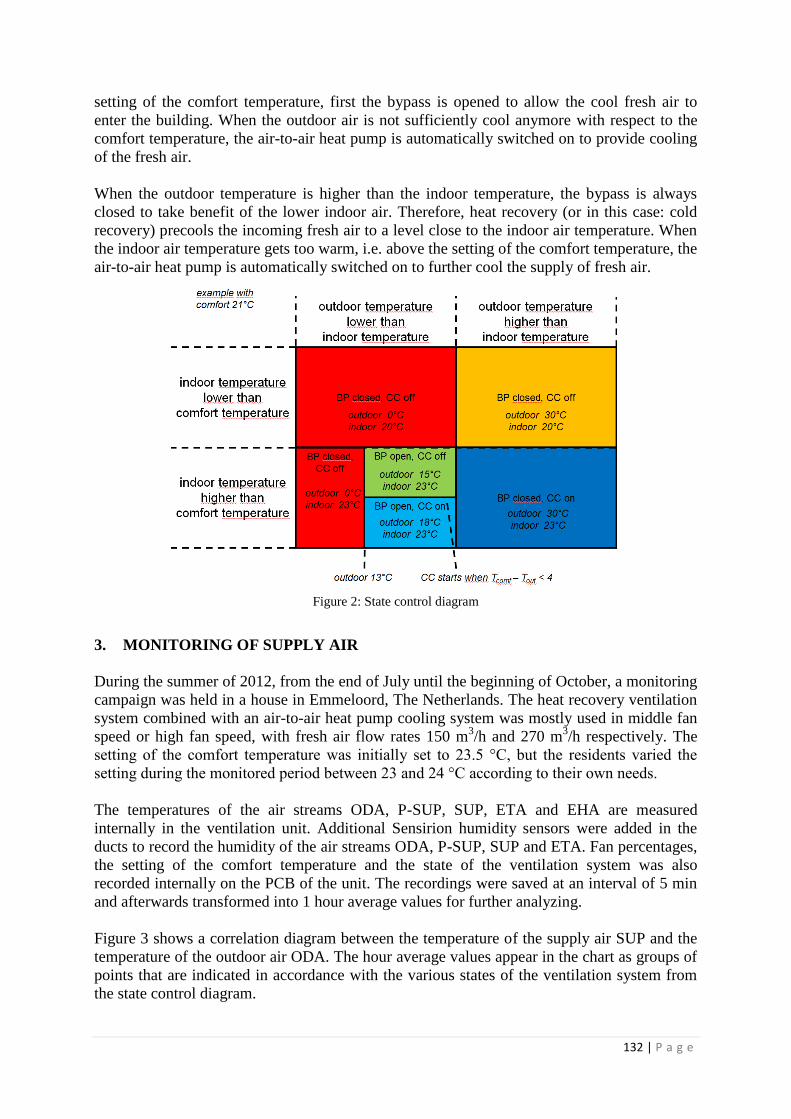
132 | P a g e

setting of the comfort temperature, first the bypass is opened to allow the cool fresh air to

enter the building. When the outdoor air is not sufficiently cool anymore with respect to the

comfort temperature, the air-to-air heat pump is automatically switched on to provide cooling

of the fresh air.

When the outdoor temperature is higher than the indoor temperature, the bypass is always

closed to take benefit of the lower indoor air. Therefore, heat recovery (or in this case: cold

recovery) precools the incoming fresh air to a level close to the indoor air temperature. When

the indoor air temperature gets too warm, i.e. above the setting of the comfort temperature, the

air-to-air heat pump is automatically switched on to further cool the supply of fresh air.

Figure 2: State control diagram

3. MONITORING OF SUPPLY AIR

During the summer of 2012, from the end of July until the beginning of October, a monitoring

campaign was held in a house in Emmeloord, The Netherlands. The heat recovery ventilation

system combined with an air-to-air heat pump cooling system was mostly used in middle fan

speed or high fan speed, with fresh air flow rates 150 m3/h and 270 m

3/h respectively. The

setting of the comfort temperature was initially set to 23.5 °C, but the residents varied the

setting during the monitored period between 23 and 24 °C according to their own needs.

The temperatures of the air streams ODA, P-SUP, SUP, ETA and EHA are measured

internally in the ventilation unit. Additional Sensirion humidity sensors were added in the

ducts to record the humidity of the air streams ODA, P-SUP, SUP and ETA. Fan percentages,

the setting of the comfort temperature and the state of the ventilation system was also

recorded internally on the PCB of the unit. The recordings were saved at an interval of 5 min

and afterwards transformed into 1 hour average values for further analyzing.

Figure 3 shows a correlation diagram between the temperature of the supply air SUP and the

temperature of the outdoor air ODA. The hour average values appear in the chart as groups of

points that are indicated in accordance with the various states of the ventilation system from

the state control diagram.

133 | P a g e

With closed bypass and outdoor temperatures below indoor temperature, the supply air

temperature is at a comfortable level between 16 °C and 23 °C, in relation to the actual indoor

air temperature because of the heat recovery. The average practical heat recovery efficiency

based on the supply air temperature during the monitoring period is 87%. The heat recovery

in this period saves heating energy for the central heating system of the house, indicated as

avoided heating.

With closed bypass and outdoor temperature above indoor temperature, the supply air

temperatures are also held close to the indoor air temperature because of the heat (cold)

recovery. This gives a comfortable supply of fresh air and reduces the heat load for the

building. This state is however not occurring often as the indoor air temperature rises to a

level above the comfort temperature where the air-to-air heat pump is started.

When the indoor air temperature rises above the comfort temperature (and outdoor air

temperature is above 13 °C), cooling is requested. With enough cooling capacity with the

outdoor air, passive cooling is started (bypass open, heat pump off), resulting in supply air

temperature 1 to 2 °C above the outdoor air temperature. The small rise in temperature is the

effect of heat gains in outdoor air ducts and heat dissipation by the supply fan.

If the outdoor air itself had not enough cooling capacity, the air-to-air heat pump is started

with open bypass to give a supply air temperature ranging between 10 °C for relatively low

outdoor temperature to about 16 °C for outdoor temperature close to indoor air temperature.

In this state, the ventilation system is giving passive cooling and active cooling at the same

time, resulting in comfortable cooling throughout the house with the minimum of cooling

energy.

When the outdoor air temperature is above the indoor air temperature, the bypass closes so

that the incoming fresh air is first reduced in temperature by heat (cold) recovery and

afterwards by the air-to-air heat pump. This results in supply air temperatures ranging from

12 °C to 22 °C depending on outdoor air temperature.

Figure 3: Monitoring results of supply air vs. outdoor air.

134 | P a g e

Figure 4 shows the correlation between the supply air and the indoor air, both in terms of

temperature and absolute humidity. The sensors for this graph are positioned at another place

as the internal sensors, so the values differ slightly. Without any cooling, the supply air is

close to the indoor air, thanks to heat recovery. With passive cooling (heat pump off), the

fresh air is supplied with a temperature 1 to 6 °C lower than the indoor air temperature. With

active cooling (heat pump on), the fresh air is supplied with a temperature 6 to 12 °C lower

than the indoor air temperature. Therefore, one could say that the sensible cooling power for

the indoor air with active cooling can be doubled when compared to passive cooling.

a) b)

Figure 4: Monitoring results of supply air vs. indoor air: a) temperature, b) absolute humidity.

Figure 4b shows the absolute humidity of the indoor air and the supply air. When the heat

pump is on, the dots are colored blue. It is obvious that the air-to-air heat pump is also

supplying the fresh air with lower humidity than the indoor air (difference up to 3.5 g/kg),

maintaining comfortable summer humidity levels in the house.

Figure 5: Total cooling power

135 | P a g e

The total cooling power (sensible + latent) of the heat pump has been calculated for the air-to-

air heat pump by the difference in conditions in front of the evaporator (P-SUP) and after the

evaporator (SUP) of the heat pump. Figure 5 shows the total cooling power in relation to the

outdoor air temperature. Depending on actual temperature and humidity conditions, the total

cooling power ranges between 700 and 1100 W for middle fan position (150 m3/h) and ranges

between 1200 and 1700 W for high fan position (270 m3/h). The power consumption of the

system was not monitored in this project. According to the specifications of the product, the

heat pump has a power consumption of 800 W when active.

With the help of this cooling system, comfortable fresh air is supplied into the rooms, keeping

the indoor temperatures throughout the whole house at a maximum of 26 °C as indicated by

figure 4a.

4. WORKING AREA

A technical limitation of the air-to-air heat pump is to prevent damage to the condenser when

it gets too hot. If the condenser temperature is reaching a safety limit, the fresh air flow rate is

first increased to the maximum. If the safety limit is reached with maximum air flow rate, the

heat pump is shut off intermittently to allow temporary cooling down of the condenser.

This effect is shown in figure 6 where the condenser temperature is shown in relation to the

outdoor air temperature. With the heat pump shut off, the condenser is close to the outdoor air

temperature. When the heat pump is on, the condenser takes temperatures roughly between

35 °C and 57 °C for outdoor air temperatures ranging from 15 °C to 30 °C. For outdoor

temperature above 30 °C, the hourly values of the condenser temperatures start decreasing

because of intermittent switching on and off of the heat pump.

Although the monitoring period did not show very warm periods, extrapolation of the

monitoring data indicates that for high outdoor temperatures the air-to-air heat pump will not

be active anymore. The combination of heat recovery ventilation and air-to-air heat pump

cooling system is therefore intended for climates where the summer outdoor air temperatures

are not often above 32 °C. This limitation holds only for the selected refrigerant and heat

pump parts in the product used in this monitoring study.

136 | P a g e

Figure 6: Condenser temperature

5. CONCLUSIONS

The heat recovery ventilation system in combination with an air-to-air heat pump cooling

system is investigated by a summer monitoring period in a house in Emmeloord, The

Netherlands. The ventilation system can act in various states that are explained by a state

control diagram.

The monitoring results show that the various states produce a comfortable supply of fresh air

throughout the whole building. When cooling is requested, the system automatically enters

the optimal cooling strategy: passive cooling when possible, and active cooling when

necessary.

The active cooling strategy can double the sensible cooling power for the house when

compared to the passive cooling strategy, and it can be used in a wider range of conditions.

The total cooling power of the air-to-air heat pump cooling system can reach up to 1100 W at

150 m3/h and up to 1700 W for 270 m

3/h.

The total ventilation and cooling system has proven to provide a comfortable summer indoor

climate with indoor air temperatures at maximum 26 °C for outdoor air temperatures up to

30 °C.

Opposite to circulation air-conditioning units, this ventilation/cooling combination not only

brings fresh air to the house, but also provides comfortable indoor climate in all of the

ventilated rooms in the house.

137 | P a g e

HEATING "PASSIVE HOUSE" OFFICES IN COLD

CLIMATE USING ONLY THE VENTILATION SYSTEM

– COMPARISON OF TWO VENTILATION

STRATEGIES

Hugo Lewi Hammer1*

, Mads Mysen2, Axel Cablé

2, Kari Thunshelle

2

1 Oslo and Akershus University

College of Applied Sciences

Pilestredet 35

N-0166 Oslo

Norway



Forskningsveien 3 b

N-0314 OSLO

NORWAY

Address, Country

ABSTRACT

In this article we compare to ventilation strategies to heat a “passive house” office building using only the

ventilation system. Two ventilation strategies with supply air temperature above and below the current room

temperature were compared through a cross over experiment. A questionnaire was used to measure the perceived

health and well being. Both strategies documented very good indoor climate with highly positive scores on the

questionnaire. The strategy with supply air temperature above the room temperature resulted in a little better

perceived health and well being compared to the other strategy.

KEYWORDS

cold climate, heating, questionnaire, passive house, ventilation strategies

1. INTRODUCTION

GK environmental house is the first office building in Norway satisfying the passive house

standard (NS 3701, 2012). The building is located in Oslo and has been operational since

August 2012. The building is mostly heated by supplying warm air into the rooms through the

ventilation system. In addition, active air supply diffusers with integrated presence and

temperature sensors are used in each room to control the ventilation rate according to room

demand. In this paper, we investigate the potential effects on health and well-being when the

heating demand is covered entirely with the ventilation system. The concern is whether air

mixing is poor when over-tempered air is supplied into the rooms. In this context, we assessed

the perceived indoor climate resulting from two different ventilation control strategies. The

first strategy (named strategy 1) resulted in a supply temperature somewhat higher than room

temperature, while the second strategy (strategy 2) resulted in a supply temperature slightly

below room temperature. Perceived health and well being is measured using a questionnaire.

2. MATERIAL AND METHODS

Both control strategies used consisted in having an initial room temperature of around 21oC

138 | P a g e

when the users arrived in the building. The supplied air temperature at the exit of the Air

Handling Unit (AHU) was then controlled depending on the average temperature measured in

all the rooms. The curve used to control the supply temperature was different for both

strategies and is presented on Figure 1 and Figure 2.

Figure 1: Control of the supply temperature at the exit of the AHU according to average room temperature in the

building: strategy 1.

Figure 2: Control of the supply temperature at the exit of the AHU according to average room temperature in the

building: strategy 2.

Globally, strategy 1 results in a higher supply temperature than strategy 2.

The two ventilation strategies described above were compared using a cross over design, see

Table 1.

139 | P a g e

Table 1: The plan for the cross-over experiment.

19th Nov. 13

th January 14

th January

Part of building Both South North South North

Ventilation strategy Normal 1 2 2 1

Ventilation temperature

control

Normal Fast

(Figure 1)

Slow

(Figure 2)

Slow

(Figure 2)

Fast

(Figure 1)

Ventilation rate [l/s] Varying Varying Varying Varying Varying

On the 13th of January the users in the south and north part of building were exposed to

strategy 1 and strategy 2, respectively and on the 14th of January the exposing were switched

(Table 1). With such a cross-over design, each user in the building was exposed to both

ventilation strategies. On the 19th of November the ventilation were run as normal and the

indoor climate were expected to be good. This case was used as control.

A questionnaire was used to measure the users’ perceived health and well-being under the

different cases in Table 1. The questions are shown in Table 3. On each question the users

gave a value between one and ten ranging from very uncomfortable and very comfortable.

The sum, S, of all the scores for a given user, represents the overall health and well-being for

this user. The questionnaire also included health question like whether a used suffered from

asthma or cold.

Data from the questionnaires were analyzed using a random effect linear regression model

with S as the dependent variable. The three cases 19th November, strategy 1 and strategy 2

represent the main independent variable, but also office temperature is included. The office

temperature is varying with date and place in the building and including this as an

independent variable, we were able to study the effect of the ventilation strategies

independent of the room temperature. We also include as independent variables gender and

whether the participants suffered from cold or asthma such that we are able to compare the

ventilation strategies independent of these factors. We expect that repeated measures from the

same user is correlated, e.g. some users are always too cold and some users are always tired,

and this is taken into account by including a random effect on the user level in the regression

model. Statistical analyses were performed using the program R (R development team, 2013)

and the R package lme4 (Bates et al., 2013).

3. RESULTS

Table 2 shows some technical measurements from the experiment.

Table 2: Technical measures.

Date 19.November 13 th January 14

th January

Part of building Both South North South North

Ventilation strategy Normal 1 2 2 1

Initial supply air temperature

(7 am)[oC]

North: 15.9

South: 17.8

24.3 17.3 15.8 24.4

Average room temperature

(6 am – 2 pm)

North: 22.1

South: 22.0

21.7 20.7 21.5 21.4

Average supply air temperature

(6 am – 2 pm)

North: 15.6

South:15.9

22.8 19.3 21.0 23.4

Outdoor temperature [oC] 4.1 – 10.9 – 5.9

Outdoor condition Partly cloudy Cloudy Cloudy

140 | P a g e

The average supply temperature during the length of the questionnaire (6 hours) as well as the

average room temperature are presented in Table 2. We can see that strategy 1 resulted in a

supply temperature above room temperature, while strategy 2 resulted in a supply temperature

slightly below room temperature . Furthermore, the supply temperature was relatively low on

November 19 (15.6-15.9°C). This results from the fact that the outside temperature was

relatively high (4.1°C) compared to the tests performed on January 13 and January 14 ( –

10.9°C and – 5.5°C, respectively). It was therefore necessary to compensate for the internal

heat gains by supplying cool air into the rooms.

For each of the three dates in the experiment, 19th November, 13

th and 14

th January, the

questionnaire was sent out to 133 users and we received 46, 35 and 36 answers, respectively.

18 users answered all the three questionnaires. Table 3 shows average score on each question

in the questionnaire under the two ventilation strategies and 19th November.

Table 3: Questionnaire with average score under the two ventilation strategies.

Questions 19th November Vent. strat. 1 Vent. strat. 2

Are you tired? 6.43 7.97 7.46

Does your head feel heavy? 6.83 8.70 7.68

Do you have a headace 8.07 8.77 8.32

Do you feel faint or dizzy? 8.26 9.17 8.49

Do you have problems concentrating? 6.87 8.00 7.61

Do you feel itching or burning in your eyes? 8.39 8.43 8.32

Do you feel hoarse or dry throat? 8.17 8.77 8.39

Do you feel itching or burning in your face

or on your hands? 9.20 8.90 8.85

Do you feel nauseous or otherwise unwell? 9.37 9.47 9.58

Is it too warm? 7.76 8.77 8.29

Is there bothersome warmth because of

sunshine? 8.26 9.60 8.68

Is it too cold? 8.00 7.57 7.17

Do you feel a draught around your feet or

your neck? 9.37 8.93 8.73

Does the temperature in the room vary? 8.85 8.90 8.43

Does the air feel heavy? 7.80 9.00 8.26

Does the air feel dry? 8.02 8.57 8.14

Is there any unpleasant smell? 9.48 9.70 9.39

Do you have a stuffy or runny nose? 9.30 8.50 8.41

Do you cough? 8.96 8.70 8.53

We see that overall the users feel quite well with almost all average scores above eight. We

also see that the scores under strategy 1 are higher (more comfortable) than under strategy 2.

Table 4 shows the results from the regression analysis. All answered questionnaires

(46+35+36=117) were included in the analysis.

141 | P a g e

Table 4: Results from linear regression.

Parameter Estimate St. err. df t value p value

Vent. strat. 1

(reference: vent. strat. 2) 6.6 2.9 42.5 2.26 0.029 *

19th November

(reference: vent. strat. 2) 2.8 2.9 44.9 0.98 0.332

Office temperature 5.1 6.0 46.4 0.84 0.405

Gender male (reference: female) 20.8 6.9 67.9 3.01 0.004 **

Asthma (reference: No asthma) – 31.1 10.9 69.6 2.83 0.006 **

Cold (reference: No cold) – 5.3 4.1 49.4 1.28 0.205

Signif. codes: p-value < 0.01:**, p-value < 0.05:*

We see that the perceived health and well-being is significantly better under strategy 1

compared to strategy 2 and that strategy 2 is not significantly poorer than the control autumn

(19th November). We also observe that the perceived health and well-being is better for male

users and users with no asthma or cold.

4. DISCUSSION

For the winter conditions considered (13 and 14 January), a better perceived indoor climate

was obtained for a supply temperature higher than room temperature (strategy 1) than for a

supply temperature slightly lower than room temperature (strategy 2).

Furthermore, no significant discomfort regarding perceived indoor air quality was obtained

compared to the control case (19 th November). This is an indication that the active air supply

diffuser employed display good mixing properties for a broad range of supplying conditions,

and that the short-circuiting of the fresh and warm ventilation air is reduced to a great extent.

Therefore, supplying warm ventilation air to cover the heating demand appears to be a

relevant solution for office buildings with passive house standard.

5. REFERENCES

Standard Norge NS 3701 (2012) Criteria for passive houses and low energy buildings.

Douglas Bates, Martin Maechler, Ben Bolker and Steven Walker (2013) lme4: Linear mixed-

effects models using Eigen and S4, R package version 1.0-5. Available at http://CRAN.R-

project.org/package=lme4

R Development Core Team (2013) R: A Language and Environment for Statistical

Computing, R Foundation for Statistical Computing, Vienna, Austria. Available at

http://www.R-project.org/.

142 | P a g e

MONITORING OF AN INNOVATIVE

ROOM-BY-ROOM DEMAND CONTROLLED

HEAT RECOVERY SYSTEM ON FOUR LOCATIONS

Colette Madeline, Stéphane Berthin, Pierre Kraus

Aereco SA

62, rue de Lamirault

77615 Marne la vallée, France

ABSTRACT

Demand controlled heat recovery ventilation systems, which combines heat recovery (HRV) and demand

controlled (DCV) is growing fast among ventilation manufacturers.

Several categories can be identified, from global dwelling regulation, to fine room-by-room regulation of the

airflow rate. Simulations show that room-by-room demand controlled heat recovery ventilation is the best

compromise to optimize at the same time indoor air quality, comfort, and energy savings.

To reinforce this assessment, four room-by-room demand controlled HRV have been monitored since May 2013.

The system is an innovative ventilation for individual treatment, which modulates automatically the supply

airflow according to CO2 concentration in the main rooms, and exhaust airflow according to humidity

concentration in the wet rooms. The balance of the airflow is made using two specific compensation valves at the

exhaust and at supply.

Three projects are located in Germany: Nuremberg, Dortmund and Frankfurt, and one takes place in France, near

Paris. The dwellings have from three to five main rooms, and a real occupancy of two to five people. They are

all existing dwellings. The comparison was made between three different types of installation: two in the heated

space, one in the attic (slightly insulated), and one with the heat recovery unit in the heated space and the

ductwork in the attic (non insulated).

The results have shown the good functioning of the system in terms of balancing, adaptation of the airflow rates

to the needs, and filtration. The relevance of using CO2 concentration to modulate the airflow rate at supply has

been verified by presence sensors in the main rooms. Temperature sensors revealed the necessity to carry on the

installation in the heated space to optimize energy savings. Besides, the collected data gave the opportunity to

validate a simulation model of the system using CONTAM (multizone indoor air quality and ventilation analysis

program developed by NIST).

The monitoring also demonstrated the good performance of this type of heat recovery, in terms of indoor air

quality, comfort and energy savings. The CO2 and the humidity level stayed in the comfortable range thanks to

demand controlled ventilation. The supply temperature, when the HRV is located in the heated space, is mostly

between 18 and 20°C, thanks to heat recovery (the outdoor temperature being in the range of 0 to 14°C). In-situ

measures and surveys occupants supplied complementary information regarding the acoustic and thermal

comfort.

1. KEYWORDS

Heat recovery ventilation; demand controlled ventilation; indoor air quality; energy savings

143 | P a g e

2. INTRODUCTION

The need to reduce more and more the energy consumption in residential buildings has lead

several manufacturers of ventilation systems to associate heat recovery ventilation (HRV)

with demand controlled ventilation (DCV). Some systems control the supply or the exhaust

only, and some other control both, room by room or in a global way. Simulations made on

CONTAM (a multizone indoor air quality and ventilation analysis program) show that room-

by-room demand controlled heat recovery ventilation is the best compromise to optimize at

the same time indoor air quality (IAQ), thermal comfort, and energy savings. A monitoring of

this last type of HRV was carried out in four dwellings. This study shows the results of this

monitoring campaign and some of the results of the simulations.

3 SIMULATIONS

3.1 Energy efficiency / Indoor air quality

The simulations compare five types of HRV systems on the energy and IAQ aspects in a three

bedroom house occupied by three people (Table 1). As CO2 concentration results are very low

in the dwelling (no exposure over 2 000 ppm for none of the HRV systems), the CO2

comparison level has been set to 1 200 ppm.

Table 1: Simulated HRV systems

System Exhaust Supply Balance

Fixed airflow

rate

Fixed airflow in the wet rooms

according to French regulation

Qsupply_room=Qextr./4 Fixed balanced airflow rates

Preset speed

level

Humidity sensor in the wet

rooms

CO2 sensor in the parents’

bedroom

Qtot = f (Max(RH; CO2))

Instantaneous distribution of

the total airflow rate between

the rooms

Exhaust

DCV

Humidity controlled exhaust

units in the wet rooms

Qsupply_room =Qextr./4 Instantaneous distribution of

the total airflow rate in the

main rooms

Supply DCV Qextr._room=Qsupply/3 CO2 controlled supply

units in the main rooms

Instantaneous distribution of the

total airflow rate in the wet

rooms

Exhaust and

supply DCV

Humidity controlled exhaust

units in the wet rooms

CO2 controlled supply

units in the main rooms

Supply and exhaust

compensation valves

Looking at the results below (Figure 1, Figure 2, Figure 3), the supply DCV is the best system

regarding energy and CO2 aspect (very few heat losses and acceptable CO2 concentration), but the

RH (relative humidity) in the bathroom and in the kitchen is very high. The exhaust DCV has a

good RH level in the wet rooms but it has more hours of exposure over 1200 ppm (which is easily

satisfactory), and the fixed airflow and the preset speed level systems have too many heat losses.

According to the simulation results, the exhaust and supply DCV seems to be the best

compromise to optimise at the same time the indoor air quality and the energy consumption.

144 | P a g e

Figure 1: HRV energy / CO2 exposure over the heating season (CONTAM simulation)

Figure 2: HRV energy / RH in the bathroom

(CONTAM simulation)

Figure 3 : HRV energy / RH in the kitchen

(CONTAM simulation)

3.2 Filter clogging

The monitored system tests the total pressure drop of the HRV every two months in order to

give a signal to change the filters if necessary. This filter test has been simulated on 5 HRV

systems using G4 + F7 filters at supply. The results are showed for filter F7 only (Figure 4).

During the four first months of the simulation, the pressure drop is more or less the same for

all the systems. The dust mass of the filter increases a lot after eight months of operation in

the system with fixed airflow and in the preset speed level system. DCV systems have almost

the same dust mass increase, which is the slowest of the five simulated systems, thanks to the

modulation of the airflow rates.

In Dortmund, after eleven months of functioning, filter F7 has a pressure drop of 21.5 Pa,

which is even less than the result showed by the calculation. In Nuremberg, the filter F7 has a

pressure drop of 26.4 Pa after 9 months of functioning.

145 | P a g e

Figure 4: F7 filter tested at 170 m3/h every 2 months (CONTAM simulation)

4 MONITORING

4.1 Monitored room-by-room demand controlled HRV

Figure 5: Monitored room-by-room demand controlled HRV

The ventilation is a heat recovery system involving a heat recovery unit connected to exhaust

units and a distribution box that modulates the supplied airflows (Figure 5).

The airflows are automatically modulated according to the needs of each room in the dwelling:

the air supplied to the bedrooms and living room and the air exhausted from the kitchen, the

bathroom, and the WC. Each supply unit is directly connected to the distribution unit, which

adjusts the supplied airflow in the main rooms according to the level of CO2. On the exhaust side,

the units adjust the airflow, according to parameters that depend on the room concerned: humidity

in the bathroom, occupancy in the WCs, humidity and switch for the boost airflow in the kitchen.

At all times, the total supplied and exhausted airflows are measured in the heat recovery unit

and balanced by two controlled compensation valves that are located in the living room, the

kitchen, or a corridor. For example, when the need increases in the kitchen as a meal is being

prepared, and is not accompanied by high demand in a bedroom or in the living room, the

exhaust airflow can be balanced by opening the compensation valve of the supply ductwork.

146 | P a g e

4.2 On-site installations and monitored values

Figure 6: Monitored dwelling in Dortmund

Three projects are located in Germany: Nuremberg, Dortmund (Figure 6) and Frankfurt, and

one takes place in France, near Paris. The dwellings have from three to five main rooms, and

a real occupancy of two to five people. They are all existing dwellings. The comparison was

made between three different types of installation: two in the heated space (Figure 8), one in

the attic (slightly insulated, Figure 7), and one with the heat recovery unit in the heated space

and the ductwork in the attic (non insulated).1

Figure 7: Installation in the attic

Figure 8: Installation in the false ceiling

Every parameter of the system has been monitored every 1:30 minute in Nuremberg and in

Dortmund, and every minute in Frankfurt and in Paris (Table 2). The first projects in

Nuremberg and Dortmund have presence sensors in every main room (presence detection

measure every 1:30 minute). The last projects in Frankfurt and Paris have temperature and

relative humidity sensors in every main room (measure every minute).

1As the last installation in Paris was installed in the beginning of May 2014, there is not enough data to include its results in

this study for the moment.

147 | P a g e

Table 2: Monitored parameters

Parameter Location Monitoring

project

Parameter Location Monitoring

project

CO2 sensors In every main

room

All

Exhaust airflow

rate

At the main

unit

All

Opening of the

damper at supply

At the supply

dispatching box

All Supply airflow

rate

At the main

unit

All

Fresh air

temperature

At the main unit All Pressure at the

exhaust

At the main

unit

All

Supply air

temperature

At the main unit All Pressure at supply At the main

unit

All

Exhaust air

temperature

At the main unit All Speed rotation of

the exhaust fan

At the exhaust

fan

Nuremberg,

Dortmund

Used air

temperature

At the main unit All Speed rotation of

the supply fan

At the supply

fan

Nuremberg,

Dortmund

Opening of the

exhaust

compensation valve

At the exhaust

compensation

valve

All Defrosting state At the main

unit

All

Opening of the

supply

compensation valve

At the supply

dispatching box

All By-pass state At the main

unit

All

Exhaust fan setting At the exhaust

fan

All Supply fan setting At the supply

fan

All

Presence sensors In every main

room

Nuremberg,

Dortmund

Temperature and

humidity sensor

In every room Frankfurt,

Paris

4.3 Check of the working of the HRV

The graph presenting the total supply airflow rate as a function of the total exhaust airflow

rate shows a positive and linear correlation between supply and exhaust airflow rate (Figure

34). These results allowed to highlight a program default for airflow rates under 40 m3/h,

which was corrected on the standard mass-production product.

Considering the total airflow rate over 40 m3/h only, the correlation coefficient is 0.86. Moreover,

the peak of correlation happens with no interval, so the balance of the airflow is instantaneous.

The instantaneous difference between supplied and exhaust airflow rate is mainly around zero,

and is 97.98 % of the time included in the interval [-10; 10[ m3/h (Figure 10).

148 | P a g e

Figure 9: Relationship between total exhaust airflow rate and

total supply airflow rate.

(Frankfurt, from 2014/01/03 to 2014/05/31)

Figure 10: Balance of exhaust and supply

airflow rate.

(Frankfurt, from 2014/01/03 to 2014/05/31;

above 40 m3/h).

Four preset supply airflow rate are defined, according to the concentration of CO2 in each

main room. The results show that the supply airflow is well distributed among the 4 preset

rates, depending on the occupancy of the room (Figure 11, Figure 12).

Figure 11: Use of preset supply airflow rate

(Frankfurt, from 2013/11/15 to 2014/05/31)

Figure 12: Preset CO2 level

(Above ambient concentration)

5 PERFORMANCE OF THE ROOM-BY-ROOM DCV HRV

5.1 Indoor air quality

The RH distribution in the dwelling shows that the concentration is between 30 and 60 % for

the considered period (from 2014/02/13 to 2014/05/31). This range of RH concentration is

comfortable according to ASHRAE comfort zones (Figure 13).

149 | P a g e

Figure 13: RH distribution (Frankfurt, from 2014/02/13 to 2014/05/31)

The risk of condensation in the dwelling is almost null if we consider that such an efficient

HRV system should be installed in a dwelling having an energy efficient envelop (Table 3).

The worst case would occur in the kitchen, with a maximum of 2 hours of condensation risk

on a PVC double glazing with an air space of 12 mm (note that the bathroom has not been

monitored). All the main rooms have nearly zero risk of condensation, independently of the

external wall composition.

Table 3: Risks of condensation in the dwelling (Frankfurt, from 2014/02/13 to 2014/05/31)

Room (Mean

dew point

temperature

[°C])

Mean internal wall temperature [°C]

(March 2014)

Risk of condensation [number of minutes]

(From 2014/02/13 to 2014/05/31)

Double

glazing

U=1.2

W/(m².K)

Double

glazing

U=2.3

W/(m².K)

Insulated

ext. wall

U=0.51

W/(m².K)

Non

insulated

ext. wall

U=2.25

W/(m².K)

Double

glazing

U=1.2

W(/m².K)

Double

glazing

U=2.3

W/(m².K)

Insulated

ext. wall

U=0.51

W/(m².K)

Non

insulated

ext. wall

U=2.25

W/(m².K)

Kitchen

(6.5)

16.2 12.6 18.5 12.8 26 116 3 112

Bedroom

(6.2)

15.1 11.9 17.1 12.1 0 2 0 2

Living

room

(5.7)

16.4 12.7 18.7 12.9 0 0 0 0

Office

(5.5)

15.4 12.1 17.4 12.3 0 0 0 0

CO2 distribution in the bedrooms has been observed thanks to the sensors located in each main

room, which control the supply airflow rate. In the bedrooms with an occupancy of one person,

the CO2 concentration is less than 1 150 ppm 80 % of the time. In the bedrooms with an

occupancy of two people, the CO2 concentration doesn’t exceed 1 250 ppm 80 % of the time. In

any case, CO2 concentration won’t exceed 1 650 ppm, whatever the occupancy (Table 4).

150 | P a g e

Table 4: CO2 distribution: main results in bedrooms

Monitoring ref. Max

distributed area

(peak %)

100 % of time

under X ppm

90 % of time

under X ppm

80 % of time

under X ppm

Nuremberg: 1 child 950-1000 ppm

26.7 %

1 400 1 150 1 100

Nuremberg: 2 children 1100-1150 ppm

25.5 %

1 600 1 300 1 200

Nuremberg: 2 adults 1150-1200 ppm

15.0 %

1 650 1 350 1 250

Dortmund: 1 adult 1000-1050 ppm

19.8 %

1 250 1 150 1 100

Dortmund: 1 child 1100-1150 ppm

23.1 %

1 550 1 250 1 150

Frankfurt: 2 adults 950-1000 ppm

10.9 %

1 600 1 200 1 050

The CO2 concentration distribution shows a fast reduction on the right side of its peak, which

implies a good management of the air renewal in case of high CO2 concentrations (Figure 14).

Figure 14: CO2 distribution in a bedroom occupied by 2 adults (Nuremberg, from 2013/11/15 to 2014/05/31)

5.2 Thermal comfort

The survey fulfilled by the occupant in February showed no annoyance due to the supply air in the

main rooms in Nuremberg and in Dortmund. If we look at the supply temperature distribution, we

can observe that during the heating period the supply temperature is between 16 and 26°C 99.3 %

of the time in Nuremberg, 95.6 % of the time in Dortmund, and 39.5 % of the time in Frankfurt.

These results show the huge impact of the location of the installation. In Frankfurt, the

ductwork is insulated with 2*30 mm of glass wool, and the main unit is also insulated with

blocks of polyurethane foam. The thermal efficiency is decreased by more than 50 % for an

151 | P a g e

insulated installation located in the attic compared with an installation located in the heated

space (Figure 15).

Figure 15: Supply air temperature as a function of fresh air temperature (From left to right: Dortmund and Frankfurt)

The discomfort due to draught can be expressed as the percentage of people predicated to be

bothered by draught. This criterion is called draught rate (DR) and is calculated through empirical

values. According to the draught rate and some other parameters, it is possible to define the

comfort level category (ISO 7730:2005). An estimation of this criterion has been calculated at 2

meters from the unit, using the instantaneous airflow rate, the local air temperature being the

supply and the extract air temperature average at the main unit. The DR is less than 15 % almost

100 % of the time in Nuremberg and in Dortmund, as recommended by the scientific literature. In

case of an installation in the attic (as showed in Frankfurt), the DR which depends on the supply

temperature is higher than for an installation in the heated space (Figure 16).

Figure 16: DR < 15% in parents’ bedroom (at 2 meters)

5.3 Energy efficiency

An estimation of heat losses due to the ventilation system has been calculated, using the

temperatures and the instantaneous total airflow rates at the main unit. The calculation is not made

for fresh air temperature over 15°C, and the extract air temperature is taken as an estimation of the

inside temperature. The monitoring in Dortmund has very low heat losses in comparison with the

monitoring in Nuremberg, because the extract air temperature is about 3°C more in Nuremberg

than in Dortmund2. The electrical consumption of the fans has also been estimated, using the

instantaneous speed level of the fans and the total airflow rates (Table 5).

2The monitoring in Frankfurt is not presented because its data doesn’t include the whole heating period (beginning of the results in

January).

152 | P a g e

Table 5: Mean airflow rates, heating needs, and electrical consumption of the fans over the considered period

Monitoring ref.

(Surface m²)

Considered

period

Mean

airflow

rate [m3/h]

Mean

extract /supply

temperature [°C]

Heat losses

(final energy)

[kWh/(m².an)]

Mean fan power

(exhaust +

supply) [W]

Nuremberg

(106 m²)

2013/11/15 to

2014/05/31

101.6 23.6/19.4 6.5 21.9

Dortmund

(111 m²)

2013/11/15 to

2014/05/31

116.9 20.3/19.1 2.2 30.7

Considering a gas appliance for heating, with a mean cost of 6.89 c€(incl tax)/kWh, and a cost

of 29.21 c€(incl tax)/kWh for electricity, the mean monthly cost due to the monitored HRV

would be 10.13 €(incl. Taxes)/month in Nuremberg, and about 6.91 €(incl tax)/month in

Dortmund during heating season. Prices of S2-2013 in Germany (Eurostat European

comission, 2014).

6 ADDITIONAL SENSORS

The two first monitoring (Nuremberg and Dortmund) have been equipped with presence

sensors in the main rooms. From these data, two analyses can be made: Is CO2 a good

indicator of human presence? Is it possible to use presence sensors instead of CO2 sensors to

control the supply airflow rate?

In addition, relative humidity and temperature sensors have been added in monitoring Frankfurt

since the middle of February, and in Paris since May. There are located in the main rooms

(bedrooms, living room, office) and in the wet rooms. These sensors have been added in order to

study the possibility of using humidity sensors instead of CO2 to control the supply airflow rates.

The results confirm the fact that CO2 is a good indicator for presence detection, the CO2

concentration increasing in the dwelling when a detection of presence occurs. Presence

sensors, as an alternative to CO2, could be relevant using more accurate sensors. In the same

way, relative humidity sensors could be used instead of CO2, but they would need to be

corrected from outside humidity variation, like the humidity controlled air inlets currently

used in MEV (mechanical exhaust ventilation) systems for instance.

7 CONCLUSIONS

This monitoring campaign has shown the good working of the tested demand controlled heat

recovery ventilation system. It has also helped to improve the management of the program for

specific points. Regarding the efficiency of the system, the indoor air quality is very good: no

hours over 2 000 ppm of CO2, and a relative humidity between 30 and 60 % in the main

rooms. For the installations in the heated space, the supply temperature is more than 95 % of

the time between 16 and 26°C. Looking at the results for the installation in the attic, the study

confirms that it is necessary to put the HRV in the heating space, in order to use the entire

potential of the HRV system.

In terms of energy consumption, the results are very positive, with a maximum of

6.5 kWh/(m².year) for the ventilation heating needs, and a mean electrical power of 30.7 W in

the worst case.

This monitoring is going to continue until spring 2015, in order to be able to study the

summer functioning and to generalize the efficiency results of the HRV during winter.

153 | P a g e

8 ACKNOWLEDGEMENTS

This project would not have been possible without the agreement of the owners of the dwellings,

that is why we would like to thanks a lot the occupants of the four monitored dwellings.

9 REFERENCES

Eurostat European comission. (2014, 05 20). Eurostat Database. Retrieved 06 24, 2014, from

http://epp.eurostat.ec.europa.eu/portal/page/portal/statistics/search_database

ISO 7730:2005. Ergonomics of the thermal environment - Analytical determination and

interpretation of the thermal comfort using calculation of the PMV and PPD indicies and

local thermal comfort criteria.

154 | P a g e

CLEANLINESS OF AIR FILTERS IN THE

EXPERIMENTAL PASSIVE HOUSE

Michal Michalkiewicz 1, Malgorzata Basinska

*2

1 Poznan University of Technology

Pl. Sklodowskiej – Curie 5

Poznan, Poland



Poznan, Poland

*Corresponding author:

[email protected]

ABSTRACT

An inherent element of the passive house is the system of exhaust ventilation in air supply. According to their

class, air filters used in ventilation systems stop the contamination, but may also be the main source of secondary

indoor contamination during long-term use.

The aim of the study was to determine the contamination of different air filters after several months of their

continuous work. The weight of the filter and its pollution with dust and microbiological contamination were

determined. Research was carried out for four sets of filters working in the experimental passive house in the

Poznan University of Technology – DoPas. The measurements were focused on the quality of the

microbiological contamination of air filters. During microbiological examination of filters, the following

microorganisms were determined: the general count of mesophilic bacteria, the general count of psychrophilic

bacteria, the count of Staphylococcus (Staphylococcus) mannitol positive (type α) and mannitol negative (type

β), the count of Pseudomonas fluorescens bacteria, actinomycetes (Actinobacteria) as well as the general count

of microscopic fungi. Performed measurements of studied microorganisms count revealed that psychrophilic

bacteria, microscopic fungi and mesophilic bacteria were most numerous. Their count was about ten times higher

in the intake duct filter than in the exhaust duct filter. After disinfecting air ducts their cleanliness level dropped

from moderate contamination to low.

KEYWORDS

Passive house, office building, air filters, microbiological contamination, ventilation installations

1. INTRODUCTION

Recent years have witnessed a growing focus on the quality of air in buildings, since people

spend over 70% of their time there. More and more buildings (especially office complexes)

are equipped with mechanical ventilation systems, which is connected, among others, with

limiting the amount of energy supplied to the building through air flow control. Moreover, the

purposed of ventilation systems is to eliminate contamination generated indoors or dilute it till

it reaches an acceptable level. Despite vast interest in indoor air cleanness, some parameters

that contribute to the quality of air have not been fully known. One of these elements is an air

filter whose purpose is to stop physical as well as microbiological contamination of air.

Depending on the quality of filtering material and the type of filter, it stops:

– insects, dust, plant spores, bacteria – on coarse filters and fine filters,

– microorganisms, viruses, particles floating in the air – on HEPA, ULPA and special filters.

155 | P a g e

The quality of filtering depends not only on proper class of filter used for various expected

results but also on the filter's own cleanness which deteriorates while the filter is in service.

Figure 1 presents a picture of both a clean filter and a contaminated one, magnified 160 times.

a)

b)

Figure 1: Air filter cleanness level, magnification 160 times, a) clean filter, b) contaminated filter

Chin (Chin 1999) writes that a hygroscopic filtering material can absorb moisture from the air

and when moisture level on dust particles stopped by the filter is high enough, a process of

sprouting and growth of a fungus colony may start. The author claims that the primary bio-

contamination is fungi and bacteria, the next is mites, insects and nematodes, whose count is

related to the growth of fungi. The dampness in a ventilation system also leads to an increase

in the count of bacteria in the system, which was proven a study by Ahearn (Ahearn et al.,

1997) who revealed that an air conditioning system can contribute to an increase in fungi

contamination indoors.

In order to evaluate the cleanness of filters after an eighteen-month use period,

a microbiological contamination assessment of the filters was performed. The measurements

were taken in an experimental passive house in the Poznan University of Technology –

DoPas, modernized in 2007 to meet the standard of passive construction. Having a light frame

structure, the building is a detached house, with single floor, fully cellared. The cellar has

mass structure, with walls made of concrete. Total area of the building is 143,7 m2, with

cubage of 620 m3. As a heat source, the building utilizes a central AHU 1 (Air Handling Unit)

with two EU5 type filters mounted on intake and exhaust lines. As an independent source (an

option to diversify heat sources) a compact heating and cooling unit can be installed,

connected with a ground heat exchanger and a solar collector (AHU 2). External air, having

been initially cooled in the exchanger, can be a bottom heat source for the heat pump in the

unit. One of the elements of the passive house ventilation system is a GWC ground exchanger

with a pipe that is 38 m long with a diameter of =200 mm, placed in the ground at a depth of

1.8 to 2.2 meters.

2. MATERIALS AND METHODS

The operation of replacing filters in the ventilation system in the DoPas passive house in

Poznan University of Technology allowed to perform a microbiological examination of

contamination in air filters. Replacement of filters after an eighteen-month use period,

performed by a specialized company, was completed with cleaning and disinfecting the

ventilation system. During the operation, the ventilation system, the AHU 1 ventilation unit,

as well as the intake and exhaust were mechanically and pneumatically cleaned and

disinfected. Mechanical cleaning was done with power brushes driven externally and with

compressed air. During the process of duct cleaning, the cleaning machinery collected

impurities do level I and II bags. For the purpose of disinfection, a biocide was used,

156 | P a g e

registered as medical product, with CE conformity marking and approval from the National

Institute of Hygiene.

Microbiological examination employed:

EU5 type filter from the AHU 1 ventilation unit, mounted on air intake – Filter 1,

EU5 type filter from the AHU 1 ventilation unit, mounted on air exhaust – Filter 2,

level I bag type EU 5 from cleaning machine, used for mechanical and pneumatic duct

cleaning – Filter 3,

level II bag type EU 5 from cleaning machine, used for mechanical and pneumatic duct

cleaning – Filter 4.

Table 1 presents the parameters of aforementioned filters and bags.

Table 1: Characteristics of examined filters

Filter Filter pack weight [g] Filter type Filter parameters

Filter 1 230,0 EU5 Ventilation unit, intake line,

Filter 2 1100,0 EU5 Ventilation unit, exhaust line,

Filter 3 320,0 EU5 Bag from ventilator of level I cleaning machine

(acc. to PN-EN 779)

Filter 4 190,0 EU5 Bag from ventilator of level II cleaning machine

Filters and bags were dismounted very gently and packed in sterile gauze. Complete filters

with their casing were weighed in the laboratory, then filter packs were removed and also

weighed. Segments were cut out from the removed filter pack and weighed on sterile Petri

dishes. After weighing they were placed in glass-stoppered flasks containing 100ml of sterile

water. Next, flasks with water and filter pack segments were shaken and the obtained water-

based suspension with microorganisms was used for microbiological examination.

Water samples with microbe suspension were used to make deep inoculations on Petri dishes,

flooded with proper nutrients. Various kinds of dilutions were used while making inoculations

and only those dishes that yielded from a dozen to 100 microorganism colonies were selected

for calculations. Knowing the volume of the inoculated fluid, the value of dilution, the count

of microbes grown and the weight of the shaken segment of filter pack it was possible to

recalculate the results from the culture into 1g of dry filtering material and the entire weight

of the filter pack.

While conducting microbiological examination of filters and bags, the following

microorganisms were determined: the general count of mesophilic bacteria, the general count

of psychrophilic bacteria, the count of Staphylococcus (Staphylococcus) mannitol positive

(type α) and mannitol negative (type β), the count of Pseudomonas fluorescens bacteria,

actinomycetes (Actinobacteria) as well as the general count of microscopic fungi.

Examination results were presented as number of colonies (colony forming unit [CFU]) which

had grown on the Petri dish. Microbiological examination utilized nutrients and culture

conditions recommended for the analysis of microbiological contamination of air according to

Polish Standards PN-89/Z-04111.02 and PN-89/Z-04111.03 (table 2).

Möritz and Martiny (Möritz, Martiny, 1997) used similar methodology of isolating bacteria

and microscopic fungi from filters used in HVAC systems.

157 | P a g e

Table 2: Culture conditions of selected microorganisms according to Polish Standards (PN-89/Z-04111.02, PN-

89/Z-04111.03)

Microorganisms Type of medium Temperature incubation [oC] Time incubation [h]

Mesophilic bacteria Nutrient agar culture 37 48

Psychrophilic bacteria * Nutrient agar culture 22 72

Staphylococcus Chapman medium 37 48

Actinobacteria Pochon medium 26 120

Pseudomonas fluorescens

King B medium and

identification of

colonies in UV rays

26 120

4 168

Microscopic fungi Waksman medium 26 168

Czapek-Dox medium 26 168

* not included in the Polish Standards

After culture period was finished, microorganism colonies that had grown on Petri dishes

were counted. The obtained results were recalculated into 1g of filtering material and the

entire weight of the filter.

3. EXAMINATION RESULTS

Tables 3, 4, 5 and 6 compile the examination results for microorganisms taken from the

filtering material of the dismounted filters and bags from the cleaning machine. Microbes

obtained from the culture were recalculated into 1g of filtering material and the weight of the

entire filter or bag.

Table 3: Average count of mesophilic and psychrophilic bacteria (CFU) abd standard deviation [σ] in the

examined filtering material

Filter Average bacteria count

Mesophilic Psychrophilic

CFU/1g of filter CFU/ entire filter CFU/1g of filter CFU/ entire filter

Filter 1 – intake 14 700

σ=1152,9875

3 381 000 25 640

σ=3041,7810

5 897 200

Filter 2 – exhaust 1 235

σ=91,9967

1 358 500 2 980

σ=284,5182

3 278 000

Filter 3 – level I

cleaning machine

1 990

σ=636,2199

636 800 19 250

σ=1341,4436

6 160 000

Filter 4 – level II

cleaning machine

3 910

σ=150,8235

742 900 15 325

σ=2002,9593

2 911 750

Table 4: Average count of staphylococcus (CFU) and standard deviation [σ] in the examined filtering material

Filter Average count of staphylococcus

Mannitol positive Mannitol negative



σ=184,9711

315 100 170

σ=25,0233

39 100

Filter 2 – exhaust 300

σ=50,8299

330 000 128

σ=9,2171

140 800


cleaning machine

186

σ=58,3811

59 520 62

σ=13,3936

19 840


cleaning machine

80

σ=8,6410

15 200 40

σ=8,6410

7 600

158 | P a g e

Table 5: Average count of microscopic fungi (CFU) and standard deviation [σ] in the examined filtering material

Filter Average count of microscopic fungi

Waksman medium Czapek-Dox medium



σ=1847,0111

3 933 000 20 500

σ=5447,0569

4 715 000

Filter 2 – exhaust 2 550

σ=261,9876

2 805 000 1 280

σ=92,1705

1 408 000


cleaning machine

12 420

σ=1105,0776

3 974 400 16 150

σ=3550,1899

5 168 000


cleaning machine

2 420

σ=183,3578

459 800 7 650

σ=1150,6156

1 453 500

Table 6: Average count of actinomycetes and Pseudomonas fluorescens (CFU) and standard deviation [σ] in the

examined filtering material

Filter Average bacteria count

Actinomycetes Pseudomonas fluorescens


Filter 1 – intake 855

σ=298,2304

196 650 0 0

Filter 2 – exhaust 850

σ=91,8105

935 000 0 0


cleaning machine

2 485

σ=182,8910

795 200 0 0


cleaning machine

1 610

σ=150,6017

305 900 0 0

4. EXAMINATION CONCLUSIONS

Analyzing the count of the examined microorganisms present in 1g of filtering material it is

concluded that most numerous microbes in Filter 1 (intake line) were psychrophilic bacteria

(25 640 CFU/1g), microscopic fungi (17 100 – 20 500 CFU/1g) and mesophilic bacteria

(14 700 CFU/1g). Among staphylococcus, mannitol positive staphylococcus (type α)

prevailed over mannitol negative staphylococcus (type β), with eight times the count than the

latter. Actinomycetes were found at relatively low numbers – 855 CFU/1g of filtering pack

weight (Fig. 2-4). Most numerous microbes in Filter 2 (exhaust line) were also psychrophilic

bacteria, microscopic fungi and mesophilic bacteria, however their count was 10 times less

than that of Filter 1 in some cases. The count of staphylococcus was also lower, especially

mannitol-positive staphylococcus, while actinomycetes indicated similar strength to the ones

in Filter 1. In level I cleaning machine bag (Filter 3) the prevailing microbes were

psychrophilic bacteria (19 250 CFU/1g) and microscopic fungi (12 420 – 16 150 CFU/1g) in

1g of filtering material, while in level II cleaning machine bag (Filter 4) the count of

psychrophilic bacteria and microscopic fungi was lower than in Filter 3, however the count

mesophilic bacteria was much higher (by 100%) reaching 3 910 CFU/1g. In both bags,

staphylococcus count was low while the count of actinomycetes was higher than in Filter 1

and Filter 2. In all examined filters, no presence of Pseudomonas fluorescens was recorded.

Figures 2-4 compile average count of microorganisms from all examined filters, recalculated

into 1g of filtering material.

159 | P a g e

Figure 2: Count of mesophilic bacteria (Meso), psychrophilic bacteria (Psychro) and actinomycetes (Actino),

recalculated into 1g of filtering material

Figure 3: Count of staphylococcus mannitol positive (Staph M+) and mannitol negative (Staph M-) recalculated

into 1g of filtering material

Figure 4: Count of microscopic fungi grown on Waksman medium (Waks) and Czapek-Dox medium (Cz-D)

recalculated into 1g of filtering material

Because of different weight of the examined filter packs, other values were obtained after

recalculating the count of microorganisms on the weight if the entire filters (table 3-6). Each

filter pack had the following weight: Filter 1 = 230 g, Filter 2 = 1100 g, Filter 3 = 320 g,

160 | P a g e

Filter 4 = 190 g. Considering these values, the highest count of mesophilic bacteria was

recorded in Filter 1 (over 3.3 million CFU/230g), the highest count of actinomycetes and

staphylococcus mannitol positive and mannitol negative was recorded in Filter 2 (over 935

thousand CFU/1100g, 330 thousand CFU/1100g and over 140 thousand CFU/1100g

respectively) and the highest count of psychrophilic bacteria and microscopic fungi was

recorded in Filter 3 (over 6.1 million CFU/320g and over 5.1 million CFU/320g respectively).

Filter 4 normally yielded the lowest count of the examined microbe groups. One might

understand that if Filter 1 and Filter 2 functioned as air cleaners for external air inflowing

from outside environment and for air contained indoors, with users inside the building, these

filters stopped mostly human-related microbes (mesophilic bacteria and staphylococcus) as

well as microscopic fungi that penetrated indoors from outside environment. While the

mechanical cleaning of air intake ducts was in progress, numerous impurities found there

were released from the surface where they settled and penetrated the bags of the cleaning

machine. Thus, especially in level 1 bag (Filter 3), the strength of numerous microbes

naturally present in the environment was high (psychrophilic bacteria, actinomycetes,

microscopic fungi), while the count of human-related microbes (mesophilic bacteria,

staphylococcus) in the bags of the cleaning machine was lower. In vast majority of the

examined microorganisms, their count was higher in level 1 cleaning machine bag than in

level II bag. This proves, that the first stage of duct cleaning was already very effective in

terms of eliminating bacteria and fungi that settled in the lines supplying air indoors to the

rooms of the passive house.

In order to assess the influence of filter replacement and air duct cleaning on the quality of

indoor air in the passive house, the level of microbiological contamination in the air was

analyzed before and after filter replacement. Air examination, performed with MAS-100 Eco

microbiological air sampler and using impact method, was conducted by the same company

that performed the ventilation system cleaning and disinfecting process. The examination

revealed that, after a complex procedure, the microbiological quality of air supplied to the

rooms of the passive house was good. At the same time, it was revealed that after cleaning

and disinfecting the system, a decrease in the general count of microbes was noted, compared

to the quality of air before replacing the filters and cleaning the ducts (table 7). During

identification process of the detected microorganisms, microbes were grown that form

saprophytic and opportunistic flora represented by Micrococcus spp., mould fungi and

sporulating bacilli.

Table 7: Microbiological cleanness of air from intake duct before and after the ventilation system cleaning and

disinfecting process

Determination Before cleaning [CFU/m3] After cleaning [CFU/m

3]

General microorganism count 107 40

Air pollution level [4] Moderate Very low

Air quality assessment was also performed in the experimental house, according to the

guidelines of Polish Standards (PN-89/Z-04111.02, PN-89/Z-04111.03). The examination

confirmed an improvement in the quality of air and a decrease in the general count of

mesophilic bacteria, psychrophilic bacteria, staphylococcus bacteria (Staphylococcus)

mannitol positive (type α) and mannitol negative (type β), Pseudomonas fluorescens,

actinomycetes (Actinobacteria) and the general count of microscopic fungi.

161 | P a g e

5. CONCLUSIONS

Usage period of filters and the condition of the ventilation system in the building has a very

big influence on the quality of indoor air. Polluted filters in the passive house (DoPas) caused

a drop in the effectiveness of air filtration. The impurities gathered and the growth of

microorganisms in filters could influence their filtrating capabilities making the filters

contribute to a deterioration of the quality of indoor air. Over many years, ventilation ducts

had gathered numerous physical and gas impurities. Apart from blowing new impurities from

external air, various substances concentrated in ventilation ducts could also penetrate indoors.

They could be dust and solids dated back to the construction of the system, soot, grease

particles, gases and bioaerosol-forming biological impurities, including flower pollen, viruses,

bacteria and fungi. They can impair the well-being of people in the building. It depends on the

count of substances blown indoors and the type of negative effect they have on humans.

Ventilation system contamination is a problem connected both with the health of residents in

the ventilated rooms and with the technical condition of the system which for instance may be

subject to biological corrosion due to large numbers of microbes. Such situation contributed

to the deterioration the quality of indoor air, one symptom of which being the so-called sick

building syndrome (SBS). The occurrence of ailments related to SBS is mainly connected

with insufficient amount of supplied clean air and its bad quality. The sources of indoor air

contamination may be construction materials, furnishing elements, also residents themselves,

microbe metabolites (endotoxins, enterotoxins, mycotoxins, glucans), contaminated

ventilation and air conditioning systems and low quality of outdoor air. Symptoms of SBS

include headaches, dizziness, fainting, malaise, fatigue, allergic reactions and other ailments

described by researchers such as (Charkowska, 2003; Joshi, 2008; Gąska-Jędruch, Dudzińska,

2009; Joe et al., 2013; Miaśkiewicz-Pęska, Łebkowska, 2011).

With favorable temperature, humidity and access to nutrients, air filters can become a habitat

for numerous microbes. Examining the filtering material can yield the presence of both

harmless and pathogenic microorganisms, among them dangerous species of bacteria, e.g.

Pseudomonas aeruginosa and Legionella pneumophila, as well as fungi, e.g. Alternaria spp.,

Aspergillus spp., Fusarium spp., Mucor spp., or Rhizopus spp. In order to limit the growth and

colonization of microbes in filters and air ventilation and conditioning systems, it is necessary

to perform periodical maintenance and cleaning of the systems and use antibacterial agents

(e.g. AgNO3), to cover the filtering material (Charkowska, 2000; Miaśkiewicz-Pęska,

Łebkowska, 2011).

Organic particles stopped in filters are a source of carbon for microbes and moisture

contained in the flowing air is their source of water. Such conditions not only help microbes

survive but also help them grow in significant numbers. As a result, it leads to an emission of

microorganisms from filters and secondary contamination of the treated air. An examination

of used filters conducted by Miaśkiewicz-Pęska (Miaśkiewicz-Pęska et al., 2007) revealed

very high concentration of living microorganisms, among which most numerous were moulds

(10 000 CFU/cm3 of filter), and the number of bacteria reached 6000 CFU/cm

3 (Miaśkiewicz-

Pęska et al., 2007).

Therefore, it is necessary to perform periodical inspection, cleaning and disinfection of

ventilation systems as well as regular filter replacement (according to manufacturer

recommendation) to ensure proper operation of the system and to create air comfort in rooms

(Fanger et al., 2003; Gołofit-Szymczak, Skowroń, 2005; Charkowska, 2000; Miaśkiewicz-

Pęska et al., 2007).

162 | P a g e

6. REFERENCES

Chin S. Yang. (1999). Biological contamination in the HVAC system. www.

invironment.com.

Ahearn, D.G.; Crow, S.A.; Simmons, R.B.; Price, D.L.; Mishra, S.K.; Pierson, D.L. (1977).

Fungal colonization of air filters and insulation in a multi-story office building.

Production of volatile organics. Curr. Microbiol., 35, 305-308.

PN-89/Z-04111.02. (Polish Standard). Air purity protection. Microbiological testings.

Determination number of bacteria in the atmospheric air (imision) with sampling by

aspiration and sedimentation method (Badania mikrobiologiczne. Oznaczenie liczby

bakterii w powietrzu atmosferycznym (imisja) przy pobieraniu próbek metodą

aspiracyjną i sedymentacyjną) [In Polish].

PN-89/Z-04111.03. (Polish Standard). Air purity protection. Microbiological testings.

Determination number of the fungi in the atmospheric air (imision) with sampling by

aspiration and sedimentation method (Badania mikrobiologiczne. Oznaczenie liczby

grzybów mikroskopowych w powietrzu atmosferycznym (imisja) przy pobieraniu

próbek metodą aspiracyjną i sedymentacyjną) [In Polish].

Möritz, M.; Martiny, H. (1997). Fungi and bacteria on air filters from heating, ventilation,

and air-conditioning systems: A method for the determination of fungi and bacteria on

air filters. Zentralbl Hyg Umweltmed., 199(6), 513-526.

Charkowska, A. (2003). Contamination of air conditioning systems and methods to eliminate

it (Zanieczyszczenia w instalacjach klimatyzacyjnych i metody ich usuwania). IPPU

MASTA Sp. z o.o. [In Polish].

Joshi, S.M. (2008). The Sick building syndrome. Indian J Occup Environ Med., 12(2), 61-64.

Gąska-Jędruch, U.; Dudzińska, M.R. (2009). Microbiological pollution in indoor air

(Zanieczyszczenia mikrobiologiczne w powietrzu wewnętrznym). Polska Inżynieria

Środowiska pięć lat po wstąpieniu do Unii Europejskiej, Monografie Komitetu

Inżynierii Środowiska, T 2, 59, 31-40 [In Polish].

Joe, Y.H.; Ju, W.; An, J.H.; Hwang, J. (2013). A quantitative determination of the

antibacterial efficiency of fibrous air filters based on the disc diffusion methods.

Aerosol and Air Quality Research, 14, 928-933.

Miaśkiewicz-Pęska, E.; Łebkowska, M. (2011). Effect of Antimicrobial Air Filter Treatment

on Bacterial Survival. FIBRES & TEXTILES in Eastern Europe, 19, 1 (84), 73-77.

Charkowska, A. (2000). Contamination of air conditioning systems and its elimination

(Zanieczyszczenia instalacji klimatyzacyjnych i ich usuwanie). Problemy jakości

powietrza wewnętrznego w Polsce’99. Materiały konferencyjne, Wydawnictwo

Instytutu Ogrzewnictwa i Wentylacji Politechniki Warszawskiej, Warszawa, 19-37 [In

Polish].

Miaśkiewicz-Pęska, E.; Karwowska, E.; Grzybowski, P. (2007). Microorganisms in office

buildings. Biological purity of ventilation system elements (Mikroorganizmy

w budynkach biurowych. Biologiczna czystość elementów instalacji wentylacyjnej).

Chłodnictwo i Klimatyzacja, 8, 60-65 [In Polish].

Fanger, P.O.; Popiołek, Z.; Wargowski P. (2003). Indoor environment. Its influence on health,

comfort and productivity (Środowisko wewnętrzne. Wpływ na zdrowie, komfort i

wydajność pracy). Gliwice [In Polish].

Gołofit-Szymczak, M.; Skowroń, J. (2005). Microbiological threats in office rooms

(Zagrożenia mikrobiologiczne w pomieszczeniach biurowych). Bezpieczeństwo pracy,

3, 29-31 [In Polish].

163 | P a g e

COMPARISON OF TWO VENTILATION CONTROL

STRATEGIES IN THE FIRST NORWEGIAN SCHOOL

WITH PASSIVE HOUSE STANDARD

Axel Cablé*1

, Hugo Lewi Hammer2, and Mads Mysen

1,2

1 SINTEF

Forskningsveien 3B

N-0314, Oslo, Norway


2 Oslo and Akershus University College

of Applied Sciences

Pilestredet 35


ABSTRACT

The Marienlyst School is the first educational building in Norway built according to the passive house standard.

This building benefits from a super-insulated and airtight envelope. While this reduces the heating demand

largely, it also enhances the risk for poor indoor air quality and overheating compared to conventional buildings.

It is therefore particularly important to implement an efficient ventilation strategy in order to avoid adverse

effects on the health, well-being and productivity of the pupils.

In this context, the perceived indoor climate resulting from two different ventilation control strategies was

evaluated in one classroom of the building. Both strategies consisted in varying the ventilation rate according to

room demand, ie. Demand Controlled Ventilation (DCV). The existing strategy consisted in varying the

ventilation rate in order to maintain a constant carbon dioxide concentration of 800 ppm in the classroom. A new

strategy was implemented which consisted in a combined CO2 and temperature DCV, ie. to control towards a

proportionally lower CO2 concentration when the indoor temperature increased. The aim with this strategy was

to address both overheating and the fact that perceived indoor air quality decreases when temperature rises.

Indoor climate measurements, as well as questionnaires on the perceived indoor air quality and thermal comfort

filled up by the pupils were used to compare both strategies. The data from the questionnaires were then

analyzed using a random effect linear regression model. The regression analysis revealed that the initial

ventilation strategy was responsible for discomfort resulting from too high variations in the indoor temperature.

The new combined CO2 and temperature DCV strategy provided a perceived indoor climate which was

significantly better than the existing strategy. Therefore, the developed ventilation strategy appears to be a

relevant solution in order to address the problem of overheating and perceived indoor air quality in educational

buildings with passive house standard.

KEYWORDS

Demand-Controlled Ventilation, passive house, questionnaires, indoor climate, school

1. INTRODUCTION

The Marienlyst School is the first educational building in Norway built according to the

passive house standard (NS 3701, 2012); see Fig.1. It has been operational since 2010, with

around 500 pupils of age 13 to 15. This building benefits from a super-insulated and airtight

envelope (U-values ranging from 0.05 to 0.12 W/m²K for the envelope, and air leakage

inferior to 0.6 vol/h under 50 Pa). While this reduces the heating demand largely, it also

enhances the risk for poor indoor air quality and overheating compared to conventional

164 | P a g e

buildings. It is therefore particularly important to implement an efficient ventilation control

strategy in order to avoid adverse effects on the health, well-being and productivity of the

pupils and school staff (Wargocki, 2000) (Sundell, 2011).

Figure 1: a) Marienlyst school, Oslo. b) View of a classroom.

In educational buildings, large variations of occupancy occur between periods with empty and

occupied classrooms. This results in large variations of the heat and pollutant loads in the

rooms, which is especially challenging in terms of control of the ventilation system.

Demand Controlled Ventilation systems (DCV) consist in varying the ventilation rate

according to a demand measured at room level, and seems therefore particularly fitted to

educational buildings. In fact, previous studies have reported that DCV systems can reduce

the energy use due to ventilation in the average classroom up to 51% compared to a system

operating with full airflow from 7:00 am to 5:00 pm (Mysen, 2005). It is however necessary

to evaluate how DCV strategies perform in practice, particularly in the new context of

educational buildings with low energy demand.

In this prospect, a new combined CO2 and temperature DCV strategy was implemented in a

classroom of the building. The objective of this study was to assess whether the new strategy

provided a better perceived indoor climate than the existing ventilation control strategy, using

both indoor climate measurements and questionnaires filled in by the pupils.

2. METHODOLOGIES

2.1 Ventilation control strategies

The existing control strategy in the building consisted in varying the ventilation rate in order

to maintain a constant carbon dioxide concentration of 800 ppm in the classroom (constant

CO2 control). In fact, the indoor CO2 concentration can be used as a proxy for the bio-

effluents concentration in the room. Staying under a given value therefore guarantees a certain

indoor air quality level.

In addition, an "overheating mode" was included in the existing strategy. It consisted in

forcing the opening rate of the Variable Air Volume ventilation dampers to 100% when the

indoor temperature reached 23.8°C and until the temperature got down to 23°C,

independently of the CO2 concentration in the room. This resulted in a larger amount of

outdoor air being supplied through the ventilation system, which aimed to prevent overheating

in the classroom.

165 | P a g e

A new strategy was implemented which consisted in a combined CO2 and temperature

control. It consisted in controlling the ventilation rate towards a proportionally lower CO2

concentration when the indoor temperature increased over 22.5°C; see Figure 2. The aim with

this strategy was to address both overheating and the fact that perceived indoor air quality

decreases when indoor temperature rises. In fact, previous studies have revealed that a lower

concentration of bio-effluents is perceived as acceptable when the indoor temperature is high

(Mysen, 2005). As a consequence, the ventilation rate should be increased for higher indoor

temperatures in order to maintain an acceptable perceived indoor air quality in the classrooms.

Figure 2: Combined CO2 and temperature control (Mysen, 2005).

2.2 Questionnaires and regression analysis

In order to compare the performance of the two ventilation strategies described above, a case

cross over study was carried out in one classroom of the building during February, March, and

May 2012, see Table 1.

Table 1: Date and ventilation control for the interventions

Date 20 February 2012 14 March 2012 30 May 2012

Ventilation control Constant CO2 with

"overheating mode"

Combined CO2 and

temperature

Combined CO2 and

temperature

At the end of each class session, the pupils were given a questionnaire with 19 questions

relating to Sick Building Syndrome-symptoms and perceived indoor climate. On each

question, the pupil gave a value between 0 and 1, ranging from very comfortable to very

uncomfortable. The questionnaire also included health questions, such as whether a pupil

suffered from asthma or cold.


with the score for each question as the dependent variable. The two ventilation control

strategies: "Constant CO2 control" and "Combined CO2 and temperature control" represent

166 | P a g e

the main independent variable. We also include gender and whether the pupils suffered from

cold or asthma as independent variables, in order to be able to compare the ventilation control

strategies independently of these factors. Statistical analyses were performed using the

program R (R development team, 2013) and the R package lme4 (Bates, 2013).

3 RESULTS

3.1 Actual conditions during the interventions

The CO2 concentration inside of the room, as well as indoor temperature were measured every

2 minutes.

The measurements during the intervention on February 20 with constant CO2 control are

plotted on Figure 3. The setpoint for the indoor CO2 concentration derived from the

ventilation control strategy is also indicated on Figure 3, as well as the periods where the

"overheating mode" was used (override of the constant CO2 control and full opening of the

ventilation dampers).

Figure 3: Measured indoor climate parameters on February 20 (constant CO2 control with "overheating mode")

The measurements during the interventions on March 14 and May 30 with combined CO2 and

temperature control are plotted on Figure 4 and Figure 5, respectively. Similarly, the setpoint

for the indoor CO2 concentration derived from the curve presented on Figure 2 is also

indicated.

400

500

600

700

800

900

1000

1100

12

14

16

18

20

22

24

26

10:59 11:28 11:57 12:25 12:54 13:23 13:52

CO

2 c

on

cen

tra

tio

n (

pp

m)

Ind

oo

r te

mp

era

ture

(°C

)

Time (h:m)

February 20: constant CO2 control with overheating mode

Indoor temperature Indoor CO2 concentration

Setpoint CO2 concentration Overheating mode

167 | P a g e

Figure 4: Measured indoor climate parameters on March 14 (combined CO2 and temperature control)

Figure 5: Measured indoor climate parameters on May 30 (combined CO2 and temperature control)

The following observations were made:

On February 20, the indoor temperature reached 23.8°C on three occasions, causing the "overheating mode" to override the constant CO2 control of the ventilation rate,

and supplying an increased amount of fresh air into the room. As a consequence, the

400

500

600

700

800

900

1000

1100

12

14

16

18

20

22

24

26

10:59 11:28 11:57 12:25 12:54 13:23 13:52

CO

2 c

on

cen

tra

tio

n (

pp

m)

Ind

oo

r te

mp

era

ture

(°C

)

Time (h:m)

March 14: combined CO2 and temperature control


Setpoint indoor CO2 concentration

400

500

600

700

800

900

1000

1100

12

14

16

18

20

22

24

26

10:00 10:29 10:58 11:26 11:55 12:24 12:53

CO

2 c

on

cen

tra

tio

n (

pp

m)

Ind

oo

r te

mp

era

ture

(°C

)

Time (h:m)

May 30: combined CO2 and temperature control


Setpoint indoor CO2 concentration

168 | P a g e

indoor CO2 concentration was lower than 800 ppm. A clear drop of the indoor

temperature and indoor CO2 concentration can be noticed subsequently to each of

period of "overheating mode".

On March 14 and May 30, the indoor temperature exceeded 22.5°C. As a consequence, the combined CO2 and temperature control strategy controlled towards a

lower concentration of CO2 (see the red dotted line on Figure 4), down to 600 ppm.

The actual CO2 concentration in the room agreed fairly well with the CO2

concentration setpoint on both days.

On May 30, the classroom was empty from 12:00 to 12:30. As a consequence, the

indoor temperature dropped down to 20.5°C, which caused the combined CO2 and

temperature control strategy to control towards a higher concentration of CO2. This

illustrates the ability of this ventilation control strategy to help saving energy by

reducing the ventilation rate when the room is empty.

The temperature in the classroom was relatively high for all cases, ranging from

23.1°C to 23.7°C on average. This is most certainly due to the high efficiency of the

building envelope. Moreover, the temperature was relatively similar during all three

interventions; see Table 2 for average values during the interventions.

Likewise, the indoor CO2 concentration was similar for all cases and relatively low,

ranging from 622 ppm to 652 ppm, see Table 2.

Table 2: Average indoor temperature and CO2 concentrations during the interventions

Average indoor

temperature (°C)

Average indoor CO2

concentration (ppm)

20 February (constant CO2 control with

overheating mode) 23,1 622

14 March (combined CO2 and temperature

control) 23,5 652

30 May (combined CO2 and temperature

control) 23,7 635

3.2 Regression analysis

39 pupils answered to the questionnaires. Among them, 19 answered to all three

questionnaires and were considered in the regression analysis.

The regression strategy revealed that there is a significant relationship between the ventilation

control strategy and to what extent the pupils are bothered by temperature variations in the

classroom (p-value = 0.018); see Table 5 for the results from the linear regression. The new

combined CO2 and temperature strategy reduced the discomfort by variations of the indoor

temperature significantly compared to the existing strategy (constant CO2 control with

"overheating mode"). The fact that the pupil had a cold, or the gender of the pupil did not

have any significant impact on the results.

169 | P a g e

The other questions did not reveal any significant difference between both control strategies.

Table 5: Results from the linear regression

Variables Estimate Std. Error Df T-value P-value

Combined CO2 and

temperature control

(reference: constant CO2

control)

–0.28 0.11 26.24 –2.53 0.018 *

Gender male

(reference: female) –0.22 0.14 19.33 –1.62 0.121

Has a cold

(reference: Does not have

a cold)

0.15 0.12 34.45 1.21 0.238


4 DISCUSSION

The regression analysis revealed that the initial ventilation strategy was responsible for

discomfort resulting from too high variations of the indoor temperature. The hypothesis is that

the rough control of the ventilation rate for this control strategy was accountable for this.

In fact, right after a period under "overheating mode" with high ventilation rate, the indoor

CO2 concentration was much lower than 800 ppm; see Figure 3. As a consequence, as soon as

the constant CO2 control mode was active again (ie. indoor temperature 23°C), it controlled

towards the lowest ventilation rate. This resulted in fluctuations between maximum and

minimum ventilation rate, which may be responsible for the obtained results.

The combined CO2 and temperature control strategy allowed to have more gradual variations

of the ventilation rate according to room temperature, which is likely the reason why it

allowed to significantly reduce the perceived discomfort by temperature variations.

Moreover, the results from the measurements revealed that the indoor temperature was

somewhat high in the classroom, which is certainly accountable to the efficient building

envelope. This underlines the importance of having a ventilation control strategy capable of

providing a higher ventilation rate when this occurs, in order to maintain an acceptable

perceived indoor air quality.

5 CONCLUSIONS

A combined CO2 and temperature ventilation control strategy was efficiently implemented in

a classroom of the first school in Norway with passive house standard.

Questionnaires concerning the perceived indoor comfort and indoor air quality were carried

out. The regression analysis revealed that the existing ventilation strategy was responsible for

discomfort resulting from too high variations in the indoor temperature.

The new combined CO2 and temperature strategy provided a perceived indoor climate which

was significantly better than the existing strategy. Therefore, this ventilation strategy appears

170 | P a g e

to be a relevant solution in order to address the problem of overheating and perceived indoor

climate in educational buildings with passive house standard.

6 ACKNOWLEDGEMENTS

This paper is funded by contributions from the industry partners VKE, Undervisningbygg

Oslo KF, Skanska, Optosense AS, MicroMatic AS, Swegon AS and TROX Auranor AS, and

public funding from the Norwegian Research Council as part of R&D project

“reDuCeVentilation”.

7 REFERENCES


Wargocki P, et al. (2000) The effects of outdoor air supply rate in an office on perceived air

quality, sick building syndrome (SBS) symptoms and productivity. Indoor Air, 10, 4: 222-

236.

Sundell, J., Levin, H., Nazaroff, W. W., Cain, W. S., Fisk, W. J., Grimsrud, D. T., ... &

Weschler, C. J. (2011). Ventilation rates and health: multidisciplinary review of the scientific

literature. Indoor air, 21(3), 191-204.

Mysen, M. (2005). Ventilation systems and their impact on indoor climate and energy use in

schools: studies of air filters and ventilation control.

Bates, D., Maechler M., Bolker B. and Walker S. (2013) lme4: Linear mixed-effects models

using Eigen and S4, R package version 1.0-5. Available at http://CRAN.R-





171 | P a g e

SELF-EVALUATED THERMAL COMFORT

COMPARED TO MEASURED TEMPERATURES

DURING SUMMER IN THREE ACTIVE HOUSES

WHERE VENTILATIVE COOLING IS APPLIED

Peter Foldbjerg *1, Thorbjørn Færing Asmussen

1, Moritz Fedkenheuer

2, and

Peter Holzer3

1 VELUX A/S

Daylight Energy and Indoor Climate

Ådalsvej 99

2970 Hørsholm, Denmark


2 Humboldt-Universität zu Berlin

Unter den Linden 6

10099 Berlin, Germany

3 Institute for Building research & Innovation

Luftbadgasse 3/8

A - 1060 Wien, Austria

ABSTRACT

The thermal comfort of the residential buildings Sunlighthouse in Austria and LichtAktiv Haus in Germany are

investigated with a particular focus on the summer situation and the role of solar shading and natural ventilation.

The houses have generous daylight conditions, and are designed to be CO2 neutral with a good indoor

environment. The thermal environment is evaluated according to the Active House specification (based on the

adaptive method of EN 15251), and it is found that the houses achieve category 1 for the summer situation. It is

found that ventilative cooling through window openings play a particularly important role in maintaining thermal

comfort in the houses and that both window openings and external solar shading is used frequently. The

occupants have reported their thermal sensation daily during most of a one-year period. The thermal sensation

votes show good correlation with the thermal comfort category.

KEYWORDS

Thermal comfort; ventilative cooling; residential buildings; solar shading, Post Occupancy Evaluation

1 INTRODUCTION

Five single-family houses in five European countries were built between 2009 and 2011 as a

result of the Model Home 2020 project. Sunlighthouse (SLH) in Austria and LichtAktiv Haus

(LAH) in Germany were both completed in 2011. The houses were occupied by test families

in a one-year period (SLH) and a two-year period (LAH), and measurements were made

during the period in both houses (Foldbjerg, 2013). The present paper focuses on the

occupant’s evaluation of the thermal comfort.

The houses follow the Active House principles (Eriksen, 2011), which mean that a balanced

priority of energy use, indoor environment and connection to the external environment must

172 | P a g e

be made. The design has particularly focused on excellent indoor environment and a very low

use of energy. There is a particular focus on good daylight conditions and fresh air from

natural ventilation.

Measurements of IEQ include light, thermal conditions, indoor air quality, occupant presence

and all occupant interactions with the building installations, including all operations of

windows and solar shading. Use of natural ventilation for summer comfort is based on

ventilative cooling principles (Venticool, 2014).

The presented results focus on thermal conditions, and the occupant’s evaluation of the

thermal environment. Some demonstration houses in Scandinavia have experienced problems

with overheating, often due to insufficient solar shading and use of natural ventilation

(Isaksson, 2006 and Larsen, 2012). Two British government reports similarly find that both

new and refurbished low energy residential buildings have an increased risk of overheating

(AECOM, 2012 and Carmichael, 2011).

The houses use natural ventilation in the warm part of the year to prevent overheating.

Additionally there is external automatic solar shading on all windows towards south, east and

west.

Figure 1. Photos of Sunlighthouse (left) and LichtAktiv Haus (right) by Adam Mørk.

Each room is an individual zone in the control system, and each room is controlled

individually. There are sensors for humidity, temperature, CO2 and presence in each room.

The building occupants can override the automatic controls, including ventilation and solar

shading at any time. Override buttons are installed in each room, and no restrictions have been

given to the occupants. As house owners they have reported a motivation to minimise energy

use on an overall level, and to maximise IEQ on a day-to-day basis.

The recorded temperature data is evaluated according to the Active House specification

(Eriksen, 2011), which is based on the adaptive approach of EN 15251 (CEN, 2007). The

results presented here are based on the measurements and analyses for the period in which test

family have occupied the house, i.e. from March 1, 2012 to February 28, 2013.

The occupants responded to a questionnaire every day, where they reported their thermal

sensation on a simplified 5-step version of the ISO 7730 (ISO, 2005) thermal sensation scale

(as used in the present paper: hot, warm, neutral, cool, cold). They were asked to provide a

response that represented the entire day.

173 | P a g e

2 RESULTS

Figure 2 shows thermal comfort categories for the two houses. Sunlighthouse experiences

temperatures in category 1 for 85% of the year or more for most main rooms. The

temperatures outside category 1 are mainly in category 2 (low), i.e. between 20°C and 21°C.

Temperatures above category 1 are very limited, and all main rooms achieve category 1 when

temperatures below category 1 are disregarded.

LichtAktiv Haus shows very similar performance for the summer situation, with very few

hours above category 1 for the main rooms. The “Hall” and “Technique” rooms are secondary

rooms and not used for occupancy.

Given the large glazed areas of both houses, the practically non-existing overheating in both

houses is remarkable.

Figure 2. Sunlighthouse (above) and LichtAktiv Haus (below). Thermal comfort for each of the rooms evaluated

according to Active House specification (based on adaptive method of EN 15251). Criteria are differentiated

between high and low temperatures.

174 | P a g e

The results in Figure 2 sum up the rooms’ performance as regards thermal summer comfort

over the stretch of one year. The variation over time-of-day and time-of-year is further

investigated in

Figure 3, which is using temporal maps (carpet plots), indicating each hour of the year

according to its position in the day-of-year (horizontal axis) and time-of-day (vertical axis).

The figure focuses on the kitchen-living room in each house, as both of these rooms have

particularly large glazed areas and therefore an increased risk of overheating.

For Sunlighthouse, three to five episodes with temperatures below category 1 are seen, each

lasting a day or two. In June, a few episodes with temperatures that reach category 2 are

observed between 16:00 and 23:00. These episodes last for 2-3 days. LichtAktiv Haus

experience similar results.

175 | P a g e

Figure 3. The comfort category for the kitchen-living room of each hour of the year is plotted as a temporal map.

Sunlighthouse (above) and LichtAktiv Haus (below). Evaluated according to Active House specification (based

on adaptive method of EN 15251). Criteria are differentiated between high and low temperatures.

The important role of window openings and solar shading in maintaining thermal comfort has

been reported previously (Foldbjerg, 2013).

176 | P a g e

Figure 4 shows measured temperatures, thermal comfort category, and occupant-reported

thermal sensation in the two houses. During the very warm period in Austria at the end of

June and beginning of July, the outdoor temperature reached 30°C. The peak indoor

temperatures in Sunlighthouse are 1 to 2°C lower during these warm periods, which means

that the cooling potential of the outdoor air is used to a high degree. The indoor temperature

does rise above category 1, but not higher than category 2.

In the summer period the occupants of SLH rate their thermal sensation as “warm” or “hot”.

The same correlation is seen in the beginning of August. During the last weeks of January

2013, the indoor temperature drops slightly below 20°C, which corresponds to category 2

(low). On these days the occupants reported their thermal sensation as cool.

1

2

3

4

5

6

7

8

-20

-15

-10

-5

0

5

10

15

20

25

30

25-05-12 14-07-12 02-09-12 22-10-12 11-12-12 30-01-13 21-03-13

Tem

per

atu

re [

°C]

ø Outdoor temperature ø Indoor temperature Thermal sensation Active House Category

TS AH cat.

Hot 3 (high)

Warm 2 (high)

Neutral 1

Cool 2 (low)

Cold 3 (low)

1

2

3

4

5

6

7

8

-20

-15

-10

-5

0

5

10

15

20

25

30

22-01-2013 11-02-2013

Tem

per

atu

re [

°C]

ø outdoor temperature ø Indoor temperature Thermal sensation AH category

177 | P a g e

Figure 4 The dotted lines show measured indoor and outdoor temperatures in the living room of the two houses.

The dotted grey line shows the thermal comfort category According to the Active House category. The solid

grey line show the reported thermal sensation by the occupants. In SLH both occupants responded, for LAH, the

responses of the father in the family are shown. In LAH the occupants responded during winter, spring/summer

and autumn with in-between periods without responses.

In some episodes the occupants of SLH rate the thermal environment as warmer than the

comfort category indicates (late July and late august). In other episodes the occupants rate the

thermal environment as cooler than the comfort category (mid and late August). In general

there is good correspondence between the occupant’s thermal sensation vote and the thermal

comfort category based on measured data.

In LAH the winter period January to February is characterised by stable indoor temperatures

and more frequent votes of “warm” than “cool”. The thermal comfort category is steadily 1 in

1

2

3

4

5

6

7

8

-20

-15

-10

-5

0

5

10

15

20

25

30

25-05-12 14-07-12 02-09-12 22-10-12 11-12-12 30-01-13 21-03-13

Tem

per

atu

re [

°C]

ø Outdoor temperature ø Indoor temperature Thermal sensation Active House Category

TS AH cat.

Hot 3 (high)

Warm 2 (high)

Neutral 1

Cool 2 (low)

Cold 3 (low)

1

2

3

4

5

6

7

8

-20

-15

-10

-5

0

5

10

15

20

25

30

22-01-2013 11-02-2013

Tem

per

atu

re [

°C]

ø outdoor temperature ø Indoor temperature Thermal sensation AH category

Sunlighthouse

LichtAktiv Haus

178 | P a g e

this period. During the warm spring period in April to May, the outdoor temperature peaks

between 25°C and 30°C. On the days with peak outdoor temperatures, the indoor temperature

is generally maintained 3-5°C lower. The occupant often respond with “warm”. The thermal

comfort category changes from 1 to 2 on three days in this period; there is a delay between

category and thermal sensation, typically only of one day.

In the autumn period from October to November the thermal sensation of the occupant of

LAH varies between “cool” and “hot”. The votes occur on the same days as the indoor

temperatures increase or decrease, but the absolute variations in indoor temperatures are

small, as indicated by the comfort category, which is 1 through the period with the exception

of one day where it drops to 3.

3 CONCLUSIONS

The houses are evaluated according to the Active House specification, which uses the same

methodology and criteria as the adaptive approach for naturally ventilated buildings in EN

15251 with regards to thermal comfort.

Despite high daylight levels, the houses experience very little overheating, and less than

reported for other low energy houses. All main rooms of the houses achieve category 1

regarding overheating. Due to some hours with temperatures below 21°C during winter (by

occupant preference), most main rooms achieve category 2.

Dynamic external solar shading and ventilative cooling by natural ventilation are key

measures that have been used to achieve the very satisfying thermal conditions during

summer.

The occupants rated the thermal environment on a 5-level thermal sensation scale. In

Sunlighthouse, the ratings were made through almost a year, while in LichtAktiv Haus the

ratings were made for three 30-day periods during winter, spring/summer and autumn. The

thermal sensation votes are compared to the comfort category. There is good correspondence

between thermal sensation votes and comfort category.

The results indicate that the adaptive approach of EN 15251 is reasonably accurate at

predicting the actual thermal sensation of the occupants.

4 REFERENCES

AECOM (2012). Investigation into overheating in homes: Literature review. For the UK

Department of Communities and Local Government

Carmichael, K , Anderson, M, Murray, V. (2011). Overheating and health: a review into the

physiological response to heat and identification of indoor heat thresholds. UK

Health Protection Agency

CEN (2007). CEN Standard EN 15251:2007. Indoor environmental input parameters for

design and assessment of energy performance of buildings addressing indoor air

quality, thermal environment, lighting and acoustics. European Committee for

Standardisation.

179 | P a g e

Eriksen, K.E. et al (2011). Active House – Specification. Active House Alliance. 2011.

Foldbjerg, P., Rasmussen, C. and Asmussen, T. (2013). Thermal Comfort in two European

Active Houses: Analysis of the Effects of Solar Shading and Ventilative Cooling.

Proceedings af Clima 2013, Prague.

Isaksson, C. and Karlsson, F. (2006) Indoor Climate in low-energy houses – an

interdisciplinary investigation. Building and Environment, Volume 41, Issue 12,

December 2006

ISO 7730: 2005. (2005). Moderate thermal environments - Determination of the PMV and

PPD indices and specification of the conditions for thermal comfort. ISO.

Larsen, T.S. and Jensen, R.L (2012). The Comfort Houses - Measurements and analysis of the

indoor environment and energy consumption in 8 passive houses 2008-2011.

Aalborg University.

Venticool, the International platform for ventilative cooling. Published by Venticool. Last

accessed May 2014. http://venticool.eu/faqs/.

180 | P a g e

EXPERIENCES WITH VENTILATIVE COOLING IN

PRACTICAL APPLICATION BASED ON

EXPERIENCES WITH COMPLETED ACTIVE

HOUSES

Peter Foldbjerg *1

, Kurt Emil Eriksen 2 and Karsten Duer

1

1 VELUX A/S

Ådalsvej 99



2 Active House Alliance

Groothandelsgebouw, Stationsplein 45, unit A6 0 16

3013 AK Rotterdam, Holland

Note: the contact addresses may be re-arranged

ABSTRACT

The present paper addresses experiences with ventilation and thermal comfort in the Active House concept,

based on the Active House Specification and realized Active Houses. The Active House Specification is based

on a holistic view on buildings including Comfort, Energy and Environment. It uses functional requirements to

indoor air quality and thermal comfort. Experiences from realised Active House projects show that better

airtightness than nationally required has been achieved. Indoor air quality is generally good, independently of the

type of ventilation system installed (mechanical, natural and hybrid have been used). Good thermal comfort can

be achieved in houses with generous daylight conditions. To succeed, natural ventilation and dynamic solar

shading (ventilative cooling) must be applied and controlled to avoid overheating, which is possible under

European climate conditions, where humidity is not a main issue during summer. The identified barriers have

been that the current methods in standards and legislation that are used to determine the performance of

ventilative cooling need to be further strengthened. And that affordable, intuitive and simple control systems for

residential hybrid ventilation and dynamic solar shading are needed.

KEYWORDS

Active House, natural and hybrid ventilation, renovation, standards, controls systems

1 INTRODUCTION

Overheating is an important issue for building designers. Some demonstration houses in

Scandinavia have experienced problems with overheating, often due to insufficient solar

shading and use of natural ventilation (Isaksson, 2006, Larsen, 2012, Rohdin 2013). Similar

results were found in a review on the situation in UK, stating that in certain cases, dwellings

that were recently built or refurbished to high efficiency standards have the potential to face a

significant risk of summer overheating (AECOM, 2012). Porritt et al. (Porritt, 2011) found

that living room temperatures could be maintained below the CIBSE overheating thresholds,

as a result of a combination of intervention measures that include external wall insulation,

external surface albedo reduction (e.g. solar reflective paint), shading (e.g. external shutters)

and intelligent ventilation regimes. Orme et al. found that night ventilation is a particular

181 | P a g e

important measure to prevent overheating (Orme et al., 2003), and also found that the risk of

overheating will increase in the future due to climate change.

The Active House Specification (Eriksen et al., 2013) has requirements in three categories,

and has a main ambition that the three categories should have an equally high focus. The three

categories are:

Comfort (incl. indoor environment)

Energy

Environment

The Specification addresses residential ventilation as functional requirements to Indoor Air

Quality (IAQ) and thermal comfort. All main rooms for occupancy must be evaluated

separately. Four categories of IAQ are defined, based on the CO2-concentration, which must

be achieved for minimum 95% of the occupied time:

1. 500 ppm above outdoor concentration




It is a requirement that the air change rate can be manually influenced in all main living

rooms, regardless whether mechanical, natural or hybrid ventilation is used. To reduce the

risk of overheating, operable windows are recommended. Ventilation inlets, including natural

ventilation openings, must be located so that draught risk is minimised.

There are no specific requirements to airtightness, or to performance of ventilation

components, and no specific type of ventilation systems is required. The designer of the

project can choose the most relevant system for the specific project, but to meet the ambitious

requirements to energy performance, an energy efficient ventilation system and an airtight

building envelope is needed (and therefore required indirectly).

Natural ventilation in combination with dynamic solar shading is a key instrument to avoid

overheating with minimal use of energy. Four categories of maximum operative temperature

are defined, setting requirements to air-conditioned and non air-conditioned buildings, using

the definitions of EN 15251. For non-air conditioned buildings, the adaptive approach is used:

1. Ti,o < 0.33 x Trm + 20.8°C, for Trm of 12°C or more




Daylight is important for humans, and the requirements are based on average daylight factors

on a work plane in the main living room, which must be determined by a validated simulation

tool. The criteria are:

1. DF > 5% on average




Criteria for energy and environment are found in the Specification (Eriksen et al., 2013),

which can be downloaded at no cost from the website of the Active House Alliance.

182 | P a g e

2 EXPERIENCES FROM COMPLETED ACTIVE HOUSES

2.1 Increasing number of Renovation Projects: Climate Renovation as new

Paradigm

Two types of Active Houses have been completed: New buildings and Renovation projects.

New buildings dominated in the first years after the launch of the Specification, but in recent

years a shift towards more renovation projects have been seen. A common characteristic for

the renovation projects is that they do not have improved energy performance as the only

objective – improved indoor climate is often just as important. Climate Renovation has been

adopted by some Active House Alliance members as the term to describe this new paradigm.

Examples of recent renovation projects are (Active House, 2014):

LichtAktiv Haus: A typical 1950’s post-war, one-family house in Hamburg, Germany.

The renovation has transformed it to a modern, spacious house

De Poorters van Montfoort: Ten row-houses in a social housing corporation were

renovated to offer excellent energy performance, more space, better daylight conditions

and improved indoor climate.

RenovActive: a semi-detached house in a social housing cooperation of 3.600 similar

houses in the Anderlecht area of Brussels, renovated within the public financial frame and

following Active House principles

2.2 Ventilation System Configurations

Many of the realized Active House have been built with demand-controlled, hybrid

ventilation systems for optimal IAQ and energy performance.

An example is from the project Sunlighthouse in Austria. Natural ventilation is used during

warm periods and mechanical ventilation with heat recovery is used during cold periods. The

switch between mechanical and natural ventilation is controlled based on the outdoor

temperature. The set point is 12,5oC with a 0,5

oC hysteresis. Below the set point the

ventilation is in mechanical mode, above the set point the ventilation is in natural mode. In

both natural and mechanical mode, the ventilation rate is demand-controlled. CO2 is used as

indicator for IAQ, and a set point of 850 ppm CO2 is used.

LichtAktiv Haus in Germany is an example of a house where natural ventilation is used as the

only ventilation system.

2.3 Measured airtightness

It is not required in the Active House Specification to measure airtightness. But in order to

meet energy efficiency targets, airtightness has been measured with blower door tests in many

cases. Table 1 presents examples of measured airtightness in realised Active Houses. This is

in most cases well below the requirements in the national building codes.

183 | P a g e

Table 1: Measured airtightness in five Active Houses

Home for Life

DK, 2009

Sunlighthouse

AT, 2010

Maison Air et

Lumiére

F, 2011

Carbonlight

Home

GB, 2011

LichtAktiv

Haus

D, 2010

n50 (h-1

) 1,5 0,52 0,60 - 1,07

l/s/m2 @ 50 Pa - - - 1,33 -

The experience from the completed Active Houses and other houses built according to other

standards for low energy buildings, is that the achieved airtightness is related to the

competence level of the craftsmen building the house. It is also the experience that the

competence level has increased in the relatively short period from 2009 to 2011 due to the

increased awareness of the importance of airtightness for low energy buildings.

2.4 Measured IAQ and Thermal Comfort

Temperatures and CO2-concentrations have been measured on hourly level in several projects,

e.g. in LichtAktiv Haus (LAH), Germany. LAH is designed with a demand controlled IAQ,

with the aim to achieve category 1 (500 ppm above outdoor levels) or 2 (750 ppm above

outdoor levels) (Feifer et al., 2013). The measured CO2-concentration in the living/dining

room is presented in Figure 1.

Figure 1: Measured CO2 concentration in the kitchen/living room of LichtAktiv Haus, Germany. The data is

categorized according to the Active House Specification

It is seem on Figure 1 that category 1 or 2 is achieved for 60% to 70% of the time during

winter, and approx. 100% of the time during summer. The CO2-concentration is lowest during

the summer period as natural ventilation is also used to prevent overheating in this part of the

year. Good summertime IAQ is thus a side-effect of applying ventilative cooling to prevent

overheating. CO2 concentration above category 2 during winter is caused by user override of

automated controls. These results are similar to those seen in Active Houses with

mechanical/hybrid ventilation.

It is the general experience that both natural, mechanical and hybrid ventilation systems are

able to deliver the right ventilation rates and achieve the right IAQ. The key issue is that the

systems must be designed, installed and maintained correctly, and most importantly, the

controls must be transparent and intuitive for the occupants of the buildings.

Foldbjerg (Foldbjerg et al., 2013) reported on the thermal comfort in LAH and two other

Active Houses. A typical characteristic of the realized Active Houses is that they have very

184 | P a g e

generous daylight conditions. It is seen on Figure 2 that the living-dining room in LAH

achieve category 1 in most months, with the exception of three summer months. Annually, the

room achieves category 1. There are very few hours with temperatures below category 1. This

means that there is no issues with overheating or low temperatures (undercooling).

Figure 2: Measured indoor temperature in the kitchen/living room of LichtAktiv Haus, Germany. The data is

categorized according to the Active House Specification. The number on the right side of the figure is the Active

house category achieved for each month (max 5% of the time can exceed the category)

It is the general experience that good thermal conditions with only insignificant periods with

high or low temperatures can be achieved. Prevention of overheating is a key issue, as low

energy buildings can easily overheat, as reported by Larsen (Larsen, 2012) and others. The

important elements to consider are natural ventilation and dynamic solar shading, as

combined in ventilative cooling (venticool, 2014).

2.5 Ventilative Cooling in Standards

Peuportier (Peuportier et al, 2013) measured the air change rates achieved with natural

ventilation as the means of ventilative cooling in the Active House called Maison Air et

lumière near Paris, France. Air change rates in the range of 10 to 22 ACH were achieved.

These results were confirmed by simulations in CONTAM. However, later calculations with

the methods presented in EN 15242 show much lower results despite similar geometry and

boundary conditions. This is to some extent explained by the fact that EN 15242 only includes

single-sided ventilation. BS 5925:1991 presents a method that allows for a two-sided window

configuration, still with very conservative results. In the on-going revision of EN 15242 it is

being discussed if a more accurate and generally applicable method can be included. The

work in IEA Annex 62 will further support this goal.

2.6 Ventilative Cooling in legislation

Ventilative cooling is addressed in legislation through building codes and compliance tools.

Some compliance tools specify ventilative cooling with default ventilation flow rates that are

difficult to change to address the performance of the actual ventilation design. To correctly

185 | P a g e

account for the effect of ventilative cooling, more accurate methods are needed. There is

currently work on-going in Denmark and France to improve the methodology for the

calculation of ventilative cooling.

Also in France and Denmark, requirements to thermal comfort is likely to be stricter in

coming revisions. This is a necessary step to prevent overheating, but requires that the

underlying methodology adequately accounts for the actual performance.

2.7 Experience with Control Systems in Active Houses

Holzer (Holzer et al, 2014) is investigating the characteristics of Active Houses and

particularly how the control systems should be designed to allow the houses to deliver the

expected performance, and at the same time offer the occupants the experience they expect.

The preliminary conclusions are:

Active Houses are react fast towards direct sunlight. Thus, an effective and fully

automatically controlled system of dynamic shadings is obligatory for achieving good

summer comfort.

Hybrid ventilation systems stand the test, combining automated window operation, and

mechanical ventilation systems as well as manual window operation. The learning is to

consequently separate the operation periods of automated window and mechanical

ventilation, depending from outside temperature.

Beyond technical automation it’s essential offering intuitively manually operable devices

such as windows, doors, and awning blinds. Furthermore it’s preferable having some

devices literally manually operated than having them only manually telecommanded.

Sun protection together with night ventilation is an effective combined strategy towards

summer comfort, which turned out to be preferably automized. At least in central and

northern Europe areas there turned out to be a somehow weak intuitive understanding of

heat protective building operation.

There are few control systems currently available that deliver control of both mechanical and

natural ventilation (as a hybrid solution), and which controls both ventilation, window

openings and dynamic solar shading in a combined effort to maintain both good IAQ and

good thermal comfort. Such systems should be cost-effective and are needed for the

residential market.

3 CONCLUSIONS

A shift from focus on new buildings to also focus on renovation projects has been observed.

The main driver is improved energy performance, but multiple benefits are actually expected,

mainly related to good indoor climate. Some Active House members have used the term

Climate Renovation to describe this new paradigm.

Airtightness is important to ensure the planned energy performance, and relies to a large

extent on the competences of the craftsmen. There are indications that the competence level is

increasing from year to year, and good results have been observed in the most recent houses.

There seems to be a reduced need for focus on building airtightness now compared to the

situation 5 to 15 years ago.

186 | P a g e

Good IAQ can be achieved with both natural, mechanical and hybrid ventilation systems. The

important lesson is that they must be planned, installed and maintained right. This has been

achieved in the investigated houses. By correct planning in the design process good IAQ can

be reached with a minimum use of energy. Particular good IAQ during the summer period has

been observed as a side-effect of applying ventilative cooling.

Whereas the above themes have been relatively unproblematic, some issues, mentioned

below, have a greater need for increased focus regarding quality and compliance.

The realized houses are characterised by generous daylight conditions, which could

potentially lead to overheating. This has not been the case. The houses show that good

thermal comfort can be achieved in all seasons, regardless whether natural, hybrid or

mechanical ventilation is used. But a strong relation between efficient natural ventilation in

the summer (ventilative cooling) as well as dynamic solar shading has been a key element in

achieving this, supported by windows being located towards more than one orientations in

each room and not mainly towards the south as sometimes seen in low energy houses.

There is currently only weak support in standards and legislation to give a true and fair

account of the performance of ventilative cooling and dynamic solar shading, and this needs

to be improved.

There remains a need to identify and to discuss how ventilative cooling can become a

standard solution in legislation and standards throughout Europe especially regarding

renovation but also regarding Nearly Zero Energy Buildings.

Transparent and intuitive control systems scaled for residential buildings with regards to

system architecture and price are needed. Such a control system should be able to control

ventilation and dynamic solar shading to maintain both good IAQ as well as good thermal

comfort.

4 REFERENCES

Active house (2014). Case stories.

RenovActive: http://www.activehouse.info/news/first-affordable-and-scalable-climate-

renovation-brussels-based-active-house-principles

LichtAktiv Haus: http://www.activehouse.info/cases/lichtaktiv-haus

De Poorters van Montfoort: http://www.activehouse.info/cases/de-poorters-van-

montfoort

Eriksen, K.E. et al. (2013). Active House – Specification. Active House Alliance. 2013

Feifer, L. et al. (2013) LichtAktiv Haus – a Model for Climate Renovation. Proceedings of

PLEA Conference 2013.

Foldbjerg, P. and Asmussen, T. (2013) Ventilative Cooling of Residential Buildings:

Strategies, Measurement Results and Lessons-learned from three Active Houses in

Austria, Germany and Denmark. Proceedings of AIVC conference 2013, Athens,

Greece.

187 | P a g e

Isaksson, C. and Karlsson, F. (2006) Indoor Climate in low-energy houses – an

interdisciplinary investigation. Building and Environment, Volume 41, Issue 12,

December 2006


indoor environment and energy consumption in 8 passive houses 2008-2011. Aalborg

University.

Orme et al. (2003). Control of overheating in future housing, Design guidance for low energy

strategies. Hertfordshire, UK, Faber Maunsell Ltd.

Porritt, S. M. et al. (2011). Adapting dwellings for heat waves. Sustainable Cities and Society,

1(2): 81-90.

Rohdin, P, Molin A and Moshfegh, B. (2013). Experiences from nine passive houses in

Sweden - Indoor thermal environment and energy use. Building and Environment,

Volume 71.

Holzer, P. et al. (2014). Control of indoor climate systems in Active Houses. Submitted to

World Sustainable Buildings Conference 2014, Barcelona (currently in review).


indoor environment and energy consumption in 8 passive houses 2008-2011. Aalborg

University.

Peuportier, B. et al. (2013) Evaluation of Ventilative Cooling in a Single Family House.

Proceedings of AIVC conference 2013, Athens, Greece.

Venticool (2014). http://venticool.eu/

188 | P a g e

INDOOR CLIMATE IN A DANISH KINDERGARTEN

BUILT ACCORDING TO ACTIVE HOUSE

PRINCIPLES: MEASURED THERMAL COMFORT

AND USE OF ELECTRICAL LIGHT

Peter Foldbjerg *1, Thorbjørn Færing Asmussen

1 and Jens Christoffersen

1

1 VELUX A/S

Ådalsvej 99



ABSTRACT

The Kindergarten Solhuset is built according to the Active House vision with an emphasize of good daylight

conditions and fresh air. The house was completed in 2011, and detailed measurements of the indoor

environment have been performed since the completion. The daylight performance is evaluated with daylight

factor simulations. The main activity rooms have daylight factors of 7%, while the innermost rooms with only

roof windows achieve a high daylight factor of 4%. Electrical light is used frequently in daytime during the

winter, but much less frequently during summer.

The thermal environment is evaluated according to the Active House specification (based on the adaptive

method of EN 15251), and it is found that the house reaches category 1 for the summer situation. Some hours

with temperatures below category 1 are observed during winter, and the building achieves category 2 for the

winter situation. It is found that ventilative cooling through window openings play a particularly important role

in maintaining thermal comfort and that both window openings and external solar shading is used frequently

KEYWORDS

Thermal comfort; daylight; ventilative cooling; solar shading; kindergartens

1. INTRODUCTION

Childcare centres and schools have a particular need for a good and healthy indoor climate as

it strengthens wellbeing and learning capacity as well as reduces the risk of diseases.

The vision for Solhuset (The Sunhouse) was to set new standards for future sustainable

childcare centres. It rests on the Active House principles (Eriksen, 2011) of buildings that

give more than they take – to the children, adults, environment, and surroundings. Solhuset is

showing the way; it has the framework for a healthy indoor climate where children learn to

live in harmony with nature and without negative impact on the environment.

189 | P a g e

Daylight and a healthy indoor climate play a vital role in Solhuset. From the very beginning,

the vision was to create a building with a positive impact on its surrounding environment and

daily users. There is a particular focus on good daylight conditions and fresh air from natural

ventilation

Solhuset was developed in a strategic partnership between Hørsholm Municipality, VKR

Holding A/S and Lions Børnehuse, and built by Hellerup Byg A/S in co-operation with

Christensen & co arkitekter a/s and Rambøll A/S.It was completed in 2011.

Solhuset is laid out as a small village with streets, lanes, small squares and niches, and is

divided into three zones: an arrival zone; a small children’s zone with access to group rooms,

an outdoor area and an open-air shelter; and a large children’s zone with access to group

rooms and the outdoor area. Common exercise rooms and eating facilities are placed in the

middle of the house for easy access. It has high-ceilinged rooms and strategically placed

windows to ensure optimum use of daylight. The sloping roof, with roof windows that open

and close automatically, creates varied ceiling heights for good air circulation in the rooms.

Intelligently controlled sun screening and window opening make the house flexible, allowing

the flow of daylight and fresh air to adapt continuously to the weather conditions outside and

the needs indoors. Solhuset is built of sound materials that have minimal impact on the indoor

climate. Vertical windows in the southeast and south-west facades and roof windows let in

more than three times as much light as in a traditional house. A weather station on the roof,

together with temperature and CO2 sensors in every room, is used to control the indoor

climate – protecting against overheating, ventilating with fresh air, and switching the lights on

and off according to needs and weather conditions.

Figure 1. Solhuset (exterior, interior and floor plan).

Solhuset has the following characteristics:

All rooms get daylight from at least two sides.

Vertical windows with iron-free glass ensure that up to 85% of the light is transmitted

through the windows.

Plenty of fresh air is ensured by a combination of automatically controlled natural and

mechanical ventilation with heat recovery (hybrid ventilation).

Strategically placed windows ensure optimal use of daylight and adequate air flow.

The special design and volume of the rooms, together with the use of sound absorbers,

ensure a good acoustic climate.

Use of healthy materials ensures minimal impact on the indoor climate.

190 | P a g e

Measurements of IEQ include light, thermal conditions, indoor air quality and occupant

presence. Measurements of energy performance include space heating, domestic hot water

and electricity for appliances, lighting and technical installations.

The present paper describes the performance of the house in relation to light and thermal

comfort, particularly the natural ventilation system and the solar shading. Use of natural

ventilation for summer comfort is based on ventilative cooling principles (Venticool, 2014).

The presented results focus on the use of electrical light and the thermal conditions.

Each room is an individual zone in the control system, and each room is controlled

individually. There are sensors for humidity, temperature, CO2 and presence in each room.

The building occupants can override the automatic controls, including ventilation and solar

shading at any time. Override buttons are installed in each room, and no restrictions have been

given to the occupants. As house owners they have reported a motivation to minimise energy

use on an overall level, and to maximise IEQ on a day-to-day basis.

The data from the sensors that are used for the controls of the house is recorded. The IEQ data

is recorded for each individual zone as an event log, where a new event is recorded when the

value of a parameter has changed beyond a specified increment from the previously recorded

value. The event log files are automatically converted to data files with fixed 15-minute time

steps, which are used for the data analysis.

The recorded temperature data is evaluated according to the Active House specification

(Eriksen, 2012), which is based on the adaptive approach of EN 15251 (CEN, 2007).

2. RESULTS

2.1 Light

Figure 2 presents calculated daylight factors. The building has an average daylight factor of

7% in living rooms and up to 4% in the innermost part of the rooms – even with a window

area of only 28% of the floor area. This gives a score of 2 according to the Active House

specification. For the Active House parameter of Direct Sunlight Availability, the score is 1.

191 | P a g e

Figure 2. Calculated daylight factors in Solhuset.

The monthly lighting energy consumption varies naturally according to time of year; higher in

the winter than summer. The overall lighting energy consumption in 2013 is 6100 kWh,

which correspond to 4,7 kWh/m2 (i.e. Solhuset is 1300 m

2) and only 1/3 of lighting use in

commercial-sector buildings for six EU countries (average values of 15 - 18 kWh/m2

according to Kofod. (Kofod, 2001). See Figure 3.

192 | P a g e

Figure 3. Monthly (blue) and total (red) lighting energy consumption (KNX_EM05_E) in kWh.

Measured lighting energy data (Figure 4) show each day of the year along the X axis and the

time of day along the Y axis. In addition, the two curves mark the sunrise (blue) and sunset

(red), and the curves are adjusted according to local time and Daylight Saving Time (DST).

The colour map show blue colour for lighting energy consumption less than 500 Wh (mostly

standby effect; around 60% of the total hours).

Figure 4. Temporal map of lighting use in Solhuset, 2013, including the sunrise (blue) and sunset (red). Lighting

use and sunrise/sunset is according to local time, which account for Daylight Saving Time (DST). Measurements

from August is missing.

The yellow and red colours reflect lighting energy use above 500 Wh, while the grey area has

no measured data. There is a clear tendency that winter months have lights on most of the

days (yellow/red), while the summer months show more frequent switch-off (blue).

Furthermore, the switch-off in summer is more frequent in the afternoon than in the morning

0

1000

2000

3000

4000

5000

6000

7000

0

100

200

300

400

500

600

700

800

900

kWh

per

Yea

r

kWh

per

Mo

nth

Month (2013)

Lighting Energy Consumption, kWh

Electric Light

24

23

22

21

20

19

18

17

16

15

14

13

12

11

10

9

8

7

6

5

4

3

2

1

MAYJAN FEB MAR APR DECJUN JUL AUG SEP OCT NOV24

193 | P a g e

hours, which could be an indication that the staff of the kindergarten experience significant

amount of daylight, while morning lights on is more a behavioural ritual. The results are

based on the measurements from January 2013 to December 2013.

2.2 Thermal comfort

Figure 54 shows thermal comfort categories for 15 rooms in Solhuset, which represent the

spread of different room types and functions in the building. Solhuset experiences practically

no episodes with temperatures above category 1. This demonstrates that overheating has not

occurred during the year of 2012.

Temperatures below category 1 are seen in all rooms. All rooms fall in category 2 for this

reason, with the exception of two semi-outdoor rooms.

The focus of the present report is on the performance related to ventilative cooling and

potential overheating. The further analyses will focus on the performance of group room 3,

which is a representative room located at the perimeter of the building oriented towards south-

west, which has a higher risk of overheating than other orientations.

Figure 5. Thermal comfort for 15 representative rooms in Solhuset evaluated according to Active House

specification (based on adaptive method of EN 15251). Criteria are differentiated between high and low

temperatures.

Figure 6 shows the indoor temperature at each hour of the year plotted against the running

mean outdoor temperature as defined in EN 15251. The figure shows Group room 3. The

figure clearly shows that there are no hours with temperatures above category 1 (no

overheating).

194 | P a g e

As seen before, the temperature in many hours during winter fall below category 1, with a few

episodes with temperatures below category 2. There has been an issue with the heating system

in the reported period which is part of the explanation why the temperatures are low.

Figure 6. Measured indoor air temperature for Group room 3, plotted against the running mean outdoor

temperature. Each dot represent the average temperature for an hour of the year.

The variation over time-of-day and time-of-year is further investigated in Figure 7. It is clear

that the episodes with temperatures in category 4 or below are limited to two episodes, each

lasting for two to four days. The hours with temperatures in category 2 (low) mainly occur

during winter between 24:00 and 12:00, which indicates that the solar gains contribute to

heating up the room from midday.

Figure 7. Group room 3. The comfort category of each hour of the year is plotted as a temporal map

195 | P a g e

Figure 8 Presents a temporal map of the same room as Figure 56, but Figure 57 also shows the

use of windows in the room. Green or light green indicates that the temperature is within

category 1 or 2, which is the case almost all the year. Light green indicates that windows are

open in the room, dark green that they are closed. The figure shows that in the warmest period

from June to the end of August, windows are open continuously from 07:00 to 19:00.

Windows are also open during the night in this period, not constantly, but with airings at

22:00, 24:00 and 04:00 every day.

During almost all days of the year an airing at 07:00 seen, activated by the automatic control

system. In the spring/autumn seasons, windows are used frequently during the day.

The combination of frequent use of windows and thermal comfort in the two best categories,

underlines that windows have been important in maintaining good thermal comfort.

Figure 8 Temporal map for Group room 3 showing open or closed window in combination with thermal comfort

category. Windows are marked as open, if one or more windows in the room are open For the sake of the

illustration, category 1 and 2 are called “comfort”, category 3 and 4 are “discomfort”.

Figure 9 is similar to Figure 8, except that the use of awning blinds and not windows is

shown. The figure shows that awning blinds are used almost constantly from January to May,

which cannot be explained from the data alone. There is little or no risk of overheating during

winter, so the use in this period must be caused by something else than prevention of

overheating.

196 | P a g e

Figure 9 Temporal map for Group room 3 showing active or inactive awnings blinds in combination with

thermal comfort category. Awning blinds are marked as active, if one or more awning blinds in the room are

open For the sake of the illustration, category 1 and 2 are called “comfort”, category 3 and 4 are “discomfort”.

From June until December, the use of awning blinds is as could be expected to prevent

overheating, with frequent, but not constant, use during daytime.

The frequent use of awning blinds underlines, that the awning blinds in combination with

window openings were important for maintaining good thermal comfort.

3 CONCLUSIONS

Solhusets lighting energy use is low, and clear tendency of natural switch-on probability when

outdoor light levels are low in the winter months. The summer months show less lighting

energy use and more frequent switch-off probability due to plenty of daylight.

Daylight factors are 7% for the rooms near the facade, and 4% for the inner-most rooms,

which is remarkable high for this type of building. The analysis shows Active House category

2, when the innermost part of the rooms are included, while direct sunlight availability is

category 1 due to insignificant outdoor obstructions.

Solhuset is characterised with having no problems with overheating in summer. Temperatures

do not exceed Active House category 1 for summer. Windows and awning blinds play an

important role in maintaining good thermal comfort.

In winter, the temperatures in most main rooms are between 20°C and 21°C, which

corresponds to Active House category 2. Category 2 is the standard category for normal, new

buildings and considered as good performance.

197 | P a g e

4 REFERENCES

CEN. CEN Standard EN 15251:2007, Indoor environmental input parameters for design and

assessment of energy performance of buildings addressing indoor air quality, thermal

environment, lighting and acoustics. European Committee for Standardisation. 2007.

Kofod, C. (2001), Market Research on the Use of Energy Efficient Lighting in the

Commercial Sector: Final Report, for DEFU and DG TREN of the European

Commission, SAVE Contract No. 4.1031/Z/97-029, DEFU, Denmark.

K. E. Eriksen et al. Active House – Specification. Active House Alliance. 2011.

Venticool, the International platform for ventilative cooling. Published by Venticool. Last

accessed July 2014. http://venticool.eu/faqs/.

198 | P a g e

AIR HEATING OF PASSIVE HOUSE OFFICE

BUILDINGS IN COLD CLIMATES – HOW HIGH

SUPPLY TEMPERATURE IS ACCEPTABLE?

Axel Cablé*1

, Mads Mysen1,2

, Hugo Lewi Hammer2 and Kari Thunshelle

1

1 SINTEF

Forskningsveien 3B




of Applied Sciences

Pilestredet 35


ABSTRACT

The impact of over-tempered air on the perceived indoor climate was evaluated by questionnaires filled in by the

users of the first office building with passive house standard in Norway. In this building, the heating demand is

covered entirely by warm air supplied into the rooms through the ventilation system.

On the coldest days of January 2014, warm ventilation air was supplied into the rooms at a constant temperature

during half an hour. Each user of the building was exposed to 3 different supply temperatures (around 21.5°C,

24°C and 26°C) under the minimum ventilation rate according to the Norwegian standards (17 l/s). Questions

related to both perceived thermal comfort and Sick Building Syndrome-symptoms (SBS; feeling tired, headache,

etc.) were answered by all the occupants on a scale of 0 (unsatisfied) to 10 (satisfied). The data from the

questionnaires were then analyzed using a random effect linear regression model.

The regression analysis did not report any significant relationship between the supply air temperature, and

perceived thermal comfort and SBS. It enables to document with a 95% certainty that increasing the difference

between supply air and room temperature by 1°C would cause a maximum reduction of the SBS score of 1.02

points on a scale of 190. The impact of an increase of the supply temperature on the perceived SBS seems

therefore very limited.

Using air heating to completely cover the heating demand therefore appears to be a relevant solution for office

buildings in cold climate with passive house standard.

KEYWORDS

Ventilation, air heating, passive house, questionnaires, indoor climate

1. INTRODUCTION

The GK environmental house is the first office building with passive house standard in

Norway (see Figure 1a). It is located in Oslo, and was taken into use in August 2012. In this

building, the heating demand is covered entirely by warm air supplied into the rooms through

the ventilation system. Active air supply diffusers are then used to control the ventilation rate

according to room temperature and occupancy (Demand-Controlled Ventilation).

While this solution sounds appealing, it is not clear whether air heating alone can ensure an

acceptable indoor climate in the cold climate of Norway. In fact, short-circuiting of the warm

199 | P a g e

ventilation air may occur if the temperature difference between supply and room temperature

is high, which may be the case during the coldest days.

This can be responsible for a poor perceived indoor air quality and impact the well-being and

productivity of the occupants (Sundell, 2011).

In this context, the research and development project Forklima is carried out in the building

(http://www.sintef.no/Projectweb/For-Klima/). The aim of this project is to assess whether it

is possible to cover the heating demand with warm ventilation air exclusively in office

buildings with passive house standard, while maintaining an acceptable thermal comfort and

indoor air quality. In the present paper, the impact of over-tempered air on the perceived

indoor climate was evaluated by questionnaires filled in by the employees located in the open

plan offices of the building, see Figure 1b.

Evaluating the perceived indoor climate in buildings satisfying the passive house standard

(NS3701, 2012) is crucial to validate their use in countries with cold climate. The aim of this

study is to do so with occupants carrying out their daily tasks in real conditions, and therefore

to provide a valuable addition to studies of the perceived indoor climate in controlled

conditions.

Figure 1: a) GK environmental building, Oslo. b) View of the open plan offices.

2. METHODOLOGIES

The experiments were carried out on January 23 and January 24, 2014 which were among the

coldest days of January 2014 in Oslo. In order to assess the impact of air heating on the

perceived indoor climate, over-tempered ventilation air was supplied into the open plan

offices through mixing ventilation diffusers located at ceiling height.

An active supply diffuser is located above each desk, covering 2 to 4 persons, and

continuously recording the supply airflow rate, supply temperature, as well the air

temperature in the room. The control and monitoring were carried out from a distance through

the Building Management System, see Figure 2.

200 | P a g e

Figure 2: Remote control and monitoring of the supply airflow rate, supply temperature and room temperature

for each diffuser of the building.

Interventions on the supply temperature were carried out from 10:00 to 10:30 and from 14:00

to 14:30, on both January 23 and 24. On January 23 from 10:00 to 10:30 am, the plan for the

interventions were to have a supply temperature for the south and north part of the building of

24oC and 21

oC, respectively (see Table 1). On January 23 2:00 – 2:30 pm, the supply

temperatures were switched for the two parts of the building. On January 24, the interventions

were carried out in the same way as the previous day, except that the high supply temperature

was changed from 24oC to 26

oC, see Table 2. In such a cross-over experiment, each user in

the building was exposed to all three supply temperatures. In addition, the minimum

ventilation rate according to the Norwegian standards was used (17 l/s).

A consequence of the high performance of the envelope of the building is that there is no need

for a too high supply air temperature to maintain an acceptable indoor temperature. Therefore,

the length of the interventions was reduced to half an hour in order to not cause a rise of the

indoor temperature, and therefore study the impact of over-tempered air of the perceived

indoor climate, and not the impact of the temperature level.

201 | P a g e

Table 1: Plan for the cross-over experiment on January 23

Date 23

rd January

10:00-10:30

23rd

January

14:00-14:30

Part of building South North South North

Supply

temperature Ts 21,5°C 24°C 24°C 21,5°C

Ventilation rate 17 l/s 17 l/s 17 l/s 17 l/s

Table 2: Plan for the cross-over experiment on January 24

Date 24

th January

10:00-10:30

24th

January

14:00-14:30


Supply

temperature Ts 21,5°C 26°C 26°C 21,5°C

Ventilation rate 17 l/s 17 l/s 17 l/s 17 l/s

A questionnaire was answered by the users at the end of each of the four interventions in

order to measure the users’ perceived health and well-being. The questions included in the

questionnaire are shown in Table 6, and the questionnaire was handled to the occupants

through a web-based application. On each question, the users gave a value between one and

ten ranging from very uncomfortable to very comfortable. The sum, S, of all the scores for a

given user, represents the overall health and well-being for this user. The questionnaire also

included health question like whether a used suffered from asthma or cold.


with S as the dependent variable. The supply air temperature was included in the model as a

continuous independent variable. The effect of supply temperature on S was controlled for

differences in gender and whether a user suffered from asthma or cold by including these

variables in the model. Furthermore, we expect that repeated measures from the same user is

correlated, ie. some users are always too cold and some users are always tired, and this was

taken into account by including a random effect on the user level in the regression model.

Statistical analyses were performed using the program R (R development team, 2013) and the

R package lme4 (Bates, 2013).

In addition, the results obtained during both days were compared to the results obtained from

a questionnaire run on November 19, 2013 under normal operating conditions for the

building. That corresponds to a supply temperature and a ventilation rate varying according to

the demand measured in each room, ie. Demand-Controlled Ventilation.

The numbers of participants answering the questionnaire for the four interventions were 34,

31, 24 and 25. On November 19, 46 persons answered.

3. RESULTS AND DISCUSSION

3.1 Actual conditions during the experiments

The measured conditions (supply and average room temperature for each part of the building)

during the experiments are reported in Table 3 for January 23, and in Table 4 for January 24.

The reported supply temperatures correspond to the average of the temperature at the exit of

the Air Handling Unit over the 30 minutes of each intervention. The average room

202 | P a g e

temperature corresponds to the average of the temperature measured by all the active diffusers

in the buildings.

Table 3: Measured conditions during the test on January 23, 2014

Date January 23

10:00-10:30

January 23

14:00-14:30


Supply temperature Ts [oC]

24.5

21.0 21.2 24.1

Average room temperature [oC]

22.3

22.0 22.4 22.4

Outdoor temperature [oC]

-6.2

-4.9

Outdoor conditions Cloudy Cloudy

Table 4: Measured conditions during the test on January 24, 2014

Date January 24

10:00-10:30

January 24

14:00-14:30



26.7

21.3 21.4 26.3


22.0 22.1

22.2 22.3


-6.3

-4.5

Outdoor conditions Cloudy Cloudy

We can see that the measured supply air temperature during the tests on January 23 and 24 in

both parts of the building are in good agreement with the plan for the cross-over experiments

presented in Table 1 and Table 2. In addition, the outdoor conditions were similar on both

days. Futhermore, the average room temperature during the experiments is similar during all

experiments, ranging from 22.0°C to 22.4°C. This enables to say that the evaluated parameter

is indeed the use of over-tempered air, and not the temperature level. In fact, the temperature

rose only slightly during the interventions by about 0.5 oC.

The measured conditions inside of the building during the intervention on November 19 under

normal operating conditions are presented in Table 5. We can see that the conditions on that

day corresponds to the use of a supply air temperature below room temperature in order to

compensate for the internal heat gains, and maintain an acceptable indoor temperature. There

again, the average room temperature was similar to the average room temperature during the

interventions on January 23 and 24.

203 | P a g e

Table 5: Measured conditions during the test on November 19, 2013

Date November 19

06:00-14:00

Part of building South North


15.9

15.6


22.3

22.0


4.1

Outdoor conditions Slightly cloudy

3.2 Perceived indoor climate on January 23 and 24

The questionnaire handled to each occupant of the building is presented in Table 6, as well as

the average score for each question of the questionnaire, describing the well-being on a scale

of 1 (uncomfortable) to 10 (comfortable), for the different supply temperatures.

Table 6: Questionnaire with average score corresponding to the different ventilation strategies.

Questions November 19 Ts=21°C Ts=24°C Ts=26°C

Are you tired? 6.43 7.67 7.16 8.08

Does your head feel heavy? 6.83 8.29 7.46 8.48

Do you have a headache? 8.07 8.73 8.16 8.92

Do you feel faint or dizzy? 8.26 8.79 8.65 8.60

Do you have problems concentrating? 6.87 7.52 7.46 8.20

Do your eyes feel itchy or burning? 8.39 8.65 8.46 8.64

Do you feel hoarse or does your throat feel dry? 8.17 8.90 8.43 9.24

Does your face or your hands fell itchy or burning? 9.20 8.77 8.57 9.16

Do you feel nauseous or otherwise unwell? 9.37 9.62 9.49 9.16

Is it too warm? 7.76 8.37 7.86 8.48

Is there bothersome warmth because of sunshine? 8.26 9.15 9.05 9.60

Is it too cold? 8.00 8.27 8.54 9.12

Do you feel a draught around your feet or your neck? 9.37 8.71 8.86 9.32

Are there bothersome variations of temperature? 8.85 8.19 8.59 8.56

Does the air feel heavy? 7.80 8.48 7.62 8.04

Does the air feel dry? 8.02 8.29 8.00 8.84

Is there any unpleasant smell? 9.48 9.54 9.49 9.80

Do you have a stuffy or runny nose? 9.30 9.33 8.95 9.80

Do you cough? 8.96 9.04 8.84 9.12

The users feel quite well overall, with almost all average scores above eight. Furthermore, the

average scores appears to be relatively close to each other.

Table 7 shows the results from the regression analysis. All answered questionnaires (34+31+

24+25=114) were included in the analysis.

204 | P a g e

Table 7: Results from the linear regression


Supply temperature -0.16 0.52 59.55 -0.31 0.755

Gender male (reference: female) 19.42 7.82 51.01 2.48 0.016 *

Asthma (reference: No asthma) 17.29 16.83 50.42 1.03 0.309

Has a cold (reference: No cold) 4.98 5.37 72.07 0.93 0.357


This regression analysis did not report any significant relationship between the supply air

temperature, and perceived thermal comfort and SBS (S). On the other hand, the regression

analysis documents with a 95% certainty that increasing the difference between supply air and

room temperature by 1°C will cause a maximum reduction of the SBS score (S) of 1.02 point

(-0.16 - quantile_studT(0.95, 59.55)*0.52 = -0.16 -1.67*0.52 = -1.02). This reduction is

minimal, since a typical score for S is between 100 and 160 for the users on the questionnaire.

We also observe that the perceived indoor climate is better for male users, but that there is no

significant difference in the perceived indoor climate for users with asthma or cold.

3.3 Comparison with the perceived indoor climate on November 19

In a second time, the perceived indoor climate on November 19 during normal operating

conditions in the building is compared to the perceived indoor climate with a supply

temperature of 24°C and 26°C; see Table 8 and Table 9 for the results from the regression

analysis. All answered questionnaires (34+31+ 24+25+46=160) were included in the analysis.

Table 8: Comparison of the perceived indoor climate with Ts=24°C with control Ts=21°C and control November

19 (normal operating conditions).


Ts=24°C (reference: Ts=21°C) 2.836 2.361 60.640 1.201 0.2343

November 19 (reference: Ts=21°C) -2.151 2.686 65.150 -0.801 0.4262

Gender male (reference: female) 17.996 6.818 71.520 2.640 0.0102 *


Has a cold (reference: No cold) 10.005 4.427 72.080 2.260 0.0268 *


Table 9: Comparison of the perceived indoor climate with Ts=26°C with control Ts=21°C and control November

19 (normal operating conditions).


Ts=26°C (reference: Ts=21°C) -0.3305 2.9678 52.3600 -0.111 0.91174

November 19 (reference: Ts=21°C) -6.9514 3.3516 57.9300 -2.074 0.04253 *

Gender male (reference: female) 20.8096 6.6642 66.8900 3.123 0.00265 **


Has a cold (reference: No cold) 9.6786 4.9827 70.1200 1.942 0.05610


The regression analysis documents with a 95% certainty that:

the mean score S with supply temperature 24°C is with 95% certainty less than –2.836

+ 1.67*2.361 = 1.11 worse than the mean score S with supply temperature 21°C, and a

supply temperature of 26°C is with 95% certainty less than 5.3 worse than 21°C.

205 | P a g e

the mean score S with supply temperature 24°C is less than 1.67 worse than the mean

score S on November 19 under normal operating conditions.

The score S with supply temperature 26°C is significantly better (higher score) then

compared to November 19 with p-value 0.043.

The results indicate that the perceived indoor climate was better for short periods with supply

temperature of 24°C and 26°C compared to November 19. This result may be due to the fact

that the supply temperature on November 19 was of on average of 15.6°C and 15.9°C, see

Table 5, which is quite low. Indeed, the scores in Table 6 indicate that the users find the

environment slightly cold (with a score of 8.00 for the question "Is it too cold?"). There is

however no indication that the users suffered from discomfort by draught, with a score of 9.37

to the related question. Furthermore, it can be noticed that the users were feeling more tired

and had more trouble to concentrate on November 19 than on January 23 and 24. It could be

possible that we observe the fact that November is a month were many people are typically

feeling tired in Norway (transition to winter, poor weather, many have worked all autumn

without vacations etc.).

4 CONCLUSIONS

This study enabled to document that the supply of over-tempered air as high as 4°C above

room temperature over short time periods provided a good perceived indoor climate in the

open plan offices of the building. Using air heating to completely cover the heating demand

therefore appears to be a relevant solution for buildings in cold climate with very low heating

demand.

This confirms the results presented in a previous paper (Cablé, 2014) concerning field

measurements of the thermal comfort and ventilation efficiency in a cubicle office of the same

building. The latter reported a good ventilation efficiency and thermal comfort even under

unfavourable conditions (ie. high supply air temperature and low ventilation rate), provided

that heat sources were present in the room.

However, winter 2013/2014 was particularly mild in the Norwegian context. The study will

therefore be repeated during winter 2014/2015 in order to confirm the obtained results and

conclusions.

5 ACKNOWLEDGEMENTS

This paper was written in the context of the research and development project Forklima,

funded by the Norwegian Research Council. The latter, as well as the partners of the project

are gratefully acknowledged.

6 REFERENCES


Sundell, J., Levin, H., Nazaroff, W. W., Cain, W. S., Fisk, W. J., Grimsrud, D. T., ... &

Weschler, C. J. (2011). Ventilation rates and health: multidisciplinary review of the scientific

literature. Indoor air, 21(3), 191-204.

206 | P a g e

Cablé, A., Mysen M., and Thunshelle K. (2014). Can Demand-Controlled Ventilation replace

space heating in buildings with low-energy demand? Proceedings of Indoor Air 2014, July 7-

12 2014, Hong-Kong.

Bates, D., Maechler M., Bolker B. and Walker S. (2013) lme4: Linear mixed-effects models

using Eigen and S4, R package version 1.0-5. Available at http://CRAN.R-





207 | P a g e

ENERGY-OPTIMAL VENTILATION STRATEGY

OUTSIDE OF THE OPERATING TIME FOR PASSIVE

HOUSE OFFICE BUILDINGS IN COLD CLIMATES

Per M Holth1, Mads Mysen

2, Axel Cablè

3*, Kari Thunshelle

4


St. Olavs plass

Box 4, Norway

2 Sintef Building and Infrastructure

Box 124 Blindern

0314 Oslo, Norway

3* Sintef Building and Infrastructure

Box 124 Blindern

0314 Oslo, Norway

[email protected]

4 Sintef Building and Infrastructure

Box 124 Blindern

0314 Oslo, Norway

Abstract

The GK environmental house is the first office building in Norway built according to the passive house concept.

In such buildings, it is crucial to develop a ventilation strategy to reduce the energy use outside of the operating

time. An optimal operating strategy has been developed for cold days, when the outdoor temperature falls well

below 0 °C, which is presented in this paper. Indeed, these conditions correspond to the largest heat loss.

The building is mainly heated with warm air supplied through the ventilation systems, with power poles down in

each area for peak load. The air handling units(AHU) can be turned into a recirculation of the indoor air mode by

night, when there is no need for fresh air since there are no person presents. Data from the active supply air

diffusers and AHU’s are logged in a central control and monitoring system.

The approach followed in this paper, was to develop different models for running the AHU by night in the

building. Energy consumption for the AHU are then downloaded from the central control and monitoring system

after each test. Tests at Environmental house GK is then used as foundation for verifying calculations, by

comparing the logged data and calculations.

Room temperature data from the supply air diffusers, were used to calculate the building time constant. The

latter describes the thermal inertia of the building, and represents the relationship between the heat storage and

heat loss capacity. The NS 3031 standard (“Calculation of energy performance of buildings – Method and data”)

was used as a foundation to create a dynamic model for the building. This model enabled to see the temperature

development in the building and find the time constant corresponding to the measurements.

The tests are showing that turning the AHUs in recycling mode by night, enables to easily maintain the

temperature throughout the night and also save energy. The results show that the studied building with very low

heating demand has a long time constant compared with conventional buildings. Therefore, even for low outside

temperatures, the drop in inside temperatures is slow. This makes it possible for intermittent operation without

compensating for the heat loss in the off mode.

The developed strategy provides a good example of how to reduce the energy use in in office buildings with very

low heating demand in a cold climate.

Keywords: Thermal inertia, cold climate, heating by ventilation, office building, low heat demand

1. Introduction

This paper is part of a bigger scientific research project by name “For Klima”(Forklima,

2012). That addresses “Simplified demand controlled air conditioning of office buildings with

very low heating demand”. The project is implemented by GK Norway and GK

environmental house is made available as case. SINTEF building and infrastructure is project

208 | P a g e

manager and will conduct field / lab studies, which will help develop and disseminate

knowledge.

The overall idea of this research project is that “future well-insulated building shells will have

a very low heating demand. With sufficiently low heating requirements, it is possible to

simplify the current air conditioning solutions and achieve good indoor air quality with lower

investment and operating costs”

As of 2015, the public policy in Norway is that all future buildings will be constructed

according to the Passive House Standard NS 3701. These are buildings that use passive

measures in building construction, which lowers heating demand and thus gives energy

efficiency buildings(Government Stoltenberg II, 2013).

By carrying out calculations and experiments in Environmental house GK outside of the

operating time, by making use of the supply air temperature of the coldest days of the year.

Would it be possible to develop optimal solutions for the operation of the office buildings in

the future, which maintain a good thermal comfort, good indoor air quality and lowers the

energy demand.

This will provide documentation that the buildings built by the passive standard, has no need

for traditional heating system such as radiators. This is also shown in other papers(Feist &

Schnieders, 2009) (Feist, Schnieders, Dorer, & Haas, 2005). This will simplify air

conditioning solutions in the future, lead to more sustainable buildings, simpler design and

leading to lower investment and operating costs. In particular, low investment and operating

costs for the building, should make this an affordable option for building owners and provide

a competitive edge on other types of buildings. By utilizing the building construction and

internal loads in the premises, would the energy demand for heating be lowered further. This

is also documented in other works(Lehmann et al., 2010) (Karlsson, Wadso, & Oberg, 2013).

The purpose of this paper is to create “Energy-optimal ventilation strategy outside of the

operating time for passive house office buildings in cold climates”. This means that the

heating demand in GK environmental house, must be covered by an over temperature supply

air flow from ventilation units outside the operating time without use of traditional heating.

The hypothesis is therefore whether the ventilation air with the over temperature can

contribute to good indoor air quality if the heating demand is sufficiently low.

The approach is therefor:

1. Can supply air from the AHU warm up the building outside of the operating time and

satisfy the heating demand at low outdoor temperatures and how is this effecting the

energy consumption?

2. Can recirculation of air outside of the operating time be used to keep the temperature

steady in the building?

3. Under what conditions is this okay?

This with earlier works, will help to contribute to the documentation of the function and the

conditions that must be the basis for future dimensions projections of passive houses. It will

also prove due. stricter energy requirements, will open for ventilation solutions that provide

good thermal comfort without using other heating systems.

2. Theory

In the following sections is the current theory that explains the features of the building and

systems closer.

209 | P a g e

2.1 Environmental house GK

Environmental house GK is an office

building located at Ryen in Oslo. The

building was opened on 23. August

and was then the first office building

in Norway built after the passive

house standard NS 3701.

Environmental house GK is divided

into 3 parts, where it’s 2 balanced

ventilation systems in each section

that distributes air to the premises.

The systems are built on the principle

DCV (Demand Controlled

Ventilation) and needs are controlled

by temperature and the presence. In

the premises the air are distributed

through active supply diffusers,

which may vary the slot height in the blowout sone so that the speed of the valve is kept

constant regardless of the airflow.

The heating of the building occurs through heated air through ventilation systems using heat

batteries installed the AHU’s. Heating coils in the heating batteries is designed for a

temperature of 35,0/27,9 ˚C, with a maximum capacity of 103.56 kW at 20,000 m3/h. The

energy distributed through the heating coils is supplied by 2 pcs. reversible air / water heat

pumps.

Since not all of Environmental House GK is implemented yet, will building C be the focus for

further work. Building C is the southeastern part. Building C has a total floor area of 3687.4

m2. Ventilation systems are divided into a southern and northern part. Data from the active

supply air diffusers and AHU’s are logged in a central control and monitoring system.

2.2 Heat storage and heat loss

Since modern buildings gets better and better insulated, the heat loss will be greatly reduced.

In passive houses heat losses are so low that much of the heating demand could be covered by

internal loads within the operating time even at low outdoor temperatures.

Different materials have different properties, when it comes to heat storage C (J/m2K). This

tells us how much energy is required to raise the temperature by 1 K. If a material is covered

by something, usually the heat storage capacity for the material is greatly reduced.

With the heat storing properties as base in combination with heat loss to the building, the

temperature development of a room can be determined. This can be calculated from the

building time constant, which is a term for the building's internal thermal inertia.

2.3 Demand controlled ventilation

Demand controlled ventilation is ventilation systems where airflow needs are controlled

automatically based on measured demand at room level. The system is a variation of VAV

(Variable Air Volume) where there is a variable air volume system over the operating time.

DCV include ventilation systems where supplied ventilation air flow is controlled

automatically and in real time by measured needs at room level. That is DCV must have a

room sensor, which provides a target / signal on the room air quality, and this signal is used to

Figure 1: Environmental hlouse GK

210 | P a g e

control the flow in direct relation to the required quality standards(Mysen & Shcild, 2013).

3. Method

Experiments are conducted on nights when the outdoor temperature has dropped well below

0. Operating personnel at Environmental House GK is contacted to implement the desired

strategy.

The paper looks at 3 different air volumes that have organized after the amount of air in each

flow, V’min, V’HygMin and V’Max. V'min has an airflow of 2,5 m3/hm

2, representing the

minimum airflow by NS 15251 without present(Standard Norge, 2007a). V’HygMin are with

presence, with an airflow of 4,2 m3/hm

2. V’Max are the maximum airflow for the AHU’s,

with an total airflow of 10,8 m3/hm

2. This corresponds to an airflow at 40.000 m

3/h.

Tests at Environmental house GK is then used as the basis for verifying calculations. Basic

equations for heat loss by NS 3031 are as follows(Standard Norge, 2007b):

Transmissions losses (eq.1) are the heat loss caused by heat transfer through the building

envelope like floor, walls, windows and roof. U represents the u-value of the relevant building

part, while A is the area of heat transfer area. Ψ is the thermal bridge constant and l is the

length of the thermal bridge part.

(

⁄ ) (1)

Ventilation losses (eq.2) are heat loss due to AHU’s that extracts air from the building. V is

the ventilation air rate and Ƞ is the degree of recuperation in the rotating recuperator. By

recirculating the air in the AHU’s, the recuperation rate will be 100%, this means that the

ventilation heat loss will be 0 W/K. This would also be accomplished by turning off the

AHU’s. Factor 0.33 is the air heat capacity (Wh/m3K)

( )(

⁄ ) (2)

Infiltrasion losses (eq.3) are heat loss caused by leaks in the building envelope. n50 is leakage

number at 50 Pa, and V is the heated air volume.

( ⁄ ) (3)

The overall heat loss is then presented in equation 4. Where heat loss figures are summed and

divided by the floor area.

(

⁄ ) (4)

When calculating the optimal supply air temperature and heating demand for the building, is

the heat balance by NS 3031 for heat gains and heat losses used (eq.5).

(5)

The cumulative capacity C”, refers to the accumulating layers in the building. A is the area of

the material that accumulate heat, and C is the accumulating ability for the material.

( )

(

⁄ ) (6)

According to NS 3031, the time constant is defined as

( ) (7)

4. Results

Logged indoor temperature in Environmental house GK is illustrated in Figure 2. This is a test

from the night of January 24, where internal loads and the AHU’s was shut down in 5 hours

and the outside temperature was -8,14 ˚C. Results show that the temperature drop during 5

hours is minimal. The average temperature in the building falls with a total of 0,273 °C in the

southern part and 0,245 °C in the northern part. Calculated average temperature drop in

211 | P a g e

Environmental house is presented by the red graph. The calculated temperature drop is almost

identical to the logged temperature drop in part north and south of building C. Over a period

of 5 hours, the difference between the calculated and logged temperature was 0.10 °C. The

calculated temperature drop is based on heat loss and heat storage capacity of the building.

Internal loads are valued at 1 W/m2, due. an assessment of the operational scenario. After

Project Report 42 from SINTEF, the internal loads for lighting, equipment and people have a

load of respectively 5, 6 and 4 W/m2 in low energy buildings - non-residential in the

operating time(Dokka, Klinski, Haase, & Mysen, 2009). Outside life will lighting and

personal burden be eliminated, the loads will be approximately 0. It is therefore estimated that

the internal loads is 1 W/m2, since there will always be some equipment that can affect the

temperature in the building. Since the temperature drop is almost identical to the real case,

input in calculations are approved.

Figure 2: Logged and calculated temperature drop in Environmental house GK, building C, at an outdoor

temperature of -8.14 ˚C.

Heat loss figure for Environmental house GK is stated to be 0.36 on their website(GK Norge

AS). Table 4 shows heat loss figures for operation without recirculation mode for different

airflows in night mode during winter. It shows that the heat loss increases with increasing air

flow, which will have a negative impact on the heating demand.

212 | P a g e

Table 4: Heat loss figures without recirculation of air.

Table 5: Heat loss figures with recirculation of air.

Table 5 shows AHU’s in recycling mode, it will ensure that the heat loss from ventilation will

be zero. Heating will therefore only consist of transmission and infiltration. This would also

be accomplished by turning off the AHU’s. The overall heat loss for the building falls to 0,23

W/m2K.

The specific power requirements at different air flows based on the heat loss figures, are

shown in Figure 3. V’Min, V’HygMin and V’Max are air flows without recirculation with an

efficiency for the recuperator at 88 %. Since the heat loss is unaffected by the air flow in

resirculation, is this constant and only presented with a purple graph. The figure shows that

the power requirement for heating increases with increasing air flow when it’s not

recirculation.

Figure 3: Power requirement by various air flow without recirculation of air and power

requirement in recirculation mode.

Based on the power needed to meet the heating requirements, that is presented in Figure 62.

Will this give a total power requirement at an outdoor temperature of -20 ˚C for building C on

32-, 47-, 57- and 98 kW respectively for recirculation, V’Min, V’HygMin and V’Max.

Optimal supply air temperature to keep an indoor temperature at 22 ˚C, is presented in Figure

4. Set-point temperature of the supply air will have a maximum value at an outdoor

temperature of -20 ˚C, on 24,4-, 28,2- and 32,4 ˚C respectively for V’Max, V’HygMin and

V’Min. With lower air flows the higher temperature of the supply air is required to meet the

heating demand.

V'' H"

(m3/hm2) (W/m2K)

V'Min 2,52 0,88 0,33

V'HygMin 4,2 0,88 0,40

V'Max 10,8 0,88 0,66

ȠrecV''

Htra Hinf Hvent H H"

(W/K) (W/K) (W/K) (W/K) (W/m2K)

793,19 51,23 0 844,42 0,23

213 | P a g e

Figure 4: Optimal supply air temperature at different airflows.

Heating coils in the heating batteries is designed for a temperature of 35,0/27,9 ˚C, with a

maximum capacity of 103.56 kW at 20,000 m3/h per piece. Maximum heating demand is 98

kW for the airflow V’Max, the largest optimal supply air temperature is 32,4 ˚C for V’Min.

This proves that Environmental house GK covers the heating demand, by only using over

tempered air from the AHU’s. Since the heating demand and optimal supply air temperature

is under the batteries capacity. By making use of recirculation in the AHU’s, the heating

demand to Environmental house GK will be reduced, compared with fresh air strategies.

Recirculation would therefore be a beneficial strategy to maintain a constant temperature in

the building and to reduce energy requirements for heating even further outside of the

operation time. It was not chosen to look at lower airflows, since optimal supply air

temperature will pass the trip temperature in the heating coil

The time constant that was calculated for Environmental house GK night of January 24, is

shown in Error! Reference source not found. is an average of the southern and northern part

of building C. The mean time constant tau that appears in the table is 285.43 hours. It is

important to emphasize that this is with turned off AHU’s and heating elements in the electric

poles

By turning off the AHU’s shows the dynamic calculations for the building that the building

time constant is approximately around 335.63 hours (Table 4.). The difference is

approximately 50 hours between dynamic calculations and calculated from the logged data.

Reading error could occur for the recorded temperature profile for the building, since this is

presented in a graph. When the time constant achieves this size, decimals will affect the

outcome of the final result in a big scale. The difference is therefore accepted, since a small

change for the read temperature profile, would make logged time constant passing the

dynamic calculated time constant.

214 | P a g e

Table 4 also shows that the result around the time constant of the premises is heavily

dependent on how much air flow being pulled out of the premises. V’Min V'min will have a

time constant of 3 days, V’HygMin 2 days and V’Max about 1 day. This means that it

requires very large volumes of air to achieve a temperature change in the building, but it will

also mean that the temperature remains stable at low flows and turned off AHU’s. This is due

to good heat storage capacity and low heat loss figures. With such a large time constant in the

off mode, will it confirm the potential for intermittent operations outside the operating time.

Figure 5 shows that the temperature drop for an outdoor temperature of -20 °C, will be

approximately 0.33 °C for a time interval of 3 hours a night where the AHU’s and the heating

elements in the power poles is turned off. The temperature drop will only be 0.16 °C for a

temperature of 0 °C. To exploit Environmental house GK's thermal inertia and low

temperature drops, will be ideal to make use of intermittent operations. If one allows that the

temperature in the premises to fall outside the operating time and let internal loads heat up

construction during the work day, would this be an ideal solution for saving energy.

Figure 5: Average temperature drop in Environmental house GK, building C, based on calculations.

Table 5 shows the energy savings for heating, during a normal winter for Oslo. A normal

winter is considered the months of December, January and February with normal outdoor

temperatures. Recirculation will have a energy consumption on 13,095.34 kWh/winter, and

have the lowest energy consumption compared with strategies with outdoor air. Without

recirculation would the energy consumption be at 19,929.27 -, 24472.99 - 42403.95 and

kWh/month at airflows V'Min, V'HygMin and V'Max.

Table 5: Energy demand for a normal winter and the difference between air flows and recirculation mode.

Table 6 presents the potential saved energy for a deactivated AHU’s, for a time interval of 3

hours a night for a winter. GK has stated on their website, they have a total heating demand

on 9 kWh/m2year in Environmental house GK. With the potential of intermittent operation,

this could be lowered to 7.7 kWh/m2year.

V'' EHeating EHeating Ediff

(m3/hm2) (kWh/night) (kWh/winter) (kWh/winter)

V'Min 2,5 221,5 19929,4 6834,0

V'HygMin 4,2 272,0 24473,0 11377,6

V'Max 10,8 471,3 42403,9 29308,6

Reciculation - 145,5 13095,3 0,0

V''

215 | P a g e

Table 6: Total heating demand due to intermittent operation.

5. Conclusion

Results from the paper will thus provide evidence that the office building built by the passive

house standard NS 3701, are able to meet their heating demand just by making use of the

supply air temperature even at outdoor temperatures down to -20 °C. This relates to office

buildings with the same or better heat loss figures, or in warmer climates. It is necessary in

this type of heating, that warm air will have the opportunity to flow into the room without

heating or with greater heat loss.

Average heat loss figures for Environmental house GK is given to be 0.36 W/m2K on their

webpage. By using recirculation in the AHU’s ensures however that the heat loss figure drops

to 0.23 W/m2K, which is almost a halving of the declared value. This would also be achieved

by turning off the AHU’s. This is due to the heat loss of ventilation will be eliminated and

will only consist of transmission and infiltration at this strategy. By running with recirculation

outside operation time, will therefore ensure energy saving compared with heating with fresh

air and be ideal strategy. A good recirculating solution would also even out temperature

differences in the building.

The paper reveals that the future office buildings with low heating demand, could use

intermittent operation as a strategy in combination with recycling mode. Due to the buildings'

low heat loss figures in combination with high heat storage capacity, will cause a large time

constant that makes the buildings thermal slow and causes low temperature drops. By

allowing the construction dissipate heat outside the operating time by declined ventilation,

will provide minimal temperature drop in the premises during the night. It is important that

the AHU’s do not compensate for heat loss that has occurred in off mode at a later stage, but

let internal loads during the work day compensate for the heat loss during the night in the off

mode.

Questionnaires related to indoor climate in the occupied open plan offices during the working

day are ongoing, and will be presented in completed study. If interested, see

http://www.sintef.no/Projectweb/For-Klima/ for more information.

6. Acknowledge

This paper was written in the context of the research and development project Forklima,

founded by the Norwegian Research Council. The latter, as well as the partners of the project

are gratefully acknowledged.

References

Dokka, T. H., Klinski, M., Haase, M., & Mysen, M. (2009). Prosjektrapport 42. Kriterier for

passivhus- og lavenergi bygg – Yrkesbygg: Sintef Byggforsk. ISBN 978-82-536-1107-

5

Feist, W., & Schnieders, J. (2009). Energy efficiency - a key to sustainable housing.

European Physical Journal-Special Topics, 176, 141-153. doi: 10.1140/epjst/e2009-

01154-y

Heating demand Heating demand Intermittent savings New heating demand New heating demand

(kWh/m2year) (kWh/year) (kWh/vinter) (kWh) (kWh/m2year)

9,0 33183,9 4910,8 28273,1 7,7

216 | P a g e

Feist, W., Schnieders, J., Dorer, V., & Haas, A. (2005). Re-inventing air heating: Convenient

and comfortable within the frame of the Passive House concept. Energy and

Buildings, 37(11), 1186-1203. doi: 10.1016/j.enbuild.2005.06.020

Forklima. (2012). Forklima - Forenklet behovsstyrt klimatisering av kontorbygg med svært

lavt oppvarmingsbehov. from http://www.sintef.no/Projectweb/For-Klima/

GK Norge AS. Demands for the building. Retrieved 01. Oct, 2013, from http://miljohuset-

gk.no/passivhus/krav-til-bygningen/

Government Stoltenberg II. (2013). good experiences with passive houses. Retrieved 23

Des, 2013, from http://www.regjeringen.no/nn/dokumentarkiv/Regjeringa-

Stoltenberg-II/Kommunal--og-regionaldepartementet/Nyheter-og-

pressemeldinger/nyheter/2013/gode-erfaringar-med-passivhus.html?id=714278

Karlsson, J., Wadso, L., & Oberg, M. (2013). A conceptual model that simulates the influence

of thermal inertia in building structures. Energy and Buildings, 60, 146-151. doi:

10.1016/j.enbuild.2013.01.017

Lehmann, B., Guttinger, H., Dorer, V., van Velsen, S., Thiemann, A., & Frank, T. (2010).

Eawag Forum Chriesbach-Simulation and measurement of energy performance and

comfort in a sustainable office building. Energy and Buildings, 42(10), 1958-1967.

doi: 10.1016/j.enbuild.2010.06.002

Mysen, M., & Shcild, P. G. (2013). DCV - Requirements and hand-over documentation. (pp

11-17 ): ISBN 978-82-536-1369-7.

Standard Norge. (2007a). NS-EN 15251:2007. Indoor environmental input parameters for

design and assessment of energy performance of buildings addressing indoor air

quality, thermal environment, lighting and acoustics. (pp. 34): ICS 91.140.01

Standard Norge. (2007b). NS 3031:2007. Calculation of energy performance of building -

Method and data(pp. 17-41): ICS 01.040.91;91.120.10

217 | P a g e

CAN AIR HEATING ALONE BE USED IN PASSIVE

HOUSE OFFICE BUILDING IN COLD CLIMATES?

REVIEW OF THE OBTAINED RESULTS

Kari Thunshelle*1

, Axel Cable1, Mads Mysen

1,2, and Hugo Lewi Hammer

2

1 SINTEF

Pb.124Blindern

0314 Oslo, Norway

2 Oslo and Akershus University Collage of applied

science

Pb 4, St Olavs plass

0130 Oslo, Norway


ABSTRACT

The future is well-isolated buildings with low heating demand. The first office building in Norway satisfying the

passive house standard, the GK environmental house in Oslo, was taken into use in August 2012.

Low energy building is the standard for new buildings according to the building codes today, and since passive

house standard seems to be included in the building codes in Norway from 2015 there is a great change in the

building industry. To meet the low energy concept, the ventilation industry must cope with a massive change

from use of installations with constant air volume (CAV) to demand controlled ventilation.

At the same time new technology with active air handling units makes new ventilation systems more flexible to

demand controlled ventilation and temperature control, air velocity and draft. The low heating demand in future

buildings address the question – is it possible to use simplified heating systems, or even only air heating without

any backup heating system, also for the coldest days in Norway and still have satisfied users?

However, given the cold climate in Norway, totally eliminating a backup heating system for the coldest days and

only use overheated supply air would be a tough decision without proper documentation.

The R & D project "Simplified demand controlled air conditioning in office buildings with very low heating

demand" will develop concepts for ventilation based space heating fit to buildings with very low heating

demand, as well as develop documentation on the function and the conditions that must be fulfilled.

(www.sintef.no/projectweb/For-Klima). The project period is three years, starting 2013. This paper reviews the

results so far.

So far a broad range of studies have been done: Field measurements and intervention studies with user survey on

perceived indoor climate at GK environmental house, laboratory measurements, calculations and theoretical

evaluations. This paper discusses the results so far after the first winter period. These are preliminary results that

will have to be confirmed by further studies next winter.

KEYWORDS

Ventilation, air heating, passive house, indoor climate survey, measurements

218 | P a g e

1. INTRODUCTION

The future is well-isolated buildings with low heating demand. Low energy building is the

standard for new buildings according to the building codes today, and since passive house

standard seems to be included in the building codes in Norway from 2015 there is a great

change in the building industry. To meet the low energy concept, the ventilation industry

must cope with a massive change from use of installations with constant air volume (CAV) to

demand controlled ventilation.

At the same time new technology with active air handling units makes new ventilation

systems more flexible to demand controlled ventilation and temperature control, air velocity

and draft. The low heating demand in future buildings address the question – is it possible to

use simplified heating systems, or even only air heating without any backup heating system,

also for the coldest days in Norway and still have satisfied users?

Such simplification with air heating was attempted in the '70s. At that time maximum heating

demand was 5-10 times greater than is the case with the upcoming building regulations on

passive house level. The result was unsatisfactory indoor climate. There is reason to believe

that current premises and technical solutions provide significantly better results.

Many building owners are interested in simplified systems, but without good documentations

few are willing to go all in. The R & D project "Simplified demand controlled air

conditioning in office buildings with very low heating demand" will develop concepts for

ventilation based space heating fit to buildings with very low heating demand, as well as

develop documentation on the function and the conditions that must be fulfilled. The project

period is three years, starting 2013. (www.sintef.no/projectweb/For-Klima)

The first results from the project are presented in this paper.

2. OBJECTS

The object of this paper is to review the project results after the first winter and discuss what

these results can indicate.

The main object of the project is to

Develop concepts for ventilation based space heating for buildings with very low

heating demand– knowledge about limitations and premises for ventilation with over

temperature.

Develop knowledge about thermal comfort without traditional draft protection. –

Documentation of actual conditions the coldest days, and document what operation

strategy will give the best conditions.

Develop documentation of function and premises that have to be met Then as a result recommend a documented simplified and cost efficient solution to the future

office buildings.

Analyses are mainly based on the following approaches: field measurements, intervention

studies with user survey on perceived indoor climate at GK environmental house, laboratory

measurements, calculations and theoretical evaluations. Reports from the Central control and

monitoring system will be available upon requests.

219 | P a g e

3. THE GK ENVIRONMENTAL HOUSE

Figure 1: The GK Environmental house and the active air supply diffusor used

Norway's first passive office building - the so called GK environmental house -was taken into

use in August 2012. This building located in Oslo is the "home" for GK, one of the leading

engineering contractor and service partner in Scandinavia for new and existing commercial

buildings. Given the owner, they wanted this building to be a show case. The compact shaped

building of 5 stories and 14300m2

is well analyzed and calculated up front, and Breeam Nor

certified as 'Very good'.

The net energy demand is calculated according to NS 3701 (NS 3701:2010) to 64

kWh/m2/year, and measured delivered energy to 49 kWh/m

2/year according to NS 3031. The

energy source for heating is air/water heat pump, heating of hot water is from the refrigerating

machine, and there is no cooling of the space areas. The air leakage number (50Pa) is 0,23

and the u values are for external wall 0,14 W/(m2K), roof 0,10 W/(m2K), floor 0.07

W/(m2K) and doors and windows 0,78W/(m2K).

The heating demand is entirely covered by the ventilation system, using active air supply

diffusors to adapt to changes in demanded ventilation rate and temperature. The diffusors can

regulate the supply area according to the ventilation rate, and then keep a more stable supply

air velocity than more traditional supply units. Furthermore, the system can be switched to

recirculating air during night time. However, to be sure the owners have installed small

electric poles as backup if needed on the coldest days of the year. The office building consists

of open plan offices, meeting rooms and some separate offices. The ventilation is now

controlled by presence, but can be controlled separate unit by unit. The building management

system is designed with detailed logged data.

4. REVIEW OF THE PROJECT RESULTS SO FAR

4.1 Field measurements

The objective is to evaluate the indoor climate in a room heated by high supply temperature,

especially on the coldest days of the year. By using a cubic office as a simple test scenario, it

is possible to get principal knowledge about ventilation effectiveness and thermal comfort

220 | P a g e

with this kind of solutions that can be transferred to areas with less controlled conditions. The

goal is to do the evaluation on the coldest days of the year. Unfortunately the winter 2013/14

was not a very cold winter.

Thermal comfort in a standard cubic room of 9,6m2 was assessed according to EN 15251

(2007) standard in terms of operative temperature, thermal stratification and draught rate.

In addition tracer gas tests (SF6) according to NS-ISO 12569 were carried out in order to

evaluate the ventilation effectiveness in the room.

The test were conducted as 4 different ventilation strategies (test cases)

- Low airflow rate and high supply temperature 1) without and 2) with occupants.

- High airflow rate and low supply temperature 3) without and 4) with occupants.

High airflow rate is based on maximum available airflow, and low airflow rate is the

minimum needed for an office with low emitting materials and one person present.

Data for the different cases are given in the table below. Further details of method and results

are given in (Cablé 2014).

Table 1: Test conditions for the four different cases studied

Low airflow rate

High supply temperature

High airflow rate

Low supply temperature

Measured parameter Designation Unit Case 1 Case 2 Case 3 Case 4

Ventilation rate Qs l/s 17.4 16.8 48.1 49.4

Supply temperature Ts °C 31.1 32.0 24.2 24.1

Temperature difference ΔT °C 7.5 5.0 1.2 0.8

Outside temperature Tout °C -4.8 -7.0 -2.9 -1.8

Heating power Ps W/m2 16.4 10.7 7.6 4.8

Internal heat gains P W/m2 3.1 29.9 3.1 29.9

The results fulfil the best category in EN 15251 on operative temperature, above 22,9°C, but

gets too high with internal gains as persons and equipment. Preheating of the supplied air

above room temperature seems necessary only during colder days or when the offices are

empty.

According to the standard (ISO 7730, 2005) a gradient of 4,2°C between ankle and head leads

to 10% dissatisfied. For the two cases with low airflow rate, the gradient is 0,8°C and 1,4°C.

Higher airflow rate gives an even more homogenous temperature in the room. The

stratification seems to be marginally influenced by the presence of the internal heat gains.

Draught risk depends on local air velocity magnitude, temperature and turbulence. Using 10%

dissatisfied according to the standard (ISO 7730, 2005), the velocity magnitude should be

lower than 0,15 m/s. In case 4 this value is measured at ankle level. The draught risk is

limited in this case. All other measurements show much lower air velocity and there is no

draught risk. As expected, the air velocity is higher in the caser with higher airflow rate.

The tracer gas study indicates that short-circuiting might occur in an empty room with low

airflow rate and high supply temperature. When the rooms are occupied, the mixing increase

to perfect mixing and leads to good ventilation effectiveness.

221 | P a g e

4.2 Intervention studies with user survey

Two different intervention studies on user perceived health and well-beeing have been done

in January 2014. The object with these studies is to evaluate which ventilation strategy that

gives the best perceived indoor climate.

Each of the intervention studies compared two different ventilation strategies using cross over

design. The building was divided in two parts. The first day, one part was exposed to

strategy 1 as the other part was exposed to strategy 2. The next day the strategies were

switched.

A questionnaire was used to measure the user's perceived health and well-being under the

different cases. This was filled out at the end of each day. A reference study was conducted

during the autumn. The results were analysed using a random effect linear regression model.

In the first study the initial room temperature was 21ºC. Then the supply temperature was

regulated slightly above room temperature for strategy 1, and slightly below room

temperature for strategy 2. The outside temperature for the two test-days in January was -

10.9ºC and -5.5ºC. More details are given by (Hammer et. al, 2014).

In the second study, a supply temperature of 24ºC and 26ºC was compared with supply

temperature of 22ºC, in both cases the room temperature was around 22 ºC. The outside

temperature these days were -6 ºC.

Overall the users seem to feel quite well. According to (Hammer 2014 better perceived indoor

climate was obtained for a supply temperature higher than room temperature than for a supply

temperature slightly below room temperature. No significant discomfort regarding perceived

indoor air quality was obtained compared to the control case in the autumn. This is an

indication that the active supply diffuser employed display good mixing properties for a broad

range of supplying conditions and that the short-circuiting of fresh and warm ventilation air is

reduced to a great extent. This is corresponds to the results obtained by the measurements in

the cubic office presented above. According to the results from the second study (Cablé 2014)

the impact of the different supply temperature were limited.

4.3 Tracer gas measurements for different strategies on overheating, air change

rates and placing of exhaust valve

In a Master thesis connected to the ForKlima project, (Aslaksen, 2014) has studied the results

of ventilation with heated supply air in a laboratory test room according to NS-EN 442-2.

Tracer gas studies were conducted according to NS-EN ISO 12569, in order to analyse the

impact of the following parameters on the ventilation efficiency:

Placing of exhaust outlet

Air flow rate

Temperature difference between supply and room air

The tests are done with a supply air temperature of 2, 4, 6 and 10ºC above room temperature

with ventilation rates 50l/s, 34l/s, 18l/s and 9l/s. The two first ventilation rates are, as for the

field measurements, corresponding to maxima available air flow and ventilation of an office

with one person present and low emitting materials. The two other values are chosen to be

able to describe a trend in the results.

222 | P a g e

All tests are done both for exhaust located at floor level and at ceiling level. There were no

heat gains, but a dummy and a lamp were placed in the room. Later two tests were conducted

with heat gains according to Project report 42 (Mysen et al 2009), and the need for heating

was calculated according to NS 3701 for Passive house office buildings.

Table 2: Heat loss and internal heat gains used for calculation of neded heating

Persons: 70W

Lights 5W/m2

Technical equipment 6W/m2

Heat loss 0,50W/(m2*K)

The results show that exhaust at floor level is more favorable than exhaust at ceiling level.

The measured ventilation effectiveness with exhaust placed at floor level is 85-90% and

higher for all ventilation rates as the heating demand is low. When supply temperature

exceeds room temperature with 5-6 ºC the trend is reduced ventilation rate especially for the

high ventilation rates.

For exhaust at ceiling level the ventilation effectiveness is around 90% and higher with supply

temperature 2-3 ºC higher than room temperature. With supply temperature 4-5 ºC higher

than room temperature the curves for the highest ventilation rates goes noticeably downwards

and under 80%. With supply temperature10 ºC above room temperature and 34l/s airflow it is

as low as 40%. The two lowest ventilation rates keep above 80% until around 6 ºC. All these

results are with no internal heating from persons, light and equipment. With internal heating

at ventilation rate 34l/s, the ventilation effectiveness increases considerable.

From the results of the calculating of heating demand (Aslaksen 2014) the following rough

overview on need for over temperature can be made:

Table 3: Outdoor temperature where different over temperature is needed for different ventilation rates

Over temperature ºC

Ventilation rate

1 2 3 4 5 6

50l/s -17 -23 - -

34l/s -14 -19 - -

18l/s -11 -14 -16 -22 -

9l/s -9 -11 -12 -14 -15 -16

There is a marginal heating demand before an outside temperature of -10 ºC. At this

temperature, a supply temperature of 1 ºC above room temperature is necessary only for the

lowest ventilation rates. A supply temperature of 2ºC above room temperature is needed at

outside temperature below -23 ºC and 50l/s and at -18 ºC outside temperature with 34l/s. A

supply temperature of 4ºC higher than room temperature is likely to be needed first at -22 ºC

outside temperature and 18l/s

Average number of the last 10 years of days with outside temperature at the metrological

institute at Blindern , Oslo, is by (Aslaksen 2014) as given in Table 4.

223 | P a g e

Table 4: Average number of days a year with given outdoor temperature

Outside temperature Number of days

Days with -8 ºC 29,0



5 DISCUSSIONS

Both the field measurements in the GK environmental house and the laboratory tests show by

tracer gas measurements that good ventilation effectiveness is obtained for a broad range of

supply temperature and ventilation rate.

When the exhaust is located at floor level, an almost perfect mixing is achieved, while the

ventilation effectiveness is a bit lower when the exhaust is located at ceiling level.

Furthermore, the ventilation effectiveness is reduced when the supply air temperature exceeds

the room temperature with 4-6 ºC. However, according to calculations (Akselsen 2014) with

an outside temperature of -20 ºC, a supply air temperature a little higher than 4 ºC above room

temperature give good thermal comfort with a ventilation rate 18 l/s, 2 ºC above room

temperature with ventilation rate 34 l/s, while a supply temperature of only 1 ºC above room

temperature is necessary with a ventilation rate of 50 l/s. According to the statistics the last

ten years, an outside temperature of -20ºC has only occurred 2 days in January in Oslo.

Results so far indicate that the ventilation effectiveness for these conditions should be around

90% or higher without internal loads, and increasing with internal loads. The risk for short-

circuiting seems to be limited.

Furthermore the field studied measurements show that within the criteria of 10% dissatisfied

users, the risk for discomfort by draught, and thermal stratification is very low. The only case

that might give draught by ankle level is with high ventilation rate, 50 l/s and 2 ºC and

internal heat gains. This is an unusual situation, and a condition with high air velocities in the

room.

The results from both of the intervention study on the users' perceived health and well-being

show marginal difference in score from the reference study. Supplying air at 24 ºC and 26ºC

with short periods of heating seem not to influence on the perceived indoor climate compared

to supplying air at temperature of around 22 ºC. The results correspond with the

measurements showing that this degree of over temperature gives marginal reduction in

ventilation effectiveness and nearly no risk for draught and thermal stratification.

6 SUMMARY

The first years of studies in the ForKlima project indicates that demand control ventilation can

be used alone to cover the heating demand, thanks to the high performance of the building's

envelope and the air supply diffusor. An air supply temperature of 2-4 ºC is necessary for the

coldest days of the year, and up to 4ºC the ventilation effectiveness seems to be at a higher

level. Good thermal comfort seems possible to be obtained at these conditions. Active air

224 | P a g e

supply diffusors whose supply section varies according to the airflow rate seems to be an

important contribution to these results.

These are preliminary results that will have to be confirmed by further studies next winter,

and compared to other strategies. It is also to mention that the winter of 2013/14 was a mild

winter with a measured minimum of -11 ºC outside temperature.

7 FURTHER WORK

The research and development project ForKlima is now half way through a project period of 3

years. It must be emphasized that the results discussed in this paper are preliminary results.

Studies at the GK environmental house will be repeated next winter 2014/15. We then hope

for colder outside temperature, to test the solutions under more extreme conditions. New

intervention studies will be conducted based on the results and analyzes so far.

8 ACKNOWLEDGEMENTS

This paper was written in the context of the research and development project ForKlima

founded by the Norwegian Research Council. The latter, as well as the project partners of the

project are gratefully acknowledged.

9 REFERENCES

Aslaksen,V (2014). Klimatisering med overtemperatur og inneklima i kontorlokaler. Master

theses Høgskolen i Oslo og Akershus, Norway

Cablé, A. et al. (2014). Can demand controlled ventilation replace space heating in office

buildings with low heating demand? Indoor Air conference 2014, Hong Kong

Cablé, A. et al. (2014). Air heating of passive house office buildings in cold climates - how

high supply temperature is acceptable? AIVC conference2014 Poznan, Poland.

Hammer, HL. et al (2014). Heating "passive house"offices in cold climate using only

ventilation system – comparison of two ventilation strategies. AIVC conference 2014

Poznan, Poland.

Mysen, M et al (2009). Project report 42 - Criteria for passive houses and low energy

buildings - non-residential buildings. SINTEF Academic press. Oslo, Norway

NS 3701:2012.Criteria for passive houses and low energy buildings- Non-residential

buildings. Standards Norway

NS 3031:2007+A1:2011. Calculation of energy performance of buildings - Method and data.

Standards Norway

NS-EN 442-2: 1996. Radiators and convectors - Part 2 : Test methods and rating. Standards

Norway

225 | P a g e

NS-EN 15251:2007 Indoor environmental input parameters for design and assessment of

energy performance of buildings addressing indoor air quality, thermal environment,

lighting and acoustics. Standards Norway

NS-EN-ISO 12569:2012 Thermal performance of buildings and materials - Determination of

specific airflow rate in buildings - Tracer gas dilution method. Standards Norway.

226 | P a g e

IMPACT OF THE USE OF A FRONT DOOR ON

THERMAL COMFORT IN A CLASSROOM IN A

PASSIVE SCHOOL Hilde Breesch

*1, Barbara Wauman

1,2 and Alexis Versele

1

1 KU Leuven Campus Ghent, Faculty of Engineering

Technology, Sustainable Building

Gebroeders De Smetstraat 1

B-9000 Ghent, Belgium


2 KU Leuven, Department of Civil Engineering

Building Physics Section,

Kasteelpark Arenberg 40, box 2447

B-3001 Heverlee, Belgium

ABSTRACT

A new school building block in Passivehouse standard near Kortrijk (Belgium) is in use since spring 2013. The

urban development regulations required that this new building did not influence the incidence of daylight in the

adjacent dwellings. This results in an open corridor on the first floor and classrooms with a front door. Draught

and increased energy losses are expected. This design choice is contradictory to the basic idea of a passive

school that aims to be very airtight and to have very low energy use and excellent thermal comfort.

The aim of this paper is to evaluate the impact of the use of the front door on the thermal comfort in the

classroom in this passive school in winter season. The requisite heating capacity at the time the door is opened is

also determined and compared to the installed capacity.

This evaluation is based on a survey of pupils and teachers and on measurements in the classroom in winter

2014. The survey studies the experiences of the users. The measurements determine the use of the front door, i.e.

the duration and frequency of opening, during one week. In addition, operative temperatures are measured on

several positions and heights in the classroom. Finally, the airflow through the door is determined by tracer gas

measurements.

The survey concluded that every respondent experiences cold draught and almost all users are annoyed by this

draught. Monitoring showed that less than half the openings were expected based on the timetable of the

classroom. The most occurring opening durations are 6 and 20s. The airflow was determined by tracer gas

measurements for these opening durations. A significant temperature decrease was found close the door. Impact

factors on the magnitude of decrease are opening duration, indoor-outdoor temperature difference, wind speed

and direction, successive openings. The effect on the temperature is not evenly spread in the classroom. The

temperature decrease significantly reduces as the distance to the front door increases. Temperature decrease is

more pronounced close to the floor.

Survey and monitoring showed that a the use of the front door influences thermal comfort and increases

infiltration losses in this classroom in this passive school. It is advised to consider this effect in the design of

heating system in and the assessment of energy performance of future Passive House projects including rooms

with front doors.

KEYWORDS

User impact, passive school, thermal comfort, infiltration losses

1. INTRODUCTION

Since the implementation of the European Directive 2002/91/EC on the Energy Performance

of Buildings the number of passive non-residential buildings has increased significantly

(Kaan, 2006). In Flanders (Belgium), the evolution towards more energy efficient schools in

particular was boosted in 2009 by the approval and subsidizing of 24 passive schools,

227 | P a g e

covering almost 65000 m². The following criteria for Flemish passive schools were set

forward by the government:

1° annual net energy need for heating ≤ 15 kWh/(m².a)

2° annual net energy need for cooling ≤ 15 kWh/(m².a)

3° maximum air tightness level (n50) ≤ 0,6 h-1

4° maximum E-level = 55 (primary energy performance level as required by EPB (EPB,

2013)

The new school building block in Passive House standard near Kortrijk (Belgium) is one of

these 24 schools. The urban development regulations required that this new building did not

influence the incidence of daylight in the adjacent dwellings. This results in an open corridor

on the first floor and classrooms with a front door (see Figure 67). As this door is expected to

be used intensively, draught and increased infiltration losses and thus heat losses are

expected. This design choice is contradictory to the basic idea of a passive school that aims to

be very airtight (and thus having very low infiltration losses), to have very low energy need

for heating and a low primary energy performance level and an excellent thermal comfort.

Infiltration losses due to the front door in a German passive school was already studied by

Peper et al. (2007, 2008). Extrapolated to a full occupancy of the school, an additional heat

loss of 0.5 kWh/m².a was calculated.

The objective of this paper is to evaluate the impact of the use of the front door on thermal

comfort and the infiltration losses in a classroom in this passive school in winter season. This

paper is based on the results of Houwen and Van Lerberghe (2014).

2. BUILDING DESCRIPTION

The new school building block in Passive House standard has a floor area of about 1500 m²

and includes 3 floors with classrooms, labs, offices and a study hall. A plan of the first floor

and a cross section are shown on Figure 1 and Figure 2. Dimensions of the class room and SE

wall with front door are indicated on Figure 3. The classroom has a floor are of 49.8 m²,

dimensions of front door are 1.15m x 2.36m. Balanced mechanical ventilation is provided, the

airflow in the classroom is 750 m³/h. For heating purposes, the air is preheated by an air-to-air

heat recovery. Additionally, a central and local heating coil of 24 kW and 2.5 kW

respectively are integrated in the supply duct. Lessons start at 8h20 and ends at the latest at

16h50. Table 1 defines in detail the use of the classroom.

Figure 1: Floor plan of new passive school building block, classroom indicated with a black rectangular

228 | P a g e

Figure 2: Cross section of new passive school building block, classroom with open corridor indicated with a

black rectangular

(a)

(b)

Figure 3: Floor plan (a) and SE wall (b) of the classroom

Table 1: timetable of lessons in the classroom

Day 8h20 9h10 10h15 11h05 13h15 14h05 15h10 16h

Mon

Tue

Wed

Thu

Fr

SE

790

229 | P a g e

3. METHODS

3.1 Survey

The evaluation of the impact of the use of the front door is based on a survey of 48 pupils and

teachers. The survey was conducted during the week of January 6 to 10, 2014. The survey

studies the experiences of the users and tries to answer to following questions. How do they

evaluate the thermal comfort in the classroom? Do they feel a draught due to the opening the

front door? Are they annoyed by this draught due to the opening of the door? Can this

experience linked to their position in the classroom, the time of the day or the weather?

Which actions do they take?

3.2 Measurements

Measurements determine the use of the front door, i.e. the duration and frequency of opening,

during one week. An event data logger, recording the changes in state: open/closed, was put

on the front door. In addition, operative temperatures are measured on 6 positions and 2

heights, i.e. on 10 cm and 60 cm as advised by EN ISO 7726, in the classroom. Figure 4

shows the measurement set up. Two aspects are studied: the local effect close to the door

(sensor T1 at 10 cm above the floor) and the zone of influence in the classroom. The accuracy

of temperature sensors is ± 0.35°C. The measurements were carried out every 10s from

February 24 to 28 2014. Furthermore, the airflow through the door is determined by tracer gas

(SF6) measurements according to EN ISO 12569. The concentration decay test method is

used. A small test room of 7.54 m³ is constructed around the front door. Tracer gas is injected

at a height of 2.4 m, samples are taken at a height of 1.1 m and 1.8 m every 2 min. A fan

ensures a uniform distribution of the tracer gas. The measurement is repeated 3 times for each

opening duration. Outdoor temperature, wind speed and direction are obtained from the

nearby meteorological station of Izegem. Measurements are conducted on March 27 2014.

Figure 4: Position of temperature (T) sensors in the classroom

230 | P a g e


4.1 Survey

Figure 5 evaluates the general thermal comfort in the classroom at the start of the day,

classified as predicted mean vote (PMV). The majority of the respondents is satisfied with

the thermal comfort in this week in January. Thermal comfort is experienced as neutral or

slightly cool/warm by 79% of the respondents. Figure 6 shows the experience of and

annoyance to draught due to opening of the front door. Everyone experiences cold draught of

whom about half of the pupils always or often. 90% of the pupils are annoyed by this draught,

38% always or often. This means that this experience has to be examined more in detail.

Figure 5: Experience of thermal comfort (PMV-values)

Figure 6: Experience of and annoyance to draught caused by front door opening

Pupils were also questioned about the conditions of this experience. No clear link to the

position in the classroom was found. There is no significant difference in experience in pupils

sitting next to the door and sitting in the rest of the classroom. In addition, respondents answer

that the time of the day has no impact on their experience. By contrast, strong link is found to

the following situations: 83% of the pupils experience draught when someone enters the

classroom and 60% at the start of the course. Moreover, 69% of the people link their

experience to the weather conditions: wind (56%) and cold weather (29%) are the most

231 | P a g e

reported. No link is reported to rain. This can be explained by the orientation of the front door

(southeast) related to the dominant wind direction (south) as shown in Table 30. This table

summaries the weather conditions from January 6 to 10, measured in the local weather station

of Izegem, at 16 km of the school building. Weather was determined by mild maritime

airflows. Temperatures were abnormally high for January. Dominant wind direction was

south. Wind speed and amount of rain were normal for January (RMI, 2014).

The pupils also responded the positions on the body where they feel the draught: mostly at the

head (67%), hands (54%), legs (52%) and arms (48%). This means that cold was spreaded

throughout the height of the classroom. This will be checked by the temperature

measurements.

Table 2: Weather conditions Jan 6-10, Feb 24-28 2014 weather station Izegem (Extreme Weather, 2014)

Date Temperature

(daily min)

(°C)

Temperature

(daily mean)

(°C)

Wind speed

(daily mean)

(km/h)

Wind speed

(daily max)

(km/h)

Wind direction

(daily mean)

(°)

Rain

(daily total)

(mm)

Jan 6 9 12 23 65 188 2.0

Jan 7 9 10 22 61 189 0

Jan 8 7 9 10 39 180 3.3

Jan 9 5 9 13 54 174 2.5

Jan 10 3 5 10 35 190 0

Feb 24 5 9 10 43 168 0

Feb 25 5 9 16 56 182 7.9

Feb 26 3 6 7 30 189 0

Feb 27 2 5 12 69 182 4.8

Feb 28 3 4 7 30 159 7.6

4.2 Measurements

First, the use of the front door, i.e. the frequency and duration of opening, is determined.

Frequency of opening is shown on Figure 7 for February 24. The door was intensively used

and was opened 110 times during one week. It has to be remarked that classroom was not

used on Thursday. Only 39% of the openings were expected based on the timetable in Table

1. This means that 61% of the openings were not linked to this schedule: 45% extra openings

during classes, 16% before or after classes.

Figure 7: Use of the front door on Monday February 24 2014

In addition, Figure 8 shows the distribution of the opening durations of the front door in

classes of 5s. It can be noticed that 50% of the time the door is opened less than 10s and 5%

of the time even more than 200s. Distribution shows peaks at 5-10s and 20-25s. Therefore,

data is studied more in detail by dividing it into classes of 2s: a peak at a duration of 6-7 s and

8:0

0:0

0

9:0

0:0

0

10

:00

:00

11

:00

:00

12

:00

:00

1:0

0:0

0

2:0

0:0

0

3:0

0:0

0

4:0

0:0

0

5:0

0:0

0Les in het lokaal Toestand van de deurclassroom

occupied status of the door

open

closed

232 | P a g e

20s is concluded. Subsequently, the airflow is determined by tracer gas measurements for

these opening durations.

Figure 8: Duration of front door opening

Figure 9 shows the results of concentration decay method (trial 6) for an opening duration of

20s, sampled at a height of 1.1 m. The influence of door opening is clearly noticeable: the

concentration decreases significantly after opening the door (indicated with red squares). The

air change rate is calculated from the gradient of this curve. Figure 9 also shows that the

concentration was decreasing a little bit before the door was opened (curve with blue

diamonds). This means that the test room was not sealed completely airtight. This small air

change rate is considered in the calculation of the airflow rate. The average airflow rates and

exchanged volume for a duration of 6s respectively 20s are determined in Table 3. An average

airflow rate of 72.7 and 232.8 m³/h respectively is found. The weather conditions during the

tracer gas measurements are summarised in Table 4. The outdoor temperature was extremely

high for March. An average indoor-outdoor temperature difference of 10.2 °C and 8.9°C

respectively was noticed during measurements of opening duration 6 and 20s. The main wind

direction was east, the wind speed was light to moderate.

Figure 9: Result of concentration decay method of front door opening of 20s (trial 6)

0

5

10

15

20

25

30

frequency[%]

Opening duration [s]

233 | P a g e

Table 3: results of tracer gas measurements

Duration

(s)

Air volume

(m³)

Air flow

(m³/s)

Air flow

(m³/h)

6 0.14 ± 0.06 0.020 ± 0.007 72.7 ± 26.0

20 1.29 ± 0.31 0.065 ± 0.015 232.8 ± 55.8

Table 4: Weather conditions March 27 2014 Izegem (Extreme Weather, 2014)

trial Duration

(s)

time Temperature

indoor (°C)

Temperature

outdoor (°C)

Wind speed

(km/h)

Wind direction

(°)

1 6 11:47 21.9 10.5 11.1 88

2 7 12:29 22.4 11.5 16.7 132

3 7 14:48 21.7 13.4 7.6 88

4 20 13:33 21.8 12.1 13.0 88

5 20 14:20 21.7 13.1 10.9 88

6 20 15:19 21.5 13.0 7.4 110

Furthermore, the effect of front door opening on the temperatures in the classroom is

determined. Figure 10 shows the local effect close to the door, measured in temperature

sensor 1 (T1, see Figure 4) on Friday February 28 2014. A significant temperature decrease is

noticed when the door is opened. Impact factors on the magnitude of decrease are opening

duration, indoor-outdoor temperature difference, wind speed and direction, successive

openings. Weather conditions are shown in Table 2. The average indoor-outdoor temperature

was 16°C. Dominant wind direction was the same as the orientation of the front door, i.e.

southeast. The wind speed was light to moderate.

Zone of influence in the classroom is also determined. Figure 76 shows the temperature

decrease on every position (see Figure 4) and the duration to the minimum temperature after

closing the front door for an opening duration of 47s on Friday Feb 28 2014, 3.12 pm. The

effect on the temperature is not evenly spread in the classroom. The temperature decrease in

T3 and T5 (closest to T1) is significantly reduced. Temperature decrease is more pronounced

on a height of 10cm than of 60cm. This difference reduces as the distance from the front door

increases. Duration to minimum temperature after closing the door is reached within 1 min

close to the door. This time increases with increasing height and distance the door.

Figure 10: Temperature course measured in sensor T1 on Friday Feb 28 2014

Textern

234 | P a g e

Figure 76: Zone of influence, opening duration of 47s on Friday Feb 28 2014, 3.12 pm

5 CONCLUSIONS

The impact of the use of the front door on thermal comfort and the infiltration losses in a

classroom in a passive school in winter season was studied. The survey of pupils and teachers

concluded that every respondent experiences cold draught of whom about half always or

often. Almost all users are annoyed by this draught. No clear link to the position in the

classroom was found. A strong link was found to situation where someone enters the

classroom and to the start of the lesson. Moreover, the majority of the respondents link their

experience to wind and cold weather.

The status (open/closed) of the front door was monitored during one week. It was shown that

less than half the openings were expected based on the timetable of the classroom. Duration

of opening was also studied: 50% of the time the door is opened less than 10s and 5% of the

time even more than 200s. The most occurring opening durations are 6 and 20s. The airflow

was determined by tracer gas measurements for these opening durations. An average airflow

rate of 72.7 and 232.8 m³/h was found for 6s and 20s respectively for an average indoor-

outdoor temperature difference of 10.2 °C and 8.9°C and a light to moderate wind speed. The

effect of front door opening on the temperatures in the classroom was determined. A

significant temperature decrease was found close the door. Impact factors on the magnitude of

decrease are opening duration, indoor-outdoor temperature difference, wind speed and

direction, successive openings. Zone of influence in the classroom was also determined. The

effect on the temperature is not evenly spread in the classroom. The temperature decrease

significantly reduces as the distance to the front door increases. Temperature decrease is more

pronounced close to the floor.

Survey and monitoring showed that a the use of the front door influences thermal comfort and

increases infiltration losses in this classroom in this passive school. It is advised to consider

this effect in the design of heating system in and the assessment of energy performance of

future Passive House projects including rooms with front doors.

T12 -0,3

T8 -0,3

T4 /

380 230 / T11

-0,2 T7

-0,4 T3

-0,5

340 190 130

T10 -0,2

T6 -0,3

T2 -0,3

270 330 250 T9

-0,3 T5

-0,4 T1

-1,6

270 270 0

Tie = 15,0 °C

Temperature sensor ← → Temperature decrease [°C]

→ duration to minimum after closing the door [s]

235 | P a g e

6 REFERENCES

EPB (2013), Calculation Method for the Characteristic Annual Primary Energy Consumption

in Tertiary Buildings, Annex VI to the Flemish EPB-legislation.

Extreme Weather (2014), www.extremeweather.be

ISO (2000), Thermal insulation in buildings – Determination of air change in buildings –

Tracer gas dilution method, ISO 12569:2000

ISO (1998), Ergonomics of the thermal environment -- Instruments for measuring physical

quantities, ISO 7726:1998

Houwen, V., Van Lerberghe, P. (2014), Invloed van een buitedeur op het thermisch comfort

in een klaslokaal van een passiefschool, Masterproof KU Leuven Campus Ghent

Kaan, H. (2006), PEP project - Passive Houses Worldwide: International Developments, 10th

International Passive house conference, Hanover, Germany (May 19-20, 2006) pp.299-308

Peper, S., Kah, O., Pfluger, R., Schnieders, J. (2007). Passivhausschule Frankfurt Riedberg:

Messtechnische Untersuchung und Analyse. Darmstadt: PASSIVHAUS INSTITUT

Peper, S., Kah, O., Pfluger, R., Schnieders, J. (2008) Erkenntnisse über Lüftung und

Energieverbrauch sowie Bodenplattendämmung aus Monitoring-Untersuchungen an einem

Passivhaus-Schulgebäude, Bauphysik 30 (2008), Heft 1

RMI (2014). Klimatologisch overzicht van Januari 2014 (in Dutch)

http://www.kmi.be/meteo/view/nl/13055987-Januari+2014.html

236 | P a g e

A NOZZLE PULSE PRESSURISATION TECHNIQUE

FOR MEASUREMENT OF BUILDING LEAKAGE AT

LOW PRESSURE

Edward Cooper*1

, Xiaofeng Zheng1, Mark Gillot

1, Saffa Riffat

1 and Yingqing

Zu2

1 Architecture, Climate and Environment Research

Group, Faculty of Engineering, University of

Nottingham, University Park, Nottingham NG7 2RD,

UK


[email protected]

2 Department of Mechanics and Engineering Science,

Fudan University

220 Handan Road, Shanghai, China

ABSTRACT Air tightness is essential to building energy performance, which has been acknowledged for a long time. It plays

a significant role in improving building energy efficiency by minimising the heating/cooling loss incurred during

unwanted air movement through the building envelope, consequently reducing the building’s energy demand and

cutting down carbon emission in the building sector. A novel nozzle pulse pressurisation technique for

determining the adventitious leakage of buildings at low pressure around 4 Pa, which is regarded as a more

accurate indicator than conventional steady state measurement at 50 Pa, is investigated theoretically, numerically

and experimentally. The investigation is based on the ‘quasi-steady pulse’ concept which produces a pressure

pulse inside the building by introducing a certain amount of air in a very short time using an air compressor,

solenoid valve, nozzle and control unit. The mass flow rate from the nozzle is obtained by measuring the

transient pressure in the air receiver of the compressor during a test run. Simultaneously, the pressure difference

across the building envelope is measured by differential pressure transducers. The quadratic equation, which can

more closely represent the flow characteristics of adventitious openings, is used to determine the characteristic of

building air leakage. Due to short time operation, the technique minimizes the effects of wind and buoyancy

force and has proven to be highly repeatable. The pulse pressurisation using nozzle technique is compared with

that using the piston technique. The comparison indicates that the present technique is reliable for determining

building leakage at low pressure. It also gives great convenience in practical applications due to being more

compact and portable. Moreover, it needs only a few seconds for a test run, barely needs to penetrate the

building envelope and therefore can establish the leakage of a building very quickly and efficiently.

KEYWORDS

Air tightness, quasi steady, nozzle pulse pressurisation, low pressure;

1. INTRODUCTION

In European Directive 2010/31/EU (Directive, 2010) [1] on the energy performance of

buildings, it is stated that the energy efficiency of buildings has to be calculated in the

member states. Air leakage of a building envelope has a significant effect on the building’s

energy efficiency and making a building substantially air tight can make a considerable

reduction in energy consumption and hence CO2 production. In the UK, the adventitious

leakage of buildings has received particular attention and a standard has been set in the form

237 | P a g e

of a maximum value for the air permeability at a pressure of 50 Pa (Q50) in Building

Regulation (Building Regulation part L, 2010) [2]. The adoption of 50 Pa is a compromise,

because leakage measurements at lower pressures are perceived to be subject to large errors

arising from pressures generated by wind and buoyancy during the test. However, natural

ventilation pressures are typically at an order of magnitude <50 Pa and therefore Q50 is not an

ideal indicator of the infiltration potential of an envelope. In fact, a pressure difference of 4 Pa

is commonly taken to be typical of natural ventilation and, ideally, the leakage at 4 Pa (Q4)

would be determined.

In order to test the leakage at 4 Pa directly, some investigations have been done on the basis

of a pulse pressurisation technique by Roulet (Roulet, 1991) [3]. In early tests, a simple

gravity-driven piston device was used to generate a pulse by Carey (Carey, 2001) [4].

Following this, a more practical version was devised by Cooper and Etheridge (Cooper, 2004)

[5] in which the piston was driven by a supply of compressed air. Then, a quasi-steady piston

pulse technique was developed by Cooper and Etheridge (Cooper, 2007) [6]. It has been

demonstrated that direct measurement of Q4 could give a much more accurate measure of the

infiltration potential of an envelope than the current high-pressure technique in CIBSE

(CIBSE 2000) [7]. The former could reduce the uncertainty by a factor of three or more,

described by Cooper (Cooper, 2007) [8].

In this paper, a nozzle pulse pressurisation technique is explored, using a compressor nozzle

to generate the pulse, so as to make the test rig more compact and portable. Unlike the piston

pulse technique, which obtains the mass flow rate on the basis of the velocity of the piston,

the present technique can obtain the mass flow rate from the compressor nozzle more directly

and accurately.

2. PREVIOUS RESEARCH

Previous research carried out in measuring air tightness of buildings or ventilation systems

can be classified into two categories, steady technique and unsteady technique, according to

the way in which they approach the measurement. Steady technique does it by establishing a

steady state pressure difference across the envelope and recording the induced leakage rate of

airflow through the envelope.

“Blower door” is the most commonly used steady technique for measuring the building air

tightness in construction industry. It typically uses a door fan to take the air in or out of the

building to create a range of pressure difference (usually between 10Pa-60Pa) across the

building envelope and the corresponding airflow rate of the fan is recorded. This technique

was firstly used in Sweden around 1977 (Sherman 2004) [9]. The uncertainties existed in fan

pressurization has been analyzed by Sherman [10], who introduced the uncertainties in

measurements of airflow and pressure, and pointed out model specification errors may also

contribute to the overall uncertainty in the estimation of 4Pa leakage. Cooper (Cooper, 2007)

analysed and compared the uncertainties in 50Q measurement and 4Q measurement and came

to the conclusion that direct measurement of 4Q can reduce the uncertainty by a factor of

four.

According to the recent UK standard, the pressurisation at 50Pa has been widely recognised

as the method for measuring the air permeability. It is selected at such a level because it is

much higher than the level of pressure change caused by the wind and buoyancy effect so as

to be able to neglect the errors caused by wind and buoyancy effects in the test. However, this

method is a compromise due to the following deficiencies:

The pressures it exerts on the building envelope are significantly higher than those

experienced under natural conditions, which is typically around 4Pa. Therefore, it

requires extrapolation from the measurement at high pressure level to calculate the

238 | P a g e

leakage under natural condition. This adds uncertainty into the accuracy. The

hydraulic characteristic of the opening is also changed by testing the pressure level

which is much higher than the level given under natural conditions.

It cannot make real-time leakage area measurements as the pressure and temperature

vary with the weather condition, making the reading unstable and determination of the

value unsure.

The large volumes of air displaced by the fan can cause inconveniences such as large

indoor temperature changes, which deviates from the thermal conditions in reality.

The installation of blower door requires the removal or reposition of the window or

door in the external opening where the blower door devices are installed and this

changes the air leakage characteristic of the opening where the blower door is

installed.

One set of test can only obtain a single point result which is used to predict the leakage

under natural condition using empirical value of C and n in the power law equation.

This could cause non-negligible error to the prediction due to inaccuracy at low

pressure. Multiple points test would give better accuracy than the single point test as it

acquires the characteristic curve of the building air tightness (usually at an increment

or decrement of 10 Pascal in the range of 10-60Pa). But it takes longer time to conduct

and still needs to use the power law equation to extrapolate the leakage to that under

natural condition.

Such high level of pressure difference presents a risk of damaging the building

structure or the fabric of the dwelling.

The non-uniform pressure distribution cannot be avoided when large fan is used to

pressurise buildings with large volume.

These deficiencies stand out more obviously when the measured buildings are in large scale

because the required fan flow rate increases more or less in direct proportion to the volume of

the building. The problem can be reduced by relaxing the requirement for 50 Pa down to 25

Pa or even lower, but another issue arises. The lower the pressure becomes, the less accurate

the measurement is, due to being close to the pressure generated by buoyancy and wind. In

order to control the error caused by this procedure within an acceptable range, the standard

E779-03 (ASTM 2003) [11]recommends to only conduct the test when the product of the

absolute value of indoor/outdoor air temperature difference multiplied by the building height,

gives a result less than 200mºC. Hence, a preferable outside temperature, which is from 5ºC to

35ºC, is recommended in the standard to avoid any significant error caused by fan

pressurisation. This also applies to the wind speed, which is under 2m/s preferably.

The unsteady technique, known as dynamic air tightness measurement technique, analyses the

pressure-flow correlation when the building envelope is exposed to varying pressure. With

unsteady techniques, the required information is determined indirectly by measuring the

pressure response to a known disturbance (Carey 2001). It is able to accurately generate a

known volume change to the building enclosure which makes the sources of error introduced

by this technique less than the steady technique.

The key part of unsteady techniques is to pressurise the building enclosure or cavity to the

desired pressure level by supplying air or extracting air in some occasion using pre-

compressed air or outdoor air. Then the pressure is varied by devices like piston or left to

decay naturally. During the pressure decay over a certain period of time, the relation between

the air leakage rate and pressure difference across the building envelope is recorded.

According to the pressurisation style, the unsteady technique includes three types, which are

AC pressurisation, gradual pressurisation and pulse pressurisation, respectively. This paper

introduces the pulse pressurisation method.

239 | P a g e

3 METHOD

3.1 Equipment and tests

The low pressure nozzle pulse technique generates an instant pressure pulse in the building

enclosure by releasing compressed air into it via nozzle and the pressure pulse is left to decay

naturally. Pressure decay is monitored and used to determine the building air tightness. This

technique is worth attention due to the fact that relatively simple devices can be used to

generate a pressure increase by adding a known volume of air to the enclosure. It only

requires a volume change at the order of 0.004% to generate a pulse pressure in the order of 4

Pa. This technique can be implemented by releasing compressed air in a building enclosure to

obtain the required pressure increase approximately.

A diagrammatic representation of the nozzle pulse generation unit is shown in Figure 1. It

consists of a compressor with a 50 Litre tank and a maximum working pressure of 10 bar, a

solenoid valve and a nozzle, shown in Figure 2.

Figure 1 Schematic diagram of a single nozzle unit Figure 2 Set-up for one nozzle unit

The pulse generation is achieved by opening the solenoid valve for a short period. The

pressure difference across building envelope and the pressure inside compressor tank are

measured by differential pressure transducer and pressure transducer, respectively. At a

sampling rate of 200Hz, the data is recorded by a laptop using a BNC box and A/D converter.

In the piston pulse technique, the pulse is generated by a certain volume of air which is

rapidly released from a compressor tank via a solenoid valve. The solenoid valve is operated

by an electronic controller which enables the air to be released in seconds. The released air is

injected to the cylinder which is connected to the outlet of solenoid valve through a pipe, as

shown in Figure 4. On receiving the released air from the compressor tank, the piston is

moved in the cylinder due to the instant pressure increase. The piston is displaced by injecting

air from the tank. A cable extension transducer (CET) is used to measure the instantaneous

position of the piston. The displacement of the piston is recorded and used to calculate the

volume of released air over the operating time.

The schematic diagram of piston pulse unit is presented in Figure 3. The electronic controller

operates the solenoid valve by allowing it to be open for 1.5 seconds. The released air is

injected to the cylinder and pushes the piston to the other side with a certain displacement. In

this process, the instantaneous position of the piston, the internal pressure and external

pressure are recorded by CET and differential pressure transducer respectively, and sent to the

BNC terminal box via A/D converter card at a sampling rate of 200Hz.

240 | P a g e

Figure 3 Schematic diagram of pulse technique using piston

unit

Figure 4 Installation of Pulse unit using Piston

Like the nozzle pulse unit, this technique is also designed to measure the building air leakage

at low pressure. It only needs a few seconds to run the test and does not need to penetrate the

building envelope. However, the airflow rate is measured indirectly through piston

displacement which is driven by the injecting air from compressor tank. The recorded data of

the airflow rate might be smaller than the actual value due to the unavoidable leakage at the

small gap between piston and cylinder wall.

3.2 Theory

It has been shown previously that the pulse pressurisation technique creates a period of quasi-

steady flow (Cooper, 2007) [6], which can be used to determine the leakage of a building. To

determine it the volume flow rate of released air from compressor tank and pressure

difference across the envelope must be obtained. The latter can be measured directly, but the

former requires the use of a theoretical model for the nozzle technique. The air leakage rate is

determined by using the gas law which correlates the time derivative of the pressure

difference to a change in mass per unit time. CFD simulation (FLUENT 6.3 based on the

finite volume method) has been used to numerically validate the model, specifically the

following items:

1. The air pressure in the compressor tank is uniform.

2. The mass flow rate of released air via nozzle is calculated.

3. The air density in the building envelope is uniform and constant.

Due to the patent related issues, the detailed mathematical model is required to be confidential

at the present stage and can’t be revealed in this paper.

3.3 Results

Two separate sets of tests have been conducted to compare the nozzle pulse with the piston

pulse as well as the conventional steady state technique-blower door. The building used for

the comparison between the nozzle pulse technique and the piston pulse technique has a

regular cube shape with a volume of 136.1 m3 and an envelope area of 185.8 m

2. The building

used for comparing the nozzle pulse technique with the conventional blower door technique

has a volume of 273.1 m3 and an envelope area of 264.3 m

2.

Figure 5 shows the pressure pulses of five repeated tests. The curves are adjusted to take

account of any variation of p due to wind during the pulse period, for the reason given by

Cooper (Cooper, 2007) [8]. This is performed by fitting a curve to the data before and after

the pulse, and then subtracting the curve from the raw data. In Figure 81 the wind effect is

apparent as a variation of )(tp before and after the imposed pressure pulses, and the quasi-

241 | P a g e

steady period occurs between 0.4 and 1.4 s. The calculated transient mass flow rate for one of

the tests is shown in Figure 6.

Figure 5 Five repeated pulse tests Figure 6 Transient mass flow rate of the air released

from nozzle

The good repeatability of the technique can be seen in the plotted )(tp - )(tq correlation

curve, as shown in Figure 7, where the average Q4 = 0.17598 m3/s. Further tests were done to

assess the sensitivity of the technique by sealing and unsealing the openings around the test

room door. The technique measured an average difference of 0.01626 m3/s, suggesting the

technique is sufficiently sensitive to small changes in leakage.

The previously mentioned piston technique [6]was tested in the same test room under the

same conditions and a comparison is shown in Figure 8. Good agreement appears and

indicates that the nozzle technique is reliable for determining building leakage at low

pressures. However, from Figure 8, it can be seen that the piston tests always give slightly

lower values of leakage under the same pressure differences. During the piston test, there is

an unavoidable leak of air from the narrow gap between the piston and cylinder wall.

Therefore, the piston test may underestimate the )(tQp slightly because it obtains )(tQp

indirectly from the velocity of the piston.

Figure 7 Nozzle test results Figure 8 Comparison of nozzle and piston results

Blower door technique, which has been a globally adopted method for measuring airtightness

(ISO 9972: 2006, EN 13829:2000), has been used to test the same property along with the

nozzle pulse technique to see the correlation between the air leakage results given by these

two techniques. There isn’t a straightforward comparison between them because the air

leakage rate is obtained under different pressure difference level. It is inappropriate to simply

conclude the accuracy of one technique over the other. However, by plotting them together in

a graph enables us to gain insight into the relation between them. As shown in Figure 9, the

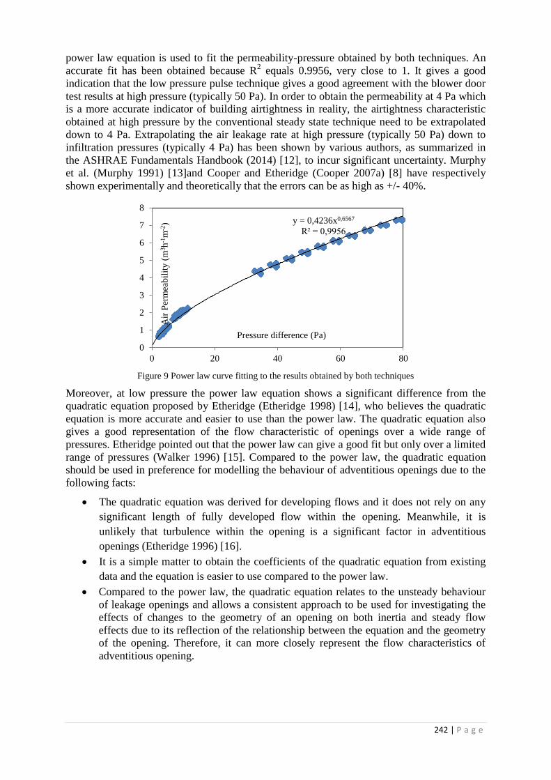
242 | P a g e

power law equation is used to fit the permeability-pressure obtained by both techniques. An

accurate fit has been obtained because R2 equals 0.9956, very close to 1. It gives a good

indication that the low pressure pulse technique gives a good agreement with the blower door

test results at high pressure (typically 50 Pa). In order to obtain the permeability at 4 Pa which

is a more accurate indicator of building airtightness in reality, the airtightness characteristic

obtained at high pressure by the conventional steady state technique need to be extrapolated

down to 4 Pa. Extrapolating the air leakage rate at high pressure (typically 50 Pa) down to

infiltration pressures (typically 4 Pa) has been shown by various authors, as summarized in

the ASHRAE Fundamentals Handbook (2014) [12], to incur significant uncertainty. Murphy

et al. (Murphy 1991) [13]and Cooper and Etheridge (Cooper 2007a) [8] have respectively

shown experimentally and theoretically that the errors can be as high as +/- 40%.

Figure 9 Power law curve fitting to the results obtained by both techniques

Moreover, at low pressure the power law equation shows a significant difference from the

quadratic equation proposed by Etheridge (Etheridge 1998) [14], who believes the quadratic

equation is more accurate and easier to use than the power law. The quadratic equation also

gives a good representation of the flow characteristic of openings over a wide range of

pressures. Etheridge pointed out that the power law can give a good fit but only over a limited

range of pressures (Walker 1996) [15]. Compared to the power law, the quadratic equation

should be used in preference for modelling the behaviour of adventitious openings due to the

following facts:

The quadratic equation was derived for developing flows and it does not rely on any

significant length of fully developed flow within the opening. Meanwhile, it is

unlikely that turbulence within the opening is a significant factor in adventitious

openings (Etheridge 1996) [16].

It is a simple matter to obtain the coefficients of the quadratic equation from existing

data and the equation is easier to use compared to the power law.

Compared to the power law, the quadratic equation relates to the unsteady behaviour

of leakage openings and allows a consistent approach to be used for investigating the

effects of changes to the geometry of an opening on both inertia and steady flow

effects due to its reflection of the relationship between the equation and the geometry

of the opening. Therefore, it can more closely represent the flow characteristics of

adventitious opening.

y = 0,4236x0,6567

R² = 0,9956

0

1

2

3

4

5

6

7

8

0 20 40 60 80

Air

Per

mea

bil

ity (

m3h

-1m

-2)

Pressure difference (Pa)

243 | P a g e

4. CONCLUSIONS

A novel nozzle pulse pressurisation technique for determining the leakage of buildings at low

pressures has been developed. The technique generates the pulse using a compressor and

nozzle, so as to make the test rig compact and portable. A theoretical model for determining

the pulse volume flow rate has been briefly introduced. The test results show that the present

nozzle pulse technique can minimize the effects of wind and buoyancy force and has proven

to be very repeatable and sensitive to small changes in leakage. In addition, a comparison

between the nozzle test and piston test has been performed and indicates that the nozzle

technique is more reliable, as some uncertainties in determining the volume flow rate can be

avoided. In a power law fitting, a good agreement with the steady state test has been shown

by the experimental results obtained in a test using the nozzle pulse technique. The

mathematical representations for these two different techniques, that approach the

measurement of building air tightness in different ways, are worth further experimental

verifications and discussions.

5. ACKNOWLEDGEMENTS

This work is supported by the UK EPSRC (Engineering Physical Science Research Council)

under grant EP/H023240/1 and led to further support from TSB to further research work

towards commercialisation. The authors thank Dr. David Etheridge in the Department of

Architecture and Built Environment for helpful discussion.

6. REFERENCES

[1] Directive 2010/31/EU of the European Parliament and of the Council of 19 May 2010 on

the energy performance of buildings.

[2] Building Regulations: Part L. (2010) (Conservation of fuel and power). Approved

Documents Part L1A (new dwellings), L2A (new buildings other than dwellings). London,

UK: NBS for the Office of the Deputy Prime Minister.

[3] Roulet C, Vandaele L. (1991). Airflow patterns within buildings - measurement

techniques. AIC-TN-34-1991. Coventry, UK: AIVC.

[4] Carey PS, Etheridge DW. (2001). Leakage measurements using unsteady techniques with

particular reference to large buildings. Building Serv. Eng. Res. Technol; 22: 69-82.

[5] Cooper EW, Etheridge DW. (2004). Measurement of building leakage by unsteady

pressurisation. AIVC Conference, Prague.

[6] Cooper EW, Etheridge DW. (2007). Determining the adventitious leakage of buildings at

low pressure. Part 2: pulse technique. Building Serv. Eng. Res. Technol; 28: 81-96.

[7] CIBSE. (2000). Testing buildings for air leakage, CIBSE TM23. London, UK.

[8] Cooper EW, Etheridge DW. (2007). Determining the adventitious leakage of buildings at

low pressure. Part 1: uncertainties. Building Serv. Eng. Res. Technol; 28: 71-80.

[9] M.H. Sherman, R.Chan. (2004). Building Airtightness: Research and Practice, Lawrence

Berkeley National Laboratory Report No. LBNL-53356.

[10] M. Sherman. (1995). Uncertainties in fan pressurization measurements. Airflow

Performance Conference 10/93. LBL-32115.

[11] ASTM. (2010). International. Standard Test Method for Determining Air Leakage Rate

by Fan Pressurisation. ASTM International Designation: E779-03.

[12] ASHRAE, 2013. ASHRAE Fundamentals Handbook. ISBN 978-1-936504-46-6. pp.

420.

[13] Murphy, W.E., D.G. Colliver, and L.R. Piercy. 1991. Repeatability and reproducibility of

fan pressurization devices in measuring building air leakage. ASHRAE Transactions

97(2):885-895.

[14] Etheridge, D.W., A note on crack flow equations for ventilation modelling, Building and

Environment, Vol. 33, No.5, pp.325-328, 1998.

244 | P a g e

[15] Walker, I.S., Wilson, D.J. and Sherman, M.h., Does the power law rule for low pressure

building envelope leakage? 1966. Proceedings of 17th AIVC Conference, Gothenburg,

Sweden. 17-20 September 1996.

[16] Etheridge, D.W., Sandberg, M., Building Ventilation-Theory and Measurement, John

Wiley & Sons, Chichester 1996. Pp. 78-89, 99-108 and 144-6.

245 | P a g e

EXERGY EVALUATION OF MECHANICAL

VENTILATION SYSTEMS

Anna DUTKA*1, Tomasz M. MRÓZ

2

1 Poznań University of Technology,

ul. Piotrowo 3a,

60-965 Poznań, Poland


[email protected]

2 Poznań University of Technology,

ul. Piotrowo 3a,

60-965 Poznań, Poland

ABSTRACT

Energy performance of mechanical ventilation systems in modern low energy and passsive buildings

is a crucial factor influencing overall energy performance of building. Energy balance is commonly used tool in

evaluation of mechanical ventilation systems. In the case of low energy and passive buildings that tool might be

insufficient and should be replaced by exergy analysis taking into account the first and the second Law of

Thermodynamics. The paper presents principles of exergy evaluation of mechanical ventilation systems and case

study calculations for an office building.

KEYWORDS

Exergy analysis, mechanical ventilation systems, demand controlled ventilation (DCV)

1. INTRODUCTION

Reduction of energy consumption is one of the biggest challenges in the modern

world. Buildings consume about 40% of final energy in European Union. Heating and cooling

is more than 50% of the annual energy demand of buildings in the operational phase, thus

building sector requires significant energy efficiency improvement.

One of the most promising strategies in the improvement of energy performance of

buildings is optimal control algorithm or control strategy of ventilation systems. Several

control strategies are proposed for ventilation systems. The CO2-based demand controlled

ventilation (DCV) is one of the strategies that allow for the energy use reduction.

The performance evaluation of ventilation systems is usually based on an energy

analysis (first law of thermodynamics). The exergy analysis, which takes into account both

first and second law of thermodynamics, is much better evaluation tool, which can give better

and more accurate indication of system inefficiencies. The results from exergy analysis can be

used to assess and optimize the performance of HVAC including ventilation systems [1].

Exergy analysis is not so commonly used, the examples of exergy balance calculations for

different buildings and technical systems of buildings can be found in [2,3,4,7,10,14].

The paper present the application of exergy analysis of DCV system installed in office

buildings.

246 | P a g e

2 THE CONCEPT OF EXERGY ANALYSIS

All real thermodynamic processes taking place in nature are irreversible, which means

that they are a source of entropy. It is described by the Gouy-Stodoli Law, whose differential

form is given by equation 1 [8]:

genSTB 0

(1)

where:

B flux of the internal exergy loss of a thermodynamic system in

an infinitely short time d , W,

genS

flux of total increase of entropy of a thermodynamic system in

an infinitely short time d , W K-1.

The flux of increase of entropy is very often referred to as the source of entropy. There

are six causes of irreversibility of real thermodynamic processes - six potential entropy

sources [7, 8]:

– heat exchange caused by a finite temperature difference,

– electric current flow caused by a finite potential difference,

– chemical reactions,

– mixing of fluids,

– mechanical friction

– hydraulic friction.

The exergy balance of the thermodynamically open system can be presented in a

mathematical form – equations 2, or a graphical form (Grassmann-Szargut graph) – figure 1.

[8]:

HSext

use

outin BBBBB (2)

where:

inB

flux of exergy entering the control volume of a thermodynamically open

system, W, use

outB

flux of useable exergy leaving the control volume of a thermodynamically

open system, W.

B flux of the internal exergy losses of a thermodynamically open system, W,

extB

– flux of external exergy losses of a thermodynamically open system, W,

HSB

– flux of change of exergy of an external heat source being in contact with a

thermodynamically open system, W.

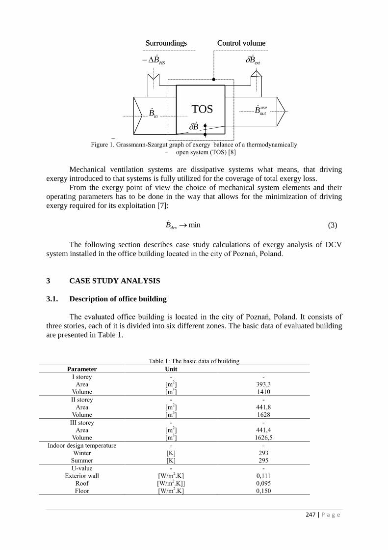
247 | P a g e

–

Surroundings Control volume

use

outB

extB

TOS

HSB

B

inB

Surroundings Control volume

use

outB

extB

TOS

HSB

B

inB

Figure 1. Grassmann-Szargut graph of exergy balance of a thermodynamically

– open system (TOS) [8]

Mechanical ventilation systems are dissipative systems what means, that driving

exergy introduced to that systems is fully utilized for the coverage of total exergy loss.

From the exergy point of view the choice of mechanical system elements and their

operating parameters has to be done in the way that allows for the minimization of driving

exergy required for its exploitation [7]:

mindrvB (3)

The following section describes case study calculations of exergy analysis of DCV

system installed in the office building located in the city of Poznań, Poland.

3 CASE STUDY ANALYSIS

3.1. Description of office building

The evaluated office building is located in the city of Poznań, Poland. It consists of

three stories, each of it is divided into six different zones. The basic data of evaluated building

are presented in Table 1.

Table 1: The basic data of building

Parameter Unit

I storey

Area

Volume

-

[m2]

[m3]

-

393,3

1410

II storey

Area

Volume

-

[m2]

[m3]

-

441,8

1628

III storey

Area

Volume

-

[m2]

[m3]

-

441,4

1626,5

Indoor design temperature - -

Winter [K] 293

Summer [K] 295

U-value - -

Exterior wall [W/m2.K] 0,111

Roof [W/m2.K]] 0,095

Floor [W/m2.K] 0,150

248 | P a g e

3.2. Description of mechanical ventilation system

The schematic drawing of the mechanical ventilation system is shown in Figure 2. The

system consists of three main items: air handling unit, air distribution system and rooms

(control zones). The exergy analysis for the main part of air handling unit: rotating heat/mass

regenerator, air heater, air cooler, steam humidifier, fans, air filters and air dampers has been

performed. Rotating heat/mass regenerator works as long as outside air temperature is lower

than (Tin,4-1K). This study calculates also air heater thermal capacity, cooling capacity,

electrical power of inlet and exhaust fans in one example week in winter and summer. Typical

meteorological data were taken for the city of Poznań (winter period between 1st and 7

th

February and summer period between 1st and 7

th July) [13]. All calculations have been

conducted using Matlab R2008 simulation tool.

Figure 2: The schematic of mechanical ventilation system.

As the calculation experiment the simulation of exergy performance of one builing’s

storey divided into six separate CO2 control zones has been performed. One zone is a

conference room – the maximum occupancy is 14 peoples, the rest zones are office rooms –

the maximum occupancy density is form 5 to 10 people/zone. The office works from Monday

to Friday between 8 a.m. – 8 p.m. Occupancy profiles of all six zones are presented in Figure

3. The ventilation system operates continuously from 8 a.m. – 8 p.m during work day. In all

the zones CO2 sensor were installed, which measure concentration of carbon dioxide. The

ASHARE 62 recommended a limit of 1000 ppm CO2 to satisfy comfort criteria for indoor

space. The outside air CO2 concentration in the location of analyzed building has been 400

ppm.

The air flow per person was determined using equation (4) [9]:

OS CC

NV

(4)

where:

N – CO2 generation per person, based on activity level; N=0,02 m3/h,

CS – CO2 concentration inside zone, ppm,

Co – CO2 concentration outside air, ppm.

249 | P a g e

Figure 3: The daily occupancy profile of all six zones

Figure 4: Modelled hourly air flow for all zones during work day

Figure 5: Modelled hourly air flow for all zones during a week

The climatic condition for winter and summer weeks taken as input data are presented in

Figures 6 and 7.

250 | P a g e

Figure 6: The ambient temperature for reference winter and summer week (data for Poznań from [13]).

Figure 7: The ambient humidity for the reference winter and summer weeks (data for Poznań from [13]).

The other input data used in exergy simulations are given in Table 2.

Table 2: The input data

Parameter Unit Winter Summer

Tin,4 [K] 291 293

Xin,4 [g/kg] 8 Resulting

Δpin [Pa] 650 650

Δpex [Pa] 500 500

ηHR,t [%] 65 65

ηHR,x [%] 65 65

ηv,in,i= ηv,ex,i [%] 70 70

ηv,in,em= ηv,ex,em [%] 90 90

Tw1/Tw2 [K] 348,15/333,15 -

Tch1/Tch2 [K] - 280,15/285,15

3.3 Theoretical model

Exergy balance equations have been constructed for each of the items of energy chain

creating analyzed ventilation system. They are represented by following equations:

The flux of the internal exergy loss in the air damper:

- Inlet side:

dineininD bbmB ,, (5)

- Exhaust side:

dexexexexD bbmB ,1,, (6)

251 | P a g e

The flux of the internal exergy loss in the air filter:

- Inlet side:

findinininF bbmB ,,, (7)

- - Exhaust side:

fexdexexexF bbmB ,,, (8)

The flux of the internal energy loss in the heat recovery device:

3,2,1,, exexexinfininHR bbmbbmB (9)

The flux of the internal exergy loss in the air heater:

2,1,2,1, wwwinininAH bbmbbmB (10)

The flux of the internal exergy loss in the cooler:

2,1,

*

2,2, chchchinininCH bbmbbmB (11)

The flux of the internal exergy loss in the fan:

- Inlet side:

inelininininV NbbmB ,3,

*

2,, (12)

- Exhaust side

exelexfexexexV NbbmB ,2,,, (13)

Electrical power of the fan motor Nel,in and Nel,ex depends on the volumetric flow of

humid air, its static pressure growth and total efficiency of the fan.

inV

inin

inininel

ppmN

,

*

2,3,

,

(14)

inV

exfex

exexexel

ppmN

,

2,,

,

(15)

The flux of the internal exergy loss in the steam humidifier:

252 | P a g e

bmbbmB inininSH 4,3, (16)

Specific thermal exergy of humid air can be calculated using the equation:

0,

0

0

00

0,

0

0

00, lnlnlnln

p

pRT

T

TTTTcx

p

pRT

T

TTTTcb v

a

aaaexin

(17)

Specific thermal exergy of water can be calculated using the formula:

0

00 lnT

TTTTcb ww (18)

Specific thermal exergy of saturated water vapor (x=1) can be calculated using the equation:

0,

0

0

00 lnlnvp

pRT

T

TTTTcb

(19)

Heating capacity of the air heater can be calculated:

)( 1,2, ininainAH TTcmQ (20)

Cooler capacity of the air heater can be calculated:

)( *

2,2,: ininainCH TTcmQ (21)

4 CALCULATION RESULTS AND DISCUSSION

The results of the exergy balance calculations, electrical power of the fan motor, air

heater capacity and air cooler capacity for one week in winter and one week in summer are

presented below.

The results of internal exergy loss of all energy chain in air handing unit for reference

winter and summer weeks are presented in Table 3 and Figures 8 and 9.

253 | P a g e

Table 3: Case study – exergy calculation result

Parameter Winter Summer

[W/week] [%] [W/week] [%]

δ 451,62 0,63 351,9 1,97

δ 753,0 1,05 856,4 4,8

δ 20165,2 28,2 687,97 3,86

δ 19261,8 26,94 0 0

δ 0 0 4177,8 23,39

δ 6884,1 9,63 5928,6 33,2

δ 17386,8 24,31 0 0

δ 464,5 0,65 352,2 1,97

δ 753 1,05 856,4 4,8

δ 5379,0 7,52 4644,35 26,01

δ 39759,57 100 9928,96 100

Figure 8: Calculation results – exergy loss in all analysed energy items during reference winter week.

Figure 9: Calculation results – exergy loss in all analysed energy items in reference summer week.

254 | P a g e

The results of air heater thermal capacity, cooler capacity, electrical power of inlet and

exhaust fans for reference winter and summer weeks are presented in Table 4 and Figures 10

and 11.

Table 4: Case study – calculation results

Parameter Unit Winter Summer

QAH [kW/week] 89,26 0

QCH [kW/week] 0 126,37

Nel,in [kW/week] 16,8 17,03

Nel,ex [kW/week] 13,11 13,1

Figure 10: Electrical power of inlet and exhaust fans for reference week in winter and summer.

Figure 11: Air heater thermal capacity, cooling capacity for reference week in winter and summer.

Exergy analysis pinpoint the location, where the losses are the highest

In reference winter week three items (heat recovery, air heater, steam humidifier)

generated more than 80% exergy losses. Exergy loss in heat recovery can not be perceived as

a problem. Main part of heat is recovered from exhaust air, what can be treated in positive

255 | P a g e

way, due to reduction of energy consumption of air heater and steam humidifier. The main

sources of irreversibility of air heating process in cold days were: the air heater responsible

for approximately 27% of the total flux of the exergy loss and air humidifier responsible for

24% of the total flux of the exergy loss.

In reference summer week the highest exergy losses were caused by fans and air cooler.

Heat recovery works if temperature of outdoor air is below 292K, thus during summer season

it is usually turned off, because of significant cost of work to expected profits. Supreme

exergy loss during warm days is caused by air cooler, thus air handling unit needs

improvements to limit exergy loss in this area. Exergy loss on fans are similar during whole

year – both during summer and winter season.

During winter week exergy loss is more than four times higher than during summer

season. In summer more devices are turned off, because of the high temperature and humidity

and the fact that air cooler does not work as a dehumidifier – air cooler reduces the inlet air

temperature only. If HVAC system controls also humidify, the exergy loss in summer would

be much higher.

The above-mentioned three items of the energy chain - air heater, air humidifier in cold

days and air cooler in warm days should be taken into detailed consideration in the

optimization procedure.

5 CONCLUSIONS AND FUTURE WORK

Exergy analysis tool is the powerful tool for analysing, assessing, designing, improving

and optimizing different systems and processes. Exergy analysis has a lot of benefits. This

methods can assist for evaluation of the thermodynamic values of the energy products. Exergy

losses clearly pinpoint the location, causes and sources of deviations from ideal conditions of

system operation. Exergy efficienciy is the measure of the approach to ideal [11].

Subsequent steps of presented analysis should include: (i) exergy analysis for other main

items in HVAC system: air distribution system and office rooms, (ii) chemical exergy

analyses of the fossil fuels needed for the air handling unit operation and (iii) analysis of

vetilation system for one typical year.

6. REFERENCES

1. Benz- Karlstrom P. (2010). Calculations with SEPE – Exergy analysis of cooling

systems. Zurich Switzerland

2. Dovjak M., Shukuya M., Olesen B.W., Krainer A. (2010): Analysis on exergy

consumption patterns for space heating in Slovenian buildings. Energy

3. Hepbasli A. (2012) Low exergy (LowEx) heating and cooling systems for sustainable

buildings and societies. Renewable and Sustainable Energy Reviews

4. Hepbasil A., Kecebas A.(2013): A comparative study on conventional and advanced

exergetic analyses of geothermal district heating systems based on actual operational

data. Energy and Buildings

5. Iliev V., Badunski D., Seso I., Andovski S. (2014). Direct Digital Control of HVAC

System and CO2-Based Demand Controlled Ventilation. International Journal of

Innovative Technology and Exploring Engineering

6. Nassif N. (2012). A robust CO2 –based demand – controlled ventilation control

strategy for multi-zone HVAC system. Energy and Buildings

7. Mróz T. M., Bogusławska Ż.(2012). Exergy analysis of an air heating system, Poland.

Foundation of civil and environmental engineering. Poznań University of Technology

8. Mróz T. M.: (2013) Energy management in built environment. Tools and evaluation

procedures. Publishing House of Poznan University of Technology

256 | P a g e

9. Shell M.B., Turner S.C., Shim O.R. Application of CO2-Based Demand – Controlled

Ventilation Using ASHRAE Standard 62: Optimizing Energy Use and Ventilation.

ASHARE Transaction Symposia

10. Sakulpipatsin P., Itard L.C.M., Kooi H.J., Boelman E.C., Luscuere P.G. (2010) An

exergy application for analysis of buildings and HVAC systems. Energy and

Buildings.

11. Sakulpipatsin P. (2008) Exergy efficient building design.

12. Szargut J. Petela R. (1965) Egzergia. Warszawa

13. http://www.mir.gov.pl

14. Zmeureanu R., Yu Wu X.(2007) Energy and exergy performance of residential

heating systems with separate mechanical ventilation. Energy.

257 | P a g e

STRATEGIES FOR EXPLOITING CLIMATE

POTENTIAL THROUGH VENTILATIVE COOLING IN

A RENOVATED HISTORIC MARKET

Annamaria Belleri*1

, Federico Noris1, and Roberto Lollini

1

1 EURAC research

1 Druso

Bolzano, Italy


ABSTRACT

Nearly all retail locations use ventilation and cooling systems to ensure adequate air exchange for health reasons

and indoor comfort temperatures. These systems can run for over 2,000 hours per year and we expect that

average operating hours will continue to rise across Europe because of the continued trend towards longer

opening hours and increased number of opening days. Shopping malls often enclose large open spaces and atria

with high solar and internal gains that can drive ventilative cooling. This study presents the methodology applied

to a historical market located in Valladolid (Spain) for the assessment of the ventilative cooling potential and the

definition of a ventilative cooling strategy. The climate suitability and potential was evaluated based on the

building internal gains rate and the considered ventilation strategies options (e.g. night cooling, daytime direct

ventilation). Significant performance indicators were defined for each considered ventilation strategy. Once we

determined the climate suitability, we defined a ventilative cooling strategy, that exploits openings in the façade

and in the skylight to promote stack effect ventilation. We sized openings area and location on the façade, taking

into account design constraints, and we assessed their performances by dynamic simulations in Trnsys coupled

with Trnflow airflow network. Results show the potential cooling load reduction, with the achievement of

acceptable thermal comfort due to the ventilative cooling in the shopping mall. The proposed methodology can

support the design decision process towards cost effective low energy shopping malls.

KEYWORDS

Climate potential, ventilative cooling, retail buildings, refurbishment, dynamic simulations

1. INTRODUCTION

Retail buildings are a significant part of the EU building stock and, among them, the

wholesale and retail sector presents an average specific energy use of 200 kWh/m2a and

account for 7% of the total building stock in Europe (Atanasiu B., 2011). Nearly all retail

locations use ventilation and air conditioning systems to ensure adequate air exchange and

indoor comfort temperatures. These systems run for over 2,000 hours per year and average

operating hours will continue to rise across Europe because of the continued trend towards

longer opening hours and increased number of opening days.

According to the British Council for Shopping Centre (BCSC, 2012), natural ventilation

solutions can reduce capital and maintenance cost over traditional mechanical heating,

ventilation and air conditioning and they typically need less plant and equipment place.

Shopping malls often enclose large open spaces and atria with high solar and internal gains

that can be drivers for ventilative cooling. However, nearly all retail buildings use mechanical

258 | P a g e

ventilation systems as they require less design efforts assuring minimum requirements for

indoor air quality.

The CommONEnergy EU FP7 project (www.commonenergyproject.eu) will contribute to the

development of ventilative cooling strategies for the retrofit of existing shopping malls to

exploit the architectural and climate drivers potential. The retrofitting solution sets developed

within the project will be applied to three demo cases located in Spain, Italy and Norway,

selected because of their high replication potential. This paper presents the methods and tools

applied to assess the ventilative cooling potential and to define an efficient ventilative cooling

strategy for one of the democases: the historic market of the city of Valladolid.

First, we evaluated the climate suitability and potential according to several building internal

gains rates and ventilation strategies (e.g. night cooling, daytime direct ventilation). Once we

determined the climate suitability, we defined a ventilative cooling strategy that exploits

openings in the façade and in the skylight to activate stack effect ventilation. Coupled thermal

and airflow building energy simulations allowed to assess the potential cooling load

reduction, the air change rates and the indoor comfort conditions for several opening factors.

2. CASE STUDY

2.1 Building description

The “Mercado del Val” is an iron market located within the old town of Valladolid. Its

construction was completed in 1882. Its floor plan is a rectangle of 112 meters long and 20

meters wide, with chamfered corners.

The Valladolid municipality planned a refurbishment intervention to transform the market

into an innovative building that meets the contemporary commercial needs being respectful of

its historic representativeness. As required by the Heritage Council, the refurbishment project

aims at emphasizing the old iron structure by using glazed facade over the entire building

perimeter. The new indoor layout configuration and the glazed façade will contribute to a

better understanding of the global iron structure, to increase daylighting and to make the

commercial activities visible from outside. The glazed façade is made by modular façade

elements that aims at integrating thermal, daylighting and ventilation functions, being

responsive when internal and external loads change.

Figure 1: Mercado del Val (Valladolid) building

view. Source: www.commonenergyproject.eu

Figure 2: Mercado del Val (Valladolid), interior building

view. Source: www.commonenergyproject.eu

2.2 Design constraints

The building shape has high potential for exploiting stack effect ventilation by integrating

openings in the facade and exploiting the existing skylight openings located at 10 m height

from the ground level where air can exhaust.

259 | P a g e

Therefore, the definition of a ventilative cooling strategy involves the whole building

envelope as openings have to be located at opposite sides and at different height on the

building envelope.

Main constraints regard inlet openings location at ground level. A large temperature

difference between indoor and outdoor might cause cold draughts inside the building if the

openings are placed near people’s height. Therefore we decided to avoid openings within 3 m

height of the building façade to prevent local discomfort situations. Inlet air at 5 m height,

which is approximately the height of the upper part of the modular façade, would allow air

mixing and prevent cold draughts in the occupied zones of the building. Additionally, inlet

openings in the lower part of the façade might cause safety issues.

Lower inlet openings in urban environments might affect negatively indoor air quality due to

transfer of outdoor pollution. Filters on the opening would cause a high pressure drop of the

air reducing significantly natural ventilation effectiveness. In order to avoid water infiltration

in case of precipitation, top hung windows could be used. Top hung windows have usually an

opening angle of 20°, which reduces the opening effective area by 80%. Therefore, for the

definition of the opening area we considered opening angles capabilities and actuators power.

As enforced by the heritage council, skylights have to maintain the original design. This could

reduce the effective area of the openings.

3 METHODS

The following methods were used within the first phases of the design project to analyse the

climate potential and assess possible energy savings of a defined ventilative cooling strategy.

3.1 Climate suitability analysis

To estimate ventilative cooling potential we applied the method proposed by NIST

(Emmerich S. J., 2011) to shopping mall building typology and fit it according to their

specific needs.

This method assumes that the heating balance point temperature ( ) establishes the outdoor

air temperature below which heating must be provided to maintain indoor air temperatures at

a defined internal heating set point temperature ( ).

Therefore, when outdoor temperature ( ) exceeds the heating balance point temperature,

direct ventilation is considered useful to maintain indoor conditions within the cooling set

point temperature ( ). At or below the heating balance point temperature, ventilative

cooling is no longer useful but heat recovery ventilation should be used to meet minimum air

change rates for indoor air quality control and reduce heat losses.

We considered the building occupied for 11 hours per day and set the cooling set point

temperature to 25°C during the day and to 28°C during the night, as well as the heating set

point temperature to 16°C during the day and 14°C during the night. Those set point

temperatures refer to the operative temperature recommended by the standard EN 15251:

2008 for building Category II.

The heating balance point temperature ( ) can be calculated using Equation 1. Table 33

reports the balance point temperature values calculated at different internal gains level.

∑ (11)

where:

= total internal gains [W/m²]

= air capacity [J/kg-K]

= minimum required mass flow rate [kg/s]

260 | P a g e

∑ = envelope heat exchange [W/K]

The average U-value of the envelope was estimated at 0.49 W/m²K according to the local

minimum building code requirements and the actual building shape.

The minimum ventilation rate which has been estimated as 1.7 l/s-m² (0.00204 kg/s-m²)

according to the EN 15251 values for department stores (Cat. II – low polluting building).

Table 1. Heating balance point temperature calculated for different internal gain values.

= 10 W/m2 = 20 W/m

2 = 40 W/m

2 = 80 W/m

2

12.7 °C 9.4 °C 2.85 °C -10.3 °C

For each hour of an annual climatic record for the Valladolid city we assessed the number of

hours when:

1) Ventilative cooling is not required: when the outdoor temperature is below the heating

balance point temperature no ventilative cooling can be used since heating is needed;

If To < Tb then

2) Direct ventilative cooling with ventilation rate maintained at the minimum: when the

outdoor temperature exceeds the balance point temperature, yet falls below the lower limit

of the comfort zone – given the width of the comfort zone (Tcsp-Thsp) - and outdoor dew

point temperature is below 17°C (or 65% relative humidity), the cooling ventilation rate

may be maintained at the minimum ventilation rate required by the EN 15251;

If Tb ≤ To < Tb + (Tcsp-Thsp) and To-dp ≤ 17°C then = 0.00204 kg/s-m²

3) Direct ventilative cooling useful: when the outdoor temperature is within the comfort zone

– given the upper limit as the cooling set point temperature - and outdoor dew point

temperature is below 17°C (or 65% relative humidity), the minimum cooling ventilation

rate needed to maintain indoor air conditions within the cooling set point temperature are

computed as Equation 2;

If Tb + (Tcsp-Thsp) ≤ To ≤ Tcsp - 1 and To-dp ≤ 17°C then

( ) [kg/s-m²] (12)

4) Direct ventilative cooling not useful: when the outdoor temperature exceeds the cooling

setpoint temperature and the dew point temperature is above 17°C (or 65% relative

humidity) for at least one hour during the day, the ventilative cooling is no longer useful

and nighttime cooling potential (NCP) over the following night is evaluated as the internal

gains that may be offset for a nominal unit night-time air change rate have been computed

as Equation 3:

If To > Tcsp – 1 or To-dp > 17°C then

( )

[W/m

2-ach] (13)

where:

= floor height [m]

= air density [kg/m³]

= temperature cooling set point at night [°C]

The weather file used for the analysis derives from historical data series (2000-2009) of a

weather station located in the city of Valladolid, which is part of the Meteonorm database

(Weather station ID 81410).

261 | P a g e

3.2 Coupled thermal and airflow simulations

In order to assess energy savings in terms of cooling need and to evaluate thermal comfort,

we performed dynamic simulations using a specific Trnsys module for airflow and thermal

models coupling, Trnflow.

The proposed strategy would allow to obtain stack effect ventilation by integrating openings

in the upper part of the modular facade and exploiting the existing skylight openings (Figure

3). Openings area and location fits to the modular façade design to reduce frame dividers

number.

Figure 3. Building cross section with proposed strategy schema.

Table 2 reports the geometrical data about the operable area used in the simulations. Same

windows are located both on south-west side and on north-east side covering 18 façade

modules, all the modules directly connected to the atrium space. The window height matches

the height of the upper part of the façade module. The skylight height matches the existing

skylight opening height.

We considered the opening factors as varying between the standard top hung window opening

angle and the maximum feasible opening factor:

Opening factor 0.2 : top hung window with 18°C open angle



Figure 4: South-west front view of the building where openings locations are highlighted in red.

262 | P a g e

Table 2. Simulation input data on operable area.

Opening

type

Width

[m]

Height

[m]

Number of

modules

Tot opening

area [m²]

Height from the

reference ground [m]

Window Top hung 3.4 0.78 18 48 5.10

Skilight Top hung 4 0.56 18 40 10.45

In each simulation model, both windows and skylights are operated in the same way and

using the same opening factors. Windows are opened if outdoor temperature is above 12°C

and controlled depending on the indoor - outdoor temperature difference and the control value

at the previous time step.

If the controller was previously on and:

then windows stay open;

then windows close.

If the controller was previously off and:

then windows open;

then windows stay close.

However the control function is set to 0 if the outdoor temperature is lower than 12°C.

Minimum run time period for window operation is set to 20 min.

When outdoor temperature conditions do not allow window opening, mechanical ventilation

supply to the building the minimum air change rates required by the EN 15251 standard to

maintain an acceptable level of indoor air quality:

7.35 kg/hr-m2 (around 2 ach) during the occupied hours

3.02 kg/hr-m2 (around 0.8 ach) during the non-occupied hours

Simulations were run from April to October both in free-floating mode to analyse comfort

according to EN 15251 adaptive comfort model. To assess cooling needs, simulations were

also run by setting an unlimited power cooling system with temperature set point of 25°C

during the occupied hours according to the recommended indoor temperatures by EN

15251:2008 for department stores at comfort category II.

The results are compared with a baseline where mechanical ventilation always provides the

minimum air change rates required by the EN 15251 standard with supplied air temperature

equal to the outdoor temperature.


In the following paragraphs we present and discuss the obtained results of the climate

suitability analysis and the coupled thermal and airflow simulations.

4.1 Climate suitability analysis results

In the Valladolid weather file we identified 95 CD1, 8567 CDH

2 and an average monthly

diurnal temperature swing between 4.5 K (April) and 5.9 K (July).

The graph in Figure 5 shows the percentage of hours within a whole year when direct

ventilative cooling is useful according to the classification method described in par. 3.1 and

different levels of internal gains.

Depending on the internal gains level, direct ventilative cooling can be useful up to 90% of

the hours within a year, whereas for around 10% of the hours the outdoor temperature is

higher than the cooling set point temperature and therefore night-time ventilation potential has

1Cooling Days defined as the number of days with an average ambient temperature higher than 18°C. 2Cooling Degree Hours defined as the integral of the positive temperature differences between the hourly average ambient

temperature and a base temperature of 18°C.

263 | P a g e

to be investigated.

The higher are the internal gains, the higher is the number of hours when direct ventilative

cooling is required.

Figure 5: Percentage of hours within a year when direct ventilative cooling is required, useful or not useful in the

Valladolid climate considering different values of internal gains.

Mean ventilation rates needed for direct ventilative cooling are reported in Figure 6

depending on internal gains level. For instance, considering the outdoor temperature series for

Valladolid and an internal gain rate of 80 W/m2, up to 4 ach are required on average to

effectively cool the building during the occupied hours. As a consequence, the number of

effective hours for direct ventilative cooling decreases with the decrease of internal gains.

Figure 6. Average direct ventilative cooling rate (ach) for each internal gain level considered and percentage of

effective hours within the year in Valladolid.

0% 20% 40% 60% 80% 100%

Qin = 10 W/m²

Qin = 20 W/m²

Qin = 40 W/m²

Qin = 80 W/m²

Hours

Ventilative cooling not required

Direct ventilative cooling with ventilation rate maintained at the minimum (EN 15251)

Direct ventilative cooling useful

Direct ventilative cooling not useful --> consider nighttime ventilation

0,001,002,003,004,005,006,007,00

jan

feb

mar

apr

may

jun

jul

aug

sep

oct

nov

dec

Qin = 10 W/m²

Qin = 20 W/m²

Qin = 40 W/m²

Qin = 80 W/m²

264 | P a g e

The graph in Figure 7 shows an estimation of the internal gains that may be offset for a

nominal unit night-time air change rate. On average among the summer period an air change

rate during the night would be able to offset around 23.5 W/m2 of internal gains. The number

of activation hours matches the percentages identified in the graph in Figure 5.

Figure 7. Night cooling potential and number of hours when night cooling can be activated in Valladolid.

4.2 Simulations results

As reported in Table 3, 41% of cooling need reduction can be obtained using an opening

factor of 0.4 and 55% using an opening factor of 0.8. Windows with an opening factor of 0.2

cannot assure the minimum air change rates requirements and therefore simulation results

show an increase in cooling need by 21% compared to the baseline model. In fact, in the

baseline model the minimum air change rates requirements are provided at a constant rate by

the mechanical ventilation system. The graph in Figure 8 represents the air change rates

frequencies.

Figure 9 shows the simulations results in free floating mode. From April until October the

baseline model predict temperatures within the acceptable comfort range, identified according

to the adaptive comfort model (EN 15251:2008 standard), for over 85% of the occupied

period. This means that, providing fresh air at the minimum air change rates required by the

standard, adaptive thermal comfort requirements are met for 85% of the occupied hours. The

discomfort is in this case mainly due to too hot temperatures.

Using a window opening factor of 0.8, the ventilative cooling strategy would allow us to

reduce or almost zero the discomfort hours due to too hot temperature, even though the

number of discomfort hours increase because of too cold temperatures.

Using a window opening factor of 0.2, the number of hours within comfort ranges is 86%

compared to the 85% of the baseline case, even though the number discomfort hours is mainly

due to too hot temperatures. While an opening factor of 0.2 would cause less 63% of

operation hours of the mechanical ventilation system, during most of the time the air change

rates are below the minimum required by the standard.

0

50

100

150

200

250

300

350

0

5

10

15

20

25

30

jan feb mar apr may jun jul aug sep oct nov dec

Nu

mb

er o

f a

ctiv

ati

on

ho

urs

Nig

ht

Co

oli

ng

Po

ten

tia

l [W

/m²-

AC

H]

265 | P a g e

Table 3: Cooling need and number of operation hours of the mechanical ventilation system predicted by the

baseline model and the models with ventilative cooling strategy.

Cooling need

[kWh/m²]

Cooling need

reduction [%]

Number of operation hours of the

mechanical ventilation system

open factor = 0.2 20.68 +21% 1897

open factor = 0.4 10.10 -41% 2858

open factor = 0.8 7.69 -55% 3617

baseline 17.04 - 5136

Figure 8: Frequency analysis of the predicted air changes per hour with different opening factors.

Figure 9: Percentage of occupied hours during which EN 15251:2008 requirements on thermal comfort are met

by the baseline model and the models with ventilative cooling strategy.

In our simulation models, the window opening angle is not modulated according to indoor-

outdoor temperature difference and therefore discomfort hours due to too cold temperatures

increase by increasing the opening factors. This problem can be solved developing a more

complex control strategy and using window actuators that allow different opening angles.

Therefore, our design proposal was to define a control strategy which considers opening

factor modulation and optimizes it according to indoor-outdoor temperature differences.

5 ADDITIONAL CONSIDERATIONS AND NEXT DESIGN STEPS

Further integration constraints arise from the simulations results. Considering the openings

geometry (W >>H) and the high opening angle needed (up to 70°), proper actuators must be

selected.

In case of top hung windows, it is recommended the installation of actuators protected from

water and solid bodies (dust etc.) and enough powerful to support with sufficient rigidity the

maximum load that occurs when the window is completely opened.

0

500

1000

1500

2000

2500

3000

3500

ACH ≤ 2 2 < ACH ≤ 4 4 < ACH ≤ 6 6 < ACH ≤ 8 8 < ACH ≤ 10 ACH > 10

Nu

mb

er o

f h

ou

rs

Open factor = 0.2 Open factor = 0.4 Open factor = 0.8

0% 20% 40% 60% 80% 100%

baseline

open factor = 0.8

open factor = 0.4

open factor = 0.2

% of occupied hours (h8.00-18.00)

CAT I

CAT II

CAT III

discomfort too cold

discomfort too hot

266 | P a g e

Linear actuators are generally more powerful than chain actuators but actuator encumbrance

inside the room has to be considered as it affects the aesthetic appearance. Very large

windows might also require two thrust points.

Next design step will be focused on:

the definition of a control strategy once constraints on window opening factor and

operable area are defined;

the optimization of the control strategy parameters;

the integration of the ventilative cooling strategy within the whole building solution

sets concepts (shadings, glazing system, daylighting concept) taking into account for

the respective internal and solar gains;

the integration of openings within the modular façade concept and its replicability on similar buildings;

a CFD analysis of the building for results validation and evaluation of possible local

discomfort situations.

6 CONCLUSIONS

The presented study focuses on the methodology applied to a historical market located in

Valladolid (Spain) for the assessment of the ventilative cooling potential and the definition of

a ventilative cooling strategy within its refurbishment project.

The climate suitability analysis showed that, depending on the internal gains level, direct

ventilative cooling can be useful up to 90% of the hours within a year, whereas for 10% of the

hours the outdoor temperature is higher than the cooling set point temperature and therefore

night-time ventilation potential was investigated. Considering the outdoor temperature series

for Valladolid and an internal gain rate of 80 W/m2, up to 4 ach are required on average to

effectively cool the building during the occupied hours.

According to the resulting climate performance indicators, we defined a ventilative cooling

strategy that exploits openings in the façade and in the skylight to activate stack effect

ventilation. Openings area and location on the facade have been sized taking into account

design constraints and climate potential and tested by dynamic simulations in Trnsys coupled

with Trnflow airflow network.

Results show up to 55% of potential cooling load reduction due to the ventilative cooling

strategy in the shopping mall maintaining indoor temperatures lower than 25°C. Higher

energy savings could be obtained by considering the adaptive behaviour of building

occupants. Discomfort situations were mainly due to too cold indoor temperatures in case of

high opening factors. Therefore, we suggested window openings to be automated, modulated

and controlled depending on indoor and outdoor temperature and humidity.

The proposed methodology was applied to support the design decisions providing quantitative

building performance evaluations and allowing a more robust cost estimation. The design

team reacted positively at the proposed ventilative cooling solution.

7 ACKNOWLEDGEMENTS

The research leading to these results has received funding from the European Community’s

Seventh Framework Programme (FP7/2007-2013) under grant agreement n° 608678. The

authors would like to thank Javier Antolín Gutierrez, Samaniego Muñoz J. Jesús and Luis A.

Bujedo from Cartif for the simulation model production, the design team for the cooperative

and positive approach to the collaboration and Magdalena Rozanska from Acciona for

activities’ coordination regarding the modular façade development.

267 | P a g e

8 REFERENCES

Atanasiu B., D. C. (2011). Europe's building under the microscope. A country-by-country

review of the energy performance of buildings. Building Performance Institute Europe

(BPIE).

BCSC. (20 de August de 2012). Shopping centre natural ventilation design. Obtido de

Guidance 68: http://www.bcsc.org.uk/publication.asp?pub_id=459

Emmerich S. J., P. B. (2011). Impact of adaptive thermal comfort on climatic suitability of

natural ventilation in office buildings. Energy and Buildings, 43(2101-2107).

Weather station ID 81410. (s.d.). Obtido de Meteonorm: http://meteonorm.com/

268 | P a g e

DURABILITY OF AIR TIGHTNESS SOLUTIONS FOR

BUILDINGS

Peter Ylmén, Magnus Hansén and Jörgen Romild

SP Technical Research Institute of Sweden

Box 857

SE-501 15 Borås, Sweden

ABSTRACT

The aim of the project was to evaluate how the air tightness of buildings changes over time and how the sealing

materials are affected during the expected life length of 50 years. The project was divided into two parts were

one was laboratory tests of different products with accelerated ageing, and the other part were evaluation of older

existing buildings. The laboratory test was conducted in a temporary room with lightweight construction in wood

and different sealing products. The room was then heated to 80 °C and had changing relative moisture content in

the air. The results showed that most products still maintained their function after accelerated ageing but some

products considerably lost their ability to seal air through the building envelope.

In the testing of existing buildings, six single family houses that are between ten to twenty years old have been

tested for air leakage. Test reports regarding air tightness from when the buildings where newly constructed were

compared to new measurements. Three buildings had made changes to the building envelope while the other

three had original structures. The results from the measurements showed that two of the tested buildings had

considerably more air leakages than when they were new but that the rest had not changed. The change in air

tightness for the two buildings are very likely due to changes made in the building envelope a few years after

they were build.

KEYWORDS

Air tightness in buildings, durability, testing, infiltration, jointing, taping

1. INTRODUCTION

The method of constructing houses and buildings in Sweden changed successively during the

60’s and 70’s. Fiberglass and mineral wool insulation were starting to be used on a large scale

instead of for example, massive wooden construction.

This change in building method led also to an increase in the use of tightening and barrier

layer solutions to reduce the flow of moisture and air through the different construction

sections. Different flexible barriers and seals of plastic were introduced and tested on the

market, an early example of which is polythene film (PE-film), which had begun to be

frequently used as air and moisture barrier in the wall building envelope.

The oil crisis in the 70’s led to a requirement to reduce energy consumption. One method to

help with this is to decrease thermal losses in houses by means of, for example, the use of

more airtight windows and doors.

By the beginning of the 70’s it was apparent that these new methods of construction resulted

in some accompanying problems. Moisture problems could arise resulting in different types

of moisture damage in house and buildings. Many of these problems could occur and be

found very early after the completion of construction. In certain cases it was possible to see

that the durability of a building had already been compromised by the use of sub-standard

polythene, which had broken down, become cracked, opened up and caused damage.

269 | P a g e

In the interest of everybody, an extensive investigation with further research project was

started. Statliga planverket (now Boverket), Sweden’s plastic federation SPF (plastic

manufacturers) and the National testing establishment (now SP Technical research institute of

Sweden) all worked in cooperation on this. The aim of the project was to obtain a more

reliable and durable quality of specific chosen building products (in the first case material for

the air and vapour barriers) and tightening solutions. One result of this was the example that

the Works Norm (VN) was designed as a basis for voluntary quality and type approval

marking for a more reliable higher quality of plastic building products. Included in this was

also the requirement that the built in material, not least because of the high cost involved with

maintenance or even replacement, should have a minimum life length of 50 years. This means

that in the Swedish building trade today it has become the “norm” to use a durable building

polythene film with a minimum life length of 50 years.

One example of the works norm for air and vapour barrier using LD-polythene film (which

was also the first) is:

[1]. Material requirements plus other demands are written down here, together with, amongst

others, how the film should be mounted, how clamped joints and overlaps should be formed

as well as requirements for jointing aids. “Joints, including joint material shall meet the

minimum requirements set out in the Works Norm for the barrier layer, especially when

considering age durability. Joints and joint material shall not affect the function and properties

of the building film in a negative manner.” [2].

A common problem today regarding the choice of building material is that the question ”How

long is the product expected to work without the need for maintenance or replacement?”

cannot be answered by just looking at the material specification.

There can be many reasons as to why this information isn’t available. It can be too expensive

or impossible to find out how long the material can work. There may also not be any methods

or knowledge available regarding the evaluation of the life length of a building material.

There are a number of investigations that show the importance of airtight construction

together with the possibilities of energy savings if the building has good air tightness

[Emmerich 2005]. It has been shown that infiltration losses in some cases are higher than the

intentional losses from ventilation and much higher than transmission losses.

Air tightness in a building is created by having an airtight barrier with airtight joints and

voids/services/penetrations. In many instances the airtight layer is created using a flexible

material, such as polythene sheeting. The jointing for this sheeting usually involves the use of

stapling, clamping or the use of joint adhesives, bands or tape. Both the polythene sheet and

joint material age/degenerate with time, which can lead to a reduction in the air tightness of

the building. The same principle applies to joints and voids/services/penetrations in massive

constructions. The ageing of the material can be caused by many factors, some of which are

heat, cold, moisture, sun (UV radiation) oxygen, ozone, chemicals and mechanical impacts.

Furthermore, materials in and around the joints can affect each other by, for instance, the

migration of plasticizers.

2. AIM

The aim of the project is to evaluate how the air tightness of a building changes over time,

and show which air tightening solutions that are good and durable, and those which are not so

good and should be avoided, and transfer this knowledge to the building industry.

2.1 Method

No literature describing durability testing for how building materials affect each other could

be found for the project; therefore it was necessary to create a new test method. Since the air

tightening materials are to be found inside the building construction and to a certain extent

protected from air borne pollution and sunlight when construction is complete, then these

270 | P a g e

parameters were deemed to have a negligible effect regarding durability. However, moisture

content in the construction does vary since the relative humidity inside and outside varies

throughout the year. The parameters chosen for accelerated ageing of the material were

increased temperature together with varying air moisture content. A test rig with humidity and

temperature controls was constructed in order to produce a representative scale for actual

buildings as well as measuring as many different material combinations as possible.

Construction of test rig

It is most usual with durability testing that smaller samples of material are tested then their

physical properties evaluated, for example the measurement of tensile strength. For this

testing a 2.2 m square by 2.4 m high room was built, see attached figure 1, together with the

different air tightening solutions built in as with a normal building. The material was therefore

used in realistic amounts and lengths and subjected to realistic movements that would be

expected in a real building.

Figure 1. Diagram of the test room construction.

Different methods of jointing polythene sheeting, in particular where the sheeting meets

concrete flooring/other concrete sections plus forming around doors, windows, services etc, in

other words different variations of taping, jointing, stapling and sill sealing were all

prioritized in the construction. This was because of the frequency of problems that arise

regarding these particular points with respect to air tightness of a building. The choice of

sealing products was governed by those that are readily available in Sweden. Interviews were

also conducted with test and construction representatives from Skanska, NCC and Wäst bygg

to ascertain which were the most commonly used air tightness solutions used in the industry.

This was complemented with information collected from building site visits. The sealing

products used were also ones that were described in the manufactures product information as

suitable for this type of construction, and that the material could withhold it’s durability up to

to the 80 °C temperature used in testing.

The building framework was made from wood with fiberglass insulation. The walls were

sealed with polythene plastic sheeting, and the joints taped with polythene tape. The floor was

in situ cast concrete. At the sill level the polythene sheet was clamped between the inner and

outer sill and folded under the inner sill. Sill insulation or joint sealant was applied between

the concrete floor and the polythene sheet.

At the eaves the roof plastic sheet was drawn down behind the wall plastic sheet with an

overlap of 0.5m. The sheet joints were taped at the top plate and clamped using battens and

271 | P a g e

inner wall studs. Alternative air tightening solutions were used on walls A to D, see attached

figure 1.

The air tightness solutions used are explained in figure 2. Service pipes were mounted

through walls B, C and D to test alternative sealing methods around services. The pipes used

were:

Zinc plated ventilation canal, marked in grey in Figure 2.

PVC-free conduit for electricity, marked in red in Figure 2.

PEX-pipe, used usually in heating systems, marked in green in Figure 2.

PP-pipe, used usually in heating systems and drainage, marked in blue in Figure 2.

Copper pipe, used in the test for chemical interest, and is most often clad in

insulation, marked in yellow in Figure 5.

Figure 2. Air tightness solutions for walls A, B, C and D.

Three windows and one door were mounted in the test room, each with a unique individual

solution for air tightening.

There are several ways of fixing the plastic sheeting around the windows. For the purpose of

this testing it was chosen to fix the sheet in place on the timbers around the windows with

double side butyl band. Therefore the air tightening between the window frame and the wall

was not protected by the polythene sheet.

Testing and measurement

As a time horizon the durability was chosen as a minimum of 50 years, which roughly

speaking was assumed to be equivalent to one year at a temperature of 80 °C and relative

humidity of around 50 % in intended use. With the assumption that an increase in temperature

of 10°C doubles the acceleration rate of ageing, then one year at 80°C roughly equates to a

thermoxidative degradation of the material over a period of 50 years at 20°C. The relative

humidity was reduced for one week to 30% to simulate the inside moisture content under the

winter season. Heat in the test room was provided by two sauna heaters and a small hole was

272 | P a g e

made in the wall for low ventilation so that emissions from the materials could be aired away.

Temperature and relative humidity were continuously logged with a sensor placed in the

middle of the room. A fan was mounted internally in order to reduce temperature variations in

the room. The temperature was increased gradually after the start of the test to release any

tension in the materials.

Visual inspections were carried out on a regular basis to understand how the materials were

affected by the climate under the test period.

Pressure testing was carried out on the test room before and after ageing to see how much air

tightness had been affected. An air speed sensor was used at the same time as the pressure

testing to find any specific air leakage locations.

When the test was complete the room was dismantled and the individual tightening solutions

removed and examined visually for any changes that have occurred under the 50 year period,

for example, is the material still in position, has it broken down or has it had any effect on the

other materials surrounding it. Specific areas we were looking at were if:

The materials were still in position and were not loose.

The elasticity of the materials has degraded so much that some cracks have appeared

and/or have released from surrounding materials.

The materials have shrunk resulting in a decrease in airtightness.

Free standing samples in the test room

Test samples were placed in the room of different sealing products which could be tested for

tensile strength and shear after completion of the ageing process. 30 x 40 cm test specimens

of the same type and material were also constructed with joint dimensions 12x12x50 mm.

Table 1. Products tested as free standing samples in the room.

Nr. Product Description Test type Evaluation

1 Tape A Single sided tape Film joint Shear test

2 Tape B Single sided tape Film joint Shear test

3 Spigot Rubber spigot with single sided tape Film joint Shear test

4 Butyl tape Double sided band of butyl rubber Film joint Shear test

5 Joint sealant A Butyl sealant in a tube Film joint Shear test

6 Joint sealant B Silane polyurethane polymer Concrete/concrete joint Tensile strength

7 Joint sealant D Moisture curing MS polymer Wood/wood joint Tensile strength

8 Joint foam A Moisture curing polyurethane foam Wood/wood joint Tensile strength

The constructed joint samples were placed and subjected to the ageing process in the test

room in order to evaluate and compare them using the tensile tester with reference samples.

After exposure the joints/sealants were tested for tensile strength or shear. The evaluation of

taped joints, tape against film was carried out according to SP-method 1380, third edition for

materials 1-5.

Evaluation of joint sealants/joint foam was carried out according to SP-method 4372, edition

2.3 for materials 6-8.

On site measurements in existing houses

Testing was executed in older properties in order to see how air tightness is affected by time.

One of the requirements for choosing which houses should be tested was that the houses were

already tested for air tightness when new plus the method and documentation were still

available, as well as any relevant leakages. It was therefore necessary to go through all the

documentation from measurements carried out by SP on primarily small houses. For

buildings made up of apartments it is very difficult in practice to measure air tightness for the

whole building since all the doors of the apartments need to stand open when measurements

273 | P a g e

are taken. It has not been possible either to find sufficiently reliable documentation from

earlier measurements for any apartment blocks. This means that it is only small houses that

have been investigated.

A request was sent to several house owners that had a suitable test house, and six owners

decided to allow testing.

Testing of the buildings climate envelope was carried out according to Europe standard EN

13829:2000.

A Minneapolis fan equipment Blower Door was used for the measurement of the buildings air

tightness. A survey of air leakage at around 50 Pa inside pressure in comparison to outside

pressure was undertaken. Negative pressure was formed by use of the fan to measure the

buildings airtightness, plus air speed sensors and thermal cameras were used to find air

leakages.

Building extensions have been included in the testing which has meant that in three cases the

envelope area has been corrected. This also means that changes can have been made in the

original building envelope which can give another source of error. Optimally it would have

been best if no changes had been made to the houses measured. However, we had only these

six houses available so measurements were carried out even if the house had an extension.

3 RESULTS

3.1 Results from the test room

Air leakage through the building envelope at 50 Pa pressure difference calculated according to

EN 13829 was 0,11 l/(sm²) before ageing and 0,22 l/(sm²) after ageing.

Most of the solutions have maintained their air tightness after a representative ageing period

of 50 years. Solutions which have resulted mainly in a deterioration in air tightness are tape

A, tape B, spigot tape, sill insulation B plus sealants C and D.

Solutions using tape on the plastic sheeting have become less airtight because of channels

formed in the tape, most likely caused by differences in shrinkage rate of the two materials,

see figures 3 and 4.

A similar phenomenon occurred with the only sill insulation of rubber seals which were glued

to a plastic strip, see figure 4. Tape joints in the eaves had also similar channels as the tape in

other sections, but the leakage wasn’t as much here because the joint was clamped by the

studs and battens.

Figure 3. Air channels forming in the tape joint

274 | P a g e

Figure 4. Air channels in the spigot tape (on the left) and sill insulation (on the right)

It is worth mentioning that the butyl band used in this test also creased together with the

plastic sheet, but it was very well fixed to the plastic sheet and no air channels were formed,

see figure 5

Figure 5. Butyl band had creased together but maintained an airtight joint.

The joint sealants used in this test which became dense and hardened homogenously remained

so, whilst other less dense sealants had set in an uneven manner, with hard sections and soft

sections..

This can be caused by the less dense joint sealants do not harden or cure sufficiently quickly

and thus are not able to cope when the building sections move , with cracks occurring as a

result, see figure 6.

Besides the results from the free standing samples, the visual inspection of the joints doesn’t

appear to show any chemical reaction with the different building materials, such as wood,

concrete, frame paint and the service voids. It appears to be that it is the chemical and

mechanical factors in the products themselves which lead to a decrease in air tightness, such

as movements in the material and shrinkage (dimensional stability). The results from all the

samples are documented in appendix 2.

Figure 6. Joint sealant around a window.

275 | P a g e

During testing the materials were checked about once a month for any noticeable changes.

Channels and cracks were first noted from between one to three months, however, not from

the sill insulation as this was a hidden construction. A deterioration of air tightness occurred

amongst the tested products before completion of the ageing of 50 years, or not at all. One to

three months of accelerated testing represents an ageing time frame of four to 13 years.

Furthermore, the size of the channels and cracks increased gradually as the test progressed.

3.2 Summary of results from free standing samples

The results from the free standing samples are summarized below in table 2. The

requirements that the products have been compared with in this case is described in the report.

The results must be compared with the visual results obtained from the in-built products of

the test room as well as the air tightness measurements of the room to obtain an overall

picture. The results and requirements must also be compared with the installation method and

form of the tested products. The results refer only to the tested properties of the tested

materials. The raw data from the tensile strength and shear testing is reported in appendix 3.

Table 2. Summary of the results from the standardized tests of the smaller test samples

Product Fulfils requirements of SP-method 1380/SP-method 4372

Tape A Yes

Tape B Yes

Rubber spigot with tape No

Butyl tape Yes

Joint sealant A Yes

Joint sealant B No

Joint sealant D No

Joint foam A No

Materials 1-2 and 4-5 fulfil the requirement for shear strength and appear to be “visually

vapour tight” with no noticeable channels, cracks or damage. Material 3 did not fulfil the

requirement, with damage and air channels clearly visible.

Materials 6-8 did not meet the requirements. Joint sealant D was already “broken” after the

ageing process and before tensile strength evaluation. Joint foam A did not meet the

requirement for air tightness with 3 mm elongation, and also the maximum tension

requirement was not fulfilled >0.3MPa after exposure.

Joint sealant B had a reduction in elongation of 38 % at maximum peak force compared with

the result from an unexposed sample of joint sealant.

3.3 Summary of results from on-site measurements

The results obtained for air tightness of the investigated houses is shown in table 3 below.

Table 3. Summary of investigated houses.

House Year built Air leakage when

built [l/(sm²)]

New measurement of air

leakage 2011-2012[l/(sm²)]

Changes made to the

building/climate envelope

1 1990 0,14 0,95 Yes

2 1990 0,17 0,21 No

3 1993 0,92 1,54 Yes

4 1990 1,11 1,05 Yes

5 1990 0,64 0,57 No

6 2001 0,25 0,23 No

276 | P a g e

Houses 1, 3 and 4 have all had extensions which mean a change to the original climate

envelope. The air tightness of houses 1 and 3 has decreased substantially since the

construction of their extensions; however, the same result was obtained for house 4 as for 22

years ago. The reduction in air tightness in two out of the three houses that have had

extensions can point towards variations in construction techniques and/or the level of

precision used I carrying out these changes to the building envelope.

No changes to the climate envelope have been made over the years to houses 2, 5 and 6, and

the results are roughly the same as for 10-22 years ago.

Fewer areas of poor air tightness were noted from house 6, which is 10 years younger than

houses 1-5. We cannot explain exactly why this is so, but as house 6 was built as a passive

house and therefore with the awareness of building airtight, then this can be a contributable

factor for the better result.

To summarize, changes have been made to the climate envelop in three of the six houses, two

of which (house 1 and 3) showed an increase in air leakage. In the remaining three houses no

changes have been made to the climate envelope and they have maintained their original air

tightness.

4 DISCUSSION

After the measurement of air leakage in six existing houses, it has been shown that it is

possible to build a house without risking the durability of its air tightness. Regarding building

extensions or renovations then there is a large risk that the new section doesn’t come up to the

same standard as the older section. This is not a surprising result, but it is worth pointing out

because at some stage or other many people will extend or renovate their houses.

It would be of great value from this project if there were a few pointers as to how build a

comparably airtight extension on an existing property. Above all the jointing between the old

and new construction can be difficult to make airtight. The tested houses were all less than 50

years old, mainly because there were no older houses that had sufficient data to enable an

evaluation of how the air tightness had changed over the years. We cannot be sure that 50

year old buildings could have contributed anything to the results or summaries as the

construction techniques were quite different from the airtight solutions that are used today. It

is also not possible to know exactly which solutions were used in these houses as it would

involve a destructive testing of the construction.

The results from the accelerated ageing does show however that the construction material

used and application methods can have a great influence on the durability of the air tightness

of that building.

At the start of the 90’s it was most usual to clamp the plastic sheeting between the wooden

sections that make up the wall, whereas today more specialized sealing products are used.

We have not investigated in the laboratory the potential migration of volatile agents from the

materials used in the test room (compatibility test). However, it is possible to evaluate each

material individually to rule out “infection”, and not least the joints in the vicinity of all the

other materials in the test room. These migrations can both increase and decrease a material’s

durability properties.

We have not looked at other properties such as settlement, relaxation etc. Therefore this

project must be seen as a screening of the materials involved and not the absolute truth. All

the products tested in the test room could not, because of practical implications, be tested as

per the standardized test methods. It is worth noting though that there was a difference in the

results of the standardized tests of smaller test objects and the results from test room with

regard to joint foam A, joint sealant B, tape A and tape B. There are two possible explanations

as to why the joint foam and joint sealant failed the standardized tests but passed when in the

test room. Firstly, only visual inspections were carried out in the test room whereas the

277 | P a g e

standardized tests requires mechanical loading. Secondly, more of the material was used in

the test room, which makes it harder to form cracks through the material. In the standardized

tests there is an in built safety margin to ensure that the products make the grade, so it is of no

surprise that certain materials fail the standardized test but make the grade in the test room.

However, the properties of the tested tapes clearly deteriorated after the ageing process, but

passed the standardized tests. The most likely explanation for this is that the smaller sample

lengths do not give rise to air channels and are more dimensionally stable in comparison to

longer joint length samples.

Furthermore, the plastic sheeting was clamped fast on the internal wooden framework of the

walls of the test room, and as a result cannot “move with” when the tape shrinks, whereas the

movement of the test joints was not restricted.

The laboratory samples tests that have been carried out in the scope for this project is just a

screening and is not suitable for every product type. The laboratory tests of the different tape

products in this testing show that they are not a durable solution when used in jointing, plus

we cannot comment on if other tape products give a better durability than the ones tested here.

With this project as a background, it would be interesting to execute further testing and study

on not just tape but other joint solutions not included here. These further investigations could

also be used to see if there is a requirement for the standardized methods to be developed. It

can be seen to be wise though to plan the layout of the plastic sheeting so that the joints are

clamped in the internal timber framework of the walls.

Since many of the products tested withstood the ageing process and kept their air tightness,

then this leads us to believe that today’s methods can give a life length of around 50 years.

This was also apparent with the houses tested with unchanged building envelopes which had

maintained their air tightness up to 22 years after construction. One should however when

choosing materials be sure that they have been tested for durability.

5 CONCLUSIONS

Based on the results obtained from this project, the following conclusions can be drawn:

It is possible to construct buildings using plastic sheeting as a vapour barrier and

maintain its air tightness. Testing of actual buildings have shown that this solution is

durable for at least 20 years, and the laboratory tests show that if the right materials

are used then a durability of 50 years is possible.

There is a large risk that the air tightness of a building will decrease if the building is

redeveloped or extended.

There has been only a small amount of each product type used in the laboratory testing, so no

general conclusions can be drawn from this, only that the results are applicable only to the

tested products. The tested products do show however:

The chosen tape products pass the durability tests for smaller test samples, but were

not airtight in the test room with larger joints. This can mean that the methods used for

the testing of tape should be reviewed, as well as the methods for how the tape is used.

The chosen joint foam products failed the standardized durability testing but

maintained their air tightness in the test room.

Some of the joint sealants became more airtight through accelerated ageing/hardening

whereas others had poor durability. There was a difference here also between the

results obtained from the standardized tests and the results from the test room. These

differences can be attributed to the thicker joints used in the test room plus the in-built

safety margins of the standardized tests.

278 | P a g e

The durability of one sill insulation became worse after the ageing process, with a

similar property change as that which occurred with the tape – air channels form

because of different dimensional stabilities in the different materials in the air

tightening solution.

There are no indications that the materials used in the test room lead to inferior

durability of air tightening products under normal building conditions. However , the

effect of large mechanical loading for example wind load, or the impact of free water

on all the materials has not been investigated

6 REFERENCES

[1] SPF Sveriges Plastförbund, SPF Verksnorm 2000 utgåva 1, 1979

[2] SPF Sveriges Plastförbund, SPF Verksnorm 2000/2001 utgåva 2, 1992

[Emmerich 2005] Emmerich S., McDowell T. and Anis W., 2005. Investigation of the impact

of commercial building envelope airtightness in HVAC energy use. NIST National

Institute of Standards and Technology, NISTIR 7238, USA

279 | P a g e

MULTI-PIPE EARTH-TO-AIR HEAT EXCHANGER

(EAHE) GEOMETRY INFLUENCE ON THE SPECIFIC

FAN POWER (SFP) AND FAN ENERGY DEMAND

IN MECHANICAL VENTILATION SYSTEMS

Łukasz Amanowicz1, Janusz Wojtkowiak

2


Pl. M. Skłodowskiej-Curie 5

60-965 Poznań


[email protected]


Pl. M. Skłodowskiej-Curie 5

60-965 Poznań

ABSTRACT

The energy efficiency and energy consumption of mechanical ventilation systems depend mainly on the heat and

cool recovery efficiency and the operational costs of electric energy for air handling unit fans.

For free pre-heating of fresh air in winter and pre-cooling in summer and to protect the heat exchanger in the air

handling unit against freezing earth-to-air heat exchangers (EAHEs) are used. For large demand of fresh air

multi-pipe systems are used to diminish total pressure losses and provide required amount of thermal energy.

Total pressure losses in EAHEs and consequently the specific fan power (SFP) depends on their geometrical

parameters such as: the length, diameter and number of parallel pipes, angle of connection parallel pipes to the

main pipes and main pipes diameter. In this paper an influence of the angle of connection between main and

parallel pipes (45 and 90 degrees) on the SFP factor and energy demand for ventilation system operation was

investigated using experimentally obtained total pressure losses of EAHEs models. Results are shown in

graphical form. Quite significant influence of the investigated angle of connection on the fan power, and on the

SFP value is presented.

KEYWORDS

earth-to-air heat exchangers, pressure losses, specific fan power SFP, energy demand

1. INTRODUCTION

Increasing energy costs contributed to the great development of energy efficient HVAC

systems (heating, ventilation and air conditioning) for buildings. For well insulated and tight

buildings the mechanical ventilation system with heat recovery are often used to diminish the

energy demand for the building. In cold and moderate climate in order to avoid freezing of

plate-type heat exchangers in air handling units earth-to-air pipe-type heat exchangers

(EAHEs) are used (Jacovides C.P., Mihalakakou, 1995 and Lee, Strand, 2008 and Bansal,

Misra, 2009 and 2010).

EAHEs enable to obtain additional heat or cool gains because of the relatively stable soil

temperature at a depth of about 2 m during the whole year. Unfortunately the operation of

EAHEs is always connected with additional pressure losses and additional electric energy

consumed by air handling unit supply fans. Total pressure losses depends on the heat

exchanger structure and airflow. For higher airflow the multi-pipe EAHE structures are used

(De Paepe, Janssens, 2003). The experimental investigations (Amanowicz, Wojtkowiak,

2010) show that one of the structure parameter influencing the total pressure losses in multi-

pipe EAHEs is the angle of connection between main pipes and parallel pipes. In this paper

280 | P a g e

results of experimental investigations into the influence of the angle of main and parallel

pipes connection (45 or 90 degrees, see Fig 1) on the total pressure losses of earth-to-air

multi-pipe heat exchangers and specific fan power (SFP) are presented. Fig. 1 shows the

investigated multi-pipe Z-type 450 EAHE structure.

Figure 1: Multi-pipe earth-to-air heat exchanger, Z-type structure, = 450 structure

2. EXPERIMENTAL INVESTIGATIONS

Total pressure losses and total airflow were measured using multi-pipe earth-to-air heat

exchanger models made in a scale 1:4 from PCV pipes of a diameter DN50 (d = 0,0461m)

and length L/d = 76 for exchangers with 3, 5 and 7 parallel pipes connected to the main pipes

with the angle of 45 or 90 degrees. The internal diameters of the main and parallel pipes were

the same. Fig. 2 shows the schema of experimental set-up, Fig. 3 shows the view of the

experimental set-up.

Figure 2: The schema of experimental set-up

281 | P a g e

Figure 3: View of the experimental set-up: Z-type, 7 pipes 900 EAHE model in a scale 1:4

Measured values:

pA-D – pressure losses at the measuring sector between points A and D [Pa] (Fig. 2)

pC-D – pressure losses at the measuring sector between points C and D [Pa] (Fig.2 )

LC-D – length of measuring sector between C-D points [m]

LB-D – length of the sector between B-D points [m]

Lin – the developing flow region of about 20-30d, [m]

Li – distance between parallel pipes, [m]

Calculated values:

Vtot – total airflow as a function of friction pressure losses at the C-D sector (fully

developed flow), calculated from equation (1) based on Blasius formula and Darcy-Weisbach

equation,

pA-B = pEAHE – total pressure losses on EAHE, calculated from equation (2),

kEAHE,Vi – total pressure loss coefficient for the EAHE for Vi = maximum or minimum value,

calculated from the equation (3),

kEAHE – mean value of EAHE total pressure loss coefficient calculated as an average of

kEAHE,Vi for minimum and maximum airflows (equation (4)).

(

)

( ) (1)

(2)

(3)

(4)

wtot – average air velocity in main pipes, [m/s]

d – internal diameter of main pipes and parallel pipes, [m]

282 | P a g e

Minimum and maximum airflows were specified for the range of Reynolds number from

20 000 – 80 000 (typically values of Re for such systems). The mean value of the total

pressure loss coefficient valid for the above mentioned range of Re number results in only 5-

10% uncertainty, because of quite stable value of kEAHE,Vi (turbulent flow) what is shown in

Fig. 4. Retot was calculated from equation (5).

,

[m/s] (5)

Figure 4: Total pressure losses coefficient kEAHE,Vi as a function

of Reynolds number for exchanger with 5 parallel pipes

The mean values of total pressure loss coefficients for considered exchanger structures are

listed in table 1.

Table 1: Experimental average kEAHE coefficients for heat exchangers of L/d = 76, Li = 6d

Number of pipes kEAHE, 450 [-] kEAHE, 90

0 [-]

3 1,26 1,77

5 1,32 1,83

7 1,42 1,87

3. RESULTS

The specific fan power (SFP) was calculated from the equation (6) both for supply and

exhaust parts of the system with the assumption of total pressure losses of whole ventilation

system psystem,Vtot,max = 200 Pa for the maximum (nominal) flow rate Vtot,max = 600 m3/h

(ducts, air handling unit, supply and exhaust parts). For the system with EAHE the total

pressure losses were calculated using equation (7). The results are shown in Fig. 5

( ) (6)

(7)

0,0

0,2

0,4

0,6

0,8

1,0

1,2

1,4

1,6

1,8

2,0

0 20 000 40 000 60 000 80 000 100 000

kEA

HE,

Vi

[-]

Retot [-]

5 pipes, 45deg 5 pipes, 90deg

average, 45deg average, 90deg

283 | P a g e

Figure 5: SFP factors for supply fan in mechanical ventilation system

with heat recovery and multi-pipe earth-to-air heat exchanger, Vtot,max = 600 m3/h, d = 0,184 m, L/d = 76

Calculation of a whole year energy demand for 5-pipes EAHE were done for 3 cases:

whole system (supply and exhaust fan),

supply only (only supply fan),

EAHE only (only EAHE fan).

Main assumptions:

EAHE operates during a day with various flow rates, in hours 1-6: 50%, 7-16: 100%,

17-24: 30% of maximum flow rate Vtot,max = 600 m3/h,

EAHE operates 365 days per year,

d = 0,184 m, L/d = 76,

the total efficiency coefficient of the engine-fan-system was assumed to be constant:

0,30.

Total pressure losses of the ventilation systems for different airflows were calculated using

a simplified method based on an assumption of quadratic relationship between pressure losses

and air velocity (equation (8)).

(

)

(8)

Calculation results are shown in Fig. 6. The percentage differences between SFP factors and

whole year energy demand for ventilation system operation are given in table 2. The

percentage differences were calculated using formulas (10) and (11).

0,00

0,20

0,40

0,60

0,80

1,00

3 pipes 5 pipes 7 pipes

SFP

[kW

/(m

3/s

)]

45deg 90deg

284 | P a g e

Figure 6: The whole year energy demand for mechanical ventilation system

with heat recovery and 5-pipe earth-to-air heat exchanger

Table 2: Percentrage differences between SFP factors and whole year energy demand

for operation of ventilaton system

Number of pipes SFP [%] E [%]

3 4,9 - -

5 4,9 whole system 2,7

supply only 4,9

EAHE only 28,0

7 4,3 - -

(10)

(11)

For mechanical ventilation system with EAHE additional stand-alone fan only for EAHE

operation is used to overcome additional EAHE pressure losses. The required power of fans

for considered systems is presented in the Fig. 7. Required fan power for 45 degrees

structures for exchangers with 3, 5 and 7 parallel pipes is respectively: 29%, 28% and 24%

lower than for 90 degrees structures. It means that there is an opportunity to apply 25-30%

smaller (and cheaper) fan for 45 degrees structures of EAHE in comparison with 90 degrees

structure.

0

200

400

600

800

1000

whole system supply only EAHE only

E [k

Wh

/ye

ar]

45deg 90deg

285 | P a g e

Figure 7: Required fan power for EAHEs with different angles of parallel and main pipes connections

4. CONCLUSIONS

The main conclusions are listed below:

for the same total airflow the relative differences between SFP factor for 45 and 90

degrees EAHE are almost the same for 3, 5 and 7 pipes exchangers and equal to 4-5%,

EAHE branches connection of 45 degrees can reduce the energy demand for the whole

ventilation system operation of about 3% in comparison to 90 degrees,

the difference in energy demand for EAHE fan for 45 and 90 degrees EAHE is 28%,

in a case of using additional stand-alone fan for EAHE operation there is possible to

use smaller (25%-30) and cheaper one for 45 degrees structures,

EAHE structure and consequently the EAHE’s total pressure losses has quite significant influence both on the SFP and the whole energy consumption of ventilation

system.

5. REFERENCES

Jacovides C.P., Mihalakakou G., An underground pipe system as an energy source for

cooling/heating purposes, Renewable Energy Vol. 6, No. 9, 1995, 893-900

Lee K. H., Strand R.K., The cooling and heating potential of an earth tube system in

buildings, Energy and Buildings 40 (2008), 486-494

Bansal V., Misra R., Ghansyan A.D., Mathur J., Performance analysis of earth-pipe-air heat

exchanger for winter heating, Energy and Buildings 41 (2009), 1151-1154

Bansal V., Misra R., Ghansyan A.D., Mathur J., Performance analysis of earth-pipe-air heat

exchanger for summer cooling, Energy and Buildings 42 (2010), 645-648

De Paepe M., Janssens A., Thermo-hydraulic design of earth-air heat exchangers, Energy and

Buildings 35 (2003), 389-397

0

5

10

15

20

25

3 pipes 5 pipes 7 pipes

N [W

]

45deg 90deg

286 | P a g e

Amanowicz, Ł., Wojtkowiak, J., Experimental investigations concerning influence of supply

system of ground earth-to-air pipe-type heat exchanger on its flow characteristics. Part 1.

Flow characteristics, Ciepłownictwo Ogrzewnictwo Wentylacja 6/2010, 263-266, 282, (in

Polish)

Amanowicz, Ł., Wojtkowiak, J., Pressure losses in ground earth-to-air multi-pipe heat

exchangers with connection angle of 45 degrees, Ciepłownictwo Ogrzewnictwo Wentylacja

12/2010, 451-454, (in Polish)

287 | P a g e

AIRFLOW MODELLING SOFTWARE

DEVELOPMENT FOR NATURAL VENTILATION

DESIGN

Hee Joo POH*, Meow Win TAY, Petrina Shu Hui TAY, Hoang Huy NGUYEN

and Bud FOX

Institute of High Performance Computing

1 Fusionopolis Way, #16-16, Connexis North, Singapore 138632.

*Corresponding author. Tel: (65) 6419 1536; fax: (65) 6419 1580

Email address: [email protected]

ABSTRACT

As the benefit of natural ventilation in reducing operational cost is well recognised, the concept of natural

ventilation is becoming more received by residents and designers alike. For decades, Computational Fluid

Dynamics (CFD) has been employed by the architectural and heating, ventilation and air-conditioning (HVAC)

profession, as the modeling tool is able to provide detailed airflow analysis in aiding the incorporation of

innovative natural ventilation concept into the building design phase. However, major bottlenecks for the

widespread implementation of this tool has been the time-consuming effort required to prepare clean and

compliant building geometry data for the CFD mesh generation process, as well as the high cost associated with

the CFD specialists. With Singapore Building and Construction Authority’s (BCA) initiative to launch the

national usage of Building Information Modeling (BIM) solutions for the building industry, IHPC, together with

Building Systems & Diagnostic & RightViz Solutions Pte. Ltd, has developed the Green Building Environment

Simulation Technology (GrBEST) software to provide an integration of BIM and CFD simulation in one simple,

time efficient and cost effective building airflow modeling tool.

KEYWORDS

Natural ventilation, Building Information Modeling, Computational Fluid Dynamics

1. INTRODUCTION

Singapore’s current pursuit towards energy and environmentally efficient building

designs requires great emphasis to be placed upon reducing the cooling load of a building.

According to Singapore Energy Statistic Data, the total household electricity consumption has

increased by 2% from 6,514 GWh in 2009 to 6,641 GWh in 2012 (Singapore Energy

Statistics, 2012, 2013), mainly due to higher air-conditioning consumption. However,

Singapore’s monsoon conditions throughout the year with north or south prevailing wind

direction provide an opportunity to optimize naturally ventilated facade designs and reduce

the building cooling load (Wang et al., 2007). Building thermal heat gain can be minimized

through a positive passive design that considers building location and orientation such as

taking into consideration prevailing wind directions and the optimal planning of naturally

ventilated spaces. The aim is to achieve maximum cross ventilation within built spaces and

hence reduce the reliance on mechanical cooling methods. In the urban environment of

288 | P a g e

Singapore, good wind flow through the cities aid in reducing heat build-up and therefore

helps to increase the thermal comfort of building occupant.

The Building Construction Authority (BCA) Green Mark Scheme (BCA, 2013) was

launched in 2005 as an initiative to drive Singapore’s construction industry towards more

environmentally-friendly buildings and to promote sustainability in the built environment by

raising awareness among developers, designers and builders at the project conceptualisation

and design phase. The BCA Green Mark assessment identifies the specific energy efficient

and environmental-friendly features and practices that are incorporated in the projects and

points are awarded for incorporating environmental-friendly features that exceeds normal

practice. Depending on the overall assessment and point scoring, the building will be certified

to have met BCA Green Mark Platinum, GoldPlus

, Gold or Certified rating (BCA, 2013).

However, constraints associated with CFD studies have often prevented practitioners from

bringing apparent value to building projects for the following reasons: 1) complexity, 2)

turnaround time, 3) software cost and 4) hardware cost.

1) Complexity

Modeling and simulation tools are complex to use and usually require the domain

knowledge and expertise of a CFD specialist. Building design features generally have to be

simplified for CFD simulations and the validity and accuracy of these simplifications must be

verified so that the results remain accurate for use. The requirement to obtain significant

knowledge in a short time frame sometimes prevents architects who are involved in the design

of a development from undertaking the study themselves. Moreover, engineers performing

detailed CFD analyses are usually uncertain about the level of simplification required for

modeling purposes without undermining the original design intent of the building.

2) Turnaround Time

The architectural design process evolves quickly and hence requires the airflow

modeling and simulation analysis to be conducted in a timely manner for it to be relevant.

3) Software Cost

Commercially available software is generally costly to acquire and hence typically only

well capitalized specialist companies, rather than smaller enterprises, can afford investment in

applications and the necessary licences.

4) Hardware Cost

The computational time required to perform airflow simulation is often dependent on

computational hardware, including, processing, memory, and data transfer resources. The

larger and faster a CFD simulation, the greater the hardware cost required.

The Green Building Environment Simulation Technology (GrBEST) project aims to

address the above constraint by developing an intuitive and cost-effective airflow modeling

software for usage by the green building industry. The software enables master planners,

architects, sustainability consultants, BCA Green Mark officers and general green building

practitioners to perform timely CFD analyses for detailed green building conceptual design

and assessment.

2. MOTIVATION AND OBJECTIVE

The GrBEST software is catered to comply with the BCA green mark submission criteria

purpose in demonstrating a development’s design of good natural ventilation. It allows users

to run massively parallel computations on supercomputers for large scale computational

domains. The GrBEST modeling and simulation software enables a seamless workflow from

the early design stage, utilizing BIM data from the Autodesk Revit Architecture software

(Autodesk Inc., 2013) to the final airflow simulation analysis.

The GrBEST software concept is to provide cost-effective and time-efficient CFD

simulation software, through the incorporation of freely available and user-friendly third-

289 | P a g e

party applications. It is targeted for use by town planners and building designers during the

urban planning and early building design stages.

3. METHODLOGY

The GrBEST software consists of Windows and UNIX-based components, where

modeling and project management is performed on a Windows-based PC, and the more

compute intensive tasks conducted on a multiprocessor UNIX-based workstation. Fig. 1

shows the flowchart diagram representing the modeling and simulation process between the

Windows and UNIX machines and consists of the following key stages: 1) geometry

preparation, requiring geometry conversion and checking, 2) meshing, consisting of surface

triangulation and volume mesh generation, 3) flow solution, involving pre-processing,

computation, and automatic post-processing, and 4) post-processing and report generation.

The results of the meshing, solver and post-processing stages may be viewed on a Windows

machine by using ParaView, an open-source multiple-platform data analysis and visualization

application (Paraview, 2013).

Figure 1: Windows-based client and UNIX-based server module execution workflow

3.1 Geometry Preparation

In order to conduct a CFD simulation, building geometry adhering to CFD discipline is

first created using Revit. Buildings can only consist of walls, floors, flat roofs or wall

openings. Wall thickness should be at least 0.5m. Afterwards the geometry is exported to an

Industry Foundation Classes (IFC) file.

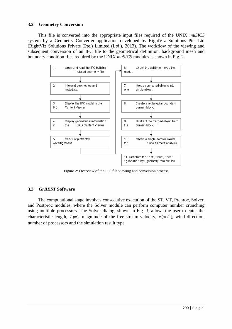
290 | P a g e

3.2 Geometry Conversion

This file is converted into the appropriate input files required of the UNIX muSICS

system by a Geometry Converter application developed by RightViz Solutions Pte. Ltd

(RightViz Solutions Private (Pte.) Limited (Ltd.), 2013). The workflow of the viewing and

subsequent conversion of an IFC file to the geometrical definition, background mesh and

boundary condition files required by the UNIX muSICS modules is shown in Fig. 2.

Figure 2: Overview of the IFC file viewing and conversion process

3.3 GrBEST Software

The computational stage involves consecutive execution of the ST, VT, Preproc, Solver,

and Postproc modules, where the Solver module can perform computer number crunching

using multiple processors. The Solver dialog, shown in Fig. 3, allows the user to enter the

characteristic length, (m), L magnitude of the free-stream velocity, ),s (m -1v wind direction,

number of processors and the simulation result type.

291 | P a g e

Figure 3: Solver dialog window showing default values

4. VALIDATION

The case study described in E. Simiu and R. Scalan (Simiu et al., 2011) is used as

benchmark test case. The geometry is a typical building complex as shown in Figure 4. Wind

tunnel studies of surface wind around this building complex have been conducted. There are

three main types of surface winds: vortex flows, corner streams and through flows.

Surface winds expressed in terms of speed ratio R_H=V/V_H where V is the wind speed

at pedestrian height (region A), V_H is wind speed at building height H. Dimensional analysis

gives: R_H = f(L/H,W/H,D/H,H/h,Re) where Re is Reynold number. If D/H is small as in

many tall buildings, then the effect of Reynolds number is insignificant.

CFD simulation using muSICS is depicted in Figure 4. Plots of V_A/V_H against W/H

(aspect ratio) for a given L/H = 0.5, H/h = 5 on both experiment data and CFD simulations is

shown in Figure 5. As can be seen from Figures 4-5, the simulation results from muSICS can

capture all three types of building aerodynamic winds and are in good agreement with wind

tunnel experiment data. The speed ratio R_H increases to a max with increasing W/H but

changes less once W/H aspect ratio reached unity.

Figure 4: Geometry of building complex used for solver validation (left), CFD simulation using muSICS

showing surface winds for a typical test case (right)

292 | P a g e

Figure 5: Speed ratio of surface wind: wind tunnel data (left), CFD simulations (right)

5. RESULTS

5.1 Natural Ventilation for External and Internal Airflow

Example 1 is presented here concerning the external airflow around a building with

walls, a curved surface and a flat roof, as shown in Fig. 6. The model geometry was prepared

using Revit to create an IFC file. The IFC file is then converted into the necessary input files

for CFD simulation (Fig. 6(a),(b)) thereafter, GrBEST is used to perform surface triangulation

followed by CFD flow solution (Fig. 6(c),(d)) using the embedded CFD solver, muSICS. The

input parameters for the flow solver are shown in the Solver dialog (Fig. 3) and the airflow is

from the northeast (NE) to the southwest, as shown by the streamlines of Fig. 6(d).

(a)

(b)

(c)

(d)

Figure 6: Simple building geometry used for external airflow simulation: (a) IFC content, (b) curve structure,

(c) surface triangulation, and (d) converged flow solution

293 | P a g e

Example 2, demonstrating internal airflow is presented in Fig. 7, where the building

geometry consists of two floors, external walls, one lower-level internal wall, and four

openings on the front and rear walls. The workflow procedure for this example is similar to

that employed in Example 1, with the only difference being that the airflow direction is from

the west to the east.

A Stream Tracer filter is created in Paraview to visualize the airflow as a set of

streamlines coloured by the magnitude of the velocity. The airflow is from the external to the

internal region and the fluid flow is from the west to the east as specified (Fig. 7 (d)).

(a)

(b)

(c)

(d)

Figure 7: Two-storey building geometry with openings and an internal wall used for internal airflow simulation:

(a) IFC content, (b) curve structure, (c) surface triangulation, and (d) converged flow solution

5.2 Case Study – Community Facility

An industrial project collaboration involving IHPC, BSD & RightViz with RSP

Architects and Planners Pte Ltd (RSP) to generate a case study on estate airflow simulation

work and evaluate the natural ventilation scenario is carried out from 1 Mar to 31 May 2014.

The results are used in determining the optimal building mass, geometry, orientation and

layout to achieve good natural ventilation conditions. Upon receiving the .rvt format of the

model from RSP, simplification of the model to suit CFD discipline commenced with the aim

of studying the natural ventilation on levels 1 and 2 in mind.

5.2.1 Geometry Simplification Steps

1. Vegetation, topology, doors, windows and basement levels are deleted.

2. Room separation lines, elevated floor, ramp, structural columns near to walls are

removed. Enclosed spaces are replaced by solid blocks. Thin walls are replaced with

0.5m walls.

3. Second, third, fourth storey and roof are replaced by a solid block. Geometry of third

level and roof are altered to enable successful meshing.

294 | P a g e

5.2.2 Results and Recommendations

Figure 8: Simulation Result with North Wind, 3 m/s (left), South Wind, 3m/s (right)

Approximately 4.5 million cells are generated on meshing. The time taken for geometry

simplification, meshing and solution generation is approximately two days. Under the present

architectural design, it is observed that under North wind condition, the airflow movement on

level 1 is slow or stagnant (illustrated by large regions of dark blue colour). To further

improve the natural ventilation performance on level 1, it is suggested that the gap move from

the present location 1, further east, to location 2 (Fig. 9). This would allow the North wind to

penetrate to the central region of level 1.

Figure 9: Recommended changes during North Wind scenario (left) South Wind scenario (right)

The overall natural ventilation performance on level 1 under South wind is better than

that of North wind. If the gap is moved from the present location 1, further to the east, to

location 2 (Fig. 9), then under South wind condition, it is anticipated that the highlighted

stagnant zone would be eliminated.

5.2.3 Modifications

Three simulation stages are proposed by RSP. The first stage consists of the following

three scenarios. In Scenario 1, the corridor is widened to 3.5m. Pantry and food preparation

area remain enclosed. In Scenario 2 – Option 1, the corridor is widened to 3.5m and the walls

at two ends of food preparation area are changed to 900mm high wall with opening above. In

Scenario 2 – Option 2, the corridor remains at 2m and the walls at two ends of food

preparation area are changed to 900mm high wall with opening above.

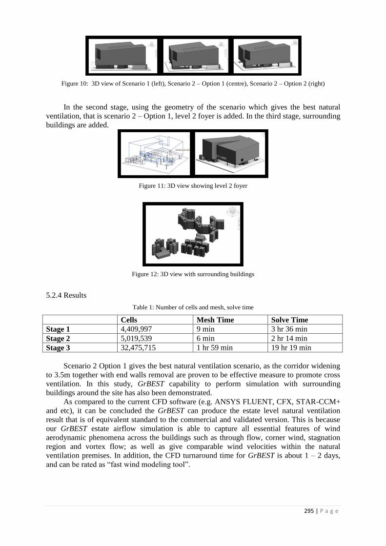
295 | P a g e

Figure 10: 3D view of Scenario 1 (left), Scenario 2 – Option 1 (centre), Scenario 2 – Option 2 (right)

In the second stage, using the geometry of the scenario which gives the best natural

ventilation, that is scenario 2 – Option 1, level 2 foyer is added. In the third stage, surrounding

buildings are added.

Figure 11: 3D view showing level 2 foyer

Figure 12: 3D view with surrounding buildings

5.2.4 Results

Table 1: Number of cells and mesh, solve time

Cells Mesh Time Solve Time

Stage 1 4,409,997 9 min 3 hr 36 min

Stage 2 5,019,539 6 min 2 hr 14 min

Stage 3 32,475,715 1 hr 59 min 19 hr 19 min

Scenario 2 Option 1 gives the best natural ventilation scenario, as the corridor widening

to 3.5m together with end walls removal are proven to be effective measure to promote cross

ventilation. In this study, GrBEST capability to perform simulation with surrounding

buildings around the site has also been demonstrated.

As compared to the current CFD software (e.g. ANSYS FLUENT, CFX, STAR-CCM+

and etc), it can be concluded the GrBEST can produce the estate level natural ventilation

result that is of equivalent standard to the commercial and validated version. This is because

our GrBEST estate airflow simulation is able to capture all essential features of wind

aerodynamic phenomena across the buildings such as through flow, corner wind, stagnation

region and vortex flow; as well as give comparable wind velocities within the natural

ventilation premises. In addition, the CFD turnaround time for GrBEST is about 1 – 2 days,

and can be rated as “fast wind modeling tool”.

296 | P a g e

6 CONCLUSION

At present, the GrBEST software application allows the user to perform a CFD modeling

and simulation to determine internal and external airflow in and around a building

development. As shown in the examples and case study, GrBEST is able to provide airflow

simulation results of simple estate building geometries with a short turnaround time, all in a

single graphical user interface, simple enough to be carried out with a few clicks of a button.

The case study also demonstrated the feasibility of using GrBEST tool to determine the

optimal building mass, geometry, orientation and layout to achieve good natural ventilation

conditions for a typical building project.

Moving ahead, further development work will involve improving the software to further

automate the reporting and result visualization processes, and to provide an Internet-based

mechanism for CFD project submission and execution on supercomputer resources. This,

together with more developmental work on geometry manipulation, software development

and muSICS computational engine extension is required to bring this software towards

commercialization stage.

7 ACKNOWLEDGEMENTS

The authors would like to acknowledge Building and Construction Authority (BCA)

(BCA, 2013), Singapore for the award of Ministry of National Development (MND) Core

Innovation Fund (CIF) for this development work. In addition, the authors would like to

thank Dr. Chiet Sing Chong from RightViz Solutions Pte. Ltd. for his work in developing

Geometry Converter application and Mr. Phay Ping Tan from Building System & Diagnostics

Pte. Ltd. for his CFD simulation work using commercial software. On top of that, the authors

are grateful to Mr. Ngian Chung Wong and colleagues from BCA and Professor Nyuk Hien

Wong from National University of Singapore (NUS) for their active involvement and

technical advices during the course of the development.

8 REFERENCES

Singapore Energy Statistics 2012 & 2013, www.ema.gov.sg/media/files/publications, Energy

Market Authority, (accessed in June 2014)

Wang, L and Wong, N.H., Applying Natural Ventilation for Thermal Comfort in Residential

Buildings in Singapore, Architectural Science Review, Vol. 50 (3), pp 224-233, 2007.

Building and Construction Authority Green Mark Scheme,

http://www.bca.gov.sg/greenmark/green_mark_buildings.html (accessed in Sep 2013).

Autodesk Revit Architecture (Revit), Building Information Modeling software application,

http://usa.autodesk.com/revit/, Autodesk Inc., 2013.

ParaView – Parallel Visualization Application, www.paraview.org/, (accessed in 2013).

Simiu, E. and Scanlan, R., Wind Effects on Structures: Fundamentals and Applications to

Design, Dover Publication, 2011.

297 | P a g e

REDUCING COOLING ENERGY NEEDS THROUGH

AN INNOVATIVE DAILY STORAGE BASED FACADE

SOLUTION

Servando Álvarez Domínguez*1, Rafael Salmerón Lissén

1, Álvaro Ruiz-Pardo

2,

José Sanchez Ramos2, and Javier García Ramos

1

1 Universidad de Sevilla (Seville University)

Camino de los descubrimientos S/N

Escuela Tecnica Superior de Ingenieros

Seville 41092, Spain


2 Universidad de Cádiz (Cadiz University)

C/ Chile,1. 11002

Cádiz, Spain

ABSTRACT

The framework of the research presented in the paper is a project oriented to promote the use of concrete

solutions in buildings based on maximizing the benefits of its thermal inertia for cooling periods.

The constructive solution developed has one configuration for summer (cooling mode). This configuration is

similar to a ventilated facade that is formed by a thermally insulated outer layer of concrete, an intermediate air

layer and an inner layer of concrete. The inner layer is cooled at night by forced ventilation using an outdoor -

outdoor scheme.

The aim of this paper is to show the preliminary results about the potential of special concrete walls as solutions

to reduce energy demand in residential buildings by thermal offset in Spanish Mediterranean climates.

In summer, the concrete building facades are used as heat sinks. The aim is to cool the inner layer of concrete

moving outdoor air through the air layer during night taking advantage of the low nigh-time air temperatures.

The cool stored is released to the interior spaces when the maximum peak load of the space takes place.

With the aim of select a proper design of the innovative element, the influence of the thickness of the inner layer,

the air velocity in the chamber and control lays to activate the ventilation are analysed. Simulations show that the

use of this element is very promising for reducing energy demand in residential buildings in the Spanish

climates.

Experiments are currently performing (summer 2014).

KEYWORDS

Cooling savings, Ventilated active facade, Cooling storage

1. INTRODUCTION

The framework in which this study takes place is the " Service Contract R + D + i Relating to

Competence Scope of the Ministry of Public Works and Housing " with the research project

298 | P a g e

entitled "Analysis of the energy performance of closures concrete based on maximizing the

benefits derived from the thermal inertia".

Meeting the "20-20-20" targets (European Commission, 2012) for reduction of CO2 emissions

necessarily involves a drastic reduction of energy consumption in buildings.

For the climatic conditions of the south of Europe, as Andalusia region in Spain, cooling is

required during the summer season, since there are high daylight temperatures an high levels

of solar radiation.

To reduce energy consumption in cooling and therefore CO2 emissions, it is previously

necessary to reduce energy demand.

There are several techniques that can be applied to reduce the cooling demand (Santamouris,

2007), but some of the most obvious alternatives is to use the relatively low night outdoor

temperature as a heat sink. In order to use this heat sink, energy (cold) storage is required

since there is a gap between the cooling needs in the building and the time when the lowest

temperatures are presented in the heat sink.

One option to storage the cold is to use the thermal inertia of the structure of the building.

A simple definition of thermal inertia would say it's the ability to keep the mass of thermal

energy received and gradually releasing it (Ruiz-Pardo 2008). Because of this ability, taking

into account the thermal inertia of the walls of a building, can be decreased the need for air

conditioning, with the consequent reduction of energy consumption and pollutant emissions.

The thermal inertia improves energy performance of buildings (Aste 2009) because it allows

the damping of the temperature variation and the phase of the internal temperature relative to

the outside.

For a situation with a high external temperature and solar radiation, the temperature outside

the enclosure rises producing a heat transfer to the interior of the building. The evolution of

the temperature of the outer face has a maximum (maximum amplitude) in a particular time of

day depending on the location and orientation of the enclosure. This wave is damped outside

temperature, in amplitude, crossing the enclosure, also emerging a time lag between the

instants at which a peak temperature is produced. The effect of phase shift and damping

allows the building to stay longer in the comfort zone without additional energy expenditure

allowing free savings because they are inherent in the material (Ruiz-Pardo 2008).

The physical characteristics of the concrete gives it a high thermal inertia , which allows to

predict optimum energy performance of the building in the event that this material forms the

inner core (structure) and external (walls and roofs) thereof. The use of concrete as façade

cladding and covered in the building:

Reduce the energy consumption of heating.

Softens variations in internal temperature.

Delay maximum temperatures in offices and commercial buildings to the exit of the

occupants.

Reduces peak temperatures (maximum and minimum) and can make the air

conditioning unnecessary.

Maybe employed with nocturnal ventilation to eliminate the need for cooling during

the day.

Makes better use of sources of low temperature heating such as heat pumps for

underfloor heating.

299 | P a g e

Overall the effect of thermal inertia in enclosures is a variable not usually considered in the

design of the building.

In addition to its modelling difficult for designers and specifies, calculation tools were not

sensitive to this parameter and the knowledge of its potential benefits have not been

adequately considered by the technical and scientific community.

The main objective of the project is to parameterize the fundamental variables that

characterize the thermal inertia of buildings overlooking substantially improve treatment

procedures for calculating the thermal performance of buildings. This would be instrumental

to value the role of concrete solutions as part of improving energy efficiency.

This setting will also allow designers can, easily, estimate the energy savings from the

thermal inertia of buildings with contour and concrete structure.

2. MATERIALS AND METHODS

An experimental cell (Figure 1) was built in order to test a “thermally active wall” available to

storage cold during the night and release it during the day.

The experimental cell is a reinforced concrete cubicle (3.0 x 3.0 x 3.0 m.) to which he

included a special front face south to investigate several special construction solutions

Figure 1. Experimental cell

The thermally active wall (Figure 2) is a facade composed of two solid layers speared by an

air ventilated layer. The inner layer is a concrete wall with high thermal inertia. The outer

layer is an insulated element having low thermal transmittance. During the night the air layer

is ventilated using fans located in the upper zone of the facade. During the day, the ventilation

is stopped.

Figure 2. module test for the analysis of the influence of nocturnal cooling of the concrete wall through the

chamber ventilated by forced ventilation.

Thermally active wall

300 | P a g e

A simulation model was performed with the following objectives: Dimensioning od the

experimental setup, prediction of the thermal behaviour of the element under conditions

different than those obtained experimentally, and to perform studies an analysis of the

potential of the active facade. Thai model is based on the preiviously defined by Ruiz-Pardo

(Ruiz-Pardo, 2010)

In simulation, previous to the construction of the experimental setup, the main variables

affecting the thermal performance of the thermally active wall were studied: the inner layer of

concrete (10-15-20 cm.), the thickness of the internal air chamber wall (2-5-10 cm.) and the

air speed walking the chamber (0.5-1-2 m/s).

In the coming months the validations of the developed models will be performed using the

results that currently we are obtaining.


Previous to the campaign of experiments, some results were obtained with the aim to select a

proper design and estimate the savings that can be obtained from the thermally active facade.

They are shown below.

The experiments are currently in developing, so some partial results had been obtained and

they are shown at the end of this section.

3.1 Simulation results

In order to select a proper design of the innovative element, several simulations were

performed with different designs in two selected localities: Sevilla and Cádiz

The process performed was the following:

Nine options were initially tested; this was the result of three air velocities in the air

layer and three thicknesses of the inner wall. The results of these cases are shown in

Table 1.

From the results, the option with highest energy savings for summer was selected.

For the selected option, some variations in the operational conditions were proved in

order to maximize its behavior for winter season even though the design was

optimized for summer.

For the two considered cities, it was found that the optimal design was the same. This result

was not expected, since they are different climates. The only difference in the design is that

for the case of Cadiz, the optimum temperature for allowing ventilation is 25°C and not 23 as

in the case of Seville. The main descriptive parameters of the optimal design are shown in

Table 1.

Table 1: Studied solutions to find a proper design of the innovative element in Seville

Inner wall

thickness

Air layer

velocity

air layer convective heat transfer coefficient (air in

circulation)

solution 5 15cm 1 m/s 5 W/m2K

The overall behavior expected for the innovative element in these two cities is shown in Table

2. It can be seen that the innovative element performs cooling in summer and heating in

winter.

301 | P a g e

Table 2. Gross heating gains for the innovative element in the three studied cities. Negative values means heating

losses (desirable behaviour in cooling season) and positive values means heating gains (desirable behaviour in

heating season). All values are in kWh/m2

Summer

month

Monthly

heat losses

kWh/ m2

Total

heat losses

kWh/ m2

Seville

Jun -7.57

-13.12 Jul -3.04

Aug -2.51

Cadiz

Jun -19.81

-36.07 Jul -9.71

Aug -6.54

The results of Table 2 show that in the two studied localities, the innovative element removes

heat and in addition when it is compared with a conventional wall, its benefit is increased

since the conventional wall has the opposite behaviour of the innovative element, namely, it

introduces heating during the summer season.

The expected savings for the innovative element are obtained from the comparison with a

conventional wall. The results of this comparison are shown in Table 3.

Table 3. Heat gains comparison between the innovative element and a conventional Wall having the same U-

value in the three tested localities

Summer

Innovative element

Heat gains

conventional wall

heat gains difference (savings)

kWh/ m

2 kWh/ m

2 kWh/ m

2

Seville -13.1 12.6 -25.8

Cadiz -36.1 4.2 -40.3

To illustrate the behaviour of the innovative element in comparison with a conventional wall,

in the Figure 3, the temperature profiles are shown for the interior layer of the innovative

element and for a conventional wall. These profiles were calculated for one typical day of the

cooling season and for a typical day of the heating season.

Cooling season

(a) Interior layer of the innovative element (b) Conventional wall

Figure 3. Temperature profile in: (a) the innovative element and (b) in a conventional wall

302 | P a g e

Figure 3 shows that the amplitude of the temperature oscillation obtained in the innovative

element, is much lower than that obtained in the conventional wall. Additionally, it is seen

how in the cooling season, the temperatures of the innovative solution are always lower than

the indoor temperature (assumed as 25°C), while the conventional wall is oscillating around

that temperature.

3.2 First experimental results

The first period of experiments were performed without night ventilation of the air layer. The

objective was to observate the behavior of the experimental cell and compares it with the

results obtained when the air layer is ventilated during the night.

In Figure 4 are shown the interior surface temperatures of the cell. The green lines are the

average temperature of the conventional walls while the orange lines correspond to the

surface temperatures of the active facade.

Figure 4. Temperatures of the interior surfaces of the experimental cell without night ventilation of the air layer

As it can be seen, the active façade shows les amplitude in the daily variation of temperature

than the other interior surfaces. This behavior is obtained because the active facade has a

greater thermal inertia. However, the mean daily temperature of the active facade is less than

0.5ºC inferior than de the mean of the other surfaces when the air layer is not ventilated

during the night.

In Figure 5 are shown the same interior surface temperatures of Figure 111, but with night

ventilation of the air layer. In this case the daily variation of temperature is closing similar for

the active façade and for the other interior surfaces. This behavior is caused by the additional

excitation suffered by the active facade when the ventilation is activated. But the most

important result is that the daily mean temperature of the active façade is approximately 2ºC

inferior than the corresponding temperature of the other walls. It is 1.5ºC colder than the

values obtained when the air night ventilation is not operating.

16

18

20

22

24

26

28

30

32

34

36

28/abr 29/abr 30/abr 01/may 02/may 03/may 04/may 05/may 06/may 07/may 08/may

[ºC]

Ts. Active facade Ts. Interior surfaces

Ts. Active facade (mean daily) Ts. Interior surfaces (mean daily)

303 | P a g e

Figure 5 Temperatures of the interior surfaces of the experimental cell with night ventilation of the air layer

4 CONCLUSIONS

An innovative facade element has been designed with the objective of reduce energy cooling

demand in buildings. This element is being evaluated by simulations and experiments.

Using the developed simulation model, a proper design was obtained for the cities of Seville

and Cadiz. The obtained design was the same in both cases with only little differences in the

adequate temperature to allow the air night ventilation.

The simulation results show that the active facade, using the selected design for the cities of

Seville and Cadiz, has the potential to provide cooling in the summer season while a

conventional wall provides heating. It means that the energy potential of this element shows a

very interesting behaviour that has to be verified experimentally.

The very first experimental results shows a promising potential for the reduction of energy

cooling consumption and seems verify the potential predicted in simulation. However, the

experimental campaign is still carrying on, so definitive results and conclusions can not be

taken yet.

5 ACKNOWLEDGEMENTS

The authors would like to thank the FEDER of European Union for financial support via

project “Análisis del comportamiento energético de los cerramientos de hormigón en base a la

maximización de las ventajas derivadas de su inercia térmica“of the “Programa operativo

FEDER de Andalucia 2012-2014”. We also thank all Agency of Public Works of Andalusia

Regional Goberment staff and reserchers for their dedication and professionalism.

Special thanks to "Grupo Cementos Valderrivas, Alcalá de Guadaira plant" for his selfless

assistance in developing the experiments.

6 REFERENCES

European Commission. (2010) Communication From the Commission to the European

Parliament, the Council, the European Economic and Social Committee and the

20

22

24

26

28

30

32

34

36

38

40

08/jun 10/jun 12/jun 14/jun 16/jun 18/jun 20/jun

[ºC]

Ts. Active facade Ts. Interior surfaces

T_media_diaria_superf_FAH T_media_diaria_superficies int.

304 | P a g e

Committee of the Regions. Analysis of options to move beyond 20% greenhouse gas

emission reductions and assessing the risk of carbon leakage. 2010.

Santamouris,M.; Pavlou,K.; Synnefa,A.; Niachou,K.; Kolokotsa,D. (2007) Recent progress

on passive cooling techniques: Advanced technological developments to improve

survivability levels in low-income households. Energy Build., 2007, 39, 7, 859-866

Ruiz-Pardo Á.(2008) Ahorro energético mediante el uso de elementos de doble envolvente

transparente-opaco [dissertation]. Tesis Doctoral, Sevilla: Universidad de Sevilla,

ETSI; 2008.

Aste,Niccolò; Angelotti,Adriana; Buzzetti,Michela (2009) The influence of the external walls

thermal inertia on the energy performance of well insulated buildings. Energy Build.,

2009, 41, 11, 1181-1187

Ruiz-Pardo Á, Domínguez SÁ, de la Flor, Francisco José Sánchez, Lissen JMS.(2010)

Simulation model for some types of double envelope elements. International Journal

of Ventilation. 2010;9(3):227-39.

305 | P a g e

SIMULATION OF STATIC PRESSURE RESET

CONTROL IN COMFORT VENTILATION

Chrysanthi Sofia Koulani 1, Remus Mihail Prunescu

2, Christian Anker Hviid

1,

and Søren Terkildsen *1

1 Technical University of Denmark (DTU),

Department of Civil Engineering

Brovej

DK-2800 Kgs. Lyngby, Denmark


2 Technical University of Denmark (DTU)

Automation and Control

Department of Electrical Engineering

Elektrovej

DK-2800 Kgs. Lyngby

ABSTRACT

Variable air volume (VAV) ventilation systems reduce fan power consumption compared to constant air volume

(CAV) systems because they supply air according to the airflow demand. However VAV ventilation systems do

not take fully into account the potential energy savings as the control strategy operates the terminal boxes and

the air handling unit (AHU) independently without pressure integration. The pressure in the main duct is

maintained at a constant static pressure (CSP) which corresponds to the pressure required under the design full

load condition. Under part load conditions, the fan provides excessive static pressure which is dissipated via

throttling at the terminal boxes. As a result significant fan power is wasted in mechanical energy losses. The

development of sophisticated direct digital controls (DDC) creates possibilities to integrate feedback from the

dampers into the building management system. In this way the operation of central plant equipment is adjusted

in real time according to the actual pressure demand; this control scheme can be implemented by the static

pressure reset (SPR) method. The SPR control method ensures that at least one damper remains fully opened;

thus the fan generates only enough pressure to satisfy the airflow demand in the most critical zone. Consequently

the airflow resistance of the ductwork is maintained at a minimum and the fan operation is optimized. There are

various approaches to implement the control scheme of the SPR method; the state of the art is represented by the

method of trim and respond based on pressure alarms.

This study investigates the operation of the SPR control method of trim and respond based on pressure alarms in

a CO2 demand application where large air volumes are provided to three classrooms. The investigation was

based on simulations performed with a fully dynamic model of a VAV ventilation system that was developed in

the Simulink programming tool which is add-on software to MATLAB mathematical programming language.

The Simulink model was developed in previous research work and was built based on the International Building

Physics Toolbox (IBPT), which is a library of blocks constructed for the thermal analysis in building physics.

For the purpose of the current investigation the IBPT toolbox was remodelled to integrate the calculation of the

airflow demand based on the CO2 concentration occurring in the zone. The performance of the Simulink model

was in previous work evaluated based on the experimental setup of a ventilation system. The investigation of the

SPR control algorithm of trim and respond based on pressure alarms disclosed some issues that need to be

addressed and optimized before the algorithm can effectively establish the pressure conditions that satisfy the

pressure demand under high airflows. In short the algorithm must be tuned to the application beforehand or,

preferably, actively learn to perform from continuous feedback before it presents a real plug-and-play solution.

KEYWORDS

CO2 demand control ventilation, static pressure reset, modelling, Simulink, energy savings.

306 | P a g e

1. INTRODUCTION

The potential energy savings in a VAV ventilation system can be boosted by integrating the

control of terminal boxes into the building management system (Hartman, 1995). In this case

it is possible to implement the SPR control method, instead of operating the fan with a CSP

set point which corresponds to the pressure required under the design full load condition (Wei

et al, 2004). The SPR control method operates the fan with a variable pressure set point which

is established based on the dynamics of the actual pressure demand occurring in the system.

Since 1999 the SPR control method has been a requirement for ventilation systems equipped

with terminal boxes with DDC (Taylor, 2007). In accordance with ASHRAE Standard 90.1

(ASHRAE 90.1, 2004), the fan pressure set point shall be reset based on the critical zone

request. A similar requirement is included in California’s Title 24 Energy Standards (Title 24,

2005). There are various approaches able to implement the control scheme of the SPR

method; the state of the art is represented by the method of trim and respond based on

pressure alarms as it is stable, flexible and it minimizes the impact of rogue zones (Taylor,

2007).

The objective of this paper is to investigate the operation of the SPR control method of trim

and respond based on pressure alarms when the airflow demand changes in different zones in

the ventilation system. The investigation is carried out by simulating the pressure and airflow

conditions occurring in a system that provides air in three classrooms. The simulations are

conducted with a fully dynamic model of a VAV ventilation system that was developed in

Simulink (Simulink, 2013) during previous research work. The Simulink model was in

previous work documented based on the experimental setup of a ventilation system that it is

able to perform accurate calculations.

2 THE SIMULINK MODEL

Figure 1: The Simulink model of the VAV ventilation system.

307 | P a g e

The model of the VAV ventilation system was created in the graphical environment of

Simulink in Matlab (Matlab, 2013). Figure 1 illustrates the Simulink model which was built

based on the blocks of the international building physics toolbox (IBPT). IBPT is library of

blocks constructed for the thermal analysis in building physics (IBPT, 2012). The default

IBPT blocks for the internal gains and the ventilation system were rebuilt to comply with the

modelling of the VAV ventilation system (Koulani et al, 2014). A detailed validation of the

model can be found in Koulani et al (Koulani et al, 2014).

2.1 The ventilation system

The IBPT ventilation system block was configured to calculate dynamically the airflow

demand based on the CO2 concentration occurring in the zone. The CO2 concentration is

approximated by equation (1) (Bekö et al, 2010) and the corresponding airflow demand is

calculated dynamically by the ramp functions shown in Figure 2. The user defined data are

the minimum (qset,min) and maximum (qset,max) airflow set point required in order to maintain a

comfortable range of CO2 concentration (CO2 set,min, CO2 set,max) in the zone.

Figure 2: The dynamic calculation of the airflow demand based on the zone CO2 concentration.

ic)e1(Vn

G)e1()cc(c ntnt

i0

(1)

Where co carbon dioxide concentration in the room at start, t = 0 (m3/m

3)

ci carbon dioxide concentration in the inlet ventilation air (m3/m

3)

G carbon dioxide supplied to the room (m3/h)

n air change rate (1/h)

V the volume of the zone (m3)

t time (h)

2.2 The fan

The mathematical model of the fan represents the operation characteristics of a typical fan

box ventilator. The details regarding the control of the fan are given in Koulani et al (Koulani

et al, 2014). Field measurements were performed on a typical box fan with large capacity

(Exhausto BESB250-4-1) in order to model a similar response. The measurements were

conducted in open loop, i.e. with no feedback and aimed at identifying the built up of the fan

pressure when different steps were given to the input signal (see Figure 3).

Figure 3: Setup for performing the field measurements.

max,)max,22

(

2

setqset

COCO

minset,2CO

maxset,CO

minset,qmaxset,q

demq

max,setmax,seta

min,setmax,set

min,setmax,set

dem q)TT(TT

qqq

308 | P a g e

The field measurements indicated that the second-order linear time-invariant (LTI) system is

appropriate for modelling a fan able to provide the pressure rise required at the design full

load condition. The second-order LTI system is implemented by using the state space method;

the state space equations (see equation 3 & 4) calculate the derivative of the system response

with respect to time (Rowell, 2002).

1 2

2 22 1 22

.

. ..n n n

x x

x y u x x

Where x1, x2 the state vectors represent values from inside the system that can change

over time

u the input vector to the system, voltage signal (V)

y the output vector from the system, fan speed (rpm)

ωn the natural frequency is relevant to the speed response of the system (rad/s)

ζ the damping ratio is relevant to the oscillation mode of the system (-)

The modelling is performed by using the state space representation because in this way it is

possible to express the operation of the fan with a variable run up time (ts). The run up time is

defined as the time required for the fan to adjust the angular speed to the current input signal,

thus the run up time changes according to the input signal to the fan. This behaviour can be

modelled by applying equation (5) (Herring, 2005) where the damping ratio is calculated as a

function of the run up time.

1.6

6.6

s nt

(5)

The data for the run up time were obtained by performing open loop measurements on a

typical box fan (Exhausto BESB250-4-1) when the input signal to the fan changed per 1 V

within a range of 0 V to 10 V. Based on the measurement points a trend line was drawn to

correlate the damping ratio with the input signal (see equation 6). The given equation was

incorporated in equation (4) and thus the damping ratio became variable of the input signal. In

this way the fan model is built with a variable run up time.

5965.34442.00222.0 2 VV (6)

Where V the input signal to the fan (Volts)

Equation (5) establishes a stable response for values of damping ratio above 0.7, for lower

values oscillations occur (Herring, 2005). In this case the natural frequency can be adjusted

accordingly.

The pressure rise of the fan is calculated according to the fan speed which is output of the

state space system (see equation 4). The correlation between the two fan parameters is

determined by collecting measurement points in open loop from a typical box fan (Exhausto

BESB250-4-1). The measurements were conducted when the input signal changed per 1 V

within a range of 0 V to 10 V; equation (7) was obtained based on the relevant measurement

data.

7401.50082.00002.0 2 speedspeedPfan (7)

Where ΔPfan the pressure rise that the fan provides (Pa)

speed the angular speed that the fan rotates (rpm)

(3)

(4)

309 | P a g e

2.3 The damper

The mathematical model implementing the operation of a typical damper (D) is built

according to equation (8) which corresponds to the second-order LTI system expressed in the

Laplace domain (Franklin et al 1993). The details regarding the control of the damper can be

found in Koulani et al (Koulani et al, 2014).

nn

nd

ss

ksD

2)(

2

(8)

Where kd the process gain correlates the system output with the system input (m3/s/Pa%)

In the damper model the system input refers to the opening position of the damper while the

system output to the corresponding resistance coefficient. The correlation between the two

parameters is obtained from table values for a typical damper. The two fundamental factors

that describe the response of the second-order LTI system, the damping ratio and natural

frequency, are determined by trial and error. The damping ratio is set to 1 as the damper

returns to equilibrium as quickly as possible without oscillating while the natural frequency is

established at 50 rad/s.

2.4 The pressure and airflow solver

The friction and single pressure losses blocks illustrated in Figure 1 implement the hydraulic

calculation of the VAV ventilation system according to the duct design shown in Figure 4.

The unknown pressure and airflow conditions are determined by setting up a system of

equations expressing the pressure losses occurring in every component of the system. The

equations used for calculating the frictional and single pressure losses are described in detail

by Koulani et al (Koulani et al, 2014). The hydraulic calculation determines the pressure

demand (P) at the beginning and end of every component as well as the airflows (q) delivered

to the different zones (see Figure 4). The system of equations derived cannot be solved

analytically; therefore the Newton-Raphson numerical method is used instead.

Figure 4: The duct design in the pressure and airflow solver block.

2.5 The static pressure reset algorithm

The operation principle of the SPR control method of trim and respond based on pressure

alarms is presented in Figure 5. Every damper of the VAV system transmits an alarm signal

when its position exceeds 85 % opening that indicates that the available pressure is critically

low but still sufficient for providing the airflow demand. The zone keeps generating a

310 | P a g e

pressure alarm until the damper closes to a position of 80 % opening. The alarms from all

zones are summed and when at least two zones request higher pressure the operation set point

of the fan is reset 10 % upwards; in the opposite case it is reset 5 % downwards. The SPR

algorithm is performed within a specific pressure range; the upper limit is set equal to the CSP

set point which corresponds to the pressure required under the design full load condition. The

lower SPR limit is determined according to the minimum pressure demand that ensures the

precise operation of the dampers. The SPR loop is iterated every 90 sec and the fan adjusts to

the new pressure set point.

Figure 5: The control logic of the trim and respond static pressure reset method.

3 THE SIMULATION SETUP

The simulations investigate the operation of a VAV ventilation system which provides air in

three classrooms, where each classroom can accommodate 20 students and has an area of 50

m2. When no students are present in the classroom the CO2 concentration is equal to 400 ppm

(CO2 set,min) that corresponds to the outdoor CO2 level. The minimum airflow demand is set to

10 l/s (qset,min) to comply with the ventilation rate of 0.2 l/s, m2 which is recommended during

unoccupied periods in non-residential buildings (see annex B.4, EN15251, 2007). At the

design full load condition a ventilation rate of 185 l/s (qset,max) is provided to maintain the CO2

concentration to 1000 ppm (CO2 set,max) that corresponds to a typical CO2 level used in

comfort ventilation. The occupancy in the three classrooms was configured as shown in Table

1.

Table 1: The occupancy profile in the three ventilated zones.

Time (min) No of students zone 1 No of students zone 2 No of students zone 3

0 - 12 20 20 20

12 - 24 20 5 3

24 - 36 20 10 20

A simulation was performed based on the occupancy profiles given in Table 1 when the VAV

ventilation system was controlled with the SPR control method. The SPR pressure set points

were adjusted by trial and error to fit to the case study simulated. Table 2 summarizes the

selected pressure range, within which the operation set point of the fan is reset.

Table 2: The pressure range of the SPR control method

Lower SPR pressure set point 15 Pa

Upper SPR pressure set point 145 Pa

311 | P a g e

4 RESULTS

4.1 System operation

Figure 6 and Figure 7 present the results of the simulation according to the occupancy profiles

given in Table 1 when the VAV ventilation system operates with the SPR control method.

The two graphs given in Figure 6 illustrate the CO2 concentration in the three zones and the

adjustment of the operation set point of the fan, respectively. The distribution of the airflows

and the operation of the dampers in the three ventilated zones are shown in the graphs given

in Figure 7.

Figure 6: CO2 concentration in the three ventilated zones and adjustment of the fan operation set point,

respectively.

Figure 7: Airflow distribution and damper operation in the three ventilated zones.

The results are analyzed according to the different occupancy periods (see Table 1).

0 min to 12 min: When the system is set to operation the design full load is occurring in the

three zones; thus the zone airflows increase and the dampers follow an upward trend. The

0

250

500

750

1000

0 3 6 9 12 15 18 21 24 27 30 33 36

CO

2 c

on

cen

trat

ion

(p

pm

) CO2 concentration (ppm)

0

40

80

120

160

200

Air

lfo

w (

m3 /

s)

Airflow, ventilated zone 1

0

20

40

60

80

100

Dam

per

po

siti

on

(%

)

Damper operation, ventilated zone 1

0

40

80

120

160

200

Air

lfo

w (

m3 /

s)


0

20

40

60

80

100

Dam

per

po

siti

on

(%

)

Damper operation, ventilated zone 2

0

40

80

120

160

200

0 3 6 9 12 15 18 21 24 27 30 33 36

Air

lfo

w (

m3/s

)


0

20

40

60

80

100

0 3 6 9 12 15 18 21 24 27 30 33 36

Dam

per

po

siti

on

(%

) Damper operation, ventilated zone 3

0

40

80

120

160

0 3 6 9 12 15 18 21 24 27 30 33 36 P

ress

ure

(P

a)

Fan operation set point

Time (min) Time (min)

Time (min)

2nd alarm

1rst alarm

Time (min)

2 alarms

312 | P a g e

position of the dampers is still below 85%; therefore no alarm is generated. Consequently the

operation set point of the fan is decreased by 5% when the SPR control loop is iterated.

12 min to 24 min: The maximum occupancy load is maintained in zone 1 whereas in zone 2

and zone 3 the load is decreased approximately to 1/4 of the maximum. As the position of the

dampers is not open enough to generate an alarm, the SPR control algorithm keeps trimming

the operation set point of the fan. The pressure that is available in the system is constantly

decreased and the dampers continue to open to wider positions. The rate that the damper

position opens depends on the amount of airflow demanded in the zone. In zone 1, where the

design full load is occurring, the position opens fast and as soon as it exceeds 85% opening an

alarm is generated. Despite that the alarm indicates that the provided pressure is insufficient

to satisfy the airflow demand in the zone, the fan operation set point is decreased even more.

This is because the SPR control algorithm is designed to reset upwards when at least two

zones are in alarm. As a result the damper saturates at 100% opening.

24 min to 36 min: Both in zone 1 and zone 3 the design full load is occurring while in zone 2

half of the maximum load is present. At the moment that the occupancy profile changes, the

fan operation set point is lower than the pressure demand that satisfies the design airflow in

zone 1. Therefore, once the occupancy in zone 3 becomes critical and the design airflow is

requested also in this zone, the damper position rises and almost immediately saturates at

100% opening. In this case there are two zones in alarm; thus at the next iteration of the SPR

control loop the operation set point of the fan is reset upwards. The pressure that is available

in the system becomes higher and the airflow provided in both critical zones increases.

However the increment is not enough to satisfy the pressure demand occurring in the system.

This is because the SPR control algorithm is designed with a pressure increment of 10%,

which is not sufficient to establish in good time the pressure conditions able to provide the

design airflow in both critical zones.

5 CONCLUSIONS

The selected values for the parameters of the SPR control method of trim and respond based

on pressure alarms were proven inappropriate to establish the pressure conditions that satisfy

the pressure demand occurring under high airflows. The SPR control algorithm

underperformed because the following parameters did not fit to the case study examined:

The threshold number of alarms above which the fan operation set point is reset upwards

The trim percentage used for resetting downwards the fan operation set point

The respond percentage used for resetting upwards the fan operation set point

The parameters need to be adjusted and optimized in order to build up an algorithm able to

control efficiently a VAV ventilation system where large fluctuations in the airflow demand

occur. The parameters were configured based on preselected values established in previous

research work where the SPR pressure range was narrow and complied with a difference of 9

Pa between the lower and the upper limit. Therefore a respond percentage of 10 % was able to

reset the fan operation set point to satisfy in good time the pressure demand of the occurring

airflow. In the case study examined the system is designed for providing high airflows; thus

the reset is performed within a wide range. The parameters of the SPR algorithm should be

adjusted to achieve an optimized solution where the system can handle efficiently large

fluctuations in the airflow demand while avoiding intense dynamics and at the same time

maximizing energy savings.

313 | P a g e

It is not recommended to apply a significantly high respond percentage for resetting upwards

the fan operation set point because the dampers would be imposed to adjust to pressure steps

that can establish unstable operation conditions in the system. The intention is to maintain a

high trim percentage for resetting downwards the fan operation set point as energy savings are

increased. A compromise should be found between the respond and trim percentage used for

resetting the fan operation set point upwards and downwards, respectively. The higher the

trimming rate, the higher the potential for energy savings as the available pressure in the

system is reduced fast. However a higher value for the respond rate should also be

implemented as the SPR algorithm should be able to increase in good time the fan operation

set point in case that high airflow demand occurs. Thus by building up a SPR algorithm with

main focus on higher energy savings may compromise stability in the system. The adjustment

of the threshold number of alarms above which the fan operation set point is reset upwards is

a parameter that can improve the response of the SPR algorithm to handle large fluctuations

in the airflow demand without causing unstable operation conditions in the system. In the

future, the algorithm, preferably, can be developed to actively learn from continuous

feedback, the necessary trim and respond increments and in the end present a real plug-and-

play solution.

6 ACKNOWLEDGEMENTS

The authors acknowledge the financial support from the Energy Technology Development and

Demonstration Programme (EUDP), Danish Energy Agency. Moreover the authors wish to express

their gratitude to Lars Kokholm Andersen, Vasilis Bellos and Christos Papoutsellis.

7 REFERENCES

ASHRAE 90.1 (2004). Energy Standard for Buildings Except Low-Rise Residential

Buildings. American Society of Heating, Refrigerating and Air Conditioning

Engineers.

Bekö, G.; Lund, T.; Nors, F.; Toftum, J. & Clausen, G. (2010). Ventilation rates in the

bedrooms of 500 Danish children. International Journal of Building and Environment,

45(10), 2289-2295. International Centre for Indoor Environment and Energy ICIEE.

Department of Civil Engineering, Technical University of Denmark.

EN15251 (2007). Indoor environmental input parameters for design and assessment of


lighting and acoustics. 1st ed. Dansk Standard.

Franklin, G.F.; Powell, J.D. & Naeini, A.E. (1993). Feedback control of Dynamic Systems.

2nd ed.Addison-Wesley Longman Publishing Co., Inc. Boston, MA, USA.¨

Hartman, T. (1995). Global Optimization Strategies for High-Performance Controls.

ASHRAE Transactions Volume 101.

Herring, D. (2005). Estimating the overshoot, rise time, and settling time. Department of

Electrical and Computer Engineering. University of Illinois.

IBPT (2012). International Building Physics in Simulink. Available from:

http://www.ibpt.org/ [accessed 15-06-2014]

Koulani, C. S.; Hviid, C. A. & Terkildsen, S.(2014). Optimized damper control of pressure

and airflow in ventilation systems. 10th Nordic Symposium on Building Physics.

Lund, Sweden.

314 | P a g e

Matlab (2013). Mathworks, version 2012b. Available from:

http://www.mathworks.com/products/matlab/ [accessed 09-07-2014]

Rowell, D. (2002). State-Space Representation of LTI Systems. Analysis and Design of

Feedback Control Systems. Available from: http://web.mit.edu/2.14/www/Handouts/

StateSpace.pdf [accessed 09-07-2014]

Simulink (2013). Mathworks, version 2012b. Available from:

http://www.mathworks.com/products/simulink/ [accessed 09-07-2014]

Taylor, S.T. (2007). Increasing Efficiency with VAV System Static Pressure Set point Reset.

ASHRAE Journal 49, (6), pp24-32.

Title 24 (2005). Title 24 Building Energy Efficiency Standards. California Energy

Commission. Code of Regulations.

Wei, G.; Liu,M. & Claridge, D.E. (2004). Integrated damper and pressure reset for VAV

supply air fan control. ASHRAE Transactions, 110, (2).

315 | P a g e

A PROTOCOL FOR ASSESSING INDOOR AIR

QUALITY IN RETROFITTED ENERGY EFFICIENT

HOMES IN IRELAND

Áine Broderick1, Marie Coggins

1, Miriam Byrne

1

1 Centre for Climate and Air Pollution Studies,

School of Physics,

National University of Ireland, Galway,

Ireland.


ABSTRACT

In recent years there has been much emphasis on improving the energy performance of Irish buildings. Much of

this impetus stems from our requirements to implement provisions in the Energy Performance Building Directive

(EPBD, 2002/91/EC, 2010/31/EU), and international targets to reduce CO2 emissions by 2020. In Ireland,

residential buildings account for 27% of Ireland’s CO2 emissions after transport. As a large proportion of the

Irish building stock has already been built home owners are encouraged to retrofit existing buildings to improve

the energy rating. The impact of retrofitting residential buildings to improve energy rating on indoor air quality

and comfort has largely been unexplored.

This study proposes to conduct an assessment of indoor air quality and occupant comfort in 60 retrofitted energy

efficient homes. Thermal comfort and occupant behaviour in retrofitted energy efficient home will also be

assessed using an occupant survey. This is the first time that a full study of indoor air quality in retrofitted

energy efficient homes will be completed in Ireland, and represents one of very few such studies conducted

internationally.

KEYWORDS

Indoor air quality (IAQ), Indoor air pollution (IAP), Energy efficient retrofits, Retrofitted energy efficient

homes, Thermal comfort

1. INTRODUCTION

In recent years there has been much emphasis on improving the energy performance of

European buildings and encouraging the design, construction and market uptake of energy

efficient domestic and public buildings. Much of this impetus stems from the EU commitment

to decarbonise the European energy system by 2025 (European Commission, 2014a). The

buildings sector accounts for 40% of the total EU energy consumption, and reducing energy

in this area is an EU priority and one of the main objectives of the Energy performance

Buildings Directive (European Commission, 2014b). In response to this challenge the Irish

Government has published a National Energy Efficiency Action Plan (NEAAP, 2012) which

defines actions to improve energy efficiency across six areas, including the residential sector,

which accounts for over quarter of the primary energy used in Ireland. The Better Energy

Home scheme is just one of many initiatives listed in the NEAAP, aimed at improving energy

efficiency in the residential sector. To date over €300 million, or 255,000 homes have availed

316 | P a g e

of house hold energy efficiency improvement under initiatives such as the Better Energy

Home, or The Warmer Home Scheme (Better Energy, 2014).

It is not clear how increased building air tightness will impact on levels of indoor air

pollutants (IAP), such as particulate matter or gases released from occupant activities in the

home (Crump et al., 2009 and Milner et al., 2014). In most developed countries the population

is known to spend upward of 80% of their time within indoor environments (Kleipeis et al.,

2001), and a substantial percentage of this time at home, as a result exposure at home is likely

to play a significant role in human health. Pollutants such as particulate matter (PM2.5) play a

significant role in the development and exacerbation of respiratory and cardiovascular

diseases (Brunekreef and Forsberg (2005), Castillejos et al., (2000), Host et al., (2008), and de

Hartog et al., (2003)). Energy efficient measures have some obvious direct health benefits

such as increasing indoor temperatures and occupant comfort (Howden-Chapman et al.,

2007). There are few studies which examine the potential health burden due to exposure to

indoor pollutants generated in the home, and only one related to standard Irish homes (Galea

et al., 2013). There have been no studies which have evaluated the health benefits of energy

efficient retrofits in Europe, partly because of the lack of data on indoor air quality (IAQ) in

energy efficient homes (Crump et al., 2009, Derbez et al., 2014, Arvela et al., 2013) or in

energy efficiency retrofits (Milner et al., 2014).

A recent UK study (Milner et al., 2014) used mathematical models to investigate the effect

that reduced home ventilation as part of a household energy efficiency retrofit would have on

deaths from radon related lung cancer deaths. Results from this study suggest that increasing

building air tightness could increase radon concentrations by 57%, resulting in an additional

annual burden of 4700 life years and (at peak) 278 deaths. Milner and co authors conclude

that reducing uncontrolled building ventilation may have a negative impact on IAQ and health

and caution that energy efficient improvements in the home needs careful management

requiring a ventilation strategy. A study on IAQ in newly built French homes incorporating

mechanical ventilation with heat recovery (MVHR) before and after occupancy, showed that

concentrations of pollutants such as benzene, PM2.5 and radon were low and other pollutants

such as CO2, and formaldehyde were comparable to concentrations in standard French homes.

The MVHR units allowed for air exchange rates of 0.5 h-1 or higher, the authors caution that

IAQ could become an issue if the MVHR units are not used correctly (Derbez et al., 2014).

It is essential that consideration is given to ensure that adequate ventilation is included in the

retrofit, to maintain thermal comfort parameters and to remove air pollutants generated

indoors. The National Standards Authority of Ireland has provided a code of practice for the

energy efficient retrofit of dwellings (National Standards authority of Ireland, 2014). Natural

ventilation and wall or window trickle vents are the most common form of ventilation in Irish

homes and may not be adequate for higher levels of building air tightness. Impacts of

increasing the energy efficiency of households are largely positive; along with reducing

energy use, helping to meet National and EU Energy targets, the building retrofit should make

the home more comfortable for the occupant as it will improve indoor temperature, and

reduce moisture. However there are some concerns that increasing building air tightness may

have a negative effect on IAQ, which in turn could affect health.

317 | P a g e

1.1 Objectives

The objectives for this study are to characterise indoor concentrations of a number of priority

pollutants, and to access occupant comfort before and after homes undergo an energy efficient

retrofit. The impact of energy efficient retrofitting on indoor air pollutant concentrations,

occupant comfort and energy consumption will be examined.

A questionnaire will be design and administered to the owners of the energy efficient

retrofitted homes to investigate the perceived benefits of retrofitting and to explore the

possibility of co-benefits from retrofitting.

2 METHODOLOGY

60 homes that are planning a household energy efficient retrofit will be recruited in

collaboration with Sustainable Energy Authority of Ireland (SEAI), Energy Agencies and

Local County and City Councils for the main study. A pilot study will be completed in winter

2014 and will include 12 homes. As part of the retrofit homes will have the levels of

insulation will be increased, windows and doors will be replaced, and the boiler will be

upgraded to at least 90% efficiency as a minimum. Homes will be recruited to participate in

the study using the following selection criteria:

a) Families, 1 or 2 adults with children, occupants will be non- smoking.

b) Three bed semi-detached houses (100 – 126 m2) with Building Energy Ratings (BER)

of less than D1, constructed of either hollow block or cavity wall insulation,

c) Homes which are planning to undergo energy efficient retrofit of up to B1 or B2 BER

over the period September 2015 – September 2016,

d) Hollow block homes planning a retrofit upgrade to include new windows, and either

external or internal insulation, and

e) Cavity wall block homes planning a retrofit upgrade to include new windows, and

either internal or cavity wall insulation.

2.1 Pilot Study

The pilot study will include 12 homes that will be monitored before and after an energy

efficient retrofit during the winter period of 2014 to assess worse case scenario for the

generation of indoor pollutants and maximum energy use in the home. Homes will be selected

for inclusion in the study by construction type as illustrated below (Figure 1).

318 | P a g e

Figure 1: Breakdown of construction types and number of homes to be monitored in each group.

2.2 Types and locations of sensors

Within each participating home, samples will be collected in the area of the home where the

occupants mainly use i.e. the main living room and the main bedroom.

a) A TSI SidePak AM510 Personal Aerosol Monitor fitted with a PM2.5 impactor will be

used to collect and log real-time data on airborne PM2.5. The monitor will be set to log at

1 minute intervals and will allow assessment of peaks and daily variability in exposure to

be determined.

b) Average indoor nitrogen dioxide levels will be measured using NO2 Passive Diffusion

Tubes (DIF100RTU-R/A) supplied by Gradko Environmental. NO2 will only be

monitored in the main living room.

c) Carbon monoxide levels will be measured using EL-USB-CO Carbon monoxide loggers

d) Radon gas levels will be measured using passive radon detectors, supplied by the

Radiological Protection Institute of Ireland.

e) Total Volatile Organic Compounds and BTEX concentrations will be collected using a

GrayWolf IQ-610 photoionisation detector.

f) Formaldehyde measurements will be made using a GrayWolf FM-801 formaldehyde

meter. Formaldehyde will be monitored only in the main living room.

g) Temperature and Relative Humidity levels will be measured during both winter and

summer, using Telaire 7001 Monitors and HOBO Data loggers and Thermo hydrographs.

h) Surface samples of dust mites will be collected from representative flooring and bed

surfaces, using an SKC Carpet Tester suction sampling kit, comprising a polycarbonate

filter cassette, connection to a Flite 2 High-volume sampling pump. The mites will be

enumerated by microscopic analysis of the polycarbonate filters, using a protocol

developed at the London School of Tropical Medicine.

i) Air exchange rates will be determined in the kitchen, living room and bedroom of each

house using tracer gas analysis.

319 | P a g e

2.3 Questionnaire

A questionnaire will be designed and administered that will investigate the co-benefits of

energy efficient retrofitting using previous studies in this area (Howden-Chapmen et al., 2014,

Cox, 2005, Walker et al., 2014). Co-benefits of energy efficient retrofitting can include

improved health and well being, energy cost savings, mould and damp reduction in the

homes, and improved indoor air quality (Chapman et al., 2009). Jacob and Nutter, (2003)

noted that co-benefits in energy efficient buildings such as improved comfort, better indoor

air quality and enhanced noise protection may have the same monitory order of magnitude as

energy-related benefits.

2.4 Data Analysis

The data obtained from before and after the retrofit will be compared to investigate the

differences in levels of air quality between the dwellings. Independent samples t test and one-

way ANOVA tests will be used to determine the differences before and after the retrofit and

between the different construction types.

Thermal comfort will be assessed using the predicted mean vote (PMV) model with zero

representing thermal neutrality on a scale from -3 to +3. However, although zero is the ideal

scenario, anywhere from -0.5 to +0.5 is acceptable. The PMV model uses a combination of

metabolic rate, clothing insulation, air temperature (dry bulb), mean radiant temperature,

operator temperature, air speed, and relative humidity to determine thermal comfort (ISO EN

7730, 2005). The data for the PMV model will come from an occupant activity diary and

from measurements taken from the house.

The relationship between IAQ and occupant behaviour will be assessed. Sharmen et al.,

(2014) suggested that occupant lifestyle and comfort can have a significant impact on the

heating energy consumption in an apartment. Geurra-Santin (2013) found that although the

overall energy consumption of energy efficient homes was less, this can lead to a rebound

effect where the occupants tend to favour higher temperatures and less ventilation.

The rebound effect is when energy savings as a result of energy efficient improvements are

negated by increased levels of energy consumption (Herring and Sorrell, 2009, Hens et al.,

2010). The rebound effect will need to be taken into account when determining occupant

behaviour relating to energy consumption. Factor analysis will be used to identify any

underlying occupant behaviour factors that can potentially predict energy consumption and

IAQ. Factor analysis will be used to investigate any possible correlation between occupant

behaviour variables.

3 RESULTS AND CONCLUSIONS

The impact of increasing the energy efficiency of households are largely positive, along with

reducing energy use, meeting EU Energy targets, the building retrofit should make the home

more comfortable for the occupant as it will improve indoor temperature, and reduce

moisture. However there are some concerns that increasing building air tightness may have a

negative effect on IAQ, which in turn could affect health. Preliminary project results and

proposed project methodologies will be presented here. This project aims to evaluate the

impact of energy efficient retrofits on indoor air quality and occupant comfort.

320 | P a g e

4 ACKNOWLEDGEMENTS

This project is sponsored by the Irish Environmental Protection Agency under the Strive

2007- 2013 Research Programme.

5 REFERENCES

Arvela, H., Holmgren, O., Resibacka, H., Vinha, J., (2013) Review of Low-Energy

Construction, Air Tightness, Ventilation Strategies and Indoor Radon: Results From Finnish Houses

and Apartments, Radiation Protection Dosimetry, pp 1 - 13

Better Energy: National Upgrade programme, (2014)

http://www.dcenr.gov.ie/Energy/Energy+Efficiency+and+Affordability+Division/Better+Energy.htm

accessed July 2014

Brunekreef, B., and Forsberg, B., (2005) Epidemiological evidence of effects of coarse airborne

particles on health, European Respiratory Journal, 26, pp 167 - 173

Castillejos, M., Borja-Aburto, V.H., Dockery, D.W., Gold, D.R., Loomis, D., (2000) Airborne

coarse particles and mortality, Inhalation Toxicology, 12, pp 61 – 72

Chapman, R., Davie, G. (2007) Effect of insulating existing houses on health inequality: cluster

randomised study in the community, British Medical Journa,l bmj.39070.573032.80v1

Chapman, R., Howden-Chapman, P., O’Dea, D., Viggers, H., Kennedy, M., (2009) Retrofitting

house with insulation: a cost-benefit analysis of randomised community trial, Journal of

Epidemiology Community Health, 63, pp 271 – 277

Cox, C., (2005) Health optimisation protocol for energy-efficient buildings, Delft, The

Netherlands: TNO, Final report

Crump, D., Dengel, A., and Swainson, M., (2009) Indoor air quality in highly energy efficient

homes – a review, NHBC Foundation report NF18, IHS BRE Press, July 2009.

De Hartog, J.J., Hoek, G., Peters, A., Timonen, K.L., Ibald-Mulli, A., Brunekreef, B., Heinrich,

J., Tiittanen, P., van Wijnen, J.H., Kreyling, W., Kulmala, M., Pekkanen ,J., (2003) Effects of fine

and coarse particles on cardiorespiratory symptoms in elderly subjects with coronary heart disease –

the ULTRA study, American Journal of Epidemiology, 157, pp 613 – 623

Derbez, M., Berthineau, B., Cochet, V., Lethrosne, M., Pignon, C., Riberon, J. and Kirchner, S.

(2014) Indoor air quality and comfort in seven newly built, energy-efficient houses in France.

Building and Environment, 72, pp 173 – 187

European Commission, (2014a), European Climate Change Programme

http://ec.europa.eu/clima/policies/package/index_en.htm accessed July 2014

European Commission, (2014b), http://ec.europa.eu/energy/efficiency/eed/eed_en.htm accessed

2014

Galea, K.S., Hurley, J.F., Cowie, H., Shafrir, A.L., Sánchez Jiménez, A., Semple, S., Ayres,

J.G., and Coggins, M. (2013) Using PM2.5 concentrations to estimate the health burden from solid

fuel combustion, with application to Irish and Scottish homes, Environmental Health, 12:50

Geurra- Santin, O. (2013) Occupant behaviour in energy efficient dwellings: evidence of a

rebound effect, Journal of House and the Built Environment, 28, pp 311 - 327

Hens, H., Parijs, W., Deurinck, M. (2010) Energy consumption for heating and rebound effects,

Energy and Buildings, 42, pp 105 – 110

Herring, H. and Sorrell, S. (2009) Energy efficiency and sustainable consumption. The rebound

effect.

Energy, climate and the environment series, Palgrave Macmillan, UK

Host, S., Larrieu, S., Pascal, L., Blanchard, M., Declercq, C., Fabre, P., Jusot, J.F., Chardon, B.,

Le Tertre, A., Wagner, V., Prouvost, H., Lefranc, A., (2008) Short-term associations between fine

and coarse particles and hospital admissions for cardiorespiratory diseases in six French cities

Occup. Environ. Med. 65, pp 544 – 551

Howden-Chapman, P., Matheson, A., Crane, J., Viggers, H., Cunningham, M., Blakely, T.,

321 | P a g e

Cunningham, C., Woodward, A., Saville-Smith, K., O’Dea, D., Kennedy M., Baker, M., Waipara,

N., Chapman, R., Davie, G. (2007) Effect of insulating existing houses on health inequality: cluster

randomised study in the community, British Medical Journal, bmj.39070.573032.80v1

ISO EN 7730, (2005) Ergonomics of the thermal environment -Analytical determination and

interpretation of thermal comfort using calculation of the PMV and PPD indices and local thermal

comfort criteria, International Standards Organisation, Geneva

Jacob, M., and Nutter, S., (2003) Marginal costs, cost dynamics and co-benefits of energy

efficiency investments in the residential buildings sector, ECEEE 2003 summer study – time to turn

down energy demand, pp 829 – 841

Kleipeis, N.E., Nelson, W.C., Ott, W.R., Robinson, J.P, Tsang, A.M., Switzer, P., Behar, J.V.,

Hern, S.C., Engelmann, W.H., (2001) The National Human Activity Pattern Survey (NHAPS): a

resource for assessing exposure to environmental pollutants. Journal of Exposure Analysis and

Environmental Epidemiology, 11(3), 231-252.

Milner, J., Shrubsole, C., Das, P., Jones, B., Ridley, I., Chalabai, Z., Hamiliton, I., Armstrong, B.,

Davies, M., Wilkinson, P., (2014) Home energy efficiency and radon related risk of lung cancer:

modelling study, British Medical Journal, 10;348:f7493

National Standards Authority of Ireland, (2014) Code of Practice for energy efficient retrofit of

dwellings, SR 54:2014

NEAAP, (2012) Ireland’s second National Energy Efficiency Action Plan (NEAAP) to 2020,

Department of communication Energy and National Resources, December 2012 Dublin 2

Sharmen, T., Gül, M., Li, X., Ganev, V., Nikalaidis, I., Al-Hussein, M., (2014) Monitoring

building energy consumption, thermal performance, and indoor air quality in a cold climate region,

Sustainable Cities and Society, 13, pp 57 - 68

Sustainable Energy Authority of Ireland, 2013 Energy in the Residential Sector, 2013 Report,

SEAI

World Health Organisation, (2014) Indoor air pollution, research and evaluation

http://www.euro.who.int/__data/assets/pdf_file/0009/128169/e94535.pdf [Accessed July 2014]

Walker, S.L., Lowery, D., Theobald, K., (2014) Low-carbon retrofits in social housing:

Interaction with occupant behaviour, Energy Research & Social Science, 2, pp 102 - 114

322 | P a g e

TESTING FOR BUILDING COMPONENTS

CONTRIBUTION TO AIRTIGHTNESS ASSESSMENT

Pedro F. Pereira

1, Ricardo M. S. F. Almeida

1,2, Nuno M. M. Ramos*

1and Rui

Sousa3

1 University of Porto, Faculty of Engineering,

Laboratory of Building Physics,

Porto, Portugal


2 Polytechnic Institute of Viseu, School of Technology

& Management

Civil Engineering Department

Viseu, Portugal

3 University of Porto, Faculty of Engineering,

GEQUALTEC,

Porto, Portugal

ABSTRACT

When one intends to evaluate buildings energy efficiency their airtightness is a fundamental parameter.

Airtightness is linked to undesirable and uncontrolled ventilation and, therefore, should be minimized.

Quantitative characterization of expected leaks of common building elements would be useful for practitioners

that intend to improve building enclosures for airtightness optimization. The most well accepted experimental

procedure to evaluate in-situ buildings’ airtightness is the fan pressurization method, typically making use of a

“blower door” device. Individual components can be tested for air permeability in laboratory conditions

according to well established standards. A systematic approach for components contribution to overall

airtightness is lacking, especially due to insufficient measured data availability.

The paper presents a case study where in-situ blower door measurements were used to define the contribution of

different building components to the airtightness of a small building. Several set-ups were established allowing

for the individual effect of the components to be measured, namely: enclosure, windows, connection of the steel

columns with the floor and ventilation ridge. An enclosure sample, including wall panel and one window, was

built in the laboratory and air permeability tests were performed. The information from both in-situ and

laboratory tests was combined in a methodology for airtightness prevision of a small building. The laboratory

results, completed with air leakage values obtained from a published database, provide the base value for

airtightness computation. That first value is then corrected and/or validated by the in-situ measurements of

individual components.

Results indicate that the application of the methodology for Mediterranean countries, with the construction

elements air leakage database available, could be questionable. A very different construction reality from the one

in the countries that contribute for the database was found. The importance of a large number of studies in the

Mediterranean countries, where constructions are less airtight, arises and should be the basis for a new database.

KEYWORDS

Airtightness, component leakage, laboratory tests, in-situ tests

1. INTRODUCTION

1.1 Motivation

Buildings airtightness represents a characteristic of the building which is fundamental for the

quality of its indoor environment. Airtightness influences the heating load, the strategies of

the ventilation system, the indoor air quality, the indoor acoustic comfort and, of course, the

323 | P a g e

energy efficiency of the building. Therefore, predicting airtightness is very important for both

the design and the in service stages of a building (Iordache at al., 2011). The most well

accepted experimental procedure to evaluate in-situ buildings’ airtightness is the fan

pressurization method, typically making use of a “blower door” device, which consists on an

adjustable door that contains a reversible fan and that replaces one of the building’s doors.

In cold climate countries, undesired ventilation, like the infiltration of air through the fabric of

the building, might lead to a situation of energy waste and sometimes discomfort. Thus, an

equilibrium between indoor air quality and energy efficiency must be achieved

(Dimitroulopoulou, 2012).

In different climates, the desired airtightness may be different however. The values found in

Italian dwellings (Alfano et al, 2012) are quite above the reference values found in EN 15242-

2007 (CEN, 2007). If even warmer climates are considered, and depending on the adopted

ventilation system, airtightness may even be undesirable.

Either airtightness is desirable or not, its estimation in design phase is important, and

therefore a contribution to that is intended in this paper.

1.2 Airtightness estimation

The estimation of airtightness has been addressed by different authors, using different

strategies to find an expected n50 value for a specific building or a type of building. The

review by Relander et al (2012) grouped the different approaches into three categories:

estimation based on multiple regression, estimation based on rough characteristics of the

building and estimation based on component leakage and geometry of the building.

Component leakage can be assessed and quantified by different methods. The most common

methodology is based on, step by step, artificially establishing a pressure difference (making

use of the “blower door”) between the two sides of the component and measure the resultant

air flow. When applied for a component of a building, this methodology requires two tests,

one with all the joints sealed and the other without any sealing. The flow rate difference

between the tests corresponds to the component air permeability. Pinto (Pinto et al., 2011)

applied this methodology to test air inlets, windows and doors of five dwellings. The studies

by Relander et al (2010 and 2011) and Van den Bosshe et al. (2012) present examples of how

laboratory tests were used in the assessment of component leakage and consequent influence

on building airtightness.

In the present paper, the authors apply the estimation based on component leakage and

geometry of the building to a very simple building used as a case study. An enclosure sample,

including wall panel and one window, was built in the laboratory and air permeability tests

were performed. In-situ “blower door” measurements were used to define the contribution of

different building components to the overall airtightness. Several set-ups were established

allowing for the individual effect of the components to be measured, namely: enclosure,

window, window frame, enclosure defects and ventilation ridge. The information from both

in-situ and laboratory tests is finally combined in a methodology that can estimate building

airtightness.

2 IN SITU EXPERIMENTAL SET-UP

2.1 Case Study

The case study corresponds to a small building with light construction. The geometric

properties are summarized in Table 1.

324 | P a g e

Table 1: Building geometric properties

Floor area

[m2]

Volume

[m3]

Envelope area

[m2]

48 150 178

The structural scheme of the building corresponds to a steel structure composed of tubular

elements. Both the façade and the roof are clad with sandwich panels with 4 cm insulation in

the interior, with mechanical fixation to the steel structure. The building includes a door and 4

aluminium frame windows, double glazed, distributed in pairs in two opposite façades. The

building depends on natural ventilation and therefore a ventilation ridge was included in the

roof.

2.2 Blower-door tests

The fan pressurization method for determination of air permeability of buildings consists of

applying a known pressure difference between the two sides of a construction element or

building and measure the resultant volume of air flow. This information his used to compute

the “permeability law”:

(14)

Where is the is the air flow rate [m3/h], Cenv is the leakage coefficient [m

3/(h.Pa

n)], is

the pressure difference [Pa] and n is the air low exponent [-] which characterizes the flow

regime (0.5 for turbulent flow and 1.0 for laminar flow).

Typically, the experimental determination of the “permeability law” is based on several

measurements on the range 10 Pa to 50 Pa with increments of 10 Pa. The procedure is

repeated twice, one for pressurization and the other for depressurization. The test is performed

according to standard EN:13829-2000.

The air permeability measurements were carried out using the Retrotec 1000 blower door

model (Figure 1). For each scenario, both pressurization and depressurization tests were

performed.

Figure 1: Experimental set-up

Exterior air temperature during tests ranged from 17.2 ºC to 19.0 ºC and the air velocity

varied between 0.6 m/s and 0.8 m/s, which according to Beaufort scale corresponds to “1-

light air” (EN:13829-2000).

325 | P a g e

2.3 Methodology

The methodology was based on the successive sealing of the following three building

components: (a) ventilation ridge; (b) window frame; (c) connection of the steel columns with

the floor. Therefore four testing scenarios were created as described in Figure 2 and Table 2.

Figure 2: Building enclosure and components which were

sealed

Table 2: Testing scenarios

Scenario (a) (b) (c)

1 NS NS NS

2 S NS NS

3 S S NS

4 S S S

NS: not sealed; S: sealed

Consecutive differences between test scenarios allowed for the evaluation of the individual

contribution of the building components for the building airtightness. In scenario 4, since the

three building components were sealed, the airtightness of the enclosure is assessed.

3 LABORATORY TESTS

Two enclosure samples, one including wall panel and one window (Figure 3a)), and the other

including only wall panel (Figure 3b)), were built in the laboratory and air permeability tests

were performed.

a) b)

Figure 3: Laboratory enclosure samples. a) wall panel and one window; b) wall panel

These samples were tested according to EN 12114-2000. Samples were built in an

uncontrolled environment in the laboratory and were tested with a temperature of 16 ºC and a

relative humidity of 66%. Testes were carried both for positive and negative pressure

differences, applying successive pressure levels starting at ±50 Pa and reaching a maximum

c

c

c c

b b

a

c

326 | P a g e

level of ±500 Pa. In each pressure level the correspondent air flow throughout the samples

was recorded.


4.1 In-situ tests

Figure 4a) shows the result of the fan pressurization method, both for pressurization and

depressurization, for scenario 1 and Figure 4b) for scenario 4. These are the two most extreme

situations which were evaluated and correspond, respectively, to method A and method B

described in EN:13829-2000.

0

5

10

15

20

0 10 20 30 40 50 60

Q [

m3 /

(h.m

2)]

Pressure difference [Pa]

Pressurization Depressurization

0

2

4

6

8

0 10 20 30 40 50 60

Q [

m3 /

(h.m

2)]



a) b)

Figure 4: Air permeability tests. a) scenario 1; b) scenario 4

These results show that for a pressure difference of 10 Pa air flow rate ranges from

2.37 m3/(h.m

2), to 6.35 m

3/(h.m

2), in depressurization, in the extreme scenarios. This

difference is explained by the effect of the ventilation ridge, the window frame and

connection of the steel columns with the floor. To evaluate their individual contribution the

results of scenario 2 and 3 should also be taken into account and the consecutive differences

between the test results must be computed. Figure 5 shows the individual contribution of each

component for the building air permeability at 50 Pa (q50).

Figure 5: Contribution of the building components for the airtightness

Results revealed that the ventilation ridge is the most important component for the building

permeability with a contribution of up to 61%. Building enclosure is responsible for 35% and

the other two components have a residual impact (1% for the window frame and 3% for the

0

2

4

6

8

10

12

ventilation ridge window frame steel columns / floor enclosure

Q50

[m3 /

(h.m

2 )]

Q50(pressurization) Q50(depressurization)

ventilation ridge61%

window frame1%

steel columns / floor

3%

enclosure35%

Depressurization

ventilation ridge60%

window frame1%

steel columns / floor

4%

enclosure35%

Pressurization

327 | P a g e

connection of the steel columns with the floor). No significant differences between

depressurization and pressurization test results were found.

Traditionally building airtightness is evaluated by the air change rate at a pressure difference

of 50 Pa, n50, which can be computed from the permeability law. Table 3 presents the results

of n50 for the four scenarios.

Table 3: Results of the air change rate at a pressure difference of 50 Pa, n50 [h

-1]

Scenario 1 Scenario 2 Scenario 3 Scenario 4

Depressurization 21.30 8.49 8.41 7.75

Pressurization 22.01 8.70 8.65 7.86

According to the current standards, regarding the energy efficiency of buildings, these are

very high values of n50, however it should be notice that this a small building with very

specific characteristics, whose purpose is to be constructed in tropical countries and,

therefore, the comfort conditions and the indoor air quality are the main preoccupation, rather

than the energy efficiency.

4.2 Laboratory tests

Figure 6 shows the air permeability results of the two enclosure samples, with and without

window.

0

10

20

30

40

50

60

70

0 100 200 300 400 500 600

Q [

m3 /

(h.m

2)]



0

10

20

30

40

50

60

70

0 100 200 300 400 500 600

Q [

m3/(

h.m

2 )]



a) b)

Figure 6: Wall panel air permeability tests. a) panel without window; b) panel with window

No significant differences between panels were found. This situation is in agreement with the

fan pressurization tests, which indicated that windows are responsible for a very small

contribution for the building airtightness. Another interesting conclusion is that results for

pressurization and depressurization are very different. Additionally, this difference increases

throughout the test and for the maximum pressure difference (500 Pa) reaches 59 m3/(h.m

2).

However, for the lowest pressure difference (50 Pa) difference between tests was null. The

explanation for this problem is related to a deformation in the wall panel connection with the

steel structure (Figure 7).

328 | P a g e

Figure 7: Wall panel deformation due to the pressure difference in depressurization test

4.3 Discussion

The information from both in-situ and laboratory tests can be compared since both include an

air permeability measurement for a pressure difference level of 50 Pa. Using both is possible

to obtain an estimation of the building permeability by calculating the n50. Equation 2

describes the method.

(15)

Where: n50 – air change rate at 50 Pa [h

-1]

Ql50,wnd – air permeability of the metal panels with and without windows [m3.h

-1.m

-1]

Lwnd – envelope area [m]

Ql50,ridge – air permeability of the ventilation ridge [m3.h

-1.m

-1]

Lridge – Ventilation ridge length [m]

Q50,enc – air permeability of the enclosure, which includes construction joints such as metal panels joints, wall

to ceiling/floor and wall to wall joints [m3.h

-1.m

-2]

Aenc – Construction joints length [m2]

50,fl_con – Air flow rate thought connections between columns and the floor [m3/h]

V – Volume [m3]

The laboratory sample doesn’t include all the parts and components of the building, such as

joints and connections between the elements (eg. wall/roof, wall/wall, wall/floor). Therefore,

to properly apply this methodology additional data is required. Several studies regarding the

individual effect of the components have been published and can be used to obtain the lacking

data (Orme and Leksmono, 2002). Building enclosure was sub-divided in three parcels (metal

panels joints, wall to ceiling/floor joints and wall to wall corner joints). Table 3 condensates

the information.

Table 3: Q values from different building elements.

In situ Laboratory Literature

Ql50,wnd* 0.61 0.94 -

Ql50,ridge 244.88 - -

Ql50,joint1

17.38

2.28 -

Ql50,joint2* - 0.87

Ql50,joint3 - -

Q50,col 108.75 - -

Ql50,joint1 – metal panels joints Ql50,joint2 – wall to ceiling/floor joints

Ql50,joint3 – wall to wall joints (corners)

* - the literature value was obtained for timber constructions.

329 | P a g e

The air permeability of the ventilation ridge, of the wall to wall corner joints and of the

columns connection with the floor couldn’t be found in the literature. Thus, only a rough

approximation of the n50 can be established for this particular case. Table 4 shows the results.

Table 4: n50 values according to the two methodologies.

In situ Laboratory

+ literature

n50 [h-1

] 7.87 2.2

A large difference between the two methodologies was obtained. The approximations and

limitations described previously help to explain it. A very different construction reality from

the one in the countries that contribute for the database was found and the applicability of this

methodology can be questioned. The importance of a large number of studies in the

Mediterranean countries, where constructions are less airtight, arise and should be the basis

for a new database.

5 CONCLUSIONS

The airtightness of a building can be tested using a blower door although an estimation

procedure applicable in design phase could be very useful. The analysis of a small building

whose components were simultaneously tested in laboratory conditions provided an

opportunity to implement a strategy of airtightness estimation.

In the in-situ tests, it was found that the ventilation ridge was responsible for the highest

percentage of airflow with a contribution of 61%. The permeability of the ventilation ridge

was 11,0 m3/(h.m

2). The window frame and the connection of the steel columns with the floor

have no significant impact on the airtightness as the permeability of the window frame and

the connection of the steel columns with the floor was 0,66 m3/(h.m

2).

The laboratory tests proved that the window frame hasn’t got a significant influence as the

result of the test sample with or without a windows lead to the same value. The laboratory

tests showed that the panel joints permeability was 1,15 m3/(h.m

2). As laboratory tests

couldn’t provide information for all the leakage components, information in the literature was

added to the estimation process. The estimated value found was quite different from the

measured one, proving that it could only be used as a lower limit n50 value.

To achieve the same n50 in the in situ tests than those achieved in laboratory, more set-ups

should be made. However, some differences could occur because of problems related to

construction defects and workmanship.

A very different construction reality from the one in the countries that contribute for the

database was found and the applicability of this methodology can be questioned. The

importance of a large number of studies in the Mediterranean countries, where constructions

are less airtight, arises and should be the added to the database.

6 REFERENCES

Alfano, F., Dell’Isola, M., Ficco, G. and Tassini F. (2012). Experimental analysis of air

tightness in Mediterranean buildings using the fan pressurization method. Building

and Environment, 53, 16 a 25.

CEN, Thermal performance of buildings - Air permeability of building components and

building elements. Laboratory test method (EN 12114-2000).

330 | P a g e

CEN, Thermal performance of buildings - Determination of air permeability of buildings -

Fan pressurization method (EN 13829-2000).

CEN. Ventilation for buildings - calculation methods for the determination of air flow rates in

buildings including infiltration. (EN 15242-2007).

Dimitroulopoulou, C. (2012). Ventilation in European dwellings: A review. Building and

Environment, 47, 109-125.

Iordache, V., Nastase, I, Damian, A., Colda, I. (2011). Average permeability measurements

for an individual dwelling in Romania. Building and Environment, 46, 1115-1124.

Orme, M., Leksmono, N., (2002) AIVC Guide 5 - Ventilation Modelling Data Guide

Pinto, M., Viegas, J., Freitas, V.P. (2011). Air permeability measurements of dwellings and

building components in Portugal. Building and Environment, 46, 2480-2489.

Relander, T., Kvande, T., Thue, J. (2010). The influence of lightweight aggregate concrete

element chimneys on the airtightness of wood-frame houses. Energy and Buildings,

42, 984-694.

Relander, T., Bauwens, G., Roels, S., Thue, J. and Uvsløkk, S. (2011). The influence of

structural floors on the airtightness of wood-frame houses. Energy and Buildings, 43,

639-652.

Relander, T., Holos, S., Thue, J. (2012). Airtightness estimation - A state of the art review and

an en route upper limit evaluation principle to increase the chances that wood-frame

houses with a vapour- and wind-barrier comply with the airtightness requirements.

Energy and Buildings, 54, 444-452.

Van Den Bossche, N., Huyghe, W., Moens, J., Janssens, A., Depaepe, M. (2012). Airtightness

of the window–wall interface in cavity brick walls. Energy and Buildings, 45, 32-42

331 | P a g e

IMPLEMENTATION AND PERFORMANCE OF

VENTILATION SYSTEMS: FIRST REVIEW OF

VOLUNTARY CERTIFICATION CONTROLS IN

FRANCE

Sarah Juricic*

1 and Florent Boithias

1

1 Cerema (ex CETE de Lyon)

Direction Territoriale Centre-Est


ABSTRACT

A voluntary certification for very low energy buildings has been implemented in 2013 in

France, which requires among other the ventilation systems to be controlled by an

independent technician. To ensure the expertise of these technicians, a certification scheme

has been implemented for the airtightness measurement of ductwork. This certification will

soon be required for the ventilation system controls.

From both these frames, inspection data has been collected. The purpose of this paper is to go

through the ductwork airtightness tests and the visual inspections to establish a picture of the

quality of the implementation of ventilation systems in low energy buildings in France.

This paper describes the diverse requirements in both regulation and voluntary certifications

and describes the ventilation systems typically implemented in French low energy buildings,

viewed from the data collected. The paper further discusses the ductwork airtightness

performance and the visual controls collected from the database. The paper finally deals with

some difficulties encountered today in implementing high quality ventilation systems.

KEYWORDS

Ventilation systems implementation quality, onsite performance, low energy buildings

1 INTRODUCTION

As a new voluntary building certification program has been implemented in France,

ventilation ducts airtightness tests in this frame have become mandatory. After a few previous

studies about ventilation performance in France, the database created from the ductwork

airtightness tests results is a first opportunity to picture ventilation systems in low-energy

buildings in France as well as to establish their performance and determine if and how

achieving high performing systems is possible in the present state in France.

332 | P a g e

2 FRENCH REGULATION AND VOLUNTARY CERTIFICATIONS: TAKING

DUCTWORK AIRTIGHTNESS PERFORMANCE INTO ACCOUNT IN LOW

ENERGY BUILDING PERFORMANCE

2.1 Evolution of the airtightness requirements in the French Regulation and other

certifications in France

For over 10 years, airtightness requirements have progressively been reinforced in the

successive French energy performance (EP) regulations. If it were at first only true for

building envelope airtightness, the possibilities to value performance in buildings in the EP

calculation is now extended to ductwork airtightness.Today, as can be seen in Figure 1, the

2012 EP regulation takes ductwork airtightness measures into account.

Figure 1: Evolution of French Thermal Regulation (credit : Cerema Direction Territoriale Centre-Est)

Furthermore, a voluntary building certification for very low energy buildings,

Effinergie+, brought a requirement on controlling ventilation system at commissioning. A

thorough inspection is required: visual control of the system as well as ductwork airtightness

measurement. Without a complete inspection, a building cannot be certified Effinergie+.

2.2 Taking ductwork airtightness into account in low energy building performance

Ventilation ducts airtightness is taken into account in the energy consumption

calculation of the French regulation, which is described in the Th-BCE 2012 calculation

method (CSTB, 2013). Indeed, leaks have an impact on the heating and cooling calculation as

well as on the energy consumption of the air handling units. Focusing on the heating and

cooling energy consumption, the air leakage flow rate is proportionate to the airtightness class

of the ventilation ductwork.

(1)

Where qv is the air leakage flow rate, Kres a coefficient depending on the class of the

ductwork, A a conventional surface area of the ductwork and dP a conventional pressure

difference.

If no specific airtightness class is input in the calculation process, a default value is

used. This value equals 0,0675 m3/s/m², which is almost 3 times as leaky as a class A at 1Pa.

It is however possible to voluntarily justify a better airtightness class in the energy

333 | P a g e

consumption calculation, up to class C. It is possible to justify one airtightness value per

ventilation zone, which can result into several measurements in one building.When it is the

case, the French regulation requires a measurement by an independent technician.

2.3 Effinergie+ certification: guarantees of the quality of a ductwork airtightness

measurement

The Effinergie+ certification program sets several requirements to guarantee the

quality and the homogeneity of measurements. The program requires aspecifically qualified

technician to fulfill the airtightness measurements of the ventilation ductwork when

commissioning a newly built building.

First, technicians must have undergone a specific training, which program and

contents is supervised by the Effinergie association. Secondly, to standardize the

measurements procedure and adapt European norms to the French landscape, the association

Effinergiehas published a measurement protocol that sets further requirements on the

measurements than norms NF EN 12237, NF EN 1507, NF EN 13403, NF EN 12599 and

French FD E51-767. The use and application of this protocol is mandatory to have a building

certified.

Finally, technicians will soon have to fulfill a second requirement: a Qualibat

qualification on measuring ductwork airtightness. To undergo the qualification, technicians

have to provide proof of their experience by giving the results of at least ten measurements.

Their skills are then analyzed and the quality of their reports is controlled.

3 A PICTURE OF VENTILATION SYSTEMS IN FRENCH LOW ENERGY

BUILDINGS

3.1 Data collection

In the frame of the Qualibat qualification, all candidates provide proof of a sufficient

and pertinent experience of at least ten measurements in different buildings by filling in a

predetermined document called tests register, summarizing their results.

So far, several technicians have undergone or are still undergoing the qualification. All

their measurement results have been collected from their tests register and allowed us to build

a small database about which the paper further deals. Seeing the requirements set by Qualibat

for the qualification, it is expected that all technicians have a homogeneous quality expertise

in ductwork airtightness measurements. Therefore, it is expected that even if the data is

collected from 5 different technicians, the results can be combined and compared to statistic

aim.

3.2 Characteristics of the collected data

As stated in Table 1 page 323, this database contains ductwork airtightness data of 33

buildings, which is the work of 5 technicians. There are 113 test results representing 93

unique ducts. From all these buildings, 2 are certified Passivhaus and 13 have another

certification.

Table 1: Characteristics of the database

Number of unique buildings in the database 33

Number of technicians who contributed 5

Number of unique tests performed 113

Number of unique ducts tested 93

Number of buildings under certification 15

Total duct surface area tested 4757,87 m²

Mean duct surface area tested 42,11 m²

334 | P a g e

The buildings in the database are quite recent: 15 have been built in 2013or after, 9 in 2012, 3

in 2011 and only 4 in 2010 or before. Most of these buildings could therefore be considered as

recent low-energy buildings.

Figure 2: Year of construction (N=31 and 2 unknown year of construction)

As can be seen in Figure 3, the buildings of the database are mostly single-family

dwellings, multi-family dwellings, office buildings and the remaining buildings are either

education buildings, sports buildings or other/unknown.

Figure 3: Type of building in the database (N=33)

31% of these buildings are located in South-East France and 61% in the East of

France. This is in a certain measure a bias in the database. Indeed, newly built buildings in

southern France are less dependent on energy gains through efficient ventilation than average.

And on the contrary, buildings in eastern France are much more dependent on energy gains

from ventilation than average in France. From this point of view, the buildings of the database

collected so far can only be held representative for a part of France buildings.

3.3 Strategies in ventilation to achieve low energy buildings in France

As stated before, the data collected gives in a certain measure a picture of ventilation

systems in low energy buildings in France. This section will only deal with detached housing,

multi-family dwelling and office buildings for the rest of the buildings cannot be considered

as representative.

Overall in the buildings of this sample, mechanical exhaust ventilation systems is

used: 73% with mechanical ventilation and 18% with mechanical exhaust ventilation and

natural air inlet. The other ducts tested were either non mechanical ventilation ducts or earth

cooling tubes.

335 | P a g e

Figure 4: Ducts per building type (N=25 and 8 unknown)

As shown in Figure 4, flexible ducts, semi-flexible ducts and galvanized steel ducts

are the three types of ducts used in the buildings of the database. Flexible ducts are mainly

found in single family dwellings. As for galvanized steel ducts they are mainly found in office

buildings but are also found in detached housing and multi-family dwellings.

It is quite unusual to find that galvanized steel ducts are found in 25% of detached

housing whereas flexible ducts are actually widely used in this type of buildings. Plus, semi-

flexible ducts are also found in 50% of detached housing. Since the database is constituted of

tests in buildings where owners were willing to have their system controlled, we can safely

assume that their goal was higher performance than basic regulation requirements. Hence we

can understand that in order to achieve higher performance, craftsmen tend to use more

reliable systems like galvanized and semi-flexible ducts, which are less likely to be damaged

by simple manipulation and during implementation.

Figure 5: Type of ventilation system per type of building (1 unknown among detached housing)

Figure 5 is mostly interesting for the distribution of mechanical exhaust ventilation and total

mechanical ventilation among the different types of buildings. Where mechanical exhaust

ventilation is very widely used in French residential buildings (between 85 and 95% see

(Promotelec,2012)), buildings in the database collected show more systems combining

mechanical air inlet and mechanic outlet. Here again, this could be considered as a trend in

very-low energy housing, especially when specific attention is brought to achieve performing

ventilation.

3.4 Ductwork airtightness performance

As mentioned earlier, the database collects 113 tests in 36 unique buildings. When

only taking into account tests that have been made at 80Pa or more in absolute, there are 103

valid tests. The rest of the data is not taken into account and concerns tests at very low

336 | P a g e

pressure because the measurement device used was not able to induce higher airflow rates.

Two are measured at 20 Pa regarding a non mechanical ventilation duct which is designed to

work at 20 Pa.

From Table 2 can be inferred that ducts and ducts samples achieve rather performing

classes. 75 % achieve a class A or better and more than a quarter achieve a class C or D.

Table 2: Airtightness classes achieved all tests included (N=103)

Class D Class C Class B Class A 3xClass A Higher than

3xClass A 4 % 25 % 29 % 17 % 19 % 6 %

4 % 29 % 58 % 75 % 94 % 100 %

However, when put in perspective, it appears that some buildings have undergone many tests:

because airtightness of all in- and outlet ducts in the buildings were measured or because the

technician made many samples. Plus, some tests have been performed during construction

work and is not representative of the ventilation ductwork at commissioning. This results in

multiplying good results whereas most of the buildings perform rather poorly as can be seen

in Figure 6.

Figure 6: Final performance of residential and office buildings in the database at commissioning (N=21

buildings tested exactly at commissioning in the database)

As a summary, Figure 7 shows the number of tests for all 33 buildings (3 naturally ventilated

buildings excluded)for both ductwork sample and final airtightness performance of the

ventilation ducts. Some buildings have several separated ducts, which explains the 41 ducts

classed.

337 | P a g e

Figure 7: Ductwork airtightness at 1Pa and final building ventilation airtightness at 1Pa (Nbuildings=33 for 41

ductwork performance calculated)

As stated in 2.2, the default value in the EP calculation is almost equal to 3 times a

class A, a value that can be considered as a reference. Figure 6 and Figure 7 show therefore

that more than half of the ducts perform worse than the default value in the EP calculation.

Furthermore, only 17 out of 41 ducts perform at a class A or better, which should be at

least the reference now in very low energy construction, if not the classes B or better.

4 DISCUSSION AROUND THE IMPLEMENTATION QUALITY OF DUCTWORK

4.1 Comparison to past and present French studies results

The results acquired from the collected data show a picture of ductwork airtightness

performance. These results, as representative as they can be considered, show in a certain

measure the performance of ventilation ducts in low-energy newly built construction in

France.

Earlier studies had shown that ventilation ducts airtightness performance in France

was quite poor in comparison to other countries. For example the 1999 Save-ductstudy from

AIVC (1999) showed that among 21 buildings in France, 60 % performed 3 x class A, 10 % a

class A, 5% a class B and the 25% left worse than 3 x class A.

The 2009 French PREBAT Performance study showed the benefits of an integrated

quality approach before and during construction with multi-family dwellings performing a

class B while a second building which had not fully integrated their quality management

system performed worse than 3 times the class A.

In comparison, it is obvious that the ventilation ducts in newly built buildings

currently in France do not perform much better than 15 years ago according to the Save-duct

project. With only a third of buildings at commissioning performing at class A or better,

ductwork performance is not easily achieved.

338 | P a g e

4.2 Visual inspection for air leakage

If the Effinergie + certification program requires a detailed visual inspection including

basic checks on the air handling unit, on the air inlet and outlet grids or on the state of the

ducts themselves, the buildings of the database have not undergone any visual inspection.

However, an air leakage inspection has been fulfilled on some of the buildings of the database

and the results are described hereunder.

Ductwork air leakage in the buildings of the database can be dissociated into two

types: leakage inherent to the ductwork system itself and leakage due to the implementation.

In the first category, leaks inherent to the ductwork elements themselves, air leakage was

found all around flexible ducts because of very small perforations of the ducts.

In the second category, leaks due to implementation and therefore manipulation are

mainly found at the connection between two ducts or between a duct and an element. In these

cases, leakage was found where the airtightness treatment was poorly managed. In particular,

leaks were found at the junction between two different types of ducts or elements, like

between flexible and galvanized steel ducts, or between flexible ducts and the plastic sleeve

joining the flexible duct and the air in- or outlet grid. Leaks were also found at the connection

between rectangular galvanized steel ducts.

4.3 Achieving high performance in ventilation airtightness today

As stated in 3.3, some configurations found in the buildings of the database were quite

unusual. We suspected a tendency among craftsmen for the use of particular systems or type

of ducts to achieve high performance. The results of the airtightness measurements of the

database corroborate the idea in a certain measure.

Figure 8: Class achieved by the 41 ducts tested (33 buildings)

Figure 8 shows the classes achieved by the ducts tested. Admittedly, the amount of ducts

tested is not statistically representative but it shows a certain tendency. The flexible ducts did

not achieve better than three times a class A. Semi-flexible ducts achieved higher

performances with at least three times a class A. Galvanized steel ducts achieved the highest

performances with more than a half of the ducts achieving a class A or better.

The results from the airtightness tests in Figure 8 and from the leakage analysis in

caption 4.2 might therefore indicate that the use of flexible ducts is a risk for airtightness of

the system. On the contrary, we can assume that it is less risky to use galvanized steel ducts,

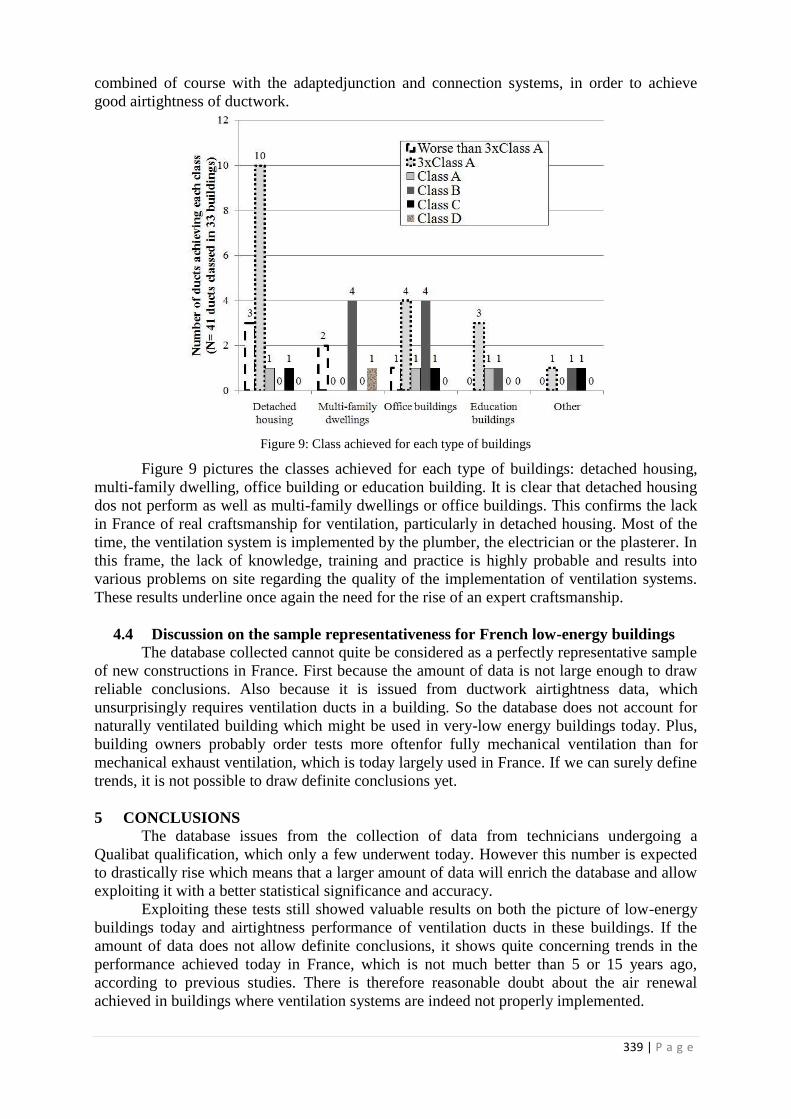
339 | P a g e

combined of course with the adaptedjunction and connection systems, in order to achieve

good airtightness of ductwork.

Figure 9: Class achieved for each type of buildings

Figure 9 pictures the classes achieved for each type of buildings: detached housing,

multi-family dwelling, office building or education building. It is clear that detached housing

dos not perform as well as multi-family dwellings or office buildings. This confirms the lack

in France of real craftsmanship for ventilation, particularly in detached housing. Most of the

time, the ventilation system is implemented by the plumber, the electrician or the plasterer. In

this frame, the lack of knowledge, training and practice is highly probable and results into

various problems on site regarding the quality of the implementation of ventilation systems.

These results underline once again the need for the rise of an expert craftsmanship.

4.4 Discussion on the sample representativeness for French low-energy buildings

The database collected cannot quite be considered as a perfectly representative sample

of new constructions in France. First because the amount of data is not large enough to draw

reliable conclusions. Also because it is issued from ductwork airtightness data, which

unsurprisingly requires ventilation ducts in a building. So the database does not account for

naturally ventilated building which might be used in very-low energy buildings today. Plus,

building owners probably order tests more oftenfor fully mechanical ventilation than for

mechanical exhaust ventilation, which is today largely used in France. If we can surely define

trends, it is not possible to draw definite conclusions yet.

5 CONCLUSIONS

The database issues from the collection of data from technicians undergoing a

Qualibat qualification, which only a few underwent today. However this number is expected

to drastically rise which means that a larger amount of data will enrich the database and allow

exploiting it with a better statistical significance and accuracy.

Exploiting these tests still showed valuable results on both the picture of low-energy

buildings today and airtightness performance of ventilation ducts in these buildings. If the

amount of data does not allow definite conclusions, it shows quite concerning trends in the

performance achieved today in France, which is not much better than 5 or 15 years ago,

according to previous studies. There is therefore reasonable doubt about the air renewal

achieved in buildings where ventilation systems are indeed not properly implemented.

340 | P a g e

This is a serious concern because in the meantime, the 2012 French Energy

Performance Regulation has set a high requirement on the airtightness of the envelope of

residential buildings. All of them undergo an airtightness test at commissioning and have to

perform better than 0,6 m3/h/m² at 4 Pa. At this level of airtightness, it is required to guarantee

a good air quality by a performing ventilation system and therefore avoid sick building

syndromes in newly-built buildings. There is today an urgent need in creating an expertise

area around ventilation craftsmanship and around control technicians to check the

performance at commissioning.

6 ACKNOWLEDGEMENTS

We would like to thank ALLIE’AIR for their kind contribution without which this paper

could not have been published.

7 REFERENCES

CSTB (2013), Méthode de calcul Th-BCE 2012, Annexe à l’arrêté du 30 avril 2013 portant

approbation de la méthode de calcul Th-BCE 2012

AIVC (1999)and SAVE-DUCT project partners, Improving ductwork – A time for tighter air

distribution systems – A status report on ductwork airtightness in various countries with

recommendations for future designs and regulations

Promotelec (2012), La construction de bâtiments basse consommation – Retour d’expérience

et analyse de Promotelec

Air-h (2009), Performance de la ventilation et du bâti, Rapport final

341 | P a g e

AIR LEAKAGES IN A RETROFITTED BUILDING

FROM 1930: MEASUREMENTS AND NUMERICAL

SIMULATIONS

Pär Johansson*

1, Angela Sasic Kalagasidis

1

1Chalmers University of Technology

Sven Hultins gata 8, 412 96 Gothenburg, Sweden


ABSTRACT

Many buildings in Sweden are in need of renovation in order to meet the current standards of energy use in

buildings. Particularly challenging are old listed buildings, the majority built before 1950, because the

renovation is restricted to the parts that do not change the appearance of the building. This paper presents

experiences gained during the renovation of a listed building where aging of materials, movements and

settlements during the building operation have left trails in form of air leakage paths that are difficult to cover by

renovation. The aim of the work is to bring up certain issues related to air movements in old houses that are not

necessarily present in new ones. In the renovation project in question, efforts were made to seal the exterior

walls with polyethylene foil before additional insulation in form of vacuum insulating panels was installed. The

blower door tests taken in the apartments showed that the air permeability of the building remained basically

unchanged after the retrofit. Complementary diagnostics with thermal imaging camera revealed that air leakage

paths in intermediate floors and interior walls substantially contributed to the overall air leakage of the building.

It was then concluded that the blower door tests alone were not sufficient for the estimation of the air

permeability of the building. In addition, hygrothermal measurements in exterior walls showed that new air

leakage paths were created between the old wall and the additional insulation. By using numerical simulations, it

has been proven that it is the outdoor air that flows through these new air paths, which is advantageous from the

moisture safety point of view. However, the flow of outdoor air through the exterior wall increases the overall

thermal transmittance of the wall and thus decreases the effects of additional insulation.

KEYWORDS

Retrofit, listed buildings, hidden air leakage paths, increased thermal transmittance, moisture safety

1. INTRODUCTION

There are approximately 2.1 million buildings in Sweden distributed on 1.9 million single

family houses, 165 000 multi-family buildings and 46 000 commercial buildings (Boverket,

2009). These buildings are from different time periods which mean they were built with

different building techniques and technical solutions. A majority (47%) of the buildings were

built before 1960, while 32% were built during 1961-1975. Buildings from the following 10

years comprise 12% of the building stock and thereafter 31% from 1986-1995 and 12% from

1995-2005 (Boverket, 2010).

342 | P a g e

Building codes were first implemented in 1946 in Sweden (IEA, 2013) and the first energy

use requirements were introduced in 1975 after the oil crisis in 1973-1974. The requirements

were specified with maximum U-values and demands on the airtightness for different building

parts. The codes have been developed during the following years, tightening the demands on

the energy use. The latest performance based energy codes are aiming at reducing the energy

use further by introducing the same demands on retrofitted buildings as for new developments

(Boverket, 2011). The requirements on airtightness have also varied over the years. Currently

there are no requirements on maximum air permeability of the buildings in Sweden, except

for specifications of passive houses (less than 0.3 l/(m2s)). Figure 1 shows the air permeability

in a selection of newly constructed buildings in Sweden. As can be seen, the majority of the

buildings have an air permeability of around 0.8 l/(m2s), which was the air permeability

requirement in the Swedish building code until 2008. However, there are buildings with much

larger air leakages (air permeability above 1.5 l/(m2s)).

Figure 1: Airtighness in 100 newly constructed Swedish buildings. The sample includes single and multi-family

buildings, (individual apartments are measured) and schools; both wooden and concrete structures (Wahlgren,

2010).

Low air permeability of a building envelope is essential to avoid unwanted consequences such

as high energy use and insufficient thermal comfort, caused by draft and cold surface

temperatures. Other consequences by a leaky building is that spreading of odour, particles and

radioactive gases, such as radon from the ground, can take place between apartments. Also the

acoustic insulation between apartments is affected by air leakages. Sandberg et al. (2007)

discussed the economic consequences by insufficient air tightness. They concluded that a

building with a good air tightness is, with a large probability, profitable for the builder and

leads to increased well-being, less spreading of odours and better acoustic insulation.

There is much knowledge and techniques on how to achieve good airtightness in buildings,

but one gets the impression that the focus is mainly on new buildings. As presented above, a

majority of the building stock in Sweden is older buildings. This is also the case for the rest of

Europe. One of the keys to successful retrofit is to achieve control over the air movements in

these buildings. Natural or climate induced aging of materials and movements and settlements

during the building operation have left trails on these buildings. These are typically visible as

angle and surface distortions, cracks, and displacements. A large number of air flow paths

through the building can be created by these geometrical changes. Since many of them are

343 | P a g e

hidden inside the building envelope, they need to be treated in renovation projects to prevent

undesired heat losses, comfort disturbances, or moisture damages.

The aim of this paper is to bring up certain issues related to air movements in old houses that

are not necessarily present in new ones. Therefore, we present here the findings from a field

study on airtightness and air movements in an old house, before and after the retrofitting.

Unexpected air paths in the building envelope are revealed by hygrothermal measurements.

These are further analysed and explained by numerical simulations.

2. CASE STUDY BUILDING

The building chosen for the study is a landshövdingehus “County governor’s house” built in

1930 in Gothenburg, Sweden, see Figure 2. Most of these buildings were constructed during

1876-1936 when fire regulations limited the height of wood buildings to two floors. Today

there are over 1 400 similar buildings in the Gothenburg region. The exterior aesthetics of the

building are protected by Swedish legislation as a cultural environment of national interest.

The building contain rented apartments and there are many complaints on draught and

insufficient thermal comfort from the occupants. Therefore the building is in great need of

retrofitting measures (Johansson et al., 2014).

Figure 2: Left: The studied Landshövdingehus “County governor’s house” with approximate location of the

hygrothermal sensors in the walls. Right: construction of the original wood wall. 1) Wooden cover boarding, 2)

Tar paper, 3) Structural wood or brick, 4) Intermediate wooden floor

In the time when the building was constructed, thermal insulation was normally not used in

the walls. This building was no exception with brick walls of 1.5 stone thickness,

approximately 340 mm, in the ground floor. In the two upper floors, the walls were made of

80 mm wooden planks in three layers. Flax fibres were used between the boards to decrease

the air permeability of the wall. On the exterior, a 22 mm thick vertical wooden cover board

with rib flanges was installed on top of a wind and waterproof tar paper as shown in Figure 2.

Retrofitted wall

Brick

Wood

23

1

4

344 | P a g e

The interior side of the walls was originally covered with a thin finish of plaster on reed

(Larsson & Lönnroth, 1972), which was later replaced by modern plaster boards.

Due to the very limited space for additional insulation in the wall, the retrofitting, presented in

Figure 3, was done with 20 mm thick vacuum insulation panels (VIPs) placed on the exterior

side of the wall and protected by 30 mm of glass wool. Between the old wall and the VIPs, a

polyethylene foil was applied as an air barrier to prevent indoor air entering the wall. An air

space, 28 mm thick, was added to the façade which makes the total additional thickness of the

wall to be 80 mm (Johansson, 2014).

Figure 3: Wall layout after retrofitting with 20 mm VIPs and 30 mm glass wool boards.

The energy use for heating and domestic hot water before retrofitting was estimated to

160 kWh/m2 (exact figures are not possible to obtain because the energy use in this building is

measured together with many other buildings in the area). It is estimated that the additional

insulation of the wall has reduced the energy use by 20% (with all VIPs functioning and all

thermal bridges included). As a comparison, changing the windows to windows with a U-

value of 1 W/m2K gave an energy use reduction of 15%. The combination of changing

windows and installing VIPs gave an energy use reduction of 34% (Johansson, 2014).

To evaluate the hygrothermal performance of the wall after the retrofitting, four temperature

and relative humidity (RH) sensors were installed in the brick and wood wall, respectively.

The sensors were located on the exterior of the existing wall, before the polyethylene foil. To

study the influence of the indoor climate in the building, one sensor was located in one of the

kitchens closest to the monitored part of the wall in the brick and wood wall, respectively.

The outdoor temperature and RH at the building site was monitored by a sensor located in a

perforated plastic box placed underneath the roof eave facing southwest (Johansson, et al.,

2014).

3. RESULTS FROM AIR PERMEABILITY MEASUREMENTS

There were complaints from the occupants on an insufficient thermal comfort in the building

due to draft and low surface temperatures. Thus, the building was investigated before and

28x70 mm wooden lath

20x50 mm glass wool boards

22 mm wooden cover board

28 mm air space

30 mm glass wool boards

20 mm VIP

0.2 mm polyethylene foil

Structural wood/brick

20 mm glass

wool boards

20 mm VIP

20 mm glass

wool boards

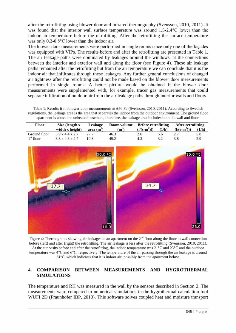
345 | P a g e

after the retrofitting using blower door and infrared thermography (Svensson, 2010, 2011). It

was found that the interior wall surface temperature was around 1.5-2.4°C lower than the

indoor air temperature before the retrofitting. After the retrofitting the surface temperature

was only 0.3-0.8°C lower than the indoor air.

The blower door measurements were performed in single rooms since only one of the façades

was equipped with VIPs. The results before and after the retrofitting are presented in Table 1.

The air leakage paths were dominated by leakages around the windows, at the connections

between the interior and exterior wall and along the floor (see Figure 4). These air leakage

paths remained after the retrofitting but from the air temperature we can conclude that it is the

indoor air that infiltrates through these leakages. Any further general conclusions of changed

air tightness after the retrofitting could not be made based on the blower door measurements

performed in single rooms. A better picture would be obtained if the blower door

measurements were supplemented with, for example, tracer gas measurements that could

separate infiltration of outdoor air from the air leakage paths through interior walls and floors.

Table 1: Results from blower door measurements at ±50 Pa (Svensson, 2010, 2011). According to Swedish

regulations, the leakage area is the area that separates the indoor from the outdoor environment. The ground floor

apartment is above the unheated basement, therefore, the leakage area includes both the wall and floor.

Floor Size (length x Leakage Room volume Before retrofitting After retrofitting

width x height) area (m2) (m

3) (l/(s·m

2))) (1/h) (l/(s·m

2))) (1/h)

Ground floor 3.9 x 4.4 x 2.7 27.7 46.3 2.6 5.6 2.7 5.8

1st floor 3.8 x 4.8 x 2.7 10.3 49.2 4.3 3.2 3.8 2.9

Figure 4: Thermograms showing air leakages in an apartment on the 2nd

floor along the floor to wall connection

before (left) and after (right) the retrofitting. The air leakage is less after the retrofitting (Svensson, 2010, 2011).

At the site visits before and after the retrofitting, the indoor temperature was 21°C and 23°C and the outdoor

temperature was 4°C and 6°C, respectively. The temperature of the air passing through the air leakage is around

24°C, which indicates that it is indoor air, possibly from the apartment below.

4. COMPARISON BETWEEN MEASUREMENTS AND HYGROTHERMAL

SIMULATIONS

The temperature and RH was measured in the wall by the sensors described in Section 2. The

measurements were compared to numerical simulations in the hygrothermal calculation tool

WUFI 2D (Fraunhofer IBP, 2010). This software solves coupled heat and moisture transport

346 | P a g e

equations by finite volumes where the temperature and RH are the driving potential for the

heat and moisture transport through the construction. The numerical simulations were

performed using the measured indoor and outdoor climate together with material data for the

materials in the construction, see Table 2. Air flow in the wall is simulated by adding a

coupling for the heat and moisture transfer between the wall and the indoor or outdoor air,

respectively. The resulting temperature and RH in the wall without air leakages is presented

in Figure 5.

Table 2: Material data used in the numerical simulations based on data from WUFI 2D material database

(Fraunhofer IBP, 2010).

Material d (mm) λ (mW/(m∙K)) ρ (kg/m3) cp (J/(kg∙K)) µ (-)

Gypsum board 20 200 625 850 8.33

Spruce, tangential 80 200 430 1600 83.3

Spruce, radial 80 200 455 1500 130

PE membrane 0.2 1 650 130 2200 8.7·104

Glass wool - 33 60 850 1.3

Glass wool board 20/30 33 115 850 3.4

Air layer 30 25 1.3 1000 0.46

Evacuated VIP core 18 5 200 850 1.3

Air filled VIP core 18 20 200 850 1.3

VIP laminate, tangential 1 540 189 134 Inf.

VIP laminate, radial 1 200 000 189 134 Inf.

Figure 5: Comparison of the hygrothermal simulations with the measurements of the temperature and relative

humidity behind the VIP in the wood wall. The simulation was based on the measured indoor and outdoor

climate from January, 2011, to June, 2014. The location of the sensor is marked by the black box with a black

arrow pointing from the left.

The average simulated temperature and RH at the sensor position in the wall was 21.9°C and

37.4% while the measurements gave 21.5°C and 37.8% on average during January, 2011, to

June, 2014. It was noted that the vapor content was on average 1.3 g/m3 higher in the

numerical simulations than in the measurements. This suggested that there was an additional

drying process in the wall. The sensor is located in an air filled void in the wall, measuring the

temperature and RH of the air closest to the sensor. The high fluctuation in the measured RH

indicated a leaky construction with air leakage from the interior or exterior side of the vapor

barrier into the construction. It is anticipated that the air could enter e.g. through details

around windows and flow along the interior of the vapor barrier to the sensor position.

0

10

20

30

40

50

60

Temp measured

RH simulated

Temp simulated

Te

mp

era

ture

( C

) a

nd

RH

(%

)

RH measured

347 | P a g e

Although measures were taken to make the exterior wall air tight with the polyethylene foil,

due to uneven surfaces certain connections have remained loose. Therefore, an air exchange

with the outdoor air was added to the model between the vapor barrier and wood. The

resulting temperature and RH is presented in Figure 6.


humidity behind the VIP in the wood wall. The air changes per hour with the outdoor air were varied from 1 1/h

to 40 1/h. The location of the sensor is marked by the black box with a black arrow pointing from the left. The

material surfaces in the wall are rather uneven which makes air flow through the small voids between them

possible.

When an outdoor air exchange rate of 40 1/h was used, the simulated average temperature

was 21.2°C. This is close to the measured average temperature 21.5°C. The simulated average

RH was 37.6% which is also close to the measured average RH 37.8%. In addition, the

simulated variations during the year corresponded well with the measurements. However, one

cannot be entirely sure that the air is really coming from the exterior without testing this.

Figure 7 presents the temperature and RH in the wall given that the air is coming from the

interior.


humidity behind the VIP in the wood wall. The air changes per hour with the indoor air were varied from 1 1/h

to 40 1/h. The location of the sensor is marked by the black box with a black arrow pointing from the left. The

material surfaces in the wall are rather uneven which makes air flow through the small voids between them

possible.

0

10

20

30

40

50

60

Temp measured

RH measured RH air changes

1, 20, 40 1/h

Temp air changes

1, 20, 40 1/h

Tem

pera

ture

( C

) an

d R

H (

%)

0

10

20

30

40

50

60

Temp measured

RH measured RH air changes

1, 20, 40 1/h

Temp air changes

1, 20, 40 1/h

Tem

pera

ture

( C

) an

d R

H (

%)

348 | P a g e

The simulated temperature and RH deviated more when the air was coming from the interior

than in the previous case. The simulation gave an average temperature 22.1°C and 43.4% RH

for the case with 40 1/h, compared to the measurements that were 21.5°C and 37.8% on

average. This shows that the air leaking into the wall is most certainly coming from the

exterior.

5. CONCLUSIONS

This work presents the findings from a field study on airtightness and air movements in an old

listed building. The building was retrofitted on the exterior with vacuum insulating panels.

Although efforts were made to seal the wall with polyethylene foil on the interior of the

additional insulation, blower door tests showed that the air permeability of the building

remained basically the same before and after the retrofitting. Complementary diagnostics with

thermal imaging camera revealed that air leakage paths at the intermediate floors and interior

walls substantially contributed to the overall air leakage of the building. This implies that the

blower door tests alone is not sufficient for estimation of the air permeability of buildings

with large internal air leakage paths, and when the blower test cannot cover the whole

building at once.

The hygrothermal measurements in the exterior wall revealed that new air leakage paths were

created between the existing wall and the additional insulation. By using numerical

simulations, it has been proven that it is the outdoor air that flows through these new air paths.

This is advantageous from the moisture safety point of view. However, the flow of outdoor air

through the exterior wall increases the overall thermal transmittance of the wall and thus

decreases the effects of the additional insulation.

Based on these findings, we conclude that one of the keys to successful retrofit of old

buildings is to achieve control over the air movements in these buildings. Knowledge of how

potential air flow paths could affect the wall is crucial for making predictions of the long-term

performance of a construction based on hygrothermal simulations.

6. ACKNOWLEDGEMENTS

The work is supported by the Swedish Research Council for Environment, Agricultural

Sciences and Spatial Planning (FORMAS) and the public housing corporation

Familjebostäder i Göteborg AB.

7. REFERENCES

Boverket. (2009). Så mår våra hus - redovisning av regeringsuppdrag beträffande

byggnaders tekniska utformning m.m. (The state of our buildings - report of governmental

mission on the technical design of buildings etc.). [In Swedish]. Karlskrona, Sweden:

Boverket.

Boverket. (2010). Energi i bebyggelsen - tekniska egenskaper och beräkningar - resultat från

projektet BETSI (Energy in the built environment - technical properties and calculations -

results from the BETSI study). [In Swedish]. Karlskrona, Sweden: Boverket.

Boverket. (2011). Regelsamling för byggande, BBR 2012 (Regulations for construction, BBR

2012). [In Swedish]. Karlskrona, Sweden: Boverket.

Fraunhofer IBP. (2010). WUFI 2D Transient Heat and Moisture Transport (Version 3.3.2)

[Computer Program]. Holzkirchen, Germany: Fraunhofer IBP.

349 | P a g e

IEA. (2013). Policy Pathway: Modernising Building Energy Codes. Paris, France:

OECD/IEA and New York, NY, USA: United Nations Development Programme (UNDP).

Johansson, P. (2014). Building Retrofit using Vacuum Insulation Panels: Hygrothermal

Performance and Durability. PhD Dissertation. Gothenburg, Sweden: Chalmers University of

Technology, Department of Civil and Environmental Engineering.

Johansson, P., Sasic Kalagasidis, A., Hagentoft, C.-E. (2014). Retrofitting of a listed brick

and wood building using vacuum insulation panels on the exterior of the facade:

Measurements and simulations. Energy and Buildings, 73(April 2014), 92-104.

Larsson, U., Lönnroth, G. (1972). Landshövdingehus och trähus i Göteborg (County

governor's houses and wooden houses in Gothenburg). [In Swedish]. Den nordiske

træstad(28).

Sandberg, P. I., Sikander, E., Wahlgren, P., Larsson, B. (2007). Lufttäthetsfrågorna i

byggprocessen - Etapp B. Tekniska konsekvenser och lönsamhetskalkyler. SP Rapport

2007:23. (Air tightness in the buliding process - Stage B. Technical consequences and cost

benefit calculations). Borås, Sweden: SP Technical Research Institute of Sweden.

Svensson, O. (2010). Termografering och lufttäthetsmätning, Wärnsköldsgatan 9B-9C,

Göteborg. (Thermography and air permeability measurement, Wärnsköldsgatan 9B-9C,

Gothenburg). Unpublished report. Borås, Sweden: SP Technical Research Institute of

Sweden.

Svensson, O. (2011). Uppföljande Termografering och lufttäthetsmätning, Wärnsköldsgatan

9B-9C, Göteborg. (Follow up thermography and air permeability measurement,

Wärnsköldsgatan 9B-9C, Gothenburg). Unpublished report. Borås, Sweden: SP Technical

Research Institute of Sweden.

Wahlgren, P. (2010). Goda exempel på lufttäta konstruktionslösningar. SP Rapport 2010:09.

(Good examples of airtight details). Borås, Sweden: SP Technical Research Institute of

Sweden.

350 | P a g e

INDOOR ENVIRONMENTAL QUALITY-GLOBAL

ALLIANCE: THE VALUE CHAIN OF IEQ

Bjarne W. Olesen

ABSTRACT

Recently a global alliance on Indoor Environmental Quality (IEQ) has been formed.

This alliance consists of several international societies dealing with the indoor

environment. The intend is that the alliance should cover all partners involved in the

value chain of IEQ from research, design, manufacturing, construction (building

properties), installation (building service systems), operation, inspection to the

behaviour of the occupants. The presentation will present the intend and scope of this

alliance and discuss the value chain of indoor environmental quality.

351 | P a g e

DO EXISTING INTERNATIONAL STANDARDS

SUPPORT VENTILATIVE COOLING?

Bjarne W. Olesen

ABSTRACT

The use of ventilative cooling must meet general criteria for indoor environmental

quality like thermal comfort, indoor air quality and noise. These criteria are often

expressed in standards, building codes and guidelines. This presentation will discuss

existing standards like EN15251, EN13779, ASHRAE-55, ASHRAE-62.1, ASHRAE

62.2 and others with regard to the use of ventilative cooling. The limitation for the use

of ventilative cooling can be the specified acceptable comfort range for room

temperatures, draft sensation, noise, safety and others. For acceptable room

temperatures the standards includes different concepts for buildings with and without

mechanical cooling (adapted approach). The presentation will discuss the difference in

these concepts and the relation to ventilative cooling.

352 | P a g e

THE INFLUENCE OF TRAFFIC EMISSION ON IAQ,

ESPECIALLY IN STREET CANYONS

Zbigniew Bagieński Institute of Environmental Engineering, Poznan University of Technology,

ul. Piotrowo 3a, 60-965 Poznan, Poland,

e-mail: [email protected]

ABSTRACT

Traffic emissions have a significant impact on urban air quality, which particularly concerns street canyons, i.e.

spaces with limited air exchange. Traffic emissions in street canyons create high concentrations of air pollutants.

Based on measurements carried out for selected routes and model experiments conducted in a wind tunnel, it is

shown that a roadway’s urban structure has a significant impact on concentrations of pollutants from traffic

emission which enter buildings by means of mechanical and natural ventilation systems. In the case of buildings

in a narrow street canyon pollution concentrations close to ventilation air intakes may be several times higher

than in buildings in wide roadways. The paper also describes a possibility of identifying building surfaces that

are particularly exposed to being infiltrated by traffic pollutants from adjacent streets.

KEYWORDS

Vehicle emission, street canyon, urban air quality

1 INTRODUCTION

Among factors that determine indoor air quality (IAQ) chemical composition of air and

concentration of fine particles PM2,5 have a special significance as quantities which are

difficult to control, which is the case for temperature and humidity. If it is assumed that the

subject of analysis does not concern industrial sites indoor air pollution concentration values

are influenced by:

Internal factors, such as furnace emissions (e.g. gas cookers) and other technological

processes, emissions from dividing structures and fittings, human emissions, flows from

other closed spaces,

External conditions such as local air pollution concentration values and their changeability

in time and space, meteorological conditions including wind direction and velocity,

Ventilation systems,

Urban structures of buildings and their surroundings.

Indoor air pollution levels are of particular concern because most people (especially in

towns and cities) spend 80 to 90% of their time indoors. According to the Environmental

Protection Agency (EPA, 2011) indoor pollution levels may be 2-5 times, and occasionally,

much higher than outdoors levels. A rise in concentration of certain air pollutants is caused by

increased use of more synthetic materials for building and furnishings, use of more

chemically formulated personal products in the more air tight buildings with reduced

ventilation rates to save energy. Pollutants generated indoors are accompanied by those

coming from the outdoor environment, including sulphur dioxide, nitrous oxides, fine and

ultra fine PM, volatile organic compounds VOCs, and tropospheric ozone. Ventilation

systems used do not alter the chemical composition of inlet (external) air. For ventilation of

houses by opening the windows Schembari et al. (2013) found a high statistically significant

correlation between personal exposure to NOx, NO2 and PM2,5 and indoor and outdoor levels

353 | P a g e

of these pollutants in Barcelona. Jensen et al. (2009) presents the results of NO2, NOx and

PM2.5 concentration measurements in various New York City’s boroughs and demonstrates

slight differences in concentration values of outdoor and indoor air with considerable

differences among particular boroughs. Vincent et al. (1997) compares indoor air quality in

office buildings with different ventilation systems and pays attention to approximate values of

average concentrations of CO2, CO and particles for systems with natural ventilation, fan coil

units and HVAC, and the approximate value of the indoor CO2/outdoor CO2 ratio equalling

1.9-2.1 for particular systems.

Urban air quality is diversified and depends not only on the kind and value of pollution

emissions, but also on the technical conditions of emissions and the urban structure of a given

area. Buildings are responsible for the disturbances in the air flow. The horseshoe vortices can

be generated over the upper and side edges of a building as well as the lower part of the

windward side. At the lee side the wake region and the cavity recirculation region are

generated with a reduced air change. According to Peterka (Peterka et al., 1985), the cavity

region can approach z=(2-2.5)HB in the range x=6HB, while the boundaries of the wake region

can approach z=3HB in the range x=16HB, where HB is the height of a building. Point-source

and line-source pollutions (short chimneys and vehicle routes, respectively) emitted in this

space cannot disperse freely, which may lead to high pollution concentrations (Bagieński,

2008, Ahmad et al., 2005, Meroney et al., 1966). Figure 1 shows a visualisation of a fume

flow in a wake effect carried out in a wind tunnel (Bagieński, 2010).

Fig. 1 Disturbed fume flow, short chimney on the

windward side of a building

Fig.2 Streamline field in the street canyon for FC>0.8

(Kwak, 2012)

Traffic emissions are the major outdoor source of directly emitted pollutants in urban

regions. Many authors (e.g. Sini et al.,1996, Baldauf et al.,2013, Carpentieri et al., 2012) pay

attention to elevated air pollutant exposures and adverse human health effects for population

living close to streets with heavy transport traffic. It is especially crucial in densely-built and

high-traffic areas in street canyons. Street canyons are not infinitely long or isolated entities in

cities, but they are often segmented and connected to other canyons at urban intersections.

High pollution levels are often associated with street canyons.

The street canyon factor Fc is the ratio of the average height of buildings delimiting the

canyon at the length L>2.5HB to the total width W of the street.

FC=HBav/W (1)

Depending on the value of the ratio Fc, three types of airflow perpendicular to the canyon

symmetry axis can be classified (Ahmad et al., 2005; Oke, 1988):

skimming flow for FC>0.8, which is characterized by a significant reduction of air

exchange inside the canyon, Fig. 2 (Kwak et al., 2012)

wake interference flow for FC=0.20-0.8, where the stream is circulated inside the canyon

and part of pollution is transported to adjacent canyons (mainly within the wake region)

354 | P a g e

isolated roughness flow for FC<0.20, when the influence of reciprocal interaction of the

canyon walls on the interference can be ignored.

The value of FC has a decisive influence on diffusion conditions of pollution from traffic

sources, but also from adjacent low stationary sources (Bagieński, 2006; Chang Cheng-Hsin,

Meroney, 2003). When the street canyon factor Fc>0.8, high concentration of traffic

pollutants can also occur on level of the upper storeys of a building delimiting the canyon

(Park et al., 2004, Kwak et al., 2012).

The aim of the paper is to determine the influence of traffic emissions on indoor air

quality especially in urban areas of compact settlement and intensive vehicle traffic in street

canyons. The assessment is based on two streets with different urban structures in Poznań,

a Polish city with over 500 000 inhabitants. For these roadways, concentrations of basic

traffic pollution were specified, measurements were taken to determine concentrations of

selected substances close to the streets and to ventilation air supplied to adjacent buildings

and areas with increased pollution concentrations were identified. Fig. 3 and Fig. 4 show

pictures of the analysed streets.

Fig. 3 Street G – street canyon

Fig. 4 Street P – four-line street

2 VEHICLE EMISSIONS

Total emission from road transport is the sum of exhaust emissions, evaporative emissions

and road vehicle tire and brake wear emissions. Exhaust emissions include hot and cold-start

emissions.

ETotal = EHot+ ECold + EEv (2)

Hot emissions depend on the kind and amount of fuel burned and the kind and age of an

engine, i.e. motion velocity and a vehicle’s technical data such as the category of a vehicle

(passenger cars, light- and heavy-duty vehicles, buses), engine capacity, the kind of fuel, time

of certification (permissible emission according to EURO standards). Cold-start emissions

concern emissions of monoxide and hydrocarbons during the initial stage of the (cold) motion

of a vehicle and depend on air temperature. In calculations they are treated as additional

emissions considered solely for urban traffic. Evaporation emissions stem from fuel

evaporating from a hot engine, carburettor and fuel tank. They are considered for fuel engine

cars and depend on air temperature, humidity and fuel tank pressure related to these values.

Vehicle emissions include pollutants such as CO, NO, NO2, PM2.5, PM10, CO2, VOCs

including mono- and polycyclic aromatic hydrocarbons (MAH, PAH) and benzene C6H6, and

to CH4, N2O, metals like Cd, Cr, Cu, Ni. Values of emission indexes for particular categories

355 | P a g e

of vehicles in road transport are specified in the EMEP/EEA air pollutant emission inventory

guidebook (European Environment Agency, 2009).

In recent years particular attention has been paid to PM emission. Fine particles PM2.5

(diameter ≤2.5μm) and ultra fine particles (diameter ≤0.1μm ) emissions in urban regions are

mainly emitted by diesel vehicles (Kim, Y. et al., 2011). Directly emitted elemental carbon

soot (black carbon) from diesel vehicles, re-suspended dust from roads, and secondary acidic

particles are major contributors of PM in urban roadside areas. The problem is particularly

serious in cities with a large proportion of diesel-powered vehicles, e.g. Barcelona – about

50% (Schembari et al., 2013). According to the Air quality in Europe –report (2013), between

2009 and 2011, up to 96% of city dwellers were exposed to fine particulate matter (PM2.5)

concentrations above WHO guidelines.

Emission values may be referred to the linear dimension Eti (mg km-1

s-1

) or the surface

as traffic emission strength of a particular area with the i-th substance Etia (mg m-2

s-1

). Traffic

emission strength values were determined for selected pollutants based on real conditions of

two streets in Poznan.

Street structure and car traffic variations:

Street G – a one-way traffic (two-line) street with the traffic volume of 1600 vehicles per

hour (v/h), passenger traffic with a 10% share of light-duty trucks, value of factor:

Fc >0.8 – street canyon

Street P – a four-line street with the traffic volume of 3800 v/h, passenger traffic with

a 15% share of light-duty trucks, value of factor: Fc <0.2

Vehicle traffic volume was averaged for the time interval from 7 a.m. to 7 p.m.

Time intervals for which calculations were made:

Summer period: averaging Poznan climatic conditions for June, July, August;

t=18.0°C, φ=45%.

Winter period: averaging climatic conditions for December, January, February; t=0.5°C,

φ=90%

Tables 1 and 2 show emission values of particular pollutants for summer and winter periods

for the analyzed streets. Table 1 Values of substance emission and heat emission for summer.

street vehicles CO NMVOC NOx PM2.5 benzene CO2 QdL

v/h mg km-1

s-1

g km-1

s-1

kW km-1

G 1600 2876.1 382.8 296.7 16.7 18.0 108.0 1594

P 3800 4921.2 643.4 760.6 35.2 30.8 209.2 3090

Table 2 Values of substance emission and heat emission for winter.

street vehicles CO NMVOC NOx PM2.5 benzene CO2 QdL

v/h mg km-1

s-1

g km-1

s-1

kW km-1

G 1600 5212.2 560.2 320.0 25.7 29.1 119.4 1762

P 3800 8965.8 1158.6 782.6 53.0 52.0 231.4 3416

A higher value of the average traffic speed and a lower share of cold emission in street P in

relation to street G contribute to lower values of CO, NMVOC and C6H6 emissions with

higher values of NOx emissions. However, in winter emission of incomplete combustion

products (CO, NMVOC, benzene) is much higher compared to summer, which results from

an increase in fuel consumption, but first of all from an increase in cold emission indexes at

a low air temperature.

The quantity QdL determines heat flux emitted by vehicles as one of the components that

generate the urban heat island (UHI). The values are relatively high. In summer as solar

radiation flux density in the UV-VIS range is higher, additional significant anthropogenic heat

emission has a considerable impact on chemical reactions that create secondary air pollution.

356 | P a g e

For example, Taha (Taha, 1996) states that an increase in the Los Angeles local air

temperature from 22oC to 32

oC caused a rise in ozone concentration from 0.120 ppm to

0.240 ppm. Such a situation takes place especially in narrow street canyons, or areas with

limited ventilation conditions, a low SVF (sky view factor) value and high radiation

absorption values.

3 INFLUENCE OF A STREET’S STRUCTURE ON VENTILATION AIR

QUALITY

3.1 Influence of a street’s structure on pollution concentrations close to the street

A street’s urban structure, often to a greater degree than traffic volumes, contributes to the

level of its nuisance defined as concentrations of polluted air – both external (close to the

ground) and internal air of the adjacent buildings. An experimental indicator of how a street’s

structure contributes to its nuisance is the ratio of pollution concentrations measured directly

close to the street to the calculated value of the emission of the pollution C/E .

CO concentrations were measured for two streets: street G and street P in the

meteorological conditions of summer and winter. The values were measured using the non-

dispersive infrared method with a detection limit of 50 ppb. CO analyzers were located

approximately 2 m from the street edge at the level of about 2 m, i.e. where the emission

source directly affects people. Measurements were taken on working days between 10 a.m.

and 12 noon (moderate traffic volume) and 4 p.m. and 6 p.m. (large traffic volume). Wind

velocity did not exceed 1 m/s. Measured CO concentration values CCO were referred to CO

emissions ECO calculated according to COPERT IV procedure. Tables 3 and 4 present the

meteorological conditions of the measurements, traffic volume N, share of light- and heavy-

duty trucks (LDT, HDT), the results of measuring the concentrations of CCOb and

computational analysis of the results comprising the concentration value of CO after

deducting the background of CCO, the calculated emission value of CO, the value of the ratio

CCO/ECO for particular measurements.

Table 3 CO concentration measurements and analysis of the results – street G

Temp. Humid. Time N LDT CCOb CCO ECO CCO /ECO

C % hours v/h % μg m-3

μg m-3

μg m-1

s-1

s m-2

21.5 42 10-12 1310 8 1400 1250 2355 0.53

26.5 34 4-6 p.m 1870 10 2100 1950 3361 0.58

20.0 42 10-12 1230 7 1100 950 2005 0.47

23.5 38 4-6 p.m 1690 12 2300 2150 3190 0.67

1.2 85 10-12 1405 10 2550 2300 4577 0.50

-0.5 90 4-6 p.m 1780 9 3500 3250 5799 0.56

2.5 78 10-12 1520 6 2270 2020 4120 0.49

0.5 85 4-6 p.m 1730 8 3450 3200 5520 0.58

average 0.55

357 | P a g e

Table 4. CO concentration measurements and analysis of the results – street P

Temp. Humid. Time N L/H-DT CCOb CCO ECO CCO /ECO

C % hours v/h % μg m-3

μg m-3

μg m-1

s-1

s m-2

20.5 40 10-12 2850 18 600 500 4132 0.12

22.0 41 4-6 p.m 3920 15 740 640 4938 0.13

21.5 38 10-12 2950 13 450 350 3835 0.09

23.5 35 4-6 p.m 4020 14 600 740 4928 0.15

2.4 85 10-12 3050 15 800 700 6405 0.11

-0.5 90 4-6 p.m 3840 12 1400 1250 7680 0.16

1.5 88 10-12 2710 14 880 730 6070 0.12

-2.0 92 4-6 p.m 3350 20 1200 1050 8207 0.13

average 0.13

The canyon structure of street G causes emitted traffic pollution to accumulate within the

canyon (Fig. 2), which is indicated by the high value of (CCO/ECO)av=0.55 being over four

times higher than that for street P. Such a structure of the street contributes to the fact that

meteorological factors such as wind velocity and direction, temperature and solar radiation

have a greater influence on average concentrations of particular pollutants and on vertical

profiles of concentrations (Kwak et al., 2012; Park et al., 2004; Ahmad et al., 2005; Liu et al.

2003; Gartmann et al., 2012).

3.2 Influence of a street structure on pollution concentration values of ventilation air

supplied to buildings

Two buildings were examined – one in street canyon G (Fig. 3) and the other in street

P (Fig. 4). The one in street G has natural ventilation by opening windows and fan coil units.

A measurement sensor was positioned outside a window at the level of 4.5 m above the street

on its western side. The building in street P has a HVAC system. The air intakes were located

on the roof of the building at the height of 17 m above the street and at the horizontal distance

of 22 m from the edge of the street on its western side. A measurement sensor was placed in

an air intake duct. Based on Gartman’s research programme concerning the contribution of

traffic emissions to air quality (Gartman et al., 2012), CO2 concentrations were accepted as

a traffic pollution indicator. Measurements were taken continuously for a fortnight from in

June, 2014. On Sunday and Monday the wind blew with the speed of 2.0-3.5 m/s from the

west, i.e. perpendicular to the axes of both streets. On the other days wind velocity did not

exceed 1.2 m/s, which means that it did not have a substantial impact on traffic emission

dispersion, especially within the street canyon.

Fig. 5 CO2 concentration values at the positions in streets G and P on Tuesday and Wednesday in June,

wind velocity u<1.2 m/s

0

200

400

600

800

1000

1200

1400

1600

1800

2000

10:0

0

12:0

0

14:0

0

16:0

0

18:0

0

20:0

0

22:0

0

0:00

2:00

4:00

6:00

8:00

10:0

0

12:0

0

14:0

0

16:0

0

18:0

0

20:0

0

22:0

0

0:00

street G

CC

O2

[p

pm]

Time

street P

Tuesday Wednesday

358 | P a g e

Fig. 6 CO2 concentration values at the positions in streets G and P on Sunday and Monday in June,

wind velocity u=2-3 m/s

Fig. 5 and Fig. 6 show CO2 concentration values for selected days with low and higher wind

velocities measured at positions close to streets G and P. Because of its placement

concentrations at the position close to street P may be considered as those approaching the

background concentration Cbac for Poznań. Concentrations in street G were 3-5 times higher

(up to 2600 ppm), especially on days with increased wind velocity. With the wind blowing

from the west the whole canyon was in the cavity recirculation region. The increased velocity

of the wind blowing from the west contributed to a rise in CO2 concentrations in the air intake

on the roof of the building in street P, which is located in the wake region. Concentration

values varied within 24 hours and for weekdays and weekends with the variations being

higher for the street canyon.

In order to identify building surfaces that are particularly exposed to being infiltrated by

traffic pollutants from roadways a series of model experiments were conducted in a wind

tunnel. The wind tunnel used for testing the diffusion of gaseous pollutants emitted from the

short-point and line sources was constructed at the Institute of Environmental Engineering,

Poznan University of Technology, Poland. A sketch of the experiment set-up is shown in

Fig. 7. Each time particular elements of the set-up and the measurement system are adapted to

an accepted program of the investigation. The explanation of such set-ups can be found in

papers by Bagienski (2008).

Fig.7 A sketch of wind tunnel and experimental set-up (Bagienski, 2008)

A set of nozzles with horizontal vents for fume from the collector was used as a line

source simulating traffic emissions. Figures 8 and 9 show a visualization of dispersion of

fume emitted from line sources in the street canyon. Air flow with the velocity uH=2 m/s was

perpendicular to the axis of the street. The highest pollution concentrations were recorded at

the leeward side of the building limiting the canyon from the windward side. Fumes were also

0

500

1000

1500

2000

2500

3000

0:00

2:00

4:00

6:00

8:00

10:0

0

12:0

0

14:0

0

16:0

0

18:0

0

20:0

0

22:0

0

0:00

2:00

4:00

6:00

8:00

10:0

0

12:0

0

14:0

0

16:0

0

18:0

0

20:0

0

22:0

0

0:00

street G

CC

O2

[p

pm]

Time

street P

Sunday Monday

359 | P a g e

identified close to the roof of the building, which means that pollution may enter an air intake

even when they are on roofs. In the case of the canyon with the index FC>0.8 high pollution

concentrations may fill the whole of the canyon, which suggests that a considerable share of

traffic emissions may enter buildings by means of natural or mechanical ventilation systems.

Fig. 8 Line source of emission in the street canyon

when FC=1.0

Fig. 9 Line source of emission in the street canyon

when FC=0.3

4 CONCLUSIONS

Traffic emission has a considerable impact on urban air quality. It may cause high

concentrations of air pollution to appear especially in street canyons – much higher than in

wide and open roadways. Building solids cause disturbances in wind flow by generating the

cavity recirculation region and the wake region on the leeward side that limit the possibility of

air pollution emitted in the areas being dispersed freely. This leads to higher concentrations of

traffic emissions at different heights of the canyon, also on roofs. The pollutants may enter

buildings by means of natural and mechanical ventilation systems. In a narrow street canyon

pollution concentrations in an air ventilation intake of a building may be 3-5 times higher than

in that located on the roof of a building in wide roadways. However, it needs to be taken into

consideration that also in these cases traffic emissions contribute considerably to ventilation

air quality. Before the location and the kind of ventilation air intake is designed for buildings,

traffic pollution dispersion from adjacent roadways need to be analysed. This is particularly

the case for buildings in street canyons.

5 REFERENCES

Ahmad K., Khare M., Chaudhry K.(2005). Wind tunnel simulation studies on dispersion at

urban street canyons and intersections a review. J. of Wind Eng. and Ind. Aerodyn.,

93, 697-717

Bagieński Z. (2010). The influence of structure of energy consumption on air quality in urban

area in temperate climate. Dissertation 440, Poznan University of Technology, Poland

(in Polish with English abstract)

Bagieński Z. (2006). The analysis of dispersion of pollutants from short point sources – wind

tunnel experimental investigation. Environment Protection Engineering, 32(4), 37-45

Bagieński Z. (2008). Analysis of diffusion within cavity region of pollutants from short-point

sources – wind tunnel experimental investigation. Environment Protection

Engineering, 34 (4), 43-50

Baldauf, R.W., Heist, D., Isakov, V., Perry, S., Hagler, G., Kimbrough, S., Shores, R., Black,

K., Brixey, L. (2013). Air quality variability near a highway in a complex urban

environment. Atmospheric Environment. 64, 169-178.

Carpentieri, M., Hayden, P., Robin, A.G. (2012). Wind tunnel measurements of pollutant

turbulent fluxes in urban intersections. Atmospheric Environment. 46, 669-674

360 | P a g e

Chang, C.H., Meroney R.N. (2003). Concentration and flow distributions in urban street

canyons: wind tunnel and computational data. J. of Wind Eng. and Ind. Aerodyn., 91,

1141-1154

European Environment Agency (2009). Air pollutant emission inventory guidebook

European Environment Agency (2013). Air quality in Europe –report

Gartmann, A., Müller M.D., Parlow, E., Vogt, R. (2012). Evaluation of numerical simulations

of CO2 transport in a city block with field measurements. Environ. Fluid Mech.,12,

185-200

Jensen, S. S., Larson, T., Deepti, K.C., Kaufman, J.D. (2009). Modeling traffic air pollution in

street canyons in New York City for intra-urban exposure assessment in the US Multi-

Ethnic, Study of atherosclerosis and air pollution. Atmospheric Environment, 43,

4544–4556

Kim, Y., Gudmann, J.M. (2011). Impact of traffic flows and wind directions on the pollution

concentrations in Seoul, Korea, Atmospheric Environment, 45, 2803-2810

Kwak, K.H., Baik, J.J. (2012). A CFD modeling study of the impacts of NOx and VOC

emissions on reactive pollutant dispersion in and above a street canyon. Atmospheric

Environment, 46, 71-80

Liu, H., Liang, B., Zhu, F., Zhang, B., Sang, J. (2003). A Laboratory Model for the Flow in

Urban Street Canyons Induced by Bottom Heating. Advances in Atmospheric Sciences,

20(4), 554-564

Meroney, R.N., Pavageau, M., Radalidis, S., Schatzmann, M. (1996). Study of line source

characteristics for 2-D physical modeling of pollutant dispersion in street canyons. J.

of Wind Eng. and Ind. Aerodyn., 62, 37-56

Oke, T.R. (1988). Street design and urban canopy layer climate. Energy Buildings, 11, 103-

113

Park S.K., Kim S.D., Lee H. (2004). Dispersion characteristics of vehicle emission in an

urban street canyon. Science of the Total Environment, 323, 263-271

Peterka, J.A., Meroney R.N., Kothari K.M. (1985). Wind flow patterns about buildings. J. of

Wind Eng. Ind. Aeroden., 21, 21-38

Schembari, A., Triguero-Mas, M., de Nazelle, A., Dadvand, P., Vrijheid, M., Cirach, M.,

Martinez, D., Figueras, F., Querol, X., Basagana, X., Eeftens, M., Meliefste, K.,

Nieuwenhuijsen, M. (2013). Personal, indoor and outdoor air pollution levels among

pregnant women. Atmospheric Environment, 64, 287-295

Sini, J.F., Anquetin, S., Mestayer, P. (1996). Pollutant dispersion and thermal effects in urban

street canyons. Atmospheric Environment, 30, 2659-2677

Taha, H. (1996). Modeling the impacts of increased Urban vegetation on the ozone air quality

in the south coast air basin. Atmospheric Environment, 30, 3423-3433

Vincent, D., Annesi, I., Festy, B.,Lambrozo, J. (1997). Ventilation System, Indoor Air

Quality, and Health Outcomes in Parisian Modern Office Workers. Environmental

Research, 75,100-112

361 | P a g e

SIMULATION OF NIGHT VENTILATION

PERFORMANCE AS A SUPPORT FOR AN

INTEGRATED DESIGN OF BUILDINGS

Jerzy Sowa*

1, Maciej Mijakowski

1, Jerzy Kwiatkowski

1,2

1 Warsaw University of Technology

Faculty of Environmental Engineering

Nowowiejska St. 20, 00-653 Warsaw, Poland


2 National Energy Conservation Agency

Świętokrzyska St. 20,

00-002 Warsaw, Poland

ABSTRACT

Passive cooling by night ventilation is one of the most promising approaches to reduce cooling energy demand

of office buildings in moderate climates. However, the effectiveness of this system depends on many parameters.

Some of them are related to characteristics of building (percentage of glass in building envelope, shading

devices, accessible thermal mass of partitions, height of building), some to installed ventilation (type of

ventilation, cross-section of ducts, location of air intake and exhaust) and finally some are related to use of

building (profile of occupation, heat gains form lighting and equipment, required indoor parameters etc.).

The existing case-study buildings with night ventilation indicate that close to optimal performance of night

ventilation requires detailed analysis performed at very early design stage when change of some input parameters

is still possible. That is typical for concept of integrated design of buildings.

The paper describes simulations of night ventilation for the office building (floor area 3640 m2 for approximately

400 persons) located in Warsaw, Poland. The calculations were performed with utilisation of quite simple but

satisfactory accurate method 6R1C that is a modification of simply hourly method described in EN ISO 13790

(Energy performance of buildings - Calculation of energy use for space heating and cooling).

Achieved results confirmed big impact of night ventilation intensity and thermal capacitance of building on

energy use in office buildings. Taking into account integrated design of buildings the paper provides also basics

of methodology for selection of the optimal level of thermal capacitance and optimal intensity of night

ventilation.

KEYWORDS

Night ventilation, Integrated design, Simulation, Energy demand

1. INTRODUCTION

The implementation of EU policies related to energy efficiency forces scientists and

technicians to pay more attention to integrated design of buildings. Collaboration in multi-

disciplinary teams, discussion and evaluation of multiple design concepts at early design stage

are of great importance. In case of buildings with high energy and environmental ambitions

integrated design seems to be necessity. Experiences from projects that applied integrated

design show that the investment costs may be slightly higher about (5 %), while at the same

time the annual running costs are reduced by as much as 40-90 %.

362 | P a g e

Meeting the EU requirement of nearly zero emission energy buildings (nZEB) in 2020 calls

for intensive studies on practical application of low energy cooling of buildings. In moderate

climates one of the most promising approaches to reduce cooling energy demand of office

buildings is passive cooling by night ventilation. As the effectiveness of this system depends

on many parameters, night ventilation is a very good example for integrated design approach.

The potential of night ventilation have been proved in number of studies and in many

countries including USA (e.g. Keeney and Braun 1997 or Braun et al. 2001), UK (e.g.

Kolokotroni and Aronis, 1999), France (e.g. Blondeau et al., 1997), Greece (e.g. Geros et al.,

2005) or China (e.g. Wang et al. 2009).

After analysis of climatic data from 259 weather stations all over Europe Artman et al,

(Artman et al, 2007) proved a high potential for night-time ventilative cooling over the whole

of Northern Europe and still significant potential in Central, Eastern and even some regions of

Southern Europe. However, in later publication Artman et al, (Artmann, et al. 2008) presented

high sensitivity of simulation results to climatic conditions that should draw attention of the

scientists to quality of climatic data for building energy simulations. They additionally state

that simulations based on commonly used semi-synthetic 1 year data sets such as DRY or

Meteonorm data tend to underestimate the extent of overheating compared to measured

weather data.

2. PERFORMANCE OF THE NIGHT VENTIALTION IN POLISH CLIMATE

2.1 Concept of the Study

Unluckily, despite huge interest of scientists all over the world in night ventilation there is

very limited information on similar studies for Polish conditions (e.g. Górzeński and Odyjas,

2003). Study of Dębowczyk and Sowa (Dębowczyk, 2012) presented huge potential for

energy saving due to night-time ventilation of office buildings. It should be pointed out that,

according to EU estimations (Pardo et al., 2012) the useful energy demands for office

buildings in Poland for 2009 are quite high: 35.2 PJ for space heating, 9.4 PJ for water heating

and 24.1 PJ for space cooling. Moreover, trends on construction market leads to the situation

that the share of demand for space cooling in recently constructed office buildings is

increasing. The aim of the study is to provide information on potential savings due to night

ventilation and to promote the concept of integrated design that can help to reverse observed

trend of rapidly rising cooling demand of office buildings.

2.2 Short description of applied simulation tool 6R1C +AHU

There are number of simple simulation tools capable to perform energy calculation for

buildings with night ventilation. Balaras (Balaras, 1996) presented 16 simplified models for

estimating the cooling load of a building, taking into account the building’s thermal mass. The

progress is quite fast and some of the models have been incorporated to Standard ISO

13790:2007 (ISO 2007). One of described methods, simplified hourly method utilizes the

analogy between heat flow in buildings and current flow within electric circuits and is often

called 5R1C (5 thermal resistances and 1 thermal capacity). The authors developed further

this concept into 6R1C model (thermal resistances of controlled ventilation and uncontrolled

infiltration have been split) and extend it by equations modelling behaviour of air handling

units 6R1C +AHU (Narowski et al., 2009).

363 | P a g e

Depending on the type of air conditioning system the following processes can be taken into

account:

heat recovery (sensible and latent) during winter and summer,

heating,

humidifying,

cooling,

dehumidifying,

preheating and precooling of air in ground-air heat exchanger.

Although the equations describing air conditioning processes are simple and well know (e.g.

from EN 15241 (CEN, 2007)) the annual behaviour of AHU may be quite complex. The

advanced logical analysis (the substitution of control system modelling) is often necessary.

The model has an open structure and may be extended by other air treatment processes (e.g.

evaporative cooling). The model introduced to Microsoft Excel spreadsheet may be utilized in

personal computers.

2.3 Description of analysed building

The annual energy consumption simulations were performed for a virtual office building

located in Warsaw, Poland. The building of total area of 3640 m2 and volume of 10920 m

3 is

occupied by 400 persons. The building is equipped with water based 4 pipe air conditioning

system and constant air volume mechanical ventilation. Total ventilation rate for whole

building is 20000 m3/h (50 m

3/h per person). Additionally it has been assumed that the air

tightness test (blower door test) gave the result n50 = 2 h-1

. Heating and cooling loads were

calculated assuming profiles of operation (from 7.00 a.m. to 8 p.m.). Peak internal heat gains

from people lighting and office equipment reach 25.6 W/m2. Simulations took into account

weekends and free days with the assumption that in these cases indoor temperature is running

freely with lower limit of 16°C.

The analysed building is quite well insulated and is characterised be the following parameters

(symbols according to ISO 13790:2008, ISO, 2008):

total thermal transmission coefficient of opaque building elements Htr_op=1651 W/K

total thermal transmission coefficient of doors, windows, curtain walls and glazed

walls Htr_w=861 W/K

It was assumed that the basic model of the building with active cooling can be additionally

equipped with night ventilation, which operation can start an hour after leaving office by

employees and can be switched off an hour before the regular operation of the building. In

addition, the following restrictions for temperatures were considered:

night ventilation is activated when indoor air temperature at the end of the work day

exceeds 25°C,

in the cooling period, minimum indoor air temperature during the operating hours is

22°C,

in the cooling period, maximal indoor air temperature during the operating hours is

28°C.

Simulation were performed for different intensity of the night ventilation 5 ACH, 10 ACH

and 15 ACH and different thermal capacitances of the building corresponding to medium,

heavy and very heavy classes of dynamic parameters of building, according to ISO

13790:2008. In medium class the area of effective thermal mass is 2.5 times higher than the

conditioned floor area, while in heavy and very heavy classes this coefficient is equal 3 and

364 | P a g e

3.5 respectively. At the same time internal heat capacity divided by the conditioned floor area

equals 165 kJ/(K m2) for medium class, 260 kJ/(K m

2) for heavy class and 370 kJ/(K m

2) for

very heavy class.

3 DISCUSSION OF SIMULATION RESULTS

3.1 Analysis of the distribution of power demand over the year

Reference building for comparisons in presented study is a building with moderate thermal

capacitance and without night ventilation. Simulations performed for this building show very

high cooling power in comparison with heating power and long cooling period in comparison

with heating period. The results can be astonishing but the experiences from other projects

confirm that this phenomenon is observed in number of office building in Poland.

a) b)

c) d)

Fig. 1. Distribution of cooling power and heating power necessary to maintain comfort conditions in analysed

office building, a) dynamic class – medium, no night ventilation, b) dynamic class – medium, night ventilation 5

ACH c) dynamic class – heavy, night ventilation 5 ACH, d) dynamic class – very heavy, night ventilation 5

ACH, (red line – heating, blue line – cooling).

-60

-40

-20

0

20

40

60

2000 4000 6000 8000

Po

we

r [k

W]

Time [h]

-60

-40

-20

0

20

40

60

2000 4000 6000 8000

Po

we

r [k

W]

Time [h]

-60

-40

-20

0

20

40

60

2000 4000 6000 8000

Po

we

r [k

W]

Time [h]

-60

-40

-20

0

20

40

60

2000 4000 6000 8000

Po

we

r [k

W]

Time [h]

365 | P a g e

The set of graphs presented at Fig. 1 allows the analysis of the influence of night ventilation

with intensity 5 ACH on variable cooling and heating power for buildings with different types

of construction. The mere fact of the introduction of night ventilation to building with

medium thermal capacitance can noticeably reduce energy consumption for cooling.

Maximum demand for cooling power decreases just by 10% after the introduction of night

ventilation, however the cooling system operating time is reduced from 1,254 to 795 hours for

the entire year. Increasing the thermal capacitance of the building allows further reduction of

both cooling power and working time of the cooling system. In building corresponding to

heavy thermal class cooling system operates only 602 hours per year while in case of building

with very high thermal capacitance (very heavy class) operating hours are reduced just to 446

hours per year. In building with medium and high thermal capacitance the use of night

ventilation slightly increases the operation period of heating system.

a) b)

c) d)


office building, a) dynamic class – medium, no night ventilation, b) dynamic class – medium, night ventilation

10 ACH c) dynamic class – heavy, night ventilation 10 ACH, d) dynamic class – very heavy, night ventilation 10


-60

-40

-20

0

20

40

60

2000 4000 6000 8000

Po

we

r [k

W]

Time [h]

-60

-40

-20

0

20

40

60

2000 4000 6000 8000

Po

we

r [k

W]

Time [h]

-60

-40

-20

0

20

40

60

2000 4000 6000 8000

Po

we

r [k

W]

Time [h]

-60

-40

-20

0

20

40

60

2000 4000 6000 8000

Po

we

r [k

W]

Time [h]

366 | P a g e

The graphs presented at Fig. 2 illustrate the impact of night ventilation with intensity of 10

ACH on power demand in analysed building assuming its different dynamic properties

(different thermal capacitances). A significant reduction in the power required for cooling is

observed as well as the reduction of the working time of the cooling system from 1254 to 707

hours can be notices. For heavy building with night ventilation 10 ACH peak demand for

cooling power is 34.53 kW that is an important reduction in comparison with reference

variant (52.76 kW). Increasing the weight of the building structure to a level corresponding to

a very heavy class (370 kJ/(Km2)), allows to reduce the peak energy consumption by 51% in

comparison with the reference variant. Cooling system operating time is reduced to 312 hours

per year.

a) b)

c) d)


office building, a) dynamic class – medium, no night ventilation, b) dynamic class – medium, night ventilation

15 ACH c) dynamic class – heavy, night ventilation 15 ACH, d) dynamic class – very heavy, night ventilation 15


Charts presented at fig 3 allow reader to analyse how different dynamic properties of the

building influence cooling and heating power in case when night ventilation with intensity 15

-60

-40

-20

0

20

40

60

2000 4000 6000 8000

Po

we

r [k

W]

Time [h]

-60

-40

-20

0

20

40

60

2000 4000 6000 8000

Po

we

r [k

W]

Time [h]

-60

-40

-20

0

20

40

60

2000 4000 6000 8000

Po

we

r [k

W]

Time [h]

-60

-40

-20

0

20

40

60

2000 4000 6000 8000

Po

we

r [

kW

]

Time [h]

367 | P a g e

ACH is used. For the moderate thermal capacitance the average working time of the cooling

system is reduced by almost 50%. However, for the heavy class building cooling time is

limited to 457 hours per year and peak demand for cooling power is just 32.00 kW. In case of

very heavy class operating time is equal 264 hours per year, which is a very good result

compared to the base building without night ventilation (1 254 hours).Moreover, peak cooling

power demand decreased by 56%, and the demand for thermal power has decreased by more

than 11% in relation to the reference variant.

3.2 Comparison of annual energy demand

Performed simulations can be summarised by presentation of energy use (fig 4). For the

reference variant (building with medium class of thermal capacitance, no night ventilation),

the total energy required for cooling in the reference year is 27 631 kWh and the demand for

energy for heating at 2 024 kWh. Application of night ventilation with intensity 5 ACH leads

to 60% reduction of total energy use for cooling, while the energy use for heating is higher by

approximately 20% (fig. 4). Increasing the intensity of night ventilation to 10 ACH allows to

reduce the energy use for cooling by an additional 5% while the heating energy requirement

of supplementary 4%. Night ventilation with intensity 15 ACH can drop cooling energy use to

below 30% of reference variant.

Fig. 4. The energy demand for cooling and heating for the presented variants in analysed building

(red - heating, blue - cooling).

An increase of thermal mass of the building to 260 kJ/(K m2) can give even higher reductions.

Additional reductions can reach 5% to 10% compared to the reference building, depending on

the intensity of the night ventilation. It is worth to point out that this scenario also, decreases

0

5000

10000

15000

20000

25000

30000

Refe

ren

ce

5 A

CH

10 A

CH

15 A

CH

5 A

CH

10 A

CH

15 A

CH

5 A

CH

10 A

CH

15 A

CH

variant Building - medium class Building - heavy class Building - very heavy class

En

erg

y u

se

[kW

h]

368 | P a g e

energy use for heating by approximately 5-15% when compared to the moderate building and

corresponding intensity of night ventilation.

The best results in terms of energy have been achieved for building with very heavy

construction (very high thermal capacitance) with additional ventilation night. Cooling energy

use for such a building with night ventilation at 5 ACH is reduced by more than 80% in

relation to the reference building (medium construction and no night ventilation). The use of

night ventilation of 10 ACH is characterised by more than 90% reduction in cooling energy

use. High intensity of night ventilation 15 ACH leads to impressive 95% reduction of cooling

energy use to 1 464 kWh per year. Furthermore the energy demand for heating of the building

is reduced by more than 10% compared to the reference building and by approximately 20-

30% compared to the building with moderate thermal capacity and active night ventilation.

4 FURTHER ECONOMIC ANALYSIS IN INTEGRATED DESIGN

The analysis described above indicated the big impact of the night ventilation intensity and

thermal capacitance of building on energy use in office buildings also in Polish climate. The

experiences of the authors indicate that similar trends can be observed in other office

buildings excluding those with low thermal capacitance.

Parameters used in simulations (intensity of night ventilation and thermal capacitance of

building) can be obtained due to variety of technical solutions at different investment costs.

Also achieved savings in energy use can be converted into different costs depending on

sources and prices of energy, efficiencies of devices etc. Further analyses are therefore

presented just as a general scheme.

As recommended by EU (EU, 2012) total costs for buildings and/or building elements shall

be calculated as a sum of the different types of costs after applying to them the discount rate

(it means expressing them in terms of value in the starting year), and taking into account

discounted residual values (equation 1).

j i

fdiaIg jViRjCCC

1

,, (1)

where:

τ the calculation period

Cg(τ) global cost (referred to starting year τ 0 ) over the calculation period

CI initial investment costs for measure or set of measures j

Ca,i(j) means annual cost during year i for measure or set of measures j

Vf,τ(j) means residual value of measure or set of measures j at the end of the calculation

period (discounted to the starting year τ 0 ).

Rd(i) means discount factor for year i based on discount rate r to be calculated by equation 2

p

dr

pR

1001

1 (2)

where p means the number of years from the starting period and r means the real discount

rate.

369 | P a g e

Than final selection of different combinations technical solutions (e.g. technical solutions for

night ventilation, materials and technology for inner surfaces influencing thermal capacitance

of the building) can be made taking into account:

the lowest energy use

the lowest primary energy consumption

the lowest payback time

the highest net present value of the investment

the lowest life-cycle cost

or any other criteria agreed upon the designing team.

5 CONCLUSIONS

Integrated design can be a valuable approach to reduce the complexity of the design process

and to facilitate the interactions between the members of the design team. This procedure

allows the design team to provide the best solution for the whole building. The design team

should have an access to simple but accurate simulation tools. Performed analysis using

calculations with 1 hour time step gave much more information (e.g. peak power demand or

operating hours) than monthly method.

Night ventilation can be a very attractive technology for low cost cooling of office buildings.

Active systems (mechanical ventilation operating during favourable conditions during nights)

require additional energy for fans but can be more efficiently controlled in comparison with

ventilation systems run by natural forces. Buildings with high thermal capacitance are more

appropriate for application of night ventilation. Achieved results confirm potential for huge

energy savings during building operation. Presented approach is quite universal, however one

should remember that recommendations for optimal variants can be different in similar cases

as economic analyses are strongly dependent on local contexts (construction technologies,

local materials, prices of energy etc.).

6 ACKNOWLEDGEMENTS

The paper was written due to the support of the project MaTrID “Market Transformation

Towards Nearly Zero Energy Buildings Through Widespread Use of Integrated Energy

Design” co-funded by the Intelligent Energy Europe Programme for European Union.

7 REFERENCES

Artmann, N., Manz, H., Heiselberg, P. (2008). Parameter study on performance of building

cooling by night-time ventilation. Renewable Energy33.12, 2589-2598.

Artmann, N., Manz, H., Heiselberg, P. (2007). Climatic potential for passive cooling of

buildings by night-time ventilation in Europe. Applied Energy 84, 187-201.

Balaras, C. A. (1996). The role of thermal mass on the cooling load of buildings. An overview

of computational methods. Energy and Buildings, 24(1), 1-10.

Blondeau, P., Spérandio, M., Allard, F. (1997). Night ventilation for building cooling in

summer. Solar energy 61.5, 327-335.

Braun, J. E., Montgomery, K. W., Chaturvedi, N. (2001). Evaluating the performance of

building thermal mass control strategies. HVAC&R Research, 7(4), 403-428.

CEN (2007) EN 15241:2007 Ventilation for buildings — Calculation methods for energy

losses due to ventilation and infiltration in commercial buildings.

370 | P a g e

Debowczyk, M. (2012), Night-time ventilation as a passive cooling method of office

buildings. M.Sc. Thesis, Warsaw University of Technology, faculty of Environmental

Engineering, supervisor Jerzy Sowa. (in Polish).

EU (2012) DELEGATED REGULATION (EU) No 244/2012 of 16 January 2012

supplementing Directive 2010/31/EU of the European Parliament and of the Council

on the energy performance of buildings by establishing a comparative methodology

framework for calculating cost-optimal levels of minimum energy performance

requirements for buildings and building elements.

Geros, V., et al. (2005). On the cooling potential of night ventilation techniques in the urban

environment. Energy and Buildings 37.3, 243-257.

Górzeński, R., Odyjas, A. (2003). Wykorzystanie "nocnego chłodzenia" w klimatyzacji

pomieszczeń. Chłodnictwo i Klimatyzacja, no 8, 39-43 (in Polish).

ISO (2008), ISO 13790: 2008 Energy performance of buildings - Calculation of energy use

for space heating and cooling.

Keeney, K. R., Braun, J. E. (1997). Application of building precooling to reduce peak cooling

requirements. ASHRAE transactions, 103(1), 463-469.

Kolokotroni, M., Aronis A. (1999). Cooling-energy reduction in air-conditioned offices by

using night ventilation. Applied Energy 63.4, 241-253.

Narowski, P. Mijakowski, M. Sowa, J. (2009) Integrated calculations of thermal behavior of

both buildings and ventilation and air conditioning systems, Proceedings of the 9th

International Healthy Buildings Conference and Exhibition. Eds.: Santanam, S.,

Bogucz, E.A., Peters, C, and Benson, T., Healthy Buildings 2009, Syracuse, NY,

USA, Paper No: 628.

Pardo, N., et al. (2012). Heat and Cooling Demand and Market Perspective. European

Commission, Joint Research Centre, Institute for Energy and Transport, Publications

Office.

Wang, Z., Yi, L., & Gao, F. (2009). Night ventilation control strategies in office buildings.

Solar Energy, 83(10), 1902-1913..

371 | P a g e

ESTIMATING THE IMPACT OF INCOMPLETE

TRACER GAS MIXING ON INFILTRATION RATE

MEASUREMENTS

Peter D McDowall

* and Manfred Plagmann

BRANZ

1222 Moonshine Rd,

Porirua,

New Zealand


ABSTRACT

The mixing of a tracer gas with zonal air was compared between two zones in an unoccupied test building in

both the horizontal and vertical direction. A constant injection of sulphur hexafluoride (SF6) tracer gas was

released into each zone separately and its concentration was measured at different positions within the zone.

Variations in concentration were observed for different horizontal positions in the southern zone indicating

incomplete mixing. The impact of incomplete mixing on the accuracy of subsequent infiltration measurements

was determined and compared to the case where good mixing was achieved. Absence of direct solar radiation

was identified as the predominant cause of incomplete tracer gas mixing observed in our experiments.

KEYWORDS

Tracer Gas, Mixing, Ventilation, Infiltration.

1. INTRODUCTION

The removal of unwanted moisture and pollutants from indoor air is an important issue.

Natural ventilation, termed infiltration, plays a vital role in the removal of these contaminants,

which has led to numerous techniques being developed that measure the air infiltration rate of

a building. Common amongst most infiltration rate measurement techniques is the use of a

tracer gas such as carbon dioxide, nitrous oxide or sulphur hexafluoride (SF6) which is used in

the experiments presented in this paper, to name a few.

Tracer gases can be used in various ways to determine the infiltration rate of a room or

building but all methods rely on the same conservation laws to infer the air infiltration rate.

Specifically, it is assumed the air flow into and out of a zone obeys the following mass flow

balance equation (Sandberg et al, 1989; Sherman, 1990; Sherman et al, 2014):

VĊ + QC = QT (16)

Where V is the volume of the zone, C is the instantaneous tracer gas concentration, Q is the

ventilation rate of the zone, and QT is the injection rate of the tracer gas into the zone. Using

modern mass flow controllers, it is straight forward to accurately know QT, whereas C can be

372 | P a g e

measured down to low levels from different sampling points within the zone using a

calibrated gas analyser.

Tracer gas concentration can only be sampled at discreet locations within a zone leading to

the assumption that the tracer gas is homogeneously mixed with both the air already present

in the zone and the air that is entering the zone (Sherman et al., 2014). However, it has been

shown that tracer gases do not always perfectly mix within a zone such that infiltration rate

measurements can be influenced by tracer gas sampling positions (Barber et al, 1984; Lunden

et a., 2012; Maldonado et al, 1983; Van Buggenhout et al, 2009).

A common solution to incomplete tracer gas mixing is to incorporate a fan into the setup to

artificially mix the air and ensure concentration homogeneity of the tracer gas (Chao, 1994;

Lunden et al, 2012). However, mixing the air by means of a device such as a fan can

introduce errors in the infiltration measurement if the device is driving ventilation as reported

by Shao et al, 1994.

We examined the horizontal and vertical mixing of a tracer gas released inside a test building

without the use of an artificial mixing device. The influence of solar radiation on the mixing

process was investigated and an estimated error associated with incomplete mixing for this

scenario was obtained.

2. EXPERIMENTAL PROCEDURE

Figure 1(a) shows the floor plan of the unoccupied test house used to conduct the tracer gas

mixing experiments. Only the northern (sun-facing) zone, labelled Zone 1, and the south-

facing zone, labelled Zone 2, were used. Separate experiments were conducted in the two

zones to determine the tracer gas mixing for different vertical heights and for different

horizontal positions across each zone. The airtightness of each zone was controlled through

removable ports in the walls, ceiling and floor of each zone while the zone door was kept

closed during experimentation. No artificial mixing devices were used and the test building

was unoccupied while the experiment was running. Wind, sun and outside temperature data

was collected via an external weather station located next to the test building.

To prevent cross contamination of tracer gas between zones, experiments conducted in the

two zones illustrated in Figure 1(b) were carried out at different times. Similarly, horizontal

and vertical mixing experiments were also conducted separately.

The zone was initially dosed with enough SF6 to ensure the overall concentration within it

was several times above background levels. The flow of SF6 into the zone was then reduced

to a constant rate to try to maintain a constant concentration. A mass flow controller allowed

us to accurately measure the injection rate. Tracer gas concentrations were measured at each

sampling point by removing a small sample of air from a given location and passing it

through an Innova 1412 Photoacoustic Field Gas Analyser. Once the concentration of the

tracer gas at that sampling point was ascertained, the air sample was released back into the

zone. Samples were taken at each sampling point every 10-15 minutes over a couple of days.

For vertical mixing tests, sampling tubes measured SF6 concentration at the centre of the zone

at three different heights; 55 mm, 1065 mm and 2065 mm from the floor. Figure 1(b)

illustrates the locations of the sampling points for the horizontal mixing tests. Each sampling

point in the horizontal tests was 1600 mm above the floor of the zone.

373 | P a g e

Figure 1: (a) Floor plan of the entire test house; (b) Locations of the sampling and dosing points in Zones 1 and 2

for horizontal mixing experiment. All sampling points were at a height of 1600 mm from the floor. Distances

indicated in the figure are in units of mm.

3. RESULTS

3.1 Vertical Mixing

Figure 2 shows the difference in tracer gas concentration between three different heights

above the zone floor for the two zones of interest together with the relevant environmental

data. We observed negligible variation between tracer gas concentrations at different heights

for the two zones. The airtightness of each zone was approximately 1 ACH at 50 Pa with

major changes in infiltration rate being wind-driven. For the majority of the two experiments,

wind speed was less than 4 ms-1

with no discernible impact on the vertical mixing of the

tracer gas.

374 | P a g e

Figure 2: Results of vertical mixing experiment for Zones 1 and 2. Three sample points were used; 2065 mm

(top), 1065 mm (middle) and 55 mm (bottom) above the zone floor. The two uppermost plots show the

difference in SF6 concentration between the top sample point and the middle and bottom sample points.

3.2 Horizontal Mixing

Figure 3 shows the difference in tracer gas concentration between four different locations of

equal height in each of the two zones together with the relevant environmental data. Zone 1

shows no discernible variation between tracer gas concentrations at the different sampling

locations suggesting good mixing in that zone.

A discrepancy between gas concentrations at different sampling points in Zone 2 indicated

incomplete mixing within that zone. This feature appears more prominently at certain times of

the day when tracer gas concentrations are greater at the southernmost sampling points than at

the northern most sampling points in the room.

The airtightness of Zones 1 and 2 during the horizontal mixing experiments was

approximately 8 ACH at 50 Pa. This was achieved by opening ports in the walls and ceiling

of the zone as described in Section 2.

Both zones were measured over periods that had similar wind velocities and sunshine hours.

However, we do note that the ambient air temperature inside the zone was on average warmer

in Zone 1 than in Zone 2. This discrepancy was expected since Zone 1 is north (sun)-facing

whereas Zone 2 faces away from the sun.

The infiltration rate of a given zone can be determined from Equation 1. Using this expression

and the concentration data for horizontal mixing in Figure 3 we were able to estimate the error

associated with an infiltration measurement under the current conditions. We did this by first

375 | P a g e

determining the infiltration rate based on the concentration data from each sampling point

individually averaged over 24 hours. We considered the true infiltration rate to be the mean of

the four values (one for each sampling point) with an error given by the standard deviation.

Incomplete mixing in Zone 2 in the horizontal plane was found to give an uncertainty in the

infiltration measurement of approximately 4%. This is in comparison to the same experiment

in Zone 1 that displayed good tracer gas mixing, where we found the infiltration rate

uncertainty to be approximately 1%.

Figure 3: Results of horizontal mixing experiment for Zones 1 and 2. Four sampling points were used in each

zone as illustrated in Figure 1(b). A consistent SF6 concentration across all sampling points in Zone 1 indicates

good mixing in the horizontal plane within that zone. Variation in tracer gas concentration at different sampling

points in Zone 2 suggests incomplete mixing within that zone.

4 DISCUSSION

The tracer gas appeared to mix reasonably well in the vertical plane for both the north (Zone

1) and south (Zone 2) facing zones regardless of external environmental conditions. The same

conclusions can also be drawn for horizontal mixing in the north-facing zone. However,

horizontal mixing in the south-facing zone appears to suffer from stratification at certain

times of the day. This stratification leads to a greater uncertainty when determining the

infiltration rate and as such is a problem that deserves consideration.

The collective mixing effects of diffusion, convection, direct solar radiation convection, and

air movement through infiltration all contribute to mixing of a tracer gas within a zone. The

two zones we considered were of roughly equal air tightness and tested under similar

environmental conditions. From this we conclude that direct solar radiation was the limiting

376 | P a g e

mechanism for mixing. In the south-facing zone, where we observed incomplete tracer gas

mixing, there was no direct solar radiation into the zone which is in contrast to the north-

facing zone.

Convections within a zone can be driven by temperature gradients caused by solar radiation.

Air within a zone can absorb heat when in contact with direct solar radiation through say a

window. Buoyancy forces cause the warm air to rise due to the stack effect (Straube et al,

1995) creating a convective process as cold air moves to fill the void left by the warm air.

This convective process increases mixing of the tracer gas with the air present in the zone.

The absence of direct solar radiation in Zone 2 meant the occurrence of this process was

minimal, leading to incomplete mixing.

We have assumed here that the stack effect is the dominant source of natural mixing within

the zone. However, it should be noted that a less airtight house or one that is more susceptible

to wind-driven ventilation (e.g. in an area of greater wind speeds) may have enough natural

ventilation to adequately mix all the air within the zone and hence not exhibit the same

behaviour we observed here.

The magnitude of infiltration rate errors resulting from incomplete mixing are due partly to

the geography of the zone being measured and the ventilation within it. Van Buggenhout et

al., 2009 observed an error of 86% between the measured and the actual ventilation rate for a

mechanically-ventilated test zone with openings at each end. Tracer gas concentration

differences of up to 44% have been observed within a single zone of a three-storey test house

(Maldonado et al, 1983). Both of these experiments were performed under different

conditions to the experiments presented here and therefore do not allow for direct comparison

of errors. However, they do show that incomplete tracer gas mixing is not a feature specific to

just our test building.

5 CONCLUSIONS

Lack of direct solar radiation can lead to incomplete mixing of a tracer gas within a zone

when no artificial mixing apparatus is used. We showed that for the test house used in our

experiments this incomplete mixing caused an increase in the uncertainty of our infiltration

measurements from approximately 1% in a sun-facing zone to 4% in a non-sun-facing zone in

the horizontal plane. Tracer gas concentrations in the vertical plane were observed to display

good mixing in both zones.

6 ACKNOWLEDGEMENTS

This work was funded by the New Zealand Building Research Levy and the New Zealand

Ministry of Business, Innovation and Employment.

7 REFERENCES

Barber, E. M., and Ogilvie, J. R. (1984). Incomplete Mixing in Ventilated Airspaces. Part II:

Scale Model Study. Canadian Agriculture Engineering, 26(2), 189-196.

Chao, C. Y., Wan, M. P., and Law, A. K. (2004). Ventilation Performance Measurement

Using Constant Concentation Dosing Strategy. Building and Environment, 39(3),

1277-1288.

377 | P a g e

Lunden, M., Faulkner, D., Heredia, E., Cohn, S., Dickeroff, D. J., Noris, F., Louge, J.,

Toshifumi, H., Singer, B., and Sherman, M. (2012). Experiments to Evaluate and

Implement Passive Tracer Gas Methods to Measure Ventilation Rates in Homes.

Lawrence Berkeley Laboratory Report LBNL-5984E.

Maldonado, E. A. B., Woods, J. E. (1983). A Method to Select Locations for Indoor Air

Quality Sampling. Building and Environment, 18(3), 171-180.

Sandberg, M., and Stymne, H. (1989). The Constant Tracer Flow Technique. Building and

Environment, 24(3), 209-219.

Shao, L., and Riffat, S. B. (1994). Tracer-Gas Mixing with Air: Effect of Tracer Species.

Applied Energy, 49, 197-211.

Sherman, M. H. (1990). Tracer-gas Techniques for Measuring Ventilation in a Single Zone.

Building and Environment, 24(4), 365-374.

Sherman, M. H., Walker, I. S., and Lunden, M. M. (2014). Uncertainties in Air Exchange

Using Continuous-Injection Long-Term Sampling Tracer-Gas Methods. International

Journal of Ventilation, 13(1), 13-27.

Van Buggenhout, S., Van Brecht, A., Eren Özcan, S., Vranken, E., Van Malcot, W., and

Berckmans, D. (2009). Influence of Sampling Positions on Accuracy of Tracer Gas

Measurements in Ventilated Spaces. Biosystems Engineering, 104, 216-223.

378 | P a g e

VENTILATIVE COOLING IN NATIONAL ENERGY

PERFORMANCE REGULATIONS:

REQUIREMENTS AND SENSITIVITY ANALYSIS

I. Pollet

*1,2, S. Germonpré

1 and A. Vens

1

1 Renson Ventilation

Maalbeekstraat 10

Waregem, Belgium

2 Ghent University

Department of Biosystems Engineering

Coupure Links 653

Gent, Belgium


ABSTRACT

Higher insulation and air tightness levels of buildings, increase the risk on overheating. Ventilative cooling as

passive technique can limit overheating and decrease cooling energy consumption. The national energy

performance regulations (EPBD) determine whether, how and under which requirements ventilative cooling can

assist to reduce cooling demand and overheating. Therefore, those regulations are a key factor in the market

uptake of ventilative cooling. Without a realistic and achievable approach, ventilative cooling will marginally be

applied in buildings.

In this study, actual and possible requirements imposed on devices or systems for ventilative cooling are

described. Besides, a sensitivity analysis is performed to assess the impact of parameter variation on the

ventilative cooling effect. One reference dwelling is selected and introduced into the EP software of Belgium,

The Netherlands and France. In that way, differences in buildings characteristics between countries on the output

are ignored. Of course, the presented results are only valid for the selected reference dwelling.

In the three countries ventilative cooling by means of openable windows can be taken into account, in Belgium

and France as a percentage of openable windows, in The Netherlands as present or not. Burglary resistance and

water tightness of ventilative cooling devices are requirements (for The Netherlands) or have an impact on the

performance of the ventilative cooling device (for Belgium). In France, openable windows are not allowed in

case of active cooling. When there are openable windows in France, they are supposed to be opened during the

heating season as well, resulting in an increased heating demand due to ventilative cooling.

As can be expected, ventilative cooling always decreases the cooling demand (26 to 96% in Belgium, 10 to 35%

in The Netherlands), especially in combination with mobile solar shading.

Similar to the cooling demand, the risk on overheating in Belgium decreases by applying ventilative cooling. In

France, summer indoor temperature can be strongly reduced by using openable windows, although the fraction

openable windows has no effect. Next to ventilative cooling, thermal capacity as well as solar shading can have a

considerable impact on summer comfort and should be considered as complementary means.

The overall primary energy consumption of the reference dwelling is lower when ventilative cooling is applied

(5 to 12% in Belgium, up to 4% in The Netherlands) except for France where openable windows remarkably

increase the heating demand (up to 38%). The lowest primary energy consumption is achieved by applying

ventilative cooling in combination with sun shading.

379 | P a g e

KEYWORDS

Energy performance regulation, Overheating, Sensitivity analysis, Ventilative cooling

1. INTRODUCTION

Higher insulation and air tightness levels of buildings reduce the energy demand of dwellings,

but increase the risk of overheating due to lower heat losses even in intermediate season. This

has been highlighted in a number of Northern, Central and Southern European reports as

listed by McLeod [1]. Experience shows that active cooling is too often considered to resolve

these overheating problems, while other options should be prioritized in building design when

relevant [2]. Possible design strategies affecting the heat balance (heat gains = heat losses +

cooling demand) are:

heat gains: - solar gains: window surface, solar protection

- internal heat gains (if variable)

heat losses: - transmission losses: U-value

- controlled ventilation losses: air flow rate

- uncontrolled ventilation losses: air tightness level n50

- ventilative cooling: air flow rate

thermal mass

The impact of some of the afore mentioned design strategies is studied before (f.i. [1], [3],

[4]) and are also integrated in the national Energy Performance (EP) calculation procedures.

Although ventilative cooling is a known technique since ancient times, this passive cooling

technique is only included in a few national EP calculations, such as Belgium, France and The

Netherlands. Ventilative cooling refers to the use of natural or mechanical ventilation

strategies to cool indoor spaces with air flow rates higher than hygienic ones. This effective

use of outside air reduces or cancels the energy consumption of cooling systems, while

increasing thermal comfort. Ventilative cooling is relevant in a wide range of buildings and

may even be necessary to realize renovated or new NZEB [5].

The national energy performance regulations (EPBD) determine whether, how and under

which requirements ventilative cooling can assist to reduce cooling demand and overheating.

Therefore, those regulations are a key factor in the market uptake of ventilative cooling.

Without a realistic and achievable approach, ventilative cooling will marginally be applied in

buildings.

In this study, actual and possible requirements imposed on devices or systems for ventilative

cooling were described in three countries: Belgium, France and The Netherlands. Besides, a

sensitivity analysis was performed to assess the impact of ventilative cooling (simulated by a

openable windows), while varying other building characteristics, on net yearly heating

demand, net yearly cooling demand, summer comfort and yearly primary energy

consumption. To this end, one reference house was selected and modelled with the Energy

Performance (EP) software of Belgium, France and The Netherlands. In this way, the effect of

different building characteristics between countries on the output was ignored.

380 | P a g e

2. EP CALCULATION METHOD

In the three countries studied in this paper, Belgium, France and The Netherlands, heating

demand, cooling demand as well as summer comfort is expressed in a different way (Table 1):

- Heating as well as cooling set points are different in each country (Table 2), and even

function of occupation. In that way, differences in absolute energy demands between

countries are enhanced.

- A (fictive) cooling demand cannot be determined within the French calculation

procedure.

- In The Netherlands, no summer comfort parameter is used.

- The overall energy performance of the dwelling (the primary energy consumption) is in

Belgium and The Netherlands expressed as a relative value, in France an absolute value

is used.

The way cooling demand and summer comfort is treated in the national methodologies is

described hereafter.

Table 1: Output of different national EP calculations

Output Belgium France The Netherlands

Heating demand Net yearly heating

demand [MJ]

Net yearly heating

demand [MJ]

Net yearly heating

demand [MJ]

Cooling demand Fictive net yearly

cooling demand [MJ] ---

Fictive net yearly

cooling demand [MJ]

Summer comfort Overheating indicator [Kh] Indoor temperature

exceed Tic [K] ---

Primary energy consumption E-level [-] Cep [kWh/m²] EPC [-] PEFel

= 2.5

PEFfuel = 1.0

PEFel = 2.58

PEFfuel = 1.0

PEFel = 2.56

PEFfuel = 1.0

Table 2: National boundary conditions for heating and cooling demand calculations

Country Heating set point Cooling set point

Belgium 18°C 23°C

France 19°C / 16°C (non occ.) 28°C / 30°C (non occ.)

The Netherlands 20°C 24°C

2.1 Belgium

The Belgian procedure to calculate the so-called “overheating indicator” for dwellings is

described in annex V of the EPB regulation [6]. The risk on overheating depends on the

overheating indicator (Ioverheat) which is determined by the normalized excessive heat gains

(Eq. 1). When the overheating indicator does not exceed the maximum allowed value,

chances of overheating are limited, but not impossible.

(1)

(2)

381 | P a g e

With:

Ioverheat Overheating indicator [Kh]

Qexcessnorm,m Monthly normalized unwanted heat gains [Kh]

util,overh,m Utilization factor of the monthly heat gains [-]

Qg,overh,m Monthly heat gains by insolation and internal heat production [MJ]

HT,overh Heat transfer coefficient by transmission [W/K]

HV,overh,m Monthly heat transfer coefficient by ventilation [W/K]

In accordance with the overheating indicator, a conventional probability of placing an active

cooling installation (pcool) in a later stage, is defined (Eq. 3). This probability augments

linearly with the overheating indicator (1 in case of active cooling).

With:

Ioverheat,thresh Threshold value overheating indicator (above this value

the risk on placing active cooling afterwards grows)

[1000 Kh]

Ioverheat,max Maximum allowed value overheating indicator (when the

overheating indicator exceeds this value, a fine is

imposed)

[6500 Kh]

When a risk on overheating occurs, without installing an active cooling system, a fictive

cooling demand is calculated to take into account a possible installation of an active cooling

installation afterwards. The fictive cooling demand equals the conventional probability

multiplied with the net energy demand for cooling (Qcool,net,princ) (Eq. 4):

With:

Qcool,net,m Monthly fictive net energy cooling demand [MJ]

Qcool,net,princ,m Monthly net energy need for cooling per month [MJ]

In case of no active cooling, a fixed system efficiency of 90% and a fixed EER of 2.5 is taken

into account to determine the secondary and primary energy consumption.

2.2 France

The French procedure to calculate the so-called “Tic” parameter is described in [7]. Tic has to

be lower than a reference value Tic,ref. Tic is the conventional indoor room temperature reached

during a reference hot day in summer. The value of Tic depends on the climate zone, the

building type and the characteristics of the building envelope.

Tic,ref is determined by substituting the actual building characteristics by reference

characteristics, such as:

- close obstacles are ignored;

- all sun screens and windows are supposed to be opened manually;

- the solar factor of the windows are fixed according to the region and altitude;

- …

(4)

(3)

382 | P a g e

In contrast with Belgium and The Netherlands, it seems that in France no fictive cooling is

taken into account when no active cooling is installed.

2.3 The Netherlands

The Dutch procedure to calculate and evaluate the overheating risk in buildings is described

in [8].

For buildings without active cooling, the fictive net cooling demand (QC;nd) is calculated:

With:

QC;nd Cooling demand [MJ]

QC;gn Total heat gains [MJ]

QC;ht Total heat losses [MJ]

C;ls Utilization factor for heat losses [-]

aC;red Reduction factor for non-continuous cooling (= 1 in case of

residential function)

[-]

In case of no active cooling, a fixed EER of 3.0 is taken into account.

3 DEVICES AND REQUIREMENTS

A lot of ventilative cooling means can be thought of, but besides openable windows (and

vents in The Netherlands) none of them is integrated in the EP calculation procedure for

residential buildings (Table 3). Additional properties of ventilative cooling devices are, in

case of natural devices: burglary resistance, insect proof, water tightness and acoustic

attenuation. In case of mechanical devices power consumption and noise production are

important properties to take into account. These properties improve the potential of ventilative

cooling and guarantee that the devices will be used. As shown in Table 4 almost none of these

parameters are integrated in the current calculation procedure. Only in Belgium burglary

proof is integrated in the EP calculation procedure. For burglary proof devices the ventilative

cooling impact is 100% considered. When a device is not burglary resistance, it is considered

as not having a cooling impact. When it is moderate burglary proof, it is considered as having

1/3 of its cooling potential. The definition of (moderate) burglary proof is not defined yet but

will be determining the potential of ventilative cooling.

Table 3: Ventilative cooling means for dwellings in Belgian, French and Dutch EPBD regulation

Ventilative cooling means Belgium France The Netherlands

Openable windows .

Turn windows Net area (m²) Max. opening ratio (%) Yes / no

Tilt windows Net area (m²) Max. opening ratio (%) Yes / no Sliding windows --- Max. opening ratio (%) Yes / no Roof windows Net area (m²) Max. opening ratio (%) Yes / no

Vents integrated in/around

windows (~ window grills) --- --- Yes / no

Wall louvres --- --- ---

Natural extract chimney --- --- ---

Mechanical extract and/or

supply fans --- --- ---

(5)

383 | P a g e

Table 4: Parameters regarding natural ventilative cooling integrated in current residential EP calculation

procedure (yes / no) and current requirements (Req) and recommendations (Rec) in national EPBD regulation

Belgium France The Netherlands

Burglary proof Yes / --- --- No / Rec

Insect proof --- --- ---

Water tightness --- --- No / Rec

Acoustic attenuation --- --- ---

4 SENSITIVITY ANALYSIS

In this study, the effect of ventilative cooling is investigated by means of openable windows.

The objective of the sensitivity analysis is to check how openable windows in combination

with other building characteristics are assessed in Belgium, France and The Netherlands since

these countries have a similar climate (in France, simulations are performed for the most

northern climate zone, namely H1a). Therefore, net yearly heating demand, net yearly cooling

demand, summer comfort and yearly primary energy consumption are determined and

analysed.

4.1 Methodology

Different parameters are varied in the EP software of the three considered countries (Table 5).

Each time the simulations are run on the same reference dwelling (Figure 1). The

characteristics of the reference dwelling are listed in Table 6, which is also the reference to

check the influence of the parameters listed in Table 7 on the ventilative cooling performance

of the dwelling in the different countries. Actually there are two reference situations

depending on the fraction openable windows. The first reference situation (REF 1) has no

openable windows, referring to a dwelling without ventilative cooling techniques. The second

reference situation (REF 2) has 50% openable windows, referring to a dwelling with

ventilative cooling devices (namely openable windows).

As stated in Table 1 there are different output parameters to evaluate the building

performance. Each of the output parameters of Table 1 is determined within the national EP

software to be able to perform an overall comparison of the effect of the parameters listed in

Table 7.

Table 5: Used EP software

Country EP software Version

Belgium 3G-Software 5.0.5

France Clima-Win 2.0

The Netherlands Enorm 1.5

384 | P a g e

Figure 1: Reference dwelling used in the simulations: a semi-detached two story building

Table 6: Characteristics reference dwelling

Geometric characteristics

External volume 472 m³

External heat loss surface 313 m²

Compactness (external volume/external heat loss surface) 1,51 m

Total floor surface 160 m²

Window surface (south window living room = 13,2 m²) 30,7 m²

Net floor surface 137 m²

Insulation of building envelope

Average U-value of building envelope 0,39 W/m²K

Average U-value of the windows 1,60 W/m²K

Air tightness of the building envelope

Belgium: 2,00 m³/hm²

France: 0,37 m³/hm²

The Netherlands: 0,19 dm³/sm²

Space heating and hot water

Heat generation system Condensing boiler (107%)

Heat delivery system Floor heating

Mobile external sun protection

Belgium: No sun protection

France: No sun protection

The Netherlands: No sun protection

Thermal mass

Belgium: Moderate heavy

France: Moderate heavy

The Netherlands: Average inertia

Openable window fraction

Belgium: 0% - 50%

France: 0% - 50%

The Netherlands: Fixed windows – openable windows

Active cooling

Belgium: No active cooling

France: No active cooling

The Netherlands: No active cooling

385 | P a g e

Table 7: Parameters and variations (default (reference dwelling) values bold) and how it is simulated in the

national EP software

n° Parameter Variations

1 Fraction openable windows 0 / 25 / 50 / 75 / 100%

Belgium: 0 / 25 / 50 / 75 / 100%

France: 0 / 25 / 50 / 75 / 100%

The Netherlands: Openable windows

2 Thermal mass moderate heavy / light

Belgium: Light construction

France: Very light

The Netherlands: Timber framed

3 Solar shading and solar control no sun shading / manual operated on South / automatically

operated on South and East

Belgium: = 8,1%

France: = 8,1%

The Netherlands: lump value of gtot

4 Window-to-floor area ratio 15 / 22% (= 20,7 / 30,7 m² window surface)

5 Building air tightness 2 / 10 m³/(h.m²)

Belgium: 2 / 10 m³/(h.m²)

France: 0,57 / 2,83 m³/(h.m²)

The Netherlands: 0,25 / 1,24 dm³/(s.m²)

6 Active cooling Yes (EER = 2.5) / no

4.2 Results

The output mentioned in Table 1 is shown for each parameter variation for Belgium (Be, red

columns), France (Fr, blew columns) and The Netherlands (Nl, orange columns) in Figure 2

to Figure 13.. In Figure 14 to Figure 17, the results are expressed relatively to REF 1. For

visibility reasons the Dutch output of primary energy consumption (EPC) is multiplied by 100

in the plotted results.

4.2.1 Fraction openable windows

For the three countries, the effect of the fraction openable windows on heating and cooling

demand, summer comfort and primary energy consumption is illustrated in Figure 2 to Figure

5. In Belgium and The Netherlands, openable windows are supposed to be closed during the

heating season in contrast to France. As can be deduced from Figure 2, in France, the heating

demand can differ considerably depending on the fraction openable windows. In this case, the

heating demand increased with 30% between no and all openable windows (100%). This

increasing heating demand is a serious disadvantage for ventilative cooling in France.

It is remarkable that the heating demand in The Netherlands is 40% lower compared to

Belgium, although the setpoint for heating is 2°C higher in The Netherlands and the outdoor

climate is slightly colder. Heating demands in France are situated in between (even though the

windows are opened during heating season).

As illustrated in Figure 3, openable windows have a great effect on the fictive cooling demand

in Belgium and The Netherlands. Unfortunately, the effect on the cooling demand is not

known in France. In for dwelling considered, a fraction of 100% openable windows can

nearly eliminate the cooling demand in Belgium. In The Netherlands, a reduction in cooling

demand of about 30% is observed independent of the fraction openable windows since this

cannot be varied in the software.

386 | P a g e

The risk on overheating in Belgium (Figure 4) follows a similar trend as the cooling demand

(Figure 3). When no openable windows are present, the risk on overheating is one. In France,

the summer indoor temperature exceed is strongly reduced by placing openable windows. The

fraction openable windows, however, has no effect.

Figure 5 illustrates the yearly primary energy consumption in the three countries. In Belgium,

ventilative cooling by means of openable windows can have a big impact on the total energy

consumption. In this case, a reduction of up to 15% is found when the fraction openable

windows is increased to 100%. In The Netherlands, the maximum reduction is 3%, which is

much smaller than in Belgium due to a smaller effect on the cooling demand (Figure 3).

However, with 25% openable windows, the reduction in primary energy consumption is

similar as in Belgium.

In France, it is remarkable that an increased fraction openable windows leads to an increased

primary energy consumption. This means that the increased heating demand (Figure 2) is not

compensated by the decreased cooling demand (not shown, but can be deduced from the

reduced indoor temperature exceed, Figure 4). Is seems that in the French EPBD, the air flow

rate through openable windows is similar in winter as in summer time. In practice, however,

windows are less opened in cold periods.

Furthermore, it is not allowed to compare the primary energy consumption for the reference

dwelling between the three countries due to difference in its determination.

4.2.2 Thermal mass

For the three considered countries, the effect of the building thermal mass is illustrated by

comparing the reference situations with the situations marked with “Light” on Figure 10 to

Figure 13.

In Belgium and France, less thermal mass leads to an increased heating demand, whereas in

The Netherlands, the heating demand decreases with decreasing thermal mass (Figure 10)..

According to building physics, however, heating demand increases with decreasing thermal

mass. In France, the light building with openable windows (Light 50% OW, Figure 10) shows

a significant increase in heating demand in comparison with the other presented cases. This

can be explained by the fact that windows are also opened during winter period, causing high

energy losses due to lack of thermal capacity.

The cooling demand clearly increases when there is less thermal capacity available (Figure

11). Again, the effect is logically higher with an increased fraction openable windows. With

openable windows, cooling demands can be more than doubled in a light construction

compared with moderate one. Especially in The Netherlands, a major impact is found.

As can be observed in Figure 12, the risk on overheating in Belgium clearly increases with

decreasing thermal capacity, similarly to the cooling demand. A similar trend is observed for

the French summer indoor temperature exceed. Logically, the temperature increase due to less

thermal mass is much smaller in the dwelling with 50% openable windows.

For the three countries, primary energy consumption increases with reduced thermal mass

(Figure 13). In The Netherlands, the relative impact of thermal mass on the total energy

consumption seems to be independent of the fraction openable windows. In Belgium and

France, however, the effect of thermal mass is more or strongly pronounced with an increased

387 | P a g e

fraction openable windows. In The Netherlands, for lower thermal capacities, the decreased

heating demand is compensated by the strongly increased cooling demand.

4.2.3 Solar shading and control strategy

Effects of solar shading and solar control is illustrated by comparing the reference situations

with the situations marked with “SS” (solar shading). In Belgium and The Netherlands,

mobile solar shading (Autom. SS, Figure 10) is supposed to be permanently open during the

heating season, causing no increase in heating demand. In France, however, especially

automated solar shading increases the net heating demand due to the supposed use of solar

shading during the heating season. Without openable windows (0% OW), the heating demand

is 50% higher when placing automated solar shading.

In Belgium, the effect of manual south oriented shading (Manual SS-S, Figure 11) on the

cooling demand is similar to the effect of 25% openable windows (Figure 3). With automated

solar shading on the south and east façades (Autom. SS on S & E), the reduction in cooling

demand is similar to nearly 50% openable windows. In case of ventilative cooling (50% OW),

the relative effect of solar shading on the cooling need is similar as when there were no

openable windows, as long as a cooling demand exists.

In The Netherlands, the effect of solar shading on the cooling demand is similar. Since the

effect of openable windows is limited, absolute effects of mobile solar shading can be

significantly higher than ventilative cooling.

Figure 12 illustrates how the overheating risk decreases with more advanced solar shading

control strategies, in Belgium and France. In contrast to the other parameters studied,

adjustable solar protection devices give rise to maximum indoor temperatures lower than the

reference value for France (negative indoor temperature exceed, Figure 12).

In Belgium and The Netherlands, the primary energy consumption (Figure 13) follows the

same trend as the cooling demand (Figure 11). This means less energy consumption with

increasing control of solar shading. Oppositely, in France, the primary energy consumption

follows the course of the heating demand (Figure 10). This means, higher energy

consumptions with more advanced solar shading. This illogical effect is similar to the impact

of an increasing number of openable windows and can only be explained by a cooling

demand which doesn’t decrease by using solar shading (although the indoor temperature

exceed becomes negative, Figure 12).

4.2.4 Window-to-floor area ratio

Windows have an impact on the heating and cooling demand via the solar gains and the

transmission losses. Traditionally a major part of the windows are south-oriented to have

maximal solar gains during heating season. In this study, the window area of the south

oriented window is lowered, marked with “Aw/Afl = 15%” on Figure 10 to Figure 13.

For the reference dwelling, the heating demand increases and the cooling demand decreases

with reduced window area, due to a reduction in solar gains which is higher than the reduction

in heat losses (Figure 10 and Figure 11). The effect is similar for different fractions of

openable windows.

388 | P a g e

The risk on overheating or indoor temperature exceed decreases logically with lower window

surface (Figure 12).

The primary energy consumption in Belgium and The Netherlands decreases with lower

window surface (Figure 13), due to a stronger effect on the cooling demand than on the

heating demand. In France, depending on the fraction openable windows, the primary energy

consumption increases or stays constant. Similar to what is observed for other parameters, the

impact on the cooling demand is much smaller.

4.2.5 Building air tightness

On Figure 10 to Figure 13 the simulations marked with “h50 = 10” show the influence of a

worse building airtightness on the reference dwelling. As can be expected, the tighter the

building envelope, the smaller the heating demand and a the higher the cooling demand

(Figure 10 and Figure 13.). Regarding ventilative cooling performance, the dwelling doesn’t

need to be very air tight. Although, for this case, in Belgium, the building air tightness, has no

influence on the overheating risk (Figure 12).

In Belgium and The Netherlands, the heating demand augments by 20 to 35% when the air

tightness (n50) changes from 2 to 10 m³/(h.m²) (Figure 10.). Openable windows don’t

influence the heating demand. Whereas in France the openable windows have a large

influence (as stated before). When there are no openable windows an augmentation of the

heating demand of 100% occurs, with 50% openable windows an augmentation of only 40%

occurs.

Regarding primary energy consumption (Figure 13.), the effect of the higher heating demand

is larger than the effect of the decreased cooling demand. This effect is greater in Belgium

than in The Netherlands. In France, when the air tightness is bad (n50 = 10 m³/(h.m²)), the

influence of openable windows becomes negligible.

4.2.6 Active cooling

The main purpose of applying ventilative cooling techniques in a dwelling is to avoid the

installation of an active cooling system. On Figure 6 to Figure 9 the influence of applying an

active cooling installation is shown. In France the combination of an active cooling

installation and openable windows is impossible.

Logically, active cooling has no influence on the heating demand (Figure 6). The cooling

demand in Belgium can only be lowered by applying openable windows since the risk on

overheating is one when there are no openable windows (Figure 7 and Figure 8). When

applying active cooling, the risk on overheating is always one (= chance active cooling is

used), resulting in a higher cooling demand in case of openable windows.

In The Netherlands, applying an active cooling system gives rise to an increased cooling

demand (Figure 7), meaning that active cooling is also penalized. Remarking on Figure 8 is

the fact that when there are no openable windows in France, the indoor temperature exceed

stays the same, despite the active cooling system.

Of course applying an active cooling systems leads to a higher primary energy consumption

(Figure 9). Because REF 1 has an overheating risk of one in Belgium and a same EER for

389 | P a g e

fictive and active cooling of 2.5 is used in the calculations, this augmentation of primary

energy consumption does not appear. In the Netherlands, the increase in primary energy

consumption due to active cooling is enlarged by the smaller efficiency of 2.5 for active

cooling instead of 3.0 for fictive cooling.

4.3 Conclusion

As stated before the goal of the sensitivity analysis is to check for which building

characteristics ventilative cooling can be applied so the cooling demand and risk on

overheating can be sufficiently reduced without influencing the heating demand. To this end,

the effect of the parameters studied, is shown relatively to REF 1 on Figure 14 to Figure 17.

In Belgium and The Netherlands, applying ventilative cooling does not result in a modified

heating demand (Figure14.). In France this is not the case, since the windows are also opened

during the heating season. A less air tight building, leads in all considered countries to the

highest heating demand. With the exception of a lightweight dwelling with 50% openable

windows in France.

Regarding cooling demand (Figure 15.), each calculated variation with ventilative cooling

results in a significant reduction of the cooling demand (26 to 96% in Belgium, 10 to 35% in

The Netherlands). When ventilative cooling is applied, the cooling demand increases when

there is less thermal mass available. For all other varied parameters, the cooling demand is

decreased compared to the reference situation with ventilative cooling (REF 2). The lowest

cooling demand is achieved by combining ventilative cooling with sun shading.

The risk on overheating can clearly be significantly lowered by applying ventilative cooling

(Figure 16.). Yet again, a lightweight dwelling performs worse than the reference situation.

Applying sun shading in combination with ventilative cooling results in the lowest risk on

overheating and temperature exceed. For this case, in Belgium, without applying ventilative

cooling, the calculated risk on overheating is only lower than one when automated sun

shading is applied.

An overall assessment of the performance of the dwelling is obtained by considering the

primary energy consumption (Figure 17.). Except for France where openable windows

increase the heating demand, the primary energy consumption, is lower when ventilative

cooling is applied. The lowest primary energy consumption is achieved by applying

ventilative cooling in combination with sun shading.

5 CONCLUSIONS

In the three countries ventilative cooling by means of openable windows can be taken into

account, in Belgium and France as a percentage of openable windows, in The Netherlands as

present or not. Burglary resistance and water tightness of ventilative cooling devices are

requirements (for The Netherlands) or have an impact on the performance of the ventilative

cooling device (for Belgium). In France, no cooling demand could be determined, whereas in

The Netherlands no summer comfort criterion is defined. In Belgium and The Netherlands, a

kind of fictive cooling is calculated when no active cooling is present. In France, openable

windows are not allowed in case of active cooling.

390 | P a g e

With respect to the heating demand, openable windows have a negative effect in France due

to supposed openable windows during heating season. It is also remarkable that in contrast to

Belgium and France, less thermal mass decreases the heating demand in The Netherlands.

As can be expected, ventilative cooling always decreases the cooling demand (26 to 96% in

Belgium, 10 to 35% in The Netherlands), especially in combination with mobile solar

shading. The effect is more pronounced with increasing thermal mass.

Similar to the cooling demand, the risk on overheating in Belgium is decreased by applying

ventilative cooling. Also in France, summer indoor temperature can be strongly reduced by

using openable windows, although the fraction of openable windows has no effect. Next to

ventilative cooling, thermal capacity as well as solar shading can have a considerable impact

on summer comfort and should be considered as complementary means.

Except for France, where openable windows remarkably increase the heating demand (up to

38%), the primary energy consumption, is lower when ventilative cooling is applied (5 to

12% in Belgium, up to 4% in The Netherlands). The lowest primary energy consumption is

achieved by applying ventilative cooling in combination with sun shading.

Although the building simulated was the same for the three countries and the outdoor climate

quite similar, huge differences in output values can be found for the same set of parameter

values. It is important to realize that these specific conclusions are based on simulations run

on one building type. Further research on different buildings types should be carried out, to

have more general conclusions.

391 | P a g e

Figure 2: Net yearly heating demand [MJ] as a function of

the fraction openable windows for Be, Fr and Nl

Figure 3: Fictive net yearly cooling demand [MJ] as a

function of the fraction openable windows for Be and Nl

Figure 4: Risk on overheating (Be, left axis) and indoor

temperature exceed (Fr, right axis) as a function of the

fraction openable windows

Figure 5: Yearly primary energy consumption [-] or

[kWh/m²/yr] as a function of the fraction openable

windows for Be, Fr and Nl

392 | P a g e

Figure 6: Net yearly heating demand [MJ] as a function of

presence of active cooling (AC) for Be, Fr and Nl

Figure 7: Fictive net yearly cooling demand [MJ] as a

function of presence of active cooling (AC) for Be and Nl

Figure 8: Risk on overheating (Be, left axis) and indoor

temperature exceed (Fr, right axis) as a function of

presence of active cooling (AC)

Figure 9: Yearly primary energy consumption [-] or

[kWh/m²/yr] as a function of presence of active cooling

(AC)

393 | P a g e

6 REFERENCES

[1] R. S. McLeod, C. J. Hopfe and A. Kwan, “An investigation into future performance and

overheating risks in Passivhaus dwellings,” Building and Environment, no. 70, pp. 189-

209, 2013.

[2] “Ventilative cooling: need, potential, challenges, strategies,” Venticool, Selection of

papers from the Proceedings of the 33rd AIVC- 2nd TightVent Conference, 2013.

[3] I. Pollet, D. Dolmans and A. Van Eycken, “Solar shading solutions to secure sustainable

summer comfort and to reduce energy consumption in buildings,” in PassiveHouse

Symposium 2011, Brussels, 2011.

[4] F. Encinas and A. De Herde, “Sensitivity analysis in building performance simulation for

summer comfort assessment of apartments from the real estate market,” Energy and

Buildings, no. 65, pp. 55-65, 2013.

[5] “What is ventilative cooling?,” Venticool, 2014. [Online]. Available:

http://venticool.eu/faqs/what-is-ventilative-cooling/.

[6] “Bijlage V Bepalingsmethode van het peil van primair energieverbruik van

woongebouwen,” 2014.

[7] “Réglementation Thermique 2012,” Centre Scientifique et Technique du Bâtiments

(CSTB), 2012.

[8] NEN 7120+C2:2012 Energy performance of buildings - Determination method, Delft: The

Netherlands Standardization Institute (NEN), 2012.

[9] NEN 8088-1+C1:2012 Ventilatie en luchtdoorlatendheid van gebouwen -

Bepalingsmethode voor de toevoerluchttemperatuur gecorrigeerde ventilatie- en

infiltratieluchtvolumestromen voor energieprestatieberekeningen - Deel 1: Rekenmethode,

Delft: The Netherlands Standardization Institute (NEN), 2012.

394 | P a g e

395 | P a g e

396 | P a g e

397 | P a g e

398 | P a g e

THE 10 STEPS TO CONCEIVE AND BUILD AIRTIGHT

BUILDINGS

Clarisse Mees

1*, Christophe Delmotte1, Xavier Loncour

1 and Yves Martin

1

1 Belgian Building Research Institute

(BBRI)

Av. Pierre Holoffe, 21

B-1342 Limelette

Belgium

www.bbri.be


ABSTRACT

Airtightness becomes a more and more important parameter in the rationalization of the energy consumption.

The quality of the works during the construction process is essential. However, this particular step is on itself

absolutely not sufficient to build airtight buildings. Airtightness has to be taken into account from the pre-

project. For that, architects have to deal with a large bunch of items. Steps as the definition of the ambition level,

the precise positioning of the airtightness barrier into the building are essential. Possible contradictions with

permanent ventilation requirements have to be taken into account. For instance, in Belgium, there are natural

ventilation requirements for fire safety reasons or for open heating devices (as stoves) and it could be difficult to

conciliate these requirements with the performance of airtightness. In addition, some equipment such as

distribution board must be adequately placed to avoid some air leakages. At last, the choice of equipment types

and their position could be crucial to achieve the airtightness level considered. The construction process on itself,

intermediate blower door tests during the construction process, the final blower door test as well as the attention

points during the occupancy have also to be taken into account.

Thereby, a path of 10 steps starting from the very beginning of the conception up to the utilization of the

building have been identified to facilitate the realisation of affordable airtight buildings.

KEYWORDS

Airtightness of buildings, fan pressurization test, conception, Belgium, air permeability class

1. INTRODUCTION

Airtightness becomes a more and more important parameter in the rationalization of the

energy consumption. The quality of the works during the construction process is essential.

However, this particular step is on itself absolutely not sufficient to build airtight buildings.

Airtightness has to be taken into account from the pre-project. For that, architects have to

deal with a large bunch of items. The present paper proposes a path decomposed on 10

practical steps to support the architect in the design and the build of an airtight building. The 8

399 | P a g e

first steps refer to the conception itself and must be carried before the start of the construction

site. The exact contain of each step depends on national norms or regulations but the general

path could be applied in every country.

2. THE 10 STEPS

2.1 Step 1: Define the ambition level

Currently in Belgium, there is no requirement regarding the airtightness in the EP regulations.

But this criterion is taken into account into the EP calculation for new buildings. Without

pressurization test, a default value is applied. This v50 default value is equal to 12 m³/(h.m²)

for the calculation of the heating consumption. The ambition level is generally chosen by the

customer.

Belgium consists of three regions which are independently responsible for the rational use of

energy in buildings on their territory. The three regions are: the Flemish Region, the Walloon

Region and the Brussels-Capital Region. Recent information indicates that the average air

permeability (v50) is 2.9 m³/(h.m²) in the Walloon Region and 3.7 m³/(h.m²) in the Flemish

Region.

In any case, the targeted value of airtightness should be fixed as soon as the pre-project. This

value should have an impact on the first choices of the architect. The different steps of the

process are all important but may be crucial if the airtightness level is severe.

2.2 Step 2: Define the airtight zone within the building – The protected volume

From the first stage of the draft, the architect should define and keep in mind the protected

volume. The protected volume is defined in the Energy Performance of Buildings regulations

as the volume including all heated spaces (and/or cooled) directly or indirectly, either

continuously or intermittently, within the considered building. The architect must know the

way that the pressurisation test will be realized in that building and which part of the building

is involved by the ambition level of airtightness. He should also check the consistency

between the thermal insulated volume and the airtight volume.

2.3 Step 3: Choose equipment types and their position regarding the airtight zone

Many technical appliances are integrated into our buildings, whether for heating, ventilation,

gas distribution, electrical and telecommunication, active cooling system, ...

Most of the rooms including these technical installations require direct outside air, e.g. for

combustion purposes.

A representative example of this step’s issue concerns the heating appliance. Belgian

standards require natural ventilation for the technical room including open heating devices.

Non-sealable openings through the outside must be provided for air supply and to evacuate

the combustion gases. These openings have a significant impact on the airtightness of the

building. Indeed, for a single-family house of 500 m³ (interior volume) with an open heating

device type B (25kW) in the protected volume, the required openings lead to an increasing of

2,4 h-1

of the ACH50. Thus, the use of this type of device is not recommended within the

protected volume. If such kind of heating system is chosen, architects should forecast an

installation space outside the protected volume.

However, room sealed appliance doesn’t require openings through the envelope. The architect

should privilege room sealed appliance and should place the installation space in the protected

volume.

400 | P a g e

Thus, for heating device and for other appliances, it is possible to conciliate fire safety,

ventilation requirements and airtightness by choosing appropriate equipment and by

positioning them relative to the protected volume. These decisions have to be taken early

enough in the process of conception.

These choices are dependant to the norms and regulations of each country. In Belgium,

summary tables are available as tools for designer. One of this tables is given below as

example.

Table 1: Examples of advices for equipment positioning relative to the airtight zone

Equipment / rooms Recommended position

Garages Foresee specific ventilation system or place them

outside the protected volume

Technical shafts Depending on the fire regulations.

If not applied in the considered building: inside the

protected volume

If applied in the considered building: outside the

protected volume or provide a partitioning of the

shafts

Elevator shafts Inside the protected volume and provide a

ventilation system with motorized valves

Or

Outisde the protected volume

Counters gas Outside the protected volume

2.4 Step 4: Place piping and ducts

The architect should place piping and ducts in order to minimize the openings through the

airtight envelope. He also should try to keep ducts in the protected volume.

2.5 Step 5: Choose the good material to achieve an airtight envelope

We could consider a material as airtight if its air permeability is below 0,1 m³/(h.m²) for a

pressure difference of 50 Pascal. This criterion could be useful to choose wood panel, for

example. In Belgium, plaster (generally at least 12mm) is traditionally used on the inner

surface. Laboratory tests have shown that the air permeability of this kind of product

whatever the masonry is below the limit value. Recent research1 has studied the initial air

permeability performance of different types and thicknesses of plaster and their durability.

2.6 Step 6: Correctly choose doors and windows

Doors and windows are one of the only building components whose the airtightness

performance is tested in laboratory. These tests are realized for CE marking reasons and are

realized according to European standards. The architect should privilege a class 4 air

permeability. However, in some cases of high level of ambition, it could be not enough

efficient.

An analysis of 300 windows tested in the laboratory of the BBRI (2008-2009) shows that

87% of tested products corresponding to the class 4, whatever the material of the frame.

Therefore, a subdivision of the class 4 seems needed to help architects and builders choose the

most appropriate product.

1 The research project DREAM funded by the Walloon Region (Belgium) investigates the durability of air barrier by testing

them in laboratory. A paper on this project is available: “Assessment of the durability of the airtightness of building elements

via laboratory tests”

401 | P a g e

A subdivision of the class 4 into two supplementary classes (5 and 6) illustrated by the figure

1 will be proposed to the Committee for Standardization (CEN).

Figure 1: Distribution of tested windows between different classes of air permeability

Currently, to achieve high airtightness level and without classes 5 and 6, it is recommended to

ask the test report and estimate if the air permeability is compatible with the ambition level of

the considered project.

2.7 Step 7: Prioritize the constructive nodes

To guide the designer, the path includes tables giving an indication of the potential leakage if

constructive nodes are not properly treated. These tables have been developed during the

research project Etanch’air. One of its goals was the quantization of common air leakages.

This kind of table is useful for the designer in order to identify the priorities he has to give to

different constructive nodes.

Note that these priorities should be considered depending upon the construction system of the

project, its geometry and its level of ambition. The cavity wall example, the mainly used

constructive system in Belgium, as well as the timber frame construction system are presented

in the next tables.

402 | P a g e

Table 2: Illustration of the priorities

Prioritization order

**** Priority 1

*** Priority 2

** Priority 3

* Priority 4

Table 3: Prioritization of the constructive nodes to be treated – Cavity walls

Constructive nodes Priority

Ground bearing floor * **

Junction between separating wall and façade *

Junction between flat roof and façade *

Junction between intermediate floor and façade **

Pitched roof: Purlins *** ****

Pitched roof : Gable ****

Pitched roof : Eaves *** ****

Pitched roof : Separating wall *** ****

Service penetration through roof ***

Junction between window and façade ** ***

Table 4: Prioritization of the constructive nodes to be treated – Timber frame

Constructive nodes Priority

Ground bearing floor ****

Junction between separating wall and façade *** ****

Junction between intermediate floor and façade *** ****

Pitched roof: Purlins *** ****

Pitched roof : Gable *** ****

Pitched roof : Eaves *** ****

Pitched roof : Separating wall *** ****

Service penetration through roof ***

Junction between window and façade ** ***

2.8 Step 8: Choose technical solutions for each constructive nodes

A library of construction details in linked to the proposed path. An example is given with the

figure 1 illustrating the treatment of a junction between façade and floor with an airtight

membrane.

403 | P a g e

Figure 2: Illustration of a technical detail: junction between façade and floor using airtight membrane

Most of the time, several solutions are possible to resolve the nodes. Thus, a comparative

table is proposed to support architect or builder in their choice. The following table compares

three technical solutions available to treat the junction between façade and floor. This

comparison is qualitative and uses three criteria: initial performance, implementation issue

and durability. In the proposed path, each solution is illustrated by a construction detail or a

picture.

Table 3: Qualitative comparison between different technical solutions for the junction between façade and floor.

Initial performance Implementation issue Durability

No specific treatment

Good if the vertical

joints of the masonry are

properly filled

Importance of filling

vertical joints

Possible cracks due to

the building movements

Junction made with

airtight membrane

(figure 1)

Very good

Risk of significant

damage to the membrane

during construction

Junction products could

be better in terms of

durability for this node

Junction made cementing

Very good Easy implementation

Possible cracks due to

the building movements

404 | P a g e

2.9 Step 9: Check the coordination and communication between all the builders

Each involved builder has to be informed about the targeted value of airtightness, the

protected volume and the nature of air barriers. The constructive details elaborated by the

architects should be given to the concerned people as soon as possible.

2.10 Step 10: Provide an intermediate pressurization test

This intermediate test realized during the construction is highly recommended especially if

the ambition level is important. The exact moment of the test will be chosen in order to be

able to correct leakages that would be detected (e.g. when airtight layers are still accessible in

roofs). The architect (of the builder) should plan it. A final test has of course also to be

planned.

3 CONCLUSIONS

To achieve an airtight building, architects have to deal with a large bunch of items. Steps as

the definition of the ambition level, the precise positioning of the airtightness barrier into the

building are essential. Possible contradictions with permanent ventilation requirements have

to be taken into account. In addition, some equipment such as distribution board must be

adequately placed to avoid some air leakages. At last, the construction process on itself,

intermediate blower door tests during the construction process, the final blower door test as

well as the attention points during the occupancy have also to be taken into account.

Thereby, a path of 10 steps starting from the very beginning of the conception up to the

utilization of the building have been identified to facilitate the realisation of affordable

airtight buildings. The goal is to use these steps as a daily tool by the architects.

4 ACKNOWLEDGEMENTS

The work described in this paper was partly developed within the research project

ETANCH’AIR supported by the Walloon Region in Belgium and the project LUCHTDICHT

BOUWEN VAN A TOT Z supported by the Flemish Region.

5 REFERENCES

NBN EN 13829 (2001) – Thermal performance of buildings — Determination of air

permeability of buildings — Fan pressurization method (ISO 9972:1996, modified)

NBN B61-001 – Générateurs de chaleur d'une puissance totale installée supérieure ou égale

à 70 kW - Exigences et prescriptions en matière d'amenée d'air, d'évacuation d'air et

d'évacuation des fumées dans les chaufferies

NBN B61-002 - Chaudières de chauffage central dont la puissance nominale est inférieure à

70 kW - Prescriptions concernant leur espace d'installation, leur amenée d'air et leur

évacuation de fumée (+ AC:2008)

NBN D51-001 - Chauffage central, ventilation et conditionnement d’air. Locaux pour poste

de détente de gaz naturel

NBN D51-003 - Installations intérieures alimentées en gaz naturel et placement des

appareils d'utilisation - Dispositions générales

405 | P a g e

NBN D51-006-3 - Installations intérieures alimentées en butane ou propane commercial en

phase gazeuse à une pression maximale de service de 5 bar et placement des appareils

d'utilisation - Dispositions générales - Partie 3: Placement des appareils d'utilisation.

NBN EN 14351-1+A1 : Fenêtres et portes - Norme produit, caractéristiques de performance -

Partie 1: Fenêtres et blocs portes extérieurs pour piétons sans caractéristiques de résistance

au feu et/ou dégagement de fumée.

NBN EN 1026 : Fenêtres et portes - Perméabilité à l'air - Méthode d'essai.

406 | P a g e

BELGIAN FRAMEWORK FOR RELIABLE

FAN PRESSURIZATION TESTS FOR BUILDINGS

Xavier Loncour1, Christophe Delmotte

1*, Clarisse Mees

1 and Maarten De

Strycker2

1 Belgian Building Research Institute

(BBRI)

Av. Pierre Holoffe, 21

B-1342 Limelette

Belgium

www.bbri.be


2 Belgian Construction Certification Association

(BCCA)

Rue d’Arlon, 53

B-1040 Bruxelles

Belgium

www.bcca.be

ABSTRACT

This paper presents the new framework for the realization of reliable pressurization tests in Belgium and the

provisions taken to widen the number of buildings where a valid pressurization test can be realized.

The pressurization test is described in standards. In Belgium, the measured airtightness performance can be used

in the regional Energy Performance (EP) regulations in order to improve the calculated performance. A few

years ago, supplementary specifications to the test standard (NBN EN 13829) describing detailed specific

elements of the test, were added to the regulations. Testing is not required by the regulations but a relatively

unfavourable default value for the airtightness has to be used if no test is carried out. With the progressive

strengthening of the energy standards included in the regulations, the airtightness performance has become more

and more important. Measuring the airtightness is a common practice nowadays. In some Regions, over 50% of

the buildings is now tested. Up to 2014, in Belgium, requirements have not been imposed on the testers.

Everyone in possession of the test equipment could realize a pressurization test and could use the test result in

the EP regulation. Moreover, several years of experience with the regulations show specific situations where the

strict respect of the test standard is not always possible (e.g. in high buildings).

KEYWORDS

Airtightness of buildings, Fan pressurization test, Quality, Large building, Competent tester

1. INTRODUCTION

Since 2006 in Belgium, the airtightness of buildings determined by fan pressurization tests

can be used on a voluntary basis as input data in the Energy Performance (EP) regulations for

new residential buildings, offices and schools. Even though the rules for these tests are well

defined, some questions are still open. Considering the increasing number of tests and

evidences that some of them are not performed as good as they should be, updated rules

including also the possibility of a quality framework imposing a competent tester scheme

have been developed.

407 | P a g e

2 SITUATION REGARDING THE PRESSURIZATION TESTS IN BELGIUM

2.1 Energy performance regulations and use of the results of pressurization tests

The regional EP regulations1 require the introduction of a final declaration at the end of the

works taking into account the actual characteristics of the buildings in order to prove the

compliance with the requirements. The result of a pressurization test can be used as input data

for new buildings (residential buildings, offices and schools). It has to be mentioned that in

these buildings, the installation of a ventilation system is mandatory.

At present, there is no requirement regarding the airtightness performance of new buildings.

Making a pressurization test is also not mandatory and no requirements are set on testers. The

Brussels Region however has announced the introduction of an explicit requirement on the

airtightness performance of new buildings from 2018 (n50 ≤ 0.6 h-1

). A similar evolution is not

planned in Flanders and in the Walloon Region.

If a test is not realized, the energy consumption for heating and cooling is calculated with

quite unfavourable air permeability default values2. These values are equal to 12 m³/(h

m²) for heating calculations and 0 m³/(h m²) for the risk of overheating and cooling

calculations.

The airtightness has an important impact on the calculated energy performance of buildings.

When the first EP requirement was set in 2006, this impact was about 5% to 15% for

residential buildings. However, according to the definition of Nearly Zero Energy Buildings

(NZEB), it could increase up to about 30% and make it nearly impossible to comply with

regulation using the air permeability default value. Even if a pressurization test is not required

by the regulations, it is becoming indispensable in practice.

2.2 Increasing number of pressurization tests in new buildings

EP regulation taking into account the airtightness of buildings has been introduced in 2006 in

the Flemish Region and in 2010 in the Walloon Region. Both regions have developed

databases with data included in the final EP declarations and they are able to produce

statistics regarding airtightness of buildings (VEA, 2013).

In the Walloon Region, 22% of the final declarations include measured air permeability

(information from early 2014). The average air permeability ( ) is 2.9 m³/h m².

In the Flemish Region, more than 14 700 final declarations include measured air permeability

(information from June 2014).

The average air permeability ( ) is 3.7 m³/h m². The percentage of final declarations

including measured air permeability is increasing every year (see Figure 1)3.

1 Belgium consists of three regions which are independently responsible for the rational use of energy in buildings on their

territory. The three regions are: the Flemish Region, the Walloon Region and the Brussels-Capital Region.

2 The air permeability (v 50) is equal to the mean air leakage at 50 Pa (V 50) divided by the envelope area of the building

based on external dimensions. The energy performance regulations define the exact way of calculating it.

3 These figures are changing with the number of final declarations introduced. The statistics of the last year presented (2012)

are based on a limited number of final declarations (3000).

408 | P a g e

Figure 1: In the Flemish Region, the percentage of final EP declaration including measured air permeability of

buildings is increasing since 2006

2.3 Rules for the realization of the pressurization test

The pressurization test has to be performed according to NBN EN 13829 (2001).

Clarifications needed in the context of the EP regulations were published by the regions in

2008. These clarifications include, for example, the preparation of the buildings in coherence

with the EP calculation procedure, the type of test (type A), specific requirements regarding

the testing material or the content of the test report. Updates published in 2010 and 2013

include clarifications about closing or opening of internal doors and prohibition of

simultaneous pressurization of adjacent spaces not included in the test volume.

When analysing reports, it appears that some tests are not performed with sufficient quality.

Though a detailed study has not been carried out, different explanations can be presented:

- Modern measuring equipment’s have automatic testing options which make it very easy to

obtain results without specific knowledge of the test procedure;

- Many small companies propose pressurization tests just as a secondary service;

- There are no requirements on the tester.

2.4 Example of problematic situations with pressurization tests

The tester measures leakage airflow. The client is generally more interested in specific

airtightness indicators, as the n50 or the -values, than in the air leakage flow on itself. The

calculations of these indicators require knowledge of the parameters such as the volumes or

areas related to the tested building. The conventions to calculate these parameters are well

defined. However, the responsibility to determine these values was up to now not really well

defined. The common practice was that this information, communicated by the client, was

integrated into the test report and used to calculate the airtightness indicators. In the past,

some testers have been asked to update their test reports and modifying the surfaces or

volumes earlier communicated by the client.

In case of measurements in high buildings, it is not always evident to strictly follow the

requirements of the test standard mainly regarding the zero-flow pressure difference criteria.

The stack effect caused by temperature differences limit in a very substantial way the

acceptable conditions the realization of a pressurization test in accordance with the rules of

the measuring standard.

In large buildings, the highest pressure difference to reach may also require many fans,

potentially installed in all available external doors. The test standard is ambiguous on the

acceptable conditions related to this highest pressure difference.

409 | P a g e

In Belgium, the EP-regulations require the tests to be made in the two measuring modes

(overpressure and underpressure). This is more restricting than NBN EN 13829 and is

sometimes not evident or even impossible. For example, it can be very difficult in presence of

non-accessible valves that progressively open with increasing overpressure. This kind of

valve can be present in exhaust ducts connected to cooker hoods. Measurements in the two

modes can also be difficult with measurement devices like large fans fixed on a trailer.

2.5 Belgian Technical Specifications

The supplementary specifications for the pressurization tests were updated in early 2014 to

take into account the development of the new STS-P 71-3.

The STS documents4 are published by the Federal Public Service Economy in Belgium

5. The

main objective of a STS is to help clients or architects to establish the technical specifications

for a specific construction project. The STS documents describe how a specific product or

construction technique has to be specified, installed and controlled. They are developed in

collaboration with all interested parties of the construction sector and are based on a

consensus. They are applicable if reference is made to them for a specific construction project

and are mandatory if this reference is made by a regulation. In case of optional elements

within the STS as recommendations or informative annexes, specific reference to these

particular elements has to be made to make them applicable.

3 UPDATED RULES FOR PRESSURIZATION TESTS IN BELGIUM – STS-P 71-3

The STS-P 71-3 developed in 2014 considers specifically pressurization tests. The schematic

content of this document is shown in Figure 2. An informative annex describes general

requirements regarding the organization of a quality framework. The complete scheme

including this informative annex will be applicable in the Flemish Region for every

airtightness measurement realized from January 2015.

The STS clearly indicates which part of the process is the responsibility of the tester. Some

elements within this process are the responsibility of the client.

4 STS stands for « Spécifications techniques unifiées – Eengemaakte technische specificaties » which means « unified

technical specifications »

5 Website : http://economie.fgov.be/en

410 | P a g e

Figure 2: Steps of a pressurization test and elements covered by the STS-P 71-3

3.1 Responsibilities of the client

If not mandatory by the regulation, the client has first to decide to make the STS applicable by

making a reference to it (step a. - Figure 2).

According to the objective of the test, different requirements are imposed on the state of the

building (step 0 - Figure 2) for the realization of the pressurization test (Figure 3). In the

context of the EP regulation, a “standard” test has to be realized. This test can only be carried

out if the building is totally closed (all windows and doors installed). No temporary closing

system is allowed. It is however recommended to wait until the end of the construction works

to perform the test.

When ordering a pressurization test, the client has to provide the tester with information

relative to the building (step 1 - Figure 2). The client has to define the tested zone in

accordance with all applicable specifications. The test report has to contain one of the

following parameters relative to the tested zone: total area of the walls around the tested zone

(information used for the determination of the -value) or internal volume (information

used for the determination of n50-value). The client is responsible for providing the

information and for its correctness.

411 | P a g e

Figure 3: Specifications relative to the state of the building to realize the test according the test objective

In some cases, the person in charge of the building preparation has to be defined (step 3 -

Figure 2). In small buildings, it is by default the responsibility of the tester. In large building,

it may require a significant effort and it is not part of the usual occupation of the tester. The

client has also to decide whether air leakage detection has to be realized (step 5 - Figure 2).

Finally, the client is responsible for the use of the test report (e.g. in the context of the EP

regulation) (step b. - Figure 2).

3.2 Responsibilities of the tester

Based on the information communicated by the client, the tester is responsible for the

realization of the steps necessary to deliver the test report. Specific steps e.g. the building

preparation in case of large buildings, can be delegated to third parties.

3.2.1 Requirements on the testing material

Requirements on the testing material going beyond the requirements of the test standard have

been introduced (step 2 - Figure 2). These requirements are mainly related to calibration

aspects. The verification of the calibration of measuring devices6 has to be realized with a

frequency of two years. This frequency is imposed on manometers and thermometers. If the

verification of the calibration shows unacceptable results, the measuring devices have to be

effectively calibrated.

In the absence of evidence that regular calibration of hardware e.g. a blower door is

necessary, a specific requirement is not imposed on the frequency of calibration of such

equipment.

3.2.2 Building preparation for the test

The building preparations for tests A and B are described in the STS (step 3 - Figure 2). In the

case of a “standard test”, the building preparation requirements are closely related to the

conventions presented in the EP regulation, in order to consistently take into account the

energy losses related to infiltration and ventilation. A summary of the requirements for the

method A is given in Table 1.

In large buildings, the building preparation can be delegated to third parties. The tester has

anyway the responsibility to check that the building preparation complies with the applicable

specifications.

6 Definition given in [JCGM 200]

412 | P a g e

Table 1: Overview of the treatment of intentional openings (method A)

Component Status Example

Opening inside the measured zone

Doors, windows, stairs and

other intentional openings

(except special

dispensation)

Opened Door to a technical room, a boiler room, etc.

Stair, greater than 1 m², to a room, accessible for purposes of

technical maintenance of installations.

Etc.

Opening in the envelope of the measured zone

Mechanical ventilation

openings

Sealed Inside air terminal devices or ducts or outside air terminal

devices

Natural ventilation system

opening with closing device

Closing required

Sealing allowed

(1)

Adjustable supply or extract air terminal device (for natural

ventilation only)

Other opening with closing

device

Closed

(2)

Exterior doors and windows

Doors to a space outside of the measured zone: to a

basement, garage, an attic, a crawl space

Letter slot, cat-flap

Evacuation of used water (3)

Air outlet with closing device for tumble-dryer, kitchen

hood (4)

Chimney with closing device (open fire place, boiler, stove,

etc.) (4) (5)

Other opening without

closing device

Open Unsealable air inlet for an open combustion appliance, etc.

Aeration of waste water discharges

Lock, openings for the belts of the shutters

Other air outlets and chimneys without closing device (4) (5)

Etc.

(1) Sealing is allowed (but not mandatory) in order to be consistent with the calculation of the infiltration and

ventilation losses in the EP regulation.

(2) By using the closing device(s) present in the opening, but no sealing.

(3) Filling of the siphon = closing.

(4) If there is no closing device in the opening itself but an apparatus is connected to the opening, the apparatus

must be closed (example: valve of a kitchen hood, door of a dryer, door of a stove, etc.).

(5) All the combustion appliances concerned must imperatively be stopped before any intervention. Note that it is

not necessary to take sealing measures for appliances.

3.2.3 Requirements regarding the pressurization test

The STS-P 71-3 introduces adapted requirements regarding the pressurization test (step 4 -

Figure 2).

3.2.3.1 Criteria to realize a measurement in accordance with the test standard in large

buildings

Among all the criteria to realize a measurement in accordance with the test standard, specific

requirements on the following three criteria are imposed:

- the pressure differences at zero-

- the pressure difference for the first measurement point

- the highest pressure difference to realize.

Figure 4 presents the measurements conditions in accordance with the test standard. These

conditions have been unchanged for measurement realized in small buildings.

413 | P a g e

Figure 4: Conditions for a measurement in accordance with the NBN EN 13829 – criteria of the STS-P71-3 for

small buildings

It is not always possible to realize a pressurization test fully in accordance with the test

standard, especially in high buildings. In particular, the criteria on maximal pressure

difference at zero- can be problematic. This pressure difference is

influenced by the wind conditions and the stack-effect. In low-rise buildings, respecting the

criteria is generally not an issue. In high-rise buildings, even small temperature differences

between inside and outside can make the measurement not conform to the test standard.

Figure 5 presents the maximal allowed temperature difference between inside and outside

according to the height of the building. In building higher than 45m, only 5K temperature

difference can cause problems for the test.

Figure 5: Maximal allowed temperature difference according to the building height to fulfil the maximal pressure

414 | P a g e

In high- the possibilities to realize

conformable measurements during periods of time where the temperature difference inside-

outside is very limited.

In large buildings, in some cases, the availability of a sufficient number of openings where

blower doors can be installed can also be an issue.

In order to enlarge the number of conformable pressurization tests, adaptations to the allowed

combinations of the above mentioned three criteria have been introduced for large buildings.

Small and large buildings are defined according to the building volume (threshold of 4000m³).

Adaptations to these criteria have been proposed while keeping a sufficient accuracy of the

measurements. The following elements have been considered:

- should not be higher than 20% of the

lowest test pressure,

- A minimal range of 25Pa should be obtained between the lowest and the highest test

pressure (= minimal criteria accepted by the test standard).

- The highest pressure difference should not exceed 100Pa,

- Extrapolate of the values at 50Pa is not recommended, especially if high pressure

differences at zero flow are measured,

- Based on the above mentioned conditions, the measuring conditions could be relaxed

when exceeding 85.000m³/h (corresponding to about 10 to 15 blower doors).

These considerations resulted in the definition of a new set of criteria presented in Figure 6.

Figure 6: Conditions for a conform measurement in large buildings – adaptation of the criteria of the test

standard

3.2.3.2 Measurements in the two modes

In the context of the EP regulations, it is required to realize the pressurization test in the two

modes (pressurization and depressurization). The average performance has to be used for the

calculation. However, in specific cases, it may happen that the measurement in one of the two

415 | P a g e

modes is problematic or even impossible. The new STS-P 71-3 still requires realizing the

measurement in the two modes. Though, if only a measurement in one mode should give

conformable results, the average performance to consider is the result of this conformable

measurement increased by 20%. Given the fact that differences of 40% between the two

modes hardly occur; this approach is considered to be at the safe side to effectively stimulate

the realization of the measurement in the two modes.

3.2.4 Air leakage detection

The air leakage detection (step 5 - Figure 2) is not mandatory. Discussions about the

opportunity to systematically realize this detection took place with sets of arguments in favour

of the two options. The main arguments against the mandatory air leakage detection were:

- This detection has an impact on the cost of the test. In many cases, the clients are not

interested in this detection. They should in this case not have to pay for it.

- It is difficult to describe what precisely an air leakage detection is and which level of

detail would be required. This part of the test cannot be controlled.

- The air leakage detection raises questions related to responsibilities of the actors –

who is responsible for the leakage and is it necessary to fix (or reduce) it.

- Even in airtight buildings build by experienced building contractors, very limited air

leakages always exist. What is the sense of this detection is such cases?

The tester can realize this air leakage detection. He is not responsible for the identification of

the cause of the leakages and is also not responsible to fix them.

A standardised list of air leakage sites has been added as an informative annex to this STS.

This list was developed and tested in the scope of a national research project.

3.2.5 Use of calculation tool

Specific requirements have been introduced regarding the correctness of calculation tools

(step 6 - Figure 2). A specific annex to the STS contains a set of input data: indoor and

outdoor temperature, pressure difference at zero flow as well as the airflows corresponding to

different pressure differences. This annex also contains the main calculation and indicators

calculated with these input data. The calculation tools must have been tested according to this

annex and produce the correct calculation results.

3.2.6 Content of the report

In addition to the requirements on the report of the test standard, supplementary requirements

have been introduced into the STS (step 7 - Figure 2). The following elements have been

introduced:

- Attestation of conformity of the test with the requirements of the STS-P 71-3

- Presence of pictures of the installed blower door: one picture taken from inside the

building as well as one picture taken from outside has to be included in the report. The

tested building has to be recognizable. This element guarantees that a test has

effectively been realized. It can also be helpful to easily identify the building (or a

specific apartment inside a building).

- To respond to an identified existing problem (see §12.4), the report has to contain the

surface of the tested zone or the internal volume. The origin of this information has to

be mentioned. It is generally communicated by the client. The tester can on a

voluntary basis add to the report the derived quantities ( , n50) based on these

values.

3.3 A new quality framework

The STS-P 71-3 contains an informative annex describing in general terms the requirements

regarding a quality framework for the realization of pressurization tests. A certification

416 | P a g e

organization may organize a system allowing to show the compliance with the STS and this

particular annex.

Quality systems demonstrating the compliance with the STS should contain a competent

tester scheme as well as a control system of all the steps of the pressurization tests described

in Figure 2. Central databases of the test reports will be developed.

From January 2015, in the context of the EP regulation, the Flemish region imposes the

respect of the STS including the annex related to the quality framework for every new

pressurization test. Systems for demonstrating the compliance to the STS are operational by

this date.

4 CONCLUSIONS

The result of a pressurization test is an input value in the context of the Energy Performance

regulations for new buildings in Belgium. The impact of this parameter is growing with the

strengthening of the EP requirements. Testing is not mandatory. Since the introduction of the

first EP regulation in 2006 in Belgium, measuring the airtightness has become a common

practice and more than half of the new buildings are nowadays tested in the Flemish Region.

Although the rules to realize these tests are already well defined; specific problems regarding

the tests exist and quality problems of the test have also been identified. To solve these

problems, updated rules for the realization of the test have been defined in the STS-P 71-3.

Specific rules have i.a. been defined for large buildings in order to widen the number of

situations where a test in accordance with the standard can be realized. The steps of the test

the tester is responsible for have been defined. The STS introduces also the possibility of a

quality framework imposing a competent tester scheme.

In the Flemish region, the rules of the STS including the quality framework will become

applicable in the scope of the EP regulation for every new test in 2015. Operational systems

enabling the conformity demonstration to this STS are developed.

5 ACKNOWLEDGEMENTS

The STS-P 71-3 described in this paper benefits from the results of the research project

ETANCH’AIR supported by the Walloon Region in Belgium.

This paper has been written in the scope of the IEE project QUALICHECK (IEE/13/610/SI

2.675574) funded by the European Union.

The sole responsibility of the content of this paper lies with the author. The Executive Agency

for Small and Medium-sized Enterprises (EASME) is not responsible for any use that may be

made of the information contained therein

6 REFERENCES

VEA. (2013). Cijferrapport energieprestatieregelgeving, Procedures, resultaten en

energetische karakteristieken van het Vlaamse gebouwenbestand - periode 2006 – 2012, –

available on www.energiesparen.be

FPS economy. (2014). STS-P 71-3 – Airtightness of Buildings – pressurization tests – (Not

published yet)

NBN EN 13829 (2001) – Thermal performance of buildings — Determination of air

permeability of buildings — Fan pressurization method (ISO 9972:1996, modified)

JCGM 200:2012 - International vocabulary of metrology – Basic and general concepts and

associated terms (VIM), Joint Committee for Guides in Metrology (JCGM)

417 | P a g e

CO-HEATING TEST AND COMFORT ASSESSMENT

OF A COUPLED SYSTEM MADE BY A VENTILATED

WINDOW AND A HEAT RECOVERY UNIT

Ludovico Danza

1, Benedetta Barozzi

1, Lorenzo Belussi

1, Francesco Salamone

1

1 Construction Technologies Institute of the Italian National Research Council

Via Lombardia 49

San Giuliano Milanese, Milano, Italy

ABSTRACT

The article describes the results of an experimental campaign carried out at ITC-CNR in outdoor test cells to

evaluate the energy performance and the related comfort level achieved through a coupled system made up of a

dynamic window and a heat recovery unit.

The test was carried out on two calibrated test cells with the same geometric, constructive and thermo-physical

characteristics. They were appropriately monitored, throughout the year 2013. In the reference cell, called C2, a

traditional window with double glazing, aluminium frame and indoor blind was installed, while the air

circulation was provided by a centrifugal extractor. In the second one, called C3, a dynamic window with

integrated blind was installed and the air circulation was provided by a heat exchanger. The air conditioning

systems consist of electric heaters in winter and heat pumps in summer.

The different operating configurations allowed the trends of the dynamic system to be assessed in two different

phases: analysis of seasonal energy behaviour and analysis of the thermal comfort conditions.

The first phase consisted in the assessment of the energy consumption of the two test cells using the co-heating

methodology. The results showed an overall lower consumption of C3 compared to C2, both in winter and in

summer, with 20% and 15% peak energy savings, respectively. The results were also confirmed by the analysis

of Energy Signature.

During the second phase, the psychrometric analysis was introduced to better understand the complex heat fluxes

management actions carried out by the dynamic window-heat recovery integrated system: action of heat

recovery unit; dual action to reduce heat transfer in the dynamic window; air pre-heating action by the dynamic

window, before entering in the exchanger.

The transformed patterns confirmed the positive synergy during the winter season (maximum yield equal to 1.9),

while, for the summer season, they provided a clear interpretation of the better operation of the system only with

the heat recovery unit turned on (average yield minimum of 0.7).

The analysis of the PMV and PPD indices showed that, when the maximum solar radiation is less than 600

W/m2, the C3 recorded a slightly higher PPD. With average external temperatures equal to about 20 °C and

maximum solar radiation of approximately 900 W/m2, the values of PPD and PMV of the two cells were

equivalent. When the dynamic glass was turned off and only the recovery unit worked, the C3 provided the best

comfort conditions.

Finally, the Fusion Tables, a web service provided by Google, were used to extend the results to the Italian

provinces taking into account the standard monthly climate data. It was showed that with decreasing latitude, the

energy savings of the combined system increased and reached the maximum value calculated for cities located in

the south.

KEYWORDS

Dynamic system, ventilation, heat recovery, co-heating, thermal comfort

418 | P a g e

1 INTRODUCTION

This article describes the results of an experimental campaign carried out on a dynamic

window, called VetroVentilato®, consisting of a ventilated window connected to a heat

recovery unit. The system is an evolution of a previous configuration consisting of just the

ventilated glass (Lollini et a., 2012) that showed a good energy behaviour compared to a

traditional configuration.

The experiment, carried out on two test cells, involves two phases: the former aimed to

analyse the energy savings due to the installation of the dynamic system, the latter aimed to

assess the indoor thermo-hygrometric comfort. In particular, in the first phase, the energy

savings have been assessed in terms of cumulated consumption and the Energy Signature

method (Belussi and Danza, 2012) has been applied, aimed to assess the energy behaviour of

the dynamic system under variable external climatic conditions.

2 EXPERIMENTAL CAMPAIGN AND CO-HEATING TEST

The experiment includes two external test cells with the same dimensional and thermo-

physical characteristics, properly calibrated and equipped with the appropriate monitoring

devices (Stamp, 2012). The dynamic system has been installed in one cell (hereinafter C3),

while a window with a traditional double-glazing has been installed in the other cell

(hereinafter C2). The experiment was carried out with different configurations, as shown in

Table 1.

Table 1: Configurations

Code Heating Cooling Dynamic

window

Heat

exchanger Flow Rate

Heat 1 On Off On On 45 m3/h

Heat 2 On Off On On 60 m3/h

Heat 3 On Off On Off -

Cool Off On On On 45 m3/h

Comf 1 Off Off Off On 45 m3/h

Comf 2 Off Off On On 45 m3/h

2.1 Brief description of the dynamic system

The dynamic system consists of a ventilated window connected to a traditional heat recovery

unit placed above the window. The window consists of a double-glazing (3+3-16-3) and an

internal micro-drilled blind placed 2 cm from the glass so as to create an internal air gap. The

exchanger is connected to the dynamic system so the indoor inlet flow allows the air to be

drawn from the air gap.

The operation of the combined system allows the air of the internal environment to be got in

the air gap, the air pre-heats thanks to the solar radiation and the heat is recovered by the

exchanger before being ejected. The heat recovered is used to heat/cool the air from the

outdoor (Figure 1a). In C2, a centrifugal extractor is placed on the north wall (Figure 1b).

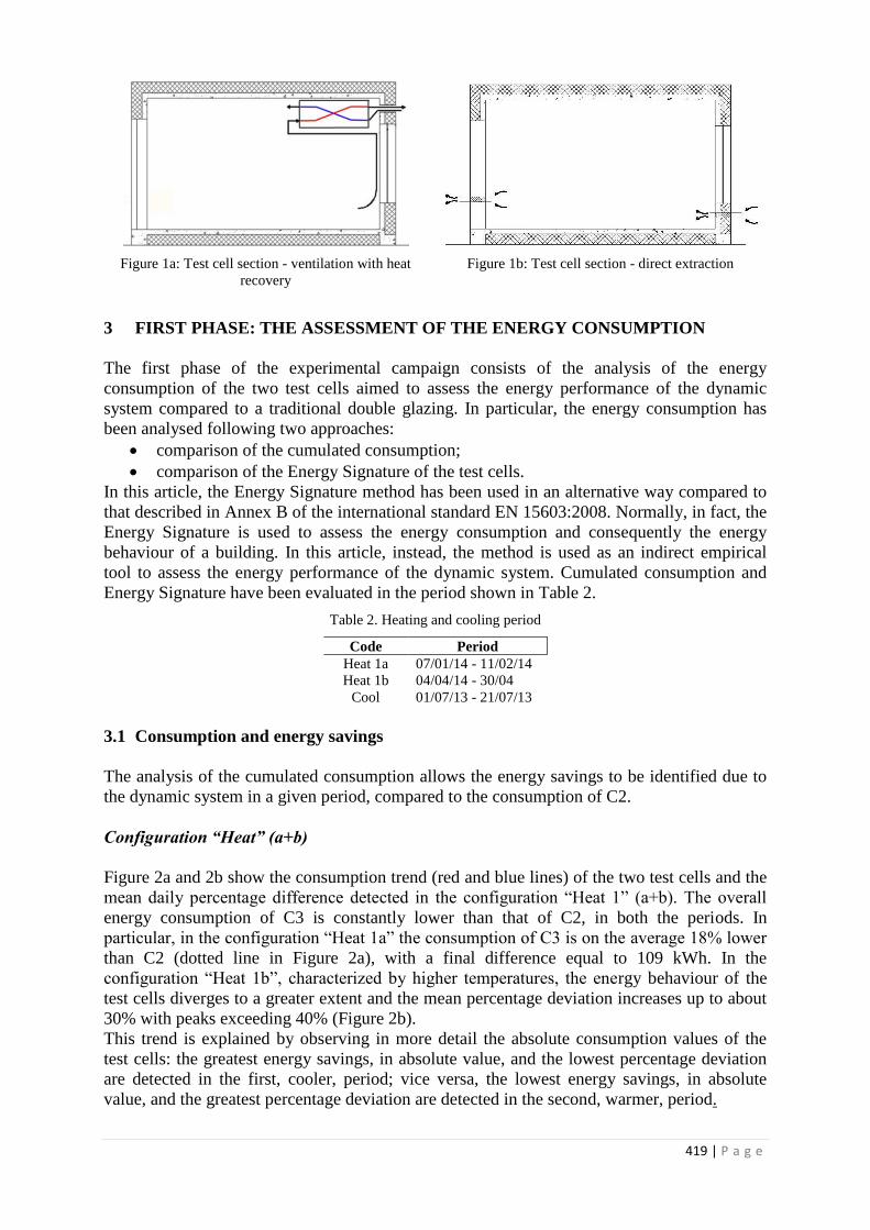
419 | P a g e

Figure 1a: Test cell section - ventilation with heat

recovery

Figure 1b: Test cell section - direct extraction

3 FIRST PHASE: THE ASSESSMENT OF THE ENERGY CONSUMPTION

The first phase of the experimental campaign consists of the analysis of the energy

consumption of the two test cells aimed to assess the energy performance of the dynamic

system compared to a traditional double glazing. In particular, the energy consumption has

been analysed following two approaches:

comparison of the cumulated consumption;

comparison of the Energy Signature of the test cells.

In this article, the Energy Signature method has been used in an alternative way compared to

that described in Annex B of the international standard EN 15603:2008. Normally, in fact, the

Energy Signature is used to assess the energy consumption and consequently the energy

behaviour of a building. In this article, instead, the method is used as an indirect empirical

tool to assess the energy performance of the dynamic system. Cumulated consumption and

Energy Signature have been evaluated in the period shown in Table 2.

Table 2. Heating and cooling period

Code Period

Heat 1a 07/01/14 - 11/02/14

Heat 1b 04/04/14 - 30/04

Cool 01/07/13 - 21/07/13

3.1 Consumption and energy savings

The analysis of the cumulated consumption allows the energy savings to be identified due to

the dynamic system in a given period, compared to the consumption of C2.

Configuration “Heat” (a+b)

Figure 2a and 2b show the consumption trend (red and blue lines) of the two test cells and the

mean daily percentage difference detected in the configuration “Heat 1” (a+b). The overall

energy consumption of C3 is constantly lower than that of C2, in both the periods. In

particular, in the configuration “Heat 1a” the consumption of C3 is on the average 18% lower

than C2 (dotted line in Figure 2a), with a final difference equal to 109 kWh. In the

configuration “Heat 1b”, characterized by higher temperatures, the energy behaviour of the

test cells diverges to a greater extent and the mean percentage deviation increases up to about

30% with peaks exceeding 40% (Figure 2b).

This trend is explained by observing in more detail the absolute consumption values of the

test cells: the greatest energy savings, in absolute value, and the lowest percentage deviation

are detected in the first, cooler, period; vice versa, the lowest energy savings, in absolute

value, and the greatest percentage deviation are detected in the second, warmer, period.

420 | P a g e

The dynamic system allows a lower utilization of the heating plant, in the warmer period.

The increase of the ventilation rate, as in configuration “Heat 2”, determines the increase of

the percentage deviation of the two test cells.

Figure 2a: Cumulated consumption configuration “Heat

1a”

Figure 2b: Cumulated consumption configuration

“Heat 1b”

Configuration “Cool”

Figure 3 shows the trend of the cumulated consumption of the test cells in the “Cool”

configuration. C3 shows the best energy behaviour and the lowest consumption, in percentage

terms (about 13%) and in absolute terms (about 25 kWh) than C2. However, in the cooling

phase, the combination of the dynamic system and the heat recovery unit does not allow the

flux to be optimally managed, because exhaust air that comes into the exchanger from the

indoor environment transfers heat to the inlet air, heating it.

In the cooling season, the reduction of the consumption is due only to the dynamic glazing.

Figure 3: Cumulated consumption configuration “Cool”

3.2 Energy Signature

The Energy Signature has been applied in order to determine the energy behaviour of the

dynamic system when the external climatic conditions vary. The Energy Signatures of the two

421 | P a g e

test cells have been compared in the different configurations. The contribution of the dynamic

system to the overall performance of C3 could be assessed thanks to this method.

Configuration “Heat”

The comparison of the Energy Signatures in the configuration “Heat 1a” (Figure 4a) shows a

better energy behaviour of C3 than C2, confirming the performance of the dynamic system

both in terms of heat losses (related to the slope of the straight lines) and in terms of switch-

off temperature of the heating system (intersection of the straight line with the x-axis). The

slope and the switch-off temperature of C3 are about 3.5 W/K and 2°C lower than those of

C2, respectively.

The same reasoning can be made for the configuration “Heat 2”. Figure 4b shows how the

energy behaviour of C3 is further improved than that of C2. This is due to the performance of

the two single components, dynamic glazing and heat recovery unit, which are more efficient

with the increasing of the airflow rate. In C3, the increasing of the airflow rate, that involves

greater ventilation losses, is balanced by the combined action of the dynamic system. In C2,

the ventilation losses are not recovered, with a consequent increasing of the overall

consumption.

Figure 4a: Energy Signature configuration “Heat 1

(a+b)” - comparison

Figure 4b: Energy Signature configuration “Heat 2” -

comparison

Configuration “Cool”

Similarly to the winter situation, it is possible to analyse the dynamic system behaviour in

summer through the Energy Signature.

The outcome of the cumulative consumption analysis is confirmed by the assessment of the

Energy Signature. The comparison, in fact, shows both a lower slope and a downward

translation of the Energy Signature of C3 with respect to C2, due to a better management of

the thermal loads of the combined system compared to the reference one.

Thus, also in summer, the dynamic system has the best energy behaviour.

422 | P a g e

Figure 5: Energy Signature configuration “cool” - comparison

3.3 Extention of results

The Energy Signature method allowed the slope and the constant term of the straight lines of

the test cells to be identified. Taking into account the average monthly temperature, it is

possible to extend the obtained results to the whole Italian territory, using an experimental

approach, aimed to theoretically assess the energy behaviour in different climatic conditions.

In this article, and by way of example, two configurations are considered: “Heat 1” and “Heat

3”. The mapping has been applied to all the Italian provinces.

Starting from the external temperature data and the Energy Signature equations (see Figure

4a), the theoretical consumption of the cells and the percentage difference of consumption

between the two cells, C2 and C3, are calculated.

Five classes, each characterized by a specific colour, have been identified as a function of the

energy savings guaranteed by the dynamic system, compared to the reference system.

The two resulting thematic maps (Figure 6 and Figure 7) allow the two cases to be compared

and the average energy savings to be evaluated. From configuration “Heat 3” to “Heat 1”, the

following savings are possible:

Northern Provinces: from 6.2% to 16.5%;

Central Provinces: from 9.8% to 19.7%;

Southern Provinces: form 13.7% to 26.5%.

The warmer the conditions, the greater the saving.

Figure 6: Thematic map - “Heat 3” Figure 7: Thematic map - “Heat 1”

423 | P a g e

4 SECOND PHASE: THE EVALUATION OF INDOOR IGRO-THERMAL

CONDITIONS AND COMFORT

4.1 The psychrometric analysis

The current operating logics of the dynamic system play a key role in the management of heat

flows, carrying out three different actions. The first takes place at the heat recovery level: the

cross-flow exchange of thermal energy between the exhaust air outgoing from the conditioned

test cell and the incoming air from the external environment involves a pre-heating action

during the winter season.

Then, the transparent component involves a reduction in heat exchanges with the external

environment: the air, drawn in by the indoor environment and passing through the ventilated

cavity, allows the surface temperature of the inner glass as close as possible to the

temperature of the indoor environment to be maintained. This action involves a reduction of

the thermal transmittance of the component as a function of the increasing flux in the air gap.

At the same time, the integrated preheating action due to the solar radiation hitting the

transparent component pre-heats the air that passes through the gap before reaching the

recovery unit (McEnvoy et al., 2003).

In this synergic plant context, the psychrometric analyses (ASHRAE 55), particularly focused

on the environment line and the straight patterns of the transforms, allow the results of the

energy evaluations to be represented and to be interpreted.

Table 3 shows the overall average data efficiency of the two test cells, related to

representative detailed analyses.

During the winter testing period, the indoor environmental monitoring data show the positive

synergy between the dynamic system and the heat recovery unit, which confirms the energy

consumption data. In fact, at constant indoor conditions (Temperature and RH%), C3 shows

an average efficiency improvement compared to C2 of approximately 7%.

On the contrary, during the summer, the combined system does not allow to effectively heat

flows to be managed.

Table 3: Heating & Cooling configurations

Season & Plant

Configurations

Reference

period

Reference

day

DT (C3-C2) D%RH (C3-C2) Avg. Efficiency

(C3-C2)

Heat1 22-29 April 2013 22 April <1°C <5% 7% ca

Cool 01-07 July 2013 03 July 1°C 1% --

C3C2

32

4

1

0 5 10 15 20 25 30 35 40 45 50

22.04 h 00.00

22.04 h 12.00

ASHRAE WINTER

ASHRAE SUMMER

4

32 1

C2

C3

0 5 10 15 20 25 30 35 40 45 50

03.07 h 00.00

03.07 h 12.00

ASHRAE WINTER

ASHRAE SUMMER

Figure 7: Psychrometric chart related to the operating

condition factor and the plant-related transforms for

“Heat1” configuration

Figure 8: Psychrometric chart related to the operating

condition factor and the plant-related transforms for

“Cool1” configuration

424 | P a g e

Figure 7 and Figure 8 show the points of the plant-related transforms:

point 1 is the inlet airflow from the outside;

point 2 is the heat recovery unit airflow to the inside;

point 3 is the intake airflow of the heat recovery unit from the inside, after passing

through the ventilated cavity of the glass;

point 4 represents the heat recovery unit airflow to the outside.

During the winter tests, as shown in Figure 7, the combined operation involves that the slope

of the operating condition factor corresponds of the slope of the line connecting points 1-3.

So, the combined system operates in synergy, generating a virtuous cycle in energy savings

through the combined action.

Instead, concerning the summer season, the possible considerations are very different.

Even if the indoor conditions in both the test cells are the same, as shown in Table 66, the

psychrometric chart in Figure 8 shows how in this configuration the slope of the operating

condition factor radically differs from the slope of the line connecting points 1-3. This

difference is more evident during direct solar radiation phases.

During winter testing the combined system contributed to the increase of the overall

efficiency, allowing to achieve the set point conditions provided for by the indoor

environment line with a reduced energy expenditure by the heating system.

The operation of the dynamic window, represented by the segment 2-3 of the orange polyline

(Figure 8), involves a daily overheating of the air pre-treated in C3, reducing the heat

recovery unit efficiency (1-2 segment). In fact the outgoing air is cooled by the exchanger (3-

4 segment).

In the summer season the combined system involves a worse phase shift than expected, which

is made evident by the psychrometric chart.

4.2 Comfort analysis

The thermo-hygrometric comfort level of the two test cells has been evaluated using the

Fanger method (EN ISO 7730:2006). The analysis has been carried out in the configurations

“Comf 1” and “Comf 2”, in different weeks (Table 4).

Table 4: Cases comfort analysis

Code Period

Comf 1 03/06/13 – 09/06/13

Comf 2 14/05/13 – 24/05/13

Configuration “Comf 1”

In Figure 9, the Predicted Percentage of Dissatisfied values (PPD), calculated assuming a

clothing value equal to 0.75 clo, are better in C3 than in C2, with a maximum deviation

slightly more than 30%. In Figure 10 the Predicted Mean Vote index (PMV) indicates, in both

cells, a thermo-hygrometric sensation average comprised between the “neutral” class and the

“slightly warm” class. In C2, higher temperature and humidity values are detected.

425 | P a g e

Figure 169: PPD trend - “Comf 1” Figure 170: PMV trend - “Comf 1”

Configuration “Comf 2”

In the configuration “Comf C2” it is possible to divide the considered period in two parts.

From May 15 to 17, the average external temperature is equal to about 17 °C and the average

solar radiation is about 400 W/m2. In these conditions, no significant changes in thermo-

hygrometric comfort between the two cells are recorded. From May 18 to 24, instead, the

external temperature and the solar radiation are lower (about 15°C) and higher (about 600

W/m2), respectively, compared to the previous period. In these conditions, C3 provides the

best thermo-hygrometric comfort (Figure 11). The PMV values highlight the differences in

the two periods: in the former, the thermo-hygrometric sensation is on the average “neutral”,

for both cells, while in the latter the thermo-hygrometric sensation is on the average “slightly

cool”, with C3 values higher than C2 and close to “neutral”.

Figure 11: PPD trend - “Comf 2” Figure 12: PMV trend - “Comf 2”

6 CONCLUSIONS

This article has investigated the energy behaviour and the comfort level of a dynamic system,

consisting of the VetroVentilato® system and a commercial heat recovery unit. The results of

the experimentation show that, in winter, the combined system allows for interesting energy

savings. When the external temperature is equal to 10 °C, the energy savings that may be

achieved with the dynamic system amount to about 38% compared to 8% obtained by the

single system alone (without the heat recovery unit) and compared to 20% obtained by the

heat recovery unit alone. The analysis shows an improvement of the performances of the

426 | P a g e

combined system. The combined operation of the dynamic system is not the sum of the single

contributions; in fact, the system detects higher values due to the pre-heating function of the

window.

In summer, the energy savings of the combined system are about 13%, which is lower than

the operation of VetroVentilato® alone.

ACKNOWLEDGEMENTS

This work was carried out according to an industrial research project with the VetroVentilato

society.

REFERENCES

Lollini, R., Danza, L., Meroni, I. (2010). Energy efficiency of a dynamic glazing system.

Solar Energy, 84(4), 526-537.

Belussi, L., Danza, L. (2012). Method for the prediction of malfunctions of buildings through

real energy consumption analysis: Holistic and multidisciplinary approach of Energy

Signature. Energy and Building, 55, 715-720..

Stamp, S. (2012) A Summary of the Co-heating test procedure and analysis method,

Technical Report.

ANSI/ASHRAE 55:2013. Thermal environmental conditions for human occupancy.

EN ISO 7730:2006. Ergonomics of the thermal environment - Analytical determination and



EN 15603:2008, For space heating - Overall energy use and definition of energy ratings.

McEvoy M.E., Southall R.G., Baker P.H., Test cell evaluation of supply air windows to

characterise their optimum performance and its verification by the use of modelling

techniques, Energy and buildings, 35 (2003), pp. 1009-1020.

J.U. Sjogren , S. Andersson, T. Olofsson, Sensitivity of the total heat loss coefficient

determined by the energy signature approach to different time periods and gained

previous energy, Energy and Buildings, 41 (2009), pp. 801–808.

427 | P a g e

DERIVATION OF EQUATION FOR PERSONAL

CARBON DIOXIDE IN EXHALED BREATH

INTENDED TO ESTIMATION OF BUILDING

VENTILATION

Masaki TAJIMA

*1, Takayuki INOUE

1, and Yuji OHNISHI

1

1 Kochi University of Technology

Tosayamada

Kami-city, Kochi, 782-8502 Japan

* [email protected]

ABSTRACT

Carbon dioxide included in exhaled breath is often used as a tracer gas when estimation of ventilation aspect

in buildings with occupants is performed. Carbon dioxide produced by occupants is the key for the estimation.

JIS A 1406 and ASTM D6245-12 refer personal carbon dioxide production rate. However JIS does not take into

account personal attribute like as body height and weight. On the other hand, ASTM does not take into account

gender difference and based on average westerner adult data. Hence, by using Douglas bag method with

approximately total 70 voluntary Japanese subjects, a prediction equation for occupants’ carbon dioxide

production rate included in exhaled breath is developed. Moreover, the equation is tested in single zone with

occupants aiming at accuracy testing. The results can allow predicting more correct carbon dioxide concentration

produced by occupants’, exhaled breath in single zone compared with the standards.

KEYWORDS

Ventilation, Exhaled breath, Carbon dioxide, Single zone, Douglas bag method

1. INTRODUCTION

Carbon dioxide included in exhaled breath is often used as a tracer gas when estimation of

ventilation aspect in buildings with occupants is performed. Amount of carbon dioxide

produced by the occupants is a key for this kind of estimation. Carbon dioxide production rate

is shown in e.g. a Japanese Industrial Standard (JIS A 14061974

, 2010) and an American

Society for Testing and Materials International Standard (ASTM D6245-12, 2012).The JIS

standard indicates a relationship between personal carbon dioxide production rate and RMR

(relative metabolic rate) including gender difference, which shows female’s production rate is

0.9 times of male’s. The ASTM standard gives a relationship between personal carbon

dioxide production rate and parameters, as body surface area and metabolic rate. These

personal carbon dioxide production rates were referenced in other standard (e.g. SHASE-

S102, 2011) and have been used for computing ventilation rate or air change rate in some

previous works (e.g. Saito et al., 2002, Stavova et al., 2006). These carbon dioxide production

rates in the standards are described simply, therefore they are useful for the estimation.

However, the JIS’s rate is not considered body height and weight. On the other hands, the

ASTM’s rate is not considered gender difference and is based on average westerner adult data

with a fixed respiratory quotient value (RQ = 0.83).

428 | P a g e

Because of these backgrounds, this study aims at derivation of a prediction equation using

variables such as Met and personal attribute for personal carbon dioxide production rate

included in exhaled breath with Japanese subjects, aims and at accuracy testing of this

equation at rooms with occupants in real use conditions.

2. DERIVATION OF EQUATION FOR PERSONAL CARBON DIOXIDE

PRODUCTION RATE

2.1 Outline of the derivation

The derivation of an equation for carbon dioxide production rate was performed with

obtained carbon dioxide production rate, Met, and subjects’ personal attribute. Then, with

using these obtained data, an equation was derived trough regression analysis.

2.2 Measurement

Using Douglas bag method, the measurement of carbon dioxide production rate was

performed with total of approximately 70 voluntary people who were mainly university

students. The testing activities and number of subjects are shown in Table 1 and testing

instruments are shown in Table 2.

Metabolic value M and carbon dioxide production value VCO2 are determined by the

following equations (ISO8996, 2004) with using obtained data which are VO2 and VCO2.

Moreover, personal attribute, age, gender, body height and weight, were also obtained.

Table 1: testing activities and number of subjects

Activity Seated, quiet Walking (2km/h) Walking(4km/h)

Work period 10 minutes 5 minutes 3 minutes

Number of Subjects* 23(9) 23(9) 23(9)

*total 69 people, ( ) means internal numbers of female

Table 2: testing instruments

Douglas bag Volume: 100L TK-11288

Gas analyser CO2 NDIR 0-5/10/20 vol%

O2 zirconia process 0-5/10/25 vol% PG-240

2

2

O

CO

V

VRQ (1)

88.5)77.023.0(EE RQ (2)

2OVEEM (3)

Where

RQ is the respiratory quotient

VO2 is the oxygen consumption rate [L/h]

VCO2 is the carbon dioxide production rate [L/h]

EE is the energetic equivalent [Wh/LO2]

M is the metabolic rate [W]

2.3 Regression analysis

The measured data was selected into for 51 subjects’ data for the regression analysis, by

considering to the aspect of the RQ value referred in former works like as the followings. RQ

varies from 0.7 to 1.0(e.g. Herman, 2007). RQ equals 0.83 for an average adult engaged in

429 | P a g e

light or sedentary activities (ASTM D6245-12 2012). RQ = 0.83 applies to a normal diet mix

of fat, carbohydrate, and protein (ASHRAE Standard 62.1, 2010)

The whole measured values range approximately from 0.6 to 1.2. Only the data ranges

from 0.7 to 1.0 were used as the selected data. Therefore, the selected RQ values finally range

from 0.78 to 0.99 and the average value is 0.93 for seated quiet, 0.92 for walking at 2km/h

and 0.91 for walking at 4km/h. Hence these measured RQ values are larger than the ASTM’s

and ASHRAE’s theoretical fixed values.

(1) Relationship between carbon dioxide production rate and metabolic rate

The relationship between carbon dioxide production rate PCO2 in m3/h and metabolic value

M, simple correlation, is shown in Figure 1. The equations (1), (2) and (3) show that the

metabolic rate M is determined by using oxygen consumption rate VO2 and carbon dioxide

production rate VCO2. Even without oxygen consumption rate VO2 this relationship has strong

correlation and the relationship can be expressed by equation (4). Thus this equation within

metabolic rate as a variable can be considered as basic equation for the prediction of personal

carbon dioxide production rate.

0.00

0.01

0.02

0.03

0.04

0.05

0.06

0.07

0.08

0.09

0.10

0 100 200 300 400 500 600

CO

2pro

ductio

n [m

3/h

]

Metabolic rate [W]

seated, quiet

Walking 2km/h

Walking 4km/h

y=1.589*10-4XR2=0.9941N=51

Figure 1: Relationship between carbon dioxide production rate and metabolic value

MPCO

410895.12

(4)

Where

PCO2 is the carbon dioxide production rate [m3/h]

(2) Relationship between metabolic rate and body height and weight

Relationship between metabolic rate M and body surface area AD is shown in Figure 2. The

body surface area is given by equation (5) (SHASE Handbook, 2010). This equation is based

on Japanese adults’ data.

From regression analysis results with explanatory variables as the BMI (body-mass index),

height and weight themselves, and body surface area, the body surface area AD has the

strongest correlation with metabolic rate as same as previous works (e.g. ASTM D6245-12

2012, Persily, 1997) .

430 | P a g e

y = 61.28x - 4.4225R² = 0.3116

y = 299.17x - 297.4R² = 0.6826

y = 354.83x - 318.91R² = 0.5294

0

100

200

300

400

500

600

1.0 1.5 2.0 2.5

Meta

bolic

rate

[W

]Body surface area [m²]

seated, quiet

Walking 2km/h

Walking 4km/h

Figure 2: Relationship between metabolic rate and body surface area

725.0425.0007246.0 bbD HWA (5)

Where

AD is the body surface area [m2] (for Japanese adult)

Wb is the body weight [kg]

Hb is the body height [cm]

(3) Relationship between metabolic rate and Met

Figure 3 indicates relationship between metabolic rate and Met given by equation (6). Met,

which is generally used as an index of occupants’ activity, is calculated by substituting each

subject’s metabolic rate obtained under the condition of “seated, quiet” as MS into this

equation. The coefficient of determination R2 shown in Figure 3 is approximately 0.82.

y = 88.542x + 14.343R² = 0.8248

0

100

200

300

400

500

600

0 2 4 6

Me

tab

olic

ra

te [

W]

Met

seated, quiet

Walking 2km/h

Walking 4km/h

Figure 3: Relationship between metabolic rate and Met

SM

MMet (6)

Where

MS is the metabolic rate of relax seated [W]

2.4 Determination of equation for personal carbon dioxide production rate

Metabolic rate is given by equation (7) which also has coefficient of gender as a variable.

Subject’s age was not employed in the equation, because most of subjects were similar ages.

The coefficient of determination did not increase even when subject’s age was taken as

variables.

431 | P a g e

Relationship between measured metabolic rate and calculated metabolic rate using equation

(7) is shown in Figure 4, in which R2 is approximately 0.88 and the RMSE is 33.1.

7.1490.219.834.94 gD CMetAM (7)

Where

Cg is the coefficient of gender (0: female, 1: male)

Finally, the prediction equation for personal carbon dioxide production rate is derived as

equation (8) using equation (4) and (7). Figure 5 represents relationship between measured

carbon dioxide production rate and calculated carbon dioxide production rate by using

equation (8). The trends agree with measured result as shown in the figure in which the R2 is

approximately 0.88 and the RMSE is 0.006.

7.1490.219.834.9410589.1 4

2

gDCO CMetAP (8)

R² = 0.8825RMSE = 33.1

0

100

200

300

400

500

600

0 100 200 300 400 500 600

Msas

ure

d m

eta

bo

lic r

ate

[W

]

Calculated metabolic rate [W]

male

female

Figure 4: Relationship between measured metabolic rate and calculated metabolic rate

R² = 0.8718RMSE = 0.006

0.00

0.01

0.02

0.03

0.04

0.05

0.06

0.07

0.08

0.09

0.10

0 0.02 0.04 0.06 0.08 0.1

Me

as

ure

d C

O2

pro

du

cti

on

ra

te[m

3/h

]

Calculated CO2 production rate [m3/h]

male

female

Figure 5: Relationship between measured carbon dioxide production rate and calculated carbon dioxide production rate

2.5 Comparison of carbon dioxide production rate of the equation, ASTM and JIS

Figure 6 shows carbon dioxide production rate of present work calculated by using the

equation (8), of ASTM and of JIS. The ASTM’s rate is calculated by equation (9) and (10)

with RQ is 0.83 as the fixed value. Japanese average adult’s body height and weight are put

into the equation (8) and (10) to calculate the rate. Originally, the JIS shows relationship

between carbon dioxide production rate and RMR (relative metabolic rate), which can be

transformed into Met by using equation (11) (Herman, 2007).

432 | P a g e

Figure 6 indicates that present work’s carbon dioxide production rate is larger than JIS’s

rate and the difference is 0.008m3/h (8L/h) at 1.0Met. The present work’s rate is also larger

than ASTM’s rate under the range of Met = 3. The difference at 1.0 Met is 0.004m3/h (4L/h).

0.77)(0.23

0.00276

RQ

MetARQF DB (9)

725.0425.0203.0 HWADB (10)

Where

ADB is the DuBois body surface area [m2]

F the carbon dioxide production rate [L/h]

W is the body weight [kg]

H is the body height [m]

11.2 MetRMR (11)

0.00

0.01

0.02

0.03

0.04

0.05

0.06

0.07

0.08

1 2 3 4 5

CO

2pro

ductio

n r

ate［

m³/

h］

Met

Present workASTMJIS

Figure 6: carbon dioxide production rate of present work, ASTM 6245-12 and JIS A1406

(using average Japanese adult’s body height and weight)

3 ACCURACY TESTING IN SINGLE ZONE

3.1 Measurement for accuracy testing

As shown in the above, there are certain differences of carbon dioxide production rate

between the equation and shown in the ASTM and the JIS. Therefore, by measuring carbon

dioxides concentration under condition of known ventilation rate in rooms considered as

single zone, the accuracy of the equation was tested.

Condition of the measurement is shown in Table 3. The room-A was occupied by a lecturer

and university students for lecture. The room-B was occupied by university students for self-

schooling. The room-A employs mechanical ventilation fans included in an air handling unit

and its ventilation rate was measured by decay method using carbon dioxide concentration

after leaving all occupants. The room-B employs mechanical fans, however, only an

experimental exhaust fan, whose air flow rate can be given even in situ situation, was

operated during the measurement.

Personal attribute, which are age, gender, body height and weight, of occupants were

obtained. Additionally, Occupants’ activities, which were Met = 1.0 and 1.2, were determined

by visual judgment.

433 | P a g e

Table 3: Condition of measurement

Case A-1 A-2 B-1

Name of room room-A room-B

air volume of room [m3] 468 141

Ventilation rate of room [m3/h] 1,300

* 140

**

Number of occupants 58 61 6

Outdoor CO2 conc. [ppm] 413 403 400 *rate of mechanical ventilation employed in AHU measured by decay method

**set by using additional experimental exhaust fan

3.2 Measurement results and discussion

Measured carbon dioxide concentration and computed results given by using equation (12)

are shown in Figure 7, 8 and 9. Carbon dioxide concentration measurement instruments were

placed at the centre of the room-A and next to the suction part of the experimental exhaust fan

in the room-B. The measurement interval was 30 seconds.

)( oo2 iiCOii CCQPV

dt

dC (12)

Where

Ci concentration of carbon dioxide of target room [m3/m

3]

Co concentration of carbon dioxide of outdoor [m3/m

3]

Qio ventilation rate [m3/h]

As shown in these diagrams, the trends of present work’s concentration are almost similar

to the measurement values except occasional risings especially in the room A compared with

other computed values. The occasional risings are considered to be caused by non-uniform

mixing state of carbon dioxide and incompleteness of visual judgement for occupants’

activities. However, the present work’s concentration of the room B, considered as being

nearly uniform concentration condition, is almost accordance with measured concentration. In

these diagrams, RMSE of the each computed concentration is shown, and they indicate that

present work using equation (8) gives the most correct carbon dioxide concentration

compared with the other ways.

0

500

1000

1500

2000

0 10 20 30 40 50 60 70 80 90 100

CO

2C

on

c. [

pp

m]

Elapsed time [minn]

MeasurementPresent workASTMJIS

case A-1Met:1.0

RMSE = 84RMSE = 178

RMSE = 269

Figure 7: CO2 concentration in case A-1

434 | P a g e

0

500

1000

1500

2000

0 10 20 30 40 50 60 70 80 90 100

CO

2C

on

c. [

pp

m]

Elapsed time[min]

Measurement

Present work

ASTM

JIS

Met:1.2 Met:1.0 Met:1.2 case A-2

RMSE = 153RMSE = 201

RMSE = 307

Figure 8: CO2 concentration in case A-2

0

500

1000

1500

2000

0 10 20 30 40 50 60 70 80 90 100

CO

2C

on

c. [

pp

m]

Elapsed time[min]

Measurement

Present work

ASTM

JIS

case B-1 Met:1.0

RMSE = 30RMSE = 38

RMSE = 88

Figure 9: CO2 concentration in case B-1

4 CONCLUSION

Based on data obtained by Douglas bag method with approximately total 70 voluntary

Japanese subjects, a prediction equation for occupants’ carbon dioxide production rate

included in exhaled breath is developed. This equation has variables, such as Met and

personal attribute (body height, body weight and gender). Therefore, the equation has certain

advantages, like as taking gender difference into the formula and based on multiple Japanese

subjects’ data, compared with the personal carbon dioxide production rates shown in JIS A

14061974

and ASTM D6245-12.

From measurement results operated at single zones, computed carbon dioxide

concentration of present work shows the closest to the measurement value compared with the

other standards’ value under the condition of occupants’ Met is 1.0 or 1.2. Therefore these

results can allow predicting more correct carbon dioxide concentration produced by

occupants’, especially Japanese occupants’, exhaled breath in single zone. Higher Met testing,

and more measurement in buildings including within multi zone will be warranted.

5 REFERENCES

JIS (2010), JIS A 14061974

Method for Measuring Amount of Room Ventilation (Carbon

Dioxide Method), Japanese Industrial Standards Committee

ASTM (2012). ASTM D6245-12 Standard Guide for Using Indoor Carbon Dioxide

Concentrations to Evaluate Indoor Air Quality and Ventilation. American Society for

Testing and Materials International

SHASE (2011). SHASE-S102-2011 Ventilation Requirements for Acceptable Indoor Air

Quality. The Society of Heating, Air-Conditioning and Sanitary Engineers of Japan

435 | P a g e

Saito, M. Ishii, A. et al., (2002). Comfort and Amenity of Classroom Environment. Part 7

Carbon-dioxide Concentration and Ventilation. summaries of Technical Papers of

Annual Meeting, Architectural Institute of Japan, D-1, 1071-1072

Stavova, P. Melikov, A. Sundell, J. Naydenov, K. (2006). A New Approach for Ventilation

Measurement in Homes Based on CO2 Produced by People. 17th Air-conditioning

and Ventilation Conference 2006, 291-296

ISO. (2004). ISO 8996 Determination of metabolic rate. International Organization for

Standardization

Herman,I.(2007). Physics of the Human Body. Biological and Medical Physics, Biomedical

Engineering, Springer-Verlag GmbH & CO.KG

ASHRAE. (2013). ASHRAE Handbook Fundamentals 2013. American Society of Heating,

Refrigerating and Air-Conditioning Engineers, 9.6

SHASE. (2010). Handbook of air-conditioning and sanitary engineering. Vol.1, The Society

of Heating, Air-Conditioning and Sanitary Engineers of Japan

Persily, A. (1997). Evaluating building IAQ and ventilation with indoor carbon dioxide.

ASHRAE Transactions, vol.103, part2, American Society of Heating, Refrigerating

and Air-Conditioning Engineers

436 | P a g e

PASSIVE COOLING THROUGH VENTILATION

SHAFTS IN HIGH-DENSITY ZERO ENERGY

BUILDINGS: A DESIGN STRATEGY TO INTEGRATE

NATURAL AND MECHANICAL VENTILATION IN

TEMPERATE CLIMATES.

Luca Guardigli*

1, Paolo Cappellacci

1, Fausto Barbolini

1

1 School of Engineering and Architecture, University of Bologna,

Via del Risorgimento 2,

Bologna, Italy

ABSTRACT

Zero Energy Buildings require airtightness and mechanical ventilation systems to provide air changes and energy

saving. These requirements contrast with the principles of natural ventilation. Through a case study located in

Modena, Italy, a design strategy is proposed as a solution to integrate natural and mechanical ventilation systems

at different times of the year to reduce the energy consumption in a newly designed high-density ZEB. The

internal comfort evaluation for the warm season is then verified with a multizone dynamic simulation and a CFD

analysis.

The proposal consists of two different approaches, the cold season and the warm one. For the cold season, a

mechanical ventilation system with earth tubes and heat recovery has been designed, together with airtightness,

solar greenhouses and high thermal mass and insulation. For the warm season the design allows a free-running

use: open trickle ventilators applied to windows which provide background ventilation, mass and insulation

mitigate the heat loads, vertical ventilation shafts support natural ventilation and free night cooling. The

ventilation shafts have been designed with aerodynamic principles to provide each apartment with additional

(and maximised) differences of pressure due to the stack effect. The indoor comfort conditions in the warm

season are then evaluated according to the ASHRAE 55 adaptive model for free-running buildings.

The results of the study confirm that in the warm season acceptable indoor comfort conditions can be achieved in

a free running building. The ventilation shaft has an important role for the free cooling of a ZEB and can also be

adopted in the renovation of existing buildings.

Keywords Integrated design, hybrid ventilation system, Zero Energy Building, adaptive thermal comfort, temperate climate

1. INTRODUCTION

A Zero Energy Building (ZEB) is a residential or commercial building with greatly reduced

energy needs through efficiency gains such that the balance of energy needs can be supplied

with renewable technologies.

The efficiency required to achieve the zero energy goal leads to many design strategies,

including airtightness to avoid infiltration and mechanical ventilation systems with heat

recovery to provide air conditioning and indoor air quality (IAQ). Natural ventilation systems

generally contrast with the principle of mechanical control of indoor environment.

437 | P a g e

The designed energy balance of a ZEB can however be invalidated with an improper use of

technologies by occupants, such as opening windows, changing the operative temperature or

not providing the right maintenance of systems.

Thermal comfort is defined as that condition of mind which expresses satisfaction with the

thermal environment and depends on physiological and psychological aspects. The former

have been widely investigated by Fanger and other scholars, the latter seem to be neglected, at

least in the current design. Psychological aspects of comfort involve the interaction of

occupants with the environment and vary with latitude, cultural and social factors. Adaptive

thermal models, essentially valid for free running buildings, are based on the assumption by

Humphreys and Nicol: ‘if a change occurs such as to produce discomfort, people react in

ways which tend to restore their comfort’. These models are entirely focused on psychological

aspects and allow wider tolerances of indoor thermal comfort conditions than the

physiological-only ones.

The mechanical control of thermal comfort, much emphasized in ZEBs, aims to reduce the

interaction of users with the outdoor environment and this contrasts with the principles of

psychological comfort. Monitoring of ultra-low energy buildings in Italy have revealed that

occupants rarely use mechanical systems properly and the energy consumption often exceeds

the expected results.

The aim of this paper is to propose an integrated design strategy to integrate natural and

mechanical ventilation systems in a high density ZEB at different times of the year,

overcoming airtightness related problems and thermal comfort ones. Energy and comfort

evaluations are then estimated according to current standards.

2. PRESENTATION OF THE CASE STUDY

The Case Study is located in Modena, Italy, in a typical temperate climate. Winter is typically

not very cold, with temperatures rarely under 0°C. Summer can instead be slightly hot, with

the average of daily temperatures in the warmest months around 30°C. Wind speed is

generally low at all times of the year, with values around 1,5 m/s, except for some gust at 5-8

m/s. The site of the building has 2258 Degree Days.

A high-density building is designed according to the best practice principles for a ZEB:

- Energy Saving through Building Design;

- Energy Efficiency of Mechanics and HVAC;

- Energy Production from Renewable Sources.

The integrated design of a building concerns all these principles at the same time, with

choices that have influences on the whole system. The aim of the case study is to investigate

the possibilities to adopt a natural ventilation strategy of use of high-density residential

buildings, reducing or cancelling the energy consumption in the warm season of temperate

climates, in a Zero Energy Building viewpoint. The strategy adopted for the case study are

listed below.

2.1 Building Design

The Energy Saving goal is achieved through several passive Building Design strategies, as

shown in Figure 1, which include both formal and technical features:

- Orientation, shape of building, tilt angle of roof and shadow analysis;

- The exposed surfaces of facades are relatively limited compared to their inner volume,

with a ratio of 0,3;

438 | P a g e

- Optimisation of solar gains through greenhouses;

- Strategies for passive cooling: cross ventilation for all apartments and shafts for additional

ventilation just in the warm season;

- Increase of green surfaces for climate mitigation;

- Air tightness windows with additional trickle ventilators(to be opened in the warm season);

- Choice of materials as reported in the table 1.

Figure 1: Building Design Strategies

Table 1: Materials

Element Materials U-Value (W/m2K)

External wall

10 mm internal plaster

250 mm perforated bricks

320 mm rockwool panels

20 mm reinforced external plaster

0,107

Outer floor

30 mm finishing flooring

50 mm sand-cement screed

240 mm concrete floor

320 mm rockwool panels

20 mm reinforced external plaster

0,109

Roof

Windows

(general)

Windows

(on greenhouses)

70 mm terracotta shingles

320 mm rigid rockwool panels

240 mm concrete floor

10 mm internal plaster

Triple glazed 3x4mm,

14 mm air gap

Double glazed 3x4mm,

14 mm air gap

0,110

1,00

1,30

The ventilation shaft has been designed to maximise the indoor-outdoor difference of pressure

in all the apartments for a better ventilation in the warm season, applying the stack.effect

equation:

439 | P a g e

∆ ps = ( ρ - ) ∙ g ∙ ( - H ) = ρ ∙ ∙ g ∙ ( - H ) (1)

The height of HNPL has been estimated according to Ashrae guidelines, with values typically

of 0,7 of total height of the shaft. To optimise its effect, the shaft has been divided in two

separate portions, the former for the lower stories, the latter for the two upper ones, as shown

in Figure 2. The difference of temperature from the inlet to the outlet of the shaft has been

initially settled at 25 °C. The pressure of wind has been also calculated at the various stories:

∆ pw = Cp ∙ ρ ∙ (2)

Cp coefficient has been estimated through both empirical tables and CpCalc+ software. As

shown in Figure 2, in the climate of the building site, the effects of wind pressure have little

relevance compared to the stack effect ones.

Figure 2: Differences of pressure due to wind and stack effect. Shaft optimisation.

Once ∆ p have been known, the airflows are calculated by the equation:

Q = Cd ∙ A ∙ (3)

Cd is a discharge coefficient for the sharp-edged orifice, taken as 0,61. The areas of the inlet

openings in the shaft are set as 0,06 m2 (30cm x 20 cm). By applying the equation (3), a first

empirical verification shows that the airflow through the shaft at each story allows a air

change rate of at least 1 volume per hour. The same results are given for a reduced difference

of temperature between inlets and the outlet of the shaft of 10°C.

The results suggest that a free running use of the building guarantees at a good IAQ.

2.2 Mechanics and HVAC

Energy Efficiency is achieved by the choice of high performance systems together with the

entire design of the building. Designing a ZEB means to choose technologies apt to reduce,

save and optimise the energy consumption, and the choice of HVAC systems is strictly

related to this scope. A first overview of the project highlights questions to be solved:

- The surfaces for PV and solar thermal collectors of roofs are relatively small related to

the numbers of apartments, and the energy production does not supply all the needs of

the building;

- An additional and renewable system of energy production has thus to be provided to

achieve the Zero Energy goal;

- The heating system of the cold season should be able to operate in reverse even in the

warm season, so that a single mechanical system serves the building;

440 | P a g e

- HVAC should be shut down in the warm season in behalf of natural ventilation;

- IAQ has to be guaranteed at all times of the year, despites air tightness of windows.

The choice adopted for the building consist of a mechanical ventilation system equipped with

earth tubes, heat recovery and a heating unit. During the cold season the system provides

heating and ventilation in each apartment (the ventilation shaft is closed). During the warm

season HVAC system should be off in behalf of natural ventilation: the background

ventilation is then provided by the trickle ventilators in windows and the open shaft. In case

of extreme climate conditions the HVAC system can be turned on and the ground-coupled

heat exchanger provides cool and de-humidified fresh air. Hot water for domestic use and

heating and electricity are then provided by a Combined Heating Power System (CHP), where

PV and solar thermal collectors are not sufficient.

The Figures 2 and 3 show the operational scheme of the system in the cold and warm seasons.

Figure 4 shows a relevant section of the building, Figure 5 the ventilation system scheme.

Figure 2. Operational scheme in the cold season.

Figure 3. Operational scheme in the warm season.

441 | P a g e

Figure 4. Relevant section of the ventilation shaft and the HVAC system shaft.

442 | P a g e

Figure 5. Ventilation system scheme.

2.3 Renewable Sources of Energy

The Energy Production in ZEBs should balance the consumption. To optimise the sun-

exposed surfaces of the roofs, PV is designed to be settled for 604 m2 while photovoltaic

thermal hybrid solar collectors are designed for the remaining 250 m2. The total energy

production is about 155100 kWh per year, and the hot water production supplies all the needs

of the building for the most part of the year.

The electric needs of the building are estimated in 171000 kWh per year through the SVI

index (StromVerbrauchsIndex), related to the number of occupants of every single apartment

according to the equation 4:

N. of occupants x 500 kWh + 500 kWh = goal value per apartment in kWh (4)

A CHP system supplies the electric deficit of PV and also provides hot water for heating and

domestic use in the cold season. A power of 80 kW is sufficient to furnish hot water and the

residual electric energy needed.

Building energy rating is evaluated according to EN ISO 13790:2008 in 7,7 kWh/m2 per year

and all the energy consumption is balanced by the production from renewable sources also

with a slight surplus.

443 | P a g e

3 ANALYSIS AND RESULTS

Thermodynamic and a CFD analyses have been carried out to evaluate the effectiveness of the

design strategies adopted. The main purpose of the analyses has been to estimate the indoor

thermal comfort conditions, especially in the warm season when a free running use of the

building is desired. The results have been so checked through the Ashrae 55 standard for

buildings with no HVAC systems working.

3.1 Multizone Thermodynamic Analysis

A relevant portion of the building has been modelled and analysed in the typical design

summer week. The internal environments have been modelled in different ways to evaluate

the influence of the shaft on performances. The settings of the simulation included air

infiltration for 0,5 volumes per hour in each apartment, a night cooling program of 5%

windows openings between 8pm and 7am and an advanced mathematical pattern for

ventilation calculation. The output results of the simulation are copious and detailed. Hence

the main and interesting outputs are presented. A global overview of the internal

temperatures, presented in Figure 6, shows that the average values range between 25°C and

28°C, despites the daily temperature fluctuations.

Figure 6. Internal and external temperatures in the typical design summer week.

A detailed analysis of the various zones shows that local temperatures vary at each story. If

the lower stories are the cooler ones, with temperatures of 1°C below the building average,

the upper floors reach in the hottest hours of the day temperatures of 29°C.

The entire results for each story and zone of the model have been evaluated according to

Ashrae 55 standard and are reported in Figure 7. As it is clearly visible, thermal comfort

conditions are satisfied within a 80% of acceptability limit in the hottest days of the year.

444 | P a g e

Figure 7. Internal comfort conditions in Ashrae 55 adaptive model chart. In blue the upper floor, in yellow the

lower floor, and in red the average of the whole building.

3.2 CFD Analysis

A more accurate analysis has been led for the rooms served by the shaft to check the internal

conditions of comfort. A simplified model of seven rooms, one for each story, and the

annexed ventilation shaft has been analysed. The boundary conditions have been set adopting

the output of the thermodynamic simulation in a typical situation of night cooling, at 4am of

7th

August, when the outdoor air temperature is about 20°C and the average of the whole

building is 26,5°C. The grid used for the model has steps of 0,1m, with 0,05m subdivisions

close to the openings, the shaft and the surfaces of walls and floors.

The results of the simulation show the temperature gradient across the height of the building,

as expected, and the air speed, never exceeding 0,25m/s in the rooms (Figure 8). The air speed

and the temperature in the shaft are instead much higher and this causes the cooling effect in

the rooms. A further detailed look at the results in every single room of the model shows the

convective movements of air just adjacent the floor and the walls, with the air speed in the

middle of the rooms quite little.

Figure 8. Model and results of the CFD analysis.

445 | P a g e

4 CONCLUSIONS

The case study presented shows the possibility to achieve good levels of comfort in Zero

Energy Buildings in temperate climates through passive strategies of design, in the

perspective of minimum impact on the environment and resources. The results are the sum of

various systems that work together, from building design to mechanics and HVAC systems.

The ventilation shaft, which is an element that characterise the project, is a part of this

integrated process of design. Indeed adopting passive strategies of cooling is not a

requirement to design a ZEB, as the zero energy goal can be achieved in many other ways.

If in winter heating is and ventilation are required, as the analyses have shown acceptable

indoor thermal comfort conditions are still achievable even without the use of HVAC systems

in the warm season. Adaptive comfort models indeed guarantee high psychological and

physical satisfaction by occupants, moreover admitting wider ranges of temperature. The

outputs of thermal simulations show acceptable conditions and are still preventive: indeed, a

simple change of a parameter can adulterate the results. The settings have so been

precautionary, e.g. the percentage of opening of the windows have just been set at 5% and

could be more, or the timing of windows opening has not intentionally set in the best

desirable conditions. A consideration should be also done on the possibility of using the

HVAC system in the hottest days: indeed the position adopted for the project is not absolute,

and in extreme climate conditions mechanics can be turned on at any time.

Hence the case study presents a strategy of integrated design of a high-density ZEB and

suggests an use of hybrid ventilation in buildings: mechanical in the cold season, just natural

in the warm one. In extremely hot conditions in summer natural ventilation can be assisted by

HVAC systems. The ventilation shaft represents an option among the various possible. In the

site of the case study its contribution to the final result is significant, as it increase the

airspeed in the room and accelerates the cooling, but it is part of a complex design. For higher

heights and windier locations its contribution for free cooling could be decisive.

Finally, the use of the ventilation shaft can be also adopted in the renovation of old buildings.

5 REFERENCE

ASHRAE, 2009 ASHRAE Handbook: Heating, Ventilating and Air Conditioning Systems and

Equipments, Atlanta, 2009.

Allard F., Natural ventilation in buildings – A Design Handbook, James & James, London,

1998.

Axley J. W., Residential Passive Ventilation Systems: Evaluation and Design (AIVC

Technical Report n°54), INIVE EEIG, Sint-Stevens-Woluwe (Bruxelles), 2001.

Liddament M. V., Occupant Impact on Ventilation (AIVC Technical Report n°53), INIVE

EEIG, Sint-Stevens-Woluwe (Bruxelles), 2001.

Santamouris M., Asimankopoulos D., Passive cooling of buildings, James & James Ltd,

London, 1996.

AIVC Centre – AIVC, Ventilation Information Paper n° 12 – Adaptive Thermal Comfort and

Ventilation, INIVE EEIG, Sint-Stevens-Woluwe (Bruxelles), 2006.

Brager G. S., De Dear R. J., Thermal comfort in naturally ventilate buildings: revisions to

ASHRAE Standard 55, 2002.

446 | P a g e

Grosso M., Marino D., Parisi E., A wind pressure distribution calculation program for multi

zone air flow models, Turin, 1994.

Prajongsan P., Sharples S., The ventilation shaft: An alternative passive cooling strategy for

high-rise residential buildings in hot-humid climates, Lima, 2012.

Torcellini P., Pless S., Deru M., Zero Energy Buildings: a critical look at the definition,

Pacific Grove, California, 2006.

American Society of Heating, Refrigerating and Air Conditioning Engineers, ANSI/ASHRAE

55-2004, Thermal Enviromental Conditions for Human Occupancy, Atlanta, 2004.

EN ISO 13790:2008 – Energy performance of buildings – calculation of Energy use for

space, heating and cooling, 2008.

447 | P a g e

ENERGY SAVING AND THERMAL COMFORT IN

RESIDENTIAL BUILDINGS WITH DYNAMIC

INSULATION WINDOWS

Daisuke Kawahara

1, Shinsuke Kato

*2

1 School of Engineering, The University of Tokyo,

IIS Cw403,

4-6-1, Komaba, Meguro, Tokyo, Japan

[email protected]

2 IIS, The University of Tokyo

IIS Cw403,

4-6-1, Komaba, Meguro, Tokyo, Japan

ABSTRACT

To realize the concept of low-energy buildings, an increase in the thermal insulation performance of building

parts, especially the openings that show poor insulation performance, is necessary. In addition, an adequate level

of thermal comfort is needed within residential buildings. We have developed window-applied dynamic

insulation (DI), and verified thermal insulation performance in chamber and field tests. The purpose of this study

is to verify the thermal comfort level within residential buildings using DI windows, via measurements obtained

from an equivalent temperature-calculated thermal manikin, and to verify energy consumption values in

consideration of disturbances by dynamic simulation. The thermal comfort evaluation results showed that, with

DI window installation, the equivalent room temperature decreased to approximately 5% of the temperature

difference between the exterior and interior. This implies that the effect of the DI window on thermal comfort

was small. The dynamic simulation results also showed that the energy consumption reduction reached a value

of approximately 1.5% during a 5-month period regardless of location. We confirmed that the proposed window

system did not cause great damage for thermal comfort in a real environment and realized the energy saving.

KEYWORDS

Dynamic insulation, thermal comfort, ventilation, energy savings, windows

1 INTRODUCTION

There is an urgent demand worldwide for the construction of low-energy buildings. Designs

for low-energy buildings generally require thicker walls or the use of thermal insulation.

However, these methods have drawbacks, such as decreased floor space and high costs.

Dynamic insulation (DI) systems are gaining prominence because they can mitigate such

problems and provide effective ventilation. A cross section of a DI window is shown in

Figure 1. A DI system has a heat recovery mechanism that uses the airflow produced by the

pressure difference between the interior and exterior of a room. This airflow transports into

the room heat that would otherwise be lost, because the airflow direction is opposite to that of

heat loss. In previous studies of DI systems, Baily (1987), Qiu (2007), Gan (2000), and

Imbabi (2013) focused on walls. However, a few studies applied DI systems to building parts

other than walls. Because building openings generally have low thermal insulation

performance, we produced a DI window prototype and used it in an existing building, and we

verified its thermal insulation performance (0.73 W/m2K) using a chamber test.

448 | P a g e

The temperature of a DI windows’ inner surface decreases during the winter, due to the

passage of air through the window. For this report, we evaluated the thermal comfort in a

residential building with DI windows installed, because the air inlet of DI windows are set at

a relatively lower position than vent holes. The experimental model house is located in

Sapporo, Hokkaido, which is a cold region in Japan.

This residence is an existing house for which the

thermal insulation performance and airtightness were

improved during the winter of 2012. The thermal

comfort evaluation criterion was equivalent

temperature, which is based on local drift and air

temperature. We measured the local equivalent

temperature using a thermal manikin in the winter of

2014. The indoor air temperature was set to

approximately 20°C–22°C, which is the daily average

interior temperature range in this area. We also verified

the energy consumption by dynamic simulation using a

chamber test result, which is a regression equation

between the airflow amount and the thermal insulation

performance. The dynamic simulation period is one-

year, and we compared two different climate locations.

2 THERMAL COMFORT ANALYSIS

The ventilation inlet of the DI window is in a relatively low position, although the general

ventilation inlet is arranged in a higher position. In this study, we measured thermal comfort

by using a thermal manikin and compared the general vent cap to the DI window.

2.1 Measurement

To verify the effects of DI windows on thermal comfort, we utilized a thermal manikin. The

manikin has a total of 16 body parts, as shown in Figure 2, which control the surface

temperature and heat flux. The heat regulation mode of the manikin that controlled surface

temperature satisfied the below thermal neutral equation:

Θi = 36.4 - 0.054Qi (1)

where Θi (°C) is the area-weighted average surface temperature of a certain part i, and Qi (°C)

is the area-weighted average heat flux on a certain part i. An index of this measurement,

equivalent temperature Θeq,i (°C) as defined by ISO 14505-2 2006, is stated as the

“temperature of a homogenous space, with mean radiant temperature equal to air temperature

and zero air velocity, in which a person exchanges the same heat loss by convection and

radiation as in the actual conditions under assessment” (ISO 13731). The associated equation

is shown below:

Θeq,i = Θi - Qi / αi (2)

where αi (W/m2K) is the area-weighted average total heat transfer coefficient on a certain

part i.

A measurement in which the thermal manikin is nude effectively evaluates the draft from the

DI window, and another measurement in which the thermal manikin is clothed evaluates

thermal comfort in a normal mode of life.

Figure 1: Cross section of a DI Window

449 | P a g e

Figure 2: Thermal manikin parts Figure 3: Position of the thermal manikin within

the room Note: 1:Left foot, 2:Right foot, 3:Left leg, 4:Right leg, 5:Left thigh, 6:Right thigh, 7:Pelvis, 8:Head, 9:Left hand, 10:Right hand, 11:Left forearm, 12:Right forearm、13:Left shoulder, 14:Right shoulder, 15:Chest, 16:Back

Figure 3 shows the position of the thermal manikin within the room; position A is 1.5 m,

position B is 3 m, and position C is 4 m from the DI window. Table 1 shows measurement

cases, which study the equivalent temperature changes based on the following effective

factors: position, ventilation type, and airflow amount. The measurements were carried out in

January of 2004 in Sapporo, Hokkaido. The exterior temperature ranged from -5.1°C to -

2.1°C during the measurement period, and the interior room temperature was approximately

20°C with utilization of an air conditioner. However, the indoor room temperature fluctuated

because of changes in the exterior temperature and solar radiation. The temperature of the

interior environment, prior to measurements, ranged from 19°C to 20°C.

Table 1: Measurement cases 15

th Jan 16

th Jan 17

th Jan

Position B A B B C A B B C

Ventilation type DI DI※ DI D General DI DI※ DI※ General※ DI※

Air change rate 0 m3/h 0.5 ACH 0.5 ACH

※denotes the addition of clothes (=approximately 0.6 clo) Table 2. Measurement equipment

Sensor Type Range Accuracy

Surface temperature

Inlet air temperature Thermocouple type T -200°C to 400°C ±1.0

Pressure difference between

interior and exterior SDP1000-L025 -62 Pa to 62 Pa 0.5% FS /1.5% m.v.

Data logger GRAPHTEC mini logger GL 820

The measurement results are shown in Figures 4 to 7 and the measurement conditions are

shown in Tables 2 and 3. The equivalent temperature with DI window installation decreased

to approximately 5% of the temperature difference between the room interior and exterior,

regardless of whether the manikin was clothed or nude, showing that the effect of the DI

window on thermal comfort was minor.

450 | P a g e

Figure 4: Equivalent Temperature “nude-position” Figure 5: Equivalent Temperature “nude-ventilation type”

Figure 6: Equivalent Temperature “cloth-position” Figure 7: Equivalent Temperature “cloth-ventilation type”

Table 2: Measurement Condition “nude” Position A Position B Position C Position B

Ventilation type DI window DI window DI window General vent cap

Airflow amount (m3/h) (Standard deviation)

20.8 (1.1)

19.6 (3.0)

21.2 (0.3)

21

Inlet air temperature (℃) (Standard deviation)

22.3 （0.8）

23.0 （0.4）

7.7 （0.1） -4.9

(0.1) Exterior temperature (℃)

-3.3 (0.2)

-2.1 (0.1)

-2.9 (0.1)

Table 3. Measurement Condition “cloth” Position A Position B Position C Position B

Ventilation type DI window DI window DI window General vent cap

Airflow amount (m3/h) (Standard deviation)

21.6（0.4） 21.2（0.4） 21.0（0.6） 21※

Inlet air temperature (℃) (Standard deviation)

10.0 （1.5）

12.8 (0.5)

7.2 (0.2) -4.8

(0.1) Exterior temperature (℃)

-5.6 (0.1)

-3.7 (0.1)

-3.7 (0.1)

※denotes the additi

18,0

19,0

20,0

21,0

22,0

23,0

24,0

25,0

26,0

L. F

oo

t

R.

Foo

t

L. L

ow

Leg

R.

Low

Leg

L. T

hig

h

R.

Thig

h

Pel

wis

Hea

d

L. H

and

R.

Han

d

L. F

ore

arm

R.

Fore

arm

L. S

ho

uld

er

R.

Sho

uld

er

Ch

est

Bac

k

All

Eq

uiv

ale

nt

Tem

pera

ture [℃

]

Position C Position B Position A

18,0

19,0

20,0

21,0

22,0

23,0

24,0

25,0

26,0

L. F

oo

t

R.

Foo

t

L. L

ow

Leg

R.

Low

Leg

L. T

hig

h

R.

Thig

h

Pel

wis

Hea

d

L. H

and

R.

Han

d

L. F

ore

arm

R.

Fore

arm

L. S

ho

uld

er

R.

Sho

uld

er

Ch

est

Bac

k

All

Eq

uiv

ale

nt

Tem

pera

ture [℃

]

DI window General vent cap None ventilaiton

18,0

19,0

20,0

21,0

22,0

23,0

24,0

25,0

26,0

L. F

oo

t

R.

Foo

t

L. L

ow

Leg

R.

Low

Leg

L. T

hig

h

R.

Thig

h

Pel

wis

Hea

d

L. H

and

R.

Han

d

L. F

ore

arm

R.

Fore

arm

L. S

ho

uld

er

R.

Sho

uld

er

Ch

est

Bac

k

All

Eq

uiv

ale

nt

ten

pera

ture [℃

]

Position C Position B Position A

18,0

19,0

20,0

21,0

22,0

23,0

24,0

25,0

26,0

L. F

oo

t

R.

Foo

t

L. L

ow

Leg

R.

Low

Leg

L. T

hig

h

R.

Thig

h

Pel

wis

Hea

d

L. H

and

R.

Han

d

L. F

ore

arm

R.

Fore

arm

L. S

ho

uld

er

R.

Sho

uld

er

Ch

est

Bac

k

All

Eq

uiv

ale

nt

tem

eper

atu

re [℃

]

DI window General vent cap None ventilaiton

451 | P a g e

3 DYNAMIC SIMULATION FOR ENERGY SAVINGS

3.1 Dynamic simulation conditions

We also simulated differences in energy consumption and comfort as compared to static

insulation, and then evaluated these results in relation to the additional cost of DI windows.

The thermal insulation performance of DI windows depends on airflow amount, which is

determined by the temperature difference between the interior and exterior of the room, and

the outdoor wind velocity. In consideration of disturbances by dynamic simulation, we used

TRAFlow as based on COMIS 3.1, which is an add-on program of TRNSYS. The model we

used was a standard Japanese residential building, as shown in Figure 8.

The simulation conditions were determined by a number of reports and measurement data. In

this study, the clearances of the DI window and residential building were both 60 cm2, and the

clearance was partitioned into major sections. The partition ratios, as reported by Seiichi et al.

(2001), were 39% for the building frame, 28% for the opening, and 33% for the ventilation

equipment. In this study, the clearance of the residential building limits building frame and

ventilation, because the clearance of the DI window, including that around the window frame,

was made so purposely. The air link in the residential building is shown in Figure 10. In the

case with DI window installation, one ventilation fan in an attic space exhausted 120 m3/h to

the exterior, and two ventilation fans in the restrooms exhausted a total of 40 m3/h, which

were ineluctable ventilation amounts in the residential building. On the other hand, in the case

with general window installation, the air change rate was 0.5ACRand this ventilation was

present in each room. To simulate the ventilation under practical conditions, wind pressure

coefficients were determined through reports by Shin-ichi et al. (1994). There were no

internal loads and ventilation control, and the regression equation used in this simulation,

which determines thermal insulation performance, assumed a DI window with blind

installation. The thermal performance of the residential building is shown in Table 4. The

positions of the DI windows were arranged at the four points of the compass, as shown in

Figure 9. The diagram of airflow direction shows in Figure 10.

Figure 8: Diagram of a standard residential

building.

Figure 9: Diagram of airflow direction.

A: Living room

B: Japanese room

I: Bedroom

J: Bedroom

K: Bedroom

M: Passageway

E: Kitchen

2F Plan

1F Plan

452 | P a g e

Figure 10: Air link of a residential building

453 | P a g e

Figure 11: Data from the fan located in the rest room Figure 12: Data from the fan located in the attic space

Table 4: The simulated thermal performance of the residential building

Building parts Thermal performance

[W/m2K]

Wall External 0.254

Internal 3.583

Ceiling 0.167

Floor 0.208

Window 1.240

Table 5: Conditions of residential building clearance

Building Parts

Percentage of

total clearance [%] [%]

[%]

Clearance of the residential

building

Wall 2.10

North

1F 0.33

B 0.03

C 0.08 H 0.05

G 0.05 F 0.03

E 0.08

North

2F 0.3

N 0.06 M 0.16

L 0.09 South

1F 0.33

B 0.14

A 0.19

South

2F 0.3

I 0.12 J 0.09

K 0.09 East

1F 0.24

E 0.12

A 0.12

East

2F 0.22

N 0.04

M 0.04

K 0.15

West

1F 0.23

H 0.06

C 0.06 B 0.11

West

2F 0.17

L 0.06

I 0.12

Ceiling 1.29 Q 0.99

P 0.18 O 0.12

Floor 0.39

A 0.12

B 0.09 C 0.03

D 0.05

Pre

ssure

(P

a)

Airflow Amount (m3/h)

Pre

ssure

(P

a)

Pre

ssure

(P

a)

Airflow Amount (m3/h)

Weak operation

Strong operation

454 | P a g e

E 0.05 F 0.01

G 0.02 H 0.02

Joint between

foundation and floor 50.37

North 14.8

5

B 1.24

C 3.71 H 2.47

G 2.47 F 1.24

E 3.73

South 14.8

5

B 6.46 A 8.39

East 10.3

3

E 5.17 A 5.17

West 10.3

3

H 2.58 C 2.58

B 5.17

Ventilation Equipment Kitchen 45.84

45.8

4

3.2 Dynamic simulation results

Figure 13 shows outdoor temperature at Sapporo (cold region) and Tokyo. The temperature of

Sapporo is smaller than that of Tokyo by approximately 10 ℃. Figure 14 shows differences of

airflow amount that come into interior through DI window. Buoyancy effect affected the

difference between 1F and 2F, especially during the period of large demands for heating.

Figures 15 and 16 show the energy consumption reduction for heating in a 5-month period,

from November to April. The reduction rate in Sapporo (a cold region) and Tokyo are 1.6%

and 1.5%, respectively. The energy consumption of Sapporo was higher than that of Tokyo,

because the heat loss was proportional to the temperature difference between the room

exterior and interior.

Figure 13: Outdoor air temperature at Sapporo (cold region) and Tokyo

-20,0

-10,0

0,0

10,0

20,0

30,0

40,0

1/1 4/1 7/1 10/1 12/31Outd

oo

r te

mp

erat

re [℃

]

Sapporo Tokyo

455 | P a g e

Figure 14: Differences of airflow amount among each DI window

Figure 15: Energy consumption in Sapporo Figure 16: Energy consumption in Tokyo

4. CONCLUSIONS

To verify the thermal comfort of residential buildings using DI windows and energy

consumption reduction, we performed various measurements and a dynamic simulation. The

result of the thermal comfort measurements showed that the equivalent temperature decreased

to approximately 5% of the temperature difference between the room interior and exterior.

This suggests that the effect of the DI window on thermal comfort was minor. As well, the

dynamic simulation results show that the energy consumption reduction was approximately

1.5 % during 5-month in winter regardless of location.

5. REFERENCES

Annex44 (2009). Expert guide RBE, APPENDIX 8A, 3.

American Society of Heating Refrigeration and Air Conditioning Engineers (2001). ASHRAE

Handbook. FUNDAMENTALS, 8.

Baily, R. (1987). Dynamic insulation systems and energy conservation in buildings. ASHRAE

Transactions, 93(1), 447-466.

Gan, G. (2000). Numerical evaluation of thermal comfort in rooms with dynamic insulation.

Building and Environment, 35(5), 445-453.

Imbabi, M. (2013). A passive-active dynamic insulation system for all climates. International

Journal of Sustainable Built Environment, 1(2), 247-258.

Seiichi, H. (2001). Study on airtight performance of various building material joints: Part 2,

Characteristics of air gap on envelope parts and comparison between measurement and

8,0

8,5

9,0

9,5

10,0

10,5

11,0

1/1 4/1 7/1 10/1 12/31

Air

flo

w a

mo

unt

[kg/h

]

2F-I1 2F-I2 2F-K 2F-M 2F-J

1F-A1 1F-A2 1F-B 1F-E

107,0

108,0

109,0

110,0

111,0

112,0

General window DI windowEner

gy c

onsu

mp

tio

n

for

5-m

onth

[G

J]

Sapporo (Cold region)

53,0

54,0

55,0

56,0

57,0

58,0

General window DI window

Ener

gy c

onsu

mp

tio

n

for

5-m

onth

[G

J]

Tokyo

1F Airflow amount

2F Airflow amount

456 | P a g e

estimation. Summaries of technical papers of annual meeting Architectural Institute of

Japan, 11-12.

Shin-ichi, A. (1994). Wind tunnel test on surface wind pressure and prediction of air change

rate of detached house: Experimental study on natural ventilation of detached house

Part1. Journal of Architecture, Planning and Environment Engineering, AIJ, No.456,

9-16.

Qiu, K. (2007). Modeling the combined conduction-air infiltration through diffusive building

envelope. Energy and Buildings, 39, 1140-1150.

457 | P a g e

EXPERIENCES IN THE AIRTIGHTNESS OF

RENOVATED TERTIARY EXEMPLARY BUILDINGS

IN THE BRUSSELS CAPITAL REGION

Bram De Meester

*1, Thibaut Hermans

2 and Hendrik-Jan Steeman

1

1 ARCADIS Belgium

pp Brussels Environment

Rue Royale 80

Brussels, Belgium


[email protected]

2 Brussels Environment

Gulledelle 100

Brussels, Belgium

ABSTRACT

In the “Exemplary Buildings” program of the Brussels Capital Region, building owners and designers are

challenged to realise building projects of both high architectural quality and superior environmental

performance. After a project competition phase in which the Exemplary Buildings are selected, winning projects

are supported by grants and expert guidance throughout further design development and construction. Building

envelope airtightness is an important aspect during the follow-up, given its influence on the net energy demand.

This article describes through cases and general trends, the airtightness of renovated non-residential buildings.

Several cases studies demonstrate that the resulting airtightness for renovated non-residential buildings, can be as

low as the current standards for new-built buildings. The case studies are supported by photographs and technical

information, showing the design approach and construction methods which were applied to obtain good

airtightness. Airtightness testing will be discussed for the studied cases. This is particularly interesting as

intermediate testing has been undertaken in order to enable airtightness improvement works well before final

building acceptance. These tests also allow to determine the importance of some of the imperfections before they

were mitigated.

General trends can be made by analysing the dataset of renovated tertiary buildings, realised within the

Exemplary Buildings program. Keeping in mind that these projects aimed – and were supported – to reach

superior environmental performance, the results show that it is possible to obtain excellent airtightness levels

when renovating tertiary buildings. Although the dataset for this particular type of buildings is small, overall

results of the Exemplary Buildings program indicate a learning effect throughout the years.

The cases and general trends demonstrate that excellent building airtightness can be realised when renovating

non-residential buildings, when a coherent design approach, building methods and follow-up during construction

are maintained. These results are important, given the necessity of renovating existing building stock in Brussels

and the energy performance legislation evolutions, proving feasibility of gradually moving towards airtightness

performance requirements similar to passivehouse criteria.

KEYWORDS

Renovation, airtightness, tertiary buildings, practical experiences

458 | P a g e

1. INTRODUCTION

The Brussels Capital Region started the Exemplary Buildings program in 2007 to illustrate

leverage the building and renovation of buildings with high environmental performance. The

aim was to demonstrate that both high architectural quality and superior environmental

performance could be reached, even if financial means are limited. After a project competition

phase in which the Exemplary Buildings are selected, winning projects are supported by

grants and expert guidance throughout further design development and construction. The

competitions of 2007, 2008, 2009, 2011, 2012 and 2013 yielded 243 projects of all sizes

(Deprez et al, 2012), of a total built surface of over 621.000 m² which were supported by 33

million euros in total, according to the Brussels Environment administration (Brussels

Environment, 2014). Over the years, the required levels of performance set forward as an

ambition in competition phase were elevated, in order to challenge the market further.

To illustrate the leverage effect of this program, it suffices to mention that in 2007 no building

in the Brussels Capital Region answered to the passivehouse criteria, while the Region will

have 350.000m² of passivehouse compliant buildings by 2017 thanks to the program.

Part of the program criteria and the passivehouse requirements is the respect of a very high

airtightness standard. Next to being key to come to a low energy demand, airtightness also has

considerable influence on the thermal and acoustical comfort of the future building owners,

by avoiding draught and limiting airborne noise nuisance, which is particularly interesting in

an urban environment. However, during technical design and construction works, the aspect

of airtightness is an element raising a considerable number of issues. Certainly in the case of

renovation, where existing building components with unknown airtightness performance are

reused and possibilities in terms of joints and connections between components are limited.

This article describes, by explaining two case studies and an analysis of the exemplary

buildings data, the airtightness of renovated tertiary buildings in particular.

2. CASE STUDY 1: EUROPEAN FOUNDATION HOUSE

2.1 Project description

The European Foundation House project (hereafter referred to as EFH), was an existing office

building built in 1988, which is renovated and currently occupied by the European Foundation

Center (EFC), an international membership association of foundations and corporate funders

promoting maecenatism. The 5-story building houses a conference room, meeting rooms,

exposition area, office floors (floors 2 to 4) and a cafeteria.

It was decided to maintain the existing façade of natural white stone (see Figure 1) and the

existing concrete structure, including the roof structure. Windows and doors were replaced. In

order to obtain the targeted energy performance, the existing 6 cm of mineral wool wall cavity

insulation were insufficient and internal insulation had to be added. 20cm of insufflated

cellulose were added and an interior finishing of a wooden panel and plasterboard was

applied. Extensive research was done on thermal bridging and hygrothermal effects, which

were reported by Roger France (2013). More details can be found in Table 69 below.

459 | P a g e

Figure 1: Façade of the EFH building during an airtightness measurement

2.2 Airtightness approach

Airtightness measures taken were taping of joints of panels (Figure 2), use of airtight

membranes around the new windows (Figure 3), the implementation of a motorized

ventilation grill in the elevator shaft (Figure 4). An intermediate airtightness test has been

realised in an upper corner of the building using a temporary wall, which gave the opportunity

of testing both exterior wall and roof (Figure 5). These elements are illustrated in the

photographs below. As a conclusion of this intermediate and partial testing, it was found that

the airtightness membranes around the window frames were able to minimize infiltration,

only minor infiltrations in the corner joints were experienced. It was also shown that the bored

holes to screw the metal studs to the concrete did not endanger the airtightness. It was

difficult to quantitatively predict the airtightness of the building, given the presence of the

(not entirely airtight) temporary wall and its temporary joints with walls and roof. In Belgium,

airtightness is usually quantitatively characterized as a n50 value, which is the measured

infiltration rate (in m³/h) at a pressure difference of 50 Pa between interior and exterior

divided by the interior heated volume (in m³) of the building. As this worst case intermediate

testing yielded a n50 value of about 1 (h-1

) for a building part with several types of walls,

corners and joints, it was deemed possible to obtain the same value for the rest of the

envelope.

A second and third intermediate testing were done on the entire heated volume of the building

(internal volume of about 5750 m³), which were not yet conclusive as the entrance door was

missing, some of the automatic drop seals of the doors appeared to not be adjusted yet, the

motorized grills in the elevator shafts was not responding correctly to building controls, etc.

For some of the issues, a test was done before and after closing a certain opening by tape or

membranes, in order to evaluate the impact on the final airtightness.

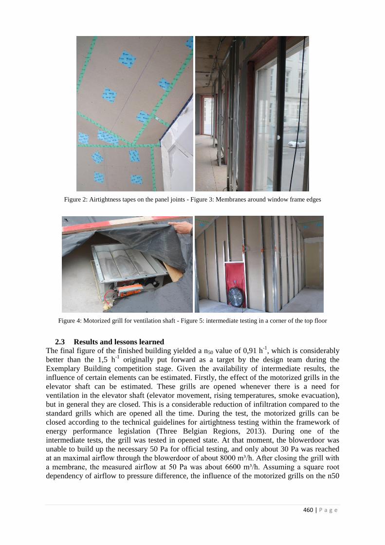
460 | P a g e

Figure 2: Airtightness tapes on the panel joints - Figure 3: Membranes around window frame edges

Figure 4: Motorized grill for ventilation shaft - Figure 5: intermediate testing in a corner of the top floor

2.3 Results and lessons learned

The final figure of the finished building yielded a n50 value of 0,91 h-1

, which is considerably

better than the 1,5 h-1

originally put forward as a target by the design team during the

Exemplary Building competition stage. Given the availability of intermediate results, the

influence of certain elements can be estimated. Firstly, the effect of the motorized grills in the

elevator shaft can be estimated. These grills are opened whenever there is a need for

ventilation in the elevator shaft (elevator movement, rising temperatures, smoke evacuation),

but in general they are closed. This is a considerable reduction of infiltration compared to the

standard grills which are opened all the time. During the test, the motorized grills can be

closed according to the technical guidelines for airtightness testing within the framework of

energy performance legislation (Three Belgian Regions, 2013). During one of the

intermediate tests, the grill was tested in opened state. At that moment, the blowerdoor was

unable to build up the necessary 50 Pa for official testing, and only about 30 Pa was reached

at an maximal airflow through the blowerdoor of about 8000 m³/h. After closing the grill with

a membrane, the measured airflow at 50 Pa was about 6600 m³/h. Assuming a square root

dependency of airflow to pressure difference, the influence of the motorized grills on the n50

461 | P a g e

value is 0,3 h-1, corresponding to an airflow of 1800 m³/h at 50 Pa. This proves the importance

of this kind of device to achieve airtight buildings.

A second influence was the effect of the air-water heat pump. The air intake of this device

was combined with the air intake of the ventilation air handling unit. While the latter can be

sealed off during testing according to the method A of the European norm (NBN, 2001)

which is to be used for official testing in Belgium (Three Belgians Regions, 2013), this is not

the case for the former. As a result, this combined air intake had to be left open during

measurement, giving rise to infiltration via the metal casing of the heat pump device. By

measuring both with opened and closed air intake, this effect could be quantified to an airflow

of about 550 m³/h at 50 Pa, corresponding to a difference of about 0,1 h-1

on the n50 value.

Thirdly, the infiltration airflow through the chinks around doors has been evaluated. By

taping all around the doors (in this case, the double entrance door and 3 doors in the

basement), it could be established that an airflow of about 700 m³/h at 50 Pa passed through

these openings around the – at that time unfinished – doors. This shows the importance of

taking the necessary measures (automatic drop seals, flexible draught strips, brushes, filling

up voids around door locks) for doors.

Table 1: Key data on the case studies

European Foundation House (EFH) Police office Tritomas

Building owners European Foundation House Zone de police 5342 : Uccle, Watermael-

Boitsfort et Auderghem

Architects GREENARCH architecture +

environment sprl

bg&k associati

Engineers MATRIciel, Delvaux Crea-tec sprl

Contractors Valens-Eiffage CFE

Location Brussels Watermael-Boitsfort

Gross building area 2.229 m² 2.327 m²

Start of works 1/12/2012 1/1/2013

Completion of works 9/10/2013 1/1/2014

Energy demand for heating 15 kWh/m²/yr 24 kWh/m²/yr

Energy saving strategy Interior insulation, window replacement,

mechanical ventilation with heat

recovery, air-water heat pump, use of

radiant ceilings and thermal inertia of the

structure

Interior insulation, window replacement,

mechanical ventilation with heat

recovery, PV panels, geothermal heating

and cooling, chilled beams

3 CASE STUDY 2: POLICE OFFICE TRITOMAS

3.1 Project description

Converting a former telephone exchange building into a modern and sustainable police

station, was the challenge of the Tritomas project. Given the modernist architecture, which

can be considered as part of Brussels architectural partrimony, the choice was made to

maximally preserve the building’s exterior, shown in Figure 6. More details of the building

are listed in Table 1.

462 | P a g e

Figure 6: Entrance of the Police Office Tritomas

3.2 Airtightness approach

The technical measures to come to an airtight building were very similar to the first case

study, with the use of internal insulation, new windows provided with airtight membranes,…

Particular to this project, was the fact that part of the existing building was not touched during

the renovation project, moreover, this was in use throughout the construction works by

another user (grey zones in Figures 7 and 8). As a consequence, in order to establish good

airtightness for the police station, not only external building envelope, but also internal walls

and doors had to be airtight. In this project, an intermediate airtightness test was performed on

one level (on the first floor, red zone in Figure 8) in order to check the façade concept

(internal plasterboard finishing) and its joints. At the end of the project, a measurement was

performed on the entire project.

Figure 7: Underground floors (left -2, right -1), coloured zones are part of the renovation project,

taken from the test report (Delire et al., 2013)

463 | P a g e

Figure 8: Building floors (left ground floor, right +1), coloured zones are part of the renovation project,

taken from the test report (Delire et al., 2013)

3.3 Results and lessons learned

The result of the intermediate test showed clearly that the applied concepts of façade

insulation and window-wall joints for the tested floor were sound, yielding a n50 of 0,73 for

the tested volume. However, during the testing of the entire building, interaction with the

untouched building volume influenced the results. Indeed, during the testing, all doors within

the tested volume were opened to enable internal air circulation during the test, and doors to

the untouched volume were closed, as shown in Figure 9. As the previous case study showed,

doors can influence the airtightness to an important extent. Even when care is taken during

selection and installation of the doors – most of the doors were escape exits and had to

comply to fire regulations as well – some infiltration losses are inevitable. Given the complex

geometrical interface between the tested volume and the untouched volume and the number of

doors, the final result of 1,08 h-1

is a very good result, compared to the initial target of 1.5 h-1

.

Figure 9: Opened and closed internal doors on the first floor, taken from the test report (Delire et al., 2013)

464 | P a g e

4 GENERAL TRENDS

The dataset of the Exemplary Buildings currently contains information on the measured

airtightness of 26 completed tertiary Exemplary Buildings, of which 11 buildings are

renovation projects. The entire Exemplary Buildings dataset considers residential buildings

as well, however they are not considered in the scope of this article. Also, the design and

construction time of tertiary buildings, generally several thousands of square meters,

overspans several years, explaining the limited number of completed buildings.

Figure 10 shows the range of building airtightness values measured in the completed

buildings, for both new built and renovation projects. It is expected and clearly visible that

new built projects have better airtightness, however, our case studies (boxed in the graph) and

other renovation projects show that also for renovation projects low n50 values are feasible.

Figure 10: Range of measured building airtightness for new built and renovation in the Exemplary Buildings

program. Case studies are indicated in the dotted boxes (case study EFH = number 176, Tritomas = number 180)

Although the dataset for this particular type of buildings is relatively small – too limited to

perform full statistical analysis – the overall results of the Exemplary Buildings program

indicate a learning effect throughout the years, which is shown in Figure 11. As a complement

of information, this effect can also be noticed in the dataset for new built Exemplary projects

in Figure 12.

465 | P a g e

Figure 11: Evolution of airtightness of renovated tertiary buildings in time,

dataset of the Exemplary Buildings program

Figure 12: Evolution of airtightness of new built tertiary buildings in time,

dataset of the Exemplary Buildings program

5 CONCLUSIONS

The airtightness is an important factor in the energy demand of buildings, but it is a rather

challenging aspect of building performance, certainly in the case of renovation projects. The

Exemplary Buildings program of the Brussels Capital Region provides – through case studies

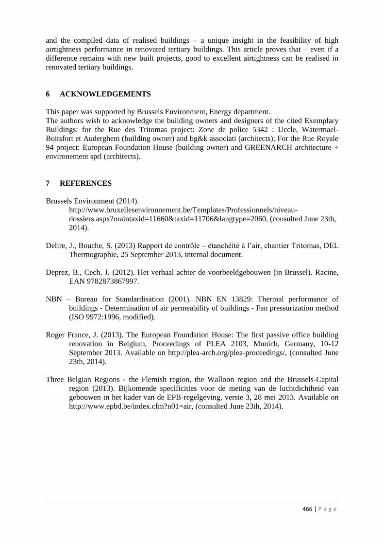
466 | P a g e

and the compiled data of realised buildings – a unique insight in the feasibility of high

airtightness performance in renovated tertiary buildings. This article proves that – even if a

difference remains with new built projects, good to excellent airtightness can be realised in

renovated tertiary buildings.

6 ACKNOWLEDGEMENTS

This paper was supported by Brussels Environment, Energy department.

The authors wish to acknowledge the building owners and designers of the cited Exemplary

Buildings: for the Rue des Tritomas project: Zone de police 5342 : Uccle, Watermael-

Boitsfort et Auderghem (building owner) and bg&k associati (architects); For the Rue Royale

94 project: European Foundation House (building owner) and GREENARCH architecture +

environement sprl (architects).

7 REFERENCES

Brussels Environment (2014).

http://www.bruxellesenvironnement.be/Templates/Professionnels/niveau-

dossiers.aspx?maintaxid=11660&taxid=11706&langtype=2060, (consulted June 23th,

2014).

Delire, J., Bouche, S. (2013) Rapport de contrôle – étanchéité à l’air, chantier Tritomas, DEL

Thermographie, 25 September 2013, internal document.

Deprez, B., Cech, J. (2012). Het verhaal achter de voorbeeldgebouwen (in Brussel). Racine,

EAN 9782873867997.

NBN – Bureau for Standardisation (2001). NBN EN 13829: Thermal performance of

buildings - Determination of air permeability of buildings - Fan pressurization method

(ISO 9972:1996, modified).

Roger France, J. (2013). The European Foundation House: The first passive office building

renovation in Belgium, Proceedings of PLEA 2103, Munich, Germany, 10-12

September 2013. Available on http://plea-arch.org/plea-proceedings/, (consulted June

23th, 2014).

Three Belgian Regions - the Flemish region, the Walloon region and the Brussels-Capital

region (2013). Bijkomende specificities voor de meting van de luchtdichtheid van

gebouwen in het kader van de EPB-regelgeving, versie 3, 28 mei 2013. Available on

http://www.epbd.be/index.cfm?n01=air, (consulted June 23th, 2014).

467 | P a g e

MONITORING THE ENERGY- & IAQ

PERFORMANCE

OF VENTILATION SYSTEMS IN DUTCH

RESIDENTIAL DWELLINGS

Rob C.A. van Holsteijn, William L. Li,

ABSTRACT

MONICAIR --MONItoring & Control of Air quality in Individual Rooms-- is a pre-competitive field research

project of a broad consortium of Dutch ventilation unit manufacturers and research institutes, supported by the

Dutch government. The aim is to investigate the indoor air quality (IAQ) performance and energy characteristics

of 9 different mechanical ventilation solutions in dwellings that meet strict air-tightness standards and comply

with current building regulations. Over a full year 62 residential dwellings were monitored, with in each

habitable room sensors for occupancy, CO2, relative humidity and air temperature. Energy consumption of the

mechanical ventilation units and space heating boilers were also continuously monitored. The ventilation

solutions included mechanical exhaust ventilation (MEV) systems (mechanical exhaust in the wet rooms, and

with natural air supply in habitable rooms), systems with mechanical exhaust in all rooms, as well as local and

central balanced (MVHR) systems with various types of control systems. Sampling and data evaluation were

handled by specialists. The monitoring part of the MONICAIR project is nearing completion and the first results

are now available.

The data show that (from the ventilation systems under investigation) systems with mechanical air supply and/or

exhaust provisions for each individual room are more robust in maintaining certain IAQ-levels, whereas systems

with only natural air exchange provisions in the habitable rooms show larger variations in IAQ and depend to a

large degree on the number and behaviour of inhabitants. In dwellings with MEV-systems the CO2 concentration

in the average habitable room is 380 ppm above the limit value of 1200 ppm during 10% of the heating season

(515 of 5088 hours). If inhabitants spend only half of the time at home, then 20% of this time the air exchange is

insufficient. Looking at individual houses these percentages vary from 2% to over 50%. In dwellings with

MVHR systems the CO2 concentration in the average habitable room is 320 ppm above the limit value of 1200

ppm during 4.6% of the heating season (237 of 5088 hours). Again, if inhabitants spend half of the heating

season indoors and at home, 9.2% of these hours have insufficient air exchange. Per dwelling this figure varies

from 0.1% to more than 20%.

Looking at the energy performance of the ventilation systems under investigation, monitoring data show that

also in this respect significant differences occur. The average primary energy consumption for mechanical

ventilation without heat recovery is 125 MJ/m2. For the ventilation systems with heat recovery the average

primary energy consumption is 22 MJ/m2.

KEYWORDS

Ventilation systems, Monitoring, IAQ-performance, energy-performance

1. INTRODUCTION

The built environment accounts for approximately 40% of the EU total energy consumption

with space heating as the largest contributor (>50%). Not surprisingly, EU-legislation focuses

on increasing the insulation levels and improving the air tightness of buildings. As a result,

Van Holsteijn en Kemna BV (VHK)

Elektronicaweg 14

2628 XG Delft, Netherlands

Consortium member and project manager MONICAIR

e-mail address: [email protected]

468 | P a g e

the contribution of air infiltration to Indoor Air Quality (IAQ) is reduced and ventilation

systems become more and more the sole responsible for the IAQ. Relevant question in the

light of this development is: “How well do ventilation systems perform in terms of IAQ and

energy consumption in well insulated and air tight dwellings in real life, and how can their

performance be further improved?” Past research has focussed on compliance with standards

at nominal conditions -- and improvements are certainly necessary there [1] – but research on

IAQ and energy performance at real life conditions is definitely scarce [2,3]. While housing

stock is being improved in terms of insulation and air tightness as we speak, we do not know

whether ventilations systems sufficiently perform and are capable to compensate for the

reduced infiltration.

To answer these key questions, a consortium of manufacturers and specialized

consultancy firms from the Dutch ventilation industry was established that initiated the long

term monitoring project “MONICAIR” (MONItoring & Control of Air quality in Individual

Rooms). MONICAIR is a 1,6 million euro research project, partly financed by the consortium

members and partly by the Dutch Ministry of Economic Affairs within the framework of TKI

(Top consortia for Knowledge & Innovation). One of the aims of the monitoring project is to

assess the real life IAQ performance in all individual rooms during presence of the occupants

and the related primary energy consumed by the ventilation system. The assumption is that

with a full analysis of the acquired monitoring data, system parameters can be identified that

can help the participating manufacturers further improve their ventilation systems on both the

IAQ- and energy performance. This paper reports the first results from a full year monitoring,

covering nine commonly used ventilation systems in Dutch residential dwellings. Before the

start of the monitoring project, all ventilation systems were checked and – when necessary -

adjusted according to building code practice, thus securing correct system specifications and

ensuring that possible design- or installation errors do not influence performance.

2. SELECTION OF VENTILATION SYSTEMS AND DWELLINGS

Ventilation systems

The manufacturing partners in the MONICAIR consortium produce both type C (MEV) and

type D (MVHR) ventilation systems. Most commonly used in the Netherlands is ventilation

system type C (mechanical extraction in wet rooms combined with natural air supply vents in

habitable rooms). Ventilation systems type D (mechanical air extraction and mechanical

supply) are applied in the new built sector when the budget allows for more expensive

ventilation systems. Both types of ventilation systems are selected for the monitoring study,

both with their specific variants and combinations as described in Table 1. The table describes

per type of ventilation system 1) the air exchange provisions in both the wet rooms

(bathroom, kitchen, toilets) as well as the habitable rooms (living room, bedrooms), 2)

whether heat recovery is applicable and 3) what type of controls are used for the exhaust and

supply provisions. The system type numbers refer to classification used in the Netherlands

Standard NEN 8088-1, 2011 [4].

469 | P a g e

Table 1: Type of ventilation systems selected for MONICAIR

System

type

Section of house

that is served

Air exchange provisions Controls

Exhaust Supply Heat

Recovery

Exhaust Supply

Type C ventilation systems

C.1 Whole house Mech. extraction

in wet-rooms

Stnrd nat.supply

vents in hab.rooms

No Manual

3-pos. switch

Manual

C.2c Whole house Mech. extraction

in wet-rooms

wind contrl. nat.

supply in hab.rooms

No Manual

3-pos. switch

Manual

C.4a Whole house Mech. extraction

in wet-rooms

wind contrl. nat.

supply in hab.rooms

No CO2-sensor

in living room

Manual

C.4c Whole house Mech. extraction

in all rooms

wind contrl. nat.

supply in hab.rooms

No CO2-control on

all hab.rooms

Manual

Type D ventilation systems

D.2 Whole house Mech. extraction

in wet-rooms

Mech. supply

in hab.rooms

Yes Manual 3-pos. switch

D.5a Whole house Mech. extraction

in wet-rooms

Mech. supply

in hab.rooms

Yes Manual 3-pos. switch

with CO2-contrl in 2 zones

D.5b Whole house Mech. extraction

in all rooms

Mech. supply

in hab.rooms

Yes CO2 and RH -controlled

ventilation rate in all rooms

Combination of systems

X1/C

Living section: D Mech. extraction

in hab.rooms

Mech. supply

in hab.rooms


ventilation rate in living room

Sleeping section:C.2c Mech. extraction

in wet-rooms

wind contrl. nat.

supply in bedrooms

No Manual

2-pos. switch

Manual

X1/A

Living section: D Mech. extraction

in hab.rooms

Mech. supply

in hab.rooms


ventilation rate in living room

Sleeping section: A Nat. extraction

in wet-rooms

wind contrl. nat.

supply in bedrooms

No No control Manual

Dwellings

Selecting and finding suitable dwellings for the monitoring project proved to be challenging

and could not have been done without the help of the housing corporations. The first

requirement was to find groups of 5 to 6 identical clustered terraced houses with an air

tightness of qv;10 ≤ 1.0 dm3/s.m

2, that all have the same system, which also had to be one of

the ventilation systems selected for the project. Initially the air tightness requirements were

set at a higher level, but blower door tests proved that – although dwelling specifications

stated otherwise – these higher levels of air tightness were not always achieved. The second

requirement was to find inhabitants that were prepared to allow sensors being installed in all

rooms that monitor the IAQ and their behaviour for more than a year. The last requirement

was that all dwellings needed to have the same condensing combi boiler that enable the

monitoring of gas consumption for space heating and domestic hot water (dhw). In dwelling

clusters that complied with the first two requirements but had a different combi boiler, the

combi boilers were replaced. Eventually 62 families with as many dwellings were found

prepared to participate in the MONICAIR project. Before the start of the actual monitoring,

all ventilation systems were checked and adjusted to the latest building code requirements.

The monitoring results can thus also be used to re-evaluate the existing building code

requirements for ventilation.

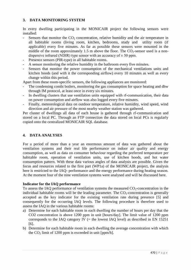
470 | P a g e

3. DATA MONITORING SYSTEM

In every dwelling participating in the MONICAIR project the following sensors were

installed:

- Sensors that monitor the CO2 concentration, relative humidity and the air temperature in

all habitable rooms (living room, kitchen, bedrooms, study and utility room (if

applicable) every five minutes. As far as possible these sensors were mounted in the

middle of the room approximately 1.5 m above the floor. The CO2-sensor used is a non-

dispersive infrared (NDIR) type sensor with an accuracy of ± 50 ppm.

- Presence sensors (PIR-type) in all habitable rooms.

- A sensor monitoring the relative humidity in the bathroom every five minutes.

- Sensors that monitor the power consumption of the mechanical ventilations units and

kitchen hoods (and with it the corresponding airflow) every 10 minutes as well as every

change within this period.

Apart from these room-specific sensors, the following appliances are monitored:

- The condensing combi boilers, monitoring the gas consumption for space heating and dhw

through IM protocol, at least once in every six minutes.

- In dwelling clusters that use ventilation units equipped with rf-communication, their data

on power consumption and airflow was also logged every five minutes.

- Finally, meteorological data on outdoor temperature, relative humidity, wind speed, wind

direction and air pressure of the most nearby weather station was gathered.

Per cluster of dwellings all data of each house is gathered through rf-communication and

stored on a local PC. Through an FTP connection the data stored on local PCs is regularly

copied onto the centralized MONICAIR SQL database.

4. DATA ANALYSES

For a period of more than a year an enormous amount of data was gathered about the

ventilation systems and their real life performance on indoor air quality and energy

consumption, as well as data on consumer behaviour regarding the preferred temperature per

habitable room, operation of ventilation units, use of kitchen hoods, and hot water

consumption pattern. With these data various angles of data analysis are possible. Given the

focus and resources related to the first part (WP1a) of the MONICAIR project, the analysis

here is restricted to the IAQ- performance and the energy performance during heating season.

At the moment four of the nine ventilation systems were analysed and will be discussed here.

Indicator for the IAQ performance

To assess the IAQ performance of ventilation systems the measured CO2-concentration in the

individual habitable rooms will be the leading parameter. The CO2-concentration is generally

accepted as the key indicator for the existing ventilation rate during presence [5] and

consequently for the occurring IAQ levels. The following procedure is therefore used to

assess the IAQ in the various habitable rooms:

a) Determine for each habitable room in each dwelling the number of hours per day that the

CO2 concentration is above 1200 ppm in unit [hours/day]. The limit value of 1200 ppm

corresponds to the IAQ category IV (= the lowest IAQ level) as described in EN 15251

[6].

b) Determine for each habitable room in each dwelling the average concentration with which

the CO2 limit of 1200 ppm is exceeded in unit [ppm/h].

471 | P a g e

c) Calculate the CO2 excess dose per heating season in kppmh by multiplying the outcome

of a) with the outcome of b) and then multiplying the result with the number of days in a

heating season (212) and dividing it with 1000 to convert the ppm-figure to kppm.

d) Add all the CO2 excess doses per habitable room per dwelling and divide it with the

number of rooms of that specific dwelling to determine the average achieved IAQ level

per dwelling.

(Note 1: The calculations for a) and b) are made with a resolution of five minutes and

summarised to obtain either the number of hours per day or the excess value per hour. Note 2:

This procedure is comparable to the methodology used in the declaration of equivalence of

the VLA [7])

Indicator for the Energy performance

The indicator for the Energy performance of the ventilation systems is obtained according to

the following procedure:

I) Determine the total average hourly mechanical ventilation rate of all ventilation units in

the dwelling (kitchen hood excluded).

II) Determine the hourly average of the indoor temperatures and indoor humidity of the

sleeping section and the living section separately and use these two values to calculate the

average indoor climate conditions.

III) Determine the hourly average of the outdoor climate conditions, in casu air temperature,

relative humidity and air pressure (data from the Royal Netherlands Meteorological

Institute)

IV) Calculate the thermal energy exchange per hour on the basis of I), II) and III) in relation

to the hourly temperature difference between indoors and outdoors (ΔTin-out).

For systems with heat recovery this energy figure is corrected with the heat recovery

efficiency as determined according to EN 13141-7 and -8.

V) Calculate the total daily thermal energy exchange in relation to the daily average ΔTin-out.

VI) Calculate the total primary energy consumption for mechanical ventilation for an average

heating season by multiplying the daily average thermal energy exchange (the value

corresponding to the annual average ΔTin-out of 13°C) by 212 days (duration of the

heating season) and divide this figure by the average system efficiency of 85% (for

condensing heating system with limited distribution losses); add to this figure the total

power consumption of all ventilation units during heating season, after converting it to

primary energy.

VII) Divide the outcome of VI) with the total heated surface area of the dwelling to obtain the

average energy consumption of the mechanical ventilation system per m2 during heating

season.

Note : Energy consumption related to cross ventilation (air that enters the dwelling through

infiltration or airing on one façade and leaves through another façade) is not included; also

internal and solar gains are not included in this assessment of the energy performance.

5. RESULTS

IAQ-performance

So far, data of four ventilation systems have been analysed on IAQ performance and energy

performance. The following graphs give an overview of the results.

472 | P a g e

Ventilation system C.2c

Figure 1. IAQ performance of ventilation system C.2c in six comparable dwellings

The arithmetic mean of the IAQ performance of these six houses with ventilation system C.2c

is 181 kppmh. This average is very much influenced by dwelling number 6. The qualitative

data that was gathered through face-to-face interviews before the start of the monitoring

project however show, that there are valid reasons for the high kppmh figure. The intake

interview reveals that, compared to the other dwellings, people in house nr. 6 stay at home for

much longer periods per day, they keep the vents in the bedrooms closed during presence and

airing of the room is less frequent than in the other houses.

Ventilation system C.4a

Figure 2. IAQ performance of ventilation system C.4a in five comparable dwellings

The arithmetic mean of the IAQ performance of these five houses with ventilation system

C.4a is 215 kppmh. Without dwelling nr.4 (Passive Stack Ventilation (PSV) system) the mean

value is 238 kppmh. Also in this cluster the average is largely influenced by dwelling nr. 5

where people also stay at home for much longer periods per day. The inhabitants state in the

473 | P a g e

intake interview that the air vents in the bedrooms are open, but the CO2 concentrations of the

bedrooms suggest that they are closed when people are present. Ventilation system D.2

Figure 3. IAQ performance of ventilation system D.2 in six comparable dwellings

The arithmetic mean of the IAQ performance of these six houses with ventilation system D.2

is 54 kppmh.

Ventilation system D.5a

Figure 4. IAQ performance of ventilation system D.5a in six comparable dwellings

The arithmetic mean of the IAQ performance of these six houses with ventilation system D.5a

is 98 kppmh. In dwelling 6 the size of the air supply opening in bedroom 3 was reduced after

the start of the project, resulting in a higher CO2-excess dose for that particular room and

consequently for the whole dwelling.

474 | P a g e

Energy performance

The energy performance of each ventilation system is determined according to the method

described under the paragraph ‘Data analyses’, and presented in the graph below. The

electricity consumption of the mechanical ventilation units during a heating season is

displayed separately from energy related to the air exchange.

Figure 5. Energy performance of the ventilation systems

6. CONCLUSIONS

Data analyses will continue for the other five ventilation systems (thirty-nine dwellings), but

based on the results of the four systems analysed so far, it can already be concluded that there

are significant differences in both the real-life IAQ- and energy performance of ventilation

systems.

475 | P a g e

Figure 6. IAQ- and energy performance of the ventilation systems

The differences in energy performance are evident. For the average EU-heating season (ΔTin-

out = 13°C) the average primary energy consumption for ventilation is 22 MJ/m2 for systems

with heat recovery and 125 MJ/m2 for systems without heat recovery. Further analysis will be

necessary to determine if the use of IAQ-sensors has an effect on the energy performance.

The preliminary analyses furthermore suggest that systems with mechanical air supply and/or

exhaust provisions in each room are more robust in maintaining a certain IAQ- performance

compared to systems that use only natural air exchange provision in habitable rooms. Systems

with natural air exchange provisions in habitable rooms achieve an average CO2 excess dose

of 196 kppmh in each habitable room per heating season, whereas systems with a mechanical

component serving either the air supply and/or exhaust in each room achieve 76 kppmh.

In terms of time spent in rooms with insufficient air exchange, this means that:

- In dwellings with MEV-systems combined with only natural air exchange provisions in

habitable rooms, the CO2 concentration in the average habitable room is 380 ppm above

the limit value of 1200 ppm during 10% of the heating season (515 of 5088 hours). Since

inhabitants are not continuously at home, this percentage will be higher when related to

the actual time spent at home. If the occupants are only 12 hours per day at home (2544

hours per heating season), then 20% (515/2544) of this time the air exchange is

insufficient. Looking at individual houses these percentages vary from 2% over 50%.

- In dwellings with MVHR-systems the CO2 concentration in the average habitable room is

320 ppm above the limit value of 1200 ppm during 4.6% of the heating season (237 of

5088 hours). Again, if inhabitants spend half of the heating season indoors and at home,

9.2% of these hours have insufficient air exchange. Per dwelling this figure varies from

0.1% to more than 20%.

476 | P a g e

7. DISCUSSION

Current practice is that ventilation systems are primarily selected on the basis of their

purchase- and installation costs. Building codes determine the minimal level of air exchange

rates that must be installed as well as its minimal energy performance level (EPBD-

legislation). But whether ventilation systems actually deliver the required air exchange rates

in the right rooms at the right times is not a topic or a criterion in selecting ventilation

systems. More monitoring studies will certainly be necessary but the preliminary results argue

in favour of an approach that looks more specifically at the real-life IAQ-performance of the

various systems, especially with a building stock that is becoming more insulated and more

air tight. Furthermore, like with all other energy using products, the energy performance of

ventilation systems can only be compared between systems that have equal IAQ-performance.

Without an IAQ assessment we are comparing apples with oranges. Further discussion on the

method for determining the IAQ-performance will be necessary as well as discussions on the

limit values and IAQ- classes than can be set as guidelines.

8. ACKNOWLEDGEMENTS

This paper was prepared within the MONICAIR project part WP1a. The project is partly

financed by the consortium members and partly by the Dutch Ministry of Economic Affairs

within the framework of TKI (Top consortia for Knowledge & Innovation). Particular thanks

are due to the consortium members and their representatives involved in this part of the

MONICAIR study:

Jelmer de Jong and Rudolf Tolj (Brink Climate Systems BV), Peter Schabos, Rutger Vasters

and Rolf-Jan Hans (ClimaRad BV), Hans van Klooster and Roelof Ziengs (Honeywell

Customized Consumer Products), Leon van Bohemen, Jan Rijnbeek and Douglas Budde (Itho

Daalderop BV), Harm Valk (Nieman Raadgevende Ingenieurs), Wim Kornaat (TNO), Bart

Cremers and Rick Bruins (Zehnder Group Nederland BV).

The MONICAIR consortium further owes thanks to Peter Cool (Intergas Verwarming BV) for

his support on the data monitoring of the boilers, to Robèrt de Haas (Alparo) for his patience

and support in developing the MONICAIR database and queries, to Wilbert van den Eijnde

(Consumersvoice) for the face-to-face interviews with all the inhabitants and finally to the

housing corporations for their support in the selection of dwelling for this part WP1a of the

MONICAIR project: Barry Top (De Woonplaats), Gerben Heering (WBO) and Winfried van

Emmerik (WSDH).

9. REFERENCES

[1] Janssens, A., Carrié F.R., Durier, F. ed. (2013). Securing the quality of ventilation

systems in residential buildings: existing approaches in various countries, Edited

proceedings of the AIVC-Tightvent international workshop, Brussels.

[2] Savin J.L., Bernard A., (2009). Improvement of the ventilation and building

airtightness performance in occupied dwellings in France, 4th

International Symposium

on Building and Ductwork Air Tightness – BUILDAIR, Berlin.

[3] De Gids, W.F., Op ’t Veld, P.J.M., (2004). Onderzoek naar ventilatie in relatie tot

gezondheidsaspecten en energieverbruik voor een representatieve steekproef van het

Nederlandse woningbestand.

477 | P a g e

[4] NEN 8088, (2011). Ventilation and infiltration for buildings – Calculation method for

the supply air temperature corrected ventilation and infiltration are volume rates for

calculating energy performance – Part 1: Calculation method.

[5] De Gids, W.F., Wouters, P., (2010). CO2 as indicator for the indoor air quality,

General principles, AIVC Paper N° 33.

[6] EN15251 (2007). Indoor environmental input parameters for design and assessment of


lighting and acoustics.

[7] Vereniging Leveranciers Luchttechnische Apparaten, VLA, (2012). VLA methodiek

gelijkwaardigheid voor energiebesparende ventilatieoplossingen in woningen.

478 | P a g e

DUCTWORK AIRTIGHTNESS: RELIABILITY OF

MEASUREMENTS AND IMPACT ON VENTILATION

FLOWRATE AND FAN ENERGY CONSUMPTION

Sylvain BERTHAULT*1

, Florent BOITHIAS1, Valérie LEPRINCE

2

1 CEREMA

Direction Territoriale Centre-Est 1 Boulevard Giberstein 71404 Autun, FRANCE


2 PLEIAQ 84 c Avenue de la Libération 69330 Meyzieu, FRANCE

ABSTRACT

Reduction of energy consumption and green house gas emissions of buildings is a great challenge in Europe. In

this context French energy performance regulation, RT2012, requires an improvement of the buildings'

airtightness. In airtight buildings, ventilation must be perfectly controlled to ensure good indoor air quality.

However, many failures are observed when ventilation systems are inspected (Jobert, 2012). They are mainly

due to bad conception, poor implementation and lack of maintenance. Most of the time, dysfunction leads to a

reduction of the ventilation flowrates and to poor indoor air quality. To improve the ventilation systems' reliability, French energy label “Effinergie +” imposes the ductwork

airtightness to be at least Class A. This leads to various issues regarding ductwork airtightness: - What is the impact of each component of a ductwork on the leakage rate? Is good airtightness reachable

with existing products? - What is the impact of airtightness on ventilation flowrate and fan energy consumption? - Are ductwork pressurization tests reliable? Do the position of the measurement devices, leakage

distribution and ductwork pressure drop have an impact on the result of the test?

To answer those questions a full-scale exhaust ductwork of multi-family building was set in our laboratory. The

impact of each components of the ductwork (rigid, circular GALVA) was tested. Holes were then drilled in the

ductwork to vary airtightness. Our study showed that:

- Even with good implementation it is difficult to reach class C for ductwork airtightness because of some

leaky components in the ductwork; - A decrease of the airtightness (from class C to 1,6*class A) may either reduce flowrates by 10% at the

air terminal devices or increase the energy consumption of the fan by 10 to 40% ; - Neither the position of the fan, nor the leakage distribution, nor the pressure drop has an impact on the

result of the airtightness test (at class C and 1,6*class A).

KEYWORDS

Ventilation – Airtighness – Ductwork – Implementation – Measurement

1 INTRODUCTION

The improvement of thermal regulation in France leads to more and more efficient and

airtight buildings. Therefore, an issue which was forgotten till recently is becoming crucial:

how to ventilate buildings well enough to ensure healthy indoor air (Kirchner et al., 2011) and

durable building structure while keeping good energy performance?

479 | P a g e

To achieve such opposite targets, new mechanical ventilation systems were designed with

growing complexity. These systems make it possible to meet both sanitary and energy targets

provided that they are very well implemented and maintained.

However, literature shows that design, implementation and maintenance are often neglected

(Jobert, 2012; Lucas et al., 2009; Save-Duct, 1999; Observatoire CSTB-ORTEC, 2009).

Ventilation systems' quality therefore becomes a growing concern because of observed

dysfunctions, which highlight a need for information and technical support to professionals

together with control of the proper operation of these systems. The ductwork airtightness is

one of the various implementation issues.

In such a context, this study aims to better understand:

1. The airtightness of ductworks and its impact on flowrates and fan consumption

2. The reliability of ductwork airtightness tests

by implementing a simple flux ventilation ductwork in our laboratory. This ductwork

represents a small collective housing's system which is described in the following section.

2 DESIGN OF THE DUCTWORK STUDIED

The ductwork is made of two main columns which are supposed to connect to four dwellings

of different sizes (figure 1 and 2). Each dwelling included a kitchen and a bathroom both

connected to ventilation.

The ductwork was made of:

Circular GALVA ducts

Specific elements with joint such as curves, branch connections, dampers, T-

connections, inspection hatches, conical reduction, ... (figure 3)

A "C.VEC micro-watt +" extraction fan and automatic constant-flow regulated

terminal devices

The extraction fan is a constant pressure one. This means that it automatically adapts its speed

to maintain a constant pressure when the flowrate varies (when kitchen terminal devices open

and close).

Figure 1: The ductwork studied

480 | P a g e

Figure 2: Outline of the ductwork

3 METHODOLOGY

3.1 Impact of airtightness

3.1.1 Impact of each specific element of the ductwork on airtightness

The aim was to quantify the leakages of each specific element of the ductwork (figure 3). The

methodology was as follows:

1. Connect each specific element one by one

2. Measure airtightness after each element is connected without being screwed (20

measurements were carried out)

3. Measure airtightness after each element is connected and screwed (20 measurements

were carried out)

481 | P a g e

GALVA ducts Damper Roof T-

connections

T-connections Inspection hatch

Simple connection Plug Curve Conical reduction Branch connection

Figure 3: Specific elements tested in this study

3.1.2 Impact of the airtightness level on ventilation flowrates and fan energy

consumption

The aim was here to quantify the fan's energy overconsumption due to a decrease of the

ductwork's airtightness, and the associated impact on ventilation flowrates observed at air

terminal devices.

The methodology consisted in measuring flowrates and the fan's energy consumption in the

following conditions:

1. Ductwork airtightness: class C, B, A and 1.5 * class A (from class C, the ductwork was

drilled to reach other classes)

2. Pressure setpoint of the fan: 90 Pa and 120 Pa

3.2 Reliability of ductwork airtightness test

3.2.1 Impact of pressure drop in the ductwork

The aim was to quantify the impact of pressure drop in the ductwork on the result of the

airtightness test. To induce pressure drop, two dampers were placed in the ductwork (see

figure 4). Measurements were carried out in the following configurations:

1. Ductwork airtightness: class C and 1.5 * class A

2. Dampers' position: 7 different positions from closed to open position

The pressure drop due to the damper was estimated by measuring the pressure variation at an

air terminal device. Leakages were equally distributed along the ductwork.

3.2.2 Impact of leakage distribution and location of the measurement device

The aim was to quantify the impact of leakage distribution and location of the measurement

device on the result of the airtightness test.

Four different leakage distributions inducing approximately the same airtightness level were

tested:

482 | P a g e

1. Concentrated leaks close to the fan

2. Concentrated leaks at the bottom of columns 1 and 2

3. Concentrated leaks at the bottom of column 2

4. Equally distributed leaks all along the ductwork

Leakages were created by drilling.

Tests were carried out by placing the measuring device at three different locations:

1. By the fan

2. On column 1

3. On column 2

4 RESULTS

4.1 Impact of airtightness

4.1.1 Impact of each specific element of the ductwork on airtightness

Main leaks were observed at (figure 4):

Roof T-connections

Dampers

Even with careful implementation, the ductwork was only class B if the plug of the roof T-

connection was not tightened with tape. With tape on the plug, the ductwork reached class C.

It was also observed that elements were slightly leakier when screwed than when just

connected together.

Figure 4: Leakage rates of specific elements

Damper

Damper

483 | P a g e

4.1.2 Impact of the airtightness level on ventilation flowrates and fan energy

consumption

Figure 5: Operating conditions of the ductwork with airtightness varying from class C to 1.5 * class A

(pressure setpoint at the fan: 90 Pa)

The first result, shown on Figure 7, is that flowrate targets are no longer met for 4 of the

terminal devices for a 90 Pa pressure setpoint at the fan if the ductwork is class 1,5 * A, while

it is met when it is class C. For this configuration, the leaky ductwork would lead to a lack of

ventilation and maybe poor indoor air quality.

Figure 6: Operating conditions of the ductwork with airtightness varying from class C to 1.5 * class A (pressure

setpoint at the fan: 120 Pa)

484 | P a g e

Figure 7: Flowrates at terminal devices with airtightness varying from class C to 1.5 * class A

Flowrate targets:

Terminal devices 1, 5 and 7: 45 m3/h

Terminal devices 2, 6 and 8: 30 m3/h

Terminal device 3: 20 m3/h

Terminal device 4: 15 m3/h

Thus, to maintain the flowrate target at air terminal devices, when the airtightness of the

ductwork decreases, it is necessary to change the setpoint of the fan from 90 Pa to 120 Pa. We

can see from figures 5 and 6 that it leads to an increase of the fan's power from 40 W to 50 W

(comparing with class C consumption).

Moreover, when airtightness varies from class C to 1.5 * class A and the fan is set at 120 Pa,

the fan's energy consumption increases by 12%.

Therefore, for this configuration, poor airtightness can either lead to an overconsumption of

fan of 40% (16W) or to flowrates not complying with the regulation.

4.2 Reliability of ductwork airtightness test

4.2.1 Impact of pressure drop in the ductwork

Even if the damper's position induces a high pressure drop in the ductwork, as can be seen in

figure 8, it does not significantly affect the result of the ductwork airtightness test, as shown

in figures 9 and 10, at airtightness levels of class C and 1.5 * class A.

For this ductwork, at class C, the damper's position has no impact at all (see figure 10). At

1.5 * class A, the results of the test is 15% smaller when the two dampers are closed

compared to when they are open.

An interpretation could be that it depends to the tightness of the damper with respect to the

tightness of the ductwork. A mathematical model could be set to explain this phenomenon.

485 | P a g e

CVEC 90 Pa CVEC 120 Pa0

20

40

60

80

100

120

140

93,0

128,0

92,8

126,5

86,8

125,2

92,2

108,6

50,9

71,7

19,4

28,2

7,29,5

Pressure at the airterminal devices (top of columne 2) according damper position

Low Flowrate - Ductwork airtightness: class C

Registre position 0

Registre position 1

Registre position 2

Registre position 3

Registre position 4

Registre position 5

Registre position F

Pre

ssur

e (

PA

)

Figure 8: Pressure at the kitchen's terminal device (top of column 2) as a function of the damper's position

Figure 9: Leakage flowrate of the ductwork as a function of the damper's position at 1.5 * class A (position 0:

open; position F: closed)

486 | P a g e

Figure 10: Leakage flowrate of the ductwork as a function of the damper's position at class C (position 0: open;

position F: closed)

4.2.2 Impact of leakage distribution and location of the measurement device

Figure 11 shows that the location of the measurement device does not modify the result of the

ductwork airtightness test whatever the leakage distribution is.

Leakage equally distributed

Leakage at the bottom of column 1 and 2

Leakage at the bottom of column 2

Leakage at the fan

0

10

20

30

40

50

60

70

59,3 58,857,5

59,2 60,057,6

52,2

58,3 58,957,0

52,4

Impact of the position of measurement devices with respect to the leakage repartition

Measurement pressure: 120 Pa

Measurement

device on

column 2

Measurement

device on

column 1

Measurement

device at fan

Le

aka

ge

flo

wra

te (

m3

/h a

t 1

20

Pa

)

Figure 11: Leakage flowrate as a function of leakage distribution and location of the measurement device at 1.5 *

class A

5 CONCLUSIONS

In its first part, this study showed that a careful implementation of the ductwork only makes it

possible to reach class B. To achieve class C it is necessary to treat roof T-connections with

tape.

487 | P a g e

Moreover, the airtightness level of the ductwork has proved to have a major impact on the fan

consumption (till 40% in this case). Furthermore, if the ductwork is too leaky the flowrate

target at air terminal devices may not be reached which may have a major impact on indoor

air quality. In its second part, regarding the ductwork airtightness test, this study concluded

that for this ductwork, the result of the test is neither influenced by the pressure drop in the

ductwork nor by the location of the measurement device whatever the leakage distribution is.

This study could now be completed by a mathematical model to explain those results.

6 ACKNOWLEDGEMENTS

This study was carried out as an internship for a master degree. A defense took place in June

2014 at Joseph Fourrier University in Grenoble (France). The authors would like to thank

Simon Salager, from Joseph Fourrier University, for his help and the board of examiners.

The contribution of Cerema is funded by the French ministry for ecology, sustainable

development, and energy (MEDDE). The sole responsibility for the content of this publication

lies with the authors. It does not necessarily reflect the opinion of the ministry.

7 REFERENCES

Jobert, R. (2012). La ventilation mécanique des bâtiments résidentiels neufs. Rapport ENTPE

–GBBV, 2012, 91p.

Kirchner et al. (2011). Qualité de l'air intérieur - Dix ans de recherche pour mieux respirer.

Observatoire de la qualité de l'air intérieur (OQAI). Éditions CSTB, 208p.

Lucas et al. (2009). État de la ventilation dans le parc de logements français. Rapport final

DESE/SB, Éditions OQAI, 84 p.

SAVE-DUCT European Project (1999). Improving ductwork – A time for tighter air

distribution systems – Final Report CE DG XVII.

Observatoire CSTB-ORTEC (2005-2009). Rapport de synthèse de la rubrique aération.

488 | P a g e

AIRTIGHTNESS OF BUILDING PENETRATIONS: AIR

SEALING SOLUTIONS, DURABILITY EFFECTS AND

MEASUREMENT UNCERTAINTY

Wolf Bracke

*1, Nathan Van Den Bossche

1, Arnold Janssens

1

1 Ghent University

Jozef Plateaustraat 22

9000 Gent, Belgium


ABSTRACT

During field measurements on the airtightness of passive houses, ventilations system’s roof penetrations showed

to be one of the major leakage paths, as they were not sealed using the appropriate, durable techniques.

Therefore, a series of laboratory measurements was conducted on wood-frame walls to study different air sealing

solutions. The use of special airtight gaskets is compared to less advanced sealing methods such as sprayed

polyurethane foam and the use of pieces of tape.

The airtightness of different solutions is tested on two different test setups at the Test Centre for Façade

Elements, Ghent University. One large-scale setup, designed to measure the air leakage rate of windows, was

used and an additional smaller-scale test setup was built. For both setups, measurement principle, test setup and

results are reported.

As workmanship quality is an essential aspect for achieving airtight building connections, the repeatability of the

sealing methods was addressed by installing multiple identical setups. The quality was reviewed with the use of

a smoke generator and the samples were subjected to multiple water tightness tests under static and pulsating

pressure. To evaluate the durability of the different solutions, the impact of the water tightness tests is discussed.

A classification for the airtightness of building penetrations is reviewed together with the impact of the air

leakage through building penetrations on the overall air leakage of buildings. In the laboratory, all tested

solutions could be classified in the best airtightness classification, though large differences between executions

methods were evident. The use of standard, rigid airtightness tape is not recommended for sealing 3-dimensional

connections such as building penetrations, and is not regarded as a durable sealing method. However, specific

flexible tapes are on the market which perform very well and sprayed PUR also showed excellent results when

executed correctly. EPDM gaskets showed a higher leakage than flexible tape and PUR, but are also a very good

choice. The adaptability of the penetration is a great advantage regarding the durability of the connection.

KEYWORDS

Airtightness, penetrations, laboratory test results, durability

1. INTRODUCTION

A blowerdoor measurement campaign in Belgium on the durability of airtightness of passive

houses (ACH50 < 0.6 upon completion), showed that the average air leakage of the houses had

raised by 30% only two years after completion. Though this raise can be attributed to

durability effects of various building components (windows, doors, …) and interventions of

the inhabitants (installation of outdoor lighting, hanging of paintings, … ), the roof

penetrations were responsible for a significant part of the additional leakage. Large air

489 | P a g e

leakages were observed around the air supply and exhaust pipes of the ventilation system

(Bracke et al., 2013).

In one house, which was tested on a regular basis during 18 months to investigate seasonal

and durability effects, the leaky roof penetration of the air exhaust was replaced with an

airtight, flexible EPDM gasket. This small intervention caused the total air leakage of the

house to drop from 254 to 239 m3/h @ 50 Pa, meaning this one penetration was responsible

for 6% of the overall air leakage.

Even though an air leakage rate of 15 m3/h @ 50 Pa might seem relatively small, as multiple

other roof and wall penetrations can exist (e.g. ventilation ductwork, solar boiler connections,

drain-waist-vents) these can be responsible for a significant share of the total air leakage,

causing energy losses, malfunctioning of the ventilation system, draft and sound insulation

problems.

Though it is clear that problematic connection such as wall-wall, wall-roof and window-wall

interfaces are typically responsible for a larger share of the total air leakage, the leakage

around roof and wall penetrations should not be disregarded. From field measurements it

became clear that with very little effort and investment, a significant improvement could be

achieved.

This paper starts with a review of the research that was published in literature on this topic.

Laboratory measurements were performed on two different scales for which the test method,

test setup and results are reported. Subsequently, test results are compared to an airtightness

classification scale found in literature, and finally workmanship reproducibility and durability

are discussed.

2. LITERATURE REVIEW

A good overall airtightness is considered as an essential requirement to obtain energy efficient

and comfortable buildings. A lot of research has been done on the air leakage of buildings but

little to none focusses on the air leakage of individual building components or building

envelope interfaces. As the total air leakage is the sum of various smaller leakages, the

isolation of a particular building element can help to acquire certain insights so the overall air

leakage can be improved. This approach was also used by Van Den Bossche (Van Den

Bossche et al., 2012) to propose an airtightness classification for different solutions to seal the

window-wall interface, which is often a weak spot in the airtightness of buildings.

Very little is written on the airtightness of building penetrations. In one study performed by

Kalamees (Kalamees et al., 2008), the air leakage distribution of 32 houses in Finland was

analysed qualitatively using thermography and smoke detection. Air barrier penetrations for

ductwork were held responsible for 3 to 10% of the total air leakage, depending on the

building type (detached/apartment) and the presence of other critical connections such as the

junction between intermediate floors and external walls.

To the knowledge of the authors, no test standards, classification systems or performance

requirements exist for air barrier penetrations in the European framework for standards and

codes. The American standard ASTM E2357 describes a test method for the assembly of air

barrier systems, wherein two penetrations are part of a standard test wall, but are not tested

separately.

In the Netherlands, three airtightness performance levels are specified according to NEN

2687: Class 1 (basic), Class 2 (good) and Class 3 (very good, passive houses). SBR, a Dutch

research foundation, has published practical information on how to achieve the different air

tightness classes. For several building components and interfaces, maximum air leakage rates

are available to ensure the feasibility of the aspired maximum overall leakage of the building.

Table 1 shows the maximum leakages for roof, wall and floor penetrations according to

different penetration diameters. The values were derived from an area-based leakage rate for a

gap of a few millimetres around the penetration.

490 | P a g e

Table 1: Maximum penetration leakages according to SBR

Diameter (mm) Air leakage @ 50 Pa (m3/h)

Class 1 Class 2 Class 3

15 9.3 3.4 0.7

25 15.6 5.4 1.1

50 27.8 10.7 2.1

80 91.9 17.1 3.4

100 112.9 21.5 4.3

125 139.7 27.4 5.5

150 167.1 32.2 6.4

200 220.4 43.0 8.6

The air flow of 15 m3/h @ 50 Pa through the 200 mm roof penetration of the air exhaust, as

mentioned in the introduction, can thus be regarded as too high for a Class 3 passive building.

The air sealing probably complied with airtightness Class 3 after installation, but was not

executed in a durable way. The question rises whether durability aspects should be taken into

account when classifying airtightness solutions. Currently, very little is known about the

durability of sprayed PUR foam, tapes and glues and no normative documents exist which

prescribes a test protocol. It is still unclear how artificial ageing correlates with the expected

aging in practice and how mechanical impacts (wind pressures, contractors working on the

penetrations, …) should be translated in standard test protocols. In Germany, the FLiB

(Fachverbandes Luftdichtheit im Bauwesen) is working on a test method to evaluate the

durability of tapes and glues, which should result in a future normative document DIN 4108

part 11. At Ghent University, about 5000 tests on the peel and tear strength of the bonding of

different tapes to different substrates were executed (Van Den Bossche et al., 2009). The

samples were subjected to different temperatures and relative humidity levels in a climate

chamber to evaluate the durability. Large differences in bonding strength were observed, not

only between different products and different substrates, but also between different

manufacturers of very similar products..

3. EXPERIMENTAL RESEARCH

Appropriate sealing materials are available on the market, but in practice, the poorly sealing

of air barrier penetrations can cause significant amounts of air leakage due to the use of wrong

materials and/or bad workmanship. The sealing of certain penetrations is often done by a

variety of contractors, which may have a lack of awareness about the importance of

airtightness.

In the context of a Belgian research project ‘DO-IT’ on wood-frame constructions, laboratory

measurements on the airtightness of wood-frame building components were performed in the

Test Centre for Façade Elements at Ghent University. A part of these measurements focus on

the air leakage of wall penetrations, for which the results are reported in this paper.

Two test setups were used: one large-scale setup where a wood-frame wall was built and a

variety of penetrations were installed together, and one small-scale setup where different

specimens could be installed with one penetration in each specimen.

3.1 Test method and error analysis

A. Large scale test setup

The airtightness of the wall penetrations was measured in a standard calibrated test rig

according to EN 12114. Because the setup is unable to obtain a certain pre-set pressure, the

airflow was measured at 10 random pressure differences in the interval 0 – 600 Pa. The

airflow was derived by measuring the pressure difference over a calibrated orifice opening.

491 | P a g e

These measurement points are controlled for outliers using Chauvenet’s criterion (Taylor,

1982), a power law function is fitted through the results after which the leakage is calculated

for a 50 – 100 – … – 500 Pa pressure difference. A standard deviation is defined, taking into

account the error on airflow measurements and the fitting to a power law.

The air leakage through the tested wall penetrations was not measured separately for every

penetration. Instead, a wall was built in a steel test rig, in which different penetration

diameters and sealing solutions were installed. After each newly installed penetration, an

airtightness test was conducted according to EN 12114. The air leakage of a certain

penetration can be derived by subtracting the air leakage of the previous measurement from

the new measurement. The error on the leakage through the tested penetration will thus be a

combination of the error on the previous and on the new measurement. As the errors are

primarily the result of the fitting of the power law, which is uncorrelated for different

measurements, the total error is calculated by adding in quadrature the errors of both

measurements.

The penetrations tested in Figure 1 are almost perfectly airtight. The power laws fitted

through the measurement points of the previous and the new measurement cross each other,

meaning the test setup is unable to measure the difference between both measurements

accurately.

Figure 1: Measurement principle and calculation of net leakage (2 x EPDM gasket Ø 75 mm)

B. Small scale test setup

The measurements are conducted using a Lindab LT600, a test instrument designed to

measure the airtightness of ductwork and chimneys. The instrument calculates the airflow by

measuring a temperature difference over a hotplate, which is heated and cools down as the air

passes over it. The hot plate principle is a more accurate solution to measure very small

airflows than measuring a pressure difference over an orifice opening.

As the Lindab LT600 is able to measure the airflow at a given pressure difference, no

complete pressure sequence was performed and no power law was derived. Measurements

were taken at 3 pressure differences: 50 Pa, 250 Pa and 500 Pa.

Because the device is designed to test the air leakage of ductwork, it follows EN 12237,

which states that the pressure difference should be applied for 5 minutes to obtain a stable

airflow. The measurements were logged to Excel, and the average airflow is calculated over

the last 2 minutes of the measurement. Every measurement was executed 5 times and the

average value and standard deviation are calculated.

492 | P a g e

Before the measurement of the wall penetrations, the extraneous air leakage through the test

setup is determined. The net leakage through the different specimens is derived by subtracting

the extraneous air leakage from the measured leakage and the standard deviation is calculated

by adding in quadrature the standard deviation of both measurements.

3.2 Test setup


The tests were executed on a full-scale setup built in a steel test rig. A wood-frame wall of

228 cm by 196 cm was built consisting of a framework and exterior sheathing of 18 mm

bituminous impregnated fibreboard. As the fibreboard contains more bitumen than most

similar products, it does not only act as a rain screen, but also as an additional air barrier next

to the interior barrier and provides enough structural stiffness to avoid the need of OSB

sheathing on the interior side. To make an abstraction of the real-world situation, the use of

OSB panels and interior insulation was omitted in the test setup.

Four different penetration diameters were tested: 4 mm (single electrical cable), 20 mm

(ribbed conduit pipe for electrical cables), 75 mm (PVC pipe) and 130 mm (PVC pipe). The

openings for the different penetrations were respectively 6 mm, 22 mm, 85 mm and 140 mm.

Every case was sealed using three different methods

- gasket: A piece of flexible EPDM rubber with an opening smaller than the

penetration’s diameter is stretched over the penetration. The EPDM slab is taped to

the fibreboard using a standard airtightness tape.

- PUR: Flexible polyurethane foam is sprayed with a PU-pistol on the joint between

the penetration and the fibreboard. As the board has a limited thickness, the PUR is

not truly applied in the cavity between the penetration and the wall, but is rather

sprayed on the surface of the fibreboard. Water was sprayed to increase the

humidity, which enhances the expansion of the foam and the bonding to

surrounding surfaces.

- tape: Multiple pieces of tape were radially applied on the fibreboard and

penetration. The tape is designed to seal the 2-dimensional joints of vapour

retarder membrane and consists of a reinforced PE membrane and a acrylate

adhesive.

The last method, which is not typically recommended, was executed to compare test results

with better solutions, and investigate durability effects and workmanship quality. To test the

worst-case scenario, the air leakage without applying any air sealing was also evaluated.

Especially in this case, the diameter of the openings in the fibreboard is of great influence. In

most of the test cases, the penetration was executed multiple times to extract a reliable

average value for the air leakage rate.

Figure 2 shows the tested wall with different penetration diameters and sealing solutions. The

wall is connected airtight to the test rig using butyl-aluminium tape and the joints between the

different fibreboards are also sealed to minimize extraneous air loss and resulting

measurement uncertainty.

493 | P a g e

Figure 2: Wood-frame wall with different air sealing solutions in steel test rig


A small test box measuring 300 x 300 x 300 mm was built using plywood with an epoxy

coating. To minimize extraneous air leakage, silicone sealant and butyl tape are used to seal

every joint. The different test specimens were clamped against the test box and the connection

was made airtight by compressing a closed-cell foam band attached to the specimens.

Figure 3: Small scale test setup

Four specimens were built to test different methods to seal a 75 mm PVC pipe wall

penetration in a 90 mm opening.

- PUR: PUR foam was sprayed in the gap (7,5 mm wide) between the PVC pipe and the

wall element. Plywood with an epoxy coating was attached to a PUR foam board to

provide enough thickness for the expansion of the sprayed PUR.

- gasket: An EPDM gasket with an opening of 55 mm was pulled over the PVC pipe and

taped to the plywood.

- tape (1): The PVC pipe is sealed to the plywood using pieces of tape. The tape is

designed to seal the 2-dimensional joints of vapour retarder membrane and consists of

a reinforced PE membrane and an acrylate adhesive.

tape (2): The PVC pipe is sealed to the plywood using pieces of tape. The elastic tape is

designed to seal difficult corners and 3-dimensional connections and consists of an elastic PE

membrane and a butyl rubber adhesive.

494 | P a g e

Figure 4: Test specimens: tape (1), tape (2), PUR, gasket

3.3 Measurement results


As explained in paragraph 3.1, the calculated net leakages are accompanied by large error

intervals. As different penetrations are tested, and thus additional leakages are created during

the testing sequence, the total air leakage and accompanying errors are increasing. Sometimes,

due to measurement uncertainty, small negative net leakages are calculated for a certain

pressure difference as Figure 1 illustrates. For a better interpretation and comparison, the

calculated leakages at 50 Pa, 250 Pa and 500 Pa and associated standard deviations are

presented in the following tables.

For a first test, the air leakage through the bituminous fibreboard was measured. Joints around

the wall and between the boards were sealed so only the air leakage through the material itself

was measured. Table 2: Test results bituminous impregnated fibreboard

50 Pa 250 Pa 500 Pa

Air leakage σ Air leakage σ Air leakage σ

(m3/h.m

2) (m

3/h.m

2) (m

3/h.m

2) (m

3/h.m

2) (m

3/h.m

2) (m

3/h.m

2)

fibreboard 0.266 0.028 1.249 0.091 2.341 0.160

When a hole is cut out of the fibreboard, airtight tape or EPDM is placed over the board and

the leakage through the test wall will be lower due to a smaller fibreboard surface. In the

following tests, the covered surfaces are measured and multiplied with the measured

characteristic air leakage through the fibreboard. The results are subtracted from the newly

measured air leakage to correct for this smaller fibreboard surface.

Table 3 shows the test results for the 4 mm electrical cables. For every case, 16 cables were

installed, the total air leakage is measured and the average leakage rate for one penetration is

calculated. At 50 Pa, both the tape and gasket seem to perform very well, but for higher

pressure differences the EPDM gasket is clearly the best solution. Applying the sprayed foam

around the electrical cables was very inconvenient and resulted in a large air leakage rate.

Table 3: Test results 4 mm electrical cable

# 50 Pa 250 Pa 500 Pa


(m3/h) (m

3/h) (m

3/h) (m

3/h) (m

3/h) (m

3/h)

no seal 16 0.030 0.006 0.115 0.026 0.206 0.049

tape 16 0.001 0.005 0.017 0.018 0.039 0.033

PUR 16 0.026 0.006 0.077 0.022 0.123 0.040

gasket 16 0.001 0.004 0.003 0.017 0.005 0.032

495 | P a g e

The leakage results for the 20 mm conduit pipes are reported in Table 4. Two types of EPDM

gaskets were tested: 8 single gaskets (gasket_1) for 1 penetration, and 1 gasket for 9

penetrations (gasket_9). The gasket with multiple penetrations was harder to install correctly,

because the holes in de EPDM might not be completely aligned with the conduit pipes

coming through the fibreboard. Probably this caused a higher leakage than the single gaskets,

but both types are a better solution than using pieces of tape or sprayed PUR foam.

Table 4: Test results 20 mm conduit pipe

# 50 Pa 250 Pa 500 Pa


(m3/h) (m

3/h) (m

3/h) (m

3/h) (m

3/h) (m

3/h)

no seal 9 0.600 0.012 1.788 0.043 2.850 0.076

tape 16 0.140 0.042 0.343 0.154 0.488 0.275

PUR 16 0.118 0.014 0.327 0.050 0.501 0.088

gasket_1 8 0.001 0.007 0.003 0.027 0.005 0.049

gasket_9 9 0.005 0.007 0.017 0.029 0.030 0.053

The results of the 75 mm PVC pipe penetrations are shown in Table 5. Again, tape and PUR

show similar results and perform worse than the gasket. The net air leakage rate for the gasket

calculated at 50 Pa is higher than the leakage rate at 250 Pa, and for 500 Pa, a negative result

is calculated. Because the gasket is almost perfectly airtight, the difference between both

measurements could not be quantified by the test setup and subtracting both fitted power laws

rendered these physically impossible results. The power laws and calculated net leakage are

visualised in Figure 1.

Table 5: Test results 75 mm PVC pipe

# 50 Pa 250 Pa 500 Pa


(m3/h) (m

3/h) (m

3/h) (m

3/h) (m

3/h) (m

3/h)

no seal 2 6.275 0.186 16.130 0.566 24.148 0.930

tape 2 0.128 0.043 0.325 0.106 0.477 0.176

PUR 2 0.077 0.056 0.298 0.119 0.526 0.194

gasket 2 0.049 0.068 0.022 0.131 -0.057 0.208

For the 130 mm PVC pipe, two pipes were again installed and sealed with tape, PUR and a

gasket. The pipes sealed with pieces of tape and sprayed PUR foam were installed and tested

one by one, as visible in Table 6. Although the intention was to execute the sealing in exactly

the same way, a large spread is evident between the results. This is an indication that

workmanship quality is a very important factor but also that the solutions are very prone to

errors. The results from the EPDM gasket are again unreliable, as air leakage at 500 Pa is

lower than that at 50 and 250 Pa. It is clear however that the sealing with a gasket is by far

superior over the sealing with PUR or pieces of tape.

Table 6: Test results 130 mm PVC pipe

# 50 Pa 250 Pa 500 Pa


(m3/h) (m

3/h) (m

3/h) (m

3/h) (m

3/h) (m

3/h)

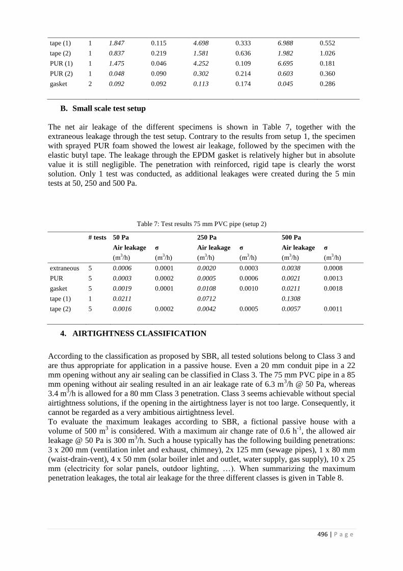
496 | P a g e

tape (1) 1 1.847 0.115 4.698 0.333 6.988 0.552

tape (2) 1 0.837 0.219 1.581 0.636 1.982 1.026

PUR (1) 1 1.475 0.046 4.252 0.109 6.695 0.181

PUR (2) 1 0.048 0.090 0.302 0.214 0.603 0.360

gasket 2 0.092 0.092 0.113 0.174 0.045 0.286


The net air leakage of the different specimens is shown in Table 7, together with the

extraneous leakage through the test setup. Contrary to the results from setup 1, the specimen

with sprayed PUR foam showed the lowest air leakage, followed by the specimen with the

elastic butyl tape. The leakage through the EPDM gasket is relatively higher but in absolute

value it is still negligible. The penetration with reinforced, rigid tape is clearly the worst

solution. Only 1 test was conducted, as additional leakages were created during the 5 min

tests at 50, 250 and 500 Pa.

Table 7: Test results 75 mm PVC pipe (setup 2)

# tests 50 Pa 250 Pa 500 Pa


(m3/h) (m

3/h) (m

3/h) (m

3/h) (m

3/h) (m

3/h)

extraneous 5 0.0006 0.0001 0.0020 0.0003 0.0038 0.0008

PUR 5 0.0003 0.0002 0.0005 0.0006 0.0021 0.0013

gasket 5 0.0019 0.0001 0.0108 0.0010 0.0211 0.0018

tape (1) 1 0.0211 0.0712 0.1308

tape (2) 5 0.0016 0.0002 0.0042 0.0005 0.0057 0.0011

4. AIRTIGHTNESS CLASSIFICATION

According to the classification as proposed by SBR, all tested solutions belong to Class 3 and

are thus appropriate for application in a passive house. Even a 20 mm conduit pipe in a 22

mm opening without any air sealing can be classified in Class 3. The 75 mm PVC pipe in a 85

mm opening without air sealing resulted in an air leakage rate of 6.3 m3/h @ 50 Pa, whereas

3.4 m3/h is allowed for a 80 mm Class 3 penetration. Class 3 seems achievable without special

airtightness solutions, if the opening in the airtightness layer is not too large. Consequently, it

cannot be regarded as a very ambitious airtightness level.

To evaluate the maximum leakages according to SBR, a fictional passive house with a

volume of 500 m3 is considered. With a maximum air change rate of 0.6 h

-1, the allowed air

leakage @ 50 Pa is 300 m3/h. Such a house typically has the following building penetrations:

3 x 200 mm (ventilation inlet and exhaust, chimney), 2x 125 mm (sewage pipes), 1 x 80 mm

(waist-drain-vent), 4 x 50 mm (solar boiler inlet and outlet, water supply, gas supply), 10 x 25

mm (electricity for solar panels, outdoor lighting, …). When summarizing the maximum

penetration leakages, the total air leakage for the three different classes is given in Table 8.

497 | P a g e

Table 8: Maximum total penetration leakages according to SBR

Air leakage @ 50 Pa (m3/h)

Class 1 Class 2 Class 3

Total air leakage 744.6 178.3 35.7

share of allowed leakage 321.1% 99.2% 19.8%

For this example, the penetrations executed with an airtightness according to Class 3, are

responsible for 19.8% of the total allowed leakage. This does not seem dramatic, but could be

improved with little effort and investment, as only 15 local and easily detectable spots have to

be sealed using the appropriate techniques.

5 WORKMANSHIP REPRODUCIBILITY

In the wood-frame research project, of which a part of the results are reported in this paper,

the water tightness of building components was evaluated next to the air leakage rate. The

results of these tests are also useful to evaluate the difference in workmanship quality between

identical sealing solutions, as leakages can be visualised. Water tightness tests were executed

according to

- EN 1027: water is sprayed at a rate of 120 l/(h.m2), first 15 min without pressure,

then a static pressure is applied in consecutive 5 min time steps at 50 Pa, 100 Pa,

150 Pa, 200 Pa, 250, 300 Pa, 450 Pa, 600 Pa, …

- EN 12865: water is sprayed at a rate of 120 l/(h.m2), first 20 min without pressure,

then a pulsating pressure (10 seconds with pressure, 5 seconds without pressure) is

applied for 10 minutes at 150 Pa, 300 Pa, 450 Pa, 600 Pa, …

As the wall has an area of 4 m2, a total spray rate of 480 l/h was applied. The following water

infiltrations were observed for the water tightness tests. Due to practical reasons, the complete

pressure sequence was not executed during some tests, which is indicated with a ‘/’ in Table

9.

Table 9: Infiltration pressures

static pressure pulsating pressure

Pressure (Pa) # 0 50 100 150 200 300 900 0 150 300 450 600 750

4 mm tape 16 2

1 1 / / 1

10

1

PUR 16

2 / /

7 3 3

gasket 32

/ /

2

20 mm tape 4 2

2 / / 1 2

/ / /

PUR 16 6

3 1 / / 4 12

/ / /

gasket_1 4

1

1 / /

2 2 / / /

gasket_9 9 1

/ /

1 9 / / /

75 mm tape 2 1

1 / 1

1

PUR 2 2

/ 2

gasket 4

2

1 1 /

1 3

130 mm tape 2 2

2

PUR 1 1

1

gasket 2

1

1

1

498 | P a g e

A large spread in the pressure at which infiltration occurred was visible during most of the

tests, suggesting workmanship quality plays an important role in the leakage around

penetrations. Applying a positive pressure in combination with a smoke generator confirmed

the differences in air leakages which accompany the differences in water infiltration, in

particular when PUR or tape were used to seal the penetrations. As the PUR was sprayed on

the fibreboard, the foam did not expand into the cavity and in some cases, large openings

were present around the penetrations, which could easily be detected using the smoke

generator. The installation with rigid tape was also prone to errors, as the overlapping parts of

the pieces of tape showed significant leakages.

In general, the water infiltration around the penetrations sealed with EPDM gaskets was much

smaller than the penetrations sealed with tape or PUR.

6 DURABILITY

The air leakage rate through the complete wall was measured after the execution of the water

tightness tests reported above. In this way, the effect of the sprayed water on the bonding of

the tapes and the mechanical impacts of the pressure pulsations were evaluated.

Table 10: Additional air leakage after water tightness tests

50 Pa 250 Pa 500 Pa


(m3/h) (m

3/h) (m

3/h) (m

3/h) (m

3/h) (m

3/h)

combined 0.581 0.168 1.188 0.284 1.658 0.462

As the air leakage rate of the installed penetrations could not be measured separately, the

individual increase in air leakage was not determined. As shown in Table 10, the overall

increase in air leakage was limited, and visual inspection indicated which air sealing solutions

were problematic.

No tapes were detached from the surface of the fibreboard as a result of the large amounts of

sprayed water, but the impact of the pressure pulsations on the taped PVC pipes was clearly

visible. As Figure 5 illustrates, the pipes are pressed through the opening in the fibreboard,

and additional leakages are created.

Figure 5: Durability effects taped PVC pipe: before and after water tightness testing

499 | P a g e

The flexible PUR foam should be able to tolerate mechanical impacts up to a certain level and

no degradation was detected after the water tightness tests. However, one can reasonably

assume that contractors working on a penetration could damage the foam or the adhesion

between the foam and the wall. The execution with an EPDM gasket is less sensitive to these

problems. As the penetration is not attached to the wall, it can be moved back and forth

through the gasket or even be replaced without damaging the air sealing.

7 CONCLUSIONS

Three different methods to ensure an airtight connection around building penetrations were

evaluated in this paper: airtightness tape, sprayed polyurethane foam and EPDM gaskets. Air

leakage tests were executed on two setups of a different scale. In one setup, a wall was built

and a variety of sealing methods and penetration diameters were installed. This setup was able

to compare the quality of the different tested solutions and to investigate differences in

workmanship quality between identically installed elements. Due to the measurement

principle of the test setup and the calculation method of the net leakages through the installed

penetrations, a high measurement uncertainty is involved. A second setup was built on a much

smaller scale to test individual components, which was able to measure the air leakage rate

through different sealing methods very accurately.

In the large-scale setup, PUR foam was sprayed around the penetration on the surface of the

wall. As the foam could not expand into the cavity and fill the connection, significant local

leakages were observed. In the small-scale setup, a thicker wall element was used, and the

foam could expand in the cavity between the wall and the penetration, resulting in an almost

perfect airtight connection.

The use of standard airtightness tape, which is designed to seal joints between panels, is not

recommended to seal 3-dimensional connections such as building penetrations. As the tape is

very rigid, it is unable to follow the shape of the pipes and large leakages can arise. Air and

water tightness tests showed these connections can be very tight, but most of the times they

result in large air leakage rates. Furthermore, the use of rigid tape in this situation is very

sensitive to mechanical impacts and cannot be regarded as durable.

In the smaller setup, a flexible butyl tape was tested which is designed for 3-dimensonal

connections, which proved to be very airtight.

EPDM gaskets showed to be less airtight then sprayed PUR, or flexible butyl tape, but in

absolute values, the air leakage rate is still negligible. Contrary to PUR or tape, the connection

is not permanent and can be adapted after installation, which is a very important aspect in

respect to long-term durability.

8 REFERENCES

ASTM E2357-11. Standard Test Method for Determining Air Leakage of Air Barrier

Assemblies.

Bracke W., Laverge J., Van Den Bossche N., Janssens A. (2013). Durability and

measurement uncertainty of airtightness in extremely airtight dwellings. 34th AIVC

conference and 3th TightVent Conference: Towards Optimal Airtightness Performance,

500 | P a g e

Athens.

Kalamees T., Korpi M., Eskola L., Kurnitski J., Vinha J. (2008). The distribution of the air

leakage places and thermal bridges in Finnish detached houses and apartment buildings.

Proceedings of the 8th Symposium on Building Physics in the Nordic Countries

NSB2008, Copenhagen, 1095-1102.

NBN EN 12114 (2000). Thermal Performance of Buildings – Air Permeability of Building

Components and Building Elements – Laboratory Test Method, CEN, Brussels, Belgium.

NBN EN 12237 (2003). Ventilation for buildings - Ductwork - Strength and leakage of

circular sheet metal ducts, CEN, Brussels, Belgium.

NBN EN 1027 (2000). Windows and doors - Watertightness - Test method, CEN, Brussels,

Belgium.

NBN EN 12865 (2001). Hygrothermal performance of building components and building

elements - Determination of the resistance of external wall systems to driving rain under

pulsating air pressure, CEN, Brussels, Belgium.

NEN 2687. Luchtdoorlatendheid van woningen - Eisen.

SBRCURnet (2007). Luchtdicht bouwen: Theorie – ontwerp – praktijk.

Taylor J.R. (1982). An introduction to error analysis – The study of uncertainties in physical

measurements, 2nd ed., University Science Books, Sausalito, Canada.

Van Den Bossche N. (2012). Airtightness of the window-wall interface in cavity brick,

Energy and buildings 45, 32-42.

Van Den Bossche, N., Janssens, A., Moens, J., & Ost, T. (2009). Performance assessment of

building envelope interfaces: self-adhering flashings. The future is in the balance (pp. 113–

126). Presented at ‘The future is in the balance : symposium on building envelope

sustainability’, Washington, DC, USA: Roof Consultants Institute Foundation.

501 | P a g e

COMPARISON OF BUILDING PREPARATION RULES

FOR AIRTIGHTNESS TESTING IN 11 EUROPEAN

COUNTRIES

Valérie LEPRINCE1*, François-Rémi Carrié

2

1 PLEIAQ

84 C Avenue de la Libération

69330 Meyzieu, FRANCE


2 ICEE

93 rue Molière

69003 Lyon, FRANCE

ABSTRACT

Mandatory building airtightness testing came gradually into force in the UK, France, Ireland and Denmark. It is

considered in many other European countries because of the increasing weight of the building leakage energy

impact on the overall energy performance of low-energy buildings. Therefore, because of related legal and

financial issues, the building airtightness testing protocol and reporting have become crucial issues to have

confidence in the test results as well as the consistency between the measurement results and values used in the

energy performance calculation method.

The reference testing protocol in Europe is described in EN 13829, but many countries have developed specific

guidelines to detail or adapt EN 13829 requirements.

This study compares building preparation rules for airtightness testing in 11 European countries.

Information has been collected through a questionnaire sent to TAAC (TightVent Airtightness Associations

Committee) members. We found that building preparation differs significantly from one country to another and

that the two methods described in the standard are either too detailed or insufficiently described to fit with the

specificities of each country regarding building preparation. It concludes on possible improvement for EN 13829

including:

- In one hand describing more precisely the basic principles of the preparation to avoid ambiguities

and,

- In another hand, allowing some flexibility to the countries to specify rules consistent with their

energy performance calculation method.

KEYWORDS

Airtightness testing, building preparation

1. INTRODUCTION

Building airtightness is a key issue to reach low- and very low-energy targets. Therefore an

increasing number of tests are performed in European countries for various reasons:

compliance to the energy performance regulation; compliance to a specific energy

programme; or will of the building owner. For instance, to our knowledge, measuring the

airtightness of all new buildings or at least part of them is required by the energy performance

502 | P a g e

regulation in UK, France, Ireland and Denmark. Besides, specific energy programs (such as

Passivhaus or Minergie) that require or encourage building airtightness testing are

increasingly popular in many other countries. Likely, within a few years, over a million tests

will be performed every year in Europe.

Airtightness measurements are useful to check that the building envelope complies with a

given requirement. The measurement protocol is described in the European standard EN

13829 adapted from ISO 9972 which is now under revision.

Measurement uncertainty has been discussed in various publications (Bailly, 2012) (Delmotte

C. , 2013) (Delmotte C. L., 2011) (Rolfsmeier, 2010) (Sherman, 1995) and it is widely

accepted that the building preparation (i.e., the way openings and vents are sealed, closed, or

left as during the airtightness test) represents one of the main sources of uncertainty.

Rolfsmeier et al (Rolfsmeier, 2010) have had tests performed by 17 testers on the same

building, firstly with a preparation made by the tester himself, and secondly with homogenous

preparation rules. 70% of testers obtained a V50 within 7% of the right result, but for the 30%

the error could reach 63% because of an inappropriate preparation and a misinterpretation of

the volume to be tested. When the preparation was done correctly, results stayed within 6% of

the right results for all testers. The consequences of such discrepancies can be crucial for

building professionals or owners seeking e.g., if the subsidies are given on condition to meet a

given airtightness level, or if the remedial actions are costly and impractical to implement.

Moreover, if the result is used in energy performance calculation method, the building

preparation has to be consistent with the calculation method. Logically, one should seal or

close the openings through which the airflow rate is taken into account elsewhere in the

calculation method and leave as what is not. In principle, this is clear for instance for the air

terminal devices of a mechanical ventilation system, but it may be ambiguous for devices

such as unvented combustion appliances.

Therefore, to address the question raised by the increasing number of airtightness tests, we

have collected and analysed information on building preparation.

2. OBJECTIVES

This study aims at answering the following questions:

- How is EN 13829 used and interpreted in European countries?

- Does EN 13829 fit with countries’ needs in terms of protocol description?

- How can the standard be improved to better march those needs?

3. APPROACH

This work has been done in the context of the TightVent Airtightness Associations

Committee (TAAC). TAAC is a European working group, set up and hosted within

TightVent. The scope of this working group includes various aspects such as:

- Airtightness requirements in the countries involved

- Competent tester schemes in the countries involved

- Applicable standards and guidelines for testing

- Collection of relevant guidance and training documents.

At present, the participants are from Belgium, Czech Republic, Denmark, Estonia, France,

Germany, Latvia, Ireland, Poland, Sweden, UK and contacts have been established with other

European countries.

A questionnaire has been developed within the group to compare building preparation with

the objective of being useful for someone who:

- plans to perform a test in a foreign country

- would compare the test results from different countries

- prepares guidelines for airtightness measurements in its country

503 | P a g e

A representative from each country has kindly accepted to answer the questionnaire.

This document summarizes their answer.

Note that the scope of the answers differs between countries:

- For the UK, Denmark, Germany and Ireland, the answers concern only the energy

performance regulations

- For France and Belgium, the answers concern both energy performance regulation and

specific energy savings programs.

- For Czech Republic, Poland and Sweden, they concern specific energy saving

programs only.

3.1 Analysis of questionnaire results

Airtightness requirements and guidelines

Out of the 11 countries who have answered the questionnaire only four of them have

requirements in the building regulation to measure airtightness (Denmark, France, Ireland and

UK)1. Those four countries have all developed specific guidelines to detail airtightness testing

conditions.

Three other countries (Belgium, Czech Republic and Germany) have also developed specific

guidelines for airtightness testing in the context of specific energy saving program or for

voluntary testing in the context of energy performance regulation.

This means that 7 out of the 11 countries have developed specific guidelines beyond the

European standard EN 13829.

1 The regulation does not impose to measure every buildings but at least part of them have to be

Time of measurement

This question concerns the requested completion of the building. EN 13829 specifies that

even if preliminary measurement may be done during the constructions, the effective

measurement can take place only when the envelope of the building is completed.

We noticed large differences between countries:

- In Sweden, for example, as building regulation and even energy performance

programs give very few guidelines to perform airtightness tests, most of the time it is

the client himself who chooses time and condition of measurements. As a

consequence, most of the time, he prefers to make the test when it is still possible to

reach the airtight layer in case leakages have to be repaired. Thus the building

envelope may not even be completed (some doors or traps could be missing and sealed

instead). Most often, a final test is not performed.

- In Belgium, test has to be performed when the envelope is completed. It is

recommended to have it done when all works are finished.

- In Denmark and UK the building envelope has to be in its final complete state.

- Germany requires that the building envelope – all airtightness concerning parts – shall

be completed.

- In France and Czech Republic, the tests have to be done after all work that may affect

airtightness is completed.

- In Ireland, the building must be in “practical completion”, i.e., almost ready for

occupation (possibly just need to have painting done and furniture placed)

504 | P a g e

General rules for the building preparation

Testing according to EN 13829 requires that all intentional exterior openings of the building

or part of the building to be tested (windows, doors, fireguard) be closed. Besides all

interconnecting doors in the part of the building to be tested shall be opened to have a

homogeneous pressure in the building (except for cupboards and closets, which should be

closed).

Beyond these basic rules, “method A” of the standard does not allow further improvement of

the air tightness of building components. On the other hand, with “method B”, all adjustable

openings shall be closed and remaining intentional openings shall be sealed.

The underlying ideas behind the methods are the following:

- Method A: the building as prepared represents its condition during the season in which

heating or cooling systems are used.

- Method B: the leakage measured represents the leakage through the envelope

excluding those due to the HVAC equipment and its penetrations.

Method A is used in the energy performance regulation only in two countries (Ireland and

Belgium). Three countries (Czech Republic, France and Germany) have developed a specific

method. However, in the Czech Republic and Germany, this method is used only for specific

energy saving program and method B is required by energy performance regulation.

Therefore, in 8 out of the 11 countries, method B is used to estimate the building airtightness

in the energy performance regulation context.

To further describe the building preparation, we have defined six categories to classify how

each opening shall be processed:

- “Sealed”: make hermetic by any appropriate means (adhesive, inflatable balloon,

stopper, etc.)

- “Depends on EP-calculation”: sealed if the associated flow rate is already taken into

account in the energy performance calculation method, left as if not

- “Closed": Closed if there is a closing device, left as if not

- “Held with tape”: the device is closed with a tape to prevent it from moving during

the test, but the tape should not sealed the opening

- “Left as”: left in normal position of us (this can be closed if the normal position is

close like some fire-door or open of if normal position during heating or cooling

period is “open”)

- “Open”

Those categories were re-constructed after the survey to fit with respondents’ answers but

there is still some specificity. In UK the rule can be “closed if closing device exists, sealed if

not”: in those cases both categories are selected in the analysis. In Sweden, the rule can be

“closed if the closing device leads to a perfect airtightness of the opening, sealed if not”, thus

in those cases, for Sweden, the category “sealed” has been selected.

The category “depends on EP-calculation” is only used in Czech Republic and France.

Openings for ventilation

EN 13829 requires to seal air terminal devices of mechanical ventilation or air conditioning

system and to close other ventilation openings for purposes of method A and seal them for

method B.

505 | P a g e

The general requirements of EN 13829 (§5.2.3) does not detail what is included in air

terminal devices of mechanical ventilation (local, general, permanent, intermittent…) and do

not detail what shall be done with openings for natural ventilation that do not have closing

devices.

To overcome this problem, we have agreed on the following additional definitions:

- Openings for whole building mechanical ventilation or air conditioning: openings that

have one side plugged on a duct linked to a fan that provides general and permanent

ventilation for the building. ”Permanent” means that it cannot be turned off manually;

this includes permanently regulated system which may sometimes be automatically

turned off (for example when offices are unoccupied).

- opening for local mechanical ventilation of air conditioning with intermittent use:

openings that have one side linked to a local fan that can be turned off manually (not

including kitchen hood)

- ventilation openings for natural ventilation: straight openings from outside to inside

(or vice-versa) including opening that contribute to the general ventilation system in

association with openings for mechanical ventilation

All respondents agreed that openings for whole building mechanical ventilation or air

conditioning have to be sealed.

Regarding openings for local mechanical ventilation of air conditioning with intermittent use,

the answer is “sealed” for 7 out of the 9 respondents (or closed in UK) and “Depends on the

EP-calculation” for 2 out of the 9.

Last, regarding ventilation openings for natural ventilation, the answer is sealed for 7

countries out of 9 (or closed in UK), “depends on EP-Calculation” for one and closed for

Belgium (which is consistent with Method A).

Opening for the heating system and smoke exhaust

EN 13829 only requests to avoid exhaust hazards from heating systems.

Inlet and outlet openings for the main heating system (this may include air intake of a

combustion appliance, chimney flue, air handling unit…) shall be sealed in Estonia, Denmark,

France, Germany and UK and closed in Ireland and Belgium.

Inlet and outlet openings for additional heating system shall be sealed in Estonia, Denmark,

Germany and UK, prepared consistently with energy performance calculation method in

France and closed in Belgium and Ireland.

If we take a closer look at the preparation of various specific components we can see that the

interpretation on general rules differs (Figure 1 and Figure 2).

For example, chimney flue either have to be sealed (5 out of 9) or it “depends on EP-

calculation” (1 out of 9), or it shall be closed (1 out of 9) or it shall be left as (2 out of 9). And

it is about the same with chimney rear ventilation opening.

506 | P a g e

Figure 1: Preparation of openings for heating system and smoke exhaust

Specific openings

We have listed 6 “other envelope openings” but this list is not exhaustive.

Belgium remains consistent with method A: those openings are “left open” or only “held with

a tape”. France mostly recommends to leave them in normal position of use or to be

consistent with energy performance calculation. Estonia is consistent with method B and seals

all of them. Other countries (Czech Republic, Denmark, Germany, Ireland, Sweden and UK)

have a preparation depending on the kind of opening Figure 2 .

Figure 2: Preparation for "other openings"

4 DISCUSSION

The analysis of the questionnaires brings to light the importance of the purpose of the

measurement. Regarding the time of measurement, if the purpose of the test is to estimate the

energy losses of the building by leakage it seems obvious that the test shall be done after all

work that may affect airtightness is completed.

507 | P a g e

Nevertheless, requiring test after the completion of the building can lead to organization

problem in some cases --e.g., in multi-family buildings some dwelling may be occupied while

others are not completed yet. Furthermore when the work is completed it is hard to improve

efficiently the airtightness. This probably explains why some countries (BE, SE) have chosen

not to require the completion of the building before the test is performed.

Of course, some designs allow testing before completion without compromising the validity

of the test for regulatory compliance purposes. This could apply for instance when interior

membranes are used as air barriers and the design is such that there are little penetrations of

this barrier after it is installed. On the other hand, other systems may be severely affected by

works until completion—e.g., interior gypsum boards used as air barriers. It seems difficult to

go into that level of detail in a regulatory framework.

Regarding the building preparation, the survey shows that most countries agree on basic

principles such as closing windows, doors and trapdoors and leaving internal doors open. On

the other hand, the interpretation of the purpose and details of methods A and B varies

significantly.

To check the compliance to the energy regulation, the general rule should be to seal all

openings for which the air flow is taken into account in the calculation, and leave in normal

position of use all other openings. The underlying idea is closer to method A but it can

deviate significantly depending on aspects and components taken into account in the

calculation method.

Method B is appropriate if the purpose is to impose a minimum requirement for the envelope

only, excluding all penetrations (due to HVAC equipment’s, mailbox, etc.). However, it is

unclear to us how useful this requirement would be. It would be similar to a minimum

requirement for the level of insulation of some of the walls but not all of them. Therefore,

motivations behind the choice of method B versus method A are rather unclear to us. It seems

that the issue of consistency with the energy performance calculation method is not well

understood. Method B seems mostly chosen by default because method A is too restrictive.

Those variations in interpretations mean that it is impossible to compare measurements and

building airtightness performance from one country to another, unless prior check of the

consistency of the building preparation on the samples analyzed. Moreover, it appears

challenging for a tester to perform tests in a foreign country unless he well acquainted with

the specificities of building preparation in that context.

Nevertheless, there are two obstacles to harmonize pressurization test methods between

countries:

- In each country the test method shall be consistent with the energy performance

calculation method. But, there are significant differences in calculation methods

between countries in the way airflow rates are taken into account.

- There are specific devices and construction traditions in each country that may require

tailored rules.

As an illustration of the last obstacle, closing devices are forbidden on air inlets in France.

However, the test can only be done with those inlets sealed as most of them self-adjust their

position according to the pressure difference. This is nevertheless consistent with the

calculation method which takes into account the contribution of these devices to the airflow

rates.

Maybe, the standard could leave the possibility to define a measurement protocol at national

level consistent with the purpose of airtightness testing.

Nevertheless, to help decision makers setting it, a protocol schemes could be defined in the

standard. This scheme may give a detailed list of openings and how to determine the way they

should be prepared to be consistent with the test purpose.

508 | P a g e

5 CONCLUSION

This study shows that building preparation in the 11 countries investigated differs

significantly from one country to another even when the same method is used and without

clear and technically-sound motivations behind the choices. Therefore, it is clear that building

airtightness should not be compared between countries unless precaution is taken in the

sample analyzed and in the interpretation of the results.

To address this issue, the revision of the standard shall, in one hand, describes more precisely

the basic principles and avoid ambiguities and, in another hand, allows some flexibility to the

countries to specify rules consistent with the energy performance calculation method. At the

same time, it should allow the identification of tests performed under comparable conditions

to allow meaningful comparative analysis between countries.

6 ANNEX

The following table gives references of specific guidelines for each country

Country France UK Czech republic

Name of the

document

where the

guidelines are

specified

GA –P 50-

784

(application

guide of NF

EN 13829)

ATTMA Technical

Standard L1 –

Measuring Air

Permeability of

Building Envelopes

(Dwellings)

Metodický pokyn - Pravidla pro

měření průvzdušnosti obálky

budovy (Methodical instruction –

Rules for measurement of air

permeability of building envelopes,

in Czech)

Author or

editor of the

document

Afnor The Air Tightness

Testing and

Measurement

Association

(ATTMA) Technical

Committee

Association Blower Door CZ,

www.asociaceblowerdoor.cz

Institution

which issued

the document

Working

group set by

the ministry

of ecology

The Air Tightness

Testing and

Measurement

Association

(ATTMA)

Státní fond životního prostředí

České republiky (State

environmental fund of the Czech

Republic)

Date of issue February

2010

October 2010 not yet issued, prepared for

publication (state from September

2013)

The

document is

available (for

downloading

or purchase)

at:

http://www.b

outique.afnor

.org

www.attma.org http://www.nzu2013.cz/zadatele-o-

dotaci/rodinne-

domy/dokumenty/metodicke-

pokyny/

Comments: This

document is

under

revision

Document issued as a part of

instructions for subsidy applicants

from the New green savings

programme

509 | P a g e

Country Belgium Denmark Germany Ireland

Name of the

document

where the

guidelines are

specified

Spécification

s

supplémentai

res

“Metoder for

certificerede

virksomheders

trykprøvning efter

EN

13829 og gældende

bygningsreglement”

version 1,

EnEG_Staffel

11 –

Auslegungsfra

gen zur

Energieeinspa

rverordnung –

Teil 11

ATTMA

publication

“Measuring air

permeability of

Building

Envelopes” & EN

13829

Author or

editor of the

document

Governments

of the three

regions

Klimaskærm Dr. Justus

Achelis, DIBt

ATTMA/CEN

Institution

which issued

the document

Governments

of the three

regions

Klimaskærm Fachkommissi

on Bautechnik

der

Bauministerko

nferenz

ATTMA/CEN

Date of issue 5. September 2013 9.3.2004;

9.12.2009

October 2010 Issue

- 18 October 2000

The

document is

available (for

downloading

or purchase)

at:

www.epbd.be www.klimaskaerm.d

k

https://www.d

ibt.de/de/Servi

ce/Dokumente

-Listen-

EnEV.html

http://www.attma.o

rg/wp-

content/uploads/20

13/10/ATTMA-

TSL1-Issue-1.pdf

7 ACKNOWLEDGEMENT

Authors address a special thanks to the TAAC members who have kindly accepted to answer

the questionnaire:

- Clarisse Mees, Belgium

- Jiri Novak, Czech Republic

- Walter Sebastian, Denmark

- Valerie Leprince, France

- Oliver Solcher, Germany

- Paul Carling , United Kingdom

- Targo Kalamees , Estonia

- Andrejs Nitijevskis, Latvia

- Andrzej Gorka, Poland

- Owe Svensson, Sweeden

- Mark A. Shirley, Ireland

This work was supported by INIVE and BCCA.

510 | P a g e

8 REFERENCES

Bailly, A. L. (2012). Numerical evaluation of airtightness measurement protocols.

Copenhagen: AIVC conference 2012.

Delmotte, C. (2013). Airtightness of buildings - Calculation of combined standard

uncertainty. Athens: AIVC conference 2013.

Delmotte, C. L. (2011). Interlaboratory Test for the Determination of repeatability and

Reproducibility of Buildings Airtightness Measurements. Brussels, Belgium: AIVC

Conferences, 32nd, Proceedings.

Rolfsmeier, S. V. (2010). Ringversuche zu Luftdurchlässigkeitsmessungen vom Fachverband

Luftdichtheit im Bauwesen e.V.,. Buildair.

Sherman, M. a. (1995). Uncertainty in Fan Pressurization Measurements. Lawrence Berkeley

National Laboratory: ReportLBNL-32115.

511 | P a g e

THE IMPACT OF AIR-TIGHTNESS IN THE

RETROFITTING PRACTICE OF LOW

TEMPERATURE HEATING

Qian Wang*1

, Sture Holmberg1,

1 Division of Fluid and Climate Technology, Department of Civil and Architectural Engineering, Royal Institute

of Technology (KTH)

Brinellvägen 23, 100 44 Stockholm, Sweden


ABSTRACT

In Sweden, the energy usage in existing residential buildings amounted to 147 TWh in 2012, equivalent to

almost 40 % of the final overall national energy usage. Among all the end users in building service sectors, 60 %

of the final energy in Sweden is used for space heating and domestic hot water (DHW) production in 2013. In

order to reduce the supply temperature for space heating in existing buildings, combined approaches are

favorably adopted: to reduce the net energy demand by air-tightness and insulation retrofits; and renovate the

conventional high temperature heating to low temperature heating (LTH) systems. As an energy-efficiency

alternative, LTH technology has shown promising advantages and shortcuts to improve the coefficient of

performance (COP) of heat pump system, which further saves primary energy. However, existing modeling

achievements and field testing reveal that the attained application of LTH has a relatively high requirement to the

air-tightness in new constructed single-family houses. Moreover, in some leaky multi-family building stock with

low envelope surface temperature, LTH may have limited energy saving potentials. How to evaluate the impact

of air-tightness for the LTH implementation and energy saving potentials in existing houses are not sufficiently

attained so far. This paper presents a modeling approach combining LTH simulation with air-tightness

evaluation, aimed to estimate whether the selected existing building types can cope with LTH with upgraded

primary energy savings. In addition, the impact of air-tightness retrofits for LTH implementation in selected

Swedish residential buildings is of interests.

In the simulation Consoli Retro are employed to simulate the energy performance. It is revealed that the

combined effect of floor heating/ ventilation radiators and air-tightness retrofits to 1/1.5 ACH can contribute 19

% to 36 % primary energy savings in total. However, different LTH systems and archetypes have varies

sensitivities to air-tightness retrofits. Benchmark the impact of air-tightness to different LTH systems needs

further investigations among other archetypes and on-site measures for future application of LTH on a larger

scope.

KEYWORDS

Air-tightness, retrofitting, energy savings, low temperature heating, Swedish residential buildings

Nomenclatures

Acronyms

ACH

BBR

Air changes rate, h-1

Swedish building regulations

CHP Combined heat and power

COP Coefficient of performance

DH District heating

DHW Domestic hot water

FH Floor heating (hydraulic)

HP Heat pump

LTH Low temperature heating

PE Primary energy

PEF Primary energy factor

VR Ventilation radiator (low-temperature)

512 | P a g e

T1 Building type 1, Swedish slab houses (low raise), before 1950

T2 Building type 2, Swedish slab house (three- to four storeys), 1960–1975

T3 Building type 3, Swedish slab house (high raise), 1970–1975

Symbols

Heat transfer coefficient of building elements, W/m2K

Operative temperature, ℃

Air temperature, ℃

Mean radiant temperature, ℃

( )

( ) Energy for fuel type i during heat production provided in heat boilers

Energy for fuel type i during heat production provided in CHP

( ) Primary energy factor for fuel type i during heat production provided in heat boilers

( )

Primary energy factor for fuel type i during heat production provided in CHP

Allocation factor for on-site or off-site production for fuel type I

Total energy demand, kWh/m2

Monthly heating demand, kWh/m2

Electricity demand, kWh/m2

Domestic hot water energy demand, kWh/m2

Transmission heat loss, kWh/m2

1. INTRODUCTION

In Sweden, existing residential building stock comprises approximately 2.5 million dwellings,

including apartment units and multi-family houses, and approximately 2 million detached or

semi-detached single-family houses/villas [1]. The energy usage in this part amounted to 147

TWh in 2012, equivalent to almost 40 % of the final overall national energy usage [2]. As a

baseline and essential technique, energy retrofitting is considered as an effective way to

accelerate the sustainable transformation of existing Swedish building stock [3]. However, the

industry approach and pilot project typically oriented with operational energy costs savings or

tap-water savings/treatments, therefore, the retrofitting solutions tend to be highly case-

specific and conventional, the primary energy saving potentials are limited [4][5][6].

As an energy-efficiency alternative, low temperature heating (LTH) technology has shown

promising advantages and shortcuts to improve the efficiency of heat supply in terms of

improved coefficient of performance (COP) with HP (heat pump), thermal comfort

contributions and easily installed solution [7]. The advantages further provides more

renewable based heating solutions with upgraded primary energy (PE) savings [8].

Nevertheless, theological studies have revealed that the air-tightness and energy demand of

the existing buildings play major roles for the energy performance of LTH [9][10]. More

importantly, little is known about the impact of air-tightness, particularly to those buildings

which are planning to be renovated by low-temperature ventilation radiator (VR) or hydraulic

floor heating (FH). Available models and studies from other countries are mainly based on

local building energy codes and national heating directives. For example, Hasan et al. [8] and

Cellura et al. [11] investigated both the delivered and primary energy saving potential of FH

and low temperature radiators with respect to the Finnish climate condition. The findings

revealed that with a reduction of supply/return temperature to 40/35℃, the LTH can save both

delivered energy and PE without compensations on thermal comforts (1.0 m-1.3 m

elevations). Furthermore, the energy usage of FH in the bathroom of the studied buildings can

be amounted up to 33% to 43% of the total energy use. Specific to Swedish residential

buildings, Energy Europe TABULA project [12] performed a general energy retrofitting

guideline based on 44 typology categories of existing Swedish residential buildings for

simplified heating system alternatives with respect to energy demand retrofits. Zou [13]

developed a bottom-up approach to classify and assess existing Swedish buildings by

improving the air infiltration database and construction techniques. Hesaraki and Holmberg

[14] and Myhren and Homberg [7] evaluated long-term energy savings by low-temperature

513 | P a g e

VR in Swedish multi-family houses. It is found that with the air-tightness level of 0.68 l/(s

m2), annual on-site measurements shows 48 kWh/(yr m

2) to 55 (kWh/yr m

2) energy usages

for both space heating and DHW can be achieved when the buildings are equipped with LTH

and HP. Gustavsson, Dodoo, Truong and Danielski [15][16] modeled the combined effects of

heat supply and demand retrofits considering four major types of heat production systems in

Sweden. It is found that the PE savings are largely dominated by the heat producing systems

and the capacities to reduce the existing energy demand, in which air-infiltrations are

commonly one of the most sensitive parameters for the studied archetypes. Other possible

software and modelling techniques, including IDA ICE, Design Builder/EnergyPlus, Trnsys,

eQuest@

, have been employed in some LTH practices to evaluate different heating parameters

that impact the energy performance and thermal comfort before and after retrofitting

[8][17][18][19]. The models are capable of providing relatively accurate one- or multi-zone

air temperature and radiant temperature simulations for the reference buildings. However,

these tools have had limited usage in retrofitting Swedish residential buildings and are not

easily adapted to larger contingents of similar archetypes under Swedish climate conditions.

Based on the target, this study simulated the PE saving potentials led by LTH retrofits and

further defines the impact from air-tightness variances based on the current air penetration

levels in the selected archetypes.

2 METHODOLOGY AND SIMULATION MODEL

2.1 Energy performance model

The main advantages of installing LTH in retrofits are the potential of reducing primary

energy and providing more sustainable heating energy alternatives along with thermal

comfort contributions. Designed with Excel tools, Consolis Retro is employed in the study.

The model is based on the simplified calculation and parametric analysis of energy usage,

applying EN ISO 13790 calculation methodologies [20]. The model is capable of handling 1

or 2-zones at the same time for the reference building. The building block was set heat

balanced with variable major parametric factors that impact the heat loss and heat

distributions in the calculation zone. Parameters are set previously to indicate the building

archetypes. The total net energy usage is calculated from Equation (1):

(1)

To simplify the calculation process, the transmission heat loss is calculated by building

envelope parameters and linear thermal bridges. Old Swedish slab houses might be

constructed with no insulations with cold surface temperatures, this will lead to rather high

differences between operative and air temperature [11]. In another word, occupants may feel

colder than the air temperature is set 20 C. As a result, 22 C is set for air temperature of

heated space in the modeled archetypes. The operative temperature of the buildings are gained

by Equation (2)

( ) (2)

In the model, delivered energy are calculated as net building demand of the selected

archetypes, primary energy saving potentials is calculated by both the delivered energy and

primary energy factor (PEF) variances before and after LTH retrofitting, which is obtained as

Equation (3) [21]:

PEF = ∑ ( ( )

( )) ∑ ( ( )

( ))

∑

(3)

In Sweden, district heating (DH) accounted for around 60 TWh in 2013, which is considered

as the most common space heating system for existing multi-family houses and apartment

blocks. In single family houses, district heating and electricity are used in 7 % and 22 % of all

detached and semi-detached houses, respectively[22]. Swedish district heating are mainly

514 | P a g e

produced by combined heat and power (CHP) for residential buildings, it has a PEF of 0.5-1.3

depending on the energy sources (waste heat, biomass, coal and natural gas, etc) [23].Within

the last decades, heat pump (HP) shows increasing competences with DH because of its PE

saving potentials when designed with LTH. Up to 2012, Sweden has the largest application of

HP systems for both new and retrofitting buildings among EU [24]. The PEF of LTH

combined HP systems are calculated based on the supply temperature and the COP of the heat

pump [25]. Validation and testing of the calculation model was conducted [26]. The tool was

compared with IDA ICE and EnergyPlus for accuracy analysis, with an acceptable agreement

of 0 to 8 % error [27]

2.2 Air-tightness retrofits in existing Swedish residential buildings

Air-tightness is one of the most significant parameters to not only provide hygienic protection

for the occupants but also reduce the operational energy usage[28]. Sweden has a relatively

long heating season (6-7 months), it is found that the impact of air-tightness can be higher

than transmission heat loss through building envelopes in some Swedish detached/semi-

detached houses. In addition, the large application of exhaust ventilation systems in Sweden

led to a relatively higher air-infiltration compared with balanced ventilation systems [29]. The

air-tightness retrofits have been commonly recommended in some conventional renovation

projects, nevertheless, despite measurements and blow-door tests have been conducted in

pilot houses, the existing information on ait-tightness and its impact to energy usage are still

scarce, particularly for those buildings heated with reduced supply temperature lower than

50℃ [30]. In 2012, the revised BBR (Swedish building regulations) provides no specific limit

values in respect of tightness, but the significance of good ventilation is stressed in an

advisory in order to decrease the moisture damage and hygienic issues. To obtain a well

performance of LTH, a good guideline minimum value for 0.80 l/(s m2) and 0.35 l/(s m

2)

surface area at a pressure difference of +/- 50 Pa are recommended for existing and new

Swedish residential buildings, respectively [31]. However, 1400 existing Swedish building

stock statistics from derived field studies shows that the actual air-tightness level ranges from

less than 0.3 l/(s m2) to approximately 1.5 l/(s m

2), at pressure difference of 50 Pa [13]. And it

varies largely among different archetypes and exhaust/balanced ventilation systems. Figure 1

shows the air-tightness level of existing residential buildings in Sweden compared with other

countries [13][29].

Figure 1 The air-tightness level (50 Pa) of Swedish residential buildings compared with other countries.

The existing retrofitting techniques in Swedish residential buildings are based on the

following three perspectives in the models [32]:

0

2

4

6

8

10

12

Australia Estonia UK France Germany Finland Norway Sweden

The

level

of

air-

tightn

ess

(50

Pa,

AC

H)

in e

xis

ting r

esid

enti

al

buil

din

gs

High Low Average

515 | P a g e

Insulate the air gaps existed in joints between ceiling/floor/balcony to the walls,

particularly for two or three storey slab houses.

Install more efficient mechanical (balanced preferably) ventilation systems.

Insulate the ventilation studs and piping systems.

The improvements and variances of air-tightness level are based on the existing performance

of in the selected building types.

2.3 LTH retrofits and selected archetypes

The heating system in Swedish slab houses is usually district heating (DH), occasionally

heated partially by electricity, gas, oil and renewable sources in some renovated cases [23].

To standardize the archetypes, low-rise slab houses are classified in this study by age

according to three periods: pre-1950 (T1), 1951-1960 (T2). Additionally, special booming time

1965-1975 for high slab apartments (T3) is chosen in the category. Two types of LTH are

selected as the retrofitting alternatives: FH and VR, the structure and components are shown

in Figure 2. For FH, in order to fit the existing old slab floor in renovation practice, overlay

floor panels are installed with embedded PEX tubing circus, shown in Figure 2, left. FH is set

as 100 W/m2 heat outputs with design temperature 35 ℃/ 29 ℃. The coverage area is 12

m2/circuit. The new floor layers are set as tiles in bathroom and laminate in other rooms. For

VR (shown in Figure 2, right), the cold air is preheated by the radiator through the slab wall

vents and filtered as clean warm air. Because most of the selected multi-family houses have

installed exhaust ventilation, 10 P pressure drop between indoor and outdoor are set as the

driven force for the cold air , no extra energy is needed for the convection [33]. The

supply/return temperature is designed with 45 ℃/ 35 ℃ in the study for VR.

Figure 2 Left, The principle of overlay FH, floor panel units embedded with PEX tubing and, Right, VR,

designed as preheated air and low-temperature radiator

In each archetype, four retrofits are designed and compared for implementing LTH, these are

indicated in Table 1. For system 1, living rooms are renovated with VR under the windows,

two-pipe hydraulic existing radiators are kept in the rest rooms. For system 3, hydraulic FH

are implemented only in bathrooms, the rest rooms are kept with existing high temperature

radiators. For system 2 and 4, the whole buildings are renovated by VR and FH, respectively.

The parameters of the LTH retrofits are indicated in Table 1.

The building material for floors and ceilings in the studied archetypes was primarily 10- 50-

centimeter-thick, reinforced concrete, and relatively thinner slabs were applied as exterior

paving and coating [6][1]. Although Swedish slab houses may have different facades and

terraces, the buildings’ main elements and service systems are similar. Three types of

Swedish slab houses (T1, T2, T3) constructed during different years were selected for this

retrofitting investigation. The archetypes, building features and parameters were generalised

and collected through surveying the statistics; these are presented in Table 2. The

516 | P a g e

corresponding energy system retrofits are designed as water-to-water HP. The PEF are

calculated by the supply temperature and the COP of HP [34], shown in Table 3.

Table 1: LTH retrofitting designs

System Retrofit room Supply/return

temperature (℃)

Non-retrofit room Supply/return

temperature (℃)

System 1 VR in living rooms 45/35 Conventional radiator 55/45

System 2 Whole building VR 45/35 -

System 3

System 4

FH only in bathroom

Whole room FH

35/30

35/29

Conventional radiator

-

55/45

-

Table 2: Selected archetypes and energy systems for retrofitting analysis

T1 T2 T3

Archetypes

Dwelling types Single family house Multi-family house Apartment block

Age

Foundation

External wall

Window

Roof /ceiling

Ground floor

Heating

Radiator

Ventilation

Energy mix

Air-tightness

Before 1950

Lightweight concrete

10 cm mineral wool insulation

Double glazing, aluminium

frame

Brick and cutter coke ash

insulation

Linoleum and coke ash

Furnaces /electricity

Furnaces/electricity

Natural ventilation

Gas/oil/partly el.

2 ACH

1960-1975

Concrete slab

13 cm mineral wool

insulation

Double glazing, timber

frame with ventilation fan

Flat roof covered with

cardboard and mineral wool

Slab covered with linoleum

mats or plastic board

District heating

Single-pipe hydraulic

radiator

Exhaust ventilation

CHP

2 ACH

1970-1975

Polished concrete

15 cm mineral wool

insulation

Double glazing,

aluminium frame with one-

side ventilation fan

Concrete foundation with

galvanized sheet metals,

mineral wool insulation

Slab covered with mineral

wool or linoleum

District heating

Two-pipe hydraulic

radiator

Exhaust ventilation

CHP

5 ACH

Table 3: PEF modeling of LTH retrofits

Supply/return

Temperature (℃)

Heating system COP Energy mix PEF

70/60 Conventional supply temperature

District heating - CHP 0,90

50/40 Medium supply temperature output

District heating

3.1 CHP 0.80

45/35 Low supply temperature output 3.5 HP 0.68

40/30

35/29

Low supply temperature output

Low supply temperature output

3.6

3.8

HP, Nordic mix

HP, Nordic mix

0.68

0.60

3 REUSLTS AND DISCUSSION

All archetypes were selected within the same Swedish climate zone III, Stockholm, for

comparison. Figure 3 shows the monthly energy flow before and after implementing

retrofitting for the selected archetypes. Among the four archetypes, system 4 (whole building

with FH) shows the largest energy savings from 26 % to 33 % after retrofitting compared with

other systems. Among all the archetypes, relatively new archetype (T3) shows the highest PE

saving potentials. Followed by system 2 and system 1 (whole building VR and living room

VR), PE savings range from 20 % to 25 % and 15 % to 18 %, respectively. Among the three

archetypes, older houses (T1) show lower saving potentials compared with apartment block.

517 | P a g e

The reason could be that the old multi-family houses are more sensitive to the air-infiltrations

due to their existing leaky conditions. The exhaust ventilation system installed in T2 and

natural ventilation in T1 make the envelope leakage larger when installed with VR, compared

with other archetypes. System 3 shows the lowest energy saving potentials compared with

other types in both FH and VR. It didn’t show promising energy savings in selected single

family houses and low-raise multi-family houses. Furthermore, T1 shows the lowest energy

savings when renovated only in bathroom FH (system 3). The reason can be its limited heated

bathroom areas. Among the archetypes, the bathroom FH retrofits shows the greatest savings

for apartment block T3 (5 % savings). Attention should be paid that the operative temperature

in bathrooms sometimes can be 3℃ to 5 ℃ higher than the rest rooms, practically. With

respect to the occupations, this will lead to an increased uncertainties when focusing on

modeling the energy savings only in bathrooms and its conjunct effects with other heated

zones [8].

Figure 4 shows the primary energy saving potential after implementing both LTH and air-

tightness retrofits. The impact of air-tightness shows linear reduction of PE. Due to the high

variety of ventilation vent designs in the windows, the high slab house (T3) is set with greater

variances. The rests of the archetypes are set as approximately from 2.0 ACH to 1.5/1.0 ACH

before and after retrofitting. The combined effect of LTH and air-tightness shows that the

energy saving potentials from 28 % to 36 % in most of the archetypes can be achieved.

Among all the archetypes, T2 shows the highest sensitivity to the air-tightness retrofits,

particularly for VR. When the air-tightness level is reduced to 1.5 ACH, 38 % of PE savings

can be achieved by VR retrofits. In addition, T3 shows the lowest impact by air-tightness to

the LTH in general (approximately 6 % to 19 %). The reason can be the existing ventilation

systems have a relatively higher performance in the archetypes. In addition, the modern

constructions made the building envelope much less sensitive by the air-infiltration through

joists and ventilation ducts.

4 CONCLUSIONS

In the study, a simplified calculation model is developed and integrated with parametric

investigations to three major Swedish archetypes that are planned to be renovated with FH

and VR. PE (Primary energy) saving potentials led by LTH retrofits is in focus. The variation

in terms of air-tightness levels among the archetypes are of interests. It is revealed that the PE

savings can be up to 33 % depending on the LTH systems. FH in all rooms shows the highest

savings in most archetypes while VR shows high savings in relatively modern archetypes.

The air-tightness retrofits shows 4.5 % to 6 % energy savings in most archetypes except the

highest savings 18 % in T2. The combined effect of air-tightness and LTH retrofits can

contribute 19 % to 36 % PE savings in total; however, the VR retrofits shows high limitation

and sensitivities in T2. Furthermore, high slab houses T3 shows the relatively stable PE saving

levels and the impact by air-tightness is relatively low among all the studied archetypes.

Given the limited data sources and the basic target for performing the air-tightness impact

analysis, retrofits from building demand sides in terms of wall insulation, windows and on-

site measurements are not included in the current analysis, which will be further performed

and verified.

5 ACKNOWLEDGEMENTS

The authors are grateful to Nordic Innovation (project NB 13339), Formas for providing

financial support, as well as the building owners and radiator industries for contributing

valuable information and empirical documents.

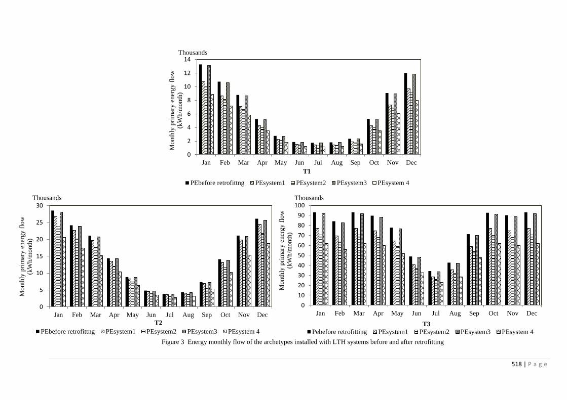
518 | P a g e

Figure 3 Energy monthly flow of the archetypes installed with LTH systems before and after retrofitting

0

2

4

6

8

10

12

14

Jan Feb Mar Apr May Jun Jul Aug Sep Oct Nov Dec

Mo

nth

ly p

rim

ary e

ner

gy f

low

(kW

h/m

onth

)

Thousands

T1

PEbefore retrofittng PEsystem1 PEsystem2 PEsystem3 PEsystem 4

0

5

10

15

20

25

30


Mo

nth

ly p

rim

ary e

ner

gy f

low

(kW

h/m

onth

)

Thousands

T2

PEbefore retrofittng PEsystem1 PEsystem2 PEsystem3 PEsystem 4

0

10

20

30

40

50

60

70

80

90

100


Mo

nth

ly p

rim

ary e

ner

gy f

low

(kW

h/m

onth

)

Thousands

T3

Pebefore retrofitting PEsystem1 PEsystem2 PEsystem3 PEsystem 4

519 | P a g e

Figure 4 The impact of air-tightness variance levels to the primary energy usage of studied archetypes (kWh/yr m2)

50

60

70

80

90

100

110

120

130

0,811,21,41,61,822,2

Pri

mar

y en

ergy

usa

ge ,

kWh

/(yr

m2

) T1, Air-tightness retrofits variance level (ACH, p50))

PEbefore retrofitting PEsystem1 PEsystem2

PEsystem3 PEsystem4

50

60

70

80

90

100

110

120

130

2 1,9 1,8 1,7 1,6 1.5

Pri

mar

y en

ergy

usa

ge ,

kWh

/(yr

m2

)

T2, Air-tightness retrofits variance level (ACH, p50))


PEsystem3 PEsystem4

50

60

70

80

90

100

110

120

130

0123456T3, Air-tightness retrofits variance level (ACH, n50))


PEsystem3 PEsystem4

520 | P a g e

6 REFERENCES

[1] C. Björk, P. Kallstenius, and L. Reppen, Så byggdes husen 1880-2000 (As built houses

1880-2000). Forskningsrådet Formas, 2002.

[2] Energimyndigheten (Energy Agency), “Energy in Sweden,” Swedish Energy Agency,

Eskilstuna, Sweden, 2012.

[3] V V S Företagen, Renoveringshandboken - för hus byggda 1950-75 (Renovation

handbook for houses built in 1950-75). Stockholm: Wallén Grafiska AB, 2009.

[4] A. Göransson and B. Pettersson, “Energieffektiviseringspotential i bostäder och

lokaler - Med fokus på effektiviseringsåtgärder 2005 – 2016,” Chalmers University of

Technology, Report, 2008.

[5] M. Economidou, B. Atanasiu, C. Despret, J. Maio, I. Nolte, and O. Rapf, “Europe’s

Buildings under the Microscope. A Country-by-Country Review of the Energy Performance

of Buildings,” Buildings Performance Institute Europe (BPIE), 2011.

[6] Q. Wang, “Toward Industrialized Retrofitting : Accelerating the Transformation of the

Residential Building Stock in Sweden,” 2013.

[7] J. A. Myhren and S. Holmberg, “Improving the thermal performance of ventilation

radiators – The role of internal convection fins,” Int. J. Therm. Sci., vol. 50, no. 2, pp. 115–

123, Feb. 2011.

[8] A. Hasan, J. Kurnitski, and K. Jokiranta, “A combined low temperature water heating

system consisting of radiators and floor heating,” Energy Build., vol. 41, no. 5, pp. 470–479,

May 2009.

[9] J. A. Myhren and S. Holmberg, “Flow patterns and thermal comfort in a room with

panel, floor and wall heating,” Energy Build., vol. 40, no. 4, pp. 524–536, 2008.

[10] K. Högdal and WSP Environmental, “Halvera Mera,Slutrapport (Half more, final

report),” BeBo (Energy Agency purchaser group for energy efficient apartment buildings),

Stockholm, 2013.

[11] M. Brand and S. Svendsen, “Renewable-based low-temperature district heating for

existing buildings in various stages of refurbishment,” Energy, vol. 62, pp. 311–319, Dec.

2013.

[12] TABULA, “Byggnadstypologier Sverige (Building typology in Sweden).” Mälardalen

University Sweden, 2009.

[13] Y. Zou, “Classification of buildings with regard to airtightness,” 2010.

[14] A. Hesaraki and S. Holmberg, “Energy performance of low temperature heating

systems in five new-built Swedish dwellings: A case study using simulations and on-site

measurements,” Build. Environ., vol. 64, pp. 85–93, Jun. 2013.

[15] L. Gustavsson, A. Dodoo, N. L. Truong, and I. Danielski, “Primary energy

implications of end-use energy efficiency measures in district heated buildings,” Energy

Build., vol. 43, no. 1, pp. 38–48, Jan. 2011.

[16] N. L. Truong, A. Dodoo, and L. Gustavsson, “Effects of heat and electricity saving

measures in district-heated multistory residential buildings,” Appl. Energy, vol. 118, pp. 57–

67, Apr. 2014.

[17] F. Ardente, M. Beccali, M. Cellura, and M. Mistretta, “Energy and environmental

benefits in public buildings as a result of retrofit actions,” Renew. Sustain. Energy Rev., vol.

15, no. 1, pp. 460–470, Jan. 2011.

[18] S. V. Russell-Smith, M. D. Lepech, R. Fruchter, and Y. B. Meyer, “Sustainable target

value design: integrating life cycle assessment and target value design to improve building

energy and environmental performance,” J. Clean. Prod.

[19] T. Y. Chen, J. Burnett, and C. K. Chau, “Analysis of embodied energy use in the

residential building of Hong Kong,” Energy, vol. 26, no. 4, pp. 323–340, Apr. 2001.

521 | P a g e

[20] ISO, EN, “Energy performance of buildings–Calculation of energy use for space

heating and cooling (EN ISO 13790: 2008).” European Committee for Standardization

(CEN), Brussels, 2008.

[21] Sweden Green Building Council, “Treatment of Scandinavian District Energy Systems

in LEED v1 2012, Energy models for LEED EA credit 1,” Stockholm, 2012.

[22] Boverket (Swedish National Board of Housing, Building and Planning), Teknisk status

i den svenska bebyggelsen: resultat från projektet BETSI (Technical status of the Swedish

settlements: results from the project BETSI). Boverket, 2010.

[23] K. Ericsson, “Introduction and development of the Swedish district heating systems -

Critical factors and lessons learned,” RES-HC Policy Proj. Rep. D23, 2009.

[24] K. Klein, K. Huchtemann, and D. Müller, “Numerical study on hybrid heat pump

systems in existing buildings,” Energy Build., vol. 69, pp. 193–201, Feb. 2014.

[25] A. Hepbasli and Y. Kalinci, “A review of heat pump water heating systems,” Renew.

Sustain. Energy Rev., vol. 13, no. 6–7, pp. 1211–1229, Aug. 2009.

[26] G. Jóhannesson, “Building energy - a design tool meeting the requirements for energy

performance standards and early design - validation,” presented at the Research in Building

Physics and Building Engineering, 2006, pp. 627–634.

[27] T. Kalema, G. Jóhannesson, P. Pylsy, and P. Hagengran, “Accuracy of Energy

Analysis of Buildings: A Comparison of a Monthly Energy Balance Method and Simulation

Methods in Calculating the Energy Consumption and the Effect of Thermal Mass,” J. Build.

Phys., vol. 32, no. 2, pp. 101–130, Oct. 2008.

[28] T.-O. Relander, S. Holøs, and J. V. Thue, “Airtightness estimation—A state of the art

review and an en route upper limit evaluation principle to increase the chances that wood-

frame houses with a vapour- and wind-barrier comply with the airtightness requirements,”

Energy Build., vol. 54, pp. 444–452, Nov. 2012.

[29] P. I. Sandberg, P. Wahlgren, C. Bankvall, B. Larsson, and E. Sikander, “The effect

and cost impact of poor airtightness-Information for developers and clients,” in Proceedings

of the 10th Conference on the Thermal Performance of the Exterior Envelopes of Buildings,

Clearwater Beach, Florida, 2007.

[30] P. Levin, A. Jidinger, and A. Larsson, “Rekorderlig renovering,

Demonstrationsprojekt för energieffektivisering i befintliga flerbostadshus från

miljonprogramstiden, Objektrapport för Norrbacka – Sigtunahem Etapp 1 & 2 (Record our

renovation, Demonstration projects for energy efficiency in existing apartment buildings from

the million program, Object Report for Norrbacka - Sigtunahem Stage 1 & 2),” Jul. 2010.

[31] Boverket (Swedish National Board of Housing, Building and Planning), “Swedish

Building Regulations-Building codes BBR.” 2012.

[32] M. Dahl, M. Ekman, T. Kuldkepp, and N. Sommerfeldt, Energy Saving Measures in

Existing Swedish Buildings : Material for a book to be published by VVS Företagen. 2011.

[33] S. Holmberg, J. A. Myhren, and A. Ploskic, “Low-temperature heat emission with

integrated ventilation air supply,” presented at the Proceedings of International Conference

Clima 2010, 2010.

[34] A. Ploskic, “Low - Temperature Basedboard Heaters in Built Environments,” 2010.

522 | P a g e

THE USE OF A ZONAL MODEL TO CALCULATE THE

STRATIFICATION IN A LARGE BUILDING

Lien De Backer*

1, Jelle Laverge

2, Arnold Janssens

3, and Michel De Paepe

4

1 Ghent University- Architecture and Urban planning

Sint-Pietersnieuwstraat 41B4

9000 Ghent, Belgium




9000 Ghent, Belgium



9000 Ghent, Belgium

4 Ghent University-Flow, Heat and Combustion

Mechanics


9000 Ghent, Belgium

ABSTRACT

In the past, many churches were raised and in a church building no heating no heating system was installed,

except a simple individual coal or peat stove, which could be rented by the churchgoers. The thick high stone

walls of the church alleviated the fluctuations of the ambient air temperature and relative humidity. Accordingly,

the indoor climate in the church building was quite stable. After the Second World War the living standard of the

people increased and the increased prosperity also led to higher comfort demands in churches. As a consequence,

many “local” heating systems were often replaced by rugged air inlets, designed to quickly heat the space to

increase the thermal comfort. These were designed and operated without taking the effect of the fluctuating

temperature and relative humidity on the artwork in the church into account. Consequently, the many artworks in

the church building like the organ, the pulpit and the panel paintings are also exposed to this changing climate,

leading to faster deterioration or even to damage. Evaluating the conservation conditions for the artworks in a

large space requires knowledge of the stratification in temperature and humidity inside a large space that occurs

during heating. The use of Computational Fluid Dynamics (CFD) is probably the most suitable method to predict

the airflow pattern, but it is quite time consuming and requires a powerful computer. As an alternative a zonal

model is a suitable method to predict the airflow in a large space in a simplified way. These models can be

linked to a BES- software in which each zone is assumed to be perfectly mixed. By this coupling, the influence

of the airflow on the temperature distribution and vice versa can be calculated, in order to judge the thermal

comfort and preservation conditions in one zone. This paper presents the coupling of the existing thermal zonal

model of Togari with the BES-software TRNSYS. In addition a moisture preservation equation was added to the

thermal zonal model to predict the vertical relative humidity gradient in a large space. Further the model also

was extended with a EMPD-model to include the moisture buffering of the walls in a simplified way.

523 | P a g e

KEYWORDS

Thermal stratification, zonal airflow model, dynamic simulation

1. INTRODUCTION

In the past , church buildings were usually unheated, except for a simple individual coal or

peat stove, which could be rented by the churchgoers. The thick high stone walls of the

church alleviated the fluctuations of the ambient air temperature and relative humidity. As a

result, the indoor climate in the church building was quite stable (Schellen, 2002). After the

Second World War the living standard of the people increased and the increased prosperity

lead to higher comfort expectations (Camuffo et al., 2010), not only in residential dwellings,

but also in churches. As a consequence many “local” heating systems were replaced by

heating systems that heated the whole indoor air volume of the church. Often these systems

were rugged air inlets, designed to quickly heat the space and achieve thermal comfort during

services. These systems were designed and operated without taking the effect of the

fluctuating temperature and relative humidity they caused on the artworks in the building into

account. Consequently, the many wood based artworks usually present in the church, like the

pulpit, the organ and the panel paintings are also exposed to this changing climate. According

to the preservation needs determined by the ASHRAE conservation classes (Anon, 2011),

changes in temperature and relative humidity or space gradients could lead to faster

deterioration or even to damage at these artworks.

Table 1: ASHRAE conservation classes (Anon, 2011) related to the risk on damage at wooden artworks

Class Temperature Relative Humidity Risks

ΔTshort

Space gradients

ΔTseasonal ΔRHshort

Space gradients

ΔRHseasonal

AA ±2°C ±5°C ±5% No changes No risk of mech. damage

A As ±2°C +5°C

-10°C

±5% ±10% Small risk of mech. damage

A ±2°C +5°C

-10°C

±10% No changes

B ±5°C +10°C

max. 30°C

±10% ±10% Moderate risk to high-

vulnerability artefacts but

tiny risk to most paintings

C <25°C (<30°C) 25-75% High risk of mech. damage

D - <75% Prevent dampness

To reconcile the heating demand due to comfort expectations of the visitors with the

preservation needs for the artworks in designing a heating system for such churches including

artwork, computer simulations can be helpful. During heating, thermal stratification occurs

and in order to make a correct assessment of the stratification, in addition to the calculation of

the energy exchange, the calculation of the airflow in the space is necessary. To predict the

temperature and humidity distribution, different modelling approaches can be used: namely

Computational Fluid Dynamics (CFD) models and the linking of a Building Energy

Simulation (BES) software with an airflow model (the so-called zonal models).

The CFD-method is a widespread approach to model the airflow with a computational

simulation. Models, based on this method, predict the temperature, velocity and other flow

524 | P a g e

parameters by numerically solving the Navier-Stokes equations with a high degree of

accuracy. However, for this research, the fluctuations in temperature and humidity over a

longer time period and the effects of heating on the temperature and humidity distribution in

large historical buildings, related to damage occurring at wooden artifacts are of interest. To

simulate longer time periods, the mentioned CFD models are less suitable because of their

need for powerful computers with a large amount of memory. In reality, these resources are

often not available. To be able to predict the airflow in a building in a fast way and for a

longer time period, the use of a macroscopic airflow model offers a solution. These so-called

zonal models are an intermediate approach between the CFD and the multizone models used

in BES, which consider the air as perfectly mixed. The difference with a CFD model is that

the grid is much coarser and the differential equations between the cells are simplified. Based

on the simplifications made, the zonal models can be further subdivided into pressure-zonal,

temperature-zonal and momentum-zonal models.

As pointed out above, a BES-software considers a zone perfectly mixed. However, a BES

software is commonly used for the evaluation or comparison of different heating techniques

to meet sizing and energy operating cost requirements (Bouia & Dalicieux, 1991). Though, a

BES software, because of this assumption of a well-mixed zone is unable to calculate the

temperature stratification in the air. So to determine the thermal comfort and the preservation

conditions the BES model has to be extended with an airflow model. Because the emphasis

lies on predicting the airflow in a building in a fast way, we chose to implement a

temperature-zonal model in the BES-software. For this purpose the thermal-zonal model of

Togari(Togari, Arai, & Milura, 1993) was recoded in C++ and coupled to the commercial

BES simulation environment TRNSYS (v17). In this paper the possibilities of the model and

its shortcomings are discussed by applying it on the case of a typical church building.

2 THE COUPLED THERMAL ZONAL MODEL

The model proposed by Togari et al.(Togari et al., 1993) is a simplified model for calculating

the vertical temperature distribution in a single large space. They assumed that the main

components of the air movement in the large space are airflows along the vertical wall

surfaces (so-called wall currents) and supply airstreams. Further, they also assumed that the

horizontal temperature is uniform, except for the regions affected by supply air jet ventilation.

Based on these assumptions a method was proposed to calculate the stratification.

First the space is divided into a finite number of horizontal layers or blocks. Each layer

consist of a core cell and walls cells. The core cell represents a layer and when the layer is

bounded by a wall, a wall cell is defined which accounts for the mass flows in the boundary

layer. The method considers three major paths for the heat and mass transfer: (1) heat and

mass transfer between the core cell and the wall cells, (2) heat transfer and air movement

between the different core cells and (3) heat transfer through the wall. To calculate these

transfers some decision were made:

To predict the air and heat transport to the wall elements, the aid of the boundary layer

theory is applied.

Since the heat transfer through the walls, which is affected by both outdoor and indoor

conditions, is rather complicated, a heat balance equation for coupled thermal

conduction, convection and radiation is necessary to predict the wall surface

temperature. For this the implementation of the model in a BES-software was used.

525 | P a g e

2.1 The wall currents

When the air in a space is warmed up or cooled down , the air is cooled at the colder walls or

warmed up at the hotter walls. By consequence an airflow along the vertical walls is induced.

The heat and air mass transfer along the wall is modelled using a so-called wall current

model. This model assumes that the heat convection drives mass flow ( ) with an

average temperature ( ) from layer i to its related boundary layer.

Figure 1: Schematic representation of the composition of the wall currents and the mass flow in and between the wall cell

and the core cells

To calculate ( )with temperature ( ) following equations were applied:

( ) ( ) ( ) (17)

( ) ( ) ( )

(18)

The current flow from layer i will combine with the current flow ( ) from layer i+1 to

form a total flow with mass ( ) with average temperature ( ), yielding:

( ) ( ) ( ) (19)

( ) ( ) ( ) ( ) ( )

( ) (20)

Some of the air of this current ( ) returns to the air layer i ( ( )) and some continues

to the cell down or up ( ( )), depending on the direction of the current flow. The splitting

of the mass ( ) into ( ) and ( ) is calculated by the ratio P(i,K):

( ) ( ) ( ) (21)

( ) ( ) (22)

The ratio P(i,K): is dependent on the relationship between the air temperature in zone i and in

zone i+1 or zone i-1, associated with the current temperature ( ). Table 1 presents the

judgment criteria for the airflow pattern.

𝑚𝑚𝑑(𝑖 𝐾) 𝑌(𝑖 )

𝑚𝑚𝑑(𝑖 𝐾) 𝑌(𝑖 )

𝑌(𝑖) 𝑚𝑚(𝑖 𝐾)

𝑚𝑖𝑛(𝑖 𝐾)

𝑌𝑚(𝑖 𝐾)

𝑌(𝑖 𝐾)

𝑚𝑜𝑢𝑡(𝑖 𝐾) ( )

526 | P a g e

Table 2: judgment criteria for the airflow pattern

Flow

direction

Temperature

conditions

Des

cen

din

g

( ) ( )

( ) ( )

( )

( ) ( )

( ) ( )

( ) ( ) 1

Asc

end

ing ( ) ( )

( ) ( )

( )

( ) ( )

( ) ( )

( ) ( ) 1

2.2 Conservation equations

The calculation of the mass balance in every zone, was started from the lowermost zone.

Flows are defined as positive in the upward direction and from the wall cells to the layers.

The mass balance for a layer i is then calculated by:

∑(

) (23)

Where is the mass flow from layer i to i+1 [kg/s] and is the mass flow coming

from a source [kg/s].

In the air the heat transfer equation can be written as:

( ) ( )

(24)

Where is the heat coming from a source, means the heat transfer between the

layers and represents the heat flow from or to the wall currents. expresses the heat

transfer between the layers due to thermal stability yielding:

( ) ( ) (25)

Where is the boundary area between zone i-1 and zone i. ( ) is the heat transfer factor

and is defined as “the value obtained when a stable (Cb = 2,3W/m²K) or unstable (Cb =

112W/m²K) temperature stratification is formed.

The model of Togari was extended by an equation for moisture conservation. Hereby the air is

assumed as a mixture of dry air and water vapour, each component (vapour and dry air)

obeying the ideal gas equation. Taking into account the time dependency of the moisture

content of the air, the moisture balance equation for a layer i can be expressed as:

(

)

(26)

represents the vapour flow produced by people, systems activities such as

washinh,…and is the vapour mass flow between the layers. The vapour mass flow

from the wall current is calculated by:

∑ ( ) ( )

∑ ( )

(27)

Where ( ) is the humidity ratio of wall current and is determined by the moisture flux

( )coming or going to the wall, the humidity ratio of the mass coming from the

527 | P a g e

adjacent layer and the humidity ratio from the wall current under or above (see Figure 197).

The equation to determine the humidity ratio of the wall current ( ) is:

( ) ( )

( ) ( ) ( ) ( )

( ) (28)

The amount of water vapour exchange between room air and the wall (i,K) was modelled with

a simplified algorithm. The chosen model was an effective moisture penetration depth

(EMPD) model (Janssens, Rode, De Paepe, Woloszyn, & Sasic-Kalagasidis, 2008). This

approach assumes that the moisture transfer takes place between the zone air and a thin

fictitious layer of a uniform moisture content with a thickness dbuf, which is related to the

variation of water vapour pressure at the material surface. The effective penetration depth dbuf

is calculated by equation 13, in which tp is the period of cyclic variation (s).

√ ( ) ( )

( ) (29)

Where ( ) is vapour permeability [s], ( ) is the moisture capacity in terms of humidity

derived from the material sorption isotherm [kg/m³] and ( ) represents the saturation

water vapour pressure at temperature T [Pa]. The following equation is then solved together

with the moisture balance equation for indoor air within a space under the non-steady-state.

( )

( )

(

( ))

(

( ))

(30)

Where represents the water vapour pressure indoor and is the average water

vapour pressure in the layer[Pa]. is the surface convection coefficient of the wall [m/s] and

is the vapour diffusion resistance between the surface and the moisture storage centre of

the layer.

2.3 Adding infiltration

Infiltration is due to wind-driven or buoyancy-driven ventilation.With buoyancy-driven

ventilation the pressure differences are due to air density differences, which in turn are due to

temperature differences. Following equation was used to calculate the infiltration rate:

(

) (31)

Where is the infiltration defined in air changes per hour; i.e. zone volume per hour, when

the pressure difference between inside and outside is 50 Pa. ‘n’ is equal to 2/3 and is the

pressure difference[Pa] related to the height H [m] of the zone and the temperature difference

[°C] which is calculated by:

( ) (32)

2.4 Adding a jet flow model

To model a free jet stream, the following assumptions were made:

- First the trajectory of the path was determined.

For horizontally compact free jets, the trajectory of the centreline is described by Koestel

(Awbi, 2003), yielding:

√

(

√

)

(33)

The centreline velocity decay of compact jets can be described by the following equation.

528 | P a g e

√

(34)

Theoretical values of the characteristic K1 depend upon the type of velocity profile equation

and supply conditions assumed (Goodfellow & Tahti, 2001). For a 3D-jet the value of

equals 7,2 (Awbi, 2003). The temperature decay in the centreline of the jet was calculated

with the following equation.

√

(35)

In this equation the value for K2 was calculated by the formula of Shepelev (sec (Goodfellow

& Tahti, 2001)):

( )

(36)

- To evaluate the total airflow rate transported by the jet to some distance from the

diffuser, the entrainment rate was determined.

For a given opening area A0, the entrainment ratio is proportional to the distance x. For a

compact jet, the following equation by Grimithlyn was used (sec (Goodfellow & Tahti,

2001)):

√

(37)

3 VALIDATION OF THE MODEL

The validation case studied in this paper is the case that can be found in the report of Togari et

al. (Togari et al., 1993) and that of Arai et al.(Arai, Togari, & Miura, 1994). The

geometrically simple test room has a ground plane of 3m x 3m and measures 2,5m in height.

The room consist of insulated boards (three vertical walls, ceiling and floor) and 1 glass wall.

In the wall opposite to the glass wall, two openings were made in the symmetry plane: a

supply inlet at 0,625m above the floor and a return outlet at 0,250m above the floor. The

simulated cases are visualized in Table 3.

Table 3: Overview of the simulated case studies

Name Case Supply air condition Inlet

location

Outside

temperature outlet size air volume velocity temperature momentum

[mm x mm] [m³/h] [m/s] [°C] [kg m/s²]

N-11 500 x 74 42 (14)

N-10 500 x 74 12 (42)

H-100 500 x 74 150 1,13 40,7 0,053 zone 1 11

529 | P a g e

The room described above was fully modelled in TRNSYS. The space was vertically divided

into 5 layers. In the model described by Togari the calculations of the stratification started

based on measured wall surface temperatures, while in the model in TRNYS only outdoor

conditions can be used. As a consequence the behaviour of the walls and the inside surface

temperature is calculated by TRNSYS. For the case of natural convection (case N-11 and case

N-10) good agreement was found (De Backer, Laverge, Janssens, & De Paepe, 2014). On

Figure 198 results are shown for the case H-100 where the measured results by Togari were

compared with the calculated results by the thermal-zonal model. The measured results were

predicted well enough by the jet-model.

Figure 2: The progress of the temperature in case of hot air supply condition (jet)

4 A CASE STUDY

The goal of this study was to look how a church building could be modelled with the thermal

zonal model. As already pointed out, the thermal zonal model had some limitations. One of

the limitations is that it can only deal with simple geometries and the geometry can only be

subdivided into horizontal layers. For that, the geometry of the church building had to be

simplified.

For this study, a church was modelled with a floor plan and dimensions typical for a church in

Belgium. The geometry of the church includes a rectangular nave of 32m in length, 17m in

width and 15m in height (internal dimensions). The floor plan also containes side aisles. Each

side aisle measures 5x5m. The church has 0,9m thick masonry walls . The windows are

single-glazed. Based on literature (Fawcett, 2001), the following structure was assumed for

the build-up of the church floor: a plain square paving stone, laid on a bed of lime mortar. The

floor was modelled using the standard ISO 13370:2007. Figure 199 shows the model used in

the simulation study, where the church building was divided into 5 layers. Initially, the attics

of the church were not included in the model.

Figure 3: Simplified geometrical model of a church building

0

0,5

1

1,5

2

2,5

10 15 20 25 30Hei

ght

abo

ve

flo

or

level

[m]

Temperature [°C]

measured zonal model + TRNSYS

530 | P a g e

In the simulation study, 24 hours were simulated during which heating only occurred once,

during service. The service started at 10h00 and ended at 11h00, so the heating device was

operated from 9h30 till 11h30 with a set point temperature of 16°C. The temperature at the

supply inlet was 45°C and the flow rate was 30000kg/h. The initial conditions in the church

building were 8°C and 80%RH. Figure 200 and Figure 201 show results for the temperature

and relative humidity profile in the church building. The temperature is the lowest zone rises

to 16°C and achieves the set comfort temperature. The relative humidity decreased to 50%. In

contrast, the temperature in the highest zone rose to 21°C, while relative humidity dropped

down to 35%. For an artwork that encompasses several subsequent layers, like an organ, large

relative humidity gradients occur during heating. Furthermore, there also can be concluded

that the ASHREA class B , the highest class that can be reached in a church building

(Ankersmit, december 2009), cannot be achieved if the church is only heated during a church

service and one wants to achieve comfort temperature.

Figure 4: Temperature distribution in the church building

Figure 5: Relative humidity distribution in the church building

5 CONCLUSIONS

As an alternative to the complex CFD models, zonal models are a suitable method to predict

the airflow in a large space in a simplified way. These zonal models can be linked to a BES-

software, in which each zone is assumed to be perfectly mixed. By this coupling, the

influence of the airflow on the temperature distribution and vice versa can be calculated, in

order to assess the thermal comfort and preservation conditions in the zone. This paper

presents the coupling of the existing thermal zonal model of Togari with the BES-software

TRNSYS. In addition a moisture preservation equation was added to the thermal zonal model

to predict the vertical relative humidity gradient in a large space. The model was additionally

extended with a EMPD-model to include the moisture buffering of the walls in a simplified

0

5

10

15

20

25

8 10 12 14 16 18 20

Tem

per

atu

re [

°C]

time [h]

Tamblayer1layer2layer3layer4layer5

30

40

50

60

70

80

90

100

8 10 12 14 16 18 20

Tem

per

atu

re [

°C]

time [h]

RHamblayer1layer2layer3layer4layer5

531 | P a g e

way. To validate the model, the cases described in the paper of Togari were simulated. Good

agreement was found between the measurements and the thermal-zonal model. A case study

of a typical church building was modelled. The results showed how stratification in the

church building occurs during heating with a typical rugged air inlet, demonstrating that the

ASHREA conservation class B, cannot be achieved when heating solely during church

services.

6 REFERENCES

Ankersmit, B. (december 2009). Klimaatwerk: richtlijnen voor het museale binnenklimaat:

Amsterdam University Press.

Anon. (2011). ASHRAE handbook: Heating, ventilating, and air-conditioning applications, SI

edition (pp. 23.21-23.22): American Society of Heating, Refrigerating and Air-

Conditioning Engineers.

Arai, Y., Togari, S., & Miura, K. (1994). Unsteady-state thermal analysis of a large space

with vertical temperature distribution. ASHRAE Transactions, 100(part 2), 396-411.

Awbi, H. B. (2003). Ventilation of Buildings. London: Spon Press

Taylor & Francis.

Bouia, H., & Dalicieux, P. (1991). Simplified modeling of air movements inside dwelling

room. Paper presented at the IBPSA (The International Building Performance

Simulation Association), Nice, France.

Camuffo, D., Pagan, E., Rissanen, S., Bratasz, L., Kozlowski, R., Camuffo, M., & della Valle,

A. (2010). An advanced church heating system favourable to artworks: A contribution

to European standardisation. Journal of Cultural Heritage, 11(2), 205-219. doi: DOI:

10.1016/j.culher.2009.02.008

De Backer, L., Laverge, J., Janssens, A., & De Paepe, M. (2014). On the coupling of a zonal

model with a multizone building energy simulation model. Paper presented at the NSB

2014, Lund, Sweden.

Fawcett, J. (2001). Historic floors: their history and conservation: Butterworth-Heinemann.

Goodfellow, H. D., & Tahti, E. (2001). Industrial Ventilation Design Guidebook California

San Diego: Academic Press.

Janssens, A., Rode, C., De Paepe, M., Woloszyn, M., & Sasic-Kalagasidis, A. (2008). From

EMPD to CFD – overview of different approaches for Heat Air and Moisture

modeling in IEA Annex 41 Copenhagen: IEA ECBCS Annex 41, Closing Seminar.

Schellen, H. L. (2002). Heating monumental churches : Indoor Climate and Preservation of

Cultural Heritage. (PhD thesis), Technische Universiteit Eindhoven.

Togari, S., Arai, Y., & Milura, K. (1993). A Simplified Model for Predicting Vertical

Temperature Distribution in a Large Space. ASHRAE Transaction, 99(part 1), 84-90.

532 | P a g e

RECENT ADVANCES ON FACTORS INFLUENCING

HUMAN RESPONSES AND PERFORMANCE IN

BUILDINGS AND POTENTIAL IMPACTS ON

VENTILATION REQUIREMENTS

Pawel Wargocki

International Centre for Indoor Environment and Energy,

Department of Civil Engineering,

Technical University of Denmark ([email protected])

Implementation of sustainability and energy efficiency measures creates opportunity to revisit

some requirements regarding indoor environmental quality and also necessitates examining,

whether these measure do not incidentally increase the risk for human health, and do not

compromise human comfort and work performance. This presentation attempts to address

these issues.

Brief review is provided of the effort to define principles for building ventilation in

commercial and residential buildings based on health requirements and on the role of carbon

dioxide in setting ventilation requirements with focus on potential negative effects on work

performance. Building and environmental factors, which influence human comfort and

performance are reviewed, as well as the newest research summarized on the role of bedroom

ventilation for sleep quality and the next day performance. An account is given on whether

humans can tolerate slowly increasing temperatures and what potential consequences are

brought for health and human performance when this is taking place in buildings.

It is postulated that future ventilation standards should be based on health requirements

and should to a much larger extent map and be related to the actual exposures to pollutants.

The source control should be considered as the main mitigation measure of poor air quality

(both indoors and outdoors) and ventilation used only when source control methods are

ineffective; ventilation can be supplemented (not replaced) by air cleaning. There is no

evidence that carbon dioxide is detrimental to comfort and health at levels typically occurring

indoors, though there is potential for negative effects on some aspects of performance; carbon

dioxide is a good proxy for pollution from humans which do reduce perceived air quality and

increase acute health symptoms. To maximize overall satisfaction with one's personal

workspace, investments should first be made that lead to increasing satisfaction with the

amount of space, noise level and visual privacy. These investment will not guarantee the

highest output as regards work performance. This can be achieved by improving satisfaction

with temperature, noise level and air quality. Results suggest that insufficient bedroom

ventilation does negatively affect sleep quality and the next day performance though the

results are preliminary and need further verification. There are some seasonal differences in

human responses to increasing temperatures, subjects being slightly more tolerant to slowly

increasing temperature in warm season rather than in cold season. Too high temperatures may

compromise work performance.

The above results provide an important and rational supplement to already existing

large body of evidence on the factors influencing human responses in indoor environments

and advance our understanding of the underlying mechanisms. They allow enhancing the

process of design and operation of the buildings by providing further guidance to building

533 | P a g e

stakeholders. However, there is still very little systematic evidence on the impact of

certification schemes, which promote sustainability and energy, on the indoor environmental

quality and human responses; these schemes become widespread standard in case of new

construction and major renovations. Such studies are undergoing and will provide input to

revise and improve the schemes, so that the objectives of human centric design of buildings,

one of the major reason why we have buildings, can be accomplished.

534 | P a g e

STRATEGIES FOR EFFICIENT KITCHEN

VENTILATION

Bas Knoll1 & Wouter Borsboom

1

1 TNO

Netherlands

1 HEALTH RISKS

Cooking devices are a major source of contaminants in dwellings. They cause exposure to

combustion products and vapors. The type and production rate of contaminants depend on the

heating type (gas vs. electric cooking) and cooking process (frying vs. boiling).

Major health risks appear to be fine dust particles (which may contain carcinogenic PAH),

NOx, CO, CO2, VOC like acrolein and micro-biological contaminants due to excess

moisture.

Apart from this, odors from the cooking appliances may be annoying as well as excessive

heat, which (especially in combination with a high humidity) even may be a physiological

burden.

2 MINIMIZE DISPERSION FLOW AND CHARACTERIZE IT

To control the cooking contaminants, it is important first to restrict their dispersion and to

know their characteristics. This depends on:

Type of heat source, e.g. gas burning, electric hot plate, electric induction plate;

Pan type (casserole, saucepan, frying pan, griddle, pressure cooker), pan height, lid

type;

Status of the cooking or frying process (warming, cooking or frying stage) and typical

temperature (depending on the major substance, e.g. water, oil, sugar);

Free flow space (height to cooker hood, closed back or corner or island arrangement),

flow conduction (Coanda effect) and local flow disturbance (nearby windows, doors

and pathways);

Cook behavior (stirring, temperature control, lid use, moving along).

The first step to control contamination is to try and minimize the production rate and

dispersion forces by altering said factors (processes and geometry).

For the design of an effective cooker hood, the flow characteristics (flow velocities, flow

directions and flow field geometry) needs to be measured in critical situations.

3 LOCAL CAPTURE IS PREFERRED OVER DILUTION

Local capture is by far the most effective way to control the dispersion of cooking

contaminants. Once dispersed into the room a larger air volume becomes contaminated and

needs to be replaced by a much larger ventilation air volume during a longer period. In the

meantime people present in the kitchen are still exposed to the resulting concentrations.

Hence, local capture potentially is much more efficient, concerning both exposure and energy

use.

535 | P a g e

In airtight, energy efficient buildings with minimized ventilation due to demand control, the

low background ventilation level leads to long lasting, high concentrations of (cooking)

contaminants. Therefore, in general the need for a high capture efficiency rises with

increasing energy efficiency of dwellings.

4 MAJOR SPECIFICATIONS FOR USER-FRIENDLY COOKER HOODS

For users two major drawbacks prevent an unrestricted use of the cooker hood:

1. It does not sufficiently reduce odor spread;

2. There is a high noise nuisance.

Odor sensation has a logarithmic relation with pollutant concentration (e.g. 90% reduction of

odor concentration will reduce odor complaints by maximal half). So, only a nearly perfect

capture efficiency will meet the requirements for odor control. Since the design of an 80 or

90% effective hood only slightly alters from a 100% efficient one, the latter should be the

design goal.

For the cooker hoods noise production a threshold value of 40 dB is proposed.

Apart from this, important demands are an attractive design and no adverse effect on the

usability of the cooking appliances.

5 IMPROVE LOCAL CAPTURE EFFICIENCY

For common cooker hoods the capture efficiency is poor. Recommended steps to improve this

are:

Redesign the cooker hood, i.e. minimize the capture distance (hood height), maximize

the overhang, move the suction slots to the critical contaminant escape spots at the

perimeter, avoid large internal pressure drops;

Enclose the contaminant flow by conducting plates and/or direct it to the hood by

support flows. Automatically close down openings when no activities (like stirring)

are ongoing;

Derive the correct capture (and support) flow rates from the flow characteristics and

the new hood geometry, using known design rules. Evaluate and tune this with tests;

Control the flows and the distribution over the hood depending on production spots

and intensity, favorably automated control using sensors.

There are interesting examples of improving capture efficiency in professional kitchens.

6 RECIRCULATION OR EXHAUST?

If captured contaminated air is exhausted from the kitchen area the flow equilibrium means

that provisions for comparable supply flows are necessary, especially in airtight dwellings.

Some imbalance (overflow from surrounding rooms) may be useful to prevent dispersion of

poor quality kitchen air to surrounding rooms. In general this (temporary applied) supply flow

is quiet large compared to normal ventilation system flows. Therefore, a special kitchen

supply provision is recommended.

This kitchen supply needs special attention concerning draught risk. Furthermore a temporary

high energy loss may occur due to the temperature deviation of the incoming outside air. Heat

recovery, favorably including latent heat exchange to maximize the re-gain, enables the re-use

of the heat of the exhaust air.

Another option is to recirculate contaminated air after filtration. However, filter demands will

be high due to the complex mixture of (fine) particles, aerosols, gaseous components and

odors. To filter the water vapor, condensation on an additional cold heat pump element may

be required. Also this element may extract excess heat to control the kitchen temperature.

536 | P a g e

Finally, necessary periodic filter replacement will have its drawback on user-friendliness and

filter inefficiency will still require (possibly extra) background ventilation to reduce rest

exposure.

7 BACKGROUND VENTILATION

Some rest contamination into the kitchen may be unavoidable, e.g. because of incidentally

escaping flares of cooking air or due to exhalation of food that is further processed after it is

taken of the stove. Therefore some background ventilation is considered to be necessary. Also

after preparing food some low level elongation of exhaust fan operation time is

recommended.

537 | P a g e

COUPLING HYGROTHERMAL WHOLE BUILDING

SIMULATION AND AIR-FLOW MODELLING TO

DETERMINE STRATEGIES FOR OPTIMIZED

NATURAL VENTILATION

Matthias Pazold

*1, Florian Antretter

1, Marcus Hermes

2

1 Fraunhofer Institute for Building Physics

Fraunhoferstrasse 10

83626 Valley, Germany


[email protected]

2 Fraunhofer Institute for Building Physics

Nobelstrasse 12

70569 Stuttgart, Germany

ABSTRACT

In both, newly built and renovated buildings the building air-tightness has to be ensured. With a tight building

envelope comes a low infiltration air-exchange. A minimum outdoor air exchange to ensure acceptable moisture

and indoor air quality levels must be maintained.

A model is introduced, that couples hygrothermal whole building simulation with a multi-zone air-flow

simulation. This coupling allows assessing the combined effects of air-flow on building energy use, comfort

conditions, air quality and possible hygric issues.

An application example shows the use of the software for a low rise residential building. In a first step the

parameterization of the air-flow network is checked by computing the resulting infiltration air-flow with closed

windows. The maximum achievable natural air exchange for different window types and openings, like pivot-

hung windows, windows opened with a small parallel gap around and side-hung windows is assessed. Based on

these numbers it is assessed if any of the above mentioned opening options alone with a certain opening duration

is able to achieve good indoor air quality and acceptable indoor moisture levels to avoid any hygric problems or

if a combination of some of the measures is required.

The presented dynamic hygrothermal whole building simulation coupled with a multi-zone air-flow model is

capable of simulating the effects of different window opening options and strategies on building energy demand,

indoor comfort conditions and air quality and on the hygrothermal building component performance. It is shown,

that a sufficient air exchange can be realized even with a parallel-action window with small opening gaps which

can be run with motor drives. Especially demand controlled opening strategies can be developed that ensure high

indoor air quality and comfort conditions while also controlling humidity indoors to avoid moisture damage.

Also an improvement for summer conditions can be achieved by ventilative cooling with this type of window

opening.

KEYWORDS

hygrothermal building simulation, air-flow-model, WUFI®

Plus, natural ventilation

1 INTRODUCTION

The model development bases on a building component tool to simulate the coupled heat and

moisture transport across building components, like walls, roofing and floors (Künzel, 1994).

It simulates the unsteady temporal development of the heat and moisture profile within a

component and, of course the heat and moisture exchange on the component surfaces.

Combining simulations for all components of the building envelope and inner walls with a

538 | P a g e

zone model leads to the hygrothermal whole building simulation tool, called WUFI® Plus

(Holm, Künzel, & Sedlbauer, 2003). One or different zones describe one or more rooms

within the building with equal air properties for each simulation time step. The boundaries of

each zone are the building components. Regarding this, the inner and the outer surface of a

component are assigned to zones. Besides the heat and moisture transport across the

components, solar radiation through windows, inner sources or sinks, HVAC systems and of

course the air exchange influence the indoor climate and are taken into account. The indoor

climate within zones is calculated with a heat and moisture balance for the whole building

model.

An assumed or measured air exchange can be considered as constant, or time scheduled

before running the hygrothermal building simulation. But, in fact, the air flow depends on the

simulated indoor climate. It also depends on the wind velocity and direction mostly delivered

with the outdoor climate data. Therefore a pressure driven multi-zone airflow model (Pazold

& Antretter, 2013), quite similar to the model used within CONTAMN (Walton & Dols,

2008), is implemented, to simulate this air flow for each time step. The multi-zone definition

of the airflow model is equal to the definition of the zones within the whole building software.

If a building component is not fully airtight, is has to be defined as air flow path. Furthermore

air openings and fans have to be defined as air flow paths. Therefore different types of sub-

models, to calculate the mass flow rate depending on the pressure difference, are used for the

different flow patterns. The wind pressure on the outer side of the building envelope and the

hydrostatic air pressure are calculated for each path in a respective relative height, to simulate

stack effects.

The introduced hygrothermal building simulation tool coupled with the described multi-zone

air flow model is used for the investigation of ventilation strategies to determine the

optimized natural ventilation for an example low rise building. This paper describes the

application of the tool. Different window opening options and strategies are assumed to assess

their effect on the indoor comfort conditions, the air quality and the hygrothermal building

component performance of the building.

2 LOW RISE RESIDENTIAL BUIDLING MODEL

The visualisation of the investigated two-storey residential building is shown in Figure 1.

Each room is regarded as one zone; hence the building exists of 10 heated zones. The attic

and the basement excluded the basement stairwell, is regarded unheated. The zone separation

enables the assessment of the differing indoor climates within the building because of the

inter-zone air flow and among other things, like different inner sources. The treated floor area

of the building is 148.51 m² and the net volume (air volume) is 349.3 m³. The characteristic

length of the building is 10m and the width 9 m.

539 | P a g e

Figure 1: 3-D view and floor plans with zoning of the modelled building

2.1 General simulation assumptions

The location of the building is Holzkirchen in Germany. The used reference outdoor climate

data is representative for the temperate climate region. The average outdoor temperature is

6.6°C with a range from -20.1°C up to 32.1°C in summer. The average outdoor relative

humidity is 81 %. The average wind velocity is 2.2 m/s mostly from west. An open terrain is

assumed to calculate the wind pressure at building height and solar shading.

The investigated simulation period is one year, beginning in January. The result time step is

one hour. Built-in moisture effects are taken into account by initializing the envelope

components to realistic built-in moisture contents. But 2 months are pre-calculated and not

assessed to allow a short dry-out period because of differing boundary conditions after the

completion of the building and the following usage. During the investigated simulation

period, the building is continuously occupied by four persons, two adults and two kids.

Different inner heat-, moisture, and CO2- daily profiles for each room reflect the day-presence

of the residents (Figure 2 and Figure 3). In sum the overall internal heat gain is 11.14 kWh per

day; the moisture production is 8.96 kg per day and the CO2-gain is 3 kg per day for the

whole building.

Figure 2: Daily-profile of inner heat gains (summarized for all zones)

540 | P a g e

Figure 3: Daily profile of inner moisture sources (summarized for all zones)

An ideal heating system is used to keep the indoor climate at a minimal design temperature of

20°C. If the inner temperature would decrease below this design condition, because of more

heat loss than gains within a zone, the actual heating demand is calculated to keep the

minimal temperature. The maximal design temperature of 24°C is used for activating the

temporary sunscreen device. If the inner temperature would increase above the design

condition, the incident solar radiation through the windows is decreased to 10 % due to an

activated sunscreen device.

2.2 Building envelope

The simulation tool calculates the coupled heat and moisture transfer through multi-layer

building components. Within this paper only a few parameters of the components are

presented. The exterior wall is made of aerated concrete with a mineral plaster at the outer

side and a gypsum board at the inner side. The resulting thermal resistance is 3.6 m²K/W. The

thermal resistance of the roofing is 5.0 m²K/W and for the basement slab 2.85 m²K/W. The U-

Value of the windows is 1.3 W/(m²K) and the solar heat gain coefficient for the transparent

area 0.6. Those values meet the current German energy saving ordinance requirements.

2.3 Air flow parameters

The whole building envelope is assumed to be not air-tight. As described in the introduction

the air flow across the different components is calculated with the pressure driven multi-zone

air flow model for each time step, taking into account the actual inner climate and wind

pressure. The mass flow rate through the components is mostly calculated with a power law,

fitted for different kinds of flow patterns. The opening state of windows and inner doors can

vary during the simulation. The opening times and durations are predefined for different

natural ventilation strategies. The model calculating the air flow depends on the opening

condition and can change for each time step.

Inner doors can be open or closed. Three states of the windows are investigated. They can be

closed or opened in turn-position. As a third position, windows with parallel action fittings are

investigated. They can be opened by parallel offsetting the sash by approx. 6 mm to the

frame. This creates an air gap on all sides of the casement. With a motor fitting drive the

parallel offsetting of the window can be automated, without any user interaction.

The parameters used for each component are given in Table 1. Some are based on (Orme,

1999) Appendix E but adjusted to get a requested air change rate at 50 Pa pressure difference

n50 = 1.5 h-1

. This is checked by a simulated pressure difference test and a whole year

simulation with a closed envelope (closed windows and open inner doors). For the difference

pressure test, a constant volume flow rate fan is added in the entry door. With an iterative

541 | P a g e

method, the volume flow rate of the fan is adjusted to reach different pressure differences

between the inside and outside air. For the test the wind pressure is neglected and an equal

temperature of 20°C, also in the outdoor zone is assumed. With those different pressure

differences and their associated volume flow rates, a n50-value of 1.48 h-1

is calculated for the

closed building air flow network with the defined air flow parameters. This is in good

agreement to the requested air permeability, so the chosen air flow parameters seem to be

reasonable with this first check.

Table 1: Used air flow parameters

Building Component Air flow parameters Related to

Exterior walls Flow coefficient 0.021 dm³/(s m² Pan); Flow exponent 0.84 Wall area

Inner walls Flow coefficient 0.021 dm³/(s m² Pan); Flow exponent 0.84 Wall area

Roofing Effective leakage area 20cm² on each roof side Roof sides

Entry door, closed Flow coefficient 0.12 dm³/(s m Pan); Flow exponent 0.6 Joint length

Inner doors, closed Flow coefficient 1 dm³/(s m Pan); Flow exponent 0.6 Joint length

Inner doors, open Two-way-flow pattern; Discharge coefficient 0.6; Exponent 0.5 Opening area

Windows, closed Flow coefficient 0.12 dm³/(s m Pan); Flow exponent 0.6 Joint length

Windows, open Two-way-flow pattern; Discharge coefficient 0.6; Exponent 0.5 Opening area

Windows, parallel open Two-openings; Opening Areas 0.058m² (at the top and bottom

of the window); Discharge coefficient 0.162; Flow exponent 0.5

Opening area

3 NATURAL VENTILATION STRATEGIES AND RESULTS

Different natural ventilation strategies are analysed by designing cases with different opening

times and states for the windows. Beside the inner air temperature, relative humidity and CO2-

concentration, the air change rate with the outside climate and the inter-zonal air change rates

are calculated for each time step and every defined zone. The huge amount of results is

evaluated for each case and some average annual values are presented in this paper. Some

additional assessments available with the coupled hygrothermal building simulation with the

air flow model are shown.

3.1 Closed envelope

In a first step, the natural infiltration due to air leakage was investigated. The windows are

kept close for the whole simulation time. In fact, this is not a realistic case, but should also

prove the designed air flow network with the air flow parameters. As a result, the average

annual natural air change rate for this case is 0.11 h-1

. This value can be expected for the

requested air permeably of n50 = 1.5 h-1

and the used outer climate. In 25 % of the year, the air

change rate is below 0.04 h-1

. The room with the lowest outside air change rate is the upstairs

bedroom facing north-east with an average annual value of 0.01 h-1

. The inter-zonal air

change rate for this room is on average 0.2 h-1

. The most outside air ventilated room is the

kitchen, (0.26 h-1

) facing north-west. The heating demand due to air leakage and without any

other ventilation is 51 kWh/(m² year).

542 | P a g e

3.2 Normal window turn-opening

Figure 4: Accumulated window opening time over the simulation year for normal window turn-opening

This case should represent normal user ventilation behaviour by turn-open the windows. The

opening times are pre-defined by calculating possible opening durations for each simulated

time step depending on climate conditions and user presence. If the possible opening duration

is more than zero, the actual opening is randomly calculated with a probability of 20 %.

Only when there is a very low rain load (below 0.1 liter/(m² h)), or when a person is presence

in a room the possible opening duration for each window is calculated. Further, if the outdoor

temperature in is above 20°C (for the window in the bedroom above 15°C) the window can be

opened for the whole time step, one hour. Is the outdoor temperature below this boundary, a

short opening for 10 minutes (0 – 20°C) or 5 minutes (below 0°C) can only happen, when a

person enters or before leaving a room. With this algorithm, the window in the kitchen is

averagely opened twice a day and the windows in the other rooms averagely once a day. In

the heating period, the opening duration is 5 to 10 minutes. In the summer a window can

stand open for one or more hours. The accumulated window opening times for each window

in the different rooms are shown in Figure 4.

The resulting outer air and inter-zonal air change rate for each zone is shown on Figure 5. The

resulting average annual air change rate for the whole building is 0.31 h-1

, the moving average

is shown in Figure 6.

As indicator for the air quality the CO2-concentration within the rooms is used. For this case

the average concentration in the whole building is 44 % of the year above 1500 ppm. Within

the worst room, a child’s room, it is 73 % of the year above 1500 ppm. Following this the air

quality is rather poor. As indicator for the comfort condition the inner air temperature is used.

It is 4.3 % of the year above 26°C. The heating demand in this case is 59 kWh/(m² year).

As a first indicator for the hygric issues the relative humidity within the rooms is used. In the

winter months the average relative humidity is about 50 %. However, especially in the

bathroom, with short high moisture loads, the relative humidity is more than half of the year

above 60 % and even one third of the year above 70 % up to 99 %. So the first assumption is

that there will be hygric issues at least within the bathroom. Further investigations in order to

assess the risk of mould growth under transient conditions can be made with a bio-

hygrothermal method. For this investigation, the tool WUFI Bio (the basics are discussed in

(Sedlbauer, 2001)), is used to predict mould growth on the interior surfaces. It calculates the

moisture content available for mould and compares it with a critical water content which

allows a spore to germinate. On the inner surface on the exterior wall of the bathroom, for the

substrate category II (materials with porous structure such as the gypsum board) the predicted

mould growth rate is 4.6 mm/year and the mould growth index is about 0.008, which seems to

543 | P a g e

be no issue. However, the simulation is made with an interior thermal resistance of 0.13

(m²K)/W which might have to be increased due to less convection in corners or behind

cupboards. Then the surface temperature and the risk of mould growth would increase.

Figure 5: Resulting average annual outer air and inter-zonal air change rates for the different rooms.

Results for normal window turn-opening

Figure 6: Moving daily and monthly average air change rate within the whole building.

Results for normal window turn-opening

3.3 Frequent window turn-opening

This case should represent a frequently user ventilation behaviour by turn-open the windows

up to four times a day for 5 till 60 minutes in summer, shown in Figure 7. The algorithm to

calculate the opening durations, depending on climate conditions and person presence is equal

to the case before with the assumed normal user behaviour. However, the probability

calculating the actual opening randomly is set to 50 %.

The average annual air change rate within the whole building is 0.69 h-1

for this case. The

moving monthly average is mostly above 0.5 h-1

and increase in summer up to1.0 h-1

. In the

kitchen, where the window is west-faced and most frequent turn-opened, the average annual

outside air change is 2.5 h-1

. The higher infiltration rate increase the calculated heat demand to

84 kWh/(m² year) but the CO2-concentration is only for 12 % of the year above 1500 ppm and

mostly below 2000 ppm. Only in the sleeping rooms, with the high continuous CO2-source

during night time, the CO2-concentration is about 30 % of the year above 1500 ppm. The

544 | P a g e

average inner air temperature used for assessing the comfort condition is only for a short time

during summer, when the outer temperature is quite high, above 26°C, for 2.4 % of the year.

The average relative humidity is decreased to 36 % during the winter months and in the

bathroom for quite a few hours above 70 %. The bio-hygrothermal model predicts no mould

growth on the inner surfaces, the moisture content available for spores is significantly below

the critical water content for spore germination.

Figure 7: Accumulated window opening time over the simulation year for frequent window turn-opening

3.4 Automatic parallel action window

This presented natural ventilation strategy uses the described automated parallel offsetting of

the windows with a parallel action fitting. This ventilation method should require no further

occupant interaction to get a good air quality, good comfort conditions, no risk for mould

growth and a low heating demand. This shall be checked with this simulation case. The

parallel offset of the windows is set to last four hours a day nearby high moisture and CO2

contribution in the rooms. It is assumed that they automatically open from 5:30 to 7:30, 12:30

to 13:00 and from 18:30 to 20:00. During summer time, when there is no heating demand and

the outer air is useful for night cooling, the parallel offsetting of the windows should

automatically last longer, even the whole night. For this case the user behaviour is not

neglected. It is additionally assumed that the occupants turn-open the windows at least every

4th

day for 5 to 10 minutes.

Figure 8: Moving daily and monthly average air change rate within the whole building.

Results for Automated window opening by parallel offsetting the casement

The resulting average annual air change rate is 0.4 h-1

, with the moving daily and monthly

averages shown in Figure 8. The calculated heating demand, to keep the inner air temperature

545 | P a g e

above 20°C is 67.5 kWh/(m² year). Even with this lower air change rate, and lower heating

demand, compared to the case before, the CO2-concentration within the rooms is on average

only 7 % of the year above 1500 ppm and in the sleeping rooms only for 15 % of the year.

The inner air temperature is 3.8 % of the year above 26°C. The relative humidity during

winter is averaged for the whole building 44 % and in the bathroom lower than in the cases

before. The bio-hygrothermal model predicts no mould growth on the inner surfaces.

4 CONCLUSIONS

At first, the coupled hygrothermal whole building simulation with a multi-zone air flow

model is introduced. In the following parts of this paper the application of this coupled

simulation method is shown exemplary for a low rise building. It is used to determine natural

ventilation strategies to optimize the air quality and the comfort conditions by minimizing the

heating demand and the risk of mould growth. Only the opening times and durations of the

windows are investigated in three presented cases. The first case assumes a normal window

opening occupant behaviour. For the second case the turn-opening durations of the windows

are more frequent. In fact, for longer turn-opening times, the air quality getting better and the

risk of mould growth is decreased, but also the heating demand is increased about 40 %, for

the well-insulated building. Both named cases require user interaction. This is not necessary

in the last case where the windows should be opened automatically by parallel offsetting the

sash to get a 6 mm air gap around the casement. The parallel offsetting of the windows for at

least four hours a day show better indoor conditions by less heating demand (14 % more

compared to the first case) due to the lower but more continuous air change rates. Of course,

there is a lot of input data and results not presented in this paper, but at least some of the

results that can be expected by the application of such a coupled whole building simulation

tool are presented. Hygrothermal whole building simulation coupled with an airflow model

enables a holistic air-flow, air-quality, comfort and energy assessment while also being able

to determine possible hygric issues on and in the building components.

5 ACKNOWLEDGEMENTS

This study, especially the coupling of the hygrothermal building software with the air flow

model was funded by the German Federal Ministry of Economics and Technology (BMWi

0329663L). The application cases, especially the last with the parallel action fitting windows

originated in a project called “Natürliche Lüftung” realised with D+H Mechatronic AG, Hella

Automation GmbH, H.O. Schlüter GmbH und Aug. Winkhaus GmbH & Co. KG.

6 REFERENCES

Holm, A., Künzel, H. M., & Sedlbauer, K. (2003). The hygrothermal behaviour of rooms :

combining thermal building simulation and hygrothermal envelope calculation.

Proceedings of the 8th International IBPSA Conference. Eindhoven, Netherlands.

Künzel, H. M. (1994). Simultaneous Heat and Moisture Transport in Building Components.

Dissertation. University of Stuttgart.

Orme, M. (1999). TN 51: Applicable Models for Air Infiltration and Ventilation Calculations.

AIVC Technical Note 51.

Pazold, M., & Antretter, F. (2013). Hygrothermische Gebäudesimulation mit Multizonen-

Gebäudedurchströmungsmodell. Bauphysik, 35.(2), pp. 86-92.

546 | P a g e

Sedlbauer, K. (2001). Prediction of mould fungus formation on the surface of and inside

building components. Dissertation. University of Stuttgart.

Walton, G. N., & Dols, W. S. (2008). CONTAM 2.4c User Guide and Program

Documentation. NISTIR 7251, National Institute of Standards and Technologiy.

547 | P a g e

EXPERIMENTAL CHARACTERISATION OF

DOMINANT DRIVING FORCES AND FLUCTUATING

VENTILATION RATES FOR A SINGLE SIDED SLOT

LOUVER VENTILATION SYSTEM

Paul D O’Sullivan1, 2

, Maria Kolokotroni 2

1. School of Mechanical, Electrical & Process Engineering, Cork Institute of Technology, Cork, Rossa

Avenue, Bishopstown, Cork, Ireland

2. Howell Building, Mechanical Engineering, School of Engineering and Design, Brunel University, Uxbridge

UB8 3PH, United Kingdom

ABSTRACT

Adopting natural ventilation as a retrofit strategy for cooling, due to the low impact nature of the installation, is

attractive due to the cooling potential of untreated outdoor air for large periods of the extended cooling season,

particularly in northern climates. In line with this it is important to characterise the performance of natural

ventilation components in low energy buildings in successfully transferring the cooling potential of outdoor air

to the occupied zone. This paper presents an analysis of the results from 25 individual ventilation rate tests of a

single sided slot louver ventilation system installed in a low energy retrofit application and 13 tests from a pre-

retrofit window opening, taken as a control space for comparative purposes. Results for 3 opening configurations

for the slot louver ventilation system are compared. Parameters characterising momentum and buoyancy driving

forces during each test were also recorded. A number of different permutations for combined wind and buoyancy

effects were recorded allowing an investigation of the existence of any underlying patterns as well as the relative

effect of the different opening configurations. Owing to the nature of single sided ventilation and the primary

airflow exchange mechanisms normally present, the transient evolution of the normalised tracer gas

concentration during tests is also discussed and compared. Analysis shows that different patterns emerge for the

dominant driving forces depending on opening configuration in the slot louver system. The slot louver

ventilation system has led to steadier ventilation rates. Opening height and geometry is shown to have a

significant effect on the net contribution from momentum driving forces and the fluctuation amplitude of the

ventilation rate and this effect is wind direction dependant. Ventilation rates are shown to correlate well with

fluctuation amplitude. The nature of the ventilation rate during tests for different wind directions is shown to

vary depending on wind patterns at the building envelope.

KEYWORDS

Single sided ventilation, dominant forces, warren plot, buoyancy asymptote, fluctuating ventilation rate

1 INTRODUCTION

While experimental data exists for single sided ventilation rates, (Dascalaki et al 1996)

(Dascalaki et al. 1995) (de Gids and Pfaff. 1982) (Caciolo et al 2011), information is not

exhaustive for opening types other than common window types. Single sided ventilation

techniques are generally reserved for single cell (Irving et al 2005), isolated spaces and when

considering older office buildings that need retrofitting, the floor plan can often be cubicle

and not intended as open plan spaces. Developing ventilation components that can be

externally applied, provide sufficient weather protection and are effective at ensuring good

ventilation rates by responding to contributing airflow mechanisms is central to ensuring

successful implementation of climate change adaptation strategies. This paper presents an

analysis of the mechanisms contributing to time average single sided ventilation rates from

test results for a slot louvre ventilation component operated as part of a single sided

ventilation strategy. It considers two key aspects of the ventilation rate; the combined effect

548 | P a g e

of momentum and buoyancy forces on mean ventilation rates and analysis of the nature of the

ventilation rate during tracer decay tests using a fluctuation parameter, . The objective is to Nomenclature

Symbols Subscripts

Archimedes Number inside

Flow Number outside

constant related to for opening internal to external

discharge coefficient Air change rate

Reynolds Number Tracer, total

temperature (K) Thermal, stack effect

height, (m) opening

gravitational constant, ( ⁄ ) effective

velocity, ( ⁄ ) wind , test space envelope wall

time averaged air change rate, ( ) Normalised concentration

opening area ( ) Zone interior

Power law exponent h hydraulic

L Characteristic length (m) c concentration (relating to fluctuations)

Density ( ⁄ )

tracer gas concentration (ppm) Abbreviations

time, (h) CS Control space

Total pressure (kg/ms2) RS Retrofit space

standard error of estimate of predictions ACH Air change rate

P Parallel incidence direction

L Leeward incidence direction

W Windward incidence direction

WD Wind direction

investigate the conditions contributing to mean ventilation rates for a slot louvre system used

in single sided ventilation. Data presented was recorded in a full scale test room for different

opening configurations. Literature review has revealed little reported work of full scale

experiments characterising how slot louvre systems with low hydraulic diameters perform

within ventilation strategies where mechanisms such as turbulent eddy diffusion play an

important function.

2 EXPERIMENTAL SETUP

A total of 25 full scale ventilation rate tests from the retrofit space for different component

opening configurations were compared to 13 tests in a control space in the existing building

with dynamically similar characteristics. Ventilation components tested are described in

section 3. Experimental measurements were recorded using a tracer gas decay technique with

the regression method applied to spatially averaged and normalised concentration values. All

tests were completed under normal operating mode for the ventilation system resulting in the

inclusion of effects from some complex geometry at the openings as well as a number of

openings serving the test space being included in the recordings.. A detailed summary of the

experimental setup and test conditions for both retrofit space and control space has recently

been published by the authors and is not repeated here (O’Sullivan and Kolokotroni, 2014).

549 | P a g e

3 VENTILATION COMPONENT DETAILS

3.1 Slot louvre ventilation system (RS.02, RS.03, RS.04)

The installed slot louvre system has a net 50% free open area for airflow and overall structural

opening dimensions are 0.30m (w) x 1.60m (h) with a net opening area of 0.102 m2 (2

openings at low level and 2 openings at high level in the test space). On the internal side of

the slot louvres there are automated higher level insulated doors and manual lower level

insulated doors providing different control mechanisms. The ventilation system forms part of

an externally applied retrofit fenestration module supplied with two glazed sections and two

ventilation sections. The louvres are manufactured in anodized aluminium alloy 6063-T6 with

a resulting smooth surface finish, see Figure 1. Each of the ventilation openings has 17

airflow slots across the louvre bank. Taken individually the louvre slots have an extremely

low porosity at 0.057%. Table 1 summarises key information regarding the slot louvre

system.

Figure 1: Slot louvre component details (a) sample louvre profile, (b) opening dimensions (c) installation

3.2 Top hung outward opening window (CS.01)

The control space ventilation component consists of an outward opening top hung window

unit. This was used as a basis for comparison of time average ventilation rates and ventilation

unsteadiness during tests with the slot louvre system. Details are summarised in Table 1 and

in (O’Sullivan and Kolokotroni. 2014). There appears to be limited data available on full scale

performance of this type of window in the literature. Recently Grabe has done some work

characterising flow resistance (Grabe 2013).

Table 1: comparison of purpose provided ventilation opening types in CS & RS

Parameter CS RS Units

Plain structural opening dimensions (W x H) 0.92 x 1.14 0.30 x 1.60 m

Total opening area At 0.32 0.42 m2

Porosity 0.18 0.057 (%)

Total opening “wetted” perimeter 5.96 0.99 m

Hydraulic diameter (dh) (At & based on “wetted” perimeter) 0.214 0.02 m

Aspect Ratio (L/dh) 1.070* 1.075 (-)

Opening type (categories according to Etheridge 2011) short short (-)

*Note: length dimension for measured along perimeter of opening window section

3.3 Definition of asymptote for ventilation components

Dimensional Analysis using Warren plots is predicated on the correct selection of the

asymptote through the origin defining flow number due to buoyancy alone, . The gradient

of this asymptote is sensitive to correct selection of both the still air discharge coefficient,

and the exponent used in the power law relationship for pressure and flow (i.e. = 0.5 for

orifice flow). is an important parameter for a ventilation opening as it depends on the

geometry of the opening and the Reynolds number, of the flow, and is normally taken as

550 | P a g e

0.61 for a flush faced sharp edged orifice. Various research studies have considered the effect

on of different opening types and their geometry, shape and porosity under wind driven

flow (Karava et al 2004) (Heiselberg et al 2001), while other studies have concentrated on the

effects of wind in terms of direction and the effects of dynamic pressure (Chiu and Etheridge

2007). Caciolo et al (Caciolo et al 2011) used a value of 0.6 to describe the flow

characteristic when calculating for various open window geometries while a of 1.0 is

used in (Dascalaki et al 1996). Grabe has recently presented findings specific to flow

conditions under buoyancy alone that relates to the definition of for top hung outward

opening windows (Grabe 2013; von Grabe et al 2014). The value selected for for the

control space window opening to facilitate analysis is 0.55 and is largely based on Grabe et al.

Both Pinnock (Pinnock 2000) and Sharples et al (Sharples and Chilengwe 2006) have carried

out experimental work considering the use of alternative exponent values in the power law

equation when dealing with buoyancy alone case and slot louvres respectively. Pinnock

proposed = 0.6348 and Sharples suggested = 0.9301. The orifice flow equation is retained

for analysis here although this is something that warrants further investigation given the

significant impact on this would have. The slot louvre system used here is a flush

faced sharp edged orifice at the inlet and flow is likely unidirectional through the individual

slot openings. There is a length component of the louvre in a circular shape (see Figure 1) that

might promote some flow reattachment allowing viscous forces and a boundary layer to

develop, reducing the flow separation that normally results in being independent of .

However, for the purposes of establishing a value under buoyancy alone conditions 0.61

may be a little low but acceptable for RS.04 and RS.02 for the purposes of initial analysis.

The RS.03 configuration has the combined effect of slot louvre and inward opening

ventilation door due to its restricted opening angle and a probably lower than 0.61 as a

result. A value of 0.55 is assumed for RS.03. Quantifying a correct value and power

law exponent for the slot louvre system is still under investigation and is not presented here.

4 CHARACTERISING DRIVING FORCES FOR SINGLE SIDED VENTILATION

The mechanisms that produce airflow in single sided ventilation are generated through

varying combinations of wind and buoyancy forces acting at the opening. Depending on wind

incidence angle the dominant mechanisms are either from a pulsating flow due to pressure

difference at the opening, turbulent diffusion through a mixing layer at the opening plane or a

combination of both. When due to buoyancy forces alone, the flow will be bidirectional with

a neutral pressure at the opening mid height point. The temperature difference at the opening

results in a buoyancy effect that produces a stable airflow exchange. However, at low wind

speeds and a leeward incidence direction the effective enveloped temperature has been shown

to be reduced due to a recirculation zone counteracting buoyancy effects resulting in air

change rates lower than in the absence of wind (Caciolo et al 2013). When wind is normal to

the opening plane a pulsation airflow effect will dominate increasing compression of the air

mass but not necessarily adding to ventilation rate. Cockroft and Robertson suggested that

37% of the volume flowrate across the opening due to pulsation will contribute to an air

change rate (Cockroft and Robertson. 1976). The local wind speed at the opening is very

much dependant on wind direction due to changes in flow patterns along the envelope given

different wind incidence directions. Larsen shows how air change rate depends on wind

incidence direction with effect more pronounced at low wind speeds and the dominating force

differs between wind speed and depending on the ratio between these forces and the

wind direction (Larsen and Heiselberg 2008). A number of semi empirical models exist that

use Bernoulli flow theory and can also account for contributions from wind effects. Warren

and Perkins (Warren and Parkins 1985) proposed 2 separate correlations for buoyancy and

wind effect, taking the larger of the two to quantify ventilation rate. Dascalaki (Dascalaki et al

551 | P a g e

1996) proposed an alternative correlation to take account of wind effects. See also for

example (Crommelin and Vrins. 1988), (De Gids and Pfaff. 1976), (Wang and Chen 2012).

When studying permutations of contributing forces for ventilation rate tests Warren used the

relationship between a dimensionless ventilation parameter, Flow Number , and an adjusted

Archimedes Number, . The purpose of the Warren plot is to separate out the data

dominated by buoyancy effect. Warren plots have been used by researchers to analyse air

change rate data, for example see (Warren and Parkins 1985) (Van Der Mass. 1992), (Caciolo

et al 2011). Archimedes Number, , is used as a measure of the relative magnitudes of the

buoyancy (gravity) forces and the momentum (inertial) forces acting on elements of fluid.

This ratio can be expressed in (1) where L is a characteristic height.

(1)

For dynamically similar flows substituting for total wind pressure, , and taking the

square root one obtains a dimensionless parameter which is basically the same as that known

as (Etheridge, 2011):

√

(2)

The ratio can be replaced with for cases of interest. It should be noted that the

square root in the definition of is only used in connection with envelope flows, when it can

be interpreted as a velocity ratio. For large values buoyancy forces will dominate.

can be defined in (3) as where H is the opening height in question.

(3)

The ventilation parameter, Flow Number , is a practical dimensionless number to describe

wind induced ventilation. Generally where flow is buoyancy dominated should approach

the asymptote defined by . When wind dominates tends to zero and F becomes

independent of . For parallel flows should be approximately constant at 0.03. can be

defined as:

(4)

Plotting these vales for each test allows an interpretation of the influence wind forces have on

the buoyancy effect, either assisting or opposing its contributing force.

5 TEST CONDITIONS & RESULTS

5.1 Test conditions

Figure 2 presents polar frequency plots of wind speeds distributed according to wind direction

for each test configuration summarised in Table 3 of (O’Sullivan and Kolokotroni. 2014). An

analysis of wind data for each test using directional statistics (Mardia. 1972) shows that the

mean resultant length of direction vectors, a measure of “concentration” for circular data such

as wind direction, were in many instances close to 1.0 with low dispersion of wind orientation

during individual tests. This suggests that wind direction was consistent during a given test

and the resulting analysis can assume to represent the effects from flow phenomena present

for this type of orientation relative to the ventilation opening. We have taken Parallel flow to

occur between wind directions of 347.5° – 22.5° & 157.5° – 202.5°. 270° wind direction is

normal to the ventilation opening.

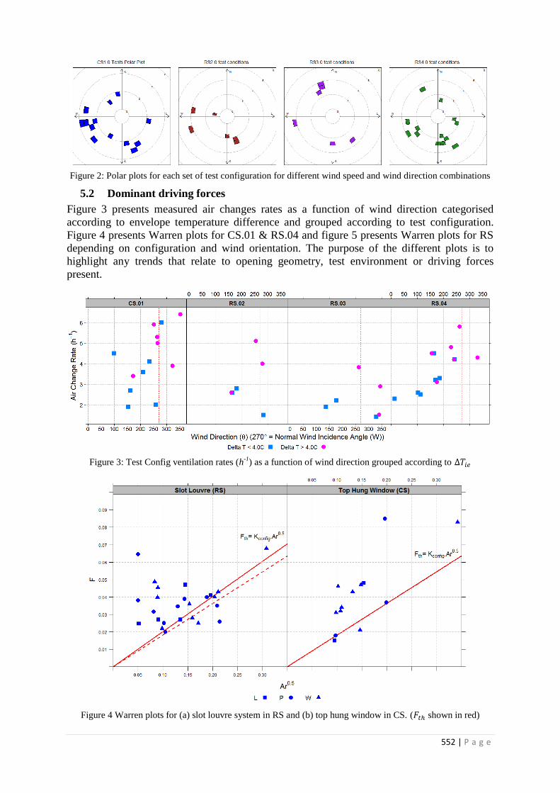
552 | P a g e

Figure 2: Polar plots for each set of test configuration for different wind speed and wind direction combinations

5.2 Dominant driving forces

Figure 3 presents measured air changes rates as a function of wind direction categorised

according to envelope temperature difference and grouped according to test configuration.

Figure 4 presents Warren plots for CS.01 & RS.04 and figure 5 presents Warren plots for RS

depending on configuration and wind orientation. The purpose of the different plots is to

highlight any trends that relate to opening geometry, test environment or driving forces

present.

Figure 3: Test Config ventilation rates (h-1

) as a function of wind direction grouped according to

Figure 4 Warren plots for (a) slot louvre system in RS and (b) top hung window in CS. ( shown in red)

553 | P a g e

Figure 5 Warren plot categorised according to (a) configuration and (b) wind direction. ( shown in grey)

5.3 Transient ventilation rates

Single sided ventilation strategies rely on a number of low and high frequency unsteady flow

phenomena relating to wind pressure, gustiness and turbulence. Tracer decay rates were

measured at a frequency of 1Hz during each test and figure 6 presents ACH values as a

function of wind direction, (270° = Normal to surface), grouped according to, , that is based

on the estimate of error in prediction from the regression model fitted to the normalised

concentration decay, to determine the ACH values (O’Sullivan and Kolokotroni. 2014).

This is taken as an indicator of the level of unsteadiness present during each test.

Figure 6: Air Change rate as a function of wind direction grouped according to magnitude of

554 | P a g e

6 ANALYSIS & DISCUSSION

6.1 Dominant driving forces

Considering figure 3 in all instances the highest recorded air change rates occurred with

greater than 4°C and a windward incidence direction. This occurs in both control and retrofit

spaces. Leeward conditions lead to the lowest ventilation rates (although the test population is

small for this wind incidence) with parallel incidence directions showing less defined

patterns. Low generally resulted in lower ventilation rates for low opening height RS.02

& RS.03 and some CS.01 & RS.04 tests have ACH values higher than 4.0 h-1

even at

below 4.0°C. It appears that where the wind incidence angle is not approximately normal to

the surface then it is more likely to have lower ventilation rates even at relatively high

values. This suggests that leeward and parallel flows at the opening are more likely to oppose

buoyancy forces. Considering Figure 4(a) & 4(b) we see a comparable spread of values for

both spaces with the retrofit range extending further towards zero ordinate. seems to

display slightly higher dependency on in CS.01. No clear patterns are visible from

review of the combined datasets. However, when looking at figure 5(a), when the data in

figure 4(a) is split according to RS opening configuration three different patterns emerge.

RS.04, ( ), shows a clear pattern of buoyancy dominant ventilation irrespective

of the wind incidence angle, which seems to agree with data in figure 3 where the highest

RS.04 ventilation rates had high values. Alternatively RS.03 has ( =

2.43m (above floor level)) and also has a potentially lower value than RS.02. It exhibits

increased contributions from wind forces with similar values but consistently lower

values compared to RS.04. It appears that with lower opening height buoyancy forces have

less ability to establish resulting in lower values and as a result values appear more

independent of in lower ranges. RS.02 ( ) (( ) has a greater

internal door opening angle than RS.03. It exhibits the least dependency on buoyancy forces

with nearly all tests showing wind dominant values. The clear variation in response of each

opening location presents a situation where for the slot louvre system the contribution from

momentum forces is a function of the overall structural opening height and vertical location

on the envelope. Considering figure 4(b) leeward tests seem to display a good range of

values and a general trend of values near the asymptote . According to (Caciolo et al.

2013) leeward conditions should be counteractive to buoyancy forces. This is not the case

here with the slot louvre opening. Only one of the five leeward tests had < 4.0°C. Both

Parallel and Windward incidence angles show a pattern of reducing dependency of on

as its value tends to zero. At low is a function of wind incidence direction. At higher

values these incidence angles show a tendency towards the asymptote and the wind direction

effects are diminished. These results are in line with (Larsen and Heiselberg, 2008) in

showing the interdependence of on both and wind direction and suggest that at low

wind incidence angle becomes important in determining whether or not wind becomes

dominant.

6.2 Ventilation rate characteristics

While it is difficult to draw any clear quantitative conclusions regarding high frequency

fluctuating phenomena when examining time averaged test data, the concentration fluctuation

parameter, (based on 10 second averages of readings taken at 1Hz), can still give a

measureable indication of the overall unsteadiness present in a ventilated space during a tracer

decay test. Figure 6 groups ACH data according to . The causes of this unsteadiness can be

due to several factors: pulsation flow, penetration of eddies, and static or molecular diffusion.

It is difficult to isolate the specific causes without detailed measurements of these various

phenomena and an assessment of overall trends is the most that can be achieved at this point.

10 of the 13 CS.01 window opening tests exhibited unsteadiness at the upper end of all

555 | P a g e

recorded values and these appeared to happen primarily under windward incidence

directions. These tests had averaged wind speeds > 3.0 ms-1

, > 5.0°C and appear wind

dominant according to the Warren plot analysis. This would suggest that unsteady ventilation

rates are more pronounced when wind is normal to the outward opening window. This may be

due to the nature of flow impingement with the window obstructing entry resulting in

increased turbulence. The highest fluctuation value for parallel flow in CS.01 happened with

one of the lowest average test wind speeds ( ) while the two other parallel flow tests

showed lower unsteadiness profiles with lower values suggesting that with parallel flow and

an outward opening window fluctuating components of ventilation rate are less pronounced

and buoyancy driven flow is able to better establish. This may be due to the fact the opening

section of the window does not obstruct parallel flow at the boundary layer of the structural

opening. More parallel flow tests are needed before this is conclusive. In the slot louvre

system only RS.04 exhibits tests with significant unsteadiness and all these tests occurred at

windward incidence angles. Higher fluctuation parameters are associated with higher

ventilation rates in RS.04 suggesting the importance of turbulence and wind induced

phenomena to single sided ventilation rates. These also occurred at windward incidence

directions. For RS.03 & RS.02, irrespective of wind incidence angle fluctuation parameters

were always low as were ventilation rates. Warren plot analyses suggest these are generally

wind dominant with low but they consistently exhibited low values appearing

counter intuitive. When comparing fluctuation rates for parallel flow in the RS configuration

they are generally lower than windward incidence angles. What is apparent from the test data

is the opening geometry has a direct influence on the nature of ventilation rate and wind

incidence direction also plays an important role with its effect dependant on the opening

geometry.

7 CONCLUSIONS

Previous work presented in (O’Sullivan and Kolokotroni, 2014) have highlighted the potential

interdependence of on both and wind direction, particularly at low values. This

paper investigated this further and has shown that the magnitude of to be dependent on

opening geometry. In physical terms this interdependence highlights the challenges in

predicting the correct airflow phenomena driving ventilation for different types of natural

ventilation components. An allowance for wind incidence direction, opening height and

aspect ratio and opening location in relation to the internal space will affect ventilation rates.

If is taken as an indicator of internal airflow environment for single sided ventilation this

suggests the interdependence of opening geometry and wind incidence direction has a large

influence on the penetration of wind-generated air exchange mechanisms. Modification of

thermophysical properties due to the retrofit have reduced the magnitude of for similar

values suggesting wind driving forces have an increased contribution even though the slot

louvre system is perceived as restricting flow. Further tests including measurements directly

at the external and internal faces of the opening will increase understanding of the providing a

more definitive allocation of the effect of the parameters investigated; such measurements are

under progress. Further work will include CFD model of the slot louvre systems and this

would allow further analysis of the effect of opening geometry on unsteadiness magnitudes.

8 ACKNOWLEDGEMENTS

The authors wish to thank Dr Peter Warren for his very helpful discussions and advice regarding the

use of the Warren plots. The original pilot project works was supported through a grant from the

Department of Education and Skills, Ireland. The authors wish to acknowledge the co-work of the

pilot project design and research team in the design and development phases of the pilot project

556 | P a g e

9 REFERENCES

Caciolo, M., Cui, S., Stabat, P., Marchio, D. (2013) “Development of a new correlation for single-sided natural

ventilation adapted to leeward conditions,” Energy & Buildings, 60, 372–382,

Caciolo, M., Stabat, P., Marchio, D. (2011) “Full scale experimental study of single-sided ventilation : Analysis

of stack and wind effects,” Energy & Buildings, 43(7), 1765–1773,

Chiu, Y.-H., Etheridge, D.W. (2007) “External flow effects on the discharge coefficients of two types of

ventilation opening,” Journal of Wind Engineering and Industrial Aerodynamics, 95(4), 225–252,

Cockroft, J. P., & Robertson, P. (1976), Ventilation of an enclosure through a single opening, Building and

Environment, 11(1), 29-35

Crommelin, R. D., & Vrins, E. M. H. (1988), Ventilation through a single opening in a scale model, Air

Infiltration Review, 9(3), 11-15

Dascalaki, E., Santamouris, M., Argiriou, A., Helmis, C., Asimakopoulos, D.N., Papadopoulos, K., Soilemes, A.

(1996) “On the combination of air velocity and flow measurements in single sided natural ventilation

configurations,” Energy and Buildings, 24(2), 155–165

Dascalaki, E., Santamouris, M., Argiriou, A., Helmis, C., Asimakopoulos, D. N., Papadopoulos, K., & Soilemes,

A. (1995). Predicting single-sided natural ventilation rates in buildings, Solar Energy, 55(5), 327-341

de Gids, W., & Phaff, H. (1982). Ventilation rates and energy consumption due to open windows: a brief

overview of research in the Netherlands. Air infiltration review, 4(1), 4-5

Etheridge, D., 2011. Natural Ventilation of Buildings: Theory, Measurement and Design, Wiley-Blackwell.

Grabe, J. Von (2013) “Flow resistance for different types of windows in the case of buoyancy ventilation,”

Energy and Buildings, 65, 516–522,

Von Grabe, J., Svoboda, P., Bäumler, A. (2014) “Window ventilation efficiency in the case of buoyancy

ventilation,” Energy and Buildings, 72, 203–211

Heiselberg, P., Svidt, K., Nielsen, P. (2001) “Characteristics of airflow from open windows,” Building and

Environment, 36, 859–869

Irving, S., Etheridge, D., Ford, B. (2005) Natural Ventilation in Non-Domestic Buildings CIBSE AM10, The

Chartered Institution of Building Services Engineers, CIBSE.

Karava, P., Stathopoulos, T., Athienitis, A. (2004) “Wind driven flow through openings–a review of discharge

coefficients,” International Journal of …, 3(3)

Larsen, T.S., Heiselberg, P. (2008) “Single-sided natural ventilation driven by wind pressure and temperature

difference,” Energy and Buildings, 40(6), 1031–1040

Mardia, K. V. (1972). Statistics of directional data, Academic Press

O'Sullivan, P., Kolokotroni, M. (2014) “Time-averaged single sided ventilation rates and thermal environment in

cooling mode for a low energy retrofit envelope system.” International Journal of Ventilation (In Press)

Pinnock, D. (2000) An Investigation into the Influence of Wind in Single-Sided Natural Ventilation, available:

https://dspace.lboro.ac.uk/xmlui/handle/2134/7465

Sharples, S., Chilengwe, N. (2006) “Performance of ventilator components for natural ventilation applications,”

Building and Environment, 41(12), 1821–1830,

Van der Maas, J. (1992). Air Flow Through Large Openings in Buildings (Subtask 2): IEA Annex 20–Air Flow

Patterns Within Buildings, LESO-PB, EPEL, CH-1015. International Energy Agency, Lausanne,

Switzerland

Wang, H., Chen, Q. (2012) “A new empirical model for predicting single-sided , wind-driven natural ventilation

in buildings,” Energy & Buildings, 54, 386–394,

Warren, P., Parkins, L. (1985) “Single-sided ventilation through open windows,” ASHRAE SP49, (1),

557 | P a g e

A STUDY OF CARBON DIOXIDE CONCENTRATIONS

IN ELEMENTARY SCHOOLS

John Sifnaios*, Paraskevi Vivian Dorizas, Margarita-Niki Assimakopoulos

Faculty of Physics, Departments of Environmental Physics and Meteorology, University of Athens,

University Campus,

Athens, 157 84, Greece


ABSTRACT

The present study aims at investigating carbon dioxide (CO2) concentrations inside elementary schools’

classrooms and how students’ productivity is affected. Measurements were conducted in 9 naturally ventilated

schools of Attica from April to May 2013. Monitoring lasted for 7 hours per day, for a period of one to five days

per school. CO2 concentrations were monitored simultaneously in the inside and the outside environment of the

classrooms. Indoor concentrations of CO2 in almost all schools were higher than the ASHRAE threshold limit

values. In order to examine the effect of CO2 concentrations on students’ productivity, they were asked to take

two productivity tests during their stay at school. Results showed that, higher concentrations of CO2 have a

negative impact on students’ productivity. Also, the effect of window opening on CO2 concentration was further

examined and there has been an effort to correlate indoor and outdoor CO2 concentrations. Finally, the

correlation between the occupancy density and the increase of CO2 concentrations was also investigated.

KEYWORDS

Schools, student performance, ventilation, occupant density, CO2

1 INTRODUCTION

Air quality in school buildings is a matter of great concern with students spending almost

30% of their time inside classrooms, more time than in any other building environment except

their home (Mendell and Heath 2005; Grimsrud et al. 2006). Furthermore, schools present a

much higher occupancy than any other building, having four times as many occupants per

unit of area compared to office buildings (EPA 1995). In addition, students belong to a quite

vulnerable group of people who can easily be affected by chemical factors emitted in schools’

premises (EFA 2001).

For the past decade there has been a scientific interest on the effects of the degraded indoor

environment to students and office workers performance and productivity (Wargocki et al.

1999; Wargocki et al. 2000; Witterseh et al. 2004; Mendell and Heath 2005) however

knowledge on that area is insufficient.

The main objectives of this study are to examine: 1. the effect of CO2 to students’

productivity, 2. the effect of occupancy density, window opening and ventilation rate to the

CO2 concentration, 3. the correlation between indoor and outdoor CO2 concentration and 4. to

evaluate the schools’ ventilation rate.

558 | P a g e

2 METHODOLOGY

In this paper secondary data analysis is conducted, based on existing data, in order to

investigate research questions other than the ones raised during the original study. Details on

the original methodology can be found in Dorizas’ papers (Dorizas et al. 2013a; Dorizas et al.

2013b; Dorizas et al. 2013c). In brief the above mentioned studies were carried out in 9

naturally ventilated primary schools of Attica, Greece (Figure 1), for a 32 days period,

between April and May 2013. Details on the schools and the classrooms where the

measurements were conducted are shown in Table 1. In total 193 students participated in the

survey and undertook 1310 performance tests.

The current study comprises the effect of CO2 concentration on students’ performance and the

correlation of occupancy density to CO2 concentrations and diurnal CO2 concentrations. Also

it involves the comparison between indoor to outdoor CO2 concentrations, the correlation of

CO2 concentration to window opening, ventilation rate and lastly the evaluation of the

schools’ ventilation rate.

Figure 1 : Map of Attica (left) and locations of schools under study (right)

559 | P a g e

Table 1: Schools’ characteristics

School Code School Name Classroom’s

Volume (m3)

Number of

Students in

the

Classroom

Measurement Period

School 1 Thrakomakedones 1 198 25 8-12/4/13 (5 days)

School 2 Thrakomakedones 2 162 25 20-24/5/13 (5 days)

School 4 Acharnae 4 155 24 14-18/4/13& 24/4/13 (5 days)

School 8 Acharnae 8 159 19 27-29/5/13 (3 days)

School 11 Acharnae 11 172 15 31/5/13 (1day)



School 18 Acharnae 18 138 18 23/4/13 (1 day)

School Pal Pallini 137 25 19&22/4/13

(3 days)

2.1 Measurements of CO2 and Ventilation

The concentrations of CO2 were measured in one classroom of each school from 7.30 a.m. to

2.30 p.m. Inside the classrooms the measurements were conducted using the MultiRAE IR

(RAE Systems) while outside the classrooms, the concentrations were measured using the

Innova 1312 & 1303. Both instruments calculated CO2 concentrations in units of parts per

million (ppm). In order to be able to compare the indoor to the outdoor concentration, lab tests

were conducted, under controlled conditions, so as to calculate a correction coefficient

between the two instruments. Classroom ventilation was also measured with Innova 1312 &

1303. The “Rate of Decay” method (Hitchin & Wilson 1967) was used in which, a quantity of

sulfur hexafluoride (SF6) was released in the classrooms near a low speed fan, after school

hours. The purpose of the fan was to produce a uniform concentration inside the classrooms.

The concentration decay was exponential and by sampling the air at several times the

apparent ventilation rate was determined in air changes per hour (ach).

2.2 Performance tests

The performance tests and operative protocol were taken from the SINPHONIE project, the

Schools Indoor Pollution and Health: Observation Network in Europe aiming to improve the

air quality in schools. Students were given a ‘code’ of symbols, in which each symbol was

associated to a digit number. They had 120 sec. to complete the relevant symbols at a given

series of numbers. They were asked to fulfil two tests each day, one in 10.00 a.m. and one in

13.30 p.m. Full detail of the methodology followed for the productivity tests is described in

Dorizas’ paper (Dorizas et al. 2013c).


3.1 Performance Scores vs CO2 Concentrations

In order to be able to compare the concentration of CO2 to the results of the productivity test,

a 15 minutes average was calculated (approximately 15 minutes was the duration of the test).

Figure 2 shows the average test scores of each day of each school for the code test (1st and

2nd). Also the figure illustrates the average concentration of CO2 at the time students took the

test. From the graph we can see that, in 26 out of the 28 days the score of the second test was

560 | P a g e

higher compared to the first. Also, the concentration of CO2 during the second test was lower

than the CO2 concentration of the first test. As a result, in the great majority of the cases (24

out of 28), lower CO2 concentration led to a higher test score. Taking into consideration the

above finding, we can conclude that there is a negative correlation between the performance

scores and CO2 concentrations. This result comes in agreement with Dorizas’ result (Dorizas

et al. 2013c) where, there had been a similar analysis calculating the average productivity test

score for each school (not for each day of the measurements).

Figure 2 : The trend of test scores per school per day and corresponding CO2 concentrations

3.2 Increase of CO2 Concentration due to Occupancy Density

Occupancy density was correlated to CO2 concentration so as to investigate the impact of the

class’ area available to each student to the increase of CO2. In order to calculate the effect of

students’ presence on CO2 concentrations, we subtracted from the CO2 peak the background

concentration (the one that was measured before the arrival of the students). The results were

divided into three groups depending on the window opening surface in square meters (m2)

during the lessons. In order to do that division, the surface area of the windows of each class

was measured and then the average value for each group was found. The first group

comprises the cases that the classroom’s windows were closed during the lesson and opened

in the break (Figure 3). In the second group, one window was opened halfway the lesson hour

(Figure 4). This scenario corresponds to a mean opened window surface of 1,56 m2. The third

group includes the cases during which two windows were open throughout the lesson time

(Figure 5). This scenario corresponds to a mean opened window surface of 3,28 m2.

It is obvious from all the diagrams that, there is a clear correlation between occupancy density

and CO2 concentrations. All figures indicate that the higher the occupancy density, the lower

the CO2 concentration, meaning CO2 concentrations reach lower rates when there is more

500

700

900

1100

1300

1500

1700

30%

40%

50%

60%

70%

80%

90%

2 2 2 2 2 8 8 8

11

14

14

14 1 1 1 4 4 4 4 4

12

12

12

12

12

18

Pa

l

Pa

l

CO

2 C

on

cen

tra

tio

n (

pp

m)

Stu

den

ts'

sco

re i

n p

ro

du

cti

vit

y t

est

Schools

1st

2nd

CO2

-1stCO2

-2nd

561 | P a g e

space available per person. It is also found that the value of the correlation coefficient

decreases with the window opening. That indicates that, window opening plays a key role in

CO2 concentrations. From Figure 3 it can be seen that, when the windows are closed there is a

strong correlation between CO2 and occupancy density (R2 = 0,68) with occupancy density

affecting primarily CO2 concentrations when outdoor air is not entering the classroom. For the

cases where air from the outside of the classroom comes to the inside the figures indicate that

the occupancy density does not significantly affect the CO2 concentrations. In particular, a

moderate correlation is observed for a window opening of 1,56 m2 (one window open) in

Figure 4 (R2 = 0,57) while a weak correlation is observed for a window opening of 3,28 m

2

(two windows open) in Figure 5 (R2 = 0,32).

Figure 3 : Occupancy density correlated to CO2 Figure 4 : Occupancy density correlated to CO2

concentration for closed windows during the lesson time concentration for opened window surface of 1,56 m2

Figure 5 : Occupancy density correlated to CO2

concentration for opened window surface of 3,28 m2

The average contribution of each student to the concentration of CO2 was also estimated for a

1 hour period. Results are shown in table 3. To calculate the average student contribution to

y = -827,56x + 4617,6

R² = 0,6802

0

500

1000

1500

2000

2500

3000

3500

4000

0 1 2 3 4

CO

2 c

on

cen

tra

tio

n (

pp

m)

Occupancy Density (m2/student)

y = -1185,4x + 4380,2

R² = 0,5685

0

500

1000

1500

2000

2500

3000

0 1 2 3 4

CO

2 C

on

cen

tra

tio

n (

pp

m)


y = -80,074x + 519,12

R² = 0,3156

0

50

100

150

200

250

300

350

400

450

0 1 2 3 4

CO

2 C

on

cen

tra

tio

n (

pp

m)


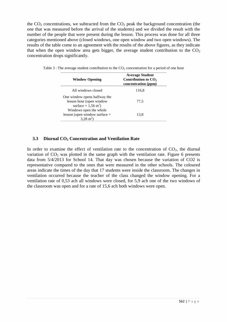
562 | P a g e

the CO2 concentrations, we subtracted from the CO2 peak the background concentration (the

one that was measured before the arrival of the students) and we divided the result with the

number of the people that were present during the lesson. This process was done for all three

categories mentioned above (closed windows, one open window and two open windows). The

results of the table come to an agreement with the results of the above figures, as they indicate

that when the open window area gets bigger, the average student contribution to the CO2

concentration drops significantly.

Table 3 : The average student contribution to the CO2 concentration for a period of one hour

3.3 Diurnal CO2 Concentration and Ventilation Rate

In order to examine the effect of ventilation rate to the concentration of CO2, the diurnal

variation of CO2 was plotted in the same graph with the ventilation rate. Figure 6 presents

data from 5/4/2013 for School 14. That day was chosen because the variation of CO2 is

representative compared to the ones that were measured in the other schools. The coloured

areas indicate the times of the day that 17 students were inside the classroom. The changes in

ventilation occurred because the teacher of the class changed the window opening. For a

ventilation rate of 0,53 ach all windows were closed, for 5,9 ach one of the two windows of

the classroom was open and for a rate of 15,6 ach both windows were open.

Window Opening

Average Student

Contribution to CO2

concentration (ppm)

All windows closed 116,8

One window opens halfway the

lesson hour (open window

surface = 1,56 m2)

77,5

Windows open the whole

lesson (open window surface =

3,28 m2)

13,8

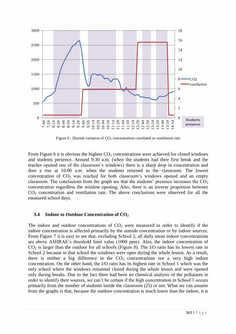
563 | P a g e

Figure 6 : Diurnal variation of CO2 concentration correlated to ventilation rate

From Figure 6 it is obvious the highest CO2 concentrations were achieved for closed windows

and students presence. Around 9:30 a.m. (when the students had their first break and the

teacher opened one of the classroom’s windows) there is a sharp drop in concentration and

then a rise at 10:00 a.m. when the students returned to the classroom. The lowest

concentration of CO2 was reached for both classroom’s windows opened and an empty

classroom. The conclusions from the graph are that the students’ presence increases the CO2

concentration regardless the window opening. Also, there is an inverse proportion between

CO2 concentration and ventilation rate. The above conclusions were observed for all the

measured school days.

3.4 Indoor to Outdoor Concentration of CO2

The indoor and outdoor concentrations of CO2 were measured in order to identify if the

indoor concentration is affected primarily by the outside concentration or by indoor sources.

From Figure 7 it is easy to see that, excluding School 2, all daily mean indoor concentrations

are above ASHRAE’s threshold limit value (1000 ppm). Also, the indoor concentration of

CO2 is larger than the outdoor for all schools (Figure 8). The I/O ratio has its lowest rate in

School 2 because in that school the windows were open during the whole lesson. As a result,

there is neither a big difference in the CO2 concentrations nor a very high indoor

concentration. On the other hand, the I/O ratio has its highest rate in School 1 which was the

only school where the windows remained closed during the whole lesson and were opened

only during breaks. Due to the fact there had been no chemical analysis of the pollutants in

order to identify their sources, we can’t be certain if the high concentration in School 1 occurs

primarily from the number of students inside the classroom (25) or not. What we can assume

from the graphs is that, because the outdoor concentration is much lower than the indoor, it is

0

2

4

6

8

10

12

14

16

18

0

500

1000

1500

2000

2500

3000

7:4

4

7:5

9

8:1

4

8:2

9

8:4

4

8:5

9

9:1

4

9:2

9

9:4

4

9:5

9

10

:14

10

:29

10

:44

10

:59

11

:14

11

:29

11

:44

11

:59

12

:14

12

:29

12

:44

12

:59

13

:14

13

:29

13

:44

13

:59

14

:14

CO2

ventilation

564 | P a g e

highly likely the increased CO2 concentration to originate from the lack of ventilation in the

lesson hours.

Figure 7 : Daily mean CO2 concentration Figure 8 : Indoor/Outdoor concentration for for the inside and outside environment of the schools each school

For the rest seven schools, the windows may had all three positions throughout the day (all

windows closed, one window open or two windows open), so we assumed in general the

window positions were the same for these schools. The correlation between indoor and

outdoor concentration for these schools is shown in Figure 9, where the correlation coefficient

is R2 ≈ 0,63 which indicates a significant correlation between indoor and outdoor CO2

concentration.

Figure 9 : Correlation of indoor CO2 concentration to the outdoor CO2 concentration

0

500

1000

1500

2000

2500

2 14 8 11 1 4 18 12 Pal

CO

2 C

on

cen

tra

tio

n (

pp

m)

Schools

in

out

ASHRAE limit value for indoor

0

1

2

3

4

5

2 14 8 11 1 4 18 12 Pal

Ind

oo

r/O

utd

oo

r C

O2

co

ncen

tra

tio

nSchools

y = 3,5303x - 815,29

R² = 0,628

800

900

1000

1100

1200

1300

1400

1500

520 540 560 580 600 620 640 660

Ind

oo

r C

O2

Co

ncen

tra

tio

n (

pp

m)

Outdoor CO2 Concentration (ppm)

565 | P a g e

3.5 Drop of CO2 vs Window Opening and Ventilation Rate

The drop of CO2 was calculated during brakes where no students were inside the classroom

and all schools had at least one open window. To calculate the drop (ppm/min), CO2

concentrations were plotted over time (for a period of 15 minutes) in order to find the gradient

of that curve for each school. That process was done in order to identify if the drop of CO2

concentration over time is primarily affected by the window opening (m2) or the ventilation

rate (ach). Figures 10 and 11 illustrate the two correlations for all nine schools.

Figure 10 : Correlation of the drop of the concentration Figure 11 : Correlation of the drop of the of CO2 to the window opening concentration of CO2 to the ventilation rate

It can be seen that, there is a strong correlation between the ventilation rate and the drop of

CO2 concentration (R2 = 0,82) and a moderate correlation between the window opening and

the drop of CO2 concentration (R2 = 0,65) indicating ventilation rate has a greater impact on

the decrease of CO2 concentration than just the window open surface. In general, the lowest

drop rate for the CO2 concentration is achieved for the lowest ventilation rate and the smallest

window opening as well as the highest drop rate for the CO2 concentration is achieved for the

highest ventilation rate and the largest window opening. It must be noted for the case where

the CO2 concentration drops with a rate of 120 ppm/min, there is a rapid decrease in CO2

concentration despite the fact that there is a low ventilation rate and a relatively small window

opening. This paradox could be justified probably by a strong wind current that was present at

the day of the measurement.

3.6 Evaluation of the School’s Ventilation

Finally, there has been an evaluation of the ventilation rates for the different cases that

occurred during teaching hours. The ventilation rates, although they were primarily measured

in ach, they were converted to l/p/s in order to be compared to the ventilation’s rate threshold

as it is set by ASHRAE (ASHRAE 2007), which is 8 l/p/s. The results are shown in Table 4.

All cases with closed widows during the lesson had inadequate ventilation rate (below 8

l/p/s). The cases of the second category had all, except one, sufficient ventilation rates. Also

sufficient ventilation rate was observed when two windows were open throughout the lesson.

y = 31,046x + 20,807

R² = 0,64880

20

40

60

80

100

120

140

160

180

200

0 2 4 6

Dro

p I

n C

O2

Co

ncen

tra

tio

n

(pp

m/m

in)

Window Opening (m^2)

y = 6,8102x + 39,18

R² = 0,8162

0

20

40

60

80

100

120

140

160

180

200

0 10 20 30

Dro

p I

n C

O2

Co

ncen

tra

tio

n

(pp

m/m

in)

Ventilation Rate (ach)

566 | P a g e

Table 4 : Ventilation rates (l/p/s) for different window opening for each school

4 CONCLUSIONS

The conclusions from this paper are:

There is a negative correlation between the students’ scores in productivity tests and the concentration of CO2.

Occupancy density affects primarily CO2 concentrations if outdoor air is not entering

the classrooms. For the cases that air from the outside of the classrooms comes to the

inside, occupancy density does not significantly affect CO2 concentrations.

As the open window area gets bigger, the average student contribution to the CO2

concentration drops significantly.

Students’ presence increases CO2 concentration regardless the window opening. Also,

there is an inverse proportion between CO2 concentration and ventilation rate.

Excluding one school, all daily mean indoor concentrations are above ASHRAE’s threshold limit value (1000 ppm). Also, the indoor concentration of CO2 is larger than

the outdoor for all schools. In addition there is a significant correlation between indoor

and outdoor CO2 concentration.

Ventilation rate has a greater impact on the decrease of CO2 concentration than the

window open surface.

All cases with closed widows during the lesson time had inadequate ventilation rate

(below 8 l/p/s), while sufficient ventilation rates were observed when there were open

windows throughout the lesson.

5 ACKNOWLEDGEMENTS

We are greatly indebted to the school directors, pupils and parents. Without their consent this

study would have not been possible.

6 REFERENCES

ASHARE (2007), American Society of Heating, Refrigerating and Air-Conditioning

Engineers Inc., Standard 62.1.2007: Ventilation for acceptable Indoor Air Quality,

Atlanta

Window Opening School Ventilation Rate (l/p/s)

Closed windows the whole

lesson time

14 1,43

1 0,99

4 0,57

12 1,18

One window opens halfway the

lesson hour (open window

surface = 1,56 m2)

8 11,72

14 12,98

4 11,09

12 3,19

18 16,55

Two windows open the whole

lesson (open window surface =

3,28 m2)

2 15,85

4 39,31

Pal 14,52

11 9,39

567 | P a g e

Dorizas P.V., Assimakopoulos M.N., Helmis C., Santamouris M. (2013a), Analysis of the

indoor air quality in Greek primary schools, 34th AIVC-3rd TightVent-2nd Cool

Roofs'-1st Venticool Conference, Athens, 25-26 September 2013, p. 110-113.

Dorizas P.V., Assimakopoulos M.N., Helmis C., Santamouris M. (2013b), A study on the

thermal environment in Greek primary schools based on questionnaires and

concurrent measurements, 34th AIVC-3rd TightVent-2nd Cool Roofs'-1st Venticool

Conference, Athens, 25-26 September 2013, p. 13-15.

Dorizas P.V., Assimakopoulos M.N., Helmis C., Santamouris M. Sifnaios J., Stathi K.

(2013c), Does indoor environmental quality affect students performance?,34th AIVC-

3rd TightVent-2nd Cool Roofs'-1st Venticool Conference, Athens, 25-26 September

2013, p. 113-115

EFA (2001), European Federation of Asthma and Allergy Associations, Indoor Air

Pollution in Schools, Sweden

EPA (1995), U.S. Environmental Protection Agency, Indoor Air Quality Tools for Schools.

IAQ Coordinator’s Guide, EPA 402-K-95-001, Washington DC.

Grimsrud D., Bridges B., Schulte R. (2006), Continuous measurements of air quality

parameters in schools, Building Research and Information 34 (5), 447– 458.

Hitchin E.R. and Wilson C.B. (1967), A Review of Experimental Techniques for the

Investigation of Natural Ventilation in Buildings, Building Science vol. 2, pp. 59 – 82

Mendell M., Heath G.A. (2005), Do indoor pollutants and thermal conditions in schools

influence student performance? A critical review of the literature, Indoor Air –

International Journal of Indoor Air Quality and Climate 15 (1), 27–52.

SINPHONIE project, Schools Indoor Pollution and Health: Observatory Network in Europe

Available at: http://www.sinphonie.eu/about, accessed on June 14th

, 2014.

Wargocki, P. Wyon, D.P., Baik, Y.K., Clausen G. and Fanger, O. (1999). Perceived Air

Quality, Sick Building Syndrome (SBS) and Productivity in an Office with Two

Different Pollution Loads, Indoor Air, 9:165-179.

Wargocki, P., Wyon, D.P., Sundell, J., Clausen, G. and Fanger, O. (2000). The effects of

Outdoor Air Supply Rate in an Office on Perceived Air Quality, Sick Building

Syndrome (SBS) Symptoms and Productivity, Indoor Air, 10:222-236

Witterseh, T., Wyon, T. and Clausen, G. (2004). The effects of moderate heat stress and

open-plan office noise distraction on SBS symptoms and on the performance of the

office work, Indoor Air, 14: 30-40

568 | P a g e

MEASUREMENT OF INFILTRATION RATES FROM

DAILY CYCLE OF AMBIENT CO2

João Dias Carrilho

a,*, Mário Mateus

a, Stuart Batterman

b and Manuel Gameiro da

Silvaa

aADAI-LAETA

Dep. Mechanical Engineering, University of Coimbra

3030-788 Coimbra, Portugal

bDepartment of Environmental Health Sciences

University of Michigan

Ann Arbor, MI 48105 USA


ABSTRACT

We propose a new approach for measuring air infiltration rates in buildings. The method belongs to the class of

tracer gas techniques but, unlike conventional CO2 based methods that assume the outdoor ambient CO2

concentration is constant, the proposed method recognizes that photosynthesis and respiration cycle of plants and

processes associated with fuel combustion produce daily, quasi-periodic, variations in the ambient CO2

concentrations. These daily variations, which are within the detection range of existing monitoring equipment,

are utilized for estimating ventilation rates without the need of a source of CO2 in the building. The new method

has the advantages that no tracer gas injection is needed, and time resolved results are easily obtained.

KEYWORDS

Tracer gas techniques; Air infiltration; Atmospheric CO2; Discrete Fourier transform

1 INTRODUCTION

There are two main methodologies available to assess infiltration rates in buildings: one based

on fan pressurization techniques; and another based on tracer gas techniques. The methods

based on fan pressurization techniques have the potential advantage for providing quick

results, but can be costly to implement an may not accurately represent infiltration rates at the

lower pressure differentials found during normal operation of the building. The methods

based on tracer gas techniques can be comparatively cheap and easy to implement but rely

heavily on the assumptions of uniform mixing of the tracer gas and the indoor air. Carbon

dioxide (CO2), which is naturally present in the atmosphere and is also produced by the

building occupants, has been shown to satisfy the uniform mixing assumption and can be used

effectively in determining ventilation rates in buildings (Barankova, Naydenov, Melikov &

Sundell, 2004). Metabolic CO2 produced by the building occupants is commonly used as the

source of the tracer gas, and an estimate of infiltration rates can be obtained from the step

response of a first order system, either in concentration rise or in concentration decay

situations. A fundamental assumption in the conventional CO2 tracer gas techniques,

however, is that the outdoor ambient concentration is constant (Sherman, 1990; Persily,

1997).

In the present paper, the authors propose a new approach for determining infiltration rates,

which does not require the presence of building occupants as the source of CO2. The method

569 | P a g e

belongs to the class of tracer gas techniques, but instead of relying on a step forcing function,

it uses a naturally occurring periodic forcing function. Despite being a common assumption in

the existing methods, the outdoor ambient CO2 concentration is not constant (e.g., see Refs.

(Massen, Kies & Harpes, 2003) and (Miyaoka, Yoshikawa Inoue, Sawa, Matsueda &

Taguchi, 2007)). The photosynthesis and respiration cycle of plants, and other processes

associated with burning of fuels, are the cause of variations in the ambient CO2 concentration

which can be of the order of 100 ppm in amplitude, on a daily basis. This quasi-periodic

variation is taken into advantage for estimating infiltration rates without the need of a source

of CO2 in the building. This method is particularly suited for measurement during extended

periods of no occupancy, e.g., during the pre-commissioning test phase of a new or a

renovated building, when the building is ready for operation but has not yet been occupied.

The application of the new method is demonstrated with real data obtained in a residential

building.

2 THEORETICAL FORMULATION

Consider a single zone with volume , such that air is exchanged with the outdoor

environment, through one or more of its boundaries, at a volume flow rate cubic meters per

hour. Assuming complete mixing, and in the absence of filtering mechanisms, deposition and

absorption processes, the time evolution of the CO2 concentration within the enclosure,

int( ), is well described by the mass balance equation (Etheridge & Sandberg, 1996, p. 277)

int ( ) int( ) ext ( ), (1)

where the prime denotes differentiation with respect to time, ext is the outdoor CO2

concentration, ( ) is the rate of CO2 generation within the enclosure, and is the volume

flow rate of new air entering the enclosure or, equivalently, the volume flow rate of old air

leaving the enclosure.

In writing (1), it was implicitly assumed that the outdoor CO2 concentration, ext, does not

vary in time. Allowing for ext( ) to be now an explicit function of time, setting the rate of

generation of CO2 to zero and writing ⁄ , (1) becomes

int ( ) int( ) ext( ) . (2)

Dividing both sides of the equation by and moving ext( ) to the right-hand side gives

int

( ) int( ) ext( ), (3)

which is a mathematical representation of a first order Linear Time Invariant (LTI) system

with the input ext( ), output int( ), and time constant ⁄ .

Assuming that the input to the system is the outdoor concentration time series, represented by

a periodic sinusoidal function, with an amplitude Aext and an angular velocity = 2πf

ext( ) ext ( ) , (4)

the output, after a long enough time such that transients have died away, will be another

sinusoidal function attenuated in amplitude and phase lagged and will have the form

int( ) int ( int) , (5)

570 | P a g e

where int = atan () is the phase lag angle. The ratio of amplitudes int ext⁄ , the time

constant , and the frequency of excitation are related by the well-known expression for

first order, linear time invariant (LTI) systems (Holman, 1994, pp. 23)

int ext

√ ( ) . (6)

So, in the case of sinusoidal excitation, both the time delay between input / output and the

amplitude attenuation depend on the system time constant, that for our situation has the

physical interpretation of the mean age of air inside the compartment. By rearranging (6), the

air infiltration rate, which is the inverse of the mean age of air ( ⁄ ) can be calculated

from

√(

)

,

(7)

where int ext⁄ . To estimate ext and int, and associated uncertainty bounds, we make

use of the Discrete Fourier Transform (DFT):

∑ ⁄

, (8)

where the complex coefficient carries information on the amplitude and relative phase of

the th sinusoidal component of the sample time series . The frequency of the sinusoidal

component is ⁄ , where is the sampling frequency, and its amplitude is

| |

. (9)

Assuming that most of the signal’s energy in is concentrated in a single frequency

component, in this case the frequency corresponding to a 24 h period, a model for is

[

⁄ ( ) ⁄ ] , (10)

where is the number of sample in a 24 h period and accounts for noise, i.e., it is the time

series of the residuals obtained by subtracting the deterministic part of the model in (10) from

the measured data . Letting var( ) be the power in the residuals in a complete period,

an estimate of the standard uncertainty associated with the determination of the Fourier

coefficient is (Thibos, 2003)

( )

, (11)

where ( ) ⁄ and is the F-distribution with a numerator degrees of freedom, b

denominator degrees of freedom, and is the critical value such that corresponds to the

level of confidence. For a sampling rate of one sample every 30 min, the number of samples

in 24 h is , so that and, for a level of confidence of 68.2%, . In practice, (11) has the meaning of a radius defining a circle in the complex plane,

571 | P a g e

centred in (Figure 1). With the specified level of confidence of 68.2%, we can say that the

true value of the Fourier coefficient is inside this circle.

Figure 1 - Graphical representation of the standard uncertainty associated with the determination of the Fourier

coefficient , estimated from the confidence bound (11).

The standard uncertainty associated with the determination of can then be estimated from

( ) √(

)

( ) , (12)

where

( )

, (13)

and ( ) var( int ext⁄ ) is estimated from the first order Taylor expansion

approximation to the variance of the ratio by

var ( int ext

) E( int)

E( ext) [var( int)

E( int)

cov( int ext)

E( int)E( ext) var( ext)

E( ext) ] , (14)

where E( ) denotes the expected value of and cov( ) denotes the covariance between

and . Since the covariance between the output and the input amplitudes of a first order LTI

system is always positive, we can safely neglect the covariance term in (14) to obtain an

upper bound for the variance of the ratio:

var ( int ext

) E( int)

E( ext) [var( int)

E( int) var( ext)

E( ext) ] , (15)

Finally, we identify the variance of the amplitude with the square of the standard uncertainty

obtained from (11).

(𝑋𝑘)

I (𝑋𝑘) 𝑢(𝑋𝑘)

572 | P a g e

3 MATERIALS AND METHODS

Two Extech SD800 devices were used to record CO2 concentration, at a rate of one sample

every 30 min, in a two bedroom flat, built in the 1990s, located in a rural village near Oliveira

do Bairro, Portugal. The flat has an interior floor area of approximately m and height

m, and is at the first floor above ground of a three level building. The exterior device was

placed in the east-facing balcony, shielded from direct solar radiation, whereas the interior

device was placed in the living-room, leading to the same balcony. Figure 2 shows a floor

plan of the flat, with the approximate locations of the measuring devices.

All windows and exterior doors were left fully closed, while all interior doors were left fully

open. There were no occupants or other sources of CO2 inside the flat, and there was no

heating, cooling or mechanical ventilation in operation during the entire measurement period.

Figure 2 - Sketch of the residential flat were the measurement campaign took place. The locations of the interior

and exterior measuring devices are shown with crosses, in the living room and in the balcony. All windows and

exterior doors were left closed during the measurement period


Continuous CO2 concentration time series were obtained between 15:49 on August 26 and

15:19 on August 28, 2013. Figure 3 shows the raw data obtained from both the exterior and

the interior devices. The time series are shown with an artificial vertical offset for better

visualization. The shaded areas indicate the time periods from 20:00 to 07:00, which

correspond approximately to the night periods.

The daily quasi-periodic nature of the atmospheric CO2 is well visible in Figure 3. During the

night periods, plants enter the respiration phase and produce CO2, which reaches a maximum

concentration around the early hours of the morning, before the sunrise. In the morning, as the

sun rises above the horizon, plants enter the photosynthesis phase and the exterior CO2

concentration starts decreasing, until it reaches a minimum around midday. As the sun sets in

the evening, the exterior concentration starts to increase again. The interior time series clearly

follows the trend of the exterior time series, with a lower amplitude and a phase lag. This

behaviour is characteristic of the input-output relation of a first order system.

Both exterior and interior time series where segmented in overlapping periods of 24 h, with

48 samples each, i.e. the first segment starts at sample 1 and ends at sample 48; the second

segment starts at sample 2 and ends at sample 49, and so on. The DFT was then applied to

each segment, from which the amplitude of the second Fourier component (corresponding to

the 24 h period) was calculated. The infiltration rate corresponding to each 24 h segment was

573 | P a g e

then calculated from (7). The infiltration rate, as a function of time, is shown as a solid line in

Figure 4, where each point on the line represents an average infiltration rate for the last 24 h.

The dashed lines represent upper and lower expanded uncertainty estimates (coverage factor

). The infiltration rate is seen to vary randomly about a mean value of 0.19, which is in

agreement with typical values for infiltration rates in Portuguese residential buildings built in

the last 30 years (Gomes, Gameiro da Silva & Simões, 2013). The expanded uncertainty

varies from 10% to 20% of the estimated infiltration rate.

Figure 3 - Time series, recorded over 3 days, of exterior and interior CO2 concentrations: raw data shown with an

artificial vertical offset for better visualization. Ticks on the vertical axis are 50 ppm apart and the shaded areas

identify night periods, between 20:00 and 07:00.

Figure 4 – Air infiltration rate results obtained from the raw data in Figure 3. Each point on the solid line

represents an average infiltration rate corresponding to the previous 24 h. The dashed lines are estimates of the

expanded uncertainty associated with the determination of the infiltration rate (coverage factor ).

5 CONCLUSION

A new method to determine air infiltration rates in buildings has been proposed. The method

belongs to the class of tracer gas techniques but, contrary to established methods that are

based on the step response to the sudden introduction or extinction of a source of tracer gas, it

uses the naturally occurring variation in atmospheric ambient CO2 concentrations to derive 24

574 | P a g e

h moving average estimates of the infiltration rate. This novel approach has several

advantages: it does not rely on the injection of a tracer gas or the use of metabolic CO2

generated by the building occupants; it produces 24 h moving average time series of

infiltration rates with the time resolution dictated only by the sampling frequency; and it may

be less sensitive to mixing assumptions compared to methods which require the injection or

generation of a tracer gas inside the building. The new method may provide a very useful tool

for studying the dynamic behaviour of ventilation in buildings, which remains a main source

of uncertainty in modelling building systems and, consequently, in the assessment of the

energy balance in buildings as well as the quality of the indoor environment.

6 ACKNOWLEDGEMENTS

The presented work was framed under the Energy for Sustainability Initiative of the

University of Coimbra and LAETA (Associated Laboratory for Energy, Transports and

Aeronautics) Project Pest E/EME/LA0022/2011. The first author wishes to acknowledge the

Portuguese funding institution FCT – Fundação para a Ciência e Tecnologia, for supporting

his research through the Ph.D. grant SFRH/BD/77911/2011.

7 REFERENCES

Barankova, P. Naydenov, K. G. Melikov, A. K. and Sundell, J. (2004). Distribution of carbon

dioxide produced by people in a room: Part 1 – Laboratory study. in CD of Proceedings of the

9th International Conference on Air Distribution in Rooms (ROOMVENT 2004), 5-8

September 2004, Coimbra, Portugal.

Sherman, M. H. (1990). Tracer-gas techniques for measuring ventilation in a single zone.

Building and Environment, 25, 365-374.

Persily, A. K. (1997). Evaluating building IAQ and ventilation with indoor carbon dioxide.

ASHRAE Transactions, 103, 193-204.

Massen, F. Kies, A. Harpes, N. (2003). Seasonal and Diurnal CO2 Patterns at Diekirch, LU

2003 – 2005. Retrieved June 10, 2014, from

http://meteo.lcd.lu/papers/co2_patterns/co2_patterns.html.

Miyaoka, Y. Yoshikawa Inoue, H. Sawa, Y. Matsueda, H. Taguchi, S. (2007). Diurnal and

seasonal variations in atmospheric CO2 in Sapporo, Japan: Anthropogenic sources and

biogenic sinks. Geochemical Journal 41, 429-436.

Etheridge, D. W. Sandberg, M. (1996) Building ventilation: theory and measurement.

Chichester: Wiley.

Holman, J. P. (1994). Experimental methods for engineers. New York: McGraw-Hill.

Thibos, L. N. (2003). Fourier analysis for beginners. Retrieved July 14, 2014, from

http://research.opt.indiana.edu/Library/FourierBook/ch09.html#E14

Gomes, M. R. Gameiro da Silva, M. Simões, N. (2013). Assessment of air infiltration rates in

residential buildings in Portugal. In Proceedings of CLIMA 2013, 11th REHVA world

congress – Energy efficient, smart and healthy buildings, Prague, Czech Republic, 16-19 June

2013.

575 | P a g e

PREDICTING THE OPTIMUM AIR PERMABILIY OF

A STOCK OF DETACHED ENGLISH DWELLINGS

Benjamin Jones*1

, Robert Lowe2

1 Department of Architecture and Built Environment

Lenton Firs House, University of Nottingham

NG7 2RD, United Kingdom


[email protected]

2 Energy Institute

University College London

Central House, 14 Upper Woburn Place

London, WC1H 0NN, United Kingdom

ABSTRACT

Mechanical positive input and extract ventilation are common strategies employed in English houses, generally

because they provide adequate indoor air quality and specifically because they are effective at minimizing mould

growth and its associated negative health consequences. Air is either exclusively supplied or extracted (never

both) by a mechanical system at a prescribed airflow rate designed to ensure adequate indoor air quality. The

remaining airflow, required to balance mass through the building, occurs through the fabric, through a mix of

purpose provided and adventitious airflow paths. However, there is an important need to reduce adventitious

airflow during the heating season in order to save energy and this is highlighted by the building standards of

many countries who advocate increasing the airtightness of their housing stocks. Increasing a fabric’s

airtightness also increases its resistance to airflow and so a positive displacement or extract ventilation system

must balance the corresponding increase in the fan power required to overcome this resistance with the need to

provide an adequate supply of fresh air. Accordingly, the total energy consumption attributable to these

ventilation systems during the heating season is a function of the dwelling’s infiltration rate and heating system

efficiency, and the fan’s hydraulic power and efficiency.

This paper explores the possibility of an optimum air permeability for detached (single family) English houses

ventilated by a mechanical positive input or an extract ventilation strategy. Firstly a theoretical model of air

infiltration and exfiltration is used to investigate the underlying relationship between the fabric airflow rate, the

mechanical ventilation rate (supplied or extracted), and the air permeability in a single detached dwelling. A

meta-model of the total ventilation rate and heating system energy demand is developed. Secondly, the

infiltration model then utilises a sample of over 16,000 English houses located in 10 different regions to

investigate the relationship between the fan power and air permeability in a randomly chosen sub-sample of

detached English houses. Thirdly, it is shown that there is indeed an optimum permeability for detached English

houses with such systems and the effects of heating system and fan efficiencies on this value are identified.

Finally, these predictions are contextualised by exploring their relevance to the current English housing stock.

KEYWORDS

Ventilation, infiltration, mechanical, positive-input, DOMVENT

1 INTRODUCTION

Mechanical ventilation systems are found in many European dwellings, particularly in the

kitchen and bathroom where they are used maintain adequate indoor air quality (IAQ). A

mechanical extract ventilation (MEV) fans reduce the internal air pressure below ambient and

causes fresh air to be drawn through openings (commonly adventitious air leakage paths

(ALPs) (Stephen, 2000)) in the thermal envelope. Positive input ventilation (PIV) reverses

this process by supplying a steady flow of fresh air through a single opening located at the top

of a stairwell.

576 | P a g e

The need to save energy is highlighted by the building codes of many countries that advocate

increasing the airtightness of their housing stocks to save energy by reducing adventitious

infiltration and exfiltration during the heating season. However, increasing the airtightness of

a dwelling’s fabric increases its resistance to airflow and when using a continuous CMEV

(CMEV) or PIV system one must balance the corresponding increase in the fan power

required to overcome this fabric resistance with the consequent reduction in spatial and

temporal variation in air flow (Lowe, 2000). Accordingly, the total energy consumption

attributable to these ventilation systems during the heating season is a function of the

dwelling’s permeability, the heating system efficiency, and the fan’s specific power.

An understanding of the interaction between CMEV and PIV, and infiltration and exfiltration

is critical to the optimization of their performance and the minimization of energy

consumption. Accordingly, this paper uses a theoretical approach to explore these

relationships and asks the question: is there an optimum permeability for English houses

ventilated using a CMEV or PIV system?

2 A MODEL OF VENTILATION AND ASSOCIATED HEAT LOSS

This paper applies DOMVENT3D, a model of infiltration and exfiltration through any

number of façades that incorporates a mechanical ventilation system. The model was

conceived by Lyberg (2000), initially developed and applied by Lowe (2000) and extended

significantly by Jones et al. (2013a, 2014). Its assumptions, merits, limitations, and the

corroboration of its predictions are discussed widely by Jones et al. (2013a, 2014), and an

analysis of the sensitivity of its predictions to its inputs is undertaken by Jones et al. (2013b).

The model, which is implemented using bespoke MATLAB (MathWorks, 2013) code, is

discussed in Section 2.1. It requires inputs that may be unique to each dwelling or are general

to a geographic region. Unique inputs comprise dwelling geometry, the flow exponent,

internal air density, scaled wind speed, and façade wind pressure coefficients. General inputs

are the ambient air temperature, regional wind speed, and wind orientation. Sources of data

are discussed in Section 2.2.

2.1 Model of Ventilation and Associated Heat Losses

DOMVENT3D makes two assumptions about a façade: (i) it is uniformly porous; (ii) the

pressure distribution over it is linear. It integrates the airflow rate in the vertical plane to

predict the total airflow rate (m3/s) through the i

th of j façades (Jones et al., 2014) where

(| | ⁄ )∫ (| |)

(1)

Here, and are the upper and lower height of a façade, (Pa) is the pressure

difference across an infinitesimal section (m) of a façade in the vertical plane, and (Pa-β

)

is a flow coefficient. Jones et al. (2014) show that ( ) , where E is a

dimensionless relative leakage area calculated from a known value of air permeability

(m3/h/m

2) or an equivalent metric, (kg/m

3) is the mean of the internal and external air

densities, and (m) is the façade width. The net airflow through all j façades is zero

∑ (2)

where (m3/s) is the airflow through a mechanical system and the positive sign indicates

airflow into a building. An important feature of the model that makes it suitable for this study

is its dynamic neutral height (m) which is described by

( ) . (3)

Here, is the air density (kg/m3), is the wind speed at building height (m/s), is a mean

façade wind pressure coefficient, is the gravitational acceleration (m/s2), (Pa) is the

internal air pressure (gauge), and the subscripts and represent internal and external

577 | P a g e

conditions, respectively. DOMVENT3D makes two further assumptions about the dwelling:

(i) all rooms are interconnected and internal flow resistances are small so that a dwelling can

be treated as a single-zone (Jones et al., 2013a); (ii) each horizontal and vertical surface of the

external envelope requires only a single flow equation linked by a continuity equation; Once

the total ventilation rate at an instant in time ( ) (m3/s) is predicted by DOMVENT 3D, the

ventilation heat loss (W) is calculated by

( ) ( ) ( )| ( ) (4)

where is the specific heat capacity of air (Jkg-1

K-1

), is the mean of and , and

is the difference between the internal and ambient air temperatures. The internal air

temperature, (ºC), of an average unheated English house is, on average, 3ºC higher than

the ambient air temperature, (ºC), and so the heating system is assumed to function only

when the ambient air temperature is 3ºC below the internal air temperature (Hamilton et al., 2011). Heat loss is only calculated when the heating system is “on” and so Equation (4)

is integrated over the entire heating season to estimate the total energy required by a heating

system, (MWh). Further energy may be required by a fan whose hydraulic power

| | (W) is also integrated over the heating season to estimate the total fan energy demand,

(MWh). The total energy demand (MWh) is given by ⁄ ⁄ , where

and are the heating system and fan efficiencies, respectively.

3 SOURCES OF DATA

The model is now used to predict the total heat lost from a typical detached (single family)

dwelling located in an urban area of London and to investigate the underlying relationships

between a CMEV or PIV system and adventitious airflow. The dwelling’s geometry, physical,

and environmental properties are largely obtained from the 2009 English Housing Survey

(EHS) (DCLG, 2011), a statistically representative sample of 16,150 dwellings that represents

the 22.3 million dwellings of the English Housing stock. The sources of data are documented

by Jones et al. (2013a) and so are only briefly discussed here.

Data inputs to DOMVENT3D may be divided into three distinct types: geometric, physical,

and environmental. We now discuss each data type in turn beginning with geometric data.

The EHS assumes that two connecting cuboids can reasonably represent the geometry of

~98% of English dwellings. The cuboid model applied here directly follows the Cambridge

Housing Model (CHM) (Hughes et al., 2012) used to estimate energy use and CO2 emissions

in the English stock for the UK government. For each façade the model requires the

parameters , , and . Dwelling orientation is not given by the EHS and so it is

assumed to be a uniformly distributed random variable between 0 and 359 degrees ( ). DOMVENT3D requires three key physical parameters: , dwelling , and façade . The

former is varied between limits of 0.1 and 20m3/h/m

2 in order to evaluate its effect on and

; see Sections 4 and 5. The flow exponent variable characterises the airflow regime through

an ALP and is a function of its geometry and surface roughness. Its value affects both the

pressure difference across an ALP and the airflow rate through it. Sherman & Dickerhoff

(1998) show that a mean value of µ=0.65 with a standard deviation of σ=0.08 best represents

more than 1900 measurements made in U.S. dwellings. This distribution is similar to the

smaller international AIVC data set (Orme et al., 1998) and so is applied with confidence as a

Gaussian random variable. Wind pressure coefficients ( ) are defined for the horizontal and

vertical surfaces. For the latter, the algorithm of Swami and Chandra (1987) gives a

normalized average wind pressure coefficient for long-walled low-rise dwellings and is a

function of the angle of incidence of the wind, and local sheltering. The coefficient is then

scaled to account for local shielding. Horizontal surfaces are assumed to be completely

shielded from the effects of the wind following Sherman and Grimsrud (1980).

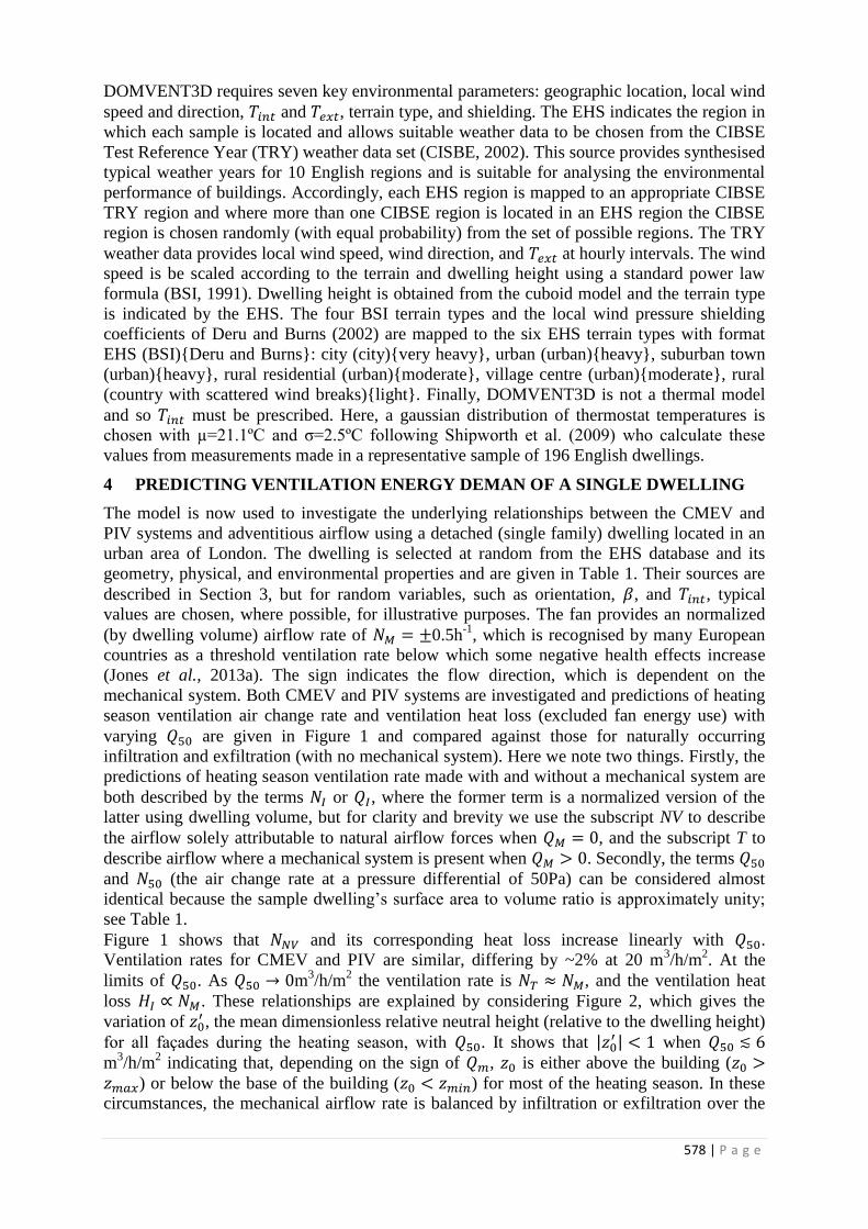
578 | P a g e

DOMVENT3D requires seven key environmental parameters: geographic location, local wind

speed and direction, and , terrain type, and shielding. The EHS indicates the region in

which each sample is located and allows suitable weather data to be chosen from the CIBSE

Test Reference Year (TRY) weather data set (CISBE, 2002). This source provides synthesised

typical weather years for 10 English regions and is suitable for analysing the environmental

performance of buildings. Accordingly, each EHS region is mapped to an appropriate CIBSE

TRY region and where more than one CIBSE region is located in an EHS region the CIBSE

region is chosen randomly (with equal probability) from the set of possible regions. The TRY

weather data provides local wind speed, wind direction, and at hourly intervals. The wind

speed is be scaled according to the terrain and dwelling height using a standard power law

formula (BSI, 1991). Dwelling height is obtained from the cuboid model and the terrain type

is indicated by the EHS. The four BSI terrain types and the local wind pressure shielding

coefficients of Deru and Burns (2002) are mapped to the six EHS terrain types with format

EHS (BSI){Deru and Burns}: city (city){very heavy}, urban (urban){heavy}, suburban town

(urban){heavy}, rural residential (urban){moderate}, village centre (urban){moderate}, rural

(country with scattered wind breaks){light}. Finally, DOMVENT3D is not a thermal model

and so must be prescribed. Here, a gaussian distribution of thermostat temperatures is

chosen with µ=21.1ºC and σ=2.5ºC following Shipworth et al. (2009) who calculate these

values from measurements made in a representative sample of 196 English dwellings.

4 PREDICTING VENTILATION ENERGY DEMAN OF A SINGLE DWELLING

The model is now used to investigate the underlying relationships between the CMEV and

PIV systems and adventitious airflow using a detached (single family) dwelling located in an

urban area of London. The dwelling is selected at random from the EHS database and its

geometry, physical, and environmental properties and are given in Table 1. Their sources are

described in Section 3, but for random variables, such as orientation, , and , typical

values are chosen, where possible, for illustrative purposes. The fan provides an normalized

(by dwelling volume) airflow rate of 0.5h-1

, which is recognised by many European

countries as a threshold ventilation rate below which some negative health effects increase

(Jones et al., 2013a). The sign indicates the flow direction, which is dependent on the

mechanical system. Both CMEV and PIV systems are investigated and predictions of heating

season ventilation air change rate and ventilation heat loss (excluded fan energy use) with

varying are given in Figure 1 and compared against those for naturally occurring

infiltration and exfiltration (with no mechanical system). Here we note two things. Firstly, the

predictions of heating season ventilation rate made with and without a mechanical system are

both described by the terms or , where the former term is a normalized version of the

latter using dwelling volume, but for clarity and brevity we use the subscript NV to describe

the airflow solely attributable to natural airflow forces when , and the subscript T to

describe airflow where a mechanical system is present when . Secondly, the terms

and (the air change rate at a pressure differential of 50Pa) can be considered almost

identical because the sample dwelling’s surface area to volume ratio is approximately unity;

see Table 1.

Figure 1 shows that and its corresponding heat loss increase linearly with .

Ventilation rates for CMEV and PIV are similar, differing by ~2% at 20 m3/h/m

2. At the

limits of . As m3/h/m

2 the ventilation rate is , and the ventilation heat

loss . These relationships are explained by considering Figure 2, which gives the

variation of , the mean dimensionless relative neutral height (relative to the dwelling height)

for all façades during the heating season, with . It shows that | | when

m3/h/m

2 indicating that, depending on the sign of , is either above the building (

) or below the base of the building ( ) for most of the heating season. In these

circumstances, the mechanical airflow rate is balanced by infiltration or exfiltration over the

579 | P a g e

whole envelope. The location of is a function of and so by rearranging Equation (3) it is

possible to identify the environmental conditions when or . Here,

Equation (3) shows that a CMEV system raises on any façade when

[

( ) ]. For the rare situation where and (

) , the pressure difference across a façade does not vary with height, but the inequality still applies. Instead it describes the required to overcome the prevailing environmental

conditions and reverse the airflow direction through an entire leeward façade (when )

so that air flows into a building. For the inequality to be true for a specific façade, either the

term is small in magnitude or . The latter occurs in airtight dwellings; for

example, in the sample detached dwelling, Figure 1 suggests this is when m3/h/m

2.

Conversely, a PIV system lowers when [

( ) ].

When ( ) , the inequality still applies and describes the required to overcome

the prevailing environmental conditions and reverse the airflow direction through a windward

façade (when ) so that air flows out of a building. For the inequality to be true, either

the term is small in magnitude or . The latter also occurs in airtight dwellings,

which for the sample detached dwelling Figure 1 shows is when m3/h/m

2. This value

of is identified by Lowe (2000) as a critical air permeability because it is the point where

the gradients of and for PIV and MEV systems increase. It is interesting to note that

Lowe also predicts the critical to be around h-1

, which is equivalent to m3/h/m

2

when the surface area to volume ratio is unity, although it is likely to vary across a housing

stock.

When m3/h/m

2 the dwelling can be considered to be leaky because Figure 1 shows

that the total ventilation rate with mechanical assistance through the dwelling is predicted to

be significantly more than the mechanical ventilation rate, . It is also clear from Figure 1

that the total ventilation rate with mechanical assistance is , where is the

change in the ventilation rate attributable to the mechanical system. In these circumstances a

CMEV system with a small airflow rate is responsible for a slight increase in the of all

façades (see Figure 2) and a concurrent increase in the infiltration rate increases by

(m3/s) and decrease in the exfiltration rate by (m

3/s). The and terms are

equal in magnitude but opposite in sign and so the total change attributable to the mechanical

system is | | , or | | ⁄ . The same proof applies to a leaky

dwelling ventilated by a PIV system, where decreases in all façades and when ,

where the CMEV or PIV system amends the magnitude of and so that and are

similarly equal in magnitude but opposite in sign. Here we note that the change in the total

heating season space heating (MWh) required to compensate for the increased airflow

rate caused by the addition of a CMEV or PIV system can be described in the same way, and

so in the limit of small mechanically induced airflows ⁄ . A simple function that

fits the simulated data over the whole range of air leakage is given by

{| | (

| |

)

}

(5)

where gives a maximum absolute error (MAE) of 1% over the entire range of for a

CMEV system, and gives a MAE of 3% over the entire range of for a

PIV system, where the MAE is a measure of the largest deviation of the model’s outputs.

Figure 4 shows that the relationship between and the MAE is for the sample detached

dwelling is non-symmetric about a minimum MAE. However, when the value of is greater

than the location of the minimum MAE, the gradient is small and tends to an asymptote.

Accordingly, if the most appropriate value of is unknown, a high value should be selected

580 | P a g e

so that . For the sample detached dwelling, gives a MAE of <0.03h-1

or <5%

across the range of .

The model can be augmented by applying another simplified models that predicts from

or ; see Jones et al. (2013). Further work is required to investigate the suitability of

Equation (5) for predicting in English houses that accounts for the variance of the inputs to

the DOMVENT3D model (see Section 3). This is undertaken in Section 5.

Figure 5 shows the total predicted fan energy demand during the heating season, . There is

little difference between the predictions for the CMEV and PIV systems, but Figure 5 shows

that there is a minimum value that occurs in the region of the critical permeability, where

Table 1: Properties of sample detached dwelling.

EHS sample G0322417

Dwelling type Detached

Location London, England

Terrain type Urban

Sheltering Heavy

Orientation North/south

Height (m) 5.1

Width (m) 6.4

Depth (m) 7.2

Volume, (m3) 232.7

Surface area, (m2) 229.5

(m2/m

3) 1.01

0.6

(°C) 21.1 Figure 1: Predicted ventilation rate and heat loss,

(MWh), during the heating season. ____

, natural infiltration; ----, CMEV; …..

, PIV

Figure 2: Predicted mean relative neutral height,

, for all façades during the heating season. ____


, PIV.

Figure 3: Predicted mean internal air pressure,

(Pa), for all façades during the heating season. ____


, PIV.

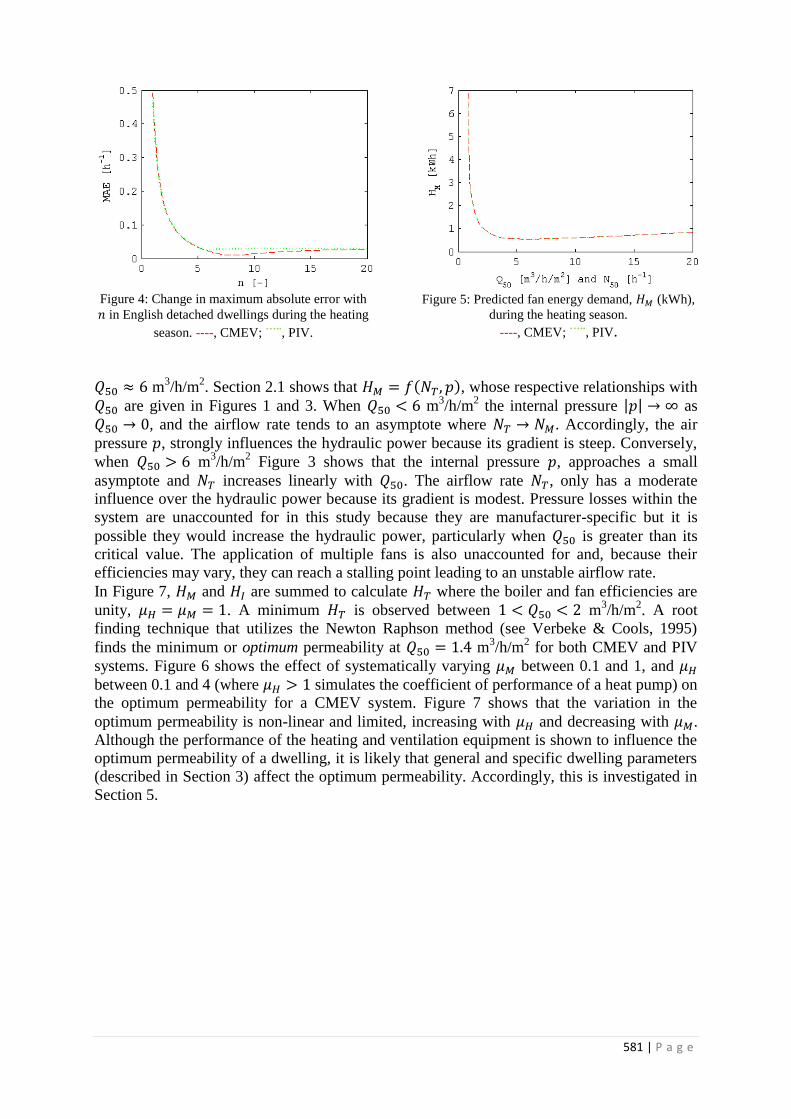
581 | P a g e

Figure 4: Change in maximum absolute error with

in English detached dwellings during the heating

season. ----, CMEV; …..

, PIV.

Figure 5: Predicted fan energy demand, (kWh),

during the heating season.

----, CMEV; …..

, PIV.

m3/h/m

2. Section 2.1 shows that ( ), whose respective relationships with

are given in Figures 1 and 3. When m3/h/m

2 the internal pressure | | as

, and the airflow rate tends to an asymptote where . Accordingly, the air

pressure , strongly influences the hydraulic power because its gradient is steep. Conversely,

when m3/h/m

2 Figure 3 shows that the internal pressure , approaches a small

asymptote and increases linearly with . The airflow rate , only has a moderate

influence over the hydraulic power because its gradient is modest. Pressure losses within the

system are unaccounted for in this study because they are manufacturer-specific but it is

possible they would increase the hydraulic power, particularly when is greater than its

critical value. The application of multiple fans is also unaccounted for and, because their

efficiencies may vary, they can reach a stalling point leading to an unstable airflow rate.

In Figure 7, and are summed to calculate where the boiler and fan efficiencies are

unity, . A minimum is observed between m3/h/m

2. A root

finding technique that utilizes the Newton Raphson method (see Verbeke & Cools, 1995)

finds the minimum or optimum permeability at m3/h/m

2 for both CMEV and PIV

systems. Figure 6 shows the effect of systematically varying between 0.1 and 1, and

between 0.1 and 4 (where simulates the coefficient of performance of a heat pump) on

the optimum permeability for a CMEV system. Figure 7 shows that the variation in the

optimum permeability is non-linear and limited, increasing with and decreasing with .

Although the performance of the heating and ventilation equipment is shown to influence the

optimum permeability of a dwelling, it is likely that general and specific dwelling parameters

(described in Section 3) affect the optimum permeability. Accordingly, this is investigated in

Section 5.

582 | P a g e

Figure 6: Predicted total energy demand,

(MWh), during the heating season.

----, CMEV; …..

, PIV.

Figure 7: Optimum heating season and with

varying and for a CMEV system.

5 CONSIDERING STOCK VARIANCE IN ENERGY DEMAND

Section 4 considered the use of a CMEV or PIV in a single detached dwelling and identified a

simple equation to predict the total ventilation rate from known mechanical and natural

airflow rates; see Equation (5). However, it is desirable to know what the variance of the

exponent , is across the stock of English detached dwellings so that a general value can be

identified. Section 4 shows that differs according to the system employed and so both

CMEV and PIV types are investigated using DOMVENT3D and a Monte Carlo (MC)

sampling approach. There are four stochastic inputs to DOMVENT3D: the EHS sample

(using dwelling weight), dwelling orientation, indoor air temperature, a flow exponent, and air

permeability. A set of twenty samples of the 1st four inputs (hence excluding ) are chosen

at a time using a Latin Hypercube. However, the is varied systematically for each sample

at values of 0.1, 2, 4, 6, 8, 10, 15, 20, and 50 m3/h/m

2 (a total of 9 values). Accordingly, with

a fan airflow rate of 0.5h-1

(see Section 4) nine predictions of are made by

DOMVENT3D for each sample to identify its relationship with ; see Figure 1. In addition,

Figure 1 shows that the natural ventilation rate , during the heating season varies linearly

with and so only a single prediction of is needed (apply the sample inputs used to

estimate ) and is scaled by . The predictions of DOMVENT3D are then compared to

those of Equation (5) for a range of exponents where . The MAE for each value of

is used to identify the best for each dwelling. The total sample size increases

incrementally according to the set size. After each set of predictions is made, the mean (µ)

and standard deviation (σ) of for the whole sample are calculated and used to decide if a

stopping criterion has been met. The number of samples is deemed adequate if the change in

µ and σ from one set of 20 samples to the next is less than 0.2% after a minimum of 5 sets

(100 samples) have been obtained. The model is run twice because a distribution is required

for each mechanical system.

Figure 8 gives distributions of (see Equation (5)) for CMEV and PIV systems estimated

using MATLAB’s ksdensity kernel smoothing function (with a moderated bandwidth of 1.6

for the PIV system). The CMEV sample required 27 sets (540 samples) to converge, whereas

the PIV sample required 11 sets (220 samples). Here, the mean and standard deviation of

for a PIV system are µ=4.5 and σ=1.5, and the mode value is approximately equal to the mean

value. A two-sample Kolmogorov-Smirnov (KS) test is used to test the null hypothesis that

the data given in Figure 8 for a PIV system is Gaussian (with µ=4.5 and σ=1.5) is rejected at a

5% significance level (p=1.09×10-4

). Accordingly, the mean value of 5.1 is more

appropriate for this stock of detached dwellings. The need for simplicity and brevity often

necessitates the use of whole numbers, rather than fractions. Accordingly, Figure 8 suggests

583 | P a g e

that an exponent of 5 is broadly appropriate for detached English dwellings. Applying

5 to the sample dwelling discussed in Section 4 gives a MAE of 0.03h-1

or 6% within the

limits of .

Figure 8 shows that the distribution of for a CMEV system is tri-model, although it is clear

that the majority of the data is located where . Here, µ=15.6, σ=9.6, and the median value is 11. A two-sample Kolmogorov-Smirnov (KS) test rejects the null hypothesis (at

5% significance) that the distribution is Gaussian (with µ=15.6 and σ=9.6) (p=2.86×10-8

).

Applying a rounded value of to the sample dwelling discussed in Section 4 gives a

MAE of 0.02h-1

or 3% within the limits of . Here note that Figure 3 shows the

relationship between and the MAE to be asymmetric and so if the most appropriate value of

is unknown, a high value should be selected. Figure 8 suggests that the value of propose

in Section 4 should be increased to in order to minimize the MAE for the whole stock

of English detached dwellings.

The sampling method described earlier in this Section is now applied to estimate the

distribution of the optimum permeability across the English stock of detached dwellings,

although some small amendments are required. Firstly, Figure 5 shows that the minimum is

likely to occur at low and so it is varied using a root finding technique (see Section 4) that

searches for the minimum value of . In addition, the boiler and fan efficiencies are given

typical values. Here, Lowe (2000) suggests that a boiler efficiency of 90% ( ) is

appropriate for most UK houses because many now contain condensing gas-fired systems,

584 | P a g e

although extending the approach to other heating and electrical supply systems in the future

would be trivial. CIBSE (2005) suggest that the total efficiency of an axial-flow fan (with or

without guiding vanes) is approximately 65% ( ). The model is run twice because a

distribution is required for each mechanical system.

Figure 9 shows predicted distributions of optimum in English detached dwellings during

the heating season, when and . The CMEV sample required 26 sets (520

samples) to converge, whereas the PIV sample required 24 set (480 samples). The optimum

permeability for CMEV and PIV are respectively found to occur at 1.5 and 1.4m3/h/m

2,

respectively, with most of the date lying between 1 and 2m3/h/m

2. These airtightness values

are considered to be very tight because they and comprise <1% of UK dwellings built before

2000 (Stephen, 1998) and <2% of UK dwellings built after 2006 (Pan, 2010). Furthermore,

Figure 3 shows that the required change in internal air pressure is up to 18Pa, and so non-

standard fan may be required. Lowe (2000) notes that the default system of an airtight

dwelling is a balanced mechanical ventilation with heat recovery (MVHR), but shows that a

badly designed, low-efficiency, system will always be outperformed by a CMEV system. This

study confirms that there is merit in increasing the airtightness of dwellings that apply CMEV

or PIV strategies to reduce ventilation heat loss. A demand control strategy could further

reduce energy demand. Increasing fabric tightness is also important to ensure adequate IAQ

because it is shown (Stephen, 2000) that a PIV system can force stale, warm, and moist air

into the loft space where the moisture condenses and where it is recirculated back into the

house reducing IAQ. A mechanical system can help to provide adequate indoor air quality in

a dwelling and reduce the negative health consequences associated with under-ventilation.

The increase in total energy demand that occurs at very low permeabilities is unlikely to be a

problem in practice.

6 CONCLUSIONS

This paper utilises an existing model of infiltration and exfiltration and databases of dwelling

geometry, dwellings’ physical parameters, and environmental information to investigate the

performance of mechanical extract ventilation and positive input ventilation systems in

English detached houses during the heating season.

A sample detached house is used to investigate the underlying physics of the problem and

finds that at low detached houses values of dwelling air permeability the total infiltration rate

is approximately equal to the fan airflow rate. As the infiltration rate increases significantly,

the total ventilation rate of the dwelling is approximately equal to the sum of the airflow rate

found the same detached dwelling without a fan (naturally occurring infiltration and

exfiltration) and half the fan’s airflow rate. The same relationship applies to the demand

placed on a heating system to replace lost warm air during the heating season. The

relationship is described using a simple equation that includes an exponent. For the sample

detached house the exponent is found to be different for the CMEV and PIV systems. Then, a

stochastic method is used to predict distributions of the exponent for a stock of detached

English dwellings. They distributions show that geometric, physical, and environmental

dwelling information does influence the most appropriate choice of exponent and a method

that minimises the maximum absolute error is used to enables an appropriate value to be

chosen for each of the CMEV and PIV systems. The model is of interest to policy makers of

any country who use simplified energy models, such as the UK’s standard assessment

procedure, to make informed decisions.

When the energy demand of the mechanical demand ventilation system is considered in a

sampled detached dwelling, an optimum air-permeability is found where the total energy

demand is minimized. Then, a similar stochastic approach is used to investigate the location

of the optimum air-permeability in the stock of English detached dwellings. It is found to

585 | P a g e

occur at between 1 and 2 m3/h/m

2, which is only found in <1% of all UK dwellings

constructed before 2000. Accordingly, although theoretically possible, the reality of achieving

an optimum permeability in a large number of houses ventilated by CMEV and PIV systems

is unlikely. However, this highlights that the increase in total energy demand that occurs at

very low air permeability is unlikely to be a problem in practice and that it is difficult to make

a house too airtight.

7 REFERENCES

CIBSE. (2002). Guide J - Weather, Solar and Illuminance data. London, CIBSE Publications.

CIBSE. (2005). Guide B - Heating, Ventilating, and Air Conditioning. London, CIBSE.

DCLG (2011). English Housing Survey: Headline report 2009-10. London, Department for

Communities and Local Government.

Deru, M.P. and Burns, P.J. (2003). Infiltration and natural ventilation model for whole

building energy simulation of residential buildings. ASHRAE Transactions 109(2), 801-811.

Hamilton, I., et al. (2011). The impact of housing energy efficiency improvements on reduced

exposure to cold — the ‘temperature take back factor’. BSER&T 32(1), 85-98.

Hughes, M., et al. . (2012). Converting English Housing Survey Data for Use in Energy

Models, Cambridge Architectural Research Ltd. and University College London.

Jones, B.M., et al. (2013a). The Effect of Party Wall Permeability on Estimations of

Infiltration from Air Leakage. International Journal of Ventilation 12(1): 17-29.

Jones, B.M., et al. (2013b). A stochastic approach to predicting the relationship between

dwelling permeability and infiltration in English apartments. 34th

Air Infiltration and

Ventilation Centre, 3rd

TightVent, 2nd

Cool Roofs', and 1st Venticool Conference. Athens,

Greece: 199-209. Jones, B.M., et al. (2014). Modelling uniformly porous façades to predict dwelling infiltration

rates. Building Services Engineering Research and Technology. 35(4).

Lowe, R.J. (2000). Ventilation strategy, energy use and CO2 emissions in dwellings − a

theoretical approach. Building Services Engineering Research and Technology 21(3), 179-

185.

Lyberg, M. (1997). Basic air infiltration. Building and Environment 32(2), 95-100.

MathWorks (2013). MATLAB Version 8.3.0.532 (R2014a). The MathWorks Inc.

Orme, M., Liddament, M.W. and Wilson, A. (1998). TN 44: Numerical Data for Air

Infiltration and Natural Ventilation Calculations, Air Infiltration and Ventilation Centre.

Pan, W. (2010). Relationships between air-tightness and its influencing factors of post-2006

new-build dwellings in the UK. Building and Environment 45(11), 2387-2399.

Sherman, M.H. and Dickerhoff, D.J. (1998). Airtightness of U.S. dwellings. ASHRAE

Transactions 104(4), 1359-1367.

Sherman, M.H. and Grimsrud, D.T. (1980). Infiltration–pressurization correlation: simplified

physical modelling. Lawrence Berkeley Laboratory Report LBL-10163.

Shipworth, M., et al. (2009). Central heating thermostat settings and timing: building

demographics. Building Research & Information 38(1): 50-69.

Stephen, R.K. (2000). IP 12/00: Positive Input Ventilation in Dwellings. BRE, Watford, UK.

Stephen, R.K. (1998). Airtightness in UK dwellings: BRE's test results and their significance,

Building Research Establishment.

Swami, M. and Chandra, S. (1987). Procedures for Calculating Natural Ventilation Airflow

Rates in Buildings, ASHRAE.

586 | P a g e

Verbeke, J. and Cools, R. (1995). The Newton-Raphson method. International Journal of

Mathematical Education in Science and Technology 26(2): 177-193.

587 | P a g e

DEVELOPMENT OF AN EVALUATION

METHODOLOGY TO QUANTIFY THE ENERGY

POTENTIAL OF DEMAND CONTROLLED

VENTILATION STRATEGIES

Samuel Caillou

*1, Nicolas Heijmans

1, Jelle Laverge

2, and Arnold Janssens

2

1 Belgian Building Research Institute (BBRI)

Avenue P. Holoffe 21, B-1342 Limelette, Belgium

2 Ghent University (UGent)

Department of Architecture and Urban Planning

Faculty of Engineering

Jozef Plateaustraat 22, B-9000 Gent, Belgium


ABSTRACT

Demand controlled ventilation (DCV) is seen more and more as a promising way to limit the energy

consumption due to ventilation in buildings. However DCV is always a compromise between decreasing the

ventilation flow rates and assuring the indoor air quality (IAQ). Ventilation requirements are usually expressed

as required air flow rates in the ventilation standards and regulations. Up to now, no consensus for an absolute

criterion of IAQ exists in the international scientific community. Quantifying the energy potential of DCV

strategies taking into account the indoor air quality is still a big challenge. This paper describes a preliminary

study for the development of such an assessment method for DCV strategies in the context of the regulation for

the energy performance of buildings in Belgium.

This method was based on numerical simulations using the CONTAM software, with a Monte Carlo approach

and representative occupation profiles.

An important question in this study was the choice of the reference system and/or flow rate used to quantify the

energy potential of DCV strategies. Different possible references have been compared and discussed. In the

absence of an absolute IAQ criterion and because manual regulation strategies cannot be considered as DCV, we

propose to quantify DCV strategies by comparing the DCV strategy to be tested with a system, working at

constant flow rate, achieving the same IAQ-level as the tested DCV system.

Different DCV strategies have been evaluated using this methodology. The following types of detection have

been studied: CO2 or presence detection in the living spaces, and/or relative humidity (RH) detection in the

service spaces. The regulation strategies ranged from very complex, with local detection and local regulation in

each room independently, to very crude, with central detection and central regulation for the whole dwelling, and

a series of intermediary strategies.

The main results can be summarized as follows. Applying this methodology to a large range of different DCV

strategies, the simulation results lead to reduction factors of 0.61 for a complete DCV system combining CO2

detection in the living spaces and RH detection in the service spaces, 0.64 for the DCV system with only CO2

detection, and around 1 for DCV system with only RH detection in the service spaces. DCV strategies with only

RH detection in the service rooms showed a poor energy potential because this kind of detection is not sufficient

to control the IAQ in the living spaces. In contrast, DCV strategies with only CO2 detection in the living spaces

gave a higher energy potential, depending also on the number of living spaces equipped with a detection sensor.

KEYWORDS

Manually regulated ventilation systems, CO2 detection, relative humidity detection, presence detection, Contam

simulations

588 | P a g e

1 INTRODUCTION

1.1 Context and objective

Demand Controlled Ventilation (DCV) is one of the promising solutions to decrease the

energy impact of the building ventilation. The aim of DCV is to automatically adapt the

ventilation flow rates to the ventilation needs in the building. By decreasing the ventilation

flow rates, DCV also possibly influences the indoor air quality (IAQ). DCV is then always a

compromise between energy savings (lower flow rates) and IAQ (higher flow rates). In the

context of the energy performance of buildings (EPB), taking this trade off into account is

crucial to carefully quantify the potential of energy savings for DCV systems.

The aim of this study was (1) to develop a methodology to quantify the energy savings of

DCV and (2) to apply this methodology to a range of different DCV strategies as complete as

possible, in order to quantify de energy savings of these DCV strategies in the form of

reduction factors (value lower or equal to 1). To achieve this aim, numerical simulations using

the software Contam have been carried out.

1.2 What is DCV?

First of all, a DCV system is a ventilation system, aiming to assure a sufficient air exchange

rate of the building in order to maintain a sufficient level of IAQ at all times.

Specifically, a DCV system is an automatic control system aiming to modulate the ventilation

flow rates by adapting the ventilation flow rates to the real, varying ventilation needs in the

building. To achieve this, a DCV system is composed of:

One or several sensors (CO2, humidity, etc.) to measure the ventilation needs in the

building,

One or several regulation devices (adjustable fans, control valves, etc.) to regulate the

ventilation flow rates in the building.

1.3 Origin of the energy potential of DCV

The energy potential of DCV is related to the real ventilation needs which are sometimes

lower than the ventilation requirements for which the building has been designed:

Lower real occupancy compared to the design capacity of the building (for example 2

occupants are living in a dwelling designed for 4 occupants);

Variable occupancy in time (for example the occupants are not present during the day

because they are at work or at school).

The key goal of DCV is to achieve flow rate reduction due to lower ventilation needs and

DCV should be evaluated as such, independently of other ventilation parameters, such as:

Effect of natural ventilation versus mechanical ventilation;

Effect of the airtightness of the building and possible interactions between ventilation

and in/exfiltration or adventitious ventilation.

Although some of these aspects of ventilation systems are sometimes discussed and evaluated

together with DCV, they should be considered separately. In order to evaluate DCV

independently from these others aspects, the evaluation of DCV was carried out in the

following conditions:

Mechanical supply and exhaust system (the ventilation system which provides the

most controlled flow rates),

Airtight building envelope (avoiding interaction between ventilation and airtightness),

Model dwelling situated on one floor (avoid effect of buoyancy related adventitious

ventilation).

589 | P a g e

2 METHODOLOGY

2.1 Modelling

The performances of the reference and DCV ventilation systems were evaluated using

numerical simulations in the multi-zone airflow simulation package Contam1. The modelling

used in this study was based on those used up to now in the context of EPB procedure in Belgium

(equivalence procedure for innovative products), which is described in details in the following

references (Heijmans et al, 20072; Laverge et al, 20113) and summarized as follows.

The model dwelling has been adapted and Table 1 lists the dimensions (m²) and design

ventilation flow rates of the spaces in the model dwelling. For the results presented in this

paper, the building envelope was airtight.

Table 1: Composition of the model dwelling

Spaces Dimension (m²) Supply flow rate

(m³/h)

Exhaust flow rate

(m³/h)

Living room 30 108

Kitchen 13.5 60

Laundry 7.7 60

Toilet 1.6 30

Hall 10.9 16

Bathroom 7.5 60

Sleeping room 1 12.2 44



TOTAL 104 226 226

To take the sensitivity of the simulation results to variations in the input data into account, a

Monte Carlo approach has been used in this study. In this approach, instead of fixing 1 value for

each input data, a distribution is determined for the key parameters and multiple simulations are

carried out with different values of these parameters. In this study, this approach was carried out

with 100 simulations with distributions of input data, such as different occupancy profiles. The

number of occupants in the dwelling varies from one to six (1: 3%, 2: 21%, 3: 31%, 4: 32%, 5:

10%, 6: 3%), with an average of 3.34 persons per building.

2.2 IAQ criteria

In dwellings, the main reasons to ventilate are:

To evacuate polluted air due to human occupancy for comfort and health reasons,

To evacuate moisture produced by human activities such as cooking, baths and

showers, clothes drying, etc., to avoid moisture and mould problems.

For the first ventilation rationale, CO2 concentration is usually used as tracer of the human

exposure to unpleasant IAQ. A first criterion is therefore based on the CO2 exposure of the

occupants. The cumulative CO2 concentration above 600 ppm to which the occupants are

exposed during their time of residence in the dwelling is used in this study. For the second

ventilation rationale, the relative humidity is a useful indicator. The second IAQ criterion is

based on the risk of high humidity levels on thermal bridges. The monthly averaged relative

humidity on a thermal bridge with a temperature factor of 0.7 cannot be higher than 80%,

which is a typical threshold for higher risk of mould development.

Two other criteria were also used in the study but not detailed in this paper: dispersion of

odours due to the use of the toilets and exposure to pollutant emissions from building

materials and furniture.

The main outputs from the simulations are (1) the total average ventilation heat loss, (2) the

total exposure of the occupants to CO2, and (3) the relative humidity in the service spaces.

590 | P a g e

Thanks to this method, the performance of different DCV strategies can be compared to

different reference ventilation systems.


3.1 Reference systems to quantify DCV

The most important question of this study was the choice of the reference system and/or flow

rate used to quantify the energy potential of DCV strategies. This choice is particularly

complex because DCV is always a compromise between flow rate reduction and IAQ.

However, up to now, no consensus for an absolute criterion of IAQ exists in the international

scientific community. Different possible references have been compared (see Figure 1):

A mechanical supply and exhaust system working permanently at the design flow

rates as required in the EPB regulation in Belgium for the model dwelling (red spot

100 % in the figure), as a result of the simulation methodology used in this study;

The same system working at the flow rate used in the EPB calculation in Belgium for

the model dwelling, which is around 150 m³/h (red arrow in the figure);

Mechanical supply and exhaust systems working permanently at a constant flow rate,

ranging from 100% to 30% of the design flow rate as required in the EPB regulation in

Belgium for this model dwelling (blue curve in the figure), as a result of the

simulation methodology used in this study.

Figure 1: Comparison of different possible references: mechanical supply and exhaust system working at 100 %

of required flow rate (red spot 100%), the flow rate used in the EPB calculation in Belgium for the model

dwelling (red arrow), and the curve of different mechanical supply and exhaust systems working permanently at

a constant flow rate, ranging from 100% to 30% of the required flow rate (blue curve).

As in most of the ventilation regulation and standards, there is no requirement on the IAQ in

the ventilation regulation in Belgium, neither does it prescribe an average operational flow

rate, but there are requirements on the flow rates for the design capacity of the ventilation

systems.4 The required flow rate (see red spot 100% in the figure) corresponds to a minimum

capacity of the ventilation system, but at the same time, it is allowed to regulate the

591 | P a g e

ventilation by adjusting, the flow rates, manually or automatically. The flow rate used in the

EPB calculation in Belgium is around 2/3 of the required design flow rate (see red arrow in

the figure), and takes already into account a certain regulation of the flow rate, such as manual

regulation for example, as an estimate of the average operational flow rate.

The blue curve presented in Figure 1 for a mechanical supply and exhaust systems working

permanently at a constant flow rate, ranging from 100% to 30% of the required flow rate,

shows that a simple fixed reduction of the flow rates allows already a certain reduction of

ventilation heat losses, by degrading the IAQ first very slightly (down to flow rates of around

60%) and then more significantly (flow rate between 60% and 30%). However, it is clear that

such a fixed regulation of the flow rates is not a DCV system because DCV means, by

definition, an automatic regulation of the flow rate. Nevertheless, a DCV system that does

not performs better than such a fixed reduction seems of little value.

Required flow rate as reference.

One could consider that the required flow rate (red spot 100% in the figure) should be the

reference to quantify DCV strategies. Such an approach is used in the current methodology to

evaluate DCV in Belgium (but with additional interpolation between the results of the

different ventilation systems, natural or mechanical, allowed in the ventilation regulation in

Belgium).

But the main limitation of this approach is that there is no IAQ requirement in the ventilation

regulation. A given DCV strategy can then provide a lower IAQ (and a lower flow rate) in

this figure, while this strategy is perfectly authorized by the ventilation standard in Belgium.

In the absence of an absolute IAQ criterion, this approach therefore leads to more favourable

reduction factors for DCV strategies decreasing drastically both the flow rate and the IAQ.

A simple fixed reduction evaluated with this methodology and reference could lead to large

energy savings, up to around 50%! However it would not be convincing to attribute such

favourable reduction factors to a simple manual regulation system, because the calculation of

ventilation heat losses in Belgium takes already into account a certain regulation of the flow

rate, for example with manual regulation. This approach therefore leads to an embarrassing

contradiction.

Flow rate used in EPB calculation as reference.

One could then consider the flow rate used in EPB calculation (red arrow in the figure) as

reference to quantify DCV strategies, because this flow rate assumes implicitly a certain

reduction of the flow rates, for example thanks to manual regulation strategies. Nevertheless,

this only offsets the absolute value of the reduction factor, without addressing the problem of

neglecting IAQ in the assessment.

Curve of systems with fixed flow rate reduction as reference.

Finally one could consider quantifying the DCV strategies by comparison with the curve of

mechanical supply and exhaust systems working permanently at flow rates from 100% to

30% of the required flow rate (blue curve in the figure).

In this approach, the manual regulation strategies become the reference and correspond

logically to a reduction factor equal to 1.0 (default value).This approach takes into account

not only the flow rate reduction but also the IAQ provided by the DCV strategy to be tested.

That is why this approach has been adopted in this study. The following arguments are also in

favour of this approach:

Most of the ventilation systems today on the market are equipped, as standard, with a

manual regulation (for example a switch with 3 positions) and most AHU units allow

to adjust the total flow rate in several steps.

592 | P a g e

The flow rate used in the EPB calculation in Belgium takes already into account a

certain reduction of the flow rates, for example using manual regulation.

To be really effective, a given DCV strategy should be able to reduce the flow rate

compared to a system working permanently at a constant flow rate and providing an

equivalent IAQ.

It is particularly important to repeat at this point that the different ventilation systems used in

this reference curve are systems working permanently at a constant flow rate. They are not

systems manually adjusted by the occupants according to their needs.

This curve allows comparing a DCV system with a system, working at constant flow rate,

giving the same IAQ than the DCV system tested. In the following of this study, the DCV

systems are evaluated by comparison with this curve and the reduction factor of a given DCV

strategy is calculated by X1/X2 as illustrated in Figure 1.

3.2 Tested DCV strategies

Different DCV strategies have been investigated and can be classified according to the

following parameters:

Type of detection: type of sensor, spaces where detection takes place (living spaces

and/or service spaces), local detection (sensor in each space) or centralised detection

(sensor in a plenum for example), etc.

Type of regulation: regulation of the supply and/or the exhaust flows, local regulation

(the flow rates are adjusted in each space) or centralised (the flow rates are adjusted at

the fan for example), etc.

The types of sensor simulated in this study were:

For the living spaces: CO2 sensors or presence detection;

For the service spaces: humidity (RH) detection in the kitchen, the bathroom and the

laundry, and presence detection in the toilets.

For each DCV strategy to be tested, different variants of the regulation algorithms have been

tested, to check the impact of, for example, the setpoint (for example 950 ppm CO2), the

shape (eg. linear, hysteresis, PID) and the minimum/maximum flow rates (for example

10/100% or 30/100%). The investigation of these variants allowed to identify additional

conditions corresponding to each DCV strategy to assure a sufficient effectiveness (for

example, conditions on the threshold, the minimum/maximum flow rates, etc.). For the

different types of algorithms tested, the main influencing parameters have been found to be

the threshold values in terms of flow rates and detected concentrations (for example 950 ppm

for CO2 or 70% for RH), rather than the shape of the relation between the detected

concentration and the flow rate.

3.3 Maximum potential of DCV

The most complete DCV system investigated combines:

CO2 detection locally in each living space, and local regulation of the supply flow rate

in each living space;

RH detection in each service space (presence detection in toilets), and local regulation

of the extract flow rate in each service space.

According to the methodology used in this study, and compared to a system working

permanently at a constant flow rate and giving the same IAQ, the average reduction factor for

this most complete system was 0,61. This result is somewhat higher than but comparable to

reduction factors mentioned in other references. For example, the most favourable reduction

factor for a DCV system (similar to the one tested in this study) is 0,52 in the EPB regulation

in The Netherlands (standard NEN 8088). 5

In the context of the preparation of the Ecodesign

593 | P a g e

Directive for ventilation units, the value of 0,50 is also mentioned as the most favourable

reduction factor (for multi-variable DCV) in the draft of Directive. 6

Figure 2: Result of DCV strategies combining CO2 in the living spaces (local detection and local regulation) with

RH in the service spaces (local detection and local regulation). The blue curve is the reference.

3.4 DCV with only CO2 detection in the living spaces

The most complete DCV system with only detection and regulation in the living space

combines:

CO2 detection locally in each living space, and local regulation of the supply flow rate

in each living space;

Total flow rate in the service spaces adjusted to the total flow rate for supply in the

living spaces.

Figure 3: Result of DCV strategies with CO2 in the living spaces (local detection and local regulation). The blue

curve is the reference.

The DCV systems with only CO2 detection in the living spaces showed an important potential

of energy savings compared to a system working permanently at a constant flow rate and

giving the same IAQ. But they showed also a higher risk for the humidity criteria in some

cases. For the CO2 criteria, these systems are, as expected, quite effective because the

regulation is directly based on the IAQ detected in the living spaces although most of the

594 | P a g e

occupancy time is concentrated in these spaces. Nevertheless, excessive reduction of the flow

rates can lead to systems that cannot meet the humidity criterion, while the CO2 criterion is

easily fulfilled. Thus, to meet the humidity criterion and limit the risk of mould development,

the results showed that a minimum flow rate of 30-35% for the supply flow rates (compared

to the required flow rates) is necessary. The average reduction factor obtained for the DCV

systems satisfying the humidity criteria was 0,64.

3.5 DCV with only presence detection in the living spaces

For the detection of the need in the living spaces, presence detection was also investigated as

an alternative to CO2 detection. The results of the simulations showed that the DCV strategies

with presence detection are less effective than those with CO2 detection, with reduction

factors 33% higher compared to those for CO2 detection. The lower performance obtained for

the presence detection can be explained by the binary working of the presence detection (“on”

or “off”), while the CO2 detection takes into account variation of demand during occupancy,

for example as a function of the number of persons in the space.

3.6 DCV with only RH detection in the service spaces

The most complete DCV system with only RH detection in the service spaces combines:

RH detection in each service space (presence detection in toilets), and local regulation

of the extract flow rate in each service space.

Total flow rate in the living spaces adjusted to the total flow rate for extraction in the

service spaces.

Figure 4: Result of DCV strategies for RH in the service spaces (local detection and local regulation). The blue

curve is the reference.

According to the methodology used in this study, and compared to a system working

permanently at a constant flow rate and giving the same IAQ, the average reduction factor for

the DCV strategies with only RH detection in the service spaces was around 1. This means no

advantage compared to a system working permanently at a constant flow rate and giving the

same IAQ. This result is maybe not as surprising as it seems and can be explained among

other by the too weak link between the RH detected in the service spaces and the human

occupancy in the living spaces. This type of DCV strategies is mainly working when humidity

is released in the services spaces (shower, cooking, etc.). But it is working on the lowest

regime when there are little or no humidity sources, during periods of possibly higher

occupancy in the living spaces, for example during the night. In contrast to this DCV strategy

595 | P a g e

with RH only, the systems working permanently at a constant flow rate (the reference curve)

assure permanently minimum ventilation:

By supplying outdoor air to the living spaces, assuring sufficient IAQ for the

occupants;

By evacuating continuously humidity from the service spaces.

3.7 Intermediate DCV strategies

Besides the most complete DCV strategies (local detection and local regulation) presented in

§ 3.3 to § 3.6, different intermediate DCV strategies have been investigated with a lower

number of sensors and moving from local regulation to zonal and centralised regulation.

Based on the simulation results, the most promising intermediate DCV strategies were

identified as follows (results presented for CO2 detection in the living spaces).

Table 2: Results for the most promising intermediate DCV strategies with CO2 detection in the living spaces.

Hatched zones indicate irrelevant combination of detection and regulation.

Type of detection in the living spaces Type of regulation in the living spaces Reduction

factor

Locally :

One sensor or more in each space

Locally 0.64

2 zones (day/night) or more 0.70

Centralised 0.80

Partially locally :

One sensor or more in each sleeping room

Locally

2 zones (day/night) or more

Centralised 0.88

Partially locally :

One sensor or more in the living room and

one sensor or more in the sleeping room

Locally

2 zones (day/night) or more 0.73

Centralised 1.03

Other or no detection in the living spaces aucune, locale, par zone, ou centrale 1.00

= default value

3.8 Influence of the type of ventilation system (natural versus mechanical)

The results presented above are for the mechanical supply and exhaust system (type D in

Belgium). To evaluate the influence of the type of ventilation system (for example the natural

ventilation system, type A; or the mechanical exhaust system, type C), DCV systems of type

A have been compared to a reference curve of type A, and DCV systems of type C have been

compared to a reference curve of type C. The results of the simulations showed that the

reduction factor, determined by this way, were close to each other whatever the system type

(A, C or D) for a given DCV strategy. The difference between the system types was lower

than 10%, sometimes positive, sometimes negative.

4 CONCLUSIONS

This study aimed to develop a methodology to quantify the energy savings of DCV strategies.

In the absence of an absolute IAQ criterion and because manual regulation strategies cannot

be considered as DCV, it was proposed to quantify DCV strategies by comparing the DCV

strategy to be tested with a system, working at constant flow rate, achieving the same IAQ-

level as the tested DCV system.

Applying this methodology to a large range of different DCV strategies, the simulation results

lead to reduction factors of 0.61 for a complete DCV system combining CO2 detection in the

living spaces and RH detection in the service spaces, 0.64 for the DCV system with only CO2

detection, and around 1 for DCV system with only RH detection in the service spaces.

596 | P a g e

5 ACKNOWLEDGEMENTS

This study was funded by the Brussels Capital Region, which is one of the 3 Regions in

Belgium, responsible for the EPB regulation.

6 REFERENCES

1 “Multizone Airflow and Contaminant Transport Analysis Software” developed by the “National Institute of

Standards and Technology” (NIST) in the years 2002-2003 (Dols en Walton, 2002; Walton en Dols, 2003) 2 N. Heijmans, N. Van Den Bossche, A. Janssens. (2007). Berekeningsmethode gelijkwaardigheid voor

innovatieve ventilatiesystemen in het kader van de EPB-regelgeving Toegepast op SYSTEEM C+ RENSON

Ventilation NV. Eindrapport – maart 2007,UGent-CSTC.

3J. Laverge, N. Van Den Bossche, N. Heijmans, A. Janssens. (2011). Energy saving potential and repercussions

on indoor air quality of demand controlled residential ventilation strategies. Building and Environment, 46 (7)

1497-1503. 4 NBN D 50-001. (1991). Dispositifs de ventilation dans les bâtiments d’habitation.

5NEN 8088-1. (2011). Ventilatie en luchtdoorlatendheid van gebouwen - Bepalingsmethode voor de

toevoerluchttemperatuur gecorrigeerde ventilatie- en infiltratieluchtvolumestromen voor

energieprestatieberekeningen - Deel 1: Rekenmethode (Ventilation and infiltration for buildings - Calculation

method for the supply air temperature corrected ventilation and infiltration air volume rates for calculating

energy performance - Part 1: Calculation method). 6 Draft Working Document - with draft Ecodesign and draft Energy Labelling Requirements for Ventilation

Units. Downloaded on 10/04/14 from: http://ec.europa.eu/enterprise/policies/sustainable-

business/ecodesign/product-groups/airco-vent/index_en.htm

597 | P a g e

SYSTEM FOR CONTROLLING VARIABLE AMOUNT

OF AIR ENSURING APPROPRIATE INDOOR AIR

QUALITY IN LOW-ENERGY AND PASSIVE

BUILDINGS Kamil Szkarłat PhD, Eng.

1, Prof. Tomasz Mróz PhD, Eng.

2

1 Applied Information Technology Institute

Department of Physics

Adam Mickiewicz University in Poznań

2 Environmental Engineering Institute

Department of Building and Environmental

Engineering, Technical University in Poznań

ABSTRACT

In low energy buildings and passive houses due to very low heating demands integrated heating and ventilation

(VAV or DCV) systems are used to provide proper indoor climate conditions – thermal comfort and indoor air

quality. Dynamic changes of indoor conditions result in permanent changes in air flow. Control systems have to

follow those changes and on the other hand have to minimize energy consumption for the system as a whole.

The article presents advanced simulation methods and the results of experimental investigation of control of

variable volume system installed in passive house located in Poznań, Poland.

KEYWORDS

Low energy and passive buildings, VAV and DCV systems, Simulation

1 INTRODUCTION

In low-energy buildings, ventilation and heating systems are the main elements that form the

microclimate due to a very low heat load. This requires the application of integrated systems

that form indoor climate quality, i.e. thermal comfort (TC) and indoor air quality (IAQ). The

systems of Variable Air Volume (VAV) and Demand Control Ventilation (DCV) are the

examples of such solutions. In these systems dynamically changing internal conditions

enforce continual change of air volume. Therefore, on one hand control systems must

maintain a given CO2 concentration at a predefined level and on the other hand they must

minimize energy consumption. At the same time variable air volume along the whole

operated ventilation line must result in stable and optimal performance of the source itself (air

handling unit). Undoubtedly, proper and predefined usage schedules for given zones and

algorithms supporting e.g. footfall systems are helpful in case of control systems for CO2

concentration.

The article presents the application of advanced calculation and simulation methods together

with the results of real measurements of variable air volume control using different

configurations of connections between controllers.

2 CLIMATE COMFORT IN LOW-ENERGY AND PASSIVE BUILDINGS

Nowadays over 80 percent of the time is spent by a human being in confined spaces (houses,

offices, shops, schools, etc.) [31], the objective function of buildings for people should be to

ensure and maintain, in variable conditions, climate comfort and user’s comfort. It is the main

task of heating, ventilation and air condition devices and systems to ensure wellbeing in a

building. There are several various physical and chemical parameters, very often time-

598 | P a g e

changing, which determine the microclimate and have direct impact on living organisms.

Microclimate parameters are usually grouped in two categories:

heating and humidity conditions, creating the feeling of thermal sensation related to

heat exchange between a human being and close environment,

health and sanitary conditions covering indoor air quality in a broad sense [19].

One of the main components determining climate comfort is thermal comfort. It is an ideal

temperature condition of a room that guarantees people in there that a sustainable thermal

balance is kept [11,27,28,29,32]. Creating certain microclimate in rooms facilitates such

thermal conditions in which every present person would feel thermal comfort, i.e. satisfaction

from thermal conditions of the environment. [1,2,3,4].

The next important element of climate comfort is good quality of indoor air (IAQ - Indoor Air

Quality) that defines such an air condition which is free from contaminants and does not

cause any irritation, discomfort or illnesses of the users [3,16].

The role of contamination of a given kind which occurs individually or in coexistence, is

decisive for Sick Building Syndrome or Building Related Illness to occur or not [17].

2.1 Correlation of main climate comfort parameters

The results of the microclimate research proves that as a consequence of correlation of

individual parameters being the components of a thermal balance equation, it is necessary to

steer and control several factors concurrently. Only in this way it is possible to improve the

perceived climate comfort. In recent years there have been many unconventional approaches

to microclimate issues. As an example, in air quality research the influence of temperature

and humidity is considered jointly, as the effect of enthalpy of humid air on the perception of

the environment quality [8]. A similar approach to analyses can be noticed when taking into

consideration the effect of carbon dioxide concentration which defines air freshness of a given

space. The effects and mutual influences of the main regulation parameters may lead to

establishing a “golden mean” that gives the required comfort. At the same time it may result

in elimination of at least one of the regulation parameters and therefore significantly reduce

costs already at the stage of investment.

One of the dependencies in correlations with other basic parameters for climate comfort

regulation is CO2 concentration which, when changing along the changes of temperature and

relative air humidity in the space (therefore identifying the presence of a human being), has a

great influence on indoor microclimate and comfort perception. As an example the papers

[7,12] present these dependencies in detail. Figure 1 presents percentage share of increasing

satisfaction from climate comfort in a ventilated space depending on CO2 concentration.

Figure 1: Percentage of occupants that were satisfied or dissatisfied with ventilation at each level of

carbon dioxide concentration [39].

599 | P a g e

3 SYSTEMS FOR MAINTAINING CLIMATE COMFORT IN LOW-ENERGY

AND PASSIVE BUILDINGS

Thanks to significant reduction of heat demand, in low-energy buildings, and first and

foremost in passive ones, it is possible to eliminate a traditional static heating system – a

convection-radiant or radiant system – to use an air heating system. Therefore a ventilation

system is the main structure that provides climate comfort in passive building spaces. Its task

is to keep thermal parameters at an appropriate level and at the same time to provide fresh air.

Thanks to good insulating power and tightness of a passive building, combined supply and

exhaust ventilation has a defined and targeted cascading flow. Fresh air is supplied to so-

called occupant’s “clean” spheres – bedroom, living room, guests room, office, laboratory,

and it is removed from these spaces where the level of contamination is higher – kitchens,

bathrooms, toilets. In passive buildings a ventilation system delivers all functions of climate

comfort at the same time. This is a system that provides fresh air through ventilation itself but

concurrently ensures thermal comfort by air heating in winter or providing cool air in summer

(e.g. using a ground-coupled heat exchanger).

When analysing ventilation systems in passive and low-energy buildings in terms of

regulation and control, two solutions can be distinguished:

Centralized heat-ventilation system: where the supplied air is prepared to suit

appropriate technological parameters, most frequently in a compact device, based on

one measurement from so called “equivalent sphere”, or a point of reference

representative for the whole building and supplied in a cascade manner to all

regulation spheres; the operation of such a system ensures rather a permanent air flow

fulfilling maybe several saving functions (such as e.g. reduction planning, etc.),

decentralized heat-ventilation system: where every regulation sphere e.g. a space or a

group of spaces that have the same or similar functions is measured separately;

additionally in each of the regulation spheres there is a separate system that prepares

the supplied air (local heater) and a controller, e.g. VAV (Variable Air Volume) that

makes it possible to provide proper doses of air stream to a given sphere; the system is

fully integrated with the central unit where the supplied air is initially prepared

(central heater) based on adaptive regulation connected with air temperature sucked

from the outside and current parameters of individual regulation spheres (spaces in a

passive building); additionally, the central unit by maintaining a pressurization level in

a central ventilation duct operates in a master (air supply)-slave (air exhaust)

configuration, changing the supplied air stream in the central duct depending on

current needs of air streams in all spheres (forced by the location of VAV controllers).

The first solution of the centralized heat-ventilation system gives quite small possibilities of

control optimization with a concurrent climate comfort maintained in every of control

spheres. Maintaining the supplied air stream at the permanent level that ensures appropriate

temperature and fresh air may on the other hand lead to dry air. However, limiting the overall

air stream will automatically cause the increase of CO2 concentration in occupied spaces or

worsen thermal comfort.

In this respect it seems reasonable to use a decentralized heat-ventilation system. This

solution gives much bigger possibilities of steering and control optimization, making it

possible to dynamically influence climate comfort in a given regulated sphere (spaces of a

passive building) depending on a current load.

From the control point of view a given system of ventilation, heating and air conditioning

should be perceived as a dynamic multidimensional system which at a given point of time is

influenced by any internal (Xintern1÷Xextern) and external (Xintern1÷Xextern) input signals as well

as by disturbances (Z1÷ZO), but also as a system which at the same time should generate

output signals (Y1÷Yk) causing first and foremost stability of performance and the control

600 | P a g e

optimum in terms of any control factors. In Figure no.2 such a dynamic system has been

symbolically depicted. [based on 36].

Figure 2: Symbol of HVAC system as a dynamic multidimensional system.

4 SYSTEM FOR CONTROLLING CLIMATE COMFORT PARAMETERS IN

PASSIVE AND LOW-ENERGY BUILDINGS

When talking about control and all the more its optimization, at the very beginning a question

must be asked: „What is in fact to be controlled and how the regulation itself can be

conducted?”. When it comes to passive and low-energy buildings, it is necessary to start the

analysis from a definition of the required climate comfort parameters, meeting of which is the

main task when using technical building equipment [30].

When designing the technology of the air preparation process only two courses of the process

are analyzed for two calculation parameters of internal and external air: one for winter and

one for summer. In both cases the condition of external air and nominal values of heat gains,

humidity, CO2 emission and other contaminants are applied as input parameters and output

parameters encompass a target status of supplied air and air status in a space [37,38].

In order to provide climate comfort in passive and low-energy building spacer, first and

foremost appropriate regulation must be performed:

of the temperature in a room,

of relative air humidity in a room,

of CO2 concentration in the air,

by delivering the prepared air for the mechanical ventilation system of a building. This

process needs technically advanced systems together with an automatic steering and control

system already in case of several or more spaces. Variable Air Volume Systems (VAV) or

Demand Control Ventilation Systems (DCV) are the examples of such structures.

Air parameters in spaces are a derivative of internal and external disturbances [6] which must

be taken into consideration by the control system.

The whole control system of a given parameter should be resistant to any internal and external

disturbances which may include, among others:

changes of external air parameters,

changes of thermal and humidity load of chambers,

changes of energy parameters of factors which feed the air supply system itself.

An example of a block diagram showing an automatic control system for climate comfort in a

passive building has been outlined in Figure no. 3.

601 | P a g e

Figure 3: An example of an automatic climate comfort control system in passive and low-energy buildings.

5 MODELLING OF THE STRUCTURE AND OPTIMIZATION OF CONTROL

SYSTEMS

If a fragment, for which it is possible to define the input and output signal, is separated from

the automatic control system, then this fragment can be called an element of the system. It can

be a single set or a subset, it can be a measuring instrument or a larger element of the system.

It is important to ensure that the operation of the element is triggered by a certain reason and

results in the required effect. For every element defined this way, one can define its intended

use because it has a strictly defined distinctive function. In order to be able to assign a given

element in the appropriate manner, its static or dynamic characteristics must be known as well

as its function defined as a quotient of the function which defines the output signal and the

function which defines the input signal.

The mathematical description of the control system encompasses descriptions of it

components. The mathematical description of continuous element or automation system

covers two parts:

an equation or a diagram of static characteristics defining the dependency of the

output signal on the input signal in defined situations.

a differential or an operator equation that describes static and dynamic properties in

the environment of performance point selected on a static characteristics.

Dynamic properties are evaluated based on y(t) curve as a response to the defined input signal

x(t). Theoretically, plotting these curves, known as responses to a typical force, requires a

solution of an equation of a dynamic system, which can be carried out by two methods:

classical method consists in calculation of the root of an equation and setting

constants based on initial conditions;

operator method – commonly used in automation – consists in application of a

transformation which would make it possible to replace an integral-differential

equation with an ordinary algebraic equation. This is a Laplace transform. It assigns a

transform (a transformation image) to a given function and the other way round f(t) ↔

F(s).

5.1 Modelling of an automatic control system using a simplified transfer function

Each complex system may be converted to a simplified transfer function. It can be performed

by dividing the system into its individual parts. Then for each of the created subsystem

602 | P a g e

individual elements are described and combined using appropriate controllers, which results

in modelling of the automatic regulation system. For the climate comfort systems a model

consisting of a pure time delay and a series of n intertial elements of 1st order is very often

used [34,36]. Taking advantage of the fact that a Laplace transform of the function adjusted

by τ time units equals:

setfL )( (1)

which, when using Padé approximation, can be converted to adopt the following form:

s

se s

21

21

(2)

the equivalent transfer function of such an element adopts the form of:

sT

nsys esT

ksG 0

1)( 0

(3)

or

sT

sT

sT

ksG

nsys

21

21

1)(

0

0

0 (4)

where:

k0 – equivalent gain of the plant

T – equivalent time constant of the plant,

T0 – equivalent time delay of the plant,

n – interial order.

By adopting basic data in a simplified way, time constants and time delay of individual

elements of the whole system have been set and then the parameters of the simplified

equivalent transfer function of the whole system have been defined. For the controlled system

defined in this way, there have been simulations carried out of the automatic control systems

with classical controllers (P, PI, PID) as well as fuzzy controllers (Mamdani type P, PI and

Tagaki-Sugeno type P, PI).

5.1.1 Classically controlled systems

Looking for optimal settings for classical systems of automatic control, advanced

optimization methods have been used – namely gradient and hessian algorithms with the

application of NCD-Outport Block in the Matlab/Simulink software. In the simulation tests

for all modelled automatic control systems a unit step has been given as a standard signal

which activate automation systems.

When analysing the received quality of control, apart from linear indexes read from the

control run, in the simulation process additionally integral indexes have been used in a

dynamic calculation of an integral from the product of a control error signal and an integral

from the module of a control error signal.

An example of a model of a continuous automatic control with a PID controller has been

depicted in Figure 4a and Figure 4b shows the response of the control system.

603 | P a g e

Figure 4. Model of the tested automatic control system with a PID-type controller (a) and the response

of the control system as a simulation result (b).

5.1.2 Control system with unconventional control (fuzzy logic control)

Publications [8,10,23] show the modelling of fuzzy logic control dedicated to the process of

forming the microclimate of the room.

In the first stage, when creating an automatic control system with a fuzzy logic controller, the

construction of the FLC model (Fuzzy Logic Control) is important. Depending on a type of a

given controller, input and output data must undergo fuzzification.

Figure 5a depicts an example of an automatic control system with FCL of PI type (Mamdami)

modelled in Simulink (Matlab). Figure 5b however shows a response signal of given control

during ongoing simulation.

Figure 5. Model of the tested automatic control system with a fuzzy logic controller PI (a) and the

response of the control system as a simulation result (b).

Simulation tests that have been conducted explicitly indicate that it is possible for continuous

PID controllers with a precise selection of the parameters of the controller itself and fuzzy

logic controllers with fuzzy values of the control process to be optimally controlled for the

systems under test.

5.2 Modelling automatic control systems using system equations

Every automatic control system can be described in terms of equation constituents, equations

describing process that take place in the system as well as equations describing the whole

analysed system. In case of the climate comfort analysis in a passive building, energy balance

equations based on individual spheres’ load can become a starting point to mathematical

modelling and simulation.

The whole modelling and simulation process has been performed using Matlab v 7.10 and its

subprogram Simulink v.7.5 of Mathworks for dynamic system modelling.

Based on the VDI2078 guidelines [33], the load of the whole building can be determined

using two methods:

604 | P a g e

simplified – statically calculating individual internal and external loads, and

advanced – allowing for dynamics and based on combination of recursive filters.

5.2.1 Building loads – simplified method

According to VDI2078 [33] the whole building load will be in line with the equation no. 5. .

1

)(

n

j

KRjKR tQQ (5)

where: KRj

Q – loads of a given j-th room,

n – number of rooms in a building.

The load of a given space consists of internal loads (IQ

) and external loads (AQ

). This

relation is depicted in the equation no. 6:

AIKR QQQ

(6)

where:

IQ

– cooling loads coming from internal sources,

AQ

– cooling loads coming from external sources.

Load calculations for all spaces in a given passive building have been programmed and

modelled based on the algorithm as defined in VDI2078 guidelines, using all climate data and

also in line with the character of a passive building under test. An example of individual load

constituents for one room and for a selected period of time has been depicted as daily and

hourly diagrams in Figure 6.

Figure 6. example of loads (for February) for a passive building under test:

a-internal, b-external, c-total, d-unit.

605 | P a g e

Calculations and simulations that have been carried out explicitly imply a huge domination of

internal loads. The results of the simulations for the whole calculation year together with the

use of standard data for calculations, the application of use profiles in line with the

requirements in the norm and the adoption of given accumulation matrices imply that

basically the examined passive building should be cooled all year round as a result of higher

values of internal load. This however does not correspond to the actual situation. Therefore it

should be explicitly stated that it is a mistake to adopt standard calculation data connected

with cooling and heating loads for general building industry also in case of low-energy

buildings and especially for passive ones.

Very good thermal insulation of all bulkheads and high tightness are the reason why the

biggest influence on formation of the microclimate in passive buildings refers to internal

loads. Therefore, all constituents which have this impact on internal load must be very

precisely defined for all analyses, research and calculations.

Similar conclusions can be drawn when applying the methods for calculating design heat load

for passive buildings as set forth in PN-EN 12831 [21,22,24,25,26]. In the publication [20]

calculations made based on this method show a design heat load for a passive building of

about 2500W and in case of a unit heat load – of about 35

.

Therefore, as far as a passive house is concerned, it would be necessary to properly modify

accumulation matrices providing a detailed description of internal loads which give the

possibility to make calculations in a continuous utilization profile. Regardless of

accumulation matrices, this utilization profile of a given room in a passive building must be

precisely defined: its occupation, using of lighting as well as any machines and devices.

5.2.2 Building loads - advanced method

Another possibility of comprehensive load setting is the simulation method suggested in [33]

and its modification included in [18].

This calculation method is based on the combination of so called recursive filters. The

definition of the combination defines the values of the output function (in a given point) as an

integral of the weighted function multiplied by the input function calculated one stage earlier:

0

)()()( dtugty (7)

where:

u – input function,

y – output function,

g – weighted function,

t – calculation time (in a given moment).

Transforming the equation (7) to the discrete sum we will receive:

0

1

i

kik ugy (8)

where:

g – weighted coefficient,

y – calculation time (in a given moment).

By using recursive filters the number of necessary weighted coefficients is significantly

reduced. If dynamic conversion is approximated by the second-grade model, then a discrete

filter equation is obtained (9).

606 | P a g e

3

0

2

1m n

nknmkmk ybuay (9)

where:

a – load coefficient for u,

b – load coefficient for y.

The results of the simulations based on the method described above have been depicted in

Figure 7 as daily diagrams of internal and external loads as well as total and unit loads for the

whole year (all months separately) for the whole building in question. The share of

convection and radiation has been adopted according to [35].

Figure 7. Daily loads of a passive building in question set for the whole year:

a-internal, b-external, c-total, d-unit.

5.3 Setting an air stream that provides the climate comfort

Having all loads set for each and every rooms in a given passive building using a load

criterion and when it is wished to control a given value, it is possible to set an optimal air

stream variable in terms of demand:

Based on sensible heat balance of temperature control,

Based on latent heat balance of relative humidity control,

Based on contamination balance (CO2 emission) for control of carbon dioxide (CO2)

content in the air.

For example, in control for which carbon dioxide concentration is the main parameter, first

and foremost one should take into consideration CO2 concentration emitted by a human being

and contamination of the air in the inlet duct of a ventilation system.

Taking these factors into account, the process of setting a ventilating air stream will adopt the

following form:

nw kk

CV

h

m3

(10)

607 | P a g e

where:

ico SsnC (11)

nk – CO2 concentration in the supply air,

wk – CO2 concentration in the exhaust air (in a controlled room),

C – amount of CO2 concentration emitted by a human being,

Si – human co-presence coefficient,

n – number of people in a room [person],

sco – carbon dioxide concentration emitted by a human being [

].

It has been assumed in calculations that a carbon dioxide concentration emitted by a human

being is proportional to the emitted heat stream [14] and equals 4∙10-5

[9,13] 0. The

calculation is made based on the assumption of a unit CO2 concentration coming from persons

at the level of 18

. In the simulation examination the inlet air contamination has been

assumed at the level of 350ppm and as an expected value of CO2 concentration inside a room

the value of 750ppm has been adopted.

Carbon dioxide concentration in a room after τ time can be set from the relation (12) [15]

n

n

n

nw ekek

V

Ck

1)( (12)

where n – is the multiplication of air exchange after τ time.

Figure 8 shows a model for CO2 concentration control with classical PID control and with PI

fuzzy control. Figure 9a shows a defined optimal air stream and subsequently in Figure 9b –

the result of stream control simulation with classical PID control and in Figure 9c – the result

of stream simulation with a FLC fuzzy control (Mamdani type).

Figure 8. CO2 concentration control model with classical PID control and PI fuzzy control.

608 | P a g e

Figure 9. Setting the optimal air stream based on the CO2 concentration balance (a) and the result of

the simulation of the requested air stream control with a PID controller (b) and FLC Mamdami fuzzy

controller (c).

6 EXPERIMENTAL TEST

As part of the experimental test a number of measurements have been carried out on a real

controlled system – in a passive building located at the premises of the Technical University

in Poznan. The research has been divided into two parts: in the previously existing centralized

structure and in a decentralized structure specially created for the purpose of this test. When

configuring the centralized system the attention has been drawn to the measurements only, but

in case of decentralized system, apart from continuous daily measurements (within one year),

the control system has been tested in different configurations.

6.1 Description of the test site

The real passive building is located at the campus of the Technical University in Poznan. It is

a one-storey detached building. It has a basement where all devices have been installed for the

preparation of the appropriate air to maintain the climate comfort in the rooms of the ground

floor which function as offices for the employees of the Environmental Engineering Institute

of the Technical University in Poznan.

The building has a wooden construction. DZ-3 technology has been used for the ceiling over

the cellar. The roof has a wooden construction with a metal roofing thatch. The foundation

grillage made of wooden beams with the size of 100 x 60 mm forms the structural elements of

the walls. The spaces between the beams have been filled with mineral wool. The external

walls have been constructed using ecological and recyclable products [5].

The ground floor level after the modernization of the building in question has been

constructed in the passive building technology. It has 5 office spaces (rooms), a bathroom, a

toilet and a hall.

Each of the office spaces has become a separate VAV control sphere and the rooms 4 and 5

create so called “an open space” with an “artificial” separation of the rooms from one another

and from the hall.

The projection at the level of the ground floor is depicted in Figure 10a. The photograph of

the building itself in presented in Figure 10b.

609 | P a g e

Figure 10. Projection of the ground floor (a) a photograph (b) of a real passive building.

In the passive building in question at the level of the ground floor there are five rooms which

function as office spaces. Each office has been treated as a separate control area.

6.2 Real measurements

Research has been carried out based on two measuring and ventilation systems:

Viessmann’s Vitotres 343 heat and ventilation unit as an example of a centralized system,

Swegon GOLD air handling unit with a control, measuring and operating system by

Siemens and Trox – as an example of a decentralized system.

6.2.1 Centralized system

The first variant – so called a measuring and control variant – referred to the analysis of the centralized

control based on a representative measurement in the selected representative sphere of the whole

passive building. The heat and ventilation central unit is located in the cellar of the building in

question. It provides power supply to the air heating system and ventilation unit.

The control algorithm in the first variant consisted in measurement of the representative

temperature, theoretically corresponding with the one present in the whole building. Then,

based on this temperature, the central unit adjusted the temperature of the air supply in the

central ventilation duct according to internal control algorithms with a continuous air stream

of 150m3/h for the whole passive building.

An example of the changes of measured CO2 concentration for each of the sphere has been

presented in Figure 11.

610 | P a g e

Figure 11. Example of daily changes of CO2 concentration for each sphere (room)

6.2.2 Decentralized system

In the second measurement and control variant the analysis has been focused on the decentralized

system. Each sphere (office room) has been treated as a separate controlled system. Therefore the

whole system has been significantly extended. The comprehensively modernized system has been

symbolically depicted in Figure 12.

Figure 12. Symbolic diagram of a modernized system with all measurement devices, actuators and

control

611 | P a g e

For control with CO2 concentration priority as a controlled value, the algorithm checks the

occupation of the building in question. If there are no people inside, then VAV controllers are

closed to leave minimum air flows, so called representative air flows, that only keep the airing

of given spheres. In the opposite situation, what is compared is the current CO2 concentration

with the set one and then VAV controllers are used to ensure the air flow control. An example

of the CO2 concentration regulation curve for the examined spheres has been depicted in

Figure 13a (April) and 13b (May).

Figure 13. Daily changes of CO2 concentration in each of the controlled spheres of a passive building:

April (a) and may (b).

So far conducted measurements and research unequivocally show that the decentralized

system used gives the possibility of more stable performance, fixed set point control of the

parameters, thus it allows for optimal formation of the climate comfort in a given space. In

case of the decentralized system with so-called measurement in an equivalent sphere, it often

happened in the heating period that in case of temporary load caused by a larger group of

people, continuous air stream delivered to a given room was insufficient. Therefore, the CO2

concentration value of 1000ppm was very often exceeded and sometimes even reached the

value of 1500ppm or more.

7 SUMMARY AND CONCLUSIONS

The article has presented the analysis of the process of variable air volume control which was

to ensure the required freshness of air as one of the main elements of climate comfort in low-

energy and passive buildings. Concurrently it must be stated that heat and ventilation systems

can shape the microclimate in rooms of passive buildings because of very low heat demand.

The starting point to optimization of the control process of the main components of the

climate comfort in the presented research was modelling of heat load of the passive building

in question. The standard data adopted from different calculation methods have shown that

internal loads are dominant as a result of big insulation and tightness of a passive building.

Generating internal heat gains have such a huge influence that standard calculation methods

proves insufficient. Therefore, what should be very precisely defined is the profile for using a

particular sphere in a passive building with a concurrent indication of internal gains emission.

Simulation research that has been carried out show that for a proper and optimal control of the

parameters that define the climate comfort, continuous PID control must be used together

with control parameters precisely set or control with the use of e.g. fuzzy logic controllers

(FLC). Application of fuzzy logic controllers with the appropriate fuzziness of signals used in

the control process gives much more stable results (without overshoot), however, sometimes

with longer control time.

612 | P a g e

Undoubtedly, more stable and more precise reflection of signals increases the efficiency of

control itself and at the same time results in bigger savings in energy consumption.

So far conducted measurements and research unequivocally show that the decentralized

system used offers the possibility of more stable performance, fixed set point control of the

parameters, thus it allows for optimal formation of the climate comfort in a given space.

The application of the decentralized system facilitated precise control separately for each of

the spheres. In every controlled sphere the user was able to define different requirements. The

possibility of dynamically variable air volume coming to the sphere on one hand ensures

given air freshness kept at a high level (below the assumed level of 750ppm) and on the other

hand reduces energy consumption of useful energy of a given system and in case of lack of

load the flow decreased to the set level, so called equivalent level, fulfilling only the function

of airing of a given sphere.

8 REFERENCES:

[1] Alexei A., Geoegescu S.: Komfort cieplny w budynkach, Arkady Warszawa 1971,

[2] ASHRAE: Thermal environmental Conditions for Human Occupancy, Atlanta GA (1992),

[3] ASHRAE: Fundamentals Handbook, Thermal comfort, Atlanta 2005,

[4] ASHRAE: HVAC Fundamentals Handbook, 2001,

[5] Basińska M., Górka A., Górzeński R., Kaczorek D., Szymański M.: Materiały instalacyjno

remontowe doświadczalnego budynku pasywnego DoPas Politechniki Poznańskiej; wewnętrzne

materiały niepublikowane,

[6] Basińska M., Krzyżaniak G.: Zintegrowany układ grzewczo-chłodzący z wymiennikiem

gruntowym. Koncepcja stanowiska doświadczalnego, Chłodnictwo 11/2008,

[7] Charles K., Reardon T., Magee R.J.: Indoor Air Quality and Thermal Comfort in Open-Plan

Offices; NRC-CNRC, Construction Technology Up. No. 64, Ottawa,

[8] Chen K., Jiao Y., Lee S.: Fuzzy adaptive networks in thermal comfort, Applied Mathematics

Letters 19/2006,

[9] Clark J. et al: ESP-r User Guide, Glasgow, 2002,

[10] Dounis A., Santamouris M., Lefas C., Argiriou A.: Design of a fuzzy set environment comfort

system, Energy and Buildings 22 1995,

[11] Fanger P.O.: Komfort cieplny, 1974,

[12] Gładyszewska-Fiedoruk K.: Badania stężenia dwutlenku węgla w sali dydaktycznej,

Ciepłownictwo, Ogrzewnictwo, Wentylacja nr 5/2009,

[13] Górzeński R.: Sterowanie pracą układu wentylacji mechanicznej w budynku mieszkalnym w

funkcji zapotrzebowania, PP Poznań 2011,

[14] Jokl .: Indoor Air Quality Assessment Based on Human Physiology, Acta Polytechnica 43/2003,

[15] Jones W.: Klimatyzacja Arkady Warszawa 2001,

[16] Kabza Z. Kostryko K. i zespół: Regulacja mikroklimatu pomieszczenia, Agenda Wydawnicza

PAK, Warszawa 2005,

[17] Melikov A.K.: Indoor Environmental Requirements and Assessment; Proceedings of Workshop

„Measurement and control Techniques for HVAC Systems and Indoor Climate” – April 2005,

[18] Nadler N.: Korrekturvorschläge zum EDV-Verfahren der VDI2078, Oranienburg 2004

[19] Niedzielko J.: Wybrane problemy związane z mikroklimatem w budynkach edukacyjnych;

Problemy jakości powietrza wewnętrznego w Polsce, 2001,

[20] Pańczak M.; Basińska M.: Budynek pasywny DoPas – ocena w czasie jego eksploatacji;

613 | P a g e

Politechnika Poznańska 2010,

[21] PN-EN 12831:2004 Instalacje ogrzewcze w budynkach. Metoda obliczania projektowego

obciążenia cieplnego,

[22] Ruszel F. Obciążenie cieplne pomieszczeń wg norm PN-EN 12831 i PN-B-03406,

Ciepłownictwo, Ogrzewnictwo, Wentylacja nr 3/2008,

[23] Saade J., Ramadan A. Control of thermal-visual comfort and air quality in indoor environments

through a fuzzy inference-based approach, International Journal of Mathematical Models and

Method in Applied Sciences vol.2 2008,

[24] Strzeszewski M. Obliczanie projektowej straty ciepła przez przenikanie, Ciepłownictwo,

Ogrzewnictwo, Wentylacja nr 1/2007,

[25] Strzeszewski M. Obliczanie projektowej wentylacyjnej straty ciepła w przypadku instalacji

wentylacyjnej wg PN-EN 12831,

[26] Strzeszewski M., Wereszczyński P.: Norma PN-EN 12831 Nowa metoda obliczania

projektowego obciążenia cieplnego. Poradnik. Purmo Warszawa 2007,

[27] Sudoł-Szopińska I., Chojnacka A.: Komfort termiczny w pomieszczeniach biurowych w aspekcie

norm, Bezpieczeństwo pracy 6/2007,

[28] Sudoł-Szopińska I., Chojnacka A.: Określenie warunków komfortu termicznego

w pomieszczeniach za pomocą wskaźników PMV i PPD, Bezpieczeństwo pracy 5/2007,

[29] Sudoł-Szopińska I., Chojnacka A.: Wybrane aspekty dotyczące komfortu termicznego w

pomieszczeniach, Ciepłownictwo. Ogrzewnictwo, Wentylacja 4/2007,

[30] Szkarłat K., Mróz T.: Strategia optymalnego sterowania układami utrzymania komfortu

klimatycznego w budynku pasywnym, INSTAL 6/2009, Warszawa 2009,

[31] Szymański T. Wasiluk W.: Ilość i jakość powietrza wewnątrz pomieszczeń w świetle

obowiązujących norm, Ciepłownictwo, Ogrzewnictwo, Wentylacja nr 12/2008,

[32] Śliwowski L.: Mikroklimat wnętrz i komfort cieplny ludzi w pomieszczeniach, Wrocław 1999,

[33] VDI2078 Berechnung der Kühllast klimatisierter Räume, Juli 1996,

[34] Würstlin D.: Regulacja urządzeń ogrzewczych, wentylacyjnych i klimatyzacyjnych, Arkady

1978,

[35] Xu Y., Hosni M., Jones B., Sipes J.: Total heat gain and the split between radiant and

convective heat gain from office and laboratory equipment in buildings, ASHRAE Transactions:

Research SF-98-29-3,

[36] Zawada B.: Układy sterowania w systemach wentylacji i klimatyzacji, Oficyna Wydawnicza

Politechniki Warszawskiej, Warszawa 2006,

[37] Zawada B.: Układy w systemach wentylacji i klimatyzacji. Od klimatyzatorów indywidualnych

po systemy VAV (cz.I), Chłodnictwo & Klimatyzacja nr 4/2004,

[38] Zawada B.: Układy w systemach wentylacji i klimatyzacji. Od klimatyzatorów indywidualnych

po systemy VAV (cz.II), Chłodnictwo & Klimatyzacja nr 5/2004,

[39] ZCharles K., Reardon T., Magee R.J.: Indoor Air Quality and Thermal Comfort in Open-Plan

Offices; NRC-CNRC, Construction Technology Up. No. 64, Ottawa

614 | P a g e

MULTI-ZONE DEMAND-CONTROLLED

VENTILATION IN RESIDENTIAL BUILDINGS:

AN EXPERIMENTAL CASE STUDY

Arefeh Hesaraki

1*, Jonn Are Myhren

2 and Sture Holmberg

1

1 Division of Fluid and Climate Technology, School of

Architecture and the Built Environment, KTH Royal

Institute of Technology, Stockholm, Sweden


2 Construction Technology,

School of Technology and Business Studies,

Högskolan Dalarna,

Falun, Sweden

ABSTRACT

Numerous studies have investigated the application of multi-zone demand-controlled ventilation for office

buildings. However, although Swedish regulations allow ventilation rates in residential buildings to be decreased

by 70 % during non-occupancy, this system is not very common in the sector. The main focus of the present

study was to experimentally investigate the indoor air quality and energy consumption when using multi-zone

demand-controlled ventilation in a residential building. The building studied was located in Borlänge, Sweden.

This building was recently renovated with better windows with low U values, together with internally-added

insulation materials. The building had natural ventilation, which decreased significantly after retrofitting and

resulted in poor indoor air quality. Therefore, a controllable mechanical ventilation system was installed. The

ventilation rate was controlled according to the demand in each zone of the building by CO2 concentration as an

indicator of indoor air quality in habitable spaces and relative humidity and VOC level in the toilet and

bathroom. The study showed that multi-zone demand-controlled ventilation significantly reduced the CO2

concentration leading to improvement in indoor air quality. However, building with demand-controlled

ventilation consumed more energy than natural ventilation as it increases the ventilation loss by forcing more air

into the building. Nevertheless, in the demand-controlled ventilation system, the energy consumption for the

ventilation fan and ventilation loss was almost half of the constant high rate ventilation flow.

KEYWORDS

Demand-controlled ventilation, Indoor air quality, Energy consumption

1 INTRODUCTION

Approximately 73 % of the total energy demand in north European residential buildings is

used for space and ventilation heating (Anisimova 2011). Poor insulation in old houses means

that the share of space heating is higher than it is for ventilation heating. On the other hand,

the addition of more insulation layers with low heat transfer coefficient (U value) in new and

retrofitted buildings means that space heating demand is lower than it is for ventilation

heating. Nevertheless, indoor air quality should not be sacrificed for energy saving through

retrofitting; in other words, in buildings with natural ventilation, air circulation should not be

lost by renovation. In Sweden 90 % of single family houses built before 1975 have natural

ventilation (boverket 2009).

615 | P a g e

People spend around 90 % of their time indoors (Höppe 2002), and 60 % of it is spent in

residential buildings. Previous studies (Joint Research Center, JRC) have shown that indoor

contaminants are much more dangerous than outdoor pollutant. Therefore, it is essential to

have enough ventilation rates to achieve acceptable indoor air quality in residential buildings.

In order to decrease ventilation heat loss, energy-efficient ventilation systems, including heat

recovery, or demand-controlled ventilation systems are advised. In heat recovery system, the

heat from exhaust air is recycled and transferred to the incoming air. This system is more

profitable in cold climates with high number of degree hours. In a demand-controlled

ventilation system, the amount of ventilation air is adjusted to the occupants’ needs, in

addition to the constant rate for removing pollutants from furniture or building materials. This

system decreases ventilation heat loss and energy for driving ventilation fans during un-

occupancy compared to constant air volume. According to the Swedish building regulations

(BBR), ventilation rates can be decreased from 0.35 to 0.10 l∙s-1∙m

-2 when no one is home. A

constant low rate of 0.1 l∙s-1∙m

-2 is used to remove pollutants from furniture and building

materials.

Demand-controlled ventilation systems are more common in office buildings due to more

unpredictable occupancy levels. However, the need to reduce energy demand has led to this

system also becoming interesting in residential buildings. Usually, if occupants are the main

pollutants in the room, the CO2 level is used as an indicator of indoor air quality. The general

threshold for CO2 is 1000 ppm. If the CO2 concentration is greater than this threshold, the

ventilation rate is increased. In residential buildings, odours from occupants, relative humidity

(RH), and emissions from building materials, i.e. volatile organic compounds (VOC), all have

a role in polluting the indoor air. Therefore, the efficient controlled set point for ventilation

rates can be sensitive to VOC, RH and CO2 variables. A system in which the ventilation rate

is adjusted based on the demand in each zone is called a multi-zone demand-controlled

ventilation system.

A previous study (Hesaraki and Holmberg, 2013) has shown that in new buildings with

mechanical exhaust ventilation systems, reducing the ventilation rate during un-occupancy for

eight hours caused a problem with indoor air quality (IAQ) regarding VOC concentration;

specifically it was more than 0.1 ppm when the occupants returned home. This was due to

high emission rates from building materials in initial years of construction. Therefore, a

suggestion was made to increase the ventilation rate two hours prior to the occupants arriving

home. In addition, in investigated time-controlled ventilation system the heating requirements

for ventilation air and electricity consumption for the ventilation fan were decreased by 20 %

and 30 %, respectively.

In old buildings usually there is no problem with VOC concentration. Therefore, as previous

study (Hesaraki and Holmberg, 2013) suggested time-controlled ventilation is not needed in

old houses to increase the ventilation rate before occupants arrive home. The aim of this study

was to investigate the performance of multi-zone demand-controlled ventilation system in a

retrofitted old house with respect to energy consumption and IAQ.

2 DESCRIPTION OF THE STUDIED BUILDING

A 92 m2 two-story single-family house built in the 1950s, located in Borlänge, Sweden, was

chosen for this study (see Fig. 1). To make the building more environmentally-friendly, the

heating system of this building was changed from furnace to ground-source heat pump. In

616 | P a g e

addition, to save energy this building was renovated with better windows with low U values,

together with internally-added insulation materials. The building had natural ventilation,

which decreased significantly after retrofitting. This was due to reducing the pressure

difference caused by chimney (wind-effect) and decreasing the temperature difference (stack-

effect) between indoors and outdoors by adding more insulation layers in the building

envelope. Hence, because of insufficient air circulation in this building, mechanical

ventilation was mounted to force the air to provide acceptable indoor air quality. To decrease

heat loss and provide the exact amount of ventilation needed in each zone in this building,

multi-zone demand-controlled ventilation system was installed. The controlled variables were

VOC and relative humidity (RH) in the toilet and bathroom, and CO2 for habitable spaces (see

Fig. 2).

3 METHOD

Experimental investigation was the main method used in this study. For measurements,

concentration of CO2 and RH was monitored as indicators of IAQ before and after installing

demand-controlled ventilation. The indoor CO2, RH and temperature is not uniform in the

whole room (Seppanen et al. 1999). Therefore, to detect a mean value of CO2, RH or

temperature, the sensor should be placed in the breathing zone or in the exhuast valve. The

latter was chosen for this study. In addition, with regard to energy consumption, ventilation

fan energy consumption and ventilation heat loss were measured and calculated. In the

ventilation heat loss calculation shown in Eq. (1), the ventilation flow rate was estimated from

ventilation fan electrical energy consumption by having flow chart of installed fan in this

system (see Fig. 3). The specific power for this fan was 0.14 W / (m³∙h-1

) at pressure 100 Pa

and airflow 250 m³∙h-1

.

)( outinpventloss TTcqP (1)

where q is ventilation rate (m3∙s

-1), ρ is air density (kg∙m

-3), cp is specific heat capacity (J∙kg

-1∙

°C -1

) and Tin and Tout are indoor and outdoor temperature (°C), respectively.

Figure 2 The two-story single family house

selected for study in Borlänge, Sweden Figure 2 Multi-zone demand-controlled

ventilation system for the studied building

with RH, VOC and CO2 sensor

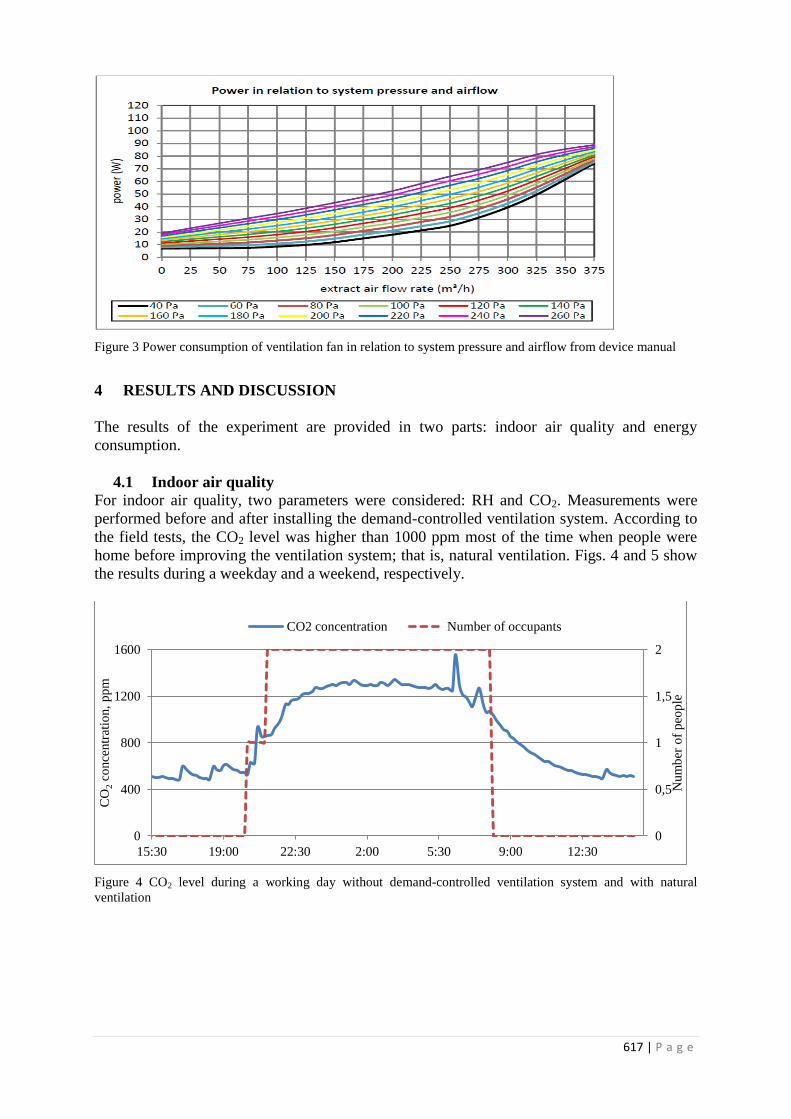
617 | P a g e

Figure 3 Power consumption of ventilation fan in relation to system pressure and airflow from device manual


The results of the experiment are provided in two parts: indoor air quality and energy

consumption.


For indoor air quality, two parameters were considered: RH and CO2. Measurements were

performed before and after installing the demand-controlled ventilation system. According to

the field tests, the CO2 level was higher than 1000 ppm most of the time when people were

home before improving the ventilation system; that is, natural ventilation. Figs. 4 and 5 show

the results during a weekday and a weekend, respectively.

Figure 4 CO2 level during a working day without demand-controlled ventilation system and with natural

ventilation

0

0,5

1

1,5

2

0

400

800

1200

1600

15:30 19:00 22:30 2:00 5:30 9:00 12:30

Num

ber

of

peo

ple

CO

2 c

once

ntr

atio

n,

pp

m

CO2 concentration Number of occupants

618 | P a g e

Figure 5 CO2 concentrations during weekend with natural ventilation and without demand-controlled ventilation

system

In the demand-controlled ventilation system, the CO2 level was the main factor determining

the ventilation flow rate. The threshold level was set to 800±50 ppm. As Fig. 6 shows, the

CO2 level never exceeded 800 ppm when using the demand-controlled ventilation system.

Figure 6 CO2 concentrations during a working day with demand-controlled ventilation system

Measurements showed that the RH only affected flow rates during showering when using the

demand-controlled ventilation system. For the rest of the time, the relative humidity was 40–

60 % within healthy range.

4.2 Energy consumption

The degree hours method was used to estimate the ventilation heat loss. This is a simplified

method of calculating the building energy demand for active heating. The degree hours

depends on the building location, the chosen indoor temperature and the indirect/passive heat

supply. The heating contribution from the limit temperature to comfort temperature is given

by indirect/passive heating. Degree hours is 115080 °C∙h∙ year-1

for an assumed active

temperature of 17 °C and a mean outdoor temperature of 4.2 °C in Borlänge (Warfvinge and

Dahlblom 2010).

0,0

0,5

1,0

1,5

2,0

2,5

3,0

600

800

1000

1200

1400

1600

1800

0,375 0,51390,65280,79170,93061,06951,20841,34731,48621,6251 1,764 1,90292,04182,1807

Num

ber

of

peo

ple

CO

2 c

once

ntr

atio

n,

pp

m

CO2 concentration

0

0,5

1

1,5

2

2,5

3

500

600

700

800

900

1000

1100

11:40 14:30 17:20 20:10 23:00 1:50 4:40 7:30 10:20

CO2 concentration Number of people

619 | P a g e

ventilation heat loss and ventilation fan energy consumption for high constant ventilation

rates, which is dominant in most multi-family houses in Sweden, was also calculated. Having

degree hours, ventilation heat loss for natural, demand-controlled ventilation and high rate

constant ventilation was calculated for this building (see Fig. 7). As can be seen, the lowest

consumption is for natural ventilation due to the low flow rate and not having any mechanical

ventilation. In the demand-controlled ventilation system, the energy consumption for the

ventilation fan and ventilation loss was almost half of the constant high rate ventilation flow;

in other words, 45 % and 22 % of ventilation heat loss and ventilation fan, respectively, are

saved by demand-controlled ventilation. Due to the very low specific fan power of ventilation

fan used in this system, there was not a great deal of saving in terms of ventilation fan power

by using the demand-controlled ventilation system. However, savings for ventilation heat loss

was significant compared to the constant high-rate ventilation.

Figure 7 Energy consumption for ventilation heat loss and ventilation fan electricity consumption for natural,

high, and multi-zone demand-controlled ventilation system

5 CONCLUSION

This study investigated the performance of multi-zone demand-controlled ventilation in a

single-family house in Sweden. The studied building had been renovated with improved

windows with lower leakage and insulated internally with more insulation layers. In addition,

the heat source was changed from furnace to ground source heat pump. All these changes

resulted in lower ventilation flow rate in this building, leading to poor indoor air quality. This

was proved by measuring the CO2 level, which was approximately 1400 ppm when the

occupants were at home. This value is much higher than the common threshold level of CO2

(that is 1000 ppm) as an indicator for acceptable IAQ. This indicated the need to improve the

ventilation system in this building. For this purpose, a multi-zone demand-controlled

ventilation system was installed in this building. The control set point for ventilation flow rate

was based on the CO2 level in habitable spaces and the relative humidity and VOC for the

toilet and bathroom. Measurements showed significant reduction in CO2 concentration

leading to improvement in IAQ by using demand-controlled ventilation system. However, in

demand-controlled ventilation energy consumption for ventilation heating was almost twice

compared to natural ventilation due to higher ventilation rate. Nevertheless, using demand-

controlled ventilation resulted in 44 % saving in ventilation heating and ventilation fan

consumption compared to constant ventilation system. More experiments to measure actual

heating consumption in the building studied are planned for autumn. The need to decrease

0

10

20

30

40

50

1 2 3

Ventilation loss, kWh ∙m

-2

ventilation fan Ventilation heat loss

Natural ventilation Demand-controlled ventilation High rate ventilation

0.1 l∙s-1∙m-2 0.2 l∙s-1∙m-2 0.35 l∙s-1∙m-2

620 | P a g e

energy demand in residential buildings without sacrificing indoor air quality highlights the

application of demand-controlled ventilation system.

6 ACKNOWLEDGEMENTS

We are grateful to the Swedish Energy Agency (Energimyndigheten) and SBUF, The

Development Fund of the Swedish Construction Industry for financial support.

7 REFERENCES

Anisimova N (2011). The capability to reduce primary energy demand in EU housing.

CzechTechnical University in Prague. Energy and Buildings 43. Issue 10. Pages 2747–2751

Boverkets byggregler (BBR 2009), Swedish building regulations

Höppe P (2002). Different aspects of assessing indoor and outdoor thermal comfort, Energy

and Buildings (34) 661–665

Joint Research Center (JRC). [Online]. http://ec.europa.eu/dgs/jrc/index.cfm

Hesaraki A, Holmberg S (2013) Demand-controlled ventilation in new residential buildings:

consequences on indoor airquality and energy savings," Indoor and Built Environment, DOI:

10.1177/1420326X13508565.

Warfvinge C and Dahlblom M 2010, Projektering av VVS-installationer. Lund, Sweden

Seppanen OA, Fisk WJ and Mendell MJ (1999) Association of Ventilation Rates and CO2

Concentrations with Health and Other Responses in Commercial and Institutional Buildings,"

Indoor Air, vol. 9, pp. 226-252, 1999

621 | P a g e

SEASONAL VARIATION IN AIRTIGHTNESS

Paula Wahlgren

Chalmers University of

Technology

Building Technology

SE-41296 Göteborg, Sweden

[email protected]

ABSTRACT

Airtightness of buildings is necessary to obtain healthy, sustainable and energy efficient buildings. Measuring

the airtightness of a building has become more common lately, much due to the higher energy use in leaky

buildings. The airtightness of a building can for example be measured in order to attain a certification, or on

demand from a developer.

In some studies, there have been large seasonal variations in airtightness. In most cases, the buildings are more

leaky in wintertime, but there are also some investigations that show the opposite. In the current project, the aim

is to investigate how, and if, the airtightness varies over the year. The airtightness is measured, using a blower

door, approximately eight times a year, in three different buildings. The air leakages in the buildings are also

detected and the air velocities at a number of leakages are measured. Two of the buildings are one-family, two

story, wooden frame houses and one is a multi-family, concrete building (where one apartment is measured). In

Swedish wooden houses, the air barrier is often a polyethylene foil, which is also the case in these two buildings.

The measurements have been analyzed with respect to indoor/outdoor temperature and indoor/outdoor relative

humidity. The trend in the measurements is that the airtightness is lower (more leaky envelope) when the indoor

air is drier (low relative humidity). Consequently, the air leakage is largest during the winter measurements. The

decrease in airtightness from summer to winter is in the order of 8-10%.

KEYWORDS

Airtightness, seasonal variation, air leakage, fan pressurization method

1 INTRODUCTION

The airtightness of a building has an impact on the energy use and on the moisture safety of a

building. It also affects the thermal comfort, the air quality in a building, sound insulation and

the spread of fire gases (Sandberg et al. 2007). Measuring the airtightness of a building has

become more common lately, much due to the increased energy use in leakier buildings. The

airtightness of a building can be measured in order to attain a certification or on demand from

a developer. The consequences if failing the target can sometimes be severe. Therefore, it is

of great importance to obtain a correct and representative measure of the airtightness.

622 | P a g e

The airtightness in a building is created by a continuous and airtight thermal envelope. The

airtight layer in a thermal envelope can be either a thin layer, such as a polyethylene foil, a

board, such as plywood, a homogeneous construction (e.g. a concrete component) or an outer

coating, such as rendering. In all examples it is of great importance that the joints are properly

sealed.

Airtightness measurements are usually performed in accordance with EN 13829:2000 (Fan

pressurization method). In this standard there are limitations with respect to the climatic

conditions during measurements. There is for example a limit on the maximum allowed wind

speed and the maximum allowed temperature difference over the thermal envelope. The

purpose of the limitations is to assure a correct measured airtightness. Nevertheless,

measurements have shown that there is a variation in the measured airtightness with respect to

the time of year for the measurement. Yoshino (2012) described variations of ±20% over the

year. Boorsboom et al. (2012) analyzed airtightness measurements, from the 80ies, made on

21 window frames mounted in masonry or concrete walls. The average difference in air

tightness between summer and winter was about 30% (higher leakage during winter) and the

maximum seasonal difference was 120%. To be noted, some window frames showed a lower

leakage rate during winter. Boorsboom et al. suggest measurements during three subsequent

seasons in order to obtain correct values. Also Kim and Shaw (1986) showed increased

leakages during winter time. The highest leakages occurred in winter and early spring, and the

lowest in late summer and fall. Two wood frame constructions were studied and the effect

was more pronounced in the leakier building. The measurements indicate that there is a

correlation between indoor humidity and envelope leakage.

There are also measurements showing a higher leakage during the summer. An example is

Dickinson et al. (1986) who, in one out of three residential, wooden frame houses, measured a

lower air leakage in winter time. They speculate in the influence of snow and ice on the

airtightness. Alev et al. (2014) also show a lower leakage in wintertime. The investigated

houses are log houses in Estonia. They give as possible explanation that the weight of the

snow in wintertime tightens the log house.

Bracke et al. (2013) measured the airtightness in two new buildings during almost four

months (December to April). In the masonry building, there was an increase in air leakage

over time. A possible explanation is the different thermal expansion of the masonry/concrete

structure and the plaster that assures most of the airtightness in these buildings. This

difference in thermal expansion could create cracks in the plaster. Another possible

explanation is a gradual deterioration of the ventilation ductwork due to repeated dismantling

for the preparation of the pressurization tests.

In this project, full scale measurements and numerical simulations have been performed in

order to investigate the possible variations in airtightness at different seasons, and the relation

to climate.

2 METHOD

The air tightness’ variation over season and climate is studied by measuring the air tightness

of three buildings, during one year, and by performing numerical simulations on the climate

and the effect on airtightness. The first measurements, on two one-family wooden buildings,

started in June 2013. Measurements on a multi-family concrete building stared in March

2014. The measurements have been performed by SP, Technical Research Institute of

Sweden. Initial numerical calculations have been made on the influence of wind, and on air

properties.

623 | P a g e

The first airtightness measurements were performed on two residential one family houses,

both located in the south west part of Sweden, one house in Landvetter and one in Sevred,

located outside Borås. The houses are light weight wooden houses in two floors (plain wood

beams/joists in Landvetter and light weight wooden beams/joists in Sevred) and they both

have slab on ground and cold, ventilated attics. Both buildings have mineral wool insulation

and polyethylene foil on the inside (between insulation and interior board) as air barrier and

moisture barrier. The house in Landvetter is built in 2004 and the house in Sevred is built in

1993. Both houses have mechanical exhaust ventilation systems. The multi-family concrete

building was finished early 2014 and one apartment has been measured. The apartment has

3.5 external walls.

Figure 1. The tested wooden buildings, Landvetter (2004) to the left and Sevred (1993) to the right.

The airtightness quantity used is air permeability, q50 (l/sm²). It is the amount of air that

passes through the thermal envelope at a pressure difference of 50 Pa, per area of thermal

envelope. The air flow is measured both when the building is pressurized and depressurized

and the mean value is used. The airtightness measurements are made according to EN

13829:2000, using a Minneapolis BlowerDoor. Temperature and relative humidity, indoor

and outdoor, is measured at each airtightness measurement occasion, as well as the outdoor

wind speed. In addition, the temperatures and relative humidities are continuously logged, and

these measurements will be analyzed at the end of the study. The airtightness measurements

are performed 6-8 times a year to study the different seasons and climate conditions.

3 NUMERICAL SIMULATIONS

Simulations have been performed in order to study how the measured air flow is affected by

different densities of the air. The density of the air is different due to variations in temperature

and relative humidity over the year. Both high temperatures and high relative humidities

result in low air densities. Numerical investigations have also been performed on the effect of

wind.

During a pressurization test, the air is drawn into the building through leakages in the air

barrier of the thermal envelope. These leakages can have different geometry and surface

roughness and the air flow can also pass through an air permeable material. The magnitude of

the air flow depends on the pressure difference over the leakage path, of the characteristics of

the leakage path, but also on the characteristics of the air. The density of the air changes due

to temperature and relative humidity, and is thus not the same for all measurement conditions.

When measuring according to standard EN 13829:2000, the density change that affects the

measurement equipment is corrected for. However, there is also the air flow through the

leakages, which is slightly different at different air densities. This is investigated with

numerical simulations.

624 | P a g e

The geometry of the building in the calculations is a box with an, initially, equal amount of

leakages on all sides (including the roof), see Figure 2. The leakages are assumed to be long

gaps, having a width of 2 mm, in walls with a thickness of 120 mm. The air leakages are

calculated according to Hagentoft (2001). The effect of air temperature and relative humidity

(RH) is determined by investigating two temperature conditions, -20°C and 30°C (RH = 40%),

and two relative humidity conditions, 0 and 100% (Tmean =10°C). A pressure of 50 Pa is used

for the calculations and the resulting airtightness of the building is approximately 0.8 l/sm²

(varying slightly in the different cases). By investigating extreme temperatures and relative

humidities, the factors that possibly influence the airtightness measurements are determined.

Figure 2: Simulated box with evenly distributed gaps.

The investigation shows that the temperature of the air can affect the measurements by

affecting the air flow through the air gaps, see Table 1. Using -20°C, the measured

airtightness is 0.76 l/sm² and at a temperature of 30°C the measured airtightness is 0.81 l/sm².

Consequently, the difference between the two extreme measurement situations is 5.7%.

Different relative humidities, however, have minor importance. At 0% relative humidity the

airtightness is 0.789 l/sm² and at 100% it is 0.791 l/sm². The difference is 0.14%, thus

negligible. The effect of the air density on the measurement equipment (not leakages as

above) is compensated for when measuring according to EN 13823:2000.

TABLE 1. Airtightness at different temperatures and relative humidities.

Air tightness at

minimum temperature

(l/sm²)

Air tightness at

maximum temperature

(l/sm²)

Air tightness at

minimum relative

humidity (l/sm²)

Air tightness at

maximum relative

humidity (l/sm²)

0.763 0.807 0.789 0.791

5.7% 0.14%

The simulations on wind are made to investigate if different wind speeds give different

airtightness results. Since the average wind speed can be different during different seasons of

the year, this could be a part in explaining why different seasons have different airtightness.

In the standard, it is noted that if the meteorological wind speed exceeds 6 m/s or reaches 3 on

the Beaufort scale, it is unlikely that a satisfactory zero flow pressure difference will be

obtained. Three kinds of zero flow pressure is measured before and after the pressurization

test and if either of these zero flow pressures is over 5 Pa, the test does not meet test

conditions according to EN 13823:2000.

The shape of the simulated building is quadratic, with a flat roof. The shape factor Cp (-), that

determines the pressure difference over a wall at a certain wind influence, is for the windward

wall, 0.4, of the leeward wall, -0.2, and for the other walls, -0.3. The roof is -0.6 and the shape

factor of the inside of the building, Cpi, is determined by a mass air flow balance. The pressure

difference, ΔP (Pa), over a wall subjected to wind, v (m/s), is

625 | P a g e

2)(

2vCCP pip (1)

The building is first simulated with equally distributed leakages, and then with a windward

side that is twice as leaky as the other sides.

The results from the simulations show that there in many cases is a small difference in the

measured airtightness values for pressurization and depressurization when wind is present.

However, the average value is not affected until the wind speed increases. For example, at a

wind speed of 9 m/s, the building is estimated 2% more airtight with wind than without wind.

At a wind speed of 9 m/s, the zero flow pressure difference is most likely exceeding the value

accepted in EN13823:2000. In the simulations, a higher wind speed resulted in lower

calculated air permeability (more airtight building).

For the case of a non-uniform air leakage distribution, simulations were made for a wind

speeds up to 9 m/s. The results are similar to those of the equal leakage distribution, i.e.

unless the wind speeds are high there is little error due to wind.

4 AIRTIGHTNESS MEASUREMENT RESULTS

Full scale airtightness measurements have been performed in three buildings, two light-weight

wooden buildings and one apartment in a residential concrete building. Only three

measurements have, so far, been made on the concrete buildings, March, May and July 2014.

Even though this is a newly erected building, there is no change in the air permeability. All

measurement occasions showed an air permeability of 0.35 l/sm². This building will be further

studied when more measurements have been made, in particular winter measurements.

The light-weight wooden buildings have, so far, been measured 5 or 6 times each. The lowest

measured relative humidity outdoor is 54% (July, Landvetter) and it reaches 100% in

November in Landvetter. Indoor, the relative humidity ranges from 23% (January,

Landvetter) to 60% (September, Landvetter).

In the house in Sevred, there is a constant decrease in relative humidity indoor from July to

November, while the house in Landvetter has the highest indoor relative humidity at the

measurement in September. Both buildings have the lowest relative humidity indoor at the

winter measurements. The wind speed is low during the measurements.

Both buildings have the lowest airtightness (highest air permeability) at the winter

measurement (January-February). This coincides with the lowest indoor air relative humidity.

The measured airtightness (expressed as air permeability) as a function of time is shown in

Figure 3, and as a function of indoor air relative humidity in Figure 4.

626 | P a g e

Figure 3: Measured air permeability as a function of time for the two wooden buildings.

Figure 4: Measured air permeability as a function of relative humidity indoor.

There is an increase in air leakage from summer to winter. The increase from summer to

winter is 10% for the building in Sevred and 7.7% for the building in Landvetter. For both

buildings, the airtightness is less (higher air permeability) when the indoor relative humidity

is the lowest. There is no clear correlation with indoor or outdoor temperature, or outdoor

relative humidity. The correlation between air tightness and indoor air relative humidity will

be more thoroughly investigated when the loggers that continuously measure indoor air

relative humidity are collected. The variations in airtightness from summer to winter can be

noticeable for stakeholders aiming for a certification.

627 | P a g e

In the two measured wooden buildings, the reason for the increase in permeability during

winter could be that the wooden construction dries when the relative humidity indoor

decreases. This, in combination with a poor connection to the polyethylene foil, causes the

leakages to increase when the wood, exposed to indoor air, is dried.

The main leakages in the leakiest building (Landvetter) are found around the attic hatch, at the

connection between the upper and lower floor (see Figure 5) and over a window in the kitchen

at the bottom floor, Figure 6. The reasons are probably a poor connection between window

and polyethylene foil for the windows, both a poor connection between hatch and

polyethylene foil plus a leaky hatch (poor seal) for the attic hatch. The leaky connection

between the upper and lower floor, that is evident in the stairs, is probably caused by a

discontinuous air barrier that does not pass the floor/wall connection.

Figure 5: Thermographic image of attic hatch (left) and hand rail (right) in corner of stairs in January 2014. The

hand rail is at the position of the connection between the top and bottom floor.

Figure 6: Thermographic image of kitchen window in July, and photo of the same.

5 CONCLUSIONS

Airtightness has been measured for ten months in two residential wooden buildings. The trend

in the airtightness measurements is that the airtightness is lower when indoor air is drier. The

winter measurements have the lowest airtightness of all measurements. The decrease in

airtightness from summer to winter is in the order of 8-10% (from July to February). The

measurements will continue so that a whole year will be covered for all buildings.

The numerical simulations show a small change in air flow through the leakages due to high

or low air temperatures (affecting the air density of the air that flow in the leakages), but no

628 | P a g e

change in air flow due to different relative humidities. The effect of the air density on the

measurement equipment (not leakages) is compensated for when measuring according to EN

13823:2000.

6 ACKNOWLEDGEMENTS

The research and the measurements have been financed by SBUF, the Development Fund of

the Swedish Construction Industry, and supported by FoU-väst (regional comittee), which is

greatly appreciated.

7 REFERENCES

Alev, U. Uus, A., Teder, M., Miljan, M-J., Kalamees, T. (2014). Air leakage and hygrothermal

performance of an internally insulated log house, Proceedings from the 10th Nordic Symposium on

Building Physics, Lund, Sweden, June 2014.

Borsboom, W., de Gids W. (2012). Seasonal variation of facade airtightness: field observations and

potential impact in NZEB. Proceedings of the AIVC-TightVent International Workshop, Brussels,

Belgium, March 2012.

Bracke, W., Laverge, J., Van Den Bossche, N., Janssens, A. (2013). Durability and measurement

uncertainty of airtightness in extremely airtight dwellings. Proceedings of the AIVC-TightVent

International Conference, Athens, Greece, September 2013.

Dickinson, J.B., Feustel, H.E. (1986). Seasonal variations in effective leakage area, Thermal

performance of the exterior envelops of buildings III, Atlanta,,USA, ASHRAE, 144-160.

Hagentoft, C-E., (2001). Introduction to Building Physics, Studentlitteratur, Lund, 2001.

Kim, A.K., Shaw, C.Y. (1986). Seasonal Variation in Airtightness of Two Detached Houses, Measured

Air Leakage of Buildings, ASTM STP 904, 1986.

Sandberg, P-I., Bankvall, C. Sikander, E., Wahlgren, P., Larsson, B. (2007). The effects and cost

impact of poor airtightness- Information for developers and clients. Proceedings of the Thermal

Performance of the Exterior Envelopes of Whole Buildings X, Florida, USA, December 2007.

Yoshino, H. (2012). System for ensuring reliable airtightness level in Japan. Proceedings of the AIVC-

TightVent International Workshop, Bryssel, Belgium, March 2012.

EN 13829:2000 (Thermal performance of buildings - Determination of air permeability of buildings -

Fan pressurization method (ISO 9972:1996, modified))

629 | P a g e

OPTIMIZATION OF DATA CENTER CHILLED

WATER COOLING SYSTEM ACCORDING TO

ANNUAL POWER CONSUMPTION CRITERION

Piotr Kowalski

1, Mieczysław Porowski

2

1Poznan University of Technology

Piotrowo 5

60-695 Poznan, Poland

[email protected]

2Poznan University of Technology

Piotrowo 5


[email protected]

ABSTRACT

The paper presents optimization model of the chilled water based data center cooling system. The optimization

procedure includes system technological and mathematical model, limiting conditions and optimization criterion,

which in this case is annual power consumption minimum. The cooling system model is defined by constant

parameters and decision variables and consists of aircooled chiller, independent external freecooling heat

exchanger (drycooler), computer room air handling unit (CRAH) and constant flow chilled water system with

circulation pump. Influence of the server racks architecture (open or closed rack aisle), server inlet temperature

and chilled water regime on the annual power consumption of the cooling system has been shown. Case study

calculation based on the described model has been presented, including optimum variant designation and power

usage effectiveness ratio of mechanical system calculation.

KEYWORDS

data center, efficiency, optimization, precision cooling, chilled water

NOMENCLATURE

cp – specific heat, [kJ/kgK]

CRAH – computer room air handler

ECR – CRAH unit fan power consumption, [kWh]

ECWP – chilled water pump power consumption,

[kWh]

EDX – compressor power consumption, [kWh]

EFC – freecooling coil fan power consumption,

[kWh]

EIT – server power consumption, [kWh]

EK – condenser fan power consumption, [kWh]

ETOT – cooling system power consumption, [kWh]

hCRS, hCRR – CRAH unit supply specific enthalpy,

[kJ/kg]

hKA, hKe – condensing coil supply/return specific

enthalpy, [kJ/kg]

hFA, hFe – freecooling coil supply/return specific

enthalpy, [kJ/kg]

l – hydraulic system length, [m]

p – absolute air pressure, [Pa]

PCR – CRAH unit fan power input, [kW]

PCWP – chilled water pump power input, [kW]

PDX – compressor power input, [kW]

PFC – freecooling coil fan power input, [kW]

PIT – IT systems power input, [kW]

PK – condenser fan power input, [kW]

PTOT – mechanical systems total power input, [kW]

PUE(m) – power usage effectiveness of mechanical

systems, [-]

QCW – chilled water cooling capacity, [kW]

QE – evaporator cooling capacity, [kW]

QFC – freecooling coil cooling capacity, [kW]

QIT – server room cooling load, [kW]

QK – condenser capacity, [kW]

R – pressure loss coefficient, [Pa/m]

Rp – gas constant of air, 287,05 [J/kgK]

tA – ambient temperature, [°C]

tAmax – max amb. temperature for a given profile,

[°C]

630 | P a g e

tAmin – min amb. temperature for a given profile, [°C]

tCHR – condensing coil return air temperature, [°C]

tCHS – condensing coil supply air temperature, [°C]

tCRR – CRAH unit return air temperature, [°C]

tCRS – CRAH unit supply air temperature, [°C]

tCWE – chilled water temperature before evaporator,

[°C]

tCWR – chilled water return temperature, [°C]

tCWS – chilled water supply temperature, [°C]

tE – evaporating temperature, [°C]

tFA, tFe – freecooling coil supply/ return air

temperature, [°C]

tFC,0% – freecooling start ambient temperature, [°C]

tFC,100% – full freecooling ambient temperature, [°C]

tFCR – freecooling coil return air temperature, [°C]

tFCS – freecooling coil supply air temperature, [°C]

tKA, tKe – condensing coil supply/return air

temperature, [°C]

TE – evaporating temperature, [K]

TK – condensing temperature, [K]

VCR – CRAH unit airflow volume rate, [m3/s]

VCW – chilled water flow volume rate, [m3/s]

VFC – freecooling coil airflow volume rate, [m3/s]

VK – condensing coil airflow volume rate, [m3/s]

ΔpCR – CRAH unit pressure drop, [kPa]

ΔpCWP – chilled water pump available pressure,

[kPa]

ΔpE – evaporator pressure drop, [kPa]

ΔpFC – freecooling coil pressure drop, [kPa]

Δpp – hydraulic system pressure drop, [kPa]

ΔQFC – freecooling coil capacity difference, [kW/°C]

ΔtCR – CRAH unit air temperature difference, [°C]

ΔtE – evaporating and chilled water supply

temp. difference, [°C]

ΔtEXV – min. evaporating and condensing


ΔtFC,100% – 100% freecooling capacity


ΔtIT – server air temperature difference, [°C]

ΔtK – condensing and ambient temp. difference, [°C]

Δτ – duration of a given ambient temperature, [h]

ηCR – CRAH unit fan efficiency, [%]

ηCWP – chilled water pump efficiency, [%]

ηDX – compressor efficiency, [%]

ηFC – freecooling coil fan efficiency, [%]

ηK – condenser fan efficiency, [%]

ρCRS – mass density, CRAH unit supply air

temperature [kg/m3]

1 INTRODUCTION

Data Center cooling is one of the most energy consuming mechanical systems available.

There are several factors that contribute to high power demand including continuous

operation independently of ambient conditions (cooling load depends mostly on IT equipment

and external heat gains have minor impact on it), high expenditures on cooling and movement

of load carriers (especially air and water) and constant growth of heat gains and density of

servers. Power consumption of mechanical systems has large impact on total cost of

ownership and carbon footprint of data center class buildings, so many different researches to

minimize this impact have been carried and the problem is still valid.

Application of optimization methods to design chilled water based HVAC systems have been

presented by Lu (Lu, Cai, Chai, 2005; Lu, Cai, Xie, 2005), while Porowski (Porowski, 2011)

presented composite strategy to select optimum ventilation and air-conditioning system based

on energy consumption criterion. Research on data center cooling system optimization have

been carried by i.e. Shah et al., (Breen, Walsh, Shah, 2010; Breen, Walsh, Punch, 2010;

Breen, Walsh, Punch, Shah, Kumari, 2010) Iyengar et al. (Iyengar, 2009) and Demetriou et al.

(Demetriou, 2011), who presented holistic, analytic models taking into account the heat flow

from servers to ambient air with a watercooled chiller and cooling tower as a cooling source.

The subject of presented paper is optimization model of the data center chilled water based

precision cooling system with external, aircooled chiller and additional freecooling heat

exchanger (water economizer) as a mechanical cooling source.

631 | P a g e

2 PROBLEM FORMULATION

Data center cooling system optimization problem includes formulation of the system model

(including constant parameters and decision variables), definition of the limiting conditions

and optimization criterion. Simplified technological scheme of the analyzed system is shown

on Fig. 1.

Figure 1. Technological scheme of the chilled water based data center cooling system

The data center cooling system model is described by the constant parameters and decision

variables. Constant parameters, by definition, remain constant throughout optimization

procedure (in general they can be a function of time). Decision variables, by definition, are

changing throughout optimization procedure. Cooling system model described in this paper

has following constant parameters: system structure, thermo-dynamical parameters of load

carriers (air, water, refrigerant), ambient temperature distribution profile, server room heat

load, mechanical efficiency of various components (pump, fans, compressor), difference

between chilled water supply and evaporating temperature, minimum difference between

refrigerant evaporating and condensing temperature, difference between ambient and

refrigerant condensing temperature, length of the chilled water piping.

There are two types of decision variables used in the described model:

incommensurable variables - server rack architecture. There are two variables of this

kind included in the model: closed aisle architecture (separation of the hot and cold

aisle, cooling system control according to supply air temperature, mass flow of the

CRAH air as a function of server temperature rise) or open aisle architecture (no

cold/hot aisle separation, cooling system control according to the return air temperature

and CRAH unit airflow 30% higher compared to closed aisle architecture),

measurable variables: server air temperature raise, supply and return chilled water

temperatures (thus chilled water mass flow), freecooling coil operation starting ambient

temperature, temperature difference to reach full required capacity of the freecooling

coil.

There are following limiting conditions used in the optimization procedure: CRAH unit return

air temperature (for open aisle option) or server inlet air temperature, thus supply air

632 | P a g e

temperature range according to ASHRAE 2011 A1 class recommended envelope – for closed

aisle architecture.

The optimization criterion used in the described model was minimum annual electrical power

consumption of the cooling system according to the below account:

ETOT=min (ETOT1,…ETOTj,…ETOTj max) (1)

3 MODEL ASSUMPTIONS AND SOLVING PROCEDURE

For each of the components of the cooling system model (CRAH, freecooling coil, water

chiller) balance equations have been formulated including power input of the components, i.e.

cooling capacity delivered by the chilled water system includes the additional heat dissipated

by the CRAH unit fans according to the equation:

QCW=Q

IT+PCR(1-ηCR) (2)

CRAH unit fan power input depends on the volume flow of the server room air, which further

depends on the mass flow and supply air temperature. It has been calculated as a function of

the reference values of the fan power input and volume airflow according to the following

equations:

PCR=PCR ref (VCR

VCR ref)3

(3)

mCR=QIT

CP(tCRR-tCRS) (4)

VCR=mCR

ρCRS (5)

ρCRS=

p

RpTCRS (6)

Cooling capacity of the external freecooling coil has been calculated in a simplified way,

including decision variables Δt100%FC and tA,0%FC according to the equations:

tFC,100%= tCWS+tCWR

2-ΔtFC,100% (7)

QFC=

{

0, tA≥tA,0%FC

QCW

-(tA-tFC,100%)ΔQCF, tFC,0%>tA

>tFC,100%

QFC=Q

CW, tA≤tFC,100%

(8)

ΔQFC=

QCW

tFC,0%-tFC, 100% (9)

633 | P a g e

Power input of the freecooling coil fan has been calculated using equations (3,4,5,6) described

for the CRAH unit, with the assumption of constant ambient temperature raise across the coil.

Cooling load of the evaporator has been calculated according to the equation:

QE=Q

CW-QFC

(10)

Heatload of the aircooled condenser includes power input of the compressor and has been

calculated according to the equation:

QK=Q

E+PDX (11)

Power input of the compressor has been calculated according to following equations:

PDX=QE

COPDX (12)

COPDX= (TE

TK-TE) η

DX (13)

tE=tCWS-ΔtE (14)

tK={

tA+ΔtK,(tK-tE)≥ΔtEXV

tE+ΔtEXV, (tK-tE)<ΔtEXV

(15)

where ηDX, ΔtEXV, ΔtK are decision variables based upon chiller manufacturer data.

Power input of the aircooled condenser fan has been calculated using equations (3, 4, 5, 6)

with the assumption of constant temperature rise of the ambient air. Power consumption of

the circulating pump has been calculated using following equations:

PCWP=VCWΔpCWP

ηCWP (16)

ΔpCWP

=ΔpP+Δp

CR+Δp

FC+Δp

E (17)

ΔpP=1,3Rl (18)

with the simplifying assumption, that local pressure drop is 30% of the linear. Pressure drop

of the CRAH unit, freecooling coil and evaporator has been calculated using below equations:

ΔpCR=Δp

CR ref(VCW

VCW ref)2

(19)

ΔpFC=Δp

FC ref(VCW

VCW ref)2

(20)

ΔpE=Δp

E ref(VCW

VCW ref)2

(21)

where values of reference pressure drops have been taken from manufacturers datasheets.

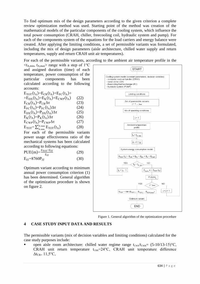
634 | P a g e

To find optimum mix of the design parameters according to the given criterion a complete

review optimization method was used. Starting point of the method was creation of the

mathematical models of the particular components of the cooling system, which influence the

total power consumption (CRAH, chiller, freecooling coil, hydraulic system and pump). For

each of the components system of the equations for the load carriers and energy balance were

created. After applying the limiting conditions, a set of permissible variants was formulated,

including the mix of design parameters (aisle architecture, chilled water supply and return

temperatures, supply and return CRAH unit air temperatures).

For each of the permissible variants, according to the ambient air temperature profile in the

<tA,min, tA,max> range with a step of 1°C

and assigned duration (time) of each

temperature, power consumption of the

particular components has been

calculated according to the following

accounts:

ETOT(tA)=ECR(tA)+EFC(tA)+

+EDX(tA)+EK(tA)+ECWP(tA) (22)

ECR(tA)=PCRΔτ (23)

EFC(tA)=PFC(tA)Δτ (24)

EDX(tA)=PDX(tA)Δτ (25)

EK(tA)=PK(tA)Δτ (26)

ECWP(tA)=PCWPΔτ (27)

ETOT=∑ ETOT(tA)tA maxtA min

(28)

For each of the permissible variants

power usage effectiveness ratio of the

mechanical systems has been calculated

according to following equations:

PUE(m)=ETOT+EIT

EIT (29)

EIT=8760PIT (30)

Optimum variant according to minimum

annual power consumption criterion (1)

has been determined. General algorithm

of the optimization procedure is shown

on figure 2.

4 CASE STUDY INPUT DATA AND RESULTS

The permissible variants (mix of decision variables and limiting conditions) calculated for the

case study purposes include:

open aisle room architecture: chilled water regime range tCWS/tCWR= (5-10/13-15)°C,

CRAH unit return temperature tCRR=24°C, CRAH unit temperature difference

ΔtCR= 11,5°C,

Figure 1. General algorithm of the optimization procedure

635 | P a g e

closed aisle room architecture: chilled water regime range tCWS/tCWR= (12-21/20-26)°C,

temperature of the cold aisle (server inler) according to ASHRAE 2011 A1 Data Center

class recommended range (A. T. C. TC 9.9., 2011), CRAH unit temperature difference

ΔtCR= 15°C.

There have been 24 permissible variants calculated. List of decision variables of the selected

five calculations for the case study example is shown in Table 1.

Table 1. Case study calculation selected input data

Variant No. Architecture QIT tCWS tCWR ΔtCR ΔtFC0% ΔtFC100%

[ - ] [ - ] [kW] [°C] [°C] [°C] [°C] [°C]

1 open 200 8 13 11,5 1 12

2 open 200 8 15 11,5 1 12

3 closed 200 15 22 15 1 12

4 closed 200 16 24 15 1 12

5 closed 200 18 26 15 1 12

The case study calculation results of the selected permissible variants are shown in Table 2.,

which includes annual power consumption of the respective components of the modelled

system, total annual power consumption of the system and PUE(m) ratio. Energy

consumption of the optimum variant (No. 5) based on the minimum annual energy

consumption criterion (variant No. 5) is 60% lower compared to most energy consuming

system (variant No. 5). Figure 3. shows energy consumption split of the optimum calculated

system, while Figure 4. shows energy consumption split of the maximum calculated variant

(No. 1).

Table 2. Case study calculation selected results

tCWS/tCWR EDX EK EFC ECWP ECR ETOT PUE(m)

[°C] [kWh/year] [kWh/year] [kWh/year] [kWh/year] [kWh/year] [kWh/year] [-]

8/13 176020 26541 43332 50189 83134 379215 1,22

8/15 165007 23416 47376 22547 83861 342208 1,20

15/22 77413 10382 46793 22547 40514 197649 1,11

16/24 63051 7687 44699 16887 41108 173432 1,10

18/26 46337 5265 40973 16887 41958 151420 1,09

Figure 3. Cooling system energy consumption split (optimum variant – No. 5)

46337; 31%

5265; 3%

40973; 27%

16887; 11%

41958; 28%

Edx [kWh/year; %]

Ek [kWh/year; %]

Efc [kWh/year; %]

Ecwp [kWh/year; %]

Ecr [kWh/year; %]

EDX [kWh/year; %]

EK [kWh/year; %]

EFC [kWh/year; %]

ECWP [kWh/year; %]

ECR [kWh/year; %]

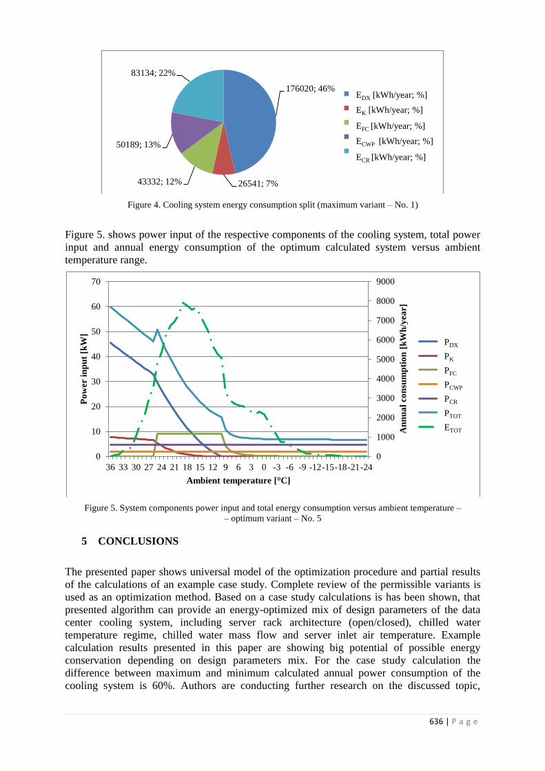
636 | P a g e

Figure 4. Cooling system energy consumption split (maximum variant – No. 1)

Figure 5. shows power input of the respective components of the cooling system, total power

input and annual energy consumption of the optimum calculated system versus ambient

temperature range.

Figure 5. System components power input and total energy consumption versus ambient temperature –

– optimum variant – No. 5

5 CONCLUSIONS

The presented paper shows universal model of the optimization procedure and partial results

of the calculations of an example case study. Complete review of the permissible variants is

used as an optimization method. Based on a case study calculations is has been shown, that

presented algorithm can provide an energy-optimized mix of design parameters of the data

center cooling system, including server rack architecture (open/closed), chilled water

temperature regime, chilled water mass flow and server inlet air temperature. Example

calculation results presented in this paper are showing big potential of possible energy

conservation depending on design parameters mix. For the case study calculation the

difference between maximum and minimum calculated annual power consumption of the

cooling system is 60%. Authors are conducting further research on the discussed topic,

176020; 46%

26541; 7% 43332; 12%

50189; 13%

83134; 22%

Edx [kWh/year; %]

Ek [kWh/year; %]

Efc [kWh/year; %]

Ecwp [kWh/year; %]

Ecr [kWh/year; %]

EDX [kWh/year; %]

EK [kWh/year; %]

EFC [kWh/year; %]

ECWP [kWh/year; %]

ECR [kWh/year; %]

0

1000

2000

3000

4000

5000

6000

7000

8000

9000

0

10

20

30

40

50

60

70

36 33 30 27 24 21 18 15 12 9 6 3 0 -3 -6 -9 -12-15-18-21-24

An

nu

al

co

nsu

mp

tio

n [

kW

h/y

ea

r]

Po

wer i

np

ut

[kW

]

Ambient temperature [°C]

Pdx

Pk

Pfc

Pcwp

Pcr

P tot

E tot

PDX

PK

PFC

PCWP

PCR

PTOT

ETOT

637 | P a g e

purpose of the research is further refinement of the cooling system particular components and

introduction of more complex optimization procedures.

6 REFERENCES

A. T. C. TC 9.9. (2011). Thermal Guidelines for Data Processing Environments – Expanded

Data Center Classes and Usage Guidance. American Society of Heating, Refrigerating and

Air-Conditioning Engineers, Inc.

Breen, T. J.; Walsh, E. J.; Punch, J.; Shah, A. J.; Bash, C. E. (2010). From chip to cooling

tower data center modeling: Part II Influence of chip temperature control philosophy. IEEE.

Breen, T. J.; Walsh, E. J.; Punch, J.; Shah, A. J.; Kumari, N.; Bash, C. E.; Lyon, G. (2010).

From Chip to Cooling Tower Data Center Modeling: Validation of a Multi-Scale Energy

Management Model. 13th IEEE ITHERM Conference.

Breen, T. J.; Walsh, E. J. P. J.; Shah, A. J.; Bash. C. E. (2010). From chip to cooling tower

data center modeling: Part I Influence of server inlet temperature and temperature rise across

cabinet. IEEE.

Demetriou, D. W.; Khalifa, H. E.; Iyengar, M.; Schmidt, R. R. (2011). Development and

experimental validation of a thermo-hydraulic model for data centers. HVAC&R Research,

vol. 17:4, pp. 540-555.

Iyengar, M.; Schmidt, R. R. (2009). Analytical Modeling for Thermodynamic

Characterization of Data Center Cooling Systems. Journal of Electronic Packaging, vol. 131,

no. June, pp. 021009-1 - 021009-9.

Lu, L.; Cai, W.; Chai, Y. S.; Xie, L. (2005). Global optimization for overall HVAC systems -

Part I problem formulation and analysis. Energy Conversion & Management, vol. 46, pp. 999-

1014.

Lu, L.; Cai, W.; Xie, L.; Li, S.; Soh. C. (2005). HVAC system optimization - in-building

section. Energy and Buildings, vol. 37, pp. 11-22.

Porowski, M. (2011). Strategia wyboru energooptymalnego systemu wentylacyjnego lub

klimatyzacyjnego. Wydawnictwo Politechniki Poznańskiej, Poznań.

638 | P a g e

NUMERICAL SIMULATION OF INDOOR AIR

QUALITY - MECHANICAL VENTILATION SYSTEM

SUPPLIED PERIODICALLY VS. NATURAL

VENTILATION.

Ewelina Kubacka

1, Dariusz Heim

2

1 Lodz University of Technology

Department of Heat and Mass Transfer

Wolczanska 213, 90-924, Poland


[email protected]

2 Lodz University of Technology

Department of Heat and Mass Transfer

Wolczanska 213, 90-924, Poland

90-924, Poland

ABSTRACT

Building integrated renewable energy sources e.g. photovoltaic system is one of the promised solution for

improving energy efficiency in building. However such kind of the system is restrained by irregular power

supplied and necessity to convert current from direct to altering form. Therefore, very often the electrical energy

generated by photovoltaic system cannot be effectively utilised to supply building devices, e.g. components of

HVAC or lighting system. The other problem is energy storage during the day to be successfully used during the

night.

The paper is devoted to analysed numerically overall effectiveness of two types of ventilation system: low-

power, direct current mechanical ventilation and natural ventilation. Both systems were applied for office

building, generally occupied during a day. A comparison of both system were conducted for the whole calendar

year.

Mechanical system considered in the paper is fully supplied from the photovoltaic panels integrated with façade

cladding system. Panels covers a total opaque area of external wall, transferring solar energy into electricity with

constant performance 15%. The proposed, low-power, mechanical ventilation system can be treated as an

alternative for natural ventilation, because both are free from exploitation costs. On the other hand the

effectiveness in providing proper indoor air quality of both systems is expected to be different. Efficacy of

natural ventilation strongly depends on environmental conditions, while efficiency of proposed mechanical

system can productively work during the day only.

Taking into account the changeably character of both ventilation systems work a dynamic simulation methods

were proposed to analysed their effectiveness. The model of one office zone, occupied during a day were

modelled in ESP-r system. The geometry of the room was discretized by control volume elements. The air flow

inside the room was defined by a nodal network method. In the case of natural ventilation the window cracks and

openings characterized the inlet, while outlet was defined as a ventilation chimney. On the other hand, while

mechanical system is considered the inlet and outlet were defined as a mechanical ventilation devices.

Presented results shows the effect of both system on indoor air quality and thermal comfort. The results are

limited to the period of occupancy only, during the whole calendar year.

KEYWORDS

Mechanical, natural, thermal comfort, photovoltaic, efficiency, simulation.

1 INTRODUCTION

Building integrated PV, e.g. façade system can be one of the renewable sources of electricity

in zero or plus energy buildings. In the first place PV power should be used by any devices

providing proper indoor environment conditions according to the main idea of sustainability

639 | P a g e

building. Therefore, any technical building systems that use electrical energy for heating,

cooling, ventilation and/or domestic water to satisfy energy needs can be supply directly from

renewable electricity sources.

Photovoltaic is one of the most promised technology, because of easy installation, building

integration and cost effectiveness. On the other hand, the periodical, changeable character of

its operation generates the following two problem. Renewable energy is providing during the

day only and in some characteristic periods of time the supply exceeds the demand.

Therefore, the proper size and arrangement of electrical network components including

battery, can provide an appropriate and effective operation of the whole system. One of the

most precisions method of system design is dynamic numerical simulation using relatively

short, e.g. one hour time step. For the purpose of this work the numerical model were

developed using ESP-r (Energy System Performance) software.

The main goal of presented work was to investigate the effectiveness of proposed mechanical

ventilation system supplied from photovoltaic modules under local, moderate weather

conditions. It was assumed that analysed office building is occupied from 8:00 to 16:00, while

façade ventilation unit is furthermore active one hour before and after that time. Outside

working hours, the ventilation system is switch off. The only source of electrical energy for

mechanical ventilation is energy from PV panels and reserve energy stored in battery. For the

purpose of presented analysis different amount of panels was considered taking into account

solar irradiation according to Typical Meteorological Year, TMY weather file. The

effectiveness of solar energy conversion (15%) and stored (85%) were considered in analysis.

The second objective of the study was devoted to compare effectiveness of natural and

proposed mechanical system supply from PV. Both systems works at no cost but theirs

effectiveness depends on local climatic conditions: wind and temperature for natural or solar

radiation for mechanical ventilation. Comparison of both systems were done based on the

following parameters: air flow rates in analysed room (pollutant removal efficiency) and

comfort indices (user thermal sensation).

2 METHODOLOGY

To conduct the analysis of indoor air quality, the computational model had to be subjected to

a dynamic simulation, requiring the use of a suitable model of air flow. In order to determine

the appropriate coupling phenomena of the heat and mass transfer, an Air Flow Network

method was applied. In the presented approach, all of the components are defined by the

nodes representing the volume of solids or the volume of air and the associated heat capacities

[6]. The thermal model is based on the finite-volume discretization heat balance method, in

which elements of the building structure, zones and associated systems are represented via

nodes. Nodes with different physical parameters are connected by the flow path and they are

remaining in the thermodynamic equilibrium state. A system of nonlinear differential

equations characterise the properties and the form of the flow and they are describing the

network connection. The flow through each connection is performed in such a manner that the

amount of air flowing into and flowing out of each zone remains at equilibrium (as the

principle of conservation of mass).

3 SIMULATION MODEL

3.1 Geometry and materials

The simulation was performed for the model of a single office room. Climate database was

built on the basis of meteorological data type WYEC (Weather Year for Energy Calculation,

Version 2) [5], developed for the city of Lodz. The room has been defined based on the actual

640 | P a g e

area dimensions (depth x width x height) 5.8 x 3.0 x 3.6 m. All partitions were designed with

the assumption of good thermal insulation of the area. The mineral wool with a thickness of

200 mm was used as a basic insulation material and it was located on the inside of both

vertical and horizontal partitions. Window with dimensions of 1.2 x 1.2 m and a thickness of

0.01 m oriented to the west was located at the central part of the outer wall. In order to obtain

accurate simulation results, the area of the room was divided into 3 zones with finite volumes

equal 19.44 m3 and 21.6 m

3.(Figure 1). The article authors assumed that the work spot is

placed in the central part of Zone A.

Figure 1: Model geometry

3.2 Computational assumptions

For the purposes of the article indoor air quality evaluation was made by using two thermal

comfort indices: PMV and PPD. The parameters necessary for their designation were adopted

in accordance with the standards for the required parameters of the proposed internal

environment [4]. It was assumed that during cooling season (from October to March) the

thermal resistance of clothing is Icl = 0.5 clo (clothing in the form of thin trousers and a shirt

with short sleeves), the activity level of 1.2 met = 70 W/m2 (the characteristic value for office

work). During the heating season (from April to September) thermal resistance of clothing

assumed equal to 1.0 clo (shirt, pants, jacket). The level of activity remains unchanged and

the air velocity was taken as the average air velocity value for each month.

Analyses were performed with the assumption the zone is occupied by one person from

Monday to Friday from 8:00 ÷ 16:00. The total heat load being defined as 215 W/person [3],

where 100 W is derived from the equipment room (electronic devices). It was assumed that

solar irradiation is sufficient light source from 8:00 ÷ 15:00, and therefore heat gain from

artificial lighting assumed equal to 10 W/m2 between 15:00 ÷ 16:00.

3.3 Air Flow Network

The Air Flow Network is designed by five nodes (three internal - A, B and C and two external

- 1 and 2, where the flow is caused by the effects of wind pressure on the surface elevation)

(Figure 2). Wind pressure distribution coefficient is specified as for the partially exposed

walls in the inlet node (1), while in the outlet node (2) as for the roof with inclination angle of

less 10 ° [1]. It was assumed that the distance from the roof to the floor of the considered

room is 15.0 m The flows in the nodes are a function of pressure and the properties of the

components to which the nodes are attached. The area of the hole and the coefficient of

discharge are two features of the components that were crucial for the analysis.

641 | P a g e

Figure 2: The Air Flow Network in the model

3.4 Adopted ventilation systems

For the purposes of the article two different types of ventilation systems was modelled to

compare the indoor air quality - low-power, direct current mechanical ventilation and natural

ventilation. Both systems were applied for an office room described above.

Mechanical system consists of the ventilation unit with constant volume of supply air at the

level of 90 m3/h which works from 7 am to 5 pm to fully ventilate the room before and after it

is being occupied. It is fully supplied from the photovoltaic panels integrated with façade

cladding system. Building integrated photovoltaic components were implemented into ESP-r

by Clarke et al. [2] as a multi-layer construction model. Photovoltaic facade consisted of

outer glazing, PV element, resin binder and back sheet glazing. Photovoltaic material was

formed as a layer of number of solar cells. The PV properties were determined in form of

specific components using ‘special material’ database. The 13 PV panels, 0,72 m2 surface

area each, covers a total opaque area of external wall that equals 9.36 m2. It was assumed that

panels are transferring solar energy into electricity with constant efficiency 15%. Whole

system is supplied with a battery which efficiency is equal to 85%. It was assumed that the

battery can accumulate up to 1320 Watts of the power.

In the case of natural ventilation the window cracks and openings characterized the inlet,

therefore its efficiency strongly depends on environmental conditions. In both cases the outlet

was defined as a ventilation chimney.

4 RESULTS

Simulations were performed for the whole calendar year with the time step of 60 minutes.

Results were presented in the form of monthly averaged and daily distribution for selected

weeks of summer and winter.

4.1 PV energy supply

The energy comes from PV panels needs to cover the power demanded by a ventilation unit

which stands at the level of 37 Watts. Efficiency of proposed mechanical system supplied

from the photovoltaic panels strongly depends on intensity of solar radiation throughout the

year. Periods when the solar radiation intensity is the highest and the lowest can be

distinguished. According to climate database two occupancy weeks were highlighted: week

with the highest and the lowest values of solar radiation intensity – respectively from 23rd

to

27th

of June and from 8th

to 12th

of December.

642 | P a g e

Figure 3: Power generated from PV panels during week the highest values of solar radiation intensity

Figure 4: Power generated from PV panels during week the lowest values of solar radiation intensity

Figures 3 and 4 presents power generated from PV (including the battery efficiency 85%)

during these weeks with an indication of power required by the ventilation unit.

The graphs shows that during the whole calendar year seasons in which the PV panels cover

the whole energy demanded for efficient work of ventilation unit as well as those over which

accumulated power there is required appear. Maximum value of the excess of the energy

occurs on 26th

of June and it equals 1040 W. The amount of the energy supplied by PV panels

is not sufficient to provide work of the ventilation unit from 8th

to 11th

of December.

Amount of the energy that can be stored depends on the number (surface area) of PV panels.

Figure 5 presents possible amount of the solar energy to be storage for different number of

panels installed in the building, including energy consumption of ventilation unit.

643 | P a g e

Figure 5: Power generated from PV panels during week the lowest values of solar radiation intensity

Figure 5 shows that installing from one to three PV panels cannot provide a sufficient

powering of the ventilation unit from solar energy. Application of four PV panels on the

building wall will cause the possibility energy storage in the second half of the year at the

level of 50 kWh. However, the great amount of the solar energy cannot be stored and

exploited due to the low capacity of the storage cell.


Presented results for indoor air quality are restricted to the hours and days of the room

occupancy – from 8 am to 4 pm and from Monday to Friday each week.

Mean values of interior temperature in Zone A, air velocity in Zone A, PMV and PPD rate for

each month of the year for both models – room with natural and mechanical ventilation

system are presented in Table 1.

Table 1: Monthly mean values indoor air quality indices in Zone A in both models – room with natural and

mechanical ventilation system

The results presented in the Table 1 show that indoor air quality in room supplied in

mechanical ventilation system is on higher level than in room ventilated by natural ventilation

system. Differences between mean values of the interior .temperature reach to 1.8oC and

differences between mean values of the air velocity are at the level of 0.006 m/s. Almost all

monthly mean values of PMV in room with mechanical ventilation system are included in the

interval -0.5<PMV<+0.5, mean value in April is the exception. The most unfavorable

conditions of thermal comfort occur in period from April to September. The reason for this

occurrence is insufficient cooling during the heating season.

Figures 6 and 7 presents daily mean values of PMV and PPD rates for week with the highest

and the lowest values of solar radiation intensity – from 23rd

to 27th

of June and from 8th

to

12th

of December.

644 | P a g e

a)

b)

Figure 6: Daily mean values of PMV rate for a) 23rd

to 27th

of June b) 8th

to 12th

of December

645 | P a g e

a)

b)

Figure 7: Daily mean values of PPD rate for a) 23rd

to 27th

of June b) 8th

to 12th

of December

Results show that values of PMV and PPD rate are within the standard in the model with the

room equipped with mechanical ventilation system for both distinctive periods. The number

of people dissatisfied with indoor air quality in the room does not exceed 7.23%. For the

naturally ventilated room the PPD rate exceeds the optimal value even by 50% in the week of

June.

Figure 8 presents volume flow rate of the internal air in area of work spot for two selected

weeks for both models of ventilated office room.

646 | P a g e

a)

b)

Figure 8 : Volume flow rate in Zone A for a) 23rd

to 27th

of June b) 8th

to 12th

of December

Graphs show that volume flow rate is higher during the winter week. For room with natural

ventilation values of the volume flow rate in occupied zone are lower than for room equipped

with mechanical ventilation system. Differences vary from 0.002m3/s in December to

0.009m3/s in June. It is easy to observe that the volume flow rate of the air supplied form the

mechanical ventilation unit is maintained constant level while volume flow rate of the air in

natural ventilated room is variable and its values equal from 0.000 to 0.009m3/s. The unstable

character of air flow for natural ventilation system effects from changeable wind speed and

direction as well as indoor and outdoor temperature differences for analysed period.

5 CONCLUSIONS

Conducted simulations showed that PV panels as a source of renewable energy acquired from

solar radiation characterise with a very high efficiency. Installation of PV panels in the

building has the potential to supply it with enough power to power one or more electrical

device. The amount of energy supplied from the panel of a surface area about 3m2 greatly

exceeds the capacity of an average battery. Installing the appropriate number of panels gives

the possibility of obtaining energy amounting to several hundred thousand Watts per hour

during the calendar year. A proper project of PV system equipped with a battery of high

efficiency and capacity allows to power high number of electrical devices in building that are

used in everyday life. One of these appliance can be a mechanical ventilation unit supplying

building in the proper amount of high quality air. This is especially useful for office buildings

which are workplaces for many people. Employee satisfaction with thermal conditions and

indoor air quality increases his work efficiency and reduces the likelihood of diseases. The

647 | P a g e

results of the calculations confirm that the mechanical ventilation system works much better

than the natural ventilation system, even it is supply from renewable energy source. It

provides significantly better thermal comfort and indoor air quality thanks to higher volume

of the air stream supplied during the entire calendar year. Nowadays, in order to gain a high

comfort conditions currently existing and new buildings are being equipped with more and

more mechanical ventilation devices. Buildings supplied with such an installation have a great

opportunity to obtain the status of a zero-energy building with high indoor air quality.

6 ACKNOWLEDGEMENTS

This work was funded by The National Centre for Research and Development as part of the

project entitled: “Promoting Sustainable Approaches Towards Energy Efficiency in Buildings

as Tools Towards Climate Protection in German and Polish Cities: developing facade

technology for zero-emission buildings” (acronym: GPEE).

7 REFERENCES

[1]Clarke, J.A. (2001). Energy simulation in building design, Oxford/2nd-

edition/Butterworth-Heineman.

[2] Clarke, J.A., Kelly, N.J. (2001). Integrating power flow modelling with building

simulation, Energy and Building, (33), 333-340.

[3] Comstock, W.S. (2001). Chapter 29, Nonresidential Cooling and Heating Load

Calculations, ASHRAE Handbook – Fundamental.

[4] Olesen, B.W., Parsons, K.C. (2002). Energy and Buildings, vol. 34, 537-548, Introduction

to thermal comfort standards and to the proposed new version of EN ISO 7730.

[5] Narowski, P., Janicki, M., Heim, D. (2013). Comparison of Untypical Meteorological

Years (UMY) and their influence on building energy performance simulations, Le Bourget-

du-Lac/Proc. of Conference "Building Simulation - BS2013", 1414-1421.

[6] Hensen J. L. M., Lamberts R. (editors) (2011), Building Performance Simulation for

Design and Operation”, Routledge, UK.

648 | P a g e

DEVELOPMENT OF A DECENTRALIZED AND

COMPACT COMFORT VENTILATION SYSTEM WITH

HIGHLY EFFICIENT HEAT RECOVERY FOR THE

MINIMAL INVASIVE REFURBISHMENT OF

BUILDINGS

Janez Zgaga

*1, David Lanthaler

1, Christoph Speer

2, and Rainer Pfluger

2

1) Fraunhofer Innovation Engineering Center,

Fraunhofer Italia Research

Via Macello 57

Bolzano 39100, Italy


2) Institute for Structural Engineering and Material

Sciences, University of Innsbruck

Technikerstraße 13

Innsbruck 6020, Austria

ABSTRACT

To ensure adequate indoor air quality, ventilation is necessary in new constructions as well as in modernized

existing buildings. In order to minimize energy losses, ventilation systems with integrated heat recovery should

be used. Particularly in building refurbishment, ventilation systems need to be designed as compact as possible,

to allow a subsequent integration in the existing building stock. Ventilation systems in which one component is

responsible for ventilation and simultaneously for heat recovery are well suited for this application area. Already

existing systems like the Heat Recovery Centrifugal Fan (HRCF) have a systemic performance limitation

regarding ventilation and heat recovery efficiency. These disadvantages still prevent the wide usage in building

renovation.

Based on the already known HRCF principle and the unsatisfying market-ready solutions, the “Interreg IV”

project VENT4RENO, in which the Fraunhofer Innovation Engineering Center (Italy) and the University of

Innsbruck (Austria) collaborate, has the aim to improve the efficiency of such systems and its management, so

that they can compete with other systems offered on the market. Beside the design of a compact device, heat

recovery, anti-freeze protection, absorption of condensate as well as device control management should be

enhanced. In this regard, the University of Innsbruck optimizes the aero- and thermodynamic aspects of the

system, while the Fraunhofer Innovation Engineering Center implements the enhanced automatic control as well

as the usability of the device.

The modified concept of the Counterflow Heat Recovery Fan (CHRF) allows enhancing ventilation and heat

recovery performance at the same time, by using only one cross flow fan for the generation of both flows.

Thereby the blades work simultaneously as fan and heat exchanger. Moreover, this modified concept has an

integrated systemic anti-freeze protection and allows moisture recovery, making a condensate drain superfluous.

A summer bypass is integrated in order to switch off the heat recovery to avoid overheating in the warm season.

Besides measuring and reacting to air parameters like temperature, humidity and carbon dioxide levels, the

device needs airflow balancing. By using just one fan, a balance mechanism must control the airflow rate

between the intakes. This is essential to avoid over or under pressure, which can cause low efficiency due to

leakages or even mold formation. Different operating scenarios were identified, which the device handles

automatically or semi automatically. In the latter case, the user can intervene, if wanted, via control panel.

The characteristics of this CHRF concept makes it well suited for decentralized ventilation in refurbished

building stock. The simple and compact design allows wall and envelope integration as well as low running

costs.

649 | P a g e

KEYWORDS

Heat Recovery Centrifugal Fan (HRCF)

Counterflow Heat Recovery Fan (CHRF)

Sustainable Building Refurbishment

Demand-controlled Ventilation Strategy

Airflow Balancing Mechanism

1 INTRODUCTION

Nowadays good climate comfort in new buildings is a matter of course, but having the same

standards also in refurbished buildings, requires substantial interventions together with

continuous and major energy wastage. Since both the number of buildings and their life cycle

duration grow, reducing their energy usage has become a major priority and challenge. In the

European Union 40% of the total energy consumption is caused by buildings (European

Parliament and the Council, 2010). The directive 2010/31 published by the European

Parliament and Council in May 2010 (based on the Kyoto-Protocol), provides that the entire

energy consumption in the European Union has to be reduced by 20%, compared to the

energy consumption in 1990, until 2020 (European Parliament and the Council, 2010). To

fulfill this objective while ensuring climate comfort and efficiency, ventilation systems should

use integrated heat recovery. Given that the existing building stock outnumbers by far the

number of new buildings, ventilation systems should be designed in such a way, to allow a

minimally invasive installation and therefore ensure low renovation costs.

The components of such a system should be multifunctional to allow a very compact system

design. There are already existing HRCF systems (Heat Recovery Centrifugal Fan) based on

this concept, but these market ready products have several weaknesses in terms of thermal

and electric efficiency as well as usability. These disadvantages still prevent a wide market

penetration of this type of system.

Based on the already known HRCF principle and unsatisfying market-ready solutions, the

“Interreg IV” project VENT4RENO, in which the Fraunhofer Innovation Engineering Center

(Italy) and the University of Innsbruck (Austria) collaborate, has the aim to improve the

efficiency of such systems and its management, so that they can compete with other systems

offered on the market. Beside the design of a compact device, heat recovery, anti-freeze

protection, absorption of condensate as well as device control management should be

enhanced.

2 OVERALL DESIGN CONCEPT AND FEATURE DESCRIPTION

The main components of state of the art ventilation systems with heat recovery are two fans

for extract/exhaust air and outdoor/supply air as well as a heat exchanger. Combining these

three components into one single component enables the chance to develop very compact

ventilation systems. Based on the studies of Dr.-Ing. Sprenger and De Fries (De Fries, 1969)

for the development of a rotating heat exchanger (Heat Recovery Centrifugal Fan, HRCF) the

company Josef Friedl GmbH has developed the “Frivent®-Wärmerückgewinner” (Josef Friedl

GmbH, 2011). As shown in Figure 1, this system aspirates the cold outdoor air as well as the

warm extract air separately and axially in the center and blows out the supply and exhaust air

radially using the centrifugal force of a rotating porous foam. While the airstreams pass the

foam, thermal energy is transferred from one to the other airflow.

650 | P a g e

Figure 1: Functional diagramm of the cross section of the Frivent® HRCF (Josef Friedl GmbH, 2011).

The main advantages of this concept are a very simple, cost-efficient and compact ventilation

unit design. The disadvantages, like limited fluid-mechanical and thermal efficiency, on the

other hand prevent the widespread use in building modernization. The objective of the

research project is the development of an innovative decentralized ventilation unit with heat

recovery, which maintains the advantages of the HRCF and, at the same time, increases the

fluid-mechanical and thermal efficiency. An initial concept idea, where the porous foam was

replaced by a cross flow fan and the flow conduction was modified, has been presented in

(Pfluger, et al., 2013). Through these modifications, the heat recovery rate can be increased

from less than 50% (Josef Friedl GmbH, 2011) to more than 80% (Pfluger, et al., 2013)

because the flow regime is switched to a counterflow principle. In addition, the fluid-

mechanical efficiency can be improved because the cross flow fan is much better suited to

generate airflows. Both air aspiration and air blow out is done radially through the fan blades.

Walls in the center of the cross flow fan separate the two airflows and also induce them to

change level, in order to use the counterflow heat recovery twice. The results of the numerical

CFD simulation of the modified concept can be seen in Figure 2. A detailed description of the

flow behavior can be found in (Pfluger, et al., 2013).

Figure 2: Numerical CFD simulation of the modified concept.

Due to different flow resistances caused by filters or ventilation ducts, the airflows might not

be equally balanced. An additional adjustable bypass airflow, which passes through the unit

without level change is implemented to enable a volumetric flow balance. To avoid over or

under pressure inside the building, the additional bypass airflow can compensate for eventual

pressure drops. Moreover, during the warm season the system can operate in pure bypass

mode to disable the heat recovery. In this case, both airflows pass the unit without changing

level; in this way no heat transfer from the warmer to the colder air stream takes place. An

additional advantage of the system is the automated moisture recovery during cold periods.

Condensed water of cooled extract air can be absorbed by heated outdoor air, which on the

one hand prevents dry supply air and on the other hand prevents the icing of the cross flow

fan.

651 | P a g e

3 MECHATRONIC COMPONENTS AND VENTILATION CONTROL

Before implementing the design concept into a physical prototype, a topology of the system

has been created. This gives an overview of all the information (flow rate, temperature,

pressure, motor voltage, etc.) and mechatronic components (sensors and actuators) that are

needed to control and manage the device. Figure 3 shows the system topology and the

correlations, flows, connections and interaction between airflows, mechanical and electrical

components.

Figure 3: System topology of the design concept.

3.1 Sensors, actuators and ventilation strategy approaches

Depending on the usage scenario and the information given from the sensors (temperature,

humidity, CO2 level, etc.), a certain target airflow rate is preset. The fan motor is led by this

target airflow rate and any measured actual/target deviation is dynamically compensated in an

inner control loop. The balanced ratio between exhaust and outdoor airflow rate is

fundamental for an efficient indoor ventilation system. To guaranty a symmetrical flow rate,

the modified design concept uses measuring diaphragms at each inlet (supply and exhaust

port) with differential pressure sensors. The respective airflow rates can be derived from the

dynamic pressure, which the differential pressure sensors can determine. In addition, to

652 | P a g e

prevent dangerous scenario like fireplaces interacting with the ventilation system, a highly

sensitive differential pressure gauge monitors the barometric differential pressure between

inside and outside.

The most commonly used control strategies are airflow based; alternative strategies to realize

a CO2-based demand-controlled ventilation are discusses in the work of Nabil Nassif (Nassif,

2012). This concept implies the monitoring of the indoor air quality (IAQ) by the use of low-

cost sensors, in order to add the CO2 level as process variable. Based on the geometry of the

fan and due to superior energy efficiency a speed variable high torque brushless direct current

(BLDC) motor with integrated hall-sensors is used.

3.2 Airflow balancing mechanism

It is important to ensure equal flow rates in both directions to avoid low efficiency due to

leakages or even high moisture in walls (mold formation) caused by over or under pressure.

The airflow balancing between both airflows is realized in a non-common way, by

introducing a small imbalance of the intake apertures. This non-adequate difference causes a

significant offset flow in one direction. In combination with a flow-regulating iris diaphragm

in the other intake aperture, positive, zero or even negative balance rates can be obtained.

Normally the system tries to stabilize the two synchronous flows to prevent the deficiencies.

The iris diaphragm was chosen because round apertures are most suitable concerning flow

rates.

Figure 4: Concept drawing and positioning of the mechatronic components.

A concept drawing and the preliminary positioning of the mechatronic components are shown

in Figure 4. The colors used in Figure 4 correspond to the cluster colors in Figure 3.

653 | P a g e

4 SCENARIO-BASED VENTILATION STRATEGY AND DEVICE USABILITY

The usage of this kind of ventilation system depends on various and some non-daily

scenarios. This requires that several scenarios can occur without failure of the ventilation

system. Also after installation, only a minimum of maintenance should be required. In the

following three scenarios will be discussed.

4.1 Ventilation in combination with a fireplace

If the system is installed in a room near an integrated fireplace, the sensors must be able to

detect a sparked fire. The fire will be detect by recognizing an underinflation caused by

outdoor back pressure. The system detects this condition within a few seconds and switches

itself off.

4.2 Summer bypass

In the warm season, it is important to have an air exchanger without heat recovery. In summer

nights, when the outdoor temperature drops and gets lower than the indoor temperature the

ventilation system can be used as indoor air cooler, exchanging fresh outdoor air with warm

indoor air. The design concept includes two additional ducts and two switchable flaps, which

in summer mode position only allow the airflows to pass through the fan on the upper,

respectively lower side. Thus, heat exchange can only occur by the thermal longitudinal

conduction of each blade, but no more by convection. This - in this case - parasitic heat

exchange is reduced to a minimum by manufacturing the fan out of material with low thermal

conductivity. This does not affect the normal heat exchange ability, because the thermal

conductivity coefficient has no impact on thermal storage capability.

4.3 Indoor air quality (IAQ) control strategy

Besides discussing common controlled ventilation strategies, (Mossoly, et al., 2009) also

present two new ventilation strategies using a genetic algorithm. The goal of the first strategy

is to maintain the temperature set point while assuring indoor air quality (IAQ). The second

strategy controls the supply air rate and temperature to ensure an acceptable thermal comfort

and IAQ. Comparing these two strategies with conventional control strategies that only

maintain a temperature set point results in considerable energy savings. Conventional control

strategies use only a constant airflow rate to guarantee an acceptable IAQ.

The multi strategy modes of the modified design concept for the ventilation system are based

on IAQ (more specific, the indoor CO2 level), thermal and overall efficiency and maximum

airflow (for non-common situations).

While running in the IAQ-based mode, the carbon-dioxide concentration is measured and

ventilation runs to keep the CO2 level under a certain level. Lowest possible energy

consumption is the target of the efficiency-based mode. The ventilation system tries to run in

the most efficient way regarding the total energy consumption, but still monitoring the IAQ

and remaining below the maximum acceptable carbon-dioxide concentration. The maximum

airflow mode, often called “party mode”, keeps the fan motor at full speed. This is used for

rooms and situations that needs intensive ventilation.

On top of these modes a control loop monitors that the air exchange always complies with the

legal required minimum and the CO2 level doesn’t exceed legal limits. At the highest level, a

control loop guarantees maximum safety by shutting down the ventilation system in potential

failure-cases. A graphical user interface, consisting of a color display with joystick, allows the

change of usage modes and displays warning messages in failure-cases.

654 | P a g e

5 CONCLUSION

An important part of this research project is of course the construction and realization of a

functional prototype to verify and validate the calculated results. The components used in the

modified concept are shown in Figure 4: Concept drawing and positioning of the

mechatronic components. At the moment the prototype is not yet fully engineered,

nevertheless Table 1 gives an overview of the expected characteristics. The major

improvements of the modified design concept are an enhanced counterflow concept in

combination with an efficient IAQ-based ventilation control. The theoretical efficiency

improvement between the modified counterflow concept and the existing co-flow concept is

expected to be more than 30%.

Table 1: Comparison between the existing system and the modified design concept

Feature Existing system Modified design concept

Dimensions 570 x 460 x 160 mm 560 x 350 x 160 mm

Fan outer diameter Ø 250 mm Ø 260 mm

Fan width 60 mm 120 mm

Air flow 100 m³ per hour 100 m³ per hour

Rotational speed 15,2 rotations per second 20 rotations per second

Heat recover efficiency up to 48% 80%

Summer bypass No Integrated

For the modified design concept a controlled balance mechanism, which regulates the flow

rate with a maximum differential flow rate of 10%, is essential to avoid the risk of permanent

excess or negative pressure. It is hardly possible to give a forecast about the real efficiency of

the two control strategies. Upcoming tests in the climatic chamber of the University of

Innsbruck will demonstrate and prove how close the measured values of the prototype will

meet the theoretical calculated characteristics.

6 ACKNOWLEDGEMENTS

This work was carried out as part of the research project VENT4RENO within the framework

of the funding program “Interreg IV” of the European Regional Development Fund.

7 REFERENCES

De Fries, J. R., 1969. Heat Recovery Centrifugal Fan. US, Patent No. 3456718.

European Parliament and the Council, 2010. Directive 2010/31/EU of the European

Parliament and of the Council of 19 may 2012 on the energy performance of buildings, s.l.:

Official journal of the European Union.

Josef Friedl GmbH, 2011. Frivent-Wärmerückgewinner - Technische Daten Abmessungen.

[Online] Available at: http://www.frivent.com/userdata/4034/uploads/Produkte/pdf-

files/WRG-Katalog-DE-2011.pdf

Mossoly, M., Ghali, K. & Ghaddar, N., 2009. Optimal control strategy for a multi-zone air

conditioning system using a genetic algorithm. Energy 34, pp. 58-66.

Nassif, N., 2012. A robust CO2-based demand-controlled ventilation control strategy for

multi-zone HVAC systems. Energy and Buildings vol. 45, February, pp. 72-81.

Pfluger, R. et al., 2013. Entwicklung eines hocheffizienten Ventilators mit integrierter

Gegenstromwärmerückgewinnung für den Einsatz in der Gebäudemodernisierung. Bauphysik,

August, pp. 242-249.

655 | P a g e

CFD SIMULATION OF AN OFFICE HEATED BY A

CEILING MOUNTED DIFFUSER Bård Venås

*, Trond Thorgeir Harsem, and Bent A. Børresen

Norconsult AS

Vestfjordgaten 4

1338 Sandvika, Norway


ABSTRACT

The paper investigates the possibility for using a traditional ventilation system with ceiling mounted diffusers to

provide heating under winter time conditions in relatively cold climates – in buildings with low transmition

losses such as “passive houses”. The analysis is done through a number of CFD simulations of a simplified

office. It is shown that even small over-temperatures reduce the Air Change Efficiency substantially. On the

other hand even very small internal heat sources increase the efficiency. It is concluded that the principle as it is

works fairly well when the building is occupied, i.e. for providing peak load heating, but quite poorly without

internal heat sources.

KEYWORDS

Ventilation, Heating, Air Change Efficiency, Passive House, CFD

1. INTRODUCTION

It is a general conception that using ventilation for room heating may lead to low ventilation

efficiency and reduce the quality of the indoor climate. This, as buoyancy will tend to gather

the introduced warm air below the ceiling with limited mixing into the occupied zone.

In most cases ventilation air is therefore introduced with lower temperature than the one that

is desired for the room. Heating is instead provided by a separate system, traditionally being

radiators mounted below windows in the exterior walls. In addition to the heating of room air,

radiators are located in such positions to improve indoor climate, by 1) reducing cold drafts,

and 2) counter the effect of cold windows on operative temperature.

However, new buildings for instance adhering to “the passive house standard” have highly

insulating and airtight building envelopes. Standards Norway NS 3701 (2012) states that for

an office building the U-values of windows should be lower than 0.8 W/m2K, including the

frame, and the remaining wall below 0.12 W/m2K.

From simple hand calculations one may conclude that internal heat loads (from occupants,

lightning, computers and other technical equipment) are likely to provide most of the heating

during the day when office buildings are occupied. In addition to the specific use of the

building and the heat loads, this evidently also depends on the ambient temperatures in the

region.

This paper investigates the possibility for using a traditional ventilation system, with ceiling

mounted diffusers, to provide heating under typical winter time conditions in relatively cold

656 | P a g e

climates. The work is part of the research and development project “ForKlima” funded by the

Research Council of Norway.

2 METHOD

2.1 Test room model

A Computational Fluid Dynamics (CFD) analysis has been performed for an “office”, based

on a set-up in a laboratory test, performed by another group in the project (data have not yet

been studied in detail and comparisons with measurements are not presented in this paper).

The test room has a floor area of 4 m × 4 m and a nominal height of 3 m. The walls are highly

insulated and equipped with a cooling system able to control the different wall temperatures.

In the laboratory test, suspended ceiling plates were mounted 2.4 meters above the floor, and

the 0.6 meter high volume above the plates used for the ducting and mounting the diffuser.

Experiments were then performed by introducing air of varying temperature from the diffuser,

and cooling down one of the walls in the room to represent an exterior wall.

2.2 Computational Fluid Dynamics

For simplicity, and generality, the suspended ceiling was set as the upper boundary for the

CFD model, and the cavity above the ceiling plates neglected.

All walls, including the suspended ceiling, were defined as adiabatic. Adiabatic conditions

imply that there is no conduction through the wall, and thus, local balance along the wall

between convective heat flux and radiation heat flux:

Convective Wall Heat Flux + Radiative Wall Heat Flux = 0 (38)

This is a simplification, as there in practice always will be some thermal interactions with the

surrounding volumes (such as the cavity above the suspended ceiling). For non-stationary

conditions thermal storage in the building itself will also be paramount.

Figure 1 shows the computational domain and the numerical mesh along the surfaces. There

are in addition internal heat loads in the form of a “laptop” (a point heat source, not

represented by the mesh) and a thermal dummy representing a person in the laboratory tests.

As in the experiments, to mimic an exterior wall, one of the surfaces was chilled to a specified

temperature which was kept constant for each simulation. All other walls were adiabatic.

The simulations were performed using ANSYS CFX 14.5. Due to the unsteady nature of the

flow the simulations were run transient to achieve proper convergence. The time steps were

chosen in order to reach convergence within three inner-loop iterations for every time step.

The simulations were allowed to run until sufficiently stationary conditions were judged to

have been achieved. This took three hours room model time or more, depending on the

ventilation rate and heat loads in the room (typically 3-5000 time steps).

The mesh is a variable density hexahedral mesh consisting of a total of 460.000 cells. The cell

sizes expand from 1 mm in the normal direction close to the walls, through an inflation layer

of 500 mm, up to 10 cm × 10 cm in the core of the room.

657 | P a g e

Turbulence was modelled using the two-equation SST (Shear Stress Transport) model and

automatic wall functions accounting for viscous effects in low Reynolds number regions. The

fine mesh resolution close to the walls was chosen to obtain y+ values of the order of 1, to

Figure 1: Geometry, boundary conditions and mesh used in the simulations. Grey walls are adiabatic.

better represent the “non-boundary layer” structure of natural convection (see e.g. Venås, B.&

Børresen, B.A. (2008)) and wall-jets, flow features that are very important for the case under

consideration.

Thermal radiation was modelled using the Discrete Transfer Model with 322 rays for

ca. 13000 separate radiation elements. The turbulent Schmidt number was kept at its default

value of 0.9 for all scalars.

2.3 Diffuser model

A specific type of radial VAV diffuser was mounted in the test room. This diffuser consists of

a number of parallel baffles whose internal separation is controlled by the unit as a function of

desired air flow rate and air pressure in the supply duct.

Due to the complexity of this geometry the CFD simulations were performed in two steps.

First initial runs were performed with a highly resolved 2D diffuser-only model. These results

were then loaded into the test room model to provide "effective" diffuser boundary conditions

for the room model.

658 | P a g e

Figure 2 shows results from the diffuser model. One can notice how the exit jets between the

individual baffles, first joins together, and then attaches as one to the ceiling due to the

Figure 2: Air Velocity from CFD diffusor model. The centreline of the diffuser (rotational symmetry axis)

follows the left edge of the figure. Note that a logarithmic velocity scale is been used.

Coanda effect. The flow then continues outwards, as a radial wall-jet, sticking to the ceiling as

it expands away from the diffuser.

Two volume flows have been investigated in this work, respectively 18 litres per second (l/s)

and 34 litres per second (the case shown Figure 2).

The diffuser models were run isothermally and the mixing of inlet air and entrained air was

represented based on the concentration of an inlet air scalar at the diffuser model interface.

This concentration marker was used to evaluate the scalar quantities in the effective diffuser

inlet for the room model (temperature and age of air), i.e. determining the mixing between

inlet air and entrained air near the diffuser.

In the current simulations the individual baffle separation was kept at “82.5 % opening ratio”

(equal to 1.23 mm), as this was typically the opening ratio in the lab measurements.

Figure 3 shows air velocity in a cut through the room for an isothermal case. In this situation

there were no heat loads or wall cooling, so that the room temperature perfectly equals the

inlet air temperature. The inserted lower left frame shows how the diffuser model is interfaced

with the room model.

In the figure one can notice how the air flow from the diffuser spreads out along the ceiling,

as in the diffuser model, but is diverted downwards when the flow hits the vertical walls. A

distance down along the wall a fluctuating separation of the flow from the wall takes place,

and large vortices are formed in the room. The air velocities are generally low, typically less

than 5 cm/s, except for close to the ceiling and the upper parts of the walls.

2.4 Air Change Efficiency

To investigate the efficiency of the ventilation system in replacing the air in the room – while

simultaneously providing heating – the Air Change Efficiency has been evaluated. This

659 | P a g e

measure represents how efficient the ventilation works; i.e. relative to the specific amount of

ventilation.

Air Change Efficiency (or Ventilation Efficiency in general) can be evaluated in different

ways. The method employed here is to calculate the local Mean Age of Air based on the CFD

data for flow pattern advection and turbulent mixing in the room. In practice this is done by

introducing a constant scalar flux throughout the volume inside the room, and letting the

scalar accumulate until stationary conditions are achieved. The scalar then represents the time

the air has been in a certain position.

The nominal time constant is used as reference. This time always corresponds to the mean

age of the air exiting the room

(39)

The overall room Air Change Efficiency is then found as

⟨ ⟩ (40)

where ⟨ ⟩ is the volumetric average of the mean age of air. The Air Change Efficiency in a

specific location equals

(41)

where is the local mean age of air in that location.

The factor “2” in the denominator of eq. (2) and (3) normalizes the expression so that perfect

“piston flow” corresponds to ε = 100 %, whereas “full mix” equals ε = 50 %.

In theory the full mix definition stems from an idealized situation where the mean age of air is

equal in the whole room (and thus also at the outlet). This is typically assumed to be the best

practically achievable value for small rooms where there is not any possibility of obtaining

efficient displacement ventilation.

The scale to the left in Figure 4 shows the mean age of air for the isothermal simulation in

Figure 3. As the Air Change Efficiency simply is an inverse of the mean age of air it can be

represented by the “inverse scale” which is shown to the right in the figure.

In the figure one can notice that new air inserted from the diffusor flows along the ceiling and

“ages” with distance from the diffuser due to the elapsing time, and due to mixing with older

air in the central parts of the room.

For more on Air Change efficiency see e.g. Novoselac & Srebric (2003).

660 | P a g e

Figure 3: Air velocity in a cut through the room (note: logarithmic scale). Isothermal case with 18l/s ventilation.

Close-up on diffuser model inserted lower right.

Figure 4: Local Mean Age of Air and Air Change Efficiency (shown by inverse scale to the right). Isothermal

case with 18l/s ventilation.

661 | P a g e

3 RESULTS

A total number of 30 simulations have been performed, combining varying inlet temperatures,

with different internal temperatures on the “exterior wall” and different internal heat loads.

Figure 5 shows Air Change Efficiency, as function of over-temperature, for the simulations

performed without any internal heat loads. The isothermal cases here correspond to the

leftmost measuring points in the figure. The fully drawn lines represent the efficiency in a

measuring point 1.1 m above the floor next to the “desk” in model, whereas the dashed lines

represent results for the room as a whole.

We can see that the efficiency is 46 to 47 % for the isothermal cases, both for the occupied

zone and the whole room. Thus all being close to the full mix value.

When increasing the over-temperature (by increasing inlet temperature and decreasing the

temperature of the chilled surface) the efficiency drops rapidly. For the 18 l/s ventilation case

just 1 K over-temperature is enough to reduce the efficiency considerably. For 34 l/s one

degree does not significantly change the efficiency, but it starts dropping for 2 K.

Another way of interpreting these results, which may be even more relevant for the problem

at hand, is to calculate which ambient temperatures the total heating corresponds to. This has

been done by using the upper limiting U-values for a passive house (see page 1), combined

with an assumption that 2/3 of the exterior wall consists of windows.

The upper part of Figure 6 shows the same results as Figure 5 presented in this way. One can

see that when heating using only ventilation at ambient temperatures of e.g. -10°C or -20°C

the efficiency is low. Increasing the ventilation rate to 34 l/s improves the results, and the

natural trend seems to be that using more ventilation at lower temperature is more efficient.

Figure 5: Air Change Efficiency without any heat load in room. Dotted lines are room averages.

662 | P a g e

Figure 6: Air Change Efficiency at function of ambient temperatures when ventilation is used for heating – and

for situations with respectively: a) no internal heat load (upper); b) with a laptop turned on (middle); and c) with

laptop and person (bottom). Fully drawn lines are results from the occupied zone, and dotted lines room

averages.

a) No internal heat load

b) With a laptop turned on

c) With laptop & person

663 | P a g e

The middle and lower parts of Figure 6 show the corresponding curves when introducing, first

a “laptop” computer releasing 40 Watt of convective heat, and then adding a person releasing

35 Watt convective and 35 Watt radiative heat.

One can see that the Air Change Efficiency increases substantially as more of the heat is

added from internal sources. It is considered probably to be an important factor that the heat is

introduced at low heights, as the rising plume in this case entrains more room air and thus

increases the circulation in the occupied zone, than if the they were located high (e.g. lights).

Figure 7 shows plane cuts of Air Change Efficiency through the location of the “laptop” and

the “thermal dummy” for different simulations with 18 l/s ventilation rate.

The upper left part (a) shows the results for the fully isothermal case: the flow is circulating

and being distributed in the whole room (same as Figure 4 but shown with a different scale).

The upper right part (b) represents the situation for an over-temperature of ca. 2 K without

internal heat gains. One can see that there is high efficiency near the ceiling and low

efficiency in the occupied zone. The downdraft along the chilled wall brings some new air

into the occupied zone.

In the lower left part (c) the plume caused by the 40 W released by the laptop increases the

mixing in the occupied zone considerably, bringing old air upwards, and a consequently new

fresher air into the zone. The Air Change Efficiency thus increases.

The lower right figure (d) exhibits even more improvement. It is mostly the convective part of

the heat that sets up the plume updraft, and this is roughly doubled by introducing a person in

addition to the laptop.

Figure 7: Comparison of Air Change Efficiency with 18 l/s ventilation, combined with respectively:

a) isothermal; b) ΔT ≈ -2K, no internal loads; c) ΔT ≈ -2K; “laptop” only; and d) ΔT ≈ -2K, “laptop”+ “person”.

Downdraft along chilled wall

664 | P a g e

4 DISCUSSION AND CONCLUSION

The main findings considering the flow physics are summarized in Figure 8. The radial wall-

jet flows outwards and is bent downwards by the side walls. The downwards “penetration

depth” is reduced when thermal stratification in the room increases. At the same time all

simulations with a cold wall exhibit a low-velocity downdraft that flows down the entire wall

and into the room along the floor, and thus brings fresh air to the occupied zone.

Introducing internal heat loads, which represent low-level heat sources, increase the mixing

by setting up thermal plumes which improve the ventilation efficiency considerably. A laptop

computer or a person is enough.

When it comes to conclusions for using this type of ventilation for heating it seems like

adding additional heat for peak loads is fully possible when the building is occupied, i.e.

during work days and work hours for an office.

On the other hand the efficiency is quite low when using over-temperature in a situation

without internal heat loads. Work continues on finding ways to improve this.

Figure 8: Sketch showing the interpretation of working principle of the studied flows.

5 ACKNOWLEDGEMENTS

This paper was written in the context of the research and development project ForKlima,

funded by the Research Council of Norway. RCN as well as the partners of the project are

gratefully acknowledged.

6 REFERENCES

Novoselac, A., & Srebric, J. (2003). Comparison of Air Exchange Efficiency and

Contaminant Removal Effectiveness as IAQ Indices. ASHRAE Transactions 109 (2),

pp. 339-349.

Standards Norway NS 3701. (2012). Standards Norway NS 3701:2012: Criteria for passive

houses and low energy buildings - Non-residential buildings (in Norwegian).

Venås, B., & Børresen, B. (2008). On the Use of Downdraft Spoilers in Glazed Atria. 29th

AIVC Conference, Kyoto, Japan, 14-16 October 2008.

665 | P a g e

OPTIMAL POSITIONING OF AIR-EXHAUST

OPENINGS IN AN OPERATING ROOM BASED ON

RECOVERY TEST: A NUMERICAL STUDY

Sasan Sadrizadeh*, Sture Holmberg

Division of Fluid and Climate Technology, School of Architecture and the Built Environment, KTH Royal

Institute of Technology, Stockholm, Sweden


ABSTRACT

This study investigates the influence of outlet location on conventional, turbulent-mixing operating-room (OR)

ventilation performance. This was done by numerical simulation using computational fluid dynamics. Multiple

configurations of OR outlets, both at floor and ceiling level, were examined, and the results were compared. OR

ventilation-system performance in each case was examined by conducting a tracer-recovery test. Two common

anesthetic gases, halothane (C2HBrClF3) and desflurane (C3H2F6O), were used to perform the test. Particle

simulation was also considered to simulate bacteria-carrying particles.

Based on achieved results, the floor-level exhaust outlets effectively removed anesthetic gases and other odors

that might be released in the OR during surgery. Such gases are most likely found at floor level, since they are

usually heavier than the air. On the other hand, air-exhaust openings at ceiling level very efficiently evacuated

any airborne particles carrying microorganisms, lighter anesthetic gases, or other chemical substances. It is found

that floor-ceiling mounted exhaust outlets at every corner of the OR is the optimal arrangement.

KEYWORDS

Hospital operating room, ventilation system, particle distribution, exhaust outlets

1 INTRODUCTION

It is very important to preserve good indoor air quality in the operating room (OR) to ensure

health and safety for both surgical team members and the patient. It is well-known that the

surgical staff and the patient are the main sources of airborne particles. Human skin is

continually being renewed, and the outer skin is shed as squames, or scales. The size

distribution of such particles are anywhere between 4 μm and 60 μm, with a mean size of 12

μm in diameter (Noble et al., 1963; Noble, 1975). Microorganisms or bacteria are carried on

more than 10 percent of these skin particles, which drift around in the air until they settle

down or are evacuated. A substantial amount of anesthetic gases and odors are also released

into the OR air from equipment. The highest concentrations of gases during surgery are at

floor level. Nevertheless, these gases can be mixed with OR air due to staff movement, and be

inhaled by both staff and patient.

The ventilation system of a hospital OR preserves indoor air quality, dilutes and reduces

microorganisms concentration to acceptable levels, and removes anesthetic gases and odors

released during an operation. OR ventilation-system performance depends on several factors,

666 | P a g e

including type of ventilation system (such as mixing, displacement, or laminar), the air

exchange rate, and position of air-exhaust grills (Cao et al., 2014; Kruppa & Ruden, 1996).

The air-exhaust openings within ORs vary in size, number and geometry, depending on type

of ventilation system and the function of the space. Typically, there should be at least two air

discharge outlets inside the OR, usually at floor level. Different studies use different numbers

and locations of air-exhaust openings (Chow & Yang, 2003; Chow & Wang, 2012;

Sadrizadeh et al., 2014). However, a great deal of care should be given to considering

possible airflow obstructions, such as improper positioning of staff members, equipment, and

other furniture.

This study assesses and explores the influence of different numbers and locations of air-

exhaust openings on OR mixing-ventilation system performance.

Use of commercially available computational fluid dynamics (CFD) tools is now

commonplace in the OR design process. Using these techniques, the airflow and temperature

distribution in a room can be predicted before the room is built, making it possible to base

design decisions on predicted flow conditions.

2 METHOD

A numerical simulation by the CFD technique was performed to investigate the influence of

outlet positions on ventilation performance. Three-dimensional airflow and pollutant

dispersion were modeled using the RNG k–ε turbulence model, which was numerically solved

using the finite-volume method. ICEM CFD was used for grid generation, and double-

precision FLUENT 14.5 was used to solve the flow field. The airflow simulation was

subjected to grid-sensitivity analysis to find the grid-independent solution.

Figure 1: Geometric configuration of operating room and different configuration of air-exhaust outlets

Figure 1 shows the physical arrangement of the OR in this study, based on a Nya Karolinska

hospital in Stockholm, Sweden. The overall dimensions were 8.5 m (L) 7.7 m (W) 3.2 m

(H). Ten surgical staff members, with 100 W/m2 heat flux, were considered in upright,

stationary positions surrounding the patient. In this model, staff members, medical lamps, and

equipment were located relative to the operating table, according to the DIN 1946-4 (2008)

specification. Incoming air was introduced to the OR at a total airflow rate of 2 m3/s in a

turbulent-mixing flow pattern. Three different configurations of exhaust opening were

considered, at both ceiling and floor levels:

Case 1: Four air-exhaust outlets considered at floor level

667 | P a g e

Case 2: Four air-exhaust outlets considered at ceiling level

Case 3: Eight air-exhaust outlets considered at both ceiling and floor level

The air-exhaust outlets were mounted in every corner of the OR, for a total of four floor and

four ceiling exhausts. Bacteria-carrying particles, at a source strength of four colony-forming

units (CFUs)/s per person, were simulated in a Lagrangian framework to evaluate

transmission risk of airborne particles (Sadrizadeh et al., 2014). Particle-carrying

microorganisms, with an aerodynamic diameter of 12 μm, were emitted from staff skin to the

OR air. The particle trajectory terminated when particles reached rigid surfaces (trap

boundary) or were evacuated from the OR air through the exhaust opening (escape boundary).

No recycling from the walls was considered.

2.1 Recovery Test

ISO 14644-3 (14644-3:2005, 2006) describes methods, called recovery tests, that show the

ability of the OR ventilation system to remove particles and gases. It also states if the OR can

change from a dirty to clean state within the specified time. Recovery time is the time, in

minutes, to decrease particle concentrations by two orders of magnitude (100:1). Recovery

performance can also be determined from the slope of the particle concentration decay-curve.

Cleanliness recovery rate in minute-1

is determined by measuring the effect of ventilation on

the decay rate of test particles introduced into the OR, calculated from the following:

1 1

0

2.3 logC

n tC

(42),

where n is the cleanliness recovery rate (/min), 0C is the initial concentration,

1C is the final

concentration, and t is the time taken from initial to final concentration.

In this study, based on the German DIN 1946-4 standard (2008), the OR was exposed to

3,500 particles/m3 of air (0.5 μm). The time taken to reduce the particle concentration by two

orders of magnitude (100:1) was then calculated and listed as recovery time.

According to Zhao and Wu (2005), this size of particles can be treated as a passive

contaminant. Therefore, to examine the recovery test, we sampled two commonly used gases

in anesthetic practice, halothane (C2HBrClF3) and desflurane (C3H2F6O), to perform the

tracer-based methodology (Habre et al., 2001).


To investigate the effect of numbers and locations of exhaust outlets on the airflow field and

particle distribution during surgical procedures, different configurations of exhaust openings

were simulated, and results were compared. The steady airflow field was first obtained by

steady-state simulation. Convection and diffusion of contaminants within the OR were then

modeled by solving conservation equations in transient simulation. Moreover, BCP

distribution was examined using Lagrangian particle tracking method.

Figure 2 shows the recovery test result for all three cases. The cleanliness recovery rates

respectively were -2.6/min, -3.2/min and -3.5/min for ceiling, floor, and ceiling-floor air-

exhaust outlets.

668 | P a g e

0 2 4 6 8 1010

-2

100

102

104

106

time [min]

Concentr

ation p

er

tota

l O

R v

olu

me

Recovert test

Ceiling

Floor

Ceiling-Floor

Figure 2: Recovery test results for three different air-exhaust outlet configurations

The lowest possible recovery time was achieved with Case 3 (ceiling-floor exhaust). When

the exhaust openings were at both floor and ceiling levels, all the released gases were easily

evacuated. Desflurane gas concentration was much higher at the floor-level outlets, since it is

heavier than air. Conversely, Halothane concentration was higher at the ceiling level outlets,

as it is lighter than OR air.

Figure 3 shows normalized particle concentration contour plots on a vertical plane (x = 1 m)

for all three cases. Particle concentration was normalized with outlet concentration. Particle

density (ρ = 1000) was much higher than OR air. However, the lowest possible particle

concentration was achieved by positioning multiple outlets (ceiling-floor exhaust opening).

This layout may contribute to more uniform air movement within the OR. Fewer eddies were

generated by the air circulation inside the OR, so particles may not be trapped by such eddies

and evacuated from the OR.

669 | P a g e

Figure 3: Normalized particle concentration over a vertical plane, x = 1 m . Air-exhaust opening at: a) ceiling

level, b) floor level, c) ceiling-floor level

4 CONCLUSIONS

Ceiling-floor exhaust opening had the best performance in terms of recovery-test and particle

simulation. This exhaust-mounting strategy achieved the lowest possible particle

670 | P a g e

concentration and shortest recovery time. Positioning multiple air-exhaust outlets inside the

OR is highly suggested. Floor-level outlets are more efficient at removing various anesthetic

gases and infectious particles that may be heavier than the air. The ceiling exhaust openings

that are mounted high on the wall are the most effective at removing any bacteria or other

pathogen-containing particles and chemical substances that may become airborne during a

surgical procedure. The optimum layout is both ceiling- and floor-height fixed exhausts at

every corner of the OR. That makes a total of four floor- and four ceiling-mounted exhausts.

This arrangement contributes to a more uniform airflow pattern within the OR. This layout

avoids producing big eddies that may trap particles for a long time.

5 REFERENCES

14644-3:2005, EN ISO (2006). Cleanrooms and associated controlled environments: Part 3:

Test methods (ISO 14644-3:2005).

Anon (2008). DIN standard 1946-4, Ventilation and air conditioning – Part 4: VAC systems

in buildings and rooms used in the health care sector.

Cao G (2014). A review of the performance of different ventilation and airflow distribution

systems in buildings. Building and Environment, 73:171–186.

http://linkinghub.elsevier.com/retrieve/pii/S036013231300365X

Chow TT, Wang J (2012). Dynamic simulation on impact of surgeon bending movement on

bacteria-carrying particles distribution in operating theatre. Building and Environment, 57:68–

80. http://linkinghub.elsevier.com/retrieve/pii/S0360132312001266

Chow TT, Yang XY (2003). Performance of ventilation system in a non-standard operating

room.Building and Environment, 38:1401–1411.

http://linkinghub.elsevier.com/retrieve/pii/S0360132303001550

Habre W, Asztalos T, Sly PD, Petak F (2001). Viscosity and density of common anaesthetic

gases: implications for flow measurements. British Journal of Anaesthesia 87:602–7.

http://www.ncbi.nlm.nih.gov/pubmed/11878731

Kruppa B, Ruden H (1996). The influence of various air exchange rates on airborne particles

and microorganisms in conventionally ventilated operating rooms. Indoor Air 6:93–100

http://doi.wiley.com/10.1111/j.1600-0668.1996.t01-2-00005.x

Noble WC (1975). Dispersal of skin microorganisms. British Journal of Dermatology 93:

477–485. http://doi.wiley.com/10.1111/j.1365-2133.1975.tb06527.x

Noble WC, Lidwell OM, Kingston D (1963). The size distribution of airborne particles

carrying micro-organisms. J Hyg (Lond) 385–391.

Sadrizadeh S, Tammelin A, Ekolind P, Holmberg S (2014). Influence of staff number and

internal constellation on surgical site infection in an operating room. Particuology 13:42–51.

http://linkinghub.elsevier.com/retrieve/pii/S167420011300223X

Zhao B, Wu J (2005). Numerical investigation of particle diffusion in a clean room. Indoor

and Built Environment 14:469–479.

http://ibe.sagepub.com/cgi/doi/10.1177/1420326X05060190

671 | P a g e

STRATEGIES FOR THE PLANNING AND

IMPLEMENTATION OF AIRTIGHTNESS ON

EXISTING SLOPED ROOFS

Wilfried Walther

Energie- und Umweltzentrum am Deister (e.u.[z.])

Zum Energie- u. Umweltzentrum 1

D-31832 Springe, Germany

ABSTRACT

A project at the Energie- und Umweltzentrum (e.u.[z].) Springe looked into strategies how insulation and sealing

components can be installed in existing constructions to improve the best airtightness.

KEYWORDS

Air tightness issues, building physics, vapor retarder, Quality assurance

1 INTRODUCTION

Figure 1: Melting snow in some regions shows a bad airtightness

Sloped roofs on existing buildings have a number of penetrations, connecting walls and

beams with poor airtightness.

The attics are completely developed, with a layer of plaster applied to baseboards on the inner

side of the rafters. Unfortunately, connecting light-construction interior walls and the visible

beam construction so frequently penetrate the air tight layer that an n50-value of app. 3.5 1/h

was the best that could be done despite comprehensive improvements.

672 | P a g e

Now, roof renovation from the

outside should considerably

improve that value.

2 FOCUS AND AIRTIGHTNESS CONCEPT

When adding insulation from the outside (externally) of a roof U-values below 0.20 W/(m²K)

are relatively easy to attain with a combination of completely insulated rafters and rooftop

insulation. Though, it is not self-evident that the airtightness is improving. In many cases we

don’t know, whether there are problems or not. A measurement of the building's airtightness

before renovation is a big help for the planning process. By looking for leaks based in the old

airtightness layers, we can determine:

- Which connection and which layers are sufficient?

- Which ones need to be changed and improved?

Figure 3: Fog in a room and pressurizing shows the air passage

from the inside to the outside

Figure 4: Depressurizing shows airflow

on gaps of timber construction

Figure 2: View Eastern side – main e.u.[z.] building, constructed

in 1925

673 | P a g e

1. attic

2. attic

3.cold attic

In our object we find following

materials air tight:

- Plaster of walls in the ground floor

- Plaster of walls on eaves storage

space

- Concrete ceiling of the ground floor

Not air tight:

- sealing to roof windows

- sealing to light-construction and

- Gaps from timber that penetrates the

wood-wool slab

- Gaps from electric cables and pipesac

- Grove and tongue boards in the attic

floor

It is quite obvious, that the airtightness

must be achieved in the surface area

from the exterior and not through

sealing from indoor.

To characterize the air permeability

of the building it is not so important

to calculate the n50-Value but rather

air permeability with reference to

the envelope's surface (q50). Values

above 3.0 m³/(hm²) show us a

surface that should be upgraded.

In our object, we measured a

permeability of q50 = 4,1 m³/(h m²).

Figure 5: Airpath from the outside through the leaky

construction

Figure 6: After removing the roof tiles you can see the big cavity

where the floor structure between the 1. attic und 2. attic is

located.

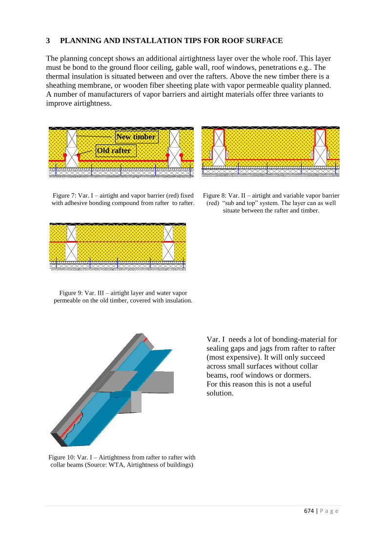
674 | P a g e

3 PLANNING AND INSTALLATION TIPS FOR ROOF SURFACE

The planning concept shows an additional airtightness layer over the whole roof. This layer

must be bond to the ground floor ceiling, gable wall, roof windows, penetrations e.g.. The

thermal insulation is situated between and over the rafters. Above the new timber there is a

sheathing membrane, or wooden fiber sheeting plate with vapor permeable quality planned.

A number of manufacturers of vapor barriers and airtight materials offer three variants to

improve airtightness.

Figure 7: Var. I – airtight and vapor barrier (red) fixed

with adhesive bonding compound from rafter to rafter.

Figure 8: Var. II – airtight and variable vapor barrier

(red) “sub and top” system. The layer can as well

situate between the rafter and timber.

Figure 9: Var. III – airtight layer and water vapor

permeable on the old timber, covered with insulation.

Var. I needs a lot of bonding-material for

sealing gaps and jags from rafter to rafter

(most expensive). It will only succeed

across small surfaces without collar

beams, roof windows or dormers.

For this reason this is not a useful

solution.

Figure 10: Var. I – Airtightness from rafter to rafter with

collar beams (Source: WTA, Airtightness of buildings)

Old rafter

New timber

675 | P a g e

Var. II solves this problem of

sealing gaps and jags. The air

barrier, installed on the bottom, runs

by the rafter to the cold site

covering the whole rafter und runs

to the warm site to the bottom. In

terms of building physics the layer

must be a variable vapor retarder.

This material becomes more

permeable if there is a hight relative

humidity around it. This

characteristic is needed on the

outside (cold side) of a construction.

The same material reacts on the

warm site (dry condition) like a

vapor retarder.

The “sub and top” system has three

disadvantages:

- The bonding to roof-Windows is

difficult

- The bonding and sealing to the

eaves is difficult, because the

rafters do penetrate the airtight

layer

- The bonding and sealing by

alteration to the inside

airtightness (fig. 12)

A retaining ledge on the bottom of

the rafter makes sure that the layer is

fixed to the rafter and there are no

gaps where warm air moves fast to

the cold site of the timber.

Experience on the construction site

has shown that there are considerable

tricky situations in applying

adhesives for this variant and that the

success of sealing systems should not

be taken for granted.

Var. II is possible with a modest roof

area with few roof windows and

dormers,

Figure 11: Var. II – Airtightness with sub-top implementation

(Source: WTA, Airtightness of buildings)

Figure 12: Gaps by alteration the airtightness with sub-top to

a system of indoor airtightness. There are a lot of air paths

(Source: WTA, Airtightness of buildings)

Figure 13: Var. III Airtightlayer above the timber

676 | P a g e

Var. III uses this opportunity: In

terms of building physics it is

possible to separate airtightness-

layer and vapor barrier. The old

construction with plaster and

wood-wool slab has the character

of the vapor retarder und the new

layer above rafter has the

character of the airtightness

layer.

Rafter heads have to be cut off in

variants II and III, and the eaves

and roof overhang have to be

constructed new.

Var. III is advantageous in all

respects. Connections and folds

are minimized.

The airtight layer must be covered

with an insulation material, so

there will be no condensation if

warm air circulation from the

inside moves to this layer.

Figure 14: Var. III (left) and Var.II (right) on site. In Var.III the rafter

space is already filled with insulation (cellulose-fiber)

Figure 16: Var.III the rafter space is quiet filled with

insulation (cellulose-fibre) and now the timber cavity will be

filled with cellulose fibre.

Figure 15: Var. III airtightlayer above the original rafters

677 | P a g e

4 PLANNING AND INSTALLATION TIPS FOR DORMER

The new dormer elements

(front, sides) also now have

an airtight layer outside in

accordance with the

airtightness concept. It is

covered with 8 cm wood

fiber insulating board.

Inside, the wall elements

have a variable vapor

retarder in the flat roof and

an OSB panel, like those

generally used in timber

frame construction as a

moderate vapor retarder in

the wall.

The flat dormer roof has a

impermeable airtight layer

outside. In terms of building

physics this construction is

free of failure, if there is a

variable vapor retarder

inside and the roof gets solar

heat in the summertime. The

surface must be grey or of

dark colour, a green roof can

not be applied.

The airtight layer must be sealed

to the threshold and then to the

concrete of the ceiling.

To realize that, it is necessary to

sweep and vacuum-clean the

ground. A primer is needed when

the surface is still draggled. If the

surface is to rough it is necessary

to smooth the surface with

plaster.

Figure 17: Horizontal section of a dormer, different kinds of vapor

barriers are necessary

Figure 18: Connection of the dormer-base to the concrete Ceiling,

different kinds of vapor barriers are necessary

678 | P a g e

5 QUALITY ASSURANCE

The success of adhesives and sealants largely depends on whether the people to use them are

informed. In advance of plans to review the targets for the maximum air permeability value

q50 must be provided to support quality assurance. After renovation, measurements can be

taken to determine success.

WTA Workgroup 6.14 (Wissenschaftlich-Technische Arbeitsgemeinschaft für Denkmal-

pflege und Bauwerkserhaltung e.V.) “Luftdichtheit im Bestand” (Airtightness of buildings)

aims to work up measurement procedures, target values for air permeability and planning tips.

These issues were studied in this project.

The existing envelope permeability is measured with a value q50 = 4,2 m³/hm².

The new airtightness specifications of the layer should go below the value q50 = 1,5 m³/hm².

Under the assumption that the air permeability with reference to the envelope's surface (q50)

of the existing structure is equally spread over the surface of the building envelope, we can

generate a new value q50 by relating the reverence q50 (1,5 m³/hm²) to the new/renovated

surface area to the surface area that has not been changed.

The new default values q50 for the whole building are calculated according to the following

equation (1):

( ) ( ) ( ) ( ) ( )

( ) ( ) ( )

After the completion of the

reconstruction we measure a n50 of

1,5 1/h just reaching the target-

setting. The high demands of

Passivhouse-Standard with a q50

of 0.6 till 0.8 m³/hm² could not be

achieved.

Here we see the limits of what can

be done in current practice and on

the other hand the need of quality

control.

Figure 19: After renovation, 2011

679 | P a g e

6 CONCLUSIONS

In the project the discussion with planners and craftsman has show us, that the success of

adhesives and sealants largely depends on whether people are well informed. The knowledge

about which material is the airtight layer and which sealants are not tight helps construction

workers a lot.

To inspire planners and craftsman it is of advantage that targets for the maximum air

permeability value q50 are provided. After the renovation work has finished, measurements

should be taken to determine successful airtightness.

7 ACKNOWLEDGEMENTS

This project has been realized in different workshops with the help of voluntary craftsmen and

planners during 2006 until 2011 where we developed good practice solutions. Many thanks to

all of you.

8 REFERENCES

WTA Guideline E-6-9 (2014). Airtightness of buildings, Part 1: General principles of

planning; WTA Publications, email: [email protected]; (available in English 2015)

WTA Guideline E-6-10 (2014). Airtightness of buildings, Part 2: Planning details; WTA

Publications, email: [email protected]; (available in English 2015)

WTA Guideline E-6-11 (2014). Airtightness of buildings, Part 3: Measuring procedure; WTA

Publications, email: [email protected]; (available in English 2015)

680 | P a g e

ACH AND AIR TIGHTNESS TEST RESULTS IN THE

CROATIAN AND HUNGARIAN BORDER REGION

Dr. László Fülöp

1, György Polics

2,

1 Faculty of Engineering and Information

Technology, University of Pécs, Hungary

[email protected]

2 Faculty of Engineering and Information

Technology, University of Pécs, Hungary

[email protected]

ABSTRACT

The article presents the results of our research, which was realized under a cooperation project between the

University of Pécs, Hungary and the University of Osijek, Croatia. The aim was to gather 50 Pa ACH, air

tightness and spontaneous ACH information of residential houses by the Croatian and Hungarian border. The

budget of the project allowed approximately 50 tests for each university; these summarized results are presented

together with correlations found between the results.

KEYWORDS

Blower Door; tracer gas, ACH; leakage; air tightness

1. INTRODUCTION

For determining ACH and air tightness of the buildings, we have used Blower Door tests,

which have two types:

Type “A” which can serve for checking the building in use, and provides ACH

information in case of 50 Pa pressure difference. In this case, the purposely made vents on the

building envelope (e.g.: chimneys, ventilation shafts, etc.) are not sealed. Concerning this case

there have been measurements conducted on both sides of the border.

Type “B” Blower Door, which provides information on the air tightness of the building,

at standard 50 Pa pressure difference. Before the test, each of the purposely installed vents on

the building envelope must be sealed. The result can be applied for qualification, according to

the air tightness limits. Currently, in Hungary air tightness testing is a requirement only for

passive house qualification, but in the future it is expected to be introduced also as part of the

standard certification procedure for all new buildings. Type “B” tests have been conducted

only on the Hungarian side of the border. This test, with a little complementation, could be

suitable for exploring air tightness faults as well,: using e.g. smoke test, thermography, air

velocity meter, etc.

Blower Door tests presented above are valid at 50 Pa pressure difference, which shall not

provide information about actual spontaneous ACH. An interesting field of research is to

examine how we can derive the spontaneous ACH number of the building from 50 Pa ACH,

which can be derived for Hungary as 4 Pa for annual average pressure difference.

681 | P a g e

Another possible testing method for measuring spontaneous ACH is using tracer gas, which

has an advantage as compared to Blower Door is that this test method does influences the test

results to the least extent. During our research we have conducted tracer gas tests as well on

the Hungarian side of the border, and we have chosen SF6 gas for this purpose.

2. TYPE “A” BLOWER DOOR TEST REUSLT

During choosing the buildings in order to gain somewhat representative results for a certain

area, we have focused only on residential houses on both sides of the border, although we

have conducted some tests for a single room, or office.

As far as the construction method of the buildings concerned, residential houses belonging to

a period of 100 years have been tested; therefore they included brick, adobe, panel-block, and

light-weight buildings.

Table 1 presents the usual ACH rates according to the recommendation of the German

Passive House Institute:

Table 1. Usual ACH rates

The summary of test results according to table 3, as presenting Croatian results and table 4.

presenting Hungarian results in a similar form. The buildings are shown in chronological

order in the table, indicating their year of reconstruction (first of all referring to the change of

windows and doors), and the 50 Pa type “A-type” Blower Door test results. In order to offer

better overview, according to figure 1, the summarized results of the 2 countries are shown by

point charts, where we have fitted trend lines on the summarized ACH results. It can be

observed that there is a significant deviation for a more than one hundred years period: at

50 Pa ACH it is changing between 1 and 20. However, evaluating the trend lines, a

consequent decrease can be observed in parallel with the increase of the age of the buildings;

this decrease met our previous assumptions, since, as time went on construction standards

became ever stricter and together with energetic requirements and more up-to-date

construction technologies together resulted in the decrease of ACH.

Fig 1. n50 ACH values in all tested houses Fig 2. n50 ACH values in refurbished houses

magnitude of n50 ACH n50 [1/h]

old building 7..

today’s new buildings HU 5..10

today’s new buildings DE 2..6

low energy consumption house 0,17..5passive house 0,17..0,6

0

2

4

6

8

10

12

14

16

18

20

1900 1920 1940 1960 1980 2000

n5

0

AC

H (1

/h

)

Year of buildings construction

Hungarian database n50 ACH results Croatian database n50 ACH results

0

2

4

6

8

10

12

14

16

18

20

1900 1910 1920 1930 1940 1950 1960 1970 1980 1990 2000

n5

0

AC

H (1

/h

)

Year of buildings construction

Refurbished buildings in Hungary Refurbished buildings in Croatia

682 | P a g e

Table 2. Croatian test results Table 3. Hungarian test results

Year of

constructionNO. Type of building

Year of

constr

uction

Year of

reconstr

uction

ACH, n50

[1/h]

Average

ACH, n50

[1/h]

1.1 Apartment house 1912 2007 7,35


1.3 House 1920 - 16,21

1.4 Terraced House 1925 2006 3,94

1.5 House 1925 - 3,16

2.1 Terraced House 1958 2011 2,51



2.4 Terraced House 1961 2007 2,12

2.5 Terraced House 1961 - 8,77

2.6 House 1962 1994 3,22

2.7 House 1962 - 10,12

2.8 House 1962 1993 9,77

2.9 Apartment house 1964 - 6,39


2.11 Terraced House 1965 1975 6,01



3.3 House 1968 2008 6,49






3.9 House 1974 1998 2,86


3.11 House 1975 2003 0,76


3.13 House 1975 1998 2,18

4.1 House 1976 2010 10,95








4.9 House 1982 2012 2,63

4.10 Terraced House 1982 2012 14,91

4.11 Terraced House 1985 1994 2,56








5.6 House 1990 2009 1,45

5.7 House 1990 - 2,37



6.2 House 1999 - 3,69

6.3 House 2000 - 1,81

6.4 House 2005 - 1,45

7.1 House 2008 - 2,82

7.2 House 2011 - 0,86

7.3 House 2011 - 3,4

7.4 House 2013 - 4,88

Be

fore

19

45

7,84

19

45

.-1

96

5.

6,31

19

66

.-1

97

5.

5,08

Fro

m 2

00

6

2,99

19

76

. -

19

85

.

5,24

19

86

.-1

99

5.

2,47

19

96

. -

20

05

.

2,48

Year of

constructionNO. Type of building

Year of

constr

uction

Year of

reconstr

uction

ACH, n50

[1/h]

Average

ACH, n50

[1/h]

1.1 House 1900 2012 7,75

1.2 Room 1900 2012 9

2.1 House 1948 2012 1,68

2.2 House 1957 1994 11,3

3.1 Office room 1975 2008 6,94

3.2 Office room 1975 2008 4,59

3.3 Office room 1975 2008 5,36

3.4 Library 1975 2008 1,68

3.5 Classroom 1975 2008 7,21

4.1 House 1979 - 11,42

4.2 Room 1979 - 6

4.3 Room 1979 - 5,5

4.4 House 1979 2010 7,23

4.5 Room 1979 2010 6,96

4.6 Room 1980 - 1

4.7 House 1984 - 6,08

4.8 Flat 1985 2008 4

5.1 House 1989 - 10

5.2 House 1991 2011 1,68

6.1 House 2000 1,68

6.2 House 2002 - 2,41

6.3 House 2003 - 5

6.4 House 2004 - 2,48

7.1 House 2006 - 6,25

7.2 House 2008 - 8,1

7.3 House 2010 - 2,89

7.4 House 2011 - 3,19

7.5 House 2011 - 8

7.6 House 2011 - 1,86

7.7 Room 2011 - 3,45

7.8 Room 2012 - 3,49

fro

m 2

00

6

4,65

be

fore

19

45

8,38

19

45

.-

19

65

.

6,49

19

66

.-1

97

5.

5,16

19

76

. -

19

85

.

6,02

19

86

.-

19

95

.

5,84

19

96

. -

20

05

.

2,89

683 | P a g e

In case of the flats where ACH is outstandingly high (over 10/h) this phenomenon is

explained by the use of open-chamber furnaces or fire places, or the existence of uncontrolled

ventilation shafts. At the same time, the too low ACH figures can be concerning, too (i.e.

under 2/h) in case the flat did not have artificial ventilation system, but they can be considered

as traditional window-ventilation buildings. According to the trend lines, as time went on the

Croatian ACH results are lower than those of measured on the Hungarian side of the border,

however, studying tables 2 and 3, it is clearly seen, that following the Bosnian war, nearly all

of the Croatian flats were renovated, unlike the ones on the other side of the border. Therefore

the interim renovation of flats can be a significant factor of influence. This uncertainty can be

eliminated by limiting the results, and presenting only the results of the flats that had been

renovated earlier, according to the results of figure 2. In the figure presented this way

deviance can still be observed, and the results still show a decreasing tendency in favour of

the Croatians. However, this statement is based on a sample of relatively small number of

flats that had been renovated on the Hungarian side of the border.

3. DETERMINING SPONTANEOUS ACH BY TYPE “A” 50 PA BLOWER DOOR

TEST

Tectitle 3.6 software provides test results together with trend line as shown in figure 3

(presenting the results of the house 7.6 in table 3.)

Averages:

Δpn [Pa] 60 55 50 45 40 35 30 25

Δp [Pa] 60,6 55,3 51 44,7 39,9 35,4 30,2 25,3

V [m3/h] 760.8 722.3 685.5 634.5 587.0 542.4 484.1 430.7

Fig 3. Extrapolating ACH values by the trend line of the test results

The software provides both the multiplying factor and the exponent of the describing equation

belonging to the trend lines created for both pressurization and depressurization, or else they

can be even derived exporting the software results (measured pressure difference and the

related air flow) by an excel program, such as seen in figure 4.

V [

m3 /h

]

p [Pa]

Exhaust

Supply

Trend line

684 | P a g e

4. figure

Next, the values of air change number typical for the building can be calculated. The following results were

yielded for the detached house tested:

- In case of overpressure (supply):

The exponent of the descriptive equation: n=0,6427

The multiplying factor of the describing equation: C=54,4943

ACH for 50 Pa pressure difference: n50=1,85 1/h

- In case of depression (exhaust):




- In case of the mean of depression (exhaust)and overpressure (supply):




The equation describing the results:

(1)

Where:

- the measured air flow by the Blower Door

C – the multiplying factor of the describing equation

Δp – pressure difference at the point of testing

n - The exponent of the descriptive equation

Following the 50 Pa type “A” Blower Door test, knowing the multiplication factor and the

exponent of the describing equation depending on the characteristics of the buildings, ACH

can be calculated of any pressure difference. A good approximation by statistic methods

achieved despite the fact that some leaks can behave quite differently in case of diverse

pressure differences. The most important factors are: turbulent or laminar flow or opening

pressure difference.

y = 49,7909x0,6684 R² = 0,9978

y = 54,4943x0,6427 R² = 0,9990

Mea

sure

d a

ir f

low

[m

3/h

]

Measued pressure difference [Pa]

hmpCV n /3

V

Exhaust

Supply

Exponent

685 | P a g e

For testing spontaneous ACH the annual natural pressure difference should be known which

is quite dependent on the weather conditions, such as actual indoor and outdoor temperature

difference or the prevailing wind force. In Hungary, the annual average pressure difference is

4 Pa, and taking it into account when using the equation (1) we could get quite accurate

results for spontaneous ACH. Regarding the initial example, substituting the data:

With 4 Pa spontaneous pressure difference, the filtration ACH is:

With 4 Pa spontaneous pressure difference, ACH value is:

Completing the data of table 3 by the 4 Pa ACH calculated for brickwork houses:

Table 4. ACH values of traditional brickwork houses

It could be important to know that the expected 4 Pa spontaneous ACH can be determined

quite precisely from the result of type “A” 50 Pa Blower Door ACH test results without

forming any functions. For this, as shown in figure 5. using the results of table 4, imaging the

measured 50 Pa and calculated 4 Pa pairs of figures, whereby a trend line is fitted indicating

the equation describing the function concerned. Using this equation, any the 4 Pa spontaneous

ACH can be determined from the relevant 50 Pa ACH result. The high standard deviation

figure, R2=0,9819 suggests that the results can be considered reliable. In order to provide

hV

Vn /136,0

2,363

8,13044

No. Year of

construction

Type of

building C n n50 n4

- - [1/h] [1/h]

1 1900 House 96,9 0,563 7,75 1,87

2 1979 House 150,4 0,569 11,42 2,71

3 1979 House 243,9 0,595 7,23 1,61

4 1980 Room 6 0,632 1,10 0,23

5 1984 House 135,9 0,59 6,08 1,37

6 1985 Flat 87,5 0,649 4,85 0,94

7 1989 House 471,7 0,596 10,00 2,22

8 2002 House 24,5 0,596 2,41 0,54

9 2003 House 192,5 0,609 5,02 1,08

10 2004 House 64,1 0,664 2,48 0,46

11 2006 House 89,1 0,566 6,25 1,49

12 2008 House 162,9 0,601 8,10 1,52

13 2010 House 75,3 0,591 2,89 0,65

14 2011 House 57,7 0,636 3,19 0,64

15 2011 House 171,7 0,689 8,28 1,45

16 2011 House 53,1 0,65 1,86 0,36

17 2012 Room 15 0,628 3,49 0,72

hmpCV n

LPa /38,130414,53 65,04

686 | P a g e

better illustration the results are also shown by a bar chart by figure 6, compared to the

calculated 4 Pa results, and the 4 Pa results calculated by the describing equation of figure 5.

It can be seen in figure 6 that 4 Pa ACH can be calculated by approximately 90% accuracy.

Figure 5. n4 ACH values as a function of n50 values

Fig 6. Comparison of test results and calculated ACH values

Spo

nta

ne

ou

s A

CH

[1

/h]

# of test site

Spontaneous ACH from the testSpontaneous ACH calculated by the correlation

687 | P a g e

4. DETERMINING SPONTANEOUS ACH BY TRACER GAS:

For carrying out the tests, we used an INNOVA 1412i Photoacoustic Gas Monitor sold by

LumaSense Technologies. The gas chosen for the tests is Sulphur-hexafluorid (SF6). A

specific characteristic of the test is that it is hard to apply for measuring the ACH of multi-

space buildings due to the lack of appropriate mixture of air, however, it is perfectly suitable

for measuring the spontaneous ACH of only one space. SF6 gas is approximately 5 times

heavier than air, therefore during the test the appropriate mixture of the gas inserted should be

provided by a fan. The test cycles as a function of time and their evaluation is presented in

figure 7.

Fig 7. Procedure of tracer gas test

The evaluable period of the change of gas concentration is seen by the enlarged figure 8.

Fig 8. Concentration decay test method

Test time [s]

Mea

sure

d c

once

ntr

atio

n [

ppm

]

688 | P a g e

The spontaneous ACH can be calculated if concentration decline is divided by the time

elapsed:

(2)

Where:

Cr1: is the concentration at the beginning of the phase suitable for evaluation

Cr2: a is the concentration at the end of the phase suitable for evaluation

Δτ: is the time elapsed in between

5. CORELATION BETWEEN BLOWER DOOR TYPE “A” 50 PA AND BLOWER

DOOR TYPE “B” 50 PA

Blower Door Tests of both type “A” and “B” have been completed only in Hungary. The

summarized results concerned are included in table 5 and figure 9.

Table 5. Comparison of A-type and B-type test results

no Year of

Construction

Type of

building

A-type Blower

Door n50 ACH

[1/h]

B-type Blower

Door n50 Air

tightness [1/h]

1 1900 room 9,28 9,28

2 1979 house 11,42 10,11

3 1979 room 5,5 5,5

4 1979 room 6 6

5 1979 room 6,96 6,96

6 1980 room 1,1 1,1

7 1984 house 6,08 5,31

8 1984 flat 8,91 7,14

9 1989 house 10 10

10 2002 house 2,41 1,45

11 2004 house 2,48 2,4

12 2006 house 6,25 5,25

13 2008 house 8,1 6,92

14 2011 house 3,19 2,75

15 2011 house 1,86 1,38

16 2011 room 3,45 3,45

17 2012 room 3,49 3,49

Evaluating the results of the above table, it can be seen that if air tightness or ACH measures

were completed only for one room, generally the results show no differences. The reason for

this lies in the fact that in case of traditional window-ventilation spaces usually there are not

further artificial leaks on the envelope of the building which should be sealed according to the

requirements of air-tightness tests, and which would show changes in the results. This occurs

in every such a case even in case of complete house test where there no artificial leaks on the

building envelope that should be sealed. Limiting the data of table 5 focusing only the figures

which show differences between type “A” and “B” test results, we have presented these pair

r1 r2ln(C ) ln(C ) 1n

h

689 | P a g e

of data in a graph in figure 10 where, by means of curve fitting, we have determined the

equation describing the trend line. Since the deviation R2=0.9893 is high, the equation can be

considered reliable, thus, we have found a quasi correlation between the “A” and “B” ACH

tests at 50 Pa. However, it is important to point out that there are several factors which can

influence the outcome of the results e.g. the shape and size of the leak can result in significant

differences as compared to their determined equation.

Fig 9. Comparison of A-type and B-type test results

Fig 10. Comparison of A-type (ACH) and B-type (air tightness) test results

6. CONCLUSION

Results of air tightness and ACH tests in Hungary and in Croatia presented. The project was

supported by the EU IPA cooperation project. Correlations found between the spontaneous

ACH and Blower Door type “A” 50 Pa ACH results.

Correlations found between the results Blower Door type “A” 50 Pa and Blower Door type

“B” 50 Pa tests. The research and results presented could be helpful for conducting

measurements and evaluating their results.

Furthermore the tracer gas concentration decay test method is presented which is most

suitable to determine spontaneous ACH. This method does not influence the tested

n5

0 (

1/h

)

Year of construction

n50 ACH results n50 Air Tightness results

y = 0,8795x - 0,2089 R² = 0,9893

Air

tig

htn

ess

n5

0 [

1/h

]

ACH n50 [1/h]

690 | P a g e

parameters. However it cannot be applied to measure complex spaces simultaneously and it is

especially sensitive to the changes of the external conditions.

7. REFERENCES

Fülöp, László, et al: Air tighness tests of buildings from the point of view of energy and

comfort, IPA HUHR/1001/2.1.3/0009 project summary, Pécs, HU, 2013.

Polics, György PTE-PMMIK ÉG Tanszék, Summary and comparison of test results. IPA

HUHR/1001/2.1.3/0009 project closing conference. Pécs, HU 27-28 June 2013

Luftdichte Projektierung von Passivhausen, CEPHEUS, Passivhaus Institut, 2002.

691 | P a g e

MEASURED MOISTURE BUFFERING AND LATENT

HEAT CAPACITIES IN CLT TEST HOUSES Ivana Katavic

1, Kristine Nore

*2, and Tormod Aurlien

1

1 Department of Mathematical Sciences and

Technology, Norwegian University of Life Sciences

Universitetstunet 3

1430 Ås, Norway

2 Norwegian Institute of Wood Technology

Forskningsveien 3B

0373 Oslo, Norway

*[email protected]

ABSTRACT

This research investigates the significance of the moisture buffering and latent heat capacities in exposed cross-

laminated timber (CLT) walls with the respect to indoor climate and energy consumption. Hygroscopic materials

have the ability to accumulate and release moisture due to change in the surrounding humidity. The moisture

buffer capacity is regarded as this ability to moderate, or buffer, the indoor humidity variations. Latent heat

refers to the heat of sorption due to the phase change from vapour to bound water in the material and the other

way around. The indoor relative humidity (RH) is closely related to indoor comfort, more specifically to thermal

and respiratory comfort and perceived air quality. Both persistently low RH (<20 %) and high RH (>75 %) can

cause health threats for humans such as respiratory infections or the growth of mould. Wood is naturally

hygroscopic, which enables it to act passive and efficient to stabilize the indoor humidity and thus, temperature

variations. A better understanding and more deliberate implementation of these properties could potentially

reduce the need for ventilation and heating without compromising the indoor comfort. A full-scale experimental

study compares the responses of two 25 m2 test houses to an applied moisture load. The test houses are identical

constructions made of CLT elements, where the exposed spruce interior in module A is kept as is, while the

interior in module B is covered with PE foil emulating an impermeable surface. The moisture load is applied as

continuous flow of mist under several various conditions, including different magnitudes of the load and altered

air change rates of the ventilation fan. The responses are measured in terms of RH, moisture content in the wood,

changes in surface and air temperature and the time needed for the system to restore itself to the initial state. The

software WUFI®Plus is utilized to perform a hygrothermal building performance simulation for comparison and

evaluation. Both the experimental and calculated results show that exposed wood is an efficient moisture buffer

capable of reducing daily fluctuations in RH. The results also show a rise in surface temperature, which is a

contribution from the latent heat of sorption.

KEYWORDS

Moisture buffer capacity, latent heat, indoor climate, energy, buildings, exposed wood surface, Cross Laminated

Timber, (CLT)

1 INTRODUCTION

In the last decades a global “green awakening” has led to new standards and requirements

concerning environmental awareness and sustainable development. According to the

International Energy Agency (IEA), commercial and residential buildings represent 32 % of

the worlds total final energy consumption (IEA 2014). In reducing this figure, the potential is

mainly related to reducing the need for heating and cooling. The public and legislative

demands for energy efficient building design have led to increased air tightness and insulation

in modern dwellings. In these modern buildings, the ventilation accounts for a large amount

692 | P a g e

of the heat loss through air renewal. One solution to keep the energy consumption down

whilst providing a comfortable and healthy indoor climate is the use of passive design

strategies. In its simplest form, passive methods include considerations such as shape and

orientation of buildings to reduce the ventilation, cooling and/or heating demands. Thermal

inertia associated with heavy walls is another type of passive design that is actively

implemented. Thermal mass design takes advantage of the heat capacity, which enables heavy

buildings to heat up and cool down up to three times slower compared to light buildings

(Karlsson 2012). Well-controlled HVAC systems or ventilation that is RH or CO2 sensitive

are other options.

Studies on the moisture buffer capacity of hygroscopic materials have shown that these

materials have a great ability in terms of moderating the indoor RH levels (Rode & Grau

2008). Moisture buffering is described as the ability of porous materials to buffer changes in

the RH by absorbing and desorbing water vapour from the surrounding air. Indoor humidity

varies significantly through the day and seasons. Materials that can store and release moisture

can reduce the extreme values of these fluctuating humidity levels. This results in improved

thermal comfort while keeping the energy consumption low.

Another phenomena closely connected to the moisture buffer capacity, is the latent heat of

sorption. In the process of moisture exchange between the hygroscopic material and

surrounding air, the humidity undergoes a phase change. The energy associated with this

phase change from vapor state in air to liquid water in hygroscopic pores, or vice versa, is the

latent heat of sorption. (Osanyintola. & Simonson, 2006).

This paper aims to measure the significance of the moisture buffering capacity and latent heat

of sorption of exposed spruce CLT in full-scale experimental facilities. The experimental

facilities include two test houses: one with exposed spruce interior surface; and one control

house with impermeable surface where moisture buffering and latent heat are limited. The

responses of the test houses are compared to one another, as well as to results from a

computer performed hygrothermal whole building performance simulation using WUFI®Plus

(2007) in order to evaluate these models.

2 BACKGROUND

2.1 Indoor climate

The main purpose of air ventilation is to ensure adequate indoor air quality (IAQ) for users

with regard to health and comfort (TEK10, 2010), and to keep the indoor humidity at correct

levels to maintain the building structure and envelope. The indoor RH is affected by different

factors, such as internal moisture sources (human activity and respiration, household

appliances and equipment), airflow, leakages and external air moisture content. There is also a

significant seasonal impact on the RH, more dependent on outdoor temperature than outdoor

humidity. Heated homes are usually dry because the infiltrating cold winter air contains little

water vapour. RH reaches its lowest levels during the coldest days. During hot summer days,

the outdoor air contains plenty of vapour even if the RH is lower than in winter. But because

of high vapour pressure outdoor, vapour generated inside hardly migrates out. (Kubler 1982)

Daily indoor moisture loads due to normal life activities leads to fluctuations and peaks in

RH, which easily reaches 80-100 % in airtight spaces, like bathrooms. The moisture

production in residences differs among people depending on habits and behaviour. The total

moisture generation (sum of respiration and transpiration) of an adult at rest is in the range of

693 | P a g e

0.8-1.7 kg/day, while the total water vapour production (including daily chores, plants, pets

etc.) for a family of five is in the range of 6.6-10.2 kg/day (TenWolde & Pilon 2007).

Keeping the RH at correct levels is vital for both the durability of the building materials and

the indoor climate comfort. Surveys show that humans feel most comfortable at certain

temperatures and humidities (ANSI/ASHRAE; ISO). The RH is important for skin humidity

(Toftum et al. 1998a), respiratory comfort (Toftum et al. 1998b) and perceived IAQ. High RH

can be associated with moisture problems in the building envelope, such as mould growth, as

well as human health problems, including asthma and allergies. Arlian (Arlian et al. 1999)

suggests maintaining mean daily RH below 50 % to effectively restrict population growth of

house dust mites.

In a wide variety of commercial buildings the right levels of RH can be of even higher

importance. Swimming halls and laundry facilities often have excess humidity, while offices

and production facilities with heavy machines tend to be perceived as too dry. Museum and

gallery artefacts require specific and steady humidity and temperature levels to minimize

deterioration (Janssen & Christensen 2013).

2.2 Energy efficient design strategies

By 2020, the EU Energy Performance of Buildings Directive (2010/31/EU) aims for a 20 %

reduction in European primary energy consumption and Nearly Zero-Energy Building norm

for all new buildings. Mandatory energy performance certificates are already implemented in

commercial property development, and recent studies show that better energy efficiency is

rewarded in the market.

The energy consumption in dwellings can be divided into three main categories: electricity for

lightning and equipment, room heating/cooling and water heating. In Norwegian households,

an estimated 60 % of the consumed energy is used on room heating alone. (Edvardsen et al.

2006) In more southern climates, the cooling and air conditioning in the hot season is the

main energy drain. Energy efficient development means utilizing plan strategies where the

total purchased energy need for a building is kept at a minimum.

Sustainable development requires that the choice of materials for building take into account

the environmental impact of the materials being used, the energy consumption of building and

the indoor environment. Manufacture, use and disposal of wood is associated with low energy

cost and low emissions. Furthermore, wood used as indoor surface material enables its

hygrothermal inertia to act as a passive system regulating the temperature and moisture

fluctuations. Hameury and Lundström (2003) describe an experimental study performed in

four occupied apartments in Sweden with large areas of exposed massive wood surfaces. The

results show evidence of the wood contributing to buffer the indoor temperature.

A Canadian study estimated that applying hygroscopic materials in combination with RH and

user presence control of HVAC systems reduces the heating energy consumption with 2-3 %

and the cooling energy consumption with 5-30 % in moderate climates. (Osanyintola &

Simonson 2006).

Compared with other materials, the heat conductivity of wood is low, especially perpendicular

to the fiber axis. This makes (dry) wood a good insulator, but also poses as a limitation for

heat storage purposes. Nevertheless, because wood is excellent at holding water, this captured

moisture increases its basic heat storage capacity. This gives wood a beneficial compromise

between insulation and heat storage. Since the thermal and hygroscopic behaviors of building

694 | P a g e

physics are closely related, the wood moisture content also affects the thermal fluctuations

through the material. A high moisture content enhances the heat flux.

2.3 Hygroscopic potential

The total moisture buffer capacity depends on the moisture buffer capacities of each material

and furniture in the room together with the moisture production, air change rate and the ratio

between the material surface area and the air volume. The materials active thickness, vapor

permeability and moisture storage capacity, as well as the thickness of the boundary air layer

are factors that determine the moisture buffering.

Moisture content in wood is expressed as a percentage of dry wood mass. Most hygroscopic

properties in wood, including the wood surface – ambient air moisture exchange, are related

to the hygroscopic moisture range where minimal capillary forces occur (Wood moisture

content <30 %). The hygroscopic water is bound to the wood cells via hydrogen bonds, and

its amount is limited by the number of sorption sites available and how many water molecules

each site can hold. More energy is needed to release bound, as opposed to free, capillary

water. As the bound-water content increases, the physical properties of the wood are altered:

swelling, decrease in the mechanical strength, increase in thermal and electrical conductivity

and higher rate of bound water diffusion (Siau, 1984).

In a hygrothermal simulation, Korsnes (2012) attempted to identify the magnitude of the

latent heat exchange in a small bathroom under normal conditions. The comparison of case 1

with wood panels on the walls and ceiling to case 2 with solely impermeable surfaces shows

huge advantages to the former. Not only are the values of RH lower and more stable, but there

is also an increase in indoor air temperature of 2.5 °C due to the latent heat. In a follow-up

laboratory test conducted to verify the hygrothermal simulation, Nore (2014) subjected wood

samples in a climate chamber to rapid increase in RH (from 20 % to 90 % RH).

Thermography was used to measure the surface temperature change. In a few minutes, the

exposed wood sample reached its maximum surface temperature nearly 2 °C higher than the

reference sample covered in low-emitting PE-foil.

The latent heat is naturally user controlled in the sense that a space has to be occupied or

employed, with a following moisture load, in order to be released. This has potential as local

heating in spaces when it is actually needed. For instance, both kitchens, bathrooms and

laundry rooms, are only occasionally used during the day. If the operating temperature of a

room can be raised with 2 ºC upon being occupied, the set temperature can be lowered

accordingly when the room is not in use.

The latent heat of desorption may also be of practical use in building design. Desorption is the

opposite process of sorption; here excess moisture in the wood is dried out by energy

contribution from the ambient air. This may be applied to buildings which need cooling

during the day in hot seasons. By airing the building during the night when the temperature is

lower and humidity higher, humidity can accumulate in the indoor surfaces. During day time,

this moisture will require heat from the indoor air to vaporize thus lowering the indoor

temperature. A known problem to cabin owners in Norway, is the time it takes to heat the

wood cabin during winter times; lot of energy is needed to firstly dry out the walls before the

indoor temperature rises.

695 | P a g e

3 METHODOLOGY

This paper assesses the issues of moisture buffering and latent heat of sorption of CLT in two

different ways; measurements under controlled conditions in experimental field facilities; and

hygrothermal whole building performance simulation with WUFI®Plus. The test houses have

been exposed to large moisture loads, 616 g/h and 1232 g/h over a 9 h 25 min. period, in an

attempt to aggravate a response with as high RH as possible. The studied scenarios are

presented in Table 1. Case I and II are conducted in multiple runs. Case III is only performed

in module A, meaning the permeable hygroscopic module. The initial conditions differ in

each case, and are here only approximately presented. Table 1: Presentation of test cases and initial conditions

3.1 Field experiment

The field facilities consists of two

identical test houses, module A and

module B (see Figure 1) situated in a

meteorological field, Søråsfeltet,

affiliated to the Norwegian University

of Life Sciences (NMBU) in Ås,

Norway. The test houses are constructed

of CLT made of spruce. The walls are

made up 100 mm CLT and externally

insulated with 100 mm mineral wool in

the south and east directions, and 150

mm mineral wool in the west and north

directions. There is a layer of weather

resistive barrier between the CLT and

insulation, and on the exterior side of

the insulation, which can be seen in Figure 1. This barrier is vapour diffusion-open. The

ceiling and roof consist of 140 mm CLT and 250 mm mineral wool insulation with a wind

barrier in-between, and sheet metal roofing on top. The floor has 14 mm oak parquet over 22

mm chipboard and 100 mm mineral wool insulation. The modules are placed on top of 200

mm Rockwool with vapour barrier inhibiting any moisture to penetrate from the ground. The

internal dimensions of the modules are 7,.0 x 3,.6 metres and 2,.2 metres height from floor to

ceiling. Table 2 shows the exact materials of the wall assembly.

The test houses do not fulfil the requirements demanded by the Norwegian Building

Regulations (TEK 10) in terms of insulation, and are thus not comparable within these

standards. Blower door tests ran in module A have shown that the air infiltration n is 1.63 and

meets the national guideline requirements for residential houses with n < 2.5 (Olaussen 2014).

In module A the spruce walls and ceiling are kept exposed and untreated, in direct contact

with the indoor climate. In module B the spruce surface has been upholstered with PE-foil to

Moisture load Initial conditions Experimental Simulated

Case Diffusion

rate [g/h]

Total

load [kg]

Operative

temperature [°C]

Indoor

RH [%]

WME

[%]

ACH

[h-1

]

A B A B

I 616 5.8 20.2 23-24 7.4 0.5

x x x x

II 616 5.8 20.1-20.5 32-37 7.4 0.3

x x x x

III 1232 11.6 20.2-20.5 31 7.4 0.5

x x x

696 | P a g e

make the ceiling and walls impermeable and limit the effects of moisture buffering and latent

heat (Figure 2).

The instrumentation inside the modules includes heat and ventilation flow control;

registration of temperature and RH of air into and out the modules; wood moisture content

sensors; and energy meter. The instrumentation system is limited to 9 nine parameters in each

test house. An additional 5 five freestanding moisture sensors are mounted on small timber

blocks of spruce and placed in the test houses, 3 three

in module A and 2 two in module B. Each of these

sensors monitors the RH, ambient air

temperature and wood moisture content.

The 3rd sensor in module A is mounted

directly on the CLT element of the south

wall. Table 3 displays all the

measured parameters and Figure 4 depicts

the floor plan.

The indoor air temperature was held at

20°C using an electric heater with

temperature control. The extract

ventilation system supplies constant air

change, controlled by differential

pressure sensors. The ventilation is pre-

set to n = 0.5 h-1 for both modules, in

accordance with Norwegian building

regulations (TEK 10), but later adjusted

in Case 2. The moisture loads were

introduced by ultrasonic evaporative

humidifiers, each with a total capacity of

5.8 litres and diffusion rate 616 g/h. To Figure 2: Interior view of module B where the walls

and ceiling are upholstered in PE foil

prevent the humidity of being extracted straight out through the ventilation canal, a small

table fan was placed on the floor to stir up the air and distribute the moist more evenly in the

space. This fan was directed towards the floor to avoid disturbing the laminar boundary layer.

Table 3: Measured parameters. The placement

of the sensors is shown in Figure 3.

Table 2: Wall assembly

697 | P a g e

Figure 3: The ground plan of the modules and a schematic figuration of the instrumentation placement.

(Figure 3) Some assumptions have

been made regarding the

experimental setup: the moisture load

is applied with steady flow. The

diffusion rate was measured in a

laboratory and divided on the water

container capacity to get the moisture

load duration.

3.2 Simulation set-up

In the simulation part of this study, the hygrothermal building simulation software

WUFI®Plus (2007) is used. This software is developed by Fraunhofer Institute IBP, and has

been validated through experimental studies. The simulation cases are based on and designed

after the real life test houses from the experimental study. The outdoor boundary conditions

are the recorded weather data provided from the meteorological station in which the test

houses are situated. The indoor initial conditions, including operating temperature, RH and

wood moisture content, are set equal to the measured initial conditions from the equivalent

experimental case.


The results are presented in Figures 4-6, with the permeable cases on the left and the

impermeable on the right. The experimental data is depicted with full line and the calculated

results with a dotted. A summary of the complete results is presented in Table 34. The values

698 | P a g e

are recorded with 1 minute intervals. A moving average data treatment of 10 steps have been

applied to smoothen the all the curves. The exception is the temperature measurements from

module B which have been treated with a 30 step moving average smoothing. The reason

being an unsteady meter controller in this module making the recorded data flutter.

The RH curve starts rising as soon as the moisture is applied. The RH in the impermeable

cases reaches 100 % in a short amount of time. The curves are steep, both increasing and

decreasing. Under the permeable conditions, the RH has a lower interval, a gentler slope and

delayed peak. In case 1, which is the first case conducted in the wood active module A, the

initial RH is the same in both modules due to the fact that they both where dried out a long

time ahead. In following experiments the initial RH differs with about 5 % percentage points

less in the impermeable module, demonstrating clearly the hygroscopic inertia of wood. In

Figure 4b the PE covered module B doesn’t seem to reach 100 % RH, which has to do with

the built-in hygrostat in the humidifier kicking in. In case 4, which has the same setup, but

with the built-in hygrostat being disconnected, this curve looks like the B module RH curve in

Figure 5b. The peak in RH in the permeable module is in all cases at the max (end point) of

the moisture load. The wood moisture content also reaches its highest value when RH is max.

The surface temperature curves follow the same path as the curves for wood moisture content,

showing the effect of latent heat of sorption. After case 3 (last case) is conducted and the

module is left closed, the wood moisture content reaches its initial state of 7.4 % 60 hours

after the moisture load is fully applied.

There is a drop in temperature at the start of every case which is caused by the entrance door

opening and shutting while launching the experiment. Temperature prior to this decrease is

considered as the initial temperature, thus the increase in temperature due to the latent heat of

sorption is quite conservatively estimated.

699 | P a g e

Figure 4-6, a-d: Results from case 1-3 from top to bottom. The wood active module A is

depicted on the left side and the PE-covered module B on the right side.

700 | P a g e

Table 4: Summary of the test results

The summarized Table 4 shows the initial/max temperatures from the ceiling surface sensor

in the experimental tests. This curve was representative in all the cases, not being extreme

either ways, as well as being given by WUFI. The temperatures from the different

measurement points differ with at least 1 ºC within each case. There are certainly some

temperature differences from point to point due to air circulation and humidity not being

distributed evenly. The latent heat effect from the south (See attachment)wall is higher in

every case, compared to the other surfaces. It is reasonable to assume that the south walls are

more dried out than the other surfaces by solar radiation, as well as being less insulated than

the north wall. The increases in temperature due to latent heat lies around 0.5-1º C, not taking

into account the temperature drop at the start. Nevertheless, there are clear trends regarding

the permeable vs. impermeable cases when it comes to temperature rise.

Concerning the simulated cases; the accordance is quite accurate between the experimental

and calculated impermeable cases. In the impermablepermeable cases however, there is more

discrepancy. The max RH is too high in the simulations, and the RH decline to gentle

compared to the measured cases. This problem might be linked to the values for the heat and

moisture transfer coefficients used by the simulation program. Furthermore, the thickness of

the CLT might cause the permeability to become too complex a process. The surfaces

temperature curves returned from WUFI®Plus (mean surface and mean ceiling temperatures)

do look more cohesive than the experimental results, as can be expected from an ideal

computer simulation.

When RH is the primary factor for ventilation, energy savings can be made by reducing the

air exchange rate. In situations where humidifying/dehumidifying is necessary, exposed wood

can help stabilize the environment and decrease this need. Another option for energy profit

includes applying moisture buffering to cooling strategies; moistened exposed wooden

surfaces absorb heat from the ambient air during hot days.

5 CONCLUSIONS

The results from this paper show that the buffering effect from large areas of exposed wood

surfaces helps keep the RH within a closer interval, with slower alteration upon moisture load

being applied/removed compared to impermeable surfaces. The latent heat exchange gives

rise to the indoor temperature. There is a significant potential regarding exposed wood and

# Setup DateVentillation

rate [h-1

]

Diffusion

rate [g/h]

Duration

[t]

Total

load

[litres]

1 I 31.3. 0.54 616 09:25 5.8

initial

max

variance

23.9

75.4

+51.5

20.2

20.9

+0.7

7.4

8.6

+1.6

23.1

98.1

+75

20.2

20.2

0

23.9

70.4

+46.

20.2

21

+0.8

23.1

100

+76.9

20.2

20.2

0

2 II 11.4. 0.32/0.31 616 09:25 5.8

initial

max

variance

37.3

83.8

+46.5

20.1

21

+0.9

7.4

9.2

+1.8

32.4

100

+67.6

20.5

20.2

-0.3

37.3

73.8

+36.

20.1

20.8

+0.7

32.4

100

+67.6

20.5

20.5

0

3 III 15.4. 0.54 1232 09:25 11.6

initial

max

variance

30.8

97.1

+66.3

20.3

21.2

+0.9

7.4

12

+4.6

30.8

82.3

+51.

20.3

21.6

+1.3

30.8

100

+69.2

20.3

20.3

0

4 I 9.4. 0.53 616 09:25 5.8

initial

max

variance

34

74

+40

20.2

20.4

+0.2

7.4

8.8

1.4

27.1

100

+72.9

20.5

20.5

0

34

72.4

+38.

20.2

20.3

+0.9

27.1

100

+72.9

20.5

20.5

0

RH Temp. WMC RH Temp. RH Temp RH Temp

Simulation test

Permeable Impermeable

Moisture loadCase

Permeable Impermeable

Experimental test

701 | P a g e

indoor climate, especially in combination with a well-controlled HVAC system. For this to

become practically applicable there is however still need for research and engineering.

6 ACKNOWLEDGEMENTS

This study was conducted within the research project Wood – Energy, Emission, Experience

(WEEE). All participants are gratefully acknowledged. A thank to Florian Antretter and

Fraunhofer IBP for great assistance. The financial assistance from Innovation Norway is

greatly appreciated.

7 REFERENCES

ANSI/ASHRAE. Standard 55 - Thermal environmental conditions for human occupancy.

Arlian, L. G., Neal, J. S. & Vyszenski-Moher, D. L. (1999). Reducing relative humidity to

control the house dust mite Dermatophagoides farinae. Journal of Allergy and Clinical

Immunology, 104 (4): 852-856.

Edvardsen, K. I., Haug, T. & Ramstad, T. Ø. (2006). Trehus. 9. utg. ed. Håndbok / [Norges

byggforskningsinstitutt]. Oslo: Norges byggforskningsinstitutt. 333 s. pp.

Geving, S. & Thue, J. V. (2002). Fukt i bygninger. Håndbok (Norges byggforskningsinstitutt :

trykt utg.). Oslo: Norges byggforskningsinstitutt.

Hameury, S. and Lundström (2003) Contribution of indoor exposed massive wood to a good

indoor climate: in situ measurement campaign. Energy and Buildings, 36 (3): 281-292.

International Energy Agency. (2014). IEA. 2014 [ONLINE] Available at: http://eur-

lex.europa.eu/ LexUriServ/LexUriServ.do?uri=OJ:L:2010:153:0013:0035:EN:PDF.

[Accessed 2014].

ISO. 7730:2005 (en) Ergonomics of the thermal environment - Analytical determination and

interpretation of thermal comfort using calculation of the PMV and PPD indices and local

thermal comfort criteria.

Janssen, H. & Christensen, J. E. (2013). Hygrothermal optimisation of museum storage

spaces. Energy and Buildings, 56 (0): 169-178.

Karlsson, Jonathan (2012) Possibilities of using thermal mass in buildings to save energy, cut

power consumption peaks and increase the thermal comfort. Licentiate thesis, Lund Institute

of Technology, Division of Building Materials, Lund, Sweden

Korsnes, S. & Nore, K. (2012). Moisture buffering and the influence of exposed wooden

surfaces on the indoor environment. Master thesis, Department of Civil and Transport

Engineering, Norwegian University of Science and Technology, Trondheim, Norway

Kubler, Hans (1982) Effect of wood on humidities in homes. Forest Products Journal, Vol 32,

No 6: 47-50.

Nore, K. Englund F, Aurlien, T. and Nyrud, A.Q. (2014) Wood construction: Energy,

Emissions and Experience. In: 10th Nordic symposium of building physics. Lund, Sweden

June, 2014.

Osanyintola, O. F. & Simonson, C. J. (2006). Moisture buffering capacity of hygroscopic

building materials: Experimental facilities and energy impact. Energy and Buildings, 38 (10):

1270-1282.

Rode, C. & Grau, K. (2008). Moisture buffering and its consequence in whole building

hygrothermal modeling. Journal of Building Physics, 31 (4): 333-360.

TEK 10, (2010). Norwegian building regulations.

TenWolde, A. & Pilon L. C. (2007) The effect of indoor humiduty on water vapor release in

homes. Proceedings of Thermal Performance of the Exterior Envelopes of Whole Buildings

X, Atlanta, USA

Thue-Hansen V. and Grimenes A.A. Meteorological data for Ås, Norwegian University of

Life Sciences, 2014, Ås, Norway

702 | P a g e

Olaussen, P. A. (2014) Master Thesis (In progress), Department of Mathematical Sciences

and Technology, Norwegian University of Life Sciences, Ås, Norway

Toftum, J., Jorgensen, A. S. & Fanger, P. O. (1998a). Upper limits for indoor air humidity to

avoid uncomfortably humid skin. Energy and Buildings, 28 (1): 1-13.

Toftum, J., Jorgensen, A. S. & Fanger, P. O. (1998b). Upper limits of air humidity for

preventing warm respiratory discomfort. Energy and Buildings, 28 (1): 15-23.

WUFI®Plus (2007) Fraunhofer Institut für Bauphysik, Holzkrichen, Germany.

703 | P a g e

BREATHING FEATURES ASSESSMENT OF POROUS

WALL UNUITS IN RELATION TO INDOOR AIR

QUALITY

Başak Yüncü

*1, Ayşe Tavukçuoğlu

2 and Emine N. Caner-Saltık

3

1 Middle East Technical University

Department of Architecture

Graduate Program in Building Science

Dumlupinar Bulvari, No:1

Ankara, Turkey


2,3 Middle East Technical University

Department of Architecture

Materials Conservation Laboratory

Dumlupinar Bulvari, No:1

Ankara, Turkey

ABSTRACT

Traditional building technologies establishing highly-breathing multi-layered wall systems provide healthy

indoor environment and energy efficiency in buildings due to the use of lightweight, porous, water vapour

permeable and thermal resistive building materials. The breathing performance of traditional buildings and

materials that contribute to the healthy indoor conditions and air quality are needed to be investigated in detail.

That knowledge on breathing performance has also vital importance for the improvement of the contemporary

building and materials technologies.

The study was conducted on three kinds of porous masonry units: mud brick, collected from the sound parts of

the traditional houses of Hamzalı Village, Kırıkkale (Turkey) and autoclaved aerated concrete (AAC) type G2

and type G4, the commonly used lightweight concrete material which are also produced in Kırıkkale. These

three groups of materials were examined in terms of their air exchange properties by means of laboratory

analyses. Some supportive laboratory analyses were also done on material characterization of the samples. The

experimental setup is developed for the analyses of the samples, particularly for the assessment of air flow

through the material by using CO2 as tracer gas.

The interpretation of the results were done in order to compare the porous building materials in terms of their

effects on indoor air quality. The double-zone experimental setup based on concentration decay procedure was

found to be useful to better-understand the air exchange features of a material in terms of rates of concentration

decrease and increase in neighbouring zones by monitoring the concentration of outgoing air. The data achieved

is expected to improve the contemporary building walls by benefitting from the self-ventilation capability of

building materials and to provide healthier indoor conditions for the occupants. The results are also useful to

discuss the airtightness aspect of passive house technology and to minimize the mechanical ventilation needs for

fresh air intake by benefitting from the self-ventilation performance of air permeable skin.

KEYWORDS

Indoor air quality, breathing walls, mud brick, autoclaved aerated concrete, air exchange properties.

1. INTRODUCTION

Traditional building technology provides energy efficiency and good indoor air quality in

houses by using porous, water vapour permeable building materials establishing highly-

breathing multi-layered wall systems (Meriç et al., 2013; in press). Each layer of a mud brick

traditional wall section has particular performances, such as water impermeable exterior

finishing layers and thermal resistive intermediate layers while each layer allows continuous

passage of water vapour along the overall wall section. The breathing performance of

704 | P a g e

traditional buildings that contribute to the healthy indoor conditions and air quality needs to

be investigated in detail. That knowledge is essential for the improvement of the

contemporary building materials and construction technologies. Due to the high porous and

breathing characteristics of autoclaved aerated concrete (AAC), it appears to be an alternative

material to establish contemporary breathing walls. The potentials and restrictions of AAC,

therefore, need to be examined in terms of its breathing properties. In this regard, the

experimental study was shaped to discover the air exchange characteristics of traditional mud

brick and AAC unit samples. Supportive laboratory analyses were done to define the raw

material characteristics of traditional mud brick.

The concept of airtightness is mostly defined as absence of air leakage and excluded from the

issues of ventilation in buildings (Fennell and Haehnel, 2005). Some others focus on

minimum airtightness levels required for energy saving and support that the higher

airtightness levels the lower energy costs (Katunsky et al,.2013). The studies that support

maximum airtightness propose controlled mechanical ventilation systems. The operating and

maintenance expenses of mechanical ventilation systems as well as the risk of health

problems associated with the mechanical ventilation systems, such as Legionnaire’s disease,

are some of main reasons of why natural self-ventilation properties of building materials have

vital importance on the healthy indoor conditions and air quality (US EPA, 1991; Hodgson,

1992). On the other hand, most studies point out that indoor air quality would suffer in case of

over-airtightness (Sherman and Chan, 2004; Kirch, 2008a; Kirch, 2008b). The inherent

breathing features of building components can provide self-ventilation at a certain level while

minimizing the energy cost for mechanical heating, ventilation, and air conditioning (HVAC)

systems. The breathing features of porous building materials and their contribution to the

indoor air quality, therefore, are the key concerns of this study.

2. MATERIAL AND METHOD

The study was conducted on mainly mud brick and AAC samples, both of which were porous

masonry units and well-known with their good breathing capability (Andolsun, 2006;

Andolsun et al., 2006; Jacobs et al., 1992; Kömürcüoğlu, 1962; Meric et al. 2013; Meric et al.

in press; Naranyan et al., 2000, Torraca, 2009): The mud brick units were collected from the

sound parts of the traditional houses of Hamzalı Village, Kırıkkale (Turkey), together with

mud mortar and mud plaster samples complementing the mud brick wall section. Those

houses are about 70 year old. The AAC units are manufactured in Kırıkkale (Turkey). The

commonly-used types of AAC blocks, type G2 (infill unit) and type G4 (load-bearing unit),

were selected for the study. The breathing features of these materials were examined with an

emphasis on their air exchange rate. Supportive analyses were also done on some basic

physical and physicomechanical characteristics of mud brick and AAC samples, such as

density (, g.cm-3

), effective porosity (, % by volume), ultrasonic pulse velocity (UPV, m.s-

1) and modulus of elasticity (MoE, GPa) as well as on some raw materials characteristics of

original mud brick samples, such as silt & clay ratio, binder-aggregate ratio and fibre ratio.

The air exchange properties of each sample were determined by measuring the air flow

through the material by using CO2 as tracer gas and an experimental setup was developed for

this purpose by adapting the concentration decay method defined in the international standard

ASTM E 741-11 (2011). This method was assumed to represent the case for an indoor having

a very high carbon dioxide concentration level (after it has been occupied) and ventilating

itself only by the porous wall section. The experimental setup developed for the determination

of air change rate was composed of mud brick or AAC block samples positioned in between

two chambers/zones (Figure 1). Each block sample with the sizes of 180mm x 125mm x

705 | P a g e

310mm (thickness x height x length) sealed two plexiglass chambers positioned at its both

sides. The volume of each chamber was 0.016m3 with the dimensions of 130mm x 390mm x

310mm. The concentration of CO2 (in ppm) in each chamber was measured by using a CO2

analyser “Testo 480” with two indoor air quality measuring probes. One probe was placed in

each chamber. During the experiment, the ambient temperature, relative humidity and

absolute pressure in the chambers were also recorded for the analyses. The solution composed

of 2g sodium hydrogen carbonate powder in 50ml pure acetic acid which was put in a glass

beaker acted as the source of CO2 in the Chamber 1(Ch-1) and provided a CO2 concentration

about 15000 ppm. This high concentration level was assumed to simulate over-occupied

indoor environment. The CO2 concentration in the Chamber 2 (Ch-2) was filled with fresh air

which has a CO2 concentration level around 400 ppm. The change in the CO2 levels in the

chambers in time was recorded at 5s intervals by the CO2 analyser for a period of 24 hours.

The concentration decay curves were produced showing the CO2 concentration in the

chamber, C, as a function of square root of time. The slope of the linear regression presented

the rate of decrease in CO2 concentration in Ch-1, RD and the rate of increase CO2

concentration in Ch-2, RI, for each sample block.

Figure 1: Experimental setup for the analyses of air exchange in double zone by using CO2 as tracer gas.

Density and porosity of the material samples were examined by the standard analyses

described in RILEM (1980). The modulus of elasticity of the samples were determined

indirectly by means of equations described in ASTM D 2845-08 (2008) and RILEM (1980),

using their ultrasonic pulse velocity (UPV) and density values. The UPV values were

measured in the direct transmission mode (cross direction) by using a portable PUNDIT Plus

CNS Farnell Instrument with 220 kHz transducers.

For the determination of binder-aggregate ratio, fibre ratio and clay-silt content of mud brick,

mud plaster and mud mortar samples were examined by sieve analysis (Teutonico, 1986). The

samples were kept in water. First, fibre ingredients suspended in water were separated.

Following the drying out of the samples, they were sieved by using a set of sieves with

specific sizes of 4mm, 2mm, 1mm, 0.500mm, 0.250mm, 0.125mm and 0.063mm.

706 | P a g e


The results were evaluated to compare the air exchange characteristics of mud brick and AAC

block samples. The relevant material characteristics of the samples were also determined for

the joint interpretation of the results.

The mud brick samples were found to have considerable high ratio of silt & clay (the grain

size below 0.063mm) with the value of 48.9% by weight (Table 1). The largest portion of the

aggregate was determined to be within the grain sizes of 0.25mm and 0.063mm with 41.8%

by weight while 10% of belonging to the particles between 4mm and 0.25mm. The ratios of

the aggregates and fibres were determined to be 52.8% and 0.2%, respectively, by weight

(Table 1). The mud plaster and mud mortar samples complementing the mud brick masonry

wall section seemed to have similar binder-aggregate ratios which may signal the use of same

local and natural raw material sources.

Table 1: The results of some raw materials characteristics for the mud brick, mud plaster and mud mortar

samples.

Sample Type Silt&Clay Ratio

(%)

Aggregate Ratio

(%)

Fibre Ratio

(%)

Mud brick 48.86 4.40 52.75 5.53 0.15 0.12

Mud plaster 43.03 + 6.14 56.97 6.14 0.89 0.06

Mud mortar 43.27 0.87 56.73 0.87 1.57 0.21

The data on air exchange characteristics of mud brick and AAC block samples are presented

in Table 1 together with their density, porosity, modulus of elasticity and water vapour

diffusion resistance index properties. All samples were less dense and highly porous materials

while the mud brick had higher density and lower effective porosity values G2 and G4 types

of AAC. The mud brick seemed to have higher MoE than the AAC samples while having the

lowest UPV value. The G2 type of AAC used as infill block presented very low MoE among

all samples. All samples were highly-breathable materials due to their very low resistance to

water vapour permeation while the mud brick presented noticeable higher breathing capability

than the AC samples. The physical and physicomechanical properties of the samples signalled

the differences in the pore structure of the mud brick and AAC samples.

The results of air exchange properties of the samples were summarized below (Figures 2-4):

The concentration decay of CO2 in Ch-1 was observed to be the fastest at G4 type of AAC

block with the RD of 98.4 ppm.s-1/2

while a very slight passage of CO2 to the other side

(Ch-2) was observed with the RI value of 2.3 ppm.s-1/2

(Figure 4). This signalled that G4-

AAC sample have tendency to absorb CO2 while not permitting its passage to the other

side. The G4-AAC material may filter CO2 particles in its pore structure.

The reduction in CO2 concentration seemed to be fast in G2 type of AAC block with the

RD value of 70.9 ppm.s-1/2

, however, that rate is slower when compared with the RD of

G4-AAC sample (Figure 3 and Figure 4). G2-AAC sample presented faster increase in

CO2 concentration in Ch-2 with the RI value of 37.6 ppm.s-1/2

. That designated the air

permeability G2-AAC sample from one side to the other is more than G4-AAC sample

while both AAC samples have tendency to absorb CO2 at certain extents.

The highest transmission of CO2 from Ch-1 to Ch-2 was observed in mud brick sample

with the RI value of 61.6 ppm.s-1/2

. The reduction in CO2 concentration in Ch-1, on the

other hand, was lower than expected with the RD value of 31.5 ppm.s-1/2

. The very fast

increase in CO2 concentration in Ch-2 may decrease the difference in the CO2

707 | P a g e

concentration between two chambers. This phenomenon may be one of the reasons for the

slowing down the RD in Ch-1.

It is known that the main mineral in the composition of AAC is tobermorite-11Å (Narayanan

and Ramamurthy, 2000), which may react with atmospheric carbon dioxide (CO2) gas in the

presence of moisture and be converted to silica and calcium carbonate (Matsushita, et al.,

2000; 2004). AAC blocks was observed to be attractive for CO2 gas by keeping it in its

porous fabric and acting like an indoor air cleaning material, that could be attributed to its

inherent material characteristics.

Table 2: The data on density (), effective porosity (), ultrasonic pulse velocity (UPV), modulus of elasticity

(MoE), water vapour diffusion resistance index (µ) and the rates of CO2 concentration decrease (RD) and

increase (RI) of the mud brick and AAC samples

Sample Type (g.cm

-3)

(%)

UPV

(m.s-1

)

MoE

(GPa)

µ

(unitless)*

RD in Ch-1

(ppm.s-1/2

) RI in Ch-2

(ppm.s-1/2

)

Mud brick 1.600.03 42.370.34 1321±65 2.5690.242 1.4 – 1.6 -31.539 61.595

G2-AAC 0.420.00 74.101.23 1703±20 1.1090.017 3.8 - 5.7 -70.908 37.635

G4-AAC 0.620.02 67.672.49 1955±30 2.1680.119 3.2 - 6.4 -98.370 2.265

* The µ values of mudbrick and AAC samples was obtained from the literature, Meric et al. (2013) and Andolsun (2006),

respectively.

Figure 2: The CO2 concentration curves in Ch-1 and Ch-2 during the 24 hours examination period of mud brick

block sample: The linear fitting of CO2 concentration versus square root of time showing the rates of

concentration decrease in Ch-1 (RD Ch-1) and concentration increase in Ch-2 (RI Ch-2) as the slope of the

regression line.

708 | P a g e

Figure 3: The CO2 concentration curves in Ch-1 and Ch-2 during the 24 hours examination period of G2 type of

AAC block sample (G2-AAC): The linear fitting of CO2 concentration versus square root of time showing the

rates of concentration decrease in Ch-1 (RD Ch-1) and concentration increase in Ch-2 (RI Ch-2) as the slope of

the regression line.

Figure 4: The CO2 concentration curves in Ch-1 and Ch-2 during the 24 hours examination period of G4 typeof

AAC block sample (G4-AAC): The linear fitting of CO2 concentration versus square root of time showing the

rates of concentration decrease in Ch-1 (RD Ch-1) and concentration increase in Ch-2 (RI Ch-2) as the slope of

the regression line.

4. CONCLUSIONS

Breathing features of building envelopes should be taken into consideration for the

improvement of contemporary building walls by benefitting from air exchange ventilation

through building materials and to provide healthier and sustainable indoor conditions for the

occupants. The preliminary results of the study are also expected to discuss the airtightness

aspect of passive house technology and to minimize the mechanical ventilation needs for

fresh air intake by benefitting from the self-ventilation performance of air permeable skin.

709 | P a g e

Comprehensive studies are required to benefit more from the inherent breathing features of

porous building materials.

The preliminary examination on the air exchange properties of traditional mud brick and

autoclaved concrete masonry blocks have shown that those highly-breathable materials have

different air exchange properties depending on their physical, physicomechanical and

compositional properties, all of which shape their particular porosity characteristics. The air

exchange capability of highly breathing materials may contribute to the indoor air quality by

considering their self-ventilating capacities during the design stage of buildings and by

improving the consciousness on materials selection for constructions.

The double-zone experimental setup based on concentration decay procedure was found to be

useful to better-understand the air exchange features of a material in terms of rates of

concentration decrease and increase in neighbouring zones by monitoring the concentration of

outgoing air. That method allowed differentiating particular performances of porous

materials. For instance, the relatively rapid reduction of CO2 level in a room may signal the

higher air exchange characteristics of a material or may be due to the reacting capability of

the material composition with CO2 particles.

Further studies on measuring self-ventilation capacity of building materials are required,

especially on measurable parameters that can be used to assess and estimate their self-

ventilation characteristics.

5. ACKNOWLEDGEMENTS

The authors would like to acknowledge the project METU Research Grant No. BAP 02-01-

2014-003: Breathing features of building walls and their contribution to the indoor air quality:

testing and assessment; and to thank Dr. B. Alp Güney and Dr. Evin Caner for their

invaluable technical support throughout the experiments, Mr. Ömer Taşkazan and AKG

Gazbeton Company who provided the necessary AAC block samples as well as Mr. Mert

Öcal who provided original mud brick samples.

6. REFERENCES

Andolsun, S. (2006). A study on material properties of autoclaved aerated concrete (AAC)

and its complementary wall elements: Their compatibility in contemporary and historical wall

sections. Unpublished Master Thesis. Graduate Program in Building Science, Department of

Architecture, Middle East Technical University, Ankara, Turkey.

Andolsun, S., Tavukcuoglu, A., Caner-Saltik, E.N, Düzgüneş, A. (2006) A study on the

compatibility of contemporary neighbouring plasters with autoclaved aerated concrete (AAC).

In, S. Andolsun, A. Temizsoy & M. Ucar (Eds), Proceedings of the First International CIB

Endorsed METU Postgraduate Conference on Built Environment and Information

Technologies (PGRC’06), Ankara, Turkey, 17 – 18 March 2006 (pp. 587-599). Ankara:

METU Faculty of Architecture.

ASTM D 2845-08, Standard Test Method for Laboratory Determination of Pulse Velocities

and Ultrasonic Elastic Constants of Rock. (2008). American Society for Testing and

Materials, Philadelphia.

710 | P a g e

ASTM E 741-11, Standard Test Method for Determining Air Change in a Single Zone by

Means of a Tracer Gas Dilution. (2011). American Society for Testing and Materials,

Philadelphia.

Fennell, H.C. and Haehnel, J. (2005). Setting Airtightness Standards, ASHRAE Journal,

47(9), 26-30.

Hodgson, M. (1992). Field Studies on the Sick Building Syndrome, Annals of the New York

Academy of Science, 641(1), 21-36.

Jacobs, F. and Mayer, G. (1992). Porosity and permeability of autoclaved aerated concrete,

Proceedings of the Third RILEM International Symposium on Autoclaved Aerated Concrete

(p.71-75). 14-16 October, 1992. Advances in Autoclaved Aerated Concrete, F.H. Wittmann,

ed. A.A. Balkema, Rotterdam, Brookfield.

Katunsky, D., Nemec, M.,and Kamensky, M. (2013). Airtightness of buildings, Advanced

Materials Research, 649, 3-6.

Kirch, W. (2008a). Sick Building Syndrome, Encyclopedia of Public Health, v.2, pp.1303,

New York, USA: Springer Science+Business Media, LLC.

Kirch, W. (2008b). Chemical Sensitivity Syndromes, Encyclopedia of Public Health, v.1,

pp.107, New York, USA: Springer Science+Business Media, LLC.

Kömürcüoğlu, E. A. (1962). Yapı Malzemesi olarak Kerpiç ve Kerpiç İnşaat Sistemleri.

İstanbul: İTÜ Matbaası.

Meric, I., Erdil, M., Madani, N., Alam, B. A., Tavukcuoglu, A. and Caner Saltik, E. (2013).

Technological Properties of Earthen Building Materials in Traditional Timber Frame

Structures. In: Kerpic’13 3rd

International Conference – New Generation Earthern

Architecture: Learning from Heritage, 11-15 September 2013 (pp.465-473),. Istanbul,

Turkey: Istanbul Aydın University

Meriç, I., Erdil, M., Madani, N., Alam, B. A, Tavukçuoğlu, A.and Caner Saltık, E.N. (In

Press). Material characterization of mudbrick and neighbouring plasters in traditional timber

framed structures. 9th

International Symposium on Conservation of Monuments in

Mediterranean Basin, Ankara, Turkey, 2-5 June 2014. Ankara, Turkey: Middle East

Technical University.

Narayanan, N., and Ramamurthy, K. (2000). Structure and properties of aerated autoclaved

concrete: a review, Cement and Concrete Composites, 22, 321-329.

Matsushita, F., Aono, Y. and Shibata, S. (2000). Carbonation Degree of Autoclaved Aerated

Concrete, in: Cement and Concrete Research (p.1741- 1745, v.30).

Matsushita, F., Aono, Y., and Shibata, S. Calcium silicate structure and carbonation shrinkage

of a tobermorite-based material. Cement and Concrete Research, 34 (2004), 1251-1257

711 | P a g e

RILEM (1980) Tentative Recommendations, in: Commission — 25 - PEM, Recommended

Test to Measure the Deterioration of Stone and to Assess the Effectiveness of Treatment

Methods. Materials and Structures (13:73) 173-253.

Sherman, M.H. and Chan, Z. (2004). Building Airtightness: Research and Practice. Lawrence

Berkeley National Laboratory Report No. LBNL-53356.

Teutonico, J.M. (1986). A Laboratory Manual for Architectural Conservators, ICCROM,

Rome.

Torracca, G. (2009). Earth as a building material, Lectures on Materials Science for

Architectural Conservation, pp.38-41, Los Angeles, USA: The Getty Conservation Institute.

US EPA (1991). Indoor Air Facts No.4 (revised), Sick Building Syndrome, Fact Sheets.

United States Environmental Protection Agency. Retrieved from

www.epa.gov/iaq/pdfs/sick_building_factsheet.pdf

712 | P a g e

LARGE BUILDINGS AIRTIGHTNESS

MEASUREMENTS USING VENTILATION SYSTEMS

Szymański Michał

*1, Górka Andrzej

1, Górzeński Radosław

1





ABSTRACT

The airtightness test of the building is one of a few building envelope measurements used in practice, which is

quantitative, not just qualitative as e.g. infrared thermography. The so-called blower-door test result may be a

measure of the building design and construction quality and could also be used for the energy demand for

heating and cooling analyses.

With the development of energy-efficient buildings, the awareness of the airtightness importance increases,

which results in a growing number of measurements of small and mid-size structures. Due to the high cost and

limitations in availability of measurement equipment, tests of large buildings are relatively uncommon.

Sometimes in the existing buildings the leakage measurements could be conducted with the use of ventilation

systems, which is allowed by the (EN 13829) standard. For this kind of tests one can use the measurement of the

air flow rate at fans (fan nozzles), at variable air volume terminals (VAV) or in the duct system. The accuracy of

the air flow measurement is crucial in these cases.

Attention should be paid to a number of aspects related to the building preparation and the test procedure. The

problems of large buildings leakage tests are discussed in this paper, as well as typical design and workmanship

mistakes. This paper presents the methodology and results of airtightness measurements of the selected facilities

envelopes using a ventilation system in comparison to blower-door set.

In the case of multi-zone airtightness measurements, the ventilation system is suitable to generate an appropriate

pressure in the adjacent zones. Another application is the coarse testing of the airtightness of the building, when

the result of the measurement can be approximate. In the case of final measurement of the airtightness of the

building with the use of ventilation system, the biggest problem is the reliable measurement of the air flow rate

with the accuracy required by the standards. Measurement of airtightness of large buildings with use of existing

ventilation system can be completed correctly in some cases, however, to obtain accurate results more expertise

and effort are required than in the case of measurement with a set of typical blower-door fans.

KEYWORDS

large building airtightness, envelope air permeability, air leakage, blower door, air handling unit (AHU)

1. INTRODUCTION

Measurements of airtightness of large buildings usually require huge air streams during the

test. In the case of standard blower door fans (BD) use for testing of a large building, a set of

multiple devices must be built. Large fans (100.000 – 300.000 m³/h pro unit), powered by

combustion engine and mounted on truck or trailer, are rarely used.

In the case of multi-zone buildings, each zone can be tested separately. Thereby the necessary

number of fans is reduced, but air pressure in all adjacent zones must be equal to the tested

zone, to eliminate the air flows between zones. Existing ventilation system can be effectively

applied for this task, the air flow does not need to be measured, however, the possibility of

713 | P a g e

individual control of dampers and fans in the air handling units (AHU) is necessary, which

often requires the cooperation with the facility technical staff.

Reduction of the test cost leads to a use of ventilation systems also directly to the

measurements. Here, however, arises the question of air flow measurement accuracy.

According to the European Standard (EN 13829), the accuracy of the device for measuring of

air flow rate should be ± 7% of the measured value or better. In practice, the airflow can be

determined, e.g. as a function of differential pressure measured at the inlet nozzle of the fan,

but this applies almost exclusively to diagonal fans (axial-radial fans). Manufacturers of this

type of fans declare the measurement accuracy worse than required by the standard (EN

13829) and the declared measurement accuracy is achieved only if the manufacturer of air

handling unit (AHU) follows the guidelines for the clearances from other elements of AHU

(Ziehl-Abegg, 2013). Another problem is the lack of continuous reading and recording of the

measured air flow rate.

When using air handling unit fans to pressurize/depressurize the building, a problem

regarding continuous reading and recording of the measured air flow may occur. In the case

of AHU integrated in a Building Management System (BMS), recording of the variables with

use of BMS is usually possible, but mainly with some constraints – e.g. low refresh rate and

discretization of the measured values.

2. LARGE BUILDINGS AIRTIGHTNESS MEASUREMENTS

Large buildings are often much more complicated than single-family houses and equipped

with lots of installations (except of warehouse buildings).

Compared to measurement of small buildings, testing of large buildings - especially in the

case of public buildings – require:

a) more equipment and

b) higher labor input,

but also

c) better familiarity with a building and its technical equipment and

d) deeper understanding of the laws governing the air flows in the building.

To avoid the costs associated with the use of a large number of fans (BD), some measuring

teams try to perform an air leakage test using the existing ventilation systems in the building,

which is permitted by the standard (EN 13829). Sometimes, even with an adequate amount of

equipment, one can forget about the points b) ÷ d) and this could be a source of measurement

errors many times larger than the result of allowable measurement errors of air flow and

differential pressure.

2.1 Preparation of the building

The influence of building preparation on the result of measurement is high. In the case of

large buildings, the provisions of the standard (EN 13829) raise objections concerning the

sealing of mechanical ventilation systems. Recommendation of diffusers and exhaust

terminals sealing is sometimes very difficult to perform or practically impossible.

In the case of method A (testing of an operated building), most commonly the installation is

cut off by closing the dampers on the side of the air intake and extract. This corresponds to

the period of standstill of the building ventilation system (e.g. during the night), and do not

introduces an error resulting from the ducts leakages, which in the case of ducts within the

enclosure of the building, does not affect the air infiltration at normal operation.

Comprehensive preparation of the large building consumes in most cases much more time

than just testing and leakage detection.

714 | P a g e

In practice, due to the lack of education in the area of building construction and installations,

you can meet the contractors, who underestimate the role of this stage and concentrate only on

achieving of appropriate levels of positive and negative pressure during the measurement.

Effect of this approach is getting results differing from the real airtightness of the object, an

example of which is described in Section 4.

2.2 Location of air leakages

Large buildings are often characterized by a large number and variety of air leakages, also

located in difficult to reach or inaccessible places. This requires leakage detection techniques

different than for small buildings. Instead of smoke tubes and hot-wire anemometers, rather

infrared cameras, as well as powerful smoke generators are mainly used.

Appropriate lifting equipment and permissions required by legal regulations to work at

heights are also often necessary.

3. SPECIFIC NATURE OF AIRTIGHTNESS MEASUREMENT USING EXISTING

VENTILATION SYSTEM

3.1 Introduction

Measurements of the building airtightness using air handling unit fans are rarely reported in

the literature. There is a dedicated Canadian standard on this issue (CGSB-149.15) and some

of the literature, of which the most important may be considered (Jeong, 2008) and (Kim,

2013).

The airtightness test performed with use of the ventilation system differs from standard

measurement using BD fans mainly by the method of movement of the air (AHU fans instead

of BD fans) and by the method of the air flow rate measurement. The measurement of the

pressure inside the building envelope can be carried out in a standard way. In large or

complex, low-energy commercial/educational buildings, the maximum air flow rate of the

existing mechanical ventilation is more than enough for the realization of airtightness test. In

the cases described below, the air change rate induced by the ventilation system were 2.8 h-1

and 2.1 h-1

, and the results of the airtightness test n50 were 0.6 h-1

and 0.3 h-1

. This means that

the performance of the ventilation system was 4 7 times higher than the performance needed

to conduct an airtightness test of the building, what is opposite to Kim (Kim, 2013).

The remaining problem is the precise measurement air flow rate supplied to the building. This

measurement can be performed in the following locations:

a) on the air intake or air outlet,

b) on the elements of the air handling unit,

c) on the ventilation ducts upstream or downstream of the air handling unit,

d) on the supply or exhaust grilles (terminals of the ventilation system).

In the cases b) ÷ d) one should bear in mind the impact of airtightness of ventilation

components and properly to take into account/ in the results.

3.2 Measurement of the air flow inside the air handling units (AHU)

The air flow passing through the air handling unit can be determined on the basis of e.g.:

a) measurement of the dynamic pressure at the inlet to the fan,

b) measurement of the differential pressure between the static pressures in front of the

inlet ring and the static pressure in the inlet ring of the narrowest point (Fig. 1) (Ziehl-

Abegg, 2013),

715 | P a g e

c) measurement of the average dynamic pressure at the place of the air filter replaced

temporarily by measuring element (Fig. 3) (The Energy Conservatory, 2014).

Case b) has occurred in the building analyzed in section 5. The accuracy of the air flow

measurement, declared by the manufacturer of the fan is 8%, and does not meet requirements

of the standard (EN 13829). Moreover the declared accuracy of 8% is achieved only when the

air velocity at the inlet to the fan is more than 9 m/s and when required clearances between

the fan and other elements of the air handling unit are preserved (Fig. 1).

Case c) is a solution of one of the companies operating in the field of measurement of

airtightness of buildings (Fig. 3) (The Energy Conservatory, 2014). The declared accuracy is

7% of the measured value, which meets the requirements of (EN 13829). This measurement

can be useful also in other locations of the ventilation system, because of very small required

clearances: 15 cm upstream and 5 cm downstream.

Fig. 1. Method of the air flow measurement inside AHU and location of the measuring connector

(Ziehl-Abegg, 2013)

Fig. 2. Mounting conditions of VAV controller for correct air flow measurement and its accuracy (Trox)

V/Vnom Accuracy

20% 14%

40% 8%

70% 5%

100% 5%

716 | P a g e

Fig. 3. Air handler flowmeter temporarily mounted in the place of air filter (The Energy Conservatory, 2014)

3.3 Measurement of the air flow using VAV terminals

The measurement of the air flow on the VAV controllers is attractive because these devices

are factory-equipped with a sensing element that generates an analog output signal

proportional to air flow. However, the accuracy is variable and satisfies the requirements of

(EN 13829) only when the elements are correctly mounted and when the flow is higher than

70% of the nominal flow (Fig. 2). Additionally, the measurement of the air flow using the

terminal devices of ventilation system should take into account the possible leakage of air in

the ventilation system – it was estimated for the case described in Section 5.

3.4 Application of the Building Management System (BMS)

In a modern public building, equipped with mechanical ventilation and appropriately designed

control system and BMS, it is theoretically possible to perform the airtightness test even

remotely. The only task to do on site is to close external doors and windows, and open the

inner door, which does not require skilled staff. With the use of BMS, appropriate dampers

have to be closed and selected fans should be operated at variable speed to reach the desired

pressure in the building envelope. The results of the measurement is obtained from BMS as a

record of key parameters: air flow rates, differential pressures etc. Such a measurement would

be performed according to the method A of (EN 13829) and would correspond to the actual

state of unused building, which takes place at night or on weekends. In practice, such a

method of measurement encounters serious problems, examples of which are described in

Section 5. Nevertheless BMS system in a building can be an effective support when carrying

out airtightness test using AHU fans.

4. AQUAPARK - POZNAŃ

The tested building is a new, large waterpark, with an internal volume of about 200.000 m³ and

the A/V ratio of 0.20 m-1

– see Figure 4.

717 | P a g e

Fig. 4. Aquapark (sports and leisure complex) – Poznań, 2011

The initial air leakage test was ordered by the investor in 2012 to measurement company,

which used the existing mechanical ventilation system. The contractor declared the flow

measurement accuracy at AHUs of ± 2÷5%, despite no such a data from the manufacturer. During

the building preparation and the airtightness test, several mistakes were made. The most important

measurement mistakes were as follows:

three-zone test with no simultaneous pressurization of adjacent zones (uncontrolled flows),

airflow measurement was performed with unknown accuracy and several ventilation

systems (not involved in the test) operating,

building not prepared properly for the test: conducted with no control on inter-zonal

opening positions (doors), some windows were opened.

The final, control measurement with use of BD set-up was carried out in 2013, as a part of the

research of Institute of Environmental Engineering, Poznań University of Technology (IEE PUT).

The facility was divided for this purpose into two zones: A – recreation area, B – sports pool hall

and office area (Fig. 5).The pressurization in the tested zone was made by seven blower door fans

set. In the adjacent zone the pressure was maintained at the same level (±3,0 Pa) with use of

AHUs. Measurement of the flow rates on the fans (registered by the central BMS), gave the

opportunity to compare the results for both zones, using concurrently Blower Door units and air

handling units of unknown accuracy.

Table 1 presents the results of the primary and control measurements.

Table 1. The zone measurements results of the aquapark building V≈200.000 m3

Year of

measurement

Method of

measurement

Accuracy of

measurement

Adjacent zone

pressurized?

Measuring

team

n50

(h-1

)

q50

(m³/(h∙m²))

2012 AHU unknown No External, 2 pers. 1,30 6,46

2013 BD 5% Yes IEE PUT*), 10 pers. 0,64 3,17

2013 AHU unknown Yes IEE PUT*), 10 pers. 0,83 4,11

*) IEE PUT = Institute of Environmental Engineering, Poznań University of Technology

Considering the measurement with use of BD devices as a reference, for the entire facility the

following indicators were obtained: n50 = 0,64 h-1

and q50 = 3,17 m³/(h∙m²).

718 | P a g e

Fig. 5. Air tightness measurement with pressurization of adjacent zones (description: A, B - building zones, E -

environment, AHU - Air Handling Units, BD - Blower Door); 3D model (middle); Sample measurements using

a Blower Door for underpressure in zone B (left) and the overpressure in zone A (right)

The results obtained with the ventilation system use, with adjacent zones pressurized, are about

30% higher (n50 = 0,83 h-1

). It should be noted however, that the accuracy of airflow

measurement in air handling units was not determined.

The primary measurement, performed in 2012 by the external test company, with the mistakes

listed above, gave the result (n50 = 1,30 h-1

) of more than twice higher than reference one.

5. EDUCATIONAL AND RESEARCH BUILDING - POZNAŃ

The Mechatronics, Biomechanics and Nanoengineering Centre (MB&N) is a facility used for

educational and scientific (research and development) purposes, with an internal volume of

about 50 000 m³ and the A/V ratio of 0.20 m-1

– see Fig. 6.

Fig. 6. Educational and research building – Poznań, 2011

A

B

719 | P a g e

The building is equipped with 36 supply-exhaust ventilation lines and 40 exhaust lines, the

total supply air flow is approximately 118.000 m³/h (2,3 h-1

). During the building

commissioning process, the airtightness test with use of BD devices was properly carried out.

After three years, in 2014, as part of research conducted by IEE PUT, the airtightness of the

building was re-tested in two ways:

a) with use of BD set-up,

b) with use of ventilation system and BMS (air flow readings from VAV terminals).

The summary of measurements results is presented in Table 2.

Table 2. The measurements results of the educational building V≈50.000 m3

Year of

measurement

Method of

measurement

n50

(h-1

)

q50

(m³/(h∙m²))

2011 BD 0,30 1,18

2014 BD 0,44 1,70

2014 VAV 0,54 2,07

Leakages in the building, during the first three years of operation increased by almost 50%.

Major leaks were caused by ventilation dampers and their actuators damages as well as

windows and doors damages.

The accuracy of VAV controllers installed in the building, according to the manufacturer's

declaration, is 5-14% when properly assembled - Figure 2.

The measurement error resulting from the ventilation ducts leakages was estimated, based on

the surface of ventilation ducts and their air tightness class, for about 2%. Possible leakages of

the duct system would cause an underestimation of the test results in both cases,

pressurization and depressurization.

The measurement with VAVs was more labor-intensive than using the BD, because of the

need to manually adjust the ventilation system components. It was not possible to use the full

capabilities of the BMS according to the approach described in section 3.4, mostly because of:

a) air intake and extract dampers are controlled by a common signal from the BMS - it is

not possible e.g. remotely open intake damper and while closing the extract,

b) air handling units have safeguards to ensure equal supply and exhaust air flows - for

example, it is not possible remotely turn on a supply fan with exhaust fan turned off.

Accordingly, dampers and fans control was carried out mainly in manual mode, and the BMS

system was used primarily for data acquisition, on the air flow and pressure in the building –

Figure 7.

Fig. 7. Example data: air flows (SA – supply air, EA – exhaust air) and pressure difference (Dp) recorded by the

BMS during the airtightness test.

720 | P a g e

6. CONCLUSIONS

Large buildings airtightness measurements using ventilation systems is a method acceptable by

the (EN 13829) standard. It allows to conduct the airtightness test of a large building without

application of blower-door fan set-ups, which can reduce the cost of the test. The accuracy of the

air flow measurement is crucial in these cases. For this kind of tests the air flow rate can be

measured at air intake, at fans (fan nozzles), at variable air volume terminals (VAV) or in the duct

system. Standard equipment of the air handling units and of the ventilation system is often

insufficient to achieve the desired accuracy of the measurement.

In the case of multi-zone airtightness measurements, the ventilation system is very suitable to

generate a corresponding pressure in the adjacent zones. Another application is the coarse testing

of the airtightness of the building, when the result of the measurement can be approximate.

Measurement of airtightness of large buildings with the use of the existing ventilation system can

be completed correctly in some cases, however, to obtain accurate results more expertise and

effort are required than in the case of measurement with a set of typical Blower Door fans.

Lack of knowledge of airtightness testing procedures on the side of clients results in accepting

the measurements which are conducted in the wrong way and whose results are incorrect.

Establishment of an association of persons or companies, carrying out airtightness

measurements could ensure a proper quality of services provided on the market.

7. REFERENCES

Canadian General Standards Board, CGSB-149.15-96, Determination of the overall envelope

airtightness of buildings by the fan pressurization method using the building’s air handing

systems.

European Committee for Standardization (2002), EN 13829, Determination of Air

Permeability of Buildings. Fan Pressurization Method.

European Committee for Standardization (2006), EN 1507, Ventilation for buildings - Sheet

metal air ducts with rectangular section - Requirements for strength and leakage.

Górzeński R., Szymański M., Górka A., Mróz T., (2014), Airtightness of Buildings in Poland,

The International Journal of Ventilation, 12/4, 391–400.

Jeong J.W., Firrantello J., Freihaut J., Bahnfleth W., Musser A., (2008), Case studies of

building envelope leakage measurement using an air-handler fan pressurization approach,

Building Services Engineering Research and Technology 29, 137–155.

Kim M.H., Jo J.H., Jeong J.W., (2013), Feasibility of building envelope air leakage

measurement using combination of air-handler and blower door, Energy and Buildings, 62,

436–441.

The Energy Conservatory, TrueFlow® Air Handler Flow Meter,

http://www.energyconservatory.com/products/trueflow%C2%AE-air-handler-flow-meter,

(accessed 2014-07-15)

Trox Technik (2012), Regelgeräte 2012,

http://www.trox.at/xpool/download/de/technische_unterlagen/regelgeraete/regelgeraete.pdf,

(accessed 2014-07-15)

Ziehl-Abegg (2013), Centrifugal Fans. Main Catalogue Part 1, Edition 2013.

721 | P a g e

SIMULATION ANALYSIS FOR INDOOR

TEMPERATURE INCREASE AND REDUCTION OF

HEATING LOAD IN THE DETACHED HOUSE WITH

BUOYANCY VENTILATED WALL IN WINTER

Kan LIN

1, Shinsuke KATO

2

1 Institute of Industrial Science,

The University of Tokyo

Room Cw403, Building of IIS, 4-6-1 Komaba,

Meguro-ku, Tokyo, 153-8505 Japan

2 Institute of Industrial Science,

The University of Tokyo

Room Cw403, Building of IIS, 4-6-1 Komaba,

Meguro-ku, Tokyo, 153-8505 Japan


ABSTRACT

Detached residential wooden houses are a common type of housing in Japan. Decay of wooden components

within the walls is easily caused by condensation or defective flushing. To solve this problem, a double-skin

system with a room-side air gap was developed. In this system, during winter, the airflow in the ventilated wall

circulates freely around the whole house. Therefore, during daytime, the airflow moves solar heat to base, and

releases heat to the house at night which can increase indoor temperature. The purpose of this study is to

evaluate the flow rate in the ventilated wall and evaluate indoor temperature increase and reduction of heating

load in winter. Therefore, it is important to develop an expression for flow rate in the wall. An airflow-energy

simulation program was used to predict flow rates in the ventilated wall, and the performance of air-flows in

several exterior walls of the house was investigated. The results verify that the flow rate in the ventilated walls

increase with solar radiation. By using the double-skin system with a room-side air gap, the heating load in

winter was reduced by 5%.

KEYWORDS

Double-skin system, Simulation, Buoyancy ventilation, Heating load, Reduction

INTRODUCTION

Wooden detached houses, which have wood-based structural insulation materials for walls

and flooring, are widely used in Japan. However,

many problems exist with this type of home

construction. For example, during the summer period,

incoming solar radiation is not equally distributed,

leading to uneven indoor temperature distribution. In

the winter period, indoor humidity is closely related to

the durability of the building envelope. Moisture

leaking from the interior rooms increases the risk of

condensation on the walls, because the surface

temperature of the wall is low. Condensation on the

walls may cause the wood used in the houses’

construction to decay. In addition to condensation Figure 3: Double-skin system of room-side

air gap with buoyancy ventilated wall

applied to detached house in winter

722 | P a g e

from interior rooms, water vapour condenses on wooden window frames, and rainwater can

leak through the roof and walls. The increased moisture is absorbed by the wooden structure

of the house, and reduces the endurance and strength of the wood, and also accelerates its

decay.

To remove the moisture between the external and internal walls, a double-skin system is

commonly installed to detached houses. A double-skin system consists of a multi-layered

façade, with a buffer space used for ventilation. This system can integrate the mechanical

ventilation with natural ventilation so that air can move freely in the buffer space.

In summer, air vents in the basement are opened and the ventilation fans on top of the roof

are turned on to facilitate airflow through the ventilated wall, and out the roof. Airflow in the

ventilated wall removes heat from solar radiation and from the internal wall. The airflow

discharges heat in the wall and attic space, while obtaining cold heat from the ground under

the floor. This ensures that the rooms are kept in moderate temperature and comfort.

In winter, the airflow in the ventilated wall circulates freely around the whole house.

Therefore, during daytime, the airflow moves solar heat to base, and releases heat to the house

at night which can increase indoor temperature.

Although houses using this system have been built for about 30 years in Japan, only a

few studies have been conducted on them. Using a simulation of a model house from previous

research, Ozaki et al. analyzed the airflow speed in the wall, as well as the airflow in the space

under the floor during the summer period. However, there is hardly any information available

regarding the actual airflow and thermal effects of this system. For this reason, it is difficult to

select appropriate strategies to maintain airflow rate in the ventilated wall.

The objective of this study is to understand the basic properties of the double-skin

system, temperature increase, and reduction in heating load during the summer period by

performing a ventilation network simulation. To perform calculations during the winter

period, we used a network simulation by creating two building models with spaces in the air

gap and rooms of the house that were regarded as independent nodes. The impact of each

element to the airflow rate was estimated, and the heating load reduction effect of the system

was examined in the simulation.

The results show airflow rate and speed for each wall and reduction in the heating load

when buoyancy ventilated wall was used to detached house. The reduction in the heating load

increased significantly when buoyancy wall was used. In addition, natural indoor temperature

increased slightly.

METHODOLOGIES

Simulation Software

To calculate the airflow in the buffer space, we used the variable energy calculation

software TRNSYS17, and its add-on program TRNFlow. TRNFlow is designed based on

COMIS3.1, a ventilation network calculation software, and can perform the iterative

calculations by resolving the movement of the air and heat at the same time in TRNSYS.

Building Model

In this research, the house model (4th region) proposed by IBEC, Institute for Building

Environment and Energy Conservation, as a standard detached house in Japan was used in the

simulation. This house model is a two-story house with 120.07 m2 total floor area, and it is

intended for a four-person family. There are several spaces divided by rooms, as shown in

figure 2. Occupants’ schedules as well as the lighting, equipment, ventilation, and air

conditioning are based on the investigation. The dimensions and the basic configuration of the

723 | P a g e

building were set based on this model. In addition, the dimensions of the air gap in the

ventilated wall were set based on the real house.

The air gap in the ventilated wall is shown in figure 3. The area of the air gap in which air

moves upwards is represented as the blue portion. Grooves are arranged on the surface of the

insulation material in equal intervals. These create openings between the insulation and the

other components, so that air flows freely. The air gap is divided into several zones by

resistance parts, such as vents or these openings. In such zones, the flow path is narrower than

the open air gap. For the calculations by TRNFlow, we modeled the air gap as an “airnode,”

and defined any resistance parts as an “airlink.” For each airlink, the relationship of the mass

flow rate and the pressure difference is calculated based on equation (1). In equation (1), a

common formula for ventilation, the value of Cs, for each airlink, was decided by fixing α to

0.6 as a typical value. Also determined was the opening area A of the airlink, from the actual

specification of this house. The value of n was determined to be 0.5, from the above

substitution for the opening area, which is reflected in equation (2).

m= Cs×(Dp)n (1)

m=aA 2r×Dp (2)

: mass flow rate [kg / h], α: flow coefficient [-], A: opening area [m

2],

ρ: air density [kg/m3] , Δp: pressure difference [Pa]

In this simulation, a simple building model that does not take into account the air

infiltration, was used; neither air leaking into the rooms, nor outside air from the gas passage

is considered. A simple network that connects the air gap to the outside air was created, as

shown in figure 4.

With this model, it is possible to estimate the potential of the maximum amount of

airflow generated by mechanical ventilation, regardless of the influence of air infiltration. On

the other hand, because heat from solar radiation and internal heat cannot be discharged by

infiltration, simulation results may show that the room temperature is higher than the actual

environment.

Figure 2: Zones and airnodes of the building model in TRNSYS

724 | P a g e

Figure 3: Overview of the air gap and insulation material

Figure 4 : Overview of airlinks in TRNFlow

Table 1: Building Properties

Wall of external side Extruded polystyrene foam = 50 mm + Air layer = 15 mm + Tile = 10

mm

Wall of internal side Gypsum board = 13 mm

Air gap thickness 120 mm

Roof Extruded polystyrene foam = 50 mm + Air layer = 30 mm + Plywood

= 10 mm + Slate = 5 mm

Base EPS 50 mm + RC 150 mm + EPS 50 mm

Internal wall, Ceiling, Floor U = 3.125 W/m2K, 4.082 W/m

2K, 4.082 W/m

2K

Window, double-glazing U = 1.8 W/m2K, Shading coefficient = 0.5

Infiltration None

Table 2: Ventilated Wall Setting

Opening area A

[m2]

Part of resistance in the air gap 0.00396 m2/m (opening area per unit length wall)

Ventilation unit at the rooftop to outside 0.0919

Attic space to the ventilation unit at the

rooftop 0.0755

Outside to under-floor space 0.0720

Constants α = 0.6, ρ = 1.2, n = 0.5

Table 3: Calculation Conditions

Internal heat gain Exists (based on the schedule by IBEC)

Ventilation None

Air-conditioning None, Exists (based on the schedule by IBEC)

Ground temperature at 1m depth 9°C

Weather data Expanded AMeDAS standard data (2000) , Tokyo

External wind None

Calculation period 11/1 - 2/28 (plus 3 days for run-up period)

Calculation Conditions

The calculation conditions used in this study are listed in Table 1 through Table 4. Table

1 lists the properties of the walls, air gap, windows, etc. The conditions of the ventilated wall

725 | P a g e

are listed in Table 2, and the calculation conditions are listed in Table 3. For evaluating the

airflow rate and reduction effects, a case with buoyancy ventilated wall and a case without

buoyancy ventilated wall are supposed.

To estimate the properties of airflow in the ventilated wall at natural room temperature,

the simulation was first performed without air-conditioning. Then, calculations were carried

out with air conditioning, and the effect of heating load reduction due to heat carried by

airflow in the wall was estimated. The air-conditioning temperature was set to 20°C, and a

total of five rooms—living room, kitchen, bedroom, and two children’s rooms—were

regarded as air-conditioned.

As shown in Table 3, the schedule of internal heat generation, ventilation, and air-

conditioning was set according to the criteria of the IBEC standard. The ground temperature

at 1m depth was set to 9°C, in reference to the results of past measurements. For weather data,

including external wind, AMeDAS’ expansion 2000 standard data in Tokyo was used. The

calculation period was 11/1 - 2/28 (plus 3 days for run-up period) in the study.

RESULTS AND DISCUSSION

The temperature decrease during representative day is shown in Figure 5. Indoor

temperature and the temperature of base change along with the variation of ambient

temperature. The figure shows the average temperature of base is around 12°C when the

ground temperature at 1m depth was set to 9°C.

Figure 6 shows the temperature decrease during representative day. The effect of the

temperature decrease in 2 rooms is slight. The temperature in the living room increases by

0.3°C, when buoyancy ventilated wall is used. Temperature decrease in the bedroom is

smaller than temperature decrease in the living room. This is because the heating schedule in

the living room concentrates during the daytime while heating schedules of the bedroom

concentrate in the nighttime.

Figure 7 shows flow rate for each wall during representative days, by direction. The

figure shows both positive airflow and negative airflow in walls, and flow direction along a

wall (upward direction) is considered positive. Based on the graph, the flow rate for each wall

is affected by the outdoor temperature. The flow rates in the wall N1and N4 change

drastically, and the biggest flow rate is as much as 2m3/h. The flow rates in the walls N2, N3,

and N5 are low when compared to the walls N1 and N4, which range from -0.5 to 0.5m3/h. In

east walls and south walls, all walls change drastically due to the influence of solar radiation

during daytime. The biggest flow rate is as much as -2m3/h, which range from -2 to 0.5m

3/h.

In west walls, all walls change slightly because these walls are not seriously affected at solar

radiation during daytime.

Figure 8 shows flow speed for each wall during representative days. The figure shows

both positive airflow and negative airflow in walls, and flow direction along a wall (upward

direction) is considered positive. Based on the graph, the flow rate for each wall is affected by

the outdoor temperature. The flow rates in the wall N3and N5 change drastically. The flow

speed in the walls N1, and N4 change gently when compared to the walls N3 and N5, which

range from 1 to 2.5cm/s. In east walls and south walls, all walls change drastically due to the

influence of solar radiation during daytime. The biggest flow rate is as much as 2cm/s, which

range from -1 to 2cm/s.

726 | P a g e

Figure 6: Temperature decrease during representative days

0

0.05

0.1

0.15

0.2

0.25

0.3

0.35

0.4

0 2 4 6 8 10 12 14 16 18 20 22 0 2 4 6 8 10 12 14 16 18 20 22 0 2 4 6 8 10 12 14 16 18 20 22

Jan.23 Jan.24 Jan.25

Tem

per

ature

dif

fere

nce

[℃

]

1F_LD 2F_BEDROOM ROOF2 BASE

Figure 5: Temperature during representative days

0

4

8

12

16

20

24

0 2 4 6 8 10 12 14 16 18 20 22 0 2 4 6 8 10 12 14 16 18 20 22 0 2 4 6 8 10 12 14 16 18 20 22


Tem

per

atu

re [℃

]1F_LD 2F_BEDROOM ROOF2 BASE Ambient temperature

727 | P a g e

0

5

10

15

20

25

30

35

-2.50

-2.00

-1.50

-1.00

-0.50

0.00

0.50

1.00

1.50

2.00

2.50

0 2 4 6 8 10121416182022 0 2 4 6 8 10121416182022 0 2 4 6 8 10121416182022


Flo

w r

ate

[m3/h

]

N1

N2

N3

N4

N5

Ambient

Temperature

0

5

10

15

20

25

30

35

-2.50

-2.00

-1.50

-1.00

-0.50

0.00

0.50

1.00

1.50

2.00

2.50

0 2 4 6 8 10121416182022 0 2 4 6 8 10121416182022 0 2 4 6 8 10121416182022


Flo

w r

ate

[m3/h

]

E1

E2

S1

S2

Ambient

Temperature

0

5

10

15

20

25

30

35

-2.50

-2.00

-1.50

-1.00

-0.50

0.00

0.50

1.00

1.50

2.00

2.50

0 2 4 6 8 10121416182022 0 2 4 6 8 10121416182022 0 2 4 6 8 10121416182022


Flo

w r

ate

[m3/h

]

W1

W2

W3

W4

W5

Ambient

Temperature

Figure 7: Flow rate for each wall during representative days

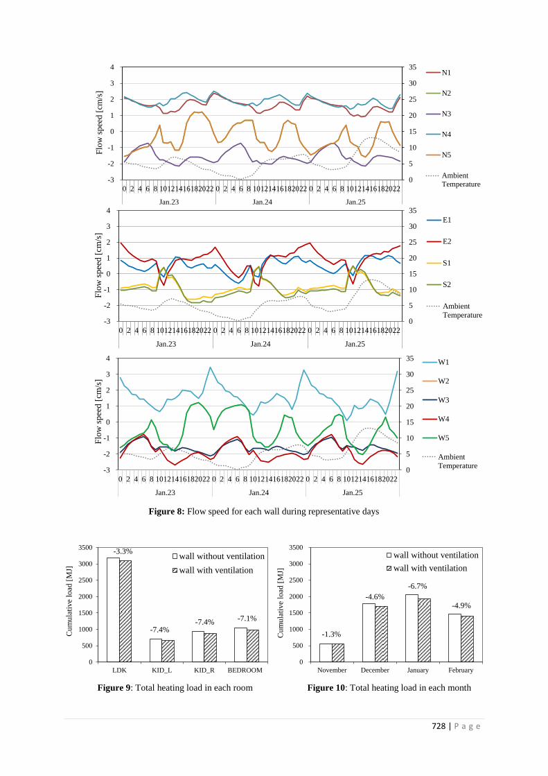
728 | P a g e

0

5

10

15

20

25

30

35

-3

-2

-1

0

1

2

3

4

0 2 4 6 8 10121416182022 0 2 4 6 8 10121416182022 0 2 4 6 8 10121416182022


Flo

w s

pee

d [

cm/s

]

N1

N2

N3

N4

N5

Ambient

Temperature

0

5

10

15

20

25

30

35

-3

-2

-1

0

1

2

3

4

0 2 4 6 8 10121416182022 0 2 4 6 8 10121416182022 0 2 4 6 8 10121416182022


Flo

w s

pee

d [

cm/s

]

E1

E2

S1

S2

Ambient

Temperature

0

5

10

15

20

25

30

35

-3

-2

-1

0

1

2

3

4

0 2 4 6 8 10121416182022 0 2 4 6 8 10121416182022 0 2 4 6 8 10121416182022


Flo

w s

pee

d [

cm/s

]

W1

W2

W3

W4

W5

Ambient

Temperature

Figure 8: Flow speed for each wall during representative days

0

500

1000

1500

2000

2500

3000

3500

LDK KID_L KID_R BEDROOM

Cu

mu

lati

ve

load

[M

J]

wall without ventilation

wall with ventilation

-3.3%

-7.4%-7.4%

-7.1%

0

500

1000

1500

2000

2500

3000

3500

November December January February

Cu

mu

lati

ve

load

[M

J]

wall without ventilation

wall with ventilation

-1.3%

-4.6%

-6.7%

-4.9%

Figure 9: Total heating load in each room Figure 10: Total heating load in each month

729 | P a g e

Figure 9 shows the total heating load in the ventilated walls for each room, for the case

with air-conditioning set at 20°C. Results for the four rooms are shown in the graph. The two

children’s rooms receive the largest heating load reduction because it consumes the least

energy among the four rooms. The average heating load reduction for the dining room from

June to September was reduced by 5.1%.

Figure 10 shows the total heating load from November to February for each month. The

heating load during the period from November to February was reduced by 1.3%, 4.6%,

6.7%, and 4.9%, respectively. The reduction was largest in January in which the temperature

was lowest.

CONCLUSIONS

In this study, we evaluated the airflow rate in the air gap of a double-skin system, the

heating load reduction, and the temperature increase by performing a ventilation network

simulation. The temperature in the living room increases by 0.3°C, when buoyancy ventilated

wall is used. Temperature decrease in the bedroom is smaller than temperature decrease in the

living room. This is because the heating schedule in the living room concentrates during the

daytime while heating schedules of the bedroom concentrate in the nighttime.

In general, the average heating load reduction for the dining room from June to September

was reduced by 5.1%. The two children’s rooms receive the largest heating load reduction

because it consumes the least energy among the four rooms. The heating load during the

period from November to February was reduced by 1.3%, 4.6%, 6.7%, and 4.9%,

respectively. The reduction was largest in January in which the temperature was lowest.

It was found that the total period heating load is reduced while the ventilated wall is

working and the air-conditioning is on. It seems that this effect is mainly because the air-

conditioning settling time was reduced by the room temperature increases. As a result, it is

expected that the heating load supplied from subfloor ground surface Therefore, a further

simulation of geothermal heat is necessary for future study. Furthermore, because heat from

solar radiation and internal heat cannot be discharged by infiltration, the simulation result

shows the room temperature is higher than that of the actual environment. To evaluate the

influence of infiltration, a simulation that considers infiltration between the interior-exterior

wall interface and the wall-room interface is needed in further research.

REFERENCES

Ozaki, A. (1992). Heat and water transfer through an ventilated structure using urethane

panels [in Japanese]. Summaries of technical papers of Annual Meeting Architectural Institute

of Japan, D, 945-946.

Institute for Building Environment and Energy Conservation. (2009). Description of the

energy consumption calculation method in the standards of judgment of the housing business

building owners [in Japanese].

Kurabuchi, T. (2009). Wind tunnel experiments on surface wind pressure and cross-

ventilation flow rate in densely populated residential area: study on proper design method of

locating windows aiming at utilization of cross-ventilation in densely populated residential

area (part 1) [in Japanese]. Journal of environmental engineering 74(642), 951-956.

730 | P a g e

DEVELOPMENT OF A UNIQUE THERMAL AND

INDOOR AIR QUALITY PROBABILISTIC

MODELLING TOOL FOR ASSESSING THE IMPACT

OF LOWERING BUILDING VENTILATION RATES

James McGrath

1, Miriam Byrne

*1

1 School of Physics and Centre for Climate and Air Pollution Studies,

Ryan Institute,

National University of Ireland, Galway,

University Road,

Galway

Ireland

ABSTRACT

Adequate ventilation is necessary to maintain thermal comfort and remove indoor air pollutant concentrations

(Crump et al., 2005). Indoor pollutant concentrations vary considerably depending on occupants’ behaviour

patterns, building characteristics and meteorological parameters and seasonal effects. Experimental

measurements are time consuming and expensive to carry out, while computational models are regarded as a

valid complement. The team at NUI, Galway have recently developed the IAPPEM model (described in

(McGrath et al., 2014a)representing the state-of-the-art in probabilistic modelling of indoor air quality; the

model is currently capable of highlighting locations of different pollutant concentrations within the same

building by considering the infiltration of outdoor air pollutants, meteorological parameters and seasonal effects,

indoor activities of occupants, emissions from indoor air pollutants, removal by deposition, the dilution of indoor

air pollutants through external and internal air exchange and internal house layout.

To date no computational model exists that examines both inter-zonal and external temperatures in combination

with assessing indoor air pollutants, and the enhancement of the IAPPEM source code framework to incorporate

these features constitutes the main tasks of the current work. This will allow an assessment of individuals’

thermal comfort and exposure to airborne pollutants, and will also allow an assessment of the heat loss to

surroundings as a result of changing ventilation rates, a feature that is highly relevant in the context of energy

efficient homes. While previous studies have examined the effect of heat loss due to ventilation, no model to date

has combined the temperature and airborne pollutant components in a single computational structure.

In this paper, a plan to incorporate a temperature parameter into the existing model is described; this would allow

the unique capability to assess, for the first time, the effects of ventilation and occupant behaviour on both an

individual’s thermal comfort and airborne pollutant exposure. The basis of the IAPPEM code adaptation strategy

will be the addition of a source term and a loss term to account for localised heating sources, such as radiators in

each room, solid fuel fires, and cooking events. A loss term will account for the removal of heat through the

building walls and windows. Ventilation rates will define the transfer of heat between rooms but also between

indoor and outdoor, allowing the assessment of heat loss as well as thermal comfort. This would provide a vital

tool in defining optimum building air exchange rates that do not have a negative impact on human health.

.

KEYWORDS

Indoor Air Quality, Thermal Comfort, Probabilistic modelling, emission sources,

731 | P a g e

1 INTRODUCTION

Particulate Matter (PM) has become a major environmental concern because of its known

impacts on human health (COMEAP, 2009, COMEAP, 2010). A WHO project REVIHAAP

(WHO, 2013) reported a large body of evidence linking the effects of long term PM exposure

on both cardiovascular mortality and all causes of mortality. PM related morbidity outcomes

include aggravated asthma, chronic respiratory disease, increased emergency room visits and

hospital admissions, acute respiratory symptoms, decrease in lung function and even

premature mortality. (Brook et al., 2010) reported that short-term PM2.5 exposure over a few

hours to weeks can trigger cardiovascular morbidity and mortality events. WHO (2013)

reported that significant evidence, based on toxicological and clinical studies, linking peak

exposures to combustion-derived particles of short duration (ranging from less than an hour to

a few hours) leads to immediate physiological changes.

Most of the general population in North America or Europe spent 89% of their time

indoors, with 69% spent in the residential indoor environment (Klepeis et al., 2001,

Schweizer et al., 2006), and homemakers or the elderly spending up to 90% of their time in

the residential indoor environment (Torfs et al., 2008). Therefore, the residential environment

deserves particular attention.

The need to achieve carbon and greenhouse gas emissions has promoted energy

efficiency improvements because of the potential saving in energy costs. Reduction in energy

usage in buildings is a significant component of the national CO2 reduction strategies. For

example, the Technical Guidance Document L of Part L of the Irish Building Regulations (SI

259 of 2011) sets out new performance levels for air permeability to be 7 m3/hr/m

2 at 50Pa.

Under the European directive (2010/31/EU, 2010), all new building must adhere to minimum

energy performance requirements. Irish legislation (S.I. No. 259/2008, 2008) refers to

reducing heat loss in building through increasing the air tightness.

However, as buildings air-tightness increases, a reduction occurs in the air exchange

rates (AERs) reducing heat loss, while increasing the indoor pollutant concentrations if

significant indoor sources are present (Gens et al., 2014). Wilkinson et al. (2009) reported that

changes in energy efficiencies in domestic homes may impact on indoor air quality, due to

increasing air-tightness without alternative methods of reducing indoor generated pollutants.

Bone et al. (2010) highlights that the driver for more energy efficiency homes will harm

occupant health.

The World Health Organization's (WHO, 2010) guidance on thermal comfort ensures

satisfaction with the ambient temperature, but also links to human health. The guidance for

the home environment aims at protecting human health particularly those most susceptible,

such as the very young and the elderly (Ormandy and Ezratty, 2012). Additionally, thermal

comfort has been reported to influence individuals’ behavioural patterns; Andersen et al.

(2009) reported that window opening behaviour in Danish dwellings is strongly linked to the

outdoor temperature. (Rijal et al., 2007, 2008) found relationships between the thermal

environment and the occupants’ behaviour in relation to windows/doors opening patterns and

the usage of HVAC system. McGrath et al. (2014b) investigated variations in PM

concentrations due to interzonal airflow in a six-room apartment layout. The study found that

peak concentrations in adjoining rooms were directly linked to the time of the door

opening/closing events.

Andersen et al. (2009) reported that the use of internal heating was correlated with the

outdoor temperature and the presence of a wood-burning stove within the dwelling. In

Ireland, the use of solid fuel burning in fireplaces is often used as means of secondary heating

source (McGrath et al., 2011, Semple et al., 2012).

Indoor PM concentrations are affected by infiltration of outdoor particles,

732 | P a g e

meteorological parameters and seasonal effects, indoor activities of occupants, emissions

from indoor PM sources, removal of particulates by deposition, the dilution of indoor PM

through external and internal airflow and internal house layout (Ferro et al., 2009, Singer et

al., 2002, Ott, 1999). Numerous studies have highlighted the indoor activities that contribute

to PM concentrations, such as smoking, frying, solid fuel fire and use of incense and candles

(He et al., 2004, See and Balasubramanian, 2011, Semple and Latif, 2014) and also

resuspension activities such as walking, dusting or sitting on furniture (Ferro et al., 2004, Jing

et al., 2008).

It is often impractical or expensive to obtain large-scale indoor or personal exposure

measurements to account for the range of indoor factors (indoor emission sources, indoor

deposition and resuspension, and the occupant’s behaviour). Computational modelling is an

effective tool at separating out the contribution of indoor emission source from outdoor

generated air pollution; this approach allows for effective exposure reduction strategies to be

devised. For the proper management of air quality to be fully evaluated, indoor exposures

need to be further separated into the contributions of indoor sources and the penetration of

outdoor pollution. Modelling approaches are essential if this is be effectively achieved

(Dimitroulopoulou et al., 2000).

Steinle et al. (2013) highlights that exposure models are an appropriate tool to increase

sample sizes and reduce the cost of experimental exposure studies. Exposure models need to

integrate a wide range of factors (e.g. economic, social and demographic), to assess relations

and associations between human exposure to environmental air pollutants and potential health

effects. In recent years, a number of models have predicted indoor pollutant concentrations in

indoor environments (Dimitroulopoulou et al., 2006, Fabian et al., 2012, Sohn et al., 2007,

Parker and Bowman, 2011). Fabian et al., (2012) reported challenges imposed on simulations

due to the large variation in emission strengths. Limitations in these physical pollutant models

have led to poorer estimations of indoor air pollutant exposure assessment.

Probabilistic modelling is one approach that overcomes these issue. McGrath et al.

(2014a) developed IAPPEM, a state-of-the-art probabilistic model for indoor PM

concentration estimation, capable of simulating up to 15 interconnecting rooms with the

incorporation of up to 12 simultaneously-operating emission sources. IAPPEM proved to be

capable of simulating the large variation in emission rates, predicting both peak and mean

PM10 and PM2.5 concentrations. IAPPEM provided a detailed analysis of overall PM

contribution from multiple different emission sources, in a variety of different internal

locations in a dwelling, and the effect that both emission source location and internal

household configuration has on PM transfer throughout a dwelling has been quantified.

The current work plans to incorporate temperature parameters into the existing model;

this would allow the unique capability to assess, for the first time, the effects of ventilation

and occupant behaviour on both an individual’s thermal comfort and airborne pollutant

exposure. This would provide a vital computational tool that has wide relevance in

epidemiology studies, building design, ventilation studies, traffic management studies, and

many other fields.

2. METHODOLOGY

2.1 Air pollutant model

The current model, titled Indoor Air Pollutant Passive Exposure Model (IAPPEM), is an

advanced probabilistic modelling tool that evaluates the contribution of both indoor and

outdoor sources to the air pollution concentration in the indoor environment. IAPPEM

calculates the change in indoor pollutant concentrations by solving the differential equation 1;

considering the infiltration of outdoor air pollution, the generation of air pollution indoors and

its transport between rooms, and the indoor deposition of air pollution. At each time interval,

probability density functions are used to simulate a range of possible values for each

733 | P a g e

parameter, assessing the range of likely outcomes when specific details are unavailable. This

can encompass uncertainties in experimental obtained data, but can also encompass

uncertainties in the selection of appropriate modelling parameters between studies. Further

details on the parameterisation of the pollutant model are available in McGrath et al. (2014a).

(1)

Equation 1 is solved for each k, where k represents each individual room. Subscripts of 0, 1

and 2 are used to represent outside, room 1 and room 2 for different parameters. Ck represents -3

, where C represents the outdoor -3

). fk represents the building filtration factors between the outdoor and

that room. vg is the deposition velocity of the pollutant (m hr-1

ik is the interzonal airflow

12 represents the transport of pollutants from room 1 into room

0k the external airflow between the outside and room k (m3 hr

-1). Ak is the surface

area of room k (m2). Vk is the volume of room k (m

3). Qk is the indoor emission rate of the

-1).

2.2 Addition of a Temperature Parameter

The current work comprises of altering the model’s source code to include the temperature

parameters, allocating a source file to account for time-varying outdoor temperature

concentrations, as well as incorporating a temperature parameter to each room. A

‘source’ term will allow for internal heating sources (solid-fuel burning, central heating,

electric fan heater or HVAC). A ‘decay’ term will allowing for heat losses through the

building fabric through external and internal walls, as well as floors and ceilings. Airflow

rates in Equation 1 will be used to assess the heat loss to the outdoors but also the internal

transfer of heat between zones. Additionally, a heat ‘recovery’ term will be added to account

for any heat recovery systems.

The model’s parameterisation will account for variation in building fabrics; window

types and wall and roof insulation. Altering the model’s parameterisation will allow

assessments of performance pre and post retrofitting a building.

3. RESULTS

The application of the air pollutant model is demonstrated by a number of simulations below.

The simulation are based on the 11-room dwelling described in McGrath et al. (2014a). The

emission scenarios comprised of two frying events in the kitchen and five smoking events in

the living room while internal doors remained closed. Each frying event lasts for 15-minutes,

while each smoking event lasts for nine minutes. Figure 1 and 2 shows a section of the 24hour

time-series profile for PM2.5 concentrations in both the kitchen and the living room.

dCkdt

=(l0k)

Vk( fk *(C0 -Ck))- vg(

AkVk

)Ck +QkVk

+likVk

(Ci -Co)

i=1

n

å

734 | P a g e

Figure 1. PM2.5 concentrations in the living room. The time axes have been scaled to focus on the emission

periods. The ‘y’ bars represent one standard deviation at each time step, highlighting the probabilistic nature of

the model. Each of the peak concentrations refers to the end of the smoking events.

Figure 2. PM2.5 concentrations in the kitchen. The time axes have been scaled to focus on the emission periods.

The ‘y’ bars represent one standard deviation at each time step, highlighting the probabilistic nature of the

model. Each of the peak concentrations refers to the end of the frying event.

Table 1 shows the effect that reducing AERs have on indoor PM2.5 concentrations. The values

of 0.30, 0.44, 0.70 ACH-1

reflect similar AERs reported in literature for European dwelling

(Crump et al., 2005, Dimitroulopoulou, 2012). It can be seen that PM concentrations increase

with decreasing AERs; this is a major concern considering that the World Heath Organisation

(WHO, 2006, 2013) recommends a 24-hour mean PM2.5 -

3.

735 | P a g e

Table 1 shows the 24-mean PM2.5 concentrations in both the kitchen and sitting room under three

different air exchange rates in units of Air Changes per Hour (ACH-1

).

Location 0.7 ACH-1

0.44 ACH-1

0.3 ACH-1

Kitchen -3

-3

-3

Sitting Room -3

-3

1-3

The proposed enhancement to the model will simultaneously allow time-series analysis

of internal room temperatures in combination with indoor air quality. Any proposed changes

in AERs can then be assessed in terms of potential energy saving strategies to analyse the

effect on the reduction in heat loss but also the effect on indoor air quality.

4. CONCLUSIONS

The modified model will make simulations to assess both thermal comfort and indoor air

pollutants, resulting in a time-series analysis of both parameters. This will allow simulations

of variations in household characteristics, occupants behavioral patterns, mechanical and

natural ventilation.

The results of this project will inform policy makers and the public on energy usage

reduction in the built environment sector, and any mis-understanding regarding potentially

adverse effects of reduced ventilation on indoor air quality could be extremely detrimental in

this regard. The model can assess the potential benefits of retrofitting a residential dwelling

while ensuring there is no reduction in indoor air quality.

This unique computational tool can be used to define the optimum ventilation rates for

energy efficient homes ensuring thermal comfort and also an appropriate level of indoor air

quality. One potential strategy could examine increasing the external airflow in rooms that

experience higher air pollutant concentrations while reducing the external airflow in rooms

that experience lower air pollutant concentrations.

5 ACKNOWLEDGEMENTS

This work was funded by Sustainable Energy Authority of Ireland (SEAI) under the SEAI

Renewable RD&D Programme 2014.

6 REFERENCES

ANDERSEN, R. V., TOFTUM, J., ANDERSEN, K. K. & OLESEN, B. W. 2009. Survey of

occupant behaviour and control of indoor environment in Danish dwellings. Energy

and Buildings, 41, 11-16.

BONE, A., MURRAY, V., MYERS, I., DENGEL, A. & CRUMP, D. 2010. Will drivers for

home energy efficiency harm occupant health? Perspectives in public health, 130,

233-238.

BROOK, R. D., RAJAGOPALAN, S., POPE, C. A., BROOK, J. R., BHATNAGAR, A.,

DIEZ-ROUX, A. V., HOLGUIN, F., HONG, Y., LUEPKER, R. V. & MITTLEMAN,

M. A. 2010. Particulate matter air pollution and cardiovascular disease an update to

the scientific statement from the American Heart Association. Circulation, 121, 2331-

2378.

COMEAP 2009. Long term exposure to air pollution: Effect on mortality.: Committee on the

Medical Effects of Air Pollutants.

736 | P a g e

COMEAP 2010. Review of Evidence on Health Aspects of Air Pollution REVIHAAP

Project: Final technical report.

CRUMP, D., DIMITROULOPOULOU, S., SQUIRE, R., ROSS, D., PIERCE, B., WHITE,

M., BROWN, V. & COWARD, S. 2005. Ventilation and indoor air quality in new

homes. Pollution atmosphérique, 1, 71.

DIMITROULOPOULOU, C. 2012. Ventilation in European dwellings: A review. Building

and Environment, 47, 109-125.

DIMITROULOPOULOU, C., ASHMORE, M. R., BYRNE, M. A., HILL, M. T. R.,

KINNERSLEY, R. P., MARK, D. & NI RIAIN, C. 2000. Modelling of indoor aerosol

concentrations in UK buildings. Journal of Aerosol Science, 31.

DIMITROULOPOULOU, C., ASHMORE, M. R., HILL, M. T. R., BYRNE, M. A. &

KINNERSLEY, R. 2006. INDAIR: A probabilistic model of indoor air pollution in

UK homes. Atmospheric Environment, 40, 6362-6379.

FABIAN, P., ADAMKIEWICZ, G. & LEVY, J. I. 2012. Simulating indoor concentrations of

NO 2 and PM 2.5 in multifamily housing for use in health-based intervention

modeling. Indoor Air, 22, 12-23.

FERRO, A. R., KLEPEIS, N. E., OTT, W. R., NAZAROFF, W. W., HILDEMANN, L. M. &

SWITZER, P. 2009. Effect of interior door position on room-to-room differences in

residential pollutant concentrations after short-term releases. Atmospheric


FERRO, A. R., KOPPERUD, R. J. & HILDEMANN, L. M. 2004. Source strengths for indoor

human activities that resuspend particulate matter. Environmental science &

technology, 38, 1759-1764.

GENS, A., HURLEY, J. F., TUOMISTO, J. T. & FRIEDRICH, R. 2014. Health impacts due

to personal exposure to fine particles caused by insulation of residential buildings in

Europe. Atmospheric Environment, 84, 213-221.

HE, C., MORAWSKA, L., HITCHINS, J. & GILBERT, D. 2004. Contribution from indoor

sources to particle number and mass concentrations in residential houses. Atmospheric


JING, Q., FERRO, A. R. & FOWLER, K. R. 2008. Estimating the Resuspension Rate and

Residence Time of Indoor Particles. Journal of the Air & Waste Management

Association (Air & Waste Management Association), 58, 502-516.

KLEPEIS, N. E., NELSON, W. C., OTT, W. R., ROBINSON, J. P., TSANG, A. M.,

SWITZER, P., BEHAR, J. V., HERN, S. C. & ENGELMANN, W. H. 2001. The

National Human Activity Pattern Survey (NHAPS): a resource for assessing exposure

to environmental pollutants. Journal of Exposure Analysis and Environmental

Epidemiology, 11, 231-252.

MCGRATH, J., BYRNE, M., ASHMORE, M., TERRY, A. & DIMITROULOPOULOU, C.

2014a. Development of a probabilistic multi-zone multi-source computational model

and demonstration of its applications in predicting PM concentrations indoors. Science

of The Total Environment, 490, 798-806.

MCGRATH, J. A., BYRNE, M. A., ASHMORE, M. R., TERRY, A. C. &

DIMITROULOPOULOU, C. Simulation of Solid Fuel Burning Events in Irish

Fireplaces under Varying Air Exchange Rates. The 12th International Conference on

Indoor Air Quality and Climate. Indoor Air 2011., 2011 Austin, Texas.

MCGRATH, J. A., BYRNE, M. A., ASHMORE, M. R., TERRY, A. C. &

DIMITROULOPOULOU, C. 2014b. A simulation study of the changes in PM2.5

concentrations due to interzonal airflow variations caused by internal door opening

patterns. Atmospheric Environment, 87, 183-188.

ORMANDY, D. & EZRATTY, V. 2012. Health and thermal comfort: From WHO guidance

to housing strategies. Energy Policy, 49, 116-121.

737 | P a g e

OTT, W. R. 1999. Mathematical models for predicting indoor air quality from smoking

activity. Environmental Health Perspectives, 107, 375-381.

PARKER, S. & BOWMAN, V. 2011. State-space methods for calculating concentration

dynamics in multizone buildings. Building and Environment, 46, 1567-1577.

RIJAL, H. B., TUOHY, P., HUMPHREYS, M. A., NICOL, J. F., SAMUEL, A. & CLARKE,

J. 2007. Using results from field surveys to predict the effect of open windows on

thermal comfort and energy use in buildings. Energy and Buildings, 39, 823-836.

RIJAL, H. B., TUOHY, P., NICOL, J., HUMPHREYS, M. A., SAMUEL, A. & CLARKE, J.

2008. Development of adaptive algorithms for the operation of windows, fans and

doors to predict thermal comfort and energy use in Pakistani buildings. ASHRAE

transactions, 114, 555-573.

SCHWEIZER, C., EDWARDS, R. D., BAYER-OGLESBY, L., GAUDERMAN, W. J.,

ILACQUA, V., JANTUNEN, M. J., LAI, H. K., NIEUWENHUIJSEN, M. &

KÜNZLI, N. 2006. Indoor time–microenvironment–activity patterns in seven regions

of Europe. Journal of Exposure Science and Environmental Epidemiology, 17, 170-

181.

SEE, S. W. & BALASUBRAMANIAN, R. 2011. Characterization of fine particle emissions

from incense burning. Building and Environment, 46, 1074-1080.

SEMPLE, S., GARDEN, C., COGGINS, M., GALEA, K. S., WHELAN, P., COWIE, H.,

SANCHEZ-JIMENEZ, A., THORNE, P. S., HURLEY, J. F. & AYRES, J. G. 2012.

Contribution of solid fuel, gas combustion, or tobacco smoke to indoor air pollutant

concentrations in Irish and Scottish homes. Indoor Air, 22, 212-223.

SEMPLE, S. & LATIF, N. 2014. How Long Does Secondhand Smoke Remain in Household

Air: Analysis of PM2. 5 Data From Smokers’ Homes. Nicotine & Tobacco Research,

ntu089.

SINGER, B. C., HODGSON, A. T., GUEVARRA, K. S., HAWLEY, E. L. & NAZAROFF,

W. W. 2002. Gas-phase organics in environmental tobacco smoke. 1. Effects of

smoking rate, ventilation, and furnishing level on emission factors. Environmental

Science & Technology, 36, 846-853.

SOHN, M. D., APTE, M. G., SEXTRO, R. G. & LAI, A. C. 2007. Predicting size-resolved

particle behavior in multizone buildings. Atmospheric Environment, 41, 1473-1482.

STEINLE, S., REIS, S. & SABEL, C. E. 2013. Quantifying human exposure to air

pollution—moving from static monitoring to spatio-temporally resolved personal

exposure assessment. Science of the Total Environment, 443, 184-193.

TORFS, R., BROUWERE, K. D., SPRUYT, M., GOELEN, E., NICKMILDER, M. &

BERNARD, A. 2008. Exposure and risk assessment of air fresheners. VITO.

WHO 2006. WHO Air quality guidelines for particulate matter, ozone, nitrogen dioxide and

sulfur dioxide. World Health Organisation.

WHO 2010. Housing, Energy and Thermal Comfort. A review of 10 countries within the

WHO European Region. World Health Organisation.

WHO 2013. Review of Evidence on Health Aspects of Air Pollution REVIHAAP Project:

Final technical report. World Health Organization.

WILKINSON, P., SMITH, K. R., DAVIES, M., ADAIR, H., ARMSTRONG, B. G.,

BARRETT, M., BRUCE, N., HAINES, A., HAMILTON, I. & ORESZCZYN, T.

2009. Public health benefits of strategies to reduce greenhouse-gas emissions:

household energy. The Lancet, 374, 1917-1929.

738 | P a g e

ASSESSMENT OF THE DURABILITY OF THE

AIRTIGHTNESS OF BUILDING ELEMENTS VIA

LABORATORY TESTS

Benoît Michaux

*, Clarisse Mees, Evelyne Nguyen, Xavier Loncour

Belgian Building Research Institute

Lombard Street, 42

BE 1000 Brussels, Belgium

*Corresponding author: e-mail address

ABSTRACT

The airtightness just after the end of a building phase is assumed to be relevant criteria for high energy

performance. Testing on site the initial performance of the airtightness via the blower door test has become

nowadays a common practice. This test is generally realized at the end of the construction works. What about the

influence of ageing on the airtightness? Many questions exist on the durability of this initial performance. Even

if retesting a building a few years after the initial test can provide a general view on the evolution of this

performance, this could generate adding cost and couldn’t give information on the origin of potential changes.

Another approach may be to validate technology and building technics as sustainable solutions. In order to

quantitatively evaluate the durability of the airtightness of building elements as well as building technics, a

research realized in Belgium has tested in laboratory the initial performance of more than 50 building walls and

their materials.

This performance has afterwards been tested after an accelerated ageing process including a.o. exposure to wind

cycles (storms) corresponding to 10, 25 and 40 years of lifetime. The paper presents the main results of this

research and points out the principal recommendations to guarantee the sustainability of this performance.

KEYWORDS

Durability, Airtightness, Building Technology

1 INTRODUCTION

Even we focus more and more on the airtightness of the new building to reach high energy

standards, a lot of questions are still remaining targeting the sustainability of the

performances. As of now, the blower door test confirms the initial airtightness just at the end

of the building phase. This test will not provide any information on the long term

performances of the airtightness. To consider the sustainability of the airtightness we should

use some different ways.

The monitoring of the performances may cost and is intrinsically not a quality guarantee but

only a control. But it’s more efficient to be proactive and to choose combinations of products

which will therefore ensure the durability of these performances.

The research project conducted from 2012 to 2013 by the Belgian Building Research Institute

in partnership with the University of Liège has targeted the basic criteria and useful

technologies insuring the durability of the airtightness.

This article will not analyse all the results of the research but provide the important learnings

from the research.

739 | P a g e

2 THE « DREAM » RESEARCH PROJECT

The research project called “DREAM” aims to evaluate and improve the durability of the

airtightness of buildings quantifying the airtightness performance of different materials before

and after ageing for 46 different walls (divided into 4 families).

Four different families of system ensuring the airtightness have been targeted in this project.

• Walls of blocks / bricks whose airtightness is ensured by coatings/plastering.

Seventeen different walls were analysed in this family (inside plastering or outside coating);

• Walls whose airtightness is ensured by wood panels. Eleven different walls were

analysed in this family

• Walls whose airtightness is ensured by a membrane. Eleven different walls were

analysed in this family;

• Walls composed by industrialized systems (sandwich panels, architectural concrete

panels, ...). Seven different walls have been tested for this family.

2.1 Ageing types

All the samples were tested before and after ageing phases. Three types of ageing

were implemented successively on the samples.

- Ageing representing wind effects and storms.

- Ageing representing the variation of moisture

- Ageing representing the variation of temperature

The succession of ageing are adapted to the influence of the ageing on the type of walls

The ageing representing the wind effect is implemented through storms. Each storm has

1,415 wind cycles ranging from 40% to 100% of the maximum value of wind pressure

(as described on figure 1). Four different storms were applied on the walls. After each

storm, the air permeability has been measured.

Figure 1: Ageing due to wind effect

740 | P a g e

The ageing representing the

variation of moisture is

implemented through rapid

variation of the air moisture.

After a first stabilisation up to

50% HR, three cycles from 20 to

80% are applied on the inside

part of the walls (as described on

figure 2). Each cycle lasts one

day. It represents short-term

variations therefrom that may

occur in buildings with indoor

climate control (for example in

bathrooms, ...).

Ageing types due to temperature

effect are applied to the outer side of

the walls. 50 temperature cycles are

performed (as described on figure 3).

An airtightness tests is realized after

at the end of the ageing procedure.

All the permeability tests are realized

both in over- and underpressure.

Based on these tests, it is possible to

determine the following equations Qn= kA Pn

(as described on figure 4).

Figure 4: Graph (Q, – Sampling (plastering)

46walls were tested representing more than 700 graphs (Q, P). All the ageing tests

realized on a specific wall are summarized on one graph (Q50, Ageing test) to represent

Figure 2: Ageing due to Moisture effect

Figure 3: Ageing due to temperature effect

741 | P a g e

the evolution of the airflow at 50Pa after each step of the ageing process. The figure

5shows an example of the evolution for walls whose airtightness is ensured by a wood

panel with tape.

Figure5:Evolution of the Q50Pa (case of OSB12mm panel with tape (type 3)and lathing)

The tested samples are representative of the existing building method in Belgium. The results

of this research are not exhaustive and could not cover all the existing technics.

The samples were built carefully in laboratory conditions in order to start in optimal situation

before proceeding with ageing. The purpose of this research is to confirm the durability of the

performance of the investigated systems.

2.2 « Walls of blocks / bricks whose airtightness is ensured by coatings/plastering »

2.2.1 Walls of blocks / bricks whose airtightness is ensured by internal plastering

On those samples the ageing steps are established by a first application of moisture

variation, temperature variations and finally storm cycles.

The interior coating systems achieve good airtightness performance, as well the initial

performance as after ageing (q50<0.1m³/h/m²). However we can note some learnings:

Only moisture and thermal ageing influence the airtightness;

The thickness of the plastering and the smoothness influence the initial

performance;

The storms ageing up to 1000 Pa haven’t any influence on the

performances;

Thin plastering (thickness ≤ 6mm) shows a significant loss of

airtightness after hygrothermal cycles. This loss is due to micro-cracks

in the plastering. The effect of hygrothermal cycles in steps 2 (moisture

variation) and 3 (thermal variation) of a 6 mm plaster (evolution shown

in figure 6) are higher than the influence from wind effect ageing.

Performance after ageing are still remaining acceptable;

742 | P a g e

Figure 6: Evolution of the Q50Pa (case of 6mm plastering)

It’s also interesting to note the quality of the surface (finishing)

influences the level of the initial performance but does not influence the

risk of micro-cracking (this is even more pronounced in thin

plastering). Some samples have required the application of new

plastering to start with better initial performances;

Applying a double plastering influences the initial airtightness

performance. However the risk of degradation of the plastering is

influenced by the thicknesses of the layers.

In the case of clay-based coatings, the airtightness is influenced by the thickness.

The grain size fluctuations of the clay are compensated by the thickness of

the applied clay (in the research : 28 and 51 mm); For the 28mm thick, the

Q50Pa stays around 0.1m³/h/m² all along the aging procedure. For the 51mm

thick, the Q50Pa stays between 0.012 and 0.02 m³/h/m² all along the aging

procedure.

For both thicknesses, with clay-based coatings, the storms cycles have no

significant influence on the evolution of the performances. The action of

hygrothermal ageing has less influence on the airtightness especially for the

higher thickness. This could be explained because of the test procedure (the

thermal and moisture variation are quite rapid – the clay did not have any

time during humidity cycles to stabilize the humidity in the material). The

initial airtightness performance of thicker clay-based coating was maintained.

A consequent loss of airtightness could come into consideration for buildings

where moisture conditions are not mastered quickly.

2.2.2 Walls of blocks / bricks whose airtightness is guaranteed by external

coatings/plastering

The same ageing procedure was followed (see§2.2.1).The following outputs emerge:

The influence of humidity cycles depends strongly on the used coating

system (as well as the methods of implementation). For each product,

an initial performance testing by the fabricant should be required;

743 | P a g e

The overriding factors influencing the initial performance are:

o The particle size of the products used

o Pre-layers and preparation layers

o The thickness of the layers

o The nature of the binder

The initial values (Q50Pa) are varying between 0.004 up to 0.8 m³/h/m².

After ageing procedure, the Q50Pa is going up to 0.01 m³/h/m² for the

best airtight one and up to 1.7m³/h/m² for the most degraded one.

The action of pressure cycles is only marked from high pressures

storms (over 800 Pa) but it should be noted that the influence of ageing

is relatively limited on the coatings. These coatings have been

developed to meet the external application and watertight requirements.

So the number of cracks is rather limited with these products.

2.3 Walls whose airtightness is ensured by panels

The fixing of panels and techniques of airtightness

(continuity between panels) can significantly

influence the performance of the wall.

The ageing procedure is defined by a first

application of temperature variations and moisture

variations and finally ageing due to pressure.

We can note the following findings:

When walls with joints between panels are glued, they

delivers a performance for which ageing has limited

influence. Note that the (PU based) glue in the grooves

was carried out with particular care along the grooves to

ensure the continuity of all the collages. The analysis does

not include the variability of implementations. The effect

of ageing is limited in time and humidity fluctuations were

fast enough (cycles less than 24 hours). This glue must meet the criteria for structural

bonding.

When sealing between panels is ensured by tape, it is essential to ensure the compatibility

between the panels and the tape. Strengthen the tape by a lathing ensures the continuity of the

airtightness. Indeed, tests have shown that the storms 800 and 1000 Pa generate significant

impairments in tape (although this is limited for optimal combinations tape / panel). The

effect of hygrothermal cycles (short period) remains low on these systems (in case of rapid

management of internal conditions). However, tests realized by realizing longer

hygrothermal cycles (no active control) generate higher damage. The following figure shows

the evolution of airtightness for complete walls whose airtightness is ensured by panels

(OSB3-15mm) and tapes between panels without lathing.

Figure 7: Sample with panel

744 | P a g e

Figure 8: Evolution of the Q50Pa (case of panels with tape)

When a strapping protects these tapes, the degradation is significantly reduced. This

construction method ensures the sustainable performances. It is also clear that in the case of

tapes placed on non-reinforced seams (upper parts of frames), the tapes are strongly solicited

and damages appear with high pressure storms (from 800Pa).

When tightness between panels is provided by sealants under lathing, the solution offers a

sustainable solution. The following figure gives the evolution of the Q50 for panels whose

continuity is ensured by a compressed sealant.

Figure 9: Evolution of the Q50Pa (case panel + compressed sealant)

2.4 Walls whose airtightness is guaranteed by a membrane

The ageing procedure is defined by a first application of temperature variations and

moisture variations and finally ageing due to pressure.

745 | P a g e

Figure 10: Evolution of the Q50Pa (case of stapling membrane)

Stapling the membrane is a risky

method, the ageing effect has a

consequent impact if the stitching is

not supported by lathing or a

compatible tape;

Connections between membranes

need to be done with tape single

sided or double sided, or folded and

lathing, or mastic bound. If

construction is exposed to wind, it

will be applied by the additional

lathing recovery;

The horizontal lathing (technique

applied to hold the membrane during the insulation blowing) is not

sufficient when the construction is exposed to wind;

The compatibility between membrane and tape requires verification.

Indeed, although the initial bonding seems appropriate, hygrothermal or

mechanical (wind) ageing may degrade the airtightness of these

collages;

When the membranes are glued with a flexible stand, folding the two

membranes with double-sided tape gives significant performance;

However, if the building is exposed to the wind, the protection of such

recovery is necessary.

Figure 11: Sample with membrane 1

746 | P a g e

2.5 Walls whose airtightness is ensured by industrialized systems (sandwich panels,

architectural concrete panels, ...).

The prefabricated sandwich panel construction requires improved joints between

panels design. For these walls, the ageing procedure is a first application of pressure

cycles, variations in temperature and finally humidity variations.

When the links between sandwich panels is provided by a closed cell

foam seal and a silicone, if the closed cell seal is compressed by fixing

the panel, the continuous seal is ensured. The features of construction

must allow the compression of the seal. Continuity at the corners

remains difficult. The silicone gasket completes the seal. The ageing

will not have any effect on the airtightness of this system

If the sealing wall is provided by a closed cell foam seal, the gasket

must be compressed with panels fixations therefore continuity is sealed.

Continuity at the corners remains difficult. However, additional gasket

or mastics must ensure the continuity of the seal. The compressed seals

have not shown any degradation;

3 CONCLUSIONS

Several techniques can be identified in terms of airtightness sustainability. Some resist more

at higher loads; it is then necessary to adapt the construction method according to the stresses.

Thus, a construction particularly exposed to the wind requires additional lathing on

membrane’s connections. It is also important that the manufacturer communicates on the

compatibility and performance of their product.

The results of this research will be used in future publications of the Belgian Building

Research Institute.

4 ACKNOWLEDGEMENTS

The results presented in this paper were obtained within the DREAM research project

supported by the Walloon Region in Belgium.

747 | P a g e

CONTROL OF INDOOR CLIMATE

SYSTEMS IN ACTIVE HOUSES

Peter Holzer

*1, Peter Foldbjerg

2

1 Institute of Building Research & Innovation

Luftbadgasse 3/8

1090 Vienna, Austria

[email protected]

2 VELUX A/S

Ådalsvej 99


ABSTRACT

The term of “Active House” recently developed, addressing houses that target a balanced optimization of indoor

environmental quality, energy performance and environmental performance. According to the idea of not only

being energy efficient and eco-friendly, Active Houses equally focus on indoor environmental qualities, in

particular daylight and air. With their tendency towards intensive sun penetration, natural ventilative systems and

generally intensive connections to the exterior, Active Houses challenge the balance of technical and individual

indoor climate control.

The paper in hand presents and discusses challenges and findings from six model Active House homes in five

European countries:

How to design and run heating, cooling control systems in Active Houses.

How to balance hybrid ventilation systems in Active Houses.

How to open the houses to the delight of sunlight but effectively protect against overheating.

Finally how to balance technical control and still encourage spontaneous individual interference.

From 20010 to 2013 six model homes in Active House Standard have been erected and monitored in five

European countries, funded by the company of VELUX. The authors have been deeply involved in design,

erection and post occupancy performance monitoring of these model homes.

KEYWORDS

Active Houses, Indoor environmental control, daylight, hybrid ventilation

1 INTRODUCTION

The term of “Active House” recently developed, addressing houses that target a balanced

optimization of indoor environmental quality, energy performance and environmental

performance. A lively international network, the “Active House Alliance”, has been founded

and numerous pilot projects in a widespread range of nations and climates have been erected.1

According to the idea of not only being energy efficient and eco-friendly, Active Houses

equally focus on indoor environmental qualities, in particular daylight and air. With their

tendency towards intensive sun penetration, natural ventilative systems and generally

1 For further information see http://www.activehouse.info (22.08.2014).

748 | P a g e

intensive connections to the exterior, Active Houses challenge the balance of technical and

individual indoor climate control.

Funded and very actively accompanied by the Danish roof window manufacturer

VELUX A/S there have been Active Houses erected in five different European countries and

had them intensively monitored through a period of at least one full year, including energy

monitoring, comfort monitoring and social monitoring.1

The paper in hand presents and discusses the findings from those six model homes as regards

the aspects of technical control such as

How to design and run heating, cooling control systems in Active Houses.

How to balance hybrid ventilation systems in Active Houses.

How to open the houses to the delight of sunlight but effectively protect against

overheating.

Finally how to balance technical control and still encourage spontaneous individual

interference.

2 ACTIVE HOUSES

2.1 Goal and Definition

Goal and definition of Active Houses is precisely but still lively and even poetically defined

in the Active House Specifications.2

The most poetic definition is: Active Houses are Buildings that give more than they take.

The lively programmatic definition is, already structured in three fields of equal interest:

Indoor Environmental Quality

An AH creates healthier and more comfortable life.

An AH ensures a generous supply of daylight and fresh air.

Energy

An AH is energy efficient.

All AH’s energy needed is supplied by renewable sources.

Environment

An AH interacts positively with the environment

through an optimized relationship with the local context

Precise quantitative benchmarks as regards indoor environmental standards, energy demand

key figures and environmental impacts are defined in Active House Specifications, having

already been mentioned before.

It’s this balanced approach of Indoor Environmental Quality, Energy and Environment that

makes the Active House quite unique amongst other building standards and which, indeed,

brings along some challenges, not least in technical control systems.

1 For further information see http://www.velux.com/sustainable_living/demonstration_buildings (22.08.2014)

2 Active House Specifications, 2nd edition, http://www.activehouse.info/download-specifications (23.08.2014)

749 | P a g e

2.2 Specific Features and Physical Challenges of Active Houses

Following the balanced three tier approach of Indoor Environmental Quality, Energy and

Environment leads to specific features and physical challenges of Active Houses, which can

be addressed as benefits as well as threats:

Usually, an Active House is generously daylit, it is generously supplied with fresh air and it

connects significantly to the out-of-doors. Thus, seen positively, it‘s fast and strong reactive

to the healing sun, to the warm breeze, to sounds and smells of nature. Seen negatively, it is

fast and strong reactive to the burning sun, to heatwaves and storms, to external noise and air

pollution.

This paradox of very different possible perceptions of the same physical qualities finds its

equivalence in the possible and yet contradicting expectations towards the qualities of

technical control systems, between full automation and individual behaviour.

2.3 The VELUX model homes 2020

From 2010 to 2013 six model homes in Active House Standard have been erected and

monitored in five European countries, funded by the company of VELUX. Altogether, this

“model home 2020” program was the biggest and most practical concerted research action in

the field of Active Houses. The authors have been deeply involved in design, erection and

post occupancy performance monitoring of these model homes.

Detailed information on the research program of model home 2020 can be found at

http://www.velux.com/sustainable_living/demonstration_buildings

Home for Life, Denmark

Green Lighthouse, Denmark

Sunlighthouse, Austria

750 | P a g e

LichtAktiv Haus, Germany

Carbon Light Homes, Great Britain

Maison Air et Lumière, France

3 DISCUSSION OF INDOOR ENVIRONMENTAL QUALITY TARGETS

3.1 Comfort versus Health

Indoor Environmental Quality, often but improperly referred to as Indoor Comfort, is a major

issue of today’s building design research. Design decisions towards Indoor Comfort are

intrinsically linked to the energy demand of buildings. And, which is overseen too often,

Indoor Environmental Quality is not only about comfort but it’s very much about health. This

correlation is gaining importance rapidly, with today’s urban lifestyle leading to 95% of the

lifetime being spent indoors. Thus, it is important to discuss Indoor Comfort very much

together with Indoor Health.

Indoor Comfort is a state of mind, based on a set of physiological, psychological and physical

parameters. You may speak of the physio-psycho-dualism of comfort. Furthermore, Indoor

Comfort very much varies with the level of personal expectations and with the level of

personal possibilities. And finally, Indoor Comfort gives instantaneous feedback: A person

per definition feels uncomfortable in the instant moment it feels uncomfortable.

Indoor Health is expected to be much less psychologically based, but being much more based

on physiological settings which themselves having their roots back in evolution of mankind.

The basic physiological needs cannot be changed and triggered to the same extent as comfort

expectations can be. And unhealthy indoor environments do not give such strong and

instantaneous feedback than uncomfortable environments do.

Thus: In building design indoor health is a “must have” issue and indoor comfort is a “nice to

have”. To have both is perfect and nothing less is the aim of modern sustainable building

design.

751 | P a g e

3.2 Indoor Thermal Comfort & Health Targets

3.2.1 The physiological thermal comfort definition according to Fanger

Traditional 20th century indoor comfort research focused on the physiological aspect only.

Fanger et al. developed a physical model for thermal comfort starting from the 1960’s, being

now worldwide established and forming the basis for HVAC design around the globe.

The model is based on the assumption that thermal comfort derives from an equated body’s

heat balance together with a limitation of the sweat rate and a limitation of the skin

temperature. Within this model, general thermal comfort can be described as a strict function

of six physiological and physical parameters: activity level, clothing level, air temperature,

radiant temperature, air humidity and air velocity. Additionally four phenomena of local

discomfort are described, again on physical level. The Fanger-model was validated by

numerous experiments with groups of test persons in climatic chambers and is implemented

into international standardization, such as ISO 7730 and ASHRAE 55. 1, 2

3.2.2 The physio-psychological thermal comfort definition according to Humphreys

As an important improvement, exhaustive empiric comfort research has been carried out by

Humphreys et al., investigated thermal comfort not merely as a function of physiological

parameters, but as a both physiological and psychological status. This additional approach is

known as the Adaptive Principle, leading to the following findings: People are not passive

receptors of their thermal environment, but continually interact with it. People become

adjusted to the conditions they normally experience. People therefore must be studied in their

everyday habitats. Discomfort arises from insufficient adaptive opportunity. The Principles of

Adaptive Comfort have been derived from and validated by field studies in all climate zones

of the world, with over 200.000 comfort-votes. Very recently they have been even

implemented into international standardization, with the limitation of validity to non AC, but

free running mode buildings, again in ISO 7730 and ASHRAE 55 and EN 15251.3

3.2.3 Indoor Thermal Environments and Health

Against to the comprehensive research outputs on indoor thermal environments and comfort,

there’s a significant lack of research outputs on indoor thermal environments and health. The

new question arising is: Is it healthy to continuously stay in the thermal comfort zone?

First research steps have been made by Wouter van Marken Lichtenbelt (van Marken

Lichtenbelt, 2011), and Christel M.C. Jacquot (Jacquot, 2014) indicating a possible positive

health aspect of periodically leaving the strict comfort zone.

3.2.4 Personal Thermal Comfort Expectations

It has to be understood that human indoor comfort expectations and indoor comfort targets are

intrinsically tied to the possibly achievable level of indoor comfort. Thus, comfort cannot be

discussed as an independent variable: The demand level rises together with the supply level.

1 ISO 7730, 2005

2 AHRAE 55, 2013

3 EN 15251, 2007

752 | P a g e

Numerous investigations on comfort sensation in free running mode buildings revealed a

systematic connection between the existing outdoor comfort, the personal adaptive options

and the indoor comfort expectations: The neutral temperature (i.e. the temperature preferred

by the inhabitants) significantly depends on the mean outdoor temperature. This dependency

is most significant under ‘free-running mode’ conditions (no heating, no cooling)

Bridging to modern homes, especially to Active Houses, it’s an important question, which

elements of a house are perceived “forgiving” in the tradition of free running mode buildings

and which ones are perceived as “demanding” in the tradition of HVAC buildings. Existing

results, not at last from the model home 2020 program reveal a close correlation of thermal

comfort in Active Houses with the adaptive comfort model of Humphreys et al. as set in

EN 15251. Thus, the Active House Specifications define indoor thermal comfort according to

the EN 15251 benchmarks.

3.3 Indoor Lighting Comfort & Health Targets

As regards lighting there’s young but comprehensive research on both comfort and health

available and has found its way into standardisation already. Besides the author published his

PhD on the topic of Quality and Quantity of indoor daylight supply.1

It is known that apart from visual comfort with its characteristic 500 lx minimum illumination

level there are significantly higher requirements from the perspective of alertness and

circadian rhythm, reaching up to a demand of 1.000 lx up to 10.000 lx at the retina.

Furthermore it is known that health aspects of light do not only correlate with illumination

levels but intrinsically with the spectral distribution of the radiative intensity, which tends to

be significantly changed by daylight passing glass panes.

As a result, daylight must be regarded as a major indoor comfort and health issue. Daylight

design should guarantee levels of daylight factor of 5% and above. Furthermore, the

penetration of indoor space by direct sunlight is an important issue. And finally, periodically

skin exposition to spectrally unfiltered sunlight is a must have.

3.4 Indoor Air Quality Comfort & Health Targets

As regards indoor air quality it is necessary to differentiate between the aspects of a) building

design and b) the aspects of interior design, materials used in interior design and finally usage

itself. From the point of view of building design the ventilation rate is the major parameter of

air quality, with air quality being measured by the CO2 concentration level or by the VOC

concentration level. In the Active House specifications the relative CO2 concentration level

above outdoor CO2 concentration is defined as the benchmark.

1 Holzer, Hammer (2009)

753 | P a g e

4 BASIC ASPECTS OF INDOOR ENVIRONMENT CONTROL SYSTEMS

4.1 Logic Structure of Control Systems

Technically every control system consists of at least the basic elements illustrated in the flow

chart below:

Figure 1: flow chart of an automated technical control

At the beginning of the control system the command variable represents the desired set point

of the specific quality that shall be controlled, e.g. the setpoint of the room’s air temperature.

At the end of the control system the control variable represents the actual value of the specific

quality that shall be controlled, e.g. the room’s air temperature.

The difference between them is the control deviation, being reported to the controller, being

the “brain” of the control system, translating the control deviation into the manipulated

variable, e.g. the flow temperature and/or the flow rate of the heating circuit.

The manipulated variable is introduced into the control route, which is the full system of

interdepending phenomena that finally influence the control variable, not at least including

the disturbances, e.g. the outside temperature. In case of an indoor environment control the

control route is nothing less than the house itself, even including its users and their hardly

predictable behaviour.

4.2 The range of users’ intervention

Practically, an indoor environmental control system may be

1. fully automated without users’ intervention

2. automated with users’ intervention as regards setpoints

3. users’ manual operation

4. automation plus manual operation,

guided by feedback from the automated control system

5 LEARNINGS AND RECOMMENDATIONS

Based on the experiences of the six VELUX model homes 2020 together with experiences

from other post occupancy monitoring, the following chapters sum up the major learnings and

recommendations as regards the technical control of indoor climate systems in Active Houses.

- command

variable

control

deviation

manipulated

variable

control

variable

feedback

controller control

route

disturbance

754 | P a g e

5.1 Heating Control Systems

All six model homes have automated, thermostat-controlled heating systems, in the majority

of the houses on basis of single room controllers. The controllers work without problems or

disturbances and inhabitants never reported problems with this system.

It’s our recommendation always automating the heating on a thermostat-controlled basis with

single room controllers. The single-room controllers allow specific temperature setpoints for

different rooms, what is especially beneficial in case of sleeping rooms. If single room

controllers are in operation, the traditional coupling of the heating system’s flow temperature

to the outside temperature may be replaced by a demandside-controlled flow temperature,

which turns out beneficial, since in passive solar driven homes the occurrence of maximum

heat load doesn’t necessarily come along with the occurrence of minimum outside

temperature.

5.2 Ventilative Cooling Control Systems

The six model homes are located in middle/northern Europe, from 48°N to 57° northern

latitude. Thus they haven’t been equipped with technical cooling, but with Ventilative

Cooling by night ventilation.

In the model homes Ventilative Cooling was a major issue in building design and turned out

working up to the high expectations in reality – if automatically controlled. The combination

of automated window opening and automated sunblind, controlled from room temperature,

outside temperature and solar irradiation did the job.

Ventilative Cooling, if automated, did stand the test. Experimental operation without night

ventilation during summer heat waves resulted in up to five degrees higher indoor

temperatures than with night ventilation under comparable outside climate conditions.

Monitoring proved that when people overrode the building automation as regards Ventilative

Cooling and sunblind control they only made it worse. It’s our learning and recommendation

to automate ventilative cooling together with sunblind operation. Additionally, heat protection

could be an issue to user information. See chapter 5.6.

5.3 Natural and Hybrid Comfort Ventilation Systems

All model homes are equipped with automated windows for both Ventilative Cooling and

comfort ventilation. Many of the houses are additionally equipped with mechanical

ventilation systems.

Apart from Ventilative Cooling the automated windows have been controlled according to

indoor VOC levels. This, again, did work without any complaints during the warm seasons. In

the winter season good performance and acceptability was recorded from pivot hung,

horizontally oriented ventilation openings, positioned in the upper regions of the walls. They

proved to be much better adjustable and much less draft risky than side hung windows with

vertical orientation.

755 | P a g e

There have been recordings form occupants noticing the noise from the actuators during the

first weeks after moving to the place, but getting used to the sound soon.

It’s our learning and recommendation to automate ventilative cooling together with sunblind

operation. Additionally, heat protection could be an issue to user information. See chapter 5.6.

As regards hybrid ventilation it was a significant learning to properly and strictly define the

setpoint when automated natural ventilation stops and mechanical ventilation with heat

recovery takes over. From theoretical analysis and from practical experience a one hour mean

value of between 12°C and 14°C outside temperature proved to be a good choice as regards

energy optimization as well as regards comfort.

Finally, there turned out a specialty of automating windows, which is also true for automating

sunblinds: The automated operation of both windows and sunblinds is instantaneously visible

to occupants. Unexpected ‘behaviour’ of the control system causes instant discomfort and

complaints, which is very different from e.g. a heating control, which cannot be recognized in

a comparably immediate way.

5.4 Daylight Supply and Sun Protection Systems

It’s a major target of Active Houses to extensively supply the rooms with daylight. Daylight

Factors of 5% and higher are aimed at, for good reasons. See chapter 3.3.

Thus, Active Houses tend to have windows oriented not only driven by energy design rules,

but by daylight design rules, which can be sometimes contradictory and what always leads to

significant glazing. As a result, Active Houses are fast reactive towards direct sunlight. An

effective and automated system of movable shadings is obligatory for achieving good summer

comfort.

Sunblind control performed best when correlated to the outside irradiation, which certainly

have to differentiate between the compass orientations.

There turned out a specialty of automating windows, which is also true for automating

sunblinds: The automated operation of both windows and sunblinds is instantaneously visible

to occupants. Unexpected ‘behaviour’ of the control system causes instant discomfort and

complaints, which is very different from e.g. a heating control, which cannot be recognized in

a comparably immediate way.

Therefore, sunblind control must be designed deliberately correct, using the solar irradiation

at the specific façade as a trigger for shutting and being equipped with a time lag of a quarter

of an hour in case of shutting and half an hour in case of reopening.

5.5 Building Automation together with user information and individual control

The model homes have been equipped with extensive monitoring and control devices. Users

have been informed via significantly big, wall-mounted info screens, informing about actual

and historic levels of air temperature, VOC, humidity, energy consumption and supply and

others.

756 | P a g e

In the beginning there have been reportings from users feeling overloaded by all the options

of the system, but after getting used to it, those complaints disappeared. About half of the

users set to not changing any setpoints apart from simple room temperature. The other half

actively used the options for personalizing the control system.

Based on the already mentioned learnings on the users’ sensitivity towards automation of the

‘visible’ devices as sunblinds and windows and based on the learnings on users’ difficulties to

intuitively operate the houses towards heat protection we consider the idea of suggestive

control system feedback being a good choice.

The idea behind suggestive control system feedback is to automate the basic functions and

additionally inform the user on firstly the reasons behind the automated actions taken and on

secondly additional actions the user might take to achieve best comfort.

For example, during a hot summer day, the system would shut the windows and shut the

sunblinds, while the info screen would say: “It’s a hot and sunny day. In Order to keep the

house cool, the sunblinds and ventilation openings have been automatically shut and will stay

shut until irradiation and temperature will lower. It’s recommended to keep the manually

operated windows and doors shut and to avoid unnecessary internal heat loads.”

Designing such a suggestive control system feedback could be a challenging and rewarding

subject to an engineer-psychologist-cooperation.

6 CONCLUSIONS

The evaluation of the six Active Houses of the model home 2020 program revealed an overall

good performance of the indoor environment control systems.

Heating control caused no problems.

Ventilative Cooling Control should be automated, with combined operation of

automated windows and sunblinds. Individual operation won’t work.

Hybrid comfort ventilation calls for a strict switch point between automated window

ventilation and mechanical ventilation.

Daylight Supply and Sun Protection can be well balanced with effective sunblinds,

again automated. Control algorithms have to be ‘understandable’ to the users.

Beyond technical automation it’s essential offering intuitively manually operable (not only manually telecommanded) devices such as windows, doors, awnings.

Building Automation together with user information and individual control offers

additional chances balancing the gap between automation and individuality.

7 ACKNOWLEDGEMENTS

The paper in hands is based on the research reports of the model home 2020 program, funded

and scientifically lead by VELUX A/S.

757 | P a g e

8 REFERENCES

ISO 7730 (2005). Ergonomics of the thermal environment -- Analytical determination and



ASHRAE Standard 55 (2013). Thermal Environmental Conditions for Human Occupancy.

van Marken Lichtenbelt, WD. & Schrauwen, P. (2011). Implications of non-shivering

thermogenesis for energy balance regulation in humans. Am J Physiol Regul Integr

Comp Physiol 301, R285-296.

Jacquot, C.et al. (2014). Influence of thermophysiology on thermal behavior: the essentials of

categorization. Physiology & Behavior 128 (2014) 180–187

EN 15251 (2007). Indoor environmental input parameters for design and assessment of


lighting and acoustics.

Holzer, P., Hammer, R., Krec, K. (supervisor) (2009). Quality and Quantity of indoor

daylight supply. Potential study specifically taking into account the radiation

induced thermal indoor quality and the human photophysiology. Technical

University Vienna, 2009.

758 | P a g e

TIPS FOR IMPROVING REPEATABILITY OF AIR

LEAKAGE TESTS TO EN AND ISO STANDARDS

Colin Genge

ABSTRACT

Numerous tests are being performed throughout Europe. While most are or appear to be

successful others have high calculated uncertainty values and others don’t correlate well when

repeated by the same tester with the same equipment or where someone else does the repeated

test. Some feel that equipment calibration is the key to consistent results but in most cases that

it could be one of the smallest causes for lack of repeatability. We will take a look at how

much different factors affect results and how to get the best results.

Repeating the same test on the same building with the same equipment and operators over

time has yielded results at 50 Pa that are within +/-2% of each other while results at 4 Pa are

within +/-15%. We can assume those errors are all due to wind which was light in all cases of

the experiment so far. Since this precludes any building set up error, operator error or

equipment error, it is useful to take a look at how EN and ISO Standards should be used to

first to reduce the effects of wind and secondly to look at the combined effects of gauge and

fan calibration as well as set up.

Building set up accounted for a 15% variation in results at 75 Pa on a large building. The tests

were performed by 6 teams of experts on the same building but at different times. Each team

was instructed on how to set up the building and all teams took results in the same manner.

Retrotec has performed several rounds of air leakage tests on a fixed enclosure to determine

what the variation due to wind. Some were done at the minimum number of 5 points while

another set was done at 12 Points. Most often the results were closer to the mean of all tests

than the calculated uncertainty indicated but 12% of the tests had uncertainties that were 4

times greater than the calculated value. More testing is being performed to arrive at suitable

recommendations.

EN and ISO both require gauge accuracy of +/- 2 Pa from 10 to 100 Pa. when this accuracy

range is introduced to results, the potential errors increase by 3% at 50 Pa and 22 % at 4 Pa.

Clearly most gauges in current use are typically within 0.2 Pa which eliminates 90% of this

error but this is an area that must be controlled if repeated tests after retrofit are to be

correlated.

EN and ISO both require flow measurement accuracy of +/- 7% which can realistically be

reduced to say 5% but not much lower. Combining gauge and fan accuracy could give a

variation of 9% at 50 Pa and 37% at 4 Pa.

Adding up all these error is usually done as the sum of squares. Currently the situation looks

like this:

759 | P a g e

Reference gauge fan wind set up

sum of

squares

4 0.22 0.07 0.15 0.15 0.31

50 0.03 0.07 0.02 0.15 0.17

With some tweaking our potential is:

Reference gauge fan wind set up

sum of

squares

4 0.05 0.05 0.05 0 0.09

50 0.01 0.05 0.02 0 0.05

To accomplish this goal, careful guidelines must be established for performing the test which

will be proposed. The Set Up variable must be controlled by local committees who are

enforcing their standards. Currently, tests are being performed to the absolute minimum of

the Standards will start to cause problems in future when results from one test group and

another do not coincide.

Recommendations using the current version of EN and ISO Standards:

1. Perform a field calibration check of your gauge and tubes before each test. Simply

connect the yellow tube between Channel A and B. The results should be within 2% and

should not fall rapidly indicating a tube leak. A large difference will identify a tube

blockage. Check the other color tubes in the same fashion.

2. After the building has been set up and before any automated test is attempted, run the fan

up to full speed to ensure you can reach at least 60 Pa on the existing range. If you reach

100 Pa, change to a lower flow range. If you cannot achieve 50 Pa, change to a higher

flow range. Then, see how low you can go on that range, let’s say 22 Pa. Then set the

pressure range in your software to run the fan from just under the maximum to 25 Pa.

Before starting your automated test, you must ensure you can reach the maximum and

minimum pressures and still get flow readings. Ensure your gauge is set to the range your

fan is on and that the gauge will display a flow reading.

3. Although the Standards say the Minimum Test Pressure must be 10 Pa, I believe it really

means it must not be lower than 10 Pa. If your Bias pressure is 2 Pa initially and your test

pressure is set to 10 Pa on the gauge, later this Baseline will be subtracted so your actual

test pressure will be only 8 Pa.

4. Test from the maximum to minimum test pressure to decrease the likelihood that a door or

some building feature will open during the test and spoil the result. If you do it the other

way around and your arrival criteria is +/- 1 Pa then you system could start taking

readings at only 9 Pa if you had set your lowest test pressure to 10 Pa. With a 2 Pa Bias

pressure, your true test point may only be 7 Pa which will fall below the Minimum

Allowable Test Pressure.

5. The above steps will reduce the chances that you’ll have to change ranges in mid test. This slows the test down and will always produce a small notch because calibrations from

one range to another are not exact. This notch, if it appears at the top or bottom of your

test will cause the result at 4 Pa in particular to vary a lot.

760 | P a g e

THE INDOOR AIR QUALITY OBSERVATORY -

OUTCOMES OF A DECADE OF RESEARCH AND

PERSPECTIVES

Séverine Kirchner* and Corinne Mandin

University of Paris-Est, Scientific and Technical Center for Building (CSTB)

Observatory of Indoor Air Quality (OQAI),

84 avenue Jean Jaurès Champs sur Marne Cedex02

Marne-la-Vallée, France


ABSTRACT

For over a decade now, the OQAI — Observatoire de la qualité de l’air intérieur [French observatory for indoor

air quality] — has been leading research into indoor air quality and occupant comfort in living spaces: housing,

schools, offices, leisure spaces. The objective is to gain insight into patterns of pollution and occupant

discomfort in order to root out the causes, evaluate the health risks, and issue policy recommendations.

Further to a national-scale survey on dwellings, OQAI has launched two new national-scale campaigns focused

on indoor air quality and comfort in schools and office buildings. A national system for collecting indoor air

quality and occupant comfort data on newly-built or retrofitted energy-efficient buildings has been deployed

since 2013. The OQAI also continues to press ahead with its work on indoor air quality indexes and participate

to the evaluation of the health-impact of emerging pollutants such semi-volatile organic compounds.

KEYWORDS

Indoor air quality, comfort, population exposure, national-scale survey

1 INTRODUCTION

The French observatory for indoor air quality (OQAI) has the mission to gain insight and

inventory knowledge on indoor environments in order to evaluate and control the health risks

tied to chemical, physical or biological pollutants in indoor living spaces. Through an array of

actions and initiatives, the OQAI helps drive improved air quality and occupant comfort in the

national building stock as part of a wider energy efficiency policy. Founded in 2001, it is

public founded by three French ministries ― Housing, Environment and Health ― in

collaboration with ADEME [French environment and energy management agency] and

ANSES [French agency for food, environmental and occupational health and safety].

Operational mobilization and scientific coordination is led by the CSTB [Scientific and

Technical Centre for Building].

The governance of OQAI is organized around three main boards: a Supervisory Board

defining and coordinating OQAI research strategy, ensuring the OQAI stays independent

and immune to lobbying and promoting open accountability; a Scientific Advisory Board

761 | P a g e

ensuring quality and scientific cogency across all OQAI research; an Advisory Panel whose

mission is to canvass opinion and feedback from organizations and institutional stakeholders

potentially impacted by OQAI research projects and help identify specific issues or situational

contexts. CSTB is the fieldwork operator appointed to handle OQAI programs leading and

coordinating a network of scientific and implementing partners needed for OQAI to fulfil its

missions.

OQAI currently manages six programs related to housing, living spaces and venues for

children, office building, energy efficient buildings, decision support tools and information &

communication.

2 THE AIR AT HOME: A NATIONAL INVENTORY

The first nation-scale survey conducted by OQAI on 2003-2005 was focused on the primary

residences in mainland France. The aim of this survey was to have a first snapshot of indoor

air quality (IAQ) in these occupied buildings and to sketch out a preliminary shortlist of the

factors driving this indoor air pollution among building conditions (i.e. environment, building

materials, equipment’s, ventilation status, etc.) and household activities.

A total of 567 randomly selected primary residences were investigated. The target pollutants

were selected from the indoor air pollutants shortlist originally established by the OQAI back

in 2002 (Mosqueron et al., 2003; Kirchner, 2011) and revised in response to talks held by the

OQAI Scientific Advisory Board, where certain biocontaminants featured high on the agenda:

animal allergens, carbon monoxide, volatile organic compounds and aldehydes, particulate

matter, radon and gamma radiation. Other parameters were collected such as carbon dioxide,

temperature and relative humidity, exhaust airflow rates at air outlets in the houses

specifically equipped with ventilation ducts.

This field campaign generated a snapshot giving the very first picture of the kind of air people

breathe every day by people living in mainland French towns and cities. The vast dataset

compiled (featuring over 650 variables) was distilled to yield the following lessons (Kirchner

et al., 2009):

• indoor pollution has its own specific profile, where pollutant concentrations are often

higher than outdoors;

• mould, which is a cause of allergies and respiratory disorders, is found in 37% of

homes;

• 10% of homes are exposed to multiple pollution; up to 8 compounds were found at

high indoor concentrations, confirming how different households face different

pollution issues;

• formaldehyde is found in 100% of homes.

In France and across Europe, the pollutant distributions from the OQAI nationwide housing

survey have been used to assess the health risk tied to numerous substances and to inform the

risk management and prevention measures, such as for contextualizing existing guideline

values.

A clear set of pollution factors emerged, including occupancy density, the presence of an

attached garage, outdoor air and soil pollution, water damage, smoking, dry-cleaning clothing,

762 | P a g e

and the use of air fresheners, candles or incense sticks. A 2009 report on ventilation levels in

French housing stock highlighted that (Deroubaix et al., 2009):

• overall, looking at the entire building stock studied, room air change rate in housing is

not dependent on the ventilation systems installed;

• the occupant – through his behaviour and building use, by opening windows for

example – actually plays a role in shaping indoor air quality as important as the

building’s own technical performances and ventilation modes;

• 56% of housing equipped with mechanical ventilation do not meet the minimum air

exchange rate requirements for buildings, thus highlighting the need to step up efforts

on system scale-up, implementation and maintenance measures.

The research also identified a relationship between pollution and occupant health. There was a

higher prevalence of respiratory symptoms (asthma and rhinitis) in homes exposed to

pollution by one or more volatile organic compounds (Billionnet et al., 2011). The objective

assessment of fungal contamination of the dwellings also extends previous results suggesting

positive associations between exposure to molds and asthma and chronic bronchitis (Hulin et

al., 2013).

The housing program is currently completed with a focus on household exposure to semi-

volatile organic compounds (SVOCs). SVOCs such as phthalates, polybrominated diphenyl

ethers, synthetic musks and polychlorinated biphenyls are attracting growing concern due to

their ubiquitous presence and their potential adverse health effects, particularly endocrine

disruption. The findings, once compiled, will be the first results obtained in France at housing

stock scale.

As part of a wider overarching project named ECOS (cumulative indoor exposures to semi-

volatile organic compounds in dwellings) co-coordinated by the EHESP and the CSTB, this

project concerns data obtained from analyzing samples of indoor airborne particles and floor-

settled dust collected over the course of two national-scale surveys: the OQAI-led 2003–2005

national campaign on indoor air quality in primary residences in mainland France; and the

CSTB-coordinated 2008–2009 national “Lead in Homes” campaign on contamination by lead

and eight other metals in the homes of children aged 6 months to 6 years. Pre-campaign

groundwork phases of these studies provide solid assurances of their current feasibility. First,

the substances of interest have been ranked and prioritized based on a review of air and dust

concentrations reported in the scientific literature, and toxicity reference values (Bonvallot et

al., 2010). Next, the EHESP [French school of advanced research on public health issues]

developed dedicated analytical methods for the prioritized compounds (Mercier et al., 2014).

Finally, laboratory tests on dust samples have made it possible to confirm zero breakdown of

the analysed molecules during the freezing-phase step between collection and analysis

(Blanchard et al., 2014). The analyses are underway (Mandin et al., 2014a, 2014b) and should

be published early 2015.

3 LIVING SPACES AND VENUES FOR CHILDREN

No French study has yet emerged that gives the ‘big picture’ on indoor air quality and

occupant comfort in schools at a national scale (Kirchner et al., 2011). What little information

is available is generally limited to some pollutants such as formaldehyde or benzene.

763 | P a g e

However, the fact is that indoor air pollutant concentrations can sometimes prove higher in

schools than in other living spaces and venues, due to a combination of dense rates of

occupancy, frequent use of cleaning agents and classroom supplies like felt pens, rubbers,

chalk, and so on, and very low air exchange.

The aim of the on-going OQAI nationwide campaign in schools is to gain key insight into air

quality and occupant comfort in classrooms and dorms at nursery and primary schools, so as

to propose appropriate solutions for improving the school indoor environment. The campaign

is coordinated by the CSTB with technical mobilization and on-the-ground logistics support

from an array of partner teams, field investigators and laboratories across France.

600 classrooms from 300 schools randomly-selected across mainland France are instrumented

to measure a panel of pollutants: volatile or semi-volatile organic compounds, nitrogen

dioxide, particles, metals, and allergens. Measurements and occupant questionnaire are also

taken to document visual and acoustic comfort. In addition, walkthrough survey allows

describing the building condition and occupation.

The results will be analyzed and unveiled in 2016. The new knowledge obtained will be

processed to propose specific opportunities for improving school environments so that

children get better protection and a better space in which to learn and grow.

4 OFFICES: NATIONAL-SCALE OFFICE BUILDING SURVEY

In France today, there is still a dearth of information on indoor air quality in office buildings

and the perceived comfort levels of their occupants, yet studies in other countries show that

there could be indoor pollution profiles and features that are specific to office environments.

People spend significant amounts of time at the office, and the air they breathe can impact not

just their health but also their on-job performance. Therefore, responding to demand from

public authorities and environmental health and safety agencies, in 2013 the OQAI launched a

national-scale office building survey (Mandin et al., 2012).

The data collection campaign, set to cover all of France, is running until 2016. It focuses on a

sample population of 300 buildings, and is designed to representatively cover as many

different office-space configurations as possible. The campaign is coordinated by the CSTB

with technical mobilization and on-the-ground logistics support from an array of partner

teams, field investigators and laboratories deployed across France.

The campaign will serve to provide a state-of-play inventory of office buildings in France in

terms of both indoor environment quality and occupant comfort and health. The stakes and

issues involved, given the amount of time much of the French population spends at the office,

make the OQAI’s new “office spaces” campaign a major step forward for occupational health

risk assessment and prevention efforts.

Furthermore, with issues tied to reducing energy demand high on the agenda, especially in the

building sector, the campaign extends to recording the energy efficiency of the office

buildings surveyed.

The campaign is deployed in two phases:

• Phase 1, 300 office buildings, 2013 to 2015 including an all-day survey to: a) collect

the data on the building, its envelope, facilities and immediate environment, b)

764 | P a g e

measure various air quality parameters (volatile organic compounds, aldehydes,

ultrafine particles, plus temperature, relative humidity and CO2 concentrations); and c)

poll the occupants on their perceptions of in-building health and comfort. A team of

3 investigators is mobilized for this day-long effort.

• Phase 2, starting in 2016, focusing in on a subsample of 50 office buildings, to drill

down deeper into the data collected during phase 1. Phase 2 will analyze a new subset

of air quality parameters: fungal and bacterial contamination; man-made mineral

fibres and asbestos fibres (if found under the phase 1 survey); and cat, dog, and mite

allergens. Noise measurements and light levels will also be measured during the week-

long field survey.

Phase 1 was launched in June 2013. The results will be analyzed and unveiled in 2016.

In the meantime, the early emerging trends in air quality and occupant comfort in new or

recently-retrofitted office buildings will be published in 2014 under the European OFFICAIR

project (www.officair-project.eu). The OQAI coordinated and led the French strand of this

work, in 21 office buildings (Dijkstra et al., 2014; Mandin et al., 2014c).

5 ENERGY-EFFICIENT BUILDINGS: FULLY COMPREHENSIVE DATASETS

ON ENERGY-EFFICIENT BUILDINGS

Since 2008, OQAI has launched a program dedicated to energy efficient building aiming at

evaluate the indoor environment and occupants’ habits in these new buildings with reinforced

airtight envelope.

A first study was carried out in seven energy-efficient newly built houses before and during

the houses’ first year of occupancy (Derbez et al., 2014a). It provided the indoor

concentrations of some pollutants such volatile organic compounds (VOCs), aldehydes and

particles and made possible to find some hypotheses concerning the pollutants sources. The

monitoring of IAQ and occupant comfort over time was extended by two supplementary years

in two of these houses (Derbez et al., 2014b). IEQ was generally acceptable over time except

when ventilation systems were shut down. The ventilation systems presented some

shortcomings, including the failure to reach the designed exhaust air flow rate and induced

occupant dissatisfaction. Regarding the measured pollutants, houses didn’t present any

specific indoor air pollution. The variability of indoor air quality over time was explained by

the high emissions from the new building materials, products, and paints during the first

months after completion and then more episodically by human activities during occupancy.

Regarding the thermal comfort and even if occupants were globally satisfied, overheating and

under heating were observed.

Based on this first experience, the OQAI is heading the deployment of a unique platform in

France developed to collect indoor air quality and occupant comfort data in newly-built or

freshly-refurbished buildings (Derbez et al., 2014c).

The objective is to populate a dedicated database with all available information on energy-

efficient buildings. This is to be achieved by proposing a harmonized protocol targeted at the

public-sector agencies and private-sector organizations tasked with measuring air quality in

these buildings.

765 | P a g e

Within the framework of its “Energy-efficient buildings” agenda for action, the OQAI is

deploying a data feedback and information sharing platform named “OQAI – ENERGY-

EFFICIENT BUILDINGS”. This platform is open to all public-sector agencies and private-

sector stakeholders with an interest in assessing indoor air quality and occupant comfort in

buildings that meet the latest building regulations on thermal performance.

The purpose of this platform is to provide support tools for the deployment of new-build

projects and decisions on thermal efficiency retrofit options, to help identify the steps to be

taken and optimize the transitional retrofitting of existing building stock.

It is grounded in the principle of steadily building up a common pool of data, obtained

through the deployment of a “harmonized measurement, collection and transfer protocol”

developed by the OQAI with input from its network of science and technology partners.

This “harmonized protocol” spans the entire data collection and sampling strategy in order to

systematically characterize a panel of indicators on indoor air quality and occupant comfort in

energy-efficient buildings. The protocol-compliant data thus collected is transferred into a

national reference database run by the OQAI, and the output provided to ministries and

government agencies.

A hundred-plus operations are already on-going in several regions of France, notably under

impetus from the PREBAT programme, thanks to backing from the ADEME [French

environment and energy management agency] and local-level co-financers. These first-wave

operations are deployed by AASQA [local air quality monitoring authorities], CEREMA

[national technical centre for risks, environment, and infrastructure planning], INERIS

[national institute for industrial environment and risks], universities, consultants, etc.

6 DECISION SUPPORT TOOLS

The development of decision support tools, such as indoor air quality indicators or predictive

indoor air pollution models, is the focus of a dedicated OQAI action programme.

Since 2006, the OQAI has been leading work to produce composite indoor air quality indexes

capable of giving an intuitive snapshot of the full range of indoor air pollution geometries, not

just to yield a fresh information tool but also to facilitate building/facility management. The

first step - compilation of an inventory of the air quality indexes available in France and the

international arena in 2006 - showed that existing indexes associated occupant symptoms not

just with indoor air quality but also the quality of the wider indoor environment.

In 2007, CSTB conducted a survey to gain insight on the perceived incentives and

disincentives of using indoor air quality indexes among facility managers (residential,

tertiary-sector and school buildings), institutional clients, and other key people. The

conclusions suggested that indexes held potential for sparking awareness of the indoor air

quality issue, which at the time was still poorly understood and plagued by misconceptions.

Indexes were believed to be a way to gauge the scale of the problem, from both an

environmental perspective and a health safety standpoint. However, they were also perceived

as a threat carrying an array of risks, not just in terms of health but also on the social,

psychological, economic and legal fronts, all of which could incur the liability of the building

managers if the indexes are ‘negative’.

766 | P a g e

In 2009, the OQAI developed an indicator to qualify the level of stuffiness of the air in a

classroom (schools) or activity room (day-care centre) while children are present: index of air

stuffiness in schools, acronymed "ICONE". ICONE takes into account both the frequency and

intensity of CO2, which are measured over a minimum period of one week while children are

present (Ramalho et al., 2013). The ICONE rating ranks stuffy air on a scale of zero to five: 0

is non-stuffy air (CO2 concentration under 1,000 ppm 100% of the time) and 5 represents an

extreme stuffy air condition (CO2 concentration over 1,700 ppm 100% of the time). An

indicator device was also developed in order to provide a visual cue at all times to allow

management of open doors and windows to achieve the best balance between satisfactory

indoor air quality and superfluous energy expenditure. OQAI is currently finalizing a new

device to measure and visualize the air stuffiness in housing, after the final test results came

in from trial-volunteer occupants.

Beside these developments, a first exploratory study assessing the social–economic cost of

indoor air pollution in France has been conducted (Kopp et al., 2014). This research, led

jointly with the Université Paris–Sorbonne, ANSES and the CSTB, was conducted on six

pollutants: benzene, trichloroethylene, radon, carbon monoxide, particles and environmental

tobacco smoke. Based on the method used, the French social cost of indoor pollution,

described by the six pollutants, would be of the order of € 19 billion for one year. While these

results have to be considered as a first estimation due to assumptions taken into account, it

appears that the magnitude of these costs is significant and that the particulate matters make

up a major part.

7 KNOWLEDGE FOR OUTREACH

OQAI-acquired knowledge and insight is widely extended through science outreach to

industry and the wider public.

An illustrative example is the research used to construct the inventory of French and

international data on indoor air quality, which is regularly updated and downloadable directly

from the OQAI website (www.oqai.fr).

The OQAI also shares its knowledge through extension and outreach service programmes

undertaken jointly with the building sector, the health community, and the wider public. The

OQAI workshops offer a forum for various audiences to voice opinion on the issues covering

topic areas: socio-economic costs due to IAQ (2014), IAQ in schools (2013), Photocatalytic

air purification (2012), the potential of botanical air filtration (2010), Ventilation at home

(2008), etc..

Since 2003, OQAI has hosted conference seminars, which serves as a regular forum for

dialogue with building air quality sector professionals. The OQAI has followed up each of

these conference seminars with papers and reviews keynoting the discussions.

8 CONCLUSIONS

Over the course of a decade of research, the OQAI has acquired a unique body of knowledge

and insights into the living spaces and venues where the French spend most of their time: the

wealth of information can be harnessed to describe living spaces at building-type scale and

hence across the entire occupant population, while integrating the full range of real-world

occupancy settings and scenarios. This reference data is used by health risk assessors to

767 | P a g e

inform on exposure levels in populations where representative data is often notably lacking,

and by community facility managers to forge public policy such as the mandatory monitoring

of indoor air quality in public buildings and labelling of construction products, floorings, wall

coverings, paints and varnishes regarding their volatile pollutant emissions. . However the task is far from complete, as there is still only a fragmentary understanding of

indoor air quality and its driving factors in a significant proportion of our living spaces.

Effective countermeasures to guard against at-risk situations will hinge on gaining a deeper

understanding of these spaces.

Every day sees new construction materials and new building products and fittings hit the

marketplace, yet experience teaches us that new products sometimes cause unforeseen

problems for indoor air quality. The building industry is continually adapting and readapting,

especially now that greenhouse gas mitigation policy has the building sector in its sights. The

construction sector is set to make a major contribution on rational energy use, bringing with it

radical shifts that should be tightly monitored to stay a step ahead of any potential impacts on

indoor air quality, occupant comfort and health.

The holistic approach strategy that OQAI adopted from the outset to survey living spaces has

given shape to a one-of-its-kind research programme producing unique insights into building

technical performances, building equipment and their immediate environment, and unique

research output on the occupants, their patterns of behaviour and their perceptions of the

spaces they live in. Indeed, OQAI-led research has demonstrated how occupants play a major

role in shaping indoor air pollution levels, largely through their behaviour patterns that will

either worsen (smoking, using cleaning agents and DIY products, odour neutralizers, etc.) or

improve (regularly airing rooms) their indoor environment. If we are to learn to build healthy,

comfortable buildings, it is vital to gain a more fine-grained understanding of occupant usage

patterns, needs and perceptions of the living space they evolve and interact with.

9 ACKNOWLEDGEMENTS

The French Indoor Air Quality Observatory is funded by the Ministries in charge of Housing,

Environment and Health, the Scientific and Technical Building Centre (CSTB), ADEME

(French environment and energy management agency) and ANSES (French agency for food,

environmental and occupational health and safety).

The project focused on household exposure to semi-volatile organic compounds is co-funded

through the national research programme on endocrine disruptors and the ANSES research

program.

The authors thank the network of scientific and operational partners involved in the different

OQAI programs.

10 REFERENCES

Billionnet C., Gay E., Kirchner S., Leynaert B., Annesi-Maesano I. (2011). Quantitative

assessments of indoor air pollution and respiratory health in a population-based sample of

French dwellings. Environmental Research, 111/3, April 2011, p. 425-434

[doi:10.1016/j.envres.2011.02.008]

768 | P a g e

Blanchard O., Mercier F., Ramalho O., Mandin C., Le Bot B., Glorennec P. (2014)

Measurements of semi-volatile organic compounds in settled dust: influence of storage

temperature and duration. Indoor Air 2014;24: 125-135.

Bonvallot N., Mandin C., Mercier F., LeBot B., Glorennec P. (2010) Health ranking of

ingested semi-volatile organic compounds in house dust: an application to France. Indoor Air

2010;20:458–472.

Derbez M., B, Cochet V., Lethrosne M., Pignon C., Riberon J., Kirchner S. (2014a). Indoor

air quality and comfort in seven newly built, energy-efficient houses in France. Building and


Derbez M., Berthineau B., Cochet V., Mandin C., Pignon C., Riberon J., Wyart G., Kirchner

S. (2014b). Longitudinal study of indoor air quality and comfort of two low-energy single-

family houses. Indoor Air 2014, 13th International conference on indoor air quality and

climate, July 7-12, 2014, Hong Kong, CHN.

Derbez M., Lucas J.P., Ramalho O., Riberon J., Mandin C., Kirchner S. (2014c). French

national data collection system on indoor air quality and comfort in energy-efficient

buildings. Indoor Air 2014, 13th International conference on indoor air quality and climate,

July 7-12, 2014, Hong Kong, CHN.

Deroubaix P., Lucas J.P., Ramalho O., Ribéron J. & Kirchner S. (2009). Ventilation in French

buildings. Air Information Review, 30/4, 2009, p. 1-8.

Dijkstra N.E., De Kluizenaar Y., F, Bluyssen P.M., Mandin C., Mihucz V.G., Wolkoff P.,

Hänninen O., De Oliveira Fernandes E., Silva G.V., Carrer P., Bartzis J. (2014). Modern

office related determinants of dry eye complaints: the Officair study. Indoor Air 2014, 13th

International conference on indoor air quality and climate, July 7-12, 2014, Hong Kong,

CHN

Hulin M., Moularat S., Kirchner S., Robine E., Mandin C., Annesi-Maesano I. (2013).

Positive associations between respiratory outcomes and fungal index in rural inhabitants of a

representative sample of French dwellings. International Journal of Hygiene and

Environmental Health, 216/2 March [doi:10.1016/j.ijheh.2012.02.011]

Kirchner S., Derbez M., Duboudin C., Elias P., Garrigue J., Grégoire A., Lucas J.P., Pasquier

N., Ramalho O., Weiss N.(2009).Indoor air quality in French dwellings

AIVC - International Energy Agency, Contributed report 12, p. 1-30

Kirchner S. (dir.). (2011). Qualité d'air intérieur, qualité de vie : 10 ans de recherche pour

mieux respirer Observatoire de la Qualité de l'Air Intérieur. CSTB, September 2011, 208 p.

2011 [ISBN 978‐2‐86891‐505‐4].

Kopp P., Boulanger G., Bayeux T., Mandin C., Kirchner S., Vergriette B., Pernelet-Joly V.

(2014). Socio-economic costs due to indoor air pollution: a tentative estimation for France.

Indoor Air 2014, 13th International conference on indoor air quality and climate, July 7-12,

2014, Hong Kong, CHN.

769 | P a g e

Mandin C., Ramalho O., Riberon J., Kirchner S. (2012). IAQ, ventilation, comfort and health

in office buildings: a French nationwide survey Ventilation 2012, 10th International

conference on industrial ventilation, September 17-19, 2012, Paris, FRA.

Mandin C., Mercier F., Lucas J.P., Ramalho O., Blanchard O., Bonvallot N., Raffy G., Gilles

E., Glorennec P., Le Bot B. (2014a). ECOS-POUSS: a nationwide survey of semi-volatile

organic compounds in home settled dust. Indoor Air 2014, 13th International conference on

indoor air quality and climate, July 7-12, 2014, Hong Kong, CHN.

Mandin C., Mercier F., Lucas J.P., Ramalho O., Gilles E., Blanchard O., Bonvallot N.,

Glorennec P., Le Bot B. (2014b). ECOS-PM: a nationwide survey of semi-volatile organic

compounds in indoor air. Indoor Air 2014, 13th International conference on indoor air

quality and climate, July 7-12, 2014, Hong Kong, CHN.

Mandin C., Fossati S., Canha N., Cattaneo A., Cornelissen E., Hänninen O., de Kluizenaar Y.,

Mihucz V.G., De Oliveira Fernandes E., Peltonen M., Sakellaris Y., Saraga D., Ventura G.,

Mabilia R., Perreca E., Szigeti T., Carrer P., Bartzis J. (2014c) Indoor air quality in office

buildings in Europe: the Officair project. Indoor Air 2014, 13th International conference on

indoor air quality and climate, July 7-12, 2014, Hong Kong, CHN

Mercier F., Gilles E., Raffy G., Glorennec P., Mandin C., Le Bot B. (2014). A multi-residue

method for the simultaneous analysis of several classes of semi-volatile organic compounds in

airborne particles. Indoor Air 2014, 13th International conference on indoor air quality and

climate, July 7-12, 2014, Hong Kong, CHN.

Mosqueron L., Nedellec V., Kirchner S., Gauvin S., Dor F., Cabanes P., Golliot F., Blanchard

O., Derbez M., De Blay F., Lieuter-Colas F. (2009). Ranking indoor pollutants according to

their potential health effect, for action priorities and costs optimization in the French

permanent survey on indoor air quality. Healthy Buildings, December 7-11, 2003, Singapore,

SGP, Vol. 3, p. 138-143

Ramalho O., Mandin C., Ribéron J., Wyart G. (2013) Air Stuffiness and Air Exchange Rate in

French Schools and Day-Care Centres, International Journal of Ventilation 2013;12:175-180.

770 | P a g e

MODEL ERROR DUE TO STEADY WIND IN

BUILDING PRESSURIZATION TESTS

François Rémi Carrié

1 and Valérie Leprince

2

1 ICEE

93 rue Molière

69003 Lyon, France

2 PLEIAQ

84 C Avenue de la libération

69330 Meyzieu, France

ABSTRACT

We have analysed the steady wind model error based on a simplified building model with one leak on the

windward side and one on the leeward side of the building. Our model gives an analytical expression of this

error that depends on the leakage distribution and pressure coefficients. Using a test pressure of 50 Pa in this

model, standard measurement protocol constraints contain the steady wind model error within about 3% and

11% with wind speeds below 6 m s-1

and 10 m s-1

, respectively. At 10 Pa, the error is in the range of 35% and

60% at 6 m s-1

and 10 m s-1

, respectively. The results are very sensitive to the leakage distribution at the low

pressure point. Averaging pressurization and depressurization test results may be more or less beneficial

depending on the leakage distribution, pressure coefficients and test pressure.

KEYWORDS

Airtightness, pressurization test, infiltration, measurement

NOMENCLATURE

C Air leakage coefficient (m

3 s

-1 Pa

-n) Subscripts and superscripts

Cp Pressure coefficient (-) bd Pertaining to blower door measurement device

n Flow exponent (-) down Downstream (leeward façades)

p Pressure relative to external pressure (Pa) est Estimated value

q Volumetric airflow rate (m3 s

-1) H High pressure point

U Wind speed at the building level (m s-1

) i Interior of building

x Dimensionless pressure (-) j Index of a variable

y Dimensionless pressure coefficient (-) k Integer

z Dimensionless leakage distribution (-) model Pertaining to model errors

Greek symbols s Pressure measurement station

Pressure difference (Pa) up Upstream (windward façades)

Error of x (units of x) wind Pertaining to wind errors

Air density (kg m-3

) zp Zero-flow pressure measurement

1 INTRODUCTION

The most common way to perform a building airtightness test is to measure the airflow rate

leaking through the building envelope at a given pressure. The test protocol is detailed in

771 | P a g e

several standards (e.g. ISO 9972). Sherman and Palmiter (1994) have analysed uncertainties

in those tests due in particular to precision and bias errors of pressure and flow measurement

devices, as well as the deviation of the flow exponent. Other authors have estimated the

repeatability and reproducibility of those tests (see for example Delmotte and Laverge, 2011).

The error due to wind is known to be a major source of error in building pressurization tests.

However, it has rarely been studied in depth. To our knowledge, only recently Walker and

collaborators (2013) have investigated the impact of the wind on the uncertainties based on

the analysis of large measurement datasets and give interesting practical guidelines to reduce

the size of the uncertainties due to wind.

To further understand the impact of wind on the results of pressurization tests, this paper

looks more specifically at the governing equations giving the airflow rate through the blower

door as a function of wind speed. It proposes an analytical approach to characterize the error

due to a steady wind in building pressurization tests with a one-zone model.

2 BUILDING IDEALIZATION AND DIMENSIONAL ANALYSIS

In our analysis, we assume that the building can be represented by a single zone separated

from the outside by 2 types of walls: walls on the windward side of the building which are

subject to the same upwind pressure; and walls on the leeward side which are subject to the

same downwind pressure. We further assume that the airflow rate through the leaks of the

envelope is given by a power-law with the same flow exponent. Therefore, the building can

be represented by only 2 leaks, one upwind, and one downwind. In this simple case, the true

leakage flow coefficient of the building is strictly equal to the sum of the leakage flow

coefficients. The leakage airflow rate at pi is:

(1)

The zero-flow pressure may be derived analytically from the mass balance equation:

(2)

where:

(3)

Therefore, assuming Cup and Cp,up are not null:

(4)

It is useful to use dimensionless quantities to reduce the number of parameters.

Assuming , let:

(5)

Therefore, if

⁄ then pzp,i = 0 ; else:

nidowndown

n

iupupbd ppCppCq

0,, n

izpdowndown

n

izpupup ppCppC

22

2

,

2

,

UCp

UCp downpdownuppup

2

1

12

,1

,

,

1

,

UC

C

C

C

C

C

C

p uppn

up

down

upp

downp

n

up

down

izp

up

down

C

Cz

772 | P a g e

(6)

If the pressurization test is based on the leakage airflow rate measurement at a single pressure

station pi =ps, the estimate of the leakage flow coefficient is:

(7)

and the error on the estimated leakage airflow rate at any reference pressure is:

(8)

In dimensionless quantities, this gives:

(9)

Standard test protocols implicitly require the test pressure to be much greater than the

upstream pressure. Therefore, xs is small compared to 1 and assuming

⁄ , developing

equation (9) in Taylor series truncated at order 2 near xs gives to the following equation:

(10)

Note that the first order term is null only when z = 0 or z = 1. This expansion remains true

with which is equivalent to for .

3 PRESSURIZATION TEST CONDITIONS

3.1 Standard constraints for airtightness pressurization tests

For a test to be valid according to ISO 9972, the following constraints must be met:

Constraint (a): | | Pa

Constraint (b): | | | |

Constraint (c): | | Pa

Constraint (d): | | Pa

n

n

izp

up

izp

zy

z

p

px

1

1

,

,

1

1

nsizp

n

sdowndown

n

supup

estpp

ppCppCC

,

nsizpdownup

n

sizpdownup

n

sdowndown

n

supup

downup

downupest

nowind

nowindest

ppCC

ppCCppCppC

CC

CCC

q

qq

q

q

,

,

1

1

11

11

1

1

1

1

n

sn

n

n

s

n

s

model,wind

xz

zy

xyzx

zq

q

32

2

,,

22

,

2

1111

2

1

11

1

1

ss

izpizp

s

izpmodel,wind

xOxx

nnz

x

nzyzy

nn

xx

zzyn

zq

q

izpx , 0, izpp

773 | P a g e

Since we are looking at the error at one specific pressure station, constraint (c) is not relevant

for us, but we have applied the other constraints. Note that these constraints apply to

measured pressure differences, not to the induced pressure difference.

3.2 Range of input parameters

The sensitivity analysis performed further in this paper is restricted to the following ranges of

the input parameters (note that constraints apply which may further restrict those ranges):

— The wind velocity U varies between 0 and 10 m s-1

;

— The pressure measurement stations are initially set to 50 Pa and 10 Pa. Note however that

constraint (b) may impose a pressure measurement station higher than those values.

— Table 1 gives 3 pairs of possible values of Cp,up and Cp,down inspired from Liddament

(1996).

— The leakage distribution ratio ( ) ranges from 0.1 to 160.

3 RESULTS

4.1 Impact of wind velocity and zero-flow pressure

Given that pzp,i is strictly decreasing with z from pup down to pdown, limiting the zero-flow

pressure to 5 Pa (Constraint (d)) for all possible input values implies U ≤ 3.45 m s-1

for our

range of Cp values. Our model confirms that Constraint (d) is unlikely to be met above 6 m s-1

as stated in ISO 9972. In fact, it is impossible for values of z greater than 1.5. However, this is

not true for values of z smaller than approximately 1.5 (the zero-flow pressure may be much

smaller than 5 Pa for wind velocities greater than 6 m s-1

). Figure 1 shows that the error (in

absolute value) is below about 3% for wind speeds up to 6 m s-1

at building height and 11%

up to 10 m s-1

for a test pressure at 50 Pa. The error is much greater at a test pressure of 10 Pa:

it is in the region of 40% and 60% for wind speeds up to 6 m s-1

and 10 m s-1

, respectively

(Figure 2).

4.2 Averaging pressurization and depressurization

Developing equation (9) in Taylor series (for xs << 1) shows that averaging the results of two

tests performed at opposite pressures ps and – ps eliminates the first order term of the series

and thereby yields a smaller error when the first order term is not null. This is confirmed in

Figure 1-Figure 2 where the error of the average value is indeed smaller, but the benefit is

relatively small.

4.3 Relaxing Constraint (d)

Constraint (d) (| | Pa) is directly related to the wind pressure (see equation (4)).

Therefore, relaxing constraint (d) allows testing at higher wind velocities. We have not found

a significant impact on the error range when relaxing constraint (d) (see Figure 1-Figure 2). It

remains in the same range in either pressurization or depressurization mode (when averaging

or not).

up

down

C

Cz

774 | P a g e

4.4 Restricted leakage distribution

With a restricted leakage distribution to 2 < z < 8 which is meant to represent a deviation of a

factor of 2 from an even distribution1, we have found a significant effect on the error (Figure

3-Figure 4), in particular at 10 Pa, where the error drops below 3%.

5. CONCLUSIONS AND FUTURE WORK

One key result is that alone, the model error due to the wind on the estimated airflow rate is

relatively small for the high pressure point, but it can become very significant with a low

pressure point. While the error lies within 12% for wind speeds up to 10 m s-1

at 50 Pa, it can

reach 60% at the low pressure point (10 Pa). However, these results are very sensitive to the

leakage distribution for the low pressure point. Our analysis does not include other errors, in

particular those due to precision and bias of the measurement devices used or the deviation of

the flow exponent over the range of pressures. Because tests are usually performed at multiple

pressure stations including relatively low pressures (close to 10 Pa), it would be useful to

extend our model to include these additional source of errors.

6. REFERENCES

[1] ISO 9972. 2006. Thermal performance of buildings – Determination of air permeability

of buildings - Fan pressurization method. ISO. 30 pp.

[2] Sherman, M.H., and Palmiter, L. 1994. Uncertainty in Fan Pressurization

Measurements. Airflow Performance of Envelopes, Components and Systems STP

1255: 262-283. Also published as LBNL report LBNL-32115.

[3] Delmotte, C. and Laverge, J. 2001. Interlaboratory tests for the determination of

repeatability and reproducibility of buildings airtightness measurements. In proceedings

of the 32nd

AIVC conference. pp. 183-187.

[4] Walker, I.S., Sherman, M.H., Joh, J. and Chan, W.R. 2013. Applying large datasets to

developing a better understanding of air leakage measurement in homes. International

Journal of Ventilation. ISSN 1473-3315, 111: 323-337.

[5] Liddament, M.W. 1996. A guide to energy efficient ventilation. AIVC Document AIC-

TN-VENTGUIDE-1996. ISBN 0946075859. 254 pp.

1 Evenly distributed leaks on the facades of a cube would give z = 4 (there are 3 facades on the leeward side plus

the roof).

775 | P a g e

Figure 1 : Error due to wind as a function of wind speed and leakage distribution.


776 | P a g e


Figure 4 : Error due to wind of average result between pressurization and depressurization tests as a function of

wind speed and leakage distribution.

777 | P a g e

Test case ID Cp,up Cp,down

1 0.05 -0.30 6.0

2 0.25 -0.50 2.0

3 0.50 -0.70 1.4

Table 1: Values of wind pressure coefficients used in sensitivity analyses.

778 | P a g e

TEMPERATURE AND PRESSURE CORRECTIONS

FOR POWER-LAW COEFFICIENTS OF AIRFLOW

THROUGH VENTILATION SYSTEM COMPONENTS

AND LEAKS

François Rémi Carrié

ICEE

93 rue Molière

69003 Lyon, France

ABSTRACT

The characterization of power-law coefficients of the airflow through ventilation system components and

ductwork or building leaks should include corrections on the airflow rate measurement because of two

phenomena: a) the temperature and pressure conditions at the flow measurement device may not be the same as

those seen by the test object; b) the temperature and pressure conditions experienced by the object may differ

from reference conditions. This paper gives the analytical expression of these corrections depending on the air

viscosity, air density and flow exponent. Corrections may be significant in possible test conditions and therefore

should be applied systematically when performing such measurements.

KEYWORDS

Airflow measurement, ventilation, building, airtightness, leak

NOMENCLATURE

A Cross-sectional area (m2)

C Airflow rate coefficient (power-law coefficient) (m3 s

-1 Pa

-n)

Cd Discharge coefficient (-)

k Airflow rate coefficient (power-law coefficient) (m2-3/n

s-2+1/n

)

L Length (m)

n Flow exponent (-)

p Relative pressure (Pa)

patm Absolute pressure (Pa)

Volumetric airflow rate (m3 s

-1)

Greek symbols

Real numbers (-)

p Pressure difference (Pa)

Dynamic viscosity of the air (kg m-1

s-1

)

Air density (kg m-3

)

Subscripts and superscripts

779 | P a g e

i Pertaining to inside of ductwork or envelope where test object is located

e Pertaining to outside of ductwork or envelope where test object is located

max Maximum value

meas At airflow measurement device

object Pertaining to test object

test Pertaining to conditions near the test object

0 Pertaining to reference temperature and pressure conditions

Physical constants

kg m-3

1 INTRODUCTION

Ventilation system components and leaks in ductwork or buildings are commonly

characterized by a power-law with parameters that may be determined experimentally by

creating artificially a series of pressure differences across the components or leaks. There may

be differences either:

between the temperature observed at the flow measurement device and the temperature

experienced by the tested object;

between the temperature experienced by the tested object and the temperature in reference

conditions.

Therefore, to be able to compare test results, one shall apply corrections to account for both

effects described above. There are a number of standards that propose such corrections, but

there are differences between those.

The objective of this paper is to give the common background for these corrections. The

analyses shown here apply when mass conservation between the test object and the flow

measurement device applies.

2 BACKGROUND

We may divide the types of methods used to characterize ventilation system components or

leaks in 4 major categories:

a. Envelope or ductwork depressurisation tests

b. Envelope or ductwork pressurisation tests

c. Ventilation system component tests with measurement device downstream

d. Ventilation system component tests with measurement device upstream

Common application of these methods is represented in Figure 1. This figure shows that the

conditions seen by the test object are different depending on the method. Note however that

all methods implicitly assume that there is no significant temperature and absolute pressure

change across the test object, i.e., that the object can be characterized at the temperature and

absolute pressure conditions of the air entering the object.

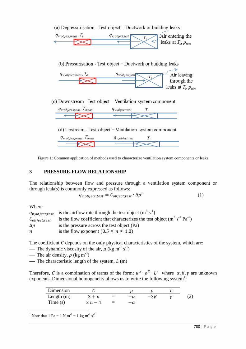
780 | P a g e

Figure 1: Common application of methods used to characterize ventilation system components or leaks

3 PRESSURE-FLOW RELATIONSHIP

The relationship between flow and pressure through a ventilation system component or

through leak(s) is commonly expressed as follows:

(1)

Where

is the airflow rate through the test object (m3 s

-1)

is the flow coefficient that characterizes the test object (m3 s

-1 Pa

-n)

is the pressure across the test object (Pa)

is the flow exponent ( )

The coefficient depends on the only physical characteristics of the system, which are:

The dynamic viscosity of the air, (kg m-1

s-1

)

The air density, (kg m-3

)

The characteristic length of the system, (m)

Therefore, is a combination of terms of the form: where are unknown

exponents. Dimensional homogeneity allows us to write the following system1:

Dimension

(2) Length (m) = Time (s) =

1 Note that 1 Pa = 1 N m

-2 = 1 kg m

-1 s

-2

781 | P a g e

Mass (kg) =

Therefore:

= (3) =

=

Leading to:

(4)

Note that equation (4) is consistent with the correction proposed by Walker (1998) and ASTM

E 779-2010.

When n = 0.5, we find:

(4)

In this particular case (n = 0.5), proportionality is consistent with the commonly used

relationship for an inertial flow through a perfect orifice:

(

)

(4)

Another common expression of the flow-pressure relationship is:

⁄ (5)

Similarly, we obtain:

(6)

4 MASS CONSERVATION THROUGH THE TEST OBJECT

The temperature and pressure conditions around the test object are not necessarily the same as

the ones near the airflow measurement device. Therefore, mass conservation gives:

(7)

782 | P a g e

5 FLOW COEFFICIENT CORRECTION

To allow comparison between tests, we are interested in the flow through the test object under

reference conditions (“0”) for the same pressure difference, . Therefore:

(8)

and

(9)

If is unknown, and may be determined together with a regression analysis

based on equation (8). (Note that this implicitly assumes that all test points are obtained under

similar temperature and pressure conditions.) Then, using equation (4) allows one to obtain

the airflow rate coefficient at reference temperature and pressure conditions:

(

)

(

)

(10)

This also yields:

(11)

and therefore:

(

)

(

)

(12)

Note that when n = 0.5, the air viscosity vanishes from equation (12).

6 APPLICATION TO PRESSURISATION TESTS WITH UNKNOWN FLOW

EXPONENT

This paragraph is relevant to tests performed at multiple pressure stations to obtain both the

airflow rate coefficient and the flow exponent. In this case, we proceed with the following

steps:

Apply mass conservation correction equation (7) to obtain the air leakage flow rate

through the test object for various pressure differences;

Extract and from the values of obtained;

Apply equation (10) to characterize the envelope or ductwork airtightness in reference

conditions.

In depressurisation mode, the air entering the measurement device is inside air (so at

temperature ) while the air passing through the leaks is at temperature (see Figure 1).

Therefore:

(13)

(

)

(

)

(14)

783 | P a g e

In pressurisation mode, we obtain:

(15)

(

)

(

)

(16)

These equations are identical to those used in ASTM E 779-2010. They differ from ISO 9972

where viscosity dependence is neglected.

7 APPLICATION TO PRESSURISATION TESTS WITH DEFAULT FLOW

EXPONENT

This paragraph is relevant either:

When the measurement is performed at only one pressure station;

When the leakage airflow rate(s) at one or several pressure stations is (are) compared

to a threshold value.

In both cases, the exponent is set to a default value and the underlying criterion is:

(17)

Therefore, we will need to derive to check this criterion.

In pressurisation mode:

(

)

(

)

(18)

In depressurisation mode:

(

)

(

)

(19)

8 APPLICATION TO CHARACTERIZATION OF VENTILATION SYSTEM

COMPONENTS

Equation (7) is used to obtain . However, unlike in envelope or ductwork

pressurisation tests, the temperature of the air flowing through the measurement device is

specific to the test apparatus. It may not be assumed in all cases that or as we did previously: this may or may not be true depending on where the air flowing

through the measurement device comes from.

As for the airflow rate or the airflow coefficient, because the test conditions seen by the object

are those inside the ducts in which the object is placed, we may write:

(

)

(

)

(20)

784 | P a g e

9 TEMPERATURE AND PRESSURE DEPENDENCE OF AIR VISCOSITY AND

AIR DENSITY

To apply those corrections, it is useful to know the how the air viscosity and air density vary

with temperature and absolute pressure. When the humidity can be neglected, the following

correlations may be used:

(21)

and

( ( )) (22)

Giving 10-6

kg m-1

s-1

Of course, depending on the accuracy needed and test conditions, other correlations may be

used, such as those proposed in ASTM E779 (2010) and CR 14738 (2002).

10 NUMERICAL APPLICATION

To see the magnitude of the changes induced by those corrections, we have calculated the

airflow rate correction defined as follows in various test conditions:

For equations (18) and (19):

(23)

For equation (20):

(24)

The results show relatively high deviations in possible test conditions (see Table 1 and Table

2).

Airflow correction assuming

meas = i

patm (Pa) i (°C) i (kg m-3

) i (kg m-1

s-1

)

Eq. (20), n =

0,5 Eq. (20), n = 0,65

101325 0 1,29 17,1 · 10-6

-3,5% -0,8%

101325 5 1,27 17,3 · 10-6 -2,6% -0,6%

101325 10 1,25 17,6 · 10-6 -1,7% -0,4%

101325 15 1,22 17,8 · 10-6 -0,9% -0,2%

101325 20 1,20 18,1 · 10-6 0,0% 0,0%

101325 25 1,18 18,3 · 10-6 0,8% 0,2%

101325 30 1,16 18,5 · 10-6 1,7% 0,4%

90000 0 1,15 17,1 · 10-6 2,4% 3,4%

90000 5 1,13 17,3 · 10-6 3,4% 3,6%

90000 10 1,11 17,6 · 10-6 4,3% 3,8%

90000 15 1,09 17,8 · 10-6 5,2% 4,0%

90000 20 1,07 18,1 · 10-6 6,1% 4,2%

90000 25 1,05 18,3 · 10-6 7,0% 4,4%

90000 30 1,03 18,5 · 10-6 7,9% 4,6%

Table 1: Airflow correction (in %) derived from equation (20).

785 | P a g e

Airflow correction assuming e = 10 °C

patm (Pa) i (°C) Eq. (18), n = 0,5 Eq. (18), n = 0,65 Eq. (19), n = 0,5 Eq. (19), n = 0,65

101325 0 0,1% 2,8% -5,2% -3,9%

101325 5 -0,8% 1,2% -3,5% -2,2%

101325 10 -1,7% -0,4% -1,7% -0,4%

101325 15 -2,6% -1,9% 0,0% 1,4%

101325 20 -3,4% -3,4% 1,8% 3,1%

101325 25 -4,2% -4,8% 3,5% 4,9%

101325 30 -5,0% -6,2% 5,2% 6,6%

90000 0 6,2% 7,2% 0,6% 0,1%

90000 5 5,2% 5,5% 2,4% 2,0%

90000 10 4,3% 3,8% 4,3% 3,8%

90000 15 3,4% 2,2% 6,1% 5,6%

90000 20 2,5% 0,7% 8,0% 7,5%

90000 25 1,6% -0,8% 9,8% 9,3%

90000 30 0,8% -2,3% 11,6% 11,1%

Table 2: Airflow correction derived from equations (18) and (19).

11 CONCLUSION

Our analyses show that because the airflow rate coefficient depends on air viscosity, air

density and flow exponent, the corrections that have to be applied to airflow rates through

ventilation system components and leaks to characterize these objects depend on these

variables as well. However, when the flow is inertial (n = 0.5), these corrections do not

depend on air viscosity. Still, the corrections may be significant, which calls for including

these effects systematically when such measurements are performed.

12 REFERENCES

1.ASTM E779-10. 2010. Standard Test Method for Determining Air Leakage Rate by Fan

Pressurization. ASTM. 10 pp

2.CR 14378. 2002. Ventilation for buildings - Experimental determination of mechanical

energy loss coefficients of air handling components. CEN Report 14378.

3.ISO 9972. 2006. Thermal performance of buildings – Determination of air permeability of

buildings - Fan pressurization method. ISO. 30 pp.

4.Walker, I.S., Wilson, D.J., Sherman, M.H. 1998. A comparison of power law to quadratic

formulations or air infiltration calculations. Energy and Buildings, 27: 293-299. Also

published as LBNL report LBNL-41447.

786 | P a g e

TOPICAL SESSION: STATUS OF THE REVISION OF

EN VENTILATION STANDARDS SUPPORTING THE

EPBD RECAST

Jaap Hogeling

*1, Gerhard Zweifel

2,

Bjarne W. Olesen3, and François Rémi Carrié

4

1 ISSO

Kruisplein 25

Rotterdam, The Netherlands


2 Lucerne University of Applied Sciences and Arts

Technikumstrasse 21

CH-6048 Horw

3 Technical University of Denmark

ICIEE, Department of Civil Engineering

Nils Koppels Elle, Building 402

DK-2800 Kgs, Lyngby, Benmark

4 ICEE

93 rue Molière

69003 Lyon, France

1 SYNOPSIS

This session will discuss the major changes of the ventilation standards supporting the

implementation of the Energy Performance of Buildings Directive recast. It is foreseen that

some of these standards will serve as basis of future ISO standards as well.

2 SESSION PROGRAMME

Chairpersons: Jaap Hogeling (Netherlands) and Gerhard Zweifel (Switzerland)

The session will start with an introduction giving the overall context of the revision of the

EPBD standards. Then, session will be structured around 3 presentations that will outline the

major changes in the versions submitted for public enquiry during the summer 2014.

The second generation CEN-EPBD standards, Jaap Hogeling, Chair of CEN TC 371

"Project Committee - Energy Performance of Buildings"

Indoor environmental parameters: revision of EN 15251, Bjarne Olesen, Convenor of

CEN TC 156 / WG 19 "Joint Working Group between CEN/TC 156 and CEN/TC 371

- Revision of EN 15251;2007"

Calculations methods: revision of EN 15241-15242-15243, Gerhard Zweifel,

Convenor of TC 156 / WG 21 "Revision of calculation standards EN 15241, 15242

and 15243"

Inspection of ventilation systems and air conditioning systems, François Rémi Carrié,

Convenor of TC 156 / WG 23 "Guidelines for inspection of ventilation systems and air

conditioning systems"

787 | P a g e

3 CONTEXT

The Energy Performance of Buildings Directive, first published in 2002 (2002/91/EC),

required all EU countries to take measures to improve the energy performance of new and

renovated buildings, in particular through energy regulations and energy certification schemes

for buildings, as well as inspections of boilers and air-conditioners. To help member states

achieve this while allowing fair comparisons of best practices and use of construction

products, the European Commission issued a mandate to European standardisation bodies

which resulted in the publication of a first EPBD package standards in 2007-2008.

In parallel, the European Concerted Action as well as European projects of the Intelligent

Energy Europe such as IEE-CENSE and Harmonac provided feedback on the first EPBD

calling for a second mandate to revise the standards to support the EPBD directive recast

(2010/31/EU).

According to mandate M480, "the improved set of EPBD standards shall become a

systematic, clear and comprehensive package for the benefit of professionals, Member States

and relations with third countries." This new mandate work was divided into two phases:

Phase 1 (2011-2012): This phase included:

Preparation of basic principles and rules, together with the member states, and

based on the overall requirements & expectations on the standards

Development of a modularly structured overarching standard

Preparation of technical rules for drafting all standards. To ease the understanding

and application of the standards, templates have been developed for the standard

texts as well as for checking the consistency of the equations and results provided

by the standards.

Phase 2 (2012-2015): This phase deals with the actual revision of the standards in

separate working groups.

With regard to ventilation, there are 7 EPBD standards under revision within CEN Technical

Committee 156 (Ventilation for Buildings) (Table 1).

Table 1: Ventilation EPBD standards under revision and scope

Input parameters for energy

calculations

Calculation Inspection

Standard(s)

under

revision and

scope

EN 15251 – Indoor

environmental input

parameters

EN 13779 — Performance

requirements for ventilation,

air conditioning and room-

conditioning systems (non-

residential buildings)

EN 15241, EN 15242, EN

15243

These 3 standards have been

re-arranged into a set of 5

standards dealing with

calculation methods for

energy requirements of

ventilation and air-

conditioning systems

(generation, distribution and

emission).

EN 15239, EN 15240

Guidelines for inspection of

ventilation and air conditioning

systems

These 2 standards have been

merged into a single standard

dealing with ventilation and air

conditioning systems, while the

two aspects were divided

between EN 15239 and EN

15240.

The texts are progressively submitted to TC 156 approval and progression to public enquiry.

The enquiry phase should last until spring 2015 and, after addressing comments, the new

standards should be published by the end of 2015.

788 | P a g e

INTEGRATED APPROACH AS A PREREQUISITE FOR

NEARLY ZERO ENERGY SCHOOLS IN

MEDITERRANEAN REGION-ZEMEDS PROJECT

Niki Gaitani

1*, Clara Ferrer

2, Mat Santamouris

1, Claudia Boude

3, Michael

Gerber4, Roberta Ansuini

5,

1. National & Kapodistrian University of Athens, Group of

Building Environmental Research, Building of Physics-5,

University Campus, 15784, Athens, Greece

2. Fundació Privada Ascamm - Parc Tecnològic del Vallès,

Av. Universitat Autònoma, 23 - 08290 Cerdanyola del

Vallès (Barcelona) - Spain

3. Gefosat, 11 ter avenue Lepic – 34070 Montpellier -

France

4. Local Energy Agency of Montpellier

2 Place Paul Bec

34 000 Montpellier - France

5. Province of Ancona, via Ruggeri, 5, Ancona, Italy


ABSTRACT

The present article deals with an integrated nearly zero-energy buildings (nZEB) approach for the retrofit of

Mediterranean school buildings, in the framework of ZEMedS project. EU energy policy encourages member

states to start converting building stock into nZEB and public authorities to adopt exemplary actions. In

Mediterranean regions of Italy, Greece, Spain and France, there are approximately 87.000 schools, consuming in

a rough estimation around 2Mtoe/year. The final energy consumption of typical Mediterranean school built in

the period 60-80’s was estimated, on an average of 100 kWh/m2/y in final energy for all uses. An holistic

approach should combine measures to achieve energy performance and indoor environmental quality (IEQ), as

well as strategies to involve the users, particularly the future generations. ZEMedS project covers a complete

renovation path, tackling strategies for the envelope, the systems and renewable energy applications as well as

the energy management and users' behaviour. In this context, the first results are presented with case studies of

school buildings to be analyzed in terms of the energy efficiency and cost optimality so as to define a detailed

renovation action plan.

KEYWORDS NZEB, Schools, Energy-efficient Retrofitting, IEQ, Mediterranean

1 NZEB EU FRAMEWORK

Buildings represent the largest available source of cost effective energy saving and CO2

reduction potential within Europe. The aim to reduce energy consumption in buildings has led

to Zero Energy Building (ZEB) concept. EU energy policy encourages Member States (MS)

to start converting building stock into nearly zero-energy buildings (nZEB) and public

789 | P a g e

authorities to adopt exemplary actions (EPBD recast). The Energy Efficiency Directive aims

to accelerate the refurbishment rate of public buildings through a binding target. The

commitment to implement energy efficiency in buildings requires efforts from all MS to

contribute to energy efficiency in the building sector, through the adoption of suitable

regulatory and policy instruments. Energy Efficiency Directive (EED, 2012/27/EU) adopted

in October 2012, includes a requirement for Member States to develop long term renovation

strategies for their national building stocks. EED was developed in order to help deliver the

EU’s 20% headline target on energy efficiency by 2020, as well as to pave the way for further

improvements thereafter. Alongside EED, the Energy Performance of Buildings Directive

(EPBD, 2010/31/EU) recast in 2010, sets out numerous requirements including energy

performance certification of buildings, inspection regimes for boilers and air conditioning

plants, and requirements for new buildings to be nearly zero energy. EPBD sets minimum

energy performance standards for buildings undergoing renovation. According to Article 2.2

of the EPBD recast “’nearly zero-energy building’ means a building that has a very high

energy performance, as determined in accordance with Annex I. The nearly zero or very low

amount of energy required should be covered to a very significant extent by energy from

renewable sources, including energy from renewable sources produced on-site or nearby;”

Specifically Annex I states that “The energy performance of a building shall be determined on

the basis of the calculated or actual annual energy that is consumed in order to meet the

different needs associated with its typical use and shall reflect the heating energy needs and

cooling energy needs (energy needed to avoid overheating) to maintain the envisaged

temperature conditions of the building, and domestic hot water needs”. Each Member State

shall ensure that, as from 1 January 2014, 3% of the total floor area of heated and/or cooled

buildings owned and occupied by its central government is renovated each year to meet at

least the minimum energy performance requirements that it has set in application of Article 4

of Directive 2010/31/EU. Furthermore, the Energy Roadmap 2050, published on the 15

December 2011, goes beyond the 2020 goals and provides an analysis of the long term energy

policy orientations: EU is committed to reducing greenhouse gas emissions to 80-95% below

1990 levels by 2050.

In Europe most renovation activity currently achieves only modest energy savings, perhaps

20-30%, but this needs to increase to profound renovations of at least 60% if the full

economic potential is to be realized. Buildings Performance Institute Europe (BPIE) has

studied impact of different renovation pathways on the resulting energy and carbon savings.

The outcome shows scenarios where both the rate and the depth of renovation were

substantially increased, rapid decarbonisation of the energy supply system, could be achieved.

The qualitative definition and the different approaches worldwide to achieve net zero have led

to discussion amongst experts. There have been attempts to tackle a wide spectrum of

additional specifications and issues pertaining to terminology and definitions around buildings

that consume very low or zero energy (or carbon), including those with net energy production

– ‘energy positive’ (Ferrante, 2012). Torcellini et al (2006) have reported four well-

documented definitions based on extensive data from existing low energy buildings: net-zero

site energy, net-zero source energy, net-zero energy costs and net-zero energy emissions.

Moreover, many methodologies have been proposed. They deal with different features such

as: Metric of the balance: delivered energy, primary energy, CO2 (equivalent) emissions,

energy cost, Period of balance: annual, monthly, Type of energy use: operating energy, total

energy and energy use and EE (embodied energy), Type of balance: generation/use, grid

in/out, Renewable supply options: footprint, on-site, off-site, Conversion factors (for primary

energy and CO2 emissions). Even with the recent methodologies and projects, the complexity

of nZEB concept and the existing national and regional policies have led to this current

situation, where only few countries have already set up a nZEB standard. At the end of

November 2012, according to the European Commission only 9 Member States (BE, DK,

790 | P a g e

CY, FI, LT, IE, NL, SE and UK) had reported their nZEB national plans to the Commission

as required. As regards the practical definition of nZEBs, only 5 Member States (BE, CY,

DK, IE and LT) presented a definition that contains both a numerical target and a share of

renewable energy sources.

As the qualitative nature of the nZEB definition leaves some room for interpretation, MS may

follow different paths and uphold different standards in order to fulfil the directive.

ZEMedS project focuses on renovating schools to nZEB in the Mediterranean regions, an area

which represents 17% of EU-27 population. This document presents the current situation in 4

Mediterranean countries (France, Greece, Italy and Spain) regarding nZEB approach and first

developments to tackle school nZEB renovation in a holistic approach.

2 CURRENT SITUATION OF MEDITERRANEAN SCHOOLS

2.1 Spanish School Buildings

Spain is gradually implementing the European Directives related to energy efficiency in

buildings. As regards to nearly Zero Energy Buildings, a roadmap is still to be made available

and no national voluntary labels exist in this approach or even in positive energy buildings.

Concerning best practices, some initiatives are in place to reduce energy consumption in

schools, regarding mainly the use and management. However, no school has been identified

to be renovated following a holistic approach and reaching low energy consumption. In Spain,

the lack of data regarding energy performance of current buildings is an important barrier

when it is time to renovate the built stock. In addition, even that the current indoor conditions

are not satisfying minimum standards in many schools (low ventilation rates, overheating,

glare problems, etc.), indoor environmental quality has not been assessed in scholar buildings

up to date. A program to carry out energy and IEQ assessments in schools would constitute a

good option to provide data to a “Schools observatory” or even a “Buildings observatory”.

Even so, some available information on mean energy consumption in 354 Catalan schools

have shown a wide range of values, 68-122 kWh/m2/year, being the thermal contribution 60-

90%. At first, buildings built before first thermal regulations in force are generally supposed

to consume more energy than recent built. However, increased comfort and use of new

technologies, has led to the situation where often schools built last decades may consume

more than that from the 60-70’s.

2.2 Greek School Buildings

In Greece, transposition of the European Directive 2009/28/EC took effect in June 2010 by

the national law N.3851/2010 on RES (FEK 85/A/4.6.2010). All public buildings by 2015 and

all new buildings by 2020 should cover their primary energy consumption from RES,

combined heat and power, district heating or cooling, and energy efficient heat pumps. The

latest Greek energy regulation exacts from the 2010/31 EPBD recast was laid out on February

of 2013. This law describes a more command and control approach and also encompasses the

2020’s nZEB time-restriction. However, research has to be done to define the Greek roadmap

for nZEBs, with numerical indicator for energy demand and the share of renewable energy

sources. So far there is not any national law that embodies the 2012/27 EED as far as

renovation rates of public buildings are concerned. Greece currently has 15,446 schools of

which 4,500 are over 45 years old. The total energy consumption of school buildings is

around 270,000 MWh. As of 2011, in order to get a new building permit it is necessary to

achieve an annual solar fraction of 60% for sanitary hot water production from solar thermal

systems (Greek NREAP, 2010), or demonstrate the technical difficulties that prevented

791 | P a g e

compliance. New buildings and existing buildings undergoing major renovation must be able

to obtain a class B energy certificate upon completion and are required to have certain

minimum U-values and heat recovery in central air-conditioning units. According to the

scientific research and literature, the average energy consumption in Greek Secondary

Schools was bill-based estimated at 16 kWh/m²/y for electricity and for space heating with oil

at 68 kWh/m²/y (Gaitani, 2010). The mean energy consumption has been categorized per

climate zone with a range from 49kWh/m2/year up to 90kWh/m

2/year (Dascalaki, 2012). For

Greek Schools, the School Building Organisation (SBO) is credited by the national budget for

all the expenditures related to infrastructure throughout the country. SBO is undertaking the

construction of schools through the alternative finance method of PPPs.

2.3 Italian School Buildings

Italy adopted the EPBD-Recast Directive in August 2013 but the decrees (action plan and

definitions) are still missing. This is slowing down the diffusion of the nZEB concept and its

application, as technical regulation in force is still the one related to the previous Directive

2002/91/CE – EPBD. Regulation constraints refer mainly to heating consumption, while for

cooling consumption only few aspects are considered. More than 60% of Italian school

buildings were built without any energy-related regulation in force (before 1976) and less

than 10% were built after the adoption of the Law 10:1991 which is the first regulation in

Italy introducing clear constraints about energy efficiency. Currently, the lack of appropriate

energy management may often conduct to the situation during mid seasons where the heating

system is on but school users open the windows. The great majority of schools are public, and

as the public bodies facing a lot of economical problems in the last years due to the financial

crisis, the possibilities for deep renovations are minor. The status of school buildings is

getting worse but there is a vast lack in funding. Furthermore, a lot of school buildings would

need a seismic upgrading, that is considered more urgent than energetic upgrading, and

however it is a lot more expensive.

2.4 French School Buildings

In France a series of targets have been set by the Environment Round Table and implemented

in law as of 2009. The widespread development of new, low consumption buildings has been

encouraged, the next step being the development of positive energy buildings by 2020.

Extensive renovations of the existing building stock are under way, with the goal being about

400,000 renovations per year (Ecofys, 2013) leading to a 38% reduction in primary energy

consumption by 2020. Public buildings are to be renovated to achieve a minimum reduction

of 40% in energy and 50% in greenhouse gas emissions within 8 years (French NREAP,

2010). Local authorities are the decision makers when it comes to renovating a school. But

they often do not have information about the energy consumption or indicators to assess

comfort in their buildings. Thus, the decision to renovate a school is not always dependent on

the level of consumption of the building but, in fact, is a political choice. However, when a

renovation project is approved, the local authorities set the goals of energy efficiency and

comfort level and budget of the operation. They appoint a technical team (architects and

consultants) for this project and to connect with companies that carry out the mission. In

addition, other induced work is necessary and can have a significant impact on the budget of

the operation. Indeed, other regulatory constraints related to the accessibility of the disabled

or fire safety must be taken into account. Cities so often encounter funding problems and must

set priorities. Currently, thermal regulation for existing buildings does not go far enough and

to achieve a NZEB goal, is up to the owners to set the target at the beginning of the project.

Although they might lack the expertise in this domain. In France, especially in Languedoc-

792 | P a g e

Roussillon, the first examples of successful renovation are becoming increasingly known.

They were initiated and financially supported by the Languedoc -Roussillon and ADEME

through calls for proposals. They gave a good example of how the project should be managed

in terms of energy performance and how to take into consideration summer comfort.

Nevertheless, the accurate results will be derived in the future and current quantitative

indicators are missing.

2.5 MED particularities

The majority of the regions with Mediterranean climates have relatively mild winters and hot

summers. Although significant variations can be found among the places that satisfy the

Mediterranean climate criteria, the countries bordering the basin share some similarities: in

almost all the coastline cities, the minimum yearly average temperature is between 5–10oC

and the maximum is between 27–34oC.For the past few decades there has been a sizeable

increase in summer cooling demand in the Mediterranean area, especially in urban areas.

Global warming is expected to adversely affect both the environment and human activities in

the Mediterranean area, with scenarios for average yearly air temperatures predicting an

increase between 2.2 and 5.1ºC by 2100, or even sooner than that. According to the IPCC

(2007), an average temperature rise above 1.5oC is likely to have severe impacts in local

environments and ecosystems, while increased temperatures are expected to bring about

longer heat waves, decreased precipitation and a longer summer in general. These predictions

should be taken seriously into consideration when renovating buildings and, particularly,

schools.

School holidays in Mediterranean are mainly in Summer (2 months for teachers, 3 months for

students) and this is why the almost the totality of schools has not a cooling system. As a

result, schools have a not-too-high consumption, but this causes also a lot of comfort

problems (from April to October).

Decision makers in MED regions are facing a complex situation, where needed energy

renovations should integrate not only energy savings but also health and comfort

requirements, especially in the framework of climate change. Moreover, current economic

crisis makes this need more challenging. Overall cost analysis would be a great tool for

decision makers to help identify the best solution. Training of decision makers as well as of

the designers is necessary to raise awareness of these issues.

3 INTEGRATED APPROACH TOWARDS NZEB

European supported project ZEMedS, standing for Zero Energy Mediterranean Schools, will

help overcome two main barriers: insufficient knowledge about existing technologies to

renovate schools up to nZEB goals and inefficient tools for decision makers undergo these

renovations. ZEMedS includes, among other activities, developing high quality TOOLkit for

both building designers and decision makers, studying 10 real schools and developing

tendering specifications.

3.1 Integrated Design

Buildings demand energy in their life cycle, directly for their construction, operating energy

as well as for the rehabilitation/ demolition. In addition, they demand indirectly through the

embodied energy. Integrated design is a concerted methodology which emphasizes the

development of a holistic building design. This approach invites all parties into the planning

process, and takes into account all the areas of building's expertise plus the users.

793 | P a g e

In the framework of ZEMedS project, it is proposed to follow a holistic approach. Integrated

Design methodology offers taking into account all the related criteria and actors involved.

According to MaTrID project, ID steps are the following: 0. Project development; 1. Design

basis; 2. Iterative problem solving; 3. On track monitoring; 4. Delivery; 5. In use.

Focusing on school renovation, the project SchoolVentCool proposes a school renovation

methodology that considers: technical and structural aspects, ecological aspects, educational

and socioeconomic aspects and economic aspects. The methodology starts with having an

overview of the entire building portfolio of public bodies, in order to make the investment

following a master plan.

Figure 1SchoolVentCool methodology

Finally, integrated approach must consider from the beginning the costs and benefits during

all building life cycle. If the focus is on the investment costs, without having the overall

picture of the savings and benefits in the energy use, but also in better health learning

outcomes, among other, short-term oriented decisions may be taken, compromising the way

towards nZEB goals.

3.2 Energy efficiency in MED Schools

Realization of nearly zero energy buildings entail a wide range of measures related to

technologies, systems, and solutions with varying degrees of complexity depending upon the

location and surrounding environmental conditions. Lighting, heating, cooling, ventilation

and various plug loads need to be minimized while behavioural aspects of the users should be

analysed to become more environmental conscious.

Figure 2Key issues for NZEB renovation in Mediterranean schools

NZEB school

Very low heating demand

Avoid overheating

Renewable energy supply

Guarantee of IEQ

Raise awareness

Users/Education for future

generations

794 | P a g e

As shown in Fig 1, NZEB renovation of Mediterranean schools not only should consider the

energy performance (reduction of energy consumption and renewable energy supply), but

should also incorporate criteria which may compromise the objectives of reducing

consumption, such as the behaviour of building’s user. In Mediterranean climate, summer

comfort needs to be seriously addressed. The designers and decision makers of school

buildings need to pay particular attention to the quality of indoor environment which will

impact on health but also in raising awareness of future generations about these issues.

Figure 3Energy steps paving the way to NZEB

ZEMedS project proposes an “energy steps” methodology (fig. 3) in order to achieve the final

nZEB goal. Energy strategies to be implemented need to pay particular attention to:

- Users. Energy management should not rely on their sole responsibility. However they

are going to play a key role in energy consumption in the school and beyond, when

pupils will leave de school. For this reason, users need to be part of the renovation

process and take an active role in school every day energy management;

- Heating is the main contributor to the energy demand. Passive heating techniques have

been largely applied in colder climates. In MED regions they need to be implemented,

taking care of not increasing cooling demand and of cost-effective criteria. For

example, heat recovery ventilation may be not cost-effective for a school located on

the MED coast.

- Overheating problems appear because of solar radiation and users’ heat production

(internal gains). In Mediterranean regions, just a range of passive cooling techniques

can result to avoid implementing a cooling system. At least, solar shading, cool

surfaces and ventilative cooling are to prescribe for all the cases;

- Renewable energy supply. The leading RES potential in whole MED is solar energy.

However, other sources may be needed. Biomass from local woods is generally

underexploited; however, sustainability and gas emissions need to be studied

previously. Wind and geothermal will constitute the other major alternatives.

- Ventilation (See following chapter)

Particularly, a detailed energy and cost analysis will be applied with EnergyPlus software for

a year in 10 typical school buildingsfrom 5 regions (Barcelona (ESP) Montpellier (FR),

Ancona (IT), Peristeri (GR) , Tuscany (IT)). The main objectives are (1) to assess how an

existing building is far from the performances of a nZEB, and (2) is to assess the effort in

retrofitting up to NZEB goal.

Current situation

Use & management

Demand reduction

Efficient systems

RES BMS NZEB

795 | P a g e

3.3 Indoor Environmental Quality

Together with the energy demand, the general requirements of indoor climate conditions

should be considered, in order to avoid possible adverse consequences. The school buildings

in general are characterized by a high density of people per unit area, which is associated with

increased concentrations of certain pollutants and therefore with reduced attentiveness of

students and less ability to learn. Moreover, students are a vulnerable group necessitating a

special attention. Characterized by: (1) Greater respiratory rate compared with adults; (2)

Lower weight; (3) Higher levels of physical activity; (4)The human lung continues to develop

until adolescence. As it concerns Indoor Environmental Quality (IEQ) in Mediterranean

schools, the key issues could be summarized:

Indoor environment/Ventilation: The priority is to reduce indoor pollutant sources

(and outdoors when possible), After that, a ventilation strategy needs to be defined

according to many criteria (building characteristics, local climate, current outdoor and

indoor pollutants, energy performance, thermal comfort, users, cost). The existing

strategy is usually natural ventilation but often results in poor indoor conditions.

Setting the ventilation requirements is quite challenging (current standards for schools

may vary 1000-1500 ppm limit value for CO2, while ventilation rates range 5.5-12.5

l/s/person). In addition, according to ANSES, current knowledge in IAQ and health

effects is not enough consistent to set limit values that will guarantee health

protection, performance and comfort perception. Some key findings (Simoni et al,

2010) point out that a higher frequency of symptoms linked to child asthma could be

associated to CO2 concentrations higher than 1000 ppm. Apart from that, ANSES

states that a unique CO2 indicator is not enough to monitor and guarantee IAQ because

of other so important pollutants that may not be always linked (VOC’s, particulate

matter (PM2.5; PM10...)...). The chosen ventilation strategy should guarantee a

healthy air, help preventing overheating and achieve energy performance.

Daylighting is often easy to be guaranteed as most of the schools do not usually have

important depths and are also equipped with large window areas. Nevertheless shading

system must be optimized with daylight requirements to avoid glare problems

Thermal discomfort conditions have to be considered carefully mainly because of the

high occupant density in classrooms and because of the negative influences that an

unsatisfactory thermal environment has on learning performance of the pupils.

Overheating is a problem for MED school building design. Generally, there are no

cooling systems in school buildings. As new buildings are built with more thermal

insulation and to improved standards of air tightness, concerns are emerging of an

increased risk of overheating. Alongside the key issue of indoor air quality,

overheating is a risk that needs to be managed carefully as we move further towards

the aim of nZEB and now ranks among greatest concerns that need to be addressed as

a priority

4 CONCLUDING REMARKS

The main objectives of ZEMedS project includes the assessment of energy conservation

potentials in Mediterranean schools in relation to the environmental quality perspectives.

School buildings feature indoor air quality problems while their energy consumption and

global environmental quality could be improved significantly. Many studies have identified

796 | P a g e

the lack of date base, knowledge, experience and best-practice examples as barriers in

refurbishment projects. School renovation should be focused on energy savings but also on

improving indoor environment for better learning outcomes. Setting the priorities on different

needs (safety, maintenance, spatial requirements, energy savings, etc.) is profoundly depend

on the budget availability and the existing funding channels. Nowadays, the economic crisis

in most of Mediterranean countries has led to very reduced self financing capacity, being the

budgets allocated to cover only urgent needs and significantly reducing the capacities of

municipalities and regional administrations.

ZEMedS actions are mainly addressed to involve two target groups, school decision makers

and building designers, by providing technical and financial assistance on nZEB renovation of

schools in Mediterranean climates, and giving support in succeeding in implementing school

renovation with nZEB goals. An holistic approach will combine cost optimal measures to

achieve energy performance and indoor environmental quality (IEQ) in schools. ZEMedS

project will pave the way for a complete renovation path, tackling strategies for the envelope,

the systems and renewable energy applications as well as the energy management and users'

behaviour of Med Schools.

References

1. European Parliament and Council (2010) DIRECTIVE 2010/31/EU of 19 May 2010

on the energy performance of buildings (recast). Official Journal of the European Union,

18.6.2010

2. Directive 2012/27/EU of the European Parliament and of the Council of 25 October

2012 on energy efficiency, amending Directives 2009/125/EC and 2010/30/EU and repealing

Directives 2004/8/EC and 2006/32/EC

3. [French NREAP] French Ministry for Ecology, Energy, Sustainable Development and

Sea (2010) National Action plan for the promotion of renewable energies 2009-2020

4. [Greek NREAP] Greek Ministry of Environment, Energy and Climate Change (2010)

National Renewable Energy Action Plan in the Scope of Directive 2009/28/EC

5. [Italian NREAP] Italian Ministry for Economic Development (2010) Italian National

Renewable Energy Action Plan

6. [Spanish NREAP] Spanish Ministry of Industry, Tourism and Commerce (2010)

Spain's National Renewable Energy Action Plan 2011-2020

7. IEA ECB&CS Annex 36 - Retrofitting in Educational Buildings - Energy Concept

Advisor for Technical Retrofit Measures. Heike Kluttig Evaluation of Questionnaire on the

Energy Consumption of Educational Buildings . In: T. Mroz& H. Erhorn, State of the Art

Overview: Questionnaire Evaluations. IEA ECB&CS Annex 36

8. ECOFYS 2011. Panorama of the European non-residential construction sector

9. Ferrante, A (2012) ‘Zero- and low-energy housing for the Mediterranean climate’,

Advances in Building Energy Research, 6:1, pp. 81-118

797 | P a g e

10. Gaitani N. PhD. Energy Rating & Environmental Quality of School Buildings in

Greece (2010)

11. Dascalaki, E.G., Balaras, C.A., Gaglia, A.G., Droutsa, K.G., Kontoyiannidis, S. (2012)

‘Energy Performance of Buildings – EPBD in Greece’, Energy Policy 45, pp. 469–477

12. Ecofys (2013). Towards nearly zero-energy buildings - Definition of common

principles under the EPBD - Final report. Available at:

http://ec.europa.eu/energy/efficiency/buildings/doc/nZEB_full_report.pdf [Accessed 12th

September 2013]

13. Torcellini, P., Pless, S., &Deru, M., Crawley, D. (2006) Zero energy buildings: A

critical look at the definition; Preprint. Available at

http://www.nrel.gov/docs/fy06osti/39833.pdf [Accessed 12th September 2013]

14. 2013 ANSES (French Agency for Food, Environmental and Occupational Health &

Safety). CO2 concentrations in indoor air and health effects (Concentrations de CO2 dans

l’air intérieur et effets sur la santé). Scientific edition (in French) Free download:

https://www.anses.fr/en/documents/AIR2012sa0093Ra.pdf

15. Integrated Design Guidelines. MaTrID project.

http://www.integrateddesign.eu/downloads/MaTrID_Process-Guideline.pdf

16. Brochure SchoolVentCool_The Way Towards Your Cool School.

http://www.schoolventcool.eu/

17. HealthVent project. http://www.healthvent.byg.dtu.dk/

18. Simoni M, Annesi-Maesano I, Sigsgaard T, Norbäck D, Wieslander G, Nystad W,

Canciani M, Sestini P, Viegi G (2010), School air quality related to dry cough, rhinitis and

nasal patency in children, European Respiratory Journal, 35:742-749

19. ZEMedS: http://www.zemeds.eu/

798 | P a g e

Event sponsors The conference organizers are grateful to the following companies for their support to this

event

ISBN : 2-930471-44-1

EAN: 9782930471440

Paper title for the 2011 AIVC-TIGHTVENT conference

Documents

Transcript of Paper title for the 2011 AIVC-TIGHTVENT conference