Paper Template in Two-Column Format -..: Conference on ...
97
Number 2 ISSN: 2085-6350 PROCEEDINGS OF CONFERENCE ON INFORMATION TECHNOLOGY AND ELECTRICAL ENGINEERING INTERNATIONAL SESSION Signals, Systems, and Circuits DEPARTMENT OF ELECTRICAL ENGINEERING FACULTY OF ENGINEERING GADJAH MADA UNIVERSITY
-
Upload
khangminh22 -
Category
Documents
-
view
1 -
download
0
Transcript of Paper Template in Two-Column Format -..: Conference on ...

Number 2 ISSN: 2085-6350
PROCEEDINGS OF CONFERENCE ON
INFORMATION TECHNOLOGY AND ELECTRICAL ENGINEERING
INTERNATIONAL SESSION
Signals, Systems, and Circuits
DEPARTMENT OF ELECTRICAL ENGINEERING FACULTY OF ENGINEERING GADJAH MADA UNIVERSITY

Conference on Information Technology and Electrical Engineering (CITEE)
Organizer
Steering Commitee • Adhi Susanto (UGM) • Hamzah Berahim (UGM) • Thomas Sri Widodo (UGM) • Dadang Gunawan (UI) • Heri Mauridi (ITS) • Yanuarsyah Harun (ITB) • Anto Satrio Nugroho (BPPT) • Son Kuswadi (PENS)
Advisory Board
• Tumiran (UGM) • Lukito Edi Nugroho (UGM) • Anto Satrio Nugroho (BPPT) • Son Kuswadi (PENS)
General Chair
• Bambang Sutopo Organizing Chairs
• Risanuri Hidayat • Sri Suning Kusumawardhani • Ridi Ferdiana • Adha Imam Cahyadi • Budi Setiyanto
Program Chairs
• Prapto Nugroho • Agus Bejo • Cuk Supriyadi Ali Nandar (BPPT) • Yusuf Susilo Wijoyo
Publication Chair
• Enas Dhuhri K Finance Chairs
• Eny Sukani Rahayu • Maun Budiyanto • Roni Irnawan
Secretariats
• Astria Nur Irfansyah • Lilik Suyanti
YOGYAKARTA, AUGUST 4, 2009

Conference on Information Technology and Electrical Engineering (CITEE) 2009
FOREWORD
First of all, praise to Almighty God, for blessing us with healthy and ability to come here, in the Conference of Information and Electrical Engineering 2009 (CITEE 2009). If there is some noticeable wisdoms and knowledge must come from Him.
I would like to say thank you to all of the writers, who come here enthusiastically to share experiences and knowledge. Without your contribution, this conference will not has a meaning.
I also would like to say thank you to Prof. Dadang Gunawan from Electrical Engineering, University of Indonesia (UI), Prof. Yanuarsyah Haroen from Electrical Engineering and Informatics School, Bandung Institute of Technology, ITB, Prof. Mauridhi Hery Purnomo from Electrical Engineering Department, Surabaya Institute of Technology (ITS). And also Prof. Takashi Hiyama from Kamamoto University, Japan, Thank you for your participation and contribution as keynote speakers in this conference.
This conference is the first annual conference held by Electrical Engineering Department, Gadjah Mada University. We hope, in the future, it becomes a conference of academics and industries researchers in the field of Information Technology and Electrical Engineering around the world. We confine that if we can combine these two fields of sciences, it would make a greater impact on human life quality.
According to our data, there are 140 writers gather here to present their papers. They will present 122 titles of papers. There are 47 papers in the field of Electrical Power Systems, 53 papers in the area of Systems, Signals and Circuits, and 22 papers in Information Technology. Most of these papers are from universities researchers.
We hope, the result of the proceedings of this conference can be used as reference for the academic and practitioner researchers to gain
At last, I would like to say thank you to all of the committee members, who worked hard to prepare this conference. Special thanks to Electrical Engineering Department, Gadjah Mada University, of supporting on facilities and funds. Thank you and enjoy the conference, CITEE 2009, and the city, Yogyakarta
August, 4Th, 2009
Bambang Sutopo
Electrical Engineering Dept., Fac. of Engineering, GMU


Proceedings of CITEE 2009 Number 2 ISSN: 2085-6350
Table of Contents
Organizer ii Foreword iii Table of Contents v Schedule vii KEYNOTE Social Intelligent on Humanoid Robot: Understanding Indonesian Text Case Study 1 Mauridhi Hery Purnomo (Electrical Engineering Department, ITS, Indonesia) Signal Processing: Video Compression Techniques 4 Dadang Gunawan (Electrical Engineering Department, University of Indonesia) Intelligent Systems Application to Power Systems - Prof. Takashi Hiyama (Kumamoto University, Japan) INTERNATIONAL SESSION: Signals, Systems, and Circuits Analysis and Simulation of Bus-Clamping PWM Techniques Based on Space Vector Approach 7 Ms.M.Thanuja, Mrs. K. SreeGowri Medical Image Processing of Proximal Femur X-Ray for Osteoporosis Detection 15 Riandini, Mera Kartika Delimayanti, Donny Danudirdjo Performance Evaluation of Free-Space Optical Communication System on Microcell Networks in Urban Area 22 Purnomo Sidi Priambodo, Harry Sudibyo and Gunawan Wibisono A Measure of Vulnerability for Communication Networks: Component Order Edge Connectivity 27 A. Suhartomo, Ph.D. The Speech Coder at 4 kbps using Segment between Consecutive Peaks based on the Sinusoidal Model 31 Florentinus Budi Setiawan Automatic Abnormal Waves Detection from the Electroencephalograms of Petit Mal Epilepsy Cases to Sort Out the Spikes Fp1 - Fp2, the Sharps, the Polyphase Based on Their Statistical Zerocrossing
35
Siswandari N, Adhi Susanto, Zainal Muttaqin Studies on the Limitation of Fighter Aircraft Maneuver Caused by Automatic Control Design 39 Okky Freeza Prana Ghita Daulay, Arwin Datumaya Wahyudi Sumari Feature Extraction and Selection on Osteoporosis X-Ray Image for Content Based Image Retrieval (CBIR) Purposes 45 Usman Balugu, Ratnasari Nur Rohmah, Nurokhim The Implementation of Turbo Encoder and Decoder Based on FPGA 51 Sri Suning Kusumawardani and Bambang Sutopo BER Performance Analysis of PAM and PSM for UWB Communication 55 Risanuri Hidayat Hardware Model Implementation of a Configurable QAM Mapper-Demapper for an Adaptive Modulation OFDM System 61 Budi Setiyanto, Astria Nur Irfansyah, and Risanuri Hidayat Hardware Model Implementation of a Baseband Conversion, Chip Synchronization, and Carrier Synchronization Technique for a Universal QAM System
69
Budi Setiyanto, Mulyana, and Risanuri Hidayat Comparison Study of Breast Thermography and Breast Ultrasonography for Detection of Breast Cancer 75 Thomas Sri Widodo, Maesadji Tjokronegore, D. Jekke Mamahit Adaptive Polynomial Approximation for Gravimetric Geoid: A case study using EGM96 and EIGEN-GL04C Geopotential Development
78
Tarsisius Aris Sunantyo, Muhamad Iradat Achmad Cerebellar Model Associative Computer (CMAC) for Gravimetric Geoid study based on EGM96 and EIGEN-GL04C Geopotential Development
83
Muhamad Iradat Achmad, Tarsisius Aris Sunantyo, Adhi Susanto
Conference on Information Technology and Electrical Engineering (CITEE)


Conference on Information Technology and Electrical Engineering (CITEE)
SCHEDULE Tuesday, August 4, 2009
07.30 – 08.00: Registration 08.00 – 08.15: Opening
1. Welcome speech by conference chairman 2. Speech by GMU’s Rector
08.15 – 09.20: PLENARY SESSION Prof. Takashi Hiyama (Kumamoto University, Japan): Intelligent Systems Application to
Power Systems Prof. Dr. Mauridhi Hery Purnomo (Electrical Engineering Department,ITS, Indonesia):
Social Intelligent on Humanoid Robot: Understanding Indonesian Text Case Study Prof. Dr. Dadang Gunawan (Electrical Engineering Department, University of
Indonesia): Signal Processing: Video Compression Techniques Prof. Dr. Yanuarsyah Haroen (Electrical Engineering and Informatics School, ITB,
Indonesia): Teknologi Sistem Penggerak dalam WahanaTransportasi Elektrik 09.20 – 09.30: Break
PARALLEL SESSION
INTERNATIONAL SESSION (Room 1, 2) Room: 1
Time Group Country/City Author(s) or Presenter(s)
09.30 – 09.45 P Malaysia Zulkarnain Lubis, Ahmed N. Abdalla, Samsi bin MD said .Mortaza bin Mohamed
09.45 – 10.00 P Papua Adelhard Beni Rehiara 10.00 – 10.15 P Medan Zakarias Situmorang 10.15 – 10.30 P Bandung Kartono Wijayanto, Yanuarsyah Haroen 10.30 – 10.45 Coffee Break 10.45 – 11.00 P Bandung Hermagasantos Zein 11.00 – 11.15 P Surabaya Ali Musyafa, Soedibjo, I Made Yulistiya Negara , Imam Robandi 11.15 – 11.30 P Surabaya Buyung Baskoro, Adi Soeprijanto, Ontoseno Penangsang 11.30 – 11.45 P Surabaya Eko Prasetyo, Boy Sandra, Adi Soeprijanto 11.45 – 12.00 P Yogyakarta T. Haryono, Sirait K.T., Tumiran, Hamzah Berahim 12.00 – 13.00 Lunch Break 13.00 – 13.45 P Surabaya Dimas Anton Asfani, Nalendra Permana 13.15 – 13.30 P Surabaya Dimas Anton Asfani, Iman Kurniawan, Adi Soeprijanto
13.30 – 13.45 I Surabaya F.X. Ferdinandus, Gunawan, Tri Kurniawan Wijaya, Novita Angelina Sugianto
13.45 – 14.00 I Surabaya Arya Tandy Hermawan, Gunawan, Tri Kurniawan Wijaya 14.00 – 14.15 I Surabaya Herman Budianto, Gunawan, Tri Kurniawan Wijaya, Eva Paulina Tjendra 14.15 – 14.30 Coffee Break 14.30 – 14.45 I Yogyakarta Bambang Soelistijanto 14.45 – 15.00 I Surakarta Munifah, Lukito Edi Nugroho, Paulus Insap Santosa 15.00 – 15.15 P Yogyakarta Nurcahyanto, T. Haryono, Suharyanto. 15.15 – 15.30 P Yogyakarta Agni Sinatria Putra, Tiyono, Astria Nur Irfansyah
Notes:
1. P: Electrical Power Systems; S: Signals, Systems, and Circuits; I: Information Technology 2. Paper titles are listed in Table of Contents
Department of Electrical Engineering, Faculty of Engineering, Gadjah Mada University

Conference on Information Technology and Electrical Engineering (CITEE)
Room: 2 Time Group Country/City Author(s) or Presenter(s)
09.30 – 09.45 S INDIA Ms.M.Thanuja, Mrs. K. SreeGowri 09.45 – 10.00 S Jakarta A. Suhartomo 10.00 – 10.15 S Jakarta Riandini, Mera Kartika Delimayanti, Donny Danudirdjo 10.15 – 10.30 S Jakarta Purnomo Sidi Priambodo, Harry Sudibyo and Gunawan Wibisono 10.30 – 10.45 Coffee Break 10.45 – 11.00 I Yogyakarta Arwin Datumaya Wahyudi Sumari, Adang Suwandi Ahmad 11.00 – 11.15 I Yogyakarta Arwin Datumaya Wahyudi Sumari, Adang Suwandi Ahmad 11.15 – 11.30 I Lampung Sumadi, S; Kurniawan, E. 11.30 – 11.45 S Semarang Florentinus Budi Setiawan 11.45 – 12.00 S Semarang Siswandari N, Adhi Susanto, Zainal Muttaqin 12.00 – 13.00 Lunch Break 13.00 – 13.45 S Yogyakarta Thomas Sri Widodo, Maesadji Tjokronegore, D. Jekke Mamahit 13.15 – 13.30 S Yogyakarta Tarsisius Aris Sunantyo, Muhamad Iradat Achmad 13.30 – 13.45 S Yogyakarta Muhamad Iradat Achmad, Tarsisius Aris Sunantyo, Adhi Susanto 13.45 – 14.00 S Yogyakarta Usman Balugu, Ratnasari Nur Rohmah, Nurokhim 14.00 – 14.15 S Yogyakarta Okky Freeza Prana Ghita Daulay, Arwin Datumaya Wahyudi Sumari 14.15 – 14.30 Coffee Break 14.30 – 14.45 S Yogyakarta Sri Suning Kusumawardani and Bambang Sutopo 14.45 – 15.00 S Yogyakarta Risanuri Hidayat 15.00 – 15.15 S Yogyakarta Budi Setiyanto, Astria Nur Irfansyah, and Risanuri Hidayat 15.15 – 15.30 S Yogyakarta Budi Setiyanto, Mulyana, and Risanuri Hidayat
NATIONAL SESSION (Room 3, 4, 5, 6, 7)
Yogyakarta, August 4, 2009
Proceedings of CITEE, August 4, 2009 Keynote - 1
Social Intelligent on Humanoid Robot: Understanding Indonesian Text
Case Study
Mauridhi Hery Purnomo Electrical Engineering Department-Institut Teknologi Sepuluh November
Surabaya 60111, Indonesia [email protected]
Abstract— Social affective and emotion are required on
humanoid robot performance to make the robot be more human. Social intelligent are the individual ability to manage relationship with other agents and act wisely based on previous learning experiences. Here, social intelligent is intended to understand Indonesian text. How the computation process, as well as affective interaction, emotion expression of the humanoid robot to the human statement. This process is a highly adaptive complex approximation, dependently on its entire situation and environment.
Keywords—social, affective, emotion, intelligent, computing (key words)
I. INTRODUCTION Social and interactive behaviors are necessary
requirements in wide implementation areas and contexts where robots need to interact and collaborate with other robots or humans. The nature of interactivity and social behavior in robot and humans is a complex model.
An experimental robot platform KOBIE, which provides a simulation tool for emotion expression system includes an emotion engine was developed. The simulation tool provides a visualization interface for the emotion engine and expresses emotion through an avatar. The system can be used in the development of cyber characters that use emotions or in the development of an apparatus with emotion in a ubiquitous environment [1]. To improve the understandability and friendliness in human-computer interfaces and media contents, a Multimodal Presentation Markup Language (MPML) is developed. MPML is a simple script language to make multi-modal presentation contents using animated characters for presenters [2]. Other effort in the robot head which uses arm-type antennae, eye-expression, and additional exaggerating parts for dynamic emotional expression is also developed. The robot head is developed for various and efficient emotional expressions in the Human-Robot interaction field. The concept design of the robot is an insect character [3]. In regard to artificial cognitive, iCub humanoid robot systems is developed. The system is open-systems 53 degree-of-freedom cognitive humanoid robot, 94 cm tall, the same size as a three year-old child. Able to crawl on all fours and sit up, its hands will allow dexterous manipulation, and its head and eyes are fully articulated. It
has visual, vestibular, auditory, and haptic sensory capabilities [4]. An innovative integration of interactive group learning, multimedia technology, and creativity used to enhance the learning of basic psychological principles was created. This system is based on current robotic ideology calling for the creation of a PowerPoint robot of the humanoid type that embodies the basic theories and concepts contained in a standard psychological description of a human being [5]. Now days, not only visual and auditory information are used in media and interface fields but also multi-modal contents including documents such like texts. Thus, in this paper, a part of result on emotion expression and environment through understanding Indonesian text, as affective interaction between a human and a robot is explored. The paper is organized as follows. In Section 2, the general emotion and expression system on life-like agent is presented. Section 3 describes the experimental on Indonesian text classification. In Section 4, the preliminary result in emotion classification of Indonesian article text is discussed.
II. EMOTION AND EXPRESSION ON LIFE-LIKE AGENT
Social Computing, Social Agent, and Life-likeness Many Psychologists have studied a definition and classification of emotions, therefore, so many classification methods of emotions and expressions. However, we need to choose categories of emotions that are suitable expressed by robot, as well as the well-known Ekman’s 6 basic emotion expressions model can be used.
In social computing life-like characters are the key, and the affective functions create believability. To articulate synthetic emotions can be presented as; personalities, human interactive behavior or presentation skills. The personalities; by means of body movement, facial display, and the coordination of the embodied conversational behavior of multiple characters possibly including the user. Personality is key to achieving life-likeness
Some Applications of Life-Like Character
Life-like characters are synthetic agents apparently living on the screen of computers. Life-like character can be implemented as virtual tutors and trainers in interactive learning environments. On the web as an information expert, presenter, communication partners, and enhancing the search engine. The other application as actors for entertainment, in
Conference on Information Technology and Electrical Engineering (CITEE) ISSN: 2085-6350

2 Keynote Proceedings of CITEE, August 4, 2009
online communities and guidance systems as personal representatives.
Early characterization of the emotional and believable character was raised by Joseph Bates. He said, the portrayal of emotions plays a key role in the aim to create believable characters, one that provides the illusion of life, and thus permits the audience’s suspension of disbelief. In game and animation, suspension of disbelief is very important, for instance as: synthetic actors, non-player characters, and embodied conversational agents.
Emotion and personality are often seen as the affective bases of believability, and sometimes the broader term social is used to characterize life-likeness.
III. CLASSIFICATION SYSTEM FOR INDONESIAN TEXT Information growth, including texts are faster than
human ability, thus help system is quite necessary. For instance as the following illustration;
The Recent study, which used Web searches in 75 different languages to sample the Web, determined that there were over 11.5 billion (1012) Web pages in the publicly indexable Web as of the end of January 2005
As of March 2009, the indexable web contains at least 25.21 billion pages
On July 25, 2008, Google software engineers Jesse Alpert and Nissan Hajaj announced that Google Search had discovered one trillion unique URLs
As of May 2009, over 109.5 million websites operated
label
traininginput
languagedependentNLP tools
featureextractor ..features..
machinelearning
classifiermodel
testinput
languagedependentNLP tools
featureextractor ..features.. predicted
label
(b) prediction phase
(a) training phase
Figure 1. Example of Indonesian Text Classification
FreeText
KnowledgeBase
InformationRetrieval
Text-basedConversational Agent
User (Human)
TextInput
Response
TextClassification
TextMining
Figure 2. Knowledge from Free (Unstructured) Text
The illustrations as mentioned above explain the essential of help system especially in Indonesian text. We have developed a system for understanding and classifying Indonesian text, and the block diagram as shown in figure 1 and figure 2.
Figure 1 is an example how to train machine (agent) in order responsive to the external and adequate response. The case study is, Indonesian text classification. There are two types of machine learning, supervised and unsupervised learning.
Figure 2 show a block diagram process of embodied conversational agent.
IV. EMOTION CLASSIFICATION FROM INDONESIAN ARTICLE TEXT
The following sentences are sample of statements, and some emotion expressions;
• “When a car is overtaking another and I am forced to drive off the road” → anger
• “When I nearly walked on a blindworm and then saw it crawl away” → disgust
• “When I was involved in a traffic accident” → fear
• “I do not help out enough at home” → guilt
• “Passing an exam I did not expect to pass” → joy
• “Failing an examination” → sadness
• “When, as an adult I have been caught lying or behaving badly” → shame
Based on some statements and the emotion expression as mentioned above in Indonesian text, the preliminary classification results are shown in the table 1, figure 3 and figure 4.
The classification is divided into six (6) classes of emotion: disgust, shame, anger, sadness, joy and fear. Each class has 200 text files, data: “as-is”; DataNot: pre-processing only handles “not”. Split ratio 0.5 shows f-measure scores 0.59
Pre-processing Steps
Text Classification (TC) techniques usually ignore stop-words and case of input text. In pre-processing step, stop-words removal can be applied.
Stop-words such as “not”, “in”, “which” and exclamation marks (“!”) usually do not affect categorization of text.
TABLE I. NAÏVE BAYES CLASSIFICATION INTO 4 CLASS
Accuracy (%) Classification ratio
(%) Usual & original text Text without stop words
20 71.41 69.81
40 73.33 71.3
60 74.40 71.3
80 75.33 74.05
Example:
- Microsoft released Windows → categorized as “news”.
- Microsoft has not released Windows yet → still categorized as “news”.
ISSN: 2085-6350 Conference on Information Technology and Electrical Engineering (CITEE)

Proceedings of CITEE, August 4, 2009 Keynote - 3
Input text is converted to lowercase on emotion classifications, as example:
- “I do like you.” ≠ “I do not like you!”
- “I do not like you.” ≠ “I DO NOT LIKE YOU!!”
Naive Bayes
40
45
50
55
60
65
70
40 45 50 55 60 65 70
Recall
Prec
isio
n
Data
DataNot
non bayesian
Multinomial NB
40
45
50
55
60
65
70
40 45 50 55 60 65 70
Recall
Prec
isio
n
Data
DataNot
Multinomial non bayesian
Figure 3. Emotion Classification of Indonesian Text
Data
40
45
50
55
60
65
0 0,1 0,2 0,3 0,4 0,5 0,6 0,7 0,8 0,9 1
Rasio data
F-M
easu
re
Multinomial NB
Naive Bayes
Without pre processing
DataNot
40
45
50
55
60
65
70
0 0,1 0,2 0,3 0,4 0,5 0,6 0,7 0,8 0,9 1
Rasio data
F-M
easu
re
Multinomial NB
NB
With pre processing
Figure 4. Results Recapitulation of Indonesian Text Classification
V. CONCLUDING REMARKS The preliminary results of emotion expression and related environment through Indonesian text are described. We develop an Indonesian conversational agent system includes an emotion expression engine, that will used in the game engine. The use of emotion on Indonesian text is expected to the improvement of expressiveness of understanding and actions. The research are still underway, so many possibility to improve our future works and making the system more life-like.
REFERENCES [1] C Park, J W Ryu, J Kim, S Kang, J Sohn, YJ Cho, “Emotion
Expression and Environment Through Affective Interaction” Proceedings of the 17th World Congress The International Federation of Automatic Control,Seoul, Korea, July 6-11, 2008 .
[2] K Kushida, Y Nishimura, et al.“Humanoid Robot Presentation through Multimodal Presentation Markup Language MPML-HR” AAMAS’05, Utrecht, Netherlands, July 25-29, 2005.
[3] H Song and DS Kwon, “Design of a Robot Head with Arm-type Antennae for Emotional Expression”, International Conference on Control, Automation and Systems in COEX, Seoul, Korea Oct. 17-20, 2007.
[4] G Sandini, G Metta, and D Vernon,”The iCub Cognitive Humanoid Robot:An Open-System Research Platform for Enactive Cognition”, M. Lungarella et al. (Eds.): 50 Years of AI, Festschrift, LNAI 4850, Springer-Verlag Berlin Heidelberg, pp. 359–370, 2007.
[5] James L. Anderson and Erin M. Applegarth, “The Psychological Robot: A New Tool for Learning, 3rd ed., International Journal of Teaching and Learning in Higher Education 2007, Volume 19, Number 3, 305-314
Conference on Information Technology and Electrical Engineering (CITEE) ISSN: 2085-6350

4 Keynote Proceedings of CITEE, August 4, 2009
Signal Processing: Video Compression Techniques
Dadang Gunawan
Electrical Engineering Department, University of Indonesia
In our information society, signal processing has been created a significant effect. Signal processing can be found everywhere: in home appliances, in Cell Phone, TVs, Automobile, GPSs, Modem Scanner, and All kind of Communication Systems and Electronic Devices. Modern cell phones are indeed a most typical example – within these small wonders, voice, audio, image, video and graphics are processed and enhanced based on decades of media signal processing research.
Technological advancement in recent years has proclaimed a new golden age for signal processing [1]. Many exciting directions, such as bioinformatics, human language, networking, and security, are emerging from traditional field of signal processing on raw information content. The challenge in the new era is to transcend from the conventional role of processing in low level, waveform-like signal to the new role of understanding and mining the high-level, human-centric semantic signal and information. Such a fundamental shift has already taken place in limited areas of signal processing and is expected to become more pervasive in coming years of research in more areas of signal processing.
One of the huge applications of signal processing is exploited as video compression. Nowadays, video applications such as digital laser disc, electronic camera, videophone and video conferencing systems, image and interactive video tools on personal computers and workstations, program delivery using cable and satellite, and high-definition television (HDTV) are available for visual communications. Many of these applications, however, require the use of data compression because visual signals require a large communication bandwidth for transmission and a large amounts of computer memory for storage [2][3]. In order to make the handling of visual signals cost effective it is important that their bandwidth be compressed as much as possible. Fortunately, visual signals contain a large a mount of statistically and psychovisually redundant information [4]. By removing this unnecessary information, the amount of data necessary to adequately represent an image can be reduced.
The removal of unnecessary information generally can be achieved by using either statistical compression techniques or psychovisual compression techniques. Both techniques result in a loss information, but in the former the loss may be recovered by signal processing such as filtering and inter or intra-polation. In the later, information is in fact discarded, but in way that is not perceptible to a human observer. The later techniques offer much greater levels of
compression but it is no longer possible to perfectly reconstructed the original image [4]. While the aim in psychovisual coding is to keep these differences at an imperceptible level, psychovisual compression inevitably involves a tradeoff between the quality of the reconstructed image and the compression rate achieved. This tradeoff can often be assessed using mathematical criteria, although a better assessment is in general provided by human observer.
The applications of image data compression, in general, are primarily in the transmission and storage of information. In transmission, applications such as broadcast television, teleconferencing, videophone, computer-communication, remote sensing via satellite or aircraft, etc., require the compression techniques to be constrained by the need
For the real time compression and on-line consideration which tends to severely limit the size and hardware complexity. In storage applications such as medical images, educational and business documents, etc., the requirements are less stringent because much of the compression processing can be done off-line. However, he decompression or retrieval should still be quick and efficient to minimize the response time [5].
All images of interest usually contain a considerable amount of statistically and subjectively superfluous information [6]. A statistical image compression technique exploits statistical redundancies in the information in the image. This technique reduces the amount of data to be transmitted or to be stored in an image without any information being lost. The alternative is to discard the subjective redundancies in an image, which leads to psychovisual image compression. These psychovisual techniques rely on properties of the Human Visual characteristic system (HVS) to be determined which features will not be noticed by human observer.
There are numerous way to achieve compression in statistical image compression techniques such as Pulse Code Modulation (PCM), Differential PCM (DPCM), Predictive Coding, Transform Coding, Pyramid Coding and Subband Coding, as well as Psychovisual Coding techniques. Statistical compression techniques all use a form of amplitude quantization in their algorithms to improve compression performance. Simple quantization alone, however, is not the most efficient or flexible techniques to combine with a statistical compression algorithm [7]. The combination of quantization and psychophysics, on the other hand has the potential to remove most subjectively redundant information efficiently
ISSN: 2085-6350 Conference on Information Technology and Electrical Engineering (CITEE)
Proceedings of CITEE, August 4, 2009 Keynote - 5
from an image, a process which is based on the actual behavior of the HVS. Furthermore, subband coding and pyramid coding schemes can be combined with visual psychophysics-based compression techniques, since both of these statistical schemes break the original image data down into separate frequency bands. A process that similar to the bandpass filter characteristics of the HVS and can be used to quantized the information in each band depending on the relative frequency band.
Transform coding is able to achieve optimum statistical compression ratios, especially the Discrete Cosine Transform (DCT). Much research has been performed in combining the DCT transform coding and visual psychophysics-based compression techniques [8][9][10] resulting in a higher compression ratio and good reconstruction of the original image.
Image compression techniques mentioned above, involve spatial correlations in single frames where redundancies are exploited either statistically or subjectively, are known as intraframe coding techniques. Interframe coding techniques known video compression, by contrast, attempt to exploit the redundancies produced by temporal correlation as well as spatial correlations in successive video signals. These techniques hold the promise of significantly greater reduction in the data required to transmit the video signal as compared to interframe coding.
The simplest interframe coding technique is called “conditional replenishment [11][12][13]. This technique bases the coding scheme on the previous frame and is also often called predictive coding. In the conditional replenishment technique, only pixels the values of which have changed significantly since the last frame, as compared to a certain threshold, are transmitted. Another technique, which still uses predictive coding from previous frame, is adaptive intra-inter-frame prediction [14]. In this technique, interframe prediction is used for scenes in images where there is little motion, while intraframe prediction is used for areas where this is much motion. The switching between intra- and inter-frame prediction or a combination of both, is usually controlled by the signal changes of previously transmitted pixels so that no overhead control information need to sent. The prediction error can be quantized and transmitted for every pixel or can be thresholded into predictable and non-predictable pixels [15].
Adaptive prediction displacement of a moving object which is based on information obtained from successive frames is known as Motion Compensation. This scheme was studied by [16] and [17] by measuring small displacements based on very simple model of moving objects in a stationary background scene for segmentation purposes. A later refinement developed by [18][19][20] led to one set of techniques known as Pel Recursive Motion Compensation, which recursively adjusts the translational estimates at every pixel or every small block of pixels. [21] developed another technique known Block Matching Motion Estimation. This technique estimates the location of a block of pixels in the current frame by using a search in a
confined window defined in the previous frame. Location of the block results in the displacement vector for that block. Different search methods have been proposed to avoid an exhaustive search [22][23][24][25].
In order to produce a higher compression ratio, transform coding has been applied to video coding, and can be carried out as a three-dimensional transform [26] or in an interframe coding scheme [27][28]. In the latter case motion compensation can be performed in either the spatial domain or the frequency domain. Transform coding can also be combined with predictive coding so that the transform coefficients from intraframe transformations of the previous frame can be used to predict the transform coefficients of the current frame [29]. CCITT H.261 Recommendations [30], JPEG standard [31] and the MPEG draft [32], are also DCT transform based and intra-inter-frame adaptive with optional motion compensation. Their schemes result in a blocking effect for low bit rates. Wavelet transform coding can effectively eliminate this blocking effect [33][34][35][36][37] because the wavelet bases in adjacent subbands overlap one another. Another advantage of wavelet transform coding is that it is very similar to subband coding. Wavelet transform combined by psychovisual coding resulted a very good performance in term of compression ratio and reconstructed images [4].
Since then, the DCT is replaced to the WT in order to achieve high compression algorithms and good quality reconstructed images, and has been adopted to be standard. These standards are ITU standard for H-261, H-263, H-264; ISO/IEC for JPEG, JPEG-2000, MPEG-2, MPEG-4, and MPEG-7. However, there is inevitably space for improvements and extension within this area of research, such as a hybrid system by using combining transform method and Fuzzy, Neural Network, etc. For instance, the TEMATICS Team has been developed some algorithm and practical for analysis and modeling of video sequences; sparse representations, compression and interaction with indexing; Distributed source & Joint Source-Channel Coding, etc [38].
References: [1] Li Deng, “Embracing A new Golden Age of Signal
Processing”, IEEE Signal Processing, Jan., 2009. [2] Dadang Gunawan, “Interframe Coding and Wavelet
Transform”, Journal IEICE, Vol. 1, No 1, pp. 22 – 37, Oct., 1999.
[3] Dadang Gunawan, “From Image to Video Compression”, Jurnal Teknologi, Vol. IX, No. 2, Sep., 1995.
[4] Dadang Gunawan & D.T. Nguyen, “Psychovisual Image Coding using Wavelet Transform”, Australian Journal of Intelligent Information Processing Systems, Autumn Issues, Vol. 2, No. 1, Mar.,1995.
[5] A. K. Jain, “Image Data Compression”, Proceeding of the IEEE, Vol. 69., pp. 349 – 389, Mar., 1981.
[6] Arun N Netravali & Barry G Haskell’ “Digital Pictures : Representation and Compression”, Plenum Press, new York, 1988.
[7] David L McLarent, “Video and Image Coding for broadband ISDN”, Ph.D. Thesis, University of Tasmania, Australia, 1992.
Conference on Information Technology and Electrical Engineering (CITEE) ISSN: 2085-6350
6 Keynote Proceedings of CITEE, August 4, 2009
[8] K. N. Ngan, K. S. Leong & H. Singh, “Adaptive Cosine Transform Coding of Images in perceptual Domain”, IEEE Transaction ASSP, Vo. 37, pp. 1743 – 1750, Nov., 1989.
[9] B Chitprasert & K. R. Rao, “Human Visual Weighted progressive Image Transmission”, IEEE Transaction on Communication, Vol. 38, pp. 1040 – 1044, Jul. 1990.
[10] D. L. McLaren & D. T. Nguyen, “The Removal Subjective redundancy fro DCT Coded Images”, IEE Proceeding – Part I, Vol. 138, pp. 345 – 350, Oct. 1991.
[11] F. W. Mounts, “A Video Coding System with Conditional Picture-Element Replenishment”, The Bell System Technical Journal, Vol. 48, pp. 2545 – 2554, Sep. 1969.
[12] J. C. Candy, “Transmitting television as Clusters of Frame to frame Differences”, The Bell System Technical Journal, Vol. 50, pp. 1889 – 1917, Aug. 1971.
[13] [B. G. Haskel, F. W. Mount and C. Candy, “Interframe Coding of Videotelephone Pictures”, Proceeding of IEEE, Vol. 60, pp. 792 – 800, Jul. 1972.
[14] D. Westerkamp, “Adaptive Intra-Inter frame DPCM-Coding for Transmission TV-Signals with 34 Mbps”, IEEE Zurich Seminar on digital Communication, pp. 39 – 45, Mar. 1984.
[15] M. H. Chan, “Image coding Algorithms for Video-conferencing Applications”, Ph.D. Thesis Imperial College – University of London, 1989.
[16] J. O. Limb & J. A. Murphy, “Measuring the Speed of Moving Objects from television Signals”, IEEE Transaction on Communication, Vol. 23, pp. 474 – 478, Apr. 1975.
[17] C. Cafforio & F Rocca, “Methods of Measuring Small Displacements of Television Images”, IEEE Transaction on Information Theory, Vol. 22, pp.573 – 579, Sep. 1976.
[18] A. N. Netravali & J. D. Robbins, “Motion Compensated television Coding ; Part 1”, The Bell-System Technical Journal, Vol. 58, pp. 631 – 670, Mar. 1979.
[19] C. Cafforio & F Rocca, “The Differential method for Motion Estimation”, Image Science Processing & Dynamic Scene Analysis, Springer Verlag, New York, pp. 104 – 124, 1983.
[20] J. D. Robbins & A. N. Netravali, “Recursive motion compensation : A Review”, mage Science Processing & Dynamic Scene Analysis, Springer Verlag, New York, pp. 75, 1983.
[21] J. R. Jain & A. K. Jain, “Displacement measurement & Its Application in Interframe Image Coding”, IEEE Transaction on Communication, Vol. 29, pp. 1799 – 1808, Dec. 1981.
[22] T. Koga, K.Iinuma, A. Hirano, Y. Iijima & T. Ishiguro, “Motion-compensated Interframe Coding for Video Conferencing”, Proceeding National Telecommunication Conference, New Orleans, LA., pp. G5.3.1 – 5.3.5, Nov. 1981.
[23] R. Srinivasan & K. R. Rao, “Predictive Coding Based on Efficient Motion Compensation”, IEEE International Conference on Communication, Amsterdam, pp. 521 – 526, May 1984.
[24] A. Puri, H. M. Hang & D. L. Schilling, “An Efficient Block matching Algorithm for Motion Compensated Coding”, Proceeding IEEE ICASSP, pp. 25.4.1 – 25.4.4, 1987.
[25] M. Ghanbari, “The Cross Search Algorithm for Motion Compensation”, IEEE Transaction on Communication, Vol. 38, pp. 950 – 953, Jul. 1990.
[26] M. Gotze & G Ocylock, “An Adaptive Interframe Transform Coding System for Images”, proceeding IEEE ICASSP 82, pp. 448 – 451, 1982.
[27] J. R. Jain & A. K. Jain, “Displacement measurement & Its Application in Interframe Image Coding”, IEEE Transaction on Communication, Vol. 29, pp. 1799 – 1808, Dec. 1981.
[28] J. A. Roese, W. K. Pratt & G. S. Robinson, “Interframe Cosine Transform Image Coding, “ IEEE Transaction on Communication, Vol. 25, pp. 1329 – 1338, Nov. 1977.
[29] J. A. Roese, “Hybrid Transform predictive Image Coding in Image Transmission Techniques, Academic Press, new York, 1979.
[30] CCITT H.261 Recommendations, “Video Codec for Audiovisual Services at p x 64 kbps”, 1989.
[31] G. Wallace, “The JPEG Stil Picture Compression Standard”, Communication ACM, Vol. 34, pp. 30 – 44, Apr. 1991.
[32] D. LeGall, “MPEG : A Video Compression Standard for Multimedia Applications”, Communication ACM, Vol. 34, pp. 46 – 58, Apr. 1991.
[33] S. G. Mallat, “A Theory for Multiresolution Signal Decomposition : the Wavelet Representation” IEEE Transaction on Pattern Analysis & Machine Intelligent, Vol. 11, pp. 674 – 693, Jul. 1989.
[34] S. G. Mallat, “Multifrequency Channel Decomposition of Image and Wavelet Models”, IEEE Transaction on ASSP, Vol. 37, pp. 2091 – 2110, Dec. 1989.
[35] O Riol & M. Vetterli, “Wavelet & Signal Processing”, IEEE Signal Processing Magazine, Vol. 8, pp. 14 – 38, Oct. 1991.
[36] Y. Q. Zhang & S. Zafar, “Motion-Compensated Wavelet Transform Coding for Color Video Compression”, IEEE Transaction on Circuit & Systems for Video Technology, Vol. 2, pp. 285 – 296, Sep. 1992.
[37] S. Zafar, Y. Q. Zhang & B. Jabbari, “Multiscale Video Representation Using Multiresolution Compensation & Wavelet Decompostion“, IEEE Journal Selected Area in Communications, Vol. 11, pp. 24 – 34, Jan. 1993.
[38] Project Team Tematics, “Activity Report”, INRIA, 2008.
ISSN: 2085-6350 Conference on Information Technology and Electrical Engineering (CITEE)

Proceedings of CITEE, August 4, 2009 7
Conference on Information Technology and Electrical Engineering (CITEE) ISSN: 2085-6350
Analysis and Simulation Of Bus-Clamping PWM Techniques Based On Space Vector
Approach
Abstract:
Conventional space vector pulse width modulation employs conventional switching sequence, which divides the zero vector time equally between the two zero states in every subcycle.Existing bus-clamping PWM techniques employ clamping sequences, which use only one zero state in a subcycle.In the present work a new set of BCPWM dealing with a special type of switching sequences, termed as “double-switching clamping sequences”, which use only one zero state and an active vector repeats twice in a sub cycle, will be proposed.
It is shown analytically that the proposed BCPWM techniques result in reduced harmonic distortion in the line currents over CSVPWM as well as existing BCPWM techniques at high modulation indices for given a average switching frequency. This work deals with Analysis and Simulation of “double-switching clamping sequences” in terms of stator flux ripple and line current harmonic distortion. Simulation is done on v/f controlled Induction Motor drive in MATLAB/SIMULINK environment.
Index Terms—Bus clamping pulse width modulation (BCPWM),discontinuous PWM, harmonic distortion, induction motor drives,PWM inverters, space vector PWM, stator flux ripple, switching sequences.
I. INTRODUCTION:
oltage source inverter fed induction motors are widely used in variable speed applications. The harmonic
distortion in the motor phase currents must be low for satisfactory operation of the motor drive. The harmonic distortion in the current is determined by the switching frequency and PWM Technique is employed. The switching frequency cannot be increased beyond a certain range due to
practical limitations. The distortion is reduced at a given switching frequency by a good design of PWM Technique. Specially designed PWM Techniques have been reported for high power applications where the inerter switching frequency is low. For switching frequency much higher than the maximum fundamental frequency, several modulation functions and frequency modulation of carrier have been investigated. This project focuses on developing and evaluating new real time PWM techniques for voltage source inverters. SPWM and CSVPWM are very popular real time techniques. CSVPWM and THIPWM lead to higher line side voltages for given dc bus voltage compare to SPWM. These technique results in less harmonic distortion in motor currents than SPWM at a given line voltage. Discontinuous modulation methods lead to reduction in distortion at higher line voltages over a CSVPWM for a given average switching frequency. This paper proposes high performance HSVPWM, which further reduce the distortion in the line currents over comparable real-time technique at a given average switching frequency. The superiority in performance of proposed techniques is established theoretically as well as experimentally. With SPWM, CSVPWM and THIPWM, every phase switches once in a sub-cycle or half carrier signal. This paper explores novel switching sequence that switch ‘a’ phase twice in a sub-cycle, while switching second phase once and clamping the third phase. This paper brings out all such possible sequences (including two new sequences), which results same average switching frequency as CSVPWM for a given sampling frequency. Real-time PWM techniques balance the reference volt-seconds and applied volt-second over every sub cycle or half carrier cycle. The multiplicity of possible switching sequences provides a choice in the selection of switching sequences in every sub cycle. The proposed hybrid PWM techniques employ the sequence which results in the lowest rms current ripples over given subcycle, out of given set of sequences. Consequently the total rms current ripple over fundamental cycle is reduced
II.SWITCHING SEQUENCES OF INVERTER
v
Ms.M.Thanuja1 Mrs. K. SreeGowri2 1PG-Student, Dept. of Electrical and Electronics, RGMCET, Nandyal, India.
2Assoc. Professor, Dept of Electrical and Electronics, RGMCET, Nandyal, India.
8 Proceedings of CITEE, August 4, 2009
ISSN: 2085-6350 Conference on Information Technology and Electrical Engineering (CITEE)
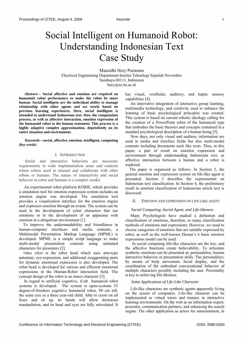
Fig.1. Two level inverter circuit diagram A three-phase voltage source inverter has eight switching states as shown in Fig. 1. The two zero states (−−− and +++), which short the motor terminals, produce a voltage vector of zero magnitude as shown in the figure. The other six states, or the active states, produce an active voltage vector each. These active vectors divide the space vector plane into six sectors and are of equal magnitude as shown. The magnitudes are normalized with respect to the dc bus voltage.
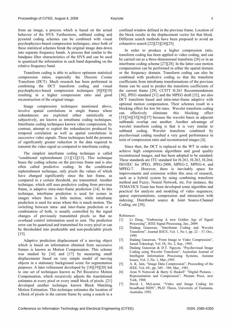
Fig.2. Inverter states and voltage vectors of three-phase Inverter The six active space vectors are represented by the following expression:
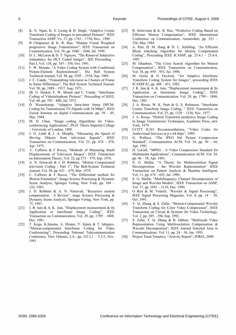
(1) In space vector-based PWM, the voltage reference, which is sampled once in every subcycle, TS. Given a sampled reference vector of magnitude VREF and angle α in sector I as shown in Fig. 2, the dwell times of active vector 1, active vector 2 and zero vector in the subcycle are given by T1, T2, and TZ, respectively, in CSVPWM divides TZ equally between 0 and 7, and employs the switching sequence 0-1-2-7 or 7-2-1-0 in a subcycle in sector I. The conditions to be satisfied by a valid sequence in sector I are as follows. 1) The active state 1 and the active state 2 must be applied at least once in a subcycle. 2) Either the zero state 0 or the zero state 7 must be applied at least once in a subcycle. 3) In case of multiple application of an active state, the total
duration for which the active state is applied in a sub cycle must satisfy (1). 4) The total duration for which the zero vector (either using the zero state 0 or the zero state 7) is applied in a sub cycle must satisfy (1). 5) Only one phase must switch for a state transition. 6) The total number of switching’s in a subcycle must be less than or equal to three. This ensures that the average switching frequency is less than or equal to that of CSVPWM for a given sampling Frequency.
From the Volt-time balance principle T1, T2 and Tz can be given as
(2)
Fig.3. Different possible switching sequences in sector I
( )( )°−°
=60sin
60sin**1α
sref TVT
( )( )°=60sin
sin**2α
sref TVT
21 TTTT sz −−=

Proceedings of CITEE, August 4, 2009 9
Conference on Information Technology and Electrical Engineering (CITEE) ISSN: 2085-6350
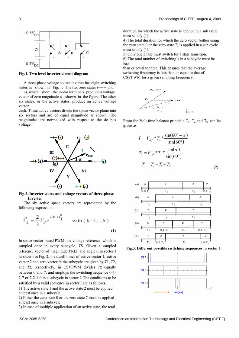
Fig.4. PWM Gate signals when the reference vector sitting in sector-I (0127)
Sequence 7212 leads to clamping of R -phase to the positive dc bus, while sequence 0121 results in clamping of B-phase to the negative dc bus. Both sequences result in Y -phase switching twice in a sub cycle. Hence, sequences 0121 and 7212 are termed “double-switching clamping sequences” here. The sequences illustrated in Fig. 3 are employed in sector I. The equivalent sequences in the other sectors are as listed in Table I. The PWM gating signals for the CSVPWM is shown in Fig 4.
TABLE I. SWITCHING SEQUENCES IN SIX SECTORS
III. MODERN PWM TECHNIQUES
The modern PWM methods can be separated into two groups and those are:
• Continuous PWM(CPWM) methods • Discontinuous PWM(DPWM) methods
In discontinuous one the modulation wave of a phase has at least one segment which is clamped to the positive or negative dc bus for at most a total of 1200 (over a fundamental cycle).Where as in continuous PWM there is no clamping in the modulation wave. The expressions for the modulation signals are given as
( ) ( )dc
max
dc
min
dc
inin V
V1µ2VV22µ1
V2VM −
+−−+=µ
i=a, b, c (4)
The selection of µ gives rise to an infinite number of PWM modulations. To obtain the generalized discontinuous modulation signal, µ is given as :
μ =1-0.5[1+sgn (cos3 (ωt+δ))] (3)
When µ = 0, any one of the phases is clamped to positive dc bus for 1200 and then DPWMMAX is obtained. When µ = 1, any one of the phases is clamped to negative dc bus for 1200 and then DPWMMIN is obtained. If µ = 0.5, then the SVPWM algorithm is obtained. Similarly, the variation of modulation phase angle δ yields to infinite
number of DPWM methods. If δ = 0, -pi/6, -pi/3, then DPWM1, DPWM2 and DPWM3 can be obtained respectively. The modulation waveforms of the different PWM methods are as shown in Fig.5. 1
Fig.5.Modulation waveforms of the various PWM methods
The conventional SVPWM algorithm employs equal division of zero voltage vector times within a sampling period or sub cycle. However, by utilizing the freedom of zero state division, various DPWM methods can be generated. GDPWM algorithm, which uses the utilization of the freedom of zero state time division. In this proposed method the zero state time will be shared between two zero states as T0 for V0 and T7 for V7 respectively, and T0 , T7 can be expressed as:
(5)
Fig.6.Existing bus-clamping PWM technique (300 clamp).

10 Proceedings of CITEE, August 4, 2009
ISSN: 2085-6350 Conference on Information Technology and Electrical Engineering (CITEE)
IV. BUS-CLAMPING PWM TECHNIQUES
A popular existing bus-clamping method clamps every phase during the middle 300 duration in every quarter cycle of its fundamental voltage. This technique, termed as and “300 clamp.” This employs sequences 721, 127, in the first half, and 012, 210, in the second half of sector I as shown in Fig. 6.
In Fig. 7(a), every phase is clamped continually for 600 duration in every half cycle of the fundamental voltage waveform. These techniques can be termed “continual clamping” techniques. In Fig. 7(b), the 600 clamping duration is split into one interval of width in the first quarter cycle and another interval of (600-γ) in the next quarter in every half cycle. Since the clamping duration is split into two intervals, these techniques are termed “split clamping” PWM techniques. Fig. 8(a) and (b) present average pole voltage waveforms that illustrate the two types of clamping for γ= 450 .
Fig.7. Existing bus-clamping PWM techniques
(a) continual clamping type (b) split clamping type.
Fig.8. Average pole voltage over a fundamental cycle for VREF = 0.75 corresponding to (a) continual clamping and (b) split clamping both with γ=450.
The design of the inverter phase voltage and common mode voltages for different pulse sequences are:
(6)
Fig.9.Simulated Phase and line voltages waveforms of the two level inverter
VOLTS/HZ CONTROL TECHNIQUE: This is the most popular method of Speed control because of simplicity. The Flux and Torque are also function of frequency and voltage respectively the magnitude variation of control variables only. The air gap voltage of induction motor is
Speed is varied by varying the frequency; maintain v/f constant to avoid saturation of flux. With constant v/f ratio, motor develops a constant maximum torque.
INDUCTION MOTOR MODELLING: Among the various reference frames, V/F uses the stationary reference frame. Hence, in this work, the induction motor model is developed in the stationary reference frame, which is also known as Stanley reference frame. Rotor and stator voltages and their flux linkages are
agφf
Vf
Eag ≈=

Proceedings of CITEE, August 4, 2009 11
Conference on Information Technology and Electrical Engineering (CITEE) ISSN: 2085-6350
The electromagnetic torque of the induction motor is given by The Electromechanical equation of induction drive is given by
Fig.10. Speed and Torque characteristics with respect to time
Fig.11. Block diagram of V/F controlled BCPWM based IM drive V. ANALYSIS OF HARMONIC DISTORTION The generalized stator q-axis and d-axis flux ripples are as shown below.
Q1 = [cos (α) −Vref] *T1
Q2 = [cos (60° − α) − Vref] *T2 QZ = −Vref*TZ
D = sin (α)*T1. Expressions for RMS Stator Flux Ripple: The rms Stator flux ripples different sequences employed and their respective vector diagram of d-axis and q-axis ripples shown in Fig 12. (7a) (7b) (7c) . . (7d) . (7e)
( ) ( ) ( ) ( )[ ]
( ) ( )( ) ( )[ ]
( ) ( )ss
zz
szzzz
szzzz
s
zz
TTTD
TTQ
TTQQQQQQ
TTQQQQQQ
TTQF
2122
221
21
1211
2220127
31
25.0
31
5.05.05.05.031
5.05.05.05.031
25.0
31
++−
+−++−+
++++++=
( ) ( )[ ]
( ) ( )ss
z
szzzz
s
zz
TTTD
TTQQ
TTQQQQQQ
TTQF
212221
1211
222012
31
31
31
31
++++
+++++=
( ) ( )[ ]
( ) ( )ss
z
szzzz
s
zz
TTTD
TTQQ
TTQQQQQQ
TTQF
212122
2222
222721
31
31
31
31
++++
+++++=
( ) ( )[ ]
( ) ( ) ( )[ ]
( ) ( ) ( )ss
szz
szzzz
s
zz
TTTD
TTQ
TTQQQQQQ
TTQQQQQQ
TTQF
212121
22111
21
1211
2220121
5.031
25.0
31
5.05.05.05.031
25.05.0
31
31
++−+
−++−++
+++++=
( ) ( )[ ]
( ) ( ) ( )[ ]
( ) ( ) ( )ss
szz
szzzz
s
zz
TTTD
TTQ
TTQQQQQQ
TTQQQQQQ
TTQF
212222
12222
22
2222
2227212
5.031
25.0
31
5.05.05.05.031
25.05.0
31
31
++−
+−++−+
++++++=
dtd
iRv
dtdiRv
dtd
iRv
dtdiRv
qrdrrqrrqr
drqrrdrrdr
qsqssqs
dsdssds
ψψω
ψψω
ψ
ψ
+−=
++=
+=
+=
dsmdrrdr
qsmqrrqr
drmdssds
qrmqssqs
iLiL
iLiLiLiL
iLiL
+=
+=+=
+=
ψ
ψψ
ψ
( )dsqsqsdse iiPT ψψ −⎟⎠⎞
⎜⎝⎛=
223
dtd
JP
Tdt
dJTT r
Lm
Leωω 2
+=+=

12 Proceedings of CITEE, August 4, 2009
ISSN: 2085-6350 Conference on Information Technology and Electrical Engineering (CITEE)
Fig.12.Stator flux ripple vector over a subcycle for sequences (a) 0127, (b) 012, (c) 721, (d) 0121 and (e) 7212.
Fig. 13. Comparison of rms stator flux ripples due to CS-0127, S1-012, S2-721, S3-0121, S4-7212, S5-1012 and S6-2721 at different modulation indices. A. Analysis of Existing BCPWM Techniques: Sequence 012 leads to less RMS current ripple over a subcycle than 721 in the first half of the sector, and vice versa in the second half of the sector. F012(α) < F721(α) , 00 < α < 300 (8a)
F012(α) > F721(α) , 300 < α < 600 (8b)
F012(α) = F721(600- α) (9)
Fig.14.Measured no-load current waveforms at VREF=0.85 for Existing BCPWM techniques.

Proceedings of CITEE, August 4, 2009 13
Conference on Information Technology and Electrical Engineering (CITEE) ISSN: 2085-6350
Table II Measured Values of ITHD for Existing BCPWM
Fig.15.Measured no-load current waveforms at VREF=0.85 for Proposed BCPWM techniques. B. Analysis of Proposed BCPWM Techniques: F0121(α) < F7212(α) , 00 < α < 300 (10a)
F0121(α) > F7212(α) , 300 < α < 600 (10b)
F0121(α) = F7212(600- α) (11)
Table III Measured Values of ITHD for Proposed
BCPWM
VI INVERTER SWITCHING LOSSES This section presents a comparison of inverter switching losses due to CSVPWM, existing BCPWM
techniques. The switching energy loss in a subcycle in an inverter leg is proportional to the phase current and the number of switchings of the phase (n) in the given subcycle. The normalized switching energy loss per subcycle (ESUB) in an inverter leg is defined in (1a), where i1 is the fundamental phase current, Im is the peak phase fundamental current and Φ is the line-side power factor angle.
( )ΦωtsinnIin
Em
1SUB −== (12a)
( ) tdω∫=Π
0SUBAVSUB E
Π1E (12b)
Fig.16. Variation of normalized switching loss ESUB over
a fundamental cycle for CSVPWM.
(a) (b)
(c) (d) Fig. 17. Variation of normalized switching loss ESUB over a fundamental cycle for Existing BCPWM techniques. Average Switching Loss for CSVPWM = 0.6366
No-Load Current THD γ=300 γ =450
continual clamping 5.32% 4.72%
Split Clamping 4.61% 5.01%
No-Load Current THD γ=300 γ=450
continual clamping 3.91% 3.46%
Split Clamping 2.66% 3.04%

14 Proceedings of CITEE, August 4, 2009
ISSN: 2085-6350 Conference on Information Technology and Electrical Engineering (CITEE)
Table IV Measured Values of Average Switching Loss
VI. CONCLUSIONS
A class of bus-clamping PWM (BCPWM) techniques, which employ only the double-switching clamping sequences, is proposed. The proposed BCPWM techniques are studied, and are compared against conventional space vector PWM (CSVPWM) and existing BCPWM techniques at a given average switching frequency. The proposed families of BCPWM techniques result in less line current distortion than CSVPWM and the existing BCPWM techniques at high line voltages close to the highest line side voltage during linear modulation. The analysis presented explains the difference in distortion due to the different techniques. The study classifies both the existing BCPWM and the proposed BCPWM techniques into two categories, namely continual clamping methods and split clamping methods, depending on the type of clamping adopted. It is shown that split clamping methods are better than continual clamping ones in terms of line current distortion. In terms of switching losses, continual clamping is better at high power factors, while split clamping is superior at low power factors.
REFERENCES
[1]“Advanced Bus-Clamping PWM Techniques Based on Space Vector Approach” G. Narayanan, Member, IEEE,
Harish K. Krishnamurthy, Di Zhao, and Rajapandian Ayyanar, Member, IEEE,2006. [2] J. Holtz, “Pulse width modulation—A survey,” IEEE Trans Ind. Electron., vol. 39, no. 5, pp. 410–420, Dec. 1992. [3] J. Holtz, “Pulse width modulation for electronic power conversion,” Proc. IEEE, vol. 82, no. 8, pp. 1194–1214, Aug. 1994. [4] D. G. Holmes and T. A. Lipo, Pulse Width Modulation for Power Converters: Principle and Practice. New York: Wiley, 2003. [5] V. Blasko, “Analysis of a hybrid PWM based on modified space-vector and triangle-comparison methods,” IEEE Trans. Ind. Appl., vol. 33, no. 3, pp. 756–764, May/Jun. 1997. [6] D. Zhao, G. Narayanan, and R. Ayyanar, “Switching loss characteristics of sequences involving active state division space vector based PWM,” in Proc. IEEE APEC’04, 2004, pp. 479–485.
ACKNOWLEDGEMENT
We express our sincere thanks to TEQIP for providing us good lab facilities. A heart full and sincere gratitude to our beloved parents for their tremendous motivation and moral support.
M.Thanuja was born in Nandyal. She has completed her B.Tech at R.G.M. College of Engg and Techng. affiliated to J.N.T.U. Hyderabad in 2002. She is currently doing M.Tech at RGMCET,Nandyal, affiliated to J.N.T.U. Anantapur. She is working in areas power electronics and Power electronics control of ac drives. E-mail: [email protected] K.SreeGowri received the B.Tech degree from SVU College of Engineering, Tirupati in 1997, the M.Tech degree from RGM College of Engineering and Technology, Nandyal and is currently pursuing the Ph.D. in Electrical Engineering Department, JNTU, and Hyderabad. She is currently an Associate Professor in the Department of EEE in RGMCET, Nandyal, A.P. Her areas of interest include Power Electronics, pulse width modulation techniques, AC Drives and Control.
Average Switching Loss Φ=00 Φ =900
continual clamping
(i) γ=300
(ii) γ=600
(a) 0.318
-----
----
(b) 0.4776
Split Clamping
γ=300
(c) 0.4041
(d) 0.4041
Proceedings of CITEE, August 4, 2009 15
Conference on Information Technology and Electrical Engineering (CITEE) ISSN: 2085-6350
Medical Image Processing of Proximal Femur X-Ray for Osteoporosis Detection
Riandini, Mera Kartika Delimayanti
Politeknik Negeri Jakarta, Electrical Engineering Department Kampus UI Depok, Indonesia 16424
Donny Danudirdjo Institut Teknologi Bandung
Jl. Ganesha 10 Bandung, Indonesia 40132
Abstract— Osteoporosis is one of the generative (aging
process) diseases which occurs because of the rise of one’s life expectancy from the age of 60s to 74s or more. This disease attacks not only women but also men. The worst impact of it is death. Although it is very important to detect it very early to avoid the worst impact of it, an early effective process of osteoporosis detection is clinically difficult and costly to do. The only method of doing so which is relatively cheap is the analysis of x-ray image (radiology) instead of DEXA (Dual Energi X-Ray Absorptiometri) which long has been used as a golden standard. But, this process may lead to subjectivity since doctors (medical staffs) do so with naked eyes. This paper describes a series of algorithm plans for medical image analysis with the support of Femur Proximal x-ray image as data input. Algorithm plans which are going to be developed are a combination of Gabor algorithm, Wavelet algorithm, Fractal algorithm and algorithm (analysis) mainly used to enhance the quality of an image through the omission of vertical lines artefact on the image, edge detection on the image and image rotation. The outcome of the plan is going to be implemented within GUI-based (Graphical User Interface) computer application which is user-friendly and usable for helping doctors diagnose osteoporosis.
Keywords—medical image analysis, x-ray image, proximal femur, osteoporosis, algoritma.
I. INTRODUCTION Osteoporosis is a degenerative disease that takes place in
many places around the world. The high prevalence of osteoporosis in Indonesia is inseparable from the rise of life expectancy, from 59.8 in 1990 up to 67 at present. An effective standard instrument largely used nowadays to detect osteoporosis is Dual Energy X-Ray Absorptiometri (DEXA). A significant shortcoming of the instrument is that it is very expensive and the number of it is limited not only at rural areas but also in big cities over Indonesia. Besides, the operational expenditure of the tool is totally high. One alternate solution to the problem is the implementation of x-ray radiology image detecting instrument. However, it still brings two primary weaknesses: (1). Data processing subjectivity – a physician analyzes and interprets the same data several times with different results; (2) Data processing with the naked eye may lead to ignorance of detailed information on a radiology image. In order to deal with those weaknesses, this paper is going to describe a system
of medical image processing algorithm with a purpose of assisting doctors for early detection of osteoporosis. The system applies femur proximal x-ray image in its operation. The algorithm operation of image texture analysis involves determination of optimum textural features of the image and the supporting classification methods of the image texture. The system used in the operation is then used by physicians to assist them diagnose osteoporosis.
II. OSTEOPOROSIS Osteoporosis is a situation when there is an over-limit
decrease of bone density and structural malfunction of bone micro-structure system that makes the bone system unable to prevent bone fracture from minimal trauma. The decrease of bone mass occurs because the velocity of bone formation process by osteoblas cell is not capable of equalizing the velocity of bone surface erodibility by osteoklas cell. Histopalogically, osteoporosis indicates the decrease of cortex density and the declining amount as well as size of bone trabucela [3].
Osteoporosis is suffered much more by women than men in that about 50 percent of menopause women are suffering from osteoporosis. However, recent research has shown that it is no longer dominated by old-aged people. Youngsters are likely to get suffered from it if they don’t have appropriate eating habit [6].
The number of osteoporosis cases in Indonesia is quite high. Prevalence of it has reached 19.7 percent. This percentage is believed to keep increasing due to the rising life expectancy and the improvement of the quality of people’s health. Osteoporosis is categorized as a degenerative disease which is commonly suffered by old people and may lead to physical disability and death. Thus, the early prevention of it is very crucial.
Efforts to prevent osteoporosis are closely related to the early bone strength diagnosis and treatment. The standard method of diagnosing the bone density is well known as DEXA (Dual Energy X-Ray Absorptiometry). In Indonesia, the application of the method faces two problems: (1) fairly expensive diagnosis and treatment, and (2) lack of medical instruments supporting the diagnosis process within some hospitals in big cities of the country. An alternate method to cope with the problem, which is aimed at doing trabekula style treatment, is Singh Index.

16 Proceedings of CITEE, August 4, 2009
ISSN: 2085-6350 Conference on Information Technology and Electrical Engineering (CITEE)
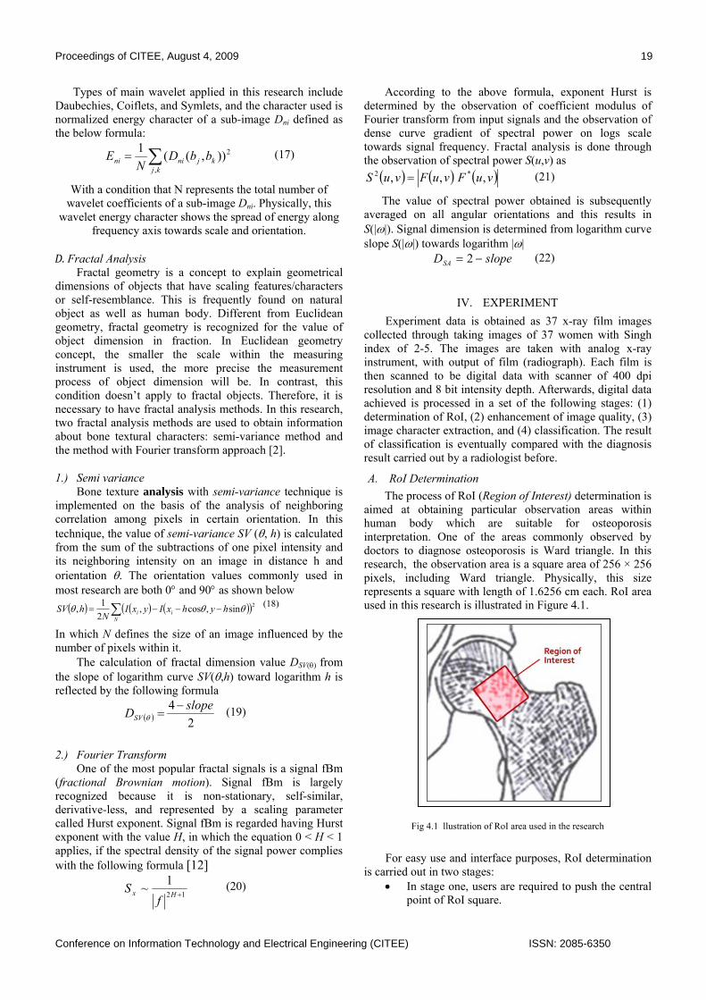
Fig 2.1. illustrates the way of determining Singh Index on femur x-ray image
Index value determination is commonly done by an orthopedic specialist. The outcome of the index value is strongly influenced by a specialist expertise and inseparable from his/her subjectivity. If he/she is doing the evaluation at two distinct times, he/she may come up with different outcomes. Therefore, the presence of the diagnosing system of trabekula texture of the femur x-ray image is in urgent need to help doctors do early osteoporosis diagnosis and detection.
III. TEXTURE ANALYSIS Texture is a two dimension intrinsic character of an image correlated with the level of roughness, granularity, and the regularity of pixel arrangement. Texture analysis runs through observing neighboring model within pixels in a spatial domain and is related to the need of the image characters extraction. In this research, an observation of textural characteristics of x-ray radiology image (connected to level of osteoporosis) is carried out with the support of four methods: co-occurrence analysis, Gabor filter, wavelet transform, and fractal analysis. These four methods are used in an attempt to obtain the most optimum method and result in an accurate diagnosis outcome. There are eight image characters used in the research, and in each method involves at least one character. Character classification process works through the support of artificial neuron system with an outcome of Singh index value of the radiology image that is observed.
A. Cooccurrence Analysis Co-occurrence analysis is the simplest analyzing method of the image texture. This analysis is completed
through two stages: (1) establishing co-occurrence matrix as a representation of the probability of neighboring interaction between two pixels in certain distance (d) and angle orientation (θ), (2) determining character as a function of the co-occurrence matrix. Co-occurrence is two concurrent events, i.e., the number of the occurrence of one level pixel value as a neighbor of another one level pixel value in certain distance (d) and angle orientation (θ). Distance is valued in Pixel and orientation in Degree. There are four angle orientations with 45° angle interval, which are 0°, 45°, 90°, and 135°. On the other hand, distance within pixels is valued 1 pixel.
Co-occurrence matrix is a square matrix with the number of elements equal to a square of the number of pixel intensity on an image. Each spot (p, q) within a co-occurrence matrix oriented to θ has a possibility of pixel occurrence with value amounting p that is neighboring with another pixel with the value amounting q in distance d and angle orientation θ and (180−θ). Figure 3.1 illustrates the formation of a co-occurrence matrix.
With the outcomes of matrix co-occurrence above, we can determine statistical character of orde 2 that represents an observed image. Haralick proposed a number of textural characters which are likely to be extracted from a matrix co-occurrence [1]. In this research, six textural characters of an image are used: Angular Second Moment, Contrast, Correlation, Variance, Inverse Difference Moment, and Entropy.
1.) Angular Second Moment (ASM) This character is used to show the level of homogeneity of an image
∑∑=i j
jipASM 2),( (1)
Where p(i,j) represents values of row i and column j on a co-occurrence matrix.
2.) Contrast (CON) This character is used to show the spread (moment of inertia) of all elements on an image matrix. If the spread (location) is located far away from the main diagonal line on the matrix, then it has a big contrast value. Visually, contrast value is the level of greyness variedness on an image.
kji
k i jjipkCON
=−
∑ ∑∑ ⎥⎦
⎤⎢⎣
⎡=
),(2
(2)
Proceedings of CITEE, August 4, 2009 17
Conference on Information Technology and Electrical Engineering (CITEE) ISSN: 2085-6350
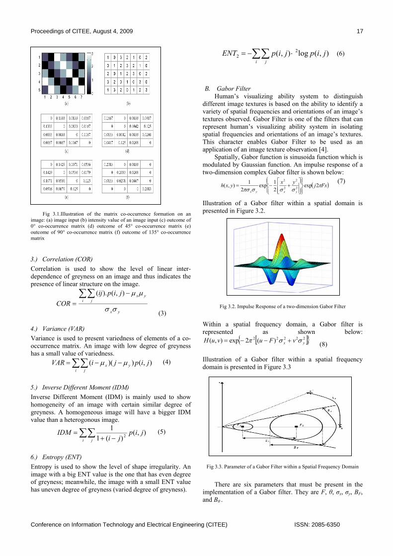
Fig 3.1.Illustration of the matrix co-occurrence formation on an
image: (a) image input (b) intensity value of an image input (c) outcome of 0° co-occurrence matrix (d) outcome of 45° co-occurrence matrix (e) outcome of 90° co-occurrence matrix (f) outcome of 135° co-occurrence matrix
3.) Correlation (COR) Correlation is used to show the level of linear inter-dependence of greyness on an image and thus indicates the presence of linear structure on the image.
yx
i jyxjipij
CORσσ
µµ∑∑ −=
),().(
(3)
4.) Variance (VAR) Variance is used to present variedness of elements of a co-occurrence matrix. An image with low degree of greyness has a small value of variedness.
∑∑ −−=i j
yx jipjiVAR ),())(( µµ (4)
5.) Inverse Different Moment (IDM) Inverse Different Moment (IDM) is mainly used to show homogeneity of an image with certain similar degree of greyness. A homogeneous image will have a bigger IDM value than a heterogonous image.
∑∑ −+=
i j
jipji
IDM ),()(1
12
(5)
6.) Entropy (ENT) Entropy is used to show the level of shape irregularity. An image with a big ENT value is the one that has even degree of greyness; meanwhile, the image with a small ENT value has uneven degree of greyness (varied degree of greyness).
∑∑ ⋅−=i j
jipjipENT ),(log ),( 22 (6)
B. Gabor Filter Human’s visualizing ability system to distinguish
different image textures is based on the ability to identify a variety of spatial frequencies and orientations of an image’s textures observed. Gabor Filter is one of the filters that can represent human’s visualizing ability system in isolating spatial frequencies and orientations of an image’s textures. This character enables Gabor Filter to be used as an application of an image texture observation [4].
Spatially, Gabor function is sinusoida function which is modulated by Gaussian function. An impulse response of a two-dimension complex Gabor filter is shown below:
( )Fxjyxyxhyxyx
πσσσπσ
2exp21exp
21),( 2
2
2
2
⎪⎭
⎪⎬⎫
⎪⎩
⎪⎨⎧
⎥⎥⎦
⎤
⎢⎢⎣
⎡+−=
(7)
Illustration of a Gabor filter within a spatial domain is presented in Figure 3.2.
Fig 3.2. Impulse Response of a two-dimension Gabor Filter
Within a spatial frequency domain, a Gabor filter is represented as shown below:
[ ] 22222 )(2exp),( yx vFuvuH σσπ +−−= (8) Illustration of a Gabor filter within a spatial frequency domain is presented in Figure 3.3
Fig 3.3. Parameter of a Gabor Filter within a Spatial Frequency Domain
There are six parameters that must be present in the
implementation of a Gabor filter. They are F, θ, σx, σy, BF, and Bθ .

18 Proceedings of CITEE, August 4, 2009
ISSN: 2085-6350 Conference on Information Technology and Electrical Engineering (CITEE)
• Frequency (F) and orientation (θ) define the location of a filter center
• BF and Bθ represent constants of the width of a frequency tape and the angular range of a filter
• Variabel σx is closely related to a response of -6 dB for a spatial frequency component
• Variabel σy is closely connected with a response of -6dB for an angular component
)2/tan(22ln
θπσ
BFy = (9)
• Position (F, θ) and tape width (σx, σy) of a Gabor filter within a frequency domain have to be determined accurately to obtain correct textural information. A middle frequency of a canal filter must be close to a frequency of an image texture characteristic.
Table 3.1. Six Parameters of a Gabor Filter
Parameter Symbol Value used in the research
Middle frequency (normalized) F 54321 2
2,2
2,2
2,2
2,22
Frequency tape width BF 1 octave
Angular tape width Bθ 45°
Frequency Spacing SF 1 oktaf
Angular Spacing Sθ 45°
Orientation Θ 0°, 45°, 90°, 135° After Gabor character is obtained, then extraction of energy character is likely to carry out. This is defined as follow:
∑∑= =
=M
i
N
jnmx
MNxE
1 1
2),(1)( (10)
This research uses frequency tape width (BF) and middle frequency distance (SF) of one octave, and angular tape width (Bθ) and angular distance (Sθ) of 45°. These values are highly likely to reflect characteristics of human’s visualizing system.
C. Wavelet Transform Textural analysis with wavelet transform works through decomposition of image input, used to observe the content of image information within several sub-bands. Decomposition process applying discrete wavelet transform (DWT) is conducted in stages, each of which will result in 4 sub-band matrix – one matrix of approximation coefficient A and three detailed matrix (horizontal H, vertical V, and diagonal D). If the process is conducted in a narrower range of frequencies, then a matrix of approximation coefficient A is likely to be re-decomposed into 4 smaller sub-band matrix [5].
Continual wavelet transform for signal 1-D f(x) is obviously defines as follow:
( ) ( ) ( )∫= dxxxfbfW baa*
,ψ (11)
Where wavelet ψa,b is counted from the main wavelet through translation and dilation
( ) ⎟⎠⎞
⎜⎝⎛ −
=a
bxa
xba ψψ 1, (12)
Wavelet decomposition at level J is written below ( ) ( ) ( ) ( )∑ ∑∑ ⎥
⎦
⎤⎢⎣
⎡+==
=++++
k
J
jkjkjkJkJ
kkk xdxcxcxf
0,1,1,1,1,0,00 ψφφ (13)
In which coefficient c0,k has been defined already and coefficients cj+1,n and dj+1,n at scale j+1 are related to coefficient cj,k at scale j through a formula:
( )∑ −=+k
kjnj nkhcc 2,,1 (14a)
( )∑ −=+k
kjnj nkgdd 2,,1 (14b)
In which equation 0 ≤ j ≤ J applies. The main wavelet is established by scale function φ(t) and wavelet ψ(t) which comply with two-scale relation as shown in a below formula:
( ) ( ) ( )∑ −=k
kxkhx 2 2 φφ (15a)
( ) ( ) ( )∑ −=k
kxkgx 2 2 φψ (15b)
With requirement: ( ) ( ) ( )khkg k −−= 11 (15c)
Coefficient h(k) is one of the main wavelet functions like Haar, Daubechies, Coiflets, Symlets, or Biorthogonal. Practically, discrete wavelet transform is calculated by applying a bank filter inseparable from function f(x) or image function I(x).
),(]]*[*[)( 2,11,21, jinyxjin bbLHHbbL ↓↓−= (16a)
),(]]*[*[)( 2,11,21,1 jinyxjin bbLGHbbD ↓↓−= (16b)
),(]]*[*[)( 2,11,21,2 jinyxjin bbLHGbbD ↓↓−= (16c)
),(]]*[*[)( 2,11,21,3 jinyxjin bbLGGbbD ↓↓−= (16d)
In which an asterisk * is a convolution operator, while ↓2,1 (↓1,2) is a sub-sampling operator along a row (or column) and L0 = I(x) defines a genuine image. H and G are low pass and band-pass h(k) and g(k)) filters on a horizontal or vertical angle. Ln is obtained from filtration of low-pass by h(k) and thus regarded as an approximation image at scale n. Dni is obtained from filtration of band-pass by g(k) on certain angle and therefore contains detailed angle information at scale n. It is then defined as a detailed image. A genuine image I is represented by a group of sub-images at various scales: Ld, Dnii=1,2,3; n=1..d which represents a compilation of multi-scale sub-images with certain depth d from an image I.
Proceedings of CITEE, August 4, 2009 19
Conference on Information Technology and Electrical Engineering (CITEE) ISSN: 2085-6350
Types of main wavelet applied in this research include Daubechies, Coiflets, and Symlets, and the character used is normalized energy character of a sub-image Dni defined as the below formula:
∑=kj
kjnini bbDN
E,
2)),((1 (17)
With a condition that N represents the total number of wavelet coefficients of a sub-image Dni. Physically, this
wavelet energy character shows the spread of energy along frequency axis towards scale and orientation.
D. Fractal Analysis Fractal geometry is a concept to explain geometrical
dimensions of objects that have scaling features/characters or self-resemblance. This is frequently found on natural object as well as human body. Different from Euclidean geometry, fractal geometry is recognized for the value of object dimension in fraction. In Euclidean geometry concept, the smaller the scale within the measuring instrument is used, the more precise the measurement process of object dimension will be. In contrast, this condition doesn’t apply to fractal objects. Therefore, it is necessary to have fractal analysis methods. In this research, two fractal analysis methods are used to obtain information about bone textural characters: semi-variance method and the method with Fourier transform approach [2]. 1.) Semi variance
Bone texture analysis with semi-variance technique is implemented on the basis of the analysis of neighboring correlation among pixels in certain orientation. In this technique, the value of semi-variance SV (θ, h) is calculated from the sum of the subtractions of one pixel intensity and its neighboring intensity on an image in distance h and orientation θ. The orientation values commonly used in most research are both 0° and 90° as shown below
( ) ( ) ( )( )∑ −−−=N
ii hyhxIyxIN
hSV 2sin,cos,21, θθθ (18)
In which N defines the size of an image influenced by the number of pixels within it.
The calculation of fractal dimension value DSV(θ) from the slope of logarithm curve SV(θ,h) toward logarithm h is reflected by the following formula
( ) 24 slopeDSV−
=θ (19)
2.) Fourier Transform
One of the most popular fractal signals is a signal fBm (fractional Brownian motion). Signal fBm is largely recognized because it is non-stationary, self-similar, derivative-less, and represented by a scaling parameter called Hurst exponent. Signal fBm is regarded having Hurst exponent with the value H, in which the equation 0 < H < 1 applies, if the spectral density of the signal power complies with the following formula [12]
12
1~+Hx
fS (20)
According to the above formula, exponent Hurst is determined by the observation of coefficient modulus of Fourier transform from input signals and the observation of dense curve gradient of spectral power on logs scale towards signal frequency. Fractal analysis is done through the observation of spectral power S(u,v) as
( ) ( ) ( )vuFvuFvuS ,,, *2 = (21)
The value of spectral power obtained is subsequently averaged on all angular orientations and this results in S(|ω|). Signal dimension is determined from logarithm curve slope S(|ω|) towards logarithm |ω| slopeDSA −= 2 (22)
IV. EXPERIMENT Experiment data is obtained as 37 x-ray film images
collected through taking images of 37 women with Singh index of 2-5. The images are taken with analog x-ray instrument, with output of film (radiograph). Each film is then scanned to be digital data with scanner of 400 dpi resolution and 8 bit intensity depth. Afterwards, digital data achieved is processed in a set of the following stages: (1) determination of RoI, (2) enhancement of image quality, (3) image character extraction, and (4) classification. The result of classification is eventually compared with the diagnosis result carried out by a radiologist before.
A. RoI Determination The process of RoI (Region of Interest) determination is aimed at obtaining particular observation areas within human body which are suitable for osteoporosis interpretation. One of the areas commonly observed by doctors to diagnose osteoporosis is Ward triangle. In this research, the observation area is a square area of 256 × 256 pixels, including Ward triangle. Physically, this size represents a square with length of 1.6256 cm each. RoI area used in this research is illustrated in Figure 4.1.
Fig 4.1 llustration of RoI area used in the research
For easy use and interface purposes, RoI determination
is carried out in two stages: • In stage one, users are required to push the central
point of RoI square.

20 Proceedings of CITEE, August 4, 2009
ISSN: 2085-6350 Conference on Information Technology and Electrical Engineering (CITEE)
• In stage two, users are obligated to decide the angular point of a square, which is the point directing to body axis (proximal direction).
Figure 4.2. shows illustration of RoI determination process within the program created
Fig 4.2. Illustration of RoI determination process
B. Image Quality Enhancement The second stage of digital data processing is image
quality enhancement. This process is implemented through two important methods (median filtering and contrast stretching) toward a RoI image of 256 × 256 pixels. Median filtering is intended to reduce noise disturbance to the image, while contrast stretching to standardize image intensity. The former method is used with the support of checking window of 5 × 5 pixels, and the latter one runs by following the below equation:
( ) ( ) ( )( )( )( ) ( )( ) 16095
,,max,,, +×
−−
=′yxIyxI
yxIyxIyxIµ
µ (23)
The above equation defines that I’ is pixel intensity that has been processed and I initial intensity. Operators µ and max refer to average and maximum operators. Number 160 represents expected average intensity for RoI which has been processed; meanwhile, number 95 is the dynamic intensity as a result of substraction of the value µ and the highest intensity value within RoI. Both numbers are achieved on the basis of a series of image quality enhancement experiments towards 111 RoI areas used in the research. Figure 4.3. illustrates the change of histogram shape in the process of image quality enhancement
Fig 4.3 Change of intensity histogram at RoI area in contrast stretching, before (left) and after (right)
Input and output of image quality enhancement processing are illustrated in Figure 4.4. below:
Fig 4.4. Image Quality Enhancement Processing: Input (left) and Output (Right)
C. Character Extraction Character extraction process is an integrated part of
trabekula textural analysis. This process is applied to an image of which the quality has been enhanced. With the four methods described previously, the research comes up with 175 textural characters:
• Co-occurrence analysis: 6 features • Gabor filter: 20 characters, achieved by combining
4 orientations with 5 middle frequency values (normalized)
• Wavelet transform: 104 characters as a combination of 2 coefficients (approximation and detail), 13 kinds of the main wavelet, and 4 observation levels
• Fractal analysis: 45 characters, obtained from a combination of 2 methods (semi-variance and fourier methods), each of which is enriched with 30 and 15 resolutions.
D. Classification Classification process is carried out with the help of
artificial neural system, exercised with the use of exercising data in the form of 111 RoI images. Testing is done toward 740 testing sampels. Before classification process is conducted, selection of certain characters significantly correspondent with Singh index is done. By the selection, there are 8 characters used in the research:
1. Level 3 approximation image energy in wavelet transform with the use of the main wavelet Symlets of orde 4.
2. Level 3 approximation image energy in wavelet transform with the use of the main wavelet Symlets of orde 5.
3. Combined fractal dimension in semi-variance method with the experiment value of 50 pixels.
4. Vertical fractal dimension in semi-variance method with the experiment value of 50 pixels.
5. Horizontal fractal dimension in Fourier analysis method with the experiment value of 12 Fourier coefficients.
6. Image energy in Gabor filter with the orientation of 135° and normalized middle frequency F = 2−4.5.

Proceedings of CITEE, August 4, 2009 21
Conference on Information Technology and Electrical Engineering (CITEE) ISSN: 2085-6350
7. Level 2 approximation image energy in wavelet transform with the use of the main wavelet Symlets of orde 3.
8. Inverse Different Moment (IDM) in co-occurrence analysis.
The exercise of the artificial neural system is run using propagation algorithm of Levenberg Marquardt with the use of Matlab software. The structure of the artificial neural system is composed with 3 layers. The first layer (input layer) consists of 8 neurons; the second layer 12 neurons; and the third layer (output layer) 6 neurons (equal to the number of grades within Singh index).
V. RESULT Testing of 740 data samples (i.e., RoIs which have been
determined before as testing samples) results in textural character classifications as shown in Table 5.1.
Table 5.1. Result of Singh Index Classification with the help of the
artificial neural system
Results of neural system diagnosis
1 2 3 4 5 6
R
esul
ts o
f neu
ral s
yste
m d
iagn
osis
by
radi
olog
ists
1 0 0 0 0 0 0
2 0 39 1 0 0 0
3 0 0 111 7 2 0
4 0 0 0 345 15 0
5 0 0 0 13 207 0
6 0 0 0 0 0 0
In summary, the classification process ran quite well in that 96,62 % of testing data (715) was classified properly; 3,11 % (23) with diagnosis error of one grade Singh index; and 0,27% (2) with diagnosis error of 2 grade Singh index.
VI. CONCLUSION This research succeeded in creating initial construction
and implementation of trabekula textural analysis method of femur x-ray image, meaning that it was successful in helping doctors do early osteoporosis detection. In this research, a series of experiments and analyses were conducted using various methods of image analysis in an effort to identify trabekula textural characters in femur proximal bone correlated with osteoporosis detection. Image analysis methods were a combination of co-occurrence technique, Gabor filter, wavelet transform, and fractal analysis. The implementation and testing of the neural system resulted in system potentials that might help early osteoporosis detection process now that 96,62% of data samples were accuraely detected (similar to the result of diagnosis by doctors/radiologists).
REFERENCES [1] R.M. Haralick, K. Shanmugam, I. Dinstein, Textural Features for
Image Classification, IEEE Transactions on Systems, Man, and Cybernetics, Vol.SMC-3, No.6, pp.610-621, 1973.
[2] J.C. Lin, S. Grampp, T. Link, M. Kothari, D.C. Newitt, D. Felsenberg, S. Majumdar, Fractal Analysis of Proximal Femur Radiographs: Correlation with Biomechanical Properties and Bone Mineral Density, Osteoporos Int, 9:516-524, 1999.
[3] B. Sankaran, Osteoporosis, Mumbai: Novelty Printers, 2000. [4] ---------, Modul Praktikum Analisis Tekstur, Imaging & Image
Processing Research Group, Institut Teknologi Bandung [5] T.R. Mengko, J.T. Pramudito, Texture Analysis of Proximal Femur
Radiographs for Osteoporosis Assessment, WSEAS Transaction on Computers, Vol.3, No.1, 2004
[6] S.W. Simson, M. Hidayat, Bone Architecture, Matrix Property and Fracture Risks, Pertemuan Ilmiah Tahunan Perhimpunan Osteoporosis Indonesia (PEROSI), 2007

22 Proceedings of CITEE, August 4, 2009
ISSN: 2085-6350 Conference on Information Technology and Electrical Engineering (CITEE)
Optical Communication System on Microcell Networks in Urban Area
Purnomo Sidi Priambodo, Harry Sudibyo and Gunawan Wibisono Department of Electrical Engineering, Faculty of Engineering, Universitas Indonesia
Depok, Jawa Barat 16424, Indonesia Email : [email protected]
HP : 0813-81153343
Abstract— The free-space optical communication (FSOC) system is a new kind of technological engineering based on the existing fiber-optic technology to obtain a breakthrough technology which is wireless, flexible, less expensive and large bandwidth capacity. Free-space optical communications is a line-of-sight (LOS) technology that transmits a modulated beam of visible or infrared light through the atmosphere for broadband communications. The entire components used in this optical free-space communication system are taken and modified from the existing fiber-optics system. Similar to fiber optical communications, free-space optics uses a light emitting diode (LED) or laser semiconductor diode source for data transmission. Free-space optical communications offer data rates comparable to fiber optical communications at a fraction of the deployment cost of microwave or fiber-optics links. The other advantages are flexible installation and extremely narrow laser beam widths provide no limit to the number of free-space optical links that may be installed in a given location. Thus advantages are justified and suitable to be implemented on microcell networks in urban areas.
The fundamental limitation of free-space optical communications arises from the atmosphere through which it propagates. Free-space optical communication systems can be severely affected by fog and atmospheric turbulence. The main design challenges in the free-space optical communications are solving to overcome the effects of thus fog, scintillation and beam wander.
In this paper, the authors elaborate optical free-space propagation parameters such as attenuation, polarization effect, Rayleigh scattering and possible fading. Further, the mathematical model is introduced for each component and path of the communication system. The model will be used to design the optimal optical free-space communication system implemented on microcell networks in urban area.
Keywords—free-space optical communication, atmos-pheric propagation, atmospheric turbulence, spatial diversity reception
I. INTRODUCTION
Free-space optical communications (FSOC) is a line-of-sight (LOS) technology where a modulated beam of visible or infrared light is transmitted through the atmosphere for broadband communications [1]. Similar to fiber optical communications, free-space optical
communication uses a light emitting diode (LED) or laser source for data transmission [2]. The beam is collimated and transmitted through space or atmosphere rather than being guided through a fiber-optics cable. Free-space optical communications offer data rates comparable to fiber optical communications at a fraction of the deployment cost of microwave or fiber-optics links. The other advantages of this technology are flexible installation and extremely narrow laser beam widths provide no limit to the number of free-space optical links that may be installed in a given location. Thus advantages are justified and suitable to be implemented on microcell networks in urban area.
At this time, this technology can be installed license-free worldwide, can be installed in less than a day. This line-of-sight technology approach uses invisible beams of light to provide optical bandwidth connections [3]. It's capable of sending up to 1.25 Gbps of data, voice, and video communications simultaneously through the air — enabling fiber-optic connectivity without requiring physical fiber-optic cable. This optical connectivity doesn't require expensive fiber-optic cable or securing spectrum licenses for radio frequency (RF) solutions. While fiber-optic communications gained worldwide acceptance in the telecommunications industry, FSOC is still considered relatively new. This FSOC technology approach has a number of advantages:
1. Requires no RF spectrum license. 2. Easy to upgrade, and its open interfaces support
equipment from a variety of vendors. 3. It is immune to radio frequency interference or
saturation. 4. It can be deployed behind windows, eliminating the
need for costly antenna building such as for RF technology.
5. No fiber-optic cables deployment required.
A. Applications:
FSOC technology can be applied for two different implementations. The first are applications for space communications between satellites, spacecrafts and deep-space between planets. The second are applications for terrestrial communications, similar to point-to-point or line-of-sight in microwave communication technology. For space communications, there are some facts that free-space optical communications will enable space missions to return 10 to 100 times more data with 1% of the antenna area of
Proceedings of CITEE, August 4, 2009 23
Conference on Information Technology and Electrical Engineering (CITEE) ISSN: 2085-6350
current state-of-the-art communications systems, while utilizing less mass and power. Data can also be exchanged between a more remote spacecraft and a station on /or near Earth. For example, planetary probes can generate a lot of image data, and a major challenge is to send large amount of data back to Earth. Until recently, radio links operating e.g. in the X band or Ka band were the only available technology. The basic advantage of the optical technology over radio links is that the much shorter wavelength allows for a much more directional sending and receiving of information. In technical terms, the antenna gain can be much higher. This is particularly important for bridging interplanetary distances. In the future FSOC will become the fundamental communication technology for deep-space communications.
The second are applications for terrestrial communications and omni-wireless, such as point-to-point communications between base-stations in cellular networks and omni Wi-Fi Local Area Networks (LANs). When the traffics increase, the cellular networks need to migrate become microcellular networks where the cell areas is about less than 1-km2. The number of cellular base-stations (BTSs) increases in large number, the consequence is to deploy the communication channels between BTSs. Fiber-optics deployments are not flexible and very expensive for short distance between BTSs, while point-to-point microwaves do not give a good large bandwidth. The answer is FSOC, which gives us flexibility such as point-to-point microwaves, large bandwidth, easy deployment, not heavy and inexpensive investment. Applications for terrestrial are more challenging than applications for space communications, because terrestrial applications facing the effects of atmospheric turbulence.
The fundamental limitation of free-space optical communications for terrestrial links arises from the atmospheric medium through which it propagates. Free-space optical communication systems can be severely affected by fog and atmospheric turbulence [4]. Fog is vapor composed of water droplets, which are only a few hundred microns in diameter but can modify light characteristics or completely hinder the passage of light through a combination of absorption, scattering, and reflection. This can lead to a decrease in the power density of the transmitted beam, decreasing the effective distance of a free-space optical link. The atmospheric turbulence is mostly due to wind and temperature gradient, causes the index of refraction gradient by time and space. This refractive index gradient deflects and diverge the light beam, while the turbulence-wind will cause the light beam wandering.
The items that limit the FSOC performance, then listed in the following systematical parameters:
1) Absorpsion occurs when suspended water molecules in the terrestrial atmosphere absorb photons. This causes a decrease in the power density (attenuation) of the FSO beam and directly affects the availability of a system. Absorption occurs more readily at some wavelengths
than others. However, the use of appropriate power, based on atmospheric conditions, and use of spatial diversity (multiple beams within an FSO-based unit) helps maintain the required level of network availability.
2) Scattering is caused when the wavelength collides with the scattering-particles. The physical size of the scattering-particles determines the type of scattering. When the particles are smaller than the wavelength, this is known as Rayleigh scattering. When the particles are of comparable size to the wavelength, this is known as Mie scattering. When the particles are much larger than the wavelength, this is known as non-selective scattering. In scattering — unlike absorption — there is no loss of energy, only a directional redistribution of energy that may have significant reduction in beam intensity for longer distances.
3) Polarization-rotation is caused by water molecules in the terrestrial atmosphere act like dipole-molecules with arbitrary orientation. Statistically it change the polarization of the light beam.
4) Scintillation is the temporaland spatial variation in light intensity caused by atmospheric turbulence. Such turbulence is caused by wind and temperature gradients that create pockets of air with rapidly varying densities and, therefore, fast-changing indices of optical reflection. These air pockets act like lenses with time-varying properties and can lead to sharp increases in the bit-error-rates of free-space optical communication systems, particularly in the presence of direct sunlight.
5) Beam-Wandering arises when turbulent wind current (eddies) larger than the diameter of the transmitted optical beam cause a slow, but significant, displacement of the transmitted beam. Beam wander may also be the result of seismic activity that causes a relative displacement between the position of the transmitting laser and the receiving photodetector.
Another concern in the implementation of FSOC is safety, because the technology uses lasers for transmission. The proper use and safety of lasers have been discussed since FSO devices first appeared in laboratories more than three decades ago. The two major concerns involve eye exposure to light beams and high voltages within the light systems and their power supplies. Strict international standards have been set for safety and performance, comply with the standards.
The main design challenges in FSOC are solving to overcome the effects of thus absorption, scattering, polarization rotation, scintillation and beam-wandering, which are due to the existence of fog and atmospheric turbulence. The first step prior to overcome the combination of atmospheric disadvantage parameters is by creating propagation model as explained in the next section.
B. Transmission Issues in Terrestrial Free Space Optical Communications
Particularly for large transmission distances, it is essential to direct the energy of the sender accurately in the
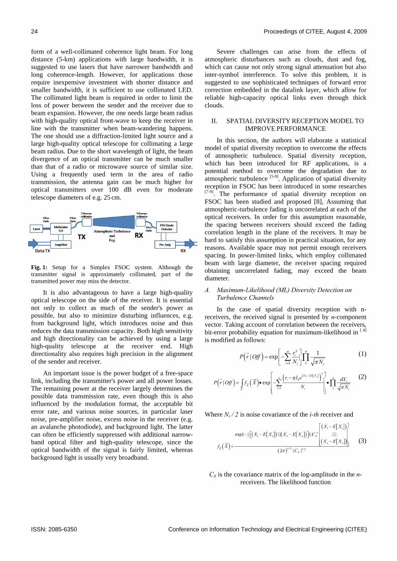
24 Proceedings of CITEE, August 4, 2009
ISSN: 2085-6350 Conference on Information Technology and Electrical Engineering (CITEE)
form of a well-collimated coherence light beam. For long distance (5-km) applications with large bandwidth, it is suggested to use lasers that have narrower bandwidth and long coherence-length. However, for applications those require inexpensive investment with shorter distance and smaller bandwidth, it is sufficient to use collimated LED. The collimated light beam is required in order to limit the loss of power between the sender and the receiver due to beam expansion. However, the one needs large beam radius with high-quality optical front-wave to keep the receiver in line with the transmitter when beam-wandering happens. The one should use a diffraction-limited light source and a large high-quality optical telescope for collimating a large beam radius. Due to the short wavelength of light, the beam divergence of an optical transmitter can be much smaller than that of a radio or microwave source of similar size. Using a frequently used term in the area of radio transmission, the antenna gain can be much higher for optical transmitters over 100 dB even for moderate telescope diameters of e.g. 25 cm.
Fig. 1: Setup for a Simplex FSOC system. Although the transmitter signal is approximately collimated, part of the transmitted power may miss the detector.
It is also advantageous to have a large high-quality optical telescope on the side of the receiver. It is essential not only to collect as much of the sender's power as possible, but also to minimize disturbing influences, e.g. from background light, which introduces noise and thus reduces the data transmission capacity. Both high sensitivity and high directionality can be achieved by using a large high-quality telescope at the receiver end. High directionality also requires high precision in the alignment of the sender and receiver.
An important issue is the power budget of a free-space link, including the transmitter's power and all power losses. The remaining power at the receiver largely determines the possible data transmission rate, even though this is also influenced by the modulation format, the acceptable bit error rate, and various noise sources, in particular laser noise, pre-amplifier noise, excess noise in the receiver (e.g. an avalanche photodiode), and background light. The latter can often be efficiently suppressed with additional narrow-band optical filter and high-quality telescope, since the optical bandwidth of the signal is fairly limited, whereas background light is usually very broadband.
Severe challenges can arise from the effects of atmospheric disturbances such as clouds, dust and fog, which can cause not only strong signal attenuation but also inter-symbol interference. To solve this problem, it is suggested to use sophisticated techniques of forward error correction embedded in the datalink layer, which allow for reliable high-capacity optical links even through thick clouds.
II. SPATIAL DIVERSITY RECEPTION MODEL TO IMPROVE PERFORMANCE
In this section, the authors will elaborate a statistical model of spatial diversity reception to overcome the effects of atmospheric turbulence. Spatial diversity reception, which has been introduced for RF applications, is a potential method to overcome the degradation due to atmospheric turbulence [5-9]. Application of spatial diversity reception in FSOC has been introduced in some researches [7-9]. The performance of spatial diversity reception on FSOC has been studied and proposed [8], Assuming that atmospheric-turbulence fading is uncorrelated at each of the optical receivers. In order for this assumption reasonable, the spacing between receivers should exceed the fading correlation length in the plane of the receivers. It may be hard to satisfy this assumption in practical situation, for any reasons. Available space may not permit enough receivers spacing. In power-limited links, which employ collimated beam with large diameter, the receiver spacing required obtaining uncorrelated fading, may exceed the beam diameter.
A. Maximum-Likelihood (ML) Diversity Detection on Turbulence Channels
In the case of spatial diversity reception with n-receivers, the received signal is presented by n-component vector. Taking account of correlation between the receivers, bit-error probability equation for maximum-likelihood in [ 4] is modified as follows:
( )2
1 1
1| expnn
i
i i i
rP r OffN Nπ=
⎡ ⎤= −⎢ ⎥
⎣ ⎦∑ ∏
r (1)
( ) ( )[ ]( )22 2
0
1 1
| expi iX E X
nn i iX
i iX i
r I e dXP r Off f XN N
η
π
−
=
⎡ ⎤−⎢ ⎥= • − •⎢ ⎥⎢ ⎥⎣ ⎦∑ ∏∫ uur
uur
r uur (2)
Where Ni / 2 is noise covariance of the i-th receiver and
( )[ ]( ) [ ]( )
[ ]( )
[ ]( )( )
1 1
111 12
/ 2 1/ 2
exp
2 | |
n n X
n n
nXX
X E X
X E X X E X CX E X
f XCπ
−
⎡ ⎤−⎢ ⎥
⎡ ⎤− − − ⎢ ⎥⎣ ⎦⎢ ⎥−⎢ ⎥⎣ ⎦=uur
uur (3)
CX is the covariance matrix of the log-amplitude in the n-receivers. The likelihood function

Proceedings of CITEE, August 4, 2009 25
Conference on Information Technology and Electrical Engineering (CITEE) ISSN: 2085-6350
( ) ( )( )
( )[ ]( )22 2 2
0
1
|
|
expi iX E X
n i i
Xi iX
P r Onr
P r Off
r I e rf X d X
N
η −
=
Λ =
⎡ ⎤− −⎢ ⎥= • −⎢ ⎥⎢ ⎥⎣ ⎦∑∫ uur
uur
rr
r
uur uur
(4)
The ML detector uses the decision rule ( ) 1On
rOff
>Λ
<
r . Since the
log-amplitude follows a joint log-normal distribution, calculation of the likelihood function in (4) involve multi-dimensional integration. It is emphasized that this decision rule has been derived under the assumption that the receiving side knows the fading correlation but not the instantaneous fading state.
The bit-error probability of the ML receiver is given by
Pb = P(Off) . P(Bit Error| Off) + P(On) . P(Bit Error|On) (5)
where P(Bit Error| Off) and P(Bit Error| On) denote the bit-error probabilities when the transmitted bit is off and on, respectively. Without considering inter-symbol interference, which can be ignored when the bit rate is not high and multipath effects are not pronounced, we have:
( ) ( )( ) 1r
P Bit error Off p r Off d rΛ >
= ∫r
r r (6)
and
( ) ( )( ) 1r
P Bit error On p r On drΛ <
= ∫r
r r (7)
To evaluate the optimal ML diversity detection scheme, we compare it with the conventional equal-gain combining (EGC) scheme [ ]. In the EGC scheme, it is assumed that the receiving side has knowledge of the marginal distribution of the channel fading, in every receiver, but has no knowledge of the fading correlation or the instantaneous fading state. For each single individual receiver output, it is able to find an optimum threshold τi. Then the EGC detector adds together the n-receivers output with equal gains and compares the sum to the threshold
1
n
th ii
T τ=
=∑ (8)
The error probability of EGC is
( ) ( )|b XX
P f X P Bit Error X d X= ∫ uur
uur
uur uur uur (9)
where
( ) ( ) ( )
[ ] [ ]( )1 1 2 22 2 2 20
2
2
th
X E X X E Xth
TP Bit Error X P Off Q P OnN
I e e TQ
N
η − −
⎛ ⎞= +⎜ ⎟⎝ ⎠
⎛ ⎞+ −⎜ ⎟⎜ ⎟⎝ ⎠
uur
(10)
B. Numerical Simulations for Multi Receivers
In this section, we intend to present numerical simulations of the performance of spatial-diversity reception/detection with multi-receivers and dual-receivers as well. However, up to this Conference submission deadline our research group has not finished the numerical simulation yet. The structure of multi-receiver link that is represented by dual-receiver is illustrated by Fig.2. As described above, the ML receiver (Fig.2a) has full knowledge of the turbulence-correlated fading matrix CX, while the EGC receiver (Fig.2b) has knowledge only the marginal distribution of fading at the receivers. It is assumed that E[I1] = E[I2] = E[I] and N1 = N2 = N and define the electrical signal-to-noise ratio SNR = (ηE[I]2)/N.
Fig. 2: Dual-receiver model on atmospheric turbulence channels with correlated turbulence fading. (a) Maximum-likelihood detection. (b) Equal-Gain combining with threshold detection.
To obtain simulation results, it is assumed that E[X]= 0 and σX = 0.1, varying the normalized correlation ρd from 0 to 0.9. It is also compared to set up value δX = 0.25. We expect that turbulence correlated fading will cause a larger degradation of bit error probability when the standard deviation noise δX is larger. Hipothetically, with two-receivers, ML detection achieves a better performance than EGC for a given SNR. The advantage of ML over EGC method is more pronounced when the correlation ρd between the two receivers is high. It is more reasonable when the SNR is high, then the errors are caused mainly by turbulence-correlated fading, as opposite to the noise.
III. CONCLUSION
Free space optical communications through atmosphere is under intensive researches, where various methods have been proposed to overcome turbulence-effects communication signal fading. In this paper we introduce
spatial diversity reception model for free space optical communications. This model can be use to analyze and later on to overcome the effects due to turbulence-correlated log-amplitude fluctuations.

26 Proceedings of CITEE, August 4, 2009
ISSN: 2085-6350 Conference on Information Technology and Electrical Engineering (CITEE)
ACKNOWLEDGMENT
This research is supported by Universitas Indonesia Research Grant called RUUI-2009, Nb.DRPM/RUUI Unggulan/2009/I/3342 .
REFERENCES [1] V. W. S. Chan, “Optical Space Communications”, IEEE J. Sel. Top.
Quantum Electron. 6 (6), 959 (2000)
[2] O. Caplan, “Laser communication transmitter and receiver design”, J. Opt. Fiber Commun. Rep. 4, 225 (2007)
[3] K. F. Büchter et al., “All-optical Ti:PPLN wavelength conversion modules for free-space optical transmission links in the mid-infrared”, Opt. Lett. 34 (4), 470 (2009)
[4] Xiaoming Zhu and Joseph M. Khan, “Free Space Optical Communication Through Atmospheric Turbulence Channels,” IEEE Transactions on Communications, Vol. 50, No. 8, August 2002
[5] G. L. Stuber, Principles ofMobile Communication. New York: Kluwer Academic, 1996.
[6] J. G. Proakis, Digital Communication, 3rd ed. New York: McGraw-Hill, 1995.
[7] M. Srinivasan and V. Vilnrotter, “Avalanche photodiode arrays for optical communication receivers,”, NASA TMO Progress Rep. 42-144, 2001.
[8] M. M. Ibrahim and A. M. Ibrahim, “Performance analysis of optical receivers with space diversity reception,” Proc. IEE—Commun., vol. 143, no. 6, pp. 369–372, December 1996.
[9] X. Zhu and J. M. Kahn, “Maximum-likelihood spatial-diversity reception on correlated turbulent free-space optical channels,” presented at the IEEE Conf. on Global Commun., San Francisco, CA, Nov.–Dec. 27–1, 2000.

Proceedings of CITEE, August 4, 2009 27
Conference on Information Technology and Electrical Engineering (CITEE) ISSN: 2085-6350
A Measure of Vulnerability For Communication Networks: Component Order Edge Connectivity
A. Suhartomo, Ph.D.
Department of Electrical Engineering President University
[email protected], [email protected]
Abstract: Graph theoretical techniques provide a convenient tool for the investigation of a communication network’s vulnerability to failure. When there are point to point connections, a communication network can be modeled by a graph. A measure of the vulnerability of a network to link failure is the so-called edge connectivity of the graph. We introduce a new vulnerability parameter, generalization of edge connectivity, called “Component Order Edge Connectivity”. It is the smallest number of edges that must be removed in order to ensure that all resulting components have fewer nodes than some given threshold value. We then derive formulas for ( )k
cλ for stars, paths, cycles, and complete graphs; but no formula has been found for an arbitrary graph G.
Keywords: edge connectivity; minimum degree; k-component edge connectivity; edge-failure set, edge-failure state
1. Introduction
Networks such as ring fiber optic, satellite
communication, terrestrial microwave, and social all can be modeled using graph-theoretic construct.
Network vulnerability is an important consideration in network design. The utilization of communication networks has grown tremendously in the last decade, for activities such as transmitting voice, data, and images around the world. With the widespread dependence upon such networks, it becomes important to find topologies that yield a high level of reliability and a low level of vulnerability to disruption.
It is desirable to consider quantitative measures of a network’s vulnerability. To obtain such measures we model the network by a graph in which the station terminals are represented by the nodes of the graph and the links are represented by the edges. The problem, in which edges are subject to failure but nodes are not will be investigated here as a new vulnerability parameter of networks called “k-component order edge connectivity” or “component order edge connectivity”. This is a departure from the classical edge failure model, but we make use of edge connectivity and are concerned with how these parameters interrelate.
2. Network vulnerability in practice Graph theoretic techniques provide a convenient
tool for the investigation of the vulnerability of a communication network to damage from natural or enemy – induced damage. Thus, a communication system can often be represented as interconnection of stations and links. The assumption is that the system is subject to natural failure or enemy attack aimed at isolating stations from each other. The problems of determining the vulnerability and designing communication network which are invulnerability to enemy attack are of paramount importance. As yet, neither the analysis nor synthesis problems have been completed proved, although a number of practical results have been discovered. One difficulty immediately encountered in vulnerability studies is lack of a completely appropriate vulnerability criterion. In this paper, we attempt to address this deficiency by introducing a new parameter: the minimum number of edges that must be deleted in order to isolate a given number of nodes, called component order edge connectivity. 3. Graph Theory and Network Vulnerability
Background
This section introduces graph theoretic concepts which are fundamental to understanding network vulnerability, and surveys the relevant existing work in the field.
A graph G = (V,E), or G, consists of a finite non-empty set of nodes V and a set E of two element subsets of V. If Evu ∈, , we say that , vu is incident at the nodes u and v, and that u and v are adjacent. If
eEnV == || ,|| , G is referred to as an (n,e) graph; n is the order of G and e is size of G.
A specific example of a graph G is given by ,,,,,,, 76543210 vvvvvvvvV = , and
.,,, ,,,,,,,,,,
,,,,,,,,
7675
6454434252
51302010
vvvvvvvvvvvvvv
vvvvvvvvE =
If it is convenient to do so, we usually represent
the graph pictorially, e.g., Figure 1 depicts the graph given in the exam
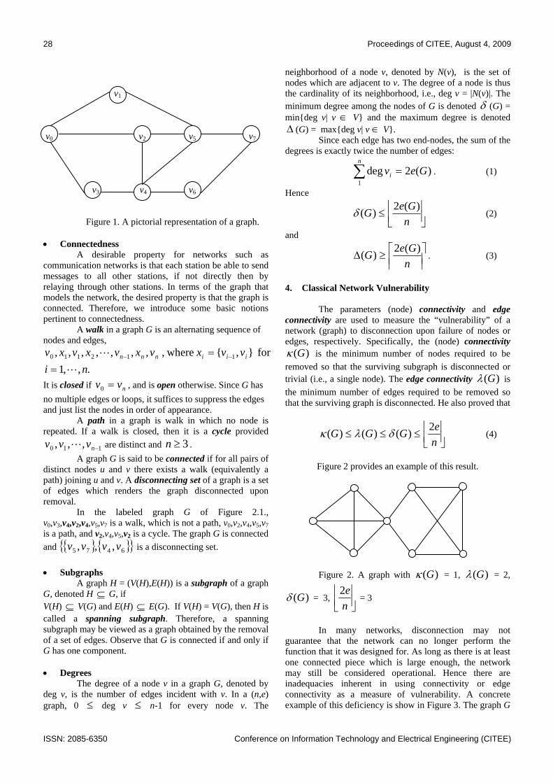
28 Proceedings of CITEE, August 4, 2009
ISSN: 2085-6350 Conference on Information Technology and Electrical Engineering (CITEE)
v1
v0 v2 v5 v7
v3 v4 v6
Figure 1. A pictorial representation of a graph.
• Connectedness
A desirable property for networks such as communication networks is that each station be able to send messages to all other stations, if not directly then by relaying through other stations. In terms of the graph that models the network, the desired property is that the graph is connected. Therefore, we introduce some basic notions pertinent to connectedness.
A walk in a graph G is an alternating sequence of nodes and edges,
.,,1for , where, ,,,,,,, 112110
nivvxvxvxvxv iiinnn
L
L
== −−
It is closed if nvv =0 , and is open otherwise. Since G has no multiple edges or loops, it suffices to suppress the edges and just list the nodes in order of appearance.
A path in a graph is walk in which no node is repeated. If a walk is closed, then it is a cycle provided
110 ,,, −nvvv L are distinct and 3≥n . A graph G is said to be connected if for all pairs of
distinct nodes u and v there exists a walk (equivalently a path) joining u and v. A disconnecting set of a graph is a set of edges which renders the graph disconnected upon removal.
In the labeled graph G of Figure 2.1., v0,v3,v4,v2,v4,v5,v7 is a walk, which is not a path, v0,v2,v4,v5,v7 is a path, and v2,v4,v5,v2 is a cycle. The graph G is connected and 6475 ,,, vvvv is a disconnecting set.
• Subgraphs
A graph H = (V(H),E(H)) is a subgraph of a graph G, denoted H ⊆ G, if V(H) ⊆ V(G) and E(H) ⊆ E(G). If V(H) = V(G), then H is called a spanning subgraph. Therefore, a spanning subgraph may be viewed as a graph obtained by the removal of a set of edges. Observe that G is connected if and only if G has one component. • Degrees
The degree of a node v in a graph G, denoted by deg v, is the number of edges incident with v. In a (n,e) graph, 0 ≤ deg v ≤ n-1 for every node v. The
neighborhood of a node v, denoted by N(v), is the set of nodes which are adjacent to v. The degree of a node is thus the cardinality of its neighborhood, i.e., deg v = |N(v)|. The minimum degree among the nodes of G is denoted δ (G) = mindeg v| v ∈ V and the maximum degree is denoted ∆ (G) = maxdeg v| v ∈ V. Since each edge has two end-nodes, the sum of the degrees is exactly twice the number of edges:
∑ =n
i Gev1
)(2deg . (1)
Hence
⎥⎦⎥
⎢⎣⎢≤
nGeG )(2)(δ (2)
and
⎥⎥⎤
⎢⎢⎡≥∆
nGeG )(2)( . (3)
4. Classical Network Vulnerability
The parameters (node) connectivity and edge
connectivity are used to measure the “vulnerability” of a network (graph) to disconnection upon failure of nodes or edges, respectively. Specifically, the (node) connectivity
)(Gκ is the minimum number of nodes required to be removed so that the surviving subgraph is disconnected or trivial (i.e., a single node). The edge connectivity )(Gλ is the minimum number of edges required to be removed so that the surviving graph is disconnected. He also proved that
⎥⎦⎥
⎢⎣⎢≤≤≤
neGGG 2)()()( δλκ (4)
Figure 2 provides an example of this result.
Figure 2. A graph with )(Gκ = 1, )(Gλ = 2,
)(Gδ = 3, ⎥⎦⎥
⎢⎣⎢
ne2
= 3
In many networks, disconnection may not guarantee that the network can no longer perform the function that it was designed for. As long as there is at least one connected piece which is large enough, the network may still be considered operational. Hence there are inadequacies inherent in using connectivity or edge connectivity as a measure of vulnerability. A concrete example of this deficiency is show in Figure 3. The graph G

Proceedings of CITEE, August 4, 2009 29
Conference on Information Technology and Electrical Engineering (CITEE) ISSN: 2085-6350
of order 1,000,001 has ( )Gκ = 1)( =Gλ . However the subgraphs G – v and G – u,v have components of order 999,999 and 1,000,000, respectively.
u v 610K
Figure 3. A graph with )(Gλ = 1
It is reasonable to consider a model in which it is not necessary that the surviving subgraph is connected so long as it contains a component of some predetermined order. Component order edge connectivity is the minimum number of edges required to be removed so that the surviving subgraph contains no component or order at least some prescribed threshold. 5. Component Order Edge Connectivity
• The Traditional Edge-Failure Model
In the traditional edge-failure model it is assumed that nodes are perfectly reliable but edges may fail. When a set of edges F fail we refer to F as an edge-failure set and the surviving subgraph G – F as an edge-failure state if G – F is disconnected. Definition 1. The edge connectivity of G, denoted by
)(Gλ or simply λ , is defined to be )(Gλ = min FEFF ,|:| ⊆ is an edge-failure set , i.e., G – F
disconnected.
One drawback of the traditional edge-failure model is that the graph G – F is an edge-failure state if it is disconnected and no consideration is given to whether or not there exists a “large” component which in itself may be viable. In this paper we introduced a new edge-failure model, the k-component edge-failure model.
• The New Edge-Failure Model
It is reasonable to consider a model in which it is not necessary that the surviving edges form a connected subgraph as long as they form a subgraph with a component of some predetermined order. Thus we introduce a new edge-failure model, the
k-component order edge-failure model. In this model, when a set of edges F fail we refer to F as a k-component edge-failure set and the surviving subgraph G – F as a
k-component edge-failure state if G - F contains no component of order at least k, where k is a predetermined threshold value.
Definition 2. Let nk ≤≤2 be a predetermined threshold value. The k-component order edge-connectivity or
component order edge connectivity of G, denoted by )()( Gk
cλ or simply )(kcλ , is defined to be
component- is ,|:min|)()( kFEFFGkc ⊆=λ
edge-failure set, i.e., all component of G – F have order 1−≤ k .
Definition 3. A set of edges F of graph G is )(k
cλ -edge set if and only if it is a k-component order edge-failure set and
)(|| kcF λ= .
Next we compute )()( Gk
cλ for specific type of graphs. The first type of graph we consider is the star,
1,1 −nK . Deletion of any set of m edges results in a subgraph
consisting of m+1 components, one isomorphic to 1,1 −−mnK and the remaining components isolated nodes. Therefore a k-component edge-failure state exists if the component
1,1 −−mnK contains at most k-1 nodes. Thus 1−≤− kmn
or mkn ≤+− 1 . Since component order edge connectivity is the minimum number of edges whose removal results in a k-component edge-failure state we obtain the following result: Theorem 1: Given 1)( ,2 1,1
)( +−=≤≤ − knKnk nk
cλ The next type of graph we consider is the path on n nodes, nP . Starting at a pendant edge label the edges consecutively from 1 to n – 1. Let F be the set of edges whose label is divisible by k – 1. The deletion of the edges in F creates |F| + 1 components, the first |F| having order exactly k-1 and the last order at most k-1 (but at least 1). We also note that if fewer edges are removed then there will be fewer components and thus by the Pigeonhole Principle, there must be at least one component of order at least k.
Since |F| = ⎥⎦⎥
⎢⎣⎢
−−
11
kn
we have:
Theorem 2: Given ⎥⎦⎥
⎢⎣⎢
−−
=≤≤11)( ,2 )(
knPnk n
kcλ .
Theorem 3. Let nT be a tree on n nodes. Then for any
value k, ,2 nk ≤≤
1)()()(11
1,1)()()( +−=≤≤=⎥⎦
⎥⎢⎣⎢
−−
− knKTPkn
nk
cnk
cnk
c λλλ
The next type of graph considered is the cycle on n nodes, nC . The formula for )()(
nk
c Cλ can be derived in a
similar manner to that of )()(n
kc Pλ . When one edge of the

30 Proceedings of CITEE, August 4, 2009
ISSN: 2085-6350 Conference on Information Technology and Electrical Engineering (CITEE)
cycle is removed, it becomes the path with n nodes, nP .
Thus 1)()( )()( += nk
cnk
c PC λλ , and since
⎥⎥⎤
⎢⎢⎡
−=+⎥⎦
⎥⎢⎣⎢
−−
11
11
kn
kn
we have the following result:
Theorem 4. Given ⎥⎥⎤
⎢⎢⎡
−=≤≤
1)( ,2 )(
knCnk n
kcλ .
The last type of graph considered in this section is the complete graph on n nodes, nK . Let )( nKEF ⊆ be
a )(kcλ -edge set set. We can compute |F| by calculating the
maximum number of edges that can remain in the k-component edge-failure state FK n − . It is easy to see that any edge in F must have its endpoints in two different components of FK n − ; thus each component of
FK n − must itself be complete. Thus we have the following: Theorem 5. Given ,2 nk ≤≤
⎟⎟⎠
⎞⎜⎜⎝
⎛−⎟⎟
⎠
⎞⎜⎜⎝
⎛ −⎥⎦⎥
⎢⎣⎢
−−⎟⎟
⎠
⎞⎜⎜⎝
⎛=
221
12)( )( rk
knn
Knk
cλ ,
where 20 ,)1(1
−≤≤+−⎥⎦⎥
⎢⎣⎢
−= krrk
knn .
References [1] Gross, D., Boesch, F., Kazmierczak, L., Suffel, C.,
Suhartomo, A.: “Component Order Edge Connectivity – An Introduction”, Congressus Numerantium 178 (2006), pp. 7-14.
[2] Gross, D., Boesch, F., Kazmierczak, L., Suffel, C., Suhartomo, A.: “Bounds For Component Order Edge Connectivity”, Congressus Numerantium 185 (2007), pp. 159-171.
[3] Suhartomo, A.: “Component Order Edge Connectivity: A Vulnerability Parameter For Communication Networks”, Ph.D Dissertation, Stevens Institute of Technology, Hoboken – NJ, USA, 2007
[4] Frank Boesch, Daniel Gross, L. William Kazmierczak, John T. Saccoman, Charles Suffel, A. Suhartomo.: “A Generalization of A Theorem of Chartrand”, Network – 2009-DOI 10.1002/net
Biography: In 1975 – 1977, Antonius Suhartomo received training courses in Radio Transmission of Microwave Terrestrial and Satellite from PT. Telekomunikasi Indonesia (TELKOM), and from 1977 – 2004 Antonius was an employee of PT. TELKOM. He received a B.S in Physics from University of North Sumatera, Medan – Indonesia in 1984, followed by a Master (M.Eng.Sc.) in Optical-Electronic and Laser Applications from University of Indonesia, Jakarta – Indonesia in 1993. He also received a Master (M.M.) in Management from Graduate School of Management, Institute Management Telkom, Bandung – Indonesia in 1994. At PT. TELKOM from 1977 – 2004, he was assigned in many departments under TELKOM business such as in Engineering Division, Training Division, R & D, Institute of Technology Telkom, and Maintenance Service Center Division before he took his Ph.D. He received his Ph.D. in Electrical and Computer Engineering Department majoring in Electrical Engineering from Stevens Institute of Technology, Hoboken – NJ, USA in 2007. He is currently in-charge in several positions such as Secretary Department of Electrical Engineering, Head of Research and Development Center, and Director Office of Residence Life at President University Kota Jababeka – Cikarang, Bekasi – Indonesia starting from year 2008..

Proceedings of CITEE, August 4, 2009 31
Conference on Information Technology and Electrical Engineering (CITEE) ISSN: 2085-6350
The Speech Coder at 4 kbps using Segment between Consecutive Peaks based on the
Sinusoidal Model
Florentinus Budi Setiawan
Electrical Engineering, Soegijapranata Catholic University, Semarang 50234, Indonesia [email protected]
Abstract— Communications equipment needs to work at low bit rate, that can reduce the need of transmission bandwidth. The proposed speech coder generates coded signal at the rate of 4 kbps with low complexity. Thus, the transmission channel can be used for great number of communications connection. The low bit rate speech coder can be realized by using segmental sinusoidal model. By using this model, signal parameters are used to generate the synthetic speech signal.. In this paper, we proposed a sinusoidal model by using the peak of signal amplitude, called as segmental sinusoidal model. The proposed coder is combined with waveform interpolation model and codebook, thus it can work at low bit rate. The coder has MOS score of 3.8 (out of 5). It means that the perception quality is fairly good. The output data rate of encoder is 4 kbps or bellow, with complexity less than 10 MIPS(Million Instruction per Second).
Keywords—analysis, frequency, interpolation, peak, period, segmental, sinusoidal, synthesis
I. INTRODUCTION The number of transmission channel for communication
become limited due to increase of the communication channel usage. Limited channel capacity had endorsed all side more efficient. Speech signal data rate can be developed by using encoder to obtain the simpler information. The research aim is obtained the low rate speech signal encoder with high quality.
The research aim is obtaining coding algorithm on the rate of 4 kbps with high perception quality, on Mean Opinion Score 3,5 - 4. Research consists of encoder and decoder development at conversation frequency between 300 Hz and 3400 Hz. Coder system can be applied for speech signal storage and it can be implemented at digital signal processor system. On the other hand, coder can be applied into communication system using digital signal controller.The main contribution of the research is obtaining the method for decreasing speech signal data rate at 4 kbps. The other contribution is saving the storage media capacity. The number of saving is 93% compared to G.711 speech coder. The coder can be implemented into speech communication hardware like cellular phone, cordless phone, VoIP, multimedia system, secret communication and many other communication system.
The speech coder system consists of encoder and decoder. The encoder function is encoding the speech signal at rate 4 kbps and the decoder function is converting the coded signal into estimation speech signal approximate with
the original speech signal. Main part of encoder is compression algorithm with segmental sinusoidal method for speech signal analysis and waveform interpolation to reduce data rate. Differentiation of the voiced signal and the unvoiced signal is useful for compression method choosing. The voiced, the unvoiced, the pitch, the segment, the decimation, and the formant parameters are coded into codebook. Decoder consists of parameters synthesis block and quality enhancing block. The coded signal is synthesised by using sinusoidal signal generator based on transmitted parameters. Code-vectors are generated from the transmitted codebooks index. Reconstructed speech signal enhancement is developed as a four parallel of band-pass filters for increasing the formant signal and decreasing the valleys between formants.
The research consists of speech signal algorithm development at the rate of 4 kbps, coder software simulation and hardware realization at digital signal processor. The simulation is developed by using the Borland C++ software at 4.5 version. Software simulation consists of speech signal acqusition, speech signal coder, speech signal reconstruction, speech signal reproduction as results of the signal reconstruction and performance tests. The hardware implementation is applied at digital signal processor starter kit (DSK) TMS320VC5416 from Texas Instrument by using Code Composed Studio software. The simulation results are implemented into DSK TMS320VC5416 hardware.
Based on the development and experiment results, I conclude that speech signal coder at 4 kbps have realized by using segmental signal model, waveform interpolation and codebook usage. Near toll perception quality have realized by using the voiced and the unvoiced differentiation, harmonic signal of the sinusoidal model and postfilter implementation. Coder system have applied for speech signal storage and it have been realized by using a hardware based on digital signal processor. The number of the memory needed for encoder and decoder routines saving is less than 16 KB, so that it is realizable for digital signal processor system implementation. The coder system also have been applied for communication system and it can be realized by using the custom integrated circuit design. The number of instruction is less than 6 million per second (6 MIPS), so that it can be implemented into the recent realtime system that work at speed of more than 160 MIPS. Suggestion for the futher research is coder implementation at the digital signal controller, that consists of DSP, memory,

32 Proceedings of CITEE, August 4, 2009
ISSN: 2085-6350 Conference on Information Technology and Electrical Engineering (CITEE)
ADC and DAC. So, it can be used as encoder and decoder at application scale.
II. SINUSOIDAL MODEL Sinusoidal model can be developed to obtain less
parameters, so that the signal data rate can be reduced. This model is called as segmental sinusoidal model. By using this model, there are two harmonic signal to estimate the original signal between two consecutive peaks, (maximum to minimum or minimum to maximum). Peak means minimum peak or maximum peak on the frame. Therefore, one segment means part of signal between maximum peak and consecutive minimum peak or part of signal between minimum peak and consecutive maximum peak.
Time distance between i-th maximum peak and consecutive minimum peak called as period information, and denoted by pd(i). Maximum peak or minimum peak called as peak information, and denoted by pk(i). Peak information is obtained by detecting the maximum peaks and minimum peaks over the frame observed. Period information is obtained by counting the time distance between the consecutive peaks. The proposed method is a process on time domain. On the extreme waveform coding, signal is fetched on its peaks [1]. On the one frame with length of N, there are M maximum peaks and L minimum peaks. On this frame, there are large number sinusoidal signal components. It can be written as :
∑=
+=K
kkkk nnnans
0
))()(cos()( φω (1)
for : 0 < k < K-1, n = 0,1,2 … N-1 , K<N
The first and second coefficients (k=0 and k=1) are used as components to reconstruct the estimated signal from one maximum peak until the consecutive minimum peak or from one minimum peak until the consecutive maximum peak. This is the equation for estimated signal
))()(cos()( 1110 nnaans φω ++= (2)
The estimated signal over the frame is a train of the spv and svp for i=0 until i=I-1. based on the previous explanation, for pk (0) > pk(1), the reconstructed signal using the segmental sinusoidal model can be written as :
⎟⎟⎠
⎞⎜⎜⎝
⎛+
−+−+
++= ππ .
)())(.(cos
2)1()(
2)1()(),( i
ipinnipipipipnis
d
kkkkkr
(3)
for i = 0,1,2 …(I-1)
If pk(0) < pk(1), the reconstructed signal using the segmental sinusoidal model can be written as :
⎟⎟⎠
⎞⎜⎜⎝
⎛++
−+−+
++= ππ ).1(
)())(.(cos
2)1()(
2)1()(),( i
ipinnipipipipnis
d
kkkkkr
(4)
for i = 0,1,2 …(I-1)
III. SPEECH CODER AT 4 KBPS In this paper, a speech signal encoder at 4 kbps and
bellow has been designed using several blocks and algorithms. Detail of the encoder is shown in fig. 6. The encoder contains existing signal detector, windowing process, and pitch detector. The next blocks are voiced and unvoiced classificator, sinusoidal based coder, and formant coder.There are some operation mode of the encoder system depends on the kind of signal to obtain the high performance of coding system [2-7]. There are two different operation modes: silent operation mode and signal operation mode. The signal operation mode consists of vibrating mode operation and non-vibrating mode operation. Input signal is speech signal in 16-bit PCM format at 8 kHz frequency sampling. The first block is signal buffer with 30 ms length. The next block is existing signal detector. Then the 30 ms signal will be detected its pitch period width. Based on pitch period information, signal would be classified into vibrating and non-vibrating signal. If it is less than 160 samples, the signal in buffer is called as vibrating signal. Then, if it is more than 160 samples, it is called as non-vibrating signal. The next process is depend on the kind of signal. For vibrating signal (voiced), characteristic signal [8][9] have to be held. One pitch period of signal is quantized using segmental sinusoidal model. The formant information for each pitch period is kept to obtain the variation information changing for 30 ms. The next block is codebook index searching based on periods, peaks, and formants. All of the coded parameter are sent to the decoder with rate 4 kbps or less than 4 kbps, depends on the kind of the speech signal.
The speech input signal exist are detected by using existing signal detector. The signals are buffered with length of 30 ms. The detector identify the input speech signals whether there are signals exist or there are no signals exist. If there are no signals exist, they are called as silence. A sign is transmitted into decoder to inform this condition, so that the decoder is not process the signal during 30 ms. But if there are signals exist, the encoding process is continued with pitch detecting process.
Pitch is the useful parameter in encoding process. Based on the pitch value, we would identify the signals whether voiced or unvoiced. Human speech pitch period of voiced part is vary from 2.5 ms until 20 ms, depend on the gender and the age. Men tend to have the longer pitch period than women and children [10]. The pitch period is detected by using autocorrelation process. The first step, the buffered signal is detected on its peak. Based on the peak value, it can be found the threshold for the center clip process. The threshold is half of the peak value over entire signal in the buffer. The speech signals on the buffer are clipped, so that we would reduce computation complexity. The clipped signals are processed in autocorrelation computation. The autocorrelation process would result two kind patterns. There are peak-valley-peak pattern and peak-valley pattern. The pitch value is detected based on the distance between peaks of the peak-valley-peak pattern. The peak-valley pattern indicates that the signals are unvoiced.

Proceedings of CITEE, August 4, 2009 33
Conference on Information Technology and Electrical Engineering (CITEE) ISSN: 2085-6350
Buffer 30 ms
Pitch detector
Peak Codesearching
Period codesearching
Segmental quantization
s(n)
c(n)
Multiplexing
Signaldetector
voiced andunvoiced decision
FFT
Spectral Smoothing
Peak codebook
Periodcodebook
Characteristicsignal
Decimation
Formant codesearching
Formantcodebook
i
Tp
D
suvsb
svsvad
cpk
cpd
Fn
vpk
vpd
svad
Tp
Tp
cpk
cpd
sp
cFn
sFFT
sss
Figure 1. Diagram of the Encoder
The voiced and the unvoiced signals are classified by using the pitch detection process results. The autocorrelation results pattern are used as reference to identify the signals whether voiced or unvoiced. If the pattern is peak-valley-peak and if the distance between peaks is longer than 2.5 ms but less than 20 ms, it means that the signals is voiced. Then, if the pattern is peak-valley or peak-valley-peak with distance between peaks is longer than 20 ms, it means that the signal is unvoiced. The voiced and unvoiced signals would process in the different methods. The unvoiced signals would be process without referring the pitch period, then the voiced signals would process based on the pitch period.
The voiced signals are fetched on the one pitch period that representing entire voiced signals on the buffer. The one pitch period signals are called as characteristic signal in waveform interpolative signal terminology [8][9]. The length of the characteristics signals is referred as the pitch period. The characteristic signal is quantized on its peaks and periods by using segmental sinusoidal model. For the unvoiced signal, the decimation process is implemented to obtain the smaller size of signal. Then the peak and period quantization is applied. Based on the segmental sinusoidal model, peaks and periods information is extracted. The processed signal would be generated by using the peaks and periods quantization.
The peak information size is reduced by applying 10 look-up tables. The look-up table is also called as codebook. The codebook is trained by using the peak information code-vector. Large amount of the peak information code-vectors are trained with k-means algorithm to obtain the peaks codebook. The index number of the peak codebook is varied from 6 to 10 to obtain the optimum process. The period information size is also reduced by applying look-up table. The index number of the peak codebook is also varied from 6 to 10 to obtain the optimum process. The period accuracy has to maintain to obtain the good receiver perception on the decoder side. Formant information is important for post-filtering process. The post-filter is arranged as four adaptive band-pass filters to increase the formants and decrease the valley between formants to enhance perception. The
formants location is detected by applying the FFT and smoothing filter. Then the low-passed spectra are detected on its peaks location. The peaks location is send to receiver to set the center frequency on the appropriate band-pass filter.
Parameters that have to be sent to the receiver are peaks, periods, pitch, formants, segment, and decimation. The peaks information needs 16-56 bits, the period information needs 6-54 bits, pitch needs 7 bits, segment information needs 6 bits and the formants information needs 0-14 bits. The maximum total coded signal bits resulted for one frame (30 ms) is 120 bits. Thus, the coded speech signals data rate is 4 kbps.
Signaldetector
silence
Demultiplexing
postfilter
Unvoicedrecons-truction
Voicedrecons-truction
cpd
Tp, i, D
+ )(ˆ ns
Fn
c(n) cpk
Se
Ss
Sr
Sr
SF
Figure 2. Diagram of the Decoder
In decoder, the coded signal is reconstructed to obtain the speech signal approximation with near toll quality at rate 4 kbps or bellow. If the coded signal is detected as silence, the decoder will generate silence over a frame length i.e. 30 ms. If, it is an existing speech signal, the decoder will generate the speech signal depends on the type of signal. Unvoiced signal is generated using the sinusoidal parameters. For voiced signal, there is a special processing, that is post-filtering process. The post-filter will enhance performance of the voiced signal by increasing the formant peaks and reducing the valley between formant. The encoder sends

34 Proceedings of CITEE, August 4, 2009
ISSN: 2085-6350 Conference on Information Technology and Electrical Engineering (CITEE)
speech signal information as a multiplexed parameter. In the decoder, parameters are de-multiplexed to obtain the useful information for signal reconstruction. Parameters would be generated are peaks, periods information, formants information, pitch, number of segment, and decimation.
The signal detector would identify the kind of signal. If there is a silence, detector would not work because. The unvoiced signal will be reconstructed if it is detected as unvoiced. The peaks and periods are used to generate the unvoiced signal. The next process is interpolation process with ratio D, inverting of the decimation process on the encoder. The voiced signal is reconstructed by generating the characteristic signal along the 30 ms segment. The number of characteristic signal along this segment varies between 1.5 until 12, depends on the pitch period. The characteristic signal is generated by using the segmental sinusoidal model from peaks and periods information. The reconstructed signal, especially the voiced signal is passed into post-filter. The post-filter proposed is a train of four adaptive band-pass filters. The center frequency of each filter is changed every 30 ms segment. The center frequencies are detected by encoder, and then they are sent to decoder. Then the comb filter and compensation filter are applied to improve the hearing perception quality [11][12].
The resulted reconstructed signal by sinusoidal approach seems smoother than the original that had arbitrary form between one peak to the consecutive peak. Nevertheless, roughness of original signal means containing high frequency component. Therefore, the spectral power is reduced on the high frequency component. Unfortunately, increasing of the number of peak would decrease the dynamic range of period changing variation for each segment. Thus, compression ratio would be increased to compensate decreasing of compression ratio caused by the number of peaks.
IV. EXPERIMENTAL RESULTS The proposed speech coder has been simulated in a
personal computer using a 4kbps coder program that was specially developed by using C++ programming language. The resulted mean opinion score (MOS) test measured for 15 Indonesian phrase in computer simulation is 3.8 (out of 5). It is tested on 46 peoples with variation on gender, background and age. The coder complexity is less than 15 MIPS, comparable with others kind of speech coder that needs 0.01 MIPS until 90 MIPS. It need less than 30 kB for encoder and 10 kB for decoder.
Then, the coder is implemented on digital signal processor starter kit TMS320VC5416, using a 4 kbps coder program specially developed for the DSP system, based on Code Composer Studio ver.2. Based on the experimental results, hearing perception of the reconstructed signal is fairly good. By using digital signal processor starter kit, the MOS test score is 3.3 (out of 5), because of reducing the number of codebooks. The resulted mean opinion score (MOS) test measured for 15 Indonesian phrase in computer
simulation is 3.8 (out of 5). It is tested on 46 peoples with variation on gender, background and age. The coder complexity is less than 15 MIPS. It need less than 16 kB for encoder and 3 kB for decoder. Therefore, it is expected that the proposed low bit rate speech coder with fairly good MOS test score and low complexity will be suitable for voice communication and telemedicine applications during and after disaster cases.
Figure 3. MOS test results
V. CONCLUSION Speech signal could be coded into 4 kbps rate and
decoded with high quality of the human perception based on segmental sinusoidal model. The maximum MOS score is 3.8 on Indonesian words. The coder complexity for the digital signal processor implementation is low, it needs less than 10 MIPS.
REFERENCES [1] Ridkosil F., Extreme Waveform Coding, US Pattent [2] TF Quatiery, RJ.McAulay, Speech Transforma tions Based on a
Sinusoidal Representation, IEEE TASSP, vol. ASSP-34, no. 6, 1986 [3] RJ.McAulay, TF Quatiery, Speech, Analysis/ Synthesis Based on a
SinusoidalRepresentation, IEEE TASSP, vol. ASSP-34, no. 4, 1986 [4] T. Abe, dan M. Honda, Sinusoidal Model Based On Instantaneous
Frequency Attractor, TSALP vol 14 No.4, 2006 [5] R. Boyer, dan Abed-Meraim, K, AudioModeling Based on Delayed
Sinusoids, TSAP vol 12, No.2, 2004. [6] CO. Etemoglu, dan V. Cuperman, V, Matching Pursuit Sinusoidal
Speech Coding, TSAP vol 11, No.5, 2003. [7] GH. Hotho, dan RJ. Sluijter, A Narrowband Low Bit Rate Sinusoidal
Audio and Speech Coder, Company Research - Philips Electronics Nederland, 2003.
[8] Gottesman, O. dan Gersho, A. (2000) : High Quality Enhanced Waveform Interpolative Coding at 2.8 kbps, Proceedings of International Conference on Acoustics, Speech, and Signal Processing, 0-0.
[9] Gottesman, O. dan Gersho, A. (2001) : Enhanced Waveform Interpolative Coding at Low Bit-Rate, IEEE Transactions on Speech and Audio Processing, 9, 1-13.
[10] JR. Deller, JG. Proakis, JHL. Hansen, Discrete-Time Processing of Speech, Macmillan Publishing Company, New York, 1993.
[11] FB. Setiawan, S. Soegijoko, Sugihartono, S. Tjondronegoro, Perbaikan Mutu Sinyal Suara Tercampur Derau Berdasarkan Bentuk Formant, SITIA Proceedings, Surabaya, 2006
[12] FB. Setiawan, S. Soegijoko, Sugihartono, dan S. Tjondronegoro, A Low Bit Rate Speech Coder using Segmental Sinusoidal Model for Disaster and Emergency Telemedicine, Journal of eHealth Technology and Application, September 2008.

Proceedings of CITEE, August 4, 2009 35
Conference on Information Technology and Electrical Engineering (CITEE) ISSN: 2085-6350
AUTOMATIC ABNORMAL WAVES DETECTION FROM THE ELECTROENCEPHALOGRAMS OF PETIT MAL EPILEPSY CASES TO SORT
OUT THE SPIKES FP1 - FP2, THE SHARPS, THE POLYPHASE BASED ON THEIR STATISTICAL ZEROCROSSING
Siswandari N, Adhi Susanto, Electrical engineering UNDARIS,Electrical engineering UGM
[email protected], [email protected]
Zainal Muttaqin neurosurgent epilepsy medical Undip
[email protected] ABSTRACT To explore the merits of the widespread digital signal processing on EEG waves the standard analyses of autocorelation, Fourier transform and zero-crossings were applied on the seizure related waves of a large number of epilepsy patients. Patient consist of 267M,140F, ages 3-55 years. Clinical status: epileptic (97M,46F: EEG with spike;39M, 28Fwithout); clinical status: nonepileptic: (93M, 41F EEG with spike ; 38M, 25F without). Numerical data were acquired with EEG dump diagnostic Biologic system at Sarjito hospital Yogyakarta etc, 2002-2009. The wave components were sorted out according to their amplitudes and time span between zerocrossings. The experimental results show a promising application of the scheme, since practically all are in line with those assessed by specialists in this field. Utilizing the hardware and software facilities at hand, marking the st arts and ends of abnormal waves could be done with +39µV threshold. The zerocrossings detection could automatically distinguished according to the 20ms–70ms time period for the “spikes” (109M,53F) ,70ms-120ms for “sharps” (101M, 51F), and the existence of multiple peaks for “polyphase”(57M,36F). The research carried out so far was to find the prospect of this digital signal processing on EEG waves to support the doctors' work in this field. Keywords : EEG, spikes, sharp
I. INTRODUCTION The clinical electroencephalographer correlates central nervous system functions as well as dysfunction and diseases with certain paterns of the electroencephalogram (EEG) on an empirical basis, Obviously, this method has been found Valuable in clinical practice The International Federation of societies for electroencephalograpy and clinical Neurophysiology ( committee chaired by G.E Chatrian, see reference for IFSECN, 1974 proposed the following definition
1. Alpha rhythm, EEG wave pattern that has frequency 8 -13 Hz, with amplitude 20 – 200 µV. This wave pattern can be found in almost all normal people who are in awaked condition but quiet.
2. Beta rhythm, wave pattern that has frequency 13 Hz, sometime in certain condition can reach 50 Hz.
Rhytmical beta activity is encountered chiefly over the frontal and central regions, it usually does not exceed 35 Hz.
3. Theta rhythm, wave pattern that has frequency 4 - 7 Hz. This wave appears in children but sometime appears in adult who are in frustrated condition.
4. Delta rhythm, wave pattern that has frequency under 4 Hz, sometime only appears once in two or three seconds. This wave happens in people sleeping tight.
The EEG utility available in a hospital have not been able to detect spike, sharp, and polyphase automatically only in subjectively perception and manually counting. Therefore, it needs a program to differentiate spike, sharp and polyphase automatically. However, it should be noticed that a small part of EEG inter epilepsy attack does not show any difference by using the autocorrelation and cross correlation EEG signal. Moreover, FFT is able to show the previous signal exploration.
II. MODEL, ANALYSIS, DESIGN, AND IMPLEMENTATION A. Research Material
Numerical data were acquired with EEG dump diagnostic Biologic system at Dr. Sardjito hospital Yogyakarta etc, 2002- by changing the file of EEG dump diagnostic into the form of .txt. format.
B. Tools Computer with Matlab 6.5 software using Windows XP System
C. How To Do The research is done with the following stages: a. First, the collection of data cm is done by
observing the EEG qualitative diagnostic and interpretation of its abnormal wave. Data can be classified into:
1. Clinical status : epileptic with spike 2. Clinical status epileptic without spike 3. Clinical status : non epileptic with spike 4. Clinical status non epileptic (normal)
without spike b. Digital data taken from the EEG biologic system of
Dr. Sardjito hospital Yogyakarta, based on Mark Dump Utility.
To determine the wave form of spike, sharp and polyphase in EEG, it uses zero crossing time with t0, t1, t2, …. Etc.

36 Proceedings of CITEE, August 4, 2009
ISSN: 2085-6350 Conference on Information Technology and Electrical Engineering (CITEE)
T 1 = t 1 - t 0
T 2 = t 2 - t 1
T 3 = t 3 - t 2 etc…………..(.1)
ten take the balance.
2.1 Interictal Paroxysmal Pattern Spike According to IFSECN (1974), a spike is a transient, clearly distinguished from the background activity, with pointed peak at conventional paper speed and a duration from 20 to under 70 msec, the main component is generally negative, Amplitude is variable. The distinction from the background activity is based on wave morphology and amplitude. In many cases, spikes stand out against the background because of their high voltage. If the voltage of spikes and background activity is approximately equal, the faster character ( short duration) of the spike is its distinctive feature. Sharp According to IFSECN (1974), a sharp is a transient, clearly distinguished from the background activity, with pointed peak at conventional paper speed and duration of 70 - 200 msec. the main component is generally negative relative to other areas. Jasper(1941) pointed out that the rising phase of the sharp waveis of the same order of magnitude as in spikes, but the descending phase is prolonged. 2.2 Signal appearance by using spectrogram: The purpose of spectral estimation is to explain about power distribution which is contained in signal at certain range frequency, according to the amount of limited data quotation. This spectrum estimation can use to analyze EEG’s power spectrum signal to see abnormal symptom that happen in activity of nerve human being brain.
1. Power spectrum from a stationer random process xn, mathematically correlating with Fourier transformation from its row correlation, in form of normalization frequency, this correlation can be written as:
.…..(2)
Sxx is power spectrum, Rxx is auto correlation, equivalent above can be expressed as frequency function f (in Hertz) by using correlation ω = 2πf/fs, with fs is quotation frequency.
…(3.)
PSD or Power Septral Density, defined as power spectrum quotation frequency.
πω
ω2
)()( xx
xxS
P = and fsfS
fP xxxx
)()( = ...(4)
III. RESULT
Figure : Spectrogram signal FP1 – FP2 for 379s.
The example of signal EEG from a patient name A who is diagnosed epilepsy petit mal taken in electrode FP1– FP2.
To see signal power spectrum clearly can be done by dividing signal become some parts and then in each part of the signal search their PSD. For example FP1.-FP2 signal recorded for 6 minutes, 1.009 seconds with the quotation frequency 256, will be separated into some parts where each part consists of 256 data quotations, with overlapping 200 data, by using 2D image (spectrogram) the result will be seen as figure 1.
The biggest figure box is power spectrum representation in the form of 2D with abscissa asserts quotation time and coordinate asserts frequency content with color that represent power per set of frequency in certain time. In that figure can be seen that frequency content with high power happens in frequency between 0 to 30 Hz (red). When the symptom of epilepsy appears in that frequency area become higher (flatten red). In that figure also visible a signal trouble that appears from power supply with frequency 50 Hz and 1.0000 Hz (orange ribbon) that appears in whole signal.
This second is special characteristic that seen by medic in electrode FP1 – FP2 appears 4 1.00 with very high amplitude, 3 1.00 with average amplitude, with pattern 1.00 sharp then multi 1.00 sharp 4.00 then multi 1.00 with very high amplitude. It approves that patient epilepsy petit mal seen from medical science that in 1.00 seconds appear 31.00
∑∞
−∞=
−=m
mjxxxx emRS ωω )()(
∑∞
−∞=
−=m
fsmfjxxxx emRfS /2)()( π

Proceedings of CITEE, August 4, 2009 37
Conference on Information Technology and Electrical Engineering (CITEE) ISSN: 2085-6350
is not be proven (or possible to be said not always). 1.00 with high amplitude about 65.20 µ V happens in a last second in elapsed time 00 : 03:48 – 00 :03 :49. In this second is special characteristic of abnormal wave of petit mal, doctor usually sees symptom clinic at first, EEG just help to build diagnose.
Figure 2: EEG Bipolar 19 channel
This pattern has been described as “petit mal absence epilepsy “. Classical 3/sec spike wave complexes are widely known even outside the community of electroencephalographers at FP1 – FP2 figure 1. It is officially termed “ spike and slow wave complex “ , this term comprises all types of spike wave complexes, which listed separately because of markedly differing associated clinical epileptological conditions.
Figure 3 : signal FP1 – FP2 time elapsed 00:04:51 – 00:05:00
Figure 4 EEG , FP1 – FP2 time elapsed 00:04:51 – 00:04:52 Tabel 1 : Zerocrossing method EEG FP1 – FP2 time elapsed 00:04:51 – 00:04:52 low high Duration
(mS) Amplitude(µ V)
Code
1.00 6.00 19.53 6.80 0 1.00
21.00 34.00 50.78 7.60 4.00 poliphase
1.00
44.00 48.00 15.63 21.60 0 1.00
69.00 83.00 54.69 9.60 4.00 poliphase
1.00
93.00 114.00 82.03 15.60 4.00 poliphase
1.00
114.00 114.00 0 0 0 1.00
122.00 128.00 23.44 43.00 1.00 spike 1.00
135.00 137.00 7.81 2.40 0.00 1.00
145.00 193.00 187.50 45.00 4.00 poliphase
1.00
202.00 206.00 15.63 16.40 0 1.00
222.00 257.00 136.72 91.00 2.00 sharp 1.00
Applying Zerocrossing of Equation (1) to the detection of epileptic spikes, sharp and poliphase . Initially, with Code 1.00 = spike, code 2.00 = sharp, code 4.00 = poliphase with frequencies sampling fs = 256. The x axis of this output represented the sample data n , i.e. time. The y axis of this output represented amplitude. For table 1, low = 122.00, high = 128.00, duration = 23,44 mS, amplitude = 43 µ V, Code = 1.00 spike,

38 Proceedings of CITEE, August 4, 2009
ISSN: 2085-6350 Conference on Information Technology and Electrical Engineering (CITEE)
4. CONCLUSION
1. The EEG wave figure shown by the recent EEG
utility can be seen from other aspect such as autocorrelation and power spectrum dense.
2. The figure of spike, sharp and polyphase can be seen in detail using zero crossing in software automatically. Therefore, many pattern introduction might appear into sharp, spike and polyphase.
3. The study can lead to the prediction of spike and sharp waves emerge since they cannot be seen using the ordinary EEG record.
4. The epilepsy sensor implant can be made in order to plan software and hardware installation for early warning system of an attack. The attack early warning system can detect an attack 10 minutes before it happens. The alarm will automatically ring. It can happen if there is cooperation between medical and engineering department.
REFERENCES [ ]1 . Ernst Neidermeyer, M.D and Fernando Lopes Da Silva,
M.D, February 1982, “ Electroencephalography Basic Principles, Clinical Applications, and Related Fields”, Williams and Wilkins, Baltimore USA.
[ ]2 A Barreto et al.,October.1993, “Intraoperative Fokus localization System based Spatio-Temporal EcoG
Analysis”, Proc. XV Amnual Intl.Conf of the IEEE Engineering in Medicine and Biology Society.
[ ]3 Mahar Mardjono, 1992, Simposium Diagnosis dini Epilepsi, MDK/ Vol. 11. No. 01/Januari 1992, Jakarta.
[ ]4 . Alan V. Oppenheim and Ronald W. Schafer, 1994, “Digital Signal Processing”, Prentice Hall of India, New Delhi.
[ ]5 . Erik Bolviken, Geir Storvik, Gutorm Hogasen and Pal G. Larsson, 2004, “Spike detection in EEG through random line segments”, The project has been performed at the Norwegian Computing Center supported by Royal Norwegian Council for Scientific and Industrial Research.
[ ]6 Lim Shih Hui , 2003, “Interictal and Ictal Epileptiform Discharges”, National Neuroscience Institute, Singapore.
[ ]7 Hamid Hassanpour, Moestefa Mesbah and Boualem Boashash, 2004,” EEG Spike detection Using Time-Frequency Signal Analysis”, 2004 IEEE.
[ ]8 Shoichiro Nakamura, 1993, “Applied Numerical methods ”, Prentice-Hall International, Inc USA
10.John G. Webster , 1995, “Medical Instrumentation Application and Design” John Wiley & Sons,Inc, New York.
.
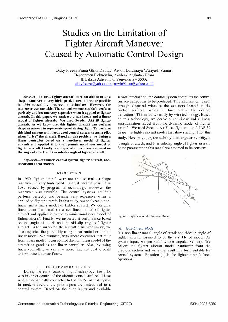
Proceedings of CITEE, August 4, 2009 39
Conference on Information Technology and Electrical Engineering (CITEE) ISSN: 2085-6350
Studies on the Limitation of Fighter Aircraft Maneuver
Caused by Automatic Control Design
Okky Freeza Prana Ghita Daulay, Arwin Datumaya Wahyudi Sumari Departemen Elektronika, Akademi Angkatan Udara
Jl. Laksda Adisutjipto, Yogyakarta – 55002 [email protected], [email protected]
Abstract— In 1950, fighter aircraft were not able to make a shape maneuver in very high speed. Later, it became possible in 1980 caused by progress in technology. However, the maneuver was unstable. The control systems couldn’t perform perfectly and became very expensive when it applied to fighter aircraft. In this paper, we analyzed a non-linear and a linear model of fighter aircraft. We used Sweden JAS-39 fighter aircraft. As we know that this fighter aircraft can perform shape maneuver in supersonic speed during flight. To perform this kind maneuver, it needs good control system to assist pilot when “drive” the aircraft. Based on this problem, we design a linear controller based on a non-linear model of fighter aircraft and applied it to the dynamic non-linear model of fighter aircraft. Finally, we inspected it performance based on the angle of attack and the sideslip angle of fighter aircraft.
Keywords—automatic control system, fighter aircraft, non-linear and linear models
I. INTRODUCTION In 1950, fighter aircraft were not able to make a shape maneuver in very high speed. Later, it became possible in 1980 caused by progress in technology. However, the maneuver was unstable. The control systems couldn’t perform perfectly and became very expensive when it applied to fighter aircraft. In this study, we analyzed a non-linear and a linear model of fighter aircraft. We design a linear controller based on a non-linear model of fighter aircraft and applied it to the dynamic non-linear model of fighter aircraft. Finally, we inspected it performance based on the angle of attack and the sideslip angle of fighter aircraft. When inspected the aircraft maneuver ability, we also inspected the possibility using linear controller to non-linear model. We assumed, with linear controller that built from linear model, it can control the non-linear model of the aircraft as good as non-linear controller. Also, by using linear controller, we can save more time and cost to build and produce it at near future.
II. FIGHTER AIRCRAFT PRIMER During the early years of flight technology, the pilot
was in direct control of the aircraft control surfaces. These where mechanically connected to the pilot's manual inputs. In modern aircraft, the pilot inputs are instead fed to a control system. Based on the pilot inputs and available
sensor information, the control system computes the control surface deflections to be produced. This information is sent through electrical wires to the actuators located at the control surfaces, which in turn realize the desired deflections. This is known as fly-by-wire technology. Based on this technology, we derive a non-linear and a linear approximation model from the dynamic model of fighter aircraft. We used Sweden Air Force fighter aircraft JAS-39 Gripen as fighter aircraft model that shows in Fig. 1 for this study. Here sr,sq,sp are stability-axes angular velocity, α is angle of attack, and β is sideslip angle of fighter aircraft. Some parameter on this model we assumed to be constant.
Figure 1. Fighter Aircraft Dynamic Model.
A. NonLinear Model In a non-linear model, angle of attack and sideslip angle of fighter aircraft assumed to be the variable of model. As system input, we put stability-axes angular velocity. We collect the fighter aircraft model parameter from the previous section and write the result in a form suitable for control systems. Equation (1) is the fighter aircraft force equations.

40 Proceedings of CITEE, August 4, 2009
ISSN: 2085-6350 Conference on Information Technology and Electrical Engineering (CITEE)
)3mgsinFcos(YmV
1rcosαpsinα
・β
)2mgFsinαL(mVcos
1)tanrsin(pcosq
・α
)1mgcosFcosD(m
1・V
+−+−=
+−−++−=
++−=
βα
ββαα
βα
.
(1)
where the contribution due to gravity are given by
)coscossinsin-sincossinsincosg(cos3g
)sinsincoscosg(cos2g
)coscoscossinsincossinsincoscosg(1g
φθβαθαβφθβ
θαφθα
φθβαφθβθβα
+=
+=
++−=
Equation (2) is the fighter aircraft dynamic non-linear model of fighter aircraft that we will use for designing the controller.
)3mgsinFcos-)(Y(mV
1sr
・β
)2mgFsin α-)L((mVcos
1tanβspsq
・α
3u・sr
・2usq1u
・sp
++−=
+−+−=
===
βαβ
αβ
.
(2)
where
)coscossinsin-sincossinsincosg(cos3g
)sinsincoscosg(cos2g
φθβαθαβφθβ
θαφθα
+=
+=
Later, we created the fighter aircraft non-linear control system inputs based on bakstepping method and bode diagram based on (2). Backstepping method is a method that built from subsystems that radiate out from an irreducible subsystem that can be stabilized using some other method. Because of this recursive structure, the designer can start the design process at the known-stable system and feedback new controllers that progressively stabilize each outer subsystem. The process terminates when the final external control is reached.
A. Linear Model In linear model, we assumed angle of attack and sideslip angle is zero and roll angular velocity assumed to be constant during calculation. This made the calculation of problem easier to solve. Equation (3) is basic model of linear equation.
buAx・x +=
(3)
Equation (4) is the state variable result from linearization of the fighter aircraft dynamic equation according to (3).
⎥⎦⎤
⎢⎣⎡⎥⎦
⎤⎢⎣
⎡⎥⎦⎤
⎢⎣⎡⎥⎦
⎤⎢⎣
⎡
⎥⎥⎦
⎤
⎢⎢⎣
⎡+=
srsq
22b21b12b11b
βα
22A21A12A11A
・β
・α (4)
where A and b are given by
021A
)mV
mgsinF(11A
=
−−=
θ
)mV
mgsin θF(22A
spmV
)L(cosmgcos12A
−−=
−−
=αφθ
021b
111b
=
=
122b
012b
−=
=
where the parameters value which we used in this research
that named body mass, force, gravity acceleration, and
velocity of fighter aircraft are
m = 9,100 [kg] F = 54,000 [N]
g = 9.8 [m/ 2s ] V = 165.811 [m/s]
III. FIGHTER AIRCRAFT CONTROLLER We designed non-linear controller based on a non-linear model and a linear controller based on linear model. We used Scilab/Scicos program to design and simulate the system. Scilab/Scicos program is a numerical computation software package similar to MATLAB/SIMULINK that has been released by Institut National de Recherché en Informatique et Automatique (INRIA) from France since 1990.
A. NonLinear Controller We referred to [1] when designed non-linear controller using Backstepping method based on non-linear model. According to the non-linear model in (1), (5), (6), and (7) are non-linear controller inputs using Backstepping method.
)sprefs(ppsk1u −= (5)
))αy,ref(ααf)refα(αα,1ks(qα,2k2u +−+−= (6)
)V
singcosββ,1ksr(β,2k3u
φθ++−= (7)
Fig. 2 is fighter aircraft non-linear model bode diagram using Backstepping method.

Proceedings of CITEE, August 4, 2009 41
Conference on Information Technology and Electrical Engineering (CITEE) ISSN: 2085-6350
-1 3u
s1
s1
s1
・α
・β
2u
psk
1,βk
βtan
α
β
+
+
+
+
+
−
−
−
−−
refsp
refqs
refsr
Figure 2. Non-linear System
B. Linear Controller We used linear quadratic regulator method when
designed linear controller based on linear model of fighter aircraft. Meanwhile, to design a servo system that suitable to appointed angle of attack and sideslip angle, we used the Enlarged system method.
Equation (8) is fighter aircraft linear model equation using enlarged system method that we used to solve the matrix problem during build the feedback gain.
⎥⎦⎤
⎢⎣⎡
++=r(t)v(t)
u(t)b(t)xA・x (8)
where
⎥⎥⎥⎥⎥⎥
⎦
⎤
⎢⎢⎢⎢⎢⎢
⎣
⎡
⎥⎦⎤
⎢⎣⎡
−−
−−
−−−
−
=−
=
00100001
00)mV
mgsinθF(0
00refsp
mV
)refL(αmgcosθgcos)
mV
mgsinθF(
0c0A
A
⎥⎥⎥⎥
⎦
⎤
⎢⎢⎢⎢
⎣
⎡
⎥⎦⎤
⎢⎣⎡ −
==
0000
1001
0b
b
According to linear model in (8), I made linear model input as shown in (9).
u = kx (9)
where k is feedback gain. We used Riccati Equation as shown in (10).
0QPPBBrPAPA T1T =+−+ −
(10)
This equation used to build feedback gain which means the controller in linear model and applied it to the linear model inputs as shown in (11).
PxTB1ru −−= (11)
refer to (11), the feedback gain for this model is
PTB1rk −−= (12)
Equation (12) is feedback gain from linear model. Fig. 3 is fighter aircraft linear model bode diagram based on (8). Here, roll angular velocity assumed to zero because it has less effect both in angle of attack and sideslip angle maneuver.
Figure 3. Linear System
A. MANEUVER AND SIMULATION In this session, we combine three control models and
controllers to inspect each combination performance. They are:
• Non-linear model with non-linear controller.
• Linear model with linear controller.
• Non-linear model with linear controller.
These three-combination-and-simulation goals was to inspect the differences on each combination, search the best combination for the model, and look forward about possibility to use new combination between model and controller. Meanwhile, we also figure out each combination effect to fighter aircraft maneuver during flight.
Fig. 4 and Fig. 5 (a) is non-linear model with non-linear controller, (b) is linear model with linear controller, and (c) is non-linear model with linear controller simulation result. Fig. 6 is non-linear model with linear controller which has been increased in feedback gain. In this result from top to below showed roll angular velocity, angle of attack targeted value, sideslip angle targeted value, angle of attack result, and sideslip angle result.
Fig. 4 described the simulation from fighter aircraft maneuver without roll maneuver. Here we inspect each controller design effect to fighter aircraft maneuver in simply maneuver environment. Fig. 4 (a) and (b) mostly showed similar movement simulation result especially in angle of attack (AoA) or pitch angle. But, Fig. 4 (b) showed that sideslip angle grew bigger. It may be said that the adjustment of the control loop for the sideslip angle is more necessary. In (c) the result was able to made similar movement especially in angle of attack (AoA) or pitch angle. But, it has too much noise with it. It was started when pilot gave the input to aircraft and continued even pilot did not give any input. Meanwhile, sideslip angle result turned unstable at all. Even pilot did not give any input, result showed movement that indicate aircraft did not work normally. When we increased input continuously, angle of attack (AoA) showed less noise on it. Meanwhile, noise on sideslip angle and last combination (non-linear model with linear controller) getting bigger continuously.

42 Proceedings of CITEE, August 4, 2009
ISSN: 2085-6350 Conference on Information Technology and Electrical Engineering (CITEE)
Fig. 5 described the simulation from fighter aircraft maneuver with roll maneuver. We inspect each controller
design effect to fighter aircraft maneuver in complex maneuver environment. Fig. 5 (a) and (b) showed similar result with first simulation result. In angle of attack (AoA) or pitch angle result, Fig. 5 (a) and (b) showed similar result for input and output. It described that was no problem during control the aircraft. Aircraft could perform maneuver as well as input that was given by pilot. Meanwhile, noise that occurred in sideslip angle was getting bigger that result in first simulation. It showed that more complex input that pilot give, the result will become more complex. Fig. 5 gave same result as first simulation.
Fig. 6 described the simulation from combination of non-linear model and linear controller. According to result
from first and second simulation, this combination did not show good result. We increased feedback gain controller by increased heaviness for the state (Q) to stabilize system. Fig. 7 (a) gave the best result among them. When I set Q = diag (100, 100, 1, 1), angle of attack (AoA) and sideslip angle result showed closer to input. If we grew feedback gain, angle of attack (AoA) result getting more unstable and could not reach the same value as input. Meanwhile, sideslip angle result showed better because it could reach the same value as input. Even after we set the heaviness for the state (Q) extremely when designed linear controller, it couldn’t improve the result at all when applied to non-linear model.
Therefore, it might be said that linear controller that built from linear model, was not able to control the non-linear model of fighter aircraft and fighter aircraft maneuver performance received big influence by it control system.
V. CONCLUDING REMARKS AND FURTHER WORKS On this study, we guessed it whether cannot control the
non-linear model of the fighter in a linear controller.
In addition, we thought it to be useful when we implemented it because the result did not become expensive, less design time, and many other positive results. However, in this study, we simulated it and inspected it, but our assumed result did not appear.
Finally, there was only two ways controller design this far. First, non-linear controller designed by it own system and linear controller designed by it own system. Each controller can only control it own system. Also, it is better to use non-linear controller for fighter aircraft non-linear model than use linear controller that built from linear model.
As reference for next research is make a computer program to control servo or stepper based on this research. This is to prove that the simulation result can be implemented on reality or not.
For our further works, we would like to try another method to resolve all the problems that appear during research. As an example, we would like to rebuild non-linear controller using Lyapunov method. Lyapunov method allow us to analyze the stability from a system, in this case is fighter aircraft stability. By using lyapunov method, we can compare the result between it when applied to build controller and the controller using Backstepping method. From this result we can compare which one has the best result, linear controller, non-linear controller using Backstepping method, or non-linear controller using Lyapunov method. We also will try new model with same research. Next model for research is F-16 Fighting Falcon. We will simulate same simulation and compare the result with JAS-39 Gripen result.
ACKNOWLEDGMENT First of all, we want to thank our mighty God. Also we want to thank National Defense Academy of Japan Department of Electronic and Electrical Engineering, especially Control System Research Group for hereby giving me the opportunity to perform research. We also want to thank my supervisor Professor Sasaki Keigo for guidance and expertise within non-linear and linear control system, respectively. We also want to thank Governor of Indonesian Air Force Academy and all member of Electrical Department for support during this research.
REFERENCES [1] O. Harkegard, “Flight Control Design Using Backstepping”,
Linkopings University, 2001 [2] M. Najafi & R. Nikoukhah, "Modeling and simulation of differential
equations in Scicos", pp.177-185, The Modelica Associations, September thth 54 − , 2006
[3] B. Etkin & L.D. Reid, "Dynamics of flight: stability and control", AAIA, 1996.
[4] Y.C. Yamaguchi, "Fundamentals of Aerospace Engineering", pp.51-58, 2003-2008
[5] O.F.P.G. Daulay, "制御器設計に起因する戦闘機の旋回性能限界に関する研究”, National Defense Academy of Japan, 2009
Control System
Gain
(k) refβ
refα
refsp
α
β
s1
s1
+
−
−
+
srsqsp
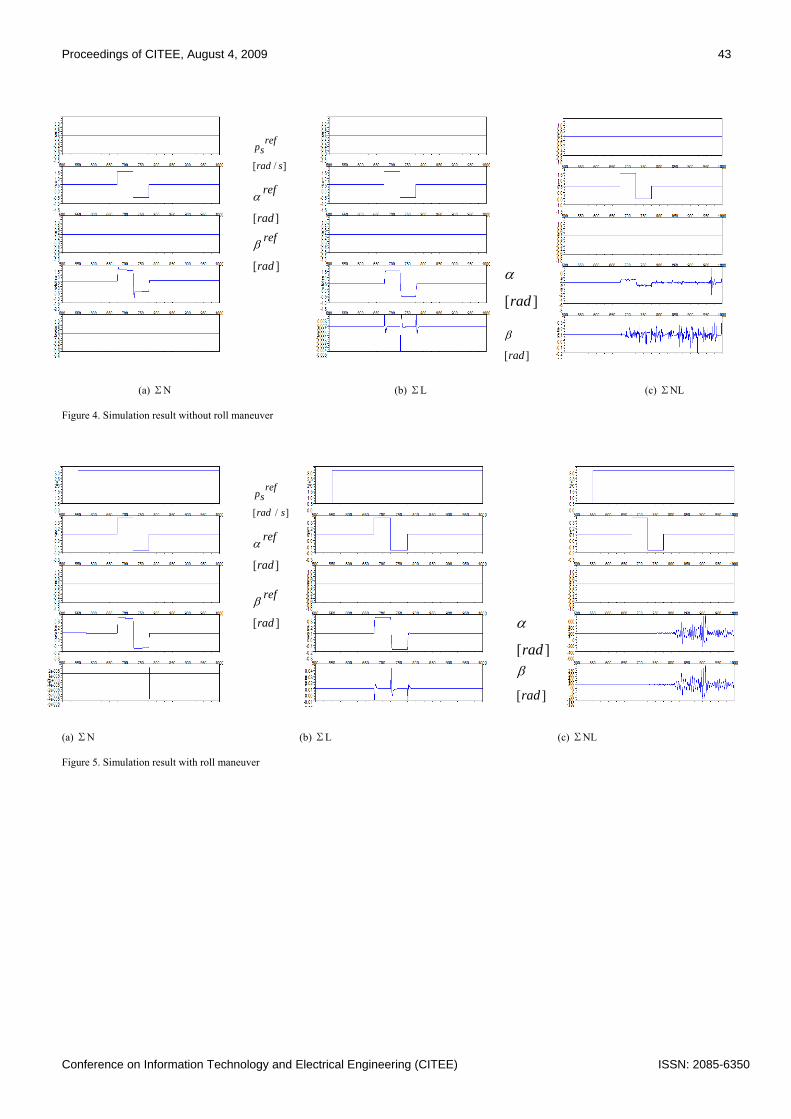
Proceedings of CITEE, August 4, 2009 43
Conference on Information Technology and Electrical Engineering (CITEE) ISSN: 2085-6350
]/[ srad
refsp
]/[ srad
refsp
][rad
refα
][rad
refα
][rad
refβ
][rad
refβ
][rad
α
][rad
β
][rad
β
][rad
α
(a) ΣN (b) ΣL (c) ΣNL Figure 4. Simulation result without roll maneuver
(a) ΣN (b) ΣL (c) ΣNL Figure 5. Simulation result with roll maneuver

44 Proceedings of CITEE, August 4, 2009
ISSN: 2085-6350 Conference on Information Technology and Electrical Engineering (CITEE)
]/[ srad
refsp
][rad
refα
][rad
refβ
][rad
α
][rad
β
(a) Q=diag(100,100,1,1) (b) Q=diag(1k,1k,1,1) (c) Q=diag(10k,10k,1,1) Figure 6. Simulation result with increased feedback gain (ΣNL)

Proceedings of CITEE, August 4, 2009 45
Conference on Information Technology and Electrical Engineering (CITEE) ISSN: 2085-6350
Feature Extraction and Selection on Osteoporosis X-Ray Image for Content Based Image Retrieval
(CBIR) Purposes
Usman Balugu1,2, Ratnasari Nur Rohmah1,3
1Jurusan Teknik Elektro, UGM [email protected], [email protected]
2Politeknik Bandung, 3UMS Surakarta
Nurokhim PTLR, Batan
City PostCode, Indonesia [email protected]
Abstract— This paper presents results on experiment in extracting feature of osteoporosis X-Ray image and finding the right feature or features to perform as descriptor in Content-Based Image Retrieval (CBIR) Systems. Consider that descriptor of each image will represent the content of each image, the decision which features of image will be the best representation of image content, is very important. Data in this experiments are digitized X-Ray proximal femur images already known osteoporosis level based on Index Singh (grade 3 – grade 6) due to simple verification on classification. We used statistical approach and log-polar wavelet transform for extracting textural feature from image. On statistical approach, we use grey-level co-occurance matrix (GLCM) methods to extract feature and used Contrast and Uniformity as quantity measured. We use Norm-1 as energy wavelet signature measured. Experiment on feature selection conduct by applying feature vector on classification process. Experiment’s results shows that two dimension feature vector using combination of Contrast on GLCM and Norm-1 on approximation component of log-polar wavelet transformed image, is the best choice image descriptor’s. Log-polar transforms proven effective in reducing wavelet energy error of rotated and scaled image. Improvement in classification accuracy also shown that, the use of log-polar transform prior to wavelet transform is useful in classification study.
Keywords—osteoporosis, descriptor, GLCM, log-polar, wavelet
I. INTRODUCTION Application computer in telemedicine has improved medical service in healthcare area. One of the applications is in applying databases on medical information such as medical record or medical image. Recently, compare to common method textual-base image retrieval, CBIR is considered as the more appropriate choice method for image retrieval in medical image databases. This method retrieves images from database using information directly derived from the contents of image themselves, rather than from accompanying text or annotation [1]. As a basic principle of CBIR, images are internally represented by numerical features, which are extracted directly from image. These features are stored in the
database, as a descriptor, along with the images, for rapid access. At retrieval time, the user presents a sample image, and the system computes the numerical features, compares them to those stored in the database, and returns all images with similar features. It is obvious that the quality of response depends on descriptor and the distance or similarity measure that is used to compare features from different images. This paper presents results on experiment in extracting feature of osteoporosis X-Ray image and choosing the right feature or features to perform as descriptor in Content-Based Image Retrieval (CBIR) Systems. Consider that descriptor of each image will represent the content of each image, the decision which features of image will be the best representation of image content, is very important. We used statistical approach Grey level co-occurance matrix (GLCM) and log-polar wavelet transform for extracting image feature. Selection on image feature is conduct by choosing feature vector gives optimum accuracy on image classification test. Data in this experiments are digitized X-Ray proximal femur images already known osteoporosis level based on Index Singh (grade 3 – grade 6) due to simple verification on classification validity.
II. FEATURES EXTRACTION AND SELECTION
A. Textural Feature on Osteoporosis X-Ray Image Osteoporosis is characterized by an absolute decrease in
the amount of bone to a level below that required for mechanical support of normal activity and by the occurrence of non-traumatic skeletal fracture [2]. Bone structure can be estimated by observing the change of trabecular pattern in proximal femur radiograph. The observation of trabecular pattern change for diagnosis of osteoporosis was first proposed in the 1960s using radiographs of proximal femur. The diagnosis was known as Singh Index grading system.
In this research, we used this structure pattern as image feature. We used 4 grades of Singh indexed image (grade 3 to grade 6) from women patients between 45 – 65 years of

46 Proceedings of CITEE, August 4, 2009
ISSN: 2085-6350 Conference on Information Technology and Electrical Engineering (CITEE)
age. Image feature extraction is done by image textural analyzing which will produce feature vector of each image. This feature vector is used as descriptor on the image retrieval systems. We used statistical approach and log-polar wavelet transform for extracting textural feature from image.
B. Feature Extraction Using GLCM On statistical approach we use GLCM methods to extract
feature. As X-Ray image represent as grey-level image, this method is considered as suitable method. From an image, f, with L possible intensity levels, GLCM is a matrix G whose element ijg is the number of times that pixel pairs with
intensities iz and jz occur in f , in position specified by an operator Q , where i≤1 , Lj ≤ [3]. The operator Q is an operator that defines the position of two image pixels relative to each others. The total number, n, of pixel pairs that satisfy Q is equal to the sum of the elements of G. Then, the quantity
n
gp ij
ij = (1)
is an estimate of the probability that a pair of points that satisfy Q will have value ( )ji zz , . These probabilities are in the range [0, 1] and their sum is 1:
11 1
=∑ ∑= =
K
i
K
jijp (2)
where K is the row (or column) dimension of square matrix G.
Because G depends on Q, the presence of intensity texture pattern can be detected by choosing an appropriate position operator and analyzing the elements of G. In this research position operator defined as “one pixel immediately to the right”. As for descriptor that useful for characterizing the content of G, we choose two descriptors, Contrast and Uniformity. Contrast is a measure of intensity contrast between a pixel and its neighbor over the entire image [3]. The range of values is 0 (when G is constant) to (K – 1)2.
( )∑ ∑ −== =
K
ii
K
jijpjiContrast
1
2 (3)
Uniformity (also called Energy) is a measure of uniformity in the range [0, 1]. Uniformity is 1 for a constant image.
∑ ∑== =
K
i
K
jijpUniformity
1 1
2 (4)
C. Feature Extraction Using Log-Polar Wavelet Transforms
Log Polar Transform
Log-polar transform is used to eliminate the rotation and scale effect in the input image by converting the image into corresponding log-polar image (Fig 1). Such log-polar image is rotation invariant and nearly scale invariant [4]. This transform algorithm is divided into two major steps. A
given NN × image ),( yxf is transforms into polar form
]2[NS × image ),( rap and then logarithm functions are applied to this polar form to obtain RS × log-polar image ),( jilp . Polar form ]2[ NS × image ),( rap of NN × image
),( yxf is compute as follows:
⎟⎟⎠
⎞⎜⎜⎝
⎛⎥⎦
⎤⎢⎣
⎡⎟⎠⎞
⎜⎝⎛−⎥⎦
⎤⎢⎣⎡
⎥⎦
⎤⎢⎣
⎡⎟⎠⎞
⎜⎝⎛+⎥⎦
⎤⎢⎣⎡=
SarN
SarNfrap ππ 2sin
2,2cos
2),( (5)
for 1,,0 −= Sa L , and [ ] 12,,0 −= Nr L , and RS × log-polar image ),( jilp is computed as follows:
⎟⎟⎠
⎞⎜⎜⎝
⎛⎥⎦
⎤⎢⎣
⎡⎥⎦⎤
⎢⎣⎡⋅
++
=2
.)2(log)2(log,),(
2
2 NRjipjilp (6)
for 1,,0 −= Si L , and 1,,0 −= Rj L .
(a) Original image
(b) Image (a) rotated
by 10 degree
(c) Image (a) scaled by
110%
(d) Log-polar transformed of (a)
(e) Log-polar transformed of (b)
(f) Log-polar transformed of (c)
Figure 1. Original, rotated, and scaled image and their log-polar
transformed.
Wavelet Transform for textural feature extraction
Discrete Wavelet Transform (DWT) useful for image analysis due to wavelets having finite duration which provides both the frequency and spatial locality and efficient implementation [4]. The hierarchical one-dimensional DWT uses pair of high-pass and low-pass filters derived from wavelet functions to decompose the original signal into two subbands: details and approximation, respectively. In 2D-DWT analysis, an image is split into an approximation and three detail images. The approximation image is then itself split into a second-
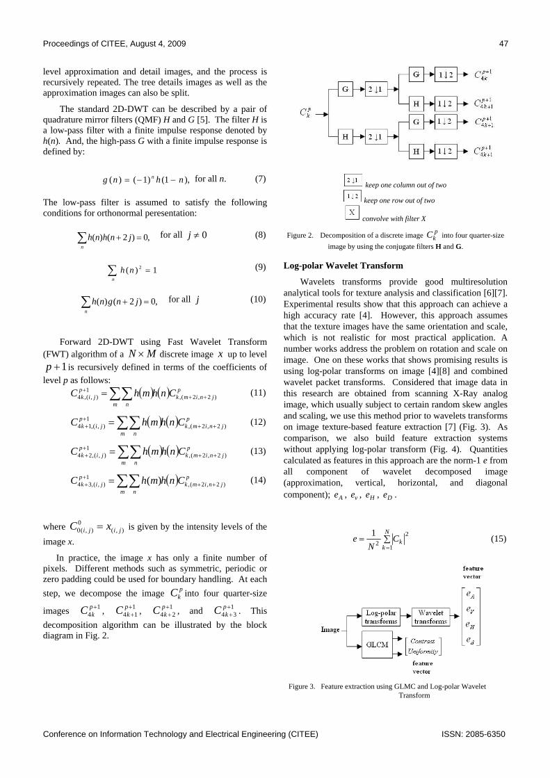
Proceedings of CITEE, August 4, 2009 47
Conference on Information Technology and Electrical Engineering (CITEE) ISSN: 2085-6350
level approximation and detail images, and the process is recursively repeated. The tree details images as well as the approximation images can also be split.
The standard 2D-DWT can be described by a pair of quadrature mirror filters (QMF) H and G [5]. The filter H is a low-pass filter with a finite impulse response denoted by h(n). And, the high-pass G with a finite impulse response is defined by:
),1()1()( nhng n −−= for all n. (7) The low-pass filter is assumed to satisfy the following conditions for orthonormal peresentation:
∑ =+n
jnhnh ,0)2()( for all 0≠j (8)
1)( 2 =∑
nnh (9)
∑ =+
njngnh ,0)2()( for all j (10)
Forward 2D-DWT using Fast Wavelet Transform (FWT) algorithm of a MN × discrete image x up to level
1+p is recursively defined in terms of the coefficients of level p as follows:
( ) ( ) pjnimk
m n
pjik CnhmhC )2,2(,
1),(,4 ++
+ ∑∑= (11)
( ) ( ) pjnimk
m n
pjik CnhmhC )2,2(,
1),(,14 ++
++ ∑∑= (12)
( ) ( ) pjnimk
m n
pjik CnhmhC )2,2(,
1),(,24 ++
++ ∑∑= (13)
( ) pjnimk
m n
pjik CnhmhC )2,2(,
1),(,34 )( ++
++ ∑∑= (14)
where ),(0
),(0 jiji xC = is given by the intensity levels of the image x.
In practice, the image x has only a finite number of pixels. Different methods such as symmetric, periodic or zero padding could be used for boundary handling. At each step, we decompose the image p
kC into four quarter-size
images 14+p
kC , 114
++
pkC , 1
24++
pkC , and 1
34++
pkC . This
decomposition algorithm can be illustrated by the block diagram in Fig. 2.
keep one column out of two
keep one row out of two
convolve with filter X
Figure 2. Decomposition of a discrete image pkC into four quarter-size
image by using the conjugate filters H and G.
Log-polar Wavelet Transform
Wavelets transforms provide good multiresolution analytical tools for texture analysis and classification [6][7]. Experimental results show that this approach can achieve a high accuracy rate [4]. However, this approach assumes that the texture images have the same orientation and scale, which is not realistic for most practical application. A number works address the problem on rotation and scale on image. One on these works that shows promising results is using log-polar transforms on image [4][8] and combined wavelet packet transforms. Considered that image data in this research are obtained from scanning X-Ray analog image, which usually subject to certain random skew angles and scaling, we use this method prior to wavelets transforms on image texture-based feature extraction [7] (Fig. 3). As comparison, we also build feature extraction systems without applying log-polar transform (Fig. 4). Quantities calculated as features in this approach are the norm-1 e from all component of wavelet decomposed image (approximation, vertical, horizontal, and diagonal component); Ae , ve , He , De .
∑==
N
kkC
Ne
1
22
1 (15)
Figure 3. Feature extraction using GLMC and Log-polar Wavelet
Transform

48 Proceedings of CITEE, August 4, 2009
ISSN: 2085-6350 Conference on Information Technology and Electrical Engineering (CITEE)
Figure 4. Feature extraction using GLMC and Wavelet Transform
D. Feature Selection
As mention in sub section above feature extraction for image is conduct using GLCM approach and wavelet transforms (Fig. 3 and Fig. 4). That is means that for each image we have six quantities measured as image feature. Not all of the measure features above are considered as descriptor. In this paper, feature vector as descriptor is a two-dimension vector using combination of two features, one from statistical approach and another from wavelet transform. From these eight combinations we define which feature vector as descriptor by trial and error (Fig. 5).
Test on image classification is conduct on some sample data using each combination of two features. A simple minimum distance classifier method was chosen for this testing process. Feature vectors giving optimum accuracy on classification is selected as descriptor.
Figure 5. Flowchart on feature vector selection process
III. EXPERIMENT AND RESULTS
A. Experiment and Result in Log-polar Transform effect in Wavelet Energy Signature
Experiment in log-polar transform is conduct to ensure positive impact of this transform in feature extraction. As mention in sub section above that image data in this research are obtained from scanning X-Ray analog image, which usually subject to certain random skew angles and scaling. Experiment results shows that log-polar transform reducing error in wavelet energy measured on rotated image (Fig. 6). On the other hands, this transform doesn’t that much significant effect on scaled image, especially for approximation image (Fig. 7). However, generally this log-polar transform has positive effect in reducing MSE of wavelet energy signature from all decomposed image.
(a) Approximation image (b) Horizontal detail image
(c) Vertical detail image (d) Diagonal detail image
Figure 6. Mean Square Error of wavelet energy measured
from rotated image.
(a) Approximation image (b) Horizontal detail
(c) Vertical detail (d) Diagonal detail
Figure 7. Mean Square Error of wavelet energy measured
from scaled image

Proceedings of CITEE, August 4, 2009 49
Conference on Information Technology and Electrical Engineering (CITEE) ISSN: 2085-6350
B. Experiment and Result in Feature Selection and impact of the log-polar transform.
Experiment on feature selection shows that only four feature vectors: [ ]TA Contraste , [ ]TA Uniformitye ,
[ ]TV Uniformitye , and [ ]TD Uniformitye , for system using log-polar transform prior to wavelet transform, that result in clustering in classification process (Fig. 8). In systems not applying log-polar transform, four feature vectors: [ ]TA Contraste , [ ]TA Uniformitye , [ ]TH Uniformitye , and [ ]TV Uniformitye shows clustering in classification process (Fig. 9). Boundary lines are performed based on feature vectors (descriptor) of 37 images in databases.
(a) Feature vector:
⎥⎦
⎤⎢⎣
⎡Contrast
eA (b) Feature vector: ⎥⎦
⎤⎢⎣
⎡Uniformity
eA
(c) Feature vector:
⎥⎦
⎤⎢⎣
⎡Uniformity
eV (d) Feature vector: ⎥⎦
⎤⎢⎣
⎡Uniformity
eD
Figure 8. Decision boundary of minimum distance classifier based on
feature vectors from feature extraction process applying log-polar wavelet transform.
(a) Feature vectors:
⎥⎦
⎤⎢⎣
⎡Contrast
eA (b) Feature vectors: ⎥⎦
⎤⎢⎣
⎡Uniformity
eA
(c) Feature vectors:
⎥⎦
⎤⎢⎣
⎡Uniformity
eH (d) Feature vectors: ⎥⎦
⎤⎢⎣
⎡Uniformity
eV
Figure 9. Decision boundary of minimum distance classifier based on
feature vectors from feature extraction process applying wavelet transform
Among all those combination, features vectors consist of Contrast on GLCM and Norm-1 on approximation component [ ]TA Contraste in system using log-polar
wavelet transform is the best choice for image descriptors. This result gives higher accuracy rate 86.25% of all classes compare to accuracy rate 83.75% for the same feature vectors in system without applying log-polar transform. These facts also show that applying of log-polar transforms has its benefits. Table I and Table II shows classification accuracy based on feature vectors.
TABLE I. CLASSIFICATION ACCURACY ACHIEVED ON CLASSIFICATION PROCESS USING FOUR FEATURE VECORS DERIVED FROM GLMC AND LOG-POLAR WAVELET TRANSFORM FEATURE EXTRACTION
Classes
Classification accuracy (%) for feature vectors:
⎥⎦
⎤⎢⎣
⎡Contrast
eA ⎥⎦
⎤⎢⎣
⎡Uniformity
eA ⎥⎦
⎤⎢⎣
⎡Uniformity
eV ⎥⎦
⎤⎢⎣
⎡Uniformity
eD
Grade 3 91.67 75.00 66.67 75.00 Grade 4 70.00 80.00 60.00 30.00 Grade 5 83.33 83.33 66.67 25.00 Grade 6 100.00 100.00 100.00 100.00
TABLE II. CLASSIFICATION ACCURACY ACHIEVED ON CLASSIFICATION PROCESS USING FOUR FEATURE VECORS DERIVED FROM
GLMC AND WAVELET TRANSFORM FEATURE EXTRACTION
Classes
Classification accuracy (%) for feature vectors:
⎥⎦
⎤⎢⎣
⎡Contrast
eA ⎥⎦
⎤⎢⎣
⎡Uniformity
eA ⎥⎦
⎤⎢⎣
⎡Uniformity
eH ⎥⎦
⎤⎢⎣
⎡Uniformity
eV
Grade 3 91.67 75.00 83.33 75.00 Grade 4 60.00 70.00 30.00 30.00 Grade 5 83.33 83.33 25.00 25.00 Grade 6 100.00 100.00 33.33 100.00
IV. CONCLUSION Combination on log-polar wavelet energy signature and
contrast on GLCM as two-dimension vector descriptor, give sufficient accuracy for the CBIR purposes. Log-polar transforms proven effective in reducing wavelet energy error of rotated and scaled image. Improvement in classification accuracy shown that, the use of log-polar transform prior to wavelet transform is useful in classification study.
However, only small database used for verification in this research, and most of data has already confirmed its index Sigh. Further works would be applying bigger database and more indistinct indicated data to find the best image feature to represent of image content as descriptor. Moreover, feature vector dimension would probably need to be increased in larger database.
ACKNOWLEDGMENT F. A. Author thanks to Mr. J. Tjandra Pramudityo for
giving copy on data of osteoporosis X-Ray images used in this research.
REFERENCES [1] El-Naqa, I., Yang, Y., Galatsanos, N. P., & Wernick, M. N., “A
similarity learning approach to content-based image retrieval:

50 Proceedings of CITEE, August 4, 2009
ISSN: 2085-6350 Conference on Information Technology and Electrical Engineering (CITEE)
[2] Application to digital mammography”, IEEE Transaction on Medical Imaging, vol. 23, no. 10, pp. 1233-1244, 2004.
[3] H.W. Wahner and Fogelman I., The Evaluation of Osteoporosis: Dual Energy X-ray Absorptiometry in Clinical Practice, Martin Dunitz Ltd., London, 1994.
[4] R. C. Gonzalez and R. E. Woods, Digital Image Processing, 3rd ed., Pearson Education, New Jersey, 2008.
[5] Chi-Man Pun and Moon-Chuen Lee, “Log-polar Wavelet Energy Signatures for Rotation and Scale Invariant Texture Classification”, IEEE Transactions on Pattern Analysis and Machine Intelligence, vol. 25, no. 5, pp. 590-603, May 2003.
[6] Stéphane Mallat, A Wavelet Tour of Signal Processing, 2nd ed., Academic Press, 1999.
[7] T. Chang, C.C. J. Kuo, “Texture Analysis and Classification with Tree-Structured Wavelet Transform”, IEEE Transaction on Image Processing, vol.4, pp. 1549-1560, Nov. 1995.
[8] A. Laine and J. Fan, “Texture Classification by Wavelet Packet Signatures,” IEEE Transaction on Pattern Analysis and Machine Intelligent, vol. 8, pp. 472 – 481, July 1986.
[9] Ratnasari N. R, Lukito E. N, Thomas Sri W., Adhi Susanto, Nurokhim. “Design and Preliminary Result on Content-Based Image Retrieval (CBIR) System for Osteoporosis X-Ray Image Database.”, Proceeding of International Conference on Rural Information and Communication Technology 2009, pp. 199–202, July 2009

Proceedings of CITEE, August 4, 2009 51
Conference on Information Technology and Electrical Engineering (CITEE) ISSN: 2085-6350
The Implementation of Turbo Encoder and Decoder Based on FPGA
Sri Suning Kusumawardani * and Bambang Sutopo †
* Dept. of Electrical Engineering, Fac. of Engineering, Gadjah Mada University, Jl. Grafika 2, Yogyakarta,
Indonesia Email : [email protected]
† Dept. of Electrical Engineering, Fac. of Engineering, Gadjah Mada University, Jl. Grafika 2, Yogyakarta, Indonesia
Email : [email protected] Abstract – Turbo Code was proposed in 1993 by Berrou, Glavieux, and Thitimajashima, who reported excellent coding gain results (Berrou, 1993), approaching Shannonian predictions. The turbo code uses two Recursive Systematic Convolutional (RSC) encoders separated by an interleaver. There are two main decoding techniques which one of them is Soft Output Viterbi Algorithm (SOVA). SOVA is a modified Viterbi Algorithm making it is able to use a-priori information between SOVA decoders. Reliability estimation, log-likelihood algebra, and soft channel outputs are the fundamentals for SOVA decoding. The iterative SOVA decoding algorithm is used to increase the performance of turbo code. Field Programmable Gate Array (FPGA) is a reprogrammable digital chip which is considered as very fast and easy to modify chip making it suitable for prototyping products. Based on above considerations, FPGA (EPF10K10LC84) is choosen to implement the Turbo Code.
There are 10 units to be implemented; encoder, 8 units composing a decoder, and control unit. Both the design process and the implementation use MAX+plus II software.
The result shows that the simulation works well, although it cannot to be implemented in a single chip. The circuit needs 1553 LEs which is much bigger than the available LEs on EPF10K10LC84. The implementation results show it is able to correct a maximum of 5 errors bits.
Keywords - Turbo Code, RSC Encoder, SOVA Decoder, Soft Output, FPGA (Field Programmable Gate Array)
I. INTRODUCTION Error Correcting Control is very important in modern
communication systems which one of them is Turbo Code. Turbo Code was proposed in 1993 by Berrou, Glavieux, and Thitimajashima, who reported excellent coding gain results (Berrou, 1993), approaching Shannonian predictions. The turbo code uses two Recursive Systematic Convolutional (RSC) encoders separated by an interleaver. There are two main decoding techniques which one of them is Soft Output
Viterbi Algorithm (SOVA). SOVA is a modified Viterbi Algorithm making it is able to use a-priori information between SOVA decoders. Reliability estimation, log-likelihood algebra, and soft channel outputs are the fundamentals for SOVA decoding. The iterative SOVA decoding algorithm is used to increase the performance of turbo code.
FPGA is a reprogrammable chip. A design in FPGA can be automatically converted from gate level into layout structure by place and route software.
This research is our preliminary research on implementation Turbo Code in FPGA.
II. BASIC THEORY
Recursive Systematic Convolutional (RSC) encoder
RSC is developed from Convolution encoder. RSC encoder written as . , and
are code generators, G1 is feedback polynomial generator and G2 is forward polynomial generator. Figure 1 show us Recursive Systematic Convolutional encoder block diagram with constraint length (K) = 3 and ak is obtained from equation (1).
(1) Where g1 = g1i if uk = dk and g2 = g2i if vk = dk
Figure 1. Recursive Systematic Convolutional Encoder

52 Proceedings of CITEE, August 4, 2009
ISSN: 2085-6350 Conference on Information Technology and Electrical Engineering (CITEE)
SOVA decoder
Turbo decoder is a modified Viterbi algorithm. The aim of this modification is to make Viterbi algorithm provides soft output values. These values are given to one of SOVA decoders as a-priori information in order to increasing the decoder performance. SISO algorithm receives a-priori information and provides a-posteriori as output (Figure 2).
Figure 2. SISO Decoder
There are two modifications in Viterbi algorithm to
make SOVA decoders able to provide soft output: 1. Defined ML path, SOVA uses former matrix path
information and a-priori information to define the ML path or chosen path.
2. Update process, SOVA must be able to provide soft output (a-posteriori) which is used as a-priori input for another SOVA. SOVA decoder use three kinds of information which is
different from Viterbi: 1. A-priori
A-priori information is encoded bit probability which is known before encoding process. Obtained from another decoder’s output and called as intrinsic information.
2. Extrinsic Extrinsic information is encoded bit probability which is obtained from a-posteriori by deleting the effect of received systematic information and a-priori information .
3. A-posteriori A-posteriori information is state series probability which is obtained based on soft channel output information and a-priori information .
III. EXPERIMENTAL RESULTS
Turbo Encoder and Decoder designed using MAX+plus II software. The designs are implemented using VHDL hardware programming language. Turbo Codes System is divided into 5 main units: parallel into serial converter (information series and error series generator), encoder, decoder, serial into parallel converter, and control unit.
Parallel into Serial Converter
Encoding and Decoding in Turbo codes are processed in serial way but information and error series are given in parallel, so we need parallel into serial converter to convert
information and error series into serial output. There are two main parts to be implemented: Information series and error series generator. The truth table of information series generator is given by Table 1.
Table 1. Truth Table of Information Series Generator
Based on the truth table in Table 1, the VHDL
program of Information series generator is shown in Figure 3.
Figure 3. VHDL Program for Information Series Generator
The truth table of error series generator is given by
Table 2.

Proceedings of CITEE, August 4, 2009 53
Conference on Information Technology and Electrical Engineering (CITEE) ISSN: 2085-6350
Table 2. Truth Table of Error Series Generator
Based on the truth table in Table 2, the VHDL
program of Information series generator is shown in Figure 4.
Figure 4. VHDL Program for Error Series Generator
Encoder Figure 5 shows the block diagram of Turbo encoder.
Figure 5. Turbo Encoder Block Diagram
Turbo encoder is obtained from two registers (Flip
Flop D) which is designed in VHDL programming language as shown in Figure 6.
Figure 6. VHDL Program for FFD
Decoder
SOVA decoders can be implemented by dividing it into 8 sub units: Branch Metric Generator (BMG), Add Compare and Select Unit (ACSU), Delta Path Metric (DeltaPM), Maximum State Select Unit (MSSU), Track Back Unit (TBU), Path Equivalence Detector (PED), Reliability Measurement Unit (RMU), and A- posteriori Measuring Unit.
Serial into Parallel Converter
Serial into Parallel circuit is given by Figure 7.
Figure 7. Serial into Parallel Converter Circuit

54 Proceedings of CITEE, August 4, 2009
ISSN: 2085-6350 Conference on Information Technology and Electrical Engineering (CITEE)
A-posteriori Circuit and Decoded Bit Figure 8 shows us the circuit which is provide a-
posteriore result and decoded bit.
Figure 8. A-posteriore Circuit
Control Unit
Figure 9 shows us the circuit which is provide control signal to control some units and components.
Figure 9. Control Signal Generator Circuit
The Turbo Codes implementation results show it is
able to correct random error up to 5 bits. Chosen metric path
and encoded bit are determined at TBU. TBU needs the biggest LE, 558 LE or 96.88% of EPF10K10LC84’s maximum capacity.
IV. CONCLUSIONS
The Turbo Codes implementation results show it is
able to correct random error up to 5 bits. SOVA decoders can be implemented by dividing it into 8 sub units: Branch Metric Generator (BMG), Add Compare and Select Unit (ACSU), Delta Path Metric (DeltaPM), Maximum State Select Unit (MSSU), Track Back Unit (TBU), Path Equivalence Detector (PED), Reliability Measurement Unit (RMU), and A-posteriori Measuring Unit.
Chosen metric path and encoded bit are determined at TBU. TBU needs the biggest LE, 558 LE or 96.88% of EPF10K10LC84’s maximum capacity.
REFERENCES [1] Altera Corporation, January 2003, “FLEX 10K
Embedded Programmable Logic Device Family”, Data Sheet version 2.2, Altera Corporation.
[2] Altera Corporation, January 2003, “FLEX 10K Embedded Programmable Logic Device Family”, Data Sheet version 4.2, Altera Corporation.
[3]Altera Corporatio, July 2002, ”Turbo Encoder/Decoder”, Megacore Function User Guide Version 1.1.2 Rev. 1, Altera Corporation.
[4] Berrou, C., 1993, Turbo Codes: Some Simple Ideas for Efficient Communications.
[5]Hagenauer, J., Hoeher, P., 1989, “A Viterbi with Soft-Decision Outputs and its Applications”, German Aerospace research Establishement, Institute for Communiaction Technology, West-Germany.
[6]Hanzo,L., Liew, T.H., Yeap, B.L., 2002, “Turbo Coding, Turbo Equalisation and Space-Time Coding”, Department of Electronics and Computer Science, University of Southampton, UK.
[7]Huang, F., May 29, 1997, “Evaluation of Soft Output Decoding for Turbo Codes”, Master's thesis, Virginia Polytechnic Institute and State University, Blacksburg, Virginia.
[8]Kusumawardani S.S., 2001, “Implementasi Sandi BCH (15,5) dengan FPGAXC4013”, EE UGM, Yogyakarta.
[9]Lin,S. dan Castello, 1983, “Error Control Coding: Fundamental and Apliccation”, Prentice-Hall International Inc, Englewood Cliff, New Jersey.

Proceedings of CITEE, August 4, 2009 55
Conference on Information Technology and Electrical Engineering (CITEE) ISSN: 2085-6350
BER Performance Analysis of PAM and PSM for UWB Communication
Risanuri Hidayat
Electrical Engineering Department Faculty of Engineering Gadjah Mada University
Yogyakarta 55281, Indonesia [email protected]
Abstract— This paper proposes BER analysis of Impulse
Radio Ultra Wideband (IR-UWB) pulse modulations. A Gaussian monocycle as UWB pulse is modulated using Pulse Amplitude Modulation (PAM) and Pulse Shape Modulation (PSM). The channel model is generated from a modified S-V model. Bit-error rate (BER) is measured over several of bit rates. The result shows that PAM gives better performance than PSM in bit rates and SNR. Moreover, as standard of speed has been given for UWB, both modulations is appropriate with high bit rates in LOS channel.
Keywords— IR-UWB, S-V Channel Model, LOS NLOS, PAM, PSM
I. INTRODUCTION Since FCC released UWB frequency band [1], UWB
performance for communication has been studied [2]-[13], including binary modulations for impulse radio include pulse amplitude modulation (PAM) [3] and pulse shape modulation (PSM) [4]. BER performance for impulse radio ultra wideband (IR-UWB) systems in multipath propagation channels has also been introduced [5][6][7][8][9]. In order to realize actual condition, a statistical model is established for the ultra-wide bandwidth in a simulation [10][11], and the channel model using a Saleh-Valenzuela (S-V) [12] that showed multipath arriving in clusters has been modified for UWB signal application [13].
This paper presents the analysis of modulations of UWB through S-V channel that has been modified for UWB communications [13] and AWGN noise especially in bit rates and BER by a simulation. PAM and PSM are implemented for this purpose. Data sent by the transceiver are converted to modulated UWB pulse and are then received by the receiver. At the receiver the pulse is then converted to data again. The comparison between the data bits sent by transmitter and the data bits received by receiver represents the BER values.
II. UWB PULSE AND ITS MODULATIONS Some references have represented several formulas of
Gaussian pulse [14] as an IR-UWB. A monocycle pulse is the first derivative of Gaussian pulse. The Gaussian pulse has formula (1), while the monocycle is given in (2).
2
2
1 .)(⎟⎠⎞
⎜⎝⎛−
= Tct
eAtxπ
(1)
2
2
2)1( .)()(
⎟⎟⎠
⎞⎜⎜⎝
⎛−
== cTt
etAdt
tdxtxπ
(2)
where cc fT /1= is the width of the pulse. The values A1 and A2 are amplitudes. The Federal Communications Commission (FCC) has recently approved the deployment of UWB on an unlicensed basis in the 3.1–10.6 GHz band subject to a modified version of Part 15.209 rules as in Fig. 1 [1]. The essence of this regulation is to limit the power spectral density (PSD) measured in a 1–MHz bandwidth at the output of an isotropic transmit antenna.
Figure 1. UWB spectral mask and FCC Part 15 limits
A number of modulation schemes may be used with IR-UWB systems. The potential modulation schemes include both orthogonal and antipodal schemes. Some common methods of modulation are to invert the called as pulse amplitude modulation (PAM) [3] and pulse shape modulation (PSM) [4] [15], which requires special pulse shapes to be generated which are orthogonal to each other.
A. Pulse Amplitude Modulation PAM is implemented by binary pulse modulation, which
is presented using two antipodal Gaussian pulses. The transmitted binary baseband pulse that is modulated information signal (t) is expressed as [3]
)(.)( twdtx trj= (3)
where wtr(t) represents the UWB pulse waveform, j represents the bit transmitted that 0,1 =−= jd j and
1,1 =+= jd j
Fig 2 (a) shows the pulse amplitude modulation of the Gaussian monocycle pulse waveform expressed in (2) with Tc = 2.22x10⁻¹ ns. Fig. 2 (b) shows the normalized Power Spectral Density (PSD) of the derivative of pulse. When a pulse is transmitted, due to the derivative characteristics of

56 Proceedings of CITEE, August 4, 2009
ISSN: 2085-6350 Conference on Information Technology and Electrical Engineering (CITEE)
the antenna, the output of the transmitter antenna can be modelled by the first derivative of the pulse [3]. The derivative can be achieved by the basics of differential calculus
(1)
0
( ) ( )( ) limdt
x t dt x tx tdt→
+ −=
(4)
PSD of the deterministic power signal, w(t), is
2( )( ) lim
T
X fP f
T→ ∞
⎛ ⎞⎜ ⎟=⎜ ⎟⎝ ⎠ (5)
where T is the pulse spacing interval. X(f) is the Fourier transform of the pulse, i.e. x(t). P(f) has units of watts per hertz. When X(f) is attained, the peak emission frequency, i.e. fM, can be found as the frequency at the maximum value of |X(f)|. The normalized PSD is used to comply with the FCC spectral mask of the pulse that is transmitted by antenna [1][16][17]. The normalized PSD can be defined as follows
2
2
)(
)()(
MfX
fXfP =
(6)
Fig. 2 (b) shows that the pulses have normalized PSD in 3.1-10.6 GHz frequency band that fulfil the FCC rules of UWB communication as shown in Fig. 1.
B. Pulse Shape Modulation Pulse shape modulation (PSM) uses different, orthogonal
waveforms to represent bit ‘0’ and ‘1’. The transmitted pulse can be represented as
(a) BPAM pulse shapes
(b) Frequency domain
Figure 2. PAM pulse shapes for ‘1’ and ‘0’ bits and its frequency domain
(a) PSM pulse shapes
(b) Frequency domain
Figure 3. Pulse waveforms used for PSM modulation and its frequency domain
)()()1()( )1()0( twdtwdtx trjtrj +−= (7)
where dj is defined as in (8) and )()0( twtr and )()1( twtr represent two different pulse waveforms.
Fig. 3 shows the pair of PSM pulses and it’s PSD. The pulse waveforms apply the Gaussian monocycle pulse defined as in (2) with Tc = 2.22x10⁻¹ ns. The second waveform is the derivative of (2). It means that the pulse shapes are the first and the second derivatives of the Gaussian pulse. These two waveforms are orthogonal according to the definition given by the cross correlation of the two waveforms,
∫+∞
∞−
= =+= 0)().(|)( 0 dttwtw trtrtc ττρ (8)
Fig. 3 (b) shows that both of the PSM pulses have the normalized PSD that comply with the FCC spectral mask.
III. CHANNEL MODEL Since UWB waveforms can be up to 7.5 GHz wide, for
example, any paths separated by more than about 133 psec. (equivalent to 4 cm path length difference) can be individually resolved at the receiver [18]. The realistic channel for IEEE 802.15 study group 3a has been developed by Saleh-Valenzuela (S-V model) and proposed for the real indoor channel model, where the clusters and rays are multi-path components [13]. This multi-path channel can be expressed as

Proceedings of CITEE, August 4, 2009 57
Conference on Information Technology and Electrical Engineering (CITEE) ISSN: 2085-6350
∑∑
= =
−−=L
l
K
klkllk Ttth
0 0,, )()( τδα
(9)
where α k,l is the multipath gain coefficient, lT is the
delay of the lth cluster, and τ k,l is the delay of the kth multipath component relative to the lth cluster arrival time ( lT ).
As suggested in [13], α k,l = p k,l β k,l is adopted, where pk,l is equally likely to take on the values of +/-1, and βk,l is the lognormal fading term, due to the simplicity of the real channel coefficients, and to avoid the ambiguity of phase for an UWB waveform.
The proposed channel model uses the definitions as previously described in the S-V model, and is repeated here for completeness. Tl is the arrival time of the first path of the l-th cluster; τk,l is the delay of the k-the path within the l-th cluster relative to the first path arrival time, Tl; Λ is cluster arrival rate; and λ = ray arrival rate, i.e., the arrival rate of path within each cluster.
Therefore, 0l lTτ = . The distribution of cluster arrival time and the ray arrival time are given by
( ) ( )
( ) ( )1 1
, ( 1), , ( 1),
exp , 0
exp , 0
l l l l
k l k l k l k l
p T T T T l
p kτ τ λ λ τ τ
− −
− −
⎡ ⎤=Λ −Λ − >⎣ ⎦⎡ ⎤= − − >⎣ ⎦ (10)
The channel coefficients are defined as lklklk p ,,, βα = ,
lk ,β is obtained by this expression
),(Normal)(10log20 2
,, σµβ lklk ∝ (11)
or 20/, 10nlk =β
where
),Normal( 2σµ ln ∝ (12)
[ ] γτβ //
02,
,lkl eeE Tlk
−Γ−Ω=
Tl is the excess delay of bin l and 0Ω is the mean power of
the first path of the first cluster, and lkp , is +/-1. Then µl is given by
20)10ln(
)10ln(/10/10)ln(10 2
,0 σγτµ −
−Γ−Ω= lkl
lT
(13)
IV. SIMULATION METHOD Fig. 4 shows the block diagram of the transmitter and
receiver communication. Transmitter converts the data bits to UWB pulses and the pulse are transmitted through the antenna. There is a channel model between the transmitter and the receiver. At receiver, the pulses are received by antenna and LNA (Low Noise Amplifier) becomes uf(t). Finally, the pulses are detected using the template pulse. The Gaussian monocycle pulse expressed in (2) with Tc = 2.22x10⁻¹ ns is implemented. PAM and PSM modulations are implemented using (3) and (7), respectively.
A channel is available between transceiver and receiver. An UWB channel model is derived from the modified Saleh-Valenzuela model suitable for home environment with both LOS and NLOS as described previously. There are 5 key parameters that define the model: Λ = cluster arrival rate; λ = ray arrival rate, i.e., the arrival rate of path within each cluster; Γ = cluster decay factor; γ = ray decay factor; and σ = standard deviation of lognormal fading term (dB). All parameters are taken into account for channel modeling as formulated in (10)-(13).
This paper uses one channel model generated from S-V model using the parameters as shown in Table I. The equation in (9)-(13) and Table I derived from and based on Intel measurements [13] are used to generate a channel model. The generated channel model is shown in Fig 10.
It should be noted that in an ideal environment the received pulse shape is the second derivative of the signal transmitted due to differentiator effect in transmitter and receiver antennas. However, the amplitude of correlation result between the first and the third derivatives of the Gaussian pulse is 80% of the autocorrelation of the received waveform [3]. This means that using the transmitted waveform as the template, the performance of the correlator is reduced by less than 1 dB. Therefore, the receiver still can use the same template waveform to demodulate the signals.
Figure 4. UWB pulse communication
TABLE I. CHANNEL MODEL PARAMETERS.
Model Parameters LOS NLOS Λ (1/nsec) 1/60 1/11 λ (1/nsec) 1/0.5 1/0.35 Ѓ (nsec) 16 16 γ (nsec) 1.6 8.5 σ (dB) 4.8 4.8
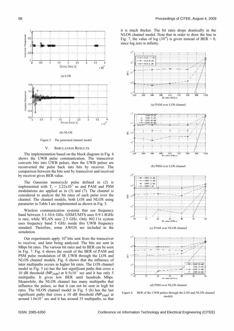
58 Proceedings of CITEE, August 4, 2009
ISSN: 2085-6350 Conference on Information Technology and Electrical Engineering (CITEE)
(a) LOS
(b) NLOS
Figure 5. The generated channel model
V. SIMULATION RESULTS The implementation based on the block diagram in Fig. 4
shows the UWB pulse communication. The transceiver converts bits into UWB pulses, then the UWB pulses are reconverted the pulse back into bits by receiver. The comparison between the bits sent by transceiver and received by receiver gives BER value.
The Gaussian monocycle pulse defined in (2) is implemented with Tc = 2.22x10⁻¹ ns and PAM and PSM modulations are applied as in (3) and (7). The channel is considered to analyze the bit rates of each pulse over the channel. The channel models, both LOS and NLOS using parameter in Table I are implemented as shown in Fig. 5.
Wireless communication systems that use frequency band between 3.1-10.6 GHz. GSM/UMTS uses 0.9-1.8GHz is rare, while WLAN uses 2.5 GHz. Only 802.11a system uses frequency band 5 GHz inside this UWB frequency standard. Therefore, some AWGN are included in the simulation.
Our experiments apply 104 bits sent from the transceiver to receiver, and later being analyzed. The bits are sent in Mbps bit rates. The various bit rates and its BER can be seen in Fig. 7. Fig. 6 shows the result of the BER of PAM and PSM pulse modulation of IR_UWB through the LOS and NLOS channel models. Fig. 6 shows that the influence of inter multipaths occurs in higher bit rates. The LOS channel model in Fig. 5 (a) has the last significant paths that cross a 10 dB threshold (NP10dB) at 0.5x10⁻⁷ sec and it has only 5 multipaths. It gives low BER until hundreds Mbps. Meanwhile, the NLOS channel has many multipaths that influence the pulses, so that it can not be sent in high bit rates. The NLOS channel model in Fig. 5 (b) has the last significant paths that cross a 10 dB threshold (NP10dB) at around 1.0x10⁻⁷ sec and it has around 33 multipaths, so that
it is much thicker. The bit rates drops drastically in the NLOS channel model. Note that in order to draw the line in Fig. 7, the value of log (10-6) is given instead of BER = 0, since log zero is infinity.
(a) PAM over LOS channel
(b) PSM over LOS channel
(c) PAM over NLOS channel
(d) PSM over NLOS channel
Figure 6. BER of the UWB pulses through the LOS and NLOS channel models

Proceedings of CITEE, August 4, 2009 59
Conference on Information Technology and Electrical Engineering (CITEE) ISSN: 2085-6350
Fig. 6 (a) shows data sent using PAM over the LOS channel model. The result shows that SNR 4 and 8 dB AWGN give high BER. SNR 12 dB gives no error (or error lower than 10-4) until 800 Mbps. BER increases drastically after 800 Mbps.
Fig. 6 (b) shows data sent using PSM over the LOS channel model. SNR 16 and 20 dB AWGN give high BER. SNR 24 dB gives error in 10-3 level until 800 Mbps and BER increases afterwards. SNR 28 dB has no error (below 10-4) until 800 Mbps, and the value of BER increases drastically afterwards. Therefore, this modulation needs higher SNR than the other modulations.
Different from the LOS channel that has much higher bit rates, the NLOS channel gives lower bit rates for the communication. In Fig. 6 (c), data are sent using PAM over NLOS channel model. It has high BER until SNR 12 dB. SNR 16 dB has no error (or error lower than 10-4) within 10 Mbps, gives BER in 10-3 level for bit rates below 30 Mbps and BER increases drastically after 30 Mbps. SNR 20 dB has no error (or error lower than 10-4) until 30 Mbps, but it has higher BER afterwards.
In Fig. 6 (d), data are sent using PSM over the NLOS channel model. It has high BER until SNR equals to 28 dB. SNR 32 dB gives BER in 10-4 level for 10 Mbps and BER in 10-3 level until 30 Mbps. It has also high BER for above 30 Mbps.
Comparing among the modulations, the result shows that for the same channel, PAM is more robust of AWGN than PSM, both in LOS and NLOS channels. From the results, it can be said that UWB pulse communication is appropriate in LOS channel, i.e., has high bit rates (hundreds Mbps). Nevertheless, this communication can be used until several Mbps in NLOS channel model.
TABLE II. ESTIMATE OF HIGHEST BIT RATES (HBR)
LOS Bit rates (Mbps) SNR 28 dB SNR 16 dB SNR 12 dB
PAM 800 800 800 PSM 800 - -
NLOS Bit rates (Mbps) SNR 32 dB SNR 20 dB SNR 16 dB
PAM 30 30 30 PSM 30 - -
Table II shows estimation of highest bit rates without
error (or error less than 10-4 level is tolerable). If the less BER is desired, then lower bit rate can be implemented. However, in high SNR environment, the high bit rate can still be implemented. It shows that PAM modulation over LOS channel gives the best performance. By looking at the UWB reference standard and compare to the others as shown in Table III [19], it seems that this communication model is preferable for the LOS channel, but PSM needs high SNR environment.
Based on Fig. 6(a)-(d), some samples of bit rate are chosen to take a closer look at each modulation over LOS and NLOS channels. Based on Table III, 400 Mbps is chosen for all modulations for the LOS channel. However, since the maximum bit rates for NLOS channel is only 30 Mbps, this rate is chosen.
There are 104 bits sent from the transceiver to receiver in Fig. 9. The figure shows the BER performance of the UWB pulses through the LOS and NLOS channel models in the chosen bit rates. Fig 13 shows that PAM is more robust both in LOS and NLOS channels.
TABLE III. COMPARISON OF UWB BIT RATE WITH OTHER STANDARDS.
Speed (Mbps) Standard 480 UWB, USB 2.0 200 UWB (4 m minimum) 110 UWB (10 m minimum) 90 Fast Ethernet 54 802.11a 20 802.11g 11 802.11b 10 Ethernet 1 Bluetooth
When 400 Mbps is chosen for LOS channel model, it
means that the pulse is sent in 2.5ns periodic time. PAM has BER in 10-3 level for SNR 8 dB, and low BER (in 10-4 level or lower) afterwards. Fig. 7 shows that data communication using PAM that needs BER 10-5 or less can be applied in SNR 12 dB or more.
PPM has BER in 10-2 level within SNR 10 dB, and in 10-4 level for SNR 10 dB. It can be estimated that using PPM, BER 10-5 or less can be applied in SNR 14 dB or more.
PSM has BER in 10-2 level within SNR 22 dB, BER in 10-3 level for SNR 24 dB, and BER in 10-4 level for SNR 26 dB. It can be estimated that using PPM, BER 10-5 or less can be applied in SNR 30 dB or more.
When 30 Mbps is chosen for NLOS channel model, it means that the pulse is sent in 0.33 ns periodic time. PAM has BER in 10-2 level for SNR 12 dB, BER in 10-4 for SNR 14 dB, and low BER (lower than 10-4 level) afterwards. Fig. 7 shows that data communication using PAM that needs BER 10-5 or less can be applied in SNR 16 dB or more.
PSM has BER in 10-2 level within SNR 28 dB, BER in 10-3 level for SNR 30 dB, and BER in 10-4 level for SNR 32 dB. It can be estimated that using PPM, BER 10-5 or less can be applied in SNR 34 dB or more.
VI. CONCLUSION The BER analysis of the Impulse Radio Ultra Wide Band
pulse communication over modified S-V channel model is presented. The pulse uses Gaussian monocycle pulse. The channel model uses a modified S-V model introduced by Intel. PAM and PSM are applied for modulation, and BER is measured over several bit rates. The result shows that all modulation are appropriate for both LOS and NLOS channel, but PAM gives the best performance in bit rates and SNR. Moreover, as standard of speed has been given for UWB, the communication is appropriate with high bit rates in LOS channel.
ACKNOWLEDGMENT The authors would like to thank the anonymous
reviewers for their constructive comments and insights that help to improve this paper.

60 Proceedings of CITEE, August 4, 2009
ISSN: 2085-6350 Conference on Information Technology and Electrical Engineering (CITEE)
(a)
(b)
Figure 7. BER performances over channels
REFERENCES [1] [1] FCC 04-48 “First Report and Order in the Matter of Revision of
Part 15 of the Commission’s Rules Regarding Ultra-wideband Transmission Systems.” Feb.14, 2002.
[2] [2] R. A. Scholtz, “Multiple access with time-hopping impulse modulation,” Proc. MILCOM ’93, vol. 2, pp. 447-450, 1993.
[3] [3] I. Oppermann, M. Hamalainen, and J. Iinatti, “UWB Theory and Applications”,John Wiley & Sons, West Sussex, 2004.
[4] [4] L. B. Michael, M. Ghavami, and R. Kohno, “Multiple pulse generator for ultra-wideband communication using Hermite polynomial based orthogonal pulses,” in IEEE Conf. Ultra Wideband Systems and Technologies, Dig. Papers, Baltimore, MD, 2002, pp. 47–51.
[5] [5] W. Xu, R. Yao, Z. Guo, W. Zhu, and Z. Zhou, “A power efficient M-ary orthogonal pulse polarity modulation for TH-UWB system using modified OVSF codes”, in Proc. IEEE Global Telecommunications Conf. (GLOBECOM), San Francisco, CA, Dec. 1–5, 2003, vol. 1, pp. 436–440.
[6] [6] S.-C. Lin and T.-D. Chiueh, “Performance analysis of impulse radio under timing jitter using M-ary bipolar pulse waveform and position modulation”, in IEEE Conf. Ultra Wideband Systems and Technologies, Dig. Papers, Reston, VA, Nov. 16–19, 2003, pp. 121–125.
[7] [7] D. J. Clabaugh, M. A. Temple, R. A. Raines, and C. M. Canadeo, “UWB multiple access performance using time hopped pulse position modulation with biorthogonal signaling”, in IEEE Conf. Ultra Wideband Systems and Technologies, Dig. Papers, Reston, VA, Nov. 16–19, 2003, pp. 330–333.
[8] [8] L. Ge, G. Yue, and S. Affes, "On the BER Performance of Pulse-Position Modulation UWB Radio in Multipath Channels", Proc. IEEE Conference on Ultra Wideband Systems and Technologies, pp. 231-234, May 2002.
[9] [9] G. Yue, L. Ge, and S. Li, “Performance of UWB time-hopping spread-spectrum impulse radio in multipath environments”, Proc. IEEE Semiannual Vehicular Technology Conference (VTC '03), vol. 3, pp. 1644–1648, April, 2003.
[10] [10] J. Karedal, S. Wyne, P. Almers, F. Tufvesson and A.F. Molisch, “Statistical Analysis of the UWB Channel in an Industrial Environment”, Proc. IEEE Vehicular Technology Conference (VTC 2004), pp. 81-85, Sept. 2004.
[11] [11] D. Cassioli, M. Win and A. Molisch, "The Ultra-Wide Bandwidth Indoor Channel: From Statistical Model to Simulations", IEEE Journal on Selected Areas in Communications, Vol. 20, No. 6, pp. 1247-1257, 2002.
[12] [12] A. M. Saleh, R. A. Valenzuela, “A statistical model for indoor multipath propagation”, IEEE Journal on Selected Areas in Communications, SAC-5 no.2, pp.128- 137, 1987.
[13] [13] J. R. Foerster, Q. Li, “UWB Channel Modeling Contribution from Intel”, IEEE P802.15 Working Group for Wireless Personal Area Networks (WPANs), June 2002, http://www.ieee802.org/15/pub/2002/Jul02/ 02279r0P802-15_SG3a-Channel-Model-Cont-Intel.doc
[14] [14] X. Chen, and S. Kiaei, “Monocycle shapes for ultra wideband system”, Proc. IEEE International Symposium on Circuits and Systems, vol. 1, pp. 597-600, May 2002.
[15] [15] R. S. Dilmaghani, M. Ghavami, B. Allen, and H. Aghvami, “Novel UWB pulse shaping using prolate spheroidal wave functions”, in Proc. IEEE Personal, Indoor and Mobile Radio Communications Conf. (PIMRC), Beijing, China, Sep. 7–10, 2003, vol. 1, pp. 602–606.
[16] [16] G. Breed, “A Summary of FCC Rules for Ultra Wideband Communications,”2005,http://www.highfrequencyelectronics.com/Archives/ Jan05/
[17] [17] S. Hongsan, P. Orlik, A.M. Haimovich, L. J. Jr. Cimini, and Z. Jinyun, “On the Spectral and Power Requirements for Ultra-Wideband Transmission”, Proc. IEEE on Communications, vol. 1, pp. 738 – 742, May 2003.
[18] [18] A.F. Molisch, J.R. Foerster, M. Pendergrass, “Channel models for Ultra wideband personal area networks”, IEEE Wireless Communications, vol. 10, Issue 6, pp.14-21, 2003.
[19] [19] M. Ghavami, L. B. Michael, R. Kohno, “Ultra Wideband Signals and Systems in Communication Engineering”, John Wiley & Sons, West Sussex, 2004.
4ll

Proceedings of CITEE, August 4, 2009 61
Conference on Information Technology and Electrical Engineering (CITEE) ISSN: 2085-6350
Hardware Model Implementation of a Configurable QAM Mapper-Demapper for an
Adaptive Modulation OFDM System
Budi Setiyanto, Astria Nur Irfansyah, and Risanuri Hidayat Electrical Engineering Department, Faculty of Engineering, Gadjah Mada University
Jl. Grafika 2 Yogyakarta, 55281, Indonesia [email protected]
Abstract—This research implemented a configurable
4/16/64/256 quadrature amplitude modulation (QAM) mapper-demapper as a part of an adaptive modulation orthogonal frequency division multiplexing (OFDM) hardware model. The model is developed as a learning-equipment. Therefore, all electronic components are selected from the general purpose types, and performance quality is beyond the target. Mapper and demapper are a sequential logic circuit controlled by a synchronized cyclic finite state machine (FSM). The stand-alone latency generated by mapper and demapper are as long as 8.5 and 0.5 bits duration, respectively. But, this 0.5 bit demapper latency will not appear when this mapper-demapper couple is integrated to the other parts in the QAM or OFDM model. This mapper-demapper can be configured to form a 4, 16, 64, or 256 orders QAM system, and capable for supporting a bit rate up to about 4 Mbps.
Keywords—adaptive modulation, OFDM, QAM
I. INTRODUCTION In any communication system, the transmission power
and frequency bandwidth are strictly limited, while the bit-rate, noise-immunity, and fading-robustness should be optimized. OFDM employing QAM is one of suitable techniques for compromising such resource constrain in one side and performance objective in other side [1, 4]. It is (and will be) widely applied in recent (and future) wired and wireless technologies [2 – 6]. Adaptive modulation is a scheme intended to optimize the performance.
A configurable 4/16/64/256-QAM hardware model has been implemented in this research. It is a part of an adaptive modulation OFDM hardware model. The model is developed as a learning-equipment. Therefore, all electronic components are selected from the general purpose types, and performance quality is beyond the target.
II. REVIEW OF THEORETHICAL BACKGROUND
A. M-QAM At the M-QAM (M = 22N, N = 1, 2, 3, …) transmitter-
side, the original bit stream, b(t), is broken-down to 2N-by-2N bits segments. Each 2N-bit segment is further split to two N-bit length groups. Alternate splitting is more suggested than sequential. In such splitting scheme, the first and second groups are built of N even-numbered bits and the N odd-numbered bits, respectively. Those two groups are converted to in-phase and quadrature baseband analog signals notated as I(t) and Q(t), respectively. Using M(t) = I(t) – jQ(t), the QAM signal can be expressed as
( ) ( ) tcfjtMts π2expRe)( = (1)
If one bit duration is Tb, then both I(t) and Q(t) have constant value during every T = 2NTb duration.
B. Conceptual OFDM At the K sub-channels OFDM system transmitter-side,
the original bit stream, d(t), is split to K sub-streams. Each sub-stream is QAM modulated. Thus, conceptually, the OFDM transmitter can be visualized in Figure 1.
Figure 1. Conceptual OFDM transmitter visualization
According to equation (1), this OFDM signal can be expressed as
( ) ( ) ( )( )tsK
ktkfjtkMts Re
12expRe)(' =∑
== π (2)
In equation (2), each Mk(t) has constant value during the symbol duration of TM = 2KNTb. To preserve the orthogonality, the sub-carrier frequency, fk for all k, must be an integer multiply of fM = 1/TM. Figure 1 is not feasible to be realized (implemented) directly.
C. Feasibly-Realized OFDM Let fk = fc + kfM. By choosing fc a sufficiently high
integer multiply of fM, the summation index (k) in equation (2) must not be started from a positive integer. By changing the summation index, the complex-valued signal in equation (2), can be expressed as
( ) ( )∑−
==
1
02exp)(
K
ktkfjtkMts π (3)
Sampling s(t) as many as K times during TM, or with sampling interval of Ts = TM/K, gives
( ) ( )∑−
==
1
0/2exp)(
K
kKknjsnTkMsnTs π (4)

62 Proceedings of CITEE, August 4, 2009
ISSN: 2085-6350 Conference on Information Technology and Electrical Engineering (CITEE)
For any k, Mk(nTs) has constant value, that is Mk(nTs) = M(k) for all n in this k. Normalizing Ts = 1 and replacing Mk(nTs) with M(k), yield
( ) ( ) ( ) kMIDFTK
kKknjkMns =∑
−
==
1
0/2exp)( π (5)
Equation (5) shows that the complex-valued OFDM signal is the inverse discrete Fourier transform (IDFT) of the M(k) = Mk(t) for mTM < t < (m + 1)TM. Using inverse fast Fourier transform (IFFT) processor, equation (5) can be implemented efficiently. Therefore, transmitting the complex-valued OFDM signal equation (5) is more feasible rather than transmitting the real-valued one equation (2).
D. Adaptive Modulation OFDM Bit error rate (BER) increases as the Eb/No decreases.
Effort which can be done to prevent the Eb/No does not fall below the desired level without increasing the power and still occupying the overall available bandwidth is decreasing the operating QAM order. OFDM in which its QAM order is changeable like this is called adaptive modulation OFDM.
III. PRINCIPLES FOR IMPLEMENTATION All of the implemented models are constructed as a
trainer, and all of the digital integrated circuit components are chosen from 74LSxx TTL series. All of the design, simulation, and lay-out works are aided by OrCAD Release 9.1 software package.
A. Principles of the QAM Hardware According to the previous M-QAM theoretical review,
principle of QAM transmitter can be modelled as shown in Figure 2, and the corresponding receiver in Figure 3.
Figure 2. Principle of QAM transmitter
Figure 3. Principle of QAM receiver
QAM mapper and demapper designs implemented in this research refer to those models. For adaptive modulation, the mapper and demapper must be configurable. In this research, they can be configured to form as a 4, 16, 64, or 256 orders.
Figure 2 and 3 are generic form. For real applications, additional sections may be inserted to improve the system performance.
B. Principles of the OFDM Hardware According to the previous feasible-realized OFDM
review, principle of OFDM transmitter can be modelled as shown in Figure 4, and the associated receiver in Figure 5.
Figure 4. Principle of OFDM transmitter
Figure 5. Principle of OFDM receiver
Figure 4 and 5 are generic form. For real applications, additional sections may be inserted to improve the system performance [4 – 6].
IV. IMPLEMENTATION OF MAPPING TECHNIQUE Previous work has been implemented a fix 16-QAM
mapper for four channels OFDM [7].
The QAM mapper implemented in this research is a configurable (selectable) 4, 16, 64, or 256 orders. Block diagram of this mapper is shown in Figure 6. In this figure, notation bIN and m are used rather than b(k) and m(k), respectively. The QAM symbol, m, takes a complex form as m = I + jQ, where I and Q represent in-phase and quadrature components, respectively. This diagram shows two parts: the signal flow section and control circuit section at the upper and lower parts, respectively. The signal flow part consists of one bit-by-bit serial-to-parallel converter, a pair of bit-by-bit gate, a pair of 4-bit latch, and a pair of optional format adapter sections.
Figure 6. Block diagram of the implemented configurable QAM mapper

Proceedings of CITEE, August 4, 2009 63
Conference on Information Technology and Electrical Engineering (CITEE) ISSN: 2085-6350
A. Signal Flow Part Following the S/P, there are two identical arms: in-phase
(I) and quadrature (Q). The main signal flow part will be elaborated further using Figure 7.
Figure 7. Signal flow part, from S/P to latch section
The bit-by-bit S/P employs an 8-bit serial-in parallel-out (SIPO) shift register 74LS164 preceded by an 74LS74 D-FF for synchronizing the input bits. According to Figure 7, the nth-stage output bit is the (8 – n) bits delayed version of the incoming serial bit. The first stage S/P output bit (b7) is shown in Figure 8. The strobe pulse (Stb) displayed in this figure is for 64-QAM. This figure also shows that bits are shifted at the beginning of their duration.
Figure 8. Bit clock, 64-QAM strobe pulse, input bit stream, and the first
stage S/P output bit
Bit-by-bit gate section consists of four AND gates using IC 74LS08. Each bit coming from S/P is AND-ed with its associate gating logic (G) generated by the control circuit, according to the selected QAM order. Operation performed by this section is illustrated in Table I. As examples, Figure 9 to 12 describe Table I for 256-QAM. The highest delay is eight bits long, which is experienced by the MSB (b0), due to the S/P operation as explained before.
TABLE I. OPERATION OF THE BIT-BY-BIT GATE SECTION
QAM Order
Gating Logic Output Bits G3 G2 G1 G0 B3 B2 B1 B0
4 1 0 0 0 b0 0 0 0 16 1 1 0 0 b0 b2 0 0 64 1 1 1 0 b0 b2 b4 0 256 1 1 1 1 b0 b2 b4 b6
Figure 9. I-arm 2 MSBs gate section output for 256-QAM
Figure 10. I-arm 2 LSBs gate section output for 256-QAM
Figure 11. Q-arm 2 MSBs gate section output for 256-QAM
Figure 12. Q-arm 2 LSBs gate section output for 256-QAM

64 Proceedings of CITEE, August 4, 2009
ISSN: 2085-6350 Conference on Information Technology and Electrical Engineering (CITEE)
The two 4-bit latch (IC 74LS374) sections provide valid bit (parallel bits) immediately after strobe. As listed in Table I, the un-gated bit (bits) will also be presented as 0 at the bit-by-bit gate sections output, and so at the latch output. As examples, Figure 13 and 14 show the latched desired bits (D3 – D2) output for 16-QAM.
Figure 13. I-arm latched desired bits for 16-QAM
Figure 14. Q-arm latched desired bits for 16-QAM
Figure 15. Principle of the 4-to-8 bit format adapter
TABLE II. OPERATION OF THE FORMAT ADAPTER
QAM Order
Format Adapter Output q7 q6 q5 q4 q3 q2 q1 q0
4 B3 B3 B3 B3 B3 B3 B3 B3 16 B3 B2 B3 B2 B3 B2 B3 B2 64 B3 B2 B1 B3 B2 B1 B3 B2 256 B3 B2 B1 B0 B3 B2 B1 B0
Figure 9 to 14 also show that strobe pulse arrives at the second half of the bit duration. Therefore, the latch sections generate an additional delay of half bit duration.
The 4-bit parallel data format from these latches may not be match with the format required by the IFFT section. Therefore, a format adapter is necessary. Such required formats may be unsigned number, signed number, 2’s complement, or others. In this research, the format adapter is a proportional expander converting the latch output to 8-bit format. Its operation principle is shown in Figure 15 and Table II.
For 4, 16, and 256 orders, these proportional expansions are perfectly performed. For 64-order, the 8-bit format is obtained by puncturing its 9-bit LSB. However, a slight distortion occurs. The seven multiplexers in Figure 15 are implemented using four dual multiplexers IC 74LS153.
Reason of employing magnitude expander is explained as follows. In fact, the latch section output word-length is 1, 2, 3, or 4 for 4, 16, 64, or 256 orders, respectively. In other words, its magnitude range is depended on the selected QAM order, due to the difference in the number of bits. The higher the order, the larger the range is. If the latch output like this is fed directly to the IFFT block, then this block must be adjusted according to the selected QAM order. Briefly, it needs an ‘adjustable’ IFFT block. This scheme is impractical, because increasing this block complexity.
By expanding the N-bit word-length to its proportional 8-bit one, the dynamic range seen by the IFFT block is equal, regardless the selected QAM order.
B. Control Circuit Part The control circuit part will be elaborated further using
Figure 16. The selected QAM orders are determined by the Y1Y0 bits. The gating logic encoder operation is described by Table III, Figure 17, and Figure 18.
Figure 16. Block diagram of the control circuit part
TABLE III. OPERATION OF THE GATING LOGIC ENCODER
QAM Order
Select Gating logic Y1 Y0 G3 G2 G1 G0
4 0 0 1 0 0 0 16 0 1 1 1 0 0 64 1 0 1 1 1 0 256 1 1 1 1 1 1 According to this table, two NOT gates (IC 74LS04),
four AND gates (IC 74LS08), and three OR gates (IC 74LS32) are needed to realize it.
Frequency divider is implemented using a cascaded two 4-bit binary counters (IC 74LS161) and produces two clock signals with frequency as high as 2fb and fb, respectively.

Proceedings of CITEE, August 4, 2009 65
Conference on Information Technology and Electrical Engineering (CITEE) ISSN: 2085-6350
Synchronization, if necessary, is possible by clearing the counters momentary at the synchronizing pulses timing instants. Figure 19 shows an example of the exciting and produced clock signals. Figure 9 to 14 informs that strobe pulse is nothing other than the QAM symbol clock. It is generated by a finite-state machine (FSM) producing the required pattern shown in Figure 20.
Figure 17. Gating logic encoder operation (2 MSBs)
Figure 18. Gating logic encoder operation (2 LSBs)
Figure 19. Example of exciting and produced clock signals
Figure 20 shows that the bit clock and QAM symbol clock (strobe pulse) are appear at the bit beginning and ending instants, respectively. These strobe pulses are formed by decoding the FSM output for the appropriate states. The strobe pulses for 4, 16, 64, and 256 orders arrive once at every 4, 8, 12, and 16 states, respectively. Therefore, the FSM must be able to produce 16 states: S0, S1, …, S15. For 4, 16, and 256 orders, this FSM is let to run freely. The 4-QAM strobes are decoded from S3, S7, S11, and S15. The 16-QAM
strobes are decoded from S7 and S15, and the 256-QAM is decoded from S15 only. Generating the 64-QAM strobe by decoding the S11, of course, needs a special trick, different from the others. Block diagram of this FSM is illustrated in Figure 21. The 4-bit binary counter is IC 74LS161, and the multiplexer is IC 74LS153.
Figure 20. Required strobe pulses timing diagram
Figure 21. Block diagram of the strobe pulse generator
Timing relationships among the strobe pulse and other signals have been shown in several previous figures. A comparison of the four strobe signals is shown in Figure 22.
Figure 22. Comparison of the four strobe signals
V. IMPLEMENTATION OF DEMAPPING TECHNIQUE The demapper must be compatible to the mapper. Block
diagram of the implemented configurable (4/16/64/256) QAM demapper is shown in Figure 23. This diagram indicates two differences with Figure 6. First, the parallel-to-serial (P/S) converter not only needs bit clock, but also load pulse. Second, the demapper operation timing must be synchronized to the arriving in-phase (I’) and quadrature (Q’) signals.
A. Signal Flow Part The signal flow part block diagram is shown in Figure
24. If the format adapter at the mapper side is just an

66 Proceedings of CITEE, August 4, 2009
ISSN: 2085-6350 Conference on Information Technology and Electrical Engineering (CITEE)
expander, as implemented in this research, then the format adapter in the demapper must be a compressor. It does not need any electronic circuit, because it just takes the four MSBs and leaves the remainder four LSBs.
Figure 23. Block diagram of the implemented configurable QAM
demapper
Figure 24. Signal flow part, from latch to P/S sections
The 4-bit latch and bit-by-bit gate sections are exactly similar to the other ones at the mapper, so those sections need not be explained again. Figure 25 shows that the Ds input bits are latched to Bs output bits at the strobe pulse time instants.
Figure 25. Latching instants of the parallel input bits
The bit-by-bit gate section operation is illustrated in Figure 26. In this figure, the selected QAM order is 16, and all parallel input bits are set to 1. The two MSBs are gated, and the remainder two LSBs are un-gated (set to 0 at output).
The P/S is implemented using an 8-bit parallel-input serial-output (PISO) shift register 74LS165. Relation between load pulse and serial output at P/S (for 256-QAM) is shown in Figure 27.
Figure 26. Bit-by-bit gate parallel output bits for 16-QAM when its
parallel input is 1111
Figure 27. Relation between load pulse and serial output (256-QAM)
B. Control Circuit Part In addition to generating signals similar to the signals
generated by the mapper control circuit, the demapper control circuit must also generate the load pulse and must be synchronized to the arriving symbol. It is the half bit duration shifted and inverted version of the strobe pulse, and can simply be generated by a manner illustrated in Figure 28. Figure 29 shows the relation between strobe and load pulse for 256-QAM.
Figure 28. Load pulse generation
If the selected QAM order is changed dynamically, the strobe pulse is also able to track this variation, as shown in Figure 30. At a fix bit rate, the higher the QAM order, the lower the strobe rate is.
Synchronizing pulse is used to synchronize the demapper bit clock, strobe, and load by resetting all of the running counters. Therefore, the arriving instants of this synchronizing pulse must be at the symbol transition instants, and not necessarily at every transition time. The synchronized bit clock and strobe pulse are shown in Figure 31 and 32.

Proceedings of CITEE, August 4, 2009 67
Conference on Information Technology and Electrical Engineering (CITEE) ISSN: 2085-6350
Figure 29. Relation between strobe and load pulse for 256-QAM
Figure 30. Effect of QAM order dynamic variation to the strobe pulse
Figure 31. Pre and post-synchronized bit clock
Figure 32. Pre and post-synchronized strobe pulse
VI. MAPPING-DEMAPPING PERFORMANCE Mapper-demapper compatibility is observed by
arranging the equipments as shown in Figure 33. External bit source generates either a regular or pseudorandom binary stream (PRBS). The synchronization pulse generator simulator is a real synchronization circuit which has also been constructed in chain with research, but the discussion is beyond the scope of this paper. Therefore, in Figure 33, this circuit is represented by a dash-lined box.
Figure 33. Compatibility test set-up
Figure 34. Demapper output bit stream compared with mapper input bit
stream for 256-QAM
Figure 35. Demapper output bit stream compared with mapper input bit
stream for 64-QAM
Figure 34 shows the demapper output (recovered) bit stream (bOUT) compared with the mapper input (original) bit stream for 256-QAM.
As explained above, the mapper parallel output is delayed from its original input bit stream as long as 8.5 bits, regardless what the QAM order is. In fact, this parallel-bit is ready to be read by the demapper, because at the same time, it has been available at the demapper input latch. But, to read these available bits, demapper must wait for the next strobe
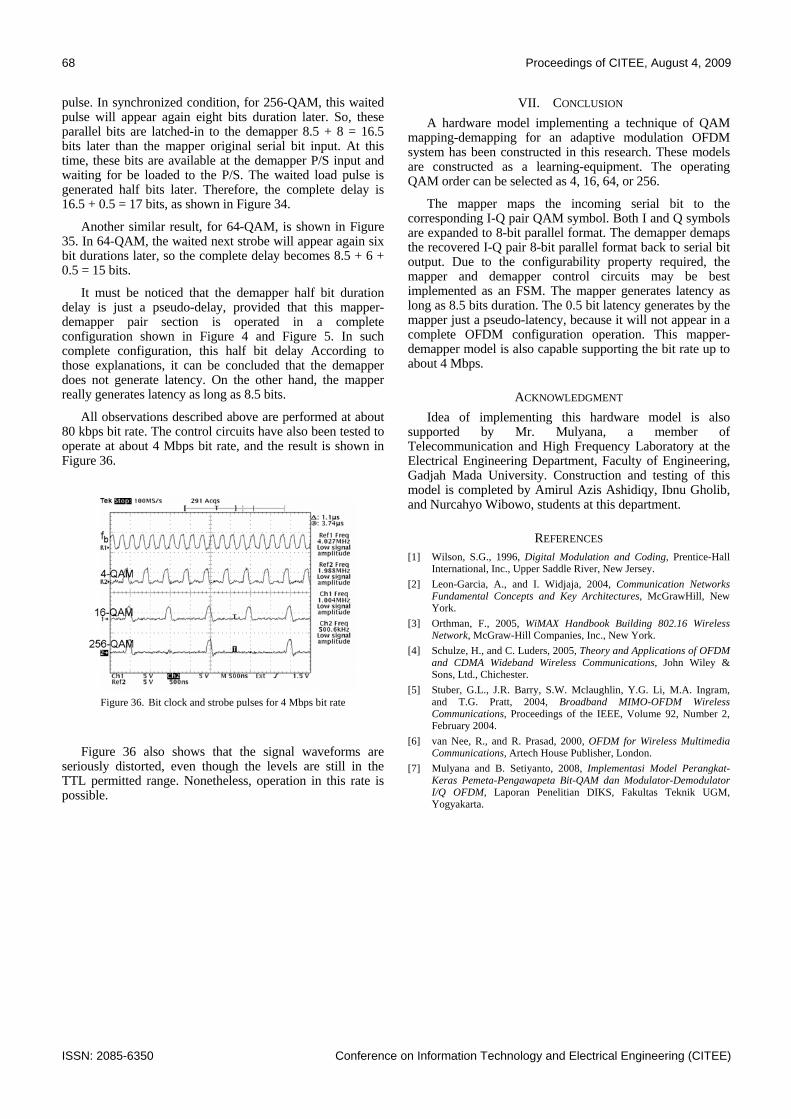
68 Proceedings of CITEE, August 4, 2009
ISSN: 2085-6350 Conference on Information Technology and Electrical Engineering (CITEE)
pulse. In synchronized condition, for 256-QAM, this waited pulse will appear again eight bits duration later. So, these parallel bits are latched-in to the demapper 8.5 + 8 = 16.5 bits later than the mapper original serial bit input. At this time, these bits are available at the demapper P/S input and waiting for be loaded to the P/S. The waited load pulse is generated half bits later. Therefore, the complete delay is 16.5 + 0.5 = 17 bits, as shown in Figure 34.
Another similar result, for 64-QAM, is shown in Figure 35. In 64-QAM, the waited next strobe will appear again six bit durations later, so the complete delay becomes 8.5 + 6 + 0.5 = 15 bits.
It must be noticed that the demapper half bit duration delay is just a pseudo-delay, provided that this mapper-demapper pair section is operated in a complete configuration shown in Figure 4 and Figure 5. In such complete configuration, this half bit delay According to those explanations, it can be concluded that the demapper does not generate latency. On the other hand, the mapper really generates latency as long as 8.5 bits.
All observations described above are performed at about 80 kbps bit rate. The control circuits have also been tested to operate at about 4 Mbps bit rate, and the result is shown in Figure 36.
Figure 36. Bit clock and strobe pulses for 4 Mbps bit rate
Figure 36 also shows that the signal waveforms are seriously distorted, even though the levels are still in the TTL permitted range. Nonetheless, operation in this rate is possible.
VII. CONCLUSION A hardware model implementing a technique of QAM
mapping-demapping for an adaptive modulation OFDM system has been constructed in this research. These models are constructed as a learning-equipment. The operating QAM order can be selected as 4, 16, 64, or 256.
The mapper maps the incoming serial bit to the corresponding I-Q pair QAM symbol. Both I and Q symbols are expanded to 8-bit parallel format. The demapper demaps the recovered I-Q pair 8-bit parallel format back to serial bit output. Due to the configurability property required, the mapper and demapper control circuits may be best implemented as an FSM. The mapper generates latency as long as 8.5 bits duration. The 0.5 bit latency generates by the mapper just a pseudo-latency, because it will not appear in a complete OFDM configuration operation. This mapper-demapper model is also capable supporting the bit rate up to about 4 Mbps.
ACKNOWLEDGMENT Idea of implementing this hardware model is also
supported by Mr. Mulyana, a member of Telecommunication and High Frequency Laboratory at the Electrical Engineering Department, Faculty of Engineering, Gadjah Mada University. Construction and testing of this model is completed by Amirul Azis Ashidiqy, Ibnu Gholib, and Nurcahyo Wibowo, students at this department.
REFERENCES [1] Wilson, S.G., 1996, Digital Modulation and Coding, Prentice-Hall
International, Inc., Upper Saddle River, New Jersey. [2] Leon-Garcia, A., and I. Widjaja, 2004, Communication Networks
Fundamental Concepts and Key Architectures, McGrawHill, New York.
[3] Orthman, F., 2005, WiMAX Handbook Building 802.16 Wireless Network, McGraw-Hill Companies, Inc., New York.
[4] Schulze, H., and C. Luders, 2005, Theory and Applications of OFDM and CDMA Wideband Wireless Communications, John Wiley & Sons, Ltd., Chichester.
[5] Stuber, G.L., J.R. Barry, S.W. Mclaughlin, Y.G. Li, M.A. Ingram, and T.G. Pratt, 2004, Broadband MIMO-OFDM Wireless Communications, Proceedings of the IEEE, Volume 92, Number 2, February 2004.
[6] van Nee, R., and R. Prasad, 2000, OFDM for Wireless Multimedia Communications, Artech House Publisher, London.
[7] Mulyana and B. Setiyanto, 2008, Implementasi Model Perangkat-Keras Pemeta-Pengawapeta Bit-QAM dan Modulator-Demodulator I/Q OFDM, Laporan Penelitian DIKS, Fakultas Teknik UGM, Yogyakarta.

Proceedings of CITEE, August 4, 2009 69
Conference on Information Technology and Electrical Engineering (CITEE) ISSN: 2085-6350
Hardware Model Implementation of a Baseband Conversion, Chip Synchronization,
and Carrier Synchronization Technique for a Universal QAM System
Budi Setiyanto, Mulyana, and Risanuri Hidayat
Electrical Engineering Department, Faculty of Engineering, Gadjah Mada University Jl. Grafika 2 Yogyakarta, 55281, Indonesia
Abstract—Baseband converters, chip synchronizer, and carrier synchronizer sections hardware model of a universal quadrature amplitude modulation (QAM) system have been implemented in this research. They are developed as a part of an adaptive modulation orthogonal frequency division multiplexing (OFDM) learning-equipment. Therefore, all electronic components are selected from the general purpose types, and performance quality is beyond the target. The transmitter baseband converter is a digital-to-analog (DAC) circuit. The receiver baseband converter is a cascaded integrate-and-dump (I/D), sample-and-hold (S/H), and analog-to-digital converter (ADC) circuit controlled by a triggered non-cyclic finite state machine (FSM). Chip synchronization is carried-out by detecting the abrupt amplitude changes of the received signal. Synchronizing the carrier phase is carried-out by shortly speeding-up or slowing-down the receiver local voltage controlled oscillator (VCO), provided that no frequency offset occurs. The ADC component limits the chip rate as high as about 10 kcps.
Keywords—quadrature modulation, DAC, ADC, chip synchronization, carrier synchronization
I. INTRODUCTION Due to its compromise bandwidth efficiency and noise-
immunity [1], QAM is (and will be) widely applied in recent (and future) wired and wireless technologies, either in single or multi carrier system [2 – 6]. Examples of application employing QAM are terrestrial microwave transmission and almost all of orthogonal frequency division multiplexing (OFDM)-based systems.
The QAM system baseband converter, chip synchronizer, and carrier phase synchronizer sections have been implemented in this research. Further, these constructed sections are prepared to be integrated with the other sections to form a complete adaptive modulation OFDM model. The model will be packed as a learning-equipment. Therefore, all electronic components are selected from the general purpose types, and performance quality is beyond the target.
II. REVIEW OF THEORETHICAL BACKGROUND General form of a QAM transmitter and receiver sides
can be modelled in Figure 1. At the transmitter-side, the input bit stream, b(nTb), is transformed to chip symbols M(kT) = Re(kT) - jIm(kT), with Tb and T = NTb represent the bit and chip durations, respectively. In general, each chip of Re and Im symbols consists of N parallel bits. These chip streams are converted to I(t) and Q(t) analog baseband
signals, modulate two orthogonal carrier signals, and finally, transmitted as a QAM signal, s(t). Receiver-side recovers the bit stream from the received QAM signal, r(t).
Figure 1. General form of QAM transmitter and receiver sides
Various processes transforming bits to chip and vice versa are beyond the scope of this research. Therefore, Figure 1 represents them as a dash-lined box. For single carrier QAM, this process just organizes the serial bits to their corresponding chip. For OFDM system, this process is complicated.
The receiver attempts to extract or estimate I(t) and Q(t) from the received signal, r(t), by carrying-out the correlations
( )( )
∫−
=−=Tk
Tkdttftr
TkTtItI
1)02cos()(1)(ˆ' π (1.a)
and
( )( )
∫−
=−=Tk
Tkdttftr
TkTtQtQ
1)02(sin)(1)(ˆ' π (1.b)
Optimum estimation result is achieved when during the integration interval, those two carrier signals are orthogonal each other. This orthogonal property is guaranteed when f0 = k/T (k = 1, 2, 3, …).

70 Proceedings of CITEE, August 4, 2009
ISSN: 2085-6350 Conference on Information Technology and Electrical Engineering (CITEE)
III. IMPLEMENTATION OF BASEBAND CONVERSION TECHNIQUE AT THE TRANSMITTER-SIDE
In Figure 1, baseband converter at the transmitter-side is represented simply as a digital-to-analog converter (DAC) only. There are two identical converters, for I (in-phase) and Q (quadrature) arms. The complete configuration of each converter is shown in Figure 2. For generality, the Re and Im symbols are represented as D(kT), and the I and Q signals are represented as a(t). The 8-bit DAC (IC 0800) is followed by a current-to-voltage (I/V) converter. Level adjuster (LA) is provided to adjust the final analog output signal range and level. I/V and LA are based on operational amplifiers LF356.
Figure 2. Configuration of baseband converter at the transmitter-side
Figure 3 shows an example of the DAC output voltage (v(t)) when its first three MSBs are varied and the others are fixed to be in zero state. This figure informs that the DAC is able to track the input variation.
Figure 3. Effect of input bits variation to analog output voltage of the
DAC-I/V section
Effect of level adjustment on the final converter output voltage is shown in Figure 4. The LA can be exploited as a level shifter, an amplitude scaling (attenuation or amplification), or both.
Figure 4. Effect of level adjustments on the converter output
Both converters linearity and dynamic response have been observed by driving the DAC with the output of a 4-bit binary counter. The result is shown in Figure 5.
Figure 5. Both converters output signal when the input is a free running
4-bit binary counter output
IV. IMPLEMENTATION OF THE BASEBAND CONVERSION TECHNIQUE AT THE RECEIVER-SIDE
At the receiver-side, baseband converter also consists of signal flow part and control circuit as shown in Figure 6.
Figure 6. Block diagram of the baseband converter and multiplier
A. Signal Flow Part The correlator and ADC in Figure 1 can be explored
further as shown in Figure 7. Correlator section consists of multiplier and integrate-and-dump (I/D) circuits. The multiplier section is beyond the scope of this research, and has ever been implemented [7]. Baseband converter consists of I/D, sample-and-hold (S/H), level adjuster (LA), and ADC circuits. There are also two identical converters, for I and Q arms.
Figure 7. Correlator and ADC sections
The I/D circuit is desired to produce
( ) ( ) ( )Tktkt
kduAtb +<<∫= δδ
δττ , (2)
where A is a constant, k is an integer, and T is the chip duration, so kδ is the instants when the dump pulse arrives. The S/H samples b(t) at t = kσ, where kσ is the instants
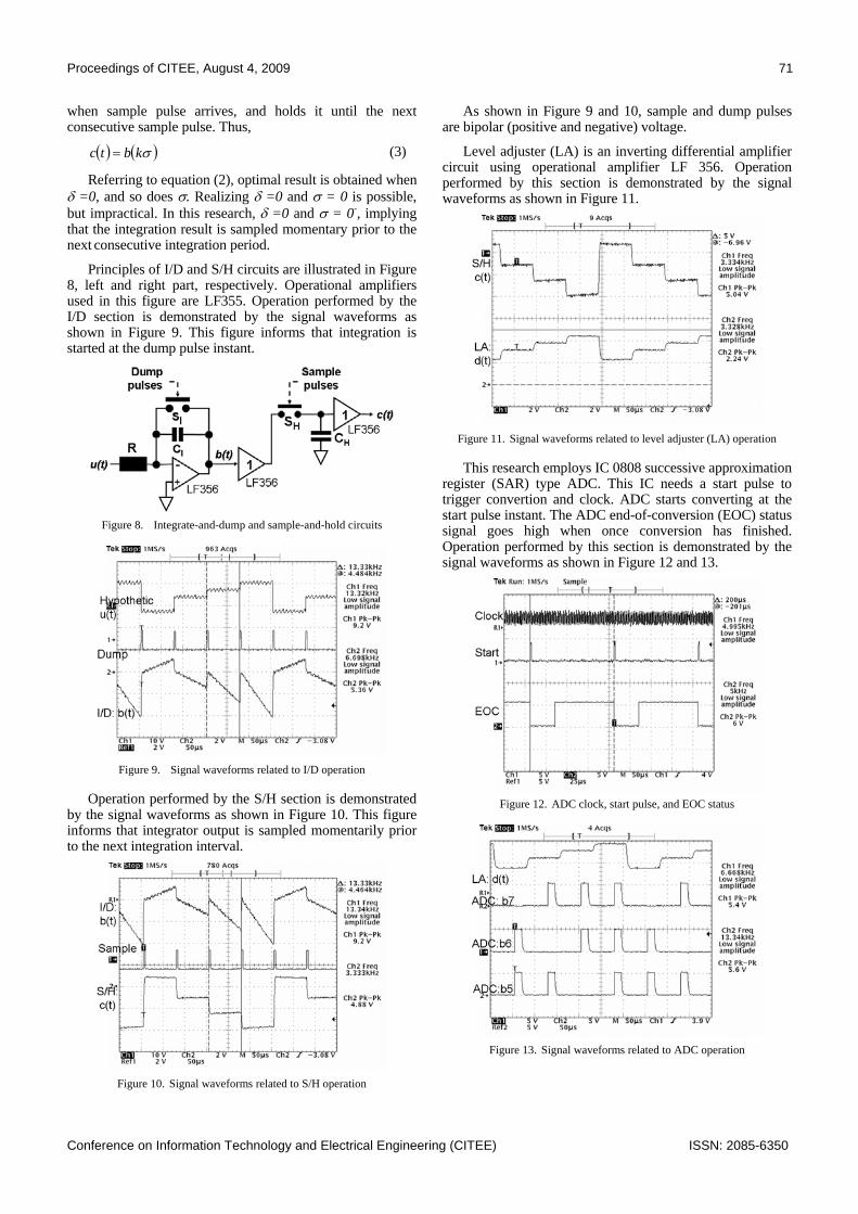
Proceedings of CITEE, August 4, 2009 71
Conference on Information Technology and Electrical Engineering (CITEE) ISSN: 2085-6350
when sample pulse arrives, and holds it until the next consecutive sample pulse. Thus,
( ) ( )σkbtc = (3)
Referring to equation (2), optimal result is obtained when δ =0, and so does σ. Realizing δ =0 and σ = 0 is possible, but impractical. In this research, δ =0 and σ = 0-, implying that the integration result is sampled momentary prior to the next consecutive integration period.
Principles of I/D and S/H circuits are illustrated in Figure 8, left and right part, respectively. Operational amplifiers used in this figure are LF355. Operation performed by the I/D section is demonstrated by the signal waveforms as shown in Figure 9. This figure informs that integration is started at the dump pulse instant.
Figure 8. Integrate-and-dump and sample-and-hold circuits
Figure 9. Signal waveforms related to I/D operation
Operation performed by the S/H section is demonstrated by the signal waveforms as shown in Figure 10. This figure informs that integrator output is sampled momentarily prior to the next integration interval.
Figure 10. Signal waveforms related to S/H operation
As shown in Figure 9 and 10, sample and dump pulses are bipolar (positive and negative) voltage.
Level adjuster (LA) is an inverting differential amplifier circuit using operational amplifier LF 356. Operation performed by this section is demonstrated by the signal waveforms as shown in Figure 11.
Figure 11. Signal waveforms related to level adjuster (LA) operation
This research employs IC 0808 successive approximation register (SAR) type ADC. This IC needs a start pulse to trigger convertion and clock. ADC starts converting at the start pulse instant. The ADC end-of-conversion (EOC) status signal goes high when once conversion has finished. Operation performed by this section is demonstrated by the signal waveforms as shown in Figure 12 and 13.
Figure 12. ADC clock, start pulse, and EOC status
Figure 13. Signal waveforms related to ADC operation

72 Proceedings of CITEE, August 4, 2009
ISSN: 2085-6350 Conference on Information Technology and Electrical Engineering (CITEE)
The ADC is followed by an 8-bit buffer 74LS373. The buffer holds the last ADC output until refreshed by the next consecutive result, as shown in Figure 14.
Figure 14. Signal waveforms related to buffer operation
Ideally, end-to-end baseband conversion test should be carried-out by building connecting the DAC output to the ADC input, exciting the DAC with a fast-varying 8-bit parallel word, and observing the 8-bit ADC output. This procedure required a 16-traces oscilloscope as a measuring instrument. This instrument has not been available.
Without loss of significance, a simpler procedure is created by reversing the configuration, as shown in Figure 15. The results are shown in Figure 16 and 17.
Figure 15. ADC-DAC compatibility test set-up
Figure 16. ADC-DAC link test result for 100 Hz sinusoidal signal
Figure 17. ADC-DAC link test result for 1 kHz signal
Figure 16 and 17 inform the ADC-DAC couple operate properly, indicated by the DAC output which is able to track the ADC input. The slower the ADC input varies, the more similar the DAC output is, of course. In these tests, the ADC is forced to operate at its maximum conversion rate as high as 10000 conversions per second as stated in data-sheet.
B. Control Circuit Block diagram of control circuit is shown in Figure 18.
Crystal oscillator generates 4.9 MHz clock. Frequency divider is a free running 4-bit binary counter. It divides the 4.9 MHz exciting clock to produce 1.225 MHz ADC clock and 306.25 triggered counter clock. Triggered counter is an up-and-stop 4-bit binary counter. It starts when triggered and stops when reaches its maximum state. The incoming external triggering pulse may be too wide for directly triggering the counter. Pulse shaper transforms this pulse to an as narrow as desired pulse. Sample, start, and dump pulses are formed by decoding three consecutive states, S0, S1, and S2, respectively.
Figure 18. Block diagram of the control circuit
The frequency divider and triggered counter are implemented using IC 74LS161. Figure 19 shows the clock signals provided by frequency divider.
Figure 19. Frequency divider available outputs
External supplied triggering pulse may be too wide to be directly fed to the triggered counter. Therefore, a pulse shaper is inserted to form this pulse as narrow as desired. The pulse shaper is a cascaded two monostable multivibrators (MMV) IC 74LS123. Pulse position and width are adjusted by the first and second stages MMV, respectively.
External trigger, sample, start, and dump pulses are shown in Figure 20. Sample and dump pulses shown in this figure are in unipolar (zero and positive polarities) format. As shown in Figure 9 and 10, these two pulses should be in

Proceedings of CITEE, August 4, 2009 73
Conference on Information Technology and Electrical Engineering (CITEE) ISSN: 2085-6350
bipolar (negative and positive polarities) format. Therefore, a unipolar-to-bipolar converter (UBC) circuit is inserted. UBC circuit is simply an analog comparator circuit.
Figure 20. Trigger, sample, start, and sample pulses
V. IMPLEMENTATION OF CHIP SYNCHRONIZATION TECHNIQUE
Example of a QAM signal waveform is shown in Figure 21 [7]. This figure shows that at every chip transition time, signal amplitude and/or phase changes are very possible.
Figure 21. Examples of a QAM signal waveform
In this research, chip synchronization is performed by searching for the abrupt change of received signal amplitude. The pulse synchronizer generates a narrow pulse when such change is detected. Block diagram of this chip synchronizer is shown in Figure 22.
Figure 22. Block diagram of the chip synchronizer circuit
The envelope detector is a diode-capacitor circuit, similar to one which is used in AM radio broadcasting receiver. The differentiator is a capacitor-resistor (C-R) circuit, and its output contains the dominant desired pulse contaminated by other ripple pulses. Level threshold must be adjusted to discard these ripples and extract the desired pulse. Level threshold adjuster is just an analog comparator circuit. The pulse width is adjusted by a pulse shaping circuit. The pulse shaper is implemented using a monostable multivibrator IC 74LS123.
Relation between the received OFDM-signal with the synchronizing pulse is shown in Figure 23. This pulse is further used for synchronizing, not for exciting, the other related circuits. Therefore, the appearance instants of this pulse must be the chip transition instants, and not necessary be at every chip transition. On the other, inter chip-transition appearance is prohibited.
Figure 23. Chip synchronized pulse compared to the simulated received
OFDM signal
Above explanation informs that the chip-transition detection like this is also applicable for general non constant-amplitude modulation systems.
VI. IMPLEMENTATION OF CARRIER SYNCHRONIZATION TECHNIQUE
Referring Figure 1, adopting equation (1.a) and (1.b) for estimating the real and imaginary parts chip gives
( )∫−
=−Tk
Tkdttftr
TkTt
1)02cos()(1)e(R π (3.a)
and
( )∫−
=−Tk
Tkdttftr
TkTt
1)02(sin)(1)m(I π (3.b)
Equation (3.a) and (3.b) inform that estimation requires a synchronous local oscillator signals: cos (2πf0t) and sin (2πf0t).
Carrier recovery technique [8] commonly used in M-ary modulation system principally is adoptable for QAM if the chip word-length (number of bits per chip) is known by the receiver. For OFDM system, this requirement is unrealistic, because it means that the receiver must know the number of bits per point of the transmitter IFFT output. Therefore, this research proposes a carrier synchronization technique which is independent to the chip word-length. This technique will be explained as follows.
Let the receiver has been successful to generate the desired frequency. The next problem is synchronizing its phase. In usual practical application, a special time-slot is provided where a specific real and imaginary parts pattern are transmitted to guide the receiver in synchronizing its phase. Using signal identification, the receiver know whether its synchronous condition has been reached or not yet.
The proposed technique in this research is illustrated in Figure 24. The voltage controlled oscillator (VCO) is

74 Proceedings of CITEE, August 4, 2009
ISSN: 2085-6350 Conference on Information Technology and Electrical Engineering (CITEE)
controlled by a positive, zero, or negative voltage through an analog multi-plexer. The control logic is generated by another smart circuit responsible for signal identification as explained above. This smart circuit is not presented here, and beyond the scope of this research.
Figure 24. Principle of the carrier phase synchronization
Control circuit must know whether the VCO is being lead or lag. Delaying or advancing the VCO is performed by shortly slowing it down or speeding it up, that is by driving it with a negative or positive voltage, respectively. The VCO is left to be in free running condition by driving it with zero control voltage.
Preliminary experiment using IC 4046 has shown that varying the control voltage from -180 mV to +180 mV varies almost linearly the frequency from 450 kHz to 550, with a free running or centre frequency of about 500 kHz. The VCO output waveforms are shown in Figure 25.
Figure 25. VCO output at various control voltage level
VII. CONCLUSION A hardware model implementing a technique of
baseband conversion, chip synchronization, and carrier synchronization for an OFDM system has been constructed in this research. At the transmitter-side, the baseband converter section is a pair of cascaded 8-bit digital-to-analog converter (DAC) and analog signal level adjuster circuits. At the receiver-side, this baseband converter is a pair of
cascaded integrate-and-dump, sample-and-hold, analog signal level adjuster, and 8-bit analog-to-digital converter (ADC) with its suitable control circuits. Chip synchronization is carried-out by detecting the abrupt changes in the received signal amplitude. This section consists of envelope detector, differentiator, threshold level adjuster, and pulse shaper circuits. Carrier synchronization is performed by adopting the delay-locked loop (DLL) technique commonly employed in a spread-spectrum system pseudorandom code tracking circuit. This section consists of a voltage difference detector, a lowpass filter (LPF), and a voltage controlled oscillator (VCO). These sections are implemented as a trainer, and operate at the chip rate as high as about 10 kcps. The chip rate and carrier frequency are constrained mainly by the ADC and VCO, respectively.
ACKNOWLEDGMENT Idea of implementing this hardware model is also
supported by Mr. Astria Nur Irfansyah, a member of Basic Electronics Laboratory at the Electrical Engineering Department, Faculty of Engineering, Gadjah Mada University. Construction and testing of this model is completed by Amirul Azis Ashidiqy, Ibnu Gholib, and Nurcahyo Wibowo, students at this department.
REFERENCES [1] Wilson, S.G., 1996, Digital Modulation and Coding, Prentice-Hall
International, Inc., Upper Saddle River, New Jersey. [2] Leon-Garcia, A., and I. Widjaja, 2004, Communication Networks
Fundamental Concepts and Key Architectures, McGrawHill, New York.
[3] Orthman, F., 2005, WiMAX Handbook Building 802.16 Wireless Network, McGraw-Hill Companies, Inc., New York.
[4] Schulze, H., and C. Luders, 2005, Theory and Applications of OFDM and CDMA Wideband Wireless Communications, John Wiley & Sons, Ltd., Chichester.
[5] Stuber, G.L., J.R. Barry, S.W. Mclaughlin, Y.G. Li, M.A. Ingram, and T.G. Pratt, 2004, Broadband MIMO-OFDM Wireless Communications, Proceedings of the IEEE, Volume 92, Number 2, February 2004.
[6] van Nee, R., and R. Prasad, 2000, OFDM for Wireless Multimedia Communications, Artech House Publisher, London.
[7] Mulyana and B. Setiyanto, 2008, Implementasi Model Perangkat-Keras Pemeta-Pengawapeta Bit-QAM dan Modulator-Demodulator I/Q OFDM, Laporan Penelitian DIKS, Fakultas Teknik UGM, Yogyakarta.
[8] Ha, T. T., 1990, Digital Satellite Communications, 2nd ed., Mc-Graw Hill, Singapore.

Proceedings of CITEE, August 4, 2009 75
Conference on Information Technology and Electrical Engineering (CITEE) ISSN: 2085-6350
Comparison Study of Breast Thermography and Breast Ultrasonography for Detection of Breast
Cancer
Thomas Sri Widodo1), Maesadji Tjokronegore2), D. Jekke Mamahit3)
1) &3) Electrical Dept., Eng. Fac., Gadjah Mada University
2) Medicine Fac., Gadjah Mada University
Abstracti-Breast thermography is a non-invasive diagnostic technique that allows the examiner to visualize and quantify changes in skin surface temperature. The objective of this research is to compare breast thermography and breast ultrasonography during abnormal physiology monitoring period for early stage cancer detection.
For this research the breast thermogram of four patients are compared with breast sonogram of the same patients with known breast diseases. The results show that thermography can be used to detect breast cancer with all stages with exception of cysts disease in the breast.
Key words: thermography, sonopgraphy, breast, cancer
I. Introduction
Thermography may be defined as a method of mapping surface temperature variations that depends entirely upon radiated energy in the infrared spectrum. A detector within the apparatus converts infrared radiation to an electrical output proportional to the emitted radiation [1]. The procedure is based on the principle that the chemical and blood vessel activity in both pre-cancerous tissue and the area surrounding a developing breast cancer is almost higher than in the normal breast. Since pre-cancerous and cancerous masses are highly metabolic tissues, they need an abundant supply of nutrients to maintain their growth. In order to do this they increase circulation to their cells by sending out chemicals to keep existing blood vessels open, recruit dormant vessels and create new ones (neoangiogenesis). This process results in an increase in regional surface temperatures of the breast [2, 3]. Criteria for the abnormal breast thermogram may be derived into vascular and nonvascular thermal patterns. The number of vessels should be relatively equal bilaterally . Vessels that are tortuous or serpiginous, or tend to cluster should be considered abnormal. Nonvascular criteria include the edge sign, which is an asymmetric flattened breast contour or localized protrusion with in the breast. Since there is a high degree of thermal symmetry in the normal body, subtle abnormal temperature asymmetry can be easily identified [1, 2].
II. Category and Stage of Tumor There are five thermo-biological (TH) categories for breast thermogram. [4]: TH1 - Normal uniform non vascular.
TH2 - Normal uniform vascular. There symmetrical streaks of thermal findings (blood vessels) in both breast. This increase in metabolism is caused by a relative progresterone deficiency (estrogen dominance). TH3 – Equivocal (questionable). There is single hot blood vessel in one breast (right or left). This thermal finding will need to be watched over time for change. If it is remain stable, or improves, this finding is normal for the physiology of the patient. TH4 – Abnormal. There is an increased temperature area (metabolism) of one breast. Especially significant is the highly vascular area. TH5 – Severely abnormal. There is an intensely increased temperature (metabolism) of the entire one breast. This is possible an inflammatory carcinoma. The currently accepted staging scheme for breast cancer is the TNM classification. The five tumor T classification values are Tis, T1, T2, T3, and T4 [5]. Tx – Primary tumor cannot be assessed. T0 – No evidence of primary tumor. Tis - Carcinoma in situ. T1 - Tumor 2 cm or less in its greatest dimension T2 - Tumor more than 2 cm but no more than 5 cm in its greatest dimension. T3 - Tumor more than 5 cm in its greater dimension. T4 - Tumor of any size with direct extension to chest wall or skin.
III. Comparison Results with Breast Ultrasonography Thermogram images of four patients with different stages were imaged using an infrared camera (Fluke Thermal Imager Model I 120) in an hospital. These images are then compared with the ultrasonography images (sonogram) of the same patients which are shown in Figure 1 to 4.
IV. Conclusion There is correlation between thermo biological breast category and breast cancer stage for breast cancer classification. Non uniform thermal findings in both breast indicates a breast cancer in one breast. This comparison study shows that breast thermography can be used to detect

76 Proceedings of CITEE, August 4, 2009
ISSN: 2085-6350 Conference on Information Technology and Electrical Engineering (CITEE)
a breast cancer. Cyst in the breast can not be detected using breast thermography.
Figure 1. (a) Entirely breast thermogram shows normal uniform
nonvascular (TH1). (b) and (c) Right and left breast sonogram show small cysts (T0).
Figure 2. (a) Entire breast thermogram shows a thermal finding at the upper part of the right breast (TH3). (b) Right breast sonogram shows a mass of disfuse dextra sinistra of 0.8x0.4 cm (T1) with malignancy and
metastasis.
Figure 3. (a) There is an increased temperature area (metabolism) of left
breast (TH4). (b). Left breast sonogram shows benign tumor without malignancy (T2).
Figure 4. (a) There is an intensely increased temperature (metabolism) of the entire left breast (TH5). (b) Left breast sonogram shows a malignancy
tumor with micro calcification of 3.5 cm (T3).

Proceedings of CITEE, August 4, 2009 77
Conference on Information Technology and Electrical Engineering (CITEE) ISSN: 2085-6350
References [1]. Carl J.D’Orsi,MD & Richard E.Wilson,MD, 1983,
Carcinoma of the breast : Diagnosis and Treatment, Boston/Toronto
[2]. Anonium, 2003., Breast Health, Meditherm Inc [3]. Gros C., Gautherie M., 1980, Breast Thermography
and Cancer Risk Prediction, Cancer
[4]. Anonymous, 2007, Breast Thermography, [email protected].
[5]. Anonymous, 2009, Breast Cancer Classification, Wilkipedia

78 Proceedings of CITEE, August 4, 2009
ISSN: 2085-6350 Conference on Information Technology and Electrical Engineering (CITEE)
Adaptive Polynomial Approximation for Gravimetric Geoid: A case study using EGM96 and
EIGEN-GL04C Geopotential Development
Tarsisius Aris Sunantyo Geodetic Department, Faculty of Engineering, Gadjah Mada University.
55000, Indonesia [email protected]
Muhamad Iradat Achmad
Electrical Department, Faculty of Engineering, Gadjah Mada University 55000, Indonesia
Abstract— In this paper, adaptive polynomial approximation method to model the gravimetric geoid is presented. The polynomial approximation model to arrange training of input is for adaptive system. Training data pairs (input and output) were compiled from latitude and longitude data sequences as input training, and an associated geopotential developments datum on each spatial position as output training. By preceded centering of latitude and longitude data, input training formed with following appropriate formula is the polynomial terms. Adaptation process used LMS (least mean square) algorithm in weight updating, and after training session, approximation of desired target was computed by reloading weights into the polynomial model. Model of assessment test used was to validate adaptive model by comparing residual distance of consecutive point from both geopotential developments data and respective adaptive model in geocentric coordinates system. Using geopotential developments data around of Merapi and Merbabu as a case study, the results show that the residual distance between geopotential developments data and respective adaptive model are about 0.0014417 m (in total absolute value with standard deviation is about 4.6906x10⁻⁵ m) using EGM96 geoid and about 0.0014468 m (in total absolute value with standard deviation is about 4.702x10⁻⁵ m) using EIGEN-GL04C geoid. Better result could be achieved by adding more training session with smaller gain factor.
Keywords— Adaptive polynomial approxima-tion,gravimetric geoid, geopotential developments, and model assesment.
I. INTRODUCTION One of the fundamental problems in geodesy is to define
the shape and size of the earth and its gravity field taking into account its temporal variation. Representation of the shape of the earth can be carried out by several methods; one of them is by geoid. Geoid is an equipotential surface of the earth at mean sea level (Heiskanen and Moritz, 1967). The use of precise geoid related data, in particular its undulation, is widespread in all branches of geodesy and it is often analyzed in other Earth sciences for example in geophysics, oceanography, as well as in civil engineering (Zhicai and Yong-qi, 2002).
Figure 1. Distribution of the Indonesian active volcanoes as the Ring of
Fire (Red color is active volcano) (Sunantyo, 2008)
Indonesia, as an archipelago, located partly on the Eurasian plate, which is subducted by the three major plates: the Indo-Australian plate in the south and in the west; the Pacific plate in the East and the Philippine Sea plate in the north. These subduction zones around Indonesia create a ring of volcanoes, which is called “the Ring of Fire” (see Figure 1). A total of 129 active volcanoes exist, and one of them is Merapi as a result of the subductions. Purbawinata et al.,(1997) state that the subduction zone is marked by a chain of active and dormant volcanoes which spreads along Sumatra, Java, Bali, Lombok, Sulawesi to the eastern part of Indonesian. North of Merapi volcano is Merbabu volcano which has not had activities more than 200 years. These two volcanoes are located in Yogyakarta city and Central Java (Purbawinata et al., (1997)). These two volcanoes are very often to be used as a research area too many scientists (i.e. geophysicist, geologist, geodesist etc) to have a comprehensive understanding about them. Merapi volcano has been labeled as one of 15 high risk volcanoes by the International Decade of Natural Disaster Reduction program (IDNDR) of UNESCO (Sunantyo, 2008). The integration a multidisciplinary approach (geodesy, geology, geophysics, seismology etc) concerning to understand the structure and volcanic activities of Merapi in more detail is very important and urgent (Zschau et al., 1998). In physical geodesy aspect, gravimetric geoid determination in these two volcanoes using geopotential developments is discussed in this research.

Proceedings of CITEE, August 4, 2009 79
Conference on Information Technology and Electrical Engineering (CITEE) ISSN: 2085-6350
Figure 2. Mechanical block of current adaptive system (Widrow and
Stearns, 1985)
II. ADAPTIVE SYSTEM DESIGN Input training of adaptive system is formed by following
associated formula in the polynomial terms. For the 4th order of 2D polynomial (Sunantyo, 2008):
.λλλλ
λλλ
λλλ
40,4
31,3
222,2
33,1
44,0
30,3
21,2
22,1
33,0
20,21,1
22,00,11,00,0
ϕϕϕϕ
ϕϕϕ
ϕϕϕ
ccccc
cccc
cccccch
++++
++++
++++++=
(1)
where λ, φ and h are longitude, latitude, and geopotential developments respectively, we have 15 terms (including constant term), and 15 parameters. For convenience, we use a1, a2,…,a14 to represent the terms: λ, φ, …, φ4 and w0, w1, w2, …, w14 for parameters: c0,0, c1,0, c0,1, …, c0,4. By preceded centering of latitude (=φ) and longitude (=λ) data, input training vector arranged by following appropriate formula in each polynomial terms. For example, the fifth term of kth input training given by
( )( )ϕϕλ −−= kkk λa4 (2)
The kth output of training data, hk, is an associated geopotential developments datum on spatial position (λk, φk). Mechanical block of current adaptive system shown in Fig. 1 where k is time index, system output fk denotes an approximation of desired output zk, and residu εk gives the difference between zk and fk. Weight updating that has a basic form (scalar input vector), gives new weight vector wk+1, and guarantees that adaptation process always parallel to input vector. Output system at time index k is given by
∑=
=L
iikikk awf
0
(5)
and residue estimation
kkk fz −=ε . (4)
Both the estimation of Cost function [ ] 22kkk E εεξ ≅= used
in computing instant gradient at the kth steps, 2kε∇ , and gain
factor µ , are used in weight updating ( )2
1 ww kkk εµ∇−=+ . (5) Gradient operator ( )•∇ defined as column vector
( ) ( ) ( ) ( )T
kpkk www ⎥⎥⎦
⎤
⎢⎢⎣
⎡
∂•∂
∂•∂
∂•∂
=•∇,,2,1
L (6)
and the ith element of gradient vector is ( )
ki
kk
ki
k
ww ,,
2
2∂∂
=∂∂ ε
εε
(7)
By using (4) in (7) and noting that fk is independent of wk, we obtain
( )ki
kk
ki
k
wf
w ,,
2
2∂∂
−=∂∂
εε
(8)
Using (3) in (8), we get ( )
kikki
k aw ,
,
2
2εε
−=∂∂
, (9)
and gradient vector become ( ) kkk a22 εε −=∇ (10)
where [ ]Tkpkkk aaa ,,2,1a L= is input vector at time
index k. Substituting (10) in (5) we get kkkk a 2ww 1 εµ+=+ . (11)
This is referred to the LMS algorithm shown in Fig. 1 as the dash line block. For N training data presentations, we define input matrix
[ ] TNn aaaaA 21 KK= (12)
where n is data index and using it to estimate gain factor as
[ ]( ) .AAEtrace
01.0T
≅µ (13)
where E[.] is expectation operator.
III. MODEL ASSESMENT TEST Model assessment test was used to validate model. This
test compares the distance between two consecutive points given by both geopotential developments data and its adaptive model in geocentric system (Sunantyo, 2008). Both residual distance (in total absolute value) and respective standard deviation are used to asses the modeling capability of adaptive system. For two consecutive points in geodetic system, ( )iii h,,ϕλ and ( )111 ,, +++ iii hϕλ , the distance (in meter) is given by
( ) ( ) ( )21
21
21 iiiiii zzyyxxd −+−+−= +++ (14)
where
( ) ,180
cos180
cos ⎟⎠⎞
⎜⎝⎛
⎟⎠⎞
⎜⎝⎛+′=
πλπϕhNx
( ) ,180
sin180
cos ⎟⎠⎞
⎜⎝⎛
⎟⎠⎞
⎜⎝⎛+′=
πλπϕhNy
( )( ) ,sin1 2 ϕheNz +−′=
,sin1 22 ϕe
KN−
=′

80 Proceedings of CITEE, August 4, 2009
ISSN: 2085-6350 Conference on Information Technology and Electrical Engineering (CITEE)
K = 6378137, e = 8.1819190842622x10⁻².
Difference between the distance given by gravimetric
data dh and one other given by adaptive model df (called residual distance) which defined as
az ddd −=∆ , (15) and has a total value
∑−
=∆ ∆=∑
1
1d
N
jjd , (16)
with standard deviation given by
( ) 21
1
1
2
d d1
1⎟⎟⎠
⎞⎜⎜⎝
⎛∆−∆
−= ∑
−
=∆
N
jjd
Nσ ,(17)
represents the closeness of model from its desired target. Denominator (N-1) in (17) referred to the number of elements of residual vector related to the consecutive points selecting.
IV. IMPLEMENTATION The two kinds of geopotential developments data are
EGM96 and EIGEN-GL04C, located in 48 different stations around Merapi and Merbabu volcanoes. The datasets consist of longitude, latitude, and an associated geoid height from both EGM96 and EIGEN-GL04C. At the design stage, we use (2) to center both longitude ( )λ= and latitude ( )ϕ= data, and arrange them following the polynomial terms in (1) to be input training data, while in the output side we use two sets of geopotential developments data to be our desired target. Using (12), it was defined input matrix
1548A ×ℜ∈ where 48 rows and 15 columns referred to the number of data presentations and the number of weights respectively. Substituting input matrix A in (13), then is was got gain factor .0095.0=µ Now, it was ready to develop an algorithm to handle our modeling task.
Algorithm of gravimetric geoid modeling using adaptive polynomial approximation is explained as follows: Input: Latitude (= ϕ ), longitude (= λ ), geopotential
developments height (=h), gain factor (= µ ), and maximum iteration (=kmax).
Output: Approximation of h (=f). 1. Centering 48λ, ℜ∈ϕ :
ϕϕϕ −=c and λ−= λλc . 2. Arranging input training based on polynomial terms:
.48,...,2,1,a 15 =ℜ∈ nn . 3. Training:
k=0,w0=0 while k<kmax for n=1,2,…,48 fn=an
Twk εn=hn-fn wk+1=wk+2µεnan end k=k+1
end 4. Computing output vector f:
for n=1,2,…,48, fn=an
Twkmax end
V. RESULT AND DISCUSSION
In the first part, distribution of TTG and its corresponding geoid using EGM96 and EIGEN-GL04C were discussed, while the second part analyzes are contour lines of geoid model and difference between geoid data and its model of EGM96 and EIGEN-GL04C. The third part is model of assessment using EGM96 and EIGEN-GL04C model for the 1D plotting of, data and model in the distance axis, distance of consecutive points and residual distance.
Figure 2. Distribution of TTG and its corresponding geoid using EGM96.
The Figure 2. show that distribution of TTG TTG and its corresponding geoid using EGM96 that all of TTG from Yogyakarta, Muntilan, Surakarta are mostly up (plus) and TTG from Surakarta to Yogyakarta are mostly down (minus).
Figure 3. Distribution of TTG and its corresponding geoid using EIGEN-
GL04C
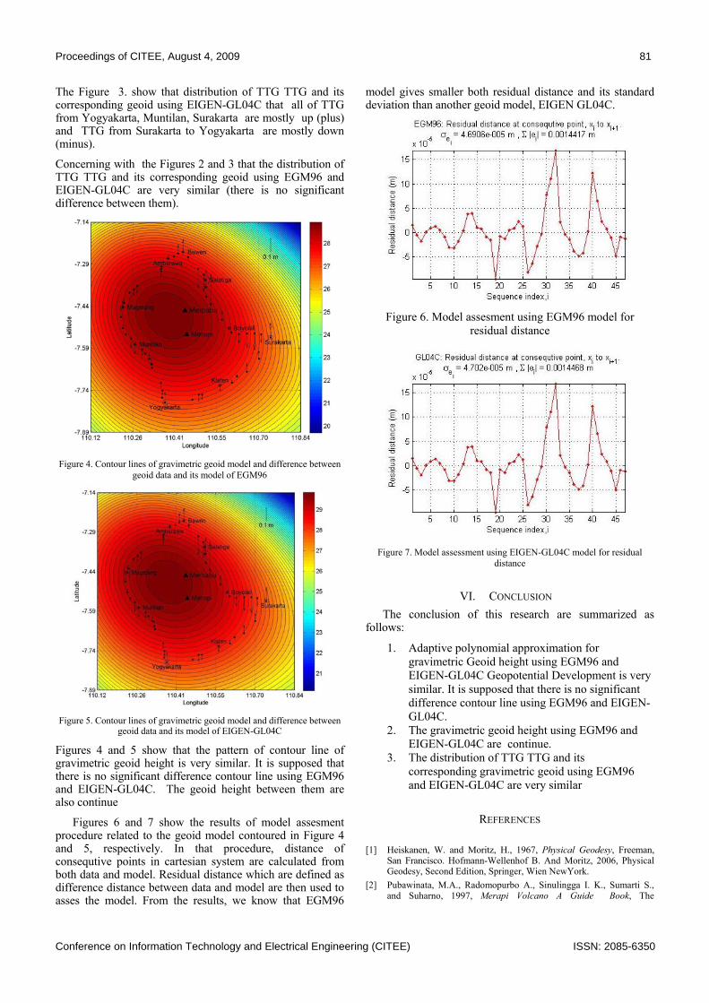
Proceedings of CITEE, August 4, 2009 81
Conference on Information Technology and Electrical Engineering (CITEE) ISSN: 2085-6350
The Figure 3. show that distribution of TTG TTG and its corresponding geoid using EIGEN-GL04C that all of TTG from Yogyakarta, Muntilan, Surakarta are mostly up (plus) and TTG from Surakarta to Yogyakarta are mostly down (minus).
Concerning with the Figures 2 and 3 that the distribution of TTG TTG and its corresponding geoid using EGM96 and EIGEN-GL04C are very similar (there is no significant difference between them).
Figure 4. Contour lines of gravimetric geoid model and difference between
geoid data and its model of EGM96
Figure 5. Contour lines of gravimetric geoid model and difference between
geoid data and its model of EIGEN-GL04C
Figures 4 and 5 show that the pattern of contour line of gravimetric geoid height is very similar. It is supposed that there is no significant difference contour line using EGM96 and EIGEN-GL04C. The geoid height between them are also continue
Figures 6 and 7 show the results of model assesment procedure related to the geoid model contoured in Figure 4 and 5, respectively. In that procedure, distance of consequtive points in cartesian system are calculated from both data and model. Residual distance which are defined as difference distance between data and model are then used to asses the model. From the results, we know that EGM96
model gives smaller both residual distance and its standard deviation than another geoid model, EIGEN GL04C.
Figure 6. Model assesment using EGM96 model for
residual distance
Figure 7. Model assessment using EIGEN-GL04C model for residual distance
VI. CONCLUSION The conclusion of this research are summarized as
follows:
1. Adaptive polynomial approximation for gravimetric Geoid height using EGM96 and EIGEN-GL04C Geopotential Development is very similar. It is supposed that there is no significant difference contour line using EGM96 and EIGEN-GL04C.
2. The gravimetric geoid height using EGM96 and EIGEN-GL04C are continue.
3. The distribution of TTG TTG and its corresponding gravimetric geoid using EGM96 and EIGEN-GL04C are very similar
REFERENCES
[1] Heiskanen, W. and Moritz, H., 1967, Physical Geodesy, Freeman, San Francisco. Hofmann-Wellenhof B. And Moritz, 2006, Physical Geodesy, Second Edition, Springer, Wien NewYork.
[2] Pubawinata, M.A., Radomopurbo A., Sinulingga I. K., Sumarti S., and Suharno, 1997, Merapi Volcano A Guide Book, The

82 Proceedings of CITEE, August 4, 2009
ISSN: 2085-6350 Conference on Information Technology and Electrical Engineering (CITEE)
Volcanological Survey of Indonesia, Directorate General of Geology and Mineral Resources, Bandung, Indonesia
[3] Sunantyo, Modeling of Local Geoid using Adaptive Scheme: A Case Study around Merapi and Merbabu Volcanoes, Central Jawa, Indonesia, Doctoral Dissertation, Faculty of Engineering, Gadjah Mada University, 2008.
[4] Widrow, B., and Stearns, S. D., 1985, Adaptive Signal Processing, Prentice Hall Inc.
[5] Zachau J., Sukhyar, R., Purbawinata, M.A., Lühr, and Westerhaus,
M., 1998, Project MERAPI – interdisciplinary research at a high-risk volcano, In : Decade–Volcanoes Under Investigation, Deutsche Geophysikalische Gesellschaft, Sonderband III/1998.
[6] Zhicai L. and Yong-qi C, 2002, Precise determination of Hongkong Geoid using heterogeneous data, FIG XXII International Congress, Washington, D.C. U.S.A.

Proceedings of CITEE, August 4, 2009 83
Conference on Information Technology and Electrical Engineering (CITEE) ISSN: 2085-6350
Cerebellar Model Associative Computer (CMAC) for Gravimetric Geoid study based on EGM96 and
EIGEN-GL04C Geopotential Development
Muhamad Iradat Achmad1), Tarsisius Aris Sunantyo2) 1) Electrical Department, Faculty of Engineering, Gadjah Mada University
[email protected] 2) Geodetic Department, Faculty of Engneering, Gadjah Mada University.
Adhi Susanto3) 3) Electrical Department, Faculty of Engineering, Gadjah Mada University
Abstract— In this paper, cerebellar model associative
computer (CMAC) algorithm is proposed to be used for geoid study. This algorithm based on the mapping scheme of input space that transforms input similarity in the input space into associated levels in the associated cells space. Similar inputs mapped to similar levels, while dissimilar inputs associated to mutual independent cells. Associated levels given by overlapping base functions selected represent a subset of “feature” to be parameterized using adaptive linear combiner (ALC) structure where a set of “feature” impersonate as input vector in the back side, parameter or weight vector in the middle side, and an output in the front side. ALC structure adjusts weights value using LMS (least mean square) recursion in the training (or analyzing) session, and accumulates weighted input to get an output in the synthesizing session. Desired output using in weights adjustment are any values from the output space that correspond to respective values in the input space. Model assessment test used to validate CMAC model by comparing residual distance of consecutive points from both EGM96 and EIGEN-GL04C geopotential global development is data and respective CMAC model in geocentric coordinates system. By utilization of EGM96 and EIGEN-GL04C geopotential global development data sets acquired from selected points of geometric geoid in around of Merapi and Merbabu volcanoes, it is simulated the proposed algorithm to study geoid. The results show that difference between data and model based on EGM96 geopotential global development are about 0.00026296 m in total absolute value with standard deviation about 8.3856 x 10(6) m, and based on EIGEN-GL04C geopotential global development is about 0.00027139 m in total absolute value with standard deviation about 8.5441 m. These results use 1x10⁶ epoch in training session with gain factor mu=1.0638 x 10(4) m better result could be achieved by adding more training session with smaller gain factor.
Keywords—cerebellar model associative computer (CMAC), adaptive linear combiner, least mean square, EGM96 and EIGEN-GL04C geopotential global development.
I. INTRODUCTION Gravimetric geoid study is a fundamental part in geodesy
and other earth sciences in case to define the shape and size of the earth and its gravity field including its temporal variation. Many applications such as EWARS (early warning system) for disaster, oil and gas discovery, land management, and many more, utilizate geoid information to
perform specific and dedicated operation in its implementation. This is the facts to be the reason of our study.
One of many tasks in gravimetric study is the modeling of gravimetric geoid that has the same meaning with the surface fitting in which two predicting variables positioned as input and one response variable as the function of two input variables to be an output. For the temporal variation of the surface, we need to add an input time variable, but this is not the case presented here. Related to the surface fitting, there are many research available in text books and references. Most of them use the generalizing of least square method where prior knowledge given in input design suspected as the characteristics of the two-dimensional (2D) plant handled.
In this paper, we propose a gravimetric geoid modeling method that differs with the previous method in the way to incorporate prior knowledge to the modeling system. The method uses an algorithm that exploits the generalization and learning capability of CMAC (cerebellar model associative computer, cerebellar model arithmetic computer, or cerebellar model articulation controller). CMAC is an associative memory neural network based on the mapping scheme of input space that transforms input similarity in the input space into associated levels in the associated cells space. Similar inputs mapped to similar levels, while dissimilar inputs associated to mutual independent cells. CMAC is interpreted as a look up table method [1], and has been used in the areas of control [2]-[6], pattern recognition [7], signal and image processing [8]-[10]. Other research related to the structure and learning of CMAC investigated in [11]-[16].
In the proposed method, CMAC used to learn a non linear mapping from a spatial position into the corresponding geoid value. A geoid position is quantized by a number of quantization levels, and the CMACs input taken from quantizers output, associated to a set of association cells by the input mapping scheme. Training (or analyzing) session uses the association cells and the corresponding geoid value to be a set of respective input and output training. By using the LMS recursion, a set of weights adjusts until a number of epoch reached. Syntesizing session accumulates the weighted inputs to approximate desired output.

84 Proceedings of CITEE, August 4, 2009
ISSN: 2085-6350 Conference on Information Technology and Electrical Engineering (CITEE)
II. CMAC In this section, we give a brief description of CMAC
with emphasis on generalization and learning capability. In the proposed method, CMAC is used to learn a nonlinear mapping from a spatial position into the corresponding geoid value. Thus, we limit our discussion to a two-input single-output CMAC, although a general CMAC is capable of learning a multi-input multi-output nonlinear function.
A. Input Mapping Scheme Let the two-dimensional (2D) input of a nonlinear
function be (x,y), where x and y are a set of L real numbers, x,y∈RL, in the closed interval, [xmin, xmax] and [ymin, ymax], respectively. The input x is quantized by 1Q diferent uniform quantizers with quantization interval 1Q, 1ui (i=0,1,2,…,U) where 1u0≤xmin and 1uU≥xmax. The pre-superscript “1” used in 1Q and in all symbols in this paper denotes the input dimension. The decision level indexs of 1ui and 1ui+1 are given by
( ) 11
011
01
1 +⎥⎦
⎥⎢⎣
⎢−
−= Q
uuux
kU
(1)
where 1k is a set of L positive integer in interval [1,1Q]. The corresponding dequantization levels of (1) are given by
( )
( ) ( )011
1
1
01
212~ uu
Qkux U −×
++= . (2)
Difference between x and x~ is called the quantization error of the dimension of x. Similarly, the input y is also quantized in the same way as in x. By changing in (1) and in (2), the pre-superscript from “1” to “2”, the quantization interval from “u” to “v”, and the index from “M” to “N”, we get a set of L positive integer , 2k, in interval [1,2Q] and the corresponding dequantization levels, y~ . Difference between y and y~ is called the quantization error of the dimension of y.
Let the two dimensional (2D) input of CMAC be (1k,2k) where 1k and 2k are positive integers in [1,1Q] and [1,2Q] respectively. A set of g address associated by these inputs is given by
( ) ( )( ) gjfcfpfa jjjjj ,,1;211 K=++= (3)
where ( )( )jjj ccp 21= , (4)
1+⎥⎥
⎤⎢⎢
⎡ −=
gdQ
c jii
ji , (5)
⎥⎥
⎤⎢⎢
⎡ −=
gdk
f jii
ji , i=1,2. (6)
The parameters of CMAC, idj and g, are displacement and generalization parameters, respectively. They are defined
prior the design. Equation (3) gives a number of g address from overall address
∑=j
jpp . (7)
On each associated address, the association levels is defined by
( )
( )( ) ( )( )⎟⎟⎠
⎞⎜⎜⎝
⎛−+−−
−=
kgZgZkga i
aaijik 5.05.0
4exp2
, (8)
where Za is the center of the covered inputs region in terms of ik (i=1,2).
B. Adaptive Linear Combiner (ALC) The structure of ALC is shown in Fig. 1. There is an
input vector, a set of adjustable weights, a summing unit, and a single output. An input vector, a, with elements a1, a2, …, ap, has a number of g non zero elements where g is integer in the open interval (0,p). These inputs are parameterized by a corresponding sub set of adjustable weights, wj∈w, j=1, 2, …, g, and summed up by the linear combiner to get a single output, y. The combiner is called “linear” because for a fixed setting of the weights its output is a linear combination of the input components. However, when the weights are in the process of being adjusted, the output of the combiner is no longer a linear function of input. Given an input vector to ALC be in the column form as
[ ]Tpnnnn aaa L21a = (9)
In this notation T stands for transpose so an, is actually a column vector. Any non zero elements in an, amn≠0∈an, is given by (8). Here we use both subscript m and n for the element index of input vector and the iteration (and or data persentation) index, respectively. The corresponding set of adjustable weights is also in the column form as
[ ]Tpnnnn www L21w = . (10)
Given an input vector an and a weight vector wn, a single output of ALC on the nth iteration is given by
Figure 1. Adaptive linear combiner (ALC).

Proceedings of CITEE, August 4, 2009 85
Conference on Information Technology and Electrical Engineering (CITEE) ISSN: 2085-6350
∑=
==g
jjnjnn
Tnn way
1
wa . (11)
At the first right of equal sign in (11), the overall elements of the weighted input including zero elements is summed up, while in the second one, only g non zero elements to be summed to get the same output, yn.
C. Learning Scheme and Generalization The multi input-single output mapping of ALC is
determined by the stored weights. The weights are adjusted based on the least mean square algorithm so that the mapping achieves the desired function given a priori. Let the output of ALC for the input vector a be y, the corresponding training datum be h, and the output error between y and h be ε. Given an input vector an and the training datum be hn, the weights wjn (j=1,2,…,g) associated with the input are adjusted according to
gjww jnjnnj ,,2,1;)1( L=+=+ δ (12)
where
nnn
jnnn
yh
aj−=
=
ε
µεδ 2
The parameter µ is a gain factor that governs a learning speed. Let the output error for the input an after the updating be ε+. Then we have
( )
( ) .aa21 aa2
a2wa
nnTn
nTnnnn
nnnTnnn
yhh
εµµε
µεε
−=
−−=
+−=+
To make nn εε ≤+ , the parameter µ is selected so it is in the interval
.aa2
10n
Tn
≤< µ (13)
The significant feature of CMAC is that the learning scheme changes the output values for the nearby inputs, because each of subregions that formed by amn∈an covers g2 inputs, ik (i=1,2). Therefore, similar inputs lead to similar outputs even for untrained inputs. This property is called generalization, which is of great use in the CMAC-based modelling. Moreover, we can control the degree of generalization by changing the size of g. A larger g gives larger subregion and wider generalization region. This is to be the reason so g is called a generalization parameter.
Fig. 2(a) shows the generalization region of CMAC with g=4. We shall give a training signal to the input h(5,6). The input then specifies four subregions denoted by the squares, and four weights stored in the subregions are updated. The number of updated weights for each input is represented by “1”, “2”, “3”, and “4”. The outputs indicated by “4”, “3”,
“2”, and “1” are increased by (2µε-aj), (3µε-aj/2), (µε-aj), and (µε-aj/2), respectively, where ε- is the output error for the input (5,6) before the updating and aj is the corresponding association levels with respect to the covered inputs (1k,2k). We see that the CMAC outputs are changed even for untrained inputs. For comparisson, Fig. 2(b) shows the generalization region of a CMAC with g=2. In this case, two weights are updated, and the outputs indicated by “2” and “1” are increased by (2µε-aj) and (µε-aj), respectively. We see that the generalization region becomes smaller than the previous one.
III. CMAC-BASED MODELING Fig. 3 shows a structure of the proposed modelling
system. Here, an input pair (x,y) is quantized by an interval quantizer to get a quantized quantity pair, (1k,2k). The input mapping uses both 1k and 2k to generate the association address, m. Those quantized quantity pair is also utilizated to calculate the association levels in m address, am. ALC then uses the association levels am and an output h to be its training data pair. After a set of weights adjusted in the training session of ALC, the association levels weighted by a fixed set of weights is summed up to get an approximation of the desired output, h
~. Because of using a quantized
quantity pair in the input mapping, the dequantizer then needs to dequantize them to get the quantized input, x~ and y~ , that corresponds to the output h
~ in ( )yxh ~,~~
.
(a)
(b)
Figrue 2. Generalization property of CMAC. (a) g=4. (b) g=2.

86 Proceedings of CITEE, August 4, 2009
ISSN: 2085-6350 Conference on Information Technology and Electrical Engineering (CITEE)
The gravimetric geoid data can be represented in general form as h(x,y) where the spatial position, x and y, is referred to longitude and latitude, respectively, and the gravimetric geoid, h, is the geoid height at position (x,y). Given a set of L positions, x,y∈RL, where x in [xmin,xmax] and y in [ymin,ymax]. Let the selected ROI (region of interest) for the dimension of x and y be in interval [1u0,1uM] and [1v0,1vN] respectively so the ROI covers all position in datasets. By deciding a number of 1Q and 2Q quantization levels for each of ROI intervals, quantizer (1) will give a set of L positive integer 1k,2k where 1k in [1,1Q] and 2k in [1,2Q]. Equation (3) then utilizated those quantized quantities, 1k and 2k, to associate a number of g address vector as the element indexs of p
n Ra ∈ (n=1,2,…,L). Those quantized quantities are also used by (8) to calculate the corresponding association levels in each associated address. ALC then uses both association vector an and geoid height h be its input-output training. By selecting a gain factor, µ, so it is in (13), a set of adjustable weights, pRw ∈ , is trained by ALC using (12) until some stoping criteria achieved. Given a fixed set of adjusted weights, pRw*∈ , and an association vector, p
n Ra ∈ ,
n=1,2,…,L, an approximation of geoid height, nh~
, is
calculated by (11). The quantity nh~
is not only an approximation value of true geoid height hn, but its corresponding position, ( )yx ~,~ , given by dequantizer (2) is also an approximation value of true position (x,y).
The last statements in the previous paragraph confirms the using of model assesment that incorporate the approximated values in both h
~ and ( )yx ~,~ . Reference [17]
was given a respective procedure in model assesment that used by this paper. In that procedure, data and model in geodetic coordinat system are transformed into geocentric cartesian system and then distance of consequtive points in the new coordinat system are calculated. Residual distances between model and data are used to asses the model.
As shown in Fig. 2, generalization regions can be control by using a pre-defined value of generalization parameter, g. In “unpublished” [18], generalization g is pre-defined so it is a positive integer in [1,max(1Q,2Q)). By first ploting the distribution of TTG (tanda tinggi geodesi) to see its coverage area and defining properly ROI so it covers all TTG, then generalization g is approximately defined in such so its value is equal or larger than the maximum distance between the ROI frames and its respective TTG area frames. For comparing purpose in this paper, we implement two CMACs with different generalization parameter in the same maximum quantization level of both x and y. Here we define CMAC with g=73 and g=123 in the maximum quantization level 1Q=2Q=256.
IV. RESULT AND DISCUSSION In this section, the distribution of TTG points around
Merapi and Merbabu volcanoes are first explained. Those TTGs are then processed by the proposed method and the results which are consist of contour lines of corresponding geoid heights model given by two CMACs with different g, wil be discussed in the second part of this section. Model assesments are then presented in the last part and also closed this section.
Fig. 4(a) and (b) show the distribution of TTG points and its corresponding EGM96 and EIGEN-GL04C geoid height, respectively. In geoid height plotting, difference of geoids by its minimum value are used instead of its original one to visually enhance its spatial distribution of geoid in each TTG. In those figures we then know that TTGs which are lie in the path from Surakarta to Yogyakarta, are mostly have minimal geoid heights, while TTGs which are lained in the path from around Muntilan to near Ambarawa are mostly have maximal and uniform geoid heights. Different with
Figure 3. Generalization property of CMAC. (a) g=4. (b) g=2.
(a)
(b)
Figrue 4. Distribution of TTG and its corresponding geoid height, (a) EGM96, (b) EIGEN-GL04C.
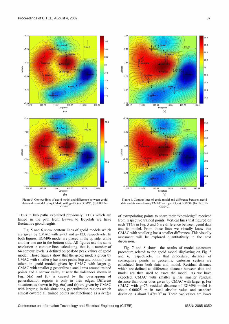
Proceedings of CITEE, August 4, 2009 87
Conference on Information Technology and Electrical Engineering (CITEE) ISSN: 2085-6350
TTGs in two paths explained previously, TTGs which are lained in the path from Bawen to Boyolali are have fluctuative geoid heights.
Fig. 5 and 6 show contour lines of geoid models which are given by CMAC with g=73 and g=123, respectively. In both figures, EGM96 model are placed in the up side, while another one are in the bottom side. All figures use the same resolution in contour lines calculating, that is, a number of 64 contour levels is defined on peak-to peak values of geoid model. Those figures show that the geoid models given by CMAC with smaller g has more peaks (top and bottom) than others in geoid models given by CMAC with larger g. CMAC with smaller g generalize a small area around trained points and a narrow valley at near the volcanoes shown in Fig. 5(a) and (b) is caused by the overlapping of generalization regions is only in their edges. Different situations as shown in Fig. 6(a) and (b) are given by CMAC with larger g. In this situations, generalization regions which almost covered all trained points are functioned as a bridge
of extrapolating points to share their “knowledge” received from respective trained points. Vertical lines that figured on each TTGs in Fig. 5 and 6 are difference between geoid data and its model. From those lines we visually know that CMAC with smaller g has a smaller difference. This visually assesment will be explored quantitatively in the next discussion.
Fig. 7 and 8 show the results of model assesment procedure related to the geoid model displaying on Fig. 5 and 6, respectively. In that procedure, distance of consequtive points in geocentric cartesian system are calculated from both data and model. Residual distance which are defined as difference distance between data and model are then used to asses the model. As we have expected, CMAC with smaller g has smaller residual distance than other ones given by CMAC with larger g. For CMAC with g=73, residual distance of EGM96 model is about 0.00025 m in total absolut value and standard deviation is about 7.47x10⁻⁶ m. These two values are lower
(a)
(b)
Figure 5. Contour lines of geoid model and difference between geoid data and its model using CMAC with g=73, (a) EGM96, (b) EIGEN-
GL04C
(a)
(b)
Figure 6. Contour lines of geoid model and difference between geoid data and its model using CMAC with g=123, (a) EGM96, (b) EIGEN-
GL04C.
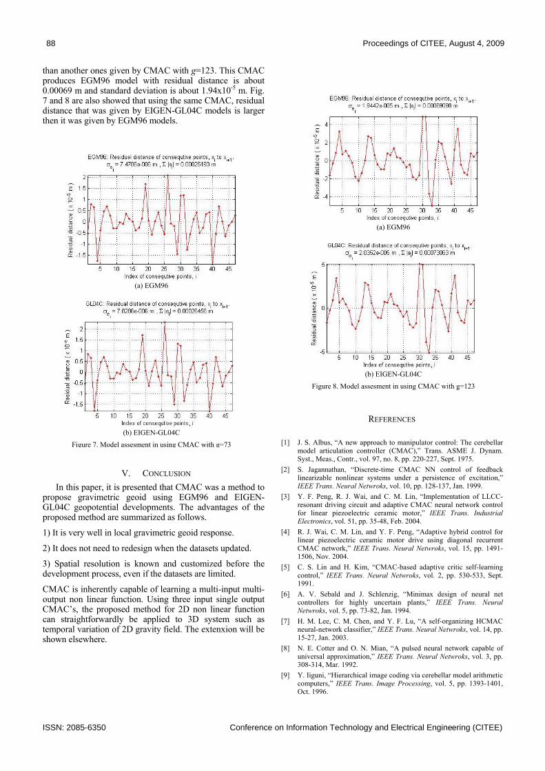
88 Proceedings of CITEE, August 4, 2009
ISSN: 2085-6350 Conference on Information Technology and Electrical Engineering (CITEE)
than another ones given by CMAC with g=123. This CMAC produces EGM96 model with residual distance is about 0.00069 m and standard deviation is about 1.94x10⁻⁵ m. Fig. 7 and 8 are also showed that using the same CMAC, residual distance that was given by EIGEN-GL04C models is larger then it was given by EGM96 models.
V. CONCLUSION In this paper, it is presented that CMAC was a method to
propose gravimetric geoid using EGM96 and EIGEN-GL04C geopotential developments. The advantages of the proposed method are summarized as follows.
1) It is very well in local gravimetric geoid response.
2) It does not need to redesign when the datasets updated.
3) Spatial resolution is known and customized before the development process, even if the datasets are limited.
CMAC is inherently capable of learning a multi-input multi-output non linear function. Using three input single output CMAC’s, the proposed method for 2D non linear function can straightforwardly be applied to 3D system such as temporal variation of 2D gravity field. The extenxion will be shown elsewhere.
REFERENCES
[1] J. S. Albus, “A new approach to manipulator control: The cerebellar model articulation controller (CMAC),” Trans. ASME J. Dynam. Syst., Meas., Contr., vol. 97, no. 8, pp. 220-227, Sept. 1975.
[2] S. Jagannathan, “Discrete-time CMAC NN control of feedback linearizable nonlinear systems under a persistence of excitation,” IEEE Trans. Neural Netwroks, vol. 10, pp. 128-137, Jan. 1999.
[3] Y. F. Peng, R. J. Wai, and C. M. Lin, “Implementation of LLCC-resonant driving circuit and adaptive CMAC neural network control for linear piezoelectric ceramic motor,” IEEE Trans. Industrial Electronics, vol. 51, pp. 35-48, Feb. 2004.
[4] R. J. Wai, C. M. Lin, and Y. F. Peng, “Adaptive hybrid control for linear piezoelectric ceramic motor drive using diagonal recurrent CMAC network,” IEEE Trans. Neural Netwroks, vol. 15, pp. 1491-1506, Nov. 2004.
[5] C. S. Lin and H. Kim, “CMAC-based adaptive critic self-learning control,” IEEE Trans. Neural Netwroks, vol. 2, pp. 530-533, Sept. 1991.
[6] A. V. Sebald and J. Schlenzig, “Minimax design of neural net controllers for highly uncertain plants,” IEEE Trans. Neural Netwroks, vol. 5, pp. 73-82, Jan. 1994.
[7] H. M. Lee, C. M. Chen, and Y. F. Lu, “A self-organizing HCMAC neural-network classifier,” IEEE Trans. Neural Netwroks, vol. 14, pp. 15-27, Jan. 2003.
[8] N. E. Cotter and O. N. Mian, “A pulsed neural network capable of universal approximation,” IEEE Trans. Neural Netwroks, vol. 3, pp. 308-314, Mar. 1992.
[9] Y. Iiguni, “Hierarchical image coding via cerebellar model arithmetic computers,” IEEE Trans. Image Processing, vol. 5, pp. 1393-1401, Oct. 1996.
(a) EGM96
(b) EIGEN-GL04C
Figure 7. Model assesment in using CMAC with g=73
(a) EGM96
(b) EIGEN-GL04C
Figure 8. Model assesment in using CMAC with g=123

Proceedings of CITEE, August 4, 2009 89
Conference on Information Technology and Electrical Engineering (CITEE) ISSN: 2085-6350
[10] A. M. Iradat, A. Susanto, dan Litasari, Pemampatan data citra menggunakan CMAC, Tesis S2, Jurusan Teknik Elektro, UGM, 2004.
[11] C. S. Lin and C. T. Chiang, “Learning convergence of CMAC technique,” IEEE Trans. Neural Netwroks, vol. 8, pp. 1281-1292, Nov. 1997.
[12] J. S. Ker, Y. H. Kuo, and B. D. Liu, “Hardware implementation of CMAC neural network with reduced storage requirement,” IEEE Trans. Neural Netwroks, vol. 8, pp. 1545-1556, Nov. 1997.
[13] F. J. G. Serrano, A. R. F. Vidal, and A. A. Rodriguez, “Generalizing CMAC architecture and training,” IEEE Trans. Neural Netwroks, vol. 9, pp. 1509-1514, Nov. 1998.
[14] J. C. Jan and S. L. Hung, “High-order MS_CMAC neural network,” IEEE Trans. Neural Netwroks, vol. 12, pp. 598-603, May 2001.
[15] Y. F. Wong and A. Sideris, “Learning convergence in the cerebellar model articulation controller,” IEEE Trans. Neural Netwroks, vol. 3, pp. 115-121, Jan. 1992.
[16] D. E. Thompson and S. Kwon, “Neighborhood sequential and random training techniques for CMAC,” IEEE Trans. Neural Netwroks, vol. 6, pp. 196-202, Jan. 1995.
[17] T. A. Sunantyo, Modeling of Local Geoid using Adaptive Scheme: A Case Study around Merapi and Merbabu Volcanoes, Central Jawa, Indonesia, Doctoral Dissertation, Faculty of Engineering, Gadjah Mada University, 2008.
[18] A. M. Iradat, Analisis-Sintesis Citra Sekuensial Berdasar Watak Citra melalui Implementasi CMAC sebagai Penyandi Laju Bit Rendah, Laporan Hasil Penelitian untuk Disertasi, Program Studi Teknik Elektro, Fakultas Teknik, Universitas Gadjah Mada, Mei, 2009.