Signal Processing 83 (2003) 283–296

www.elsevier.com/locate/sigpro

Orthogonal least squares algorithm for the approximation of amap and its derivatives with a RBF network

C. Driolia ;∗, D. Rocchessob

aDipartimento di Ingegneria dell’Informazione, University of Padova, Via Gradenigo 6/a, 35131 Padova, ItalybDipartimento di Informatica, University of Verona, Ca’ Vignal 2, Strada Le Grazie 15, 37134 Verona, Italy

Received 8 April 2002

Abstract

Radial basis function networks (RBFNs) are used primarily to solve curve-0tting problems and for non-linear systemmodeling. Several algorithms are known for the approximation of a non-linear curve from a sparse data set by means ofRBFNs. Regularization techniques allow to de0ne constraints on the smoothness of the curve by using the gradient of thefunction in the training. However, procedures that permit to arbitrarily set the value of the derivatives for the data are rarelyfound in the literature. In this paper, the orthogonal least squares (OLS) algorithm for the identi0cation of RBFNs is modi0edto provide the approximation of a non-linear single-input single-output map along with its derivatives, given a set of trainingdata. The interest in the derivatives of non-linear functions concerns many identi0cation and control tasks where the studyof system stability and robustness is addressed. The e6ectiveness of the proposed algorithm is demonstrated with examplesin the 0eld of data interpolation and control of non-linear dynamical systems.? 2002 Elsevier Science B.V. All rights reserved.

Keywords: Radial basis function networks; OLS learning; Curve 0tting; Iterated map stability; Chaotic oscillators

1. Introduction

The orthogonal least squares (OLS) algorithm [5]is one of the most popular procedures for the train-ing of radial basis function networks (RBFNs). AnRBFN is a two-layer neural network model especiallysuited for non-linear function approximation and ap-preciated in the 0elds of signal processing [8,10,11],non-linear system modeling, identi0cation and control[1,4,13,14], and time-series prediction [3,21]. With re-spect to other non-linear optimization algorithms, such

∗ Corresponding author. Tel.: +39-49-660062;fax: +39-49-8277699.

E-mail addresses: drioli@dei.unipd.it (C. Drioli),rocchesso@sci.univr.it (D. Rocchesso).

as gradient descent or conjugate gradients, the OLSalgorithm for RBFNs is characterized by a faster train-ing and improved convergence.In function approximation and data interpolation

by means of such universal approximation schemes,the derivatives of the underlying function can play animportant role in the attempt to improve the modelperformance. Regularization techniques, for example,allow to de0ne constraints on the smoothness of thecurve by using the information on the gradient duringthe training phase. Regularized networks are recog-nized to perform better than non-regularized networksin function learning and interpolation [16]. Moreover,in many applications the approximation of the map-ping alone will not suFce, and learning of the con-straints on di6erential data becomes important as well

0165-1684/03/$ - see front matter ? 2002 Elsevier Science B.V. All rights reserved.PII: S0165 -1684(02)00397 -3

284 C. Drioli, D. Rocchesso / Signal Processing 83 (2003) 283–296

Nomenclature

f R→ R function to be approximatedf′ derivative of the function to be approxi-

mated� radial kernelm; � center and width of the Gaussian kernelH number of kernels in the RBFNwi; b RBFN output weights and o6setx input training valuesy(d) output training values for the dth deriva-

tivep(d)i ith regressor vector of the dth derivativeuh; i ith orthogonalized regressor vector at it-

eration h

uh regressor vector selected at iteration hamong the uh; i’s

l(d)h; i ith orthogonalized regressor vector of thedth derivative at iteration h

l(d)h regressor vector selected at iteration hamong the l(d)h; i ’s

P(d)H 0nal matrix of regressors of the dth deriva-

tiveerr error reduction ratio for the maperr(d) error reduction ratio for the dth derivativetot err total error reduction ratio

as learning input–output relations. For example, in thesimulation of mechanical systems or plants by physi-cal modeling, the physical knowledge is given in theform of partial di6erential equations (PDEs), or con-straints on di6erential data [12]. In dynamical systemmodeling and control tasks the stability of the identi-0ed system depends on the gradient of the map [6,18],so that, exploiting the derivatives, the modeling canbe improved and the stabilization of desired dynami-cal behaviors can be achieved.Despite of the importance of learning di6eren-

tial data, the problem of eFciently approximating anon-linear function along with its derivatives seemsto be rarely addressed. Some theoretical results aswell as some application examples that apply togeneric feedforward neural networks are found in[2,9,12]. More emphasis on the procedural aspectsof di6erential data learning are found in [15], wherea back-propagation based algorithm for multilayerneural network is proposed, and [20], where a RBFNwith raised-cosine kernels is introduced, that can 0tup to 0rst-order di6erential data.In this paper, an extended version of the OLS al-

gorithm for the training of single-input single-outputRBFNs is presented, which permits to approximate anunknown function by specifying a set of data pointsalong with its desired higher-order derivatives.The paper is organized as follows: in Section 2,

the OLS algorithm is reviewed and modi0ed to add

control over the derivative of the function to be ap-proximated. The extension to higher-order derivativesis introduced in Section 3. Application examples inthe 0eld of function interpolation and non-linear dy-namics are given in Section 4. In Section 5, the con-clusions are presented.

2. Orthogonal least squares learning algorithm

The OLS learning algorithm is traditionally tied tothe parametric identi0cation of RBF networks, a spe-cial two-layer neural network model widely used forthe interpolation and modeling of data in multidimen-sional space. In the following we will restrict the dis-cussion to the single-input single-output RBFNmodel,which is a mapping f :R→ R of the form

f(x) = b+H∑i=1

wi�(x; qi); (1)

where x∈R is the input variable, �(·) is a givennon-linear function, b, wi and qi, 16 i6H , are themodel parameters, andH is the number of radial units.The RBFN can be viewed as a special case of thelinear regression model

y(k) = b+H∑i=1

wipi(k) + e(k); (2)

C. Drioli, D. Rocchesso / Signal Processing 83 (2003) 283–296 285

where y(k) is the desired kth output sample, e(k)is the approximation error, and pi(k) are the regres-sors, i.e. some 0xed functions of x(k), where x(k) arethe input values corresponding to the desired outputvalues y(k):

pi(k) = �(x(k); qi): (3)

In its original version, the OLS algorithm is a proce-dure that iteratively selects the best regressors (radialbasis units) from a set of available regressors. Thisset is composed of a number of regressors equal to thenumber of available data, and each regressor is a ra-dial unit centered on a data point. The selection of ra-dial unit centers is recognized to be the main problemin the parametric identi0cation of these models, whilethe choice of the non-linear function for the radialunits does not seem to be critical. Gaussian-shapedfunctions, spline, multi-quadratic and cubic functionsare some of the commonly preferred choices.Here, we will use the Gaussian function �(x; m; �)= exp(‖x−m‖=�)2, where ‖ · ‖ denotes the euclideannorm, and m and � denote respectively the center andwidth of the radial unit. In the following, we assumethat the width is unique for all units, and constantduring training. For simplicity of notations we thusrefer to radial units as �(x; m).

2.1. Classic OLS algorithm

Say {x(k); y(k)}, k=1; 2; : : : ; N , is the data set givenby N input–output data pairs, which can be organizedin two column vectors x = [x(1) · · · x(N )]T and y =[y(1) · · ·y(N )]T. The model parameters are given invectorsm=[m1 · · ·mH ]T, w=[w1 · · ·wH ]T and b=[b],where H is the number of radial units to be used.Arranging the problem in matrix form we have:

y =[P 1

] [ wb

]+ e (4)

with

P=[p1 · · · pH

]

=

�(x(1); m1) · · · �(x(1); mH )

.... . .

...

�(x(N ); m1) · · · �(x(N ); mH )

; (5)

where pi = [�(x(1); mi) · · ·�(x(N ); mi)]T are re-gressor vectors forming a set of basis vectors,e = [e(1) · · · e(N )]T is the identi0cation error, and1=[1 · · · 1]T is a unit column vector of length N . Theleast squares solution of this problem which satis0esthe condition that

y =[P 1

] [ wb

](6)

is the projection of y in a vector space spanned by theregressors. If the regressors are not independent, thecontribution of each regressor to the total energy ofthe desired output vector is not clear. The OLS algo-rithm proceeds iteratively by selecting the next bestregressor from a set by applying a Gram–Schmidt or-thogonalization, so that the contribution of each vectorof this new orthogonal base can be determined indi-vidually among the available regressors. This greedystrategy is known to give non-maximally compact rep-resentations when non-orthogonal basis, such as theGaussian, are used [19]. Nevertheless, it proved to beuseful and eFcient in practice.

2.2. Modi6ed OLS algorithm

The classic algorithm selects a set of regressorsfrom the ones available and determines the outputlayer weights for the identi0cation of the desiredinput–output map, but does not explicitly control thederivative of the function. We propose to modify thisprocedure so as to allow the assignment of a desiredvalue of the function derivative at each data point.The data set will then be organized in three vec-tors x = [x(1) · · · x(N )]T, y = [y(1) · · ·y(N )]T, andy(1) = [y1(1) · · ·y1(N )]T, x and y being the input–output pairs and y(1) being the respective derivatives.It has to be noted that the original OLS algorithm se-lects each radial unit from a set of units, each of whichis centered on an input data point. The maximumnumber of units is then limited to the number of datapoints. When we add requirements on the derivativeof the function, a further constraint to the optimiza-tion problem is added, and the number of units to beselected in order to reach the desired approximationmay be higher than the number of data points. A pos-sible choice is to augment the input vector with pointschosen where there is no data available, e.g. a uniform

286 C. Drioli, D. Rocchesso / Signal Processing 83 (2003) 283–296

grid with Ne points covering the input interval, and tobuild a set of Ne regressors centered over these points.

The algorithm can be summarized as follows:

• First step, initialization: the set of regressors forselection is obtained by centering theNe radial units,and the error reduction ratio (err) for each regressorvector is computed. Given the regressor vectors

pi = [�(x(1); x(i)); : : : ; �(x(N ); x(i))]T;

16 i6Ne; (7)

and de0ned the 0rst-iteration vectors

u1; i = pi ; 16 i6Ne: (8)

The error reduction ratio associated with the ith vec-tor is given by

err1; i = (uT1; iy)2=((uT1; iu1; i)(y

Ty)): (9)

In a similar way, the regressor vectors for the deriva-tive of the map are computed:

p(1)i =[@�(x(1); x(i))

@x· · · @�(x(N ); x(i))

@x

]T;

16 i6Ne; (10)

and the 0rst-iteration vectors are de0ned:

l1; i = p(1)i ; 16 i6Ne: (11)

The error reduction ratio for the derivative is

err(1)1; i = (lT1; iy(1))2=((lT1; il1; i)(y

(1)Ty(1)));

16 i6Ne: (12)

The err1; i and err(1)1; i represent the error reductionratios caused respectively by u1; i and l1; i, and thetotal error reduction ratio can be computed by

tot err1; i = �err1; i + (1− �)err(1)1; i ; (13)

where � weights the importance of the map againstits derivative. Usually, �=0:5 is the preferred choicewhen the accuracy requirements for the map and itsderivative are the same. The index i1 is then found,so that

tot err1; i1 = maxi{tot err1; i ; 16 i6Ne}: (14)

The regressor pi1 giving the largest error reductionratio is selected and removed from the set of avail-able regressors. The corresponding center is addedto the set of selected centers:

u1 = u1; i1 = pi1 ; (15)

l1 = l1; i1 = p(1)i1 ; (16)

m1 = x(i1): (17)

• hth iteration, for h= 1; : : : ; H and H6Ne: the re-gressors selected in the previous steps, having in-dexes i1; : : : ; ih−1, have been removed from the setof available regressors. Before computing the errorreduction ratio for each regressor still available, theorthogonalization step is performed which makeseach regressor orthogonal with respect to those al-ready selected:

uh; i = pi −h−1∑j=1

uj(pTi uj)=(uTj uj);

i = i1; i2; : : : ; ih−1; (18)

lh; i = p(1)i −h−1∑j=1

lj(p(1)T

i lj)=(lTj lj);

i = i1; i2; : : : ; ih−1; (19)

errh; i = (uTh; iy)2=((uTh; iuh; i)(y

Ty));

i = i1; i2; : : : ; ih−1; (20)

err(1)h; i = (lTh; iy(1))2=((lTh; ilh; i)(y

(1)Ty(1)));

i = i1; i2; : : : ; ih−1; (21)

tot errh; i = �errh; i + (1− �)err(1)h; i ;i = i1; i2; : : : ; ih−1: (22)

As before, the regressor with maximum error re-duction ratio is selected and removed from the listof availability, and its center is added to the set ofselected centers:

tot errh; ih =maxi

{tot errh; i;

i = i1; i2; : : : ; ih−1}; (23)

uh = uh; ih ; (24)

C. Drioli, D. Rocchesso / Signal Processing 83 (2003) 283–296 287

lh = lh; ih ; (25)

mh = x(ih): (26)

• Final step, computation of output layer weights:once the H radial units have been positioned,the remaining w and b parameters can be foundwith a Moore–Penrose matrix inversion (pseudo-inversion): let us call PH = [pi1pi2 · · · piH ] andP(1)H = [p(1)i1 p(1)i2 · · · p(1)iH ] the two sets of selected re-

gressors, and let 1= [1 · · · 1]T and 0= [0 · · · 0]T betwo column vectors of length N . Then we have[

y

y(1)

]=

[PH 1

P(1)H 0

][w

b

]+ eH (27)

whose solution is[w

b

]=

([PH 1

P(1)H 0

])+ [y

y(1)

]: (28)

Usually, it is convenient to stop the procedure be-fore the maximum number of radial units has beenreached, as soon as the identi0cation error is consid-ered to be acceptable. To this purpose, one can useEq. (28) at iteration h to compute the identi0cationerror eh in (27). 1

3. Higher-order derivatives

The extension of the algorithm for the identi0ca-tion of a map and its derivatives of order higher thanone is straightforward. Given that � is continuousand has continuous derivatives up to order r, thederivatives of order up to r can be identi0ed for themap f. The data set is organized in r + 1 vectorsx = [x(1) · · · x(N )]T, y = [y(1) · · ·y(N )]T, y(1) =[y(1)(1) · · ·y(1)(N )]T; : : : ; y(r)=[y(r)(1) · · ·y(r)(N )]T,where y(d)(k) is the desired dth derivative for the kthdata point. In the 0rst step, a di6erent set of regressorsis computed for each derivative order:

pi = [�(x(1); x(i)); : : : ; �(x(N ); x(i))]T;

16 i6Ne; (29)

1 Note that in this case the length of vector w and the numberof columns of matrices P in Eq. (28) is h instead of H .

p(d)i =[@d�(x(1); x(i))

@xd; : : : ;

@d�(x(N ); x(i))@xd

]T;

16 i6Ne; 16d6 r: (30)

If we now call uih−1 , l(1)ih−1; : : : ; l(r)ih−1

the orthogonalizedregressor vectors selected in the (h−1)th iteration, inthe hth iteration the corresponding r+1 error reductionratios can be computed similarly to what was shownin Eqs. (18)–(21), and the total error reduction ratiocan then be computed as the weighted sum of theseterms:

uh; i = pi −h−1∑j=1

uj(pTi uj)=(uTj uj);

i = i1; i2; : : : ; ih−1; (31)

errh; i = (uTh; iy)2=((uTh; iuh; i)(y

Ty));

i = i1; i2; : : : ; ih−1; (32)

l(d)h; i = p(d)i −h−1∑j=1

l(d)j (p(d)T

i l(d)j )=(l(d)T

j l(d)j );

i = i1; i2; : : : ; ih−1; (33)

err(d)h; i = (l(d)T

h; i y(d))2=((l(d)T

h; i l(d)h; i )(y(d)Ty(d)));

i = i1; i2; : : : ; ih−1; (34)

tot errh; i = �0errh; i +r∑d=1

�derr(d)h; i ;

i = i1; i2; : : : ; ih−1: (35)

A common choice is to uniformly weight the impor-tance of the map and its derivatives, i.e. �i=1=(r+1),i=0; 1; : : : ; r. However, a non-uniform weighting canbe chosen to reMect non-uniform accuracy require-ments.The regressors with maximum error reduction ratio

are selected and removed from the list of availability,and the corresponding centers are added to the set ofselected centers:

tot errh; ih =maxi

{tot errh; i; i = i1; i2; : : : ; ih−1}; (36)

uh = uh; ih ; (37)

l(d)h = l(d)h; ih ; 16d6 r; (38)

288 C. Drioli, D. Rocchesso / Signal Processing 83 (2003) 283–296

mh = x(ih): (39)

If we now let

PH = [pi1 · · · piH ];P(1)H = [p(1)i1 · · · p(1)iH ];

...

P(r)H = [p(r)i1 · · · p(r)iH ]:

(40)

be the 0nal set of orthogonal regressors obtained fromthe selection procedure, we can compute the outputlayer parameters by solving the matrix equation

y

y(1)

...

y(r)

=

PH 1

P(1)H 0

......

P(r)H 0

[w

b

]+ e: (41)

-3 -2 -1 0 1 2 3

-1

0

0.5

1

x

f(x)

, df(

x)/d

x

function approximation SSE =2.91672

derivative approximation SSE =22.00595

target function

derivative of target function

training data

function and derivative interpolations

-1.5

-0.5

1.5

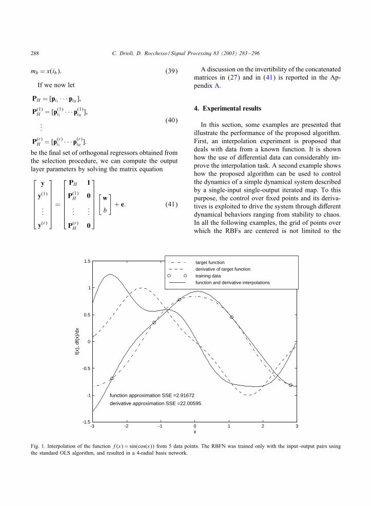
Fig. 1. Interpolation of the function f(x) = sin(cos(x)) from 5 data points. The RBFN was trained only with the input–output pairs usingthe standard OLS algorithm, and resulted in a 4-radial basis network.

A discussion on the invertibility of the concatenatedmatrices in (27) and in (41) is reported in the Ap-pendix A.

4. Experimental results

In this section, some examples are presented thatillustrate the performance of the proposed algorithm.First, an interpolation experiment is proposed thatdeals with data from a known function. It is shownhow the use of di6erential data can considerably im-prove the interpolation task. A second example showshow the proposed algorithm can be used to controlthe dynamics of a simple dynamical system describedby a single-input single-output iterated map. To thispurpose, the control over 0xed points and its deriva-tives is exploited to drive the system through di6erentdynamical behaviors ranging from stability to chaos.In all the following examples, the grid of points overwhich the RBFs are centered is not limited to the

C. Drioli, D. Rocchesso / Signal Processing 83 (2003) 283–296 289

-3 -2 -1 0 1 2 3

-1

0

1

x

f(x)

, df(

x)/d

x

function approximation SSE =0.04674

derivative approximation SSE =0.48613

target function

derivative of target function

training data

function and derivative interpolations

-1.5

-0.5

0.5

1.5

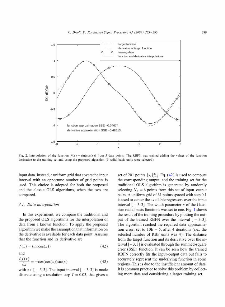
Fig. 2. Interpolation of the function f(x) = sin(cos(x)) from 5 data points. The RBFN was trained adding the values of the functionderivative to the training set and using the proposed algorithm (9 radial basis units were selected).

input data. Instead, a uniform grid that covers the inputinterval with an opportune number of grid points isused. This choice is adopted for both the proposedand the classic OLS algorithms, when the two arecompared.

4.1. Data interpolation

In this experiment, we compare the traditional andthe proposed OLS algorithms for the interpolation ofdata from a known function. To apply the proposedalgorithm wemake the assumption that information onthe derivative is available for each data point. Assumethat the function and its derivative are

f(x) = sin(cos(x)) (42)

and@f(x)@x

=−cos(cos(x))sin(x) (43)

with x∈ [− 3; 3]. The input interval [− 3; 3] is madediscrete using a resolution step T = 0:03, that gives a

set of 201 points {xi}201i=1. Eq. (42) is used to computethe corresponding output, and the training set for thetraditional OLS algorithm is generated by randomlyselecting Np = 6 points from this set of input–outputpairs. A uniform grid of 61 points spaced with step 0.1is used to center the available regressors over the inputinterval [− 3; 3]. The width parameter � of the Gaus-sian radial basis functions was set to one. Fig. 1 showsthe result of the training procedure by plotting the out-put of the trained RBFN over the interval [ − 3; 3].The algorithm reached the required data approxima-tion error, set to 10E − 5, after 4 iterations (i.e., theselected number of RBF units was 4). The distancefrom the target function and its derivative over the in-terval [−3; 3] is evaluated through the summed-squareerror (SSE) function. It can be seen how the trainedRBFN correctly 0ts the input–output data but fails toaccurately represent the underlying function in someregions. This is due to the insuFcient amount of data.It is common practice to solve this problem by collect-ing more data and considering a larger training set.

290 C. Drioli, D. Rocchesso / Signal Processing 83 (2003) 283–296

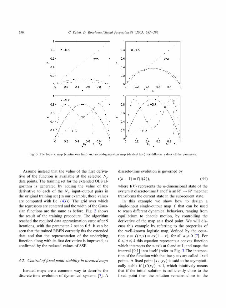
Fig. 3. The logistic map (continuous line) and second-generation map (dashed line) for di6erent values of the parameter.

Assume instead that the value of the 0rst deriva-tive of the function is available at the selected Npdata points. The training set for the extended OLS al-gorithm is generated by adding the value of thederivative to each of the Np input–output pairs inthe original training set (in our example, these valuesare computed with Eq. (43)). The grid over whichthe regressors are centered and the width of the Gaus-sian functions are the same as before. Fig. 2 showsthe result of the training procedure. The algorithmreached the required data approximation error after 9iterations, with the parameter � set to 0.5. It can beseen that the trained RBFN correctly 0ts the extendeddata and that the representation of the underlyingfunction along with its 0rst derivative is improved, ascon0rmed by the reduced values of SSE.

4.2. Control of 6xed point stability in iterated maps

Iterated maps are a common way to describe thediscrete-time evolution of dynamical systems [7]. A

discrete-time evolution is governed by

t(k + 1) = f(t(k)); (44)

where t(k) represents the n-dimensional state of thesystem at discrete-time k and f is anRn → Rn map thattransforms the current state in the subsequent state.In this example we show how to design a

single-input single-output map f that can be usedto reach di6erent dynamical behaviors, ranging fromequilibrium to chaotic motion, by controlling thederivative of the map at a 0xed point. We will dis-cuss this example by referring to the properties ofthe well-known logistic map, de0ned by the equa-tion y = f(a; x) = ax(1 − x), for all a¿ 0 [7]. For06 a6 4 this equation represents a convex functionwhich intersects the x-axis at 0 and at 1, and maps theinterval [0,1] into itself (refer to Fig. 3 The intersec-tion of the function with the line y=x are called 0xedpoints. A 0xed point (xf; yf) is said to be asymptoti-cally stable if |f′(xf)|¡ 1, which intuitively meansthat if the initial solution is suFciently close to the0xed point then the solution remains close to the

C. Drioli, D. Rocchesso / Signal Processing 83 (2003) 283–296 291

0 0.1 0.2 0.3 0.4 0.5 0.6 0.7 0.8 0.9 10

0.5

1

1.5

x

y

y=xf (xf) =-0.95

xf=

y=f(x) y=f2(x)

′

0 20 40 60 80 100 120 140 160 180 2000

0.2

0.4

0.6

0.8

k

t(k)

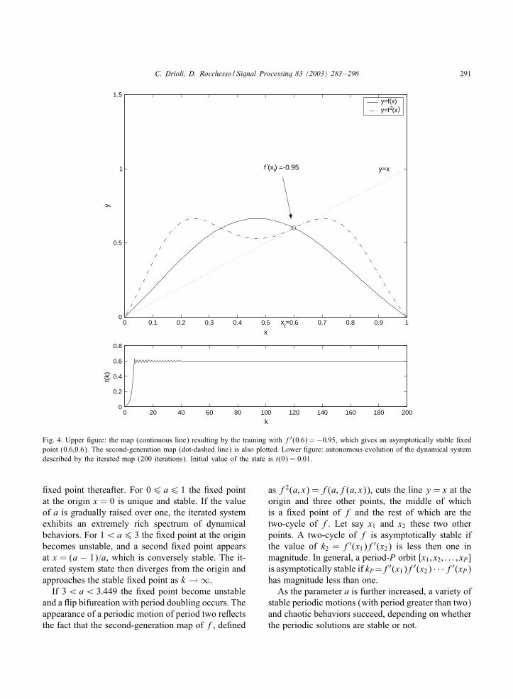
Fig. 4. Upper 0gure: the map (continuous line) resulting by the training with f′(0:6) =−0:95, which gives an asymptotically stable 0xedpoint (0.6,0.6). The second-generation map (dot-dashed line) is also plotted. Lower 0gure: autonomous evolution of the dynamical systemdescribed by the iterated map (200 iterations). Initial value of the state is t(0) = 0:01.

0xed point thereafter. For 06 a6 1 the 0xed pointat the origin x = 0 is unique and stable. If the valueof a is gradually raised over one, the iterated systemexhibits an extremely rich spectrum of dynamicalbehaviors. For 1¡a6 3 the 0xed point at the originbecomes unstable, and a second 0xed point appearsat x = (a − 1)=a, which is conversely stable. The it-erated system state then diverges from the origin andapproaches the stable 0xed point as k → ∞.If 3¡a¡ 3:449 the 0xed point become unstable

and a Mip bifurcation with period doubling occurs. Theappearance of a periodic motion of period two reMectsthe fact that the second-generation map of f, de0ned

as f2(a; x) = f(a; f(a; x)), cuts the line y = x at theorigin and three other points, the middle of whichis a 0xed point of f and the rest of which are thetwo-cycle of f. Let say x1 and x2 these two otherpoints. A two-cycle of f is asymptotically stable ifthe value of k2 = f′(x1)f′(x2) is less then one inmagnitude. In general, a period-P orbit [x1; x2; : : : ; xP]is asymptotically stable if kP=f′(x1)f′(x2) · · ·f′(xP)has magnitude less than one.As the parameter a is further increased, a variety of

stable periodic motions (with period greater than two)and chaotic behaviors succeed, depending on whetherthe periodic solutions are stable or not.

292 C. Drioli, D. Rocchesso / Signal Processing 83 (2003) 283–296

0 0.1 0.2 0.3 0.4 0.5 0.6 0.7 0.8 0.9 10

0.5

1

1.5

x

y

y=x

f (xf) =-1.2

f (x1) = -0.12218

f (x2) = -1.591

x1 x2

xf=

k2=0.19438

y=f(x)

y=f2(x)

0 20 40 60 80 100 120 140 160 1800

0.5

1

k

t(k)

x1

x2

′

′

′

Fig. 5. Upper 0gure: the map (continuous line) resulting from the training with f′(xf) = −1:2, which makes the 0xed point (0.6,0.6)unstable. From the second-generation map (dot-dashed line) it can be seen how a period-two bifurcation arises, due to the two intersectionpoints of the dot-dashed line with the line y= x (which are stable 0xed points of the second-generation map), other than the point (0.6,0.6)and the origin. The stability of the periodic orbit is due to the stability of the two new second-generation map 0xed points. Lower 0gure:autonomous evolution of the dynamical system described by the iterated map (200 iterations). Initial value of the state is t(0) = 0:01.

The qualitative behavior of the logistic map isshared by all smooth and convex functions f(x)such that f(0) = 0, f(b) = 0 for some b¿ 0, andf(x)¿ 0 for 0¡x¡b. We take b = 1 in ourexample, and we proceed in the design of a mapthat exhibits the desired dynamical behavior amongstable, periodic and chaotic motion. From the dis-cussion on the logistic map we observe that someof its features, e.g. the derivative at the origin, the0xed point xf and its derivative, and the 0xed pointsof the second-generation map play a central role in

the determination of the dynamic behavior. We fo-cus on these features to design the function, and relyon the relations between derivatives and stability todetermine the desired motion.First, we choose a 0xed point within the interval

(0,1), i.e. yf = xf = 0:6. Next, we can choose thederivative of the function f(x) at x = 0; x = 1, andx= xf. In order to obtain a convex function, we selecta pair of derivatives, e.g. f′(0)=1:7 and f′(1)=−1:3,which are compatible with the selected 0xed point(xf; yf). The derivative at the origin is taken greater

C. Drioli, D. Rocchesso / Signal Processing 83 (2003) 283–296 293

Fig. 6. Upper 0gure: the map (continuous line) resulting from the training with f′(xf) = −2, which makes the 0xed point (0.6,0.6)unstable for the map. Moreover, this value makes the other two 0xed points of the second-generation map unstable as well. No periodicorbit is observable anymore, and a chaotic motion arises. Lower 0gure: autonomous evolution of the dynamical system described by theiterated map (200 iterations). Initial value of the state is t(0) = 0:01.

than one in magnitude since we want to obtain a mo-tion divergent from the origin and evolving around thevalue yf as k → ∞. Finally, we use the derivativeat (xf; yf) to control the qualitative behavior of theevolution. To this aim, we rely on the fact that, for aderivative less than one in magnitude, an asymptoti-cally stable motion arises. Conversely, for a deriva-tive greater than one in magnitude, either a periodicor a chaotic motion can arise, depending on the stabil-ity of the 0xed points of the higher-order-generationmaps. Unfortunately, there is no straightforward wayto control such feature with the proposed method, thus

we restrict the control to the 0rst derivatives of the0rst-generation map f. To show the di6erent quali-tative behavior of the iterated system, we choose thefollowing three values for the derivative of the map,f′(xf) = {−:95;−1:2;−2}.

To summarize, the training set for the three cases is

x(1) = 0; y(1) = 0; y(1)(1) = 1:7;

x(2) = 0:6; y(2) = 0:6;

y(1)(2) = {−0:95;−1:2;−2:0};x(3) = 1; y(3) = 0; y(1)(3) =−1:3:

294 C. Drioli, D. Rocchesso / Signal Processing 83 (2003) 283–296

0 0.1 0.2 0.3 0.4 0.5 0.6 0.7 0.8 0.9 10

0.5

1

1.5

x

y

y=x

f (xf) = -2f (x1) =0.9

f (x2) = -1.05

x1 x2xf=

k2= -0.945

y=f(x) y=f2(x)

0 20 40 60 80 100 120 140 160 180 2000

0.5

1

k

t(k)

x1

x2

′′

′

Fig. 7. Upper 0gure: the map (continuous line) resulting from the training with further constraints f′(x1) = 0:9 and f′(x2) = −1:05.These values make stable the two 0xed points of the second-generation map (dashed line) at x = x1 and x = x2, thus allowing a stableperiod-two orbit. Lower 0gure: autonomous evolution of the dynamical system described by the iterated map (200 iterations). Initial valueof the state is t(0) = 0:01.

The proposed algorithm is then used to design themap given the selected points and derivatives. A uni-form grid of 31 points spaced with step 0.1 is usedto center the available regressors over the interval[ − 1; 2]. The width parameter � of the Gaussianradial basis functions was set to 0.5. These param-eters are kept the same throughout this example.Figs. 4–6 show the results of the map design and thedynamical behavior of the iterated map in the threecases. The 0rst case corresponds to an asymptoti-cally stable 0xed point at x = 0:6, with derivativemagnitude less than one. The second case reMects

the need for a period-two dynamic motion whenthe 0xed point (0.6,0.6) remains the same, althoughunstable. Note the di6erence with the simple logis-tic map case: if we desire a period-two orbit, wecan choose 3¡a¡ 3:449. However, the 0xed pointof the map would change depending on a, as it isyf = xf = (a− 1)=a. The periodic motion of the iter-ated system reMects the fact that the second-generationmap of Fig. 5 now intersects the line y = x in twomore points at x = x1 = 0:4607 and x = x2 = 0:6976other than x= xf = 0:6 and the origin. The third case(Fig. 6) demonstrate the e6ect of raising the value of

C. Drioli, D. Rocchesso / Signal Processing 83 (2003) 283–296 295

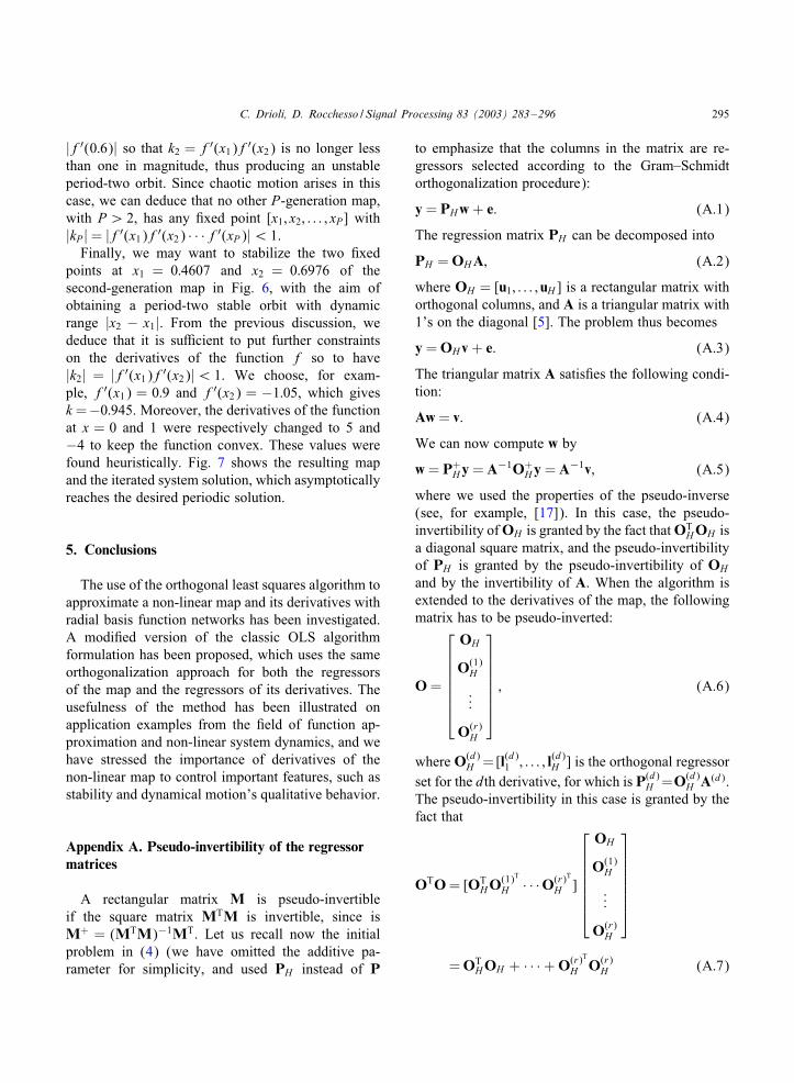
|f′(0:6)| so that k2 = f′(x1)f′(x2) is no longer lessthan one in magnitude, thus producing an unstableperiod-two orbit. Since chaotic motion arises in thiscase, we can deduce that no other P-generation map,with P¿ 2, has any 0xed point [x1; x2; : : : ; xP] with|kP|= |f′(x1)f′(x2) · · ·f′(xP)|¡ 1.Finally, we may want to stabilize the two 0xed

points at x1 = 0:4607 and x2 = 0:6976 of thesecond-generation map in Fig. 6, with the aim ofobtaining a period-two stable orbit with dynamicrange |x2 − x1|. From the previous discussion, wededuce that it is suFcient to put further constraintson the derivatives of the function f so to have|k2| = |f′(x1)f′(x2)|¡ 1. We choose, for exam-ple, f′(x1) = 0:9 and f′(x2) = −1:05, which givesk=−0:945. Moreover, the derivatives of the functionat x = 0 and 1 were respectively changed to 5 and−4 to keep the function convex. These values werefound heuristically. Fig. 7 shows the resulting mapand the iterated system solution, which asymptoticallyreaches the desired periodic solution.

5. Conclusions

The use of the orthogonal least squares algorithm toapproximate a non-linear map and its derivatives withradial basis function networks has been investigated.A modi0ed version of the classic OLS algorithmformulation has been proposed, which uses the sameorthogonalization approach for both the regressorsof the map and the regressors of its derivatives. Theusefulness of the method has been illustrated onapplication examples from the 0eld of function ap-proximation and non-linear system dynamics, and wehave stressed the importance of derivatives of thenon-linear map to control important features, such asstability and dynamical motion’s qualitative behavior.

Appendix A. Pseudo-invertibility of the regressormatrices

A rectangular matrix M is pseudo-invertibleif the square matrix MTM is invertible, since isM+ = (MTM)−1MT. Let us recall now the initialproblem in (4) (we have omitted the additive pa-rameter for simplicity, and used PH instead of P

to emphasize that the columns in the matrix are re-gressors selected according to the Gram–Schmidtorthogonalization procedure):

y = PHw+ e: (A.1)

The regression matrix PH can be decomposed into

PH =OHA; (A.2)

where OH = [u1; : : : ; uH ] is a rectangular matrix withorthogonal columns, and A is a triangular matrix with1’s on the diagonal [5]. The problem thus becomes

y =OH v + e: (A.3)

The triangular matrix A satis0es the following condi-tion:

Aw= v: (A.4)

We can now compute w by

w= P+Hy = A−1O+

Hy = A−1v; (A.5)

where we used the properties of the pseudo-inverse(see, for example, [17]). In this case, the pseudo-invertibility ofOH is granted by the fact thatOT

HOH isa diagonal square matrix, and the pseudo-invertibilityof PH is granted by the pseudo-invertibility of OH

and by the invertibility of A. When the algorithm isextended to the derivatives of the map, the followingmatrix has to be pseudo-inverted:

O=

OH

O(1)H

...

O(r)H

; (A.6)

where O(d)H =[l(d)1 ; : : : ; l

(d)H ] is the orthogonal regressor

set for the dth derivative, for which is P(d)H =O(d)

H A(d).The pseudo-invertibility in this case is granted by thefact that

OTO= [OTHO

(1)T

H · · ·O(r)T

H ]

OH

O(1)H

...

O(r)H

=OTHOH + · · ·+O(r)T

H O(r)H (A.7)

296 C. Drioli, D. Rocchesso / Signal Processing 83 (2003) 283–296

is a sum of diagonal square matrices. As a result, forthe concatenated matrix (A.6) to be pseudo-invertible,it is suFcient that the matrices OH ;O

(1)H ; : : : ;O

(r)H be

orthogonal, as it happens to be due to the orthogonal-ization process. Note that mutual orthogonality amongsets of bases related to di6erent order of derivatives isnot necessary. The last step is to compute the networkoutput weights w:

w=

PH

P(1)H

...

P(r)H

+

y

y(1)

...

y(r)

=

OHA

O(1)H A(1)

...

O(r)H A(r)

+

y

y(1)

...

y(r)

=

A 0 · · · 0

0 A(1) ...

.... . . 0

0 · · · 0 A(r)

1

OH

O(1)H

...

O(r)H

+

y

y(1)

...

y(r)

;

(A.8)

where the matrix containing the (upper) triangu-lar blocks A(i) is invertible, being a square matrixwith all zeros below the diagonal. We can concludethat the output weights can be computed from theinversion and pseudo-inversion of the two matri-ces in the last part of (A.8) or, equivalently, fromthe pseudo-inversion of the matrix containing theblocks P(i)

H .

References

[1] F.M.A. Acosta, Radial basis function and related models: anoverview, Signal Processing 45 (1995) 37–58.

[2] P. Cardaliaguet, G. Euvrard, Approximation of a functionand its derivatives with a neural network, Neural Networks5 (1992) 207–220.

[3] M. Casdagli, Nonlinear prediction of chaotic time series,Physica D 35 (1989) 335–356.

[4] S. Chen, S.A. Billings, Neural networks for nonlinear dynamicsystem modelling and identi0cation, Int. J. Control 56 (2)(1992) 319–346.

[5] S. Chen, C.F.N. Cowan, P.M. Grant, Orthogonal least squareslearning algorithm for radial basis functions networks, IEEETrans. Neural Networks 2 (2) (1991) 302–309.

[6] J.T. Connor, R.D. Martin, L.E. Atlas, Recurrent neuralnetworks and robust time series prediction, IEEE Trans.Neural Networks 5 (2) (1994) 240–254.

[7] P.G. Drazin, Nonlinear Systems, Cambridge University Press,Cambridge, 1992.

[8] C. Drioli, Radial basis function networks for conversion ofsound spectra, EURASIP J. Appl. Signal Process. 2001 (1)(2001) 36–44.

[9] A.R. Gallant, H. White, On learning the derivatives on anunknown mapping with multilayer feedforward networks,Neural Networks 5 (1992) 129–138.

[10] S. Haykin, Neural Networks. A Comprehensive Foundation,Macmillan, New York, 1994.

[11] S. Haykin, J. Principe, Making sense of a complex world,IEEE Signal Process. Mag. 15 (3) (1998) 66–81.

[12] K. Hornik, M. Stinchcombe, H. White, Universalapproximation of an unknown mapping and its derivativesusing multilayer feedforward networks, Neural Networks 3(1990) 551–560.

[13] R. Langari, L. Wang, J. Yen, Radial basis function networks,regression weights, and the expectation-maximizationalgorithm, IEEE Trans. Systems Man Cybernet. A 27 (5)(1997) 613–623.

[14] G.P. Liu, V. Kadirkamanathan, S.A. Billings, Variable neuralnetworks for adaptive control of nonlinear systems, IEEETrans. Systems Man Cybernet. C 29 (1) (1999) 34–43.

[15] R. Masuoka, Neural networks learning di6erential data, IEICETrans. Inform. Systems E83-D 6 (2000) 1291–1300.

[16] T. Poggio, F. Girosi, Networks for approximation andlearning, Proc. IEEE 78 (9) (1990) 1481–1497.

[17] C.R. Rao, S.K. Mitra, Generalized Inverse of Matrices andits Applications, Wiley, New York, 1971.

[18] F.J. Romeiras, C. Grebogy, E. Ott, W.P. Dayawansa,Controlling chaotic dynamical systems, Physica D 58 (1992)156–192.

[19] A. Sherstinsky, R.W. Picard, On the eFciency of theorthogonal least squares training method for radial basisfunction networks, IEEE Trans. Neural Networks 7 (1) (1996)195–200.

[20] R. Shilling, J.J. Carrol, A.F. Al-Ajlouni, Approximation ofnonlinear systems with radial basis function networks, IEEETrans. Neural Networks 12 (1) (2001) 1–15.

[21] P. Yee, S. Haykin, A dynamic regularized radial basisfunction network for nonlinear, nonstationary time seriesprediction, IEEE Trans. Signal Process. 47 (9) (1999)2503–2521.