*Corresponding author. Tel.: #34-958-246128; fax; #34-958-248993.E-mail address: irojas@atc.ugr.es (I. Rojas).

Neurocomputing 42 (2002) 267}285

Time series analysis using normalized PG-RBF networkwith regression weights

I. Rojas*, H. Pomares, J.L. Bernier, J. Ortega, B. Pino, F.J. Pelayo, A. PrietoDepartment of Architecture and Computer Technology, University of Granada, Campus Univ.

Fuentenueva, E-18071, Granada, Spain

Abstract

This paper proposes a framework for constructing and training a radial basis function (RBF)neural network. For this purpose, a sequential learning algorithm is presented to adapt thestructure of the network, in which it is possible to create a new hidden unit and also to detectand remove inactive units. The structure of the Gaussian functions is modi"ed using a pseudo-Gaussian function (PG) in which two scaling parameters � are introduced, which eliminates thesymmetry restriction and provides the neurons in the hidden layer with greater #exibility withrespect to function approximation. Other important characteristics of the proposed neuralsystem are that the activation of the hidden neurons is normalized which, as described in thebibliography, provides a better performance than nonnormalization and instead of usinga single parameter for the output weights, these are functions of the input variables which leadsto a signi"cant reduction in the number of hidden units compared to the classical RBF network.Finally, we examine the result of applying the proposed algorithm to time series predic-tion. � 2002 Elsevier Science B.V. All rights reserved.

Keywords: RBF neural networks; Sequential learning; Pruning strategy; Network growing;Time series prediction

1. Introduction

RBFs were originally proposed as an interpolation method and their properties asinterpolants have been extensively studied. An RBF neural network is usually trainedto map a set of observation vectors (x

�, y

�), where x

�"(x�

�,2, x�

�)3�� is the input

0925-2312/02/$ - see front matter � 2002 Elsevier Science B.V. All rights reserved.PII: S 0 9 2 5 - 2 3 1 2 ( 0 1 ) 0 0 3 3 8 - 1

and y�3� the associated output value, and 1)n)N. If this mapping is viewed as

a function in the input space ��, learning can be seen as a function approximationproblem. One way to construct the network system is to use the N vectors to de"neN radial basis functions, centred on one of these data points; thus there are as manyhidden neurons as data points. However, this is prohibitively expensive to implementin computational terms when the number of data points are high. In the context ofneural networks, on the other hand, it is commonly assumed that there are signi"-cantly fewer basis functions than data points.

Therefore, the central problem becomes the determination of the number of hiddenneurons, their placement and the calculation of all the adjusted parameters within theneural system [3]. Existing learning strategies for RBF neural networks can beclassi"ed as follows: (a) RBF networks with a "xed number of radial basis functioncentres selected randomly from the training data [6]; (b) RBF networks employingunsupervised procedures for selecting a "xed number of radial basis function centres[12] (e.g., k-means clustering of Kohonen's self-organizing maps [9]), which o!ercomputational e$ciency and convergence speed; (c) RBF networks employing super-vised procedures for selecting a "xed number of radial basis function centres, using forexample, orthogonal least-squares [17] or the Kalman "lter [4]; (d) methods combin-ing supervised and unsupervised learning techniques [7]; (e) algorithms that addhidden units to the network based on the `noveltya of the input data [15,20].

In this paper, a di!erent approach is proposed to reduce the complexity of the RBFnetworks. It comprises a sequential learning algorithm, which is able to adapt thestructure of the network; thus, it is possible to create new hidden units and also todetect and remove inactive units. A special RBF network architecture is presented;instead of using constant weights in the output layer of the network, regressionweights, which are functions of the input variables, are considered. It will be seen inthe simulation results that this modi"cation signi"cantly reduces the size of the hiddenlayer. Based on the analysis made of the principal functions required to design theneural network, which determines the variables that are most in#uential in theresponse of an RBF [16], a modi"cation in the de"nition of the nonlinear functionwithin the hidden neurons is introduced.

The remainder of this paper is organized as follows. Section 2 considers thestructure of a PG-RBF and de"nes the new type of nonlinear function. Section 3provides further details of the sequential learning algorithm used and the resultsobtained are illustrated and compared in Section 4. Section 5 summarizes theconclusions drawn from this study.

2. Structure of the PG-RBF network

The output of the networks is de"ned as the linear combination of the radial basisfunction layer, as follows:

FI���

(x�)"

�����

w���(x

�, c

�, �

�), (1)

268 I. Rojas et al. / Neurocomputing 42 (2002) 267}285

where the radial basis functions ��are the nonlinear functions, which depend on the

parameters c�3�� that represent the centre of the basis function and on �

�3�� , the

dilation or scaling factor. The basis function is expressed as ��(x

�, c

�, �

�)"

��(�x

�!c

��/�

�), with �� being the norm used. This is the expression of the weighted

sum of the radial basis function (FI���

). The alternative is to calculate the weightedaverage FI H

���of the radial basis function with the addition of lateral connections

between the radial neurons. In normalized RBF neural networks, the output activityis normalized by the total input activity in the hidden layer in the form

FI H���

(x�)"

�����

w���(x

�, c

�, �

�)

�����

��(x

�, c

�, �

�)

(2)

The use of the secondmethod has been presented in di!erent studies as an approachwhich, due to its normalization properties, is very convenient and provides a betterperformance than the weighted sum method for function approximation problems. Interms of smoothness, the weighted average provides better performance than theweighted sum [6,16]. However, it presents greater complexity, due to the need foroutput normalization. Moreover, Nowlan [14] demonstrated the superiority of nor-malized Gaussian (NGBF) units in supervised classi"cation tasks and Benaim [2]showed that NGBF networks with a single hidden layer are also universal approxi-mators in the space of continuous functions with compact support in the space¸�(R�, dz) [1]. Finally, a sequential learning algorithm is presented to adapt thestructure of the network, in which it is possible to create new hidden units and also todetect and remove inactive units.

In this paper we propose to use a pseudo-Gaussian function for the nonlinearfunction within the hidden unit. The output of a hidden neuron is computed as

��(x)"�

�

����(x�),

����(x�)"e������

�� ���

���;(x�;!R, c��)#e������

�� ���

��;(x�; c��, R), (3)

where

;(x�; a, b)"�1 if a)x�(b,

0 otherwise.

The index i runs over the number of neurons (K) while v runs over the dimension ofthe input space (v3 [1,D]). The weights connecting the activation of the hidden unitswith the output of the neural system, instead of being single parameters, are functionsof the input variables. Therefore, the w

�are given by

w�"�

�

b��x�#b�

�, (4)

where b��are single parameters.

I. Rojas et al. / Neurocomputing 42 (2002) 267}285 269

3. Sequential learning using the PG-RBF network

Learning in the RBF consists of determining the minimum necessary number ofrules and adjusting the mean and variance vectors of individual hidden neurons aswell as the weights that connect these neurons with the output layer. While consider-able e!orts have been made to develop various neural-network models and learningalgorithms, the design of the optimal structure of a network for a given task is stilla problem. Designing an optimal structure involves "nding the structure with thesmallest size network which produces minimal errors for trained cases as well as foruntrained cases. In [15] an algorithm is developed that is suitable for sequentiallearning, adding hidden units to the network based on the novelty of the input data.The algorithm is based on the idea that the number of hidden units should correspondto the complexity of the underlying function as re#ected in the observed data. Lee etal. [10] developed hierarchically self-organizing learning (HSOL) in order to deter-mine the optimal number of hidden units of their Gaussian function network. For thesame purpose, Musavi et al. [13] employed a method in which a large number ofhidden nodes are merged whenever possible.

One drawback of the algorithm for growing RBF proposed in the bibliography[13,15] is that once a hidden neuron is created it can never be removed. Thealgorithms basically increase the complexity of the neural model in order to achievea better approximation of the problem, whereas, in some problem domains, a betterapproximation may result from a simpli"cation (e.g. pruning) of the model. This isvery important in order to avoid over"tting.

Therefore, we propose a pruning strategy that can detect and remove hiddenneurons, which although active initially, may subsequently end up contributing littleto the network output. Then, a more streamlined neural network can be constructedas learning progresses. Because, in general, we do not know the number of hiddennodes, the algorithm starts with only one hidden node and creates additional neuronsbased on the novelty (innovations) in the observations which arrive sequentially. Thedecision as to whether a datum should be deemed novel is based on the followingconditions:

e�"�y

�!FI H

����'�,

����

"Max�

(��)(�.

(5)

If both conditions are satis"ed, then the data is considered to have novelty andtherefore, a new hidden neuron is added to the network, until a maximum number,MaxNeuron, is reached. The parameters � and � are thresholds to be selectedappropriately for each problem. The "rst condition states that to increment thenumber of hidden units the error between the network output and the target outputmust be signi"cant and represents the desired approximation accuracy of the neuralnetwork. The second deals with the activation of the nonlinear neurons. In thebibliography, when methods are used to detect the novelty of an input datum, itis generally stipulated that the minimum distance between the datum presentedand the centres of the neurons must be greater than a certain threshold value

270 I. Rojas et al. / Neurocomputing 42 (2002) 267}285

(Min��x

�!c

��'�). This means, in graphic terms, that the datum must be distant

from all the centres; however, this condition overlooks the fact that the de"nition ofGaussian functions within the hidden neurons contains not only the centre asa parameter, but also the amplitude �. Therefore, it may occur that although a newdatum is located far from all the centres of the Gaussian functions, surpassing thethreshold �, the activation of one of the neurons for this datum may presenta considerable value, as this neuron may have high values of � (wide Gaussianfunctions). Thus, it is more meaningful to note the activation of the neurons todetermine whether or not a datum may be considered novel. The threshold � (e!ectiveradius) decreases exponentially with the number of learning cycles.

The parameters of the new hidden node are determined initially as follows:

K"K#1,

b��

"error�"y

�!FI H

���,

b������

"0, (6)

c�

"x�(c�

�"x�

�) ∀v3[1, D],

����

"�����

"�����

Min���� ����

�x�!c

��,

where is an overlap factor that determines the amount of overlap of the dataconsidered as novel and the nearest centre of a neuron. If an observation has nonovelty then the existing parameters of the network are adjusted by a gradient descentalgorithm to "t that observation. Gradient method is one of the oldest techniques forminimizing a given function de"ned on a multidimensional input space. This methodforms the basis for many direct methods used in optimizing problems. Moreover,despite its slow convergence, this method is the most frequently used nonlinearoptimization technique due to its simplicity.

When all the input vectors have been presented in an iteration, it is necessary todetermine whether there exist any neurons that can be removed from the neuralsystem, without unduly a!ecting its performance (pruning operation). For this pur-pose, three cases will be considered:

(a) Pruning the hidden units that make very little contribution to the overall networkoutput for the whole data set. Pruning removes a hidden unit i when

�"�

����

��(x

�)�(�

�, (7)

where ��is a threshold.

(b) Pruning hidden units which have a very small activation region. These unitsobviously represent an overtrained learning. A neuron i having very low values of����

#�����

in the di!erent dimensions of the input space will be removed:

��

(����

#�����

)(�. (8)

I. Rojas et al. / Neurocomputing 42 (2002) 267}285 271

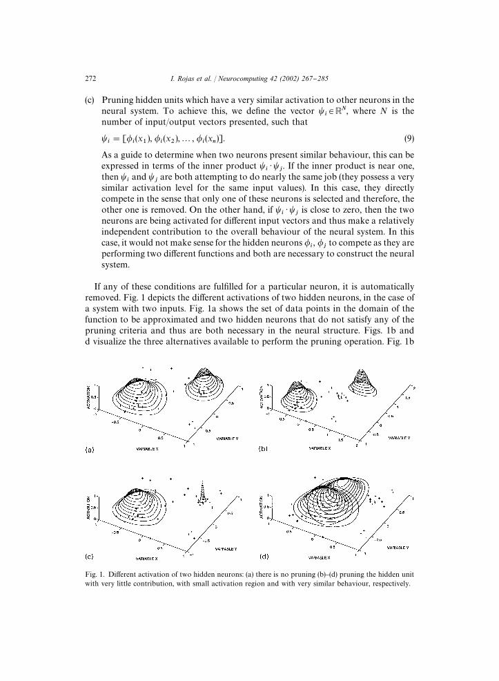
Fig. 1. Di!erent activation of two hidden neurons: (a) there is no pruning (b)}(d) pruning the hidden unitwith very little contribution, with small activation region and with very similar behaviour, respectively.

(c) Pruning hidden units which have a very similar activation to other neurons in theneural system. To achieve this, we de"ne the vector �

�3�, where N is the

number of input/output vectors presented, such that

��"[�

�(x

�), �

�(x

),2, �

�(x

�)]. (9)

As a guide to determine when two neurons present similar behaviour, this can beexpressed in terms of the inner product �

�) �

�. If the inner product is near one,

then ��and �

�are both attempting to do nearly the same job (they possess a very

similar activation level for the same input values). In this case, they directlycompete in the sense that only one of these neurons is selected and therefore, theother one is removed. On the other hand, if �

�) �

�is close to zero, then the two

neurons are being activated for di!erent input vectors and thus make a relativelyindependent contribution to the overall behaviour of the neural system. In thiscase, it would not make sense for the hidden neurons �

�, �

�to compete as they are

performing two di!erent functions and both are necessary to construct the neuralsystem.

If any of these conditions are ful"lled for a particular neuron, it is automaticallyremoved. Fig. 1 depicts the di!erent activations of two hidden neurons, in the case ofa system with two inputs. Fig. 1a shows the set of data points in the domain of thefunction to be approximated and two hidden neurons that do not satisfy any of thepruning criteria and thus are both necessary in the neural structure. Figs. 1b andd visualize the three alternatives available to perform the pruning operation. Fig. 1b

272 I. Rojas et al. / Neurocomputing 42 (2002) 267}285

shows a hidden unit that makes very little contribution to the overall network as thedata vectors are very scarce in the domain in which this neuron is de"ned. In Fig. 1cone hidden unit has a very small activation region and therefore is removed. Fig. 1drepresents an example in which the inner product of two hidden neurons is high, andtherefore one of them is removed because they are attempting to do nearly the sametask in the neural system. The "nal algorithm is summarized below:Step 1: Initially, no hidden neuron exists.Step 2: Set n"0,K"0, h"1, where n,K and h are the number of patterns

presented to the network, the number of hidden neurons and the number of learningcycles, respectively. Set the e!ective radius � Set the maximum number of hiddenneurons MaxNeuron.Step 3: For each observation (x

�, y

�) compute:

(a) The overall network output:

FI H���

(x�)"

�����

w���(x

�, c

�, �

�)

�����

��(x

�, c

�, �

�)

"

Num

Den. (10)

(b) The parameter required for the evaluation of the novelty of the observation; theerror e

�"�y

�!FI H

���� and the maximum degree of activation �

���.

If ((e�'�) and (�

���(�) and K(MaxNeuron) allocate a new hidden unit:

K"K#1,

b��

"�y�!FI H

���if v"0

0 otherwise,

(11)

c�

"x�(c�

�"x�

�) ∀v3[1, D],

����

"�����

"�����

Min���� ����

�x�!c

��.

Else, apply the parameter learning for all the hidden nodes:

c��"!

�E

�c��

"!

�E

�FI H���

�FI H���

���

���

�c��

"(y�!FI H

���)w�!y

�Den �2

x��!c�

������

e�������

�� �������;(x�

�;!R, c�

�)

#2x��!c�

�����

e�������

�� ������;(x�

�; c�

�, R)�, (12)

����

"!

�E

�����

"!

�E

�FI H���

�FI H���

���

���

�����

"(y�!FI H

���)w

�!y

�Den �2�

x��!c�

�����

�e����

����� ���

��;(x��; c�

�, R)�, (13)

I. Rojas et al. / Neurocomputing 42 (2002) 267}285 273

�����

"(y�!FI H

���)w

�!y

�Den �2�

x��!c�

������

�e����

����� ���

���;(x��;!R, c�

�)�,

b��"!

�E

�b��

"!

�E

�FI H���

�FI H���

�Num

�NM�w

�

�w�

�b��

"(y�!FI H

���)

1

Den�

�(x

�)x�

�,

b��"!

�E

�b��

"!

�E

�FI H���

�FI H���

�Num

�NM�w

�

�w�

�b��

"(y�!FI H

���)

1

Den��(x

�).

(14)

Step 4: If all the training patterns are presented, then increment the number oflearning cycles (h"h#1), and check the criteria for pruning hidden units:

�"�

����

��(x

�)�(�

�,

��

(����

#�����

)(�, (15)

��) �

�(�

�, ∀jOi.

Step 5: If the network shows satisfactory performance (NRMSE(�*) then stop.Otherwise go to Step 3.

4. Simulation results

Mathematically, predicting the future of time series involves "nding some nonlinearmapping MI with several parameters such as

x( (t#P)"MI �x(t), x(t!�),2, x(t!(n!1)�)�, (16)

where � is a lag time and n is an embedding dimension. The equation implies that anestimate x( at the time (t) ahead of P can be obtained from the unknown mappingMI with a proper combination of n points of the time series spaced � apart.

In this subsection we attempt a short-term prediction by means of the algorithmpresented in the above subsection with regard to the Mackey}Glass time series dataand the Lorenz attractor time series.

4.1. Application to Mackey}Glass time series

The chaotic Mackey}Glass di!erential delay equation is recognized as a bench-mark problem that has been used and reported by a number of researchers forcomparing the learning and generalization ability of di!erent neural architectures[19], fuzzy systems and genetic algorithms [18]. The Mackey}Glass chaotic timeseries is generated from the following delay di!erential equation:

dx(t)

dt"

ax(t!�)1#x��(t!�)

!bx(t). (17)

274 I. Rojas et al. / Neurocomputing 42 (2002) 267}285

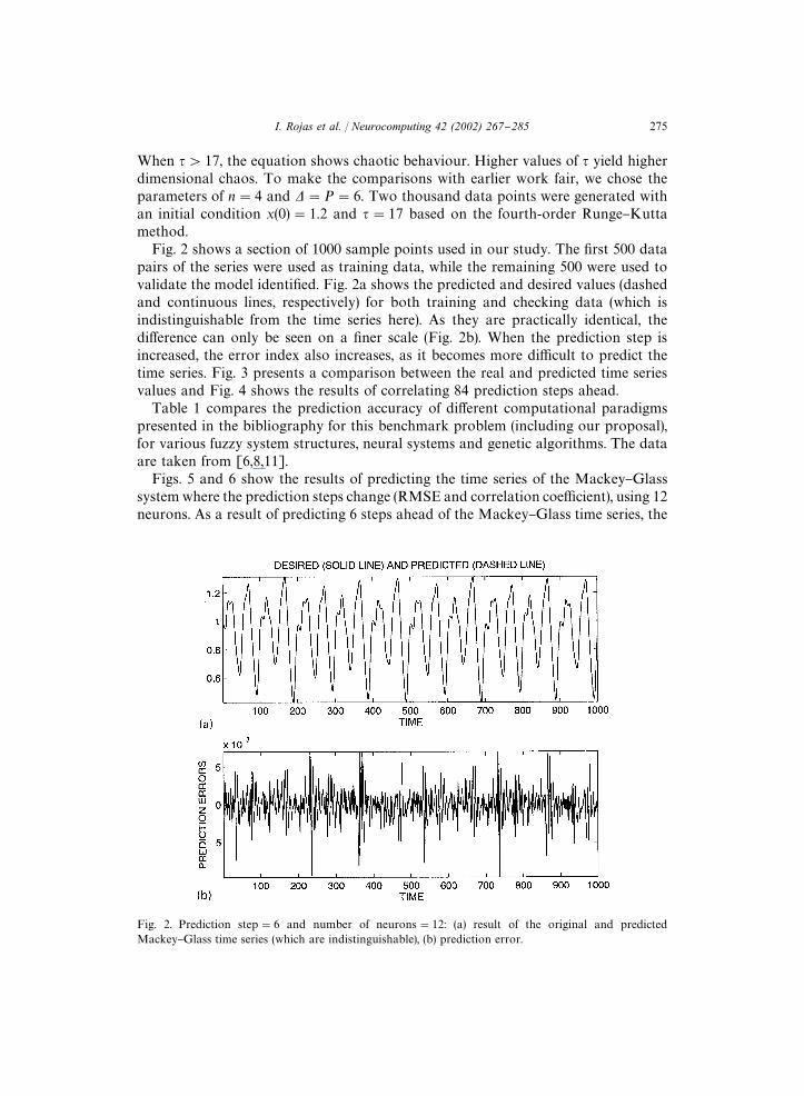
Fig. 2. Prediction step"6 and number of neurons"12: (a) result of the original and predictedMackey}Glass time series (which are indistinguishable), (b) prediction error.

When �'17, the equation shows chaotic behaviour. Higher values of � yield higherdimensional chaos. To make the comparisons with earlier work fair, we chose theparameters of n"4 and �"P"6. Two thousand data points were generated withan initial condition x(0)"1.2 and �"17 based on the fourth-order Runge}Kuttamethod.

Fig. 2 shows a section of 1000 sample points used in our study. The "rst 500 datapairs of the series were used as training data, while the remaining 500 were used tovalidate the model identi"ed. Fig. 2a shows the predicted and desired values (dashedand continuous lines, respectively) for both training and checking data (which isindistinguishable from the time series here). As they are practically identical, thedi!erence can only be seen on a "ner scale (Fig. 2b). When the prediction step isincreased, the error index also increases, as it becomes more di$cult to predict thetime series. Fig. 3 presents a comparison between the real and predicted time seriesvalues and Fig. 4 shows the results of correlating 84 prediction steps ahead.

Table 1 compares the prediction accuracy of di!erent computational paradigmspresented in the bibliography for this benchmark problem (including our proposal),for various fuzzy system structures, neural systems and genetic algorithms. The dataare taken from [6,8,11].

Figs. 5 and 6 show the results of predicting the time series of the Mackey}Glasssystemwhere the prediction steps change (RMSE and correlation coe$cient), using 12neurons. As a result of predicting 6 steps ahead of the Mackey}Glass time series, the

I. Rojas et al. / Neurocomputing 42 (2002) 267}285 275

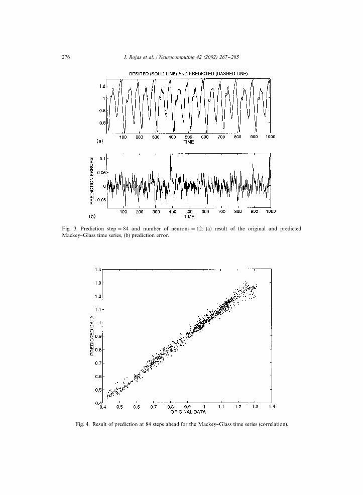
Fig. 3. Prediction step"84 and number of neurons"12: (a) result of the original and predictedMackey}Glass time series, (b) prediction error.

Fig. 4. Result of prediction at 84 steps ahead for the Mackey}Glass time series (correlation).

276 I. Rojas et al. / Neurocomputing 42 (2002) 267}285

Table 1Comparison results of the prediction error of di!erent methods for prediction step equal to 6 (500 trainingdata)

Method Prediction error (RMSE)

Auto-regressive model 0.19Cascade correlation NN 0.06Back-Prop. NN 0.02Sixth-order polynomial 0.04Linear predictive method 0.55Kim and Kim (Genetic Algorithm and Fuzzy System) [8] 5 MFs 0.049206

7 MFs 0.0422759 MFs 0.037873

ANFIS and Fuzzy System (16 rules) [6] 0.007Wang et al.[18] Product T-norm 0.0907

Min T-norm 0.0904Classical RBF (with 23 neurons) [3] 0.0114Our approach (with 12 neurons) 0.00287

Fig. 5. Result of prediction of Mackey}Glass time series (change of RMSE by prediction step).

root mean square error and the correlation coe$cient are 0.0029 and 0.9999, and for84 steps ahead these parameters are 0.0263 and 0.9876, respectively. Fig. 7 presents therelation between the error index and the maximum number of neurons the neuralsystem may possess. As expected, the greater the complexity of the neural system, thelower the error index for the training and test data.

I. Rojas et al. / Neurocomputing 42 (2002) 267}285 277

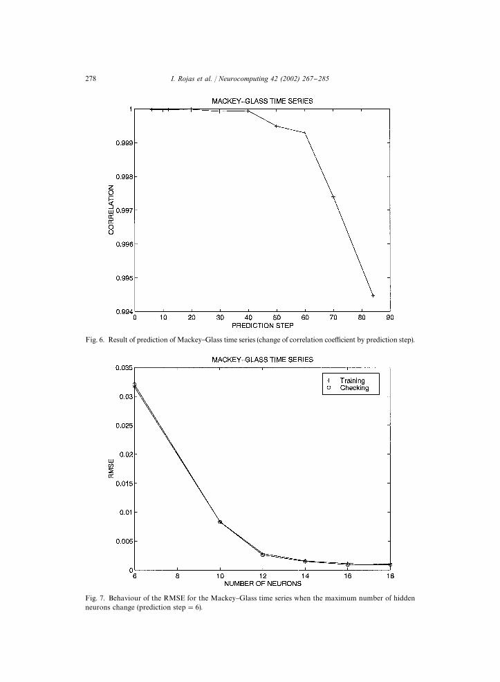
Fig. 6. Result of prediction of Mackey}Glass time series (change of correlation coe$cient by prediction step).

Fig. 7. Behaviour of the RMSE for the Mackey}Glass time series when the maximum number of hiddenneurons change (prediction step"6).

278 I. Rojas et al. / Neurocomputing 42 (2002) 267}285

Fig. 8. The characterization of the Lorenz time series: (a) histogram; (b) the phase diagram.

4.2. Lorenz attractor

The Lorenz attractor time series was generated by solving the Lorenz equations:

dx�(t)

dt"�(x

(t)!x

�(t)),

dx(t)

dt"� ) x

�(t)!x

(t)!x

�(t)x

�(t),

(18)

I. Rojas et al. / Neurocomputing 42 (2002) 267}285 279

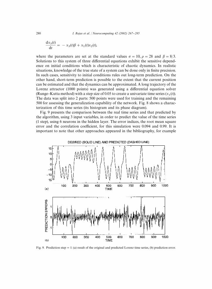
Fig. 9. Prediction step"1: (a) result of the original and predicted Lorenz time series, (b) prediction error.

dx�(t)

dt"!x

�(t)�#x

�(t)x

(t),

where the parameters are set at the standard values �"10, �"28 and �"8/3.Solutions to this system of three di!erential equations exhibit the sensitive depend-ence on initial conditions which is characteristic of chaotic dynamics. In realisticsituations, knowledge of the true state of a system can be done only in "nite precision.In such cases, sensitivity to initial conditions rules out long-term prediction. On theother hand, short-term prediction is possible to the extent that the current positioncan be estimated and that the dynamics can be approximated. A long trajectory of theLorenz attractor (1000 points) was generated using a di!erential equation solver(Runge}Kuttamethod) with a step size of 0.05 to create a univariate time series (x

�(t)).

The data was split into 2 parts: 500 points were used for training and the remaining500 for assessing the generalization capability of the network. Fig. 8 shows a charac-terization of this time series (its histogram and its phase diagram).

Fig. 9 presents the comparison between the real time series and that predicted bythe algorithm, using 3 input variables, in order to predict the value of the time series(1 step), using 6 neurons in the hidden layer. The error indices, the root mean squareerror and the correlation coe$cient, for this simulation were 0.094 and 0.99. It isimportant to note that other approaches appeared in the bibliography, for example

280 I. Rojas et al. / Neurocomputing 42 (2002) 267}285

Fig. 10. Result of prediction of Lorenz time series (change of RMSE by prediction step).

Iokibe et al. [5] obtained an RMSE of 0.244, Jang et al. [6] an RMSE of 0.143, usingfuzzy and neuro-fuzzy systems. Figs. 10 and 11 show the results of predicting theLorenz time series where the prediction step changes (RMSE and correlation coe$c-ient), using 6 neurons, while Fig. 12 shows the evolution of the RMSE when thenumber of neurons in the hidden layer changes, using a more complicated predictionstep equal to 6.

5. Conclusions

This article describes a new structure to create an RBF neural network; this newstructure has 4 main characteristics: "rstly, the special RBF network architecture usesregression weights to replace the constant weights normally used. These regressionweights are assumed to be functions of input variables. In this way the number ofhidden units within an RBF neural network is reduced. The second characteristic isthe normalization of the activation of the hidden neurons (weighted average) beforeaggregating the activations, which, as observed by various authors, produces betterresults than the classical weighted sum architecture. As a result, the output activitybecomes an activity-weighted average of the input weights in which the weights fromthe most active inputs contribute most to the value of the output activity.

I. Rojas et al. / Neurocomputing 42 (2002) 267}285 281

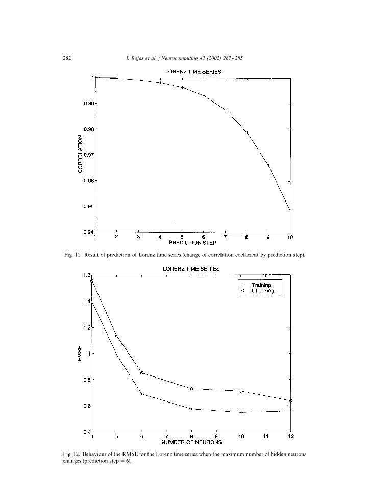
Fig. 11. Result of prediction of Lorenz time series (change of correlation coe$cient by prediction step).

Fig. 12. Behaviour of the RMSE for the Lorenz time series when the maximum number of hidden neuronschanges (prediction step"6).

282 I. Rojas et al. / Neurocomputing 42 (2002) 267}285

The third aspect is that a new type of nonlinear function is proposed: the pseudo-Gaussian function. With this, the neural system gains #exibility, as the neuronspossess an activation "eld that does not necessarily have to be symmetric with respectto the centre or to the location of the neuron in the input space. In addition to this newstructure, we propose, as the fourth and "nal feature, a sequential learning algorithm,which is able to adapt the structure of the network; with this, it is possible to createnew hidden units and also to detect and remove inactive units. We have presentedconditions to increase or decrease the number of neurons, based on the novelty of thedata and on the overall behaviour of the neural system, respectively. The feasibility ofthe evolution and learning capability of the resulting algorithm for the neural networkis demonstrated by predicting time series.

Acknowledgements

This work has been partially supported by the CICYT Spanish Project TAP97-1166 and TIC2000-1348.

References

[1] F. Anouar, F. Badran, S. Thiria, Probabilistic self-organizing maps and radial basis functionnetworks, Neurocomputing 20 (1998) 83}96.

[2] M. Benaim, On functional approximation with normalized Gaussian units, Neural Comput. 6 (2)(1994) 319}333.

[3] K.B. Cho, B.H.Wang, Radial basis function based adaptive fuzzy systems their applications to systemidenti"cation and prediction, Fuzzy Sets and Systems 83 (1995) 325}339.

[4] S. Haykin, Neural Networks*A Comprehensive Foundation, IEEE Press, New York, 1994.[5] T. Iokibe, Y. Fujimoto, M. Kanke, S. Suzuki, Short-term prediction of chaotic time series by local

fuzzy reconstruction method, J. Intelligent Fuzzy Systems 5 (1997) 3}21.[6] J.S.R. Jang, C.T. Sun, E. Mizutani, Neuro-Fuzzy and Soft Computing, Prentice}Hall, Englewood

cli!s, NJ, ISBN 0-13-261066-3, 1997.[7] N.B. Karayiannis, G. Weiqun Mi, Growing radial basis neural networks: merging supervised

and unsupervised learning with network growth techniques, IEEE Trans. Neural Networks 8(6)(November 1997) 1492}1506.

[8] D. Kim, C. Kim, Forecasting time series with genetic fuzzy predictor ensemble, IEEE Trans. FuzzySystems 5 (4) (November 1997) 523}535.

[9] T. Kohonen, Self-Organization and Associative Memory, Springer, New York, 1988.[10] S. Lee, R.M. Kil, A Gaussian potential function network with hierarchically self-organizing learning,

Neural Network 2 (1991) 207}224.[11] S.-H. Lee, I. Kim, Time series analysis using fuzzy learning, Proceedings of International Conference

on Neural Information Processing, Vol. 6, Seoul, Korea, October 1994, pp. 1577}1582.[12] J.E. Moody, C.J. Darke, Fast learning in networks of locally-tuned processing units, Neural Comput.

1 (1989) 281}294.[13] M.T. Musavi, W. Ahmed, K.H. Chan, K.B. Faris, D.M. Hummels, On the training of radial basis

function classi"er, Neural Networks 5 (1992) 595}603.[14] S. Nowlan,Maximum likelihood competitive learning, in: D. Touretzky (Ed.), Neural Inform. Process.

Systems 2 (Morgan Kaufmann) (1990) 574}582.[15] J. Platt, A resource allocating network for function interpolation, Neural Comput. 3 (1991) 213}225.

I. Rojas et al. / Neurocomputing 42 (2002) 267}285 283

[16] I. Rojas, M. Anguita, E. Ros, H. Pomares, O. Valenzuela, A. Prieto, What are the main factorsinvolved in the design of a Radial Basis Function Network?, sixth European Symposium on Arti"cialNeural Network, ESANN'98, April 22}24, 1998, pp. 1}6.

[17] A. Sherstinsky, R.W. Picard, On the e$ciency of the orthogonal least squares training method forradial basis function networks, IEEE Trans. Neural Networks 7 (1) (1996) 195}200.

[18] L.X. Wang, J.M. Mendel, Generating fuzzy rules by learning from examples, IEEE Trans. SystemsMan Cybernet, 22 (6) (November/December 1992) 1414}1427.

[19] B.A. Whitehead, Tinothy. D. Choate, Cooperative-competitive genetic evolution of radial basisfunction centers and widths for time series prediction, IEEE Trans. Neural Networks 7 (4) (July, 1996)869}880.

[20] L. Yingwei, N. Sundarajan, P. Saratchandran, performance evaluation of a sequential minimal radialbasis function (RBF) neural network learning algorithm, IEEE Trans. Neural Networks 9 (2) (March1998) 308}318.

Ignacio Rojas received his M.S. in Physics and Electronics from the University ofGranada in 1992 and his Ph.D. degree, in the "eld of Neuro-Fuzzy in 1996. During1998, he was visiting professor of the BISC at the University of California,Berkeley. He is a teaching assistant at the Department of Architecture andComputer Technology. His main research interests are in the "elds of hybridsystem and a combination of fuzzy logic, genetic algorithms and neural networks,"nancial forecasting and "nancial analysis.

Hector Pomares received his M.S. in Electronics Engineering from the Universityof Granada in 1995 and his M.S. in Physics and Electronics degree in 1997. Atpresent, he is a Fellowship holder and Doctorate student within the Department ofArchitecture and Computer Technology. His current areas of research interest arein the "elds of fuzzy approximation, neural networks and genetic algorithms, andRadial Basis Function design.

Jose Luis Bernier received the Ph.D. degree in Physics (majoring in Electronics),from the University of Granada in 1999. He has taken part in the Group's researchprogramme since 1992. His main interests are related with analog testing, arti"cialneural networks and optimisation algorithms.

284 I. Rojas et al. / Neurocomputing 42 (2002) 267}285

Julio Ortega received the B.Sc. degree in electronic physics in 1985, the M.Sc.degree in electronics in 1986, and the Ph.D. degree in 1990, all from the Universityof Granada, Spain. In March, 1988, he was at the Open University (UK) as aninvited researcher by Professor S.L. Hurst. Currently, he is an Assistant Professorin the Department of Architecture and Computer Technology at the University ofGranada. His research interest lies in the "elds of arti"cial neural networks,parallel computer architecture, forecasting analysis and Intelligent data analysis.

Begon� a del Pino is an assistant professor at the University of Granada. She teachescourses in technology of computers and design of microelectronic circuits. Hercurrent research interests include VLSI implementation of neuro-fuzzy systemsand hardware/software codesign of embedded systems. She holds a Ph.D. incomputer science from the University of Granada.

Francisco J. Pelayo, born in Granada, Spain, in 1960, received the B.Sc. degree inElectronic Physics in 1982, the M.Sc. degree in Electronics in 1983, and the Ph.D.degree in 1989, all from the University of Granada. He is currently an AssociateProfessor in the Department of Computer Architecture and Technology(http://atc.ugr.es) at that University. He has worked in the areas of multivaluedlogic, VLSI design and test, arti"cial neural networks and fuzzy systems. Hiscurrent research interest lies in the "elds of VLSI design, bio-inspired processingsystems, and fuzzy and neuro-fuzzy modeling and control.

Alberto Prieto received a B.Sc. degree in Electronic Physics in 1968 from theComplutense University (Madrid) and Ph.D. degree from the University ofGranada, Spain, in 1976. From 1971 to 1984 he was the Director of the ComputerCentre and from 1985 to 1990 Dean of the Computer Science and Technologystudies of the Univ. of Granada. Between June and August 1991, he was at theT.I.R.F. Laboratory, Institute National Polythechnique of Grenoble, as a guestresearcher of Profs. J. Herault and C. Jutten. During 1991}1992, jointly with Prof.P. Treleaven, he was main researcher of a Spanish-British Integrated Action onArti"cial Neural Networks, held between Unv. of Granada and the UniversityCollege of London. He is currently a Full Professor in the Dept. of Architectureand Computer Technology. His research interests are in the areas of arti"cialneural networks, fuzzy systems, expert systems andmicroprocessor-based systems.

He is a member of INNS, AEIA, AFCET, IEEEE and ACM, and Chairman of the Spanish RegionalInterest Group of the IEEE Neural Network Council.

I. Rojas et al. / Neurocomputing 42 (2002) 267}285 285