Optimization of Vehicle Routing for Waste Collection ... - MDPI

International Journal of

Environmental Research

and Public Health

Article

Optimization of Vehicle Routing for Waste Collectionand Transportation

Hailin Wu 1, Fengming Tao 2,* and Bo Yang 3

1 College of Mechanical Engineering, Chongqing University, Chongqing 400044, China;[email protected]

2 School of Management Science and Real Estate, Chongqing University, Chongqing 400044, China3 College of Management, Chongqing Radio and Television University, Chongqing 400044, China;

[email protected]* Correspondence: [email protected]; Tel.: +86-185-8070-7012

Received: 28 May 2020; Accepted: 2 July 2020; Published: 9 July 2020��

Abstract: For the sake of solving the optimization problem of urban waste collection and transportationin China, a priority considered green vehicle routing problem (PCGVRP) model in a waste managementsystem is constructed in this paper, and specific algorithms are designed to solve the model. Wepay particular concern to the possibility of immediate waste collection services for high-prioritywaste bins, e.g., those containing hospital or medical waste, because the harmful waste needs tobe collected immediately. Otherwise, these may cause dangerous or negative effects. From theperspective of environmental protection, the proposed PCGVRP model considers both greenhousegas (GHG) emission costs and conventional waste management costs. Waste filling level (WFL) isconsidered with the deployment of sensors on waste bins to realize dynamic routes instead of fixedroutes, so that the economy and efficiency of waste collection and transportation can be improved.The optimal solution is obtained by a local search hybrid algorithm (LSHA), that is, the initial optimalsolution is obtained by particle swarm optimization (PSO) and then a local search is performed onthe initial optimal solution, which will be optimized by a simulated annealing (SA) algorithm byvirtue of the global search capability. Several instances are selected from the database of capacitatedvehicle routing problem (CVRP) so as to test and verify the effectiveness of the proposed LSHAalgorithm. In addition, to obtain credible results and conclusions, a case using data about wastecollection and transportation is employed to verify the PCGVRP model, and the effectiveness andpracticability of the model was tested by setting a series of values of bins’ number with high priorityand WFLs. The results show that (1) the proposed model can achieve a 42.3% reduction of negativeeffect compared with the traditional one; (2) a certain value of WFL between 60% and 80% can realizehigh efficiency of the waste collection and transportation; and (3) the best specific value of WFL isdetermined by the number of waste bins with high priority. Finally, some constructive propositionsare put forward for the Environmental Protection Administration and waste management institutionsbased on these conclusions.

Keywords: waste collection and transportation; vehicle routing problem; waste bins with highpriority; greenhouse gas emissions; waste filling level

1. Introduction

Municipal solid waste (MSW) management is regarded as a challenging matter for contemporarycities [1,2] due to quick growth in the amount of waste, high waste collection costs [3], limited treatmentcapacities [4] and environmental problems [5]. In China, as the economy grows rapidly, the quantityof MSW has been growing significantly and the mean rate of growth has been around 3.5% [6].

Int. J. Environ. Res. Public Health 2020, 17, 4963; doi:10.3390/ijerph17144963 www.mdpi.com/journal/ijerph

http://www.mdpi.com/journal/ijerph

http://www.mdpi.com

http://dx.doi.org/10.3390/ijerph17144963

http://www.mdpi.com/journal/ijerph

https://www.mdpi.com/1660-4601/17/14/4963?type=check_update&version=2

Int. J. Environ. Res. Public Health 2020, 17, 4963 2 of 26

There are several factors contributing to this social phenomenon such as urbanization [7], boomingof population [7], and improvements of living standard [7], among others. Under such intricatecircumstances, the application of operational research methods can make decision-makers benefit fromprogramming [8].

MSW activities are grouped in five stages of waste life-cycle: generation, collection andtransportation, transformation, treatment and final disposal [8,9]. The cost of waste collectionand transportation accounts for 60–80% of total Waste Management System (WMS) costs, which isthe critical factor in the fiscal spending of WMS, improvements in this field will play a significantrole in saving municipal expenditure [10,11]. Thus, this article focuses on operational decisions atthe second stage, collection and transportation. Waste collection refers to the use of waste collectionvehicles to load waste from waste collection points. Waste transportation means the activity of takingthe collected waste to the disposal center [12].

Moreover, some peculiar kinds of waste are supposed to be collected and transported with theleast delay possible, because of their passive impact on people’s health, such as chemical waste,hospital waste, electronic waste (E-waste) [10] and waste close to gas stations and fuel stations [13]etc. In particular, during the global pandemic of COVID-19, the importance and necessity of givingpriority to medical waste disposal are highlighted. Bins containing such waste should be collected assoon as possible to minimize the negative impact on the environment and human lives. In this regard,it is important to give high collection priority to such waste bins with negative effect, which will betaken into consideration as one of the critical factors in the proposed priority considered green vehiclerouting problem (PCGVRP) model and solutions.

As a rule, the activity of waste collection and transportation is carried out by means of a fleetof vehicles aiming at emptying waste bins on the basis of predefined schedules [7,14,15]. However,this conventional waste collection is based on a lot of speculation about whether the filling levels ofwaste bins could vary from overflowing, partial filling, to completely emptying, which would lead tounnecessary resources consumption [16]. For these reasons, wireless sensor networks (WSN) havebeen deployed in MSW to achieve remote monitoring filling levels of waste bins [17]. In the meantime,waste collection trucks can communicate with waste bins with sensors by the Internet of things systemto acquire the data about the status of bins [18–20].

Lastly, it is worthy of mention that the growth of waste is closely related to environmentaldeterioration [7], which is because that the activity of waste collection and transportation consumes a lotof fuel resulting in GHG emissions [7,21–23].Therefore, taking into account its effect on the environment,sustainable management of waste collection and transportation with the objective of minimizing GHGemissions is indispensable both for resource savings and environmental conservation [24].

Due to the increasing amount of waste and the increasing difficulty of SWM, many areas haveestablished laws on waste collection and transportation, including all kinds of waste such as hazardouswaste [25], chemical waste [26], E-waste [27], roundwood waste [28], construction waste [29], andso on. In particular, there has been an increase in laws and regulations on hazardous waste andE-waste collection [30,31] over the past two decades, for their particularity and harmfulness. Generallyspeaking, the purpose of this legislation is to reduce its impact on the environment. Therefore, wecan see that waste collection and transportation has been paid increasing attention in legislation andby citizens.

This paper concentrates on collecting waste from waste bins and transporting them to wastedisposal centers. More specifically, we propose a waste collection and transportation model thatgives high collection priority to specific waste. We replace conventional fixed routes with dynamicsystems that respond to the actual filling levels of sensor-based waste bins. This allows us to reduce theprobability of collecting overflowing or empty waste bins. In the meantime, we consider the reductionof GHG emissions in the model and, accordingly, design a better and greener PCGVRP model. To sumup, this paper aims to reduce the cost, GHG emissions and negative impact of waste in the process of


waste collection and transportation. The novelty lies in the consideration of the collection priority ofdifferent waste and the application of sensor-based waste bins.

2. Literature Review

2.1. Research about Waste Collection and Transportation

A vehicle routing problem (VRP) is about the route optimization problem introduced by Dantzigand Ramser [32] and was applied in the field of waste collection and transportation by Beltramiand Bodin [33]. Vu et al. [34] studied route optimization of waste collection and transportation andfound that travel distance was the main research factor. Rızvanoglu et al., used linear programmingand geographic information system analysis to determine the beat routes of waste collection andtransportation and concluded with better linear programming. Yadava and Karmakarb [35] proposedplausible mathematical and computational modeling approached for sustainable collection andtransportation of municipal solid waste. Miranda et al. [36] developed and implied a mixed integerlinear optimization model for a waste collection system for serving a rural archipelago. Zhao et al. [37]studied the location and routes problem for hazardous waste with the objective of minimizing costand risk.

The traditional method of waste collection and transportation refers to taking all the waste binsand transport waste to the disposal station by trucks along the settled routes [38]. This process involveslabor costs, fuel costs, maintenance costs, etc., so the cost is very high, accounting for most of the SWMspending [38]. For these reasons, a lot of research proposed an approach to collect waste according tothe filling levels of waste bins, which are predicted based on either historical data [7,17,39] or sensorydata [18,38] obtained from waste bins and trucks [38]. Abdallah et al. [38] developed a selectionprocedure for waste bins to be collected, which have high filling levels based on historical data. Mamunet al. [17] presented a waste bin monitoring system, which is supported by a sensor technology andinteraction system and the experimental results showed that the system can assist in an optimizationmodel for route optimization.

Taking into account the impact on the environment of logistics, waste collection and transportationhas gained greater attention in recent years. Leggieria and Haouari [40] established a model of GreenVRP considering environmental issues and exact approach was proposed to solve it. Herdari et. al [41]took GHG emissions of vehicles into account which was calculated by the flow of WSM and emissioncoefficient. Mohsenizadeh et al. [24] developed a bi-objective model to investigate the impact of CO2

emissions from transportation activities of MSW. Reddy et al. [42] proposed a model to decide facilitylocations and vehicle routes while accounting for carbon footprint.

It can be seen from the above that there is a wealth of research about waste collection andtransportation and some design routes according to filling levels of waste bins from historical data orsensors with environmental concerns. However, the impact of different filling levels of sensor-basedbins including costs, collected waste percentage and so on has been rarely considered especiallywhen taking waste priority into account. Furthermore, it is important to plan the optimal route forhigh-priority waste because of its negative effect, which has been rarely studied.

2.2. Research about Priority in a Vehicle Routing Problem (VRP)

Nesmachnow et al. [8] built a waste collection model considering priorities with two objectives,the shortest distance and the best service respectively. Anagnostopoulos et al. [13] developed andcompared four models for waste collection and transportation considering waste bins with highpriority and found that different models are applicable to different situations. Tirkolaee et al. [10] builta model of waste collection and transportation, and gave the collection priority, which was realizedby time windows, to some designated sites, including medical centers, hospitals and chemical plantsthat might generate harmful waste that needs to be collected as soon as possible. Armas et al. [43]built a rich VRP model taking the customer priority into account for a trucking enterprise in Spain


and which is solved by a heuristic algorithm. Molina et al. [44] proposed a comprehensive modelwith the definition of different service priorities so as to cope with orders of high priorities as much aspossible. Wang et al. [45] integrated customer service priority into the dynamic programming approachto optimize vehicle routes by order preference by similarity to ideal solution (TOPSIS).

From the above studies, we can see priority has been considered in some areas, including customerservice, waste management and so on. Therefore, it is necessary to give thought to priority in theprocess of waste collection and transportation. However, few articles take consideration of the negativeeffects of delayed waste collection.

2.3. Research about Algorithms

VRP has been extensively and deeply studied ever since the 1960s, and a series of solving methodshave emerged, including the exact method, heuristic method and meta-heuristic method [43]. Owingto the complexity of VRPs, it is not efficient to solve it with exact methods [46]. Hence, the research onheuristic method and meta-heuristic method is increasingly rich [43].

Along with the discrete particle swarm optimization (PSO), Rau et al. [47] developed aheuristic method to improve the solution quality of PSO particle to solve a multi-objective problem.Tirkolaee et al. [10] solved a vehicle routing problem with time window (VRPTW) of wastecollection by a simulated annealing algorithm. Tirkolaee et al. [11] designed an improved antcolony algorithm for the proposed model of a capacitated arc routing problem (CARP). Wichapaand Khokhajaikia [48] designed hybrid genetic algorithm (HGA) to solve VRP for infectious wastetransportation. Delgado-Antequera et al. [34] proposed an integrated greedy algorithm coupledwith a variable neighborhood search for a multi-objective routing problem for waste collectionand transportation.

To sum up, there are lots of research of algorithms to solve the waste collection problem.Nevertheless, they are mostly single algorithms instead of hybrid algorithms that can make the best ofboth worlds. The algorithm involved in this paper combines the high efficiency of PSO and the globaloptimization capability of simulated annealing (SA) performing better than a single algorithm. Withthe consideration of the main characteristics and gaps of the research literature, the paper proposedan integrated model considering priority and GHG emissions based on waste filling-level data fromsensors for waste collection and transportation, and a hybrid algorithm is designed to solve the model.

3. Model Formulation

3.1. Problem Description

The problem involves obtaining the optimal paths of each vehicle with the objective of minimizingthe total distance, total GHG emissions, total comprehensive costs including vehicle costs and GHGemissions costs. Waste bins located in specific areas (e.g., hospital, fuel station, gas station) arecharacterized as high priority bins which should be collected as soon as possible. The vehicles arelocated at the disposal center and start their trips toward the allocated waste bins. When the wastecollection vehicle is fully loaded or the collection task is completed, it must get back to the disposalcenter so as to upload the collected waste.

Apart from the above description we make following assumptions:

• Each waste bin is only collected by one vehicle once.• There is one disposal center.• The vehicles must depart from the disposal center and go back to the disposal center when the

task ends.• There is single type of waste collection vehicle.• The location of the disposal center and each waste bin are known.

The problem formulation considers the following elements:


• Each bin, B = {b1, b2, · · · bn}, has a collection priority, which is determined in accordance with thepassive influence of waste.

• A set of vehicles V = {v1, v2 · · · vm} to collect waste, with a maximum capacity.• A disposal center D where vehicles star and end their trips.• A set of waste bin filling level L = {l1, l2 · · · ln}, for ∀ i ∈ {1, 2, · · · , n}, li ∈ [0, 1], where li indicates

the percentage of waste bin bi filled by waste.

3.2. Notation

The notations and descriptions are shown in Table 1.

Table 1. Notation of the priority considered green vehicle routing problem (PCGVRP) model.

Sets Unit Description

B Set of waste bins (B = b1, b2, · · · , bi, · · · , bn)D Waste disposal centerV Set of vehicles (V = v1, v2, · · · , vk, · · · , vK)Cp kg Maximum load capacity of vehicle

T_D km Total distance of all vehiclesT_EGHG kg Total GHG emissions of all vehicles

T_C CNY Total cost of all vehiclesε CNY/kg Cost of greenhouse gas (GHG) emissions per unite kg CO2e/L Emission coefficientr L/km Fuel consumption rate per unit distancer0 L/km Fuel consumption rate per unit distance while vehicle is emptyr∗ L/km Fuel consumption rate per unit distance while vehicle is at full load

r(Q) L/km Fuel consumption rate per unit distance with load of Q

ri j L/km Fuel consumption rate per unit distance while vehicle goes fromwaste bin i to j

EGHG kg GHG emissionsq j kg Collected waste at waste bin jdi j km Distance between waste bin i and jtki s Time of vehicle k arriving at waste bin iλi If waste bin i has a high priority, λi = 1. Otherwise, λi = 0

P f ixed CNY Fixed cost of each vehicleP f uel CNY/kg Price of fuel consumption

Variablexk

i j Whether a vehicle k goes from waste bin i to j

3.3. Analysis of Objective Function

The PCGVRP model of waste collection and transportation in this paper considers three kinds ofobjectives: minimize total distance (T_D), minimize total GHG emissions (T_EGHG) and total costs(T_C) including vehicles costs and GHG emissions costs in this paper. Firstly, we analyze the threeobjective functions respectively and describe them as mathematical expressions. On this basis, thePCGVRP model is further determined by the analysis.

3.3.1. Total Distance

T_D =∑

i∈(B∪D)

∑j∈(B∪D)

xki jdi j (1)

3.3.2. Total Greenhouse Gas (GHG) Emissions

GHG is the emission from fossil fuel consumption in the process of waste collection andtransportation [12] and usually the environmental effect of GHG emissions is approximated by CO2


equivalents (CO2e). Furthermore, GHG emissions show an approximately linear relation to the fuelconsumption of a vehicle [22], we estimate GHG emissions based on fuel consumption and express itseffect in terms of CO2 during waste collection and transportation activities.

According to the analysis of literature [22], considering the linear relationship of load and GHGemissions, the GHG emissions can be expressed as follows:

EGHG(Q) = e ∗ d ∗ r(Q) (2)

The fuel consumption rate (FCR) of the vehicle is linearly related to the vehicle load (Q), whichcan be expressed by the below equation [49]:

r(Q) = r0 +((r∗ − r0)/Cp

)∗Q (3)

Therefore, the FCR when vehicle goes from waste bin bi to b j can be expressed as:

ri j = r0 +((r∗ − r0)/Cp

)∗ (

∑i∈(B∪D)

∑j∈(B∪D)

xki jq j) (4)

In the PCGVRP model, the total GHG emissions can be expressed as:

EGHG = e∑i∈B

∑j∈B

(di j ∗ r0 +((r∗ − r0)/Cp

)∗ (

∑i∈(B∪D)

∑j∈(B∪D)

xki jq j)) (5)

3.3.3. Total Costs

The objectives of minimizing T_D and T_EGHG can only optimize routes either from theenvironmental point or from the economic point. However, the objective of T_C can take theboth into consideration, which includes vehicle costs and GHG emissions costs. Vehicle costs can bedivided into fixed vehicle costs and variable vehicle costs. Fixed costs mean the relatively fixed costin the working process of waste collection vehicles, such as depreciation expenses, all taxes and fees,driver’s salary and so on, which can be calculated as:

C f ixed =∑k∈V

∑j∈(B∪D)

xk0 jP f ixed (6)

Variable costs refer to the cost of fuel from driving between the collection nodes.

C f uel =∑

i∈(B∪D)

∑j∈(B∪D)

xki jdi jri jP f uel (7)

Therefore, vehicle costs can be expressed as follows:

Cvehicle = C f ixed + C f uel =∑k∈V

∑j∈(B∪D)

xk0 jP f ixed +

∑i∈(B∪D)

∑j∈(B∪D)

xki jdi jri jP f uel (8)

GHG emissions can be translated into GHG emissions costs by carbon price. Thus, GHG emissionscosts can be calculated by:

CGHG = εEGHG = εe∑i∈B

∑j∈B

(di j ∗ r0 + ((r∗ − r0)/Cp

)∗ (

∑i∈(B∪D)

∑j∈(B∪D)

xki jq j)) (9)

Total costs can be calculated as:

T_C = Cvehicle + CGHG (10)


3.4. Model Construction

In accordance with the above analysis, the mathematical expressions of the PCGVRP model areas below:

Min T_D =∑

i∈(B∪D)

∑j∈(B∪D)

xki jdi j (11)

Min T_EGHG = e∑i∈B

∑j∈B

(di j ∗ r0 + ((r∗ − r0)/Cp

)∗ (

∑i∈(B∪D)

∑j∈(B∪D)

xki jq j)) (12)

Min T_C =∑

k∈V

∑j∈(B∪D)

xk0 jP f ixed +

∑i∈(B∪D)

∑j∈(B∪D)

xki jdi jri jP f uel

+εe∑i∈B

∑j∈B

(di j ∗ r0 + ((r∗ − r0)/Cp

)∗ (

∑i∈(B∪D)

∑j∈(B∪D)

xki jq j))

(13)

Subject to: ∑k∈V

∑i∈(B∪D)

xki j = 1,∀ j ∈ (B∪ D) (14)

∑k∈V

∑j∈(B∪D)

xki j = 1,∀i ∈ (B∪ D) (15)

∑i∈(B∪D)

xki j =

∑j∈(B∪D)

xki j = 1,∀i ∈ (B∪ D), k ∈ V (16)

∑i∈(B∪D)

∑j∈(B∪D)

xki jq j ≤ Cp,∀ k ∈ V (17)

(λi − λ j)(tki − tk

j) ≤ 0,∀i, j ∈ B, k ∈ V (18)∑i∈(B∪D)

∑j∈(B∪D)

xki j ≤ |S| − 1, S v {1, 2, · · · , N}, S , { },∀ k ∈ V (19)

xki j ∈ {0, 1},∀i, j ∈ (B∪ D), k ∈ V (20)

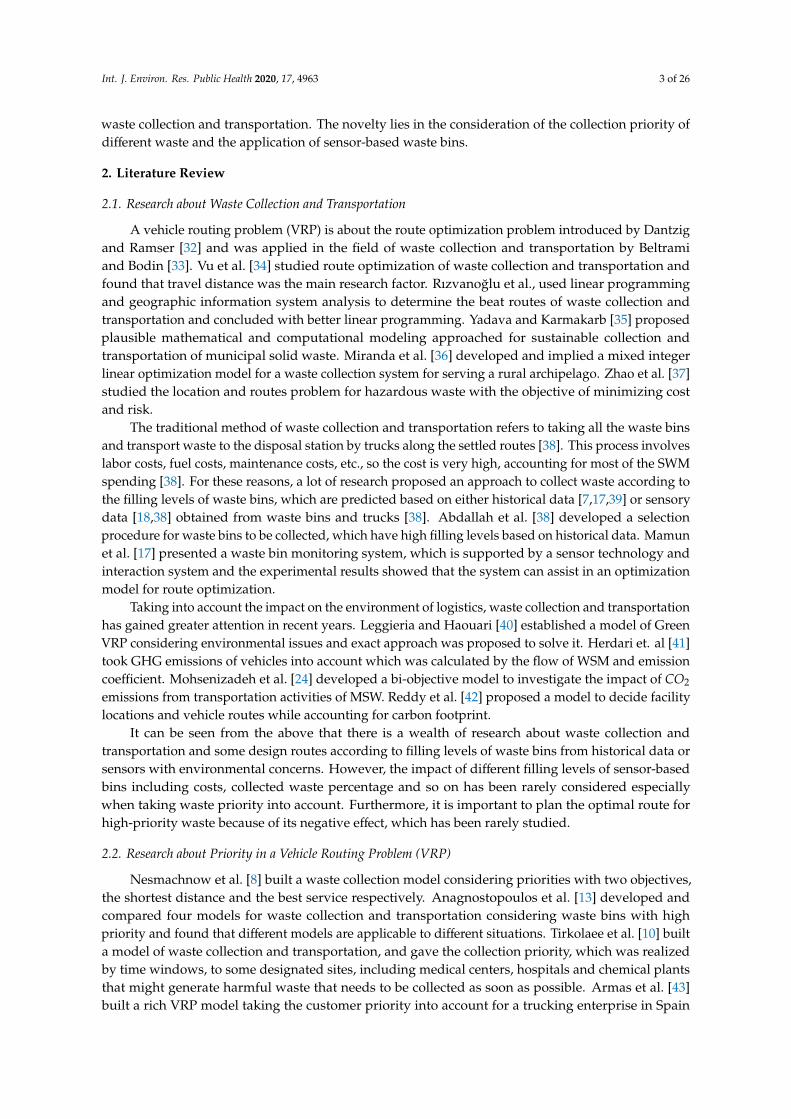
Firstly, the three objective functions (11)–(13) are to minimize total distance, total GHG emissionsand total costs, respectively, whereas each waste bin is only collected once by one vehicle, as stated byconstraint (14). A vehicle starts from the disposal center and goes back to the disposal center aftervisiting a waste bin, which is imposed by Equations (15)–(17) guarantees that the maximum capacity isrespected by all routes. Constraint (18) ensures the collection service for the high priority waste binswhile Constraint (19) eliminates sub-tours. Finally, Equation (20) specifies the types of the variables.

4. Algorithm

4.1. Algorithm Design

The exact solution method is inefficient for solving the medium and large VRPs in real life [43].For this reason, we pay attention to meta-heuristic methods which can generate suitable high-qualitysolutions within a rational computational time. In order to obtain high-quality solutions to practicalproblems, this paper proposes a hybrid local search algorithm based on PSO and SA algorithms. Itsbasic process is shown in Figure 1.

Int. J. Environ. Res. Public Health 2020, 17, 4963 8 of 26Int. J. Environ. Res. Public Health 2020, 17, x FOR PEER REVIEW 8 of 25

Start

Initialization

Calculating fitness value

Updating particle status

Whether the termination of PSO is met?

Yes

Recording the best solution Local search

Whether the termination of SA

is met?

Yes

Outputting the best solution

Updating the best solution

End

N0

No

Figure 1. Flowchart of local search hybrid algorithm (LSHA).

Firstly, the PSO algorithm is applied to generate an initial solution, and then local search will be operated to produce new solutions based on the initial solution. Finally, a SA with the ability to escape from local optimums is deployed to decide the optimal global solution.

4.2. Particle Coding and Decoding

For a vehicle routing problem with waste bins, a 2 dimension space is constructed, and each waste bin corresponds to a two-dimensional value: (1) the vehicle number that completes the waste bin collection; (2) the order of the waste bin in the route of vehicle . That is, (1) the position

of each particle is a 2 dimension vector: where represents the collection vehicle corresponding to each bin in the waste collection service, total dimensions; (2) represents the order of each waste bin in the corresponding vehicle route, total dimension. For example, suppose the number of waste bins to be collected in a waste collection activity is 10, and there are three vehicles in charge of waste collection. If, at a certain time, the position vector of a particle is shown in Table 2.

Table 2. Particle coding.

Waste Bin Number 1 2 3 4 5 6 7 8 9 10 1 1 1 2 2 2 2 3 3 3 1 3 2 3 1 2 4 2 3 1

Taking waste bin 3 as an example, dimension is 1, which means that the waste bin 3 is collected by the vehicle 1; dimension is 2, which means that the order of waste bin 3 in the route of vehicle 1 is 2, and so on; the corresponding solution of this particle is shown in Table 3.

Table 3. Particle decoding.

Vehicle Number Vehicle Route 1 0-1-3-2-0 2 0-5-6-4-7-0 3 0-10-8-9-0

Figure 1. Flowchart of local search hybrid algorithm (LSHA).

Firstly, the PSO algorithm is applied to generate an initial solution, and then local search will beoperated to produce new solutions based on the initial solution. Finally, a SA with the ability to escapefrom local optimums is deployed to decide the optimal global solution.

4.2. Particle Coding and Decoding

For a vehicle routing problem with n waste bins, a 2n dimension space is constructed, and eachwaste bin corresponds to a two-dimensional value: (1) the vehicle number a that completes the wastebin collection; (2) the order b of the waste bin in the route of vehicle a. That is, (1) the position P of eachparticle is a 2n dimension vector: where Xa represents the collection vehicle corresponding to each binin the waste collection service, total n dimensions; (2) Xb represents the order of each waste bin in thecorresponding vehicle route, total n dimension. For example, suppose the number of waste bins to becollected in a waste collection activity is 10, and there are three vehicles in charge of waste collection.If, at a certain time, the position vector of a particle is shown in Table 2.

Table 2. Particle coding.

Waste Bin Number 1 2 3 4 5 6 7 8 9 10

Xa 1 1 1 2 2 2 2 3 3 3Xb 1 3 2 3 1 2 4 2 3 1

Taking waste bin 3 as an example, Xa dimension is 1, which means that the waste bin 3 is collectedby the vehicle 1; Xb dimension is 2, which means that the order of waste bin 3 in the route of vehicle 1is 2, and so on; the corresponding solution of this particle is shown in Table 3.

Table 3. Particle decoding.

Vehicle Number Vehicle Route

1 0-1-3-2-02 0-5-6-4-7-03 0-10-8-9-0


4.3. Constructing Initial Optimal Solution Based on Particle Swarm Optimization (PSO) Algorithm

4.3.1. Initialization and Fitness Function

• Initialization

Set the parameter of PSO as shown in Table 4, and the initialized position and velocity of the ithpopulation is described as Equation (21).

xi = rand(lPar). ∗ (xmax − xmin) + xminvi = rand(lPar). ∗ (vmax − vmin) + xmin

(21)

Table 4. Parameters of particle swarm optimization (PSO).

Parameters of PSO Description

itmax Maximum number of iterationslPar Length of particle codenPop Number of population

r1 Learning factor1r1 Learning factor2c1 Acceleration factor 1c1 Acceleration factor 2

vmax Maximum velocityvmin Minimum velocity

[xmin, xmax] Particle rangeω Inertia weightrω Inertia weight damping ratio

• Fitness Function

The fitness function value is a quantitative index for judging the pros and cons of the particleposition. According to the three kinds of objective functions in Section 3.3, the three correspondingtypes of fitness functions can be constructed as Equations (22)–(24).

FitnessD = T_D +M∑

k∈Vmax(

∑i∈(B∪D)

∑j∈(B∪D)

xki jq j −Cp, 0)

+M∑

k∈Vmax(

(λi − λ j

)(tk

i − tkj), 0)

(22)

FitnessE = T_E +M∑

k∈Vmax(

∑i∈(B∪D)

∑j∈(B∪D)

xki jq j −Cp, 0)

+M∑

k∈Vmax(

(λi − λ j

)(tk

i − tkj), 0)

(23)

FitnessC = T_C +M∑

k∈Vmax(

∑i∈(B∪D)

∑j∈(B∪D)

xki jq j −Cp, 0)

+M∑

k∈Vmax(

(λi − λ j

)(tk

i − tkj), 0)

(24)

Each fitness function can be divided into three parts:The first part is the objective function: total distance T_D in Equation (22); total GHG emissions

T_E in Equation (23); total costs T_C in Equation (24).The second part, M

∑k∈V max(

∑i∈(B∪D)

∑j∈(B∪D) xk

i jq j −Cp, 0) is the treatment of vehicle loadconstraints where M is a very large positive number. When the solution corresponding to the positionof a certain particle is overloaded as an infeasible solution, that is,

∑i∈(B∪D)

∑j∈(B∪D) xk

i jq j > 0, M canmake the overall fitness value of the particle larger, so that the solution corresponding to this positionis eliminated. In this way, we can avoid the situation where an infeasible solution can survive dueto overload.


The third part, M∑

k∈V max((λi − λ j

)(tk

i − tkj), 0) is the priority treatment of specific waste bins.

When the solution does not give the priority the specific waste bins, that is,(λi − λ j

)(tk

i − tkj) > 0, M can

make the overall fitness value of the particle larger, so that the solution corresponding to this positionis eliminated. In this way, we can promise priority to the specific waste bins.

4.3.2. Obtaining Optimal Solution

In each iteration, each particle records its current optimal value through comparison, indicated aspbest

i (t), and all particles have a common global optimal value, indicated as gbest(t).

4.3.3. Particle Status Update

For each particle, update velocity according to Equation (25), and when velocity exceeds the range,take the value according to the boundary as shown by Equation (26).

vi(t + 1) = ωi(t) + c1r1(pbest

i (t) − xi(t))+ c2r2

(gbest(t) − xi(t)

)(25){

i f vi(t + 1) > vmax, vi(t + 1) = vmax

i f vi(t + 1) < vmax, vi(t + 1) = vmin(26)

After updating velocity, the position of particle i will be updated according to Equation (27).

xi(t + 1) = xi(t) + vi(t + 1) (27)

In Equation (25), inertia weight (ω) is the ability of the particle to remain in motion at the previousmoment and is very important in PSO algorithm. In this paper, a time-varying weight is used which isexpressed in Equation (28).

ω(t + 1) = ω(t) ∗ rω (28)

4.3.4. Terminating Condition

Finally, the appearing of population quantity nPop is the termination of the evolutionary.

4.4. Local Search

Next, a series of local search operations will be performed on the optimal individuals generated byPSO algorithm so as to improve the quality of the final optimal solution. Three local search operationsdesigned in this paper are as below:

Swap operation: if a random number p ∈ (0, 1/3], two points will be chosen at random in thepresent coding sequence. Next the positions of two selected points are exchange. As we can see inFigure 2, if the two selected points are 1 and 6, “623451” will be exchange for “123456”.

Int. J. Environ. Res. Public Health 2020, 17, x FOR PEER REVIEW 10 of 25

The second part, ∑ max (∑ ∑ ∈( ∪ )∈( ∪ ) − , 0)∈ is the treatment of vehicle load constraints where is a very large positive number. When the solution corresponding to the position of a certain particle is overloaded as an infeasible solution, that is, ∑ ∑ ∈( ∪ )∈( ∪ ) >0, can make the overall fitness value of the particle larger, so that the solution corresponding to this position is eliminated. In this way, we can avoid the situation where an infeasible solution can survive due to overload.

The third part, ∑ max ( − − , 0)∈ is the priority treatment of specific waste bins. When the solution does not give the priority the specific waste bins, that is, − −> 0 , can make the overall fitness value of the particle larger, so that the solution corresponding to this position is eliminated. In this way, we can promise priority to the specific waste bins.

4.3.2. Obtaining Optimal Solution

In each iteration, each particle records its current optimal value through comparison, indicated as ( ), and all particles have a common global optimal value, indicated as ( ).

4.3.3. Particle Status Update

For each particle, update velocity according to Equation (25), and when velocity exceeds the range, take the value according to the boundary as shown by Equation (26). ( + 1) = ( ) + ( ) − ( ) + ( ( ) − ( )) (25) ( + 1) > , ( + 1) = ( + 1) < , ( + 1) = (26)

After updating velocity, the position of particle will be updated according to Equation (27). ( + 1) = ( ) + ( + 1) (27)

In Equation (25), inertia weight ( ) is the ability of the particle to remain in motion at the previous moment and is very important in PSO algorithm. In this paper, a time-varying weight is used which is expressed in Equation (28). ( + 1) = ( ) ∗ (28)

4.3.4. Terminating Condition

Finally, the appearing of population quantity is the termination of the evolutionary.

4.4. Local Search

Next, a series of local search operations will be performed on the optimal individuals generated by PSO algorithm so as to improve the quality of the final optimal solution. Three local search operations designed in this paper are as below:

Swap operation: if a random number ∈ (0, 1 3⁄ ], two points will be chosen at random in the present coding sequence. Next the positions of two selected points are exchange. As we can see in Figure 2, if the two selected points are 1 and 6, “623451” will be exchange for “123456”.

(a) (b)

1 2 3

456

1 2 3

456

Figure 2. Swap operation. (a) Route before swap operation and (b) route after swap operation.

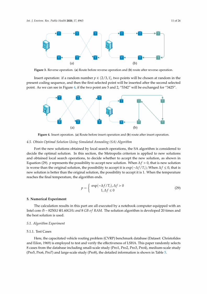
Reverse operation: if a random number p ∈ (1/3, 2/3], two points will be chosen at random in thepresent coding sequence. Next, the point sequence between the two selected points is reversed. As wecan see in Figure 3, if the two point are 2 and 5, “2435” will be exchange for “2345”.




Reverse operation: if a random number ∈ (1 3⁄ , 2 3⁄ ], two points will be chosen at random in the present coding sequence. Next, the point sequence between the two selected points is reversed. As we can see in Figure 3, if the two point are 2 and 5, “2435” will be exchange for “2345”.

(a) (b)

Figure 3. Reverse operation. (a) Route before reverse operation and (b) route after reverse operation.

Insert operation: if a random number ∈ (2 3⁄ , 1], two points will be chosen at random in the present coding sequence, and then the first selected point will be inserted after the second selected point. As we can see in Figure 4, if the two point are 5 and 2, “5342” will be exchanged for “3425”.

(a) (b)

Figure 4. Insert operation. (a) Route before insert operation and (b) route after insert operation.

4.5. Obtain Optimal Solution Using Simulated Annealing (SA) Algorithm

Fort the new solutions obtained by local search operations, the SA algorithm is considered to decide the optimal solution. In this section, the Metropolis criterion is applied to new solutions and obtained local search operations, to decide whether to accept the new solution, as shown in Equation (29). represents the possibility to accept new solution. When ∆ > 0, that is new solution is worse than the original solution, the possibility to accept it is exp(−∆ / ); When ∆ ≤ 0, that is new solution is better than the original solution, the possibility to accept it is 1. When the temperature reaches the final temperature, the algorithm ends. = exp(−∆ / ) , ∆ > 01, ∆ ≤ 0 (29)

5. Numerical Experiment

The calculation results in this part are all executed by a notebook computer equipped with an Intel core 5 − 8250 @1.60 8 . The solution algorithm is developed 20 times and the best solution is used.

5.1. Algorithm Experiment

5.1.1. Test Cases

Here, the capacitated vehicle routing problem (CVRP) benchmark database (Dataset: Christofides and Eilon, 1969) is employed to test and verify the effectiveness of LSHA. This paper randomly selects 8 cases from the database including small-scale study (Pro1, Pro2, Pro3, Pro4),

1 2 3

456

1 2

4

3

56

1 2 3

456

1 2 3

456


Insert operation: if a random number p ∈ (2/3, 1], two points will be chosen at random in thepresent coding sequence, and then the first selected point will be inserted after the second selectedpoint. As we can see in Figure 4, if the two point are 5 and 2, “5342” will be exchanged for “3425”.



Reverse operation: if a random number ∈ (1 3⁄ , 2 3⁄ ], two points will be chosen at random in the present coding sequence. Next, the point sequence between the two selected points is reversed. As we can see in Figure 3, if the two point are 2 and 5, “2435” will be exchange for “2345”.

(a) (b)


Insert operation: if a random number ∈ (2 3⁄ , 1], two points will be chosen at random in the present coding sequence, and then the first selected point will be inserted after the second selected point. As we can see in Figure 4, if the two point are 5 and 2, “5342” will be exchanged for “3425”.

(a) (b)



Fort the new solutions obtained by local search operations, the SA algorithm is considered to decide the optimal solution. In this section, the Metropolis criterion is applied to new solutions and obtained local search operations, to decide whether to accept the new solution, as shown in Equation (29). represents the possibility to accept new solution. When ∆ > 0, that is new solution is worse than the original solution, the possibility to accept it is exp(−∆ / ); When ∆ ≤ 0, that is new solution is better than the original solution, the possibility to accept it is 1. When the temperature reaches the final temperature, the algorithm ends. = exp(−∆ / ) , ∆ > 01, ∆ ≤ 0 (29)


The calculation results in this part are all executed by a notebook computer equipped with an Intel core 5 − 8250 @1.60 8 . The solution algorithm is developed 20 times and the best solution is used.


5.1.1. Test Cases

Here, the capacitated vehicle routing problem (CVRP) benchmark database (Dataset: Christofides and Eilon, 1969) is employed to test and verify the effectiveness of LSHA. This paper randomly selects 8 cases from the database including small-scale study (Pro1, Pro2, Pro3, Pro4),

1 2 3

456

1 2

4

3

56

1 2 3

456

1 2 3

456



Fort the new solutions obtained by local search operations, the SA algorithm is considered todecide the optimal solution. In this section, the Metropolis criterion is applied to new solutionsand obtained local search operations, to decide whether to accept the new solution, as shown inEquation (29). p represents the possibility to accept new solution. When ∆ f > 0, that is new solutionis worse than the original solution, the possibility to accept it is exp(−∆ f /Ti); When ∆ f ≤ 0, that isnew solution is better than the original solution, the possibility to accept it is 1. When the temperaturereaches the final temperature, the algorithm ends.

p =

{exp(−∆ f /Ti), ∆ f > 0

1, ∆ f ≤ 0(29)


The calculation results in this part are all executed by a notebook computer equipped with anIntel core i5− 8250U @1.60GHz and 8 GB o f RAM. The solution algorithm is developed 20 times andthe best solution is used.


5.1.1. Test Cases

Here, the capacitated vehicle routing problem (CVRP) benchmark database (Dataset: Christofidesand Eilon, 1969) is employed to test and verify the effectiveness of LSHA. This paper randomly selects8 cases from the database including small-scale study (Pro1, Pro2, Pro3, Pro4), medium-scale study(Pro5, Pro6, Pro7) and large-scale study (Pro8), the detailed information is shown in Table 5.


Table 5. Data about the test instances.

Problems Case Node Capacity

Pro 1 E-n22-k4 22 6000Pro 2 E-n23-k3 23 4500Pro 3 E-n30-k4 30 4500Pro 4 E-n33-k4 33 8000Pro 5 E-n51-k5 51 160Pro 6 E-n76-k8 76 180Pro 7 E-n76-k10 76 140Pro 8 E-n101-k8 101 100

5.1.2. Parameters Setting

Parameters of vehicles are shown in Table 6 according to references [21,50,51] and parameters ofthe proposed algorithm are shown in Table 7 according to references [10,52–54].

Table 6. Parameters of vehicles.

Parameter Value

e 3.15 kg CO2e/Lr0 0.16 L/kmr∗ 0.377 L/kmε 0.025 CNY/kg

P f ixed 100 CNYP f uel 8 CNY/kg

Table 7. Parameters of LSHA.

Parameter Value

itmax 1000nPop 20

c1 1.5c1 1.5rω 0.99T0 200α 0.98

Tend 1M 5

5.1.3. Results of Algorithm Experiment

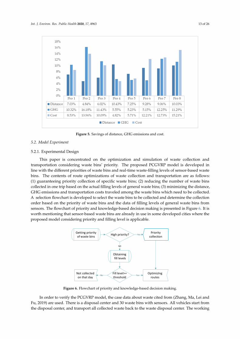
The results of PSO and the proposed algorithm are compared in Table 8, including total distance,total GHG emissions and total costs. To be clear, Figure 5 gives the distance saving, GHG emissionssaving and costs saving of the proposed algorithm LSHA compared with PSO. We can see from Table 6and Figure 5 that the proposed algorithm outperforms in all three areas.

Table 8. Test results of PSO and LSHA.

ProblemsPSO LSHA

Distance GHG Emissions Cost Distance GHG Emissions Cost

Pro 1 649.40 521.70 1738.01 603.72 467.87 1589.71Pro 2 946.06 737.81 2192.26 900.32 618.46 1886.17Pro 3 1161.74 884.11 2567.48 1091.85 783.08 2308.36Pro 4 1352.04 1028.88 3038.76 1210.99 971.73 2892.19Pro 5 1491.31 1211.97 3608.33 1383.12 1148.54 3402.13Pro 6 2331.47 1841.55 5622.99 2115.12 1746.72 4936.27Pro 7 2298.04 1746.65 5779.60 2089.77 1532.66 5043.73Pro 8 3152.75 2636.75 7562.42 2836.39 2339.05 6411.86



Pro 7 2298.04 1746.65 5779.60 2089.77 1532.66 5043.73 Pro 8 3152.75 2636.75 7562.42 2836.39 2339.05 6411.86

Figure 5. Savings of distance, GHG emissions and cost.

5.2. Model Experiment

5.2.1. Experimental Design

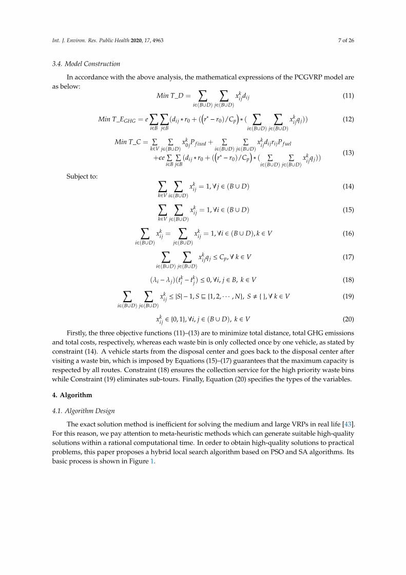
This paper is concentrated on the optimization and simulation of waste collection and transportation considering waste bins’ priority. The proposed PCGVRP model is developed in line with the different priorities of waste bins and real-time waste-filling levels of sensor-based waste bins. The contents of route optimizations of waste collection and transportation are as follows: (1) guaranteeing priority collection of specific waste bins; (2) reducing the number of waste bins collected in one trip based on the actual filling levels of general waste bins; (3) minimizing the distance, GHG emissions and transportation costs traveled among the waste bins which need to be collected. A selection flowchart is developed to select the waste bins to be collected and determine the collection order based on the priority of waste bins and the data of filling levels of general waste bins from sensors. The flowchart of priority and knowledge-based decision making is presented in Figure 6. It is worth mentioning that sensor-based waste bins are already in use in some developed cities where the proposed model considering priority and filling level is applicable.

Figure 6. Flowchart of priority and knowledge-based decision making.

In order to verify the PCGVRP model, the case data about waste cited from (Zhang, Ma, Lei and Fu, 2019) are used. There is a disposal center and 30 waste bins with sensors. All vehicles start from

Getting priority of waste bins High priority?

OptimizIng routes

Priority collection

NO

Obtaining fill levels

Fill level>=threshold

Not collected on that day

Yes

YesNo




This paper is concentrated on the optimization and simulation of waste collection andtransportation considering waste bins’ priority. The proposed PCGVRP model is developed inline with the different priorities of waste bins and real-time waste-filling levels of sensor-based wastebins. The contents of route optimizations of waste collection and transportation are as follows:(1) guaranteeing priority collection of specific waste bins; (2) reducing the number of waste binscollected in one trip based on the actual filling levels of general waste bins; (3) minimizing the distance,GHG emissions and transportation costs traveled among the waste bins which need to be collected.A selection flowchart is developed to select the waste bins to be collected and determine the collectionorder based on the priority of waste bins and the data of filling levels of general waste bins fromsensors. The flowchart of priority and knowledge-based decision making is presented in Figure 6. It isworth mentioning that sensor-based waste bins are already in use in some developed cities where theproposed model considering priority and filling level is applicable.


Pro 7 2298.04 1746.65 5779.60 2089.77 1532.66 5043.73 Pro 8 3152.75 2636.75 7562.42 2836.39 2339.05 6411.86




This paper is concentrated on the optimization and simulation of waste collection and transportation considering waste bins’ priority. The proposed PCGVRP model is developed in line with the different priorities of waste bins and real-time waste-filling levels of sensor-based waste bins. The contents of route optimizations of waste collection and transportation are as follows: (1) guaranteeing priority collection of specific waste bins; (2) reducing the number of waste bins collected in one trip based on the actual filling levels of general waste bins; (3) minimizing the distance, GHG emissions and transportation costs traveled among the waste bins which need to be collected. A selection flowchart is developed to select the waste bins to be collected and determine the collection order based on the priority of waste bins and the data of filling levels of general waste bins from sensors. The flowchart of priority and knowledge-based decision making is presented in Figure 6. It is worth mentioning that sensor-based waste bins are already in use in some developed cities where the proposed model considering priority and filling level is applicable.


In order to verify the PCGVRP model, the case data about waste cited from (Zhang, Ma, Lei and Fu, 2019) are used. There is a disposal center and 30 waste bins with sensors. All vehicles start from

Getting priority of waste bins High priority?

OptimizIng routes

Priority collection

NO

Obtaining fill levels

Fill level>=threshold

Not collected on that day

Yes

YesNo


In order to verify the PCGVRP model, the case data about waste cited from (Zhang, Ma, Lei andFu, 2019) are used. There is a disposal center and 30 waste bins with sensors. All vehicles start fromthe disposal center, and transport all collected waste back to the waste disposal center. The working


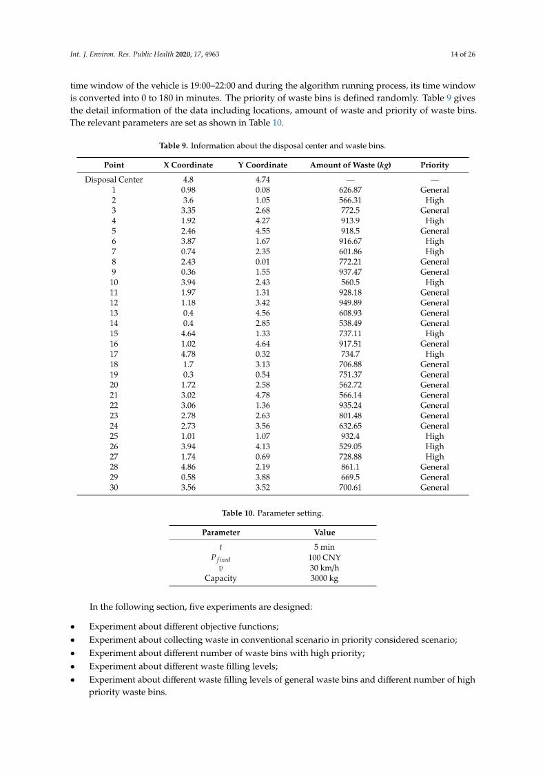
time window of the vehicle is 19:00–22:00 and during the algorithm running process, its time windowis converted into 0 to 180 in minutes. The priority of waste bins is defined randomly. Table 9 givesthe detail information of the data including locations, amount of waste and priority of waste bins.The relevant parameters are set as shown in Table 10.

Table 9. Information about the disposal center and waste bins.

Point X Coordinate Y Coordinate Amount of Waste (kg) Priority

Disposal Center 4.8 4.74 — —1 0.98 0.08 626.87 General2 3.6 1.05 566.31 High3 3.35 2.68 772.5 General4 1.92 4.27 913.9 High5 2.46 4.55 918.5 General6 3.87 1.67 916.67 High7 0.74 2.35 601.86 High8 2.43 0.01 772.21 General9 0.36 1.55 937.47 General10 3.94 2.43 560.5 High11 1.97 1.31 928.18 General12 1.18 3.42 949.89 General13 0.4 4.56 608.93 General14 0.4 2.85 538.49 General15 4.64 1.33 737.11 High16 1.02 4.64 917.51 General17 4.78 0.32 734.7 High18 1.7 3.13 706.88 General19 0.3 0.54 751.37 General20 1.72 2.58 562.72 General21 3.02 4.78 566.14 General22 3.06 1.36 935.24 General23 2.78 2.63 801.48 General24 2.73 3.56 632.65 General25 1.01 1.07 932.4 High26 3.94 4.13 529.05 High27 1.74 0.69 728.88 High28 4.86 2.19 861.1 General29 0.58 3.88 669.5 General30 3.56 3.52 700.61 General

Table 10. Parameter setting.

Parameter Value

t 5 minP f ixed 100 CNY

v 30 km/hCapacity 3000 kg

In the following section, five experiments are designed:

• Experiment about different objective functions;• Experiment about collecting waste in conventional scenario in priority considered scenario;• Experiment about different number of waste bins with high priority;• Experiment about different waste filling levels;• Experiment about different waste filling levels of general waste bins and different number of high

priority waste bins.


5.2.2. Experimental Results

• Experiment about Objective Function

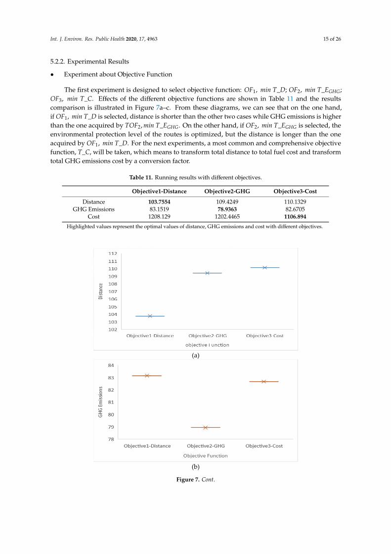
The first experiment is designed to select objective function: OF1, min T_D; OF2, min T_EGHG;OF3, min T_C. Effects of the different objective functions are shown in Table 11 and the resultscomparison is illustrated in Figure 7a–c. From these diagrams, we can see that on the one hand,if OF1, min T_D is selected, distance is shorter than the other two cases while GHG emissions is higherthan the one acquired by TOF2, min T_EGHG. On the other hand, if OF2, min T_EGHG is selected, theenvironmental protection level of the routes is optimized, but the distance is longer than the oneacquired by OF1, min T_D. For the next experiments, a most common and comprehensive objectivefunction, T_C, will be taken, which means to transform total distance to total fuel cost and transformtotal GHG emissions cost by a conversion factor.

Table 11. Running results with different objectives.

Objective1-Distance Objective2-GHG Objective3-Cost

Distance 103.7554 109.4249 110.1329GHG Emissions 83.1519 78.9363 82.6705

Cost 1208.129 1202.4465 1106.894

Highlighted values represent the optimal values of distance, GHG emissions and cost with different objectives.


5.2.2. Experimental Results

• Experiment about Objective Function

The first experiment is designed to select objective function: , _ ; , _ ; , _ . Effects of the different objective functions are shown in Table 11 and the results comparison is illustrated in Figure 7a–c. From these diagrams, we can see that on the one hand, if , _ is selected, distance is shorter than the other two cases while GHG emissions is higher than the one acquired by , _ . On the other hand, if , _ is selected, the environmental protection level of the routes is optimized, but the distance is longer than the one acquired by , _ . For the next experiments, a most common and comprehensive objective function, _ , will be taken, which means to transform total distance to total fuel cost and transform total GHG emissions cost by a conversion factor.

Table 11. Running results with different objectives.

Objective1-Distance Objective2-GHG Objective3-Cost Distance 103.7554 109.4249 110.1329

GHG Emissions 83.1519 78.9363 82.6705 Cost 1208.129 1202.4465 1106.894

Highlighted values represent the optimal values of distance, GHG emissions and cost with different objectives.

(a)

(b)

Figure 7. Cont.

Int. J. Environ. Res. Public Health 2020, 17, 4963 16 of 26Int. J. Environ. Res. Public Health 2020, 17, x FOR PEER REVIEW 16 of 25

(c)

Figure 7. Results comparison with different objectives. (a) Objective1-minimized distance, (b) Objective2-minimized GHG and (c) Objective1-minimized cost.

• Experiment about Conventional Scenario and Priority Considered Scenario

In this section we do the experiment under two scenarios: (1) collect waste in the conventional way (conventional scenario, CS), which means all the waste bins have the same priority without considering the negative effect of specific waste bins; (2) collect waste considering waste bins’ priority (priority considered scenario, PCS). The detailed information about CS and PCS are shown in Table 12 and Table 13, respectively, including service sequence of each route, waste bins with high priority included in each route, the collection order and collection time of the high priority waste bins. From the two tables, we can see that under CS, the order of waste bins with high priority is randomly assigned, resulting in the later collection time. Under PCS, the waste bins with high priority are always first in the collection sequence and then are collected earlier.

Table 12. Detailed route information under conventional scenario (CS).

Number Routes High Priority Waste Bin Collection Order Collection Time 1 {6,24,9,021,24,9,0} 17 2nd 30.54

2 {0,15,11,7,0} 15 1st 11.38 7 3rd 35.65

3 {0,8,4,12,0} 4 2st 29.03 4 {0,25,14,0} 25 1st 17.59 5 {0,13,29,22,0} - - -

6 {0,27,6,28,0} 27 1st 16.92 6 2nd 29.74

7 {0,23,16,30,0} - - -

8 {0,5,26,10,0} 26 2nd 17.95 10 3rd 28.62

9 {0,3,2,0} 2 2nd 28.62 10 {0,20,19,1,0} - - -

Total 246.03

Table 13. Detailed route information under priority considered scenario (PCS).

Number Routes High Priority Waste Bin Collection Order Collection Time 1 {0,27,5,11,0}. 27 1st 16.92 2 {0,15,1,30,16,0} 15 1st 11.38 3 {0,10,8,20,12,0} 10 1st 8.22 4 {0,7,29,14,24,0} 7 1st 15.70 5 {0,25,28,3,0} 25 1st 17.59 6 {0,17,22,19,23,0} 17 1st 14.73 7 {0,2,4,21,9,0} 2 1st 12.93

Figure 7. Results comparison with different objectives. (a) Objective1-minimized distance, (b)Objective2-minimized GHG and (c) Objective1-minimized cost.

• Experiment about Conventional Scenario and Priority Considered Scenario

In this section we do the experiment under two scenarios: (1) collect waste in the conventional way(conventional scenario, CS), which means all the waste bins have the same priority without consideringthe negative effect of specific waste bins; (2) collect waste considering waste bins’ priority (priorityconsidered scenario, PCS). The detailed information about CS and PCS are shown in Tables 12 and 13,respectively, including service sequence of each route, waste bins with high priority included in eachroute, the collection order and collection time of the high priority waste bins. From the two tables, wecan see that under CS, the order of waste bins with high priority is randomly assigned, resulting in thelater collection time. Under PCS, the waste bins with high priority are always first in the collectionsequence and then are collected earlier.

Table 12. Detailed route information under conventional scenario (CS).

Number Routes High Priority Waste Bin Collection Order Collection Time

1 {6,24,9,021,24,9,0} 17 2nd 30.54

2 {0,15,11,7,0} 15 1st 11.387 3rd 35.65

3 {0,8,4,12,0} 4 2st 29.034 {0,25,14,0} 25 1st 17.595 {0,13,29,22,0} - - -

6 {0,27,6,28,0} 27 1st 16.926 2nd 29.74

7 {0,23,16,30,0} - - -

8 {0,5,26,10,0} 26 2nd 17.9510 3rd 28.62

9 {0,3,2,0} 2 2nd 28.6210 {0,20,19,1,0} - - -

Total 246.03


Table 13. Detailed route information under priority considered scenario (PCS).

Number Routes High Priority Waste Bin Collection Order Collection Time

1 {0,27,5,11,0}. 27 1st 16.922 {0,15,1,30,16,0} 15 1st 11.383 {0,10,8,20,12,0} 10 1st 8.224 {0,7,29,14,24,0} 7 1st 15.705 {0,25,28,3,0} 25 1st 17.596 {0,17,22,19,23,0} 17 1st 14.737 {0,2,4,21,9,0} 2 1st 12.938 4 2nd 30.049 {0,26,18,13,0} 26 1st 3.52

10 {0,6,0} 6 1st 10.69Total 141.72

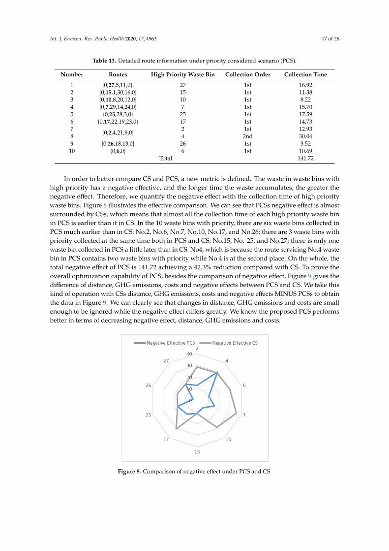
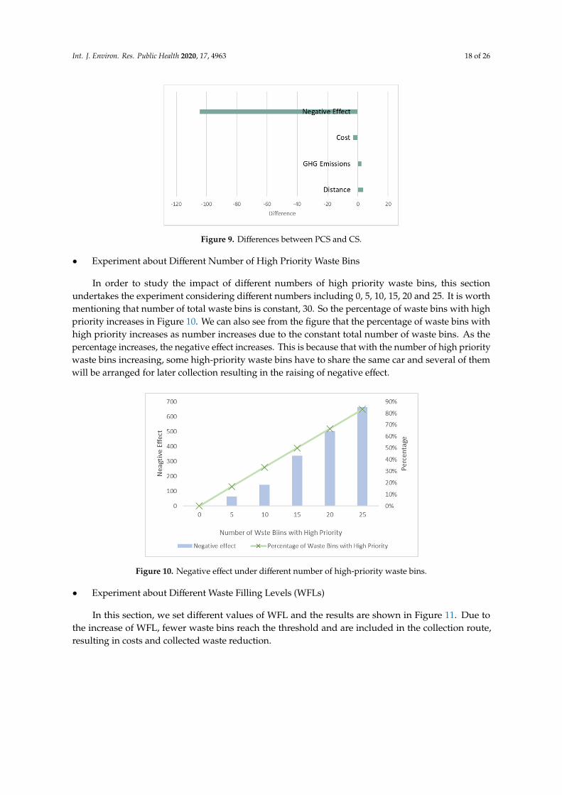
In order to better compare CS and PCS, a new metric is defined. The waste in waste bins withhigh priority has a negative effective, and the longer time the waste accumulates, the greater thenegative effect. Therefore, we quantify the negative effect with the collection time of high prioritywaste bins. Figure 8 illustrates the effective comparison. We can see that PCSs negative effect is almostsurrounded by CSs, which means that almost all the collection time of each high priority waste binin PCS is earlier than it in CS. In the 10 waste bins with priority, there are six waste bins collected inPCS much earlier than in CS: No.2, No.6, No.7, No.10, No.17, and No.26; there are 3 waste bins withpriority collected at the same time both in PCS and CS: No.15, No. 25, and No.27; there is only onewaste bin collected in PCS a little later than in CS: No4, which is because the route servicing No.4 wastebin in PCS contains two waste bins with priority while No.4 is at the second place. On the whole, thetotal negative effect of PCS is 141.72 achieving a 42.3% reduction compared with CS. To prove theoverall optimization capability of PCS, besides the comparison of negative effect, Figure 9 gives thedifference of distance, GHG emissions, costs and negative effects between PCS and CS. We take thiskind of operation with CSs distance, GHG emissions, costs and negative effects MINUS PCSs to obtainthe data in Figure 9. We can clearly see that changes in distance, GHG emissions and costs are smallenough to be ignored while the negative effect differs greatly. We know the proposed PCS performsbetter in terms of decreasing negative effect, distance, GHG emissions and costs.


8 4 2nd 30.04 9 {0,26,18,13,0} 26 1st 3.52

10 {0,6,0} 6 1st 10.69 Total 141.72

In order to better compare CS and PCS, a new metric is defined. The waste in waste bins with high priority has a negative effective, and the longer time the waste accumulates, the greater the negative effect. Therefore, we quantify the negative effect with the collection time of high priority waste bins. Figure 8 illustrates the effective comparison. We can see that PCSs negative effect is almost surrounded by CSs, which means that almost all the collection time of each high priority waste bin in PCS is earlier than it in CS. In the 10 waste bins with priority, there are six waste bins collected in PCS much earlier than in CS: No.2, No.6, No.7, No.10, No.17, and No.26; there are 3 waste bins with priority collected at the same time both in PCS and CS: No.15, No. 25, and No.27; there is only one waste bin collected in PCS a little later than in CS: No4, which is because the route servicing No.4 waste bin in PCS contains two waste bins with priority while No.4 is at the second place. On the whole, the total negative effect of PCS is 141.72 achieving a 42.3% reduction compared with CS. To prove the overall optimization capability of PCS, besides the comparison of negative effect, Figure 9 gives the difference of distance, GHG emissions, costs and negative effects between PCS and CS. We take this kind of operation with CSs distance, GHG emissions, costs and negative effects MINUS PCSs to obtain the data in Figure 9. We can clearly see that changes in distance, GHG emissions and costs are small enough to be ignored while the negative effect differs greatly. We know the proposed PCS performs better in terms of decreasing negative effect, distance, GHG emissions and costs.

Figure 8. Comparison of negative effect under PCS and CS.

Figure 9. Differences between PCS and CS.




8 4 2nd 30.04 9 {0,26,18,13,0} 26 1st 3.52

10 {0,6,0} 6 1st 10.69 Total 141.72

In order to better compare CS and PCS, a new metric is defined. The waste in waste bins with high priority has a negative effective, and the longer time the waste accumulates, the greater the negative effect. Therefore, we quantify the negative effect with the collection time of high priority waste bins. Figure 8 illustrates the effective comparison. We can see that PCSs negative effect is almost surrounded by CSs, which means that almost all the collection time of each high priority waste bin in PCS is earlier than it in CS. In the 10 waste bins with priority, there are six waste bins collected in PCS much earlier than in CS: No.2, No.6, No.7, No.10, No.17, and No.26; there are 3 waste bins with priority collected at the same time both in PCS and CS: No.15, No. 25, and No.27; there is only one waste bin collected in PCS a little later than in CS: No4, which is because the route servicing No.4 waste bin in PCS contains two waste bins with priority while No.4 is at the second place. On the whole, the total negative effect of PCS is 141.72 achieving a 42.3% reduction compared with CS. To prove the overall optimization capability of PCS, besides the comparison of negative effect, Figure 9 gives the difference of distance, GHG emissions, costs and negative effects between PCS and CS. We take this kind of operation with CSs distance, GHG emissions, costs and negative effects MINUS PCSs to obtain the data in Figure 9. We can clearly see that changes in distance, GHG emissions and costs are small enough to be ignored while the negative effect differs greatly. We know the proposed PCS performs better in terms of decreasing negative effect, distance, GHG emissions and costs.


Figure 9. Differences between PCS and CS. Figure 9. Differences between PCS and CS.

• Experiment about Different Number of High Priority Waste Bins

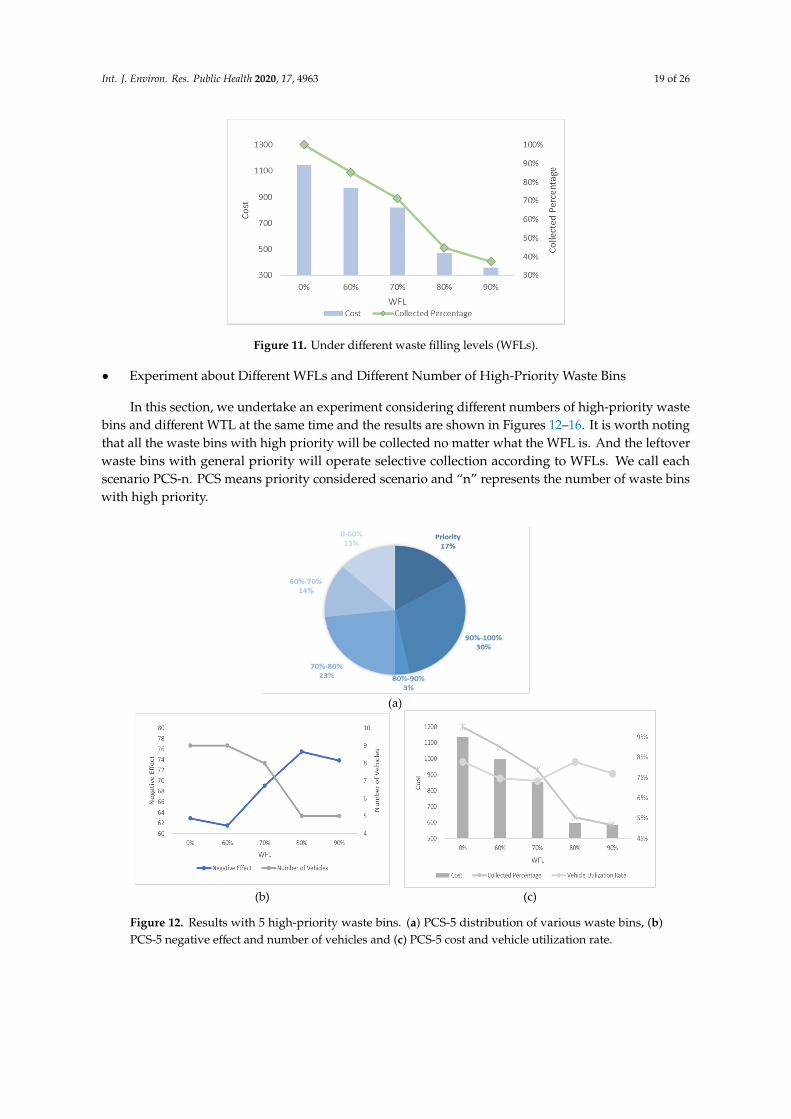
In order to study the impact of different numbers of high priority waste bins, this sectionundertakes the experiment considering different numbers including 0, 5, 10, 15, 20 and 25. It is worthmentioning that number of total waste bins is constant, 30. So the percentage of waste bins with highpriority increases in Figure 10. We can also see from the figure that the percentage of waste bins withhigh priority increases as number increases due to the constant total number of waste bins. As thepercentage increases, the negative effect increases. This is because that with the number of high prioritywaste bins increasing, some high-priority waste bins have to share the same car and several of themwill be arranged for later collection resulting in the raising of negative effect.



In order to study the impact of different numbers of high priority waste bins, this section undertakes the experiment considering different numbers including 0, 5, 10, 15, 20 and 25. It is worth mentioning that number of total waste bins is constant, 30. So the percentage of waste bins with high priority increases in Figure 10. We can also see from the figure that the percentage of waste bins with high priority increases as number increases due to the constant total number of waste bins. As the percentage increases, the negative effect increases. This is because that with the number of high priority waste bins increasing, some high-priority waste bins have to share the same car and several of them will be arranged for later collection resulting in the raising of negative effect.

Figure 10. Negative effect under different number of high-priority waste bins.

• Experiment about Different Waste Filling Levels (WFLs)

In this section, we set different values of WFL and the results are shown in Figure 11. Due to the increase of WFL, fewer waste bins reach the threshold and are included in the collection route, resulting in costs and collected waste reduction.

Figure 11. Under different waste filling levels (WFLs).

• Experiment about Different WFLs and Different Number of High-Priority Waste Bins

In this section, we undertake an experiment considering different numbers of high-priority waste bins and different WTL at the same time and the results are shown in Figures 12–16. It is worth noting that all the waste bins with high priority will be collected no matter what the WFL is. And the leftover waste bins with general priority will operate selective collection according to WFLs. We call each scenario PCS-n. PCS means priority considered scenario and “n” represents the number of waste bins with high priority.



In this section, we set different values of WFL and the results are shown in Figure 11. Due tothe increase of WFL, fewer waste bins reach the threshold and are included in the collection route,resulting in costs and collected waste reduction.




In order to study the impact of different numbers of high priority waste bins, this section undertakes the experiment considering different numbers including 0, 5, 10, 15, 20 and 25. It is worth mentioning that number of total waste bins is constant, 30. So the percentage of waste bins with high priority increases in Figure 10. We can also see from the figure that the percentage of waste bins with high priority increases as number increases due to the constant total number of waste bins. As the percentage increases, the negative effect increases. This is because that with the number of high priority waste bins increasing, some high-priority waste bins have to share the same car and several of them will be arranged for later collection resulting in the raising of negative effect.



In this section, we set different values of WFL and the results are shown in Figure 11. Due to the increase of WFL, fewer waste bins reach the threshold and are included in the collection route, resulting in costs and collected waste reduction.



In this section, we undertake an experiment considering different numbers of high-priority waste bins and different WTL at the same time and the results are shown in Figures 12–16. It is worth noting that all the waste bins with high priority will be collected no matter what the WFL is. And the leftover waste bins with general priority will operate selective collection according to WFLs. We call each scenario PCS-n. PCS means priority considered scenario and “n” represents the number of waste bins with high priority.



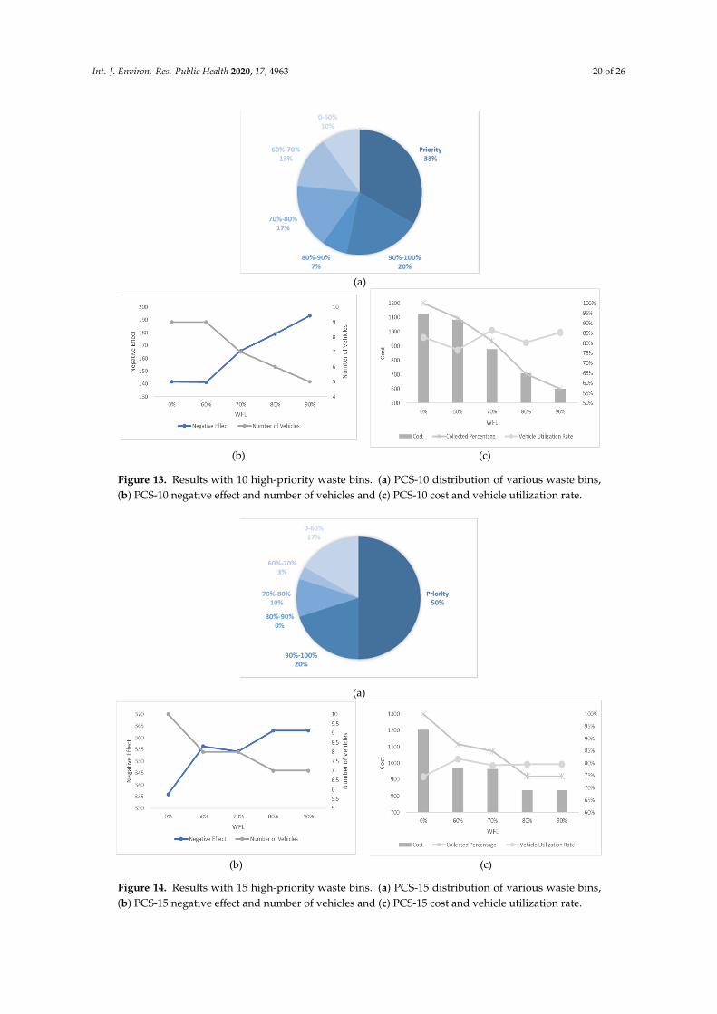
In this section, we undertake an experiment considering different numbers of high-priority wastebins and different WTL at the same time and the results are shown in Figures 12–16. It is worth notingthat all the waste bins with high priority will be collected no matter what the WFL is. And the leftoverwaste bins with general priority will operate selective collection according to WFLs. We call eachscenario PCS-n. PCS means priority considered scenario and “n” represents the number of waste binswith high priority.Int. J. Environ. Res. Public Health 2020, 17, x FOR PEER REVIEW 19 of 25

(a)

(b) (c)

Figure 12. Results with 5 high-priority waste bins. (a) PCS-5 distribution of various waste bins, (b) PCS-5 negative effect and number of vehicles and (c) PCS-5 cost and vehicle utilization rate.

(a)

(b) (c)


Figure 12. Results with 5 high-priority waste bins. (a) PCS-5 distribution of various waste bins, (b)PCS-5 negative effect and number of vehicles and (c) PCS-5 cost and vehicle utilization rate.



(a)

(b) (c)


(a)

(b) (c)

Figure 13. Results with 10 high-priority waste bins. (a) PCS-10 distribution of various waste bins, (b) PCS-10 negative effect and number of vehicles and (c) PCS-10 cost and vehicle utilization rate. Figure 13. Results with 10 high-priority waste bins. (a) PCS-10 distribution of various waste bins,(b) PCS-10 negative effect and number of vehicles and (c) PCS-10 cost and vehicle utilization rate.


(a)

(b) (c)


(a)

(b) (c)


Figure 14. Results with 15 high-priority waste bins. (a) PCS-15 distribution of various waste bins,(b) PCS-15 negative effect and number of vehicles and (c) PCS-15 cost and vehicle utilization rate.



(a)

(b) (c)


(a)

(b) (c)

Figure 15. Results with 20 high-priority waste bins. (a) PCS-20 distribution of various waste bins, (b) PCS-20 negative effect and number of vehicles and (c) PCS-20 cost and vehicle utilization rate. Figure 15. Results with 20 high-priority waste bins. (a) PCS-20 distribution of various waste bins,(b) PCS-20 negative effect and number of vehicles and (c) PCS-20 cost and vehicle utilization rate.


(a)

(b) (c) PCS-25 Cost and vehicle utilization rate


Every number of waste bin with high priority (every figure) has three Figures a–c. For example, a–c in Figure 12 are all sub-Figures of PCS-5. The first sub-Figure of each Figure is a pie chart about the priority and volume distribution. We take Figure 14 as an example and (a) is the first sub-Figure of PCS-15. We can see from Figure 14a that the number of waste bins with high priority accounts for half and the filling level of waste between [0–60%), [60–70%), [70–80%), [80–90%) and [90–100%) accounts for 17%, 3%, 10%, 0% and 20%.

The second sub-Figure of each figure is about the number of vehicles and negative effect and we take (b) of Figure 13 as an example. We set five values of WFL, 0%, 60%, 70%, 80% and 90% as abscissa, which means only the waste bins reaching preset specific WFL will be collected. We study negative effect and number of vehicles changes in the process of increasing WFL. We can see the number of vehicles decreasing as the WFL is increasing as a result of reduction of waste bins to collect. Affected by the decline in the number of vehicles, several waste bins with high priority have to share the same car resulting in the negative effect raising. Therefore, the negative effect and number of vehicles have the opposite trend.

The third sub-Figure is about the cost percentage of collected waste and vehicle utilization rate under different WFL. For the third sub-Figures of all figures, the cost and the percentage of collected waste have the same trend: decreasing as WFL is increasing. That is because when we set higher WFL, fewer waste bin can reach it and will be collected resulting in the lower percentage of collected waste and further reducing cost. Vehicle utilization rate, another indicator, is calculated by dividing total collected waste by total vehicles’ capacity, representing resource utilization efficiency. Different number of waste bins with high priority and WFL lead to different vehicle utilization rate. We can find from all the sub-Figures that there is an effective interval (60–80%) of WFL with high vehicle utilization rate. The logistic enterprises can increase the efficiency of distribution by optimizing the paths when WFL is set in this interval. Further excessive value should be avoided to prevent overflowing before the next collection.

5.3. Analysis of Results

Figure 16. Results with 25 high-priority waste bins. (a) PCS-25 distribution of various waste bins,(b) PCS-25 negative effect and number of vehicles and (c) PCS-25 cost and vehicle utilization rate.


Every number of waste bin with high priority (every figure) has three Figures a–c. For example,a–c in Figure 12 are all sub-Figures of PCS-5. The first sub-Figure of each Figure is a pie chart about thepriority and volume distribution. We take Figure 14 as an example and (a) is the first sub-Figure ofPCS-15. We can see from Figure 14a that the number of waste bins with high priority accounts for halfand the filling level of waste between [0–60%), [60–70%), [70–80%), [80–90%) and [90–100%) accountsfor 17%, 3%, 10%, 0% and 20%.

The second sub-Figure of each figure is about the number of vehicles and negative effect and wetake (b) of Figure 13 as an example. We set five values of WFL, 0%, 60%, 70%, 80% and 90% as abscissa,which means only the waste bins reaching preset specific WFL will be collected. We study negativeeffect and number of vehicles changes in the process of increasing WFL. We can see the number ofvehicles decreasing as the WFL is increasing as a result of reduction of waste bins to collect. Affectedby the decline in the number of vehicles, several waste bins with high priority have to share the samecar resulting in the negative effect raising. Therefore, the negative effect and number of vehicles havethe opposite trend.

The third sub-Figure is about the cost percentage of collected waste and vehicle utilization rateunder different WFL. For the third sub-Figures of all figures, the cost and the percentage of collectedwaste have the same trend: decreasing as WFL is increasing. That is because when we set higherWFL, fewer waste bin can reach it and will be collected resulting in the lower percentage of collectedwaste and further reducing cost. Vehicle utilization rate, another indicator, is calculated by dividingtotal collected waste by total vehicles’ capacity, representing resource utilization efficiency. Differentnumber of waste bins with high priority and WFL lead to different vehicle utilization rate. We can findfrom all the sub-Figures that there is an effective interval (60–80%) of WFL with high vehicle utilizationrate. The logistic enterprises can increase the efficiency of distribution by optimizing the paths whenWFL is set in this interval. Further excessive value should be avoided to prevent overflowing beforethe next collection.

5.3. Analysis of Results

In the paper, the PCGVRP model is developed to optimize the activity of waste collection andtransportation in SWM, which is solved by the improved algorithm of LSHA. By considering specificwaste bins with high priority and filling levels of general waste bins, we study the impact of differentnumbers of waste bins with high priority and WFLs on the negative effect, costs, the percentage ofcollected waste and vehicle utilization rate. We find that the best value of WFL with high efficiencyshould be set according to the number of waste bins with high priority, waste generation rate, wastemanagement requirements and so on. Some primary points of summary are enumerated below.

(1) For experiment 1, the objectives of minimizing distance, minimizing GHG emissions andminimizing costs are compared. The objective of minimizing costs is the compromised oneconsidering both distance and GHG emissions.

(2) For experiment 2, PCS and CS are same in distance reduction, GHG emissions reduction andcosts reduction, while PCS achieves a negative effect reduction of 42.3%.

(3) For experiment 3, the negative effect increases as the number of waste bins with high priorityis increasing.

(4) For experiment 4, the higher the WFL, the lower the percentage of collected waste and the costs.However, excessive WFL can increase the risk of overflowing before the next collection.

(5) For experiment 5, different distribution of various waste bins (waste bins with high priority, wastefilling level of general waste bins) result in different negative effect, costs, vehicles utilizationrate and so on. The WFL between 60% and 80% can obtain the optimal solution under differentnumber of waste bins with high priority.


By setting different numbers of waste bins with high priority and different WFLs, it turns outthat the proposed PCGVRP model is applicable and efficient for the activity of waste collection andtransportation in SWM.

On account of the aforementioned summary, this paper comes up with some instructional advice.From the point of view of SWM institutions, they can take scientific approaches, such as operationalresearch methods, route optimization, etc., to bring down the total negative effect and total costs.At the same time, technical means such as sensors are recommended, because they can bridge thecommunication between vehicles and waste bins and assist path optimization. In short, waste collectionand transportation can greatly benefit from these technologies. A certain value of WFL between 60%and 80% is a preferable option to enhance the efficiency of waste collection and transportation and theexact value of WFL should be decided by the number of waste bins with high priority.

From the perspective of the Environmental Protection Administration, firstly, they shouldencourage waste management organizations to take the priority of waste bins into consideration andminimize the negative effect of specific waste as much as possible. Secondly, they can introduce somerelevant policies to deploy more sensors. Finally, they ought to increase environmental consciousnessand inspire the public waste sorting to ensure that priority waste can be sorted, collected and transportedin a timely manner.

6. Conclusions

Programming a series of vehicle routes well is a challenging task in an effort to decrease collectionand transportation costs, the negative effects of some specific waste and to ensure that all inhabitantslive in a comfortable and healthy environment. Thus, the paper built a model for waste collectionand transportation with the minimized total comprehensive costs including routes costs and GHGemissions costs. An improved genetic algorithm, LSHA, is designed to solve the proposed PCGVRPmodel. Furthermore, the effectivity of LSHA is proved by a contrast experiment using data fromclassic CVRP database. After that, the applicability and validity of the proposed PCGVRP model areconfirmed by setting different numerical parameters. The negative effect, costs, vehicles utilizationrate and percentage of collected waste are computed and analyzed separately with different numbersof waste bins with high priority and WFLs. Bases on the results, some suggestions are provided forthe Environmental Protection Administration and waste collection and transportation organizations.In the case of COVID-19, the increase of medical waste makes the timely disposal of this wasteparticularly important and critical. In further research, multivariate statistical analysis (cluster analysisand principal component analysis) can be applied to analyze the parameters of PCGVRP Furthermore,recent and real data can be used to obtain more realistic and reliable conclusions.

Author Contributions: Conceptualization, H.W.; Methodology, H.W.; Software, H.W.; Validation, F.T.; FormalAnalysis, H.W.; Investigation, H.W.; Resources, F.T.; Data Curation, H.W.; Writing—Original Draft Preparation,F.T.; Writing—Review and Editing, F.T.; Visualization, F.T.; Supervision, F.T.; Project Administration, H.W. and B.Y.;Funding Acquisition, H.W. and B.Y. All authors have read and agreed to the published version of the manuscript.

Funding: This research is supported by the Natural Science Foundation Project of Chongqing(cstc2019jcyj-msxmX0100), Science and Technology Research Project of Chongqing Municipal EducationCommission (KJQN201804005) and Key Scientific Research Project of Chongqing Radio and TV University(ZD2017-04).

Conflicts of Interest: The authors declare no conflict of interest.

References

1. Kharat, M.G.; Murthy, S.; Kamble, S.J.; Raut, R.D.; Kamble, S.S.; Kharat, M.G. Fuzzy multi-criteria decisionanalysis for environmentally conscious solid waste treatment and disposal technology selection. Technol. Soc.2019, 57, 20–29. [CrossRef]

2. Andrey, P.; Valentina, I.; Yuri, S. Strategic approaches to management in the field of solid municipal wastemanagement. Talent Dev. Excell. 2020, 12, 700–709.

http://dx.doi.org/10.1016/j.techsoc.2018.12.005


3. Fernandez-Aracil, P.; Ortuno-Padilla, A.; Melgarejo-Moreno, J. Factors related to municipal costs of wastecollection service in Spain. J. Clean. Prod. 2018, 175, 553–560. [CrossRef]

4. Ferronato, N.; Torretta, V.; Ragazzi, M.; Rada, E.C. Waste mismanagement in developing countries: A casestudy of environmental contamination. UPB Sci. Bull. 2017, 79, 185–196.

5. Cocarta, D.M.; Rada, E.C.; Ragazzi, M.; Badea, A.; Apostol, T.J.E.T. A contribution for a correct vision ofhealth impact from municipal solid waste treatments. Environ. Technol. 2009, 30, 963–968. [CrossRef][PubMed]

6. Xu, Y.; Liu, X.; Hu, X.; Huang, G.; Meng, N. A genetic-algorithm-aided fuzzy chance-constrained programmingmodel for municipal solid waste management. Eng. Optim. 2019, 1–17. [CrossRef]

7. Expósito-Márquez, A.; Expósito-Izquierdo, C.; Brito-Santana, J.; Moreno-Pérez, J.A. Greedy randomizedadaptive search procedure to design waste collection routes in La Palma. Comput. Ind. Eng. 2019, 137.[CrossRef]

8. Nesmachnow, S.; Rossit, D.; Toutouh, J. Comparison of Multiobjective Evolutionary Algorithms for PrioritizedUrban Waste Collection in Montevideo, Uruguay. Electron. Notes Discret. Math. 2018, 69, 93–100. [CrossRef]

9. Ghiani, G.; Laganà, D.; Manni, E.; Triki, C. Capacitated location of collection sites in an urban wastemanagement system. J. Waste Manag. 2012, 32, 1291–1296. [CrossRef]

10. Tirkolaee, E.B.; Abbasian, P.; Soltani, M.; Ghaffarian, S.A. Developing an applied algorithm for multi-tripvehicle routing problem with time windows in urban waste collection: A case study. Waste Manag. Res. 2019,37, 4–13. [CrossRef]

11. Tirkolaee, E.B.; Alinaghian, M.; Hosseinabadi, A.A.R.; Sasi, M.B.; Sangaiah, A.K. An improved ant colonyoptimization for the multi-trip Capacitated Arc Routing Problem. Comput. Electr. Eng. 2019, 77, 457–470.[CrossRef]

12. Yaman, C.; Anil, I.; Jaunich, M.K.; Blaisi, N.I.; Alagha, O.; Yaman, A.B.; Gunday, S.T. Investigationand modelling of greenhouse gas emissions resulting from waste collection and transport activities.Waste Manag. Res. 2019, 37, 1282–1290. [CrossRef] [PubMed]

13. Anagnostopoulos, T.; Kolomvatsos, K.; Anagnostopoulos, C.; Zaslavsky, A.; Hadjiefthymiades, S. Assessingdynamic models for high priority waste collection in smart cities. J. Syst. Softw. 2015, 110, 178–192. [CrossRef]

14. Nuortio, T.; Kytöjoki, J.; Niska, H.; Bräysy, O. Improved route planning and scheduling of waste collectionand transport. J. Expert Syst. Appl. 2005, 30, 223–232. [CrossRef]

15. Jaeger, S.D.; Eyckmans, J.; Rogge, N.; Puyenbroeck, T.V.J.W.M. Wasteful waste-reducing policies? The impactof waste reduction policy instruments on collection and processing costs of municipal solid waste.Waste Manag. 2011, 31, 1429–1440. [CrossRef] [PubMed]

16. Melakessou, F.; Kugener, P.; Alnaffakh, N.; Faye, S.; Khadraoui, D. Heterogeneous Sensing Data Analysis forCommercial Waste Collection. Sensors (Basel, Switzerland) 2020, 20, 978. [CrossRef] [PubMed]

17. Mamun, M.A.A.; Hannan, M.A.; Hussain, A.; Basri, H. Theoretical model and implementation of a real timeintelligent bin status monitoring system using rule based decision algorithms. J. Expert Syst. Appl. 2016, 48,76–88. [CrossRef]

18. Ferrer, J.; Alba, E. BIN-CT: Urban waste collection based on predicting the container fill level. J. Biosyst. 2019,186, 103962. [CrossRef]

19. Shuang, X.; Li, G.; Ou, H.; Wu, W. Research and Demonstration of Dynamic Intelligent Logistics System ofthe Collection and Transportation Process of Giant Municipal Garbage. Lect. Notes Electr. Eng. 2015, 286,39–50.

20. Rada, E.C.; Grigoriu, M.; Ragazzi, M. Web oriented technologies and equipments for MSW collection.In Proceedings of the International Conference on Risk Management, Assessment and Mitigation, RIMA2010, Bucharest, Romania, 20–23 April 2010; pp. 150–153.

21. Kirschstein, T.; Meisel, F. GHG-emission models for assessing the eco-friendliness of road and rail freighttransports. Transp. Res. Part B Methodol. 2015, 73, 13–33. [CrossRef]

22. Behnke, M.; Kirschstein, T. The impact of path selection on GHG emissions in city logistics. Transp. Res. PartE-Logist. Transp. Rev. 2017, 106, 320–336. [CrossRef]

23. Li, C.-Z.; Zhang, Y.; Liu, Z.-H.; Meng, X.; Du, J. Optimization of MSW collection routing system to reducefuel consumption and pollutant emissions. Nat. Environ. Pollut. Technol. 2014, 13, 177–184.

24. Mohsenizadeh, M.; Tural, M.K.; Kentel, E. Municipal solid waste management with cost minimization andemission control objectives: A case study of Ankara. Sustain. Cities Soc. 2020, 52. [CrossRef]

http://dx.doi.org/10.1016/j.jclepro.2017.12.116

http://dx.doi.org/10.1080/09593330902989958

http://www.ncbi.nlm.nih.gov/pubmed/19803335

http://dx.doi.org/10.1080/0305215X.2019.1608979

http://dx.doi.org/10.1016/j.cie.2019.106047

http://dx.doi.org/10.1016/j.endm.2018.07.013

http://dx.doi.org/10.1016/j.wasman.2012.02.009

http://dx.doi.org/10.1177/0734242X18807001

http://dx.doi.org/10.1016/j.compeleceng.2018.01.040

http://dx.doi.org/10.1177/0734242X19882482


http://dx.doi.org/10.1016/j.jss.2015.08.049

http://dx.doi.org/10.1016/j.eswa.2005.07.009



http://dx.doi.org/10.3390/s20040978


http://dx.doi.org/10.1016/j.eswa.2015.11.025

http://dx.doi.org/10.1016/j.biosystems.2019.04.006

http://dx.doi.org/10.1016/j.trb.2014.12.004

http://dx.doi.org/10.1016/j.tre.2017.08.011

http://dx.doi.org/10.1016/j.scs.2019.101807


25. Callao, C.; Martinez-Nunez, M.; Latorre, M.P. European Countries: Does common legislation guaranteebetter hazardous waste performance for European Union member states? Waste Manag. 2019, 84, 147–157.[CrossRef]

26. Friege, H.; Kummer, B.; Steinhauser, K.G.; Wuttke, J.; Zeschmar-Lahl, B. How should we deal with theinterfaces between chemicals, product and waste legislation? Environ. Sci. Eur. 2019, 31. [CrossRef]

27. Nnorom, I.C.; Osibanjo, O. Overview of electronic waste (e-waste) management practices and legislations,and their poor applications in the developing countries. Resour. Conserv. Recycl. 2008, 52, 843–858. [CrossRef]

28. Poykio, R.; Watkins, G.; Dahl, O. Evaluation of the utilization potential of debarking residue based on therequirements of Finnish waste legislation. Clean Technol. Environ. Policy 2019, 21, 463–470. [CrossRef]

29. Faruqi, M.H.Z.; Siddiqui, F.Z. A mini review of construction and demolition waste management in India.Waste Manag. Res. 2020. [CrossRef]

30. Alam, M.; Bahauddin, K.M.J.P.E.; Development, S. E-Waste In Bangladesh: Evaluating The Situation,Legislation And Policy And Way Forward With Strategy And Approach. Present Environ. Sustain. Dev. 2015,9, 25–46. [CrossRef]

31. Kaur, H.; Goel, S.J.M.; Studies, L. E-waste Legislations in India—A Critical Review. Manag. Labour Stud.2016, 41, 63–69. [CrossRef]

32. Dantzig, G.B.; Ramser, J.H. The Truck Dispatching Problem. Manag. Sci. 1959, 6, 80–91. [CrossRef]33. Beltrami, E.J.; Bodin, L.D. Networks and vehicle routing for municipal waste collection. Networks 1974, 4,

65–94. [CrossRef]34. Delgado-Antequera, L.; Caballero, R.; Sánchez-Oro, J.; Colmenar, J.M.; Martí, R. Iterated greedy with variable

neighborhood search for a multiobjective waste collection problem. J. Expert Syst. Appl. 2020, 145, 113101.[CrossRef]

35. Yadav, V.; Karmakar, S. Sustainable collection and transportation of municipal solid waste in urban centers.J. Sustain. Cities Soc. 2020, 53, 101937. [CrossRef]

36. Miranda, P.A.; Blazquez, C.A.; Vergara, R.; Weitzler, S. A novel methodology for designing a household wastecollection system for insular zones. Transp. Res. Part E-Logist. Transp. Rev. 2015, 77, 227–247. [CrossRef]

37. Zhao, J.; Huang, L.; Lee, D.-H.; Peng, Q. Improved approaches to the network design problem in regionalhazardous waste management systems. Transp. Res. Part E-Logist. Transp. Rev. 2016, 88, 52–75. [CrossRef]

38. Abdallah, M.; Adghim, M.; Maraqa, M.; Aldahab, E. Simulation and optimization of dynamic waste collectionroutes. Waste Manag. Res. 2019, 37, 793–802. [CrossRef]

39. De Bruecker, P.; Belien, J.; De Boeck, L.; De Jaeger, S.; Demeulemeester, E. A model enhancement approach foroptimizing the integrated shift scheduling and vehicle routing problem in waste collection. Eur. J. Oper. Res.2018, 266, 278–290. [CrossRef]

40. Leggieri, V.; Haouari, M. A practical solution approach for the green vehicle routing problem. Transp. Res.Part E-Logist. Transp. Rev. 2017, 104, 97–112. [CrossRef]

41. Heidari, R.; Yazdanparast, R.; Jabbarzadeh, A. Sustainable design of a municipal solid waste managementsystem considering waste separators: A real-world application. Sustain. Cities Soc. 2019, 47. [CrossRef]

42. Reddy, K.N.; Kumar, A.; Ballantyne, E.E.F. A three-phase heuristic approach for reverse logistics networkdesign incorporating carbon footprint. Int. J. Prod. Res. 2019, 57, 6090–6114. [CrossRef]

43. De Armas, J.; Melian-Batista, B.; Moreno-Perez, J.A.; Brito, J. GVNS for a real-world Rich Vehicle RoutingProblem with Time Windows. Eng. Appl. Artif. Intell. 2015, 42, 45–56. [CrossRef]

44. Molina, J.C.; Eguia, I.; Racero, J. An optimization approach for designing routes in metrological controlservices: A case study. Flex. Serv. Manuf. J. 2018, 30, 924–952. [CrossRef]

45. Wang, Y.; Ma, X.L.; Xu, M.Z.; Wang, Y.H.; Liu, Y. Vehicle routing problem based on a fuzzy customerclustering approach for logistics network optimization. J. Intell. Fuzzy Syst. 2015, 29, 1427–1442. [CrossRef]

46. Solomon, M.M. Algorithms for the vehicle-routing and scheduling problems with time window constraints.Oper. Res. 1987, 35, 254–265. [CrossRef]

47. Rau, H.; Budiman, S.D.; Widyadana, G.A. Optimization of the multi-objective green cyclical inventoryrouting problem using discrete multi-swarm PSO method. Transp. Res. Part E-Logist. Transp. Rev. 2018, 120,51–75. [CrossRef]

48. Wichapa, N.; Khokhajaikiat, P. Solving a multi-objective location routing problem for infectious wastedisposal using hybrid goal programming and hybrid genetic algorithm. Int. J. Ind. Eng. Comput. 2018, 9,75–98. [CrossRef]


http://dx.doi.org/10.1186/s12302-019-0236-7

http://dx.doi.org/10.1016/j.resconrec.2008.01.004

http://dx.doi.org/10.1007/s10098-018-1632-1

http://dx.doi.org/10.1177/0734242X20916828

http://dx.doi.org/10.1515/pesd-2015-0023

http://dx.doi.org/10.1177/0258042X16649466

http://dx.doi.org/10.1287/mnsc.6.1.80

http://dx.doi.org/10.1002/net.3230040106

http://dx.doi.org/10.1016/j.eswa.2019.113101




http://dx.doi.org/10.1177/0734242X19833152

http://dx.doi.org/10.1016/j.ejor.2017.08.059



http://dx.doi.org/10.1080/00207543.2018.1526422

http://dx.doi.org/10.1016/j.engappai.2015.03.009

http://dx.doi.org/10.1007/s10696-016-9265-3

http://dx.doi.org/10.3233/IFS-151578

http://dx.doi.org/10.1287/opre.35.2.254


http://dx.doi.org/10.5267/j.ijiec.2017.4.003


49. Xiao, Y.; Zhao, Q.; Kaku, I.; Xu, Y. Development of a fuel consumption optimization model for the capacitatedvehicle routing problem. Comput. Oper. Res. 2012, 39, 1419–1431. [CrossRef]

50. Qin, G.; Tao, F.; Li, L.; Chen, Z. Optimization of the simultaneous pickup and delivery vehicle routingproblem based on carbon tax. Ind. Manag. Data Syst. 2019, 119, 2055–2071. [CrossRef]

51. Shen, L.; Tao, F.; Wang, S. Multi-Depot Open Vehicle Routing Problem with Time Windows Based on CarbonTrading. Int. J. Environ. Res. Public Health 2018, 15, 2025. [CrossRef]

52. Qin, G.; Tao, F.; Li, L. A Vehicle Routing Optimization Problem for Cold Chain Logistics ConsideringCustomer Satisfaction and Carbon Emissions. Int. J. Environ. Res. Public Health 2019, 16, 576. [CrossRef][PubMed]

53. Shen, L.; Tao, F.; Shi, Y.; Qin, R. Optimization of Location-Routing Problem in Emergency LogisticsConsidering Carbon Emissions. Int. J. Environ. Res. Public Health 2019, 16, 2982. [CrossRef] [PubMed]

54. Wu, H.; Tao, F.; Qiao, Q.; Zhang, M. A Chance-Constrained Vehicle Routing Problem for Wet Waste Collectionand Transportation Considering Carbon Emissions. Int. J. Environ. Res. Public Health 2020, 17, 458. [CrossRef][PubMed]

© 2020 by the authors. Licensee MDPI, Basel, Switzerland. This article is an open accessarticle distributed under the terms and conditions of the Creative Commons Attribution(CC BY) license (http://creativecommons.org/licenses/by/4.0/).

http://dx.doi.org/10.1016/j.cor.2011.08.013

http://dx.doi.org/10.1108/IMDS-02-2019-0102








http://creativecommons.org/

http://creativecommons.org/licenses/by/4.0/.

Optimization of Vehicle Routing for Waste Collection ... - MDPI

Documents

Transcript of Optimization of Vehicle Routing for Waste Collection ... - MDPI