Polymers 2021, 13, 3304. https://doi.org/10.3390/polym13193304  www.mdpi.com/journal/polymers 

Article 

Optimization of Glass Transition Temperature and Pot Life   

of Epoxy Blends Using Response Surface Methodology (RSM) 

Ramli Junid 1,*, Januar Parlaungan Siregar 1, Nor Azam Endot 2,*, Jeefferie Abd Razak 3 and Arthur N. Wilkinson 4 

1  College of Engineering, Universiti Malaysia Pahang, Gambang, Kuantan 26300, Pahang, Malaysia;   

januar@ump.edu.my 2  Department of Chemistry, Faculty of Science, Universiti Putra Malaysia, Serdang 43400, Selangor, Malaysia 3  Fakulti Kejuruteraan Pembuatan, Universiti Teknikal Malaysia Melaka, Hang Tuah Jaya,   

Durian Tunggal 76100, Melaka, Malaysia; jeefferie@utem.edu.my 4  School of Materials, The University of Manchester, Grosvenor Street, Manchester M13 9PL, UK;   

arthur.wilkinson@manchester.ac.uk 

*  Correspondence: ramli@ump.edu.my (R.J.); e_norazam@upm.edu.my (N.A.E.) 

Abstract: The  aim of  this work was  to  improve  the processability of  triglycidyl‐p‐aminophenol 

(TGPAP) epoxy resin. To achieve this improvement, a diluent, the diglycidyl ether of bisphenol F 

(DGEBF or BPF), was added to TGPAP, and the blended epoxy was then cured with 4, 4′‐diamino‐

diphenyl  sulfones  (DDS). A  response  surface methodology  (RSM) was used, with  the  target  re‐

sponse being to achieve a blended resin with a high glass transition temperature (Tg) and maximum 

pot life (or processing window, PW). Characterization through dynamic mechanical thermal analy‐

sis (DMTA) and using a rheometer indicated that the optimum formulation was obtained at 55.6 

wt.% of BPF and a stoichiometric ratio of 0.60. Both values were predicted to give Tg at 180 °C and 

a processing window of up to 136.1 min. The predicted values were verified, with the obtained Tg 

and processing window (PW) being 181.2 ± 0.8 °C and 140 min, respectively, which is close to the 

values predicted using the RSM. 

Keywords: epoxy blends; response surface methodology; polymer; crosslinking; pot life; glass tran‐

sition temperature; central composite design; optimization 

 

1. Introduction 

In a polymer matrix composite, thermosetting polymer resins (e.g., epoxy) are com‐

monly used as matrices to bind reinforcements, as well as to transfer loads during service 

[1]. These thermosetting polymers exhibit excellent chemical and corrosion resistance, as 

well as good mechanical strength and thermal properties [2], and consequently are used 

in many diverse applications including in the automotive industries, electronics (printed 

circuit boards and semiconductor encapsulants), and as adhesives and composite matri‐

ces  in  aerospace  industries  [3,4]. Typically,  in  the  aerospace  industry, multifunctional 

epoxy  resins  like  triglycidyl‐p‐aminophenol  (TGPAP) are used because  they possess a 

high glass transition temperature (Tg), due to their ability to crosslink at higher density. 

Despite showing good properties, this type of liquid epoxy resin has, however, high vis‐

cosity, which makes the liquid processing (e.g., for composite fabrication) difficult. As a 

consequence, blending this type of epoxy resin with another diluent is seen as an option 

to ease the processing and handling, for example during composite manufacturing [5]. 

Epoxy  resins are  characterized by  the epoxy  functional group, a  three‐membered 

ring (Figure 1) [6]. This is typically derived from epichlorohydrin (a highly reactive com‐

pound), and these are termed as glycidyl‐based resins [7]. Diglycidyl ether of bisphenol 

A (BPA or DGEBA) is the most commonly used epoxy resin of this type [8,9]. It is catego‐

rized as a bifunctional epoxy resin, in that it has two functional epoxy groups attached to 

Citation: Junid, R.; Siregar, J.P.;   

Endot, N.A.; Razak, J.A.; Wilkinson, 

A.N. Optimization of Glass   

Transition Temperature and Pot   

Life of Epoxy Blends Using   

Response Surface Methodology 

(RSM). Polymers 2021, 13, 3304. 

https://doi.org/10.3390/ 

polym13193304 

Academic Editor: Shazed Aziz 

Received: 29 August 2021 

Accepted: 22 September 2021 

Published: 27 September 2021 

Publisher’s Note: MDPI  stays  neu‐

tral  with  regard  to  jurisdictional 

claims in published maps and institu‐

tional affiliations. 

 

Copyright: © 2021 by the authors. Li‐

censee  MDPI,  Basel,  Switzerland. 

This article  is an open access article 

distributed under the terms and con‐

ditions of the Creative Commons At‐

tribution (CC BY) license (http://cre‐

ativecommons.org/licenses/by/4.0/). 

Polymers 2021, 13, 3304  2  of  19  

 

its molecular structure. Diglycidyl ether of bisphenol F (BPF or DGEBF) is another exam‐

ple of a bifunctional epoxy based on glycidyl resin. However, its molecular structure is 

more flexible and possesses a lower molecular weight, which makes the viscosity lower 

than the BPA (DGEBA) [10]. This means the epoxy resins based on bisphenol F are nor‐

mally used as a diluent to reduce the viscosity of other epoxy resins, especially in systems 

containing epoxy resins of higher functionality (i.e., >2) [7]. As a diluent, DGEBF can aid 

in processing, for instance allowing for faster degassing (bubble release) with a lower resin 

viscosity [11,12]. 

O

C C

 

Figure 1. Epoxy functional group. 

Epoxy resins cure by crosslinking via chemical reaction to form three dimensional 

networks. In order to crosslink, epoxy resins typically need to react with a curing agent 

(or hardener), most commonly a diamine [7]. Figure 2 shows the reaction scheme between 

the epoxy groups of the resin and the amine groups of the hardener. The main chemical 

reactions in Figure 2a,b take place whereby, first, a primary amine reacts with an epoxy 

to form a secondary amine and a hydroxyl group. After that, further non‐linear (branch‐

ing) reactions can occur, with the secondary amine reacting with an epoxy group [13] to 

form a tertiary amine. The reaction occurs through the opening of the oxirane ring to form 

a longer and linear C‐O bond [7]. R and R’ in Figure 2b are alkyl groups, where both need 

not be identical [14]. The hydroxyl group produced may also react with the oxirane ring 

of the epoxy in a branching reaction, as shown in Figure 2c. 

 

(a) Primary amine–epoxy reaction 

 

(b) Secondary amine–epoxy reaction 

 

(c) Hydroxyl group–epoxy 

Figure 2. Amine–epoxy reactions (a, b) and hydroxyl–epoxy reaction (c). 

Typically, the formulation of an epoxy blend is studied by the random selection of 

ratios between an epoxy and the diluent [15]. In some other studies, this ratio was varied 

Polymers 2021, 13, 3304  3  of  19  

 

using the classical method or named as one‐factor‐at‐a‐time, where each factor is varied 

one at a time, while other factors are held constant [10,16]. The effects of this ratio are then 

characterized and reported with a graph presentation to show the trend of variation. Even 

though this approach seems easy to plan and implement, it is, however, not effective. The 

major disadvantage of this approach is that it fails to show the interactions between factors 

[17]. In addition, this technique will apply numerous experiments, which are time con‐

suming and may lead to a waste of materials. 

A better approach in dealing with several factors (or variables) is running the exper‐

imental work through a factorial experiment. This approach is in contrast with the classi‐

cal method, in that factors are varied together, instead of one at a time. Response surface 

methodology (RSM) is a design of experiment (DoE) approach and is a useful method that 

uses mathematical and statistical techniques in which a response is affected by factors (or 

variables). Through RSM, the interaction between factors can be analyzed and an optimi‐

zation of response can be determined [18]. The relationship between response and factors 

can be expressed as 

𝑦 𝑓 𝑥 , 𝑥 𝑒  (1) 

where, x1 and x2 are  independent factors, while y  is the response that depends on both 

factors. The above relation can be read as the dependent factor y being a function of x1, x2, 

and experimental error, denoted as e. Error, e, represents the noise or any measurement 

error not counted in f. If the response is correlated with variables using a linear function, 

the function is a first‐order model [19,20], sometimes also known as a main effects model. 

For the case of two independent factors, a first‐order model can be written as 

𝑦 𝛽 𝛽 𝑥 𝛽 𝑥 𝑒  (2) 

If between these two factors, an interaction exists, that interaction can be added to 

the function. This will be 

𝑦 𝛽 𝛽 𝑥 𝛽 𝑥 𝛽 𝑥 𝑥 𝑒  (3) 

If the response surface produces a curvature, a higher degree of polynomial is used. 

This function is known as a second‐order model. For two independent factors, the func‐

tion can be expressed as 

𝑦 𝛽 𝛽 𝑥 𝛽 𝑥 𝛽 𝑥 𝛽 𝑥 𝛽 𝑥 𝑥 𝑒  (4) 

Previously, Guo et al. [21] added the reactive diluent 692 (Benzyl Glycidyl Ether) into 

epoxy resin to study its influence on workability and the effect on the mechanical proper‐

ties of  the host material. They  reported a 15%  increase  in  liquid  flow‐ability when  the 

diluent was added  to  the system, which enhanced  the processing capability. Mechani‐

cally, they also reported that properties including the toughness and compressive strength 

of  the blends all  increased significantly.  In another study, Harani et al.  [22] added hy‐

droxyl‐terminated polyester resin (polyols) at different concentrations into epoxy resin, 

with  the aim of  reducing  the viscosity and  increasing  the mechanical properties. Posi‐

tively, their findings showed an increase in impact properties, lower viscosity, and longer 

pot life of the blended mixtures. They reasoned that the improvement in impact strength 

with the addition of polyols to the epoxy was due to the increase in the degree of entan‐

glement within the mixture, which improved the strength against failures. On the other 

hand, a lower viscosity was exhibited by the liquid after blending, as a typical behavior 

when a liquid with a higher viscosity is added to a liquid with lower viscosity, producing 

a blended liquid with a viscosity between the two. 

Polymers 2021, 13, 3304  4  of  19  

 

Herein, we aim to demonstrate the workability of TGPAP‐BPF‐DDS amine mixtures 

and how these effects are simplified by incorporating the response surface methodology 

(RSM) approach as  the DoE. The requirements of  this work were:  (1)  to  find an epoxy 

blend at high Tg with minimum viscosity, and  (2)  to achieve  the maximum pot  life  (or 

processing window, PW) of the epoxy blend. Despite there being a few papers reporting 

work  related  to epoxy blending,  to  the best of our knowledge, pot  life was  rarely dis‐

cussed, and optimization using a design of experiment (DoE) approach for the blending 

of epoxy resin has also not been reported to date. The blended epoxy resin in this work is 

expected to offer the desired performance once cured and facilitate composite processing 

in later work, where it will be presented in a forthcoming paper. 

2. Materials and Methods 

2.1. Epoxy Resin 

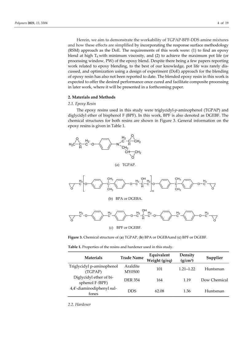
The epoxy resins used  in this study were triglycidyl‐p‐aminophenol (TGPAP) and 

diglycidyl ether of bisphenol F (BPF). In this work, BPF is also denoted as DGEBF. The 

chemical structures  for both  resins are  shown  in Figure 3. General  information on  the 

epoxy resins is given in Table 1. 

O

H2C CH

H2C O N

CH2

H2C C

H

O

CH2

CH CH2

O  

(a) TGPAP. 

O

H2C O C O

H2C C

H

H2C

OH

O C OH2C

OCH3

CH3 CH3

CH3n  

(b) BPA or DGEBA. 

O

H2C O

H2C O

H2C C

H

H2C

OH

OH2C O

H2C

O  

(c) BPF or DGEBF. 

Figure 3. Chemical structure of (a) TGPAP, (b) BPA or DGEBAand (c) BPF or DGEBF. 

Table 1. Properties of the resins and hardener used in this study. 

Materials  Trade Name Equivalent 

Weight (g/eq) 

Density 

(g/cm3) Supplier 

Triglycidyl p‐aminophenol 

(TGPAP) 

Araldite 

MY0500 101  1.21–1.22  Huntsman 

Diglycidyl ether of bi‐

sphenol F (BPF) DER 354  164  1.19  Dow Chemical 

4,4′‐diaminodiphenyl sul‐

fones DDS  62.08  1.36  Huntsman 

2.2. Hardener 

Polymers 2021, 13, 3304  5  of  19  

 

The type of hardener used to cure the blended epoxies in this work was 4,4′‐diamino‐

diphenyl sulfone (DDS). DDS exists in the form of a white powder and is suitable for aer‐

ospace engineering applications. The chemical structure of this hardener is shown in Fig‐

ure 4 [7]. The properties of this hardener are indicated in Table 1. 

S

O

O

H2N NH2

 

Figure 4. Chemical structure of 4, 4′‐diaminodiphenyl sulfone (DDS). 

2.3. Resin Mixtures 

Blending of epoxy resin was carried out using a mechanical stirrer at 2000 rpm for 30 

min in a silicone oil bath, which was heated to around 100 °C. This setup is drawn sche‐

matically in Figure 5. This process produced a miscible transparent mixture with a light‐

yellow color. The blend consisted of TGPAP epoxy, BPF as a diluent, and DDS as hard‐

ener. The amount of diluent (BPF) was obtained from subtraction of 100% TGPAP. The 

quantities of hardeners were determined from stoichiometry calculations using Equations 

(1)–(3), where [ ] refers to concentration, EEW is epoxy equivalent weight, wtTGPAP is the 

weight percentage of TGPAP, and wtBPF is the weight percentage of BPF (or DGEBF) [23]. 

Stoichiometry,𝑋2AmineEpoxy

  (5) 

Epoxy wt

EEW

wtEEW

(6) 

amine stoichiometry wt

EEWwt

EEW (7) 

 

Figure 5. Epoxy blending setup.   

Polymers 2021, 13, 3304  6  of  19  

 

2.4. Design of Experiment 

In this work, two factors were studied. The first was the BPF content (wt.%) in the 

epoxy blend (factor A). The second (factor B) was the stoichiometric ratio (g/g) between 

the amine hardener and epoxy. A DoE approach was carried out using a RSM assisted by 

Design Expert® software version 7.1. An efficient design tool, known as central composite 

design (CCD), was chosen for this study. 

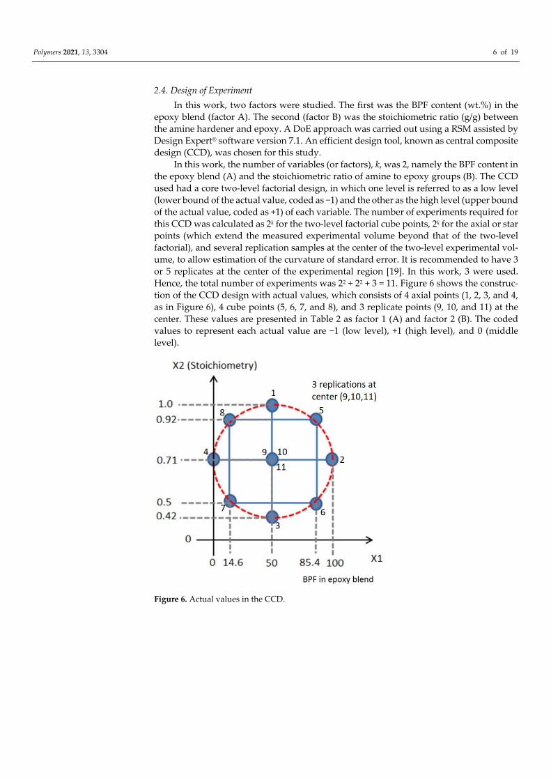
In this work, the number of variables (or factors), k, was 2, namely the BPF content in 

the epoxy blend (A) and the stoichiometric ratio of amine to epoxy groups (B). The CCD 

used had a core two‐level factorial design, in which one level is referred to as a low level 

(lower bound of the actual value, coded as −1) and the other as the high level (upper bound 

of the actual value, coded as +1) of each variable. The number of experiments required for 

this CCD was calculated as 2k for the two‐level factorial cube points, 2k for the axial or star 

points  (which extend  the measured experimental volume beyond  that of  the  two‐level 

factorial), and several replication samples at the center of the two‐level experimental vol‐

ume, to allow estimation of the curvature of standard error. It is recommended to have 3 

or 5 replicates at  the center of  the experimental region  [19].  In  this work, 3 were used. 

Hence, the total number of experiments was 22 + 22 + 3 = 11. Figure 6 shows the construc‐

tion of the CCD design with actual values, which consists of 4 axial points (1, 2, 3, and 4, 

as in Figure 6), 4 cube points (5, 6, 7, and 8), and 3 replicate points (9, 10, and 11) at the 

center. These values are presented in Table 2 as factor 1 (A) and factor 2 (B). The coded 

values  to represent each actual value are  −1  (low  level), +1  (high  level), and 0  (middle 

level). 

 

Figure 6. Actual values in the CCD. 

   

Polymers 2021, 13, 3304  7  of  19  

 

Table 2. Experimental results from the experimental design, n = 3. (Value of glass transition tem‐

perature was measured from the onset of the storage modulus curve). 

Run 

Factor 1  Factor 2  Response 1  Response 2 

A: BPF in BPF/TGPAP 

(wt.%) 

B: Stoichiometry 

Amine:Epoxy (g/g) 

Glass Transition 

Temperature (Tg) 

Processing 

Window (min) 

1  50  1  203.2 ± 1.5  59.6 ± 3.7 

2  100  0.71  141.2 ± 0.6  206.8 ± 2.7 

3  50  0.42  134.5 ± 1.0  203 ± 1.3 

4  0  0.71  239.3 ± 0.8  57.2 ± 3.4 

5  85.4  0.92  183.8 ± 0.2  105.9 ± 2.0 

6  85.4  0.5  86.6 ± 1.0  251.4 ± 3.0 

7  14.6  0.5  224.9 ± 0.2  102.3 ± 1.6 

8  14.6  0.92  226.2 ± 0.5  53.3 ± 7.1 

9  50  0.71  206.4 ± 1.0  100.9 ± 2.2 

10  50  0.71  206.6 ± 0.7  90.7 ± 2.5 

11  50  0.71  206.4 ± 1.0  92.2 ± 2.7 

Each point for an actual value, as indicated in Figure 6, was determined according to 

the location of that point. Axial points (1, 2, 3, and 4) were determined based on the min‐

imum and maximum value of the range of the factor; for example, in factor 1 (A), 0% is 

the minimum value (low level, −1) and 100% is the maximum value (high level, +1) of BPF 

content in BPF/TGPAP content. Cube points (5, 6, 7, and 8) were determined using trigo‐

nometric calculation. Figure 7 shows an example of the calculation to determine the actual 

value of the cube point at point 7. 

 

Figure 7. Cube point (−1, −1) to determine the actual value for (a) X1, and (b) X2. 

From Figure 7a, 𝑋1:  From Figure 7b, 𝑋2: 

Sin 45° 50 𝑋1

50  Sin 45°

0.71 𝑋20.29

 

50 𝑋1 50 sin 45  0.71 𝑋2 0.29 sin 45 50 𝑋1 35.4  0.71 𝑋2 0.21 

𝑋1 50 35.4  𝑋2 0.71 0.21 𝑋1 14.6  𝑋2 0.50 

From the trigonometry calculation, the actual value for the cube point at point 7 with 

a coded value (−1, −1) was (14.6, 0.50), and the values for the other 3 cube points (point 5, 

Polymers 2021, 13, 3304  8  of  19  

 

6, and 8) were determined using the same calculation. The actual values for the 3 replica‐

tion points (9, 10, and 11) with a coded point (0, 0) in CCD were determined as the middle 

value in a range from minimum to maximum of the factor in actual values. For example, 

the actual value for the replication points for factor 1 (A) is 50%, when the range is 0% to 

100% BPF of BPF/TGPAP content. These 11 values are listed in Table 2 as Factor 1 (A) and 

Factor 2 (B). 

2.5. Testing Procedures 

The response from the input factors in this work was Tg and PW (pot life). For curing, 

blended  epoxy  was  poured  into  a  flexible mold made  from  polytetrafluoroethylene 

(PTFE)‐coated fabric and degassed in a vacuum oven to eliminate trapped air at 100 °C 

for ~30 min. The degassed epoxy was then put into a circulating‐air oven and heated fol‐

lowing a cure cycle of 2 h at 130 °C, 2 h at 160 °C, and 2 h at 200 °C, followed by a post 

cure for 5 h at 200 °C. Tg was measured using a dynamic mechanical thermal analyzer 

(DMTA), where the Tg was determined from the onset of storage modulus curves. DMTA 

was performed using a Perkin Elmer 8000 from Perkin Elmer Ltd., Beaconsfield, United 

Kingdom, with a 3‐point bending mode at a frequency of 1 Hz. Rectangular specimens (40 

mm × 10 mm × 3 mm) ± 1 mm were cut using a Benetec sliding cutter. Specimens were 

heated from 30 °C to 300 °C at a rate of 5 °C/min. The curves of E′, E″, and tan δ were 

displayed as a function of temperature using Pyris software (Perkin Elmer). Three repeti‐

tions (n = 3) were performed for each run of experiments, to ensure reproducibility. 

The PW of the epoxy blends was defined as the length of time for which the epoxy 

can retain a viscosity low enough for it to be processed. In this work, the PW was deter‐

mined using rheometer and defined as the time for the epoxy blend to reach a viscosity of 

100 Pa s, as stated in ASTM D 4473‐95 [24]. The rheometer used was Haake MARS (mod‐

ular advanced rheometer system) from Thermo Scientific, Karlsruhe, Germany. Viscosity 

measurements in oscillatory shear mode were carried out by placing the epoxy between 

two parallel plates of 35 mm diameter fitted to the upper measuring head and the fixed 

lower mount. The distance between the plates was then closed to give a 0.5 mm gap, and 

the furnace was closed around the plates. For curing, the specimen was first heated to 80 

°C, at which point measurements began at a 1 Hz oscillation frequency with a controlled 

stress at 2.0 Pa. The temperature was increased further by 10 °C/min until 130 °C and then 

remained constant during curing of the specimen. The value of PW was taken from the 

graph, where the viscosity was 100 Pa.s. At least 3 repetitions were carried for every run 

in the CCD, to ensure reproducibility. 

3. Results 

3.1. Glass Transition Temperature 

The presented values shown in Table 2 indicate the results for both Tg and PW, based 

on BPF content in the epoxy blend and stoichiometric ratio. 

Figure 8 shows the representative storage modulus curve for each sample for all 11 

runs, as listed in Table 2. As mentioned earlier in Section 2.5, Tg was determined from the 

onset of the storage modulus curve. These Tg values are recorded in Table 2 as response 

1. An example of how the onset Tg was determined is presented in Figure 9. 

Polymers 2021, 13, 3304  9  of  19  

 

 

Figure 8. Representative storage modulus curve from DMTA for each run, as listed in Table 2. 

 

Figure 9. Determination of onset Tg from a representative storage modulus curve at 55.6 wt.% BPF 

epoxy blend and stoichiometry ratio = 0.6. 

The effect of BPF content and the stoichiometry ratio on the value of Tg is shown in 

Figure 10. As seen  in the 3D and contour plots of surface response, Tg  increases as the 

amount of TGPAP epoxy increases in the epoxy blend (factor A). For example, at a fixed 

stoichiometry ratio of 0.42, Tg increased by 336% when the TGPAP increased from 12.5% 

to 95% in the epoxy blend (Figure 10b). This is due to the fact that TGPAP has a higher 

functionality compared to a bifunctional epoxy such as BPF, resulting in a greater cross‐

link density. Therefore, a higher Tg was obtained in the epoxy blend with a higher amount 

of TGPAP. 

Polymers 2021, 13, 3304  10  of  19  

 

 

 

Figure 10. Response surface for Tg of BPF/TGPAP/DDS epoxy resins (a) 3D plot and (b) contour 

plot. 

On the other hand, for a fixed amount of BPF in the epoxy blend, as the stoichiometry 

increases (factor B), the Tg increases. For example, at a fixed amount of BPF = 87.50% in 

the epoxy blend, the Tg increased by 200% when the stoichiometry ratio increased from 

0.42 to 0.71 in the epoxy blend (Figure 10b). However, beyond a stoichiometry of 0.71 and 

at a lower amount of BPF in the epoxy blend, the Tg value was observed to decrease. This 

was probably due to an increased number of secondary amines, due to their lower reac‐

tivity and possible steric hindrance possibly not fully reacting with the epoxide groups 

[25]. Thus, an increased amine content may reduce the value of Tg in an epoxy system by 

reducing the crosslink density and increasing the free volume [26]. 

This finding is in agreement with the study by Palmese and Mccullough [27], who re‐

ported a significant effect on the modulus and Tg with a variation in stoichiometry ratio (r). 

They studied the effect of varying the amount of hardener added to DGEBA and showed that 

the highest Tg was obtained at 30 parts per hundred (pph), beyond which the Tg reduced. They 

mentioned  that using  the wrong  stoichiometry  ratio of  curing agent  (either more or  less) 

caused the final structure of cured composites to have a lower crosslinking density, therefore 

lowering the Tg. Guerrero et al. [28] also reported a similar pattern of Tg for epoxy resin cured 

at a different stoichiometry ratio, r, which ranged from 0.3 to 1.0. They found the maximum 

Polymers 2021, 13, 3304  11  of  19  

 

Tg was obtained when r = 0.8–0.9, and decreased thereafter. The following equations are the 

final empirical regression models generated by the Design Expert® software for Tg  in both 

coded and actual factors. Note that in the equation, BPF is the short term used to represent the 

weight of BPF in the total weight in the epoxy blend. 

𝐶𝑜𝑑𝑒𝑑 𝐹𝑎𝑐𝑡𝑜𝑟 226.53 – 18.61𝐴 10.95𝐵 14.39𝐴𝐵 – 2.84𝐴 – 18.66𝐵   (8) 

𝐴𝑐𝑡𝑢𝑎𝑙 𝐹𝑎𝑐𝑡𝑜𝑟 56.01 – 2.85 ∗ 𝐵𝑃𝐹 584.26 ∗ 𝑆𝑡𝑜𝑖𝑐ℎ𝑖𝑜𝑚𝑒𝑡𝑟𝑦 3.31 ∗ 𝐵𝑃𝐹 ∗ 𝑆𝑡𝑜𝑖𝑐ℎ𝑖𝑜𝑚𝑒𝑡𝑟𝑦 – 0.0063 ∗ 𝐵𝑃𝐹 – 443.72 ∗ 𝑆𝑡𝑜𝑖𝑐ℎ𝑖𝑜𝑚𝑒

(9) 

The relative impact of each factor (A and B) to response 1 (Tg) can be identified by 

observing each factor coefficient. The coefficient as indicated in Equation (8) for the coded 

factor represents the expected change in response 1 (Tg) per unit change of each factor (A 

and B). For Equation (8) of the coded factor, A and B are the main effects, AB is the two‐

level interaction effect, and A2 and B2 are the second order effects. According to the re‐

gression model generated using Design Expert® software,  the  two‐level  interaction be‐

tween BPF content in the epoxy blend (A) and stoichiometry (B) is the most significant 

factor associated with the Tg. This interaction produces the highest value of coefficient, of 

+14.39 of the coded value [29]. In addition, note that the contours are curved as the model 

contains a strong interaction term. In contrast, the equation for the actual factor (Equation 

(9)) is used to make predictions about the actual value of response 1 (Tg) for given actual 

values of each factor (A and B). This means that the value for each factor for Equation (9) 

should be specified in the actual values. The response (Tg) and factors (A and B), as indi‐

cated in the 3D plot and contour plot in Figure 8, are based on a prediction from the model 

in Equation (9) for actual factors. Unlike Equation (8), Equation (9) should not be used to 

compare the relative impact of each factor, since the coefficients in this equation are scaled 

to accommodate the units of each factor and the intercept is not at the center of the design 

space [30]. The values shown  in the 3D plot (Figure 10a) and contour plot (Figure 10b) 

exhibited the actual values as modeled by Equation (9) (actual factor). 

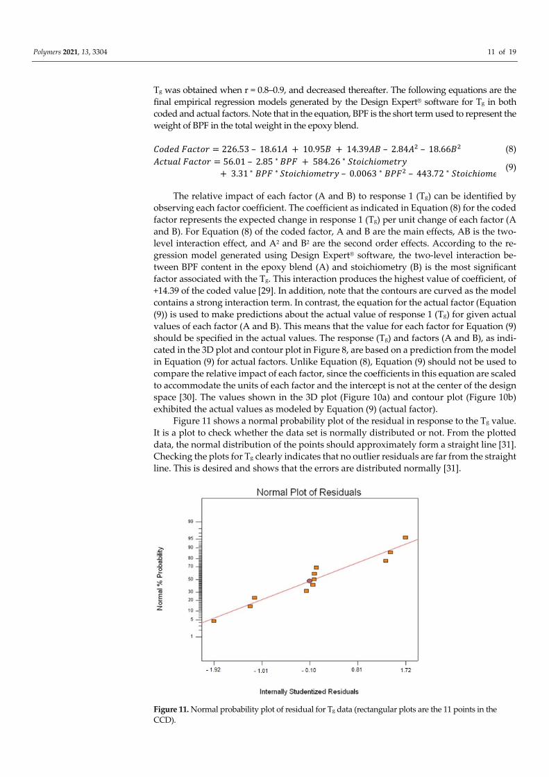
Figure 11 shows a normal probability plot of the residual in response to the Tg value. 

It is a plot to check whether the data set is normally distributed or not. From the plotted 

data, the normal distribution of the points should approximately form a straight line [31]. 

Checking the plots for Tg clearly indicates that no outlier residuals are far from the straight 

line. This is desired and shows that the errors are distributed normally [31]. 

 

Figure 11. Normal probability plot of residual for Tg data (rectangular plots are the 11 points in the 

CCD). 

Polymers 2021, 13, 3304  12  of  19  

 

A summary of the test for Tg is presented in Table 3. The confidence level, denoted 

as P, is usually selected at 95% [32]. The value of “P > F” in Table 3 for the model is less 

than 0.05 and suggests that the model is significant. Similarly, all other model terms are 

significant since the “prob > F” for each of these terms is also less than 0.05. Therefore, 

model reduction is not required. 

Table 3. ANOVA table for the surface response quadratic model (response: Tg). 

Source Sum of 

Squares df 

Mean 

Square F Value 

p‐Value 

(Prob > F) 

Model  21,837.58  5  4367.52  97.95  <0.0001 (Significant) 

A‐BPF in BPF/TGPAP  2730.24  1  2730.24  61.23  0.0005 

B‐Stoichiometry  580.89  1  580.89  13.03  0.0154 

AB  2296.01  1  2296.01  51.49  0.0008 

A2  353.05  1  353.05  7.92  0.0374 

B2  1960.37  1  1960.37  43.96  0.0012 

Residual  222.92  5  44.59     

Std. Dev.  6.68  R2  0.9899     

Mean  187.19  Adj. R2  0.9798     

C. V. %  3.57  Pred R2  0.9281     

PRESS  1585.26  Adeq. Precision  31.541     

As mentioned previously, different amounts of TGPAP in the epoxy blend affect the 

Tg of the cured epoxy blend, due to the different functionality. In addition, as was dis‐

cussed earlier, different amounts of amine hardener being added to the blended epoxy 

also produce a significant effect on the Tg  [27]. Both factors A and B have a significant 

effect on the Tg, and hence both the two‐level interaction (AB) and the second‐order effect 

are also significant. The coefficient of determination R2 value was high, close to 1, which 

is desirable. Adequate precision measures  the signal‐to‐noise  ratio, and a  ratio greater 

than four is desirable [33,34]. For this model, the value of adequate precision was 31.541, 

indicating an adequate signal [31]. 

3.2. Pot Life (Processing Window, PW) 

In this work, the PW was defined as the length of time until the viscosity of an epoxy 

blend increases and reaches 100 Pa s. Again, Table 2 shows the experimental results for 

the PW (response 2) and Figure 12 shows an example of the viscosity profiles recorded for 

two epoxy systems (at the same stoichiometric ratio of 0.60) for measuring the PW. The 

behavior of the epoxy resin during the measurement can be explained as follows. At the 

start of the experiment, the temperature of the rheometer was set at 80 °C. The initial vis‐

cosity of neat TGPAP epoxy (~0.100 Pa s) was higher than the formulated epoxy blend 

(~0.080 Pa s), due to the addition of a lower viscosity BPF to the blended epoxy. After 10 

min at 80 °C, the temperature of the furnace was raised to 130 °C, and the viscosity of the 

resin was seen to decrease. This is a normal behavior of a liquid, where higher tempera‐

ture will cause viscosity to decrease. The minimum viscosity recorded for both profiles 

was approximately 0.010 Pa s. As the temperature was raised and maintained at 130 °C, 

the viscosity profile increased due to network formation (crosslinking) and finally reached 

a plateau, suggesting the system was completely vitrified. In this work, the PW was taken 

as the time at which the viscosity of the resin reached 100 Pa s, following ASTM D4473–

95a, standard test method for plastics: dynamic mechanical properties, cure behavior [24]. 

Polymers 2021, 13, 3304  13  of  19  

 

 

Figure 12. Representative isothermal complex viscosity profile for measuring the PW for curing of 

neat TGPAP (PW ≈ 97 min) and a 55.6 wt.% BPF in epoxy blend (PW ≈ 140 min). 

Figure 13a,b show the 3D plots and contour plot of the response surface of the PW 

for the interaction between factor A (BPF in epoxy blend) and factor B (stoichiometry ra‐

tio).  It can be seen  from Figure 13  that a higher BPF  (less TGPAP)  in  the epoxy blend 

resulted in a longer time for the resin to reach 100 Pa s. For example, at a fixed stoichiom‐

etry ratio of 0.42, the PW increased by 59% when the BPF increased from 12.5% to 52% in 

the  epoxy  blend  (Figure  13b). This means more  time will  be  available  to  process  the 

blended epoxy; for example, during the fabrication and manufacturing of composites. As 

mentioned previously, TGPAP’s nominal functionality of 3 is higher than that of the bi‐

functional BPF. Therefore, as expected, a higher amount of TGPAP in the epoxy blend will 

reduce the PW due to the system reaching the gelation level earlier [35]. 

 

Polymers 2021, 13, 3304  14  of  19  

 

 

Figure 13. Response surface for PW of BPF/TGPAP/DDS epoxy blend resins (a) 3D plot, and (b) 

contour plot. 

Small increases in PW are observed towards the end of the area in the top‐left corner 

of the response plot in Figure 13a,b. The formation of this contour, which shows a small 

increase in PW in that area, was probably influenced by the value of PW obtained for that 

point (14.6, 0.92). This result could be due to experimental error, as indicated by the error 

value (standard deviation), which is anomalous. During experiments, the control temper‐

ature of the rheometer furnace was within a range of ± 10 °C. The fluctuation in control 

temperature within this range could possibly affect the rate of crosslinking and influence 

the value of PW for each test with the same sample, which would finally affect the average 

value. In addition, to minimize the errors in future, it is recommended that the three re‐

peats of the test for each sample should be performed at the closest possible time to each 

other. Otherwise, a reaction between epoxy and amine could possibly occur if the epoxy 

blend was left unused, even if the sample was placed in the freezer. This could possibly 

result in crosslinking prior to the experiment, which would affect the measured values of 

the processing window. 

The following equations are the final empirical regression models generated by the 

Design Expert® software for PW in both coded and actual factors: 

𝐶𝑜𝑑𝑒𝑑 𝐹𝑎𝑐𝑡𝑜𝑟 71.08 18.87𝐴 36.03𝐵 14.47𝐴𝐵 6.43𝐴 17.49𝐵   (10) 

𝐴𝑐𝑡𝑢𝑎𝑙 𝐹𝑎𝑐𝑡𝑜𝑟 320.84 2.39 ∗ 𝐵𝑃𝐹 666.59 ∗ 𝑆𝑡𝑜𝑖𝑐ℎ𝑖𝑜𝑚𝑒𝑡𝑟𝑦 3.33 ∗ 𝐵𝑃𝐹 ∗ 𝑆𝑡𝑜𝑖𝑐ℎ𝑖𝑜𝑚𝑒𝑡𝑟𝑦 0.0143 ∗ 𝐵𝑃𝐹 415.99 ∗ 𝑆𝑡𝑜𝑖𝑐ℎ𝑖𝑜𝑚𝑒𝑡𝑟𝑦  

(11) 

From the regression model, the most significant factor is the level of BPF in the epoxy 

blend at a coefficient of +18.87. The same explanation for Equations (8) and (9) of coded 

and actual factors for response 1 (Tg) applies here for the explanation of Equations (10) 

and (11) for response 2 (PW). 

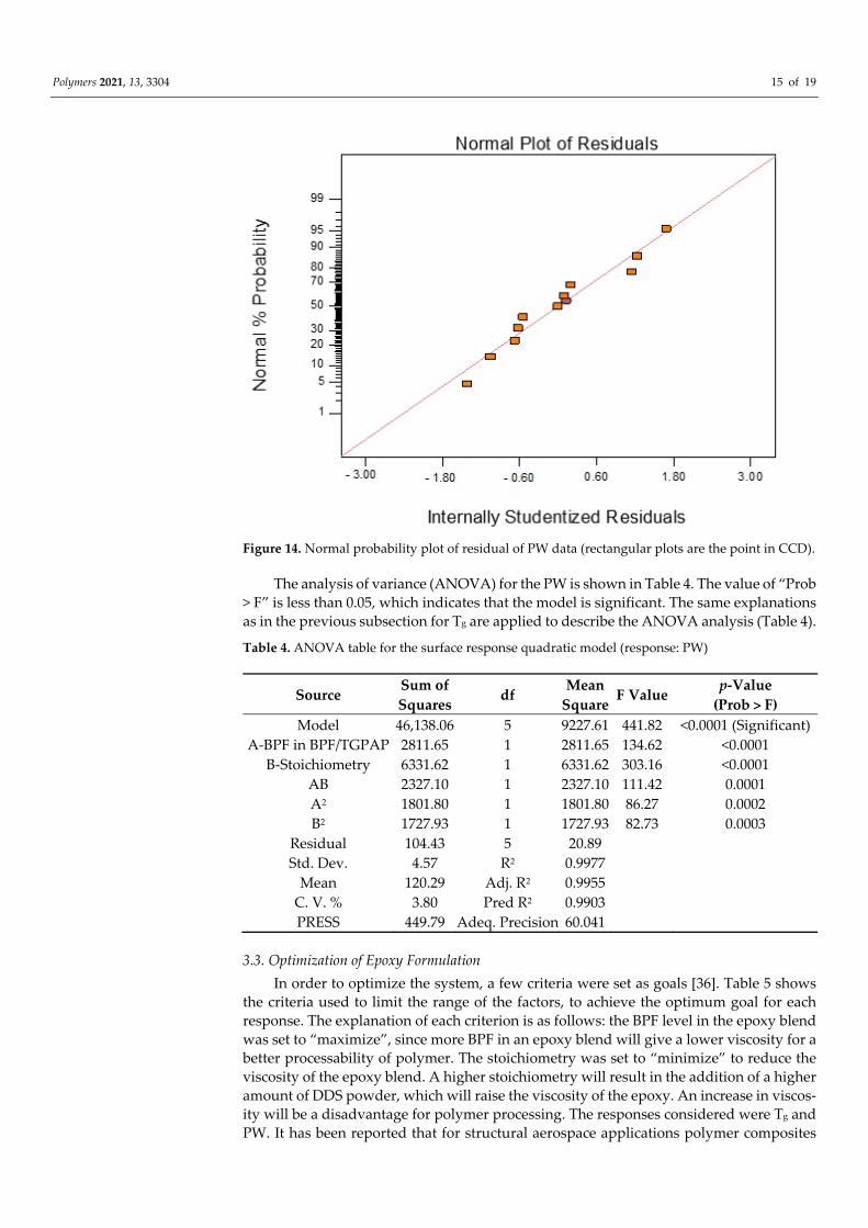
Figure 14 shows the normal probability plot of the residual in response to changes in 

the PW. As explained previously for the Tg response, similarly for the case of PW, it can 

be observed that all normal plots for PW are scattered around the straight line, which is 

desirable and illustrates that the distribution of errors is normal [31]. 

Polymers 2021, 13, 3304  15  of  19  

 

 

Figure 14. Normal probability plot of residual of PW data (rectangular plots are the point in CCD). 

The analysis of variance (ANOVA) for the PW is shown in Table 4. The value of “Prob 

> F” is less than 0.05, which indicates that the model is significant. The same explanations 

as in the previous subsection for Tg are applied to describe the ANOVA analysis (Table 4). 

Table 4. ANOVA table for the surface response quadratic model (response: PW) 

Source Sum of 

Squares df 

Mean 

Square F Value 

p‐Value 

(Prob > F) 

Model  46,138.06  5  9227.61  441.82  <0.0001 (Significant) 

A‐BPF in BPF/TGPAP  2811.65  1  2811.65  134.62  <0.0001 

B‐Stoichiometry  6331.62  1  6331.62  303.16  <0.0001 

AB  2327.10  1  2327.10  111.42  0.0001 

A2  1801.80  1  1801.80  86.27  0.0002 

B2  1727.93  1  1727.93  82.73  0.0003 

Residual  104.43  5  20.89     

Std. Dev.  4.57  R2  0.9977     

Mean  120.29  Adj. R2  0.9955     

C. V. %  3.80  Pred R2  0.9903     

PRESS  449.79  Adeq. Precision  60.041     

3.3. Optimization of Epoxy Formulation 

In order to optimize the system, a few criteria were set as goals [36]. Table 5 shows 

the criteria used to limit the range of the factors, to achieve the optimum goal for each 

response. The explanation of each criterion is as follows: the BPF level in the epoxy blend 

was set to “maximize”, since more BPF in an epoxy blend will give a lower viscosity for a 

better processability of polymer. The stoichiometry was set to “minimize” to reduce the 

viscosity of the epoxy blend. A higher stoichiometry will result in the addition of a higher 

amount of DDS powder, which will raise the viscosity of the epoxy. An increase in viscos‐

ity will be a disadvantage for polymer processing. The responses considered were Tg and 

PW. It has been reported that for structural aerospace applications polymer composites 

Polymers 2021, 13, 3304  16  of  19  

 

should have a Tg value of at  least 180 °C, due to high temperature applications during 

service [37]. Therefore, the Tg was set to a range between 180 and 185 °C for the optimiza‐

tion. Finally,  the PW was set  to be “maximize”, as  the epoxy resin system needs  to be 

processed before it starts to cure and its viscosity increases significantly. The importance 

column (as shown in Table 5) and * symbol reflect the priority of achieving optimization 

[38]. 

Table 5. Criteria for epoxy blend optimization (a greater number of * indicate that a higher 

importance was placed on that particular response or factor). 

Factor/Response  Goal  Lower Limit  Upper Limit  Importance 

BPF in BPF/TGPAP    Maximize  0  100  **** 

Stoichiometry  Minimize  0.42  1  *** 

Tg infinity  Is in range  180  185  ***** 

Processing window  Maximize  53.28  251.4  ***** 

Optimization targeting the maximum goal yielded nine suggested solutions for the 

epoxy formulation. However, the epoxy formulation with the highest desirability was se‐

lected.  In Design Expert® software,  the desirability chart can be viewed  in  two modes. 

First, in a ramp mode, as shown in Figure 15a. The view of the desirability chart in ramp 

mode will indicate the individual elements for easier interpretation, predicted in actual 

values. Each ramp in Figure 15a shows a point which reflects the optimum value for fac‐

tors and responses for that solution. The criteria, which were set as in Table 5, to achieve 

the optimum response yielded the factor value at 55.6% of BPF in the epoxy blend (factor 

A) and a stoichiometry of 0.60 (factor B). Both values are predicted to give Tg at 180 °C 

and PW at 136.1 min (Figure 15a). Second, the desirability value can be viewed in histo‐

gram chart (Figure 15b). This form of graph indicates how well each variable satisfied the 

criteria, with values near to 1 being good. The desirability for each factor and responses 

were also  indicated, as  in Figure 15b.  In  this work,  the combined desirability was pre‐

dicted using Design Expert® at a value of 0.520. A verification test was carried out, which 

gave a Tg at 181.2 ± 0.8 °C (as in Figure 9), which is close to the predicted value (180 °C in 

Figure 15a). For PW, the verification run gave a PW of ≈140 min (as  in Figure 12). The 

discrepancy between the verification test and predicted value (136.1 min as in Figure 15a) 

for PW could have been associated with the range of the control temperature in the fur‐

nace, which was within ±10 °C. As explained previously, a fluctuating temperature within 

this range could have affected the test result. 

 

Polymers 2021, 13, 3304  17  of  19  

 

 

Figure 15. Desirability chart in (a) ramp mode of factors for optimum responses of the epoxy 

blend, and (b) histogram chart with factors and predicted responses. 

4. Conclusions 

An optimum formulation for a epoxy blend of TGPAP and BPF, with the respective 

stoichiometry ratio (r), was determined  in this work using RSM. The Tg and PW of the 

blended epoxy were studied in this work, with the target response being to achieve a resin 

with high Tg and maximum PW. The result indicates that optimization can be achieved at 

55.6 wt.% of BPF and a stoichiometric ratio of 0.60, giving the predicted values of 180 °C 

for Tg and 136.1 min for PW. These values were verified, which produced a Tg of 181.2 ± 

0.8 °C and ~140 min for PW. The optimized epoxy blends obtained in this work will be 

carried forward to the next phase in our study, which will be presented in a forthcoming 

paper. 

Author Contributions: Conceptualization, R.J. and A.N.W.; methodology, R.J.; software, R.J. and 

J.A.R.; validation, A.N.W. and J.A.R.; formal analysis, R.J. and A.N.W.; investigation, R.J.; resources, 

N.A.E. and A.N.W.; writing—original draft preparation, R.J.; writing—review and editing,  J.P.S. 

and J.A.R.; supervision, A.N.W.; funding acquisition, N.A.E. All authors have read and agreed to 

the published version of the manuscript. 

Funding: This research was  funded by Ministry of Higher Education Malaysia  (MoHE)  through 

Research Management Center, Universiti Putra Malaysia (UPM) and Universiti Malaysia Pahang 

(UMP), under the internal grant number RDU190324. 

Institutional Review Board Statement: Not applicable. 

Informed Consent Statement: Not applicable. 

Data Availability Statement: Data are contained within the article. 

Acknowledgments:  Authors would  like  to  thank  the Ministry  of  Higher  Education Malaysia 

(MoHE), through Universiti Malaysia Pahang (UMP) and Universiti Putra Malaysia (UPM), for the 

awarded internal grant RDU190324 and other financial support for the study. 

Conflicts of Interest: The authors declare no conflict of interest. 

References 

1. Noor, N.; Razak, J.; Ismail, S.; Mohamad, N.; Junid, R. Review on Carbon Nanotube based Polymer Composites and Its Appli‐

cations. J. Adv. Manuf. Technol. 2018, 12, 311–326. 

2. Bakar, N.A.; Zulkarnain, M.A.; Hassan, W.A.W.; Junid, R.; Razak, J.A.; Ismail, M.M. The effect of graphite flakes (GFs) and 

hybrid graphene nanoplatelets (GNPs) particles to the mechanical properties of epoxy composites. In Proceedings of the IOP 

Conference Series: Materials Science and Engineering; IOP Publishing Ltd, 2020; Vol. 957, p. 012033. 

3. Ramli, J.; Jeefferie, A.R.; Mahat, M.M. Effects of uv curing exposure time to the mechanical And physical properties of the epoxy 

and vinyl ester Fiber glass laminates composites. ARPN J. Eng. Appl. Sci. 2011, 6. 

Polymers 2021, 13, 3304  18  of  19  

 

4. Hadi, A.E.; Hamdan, M.H.M.; Siregar, J.P.; Junid, R.; Tezara, C.; Irawan, A.P.; Fitriyana, D.F.; Rihayat, T. Application of Micro‐

mechanical Modelling  for  the Evaluation of Elastic Moduli of Hybrid Woven  Jute–Ramie Reinforced Unsaturated Polyester 

Composites. Polym. 2021, Vol. 13, Page 2572 2021, 13, 2572, doi:10.3390/Polym13152572. 

5. Barde, Y.D.; Ramezanian, N.; Nazif, A.; Behzadpour, M. Effect of Different Diluents on the Main Properties of the Epoxy‐Based 

Composite. J. Mater. Sci. Appl. 2020, 4, 1–9, doi:10.17303/JMSA.2020.4.104. 

6. Penn, L.S.; Wang, H. Epoxy Resins. In Handbook of Composites; Springer US, 1998; pp. 48–74 ISBN 978‐1‐4615‐6389‐1. 

7. Pham,  H.Q.;  Marks,  M.J.  Epoxy  resins.  Ullmann’s  Encycl.  Ind.  Chem.  2012,  156–238, 

doi:https://doi.org/10.1002/14356007.a09_547.pub2. 

8. Gibson, G. Epoxy Resins. In Brydson’s Plastics Materials: Eighth Edition; Gilbert, M., Ed.; Butterworth‐Heinemann Elsevier, 

2017; pp. 773–797 ISBN 9780323370226. 

9. Varma,  I.K.;  Gupta,  V.B.;  Sini,  N.K.  2.19  Thermosetting  Resin  –  Properties.  Compr.  Compos.  Mater.  II  2018,  401–468, 

doi:10.1016/B978‐0‐12‐803581‐8.03829‐7. 

10. Ozeren Ozgul, E.; Ozkul, M.H. Effects of epoxy, hardener, and diluent types on  the workability of epoxy mixtures. Constr. 

Build. Mater. 2018, 158, 369–377, doi:10.1016/J.Conbuildmat.2017.10.008. 

11. Qian, J.W.; Miao, Y.M.; Zhang, L.; Chen, H.L. Influence of viscosity slope coefficient of CA and its blends in dilute solutions on 

permeation flux of their films for MeOH/MTBE mixture. J. Memb. Sci. 2002, 203, 167–173, doi:10.1016/S0376‐7388(02)00004‐2. 

12. Montserrat, S.; Andreu, G.; Corts, P.; Calventus, Y.; Colomer, P.; Hutchinson, J.M.; Malek, J. Addition of a reactive diluent to a 

catalyzed  epoxy‐anhydride  system.  I.  Influence  on  the  cure  kinetics.  J.  Appl.  Polym.  Sci.  1996,  61,  1663–1674, 

doi:10.1002/(SICI)1097‐4628(19960906)61:10<1663::AID‐APP6>3.0.CO;2‐E. 

13. Nikolic, G.; Zlatkovic, S.; Cakic, M.; Cakic, S.; Lacnjevac, C.; Rajic, Z. Fast Fourier Transform IR Characterization of Epoxy GY 

Systems  Crosslinked  with  Aliphatic  and  Cycloaliphatic  EH  Polyamine  Adducts.  Sensors  2010,  10,  684–696, 

doi:10.3390/s100100684. 

14. Otter, C.; Stephenson, K. Amines and Amides. In Salters Advanced Chemistry: Chemical Ideas; Heinemann, 2008; p. 320. 

15. Everitt, D.T.; Luterbacher, R.; Coope, T.S.; Trask, R.S.; Wass, D.F.; Bond, I.P. Optimisation of epoxy blends for use in extrinsic 

self‐healing fibre‐reinforced composites. Polymer. 2015, 69, 283–292, doi:10.1016/J.Polymer.2015.02.047. 

16. Frank, K.; Childers, C.; Dutta, D.; Gidley, D.; Jackson, M.; Ward, S.; Maskell, R.; Wiggins, J. Fluid uptake behavior of multifunc‐

tional epoxy blends. Polymer. 2013, 54, 403–410, doi:10.1016/J.Polymer.2012.11.065. 

17. Mason, R.; Gunst, R.; Hess, J. Statistical design and analysis of experiments with applications to engineering and science; 2nd 

ed.; John wiley & sons: New york, 2003. 

18. Mehmood, T.; Ramzan, M.; Howari, F.; Kadry, S.; Chu, Y.‐M. Application of response surface methodology on the nanofluid 

flow over a rotating disk with autocatalytic chemical reaction and entropy generation optimization. Sci. Reports 2021 111 2021, 

11, 1–18, doi:10.1038/s41598‐021‐81755‐x. 

19. Montgomery, D.C. Design and analysis of experiments; 6th ed.; Wiley international edition, 2005. 

20. Kasina, M.M.; Joseph, K.; John, M.; Kasina, M.M.; Joseph, K.; John, M. Application of Central Composite Design to Optimize 

Spawns Propagation. Open J. Optim. 2020, 9, 47–70, doi:10.4236/OJOP.2020.93005. 

21. Guo, J.L.; Guo, W.Y.; Xie, R.J.; Li, Y.M.; Yang, Y.B. Influence of the Additives on the Workability and Mechanic Properties of 

Epoxy Mortar. Adv. Mater. Res. 2010, 168–170, 2003–2007, doi:10.4028/www.scientific.net/AMR.168‐170.2003. 

22. Harani, H.; Fellahi, S.; Bakar, M. Toughening of epoxy resin using hydroxyl‐terminated polyesters. J. Appl. Polym. Sci. 1999, 

71, 29–38, doi:10.1002/(SICI)1097‐4628(19990103)71:1<29::AID‐APP5>3.0.CO;2‐7. 

23. Plastics,  D.  Epoxy  Resin  Available  online:  http://nmt.edu/academics/mtls/faculty/mccoy/docs2/chemis‐

try/DowEpoxyResins.pdf (accessed on Sep 24, 2021). 

24. ASTM standard D4473 ‐ 95a Standard Test Method for Plastics: Dynamic Mechanical Properties: Cure Behavior, ASTM Inter‐

national; West Conshohocken, PA, 2001. 

25. Gude, M.R.; Prolongo, S.G.; Ureña, A. Effect of  the epoxy/amine stoichiometry on  the properties of carbon nanotube/epoxy 

composites. J. Therm. Anal. Calorim. 2011, 108, 717–723, doi:10.1007/s10973‐011‐2056‐x. 

26. Calventus, Y.; Montserrat, S.; Hutchinson, J.M. Enthalpy relaxation of non‐stoichiometric epoxy‐amine resins. Polymer. 2001, 

42, 7081–7093, doi:10.1016/S0032‐3861(01)00133‐1. 

27. Palmese, G.R.; McCullough, R.L. Effect of epoxy–amine stoichiometry on cured resin material properties. J. Appl. Polym. Sci. 

1992, 46, 1863–1873, doi:10.1002/app.1992.070461018. 

28. Guerrero, P.; De  la Caba, K.; Valea, A.; Corcuera, M.A.; Mondragon, I. Influence of cure schedule and stoichiometry on the 

dynamic  mechanical  behaviour  of  tetrafunctional  epoxy  resins  cured  with  anhydrides.  Polymer.  1996,  37,  2195–2200, 

doi:10.1016/0032‐3861(96)85865‐4. 

29. Mohamad, N. Development of epoxidised natural rubber‐alumina composites (ENRAN) for the absorption of ballistic impact 

energy in body armour, National university of Malaysia, 2011. 

30. Response Surface Available online: https://www.statease.com/docs/v11/tutorials/multifactor‐rsm/ (accessed on Sep 14, 2021). 

31. Noordin, M.Y.; Venkatesh, V.C.; Sharif, S.; Elting, S.; Abdullah, A. Application of response surface methodology in describing 

the performance of coated carbide tools when turning AISI 1045 steel. J. Mater. Process. Technol. 2004, 145, 46–58. 

32. Du Prel, J.B.; Hommel, G.; Röhrig, B.; Blettner, M. Confidence interval or p‐value?: Part 4 of a series on evaluation of scientific 

publications. Dtsch. Arztebl. Int. 2009, 106, 335–339, doi:10.3238/arztebl.2009.0335. 

Polymers 2021, 13, 3304  19  of  19  

 

33. Norhazimah, A.H.; Faizal, C.K.M. Optimization Study on Bioethanol Production from the Fermentation of Oil Palm Trunk Sap 

as Agricultural Waste. In Developments in Sustainable Chemical and Bioprocess Technology; Springer, 2013; pp. 19–25. 

34. Korbahti, B.K. Optimization of Electrochemical Oxidation of Textile Dye Wastewater Using Response Surface Methodology 

(RSM). In Survival and Sustainability; Springer, 2011; pp. 1181–1191. 

35. Capricho,  J.C.;  Fox,  B.;  Hameed,  N.  Multifunctionality  in  Epoxy  Resins.  Polym.  Rev.  2020,  60,  1–41, 

doi:10.1080/15583724.2019.1650063/format/epub/epub/xhtml/index.xhtml. 

36. Razak, J.A.; Ahmad, S.H.; Ratnam, C.T.; Mahamood, M.A.; Yaakub, J.; Mohamad, N. Effects of EPDM‐ g ‐MAH compatibilizer 

and internal mixer processing parameters on the properties of NR/EPDM blends: An analysis using response surface method‐

ology. J. Appl. Polym. Sci. 2015, 132, 1–15, doi:10.1002/app.42199. 

37. Stein, J. Toughening of Highly Crosslinked Epoxy Resin Systems, PhD Thesis, The University of Manchester, Manchester, UK, 

2013. 

38. Design‐Expert  7.1  User’s  Guide.  Mixture  Design  Tutorial  (Part  2  ‐  Optimization)  Available  online:  https://www.state‐

ase.com/docs/v11/tutorials/mixture‐designs‐2/ (accessed on Sep 25, 2021).