Optimization of an independent component analysis approach for artifact

identification and removal in magnetoencephalographic signals

Giulia Barbatia,*, Camillo Porcaroa, Filippo Zappasodib,Paolo Maria Rossinia,c, Franca Tecchioa,b

aDepartment of Neuroscience, AFaR – Center of Medical Statistics and Information Technology, Fatebenefratelli Hospital,

Isola Tiberina, Lungotevere degli Anguillara 12, 00153 Rome, ItalybISTC Institute of Science and Technologies of Cognition, CNR, Rome, Italy

cNeurologia Clinica, Universita Campus Biomedico, Rome, Italy

Accepted 15 December 2003

Abstract

Objective: To propose a noise reduction procedure for magnetoencephalography (MEG) signals introducing an automatic detection

system of artifactual components (ICs) separated by an independent component analysis (ICA) algorithm, and a control cycle on

reconstructed cleaned data to recovery part of non-artifactual signals possibly lost by the blind mechanism.

Methods: The procedure consisted of three main steps: (1) ICA for blind source separation (BSS); (2) automatic detection method of

artifactual components, based on statistical and spectral ICs characteristics; (3) control cycle on ‘discrepancy,’ i.e. on the difference between

original data and those reconstructed using only ICs automatically retained. Simulated data were generated as representative mixtures of

some common brain frequencies, a source of internal Gaussian noise, power line interference, and two real artifacts (electrocardiogram ¼

ECG, electrooculogram ¼ EOG), with the adjunction of a matrix of Gaussian external noise. Three real data samples were chosen as

representative of spontaneous noisy MEG data.

Results: In simulated data the proposed set of markers selected three components corresponding to ECG, EOG and the Gaussian internal

noise; in real-data examples, the automatic detection system showed a satisfactory performance in detecting artifactual ICs. ‘Discrepancy’

control cycle was redundant in simulated data, as expected, but it was a significant amelioration in two of the three real-data cases.

Conclusions: The proposed automatic detection approach represents a suitable strengthening and simplification of pre-processing data

analyses. The proposed ‘discrepancy’ evaluation, after automatic pruning, seems to be a suitable way to render negligible the risk of loose

non-artifactual activity when applying BSS methods to real data.

Significance: The present noise reduction procedure, including ICA separation phase, automatic artifactual ICs selection and

‘discrepancy’ control cycle, showed good performances both on simulated and real MEG data. Moreover, application to real signals suggests

the procedure to be able to separate different cerebral activity sources, even if characterized by very similar frequency contents.

q 2004 International Federation of Clinical Neurophysiology. Published by Elsevier Ireland Ltd. All rights reserved.

Keywords: Independent component analysis; Blind source separation; Automatic detection; Discrepancy

1. Introduction

When studying the cerebral activity through neuro-

physiological techniques, such as electroencephalography

(EEG) and magnetoencephalography (MEG), the main goal

is the discrimination of different sources of electrical

activity. The first step in this direction is to separate

the ‘cerebral’ sources from ‘the others’ generated by

non-cerebral sources, these latter often of such intensities

that the former ones are hidden (Zappasodi et al., 2001).

Typically, a MEG sensor measures the mixture of original

source signals with an adjunctive noise (Del Gratta et al.,

2001). This mixture comes from both the ‘wanted’ sources

and those ‘to be discharged’ (called artifacts).

Independent component analysis (ICA) is a promising

approach that can be useful for the elimination of artifacts

and noise from biomedical signals. Since the pioneering

work of Scott Makeig and collaborators (Makeig et al.,

1996) it is generally accepted that ICA is a good tool for

Clinical Neurophysiology 115 (2004) 1220–1232

www.elsevier.com/locate/clinph

1388-2457/$30.00 q 2004 International Federation of Clinical Neurophysiology. Published by Elsevier Ireland Ltd. All rights reserved.

doi:10.1016/j.clinph.2003.12.015

* Corresponding author. Tel.: þ39-06-683-7300; fax: þ39-06-683-7360.

E-mail address: giulia.barbati@afar.it (G. Barbati).

isolating artifacts in EEG and MEG data (Delorme and

Makeig, in press; Vigario et al., 1997; Ziehe et al., 2000,

2001; Cao et al., 2000), but not much has still been

achieved, except for the EEG recordings (Vorobyov and

Cichocki, 2002; Delorme et al., 2001), about the criteria for

selecting artifactual components in practical ICA appli-

cations. The aim of this study is to present an automatic

detection procedure that can assist researchers in classifying

the obtained independent components (ICs) as cerebral or

non-cerebral (artifacts and noise) sources based on IC

statistical properties (kurtosis, entropy) and spectral charac-

teristics (Power Spectrum Density ¼ PSD).

Moreover, the present method allows better signal

reconstruction, i.e. the retro-projection of the automatically

retained ICs: the difference between the original recorded

data and the reconstructed ones is computed and called

‘discrepancy.’ Whenever a non-artifactual part of discre-

pancy is identified on the basis of its spectral characteristics,

it is added to the reconstructed signal.

Section 2 describes the signal-generating model and each

step of the proposed blind noise-reduction procedure;

Section 2.1 makes some considerations about mathematical

ICA assumptions in a MEG data context and presents the

ICA algorithm used; Section 2.2 details the automatic

detection method based on statistical and spectral com-

ponent characteristics. Section 2.3 presents simulated and

real data chosen to test the effectiveness and coherence of

the proposed method. In Section 3 the results of each step of

the procedure are provided. Finally, in Section 4, the

significance of the results is discussed.

2. Model and procedure

We assume that the set of the observed MEG signals is

generated by a mixing noisy model:

x tð Þ ¼ As tð Þ þ v tð Þ ð1Þ

where t ¼ 0; 1; 2; :::; T is the discrete sampling time;

x�t�¼

�x1

�t�; :::; xn

�t��T

is a n-dimensional vector of

the observed noisy signal recorded by n sensors; A is a

n £ m unknown full-rank mixing matrix; s�t�¼�

s1

�t�; :::; sm

�t��T

is a m-dimensional unknown vector of

primary sources (n $ m); v�t�

is a n-dimensional unknown

vector of additive external spatially uncorrelated Gaussian

noise that represents instrumental noise, as shown in Fig. 1a.

Furthermore, we assume that the vector s�t�

contains a

subset of useful or non-artifactual sources (brain activity)

and artifactual sources (e.g. heartbeat, eye blinks, ocular

movements, etc.) and that s�t�

is not correlated with external

noise; our objective is to reduce the influence of additive

noise v�t�

and to eliminate artifacts.

In other words, our task is to obtain corrected or

‘cleaned’ sensor signals which contain only ‘interesting’

(non-artifactual) sources. Sensor signals are processed by an

ICA demixing system that is described by the following

general model:

y tð Þ ¼ Wx tð Þ ð2Þ

where y�t�¼

�y1

�t�; :::; ym

�t��T

is an m-dimensional vector of

the estimated ICs and W is a separation matrix, i.e. the

estimate of the unknown mixing matrix A:

W ¼ Aþ ð3Þ

where the apex ‘ þ ’ denotes the inverse matrix. The outputs

of the ICA demixing system pass through an automatic

‘detection system’ which takes the binary decision {0,1},

that is, to reject or to retain the corresponding IC.

Then, the retained ICs denoted as yk (k # m) pass

through the inverse system represented by the inverse W1

of the estimated separation matrix so to reconstruct data:

xpRec ¼ Wþ

k yk ð4Þ

where the apex p stresses that a part of the original signals

could be not explained by the selected ICs and Wþk denotes

the corresponding selected k columns of W1. We then

define discrepancy as:

d ¼ x 2 xpRec ¼ x 2 Wþ

k Wkx ¼ I 2 Wþk Wk

� �x ð5Þ

Fig. 1. (a) Block diagram of the mixing noisy model. (b) Block diagram illustrating the three main steps of the proposed blind noise-reduction procedure: (1)

ICA demixing system; (2) detection system; (3) control cycle.

G. Barbati et al. / Clinical Neurophysiology 115 (2004) 1220–1232 1221

To verify and possibly improve the performance of the

retro-projection process, we carry out a control cycle by

examining the spectral characteristics of the n-dimensional

discrepancy vector d�t�¼

�d1

�t�; :::; dn

�t��T

and by adding,

when evaluated necessary, some ‘useful’ (non-artifactual)

discrepancies ds (s # n) to the output of the system (4):

xRec ¼ xpRec þ ds ð6Þ

At the end of this process we obtain the final

n-dimensional vector of the reconstructed sensor signals

xRec

�t�¼

�xRec1

�t�; :::; xRecn

�t��T

of the cleaned data, as

shown in Fig. 1b.

In the noisy model (1) after separation (2) the estimated

ICs contain both sources and additive noise:

y tð Þ ¼ Wx tð Þ ¼ W As tð Þ þ v tð Þð Þ ¼ s tð Þ þ Wv tð Þ ð7Þ

This implies that if one IC is to be rejected, two types of

noises are rejected in one go. Otherwise, it can happens

sometimes that a filtering procedure should be performed

for the non-artifactual ICs (i.e. not automatically removed)

in order to reduce the term Wv(t). In our work the filter used

is a Butterworth bandpass filter (forward-backward) of order

z 5 2 and bandwidth ¼ [a,b] depending on the cases; the

same filtering procedure is applied on selected discrepan-

cies, that are in the same scale of the original recorded

signals.

2.1. ICA algorithm

The use of ICA algorithm is based on three assumptions:

(1) the existence of sources that are statistically independent

from one another; (2) the instantaneous and linear mixing of

their contributions to the sensors; (3) the stationarity of the

mixing process. A detailed discussion of all ICA assump-

tions and requirements can be found in many publications

regarding the mathematics of ICA (Te-Won Lee, 1998;

Hyvarinen et al., 2001; Cichocki and Amari, 2002). Briefly,

these hypotheses in a MEG data context can be clarified

by the following considerations: independence refers

solely to the statistical relationships among the amplitude

distributions of the signals involved; it can be reasonably

assumed that the mixing process be instantaneous since

MEG activity is somewhat below 1 kHz and the quasi-static

approximation of the Maxwell equations holds (Del Gratta

et al., 2001); the stationarity of the mixing process is

compatible with the widely accepted description of brain

sources as current dipoles and, within this model, it

corresponds to the existence of sources with fixed locations

and orientations but time-varying amplitudes.

Concerning the noisy model (1), recently several robust-

to-external-noise algorithms have been proposed (Choi and

Cichocki, 2000; Hyvarinen, 1999); among the large number

of algorithms available, we used a version of the cumulant-

based algorithm named ‘Cumulant-based Iterative

Inversion’ (CII) proposed by Cruces and collaborators

(Cruces-Alvarez et al., 2000, 2002) and implemented in

the package ICALAB of Cichocki and Amari under the

name ‘ERICA’ (Equivariant Robust ICA – based on

cumulants). We will not explain here the details of the

algorithm (see Appendix B): as shown by the authors, the

key point is that this algorithm is ‘robust’ in the sense that,

for signals contaminated by an additive external Gaussian

noise, the obtained estimate are asymptotically unbiased;

since in practice the cumulants should be estimated from a

finite data set, the robustness property holds when there is a

sufficient number of samples (typically $ 5000) which

enables reliable estimates of the cumulants.

In our version of the algorithm, that we call ‘Cumulant-

based Iterative Inversion in Signal Subspace’ (CIISS), we

achieve a ‘robust reduction’ of the problem dimensionality

by using a robust pre-whitening phase based on the signal

subspace (SS) criterion (Cichocki and Amari, 2002), before

starting with the CII separation phase. In fact, usually ICA

algorithms include a first phase of data ‘whitening,’ that

conveniently transforms the original signals into a new set

of signals having zero mean and unit variance and

operating, if necessary, also a dimensionality reduction

(Hyvarinen et al., 2001; Ikeda and Toyama, 2000;

Belouchrani and Cichocki, 2000). Generally, this is done

by applying the principal component analysis (PCA)

technique, so determining a threshold on the eigenvalue

decreasing sequence obtained from the data covariance

matrix that separates signals from noise, i.e. it is assumed

that the first m of the n eigenvalues forms an m-dimen-

sional signal subspace, whereas the remaining n 2 m

eigenvalues and the corresponding eigenvectors define a

(n 2 m)-dimensional noise subspace. In the present CIISS

algorithm, this whitening and reduction phase is performed

by subtracting an estimate of the noise variance to the

signal subspace (see Appendix A).

2.2. Detection and classification of ICs

Four markers were considered for artifact recognition:

percentage of kurtosis-outlier segments (Kurtosiso), global

kurtosis coefficient (Kurtosisg), percentage of entropy-

outlier segments (Entropyo) – all based on IC statistical

properties – and correlation coefficient with PSD of typical

artifacts (PSD corr), based on IC spectral characteristics.

2.2.1. IC marker using Kurtosiso

In the segment-partition approach we computed the

measure of the kurtosis of the jth segment of the ith IC as:

Ki j� �

¼ i;jm4 2 3pði;jm22Þ ð8Þ

where i;jmn ¼ E��

i;jx 2 i;jm1

�n�is the nth central moment of

all the activity values of the jth segment of the ith IC, i;jm1

the mean, and E the expectancy function (the average); we

used the built-in kurt.m function of MATLAB 6.1

(throughout this study all computations are made using

MATLAB version 6.1).

G. Barbati et al. / Clinical Neurophysiology 115 (2004) 1220–12321222

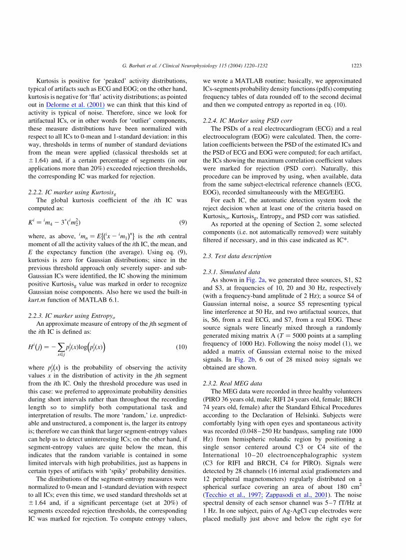
Kurtosis is positive for ‘peaked’ activity distributions,

typical of artifacts such as ECG and EOG; on the other hand,

kurtosis is negative for ‘flat’ activity distributions; as pointed

out in Delorme et al. (2001) we can think that this kind of

activity is typical of noise. Therefore, since we look for

artifactual ICs, or in other words for ‘outlier’ components,

these measure distributions have been normalized with

respect to all ICs to 0-mean and 1-standard deviation: in this

way, thresholds in terms of number of standard deviations

from the mean were applied (classical thresholds set at

^1.64) and, if a certain percentage of segments (in our

applications more than 20%) exceeded rejection thresholds,

the corresponding IC was marked for rejection.

2.2.2. IC marker using Kurtosisg

The global kurtosis coefficient of the ith IC was

computed as:

Ki ¼ im4 2 3pðim22Þ ð9Þ

where, as above, imn ¼ E��

ix 2 im1

�n�is the nth central

moment of all the activity values of the ith IC, the mean, and

E the expectancy function (the average). Using eq. (9),

kurtosis is zero for Gaussian distributions; since in the

previous threshold approach only severely super- and sub-

Gaussian ICs were identified, the IC showing the minimum

positive Kurtosisg value was marked in order to recognize

Gaussian noise components. Also here we used the built-in

kurt.m function of MATLAB 6.1.

2.2.3. IC marker using Entropyo

An approximate measure of entropy of the jth segment of

the ith IC is defined as:

Hi j� �

¼ 2Xx[j

pij xð Þlog pi

j xð Þ�

ð10Þ

where pij

�x�

is the probability of observing the activity

values x in the distribution of activity in the jth segment

from the ith IC. Only the threshold procedure was used in

this case: we preferred to approximate probability densities

during short intervals rather than throughout the recording

length so to simplify both computational task and

interpretation of results. The more ‘random,’ i.e. unpredict-

able and unstructured, a component is, the larger its entropy

is; therefore we can think that larger segment-entropy values

can help us to detect uninteresting ICs; on the other hand, if

segment-entropy values are quite below the mean, this

indicates that the random variable is contained in some

limited intervals with high probabilities, just as happens in

certain types of artifacts with ‘spiky’ probability densities.

The distributions of the segment-entropy measures were

normalized to 0-mean and 1-standard deviation with respect

to all ICs; even this time, we used standard thresholds set at

^1.64 and, if a significant percentage (set at 20%) of

segments exceeded rejection thresholds, the corresponding

IC was marked for rejection. To compute entropy values,

we wrote a MATLAB routine; basically, we approximated

ICs-segments probability density functions (pdfs) computing

frequency tables of data rounded off to the second decimal

and then we computed entropy as reported in eq. (10).

2.2.4. IC Marker using PSD corr

The PSDs of a real electrocardiogram (ECG) and a real

electrooculogram (EOG) were calculated. Then, the corre-

lation coefficients between the PSD of the estimated ICs and

the PSD of ECG and EOG were computed; for each artifact,

the ICs showing the maximum correlation coefficient values

were marked for rejection (PSD corr). Naturally, this

procedure can be improved by using, when available, data

from the same subject-electrical reference channels (ECG,

EOG), recorded simultaneously with the MEG/EEG.

For each IC, the automatic detection system took the

reject decision when at least one of the criteria based on

Kurtosiso, Kurtosisg, Entropyo and PSD corr was satisfied.

As reported at the opening of Section 2, some selected

components (i.e. not automatically removed) were suitably

filtered if necessary, and in this case indicated as IC*.

2.3. Test data description

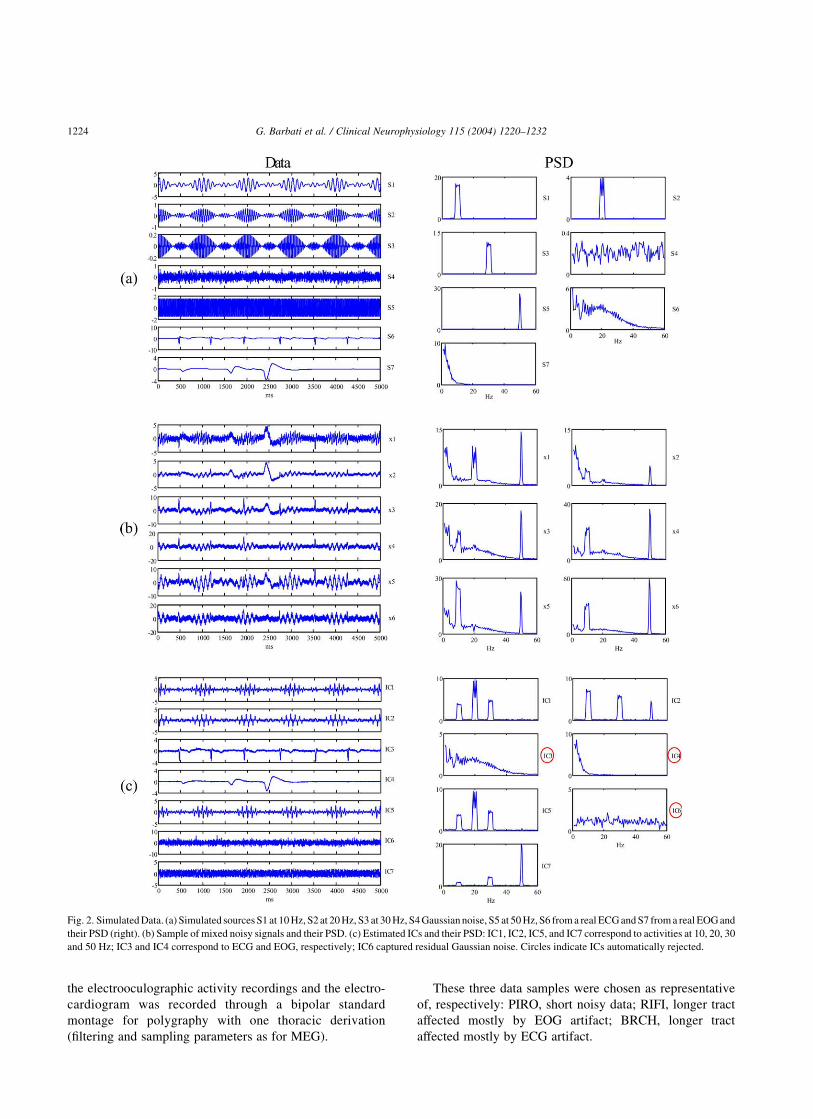
2.3.1. Simulated data

As shown in Fig. 2a, we generated three sources, S1, S2

and S3, at frequencies of 10, 20 and 30 Hz, respectively

(with a frequency-band amplitude of 2 Hz); a source S4 of

Gaussian internal noise, a source S5 representing typical

line interference at 50 Hz, and two artifactual sources, that

is, S6, from a real ECG, and S7, from a real EOG. These

source signals were linearly mixed through a randomly

generated mixing matrix A (T ¼ 5000 points at a sampling

frequency of 1000 Hz). Following the noisy model (1), we

added a matrix of Gaussian external noise to the mixed

signals. In Fig. 2b, 6 out of 28 mixed noisy signals we

obtained are shown.

2.3.2. Real MEG data

The MEG data were recorded in three healthy volunteers

(PIRO 36 years old, male; RIFI 24 years old, female; BRCH

74 years old, female) after the Standard Ethical Procedures

according to the Declaration of Helsinki. Subjects were

comfortably lying with open eyes and spontaneous activity

was recorded (0.048–250 Hz bandpass, sampling rate 1000

Hz) from hemispheric rolandic region by positioning a

single sensor centered around C3 or C4 site of the

International 10 – 20 electroencephalographic system

(C3 for RIFI and BRCH, C4 for PIRO). Signals were

detected by 28 channels (16 internal axial gradiometers and

12 peripheral magnetometers) regularly distributed on a

spherical surface covering an area of about 180 cm2

(Tecchio et al., 1997; Zappasodi et al., 2001). The noise

spectral density of each sensor channel was 5–7 fT/Hz at

1 Hz. In one subject, pairs of Ag-AgCl cup electrodes were

placed medially just above and below the right eye for

G. Barbati et al. / Clinical Neurophysiology 115 (2004) 1220–1232 1223

the electrooculographic activity recordings and the electro-

cardiogram was recorded through a bipolar standard

montage for polygraphy with one thoracic derivation

(filtering and sampling parameters as for MEG).

These three data samples were chosen as representative

of, respectively: PIRO, short noisy data; RIFI, longer tract

affected mostly by EOG artifact; BRCH, longer tract

affected mostly by ECG artifact.

Fig. 2. Simulated Data. (a) Simulated sources S1 at 10 Hz, S2 at 20 Hz, S3 at 30 Hz, S4 Gaussian noise, S5 at 50 Hz, S6 from a real ECG and S7 from a real EOG and

their PSD (right). (b) Sample of mixed noisy signals and their PSD. (c) Estimated ICs and their PSD: IC1, IC2, IC5, and IC7 correspond to activities at 10, 20, 30

and 50 Hz; IC3 and IC4 correspond to ECG and EOG, respectively; IC6 captured residual Gaussian noise. Circles indicate ICs automatically rejected.

G. Barbati et al. / Clinical Neurophysiology 115 (2004) 1220–12321224

3. Results

3.1. Simulated data

We applied ICA to the data generated as described

above. The estimated ICs with the corresponding PSD are

shown in Fig. 2c.

We applied the detection system by computing a

7-segments partition of the estimated ICs and results are

shown in Fig. 3 and summarized in the section ‘Simulated

data’ of Table 1. Kurtosiso detected IC3 (Fig. 3a), Entropyo

detected IC4 (Fig. 3b), PSD corr marked IC3 and IC4

(Fig. 3c) with ECG and EOG, respectively, and finally

Kurtosisg detected IC6 (Fig. 3d).

Therefore IC3, IC4 and IC6 were rejected on the basis of

the automatic detection system; by means of a visual PSD

inspection of the ICs, we can observe (Fig. 2c) that IC1, IC2,

IC5 and IC7 isolated brain activity sources at 10, 20 and 30

Hz, even if IC2 and especially IC7 were still corrupted by

interference at 50 Hz; IC3 and IC4 identified ECG and

EOG, respectively, and IC6 corresponded to Gaussian

noise.

The control cycle on discrepancy confirmed the good

performance of the retro-projection process using retained

IC1, IC2*, IC5 and IC7*, since discrepancy contained only

artifacts and noise. We filtered out 50 Hz from IC2 and IC7

using a Butterworth bandpass filter of z 5 2 and

bandwidth ¼ [48,52].

3.2. Real MEG data

In the first real-data example, we applied ICA to a PIRO

subset of MEG recordings (10 000 points, 10 s); a sample

of the original data and their PSD are shown in Fig. 4a.

From the PSD of the original data, the presence of low-

frequency activity (,5 Hz) corresponding to ocular and

cardiac artifacts was clearly visible (see for comparison the

PSD shown in Fig. 2a, sources S7 and S6); we used only a

portion of the original recording since we aimed to explore

blind source separation performance in a small data-

dimension context. The estimated ICs and their PSD are

shown in Fig. 4b.

We applied the detection system by computing a

14-segments partition of the estimated ICs and results are

summarized in the section ‘PIRO’ of Table 1. Kurtosiso did

not detect any component, Entropyo detected IC10, PSD

corr marked IC6 for both ECG and EOG, and finally

Kurtosisg detected IC8. This means that 3 ICs (IC6, IC8

Fig. 3. Automatic detection system on estimated ICs from simulated data; arrows indicate ICs marked for rejection. (a) Kurtosiso marked IC3, corresponding to

ECG, for rejection; (b) Entropyo marked IC4, corresponding to EOG; (c) PSD corr marked IC3 for ECG and IC4 for EOG; (d) Kurtosisg marked IC6.

G. Barbati et al. / Clinical Neurophysiology 115 (2004) 1220–1232 1225

and IC10) were automatically detected by means of the

proposed switching system. Using visual inspection of

components PSD and time activations as shown in Fig. 4b,

we could have rejected IC6, IC8, IC9 and IC10.

We then reconstructed the data with the elimination of

just the ICs automatically rejected by the system. A sample

of the PSD of the reconstructed data with retained ICs is

shown in Fig. 4c; the control cycle on discrepancy showed

that a peak at the 10 Hz activity was not captured by the

initial reconstructed data. Therefore, non-artifactual

detected filtered discrepancy channels were added in order

to obtain the final reconstructed data, as shown in Fig. 4d. In

the discrepancy vector we selected 9 out of 28 channels,

filtered using a Butterworth bandpass filter of z 5 2 and

bandwidth 5 [5,50]; moreover, we filtered IC1, IC2, IC4,

IC7, IC9 and IC11 with a Butterworth bandpass filter

ofz 5 2 and bandwidth ¼ [5,50].

In the second real-data example, we applied ICA to 3 min

(180 000 points) of RIFI MEG recordings; a sample of the

original data and their PSD are shown in Fig. 5a. Also here,

low frequencies clearly over-represented in a healthy

subject were visible (compare with Fig. 2a, source S7);

the estimated ICs and their PSD are shown in Fig. 5b.

We applied the detection system by computing a

36-segments partition of the estimated ICs. Results are

summarized in the section ‘RIFI’ of Table 1. Kurtosiso

detected IC1, Entropyo detected IC2 and IC4, PSD corr

marked IC1 and IC7 for EOG and ECG, respectively, and

finally Kurtosisg detected IC9. This means that 5 ICs were

automatically detected by means of the proposed switching

system. Adopting visual criteria we could have rejected:

IC1, IC2, IC4, IC6, IC7 and IC9.

We reconstructed data with the elimination of just the

ICs automatically rejected by the system. A sample of the

PSD of the reconstructed data with retained ICs is shown in

Fig. 5c. We filtered IC3 using a Butterworth bandpass filter

of z 5 2 and bandwidth ¼ [5,50].

The control cycle on discrepancy confirmed the good

performance of the retro-projection process, since discre-

pancy contained only artifacts and noise.

In the third real-data example, we applied ICA to 3 min

of BRCH MEG recordings; some channels of the original

data and their PSD are shown in Fig. 6a. From both raw

signals and their PSD we can recognize the presence of the

cardiac artifact in a broad spectrum of frequencies ranging

from 5 to 40 Hz (compare with Fig. 2a, source S6);

furthermore, an over-representation of low frequencies

probably due to ocular movements was present. The

estimated ICs and their PSD are shown in Fig. 6b.

We applied the detection system by computing a

36-segment partition of the estimated ICs. Results are

shown and summarized in the section ‘BRCH’ of Table 1.

Kurtosiso detected IC6, Entropyo detected IC5, PSD corr

marked IC1 and IC6 for ECG and EOG, respectively, and

finally Kurtosisg detected IC8. Therefore, 4 ICs were

automatically detected by means of the proposed switching

system. We could have visually rejected 5 ICs: IC1, IC3,

IC5, IC6 and IC8.

We reconstructed the data with the elimination of the

ICs automatically rejected by the system; a sample of the

PSD of the reconstructed data, with the selected ICs, is

shown in Fig. 6c. The control cycle on discrepancy showed

that a activity spectral peak at 10-Hertz was not captured

by the initial reconstructed data; therefore, useful dis-

crepancy filtered channels were added so to obtain the final

reconstructed data, as shown in Fig. 6d. In the discrepancy

vector we selected 12 out of 28 channels, filtered using

Table 1

MEG data

Kurtosiso

(%)

Entropyo

(%)

PSD corr Kurtosisg

ECG EOG

Simulated

data

IC1 0 0 0.3112 0.0080 3.0417

IC2* 0 0 0.2738 0.0037 3.7717

IC3 86 0 0.9957 0.5542 22.406

IC4 0 71 0.5779 0.9999 15.042

IC5 0 0 0.3113 0.0076 3.0475

IC6 0 0 0.0077 0.0681 0.5895

IC7* 0 0 0.1275 0.0073 21.1834

PIRO IC1* 0 0 0.7111 0.3748 20.2801

IC2* 7 0 0.7846 0.4950 1.0600

IC3 0 7 0.5867 0.2990 0.6476

IC4* 7 0 0.6484 0.4501 0.7178

IC5 14 7 0.6232 0.2336 1.6167

IC6 14 14 0.8345 0.7184 2.5784

IC7* 0 14 0.7593 0.5422 2.2827

IC8 7 0 0.8000 0.4292 0.4474

IC9* 0 0 0.7926 0.4901 20.3109

IC10 7 57 0.6733 0.3480 4.5413

IC11* 7 0 0.5619 0.5017 20.4297

RIFI IC1 64 0 0.6355 0.9375 2.9073

IC2 0 100 0.8071 0.4310 0.0483

IC3* 3 0 0.6688 0.7067 0.4286

IC4 5 39 0.6868 0.7024 1.5164

IC5 0 0 0.7073 0.7201 0.1937

IC6 0 0 0.7999 0.6433 0.5230

IC7 0 0 0.8483 0.7187 0.2448

IC8 0 0 0.5818 0.3485 0.8696

IC9 0 0 0.7969 0.4165 0.0393

IC10 5 0 0.7774 0.6970 0.9881

BRCH IC1 5 0 0.6474 0.7238 0.9390

IC2 0 0 0.6949 0.2067 0.2374

IC3* 11 0 0.8513 0.6651 2.3184

IC4 0 0 0.5420 0.1210 0.3322

IC5 0 100 0.7511 0.3009 0.0675

IC6 28 0 0.8730 0.6908 1.5013

IC7 3 0 0.7978 0.3168 0.3778

IC8 0 0 0.7496 0.3063 0.0379

IC9 3 0 0.7006 0.2320 0.3358

IC10 3 0 0.8346 0.3730 0.3748

Marker values in simulated and real cases. Kurtosiso and Entropyo are

percentages of outlier segments; PSD corr is the correlation coefficient

value, with respectively ECG and EOG spectra; Kurtosisg is the global

kurtosis coefficient value. In bold are detected ICs and corresponding

marker values; asterisks indicate filtered ICs.

G. Barbati et al. / Clinical Neurophysiology 115 (2004) 1220–12321226

Fig. 4. PIRO real data. (a) Selection of 4 representative original PIRO signals and their PSD: is clearly visible the presence of low-frequency activity (,5 Hz),

corresponding to ocular and cardiac artifacts. (b) Estimated ICs (circles indicate automatically rejected components) and their PSD: IC6 was marked for

rejection by PSD corr with both ECG and EOG; IC8 by Kurtosisg and IC10 by Entropyo. (c) The reconstructed data and their PSD. (d) Overlap between the 4

channels before (dotted line) and after (solid line) the data reconstruction, without (left) and with (right) adding ‘non-artifactual’ discrepancy.

G. Barbati et al. / Clinical Neurophysiology 115 (2004) 1220–1232 1227

a Butterworth bandpass filter of z 5 2 and

bandwidth ¼ [5,15]; moreover, we filtered IC3 using a

Butterworth bandpass filter of z 5 2 and

bandwidth ¼ [5,50].

4. Discussion

In this work we proposed a method for blind artifact and

noise identification and reduction in MEG signals, by using

Fig. 5. RIFI real data. (a) Selection of 4 original RIFI signals and their PSD: are visible low frequencies clearly over-represented in a healthy young subject. (b)

Estimated ICs and their PSD (PSD of IC2 and IC4 are on different scales): IC1 was marked by Kurtosiso and PSD corr with EOG, IC2 and IC4 by Entropyo, IC7

by PSD corr with ECG, IC9 by Kurtosisg and were automatically rejected (circles). (c) The 4 reconstructed data signals and their PSD: arrows indicate

‘interesting’ (non-artifactual) frequency activities around 8 and 25 Hz, more evident after the successful discharge of confounding artifact activities (see Ch4

panel a right).

G. Barbati et al. / Clinical Neurophysiology 115 (2004) 1220–12321228

Fig. 6. BRCH real data. (a) Selection of 4 original signals and their PSD: from both raw-signal activations in time and their PSD it could be recognized the

presence of the cardiac artifact in a broad spectrum of frequencies between 5 and 40 Hz and an over-representation of low frequencies. (b) Estimated ICs and

their PSD (PSD of IC5 is on a different scale); IC1 was marked by PSD corr for ECG, IC5 by Entropyo, IC6 by Kurtosiso and PSD corr for EOG, IC8 by

Kurtosisg. (c) The 4 reconstructed data and their PSD. (d) Overlap between the 4 channels before (dotted line) and after (solid line) the data reconstruction,

without (left) and with (right) adding non-artifactual discrepancy.

G. Barbati et al. / Clinical Neurophysiology 115 (2004) 1220–1232 1229

a procedure comprising three main steps: (1) ICA, (2)

discrimination between cerebral (non-artifactual)/non-cere-

bral (artifactual) ICs by an automatic detection system, and

(3) possible identification and addition of ‘useful’

discrepancies.

ICA demonstrates a powerful alternative for artifact

cancellation with respect to classical segment-rejection

approach, the latter being based on discarding segments of

raw data that are hidden at a visual inspection because of the

presence of artifacts. Moreover, ICA is mostly relevant

when studying spontaneous activity, where no event-related

average could be used for signal-to-noise ratio improve-

ment, and allows suitable information extraction from

shorter signal recordings.

The introduction of an automatic detection approach, by

which a set of measures can isolate a significant number of

artifactual ICs, results in a great simplification of successive

data analyses. In particular, this data-driven detection

system could be very useful for multichannel systems with

hundreds of sensors, where a high number of ICs is

produced and must be processed. The automatic selection

was based not only on IC statistical properties such as those

at the base of the algorithm estimation method, but also on

IC spectral characteristics. It is to be noted that the PSD corr

identified some ICs not marked by kurtosis and entropy

criteria; this indicates that estimated ICs could have

‘prototypical’ spectral characteristics (for example, typical

of electrocardiographic and electrooculographic artifactual

signals) and suggests that including frequency information

directly in the source-separation phase jointly with higher-

order criteria could improve algorithm performance in

specific MEG/EEG applications (Gorodnitsky and Belou-

chrani, 2001). In the simulated data context, the automatic

markers diagnostic selection is optimal. In the real-data

examples, the proposed automatic detection system agreed

with a visual inspection in the 79% of cases on average. We

based the retro-projection process on automatically retained

ICs instead of on visually detected ones: besides the former

procedure being obviously less time-consuming, we think

that the latter could be seriously affected by the roughness of

the cerebral activity spectra model that can be constructed

by the researcher’s experience, due for example to the high

variability in PSD shapes among different subjects, and by

the level of researcher attention. Certainly, there is a certain

number of user-defined settings in the detection system

parameters (length of segments, significant percentage of

outlier-segments, level of thresholds) and further improve-

ments could be made through the study of the robustness of

the final rejection decision with respect to these parameters

or through the research on possible other detection criteria.

The scalp distribution of retro-projected ICs is generally

used in literature in order to help the identification of

artifactual components (Jung et al., 2000). Our procedure

did not include this criterion; this feature could be suitable

when studying patients affected by cerebral lesions, in

whom low-frequency pathological activities could spatially

overlap artifactual ones.

Since, to our knowledge, a numerical index to compare

original and reconstructed data in BSS real applications is

lacking, the difference between original and reconstructed

data in the sensors space was considered. It has been

proposed the possible addition of selected ‘discrepancy’

channels, with spectral characteristics of non-artifactual

activity, to obtain final reconstructed data. In our opinion,

this could be especially relevant when dealing with small-

size data; in any case, we think it really is a crucial control

cycle in reconstructing data through blind separation

techniques. In the simulated data context the control cycle

on discrepancy is redundant, but, on the contrary, it means a

significant amelioration in two of the three real-data

examples (i.e. PIRO and BRCH).

With respect to the artifact reduction in real applications,

in the RIFI data example it can be noted that, in cleaned

reconstructed signals, ‘interesting’ frequency activities

around 8 and 25 Hz could be recognized (see Fig. 5c),

after successfully discharge of confounding artifact activi-

ties. For instance, cerebral and artifactual activities could

always coexist in the same frequency ranges: on one hand,

in the RIFI example, the 8 Hz activity was masked by the

artifactual one; on the other hand, in BRCH (see Fig. 6d),

part of the potentially physiological 20 Hz activity was

removed as an ECG artifact.

In the BRCH data case, it could be observed that

different ICs (IC4 and IC2, IC7, IC9) described activities

around 10 Hz with different frequency peaks. IC4 showed

a clear maximum at 8.5 Hz whereas IC2, IC7 and IC9 at

10.0 Hz. It is known that the spontaneous activity

generated in occipital areas and responding to visual

stimuli (alpha rhythm), and the activity generated in the

rolandic areas and responding to movement and somato-

sensory stimulation (mu rhythm) both fall in this range of

frequencies. The latter is generally at slightly higher

frequency than the former (,1 Hz), when compared in

the same subject (Gastaut, 1952; Hari and Salmelin, 1997;

Okada and Salenius, 1998). This finding suggests that ICA

can be a powerful method for separating different 10 Hz

cerebral sources, taking into account that a selection by

simply bandpass filtering in such narrow bands will cause

signal distortion. It is noteworthy that in simulated data,

sources at 10, 20 and 30 Hz appeared together in more

than one IC (see Fig. 2c: IC1, IC2, IC5 and IC7) while

ECG and EOG were completely separated in two distinct

ICs (ECG in IC3, EOG in IC4). This fact, together with

the randomly-generated source mixing matrix, stresses

that not the ‘spatial’ source distribution – lost in the

random mixing process – but solely the different source

statistical properties determined the estimated com-

ponents. In fact, simulated sources at 10, 20 and 30 Hz

are characterized by very similar distributions, which are

definitely different from those of ECG and EOG, and

these last two differ considerably from each other.

G. Barbati et al. / Clinical Neurophysiology 115 (2004) 1220–12321230

Therefore, the fact that in BRCH very similar frequencies

appeared separated in different ICs suggests that the

underlying neural activity could be separated on the basis

of different generating mechanisms, although within very

narrow frequency ranges and independently from spatial

distribution.

In conclusion, the present noise reduction procedure,

including ICA separation phase, automatic artifactual ICs

selection and ‘discrepancy’ control cycle, showed good

performances both on simulated and real MEG data.

Moreover, application to real signals suggests the

procedure to be able to separate different cerebral activity

sources, even if characterized by very similar frequency

contents.

Acknowledgements

The authors thank Professor Sergio A. Cruces-Alvarez

and Dr Sergiy Vorobyov for kindly providing the CII

algorithm.

Appendix A. Robust pre-whitening based on Signal

Subspace criterion

We started the ICA algorithm by whitening and reducing

the noisy data.

Whitening can in general be obtained by singular value

decomposition (svd) of the data covariance matrix

Rxx ¼ E�xxT

�:

svd Rxx

� �! ~x ¼ L21=2VTx ¼ Qx ðA1Þ

where V contains the eigenvectors associated with the

eigenvalues of L ¼ diag�l1 $ l2 $ ::: $ ln

�in descend-

ing order; in this way, we obtain a whitening matrix Q such

that R~x~x ¼ In, the whitened data are zero-mean, unit

variance and uncorrelated.

We achieve a ‘robust reduction’ of the dimensionality of

the problem by using the signal subspace criterion, i.e. by

assuming that the first m of the n eigenvalues forms an

m-dimensional signal subspace, whereas the remaining n-m

define a (n-m)-dimensional noise subspace. Consequently

we can write:

Rxx ¼ VxLxVTx ¼ VS;VN

� � LS 0

0 LN

" #VS;VN

� �T¼ VSLSVT

S þ VNLNVTN ðA2Þ

where VS contains the eigenvectors associated with the

eigenvalues of LS ¼ diag�l1 $ l2 $ ::: $ lm

�of the signal

subspace, whereas VN contains the eigenvectors associated

with the eigenvalues of LN ¼ diag�lmþ1 $ lmþ2 $ ::: $

ln

�of the noise subspace.

We estimate the noise variance s2v as the mean value of

the (n 2 m) minor eigenvalues:

s2v ¼

1

n 2 m

Xn

i¼mþ1

li ðA3Þ

and define the ‘robust’ whitening matrix as

Qr ¼ L21=2S VT

S ¼ LS 2 s2vIm

� 21=2VT

S ðA4Þ

The m-dimensional robust-whitened data vector (zero-

mean, unit variance and uncorrelated) can then be expressed

as:

~x ¼ L21=2S VT

S x ¼ Qrx ðA5Þ

where R~x~x ø Im.

Appendix B. CIISS algorithm

After the robust pre-whitening based on the Signal

Subspace criterion ‘SS,’ in the blind source-extraction

procedure ‘CII’ we firstly identify the mixture unknown

matrix A using the following iteration:

A t þ 1ð Þ ¼ A tð Þ þ m tð Þ C1;3x;y S3

y 2 A tð Þ�

ðB1Þ

where A�t�

is the estimation of the mixing matrix A at step t;

m�t�

is the learning-rate parameter; C1;3x;y ¼ M1;3

x;y 2 3M0;2x;y

M1;1x;y is the 4th-order cross-cumulant matrix computed using

sample moment matrices:

Mk;lx;y ¼ E x £ ::: £ x|fflfflffl{zfflfflffl}

k

y £ ::: £ y|fflfflffl{zfflfflffl}l

0B@

1CA

T8><>:

9>=>;

and S3y is the diagonal matrix of cumulant signs

S3y

h iii¼ sign C1;3

x;y

h iii

� Then we compute a separation matrix W as the pseudo-

inverse of A, iterating the process until a fixed measure of

convergence is satisfied (Cruces-Alvarez et al., 2000, 2002).

References

Belouchrani A, Cichocki A. A robust whitening procedure in blind source

separation context. Electronic Lett 2000;36:2050–1.

Cao J, Murata N, Amari S, Cichocki A, Takeda T, Endo H, Harada N.

Single-trial magnetoencephalographic data decomposition and localiz-

ation based on independent component analysis approach. IEICE Trans

Fundam Electronics Commun Comput Sci 2000;9:1757–66.

Choi S, Cichocki A. Blind separation of nonstationary sources in noisy

mixtures. Electronic Lett 2000;36:848–9.

Cichocki A, Amari S. Adaptive blind signal and image processing. New

York: Wiley; 2002.

Cruces-Alvarez S, Cichocki A, Castedo-Ribas L. An iterative inversion

approach to blind source separation. IEEE Trans Neural Networks

2000;11:1423–37.

G. Barbati et al. / Clinical Neurophysiology 115 (2004) 1220–1232 1231

Cruces-Alvarez S, Castedo-Ribas L, Cichocki A. Robust blind source

separation algorithms using cumulants. Neurocomputing 2002;49:

87–118.

Del Gratta C, Pizzella V, Tecchio F, Romani G-L. Magnetoencephalo-

graphy – a non-invasive brain imaging method with 1 ms time

resolution. Rep Prog Phys 2001;64:1759–814.

Delorme A, Makeig S. EEGLAB: an open source toolbox for analysis of

single-trial EEG dynamics including independent component analysis.

J Neurosci Methods 2003;in press.

Delorme A, Makeig S, Sejnowski T. Automatic artifact rejection for EEG

data using high-order statistics and independent component analysis.

Proceedings of the 3rd International Workshop on ICA, San Diego,

December. 2001. p. 457–62.

Gastaut H. Etude electrocorticographique de la reactivite des rhythmes

rolandiques. Rev Neurol 1952;87:176–82.

Gorodnitsky IF, Belouchrani A. Joint cumulant and correlation based signal

separation with application to EEG data analysis. Proceedings of the

3rd International Workshop on ICA, San Diego, December. 2001.

p. 475–80.

Hari R, Salmelin R. Human cortical oscillations: a neuromagnetic view

through the skull. Trends Neurosci 1997;20:44–9.

Hyvarinen A. Gaussian moments for noisy independent component

analysis. IEEE Signal Process Lett 1999;6(6):145–7.

Hyvarinen A, Karhunen J, Oja E. Independent component analysis. New

York: Wiley; 2001.

Ikeda S, Toyama K. Independent component analysis for noisy data – MEG

data analysis. Neural Networks 2000;13(10):1063–74.

Jung TP, Makeig S, Westerfield M, Townsend J, Courchesne E, Sejnowski

TJ. Removal of eye activity artifacts from visual event-related

potentials in normal and clinical subjects. Clin Neurophysiol 2000;

111:1745–58.

Makeig S, Bell AJ, Jung TP, Sejnowski TJ. Independent component

analysis of electroencephalographic data. In: Jordan MI, Kearns MJ,

Solla SA, editors. Advances in neural information processing systems,

vol. 8. Cambridge, MA: MIT Press; 1996. p. 145–51.

Okada YC, Salenius S. Roles of attention, memory and motor preparation in

modulating brain activity in a spatial working memory task. Cereb

Cortex 1998;8:80–96.

Tecchio F, Rossini PM, Pizzella V, Cassetta E, Romani G-L. Spatial

properties and interhemispheric differences of the sensory hand cortical

representation: a neuromagnetic study. Brain Res 1997;767:100–8.

Lee T-W. Independent component analysis: theory and applications.

Dordrecht: Kluwer; 1998.

Vigario R, Jousmaki V, Hamalainen M, Hari R, Oja E. Independent

component analysis for identification of artifacts in magnetoencephalo-

graphic recordings. In: Jordan MI, Kearns MJ, Solla SA, editors.

Advances in neural information processing systems, vol. 10. Cam-

bridge, MA: MIT Press; 1997. p. 229–35.

Vorobyov S, Cichocki A. Blind noise reduction for multisensory signals

using ICA and subspace filtering, with application to EEG analysis. Biol

Cybernet 2002;86:293–303.

Zappasodi F, Tecchio F, Pizzella V, Cassetta E, Romano G-V, Filligoi G,

Rossini PM. Detection of fetal auditory evoked responses by means of

magnetoencephalography. Brain Res 2001;917:167–73.

Ziehe A, Nolte G, Sander T, Muller KR, Curio G. Artifact reduction in

magnetoneurography based on time-delayed second-order correlations.

IEEE Trans Biomed Eng 2000;47(1):75–87.

Ziehe A, Nolte G, Sander T, Muller KR, Curio G. A comparison of ICA-

based artifact reduction methods for MEG. Proceedings of the 12th

International Conference on Biomagnetism. Espoo: Helsinki University

of Technolology; 2001. p. 895–8.

G. Barbati et al. / Clinical Neurophysiology 115 (2004) 1220–12321232