An Artifact-based Workflow for Finite-ElementSimulation Studies

Andreas Ruscheinskia,∗, Pia Wilsdorfa, Julius Zimmermannb, Ursula vanRienenb, Adelinde M. Uhrmachera

aInstitute for Visual and Analytic Computing, University of Rostock, 18059 GermanybInstitute of General Electrical Engineering, University of Rostock, 18059 Germany

Abstract

Workflow support typically focuses on single simulation experiments. This isalso the case for simulation based on finite element methods. If entire simulationstudies shall be supported, flexible means for intertwining revising the model,collecting data, executing and analyzing experiments are required. Artifact-based workflows present one means to support entire simulation studies, as hasbeen shown for stochastic discrete-event simulation. To adapt the approach tofinite element methods, the set of artifacts, i.e., conceptual model, requirement,simulation model, and simulation experiment, and the constraints that apply areextended by new artifacts, such as geometrical model, input data, and simulationdata. Artifacts, their life cycles, and constraints are revisited revealing featuresboth types of simulation studies share and those they vary in. Also, the potentialbenefits of exploiting an artifact-based workflow approach are shown based on aconcrete simulation study. To those benefits belong guidance to systematicallyconduct simulation studies, reduction of effort by automatically executing specificsteps, e.g., generating and executing convergence tests, and support for theautomatic reporting of provenance.

Keywords: Artifact-based Workflow, Finite Element Analysis, SimulationStudies, Provenance, Knowledge-based engineering, Process Engineering

1. Introduction

Modeling and simulation, including finite element analysis (FEA), has becomean established method for engineering and research. Typically, larger researchand engineering projects require to conduct and intertwine various simulationstudies (in silico), with their own research question, with laboratory experiments(in vitro) acquiring the data needed to validate the simulation results or to testresearch hypotheses. Thus, the results of the simulation studies and laboratory

∗Corresponding authorEmail address: andreas.ruscheinski@uni-rostock.de (Andreas Ruscheinski)

1

arX

iv:2

010.

0762

5v1

[cs

.CE

] 1

5 O

ct 2

020

experiments have to be put into relation to each other. For example, in thecontext of electrically active implants in vitro and in silico studies are combinedto study the impact of electric fields on cellular dynamics. In [1], the authorsfirst conduct a simulation study including various simulation experiments thatreveal the distribution and strengths of the electrical field (EF). Afterwards, thecellular responses that are observed in in vitro experiments are related to thedistribution of the EF. The results can be used to subsequently conduct moredetailed simulation studies, e.g., to study the EF’s impact on membrane relateddynamics, intracellular dynamics, and cellular function [2, 3].

The intricate nature of simulation studies, interleaving model refinement,the execution of simulation experiments, and the acquisition of data, leads tothe question of how to support conducting and documenting these studies [4].Answers rely on a systematic specification of the process in terms of its resources,products, and activity patterns, i.e., a workflow.

So far, workflows have been successfully exploited to support single computa-tional tasks within simulation studies, e.g., to execute simulation experimentsand to analyze simulation results [5, 6, 7, 8, 9]. However, entire simulationstudies intertwine highly interactive processes, e.g., objective and requirementsspecification, knowledge acquisition, data collection, and model development,with computational processes, e.g., experiment execution, and data analysis,where each decision in each process may influence the study outcomes [10]. Thus,more flexible workflows are required to support entire simulation studies.

In [11], a declarative, artifact-based workflow approach achieves the requiredflexibility to capture the intricate nature of stochastic discrete-event simulationstudies while adhering to the constraints that apply between the different activi-ties and to the relations between the different work products, i.e., the conceptualmodel, requirements, simulation model, and simulation experiments.

Here, we adapt the artifact-based workflow towards FEA simulation studiesto explore how such a declarative workflow approach can contribute to the desiredguidance, best practices, documentation of FEA simulation studies, reuse ofresults, and thus to the quality and credibility of a study’s results [12, 13, 14, 15].

2. An Artifact-based Workflow for FEA Simulation Studies

Artifact-based workflows are suitable for handling knowledge-intensive pro-cesses, such as simulation studies, where “a lot of knowledge and expertise isimplicit, resides in experts’ heads or it has a form of (informal) best practices ororganizational guidelines” [16]. In artifact-based workflows, we describe processesas a set of artifacts interacting with each other. Therefore, each artifact consistsof a lifecycle model and an information model [17]. The lifecycle model describeshow the artifact evolves in the process, whereas the information model structuresthe attributes and relations of the artifact.

The artifact-based Guard-Stage-Milestone meta-model (GSM) [17] allowsus to declaratively specify the lifecycles of artifacts [18, 19]. In the GSM, werepresent the activities as stages equipped with guards and milestones. The

2

guards specify the preconditions at which a stage can be entered to execute theactivity. The milestones specify what is achieved by leaving a stage, i.e., theeffect of the activity. During the execution of the process, we test the guardsand milestones against the information models to determine which activitiescan be executed and what results are achieved. Moreover, the milestones arealso stored as part of the information models of the artifacts to record whatresults are achieved. To use the GSM to specify an entire simulation study, wemap the products of a simulation study [4, 10], e.g., the conceptual model, thesimulation models, and simulation experiments, to artifacts in our workflow.The lifecycles of these artifacts describe how the products are developed andtheir information models what is developed. This knowledge can then be used toimplement support mechanisms for simulation studies, e.g., to guide the modelerthrough the simulation study, to document the provenance of the products andto generate simulation experiments (see Section 3).

In the following, we revisit our artifact-based workflow for stochastic discrete-event simulation studies [11] to summarize the existing artifacts and the con-straints that apply between them. After that, we look at the specifics of FEAsimulation studies and identify the required adaptions of the workflow. There-after, we present the adapted workflow.

2.1. Revisiting the Artifact-based Workflow

In [11], we presented an artifact-based workflow for stochastic-discrete eventsimulation studies using the GSM [17]. Here, we used the artifacts to representthe simulation model(s), the simulation experiment(s), and the conceptual model,which included a separate artifact for handling the requirements of the simulationstudy.

The Lifecycle Models. In our workflow, we perceive the conceptual model asa container for all information that helps us to develop the simulation model[20, 21, 22], e.g., real-world data the simulation model shall be validated with orinformation about the domain of interest. The lifecycle of the conceptual modelartifact consists of four stages. Each simulation study starts at the Specifyingobjective-Stage, where the modeler has to specify the overall objective of thesimulation study, e.g., to create a validated simulation model or to test hypotheseson a simulation model. After specifying the objective, the stage reaches itsmilestones which allows the modeler to continue by assembling the conceptualmodel or to create a new simulation model artifact in the Creating simulationmodel -Stage. In the Assembling conceptual model -Stage, the modeler can createa new requirement artifact or fill the conceptual model with information. Themodeler can validate the conceptual model in the Validating conceptual model -Stage. Therefore, we require that the conceptual model and its requirements haveto be assembled, indicated by the milestones of the corresponding assembling-stages. During the validation, the modeler checks the consistency of the collectedinformation and the requirements. After this, the stage reaches a milestoneaccording to the validation result. To ensure the consistency of the informationin the conceptual model, we invalidate the milestones whenever the modeler

3

changes the conceptual model in the Assembling conceptual model -Stage or itsrequirements.

The requirement artifact specifies model behavior that can be checked byvalidation experiments or serve as the calibration target for the calibrationexperiments. By this, the requirement artifact forms a constituent of theconceptual model. In the workflow, the modeler specifies the requirement in theAssembling requirement-Stage. In this stage, we require the modeler to specifythe requirement type before the specification can be provided. For example,we can use a requirement to refer to a time series expressed as a temporallogic formula or to in-vitro data collected in a CSV-file. After finishing thespecification of the requirement, the modeler can leave the assembling stagewhich achieves its milestone to indicate that the requirement has been assembled.

The lifecycle of the simulation model artifact consists of four stages to capturethe assembling of the simulation model, the creation of simulation experimentsthat should be executed with the simulation model, and the validation as wellas calibration of the simulation model. The Assembling simulation model -Stage encapsulates the process of specifying a simulation model. Therefore, themodeler has to specify the modeling formalism before the simulation modelcan be specified. For example, the modeler might choose ML-Rules [23] for arule-based model or NetLogo [24] for an agent-based model. In the Choosingrequirements-Stage, the modeler can choose the requirements that apply for thesimulation model from the requirements in the conceptual model. To leave theassembling stage, we require that the specification has to be syntactically correctaccording to the chosen formalism. The simulation experiments are createdby entering the Creating simulation experiment-Stage. We use the simulationexperiments to calibrate or to validate the simulation model but also to generatesimulation data or to analyze the model behavior for what-if scenarios. In theCalibrating simulation model -Stage calibration experiments associated with thesimulation model are executed. Therefore, we require that the simulation modeland the experiments have to be assembled. If a useful parameter assignment hasbeen found, we leave the stage and the model is marked as successfully calibratedand the stage reaches the corresponding milestone. By entering the Validatingsimulation model -Stage, the modeler triggers the execution of all validationexperiments. Consequently, we require that all validation experiments and thesimulation model are assembled but also that the conceptual model has to bevalidated. Possible outcomes of the calibrating- and validating-stage are successor failure.

The lifecycle of the simulation experiment artifacts consists of two stages.In the Assembling simulation experiment-Stage the modeler has to specifyan approach for the experiment description, e.g., an experiment specificationlanguage such as SESSL [25] or a scripting language such as R [26, 27]. Themodeler can also choose the role to indicate that the experiment forms forexample a validation or calibration experiment. If this is the case, the modeleralso has to select a requirement associated with the simulation model, e.g.,time series the simulation model shall reproduce or specific spatio-temporalpatterns that the simulation results shall exhibit [28]. In a validation experiment,

4

the requirement should be checked whereas in calibration experiments therequirement serves as the calibration target of the experiment. To leave theassembling stage, we require that the provided experiment specification has to besyntactically correct according to the specified experiment approach. Finally, thesimulation experiments can be executed by entering the Executing experiment-Stage. Consequently, the simulation experiment and the model have to beassembled.

The Information Models. As the modeler moves through the different stagesof the artifact lifecycles, the corresponding information models of the artifactsare filled with the information provided by the modeler and achieved milestones.Also, the relations between the different artifacts, e.g., the chosen requirementsfrom the conceptual model in the simulation model artifacts, are stored as partof the information model.

2.2. Specifics of FEA simulation studies

Finite-element analysis simulation studies subsume all simulation studiesusing the finite-element method to simulate physical phenomena. Therefore,FEA simulation studies can be structured into three different steps [29, 30]:1. pre-processing, 2. processing, and 3. post-processing. The pre-processing stepcomprises all activities required to specify the inputs in the FEA simulationsoftware. The inputs consist of a mesh of finite elements representing thegeometrical model, the governing partial differential equations describing theunderlying laws of physics representing the physical model, and processingparameters (solver, time step, etc.). Although the geometrical model and thephysical model appear to be equally important in their own rights [31], theprocess of defining a suitable mesh sometimes appears to dominate the overallprocess. During the processing step, the FEA simulation software transforms thegeometrical model and the physical model into a system of algebraic equations,solves them according to the processing parameters, and reports the results backto the modeler, e.g., by visualizing the solution. Moreover, these steps are oftenexecuted repeatably until an acceptable solution, e.g., in terms of smoothness orconvergence, is found. For example, incrementally refining the physical modeland the mesh are considered to be crucial in determining whether the modelhas been built right (verification) and whether the right model has been built(validation) [14].

In the field of FEA so far, workflows have been primarily focused on automat-ing these steps (see Section 4). However, they do not cover information aboutthe simulation studies, e.g., the research question, assumptions, requirements, orfurther input data despite reporting guidelines suggest to make these accessible[13, 32]. Moreover, they assume that the modeler can provide a geometricalmodel and physical model while ignoring the intricate processes involved indeveloping them and their relations to other products of the study, e.g., theinput data used to develop the mesh or the requirements which were checkedby the experiments. However, the information models of the artifacts withinour artifact-based workflow already capture some meta-information about the

5

simulation study while the lifecycle models are structuring and relating thedevelopment processes of the conceptual model, requirements, the simulationmodels, and experiments. Thus, adopting the artifact-based workflow for anentire FEA simulation study appears not only possible but also meaningful.

In contrast to stochastic discrete-event simulation studies, the FEA simulationmodel appears to consists of two parts, the geometrical model and the physicalmodel, which were fused by specifying boundary conditions. Thus, the workflowhas to be adapted to represent the geometrical model and the physical model asindividual artifacts but also to treat them as constituents of the simulation model.This also implies that the milestones of Calibrating simulation model -Stage andValidating simulation model -Stage have to be adapted to be invalidated wheneverthe modeler revises the geometrical or physical model.

Also, the data that is used as input gains weight in FEA studies, as thesemight be images that are transformed into the geometrical model and mightmake up a large part of developing the simulation model. Thus, input data haveto be represented as an artifact to make their relations with the geometrical andphysical model explicit.

Finally, the FEA simulation studies rely on solvers that approximate thecorrect solution for the simulation. Whereas in our workflow the simulationdata produced by stochastic discrete-event simulation could be assumed to becorrect (given a sound implementation of the simulation algorithm), in the caseof approximative calculations a different approach is needed. Now the simulationdata need a life cycle of their own, i.e., stages that record whether the simulationdata have been reproduced with a different simulation algorithm or a differentmesh so to test the accuracy of the results. In the latter case, the reproductionserves the verification of the geometrical model, i.e., whether the model has beenbuilt correctly.

2.3. Adaptation towards FEA Simulation Studies

To capture an entire FEA study, new artifacts, such as input data andsimulation data are introduced, and the simulation model has to be redefined, asit now consists out of the geometrical model and physical model both formingartifacts of their own.

Figure 1 shows the artifact-based workflow for FEA simulation studies. Theworkflow consists of eight artifacts, four of which are new. Also, stages of theexisting artifacts, such as the conceptual model, have to be adapted to integratethe new artifacts into the workflow, or to take the specifics of FEA workflows,e.g., the specification of boundary conditions, into account.

To be clear, the artifact-based workflow for FEA simulation studies doesnot constrain the modeler to a specific tool, e.g., SALOME [33] to generate thegeometrical model or FEniCS [34] to specify the physical model and solve thesystem of algebraic equations. Likewise, it does not support the user in applyingthese tools either. An implementation of the workflow might use these tools toimplement toolboxes to provide stage-specific editors allowing the modeler toprovide the inputs for the information models, to check the syntactical correct-

6

ness of specifications, and to execute the simulation experiments. Additionalimplementation details can be found in our original publication [11].

2.4. New Artifacts

The new artifacts for our workflow are input data, the physical model, thegeometrical model, and the simulation data.

Input Data Artifact. The input data is all the data used to assemble the physicalmodel or the geometrical model. Further, input data might also be used inthe simulation experiment to run simulations with different parameter valuesor over a range of parameter values. Consequently, the form of the input datamight differ based on the application in the workflow, e.g., the input data forthe geometrical model might comprise anatomical images from CT scans and/ormight be a CAD model [35] based on which the mesh is created. The inputdata for the physical model and simulation experiments might refer, e.g., tomeasurements from laboratory experiments or other simulation studies [36].

In our workflow, the input data artifact forms a new constituent of the con-ceptual model, as we use the conceptual model as a container for all informationthat helps us in developing the simulation model [21]. Similar to the lifecycle ofthe requirement artifact, the lifecycle of the input data artifact consists of onemain stage (Assembling input data-Stage) in which the modeler has to specifythe input data type before the input data are specified. The latter can also be alink to a data file containing the input. Further, we require that the modelerprovides the source of the input data, e.g., by adding a DOI as part of thespecification to ensure the provenance of the information (see Section 3.3).

After specifying the input data, the assembling stage can be left by themodeler. Thereby, the stage reaches its milestone which indicates that theassembling of the input data has been completed.

Physical Model Artifact. The physical model describes the physical system, i.e.,the physical laws, which should be used in the simulation to analyze the behaviorof the geometrical model. The physical laws are typically specified using partialdifferential equations (PDEs) describing the time- and space-dependent behaviorof the system.

In the Assembling physical model -Stage, the modeler can choose among thealready assembled input data from the conceptual model to explicitly relateinput data to the physical model. Further, the modeler has to specify a modelingapproach, i.e., the physical modeling toolbox, before the physical model can bespecified. After specifying the physical model, the assembling stage can be leftand reaches its milestone to indicate that the physical model was successfullyassembled.

Geometrical Model Artifact. The geometrical model specifies the spatial dimen-sion of the simulation model. Therefore, the geometrical model forms a mesh,i.e., a subdivision of a continuous geometric space into discrete geometric andtopological cells, containing information about shape and size, and spatially

7

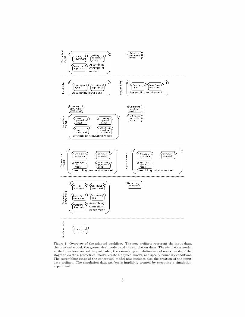
Figure 1: Overview of the adapted workflow. The new artifacts represent the input data,the physical model, the geometrical model, and the simulation data. The simulation modelartifact has been revised, in particular, the assembling simulation model now consists of thestages to create a geometrical model, create a physical model, and specify boundary conditions.The Assembling stage of the conceptual model now includes also the creation of the inputdata artifact. The simulation data artifact is implicitly created by executing a simulationexperiment.

8

resolved information, e.g., referring to material. As part of the simulation model,the geometrical model serves as the initial state, based on which the dynamicsevolve due to the constraints given by the physical model.

The development process of the geometrical model is encapsulated by theAssembling geometrical model -Stage. Within this stage, the modeler has tospecify a modeling approach, i.e., the geometrical modeling toolbox, providingthe means to create a mesh from a CAD model. Before the mesh can be created,the modeler has to choose the input data used to create the mesh, e.g., theimages from CT scans [35], and specify a CAD model, e.g., by importing anexisting model or creating a new one. After completing the meshing process, theassembling stage can be left by the modeler.

Simulation Data Artifact. The simulation data artifact represents the datagenerated by executing simulation experiments. Depending on the experiment,the data might consist of validation results, optimization results, or data whichis further analyzed, e.g., by visualization. Reproducing the simulation data byusing different solvers, etc. increases the trust in the data and also ensures theirreproducibility.

The artifact has only one stage, i.e., Reproducing simulation data-Stage withtwo possible outcomes, fail and succeed. By entering the stage, we automaticallygenerate a new experiment by adapting the original simulation experiment tocheck whether the simulation data can be reproduced. Therefore, we allow themodeler to manually update the generated experiment to specify, e.g., anothersolver or a newly meshed geometrical model. After that, the experiment canbe executed to generate new data which is compared, based on some metrics,with the previously generated data. Depending on the result, one of the twomilestones is reached to indicate that the data could or could not be reproduced.

2.5. Integrating the new artifacts

To integrate the new artifacts into the workflow, we revise the existing artifactlifecycles to enable the creation of the new artifacts and interaction betweenartifacts during the workflow. Therefore, we will add new stages and revise theguards and milestones of existing stages in our workflow.

Integrating the Input Data Artifact. As also suggested in [20] the input data shallbe part of the conceptual model. Therefore now, the Assembling conceptual model -Stage stage comprises a stage for creating a new input data artifact. Consequently,all created input data artifacts are stored as part of the information model ofthe conceptual model artifact. To ensure the coherence of the information inthe conceptual model, we further revise the guard and the milestones of theValidating conceptual model -Stage.

First, we only allow to enter the validating stage when all created input dataartifacts are assembled, i.e., fully specified. Therefore, the guard is extendedto check whether all created input data artifacts have reached the milestone oftheir assembling stage. Further, we revise the milestones of the validating stageto be invalidated whenever a created input data artifact is modified.

9

Since often simulation experiments make use of inputs, we also extend theAssembling simulation experiment-Stage to enable the modeler to choose fromthe input data artifacts. The references for the chosen input data artifacts arealso stored in the information model of the simulation experiment artifact.

Integrating the Physical Model and the Geometrical Model. The simulationmodel of FEA simulation studies consists of two parts: the physical modeland the geometrical model. To represent this in our artifact-based workflow,we need a different simulation model artifact. Therefore, we removed theSpecifying modeling formalism-Stage and the Specifying simulation model -Stagefrom the Assembling simulation model -Stage since the modeling formalism andthe specification of the model are now handled in the Assembling physicalmodel -Stage. Further, we allow creating a single physical model and a singlegeometrical model during the assembling of the simulation model. Consequently,the references to the created artifacts are stored as part of the information modelof the simulation model artifact. As before, each simulation study might containmultiple simulation model instances, each with its own information model.

The Specifying boundary condition-Stage stage allows the user to specifythe boundary conditions for the physical model given a geometrical model.Consequently, the geometrical model and the physical model has to be assembledbefore the boundary conditions can be specified. Moreover, the modeler can onlyleave the Assembling simulation model -Stage after the boundary conditions havebeen specified to ensure that the simulation model can be used in the simulationexperiments.

The milestones of the Validating simulation model -Stage are invalidatedwhenever the geometrical or physical model of the simulation is modified or theboundary conditions are changed to ensure that the changed simulation modelwill be validated again. Note that also experiments conducted in the Calibratingsimulation model -Stage may refer to either the geometrical model (e.g., findinga mesh where the solution converges) or the physical model (e.g., fitting thematerial properties to achieve a certain electric field distribution).

Integrating the Simulation Data. Unlike previous artifacts, the simulation dataartifacts are not created explicitly by a modeler via the Creating-x -Stage ofsome artifact but are created implicitly by entering the Executing experiment-Stage, the Validating simulation model -Stage or the Calibrating simulation modelstage-Stage of the simulation experiment artifact.

3. Supporting of FEA Simulation Studies

In the following, we will demonstrate how a modeler moves through theartifact-based workflow based on an exemplary FEA simulation study. Also, wewill show how the artifact-based workflow can be exploited to guide the modelerthrough the simulation study while documenting the development processes ofthe different work products, and how we can automatically generate simulationexperiments.

10

3.1. Case Study: Simulating an Electrical Stimulation Chamber

In electrical stimulation (ES), it is very important to characterize the localeffect of the applied stimulation. For that, we carry out field simulations to gobeyond simplistic analytical estimates. As FEA is a method that is capable oftreating complex geometries, it is the method of choice.

The goal of the case study is to compute the electric field (EF) distribution inan ES chamber [37, 38] following the workflow published in [39]. Therefore, themodeler begins with collecting information about the geometry of the chamber,the spacing and material of the electrodes, and the cell culture medium. Basedon this, the modeler continues by developing the geometrical model of thechamber using a CAD model to generate a mesh. Finally, the modeler specifiesa physical model describing electrical field distribution based on Maxwell’sequations, specifies the boundary conditions on the mesh, and validates thesimulation model.

Step 1: Collecting Information. The modeler begins with collecting the infor-mation about the spacing of the two electrodes (22 mm) as well as their generalshape (bent, L-shaped platinum wires) from the publications [37, 38]. Moreover,the modeler finds that standard 6-well dishes are used and assumes that thevolume of the cell culture medium is approximately the recommended volume of3 ml [40].

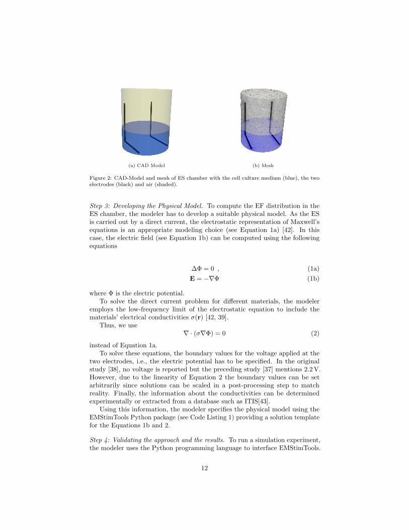
Step 2: Developing the Geometrical Model. For the geometrical model of the ESchamber, the modeler creates a new CAD model in SALOME [33]. Using theinformation about the inner diameter of the well, the modeler computes the filllevel and creates a geometry object representing the cell culture medium in theCAD model. To fit the electrodes into the well at the given spacing of 22 mm,assumptions are made on the length of the vertical part (22 mm) and length ofthe horizontal part (28 mm) of the electrode. In the next step, the cylindricalelectrodes are created in the CAD model and placed as described previously.The space between the medium and the highest point of the electrodes is filledwith air. Finally, the modeler cuts the electrodes out of the geometry as onlythe EF in the cell culture medium is of interest. The final CAD model is shownin Figure 2a.

Using the CAD model, a mesh consisting of tetrahedral elements (see Fig-ure 2b) is generated in SALOME using the Netgen mesh generator [41]. Using“a priori” knowledge that the mesh needs to have a higher resolution on theelectrode surfaces to resolve to geometry well, the choice of meshing parametersis influenced. Afterward, the modeler adds the material information aboutthe electrical conductivity of the air and cell culture medium to the respectiveelements of the mesh. Likewise, the electrode surfaces are marked where theelectrical potentials will be enforced by the specification of the boundary values.The quality of the mesh is checked visually and by the meshing algorithm. Fi-nally, the resulting mesh with the material information and the marked electrodesurfaces is exported using the MED-format supported by SALOME.

11

(a) CAD Model (b) Mesh

Figure 2: CAD-Model and mesh of ES chamber with the cell culture medium (blue), the twoelectrodes (black) and air (shaded).

Step 3: Developing the Physical Model. To compute the EF distribution in theES chamber, the modeler has to develop a suitable physical model. As the ESis carried out by a direct current, the electrostatic representation of Maxwell’sequations is an appropriate modeling choice (see Equation 1a) [42]. In thiscase, the electric field (see Equation 1b) can be computed using the followingequations

∆Φ = 0 , (1a)

E = −∇Φ (1b)

where Φ is the electric potential.To solve the direct current problem for different materials, the modeler

employs the low-frequency limit of the electrostatic equation to include thematerials’ electrical conductivities σ(r) [42, 39].

Thus, we use∇ · (σ∇Φ) = 0 (2)

instead of Equation 1a.To solve these equations, the boundary values for the voltage applied at the

two electrodes, i.e., the electric potential has to be specified. In the originalstudy [38], no voltage is reported but the preceding study [37] mentions 2.2 V.However, due to the linearity of Equation 2 the boundary values can be setarbitrarily since solutions can be scaled in a post-processing step to matchreality. Finally, the information about the conductivities can be determinedexperimentally or extracted from a database such as ITIS[43].

Using this information, the modeler specifies the physical model using theEMStimTools Python package (see Code Listing 1) providing a solution templatefor the Equations 1b and 2.

Step 4: Validating the approach and the results. To run a simulation experiment,the modeler uses the Python programming language to interface EMStimTools.

12

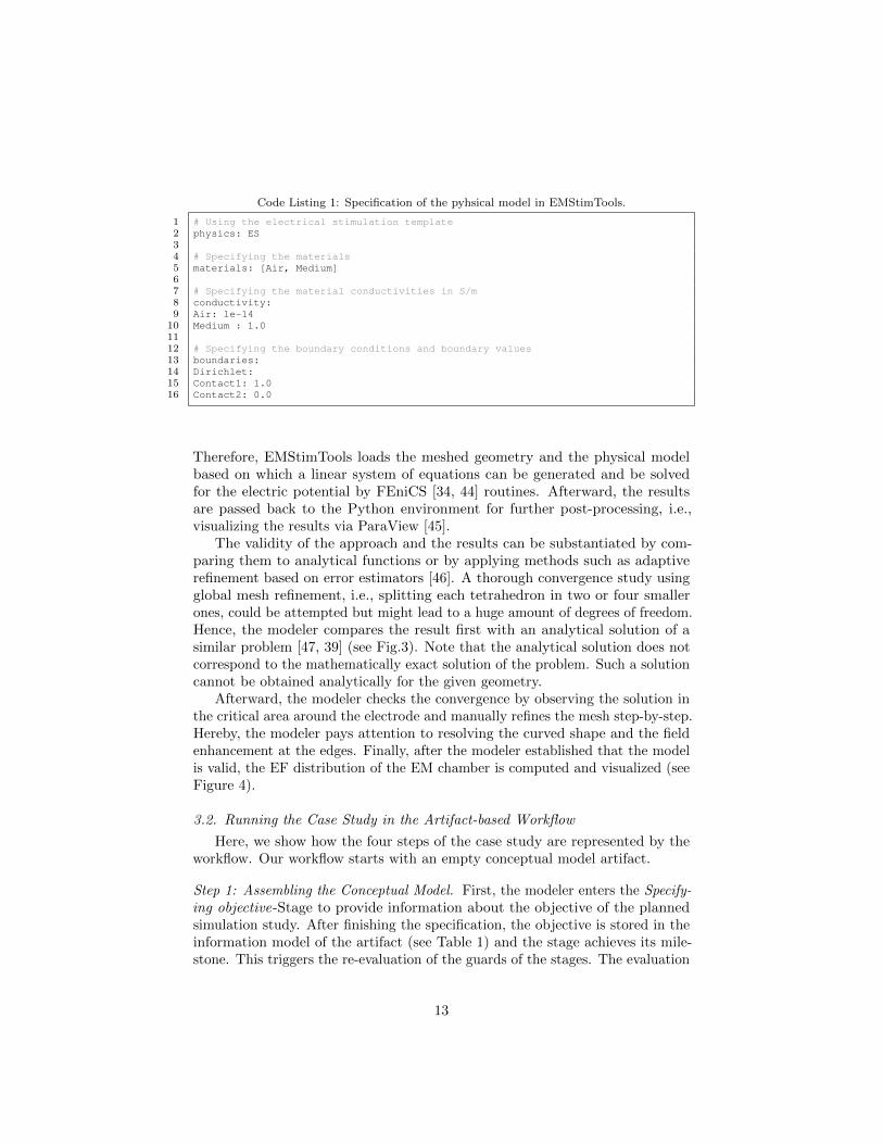
Code Listing 1: Specification of the pyhsical model in EMStimTools.

1 # Using the electrical stimulation template2 physics: ES34 # Specifying the materials5 materials: [Air, Medium]67 # Specifying the material conductivities in S/m8 conductivity:9 Air: 1e-14

10 Medium : 1.01112 # Specifying the boundary conditions and boundary values13 boundaries:14 Dirichlet:15 Contact1: 1.016 Contact2: 0.0

Therefore, EMStimTools loads the meshed geometry and the physical modelbased on which a linear system of equations can be generated and be solvedfor the electric potential by FEniCS [34, 44] routines. Afterward, the resultsare passed back to the Python environment for further post-processing, i.e.,visualizing the results via ParaView [45].

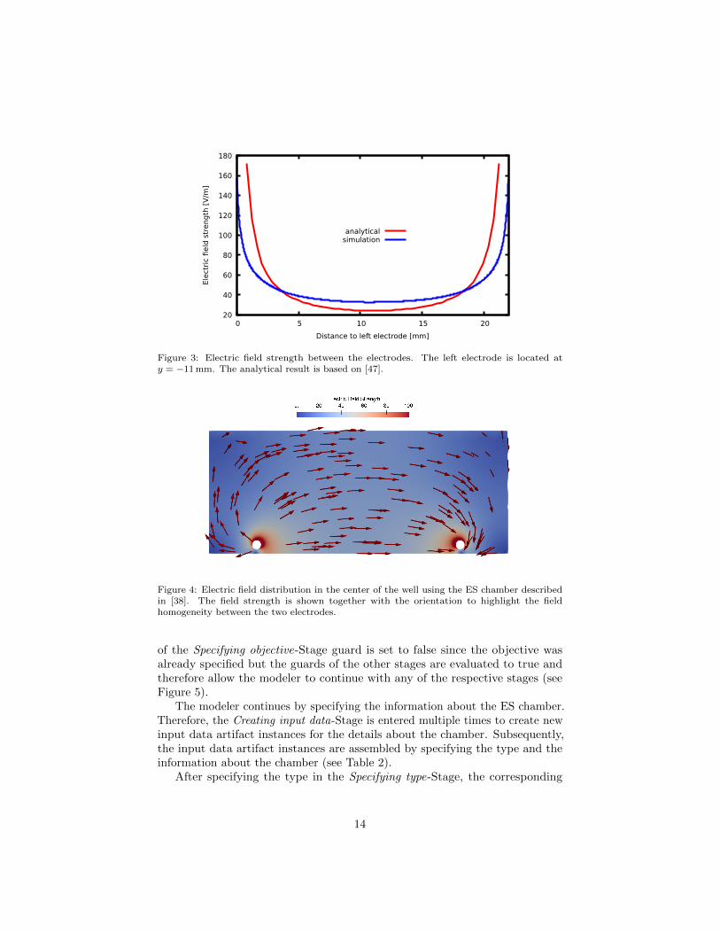
The validity of the approach and the results can be substantiated by com-paring them to analytical functions or by applying methods such as adaptiverefinement based on error estimators [46]. A thorough convergence study usingglobal mesh refinement, i.e., splitting each tetrahedron in two or four smallerones, could be attempted but might lead to a huge amount of degrees of freedom.Hence, the modeler compares the result first with an analytical solution of asimilar problem [47, 39] (see Fig.3). Note that the analytical solution does notcorrespond to the mathematically exact solution of the problem. Such a solutioncannot be obtained analytically for the given geometry.

Afterward, the modeler checks the convergence by observing the solution inthe critical area around the electrode and manually refines the mesh step-by-step.Hereby, the modeler pays attention to resolving the curved shape and the fieldenhancement at the edges. Finally, after the modeler established that the modelis valid, the EF distribution of the EM chamber is computed and visualized (seeFigure 4).

3.2. Running the Case Study in the Artifact-based Workflow

Here, we show how the four steps of the case study are represented by theworkflow. Our workflow starts with an empty conceptual model artifact.

Step 1: Assembling the Conceptual Model. First, the modeler enters the Specify-ing objective-Stage to provide information about the objective of the plannedsimulation study. After finishing the specification, the objective is stored in theinformation model of the artifact (see Table 1) and the stage achieves its mile-stone. This triggers the re-evaluation of the guards of the stages. The evaluation

13

20

40

60

80

100

120

140

160

180

0 5 10 15 20

Ele

ctri

c field

str

eng

th [

V/m

]

Distance to left electrode [mm]

analyticalsimulation

Figure 3: Electric field strength between the electrodes. The left electrode is located aty = −11 mm. The analytical result is based on [47].

Figure 4: Electric field distribution in the center of the well using the ES chamber describedin [38]. The field strength is shown together with the orientation to highlight the fieldhomogeneity between the two electrodes.

of the Specifying objective-Stage guard is set to false since the objective wasalready specified but the guards of the other stages are evaluated to true andtherefore allow the modeler to continue with any of the respective stages (seeFigure 5).

The modeler continues by specifying the information about the ES chamber.Therefore, the Creating input data-Stage is entered multiple times to create newinput data artifact instances for the details about the chamber. Subsequently,the input data artifact instances are assembled by specifying the type and theinformation about the chamber (see Table 2).

After specifying the type in the Specifying type-Stage, the corresponding

14

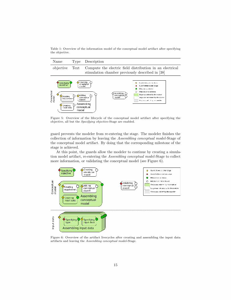
Table 1: Overview of the information model of the conceptual model artifact after specifyingthe objective.

Name Type Description

objective Text Compute the electric field distribution in an electricalstimulation chamber previously described in [38]

Figure 5: Overview of the lifecycle of the conceptual model artifact after specifying theobjective, all but the Specifying objective-Stage are enabled.

guard prevents the modeler from re-entering the stage. The modeler finishes thecollection of information by leaving the Assembling conceptual model -Stage ofthe conceptual model artifact. By doing that the corresponding milestone of thestage is achieved.

At this point, the guards allow the modeler to continue by creating a simula-tion model artifact, re-entering the Assembling conceptual model -Stage to collectmore information, or validating the conceptual model (see Figure 6).

Figure 6: Overview of the artifact livecycles after creating and assembling the input dataartifacts and leaving the Assembling conceptual model-Stage.

15

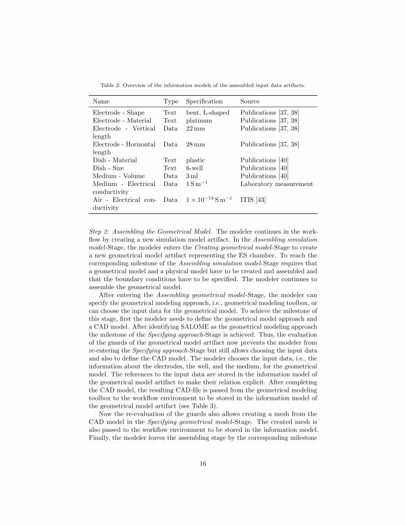
Table 2: Overview of the information models of the assembled input data artifacts.

Name Type Specification Source

Electrode - Shape Text bent, L-shaped Publications [37, 38]Electrode - Material Text platinum Publications [37, 38]Electrode - Verticallength

Data 22 mm Publications [37, 38]

Electrode - Horizontallength

Data 28 mm Publications [37, 38]

Dish - Material Text plastic Publications [40]Dish - Size Text 6-well Publications [40]Medium - Volume Data 3 ml Publications [40]Medium - Electricalconductivity

Data 1 S m−1 Laboratory measurement

Air - Electrical con-ductivity

Data 1× 10−14 S m−1 ITIS [43]

Step 2: Assembling the Geometrical Model. The modeler continues in the work-flow by creating a new simulation model artifact. In the Assembling simulationmodel -Stage, the modeler enters the Creating geometrical model -Stage to createa new geometrical model artifact representing the ES chamber. To reach thecorresponding milestone of the Assembling simulation model -Stage requires thata geometrical model and a physical model have to be created and assembled andthat the boundary conditions have to be specified. The modeler continues toassemble the geometrical model.

After entering the Assembling geometrical model -Stage, the modeler canspecify the geometrical modeling approach, i.e., geometrical modeling toolbox, orcan choose the input data for the geometrical model. To achieve the milestone ofthis stage, first the modeler needs to define the geometrical model approach anda CAD model. After identifying SALOME as the geometrical modeling approachthe milestone of the Specifying approach-Stage is achieved. Thus, the evaluationof the guards of the geometrical model artifact now prevents the modeler fromre-entering the Specifying approach-Stage but still allows choosing the input dataand also to define the CAD model. The modeler chooses the input data, i.e., theinformation about the electrodes, the well, and the medium, for the geometricalmodel. The references to the input data are stored in the information model ofthe geometrical model artifact to make their relation explicit. After completingthe CAD model, the resulting CAD-file is passed from the geometrical modelingtoolbox to the workflow environment to be stored in the information model ofthe geometrical model artifact (see Table 3).

Now the re-evaluation of the guards also allows creating a mesh from theCAD model in the Specifying geometrical model -Stage. The created mesh isalso passed to the workflow environment to be stored in the information model.Finally, the modeler leaves the assembling stage by the corresponding milestone

16

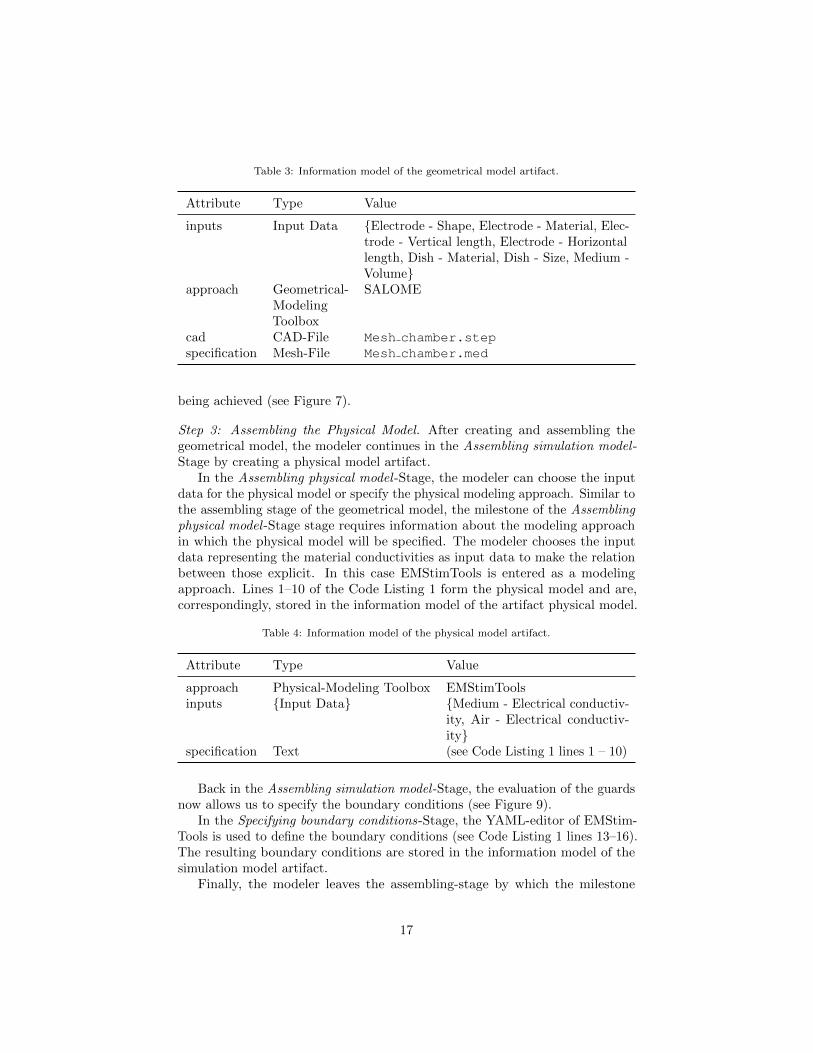
Table 3: Information model of the geometrical model artifact.

Attribute Type Value

inputs Input Data {Electrode - Shape, Electrode - Material, Elec-trode - Vertical length, Electrode - Horizontallength, Dish - Material, Dish - Size, Medium -Volume}

approach Geometrical-ModelingToolbox

SALOME

cad CAD-File Mesh chamber.stepspecification Mesh-File Mesh chamber.med

being achieved (see Figure 7).

Step 3: Assembling the Physical Model. After creating and assembling thegeometrical model, the modeler continues in the Assembling simulation model -Stage by creating a physical model artifact.

In the Assembling physical model -Stage, the modeler can choose the inputdata for the physical model or specify the physical modeling approach. Similar tothe assembling stage of the geometrical model, the milestone of the Assemblingphysical model -Stage stage requires information about the modeling approachin which the physical model will be specified. The modeler chooses the inputdata representing the material conductivities as input data to make the relationbetween those explicit. In this case EMStimTools is entered as a modelingapproach. Lines 1–10 of the Code Listing 1 form the physical model and are,correspondingly, stored in the information model of the artifact physical model.

Table 4: Information model of the physical model artifact.

Attribute Type Value

approach Physical-Modeling Toolbox EMStimToolsinputs {Input Data} {Medium - Electrical conductiv-

ity, Air - Electrical conductiv-ity}

specification Text (see Code Listing 1 lines 1 – 10)

Back in the Assembling simulation model -Stage, the evaluation of the guardsnow allows us to specify the boundary conditions (see Figure 9).

In the Specifying boundary conditions-Stage, the YAML-editor of EMStim-Tools is used to define the boundary conditions (see Code Listing 1 lines 13–16).The resulting boundary conditions are stored in the information model of thesimulation model artifact.

Finally, the modeler leaves the assembling-stage by which the milestone

17

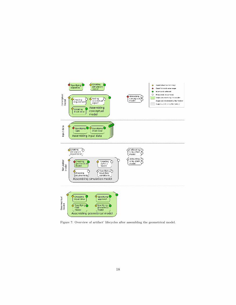
Figure 7: Overview of artifact’ lifecycles after assembling the geometrical model.

18

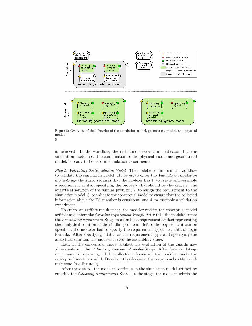
Figure 8: Overview of the lifecycles of the simulation model, geometrical model, and physicalmodel.

9

is achieved. In the workflow, the milestone serves as an indicator that thesimulation model, i.e., the combination of the physical model and geometricalmodel, is ready to be used in simulation experiments.

Step 4: Validating the Simulation Model. The modeler continues in the workflowto validate the simulation model. However, to enter the Validating simulationmodel -Stage the guard requires that the modeler has 1. to create and assemblea requirement artifact specifying the property that should be checked, i.e., theanalytical solution of the similar problem, 2. to assign the requirement to thesimulation model, 3. to validate the conceptual model to ensure that the collectedinformation about the ES chamber is consistent, and 4. to assemble a validationexperiment.

To create an artifact requirement, the modeler revisits the conceptual modelartifact and enters the Creating requirement-Stage. After this, the modeler entersthe Assembling requirement-Stage to assemble a requirement artifact representingthe analytical solution of the similar problem. Before the requirement can bespecified, the modeler has to specify the requirement type, i.e., data or logicformula. After specifying “data” as the requirement type and specifying theanalytical solution, the modeler leaves the assembling stage.

Back in the conceptual model artifact the evaluation of the guards nowallows entering the Validating conceptual model -Stage. After face validating,i.e., manually reviewing, all the collected information the modeler marks theconceptual model as valid. Based on this decision, the stage reaches the valid -milestone (see Figure 9).

After these steps, the modeler continues in the simulation model artifact byentering the Choosing requirements-Stage. In the stage, the modeler selects the

19

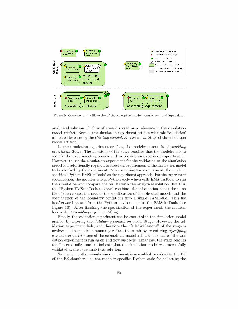
Figure 9: Overview of the life cycles of the conceptual model, requirement and input data.

analytical solution which is afterward stored as a reference in the simulationmodel artifact. Next, a new simulation experiment artifact with role “validation”is created by entering the Creating simulation experiment-Stage of the simulationmodel artifact.

In the simulation experiment artifact, the modeler enters the Assemblingexperiment-Stage. The milestone of the stage requires that the modeler has tospecify the experiment approach and to provide an experiment specification.However, to use the simulation experiment for the validation of the simulationmodel it is additionally required to select the requirement of the simulation modelto be checked by the experiment. After selecting the requirement, the modelerspecifies “Python-EMStimTools” as the experiment approach. For the experimentspecification, the modeler writes Python code which calls EMStimTools to runthe simulation and compare the results with the analytical solution. For this,the “Python-EMStimTools toolbox” combines the information about the meshfile of the geometrical model, the specification of the physical model, and thespecification of the boundary conditions into a single YAML-file. This fileis afterward passed from the Python environment to the EMStimTools (seeFigure 10). After finishing the specification of the experiment, the modelerleaves the Assembling experiment-Stage.

Finally, the validation experiment can be executed in the simulation modelartifact by entering the Validating simulation model -Stage. However, the val-idation experiment fails, and therefore the “failed-milestone” of the stage isachieved. The modeler manually refines the mesh by re-entering Specifyinggeometrical model -Stage of the geometrical model artifact. Thereafter, the vali-dation experiment is run again and now succeeds. This time, the stage reachesthe “succeed-milestone” to indicate that the simulation model was successfullyvalidated against the analytical solution.

Similarly, another simulation experiment is assembled to calculate the EFof the ES chamber, i.e., the modeler specifies Python code for collecting the

20

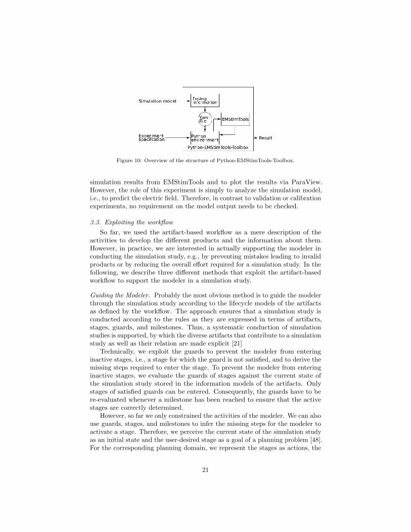
Figure 10: Overview of the structure of Python-EMStimTools-Toolbox.

simulation results from EMStimTools and to plot the results via ParaView.However, the role of this experiment is simply to analyze the simulation model,i.e., to predict the electric field. Therefore, in contrast to validation or calibrationexperiments, no requirement on the model output needs to be checked.

3.3. Exploiting the workflow

So far, we used the artifact-based workflow as a mere description of theactivities to develop the different products and the information about them.However, in practice, we are interested in actually supporting the modeler inconducting the simulation study, e.g., by preventing mistakes leading to invalidproducts or by reducing the overall effort required for a simulation study. In thefollowing, we describe three different methods that exploit the artifact-basedworkflow to support the modeler in a simulation study.

Guiding the Modeler. Probably the most obvious method is to guide the modelerthrough the simulation study according to the lifecycle models of the artifactsas defined by the workflow. The approach ensures that a simulation study isconducted according to the rules as they are expressed in terms of artifacts,stages, guards, and milestones. Thus, a systematic conduction of simulationstudies is supported, by which the diverse artifacts that contribute to a simulationstudy as well as their relation are made explicit [21]

Technically, we exploit the guards to prevent the modeler from enteringinactive stages, i.e., a stage for which the guard is not satisfied, and to derive themissing steps required to enter the stage. To prevent the modeler from enteringinactive stages, we evaluate the guards of stages against the current state ofthe simulation study stored in the information models of the artifacts. Onlystages of satisfied guards can be entered. Consequently, the guards have to bere-evaluated whenever a milestone has been reached to ensure that the activestages are correctly determined.

However, so far we only constrained the activities of the modeler. We can alsouse guards, stages, and milestones to infer the missing steps for the modeler toactivate a stage. Therefore, we perceive the current state of the simulation studyas an initial state and the user-desired stage as a goal of a planning problem [48].For the corresponding planning domain, we represent the stages as actions, the

21

guards as their preconditions, and the milestones as their postconditions (seeListing 2).

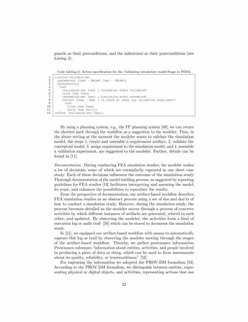
Code Listing 2: Action specification for the Validating simulation model-Stage in PDDL

1 (:action validate-smo2 :parameters (?smo - SModel ?cmo - CModel)3 :precondition4 (and5 (validated-cmo ?cmo) ; Conceptual model validated?6 (link ?cmo ?smo)7 (assembled-smo ?smo) ; Simulation model assembled?8 (exists (?exp - Exp) ; Is there at least one validation experiment?9 (and

10 (link ?smo ?exp)11 (role ?exp val))))12 :effect (validated-smo ?smo))

By using a planning system, e.g., the FF planning system [49], we can returnthe shortest path through the workflow as a suggestion to the modeler. Thus, inthe above setting at the moment the modeler wants to validate the simulationmodel, the steps 1. create and assemble a requirement artifact, 2. validate theconceptual model, 3. assign requirement to the simulation model, and 4. assemblea validation experiment, are suggested to the modeler. Further, details can befound in [11].

Documentation. During conducting FEA simulation studies, the modeler makesa lot of decisions, some of which are exemplarily captured in our short casestudy. Each of these decisions influences the outcome of the simulation study.Thorough documentation of the model building process, as suggested by reportingguidelines for FEA studies [13] facilitates interpreting and assessing the model,its reuse, and enhances the possibilities to reproduce the results.

From the perspective of documentation, our artifact-based workflow describesFEA simulation studies as an abstract process using a set of dos and don’ts ofhow to conduct a simulation study. However, during the simulation study, theprocess becomes detailed as the modeler moves through a process of concreteactivities by which different instances of artifacts are generated, related to eachother, and updated. By observing the modeler, the activities form a kind ofexecution log or audit trail [50] which can be stored to document the simulationstudy.

In [51], we equipped our artifact-based workflow with means to automaticallycapture this log or trail by observing the modeler moving through the stagesof the artifact-based workflow. Thereby, we gather provenance information.Provenance subsumes “information about entities, activities, and people involvedin producing a piece of data or thing, which can be used to form assessmentsabout its quality, reliability, or trustworthiness” [52].

For capturing the information we adopted the PROV-DM formalism [53].According to the PROV-DM formalism, we distinguish between entities, repre-senting physical or digital objects, and activities, representing actions that use

22

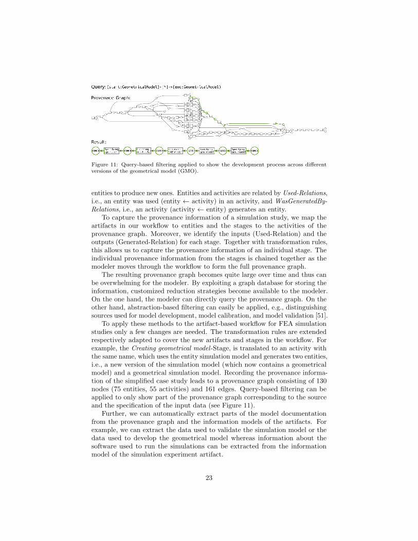
Figure 11: Query-based filtering applied to show the development process across differentversions of the geometrical model (GMO).

entities to produce new ones. Entities and activities are related by Used-Relations,i.e., an entity was used (entity ← activity) in an activity, and WasGeneratedBy-Relations, i.e., an activity (activity ← entity) generates an entity.

To capture the provenance information of a simulation study, we map theartifacts in our workflow to entities and the stages to the activities of theprovenance graph. Moreover, we identify the inputs (Used-Relation) and theoutputs (Generated-Relation) for each stage. Together with transformation rules,this allows us to capture the provenance information of an individual stage. Theindividual provenance information from the stages is chained together as themodeler moves through the workflow to form the full provenance graph.

The resulting provenance graph becomes quite large over time and thus canbe overwhelming for the modeler. By exploiting a graph database for storing theinformation, customized reduction strategies become available to the modeler.On the one hand, the modeler can directly query the provenance graph. On theother hand, abstraction-based filtering can easily be applied, e.g., distinguishingsources used for model development, model calibration, and model validation [51].

To apply these methods to the artifact-based workflow for FEA simulationstudies only a few changes are needed. The transformation rules are extendedrespectively adapted to cover the new artifacts and stages in the workflow. Forexample, the Creating geometrical model -Stage, is translated to an activity withthe same name, which uses the entity simulation model and generates two entities,i.e., a new version of the simulation model (which now contains a geometricalmodel) and a geometrical simulation model. Recording the provenance informa-tion of the simplified case study leads to a provenance graph consisting of 130nodes (75 entities, 55 activities) and 161 edges. Query-based filtering can beapplied to only show part of the provenance graph corresponding to the sourceand the specification of the input data (see Figure 11).

Further, we can automatically extract parts of the model documentationfrom the provenance graph and the information models of the artifacts. Forexample, we can extract the data used to validate the simulation model or thedata used to develop the geometrical model whereas information about thesoftware used to run the simulations can be extracted from the informationmodel of the simulation experiment artifact.

23

Experiment generation. Detailed documentation of simulation studies can beused to support the automatic generation of simulation experiments [54]. There-fore, the structure and required inputs need to be identified for specific types ofsimulation experiments, such as sensitivity analysis or statistical model checking.Once identified, they can be represented in the form of software-specific templates,or more abstractly in the form of experiment schemas to use them across differentsoftware systems [55]. Given an experiment template or schema, the informationmodels of the workflow artifacts form a rich source to fill input variables ofvarious experiment schemas. The completely filled schemas are used to generateexecutable experiments in the respective modeling and simulation environment.From the perspective of the workflow, there is no difference between the manualand automatic generation of a simulation experiment specifications, as the latterforms simply an alternative to the purely manual experiment specification inthe Specifying simulation experiment-Stage that involves the invocation of anexperiment generator. A detailed presentation of the pipeline and the genera-tors that lead from composable experiment schemas to executable simulationexperiments, such as sensitivity analysis, and which can be applied for stochasticdiscrete-event simulation as well as FEA studies can be found in [55].

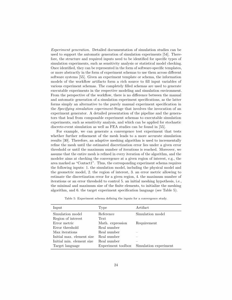
For example, we can generate a convergence test experiment that testswhether further refinement of the mesh leads to a more accurate simulationresults [30]. Therefore, an adaptive meshing algorithm is used to incrementallyrefine the mesh until the estimated discretization error lies under a given errorthreshold or until the maximum number of iterations is reached. Moreover, weassume that the entire mesh is refined in every iteration of the algorithm, and themodeler aims at checking the convergence at a given region of interest, e.g., thearea marked as “Contact1”. Thus, the corresponding experiment schema requiresthe following inputs: 1. the simulation model, including the physical model andthe geometric model, 2. the region of interest, 3. an error metric allowing toestimate the discretization error for a given region, 4. the maximum number ofiterations or an error threshold to control 5. an initial meshing hypothesis, i.e.,the minimal and maximum size of the finite elements, to initialize the meshingalgorithm, and 6. the target experiment specification language (see Table 5).

Table 5: Experiment schema defining the inputs for a convergence study.

Input Type Artifact

Simulation model Reference Simulation modelRegion of interest Text

RequirementError metric Math. expressionError threshold Real numberMax iterations Real number –Initial max. element size Real number –Initial min. element size Real number –Target language Experiment toolbox Simulation experiment

24

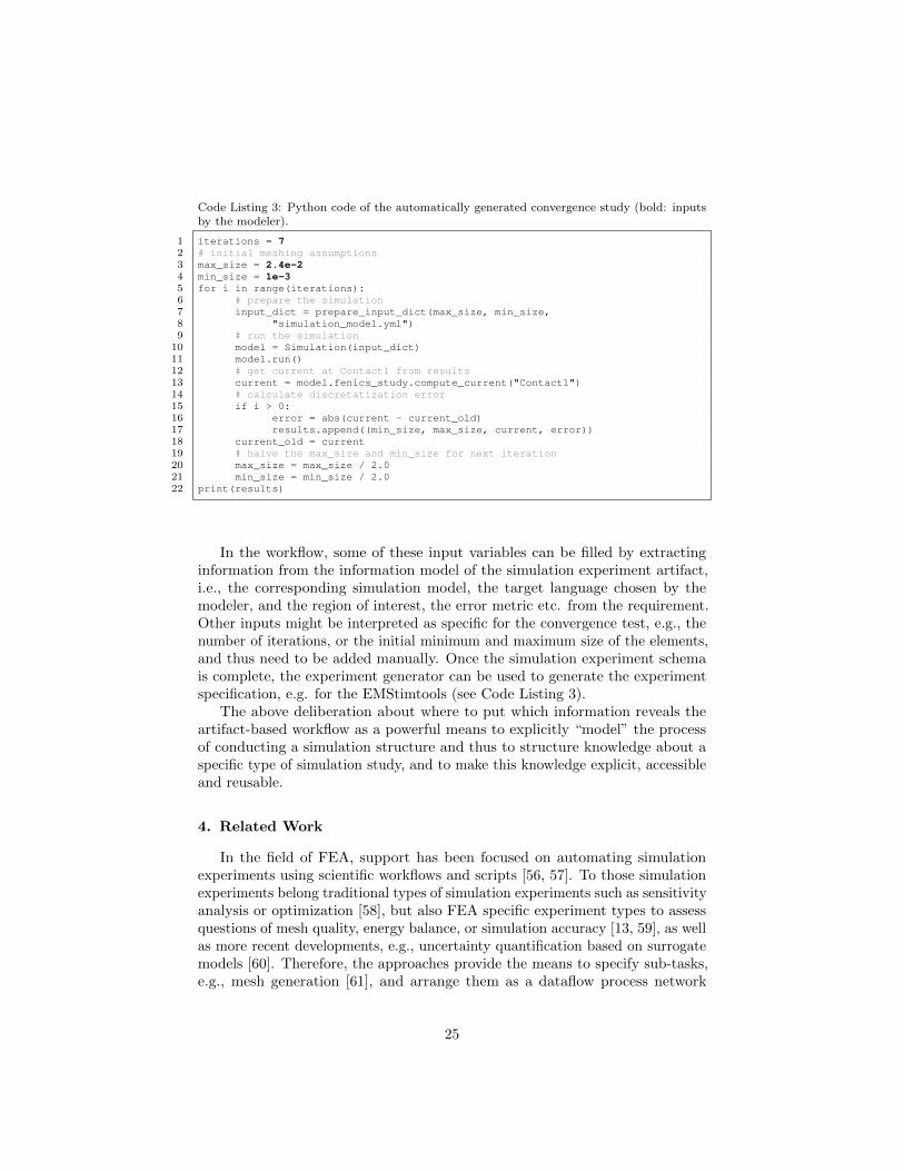
Code Listing 3: Python code of the automatically generated convergence study (bold: inputsby the modeler).

1 iterations = 72 # initial meshing assumptions3 max_size = 2.4e-24 min_size = 1e-35 for i in range(iterations):6 # prepare the simulation7 input_dict = prepare_input_dict(max_size, min_size,8 "simulation_model.yml")9 # run the simulation

10 model = Simulation(input_dict)11 model.run()12 # get current at Contact1 from results13 current = model.fenics_study.compute_current("Contact1")14 # calculate discretatization error15 if i > 0:16 error = abs(current - current_old)17 results.append((min_size, max_size, current, error))18 current_old = current19 # halve the max_size and min_size for next iteration20 max_size = max_size / 2.021 min_size = min_size / 2.022 print(results)

In the workflow, some of these input variables can be filled by extractinginformation from the information model of the simulation experiment artifact,i.e., the corresponding simulation model, the target language chosen by themodeler, and the region of interest, the error metric etc. from the requirement.Other inputs might be interpreted as specific for the convergence test, e.g., thenumber of iterations, or the initial minimum and maximum size of the elements,and thus need to be added manually. Once the simulation experiment schemais complete, the experiment generator can be used to generate the experimentspecification, e.g. for the EMStimtools (see Code Listing 3).

The above deliberation about where to put which information reveals theartifact-based workflow as a powerful means to explicitly “model” the processof conducting a simulation structure and thus to structure knowledge about aspecific type of simulation study, and to make this knowledge explicit, accessibleand reusable.

4. Related Work

In the field of FEA, support has been focused on automating simulationexperiments using scientific workflows and scripts [56, 57]. To those simulationexperiments belong traditional types of simulation experiments such as sensitivityanalysis or optimization [58], but also FEA specific experiment types to assessquestions of mesh quality, energy balance, or simulation accuracy [13, 59], as wellas more recent developments, e.g., uncertainty quantification based on surrogatemodels [60]. Therefore, the approaches provide the means to specify sub-tasks,e.g., mesh generation [61], and arrange them as a dataflow process network

25

[62, 63], i.e., processing pipelines, which we can execute but also adapt and reusefor similar simulation experiments [64, 65].

Scientific-workflows, such as Taverna [66] or Kepler [62], provide specializedlanguages or visual interfaces to describe the processing pipelines and provideadditional services, e.g., for distributing the execution of the pipeline [67, 62]or tracking different versions of the workflow specification [68, 69]. In contrast,scripting languages, such as Python [70] or R [71], provide a full programminglanguage to describe the arbitrary computational process. Consequently, theuser can not rely on a closed environment and thus needs to implement the datapipelines with the services and the execution logic.

Another approach to support FEA simulation studies is to use ontologies,which provide a formal specification of the different work products in terms oftheir attributes and relations. Thus, we can use ontologies to share knowledgeabout the geometrical and physical model across different software suites [72, 73,74, 75], to derive processing parameters [76, 77] and to document these studies[78, 79].

Our artifact-based workflow combines and extends existing workflow-basedand ontology-based approaches by describing how they are conducted and in-tegrating knowledge about the research question, assumptions, requirements,or input data into this process. Therefore, the lifecycle models of our arti-facts describe computational processes, as well as interactive processes. Existingworkflow-approaches can be integrated into the artifact-based workflow to specifyand execute simulation experiments. Further, the meta-information and the in-formation about the artifacts are made explicit by the information models of theartifacts. Process knowledge about FEA studies and meta-information togetherallows us to extend existing ontology-based support mechanisms by automati-cally documenting crucial provenance information and by (semi-)automaticallygenerating various simulation experiments for the FEA study.

5. Conclusion

We adapted the artifact-based workflow developed in [11] for FEA simulationstudies and showed based on a small case study on FEA of an electric stimulationchamber how such a declarative workflow approach can contribute to the guidance,best practices, and documentation of FEA simulation studies.

To assist in conducting FEA studies, the artifact-based workflow relies onthe definition of toolboxes, that allow integrating methods to specify simulationmodels, provide execution means for analysis, and offer and support diverseexperiments, into the workflow. Instead of a recipe enlisting a sequence of actionsto follow, the artifact-based workflow constrains the execution of activities viaguards and milestones. Pursuing a least commitment strategy opens up theneeded freedom to navigate a FEA study. The design, i.e., the artifacts andtheir relations, ensures that the conceptual model, in terms of objective, inputs,and requirements, as well as simulation experiments, are specified. Withinthe workflow, we define and explicate relations between conceptual model,

26

requirement, inputs, simulation model, simulation experiments, and simulationdata.

The number and variety of simulation experiments that are conducted witha simulation model are what determine the understanding of and trust in asimulation model [12, 14, 59]. Simulation experiments are treated as first-classcitizens in conducting a FEA study. Based on the defined requirements, theirtypes, and methods that are supported by the experiment toolboxes, the artifact-based workflow approach allows to (semi-)automatically derive, generate, andexecute simulation experiments. Thus, the conceptual model, in particular, thespecified requirements can be used to define (and in the ideal case to generateautomatically) a minimal set of simulation experiments to be conducted.

As noted e.g. in [13], for interpreting and reusing simulation models andresults, the thorough documentation of the FEA study is central. Mappingartifacts to entities and stages to activities allowed us together with a fewtransformation rules to automatically store detailed provenance informationabout FEA studies. Thereby, the process by which the simulation model wasgenerated and the activities and resources that contributed to its generation canbe traced and queried.

Only part of the parameters that are suggested in [13] for a thorough reportof FEA studies is used in our adaptation of the artifact-based workflow forFEA studies. Further could be easily integrated into the conceptual modelartifact. To do so in a structured manner, community efforts are required. Thedevelopment of more standardized vocabularies and ontologies for FEA simulationstudies would enable additional inference mechanism, e.g., to automaticallycheck the consistency of the information in the conceptual model, or can serveas a foundation to further develop experiment schemas to generate simulationexperiments automatically. Therefore, to structure and more formally definecontext information and thus make it accessible for automatic interpretation iskey for effective exploitation of workflow methods for guidance, best practice,and documentation of FEA studies.

Acknowledgment

This work was funded by Deutsche Forschungsgemeinschaft (DFG, GermanResearch Foundation) – SFB 1270/1 - 299150580 and the DFG research projectUH 66/18 GrEASE.

References

[1] S. Krueger, S. Achilles, J. Zimmermann, T. Tischer, R. Bader, A. Jonitz-Heincke, Re-Differentiation Capacity of Human Chondrocytes in VitroFollowing Electrical Stimulation with Capacitively Coupled Fields, J. Clin.Med. 8 (11) (2019) 1771.

[2] G. Thrivikraman, S. K. Boda, B. Basu, Unraveling the mechanistic effectsof electric field stimulation towards directing stem cell fate and function: Atissue engineering perspective, Biomaterials 150 (2018) 60–86.

27

[3] A. R. Farooqi, R. Bader, U. van Rienen, Numerical Study on Electrome-chanics in Cartilage Tissue with Respect to Its Electrical Properties, TissueEngineering Part B: Reviews 25 (2) (2019) 152–166.

[4] R. Fujimoto, C. Bock, W. Chen, E. Page, J. H. Panchal, Research challengesin modeling and simulation for engineering complex systems, Springer, 2017.

[5] K. Gorlach, M. Sonntag, D. Karastoyanova, F. Leymann, M. Reiter, Conven-tional workflow technology for scientific simulation, in: Guide to e-Science,Springer, 2011, pp. 323–352.

[6] M. Sonntag, D. Karastoyanova, Model-as-you-go: an approach for an ad-vanced infrastructure for scientific workflows, Journal of grid computing11 (3) (2013) 553–583.

[7] S. Rybacki, J. Himmelspach, F. Haack, A. M. Uhrmacher, WorMS-a frame-work to support workflows in M&S, in: Proceedings of the Winter SimulationConference, Winter Simulation Conference, 2011, pp. 716–727.

[8] J. Ribault, G. Zacharewicz, Time-based orchestration of workflow, interop-erability with G-Devs/HLA, J. Comput. Science 10 (2015) 126–136.

[9] B. Chopard, J. Borgdorff, A. G. Hoekstra, A framework for multi-scalemodelling, Philosophical Transactions of the Royal Society A: Mathematical,Physical and Engineering Sciences 372 (2021) (2014) 20130378.

[10] O. Balci, A life cycle for modeling and simulation, Simulation 88 (7) (2012)870–883.

[11] A. Ruscheinski, T. Warnke, A. M. Uhrmacher, Artifact-based Workflowsfor Supporting Simulation Studies, IEEE Transactions on Knowledge andData Engineering.

[12] A. E. Anderson, B. J. Ellis, J. A. Weiss, Verification, validation and sensi-tivity studies in computational biomechanics, Computer methods in biome-chanics and biomedical engineering 10 (3) (2007) 171–184.

[13] A. Erdemir, T. M. Guess, J. Halloran, S. C. Tadepalli, T. M. Morrison,Considerations for reporting finite element analysis studies in biomechanics,Journal of biomechanics 45 (4) (2012) 625–633.

[14] J. L. Hicks, T. K. Uchida, A. Seth, A. Rajagopal, S. L. Delp, Is my modelgood enough? Best practices for verification and validation of muscu-loskeletal models and simulations of movement, Journal of biomechanicalengineering 137 (2).

[15] L. Cucurull-Sanchez, M. J. Chappell, V. Chelliah, S. Amy Cheung, G. Derks,M. Penney, A. Phipps, R. S. Malik-Sheriff, J. Timmis, M. J. Tindall,et al., Best practices to maximize the use and reuse of quantitative andsystems pharmacology models: recommendations from the United Kingdom

28

Quantitative and Systems Pharmacology Network, CPT: Pharmacometrics& Systems Pharmacology 8 (5) (2019) 259–272.

[16] C. Di Ciccio, A. Marrella, A. Russo, Knowledge-intensive processes: charac-teristics, requirements and analysis of contemporary approaches, Journalon Data Semantics 4 (1) (2015) 29–57.

[17] R. Hull, E. Damaggio, R. De Masellis, F. Fournier, M. Gupta, F. T. Heath III,S. Hobson, M. Linehan, S. Maradugu, A. Nigam, et al., Business artifactswith guard-stage-milestone lifecycles: managing artifact interactions withconditions and events, in: Proceedings of the 5th ACM international confer-ence on Distributed event-based system, 2011, pp. 51–62.

[18] R. Vaculın, R. Hull, T. Heath, C. Cochran, A. Nigam, P. Sukaviriya,Declarative business artifact centric modeling of decision and knowledgeintensive business processes, in: 2011 IEEE 15th International EnterpriseDistributed Object Computing Conference, IEEE, 2011, pp. 151–160.

[19] G. De Giacomo, M. Dumas, F. M. Maggi, M. Montali, Declarative processmodeling in BPMN, in: International Conference on Advanced InformationSystems Engineering, Springer, 2015, pp. 84–100.

[20] S. Robinson, Conceptual modelling for simulation Part II: a framework forconceptual modelling, Journal of the operational research society 59 (3)(2008) 291–304.

[21] R. Fujimoto, C. Bock, W. Chen, E. H. Page, J. H. Panchal, Executivesummary, in: R. Fujimoto, C. Bock, W. Chen, E. H. Page, J. H. Panchal(Eds.), Research Challenges in Modeling and Simulation for EngineeringComplex Systems, Simulation Foundations, Methods and Applications,Springer, Cham, 2017, pp. 23–44.

[22] P. Wilsdorf, F. Haack, A. M. Uhrmacher, Conceptual models in simulationstudies: Making it explicit, in: Winter Simulation Conference (WSC 2020),2020, accepted.

[23] T. Helms, T. Warnke, C. Maus, A. M. Uhrmacher, Semantics and efficientsimulation algorithms of an expressive multi-level modeling language, ACMTransactions on Modeling and Computer Simulation (TOMACS) 27 (2)(2017) 8:1–8:25.URL http://eprints.mosi.informatik.uni-rostock.de/376/

[24] S. Tisue, U. Wilensky, Netlogo: A simple environment for modeling com-plexity, in: International conference on complex systems, Vol. 21, Boston,MA, 2004, pp. 16–21.

[25] R. Ewald, A. M. Uhrmacher, SESSL: A domain-specific language for simula-tion experiments, ACM Transactions on Modeling and Computer Simulation(TOMACS) 24 (2) (2014) 1–25.

29

[26] J. C. Thiele, V. Grimm, Netlogo meets r: Linking agent-based models witha toolbox for their analysis, Environmental Modelling & Software 25 (8)(2010) 972–974.

[27] J. C. Thiele, W. Kurth, V. Grimm, Facilitating parameter estimation andsensitivity analysis of agent-based models: A cookbook using netlogo and r,Journal of Artificial Societies and Social Simulation 17 (3) (2014) 11.

[28] A. Ruscheinski, A. Wolpers, P. Henning, T. Warnke, F. Haack, A. M.Uhrmacher, Pragmatic logic-based spatio-temporal pattern checking inparticle-based models, in: Winter Simulation Conference (WSC 2020), 2020,accepted.URL http://eprints.mosi.informatik.uni-rostock.de/611/

[29] D. Roylance, Finite element analysis, Department of Materials Science andEngineering, Massachusetts Institute of Technology, Cambridge.

[30] A. Datta, V. Rakesh, An introduction to modeling of transport processes:applications to biomedical systems, Cambridge University Press, 2010.

[31] O. C. Zienkiewicz, R. L. Taylor, J. Z. Zhu, The finite element method: itsbasis and fundamentals, Elsevier, 2005.

[32] M. Abdelmegid, V. Gonzalez, M. O’Sullivan, C. Walker, M. Poshdar, F. Ying,The roles of conceptual modelling in improving construction simulation stud-ies: A comprehensive review, Advanced Engineering Informatics 46 (2020)101175. doi:https://doi.org/10.1016/j.aei.2020.101175.URL http://www.sciencedirect.com/science/article/pii/S1474034620301464

[33] A. Ribes, C. Caremoli, Salome platform component model for numericalsimulation, in: 31st annual international computer software and applicationsconference (COMPSAC 2007), Vol. 2, IEEE, 2007, pp. 553–564.

[34] M. S. Alnæs, J. Blechta, J. Hake, A. Johansson, B. Kehlet, A. Logg,C. Richardson, J. Ring, M. E. Rognes, G. N. Wells, The FEniCS ProjectVersion 1.5, Arch. Numer. Softw. 3 (100).

[35] D. Kluess, R. Souffrant, W. Mittelmeier, A. Wree, K.-P. Schmitz, R. Bader,A convenient approach for finite-element-analyses of orthopaedic implantsin bone contact: Modeling and experimental validation, Computer Methodsand Programs in Biomedicine 95 (1) (2009) 23 – 30.

[36] A. Erdemir, T. F. Besier, J. P. Halloran, C. W. Imhauser, P. J. Laz, T. M.Morrison, K. B. Shelburne, Deciphering the “art” in modeling and simulationof the knee joint: Overall strategy, Journal of biomechanical engineering141 (7).

[37] S. Mobini, L. Leppik, J. H. Barker, Direct current electrical stimulationchamber for treating cells in vitro, Biotechniques 60 (2) (2016) 95–98.

30

[38] S. Mobini, L. Leppik, V. Thottakkattumana Parameswaran, J. H. Barker,In vitro effect of direct current electrical stimulation on rat mesenchymalstem cells, PeerJ 5 (2017) e2821.

[39] K. Budde, J. Zimmermann, E. Neuhaus, M. Schroder, A. M. Uhrmacher,U. van Rienen, Requirements for Documenting Electrical Cell StimulationExperiments for Replicability and Numerical Modeling, in: 2019 41st Annu.Int. Conf. IEEE Eng. Med. Biol. Soc., 2019, pp. 1082–1088.

[40] T. P. P. AG, Basics to determine the ideal volume of culture medium for usein tpp tissue culture vessels, https://www.tpp.ch/page/downloads/instruction_for_use/2018-Optimal_volume_vessels.pdf,Accessed: 2020-03-11 (2018).

[41] J. Schoberl, An advancing front 2D/3D-mesh generator based on abstractrules, Comput. Vis. Sci. 1 (1) (1997) 41–52.

[42] J. Malmivuo, R. Plonsey, Bioelectromagnetism: principles and applicationsof bioelectric and biomagnetic fields, Oxford University Press, USA, 1995.

[43] P. Hasgall, F. Di Gennaro, C. Baumgartner, E. Neufeld, B. Lloyd, M. Gos-selin, D. Payne, A. Klingenboeck, N. Kuster, It’is database for ther-mal and electromagnetic parameters of biological tissues, version 4.0,itis.swiss/database, doi: 10.13099/VIP21000-04-0 (2018).

[44] A. Logg, G. N. Wells, K.-A. Mardall, Others, Automated Solution ofDifferential Equations by the Finite Element Method, Springer, 2012.

[45] J. Ahrens, B. Geveci, C. Law, Paraview: An end-user tool for large datavisualization, The visualization handbook 717.

[46] M. E. Rognes, A. Logg, Automated goal-oriented error control i: Stationaryvariational problems, SIAM Journal on Scientific Computing 35 (3). arXiv:1204.6643.

[47] M. Hronik-Tupaj, W. L. Rice, M. Cronin-Golomb, D. L. Kaplan, I. Georgak-oudi, Osteoblastic differentiation and stress response of human mesenchymalstem cells exposed to alternating current electric fields, Biomedical Engi-neering Online 10 (2011) 9.

[48] J. A. Hendler, A. Tate, M. Drummond, Ai planning: Systems and techniques,AI magazine 11 (2) (1990) 61–61.

[49] J. Hoffmann, B. Nebel, The ff planning system: Fast plan generation throughheuristic search, Journal of Artificial Intelligence Research 14 (2001) 253–302.

[50] S. B. Davidson, J. Freire, Provenance and scientific workflows: challengesand opportunities, in: Proceedings of the 2008 ACM SIGMOD internationalconference on Management of data, 2008, pp. 1345–1350.

31

[51] A. Ruscheinski, P. Wilsdorf, M. Dombrowsky, A. M. Uhrmacher, Capturingand reporting provenance information of simulation studies based on anartifact-based workflow approach, in: Proceedings of the 2019 ACM SIGSIMConference on Principles of Advanced Discrete Simulation, SIGSIM-PADS’19, Association for Computing Machinery, New York, NY, USA, 2019, p.185–196.

[52] P. Groth, L. Moreau, PROV-overview. an overview of the PROV family ofdocuments, World Wide Web Consortium.

[53] K. Belhajjame, R. B’Far, J. Cheney, S. Coppens, S. Cresswell, Y. Gil,P. Groth, G. Klyne, T. Lebo, J. McCusker, et al., PROV-DM: The PROVData Model, W3C Recommendation.

[54] A. Ruscheinski, K. Budde, T. Warnke, P. Wilsdorf, B. C. Hiller, M. Dom-browsky, A. M. Uhrmacher, Generating Simulation Experiments Based onModel Documentations and Templates, in: Winter Simulation Conference(WSC 2018), IEEE, 2018, pp. 715–726.

[55] P. Wilsdorf, J. Zimmermann, M. Dombrowsky, U. van Rienen, A. M.Uhrmacher, Simulation experiment schemas - beyond tools and simula-tion approaches, in: Winter Simulation Conference (WSC 2019), 2019, pp.2783–2794.

[56] M. Reiter, H.-L. Truong, S. Dustdar, D. Karastoyanova, R. Krause, F. Ley-mann, D. Pahr, On analyzing quality of data influences on performanceof finite elements driven computational simulations, in: C. Kaklamanis,T. Papatheodorou, P. G. Spirakis (Eds.), Euro-Par 2012 Parallel Processing,Springer Berlin Heidelberg, Berlin, Heidelberg, 2012, pp. 793–804.

[57] B. Zehner, J. H. Borner, I. Gorz, K. Spitzer, Workflows for generatingtetrahedral meshes for finite element simulations on complex geologicalstructures, Computers & Geosciences 79 (2015) 105–117.

[58] S. Stipetic, W. Miebach, D. Zarko, Optimization in design of electric ma-chines: Methodology and workflow, in: 2015 Intl Aegean Conference onElectrical Machines & Power Electronics (ACEMP), 2015 Intl Conferenceon Optimization of Electrical & Electronic Equipment (OPTIM) & 2015Intl Symposium on Advanced Electromechanical Motion Systems (ELEC-TROMOTION), IEEE, 2015, pp. 441–448.

[59] T. A. Burkhart, D. M. Andrews, C. E. Dunning, Finite element model-ing mesh quality, energy balance and validation methods: A review withrecommendations associated with the modeling of bone tissue, Journal ofbiomechanics 46 (9) (2013) 1477–1488.

[60] C. Schmidt, P. Grant, M. Lowery, U. van Rienen, Influence of uncertaintiesin the material properties of brain tissue on the probabilistic volume oftissue activated, IEEE Transactions on Biomedical Engineering 60 (5) (2012)1378–1387.

32

[61] S. J. Owen, A survey of unstructured mesh generation technology., IMR239 (1998) 267.

[62] B. Ludascher, I. Altintas, C. Berkley, D. Higgins, E. Jaeger, M. Jones,E. A. Lee, J. Tao, Y. Zhao, Scientific workflow management and the keplersystem, Concurrency and computation: Practice and experience 18 (10)(2006) 1039–1065.

[63] E. A. Lee, T. M. Parks, Dataflow process networks, Proceedings of theIEEE 83 (5) (1995) 773–801.

[64] J. J. Timmons, E. Lok, P. San, K. Bui, E. T. Wong, End-to-end workflowfor finite element analysis of tumor treating fields in glioblastomas, Physicsin Medicine & Biology 62 (21) (2017) 8264.

[65] C. E. Scheidegger, H. T. Vo, D. Koop, J. Freire, C. T. Silva, Querying andre-using workflows with vstrails, in: Proceedings of the 2008 ACM SIGMODinternational conference on Management of data, 2008, pp. 1251–1254.

[66] T. Oinn, M. Addis, J. Ferris, D. Marvin, M. Senger, M. Greenwood,T. Carver, K. Glover, M. R. Pocock, A. Wipat, et al., Taverna: a toolfor the composition and enactment of bioinformatics workflows, Bioinfor-matics 20 (17) (2004) 3045–3054.

[67] E. Deelman, G. Singh, M.-H. Su, J. Blythe, Y. Gil, C. Kesselman, G. Mehta,K. Vahi, G. B. Berriman, J. Good, et al., Pegasus: A framework formapping complex scientific workflows onto distributed systems, ScientificProgramming 13 (3) (2005) 219–237.

[68] R. S. Barga, Y. L. Simmhan, E. Chinthaka, S. S. Sahoo, J. Jackson,N. Araujo, Provenance for scientific workflows towards reproducible re-search., IEEE Data Eng. Bull. 33 (3) (2010) 50–58.

[69] K. Belhajjame, K. Wolstencroft, O. Corcho, T. Oinn, F. Tanoh, A. William,C. Goble, Metadata management in the taverna workflow system, in: 2008Eighth IEEE International Symposium on Cluster Computing and the Grid(CCGRID), IEEE, 2008, pp. 651–656.

[70] T. E. Oliphant, Python for scientific computing, Computing in Science &Engineering 9 (3) (2007) 10–20.

[71] R. Ihaka, R. Gentleman, R: a language for data analysis and graphics,Journal of computational and graphical statistics 5 (3) (1996) 299–314.

[72] S. Tessier, Y. Wang, Ontology-based feature mapping and verification be-tween cad systems, Advanced Engineering Informatics 27 (1) (2013) 76 –92, modeling, Extraction, and Transformation of Semantics in ComputerAided Engineering Systems. doi:https://doi.org/10.1016/j.aei.2012.11.008.URL http://www.sciencedirect.com/science/article/pii/S1474034612001097

33

[73] W. Sun, Q. Ma, S. Chen, A framework for automated finite element anal-ysis with an ontology-based approach, Journal of mechanical science andtechnology 23 (12) (2009) 3209–3220.

[74] H. Cheong, A. Butscher, Physics-based simulation ontology: anontology to support modelling and reuse of data for physics-basedsimulation, Journal of Engineering Design 30 (10-12) (2019) 655–687.arXiv:https://doi.org/10.1080/09544828.2019.1644301,doi:10.1080/09544828.2019.1644301.URL https://doi.org/10.1080/09544828.2019.1644301

[75] A. Freitas, M. Jones, K. Asooja, C. Bellos, S. Elliott, S. Stenfelt, P. Hasapis,C. Georgousopoulos, T. Marquardt, N. Filipovic, et al., Towards a semanticrepresentation for multi-scale finite element biosimulation experiments, in:13th IEEE International Conference on BioInformatics and BioEngineering,IEEE, 2013, pp. 1–5.

[76] P. Kestel, P. Kugler, C. Zirngibl, B. Schleich, S. Wartzack, Ontology-basedapproach for the provision of simulation knowledge acquired by data andtext mining processes, Advanced Engineering Informatics 39 (2019) 292 –305. doi:https://doi.org/10.1016/j.aei.2019.02.001.URL http://www.sciencedirect.com/science/article/pii/S1474034618304270

[77] F. Boussuge, C. M. Tierney, H. Vilmart, T. T. Robinson,C. G. Armstrong, D. C. Nolan, J.-C. Leon, F. Ulliana, Cap-turing simulation intent in an ontology: Cad and cae inte-gration application, Journal of Engineering Design 30 (10-12)(2019) 688–725. arXiv:https://doi.org/10.1080/09544828.2019.1630806, doi:10.1080/09544828.2019.1630806.URL https://doi.org/10.1080/09544828.2019.1630806

[78] G. Peng, H. Wang, H. Zhang, Y. Zhao, A. L. Johnson, A collaborativesystem for capturing and reusing in-context design knowledge with an inte-grated representation model, Advanced Engineering Informatics 33 (2017)314 – 329. doi:https://doi.org/10.1016/j.aei.2016.12.007.URL http://www.sciencedirect.com/science/article/pii/S1474034616301859

[79] M. Mehdi, Y. Khan, A. Freitas, J. Jares, S. Decker, R. Sahay, A linkeddata platform for finite element biosimulations, in: Proceedings of the 11thInternational Conference on Semantic Systems, 2015, pp. 89–96.

34