
DELAMINATION STRESSES IN THIN-WALL STRUCTURES OF COMPOSITE MATERIALS
Upload
independentCategory
view
0download
0
Journal of
Mechanics ofMaterials and Structures
OPTIMIZATION OF A SATELLITE WITH COMPOSITE MATERIALS
Jorge A. C. Ambrósio, Maria Augusta Neto and Rogério Pereira Leal
Volume 2, Nº 8 October 2007
mathematical sciences publishers

JOURNAL OF MECHANICS OF MATERIALS AND STRUCTURESVol. 2, No. 8, 2007
OPTIMIZATION OF A SATELLITE WITH COMPOSITE MATERIALS
JORGE A. C. AMBRÓSIO, MARIA AUGUSTA NETO AND ROGÉRIO PEREIRA LEAL
The design of complex flexible multibody systems for industrial applications requires not only the use ofpowerful methodologies for the system analysis, but also the ability to analyze potential designs and todecide on the merits of each one of them. This paper presents a methodology using optimization proce-dures to find the optimal layouts of fiber composite structure components in multibody systems. The goalof the optimization process is to minimize structural deformation and to fulfill a set of multidisciplinaryconstraints. These methodologies rely on the efficient and accurate calculation of the system sensitivitiesto support the optimization algorithms. In this work a general formulation for the computation of thefirst order analytic sensitivities based on the direct differentiation method is used. The direct method forsensitivity calculation is obtained by direct differentiation of the equations defining the response of thestructure with respect to the design variables. The equations of motion and the sensitivities of the flexiblemultibody system are solved simultaneously and, therefore, the accelerations and velocities of the system,and the sensitivities of the accelerations and velocities, are integrated in time using a multistep multiorderintegration algorithm. Different models for the flexible components of the system, using beam and plateelements, are also considered. Finally, the methodology proposed here is applied to the optimizationof the unfolding of a complex satellite made of composite plates and beams. The ply orientations oflamination are the continuous design variables. The potential difficulties in the optimization of compositeflexible multibody systems are highlighted in the discussion of the results obtained.
1. Introduction
Modeling refers to the tools used in the construction of models of individual and coupled componentsof technical systems. The simplest models for multibody systems assume rigid body components whilemore complex models require the description of the components’ flexibility. The finite element-basedstrategies used to represent the components’ flexibility in multibody systems is a well accepted andwidely used method. For systems in which the bodies are made of standard materials, there is a widevariety of finite elements that may be used, but when bodies are made of composite materials, the modelflexibility often necessitates expensive finite element models with an inherent growth in complexity.Models of systems involving multibody dynamics methodologies also require a complete knowledge ofthe arrangement of the system components, which is achieved by the definition of kinematic joints, theintroduction of models for external forces and the incorporation of the equilibrium equations of otherdisciplines [Heckmann et al. 2005; Møller et al. 2005; Bottasso et al. 2006]. Regardless of each particulartype of joint used, the mathematical description of the restrictions involving only rigid bodies are thesimplest to obtain. The presence of flexible bodies tends to increase the complexity of the description,and methods for simplifying the description are required [Lehner and Eberhard 2006; Hardeman et al.
Keywords: flexible multibody dynamics, sensitivity analysis, automatic differentiation, large rotations, floating frame.
1397
1398 JORGE A. C. AMBRÓSIO, MARIA AUGUSTA NETO AND ROGÉRIO PEREIRA LEAL
2006]. However, the concept of virtual bodies provides a general framework for developing generalkinematic joints for flexible multibody systems with minimal effort [Ambrosio 2003].
Analyses of rigid mechanical systems are the simplest and the least expensive, regardless of model.Flexible systems, in which the bodies only experience small elastic deformations, have higher compu-tational costs. For these systems it is common to use mode component synthesis to reduce the numberof generalized elastic coordinates and, consequently, the equations of motion are written in terms ofmodal coordinates [Nikravesh and Lin 2005; Goncalves and Ambrosio 2005; Lehner and Eberhard 2006].However, when the system components experience nonlinear deformations, the use of reduction methodsis not possible, in general, and the finite element nodal coordinates are the generalized coordinates used[Ambrosio 1996; Dmitrochenko et al. 2006; Gerstmayr and Schoberl 2006; Vetyukov et al. 2006]. Fur-thermore, the analysis of these systems is more complex and, usually, computationally more expensivethan the analysis of flexible systems with bodies that experience linear deformations.
In terms of the optimization complexity, the most complex and expensive problems are global orinteger optimization problems with a large number of design variables. The simplest and cheapest prob-lems to solve are continuous local problems with a small number of design variables [Venkataramanand Haftka 1999; Venkataraman and Haftka 2002]. Stochastic optimization algorithms, like simulatedannealing methods or genetic algorithms, offer a way to perform global optimization, but they usuallyrequire several hundreds or even thousands of expensive simulation runs [He and Mcphee 2005; Kubleret al. 2005]. Eberhard and co-workers used a stochastic evolution strategy in combination with parallelcomputing in order to reduce the computation times while maintaining the inherent robustness [Eberhardet al. 2003]. Deterministic optimization algorithms, on the other hand, have a tendency to reach localminima, not necessarily the global optimum [Eberhard et al. 1999]. When supported by efficient cal-culation of the system sensitivities, these deterministic optimization algorithms often converge rapidlytowards a local minimum with smaller computation times than other optimization approaches.
In this work, a general approach for sensitivity analysis of rigid-flexible multibody systems withcomposite materials based on the automatic differentiation method is used. The direct differentiation ofthe system equations of motion is obtained by the ADIFOR program [Bischof et al. 1992]. The dynamicequations and the time derivatives of the sensitivities are all integrated at the same time, thus the controlof the time integration errors becomes more effective. The simultaneous integration of the equationsis even more important when a variable step size or variable order integration algorithm is used, as isgenerally the case in multibody dynamic systems.
The optimization of the multibody composite components is performed by taking the ply orientationsof lamination as continuous design variables. The multibody dynamic and sensitivities analysis code islinked with general optimization algorithms included in the package DOT/DOC [Vanderplaats 1992].
2. The multibody analysis methodology
2.1. Multibody equations of motion. The location of a rigid body is defined by the position of a body-fixed reference frame, ξηζ , and its orientation with respect to an inertial frame, XY Z , as shown inFigure 1. The position and the orientation of the rigid body i is defined by the translation coordinatesr i and the rotational coordinates pi . These coordinates are grouped in the vector qri = [rT
i pTi ]
T . Thecoordinate vector of the complete flexible system is designated by q = [qT
r u′T]T , which is composed

OPTIMIZATION OF A SATELLITE WITH COMPOSITE MATERIALS 1399
1
Node k
Flexible body i
X
Y
ZirG kd
G
kbG
Undeformed
[
K]
Deformed
kGG
kxGNode k
Flexible body i
X
Y
Z
X
Y
ZirG kd
G
kbG
Undeformed
[
K]
[
K]
Deformed
kGG
kxG
Figure 1. Flexible body with its body fixed coordinate system.
of the coordinate vector of the individual bodies and the elastic coordinates of the flexible bodies u′
i ,generally the nodal coordinates of the finite element mesh measured with respect to the body-fixed coor-dinate system or the modal coordinates when a mode component synthesis method is used to representthe deformation of the flexible body.
For a multibody system, a set of constraint equations associated to the kinematic joints that restrictthe relative motion between the bodies is defined as [Ambrosio and Goncalves 2001]:
8(q, t) ≡ 0, (1)
where t refers to the kinematic constraints that depend on time. The constraints equations are added tothe equilibrium equations using Lagrange multipliers
Mq + 8Tq λ = g + s − K q, (2)
where M is the system mass matrix, K is the extended stiffness matrix of the system, g is a vector ofexternal applied forces and s is the vector of the forces that depend on the square of the system velocities.Equation (2) includes n unknown accelerations and m unknown Lagrange multipliers associated with thealgebraic constraint equations, but it only has n equations. The second time derivatives of the constraintequations provide the extra set of m equations necessary to support the solution of Equation (2). Theseacceleration constraint equations are
8(q, q, q, t) ≡ 8q q − γ = 0. (3)
Therefore, the complete system of equations that needs to be solved for a flexible multibody system isgiven by [Ambrosio and Goncalves 2001] Mr Mr f 8T
qr
M f r M f f 8Tq f
8qr 8q f 0
qr
u′
λ
=
gr
g f
γ
−
sr
s f
0
−
0
K f f u′
0
, (4)

1400 JORGE A. C. AMBRÓSIO, MARIA AUGUSTA NETO AND ROGÉRIO PEREIRA LEAL
where K f f is the standard finite element stiffness matrix. The Jacobian matrix 8Tq and the right-hand-side
vector γ of Equations (3) and (4) depend on the type of kinematic constraints used. The system equationmatrix shows a large number of null elements and submatrix blocks of fixed size. The Markowitz sparsematrix solver is employed here to solve the system of equations defined by Equation (4) [Duff et al. 1986;Ambrosio 2003; Liu et al. 2007].
The equations of motion for the flexible multibody systems represented by (4) require a large numberof coordinates to describe complex models. However, using component mode synthesis, the flexiblebody is described by a sum of selected modes of vibration as
u′= Xw, (5)
where vector w represents the contributions of the vibration modes towards the nodal displacements andX is the modal matrix. Due to the reference conditions, the modes of vibration used here are constrainedmodes and due to the assumption of linear elastic deformations the modal matrix is invariant. The reducedequations of motion for the flexible body are [Ambrosio and Goncalves 2001] Mr Mr f X 8T
qr
XT M f r I XT 8Tq f
8qr 8q f X 0
qr
w
λ
=
gr
XT g f
γ
−
sr
XT s f
0
−
0
3w
0
, (6)
where 3 is a diagonal matrix with the squares of the natural frequencies associated with the modes ofvibration selected. The number of elastic coordinates in Equation (6) is equal to the number of vibrationmodes selected. For a more detailed discussion on the selection of the modes used, the interested readeris referred to [Cavin and Dusto 1977; Yoo and Haug 1986; Pereira and Proenca 1991].
2.2. Flexible bodies made of composite materials. In this work the composite finite element used forthe study of laminated plates is based on the Mindlin–Reissner plate theory, where only C◦ continuity isrequired for the approximation of the kinematic variables. At the element level and in local coordinates,the element stiffness matrix is given by [Neto et al. 2004]
K (e)f f =
1∫0
1−η∫0
BTm Dm Bm BT
m Dmb Bb 0
BTb Dbm Bm BT
b Db Bb 0
0 0 BTs Ds Bs
(e)
|J |dξdη (7)
which in a more compact form is written as
K (e)f f =
1∫0
1−η∫0
(BT DB)(e)|J |dξdη. (8)
The strain-displacement matrix is denoted by B while D is the elasticity matrix and |J | is the determi-nant of the Jacobian matrix. The subscripts m, b and s stand for membrane, bending and shear. Becauseeach layer may have different properties, the elasticity matrix D is evaluated as a summation carriedout over the thickness of all the layers. Therefore, equivalent single layer theories produce equivalent
OPTIMIZATION OF A SATELLITE WITH COMPOSITE MATERIALS 1401
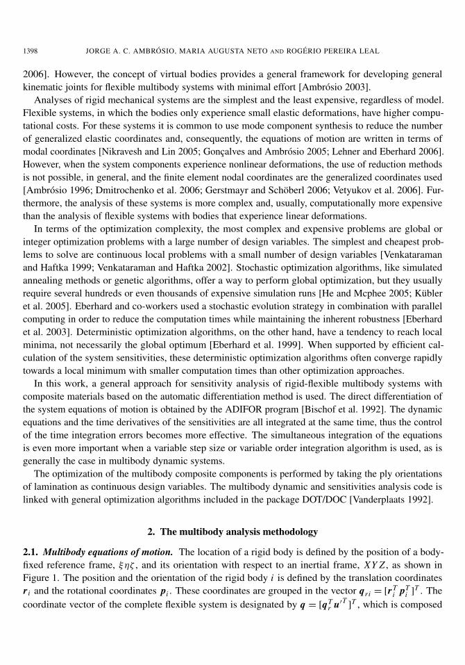
stiffness matrices as weighted averages of the individual layer stiffness through the thickness. Thesematrices are dependent on each layer orientation, and are given by
(Dm, Db, Dmb, Ds) =
n∑k=1
(Dm, Db, Dmb, Ds)k
=
n∑k=1
(C1
3×3 H1, C13×3 H2, C1
3×3 H3, C22×2 H
)k
(9)
with
Hn =
hl∫hl−1
(xn−1
3
)dz =
1n(hn
l+1 − hnl ), (10)
where hi is defined in Figure 2. The axis x3 is positive upward from the mid-plane of the plate. The Lthlayer is located between the points x3 = hl and x3 = hl+1 in the direction of the thickness.
At the element level and in local coordinates, the consistent mass matrix is given by
M(e)f f =
1∫0
1−η∫0
ρ(e)(ST mS)(e)|J |dξdη, (11)
where m is a matrix that contains the inertial terms, and ρ represents the specific mass of the element.Before the mass matrix given by Equation (11), is used in what follows, a procedure to obtain a diagonalmass matrix is applied [Cook 1987].
The description of some of the flexible bodies of the multibody systems requires the use of compositeplates, discretized by triangular finite elements. The finite element is based in the theory described andhas six degrees of freedom per node: u◦
1, u◦
2, u◦
3, φ1, φ2 and φ3. In the finite element mesh of some of theflexible bodies of the system composite beam elements are also used. For the sake of conciseness, noneof these elements is described here, but for details on the formulations of the different composite finiteelements, the interested reader is referred to [Neto et al. 2004].
1
3x
2x
1x
kk
L
1x
3x
2h
2h
1lh�
lh
Figure 2. Coordinate system and layer numbering used for a typical laminated plate.

1402 JORGE A. C. AMBRÓSIO, MARIA AUGUSTA NETO AND ROGÉRIO PEREIRA LEAL
3. Sensitivity analysis of the multibody system
The optimization algorithms used in this work require not only the evaluation of the functional valuesof the behavior functions but also their sensitivities with respect to the design variables. The calculationof these sensitivities can be carried out analytically or numerically. In this work only the analyticalsensitivities are obtained by using automatic differentiation.
3.1. Sensitivity of the equation of motion. For a rigid-flexible multibody system, the equations of mo-tion in terms of modal coordinates are given by Equation (6). The sensitivities of the system accelerationsand Lagrange multipliers with respect to the design variables are obtained by differentiating Equation(6) with respect to the design variables b: Mr Mr f X 8T
qr
XT M f r I XT 8Tq f
8qr 8q f X 0
qrb
wb
λb
=
Qb
Rb
γ b
, (12)
where (·)b denotes the sensitivity of quantity (·) with respect to b. The sensitivities of the right-hand-sideof the equation Qb, Rb and γb are
Qb =∂
∂qr
(gr − Sr − Mr qr − Mr f Xw − 8T
qrλ)qrb
+∂
∂ qr(gr − Sr )qrb
+∂
∂w(gr − Sr )wb
+∂
∂w
(gr − Sr − Mr qr − Mr f Xw − 8T
qrλ)wb +
∂
∂b(gr − Sr − Mr qr − Mr f Xw − 8T
qrλ); (13)
Rb =∂
∂qr
(XT g f − XT S f − XT K f f Xw − XT M f r qr − XT M f f Xw − XT 8T
q fλ)
qrb
+∂
∂w
(XT g f − XT S f − XT K f f Xw − XT M f r qr − XT M f f Xw − XT 8T
q fλ)
wb
+∂
∂b
(XT g f − XT S f − XT K f f Xw − XT M f r qr − XT M f f Xw − XT 8T
q fλ)
+∂
∂ qr
(XT g f − XT S f
)qrb
+∂
∂w
(XT g f − XT S f
)wb; (14)
γ b =∂
∂qr
(γ − 8qr qr − 8q f Xw
)qrb
+∂
∂w
(γ − 8qr qr − 8q f Xw
)wb
+∂
∂b(γ − 8qr qr − 8q f Xw
)+
∂γ
∂ qrqrb
+∂γ
∂wwb. (15)
After solving the linear system of Equations (12) to obtain the sensitivities qrb, wb and λb the state
variables’ sensitivities are obtained by direct integration of qrb, wb, qrb
and wb. The process is started

OPTIMIZATION OF A SATELLITE WITH COMPOSITE MATERIALS 1403
with the initial conditions given by:
qrb(t0) = q0
rb,
wb(t0) = w0b,
qrb(t0) = q0
rb,
wb(t0) = w0b.
(16)
Generally, the initial conditions for the sensitivities expressed in Equation (16) are assumed to be null.Note also that the leading matrix of (6) is equal to the leading matrix of Equation (12). Generally, thefactorized matrix used to obtain the solution of the equation of motion does not have to be calculatedagain when the sensitivities system of equations need to be solved. However, because an automaticdifferentiation tool is used [Bischof et al. 1996], the subroutine that computes the solution of the systemequations of motion is differentiated in order to obtain the sensitivity of the solution vector. The differ-entiated version of the subroutine is not only used to compute the sensitivities solution vector, but alsoto evaluate the derivative of the algorithm by which the solution is computed. The system accelerations(qr , w) and the sensitivity solution vector of Equation (6), (qrb
, wb), are obtained simultaneously.Due to the coordinate reduction, which uses component mode synthesis, the nodal displacements of
the flexible body are described by Equation (5). The sensitivity of the nodal displacement is obtained bycomputing the derivative of this equation with respect the design variables written as
du′
db=
∂ X∂b
w + X∂w
∂b= X bw + Xwb, (17)
where Xb are the sensitivities of the eigenmodes. The relation expressed in Equation (17) transformsthe modal sensitivities to nodal sensitivities. Haftka and Gurdal [1992] suggests evaluating this trans-formation by the fixed-mode approach, in which the derivatives of vibration modes are neglected, orby the updated-mode approach, where the derivatives of vibration modes are accounted for. The fixed-mode approach is computationally less expensive but the updated-mode approach can occasionally bemore accurate. The right-hand side of Equation (12) also depends on the sensitivities of the eigenmodes.Therefore, the same approach is used in the computation of the derivatives of the modal forces and inthe derivatives of the modal stiffness matrix. The modal stiffness matrix derivative is computed in theupdated-mode approach by
∂
∂b(XT K f f X) =
∂ XT
∂bK f f X + XT ∂ K f f
∂bX + XT K f f
∂ X∂b
, (18)
while in the fixed-mode approach, it is obtained as
∂
∂b(XT K f f X) = XT ∂ K f f
∂bX . (19)
The computation of the sensitivities of the eigenmodes is done using the Nelson scheme in the caseof distinct eigenvalues. However, when repeated eigenvalues are a possibility, Ojavo’s method is used[Dailey 1989].

1404 JORGE A. C. AMBRÓSIO, MARIA AUGUSTA NETO AND ROGÉRIO PEREIRA LEAL
3.2. Derivative of the element stiffness matrix. In this work, the design variables used for the laminateoptimization problem are the fiber angles of each lamina that make up the laminate, denoted by vector θ .Therefore, the derivative of the stiffness matrix of the composite flexible body with respect to the layers’orientations has to be accounted for. At the element level, in local coordinates, the stiffness matrix isgiven by Equation (8). In this equation, only the matrix D depends on the design variables. Thus, thesensitivity of this equation is given by
∂ K (e)f f
∂b=
1∫0
1−η∫0
(BT ∂ D
∂bB
)(e)|J |dξdη. (20)
The elasticity matrix D depends on the submatrices Dm , Db, Dmb and Ds , which are defined byEquation (9). The partial derivative of Equation (9) with respect to the design variables vector is
(Dm, Db, Dmb, Ds)b=( n∑
k=1
(Dm, Db, Dmb, Ds)k
)b
=
n∑k=1
(C1
3×3b H1, C13×3b H2, C1
3×3b H3, C12×2b H
)k (21)
with (Cb
)k =
(∂T T
∂bCT + T T ∂ C
∂bT + T T C
∂T∂b
)k. (22)
In Equation (22) (Cb)k is the sensitivity of the material matrix of elastic coefficients for the layer kexpressed in the local body frame, and (∂T/∂b)k is the sensitivity of the transformation matrix relativeto the design variables. Matrix T represents the transformation between the local body frame and thematerial coordinate systems for layer k. The element mass matrix does not depend on the design variablestherefore the partial derivative of this matrix with respect the design variables is null.
4. Optimization criteria
The different optimization problems in multibody systems lead, in general, to different criteria functionsand design constraints. The objective functions most widely used in multibody problems are of one oftwo types: maximum or minimum values and the integral type. Consider a general multibody responsedefined by function f0(b, z, λ, t), which is dependent on time and on the state and design variables.In multibody systems, all the terms present in the equations of motion may be functions of the designparameters. In a compact form the problem objective functions are given by Chang and Nikravesh [1985]:
9i = 9i (b, z, λ, t), i = 0, . . . , n, (23)
where the state vector z includes the coordinates, velocities and accelerations. The variables of the statevector may depend on time and on the design variables. Therefore, the dependency of the state variableson the design variables and time is explicitly written as
z(b, t) =(q(b, t), q(b, t), q(b, t)
). (24)

OPTIMIZATION OF A SATELLITE WITH COMPOSITE MATERIALS 1405
The dependencies of the state variables on the design variables are explicitly taken into account by theautomatic differentiation tool that uses the chain rule to calculate the sensitivities.
4.1. Mini-max optimization problem. The min-max optimization problem, for the time interval betweenti and te is stated as
minimize 9max0 = max f0(b, z, λ, t), ti ≤ t ≤ te, (25)
where the problem consists in the minimization of the maximum value of a specific function during agiven time interval. The use of the maximum value of a time dependent function response as the objectivefunction makes it a more difficult problem to solve. This type of objective function may appear, forinstance, when the minimization of the maximum value of acceleration or force in a given point of abody is required during dynamic analysis. In this optimization problem two situations can occur:
(1) The instant in which the function is at the maximum value is unique and perfectly defined. In thiscase, during the optimization process the instant tm is not dependent on the design variables, andtherefore the objective function (25) can be replaced by a simpler objective function as
minimize 9max0 = max f0
(b, z(tm), λ(tm)
). (26)
(2) The instant in which the function is at the maximum value, varies during the optimization process.One form of dealing with this problem is to introduce an extra design variable and make the objectivefunction equal to the value of that variable [Haftka and Gurdal 1992; Kim and Choi 1996]:
minimize 90 = bn+1 (27)
with the additional time-dependent constraint
9n+1 = f0(b, z, λ, t) − bn+1 ≤ 0, ti ≤ t ≤ te. (28)
The constraint given by Equation (28), when added to the total number of constraints ensures, that thedynamic response is below the maximum value defined by the auxiliary variable bn+1. This approachposes some difficulties for the search direction in the optimization algorithm and can lead to small stepsin the line search method, or even to a stall of the process. To overcome these difficulties, Kim and Choi[1996] proposed to handle directly the maximum value point only in the optimization process.
4.2. Minimization of an integral type criteria. The integral type objective function may be used torepresent mean values of the response over time, accumulated values, or other special criteria. For aresponse f0(b, z, λ, t) of the dynamic system, the objective function is [Eberhard et al. 2003]
90 = G0(b, zte , λte , te) +
te∫ti
f0(b, z, λ, t)dt, (29)
where f0(b, z, λ, t) depends on the dynamic behavior during the complete time interval [ti , te], while G0
considers only the final state. This type of objective function is most common in vehicle design. Comfortor injury criteria are defined by integral type functions and often are used in the optimization process.

1406 JORGE A. C. AMBRÓSIO, MARIA AUGUSTA NETO AND ROGÉRIO PEREIRA LEAL
4.3. Time-dependent constraints. Mathematical programming algorithms generally cannot deal withparametric constraints such as
9i = fi(b, z(t), λ(t), t
)≤ c, ti ≤ t ≤ te, (30)
or even with constraints such as the one described by Equation (28). Such constraints have to be refor-mulated to remove their time dependency. During the simulation the function value can only be obtainedfor discrete time points. The most straightforward way to remove the time dependency of the originalconstraint is to discretize the time interval into time points. Then, the original constraint represented byEquation (30) is replaced by ntp constraints written as [Haug and Arora 1979]:
9i = fi(b, z(tk), λ(tk), tk
)≤ c, k = 1, . . . , ntp. (31)
The distribution of the time points has to be sufficiently dense to avoid large constraint violationsbetween two adjacent time points [Hsieh and Arora 1984]. Thus, discretizing time-dependent constraintscan significantly increase the number of constraints, and thereby the cost of optimization [Haftka andGurdal 1992]. In order to reduce the number of constraints, a first alternative consists of replacing theoriginal constraints by an equivalent integrated constraint, which averages the severity of the constraintover the time interval. Hsieh and Arora [1984] showed that from an optimization theory point of view,the constraints described by Equation (30) and equivalent integral constraints are different. In fact, anequivalent integral constraint represents the behavior of the time dependent constraint fi (b, z(t), λ(t), t)on the complete time domain by a single value 9e
i , leading to a loss of information. As a consequence,equivalent constraints tend to blur the design trends [Haftka and Gurdal 1992]. Hsieh and Arora [1984]and Grandhi et al. [1986] propose an alternative procedure that consists of exchanging the initial con-straint given by (30) for a set of constraints of the type of Equation (31), in which ntp is replaced by nctp,with nctp < ntp being nctp the number of critical time points. These critical points are related with theexistence of local maxima or minima of the function.
5. Optimization algorithms
In dynamic problems the evaluation of the system dynamic behavior requires the numerical integrationof the equation of motion. The time dependency of this system makes these optimization problems morecomplex and requires that special techniques be used in the solution process. Both deterministic andstochastic optimization methods can be applied. Eberhard et al. [2003] has successfully used a stochasticevolution strategy in combination with a parallel computing environment to reduce computation time.However, in this work the Modified Method of Feasible Directions is used, which is a deterministicoptimization method implemented in the DOT optimization routines library [Vanderplaats 1992]. Inorder to calculate the gradients, the direct differentiation method is used, the sensitivities being obtainedby the automatic differentiation program ADIFOR [Bischof et al. 1996].
6. Optimization of a satellite unfolding process
The proposed methodology is demonstrated through the optimization of a complex multibody systemmade of composite material. The technical system modeled within this application consists in the un-folding process of a satellite antenna, the Synthetic Aperture Radar (SAR) antenna, which is a part of

OPTIMIZATION OF A SATELLITE WITH COMPOSITE MATERIALS 1407
1
a) b)
1
a) b)
(a) (b)
Figure 3. The SAR antenna in the (a) folded and (b) unfolded configurations.
the European research satellite ERS-1. The model of this antenna has been the object of different studiesin several studies in multibody dynamics being first proposed by Hiller [1983] and Anantharaman andHiller [1991].
6.1. Description of the SAR antenna. The folding antenna shown in Figure 3 is achieved through arelatively complex spatial mechanism. Both the solar array and the SAR antenna of the ERS-1 satellitehave the same configuration and share the same kinematic features. During transportation the antennaand the solar array are folded, as shown in Figure 3a, in order to occupy as small a space as possible.After unfolding, the mechanical components take the configuration represented in Figure 3b.
The SAR antenna consists of two identical subsystems, each with three coupled planar four-bar linksthat unfold two panels on each side. The central panel is attached to the main body of the satellite. Eachunfolding system has two degrees of freedom, driven individually by actuators located in the joints Aand B, shown in Figure 4.
The unfolding process consists of two phases, schematically represented in Figure 5. In the first phasethe panel 3 is rolled out, about an axis normal to the main body, by a rotational spring-damper-actuatorin joint A, while the panel 2 is held down by locking joints D and E, as shown in Figure 5a. The secondphase begins with joint A locked, the panels 2 and 3 being swung out to the final position by a rotational
1
1.994 m
1.3 m
a) b)
Actuator (1)
Actuator (2)
A
BC
D, E
Panel 3 (B3)
Panel 2 (B2)
Panel 1 (B1)
(a) (b)
Figure 4. The SAR antenna: (a) one half unfolded state; (b) folded antenna.

1408 JORGE A. C. AMBRÓSIO, MARIA AUGUSTA NETO AND ROGÉRIO PEREIRA LEAL
1
a)b)
Figure 5. Unfolding process of the SAR antenna: (a) first phase; (b) second phase.
spring-damped-actuator in joint B, as observed in Figure 5b. The second half of the antenna, which hasbeen omitted in Figures 4 and 5, is unfolded in the same way as the first half shown here. When thecomplete antenna is deployed all five panels are aligned in the final configuration.
The model used for one half of the folding antenna, schematically depicted Figure 6, is composedof 12 bodies (B1 a B12), 16 spherical joints (S1 a S16) and 3 revolute joints (R1, R2, R3). The centralpanel is attached to the satellite, defined as body B1, which has mass and inertias much higher than theremaining bodies.
In the first phase of the unfolding antenna a rotational spring-damper-actuator is applied to the revolutejoint R3. For the second phase, the revolute joint R3 is locked and the system is moved to the nextequilibrium position by a spring-damper-actuator positioned in joint R1. Each panel is 1.994 m longby 1.3 m wide and has a thickness of 2 mm. The linkage between the panels and the four-bar linkagemechanism is assured by a set of supports, six in body 2 and four in body 3. All truss members have auniform circular cross-section [Neto 2005].
1
1R 1B2B3B
2R3R
4B5B
6B
7B8B
,10 8B S
9B
12B
11B
1S
3S2S
5S6S
7S10S
9S
10S
12S
11S
Z
Y X4S
14S
15S
16S 13S
Figure 6. Multibody model of the SAR antenna.
OPTIMIZATION OF A SATELLITE WITH COMPOSITE MATERIALS 1409
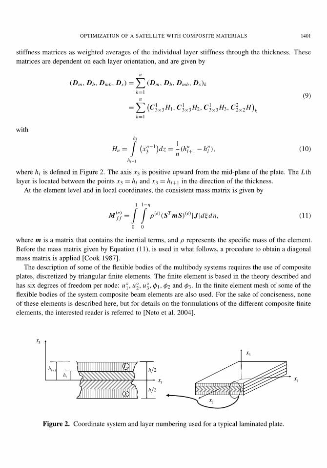
1st Layer 2nd Layer 3rd Layer 4th Layer
Lay-up 1 0o 0o 0o 0o
Lay-up 2 0o 90o 90o 0o
Thickness (m) 0.0005 0.0005 0.0005 0.0005
Table 1. Characteristics of the two lay-ups considered for the composite panels.
6.2. First phase of the antenna unfolding process. The material used in the different components of theantenna is a carbon reinforced plastic IM6/SC1081 where the matrix is made of Epoxy SC1081 and thefibers are made of Carbon IM6. Note that the material model used here is not necessarily that of the realsatellite antenna, as the characteristics of the material are not publicly available. The properties of thecomposite material, for a single layer with an orientation of 0◦ relative to the X axis are: E1 = 177 GPa;E2 = 10.8 GPa; G12 = G13 = 7.6 GPa; G23 = 8.504 GPa; ν12 = 0.27; with a specific mass of 1600 Kg/m3.Two different laminates with four layers in each, described in Table 1, are considered as potential designsolutions.
In flexible multibody models the use of all the nodal degrees of freedom, resulting from the model ofthe complex system, as generalized coordinates is not viable. The application of the modal superpositiontechnique in this kind of problem, characterized by linear elastic deformations, can be done withoutcompromising accuracy. By using of a small set of the modes of vibration associated to the lowerfrequencies it is possible to reproduce the structural deformations of the panels with a small number ofgeneralized elastic coordinates.
The modes of vibration for all flexible bodies in the antenna are obtained by performing a modalanalysis of each one of the flexible bodies independently. The structural attachment conditions used inthe eigenproblem are the same as those used to fix the body coordinate system, that is, the node in thecenter of mass is fixed to the body fixed frame. In this manner the free rigid body modes are removed.
In Tables 2 and 3 the 14 lowest frequencies are presented for panels 2 and 3 with composite material lay-ups 1 and 2, respectively. The modes corresponding to the two lower frequencies are almost rigid modes,resulting from the flexibility around a fixed node. However, these modes also represent deformation ofthe panels and cannot be neglected.
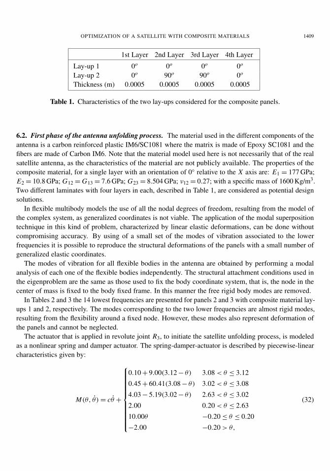
The actuator that is applied in revolute joint R3, to initiate the satellite unfolding process, is modeledas a nonlinear spring and damper actuator. The spring-damper-actuator is described by piecewise-linearcharacteristics given by:
M(θ, θ) = cθ +
0.10 + 9.00(3.12 − θ) 3.08 < θ ≤ 3.12
0.45 + 60.41(3.08 − θ) 3.02 < θ ≤ 3.08
4.03 − 5.19(3.02 − θ) 2.63 < θ ≤ 3.02
2.00 0.20 < θ ≤ 2.63
10.00θ −0.20 ≤ θ ≤ 0.20
−2.00 −0.20 > θ,
(32)

1410 JORGE A. C. AMBRÓSIO, MARIA AUGUSTA NETO AND ROGÉRIO PEREIRA LEAL
Mode Panel 2 Frequency [Hz] Panel 3 Frequency [Hz]
1 0.990 0.9922 1.457 1.4603 1.677 1.6814 1.746 1.7495 4.000 4.0016 4.609 4.6207 6.099 6.1188 6.814 6.8509 8.538 8.56410 8.578 8.58311 12.434 12.45112 12.828 12.83313 14.354 14.40414 14.415 14.485
Table 2. First 14 natural modes of vibration for panels 2 and 3 with the compositematerial lay-up 1.
Mode Panel 2 Frequency [Hz] Panel 3 Frequency [Hz]
1 1.311 1.3132 1.563 1.5663 1.694 1.6994 2.334 2.3365 4.719 4.7196 5.755 5.7707 6.220 6.2428 7.388 7.4279 12.832 12.844
10 12.953 12.97111 13.626 13.68512 13.829 13.87313 15.282 15.30314 15.969 15.986
Table 3. First 14 natural modes of vibration for panels 2 and 3 with the compositematerial lay-up 2.

OPTIMIZATION OF A SATELLITE WITH COMPOSITE MATERIALS 1411
1
Figure 7. Configuration of the composite panels with the original damped spring-actuator.
where the damping coefficient used is c = 0.5 Nms.The actuation law presented here is different from that reported by Anantharaman and Hiller [1991],
which was used to model the SAR antenna with panels made of isotropic material. In fact, when the actu-ation law used by Antharaman and Hiller is used for the composite flexible models the satellite antennais driven to a different equilibrium state than that obtained in the rigid model. The trusses connectedto the actuator quickly reach their equilibrium, but panel 3 hardly moves because the unfolding trussesbreak through the panel, as represented in Figure 7. This behavior is clearly unfeasible because contactbetween trusses and panels would take place, preventing such penetration from happening. Therefore,the reported results show that due to the deformations of the trusses the undesirable contacts betweentrusses and panels are possible if the high torques associated to the original actuator have been maintained.Consequently, the solution is to apply a ‘softer’ actuation law, in the sense of preventing such contact.
The problems associated with the unfolding of an isotropic flexible model due to the actuator deploy-ment law have been identified by Anantharaman and Hiller [1991], and the solution found was to modifythat actuation in order to prevent the wrong deployment mechanism, which is in essence similar to thesolution adopted here. When using composite material models, the problem of the first phase of theunfolding process increases in importance not only because the bending of the panels is significant butalso because torsional modes come in play. In Figure 8 the variation of the actuator angle during thesimulation period for the composite models is presented.
Figure 8 shows that the two models lead to similar simulation results. However, it is observed thatafter the equilibrium positions are reached for both models, in the period from 7 to 8 s, the direction ofrotation of the truss members of the panels made with the lay-up 1 is opposite to that of the same trussmembers of the model made with lay-up 2. This discrepancy can result from the difference between thevibration modes of the both models. In fact, the lay-up 1 has no layers with the 90◦ orientation, thus thestiffness of this model in the Y direction is smaller than that observed with lay-up 2. A similar differencein stiffness is also visible in the X direction of the lay-up 1.
When observing the fourth frame of the unfolding in Figure 9a, it can be noticed that the flexiblemodel of the satellite antenna predicts interference between panel 2 and panel 1, which is attached to thebase satellite, when bodies B7 and B8 get aligned. This can be perceived as a flaw in the design of theunfolding process of the satellite that requires being fixed. If not detected, the interference would causeimpact between the panels eventually leading to their failure.
6.3. Optimization of the SAR antenna. In this section the multibody model of the SAR antenna is usedwithin the framework of an optimization problem. The flexibility of the panels of the SAR antenna isfundamental for the functional requirements of the antenna. The use of stiffer panels can improve the

1412 JORGE A. C. AMBRÓSIO, MARIA AUGUSTA NETO AND ROGÉRIO PEREIRA LEAL
1
-100
-50
0
50
100
150
200
0 2 4 6 8 10 12 14 16 18 20Time (s)
Actua
tor an
gle (d
egre
e)
Lay-up 2Lay-up 1
Figure 8. Actuator angle during the first phase of deployment for different compositematerial lay-ups.
1
Figure 9. Configuration of the antenna unfolded process: a) first phase b) second phase.

OPTIMIZATION OF A SATELLITE WITH COMPOSITE MATERIALS 1413
Panels Design Variable Lower Bound Initial Value Upper Bound
2 = 3 θ1/θ2/θ2/θ1 −90◦/ − 90◦/ − 90◦/ − 90◦ 55◦/ − 55◦/ − 55◦/55◦+90◦/ + 90◦/ + 90◦/ + 90◦
Table 4. Design variables for panels’ layers’ orientations in the satellite optimization.
time needed to unfold the antenna, during the first phase of the unfolding process, allowing for the useof a stiffer actuator on revolute joint R3. Furthermore, the stiffness increase of the panels, in particularof panel 2, prevents the interference detected between panels in the first part of the unfolding process.
The multibody model of the flexible antenna for the first part of the unfolding process is composed oftwo flexible panels. Therefore, the antenna deformation energy of the panels for instant tn is defined as
2Um(wi , tn) =
3∑i=2
wTi XT
i K if f X iwi
=
3∑i=2
wiT 3wi = 2
(U2(w2, tn) + U3(w2, tn)
),
(33)
where the index m refers to the model used and index i refers to the body number of panels of themultibody model SAR antenna. Equation (33) indicates that the deformation energy of the multibodymodel of the SAR antenna is obtained as a summation of the deformation energy of the two panels ofthe model. Then the function f0 = 2Um is used to optimize the SAR antenna.
The goal defined by Equation (29) represents an area defined by the curve of function f0 = 2Um duringthe simulation period ti = 0 s ≤ t ≤ te = 3 s. The minimum value of the area may be achieved with apeak value of the maximum deformation energy of each panel that exceeds acceptable limits. In order toavoid this situation, the maximum value of the deformation energy, in each panel, is constrained to be
9i (θ) ≤ ci ; i = 2, 3. (34)
The values ci are defined as being the maximum values of deformation energy, in each panel, observed inthe initial design. Therefore, in the initial design the optimization algorithm has two active constraints.
All material models considered herein are symmetric laminates with the number of layers being fixed.The simulation scenario considered is restricted to the first three seconds of the unfolding process, iden-tified as the critical period. Two design variables are used in the optimization process, corresponding tothe orientation of the layers that make up the laminate used to model panels 2 and 3. The initial design oflaminate used in the panels is defined in Table 4. The optimization method used is the Modified Methodof Feasible Directions (MMFD), as available in DOT [Vanderplaats 1992]. The analytic sensitivitiescomputed by the direct differentiation method are used to compute the gradients required by the optimizer.
In Table 5 the optimization results are presented for the flexible multibody of the antenna. In Figure 10the evolution of the objective function for the antenna flexible multibody model is showed, the progressof the design variables being shown in Figure 11. Figure 12 shows the actuator angle history during thefirst phase of the unfolding antenna for the original and optimum designs.
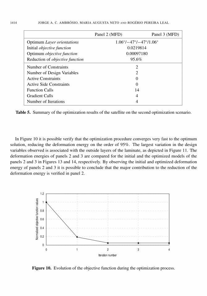
1414 JORGE A. C. AMBRÓSIO, MARIA AUGUSTA NETO AND ROGÉRIO PEREIRA LEAL
Panel 2 (MFD) Panel 3 (MFD)
Optimum Layer orientations 1.06◦/−47◦/−47◦/1.06◦
Initial objective function 0.0219814Optimum objective function 0.00097180Reduction of objective function 95.6%
Number of Constraints 2Number of Design Variables 2Active Constraints 0Active Side Constraints 0Function Calls 14Gradient Calls 4Number of Iterations 4
Table 5. Summary of the optimization results of the satellite on the second optimization scenario.
In Figure 10 it is possible verify that the optimization procedure converges very fast to the optimumsolution, reducing the deformation energy on the order of 95%. The largest variation in the designvariables observed is associated with the outside layers of the laminate, as depicted in Figure 11. Thedeformation energies of panels 2 and 3 are compared for the initial and the optimized models of thepanels 2 and 3 in Figures 13 and 14, respectively. By observing the initial and optimized deformationenergy of panels 2 and 3 it is possible to conclude that the major contribution to the reduction of thedeformation energy is verified in panel 2.
1
0
0.2
0.4
0.6
0.8
1
1.2
0 1 2 3 4Iteration number
Norm
alize
d obje
ctive
func
tion v
alues
Figure 10. Evolution of the objective function during the optimization process.

OPTIMIZATION OF A SATELLITE WITH COMPOSITE MATERIALS 1415
1
-80
-60
-40
-20
0
20
40
60
80
0 1 2 3 4
Iteration number
Des
ign
varia
bles
val
ues �(1)
�(2)
Figure 11. Evolution of the design variables during the optimization process.
7. Conclusions
A general method for the design optimization of flexible multibody systems made of composite materialshas been presented in this work and demonstrated by an application to the design of the unfolding processof a satellite antenna. First, the correct choice of the optimization methods and the optimal problemdefinition is more complex when the nonlinear dynamic response of the systems is involved. Furthermore,the need to use analytic sensitivities instead of numerical sensitivities requires that expeditious methodsof obtaining these are implemented in order to allow for the definition of more general objective functions,constraints and design variables. This has been achieved in this work by using an automatic differentiationtool to obtain the gradients required by the optimizer. Finally, the optimization of the nonlinear dynamicsystems in general, and of the flexible multibody systems in particular, often present time-dependent
1
-100
-50
0
50
100
150
200
0 2 4 6 8 10 12 14 16 18 20Time (s)
Actua
tor an
gle
Model originalModel optimized(2-dv)
Figure 12. Actuator angle for the initial and optimum laminate of the antenna panels.

1416 JORGE A. C. AMBRÓSIO, MARIA AUGUSTA NETO AND ROGÉRIO PEREIRA LEAL
1
0.0E+002.0E-044.0E-046.0E-048.0E-041.0E-031.2E-031.4E-031.6E-031.8E-032.0E-03
0 0.5 1 1.5 2 2.5Time (s)
Defor
matio
n ene
rgy Initial-Deformation energy of panel 2
Optimized-Deformation energy of panel 2(2dsv)
Figure 13. Deformation energy for the initial and optimum model of panel 2.
constraints that are difficult to tackle with common procedures. The use of min-max optimization is aform of handling most optimization problems of this type.
The application of the methodology developed for a complex system was demonstrated by consider-ing the multibody model of the SAR antenna. The optimization method was applied to minimize thedeformation energy of the SAR antenna panels. To get a stiffer antenna, the optimization problem wasformulated as minimization problems of the deformation energy of each panel. The design variablesof the optimization problem were the fiber orientations of the layers that form the lamination used tomodel the material properties of the panels. The design problem considers the case of finding optimumsymmetric lamination with four layers only. In the optimization scenario two design variables were usedto define the optimum lamination on both panels. The results of this application demonstrate that not
1
0.0E+002.0E-044.0E-046.0E-048.0E-041.0E-031.2E-031.4E-031.6E-031.8E-032.0E-03
0 0.5 1 1.5 2 2.5Time (s)
Defor
matio
n ene
rgy Initial-Deformation energy of panel 3
Optimized-Deformation energy of panel 3(2dsv)
Figure 14. Deformation energy for the initial and optimum model of panel 3.
OPTIMIZATION OF A SATELLITE WITH COMPOSITE MATERIALS 1417
only are there feasible designs for the antenna in which interference between panels is avoided but alsothat the control over of the deformation energy of the antenna was possible. In the process it was shownthat feasible designs for the actuation law during the deployment are obtained.
Acknowledgements
We would like to thank Professors Manfred Hiller and Andres Kecskemethy, of the University of Duis-burg, Germany, for providing the necessary data to model the SAR antenna and for useful discussions.
References
[Ambrósio 1996] J. Ambrósio, “Dynamics of structures undergoing gross motion and nonlinear deformations: a multibodyapproach”, Comput. Struct. 59:6 (1996), 1001–1012.
[Ambrósio 2003] J. Ambrósio, “Efficient kinematic joint descriptions for flexible multibody systems experiencing linear andnon-linear deformations”, Int. J. Numer. Methods Eng. 56:12 (2003), 1771–1793.
[Ambrósio and Gonçalves 2001] J. Ambrósio and J. Gonçalves, “Complex flexible multibody systems with application tovehicle dynamics”, Multibody Syst. Dyn. 6:2 (2001), 163–182.
[Anantharaman and Hiller 1991] M. Anantharaman and M. Hiller, “Numerical simulation of mechanical systems using methodsfor differential-algebraic equations”, Int. J. Numer. Methods Eng. 32:8 (1991), 1531–1542.
[Bischof et al. 1992] C. Bischof, A. Carle, G. Corliss, A. Griewank, and P. Hovland, “ADIFOR: generating derivative codesfrom fortran programs”, Sci. Program. 1:1 (1992), 11–29.
[Bischof et al. 1996] C. Bischof, P. Khademi, A. Mauer, and A. Carle, “ADIFOR 2.0: automatic differentiation of Fortran 77programs”, IEEE Comput. Sci. Eng. 3:3 (1996), 18–32.
[Bottasso et al. 2006] C. Bottasso, A. Croce, B. Savini, W. Sirchi, and L. Trainelli, “Aero-servo-elastic modeling and controlof wind turbines using finite-element multibody procedures”, Multibody Syst. Dyn. 16:3 (2006), 291–308.
[Cavin and Dusto 1977] R. Cavin and A. Dusto, “Hamilton’s principle: finite-element methods and flexible body dynamics”,AIAA J. 15:12 (1977), 1684–1690.
[Chang and Nikravesh 1985] C. Chang and P. Nikravesh, “Optimal design of mechanical systems with constraint violationstabilization method”, J. Mech. Transm. (Trans. ASME) 107 (1985), 493–498.
[Cook 1987] R. Cook, Concepts and applications of finite element analysis, 2nd ed., Wiley, New York, 1987.
[Dailey 1989] R. L. Dailey, “Eigenvector derivatives with repeated eigenvalues”, AIAA J. 27:4 (1989), 486–491.
[Dmitrochenko et al. 2006] O. Dmitrochenko, W.-S. Yoo, and D. Pogorelov, “Helicoseir as shape of a rotating string I): 2Dtheory and simulation using ANCF”, Multibody Syst. Dyn. 15:2 (2006), 135–158.
[Duff et al. 1986] I. Duff, A. Erisman, and J. Reid, Direct methods for sparse matrices, Clarendon Press, Oxford [Oxfordshire],1986.
[Eberhard et al. 1999] P. Eberhard, W. Schiehlen, and D. Bestle, “Some advantages of stochastic methods in multicriteriaoptimization of multibody systems”, Arch. Appl. Mech. 69:8 (1999), 543–554.
[Eberhard et al. 2003] P. Eberhard, F. Dignath, and L. Kübler, “Parallel evolutionary optimization of multibody systems withapplication to railway dynamics”, Multibody Syst. Dyn. 9:2 (2003), 143–164.
[Gerstmayr and Schöberl 2006] J. Gerstmayr and J. Schöberl, “A 3D finite element method for flexible multibody systems”,Multibody Syst. Dyn. 15:4 (2006), 305–320.
[Gonçalves and Ambrósio 2005] J. Gonçalves and J. Ambrósio, “Road vehicle modeling requirements for optimization of rideand handling”, Multibody Syst. Dyn. 13:1 (2005), 3–23.
[Grandhi et al. 1986] R. Grandhi, R. Haftka, and L. Watson, “Design-oriented identification of critical times in transientresponse”, AIAA J. 24:4 (1986), 649–656.
1418 JORGE A. C. AMBRÓSIO, MARIA AUGUSTA NETO AND ROGÉRIO PEREIRA LEAL
[Haftka and Gürdal 1992] R. Haftka and Z. Gürdal, Elements of structural optimization, 3rd rev. exp. ed., Kluwer AcademicPublishers, Dordrecht, 1992.
[Hardeman et al. 2006] T. Hardeman, R. G. K. M. Aarts, and J. B. Jonker, “A finite element formulation for dynamic parameteridentification of robot manipulators”, Multibody Syst. Dyn. 16:1 (2006), 21–35.
[Haug and Arora 1979] E. Haug and J. Arora, Applied optimal design: mechanical and structural systems, Wiley, New York,1979.
[He and Mcphee 2005] Y. He and J. Mcphee, “Multidisciplinary optimization of multibody systems with application to thedesign of rail vehicles”, Multibody Syst. Dyn. 14:2 (2005), 111–135.
[Heckmann et al. 2005] A. Heckmann, M. Arnold, and O. Vaculí n, “A modal multifield approach for an extended flexible bodydescription in multibody dynamics”, Multibody Syst. Dyn. 13:3 (2005), 299–322.
[Hiller 1983] M. Hiller, Mechanische systeme, Springer-Verlag, Berlin, Germany, 1983.
[Hsieh and Arora 1984] C. Hsieh and J. Arora, “Design sensitivity analysis and optimization of dynamic response”, Comput.Methods Appl. Mech. Eng. 43:2 (1984), 195–219.
[Kim and Choi 1996] M. Kim and D. Choi, “A new approach to the min-max dynamic response optimization”, pp. 65–72 inIUTAM-symposium on optimization of mechanical systems (Stuttgart, 1996), edited by D. Bestle and W. Schiehlen, Kluwer,Dordrecht, 1996.
[Kübler et al. 2005] L. Kübler, C. Henninger, and P. Eberhard, “Multi-criteria optimization of a hexapod machine”, MultibodySyst. Dyn. 14:3–4 (2005), 225–250.
[Lehner and Eberhard 2006] M. Lehner and P. Eberhard, “On the use of moment-matching to build reduced order models inflexible multibody dynamics”, Multibody Syst. Dyn. 16:2 (2006), 191–211.
[Liu et al. 2007] J.-F. Liu, J. Yang, and K. Abdel-Malek, “Dynamics analysis of linear elastic planar mechanisms”, MultibodySyst. Dyn. 17:1 (2007), 1–25.
[Møller et al. 2005] H. Møller, E. Lund, J. Ambrósio, and J. Gonçalves, “Simulation of fluid loaded flexible multibody systems”,Multibody Syst. Dyn. 13:1 (2005), 113–128.
[Neto 2005] M. Neto, Optimization of flexible multibody systems with composite materials, Ph. D. Thesis, Mechanical Engi-neering Department of Coimbra University, Coimbra, Portugal, 2005.
[Neto et al. 2004] M. Neto, J. Ambrósio, and R. Leal, “Flexible multibody systems models using composite materials compo-nents”, Multibody Syst. Dyn. 12:4 (2004), 385–405.
[Nikravesh and Lin 2005] P. Nikravesh and Y.-S. Lin, “Use of principal axes as the floating reference frame for a movingdeformable body”, Multibody Syst. Dyn. 13:2 (2005), 211–231.
[Pereira and Proença 1991] M. Pereira and P. Proença, “Dynamic analysis of spatial flexible multibody systems using jointco-ordinates”, Int. J. Numer. Methods Eng. 32:8 (1991), 1799–1812.
[Vanderplaats 1992] G. Vanderplaats, “DOT-Design Optimization Tools, Version 3.0”, VMA Engineering, Colorado Springs,CO, 1992.
[Venkataraman and Haftka 1999] S. Venkataraman and R. Haftka, “Optimization of composite panels: a review”, in Proc. ofthe 14th annual technical conference of the american society of composites, Technomic Publishing, Dayton, OH, Sep. 27–291999.
[Venkataraman and Haftka 2002] S. Venkataraman and R. Haftka, “Structural optimization: what has Moore’s law done forus?”, in 43rd AIAA/ASME/ASCE/AHS/ASC structures structural dynamics and materials conference, Denver, CO, 22–25 April2002.
[Vetyukov et al. 2006] Y. Vetyukov, J. Gerstmayr, and H. Irschik, “Modeling spatial motion of 3D deformable multibodysystems with nonlinearities”, Multibody Syst. Dyn. 15:1 (2006), 67–84.
[Yoo and Haug 1986] W. Yoo and E. Haug, “Dynamics of flexible mechanical systems using vibration and static correctionmodes”, J. Mech. Transm. (Trans. ASME) 108 (1986), 315–322.
Received 13 Aug 2006. Accepted 20 Apr 2007.

OPTIMIZATION OF A SATELLITE WITH COMPOSITE MATERIALS 1419
JORGE A. C. AMBRÓSIO: [email protected] de Engenharia Mecânica — Instituto Superior Técnico, Technical University of Lisbon, Av. Rovisco Pais, 1041-001,Lisbon, Portugal
MARIA AUGUSTA NETO: [email protected] de Engenharia Mecânica, Faculdade de Ciência e Tecnologia da Universidade de Coimbra (Polo II),3020 Coimbra, Portugal
ROGÉRIO PEREIRA LEAL: [email protected] de Engenharia Mecânica, Faculdade de Ciência e Tecnologia da Universidade de Coimbra (Polo II),3020 Coimbra, Portugal

Copyright © 2022 FDOKUMEN