HAL Id: pastel-00004315https://pastel.archives-ouvertes.fr/pastel-00004315

Submitted on 14 Nov 2008

HAL is a multi-disciplinary open accessarchive for the deposit and dissemination of sci-entific research documents, whether they are pub-lished or not. The documents may come fromteaching and research institutions in France orabroad, or from public or private research centers.

L’archive ouverte pluridisciplinaire HAL, estdestinée au dépôt et à la diffusion de documentsscientifiques de niveau recherche, publiés ou non,émanant des établissements d’enseignement et derecherche français ou étrangers, des laboratoirespublics ou privés.

Optimisation des signaux et de la charge utile GalileoEmilie Rebeyrol

To cite this version:Emilie Rebeyrol. Optimisation des signaux et de la charge utile Galileo. Electronique. TélécomParisTech, 2007. Français. pastel-00004315

Thèse

présentée pour obtenir le grade de Docteur

de l’École Nationale Supérieure des Télécommunications

Spécialité : Électronique et Communications

Emilie REBEYROL

Optimisation des signaux et de la charge utile GALILEO (Galileo signals and payload optimization)

Soutenue le 9 octobre 2007 devant le jury composé de

Prof. Jean-Claude Belfiore Président

Prof. Günter W. Hein Rapporteur

Dr. Christopher Hegarty Rapporteur

Jean-Luc Issler Examinateur

Prof. Michel Bousquet Examinateur

Dr. Olivier Julien Examinateur

Dr. Christophe Macabiau Directeur de thèse

Prof. Marie-Laure Boucheret Directeur de thèse

5

Résumé Le système de positionnement Galileo est un nouveau système de navigation par satellite en cours de développement pour l’Union Européenne, qui devrait être opérationnel en 2013. Tout en fournissant un service de positionnement autonome, Galileo sera interopérable avec les systèmes de navigation par satellite déjà existants comme le système américain GPS (Global Positioning System). En effet, un utilisateur pourra, avec un récepteur compatible, obtenir une position quelque soit le système utilisé. De plus, Galileo a pour objectif de garantir la disponibilité de certains services tels que le service commercial (CS) par exemple ou le service public réglementé (PRS). Mais Galileo fournit aussi, avec le service Sécurité de la vie (SOL), un message d’intégrité permettant de déterminer si l’information satellite est fiable, afin de l’utiliser pour des applications critiques telles que le transport aérien, maritime ou terrestre.

Afin de fournir une position, une synchronisation et une information d'intégrité précises, en accord avec les besoins des utilisateurs, le système Galileo doit posséder des signaux et une architecture performants. L’étude de la conception de ces signaux, leur génération et leurs performances constitue le coeur de cette thèse. En effet, l'objectif principal de ce travail est l'optimisation de la charge utile et des signaux Galileo afin d’obtenir les meilleures performances possibles du point de vue du récepteur.

Une analyse complète du système Galileo, de la charge utile au récepteur est d’abord

effectuée. Elle montre que des distorsions peuvent affecter les signaux pendant leur génération, leur propagation et leur traitement dans le récepteur. Ces distorsions, dues aux instabilités d'horloges, aux non-linéarités de l’amplificateur, aux filtrages ou aux trajets multiples (multitrajets), réduisent la performance des signaux, en particulier lors de la poursuite du code ou lors de la poursuite de la phase de la porteuse. Pour éviter ces distorsions ou pour réduire leur impact, les signaux Galileo doivent présenter certaines propriétés, comme une enveloppe constante ou une large bande par exemple. Il est donc important d’analyser ces contraintes pour la conception d’une charge utile et de signaux performants.

Une étude est ensuite menée afin de déterminer si les signaux Galileo proposés par la GJU (Galileo Joint Undertaking), en particulier en bande E5 et E1(E1-L1-E2), présentent ces propriétés et ainsi vérifient les contraintes de conception.

La modulation Interplex et la modulation ALTBOC (Alternate Binary Offset Carrier) sont les solutions proposées pour multiplexer, respectivement, les signaux E1 et E5. Les expressions théoriques et les performances de ces modulations sont analysées afin de montrer qu’elles transmettent les signaux avec une enveloppe constante permettant de réduire les distorsions dues aux non-linéarités de l’amplificateur.

Récemment, de nouvelles formes d’onde ont été proposées pour transmettre le signal « Open Service » de Galileo en bande E1, toujours avec l’objectif d’obtenir de meilleures performances. Ces nouveaux signaux sont basés sur la combinaison linéaire d’un signal BOC(1,1) avec un signal « Binary Coded Symbol (BCS) » ou avec une autre sous porteuse BOC. Ces signaux sont alors appelés Composite BCS (CBCS) ou Composite BOC (CBOC). Ces nouveaux signaux, conçus afin de réduire l’impact des multitrajets sur les performances, sont étudiés tout au long de la chaîne de transmission afin de contrôler s’ils vérifient les

6

contraintes de conception et s’ils peuvent être transmis avec la modulation Interplex. Leurs performances sont aussi évaluées et comparées à celle du signal BOC(1,1), grâce à des observables qui caractérisent les performances en réception. Ces observables sont la fonction d'autocorrélation, la densité spectrale de puissance, le coefficient d’isolation spectrale et l'enveloppe d’erreur due aux trajets multiples.

Pour terminer, des simulations permettant d’évaluer l'influence des distorsions dues aux équipements de la charge utile et du récepteur, sur les signaux Galileo et sur leur performance en réception, sont présentées. En particulier, l’influence des horloges, des amplificateurs et des filtres est évaluée grâce notamment au calcul de l'erreur de phase dans la boucle de poursuite du récepteur.

7

Abstract The Galileo positioning system is a satellite navigation system, to be built by the European Union (EU) and operational by 2013. While providing autonomous navigation and positioning services, Galileo is at the same time interoperable with the American positioning system GPS. A user will be able to obtain a position, whatever the navigation system used, with the same receiver. Moreover, one aim of the Galileo system is to guarantee the availability of some services such as the Commercial Service (CS) or the Public Regulated Service (PRS) for example. But Galileo could also provide an integrity message for the Safety-Of-Life (SOL) service, allowing to determine the reliability of the satellite information, which is essential for critical applications such as air, maritime or terrestrial transports.

To provide high precision position, timing and integrity information and to meet user needs and public obligations, the Galileo system should present high performance signals and architecture. The signals design, their performance and their generation are the heart of this thesis. Indeed the main objective of this study is the optimization of the Galileo signals and generation to obtain the best performance from a receiver point of view.

A thorough analysis of the Galileo system, from the payload to the receiver, is first

realized. It shows that impairments can affect the signals during their generation, their propagation and their processing in the receiver. These impairments, due to clocks instabilities, amplifier non-linearities, filtering or multipath can reduce signals performance, particularly during the code delay tracking and the carrier phase tracking. To avoid these distortions or to reduce their impact, Galileo signals should present some particular properties, like a constant envelope or a wide band for example. It is therefore important to analyze these constraints for the design of high-performance payload and signals.

One of the objectives of this thesis is to study if the proposed Galileo signals, especially in the E5 and E1 (former E1-L1-E2) bands, possess these properties and so if they verify the design constraints. The Interplex modulation and the ALTBOC (Alternate Binary Offset Carrier) are the solutions proposed to transmit respectively the Galileo E1/E6 and E5 signals with a constant envelope in order to reduce the distortions due to the amplifier non-linearities. The theoretical expressions and the performances of these modulations are so carefully analyzed.

To have better performance, recently, new signals waveforms have been proposed to transmit the Galileo Open Service signal in the E1 band. These new waveforms are based on a linear combination of the BOC(1,1) sub-carrier with a Binary Coded Symbol (BCS) signal or an other BOC sub-carrier. They are called Composite BCS (CBCS) or Composite BOC (CBOC). These new signals, designed to reduce the multipath impact, are examined to verify their compliance to the design constraints and to the Interplex scheme. Their performance are evaluated and compared to the baseline BOC(1,1) performance thanks to figures of merit, which characterize the receiver performance, like the autocorrelation function, the power spectrum density, the Root Mean Square (RMS) bandwidth, the spectral separation coefficient and the multipath error envelope.

8

Finally, simulations results are presented. They permit to evaluate the influence of the distortions due to payload and receiver equipment on Galileo signals and their performance from a receiver point of view thanks to, particularly, the calculation of the phase error in the receiver tracking phase lock loop (PLL).

9

Remerciements Le travail présenté dans cette thèse a été effectué au sein du Laboratoire de Traitement du Signal et de Télécommunication (LTST) de l’ENAC, en collaboration avec le CNES, l’ENST et SUPAERO. J’aimerais tout d’abord remercier mes directeurs de thèse et tous mes encadrants : Christophe Macabiau, Marie-Laure Boucheret, Michel Bousquet et Olivier Julien. Un grand merci en particulier à Christophe et Olivier pour le temps qu’ils m’ont consacré, la motivation qu’ils ont su me procurer, et tout ce qu’ils m’ont appris. Sans eux, ce travail n’aurait jamais pu aboutir. Mes remerciements s’adressent aussi à Jean-Luc Issler au CNES, qui a permis la mise en place de cette thèse et qui m’a donné la chance de travailler sur le sujet passionnant qu’est Galileo. Je le remercie aussi pour son encadrement technique et ses conseils avisés. Je remercie aussi Lionel Ries et Laurent Lestarquit pour m’avoir fait profiter de leur expérience et de leurs connaissances techniques, ainsi que Joël Dantepal pour m’avoir aidé au laboratoire. Je souhaite aussi remercier tout le « labo de l’ENAC » pour la bonne ambiance de ces 3 dernières années. Merci à mes co-bureaux : Hanaa et Damien (et son vélo, souvent présent dans le bureau !!!) pour leur bonne humeur et pour tous les bons moments passés ensemble au bureau ou lors de nos voyages sur les routes des Etats-Unis !!! Merci aussi à Anaïs pour son soutien moral et logistique, pour nos footings le long du canal et pour nos innombrables discussions « vipérines » ; à Mathieu, « l’homme à femme », pour sa cuisine vietnamienne et ses t-shirts fluos trop courts qui m’ont toujours fait rire ; à Benjamin, pour m’avoir fait traversé tout San Francisco pour trouver un magasin de skate qui n’existait pas ; à Antoine, Christophe « Wasa », Audrey, Anne-Christine, Philippe, Marianna, Na, et Axel …. Et pour finir, je tiens à remercier mes parents et ma sœur pour leurs encouragements permanents et Mathieu, pour sa patience, son aide et son soutien !

10

Résumé en français de la thèse Le système de positionnement Galileo est un nouveau système de navigation par satellite en cours de développement pour l’Union Européenne, qui devrait être opérationnel en 2013. Tout en fournissant un service de positionnement autonome, Galileo sera interopérable avec les systèmes de navigation par satellite déjà existants comme le système américain GPS (Global Positioning System). En effet, un utilisateur pourra, avec un récepteur compatible, obtenir une position quel que soit le système utilisé. Afin de fournir une position, une synchronisation et une information d'intégrité précises, en accord avec les besoins des utilisateurs, le système Galileo doit posséder des signaux et une architecture performants. L’étude de la conception de ces signaux, leur génération et leurs performances constituent le cœur de cette thèse. En effet, l'objectif principal de ce travail est l'optimisation de la charge utile et des signaux Galileo afin d’obtenir les meilleures performances possibles du point de vue du récepteur.

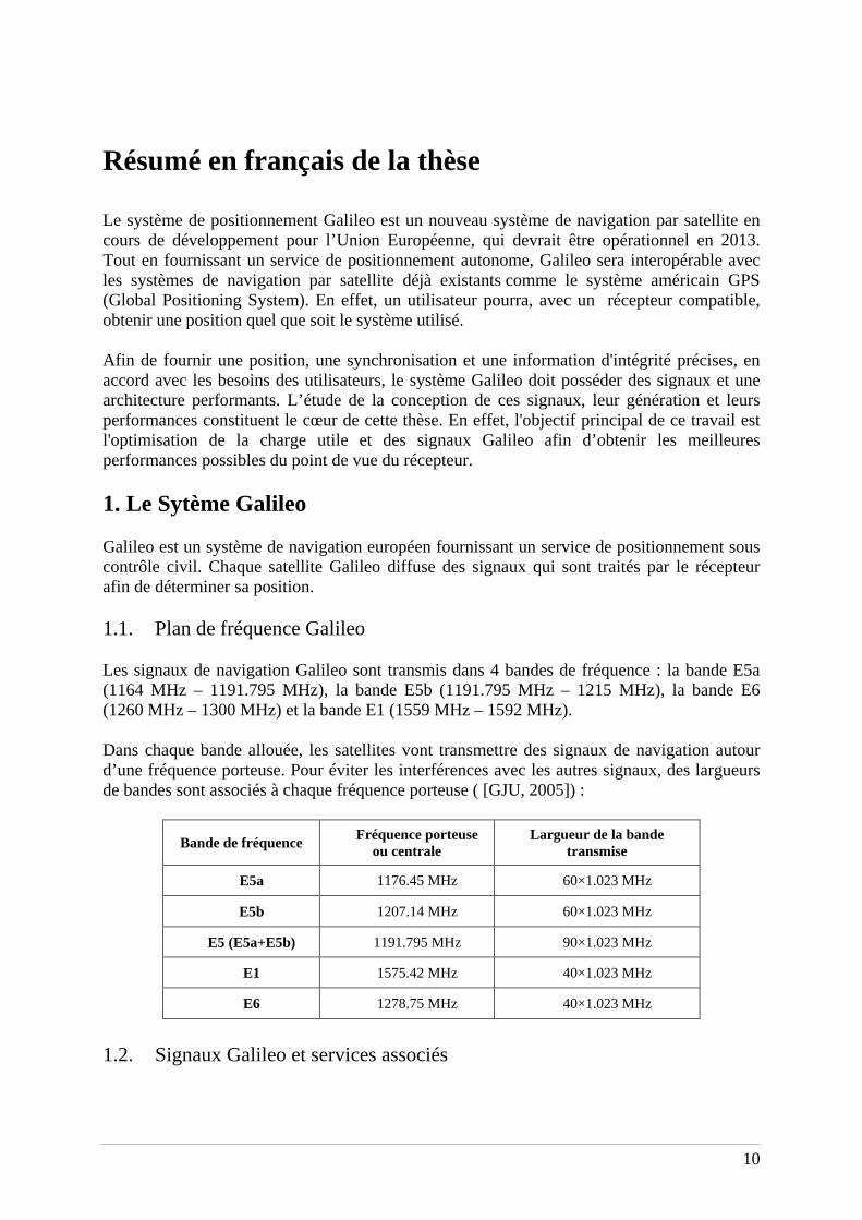
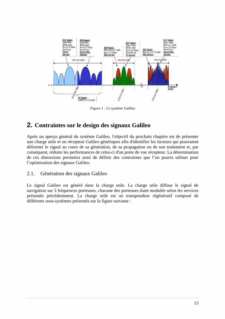
1. Le Sytème Galileo Galileo est un système de navigation européen fournissant un service de positionnement sous contrôle civil. Chaque satellite Galileo diffuse des signaux qui sont traités par le récepteur afin de déterminer sa position. 1.1. Plan de fréquence Galileo Les signaux de navigation Galileo sont transmis dans 4 bandes de fréquence : la bande E5a (1164 MHz – 1191.795 MHz), la bande E5b (1191.795 MHz – 1215 MHz), la bande E6 (1260 MHz – 1300 MHz) et la bande E1 (1559 MHz – 1592 MHz). Dans chaque bande allouée, les satellites vont transmettre des signaux de navigation autour d’une fréquence porteuse. Pour éviter les interférences avec les autres signaux, des largueurs de bandes sont associés à chaque fréquence porteuse ( [GJU, 2005]) :

Bande de fréquence Fréquence porteuse ou centrale

Largueur de la bande transmise

E5a 1176.45 MHz 60×1.023 MHz

E5b 1207.14 MHz 60×1.023 MHz

E5 (E5a+E5b) 1191.795 MHz 90×1.023 MHz

E1 1575.42 MHz 40×1.023 MHz

E6 1278.75 MHz 40×1.023 MHz

1.2. Signaux Galileo et services associés

11

1.2.1. Description des signaux et des services de navigation Galileo

Chaque satellite Galileo transmet 6 signaux de navigation: E1F, E1P, E5A, E5B, E6C et E6P [GJU, 2005]: Le signal E1F est un signal en accès ouvert transmis dans la bande E1. Il est composé

d’un canal donnée (E1-B) et d’un canal pilote (E1-C). Le signal E1P est un signal à accès restreint transmis sur le canal E1-A. Son code et

ses données de navigation sont cryptés. Le signal E5a est un signal en accès ouvert transmis dans la bande E5a et composé

d’une voie donnée (E5a-I) et d’une voie pilote (E5a-Q). Le signal E5b est similaire au signal E5a. Le signal E6C est un signal commercial transmis dans la bande E6 et composé d’une

voie donnée et d’une voie pilote. Ses codes et ses données sont cryptés. Le signal E6P est un signal à accès restreint et sécurisé transmis sur le canal E6-A.

Le système Galileo fournit 5 services différents, associés aux signaux décrits précédemment [GJU, 2005]: le service ouvert (OS - Open Service), le service de sauvegarde de la vie (SoL - Safety of Life), le service commercial (Commercial Service - CS), le service public réglementé (Public Regulated Service - PRS), et le service de recherche et sauvetage (Search and Rescue Service - SAR).

1.2.2. Forme d’ondes des signaux Galileo

Signal BPSK

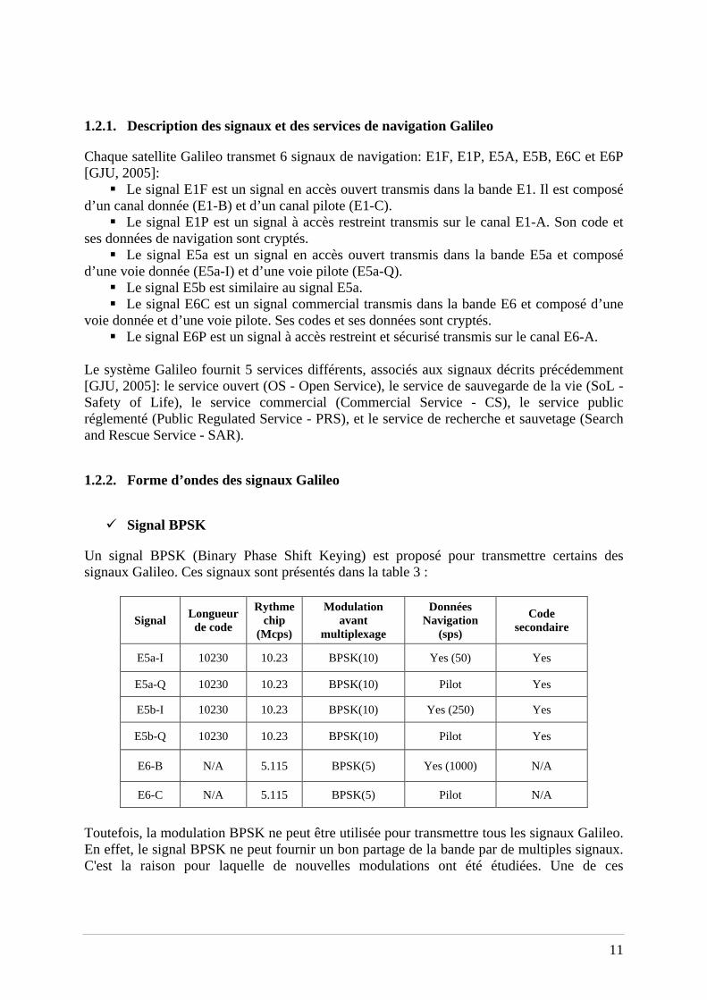
Un signal BPSK (Binary Phase Shift Keying) est proposé pour transmettre certains des signaux Galileo. Ces signaux sont présentés dans la table 3 :

Signal Longueur de code

Rythme chip

(Mcps)

Modulation avant

multiplexage

Données Navigation

(sps)

Code secondaire

E5a-I 10230 10.23 BPSK(10) Yes (50) Yes

E5a-Q 10230 10.23 BPSK(10) Pilot Yes

E5b-I 10230 10.23 BPSK(10) Yes (250) Yes

E5b-Q 10230 10.23 BPSK(10) Pilot Yes

E6-B N/A 5.115 BPSK(5) Yes (1000) N/A

E6-C N/A 5.115 BPSK(5) Pilot N/A

Toutefois, la modulation BPSK ne peut être utilisée pour transmettre tous les signaux Galileo. En effet, le signal BPSK ne peut fournir un bon partage de la bande par de multiples signaux. C'est la raison pour laquelle de nouvelles modulations ont été étudiées. Une de ces

12

modulations, présentée dans [Betz, 2002] est la modulation BOC (Binary Offset Carrier). Elle a été choisie comme modulation pour certains des signaux Galileo, mais aussi pour les nouveaux signaux GPS.

Signal BOC

En général, le signal BOC est noté BOC(p,q), p définit le ratio de la sous-porteuse et q le ratio du code d’étalement : 023.1⋅= pfs MHz et 023.1⋅= qfc MHz

Le signal BOC est défini comme étant le produit d’un code avec une sous-porteuse égale au signe d’une sinusoïde, comme le montre l’équation suivante :

( )( )tfsigntctx Sπ2sin)()( ⋅= avec )()( ck

k kTthctc −=∑

où h(t) est la matérialisation du code égale à 1 sur [0, Tc] et 0 ailleurs, 1,1−=kc .

Le BOC cosinus s’écrit quant à lui :

( )( )tfsigntctx Sπ2cos)()( ⋅= avec )()( ck

k kTthctc −=∑

Le tableau suivant présente les signaux Galileo modulés grâce à un signal BOC :

Signal Longueur de code

Rythme chip

(Mcps)

Modulation avant multiplexage

Données Navigation

(sps)

Code secondaire

E6a N/A 5.115 BOCcos(10,5) Yes N/A

E1A N/A 2.5575 BOCcos(15,2.5) Yes (the data

rate is not public info)

N/A

E1B 4096 1.023 BOC(1,1) Yes (250) No

E1C 8192 1.023 BOC(1,1) Pilot Yes

1.3. Conclusion La figure 1 résume les bandes de fréquences, les services et les signaux associés au système Galileo.

13

Figure 1 : Le système Galileo

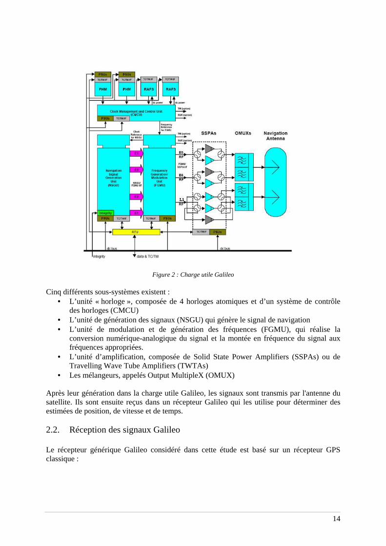
2. Contraintes sur le design des signaux Galileo Après un aperçu général du système Galileo, l'objectif du prochain chapitre est de présenter une charge utile et un récepteur Galileo génériques afin d'identifier les facteurs qui pourraient déformer le signal au cours de sa génération, de sa propagation ou de son traitement et, par conséquent, réduire les performances de celui-ci d'un point de vue récepteur. La détermination de ces distorsions permettra ainsi de définir des contraintes que l’on pourra utiliser pour l’optimisation des signaux Galileo. 2.1. Génération des signaux Galileo Le signal Galileo est généré dans la charge utile. La charge utile diffuse le signal de navigation sur 3 fréquences porteuses, chacune des porteuses étant modulée selon les services présentés précédemment. La charge utile est un transpondeur régénératif composé de différents sous-systèmes présentés sur la figure suivante :

14

Figure 2 : Charge utile Galileo Cinq différents sous-systèmes existent :

• L’unité « horloge », composée de 4 horloges atomiques et d’un système de contrôle des horloges (CMCU)

• L’unité de génération des signaux (NSGU) qui génère le signal de navigation • L’unité de modulation et de génération des fréquences (FGMU), qui réalise la

conversion numérique-analogique du signal et la montée en fréquence du signal aux fréquences appropriées.

• L’unité d’amplification, composée de Solid State Power Amplifiers (SSPAs) ou de Travelling Wave Tube Amplifiers (TWTAs)

• Les mélangeurs, appelés Output MultipleX (OMUX) Après leur génération dans la charge utile Galileo, les signaux sont transmis par l'antenne du satellite. Ils sont ensuite reçus dans un récepteur Galileo qui les utilise pour déterminer des estimées de position, de vitesse et de temps. 2.2. Réception des signaux Galileo Le récepteur générique Galileo considéré dans cette étude est basé sur un récepteur GPS classique :

15

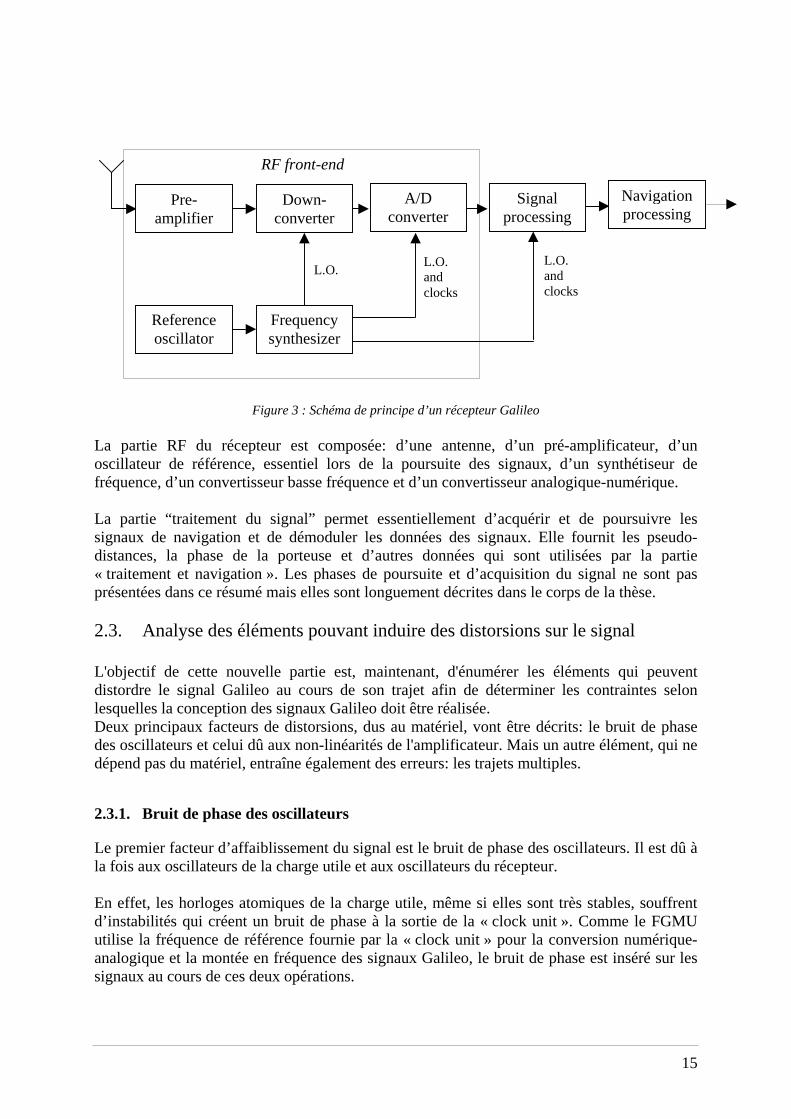
Figure 3 : Schéma de principe d’un récepteur Galileo

La partie RF du récepteur est composée: d’une antenne, d’un pré-amplificateur, d’un oscillateur de référence, essentiel lors de la poursuite des signaux, d’un synthétiseur de fréquence, d’un convertisseur basse fréquence et d’un convertisseur analogique-numérique. La partie “traitement du signal” permet essentiellement d’acquérir et de poursuivre les signaux de navigation et de démoduler les données des signaux. Elle fournit les pseudo-distances, la phase de la porteuse et d’autres données qui sont utilisées par la partie « traitement et navigation ». Les phases de poursuite et d’acquisition du signal ne sont pas présentées dans ce résumé mais elles sont longuement décrites dans le corps de la thèse. 2.3. Analyse des éléments pouvant induire des distorsions sur le signal L'objectif de cette nouvelle partie est, maintenant, d'énumérer les éléments qui peuvent distordre le signal Galileo au cours de son trajet afin de déterminer les contraintes selon lesquelles la conception des signaux Galileo doit être réalisée. Deux principaux facteurs de distorsions, dus au matériel, vont être décrits: le bruit de phase des oscillateurs et celui dû aux non-linéarités de l'amplificateur. Mais un autre élément, qui ne dépend pas du matériel, entraîne également des erreurs: les trajets multiples.

2.3.1. Bruit de phase des oscillateurs

Le premier facteur d’affaiblissement du signal est le bruit de phase des oscillateurs. Il est dû à la fois aux oscillateurs de la charge utile et aux oscillateurs du récepteur. En effet, les horloges atomiques de la charge utile, même si elles sont très stables, souffrent d’instabilités qui créent un bruit de phase à la sortie de la « clock unit ». Comme le FGMU utilise la fréquence de référence fournie par la « clock unit » pour la conversion numérique-analogique et la montée en fréquence des signaux Galileo, le bruit de phase est inséré sur les signaux au cours de ces deux opérations.

Pre-amplifier

Down-converter

A/D converter

Signal processing

Reference oscillator

Frequency synthesizer

L.O. L.O. and clocks

L.O. and clocks

Navigation processing

RF front-end

16

Cependant le bruit de phase affecte également le signal au niveau du récepteur lors de la conversion analogique-numérique et lors de la descente en fréquence parce que l’horloge du récepteur souffre, elle aussi, d'instabilités. Les oscillateurs des récepteurs sont naturellement moins stables que les oscillateurs des satellites.

Définition du bruit de phase

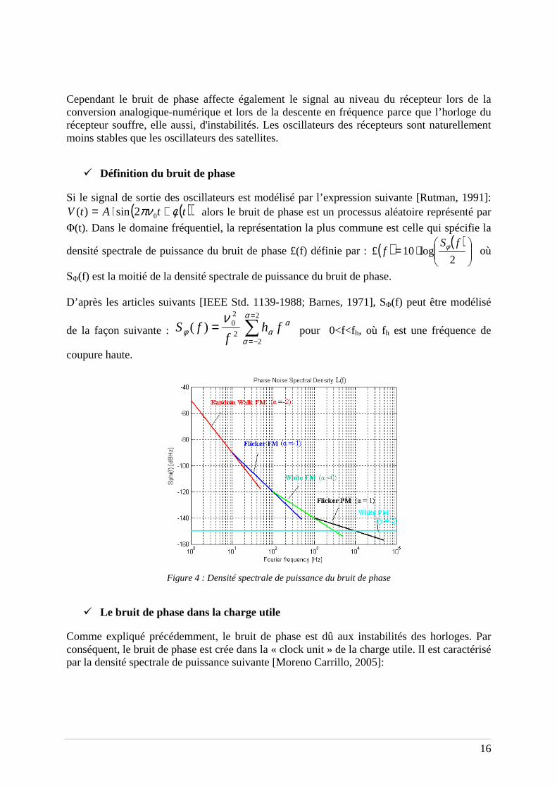
Si le signal de sortie des oscillateurs est modélisé par l’expression suivante [Rutman, 1991]: ( )( ) 2sin)( 0 ttAtV φπν +⋅= alors le bruit de phase est un processus aléatoire représenté par

Φ(t). Dans le domaine fréquentiel, la représentation la plus commune est celle qui spécifie la

densité spectrale de puissance du bruit de phase £(f) définie par : ( ) ( )

⋅=

2log10£

fSf φ où

SΦ(f) est la moitié de la densité spectrale de puissance du bruit de phase.

D’après les articles suivants [IEEE Std. 1139-1988; Barnes, 1971], SΦ(f) peut être modélisé

de la façon suivante : ∑=

−=

=2

22

20)(

α

α

ααφ

νfh

ffS pour 0<f<fh, où fh est une fréquence de

coupure haute.

Figure 4 : Densité spectrale de puissance du bruit de phase

Le bruit de phase dans la charge utile

Comme expliqué précédemment, le bruit de phase est dû aux instabilités des horloges. Par conséquent, le bruit de phase est crée dans la « clock unit » de la charge utile. Il est caractérisé par la densité spectrale de puissance suivante [Moreno Carrillo, 2005]:

17

Power Spectral Density of the CMCU phase noise [Moreno Carrillo, 2005]

-160

-150

-140

-130

-120

-110

-100

-90

-80

1 10 100 1,00E+03 1,00E+04 1,00E+05

frequency offsets [Hz]

SS

B p

hase

noi

se [d

Bc/

Hz]

Figure 5 : Densité spectrale de puissance du bruit de phase à la sortie de la « clock unit » Le FGMU utilise la fréquence de référence envoyée par la « clock unit » pour réaliser la conversion numérique-analogique et la conversion en fréquence. Par conséquent, le bruit de phase sera introduit au niveau du signal de navigation durant ces deux conversions. Le bruit de phase introduit lors de la conversion numérique-analogique est dû à l’instabilité de l’horloge d’échantillonnage et peut se traduire sur le signal par un jitter relié au bruit de phase de l’horloge de référence par la formule suivante [Da Dalt., 2002]:

( ) ( )T

ttt j ⋅=

πφ2

valable si tj << T, la période d’échantillonnage.

Evaluons à présent le bruit de phase introduit au cours de la conversion en fréquence. Les fréquences utilisées pour la conversion proviennent de synthétiseurs de fréquence, considérés comme de simples boucles de phase. Le bruit de phase à la sortie d’un synthétiseur et donc introduit sur le signal lors de la montée en fréquence peut être caractérisé par la formule suivante ([Rebeyrol03, 2006] et Appendice C):

( ) ( ) ( ) ( ) ( ) 222 1 fHfSfHNfSfSvcoCUout

−⋅+⋅⋅= φφφ

où SΦCU(f) est la densité spectrale de puissance du bruit de phase à la sortie de la “clock

unit” SΦVCO(f) est la densité spectrale de puissance du bruit de phase du VCO et, H(f) est la fonction de transfert en boucle fermée de la PLL égale à :

( )( )

( ) N

sFKKs

N

sFKK

sHPDVCO

PDVCO

⋅⋅+

⋅⋅

=

18

N dépend du rapport entre la fréquence de référence et la fréquence porteuse du signal Galileo à transmettre Par conséquent, le bruit de phase dû à l’horloge de la charge utile et introduit sur le signal durant sa génération peut être caractérisé par la formule suivante:

( ) ( ) ( ) ( ) ( ) )(1 /

222 fSfHfSfHNfSfS ADvcoCUpayload+−⋅+⋅⋅= φφφ

Le bruit de phase dans le récepteur

Comme pour la charge utile, le bruit phase au niveau récepteur est dû aux instabilités des oscillateurs. Il est donc crée par l’horloge du récepteur et affecte le signal lors de sa conversion en fréquence et lors de sa conversion analogique-numérique. En général, les oscillateurs des récepteurs sont moins stables que les oscillateurs des charges utiles. Le bruit de phase dû à l’horloge est donc plus important dans un récepteur que dans une charge utile. Différentes catégories d’oscillateurs existent mais le plus utilisé dans les récepteurs est le TCXO (Temperature Compensated Crystal Oscillators). Certains récepteurs qui nécessitent une bonne stabilité d’horloge peuvent aussi utiliser des horloges atomiques rubidium. Comme dans le cas d’un récepteur GPS, la conversion de fréquence est réalisée à l’aide synthétiseur de fréquence de type PLL. D’après les calculs réalisés pour la charge utile, nous pouvons donc déduire que le bruit de phase introduit par l’oscillateur du récepteur durant la conversion en fréquence est modélisé par :

( ) ( ) ( ) ( ) ( ) 222 1 fHfSfHNfSfSvcoclockLO

−⋅+⋅⋅= φφφ

avec SΦclock(f), la densité spectrale de puissance du bruit de phase de l’oscillateur du

récepteur SΦVCO(f), la densité spectrale de puissance du bruit de phase du VCO H(f), la fonction de transfert en boucle fermée de la PLL:

( )( )

( ) N

sFKKs

N

sFKK

sHPDVCO

PDVCO

⋅⋅+

⋅⋅

= avec F(s) la fonction de transfert du filtre de boucle,

KVCO et KPD, les gains du VCO et du détecteur de phase. N le rapport entre la fréquence porteuse du signal et la fréquence de travail du

récepteur.

19

Comme pour la charge utile et la conversion numérique-analogique, le bruit de phase introduit par la conversion analogique-numérique peut être caractérisé par un jitter relié au bruit de

phase de l’horloge du récepteur par la formule suivante : ( ) ( )T

ttt j ⋅=

πφ2

.

Par conséquent, le bruit de phase introduit sur le signal à l’entrée de la partie “traitement du signal” dans le récepteur est caractérisé par ([Rebeyrol02, 2006]):

( )( ) ( ) ( ) ( )

( ) ( ) ( ) ( )

+−⋅+⋅⋅+

+−⋅+⋅⋅=

)(1

)(1

/

222

/

222

fSfHfSfHNfS

fSfHfSfHNfSfS

DAoreceivervcreceiver

ADpayloadvcopayloadCU

clockφφ

φφ

φ

Le bruit de phase introduit sur le signal a été évalué, nous allons donc maintenant voir quelle est son influence.

Influence du bruit de phase

Pour évaluer et observer l’influence du bruit de phase, plusieurs observables peuvent être utilisés : la fonction de corrélation, la densité spectrale de puissance, l’évaluation de l’erreur de phase induite par le bruit de phase dans une PLL et la constellation de la modulation. La fonction de corrélation est utilisée comme observable car elle permet d’évaluer l’influence du bruit de phase sur la poursuite du signal grâce à l’observation du pic de corrélation. La densité spectrale de puissance permet elle d’évaluer une possible distorsion ou remontée des lobes secondaires due au bruit de phase qui pourrait entraîner des interférences avec les autres signaux. Pour évaluer l’influence du bruit de phase, l’estimation de l’erreur de phase due à ce bruit dans une PLL, utilisée pour la poursuite des signaux, doit être analysée. La variance de cette erreur de phase est donnée par la formule suivante :

( )∫∞

⋅−⋅=0

22 1)( dfjfHfSφσ avec SΦ (f) la densité spectrale de puissance du bruit de

phase entrant dans la PLL et H(f) caractérisé de la façon suivante si la PLL est une boucle

d’ordre 3 [Parkinson, 1996]: 66

62

)(1ff

fjfH

L +=− où fL= π2 *1.2*BL, et BL est la

bande de boucle. L’influence du bruit de phase peut aussi être visualisée sur la constellation de la modulation comme le montre le schéma suivant. En effet, le bruit de phase peut introduire un offset sur la phase du signal et donc les plots de la modulation peuvent tourner ou s’étaler si cet offset dépend du temps.

20

Figure 6 : Influence du bruit de phase sur une modulation 8-PSK

Conclusion

D’après cette section, il semble que la seule façon de réduire le bruit de phase introduit sur le signal est d’utiliser des horloges extrêmement stables. Au niveau de la charge utile, on utilise des horloges atomiques, ce sont les horloges les plus stables actuellement, il est donc impossible de réduire le bruit de phase des horloges dans la charge utile. Au niveau du récepteur, il est également possible d'utiliser des horloges atomiques mais cette utilisation se limite à quelques applications (stations au sol). En effet, cette option n'est pas acceptable pour le marché de masse en raison du coût de ces horloges. Par conséquent, il est difficile de réduire le bruit de phase dû aux horloges de la charge utile et du récepteur. De plus, aucune optimisation et aucune contrainte sur le design du signal ne peuvent être déduite de ce facteur de bruit.

2.3.2. Non-linéarités des amplificateurs

Le deuxième élément de distorsion est dû à l'amplificateur de la charge utile. En effet, au cours de la génération du signal, l'amplificateur peut provoquer des distorsions sur le signal, à cause de ses caractéristiques non-linéaires en amplitude (AM/AM) et en phase (AM/PM), comme le montre la figure suivante :

Signal modulation constellation

Example of plots rotation due to phase noise

Example of plots spread due to phase noise

21

Figure 7 : Caractéristiques AM/AM et AM/PM d’un amplificateur

Par conséquent, un signal à enveloppe constante, c’est à dire dont tous les points sont à la même puissance, ne sera pas distordu par l’amplificateur car tous ses points seront amplifiés de la même façon. Par contre, un signal qui ne possède pas une enveloppe constante n’aura pas ses points qui seront amplifiés de la même façon à cause des caractéristiques non-linéaires de l’amplificateur. Donc des distorsions peuvent être introduites par l’amplificateur à la fois sur l’amplitude et sur la phase du signal. Les distorsions d’amplitude sont en général négligeable devant les autres distorsions et donc nous n’étudierons que la distorsion introduite par la non-linéarité en phase de l’amplificateur. Les distorsions dues à l’amplificateur peuvent être assimilées à du bruit de phase, par conséquent les figures de mérite pour les observer seront les mêmes que celles présentées pour le bruit de phase des horloges : la fonction de corrélation, la densité spectrale de puissance, l’estimation de l’erreur de phase dans une PLL et la constellation de la modulation. Contrairement au bruit de phase des oscillateurs, il est possible de réduire au minimum les distorsions dues aux non-linéarités de l'amplificateur en transmettant un signal à enveloppe constante. Pour réduire au maximum les distorsions dues au bloc d’amplification, la modulation Galileo devra donc être optimisée afin de transmettre des signaux à enveloppe constante.

2.3.3. Multi-trajets

Les sections précédentes ont décrit les deux distorsions introduites par du « matériel » : le bruit de phase dû aux instabilités des horloges récepteur et satellite et le bruit de phase dû aux non-linéarités de l’amplificateur. Mais, un autre élément, qui ne dépend pas du « matériel », doit être pris en compte pour la conception des signaux Galileo, car il entraîne des erreurs de mesures : les trajets multiples. Un multi-trajet est un signal réfléchi qui entre dans un récepteur après diffraction ou réflexion sur le terrain environnant: les bâtiments, les murs d’un canyon, le sol ,.. Les signaux réfléchis, en entrant dans le récepteur se mélangent avec le signal principal, ce qui peut entraîner des erreurs de mesures. Le multi-trajet distord la modulation du signal principal mais aussi la phase de la porteuse.

22

En l'absence de trajets multiples, les discriminateurs du récepteur poursuivent la phase du signal principal. Or, en présence des trajets multiples, le signal entrant dans le discriminateur est un signal composé du trajet multiple et du signal principal; la boucle poursuit donc un signal composite différent du signal principal. Le pic de corrélation présente alors une distorsion qui va impacter le discriminateur et donc les performances en poursuite. L’influence des multi-trajets peut être réduite grâce à une conception particulière de la modulation du signal. En effet, certaines modulations ont une meilleure résistance aux trajets multiples que d'autres. C'est par exemple le cas de la modulation BOC, qui est plus résistante aux trajets multiples que la modulation BPSK ([Betz, 2002]). Les signaux choisis pour transmettre le signal Galileo doivent donc présenter une résistance « naturelle » aux trajets multiples. 2.4. Conclusions L'étude de la génération des signaux dans la charge utile et leur traitement dans le récepteur a permis d’identifier plusieurs facteurs qui entraînent des dégradations sur le signal : le bruit de phase introduit par l'instabilité des horloges, le bruit de phase dû aux non-linéarités de l’amplificateur de la charge utile et les multi-trajets. Tous ces facteurs peuvent distordre le signal et entraîner de mauvaises performances. Il serait donc intéressant de réduire l'influence de ces éléments en optimisant les signaux Galileo ou en optimisant la chaîne de transmission. Le bruit de phase des oscillateurs ne peut être réduit par une conception particulière du signal, mais le bruit de phase de l'amplificateur et les distorsions induites par les multi-trajets peuvent eux être réduits en générant des signaux à enveloppe constante possédant une résistance particulière aux trajets multiples.

3. Le signal Galileo dans la bande E5 L'objectif de ce chapitre est de présenter la structure du signal E5, mais aussi la modulation, appelée ALTBOC (Alternate BOC) choisie pour le transmettre. De plus, on montrera que ce signal vérifie les contraintes de design exposées dans le chapitre précédent. 3.1. Les signaux E5 Dans la bande E5, la modulation doit multiplexer 3 différents services: le service ouvert, le service commercial et le service secours qui sont transmis sur 4 composantes BOC tout en maintenant constante l’enveloppe du signal résultant. Les 4 composantes du signal E5 sont les canaux E5a donnée et pilote et les canaux E5b donnée et pilote. La modulation proposée pour multiplexer tous ces canaux est appelée Alternate Binary Offset Carrier (ALTBOC) modulation ([GJU, 2005]). C’est plus précisément un ALTBOC(15,10) qui est proposé, c’est à dire une modulation ALTBOC avec une fréquence de code égale à 10.23 MHz et une fréquence de sous-porteuse égale à 15.345 MHz.

23

3.2. Multiplexage des signaux E5 La modulation ALTBOC à enveloppe constante a été obtenue par modification de la modulation ALTBOC classique en introduisant des termes, appelés produits d’intermodulation qui permettent de garder une enveloppe constante. L’expression de cette nouvelle modulation est la suivante [Soellner, 2003]:

( ) ( )

( ) ( )

−⋅+⋅⋅++

−⋅−⋅⋅+

+

−⋅+⋅⋅++

−⋅−⋅⋅+=

4)(

4)(

4)(

4)(

)(''

''

_Ts

tscjtsccjcTs

tscjtsccjc

Tstscjtsccjc

Tstscjtsccjc

tx

apapUUapapLL

asasUUasasLL

BOCALT

avec

'''''''' LLUuLULULUULLUUL cccccccccccccccc ====

et

( )( )

( )( )

+−+

−−=

+++

−=

42cos

4

22cos

2

1

42cos

4

2)(

42cos

4

22cos

2

1

42cos

4

2)(

πππππ

πππππ

tfsigntfsigntfsigntsc

tfsigntfsigntfsigntsc

SSSap

SSSas

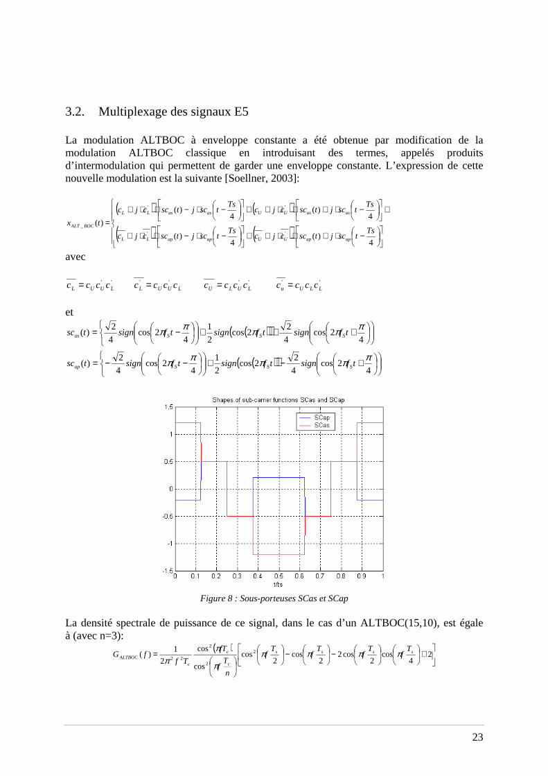
Figure 8 : Sous-porteuses SCas et SCap

La densité spectrale de puissance de ce signal, dans le cas d’un ALTBOC(15,10), est égale à (avec n=3):

( )

+

−

−

= 2

4cos

2cos2

2cos

2cos

cos

cos

2

1)( 2

2

2

22ssss

c

c

c

ALTBOC

Tf

Tf

Tf

Tf

n

Tf

fT

TffG ππππ

π

ππ

24

3.3. Propriétés du signal ALTBOC

La modulation ALTBOC à enveloppe constante a plusieurs avantages: Tout d'abord, le signal ne souffre pas des distorsions dues aux non-linéarités de

l’amplificateur de la charge utile si une bande passante infinie est conservée. Ensuite, l'enveloppe constante permet aussi un gain en précision grâce à la possibilité

de transmettre un signal à large bande de façon cohérente et non pas deux signaux QPSK à bande étroite.

Enfin, le ALTBOC représente une optimisation de l'usage des signaux E5a et E5b car des récepteurs simples peuvent utiliser une seule des deux composantes (E5a ou E5b), alors que des récepteurs plus complexes peuvent fonctionner eux en poursuivant les deux composantes, et donc obtenir davantage de précision.

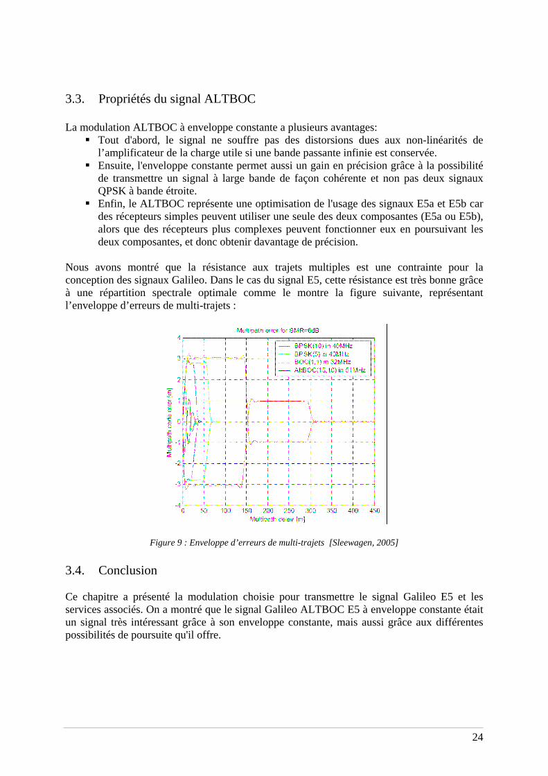
Nous avons montré que la résistance aux trajets multiples est une contrainte pour la conception des signaux Galileo. Dans le cas du signal E5, cette résistance est très bonne grâce à une répartition spectrale optimale comme le montre la figure suivante, représentant l’enveloppe d’erreurs de multi-trajets :

Figure 9 : Enveloppe d’erreurs de multi-trajets [Sleewagen, 2005] 3.4. Conclusion Ce chapitre a présenté la modulation choisie pour transmettre le signal Galileo E5 et les services associés. On a montré que le signal Galileo ALTBOC E5 à enveloppe constante était un signal très intéressant grâce à son enveloppe constante, mais aussi grâce aux différentes possibilités de poursuite qu'il offre.

25

4. Le signal Galileo dans la bande E1 Après la description du signal E5, ce chapitre présente l'autre signal « ouvert » du système Galileo: le signal E1. Nous allons vérifier comme précédemment que la conception de ce signal suit les contraintes énoncées précédemment.

En juin 2004, un accord ([CE, 2005]) a été signé entre les États-Unis et l'Union européenne. Cet accord propose un signal commun afin de transmettre le signal Galileo E1F et le signal GPS L1C. Toutefois l'accord prévoit une optimisation possible de ce signal. C'est la raison pour laquelle, différentes études ont été menées jusqu’en 2007 afin de trouver un signal qui serait plus performant mais continuerait à vérifier les contraintes imposées par l’accord de 2004.

4.1. Les signaux Galileo E1 de reference

4.1.1. Les signaux de la bande E1

La modulation en bande E1 doit combiner trois signaux associés à quatre différents services tout en respectant les contraintes de conception: une enveloppe constante à l’entrée de l'amplificateur, et une bonne résistance aux trajets multiples. Les signaux Galileo E1 sont respectivement:

Le signal E1F correspondant aux services l'OS / CS / SOL. Depuis l’accord de juin

2004, il est prévu d'adopter un BOC (1,1) sinus comme signal de référence afin de transmettre le signal Galileo E1F et le futur signal GPS L1C.

Le signal E1P correspondant au service PRS. Pour transmettre le signal E1P, un BOC (15,2.5) cosinus a été adopté par [GJU, 2005].

Ces signaux de référence doivent être multiplexés avant leur transmission grâce à une modulation à enveloppe constante afin de réduire au minimum les distorsions apportées par l'amplificateur dans la charge utile. Plusieurs techniques ont été proposées pour résoudre ce problème, mais la modulation Interplex a été préférée ([Wang, 2004]; [STF, 2002]; [GJU, 2005]).

4.1.2. Multiplexage du signal E1 : modulation Interplex

Dans la bande E1, l'objectif du multiplexage est différent de celui de la bande E5, même si le résultat final doit être le même: une modulation à enveloppe constante du signal. La modulation E1 doit multiplexer trois éléments distincts associés à deux services différents dans un signal modulé en phase. Cela peut être réalisé grâce la modulation Interplex.

26

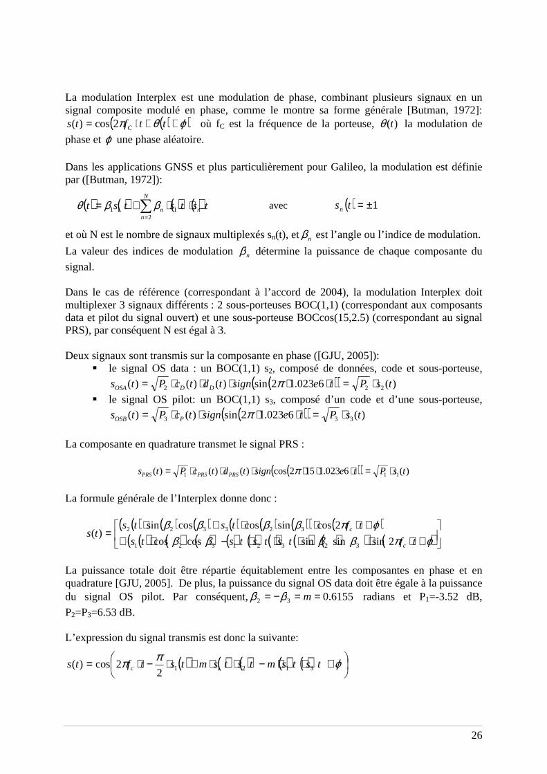
La modulation Interplex est une modulation de phase, combinant plusieurs signaux en un signal composite modulé en phase, comme le montre sa forme générale [Butman, 1972]:

( )( ) 2cos)( ϕθπ ++⋅= ttfts C où fC est la fréquence de la porteuse, )(tθ la modulation de

phase et ϕ une phase aléatoire. Dans les applications GNSS et plus particulièrement pour Galileo, la modulation est définie par ([Butman, 1972]):

( ) ( ) ( ) ( ) 2

111 ∑=

⋅⋅+=N

nnn tststst ββθ avec ( ) 1±=tsn

et où N est le nombre de signaux multiplexés sn(t), et nβ est l’angle ou l’indice de modulation.

La valeur des indices de modulation nβ détermine la puissance de chaque composante du

signal. Dans le cas de référence (correspondant à l’accord de 2004), la modulation Interplex doit multiplexer 3 signaux différents : 2 sous-porteuses BOC(1,1) (correspondant aux composants data et pilot du signal ouvert) et une sous-porteuse BOCcos(15,2.5) (correspondant au signal PRS), par conséquent N est égal à 3. Deux signaux sont transmis sur la composante en phase ([GJU, 2005]):

le signal OS data : un BOC(1,1) s2, composé de données, code et sous-porteuse, ( )( ) )(6023.12sin)()()( 222 tsPtesigntdtcPts DDOSA ⋅=⋅⋅⋅⋅⋅= π

le signal OS pilot: un BOC(1,1) s3, composé d’un code et d’une sous-porteuse, ( )( ) )(6023.12sin)()( 333 tsPtesigntcPts POSB ⋅=⋅⋅⋅⋅= π

La composante en quadrature transmet le signal PRS :

( )( ) )(6023.1152cos)()()( 111 tsPtesigntdtcPts PRSPRSPRS ⋅=⋅⋅⋅⋅⋅⋅= π

La formule générale de l’Interplex donne donc :

( ) ( ) ( ) ( ) ( ) ( )( ) ( )( ) ( ) ( ) ( ) ( ) ( ) ( ) ( )( ) ( )

+⋅⋅⋅⋅⋅−⋅++⋅⋅⋅+⋅

=ϕπββββ

ϕπββββtftstststs

tftststs

c

c

2sinsinsincoscos

2cossincoscossin)(

32321321

323322

La puissance totale doit être répartie équitablement entre les composantes en phase et en quadrature [GJU, 2005]. De plus, la puissance du signal OS data doit être égale à la puissance du signal OS pilot. Par conséquent, 6155.032 ==−= mββ radians et P1=-3.52 dB,

P2=P3=6.53 dB. L’expression du signal transmis est donc la suivante:

( ) ( ) ( ) ( ) ( ) 2

2cos)( 31211

+⋅⋅−⋅⋅+⋅−⋅= ϕππ tstsmtstsmtstfts c

27

ou

( ) ( ) ( ) ( ) ( ) ( )( ) ( )( ) ( ) ( ) ( ) ( ) ( )( ) ( )

2sinsincos

2cossincoscossin)(

2321

21

32

+⋅⋅⋅⋅⋅+⋅+

+⋅⋅⋅−⋅=

ϕπϕπ

tfmtststsmts

tfmmtsmmtsts

c

c

Les différents états du signal Interplex peuvent être représentés sur un diagramme de phase, on constate alors que le modulation obtenue a bien une enveloppe constante :

Figure 10 : Constellation de la modulation Interplex du signal Galileo E1

4.1.3. Performance du signal Galileo E1F

Tous les paramètres utilisés pour évaluer les performances du BOC (1,1) sont présentés dans cette section : la fonction d'autocorrélation, la Root Mean Square (RMS) et l’enveloppe d’erreurs de multi-trajets.

Signal s3 OSB

Signal s1 PRS

Signal IM

In-phase signal

Quadrature signal

Points of modulation constellation

Signal s2 OSA

28

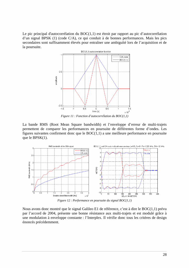
Le pic principal d'autocorrélation du BOC(1,1) est étroit par rapport au pic d’autocorrélation d’un signal BPSK (1) (code C/A), ce qui conduit à de bonnes performances. Mais les pics secondaires sont suffisamment élevés pour entraîner une ambiguïté lors de l’acquisition et de la poursuite.

Figure 11 : Fonction d’autocorrélation du BOC(1,1)

La bande RMS (Root Mean Square bandwidth) et l’enveloppe d’erreur de multi-trajets permettent de comparer les performances en poursuite de différentes forme d’ondes. Les figures suivantes confirment donc que le BOC(1,1) a une meilleure performance en poursuite que le BPSK(1).

Figure 12 : Performance en poursuite du signal BOC(1,1)

Nous avons donc montré que le signal Galileo E1 de référence, c’est à dire le BOC(1,1) prévu par l’accord de 2004, présente une bonne résistance aux multi-trajets et est modulé grâce à une modulation à enveloppe constante : l’Interplex. Il vérifie donc tous les critères de design énoncés précédemment.

29

4.2. Signaux Galileo E1 optimisés L’accord de 2004 laisse la possibilité d’optimiser le signal E1, de nouvelles études ont donc été menées afin de trouver des signaux E1F présentant de meilleures performances que le BOC(1,1). Ces nouvelles formes d'onde sont basées sur l'ajout d'une nouvelle composante au BOC (1,1).

4.2.1. Définition des signaux optimisés

Deux nouveaux signaux ont été étudiés afin d’optimiser le signal OS: le « Composite Binary Coded Symbol » (CBCS) ([Hein, 2005]) et le « Composite Binary Offset Carrier » ([Avila-Rodriguez, 2006]). Le signal “Composite Binary Coded Symbol” (CBCS) est représenté par la combinaison d’un BOC(1,1) et d’un signal BCS avec la même fréquence de code ([Hein, 2005]) :

)1],...([)1,1()( 1 mppBCSQBOCPts ⋅+⋅= où P et Q sont des valeurs en % avec la condition

P+Q=100 %. Si les signaux OS sont transmis grâce à des signaux CBCS, les composantes data (OSA) et pilot (OSB) du signal E1F sont alors exprimées de la façon suivante ([Hein, 2005]):

[ ]( ))1,...()1,1()()()( 1 mDDOSA ppBCSQBOCPtdtcts ⋅+⋅⋅⋅=

[ ]( ))1,...()1,1()()( 1 mPOSB ppBCSQBOCPtcts ⋅−⋅⋅=

avec cD et cP respectivement les codes data et pilot, dD les donnés et BOC et BCS respectivement les sous-porteuses BOC et BCS.

La forme d’onde CBCS associée à la composante OSA est notée CBCS([p1…pm],1, 22

2

QP

Q

+,

“+”) et la forme d’onde CBCS associée à la composante OSB est notée CBCS([p1…pm],1,

22

2

QP

Q

+, “-”).

Le “Composite BOC (CBOC)” est une autre forme d’onde proposée pour transmettre le signal Galileo E1 OS. Il est représenté par la combinaison linéaire d’un BOC(1,1) et d’une autre sous-porteuse BOC de fréquence supérieure mais avec la même fréquence de code [Hein, 2006] : )1,()1,1()( pBOCQBOCPts ⋅+⋅= où P et Q sont des valeurs en % avec la condition

P+Q=100 % et fs=p*1.023 MHz représente la fréquence de la sous-porteuse BOC(p,1) combinée avec le BOC(1,1). Si les signaux OS sont transmis grâce à des signaux CBOC, les composantes data (OSA) et pilot (OSB) du signal E1F sont alors exprimées de la façon suivante [Avila-Rodriguez, 2006]:

30

( ))1,()1,1()()()( pBOCQBOCPtdtcts DDOSA ⋅+⋅⋅⋅=

( ))1,()1,1()()( pBOCQBOCPtcts POSB ⋅−⋅⋅=

avec cD et cP respectivement les codes data et pilot, dD les donnés et BOC(1,1) et BOC(p,1) respectivement les sous-porteuses BOC(1,1) et BOC(p,1).

La forme d’onde CBOC associée à la composante OSA est notée CBOC(p,1, 22

2

QP

Q

+, “+”)

et la forme d’onde CBOC associée à la composante OSB est notée CBOC(p,1, 22

2

QP

Q

+, “-”).

Quel que soit le signal optimisé, l’objectif reste le même: multiplexer les différents canaux (signaux data et pilot E1F et E1P) grâce à une modulation à enveloppe constante. La modulation Interplex, présentée précédemment, est également privilégiée pour transmettre les signaux optimisés, mais certaines modifications doivent être prises en compte en raison de l'ajout de la composante BCS ou BOC(p,1). L’Interplex n'est en effet plus une modulation de trois composantes, mais une modulation de cinq composantes.

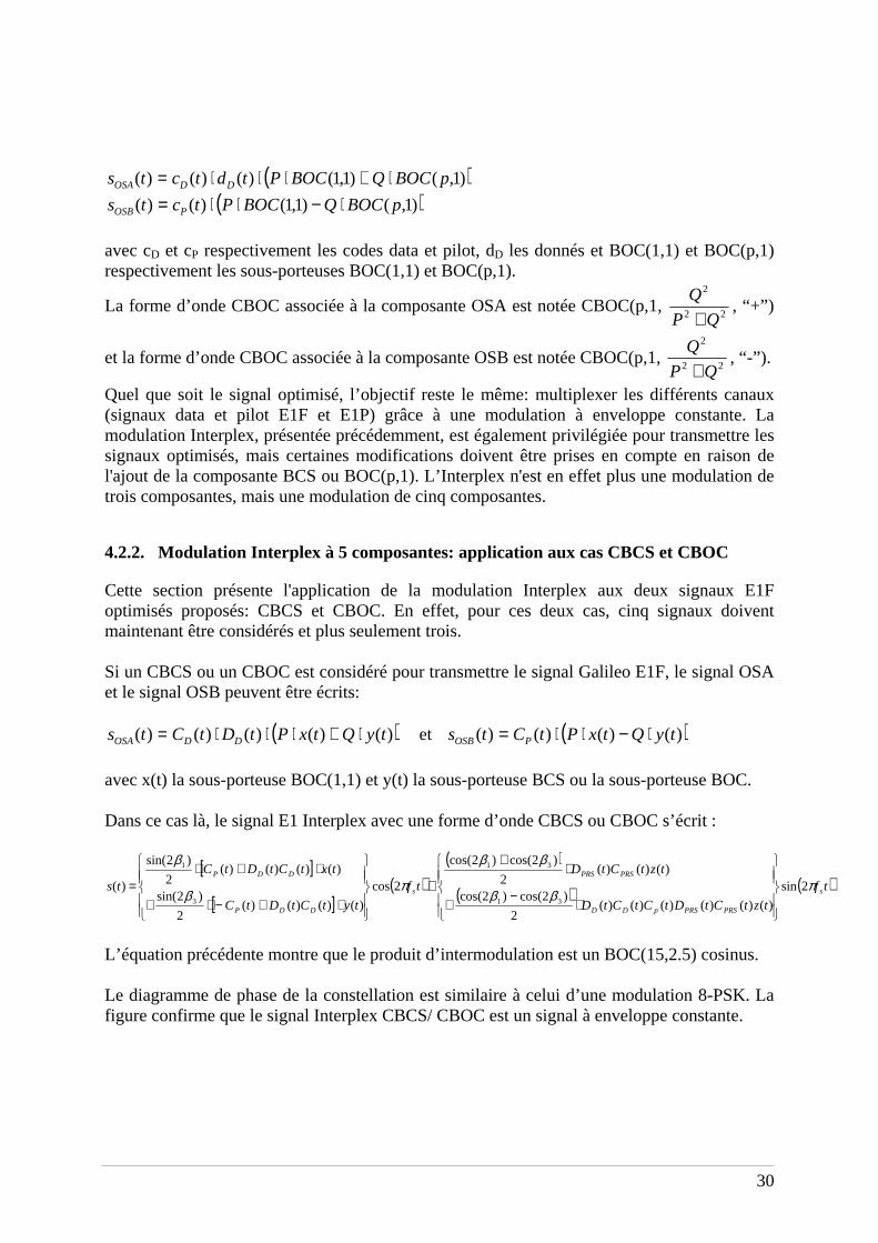
4.2.2. Modulation Interplex à 5 composantes: application aux cas CBCS et CBOC

Cette section présente l'application de la modulation Interplex aux deux signaux E1F optimisés proposés: CBCS et CBOC. En effet, pour ces deux cas, cinq signaux doivent maintenant être considérés et plus seulement trois. Si un CBCS ou un CBOC est considéré pour transmettre le signal Galileo E1F, le signal OSA et le signal OSB peuvent être écrits:

( ))()()()()( tyQtxPtDtCts DDOSA ⋅+⋅⋅⋅= et ( ))()()()( tyQtxPtCts POSB ⋅−⋅⋅=

avec x(t) la sous-porteuse BOC(1,1) et y(t) la sous-porteuse BCS ou la sous-porteuse BOC. Dans ce cas là, le signal E1 Interplex avec une forme d’onde CBCS ou CBOC s’écrit :

[ ]

[ ]( )

( )

( ) ( )tf

tztCtDtCtCtD

tztCtDtf

tytCtDtC

txtCtDtCts s

PRSPRSpDD

PRSPRS

s

DDP

DDP

πββ

ββ

πβ

β

2sin

)()()()()()(2

)2cos()2cos(

)()()(2

)2cos()2cos(

2cos

)()()()(2

)2sin(

)()()()(2

)2sin(

)(31

31

3

1

⋅−

+

⋅+

+

⋅+−⋅+

⋅+⋅=

L’équation précédente montre que le produit d’intermodulation est un BOC(15,2.5) cosinus.

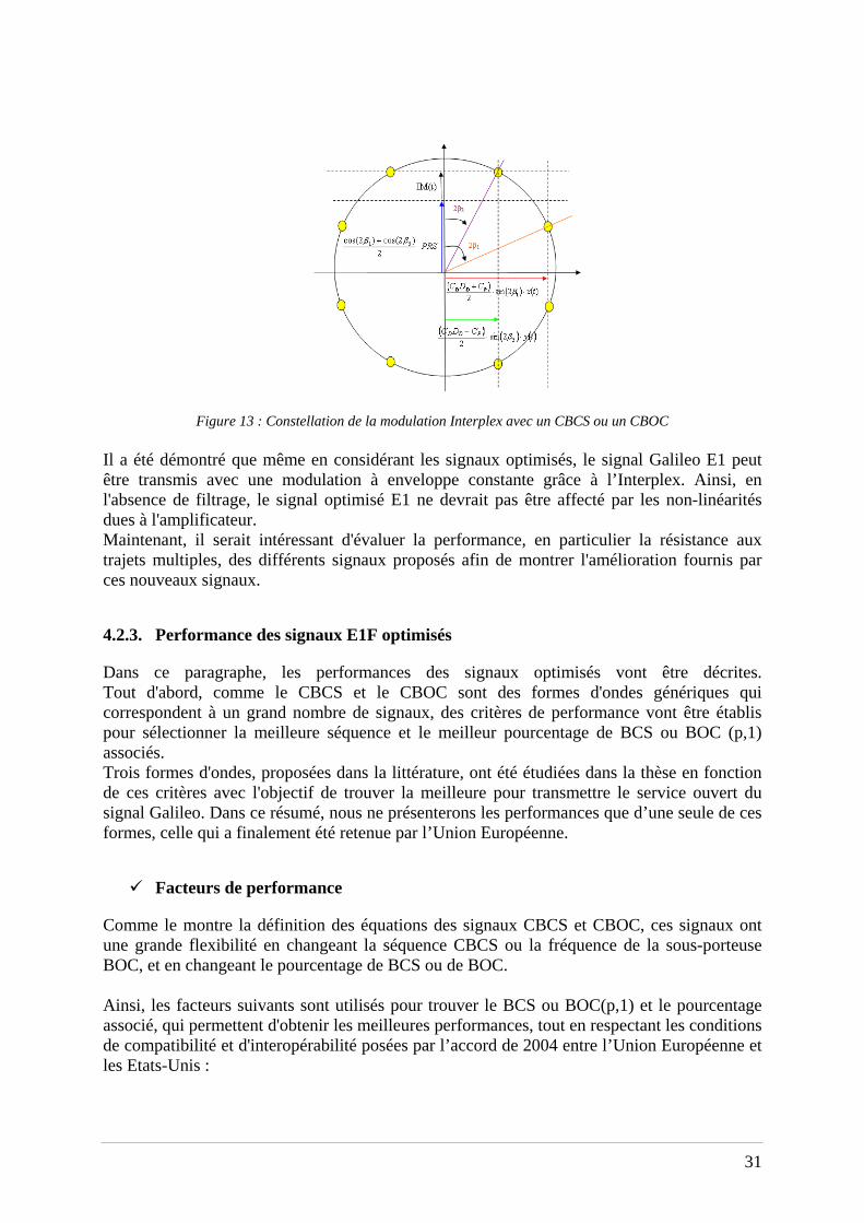
Le diagramme de phase de la constellation est similaire à celui d’une modulation 8-PSK. La figure confirme que le signal Interplex CBCS/ CBOC est un signal à enveloppe constante.

31

Figure 13 : Constellation de la modulation Interplex avec un CBCS ou un CBOC Il a été démontré que même en considérant les signaux optimisés, le signal Galileo E1 peut être transmis avec une modulation à enveloppe constante grâce à l’Interplex. Ainsi, en l'absence de filtrage, le signal optimisé E1 ne devrait pas être affecté par les non-linéarités dues à l'amplificateur. Maintenant, il serait intéressant d'évaluer la performance, en particulier la résistance aux trajets multiples, des différents signaux proposés afin de montrer l'amélioration fournis par ces nouveaux signaux.

4.2.3. Performance des signaux E1F optimisés

Dans ce paragraphe, les performances des signaux optimisés vont être décrites. Tout d'abord, comme le CBCS et le CBOC sont des formes d'ondes génériques qui correspondent à un grand nombre de signaux, des critères de performance vont être établis pour sélectionner la meilleure séquence et le meilleur pourcentage de BCS ou BOC (p,1) associés. Trois formes d'ondes, proposées dans la littérature, ont été étudiées dans la thèse en fonction de ces critères avec l'objectif de trouver la meilleure pour transmettre le service ouvert du signal Galileo. Dans ce résumé, nous ne présenterons les performances que d’une seule de ces formes, celle qui a finalement été retenue par l’Union Européenne.

Facteurs de performance

Comme le montre la définition des équations des signaux CBCS et CBOC, ces signaux ont une grande flexibilité en changeant la séquence CBCS ou la fréquence de la sous-porteuse BOC, et en changeant le pourcentage de BCS ou de BOC. Ainsi, les facteurs suivants sont utilisés pour trouver le BCS ou BOC(p,1) et le pourcentage associé, qui permettent d'obtenir les meilleures performances, tout en respectant les conditions de compatibilité et d'interopérabilité posées par l’accord de 2004 entre l’Union Européenne et les Etats-Unis :

32

Tout d'abord, la meilleure forme d’onde CBCS ou CBOC doit avoir une fonction

d'autocorrélation étroite afin d'assurer de bonnes performances en poursuite, et sa bande passante RMS doit être meilleure ou similaire à celle obtenue avec un BOC(1,1).

Ensuite, la réjection aux trajets multiples est également un facteur important ; c’est

une contrainte majeure pour la conception des signaux en raison de son importante contribution lors du calcul de la pseudo-distance.

Les facteurs ci-dessus permettent d'étudier les performances des signaux CBCS/CBOC lors d’une poursuite avec une réplique exacte. Mais l’objectif avec ces nouvelles formes d'onde n’est pas seulement d'obtenir de meilleures performances que celles obtenues avec le BOC(1,1), c’est aussi d’obtenir de bonnes performances lorsque la forme d’onde CBCS ou CBOC est seulement poursuivie à l’aide d’un BOC(1,1) et pas d’une réplique exacte. En effet, la réception de ces nouvelles formes d'onde doit également être possible avec les récepteurs bons marchés, actuellement conçus pour recevoir uniquement des signaux BOC(1,1). C'est la raison pour laquelle d'autres facteurs, prenant en compte les performances en poursuite avec une réplique BOC(1,1), ont été mis en place pour trouver la meilleure séquence BCS/BOC. Ces facteurs sont les suivants: Pertes de corrélation delta : ce paramètre a été défini par [Hein, 2005], il permet

d’évaluer le degré de compatibilité des formes d’ondes CBCS et CBOC avec le BOC(1,1). Pour minimiser ces pertes, il faut choisir une forme d’onde CBCS ou CBOC dont la corrélation avec un BOC(1,1) ne présente pas de pertes en zéro.

La symétrie de la fonction de corrélation du CBCS/CBOC avec un BOC(1,1).

Toujours avec l'objectif de poursuivre un CBCS/CBOC avec réplique BOC(1,1), il est nécessaire de disposer d'une fonction de corrélation symétrique entre les deux composantes. En effet, une dissymétrie de cette fonction pourrait induire un biais lors de la poursuite dans un récepteur conçu pour recevoir uniquement les formes d’onde BOC(1,1).

La recherche de la meilleure séquence BCS/BOC et de son pourcentage est effectuée en fonction de tous les facteurs présentés ci-dessus. [Hein, 2005] a isolé trois principaux signaux optimisés: le CBCS ([1 -1 1 -1 1 -1 1 -1 1 1], 1), le CBOC(5,1) et le CBOC(6,1). Les performances de ces 3 signaux sont présentées dans la thèse, seules celles du CBOC(6,1) vont être présentées dans ce résumé.

Performance du CBOC(6,1)

Le CBOC (6,1) a été proposé dans [Hein, 2006]. Ce nouveau signal optimisé a été proposé sur la base d'un nouvel accord signé entre l'UE et les États-Unis en juillet 2007. Cet accord notifie que les États-Unis et l'Europe adoptent conjointement un signal optimisé pour le signal GPS L1C et le signal Galileo E1 OS, appelé MBOC (Multiplexage-BOC). Ce signal, compatible

33

avec l'accord précédent, a une densité spectrale de puissance normalisée, sans l'effet de filtres de la charge utile et des imperfections, dont l’expression est la suivante:

)(11

1)(

11

10)( )1,6()1,1( fSfSfS BOCBOCMBOC +=

avec SBOC(1,1) la densité spectrale de puissance du BOC(1,1) et SBOC(6,1) la densité spectrale de puissance de la sous-porteuse BOC(6,1). [Hein, 2006] explique que la densité spectrale de puissance du MBOC(6,1,1/11) peut être obtenue en multiplexant temporellement un BOC(6,1) et un BOC(1,1) (TMBOC) ou en combinant un BOC(1,1) avec un BOC(6,1) (CBOC(6,1)). Dans cette thèse, le choix a été fait de considérer un CBOC(6,1) pour le signal OS Galileo. Dans ce cas, un CBOC(6,1,"+") est utilisé pour transmettre le signal OSA et un CBOC(6,1,"-") est utilisé pour transmettre le signal OSB afin de vérifier la densité spectrale de puissance du MBOC,

( ))()()()()( tyQtxPtDtCts DDOSA ⋅+⋅⋅⋅= et ( ))()()()( tyQtxPtCts POSB ⋅−⋅⋅=

avec x(t) la sous-porteuse BOC(1,1) et y(t) la sous-porteuse BOC(6,1). Par conséquent :

( ) ( ) 22

)1,6(2

)1,1(2 )1,6()1,1(Re2)()(

)(QP

BOCFTBOCFTQPffSQfSPfS cBOCBOC

OSA +⋅⋅⋅⋅⋅+⋅+⋅

=∗

( ) ( ) 22

)1,6(2

)1,1(2 )1,6()1,1(Re2)()(

)(QP

BOCFTBOCFTQPffSQfSPfS cBOCBOC

OSB +⋅⋅⋅⋅⋅−⋅+⋅

=∗

et

)()()()( )1,6(22

2

)1,1(22

2

fSfSQP

QfS

QP

PfS MBOCBOCBOCOS =⋅

++⋅

+=

avec P = 0.383998 et Q = 0.121431 pour vérifier la densité spectrale de puissance du MBOC. Par conséquent, le signal OSA est un CBOC(6,1,1/11,”+”) et le signal OSB un CBOC(6,1,1/11,”-“). Les performances de ces deux signaux vont maintenant être présentées. Tout d'abord, l'observation des fonctions d'autocorrélation montre que le pic le plus étroit est obtenu pour un CBOC(6,1,1/11,"-"). Aussi, il serait préférable de poursuivre le signal MBOC sur la composante avec un «-» pour obtenir de meilleures performances en poursuite.

34

Figure 14 : Fonctions de corrélation du CBOC(6,1) La figure 15 montre que la fonction de corrélation entre les deux CBOC(6,1) et la forme d'onde BOC(1,1) est symétrique. Ainsi, une poursuite avec un récepteur BOC(1,1) sera possible sans biais.

Figure 15 : Fonction de corrélation entre CBOC(6,1) et BOC(1,1)

La figure 16 montre que le CBOC(5,1,1/11,"+"), le CBCS([1 -1 1 -1 1 -1 1 -1 1 1],1,1/11,"+") et le CBOC(6,1,1/11,"-") ont les mêmes performances en poursuite. Le CBOC(6,1,1/11,"+") a la plus mauvaise performance, mais il reste plus résistants aux trajets multiples que le BOC(1,1). Ces résultats sont conformes à l'observation faite sur les fonctions d'autocorrélation.

35

Figure 16 : Performance en poursuite du CBOC(6,1) Comme le CBOC(6,1,1/11,"-") présente de bonnes performances, une autre configuration avec le CBOC(6,1) a été proposée par [Hein, 2006] pour vérifier la densité spectrale de puissance du MBOC. Cette nouvelle configuration suggère de mettre un CBOC(6,1, ‘-‘) sur la composante pilote du signal OS et un BOC (1,1) sur la composante donnée du signal OS. Les performances de ce nouveau signal ont été longuement étudiées dans cette thèse mais elles ne sont pas présentées dans ce résumé car ce n’est pas le signal qui a finalement été retenu par l’Union Européenne. 4.3. Conclusion Ce chapitre a présenté les signaux de référence adoptés en juin 2004 par les États-Unis et l’Europe pour les signaux Galileo et GPS sur la bande E1. L’accord prévoyait un BOC(1,1) sinus pour le signal Galileo OS et propose toujours un BO (15,2.5) cosinus pour le signal PRS. Toutefois, comme l’accord de 2004 prévoyait une optimisation possible des signaux, de nouvelles formes d'onde ont été proposées pour transmettre le signal E1F. Deux principales formes d'onde ont été étudiées: le CBCS et le CBOC. Il a été démontré que ces formes d'onde présentent en effet de meilleures performances en poursuite avec une réplique exacte.

36

En juillet 2007, un nouvel accord a été signé entre les États-Unis et l'Union européenne. Il propose d'adopter pour le signal GPS L1C et le signal Galileo E1 OS un signal optimisé commun, appelé MBOC(6,1,1/11). L'Europe a fait le choix de transmettre la composante donnée du signal OS avec un signal CBOC(6,1,1/11,"+") et la composante pilote du signal OS avec un signal CBOC(6,1,1/11,"-"). Il a été montré que les performances en poursuite de ce signal sont meilleures que celle du BOC(1,1) que ce soit avec une réplique exacte ou avec une réplique BOC(1,1), surtout en ce qui concerne la composante pilote.

5. Impact des distorsions dues aux équipements sur les performances en réception

Les chapitres précédents ont présenté les signaux Galileo dans les bandes E5 et E1 et les modulations utilisées pour les transmettre. Il a également été montré que les formes d’ondes de ces signaux et leurs modulations ont été choisies afin de réduire au minimum les distorsions possibles au cours de leur génération, leur propagation et leur réception. En effet, ces signaux possèdent une enveloppe constante et une excellente résistance aux trajets multiples. Toutefois, il existe des facteurs de distorsions dont l'effet ne peut être réduit par l’optimisation du signal: le bruit de phase dû aux horloges, mais également les distorsions induites par le filtrage dans la charge utile. Ce chapitre présente donc les distorsions induites par ces deux phénomènes, en particulier sur le signal Galileo E5, choisi en raison de sa large bande passante.

Tout d'abord, les caractéristiques de la charge utile et du récepteur considérés pour cette étude sont présentées. Ensuite, les résultats des simulations, obtenues avec Matlab, sont exposées afin d’évaluer l'influence des équipements (horloges, amplificateur et filtres de la charge utile) sur le signal Galileo ALTBOC E5 d’un point de vue récepteur, en observant les fonctions de corrélation et l’erreur de phase en mode poursuite.

5.1. La charge utile

Une charge utile générique Galileo et ses sous-systèmes ont été décrits précédemment. Ce modèle générique va être détaillé en présentant les caractéristiques des différentes unités choisies pour cette étude.

5.1.1. La « Clock Unit »

Les caractéristiques du CMCU, en particulier, la densité spectrale de puissance du bruit de phase ont déjà été présentées, elles ne sont donc pas rappelées.

5.1.2. Le NSGU (“Navigation Signal Generation Unit”)

Le NSGU est composé d’un modulateur et d’un filtre numérique.

37

Le modulateur génère les signaux Galileo et les combine grâce à la modulation Interplex (E1 et E6) ou la modulation ALTBOC (E5).

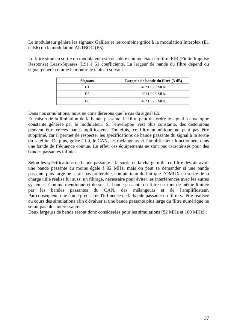
Le filtre situé en sortie du modulateur est considéré comme étant un filtre FIR (Finite Impulse Response) Least-Squares (LS) à 51 coefficients. La largeur de bande du filtre dépend du signal généré comme le montre le tableau suivant :

Signaux Largeur de bande du filtre (3 dB)

E1 40*1.023 MHz

E5 90*1.023 MHz

E6 40*1.023 MHz

Dans nos simulations, nous ne considèrerons que le cas du signal E5. En raison de la limitation de la bande passante, le filtre peut distordre le signal à enveloppe constante générée par le modulateur. Si l'enveloppe n'est plus constante, des distorsions peuvent être créées par l'amplificateur. Toutefois, ce filtre numérique ne peut pas être supprimé, car il permet de respecter les spécifications de bande passante du signal à la sortie du satellite. De plus, grâce à lui, le CAN, les mélangeurs et l'amplificateur fonctionnent dans une bande de fréquence connue. En effet, ces équipements ne sont pas caractérisés pour des bandes passantes infinies. Selon les spécifications de bande passante à la sortie de la charge utile, ce filtre devrait avoir une bande passante au moins égale à 92 MHz, mais on peut se demander si une bande passante plus large ne serait pas préférable, compte tenu du fait que l’OMUX en sortie de la charge utile réalise lui aussi un filtrage, nécessaire pour éviter les interférences avec les autres systèmes. Comme mentionné ci-dessus, la bande passante du filtre est tout de même limitée par les bandes passantes du CAN, des mélangeurs et de l'amplificateur. Par conséquent, une étude précise de l'influence de la bande passante du filtre va être réalisée au cours des simulations afin d'évaluer si une bande passante plus large du filtre numérique ne serait pas plus intéressante. Deux largeurs de bande seront donc considérées pour les simulations (92 MHz et 100 MHz) :

38

Figure 17 : Fonction de transfert du filtre numérique dans le cas du signal E5

5.1.3. Le FGMU

La conversion numérique-analogique et la montée en fréquence, réalisées dans le FGMU, introduisent un bruit de phase sur le signal, provenant du CMCU et modifié par les synthétiseurs de fréquence du FGMU. Le bruit de phase introduit pendant la conversion numérique-analogique est représenté temporellement sur la figure suivante:

0 0.001 0.002 0.003 0.004 0.005 0.006 0.007 0.008 0.009 0.01-3

-2

-1

0

1

2

3x 10

-12

time [s]

ampl

itude

D/A conversion time jitter

Figure 18 : Représentation temporelle du jitter du CAN La densité spectrale de puissance du bruit de phase introduit durant la montée en fréquence pour le signal E5 est caractérisée sur la figure 19 :

39

100

102

104

106

108

-160

-150

-140

-130

-120

-110

-100

-90

-80

frequency [Hz]

SS

B p

ower

spe

ctru

m d

ensi

ties

[dB

c/H

z]

E5 band up-conversion phase noise characterization

Simulated

theoritical

Figure 19 : Densité spectrale de puissance du bruit de phase du à la montée en fréquence

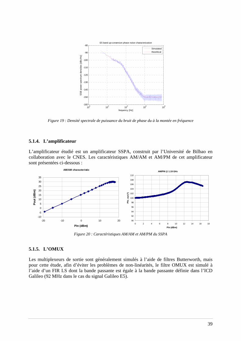
5.1.4. L’amplificateur

L’amplificateur étudié est un amplificateur SSPA, construit par l’Université de Bilbao en collaboration avec le CNES. Les caractéristiques AM/AM et AM/PM de cet amplificateur sont présentées ci-dessous :

AM/AM characteristic

-10

-5

0

5

10

15

20

25

30

35

-20 -10 0 10 20

Pin (dBm)

Pou

t (dB

m)

AM/PM @ 1.19 GHz

90

92

94

96

98

100

102

104

106

108

110

0 2 4 6 8 10 12 14 16 18

Pin (dBm)

Phi

_out

(º)

Figure 20 : Caractéristiques AM/AM et AM/PM du SSPA

5.1.5. L’OMUX

Les multiplexeurs de sortie sont généralement simulés à l’aide de filtres Butterworth, mais pour cette étude, afin d’éviter les problèmes de non-linéarités, le filtre OMUX est simulé à l’aide d’un FIR LS dont la bande passante est égale à la bande passante définie dans l’ICD Galileo (92 MHz dans le cas du signal Galileo E5).

40

-6 -4 -2 0 2 4 6

x 107

-100

-80

-60

-40

-20

0

OMUX filter transfer function

frequency [Hz]

ampl

itude

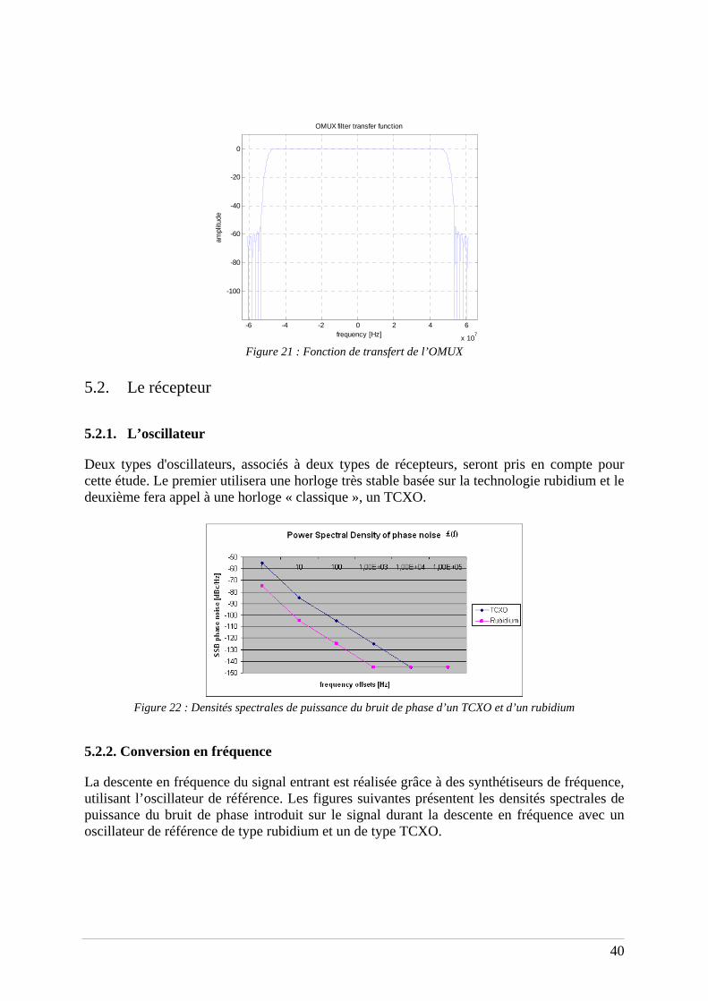
Figure 21 : Fonction de transfert de l’OMUX

5.2. Le récepteur

5.2.1. L’oscillateur

Deux types d'oscillateurs, associés à deux types de récepteurs, seront pris en compte pour cette étude. Le premier utilisera une horloge très stable basée sur la technologie rubidium et le deuxième fera appel à une horloge « classique », un TCXO.

Figure 22 : Densités spectrales de puissance du bruit de phase d’un TCXO et d’un rubidium

5.2.2. Conversion en fréquence

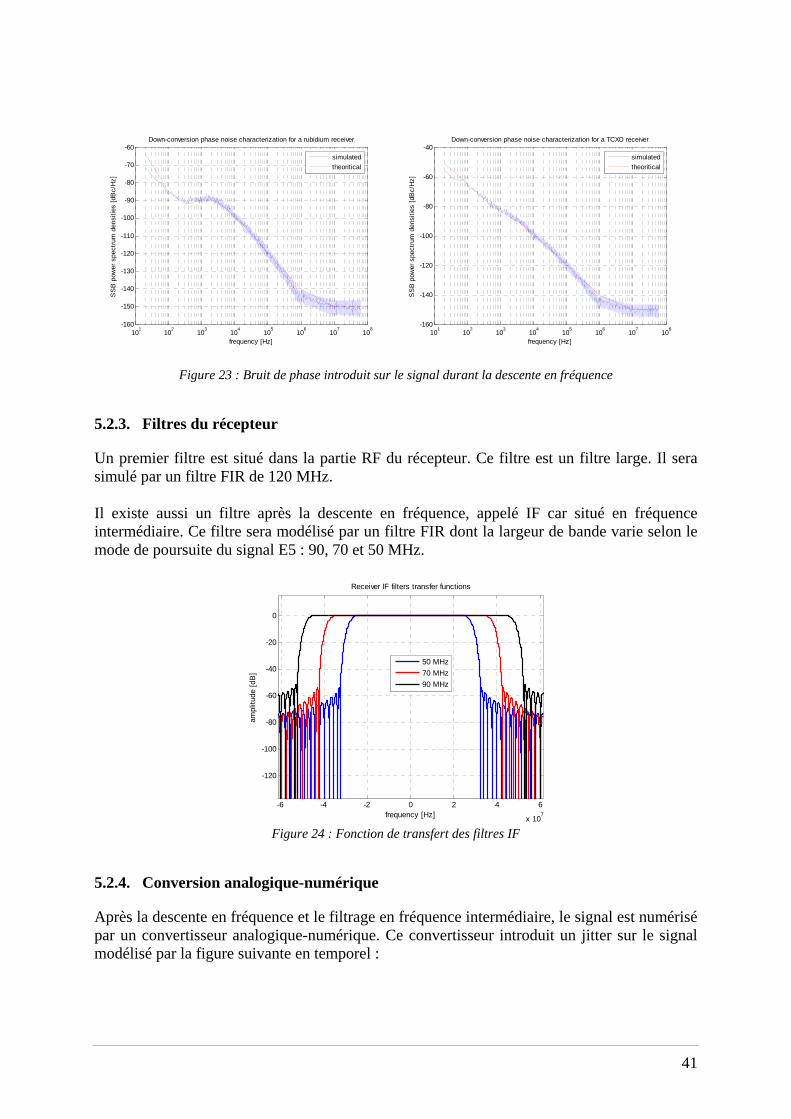
La descente en fréquence du signal entrant est réalisée grâce à des synthétiseurs de fréquence, utilisant l’oscillateur de référence. Les figures suivantes présentent les densités spectrales de puissance du bruit de phase introduit sur le signal durant la descente en fréquence avec un oscillateur de référence de type rubidium et un de type TCXO.

41

101

102

103

104

105

106

107

108

-160

-150

-140

-130

-120

-110

-100

-90

-80

-70

-60

frequency [Hz]

SS

B p

ower

spe

ctru

m d

ensi

ties

[dB

c/H

z]

Down-conversion phase noise characterization for a rubidium receiver

simulated

theoritical

101

102

103

104

105

106

107

108

-160

-140

-120

-100

-80

-60

-40Down-conversion phase noise characterization for a TCXO receiver

frequency [Hz]

SS

B p

ower

spe

ctru

m d

ensi

ties

[dB

c/H

z]

simulated

theoritical

Figure 23 : Bruit de phase introduit sur le signal durant la descente en fréquence

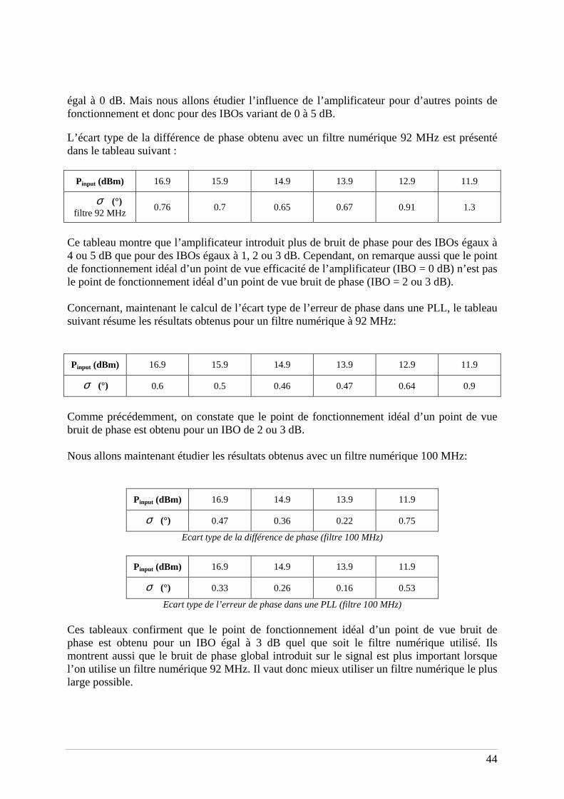
5.2.3. Filtres du récepteur

Un premier filtre est situé dans la partie RF du récepteur. Ce filtre est un filtre large. Il sera simulé par un filtre FIR de 120 MHz. Il existe aussi un filtre après la descente en fréquence, appelé IF car situé en fréquence intermédiaire. Ce filtre sera modélisé par un filtre FIR dont la largeur de bande varie selon le mode de poursuite du signal E5 : 90, 70 et 50 MHz.

-6 -4 -2 0 2 4 6

x 107

-120

-100

-80

-60

-40

-20

0

Receiver IF filters transfer functions

frequency [Hz]

ampl

itude

[dB

]

50 MHz

70 MHz

90 MHz

Figure 24 : Fonction de transfert des filtres IF

5.2.4. Conversion analogique-numérique

Après la descente en fréquence et le filtrage en fréquence intermédiaire, le signal est numérisé par un convertisseur analogique-numérique. Ce convertisseur introduit un jitter sur le signal modélisé par la figure suivante en temporel :

42

0 0.001 0.002 0.003 0.004 0.005 0.006 0.007 0.008 0.009 0.01-4

-3

-2

-1

0

1

2

3x 10

-12 A/D conversion time jitter

time [s]

ampl

itude

rubidium

TCXO

Figure 25 : Jitter temporel du à la conversion A/N

Dans les paragraphes précédents, la charge utile et les deux modèles de récepteurs considérés ont été décrits avec précision. Ces modèles vont être utilisés pour réaliser des simulations présentant l'impact des différents éléments de la charge utile et du récepteur sur le signal Galileo E5. 5.3. Résultats de simulations

5.3.1. Performance de la charge utile

Introduction

L’influence de la charge utile sur le signal va être étudier grâce aux différents facteurs de mérite présentés sur le schéma ci-dessous. Les densités spectrales de puissance, les fonctions de corrélation et les constellations ne seront pas présentées dans ce résumé mais elles sont détaillées dans le corps de la thèse.

Figure 26 : Schéma présentant l’étude de la charge utile

Génération en bande de base

Filtre numérique

N/A +

filtre large

SSPA

Montée en fréquence

+ filtre large

OMUX

- Densité spectrale de puissance, constellation, fonction de corrélation - Distorsions de phase évaluées grâce à l’écart type de l’erreur de phase dans une PLL et grâce à

l’écart type de la différence de phase entre deux éléments

43

Influence du filtre numérique

L’observation de la constellation du signal montre que l’enveloppe du signal est distordue par le filtre numérique 92 MHz, elle n’est plus constante. L’écart type de la différence entre la phase du signal sortant du filtre et la phase du signal entrant dans le filtre est égal à 5°, ce qui confirme que le filtre modifie la phase du signal. Si un filtre numérique 100 MHz est utilisé, la constellation est moins distordue et l’écart type de la différence de phase est seulement égal à 3°. Ce qui confirme qu’il est plus intéressant d’utiliser un filtre plus large si l’on ne veut pas trop impacter l’enveloppe constante du signal et ne pas voir apparaître de nouvelles distorsions lors du passage dans l’amplificateur.

Influence du convertisseur numérique-analogique

Que l’on utilise un filtre 92 MHz ou 100 MHz en amont du convertisseur, l’influence de celui-ci sur la constellation du signal est négligeable devant les distorsions introduites par le filtre numérique. L’écart type de la différence de phase est seulement de 0.003°.

La faible influence du convertisseur numérique-analogique sur le signal est confirmé par le calcul de l’erreur de phase dans une PLL, selon le schéma suivant:

Celle-ci n’est égale qu’à 8e-4° avec une bande de boucle de 10 Hz quelle que soit la largeur de bande du filtre numérique utilisé.

Influence de la montée en fréquence

La montée en fréquence a plus d’influence sur le signal que la conversion numérique-analogique mais cette influence ne s’observe pas clairement sur la constellation du signal. Elle s’observe par contre lors du calcul de l’écart type de la différence de phase car celui-ci est égal à 0.045°. L’écart type de l’erreur de phase dans une PLL est quant à lui égal à 0.045° quel que soit le filtre numérique considéré.

Influence de l’amplificateur

Après la montée en fréquence, le signal entre dans l’amplificateur. L’influence de l’amplification sur le signal dépend de son point de fonctionnement. Son point de fonctionnement initial est fixé à 2 dB de compression, dans ce cas le recul d’entrée (IBO) est

Phase error = phase(Useful signal)-

phase(Reference signal)

Mod. Num. filter

D/A conv.

Wide filter

44

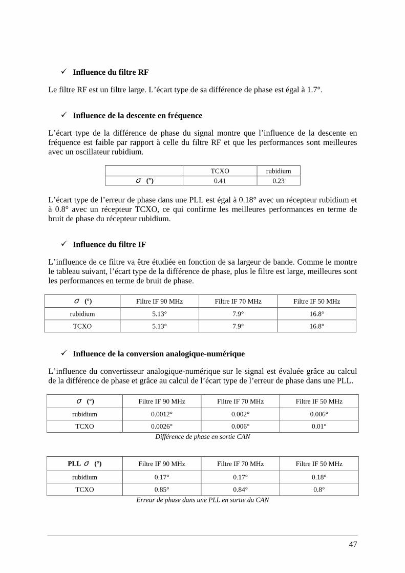
égal à 0 dB. Mais nous allons étudier l’influence de l’amplificateur pour d’autres points de fonctionnement et donc pour des IBOs variant de 0 à 5 dB. L’écart type de la différence de phase obtenu avec un filtre numérique 92 MHz est présenté dans le tableau suivant :

Pinput (dBm) 16.9 15.9 14.9 13.9 12.9 11.9

σ (°) filtre 92 MHz

0.76 0.7 0.65 0.67 0.91 1.3

Ce tableau montre que l’amplificateur introduit plus de bruit de phase pour des IBOs égaux à 4 ou 5 dB que pour des IBOs égaux à 1, 2 ou 3 dB. Cependant, on remarque aussi que le point de fonctionnement idéal d’un point de vue efficacité de l’amplificateur (IBO = 0 dB) n’est pas le point de fonctionnement idéal d’un point de vue bruit de phase (IBO = 2 ou 3 dB). Concernant, maintenant le calcul de l’écart type de l’erreur de phase dans une PLL, le tableau suivant résume les résultats obtenus pour un filtre numérique à 92 MHz:

Pinput (dBm) 16.9 15.9 14.9 13.9 12.9 11.9

σ (°) 0.6 0.5 0.46 0.47 0.64 0.9

Comme précédemment, on constate que le point de fonctionnement idéal d’un point de vue bruit de phase est obtenu pour un IBO de 2 ou 3 dB. Nous allons maintenant étudier les résultats obtenus avec un filtre numérique 100 MHz:

Pinput (dBm) 16.9 14.9 13.9 11.9

σ (°) 0.47 0.36 0.22 0.75

Ecart type de la différence de phase (filtre 100 MHz)

Pinput (dBm) 16.9 14.9 13.9 11.9

σ (°) 0.33 0.26 0.16 0.53

Ecart type de l’erreur de phase dans une PLL (filtre 100 MHz) Ces tableaux confirment que le point de fonctionnement idéal d’un point de vue bruit de phase est obtenu pour un IBO égal à 3 dB quel que soit le filtre numérique utilisé. Ils montrent aussi que le bruit de phase global introduit sur le signal est plus important lorsque l’on utilise un filtre numérique 92 MHz. Il vaut donc mieux utiliser un filtre numérique le plus large possible.

45

Influence de l’OMUX

A la sortie de l’amplificateur, le signal est multiplexé et filtre par un OMUX avant d’être transmis par l’antenne. L’OMUX considéré à une largeur de bande égale à 92 MHz, si le filtre numérique a lui aussi une largeur de bande de 92 MHz, alors les plots de la constellation sont étalés quel que soit le point de fonctionnement de l’amplificateur. La mesure de l’écart type de la différence de phase montre quant à elle, que la phase du signal est moins bruitée si l’IBO de l’amplificateur est élevé.

Pinput (dBm) 16.9 15.9 14.9 13.9 12.9 11.9

σ (°) 1.9 1.6 1.14 0.84 0.74 0.73

L’influence de l’OMUX dépend en fait de la caractéristique AM/AM de l’amplificateur et non de sa caractéristique AM/PM. L’écart type de l’erreur de phase dans une PLL confirme que plus l’IBO augmente, meilleures sont les performances en terme de bruit de phase.

Pinput (dBm) 16.9 15.9 14.9 13.9 12.9 11.9

σ (°) 1.37 1.12 0.8 0.58 0.53 0.55

Dans le cas où l’on utilise un filtre numérique 92 MHz, il y a donc un compromis à faire pour définir le point de fonctionnement idéal de l’amplificateur car celui-ci n’est pas le même que l’on se place d’un point de vue efficacité ou d’un point de vue bruit de phase. Un IBO égal à 3 dB semble être le bon compromis d’après tous les résultats précédents. Si l’on utilise maintenant un filtre numérique 100 MHz, les tableaux ci-dessous, représentant l’écart type de la différence de phase et l’écart type de l’erreur de phase dans une PLL, montrent que dans ce cas, il n’y a pas de compromis à faire, le point de fonctionnement idéal de l’amplificateur est clairement obtenu pour un IBO égal à 3 dB.

Pinput (dBm) 16.9 14.9 13.9 11.9

σ (°) 0.81 0.4 0.33 0.34

Ecart type de la différence de phase (filtre numérique 100 MHz)

Pinput (dBm) 16.9 14.9 13.9 11.9

σ (°) 0.6 0.25 0.19 0.22

Ecart type de l’erreur de phase dans une PLL (filtre numérique 100 MHz)

46

Conclusion

Pour conclure, l'évaluation de la contribution individuelle de chaque élément de la charge utile a montré que c’est le filtre numérique qui introduit le plus de distorsions sur la phase de porteuse. Toutefois, si le bruit de phase dû au filtre n'est pas considéré, le bruit de phase introduit par l’amplificateur prédomine. Il a également été démontré que, en fonction du point de fonctionnement de l'amplificateur, le bruit de phase est plus ou moins important. Le meilleur point de fonctionnement à la fois d’un point de vue efficacité et d’un point de vue bruit de phase est obtenu pour un IBO égal à 3 dB. Pour finir, il a été démontré que, si le filtre numérique a une bande passante de 100 MHz, le bruit de phase à la sortie de la charge utile est plus faible. Par conséquent, il serait peut-être plus intéressant d'utiliser un filtre à 100 MHz comme filtre numérique au lieu d’un filtre à 92 MHz, parce que l’OMUX filtre déjà le signal à la bande passante spécifiée à la sortie de la charge utile. Toutefois, le choix de la bande passante du filtre numérique dépendra aussi du bruit de phase introduit par le récepteur. En effet, si le bruit de phase du récepteur est plus élevé que le bruit de phase de la charge utile, il n'est pas intéressant d'avoir un filtre numérique plus large car aucune amélioration ne sera apportée lors du calcul de l’écart type de l’erreur de phase dans la PLL. C'est la raison pour laquelle le bruit de phase introduit par le récepteur est étudié dans la section suivante.

5.3.2. Performance du récepteur

Introduction

Nous allons maintenant étudier l’influence des différentes parties du récepteur selon le schéma suivant :

Figure 27 : Schéma du récepteur Les simulations seront réalisées en considérant les deux types d’oscillateurs du récepteur: rubidium et TCXO. Le signal entrant dans le récepteur est un signal « idéal » Galileo E5 de bande passante infinie.

Signal Filtre RF (120

MHz) Descente en fréquence

CAN

- Evaluation du bruit de phase grâce au calcul de l’erreur de phase dans une PLL - Différence de phase entre le signal entrant et le signal sortant

Filtre IF (90, 70, 50 MHz)

47

Influence du filtre RF

Le filtre RF est un filtre large. L’écart type de sa différence de phase est égal à 1.7°.

Influence de la descente en fréquence

L’écart type de la différence de phase du signal montre que l’influence de la descente en fréquence est faible par rapport à celle du filtre RF et que les performances sont meilleures avec un oscillateur rubidium.

TCXO rubidium

σ (°) 0.41 0.23

L’écart type de l’erreur de phase dans une PLL est égal à 0.18° avec un récepteur rubidium et à 0.8° avec un récepteur TCXO, ce qui confirme les meilleures performances en terme de bruit de phase du récepteur rubidium.

Influence du filtre IF

L’influence de ce filtre va être étudiée en fonction de sa largeur de bande. Comme le montre le tableau suivant, l’écart type de la différence de phase, plus le filtre est large, meilleures sont les performances en terme de bruit de phase.

σ (°) Filtre IF 90 MHz Filtre IF 70 MHz Filtre IF 50 MHz

rubidium 5.13° 7.9° 16.8°

TCXO 5.13° 7.9° 16.8°

Influence de la conversion analogique-numérique

L’influence du convertisseur analogique-numérique sur le signal est évaluée grâce au calcul de la différence de phase et grâce au calcul de l’écart type de l’erreur de phase dans une PLL.

σ (°) Filtre IF 90 MHz Filtre IF 70 MHz Filtre IF 50 MHz

rubidium 0.0012° 0.002° 0.006°

TCXO 0.0026° 0.006° 0.01°

Différence de phase en sortie CAN

PLL σ (°) Filtre IF 90 MHz Filtre IF 70 MHz Filtre IF 50 MHz

rubidium 0.17° 0.17° 0.18°

TCXO 0.85° 0.84° 0.8°

Erreur de phase dans une PLL en sortie du CAN

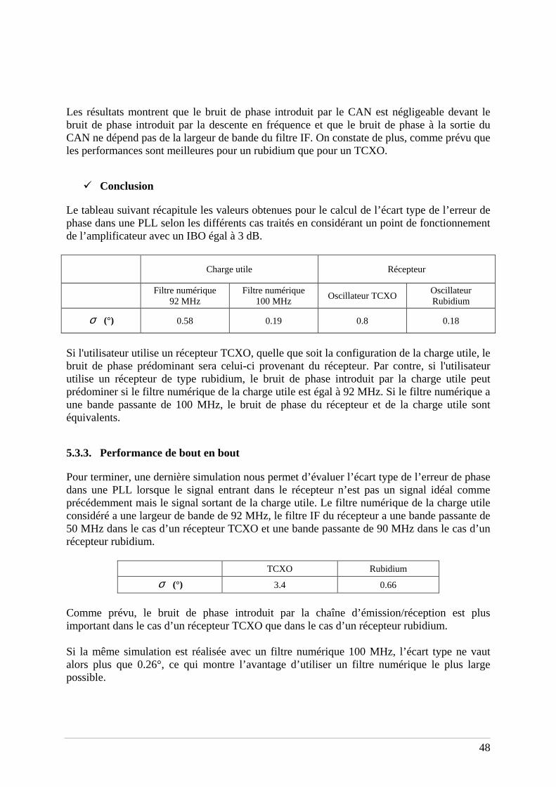
48

Les résultats montrent que le bruit de phase introduit par le CAN est négligeable devant le bruit de phase introduit par la descente en fréquence et que le bruit de phase à la sortie du CAN ne dépend pas de la largeur de bande du filtre IF. On constate de plus, comme prévu que les performances sont meilleures pour un rubidium que pour un TCXO.

Conclusion

Le tableau suivant récapitule les valeurs obtenues pour le calcul de l’écart type de l’erreur de phase dans une PLL selon les différents cas traités en considérant un point de fonctionnement de l’amplificateur avec un IBO égal à 3 dB.

Charge utile Récepteur

Filtre numérique 92 MHz

Filtre numérique 100 MHz

Oscillateur TCXO Oscillateur Rubidium

σ (°) 0.58 0.19 0.8 0.18

Si l'utilisateur utilise un récepteur TCXO, quelle que soit la configuration de la charge utile, le bruit de phase prédominant sera celui-ci provenant du récepteur. Par contre, si l'utilisateur utilise un récepteur de type rubidium, le bruit de phase introduit par la charge utile peut prédominer si le filtre numérique de la charge utile est égal à 92 MHz. Si le filtre numérique a une bande passante de 100 MHz, le bruit de phase du récepteur et de la charge utile sont équivalents.

5.3.3. Performance de bout en bout

Pour terminer, une dernière simulation nous permet d’évaluer l’écart type de l’erreur de phase dans une PLL lorsque le signal entrant dans le récepteur n’est pas un signal idéal comme précédemment mais le signal sortant de la charge utile. Le filtre numérique de la charge utile considéré a une largeur de bande de 92 MHz, le filtre IF du récepteur a une bande passante de 50 MHz dans le cas d’un récepteur TCXO et une bande passante de 90 MHz dans le cas d’un récepteur rubidium.

TCXO Rubidium

σ (°) 3.4 0.66

Comme prévu, le bruit de phase introduit par la chaîne d’émission/réception est plus important dans le cas d’un récepteur TCXO que dans le cas d’un récepteur rubidium. Si la même simulation est réalisée avec un filtre numérique 100 MHz, l’écart type ne vaut alors plus que 0.26°, ce qui montre l’avantage d’utiliser un filtre numérique le plus large possible.

49

5.3.4. Conclusion

Toutes les simulations présentées ont permis de déterminer une charge utile optimisée, composée d’un filtre numérique 100 MHz et d’un amplificateur SSPA travaillant à un IBO égal à 3 dB.

6. Conclusions Tout d’abord, une étude précise du système Galileo, de la charge utile au récepteur a été menée. Les différents éléments de la charge utile et du récepteur pouvant entraîner des distorsions sur les signaux Galileo ont été identifiés : les horloges, l’amplificateur de la charge utile mais aussi les trajets multiples. L’étude des distorsions introduites sur le signal par ces éléments a montré que les signaux Galileo devaient posséder une modulation à enveloppe constante et une bonne résistance aux multi-trajets. Les signaux Galileo E1 et E5 ont été présentés et étudiés afin de vérifier qu’ils présentaient les propriétés énoncées ci-dessus. Le signal E5 est un signal à enveloppe constante grâce à la modulation ALTBOC et des simulations ont montré qu’il présentait une bonne résistance aux multi-trajets. Le signal E1 quant à lui, possède aussi une enveloppe constante grâce à la modulation Interplex. Il a été récemment optimisé afin de présenter une meilleure résistance aux multi-trajets, ce n’est plus un BOC(1,1) classique mais un CBOC(6,1). De plus, l’influence des différents éléments de la charge utile et du récepteur a été étudiée grâce à des simulations Matlab. Cette étude a permis de déterminer une charge utile optimale pour générer le signal Galileo E5 : elle est composée d’un filtre numérique 100 MHz en sortant du NSGU et d’un amplificateur SSPA travaillant à un IBO de 3 dB.

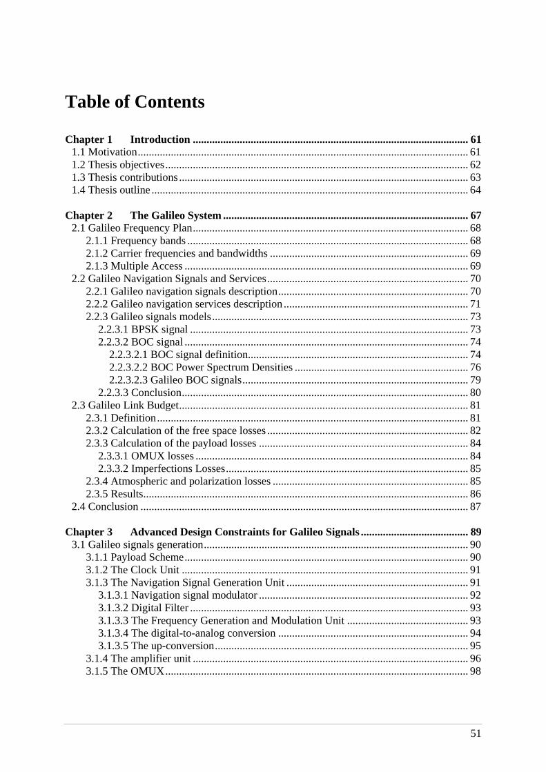
51

Table of Contents Chapter 1 Introduction .................................................................................................... 61

1.1 Motivation........................................................................................................................ 61 1.2 Thesis objectives.............................................................................................................. 62 1.3 Thesis contributions......................................................................................................... 63 1.4 Thesis outline................................................................................................................... 64

Chapter 2 The Galileo System ......................................................................................... 67

2.1 Galileo Frequency Plan.................................................................................................... 68 2.1.1 Frequency bands ...................................................................................................... 68 2.1.2 Carrier frequencies and bandwidths ........................................................................ 69 2.1.3 Multiple Access ....................................................................................................... 69

2.2 Galileo Navigation Signals and Services......................................................................... 70 2.2.1 Galileo navigation signals description..................................................................... 70 2.2.2 Galileo navigation services description................................................................... 71 2.2.3 Galileo signals models............................................................................................. 73

2.2.3.1 BPSK signal ..................................................................................................... 73 2.2.3.2 BOC signal ....................................................................................................... 74

2.2.3.2.1 BOC signal definition................................................................................ 74 2.2.3.2.2 BOC Power Spectrum Densities ............................................................... 76 2.2.3.2.3 Galileo BOC signals.................................................................................. 79

2.2.3.3 Conclusion........................................................................................................ 80 2.3 Galileo Link Budget......................................................................................................... 81

2.3.1 Definition................................................................................................................. 81 2.3.2 Calculation of the free space losses ......................................................................... 82 2.3.3 Calculation of the payload losses ............................................................................ 84

2.3.3.1 OMUX losses ................................................................................................... 84 2.3.3.2 Imperfections Losses........................................................................................ 85

2.3.4 Atmospheric and polarization losses ....................................................................... 85 2.3.5 Results...................................................................................................................... 86

2.4 Conclusion ....................................................................................................................... 87 Chapter 3 Advanced Design Constraints for Galileo Signals ....................................... 89

3.1 Galileo signals generation................................................................................................ 90 3.1.1 Payload Scheme....................................................................................................... 90 3.1.2 The Clock Unit ........................................................................................................ 91 3.1.3 The Navigation Signal Generation Unit .................................................................. 91

3.1.3.1 Navigation signal modulator ............................................................................ 92 3.1.3.2 Digital Filter ..................................................................................................... 93 3.1.3.3 The Frequency Generation and Modulation Unit ............................................ 93 3.1.3.4 The digital-to-analog conversion ..................................................................... 94 3.1.3.5 The up-conversion............................................................................................ 95

3.1.4 The amplifier unit .................................................................................................... 96 3.1.5 The OMUX.............................................................................................................. 98

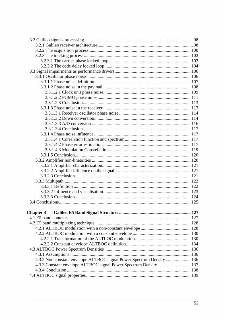
52

3.2 Galileo signals processing................................................................................................ 98 3.2.1 Galileo receiver architecture.................................................................................... 98 3.2.2 The acquisition process.......................................................................................... 100 3.2.3 The tracking process .............................................................................................. 102

3.2.3.1 The carrier-phase locked loop ........................................................................ 102 3.2.3.2 The code delay locked loop............................................................................ 104

3.3 Signal impairments as performance drivers................................................................... 106 3.3.1 Oscillator phase noise............................................................................................ 106

3.3.1.1 Phase noise definition..................................................................................... 107 3.3.1.2 Phase noise in the payload ............................................................................. 108

3.3.1.2.1 Clock unit phase noise............................................................................. 109 3.3.1.2.2 FGMU phase noise.................................................................................. 111 3.3.1.2.3 Conclusion............................................................................................... 113

3.3.1.3 Phase noise in the receiver ............................................................................. 113 3.3.1.3.1 Receiver oscillator phase noise ............................................................... 114 3.3.1.3.2 Down conversion..................................................................................... 114 3.3.1.3.3 A/D conversion ....................................................................................... 116 3.3.1.3.4 Conclusion............................................................................................... 117

3.3.1.4 Phase noise influence ..................................................................................... 117 3.3.1.4.1 Correlation function and spectrum.......................................................... 117 3.3.1.4.2 Phase error estimation ............................................................................. 117 3.3.1.4.3 Modulation Constellation........................................................................ 119

3.3.1.5 Conclusion...................................................................................................... 120 3.3.2 Amplifier non-linearities ....................................................................................... 120

3.3.2.1 Amplifier characterization.............................................................................. 121 3.3.2.2 Amplifier influence on the signal................................................................... 121 3.3.2.3 Conclusion...................................................................................................... 121

3.3.3 Multipath................................................................................................................ 122 3.3.3.1 Definition ....................................................................................................... 122 3.3.3.2 Influence and visualisation............................................................................. 123 3.3.3.3 Conclusion...................................................................................................... 124

3.4 Conclusions.................................................................................................................... 125 Chapter 4 Galileo E5 Band Signal Structure ............................................................... 127

4.1 E5 band contents ............................................................................................................ 127 4.2 E5 band multiplexing technique .................................................................................... 128

4.2.1 ALTBOC modulation with a non-constant envelope ............................................ 128 4.2.2 ALTBOC modulation with a constant envelope ................................................... 130

4.2.2.1 Transformation of the ALTLOC modulation................................................. 130 4.2.2.2 Constant envelope ALTBOC definition......................................................... 134

4.3 ALTBOC Power Spectrum Densities ............................................................................ 136 4.3.1 Assumptions .......................................................................................................... 136 4.3.2 Non constant envelope ALTBOC signal Power Spectrum Density ...................... 136 4.3.3 Constant envelope ALTBOC signal Power Spectrum Density ............................. 137 4.3.4 Conclusion ............................................................................................................. 138

4.4 ALTBOC signal properties............................................................................................ 139

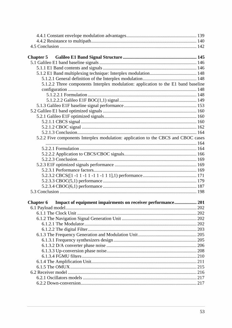
53

4.4.1 Constant envelope modulation advantages............................................................ 139 4.4.2 Resistance to multipath.......................................................................................... 140

4.5 Conclusion ..................................................................................................................... 142 Chapter 5 Galileo E1 Band Signal Structure ............................................................... 145

5.1 Galileo E1 band baseline signals ................................................................................... 146 5.1.1 E1 Band contents and signals ................................................................................ 146 5.1.2 E1 Band multiplexing technique: Interplex modulation........................................ 148

5.1.2.1 General definition of the Interplex modulation.............................................. 148 5.1.2.2 Three components Interplex modulation: application to the E1 band baseline configuration .............................................................................................................. 148

5.1.2.2.1 Formulation ............................................................................................. 148 5.1.2.2.2 Galileo E1F BOC(1,1) signal .................................................................. 149

5.1.3 Galileo E1F baseline signal performance.............................................................. 153 5.2 Galileo E1 band optimized signals ................................................................................ 160

5.2.1 Galileo E1F optimized signals............................................................................... 160 5.2.1.1 CBCS signal ................................................................................................... 160 5.2.1.2 CBOC signal .................................................................................................. 162 5.2.1.3 Conclusion...................................................................................................... 164

5.2.2 Five components Interplex modulation: application to the CBCS and CBOC cases................................................................................................................................. 164

5.2.2.1 Formulation .................................................................................................... 164 5.2.2.2 Application to CBCS/CBOC signals..............................................................166 5.2.2.3 Conclusion...................................................................................................... 169

5.2.3 E1F optimized signals performance ...................................................................... 169 5.2.3.1 Performance factors........................................................................................ 169 5.2.3.2 CBCS([1 -1 1 -1 1 -1 1 -1 1 1],1) performance.............................................. 171 5.2.3.3 CBOC(5,1) performance ................................................................................ 179 5.2.3.4 CBOC(6,1) performance ................................................................................ 187

5.3 Conclusion ..................................................................................................................... 198 Chapter 6 Impact of equipment impairments on receiver performance................... 201

6.1 Payload model................................................................................................................ 202 6.1.1 The Clock Unit ...................................................................................................... 202 6.1.2 The Navigation Signal Generation Unit ................................................................ 202

6.1.2.1 The Modulator................................................................................................ 202 6.1.2.2 The digital Filter............................................................................................. 203

6.1.3 The Frequency Generation and Modulation Unit .................................................. 205 6.1.3.1 Frequency synthesizers design ....................................................................... 205 6.1.3.2 D/A converter phase noise ............................................................................. 206 6.1.3.3 Up-conversion phase noise............................................................................. 208 6.1.3.4 FGMU filters .................................................................................................. 210

6.1.4 The Amplification Unit.......................................................................................... 211 6.1.5 The OMUX............................................................................................................ 215

6.2 Receiver model .............................................................................................................. 216 6.2.1 Oscillators models ................................................................................................. 217 6.2.2 Down-conversion................................................................................................... 217

54

6.2.2.1 Frequency synthesizers’ characteristics ......................................................... 218 6.2.2.2 Down-conversion phase noise........................................................................ 218

6.2.3 Receiver Filters...................................................................................................... 220 6.2.4 A/D conversion...................................................................................................... 221

6.3 Simulations results ......................................................................................................... 223 6.3.1 Payload performance ............................................................................................. 223

6.3.1.1 Introduction .................................................................................................... 223 6.3.1.2 Baseband Galileo E5 band signal................................................................... 225 6.3.1.3 Digital filter influence .................................................................................... 227 6.3.1.4 DAC influence................................................................................................ 231 6.3.1.5 Up-conversion influence ................................................................................ 233 6.3.1.6 Amplifier influence ........................................................................................ 236 6.3.1.7 OMUX influence............................................................................................ 245 6.3.1.8 Conclusion...................................................................................................... 254

6.3.2 Receiver performance............................................................................................ 254 6.3.2.1 Introduction .................................................................................................... 254 6.3.2.2 RF front-end filter influence .......................................................................... 255 6.3.2.3 Down-conversion influence ........................................................................... 257 6.3.2.4 IF filter influence............................................................................................ 259

6.3.2.4.1 A/D conversion influence........................................................................ 260 6.3.2.5 Conclusion...................................................................................................... 263

6.3.3 End-to-end performance ........................................................................................ 264 6.3.4 Conclusion ............................................................................................................. 265

Chapter 7 Conclusions and Recommendations for Future Work.............................. 267

7.1 Conclusions.................................................................................................................... 267 7.2 Recommendations for Future Work............................................................................... 269

Appendix A Power Spectrum Densities ........................................................................... 271

A.1 BOC Power Spectrum Densities................................................................................... 271 A.2 ALTBOC Power Spectrum Densities ........................................................................... 278 A.3 Interplex signal Power Spectrum Densities .................................................................. 282

Appendix B Phase Noise Definition and Characterisation ............................................ 289

B.1 Phase noise definition.................................................................................................... 289 B.2 Phase noise characterization in the frequency domain.................................................. 290 B.3 Phase noise characterization in the time domain.......................................................... 291 B.4 Conversion between frequency and time domain ......................................................... 292

Appendix C Phase Locked Loop....................................................................................... 295

C.1 PLL basics..................................................................................................................... 295 C.2 PLL Frequency synthesizers ......................................................................................... 296 C.3 PLL frequency synthesizer phase noise ........................................................................ 297

Bibliography ........................................................................................................................ 299

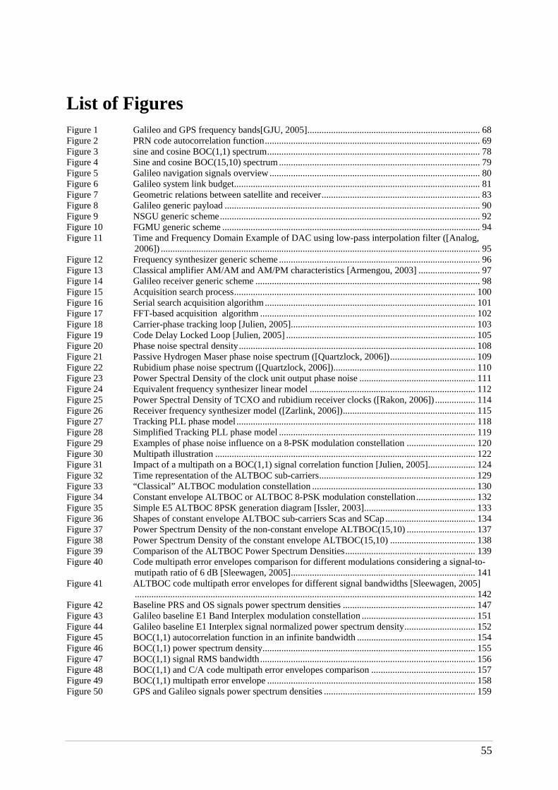
55

List of Figures Figure 1 Galileo and GPS frequency bands[GJU, 2005]......................................................................... 68 Figure 2 PRN code autocorrelation function........................................................................................... 69 Figure 3 sine and cosine BOC(1,1) spectrum.......................................................................................... 78 Figure 4 Sine and cosine BOC(15,10) spectrum..................................................................................... 79 Figure 5 Galileo navigation signals overview......................................................................................... 80 Figure 6 Galileo system link budget........................................................................................................ 81 Figure 7 Geometric relations between satellite and receiver................................................................... 83 Figure 8 Galileo generic payload ............................................................................................................ 90 Figure 9 NSGU generic scheme.............................................................................................................. 92 Figure 10 FGMU generic scheme ............................................................................................................. 94 Figure 11 Time and Frequency Domain Example of DAC using low-pass interpolation filter ([Analog,

2006]) ....................................................................................................................................... 95 Figure 12 Frequency synthesizer generic scheme ..................................................................................... 96 Figure 13 Classical amplifier AM/AM and AM/PM characteristics [Armengou, 2003] .......................... 97 Figure 14 Galileo receiver generic scheme ............................................................................................... 98 Figure 15 Acquisition search process...................................................................................................... 100 Figure 16 Serial search acquisition algorithm......................................................................................... 101 Figure 17 FFT-based acquisition algorithm ........................................................................................... 102 Figure 18 Carrier-phase tracking loop [Julien, 2005].............................................................................. 103 Figure 19 Code Delay Locked Loop [Julien, 2005] ................................................................................ 105 Figure 20 Phase noise spectral density.................................................................................................... 108 Figure 21 Passive Hydrogen Maser phase noise spectrum ([Quartzlock, 2006]).................................... 109 Figure 22 Rubidium phase noise spectrum ([Quartzlock, 2006])............................................................ 110 Figure 23 Power Spectral Density of the clock unit output phase noise ................................................. 111 Figure 24 Equivalent frequency synthesizer linear model ...................................................................... 112 Figure 25 Power Spectral Density of TCXO and rubidium receiver clocks ([Rakon, 2006]) ................. 114 Figure 26 Receiver frequency synthesizer model ([Zarlink, 2006])........................................................ 115 Figure 27 Tracking PLL phase model..................................................................................................... 118 Figure 28 Simplified Tracking PLL phase model ................................................................................... 119 Figure 29 Examples of phase noise influence on a 8-PSK modulation constellation ............................. 120 Figure 30 Multipath illustration .............................................................................................................. 122 Figure 31 Impact of a multipath on a BOC(1,1) signal correlation function [Julien, 2005].................... 124 Figure 32 Time representation of the ALTBOC sub-carriers.................................................................. 129 Figure 33 “Classical” ALTBOC modulation constellation ..................................................................... 130 Figure 34 Constant envelope ALTBOC or ALTBOC 8-PSK modulation constellation......................... 132 Figure 35 Simple E5 ALTBOC 8PSK generation diagram [Issler, 2003]...............................................133 Figure 36 Shapes of constant envelope ALTBOC sub-carriers Scas and SCap...................................... 134 Figure 37 Power Spectrum Density of the non-constant envelope ALTBOC(15,10) ............................. 137 Figure 38 Power Spectrum Density of the constant envelope ALTBOC(15,10) .................................... 138 Figure 39 Comparison of the ALTBOC Power Spectrum Densities....................................................... 139 Figure 40 Code multipath error envelopes comparison for different modulations considering a signal-to-

mutipath ratio of 6 dB [Sleewagen, 2005].............................................................................. 141 Figure 41 ALTBOC code multipath error envelopes for different signal bandwidths [Sleewagen, 2005]

................................................................................................................................................ 142 Figure 42 Baseline PRS and OS signals power spectrum densities ........................................................ 147 Figure 43 Galileo baseline E1 Band Interplex modulation constellation ................................................ 151 Figure 44 Galileo baseline E1 Interplex signal normalized power spectrum density.............................. 152 Figure 45 BOC(1,1) autocorrelation function in an infinite bandwidth .................................................. 154 Figure 46 BOC(1,1) power spectrum density.......................................................................................... 155 Figure 47 BOC(1,1) signal RMS bandwidth........................................................................................... 156 Figure 48 BOC(1,1) and C/A code multipath error envelopes comparison ............................................157 Figure 49 BOC(1,1) multipath error envelope ........................................................................................ 158 Figure 50 GPS and Galileo signals power spectrum densities ................................................................ 159

56

Figure 51 CBCS signal time sequence .................................................................................................... 161 Figure 52 CBOC signal time sequence ................................................................................................... 163 Figure 53 CBCS/CBOC on data and pilot OS components modulation constellation ............................ 168 Figure 54 Autocorrelation function of the CBCS OSA signal ................................................................ 172 Figure 55 Autocorrelation function of the CBCS OSB signal ................................................................ 173 Figure 56 CBCS([1 -1 1 -1 1 -1 1 -1 1 1],1) OSA signal RMS bandwidth ............................................. 174 Figure 57 CBCS([1 -1 1 -1 1 -1 1 -1 1 1],1) OSB signal RMS bandwidth ............................................. 175 Figure 58 CBCS([1 -1 1 -1 1 -1 1 -1 1 1],1) OSA signal multipath error envelope ................................ 176 Figure 59 CBCS([1 -1 1 -1 1 -1 1 -1 1 1],1) OSB signal multipath error envelope ................................ 176 Figure 60 CBCS waveform with a zero mismatch correlation losses .................................................... 178 Figure 61 OSA CBCS([1 -1 1 -1 1 -1 1 -1 1 1],1) correlation with a BOC(1,1) replica ......................... 178 Figure 62 OSB CBCS([1 -1 1 -1 1 -1 1 -1 1 1],1) correlation with a BOC(1,1) replica.......................... 179 Figure 63 Autocorrelation function of the CBOC(5,1) OSA signal ........................................................ 180 Figure 64 Autocorrelation function of the CBOC(5,1) OSB signal ........................................................ 181 Figure 65 CBOC(5,1) OSA signal multipath error envelope .................................................................. 182 Figure 66 CBOC(5,1) OSB signal multipath error envelope .................................................................. 182 Figure 67 CBOC(5,1) OSA signal RMS bandwidth ............................................................................... 183 Figure 68 CBOC(5,1) OSB signal RMS bandwidth................................................................................ 184 Figure 69 OSA CBOC(5,1) correlation with a BOC(1,1) replica ........................................................... 185 Figure 70 OSB CBOC(5,1) correlation with a BOC(1,1) replica............................................................ 186 Figure 71 CBOC(5,1) waveform with non zero mismatch correlation losses........................................ 187 Figure 72 Open Service signal power spectral densities considering the different optimized signals .... 189 Figure 73 CBOC and CBCS OSA autocorrelation functions.................................................................. 190 Figure 74 CBOC and CBCS OSB autocorrelation functions .................................................................. 190 Figure 75 Correlation function between CBOC(6,1) and BOC(1,1)....................................................... 191 Figure 76 Comparison of CBOC(5,1), CBCS([1 -1 1 -1 1 -1 1 -1 1 1],1) and CBOC(6,1) multipath error

envelopes................................................................................................................................ 192 Figure 77 Comparison of CBOC(5,1), CBCS([1 -1 1 -1 1 -1 1 -1 1 1],1) and CBOC(6,1) cumulative

error envelopes ....................................................................................................................... 192 Figure 78 CBOC(6,1) waveforms RMS bandwidths............................................................................... 193 Figure 79 CBOC(6,1,2/11,”+/-“) tracking performance.......................................................................... 195 Figure 80 CBOC(6,1) on pilot OS component and BOC(1,1) on data OS component modulation

constellation ........................................................................................................................... 197 Figure 81 Galileo E1 signal generation scheme [Hein,2002].................................................................. 203 Figure 82 E5 signal digital filter transfer functions................................................................................. 204 Figure 83 VCO phase noise characteristic ([Rakon, 2006]).................................................................... 206 Figure 84 Sampling frequency phase noise SSB power spectral densities.............................................. 207 Figure 85 Time representation of DAC jitter ......................................................................................... 208 Figure 86 Up-conversion phase noise SSB power spectral densities ...................................................... 209 Figure 87 E5 band up-conversion phase noise SSB power spectral densities......................................... 210 Figure 88 Transfer function of the FGMU filters after the D/A conversion and the up-conversion ....... 211 Figure 89 Studied amplifier picture......................................................................................................... 212 Figure 90 SSPA AM/AM characteristic.................................................................................................. 213 Figure 91 SSPA AM/PM characteristic .................................................................................................. 213 Figure 92 SSPA power added efficiency................................................................................................. 214 Figure 93 SSPA gain in function of the carrier frequency ...................................................................... 215 Figure 94 OMUX filter transfer function ................................................................................................ 216 Figure 95 Simulated receiver architecture............................................................................................... 216 Figure 96 Receiver VCO phase noise characteristic ([Rakon, 2006])..................................................... 218 Figure 97 Down-conversion phase noise SSB power spectral densities for a rubidium receiver............ 219 Figure 98 Down-conversion phase noise SSB power spectral densities for a TCXO receiver ............... 220 Figure 99 Transfer functions of the receiver IF filter.............................................................................. 221 Figure 100 Receiver sampling frequency phase noise SSB power spectral densities ............................... 222 Figure 101 Time jitter introduced during the A/D conversion.................................................................. 222 Figure 102 Payload simulations scheme ................................................................................................... 223 Figure 103 PLL phase error variance calculation in the payload.............................................................. 225

57

Figure 104 Infinite bandwidth Galileo E5 band signal modulation constellation ..................................... 225 Figure 105 Galileo E5 band signal autocorrelation function..................................................................... 226 Figure 106 Galileo E5 band signal estimated spectrum ............................................................................ 226 Figure 107 Galileo E5 band signal modulation constellation after a 92 MHz filtering............................. 227 Figure 108 Phase comparison between 92 MHz filter output and input ................................................... 228 Figure 109 Galileo E5 band signal modulation constellation after a 100 MHz filtering........................... 229 Figure 110 Phase comparison between 100 MHz filter output and input ................................................. 229 Figure 111 Galileo E5 band signal correlation function modulus after different filtering ........................ 230 Figure 112 Galileo E5 band signal power spectrum density after different filtering ................................ 230 Figure 113 DAC influence on Galileo E5 band signal modulation constellation (92 and 100 MHz filters)

................................................................................................................................................ 231 Figure 114 Phase study at DAC output (92 MHz digital filter) ................................................................ 232 Figure 115 DAC influence on Galileo E5 band signal correlation function with a 92 MHz filter............ 233 Figure 116 DAC influence on Galileo E5 band signal power spectrum density (92 and 110 MHz filters)

................................................................................................................................................ 233 Figure 117 Up-conversion influence on Galileo E5 band signal modulation constellation (92 and 100

MHz filters)............................................................................................................................ 234 Figure 118 Phase study after the up-conversion (92 MHz filter).............................................................. 235 Figure 119 Up-conversion influence on Galileo E5 band signal correlation function with a 92 MHz filter

................................................................................................................................................ 235 Figure 120 Up-conversion influence on Galileo E5 band signal power spectrum density (92 and 110 MHz

filters) ..................................................................................................................................... 236 Figure 121 92 MHz filtered signal modulation constellation at the amplifier output ...............................238 Figure 122 Signal points repartition on the AM/AM characteristic (IBO = 0 dB)....................................239 Figure 123 Signal points repartition on the AM/AM characteristic (IBO = 3 dB)....................................240 Figure 124 Phase difference study at the amplifier output (92 MHz filtered signal) ................................ 241 Figure 125 100 MHz filtered signal modulation constellation at the amplifier output..............................243 Figure 126 Signal points repartition on the AM/AM characteristic (IBO = 3 dB and 100 MHz filter

bandwidth).............................................................................................................................. 243 Figure 127 Phase difference study at the amplifier output (100 MHz filtered signal) ..............................244 Figure 128 92 MHz filtered signal modulation constellation at the OMUX output.................................. 246 Figure 129 Phase difference study at the OMUX output in function of IBOs for a 92 MHZ filtered signal

................................................................................................................................................ 246 Figure 130 Study of OMUX contribution for an IBO equal to 5 dB......................................................... 249 Figure 131 Study of OMUX contribution for an IBO equal to 1 dB......................................................... 250 Figure 132 100 MHz filtered signal modulation constellation at the OMUX output................................ 251 Figure 133 Phase difference study at the OMUX output in function of IBOs for a 100 MHZ filtered signal

................................................................................................................................................ 252 Figure 134 Correlation function at amplifier and OMUX outputs ............................................................ 253 Figure 135 Receiver simulations scheme.................................................................................................. 255 Figure 136 PLL phase error variance calculation in the receiver.............................................................. 255 Figure 137 RF front-end filter influence on modulation constellation...................................................... 256 Figure 138 Phase difference at the RF front-end filter output................................................................... 256 Figure 139 Down-conversion influence on Galileo E5 band signal modulation constellation.................. 257 Figure 140 Phase difference study at down-conversion output................................................................. 258 Figure 141 PLL phase error standard deviation calculation scheme at the down-conversion output........ 258 Figure 142 Modulation constellation at IF filter output ............................................................................ 259 Figure 143 Modulation constellation at ADC output for a 90 MHz IF filter ............................................ 260 Figure 144 Modulation constellation at ADC output for a 70 MHz IF filter ............................................ 261 Figure 145 Modulation constellation at ADC output for a 50 MHz IF filter ............................................ 261 Figure 146 Phase difference study at ADC output for a 90 MHz IF filter ................................................ 262 Figure 147 End-to-end performance simulation scheme........................................................................... 264 Figure 148 Time response of the sub-carrier waveform with sine and cosine phasing............................. 272 Figure 149 Power law model figure.......................................................................................................... 291 Figure 150 Allan Variance Model............................................................................................................. 292 Figure 151 Phase Lock Loop generic model............................................................................................. 295 Figure 152 Frequency divider scheme ...................................................................................................... 296

58

Figure 153 Frequency synthesizer linear model........................................................................................ 297

59

List of Tables Table 1 Galileo frequencies and associated bandwidths........................................................................ 69 Table 2 Galileo signals characteristics [GJU, 2005] .............................................................................. 71 Table 3 Galileo services and signals mapping ....................................................................................... 72 Table 4 Galileo BPSK signals................................................................................................................ 73 Table 5 Galileo BOC signals ................................................................................................................. 80 Table 6 Receiver antenna gain and input power .................................................................................... 82 Table 7 Free space losses....................................................................................................................... 83 Table 8 E1 OMUX induced losses......................................................................................................... 84 Table 9 E6 OMUX induced losses........................................................................................................ 85 Table 10 Other payload losses ................................................................................................................. 85 Table 11 Atmospheric and polarization losses........................................................................................ 85 Table 12 Galileo power link budget......................................................................................................... 87 Table 13 Galileo signals generation types ............................................................................................... 92 Table 14 Most common DLL discriminators [Kaplan, 1996]................................................................ 106 Table 15 Relationship between expression types, k1 and k2 for any combination of cu, cu’, cL, cL’ ....... 131 Table 16 Example of ALTBOC Look-up table...................................................................................... 133 Table 17 Constant envelope ALTBOC look-up tables .......................................................................... 135 Table 18 Spectral Separation Coefficient considering the Galileo baseline signal ................................ 159 Table 19 Self SSC of the CBCS([1 -1 1 -1 1 -1 1 -1 1 1],1) Open Service signal .................................177 Table 20 SSC of the CBCS([1 -1 1 -1 1 -1 1 -1 1 1],1) Open Service signal with GPS signals ........... 177 Table 21 Self SSC of the CBOC(5,1) Open Service signal ................................................................... 184 Table 22 SSC of the CBOC(5,1) Open Service signal with GPS signals ............................................. 185 Table 23 Comparison of BOC(1,1), CBOC(5,1), CBCS([1 -1 1 -1 1 -1 1 -1 1 1],1) and CBOC(6,1) SSCs

................................................................................................................................................ 193 Table 24 Digital filters bandwidths........................................................................................................ 203 Table 25 Frequency synthesizers’ ratios for the up-conversion in the different frequency bands ......... 208 Table 26 Working points’ IBOs............................................................................................................. 237 Table 27 Phase difference standard deviation at amplifier output (92 MHz filtered signal) ................. 241 Table 28 PLL phase error standard deviation at amplifier output (92 MHz filtered signal) .................. 242 Table 29 Phase difference standard deviation at amplifier output (100 MHz filtered signal)................ 244 Table 30 PLL phase error standard deviation at amplifier output (100 MHz filtered signal) ................ 244 Table 31 Phase difference standard deviation at OMUX output (92 MHz filtered signal) .................... 247 Table 32 Phase difference at OMUX output considering a linear AM/AM characteristic .................... 247 Table 33 Phase difference at OMUX output considering a linear AM/PM characteristic ..................... 247 Table 34 PLL phase error standard deviation at OMUX output (92 MHz filtered signal) .................... 248 Table 35 Phase difference standard deviation at OMUX output (100 MHz filtered signal) .................. 252 Table 36 PLL phase error standard deviation at OMUX output (100 MHz filtered signal)................... 252 Table 37 Phase difference standard deviations at down-conversion output.......................................... 258 Table 38 Phase difference standard deviation at the IF filters output .................................................... 260 Table 39 Phase difference standard deviations at ADC output.............................................................. 261 Table 40 PLL phase error standard deviations at A/D conversion output.............................................. 262 Table 41 Summary of PLL phase error standard deviations at receiver and payload output................. 263 Table 42 End-to-end PLL phase error standard deviation (92 MHz digital filter).................................264 Table 43 Frequency and phase noises.................................................................................................... 291 Table 44 Time-Frequency conversion of the phase noise...................................................................... 293

61

Chapter 1 Introduction

Contents

1.1 Motivation......................................................................................................................... 61 1.2 Thesis objectives ............................................................................................................... 62 1.3 Thesis contribution........................................................................................................... 63 1.4 Thesis outline .................................................................................................................... 64

1.1 Motivation

On May 26, 2003, the Galileo program was agreed upon officially by the European Union (EU) and the European Space Agency (ESA) with the launch of the legal entity which will have the task of coordinating ESA and EU involvement in Galileo: the Galileo Joint Undertaking (GJU). Galileo is a proposed satellite navigation system, to be built by the EU and ESA, autonomous but also complementary to the American Global Positioning System (GPS). The system is expected to be completely operational by 2013. Galileo is intended to provide to all users a greater precision than what is currently available and a positioning system upon which European nations can rely even in times of crisis. It will also provide an improvement in the coverage of satellite signals at higher latitudes, which northern regions such as Scandinavia will benefit from.

The Galileo program was divided into three main phases: the development and validation phase (until end 2010), the deployment phase with the manufacturing and the launch of the satellites of the complete constellation (2011-2012) and the commercial operating phase (at the beginning of 2013). Started a few years ago, the first phase, led by the Galileo Joint Undertaking and now by the GNSS Supervisory Authority (GSA), is a research and validation phase dedicated to the development of the Galileo architecture and design required to provide high precision navigation, position, timing and integrity information to meet both user needs and public obligations, such as safety for all transport modes.

1. Introduction

62

The development phase concerns all the elements of the Galileo system: the satellites, the receivers, the ground stations, the networks but also the Galileo signals design.

This last point is an important topic because the Galileo signals should allow the share of the frequency bands, always occupied by other system such as GPS for instance, while offering a good spectral isolation when needed, a better robustness against interference and good tracking performance. The signal choice goes also through a study of the signals generation in the satellite payload in order to identify possible factors of distortions whose effect can be reduced by choosing signals with particular properties. Moreover, payload consideration is one of the important factors involved in a GNSS signal design.

It is within the framework of the Galileo signals choice that the CNES (Centre National

d’Etudes Spatiales), member of the Galileo Signal Task Force (STF), an European committee in charge of the Galileo signals design, has sponsored this Ph.D., dedicated to contribute to the optimisation of the Galileo signals and the related payload.

1.2 Thesis objectives

The aim of this thesis is to optimize the Galileo transmission chain from a signal point of view. This optimisation focuses on the Galileo signals and their generation in the satellite payload. The tasks identified to reach this objective have been divided into the following research goals: To study and analyze the Galileo transmission chain in order to identify equipment

being able to induce impairments on the signals. This objective can be divided in more precise stages:

o To analyze the payload architecture to identify emission equipment being able

to induce impairments during the signal generation. The payload is composed of different units, that have to be carefully characterized, in particular the amplifier and the atomic clocks.

o To analyze the receiver architecture to identify, this time, equipment being

able to induce impairments during the signal reception.

o To study the signal propagation and analyze the effect of the multipath on the signal performance.

To study the tracking modules of the receiver in particular the code Delay Lock Loop

(DLL) and the carrier Phase Lock Loop (PLL) since these elements provide the observables, directly used for positioning, timing and the study of the performance from a receiver point of view.

To identify signal properties allowing to reduce the impact of the identified

impairments factors and to establish if the Galileo signals, proposed by the GJU and

1. Introduction

63

GSA, verify these properties. These properties can be linked to both the signals waveforms and the signals multiplexing modulations.

To estimate the performance of the Galileo baseline E1 signals and analyze if the new

waveforms (Composite Binary Coded Symbols (CBCS) and Composite Binary Offset Carrier (CBOC)), proposed and chosen to optimize this signal, permit both to improve the performance from a receiver point of view and to verify the signal properties reducing the influence of the transmission chain impairments.

To evaluate through simulations the impact of signals impairments due to Galileo

system equipment on receiver performance using some specific figures of merit. This evaluation will allow to deduce optimal operating point of the payload amplifier and find optimal payload architecture.

The organisation of the thesis is determined by the inter-relationship between these seven objectives, as it will be outlined in section 1.4.

1.3 Thesis contributions

The main contributions of this thesis are enumerated below and are detailed all along this dissertation: Evaluation of the Galileo power link budget

Detailed analysis of the Galileo payload and receiver in order to assess the

impairments introduced on the Galileo signals during their generation and their receiver processing, in particular:

o Elaboration of a detailed payload scheme for the Galileo system o Theoretical analysis of payload and receiver clocks phase noise and payload

amplifier distortions Analysis of the civil Galileo signals at the E1 and E5 bands, based on a new

modulation called Binary Offset Carrier (BOC), more precisely:

o Study of new waveforms: CBOC and CBCS o Performance evaluation thanks to multipath error envelope and RMS

bandwidth Analysis of the multiplexing techniques used to transmit the Galileo signals:

o Adaptation of the general definition equations of the Interplex modulation to

the navigation signals and more particularly to the E1 band signals o Study of the Alternate BOC (ALTBOC) modulation equation and generation to

multiplex the E5 band signal

1. Introduction

64

Theoretical expressions of the power spectrum densities of the global E5 and E1

signals Matlab simulations of payload and receiver equipment influence on receiver

performance:

o Computation of the error introduced by the identified impairments on a receiver Phase Lock Loop (PLL), correlation functions, spectra and modulation constellation.

o Choice of an optimal payload architecture

1.4 Thesis outline

As already mentioned, the study of the Galileo signals and payload constitutes the heart of this Ph.D. This dissertation is structured as follows.

First of all, chapter 2 gives an overview of the Galileo system. The Galileo frequency bands, the Galileo signals and the services associated are described. The waveforms proposed to transmit them, classical BPSK and innovative BOC, are also presented and the advantage of the BOC signal is underlined. Moreover the power link budget of the Galileo system is computed to evaluate the necessary power at the payload output.

Chapter 3 describes the Galileo payload and receiver by presenting their equipment and

their processing. The study of these architectures permits to identify payload and receiver elements which could induce signals impairments. Some design constraints on the Galileo signals are investigated to reduce the signals impairments.

Then, chapter 4 presents the Galileo E5 band signals, designed by the STF, and the

modulation proposed to transmit it: the Alternate BOC. It is shown that the ALTBOC signal complies with the design constraints identified in chapter 3.

The next chapter deals with the design of the Galileo E1 signals. First, the baseline

signals, decided in a 2004 EU/US agreement, are presented with the modulation associated, the Interplex. It is shown that it verifies signal design constraints exposed in chapter 3. The receiver performance of the baseline Open service signals is also exposed.

As the 2004 EU/US agreement left the door open for a possible optimization of the baseline, recently, new Galileo E1F signals have been proposed. The performances of these new signals are studied to identify the improvement, compared to the baseline performance, and if these new waveforms present properties permitting to reduce the distortions due to transmission chain impairments.

In chapter 6, the impact of the generation and processing impairments on the Galileo E5

ALTBOC is evaluated thanks to figures of merit representing receiver performance such as

1. Introduction

65

the error in the PLL or the correlation function. This evaluation is realized thanks to Matlab simulations.

Finally, chapter 7 summarizes the main results of this Ph.D. work and concludes on the

obtained results. Some outstanding issues are introduced as openings and propositions for future works.

67

Chapter 2 The Galileo System

Contents 2.1 Galileo Frequency Plan.................................................................................................... 68

2.1.1 Frequency bands ........................................................................................................... 68 2.1.2 Carrier frequencies and bandwidths.............................................................................. 69 2.1.3 Multiple Access ............................................................................................................ 69

2.2 Galileo Navigation Signals and Services ........................................................................ 70 2.2.1 Galileo navigation signals description.......................................................................... 70 2.2.2 Galileo navigation services description ........................................................................ 71 2.2.3 Galileo signals models .................................................................................................. 73

2.3 Galileo Link Budget ......................................................................................................... 81 2.3.1 Definition ...................................................................................................................... 81 2.3.2 Calculation of the free space losses .............................................................................. 82 2.3.3 Calculation of the payload losses.................................................................................. 84 2.3.4 Atmospheric and polarization losses ............................................................................ 85 2.3.5 Results........................................................................................................................... 86

Galileo will be the Europe’s own global navigation satellite system, providing global positioning service under civilian control. It will be inter-operable with GPS (Global Positioning System) and GLONASS, the American and Russian global satellite navigation systems.

Galileo is based on a constellation of 27 satellites (plus 3 in reserve) and ground stations

providing information concerning the positioning of users in many sectors such as transport (vehicle location, route searching, speed control, guidance systems, etc.), social services (e.g. aid for the disabled or elderly), the justice system and customs services (location of suspects, border controls), public works (geographical information systems), search and rescue systems, or leisure (direction-finding at sea or in the mountains, etc.).

The 27 satellites, constituting Galileo constellation, will be on a medium earth orbit (MEO) and distributed in 3 circular orbits planes at an altitude of 23222 km. Each orbit plane will have an inclination of 56° and will contain 9 operational satellites plus one operational

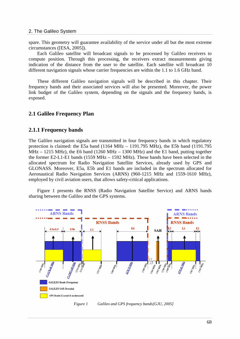
2. The Galileo System

68

spare. This geometry will guarantee availability of the service under all but the most extreme circumstances ([ESA, 2005]).

Each Galileo satellite will broadcast signals to be processed by Galileo receivers to compute position. Through this processing, the receivers extract measurements giving indication of the distance from the user to the satellite. Each satellite will broadcast 10 different navigation signals whose carrier frequencies are within the 1.1 to 1.6 GHz band.

These different Galileo navigation signals will be described in this chapter. Their

frequency bands and their associated services will also be presented. Moreover, the power link budget of the Galileo system, depending on the signals and the frequency bands, is exposed.

2.1 Galileo Frequency Plan

2.1.1 Frequency bands

The Galileo navigation signals are transmitted in four frequency bands in which regulatory protection is claimed: the E5a band (1164 MHz – 1191.795 MHz), the E5b band (1191.795 MHz – 1215 MHz), the E6 band (1260 MHz – 1300 MHz) and the E1 band, putting together the former E2-L1-E1 bands (1559 MHz – 1592 MHz). These bands have been selected in the allocated spectrum for Radio Navigation Satellite Services, already used by GPS and GLONASS. Moreover, E5a, E5b and E1 bands are included in the spectrum allocated for Aeronautical Radio Navigation Services (ARNS) (960-1215 MHz and 1559-1610 MHz), employed by civil aviation users, that allows safety-critical applications.

Figure 1 presents the RNSS (Radio Navigation Satellite Service) and ARNS bands

sharing between the Galileo and the GPS systems.

Figure 1 Galileo and GPS frequency bands[GJU, 2005]

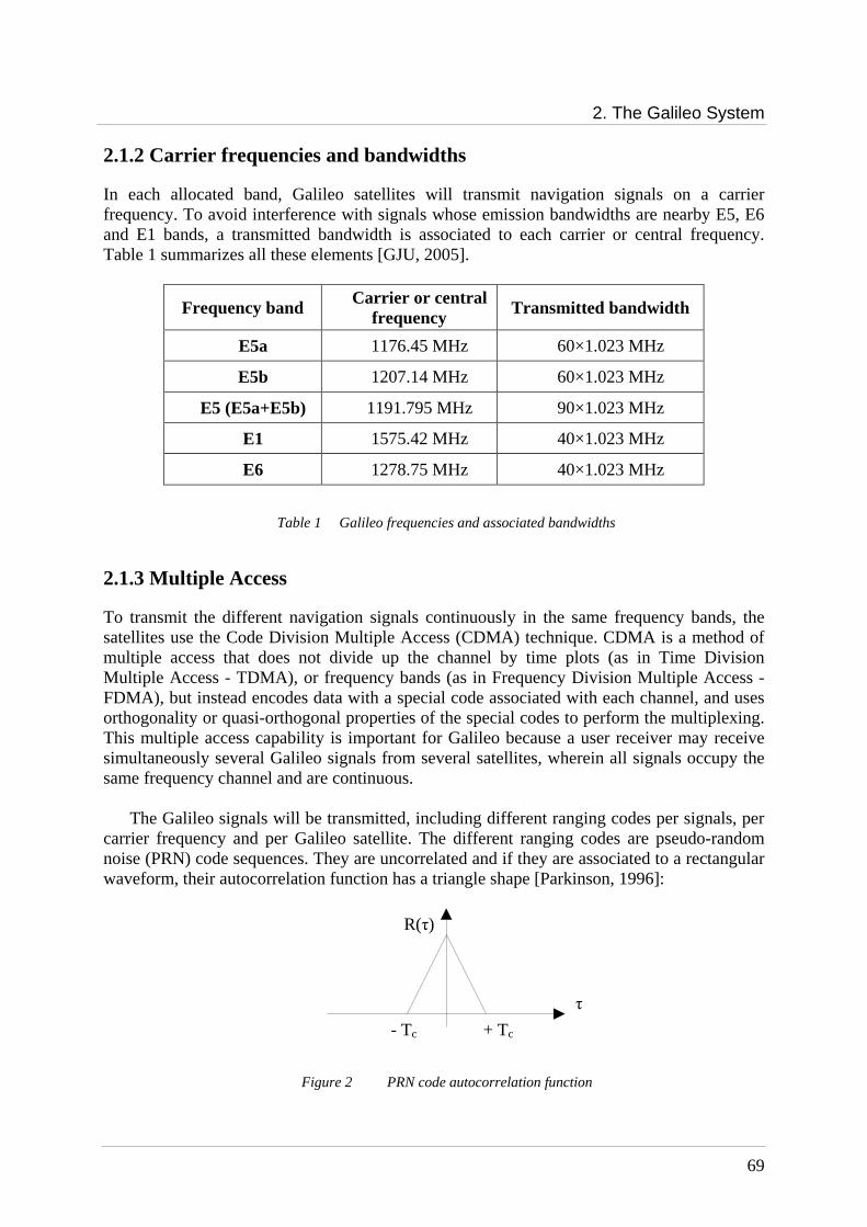
2. The Galileo System

69

2.1.2 Carrier frequencies and bandwidths

In each allocated band, Galileo satellites will transmit navigation signals on a carrier frequency. To avoid interference with signals whose emission bandwidths are nearby E5, E6 and E1 bands, a transmitted bandwidth is associated to each carrier or central frequency. Table 1 summarizes all these elements [GJU, 2005].

Frequency band Carrier or central frequency Transmitted bandwidth

E5a 1176.45 MHz 60×1.023 MHz

E5b 1207.14 MHz 60×1.023 MHz

E5 (E5a+E5b) 1191.795 MHz 90×1.023 MHz

E1 1575.42 MHz 40×1.023 MHz

E6 1278.75 MHz 40×1.023 MHz

Table 1 Galileo frequencies and associated bandwidths

2.1.3 Multiple Access

To transmit the different navigation signals continuously in the same frequency bands, the satellites use the Code Division Multiple Access (CDMA) technique. CDMA is a method of multiple access that does not divide up the channel by time plots (as in Time Division Multiple Access - TDMA), or frequency bands (as in Frequency Division Multiple Access - FDMA), but instead encodes data with a special code associated with each channel, and uses orthogonality or quasi-orthogonal properties of the special codes to perform the multiplexing. This multiple access capability is important for Galileo because a user receiver may receive simultaneously several Galileo signals from several satellites, wherein all signals occupy the same frequency channel and are continuous.

The Galileo signals will be transmitted, including different ranging codes per signals, per

carrier frequency and per Galileo satellite. The different ranging codes are pseudo-random noise (PRN) code sequences. They are uncorrelated and if they are associated to a rectangular waveform, their autocorrelation function has a triangle shape [Parkinson, 1996]:

Figure 2 PRN code autocorrelation function

+ Tc - Tc

τ

R(τ)

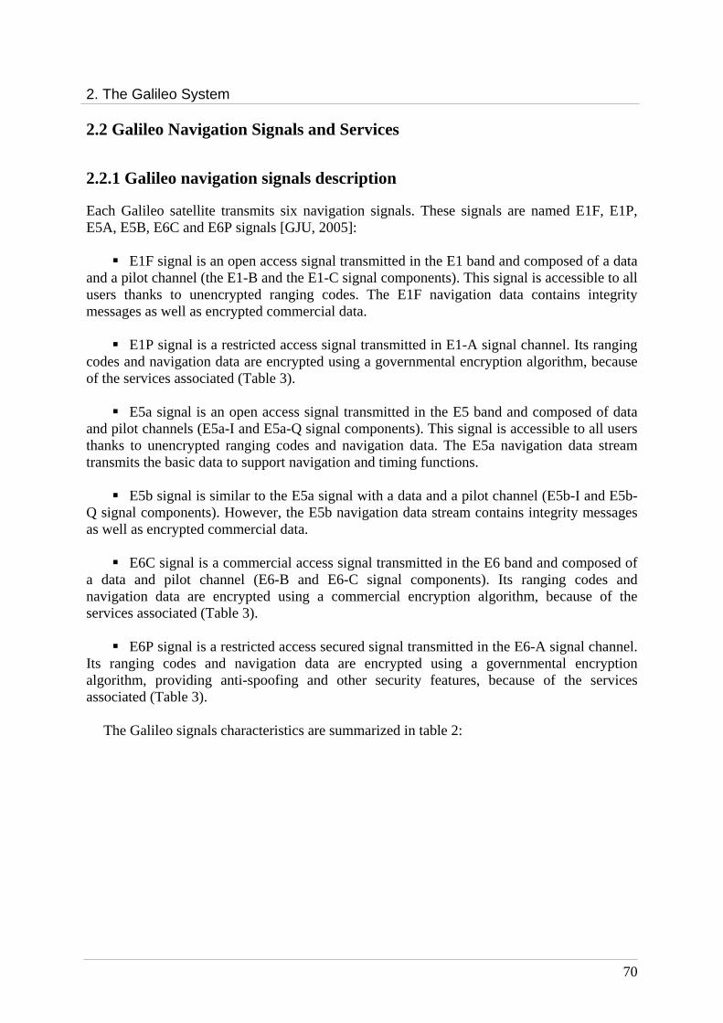
2. The Galileo System

70

2.2 Galileo Navigation Signals and Services

2.2.1 Galileo navigation signals description

Each Galileo satellite transmits six navigation signals. These signals are named E1F, E1P, E5A, E5B, E6C and E6P signals [GJU, 2005]:

E1F signal is an open access signal transmitted in the E1 band and composed of a data

and a pilot channel (the E1-B and the E1-C signal components). This signal is accessible to all users thanks to unencrypted ranging codes. The E1F navigation data contains integrity messages as well as encrypted commercial data. E1P signal is a restricted access signal transmitted in E1-A signal channel. Its ranging

codes and navigation data are encrypted using a governmental encryption algorithm, because of the services associated (Table 3). E5a signal is an open access signal transmitted in the E5 band and composed of data

and pilot channels (E5a-I and E5a-Q signal components). This signal is accessible to all users thanks to unencrypted ranging codes and navigation data. The E5a navigation data stream transmits the basic data to support navigation and timing functions. E5b signal is similar to the E5a signal with a data and a pilot channel (E5b-I and E5b-

Q signal components). However, the E5b navigation data stream contains integrity messages as well as encrypted commercial data. E6C signal is a commercial access signal transmitted in the E6 band and composed of

a data and pilot channel (E6-B and E6-C signal components). Its ranging codes and navigation data are encrypted using a commercial encryption algorithm, because of the services associated (Table 3). E6P signal is a restricted access secured signal transmitted in the E6-A signal channel.

Its ranging codes and navigation data are encrypted using a governmental encryption algorithm, providing anti-spoofing and other security features, because of the services associated (Table 3).

The Galileo signals characteristics are summarized in table 2:

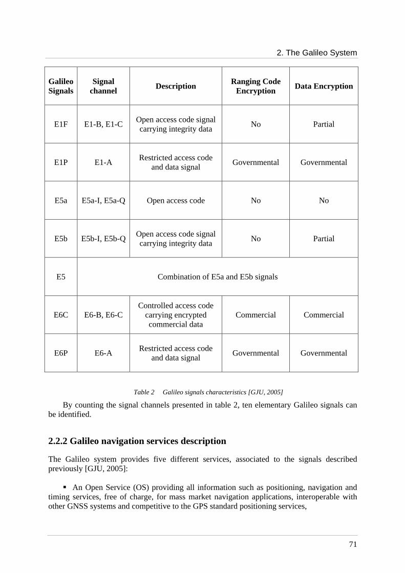
2. The Galileo System

71

Galileo Signals

Signal channel Description Ranging Code

Encryption Data Encryption

E1F E1-B, E1-C Open access code signal carrying integrity data

No Partial

E1P E1-A Restricted access code

and data signal Governmental Governmental

E5a E5a-I, E5a-Q Open access code No No

E5b E5b-I, E5b-Q Open access code signal carrying integrity data

No Partial

E5 Combination of E5a and E5b signals

E6C E6-B, E6-C Controlled access code

carrying encrypted commercial data

Commercial Commercial

E6P E6-A Restricted access code

and data signal Governmental Governmental

Table 2 Galileo signals characteristics [GJU, 2005]

By counting the signal channels presented in table 2, ten elementary Galileo signals can be identified.

2.2.2 Galileo navigation services description

The Galileo system provides five different services, associated to the signals described previously [GJU, 2005]: An Open Service (OS) providing all information such as positioning, navigation and

timing services, free of charge, for mass market navigation applications, interoperable with other GNSS systems and competitive to the GPS standard positioning services,

2. The Galileo System

72

A Safety-Of-Life service (SOL), compliant to the needs of safety critical users such as

civil aviation, maritime and rail domain. The SOL includes high integrity and authentication capability, although the activation of these possibilities will depend on the user communities. The SOL service includes service guarantees, A Commercial Service (CS) generates commercial revenue by providing added value

over the Open Service, such as by dissemination of encrypted navigation related data, ranging and timing for professional use, with service guarantees, high integrity level, precise timing services, high data rate broadcasting, provision of ionospheric delay modes, local differential correction signals and controlled access, A Public Regulated Service (PRS), for application devoted to European and member

states, for critical applications and activities of strategic importance. It makes use of a robust signal and is controlled by member states. This service provides services guarantees, high integrity, full range of value added features and an access controlled by encryption, A Search And Rescue support service (SAR) provides assistance to the COSPAS-

SARSAT system by detecting emergency beacons and forwarding return link messages to the emergency beacons. It is a service for search and rescue applications by providing near real time reception of distress message and precise location of alert.

The next table provides the mapping of the Galileo services into the Galileo navigation signals:

Signals OS users SOL users CS users PRS users

E1F X* X* X

E1P X

E5a X X

E5b X* X* X

E6C X

E6P X

* with no access to encrypted commercial data

Table 3 Galileo services and signals mapping

2. The Galileo System

73

2.2.3 Galileo signals models

The Galileo navigation signals, exposed in section 2.2.1, are designed on the basis of two waveforms: the first one is the Binary Phase Shift Keying (BPSK) modulation, already used to transmit the signals of GPS block II and the second one is the Binary Offset Carrier (BOC) modulation defined in [Aparacio, 1994] and [Betz, 2002].

2.2.3.1 BPSK signal

A Binary Phase Shift Keying (BPSK) signal with rectangular spreading symbols is proposed to transmit some of the Galileo signals. This modulation is well-known because it is used in the GPS system to transmit the C/A and the P(Y) signals.

In navigation system a base band BPSK signal could be defined as: the product between a PRN code sequence and a data sequence if it is used for a data

channel, or by only a code sequence if it is used for a pilot (data less) channel

The characteristics of the Galileo signals, transmitted thanks to BPSK modulation, are summarized in table 4:

Signal Code Length

Chip Rate

(Mcps)

Modulation before

Multiplexing

Navigation Data (sps)

Secondary code

E5a-I 10230 10.23 BPSK(10) Yes (50) Yes

E5a-Q 10230 10.23 BPSK(10) Pilot Yes

E5b-I 10230 10.23 BPSK(10) Yes (250) Yes

E5b-Q 10230 10.23 BPSK(10) Pilot Yes

E6-B N/A 5.115 BPSK(5) Yes (1000) N/A

E6-C N/A 5.115 BPSK(5) Pilot N/A

Table 4 Galileo BPSK signals

However this BPSK modulation can not be used to transmit all the Galileo signals. Indeed

the BPSK signal can not provide a good sharing of the current band spectrum by multiple signals, what is an essential element of Galileo and GPS systems, particularly at the E1/L1 band. That is the reason why new modulations were studied. These new modulations have to provide a better share of existing frequency allocation but also they must supply binary phase values, maintaining ease of signal generation and receiver processing.

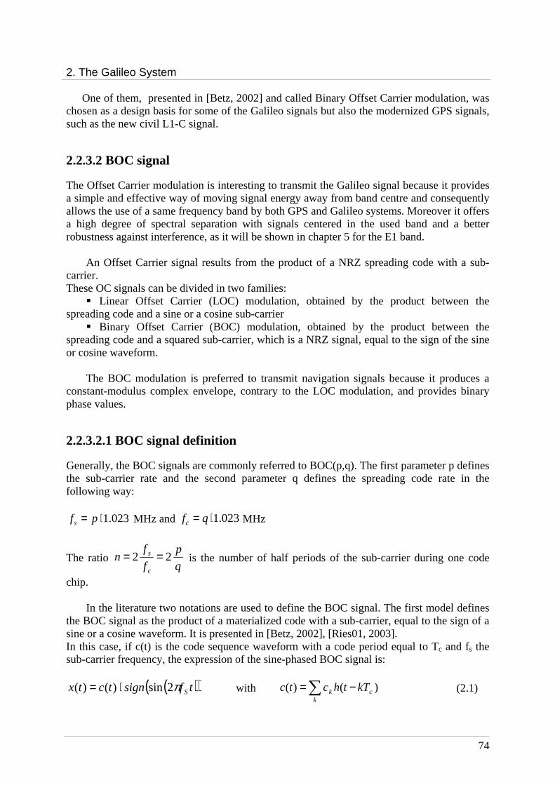
2. The Galileo System

74

One of them, presented in [Betz, 2002] and called Binary Offset Carrier modulation, was chosen as a design basis for some of the Galileo signals but also the modernized GPS signals, such as the new civil L1-C signal.

2.2.3.2 BOC signal

The Offset Carrier modulation is interesting to transmit the Galileo signal because it provides a simple and effective way of moving signal energy away from band centre and consequently allows the use of a same frequency band by both GPS and Galileo systems. Moreover it offers a high degree of spectral separation with signals centered in the used band and a better robustness against interference, as it will be shown in chapter 5 for the E1 band.

An Offset Carrier signal results from the product of a NRZ spreading code with a sub-carrier. These OC signals can be divided in two families: Linear Offset Carrier (LOC) modulation, obtained by the product between the

spreading code and a sine or a cosine sub-carrier Binary Offset Carrier (BOC) modulation, obtained by the product between the

spreading code and a squared sub-carrier, which is a NRZ signal, equal to the sign of the sine or cosine waveform.

The BOC modulation is preferred to transmit navigation signals because it produces a constant-modulus complex envelope, contrary to the LOC modulation, and provides binary phase values.

2.2.3.2.1 BOC signal definition

Generally, the BOC signals are commonly referred to BOC(p,q). The first parameter p defines the sub-carrier rate and the second parameter q defines the spreading code rate in the following way:

023.1⋅= pfs MHz and 023.1⋅= qfc MHz

The ratio q

p

f

fn

c

s 22 == is the number of half periods of the sub-carrier during one code

chip.

In the literature two notations are used to define the BOC signal. The first model defines the BOC signal as the product of a materialized code with a sub-carrier, equal to the sign of a sine or a cosine waveform. It is presented in [Betz, 2002], [Ries01, 2003]. In this case, if c(t) is the code sequence waveform with a code period equal to Tc and fs the sub-carrier frequency, the expression of the sine-phased BOC signal is:

( )( )tfsigntctx Sπ2sin)()( ⋅= with )()( ck

k kTthctc −=∑ (2.1)

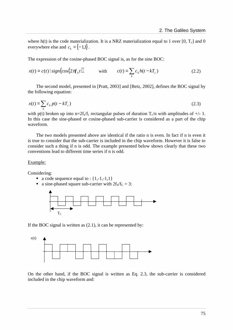
2. The Galileo System

75

where h(t) is the code materialization. It is a NRZ materialization equal to 1 over [0, Tc] and 0 everywhere else and 1,1−=kc .

The expression of the cosine-phased BOC signal is, as for the sine BOC:

( )( )tfsigntctx Sπ2cos)()( ⋅= with )()( ck

k kTthctc −=∑ (2.2)

The second model, presented in [Pratt, 2003] and [Betz, 2002], defines the BOC signal by

the following equation:

)()( ck

k kTtpctx −=∑ (2.3)

with p(t) broken up into n=2fs/fc rectangular pulses of duration Tc/n with amplitudes of +/- 1. In this case the sine-phased or cosine-phased sub-carrier is considered as a part of the chip waveform.

The two models presented above are identical if the ratio n is even. In fact if n is even it is true to consider that the sub-carrier is included in the chip waveform. However it is false to consider such a thing if n is odd. The example presented below shows clearly that these two conventions lead to different time series if n is odd. Example: Considering: a code sequence equal to : 1,-1,-1,1 a sine-phased square sub-carrier with 2fS/fC = 3:

If the BOC signal is written as (2.1), it can be represented by:

On the other hand, if the BOC signal is written as Eq. 2.3, the sub-carrier is considered included in the chip waveform and:

x(t)

TC

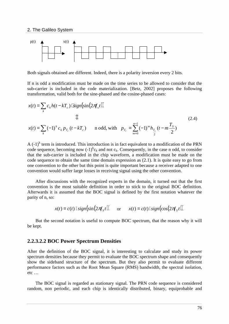
2. The Galileo System

76

Both signals obtained are different. Indeed, there is a polarity inversion every 2 bits. If n is odd a modification must be made on the time series to be allowed to consider that the sub-carrier is included in the code materialization. [Betz, 2002] proposes the following transformation, valid both for the sine-phased and the cosine-phased cases:

( )( )

)2

()1( with odd,n )()1()(

2sin)()(

2

1

0

ST

n

m

mT

kcTk

k

sk

ck

TmthpkTtpctx

tfsignkTthctx

scc−−=−−=

⋅−=

∑∑

∑

−

=

c

π

(2.4)

A (-1)k term is introduced. This introduction is in fact equivalent to a modification of the PRN code sequence, becoming now (-1)kck and not ck. Consequently, in the case n odd, to consider that the sub-carrier is included in the chip waveform, a modification must be made on the code sequence to obtain the same time domain expression as (2.1). It is quite easy to go from one convention to the other but this point is quite important because a receiver adapted to one convention would suffer large losses in receiving signal using the other convention.

After discussions with the recognized experts in the domain, it turned out that the first convention is the most suitable definition in order to stick to the original BOC definition. Afterwards it is assumed that the BOC signal is defined by the first notation whatever the parity of n, so:

( )( )tfsigntctx Sπ2sin)()( ⋅= or ( )( )tfsigntctx Sπ2cos)()( ⋅=

But the second notation is useful to compute BOC spectrum, that the reason why it will

be kept.

2.2.3.2.2 BOC Power Spectrum Densities

After the definition of the BOC signal, it is interesting to calculate and study its power spectrum densities because they permit to evaluate the BOC spectrum shape and consequently show the sideband structure of the spectrum. But they also permit to evaluate different performance factors such as the Root Mean Square (RMS) bandwidth, the spectral isolation, etc …

The BOC signal is regarded as stationary signal. The PRN code sequence is considered random, non periodic, and each chip is identically distributed, binary, equiprobable and

x(t) p(t)

2. The Galileo System

77

independent. The next formula can be used to calculate the power spectrum density of the BOC signal:

c

s T

fPfG

2)(

)( = (2.5)

with P(f) the Fourier Transform of the signal materialization and Tc the code period.

This formula assumes that the sub-carrier is included in the chip waveform or that the PRN code sequence is changed as presented above. The same formula can be used for the both cases because most of the PRN sequences used in GNSS up to now are approximated as long codes, which can be assumed as independent sequences over time.

Consequently, considering the previously hypothesis and the calculations presented in Appendix A, if the BOC signal is sine-phased, its normalized power spectrum densities are equal to:

oddn for

)cos(

)cos()sin(1

)(

evenn for

)cos(

)sin()sin(1

)(

2

2

=

=

n

fTf

fTn

fT

TfG

n

fTf

fTn

fT

TfG

c

cc

cBOC

c

cc

cBOC

ππ

ππ

ππ

ππ

(2.6)

And if the BOC signal is cosine-phased, the expressions are:

( )

( )oddn for 1cos

cos

cos1)(

evenn for 1coscos

sin1)(

2

2

−

=

−

⋅=

n

Tf

n

Tff

fT

TfG

n

Tf

n

Tff

fT

TfG

c

c

c

cBOC

c

c

c

cBOC

πππ

π

πππ

π

(2.7)

It has to be pointed out that these expressions don’t take into account the periodic

features of the PN codes used for open GPS and Galileo signals. These periodic features

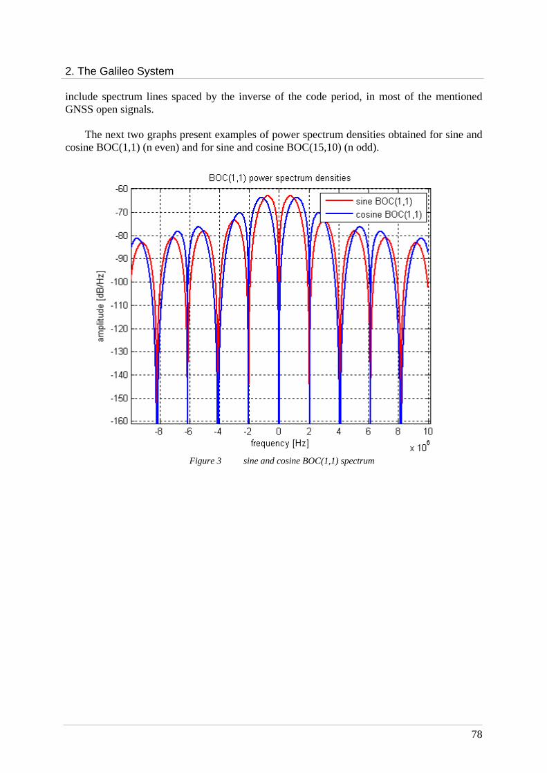
2. The Galileo System

78

include spectrum lines spaced by the inverse of the code period, in most of the mentioned GNSS open signals.

The next two graphs present examples of power spectrum densities obtained for sine and

cosine BOC(1,1) (n even) and for sine and cosine BOC(15,10) (n odd).

Figure 3 sine and cosine BOC(1,1) spectrum

2. The Galileo System

79

Figure 4 Sine and cosine BOC(15,10) spectrum

Figures 3 and 4 show that the width of each main lobe equals twice the code rate. It can also be noticed that the sine waveform secondary lobes are concentrated in-between the two main lobes of the spectrum, whereas the cosine waveform features only small secondary lobes around the carrier, most of the secondary lobes energy being rejected on the external part of the spectrum.

Moreover these graphs prove that the BOC modulation permits to move the signal power away from the band center, which offers the potential for better code tracking accuracy and multipath rejection. Thanks to its two independent design parameters: the code and the sub-carrier frequencies, the BOC modulation provides more freedom to concentrate signal power within specific parts of the allocated band to reduce interference with other signals while keeping the same central frequency (for easy antenna setting for instance). Therefore it permits a better sharing of the allocated bands between the different navigation systems than pure BPSK signals.

Finally, the BOC signal offers also practical advantages in receiver performance for signal acquisition, code tracking, carrier tracking and data demodulation as presented in [Betz, 2002] and as it will be shown in chapter 5 during the performance study of the Galileo E1 signals.

2.2.3.2.3 Galileo BOC signals

The table 5 presents the Galileo signals transmitted using a BOC modulation:

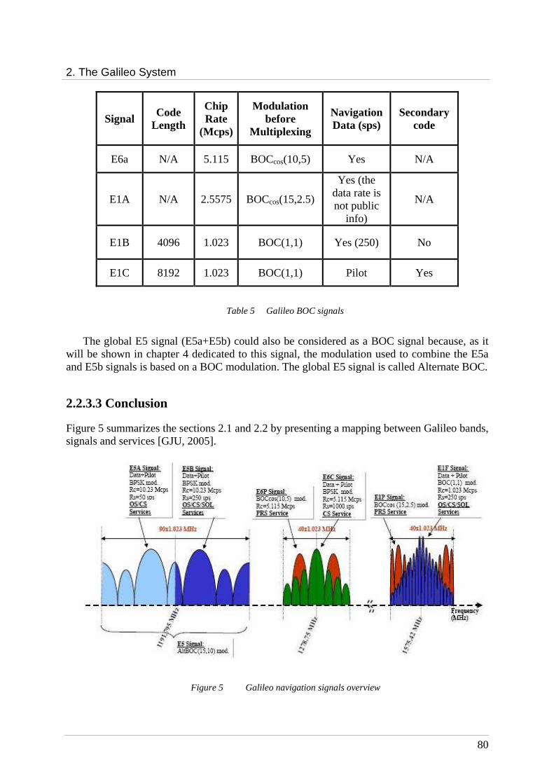
2. The Galileo System

80

Signal Code Length

Chip Rate

(Mcps)

Modulation before

Multiplexing

Navigation Data (sps)

Secondary code

E6a N/A 5.115 BOCcos(10,5) Yes N/A

E1A N/A 2.5575 BOCcos(15,2.5)

Yes (the data rate is not public

info)

N/A

E1B 4096 1.023 BOC(1,1) Yes (250) No

E1C 8192 1.023 BOC(1,1) Pilot Yes

Table 5 Galileo BOC signals

The global E5 signal (E5a+E5b) could also be considered as a BOC signal because, as it

will be shown in chapter 4 dedicated to this signal, the modulation used to combine the E5a and E5b signals is based on a BOC modulation. The global E5 signal is called Alternate BOC.

2.2.3.3 Conclusion

Figure 5 summarizes the sections 2.1 and 2.2 by presenting a mapping between Galileo bands, signals and services [GJU, 2005].

Figure 5 Galileo navigation signals overview

2. The Galileo System

81

The E5a and E5b signals are composed of a data BPSK signal and a pilot BPSK signal. Before being transmitted by the satellite payload, these four signals are multiplexed around their carrier frequency (1191.795 MHz) thanks to a particular modulation, called Alternate BOC modulation and presented in chapter 4, as mentioned previously.

The E6P signal is a BOCcos(10,5) and the E6C signal is a BPSK signal in base band. They are also multiplexed around their carrier frequency (1278.75 MHz) before being transmitted. The modulation for their multiplexing is called Interplex modulation. It is also used to combine the three E1 signals: BOCcos(15,2.5) E1P signal, the data BOC(1,1) E1F signal, and the pilot BOC(1,1) E1F signal. This modulation will be described in chapter 5.

Now that the Galileo signals, their frequency bands, their carrier frequencies, their

associated services and their waveforms have been presented, all the elements are gathered to study the power link budget of the Galileo system.

2.3 Galileo Link Budget

One of the objectives of this thesis is to examine the Galileo payload and particularly, the evaluation of the payload amplifier non-linearities influence on the Galileo signals. Consequently, the study of the Galileo link budget is interesting in order to evaluate the necessary power at the payload output and therefore the required operating range of the payload amplifier.

2.3.1 Definition

The Galileo system considered to calculate the power link budget is represented in figure 6:

Figure 6 Galileo system link budget with: PS, the power at the amplifier output GS, the satellite antenna gain PR, the power at the receiver input GR, the receiver antenna gain

PR Receiver

GR

amplifier LIL

GS

PS

L + LA satellite

2. The Galileo System

82

L, the free space losses LIL, the global losses introduced by the filter after the amplifier and the losses due to

payload components imperfections LA, the atmospheric losses and the polarization losses.

Considering figure 6, the Galileo link budget expression can be written as:

RS

RAILS GG

PLLLP

⋅⋅⋅⋅= in order to evaluate the power at the amplifier output.

The value of PR and GR are set by specifications in [GJU, 2005]. Indeed [GJU, 2005] states

the minimum and maximum signal power levels received with a 0 dBi isotropic right hand circularly polarized antenna for the different emission bands (table 6):

Signals E5 E1 E6

PR (dBW) -152 -154 -154

GR (dBi) 0 0 0

Table 6 Receiver antenna gain and input power

The minimum signal power levels received for the E1 and E6 signals are calculated considering that the power is equally shared between the E1F/E6C and E1P/E6P signals. And [GJU, 2005] set PR (E1F/E6C) = -157 dBW.

These values are valid for elevation angles between 10 and 90 degrees, considered as example angles. The Galileo signals could actually be also used at lower elevation angle like 5 degrees for instance.

The satellite antenna gain GS is function of the satellite « Off Boresight » angle. The link budget should be calculated considering the worst case that means for a receiver elevation angle equal to 10°. Consequently, according to classical satellite antenna gain values, GS is equal to about 15 dBi for each band ([Czopek, 1993]).

The values of GR, GS and PR have been determined; consequently the only missing values

necessary to evaluate the power at the amplifier output are the free space losses L, the payload losses LIL and the atmospheric losses LA.

2.3.2 Calculation of the free space losses

The free space losses depend on r, the distance between the receiver and the satellite and

the carrier frequency. Indeed, L is equal to2

4

⋅=λ

π rL with f

c=λ and r as presented in

figure 7.

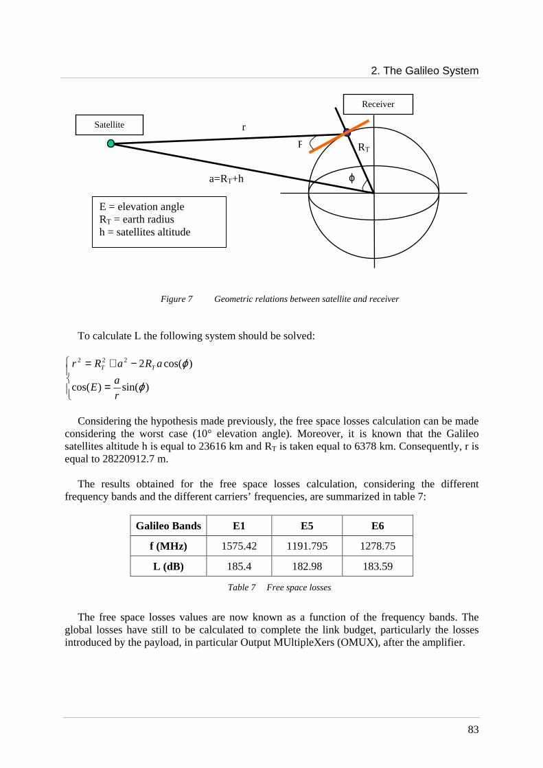
2. The Galileo System

83

Figure 7 Geometric relations between satellite and receiver

To calculate L the following system should be solved:

=

−+=

)sin()cos(

)cos(2222

ϕ

ϕ

r

aE

aRaRr TT

Considering the hypothesis made previously, the free space losses calculation can be made

considering the worst case (10° elevation angle). Moreover, it is known that the Galileo satellites altitude h is equal to 23616 km and RT is taken equal to 6378 km. Consequently, r is equal to 28220912.7 m.

The results obtained for the free space losses calculation, considering the different frequency bands and the different carriers’ frequencies, are summarized in table 7:

Galileo Bands E1 E5 E6

f (MHz) 1575.42 1191.795 1278.75

L (dB) 185.4 182.98 183.59

Table 7 Free space losses

The free space losses values are now known as a function of the frequency bands. The

global losses have still to be calculated to complete the link budget, particularly the losses introduced by the payload, in particular Output MUltipleXers (OMUX), after the amplifier.

Satellite r

a=RT+h ϕ

E

Receiver

RT

E = elevation angle RT = earth radius h = satellites altitude

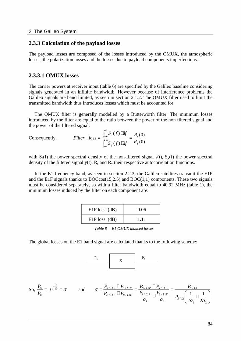
2. The Galileo System

84

2.3.3 Calculation of the payload losses

The payload losses are composed of the losses introduced by the OMUX, the atmospheric losses, the polarization losses and the losses due to payload components imperfections.

2.3.3.1 OMUX losses

The carrier powers at receiver input (table 6) are specified by the Galileo baseline considering signals generated in an infinite bandwidth. However because of interference problems the Galileo signals are band limited, as seen in section 2.1.2. The OMUX filter used to limit the transmitted bandwidth thus introduces losses which must be accounted for.

The OMUX filter is generally modelled by a Butterworth filter. The minimum losses introduced by the filter are equal to the ratio between the power of the non filtered signal and the power of the filtered signal.

Consequently, )0(

)0(

)(

)(_

y

s

y

s

R

R

dffS

dffSlossFilter =

⋅

⋅=∫

∫∞+

∞−

+∞

∞−

with Ss(f) the power spectral density of the non-filtered signal s(t), Sy(f) the power spectral density of the filtered signal y(t), Rs and Ry their respective autocorrelation functions.

In the E1 frequency band, as seen in section 2.2.3, the Galileo satellites transmit the E1P

and the E1F signals thanks to BOCcos(15,2.5) and BOC(1,1) components. These two signals must be considered separately, so with a filter bandwidth equal to 40.92 MHz (table 1), the minimum losses induced by the filter on each component are:

E1F loss (dB) 0.06

E1P loss (dB) 1.11

Table 8 E1 OMUX induced losses

The global losses on the E1 band signal are calculated thanks to the following scheme:

So, α==−

1010x

E

S

P

P and

+

=+

+=++=

211/

1/

2

1/

1

1/

1/1/

1/1/

1/1/

2

1

2

1

αααα

α

LS

LS

FLSPLS

FLSPLS

FLEPLE

FLSPLS

P

PPPPP

PP

PP

PE PS x

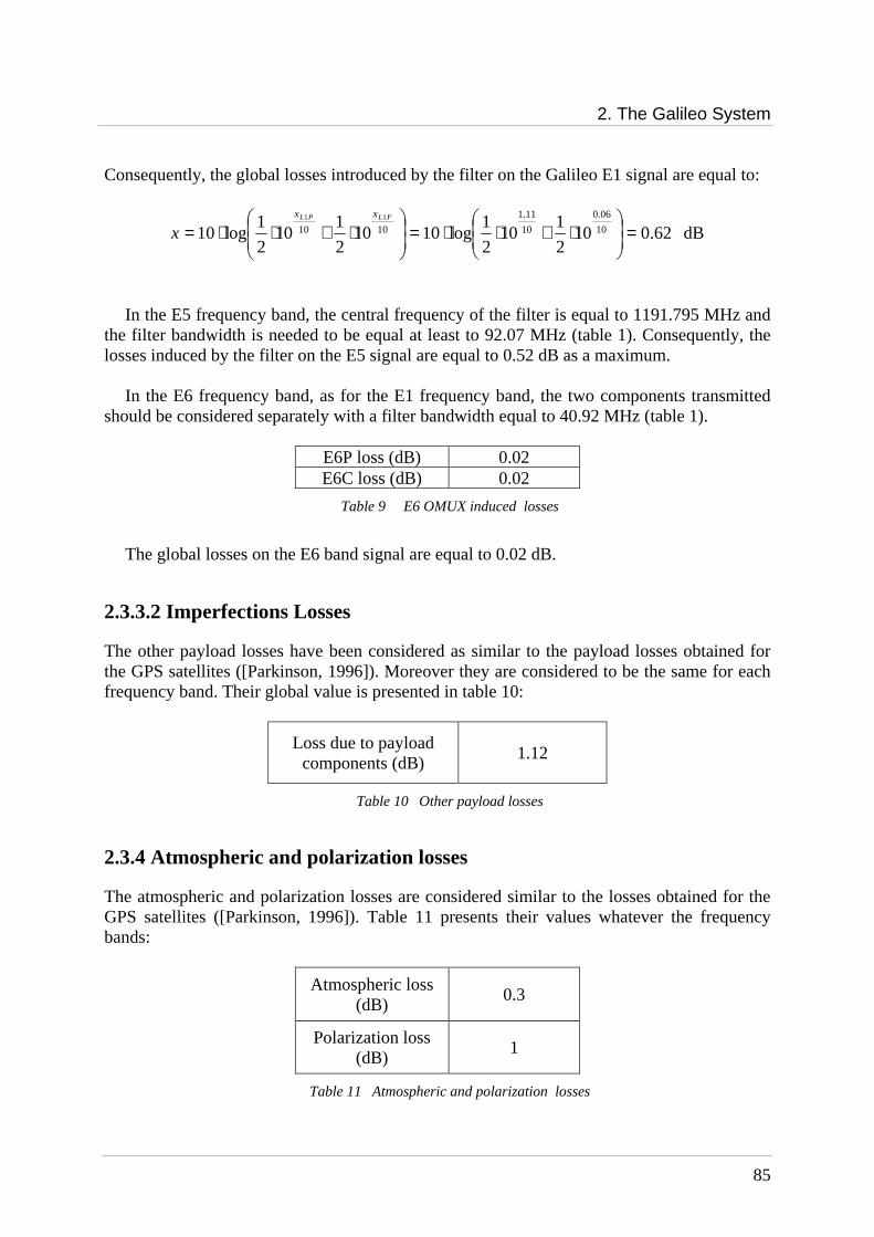
2. The Galileo System

85

Consequently, the global losses introduced by the filter on the Galileo E1 signal are equal to:

dB 62.0102

110

2

1log1010

2

110

2

1log10 10

06.0

10

11.1

101011

=

⋅+⋅⋅=

⋅+⋅⋅=

FLPL xx

x

In the E5 frequency band, the central frequency of the filter is equal to 1191.795 MHz and the filter bandwidth is needed to be equal at least to 92.07 MHz (table 1). Consequently, the losses induced by the filter on the E5 signal are equal to 0.52 dB as a maximum.

In the E6 frequency band, as for the E1 frequency band, the two components transmitted should be considered separately with a filter bandwidth equal to 40.92 MHz (table 1).

E6P loss (dB) 0.02 E6C loss (dB) 0.02

Table 9 E6 OMUX induced losses

The global losses on the E6 band signal are equal to 0.02 dB.

2.3.3.2 Imperfections Losses

The other payload losses have been considered as similar to the payload losses obtained for the GPS satellites ([Parkinson, 1996]). Moreover they are considered to be the same for each frequency band. Their global value is presented in table 10:

Loss due to payload components (dB)

1.12

Table 10 Other payload losses

2.3.4 Atmospheric and polarization losses

The atmospheric and polarization losses are considered similar to the losses obtained for the GPS satellites ([Parkinson, 1996]). Table 11 presents their values whatever the frequency bands:

Atmospheric loss (dB)

0.3

Polarization loss (dB)

1

Table 11 Atmospheric and polarization losses

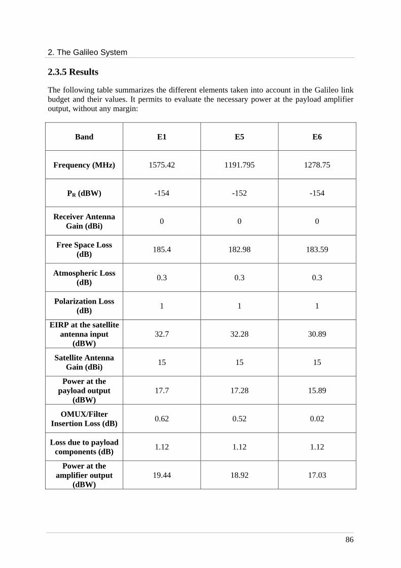
2. The Galileo System

86

2.3.5 Results

The following table summarizes the different elements taken into account in the Galileo link budget and their values. It permits to evaluate the necessary power at the payload amplifier output, without any margin:

Band E1 E5 E6

Frequency (MHz) 1575.42 1191.795 1278.75

PR (dBW) -154 -152 -154

Receiver Antenna Gain (dBi)

0 0 0

Free Space Loss (dB)

185.4 182.98 183.59

Atmospheric Loss (dB)

0.3 0.3 0.3

Polarization Loss (dB)

1 1 1

EIRP at the satellite antenna input

(dBW) 32.7 32.28 30.89

Satellite Antenna Gain (dBi)

15 15 15

Power at the payload output

(dBW) 17.7 17.28 15.89

OMUX/Filter Insertion Loss (dB)

0.62 0.52 0.02

Loss due to payload components (dB)

1.12 1.12 1.12

Power at the amplifier output

(dBW) 19.44 18.92 17.03

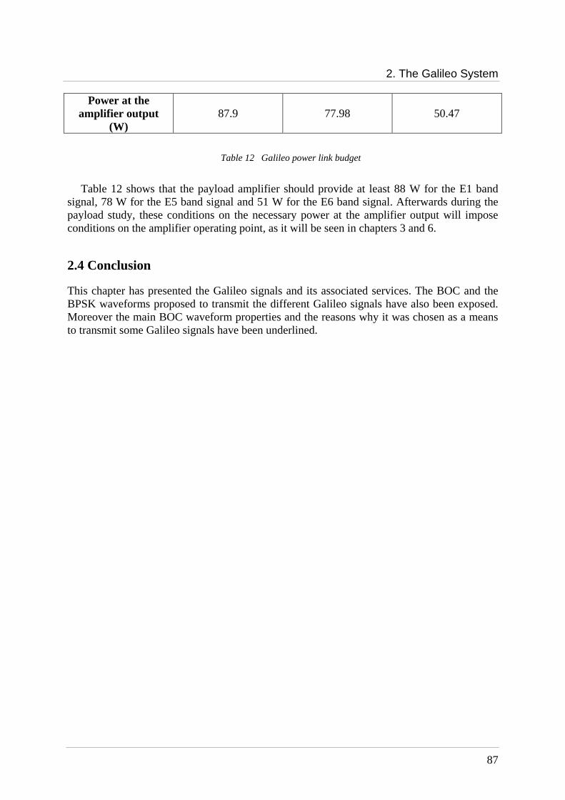
2. The Galileo System

87

Power at the amplifier output

(W) 87.9 77.98 50.47

Table 12 Galileo power link budget

Table 12 shows that the payload amplifier should provide at least 88 W for the E1 band

signal, 78 W for the E5 band signal and 51 W for the E6 band signal. Afterwards during the payload study, these conditions on the necessary power at the amplifier output will impose conditions on the amplifier operating point, as it will be seen in chapters 3 and 6.

2.4 Conclusion

This chapter has presented the Galileo signals and its associated services. The BOC and the BPSK waveforms proposed to transmit the different Galileo signals have also been exposed. Moreover the main BOC waveform properties and the reasons why it was chosen as a means to transmit some Galileo signals have been underlined.

89

Chapter 3

Advanced Design Constraints for Galileo Signals

Contents 3.1 Galileo signals generation................................................................................................ 90

3.1.1 Payload Scheme............................................................................................................ 90 3.1.2 The Clock Unit.............................................................................................................. 91 3.1.3 The Navigation Signal Generation Unit ....................................................................... 91 3.1.4 The amplifier unit ......................................................................................................... 96 3.1.5 The OMUX ................................................................................................................... 98

3.2 Galileo signals processing ................................................................................................ 98 3.2.1 Galileo receiver architecture ......................................................................................... 98 3.2.2 The acquisition process............................................................................................... 100 3.2.3 The tracking process ................................................................................................... 102

3.3 Signal impairments as performance drivers................................................................ 106 3.3.1 Oscillator Phase noise................................................................................................. 106 3.3.2 Amplifier non-linearities............................................................................................. 120 3.3.3 Multipath..................................................................................................................... 122

3.4 Conclusions ..................................................................................................................... 125 After a general overview of the Galileo system, the aim of this new chapter is to present a generic Galileo payload and receiver in order to identify the inherent impairments factors, which could distort the signal during its generation, its propagation or its processing and consequently, reduce the signal performance from a receiver point of view. The impairments determination will allow establishing some signal constraints according to which the Galileo signal optimisation should be realized.

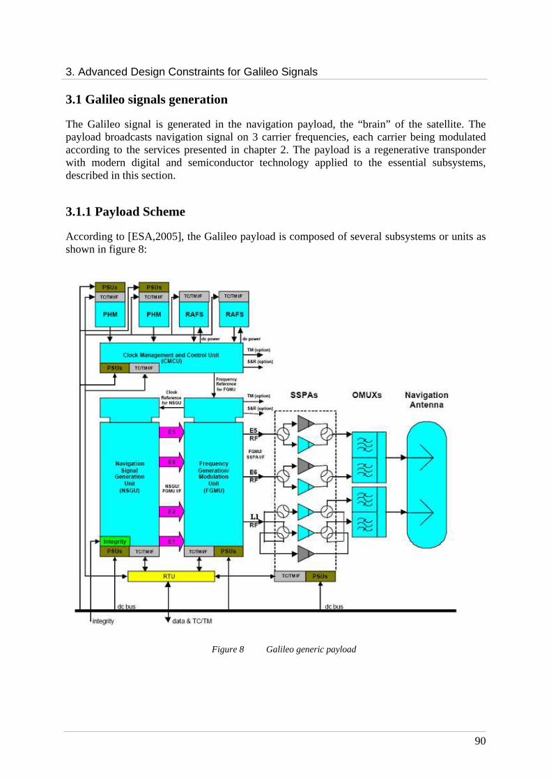
3. Advanced Design Constraints for Galileo Signals

90

3.1 Galileo signals generation

The Galileo signal is generated in the navigation payload, the “brain” of the satellite. The payload broadcasts navigation signal on 3 carrier frequencies, each carrier being modulated according to the services presented in chapter 2. The payload is a regenerative transponder with modern digital and semiconductor technology applied to the essential subsystems, described in this section.

3.1.1 Payload Scheme

According to [ESA,2005], the Galileo payload is composed of several subsystems or units as shown in figure 8:

Figure 8 Galileo generic payload

3. Advanced Design Constraints for Galileo Signals

91

Five different units can be identified: a clock unit, composed of four atomic clocks and a Clock Management and Control

Unit (CMCU), a Navigation Signal Generation Unit (NSGU), which generates the navigation signal, a Frequency Generation and Modulation Unit (FGMU), which realises the digital-to-

analog conversion of the signal and its up-conversion to the appropriate frequency band,

an amplifier unit, composed of Solid State Power Amplifiers (SSPAs) or Travelling Wave Tube Amplifiers (TWTAs), and

an Output MUltipleX unit (OMUX)

3.1.2 The Clock Unit

The Galileo satellites will carry a clock ensemble, composed of four atomic clocks: two Passive Hydrogen Maser (PHM) and two Rubidium Atomic Frequency Sources (RAFS) that provide the time reference for the generation of the navigation signal. These atomic clocks were chosen because of their high frequency and time standards. Indeed, the stability of the Rubidium clock is so good that it would be within only 3 seconds in 1 million years, while the Hydrogen Maser is even more stable and it would be within only 1 second in 3 million years. The Galileo satellites will carry two different types of clocks on-board for a 100% safe service.

The atomic reference is selected from one of the four atomic clocks and converted to the Master Timing Reference (MTR) of 10.23 MHz by the Clock Monitoring and Control Unit (CMCU). The MTR provides the time reference for the Frequency Generation and Modulation Unit (FGMU), which generates the master clock for the Navigation Signal Generation Unit and up-converts the navigation signals to their appropriate carrier frequencies.

The CMCU should not degrade the frequency stability of the atomic clocks and delivers an extremely pure frequency. That is the reason why the CMCU implements a hybrid synthesizer built on a Phase Locked Loop (PLL) ([Felbach, 2003]).

3.1.3 The Navigation Signal Generation Unit

The Navigation Signal Generation Unit generates the navigation message and modulates it for each one of the different emission bands. It is composed of a modulation circuit, called modulator and a digital filter as shown in figure 9:

3. Advanced Design Constraints for Galileo Signals

92

Figure 9 NSGU generic scheme

3.1.3.1 Navigation signal modulator

The NSGU modulator generates three digital modulated base band signals, one for each frequency bands (E1, E5, E6). After that the modulator, according mostly to the signal bandwidth, can: put the base-band signals around a digital intermediate frequency to avoid the

problems linked to the setting and ageing of an analog mixer. This is usually done for signals with a relatively low transmitted bandwidth. This scheme could be, for instance, used for Galileo E1 and E6 signals. Or,

keep the base-band signals in-phase and quadrature components because their digital

generation around an intermediate frequency would not be possible owing to their large bandwidth, which would impose a sampling frequency not currently realistic for a spatial payload. This scheme could be, for instance, used for the Galileo E5 signal because of its large bandwidth equal to at least 90*1.023 MHz.

Table 13 summarizes Galileo signals generation by the modulator :

Signals band Signals bandwidth [MHz] (N.B. : assumptions)

Central frequency [MHz]

E1 40*1.023 30*1.023

E5 90*1.023 Baseband

E6 40*1.023 30*1.023

Table 13 Galileo signals generation types

FGMU

Modulator Digital Filter

Navigation Signal Generation Unit

Sampling frequency

Navigation signals

3. Advanced Design Constraints for Galileo Signals

93

3.1.3.2 Digital Filter

After being modulated, the signals are filtered by a digital filter to respect out-of-band rejection and avoid partial spectrum mixing that could appear during the FGMU processes. This filter is also in charge of performing the compensation of DAC shaping and of the possible distortions brought by the following analog processing. The filter bandwidth should be at least equal to the transmitted signals bandwidth from a technical point of view, however it has to be noted that the choice of the filter bandwidth and shape is important (and this is true for every payload module using filtering operations), since it will cut the useful signal spectrum and, if not properly chosen, could destroy desirable properties of the signals.

3.1.3.3 The Frequency Generation and Modulation Unit

The FGMU receives the time reference from the CMCU and delivers it to the NSGU. This subsystem also achieves the digital-to-analog conversion of the navigation signals before up-converting them to their respective frequency bands for broadcast to users.

Figure 10 presents an FGMU generic structure:

3. Advanced Design Constraints for Galileo Signals

94

Figure 10 FGMU generic scheme

The FGMU is composed of: digital-to-analog converters (DAC), several frequency synthesizers which use the reference time delivered by the clock

unit to generate the intermediate frequencies, used for the signals generation in the NSGU and the signals up-conversion in the FGMU,

mixers which permit to realize the up-conversion, wideband analog filters to avoid out-of-band emissions, spectrum distortions after the

digital-to-analog conversion and spectrum re-combinations after the up-conversion.

3.1.3.4 The digital-to-analog conversion

The digital-to-analog converter generates an analog signal from the digital signal, which comes from the NSGU.

Different types of DAC exist. The two major parameters are the resolution, which indicates the number of discrete values the DAC can produce over the range of voltage values and the update rate. In space applications, the resolution is chosen around 12-14 bits and the update rate is generally higher than 100 MSPS (Mega Sample Per Second). But whichever

Nav

igat

ion

Sig

nal G

ener

atio

n U

nit

Clock Unit

Sampling frequency synthesizer

frequency synthesizer

frequency synthesizer

frequency synthesizer

D/A

con

vert

er Filter

Filter

Filter

Frequency Generation

and Modulation

Unit

L1

E6

E5

Am

plifi

er U

nit

Filter

Filter

Filter

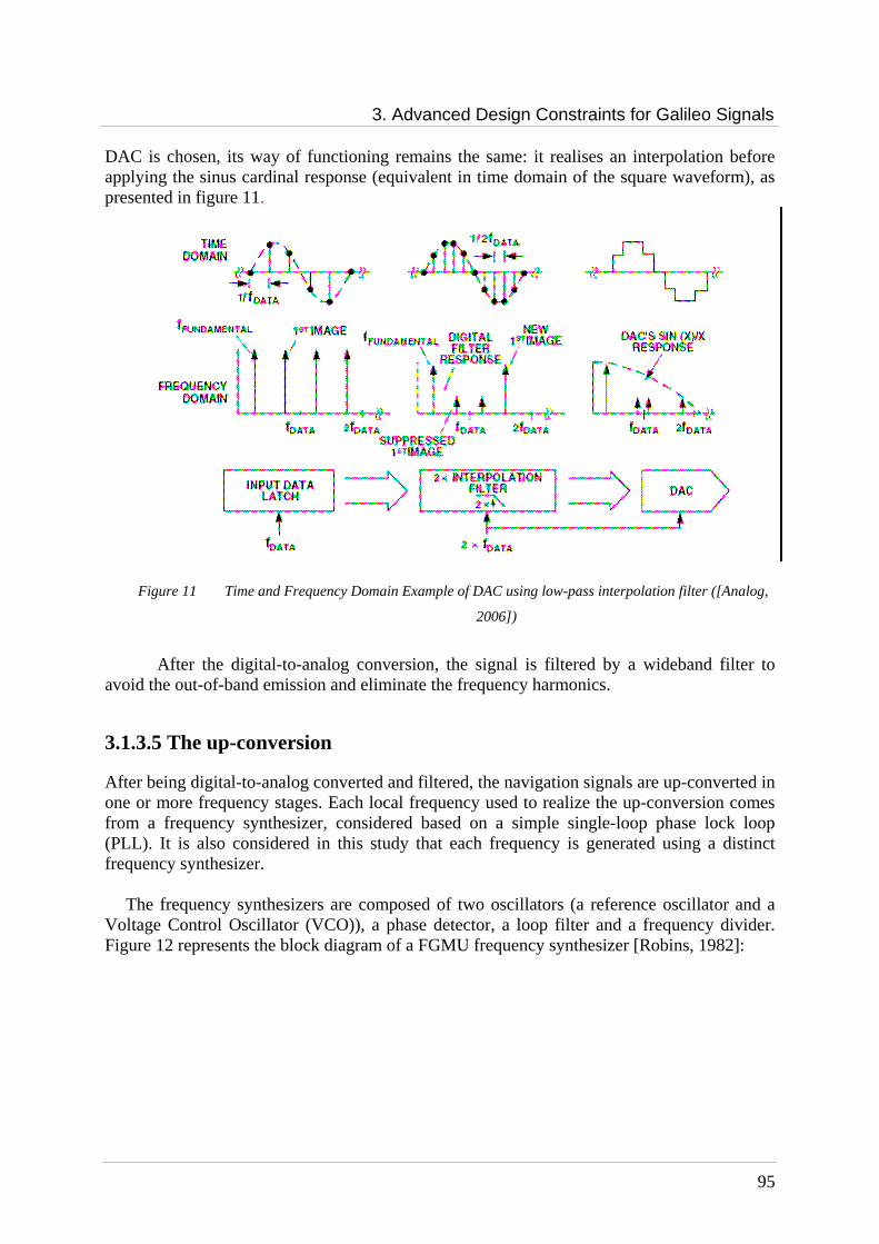
3. Advanced Design Constraints for Galileo Signals

95

DAC is chosen, its way of functioning remains the same: it realises an interpolation before applying the sinus cardinal response (equivalent in time domain of the square waveform), as presented in figure 11.

Figure 11 Time and Frequency Domain Example of DAC using low-pass interpolation filter ([Analog,

2006])

After the digital-to-analog conversion, the signal is filtered by a wideband filter to

avoid the out-of-band emission and eliminate the frequency harmonics.

3.1.3.5 The up-conversion

After being digital-to-analog converted and filtered, the navigation signals are up-converted in one or more frequency stages. Each local frequency used to realize the up-conversion comes from a frequency synthesizer, considered based on a simple single-loop phase lock loop (PLL). It is also considered in this study that each frequency is generated using a distinct frequency synthesizer.

The frequency synthesizers are composed of two oscillators (a reference oscillator and a

Voltage Control Oscillator (VCO)), a phase detector, a loop filter and a frequency divider. Figure 12 represents the block diagram of a FGMU frequency synthesizer [Robins, 1982]:

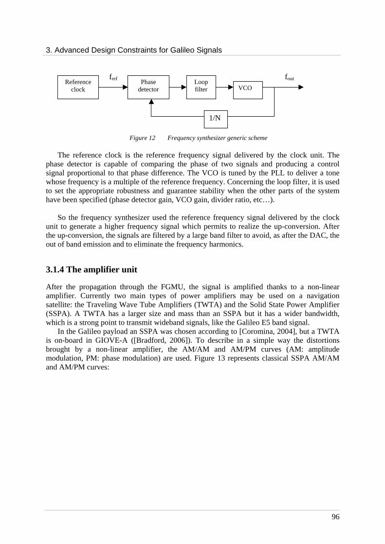
3. Advanced Design Constraints for Galileo Signals

96

Figure 12 Frequency synthesizer generic scheme

The reference clock is the reference frequency signal delivered by the clock unit. The

phase detector is capable of comparing the phase of two signals and producing a control signal proportional to that phase difference. The VCO is tuned by the PLL to deliver a tone whose frequency is a multiple of the reference frequency. Concerning the loop filter, it is used to set the appropriate robustness and guarantee stability when the other parts of the system have been specified (phase detector gain, VCO gain, divider ratio, etc…).

So the frequency synthesizer used the reference frequency signal delivered by the clock unit to generate a higher frequency signal which permits to realize the up-conversion. After the up-conversion, the signals are filtered by a large band filter to avoid, as after the DAC, the out of band emission and to eliminate the frequency harmonics.

3.1.4 The amplifier unit

After the propagation through the FGMU, the signal is amplified thanks to a non-linear amplifier. Currently two main types of power amplifiers may be used on a navigation satellite: the Traveling Wave Tube Amplifiers (TWTA) and the Solid State Power Amplifier (SSPA). A TWTA has a larger size and mass than an SSPA but it has a wider bandwidth, which is a strong point to transmit wideband signals, like the Galileo E5 band signal.

In the Galileo payload an SSPA was chosen according to [Coromina, 2004], but a TWTA is on-board in GIOVE-A ([Bradford, 2006]). To describe in a simple way the distortions brought by a non-linear amplifier, the AM/AM and AM/PM curves (AM: amplitude modulation, PM: phase modulation) are used. Figure 13 represents classical SSPA AM/AM and AM/PM curves:

Reference clock

Phase detector

Loop filter

VCO

1/N

fref fout

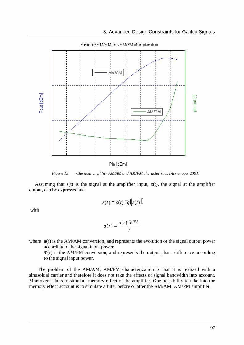
3. Advanced Design Constraints for Galileo Signals

97

Figure 13 Classical amplifier AM/AM and AM/PM characteristics [Armengou, 2003]

Assuming that s(t) is the signal at the amplifier input, z(t), the signal at the amplifier

output, can be expressed as :

( ))()()( tsgtstz ⋅=

with

r

erarg

ri )()()(

φ⋅=

where a(r) is the AM/AM conversion, and represents the evolution of the signal output power

according to the signal input power, Φ(r) is the AM/PM conversion, and represents the output phase difference according to the signal input power.

The problem of the AM/AM, AM/PM characterization is that it is realized with a

sinusoidal carrier and therefore it does not take the effects of signal bandwidth into account. Moreover it fails to simulate memory effect of the amplifier. One possibility to take into the memory effect account is to simulate a filter before or after the AM/AM, AM/PM amplifier.

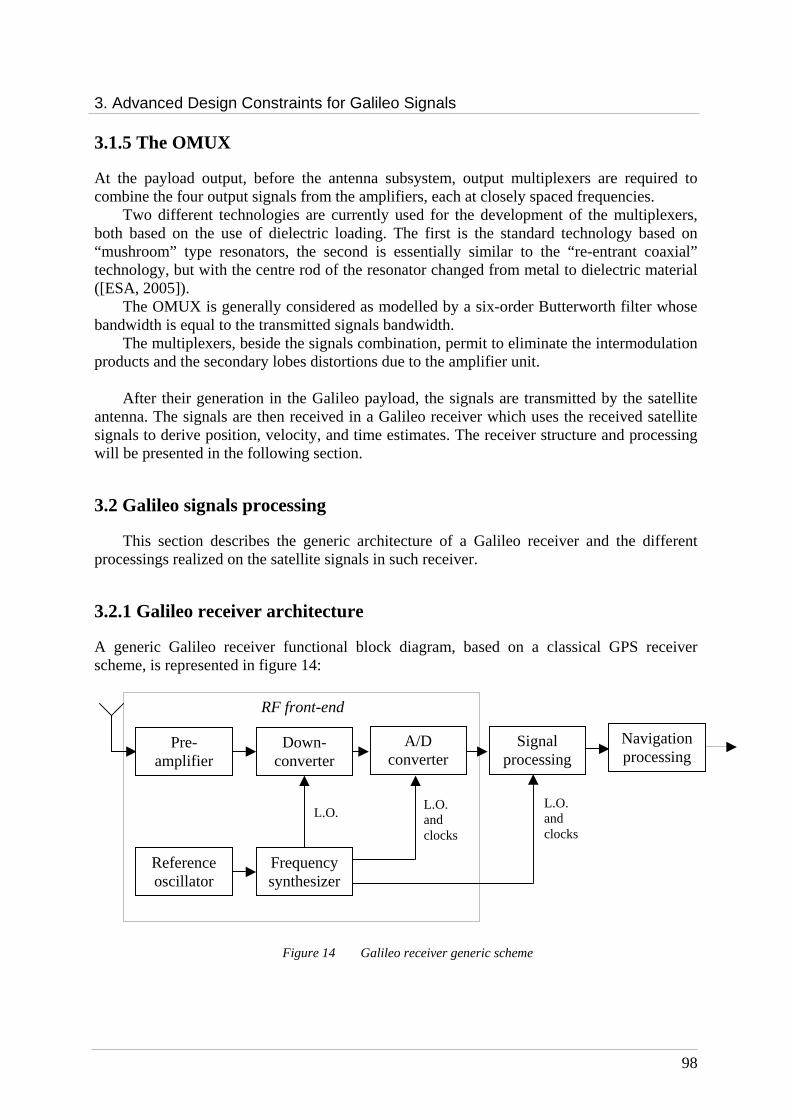
3. Advanced Design Constraints for Galileo Signals

98

3.1.5 The OMUX

At the payload output, before the antenna subsystem, output multiplexers are required to combine the four output signals from the amplifiers, each at closely spaced frequencies.

Two different technologies are currently used for the development of the multiplexers, both based on the use of dielectric loading. The first is the standard technology based on “mushroom” type resonators, the second is essentially similar to the “re-entrant coaxial” technology, but with the centre rod of the resonator changed from metal to dielectric material ([ESA, 2005]).

The OMUX is generally considered as modelled by a six-order Butterworth filter whose bandwidth is equal to the transmitted signals bandwidth.

The multiplexers, beside the signals combination, permit to eliminate the intermodulation products and the secondary lobes distortions due to the amplifier unit.

After their generation in the Galileo payload, the signals are transmitted by the satellite

antenna. The signals are then received in a Galileo receiver which uses the received satellite signals to derive position, velocity, and time estimates. The receiver structure and processing will be presented in the following section.

3.2 Galileo signals processing

This section describes the generic architecture of a Galileo receiver and the different processings realized on the satellite signals in such receiver.

3.2.1 Galileo receiver architecture

A generic Galileo receiver functional block diagram, based on a classical GPS receiver scheme, is represented in figure 14:

Figure 14 Galileo receiver generic scheme

Pre-amplifier

Down-converter

A/D converter

Signal processing

Reference oscillator

Frequency synthesizer

L.O. L.O. and clocks

L.O. and clocks

Navigation processing

RF front-end

3. Advanced Design Constraints for Galileo Signals

99

The radio-frequency chain and the A/D converter represent the RF front-end hardware of the receiver while the signal and navigation processing represent the digital part that can be implemented in hardware and/or in software.

The RF hardware part is composed of: an antenna, passive or active, depending upon the performance requirements. a pre-amplifier, generally consisting of burnout protection, filtering and a low-noise

amplifier. a reference oscillator, providing time and frequency reference for the whole receiver.

The reference oscillator is a key element of the receiver, especially during the phase tracking process.

a frequency synthesizer, which uses the reference oscillator output to derive local oscillators (L.O.) and clocks signals used during the processing. One or more of these L.O. are used by,

down-converters, to convert the radio frequency inputs to intermediate frequencies that are easier to process for filtering and in the signal-processing level. The down-conversion is realized in several stages.

an analog-to-digital converter which digitizes the last intermediate frequency (IF) signal.

These two last receiver components realize, in fact, the symmetrical functions of the

digital-to-analog converter and up-converter in the payload (except that the intermediate frequencies can be different). Moreover the receiver frequency synthesizers are, as the payload frequency synthesizers, considered herein based on a simple single-loop PLL.

The signal processing part is the core of the receiver, performing the following functions: splitting the signal into multiple channels for signal-processing of multiple satellites

simultaneously, generating the signals’ spreading codes and intermediate frequencies carriers, acquiring the satellite signals, tracking the satellite signals codes and carriers, demodulating the signals data.

The outputs of the signal processing function are pseudoranges, pseudorange rate, delta

pseudorange, carrier phase, doppler and demodulated data bits; they are used as inputs by the navigation (data processing) part.

The next sections investigate in details the main signal processing functions: acquisition and tracking. These algorithms allow the extraction of the navigation data, which provide all the necessary information to compute the pseudorange between the receiver and the visible satellites. Therefore the acquisition and tracking performances allows evaluating the quality of the transmitted (and received) signal.

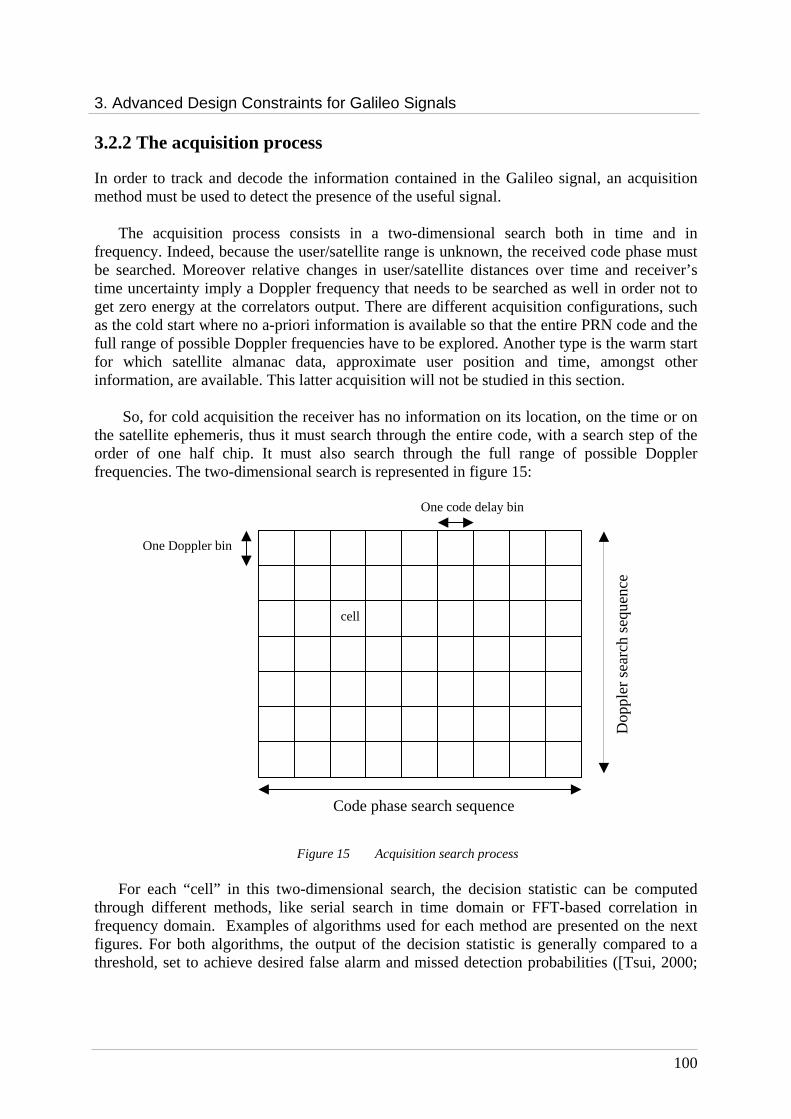
3. Advanced Design Constraints for Galileo Signals

100

3.2.2 The acquisition process

In order to track and decode the information contained in the Galileo signal, an acquisition method must be used to detect the presence of the useful signal.

The acquisition process consists in a two-dimensional search both in time and in frequency. Indeed, because the user/satellite range is unknown, the received code phase must be searched. Moreover relative changes in user/satellite distances over time and receiver’s time uncertainty imply a Doppler frequency that needs to be searched as well in order not to get zero energy at the correlators output. There are different acquisition configurations, such as the cold start where no a-priori information is available so that the entire PRN code and the full range of possible Doppler frequencies have to be explored. Another type is the warm start for which satellite almanac data, approximate user position and time, amongst other information, are available. This latter acquisition will not be studied in this section.

So, for cold acquisition the receiver has no information on its location, on the time or on

the satellite ephemeris, thus it must search through the entire code, with a search step of the order of one half chip. It must also search through the full range of possible Doppler frequencies. The two-dimensional search is represented in figure 15:

Figure 15 Acquisition search process

For each “cell” in this two-dimensional search, the decision statistic can be computed

through different methods, like serial search in time domain or FFT-based correlation in frequency domain. Examples of algorithms used for each method are presented on the next figures. For both algorithms, the output of the decision statistic is generally compared to a threshold, set to achieve desired false alarm and missed detection probabilities ([Tsui, 2000;

Code phase search sequence

One Doppler bin

cell

One code delay bin

Dop

pler

sea

rch

sequ

ence

3. Advanced Design Constraints for Galileo Signals

101

Parkinson, 1996; Kaplan, 1996]). This comparison permits to decide if a possible bit was identified or not. After several possible verification stages, the cell position can then be handled to the tracking loops to verify the lock. If the acquisition process is not successful other cells should be tested.

The serial search algorithm, presented in figure 16, usually uses a constant Doppler bin size. The search pattern starts from the known mean value of the Doppler uncertainty (zero Doppler when there is not any expected value) and tests all possible code delays. If this fails, the search is carried on to the next Doppler bin, with the sequence of bins symmetrically alternating on either sides of the initial value.

Figure 16 Serial search acquisition algorithm In the FFT-based acquisition algorithm, presented in figure 17, a Fast Fourier Transform

(FFT) is applied to the in-phase and quadrature-phase components of the IF incoming signal. The result is multiplied by the conjugate FFT of the replicated signal. The inverse FFT of the product gives the correlation result in the time domain for all of the code phase offsets for a given Doppler value. This method is computationally more efficient and faster than the conventional time domain technique, in seconds, but it can induce memory size problems.

∫2

1

t

t

∫2

1

t

t

( )²

( )²

Σ decision

Control logic

Local oscillator

π/2

Code generator

IF signal

I

Q

Local oscillator

3. Advanced Design Constraints for Galileo Signals

102

Figure 17 FFT-based acquisition algorithm As mentioned previously, once the acquisition process successfully ended after several

possible verification stages, the estimated code offset and carrier Doppler are used to initialize the tracking loops which perform a finer search over the two parameters.

3.2.3 The tracking process

In order to track the incoming Galileo signal, two tracking loops must be used: one loop to track the carrier of the incoming signal, called Phase Locked loop (PLL) and an other one to track the code, called Delay Locked Loop (DLL)

3.2.3.1 The carrier-phase locked loop

The objective of the carrier-phase tracking loop is to keep the phase error between the locally-generated carrier and the incoming signals close to zero. Any misalignment produces a nonzero phase error, which is detected and corrected by the phase discriminator and taken into account in the tracking loop, presented in figure 18:

IF signal

I FFT ( )²

( )²

decision

Local carrier samples

π/2

Local code samples

Q FFT

conj FFT

IFFT

IFFT

Control logic

3. Advanced Design Constraints for Galileo Signals

103

Figure 18 Carrier-phase tracking loop [Julien, 2005]

The incoming signal after the down-conversion and the A/D conversion is first multiplied by a spreading sequence coming from the DLL, assuming an estimate of the satellite signal code delay in order to wipe-off the spreading symbols (details in section 3.2.3.2). Then the signal is split into two branches. One is mixed with a local in-phase carrier and the other one with a local quadra-phase carrier. The resulting signals are then integrated by digital Integrate and Dump filters (I&D). The output signals of in-phase and quadra-phase digital I&D, noted I and Q, are expressed by [Parkinson, 1996]:

( ) ( ) ( ) II nTfckdA

I +⋅⋅∆⋅⋅ℜ⋅= φτ επε cossin~

)(2

and ( ) ( ) ( ) QI nTfckdA

Q +⋅⋅∆⋅⋅ℜ⋅= φτ επε sinsin~

)(2

( )τεℜ~ represents the correlation with the code replica, TI the integration time, f∆ the

frequency error on Doppler estimation,φε the carrier phase error, In and Qn independent

noises with I

én

én T

NQI 4

0== σσ .

PLL discriminator

Carrier generator

π/2

Carrier NCO

PLL Loop Filter

I&D Filter

I&D Filter

Code NCO and generator

From DLL

ADC

I

Q

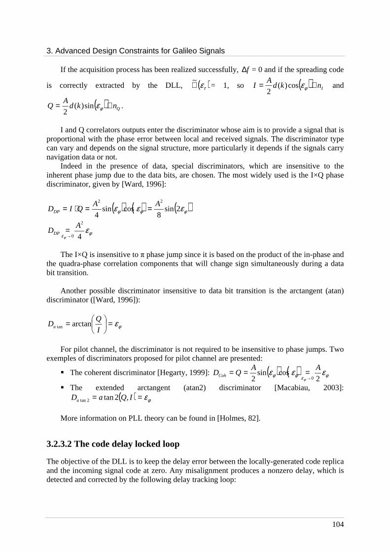
3. Advanced Design Constraints for Galileo Signals

104

If the acquisition process has been realized successfully, f∆ = 0 and if the spreading code

is correctly extracted by the DLL, ( )τεℜ~ = 1, so ( ) InkdA

I += φεcos)(2

and

( ) QnkdA

Q += φεsin)(2

.

I and Q correlators outputs enter the discriminator whose aim is to provide a signal that is

proportional with the phase error between local and received signals. The discriminator type can vary and depends on the signal structure, more particularly it depends if the signals carry navigation data or not.

Indeed in the presence of data, special discriminators, which are insensitive to the inherent phase jump due to the data bits, are chosen. The most widely used is the I×Q phase discriminator, given by [Ward, 1996]:

( ) ( ) ( )φφφ εεε 2sin8

cossin4

22 AAQIDDP ==⋅=

φεε

φ 4

2

0

ADDP →

=

The I×Q is insensitive to π phase jump since it is based on the product of the in-phase and

the quadra-phase correlation components that will change sign simultaneously during a data bit transition.

Another possible discriminator insensitive to data bit transition is the arctangent (atan) discriminator ([Ward, 1996]):

φε=

=I

QDa arctantan

For pilot channel, the discriminator is not required to be insensitive to phase jumps. Two

exemples of discriminators proposed for pilot channel are presented:

The coherent discriminator [Hegarty, 1999]: ( ) ( ) φεφφ εεεφ 2

cossin2 0

AAQDCoh →

===

The extended arctangent (atan2) discriminator [Macabiau, 2003]: ( ) φε== IQaDa ,2tan2tan

More information on PLL theory can be found in [Holmes, 82].

3.2.3.2 The code delay locked loop

The objective of the DLL is to keep the delay error between the locally-generated code replica and the incoming signal code at zero. Any misalignment produces a nonzero delay, which is detected and corrected by the following delay tracking loop:

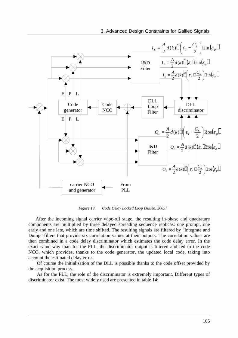
3. Advanced Design Constraints for Galileo Signals

105

Figure 19 Code Delay Locked Loop [Julien, 2005]

After the incoming signal carrier wipe-off stage, the resulting in-phase and quadrature components are multiplied by three delayed spreading sequence replicas: one prompt, one early and one late, which are time shifted. The resulting signals are filtered by “Integrate and Dump” filters that provide six correlation values at their outputs. The correlation values are then combined in a code delay discriminator which estimates the code delay error. In the exact same way than for the PLL, the discriminator output is filtered and fed to the code NCO, which provides, thanks to the code generator, the updated local code, taking into account the estimated delay error.

Of course the initialisation of the DLL is possible thanks to the code offset provided by the acquisition process.

As for the PLL, the role of the discriminator is extremely important. Different types of discriminator exist. The most widely used are presented in table 14:

carrier NCO and generator

( )φτ εε sin2

~)(

2⋅

−ℜ= SL

Ckd

AI

DLL discriminator

Code generator

Code NCO

DLL Loop Filter

I&D Filter

I&D Filter

From PLL

E P L

E P L

( )φτ εε cos2

~)(

2⋅

−ℜ= SL

Ckd

AQ

( ) ( )φτ εε cos~

)(2

⋅ℜ= kdA

QP

( )φτ εε cos2

~)(

2⋅

+ℜ= SE

Ckd

AQ

( ) ( )φτ εε sin~

)(2

⋅ℜ= kdA

I P

( )φτ εε sin2

~)(

2⋅

+ℜ= SE

Ckd

AI

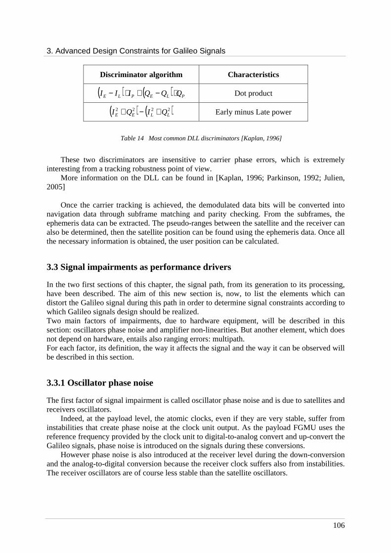
3. Advanced Design Constraints for Galileo Signals

106

Discriminator algorithm Characteristics

( ) ( ) PLEPLE QQQIII ⋅−+⋅− Dot product

( ) ( )2222LLEE QIQI +−+ Early minus Late power

Table 14 Most common DLL discriminators [Kaplan, 1996]

These two discriminators are insensitive to carrier phase errors, which is extremely

interesting from a tracking robustness point of view. More information on the DLL can be found in [Kaplan, 1996; Parkinson, 1992; Julien,

2005]

Once the carrier tracking is achieved, the demodulated data bits will be converted into navigation data through subframe matching and parity checking. From the subframes, the ephemeris data can be extracted. The pseudo-ranges between the satellite and the receiver can also be determined, then the satellite position can be found using the ephemeris data. Once all the necessary information is obtained, the user position can be calculated.

3.3 Signal impairments as performance drivers

In the two first sections of this chapter, the signal path, from its generation to its processing, have been described. The aim of this new section is, now, to list the elements which can distort the Galileo signal during this path in order to determine signal constraints according to which Galileo signals design should be realized. Two main factors of impairments, due to hardware equipment, will be described in this section: oscillators phase noise and amplifier non-linearities. But another element, which does not depend on hardware, entails also ranging errors: multipath. For each factor, its definition, the way it affects the signal and the way it can be observed will be described in this section.

3.3.1 Oscillator phase noise

The first factor of signal impairment is called oscillator phase noise and is due to satellites and receivers oscillators.

Indeed, at the payload level, the atomic clocks, even if they are very stable, suffer from instabilities that create phase noise at the clock unit output. As the payload FGMU uses the reference frequency provided by the clock unit to digital-to-analog convert and up-convert the Galileo signals, phase noise is introduced on the signals during these conversions.

However phase noise is also introduced at the receiver level during the down-conversion and the analog-to-digital conversion because the receiver clock suffers also from instabilities. The receiver oscillators are of course less stable than the satellite oscillators.

3. Advanced Design Constraints for Galileo Signals

107

The next paragraph will present the phase noise definition and its characterization. Afterwards the way the phase noise affects the signals through the payload and the receiver is studied. Finally, the parameters, which permit the evaluation of the phase noise influence on signal and receiver performance, are presented.

3.3.1.1 Phase noise definition

If the output signal of oscillators is modelled thanks to the following expression [Rutman, 1991]:

( )( ) 2sin)( 0 ttAtV φπν +⋅= (3.1)

then the phase noise is a random process represented by Φ(t).

Two sets of parameters are generally used to characterize the oscillators phase noise: the spectral densities of phase fluctuations, in the Fourier frequency domain the variance (or standard deviation) of the averaged frequency fluctuations in the time

domain

This thesis will focus on the frequency domain phase noise representation. In this case, the most common engineering characteristic used to specify the phase noise is the Single Side Band (SSB) Phase Noise Power Spectral Density £(f) defined by:

( ) ( )

⋅=

2log10£

fSf φ where SΦ(f) is the one-sided phase noise power spectral density

As shown by theoretical considerations and experimental measurements in several articles

[IEEE Std. 1139-1988; Barnes, 1971], SΦ(f) can be written as a power law model :

∑=

−=

=2

22

20)(

α

α

ααφ

νfh

ffS for 0<f<fh, (3.2)

where fh is an upper cut-off frequency. Each term is related to a given noise source in the oscillator, as presented in figure 20.

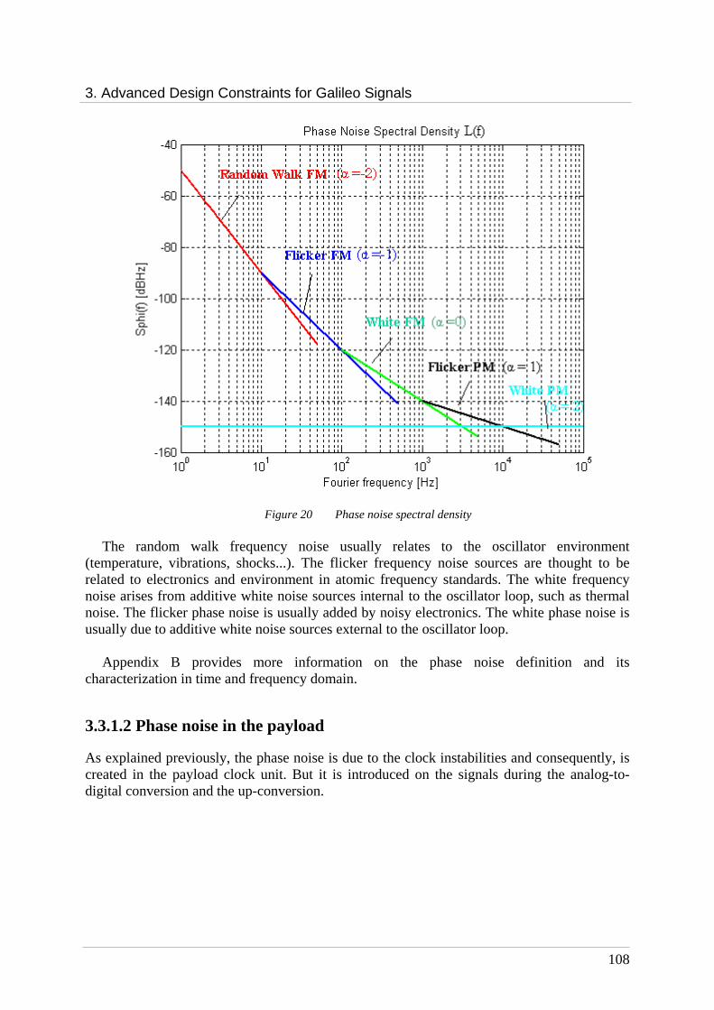
3. Advanced Design Constraints for Galileo Signals

108

Figure 20 Phase noise spectral density

The random walk frequency noise usually relates to the oscillator environment

(temperature, vibrations, shocks...). The flicker frequency noise sources are thought to be related to electronics and environment in atomic frequency standards. The white frequency noise arises from additive white noise sources internal to the oscillator loop, such as thermal noise. The flicker phase noise is usually added by noisy electronics. The white phase noise is usually due to additive white noise sources external to the oscillator loop.

Appendix B provides more information on the phase noise definition and its

characterization in time and frequency domain.

3.3.1.2 Phase noise in the payload

As explained previously, the phase noise is due to the clock instabilities and consequently, is created in the payload clock unit. But it is introduced on the signals during the analog-to-digital conversion and the up-conversion.

3. Advanced Design Constraints for Galileo Signals

109

3.3.1.2.1 Clock unit phase noise

At the satellite level, very stable clocks such as Rubidium and Hydrogen Maser atomic clocks are used to reduce the oscillator phase noise as much as possible. However, these clocks are also disturbed by unavoidable phase noise. The next two graphs represent examples of phase noise power spectra, respectively, for Passive Hydrogen Maser and Rubidium clocks whose frequency delivered is equal to 10 MHz.

Figure 21 Passive Hydrogen Maser phase noise spectrum ([Quartzlock, 2006])

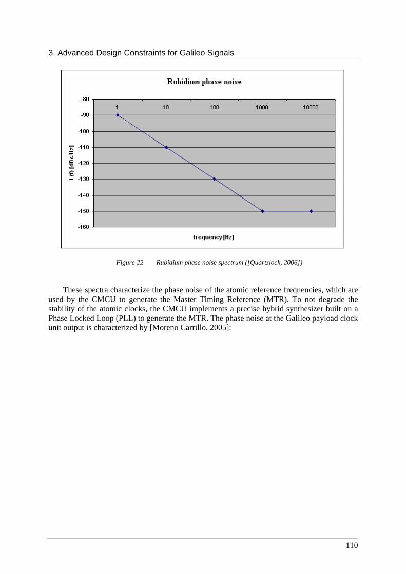
3. Advanced Design Constraints for Galileo Signals

110

Figure 22 Rubidium phase noise spectrum ([Quartzlock, 2006])

These spectra characterize the phase noise of the atomic reference frequencies, which are

used by the CMCU to generate the Master Timing Reference (MTR). To not degrade the stability of the atomic clocks, the CMCU implements a precise hybrid synthesizer built on a Phase Locked Loop (PLL) to generate the MTR. The phase noise at the Galileo payload clock unit output is characterized by [Moreno Carrillo, 2005]:

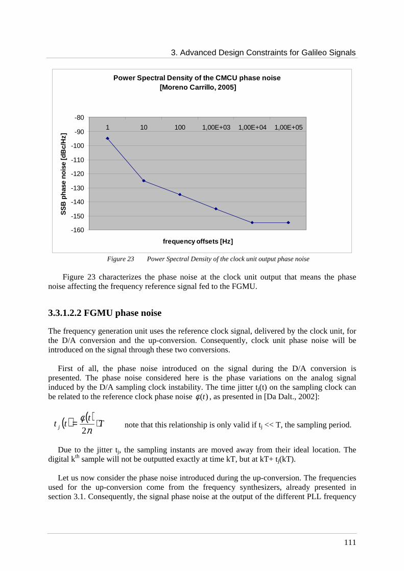
3. Advanced Design Constraints for Galileo Signals

111

Power Spectral Density of the CMCU phase noise [Moreno Carrillo, 2005]

-160

-150

-140

-130

-120

-110

-100

-90

-80

1 10 100 1,00E+03 1,00E+04 1,00E+05

frequency offsets [Hz]

SS

B p

hase

noi

se [d

Bc/

Hz]

Figure 23 Power Spectral Density of the clock unit output phase noise

Figure 23 characterizes the phase noise at the clock unit output that means the phase

noise affecting the frequency reference signal fed to the FGMU.

3.3.1.2.2 FGMU phase noise

The frequency generation unit uses the reference clock signal, delivered by the clock unit, for the D/A conversion and the up-conversion. Consequently, clock unit phase noise will be introduced on the signal through these two conversions.

First of all, the phase noise introduced on the signal during the D/A conversion is presented. The phase noise considered here is the phase variations on the analog signal induced by the D/A sampling clock instability. The time jitter tj(t) on the sampling clock can be related to the reference clock phase noise )(tφ , as presented in [Da Dalt., 2002]:

( ) ( )T

ttt j ⋅=

πφ2

note that this relationship is only valid if t j << T, the sampling period.

Due to the jitter tj, the sampling instants are moved away from their ideal location. The

digital kth sample will not be outputted exactly at time kT, but at kT+ tj(kT). Let us now consider the phase noise introduced during the up-conversion. The frequencies

used for the up-conversion come from the frequency synthesizers, already presented in section 3.1. Consequently, the signal phase noise at the output of the different PLL frequency

3. Advanced Design Constraints for Galileo Signals

112

synthesizers should be calculated to be able to evaluate the phase noise added to the signal during the up-conversion. For this, the equivalent linear model of the frequency synthesizer is used, as presented in Appendix C. This model shows the modification of the reference signal phase during the frequency synthesis:

Figure 24 Equivalent frequency synthesizer linear model with θref, the input reference phase which comes from the clock unit and consequently

contains phase noise θVCO, the VCO output phase which contains also phase noise due to the VCO

instabillities θout, the output phase used for the up-conversion θfb, the feed-back phase F(s) the transfer function of the loop filter, KVCO and KPD are, respectively the VCO and the phase detector gains.

Thanks to the calculation made in Appendix C, the phase noise at each frequency

synthesizer output can be expressed as ([Rebeyrol03, 2006]):

( ) ( ) ( ) ( ) ( ) 222 1 fHfSfHNfSfSvcoCUout

−⋅+⋅⋅= φφφ (3.3)

where SΦCU(f) is the power spectrum density of the phase noise at the clock unit output,

SΦVCO(f) is the power spectrum density of the VCO phase noise, and H(f) is the PLL closed loop transfer function equal to:

( )( )

( ) N

sFKKs

N

sFKK

sHPDVCO

PDVCO

⋅⋅+

⋅⋅

=

Eq. 3.3 implies that within the loop bandwidth, the reference noise is multiplied by the

loop division ratio (N2). Outside the loop bandwidth, the reference noise is attenuated by the loop transfer function (H is a low-pass filter). Within the loop bandwidth, the VCO noise is attenuated. Low frequency phase noise is rejected by the loop, but high frequency phase noise

KPD F(s) KVCO/s

1/N

θref

θfb

+

-

θvco

θout

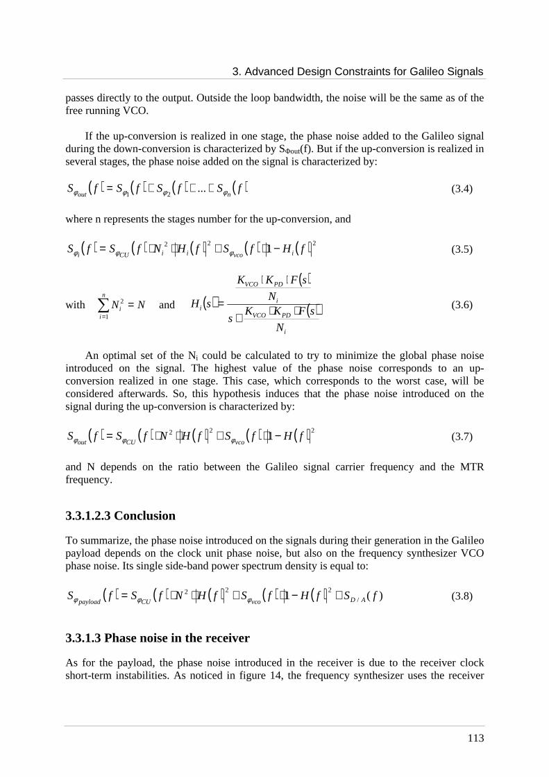
3. Advanced Design Constraints for Galileo Signals

113

passes directly to the output. Outside the loop bandwidth, the noise will be the same as of the free running VCO.

If the up-conversion is realized in one stage, the phase noise added to the Galileo signal during the down-conversion is characterized by SΦout(f). But if the up-conversion is realized in several stages, the phase noise added on the signal is characterized by:

( ) ( ) ( ) ( )fSfSfSfSnout φφφφ +++= ...

21 (3.4)

where n represents the stages number for the up-conversion, and

( ) ( ) ( ) ( ) ( ) 222 1 fHfSfHNfSfS ivcoiiCUi−⋅+⋅⋅= φφφ (3.5)

with ∑=

=n

ii NN

1

2 and ( )( )

( )

i

PDVCO

i

PDVCO

i

N

sFKKs

N

sFKK

sH ⋅⋅+

⋅⋅

= (3.6)

An optimal set of the Ni could be calculated to try to minimize the global phase noise

introduced on the signal. The highest value of the phase noise corresponds to an up-conversion realized in one stage. This case, which corresponds to the worst case, will be considered afterwards. So, this hypothesis induces that the phase noise introduced on the signal during the up-conversion is characterized by:

( ) ( ) ( ) ( ) ( ) 222 1 fHfSfHNfSfSvcoCUout

−⋅+⋅⋅= φφφ (3.7)

and N depends on the ratio between the Galileo signal carrier frequency and the MTR frequency.

3.3.1.2.3 Conclusion

To summarize, the phase noise introduced on the signals during their generation in the Galileo payload depends on the clock unit phase noise, but also on the frequency synthesizer VCO phase noise. Its single side-band power spectrum density is equal to:

( ) ( ) ( ) ( ) ( ) )(1 /

222 fSfHfSfHNfSfS ADvcoCUpayload+−⋅+⋅⋅= φφφ (3.8)

3.3.1.3 Phase noise in the receiver

As for the payload, the phase noise introduced in the receiver is due to the receiver clock short-term instabilities. As noticed in figure 14, the frequency synthesizer uses the receiver

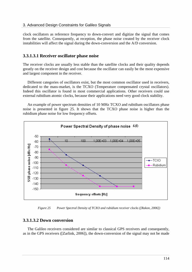
3. Advanced Design Constraints for Galileo Signals

114

clock oscillators as reference frequency to down-convert and digitize the signal that comes from the satellite. Consequently, at reception, the phase noise created by the receiver clock instabilities will affect the signal during the down-conversion and the A/D conversion.

3.3.1.3.1 Receiver oscillator phase noise

The receiver clocks are usually less stable than the satellite clocks and their quality depends greatly on the receiver design and cost because the oscillator can easily be the most expensive and largest component in the receiver.

Different categories of oscillators exist, but the most common oscillator used in receivers,

dedicated to the mass-market, is the TCXO (Temperature compensated crystal oscillators). Indeed this oscillator is found in most commercial applications. Other receivers could use external rubidium atomic clocks, because their applications need very good clock stability.

An example of power spectrum densities of 10 MHz TCXO and rubidium oscillators phase noise is presented in figure 25. It shows that the TCXO phase noise is higher than the rubidium phase noise for low frequency offsets.

Figure 25 Power Spectral Density of TCXO and rubidium receiver clocks ([Rakon, 2006])

3.3.1.3.2 Down conversion

The Galileo receivers considered are similar to classical GPS receivers and consequently, as in the GPS receivers ([Zarlink, 2006]), the down-conversion of the signal may not be made

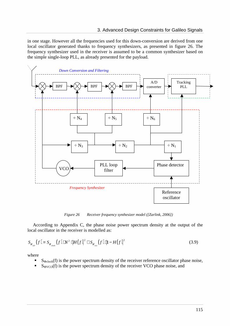
3. Advanced Design Constraints for Galileo Signals

115

in one stage. However all the frequencies used for this down-conversion are derived from one local oscillator generated thanks to frequency synthesizers, as presented in figure 26. The frequency synthesizer used in the receiver is assumed to be a common synthesizer based on the simple single-loop PLL, as already presented for the payload.

Figure 26 Receiver frequency synthesizer model ([Zarlink, 2006])

According to Appendix C, the phase noise power spectrum density at the output of the

local oscillator in the receiver is modelled as:

( ) ( ) ( ) ( ) ( ) 222 1 fHfSfHNfSfSvcoclockLO

−⋅+⋅⋅= φφφ (3.9)

where SΦclock(f) is the power spectrum density of the receiver reference oscillator phase noise, SΦVCO(f) is the power spectrum density of the receiver VCO phase noise, and

BPF A/D

converter Tracking

PLL BPF BPF

Reference oscillator

Phase detector PLL loop filter VCO

÷ N3

÷ N4

÷ N5

÷ N2

÷ N6

÷ N1

Down Conversion and Filtering

Frequency Synthesizer

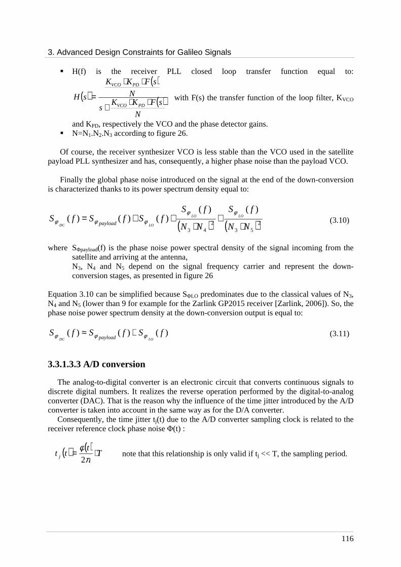
3. Advanced Design Constraints for Galileo Signals

116

H(f) is the receiver PLL closed loop transfer function equal to:

( )( )

( ) N

sFKKs

N

sFKK

sHPDVCO

PDVCO

⋅⋅+

⋅⋅

= with F(s) the transfer function of the loop filter, KVCO

and KPD, respectively the VCO and the phase detector gains. N=N1.N2.N3 according to figure 26.

Of course, the receiver synthesizer VCO is less stable than the VCO used in the satellite

payload PLL synthesizer and has, consequently, a higher phase noise than the payload VCO.

Finally the global phase noise introduced on the signal at the end of the down-conversion is characterized thanks to its power spectrum density equal to:

( ) ( )253

243

)()()()()(

NN

fS

NN

fSfSfSfS LOLO

LODC payload ⋅+

⋅++=

φφφφφ (3.10)

where SΦpayload(f) is the phase noise power spectral density of the signal incoming from the

satellite and arriving at the antenna, N3, N4 and N5 depend on the signal frequency carrier and represent the down-conversion stages, as presented in figure 26

Equation 3.10 can be simplified because SΦLO predominates due to the classical values of N3, N4 and N5 (lower than 9 for example for the Zarlink GP2015 receiver [Zarlink, 2006]). So, the phase noise power spectrum density at the down-conversion output is equal to:

)()()( fSfSfSLODC payload φφφ +≈ (3.11)

3.3.1.3.3 A/D conversion

The analog-to-digital converter is an electronic circuit that converts continuous signals to discrete digital numbers. It realizes the reverse operation performed by the digital-to-analog converter (DAC). That is the reason why the influence of the time jitter introduced by the A/D converter is taken into account in the same way as for the D/A converter.

Consequently, the time jitter tj(t) due to the A/D converter sampling clock is related to the receiver reference clock phase noise Φ(t) :

( ) ( )T

ttt j ⋅=

πφ2

note that this relationship is only valid if t j << T, the sampling period.

3. Advanced Design Constraints for Galileo Signals

117

3.3.1.3.4 Conclusion

In addition to the phase noise introduced by the payload, the receiver introduces an offset on the signal phase during the down-conversion and the digital-to-analog conversion. Consequently, at the signal processing input, the signal phase noise is characterized by ([Rebeyrol02, 2006]):

( )( ) ( ) ( ) ( )

( ) ( ) ( ) ( )

+−⋅+⋅⋅+

+−⋅+⋅⋅=

)(1

)(1

/

222

/

222

fSfHfSfHNfS

fSfHfSfHNfSfS

DAoreceivervcreceiver

ADpayloadvcopayloadCU

clockφφ

φφ

φ (3.12)

Now that the phase noise introduced by the payload and the receiver on the signal has been evaluated, the way it can be observed is presented.

3.3.1.4 Phase noise influence

To evaluate or observe the phase noise influence, different observables characteristic of receiver performance are used. These observables, detailed in this section, are: the correlation function, the power spectrum density, the phase error estimation to assess the error induced by the clocks phase noise as seen

by a typical receiver PLL, the modulation constellation.

3.3.1.4.1 Correlation function and spectrum

The correlation function is used as a characteristic, in order to evaluate the influence of payload and receiver clocks instabilities on the code tracking performance thanks to the observation of the correlation peak.

Indeed, the correlation loss and the peak sharpness give information on the code tracking effectiveness. The correlation secondary peaks level and their distortions can also be observed.

The signal power spectrum density could also be used to notice a possible spectrum distortion or a side lobe rise, which could lead to interferences with other signals. The power spectral density distortions are linked to the correlation distortions.

3.3.1.4.2 Phase error estimation

To evaluate the influence of the phase noise due to receiver and satellite atomic clocks instabilities, the phase error estimation in a typical receiver tracking PLL has to be analyzed.

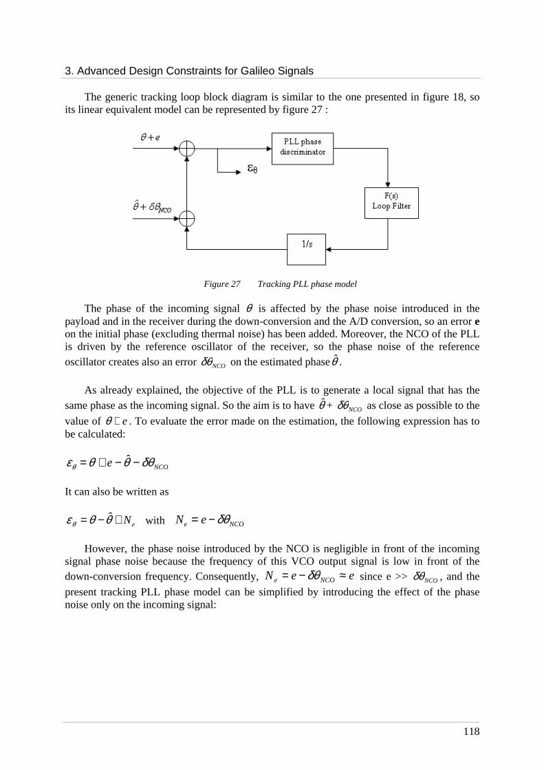
3. Advanced Design Constraints for Galileo Signals

118

The generic tracking loop block diagram is similar to the one presented in figure 18, so its linear equivalent model can be represented by figure 27 :

Figure 27 Tracking PLL phase model

The phase of the incoming signal θ is affected by the phase noise introduced in the payload and in the receiver during the down-conversion and the A/D conversion, so an error e on the initial phase (excluding thermal noise) has been added. Moreover, the NCO of the PLL is driven by the reference oscillator of the receiver, so the phase noise of the reference oscillator creates also an error NCOδθ on the estimated phaseθ .

As already explained, the objective of the PLL is to generate a local signal that has the

same phase as the incoming signal. So the aim is to have θ + NCOδθ as close as possible to the

value of e+θ . To evaluate the error made on the estimation, the following expression has to be calculated:

NCOe δθθθεθ −−+= ˆ

It can also be written as

eN+−= θθεθˆ with NCOe eN δθ−=

However, the phase noise introduced by the NCO is negligible in front of the incoming

signal phase noise because the frequency of this VCO output signal is low in front of the down-conversion frequency. Consequently, eeN NCOe ≈−= δθ since e >> NCOδθ , and the

present tracking PLL phase model can be simplified by introducing the effect of the phase noise only on the incoming signal:

3. Advanced Design Constraints for Galileo Signals

119

Figure 28 Simplified Tracking PLL phase model

Moreover according to [Parkinson and Spilker, 1996],

)()()()()(ˆ pHpNpHpp e ⋅+⋅=θθ , where H(p) is the PLL transfer function .

So, as θθεθˆ−+= eN , [ ] [ ] )()(1)()(1)( pNpHppHp e⋅−+⋅−= θεθ

Thus, the variance of the error of a PLL due to the payload and receiver clocks phase noise, in radians, is given as:

( )∫∞

⋅−⋅=0

22 1)( dfjfHfSφσ (3.13)

where SΦ (f) is the single-sideband power spectrum density of the incoming phase noise, presented in Eq. 3.12 and, H is the transfer function of the PLL. Considering a 3rd order PLL, the following model can be used [Parkinson, 1996]:

66

62

)(1ff

fjfH

L +=− where fL= π2 *1.2*BL, and BL is the loop noise bandwidth.

3.3.1.4.3 Modulation Constellation

The influence of the phase noise can also be visualized on the signal modulation constellation to examine the variation of the signal envelope.

Indeed, as the phase noise introduces an offset on the signal phase, the signal modulation plots can rotate or spread if this offset depends on time, as illustrated in figure 29.

3. Advanced Design Constraints for Galileo Signals

120

Figure 29 Examples of phase noise influence on a 8-PSK modulation constellation

3.3.1.5 Conclusion

The phase noise due to oscillators’ instabilities has been deeply described in this section. According to this presentation, it seems that the only way to reduce this element of signal distortions is to use extremely stable clocks. At the payload level, atomic clocks are considered; they are the most stable current clocks. It is so impossible to reduce the payload clocks phase noise further. In the receiver, it is possible to use also atomic clocks but this is limited to few applications (ground stations). That is not acceptable for the mass market because of the cost of such clocks. Consequently, it is difficult to reduce payload and receiver clocks phase noise. No optimization and no signals design constraints can be deduced from this parameter.

3.3.2 Amplifier non-linearities

The second element of distortion is due to the payload amplifier. Indeed, during the signal generation, in addition to the phase noise due to atomic clocks instabilities, the amplifier unit can also induce signal impairments, because of its non-linearities.

Signal modulation constellation Example of plots rotation due to phase noise

Example of plots spread due to phase noise

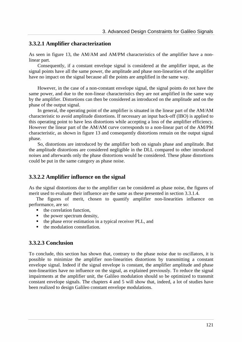
3. Advanced Design Constraints for Galileo Signals

121

3.3.2.1 Amplifier characterization

As seen in figure 13, the AM/AM and AM/PM characteristics of the amplifier have a non-linear part.

Consequently, if a constant envelope signal is considered at the amplifier input, as the signal points have all the same power, the amplitude and phase non-linearities of the amplifier have no impact on the signal because all the points are amplified in the same way.

However, in the case of a non-constant envelope signal, the signal points do not have the

same power, and due to the non-linear characteristics they are not amplified in the same way by the amplifier. Distortions can then be considered as introduced on the amplitude and on the phase of the output signal.

In general, the operating point of the amplifier is situated in the linear part of the AM/AM characteristic to avoid amplitude distortions. If necessary an input back-off (IBO) is applied to this operating point to have less distortions while accepting a loss of the amplifier efficiency. However the linear part of the AM/AM curve corresponds to a non-linear part of the AM/PM characteristic, as shown in figure 13 and consequently distortions remain on the output signal phase.

So, distortions are introduced by the amplifier both on signals phase and amplitude. But the amplitude distortions are considered negligible in the DLL compared to other introduced noises and afterwards only the phase distortions would be considered. These phase distortions could be put in the same category as phase noise.

3.3.2.2 Amplifier influence on the signal

As the signal distortions due to the amplifier can be considered as phase noise, the figures of merit used to evaluate their influence are the same as these presented in section 3.3.1.4.

The figures of merit, chosen to quantify amplifier non-linearities influence on performance, are so: the correlation function, the power spectrum density, the phase error estimation in a typical receiver PLL, and the modulation constellation.

3.3.2.3 Conclusion

To conclude, this section has shown that, contrary to the phase noise due to oscillators, it is possible to minimize the amplifier non-linearities distortions by transmitting a constant envelope signal. Indeed if the signal envelope is constant, the amplifier amplitude and phase non-linearities have no influence on the signal, as explained previously. To reduce the signal impairments at the amplifier unit, the Galileo modulation should so be optimized to transmit constant envelope signals. The chapters 4 and 5 will show that, indeed, a lot of studies have been realized to design Galileo constant envelope modulations.

3. Advanced Design Constraints for Galileo Signals

122

3.3.3 Multipath

The previous sections have described the two impairments due to hardware equipment: the phase noise due to receiver and satellite clock instabilities and the phase error due to amplifier non-linearities.

But, as already mentioned, another element, which does not depend on hardware, should be taken into account for the Galileo signal design optimization because it entails ranging errors. Indeed, navigation signals and particularly Galileo signals can also be affected by multipath issues.

3.3.3.1 Definition

Multipath is the phenomenon whereby a signal arrives at a receiver via multiple paths attributable to reflections and diffraction on surrounding terrain: buildings, canyon walls, hard ground, etc …, as presented in figure 30.

Figure 30 Multipath illustration

The reflected signals, entering the front end of the receiver and mixing with the line-of-sight signal, entail tracking errors. Multipath distorts the signal modulation but also the phase of the carrier.

For long delay multipath (higher than one chip), the multipath signal has no impact on the receiver tracking. To address shorter delay multipath, specialized antennas and special signal processing techniques may be used. This form of multipath is harder to filter out since it is

Galileo satellite

Galileo receiver

reflector Reflected signal

Direct signal

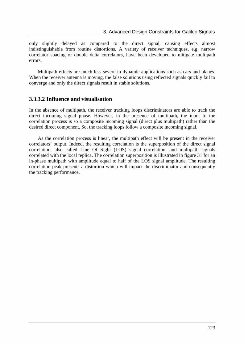
3. Advanced Design Constraints for Galileo Signals

123

only slightly delayed as compared to the direct signal, causing effects almost indistinguishable from routine distortions. A variety of receiver techniques, e.g. narrow correlator spacing or double delta correlators, have been developed to mitigate multipath errors.

Multipath effects are much less severe in dynamic applications such as cars and planes. When the receiver antenna is moving, the false solutions using reflected signals quickly fail to converge and only the direct signals result in stable solutions.

3.3.3.2 Influence and visualisation

In the absence of multipath, the receiver tracking loops discriminators are able to track the direct incoming signal phase. However, in the presence of multipath, the input to the correlation process is so a composite incoming signal (direct plus multipath) rather than the desired direct component. So, the tracking loops follow a composite incoming signal.

As the correlation process is linear, the multipath effect will be present in the receiver

correlators’ output. Indeed, the resulting correlation is the superposition of the direct signal correlation, also called Line Of Sight (LOS) signal correlation, and multipath signals correlated with the local replica. The correlation superposition is illustrated in figure 31 for an in-phase multipath with amplitude equal to half of the LOS signal amplitude. The resulting correlation peak presents a distortion which will impact the discriminator and consequently the tracking performance.

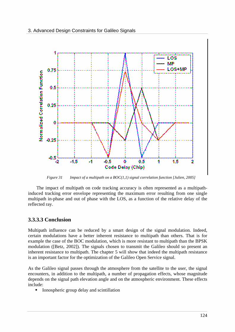
3. Advanced Design Constraints for Galileo Signals

124

Figure 31 Impact of a multipath on a BOC(1,1) signal correlation function [Julien, 2005]

The impact of multipath on code tracking accuracy is often represented as a multipath-

induced tracking error envelope representing the maximum error resulting from one single multipath in-phase and out of phase with the LOS, as a function of the relative delay of the reflected ray.

3.3.3.3 Conclusion

Multipath influence can be reduced by a smart design of the signal modulation. Indeed, certain modulations have a better inherent resistance to multipath than others. That is for example the case of the BOC modulation, which is more resistant to multipath than the BPSK modulation ([Betz, 2002]). The signals chosen to transmit the Galileo should so present an inherent resistance to multipath. The chapter 5 will show that indeed the multipath resistance is an important factor for the optimization of the Galileo Open Service signal. As the Galileo signal passes through the atmosphere from the satellite to the user, the signal encounters, in addition to the multipath, a number of propagation effects, whose magnitude depends on the signal path elevation angle and on the atmospheric environment. These effects include: Ionospheric group delay and scintillation

3. Advanced Design Constraints for Galileo Signals

125

Group delay caused by wet and dry atmosphere, troposphere and stratosphere Atmospheric attenuation in the troposphere and stratosphere.

All these effects which can introduce distortions on the Galileo signals have been neglected in this thesis. The receiver thermal noise and the impairments due to interferences with other systems have not also been considered.

3.4 Conclusions

The study of signal generation in the payload and signal processing in the receiver has led to the identification of several factors which entail signal impairments.

The first factor of signal distortions is the phase noise introduced by the clock instabilities. This phase noise is added to the signal during the digital-to-analog conversion and the up-conversion in the satellite and during the down-conversion and the analog-to-digital conversion in the receiver. The phase noise influence on signal and performance can be evaluated thanks to the observation of the correlation function, the power spectrum density, the modulation constellation and the calculation of a PLL phase error standard deviation.

The second element of signal impairment is due to the non-linearities of the amplifier characteristics in the payload. If the signal envelope is not constant, the non-linearities introduce an equivalent phase noise whose effect on signal and performance could also be characterized thanks to the observation of the correlation function, the power spectrum density, the modulation constellation and the calculation of a PLL phase error.

Finally, the last factor identified, different to the previous ones because it is not linked to hardware equipment, is the multipath which distorts the correlation function and leads to worse performance, by adding reflected signal to the LOS signal.

All these factors can distort the signal and entail worse performance. It would so be

interesting to reduce the influence of these elements on performance whether optimizing the Galileo signals or optimizing the transmission chain. It has been explained that the oscillator phase noise can not be reduced by a particular design of the signal, whereas the amplifier phase noise and multipath distortions can be minimized by generating constant envelope signal with an inherent resistance to multipath.

The following chapters (chapter 4 and 5) will present the Galileo civil signals definition

and optimisation according to at least one of the constraints, defined in this chapter: constant envelope or resistance to multipath. Once the Galileo signals will have been presented, an optimization of their generation chain and an evaluation of the influence of the last impairment factor the clocks phase noise will be realized in chapter 6.

127

Chapter 4

Galileo E5 Band Signal Structure

Contents 4.1 E5 band contents ............................................................................................................ 127 4.2 E5 band multiplexing technique ................................................................................... 128

4.2.1 ALTBOC modulation with a non-constant envelope ................................................. 128 4.2.2 ALTBOC modulation with a constant envelope......................................................... 130

4.3 ALTBOC Power Spectrum Densities ........................................................................... 135 4.3.1 Assumptions................................................................................................................ 136 4.3.2 Non constant envelope ALTBOC signal Power Spectrum Density ........................... 136 4.3.3 Constant envelope ALTBOC signal Power Spectrum Density .................................. 137 4.3.4 Conclusion .................................................................................................................. 138

4.4 ALTBOC signal properties ........................................................................................... 139 4.4.1 Constant envelope modulation advantages................................................................. 139 4.4.2 Resistance to multipath............................................................................................... 140

4.5 Conclusion....................................................................................................................... 142 The objective of this chapter is to present the civil E5 band signal structure, but also the modulation, called ALTBOC (Alternate BOC) chosen to transmit it.

Then, it will be verified that this signal verify the design constraints exposed in chapter 3. In particular, the optimization conducted on the ALTBOC modulation, in order to transmit the E5 band signal with a constant envelope will be described. And the resistance of this signal to multipath is set out.

4.1 E5 band contents

On the E5 band, the modulation objective is to multiplex three different services, the Open Service (OS), the Commercial Service (CS) and the Safety of Life Service (SoL), included

4. Galileo E5 Band Signal Structure

128

into two Binary Offset Carrier (BOC)-like signals (resulting into 4 components), while maintaining a constant envelope.

As already seen in chapter 2, the Galileo E5 signal consists of the multiplexing of four components. These four components are respectively:

The E5a data channel: it results from the modulation of the E5a navigation data stream with the E5a data channel PRN code sequence which has a 10.23 Mcps chipping rate. The primary code length is equal to 10230 chips and the secondary code length is equal to 20 chips.

The E5a pilot (dataless) channel: it results from the modulation of the E5a pilot channel PRN code sequence which has a 10.23 Mcps chipping rate. The primary code length is equal to 10230 chips and the secondary code length is equal to 100 chips.

The E5b data channel: it results from the modulation of the E5b navigation data stream with the E5b data channel PRN code sequence which has a 10.23 Mcps chipping rate. The primary code length is equal to 10230 chips and the secondary code length is equal to 4 chips.

The E5b pilot channel: it results from the modulation of the E5b pilot channel PRN code sequence which has a 10.23 Mcps chipping rate. The primary code length is equal to 10230 chips and the secondary code length is equal to 100 chips.

The modulation proposed to multiplex all these channels is called the constant envelope

Alternate Binary Offset Carrier (ALTBOC) modulation ([GJU, 2005]). This modulation is suggested with a code frequency of 10.23 MHz and a sub-carrier of 15.345 MHz, leading to an ALTBOC(15,10) configuration, as it will be seen later.

The next section will present the “classical” ALTBOC modulation and the way it is modified to obtain the constant envelope ALTBOC modulation.

4.2 E5 band multiplexing technique

4.2.1 ALTBOC modulation with a non-constant envelope

The first idea to transmit all the E5 signal components was to use an Offset Carrier modulation in order to benefit from its spectral and tracking properties, but transmitting a different service through each side-lobe of the OC spectrum. One solution was then to multiply the base band signal by a “complex” sub-carrier. In that way the different baseband signal spectra are not split up, but each is shifted to higher or lower frequencies.

In [Ries02, 2003], the ALTBOC signal is clearly defined as the product of a PRN code sequence with a “complex” square sub-carrier. It can be composed of two or four codes. Since the E5 band signal transmits four different channels, four codes are needed. If the data channels are considered on the in-phase component and the pilot channels are considered on the quadrature component, then the base band signal can be expressed as follows [Ries02, 2003]:

4. Galileo E5 Band Signal Structure

129

( ) ( ) )()()( *''_ tercjctercjctx LLuuBOCALT ⋅⋅++⋅⋅+= (4.1)

with

[ ] [ ] )()()2sin()2cos()( tsjtctfsignjtfsignter rrSS ⋅+=⋅+= ππ (4.2)

RSC is the sub-carrier frequency, cu the product between the E5a code and the E5a navigation data, cu’ the pilot E5a code, cL product between the E5b code and the E5b data, cL’ the pilot E5b code and er(t) the “complex” sub-carrier. The sub-carriers cr and sr are represented on the next scheme:

Figure 32 Time representation of the ALTBOC sub-carriers

By developing Eq. 4.1, the ALTBOC signal can also be written as:

( ) ( )[ ] ( ) ( )[ ] )()()()()( ''''

_ tscctcccjtscctccctx rLurLurLurLuBOCALT ⋅−+⋅+⋅+⋅−−⋅+= (4.3)

As presented in [Godet, 2001], according to the relative signs of the code chips cu, cu’, cL,

cL’ and the values of the ALTBOC sub-carriers, cr and sr, Eq. 4.3 can take 9 different values and consequently the ALTBOC signal could be written as:

==

==

∈⋅=

evenk 4

oddk 22

0for 0

with

8,7,6,5,4,3,2,1,0 )( 4_

k

k

k

jk

kBOCALT

A

A

kA

keAtxπ

(4.4)

Ts/2 Ts

sr(t)

cr(t)

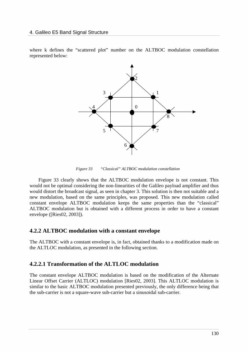
4. Galileo E5 Band Signal Structure

130

where k defines the “scattered plot” number on the ALTBOC modulation constellation represented below:

Figure 33 “Classical” ALTBOC modulation constellation

Figure 33 clearly shows that the ALTBOC modulation envelope is not constant. This would not be optimal considering the non-linearities of the Galileo payload amplifier and thus would distort the broadcast signal, as seen in chapter 3. This solution is then not suitable and a new modulation, based on the same principles, was proposed. This new modulation called constant envelope ALTBOC modulation keeps the same properties than the “classical” ALTBOC modulation but is obtained with a different process in order to have a constant envelope ([Ries02, 2003]).

4.2.2 ALTBOC modulation with a constant envelope

The ALTBOC with a constant envelope is, in fact, obtained thanks to a modification made on the ALTLOC modulation, as presented in the following section.

4.2.2.1 Transformation of the ALTLOC modulation

The constant envelope ALTBOC modulation is based on the modification of the Alternate Linear Offset Carrier (ALTLOC) modulation [Ries02, 2003]. This ALTLOC modulation is similar to the basic ALTBOC modulation presented previously, the only difference being that the sub-carrier is not a square-wave sub-carrier but a sinusoidal sub-carrier.

0

1

2

3

4

5

6

7

8

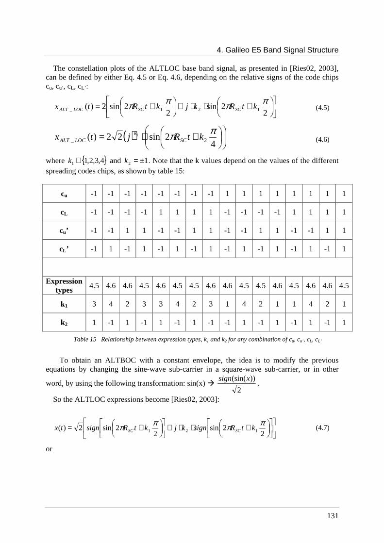
4. Galileo E5 Band Signal Structure

131

The constellation plots of the ALTLOC base band signal, as presented in [Ries02, 2003], can be defined by either Eq. 4.5 or Eq. 4.6, depending on the relative signs of the code chips cu, cu’, cL, cL’ :

+⋅⋅+

+=2

2sin2

2sin2)( 121_

ππππ ktRkjktRtx SCSCLOCALT (4.5)

( )

+⋅=4

2sin22)( 2_1

ππ ktRjtx SCk

LOCALT (4.6)

where 4,3,2,11 ∈k and 12 ±=k . Note that the k values depend on the values of the different spreading codes chips, as shown by table 15:

cu -1 -1 -1 -1 -1 -1 -1 -1 1 1 1 1 1 1 1 1

cL -1 -1 -1 -1 1 1 1 1 -1 -1 -1 -1 1 1 1 1

cu’ -1 -1 1 1 -1 -1 1 1 -1 -1 1 1 -1 -1 1 1

cL ’ -1 1 -1 1 -1 1 -1 1 -1 1 -1 1 -1 1 -1 1

Expression types

4.5 4.6 4.6 4.5 4.6 4.5 4.5 4.6 4.6 4.5 4.5 4.6 4.5 4.6 4.6 4.5

k1 3 4 2 3 3 4 2 3 1 4 2 1 1 4 2 1

k2 1 -1 1 -1 1 -1 1 -1 -1 1 -1 1 -1 1 -1 1

Table 15 Relationship between expression types, k1 and k2 for any combination of cu, cu’, cL, cL’

To obtain an ALTBOC with a constant envelope, the idea is to modify the previous

equations by changing the sine-wave sub-carrier in a square-wave sub-carrier, or in other

word, by using the following transformation: sin(x) 2

))(sin(xsign.

So the ALTLOC expressions become [Ries02, 2003]:

+⋅⋅+

+=2

2sin2

2sin2)( 121

ππππ ktRsignkjktRsigntx SCSC (4.7)

or

4. Galileo E5 Band Signal Structure

132

( )

+⋅=4

2sin2)( 21

ππ ktRsignjtx SCk

(4.8)

with 4,3,2,11 ∈k , 12 ±=k

These expressions enable to write x(t) thanks to the simple equation below because the

signal phase takes exactly 8 different values:

42)(π

jketx ⋅= 8,7,6,5,4,3,2,1∈k (4.9)

Figure 34 represents the modulation constellation corresponding to Eq. 4.9. It shows that

the signal obtained has a constant envelope, while using a complex square-wave sub-carrier. That is why the modulation presented and introduced by the CNES [Lestarquit, 2002], is called constant envelope ALTBOC modulation.

Figure 34 Constant envelope ALTBOC or ALTBOC 8-PSK modulation constellation

This definition of the constant envelope ALTBOC modulation will be used to generate the E5 signal in the Galileo payload. Note that the modulation could easily be implemented using simple look-up tables for the phase assignments. As seen above, the ALTBOC features an 8-PSK constellation. The idea is here to allocate any of the 4 codes and 8 sub-carrier phases combinations to a phase spot in the constellation, using a look-up table, and then to generate the corresponding I and Q signals. The value of the constellation spot is a function of the value of the 4 codes [-1 or +1], and the carrier period is divided into 8 time bins (related to the k values), as shown by table 16. There are 4 binary codes, resulting in 16 (24) code combinations: this means that there are a total of 128 different phase plots, whose value may vary between 1 and 8. Figure 35 presents a simple ALTBOC generation diagram and the table 16 an example of a look-up table associated [Ries02, 2003].

6

1 2

3

4

5 7

8

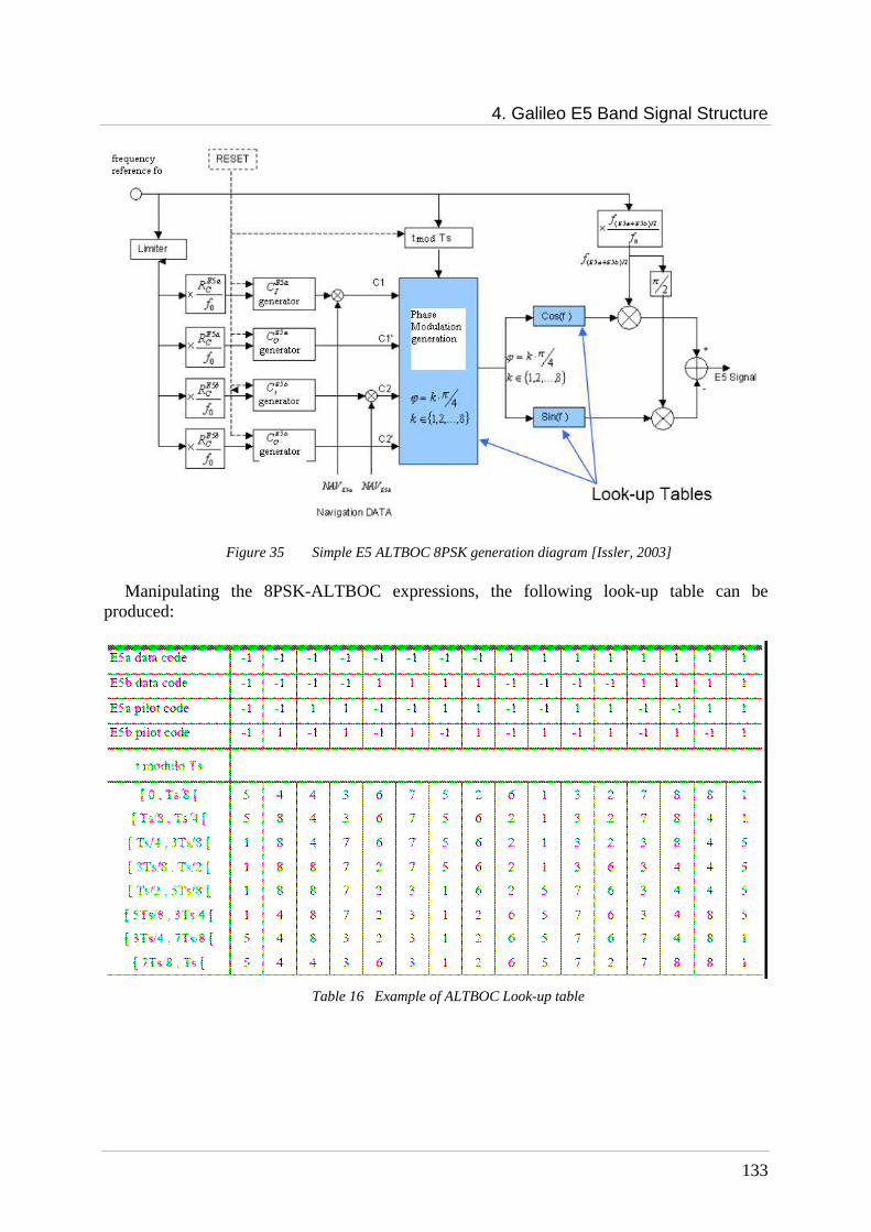
4. Galileo E5 Band Signal Structure

133

Figure 35 Simple E5 ALTBOC 8PSK generation diagram [Issler, 2003]

Manipulating the 8PSK-ALTBOC expressions, the following look-up table can be produced:

Table 16 Example of ALTBOC Look-up table

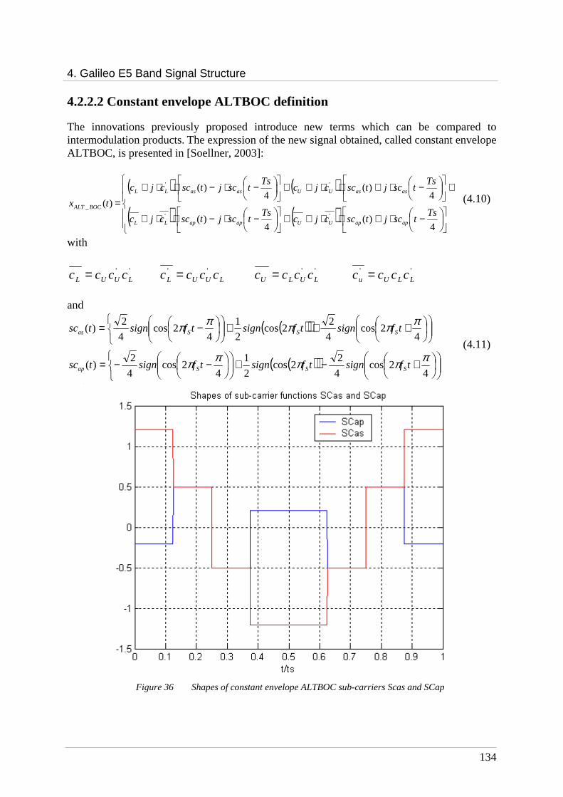
4. Galileo E5 Band Signal Structure

134

4.2.2.2 Constant envelope ALTBOC definition

The innovations previously proposed introduce new terms which can be compared to intermodulation products. The expression of the new signal obtained, called constant envelope ALTBOC, is presented in [Soellner, 2003]:

( ) ( )

( ) ( )

−⋅+⋅⋅++

−⋅−⋅⋅+

+

−⋅+⋅⋅++

−⋅−⋅⋅+=

4)(

4)(

4)(

4)(

)(''

''

_Ts

tscjtsccjcTs

tscjtsccjc

Tstscjtsccjc

Tstscjtsccjc

tx

apapUUapapLL

asasUUasasLL

BOCALT (4.10)

with

'''''''' LLUuLULULUULLUUL cccccccccccccccc ====

and

( )( )

( )( )

+−+

−−=

+++

−=

42cos

4

22cos

2

1

42cos

4

2)(

42cos

4

22cos

2

1

42cos

4

2)(

πππππ

πππππ

tfsigntfsigntfsigntsc

tfsigntfsigntfsigntsc

SSSap

SSSas

(4.11)

Figure 36 Shapes of constant envelope ALTBOC sub-carriers Scas and SCap

4. Galileo E5 Band Signal Structure

135

It can be seen that the first line of Eq. 4.10 represents the useful signal and is composed, as expected of 4 channels: the E5a data and pilot channels (on an in-phase/quadra-phase scheme) on the left part, and the E5b data and pilot channels (on an in-phase/quadra-phase scheme) on the right part.

It has to be noticed also that the second line of Eq. 4.10 represents additional terms that are not useful signal but intermodulation products. They are necessary to keep a constant envelope, but will consume a small part of the overall power. Consequently, they will take a short fraction of the available power for the useful signal, equal to 15% according to [Soellner, 2003]. It has also to be noted that the presented equations don’t take into account the filtering processes which might be applied in the future GALILEO payloads.

The next tables present the look-up tables corresponding to Eq. 4.10 in function of code

signs and sub-carriers values. These look-up tables are equivalent to the look-up table presented in table 17, the constant envelope ALTBOC can so really be expressed by Eq. 4.10.

CL -1 -1 -1 -1 -1 -1 -1 -1 1 1 1 1 1 1 1 1 Cu -1 -1 -1 -1 1 1 1 1 -1 -1 -1 -1 1 1 1 1 CL ' -1 -1 1 1 -1 -1 1 1 -1 -1 1 1 -1 -1 1 1 Cu' -1 1 -1 1 -1 1 -1 1 -1 1 -1 1 -1 1 -1 1

t 0:Ts/8 Ts/8:Ts/4 Ts/4:3Ts/8 3Ts/8:Ts/2 Ts/2:5Ts/8 5Ts/8:3Ts/4 3Ts/4:7Ts/8 7Ts/8:Ts

Scas(t) 1,2 0,5 -0,5 -1,2 -1,2 -0,5 0,5 1,2

Scas(t+Ts/4) -0,5 -1,2 -1,2 -0,5 0,5 1,2 1,2 0,5

Scap(t) -0,2 0,5 -0,5 0,2 0,2 -0,5 0,5 -0,2

Scap(t+Ts/4) -0,5 0,2 0,2 -0,5 0,5 -0,2 -0,2 0,5

t k scattered plot

0:Ts/8 5 4 4 3 6 7 5 2 6 1 3 2 7 8 8 1

Ts/8:Ts/4 5 8 4 3 6 7 5 6 2 1 3 2 7 8 4 1

Ts/4:3Ts/8 1 8 4 7 6 7 5 6 2 1 3 2 3 8 4 5

3Ts/8:Ts/2 1 8 8 7 2 7 5 6 2 1 3 6 3 4 4 5

Ts/2:5Ts/8 1 8 8 7 2 3 1 6 2 5 7 6 3 4 4 5

5Ts/8:3Ts/4 1 4 8 7 2 3 1 2 6 5 7 6 3 4 8 5

3Ts/4:7Ts/8 5 4 8 3 2 3 1 2 6 5 7 6 7 4 8 1

7Ts/8:Ts 5 4 4 3 6 3 1 2 6 5 7 2 7 8 8 1

Table 17 Constant envelope ALTBOC look-up tables

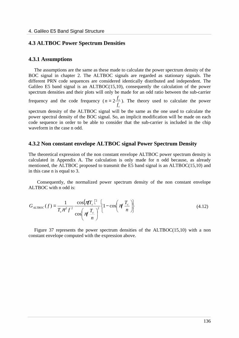
4. Galileo E5 Band Signal Structure

136

4.3 ALTBOC Power Spectrum Densities

4.3.1 Assumptions

The assumptions are the same as these made to calculate the power spectrum density of the BOC signal in chapter 2. The ALTBOC signals are regarded as stationary signals. The different PRN code sequences are considered identically distributed and independent. The Galileo E5 band signal is an ALTBOC(15,10), consequently the calculation of the power spectrum densities and their plots will only be made for an odd ratio between the sub-carrier

frequency and the code frequency (c

s

f

fn 2= ). The theory used to calculate the power

spectrum density of the ALTBOC signal will be the same as the one used to calculate the power spectral density of the BOC signal. So, an implicit modification will be made on each code sequence in order to be able to consider that the sub-carrier is included in the chip waveform in the case n odd.

4.3.2 Non constant envelope ALTBOC signal Power Spectrum Density

The theoretical expression of the non constant envelope ALTBOC power spectrum density is calculated in Appendix A. The calculation is only made for n odd because, as already mentioned, the ALTBOC proposed to transmit the E5 band signal is an ALTBOC(15,10) and in this case n is equal to 3.

Consequently, the normalized power spectrum density of the non constant envelope ALTBOC with n odd is:

( )

−

=

n

Tf

n

Tf

fT

fTfG c

c

c

cALTBOC π

π

ππ

cos1

cos

cos1)(

2

2

22 (4.12)

Figure 37 represents the power spectrum densities of the ALTBOC(15,10) with a non

constant envelope computed with the expression above.

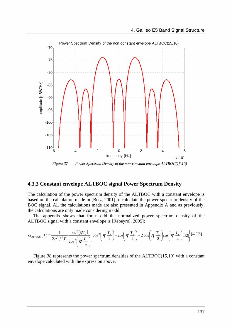
4. Galileo E5 Band Signal Structure

137

-6 -4 -2 0 2 4 6

x 107

-110

-105

-100

-95

-90

-85

-80

-75

-70

frequency [Hz]

ampl

itude

[dB

W/H

z]Power Spectrum Density of the non constant envelope ALTBOC(15,10)

Figure 37 Power Spectrum Density of the non-constant envelope ALTBOC(15,10)

4.3.3 Constant envelope ALTBOC signal Power Spectrum Density

The calculation of the power spectrum density of the ALTBOC with a constant envelope is based on the calculation made in [Betz, 2001] to calculate the power spectrum density of the BOC signal. All the calculations made are also presented in Appendix A and as previously, the calculations are only made considering n odd.

The appendix shows that for n odd the normalized power spectrum density of the ALTBOC signal with a constant envelope is [Rebeyrol, 2005]:

( )

+

−

−

= 2

4cos

2cos2

2cos

2cos

cos

cos

2

1)( 2

2

2

22ssss

c

c

c

ALTBOC

Tf

Tf

Tf

Tf

n

Tf

fT

TffG ππππ

π

ππ

(4.13)

Figure 38 represents the power spectrum densities of the ALTBOC(15,10) with a constant

envelope calculated with the expression above.

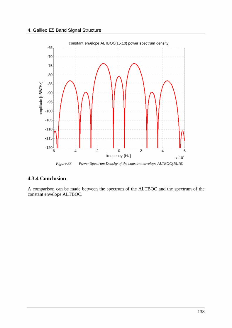
4. Galileo E5 Band Signal Structure

138

-6 -4 -2 0 2 4 6

x 107

-120

-115

-110

-105

-100

-95

-90

-85

-80

-75

-70

-65

frequency [Hz]

ampl

itude

[dB

W/H

z]constant envelope ALTBOC(15,10) power spectrum density

Figure 38 Power Spectrum Density of the constant envelope ALTBOC(15,10)

4.3.4 Conclusion

A comparison can be made between the spectrum of the ALTBOC and the spectrum of the constant envelope ALTBOC.

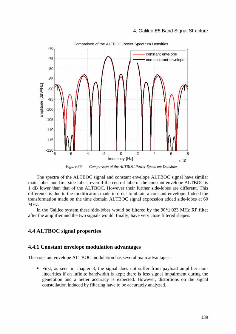
4. Galileo E5 Band Signal Structure

139

-8 -6 -4 -2 0 2 4 6 8

x 107

-120

-115

-110

-105

-100

-95

-90

-85

-80

-75

-70

frequency [Hz]

ampl

itude

[dB

W/H

z]Comparison of the ALTBOC Power Spectrum Densities

constant envelope

non constant envelope

Figure 39 Comparison of the ALTBOC Power Spectrum Densities

The spectra of the ALTBOC signal and constant envelope ALTBOC signal have similar

main-lobes and first side-lobes, even if the central lobe of the constant envelope ALTBOC is 1 dB lower than that of the ALTBOC. However their further side-lobes are different. This difference is due to the modification made in order to obtain a constant envelope. Indeed the transformation made on the time domain ALTBOC signal expression added side-lobes at 60 MHz.

In the Galileo system these side-lobes would be filtered by the 90*1.023 MHz RF filter after the amplifier and the two signals would, finally, have very close filtered shapes.

4.4 ALTBOC signal properties

4.4.1 Constant envelope modulation advantages

The constant envelope ALTBOC modulation has several main advantages: First, as seen in chapter 3, the signal does not suffer from payload amplifier non-

linearities if an infinite bandwidth is kept; there is less signal impairment during the generation and a better accuracy is expected. However, distortions on the signal constellation induced by filtering have to be accurately analyzed.

4. Galileo E5 Band Signal Structure

140

Then, the constant envelope permits also a gain in precision thanks to the possibility to transmit a coherently wideband signal and not two narrowband QPSK signals. Indeed the ALTBOC modulation does not directly improve the carrier tracking noise with respect to a BPSK modulation. But, as the ALTBOC signal is the coherent sum of the E5a and E5b components, the available C/N0 is 3 dB higher than for a loop tracking E5a or E5b only. This will lead to a reduction by half of the noise variance. The wideband ALTBOC provides also very good code tracking performance with a code tracking noise below 5 cm for C/N0 higher than 35 dB/Hz (if the pilot channel is tracked with a dot-product power discriminator) ([Sleewagen, 2005]).

Finally, the ALTBOC represents an optimisation of use of E5a and E5b signals: simple receivers can use a single band (E5a or E5b) whereas more complex receiver can operate in two modes and thus get advantages in terms of accuracy.

Indeed the ALTBOC modulation provides a very flexible signal for the user segment,

because of the various tracking configurations it allows without any major degradation: A single QPSK, on E5a or on E5b, for simple receiver. A double QPSK, on E5a and E5b independently. Thanks to the ALTBOC modulation,

which provides spectral isolation, the interferences are very low in this tracking configuration.

A BOC(15,10) reduced to its main lobes. This tracking configuration allows a high

precision while limiting the susceptibility to interference. A BOC(15,10) in a wide bandwidth for the high precision receivers.

If the upper (E5b) and the lower (E5a) bands are tracked independently as if they were

QPSK(10) signals, the correlation losses are lower than 1.5 dB compared to a full tracking.

4.4.2 Resistance to multipath

It has also been seen in chapter 3 that the resistance to multipath is a constraint on Galileo signals design. The next two figures will show that thanks to the constant envelope ALTBOC modulation this constraint is verified and that the resistance to multipath of the Galileo E5 signal is quite good thanks to an optimal spectral repartition.

Indeed, figure 40 represents multipath error envelopes plotted for different modulations. The curves show that the maximal error induced by the multipath on pseudo-range is the lowest in the case of the wideband ALTBOC signal. The signals bandwidths are chosen not to filter the main lobes of the modulation.

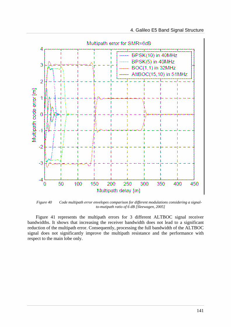
4. Galileo E5 Band Signal Structure

141

Figure 40 Code multipath error envelopes comparison for different modulations considering a signal-to-mutipath ratio of 6 dB [Sleewagen, 2005]

Figure 41 represents the multipath errors for 3 different ALTBOC signal receiver

bandwidths. It shows that increasing the receiver bandwidth does not lead to a significant reduction of the multipath error. Consequently, processing the full bandwidth of the ALTBOC signal does not significantly improve the multipath resistance and the performance with respect to the main lobe only.

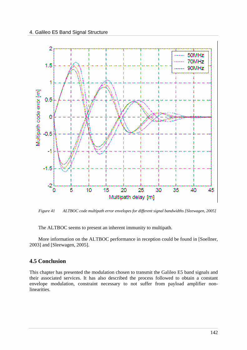
4. Galileo E5 Band Signal Structure

142

Figure 41 ALTBOC code multipath error envelopes for different signal bandwidths [Sleewagen, 2005]

The ALTBOC seems to present an inherent immunity to multipath.

More information on the ALTBOC performance in reception could be found in [Soellner,

2003] and [Sleewagen, 2005].

4.5 Conclusion

This chapter has presented the modulation chosen to transmit the Galileo E5 band signals and their associated services. It has also described the process followed to obtain a constant envelope modulation, constraint necessary to not suffer from payload amplifier non-linearities.

4. Galileo E5 Band Signal Structure

143

Moreover, constant envelope ALTBOC multipath errors envelopes have been exposed. They have shown that the ALTBOC modulation also validates the constraint of resistance to multipath.

The Galileo E5 constant envelope ALTBOC signal is so a very interesting signal thanks

to its constant envelope but also thanks to the different possibilities of tracking it offers. However, as seen in chapter 3, after being modulated the Galileo signals are filtered by a

NSGU filter. This filter distorts the constant envelope of signal and phase noise is so added on the signal during the amplification. The evaluation of this phase noise and the filter bandwidth necessary to not too degrade the constant envelope will be studied in chapter 6.

145

Chapter 5

Galileo E1 Band Signal Structure

Contents 5.1 Galileo E1 band baseline signals ................................................................................... 146

5.1.1 E1 Band contents and signals ..................................................................................... 146 5.1.2 E1 Band multiplexing technique: Interplex modulation............................................. 148 5.1.3 Galileo E1F baseline signal performance ................................................................... 153

5.2 Galileo E1 band optimized signals................................................................................ 160 5.2.1 Galileo E1F optimized signals.................................................................................... 160 5.2.2 Five components Interplex modulation: application to the CBCS and CBOC cases . 164 5.2.3 E1F optimized signals performance............................................................................ 169

5.3 Conclusion....................................................................................................................... 198 After the description of the Galileo E5 signal in chapter 4, this chapter presents the other open Galileo signal: the E1 band signal in order to verify if its design follows the constraints established in chapter 3.

In June 2004, an agreement ([E. C., 2005]) has been signed between the United States of America and the European Union. This agreement adopts a common baseline to transmit both Galileo E1F signal and GPS future L1C signals. However the agreement plans a possible optimisation of the baseline and that is the reason why recently different studies have been conducted to find an enhanced signal, while still complying with the constraints imposed by the agreement.

First, the baseline signals approved by the agreement to transmit the Galileo entire E1F

and encrypted E1P signals are presented. The constant envelope modulation chosen to multiplex them, called Interplex modulation, is also exposed. Moreover the performances of the baseline E1F signal are described, in particular to evaluate its resistance to multipath, one of the impairments exposed in chapter 3.

Then, the Galileo E1F optimized signals are presented, together with the performance criteria allowing to select them. The adaptation of the Interplex modulation to these new

5. Galileo E1 Band Signal Structure

146

signals, in order to transmit them with a constant envelope, is also explained. To finish, the performance of these optimized signals will be compared with regards to receiver performances (resistance to multipath but also RMS bandwidth …) to find the most suitable signal to provide the Open service at the E1 band.

5.1 Galileo E1 band baseline signals

5.1.1 E1 Band contents and signals

The E1 band modulation should combine three distinct signals associated to four different services (as seen in chapter 2) into a phase modulated composite signal that respects the design constraints defined in chapter 3: a constant envelope at the payload amplifier input in order to optimize the link budget and the power efficiency on-board, and a good resistance to multipath.

The Galileo E1 signals, as presented in chapter 2, are respectively: The E1F signal corresponding to the OS/CS/SOL services. As already mentioned in

introduction, for June 2004, the United States of America and the European Union have signed the "Agreement on the promotion, provision and use of GALILEO and GPS satellite-based navigation systems and related applications". This agreement plans, in particular, to adopt a sine-phased BOC(1,1) signal as a baseline to transmit both Galileo E1F signals (Open Service signals) and GPS future L1C signals. So, o the carrier of the E1F data channel corresponding to the data OS/CS/SOL

services is modulated by three components: the E1F navigation data stream, the E1F data channel PRN tiered code sequence and the E1F sine-phased BOC(1,1) sub-carrier. This signal is often called data Open Service signal, noted OSA.

o the carrier of the E1F pilot channel corresponding to the pilot OS/CS/SOL services is modulated by two components: the E1F pilot channel PRN tiered code sequence and the E1F sine-phased BOC(1,1) sub-carrier. This signal is often called pilot Open Service signal, noted OSB.

The E1P channel corresponding to the PRS service. To transmit the E1P signal, a

cosine-phased BOC(15,2.5) was adopted in [GJU, 2005]. So, for this signal, the carrier is modulated by three components: the E1P navigation data stream, the E1P channel PRN tiered code sequence and the E1P cosine-phased BOC(15,2.5) sub-carrier. This cosine BOC(15,2.5) signal is the E1 PRS baseline, according to the 2004 US/EU agreement.

The power spectrum densities of the Galileo baseline signals are represented in figure 42:

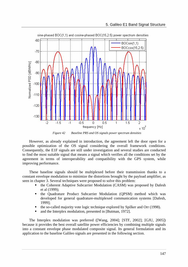
5. Galileo E1 Band Signal Structure

147

Figure 42 Baseline PRS and OS signals power spectrum densities

However, as already explained in introduction, the agreement left the door open for a

possible optimization of the OS signal considering the overall framework conditions. Consequently, the E1F signals are still under investigation and several studies are conducted to find the most suitable signal that means a signal which verifies all the conditions set by the agreement in terms of interoperability and compatibility with the GPS system, while improving performance.

These baseline signals should be multiplexed before their transmission thanks to a constant envelope modulation to minimize the distortions brought by the payload amplifier, as seen in chapter 3. Several techniques were proposed to solve this problem:

the Coherent Adaptive Subcarrier Modulation (CASM) was proposed by Dafesh et al (1999);

the Quadrature Product Subcarrier Modulation (QPSM) method which was developed for general quadrature-multiplexed communication systems [Dafesh, 1999];

the so-called majority vote logic technique explored by Spilker and Orr (1998). and the Interplex modulation, presented in [Butman, 1972].

The Interplex modulation was preferred ([Wang, 2004]; [STF, 2002]; [GJU, 2005])

because it provides the best overall satellite power efficiencies by combining multiple signals into a constant envelope phase modulated composite signal. Its general formulation and its application to the baseline Galileo signals are presented in the following section.

5. Galileo E1 Band Signal Structure

148

5.1.2 E1 Band multiplexing technique: Interplex modulation

In the E1 band, the objective of the multiplexing technique is different than in the E5 band, even if the final result should be the same: a constant envelope modulated signal. The E1 band modulation should multiplex three distinct components associated to two different services into a phase-modulated signal. This can be realized by the Interplex modulation.

5.1.2.1 General definition of the Interplex modulation

Indeed, the Interplex modulation is a phase-shift-keyed/phase modulation (PSK/PM), combining multiple signals into a phase modulated composite signal, as shown by its general form, presented in [Butman, 1972]:

( )( ) 2cos)( ϕθπ ++⋅= ttfts C (5.1)

where fC is the carrier frequency, )(tθ the phase modulation and ϕ a random phase.

In GNSS applications and more particularly in the Galileo system, the phase modulation is defined as ([Butman, 1972]):

( ) ( ) ( ) ( ) 2

111 ∑=

⋅⋅+=N

nnn tststst ββθ with ( ) 1±=tsn (5.2)

and where N is the number of multiplexed signals sn(t), and nβ is the modulation angle or modulation index.

The value of the modulation indexesnβ determines the power allocation for each signal

component.

In the baseline case, the Interplex should multiplex three distinct signals: two BOC(1,1) sub-carriers (data and pilot Open Service signals) and one BOCcos(15,2.5) sub-carrier (PRS signal), consequently N is equal to 3.

5.1.2.2 Three components Interplex modulation: application to the E1 band baseline configuration

5.1.2.2.1 Formulation

As mentioned previously, if the baseline signals are considered, three components are multiplexed on the same carrier. Without loss of generality, it can be assumed that:

one signal will be in the quadrature channel, s1 two signals will be in the in-phase channel, s2 and s3

Thus, the general formula of a three components Interplex signal can be expressed as

([Rebeyrol01, 2006]):

5. Galileo E1 Band Signal Structure

149

( ) ( ) ( ) ( ) ( )

+⋅⋅+⋅⋅+⋅−⋅= ϕββππ tstststststfts c 313212122cos)( (5.3)

Note that 1β is taken equal to 2/π− because the signal s1 has been chosen in quadrature with the two others signals.

By developing Eq. 5.3, it can be shown, considering binary signals, that:

( ) ( ) ( ) ( ) ( ) ( )( ) ( )( ) ( ) ( ) ( ) ( ) ( ) ( ) ( )( ) ( )

+⋅⋅⋅⋅⋅−⋅++⋅⋅⋅+⋅

=ϕπββββ

ϕπββββtftstststs

tftststs

c

c

2sinsinsincoscos

2cossincoscossin)(

32321321

323322 (5.4)

Thanks to Eq. 5.4, it can be noticed that the first three terms correspond to the desired

useful signal terms s1, s2, s3; the fourth term is an undesired intermodulation (IM) term. This IM term is equal to the product of the three desired signals balanced by the

modulation indexes2β and 3β . As in the case of the constant ALTBOC modulation, this term,

even if it permits to obtain a constant envelope, consumes a short fraction of the total transmitted power available for the three desired signals. Thus a small part of the transmitted power is used through this IM component and is removed from the useful signal. However, differently from the ALTBOC modulation, the modulation indexes, although dependant upon the final signal configuration, can allow the minimization of the power consumed by the IM component. This can be shown when looking at the expressions of the power of each component, obtained while assuming orthogonal signal codes:

( ) ( )( ) ( )( ) ( )( ) ( )3

22

2

32

22

3

32

22

2

32

22

1

sinsin

sincos

cossin

coscos

ββββββββ

⋅=

⋅=

⋅=

⋅=

IMP

P

P

P

(5.5)

These equations show that a trade-off must be made to have sufficient power on the desired signals and non-disadvantageous power on the IM signal.

5.1.2.2.2 Galileo E1F BOC(1,1) signal

If the current Galileo E1 OS baseline signals are considered, two signals are transmitted in the in-phase component ([GJU, 2005]):

the data OS signal: a BOC(1,1) signal s2, composed of data, code and sub-carrier, ( )( ) )(6023.12sin)()()( 222 tsPtesigntdtcPts DDOSA ⋅=⋅⋅⋅⋅⋅= π

the pilot OS signal: a BOC(1,1) signal s3, composed of code and sub-carrier, ( )( ) )(6023.12sin)()( 333 tsPtesigntcPts POSB ⋅=⋅⋅⋅⋅= π

The quadratrure channel transmits the PRS signal:

( )( ) )(6023.1152cos)()()( 111 tsPtesigntdtcPts PRSPRSPRS ⋅=⋅⋅⋅⋅⋅⋅= π

5. Galileo E1 Band Signal Structure

150

The formulation of the three components Interplex can be applied, so:

( ) ( ) ( ) ( ) ( ) ( )( ) ( )( ) ( ) ( ) ( ) ( ) ( ) ( ) ( )( ) ( )

+⋅⋅⋅⋅⋅−⋅++⋅⋅⋅+⋅

=ϕπββββ

ϕπββββtftstststs

tftststs

c

c

2sinsinsincoscos

2cossincoscossin)(

32321321

323322

and

( ) ( )( ) ( )( ) ( )

( ) ( )32

22

32

22

3

32

22

2

32

22

1

sinsin

sincos

cossin

coscos

ββββββββ

⋅=

⋅==

⋅==

⋅==

IM

OSB

OSA

PRS

P

PP

PP

PP

In this case, according to [GJU, 2005], the total power should be equally divided into the

in-phase and the quadrature components. Moreover the power of the data OS component should be equal to the power of the pilot OS component. Consequently, the parameters2β and

3β are constrained by the following relationships:

( ) ( ) ( ) ( )( ) ( ) ( ) ( )

⋅=⋅==

⋅⋅=⋅=

32

22

32

22

32

32

22

32

22

1

sincoscossin

cossin2coscos

ββββββββ

PP

P (5.6)

This system leads to 6155.032 ==−= mββ radians and P1=-3.52 dB, P2=P3=-6.53 dB.

Consequently, the expression of the transmitted signal is:

( ) ( ) ( ) ( ) ( ) 2

2cos)( 31211

+⋅⋅−⋅⋅+⋅−⋅= ϕππ tstsmtstsmtstfts c (5.7)

or

( ) ( ) ( ) ( ) ( ) ( )( ) ( )( ) ( ) ( ) ( ) ( ) ( )( ) ( )

2sinsincos

2cossincoscossin)(

2321

21

32

+⋅⋅⋅⋅⋅+⋅+

+⋅⋅⋅−⋅=

ϕπϕπ

tfmtststsmts

tfmmtsmmtsts

c

c (5.8)

As foreseen, the IM term is the product of the signals s1, s2 and s3, so in this case, it is a

BOCcos(15,2.5) as the PRS signal. The power used for the IM is thus equal to -9.54 dB compared to the unit power of the global Interplex signal.

The different states of the Interplex signal can be represented on a phase diagram whose

x-axis is the in-phase component and whose y-axis is the quadrature component. For the present case, the diagram of the modulation constellation is represented in figure 43:

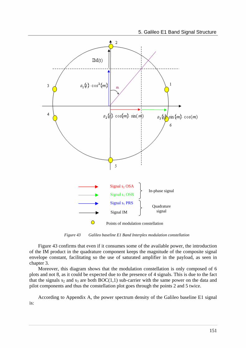
5. Galileo E1 Band Signal Structure

151

Figure 43 Galileo baseline E1 Band Interplex modulation constellation

Figure 43 confirms that even if it consumes some of the available power, the introduction of the IM product in the quadrature component keeps the magnitude of the composite signal envelope constant, facilitating so the use of saturated amplifier in the payload, as seen in chapter 3.

Moreover, this diagram shows that the modulation constellation is only composed of 6 plots and not 8, as it could be expected due to the presence of 4 signals. This is due to the fact that the signals s2 and s3 are both BOC(1,1) sub-carrier with the same power on the data and pilot components and thus the constellation plot goes through the points 2 and 5 twice.

According to Appendix A, the power spectrum density of the Galileo baseline E1 signal is:

Signal s3 OSB

Signal s1 PRS

Signal IM

In-phase signal

Quadrature signal

Points of modulation constellation

Signal s2 OSA

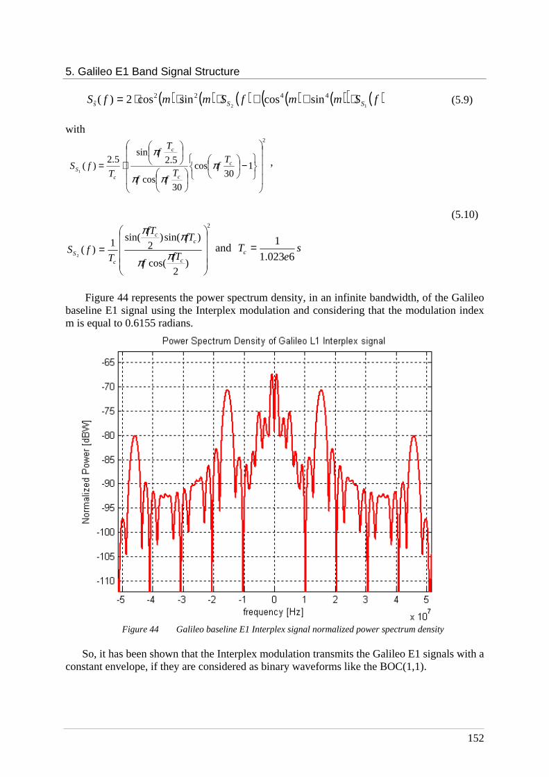
5. Galileo E1 Band Signal Structure

152

( ) ( ) ( ) ( ) ( )( ) ( ) sincossincos2)(12

4422ˆ fSmmfSmmfS SSs ⋅++⋅⋅⋅= (5.9)

with

2

130

cos

30cos

5.2sin

5.2)(

1

−

⋅= c

c

c

cS

Tf

Tff

Tf

TfS π

ππ

π ,

(5.10)

)

2cos(

)sin()2

sin(1)(

2

2

=c

cc

cS fT

f

fTfT

TfS ππ

ππand s

eTc 6023.1

1=

Figure 44 represents the power spectrum density, in an infinite bandwidth, of the Galileo

baseline E1 signal using the Interplex modulation and considering that the modulation index m is equal to 0.6155 radians.

Figure 44 Galileo baseline E1 Interplex signal normalized power spectrum density

So, it has been shown that the Interplex modulation transmits the Galileo E1 signals with a

constant envelope, if they are considered as binary waveforms like the BOC(1,1).

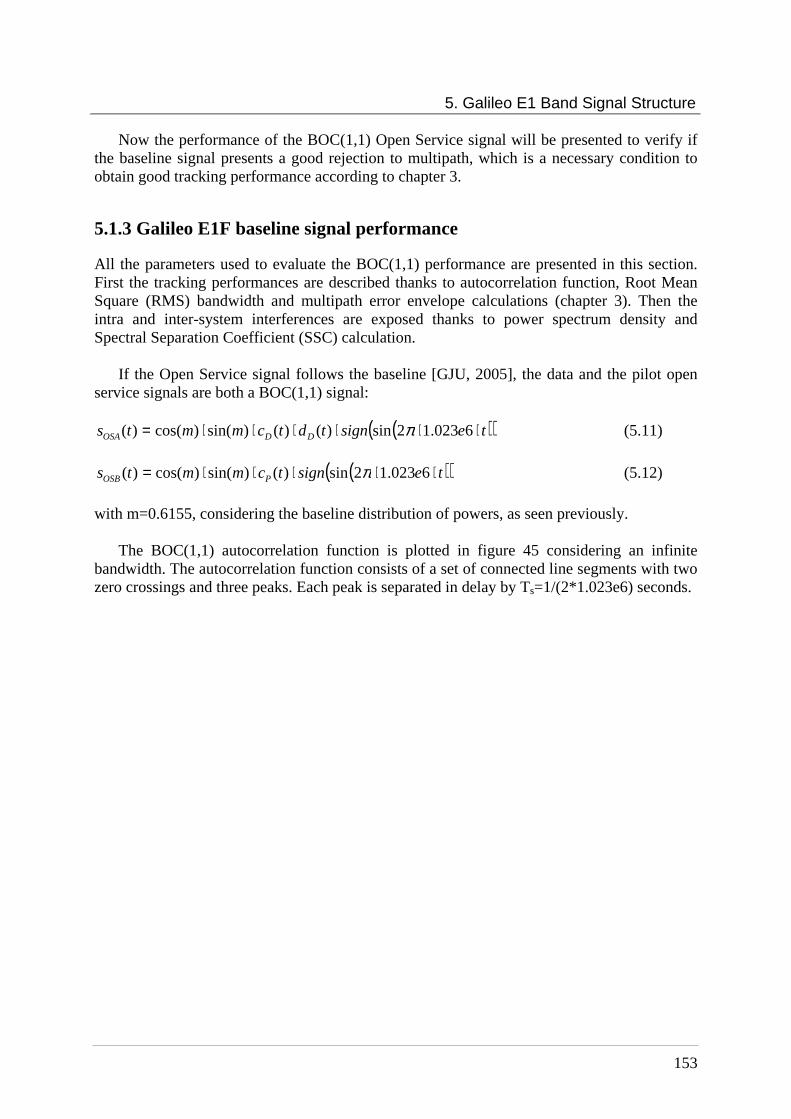
5. Galileo E1 Band Signal Structure

153

Now the performance of the BOC(1,1) Open Service signal will be presented to verify if the baseline signal presents a good rejection to multipath, which is a necessary condition to obtain good tracking performance according to chapter 3.

5.1.3 Galileo E1F baseline signal performance

All the parameters used to evaluate the BOC(1,1) performance are presented in this section. First the tracking performances are described thanks to autocorrelation function, Root Mean Square (RMS) bandwidth and multipath error envelope calculations (chapter 3). Then the intra and inter-system interferences are exposed thanks to power spectrum density and Spectral Separation Coefficient (SSC) calculation.

If the Open Service signal follows the baseline [GJU, 2005], the data and the pilot open service signals are both a BOC(1,1) signal:

( )( )tesigntdtcmmts DDOSA ⋅⋅⋅⋅⋅⋅= 6023.12sin)()()sin()cos()( π (5.11)

( )( )tesigntcmmts POSB ⋅⋅⋅⋅⋅= 6023.12sin)()sin()cos()( π (5.12)

with m=0.6155, considering the baseline distribution of powers, as seen previously.

The BOC(1,1) autocorrelation function is plotted in figure 45 considering an infinite bandwidth. The autocorrelation function consists of a set of connected line segments with two zero crossings and three peaks. Each peak is separated in delay by Ts=1/(2*1.023e6) seconds.

5. Galileo E1 Band Signal Structure

154

Figure 45 BOC(1,1) autocorrelation function in an infinite bandwidth

The main autocorrelation peak is narrow compared to the autocorrelation peak of a

BPSK(1) signal (like the C/A code), which leads to good tracking performance. But the secondary peaks are sufficiently high to lead to potential false peaks acquisition and biased tracking if it is performed using direct BOC signal acquisition and tracking algorithm. That is the reason why different new algorithms have been proposed to avoid the ambiguity due to the secondary peaks ([Heiries, 2004], [Julien, 2005]).

The Root Mean Square (RMS) bandwidth, whose expression is:

∫ ⋅⋅=B

RMS dffSf )(2β (5.13)

with B the double-sided signal bandwidth and S(f) the signal power spectrum density

([Van Trees, 1968], [Betz, 2002]), enables to compare tracking performance for different waveforms. Indeed, a lower bound on code-tracking accuracy in white noise can be obtained using the RMS bandwidth.

The expression of the smallest RMS code-tracking error that can be achieved in white noise using any discriminator is:

0

2

1

N

CBL

RMSLB

λπβσ = (5.14)

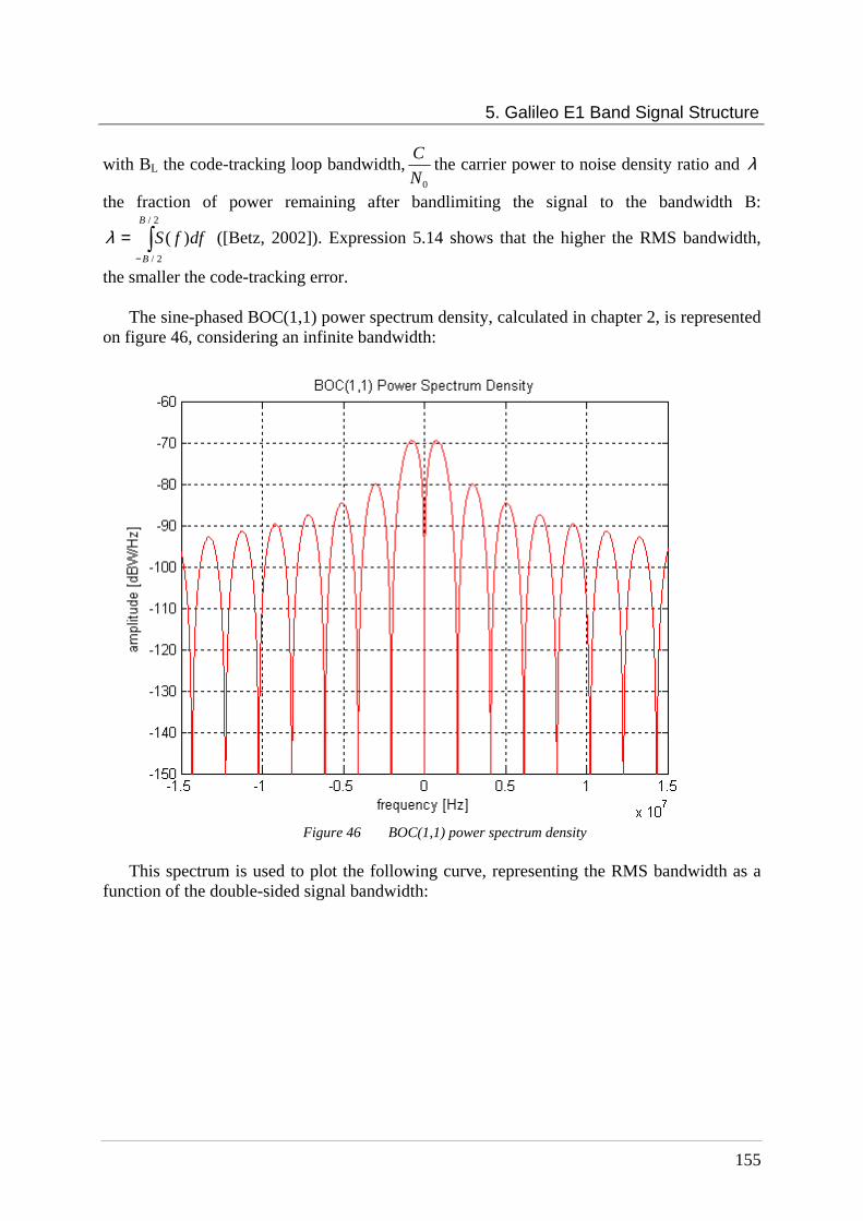
5. Galileo E1 Band Signal Structure

155

with BL the code-tracking loop bandwidth,0N

Cthe carrier power to noise density ratio and λ

the fraction of power remaining after bandlimiting the signal to the bandwidth B:

∫−

=2/

2/

)(B

B

dffSλ ([Betz, 2002]). Expression 5.14 shows that the higher the RMS bandwidth,

the smaller the code-tracking error.

The sine-phased BOC(1,1) power spectrum density, calculated in chapter 2, is represented on figure 46, considering an infinite bandwidth:

Figure 46 BOC(1,1) power spectrum density

This spectrum is used to plot the following curve, representing the RMS bandwidth as a

function of the double-sided signal bandwidth:

5. Galileo E1 Band Signal Structure

156

Figure 47 BOC(1,1) signal RMS bandwidth

The greater the RMS bandwidth; the better the inherent ability to yield small tracking

errors, as explained previously. Consequently, figure 47 confirms the advantage of using a BOC(1,1) signal instead of a BPSK(1) signal like the C/A code.

To complete the study of the BOC(1,1) tracking performance, the BOC(1,1) resistance against multipath is exposed thanks to code tracking multipath error envelopes. An early-minus-late discriminator is considered with a 0.1 chip spacing. Moreover, only one multipath signal with relative amplitude equal to 0.5 with respect to the direct signal is taken into account. The curves are plotted considering a 12 and 24 MHz receiver bandwidths.

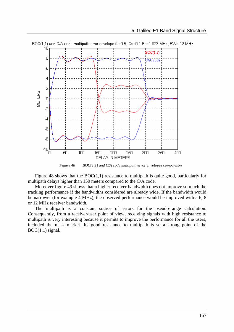
5. Galileo E1 Band Signal Structure

157

Figure 48 BOC(1,1) and C/A code multipath error envelopes comparison

Figure 48 shows that the BOC(1,1) resistance to multipath is quite good, particularly for

multipath delays higher than 150 meters compared to the C/A code. Moreover figure 49 shows that a higher receiver bandwidth does not improve so much the

tracking performance if the bandwidths considered are already wide. If the bandwidth would be narrower (for example 4 MHz), the observed performance would be improved with a 6, 8 or 12 MHz receiver bandwidth.

The multipath is a constant source of errors for the pseudo-range calculation. Consequently, from a receiver/user point of view, receiving signals with high resistance to multipath is very interesting because it permits to improve the performance for all the users, included the mass market. Its good resistance to multipath is so a strong point of the BOC(1,1) signal.

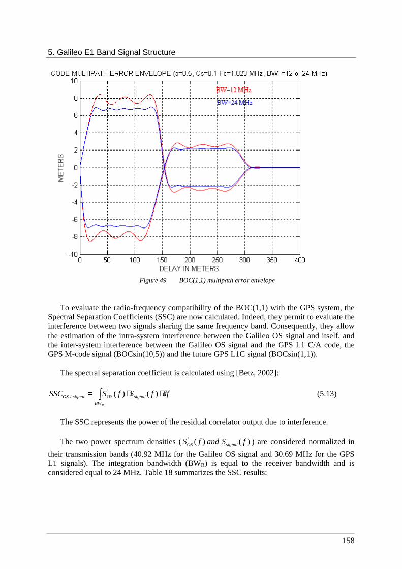
5. Galileo E1 Band Signal Structure

158

Figure 49 BOC(1,1) multipath error envelope

To evaluate the radio-frequency compatibility of the BOC(1,1) with the GPS system, the

Spectral Separation Coefficients (SSC) are now calculated. Indeed, they permit to evaluate the interference between two signals sharing the same frequency band. Consequently, they allow the estimation of the intra-system interference between the Galileo OS signal and itself, and the inter-system interference between the Galileo OS signal and the GPS L1 C/A code, the GPS M-code signal (BOCsin(10,5)) and the future GPS L1C signal (BOCsin(1,1)).

The spectral separation coefficient is calculated using [Betz, 2002]:

dffSfSSSCRBW

signalOSsignalOS ⋅⋅= ∫ )()( ''/ (5.13)

The SSC represents the power of the residual correlator output due to interference. The two power spectrum densities ( )( )( '' fSandfS signalOS ) are considered normalized in

their transmission bands (40.92 MHz for the Galileo OS signal and 30.69 MHz for the GPS L1 signals). The integration bandwidth (BWR) is equal to the receiver bandwidth and is considered equal to 24 MHz. Table 18 summarizes the SSC results:

5. Galileo E1 Band Signal Structure

159

Intra system SSC Inter system SSC

Self SSC GPS L1 C/A GPS M-code GPS L1C

BOC(1,1) baseline -64.74 dB/Hz -67.78 dB/Hz -82.29 dB/Hz -64.71 dB/Hz

Table 18 Spectral Separation Coefficient considering the Galileo baseline signal

The BOC(1,1) Open Service signal exhibits the best spectral isolation with the GPS M-

code; this result is in accordance with the spectral repartition of the different signals, as presented in figure 50. The SSC value obtained for the interference with the GPS L1C is similar to the intra-system SSC value because the baseline signals considered for Galileo OS and GPS L1C were both BOC(1,1).

Figure 50 GPS and Galileo signals power spectrum densities

These SSC values will be used as a benchmark to evaluate the intra and inter system

interferences with the optimized Open Service signals.

This section has presented and described the Galileo signals approved by the 2004 EU/US agreement. However, as already explained, the agreement left the door open for a possible optimization of the Galileo Open Service signal considering the overall framework conditions. Consequently, the E1F signals were still under investigation until a recent

5. Galileo E1 Band Signal Structure

160

agreement, signed in July 2007, notifying that EU and USA have adopted a jointly optimized signal for the GPS L1C and the Galileo E1 OS, called MBOC (Multiplexed-BOC). This chosen signal will be presented afterwards.

Several studies have so been conducted to find the most suitable signal, that means a signal which verifies all the conditions set by the agreement (interoperability and radio-frequency compatibility with the GPS system) while having improved performance.

To improve the tracking performance, the RMS bandwidth equations show that power should be added to the high frequencies components. Indeed, if the repartition of the signal power is higher for high frequencies, the RMS bandwidth is improved and the code-tracking error is reduced. One of the idea to optimize the OS signals ([Hein, 2005], [Avila-Rodriguez, 2006]) is so to combine a strong BOC(1,1) component with another square sub-carrier whose frequency is higher. Thus, the strong BOC(1,1) component permits to keep a narrow bandwidth signal (and a limited sampling frequency) with good tracking performance, and a compatibility with mass-market receivers designed to receive only BOC(1,1) signals. The high frequencies component permits, as for it, to improve the tracking performance for “more specialized” receivers/users.

5.2 Galileo E1 band optimized signals

This section will describe the optimized waveforms proposed to transmit the Open Service signal. As these new waveforms are based on the addition of a new component to the BOC(1,1), the Interplex modulation should be modified to be able to transmit not anymore three but five components with a constant envelope. The adaptation of the E1 band multiplexing will also be presented. Finally, the performances of three optimized signals, chosen according to criteria set out in this section, are exposed to evaluate the provided improvement, particularly in terms of multipath performance.

5.2.1 Galileo E1F optimized signals

Two main new signals have been studied to optimize the Open Service signal before the 2007 agreement: the Composite Binary Coded Symbol (CBCS) ([Hein, 2005]) and the Composite Binary Offset Carrier ([Avila-Rodriguez, 2006]).

5.2.1.1 CBCS signal

The Composite Binary Coded Symbol (CBCS) signal is expressed by a linear combination of a BOC(1,1) signal and a BCS signal with the same chip rate ([Hein, 2005]) :

)1],...([)1,1()( 1 mppBCSQBOCPts ⋅+⋅= (5.14)

where P and Q are values in % under the condition P+Q=100 %. The signal, noted BCS, is a Binary Coded Symbols signal, defined in [Hegarty, 2003] and [Hegarty, 2004]. It is generated using a general modulation technique referred to as direct sequence spread spectrum (DSSS) and represented as:

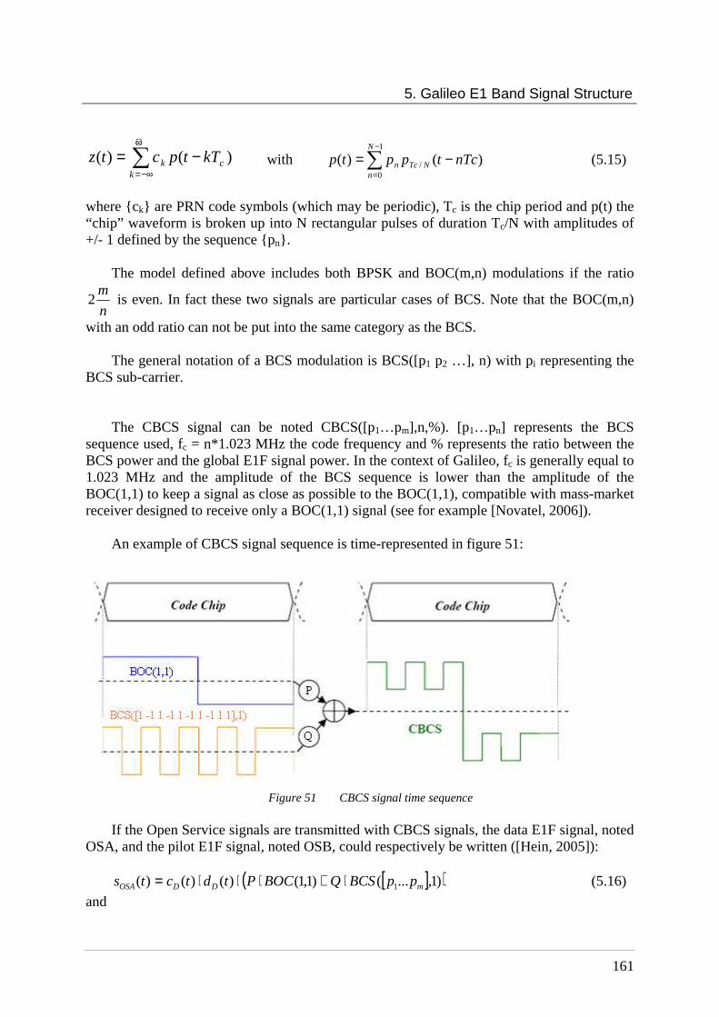
5. Galileo E1 Band Signal Structure

161

)()( ck

k kTtpctz −= ∑+∞

−∞= with ∑

−

=

−=1

0/ )()(

N

nNTcn nTctpptp (5.15)

where ck are PRN code symbols (which may be periodic), Tc is the chip period and p(t) the “chip” waveform is broken up into N rectangular pulses of duration Tc/N with amplitudes of +/- 1 defined by the sequence pn.

The model defined above includes both BPSK and BOC(m,n) modulations if the ratio

n

m2 is even. In fact these two signals are particular cases of BCS. Note that the BOC(m,n)

with an odd ratio can not be put into the same category as the BCS. The general notation of a BCS modulation is BCS([p1 p2 …], n) with pi representing the

BCS sub-carrier. The CBCS signal can be noted CBCS([p1…pm],n,%). [p1…pn] represents the BCS

sequence used, fc = n*1.023 MHz the code frequency and % represents the ratio between the BCS power and the global E1F signal power. In the context of Galileo, fc is generally equal to 1.023 MHz and the amplitude of the BCS sequence is lower than the amplitude of the BOC(1,1) to keep a signal as close as possible to the BOC(1,1), compatible with mass-market receiver designed to receive only a BOC(1,1) signal (see for example [Novatel, 2006]).

An example of CBCS signal sequence is time-represented in figure 51:

Figure 51 CBCS signal time sequence

If the Open Service signals are transmitted with CBCS signals, the data E1F signal, noted

OSA, and the pilot E1F signal, noted OSB, could respectively be written ([Hein, 2005]):

[ ]( ))1,...()1,1()()()( 1 mDDOSA ppBCSQBOCPtdtcts ⋅+⋅⋅⋅= (5.16)

and

5. Galileo E1 Band Signal Structure

162

[ ]( ))1,...()1,1()()( 1 mPOSB ppBCSQBOCPtcts ⋅−⋅⋅= (5.17)

with cD and cP respectively the data and pilot codes, dD the data stream for the data channel and BOC and BCS respectively the BOC and BCS sub-carriers. An addition between the BOC(1,1) and the BCS component is realized on the OSA component while a subtraction is realized on the OSB component so that the cross-correlation terms between the BOC(1,1) and the BCS cancel each other out to obtain a Galileo OS signal power spectrum density equal to the sum of a BOC(1,1) signal power spectrum density with a BCS signal power spectrum density, as it will be shown later.

Note also that the data and the pilot signals are interchangeable and that the most performing component would be allocated to the pilot signal because the tracking process is likely to be realized on the pilot component.

According to the power definition of a periodic signal, the OSA and OSB signals powers are equal to:

[ ]( )[ ] dtppBCSQBOCPtdtcT

PcT

mDDc

OSA ⋅⋅+⋅⋅⋅= ∫0

21 )1,...()1,1()()(

1 with Tc the code chip rate

[ ]( ) dtppBCSBOCT

QPQPPcT

mc

OSA ⋅⋅⋅⋅++= ∫0

122 )1,...()1,1(

12 (5.18)

[ ]( ) dtppBCSBOCT

QPQPPcT

mc

OSB ⋅⋅⋅⋅−+= ∫0

122 )1,...()1,1(

12 (5.19)

and the Open Service signal power is : 22 22 QPPOS += . (5.20)

So, 22

2

%QP

Q

P

P

OS

BCS

+==

The CBCS waveform associated to the OSA signal is thus noted CBCS([p1…pm],1, 22

2

QP

Q

+,

“+”) and the CBCS waveform associated to the OSB signal is noted CBCS([p1…pm],1,

22

2

QP

Q

+, “-”).

5.2.1.2 CBOC signal

The Composite BOC (CBOC) is another modulation proposed for the Galileo E1 OS signal [Hein, 2006]. It is expressed as a linear combination of a BOC(1,1) signal and another BOC signal with a higher sub-carrier frequency but the same chip rate:

)1,()1,1()( pBOCQBOCPts ⋅+⋅= (5.21)

5. Galileo E1 Band Signal Structure

163

where P and Q are values in % under the condition P+Q=100 % and fs=p*1.023 MHz represents the sub-carrier frequency of the BOC(p,1) combined with the BOC(1,1).

This signal is noted CBOC(p,1, %) where % represents the ratio between the BOC power

and the global E1F signal power. As for the CBCS case, the amplitude of the BOC sequence is, generally, lower than the amplitude of the BOC(1,1) to keep a signal as close as possible to the BOC(1,1).

The CBOC can be considered as a particular CBCS whose sub-carrier changes every bit.

The time representation of the CBOC signal is thus similar to the time representation of the CBCS signal, but the BOC(p,1) sequence is a regular alternation of 1 and -1:

Figure 52 CBOC signal time sequence

If the CBOC is proposed for the Open Service signal, the data E1F signal can be written as [Avila-Rodriguez, 2006]:

( ))1,()1,1()()()( pBOCQBOCPtdtcts DDOSA ⋅+⋅⋅⋅= (5.22)

And the pilot E1 F signal can be written as:

( ))1,()1,1()()( pBOCQBOCPtcts POSB ⋅−⋅⋅= (5.23)

with cD and cP respectively the data and pilot codes, dD the data stream for the data channel and BOC(1,1) and BOC(p,1) respectively the BOC(1,1) and BOC(p,1) sub-carriers.

An addition between the BOC(1,1) and the BOC(p,1) component is realized on the OSA component while a subtraction is realized on the OSB component so that the cross-correlation terms between the BOC(1,1) and the BOC(p,1) cancel each other out to obtain a Galileo OS signal power spectrum density equal to the sum of a BOC(1,1) signal power spectrum density with a BOC(p,1) signal power spectrum density, as it will be shown later.

5. Galileo E1 Band Signal Structure

164

Note, as for the CBCS case, that the data and the pilot signals are interchangeable and that the most performing would be allocated to the pilot signal because the tracking process is realized on the pilot component. Similar to the CBCS case,

( ) dtpBOCBOCT

QPQPPcT

cOSA ⋅⋅⋅⋅++= ∫

0

22 )1,()1,1(1

2 (5.24)

( ) dtpBOCBOCT

QPQPPcT

cOSB ⋅⋅⋅⋅−+= ∫

0

22 )1,()1,1(1

2 (5.25)

22 22 QPPOS += and 22

2

%QP

Q

P

P

OS

BCS

+==

So, the CBOC waveform proposed for the OSA signal is noted CBOC(p,1, 22

2

QP

Q

+, “+”)

and the CBOC waveform proposed for the OSB signal is noted CBOC(p,1, 22

2

QP

Q

+, “-”).

5.2.1.3 Conclusion

To conclude, new modulations have been proposed to transmit the Galileo E1F signal. The CBCS signal proposes a large variety of waveforms, whereas the CBOC, which can be considered as a particular CBCS if the code and sub-carrier frequencies ratio is even, is a simpler waveform, easier to generate because of its regular alternation of 1 and -1. But whatever the signal, one objective remains the same: multiplex the three different channels (data and pilot E1F signals and E1P signal) into a modulated constant envelope signal. The Interplex modulation, presented previously, was chosen to transmit the baseline Open Service signal. This modulation is also privileged to transmit the optimized signals but some modification must be taken into account because of the addition of the BCS or BOC(p,1) waveforms. The Interplex is not anymore a three components modulation but a five components modulation, described in the following section.

5.2.2 Five components Interplex modulation: application to the CBCS and CBOC cases

This section will focus on the application of the Interplex modulation to the two E1F optimized signals proposed: CBCS and CBOC. Indeed, for these two cases, five signals should now be considered and not only three.

5.2.2.1 Formulation

In CBCS and CBOC cases, the Interplex modulation multiplexes 5 signal components:

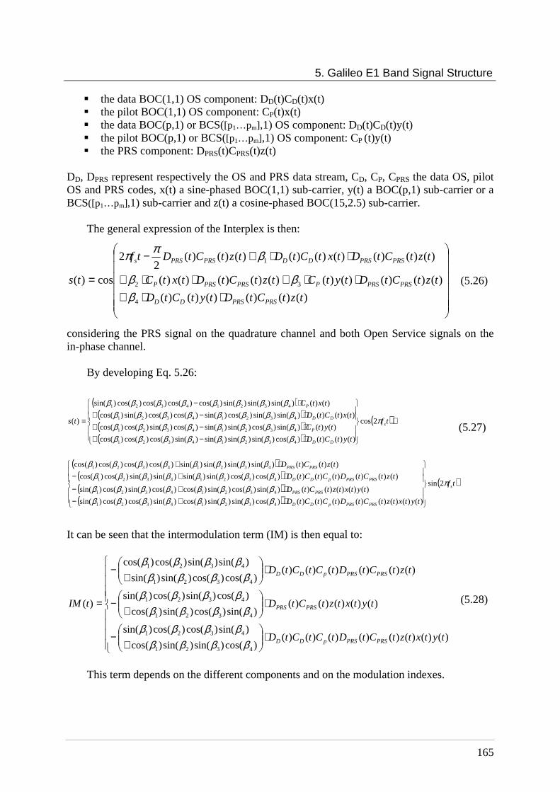
5. Galileo E1 Band Signal Structure

165

the data BOC(1,1) OS component: DD(t)CD(t)x(t) the pilot BOC(1,1) OS component: CP(t)x(t) the data BOC(p,1) or BCS([p1…pm],1) OS component: DD(t)CD(t)y(t) the pilot BOC(p,1) or BCS([p1…pm],1) OS component: CP (t)y(t) the PRS component: DPRS(t)CPRS(t)z(t)

DD, DPRS represent respectively the OS and PRS data stream, CD, CP, CPRS the data OS, pilot OS and PRS codes, x(t) a sine-phased BOC(1,1) sub-carrier, y(t) a BOC(p,1) sub-carrier or a BCS([p1…pm],1) sub-carrier and z(t) a cosine-phased BOC(15,2.5) sub-carrier.

The general expression of the Interplex is then:

⋅⋅+⋅⋅+⋅⋅+

⋅⋅+−

=)()()()()()(

)()()()()()()()()()(

)()()()()()()()()(2

2

cos)(

4

32

1

tztCtDtytCtD

tztCtDtytCtztCtDtxtC

tztCtDtxtCtDtztCtDtf

ts

PRSPRSDD

PRSPRSPPRSPRSP

PRSPRSDDPRSPRSs

βββ

βππ

(5.26)

considering the PRS signal on the quadrature channel and both Open Service signals on the in-phase channel.

By developing Eq. 5.26:

( )( )( )( )

( )

( )( )( )( )

( )tf

tytxtztCtDtCtCtD

tytxtztCtD

tztCtDtCtCtD

tztCtD

tf

tytCtD

tytC

txtCtD

txtC

ts

s

PRSPRSpDD

PRSPRS

PRSPRSpDD

PRSPRS

s

DD

P

DD

P

π

ββββββββββββββββββββββββ

ββββββββ

π

ββββββββββββββββββββββββ

ββββββββ

2sin

)()()()()()()()()cos()sin()sin()cos()sin()cos()cos()sin(

)()()()()()sin()cos()sin()cos()cos()sin()cos()sin(

)()()()()()()cos()cos()sin()sin()sin()sin()cos()cos(

)()()()sin()sin()sin()sin()cos()cos()cos()cos(

2cos

)()()()cos()sin()sin()sin()sin()cos()cos()cos(

)()()sin()cos()sin()sin()cos()sin()cos()cos(

)()()()sin()sin()cos()sin()cos()cos()sin()cos(

)()()sin()sin()sin()cos()cos()cos()cos()sin(

)(

43214321

43214321

43214321

43214321

43214321

43214321

43214321

43214321

⋅+−⋅+−

⋅+−⋅+

+

⋅−+⋅−+⋅−+

⋅−

=(5.27)

It can be seen that the intermodulation term (IM) is then equal to:

⋅

+−

⋅

+−

⋅

+−

=

)()()()()()()()()cos()sin()sin()cos(

)sin()cos()cos()sin(

)()()()()()sin()cos()sin()cos(

)cos()sin()cos()sin(

)()()()()()()cos()cos()sin()sin(

)sin()sin()cos()cos(

)(

4321

4321

4321

4321

4321

4321

tytxtztCtDtCtCtD

tytxtztCtD

tztCtDtCtCtD

tIM

PRSPRSpDD

PRSPRS

PRSPRSpDD

ββββββββ

ββββββββ

ββββββββ

(5.28)

This term depends on the different components and on the modulation indexes.

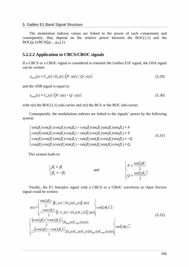
5. Galileo E1 Band Signal Structure

166

The modulation indexes values are linked to the power of each components and consequently, they depend on the relative power between the BOC(1,1) and the BOC(p,1)/BCS([p1…pm],1).

5.2.2.2 Application to CBCS/CBOC signals

If a CBCS or a CBOC signal is considered to transmit the Galileo E1F signal, the OSA signal can be written:

( ))()()()()( tyQtxPtDtCts DDOSA ⋅+⋅⋅⋅= (5.29)

and the OSB signal is equal to:

( ))()()()( tyQtxPtCts POSB ⋅−⋅⋅= (5.30)

with x(t) the BOC(1,1) sub-carrier and y(t) the BCS or the BOC sub-carrier.

Consequently, the modulations indexes are linked to the signals’ power by the following system:

=−−=−

=−=−

Q

Q

P

P

)cos()sin()sin()sin()sin()cos()cos()cos(

)sin()cos()sin()sin()cos()sin()cos()cos(

)sin()sin()cos()sin()cos()cos()sin()cos(

)sin()sin()sin()cos()cos()cos()cos()sin(

43214321

43214321

43214321

43214321

ββββββββββββββββββββββββββββββββ

(5.31)

This system leads to:

−==

34

21

ββββ

and

( )

( )

=

=

2

2sin2

2sin

3

1

β

β

Q

P

Finally, the E1 Interplex signal with a CBCS or a CBOC waveform as Open Service

signal could be written:

[ ]

[ ]( )

( )

( ) ( )tf

tztCtDtCtCtD

tztCtD

tf

tytCtDtC

txtCtDtCts

s

PRSPRSpDD

PRSPRS

s

DDP

DDP

πββ

ββ

πβ

β

2sin

)()()()()()(2

)2cos()2cos(

)()()(2

)2cos()2cos(

2cos

)()()()(2

)2sin(

)()()()(2

)2sin(

)(

31

31

3

1

⋅−+

⋅+

+

⋅+−⋅+

⋅+⋅=

(5.32)

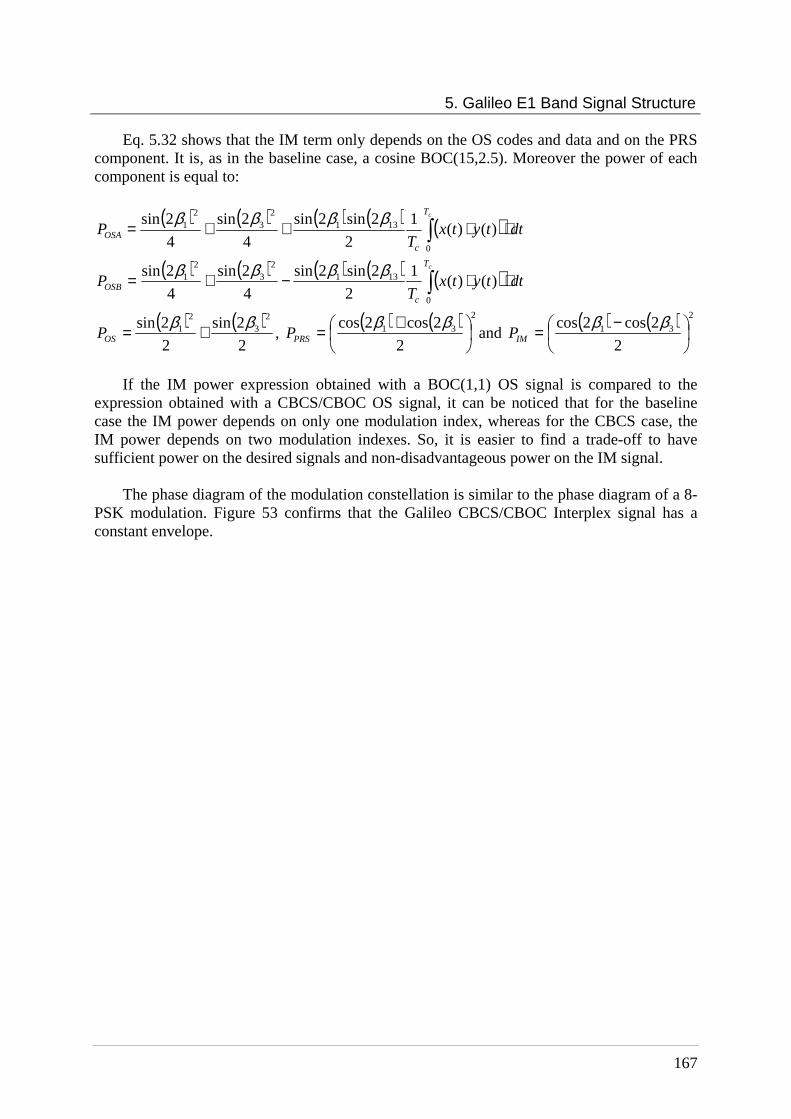
5. Galileo E1 Band Signal Structure

167

Eq. 5.32 shows that the IM term only depends on the OS codes and data and on the PRS component. It is, as in the baseline case, a cosine BOC(15,2.5). Moreover the power of each component is equal to:

( ) ( ) ( ) ( ) ( ) dttytxT

PcT

cOSA ⋅⋅++= ∫

0

1312

32

1 )()(1

2

2sin2sin

4

2sin

4

2sin ββββ

( ) ( ) ( ) ( ) ( ) dttytxT

PcT

cOSB ⋅⋅−+= ∫

0

1312

32

1 )()(1

2

2sin2sin

4

2sin

4

2sin ββββ

( ) ( )2

2sin

2

2sin 23

21 ββ +=OSP ,

( ) ( ) 2

31

2

2cos2cos

+= ββPRSP and

( ) ( ) 2

31

2

2cos2cos

−= ββIMP

If the IM power expression obtained with a BOC(1,1) OS signal is compared to the

expression obtained with a CBCS/CBOC OS signal, it can be noticed that for the baseline case the IM power depends on only one modulation index, whereas for the CBCS case, the IM power depends on two modulation indexes. So, it is easier to find a trade-off to have sufficient power on the desired signals and non-disadvantageous power on the IM signal.

The phase diagram of the modulation constellation is similar to the phase diagram of a 8-

PSK modulation. Figure 53 confirms that the Galileo CBCS/CBOC Interplex signal has a constant envelope.

5. Galileo E1 Band Signal Structure

168

Figure 53 CBCS/CBOC on data and pilot OS components modulation constellation The power spectrum density of a general CBCS E1 base band signal is calculated in

Appendix A:

( ) ( )

( ) ( )( )

⋅++

⋅+⋅=

)(2cos2cos2

1

)(2sin4

1)(2sin

4

1

)(

)5.2,15cos(32

12

32

)1,1(12

ˆ

fS

fSfSfS

BOC

BCSBOC

S

ββ

ββ (5.33)

with

2

)5.2,15cos( 130

cos

30cos

5.2sin

5.2)(

−

⋅= c

c

c

cBOC

Tf

Tff

Tf

TfS π

ππ

π

( )( )

⋅

=

cc

cBOC f

f

f

f

f

ffS

πππ

222)1,1( sin

2tan

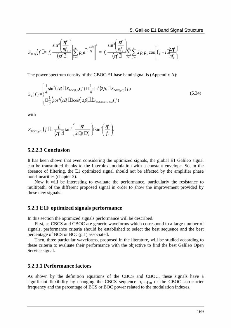
5. Galileo E1 Band Signal Structure

169

( ) ( ) ( ) ( )

−

=

= ∑∑∑= =

−

= c

m

i

m

ijji

cc

nf

fkjm

kk

ccBCS nf

fijpp

f

nf

f

fepf

nf

f

ffSπ

π

π

π

ππ

2cos2

sinsin

12

222

12

2

The power spectrum density of the CBOC E1 base band signal is (Appendix A):

( ) ( )

( ) ( )( )

⋅++

⋅+⋅=

)(2cos2cos2

1

)(2sin4

1)(2sin

4

1

)(

)5.2,15cos(32

12

)1,(32

)1,1(12

ˆ

fS

fSfSfS

BOC

pBOCBOC

S

ββ

ββ (5.34)

with

( ) ( )

⋅

⋅⋅=

cc

cpBOC f

f

fp

f

f

ffS

πππ

222)1,( sin

2tan .

5.2.2.3 Conclusion

It has been shown that even considering the optimized signals, the global E1 Galileo signal can be transmitted thanks to the Interplex modulation with a constant envelope. So, in the absence of filtering, the E1 optimized signal should not be affected by the amplifier phase non-linearities (chapter 3).

Now it will be interesting to evaluate the performance, particularly the resistance to multipath, of the different proposed signal in order to show the improvement provided by these new signals.

5.2.3 E1F optimized signals performance

In this section the optimized signals performance will be described. First, as CBCS and CBOC are generic waveforms which correspond to a large number of

signals, performance criteria should be established to select the best sequence and the best percentage of BCS or BOC(p,1) associated.

Then, three particular waveforms, proposed in the literature, will be studied according to these criteria to evaluate their performance with the objective to find the best Galileo Open Service signal.

5.2.3.1 Performance factors

As shown by the definition equations of the CBCS and CBOC, these signals have a significant flexibility by changing the CBCS sequence p1…pm or the CBOC sub-carrier frequency and the percentage of BCS or BOC power related to the modulation indexes.

5. Galileo E1 Band Signal Structure

170

So the following factors are used to find the best BCS or BOC(p,1) signal and the best associated percentage, which permit to obtain the best performance, while respecting the conditions of compatibility and interoperability put by the 2004 EU/US agreement: First, the best CBCS or CBOC waveforms should have a narrow autocorrelation

function peak to provide good performance in terms of tracking; the RMS bandwidth of the CBCS or CBOC waveforms should be better or similar to the RMS bandwidth of the BOC(1,1) waveform.

Then, the multipath rejection, studied thanks to multipath error envelopes, is also an

important performance factor. As seen in chapter 3, it is a main constraint for the signal design because of its important contribution of the pseudo-range calculation.

Moreover, the CBCS/CBOC waveform should present a sufficient spectral isolation,

similar to this obtained with a BOC(1,1), to not create interference with the GPS system.

Finally, another factor could be taken into account: the limitation of the secondary

peaks in the correlation function to avoid false acquisition and tracking. But, the current accuracy specified for the Galileo Open service is of 4 meters in horizontal and 8 meters in vertical. The offset between ambiguous peaks in the correlation function of the optimized signals are generally much higher than these accuracies. Consequently, [Hein, 2005] deduces that if the Galileo system satisfies the accuracy requirements, any pseudo-range step resulting from slips or false lock in the correlation function would be detected by the navigation algorithm of the receiver.

The factors above permit to study the CBCS/CBOC performance considering a tracking with an exact replica. But the objectives of these new CBCS or CBOC waveforms are not only to obtain better performance than the BOC(1,1) baseline by tracking the signal with an exact replica but also to obtain similar performance than the baseline by tracking the OS signal with a BOC(1,1) replica. Indeed, the reception of these new waveforms should also be possible with mass-market receivers, currently designed to receive only BOC(1,1) signals ([Novatel, 2006]). That is the reason why others factors, which take into account the tracking performance according to a BOC(1,1) replica, have been introduced to find the best BCS/BOC sequence. These factors are: The delta correlation losses. This parameter was defined in [Hein, 2005], it assesses

the degree of compatibility of a BOC(1,1) receiver receiving a CBCS or CBOC signal. The delta correlation losses compares the result of the cross-correlation in the data and pilot channel when the input is a CBCS/CBOC with the result of the autocorrelation function when the input is a BOC(1,1). They are expressed by [Hein, 2005]:

( )( )

( )( )

2

1

3

2

0

1

2

0

1

2sin

2sin1

2sin

2sin

⋅+

=∆

ββ

ββ

rA

AL with ∫ ⋅⋅=

cTc

dttytxT

r )()(1

5. Galileo E1 Band Signal Structure

171

and A1 the CBCS/CBOC input amplitude, A0 the BOC(1,1) input amplitude,0β the

BOC(1,1) modulation index, 1β and 3β the CBCS/CBOC modulation indexes, x(t)

the BOC(1,1) waveform and y(t) the BCS/BOC waveforms. The last term with r gives an idea of how similar to BOC(1,1) the CBCS/CBOC waveforms are. The contribution of this term to the correlation losses can be eliminated by two ways:

o 3β = 0, that corresponds to the BOC(1,1) baseline

o r = 0, that corresponds to a CBCS/CBOC waveform with zero mismatch correlation losses.

To minimize the delta correlation losses it would therefore be interesting to choose as Open Service signal, a CBCS/CBOC waveform which presents zero mismatch correlation losses.

The symmetry of the CBCS/CBOC correlation with a BOC(1,1) replica. Always with the objective to track a CBCS/CBOC waveform with a BOC(1,1) replica, it is necessary to have a symmetric correlation function between the two components. Indeed, a dissymmetry of this function could induce tracking bias in a receiver designed to receive only the BOC(1,1) waveform. [Pratt, 2006] underlines this problem and presents an effective method of removing or avoiding the bias. However it is preferable to not choose, as Open Service signal, a CBCS/CBOC sequence which introduces a dissymmetry on the correlation function.

The search of the best BCS/BOC sequence and its appropriate percentage thanks to the performance evaluation is carried out following all the previous constraints.

After global analysis according to the previous criteria, [Hein, 2005] has isolated three main optimized signals: the CBCS([1 -1 1 -1 1 -1 1 -1 1 1], 1), the CBOC(5,1) and the CBOC(6,1), whose performances will be studied in the following sections.

5.2.3.2 CBCS([1 -1 1 -1 1 -1 1 -1 1 1],1) performance

First have a look at the autocorrelation function of the CBCS([1 -1 1 -1 1 -1 1 -1 1 1], 1) waveform for different percentages of BCS power.

5. Galileo E1 Band Signal Structure

172

Figure 54 Autocorrelation function of the CBCS OSA signal

Figure 54 shows that when the percentage of BCS increases, the autocorrelation peak

becomes narrower, necessary condition for a successful tracking. Moreover high secondary peaks appear with the increase of the BCS percentage. As explained previously, the navigation algorithm generally permits to avoid the ambiguity induced by the secondary peaks. However, if the level of the secondary peak is too high, during a fraction of time, it can remain acquisition ambiguity, especially in the case of reduced satellite availability. That is the reason why, in the following, the percentage of BCS will not be considered higher than 20%.

The autocorrelation function of the OSB signal is represented in figure 55. In this case the main peak is less narrow than in the OSA case, but as for the OSA case it becomes narrower with the increase of BCS percentage.

5. Galileo E1 Band Signal Structure

173

Figure 55 Autocorrelation function of the CBCS OSB signal

The increase of the peak narrowness as a function of the BCS percentage can be modelled

using the equation of the autocorrelation functions, calculated in Appendix A:

( ) ( ) ( ) ( ) ( ) ( )τββτβτβτ BCSBOCBCSC

BOCC

OSA TT /)1,1(312

3)1,1(2

1 )2sin()2sin(2

1)2sin(

4

1)2sin(

4

1 ℜ+ℜ⋅+ℜ⋅=ℜ

( ) ( ) ( ) ( ) ( ) ( )τββτβτβτ BCSBOCBCSC

BOCC

OSB TT /)1,1(312

3)1,1(2

1 )2sin()2sin(2

1)2sin(

4

1)2sin(

4

1 ℜ−ℜ⋅+ℜ⋅=ℜ

Indeed these equations show that when the percentage of BCS increases, the part of the

BCS autocorrelation function increases, so the OSA and OSB autocorrelation functions come closer to the BCS autocorrelation function.

Even if the performance seems to be better for high percentage of BCS power, as already

mentioned, afterwards the percentage of BCS will not be considered higher than 20%, because if too much power is put on the BCS component, the compatibility of the Open Service signal with BOC(1,1) receiver is reduced, the delta correlation losses are not optimized and acquisition ambiguity can appear.

The potential good performance in tracking shown by the autocorrelation function is also

obvious on the RMS bandwidth curves. Figures 56 and 57 show an increase of the RMS bandwidth, while the BCS percentage increases, for filter bandwidths higher than 10 MHz

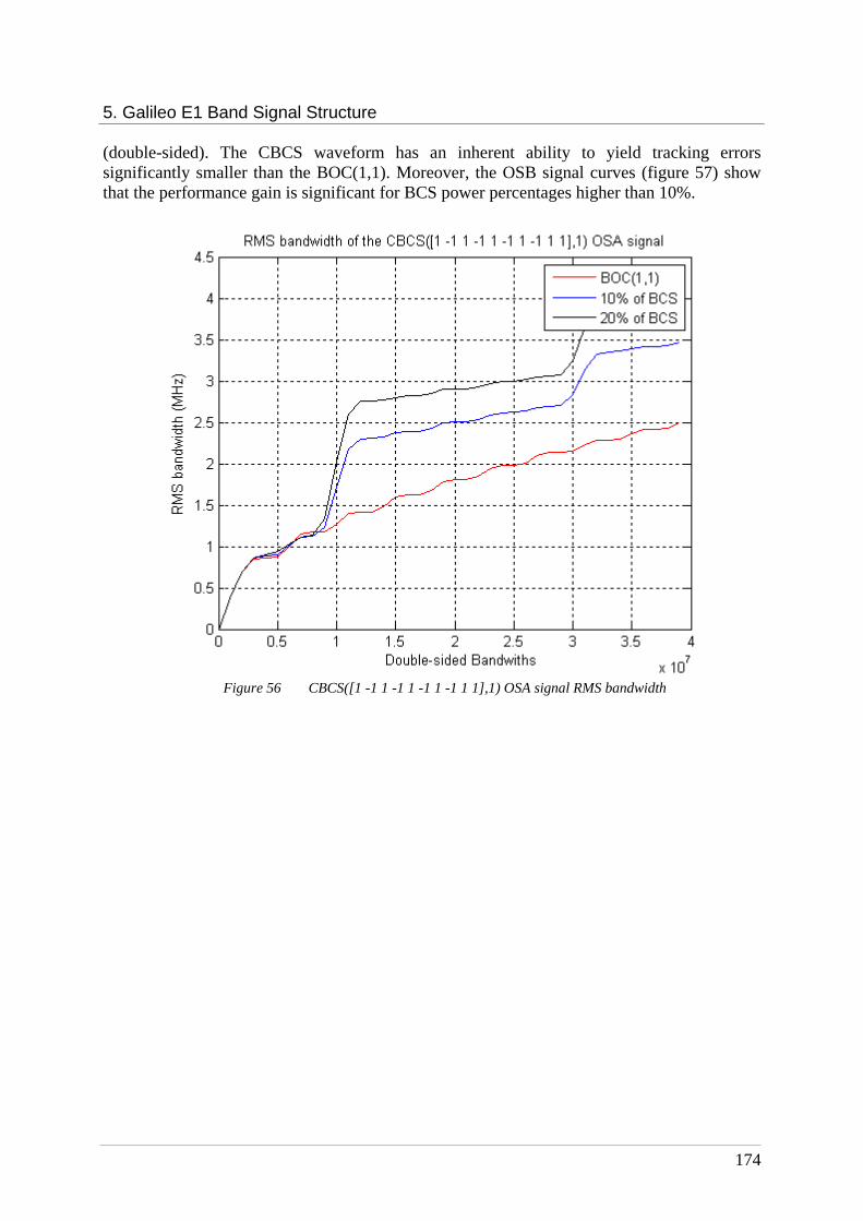
5. Galileo E1 Band Signal Structure

174

(double-sided). The CBCS waveform has an inherent ability to yield tracking errors significantly smaller than the BOC(1,1). Moreover, the OSB signal curves (figure 57) show that the performance gain is significant for BCS power percentages higher than 10%.

Figure 56 CBCS([1 -1 1 -1 1 -1 1 -1 1 1],1) OSA signal RMS bandwidth

5. Galileo E1 Band Signal Structure

175

Figure 57 CBCS([1 -1 1 -1 1 -1 1 -1 1 1],1) OSB signal RMS bandwidth

According to autocorrelation functions and RMS bandwidths, it seems that the gain in

tracking performance for this CBCS waveform starts to be interesting for percentages of BCS around 10%. Indeed for a receiver bandwidth equal to 12 MHz, the RMS bandwidth decreases from 3.25 MHz to 2.25 MHz for the OSA component and from 1.75 MHz to 1.45 MHz for the OSB.

Now the study of the multipath rejection (figures 58 and 59) shows that for percentages of

BCS power higher than 10%, the error due to the multipath on the measured pseudo-range is smaller (minimum two meters) than with the BOC(1,1) baseline for both OSA and OSB components. An early-minus-late discriminator is considered with a 0.1 chip spacing. Moreover, only one multipath signal with relative amplitude equal to 0.5 with respect to the direct signal is taken into account. The curves are plotted considering a 12 MHz receiver bandwidth.

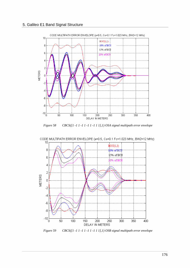
5. Galileo E1 Band Signal Structure

176

Figure 58 CBCS([1 -1 1 -1 1 -1 1 -1 1 1],1) OSA signal multipath error envelope

Figure 59 CBCS([1 -1 1 -1 1 -1 1 -1 1 1],1) OSB signal multipath error envelope

5. Galileo E1 Band Signal Structure

177

All the figures corresponding to tracking performance show that the CBCS([1 -1 1 -1 1 -1 1 -1 1 1],1) presents better tracking performance than the BOC(1,1) for BCS percentage higher than 10% and lower or equal to 20%. Moreover these figures show that a tracking with an exact replica of the CBCS([1 -1 1 -1 1 -1 1 -1 1 1],1, “+”) is more efficient than a tracking with an exact replica of the CBCS([1 -1 1 -1 1 -1 1 -1 1 1],1,”-“). So this waveform would be put on the pilot component and not on the data component, as considered on this study.

Tables 19 and 20 present the SSC calculations for different percentages of CBCS. They

show that the CBCS signal presents a spectral isolation with the GPS L1 signals similar to the spectral isolation obtained with the BOC(1,1) baseline. The CBCS SSCs are lower for GPS L1C and C/A code than the BOC(1,1) SSC. That is a strong point for this CBCS sequence. However the CBCS SSC is higher for the GPS M-code but the value obtained represents only a slight variation compared to this obtained with a BOC(1,1).

Self SSC (dB/Hz)

% of BCS in CBCS 10% 15% 20%

CBCS -65.49 -65.9 -66.27

BOC(1,1) baseline -64.74

Table 19 Self SSC of the CBCS([1 -1 1 -1 1 -1 1 -1 1 1],1) Open Service signal

Inter-system SSC (dB/Hz)

% of BCS in CBCS 0%

BOC(1,1) baseline

10% 15% 20%

SSC with GPS C/A code -67.78 -68.13 -68.33 -68.52

SSC with GPS M code -82.89 -82.41 -82.48 -82.53

SSC with GPS L1C -64.71 -65.1 -65.32 -65.53

Table 20 SSC of the CBCS([1 -1 1 -1 1 -1 1 -1 1 1],1) Open Service signal with GPS signals

All the results listed above show that the CBCS([1 -1 1 -1 1 -1 1 -1 1 1],1, 15% or 20%)

presents better performance than a BOC(1,1) according to the requirements presented previously, if the tracking is realized according to an exact replica. Now it is interesting to establish if the BCS sequence chosen presents also good tracking performance when using a local BOC(1,1) replica.

To begin, it can be noticed that the studied CBCS waveform verifies the condition which

permits to minimize the delta correlation losses. Indeed, the CBCS sequence has a zero mismatch correlation losses, as shown in figure 60:

5. Galileo E1 Band Signal Structure

178

Figure 60 CBCS waveform with a zero mismatch correlation losses

However, the correlation functions of the CBCS([1 -1 1 -1 1 -1 1 -1 1 1],1,”+”) and

CBCS([1 -1 1 -1 1 -1 1 -1 1 1],1,”-“) waveforms with a BOC(1,1) sub-carrier exhibit a dissymmetry, as shown in figures 61 and 62.

Figure 61 OSA CBCS([1 -1 1 -1 1 -1 1 -1 1 1],1) correlation with a BOC(1,1) replica

x(t)

y(t)

∫ =⋅⋅=cTc

dttytxT

r 0)()(1

Tc

Tc

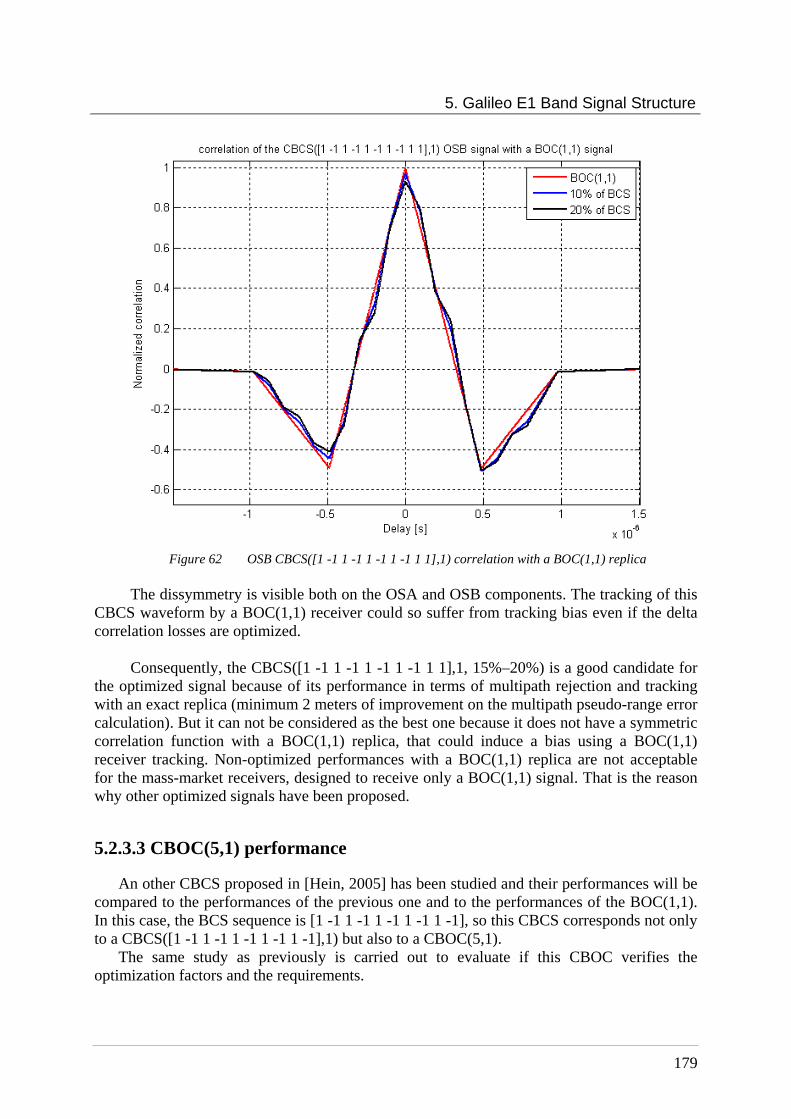
5. Galileo E1 Band Signal Structure

179

Figure 62 OSB CBCS([1 -1 1 -1 1 -1 1 -1 1 1],1) correlation with a BOC(1,1) replica

The dissymmetry is visible both on the OSA and OSB components. The tracking of this

CBCS waveform by a BOC(1,1) receiver could so suffer from tracking bias even if the delta correlation losses are optimized.

Consequently, the CBCS([1 -1 1 -1 1 -1 1 -1 1 1],1, 15%–20%) is a good candidate for

the optimized signal because of its performance in terms of multipath rejection and tracking with an exact replica (minimum 2 meters of improvement on the multipath pseudo-range error calculation). But it can not be considered as the best one because it does not have a symmetric correlation function with a BOC(1,1) replica, that could induce a bias using a BOC(1,1) receiver tracking. Non-optimized performances with a BOC(1,1) replica are not acceptable for the mass-market receivers, designed to receive only a BOC(1,1) signal. That is the reason why other optimized signals have been proposed.

5.2.3.3 CBOC(5,1) performance

An other CBCS proposed in [Hein, 2005] has been studied and their performances will be compared to the performances of the previous one and to the performances of the BOC(1,1). In this case, the BCS sequence is [1 -1 1 -1 1 -1 1 -1 1 -1], so this CBCS corresponds not only to a CBCS([1 -1 1 -1 1 -1 1 -1 1 -1],1) but also to a CBOC(5,1).

The same study as previously is carried out to evaluate if this CBOC verifies the optimization factors and the requirements.

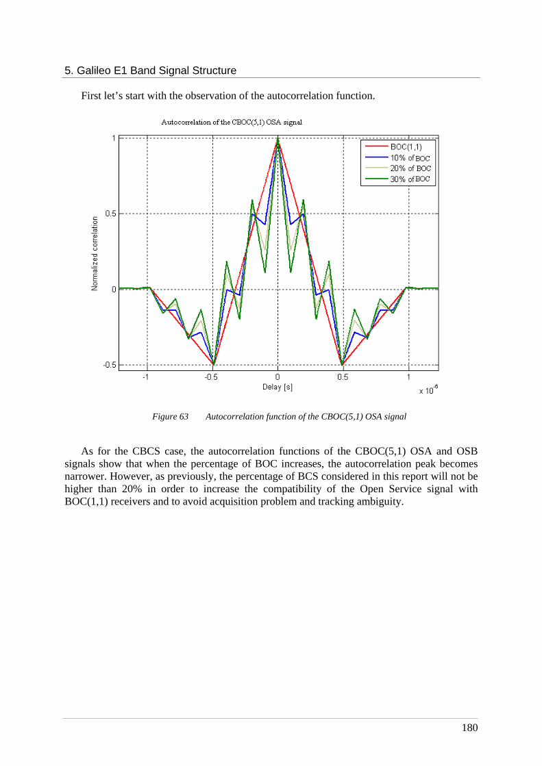
5. Galileo E1 Band Signal Structure

180

First let’s start with the observation of the autocorrelation function.

Figure 63 Autocorrelation function of the CBOC(5,1) OSA signal

As for the CBCS case, the autocorrelation functions of the CBOC(5,1) OSA and OSB

signals show that when the percentage of BOC increases, the autocorrelation peak becomes narrower. However, as previously, the percentage of BCS considered in this report will not be higher than 20% in order to increase the compatibility of the Open Service signal with BOC(1,1) receivers and to avoid acquisition problem and tracking ambiguity.

5. Galileo E1 Band Signal Structure

181

Figure 64 Autocorrelation function of the CBOC(5,1) OSB signal

Now it is interesting to verify if this CBOC waveform presents good performance in terms

of multipath rejection, RMS bandwidth, spectral isolation, correlation losses and tracking with a BOC(1,1).

An early-minus-late discriminator is considered with a 0.1 chip spacing. Moreover, only

one multipath signal with relative amplitude equal to 0.5 with respect to the direct signal is taken into account. The curves are plotted considering a 12 MHz receiver bandwidth.

The CBOC(5,1) offers a good multipath rejection as seen in figures 65 and 66. Its performance is similar to the performance obtained with the CBCS and better than the performance obtained with a BOC(1,1).

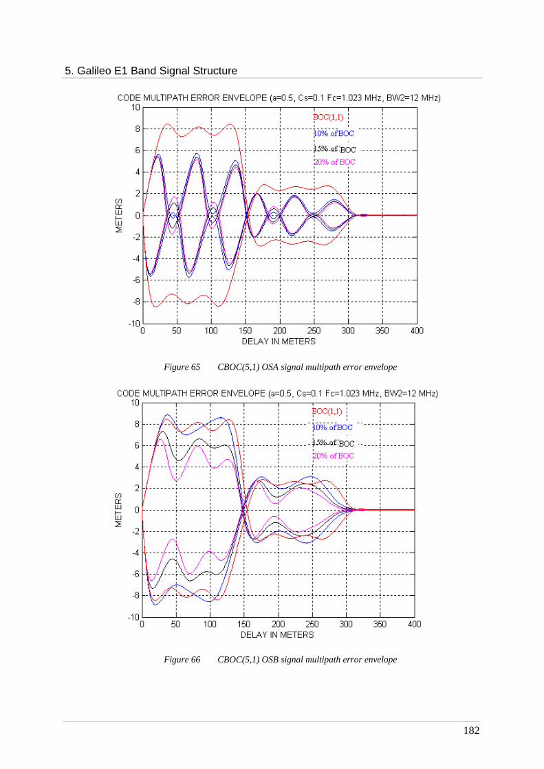
5. Galileo E1 Band Signal Structure

182

Figure 65 CBOC(5,1) OSA signal multipath error envelope

Figure 66 CBOC(5,1) OSB signal multipath error envelope

5. Galileo E1 Band Signal Structure

183

The CBOC(5,1) performances in terms of RMS bandwidth (figures 67 and 68) are also similar to the performance obtained with the CBCS. The CBOC(5,1) waveform has an inherent ability to yield tracking errors smaller than the BOC(1,1) for percentages of BOC(5,1) power higher than 10% and for filter bandwidths higher than 10 MHz.

Figure 67 CBOC(5,1) OSA signal RMS bandwidth

5. Galileo E1 Band Signal Structure

184

Figure 68 CBOC(5,1) OSB signal RMS bandwidth

Concerning the spectral isolation (tables 21 and 22), the CBOC(5,1) presents a better

spectral isolation than the BOC(1,1) with the GPS L1C and the GPS C/A code signals but its spectral isolation is slightly worse with the GPS M-code. This SSC value is however acceptable because it is nearby the SSC value obtained with the baseline BOC(1,1).

Self SSC (dB/Hz)

% of BOC in CBOC 10% 15% 20%

CBOC(5,1) -65.5 -65.91 -66.27

BOC(1,1) baseline -64.74

Table 21 Self SSC of the CBOC(5,1) Open Service signal

Inter-system SSC (dB/Hz)

5. Galileo E1 Band Signal Structure

185

% of BOC in CBOC 0%

BOC(1,1) baseline

10% 15% 20%

SSC with GPS C/A code -67.78 -68.2 -68.43 -68.65

SSC with GPS M code -82.89 -82.55 -82.7 -82.84

SSC with GPS BOC(1,1) L1C

-64.71 -65.11 -65.35 -65.56

Table 22 SSC of the CBOC(5,1) Open Service signal with GPS signals

To continue, the other parameters of optimization, which permit to evaluate performance

assuming a BOC(1,1) tracking, should be verified. Figures 69 and 70 show that the correlation between the CBOC(5,1) and a BOC(1,1) is

symmetric.

Figure 69 OSA CBOC(5,1) correlation with a BOC(1,1) replica

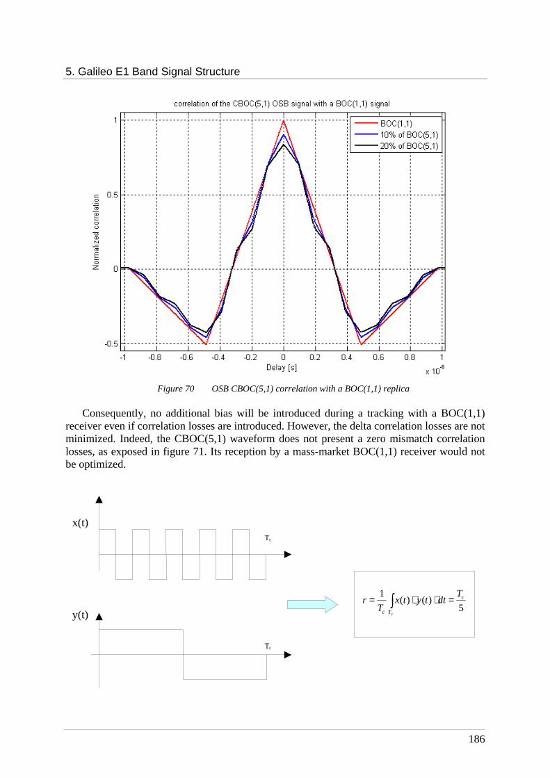
5. Galileo E1 Band Signal Structure

186

Figure 70 OSB CBOC(5,1) correlation with a BOC(1,1) replica

Consequently, no additional bias will be introduced during a tracking with a BOC(1,1)

receiver even if correlation losses are introduced. However, the delta correlation losses are not minimized. Indeed, the CBOC(5,1) waveform does not present a zero mismatch correlation losses, as exposed in figure 71. Its reception by a mass-market BOC(1,1) receiver would not be optimized.

5)()(

1 c

Tc

Tdttytx

Tr

c

=⋅⋅= ∫

y(t)

Tc

x(t) Tc

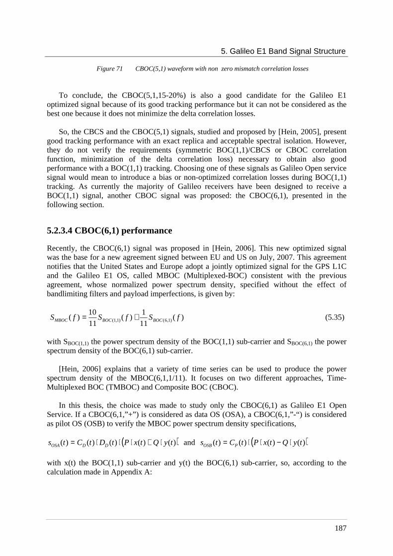
5. Galileo E1 Band Signal Structure

187

Figure 71 CBOC(5,1) waveform with non zero mismatch correlation losses To conclude, the CBOC(5,1,15-20%) is also a good candidate for the Galileo E1

optimized signal because of its good tracking performance but it can not be considered as the best one because it does not minimize the delta correlation losses.

So, the CBCS and the CBOC(5,1) signals, studied and proposed by [Hein, 2005], present

good tracking performance with an exact replica and acceptable spectral isolation. However, they do not verify the requirements (symmetric BOC(1,1)/CBCS or CBOC correlation function, minimization of the delta correlation loss) necessary to obtain also good performance with a BOC(1,1) tracking. Choosing one of these signals as Galileo Open service signal would mean to introduce a bias or non-optimized correlation losses during BOC(1,1) tracking. As currently the majority of Galileo receivers have been designed to receive a BOC(1,1) signal, another CBOC signal was proposed: the CBOC(6,1), presented in the following section.

5.2.3.4 CBOC(6,1) performance

Recently, the CBOC(6,1) signal was proposed in [Hein, 2006]. This new optimized signal was the base for a new agreement signed between EU and US on July, 2007. This agreement notifies that the United States and Europe adopt a jointly optimized signal for the GPS L1C and the Galileo E1 OS, called MBOC (Multiplexed-BOC) consistent with the previous agreement, whose normalized power spectrum density, specified without the effect of bandlimiting filters and payload imperfections, is given by:

)(11

1)(

11

10)( )1,6()1,1( fSfSfS BOCBOCMBOC += (5.35)

with SBOC(1,1) the power spectrum density of the BOC(1,1) sub-carrier and SBOC(6,1) the power spectrum density of the BOC(6,1) sub-carrier.

[Hein, 2006] explains that a variety of time series can be used to produce the power spectrum density of the MBOC(6,1,1/11). It focuses on two different approaches, Time-Multiplexed BOC (TMBOC) and Composite BOC (CBOC).

In this thesis, the choice was made to study only the CBOC(6,1) as Galileo E1 Open

Service. If a CBOC(6,1,”+”) is considered as data OS (OSA), a CBOC(6,1,”-“) is considered as pilot OS (OSB) to verify the MBOC power spectrum density specifications,

( ))()()()()( tyQtxPtDtCts DDOSA ⋅+⋅⋅⋅= and ( ))()()()( tyQtxPtCts POSB ⋅−⋅⋅=

with x(t) the BOC(1,1) sub-carrier and y(t) the BOC(6,1) sub-carrier, so, according to the calculation made in Appendix A:

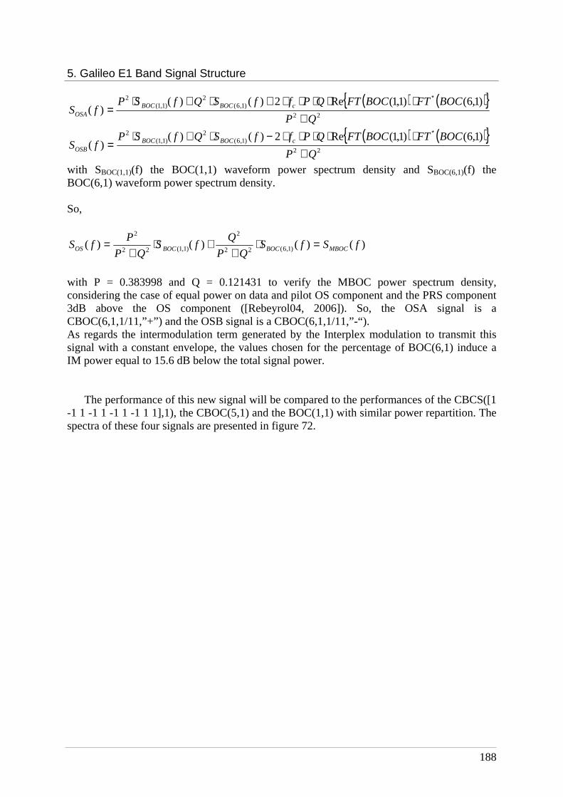
5. Galileo E1 Band Signal Structure

188

( ) ( ) 22

)1,6(2

)1,1(2 )1,6()1,1(Re2)()(

)(QP

BOCFTBOCFTQPffSQfSPfS cBOCBOC

OSA +⋅⋅⋅⋅⋅+⋅+⋅

=∗

( ) ( ) 22

)1,6(2

)1,1(2 )1,6()1,1(Re2)()(

)(QP

BOCFTBOCFTQPffSQfSPfS cBOCBOC

OSB +⋅⋅⋅⋅⋅−⋅+⋅

=∗

with SBOC(1,1)(f) the BOC(1,1) waveform power spectrum density and SBOC(6,1)(f) the BOC(6,1) waveform power spectrum density. So,

)()()()( )1,6(22

2

)1,1(22

2

fSfSQP

QfS

QP

PfS MBOCBOCBOCOS =⋅

++⋅

+=

with P = 0.383998 and Q = 0.121431 to verify the MBOC power spectrum density, considering the case of equal power on data and pilot OS component and the PRS component 3dB above the OS component ([Rebeyrol04, 2006]). So, the OSA signal is a CBOC(6,1,1/11,”+”) and the OSB signal is a CBOC(6,1,1/11,”-“). As regards the intermodulation term generated by the Interplex modulation to transmit this signal with a constant envelope, the values chosen for the percentage of BOC(6,1) induce a IM power equal to 15.6 dB below the total signal power.

The performance of this new signal will be compared to the performances of the CBCS([1 -1 1 -1 1 -1 1 -1 1 1],1), the CBOC(5,1) and the BOC(1,1) with similar power repartition. The spectra of these four signals are presented in figure 72.

5. Galileo E1 Band Signal Structure

189

Figure 72 Open Service signal power spectral densities considering the different optimized signals

First the observation of the autocorrelation functions in figures 73 and 74 shows that the

narrowest peak is obtained for CBOC(6,1,1/11,”-“). So it would be preferable to track the MBOC signal on the component with “-“ to obtain better tracking performance. For the CBOC(5,1) and CBCS waveforms, the tracking was preferable on the component with “+”, as already exposed previously.

5. Galileo E1 Band Signal Structure

190

Figure 73 CBOC and CBCS OSA autocorrelation functions

Figure 74 CBOC and CBCS OSB autocorrelation functions

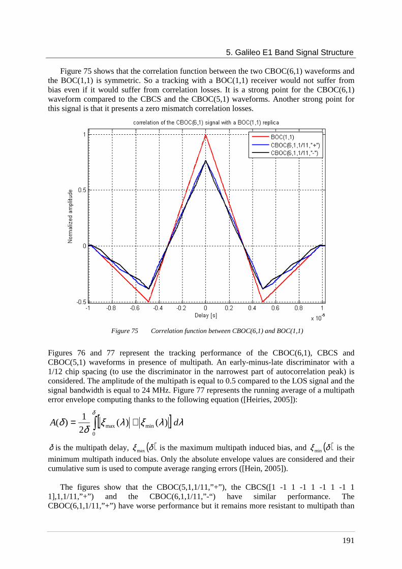
5. Galileo E1 Band Signal Structure

191

Figure 75 shows that the correlation function between the two CBOC(6,1) waveforms and the BOC(1,1) is symmetric. So a tracking with a BOC(1,1) receiver would not suffer from bias even if it would suffer from correlation losses. It is a strong point for the CBOC(6,1) waveform compared to the CBCS and the CBOC(5,1) waveforms. Another strong point for this signal is that it presents a zero mismatch correlation losses.

Figure 75 Correlation function between CBOC(6,1) and BOC(1,1)

Figures 76 and 77 represent the tracking performance of the CBOC(6,1), CBCS and CBOC(5,1) waveforms in presence of multipath. An early-minus-late discriminator with a 1/12 chip spacing (to use the discriminator in the narrowest part of autocorrelation peak) is considered. The amplitude of the multipath is equal to 0.5 compared to the LOS signal and the signal bandwidth is equal to 24 MHz. Figure 77 represents the running average of a multipath error envelope computing thanks to the following equation ([Heiries, 2005]):

[ ] λλξλξδ

δδ

dA ∫ +=0

minmax )()(2

1)(

δ is the multipath delay, ( )δξmax is the maximum multipath induced bias, and ( )δξmin is the

minimum multipath induced bias. Only the absolute envelope values are considered and their cumulative sum is used to compute average ranging errors ([Hein, 2005]).

The figures show that the CBOC(5,1,1/11,”+”), the CBCS([1 -1 1 -1 1 -1 1 -1 1

1],1,1/11,”+”) and the CBOC(6,1,1/11,”-“) have similar performance. The CBOC(6,1,1/11,”+”) have worse performance but it remains more resistant to multipath than

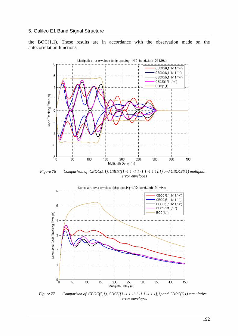
5. Galileo E1 Band Signal Structure

192

the BOC(1,1). These results are in accordance with the observation made on the autocorrelation functions.

Figure 76 Comparison of CBOC(5,1), CBCS([1 -1 1 -1 1 -1 1 -1 1 1],1) and CBOC(6,1) multipath

error envelopes

Figure 77 Comparison of CBOC(5,1), CBCS([1 -1 1 -1 1 -1 1 -1 1 1],1) and CBOC(6,1) cumulative

error envelopes

5. Galileo E1 Band Signal Structure

193

Figure 78 also shows that the CBOC(6,1,1/11,”-“) have good tracking performance,

similar to this obtained for CBOC(5,1,1/11,”+”) and CBCS(1,1/11,”+”).

Figure 78 CBOC(6,1) waveforms RMS bandwidths

To end our study of the CBOC(6,1) signals, the spectral separation coefficients are calculated. Table 23 shows that the MBOC(6,1,1/11) SSC values are similar to the values obtained with the BOC(1,1), this signal presents a sufficient spectral isolation with the GPS L1 signals.

SSC (dB/Hz)

OS signal BOC(1,1) CBCS CBOC(5,1) CBOC(6,1)

Self SSC -64.74 -65.41 -65.43 -65.45

SSC with GPS M code -82.29 -82.4 -82.53 -82

SSC with GPS C/A code -67.78 -68.11 -68.16 -68.17

SSC with GPS L1C -64.71 -65.06 -65.07 -65.08

Table 23 Comparison of BOC(1,1), CBOC(5,1), CBCS([1 -1 1 -1 1 -1 1 -1 1 1],1) and CBOC(6,1) SSCs

As the CBOC(6,1,1/11,”-“) presents good performance, another CBOC(6,1) configuration

was proposed by [Hein, 2006] to verify the MBOC power spectrum density. This new

5. Galileo E1 Band Signal Structure

194

configuration suggests to put all the BOC(6,1) power on the pilot component while having only a BOC(1,1) sub-carrier on the data component. The data and pilot Open service signals are then equal to:

)()()()( txRtDtCts DDOSA ⋅⋅⋅= and ( ))()()()( tyQtxPtCts POSB ⋅−⋅⋅=

with x(t) the BOC(1,1) sub-carrier and y(t) the BOC(6,1) sub-carrier. Thus, according to Appendix A,

)()( )1,1(222

2

fSRQP

RfS BOCOSA ⋅

++=

( ) ( ) 222

)1,6(2

)1,1(2 )1,6()1,1(Re2)()(

)(RQP

BOCFTBOCFTQPffSQfSPfS cBOCBOC

OSB ++⋅⋅⋅⋅⋅−⋅+⋅

=∗

and

( ) ( ) ( ) 222

)1,6(2

)1,1(22 )1,6()1,1(Re2)()(

)(RQP

BOCFTBOCFTQPffSQfSRPfS cBOCBOC

OS ++⋅⋅⋅⋅⋅−⋅+⋅+

=∗

This power spectrum density does not verify exactly the MBOC power spectrum density

because of the cross-correlation term between the BOC(1,1) sub-carrier and the BOC(6,1) sub-carrier. Fortunately, the cross-correlation term can be zeroed by alternating the relative polarity of the BOC(1,1) and BOC(6,1) signals in the CBOC term. This means there is an alternation between “in phase” CBOC(6,1) (where the first part of the chip is of the same polarity) and “antiphase” CBOC(6,1) (where the first part of the chip is of opposite polarity). This new CBOC is noted CBOC(6,1,”+/-“). This manipulation leads to:

( ))()()()( )1,6(222

2

)1,1(222

22

fSfSRQP

QfS

RQP

RPfS MBOCBOCBOCOS =⋅

+++⋅

+++=

with P = 0.358235, Q = 0.168874 and R = 0.396044 considering the case of equal power on data and pilot and the PRS component 3 dB above the OS component ([Rebeyrol04, 2006]).The OSA is so a BOC(1,1) and the OSB is a CBOC(6,1,2/11,”+/-“).

As expected, because of its high BOC(6,1) power percentage, the performances of the CBOC(6,1,2/11,”+/-“) are better than the performances of the CBOC(6,1,1/11,”-“) or the CBOC(5,1,1/11,”+”), as shown by figure 79:

5. Galileo E1 Band Signal Structure

195

Figure 79 CBOC(6,1,2/11,”+/-“) tracking performance

5. Galileo E1 Band Signal Structure

196

The RMS bandwidth figure shows that the CBOC(6,1,2/11,”+/-“) tracking performance is better than the performance of the other waveforms for signal bandwidths higher than 15 MHz. The CBOC(6,1,2/11,”+/-“) resistance to multipath is also better whatever the multipath delay.

Therefore, the CBOC(6,1,2/11,”+/-“) presents the best tracking performance with excellent multipath mitigation. But this signal is more complicated to generate because of the alternating sign of the BOC(6,1) sub-carrier, necessary to verify the MBOC specification. However the complexity of the generation at the payload level is not the only problem of this waveform. Indeed to transmit the CBOC(6,1,2/11,”+/-“) on the pilot component associated to the BOC(1,1) on the data component, the five components Interplex modulation should be adapted. The general formulation of a five components Interplex modulation could be applied but the system verified by the modulation indexes is different.

Indeed if the OSA signal is written: )()()()( txRtDtCts DDOSA ⋅⋅⋅= , and the OSB signal is

equal to ( ))()()()( tyQtxPtCts POSB ⋅−⋅⋅= with x(t) the BOC(1,1) sub-carrier and y(t) the

BOC(p,1), the modulation indexes should verify the following system:

=−−=−

=−=−

0)cos()sin()sin()sin()sin()cos()cos()cos(

)sin()cos()sin()sin()cos()sin()cos()cos(

)sin()sin()cos()sin()cos()cos()sin()cos(

)sin()sin()sin()cos()cos()cos()cos()sin(

43214321

43214321

43214321

43214321

ββββββββββββββββββββββββββββββββ

Q

R

P

(5.36)

If the modulation indexes verify this system, the PRS amplitude and the IM term could be

expressed in function of P, Q and R. The expressions obtained are respectively:

( ) ( ) ( ) ( )4

1111 2222 RQPRQPRQPRQPS

−−−+−+−++−−+++−= for the PRS

amplitude, and

( ) ( )( ) ( )

( ) ( )( ) ( )

( ) ( )( ) ( )

++−++−−−

−+−−−−−−+

++−−+−−+

−+−−−−−+

++−−+−−+

−+−+−−−−

=

22

22

22

22

22

22

11

11)()()(

11

11)()(

11

11)()()()()(

)(4

1)(

RQPRQP

RQPRQPtCtDtC

RQPRQP

RQPRQPtytx

RQPRQP

RQPRQPtCtDtCtytx

tztIM

DDP

DDP

(5.37)

The IM takes 8 different values, so the modulation is no more a 8-PSK modulation as previously seen, but a 16-PSK modulation as presented in figure 80:

5. Galileo E1 Band Signal Structure

197

Figure 80 CBOC(6,1) on pilot OS component and BOC(1,1) on data OS component modulation

constellation The 16-plots modulation induces that each plot is closer to another one. So if the

CBOC(6,1,2/11,”+/-“) configuration is preferred, the global Galileo E1 signal is more likely to suffer from distortions created by the payload and receiver phase noise. Indeed, the phase noise, induced by payload and receiver clocks instabilities and added to the signals during the generation and the processing, spreads the constellation plots, as seen in chapter 3. Consequently, if the number of plots is too high, two plots (or more) can be confused because of the phase noise and errors can occur during the demodulation.

Now, regarding the IM term, the values chosen for the percentage of BOC(6,1) induce an

IM power 12.2 dB below the total signal power considering that the IM term have zero cross-correlation with the PRS signal. This value is weaker than this obtained if the data and pilot OS are a BOC(1,1) but it is higher than the value obtained in the previous case (CBOC(6,1) on OSA and OSB components). This is also a weak point of this signal.

To conclude, it has been seen that for the CBOC(6,1,1/11) cases, good tracking

performances were achieved for the CBOC(6,1,1/11,”-“) modulation. This waveform is thus appropriated for pilot-only tracking. However, in this case, a CBOC(6,1,1/11,”+”) waveform has to be used on the data channel to verify the MBOC power spectrum density specification. The performances of this modulation are the worst of the CBOC(6,1) waveforms but they remain better than the baseline BOC(1,1) performance.

5. Galileo E1 Band Signal Structure

198

The other option proposed to verify the MBOC specification is the use of a CBOC(6,1,2/11,”+/-“) on the pilot channel and a pure BOC(1,1) on the data channel. This option would allow having a pilot channel with excellent tracking performances (the best multipath and tracking in white noise performance), while the data channel would use a simple BOC(1,1) modulation and consequently would present worse performance. Moreover with this option, the alternating sign of the BOC(6,1) sub-carrier complicates the generation of this modulation at the payload level and the power consumed by the IM product, to keep a constant envelope, is higher.

Therefore, the choice of the best candidate, among the CBOC(6,1) modulation is a

compromise between good tracking performance and generation complexity. But other criteria should be taken into account during this compromise study, particularly the impact of such a modulation on the different user needs, and on receiver architectures ([Julien, 2006], [Avila-Rodriguez, 2006]).

Finally, Europe has chosen to transmit the data Open Service signal with a CBOC(6,1,1/11,”+”) and the pilot Open Service signal with a CBOC(6,1,1/11,”-“).

5.3 Conclusion

This chapter has presented the baseline adopted in June 2004 by the United States and Europe for the Galileo and the new GPS L1 signals. This baseline foresaw for a sine-phased BOC(1,1) as Galileo Open Service signals and proposes always a cosine-phased BOC(15,2.5) as Public Regulated Service signal. The tracking performance of the BOC(1,1) baseline and the modulation used to multiplex the OS and the PRS signals, called Interplex, have been described to verify their compliance with the signal design constraints exposed in chapter 3: good resistance to multipath and constant envelope modulation.

However, as the 2004 EU/US agreement plans a possible optimisation of the baseline, particularly for the Open Service signals, different new waveforms have been proposed to transmit the E1F signal instead of the BOC(1,1). Two main waveforms have been studied in this chapter: the Composite Binary Coded Symbol (CBCS) signal and the Composite BOC (CBOC) signal. It has been shown in this chapter that these waveforms present indeed better tracking performance than the BOC(1,1) baseline but the CBCS([1 -1 1 -1 1 -1 1 -1 1 1],1) and the CBOC(5,1) studied do not have optimal performance assuming BOC(1,1) tracking (currently proposed in mass-market receiver). Moreover the necessary adaptation of the Interplex modulation to transmit these new signals has been exposed.

Recently (July 2007), a new agreement was signed between the USA and the European

Union. It proposes to adopt for the GPS L1C and the Galileo E1 OS signals a jointly optimized signal, called MBOC(6,1,1/11). As explained in this chapter, the MBOC can take different waveforms. Here, it was decided to study only the CBOC(6,1) and its different variations. It has been shown that the CBOC(6,1,2/11,”+/-“) has the best tracking performance with both an exact replica tracking and a BOC(1,1) replica tracking. However, it requires more complexity at the payload generation level because of the alternation “+/-“. Moreover, as seen during the study of the Interplex modulation, because of the 16 plots modulation constellation, the Galileo E1 signal assuming a CBOC(6,1,2/11,”+/-“) pilot Open

5. Galileo E1 Band Signal Structure

199

Service component, is more likely to suffer from distortions created by the payload and receiver phase noise.

Finally, Europe has made its choice and has decided to transmit the data Open Service signal with a CBOC(6,1,1/11,”+”) and the pilot Open Service signal with a CBOC(6,1,1/11,”-”).

201

Chapter 6

Impact of equipment impairments on receiver performance

Contents 6.1 Payload model................................................................................................................. 202

6.1.1 The Clock Unit............................................................................................................ 202 6.1.2 The Navigation Signal Generation Unit ..................................................................... 202 6.1.3 The Frequency Generation and Modulation Unit ....................................................... 205 6.1.4 The Amplification Unit............................................................................................... 211 6.1.5 The OMUX ................................................................................................................. 215

6.2 Receiver model................................................................................................................ 216 6.2.1 Oscillators models....................................................................................................... 217 6.2.2 Down-conversion........................................................................................................ 217 6.2.3 Receiver Filters ........................................................................................................... 220 6.2.4 A/D conversion ........................................................................................................... 221

6.3 Simulations results ......................................................................................................... 223 6.3.1 Payload performance .................................................................................................. 223 6.3.2 Receiver performance ................................................................................................. 254 6.3.3 End-to-end performance ............................................................................................. 264 6.3.4 Conclusion .................................................................................................................. 265

Chapters 4 and 5 have presented the civil Galileo signals in the E5 and E1 bands and the modulation used to multiplex and transmit them. It has also been shown that the signals and their respective modulations have been chosen in order to minimize signals impairments during their generation, their propagation and their reception. Indeed these signals have a constant envelope and an excellent resistance against multipath.

However, as seen in chapter 3, it exists another factor of impairments whose effect can not be reduced by the signal optimization: the phase noise due to clocks instabilities but also the

6. Impact of equipment impairments on receiver performance

202

distortions induced by payload filtering. This chapter will therefore present the impairments induced by the clocks phase noise on the Galileo signals, especially on the Galileo E5 signal, chosen because of its wide bandwidth. It also describes the influence of payload filters and amplifiers on this signal.

First the characteristics of payload and receiver equipment considered for this study are

presented. Then simulations results, obtained with Matlab, are set out to evaluate the influence of the equipment (clocks, payload amplifier and filters) on the Galileo E5 signals as regards receiver performance, such as correlation functions and tracking loop phase error. The effect of phase noise on the receiver code tracking loop has not been studied because of lack of time.

6.1 Payload model

A generic Galileo payload model and its sub-systems have been described in chapter 3. This generic model will be detailed in this section by presenting the characteristics of the different units’ equipment chosen for the phase noise study and simulations. The payload model characteristics are presented for the generation of the different Galileo signals even if the simulations will be carried out only for the E5 band signal.

6.1.1 The Clock Unit

Concerning the clock unit, the characteristics of the atomic clocks are not taken into account, the CMCU phase noise characteristic is directly considered. The CMCU studied is the CMCU presented in [Moreno Carrillo, 2005] and in chapter 3, its phase noise is shown in figure 23.

6.1.2 The Navigation Signal Generation Unit

As described in chapter 3, the NSGU is composed of a modulator and a digital filter.

6.1.2.1 The Modulator

As seen in the previous chapters, the modulator generates the Galileo signals and multiplexes them: thanks to the Interplex scheme for the E6 and E1 band signals or thanks to the ALTBOC scheme for the E5 band signal.

Figure 81 represents a possible simplified generation scheme for the Galileo E1 signal if the BOC(1,1) baseline is considered (chapter 3 and [Hein, 2002]). After being multiplexed, the E1 signal is put around an intermediate frequency equal to 30*1.023 MHz, as seen in chapter 3. This scheme can, of course, be adapted to multiplex the optimized Galileo E1 signal, based on the CBOC(6,1) waveform (chapter 5).

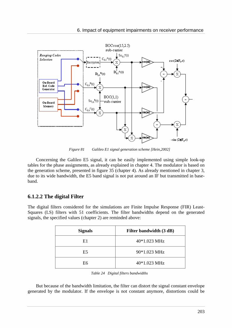
6. Impact of equipment impairments on receiver performance

203

Figure 81 Galileo E1 signal generation scheme [Hein,2002]

Concerning the Galileo E5 signal, it can be easily implemented using simple look-up

tables for the phase assignments, as already explained in chapter 4. The modulator is based on the generation scheme, presented in figure 35 (chapter 4). As already mentioned in chapter 3, due to its wide bandwidth, the E5 band signal is not put around an IF but transmitted in base-band.

6.1.2.2 The digital Filter

The digital filters considered for the simulations are Finite Impulse Response (FIR) Least-Squares (LS) filters with 51 coefficients. The filter bandwidths depend on the generated signals, the specified values (chapter 2) are reminded above:

Signals Filter bandwidth (3 dB)

E1 40*1.023 MHz

E5 90*1.023 MHz

E6 40*1.023 MHz

Table 24 Digital filters bandwidths

But because of the bandwidth limitation, the filter can distort the signal constant envelope

generated by the modulator. If the envelope is not constant anymore, distortions could be

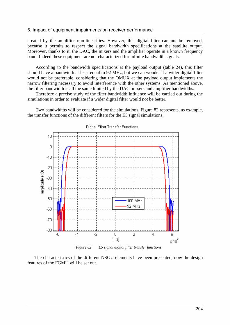
6. Impact of equipment impairments on receiver performance

204

created by the amplifier non-linearities. However, this digital filter can not be removed, because it permits to respect the signal bandwidth specifications at the satellite output. Moreover, thanks to it, the DAC, the mixers and the amplifier operate in a known frequency band. Indeed these equipment are not characterized for infinite bandwidth signals.

According to the bandwidth specifications at the payload output (table 24), this filter

should have a bandwidth at least equal to 92 MHz, but we can wonder if a wider digital filter would not be preferable, considering that the OMUX at the payload output implements the narrow filtering necessary to avoid interference with the other systems. As mentioned above, the filter bandwidth is all the same limited by the DAC, mixers and amplifier bandwidths.

Therefore a precise study of the filter bandwidth influence will be carried out during the simulations in order to evaluate if a wider digital filter would not be better.

Two bandwidths will be considered for the simulations. Figure 82 represents, as example,

the transfer functions of the different filters for the E5 signal simulations.

Figure 82 E5 signal digital filter transfer functions

The characteristics of the different NSGU elements have been presented, now the design

features of the FGMU will be set out.

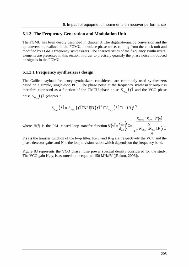
6. Impact of equipment impairments on receiver performance

205

6.1.3 The Frequency Generation and Modulation Unit

The FGMU has been deeply described in chapter 3. The digital-to-analog conversion and the up-conversion, realized in the FGMU, introduce phase noise, coming from the clock unit and modified by FGMU frequency synthesizers. The characteristics of the frequency synthesizers’ elements are presented in this section in order to precisely quantify the phase noise introduced on signals in the FGMU.

6.1.3.1 Frequency synthesizers design

The Galileo payload frequency synthesizers considered, are commonly used synthesizers based on a simple, single-loop PLL. The phase noise at the frequency synthesizer output is therefore expressed as a function of the CMCU phase noise ( )fS

CUφ and the VCO phase

noise ( )fSvcoφ (chapter 3) :

( ) ( ) ( ) ( ) ( ) 222 1 fHfSfHNfSfSvcoCUout

−⋅+⋅⋅= φφφ

where H(f) is the PLL closed loop transfer function( ) ( )( )

( )

( )N

sFKKs

N

sFKK

s

ssH

PDVCO

PDVCO

ref

out

⋅⋅+

⋅⋅

==θθ

,

F(s) is the transfer function of the loop filter, KVCO and KPD are, respectively the VCO and the phase detector gains and N is the loop division ration which depends on the frequency band. Figure 83 represents the VCO phase noise power spectral density considered for the study. The VCO gain KVCO is assumed to be equal to 150 MHz/V ([Rakon, 2006]).

6. Impact of equipment impairments on receiver performance

206

Power Spectral Density of VCO phase noise

-160

-150

-140

-130

-120

-110

-100

-90

-80

1,00E+03 1,00E+04 1,00E+05 1,00E+06 1,00E+07 1,00E+08

frequency offsets [Hz]

SS

b ph

asse

noi

se [d

Bc/

Hz]

Figure 83 VCO phase noise characteristic ([Rakon, 2006])

The phase comparator has a gain equal to 5.3 V/rad. The loop filter is an integrator and

lead/lag filter, with a transfer function equal to: 3

2

1 1

11)(

Ts

Ts

TssF

⋅+⋅+

⋅= with 111 RCT = ,

( )2122 CCRT +⋅= and 223 RCT = . It is considered that R1= 50 kΩ, R2= 270 Ω, C1= 470 nF

and C2 = 10 nF ([Zarlink, 2005]). Thanks to these parameters the phase noise at frequency synthesizers’ output used to

realize the D/A conversion and the up-conversion can be evaluated.

6.1.3.2 D/A converter phase noise

The payload sampling frequency considered is equal to 120*1.023 MHz = 12*10.23 MHz = 122.76 MHz ([Bradford, 2006]). So the DAC sampling frequency has a phase noise characterized by the following equation:

( ) ( ) ( ) ( ) ( ) 222 112 fHfSfHfSfSvcoCUDAC

−⋅+⋅⋅= φφφ

and by the following figure, representing the theoretical and simulated phase noise power spectrum densities:

6. Impact of equipment impairments on receiver performance

207

101

102

103

104

105

106

107

108

-160

-150

-140

-130

-120

-110

-100

frequency [Hz]

SS

B p

ower

spe

ctru

m d

ensi

ties

[dB

c/H

z]

Sampling frequency phase noise characterization

Simulated

theoritical

Figure 84 Sampling frequency phase noise SSB power spectral densities

The simulated phase noise power spectrum density was calculated on a 1 second time window.

Consequently, the time jitter added to the signal during the D/A conversion and

considered during the simulations, is equal to: ( ) ( )ej T

ttt ⋅=

πφ2

, and one realization is

represented in figure 85:

6. Impact of equipment impairments on receiver performance

208

0 0.001 0.002 0.003 0.004 0.005 0.006 0.007 0.008 0.009 0.01-3

-2

-1

0

1

2

3x 10

-12

time [s]

ampl

itude

D/A conversion time jitter

Figure 85 Time representation of DAC jitter

6.1.3.3 Up-conversion phase noise

As explained in chapter 3, the up-conversion is considered realized in one stage, so the FGMU frequency synthesizers’ ratios, as a function of the frequency band, are equal to:

Bands FI (MHz) N

E5 0 116.5

E1 30*1.023 151

E6 30*1.023 122

Table 25 Frequency synthesizers’ ratios for the up-conversion in the different frequency bands

The phase noise added to the signals during the up-conversion is characterized in figure

86 for the different frequency bands:

6. Impact of equipment impairments on receiver performance

209

Figure 86 Up-conversion phase noise SSB power spectral densities

As the VCO considered is the same for each frequency synthesizer, for frequency offsets

higher than 10 kHz, the three curves, corresponding to the three Galileo frequency bands, are identical because for this frequency range the VCO phase noise predominates.

Figure 87 represents the theoretical and simulated phase noise power spectrum densities

for the E5 band signal. The simulated phase noise power spectrum density was calculated on a 1 second time window.

6. Impact of equipment impairments on receiver performance

210

100

102

104

106

108

-160

-150

-140

-130

-120

-110

-100

-90

-80

frequency [Hz]

SS

B p

ower

spe

ctru

m d

ensi

ties

[dB

c/H

z]E5 band up-conversion phase noise characterization

Simulated

theoritical

Figure 87 E5 band up-conversion phase noise SSB power spectral densities

So the phase noises introduced by the FGMU during the D/A conversion and the up-conversion have been precisely characterized. The last FGMU characteristics, necessary to realize the simulations, concern the FGMU filters.

6.1.3.4 FGMU filters

The FGMU filters are used to avoid out-of-band emissions and more particularly spectrum distortions after the digital-to-analog conversion and spectrum re-combinations after the up-conversion. These filters are wideband (around 120 MHz) analog filters but for the simulations they are modelled by FIR Least-squares filters, whose transfer function is represented in figure 88.

6. Impact of equipment impairments on receiver performance

211

-6 -4 -2 0 2 4 6

x 107

-100

-80

-60

-40

-20

0

FGMU filter transfer functions

frequency [Hz]

ampl

itude

Figure 88 Transfer function of the FGMU filters after the D/A conversion and the up-conversion

Contrary to the digital filter, this filter, thanks to its wide bandwidth, has a negligible

influence on the signal envelope.

At the FGMU output, the signal enters in the amplification unit, so the features used to simulate the non-linear amplification will now be presented.

6.1.4 The Amplification Unit

The amplifier studied is an SSPA amplifier, built by the “Universidad del Paìs Vasco” in Bilbao in collaboration with the CNES. A miniature model of this amplifier is presented in the following picture:

6. Impact of equipment impairments on receiver performance

212

Figure 89 Studied amplifier picture

This prototype of amplifier has characteristics similar to the SSPA foreseen for the

Galileo satellites ([Coromina, 2004]) even if the power it delivers is weaker than the power necessary to verify the Galileo power link budget. Indeed, as seen in chapter 2, the power at the amplifier output to transmit the Galileo E5 band signal should be equal to 19 dBW, whereas the simulated prototype amplifier could only amplify to 30 dBmW, as seen on their AM/AM and AM/PM characteristics, represented in figures 90 and 91. Its gain compression point at 2 dB corresponds to (Pin2dB = 16.9 dBm, Pout2dB = 30.1 dBm, PAE2dB = 69%). Figure 92 represents the power added efficiency of this amplifier.

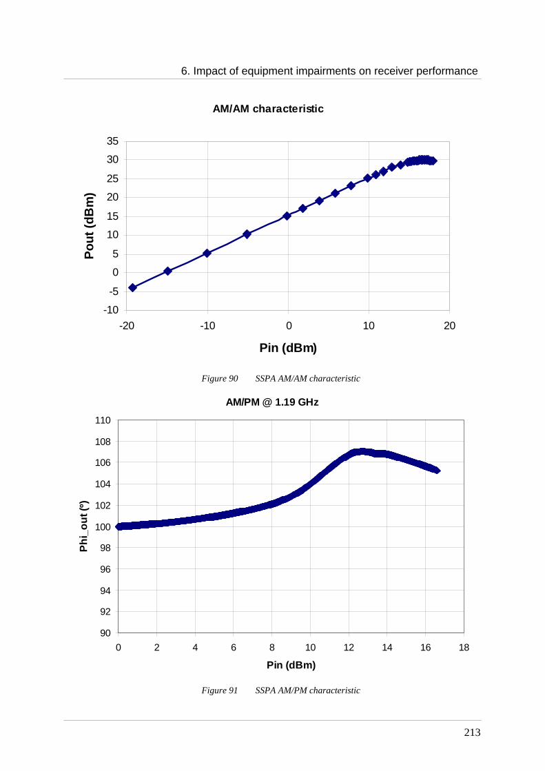
6. Impact of equipment impairments on receiver performance

213

AM/AM characteristic

-10

-5

0

5

10

15

20

25

30

35

-20 -10 0 10 20

Pin (dBm)

Pou

t (dB

m)

Figure 90 SSPA AM/AM characteristic

AM/PM @ 1.19 GHz

90

92

94

96

98

100

102

104

106

108

110

0 2 4 6 8 10 12 14 16 18

Pin (dBm)

Phi

_out

(º)

Figure 91 SSPA AM/PM characteristic

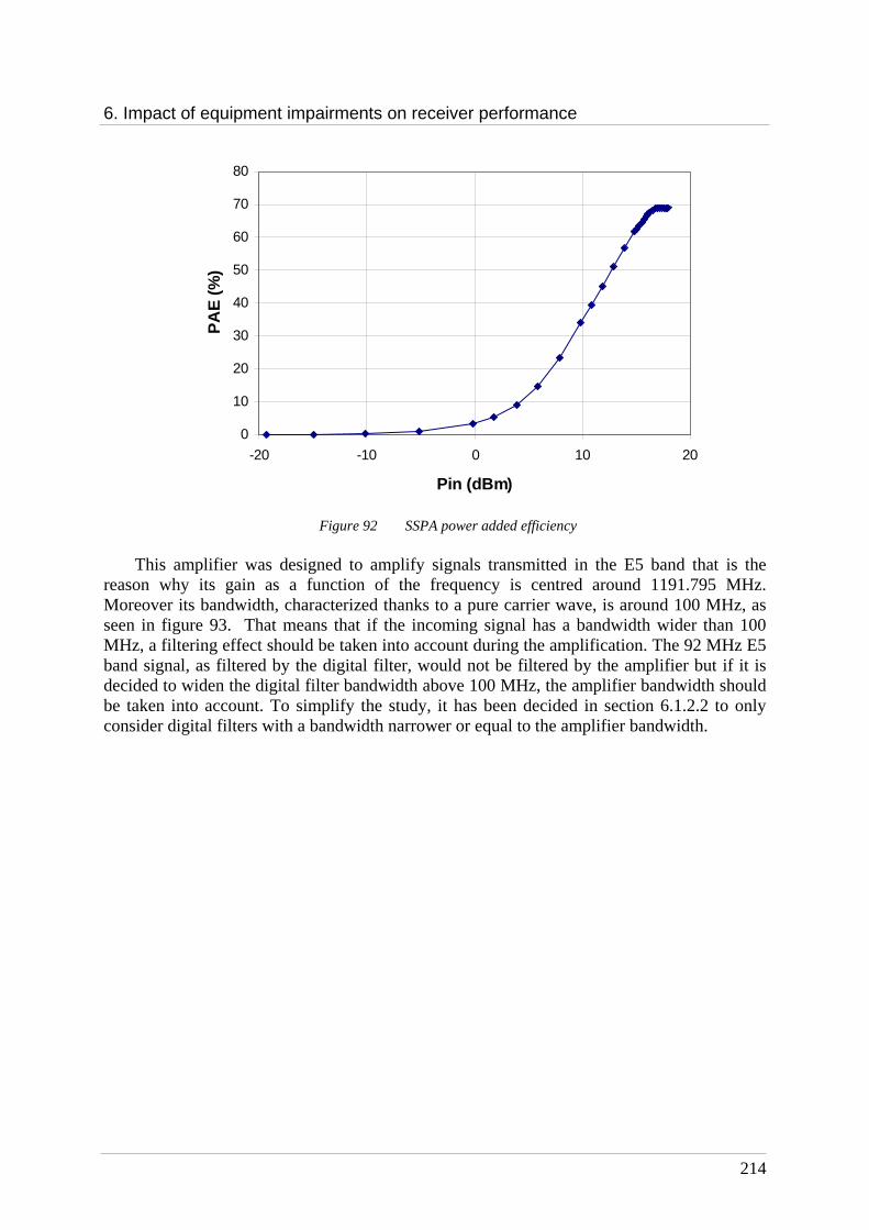
6. Impact of equipment impairments on receiver performance

214

0

10

20

30

40

50

60

70

80

-20 -10 0 10 20

Pin (dBm)

PA

E (

%)

Figure 92 SSPA power added efficiency

This amplifier was designed to amplify signals transmitted in the E5 band that is the

reason why its gain as a function of the frequency is centred around 1191.795 MHz. Moreover its bandwidth, characterized thanks to a pure carrier wave, is around 100 MHz, as seen in figure 93. That means that if the incoming signal has a bandwidth wider than 100 MHz, a filtering effect should be taken into account during the amplification. The 92 MHz E5 band signal, as filtered by the digital filter, would not be filtered by the amplifier but if it is decided to widen the digital filter bandwidth above 100 MHz, the amplifier bandwidth should be taken into account. To simplify the study, it has been decided in section 6.1.2.2 to only consider digital filters with a bandwidth narrower or equal to the amplifier bandwidth.

6. Impact of equipment impairments on receiver performance

215

Amplifier gain in function of the carrier frequency

8

9

10

11

12

13

14

15

16

1,00E+09 1,05E+09 1,10E+09 1,15E+09 1,20E+09 1,25E+09 1,30E+09 1,35E+09 1,40E+09

Fréquence (Hz)

S21

(dB

)

Figure 93 SSPA gain in function of the carrier frequency

However, the AM/AM, AM/PM curves, presented previously, are sometimes not

sufficient to precisely characterize an SSPA, as already explained in chapter 3. Indeed these curves do not take correctly into account the signal bandwidth because they are characterized thanks to pure carrier waves. The memory effects are also not represented by the AM/AM, AM/PM characterization. That is the reason why a lot of studies are carried out currently to find new models which permit to precisely characterize the amplifier by simulating their non-linear and memory effects ([Ircom, 2006]).

During the simulations, only the AM/AM and AM/PM characteristics will be used, but while being aware of the model limitation.

The last element of the payload before the signal transmission will now be precisely

presented.

6.1.5 The OMUX

The Output Multiplexers are generally simulated as Butterworth filters, as exposed in chapter 3. But for this study, to avoid the problem due to the non-linear Butterworth filter phase, the OMUX filters simulated are considered as FIR Least-Squares filters whose bandwidths are equal to the signal bandwidths defined by the Galileo ICD ([GJU, 2005]). The OMUX filter transfer function, considered for the Galileo E5 band signal, is represented in figure 94:

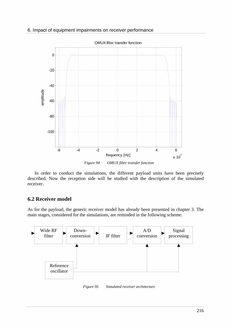
6. Impact of equipment impairments on receiver performance

216

-6 -4 -2 0 2 4 6

x 107

-100

-80

-60

-40

-20

0

OMUX filter transfer function

frequency [Hz]

ampl

itude

Figure 94 OMUX filter transfer function

In order to conduct the simulations, the different payload units have been precisely

described. Now the reception side will be studied with the description of the simulated receiver.

6.2 Receiver model

As for the payload, the generic receiver model has already been presented in chapter 3. The main stages, considered for the simulations, are reminded in the following scheme:

Figure 95 Simulated receiver architecture

Wide RF filter

Down-conversion

A/D conversion

Signal processing

IF filter

Reference oscillator

6. Impact of equipment impairments on receiver performance

217

This section will give more detail on the characteristics of the different receiver equipment chosen for the phase noise study and simulations.

6.2.1 Oscillators models

Let us start with the main receiver equipment: the reference oscillator. Two different types of oscillators, associated to two different types of receivers, will be considered for this study. The first one will use a very stable external clock based on the rubidium technology and the second one will use a classical “mass-market” oscillator, a TCXO. Both oscillators deliver a frequency equal to 10 MHz.

The phase noise characterizations of the two oscillators have already been presented in chapter 3 in figure 25, they are reminded above:

Figure 25 Power Spectral Density of TCXO and rubidium receiver clocks ([Rakon, 2006])

The oscillator is the heart of the receiver because as already mentioned in chapter 3, it is

used by the different receiver units to realize the down-conversion, the analog-to-digital conversion and the processing.

6.2.2 Down-conversion

The down-conversion of the incoming signal is realized thanks to frequency synthesizers, using the reference oscillator. The model of the frequency synthesizer considered is detailed in this section to deduce the phase noise added to the signal during the down-conversion.

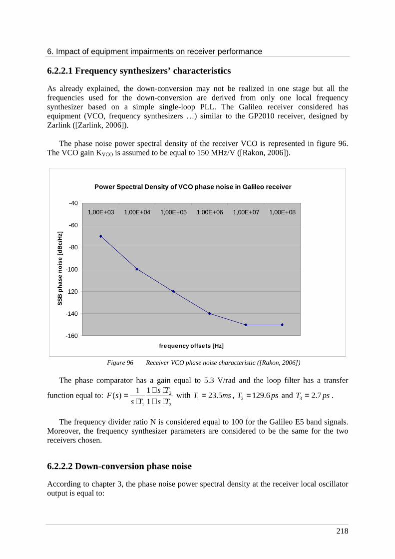
6. Impact of equipment impairments on receiver performance

218

6.2.2.1 Frequency synthesizers’ characteristics

As already explained, the down-conversion may not be realized in one stage but all the frequencies used for the down-conversion are derived from only one local frequency synthesizer based on a simple single-loop PLL. The Galileo receiver considered has equipment (VCO, frequency synthesizers …) similar to the GP2010 receiver, designed by Zarlink ([Zarlink, 2006]).

The phase noise power spectral density of the receiver VCO is represented in figure 96. The VCO gain KVCO is assumed to be equal to 150 MHz/V ([Rakon, 2006]).

Power Spectral Density of VCO phase noise in Galile o receiver

-160

-140

-120

-100

-80

-60

-40

1,00E+03 1,00E+04 1,00E+05 1,00E+06 1,00E+07 1,00E+08

frequency offsets [Hz]

SS

B p

hase

noi

se [d

Bc/

Hz]

Figure 96 Receiver VCO phase noise characteristic ([Rakon, 2006])

The phase comparator has a gain equal to 5.3 V/rad and the loop filter has a transfer

function equal to: 3

2

1 1

11)(

Ts

Ts

TssF

⋅+⋅+

⋅= with msT 5.231 = , psT 6.1292 = and psT 7.23 = .

The frequency divider ratio N is considered equal to 100 for the Galileo E5 band signals.

Moreover, the frequency synthesizer parameters are considered to be the same for the two receivers chosen.

6.2.2.2 Down-conversion phase noise

According to chapter 3, the phase noise power spectral density at the receiver local oscillator output is equal to:

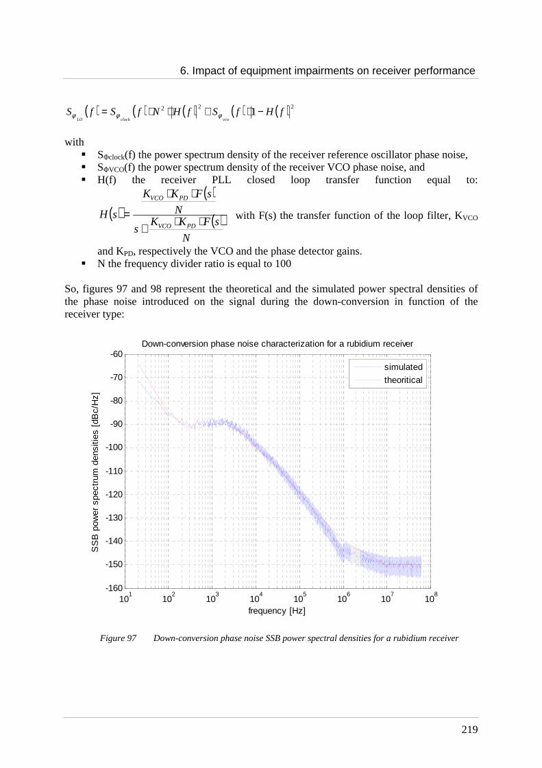
6. Impact of equipment impairments on receiver performance

219

( ) ( ) ( ) ( ) ( ) 222 1 fHfSfHNfSfSvcoclockLO

−⋅+⋅⋅= φφφ

with SΦclock(f) the power spectrum density of the receiver reference oscillator phase noise, SΦVCO(f) the power spectrum density of the receiver VCO phase noise, and H(f) the receiver PLL closed loop transfer function equal to:

( )( )

( ) N

sFKKs

N

sFKK

sHPDVCO

PDVCO

⋅⋅+

⋅⋅

= with F(s) the transfer function of the loop filter, KVCO

and KPD, respectively the VCO and the phase detector gains. N the frequency divider ratio is equal to 100

So, figures 97 and 98 represent the theoretical and the simulated power spectral densities of the phase noise introduced on the signal during the down-conversion in function of the receiver type:

101

102

103

104

105

106

107

108

-160

-150

-140

-130

-120

-110

-100

-90

-80

-70

-60

frequency [Hz]

SS

B p

ower

spe

ctru

m d

ensi

ties

[dB

c/H

z]

Down-conversion phase noise characterization for a rubidium receiver

simulated

theoritical

Figure 97 Down-conversion phase noise SSB power spectral densities for a rubidium receiver

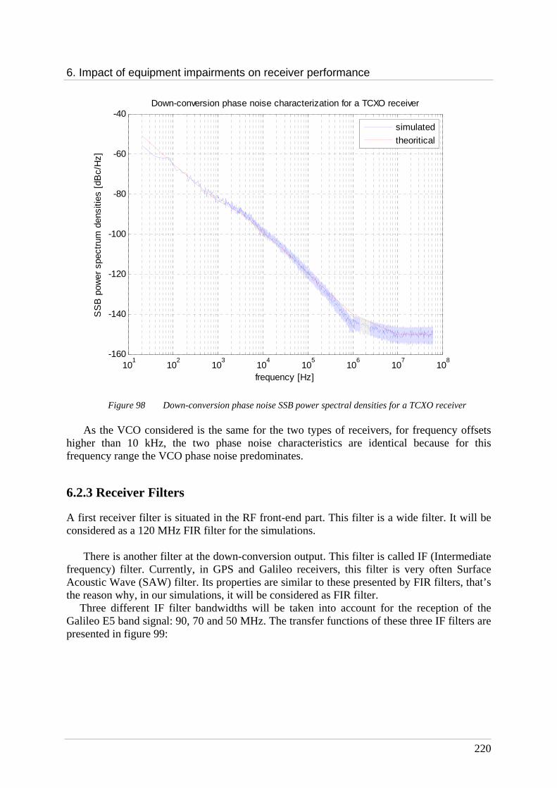
6. Impact of equipment impairments on receiver performance

220

101

102

103

104

105

106

107

108

-160

-140

-120

-100

-80

-60

-40Down-conversion phase noise characterization for a TCXO receiver

frequency [Hz]

SS

B p

ower

spe

ctru

m d

ensi

ties

[dB

c/H

z]

simulated

theoritical

Figure 98 Down-conversion phase noise SSB power spectral densities for a TCXO receiver As the VCO considered is the same for the two types of receivers, for frequency offsets

higher than 10 kHz, the two phase noise characteristics are identical because for this frequency range the VCO phase noise predominates.

6.2.3 Receiver Filters

A first receiver filter is situated in the RF front-end part. This filter is a wide filter. It will be considered as a 120 MHz FIR filter for the simulations.

There is another filter at the down-conversion output. This filter is called IF (Intermediate frequency) filter. Currently, in GPS and Galileo receivers, this filter is very often Surface Acoustic Wave (SAW) filter. Its properties are similar to these presented by FIR filters, that’s the reason why, in our simulations, it will be considered as FIR filter.

Three different IF filter bandwidths will be taken into account for the reception of the Galileo E5 band signal: 90, 70 and 50 MHz. The transfer functions of these three IF filters are presented in figure 99:

6. Impact of equipment impairments on receiver performance

221

-6 -4 -2 0 2 4 6

x 107

-120

-100

-80

-60

-40

-20

0

Receiver IF filters transfer functions

frequency [Hz]

ampl

itude

[dB

]

50 MHz

70 MHz

90 MHz

Figure 99 Transfer functions of the receiver IF filter

6.2.4 A/D conversion

After the down-conversion and the IF filtering, the signal is digitized by an analog-to-digital converter. The ADC sampling frequency is derived from the frequency generated by the local oscillator used for the down-conversion. It should be at least equal to twice the signal bandwidth which depend on the bandwidth of the IF filter. The sampling frequencies considered are therefore: 90, 70 and 50 MHz.

For example, the A/D conversion phase noise of the 90 MHz case is characterized by the following equation and figure 100:

( )( ) ( ) ( ) ( )

2

222

11

1100 fHfSfHfSfS vcoclock

ADC

−⋅+⋅⋅=

φφφ

6. Impact of equipment impairments on receiver performance

222

100

102

104

106

108

-180

-170

-160

-150

-140

-130

-120

-110

-100

-90

-80

frequency [Hz]

SS

B p

ower

sep

ctru

m d

ensi

ties

[dB

c/H

z]

A/D conversion phase noise characterization for a rubidium receiver

simulated

theoritical

10

110

210

310

410

510

610

710

8-180

-160

-140

-120

-100

-80

-60A/D conversion phase noise characterization for a TCXO receiver

frequency [Hz]

SS

B p

ower

spe

ctru

m d

ensi

ties

[dB

c/H

z]

Simulated

theoritical

Figure 100 Receiver sampling frequency phase noise SSB power spectral densities

An example of the time jitter introduced on the signal during the analog-to-digital conversion is represented in figure 101:

0 0.001 0.002 0.003 0.004 0.005 0.006 0.007 0.008 0.009 0.01-4

-3

-2

-1

0

1

2

3x 10

-12 A/D conversion time jitter

time [s]

ampl

itude

rubidium

TCXO

Figure 101 Time jitter introduced during the A/D conversion

In the two previous sections, the payload and the two receivers models considered have

been precisely described. These models will permit to carry out simulations which will present the impact of each payload and receiver units on the Galileo E5 band signal.

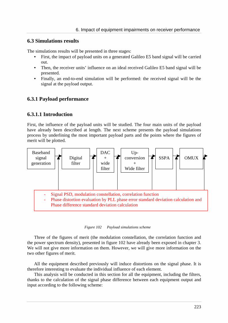
6. Impact of equipment impairments on receiver performance

223

6.3 Simulations results

The simulations results will be presented in three stages: • First, the impact of payload units on a generated Galileo E5 band signal will be carried

out. • Then, the receiver units’ influence on an ideal received Galileo E5 band signal will be

presented. • Finally, an end-to-end simulation will be performed: the received signal will be the

signal at the payload output.

6.3.1 Payload performance

6.3.1.1 Introduction

First, the influence of the payload units will be studied. The four main units of the payload have already been described at length. The next scheme presents the payload simulations process by underlining the most important payload parts and the points where the figures of merit will be plotted.

Figure 102 Payload simulations scheme

Three of the figures of merit (the modulation constellation, the correlation function and the power spectrum density), presented in figure 102 have already been exposed in chapter 3. We will not give more information on them. However, we will give more information on the two other figures of merit.

All the equipment described previously will induce distortions on the signal phase. It is therefore interesting to evaluate the individual influence of each element.

This analysis will be conducted in this section for all the equipment, including the filters, thanks to the calculation of the signal phase difference between each equipment output and input according to the following scheme:

Baseband signal

generation

Digital filter

DAC +

wide filter

SSPA

Up-conversion

+ Wide filter

OMUX

- Signal PSD, modulation constellation, correlation function - Phase distortion evaluation by PLL phase error standard deviation calculation and

Phase difference standard deviation calculation

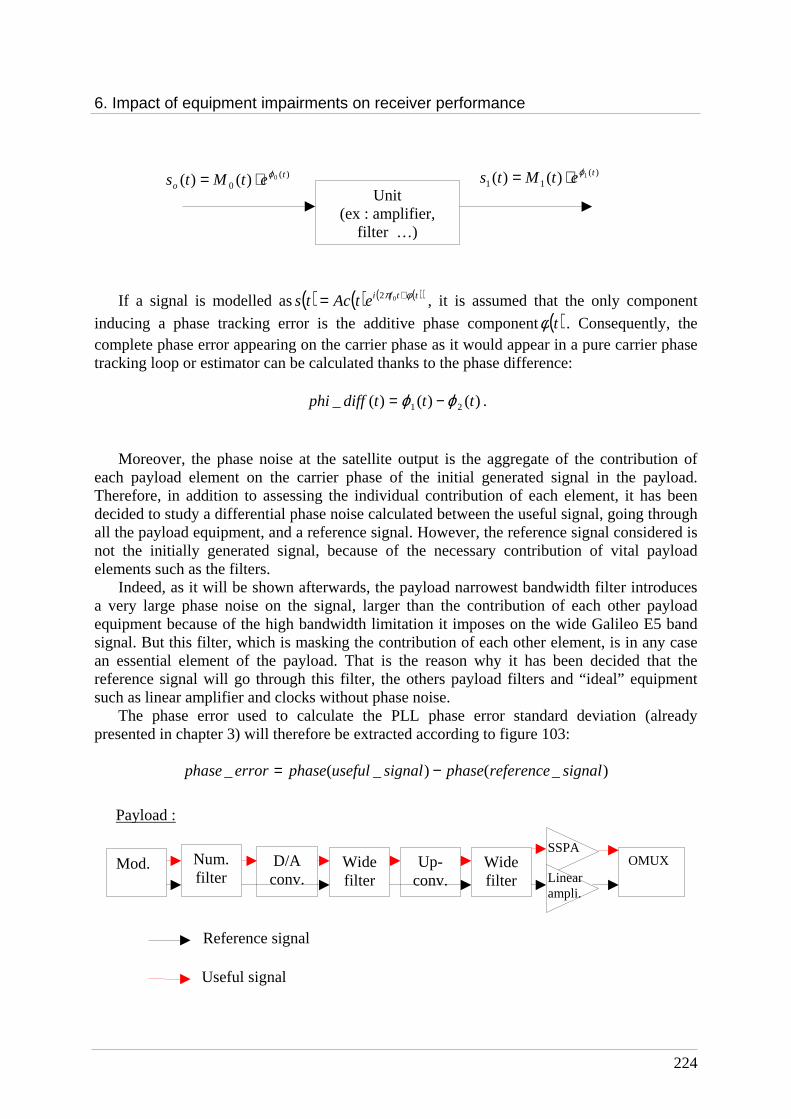
6. Impact of equipment impairments on receiver performance

224

If a signal is modelled as( ) ( ) ( )( )ttfietActs φπ += 02 , it is assumed that the only component

inducing a phase tracking error is the additive phase component( )tφ . Consequently, the complete phase error appearing on the carrier phase as it would appear in a pure carrier phase tracking loop or estimator can be calculated thanks to the phase difference:

)()()(_ 21 tttdiffphi ϕϕ −= .

Moreover, the phase noise at the satellite output is the aggregate of the contribution of

each payload element on the carrier phase of the initial generated signal in the payload. Therefore, in addition to assessing the individual contribution of each element, it has been decided to study a differential phase noise calculated between the useful signal, going through all the payload equipment, and a reference signal. However, the reference signal considered is not the initially generated signal, because of the necessary contribution of vital payload elements such as the filters.

Indeed, as it will be shown afterwards, the payload narrowest bandwidth filter introduces a very large phase noise on the signal, larger than the contribution of each other payload equipment because of the high bandwidth limitation it imposes on the wide Galileo E5 band signal. But this filter, which is masking the contribution of each other element, is in any case an essential element of the payload. That is the reason why it has been decided that the reference signal will go through this filter, the others payload filters and “ideal” equipment such as linear amplifier and clocks without phase noise.

The phase error used to calculate the PLL phase error standard deviation (already presented in chapter 3) will therefore be extracted according to figure 103:

)_()_(_ signalreferencephasesignalusefulphaseerrorphase −=

Unit (ex : amplifier,

filter …)

)(0

0)()( to etMts ϕ⋅= )(

111)()( tetMts ϕ⋅=

Reference signal

Useful signal

Mod. Num. filter

D/A conv.

Wide filter

Up-conv.

Wide filter

OMUX SSPA

Linear ampli.

Payload :

6. Impact of equipment impairments on receiver performance

225

Figure 103 PLL phase error variance calculation in the payload Now that the simulation stages and the figures of merit have been clearly explained, the

simulations results could be presented.

6.3.1.2 Baseband Galileo E5 band signal

This section reminds the “ideal” (infinite bandwidth) figures of merit of the Galileo ALTBOC signal. Figure 104 presents the E5 signal modulation constellation.

Figure 104 Infinite bandwidth Galileo E5 band signal modulation constellation

As already seen in chapter 4, the modulation constellation of the E5 band signal is similar to a 8-PSK constellation, moreover its envelope is constant in an infinite bandwidth.

The two next figures represent the absolute value of the autocorrelation function and an estimated spectrum of the Galileo ALTBOC signal.

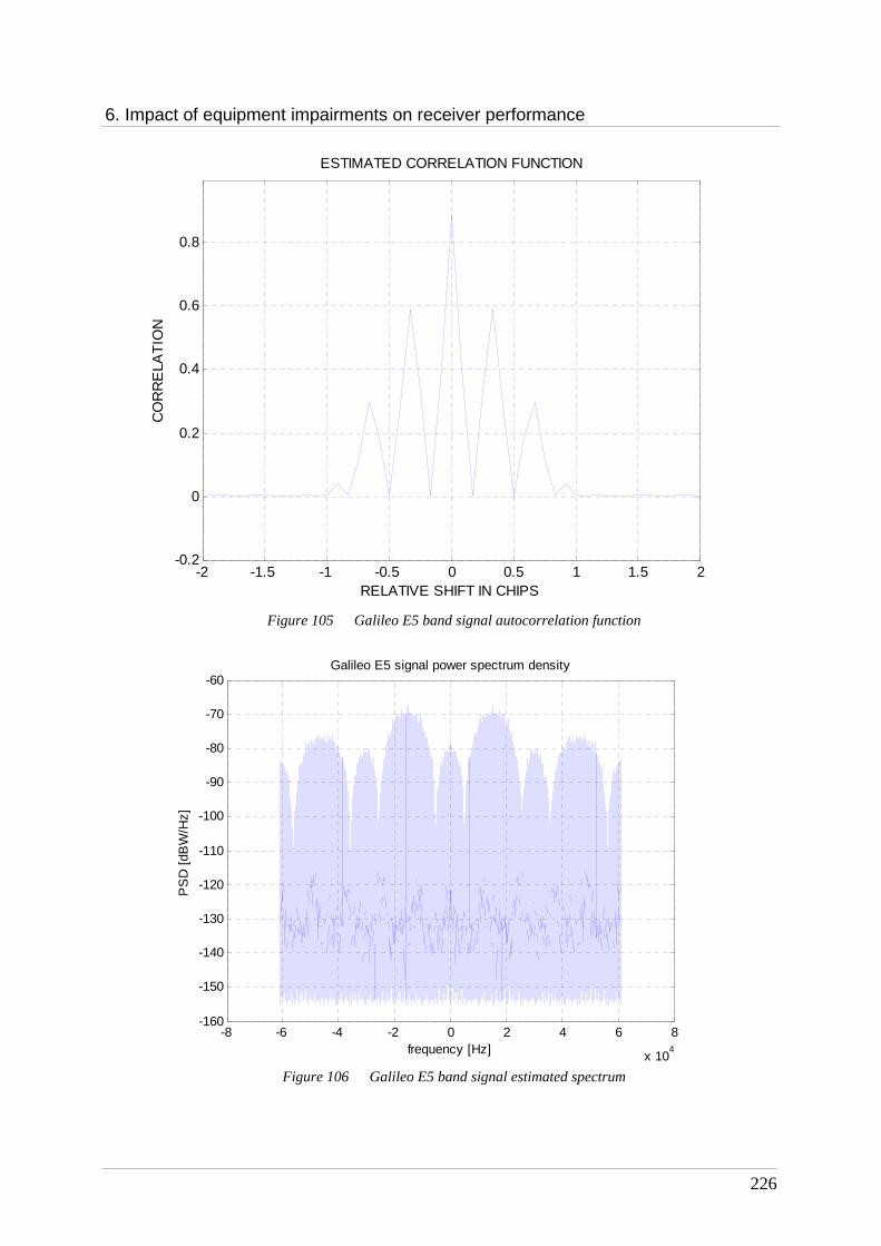
6. Impact of equipment impairments on receiver performance

226

-2 -1.5 -1 -0.5 0 0.5 1 1.5 2-0.2

0

0.2

0.4

0.6

0.8

RELATIVE SHIFT IN CHIPS

CO

RR

ELA

TIO

NESTIMATED CORRELATION FUNCTION

Figure 105 Galileo E5 band signal autocorrelation function

-8 -6 -4 -2 0 2 4 6 8

x 104

-160

-150

-140

-130

-120

-110

-100

-90

-80

-70

-60Galileo E5 signal power spectrum density

frequency [Hz]

PS

D [

dBW

/Hz]

Figure 106 Galileo E5 band signal estimated spectrum

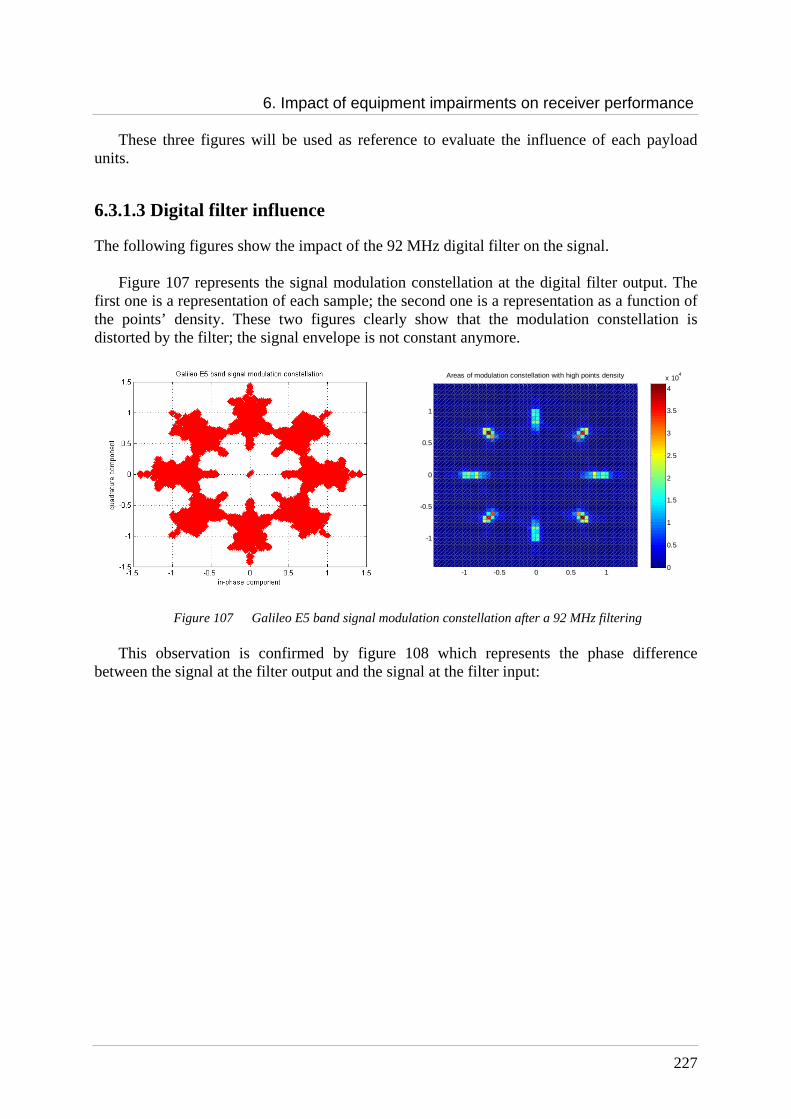
6. Impact of equipment impairments on receiver performance

227

These three figures will be used as reference to evaluate the influence of each payload units.

6.3.1.3 Digital filter influence

The following figures show the impact of the 92 MHz digital filter on the signal.

Figure 107 represents the signal modulation constellation at the digital filter output. The first one is a representation of each sample; the second one is a representation as a function of the points’ density. These two figures clearly show that the modulation constellation is distorted by the filter; the signal envelope is not constant anymore.

-1 -0.5 0 0.5 1

-1

-0.5

0

0.5

1

Areas of modulation constellation with high points density

0

0.5

1

1.5

2

2.5

3

3.5

4

x 104

Figure 107 Galileo E5 band signal modulation constellation after a 92 MHz filtering

This observation is confirmed by figure 108 which represents the phase difference between the signal at the filter output and the signal at the filter input:

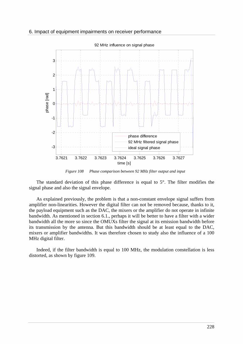
6. Impact of equipment impairments on receiver performance

228

3.7621 3.7622 3.7623 3.7624 3.7625 3.7626 3.7627

-3

-2

-1

0

1

2

3

time [s]

phas

e [r

ad]

92 MHz influence on signal phase

phase difference

92 MHz filtered signal phase

ideal signal phase

Figure 108 Phase comparison between 92 MHz filter output and input

The standard deviation of this phase difference is equal to 5°. The filter modifies the

signal phase and also the signal envelope.

As explained previously, the problem is that a non-constant envelope signal suffers from amplifier non-linearities. However the digital filter can not be removed because, thanks to it, the payload equipment such as the DAC, the mixers or the amplifier do not operate in infinite bandwidth. As mentioned in section 6.1., perhaps it will be better to have a filter with a wider bandwidth all the more so since the OMUXs filter the signal at its emission bandwidth before its transmission by the antenna. But this bandwidth should be at least equal to the DAC, mixers or amplifier bandwidths. It was therefore chosen to study also the influence of a 100 MHz digital filter.

Indeed, if the filter bandwidth is equal to 100 MHz, the modulation constellation is less

distorted, as shown by figure 109.

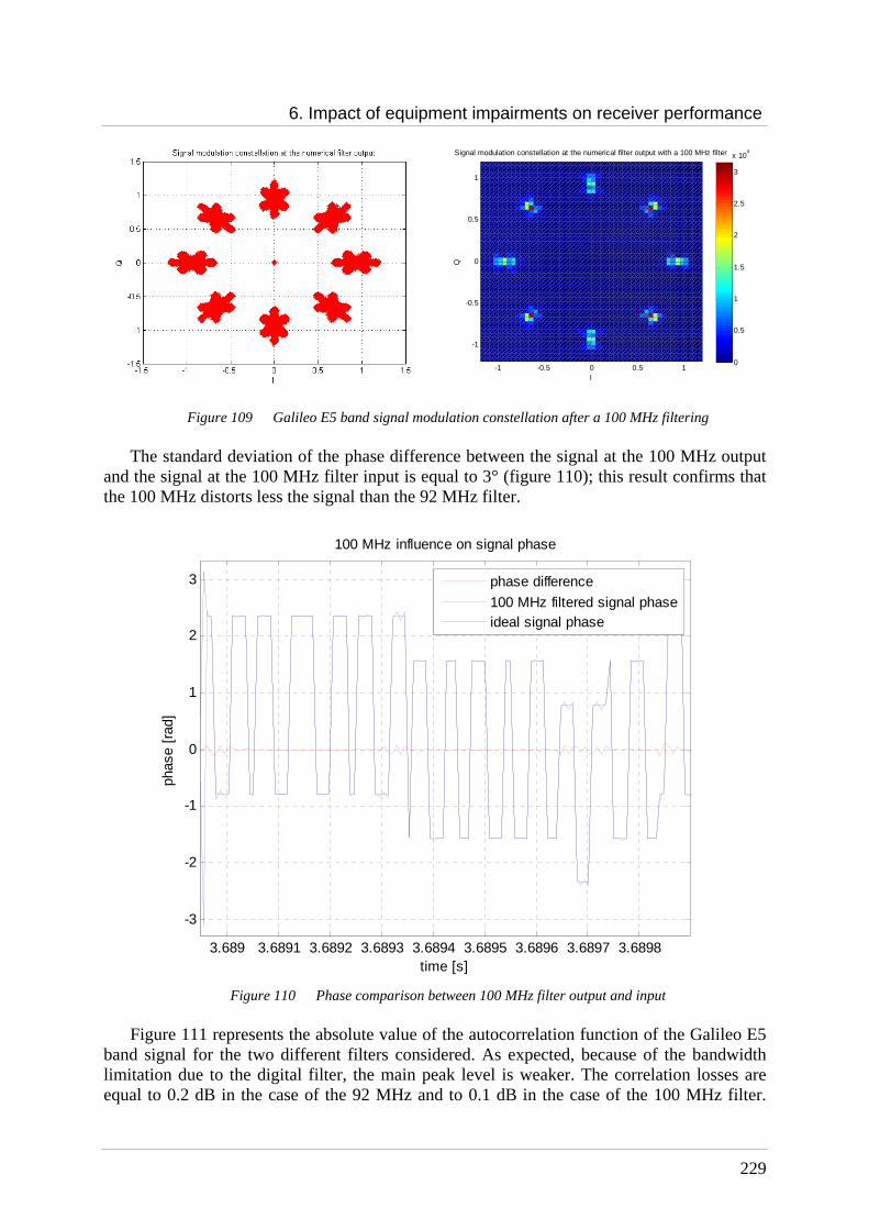
6. Impact of equipment impairments on receiver performance

229

-1 -0.5 0 0.5 1

-1

-0.5

0

0.5

1

I

Q

Signal modulation constellation at the numerical filter output with a 100 MHz filter

0

0.5

1

1.5

2

2.5

3

x 104

Figure 109 Galileo E5 band signal modulation constellation after a 100 MHz filtering

The standard deviation of the phase difference between the signal at the 100 MHz output and the signal at the 100 MHz filter input is equal to 3° (figure 110); this result confirms that the 100 MHz distorts less the signal than the 92 MHz filter.

3.689 3.6891 3.6892 3.6893 3.6894 3.6895 3.6896 3.6897 3.6898

-3

-2

-1

0

1

2

3

time [s]

phas

e [r

ad]

100 MHz influence on signal phase

phase difference

100 MHz filtered signal phaseideal signal phase

Figure 110 Phase comparison between 100 MHz filter output and input

Figure 111 represents the absolute value of the autocorrelation function of the Galileo E5

band signal for the two different filters considered. As expected, because of the bandwidth limitation due to the digital filter, the main peak level is weaker. The correlation losses are equal to 0.2 dB in the case of the 92 MHz and to 0.1 dB in the case of the 100 MHz filter.

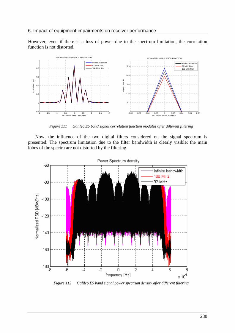
6. Impact of equipment impairments on receiver performance

230

However, even if there is a loss of power due to the spectrum limitation, the correlation function is not distorted.

-2 -1.5 -1 -0.5 0 0.5 1 1.5 2-0.2

0

0.2

0.4

0.6

0.8

RELATIVE SHIFT IN CHIPS

CO

RR

ELA

TIO

N

ESTIMATED CORRELATION FUNCTION

infinite bandwidth

92 MHz filter100 MHz filter

-0.08 -0.06 -0.04 -0.02 0 0.02 0.04 0.06 0.08

0.7

0.75

0.8

0.85

0.9

RELATIVE SHIFT IN CHIPS

CO

RR

ELA

TIO

N

ESTIMATED CORRELATION FUNCTION

infinite bandwidth

92 MHz filter100 MHz filter

Figure 111 Galileo E5 band signal correlation function modulus after different filtering

Now, the influence of the two digital filters considered on the signal spectrum is presented. The spectrum limitation due to the filter bandwidth is clearly visible; the main lobes of the spectra are not distorted by the filtering.

Figure 112 Galileo E5 band signal power spectrum density after different filtering

6. Impact of equipment impairments on receiver performance

231

Afterwards, to better evaluate the digital filter bandwidth influence on the signal performance and particularly on amplifier non-linearities, all the simulations will be made considering both a 92 MHz and a 100 MHz generated ALTBOC signal.

6.3.1.4 DAC influence

Now the influence of the time jitter due to the DAC will be evaluated. The figures of merit will be evaluated at the DAC output after a wideband filter which permits to eliminate out-of-band rejection.

To begin the DAC phase noise influence on the modulation constellation is studied.

-1 -0.5 0 0.5 1

-1

-0.5

0

0.5

1

Modulation constellation at the DAC output

0

2000

4000

6000

8000

10000

12000

14000

16000

18000

Figure 113 DAC influence on Galileo E5 band signal modulation constellation (92 and 100 MHz filters)

With a 92 MHz or a 100 MHz digital filter, the DAC does not distort or only slightly the modulation constellation. Indeed, there is no visible rotation or spread of the modulation plots. That seems normal because the phase distortions induced by the DAC are negligible in front of the phase distortions induced by the digital filter.

Indeed, the phase difference between the signal at the (DAC + wide filter) output and the signal at the (DAC + wide filter) input (figure 114) shows that the phase noise introduced by

6. Impact of equipment impairments on receiver performance

232

the DAC is very low (in accordance with figures 84 and 85) and confirms that the phase distortion introduced by the wide filter is negligible. The standard deviation of the phase difference at the DAC output is equal to 0.003°, which is negligible compared to the 5.5° obtained for the digital filter. The following figure is plotted considering a 92 MHz digital filter but the same observation can be made with a 100 MHz digital filter.

Figure 114 Phase study at DAC output (92 MHz digital filter)

The DAC phase noise influence on the absolute value of the correlation function and on the estimated spectrum is not important either. Indeed figure 115 shows that the DAC does not introduce correlation losses or distortions. The wide filter at the DAC output introduces, as for it, a slight correlation loss equal to 0.007 dB compared to the correlation function at the digital filter output. The effect on the estimated spectrum is, as for it, not really clear.

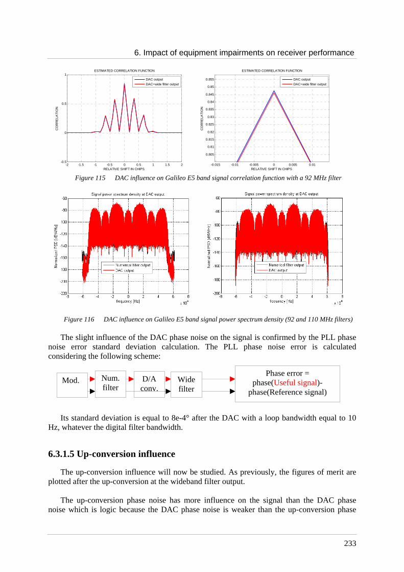
6. Impact of equipment impairments on receiver performance

233

-2 -1.5 -1 -0.5 0 0.5 1 1.5 2-0.5

0

0.5

1

RELATIVE SHIFT IN CHIPS

CO

RR

ELA

TIO

N

ESTIMATED CORRELATION FUNCTION

DAC output

DAC+wide filter output

-0.015 -0.01 -0.005 0 0.005 0.01

0.805

0.81

0.815

0.82

0.825

0.83

0.835

0.84

0.845

0.85

0.855

RELATIVE SHIFT IN CHIPS

CO

RR

ELA

TIO

N

ESTIMATED CORRELATION FUNCTION

DAC output

DAC+wide filter output

Figure 115 DAC influence on Galileo E5 band signal correlation function with a 92 MHz filter

Figure 116 DAC influence on Galileo E5 band signal power spectrum density (92 and 110 MHz filters)

The slight influence of the DAC phase noise on the signal is confirmed by the PLL phase noise error standard deviation calculation. The PLL phase noise error is calculated considering the following scheme:

Its standard deviation is equal to 8e-4° after the DAC with a loop bandwidth equal to 10 Hz, whatever the digital filter bandwidth.

6.3.1.5 Up-conversion influence

The up-conversion influence will now be studied. As previously, the figures of merit are plotted after the up-conversion at the wideband filter output.

The up-conversion phase noise has more influence on the signal than the DAC phase noise which is logic because the DAC phase noise is weaker than the up-conversion phase

Phase error = phase(Useful signal)-

phase(Reference signal)

Mod. Num. filter

D/A conv.

Wide filter

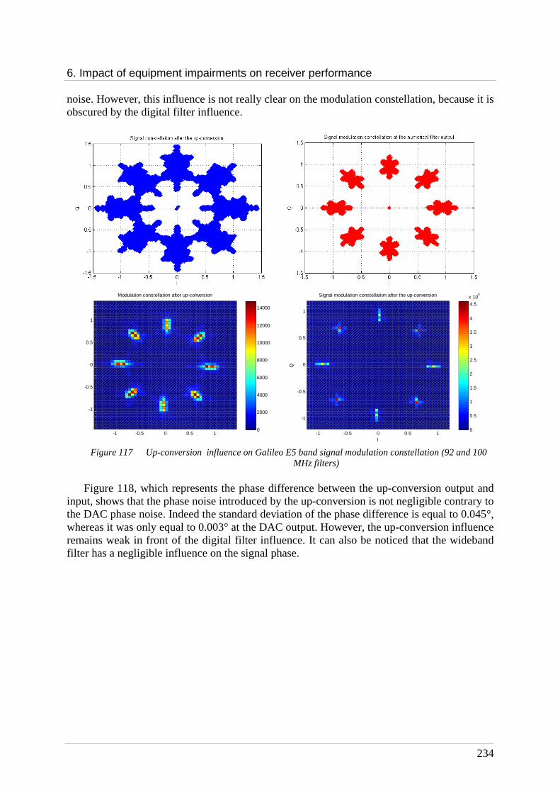
6. Impact of equipment impairments on receiver performance

234

noise. However, this influence is not really clear on the modulation constellation, because it is obscured by the digital filter influence.

-1 -0.5 0 0.5 1

-1

-0.5

0

0.5

1

Modulation constellation after up-conversion

0

2000

4000

6000

8000

10000

12000

14000

-1 -0.5 0 0.5 1

-1

-0.5

0

0.5

1

I

QSignal modulation constellation after the up-conversion

0

0.5

1

1.5

2

2.5

3

3.5

4

4.5

x 104

Figure 117 Up-conversion influence on Galileo E5 band signal modulation constellation (92 and 100

MHz filters)

Figure 118, which represents the phase difference between the up-conversion output and input, shows that the phase noise introduced by the up-conversion is not negligible contrary to the DAC phase noise. Indeed the standard deviation of the phase difference is equal to 0.045°, whereas it was only equal to 0.003° at the DAC output. However, the up-conversion influence remains weak in front of the digital filter influence. It can also be noticed that the wideband filter has a negligible influence on the signal phase.

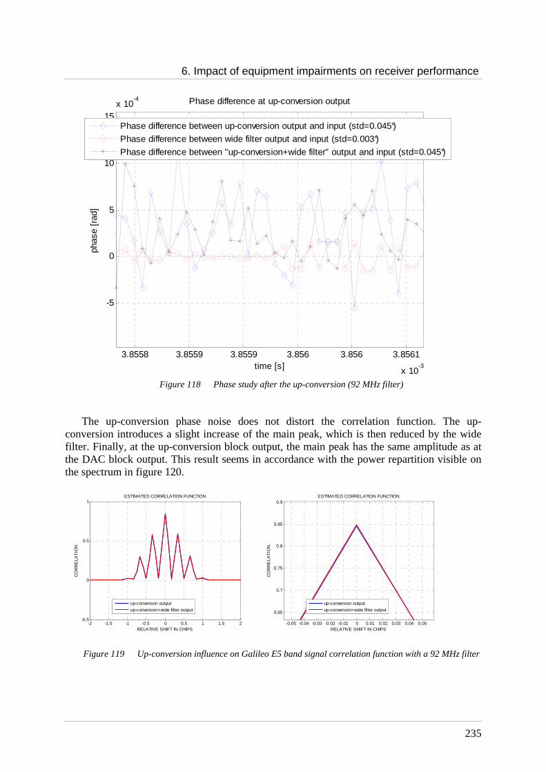
6. Impact of equipment impairments on receiver performance

235

3.8558 3.8559 3.8559 3.856 3.856 3.8561

x 10-3

-5

0

5

10

15x 10

-4

time [s]

phas

e [r

ad]

Phase difference at up-conversion output

Phase difference between up-conversion output and input (std=0.045°)

Phase difference between wide filter output and input (std=0.003°)

Phase difference between "up-conversion+wide filter" output and input (std=0.045°)

Figure 118 Phase study after the up-conversion (92 MHz filter)

The up-conversion phase noise does not distort the correlation function. The up-

conversion introduces a slight increase of the main peak, which is then reduced by the wide filter. Finally, at the up-conversion block output, the main peak has the same amplitude as at the DAC block output. This result seems in accordance with the power repartition visible on the spectrum in figure 120.

-2 -1.5 -1 -0.5 0 0.5 1 1.5 2-0.5

0

0.5

1

RELATIVE SHIFT IN CHIPS

CO

RR

ELA

TIO

N

ESTIMATED CORRELATION FUNCTION

up-conversion output

up-conversion+wide filter output

-0.05 -0.04 -0.03 -0.02 -0.01 0 0.01 0.02 0.03 0.04 0.05

0.65

0.7

0.75

0.8

0.85

0.9

RELATIVE SHIFT IN CHIPS

CO

RR

ELA

TIO

N

ESTIMATED CORRELATION FUNCTION

up-conversion output

up-conversion+wide filter output

Figure 119 Up-conversion influence on Galileo E5 band signal correlation function with a 92 MHz filter

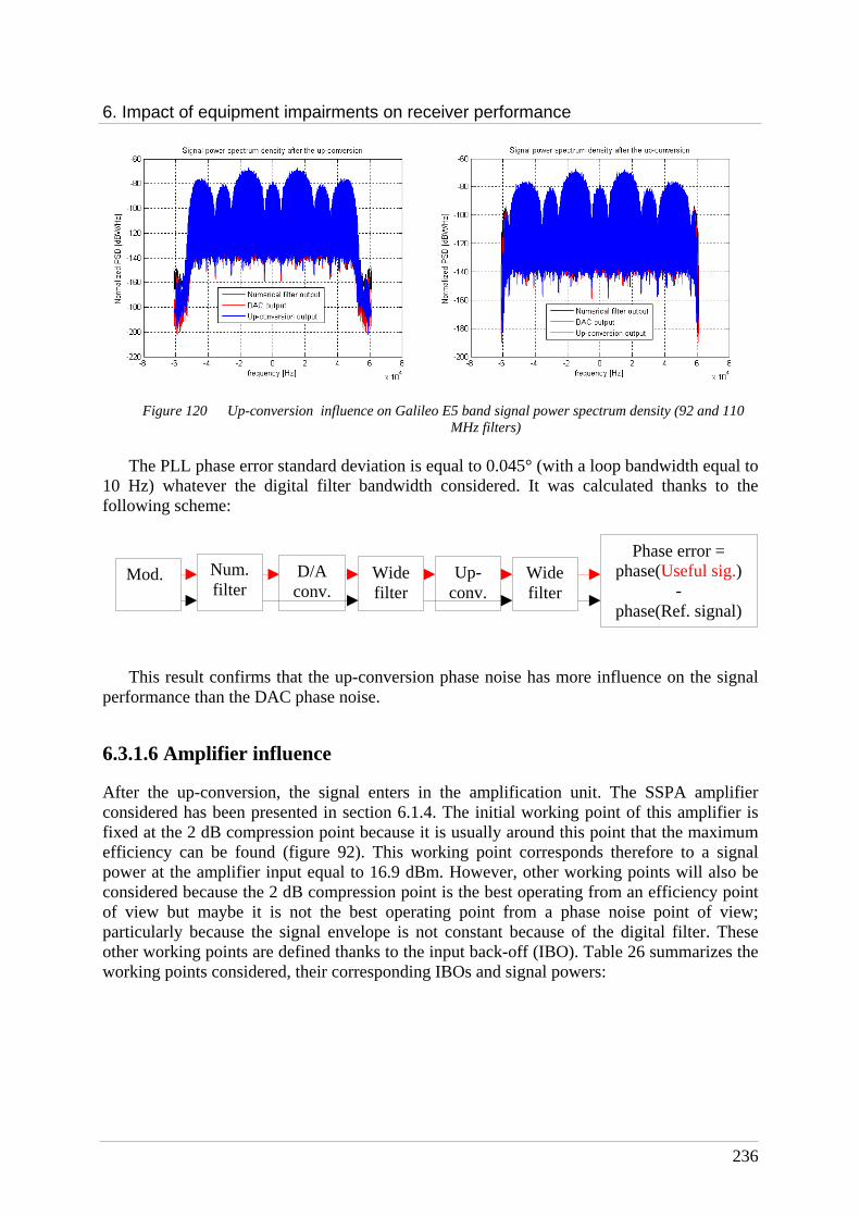
6. Impact of equipment impairments on receiver performance

236

Figure 120 Up-conversion influence on Galileo E5 band signal power spectrum density (92 and 110 MHz filters)

The PLL phase error standard deviation is equal to 0.045° (with a loop bandwidth equal to

10 Hz) whatever the digital filter bandwidth considered. It was calculated thanks to the following scheme:

This result confirms that the up-conversion phase noise has more influence on the signal performance than the DAC phase noise.

6.3.1.6 Amplifier influence

After the up-conversion, the signal enters in the amplification unit. The SSPA amplifier considered has been presented in section 6.1.4. The initial working point of this amplifier is fixed at the 2 dB compression point because it is usually around this point that the maximum efficiency can be found (figure 92). This working point corresponds therefore to a signal power at the amplifier input equal to 16.9 dBm. However, other working points will also be considered because the 2 dB compression point is the best operating from an efficiency point of view but maybe it is not the best operating point from a phase noise point of view; particularly because the signal envelope is not constant because of the digital filter. These other working points are defined thanks to the input back-off (IBO). Table 26 summarizes the working points considered, their corresponding IBOs and signal powers:

Mod. Num. filter

D/A conv.

Wide filter

Up-conv.

Wide filter

Phase error = phase(Useful sig.)

- phase(Ref. signal)

6. Impact of equipment impairments on receiver performance

237

IBO (dB) Signal power at

amplifier input: P (dBm)

0 16.9

1 15.9

2 14.9

3 13.9

4 12.9

5 11.9

Table 26 Working points’ IBOs

To begin the modulation constellation is plotted for the six IBOs defined by table 26 to

have an idea of the amplifier influence as a function of the working points. A 92 MHz filtered signal is considered. Therefore the signal envelope at the amplifier input is not constant and the signal points do not enter in the amplifier with an equal power.

-1 -0.5 0 0.5 1

-1

-0.5

0

0.5

1

I

Q

Signal modulation constellation at the amplifier output (IBO=0 dB)

0

0.5

1

1.5

2

2.5

3

3.5

4

4.5x 10

4

-1 -0.5 0 0.5 1

-1

-0.5

0

0.5

1

I

Q

Signal modulation constellation at the amplifier output (IBO=1 dB)

0

0.5

1

1.5

2

2.5

x 104

6. Impact of equipment impairments on receiver performance

238

-1 -0.5 0 0.5 1

-1

-0.5

0

0.5

1

I

Q

Signal modulation constellation at the amplifier output (IBO=2 dB)

0

2000

4000

6000

8000

10000

12000

14000

-1 -0.5 0 0.5 1

-1

-0.5

0

0.5

1

I

Q

Signal modulation constellation at the amplifier output (IBO=3 dB)

0

2000

4000

6000

8000

10000

12000

-1 -0.5 0 0.5 1

-1

-0.5

0

0.5

1

I

Q

Signal modulation constellation at the amplifier output (IBO=4 dB)

0

2000

4000

6000

8000

10000

12000

14000

-1 -0.5 0 0.5 1

-1

-0.5

0

0.5

1

I

Q

Signal modulation constellation at the amplifier output (IBO=5 dB)

0

2000

4000

6000

8000

10000

12000

Figure 121 92 MHz filtered signal modulation constellation at the amplifier output

The modulation constellation diagrams show both AM/AM and AM/PM influence. Indeed, for an IBO equal to 0 dB, the input signal power is situated at the saturation point,

so at the beginning of the AM/AM flat part. As the signal envelope is not constant, the signal points are not amplified in the same way: some have a power corresponding to the linear part of the AM/AM characteristics but the majority has a power corresponding to the flat part of the AM/AM characteristics; these ones are thus amplified to the same output power equal to 30 dBm (figure 122). The impact of the signal points’ repartition on the AM/AM characteristic is clearly visible on the modulation constellation plot: the modulation plots are spread horizontally and not vertically as they were after the up-conversion, because whatever the signal points’ input powers, they are all amplified to the same output power. At this working point, the amplifier seems to make the envelope constant.

6. Impact of equipment impairments on receiver performance

239

Figure 122 Signal points repartition on the AM/AM characteristic (IBO = 0 dB)

For an IBO equal to 1 dB, the same observations than for an IBO equal to 0 dB can be

made, even if the modulation plots are less spread horizontally and more spread vertically. The more the IBO increases, the more signal points are situated in the linear part of the AM/AM characteristics and they are amplified by the same gain (figure 123). The modulation plots are thus amplified in the same way and they keep their vertical spread.

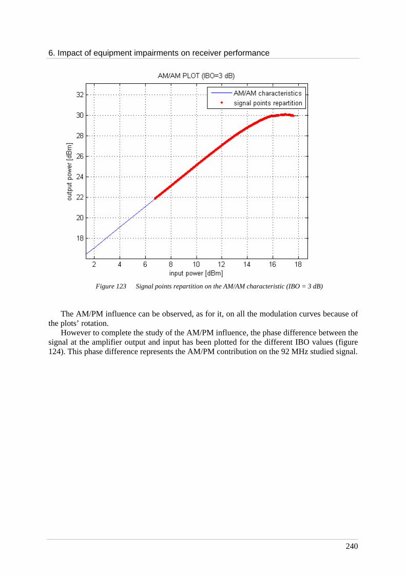
6. Impact of equipment impairments on receiver performance

240

Figure 123 Signal points repartition on the AM/AM characteristic (IBO = 3 dB)

The AM/PM influence can be observed, as for it, on all the modulation curves because of

the plots’ rotation. However to complete the study of the AM/PM influence, the phase difference between the

signal at the amplifier output and input has been plotted for the different IBO values (figure 124). This phase difference represents the AM/PM contribution on the 92 MHz studied signal.

6. Impact of equipment impairments on receiver performance

241

Figure 124 Phase difference study at the amplifier output (92 MHz filtered signal)

Moreover the standard deviations of each phase difference have been calculated, they are

presented in table 27:

Pinput (dBm)

16.9 15.9 14.9 13.9 12.9 11.9

σ (°) 0.76 0.7 0.65 0.67 0.91 1.3

Table 27 Phase difference standard deviation at amplifier output (92 MHz filtered signal)

Figure 124 and table 27 show that the AM/PM characteristics introduces more phase noise

for an IBO equal to 4 or 5 dB than for an IBO equal to 1, 2 or 3 dB. However it can also be noticed that the best operating point from a phase noise point of view is not the best operating point from a power efficiency point of view. Indeed the phase noise introduced by the AM/PM characteristics is higher for IBO equal to 0 dB (std=0.76°) than for an IBO equal to 2 or 3 dB (std=0.65°).

Moreover the amplifier phase noise is higher than the phase noise due to up-conversion or D/A conversion but it is weaker than the phase noise due to the digital filter.

Always with the objective to compare the influence of the working points, the PLL phase error standard deviation is calculated, considering the following scheme:

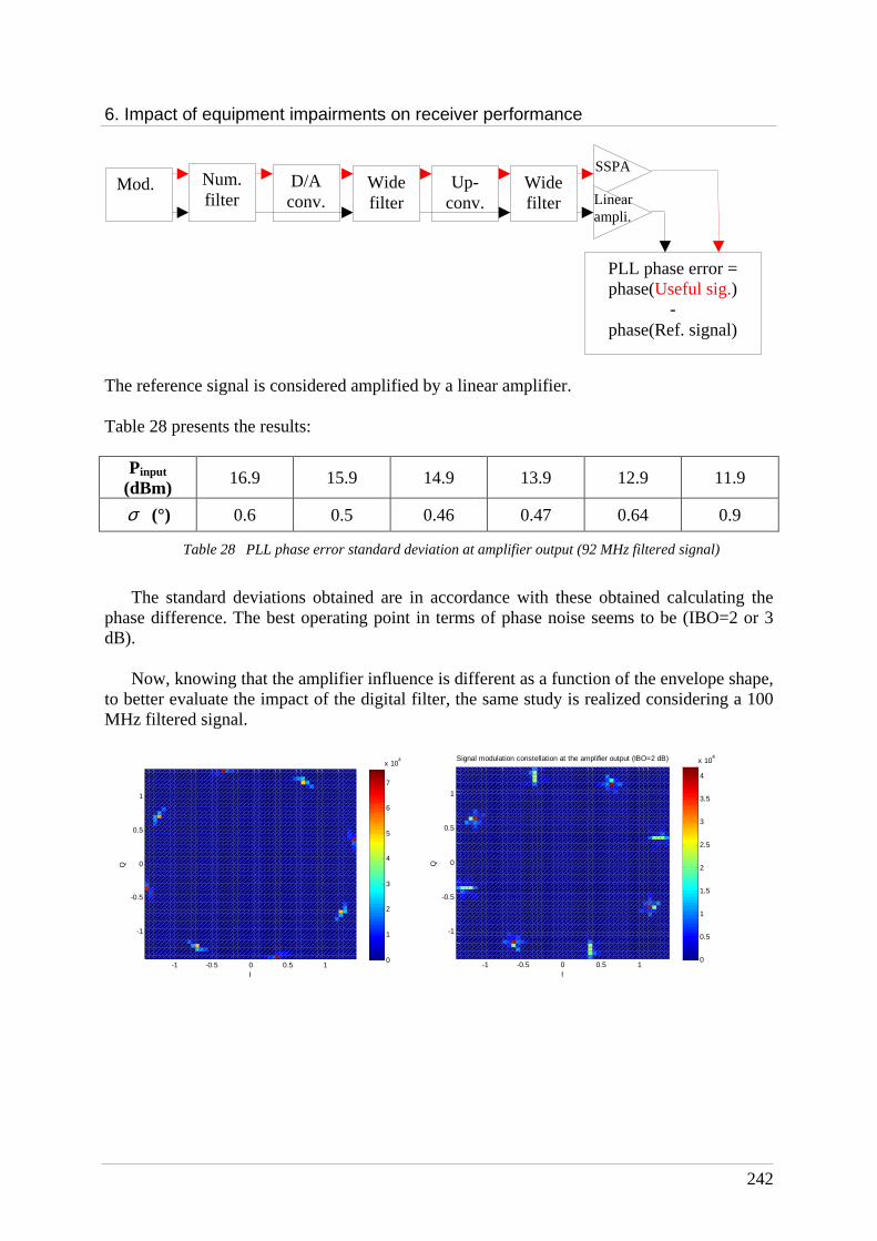
6. Impact of equipment impairments on receiver performance

242

The reference signal is considered amplified by a linear amplifier. Table 28 presents the results:

Pinput (dBm)

16.9 15.9 14.9 13.9 12.9 11.9

σ (°) 0.6 0.5 0.46 0.47 0.64 0.9

Table 28 PLL phase error standard deviation at amplifier output (92 MHz filtered signal)

The standard deviations obtained are in accordance with these obtained calculating the

phase difference. The best operating point in terms of phase noise seems to be (IBO=2 or 3 dB).

Now, knowing that the amplifier influence is different as a function of the envelope shape, to better evaluate the impact of the digital filter, the same study is realized considering a 100 MHz filtered signal.

-1 -0.5 0 0.5 1

-1

-0.5

0

0.5

1

I

Q

0

1

2

3

4

5

6

7

x 104

-1 -0.5 0 0.5 1

-1

-0.5

0

0.5

1

I

Q

Signal modulation constellation at the amplifier output (IBO=2 dB)

0

0.5

1

1.5

2

2.5

3

3.5

4

x 104

Mod. Num. filter

D/A conv.

Wide filter

Up-conv.

Wide filter

SSPA

Linear ampli.

PLL phase error = phase(Useful sig.)

- phase(Ref. signal)

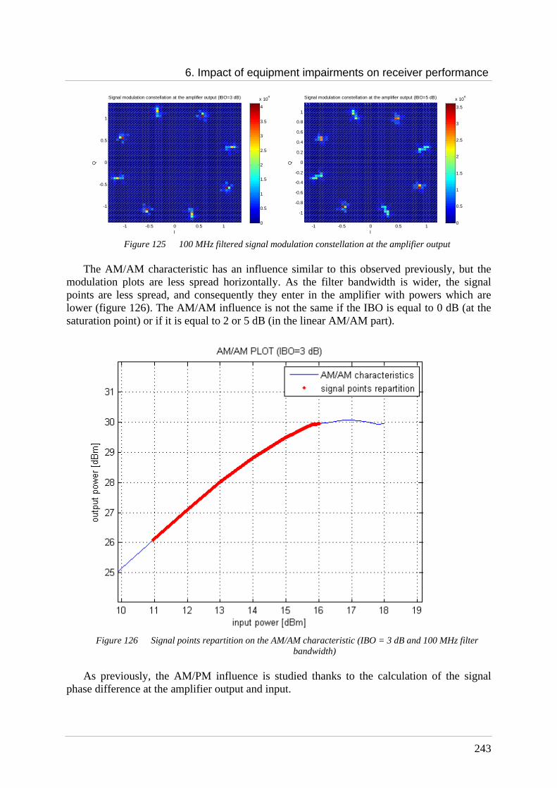
6. Impact of equipment impairments on receiver performance

243

-1 -0.5 0 0.5 1

-1

-0.5

0

0.5

1

I

QSignal modulation constellation at the amplifier output (IBO=3 dB)

0

0.5

1

1.5

2

2.5

3

3.5

4

x 104

-1 -0.5 0 0.5 1

-1

-0.8

-0.6

-0.4

-0.2

0

0.2

0.4

0.6

0.8

1

I

Q

Signal modulation constellation at the amplifier output (IBO=5 dB)

0

0.5

1

1.5

2

2.5

3

3.5

x 104

Figure 125 100 MHz filtered signal modulation constellation at the amplifier output

The AM/AM characteristic has an influence similar to this observed previously, but the

modulation plots are less spread horizontally. As the filter bandwidth is wider, the signal points are less spread, and consequently they enter in the amplifier with powers which are lower (figure 126). The AM/AM influence is not the same if the IBO is equal to 0 dB (at the saturation point) or if it is equal to 2 or 5 dB (in the linear AM/AM part).

Figure 126 Signal points repartition on the AM/AM characteristic (IBO = 3 dB and 100 MHz filter

bandwidth)

As previously, the AM/PM influence is studied thanks to the calculation of the signal phase difference at the amplifier output and input.

6. Impact of equipment impairments on receiver performance

244

2.8898 2.8899 2.89 2.8901 2.8902 2.8903

x 10-3

1.8

1.81

1.82

1.83

1.84

1.85

1.86

1.87

time [s]

phas

e [r

ad]

Phase difference at amplifier output

Pin=11.9 dBm

Pin=13.9 dBmPin=14.9 dBm

Pin=16.9 dBm

Figure 127 Phase difference study at the amplifier output (100 MHz filtered signal)

The standard deviations of the difference phase are exposed in table 29:

Pinput (dBm)

16.9 14.9 13.9 11.9

σ (°) 0.47 0.36 0.22 0.75

Table 29 Phase difference standard deviation at amplifier output (100 MHz filtered signal)

As for the 92 MHz filter case, for an IBO equal to 5 dB, the phase noise introduced is

relatively high compared to the other values obtained. Moreover the phase noise introduced at IBO equal to 0 or 2 dB is almost equivalent. This result seems correct because, as the filter bandwidth is wider, the signal points are less spread, and according to the AM/PM shape, they are distorted in the same way by the AM/PM characteristic.

The calculation of the PLL phase error standard deviation confirms the previous results:

Pinput (dBm)

16.9 14.9 13.9 11.9

σ (°) 0.33 0.26 0.16 0.53

Table 30 PLL phase error standard deviation at amplifier output (100 MHz filtered signal)

6. Impact of equipment impairments on receiver performance

245

So, the simulations have shown that from a phase noise point of view the best operating point of the amplifier is (IBO=3 dB) whatever the bandwidth of the digital filter. However the amplifier introduces less phase noise when the digital filter has a 100 MHz bandwidth. It has also been noticed that the AM/AM characteristic has also an influence on the signal, but it does not introduce phase noise, it only distorts the signal envelope. Nevertheless, the distortions due to the AM/AM curve can have an influence on the OMUX behaviour that will be studied in the following part.

6.3.1.7 OMUX influence

At the amplifier output, the signal is multiplexed and filtered by the output multiplexers before being transmitted by the antennas.

First, the OMUX influence on the 92 MHz filtered signal modulation constellation is studied as a function of the amplifier operating point. It can be noticed that whatever the IBO values, the modulation plots are spread vertically, as it has been observed at the digital filter output.

-1.5 -1 -0.5 0 0.5 1 1.5

-1.5

-1

-0.5

0

0.5

1

1.5

I

Q

Signal modulation constellation at the OMUX output (IBO=0 dB)

0

1000

2000

3000

4000

5000

6000

7000

8000

9000

10000

-1.5 -1 -0.5 0 0.5 1 1.5

-1.5

-1

-0.5

0

0.5

1

1.5

I

Q

Signal modulation constellation at the OMUX output (IBO=1 dB)

0

1000

2000

3000

4000

5000

6000

7000

8000

9000

-1.5 -1 -0.5 0 0.5 1 1.5

-1.5

-1

-0.5

0

0.5

1

1.5

I

Q

Signal modulation constellation at the OMUX output (IBO=2 dB)

0

1000

2000

3000

4000

5000

6000

7000

-1.5 -1 -0.5 0 0.5 1 1.5

-1.5

-1

-0.5

0

0.5

1

1.5

I

Q

Signal modulation constellation at the OMUX output (IBO=3 dB)

0

1000

2000

3000

4000

5000

6000

7000

8000

6. Impact of equipment impairments on receiver performance

246

-1.5 -1 -0.5 0 0.5 1 1.5-1.5

-1

-0.5

0

0.5

1

1.5

I

Q

Signal modulation constellation at the OMUX output (IBO=4 dB)

0

1000

2000

3000

4000

5000

6000

7000

8000

-1 -0.5 0 0.5 1

-1

-0.5

0

0.5

1

I

Q

Signal modulation constellation at the OMUX output (IBO=5 dB)

0

1000

2000

3000

4000

5000

6000

7000

8000

9000

Figure 128 92 MHz filtered signal modulation constellation at the OMUX output

The phase difference is also plotted in function of the amplifier operating point. Figure

129 and the standard deviations calculation (table 31) show that the signal phase is less distorted by the OMUX if the IBO value is high. We could therefore deduce that if the signal has been amplified linearly by the amplifier, it suffers less from phase distortions due to the OMUX.

4.401 4.4011 4.4012 4.4012 4.4013 4.4013 4.4013 4.4014

x 10-3

1.75

1.8

1.85

1.9

time [s]

phas

e [r

ad]

Phase difference at the OMUX output

Pin=11.9 dBmPin=12.9 dBm

Pin=13.9 dBm

Pin=14.9 dBm

Pin=15.9 dBmPin=16.9 dBm

Figure 129 Phase difference study at the OMUX output in function of IBOs for a 92 MHZ filtered signal

6. Impact of equipment impairments on receiver performance

247

Pinput

(dBm) 16.9 15.9 14.9 13.9 12.9 11.9

σ (°) 1.9 1.6 1.14 0.84 0.74 0.73

Table 31 Phase difference standard deviation at OMUX output (92 MHz filtered signal)

To confirm this assumption, the phase difference is calculated considering an amplifier

with a linear AM/AM curve and a non-linear AM/PM curve. Table 32 summarizes the standard deviation obtained:

Pinput (dBm)

16.9 14.9 13.9 11.9

σ (°) 0.5 0.6 0.6 0.7

Table 32 Phase difference at OMUX output considering a linear AM/AM characteristic

The values show that if the AM/AM is linear, the phase distortion due to the OMUX is

equivalent whatever the amplifier working point.

Now, a constant AM/PM characteristic and a non-linear AM/AM characteristic are considered. Table 33 presents the standard deviation calculation of the phase difference:

Pinput (dBm)

16.9 14.9 13.9 11.9

σ (°) 1.9 1 0.6 0.2

Table 33 Phase difference at OMUX output considering a linear AM/PM characteristic

The results are in accordance with these obtained previously, with non-linear AM/AM and

AM/PM curves (table 31).

Therefore, all these results confirm the assumption made: the OMUX influence depends on the AM/AM characteristic.

The PLL phase error standard deviation is now calculated thanks to the following scheme.

6. Impact of equipment impairments on receiver performance

248

(The reference signal is considered amplified by a linear amplifier and filtered by the OMUX)

Pinput (dBm)

16.9 15.9 14.9 13.9 12.9 11.9

σ (°) 1.37 1.12 0.8 0.58 0.53 0.55

Table 34 PLL phase error standard deviation at OMUX output (92 MHz filtered signal)

The PLL phase errors (table 34) seem to validate the previous assumption. Indeed, the

more the IBO value decreases, the more the PLL error standard deviation increases. However, if table 34 is compared to table 28, it seems that the OMUX introduces phase

noise for IBO between 0 and 3 dB and reduces the phase noise introduced by the amplifier for IBO equal to 4 or 5 dB. But this not the explanation; in fact, these results only show that the OMUX has a different influence on the signal reference and on the useful signal according to the IBO value.

Figures 130 and 131 represent the phase differences of the reference signal and useful signal at the OMUX output for two different IBOs. For an IBO equal to 5 dB, the OMUX influence is similar on the reference signal and on the useful signal. For the reference signal, the standard deviation of the phase difference is equal to 1.8°, whereas it is equal to 1.9° for the useful signal. The influence of the OMUX is so equivalent for the two signals.

Mod. Num. filter

D/A conv.

Wide filter

Up-conv.

Wide filter

SSPA

Linear ampli.

PLL phase error = phase(Useful sig.)

- phase(Ref. signal)

OMUX

6. Impact of equipment impairments on receiver performance

249

4.7117 4.7118 4.7119 4.712 4.7121 4.7122 4.7123 4.7124

x 10-3

-0.1

-0.05

0

0.05

0.1

Study of OMUX contribution thanks to phase difference calculation (IBO=5 dB)

time [s]

phas

e [r

ad]

Phase diff. of the useful signal between OMUX output and input

Phase diff. of the reference signal between OMUX output and input

Diff. between the two previous phase

Figure 130 Study of OMUX contribution for an IBO equal to 5 dB

However if the IBO is equal to 1 dB, the standard deviation of the useful signal phase difference is equal to 2.4° whereas the value obtained for the reference signal remains the same, equal to 1.8°. In this case, the OMUX influence is not the same on the useful signal and on the reference signal.

The OMUX influence on the useful signal is more similar to the OMUX influence on the reference signal for high IBO (linear part of the AM/AM characteristic), that is the reason why the PLL phase error standard deviation is reduced for high IBO values.

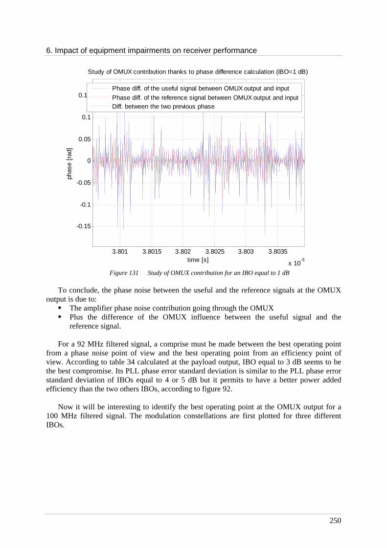
6. Impact of equipment impairments on receiver performance

250

3.801 3.8015 3.802 3.8025 3.803 3.8035

x 10-3

-0.15

-0.1

-0.05

0

0.05

0.1

0.15

Study of OMUX contribution thanks to phase difference calculation (IBO=1 dB)

time [s]

phas

e [r

ad]

Phase diff. of the useful signal between OMUX output and input

Phase diff. of the reference signal between OMUX output and inputDiff. between the two previous phase

Figure 131 Study of OMUX contribution for an IBO equal to 1 dB

To conclude, the phase noise between the useful and the reference signals at the OMUX

output is due to: The amplifier phase noise contribution going through the OMUX Plus the difference of the OMUX influence between the useful signal and the

reference signal.

For a 92 MHz filtered signal, a comprise must be made between the best operating point from a phase noise point of view and the best operating point from an efficiency point of view. According to table 34 calculated at the payload output, IBO equal to 3 dB seems to be the best compromise. Its PLL phase error standard deviation is similar to the PLL phase error standard deviation of IBOs equal to 4 or 5 dB but it permits to have a better power added efficiency than the two others IBOs, according to figure 92.

Now it will be interesting to identify the best operating point at the OMUX output for a 100 MHz filtered signal. The modulation constellations are first plotted for three different IBOs.

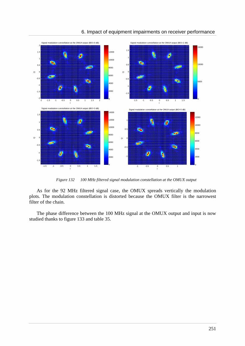
6. Impact of equipment impairments on receiver performance

251

-2 -1.5 -1 -0.5 0 0.5 1 1.5 2-2

-1.5

-1

-0.5

0

0.5

1

1.5

2

I

Q

Signal modulation constellation at the OMUX output (IBO=0 dB)

0

2000

4000

6000

8000

10000

12000

-1.5 -1 -0.5 0 0.5 1 1.5

-1.5

-1

-0.5

0

0.5

1

1.5

I

Q

Signal modulation constellation at the OMUX output (IBO=2 dB)

0

5000

10000

15000

-1.5 -1 -0.5 0 0.5 1 1.5

-1.5

-1

-0.5

0

0.5

1

1.5

I

Q

Signal modulation constellation at the OMUX output (IBO=3 dB)

0

2000

4000

6000

8000

10000

12000

14000

-1 -0.5 0 0.5 1

-1

-0.5

0

0.5

1

I

Q

Signal modulation constellation at the OMUX output (IBO=5 dB)

0

2000

4000

6000

8000

10000

12000

Figure 132 100 MHz filtered signal modulation constellation at the OMUX output

As for the 92 MHz filtered signal case, the OMUX spreads vertically the modulation plots. The modulation constellation is distorted because the OMUX filter is the narrowest filter of the chain.

The phase difference between the 100 MHz signal at the OMUX output and input is now studied thanks to figure 133 and table 35.

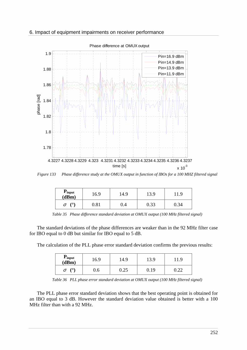
6. Impact of equipment impairments on receiver performance

252

4.3227 4.3228 4.3229 4.323 4.3231 4.3232 4.3233 4.3234 4.3235 4.3236 4.3237

x 10-3

1.78

1.8

1.82

1.84

1.86

1.88

1.9

time [s]

phas

e [r

ad]

Phase difference at OMUX output

Pin=16.9 dBm

Pin=14.9 dBmPin=13.9 dBm

Pin=11.9 dBm

Figure 133 Phase difference study at the OMUX output in function of IBOs for a 100 MHZ filtered signal

Pinput (dBm)

16.9 14.9 13.9 11.9

σ (°) 0.81 0.4 0.33 0.34

Table 35 Phase difference standard deviation at OMUX output (100 MHz filtered signal)

The standard deviations of the phase differences are weaker than in the 92 MHz filter case

for IBO equal to 0 dB but similar for IBO equal to 5 dB.

The calculation of the PLL phase error standard deviation confirms the previous results:

Pinput (dBm)

16.9 14.9 13.9 11.9

σ (°) 0.6 0.25 0.19 0.22

Table 36 PLL phase error standard deviation at OMUX output (100 MHz filtered signal)

The PLL phase error standard deviation shows that the best operating point is obtained for

an IBO equal to 3 dB. However the standard deviation value obtained is better with a 100 MHz filter than with a 92 MHz.

6. Impact of equipment impairments on receiver performance

253

To end with the study of the phase noise in the payload, the absolute value of the signal correlation function is plotted at amplifier and OMUX outputs for three different amplifier operating points, IBO is considered equal to 0, 3 and 5 dB.

-2 -1.5 -1 -0.5 0 0.5 1 1.5 2-0.5

0

0.5

1

RELATIVE SHIFT IN CHIPS

CO

RR

ELA

TIO

N

ESTIMATED CORRELATION FUNCTION (@IBO=5dB)

amplifier output

OMUX output

-0.03 -0.02 -0.01 0 0.01 0.02 0.03

0.76

0.78

0.8

0.82

0.84

0.86

0.88

0.9

0.92

0.94

RELATIVE SHIFT IN CHIPS

CO

RR

ELA

TIO

N

ESTIMATED CORRELATION FUNCTION (@IBO=5dB)

amplifier output

OMUX output

-2 -1.5 -1 -0.5 0 0.5 1 1.5 2

-0.4

-0.2

0

0.2

0.4

0.6

0.8

1

RELATIVE SHIFT IN CHIPS

CO

RR

ELA

TIO

N

ESTIMATED CORRELATION FUNCTION (@IBO=3 dB)

amplifier output

OMUX output

-0.06 -0.04 -0.02 0 0.02 0.04 0.060.8

0.85

0.9

0.95

1

1.05

1.1

RELATIVE SHIFT IN CHIPS

CO

RR

ELA

TIO

N

ESTIMATED CORRELATION FUNCTION (@IBO=3 dB)

amplifier output

OMUX output

-2 -1.5 -1 -0.5 0 0.5 1 1.5 2-0.5

0

0.5

1

1.5

RELATIVE SHIFT IN CHIPS

CO

RR

ELA

TIO

N

ESTIMATED CORRELATION FUNCTION (@IBO=0 dB)

amplifier output

OMUX output

-0.08 -0.06 -0.04 -0.02 0 0.02 0.04 0.060.85

0.9

0.95

1

1.05

1.1

1.15

1.2

1.25

1.3

1.35

RELATIVE SHIFT IN CHIPS

CO

RR

ELA

TIO

N

ESTIMATED CORRELATION FUNCTION (@IBO=0 dB)

amplifier output

OMUX output

Figure 134 Correlation function at amplifier and OMUX outputs Figure 134 shows that whatever the amplifier operating points no distortions are

introduced on the correlation function at amplifier or OMUX output. At the amplifier output, there is an increase of the correlation main peak because of the

increase of the signal power. According to the AM/AM characteristic, this increase is higher in the (IBO = 0 dB) case than in the (IBO = 5 dB) case. It can also be noticed that the OMUX introduces a slight decrease of the main peak, due to the filtering.

6. Impact of equipment impairments on receiver performance

254

6.3.1.8 Conclusion

To conclude, the evaluation of the individual contribution of each unit has shown that the digital filter introduces the most important distortions on the signal carrier phase. However, if the filters phase noise is not considered, the phase noise introduced by the payload is in majority due to the amplifier phase noise. Indeed the up-conversion phase noise is almost negligible in front of the amplifier phase noise.

It has also been shown that depending to the amplifier operating point, the phase noise introduced is more or less important. And it has been proved that the best operating point from both a phase noise and an efficiency point of view corresponds to an IBO equal to 3 dB. However we must keep in mind that the AM/AM, AM/PM model used to characterize the amplifier behaviour presents some limitations. Indeed these curves do not take correctly into account the signal bandwidth and the memory effects because they are characterized thanks to pure carrier waves.

To finish, it has been demonstrated that if the digital filter has a 100 MHz bandwidth, the phase noise at the payload output is weaker. Therefore, perhaps it would be better to use a 100 MHz filter as digital filter instead of a 92 MHz filter, because the OMUX filter the signal to the specified bandwidth at the payload output. But if the 100 MHz digital filter is chosen, the DAC, the mixers and the amplifiers should have bandwidths at least equal to 100 MHz, otherwise they could distort the signal.

However, the choice of the digital filter bandwidth would also depend on the phase noise introduced by the receiver. Indeed if the receiver phase noise is higher than the payload phase noise, it is not interesting to have wider digital filter if it can finally not improve the PLL phase error standard deviation at the global transmission/reception chain output. That is the reason why the phase noise introduced by the receiver units is studied in the next section.

6.3.2 Receiver performance

6.3.2.1 Introduction

Now, the influence of the receiver units will be studied. The different receiver parts have already been described at length. The next scheme presents the receiver simulations process by underlining the most important receiver units and the points where the figures of merit are plotted.

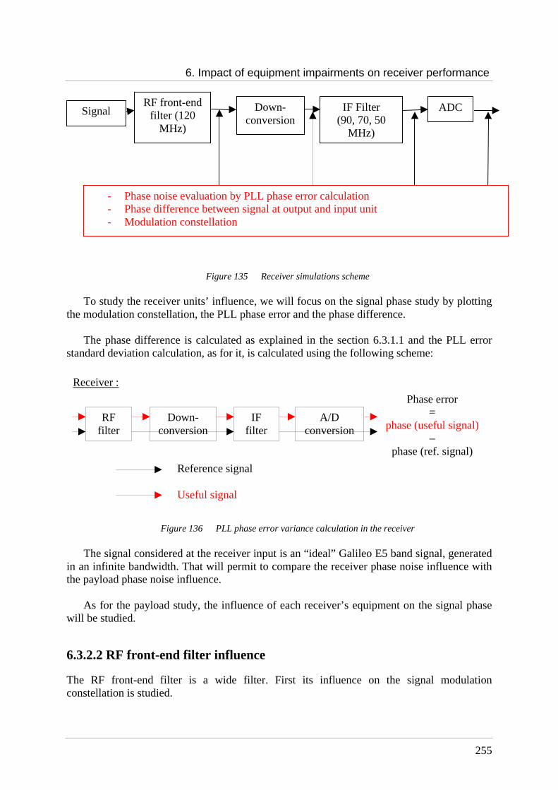
6. Impact of equipment impairments on receiver performance

255

Figure 135 Receiver simulations scheme

To study the receiver units’ influence, we will focus on the signal phase study by plotting the modulation constellation, the PLL phase error and the phase difference.

The phase difference is calculated as explained in the section 6.3.1.1 and the PLL error standard deviation calculation, as for it, is calculated using the following scheme:

Figure 136 PLL phase error variance calculation in the receiver

The signal considered at the receiver input is an “ideal” Galileo E5 band signal, generated in an infinite bandwidth. That will permit to compare the receiver phase noise influence with the payload phase noise influence.

As for the payload study, the influence of each receiver’s equipment on the signal phase will be studied.

6.3.2.2 RF front-end filter influence

The RF front-end filter is a wide filter. First its influence on the signal modulation constellation is studied.

Reference signal

Useful signal

RF filter

Phase error =

phase (useful signal) –

phase (ref. signal)

Down-conversion

IF filter

A/D conversion

Signal RF front-end

filter (120 MHz)

Down-conversion

ADC

- Phase noise evaluation by PLL phase error calculation - Phase difference between signal at output and input unit - Modulation constellation

IF Filter (90, 70, 50

MHz)

Receiver :

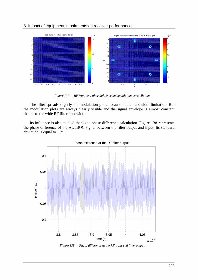
6. Impact of equipment impairments on receiver performance

256

-0.8 -0.6 -0.4 -0.2 0 0.2 0.4 0.6 0.8

-0.8

-0.6

-0.4

-0.2

0

0.2

0.4

0.6

0.8

ideal signal modulation constellation

0

5

10

15

x 104

-1 -0.5 0 0.5 1

-1

-0.8

-0.6

-0.4

-0.2

0

0.2

0.4

0.6

0.8

1

I

Q

Signal modulation constellation at the RF filter output

0

0.5

1

1.5

2

2.5

3

3.5

4x 10

4

Figure 137 RF front-end filter influence on modulation constellation

The filter spreads slightly the modulation plots because of its bandwidth limitation. But the modulation plots are always clearly visible and the signal envelope is almost constant thanks to the wide RF filter bandwidth.

Its influence is also studied thanks to phase difference calculation. Figure 138 represents

the phase difference of the ALTBOC signal between the filter output and input. Its standard deviation is equal to 1.7°.

3.8 3.85 3.9 3.95 4 4.05

x 10-3

-0.1

-0.05

0

0.05

0.1

Phase difference at the RF filter output

time [s]

phas

e [r

ad]

Figure 138 Phase difference at the RF front-end filter output

6. Impact of equipment impairments on receiver performance

257

6.3.2.3 Down-conversion influence

Now the phase noise introduced by the down-conversion will be studied in function of the receiver types.

The influence on the modulation constellation of the TCXO and rubidium receivers is

plotted in figure 139.

-1 -0.5 0 0.5 1

-1

-0.8

-0.6

-0.4

-0.2

0

0.2

0.4

0.6

0.8

1

I

Q

Signal modulation constellation at down-conversion output for a TCXO receiver

0

0.5

1

1.5

2

2.5

3

3.5

4x 10

4

-1 -0.5 0 0.5 1

-1

-0.8

-0.6

-0.4

-0.2

0

0.2

0.4

0.6

0.8

1

I

Q

Signal modulation constellation at down-conversion output for a rubidium receiver

0

0.5

1

1.5

2

2.5

3

3.5

4x 10

4

Figure 139 Down-conversion influence on Galileo E5 band signal modulation constellation

The down-conversion does not have a significant influence on the modulation constellation whatever the receiver type. Indeed, the influence of the RF front-end filter is too important to observe the down-conversion influence.

However the down-conversion influence can be observed thanks to the phase difference study. Indeed figure 140 and table 37 show that the down-conversion introduces more phase noise in the case of a TCXO receiver that is in accordance with the oscillators’ characteristics. But the phase distortions due to the down-conversion are weaker than the phase distortions due to the RF filter, as observed on the modulation constellation.

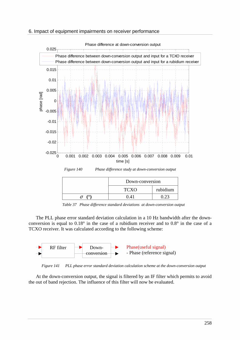
6. Impact of equipment impairments on receiver performance

258

0 0.001 0.002 0.003 0.004 0.005 0.006 0.007 0.008 0.009 0.01-0.025

-0.02

-0.015

-0.01

-0.005

0

0.005

0.01

0.015

0.02

0.025Phase difference at down-conversion output

time [s]

phas

e [r

ad]

Phase difference between down-conversion output and input for a TCXO receiver

Phase difference between down-conversion output and input for a rubidium receiver

Figure 140 Phase difference study at down-conversion output

Down-conversion

TCXO rubidium

σ (°) 0.41 0.23

Table 37 Phase difference standard deviations at down-conversion output

The PLL phase error standard deviation calculation in a 10 Hz bandwidth after the down-

conversion is equal to 0.18° in the case of a rubidium receiver and to 0.8° in the case of a TCXO receiver. It was calculated according to the following scheme:

Figure 141 PLL phase error standard deviation calculation scheme at the down-conversion output

At the down-conversion output, the signal is filtered by an IF filter which permits to avoid the out of band rejection. The influence of this filter will now be evaluated.

Phase(useful signal) - Phase (reference signal)

RF filter Down-conversion

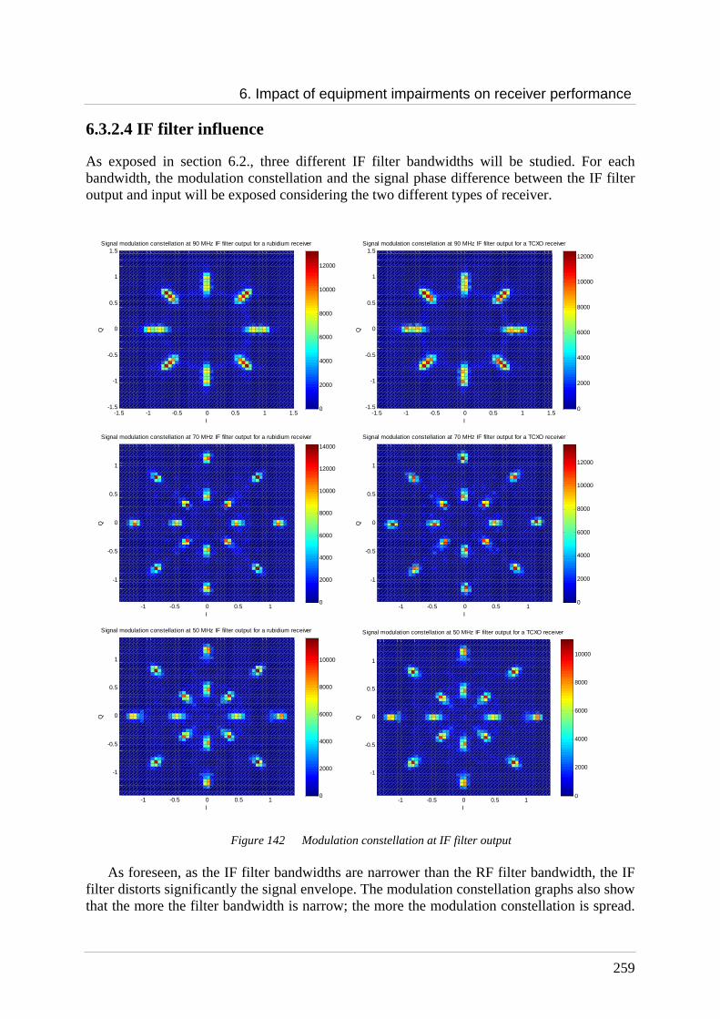
6. Impact of equipment impairments on receiver performance

259

6.3.2.4 IF filter influence

As exposed in section 6.2., three different IF filter bandwidths will be studied. For each bandwidth, the modulation constellation and the signal phase difference between the IF filter output and input will be exposed considering the two different types of receiver.

-1.5 -1 -0.5 0 0.5 1 1.5-1.5

-1

-0.5

0

0.5

1

1.5

I

Q

Signal modulation constellation at 90 MHz IF filter output for a rubidium receiver

0

2000

4000

6000

8000

10000

12000

-1.5 -1 -0.5 0 0.5 1 1.5-1.5

-1

-0.5

0

0.5

1

1.5

I

Q

Signal modulation constellation at 90 MHz IF filter output for a TCXO receiver

0

2000

4000

6000

8000

10000

12000

-1 -0.5 0 0.5 1

-1

-0.5

0

0.5

1

I

Q

Signal modulation constellation at 70 MHz IF filter output for a rubidium receiver

0

2000

4000

6000

8000

10000

12000

14000

-1 -0.5 0 0.5 1

-1

-0.5

0

0.5

1

I

Q

Signal modulation constellation at 70 MHz IF filter output for a TCXO receiver

0

2000

4000

6000

8000

10000

12000

-1 -0.5 0 0.5 1

-1

-0.5

0

0.5

1

I

Q

Signal modulation constellation at 50 MHz IF filter output for a rubidium receiver

0

2000

4000

6000

8000

10000

-1 -0.5 0 0.5 1

-1

-0.5

0

0.5

1

I

Q

Signal modulation constellation at 50 MHz IF filter output for a TCXO receiver

0

2000

4000

6000

8000

10000

Figure 142 Modulation constellation at IF filter output

As foreseen, as the IF filter bandwidths are narrower than the RF filter bandwidth, the IF filter distorts significantly the signal envelope. The modulation constellation graphs also show that the more the filter bandwidth is narrow; the more the modulation constellation is spread.

6. Impact of equipment impairments on receiver performance

260

Indeed for a 90 MHz IF filter, the modulation plots are only spread vertically, there are always only 8 plots; whereas, in the 70 MHz or 50 MHz IF filter cases, there are no more 8 plots but 16 plots. The modulation constellations observed are both similar to the non-constant envelope ALTBOC modulation constellation, presented in chapter 4 (figure 33), and to the constant envelope ALTBOC modulation constellation.

However the influence of the IF filters is the same whatever the receiver type. This result

is confirmed by the calculation of the standard deviation of the phase difference in table 38. Indeed the same phase difference standard deviation is obtained whatever the receiver type. The table also confirms that narrower the IF filter bandwidth is, higher the phase distortions are.

σ (°) 90 MHz IF filter 70 MHz IF filter 50 MHz IF filter

rubidium 5.13° 7.9° 16.8°

TCXO 5.13° 7.9° 16.8°

Table 38 Phase difference standard deviation at the IF filters output

6.3.2.4.1 A/D conversion influence

Now the influence of the last element of the receiver will be studied. First the modulation constellations are plotted considering the two receiver types and the three IF filter bandwidths.

-1.5 -1 -0.5 0 0.5 1 1.5-1.5

-1

-0.5

0

0.5

1

1.5

I

Q

Signal modulation constellation at ADC output for a TCXO receiver

0

2000

4000

6000

8000

10000

12000

-1.5 -1 -0.5 0 0.5 1 1.5-1.5

-1

-0.5

0

0.5

1

1.5

I

Q

Signal modulation constellation at ADC output for a rubidium receiver

0

2000

4000

6000

8000

10000

12000

Figure 143 Modulation constellation at ADC output for a 90 MHz IF filter

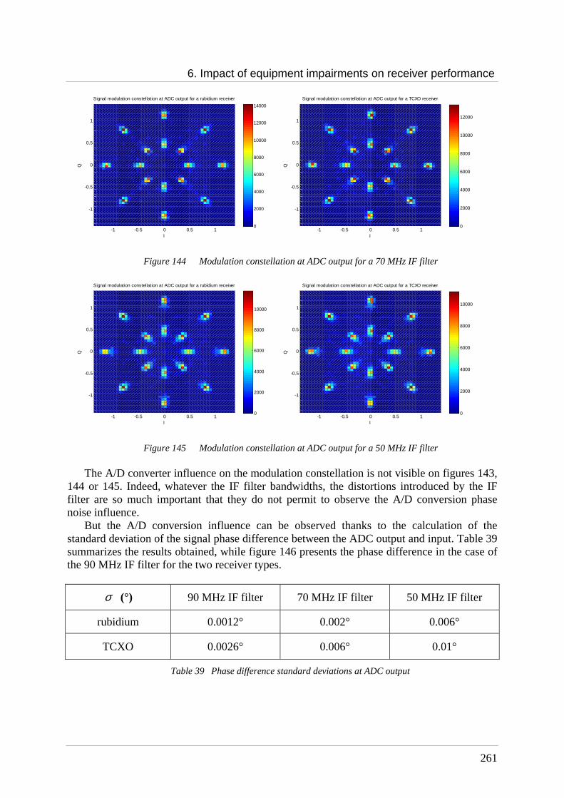
6. Impact of equipment impairments on receiver performance

261

-1 -0.5 0 0.5 1

-1

-0.5

0

0.5

1

I

Q

Signal modulation constellation at ADC output for a rubidium receiver

0

2000

4000

6000

8000

10000

12000

14000

-1 -0.5 0 0.5 1

-1

-0.5

0

0.5

1

I

Q

Signal modulation constellation at ADC output for a TCXO receiver

0

2000

4000

6000

8000

10000

12000

Figure 144 Modulation constellation at ADC output for a 70 MHz IF filter

-1 -0.5 0 0.5 1

-1

-0.5

0

0.5

1

I

Q

Signal modulation constellation at ADC output for a rubidium receiver

0

2000

4000

6000

8000

10000

-1 -0.5 0 0.5 1

-1

-0.5

0

0.5

1

I

QSignal modulation constellation at ADC output for a TCXO receiver

0

2000

4000

6000

8000

10000

Figure 145 Modulation constellation at ADC output for a 50 MHz IF filter

The A/D converter influence on the modulation constellation is not visible on figures 143, 144 or 145. Indeed, whatever the IF filter bandwidths, the distortions introduced by the IF filter are so much important that they do not permit to observe the A/D conversion phase noise influence.

But the A/D conversion influence can be observed thanks to the calculation of the standard deviation of the signal phase difference between the ADC output and input. Table 39 summarizes the results obtained, while figure 146 presents the phase difference in the case of the 90 MHz IF filter for the two receiver types.

σ (°) 90 MHz IF filter 70 MHz IF filter 50 MHz IF filter

rubidium 0.0012° 0.002° 0.006°

TCXO 0.0026° 0.006° 0.01°

Table 39 Phase difference standard deviations at ADC output

6. Impact of equipment impairments on receiver performance

262

The phase distortions introduced by the ADC are higher for TCXO receiver than for rubidium receiver that is in accordance with the oscillators’ characteristics. It can also be noticed that narrower the IF filter bandwidth is, higher the phase distortions are. This result is normal because the time jitter is proportional to the receiver sampling frequency (chapter 3), deduced from the IF filter bandwidth (section 6.2.4). Wider the IF filter bandwidth is, higher the receiver sampling frequency is, and weaker the time jitter is.

3.65 3.7 3.75 3.8 3.85 3.9 3.95

x 10-3

-3

-2

-1

0

1

2

3

x 10-4 Phase difference study at the ADC output

time [s]

phas

e [r

ad]

Rubidium receiver

TCXO receiver

Figure 146 Phase difference study at ADC output for a 90 MHz IF filter

Now the PLL phase error standard deviations are calculated thanks to the following

scheme for the two types of receiver and the three IF filter bandwidths:

The results obtained are summarized in table 40:

PLL σ (°) 90 MHz IF filter 70 MHz IF filter 50 MHz IF filter

rubidium 0.17° 0.17° 0.18°

TCXO 0.85° 0.84° 0.8°

Table 40 PLL phase error standard deviations at A/D conversion output

Phase (useful signal) - Phase (reference

signal)

RF filter

Down-conversion

IF filter

A/D conversion

6. Impact of equipment impairments on receiver performance

263

These results confirm that more phase noise is introduced in the case of a TCXO receiver than in the case of a rubidium receiver. That is normal because the rubidium oscillator is more stable than the TCXO oscillator.

However, the phase noise at the ADC output does not seem to depend on the IF filter bandwidths, whereas we have noticed that the A/D conversion introduces more phase noise in the 50 MHz IF filter case than in the 90 MHz IF filter case. This result is due to the fact that the phase noise added by the A/D converter is negligible in front of the phase noise added by the down-conversion. Indeed, if table 40 is compared to the results obtained at the down-conversion, it can be observed that the PLL phase error standard deviation values are similar. So, the A/D conversion phase noise influence is negligible in front of the down-conversion phase noise influence and consequently, the phase noise at the ADC output does not depend on the IF filter bandwidth.

6.3.2.5 Conclusion

To conclude, the phase noise introduced by the different receiver units on the infinite bandwidth ALTBOC signal is higher if the receiver uses a TCXO oscillator than if it uses a rubidium oscillator as foreseen.

Moreover, it has been shown that the distortions due to the IF filter are higher than the others. However if the filters influence is not considered, in the receiver the phase noise brought by the down-conversion predominates, whereas in the payload, it is the phase noise brought by the amplifier which predominates.

If the PLL phase error standard deviation at the payload output is compared to the PLL

phase error standard deviation at the receiver output, considering that the payload amplifier works at its best operating point (IBO = 3 dB):

Payload output Receiver output

92 MHz digital

filter 100 MHz digital

filter TCXO oscillator

Rubidium oscillator

σ (°) 0.58 0.19 0.8 0.18

Table 41 Summary of PLL phase error standard deviations at receiver and payload output

It can be noticed that if the user used a TCXO receiver, whatever the payload configuration, the phase noise due to the receiver units predominates; whereas if the user uses a rubidium receiver, the phase noise introduced by the payload units can predominate in front of the receiver phase noise if the digital filter has a 92 MHz bandwidth. If the digital filter has a 100 MHz bandwidth, the receiver and payload phase noises are equivalent.

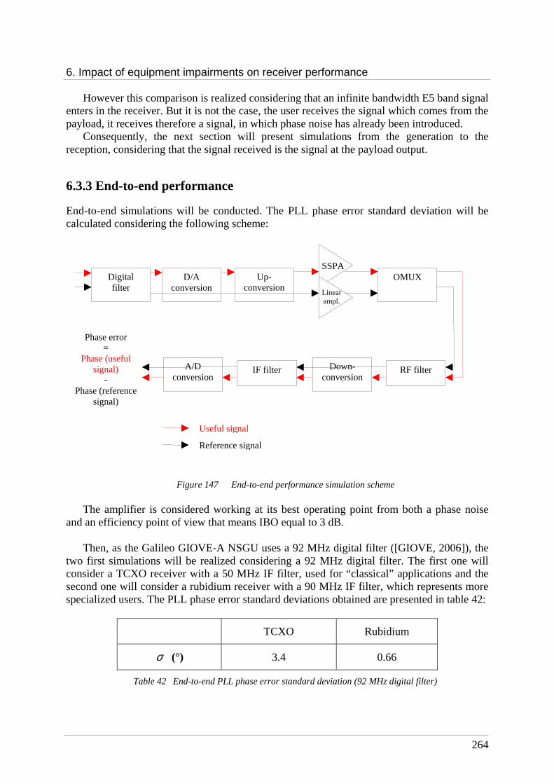
6. Impact of equipment impairments on receiver performance

264

However this comparison is realized considering that an infinite bandwidth E5 band signal enters in the receiver. But it is not the case, the user receives the signal which comes from the payload, it receives therefore a signal, in which phase noise has already been introduced.

Consequently, the next section will present simulations from the generation to the reception, considering that the signal received is the signal at the payload output.

6.3.3 End-to-end performance

End-to-end simulations will be conducted. The PLL phase error standard deviation will be calculated considering the following scheme:

Figure 147 End-to-end performance simulation scheme

The amplifier is considered working at its best operating point from both a phase noise and an efficiency point of view that means IBO equal to 3 dB.

Then, as the Galileo GIOVE-A NSGU uses a 92 MHz digital filter ([GIOVE, 2006]), the

two first simulations will be realized considering a 92 MHz digital filter. The first one will consider a TCXO receiver with a 50 MHz IF filter, used for “classical” applications and the second one will consider a rubidium receiver with a 90 MHz IF filter, which represents more specialized users. The PLL phase error standard deviations obtained are presented in table 42:

TCXO Rubidium

σ (°) 3.4 0.66

Table 42 End-to-end PLL phase error standard deviation (92 MHz digital filter)

Reference signal

Phase error =

Phase (useful signal)

- Phase (reference

signal)

Digital filter

D/A conversion

Up-conversion

OMUX SSPA

Linear ampl.

RF filter Down-conversion

IF filter A/D conversion

Useful signal

6. Impact of equipment impairments on receiver performance

265

As foreseen, the phase noise at the transmission/reception chain output is higher for a TCXO receiver than for a rubidium receiver. In the TCXO case, the phase noise introduced by the receiver predominates, whereas in the rubidium case it is effectively the payload phase noise which predominates.

To complete this study, an end-to-end simulation considering a 100 MHz payload digital

filter and a rubidium receiver has been realized. The PLL phase error standard deviation is in this case equal to 0.26° that shows once again the advantage of considering a wider digital filter.

6.3.4 Conclusion

This chapter has permitted to evaluate the phase noise introduced on the Galileo E5 band ALTBOC signal during the generation in the payload and the processing in the receiver.

First, the entire assumptions made on the payload and receiver equipment have been presented.

Then simulations have permitted to evaluate the phase noise brought by the payload units: digital filter, up-conversion, D/A conversion, amplifier and OMUX. They have shown that the phase distortions due to the digital filter are higher than the others. However, if the digital filter influence is not considered, the phase noise introduced by the amplifier predominates in front of the phase noise brought indirectly by the atomic clocks; and that this phase noise depends on the amplifier operating point. It has been demonstrated that the best amplifier operating point from both a phase noise and an efficiency point of view is obtained for an IBO equal to 3 dB. It has also been proved that if the digital filter bandwidth is equal to 100 MHz, the phase noise at the payload output is weaker than if the digital filter bandwidth is equal to 92 MHz.

Afterwards the phase noise, brought by TCXO and rubidium receivers units on an infinite bandwidth ALTBOC signal, has been evaluated. As foreseen, because of the oscillators characteristics, the phase noise introduced by a TCXO receiver is higher than the phase noise introduced by a rubidium receiver, whatever the IF filter bandwidth. It has also been underlined that the TCXO receiver phase noise is higher than the payload phase noise, whereas the rubidium receiver phase noise is weaker than the payload phase noise if the digital filter bandwidth is equal to 92 MHz.

Finally, end-to-end simulations have been conducted. They have permitted to determine the optimized payload scheme: a 100 MHz digital filter and an amplifier IBO equal to 3 dB.

However these results should be considered carefully. Indeed the AM/AM and AM/PM

characteristics used to describe the amplifier model do not take into account the wide bandwidth of the signal and the memory effect.

Moreover, the users need should be taken into account. If the receivers are designed for classical applications, they will not carry rubidium oscillators because of their expensive cost. Consequently, the receiver phase noise will predominate, and there is no need to use a 100 MHz filter, which implies to have payload equipment, such as DAC or mixers, with wide bandwidths.

267

Chapter 7

Conclusions and Recommendations for Future Work

Contents 7.1 Conclusions ..................................................................................................................... 267 7.2 Recommendations for Future Work ............................................................................ 269

This chapter presents the conclusions from the research results obtained in the previous chapters and draws recommendations for future work.

7.1 Conclusions

The purpose of this thesis was the study and the optimization of the Galileo signals and payload to obtain the best performance from a receiver point of view.

First, a precise study of the Galileo system, from the generation to the reception has been

conducted. All the payload and receiver units have been detailed in order to identify equipment likely to induce signal impairments and distort signal performance. It has been shown that payload and receiver clocks instabilities generate phase noise, introduced on signals during digital-to-analog/analog-to-digital conversion and up/down-conversion. The payload amplifier, because of its amplitude and phase non-linearities, can also introduce distortions on the signal if its envelope is not constant. Another element of impairment, already well-know because it is the main uncorrelated source of error affecting any GNSS users, has been retained: the multipath. Thanks to the identification of all these impairments, design constraints on signal waveform or modulation have been deduced: the Galileo modulation should multiplex the signals into a constant envelope not to suffer from amplifier non-linearities and the Galileo signal waveforms should present an inherent good resistance to multipath. The distortions introduced by the clocks phase noise can not be reduced by signal

7. Conclusions and Recommendations for Future Work

268

optimisation but the influence of this impairment on this signal can be minimized thanks to payload optimization.

Then, the baseline civil Galileo signals, in the E5 and E1 bands, have been analyzed in

order to verify their compliance with the design constraints, exposed previously. The chapter 4 has shown that the modulation used to multiplex the Galileo E5 band signal,

called Alternate BOC (ALTBOC) modulation, has been optimized to transmit the signal with a constant envelope. The definition, the mechanism, and the theoretical power spectrum density expression of this modulation have been exposed. Figures, proving the good resistance against multipath of the E5 signal, have also been presented. They have shown that the error induced by a multipath on an ALTBOC receiver is weaker than 1.5 meters.

The chapter 5, as for it, has presented the Galileo E1 band signal. The design of this signal

was first set out by an agreement signed between the United States of America and the European Union in June 2004. This agreement foresaw, as baseline, a BOC(1,1) sub-carrier to transmit the E1 band Open Service signal. It has been demonstrated that this waveform presents an inherent resistance to multipath and that the modulation chosen to multiplex the Open Service signal with the PRS service signal, called Interplex modulation, transmits the Galileo E1 signal with a constant envelope. The baseline E1 signal verifies therefore all the design constraints necessary to reduce impairments influence. It verifies also other constraints set out by the 2004 agreement, especially in terms of interference with the other navigation systems.

However, recently, new signals, based on CBCS (Composite Binary Coded Symbol) and CBOC (Composite Binary Offset Carrier) waveforms, have been proposed to transmit the Galileo Open Service signal. The objective of these new waveforms is to obtain better performance than the BOC(1,1) signal while verifying the constraints set out by the 2004 agreement. Three signals belong to these waveforms, chosen according to precise criteria, exposed in chapter 4, have been analyzed: the CBCS([1 –1 1 –1 1 –1 1 –1 1 1],1), the CBOC(5,1) and the CBOC(6,1). First, it has been shown that the Interplex modulation could be modified to transmit these new waveforms with a constant envelope. Then it has been demonstrated that these waveforms present indeed better tracking performance than the BOC(1,1) baseline, especially in terms of resistance to multipath. However, the CBCS([1 -1 1 -1 1 -1 1 -1 1 1],1) and the CBOC(5,1) studied do not have optimal performance assuming BOC(1,1) tracking, currently proposed in mass-market receiver. Finally, it has been proved that the CBOC(6,1), particularly the CBOC(6,1,2/11,”+/-“), presents the best tracking performance with both an exact replica tracking and a BOC(1,1) replica tracking. Indeed the error induced by a multipath on its code tracking loop according to an exact replica is smaller than 5 meters and its delta correlation losses with a BOC(1,1) replica are optimized. However, it requires more complexity at the payload generation level because of the alternation “+/-“ and that is one of the reason why Europe has finally decided to transmit the data Open Service signal with a CBOC(6,1,”+”) and the pilot Open Service signal with a CBOC(6,1,”-“).

Finally, after having verified that the proposed civil Galileo signals present the properties

necessary to minimize the impairments due to payload amplifiers and multipath, the impact of payload and receiver equipment impairments on the Galileo E5 band signal has been evaluated.

7. Conclusions and Recommendations for Future Work

269

First, all the assumptions made on payload and receiver equipment have been presented. Then, the phase noise due to clocks instabilities and added to the signal during the

generation has been evaluated. The influence of the payload digital filter has also been studied. This filter distorts the signal envelope; consequently the signal suffers from amplifier non-linearities. But it can not be removed because the payload equipment after it do not operate in an infinite bandwidth. It has been shown that the phase distortions introduced by this digital filter are the highest of the payload. However, if the filters distortions are not considered, the phase noise due to amplifier non-linearities predominates on the phase noise due to payload clocks instabilities.

It has also been demonstrated that there is a best amplifier operating point which permits to optimize the amplifier power efficiency without introducing too much phase noise on the signal. This operating point corresponds to an IBO equal to 3 dB and an input power equal to 13.9 dBm. The PLL phase error standard deviation, associated to this operating point and to a 92 MHz digital filter, is equal to 0.58°. Moreover, using a wide digital filter, which distorts less the signal envelope, permits to reduce the signal impairments; the PLL phase error standard deviation is, in this case, only equal to 0.19°.

The receiver phase noise influence has also been evaluated. If the phase distortions due to the IF filter are not taken into account, the phase noise introduced during the down-conversion predominates on the phase noise introduced during the analog-to-digital conversion. Furthermore, a TCXO receiver creates more phase noise than a rubidium receiver. Indeed, the PLL phase error standard deviation of a TCXO receiver is equal to 0.8° whereas it is only equal to 0.18° in the case of a rubidium receiver.

If a user uses a TCXO receiver, the phase noise due to the payload is negligible, whereas if the user has a rubidium receiver, the payload phase noise can predominate, particularly if the digital filter bandwidth is narrow.

This payload and receiver phase noise study has permitted to identify an “optimal” payload, which minimizes the distortions introduced by the phase noise on the signals. This payload is composed of a 100 MHz digital filter and of an amplifier operating at an IBO equal to 3 dB.

However, we must keep in mind that the model chosen to design the amplifier is not optimal because the AM/AM and AM/PM characteristics do not take into account the signal bandwidth and the memory effect. Moreover, the choice of a 100 MHz digital filter is possible only if the others payload equipment have a bandwidth at least equal to 100 MHz.

7.2 Recommendations for Future Work

Three major recommendations could be made for future work.

The first one concerns the Galileo E1 signal. Indeed, it has been shown in this thesis that the CBOC(6,1) signal was chosen by Europe to transmit the Galileo Open Service signal because of its good performance in tracking. It would so be interesting to conduct the phase noise study, already realized for the Galileo E5 band signal, for the Galileo E1 signal. This study was not conducted in this thesis because of lack of time.

Moreover, concerning the phase noise study, it will be interesting to verify if the AM/AM,

AM/PM model chosen to characterize the amplifier behaviour is sufficient for this sort of study, particularly on wide bandwidth navigation signals. This could be done thanks to

7. Conclusions and Recommendations for Future Work

270

experimentations, using a navigation signal generator and the studied miniature amplifier. It would also be interesting to use for the simulations a more “complex” amplifier model, which, for example, takes into account the memory effect.

To finish, the influence of payload and receiver phase noise has been evaluated thanks to

receiver PLL phase error standard deviation calculation. This study could be completed by the evaluation of the phase noise influence on the receiver code tracking loop.

271

Appendix A Power Spectrum Densities This Appendix presents all the calculations made to obtain the theoretical expressions of the BOC, ALTBOC and Interplex power spectrum densities.

A.1 BOC Power Spectrum Densities

The BOC signal is regarded as stationary signal. The PRN code sequence is considered random, non periodic, identically distributed, binary, equiprobable and independent.

As seen in chapter 2, the following formula can be used to calculate the power spectrum density of the BOC signal whatever the sub-carrier and the n parity:

c

BOCs T

fSfG

2)(

)( = (A.1)

If the BOC signal is written: ∑∞

=

−⋅=0

)()()(k

cboc kTtskcts with c(k) : the spreading code

sequence, Tc the code period and sboc : product of the code materialization waveform with the BOC subcarrier, equal to:

))2(sin( tfsigns sboc π= , in this case the BOC signal is called Sine BOC

))2(cos( tfsigns sboc π= , in this case the BOC signal is called Cosine BOC

For each case, the Fourier Transform of the sub-carrier should be calculated and then

deduce the power spectral density of the BOC signal. The analysis, presented in [Pratt, 2003], uses a 3-level stepped waveform as a prototype

for the sub-carrier modulation with levels (-1,0,1) and variable transition times between levels.

Appendix A – Power Spectrum Densities

272

Figure 148 Time response of the sub-carrier waveform with sine and cosine phasing In the BOC waveform case, δ is equal to 0.

A.1.1 Sine BOC case

Two different cases should be considered: n even and n odd. A.1.1.1 N even

In this case, the BOC sub-carrier waveform is defined for each Tc/n interval by:

n

Trt

n

Trts

nr

n

n

Trt

n

Trts

n

Trt

n

Trts

ccboc

ccrboc

ccboc

⋅+<<⋅−+=

−<<−⋅−+<<⋅+−=

⋅+<<⋅=

)1()1( 0)(

122

for )1() ( )1()(

)( 0)(

δ

δδ

δ

So the Fourier Transform is:

( ) ( ) ( )( )

( )

∑ ∫∫−

−=

−+

+

∞+

∞−

⋅⋅⋅−⋅−=⋅⋅⋅−⋅=12

2

1

2exp12exp)()(

n

nr

nTr

nTr

rbocboc dttfjdttfjtsfS

c

c

δ

δ

ππ

( ) ( ) ( )

+⋅⋅−−

−+⋅⋅−⋅

−⋅−= ∑−

−= n

Trfj

n

Trfj

fjfS cc

n

nr

rboc δπδπ

π2exp12exp

2

11)(

12

2

( ) ( )

⋅⋅−−

⋅−−

−⋅⋅−

−= ∑−

−= n

Trfj

n

Tfj

n

Tfj

fjfS c

n

nr

rccboc πδπδπ

π2exp12exp12exp

2

1)(

12

2

δ δ 1-2δ

Tc/n Tc/n

2δ

Appendix A – Power Spectrum Densities

273

If ( )

⋅−⋅−=n

Tfjx cπ2exp1 , ( )

12exp1

1

2212

2

12

2−

−==

⋅⋅−−= −

−−

−=

−

−=∑∑

x

xxx

n

TrfjU

nnn

nr

rc

n

nr

r π ,

So,

( ) ( ) ( )

−⋅−=−

⋅⋅−

⋅⋅−−−

⋅⋅−= −

−

−

n

Tf

fT

n

Tfjj

n

Tfj

n

Tnfj

n

Tnfj

Uc

ccn

c

cncn

π

πππ

ππ

cos

sinexp)1(

12exp)1(

22exp1

22exp1

2/

1

2/2/

Considering that n is even and δ=0,

( ) ( )

( )

( )

−=

−

⋅⋅−

=

−−

⋅−−

−⋅⋅−

−= −

n

Tf

n

TffT

f

jfS

n

Tf

fT

n

Tfj

n

Tfj

ffS

n

Tf

fT

n

Tfjj

n

Tfj

n

Tfj

fjfS

c

cc

boc

c

cccboc

c

ccnccboc

π

ππ

π

π

ππππ

π

ππδπδππ

cos

sinsin)(

cos

sinexp12exp

2

1)(

cos

sinexp)1(2exp12exp

2

1)( 2/

Consequently, the power spectral density of the Sine BOC signal, , in the case n even, is equal to:

( )2

cos

sinsin1

)(

=

n

Tff

n

TffT

TfG

c

cc

cS

ππ

ππ (A.2)

A.1.1.2 N odd In this case, the BOC sub-carrier waveform is defined for each Tc/n interval by:

Appendix A – Power Spectrum Densities

274

n

Trt

n

Trts

nr

n

n

Trt

n

Trts

n

Trt

n

Trts

ccboc

ccrboc

ccboc

⋅

+<<⋅

−+=

−<<−−⋅

−+<<⋅

+−−=

⋅

+−<<⋅

−=

2

1

2

1 0)(

2

)1(

2

)1(for

2

1

2

1 )1()(

2

1

2

1 0)(

δ

δδ

δ

The calculation is the same than in the previous case, the only difference is the sum limits:

( ) ( )∑ ∫−

−−=

−+

+−

⋅⋅⋅−⋅−=2/)1(

2)1(

2

1

2

1

2exp1)(n

nr

nTr

nTr

rboc dttfjfS

c

c

δ

δ

π

( )

⋅⋅−−

+−⋅−−

−⋅−

−= ∑−

−−=n

Trfj

n

Tfj

n

Tfj

fjfS c

n

nr

rccboc πδπδπ

π2exp1

2

12exp

2

12exp

2

1)(

2/)1(

2)1(

( ) ( )

−=

⋅⋅−−= −−−

−−=∑

n

Tf

fT

n

TrfjU

c

cncn

nr

r

π

ππcos

cos)1(2exp1 2/)1(

2/)1(

2)1(

Considering that n is odd and δ=0,

( )

( )

=

⋅−

⋅−

−−= −−

n

Tf

n

TffT

ffS

n

Tf

fT

n

Tfj

n

Tfj

fjfS

c

cc

boc

cccnboc

π

ππ

π

π

ππππ

cos

sincos1

)(

cos

cosexpexp

2

1)1()( 2/)1(

So the power spectral density of the Sine BOC signal, in the case n odd, is equal to:

( )2

cos

sincos1

)(

=

n

Tff

n

TffT

TfG

c

cc

cS

ππ

ππ (A.3)

Appendix A – Power Spectrum Densities

275

A.1.1.3 Conclusion

The power spectral density of the Sine BOC signal is so:

( )

( )oddn for

cos

sincos1

)(

evenn for cos

sinsin1

)(

2

2

⋅=

⋅=

n

Tff

n

TffT

TfG

n

Tff

n

TffT

TfG

c

cc

cS

c

cc

cS

ππ

ππ

ππ

ππ

A.1.2 Cosine BOC case

As previously, two different cases should be considered: n even and n odd. A.1.2.1 N even

In this case, the cosine BOC sub-carrier waveform is defined for each Tc/n interval by:

n

Trt

n

Trts

nr

n

n

Trt

n

Trts

n

Trt

n

Trts

ccrboc

ccboc

ccrboc

⋅+<<⋅++−−=

−<<−⋅++<<⋅−+=

⋅−+<<⋅−=

)1()2

1( )1()(

122

for )2

1()

2

1 ( 0)(

)2

1( )1()(

δ

δδ

δ

The Fourier Transform of the cosine BOC is: ( ) dttfjtsfS bocboc ⋅⋅⋅−⋅= ∫+∞

∞−

π2exp)()(

( ) ( )( )

( ) ( )( )

( )

∑ ∫∫−

−=

+

++

−+

⋅⋅⋅−⋅−−⋅⋅⋅−⋅−=12

2

1

2/1

2/1

2exp12exp1)(

n

nr

nTr

nTr

rn

Tr

nTr

rboc dttfjdttfjfS

c

c

c

c δ

δ

ππ

( )

⋅⋅−−

−

−

−= ∑−

−= n

Trfj

n

Tf

n

Tf

n

Tfj

fjfS c

n

nr

rcccboc ππδππ

π2exp1cos2cosexp

1)(

12

2

Appendix A – Power Spectrum Densities

276

If ( )

⋅−⋅−=n

Tfjx cπ2exp1 , ( )

12exp1

1

2212

2

12

2−

−==

⋅⋅−−= −

−−

−=

−

−=∑∑

x

xxx

n

TrfjU

nnn

nr

rc

n

nr

r π .

So,

( ) ( ) ( )

−⋅−=−

⋅⋅−

⋅⋅−−−

⋅⋅−= −

−

−

n

Tf

fT

n

Tfjj

n

Tfj

n

Tnfj

n

Tnfj

Uc

ccn

c

cncn

π

πππ

ππ

cos

sinexp)1(

12exp)1(

22exp1

22exp1

2/

1

2/2/

Considering that n is even and δ=0,

( )

( )

( )

−

=

−

−=

−⋅−

−

−

−=

−

−

n

Tf

n

Tf

fT

ffS

n

Tf

n

Tf

n

Tf

fT

ffS

n

Tf

fT

n

Tfjj

n

Tf

n

Tf

n

Tfj

fjfS

c

c

cboc

cc

c

cn

boc

c

ccncccboc

ππ

ππ

πδππ

ππ

π

πππδπππ

cos1cos

sin1)(

cos2coscos

sin)1()(

cos

sinexp)1(cos2cosexp

1)(

2/

2/

Consequently, the power spectral density of the Cosine BOC signal is equal to:

( )2

1coscos

sin1)(

−

⋅=

n

Tf

n

Tff

fT

TfG c

c

c

cS π

ππ

π (A.4)

A.1.2.2 N odd

For n odd, the cosine BOC sub-carrier waveform is defined for each Tc/n interval by:

Appendix A – Power Spectrum Densities

277

( )

( ) ( )

( )n

Trt

n

Trts

nr

n

n

Trt

n

Trts

n

Trt

n

Trts

ccrboc

ccboc

ccrboc

⋅

+<<⋅+−−=

−<<−−⋅+<<⋅−=

⋅−<<⋅

−−=

2

1 )1()(

2

)1(

2

)1(for 0 )(

2

1 )1()(

δ

δδ

δ

The calculation is the same than in the previous case, the only different is the sum limits:

( ) ( )( )

( ) ( )( )

∑ ∫∫−

−−=

+

+

−

−

⋅⋅⋅−⋅−−⋅⋅⋅−⋅−=2/)1(

2)1(

2

1

2

1

2exp12exp1)(n

nr

nTr

nTr

rn

Tr

nTr

rboc dttfjdttfjfS

c

c

c

c δ

δ

ππ

( )

⋅⋅−−

−

−= ∑+

−−=n

Trfj

n

Tf

n

Tf

fjfS c

n

nr

rccboc ππδπ

π2exp1cos2cos

1)(

2/)1(

2)1(

( ) ( )

−=

⋅⋅−−= −−+

−−=∑

n

Tf

fT

n

TrfjU

c

cncn

nr

r

π

ππcos

cos)1(2exp1 2/)1(

2/)1(

2)1(

Considering that n is odd and δ=0,

( )

( )

−

−=

−

−−= −−

n

Tf

n

Tf

fT

fjfS

n

Tf

fT

n

Tf

n

Tf

fjfS

c

c

cboc

c

cccnboc

ππ

ππ

π

ππδππ

cos1cos

cos1)(

cos

coscos2cos

1)1()( 2/)1(

So, the power spectral density of the Cosine BOC signal, in the case n odd, is:

( )2

cos

cos1cos1

)(

−=

n

Tff

n

TffT

TfG

c

cc

cS

ππ

ππ (A.5)

A.1.2.3 Conclusion

Appendix A – Power Spectrum Densities

278

The power spectral density of the Cosine BOC signal is:

( )

( )oddn for 1cos

cos

cos1)(

evenn for 1coscos

sin1)(

2

2

−

=

−

⋅=

n

Tf

n

Tff

fT

TfG

n

Tf

n

Tff

fT

TfG

c

c

c

cS

c

c

c

cS

πππ

π

πππ

π

A.2 ALTBOC Power Spectrum Densities

The Galileo E5 band signal is an ALTBOC(15,10), consequently the power spectrum densities will only be calculated considering the n odd case (n=3).

A.2.1 Non constant envelope ALTBOC Power Spectrum Densities

The non constant envelope ALTBOC is equal to:

)()()()()(_ tntCtmtCtx LUBOCALT ⋅+⋅=

with

)()()(

)()()('

'

tcjtctC

tcjtctC

LLL

uuU

⋅+=

⋅+=

and [ ] [ ][ ] [ ])2sin()2cos()()()(

)2sin()2cos()()()(

tfsignjtfsigntbjtatn

tfsignjtfsigntbjtatm

SS

SS

ππππ

⋅−=⋅−=⋅+=⋅+=

The autocorrelation of the ALTBOC is equal to:

ℜ⋅ℜ+ℜ⋅ℜ+ℜ⋅ℜ+ℜ⋅ℜ

+ℜ⋅ℜ+ℜ⋅ℜ+ℜ⋅ℜ+ℜ⋅ℜ=ℜ

)()()()()()()()(

)()()()()()()()()(

''

''

_ ττττττττ

τττττττττ

bcacbcac

bcacbcac

x

LLLL

uuuu

BOCALT

assuming that the crosscorrelation between the different codes is equal to zero. Moreover, the complex crosscorrelation cancels each other out.

So, the power spectrum density of the signal is equal to:

Appendix A – Power Spectrum Densities

279

22)(

4)(

4)( fB

TfA

TfG

ccALTBOC +=

with A(f) and B(f) the Fourier Transforms of sign[cos(2πfst)] and sign[sin(2πfst)].

As calculated previously in section A.1., if n is odd,

( )( )[ ]( ) 2

2

222

22

1cos

cos

cos1)(

2cos)(

−

=

=

n

Tf

n

Tf

fT

ffA

tfsignFTfA

c

c

c

S

ππ

ππ

π

and

( )( )[ ]

( )2

22

22

22

cos

sincos1

)(

2sin)(

=

=

n

Tf

n

TffT

ffB

tfsignFTfB

c

cc

S

π

ππ

π

π

Consequently the normalized power spectrum density of the non constant envelope ALTBOC with n odd is:

( )

−

=

n

Tf

n

Tf

fT

fTfG c

c

c

cALTBOC π

π

ππ

cos1

cos

cos1)(

2

2

22 (A.6)

A.2.2 Constant envelope ALTBOC Power Spectrum Densities

The ALTBOC signal with a constant envelope is expressed as:

Appendix A – Power Spectrum Densities

280

−−⋅+

−⋅++

−+⋅+

−⋅−+

−−⋅+

−⋅++

−+⋅+

−⋅−

=

4)(

4)(

4)(

4)(

4)(

4)(

4)(

4)(

)(

''

''

''

''

_

Tstscctsccj

Tstsccjtscc

Tstscctsccj

Tstsccjtscc

Tstscctsccj

Tstsccjtscc

Tstscctsccj

Tstsccjtscc

tx

apUapUapUapU

apLapLapLapL

asUasUasUasU

asLasLasLasL

BOCALT

Note in the following )(1_ tscsc asas = ,

−=4

2_Ts

tscsc asas, )(1_ tscsc apap = and

−=4

2_Ts

tscsc apap.

Different terms of crosscorrelation must be taken into account and analyzed. The code

sequences are considered independent, so the crosscorrelation between two different codes is equal to zero. Consequently, all the crosscorrelation terms in which the crosscorrelation between two different codes appears are null. Other crosscorrelation terms are null because the crosscorrelation between the different sub-carrier (scas and scap) is equal to zero. The last crosscorrelation terms are complex. Fortunately they cancel each other out. The correlation function of the constant envelope ALTBOC signal is equal to:

ℜ+ℜ+ℜ+ℜ

+ℜ+ℜ+ℜ+ℜ

+ℜ+ℜ+ℜ+ℜ

+ℜ+ℜ+ℜ+ℜ

=ℜ

)()()()(

)()()()(

)()()()(

)()()()(

)(

2_1_2_1_

2_1_2_1_

2_1_2_1_

2_1_2_1_

''

''

''

''

ττττ

ττττ

ττττ

ττττ

τ

asuasuasuasu

asLasLasLasL

asuasuasuasu

asLasLasLasL

sccsccsccscc

sccsccsccscc

sccsccsccscc

sccsccsccscc

As the autocorrelations of the different codes are equal:

2222

_ )(2_4

)(1_4

)(2_4

)(1_4

)( fSCT

fSCT

fSCT

fSCT

fG apc

apc

asc

asc

BOCALT ⋅+⋅+⋅+⋅=

with SCas_1(f), SCas_2 (f), SCap_1 (f) and SCas_2 (f) the Fourier Transform of scas_1(t), scas_2 (t), scap_1 (t) and scap_2(t) over [0,Tc]. Beginning with the calculation of the Fourier Transform of scas_1 over [0,Tc]:

−−=∑−

= 2)1()(1_ 2/

1

0

sT

n

m

mas

Tmttsc

sµ

with

Appendix A – Power Spectrum Densities

281

2

T,

8

3T

2

12

8

3T,

4

T

2

1-

4

T,

8

T

2

1

8

T0,

2

12

)(

ss

ss

ss

s

2/

+−

+

=tsTµ

Before calculating the Fourier Transform of scas_1(t) the calculation of the Fourier Transform of µts/2(t) is necessary.

∫+

−⋅

−=

−2

)1(

2

22/2/ 22

s

s

ss

Tm

Tm

ftjsT

sT dte

Tmt

TmtFT πµµ

⋅+−⋅−⋅+⋅+=

− ∫∫∫∫

+

+

−

+

+

−

+

+

−

+

−8

3

2

42

28

3

2

42

242

82

282

2

22/ 2

12

2

1

2

1

2

12

2

ss

ss

ss

ss

ss

ss

ss

s

s

TTm

TTm

ftj

TTm

TTm

ftj

TTm

TTm

ftj

TTm

Tm

ftjsT dtedtedtedte

tmtFT ππππµ

( )

+

+

+−⋅−=

−−

−

14

cos22

cos1222

22

2

2/ss

Tfj

Tfmj

sT

Tf

Tfe

fj

etmtFT

s

s

sππ

πµ

ππ

So the Fourier Transform of scas_1(t) is :

( ) ( )∑−

=

−−

−⋅

+

+

+−−=1

0

222

114

cos22

cos122

)(1_n

m

Tfmjmss

Tfj

as

s

s

eT

fT

ffj

efSC

ππ

πππ

For n odd, ( ) ( )

=−−−−

=

−

∑2

cos

2cos

1 211

0

22

s

sT

fnjn

m

Tfmjm

Tf

Tfn

eess

π

πππ

, so:

( )

+

+

+−

−=−

14

cos22

cos12

2cos

2cos

2)(1_

2ss

s

sTfjn

as

Tf

Tf

Tf

Tfn

fj

efSC

s

πππ

π

π

π

Finally,

( ) ( )2

2

2

22

21

4cos2

2cos12

cos

cos

4

1)(1_

+

+

+−

= ss

c

cas

Tf

Tf

n

Tf

fT

ffSC ππ

π

ππ

Appendix A – Power Spectrum Densities

282

The same calculation is made for SCas_2 (f), SCap_1 (f) and SCas_2 (f). Consequently,

( ) 2

2

2

22

2

4sin2

2sin

cos

cos

4

1)(2_

+

= ss

c

cas

Tf

Tf

n

Tf

fT

ffSC ππ

π

ππ

( ) ( )

2

2

2

22

21

4cos2

2cos12

cos

cos

4

1)(1_

+

−

−

= ss

c

cap

Tf

Tf

n

Tf

fT

ffSC ππ

π

ππ

( ) 2

2

2

22

2

4sin2

2sin

cos

cos

4

1)(2_

+

−

= ss

c

cas

Tf

Tf

n

Tf

fT

ffSC ππ

π

ππ

Finally, the normalized power spectrum density of the ALTBOC signal with a constant envelope is if n odd:

( )

+

−

−

=

24

cos2

cos2

2cos

2cos

cos

cos

2

1)(

2

2

2

22ss

ss

c

c

c

ALTBOCT

fT

f

Tf

Tf

n

Tf

fT

TffG

ππ

ππ

π

ππ

(A.7)

A.3 Interplex signal Power Spectrum Densities

A.3.1 Open Service: BOC(1,1)

Considering the Galileo baseline E1 signals, the signal could be written:

( ) ϕπ +⋅= tfjtsts c2exp)(ˆRe)( (A.8)

with

)( )()()()(ˆ 113322 tIMPjtsPjtsPtsPts IM ⋅⋅+⋅+−= (A.9)

s2, s3 are BOC(1,1) sub-carriers, s1 corresponds to the PRS service, it is a cosine BOC(15,2.5) and IM is the intermodulation product, it is also a BOCcos(15,2.5).

So the autocorrelation function of such a signal is:

( )tfcss πττ 2cos2

1)()( ˆ ⋅ℜ=ℜ with ( ) ( )[ ]ττ −⋅=ℜ tstsEs ˆˆ)(ˆ (A.10)

Appendix A – Power Spectrum Densities

283

( )

−⋅−⋅−⋅−

−⋅−−−−

⋅⋅⋅⋅−⋅−−

=ℜ

)()()(

)()()(

)()()()()()(

)(

321

113322

321113322

ˆ

τττ

ττττ

tststsPj

tsPjtsPtsP

tststsPjtsPjtsPtsP

E

IM

IM

s (A.11)

The different codes which compose the signals s1, s2 and s3 have a very low cross-

correlation, so the cross-correlation between the different codes is herein assumed to be equal to zero. Consequently,

( ) ( ) ( ) ( )τττττ IMIMSSSs PPPP ℜ⋅+ℜ⋅+ℜ⋅+ℜ⋅=ℜ132 132ˆ )( (A.12)

The power spectrum density of the baseline Galileo Interplex signal is the Fourier

Transform of the autocorrelation function:

)(4

1)(

4

1)( ˆˆ cscss ffSffSfS ++−= (A.13)

with

[ ] ( ) ( ) ( ) ( )[ ]τττττ IMIMSSSss PPPPTFTFfS ℜ⋅+ℜ⋅+ℜ⋅+ℜ⋅=ℜ=132 132ˆˆ )()( (A.14)

( ) ( ) ( ) ( )fSPfSPfSPfSPfS IMIMSSSs ⋅+⋅+⋅+⋅=

132 132ˆ )( (A.15)

The power spectrum density of the signal s2 and the signal s3 are equal. Their expression

is, according to the previous sections:

)

2cos(

)sin()2

sin(1)()(

2

32

==c

cc

c

SS fTf

fTfT

TfSfS ππ

ππ

(A.16)

The signal s1 is a cosine-phased BOC(15,2.5), so the power spectrum density of this

signal is:

2

130

cos

30cos

5.2sin

5.2)(

1

−

⋅= c

c

c

cS

Tf

Tff

Tf

TfS π

ππ

π (A.17)

The IM term, as already mentioned, is a BOCcos(15,2.5) as the PRS signal. Its power

spectrum density is therefore similar to the equation (A.17).

Appendix A – Power Spectrum Densities

284

So, the power spectrum density of the Galileo baseline E1 signal is:

( ) ( ) ( ) ( ) ( )( ) ( ) sincossincos2)(12

4422ˆ fSmmfSmmfS SSs ⋅++⋅⋅⋅= (A.18)

A.3.2 Open Service: CBCS or CBOC

If the Open Service signal is defined thanks to a CBCS or a CBOC signals, the expression of the signal transmitted in the Galileo E1 band is:

( ) ϕπ +⋅= tfjtsts c2exp)(ˆRe)(

with

[ ] [ ]

( ) ( )

⋅

−+⋅

+⋅

+

⋅−⋅⋅+⋅+⋅⋅=

)()()()()()(2

)2cos()2cos()()()(

2

)2cos()2cos(

)()2sin()()2sin(2

)()()2sin()()2sin(

2

)()()(ˆ

3131

3131

tztCtDtCtCtDtztCtDj

tytxtC

tytxtCtD

ts

PRSPRSpDDPRSPRS

PDD

ββββ

ββββ

(A.19) The signal ŝ could also be written:

[ ] ( ) ( )

−+

+⋅⋅++=2

)2cos(2cos)(

2

)2cos(2cos)()()()(ˆ 3131 ββββ

tIMtPRSjtStSts OSBOSA (A.20)

where SOSA and SOSB represent the data Open Service signal and the pilot Open Service signal, including respectively the code D, the data, the code P and the weighted factor depending on β1 and β 3; PRS represents the PRS signal and IM the intermodulation product, they are both cosine BOC(15,2.5) signals.

As previously, ( )tf css πττ 2cos2

1)()( ˆ ⋅ℜ=ℜ with ( ) ( )[ ]ττ −⋅=ℜ tstsEs ˆˆ)(ˆ

The crosscorrelation between the different codes is again assumed to be equal to zero.

Consequently,

( ) ( ) ( ) ( ) ( ) ( )τββτββτττ IMPRSSSs OSBOSAℜ⋅

−+ℜ⋅

++ℜ+ℜ=ℜ

2

31

2

31ˆ

2

)2cos(2cos

2

)2cos(2cos )( (A.21)

The power spectrum densities of the optimized Galileo signal is the Fourier Transform of

the autocorrelation function:

)(4

1)(

4

1)( ˆˆ cscss ffSffSfS ++−= with [ ])()( ˆˆ τss TFfS ℜ=

Appendix A – Power Spectrum Densities

285

( ) ( ) ( ) ( ) ( ) ( )

⋅

−+⋅

+++= fSfSfSfSfS IMPRSSSs OSBOSA

2

31

2

31ˆ

2

)2cos(2cos

2

)2cos(2cos)(

ββββ

The power spectrum densities of the PRS and the IM signals have already been calculated previously. So the autocorrelation and the power spectrum densities of the OSA and OSB signals must now be calculated because they are not classical BOC waveforms [Hein, 2005]:

( )( ) ( ) ( ) ( )

[ ] [ ] [ ]

−−−−−⋅⋅

+ℜ⋅+ℜ⋅=ℜ

∑∑ −

−

kCBOCBCSCBOC

jjDkDjDkD

BOCBCSC

BOCC

OSA

jTthkTthEccEDDE

TT

)()()2sin()2sin(2

1

)2sin(4

1)2sin(

4

1

)1,1(,,,,31

23)1,1(

21

θτθββ

τβτβτ

RBOC(1,1), RBCS-BOC represent the autocorrelation functions of the BOC(1,1) and the BCS([p1…pn],1) or the BOC(p,1) respectively; hBOC(1,1) and hBCS-BOC represent the BOC(1,1) and the BCS([p1…pn],1) or the BOC(p,1) materializations respectively; Tc is the code period.

( )( ) ( ) ( ) ( )

( )

−+−−−−⋅ℜ

+ℜ⋅+ℜ⋅

=ℜ

∑ ∑ ∫ −

−

m k

T

CCBOCBCSCBOCC

c

BOCBCSC

BOCC

OSA C

DmTkTthkTth

Tm

TT

0

)1,1(31

23)1,1(

21

)()(1

)2sin()2sin(2

1

)2sin(4

1)2sin(

4

1

θτθββ

τβτβτ

( )( ) ( ) ( ) ( )

( ) ( )

−ℜ⋅ℜ+

ℜ⋅+ℜ⋅=ℜ

∑ −

−

mCBOCBCSBOCc

C

BOCBCSC

BOCC

OSA

mTmT

TT

Aτββ

τβτβτ

/)1,1(31

23)1,1(

21

1)2sin()2sin(

2

1

)2sin(4

1)2sin(

4

1

An ideal code is assumed, so ( ) ( )mm

Ac δ=ℜ and:

( )( ) ( ) ( ) ( )

( )

ℜ+

ℜ⋅+ℜ⋅=ℜ

−

τββ

τβτβτ

BCSBOC

BOCBCSC

BOCC

OSA

TT

/)1,1(31

23)1,1(

21

)2sin()2sin(2

1

)2sin(4

1)2sin(

4

1

For the OSB signal, the autocorrelation function is equal to:

( )( ) ( ) ( ) ( )

( )

ℜ−

ℜ⋅+ℜ⋅=ℜ

−

τββ

τβτβτ

BCSBOC

BOCBCSC

BOCC

OSB

TT

/)1,1(31

23)1,1(

21

)2sin()2sin(2

1

)2sin(4

1)2sin(

4

1

Appendix A – Power Spectrum Densities

286

The power spectrum density of each component is equal to the Fourier Transform of the correlation function, so:

( ) ( )

( ) ( ) ( )( ) ( )

( ) ( )

( ) ( ) ( )( ) ( )

−⋅⋅⋅⋅−

⋅+⋅=

−⋅⋅⋅⋅+

⋅+⋅=

−

−

BOCBCSFTBOCFTT

fSfS

fS

BOCBCSFTBOCFTT

fSfS

fS

C

BOCBCSBOC

OSB

C

BOCBCSBOC

OSA

*31

32

)1,1(12

*31

32

)1,1(12

1,1Re2sin2sin2

1

)(2sin4

1)(2sin

4

1

)(

1,1Re2sin2sin2

1

)(2sin4

1)(2sin

4

1

)(

ββ

ββ

ββ

ββ

The Fourier Transform of the BOC(1,1) is equal to:

( ) ( )ccfTj fT

fTe

f

jBOCFT c ππ

ππ sin

2tan)1,1( ⋅

= − , according to A.1.

The Fourier Transform of a BCS(([p1…pm],n) sequence is [Hein, 2005]:

( ) ( ) ( )( )∑=

−−−−=m

kcck nfTkjnkfTjs

f

jBCSFT

1

/)1(2exp/2exp2

πππ

and the Fourier Transform of a BOC(p,1) is: ( ) ( )ccfTj fT

p

fTe

f

jpBOCFT c ππ

ππ sin

2tan)1,( ⋅

= −

The power spectrum density of the BCS sequence is given by [Hein, 2005]:

( ) ( ) ( ) ( )

−

=

= ∑∑∑= =

−

= c

m

i

m

ijji

cc

nf

fkjm

kk

ccBCS nf

fijss

f

nf

f

fesf

nf

f

ffSπ

π

π

π

ππ

2cos2

sinsin

12

222

12

2

where n refers to the number of symbols in one chip and fc=1.023 MHz. According to section A.1, the power spectrum density of the BOC(1,1) is equal to:

( )( )

⋅

=

cc

cBOC f

f

f

f

f

ffS

πππ

222)1,1( sin

2tan and ( ) ( )

⋅

⋅⋅=

cc

cpBOC f

f

fp

f

f

ffS

πππ

222)1,( sin

2tan

So the power spectral density of the optimized Open Service signal is equal to:

Appendix A – Power Spectrum Densities

287

)()()( fSfSfS OSBOSAOS +=

( ) ( ) )(2sin4

1)(2sin

4

1)( 3

2)1,1(1

2 fSfSfS BOCBCSBOCOS −⋅+⋅= ββ

with SBOC(1,1) and SBCS-BOC the power spectrum densities of the BOC(1,1) and the BCS([p1…pn],1) or BOC(p,1) modulations, calculated previously. The PRS signal and the IM product are both cosine-phased BOC(15,2.5) modulation. So, the power spectrum density of the base band E1 signal ŝ is:

( ) ( )

( ) ( )( )

⋅++

⋅+⋅=

−

)(2cos2cos2

1

)(2sin4

1)(2sin

4

1

)(

)5.2,15cos(32

12

32

)1,1(12

ˆ

fS

fSfSfS

BOC

BOCBCSBOC

S

ββ

ββ (A.22)

with

2

)5.2,15cos( 130

cos

30cos

5.2sin

5.2)(

−

⋅= c

c

c

cBOC

Tf

Tff

Tf

TfS π

ππ

π

289

Appendix B Phase Noise Definition and Characterisation This appendix presents the general definition of phase noise due to oscillators or clocks instabilities and the expressions which are used to characterize it.

B.1 Phase noise definition

The output signal of real oscillators, assuming negligible amplitude noise, can be expressed thanks to the following model which permits to study the random phase and frequency fluctuations ([Rutman, 1991]):

( )( ) 2sin)( 0 ttAtV φπν +⋅= (B.1)

The frequency noise is a random process defined by:

( )dt

tdtvtv

φπ

ν2

1)()( 0 =−≡∆ (B.2)

where ( )tφ is the random process of interest, the phase noise,

0ν the nominal carrier frequency, and

v(t) is the time dependent instantaneous frequency of the oscillator defined by:

( )( ) 22

1)( 0 tt

dt

dtv φπν

π+= (B.3)

The dimensionless frequency fluctuations could also be defined by:

0

)()(

νtv

ty∆= (B.4)

From these expressions two sets of parameters which are used to characterize the oscillators can be introduced: the spectral densities of phase and frequency fluctuations, in the Fourier frequency

domain

Appendix B – Phase Noise Definition and Characterisation

290

the variance (or standard deviation) of the averaged frequency fluctuations in the time domain

B.2 Phase noise characterization in the frequency domain

In the Fourier frequency domain, phase and frequency fluctuations can be characterized by the respective one-sided spectral densities, SΦ(f) and S∆υ(f) which are related by the simple law:

)()( 2 fSffS φν ⋅=∆ (B.5)

which corresponds to the time derivative relationship between Φ(t) and ∆v(t). The spectral density Sy(f) is also widely used and is very simply related to SΦ(f) and S∆υ(f) by:

)()(

)(2

0

2

20

fSffS

fSy φν

νν⋅== ∆

(B.6)

The most common engineering characteristic used to specify the phase noise is the Single

Side Band (SSB) Phase Noise £(f) defined by:

( ) ( )

2log10£

⋅=

fSf φ

(B.7)

£(f) represents the ratio of power in one sideband due to noise (for a 1 Hz bandwidth) to the total signal power (carrier plus sidebands).

In several articles [IEEE Std. 1139-1988] it has been shown by theoretical considerations and experimental measurements, that the spectral densities due to random noise can be modelled using a power law where the spectral densities vary as a power of f. Sy(f) can then be written as:

∑=

−=

=2

2

)(α

α

αα fhfSy for 0<f<fh, (B.8)

where fh is an upper cut-off frequency. Each term is related to a given noise source in the oscillator. These sources are given in table 43:

Sy(f) SΦ(f) Designation

h -2 f -2 υ0

2 h -2 f -4 Random walk frequency noise

h -1 f -1 υ0

2 h -1 f -3 Flicker frequency noise

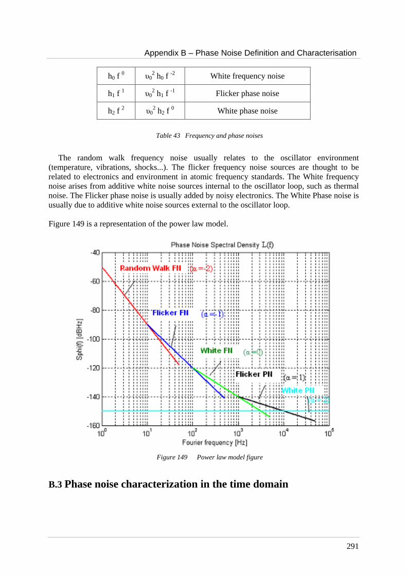
Appendix B – Phase Noise Definition and Characterisation

291

h0 f 0 υ0

2 h0 f -2 White frequency noise

h1 f 1 υ0

2 h1 f -1 Flicker phase noise

h2 f 2 υ0

2 h2 f 0 White phase noise

Table 43 Frequency and phase noises

The random walk frequency noise usually relates to the oscillator environment

(temperature, vibrations, shocks...). The flicker frequency noise sources are thought to be related to electronics and environment in atomic frequency standards. The White frequency noise arises from additive white noise sources internal to the oscillator loop, such as thermal noise. The Flicker phase noise is usually added by noisy electronics. The White Phase noise is usually due to additive white noise sources external to the oscillator loop. Figure 149 is a representation of the power law model.

Figure 149 Power law model figure

B.3 Phase noise characterization in the time domain

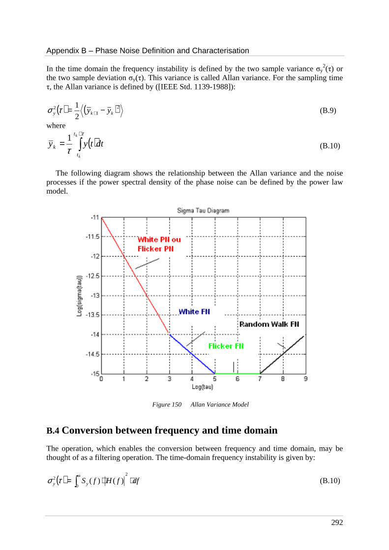
Appendix B – Phase Noise Definition and Characterisation

292

In the time domain the frequency instability is defined by the two sample variance σy2(τ) or

the two sample deviation σy(τ). This variance is called Allan variance. For the sampling time τ, the Allan variance is defined by ([IEEE Std. 1139-1988]):

( ) ( )21

2

2

1kky yy −= +τσ (B.9)

where

( )∫+

=τ

τ

k

k

t

t

k dttyy1

(B.10)

The following diagram shows the relationship between the Allan variance and the noise

processes if the power spectral density of the phase noise can be defined by the power law model.

Figure 150 Allan Variance Model

B.4 Conversion between frequency and time domain

The operation, which enables the conversion between frequency and time domain, may be thought of as a filtering operation. The time-domain frequency instability is given by:

( ) dffHfSyy ⋅⋅= ∫∞ 2

0

2 )()(τσ (B.10)

Appendix B – Phase Noise Definition and Characterisation

293

where Sy(f) is the spectral density of frequency deviations 1/T is the measurement rate

In the case of the two sample variance, ( )

( )2

42 sin

2)(f

ffH

⋅⋅⋅⋅=

τπτπ

so the Allan variance can be

computed from:

( ) ( )( ) df

f

ffS

hf

yy ⋅⋅⋅

⋅⋅⋅⋅= ∫0 2

42 sin

)(2τπ

τπτσ (B.11)

For the power-law model given previously, the time-domain measure also follows a power law:

( )22222101

2

22

)2(

3

)2(

)2(log3038.1

2

12log2

6

)2(

τπτπτπ

τπτσ hhe

ey

fh

fhhhh ++++⋅+= −− (B.12)

This assumes that the random driving mechanism for each term is independent of the others. The next table gives the coefficients of the translation among the frequency stability measures from time-domain to frequency domain and from frequency domain to time-domain.

Noise σy2(τ) Sy(f) SΦ(f)

Random Walk frequency

12 )( τ⋅⋅ fSfA y [ ] 221 )(1 −− ⋅⋅ fA y τστ [ ] 421

20 )( −− ⋅⋅ fA y τστν

Flicker frequency 0)( τ⋅⋅⋅ fSfB y [ ] 120 )(1 −⋅⋅ fB y τστ [ ] 321

20 )( −− ⋅⋅ f

B y τστν

White frequency 10 )( −⋅⋅ τfSfC y [ ] 021 )(1

fC y ⋅⋅ τστ [ ] 221

20 )( −− ⋅⋅ f

C y τστν

Flicker phase 21 )( −− ⋅⋅ τfSfD y [ ] 122 )(1

fD y ⋅⋅ τστ [ ] 121

20 )( −− ⋅⋅ f

D y τστν

White phase 22 )( −− ⋅⋅ τfSfE y [ ] 222 )(1

fE y ⋅⋅ τστ [ ] 021

20 )( f

E y ⋅⋅ − τστν

6

4 2π=A ( )2ln2 ⋅=B 2/1=C ( )

24

2ln3038.1

πτπ hfD

⋅+=

24

3

πhfE =

Table 44 Time-Frequency conversion of the phase noise

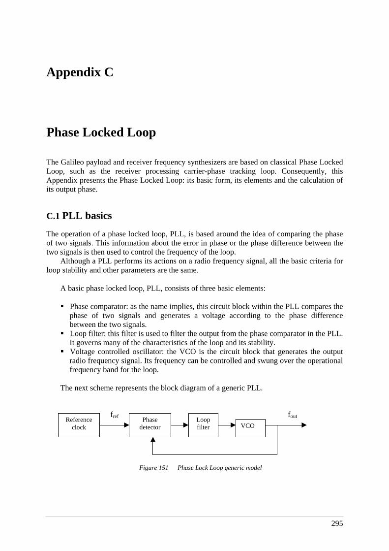
295

Appendix C Phase Locked Loop The Galileo payload and receiver frequency synthesizers are based on classical Phase Locked Loop, such as the receiver processing carrier-phase tracking loop. Consequently, this Appendix presents the Phase Locked Loop: its basic form, its elements and the calculation of its output phase.

C.1 PLL basics

The operation of a phase locked loop, PLL, is based around the idea of comparing the phase of two signals. This information about the error in phase or the phase difference between the two signals is then used to control the frequency of the loop.

Although a PLL performs its actions on a radio frequency signal, all the basic criteria for loop stability and other parameters are the same.

A basic phase locked loop, PLL, consists of three basic elements:

Phase comparator: as the name implies, this circuit block within the PLL compares the phase of two signals and generates a voltage according to the phase difference between the two signals.

Loop filter: this filter is used to filter the output from the phase comparator in the PLL. It governs many of the characteristics of the loop and its stability.

Voltage controlled oscillator: the VCO is the circuit block that generates the output radio frequency signal. Its frequency can be controlled and swung over the operational frequency band for the loop.

The next scheme represents the block diagram of a generic PLL.

Figure 151 Phase Lock Loop generic model

Reference clock

Phase detector

Loop filter

VCO

fref fout

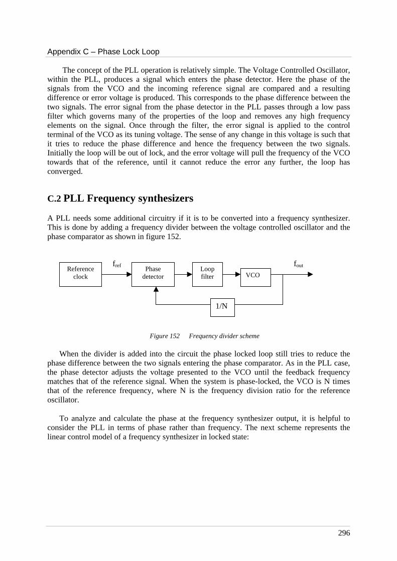
Appendix C – Phase Lock Loop

296

The concept of the PLL operation is relatively simple. The Voltage Controlled Oscillator, within the PLL, produces a signal which enters the phase detector. Here the phase of the signals from the VCO and the incoming reference signal are compared and a resulting difference or error voltage is produced. This corresponds to the phase difference between the two signals. The error signal from the phase detector in the PLL passes through a low pass filter which governs many of the properties of the loop and removes any high frequency elements on the signal. Once through the filter, the error signal is applied to the control terminal of the VCO as its tuning voltage. The sense of any change in this voltage is such that it tries to reduce the phase difference and hence the frequency between the two signals. Initially the loop will be out of lock, and the error voltage will pull the frequency of the VCO towards that of the reference, until it cannot reduce the error any further, the loop has converged.

C.2 PLL Frequency synthesizers

A PLL needs some additional circuitry if it is to be converted into a frequency synthesizer. This is done by adding a frequency divider between the voltage controlled oscillator and the phase comparator as shown in figure 152.

Figure 152 Frequency divider scheme

When the divider is added into the circuit the phase locked loop still tries to reduce the phase difference between the two signals entering the phase comparator. As in the PLL case, the phase detector adjusts the voltage presented to the VCO until the feedback frequency matches that of the reference signal. When the system is phase-locked, the VCO is N times that of the reference frequency, where N is the frequency division ratio for the reference oscillator.

To analyze and calculate the phase at the frequency synthesizer output, it is helpful to consider the PLL in terms of phase rather than frequency. The next scheme represents the linear control model of a frequency synthesizer in locked state:

Reference clock

Phase detector

Loop filter

VCO

1/N

fref fout

Appendix C – Phase Lock Loop

297

Figure 153 Frequency synthesizer linear model with θref, the input reference phase which comes from the clock unit θVCO, the VCO output phase θout, the output phase θfb, the feed-back phase F(s) the transfer function of the loop filter, KVCO and KPD are, respectively the VCO and the phase detector gains.

The phase at the PLL output is equal to:

)()()(

)()( ss

KsFK

N

sss VCO

VCOPD

outrefout θθθθ +⋅⋅⋅

−= (C.1)

)()()()(1)( ss

KsFKs

s

KsFKs VCO

VCOPDref

VCOPDout θθθ +⋅⋅⋅=

⋅⋅+⋅ (C.2)

So,

( ))(1)()()()( sHssHsNs VCOrefout −⋅+⋅⋅= θθθ (C.3)

with H(f) is the PLL closed loop transfer function equal to: ( )( )

( ) N

sFKKs

N

sFKK

sHPDVCO

PDVCO

⋅⋅+

⋅⋅

=

C.3 PLL frequency synthesizer phase noise

The frequency synthesizers are used in the Galileo payload and receiver to generate, from reference clocks, higher frequencies, which permit to up-convert and down-convert the signals. However both the receiver and the payload reference clocks suffer from instabilities which create phase noise. Consequently, the reference phases, which enter in the PLL frequency synthesizers, should be considered as the sum of two terms: the ‘real’ phase and a phase noise.

KPD F(s) KVCO/s

1/N

θref

θfb

+

-

θvco

θout

Appendix C – Phase Lock Loop

298

The voltage controlled oscillator also suffers from instabilities, so the VCO output phase is also composed of the ‘real’ VCO phase plus a phase noise. Because of the reference clock and the VCO phase noises, the frequency synthesizer output phase also contains phase noise. This phase noise is linked to the VCO phase noise and to the reference clock phase noise by the same equation than equation C.3. As seen in Appendix B, a phase noise is characterized thanks to its power spectrum densities, so the phase noise at the frequency synthesizer output is characterized by:

222 )(1)()()()( fHfSfHfSNfSVCOrefout

−⋅+⋅⋅= φφφ (C.4)

with

( )( )

( ) N

sFKKs

N

sFKK

sHPDVCO

PDVCO

⋅⋅+

⋅⋅

= (C.5)

and SΦref(f), the power spectrum density of the reference clock phase noise, SΦVCO(f) the power spectrum density of the VCO phase noise.

This equation permits to evaluate the phase noise at the payload and receiver frequency synthesizers output and consequently it permits to evaluate the phase noise which is introduced on the signal during the up-conversion and the down-conversion.

299

Bibliography

[Amoroso] F. Amoroso, Adaptative A/D Converter to Suppress CW interference in DSPN Sread-Spectrum Communications, IEEE Transactions on communications, VOL.COM-31, NO.10, OCTOBER 1983

[Aparacio, 1994] M. Aparicio, P. Brodie, J. Rajan, A. Sung, Communication Satellite Augmented GPS Payload Architecture, ION GPS-94, September 1994.

[Armengou, 20003] E. Armengou-Miret, Techniques de Multiplexage en bande L1, Pertes de corrélation associées, Rapport de stage CNES 2003.

[Avila-Rodriguez, 2006] J-A Avila-Rodriguez, S. Wallner, G. W. Hein, E. Rebeyrol, O. Julien, C. Macabiau, L. Ries, A. DeLatour, L. Lestarquit, J-L Issler, CBOC- An implementation of MBOC, 1st CNES workshop on Galileo signals, October 2006

[Barnes, 1971] J.A. barnes, A.R. Chi, L.S. Cutler, D.J. Healey, D.B. Leeson, T.E. McGunigal, J.A. Mulle, W.L. Smith, R.L. Sydnor, R. VEssot, G.M.R. Winkler, Characterization of frequency stability, IEEE Trans. Intrsum. Meas., vol IM-20, pp. 105-120, May 1971

[Betz, 2002] J. W. Betz, Binary Offset Carrier Modulations for Radionavigation, Journal of the Institute of Navigation, VOL.48, No.4, Winter 2001-2002

[Bradford, 2006] A. Bradford, P. Davies, J. Paffett, E. Rooney, M. Sweeting, M. Unwin, G. Gatti, A. Garutti, On-orbit Experience of the First Galileo Satellite GIOVE-A, 57th Annual International Astronautical Congress, October 2006, Spain

[Butman, 1972] S. Butman and U. Timor, Interplex – An efficient Multichannel PSK/PM Telemetry System, IEEE Transaction on Communications, Volume 20, No. 3, June 1972

[Coromina, 2004] F. Coromina, F. Deborgies, F. Emma, G. Gatti, On-board Applications of Active Microwave Technologies to Galileo and other European Space Programs, 12th GAAS Symposium, 2004

Bibliography

300

[Czopek, 1993] F. Czopek, Lt. S. Shollenberger, Description and performance of the GPS BlockI and II L-band antenna and Link Budget, ION GPS 1993

[Da Dalt, 2002] N. Da Dalt, M. Harteneck, C. Sandner and A. Wiesbauer , On the jitter requirements of the sampling clock for Analog-to-Digital converters, IEEE Transactions on Circuits and Systems, September 2002

[Felbach, 2003] D. Felbach, D. Heimbuerger, P. Herre, P. Rastetter, Galileo Payload 10.23 MHz Master Clock Generation with a Clock Monitoring and Control unit (CMCU), IEEE International Frequency Control Symposium, 2003

[GJU, 2005] Galileo Joint Undertaking, L1 band part of Galileo Signal in Space ICD, 3 GPP TSG GERAN2 meeting, May 2005

[Godet, 2001] J. Godet, Technical Annex to Galileo SRD Signal Plans, STF-annex-SRD-2001/003, 2001. (This document has been made publically available several years after having been issued. The ALTBOC part of this document has been inspired by Laurent Lestarquit).

[Hegarty, 1999] C. Hegarty, Evaluation of the Proposed Signal Structure for the New Civil GPS Signal at 1176.45 MHz, WN99W0000034, The MITRE Corporation, 1999

[Hegarty, 2003] C. Hegarty, Alternative Bi-phase GNSS Modulations, MITRE Memo F82-M04-004, 2003

[Hegarty, 2004] C. Hegarty, J. Betz, Saidi, Binary Coded Symbol Modulations for GNSS, Proceedings of The Institute of Navigation’s Annual Meeting, June 2004

[Hein, 2001] G. W. Hein, J. Godet, J-L. Issler, J-C. Martin, R. Lucas-Rodriguez and T. Pratt , The Galileo Frequency Structure and Signal Design, ION GPS/GNSS, September 2001

[Hein, 2002] G. W. Hein, J. Godet, J-L. Issler, J-C. Martin, P. Erhard, R. Lucas-Rodriguez, T. Pratt, Status of Galileo Frequency and Signal Design, ION GPS 2002

[Hein, 2005] G. W. Hein, J. A. Avila-Rodriguez, L. Ries, L. Lestarquit, J-L Issler, J. Godet, T. Pratt, A Candidate for the Galileo L1 OS Optimized Signal, ION GNSS 2005

Bibliography

301

[Hein, 2006] G.W. Hein, J.A. Ávila-Rodríguez, S. Wallner, A.R. Pratt, J. Owen, J-L. Issler, J.W. Betz, C. Hegarty, Lt S. Lenahan, J.J. Rushanan, A.L. Kraay, T.A. Stansell, MBOC: The New Optimized Spreading Modulation Recommended for GALILEO L1 OS and GPS L1C, ION IEEE/PLANS, 2006

[Heiries, 2004] V. Heiries, D. Roviras, L. Ries, V. Calmettes, Analysis of Non Ambiguous BOC Signal Acquisition Performance, ION GNSS 2004

[Heiries, 2005] V. Heiries, J.A. Àvila-Rodriguez, M. Irsigler , G.W. Hein, E. Rebeyrol, D. Roviras, Acquisition Performance Analysis of Composite Signals for the L1 OS Optimized Signal, ION GNSS 2005

[Holmes, 1982] J.K. Holmes, Coherent Spread Spectrum Systems, John Wiley and Sons, New York, 1982

[IEEE Std. 1139-1988] IEEE Standard Definitions of Physical Quantities for Fundamental Frequency and Time Metrology

[Issler, 2003] J-L Issler, L. Ries, L. Lestarquit, O. Nouvel, Q. Jeandel, Spectral Measurements of GNSS SatelliteSignals Need for Wide Transmitted Bands, ION GPS 2003

[Julien, 2005] O. Julien, Design of Galileo L1F Receiver Tracking Loops, PhD report, July 2005

[Julien, 2006] O. Julien, C. Macabiau, J-L Issler, L. Ries, 1-bit Processing of Composite BOC (CBOC) Signals, 1st CNES Workshop on Galileo Signals and Signal Processing, October 2006

[Kaplan, 1996] E. D. Kaplan, Understanding GPS Principles and Applications, Artech House Mobile Communications Series, 1996

[Lestarquit, 2002] L. Lestarquit, Procédé et dispositif de génération d’un signal de navigation à enveloppe constante a quatre codes indépendants, Brevet d’Invention FR 2 848 748 – A1, décembre 2002

[Macabiau, 2003] C. Macabiau, L. Ries, F. Bastide, J-L. Issler, GPS L5 Receiver Implementation Issues, ION GPS 2003

[Moreno Carrillo, 2005] F.J. Moreno Carrillo, A. Alvaro Sanchez, L. Basanta Alonso, Hybrid Synthesizers in Space Galileo’s CMCU, Data Systems In Aerospace Conference, June 2005

Bibliography

302

[Parkinson, 1996] B. W. Parkinson, J. J. Spilker, Global Positioning System: Theory and Applications, Progress in Astronautics and Aeronautics VOL. 163, 1996

[Pratt, 2003] A. R. Pratt and J. I. R. Owen, BOC Modulations Waveform, ION GPS/GNSS, September 2003

[Pratt, 2006] A. R. Pratt, J. I. R. Owen, G. W. Hein, J. A. Avila-Rodriguez, Tracking Complex Modulation Waveforms – How to avoid receiver bias, ION IEEE/PLANS, April 2006

[Rebeyrol, 2005] E. Rebeyrol, C. Macabiau, L. Lestarquit, L. Ries, J-L Issler, M-L Boucheret, M. Bousquet, BOC Power Spectrum Densities, ION NTM 2005

[Rebeyrol01, 2006] E. Rebeyrol, C. Macabiau, L. Ries, J-L. Issler, M. Bousquet, and M-L. Boucheret, Interplex Modulation for Navigation Systems at the L1 Band, ION NTM 2006

[Rebeyrol02, 2006] E. Rebeyrol, C. Macabiau, L. Ries, J-L. Issler, M. Bousquet, and M-L. Boucheret, Phase Noise in GNSS Transmission/Reception System, ION NTM 2006

[Rebeyrol03, 2006] E. Rebeyrol, C. Macabiau, O. Julien, L. Ries, J-L. Issler, M. Bousquet, M-L. Boucheret, Signal Distortions at GNSS Payload Level, ION GNSS 2006

[Rebeyrol04, 2006] E. Rebeyrol, O. Julien, C. Macabiau, L. Ries, A. Delatour, L. Lestarquit, Galileo Civil Signals Modulations, GPS Solutions, 2006

[Ries, 2002] L. Ries, L. Lestarquit, P. Erhard, F. Legrand, C. Macabiau, Q. Jeandel and C. Bourgat, Software Simulation Tools for GNSS2 BOC Signal Analysis, ION GPS/GNSS, September 2002

[Ries01, 2003] L. Ries, F. Legrand, L. Lestarquit, W. Vigneau, J.L. Issler, Tracking and Multipath Performance Assessments of BOC Signals Using a Bit-Level Signal Processing Simulator, ION GPS/GNSS, September 2003

[Ries02, 2003] L. Ries, L. Lestarquit, J-L Issler, A.R. Pratt.,G. Hein, J. Godet, P. Dondl, F. Couturier, P. Erhard, J I R Owen, R. Lucas-Rodriguez, J-C Martin, New Investigations on Wide Band GNSS2 Signals, GNSS Conference 2003, 2003

[Robins, 1982] W. P. Robins, Phase Noise in Signal Sources, IEE telecommunications Series 9, 1982

Bibliography

303

[Rutman, 1991] J. Rutman,, F.L. Walls, Characterization of Frequency Stability in Precision Frequency Sources, Proc. of the IEEE, Vol. 79, No. 6, pp. 952-960, 1991

[Sleewagen, 2005] J-M Sleewaegen, W. De Wilde, M. Hollreiser, Galileo ALTBOC receiver, Septentrio, 2005

[Soellner, 2003] M. Soellner and P. Erhard, Comparison of AWGN code tracking accuracy for Alternative-BOC, Complex-LOC and Complex-BOC modulation options in Galileo E5-Band, GNSS Conference 2003, April 2003

[Tsui, 2000] J. BY Tsui, Fundamentals of Global Positioning System Receivers: A Software Approach, Wiley Series in Microwave and Optical Engineering, 2000

[Van Trees, 1968] Van Trees, Detection, Estimation, and Modulation Theory, Part I., John Wiley and Sons, 1968

[Ward, 1996] P. Ward, Satellite Signal Acquisition and Tracking in understanding GPS: Principles and Applications, Artech House Inc., 1996

Websites:

[Analog, 2006] www.analog.com

[ESA, 2005] www.esa.int

[E. C., 2006] http://ec.europa.eu/dgs/energy-transport/galileo

[GIOVE, 2006] www.giove.esa.int

[Ircom, 2006] http://www.ircom.unilim.fr

[Novatel, 2006] www.novatel.com

[Quartzlock, 2006] www.quartzlock.com

[Rakon, 2006] www.rakon.com

[Zarlink, 2006] www.zarlink.com