Structural and Multidisciplinary Optimization manuscript No.(will be inserted by the editor)

J.-F. Collard · P. Duysinx · P. Fisette

Optimal synthesis of planar mechanismsvia an extensible link approach

Received: date / Revised: date

Abstract This paper presents a novel approach to optimizethe design of planar mechanisms for function-generator orpath synthesis. The proposed method is based on the use of aflexible mechanism model whose strain energy is minimizedto find the optimal rigid design. This enables us to get ridof assembly constraints and the use of natural coordinatesmakes the objective function simpler.

Two optimization strategies are developed and then dis-cussed. The first one relies on alternate optimizations of de-sign parameters and point coordinates. The second one usesmultiple local synthesis as starting point for a moreglobalsynthesis.

The question of finding the global optimum is also ad-dressed and developed. A simple algorithm is proposed tofind several local optima among which the designer maychoose the best one taking other criteria into account (e.g.stiffness, collision, size,. . . ).

Three applications are presented to illustrate the strate-gies while mentioning their limits.

Keywords optimal synthesis· natural coordinates·closed-loop mechanisms

Part of this paper has been presented at the Sixth WCSMO, Rio,June2005

J.-F. CollardCentre for Research in Mechatronics, Universite Catholique de Lou-vain (UCL), BelgiumTel.: +32-10-472504Fax: +32-10-472501E-mail: collard@prm.ucl.ac.be

P. DuysinxDepartment of Mechanics and Aerospace, Universite de Liege (ULg),Belgium

P. FisetteCentre for Research in Mechatronics, UCL, Belgium

1 Introduction

Optimization of complex multibody systems represents areal present interest along with the increasing developmentof computer resources. This is particularly true consideringclosed-loop mechanisms whose assembling constraints haveto be satisfied before any analysis. They thus need a specialattention when evolving the optimization process strategy. Afew solutions have been proposed to deal with them. For ex-ample, in Collard et al (2005a), the authors have suggestedto penalize properly the objective function using the condi-tioning of the assembling constraints Jacobian matrix. Thisextends the parameter space and leads to an enlarged exis-tence of the objective function but the problem may remaindifficult to optimize. Another well-known approach in pathsynthesis is to deform the mechanism subject to a perfect fol-lowing of the desired path as in Vallejo et al (1995); Jimenezet al (1997); Alba et al (2000). From this point of view, thepath-following objective becomes a optimization constraintwhile the deformation energy is the actual objective to min-imize. Therefore, the mechanism naturally assembles eachtime the optimization process computes the objective func-tion. This approach is adopted in this work.

In optimal design synthesis, a second issue consists inthe choice of the formalism to describe the geometry of themechanism. Among the different possibilities, one can men-tion the common use of relative coordinates in real form(Mariappan and Krishnamurty (1996); Cabrera et al (2002);Hansen (2002); Laribi et al (2004)) or in complex form (San-cibrian et al (2004)). This formalism has the advantages tolimit the number of assembling constraints but introducestrigonometric functions involving angular variables: it en-hances the non-linearity of the problem and makes the opti-mization more tricky. The use of natural – or point – coor-dinates is also wide-spread (see Jimenez et al (1997); Albaet al (2000); Lio et al (2000); Jensen and Hansen (2003)). Incomparison with relative coordinates, natural coordinates in-volve additional algebraic constraints. However, these equa-tions only consist of linear and/or distance functions. Thiscoordinates system is thus well suited to gradient-based op-timization techniques such as least squares methods.

2

The proposed method tries to combine these two fea-tures: deformable mechanisms and natural coordinates. Thefirst one enables to solve the problem of non-assembly whilethe second one greatly simplifies the type of objective func-tion. The optimization strategy is based on the minimizationof the deformation energy over the followed path, and a sub-sequent update of the mean lengths as suggested in Hansen(2002). This minimization-update sequence is repeated un-til convergence when the total deformation energy does notvary anymore or is sufficiently low. The method presentsa rather slow convergence rate but shows a monotonic de-crease, and may sometimes fail to find the global optimum.To improve the convergence rate, the technique is combinedwith a global synthesis approach as proposed by Alba et al(2000).

Afterwards, this improvement has enabled to outline animportant issue in mechanism optimization: different localoptima starting from different initial parameters. The choiceof the optimal mechanism among these local optima relieson other design constraints which are difficult to computeand not taken into account in the original problem. By theway, it is also shown that the use of a standard genetic al-gorithm does not necessarily enable to reach the global op-timum. Since it is interesting for the designer to keep andcompare some of the best mechanisms (i.e. local optima), aexploration strategy of the design space is proposed to ’un-earth’ most of the possible optima.

Different kinds of requirements may be encountered indimensional mechanisms synthesis: path or function gen-eration, body guidance, or mixed problems. Most applica-tions concern path synthesis problems (Mariappan and Kr-ishnamurty (1996); Zhou and Cheung (2001); Cabrera et al(2002); Hansen (2002); Marın and Gonzalez (2003); Laribiet al (2004); Sancibrian et al (2004); Shiakolas et al (2005))and the four-bar mechanism will constitute a simple run-ning example in the following. More realistic applicationsof function-generation synthesis will also be given basedon the Ackerman steering linkage problem: a four-bar andthen a six-bar synthesis. These last ones have been suggestedby Simionescu et al (2000); Pramanik (2002); Simionescuand Beale (2002).

The paper is organized as follows: in Section 2, the gen-eral optimization problem is modeled and formulated: theobjective function is build and the sensitivity analysis is per-formed. In Section 3, we develop the optimization strategyapplying two methods to the path synthesis of a four-barmechanism as illustrative example. Section 4.2 presents amore realistic application of function generation synthesisfor the four-bar Ackerman steering linkage. Section 5 dealswith the question of finding the global optimum followingby a new method to explore the design space. Before someconclusions and prospects in Section 7, a more complete ap-plication to optimize a six-bar steering linkage is presentedto illustrate the concepts in Section 6.

2 Problem formulation

The problem formulation is divided into two subsections:first, the cost function is evolved and then the correspondingsensitivity analysis is worked out.

2.1 Objective function

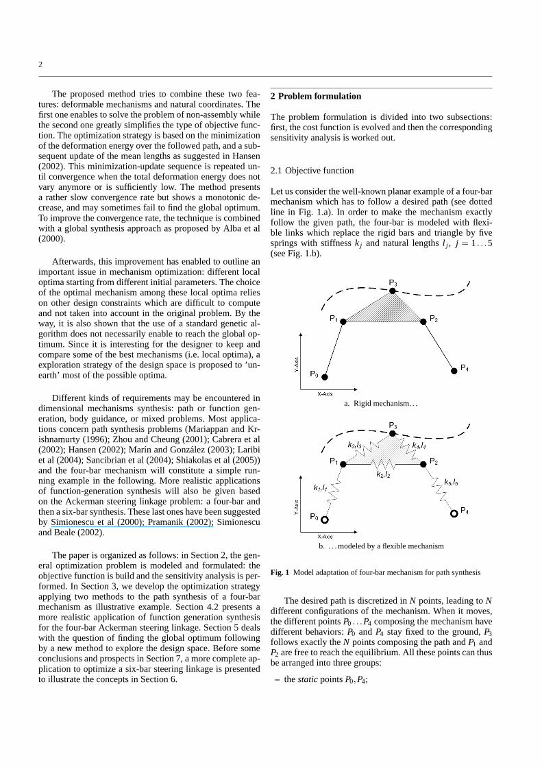
Let us consider the well-known planar example of a four-barmechanism which has to follow a desired path (see dottedline in Fig. 1.a). In order to make the mechanism exactlyfollow the given path, the four-bar is modeled with flexi-ble links which replace the rigid bars and triangle by fivesprings with stiffnessk j and natural lengthsl j , j = 1. . .5(see Fig. 1.b).

a. Rigid mechanism. . .

b. . . . modeled by a flexible mechanism

Fig. 1 Model adaptation of four-bar mechanism for path synthesis

The desired path is discretized inN points, leading toNdifferent configurations of the mechanism. When it moves,the different pointsP0 . . .P4 composing the mechanism havedifferent behaviors:P0 andP4 stay fixed to the ground,P3follows exactly theN points composing the path andP1 andP2 are free to reach the equilibrium. All these points can thusbe arranged into three groups:

– thestaticpointsP0,P4;

3

– thetrackingpointP3;– thefloatingpointsP1,P2.

Their absolute coordinates are saved respectively in the fol-lowing vectors:s, t and f. As the tracking point and thefloating points may have different coordinates for each con-figuration, t and f are referenced by the indexi: t i and f i ,i = 1. . .N.Grouping the natural lengthsl j in the column vectorl andthe stiffness parametersk j on the diagonal of the stiffnessmatrix K , we define the global strain energy as a scalar costfunction:

E (s, t1, . . . , tN, f1, . . . , fN, l,K)=12

N

∑i=1

(di − l)T K (di − l) ,(1)

where indexi stands for theith configuration of the mecha-nism anddi is a column vector containing the five distancedi

j between each couple of linked points. For the moment,the only known parameters are the 2N∗2 coordinates of thefloating points. The stiffness parametersk j may be chosenby the user. They play the role of weights in the sum of allthe contributions to the total energy. Making a bar stiffer in-creases its relative importance in the cost function but thispossibility is not used in the following. After these consid-erations, the optimization problem is stated as follows:

mins,f1,...,fN,l

12

N

∑i=1

(d(s, t i , f i)− l)T K (d(s, t i , f i)− l) , (2)

where the actual design parameters ares andl. This consti-tutes an obvious non-linear least squares optimization prob-lem. Defined that way, the problem remains difficult to solve.Therefore, two propositions are given below to improve thehomogeneity of the problem and to avoid multiple triangleconfigurations.

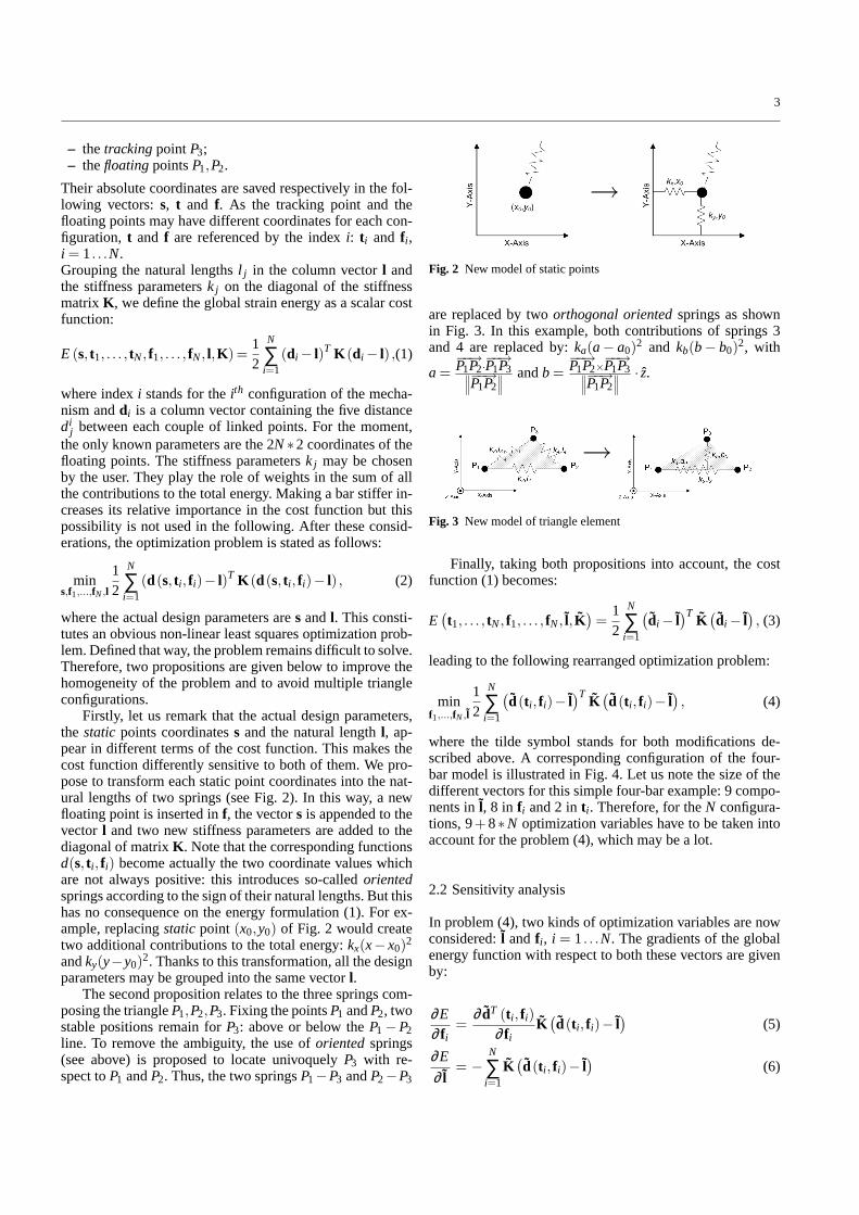
Firstly, let us remark that the actual design parameters,the static points coordinatess and the natural lengthl, ap-pear in different terms of the cost function. This makes thecost function differently sensitive to both of them. We pro-pose to transform each static point coordinates into the nat-ural lengths of two springs (see Fig. 2). In this way, a newfloating point is inserted inf, the vectors is appended to thevector l and two new stiffness parameters are added to thediagonal of matrixK . Note that the corresponding functionsd(s, t i , f i) become actually the two coordinate values whichare not always positive: this introduces so-calledorientedsprings according to the sign of their natural lengths. But thishas no consequence on the energy formulation (1). For ex-ample, replacingstaticpoint (x0,y0) of Fig. 2 would createtwo additional contributions to the total energy:kx(x− x0)

2

andky(y−y0)2. Thanks to this transformation, all the design

parameters may be grouped into the same vectorl.The second proposition relates to the three springs com-

posing the triangleP1,P2,P3. Fixing the pointsP1 andP2, twostable positions remain forP3: above or below theP1 −P2line. To remove the ambiguity, the use oforientedsprings(see above) is proposed to locate univoquelyP3 with re-spect toP1 andP2. Thus, the two springsP1−P3 andP2−P3

→

Fig. 2 New model of static points

are replaced by twoorthogonal orientedsprings as shownin Fig. 3. In this example, both contributions of springs 3and 4 are replaced by:ka(a− a0)

2 and kb(b− b0)2, with

a =−−→P1P2·

−−→P1P3

∥

∥

∥

−−→P1P2

∥

∥

∥

andb =−−→P1P2×

−−→P1P3

∥

∥

∥

−−→P1P2

∥

∥

∥

· z.

→

Fig. 3 New model of triangle element

Finally, taking both propositions into account, the costfunction (1) becomes:

E(

t1, . . . , tN, f1, . . . , fN, l, K)

=12

N

∑i=1

(

di − l)T

K(

di − l)

, (3)

leading to the following rearranged optimization problem:

minf1,...,fN,l

12

N

∑i=1

(

d(t i , f i)− l)T

K(

d(t i , f i)− l)

, (4)

where the tilde symbol stands for both modifications de-scribed above. A corresponding configuration of the four-bar model is illustrated in Fig. 4. Let us note the size of thedifferent vectors for this simple four-bar example: 9 compo-nents inl, 8 in f i and 2 int i . Therefore, for theN configura-tions, 9+8∗N optimization variables have to be taken intoaccount for the problem (4), which may be a lot.

2.2 Sensitivity analysis

In problem (4), two kinds of optimization variables are nowconsidered:l andf i , i = 1. . .N. The gradients of the globalenergy function with respect to both these vectors are givenby:

∂E∂ f i

=∂ dT (t i , f i)

∂ f iK

(

d(t i , f i)− l)

(5)

∂E

∂ l= −

N

∑i=1

K(

d(t i , f i)− l)

(6)

4

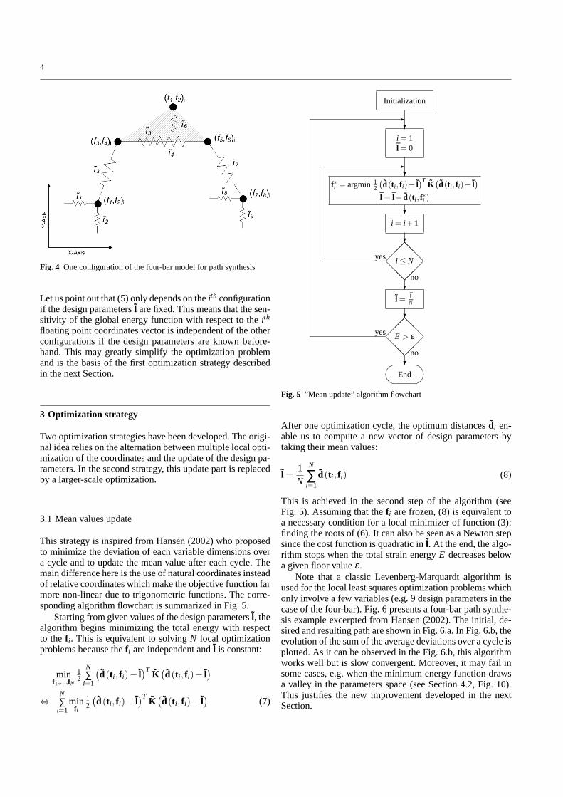
Fig. 4 One configuration of the four-bar model for path synthesis

Let us point out that (5) only depends on theith configurationif the design parametersl are fixed. This means that the sen-sitivity of the global energy function with respect to theith

floating point coordinates vector is independent of the otherconfigurations if the design parameters are known before-hand. This may greatly simplify the optimization problemand is the basis of the first optimization strategy describedin the next Section.

3 Optimization strategy

Two optimization strategies have been developed. The origi-nal idea relies on the alternation between multiple local opti-mization of the coordinates and the update of the design pa-rameters. In the second strategy, this update part is replacedby a larger-scale optimization.

3.1 Mean values update

This strategy is inspired from Hansen (2002) who proposedto minimize the deviation of each variable dimensions overa cycle and to update the mean value after each cycle. Themain difference here is the use of natural coordinates insteadof relative coordinates which make the objective function farmore non-linear due to trigonometric functions. The corre-sponding algorithm flowchart is summarized in Fig. 5.

Starting from given values of the design parametersl, thealgorithm begins minimizing the total energy with respectto the f i . This is equivalent to solvingN local optimizationproblems because thef i are independent andl is constant:

minf1,...,fN

12

N∑

i=1

(

d(t i , f i)− l)T

K(

d(t i , f i)− l)

⇔N∑

i=1min

f i

12

(

d(t i , f i)− l)T

K(

d(t i , f i)− l)

(7)

Initialization

?i = 1l = 0

?f∗i = argmin 1

2

(

d(t i , f i)− l)T

K(

d(t i , f i)− l)

l = l + d(t i , f∗i )

?i = i +1

?

���

@@@

���

@@@

i ≤ Nyes

no?

l = lN

?

���

@@@

���

@@@

E > εyes

no?�

���End

-

-

Fig. 5 ”Mean update” algorithm flowchart

After one optimization cycle, the optimum distancesdi en-able us to compute a new vector of design parameters bytaking their mean values:

l =1N

N

∑i=1

d(t i , f i) (8)

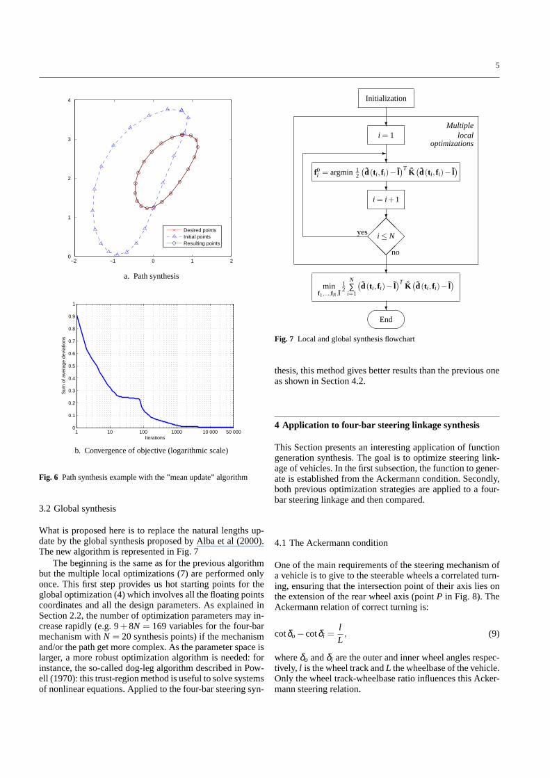
This is achieved in the second step of the algorithm (seeFig. 5). Assuming that thef i are frozen, (8) is equivalent toa necessary condition for a local minimizer of function (3):finding the roots of (6). It can also be seen as a Newton stepsince the cost function is quadratic inl. At the end, the algo-rithm stops when the total strain energyE decreases belowa given floor valueε .

Note that a classic Levenberg-Marquardt algorithm isused for the local least squares optimization problems whichonly involve a few variables (e.g. 9 design parameters in thecase of the four-bar). Fig. 6 presents a four-bar path synthe-sis example excerpted from Hansen (2002). The initial, de-sired and resulting path are shown in Fig. 6.a. In Fig. 6.b, theevolution of the sum of the average deviations over a cycle isplotted. As it can be observed in the Fig. 6.b, this algorithmworks well but is slow convergent. Moreover, it may fail insome cases, e.g. when the minimum energy function drawsa valley in the parameters space (see Section 4.2, Fig. 10).This justifies the new improvement developed in the nextSection.

5

−2 −1 0 1 20

1

2

3

4

Desired pointsInitial pointsResulting points

a. Path synthesis

1 10 100 1000 10 000 50 0000

0.1

0.2

0.3

0.4

0.5

0.6

0.7

0.8

0.9

1

Iterations

Sum

of a

vera

ge d

evia

tions

b. Convergence of objective (logarithmic scale)

Fig. 6 Path synthesis example with the ”mean update” algorithm

3.2 Global synthesis

What is proposed here is to replace the natural lengths up-date by the global synthesis proposed by Alba et al (2000).The new algorithm is represented in Fig. 7

The beginning is the same as for the previous algorithmbut the multiple local optimizations (7) are performed onlyonce. This first step provides us hot starting points for theglobal optimization (4) which involves all the floating pointscoordinates and all the design parameters. As explained inSection 2.2, the number of optimization parameters may in-crease rapidly (e.g. 9+ 8N = 169 variables for the four-barmechanism withN = 20 synthesis points) if the mechanismand/or the path get more complex. As the parameter space islarger, a more robust optimization algorithm is needed: forinstance, the so-called dog-leg algorithm described in Pow-ell (1970): this trust-region method is useful to solve systemsof nonlinear equations. Applied to the four-bar steering syn-

Initialization

?i = 1

?f0i = argmin 1

2

(

d(t i , f i)− l)T

K(

d(t i , f i)− l)

?i = i +1

?

���

@@@

���

@@@

i ≤ Nyes

no

?

minf1,...,fN,l

12

N∑

i=1

(

d(t i , f i)− l)T

K(

d(t i , f i)− l)

?��

��End

-

Multiplelocal

optimizations

Fig. 7 Local and global synthesis flowchart

thesis, this method gives better results than the previous oneas shown in Section 4.2.

4 Application to four-bar steering linkage synthesis

This Section presents an interesting application of functiongeneration synthesis. The goal is to optimize steering link-age of vehicles. In the first subsection, the function to gener-ate is established from the Ackermann condition. Secondly,both previous optimization strategies are applied to a four-bar steering linkage and then compared.

4.1 The Ackermann condition

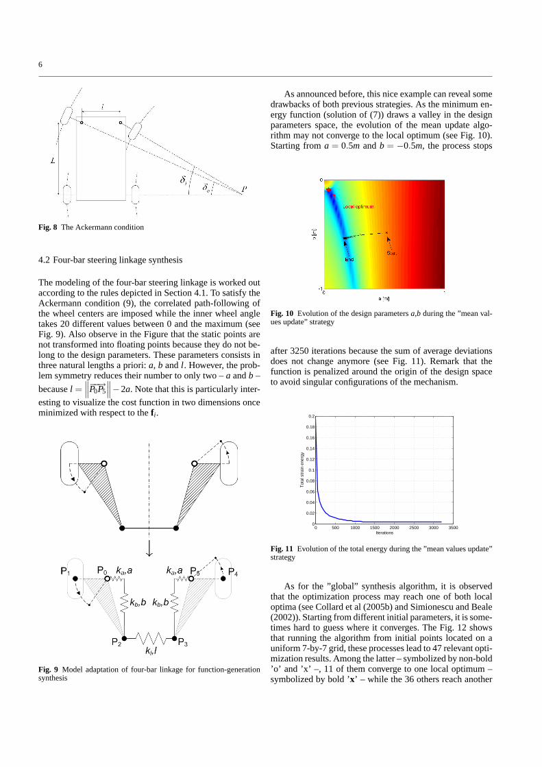
One of the main requirements of the steering mechanism ofa vehicle is to give to the steerable wheels a correlated turn-ing, ensuring that the intersection point of their axis lies onthe extension of the rear wheel axis (pointP in Fig. 8). TheAckermann relation of correct turning is:

cotδo−cotδi =lL

, (9)

whereδo andδi are the outer and inner wheel angles respec-tively, l is the wheel track andL the wheelbase of the vehicle.Only the wheel track-wheelbase ratio influences this Acker-mann steering relation.

6

Fig. 8 The Ackermann condition

4.2 Four-bar steering linkage synthesis

The modeling of the four-bar steering linkage is worked outaccording to the rules depicted in Section 4.1. To satisfy theAckermann condition (9), the correlated path-following ofthe wheel centers are imposed while the inner wheel angletakes 20 different values between 0 and the maximum (seeFig. 9). Also observe in the Figure that the static points arenot transformed into floating points because they do not be-long to the design parameters. These parameters consists inthree natural lengths a priori:a, b andl . However, the prob-lem symmetry reduces their number to only two –a andb –

becausel =∥

∥

∥

−−→P0P5

∥

∥

∥−2a. Note that this is particularly inter-

esting to visualize the cost function in two dimensions onceminimized with respect to thef i .

↓

Fig. 9 Model adaptation of four-bar linkage for function-generationsynthesis

As announced before, this nice example can reveal somedrawbacks of both previous strategies. As the minimum en-ergy function (solution of (7)) draws a valley in the designparameters space, the evolution of the mean update algo-rithm may not converge to the local optimum (see Fig. 10).Starting froma = 0.5m andb = −0.5m, the process stops

Fig. 10 Evolution of the design parametersa,b during the ”mean val-ues update” strategy

after 3250 iterations because the sum of average deviationsdoes not change anymore (see Fig. 11). Remark that thefunction is penalized around the origin of the design spaceto avoid singular configurations of the mechanism.

0 500 1000 1500 2000 2500 3000 35000

0.02

0.04

0.06

0.08

0.1

0.12

0.14

0.16

0.18

0.2

Iterations

Tot

al s

trai

n en

ergy

Fig. 11 Evolution of the total energy during the ”mean values update”strategy

As for the ”global” synthesis algorithm, it is observedthat the optimization process may reach one of both localoptima (see Collard et al (2005b) and Simionescu and Beale(2002)). Starting from different initial parameters, it is some-times hard to guess where it converges. The Fig. 12 showsthat running the algorithm from initial points located on auniform 7-by-7 grid, these processes lead to 47 relevant opti-mization results. Among the latter – symbolized by non-bold’o’ and ’x’ –, 11 of them converge to one local optimum –symbolized by bold ’x’ – while the 36 others reach another

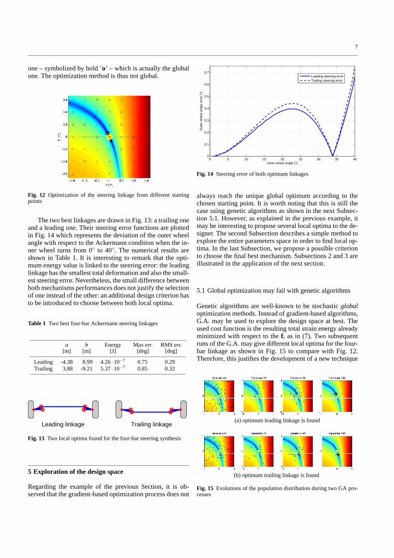
7

one – symbolized by bold ’o’ – which is actually the globalone. The optimization method is thus not global.

Fig. 12 Optimization of the steering linkage from different startingpoints

The two best linkages are drawn in Fig. 13: a trailing oneand a leading one. Their steering error functions are plottedin Fig. 14 which represents the deviation of the outer wheelangle with respect to the Ackermann condition when the in-ner wheel turns from 0◦ to 40◦. The numerical results areshown in Table 1. It is interesting to remark that the opti-mum energy value is linked to the steering error: the leadinglinkage has the smallest total deformation and also the small-est steering error. Nevertheless, the small difference betweenboth mechanisms performances does not justify the selectionof one instead of the other: an additional design criterion hasto be introduced to choose between both local optima.

Table 1 Two best four-bar Ackermann steering linkages

a b Energy Max err. RMS err.[m] [m] [J] [deg] [deg]

Leading -4.38 8.99 4.26·10−7 0.75 0.29Trailing 3.88 -9.21 5.37·10−7 0.85 0.32

Leading linkage Trailing linkage

Fig. 13 Two local optima found for the four-bar steering synthesis

5 Exploration of the design space

Regarding the example of the previous Section, it is ob-served that the gradient-based optimization process does not

0 5 10 15 20 25 30 35 400

0.1

0.2

0.3

0.4

0.5

0.6

0.7

Inner wheel angle [°]

Out

er w

heel

anl

ge e

rror

[°]

Leading steering errorTrailing steering error

Fig. 14 Steering error of both optimum linkages

always reach the unique global optimum according to thechosen starting point. It is worth noting that this is still thecase using genetic algorithms as shown in the next Subsec-tion 5.1. However, as explained in the previous example, itmay be interesting to propose several local optima to the de-signer. The second Subsection describes a simple method toexplore the entire parameters space in order to find local op-tima. In the last Subsection, we propose a possible criterionto choose the final best mechanism. Subsections 2 and 3 areillustrated in the application of the next section.

5.1 Global optimization may fail with genetic algorithms

Genetic algorithms are well-known to be stochasticglobaloptimization methods. Instead of gradient-based algorithms,G.A. may be used to explore the design space at best. Theused cost function is the resulting total strain energy alreadyminimized with respect to thef i as in (7). Two subsequentruns of the G.A. may give different local optima for the four-bar linkage as shown in Fig. 15 to compare with Fig. 12.Therefore, this justifies the development of a new technique

(a) optimum leading linkage is found

(b) optimum trailing linkage is found

Fig. 15 Evolutions of the population distribution during two GA pro-cesses

8

to explore the design space in the next Subsection.

5.2 Exploration with thegerminationmethod

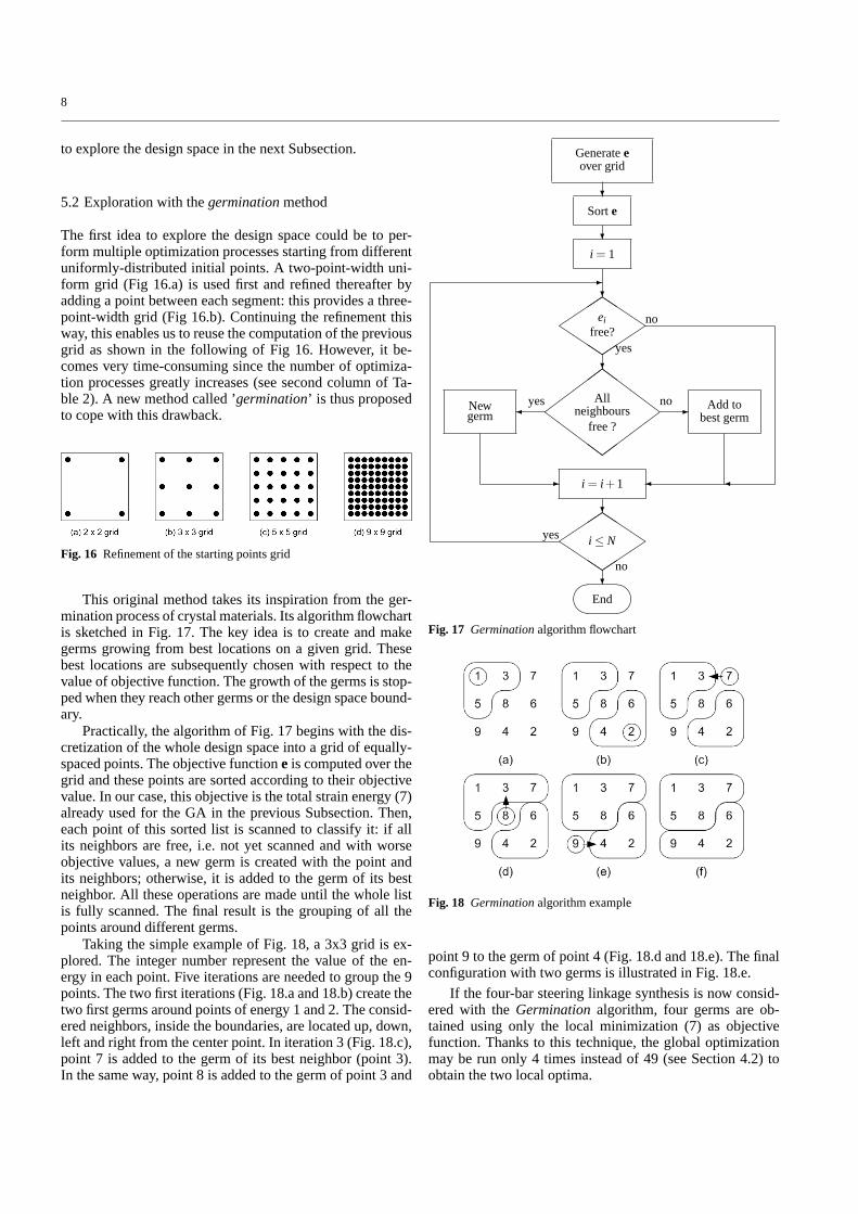
The first idea to explore the design space could be to per-form multiple optimization processes starting from differentuniformly-distributed initial points. A two-point-width uni-form grid (Fig 16.a) is used first and refined thereafter byadding a point between each segment: this provides a three-point-width grid (Fig 16.b). Continuing the refinement thisway, this enables us to reuse the computation of the previousgrid as shown in the following of Fig 16. However, it be-comes very time-consuming since the number of optimiza-tion processes greatly increases (see second column of Ta-ble 2). A new method called ’germination’ is thus proposedto cope with this drawback.

Fig. 16 Refinement of the starting points grid

This original method takes its inspiration from the ger-mination process of crystal materials. Its algorithm flowchartis sketched in Fig. 17. The key idea is to create and makegerms growing from best locations on a given grid. Thesebest locations are subsequently chosen with respect to thevalue of objective function. The growth of the germs is stop-ped when they reach other germs or the design space bound-ary.

Practically, the algorithm of Fig. 17 begins with the dis-cretization of the whole design space into a grid of equally-spaced points. The objective functione is computed over thegrid and these points are sorted according to their objectivevalue. In our case, this objective is the total strain energy (7)already used for the GA in the previous Subsection. Then,each point of this sorted list is scanned to classify it: if allits neighbors are free, i.e. not yet scanned and with worseobjective values, a new germ is created with the point andits neighbors; otherwise, it is added to the germ of its bestneighbor. All these operations are made until the whole listis fully scanned. The final result is the grouping of all thepoints around different germs.

Taking the simple example of Fig. 18, a 3x3 grid is ex-plored. The integer number represent the value of the en-ergy in each point. Five iterations are needed to group the 9points. The two first iterations (Fig. 18.a and 18.b) create thetwo first germs around points of energy 1 and 2. The consid-ered neighbors, inside the boundaries, are located up, down,left and right from the center point. In iteration 3 (Fig. 18.c),point 7 is added to the germ of its best neighbor (point 3).In the same way, point 8 is added to the germ of point 3 and

Generateeover grid

?Sorte

?i = 1

?

��

��

QQ

QQ�

���

QQ

QQei

free?no

yes?

��

���

ZZ

ZZZ

��

���

ZZ

ZZZ

Allneighbours

free ?

yes no

i = i +1

?

��

��

QQ

QQ�

���

QQ

QQ

i ≤ Nyes

no?�

���End

-

- Add tobest germ

�

�Newgerm

- �

Fig. 17 Germinationalgorithm flowchart

Fig. 18 Germinationalgorithm example

point 9 to the germ of point 4 (Fig. 18.d and 18.e). The finalconfiguration with two germs is illustrated in Fig. 18.e.

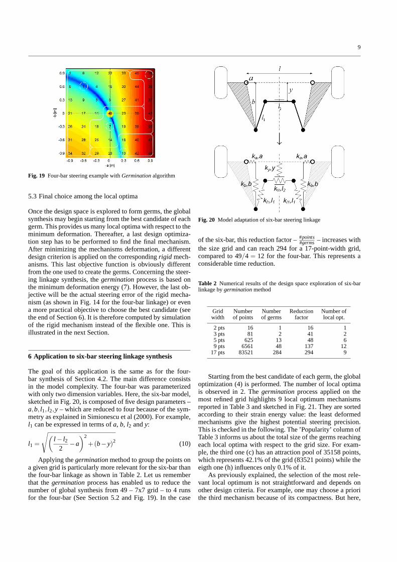
If the four-bar steering linkage synthesis is now consid-ered with theGerminationalgorithm, four germs are ob-tained using only the local minimization (7) as objectivefunction. Thanks to this technique, the global optimizationmay be run only 4 times instead of 49 (see Section 4.2) toobtain the two local optima.

9

Fig. 19 Four-bar steering example withGerminationalgorithm

5.3 Final choice among the local optima

Once the design space is explored to form germs, the globalsynthesis may begin starting from the best candidate of eachgerm. This provides us many local optima with respect to theminimum deformation. Thereafter, a last design optimiza-tion step has to be performed to find the final mechanism.After minimizing the mechanisms deformation, a differentdesign criterion is applied on the correspondingrigid mech-anisms. This last objective function is obviously differentfrom the one used to create the germs. Concerning the steer-ing linkage synthesis, thegerminationprocess is based onthe minimum deformation energy (7). However, the last ob-jective will be the actual steering error of the rigid mecha-nism (as shown in Fig. 14 for the four-bar linkage) or evena more practical objective to choose the best candidate (seethe end of Section 6). It is therefore computed by simulationof the rigid mechanism instead of the flexible one. This isillustrated in the next Section.

6 Application to six-bar steering linkage synthesis

The goal of this application is the same as for the four-bar synthesis of Section 4.2. The main difference consistsin the model complexity. The four-bar was parameterizedwith only two dimension variables. Here, the six-bar model,sketched in Fig. 20, is composed of five design parameters –a,b, l1, l2,y – which are reduced to four because of the sym-metry as explained in Simionescu et al (2000). For example,l1 can be expressed in terms ofa, b, l2 andy:

l1 =

√

(

l − l22

−a

)2

+(b−y)2 (10)

Applying thegerminationmethod to group the points ona given grid is particularly more relevant for the six-bar thanthe four-bar linkage as shown in Table 2. Let us rememberthat thegerminationprocess has enabled us to reduce thenumber of global synthesis from 49 – 7x7 grid – to 4 runsfor the four-bar (See Section 5.2 and Fig. 19). In the case

↓

Fig. 20 Model adaptation of six-bar steering linkage

of the six-bar, this reduction factor –#points#germs – increases with

the size grid and can reach 294 for a 17-point-width grid,compared to 49/4 = 12 for the four-bar. This represents aconsiderable time reduction.

Table 2 Numerical results of the design space exploration of six-barlinkage bygerminationmethod

Grid Number Number Reduction Number ofwidth of points of germs factor local opt.

2 pts 16 1 16 13 pts 81 2 41 25 pts 625 13 48 69 pts 6561 48 137 12

17 pts 83521 284 294 9

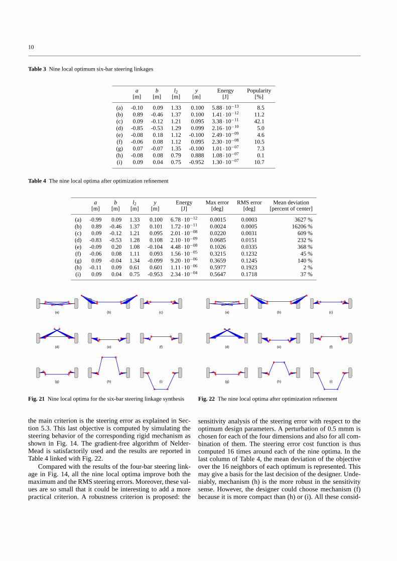
Starting from the best candidate of each germ, the globaloptimization (4) is performed. The number of local optimais observed in 2. Thegerminationprocess applied on themost refined grid highlights 9 local optimum mechanismsreported in Table 3 and sketched in Fig. 21. They are sortedaccording to their strain energy value: the least deformedmechanisms give the highest potential steering precision.This is checked in the following. The ’Popularity’ column ofTable 3 informs us about the total size of the germs reachingeach local optima with respect to the grid size. For exam-ple, the third one (c) has an attraction pool of 35158 points,which represents 42.1% of the grid (83521 points) while theeigth one (h) influences only 0.1% of it.

As previously explained, the selection of the most rele-vant local optimum is not straightforward and depends onother design criteria. For example, one may choose a priorithe third mechanism because of its compactness. But here,

10

Table 3 Nine local optimum six-bar steering linkages

a b l2 y Energy Popularity[m] [m] [m] [m] [J] [%]

(a) -0.10 0.09 1.33 0.100 5.88·10−13 8.5(b) 0.89 -0.46 1.37 0.100 1.41·10−12 11.2(c) 0.09 -0.12 1.21 0.095 3.38·10−11 42.1(d) -0.85 -0.53 1.29 0.099 2.16·10−10 5.0(e) -0.08 0.18 1.12 -0.100 2.49·10−09 4.6(f) -0.06 0.08 1.12 0.095 2.30·10−08 10.5(g) 0.07 -0.07 1.35 -0.100 1.01·10−07 7.3(h) -0.08 0.08 0.79 0.888 1.08·10−07 0.1(i) 0.09 0.04 0.75 -0.952 1.30·10−07 10.7

Table 4 The nine local optima after optimization refinement

a b l2 y Energy Max error RMS error Mean deviation[m] [m] [m] [m] [J] [deg] [deg] [percent of center]

(a) -0.99 0.09 1.33 0.100 6.78·10−12 0.0015 0.0003 3627 %(b) 0.89 -0.46 1.37 0.101 1.72·10−11 0.0024 0.0005 16206 %(c) 0.09 -0.12 1.21 0.095 2.01·10−08 0.0220 0.0031 609 %(d) -0.83 -0.53 1.28 0.108 2.10·10−09 0.0685 0.0151 232 %(e) -0.09 0.20 1.08 -0.104 4.48·10−08 0.1026 0.0335 368 %(f) -0.06 0.08 1.11 0.093 1.56·10−05 0.3215 0.1232 45 %(g) 0.09 -0.04 1.34 -0.099 9.20·10−06 0.3659 0.1245 140 %(h) -0.11 0.09 0.61 0.601 1.11·10−06 0.5977 0.1923 2 %(i) 0.09 0.04 0.75 -0.953 2.34·10−04 0.5647 0.1718 37 %

(a) (b) (c)

(d) (e) (f)

(g) (h) (i)

Fig. 21 Nine local optima for the six-bar steering linkage synthesis

the main criterion is the steering error as explained in Sec-tion 5.3. This last objective is computed by simulating thesteering behavior of the corresponding rigid mechanism asshown in Fig. 14. The gradient-free algorithm of Nelder-Mead is satisfactorily used and the results are reported inTable 4 linked with Fig. 22.

Compared with the results of the four-bar steering link-age in Fig. 14, all the nine local optima improve both themaximum and the RMS steering errors. Moreover, these val-ues are so small that it could be interesting to add a morepractical criterion. A robustness criterion is proposed: the

(a) (b) (c)

(d) (e) (f)

(g) (h) (i)

Fig. 22 The nine local optima after optimization refinement

sensitivity analysis of the steering error with respect to theoptimum design parameters. A perturbation of 0.5 mmm ischosen for each of the four dimensions and also for all com-bination of them. The steering error cost function is thuscomputed 16 times around each of the nine optima. In thelast column of Table 4, the mean deviation of the objectiveover the 16 neighbors of each optimum is represented. Thismay give a basis for the last decision of the designer. Unde-niably, mechanism (h) is the more robust in the sensitivitysense. However, the designer could choose mechanism (f)because it is more compact than (h) or (i). All these consid-

11

erations obviously depend on the way each criterion is takeninto account by the designer.

7 Conclusion and prospects

Based on a strain energy approach of flexible mechanismscoupled with the use of natural coordinates, an original opti-mization method has been developed to solve path synthesisand function generation problems of planar mechanisms. Di-vided into two stages, the first proposed method alternativelytries to minimize the total deformation energy with respectto the point coordinates and updates the natural lengths ofthe springs accordingly. This method has then been extendedto a global synthesis approach. It has seemed to be more effi-cient but still not global as it was illustrated via the four-barsteering linkage application.

Following that observation, the question of finding theglobal optimum has been discussed. Genetic algorithms op-timizations have been shown to also miss the global opti-mum mechanism. This question has thus been reviewed andextended with the exploration of the design space to find themost of local optima. To avoid ’astronomical’ CPU time, asimple method inspired from crystals germination has beenproposed to divide the design space into germs centered onlocal optima. Starting from the latter, the optimization hasbeen refined and a last criterion applied to choose the finalmechanism.

In terms of prospects, our effort will concentrate on de-veloping other exploration strategies of the design space.The comparison of these different strategies and their resultswill be useful to validate them. It could be also interesting toclassify the different local optima based on different typesof criterion. We also intend to extend the method furtherto topologies with prismatic joints or to three-dimensionalmechanisms. Extending the application field is also an inter-esting prospect: other kinematic objectives instead of pathorfunction-generator synthesis or even dynamical ones couldbe investigated. The more challenging issue of topology op-timization of mechanisms could be tackled on the basis ofthis work, involving for example an additional higher-leveloptimization process as proposed by Sedlaczek et al (2005).

Acknowledgements This research has been sponsored by the BelgianProgram on Interuniversity Attraction Poles,Advanced MechatronicSystems - AMS(IUAP5/06), initiated by the Belgian State — PrimeMinister’s Office — Science Policy Programming (IUAP V/6). Thescientific responsibility is assumed by its authors.

References

Alba J, Doblare M, Gracia L (2000) A simple method for the synthesisof 2D and 3D mechanisms with kinematic constraints. Mechanismand Machine Theory 35:645–674

Cabrera J, Simon A, Prado M (2002) Optimal synthesis of mecha-nisms with genetic algorithms. Mechanism and Machine Theory37:1165–1177

Collard JF, Fisette P, Duysinx P (2005a) Contribution to theoptimiza-tion of closed-loop multibody systems: Application to parallel ma-nipulators. Multibody System Dynamics 13:69–84

Collard JF, Fisette P, Duysinx P (2005b) Optimal synthesis of mecha-nisms using time-varying dimensions and natural coordinates. In:Proc. of the Sixth World Congress of Structural and Multidisci-plinary Optimization

Hansen JM (2002) Synthesis of mechanisms using time-varying di-mensions. Multibody System Dynamics 7:127–144

Jensen OF, Hansen JM (2003) Treating the problem of non-assemblyfor dimensional synthesis of spatial mechanisms. In: Ziegler S&(ed) The Fifth World Congress of Structural and MultidisciplinaryOptimization, ISSMO, Italian Polytechnic Press, pp 431–432

Jimenez JM, Alvarez G, Cardenal J, Cuadrado J (1997) A simple andgeneral method for kinematic synthesis of spatial mechanisms.Mechanism and Machine Theory 32(3):323–341

Laribi M, Mlika A, Romdhane L, Zeghloul S (2004) A combined ge-netic algorithm-fuzzy logic method GA-FL in mechanisms syn-thesis. Mechanism and Machine Theory 39:717–735

Lio MD, Cossalter V, Lot R (2000) On the use of natural coordinates inoptimal synthesis of mechanisms. Mechanism and Machine The-ory 35:1367–1389

Mariappan J, Krishnamurty S (1996) A generalized exact gradientmethod for mechanism synthesis. Mechanism and Machine The-ory 31(2):413–421

Marın FTS, Gonzalez AP (2003) Global optimization in path synthesisbased on design space reduction. Mechanism and Machine Theory38:579–594

Powell M (1970) Nonlinear Programming, Academic Press, chap Anew algorithm for unconstrained optimization

Pramanik S (2002) Kinematic synthesis of a six-member mechanismfor automotive steering. ASME Journal of Mechanical Design124:642–645

Sancibrian R, Viadero F, Garcıa P, Fernandez A (2004) Gradient-basedoptimization of path synthesis problems in planar mechanisms.Mechanism and Machine Theory 39:839–856

Sedlaczek K, Gaugele T, Eberhard P (2005) Topology optimized syn-thesis of planar kinematic rigid body mechanisms. In: Proc.of theMultibody Dynamics 2005, Eccomas Thematic Conference

Shiakolas P, Koladiya D, Kebrle J (2005) On the optimum synthesis ofsix-bar linkages using differential evolution and the geometric cen-troid of precision positions technique. Mechanism and MachineTheory 40:319–335

Simionescu P, Beale D (2002) Optimum synthesis of the four-bar func-tion generator in its symmetric embodiment: the ackermann steer-ing linkage. Mechanism and Machine Theory 37:1487–1504

Simionescu P, Smith M, Tempea I (2000) Synthesis and analysis of thetwo loop translational input steering mechanism. Mechanism andMachine Theory 35:927–943

Vallejo J, aviles R, Hernandez A, Amezua E (1995) Nonlinear opti-mization of planar linkages for kinematic syntheses. Mechanismand Machine Theory 30(4):501–518

Zhou H, Cheung EH (2001) Optimal synthesis of crank-rocker link-ages for path generation using the orientation structural error ofthe fixed link. Mechanism and Machine Theory 36:973–982