Energy: higher dimensions

October 2, 2015

The concepts of potential energy and conservationof energy are formulated in n dimensions. Theevaluation of the force from the potential energyleads to the gradient operator.

Contents

1 Potential energy 1

1.1 Definition . . . . . . . . . . . . . . . 1

1.2 Examples . . . . . . . . . . . . . . . 1

2 Force from PE 2

2.1 Force components in terms of partialderivatives . . . . . . . . . . . . . . . 2

2.2 Gradient operator . . . . . . . . . . 3

2.3 Curl of gradient is zero . . . . . . . . 3

3 Equipotential surface 3

3.1 Definition . . . . . . . . . . . . . . . 3

3.2 Properties . . . . . . . . . . . . . . . 3

4 Conservation of energy 4

4.1 Work and KE . . . . . . . . . . . . . 4

4.2 Work and PE . . . . . . . . . . . . . 5

1 Potential energy

1.1 Definition

This module restricts attention to forces that areconservative. If in doubt, check that (see last mod-ule)

(curl ~F )ij = 0 (1)

Thus, the work done by the force in going from areference point O (taken to be fixed and often not

indicated explicitly) to a point ~r depends only on ~rand not on the path γ(O,~r) linking the two points:

W (γ(O,~r)) = W (~r)∫γ(O,~r)

~F · d~r =

∫ ~r

O

~F · d~r (2)

Thus we are able to define the PE as a functionof the final position ~r:

U(~r) = −∫ ~r

O

~F · d~r (3)

Refer to the 1D case for the minus sign: U increasesin the direction opposite to that of ~F . In the case ofgravity, U increases upwards, so it can be thoughtof heuristically as a “height”.

1.2 Examples

Example 1Suppose the force is an anisotropic harmonic oscil-lator

~F = − (k1x i + k2y j + k3z k) (4)

First check that it is conservative, e.g.,

(curl ~F )xy =∂Fy∂x− ∂Fx

∂y

=∂(k2y)

∂x− ∂(k1x)

∂y= 0 (5)

Thus we can calculate the PE as follows, usingthe origin as the reference

U(x, y, z) = −∫ (x,y,z)

0

~F · d~r

=

∫ (x,y,z)

0

(k1x dx+ k2y dy + k3z dz)

=1

2

(k1x

2 + k2y2 + k3z

2)

(6)

1

Be careful with the evaluation. If we had encoun-tered a term such as

∫y dx, we would have to ask:

“Which path?”, because the path determines howy depends on x. This does not happen here — amatter of luck in a special case. §

Example 2Find U(~r) corresponding to the central force

~F (~r) =k

r2er (7)

where er = ~r/r is the unit radial vector. This de-scribes a repulsive inverse-square force if k > 0 (asbetween two like charges) or an attractive inverse-square force if k < 0 (as between two unlikecharges, or gravity between two masses).

Let ~r be described by polar coordinates (r, θ, φ).Choose the reference point at infinity. Choose thepath along a radius so that θ and φ are constanton the path and

d~r = dr er (8)

You may say: The path goes from infinity to r;shouldn’t there be a minus sign in (8)? No. Thesign will take care of itself, because dr is negativeonce the limits of integration are specified (lowerlimit > upper limit). Thus

U(~r) = −∫ ~r

∞~F · d~r

= −∫ ~r

∞~F · er dr = −

∫ r

∞

k

r2dr

=k

r

∣∣∣∣r∞

=k

r(9)

In the second line we have evaluated ~F ·er and thisis the only component that matters since the pathis chosen to be radial. §

2 Force from PE

2.1 Force components in terms ofpartial derivatives

The last Section has given U(~r) as an integral of ~F(see (3)). This Section asks the reverse question:

How do we find ~F if U(~r) is given? The formal-ism here is just the fundamental theorem of vectorcalculus placed in a particular physical context.

Recall the corresponding derivation in the case of1D: we compare the PE at two neighbouring pointsx and x+∆x. But now we can choose a pair ofneighbouring points three ways, being separated ineither the x, y or z direction.

Figure 1 illustrates, on the x–y plane (i.e., zsuppressed), how a point A = (x, y, z) can be com-pared to B = (x+∆x, y, z) or to C = (x, y+∆y, z).Taking the first case

U(x+∆x, y, z)− U(x, y, z)

= U(B)− U(A)

= −

(∫ B

O

~F · d~r −∫ A

O

~F · d~r

)

= −∫ B

A

~F · d~r = − ~F ·∆~r (10)

In the last step the line integral over a short in-terval is just a simple product, and ~F is evaluatedat any point in the interval, say A. Since for thiscomparison, ∆~r = ∆x i, the dot product gives

~F ·∆~r = Fx ∆x (11)

Putting this into (10) and re-arranging terms, wehave

Fx(x, y, z)

= − U(x+∆x, y, z)− U(x, y, z)

∆x

= − ∂U

∂x(12)

In the last step, upon taking the implied limit of∆x→ 0, we get a partial derivative because y andz are held fixed. Generalizing to the other compo-nents, we have

Fi = − ∂i U (13)

where ∂i = ∂/∂ri and ri is any one of the Cartesiancomponents of ~r. This is an obvious generalizationof the formula for 1D:

F (x) = − dU(x)

dx(14)

The same argument can be phrased without us-ing integrals:

U(B)− U(A)

= − [W (O→B)−W (O→A)]

= −W (A→B) = − ~F ·∆~r (15)

2

with the subsequent steps the same as before.

Problem 1For every example of U(~r) discussed in the last Sec-tion, do the reverse calculation and find the force.§

2.2 Gradient operator

Putting the three components together, we have

~F = Fx i + Fy j + Fzk

= −(∂U

∂xi +

∂U

∂yj +

∂U

∂xk

)= −

(i∂

∂x+ j

∂

∂y+ k

∂

∂z

)U (16)

In the last line above, we have put the basis vec-tors in front simply to stress that the differentiationdoes not affect them.

We are thus led to define the gradient operator

grad = ~∇ ≡ i∂

∂x+ j

∂

∂y+ k

∂

∂z(17)

in terms of which

~F = − ~∇U (18)

The symbols grad and ~∇ are used interchangeably.All these formulas have the obvious generaliza-

tion to n dimensions, with coordinates ri and basisvectors ei, so that

grad = ~∇ ≡ ei∂

∂ri(19)

with summation over repeated indices understood.Incidentally, the gradient is a vector operator : it

is an operator because it turns one function intoanother; it is a vector because it has three (or ingeneral n) Cartesian components.1

SummaryThe relationship between ~F and U can be summa-rized as

~Fline int−→ − U , U

gradient−→ − ~F (20)

This constitutes an example of the fundamentaltheorem of vector calculus: that the gradient is theinverse of the line integral.

1A more proper characterization is that it has the righttransformation properties to be a vector.

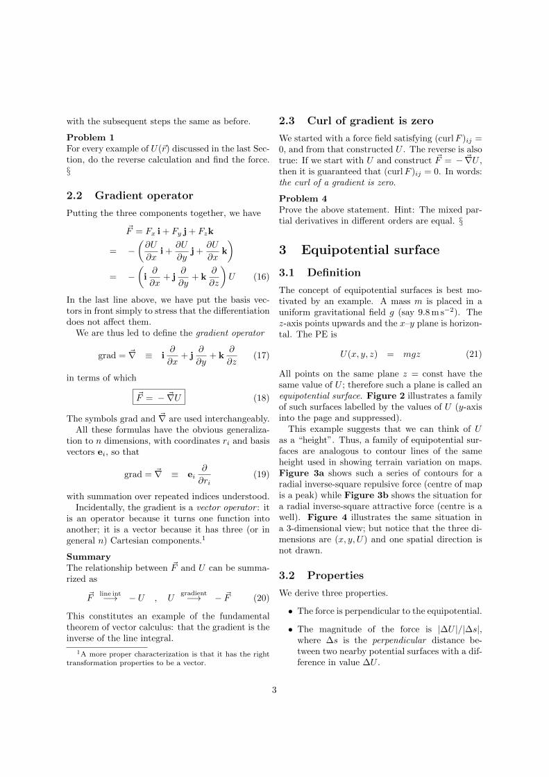
2.3 Curl of gradient is zero

We started with a force field satisfying (curlF )ij =0, and from that constructed U . The reverse is alsotrue: If we start with U and construct ~F = − ~∇U ,then it is guaranteed that (curlF )ij = 0. In words:the curl of a gradient is zero.

Problem 4Prove the above statement. Hint: The mixed par-tial derivatives in different orders are equal. §

3 Equipotential surface

3.1 Definition

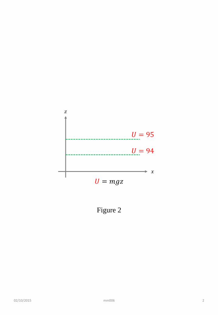
The concept of equipotential surfaces is best mo-tivated by an example. A mass m is placed in auniform gravitational field g (say 9.8 m s−2). Thez-axis points upwards and the x–y plane is horizon-tal. The PE is

U(x, y, z) = mgz (21)

All points on the same plane z = const have thesame value of U ; therefore such a plane is called anequipotential surface. Figure 2 illustrates a familyof such surfaces labelled by the values of U (y-axisinto the page and suppressed).

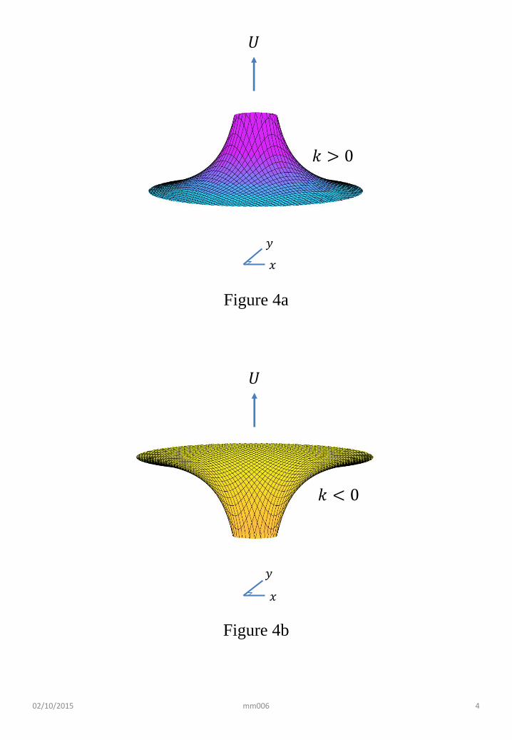
This example suggests that we can think of Uas a “height”. Thus, a family of equipotential sur-faces are analogous to contour lines of the sameheight used in showing terrain variation on maps.Figure 3a shows such a series of contours for aradial inverse-square repulsive force (centre of mapis a peak) while Figure 3b shows the situation fora radial inverse-square attractive force (centre is awell). Figure 4 illustrates the same situation ina 3-dimensional view; but notice that the three di-mensions are (x, y, U) and one spatial direction isnot drawn.

3.2 Properties

We derive three properties.

• The force is perpendicular to the equipotential.

• The magnitude of the force is |∆U |/|∆s|,where ∆s is the perpendicular distance be-tween two nearby potential surfaces with a dif-ference in value ∆U .

3

• The force points from the surface of higher Uto the surface with lower U .

These rules allow us to understand the pattern ofthe force field given a picture of the equipotentialsurfaces. The three properties are derived below.

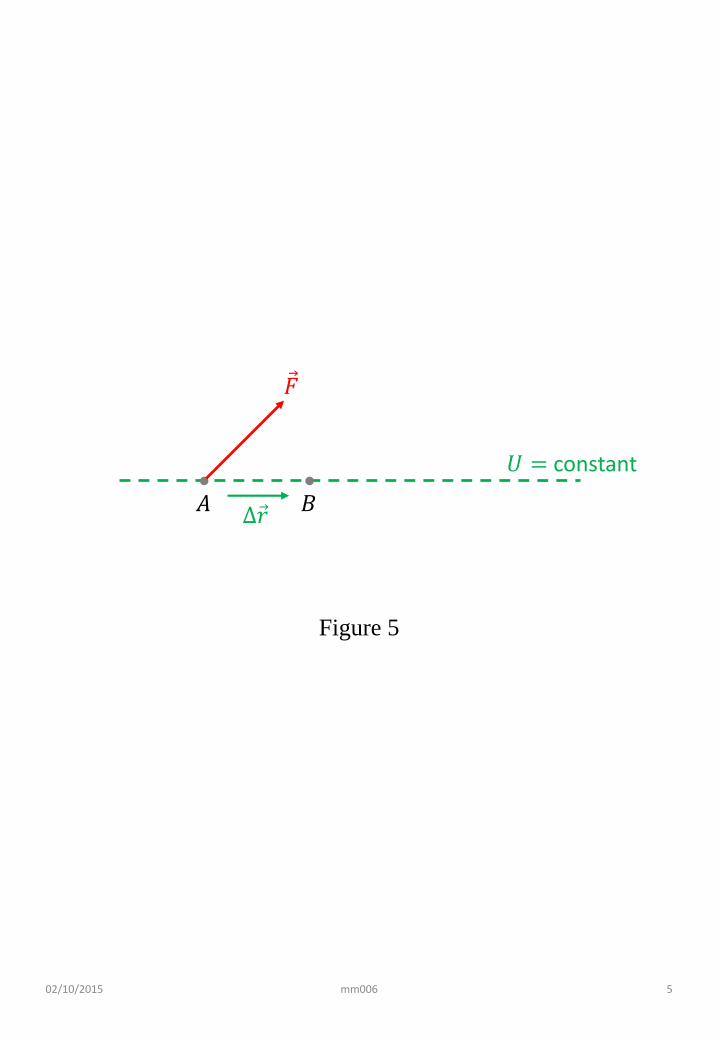
Force is perpendicular to equipotentialFigure 5 shows, schematically, an equipotential(dotted line). Because we consider only a smallportion of such a surface, the surface can be re-graded as flat. Let A, B be two neigbouring pointson the surface with separation ∆~r, and let ~F bethe force, for the moment assumed to be at an ar-bitrary direction. The difference in PE between thetwo points is

0 = ∆U = U(B)− U(A)

= ~F ·∆~r (22)

Thus we conclude ~F and ∆~r are perpendicular; andthis holds for any ∆~r lying along the equipotentialsurface. Thus, the force is perpendicular to theequipotential surface.

Force is change of U per perpendicular dis-tanceFigure 6 shows two nearby equipotential surfaces,with PE values U and U + ∆U . The point A lieson one surface, and C on the other, with AC per-pendicular to the surfaces, and having a length ∆s.Now

∆U = UC − UA = − ~F ·∆~r (23)

But ~F is along the same direction as ∆~r = AC, so

|~F ·∆~r| = F |∆~r| = F ∆s (24)

thus giving for the magnitude

F =|∆U ||∆s|

(25)

The third property is obvious.

4 Conservation of energy

The laws in this Section can be separated into twolevels:

• The relationship between work and kinetic en-ergy (KE), valid for all forces.

• The conservation of energy relating KE andPE, applicable only to conservative forces.

In both cases the derivation is a simple generaliza-tion of the 1D case.

4.1 Work and KE

Here we prove that the work done by the net forceacting on an object is equal to the increase in theKE.

Constant forceFirst consider a constant net force ~F . A mass mmoves a distance ∆~r in a time ∆t, with initial ve-locity ~v1 and final velocity ~v2. Using the averagevelocity ~V

∆~r = ~V ∆t =1

2(~v2 + ~v1) ∆t (26)

while Newton’s second law gives

~F = m~a = m~v2 − ~v1

∆t(27)

Taking the dot product of (26) and (27) eliminates∆t:

~F ·∆~r =1

2m(~v2 + ~v1) · (~v2 − ~v1)

=

(1

2mv22

)−(

1

2mv21

)(28)

Note v2i = ~vi · ~vi. Define kinetic energy (KE) K inthe usual way

K =1

2mv2 (29)

and we get

W (1→ 2) = K2 −K1 (30)

The above derivation has used the formulas forconstant acceleration, and is therefore valid (only)for a constant force.

General forceFor a general (non-constant) force, chop the motioninto short segments, in each of which the force canbe regarded as constant. Let us illustrate with twosegments:

W (1→ 3) = W (1→ 2) +W (2→ 3)

= (K2 −K1) + (K3 −K2)

= K3 −K1 (31)

4

In the above, the first equal sign relies on the ad-ditive property of W ; the second equal sign relieson (30) for a short segment in which the force isconstant. With the last equal sign, all referenceto the intermediate situation cancels, and the RHSdepends only on the initial and final states of mo-tion. It is obvious how this argument generalizesto more segments.

The following derivation may look simpler, butis exactly the same idea expressed in another lan-guage.

W (i→ f) =

∫ f

i

~F · d~r =

∫ f

i

d

dt(m~v) · (~v dt)

=

∫ f

i

d

dt

(1

2mv2

)· dt

=1

2mv2

∣∣∣∣fi

= Kf −Ki (32)

In the above, the motion is between an initial timei and a final time f . We have used the identity

d

dt

(1

2mv2

)=m

2

d

dt(~v · ~v)

= m~v · d~vdt

(33)

In doing the integral, we have cancelled dt in

d

dt(. . .) dt = (. . .) (34)

which can be regarded as the fundamental theoremof calculus (integration and differentiation are in-verse operations); it is also the analog of cancelling∆t in deriving (28).

4.2 Work and PE

First suppose there is only one force ~F , which isconservative and associated with potential energyU . Then

W (i→ f) =

∫ f

i

~F · d~r

=

∫ f

O

~F · d~r −∫ i

O

~F · d~r = − (Uf − Ui)

(35)

The minus sign comes from the definition of U .Combining (32) with (35) then gives

Kf −Ki = − (Uf − Ui)Ki + Ui = Kf + Uf (36)

In other words the total energy

E = K + U (37)

is the same at the initial and final times: energy isconserved.

If there are several conservative forces, the abovestill holds for F being the net force and U beingthe total PE, which can be expressed as the sum ofPEs due to each force — here relying on the factthat W is additive.

Thus we get the second statement: If the forcesare conservative, then total energy E is conserved.

5

02/10/2015 mm006 1

𝑦

𝑥

Δ 𝑟

Figure 1

𝐶

𝐴 𝐵

02/10/2015 mm006 2

𝑧

𝑥

𝑈 = 95

𝑈 = 94

𝑈 = 𝑚𝑔𝑧

Figure 2

02/10/2015 mm006 3

𝑈 = 4

𝑈 = 3

𝑘 > 0

𝑈 = −3

𝑈 = −4

𝑘 < 0

Figure 3a

Figure 3b

02/10/2015 mm006 4

𝑈

𝑦

𝑥

𝑘 < 0

𝑦

𝑥

𝑈

𝑘 > 0

Figure 4a

Figure 4b

02/10/2015 mm006 5

𝑈 = constant

𝐴 𝐵

𝐹

Δ 𝑟

Figure 5

02/10/2015 mm006 6

𝑈𝐴

𝐶

𝐹

𝑈 + Δ𝑈

Δ𝑠Δ 𝑟

Figure 6