Optimal Production and Admission Policies in Make-to-Stock ...

Optimal Production and Admission Policies in

Make-to-Stock/Make-to-Order Manufacturing Systems

June 8, 2009

Seyed Iravani1, Tieming Liu2, David Simchi-Levi3

Abstract

In this paper, we address production and admission control policies in manufacturing systems thatproduce two types of products. One type consists of identical items that are produced to stock, while theother has varying features and is produced to order. This general version is motivated by applicationsfrom various industries, in particular, the automobile industry and PC industry. Two models are studied.In the first model, the make-to-stock product has higher priority than the make-to-order product, andin the second model the manufacturer gives higher priority to the make-to-order product over the make-to-stock product. We characterize the optimal production and admission policies with simple structures,and using a computational analysis, we provide insights into the benefits of the new policies. We alsoinvestigate the impact of production capacity, cost structure, demand structure, and variabilities indemand and production process on system performance.

1 Introduction

In recent years, many retail and manufacturing companies have started exploring innovative revenue man-

agement techniques in an effort to improve their operations and ultimately the bottom line. Manufacturing

systems that can produce different types of products have raised more research interest in recent years as

many firms begin to practice market segmentation by providing multiple types of products to customers,

and then differentiating customers according to their choices.

Customized production is a strong trend in the manufacturing industry. For example, in the computer

industry, many companies allow customers to configure their products, and companies use the make-to-order

(MTO) mode to manage the production. The MTO production not only gives more satisfaction to cus-

tomers, but it also helps manufacturers eliminate finished goods inventory. However, the MTO environment

suggests important challenges associated with matching fixed production capacity with highly variable de-

mand. Specifically, an MTO system implies periods where the facility is idle and other times in which a

large number of orders are awaiting production.

A good example of companies that aggressively use both customized production and customized pricing

strategies is Dell Computers. Dell provides very high flexibility in configurations for customers who are

willing to pay high prices. At the same time, Dell also frequently provides promotions for some low-end

products to attract more customers, and for these products, customers usually have very little flexibility on1Department of Industrial Engineering and Management Science, Northwestern University.2School of Industrial Engineering and Management, Oklahoma State University.3Department of Civil and Environmental Engineering and Engineering Systems Division, MIT.

1

configurations. To satisfy these demands, Dell also produces some standard products to stock, the make-to-

stock (MTS) environment. This gives raise to a combination of a make-to-stock/make-to-order environment

that allows Dell to better manage their production capacity and increase expected profit.

The application of make-to-stock/make-to-order manufacturing systems is also important among part

suppliers who face demands from both original equipment manufacturers (OEMs) and the so-called after-

market. For example, in the automobile industry, a part supplier sells its products to automotive assembly

plants for installation into new vehicles, as well as repair shops for replacement in old vehicles (Carr and

Duenyas [3]). OEM and aftermarket demands are both important to the part supplier. OEM demands

guarantee high utilization of the production capacity, while aftermarket demands bring high profit margins

to the supplier. OEM sales are based on long-term contracts, and they are produced under the make-to-stock

mode. In contrast, aftermarket items are produced under the make-to-order mode due to their large variety.

Note that, as opposed to the Dell example, in this case the high priority products are produced to stock.

All these developments call for models that integrate production, sequencing and admission decisions for a

hybrid production system with both make-to-stock and make-to-order products.

There is a significant amount of literature addressing multi-product production scheduling problems

in either a make-to-stock or a make-to-order manufacturing system. Problems with or without set-ups

associated with switching from producing one product to another have both been extensively studied. We

refer the reader to Graves [12], Zheng and Zipkin [40], Pena-Perez and Zipkin [28], Wein [38], Ha [17], and De

Vericourt et al. [6] for scheduling policies in make-to-stock environments, and to Varaiya et al. [36], Gittins

[10], Duenyas and Van Oyen [9], Reiman and Wein [31] and the references therein for scheduling policies in

make-to-order environments.

Single-product models with multi-class customers in a make-to-stock manufacturing system, the so-called

stock rationing problems, have been studied in various contexts since the late 1960’s. Some of the examples

of stock rationing in uncapacitated systems are Topkis [35], Nahmias and Demmy [26], Cohen et al. [5],

and Melchiors et al. [23]. For stock rationing in capacitated systems see Ha [15, 16, 18], de Vericourt et al.

[7], and Huang and Iravani [19], Iravani et al. [21, 20], Benjaafar et al. [1]. Extensive reviews for the stock

rationing problems can be found in Kleijn and Dekker [22].

All the papers above focused on the dynamic production and sequencing problems for either make-to-order

systems or make-to-stock systems; however, none of them considered a hybrid manufacturing system, and

admission control was rarely studied. Carr and Duenyas [3] considered both the production and admission

decisions for a make-to-stock/make-to-order system, where the make-to-stock orders have higher priorities.

They found an optimal policy characterized by monotonic switching curves. Gupta and Wang [13] study

2

a MTS/MTO problem in a periodic-review model with stochastic demands and deterministic production

capacities. Leadtime is quoted in their model. Due to the complexity and the large state space, they

focused on the case with the leadtime of one period, and they developed a three-dimensional lookup table

to find the optimal decisions. For models with longer leadtimes, they acknowledge that “even if one could

compute and store look-up tables, the implementation of the resulting policy can be problematic.” Dobson

and Yano [8] consider product offering, pricing, and MTO and MTS decisions with linear deterministic

demand functions in strategic levels, while production and admission controls are not their focus. Youssef,

van Delft, and Dallery [39] examine the manufacturing scheduling problem in an MTS/MTO system under

two static policies: the classical FIFO rule and a priority policy. In the latter, preemptive priority is given

to low volume (make-to-order) products, and approximations are used to obtain analytical and numerical

results. They consider the base-stock threshold, but rationing, admission, and contingent outsourcing are

not their focus.

In the literature on inventory systems (including the above papers, except for [3, 13]), it is commonly

assumed that unsatisfied demands are either fully backordered or lost. A relatively small amount of papers

considered partial backordering, where in case of shortage, arriving customers may be either backordered

or lost, each with a certain probability that is an outcome of the customer behavior (see Montgomery [25],

Moinzadeh [24], Smeitink [33], and Nahmias and Smith [27]). In a few recent papers, partial backordering

became part of the seller’s decision. The seller determines the amount of unsatisfied demands to be back-

ordered or rejected (see Rabinowitz [32], Benjaafar et. al. [1], and Chen and Kulkarni [4]). However, the

admission decision increases the complexity of the model, and the current optimal policies in the literature

are characterized by state-dependent non-linear switching curves. The complexity of the non-linear structure

makes the optimal policies difficult to implement in the real world.

In this paper, we study policies to coordinate production, sequencing and admission controls for two

types of manufacturing systems both with make-to-stock products and make-to-order products. Our paper

is related to Carr and Duenyas [3], but it is different from [3] in the following sense: (i) Our paper studies

two types of manufacturing systems: in the first case, MTS product has higher priority than MTO product,

and in the second case, MTS product has lower priority; While Carr and Duenyas only studied the first case.

(ii) In our paper, unsatisfied high-priority demands are fully backlogged; while in [3], when the high-priority

product is out of stock, the demand is lost. Our backlogging assumption is reasonable since it is often

difficult to find a product matching all the required features from other suppliers immediately. (iii) In our

paper, the optimal policies are characterized by a linear or near-linear structure, while in [3], the threshold

levels do not have such a simple structure. (iv) We also examine the possibility of outsourcing in our model,

3

which is not considered in [3].

In the first model of this paper, we consider a manufacturing system with both high-priority MTS (e.g.,

OEM) and low-priority MTO (e.g., aftermarket) demands. High-priority customers order identical items

from the manufacturer, and these orders cannot be rejected. If the product is out of stock, high-priority

orders will still be accepted and backlogging cost will be incurred until they are satisfied. Demands for

low-priority, customized products can be rejected if the manufacturer does not have enough production

capacity, or otherwise accepted. We characterize the structure of the optimal production and admission

control policies with a near-linear structure, and we extend our results for the case where the manufacturer

can outsource low-priority orders.

In the second model, we examine the production and admission controls in a manufacturing system with

high-priority MTO (customized) and low-priority MTS (pre-configured) products. MTO products provide

high configuration flexibilities to customers, and thus are sold at higher prices, and MTS products are sold

at lower prices for promotion. Demands for high-priority MTO products will all be accepted, while demands

for low-priority MTS products could be satisfied, backlogged, or rejected. We characterize the optimal policy

with linear threshold levels. We also extend our results to systems in which the low-priority MTS orders can

be outsourced.

The paper is organized as follows. In Section 2, we study the model with both OEM and aftermarket

demands, and we extend it to cases in which the manufacturer has the option of outsourcing the aftermarket

orders, as well as to cases with multiple types of aftermarket products. In Section 3, we investigate the

model with both customized and pre-configured products, and extend the results to systems with outsourcing

option for pre-configured products. In Section 4, we use computational analysis to obtain insights into the

benefits of the new policies, and the impact of production capacity, demand structure and price structure

on system performance. In Section 5, we study the effects of variability in demand and production process

using a system with Erlang distributed demand interarrival and production times. Finally in Section 6, we

summarize and suggest future research directions.

2 Model with OEM and Aftermarket Products

2.1 Problem Formulation

We consider a manufacturing system with two types of products in an infinite horizon. Type 1 is for high-

priority orders and has standard configuration, so it is produced to stock. Demands for type 1 are satisfied if

inventory is available, or are fully backlogged with high backlogging cost b1 per item per unit time if type 1 is

4

not available in inventory. Type 2 has varying features and is produced to order. Demands for type 2 can be

either accepted or rejected. As in literature on MTO systems (see [3] and [39]), we consider backlogging cost

b2 per unit time for accepted orders of type 2. Backlogging cost serves as a proxy for the manufacturer’s cost

due to having delays in production of type 2 orders and thus becoming uncompetitive in that market, loss of

good will, as well as extra shipping and handling cost due to the tardiness. As in literature on MTO systems

(see [3] and [39]), we assume that the backlogging cost for the MTO product is charged since the order is

accepted.4 We assume b2 < b1, since suppliers usually have long-term contracts with OEMs, and delayed

fulfillments are heavily penalized. If a demand for type 2 is rejected, a rejection penalty, r2, associated with

lost sales and loss of goodwill, is incurred. The contribution margin for product i is pi, and the inventory

holding cost for product 1 is h per unit time.

We assume that customers for each type of product arrive according to a Poisson Process, and we let λi

be the demand arrival rate of Class i, for i = 1, 2. Also, we assume that the production time of each type

of product follows the same exponential distribution, with production rate µ. The same-production-time

assumption is reasonable if the production process is mainly assembly operations, where the time difference

between assembling a standard product (e.g., a Dell Inspiron 700m with a 1G memory chip) and assembling a

customized product (e.g., a Dell Inspiron 700m with a 2G memory chip) is insignificant. In Section 5, we relax

this assumption and study systems with different production rates. We further assume that preemptions are

allowed, and no set-up time is needed when the manufacturing system switches from one type of job to the

other. This assumption is also reasonable for assembly production systems where setup times are negligible

compared to production times.

The assumption of Poisson arrival demand and exponential production times is what allows us to formu-

late the problem and characterize the structure of the optimal policy. In Section 5, we extend our analysis

to Erlang distributed interarrival and production times and examine the impact of variability in demand

and production process on system performance. We show that most of the insights we obtained with our

exponential model are not influenced by the assumption on demand and production processes.

Since the system cost (e.g., backlogging or holding cost) is the same for the same type of product, it is

clear that there is no need for rationing among orders for the same type of product. Therefore, the system

state can be described by a vector of two variables, y(t) = (y1(t), y2(t)), where yi(t) is the net inventory

level of product i at time t, with y1(t) ∈ Z and y2(t) ∈ Z−, where Z is the set of all positive and negative

integer numbers, while Z− only includes non-positive integer numbers. We use y+1 (t) = max0, y1(t) to

4Another case is when the backlogging penalties are incurred only when orders spend more than a predetermined length oftime. The analysis of this case is very complex, since in addition to the number of orders in the system, the state of the systemshould also include how many time periods each order has spent in the system.

5

show the amount of inventory of type 1 at time t, and y−1 (t) = max0,−y1(t) to show the number of

waiting customers at time t. Similarly, −y2(t) is the number of waiting customers for product 2 at time t.

The system state space is Ω = Z × Z−.

In state y = (y1, y2), the system incurs a cost at rate,

c(y) = −hy+1 − b1y

−1 + b2y2.

Let α be the time discount rate, let Nai (t) be the number of accepted orders over interval [0, t] for product

i (i = 1, 2), and let Nr2 (t) be the number of rejected orders for type 2 over the same period of time. We seek

an optimal control policy π so as to maximize either the discounted system profit over an infinite horizon,

maxπ

Jπ(y(0)) = Eπy(0)

[2∑i=1

∫ ∞0

e−αtpidNai (t)−

∫ ∞0

e−αtr2dNr2 (t) +

∫ ∞0

e−αtc(y(t))dt

], (1)

or the average profit over an infinite horizon,

maxπ

Jπa = limT→∞

1T

Eπ[

2∑i=1

piNai (T )− r2Nr

2 (T ) +∫ T

0

c(y(t))dt

]. (2)

In (1), Jπ(y(0)) is the expected profit function under policy π starting from initial state y(0) = (y1(0), y2(0)).

In the rest of the paper we will mainly focus on the discount-profit problem. However, as shown in de

Vericourt, Karaesmen and Dallery [7], the theoretical results for the discounted-profit model also apply to

the average-profit problem.

Without loss of generality, we redefine the time scale such that α + µ + λ1 + λ2 = 1. According to

Bertsekas [2], the optimality equation J∗(y1, y2) under the time-discount criterion satisfies the following

Bellman’s equation:

J(y1, y2) = c(y1, y2) + µH0J(y1, y2) + λ1H1J(y1, y2) + λ2H2J(y1, y2) := HJ(y1, y2) (3)

where H0, H1, and H2 are functions defined by,

H0J(y1, y2) = maxJ(y1, y2), J(y1 + 1, y2), J(y1, y2 + 1|y2 < 0)

H1J(y1, y2) = J(y1 − 1, y2) + p1

H2J(y1, y2) = maxJ(y1, y2 − 1) + p2, J(y1, y2)− r2

.

H0 corresponds to the production decision: the manufacturer can choose to either produce or stop

production. J( T | C ) is a conditional value function, which indicates that the transition to state T is only

a valid option when condition C holds. Therefore, the third term means producing product 2 when there

are backorders for it. H1 indicates that the demands for type 1 will always be accepted. H2 is associated

6

with the admission control for an arriving order for type 2. The manufacturer can either accept (backlog)

or reject the order. We denote the overall Bellman function as HJ(y1, y2).

The optimality equation under the average-profit criterion is:

J(y1, y2) + g = c(y1, y2) + µH0J(y1, y2) + λ1H1J(y1, y2) + λ2H2J(y1, y2) (4)

where g is the optimal average profit per unit time.

2.2 The Optimal Policy

We investigate the structure of the optimal policy following the approach of Ha [16] and De Vericourt,

Karaesmen and Dallery [7]. We first define a set of optimality conditions and decision rules, and then show

that the optimal expected profit function, J(y), satisfies the conditions.

For any function f defined on Ω, let ∆1f(y1, y2) = f(y1 + 1, y2) − f(y1, y2), ∆2f(y1, y2) = f(y1, y2 +

1)− f(y1, y2), and ∆12f(y) = f(y1 + 1, y2)− f(y1, y2 + 1). We define the set of functions as C1, such that if

f(y1, y2) ∈ C1, then,

Condition C1: For (y1, y2) ∈ Ω,

• C.1.1: ∆if(y1, y2) ≥ 0, if yi < 0, i = 1, 2;

• C.1.2: ∆12f(y1, y2) ≥ 0, if y1 < 0.

• C.1.3: ∆1f(y1, y2) and ∆2f(y1, y2) are non-increasing in y1 and y2;

• C.1.4: ∆12f(y1, y2) is non-increasing in y1 and non-decreasing in y2;

To have some intuition about the above conditions, we apply the condition set C1 to the expected profit

function J(y1, y2). Condition C.1.1 implies that, if there are waiting customers for a product, it is better to

produce the product rather than idle the facility. Condition C.1.2 implies that, if there are waiting customers

for both products, type 1 has higher priority than type 2. Conditions C.1.3 and C.1.4 are the concavity and

submodularity conditions.

We first show that any functions satisfying the above conditions have the following properties.

Property 1 If f(y1, y2) ∈ C1, then

(i) ∆1f(y1, y2) ≥ 0 for y1 < Sf , where Sf = minz|∆1f(z, 0) < 0;

(ii) ∆12f(y1, y2) ≥ 0 for y2 < 0, y1 < Qf (y2), where Qf (y2) = minz|∆12f(z, y2) < 0;

(iii) ∆2f(y1, y2 − 1) ≤ p2 + r2 for y2 > Af (y1), where Af (y1) = maxz|∆2f(y1, z − 1) > p2 + r2;

(iv) 0 ≤ Af (y1)−Af (y1 + 1) ≤ 1,

(v) Sf ≥ Qf (−1) ≥ Qf (y2), for y2 < −1.

7

Please refer to On-line Appendix A for the proof for all the propositions, lemmas, and theorems in Section

2.1. Property (i) of the proposition implies that for threshold level Sf , if y1 < Sf , then producing type 1 is

better than idling the facility. Property (ii) implies that type 1 has higher priority if y1 < Qf (y2)), and type

2 has higher priority otherwise. Property (iii) implies that for threshold level Af (y1), if y2 > Af (y1), then

accepting a type 2 order is better than rejecting. Property (iv) implies that the admission threshold level

Af (y1) goes up either vertically (when Af (y1)−Af (y1+1) = 0) or in a 45 line (when Af (y1)−Af (y1+1) = 1).

Property (v) implies that the production threshold level Sf is no lower than the rationing threshold level

Rf .

In the following, we show that the optimal profit function J(y1, y2) satisfies all the conditions in set C1,

i.e., J(y1, y2) ∈ C1. Lemma 2 indicates that the structure of function f in C1 is preserved under function H.

Lemma 1 If f(y1, y2) ∈ C1, then Hf(y1, y2) ∈ C1.

In the next proposition we use the lemma to show that there exists an optimal policy satisfying all the

conditions in C1. It will be a switching-curve policy characterized by a base-stock level (S), a rationing

threshold curve (Q(y2)), and an admission threshold curve (A(y1)).

Proposition 1 The optimal policy is characterized by three thresholds: the base-stock level, S, the rationing

level, Q(y2) , and the admission level, A(y1), such that at state (y1, y2),

• Production control: when there are no orders in the system (i.e., y2 = 0), it is optimal to produce type

1 if y1 < S, and to stop production if y1 ≥ S.

• Rationing control: when there are orders in the system (i.e., y2 6= 0), it is optimal to produce type 1

if y1 < Q(y2), and to produce type 2 if y1 ≥ Q(y2) and y2 < 0, where Q(y2) decreases as y2 decreases

(the number of backorders increases).

• Admission control: when y1 < R, it is optimal to accept an arriving demand for type 2 if y2 > A(y1),

and to reject otherwise, where A(y1) decreases as y1 increases.

The above policy is similar to the switching-curve policy in Carr and Duenyas [3], and thus not surprising.

(The proof for the above policy is omitted because later we will prove a more restrictive policy using the

same approach. We denote f∗(y1, y2) as the optimal function that satisfies equation (3).

In the following, we will show that the optimal policy could be characterized more specifically by a near-

linear structure, which is a special case of the switching-curve structure. For this purpose, we introduce

C2, a set of functions that satisfy all the conditions in C1 and the following additional conditions. Denote

Rf = Qf (−1) and Bf = Af (0), we define C2, such that, if f(y1, y2) ∈ C2 ⊂ C1, then,

8

Condition C2: For y1 < Rf and y2 < 0,

• C.2.1: ∆12f(y1, y2) is independent of y2;

• C.2.2: ∆12f(y1, y2) ≥ 0;

• C.2.3: ∆12f(y1, y2) ≥ ∆12Hf(y1, y2) ≥ ∆12f∗(y1, y2).

• C.2.4: ∆2f(y1, y2) is independent of y1 and y2 as long as y1 + y2 is fixed;

Condition C.2.1 implies that the marginal difference between producing type 1 or type 2 is independent

of the number of backorders for type 2, when y1 < Rf . Condition C.2.2 implies that type 1 has higher

priority if the inventory of product 1 is less than a threshold level Rf (i.e., if y1 < Rf ), and type 2 has higher

priority otherwise. Condition C.2.3 implies that the value of ∆12f(y1, y2) monotonically decreases during

the value iteration process (until it converges). The sign of p2 + r2 −∆2J(y1, y2 − 1) determines whether to

reject an order for type 2. Condition C.2.4 suggests that admission decisions depend on the total inventory

level, but not on the inventory level of each product.

We next show that under the above additional conditions, the threshold levels have the following addi-

tional properties.

Property 2 If f(y1, y2) ∈ C2 ⊂ C1, then

(vi) ∆2f(y1, y2 − 1) ≤ p2 + r2 for y1 < Rf and y1 + y2 > Bf .

(vii) y1 +Af (y1) = Bf when y1 < Rf ,

(viii) RHf ≤ Rf .

Property (vi) implies that accepting a new order for type 2 is profitable, as long as the the total inventory

of products 1 and 2 are larger than a threshold level Bf (i.e., y1 + y2 > Bf ). Property (vii) implies that the

admission threshold Af (y1) presents a 45 line when y1 < Rf . Property (viii) of the proposition suggests that

the rationing threshold level monotonically decreases during the value iteration process (until it converges).

In the following, we show that the optimal profit function J(y1, y2) satisfies all the conditions in set C2,

i.e., J(y1, y2) ∈ C2. Lemma 2 indicates that the structure of function f in C is preserved under function H.

Lemma 2 If f(y1, y2) ∈ C2 ⊂ C1, then Hf(y1, y2) ∈ C2 ⊂ C1.

In the next theorem we use the lemma to show that a modified base-stock policy is optimal.

Theorem 1 The optimal policy is characterized by three parameters: the base-stock level, S, the rationing

level, R (R ≤ S), and the admission level, B, such that at state (y1, y2),



9

• Rationing control: when there are orders in the system (i.e., y2 6= 0), it is optimal to produce type 1 if

y1 < R, and to produce type 2 if y1 ≥ R and y2 < 0.

• Admission control: when y1 < R, it is optimal to accept an arriving demand for type 2 if y1 + y2 > B,

and to reject otherwise; when y1 ≥ R, it is optimal to accept an arriving demand for type 2 if y2 > A(y1),

and to reject otherwise.

The optimal policy is illustrated in Figure 1-Left. Under the optimal policy, the manufacturer will stop

production if the inventory level of type 1 is greater or equal to S and there are no waiting orders of type

2. When the inventory level of type 1 is higher than R and there are orders for type 2 in the system, the

manufacturer will give higher priority to type 2 orders. If the inventory level of type 1 is less than R or when

there are no orders for type 2, the manufacturer will produce type 1 to increase its inventory level. When

the inventory level of type 1 is lower than R, the manufacturer will accept an arriving order for type 2 if

the total net inventory y1 + y2 is higher than B or reject it otherwise; When y1 ≥ R, the manufacturer will

accept a type 2 order if y2 > A(y1).

The optimal policy has a near-linear structure. The rationing threshold is a horizontal line, and the

admission threshold below y1 = R represents a 45 line. Only the admission threshold above R may not be

linear. If we use a 45 to approximate the admission threshold, as shown by the dotted line in Figure 1-Left,

we come to a linear structured policy. We refer to this linear heuristic policy as the (S,R,B) policy. Due

to its simple structure, the computation complexity of the (S,R,B) policy is much lower than that of the

optimal policy. As we will later show in Section 4.1, the performance of the (S,R,B) policy is very close to

that of the optimal policy.

Remark: The near-linear structure of the optimal threshold policy can be extended to problems with a

single MTS product and multiple MTO products, using the same approach in Carr and Duenyas [3], when

all MTO products have the same production rate, the same backlogging penalty, but different profits and

rejection penalties. We present the extension in the On-line Appendix B.

2.3 Expected Due Date Quoting

Many manufacturers quote expected due dates (i.e., leadtime) to their customers. For example, Dell Com-

puters quote Preliminary Ship Date, and has the following statement on its website: “The preliminary ship

date is not intended to provide you with an actual estimated ship date. The preliminary ship date represents

the estimated time it takes to process your order and custom build your computer.” In this section we present

the expected due date for both the OEM and the aftermarket products.

10

y2

y1

S

B

R

Produce Product 1; Produce Product 2; Stop Production.

Produce 1 Accept 2

Produce 2 Reject 2

Idle

Produce 1 Reject 2

Produce 2 Accept 2

1

-1-2…

…

Admission Threshold

y2

y1

S

B

R

Produce 1 Accept 2

Produce 2 Accept 2

Idle

L

Produce 1, Reject 2

Produce 2, Reject 2

1

-1-2…

Admission Threshold

Outsourcing Threshold

Produce 2, Outsource 2


A(y1) A(y1)

K(y1)

Figure 1: Left: The Optimal and the Linear (S, R, B) Heuristic Policy; Right: The Optimal Policy with ContingentOutsourcing.

Lemma 3 If an OEM order is not satisfied immediately, its expected due date (i.e., leadtime) is T1 =

(y−1 + 1)× 1µ .

Lemma 4 When y1 < R, the expected leadtime for an arriving aftermarket order is T2 = 1µ−λ1

(R − y1 +

y−2 + 1).

When y1 ≥ R, it is difficult to obtain a simple expression to calculate the expected leadtime for an

arriving aftermarket order. We present an algorithm in On-line Appendix A for this purpose.

2.4 Contingent Outsourcing for Aftermarket Orders

In this section, we consider a manufacturer who has the option to outsource the production of some orders to

other suppliers, and the manufacturer pays by the number of units outsourced. In this model, we assume that

the manufacturer only outsources the production of aftermarket products but not the OEM orders. Such an

assumption is reasonable for manufacturers who want to provide consistent quality for OEM products. The

quality of outsourced products is not guaranteed, and it may hurt the relationship between the manufacture

and the OEM, if the quality of the outsourced product is low. In some industries, outsourcing may simply

be prohibited by the contract between a manufacturer and an OEM customer.

We focus on the case where contingent outsourcing of an order for product 2 incurs a cost of l2, higher than

the rejection penalty r2. (The case with l2 ≤ r2 is trivial, as the manufacturer will never reject any demand

– s/he will accept and then outsource the production immediately.) As a result, when an order for type 2

arrives, the outsourcing option (J(y1, y2)− l2) is always dominated by the rejection option (J(y1, y2)− r2).

11

In other words, since the outsourcing cost is higher than the rejection penalty, an arriving type 2 order will

be rejected directly (rather than being outsourced) if the production capacity is not enough. So we do not

need to consider outsourcing in our H2 function. Similarly, we do not need to consider outsourcing in our H0

function either. The outsourcing option will be adopted only when the inventory level is low. If outsourcing

is not adopted before the production completion (otherwise the pre-event state would be transient since the

outsourcing decision can be made anytime), outsourcing would not be profitable after the completion either.

Upon the completion of a job, the inventory level is just increased by one unit. Therefore, the manufacturer

only needs to decide whether to outsource an aftermarket order at the event when an OEM order arrives.

To incorporate the new outsourcing feature, we change function H1 as

H1J(y1, y2) = maxJ(y1 − 1, y2) + p1, J(y1 − 1, y2 + 1) + p1 − p2 − l2

.

To prove our main result in Theorem 2, we need to add a few more properties.

Property 3 If f(y1, y2) ∈ C2 ⊂ C1, then

(ix) ∆2f(y1, y2 − 1) ≤ p2 + l2 for y2 > Kf (y1), where Kf (y1) = maxz|∆2f(y1, z − 1) > p2 + l2,

(x) Kf (y1) ≤ Af (y1),

(xi) 0 ≤ Kf (y1)−Kf (y1 + 1) ≤ 1,

(xii) y1 +Kf (y1) = Lf when y1 < Rf , where Lf = Kf (0),

(xiii) Lf ≤ Bf when y1 < Rf .

Property (ix) implies that for threshold level Kf (y1), if y2 > Kf (y1), then keeping a type 2 order is better

than outsourcing it. Property (x) of the proposition implies that the outsourcing threshold Kf (y1) cannot

be higher than the admission threshold Af (y1). Property (xi) implies that the outsourcing threshold Kf (y1)

goes up either vertically or in a 45 line. Property (xii) concludes that when y1 < Rf , the outsourcing

threshold Kf (y1) presents a 45 line, and y1 + Kf (y1) = Lf . When y1 < Rf , outsourcing an order for

product 2 is profitable when y1 < Rf and y1 + y2 ≤ Lf . Finally, Property (xiii) is a special case of the result

in Property (x). It shows that when y1 < Rf , outsourcing threshold Lf cannot be higher than the admission

threshold Bf (both present linear functions now).

We show in the following lemma that, for systems with contigent outsourcing, the optimality conditions

in sets C1 and C2 are preserved by the modified functions.

Lemma 5 If f(y1, y2) ∈ C2 ⊂ C1, then Hf(y1, y2) ∈ C2 ⊂ C1.

The following theorem characterizes the structure of the optimal policy for the two-product problem with

outsourcing options:

12

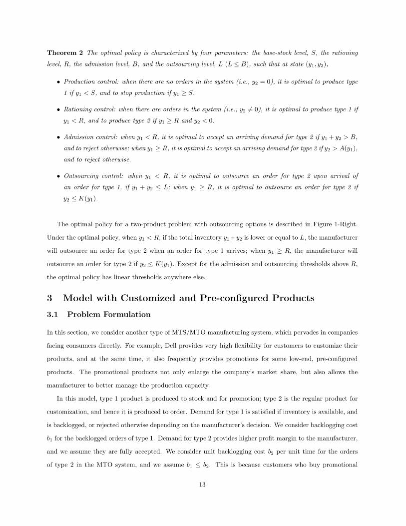
Theorem 2 The optimal policy is characterized by four parameters: the base-stock level, S, the rationing

level, R, the admission level, B, and the outsourcing level, L (L ≤ B), such that at state (y1, y2),



• Rationing control: when there are orders in the system (i.e., y2 6= 0), it is optimal to produce type 1 if

y1 < R, and to produce type 2 if y1 ≥ R and y2 < 0.

• Admission control: when y1 < R, it is optimal to accept an arriving demand for type 2 if y1 + y2 > B,

and to reject otherwise; when y1 ≥ R, it is optimal to accept an arriving demand for type 2 if y2 > A(y1),

and to reject otherwise.

• Outsourcing control: when y1 < R, it is optimal to outsource an order for type 2 upon arrival of

an order for type 1, if y1 + y2 ≤ L; when y1 ≥ R, it is optimal to outsource an order for type 2 if

y2 ≤ K(y1).

The optimal policy for a two-product problem with outsourcing options is described in Figure 1-Right.

Under the optimal policy, when y1 < R, if the total inventory y1 +y2 is lower or equal to L, the manufacturer

will outsource an order for type 2 when an order for type 1 arrives; when y1 ≥ R, the manufacturer will

outsource an order for type 2 if y2 ≤ K(y1). Except for the admission and outsourcing thresholds above R,

the optimal policy has linear thresholds anywhere else.

3 Model with Customized and Pre-configured Products

3.1 Problem Formulation

In this section, we consider another type of MTS/MTO manufacturing system, which pervades in companies

facing consumers directly. For example, Dell provides very high flexibility for customers to customize their

products, and at the same time, it also frequently provides promotions for some low-end, pre-configured

products. The promotional products not only enlarge the company’s market share, but also allows the

manufacturer to better manage the production capacity.

In this model, type 1 product is produced to stock and for promotion; type 2 is the regular product for

customization, and hence it is produced to order. Demand for type 1 is satisfied if inventory is available, and

is backlogged, or rejected otherwise depending on the manufacturer’s decision. We consider backlogging cost

b1 for the backlogged orders of type 1. Demand for type 2 provides higher profit margin to the manufacturer,

and we assume they are fully accepted. We consider unit backlogging cost b2 per unit time for the orders

of type 2 in the MTO system, and we assume b1 ≤ b2. This is because customers who buy promotional

13

products are usually sensitive to the price, but not so sensitive to the leadtime as other customers. We

continue with the notation and the assumptions in Section 2.

In the following, we use an approach parallel to Section 2 to analyze a system with both promotional

and customized products. In state y = (y1, y2), the system incurs a cost at rate

c(y) = −hy+1 − b1y

−1 − b2y

−2 .

We seek an optimal control policy π so as to maximize either the discounted profit over an infinite horizon,

maxπ

Jπ(y(0)) = Eπy(0)

[2∑i=1

∫ ∞0

e−αtpidNai (t)−

∫ ∞0

e−αtr1dNr1 (t) +

∫ ∞0

e−αtc(y(t))dt

], (5)

or the average profit over an infinite horizon,

maxπ

Jπa = limT→∞

Eπ

[2∑i=1

piNai (T )− r1dNr

1 (T ) +∫ T

0

c(y(t))dt

]. (6)

In the rest, we will mainly focus on the discounted-profit problem. The theoretical results for the

discounted-profit problem also hold for the average-profit problem.

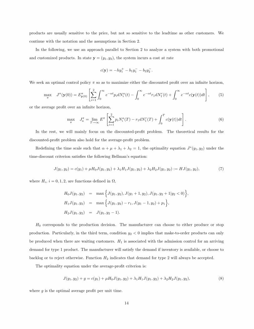
Redefining the time scale such that α + µ + λ1 + λ2 = 1, the optimality equation J∗(y1, y2) under the

time-discount criterion satisfies the following Bellman’s equation:

J(y1, y2) = c(y1) + µH0J(y1, y2) + λ1H1J(y1, y2) + λ2H2J(y1, y2) := HJ(y1, y2), (7)

where Hi, i = 0, 1, 2, are functions defined in Ω,

H0J(y1, y2) = maxJ(y1, y2), J(y1 + 1, y2), J(y1, y2 + 1|y2 < 0)

,

H1J(y1, y2) = maxJ(y1, y2)− r1, J(y1 − 1, y2) + p1

,

H2J(y1, y2) = J(y1, y2 − 1).

H0 corresponds to the production decision. The manufacturer can choose to either produce or stop

production. Particularly, in the third term, condition y2 < 0 implies that make-to-order products can only

be produced when there are waiting customers. H1 is associated with the admission control for an arriving

demand for type 1 product. The manufacturer will satisfy the demand if inventory is available, or choose to

backlog or to reject otherwise. Function H2 indicates that demand for type 2 will always be accepted.

The optimality equation under the average-profit criterion is:

J(y1, y2) + g = c(y1) + µH0J(y1, y2) + λ1H1J(y1, y2) + λ2H2J(y1, y2), (8)

where g is the optimal average profit per unit time.

14

3.2 The Optimal Policy

We use the same approach as in Section 2.2 to investigate the structure of the optimal policy for this model.

Here we only present the main results. The supporting analytical results are provided in On-line Appendix

D.

Theorem 3 The optimal policy is characterized by two parameters: the base-stock level, S, and the admis-

sion level, B (B ≤ 0), such that at state (y1, y2),

• Production control: if there are orders for type 2 (i.e., y2 6= 0), it is optimal to produce type 2; otherwise,

it is optimal to produce type 1 if y1 < S, and to stop production if y1 ≥ S.

• Admission control: it is optimal to satisfy an arriving demand for type 1 if y1 > 0, to reject if y1 +y2 ≤B, and to backlog otherwise.

The optimal policy is described in Figure 2-Left. Under the optimal policy, the manufacturer will stop

production if the inventory level of type 1 reaches S, and keep producing otherwise. When there is no

inventory available, the manufacturer will backlog an arriving demand for type 1 if the net total inventory,

y1 + y2, is higher than B, or reject otherwise. We show in Proposition 5 of On-line Appendix D that the

threshold level B is non-positive. Therefore, it is always optimal to satisfy promotional demands when the

inventory is available. In this policy, type 2 orders always have higher priority and cannot be rejected. We

refer to this optimal policy as the (S,B) policy.

Remark: Note that the optimal policy for product 2 is not affected by the system state. Orders for type 2

will always be accepted, and they always have higher priorities than type 1. An arriving demand for type 2

will receive immediate service, if there are no other orders in the system for type 2; otherwise, it will wait

until the manufacturer has satisfied the type 2 orders that arrived earlier. The expected profit generated by

type 2 product is determined by the demand process itself. The manufacturer only maximizes the “extra”

profit generated by the promotional product. Therefore, the two-product problem could be seen as a problem

with a single MTS product, but under the impact of the higher-priority product. For the same reason, this

problem can be easily extended with n− 1 types of MTO products whose holding costs, b2, b3, . . . , bn are all

higher than b1. Orders for different types of MTO products are sequenced according to their backlogging

penalties, and their impacts on the MTS product are independent of their types.

Similar to our model with OEM and aftermarket products, here we present the expected due date quoting

for type 1 and type 2 orders in Lemmas 6 and 7.

Lemma 6 The expected due date (i.e., leadtime) for a customized order is T2 = (y−2 + 1)× 1µ .

15

y2

y1

S

B


Idle

Produce 2 Satisfy 1

1

-1-2…

…

Admission Threshold

Produce 2 Accept 1

2

Produce 2 Reject 1

y2

B

-1-2…

Admission Threshold

Produce 2, Reject 1


Produce 2 Backlog 1

L Outsourcing Threshold

S

Idle

Produce 2 Satisfy 1

1…

2

y1

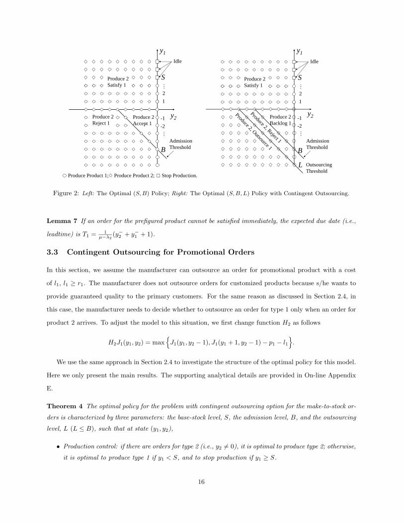
Figure 2: Left: The Optimal (S,B) Policy; Right: The Optimal (S,B,L) Policy with Contingent Outsourcing.

Lemma 7 If an order for the prefigured product cannot be satisfied immediately, the expected due date (i.e.,

leadtime) is T1 = 1µ−λ2

(y−2 + y−1 + 1).

3.3 Contingent Outsourcing for Promotional Orders

In this section, we assume the manufacturer can outsource an order for promotional product with a cost

of l1, l1 ≥ r1. The manufacturer does not outsource orders for customized products because s/he wants to

provide guaranteed quality to the primary customers. For the same reason as discussed in Section 2.4, in

this case, the manufacturer needs to decide whether to outsource an order for type 1 only when an order for

product 2 arrives. To adjust the model to this situation, we first change function H2 as follows

H2J1(y1, y2) = maxJ1(y1, y2 − 1), J1(y1 + 1, y2 − 1)− p1 − l1

.

We use the same approach in Section 2.4 to investigate the structure of the optimal policy for this model.

Here we only present the main results. The supporting analytical details are provided in On-line Appendix

E.

Theorem 4 The optimal policy for the problem with contingent outsourcing option for the make-to-stock or-

ders is characterized by three parameters: the base-stock level, S, the admission level, B, and the outsourcing

level, L (L ≤ B), such that at state (y1, y2),

• Production control: if there are orders for type 2 (i.e., y2 6= 0), it is optimal to produce type 2; otherwise,

it is optimal to produce type 1 if y1 < S, and to stop production if y1 ≥ S.

16

• Admission control: it is optimal to satisfy an arriving demand for type 1 if y1 > 0, to reject if y1 +y2 ≤B, and to backlog otherwise.

• Outsourcing control: it is optimal to outsource an order for type 1 after accepting an order of type 2

product, if y1 + y2 ≤ L.

The optimal policy is described in Figure 2-Right. Under the optimal policy, if the net total inventory

level, y1 + y2, is lower or equal to L, the manufacturer will outsource an order for type 1 when an order for

type 2 arrives. We refer to this optimal policy as the (S,B,L) policy.

4 Computational Analysis

In this section we report the results of the computational study that we performed based on the model

with OEM and aftermarket products. The computational analysis based on the model with customized and

pre-configured products presents similar properties, and is therefore omitted. The goal of our numerical

analysis is to investigate the following questions:

1. How much profit will a manufacturer lose if s/he uses the linear-structured (S,R,B) policy instead of

the optimal policy?

2. Outsourcing orders prevents large backlogging costs for the manufacturer. However, it also decreases

customer satisfaction. How much will the profit decrease if the manufacturer does not utilize the

flexibility of outsourcing?

3. What is the profit improvement of the (S,R,B) policy relative to other commonly used policies? Under

what circumstances the improvement is or is not very significant?

4. When the objective is to maximize profit, it is sometimes inevitable to sacrifice the service level of

some customers. Therefore, an important question is: What is the impact of the (S,R,B) policy on

the service level of both the aftermarket and the OEM customers?

Our numerical study consists of 320 cases generated by varying the following parameters:• ρ = (λ1 + λ2)/µ: This parameter is an indication of the manufacturer’s relative capacity compared to the

market size. We refer to ρ as potential facility utilization in the rest of the paper. Please notice that ρ is not thereal facility utilization since aftermarket demands may be rejected. We considered five values for ρ, specifically,ρ ∈ 0.6, 0.8, 1.0, 1.2, 1.4.

• λ1/(λ1 +λ2): This demand ratio represents the size of the OEM demand compared to the aftermarket demand.In our numerical study we considered four cases, namely λ1/(λ1 + λ2) ∈ 0, 0.3, 0.7, 1.0.

17

• p2/p1: The price ratio represents the price difference between the two products. Since the price of aftermarketproduct is higher than the price offered to the OEM, we consider four values for p2/p1 that are all greater thanone, namely p2/p1 ∈ 1.0, 1.3, 1.6, 2.0. We did not consider ratios grater than 2, since it is very uncommon inpractice to have cases in which an item is sold twice of its price for OEM.

• b2/b1: The penalty ratio represents the backlogging penalty difference between the two products. In thenumerical study we assume the backlogging cost of each product is proportional to its price, and we considerfour scenarios: (b1 = 20%p1, b2 = 5%p2), (b1 = 40%p1, b2 = 5%p2), (b1 = 100%p1, b2 = 5%p2), and (b1 =200%p1, b2 = 5%p2). Note that, although p1 < p2, in all the scenarios, backlogging of type 1 customers iscostlier than that of type 2 customers, which follows the assumption for the model with OEM and aftermarketproducts.

In order to better present the effects of the parameters on the system performance (and omit the effects

of discount factor), our numerical study uses total expected profit per unit time as the performance measure.

4.1 (S,R,B) Policy Versus Optimal Policy

To evaluate the performance of the (S,R,B) policy, we first compare it with the optimal policy in our

numerical study. To obtain the expected profit under the (S,R,B) policy, we revise the admission decision

in the MDP model to follow the linear threshold level B. This changes our MDP model from an optimization

model to a performance evaluation model that obtains the optimal expected profits for the (S,R,B) policy.

The thresholds (S,R,B) are found by searching. (A heuristic algorithm that can quickly approximate

thresholds (S,R,B) is also presented in On-line Appendix F.)

By examining the 320 cases in our numerical study, we found that, on average, the (S,R,B) policy results

in 0.6% less profit than the optimal policy. The maximum difference that we observed was 2.1%. Besides the

similarities between the two policies, another key reason that the (S,R,B) policy performs so close to the

optimal policy is that the probability that the system visits a state in the upper left area (where y1 ≥ R and

y2 ≤ B −R ) in Figure 1 is very small. Intuitively, on one hand, when the production capacity is tight, the

manufacturer may have low inventory or high backorders for both products most of the time, and the system

stays in the lower area (where y1 < R) most of the time; On the other hand, when the production capacity is

sufficient, the manufacturer may have high inventory level for product 1 and very few backorders for product

2, and the probability that the system stays in the upper right area (where y1 ≥ R and y2 > B−R) is high.

So although the admission threshold may not be linear when y1 ≥ R, the frequency that we need to refer to

it is very small.

The close performance of the linear (S,R,B) policy to that of the optimal policy is an indication that

changing the near-linear structured optimal policy to a linear heuristic does not have a significant impact

on the expected profit. The (S,R,B) policy approximates the optimal policy very well.

18

4.2 Effectiveness of Contingent Outsourcing

We also studied the performance of the outsourcing policy analyzed in Section 2.4. Interestingly, we found

that in all the scenarios in our numerical study, outsourcing provides very slight profit increase (i.e., less than

0.8% in maximum), compared with the (S,R,B) policy in which outsourcing is not applied. This is quite

intuitive in the sense that under the (S,R,B) policy, an aftermarket demand will be accepted only when

system has enough capacity, so the probability that an accepted order is later be outsourced is very small.

Therefore, for a manufacturer with the flexibility to accept or reject an order, having additional flexibility

of outsourcing an order later does not have much value.

4.3 (S,R,B) Policy Versus Simple Base-Stock Policy

Because of its non-linear component, the optimal policy is not easy to implement in practice. Fortunately,

the (S,R,B) policy has a simple structure and well approximates the optimal policy. In this section we

compare the performance of the (S,R,B) policy with a policy that is commonly used in practice (i.e., the

base-stock policy). The objective is to investigate how much the expected profit increases if a manufacturing

system switches from other commonly used policies to the (S,R,B) policy.

The simple base-stock policy is often used in practice, and it is characterized by two threshold levels:

base-stock level, S′, for type 1 products, and admission level, B′, for type 2 products. Under this policy,

the system produces type 1 products as long as the inventory is less than S′. When the inventory of type

1 product reaches S′, the system produces type 2 products if there is an order of type 2 in the system, or

idles otherwise. The orders for type 2 product will only be accepted if the number of orders of type 2 in

the system is less than B′. We call this policy the (S′, B′) policy. To obtain the optimal values for S′ and

B′, we searched all possible combinations for values S′ and B′ and obtained (S′∗, B′∗) that results in the

maximum expected profit.

4.3.1 Impact on Expected Profit

Denoting JSB as the system’s expected profit per unit time under the optimal (S′, B′) policy, we evaluate

the profit improvement under the (S,R,B) policy using the following measure:

Profit PotentialSRB =JSRB − JSB

JSB× 100%, (9)

where JSRB is the expected profit per unit time under the (S,R,B) policy.

Based on our numerical study, we found that, on average, the profit improvement obtained by using the

(S,R,B) policy is 8%. The maximum profit improvement can be up to 40%.

19

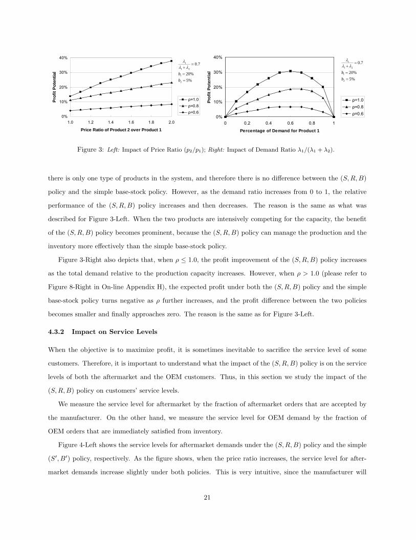
We also examined the effects of price ratio and potential facility utilization on the profit improvement.

Figure 3-Left, which is for one set of examples among several that we studied, depicts the typical behavior

of the system. In Figure 3-Left, we fix λ1/(λ1 + λ2) = 0.7 and b1 = 20%p1, and we change the price ratio

and the potential facility utilization rate. As the figure shows, when the price ratio increases, implementing

the (S,R,B) policy results in more profit improvement. The reason is as follows. Both the (S,R,B) and

the base-stock policies do not reject the type 1 orders, and thus in the long-run, the number of satisfied type

1 orders is the same under both policies. However, the number of type 2 orders satisfied under these two

polices are different. The (S,R,B) policy satisfies more type 2 orders than the base-stock policy, because as

shown in Section 2.2, the (S,R,B) policy is almost as efficient as the optimal policy (which has the highest

number of accepted orders of type 1). As a result, the gap between the performance of these two policies

(i.e., the profit potential) increases as the orders of type 2 become more profitable (i.e., the price ration

increases).

The figure also suggests that, when the capacity is sufficient (ρ ≤ 1.0), profit potential increases as ρ

increases. This is true since as potential facility utilization rate increases, i.e., capacity becomes tighter, it

is more and more important to allocate capacity effectively between the two classes of products, which is

exactly what the (S,R,B) policy achieves. However, when ρ > 1.0 (please refer to Figure 8-Left in On-line

Appendix H), the expected profit under both the (S,R,B) policy and the simple base-stock policy turns

negative as ρ further increases, and the profit difference between the two policies becomes smaller and finally

approaches zero. In this case, since the production capacity is very tight, both policies behave the same,

keeping the facility running almost all the time and rejecting aftermarket demand if capacity is not enough.

So manufacturers benefit most from implementing the (S,R,B) policy when the capacity is neither too tight

nor too loose.

We also examined the effects of backlogging penalty ratio for OEM products. For this purpose, we keep

b2 = 5% unchanged, and increase b1 from 20% to 40%, 100%, and 200%. We find that the profit potential

of the (S,R,B) policy decreases and finally approaches zero. Intuitively, as the OEM backlogging penalty

increases, giving priority to OEM product becomes more critical, and thus any policy such as our base-stock

policy that gives higher priority to the OEM also performs relatively well. Therefore, the gap between the

performance of the base-stock policy and the (S,R,B) policy (i.e., the profit potential) decreases as the

OEM backlogging penalty increases.

Figure 3-Right shows the typical system behavior of how changes in demand ratio and potential facility

utilization affect the profit improvement. Figure 3-Right corresponds to one set of our numerical study in

which p2/p1 = 1.6 and b1 = 20%p1. As the figure suggests, when the demand ratio, λ1λ1+λ2

, equals 0 or 1,

20

0%

10%

20%

30%

40%

0 0.2 0.4 0.6 0.8 1

Percentage of Demand for Product 1

Prof

it Po

tent

ial

ρ=1.0ρ=0.8ρ=0.60%

10%

20%

30%

40%

1.0 1.2 1.4 1.6 1.8 2.0

Price Ratio of Product 2 over Product 1

Prof

it Po

tent

ial

ρ=1.0ρ=0.8ρ=0.6

%5%20

7.0

2

1

21

1

==

=+

bb

λλλ

%5%20

7.0

2

1

21

1

==

=+

bb

λλλ

Figure 3: Left: Impact of Price Ratio (p2/p1); Right: Impact of Demand Ratio λ1/(λ1 + λ2).

there is only one type of products in the system, and therefore there is no difference between the (S,R,B)

policy and the simple base-stock policy. However, as the demand ratio increases from 0 to 1, the relative

performance of the (S,R,B) policy increases and then decreases. The reason is the same as what was

described for Figure 3-Left. When the two products are intensively competing for the capacity, the benefit

of the (S,R,B) policy becomes prominent, because the (S,R,B) policy can manage the production and the

inventory more effectively than the simple base-stock policy.

Figure 3-Right also depicts that, when ρ ≤ 1.0, the profit improvement of the (S,R,B) policy increases

as the total demand relative to the production capacity increases. However, when ρ > 1.0 (please refer to

Figure 8-Right in On-line Appendix H), the expected profit under both the (S,R,B) policy and the simple

base-stock policy turns negative as ρ further increases, and the profit difference between the two policies

becomes smaller and finally approaches zero. The reason is the same as for Figure 3-Left.

4.3.2 Impact on Service Levels

When the objective is to maximize profit, it is sometimes inevitable to sacrifice the service level of some

customers. Therefore, it is important to understand what the impact of the (S,R,B) policy is on the service

levels of both the aftermarket and the OEM customers. Thus, in this section we study the impact of the

(S,R,B) policy on customers’ service levels.

We measure the service level for aftermarket by the fraction of aftermarket orders that are accepted by

the manufacturer. On the other hand, we measure the service level for OEM demand by the fraction of

OEM orders that are immediately satisfied from inventory.

Figure 4-Left shows the service levels for aftermarket demands under the (S,R,B) policy and the simple

(S′, B′) policy, respectively. As the figure shows, when the price ratio increases, the service level for after-

market demands increase slightly under both policies. This is very intuitive, since the manufacturer will

21

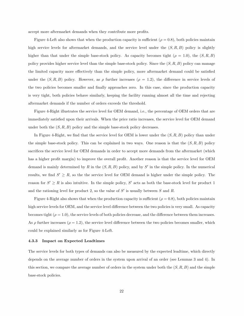
accept more aftermarket demands when they contribute more profits.

Figure 4-Left also shows that when the production capacity is sufficient (ρ = 0.8), both policies maintain

high service levels for aftermarket demands, and the service level under the (S,R,B) policy is slightly

higher than that under the simple base-stock policy. As capacity becomes tight (ρ = 1.0), the (S,R,B)

policy provides higher service level than the simple base-stock policy. Since the (S,R,B) policy can manage

the limited capacity more effectively than the simple policy, more aftermarket demand could be satisfied

under the (S,R,B) policy. However, as ρ further increases (ρ = 1.2), the difference in service levels of

the two policies becomes smaller and finally approaches zero. In this case, since the production capacity

is very tight, both policies behave similarly, keeping the facility running almost all the time and rejecting

aftermarket demands if the number of orders exceeds the threshold.

Figure 4-Right illustrates the service level for OEM demand, i.e., the percentage of OEM orders that are

immediately satisfied upon their arrivals. When the price ratio increases, the service level for OEM demand

under both the (S,R,B) policy and the simple base-stock policy decreases.

In Figure 4-Right, we find that the service level for OEM is lower under the (S,R,B) policy than under

the simple base-stock policy. This can be explained in two ways. One reason is that the (S,R,B) policy

sacrifices the service level for OEM demands in order to accept more demands from the aftermarket (which

has a higher profit margin) to improve the overall profit. Another reason is that the service level for OEM

demand is mainly determined by R in the (S,R,B) policy, and by S′ in the simple policy. In the numerical

results, we find S′ ≥ R, so the the service level for OEM demand is higher under the simple policy. The

reason for S′ ≥ R is also intuitive. In the simple policy, S′ acts as both the base-stock level for product 1

and the rationing level for product 2, so the value of S′ is usually between S and R.

Figure 4-Right also shows that when the production capacity is sufficient (ρ = 0.8), both policies maintain

high service levels for OEM, and the service level difference between the two policies is very small. As capacity

becomes tight (ρ = 1.0), the service levels of both policies decrease, and the difference between them increases.

As ρ further increases (ρ = 1.2), the service level difference between the two policies becomes smaller, which

could be explained similarly as for Figure 4-Left.

4.3.3 Impact on Expected Leadtimes

The service levels for both types of demands can also be measured by the expected leadtime, which directly

depends on the average number of orders in the system upon arrival of an order (see Lemmas 3 and 4). In

this section, we compare the average number of orders in the system under both the (S,R,B) and the simple

base-stock policies.

22

30%

50%

70%

90%

1 1.2 1.4 1.6 1.8 2


Serv

ice

Leve

l for

OE

M

(S,R,B) Policy, ρ=1.2Simple Policy, ρ=1.2(S,R,B) Policy, ρ=1.0Simple Policy, ρ=1.0(S,R,B) Policy, ρ=0.8Simple Policy, ρ=0.8

%.5%,20

7.0

21

21

1

==

=+

bbλλ

λ

%5%,20

7.0

21

21

1

==

=+

bbλλ

λ

40%

60%

80%

100%

1 1.2 1.4 1.6 1.8 2


Serv

ice

Leve

l for

Afte

rmar

ket


Figure 4: Left: Service Level for Aftermarket Demands under the (S,R,B) Policy and the (S′, B′) Policy; Right:OEM Service Level under the (S,R,B) Policy and the (S′, B′) Policy

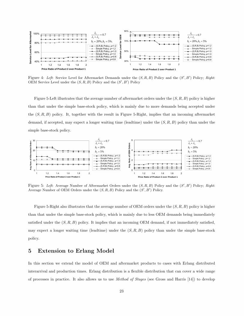
Figure 5-Left illustrates that the average number of aftermarket orders under the (S,R,B) policy is higher

than that under the simple base-stock policy, which is mainly due to more demands being accepted under

the (S,R,B) policy. It, together with the result in Figure 5-Right, implies that an incoming aftermarket

demand, if accepted, may expect a longer waiting time (leadtime) under the (S,R,B) policy than under the

simple base-stock policy.

0

2

4

6

1 1.2 1.4 1.6 1.8 2Price Ratio of Product 2 over Product 1

Avg

. Num

. of O

EM O

rder

s


0

10

20

30

1 1.2 1.4 1.6 1.8 2


Avg

. Num

. of A

fterm

arke

t Ord

ers


%5%20

7.0

2

1

21

1

==

=+

bb

λλλ

%5%20

7.0

2

1

21

1

==

=+

bb

λλλ

Figure 5: Left: Average Number of Aftermarket Orders under the (S,R,B) Policy and the (S′, B′) Policy; Right:Average Number of OEM Orders under the (S,R,B) Policy and the (S′, B′) Policy.

Figure 5-Right also illustrates that the average number of OEM orders under the (S,R,B) policy is higher

than that under the simple base-stock policy, which is mainly due to less OEM demands being immediately

satisfied under the (S,R,B) policy. It implies that an incoming OEM demand, if not immediately satisfied,

may expect a longer waiting time (leadtime) under the (S,R,B) policy than under the simple base-stock

policy.

5 Extension to Erlang Model

In this section we extend the model of OEM and aftermarket products to cases with Erlang distributed

interarrival and production times. Erlang distribution is a flexible distribution that can cover a wide range

of processes in practice. It also allows us to use Method of Stages (see Gross and Harris [14]) to develop

23

an MDP model and obtain the optimal expected profit. The objective of the extension is to answer the

following questions:

1. Will the near-linear structure of the optimal policy still hold with Erlang distributed interarrival and

production times? If not, how much profit will a manufacturer lose if s/he uses linear threshold

structure instead of the optimal policy with non-linear structure?

2. How does the difference in production rates of the two product affect the manufacturer’s inventory

control policy as well as the expected profit?

3. How does the variability in demand and production processes influence the manufacturer’s inventory

control policy as well as the expected profit?

In the extended model, we assume the demand interarrival time for product i follows an Erlang-Ki

distribution, and the production time of a type i product is an Erlang-mi random variable. The phase

arrival rate in the demand process for product i is Kiλi, so the demand arrival rate for product i is still λi.

The time to finish one phase of product i follows an exponential distribution with mean 1/γi. Thus, the

average time to produce a type i product is 1/µi = mi/γi, and the weighted average production time 1/µ is

calculated as1µ

=λ1

λ1 + λ2

(m1

γ1

)+

λ2

λ1 + λ2

(m2

γ2

). (10)

Let si be the number of production phases completed for an unfinished job of product i. The problem

can be formulated in terms of an aggregate state variable, i.e., the work storage level, xi = si + Kiyi,

which links inventory and partially completed production [18]. We describe the system state with a tuple

of four variables, (x1, x2, k1, k2), where x1 ∈ Z and x2 ∈ Z− are the work storage level of each product, and

ki ∈ 1, 2, . . . ,Ki is the number of phases until the arrival of the next type i demand. Note that, having

product i′s work storage level xi, it is easy to calculate its inventory level5, yi = b ximi c, and the number of

finished phases of a job under production, si = xi −mib ximi c.

The Erlang model is more complicated than the exponential model, and it is difficult to obtain analytical

properties (Please refer to On-line Appendix I for the MDP formulations). In the following, we therefore

perform an extensive numerical study to gain some insights into the system performance. We test the same

320 cases defined in Section 4, and for each case, we consider 50 combinations of (K1,K2) and (m1,m2), by

fixing one pair at (1, 1) and letting each parameter of the other pair take a value out of 1, 2, 3, 4, 5. This

results in an extensive set of examples consisting of 16,000 (= 320× (25+25)) cases. We compare the results

5Note that in our model, the inventory can be positive or negative.

24

of the above Erlang model and the exponential model developed in Section 2.1. To make the two models

comparable, we let the average production times in the two models to be equal to each other.

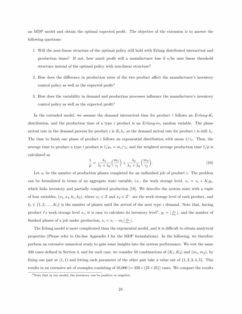
5.1 Impact on the Structure of the Optimal Policy

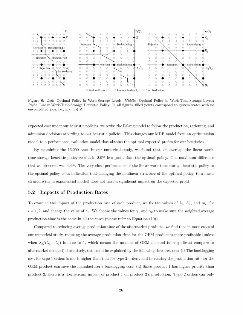
Our numerical results show that the optimal policy for the Erlang model does not always follow the same

structure as that for exponential model. Figure 6-Left shows an example of the optimal policy. The horizontal

and vertical axis in that figure correspond to x2 and x1, respectively, which are the work storage levels in

the system. As the figure shows, the optimal policy has a stepwise function and does not follow the linear

structure similar to the exponential case.

Note that, since production rates are different for both products, completing one stage of product 1

takes 1/γ1 in average, while completing one stage of product 2 takes 1/γ2. Thus, the average amount of

completed work in the system for product 1 is x1/γ1, and for product 2 is x2/γ2. So, one can use average

work-time-storage levels to represent the optimal policy, which is done in Figure 6-Middle. Figure 6-Middle

shows the optimal policy in 6-Left, but in terms of average work-time-storage levels in the system. The

vertical and horizontal axis, x1/γ1, and x2/γ2, respectively, are measured in time.

As the figure shows, the optimal threshold levels are still not linear, but they fluctuate around some

straight lines. For example, the admission control threshold, although a non-linear function, looks fluctuating

around a 45 line. We examine several different examples and we observed the same phenomenon, i.e.,

the optimal rationing thresholds fluctuate around a horizontal line, and the optimal admission thresholds

fluctuate around a 45 line. This suggests that the linear structure in the exponential model, if translated

into average work-time-storage levels in the system, may be a good heuristic policy for systems with non-

exponential (i.e., Erlang) production and demand interarrival times.

To examine this, we compared the expected profit under the optimal policy for the Erlang model, with a

heuristic policy, called Linear Work-Time-Storage (SL, RL, BL) Heuristic Policy. This policy has a similar

linear structure as the (S,R,B) policy in our exponential model. The only difference is that threshold levels

SL, RL and BL are measured in average work-time-storage level instead inventory level. An example of

the structure of this policy is shown in Figure 6-Right. Under this policy, for example, an arriving order is

accepted at state (x1, x2) if the total average work-time-storage (x1/γ1) + (x2/γ2) is greater than BL. To

find the optimal (SL, RL, BL) thresholds, we search for the values of SL, RL, and BL that maximize the

expected profit.

To evaluate the performance of the Linear Work-Time-Storage Heuristic Policy, we compared its expected

profit with that under the optimal policy for the Erlang model in an extensive numerical study. To obtain the

25

Backordering

S

Backordering

Rejection

Rejectionx2/γ2

x1/γ1


S

Rejection

Rejection x2

x1

x2/γ2

x1/γ1

SL

BL

RL

BackorderingRejection

BackorderingRejectionBackordering

Backordering

Rejection

Backordering

Figure 6: Left: Optimal Policy in Work-Storage Levels; Middle: Optimal Policy in Work-Time-Storage Levels;Right: Linear Work-Time-Storage Heuristic Policy. In all figures, filled points correspond to system states with nouncompleted jobs, i.e., xi/mi ∈ Z.

expected cost under our heuristic policies, we revise the Erlang model to follow the production, rationing, and

admission decisions according to our heuristic policies. This changes our MDP model from an optimization

model to a performance evaluation model that obtains the optimal expected profits for our heuristics.

By examining the 16,000 cases in our numerical study, we found that, on average, the linear work-

time-storage heuristic policy results in 2.0% less profit than the optimal policy. The maximum difference

that we observed was 4.4%. The very close performance of the linear work-time-storage heuristic policy to

the optimal policy is an indication that changing the nonlinear structure of the optimal policy, to a linear

structure (as in exponential model) does not have a significant impact on the expected profit.

5.2 Impacts of Production Rates

To examine the impact of the production rate of each product, we fix the values of λi, Ki, and mi, for

i = 1, 2, and change the value of γi. We choose the values for γ1 and γ2 to make sure the weighted average

production time is the same in all the cases (please refer to Equation (10)).

Compared to reducing average production time of the aftermarket products, we find that in most cases of

our numerical study, reducing the average production time for the OEM product is more profitable (unless

when λ2/(λ1 + λ2) is close to 1, which means the amount of OEM demand is insignificant compare to

aftermarket demand). Intuitively, this could be explained by the following three reasons: (i) The backlogging

cost for type 1 orders is much higher than that for type 2 orders, and increasing the production rate for the

OEM product can save the manufacturer’s backlogging cost; (ii) Since product 1 has higher priority than

product 2, there is a downstream impact of product 1 on product 2’s production. Type 2 orders can only

26

be processed after all type 1 orders are satisfied and rationing level has been built up. So reducing product

1’s production time not only reduce the average backlogging time of type 1 orders, but can also reduce

the holding time for type 2 orders. However, in the other direction, reducing product 2’s production time

has little impact on product 1. (iii) In our numerical analysis, we also find that increasing the production

rate for the OEM product results in smaller base-stock and rationing threshold levels. This is because the

manufacture tends to keep less safety stock for product 1, as the product could be produced in a faster

rate. Smaller base-stock and rationing threshold levels save the manufacturer the inventory holding cost

for the OEM product. At the same time, smaller rationing threshold level also allows the manufacturer

to process aftermarket orders earlier, as well as to accept more aftermarket demands, which increases the

manufacturer’s profit.

5.3 Impacts of Demand and Production Variabilities

To examine the impacts of the variabilities of demand and production times separately, we study two sce-

narios. In the first scenario, we fix the values of γi, mi, and λi, for i = 1, 2, and change the values of K1 and

K2 to get different demand variabilities. In the second scenario, we fix the value of λi, Ki, and µi, i = 1, 2,

and change the values of mi to evaluate the impact of the variability of production times. The values of γ1

and γ2 are adjusted at the same time in order to keep the average processing time of each product, µi = miγi

unchanged.

In the first scenario, we find that the manufacturer’s expected profit increases as the demand arrival

process becomes less variable. As the system becomes more deterministic and more predictable, the manu-

facturer accepts more aftermarket demands without sacrificing the service level for either product.

Although reducing the demand variability for either product improves the system profit, however, we

find that reducing the variability of OEM demand is more effective in most cases (unless when λ2/(λ1 + λ2)

is close to 1). Intuitively, this is caused by the downstream impact of product 1 on product 2’s production.

Reducing the variability of OEM demand results in lowered base-stock and rationing threshold levels, because

the manufacture tends to keep less safety stock for product 1, as demand arrival process becomes more

predictable. Smaller base-stock and rationing threshold levels save the manufacturer the inventory holding

cost for the OEM product. At the same time, smaller rationing threshold level also allows the manufacturer

to process aftermarket orders earlier and accept more aftermarket demands.

In the second scenario, we find that the manufacturer’s expected profit increases as the production

time of either product becomes less variable. We also find that reducing the variability in production time

of the OEM products is more beneficial compared to reducing the variability in the production time of

27

the aftermarket products. Both results could be explained similarly based on the smaller base-stock and

rationing levels for the OEM product.

6 Conclusions

In this paper, we studied the production and inventory policies in two different make-to-stock/make-to-

order manufacturing environments. For the model with both OEM and aftermarket demands, we show that

the optimal policy has a near-linear structure characterized by three parameters, the base-stock level, the

rationing level, and the admission level. We extend the optimal policy to problems in which aftermarket

orders can be outsourced, as well as to problems with multiple types of aftermarket products. Numerical

study shows that a linear structured heuristic approximates the optimal policy very well. For the model

where the manufacturer offers both customized and pre-configured (promotional) products, we show that the

optimal policy has a linear structure characterized by two parameters, the base-stock level and the admission

level. We also extend the optimal policy to problems with outsourcing option for pre-configured products.

After conducting an extensive computational analysis, we observed the following:

1. Implementing the (S,R,B) policy can result in, on average, 8% (and sometimes up to 40%) more

profit than that under the commonly used base-stock policy. This difference in profit is high when

production capacity is tight, when the backlogging cost for MTS product and the backlogging cost for

MTO product are close, or when demand arrival rates in the two classes are close.

2. When the manufacturer has the option of rejecting low priority orders, having the flexibility of out-

sourcing an accepted low-priority order does not provide a significant increase in profit.

3. The (S,R,B) policy improves the profit by allocating the production capacity more effectively, and

therefore having the capability to accept more low-priority demands. As a tradeoff, when the produc-

tion capacity is very tight, the service level for the high-priority demands under the optimal policy is

lower than that under the simple base-stock policy.

4. The linear work-time-storage policy works as a good heuristic for problems with non-exponential inter-

arrival and production times. Our numerical analysis shows that the expected profit under the linear

work-time-storage heuristic, on average, is only 2.0% lower than that under the optimal solution. The

maximum difference that we observe was 4.4%. The good performance and simple structure of our

linear inventory heuristic makes it an attractive policy to use in practice.

28

5. The production time and variability of the high-priority product has more impact on the system

performance than those of the low-priority one, because of the down stream effect of the high-priority

product.

In this paper we investigated the capacity allocation in a MTS/MTO system. An important future

research direction is the joint pricing and capacity allocation decisions for multiple products. So far, academic

literature on joint pricing and allocation decisions has confined itself mainly to single-product and single-

class-customer problems, which are not applicable to the current practice of market segmentation in the

manufacturing industry. The complexity of the joint pricing and allocation problem among multiple products

increases dramatically due to the fact of demand diversions among different products, i.e., the demands for

one product not only depends on their own price, but may also be influenced by the prices of other products.

Another issue complicating the problem is that different products may compete for same resources, i.e., the

production capacity and components.

References

[1] Benjaafar, S., M. ElHafsi and T. Huang. Optimal control of a production-inventory system with both backordersand lost sales. Working Paper. University of Minnesota.

[2] Bertsekas, D. 1995. Dynamic Programming and Optimal Control, Volume Two, Athena Scientific.

[3] Carr, S. and I. Duenyas. Optimal admission control and sequencing in a make-to-stock/make-to-order produc-tion system. Operations Research, 48, pp. 709-720.

[4] Chen F. and V. G. Kulkarni. 2007. Individual, class-based, and social optimal admission policies in two-priorityqueues. Stochastic Models, 23, pp 97127.

[5] Cohen, M.A., P.R. Kleindorfer and H.L. Lee. 1988. Service constrained (s,S) inventory systems with prioritydemand classes and lost sales. Management Science, Vol. 34, pp. 482-499.

[6] de Vericourt F., F. Karaesmen and Y. Dallery. 2000. Dynamic scheduling in a make-to-stock system: s partialcharacterization of optimal policies. Operations Research, 48, pp 811-819.

[7] de Vericourt F., F. Karaesmen and Y. Dallery. 2002. Optimal stock allocation for a capacitated supply system.Management Science, 48, pp 1486-1501.

[8] Dobson, G. and C.A. Yano. 2001. Production offering, pricing, and make-to-stock/make-to-order decisions withshared capacity. Production and Operations Management, 11, pp 293-312.

[9] Duenyas, I. and M. Van Oyen. 1996. Heuristic scheduling problem with random demand. Management Science.Vol. 42, pp. 814-829.

[10] Gittins, J.C., Multi-armed Bandit Allocation Indices, Wiley, New York, 1989.

[11] Glasserman, P., and D. Yao. 1994. Monotone optimal control for permutable GSMPs. Mathematics of OperationsResearch, 19, pp 449-476.

[12] Graves, S.C. 1980. The multi-product production cycling problem. AIIE Trans. 12, pp 233-240.

[13] Gupta, D. and L. Wang. 2007. Capacity Management for Contract Manufacturing. Operations Research, 55(2),pp. 367377.

[14] Gross D. and C.M. Harris. 1985. Fundamentals of Queueing Theory, John Wiley & Sons.

[15] Ha, A. 1997. Inventory rationing in a make-to-stock production system with several demand classes and lostsales. Management Science, 43, pp 1093-1103.

29

[16] Ha, A. 1997. Stock-rationing policy for a make-to-stock production system with two priority classes and back-ordering. Naval Research Logistics, 44, pp 458-472.

[17] Ha, A. 1997. Optimal dynamic scheduling policy for a make-to-stock production system. Operations Research,45, pp 42-53.

[18] Ha, A. 2000. Stock-rationing in an M/Ek/1 make-to-stock queue. Management Science, 46, pp. 77-87.

[19] Huang, B., and S.M.R. Iravani. 2008. Technical Note - A make-to-stock system with multiple customer classesand batch ordering. Operations Reserach, 56, 1312-1320.

[20] Iravani, S.M.R., B. Kolfal, M.P. Van Oyen. Technical Note - Inventory and Process Flexibility in a Make-to-Stock Systems with Product Substitution. Working paper. Northwestern University.

[21] Iravani, S.M.R., T. Liu, K. L. Luangkesorn, and D. Simchi-Levi. 2007. A produce-to-stock system with advancedemand information and secondary customers. Naval Reserach Logistic, 54, 331-345.

[22] Kleijn, M. and R. Dekker. 1998. An overview of inventrory systems with several demand classes. ReportEI9838/A, Econometric Institute, Erasmus University Rotterdam, The Netherlands.

[23] Melchiors, P., R. Dekker and M.J. Kleijn. 2000. Inventory rationing in an (s, Q) inventory model with lost salesand two demand classes. Journal of the Operational Research Society, 51, pp 111-122.

[24] Moinzadeh, K. 1989. Operating characteristics for the (S − 1, S) inventory system with partial backorders andconstant resupply time. Management Science, 35, 472-477.

[25] Montgomery, D. C., M. S. Bazaraa and A. K. Keswani. 1981. Inventory models with a mixture of backordersand lost sales. Naval Research Logistics, 20, pp. 255-263.

[26] Nahmias, S. and W.S. Demmy. 1981. Operating characteristics of an inventory system with rationing. Manage-ment Science, 27, pp. 1236-1245.

[27] Nahmias, S. and S. A. Smith. 1994. Optimizing inventory levels in a two-echelon retailer system with partiallost sales. Management Science, 40, pp. 582-596.

[28] Pena-Perez, A. and P. Zipkin. 1997. Dynamic scheduling rules for a multi-product make-to-stock queue. Oper-ations Research, 45, pp 919-930.

[29] Porteus, E. 1982. Conditions for characterizing the structure of optimal strategies in infnite-horizon dynamicprogramming. Journal of Optimization Theory and Applications, Vol. 36, pp. 419-431.

[30] Puterman M.L. 1994. Markov Decision Processes. Wiley, New York.

[31] Reiman, M. I. and L. M. Wein. 1998. Dynamic scheduling of a two-class queue with setups. Operations Research,46, pp. 532-547.

[32] Rabinowitz, G. A., A. Mehrez, C. Chull and B. E. Patuwo. 1995. A partial backorder control for continuous re-view (r,Q) inventory system with poisson demand and constant leadtime. Computers and Operations Research,22, pp. 689-700.

[33] Smeitink, E. 1990. A note on the operating characteristics of the (S − 1, S) inventory systems with partialbackorders and constant resupply times. Management Science, 36, pp. 1413-1414.

[34] Sennott, L.I. 1999. Stochastic Dynamic Programming and the Control of Queueing Systems. Wiley.

[35] Topkis D.M. 1968. Optimal ordering and rationing policies in a nonstationary dynamic inventory model withn demand classes. Management Science, 15, pp. 160-176.

[36] Varaiya, P., J. Walrand and C. Buyukkoc. 1985. Extensions of the multi-armed brandit problem. IEEE Trans-actions Automatic Control, Vol. AC-30, pp.426-439.

[37] Veatch, M. and L.M. Wein. 1996. Scheduling a make-to-stock queue: index policies and hedging points. Oper-ations Research, 44, pp 634-647.

[38] Wein L. M.. 1992. Dynamic scheduling of a multiclass make-to-stock queue. Operations Research, 40, pp. 724-735.

[39] Youssef, K.H., C. van Delft, and Y. Dallery. 2004. Efficient scheduling rules in a combined make-to-stock andmake-to-order manufacturing system. Annals of Operations Research, 126, pp 103-134.

[40] Zheng, Y. and P. Zipkin. 1990. Aqueueing model to analyze the value of centralized information. OperationsResearch, 38, pp 296-307.

30

ON-LINE APPENDIX A

Proof of Analytical Results

PROOF OF PROPOSITION 1

Property (i): Property (i) is a direct result of Condition C.1.3. Since ∆1f(y1, y2) is non-increasing in y1 and y2,there exists a threshold level, Sf = minz|∆1f(z, 0) < 0, such that ∆1f(y1, y2) ≥ 0 for y1 < Sf (remember y2 isnon-positive).

Property (ii): Property (ii) is a direct result of Condition C.1.4. Since ∆12f(y1, y2) is non-increasing in y1, for agiven value of y2, there exists a threshold level, Qf (y2) = minz|∆12f(z, y2) < 0, such that ∆12f(y1, y2) ≥ 0 fory1 < Rf (y2).

Property (iii): Property (iii) is a direct result of Condition C.1.3. Since ∆2f(y1, y2) is non-increasing in y2, for agiven value of y1, there exists a threshold level, Af (y1) = maxz|∆2f(y1, z − 1) > p2 + r2, such that ∆2f(y1, y2) ≤p2 + r2 for y2 > Af (y1).

Property (iv) Left: By Condition C.1.3, ∆2f(y1, y2) ≥ ∆2f(y1 + 1, y2). Therefore Af (y1)−Af (y1 + 1) ≥ 0.

Property (iv) Right: By Condition C.1.4, we have,

∆12f(y1, y2 − 1) ≥ ∆12f(y1, y2 − 2) (C.1.4)

⇒ f(y1 + 1, y2 − 1)− f(y1, y2) ≥ f(y1 + 1, y2 − 2)− f(y1, y2 − 1) (Definition)

⇒ f(y1 + 1, y2 − 1)− f(y1 + 1, y2 − 2) ≥ f(y1, y2)− f(y1, y2 − 1) (Rearrangement)

⇒ ∆2f(y1 + 1, y2 − 2) ≥ ∆2f(y1, y2 − 1) (Definition)

Suppose yA2 = Af (y1), then by Property (iii), ∆2f(y1, yA2 − 1) > p2 + r2. With the above inequality, we have

∆2f(y1 + 1, y2 − 2) > p2 + r2. By C.1.3, ∆2f(y1, y2) is non-increasing in yA2 , so yA2 − 1 ≤ Af (y1 + 1). ThereforeAf (y1)−Af (y1 + 1) ≤ 1.

Property (v) Left: By contradiction, assumeQf (−1) > Sf . By Condition C.2.2, we will have ∆12f(Sf ,−1) ≥ 0.Notice that ∆12f(Sf ,−1) = f(Sf + 1,−1)− f(Sf , 0) + f(Sf + 1, 0)− f(Sf + 1, 0) = ∆1f(Sf , 0)−∆2f(Sf + 1,−1),so we get ∆1f(Sf , 0) ≥ ∆2f(Sf + 1,−1), which cannot be true since we know that ∆1f(Sf , 0) < 0 (C.2.2) and∆2f(Sf + 1,−1) ≥ 0 (C.1.1).

Property (v) Right: By Condition C.1.4, ∆12f(y1, y2) is non-decreasing in y2, and thus, Qf (−1) ≥ Qf (y2),for y2 < −1.

PROOF OF LEMMA 1

We prove that function H preserves each condition in C1. In the following, we denote y = (y1, y2), e0 = (0, 0),e1 = (1, 0), and e2 = (0, 1).

Proof for Condition C.1.1: We prove that Hkf preserves Condition C.1.1, i.e., ∆if(y) ≥ 0, for yi < 0, andi = 1, 2. Since

∆iHf(y) = ∆ic(y) + ∆iH0f(y) + ∆iH1f(y) + ∆iH2f(y),

in order to prove that ∆iHf(y) ≥ 0 for yi < 0, we show that all terms on the right hand side of the above equationare non-negative for yi < 0 and i = 1, 2.

• For H0f , note that H0f(y+ei) can be written as H0f(y+ei) = f(y+ei +ep), where ep is one of the followingthree cases: e0, e1, or e2. Similarly, H0f(y) = f(y + eq), where eq can be e0, e1, or e2. Then we have

∆iH0f(y) = H0f(y + ei)−H0f(y) (Definition)

= f(y + ei + ep)− f(y + eq) (Above)

≥ f(y + ei + eq)− f(y + eq) (Max)

31

= ∆if(y + eq) (Definition)

≥ 0 (C.1.1)

• For H1f , we have H1f(y + ei) = f(x+ ei − e1) + p1 and H1f(y) = f(y − e1) + p1. Then we will have

∆iH1f(y) = H1f(y + ei)−H1f(y) = f(y + ei − e1) + p1 − f(y − e1)− p1 = ∆if(y − e1) ≥ 0.

• For H2f , using a similar approach as in the first case, we can write H2f(y + ei) = f(y + ei − ep) + g2(p), andH2f(y) = f(y−eq) + g2(q) with ep and eq equal to either e0 or e2, and g2(0) = −r2 and g2(2) = p2. We have


= f(y + ei − ep) + g2(p)− f(y − eq)− g2(q) (Above)

≥ f(y + ei − eq) + g2(q)− f(y − eq)− g2(q) (Max)

= ∆if(y − eq) (Definition)

≥ 0 (C.1.1)

Thus, we have ∆iHkf(y) ≥ 0 for k = 0, 1, 2. On the other hand,

∆ic(y) = c(y + ei)− c(y) =

b1(y1 + 1) + b2y2 − b1y1 − b2y2 = b1 ≥ 0 if y1 < 0, y2 ≤ 0, i = 1b1y1 + b2(y2 + 1)− b1y1 − b2y2 = b2 ≥ 0 if y1 < 0, y2 < 0, i = 2−hy1 + b2(y2 + 1) + hy1 − b2y2 = b2 ≥ 0 if y1 ≥ 0, y2 < 0, i = 2.

so ∆ic(y) = bi ≥ 0 if yi < 0. Therefore, we have ∆iHf(y) = ∆ic(y) + ∆iH0f(y) + ∆iH1f(y) + ∆iH2f(y) ≥ 0. Thiscompletes the proof for Condition C.1.1.

Proof for Condition C.1.2: The proof is similar to the proof for Condition C.1.1, and is therefore omitted.

Proof for Condition C.1.3: We must prove that ∆1Hkf(y), ∆1c(y), ∆2Hkf(y), and ∆2c(y) are non-increasingin y1 and y2.

Proof for ∆1H0f(y): First we prove that ∆1H0f(y) is non-increasing in y1 and y2. By definition ∆1H0f(y) =H0f(y + e1)−H0f(y), so we have,

∆1H0f(y) =

f(y + 2e1)− f(y + e1) = ∆1f(y + e1) if y1 < Qf (y2)− 1

f(y + 2e1)− f(y + e1) = ∆1f(y + e1) if y1 = Qf (y2)− 1, y2 = 0

f(y + e1 + e2)− f(y + e1) = ∆2f(y + e1) if y1 = Qf (y2)− 1, y2 < 0

f(y + 2e1)− f(y + e1) = ∆1f(y + e1) if Qf (y2) ≤ y1 < Sf − 1, y2 = 0

f(y + e1 + e2)− f(y + e2) = ∆1f(y + e2) if Qf (y2) ≤ y1 < Sf − 1, y2 < 0

f(y + e1)− f(y + e1) = 0 if y1 = Sf − 1, y2 = 0

f(y + e1 + e2)− f(y + e2) = ∆1f(y + e2) if y1 = Sf − 1, y2 < 0

f(y + e1)− f(y) = ∆1f(y) if y1 ≥ Sf , y2 = 0

f(y + e1 + e2)− f(y + e2) = ∆1f(y + e2) if y1 ≥ Sf , y2 < 0

By C.1.3, ∆1f(y) and ∆2f(y) are both non-increasing in y1 and y2, so ∆1H0(y) is non-increasing in y1 and y2 withineach of the nine sub-condition intervals listed above. In the following, we will show that ∆1H0(y) is non-increasingin y1 and y2 across any two adjacent intervals.

Here we only show that ∆1H0f(y) is non-increasing in y1 and y2 across the second and the third intervals (wheny1 = Qf (−1)− 1 and y2 = 0). The proofs for other intervals are similar and are therefore omitted.

Let us denote yQ0 = (Qf (−1)− 1, 0). By the results above, we have

∆1H0f(yQ0 + e1) = ∆1f(yQ0 + 2e1)

∆1H0f(yQ0) = ∆1f(yQ0 + e1)

∆1H0f(yQ0 − e1) = ∆1f(yQ0).

On the other hand, by C.1.3, we have

∆1f(yQ0 + 2e1) ≤ ∆1f(yQ0 + e1) ≤ ∆1f(yQ0),

32

so ∆1H0f(y) is non-increasing in y1 across the adjacent intervals at yQ0 .

To show that ∆1H0f(y) is also non-increasing in y2 across the adjacent intervals at yQ0 , note that

∆1H0f(yQ0 − e2) = ∆2f(yQ0 − e2 + e1)

∆1H0f(yQ0) = ∆2f(yQ0 + e1)

On the other hand, according to the definition of Qf (−1), ∆12f(yQ0 + e1) < 0, which implies ∆2f(yQ0 + e1) >∆1f(yQ0 + e1). And by C.1.3, we have

∆2f(yQ0 − e2 + e1) ≥ ∆2f(yQ0 + e1) > ∆1f(yQ0 + e1),

so ∆1H0f(y) is non-increasing in y2 across the adjacent intervals at yQ0 .

Using the same approach, it is easy to show that ∆1H0f(y) is non-increasing in y1 and y2 across other adjacentintervals.

Proof for ∆1H1f(y): Now let us prove that ∆1H1f(y) is non-increasing in y1 and y2. We know,

∆1H1f(y) = f(y + e1 − e1) + p1 − f(y − e1)− p1 = ∆1f(y − e1).

By Condition C.1.3, ∆1f(y) is non-increasing in y1 and y2. So ∆1H1f(y) is also non-increasing in y1 and y2.

Proof for ∆1H2f(y): Now we prove that ∆1H2f(y) is non-increasing in y1 and y2. By definition, ∆1H2f(y) =H2(y + e1)−H2(y), so we have

∆1H2f(y) =

f(y + e1 − e2) + p2 − f(y − e2)− p2 = ∆1f(y − e2) if y2 > Af (y1)

f(y + e1 − e2) + p2 − f(y) + r2 = ∆12f(y − e2) + p2 + r2 if Af (y1) = y2 > Af (y1 + 1)

f(y + e1)− r2 − f(y) + r2 = ∆1f(y) if y2 ≤ Af (y1 + 1)

(11)Using Condition C.1.3, it is easy to show that ∆1H2f(y) is non-increasing in y1 and y2 in the first and the lastcases. In the following, we show that it is also true in the second case. Let us denote yA = (y1, y2), such thatAf (y1) = y2 > Af (y1 + 1). In the following, we will compare ∆1H2f(yA) with ∆1H2f(yA + e1), ∆1H2f(yA + e2),∆1H2f(yA − e1) and ∆1H2f(yA − e2), one by one.

∆1H2f(yA)−∆1H2f(yA + e1) = ∆12f(yA − e2) + p2 + r2 −∆1f(yA − e2 + e1) (Equation(11))

≥ ∆12f(yA − e2) + ∆2f(yA − e2 + e1)−∆1f(yA − e2 + e1) (Property(iii))

= ∆12f(yA − e2)−∆12f(yA − e2 + e1) (∆12f = ∆1f −∆2f)

≥ 0 (C.1.4)

∆1H2f(yA)−∆1H2f(yA − e1) = ∆12f(yA − e2) + p2 + r2 −∆1f(yA − e1) (Equation(11))

≤ ∆12f(yA − e2) + ∆2f(yA − e2)−∆1f(yA − e1) (C.2.3)

= ∆1f(yA − e2)−∆1f(yA − e1) (∆12f = ∆1f −∆2f)

= f(yA − e2 + e1)− f(yA − e2)− f(yA) + f(yA − e1) (Definition)

= ∆12f(yA − e2)−∆12f(yA − e2 − e1) (Definition)

≤ 0 (C.1.4)

Thus, ∆1H2f(yA) is non-increasing in y1 across the adjacent intervals at yA. We now compare ∆1H2f(yA) with∆1H2f(yA + e2) and ∆1H2f(yA − e2) to show that ∆1H2f(yA) is also non-increasing in y2 across the adjacentintervals.

∆1H2f(yA)−∆1H2f(yA + e2) = f(yA + e1 − e2)− f(yA) + p2 + r2 − f(yA + e1) + f(yA) (Equation(11))

= −∆2f(yA + e1 − e2) + p2 + r2

≥ 0 (Property(iii))

33

∆1H2f(yA)−∆1H2f(yA − e2) = ∆12f(yA − e2) + p2 + r2 −∆1f(yA − e2) (Equation(11))

= p2 + r2 −∆2f(yA − e2) (Definition)

≤ 0 (C.2.3)

Therefore, ∆1H2f(yA) is also non-increasing in y2 across the adjacent intervals at yA.

Proof for ∆1c(y): We now show that ∆1c(y) is non-increasing in y1, y2. Note that,

∆1c(y) = c(y + e1)− c(y) =

b1(y1 + 1) + b2y2 − b1y1 − b2y2 = b1 ≥ 0 if y1 < 0−h(y1 + 1) + b2y2 + hy1 − b2y2 = −h ≤ 0 if y1 ≥ 0

which is is non-increasing in y1, y2.

In conclusion, since ∆1H0f(y), ∆1H1f(y), ∆1H2f(y), and ∆1c(y) are all non-increasing in y1, y2, then ∆1Hf(y) isnon-increasing in y1, y2. This completes the proof for ∆1Hf(y).

Proof for ∆2H0f(y): Next, we prove that ∆2Hkf(y) is non-increasing in y1 and y2. By definition, ∆2Hkf(y) =Hkf(y + e2)−Hkf(y), so we have,

∆2H0f(y) =

f(y + e2 + e1)− f(y + e1) = ∆2f(y + e1) if y1 < Qf (y2)

f(y + 2e2)− f(y + e2) = ∆2f(y + e2) if y1 ≥ Qf (y2), y2 < −1

f(y + e2 + e1)− f(y + e2) = ∆1f(y + e2) if Sf > y1 ≥ Qf (y2), y2 = −1

f(y + e2)− f(y + e2) = 0 if y1 ≥ Sf , y2 = −1

Using the same approach as in the proof for ∆1H0f(y), it is easy to show that ∆2H0(y) is non-increasing in y1 andy2.

Proof for ∆2H1f(y): Now we prove that ∆2H1f(y) is non-increasing in y1 and y2, we have

∆2H1f(y) = f(y + e2 − e1) + p1 − f(y − e1)− p1 = ∆2f(y − e1).

By Condition C.1.3, we know that ∆2f(y) is non-increasing in y1 and y2. Thus, ∆2H1f(y) is also non-increasing iny1 and y2.

Proof for ∆2H2f(y): Now we prove that ∆2H2f(y) is non-increasing in y1 and y2, we have

∆2H2f(y) =

f(y + e2 − e2) + p2 − f(y − e2)− p2 = ∆2f(y − e2) if y2 > Af (y1)

f(y + e2 − e2) + p2 − f(y) + r2 = p2 + r2 if y2 = Af (y1)

f(y + e2)− r2 − f(y) + r2 = ∆2f(y) if y2 < Af (y1)

According to Condition C.1.3, we know that ∆2f(y) is non-increasing in y1 and y2. Therefore, ∆2H2(y) is non-increasing in y1 and y2 when y2 > Af (y1) or when y2 < Af (y1). Using the same approach as in the proof of∆1H2f(y), it is easy to prove that ∆2H2(y) is non-increasing in y1 and y2 when y2 = Af (y1).

Proof for ∆2c(y): Finally, note that ∆2c(y) = c(y+e2)− c(y) = b2 is independent of y1 and y2, and therefore non-increasing in y1 and y2. Since ∆2H0f(y), ∆2H1f(y), ∆2H2f(y), and ∆2c(y) are all non-increasing in y1, y2, then∆2Hf(y) is non-increasing in y1, y2. This completes the proof for ∆2Hf(y), and therefore the proof for ConditionC.1.3.

Proof for Condition C.1.4:

Proof for ∆12H0f(y): We prove that ∆12Hkf(y) is non-increasing in y1 and non-decreasing in y2. By definition,∆12Hkf(y) = Hkf(y + e1)−Hkf(y + e2), so we have,

∆12H0f(y) =

f(y + e1 + e1)− f(y + e2 + e1) = ∆12f(y + e1) if y1 < Qf (y2)− 1

f(y + e1 + e2)− f(y + e2 + e1) = 0 if y1 = Qf (y2)− 1

f(y + e1 + e2)− f(y + e2 + e2) = ∆12f(y + e2) if y1 ≥ Qf (y2), y2 < −1

f(y + e1 + e2)− f(y + e2 + e1) = 0 if Sf > y1 ≥ Qf (y2), y2 = −1

f(y + e1 + e2)− f(y + e2) = ∆1f(y + e2) if y1 ≥ Sf , y2 = −1

34

∆12H1f(y) = f(y + e1 − e1) + p1 − f(y + e2 − e1)− p1 = ∆12f(y − e1)

∆12H2f(y) =

f(y + e1 − e2) + p2 − f(y + e2 − e2)− p2 = ∆12f(y − e2) if y2 > Af (y1 + 1)

f(y + e1)− r2 − f(y + e2 − e2)− p2 = ∆1f(y)− p2 − r2 if Af (y1)− 1 < y2 = Af (y1 + 1)

f(y + e1)− r2 − f(y + e2) + r2 = ∆12f(y) if y2 ≤ Af (y1)− 1

Using the same approach as in the proof for C.1.3, it is easy to show that ∆12Hk(y) is non-increasing in y1 andnon-decreasing in y2.

Note that,

∆12c(y) =

b1 − b2 if y1 < 0−h1 − b2 if y1 ≥ 0

which is also non-increasing in y1 and non-decreasing in y2. So in summary, ∆12Hf(y) is non-increasing in y1 andnon-decreasing in y2.


Property (vi): By Condition C.2.4, ∆2f(y1, y2) only depends on y1 + y2 when y1 < Rf , so ∆2f(y1, y2) ≤ p2 + r2for y1 + y2 > Bf , where Bf = Af (0) = minz|∆2f(0, z − 1) > p2 + r2.

Property (vii): By Condition C.2.4, ∆2f(y1, y2) is independent of y1 and y2 if y1 + y2 is fixed. Comparing thedefinitions of Af (y1) and Bf , we have 0 +Bf − 1 = y1 +Af (y1)− 1, and thus Bf = y1 +Af (y1), when y1 < Rf .

Property (viii): By Condition C.2.3, ∆12Hf(y1, y2) ≤ ∆12f(y1, y2) when y1 < Rf , and therefore RHf ≤ Rf .

PROOF OF LEMMA 2

We prove that function H preserves each condition in C2.

Proof for Condition C.2.1: We prove that ∆12Hkf(y) and ∆12c(y) are independent of y2 when y1 < RHf . Bydefinition, ∆12Hkf(y) = Hkf(y + e1)−Hkf(y + e2), so we have,

∆12H0f(y) =

f(y + e1 + e2)− f(y + e2 + e1) = 0 if y1 = Rf − 1

f(y + e1 + e1)− f(y + e2 + e1) = ∆12f(y + e1) if y1 < Rf − 1

∆12H1f(y) = f(y + e1 − e1) + p1 − f(y + e2 − e1)− p1 = ∆12f(y − e1)

∆12H2f(y) =

f(y + e1 − e2) + p2 − f(y + e2 − e2)− p2 = ∆12f(y − e2) if y1 < Rf , y1 + y2 ≥ Bff(y + e1)− r2 − f(y + e2) + r2 = ∆12f(y) if y1 < Rf , y1 + y2 < Bf

Using the same argument as in the proof for C.1.3, it is easy to show that ∆12Hkf(y) is independent of y2. Note that,∆12c(y) is also independent of y2. By Property (iv) in Proposition 2, RHf ≤ Rf , therefore, ∆12Hf(y) is independentof y2 when y1 < RHf .

Proof for Condition C.2.2: Condition C.2.2 is a direct result of Conditions C.1.4 and C.2.1. Since ∆12f(y1, y2) isnon-increasing in y1 and independent of y2, ∆12Hf(y1, y2) = ∆12Hf(y1,−1) ≥ 0 for y1 < RHf .

Proof for Condition C.2.3: Note that ∆12H[Hf(y)] = ∆12c(y1, y2)+µ∆12H0[Hf(y1, y2)]+λ1∆12H1[Hf(y1, y2)]+λ2∆12H2[Hf(y1, y2)], we first prove ∆12H[Hf(y)] ≤ ∆12Hf(y) by showing that ∆12Hk[Hf(y)] ≤ ∆12Hkf(y) wheny1 < RHf . By definition, ∆12Hk[Hf(y)] = Hk[Hf(y + e1)]−Hk[Hf(y + e2)], so we have, so we have,

∆12H0[Hf(y)] =

Hf(y + e1 + e2)−Hf(y + e2 + e1) = 0 if y1 = RHf − 1

Hf(y + e1 + e1)−Hf(y + e2 + e1) = ∆12Hf(y + e1) if y1 < RHf − 1

35

∆12H1[Hf(y)] = Hf(y + e1 − e1) + p1 −Hf(y + e2 − e1)− p1 = ∆12Hf(y − e1)

∆12H2[Hf(y)] =

Hf(y + e1 − e2) + p2 −Hf(y + e2 − e2)− p2 = ∆12Hf(y − e2) if y1 < RHf , y1 + y2 ≥ BHfHf(y + e1)− r2 −Hf(y + e2) + r2 = ∆12Hf(y) if y1 < RHf , y1 + y2 < BHf

By Condition C.2.3, ∆12Hf(y) ≤ ∆12f(y). Comparing the above results with those shown in the proof for ConditionC.2.1, we have ∆12Hk[Hf(y)] ≤ ∆12Hkf(y) when y1 < RHf .

Note that ∆12f∗(y) = ∆12Hf

∗(y) = ∆12c(y1, y2) + µ∆12H0f∗(y1, y2) + λ1∆12H1f

∗(y1, y2) + λ2∆12H2f∗(y1, y2),

using a similar argument as above, we have ∆12H[Hf(y)] ≤ ∆12f∗(y) when y1 < RHf .

Proof for Condition C.2.4: Condition C.2.4 can be derived from Condition C.2.1. Since ∆12f(y1, y2) is indepen-dent of y2 when y1 < Rf , we have

∆12f(y1 − 1, y2) = ∆12f(y1 − 1, y2 − 1) (C.2.1)

⇒ f(y1, y2)− f(y1 − 1, y2 + 1) = f(y1, y2 − 1)− f(y1 − 1, y2) (Definition)

⇒ f(y1, y2)− f(y1, y2 − 1) = f(y1 − 1, y2 + 1)− f(y1 − 1, y2) (Rearrangement)

⇒ ∆2f(y1, y2 − 1) = ∆2f(y1 − 1, y2) (Definition)

Thus, in general we have ∆2f(y1, y2) = ∆2f(y1 ∓ 1, y2 ± 1), which directly implies Condition C.2.4 (Note thatCondition C.2.4 can be obtained by adding 1 to one element and deducing 1 form the other element of vector y inthe above result.)

PROOF OF THEOREM 1

We first prove the existence of an optimal stationary policy by following the approaches in [15] and [16]. For thispurpose, we need to show: (i) The set of structured functions C is complete, and (ii) J(y1, y2) ∈ C.

Function c′(y1, y2) = −h(y1 − N)+ − b1(y1 − N)− + b2y2, where N could be any integer number, satisfies all the

conditions in C1 and C2, except for C.2.3. To make sure that C.2.3 is preserved in each iteration, we let N take a“sufficiently” large number, i.e., a number that is guaranteed to be larger than R. For example, S, whose existenceis secured in Proposition 1 is larger than R by Properties (v) and (viii). The value iteration process starts with

J(y1, y2) = c′(y1, y2). By Lemma 2, the operator H = c + µH0 + λ1H1 + λ2H2 preserves the structural properties

from Condition C.1.1 to C.2.4. Because the limit of any converging sequences of functions in C1 and C2 will be in C1and C2 as well, the set of structured functions C1 and C2 is complete. On the other hand, since c

′(y1, y2) ∈ C2 ⊂ C1,

Lemmas 1 and 2 imply that J(y1, y2) ∈ C2 ⊂ C1. So the optimal expected profit function J is structured and satisfiesall conditions in C1 and C2. Hence, the existence of an optimal stationary policy under the discounted-profit criterionfollows from the corollaries of Theorem 5.1 of [29].

The existence and convergence of the optimal profit functions and the optimal stationary policies under the average-profit criterion are more complicated since there are infinite number of states. Moreover, the cost in a period can beunbounded from above when y1 → ±∞ or y2 → −∞. We will show that our MDP model satisfies the three conditions(SEN 1), (SEN2) and (SEN3) in Sennott ( 1999, pp 132) so that the average-profit exists by letting α→ 0+.

Note that our MDP model is unichain because all the states lead to a single recurrent class for any deterministicstationary policy (see Puterman [30] (p.348)). Let πI be a policy in which the manufacturer only produces type 1if there are orders for it, and never accepts demand for type 2 product, i.e., S = R = B = 0. It is not hard toshow that πI induces a positive recurrent class and πI is a z standard policy defined in Sennott (1999, p. 43) witha distinguished single state (0, 0). By Proposition 7.5.3 and 7.2.4 in Sennott (1999), (SEN1 ) and (SEN2) hold forevery state in Ω.

Now we study the one-step expected profit function (i.e., expected profit during a small time interval δt) under policyπI : VπI (y1, y2) = −(b1y

−1 +b2y

−2 )δt+p1λ1δt−r2λ2δt. VπI (y1, y2) is bounded in both sides, −(b1y

−1 +b2y

−2 +r2λ2)δt ≤

VπI (y1, y2) ≤ p1λ1δt. As a result, the total discounted-profit under the optimal policy starting at state (y1, y2) isbounded, − 1

1−e−αδt (b1y−1 + b2y

−2 + r2)δt ≤ J(y1, y2) ≤ 1

1−e−αδt p1λ1δt.

Let M be the optimal total discounted-profit associated with the distinguished set of states (0, 0), then we get− 1

1−e−αδt (b1y−1 + b2y

−2 + r2λ2)δt−M ≤ J(y1, y2)− J(0, 0) ≤ 1

1−e−αδt p1λ1δt−M , for all (y1, y2) ∈ Ω. Thus, (SEN3)

36

holds and the average profit exists by Theorem 7.2.3 in Sennott (1999). By the same theorem, any limit point ofthe optimal stationary policies under total discount-profit criterion is average-profit optimal. The limit point can beobtained by appropriately choosing a sequence α→ 0+.

Part 1: From equation (3), we can see that when there is no order for any product, the optimal production controlonly depends on the sign of ∆1J(y1, y2): to produce if the sign is positive, and to stop otherwise. By Condition C.1.3and Property (i), it is optimal to produce if y1 < S.

Part 2: When there are orders for both products, by Condition C.1.1 and Part (i), it is always optimal to produce,and by Condition C.1.2 and Part (ii), the manufacturer will always give priority to type 1. If there are only ordersfor type 2, by Conditions C.2.1, C.2.2, and Part (ii), the manufacturer will produce type 2 if y1 ≥ R, or otherwiseproduce type 1 to build up the inventory.

Part 3: The admission control for an arriving order for type 2 depends on the sign of p2 + r2 − ∆2J(y1, y2 − 1):satisfy or backlog the demand if the sign is positive, reject otherwise. When y1 < R, by Condition C.2.4 and Part(vii), the optimal policy is to backlog an arriving type 2 demand if y1 + y2 > B, and to reject otherwise; Wheny1 ≥ R, by Condition C.1.3 and Part (iii), the optimal policy is to backlog an arriving type 2 demand if y2 > A(y1),and to reject otherwise.

PROOF OF LEMMA 3

If the inventory is not available, an OEM order cannot be satisfied immediately. The number of OEM orders inthe system (including the arriving order) is y−1 + 1, and the expected production time for each unit is 1

µ. Therefore,

the expected leadtime for the arriving OEM order is T1 = (y−1 + 1)× 1µ

.

Calculating the expected leadtime for an aftermarket order is more complicated. When y1 < R, in addition to thecurrent orders in the system, we also need to count the difference between y1 and R, because the manufacturer willincrease the inventory level of product 1 to R before producing any product 2. In addition, since OEM demandhas preemptive priority over aftermarket demand, we also need to estimate the expected number of arriving OEMdemands before the aftermarket demand is finally served. Lemma 4 shows how to quote the expected due date foran arriving aftermarket order.

PROOF OF LEMMA 4

When y1 < R, the manufacturer will first produce R − y1 units of OEM product before processing any aftermarketdemand. The number of aftermarket orders in the system (including the arriving order) is y−2 + 1. While these(R−y1+y−2 +1) items are produced, the expected number of new OEM orders is λ1

1µ

(R−y1+y−2 +1). Then while these

newly arrived OEM orders are produced, it is expected that another λ11µ

[λ1µ

(R−y1+y−2 +1)]

OEM orders will arrive,

and so on. Overall, the estimated leadtime for an arriving aftermarket demand is, (1+ λ1µ

+λ21µ2 +· · ·)(R−y1+y−2 +1) 1

µ=

1µ−λ1

(R− y1 + y−2 + 1).

CALCULATING EXPECTED LEADTIME FOR AFTERMARKET DEMAND WHEN y1 ≥ R

To calculate the expected leadtime for a newly accepted demand, we may ignore the aftermarket orders that arrivelater, since they will have lower priority than the order under consideration. So we may simplify the system withonly two types of events: production completions with rate µ and OEM arrivals with rate λ1. The aftermarket orderunder consideration is satisfied when y2 = 0 in the system space. Let T2(y1, y2) be the expected leadtime for thestate (y1, y2), and it can be calculated as,

T2(y1, y2) =1

λ1 + µ+

µ

λ1 + µT2(y1, y2 + 1) +

λ1

λ1 + µT2(y1 − 1, y2), for y1 ≥ R, y2 < 0. (12)

To calculate T2(y1, y2), we first use Lemma 4 to calculate the expected leadtime T2(R − 1, y2) for y2 = 0, . . . , y2;Second, we use Equation 12 to calculate the expected leadtime T2(R, y2) for y2 = 0, . . . , y2. We continue this processuntil T2(y1, y2) is calculated.

37

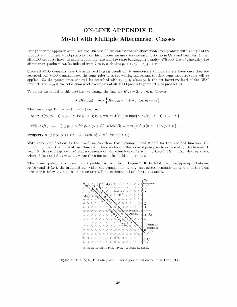
ON-LINE APPENDIX B

Model with Multiple Aftermarket Classes

Using the same approach as in Carr and Duenyas [3], we can extend the above model to a problem with a single MTSproduct and multiple MTO products. For this purpose, we use the same assumption as in Carr and Duenyas [3] thatall MTO products have the same production rate and the same backlogging penalty. Without loss of generality, theaftermarket products can be indexed from 2 to n, such that p2 + r2 ≤ · · · ≤ pn + rn.

Since all MTO demands have the same backlogging penalty, it is unnecessary to differentiate them once they areaccepted. All MTO demands have the same priority in the waiting queue, and the first-come-first-serve rule will beapplied. So the system state can still be described with (y1, y2), where y1 is the net inventory level of the OEMproduct, and −y2 is the total amount of backorders of all MTO products (product 2 to product n).

To adjust the model to this problem, we change the function Hi, i = 2, . . . , n, as follows:

HiJ(y1, y2) = maxJ(y1, y2 − 1) + pi, J(y1, y2)− ri

.

Then we change Properties (iii) and (viii) to,

(iii) ∆2f(y1, y2 − 1) ≤ pi + ri for y2 > Afi (y1), where Afi (y1) = maxz|∆2f(y1, z − 1) > pi + ri;

(viii) ∆2f(y1, y2 − 1) ≤ pi + ri for y1 + y2 > Bfi , where Bfi = maxz|∆2f(0, z − 1) > pi + ri

.

Property 4 If f(y1, y2) ∈ C2 ⊂ C1, then Bfi ≥ Bfj , for 2 ≤ i < j.

With some modifications in the proof, we can show that Lemmas 1 and 2 hold for the modified function, Hi,i = 2, . . . , n, and the updated condition set. The structure of the optimal policy is characterized by the base-stocklevel, S, the rationing level, R, and a sequence of admission levels, A2(y1), . . . , An(y1) (B2, . . . , Bn when y1 < R),where Ai(y1) and Bi, i = 2, . . . , n, are the admission threshold of product i.

The optimal policy for a three-product problem is described in Figure 7. If the total inventory, y1 + y2, is betweenA2(y1) and A3(y1), the manufacturer will reject demands for type 2, and accept demands for type 3; If the totalinventory is below A3(y1), the manufacturer will reject demands both for type 2 and 3.

y2

y1

S

B2

R


Produce 1 Accept 2

Produce 2 Accept 2

Idle

B3

Produce 1, Reject 2

Produce 2&3, Reject 2

Produce 2&3, Reject 2&3

Produce 1, Reject 2&3

1

-1-2…

Admission Thresholds

A2(y1)

A3(y1)

Figure 7: The (S, R, B) Policy with Two Types of Make-to-Order Products

38

ON-LINE APPENDIX C

Analytical Supporting Results For the OEM/Aftermarket ModelWith Contingent Outsourcing

Before proving Theorem 2, we prove Proposition 3 and Lemma 5 in the following.


Property (ix): Property (ix) is a direct result of Condition C.1.3. Since ∆2f(y1, y2) is non-increasing in y2, for agiven value of y1, there exists a threshold level, Kf (y1) = maxz|∆2f(y1, z − 1) > p2 + l2, such that ∆2f(y1, y2) ≤p2 + l2 for y2 > Kf (y1).Property (x): By contradiction, assume Kf (y1) > Af (y1). By Condition C.2.3, ∆2f(y1,K

f (y1) − 1) ≤ p2 + r2 <p2 + l2. This cannot be true, since by Property (ix), we have ∆2f(y1,K

f (y1)− 1) > p2 + l2.

The proofs for Properties (xi) and (xii) are similar to those for (iv) and (vi), thus omitted. Property (xiii) is a specialcase of the result in Property (x) when y1 < Rf .

PROOF OF LEMMA 5

The model with outsourcable aftermarket demand distinguishes original model in operator H1. So we only need togive out the proof that is related with H1. The rest of the proof is the same as for Lemma 2, and thus is omitted.

Proof for Condition C.1.1: We prove that H1f preserves Condition C.1.1, i.e., ∆iH1f(y) ≥ 0, for yi < 0, i = 1, 2.Note that we can write H1f(y + ei) = f(y + ei − e1 + ep) + p1 + g1(p), and H1f(y) = f(y − e1 + eq) + p1 + g1(q),with ep and eq equal to e0 or e2, and g1(0) = 0 and g1(2) = −p2 − l2. We have,


= f(y + ei − e1 − ep) + g1(p)− f(y − e1 − eq)− g1(q) (Above)

≥ f(y + ei − e1 − eq) + g1(q)− f(y − e1 − eq)− g1(q) (Max)

= ∆if(y − e1 − eq) (Definition)

≥ 0 (C.1.1)

Proof for Condition C.1.2: The proof is similar to the proof for Condition C.1.1, and is therefore omitted.

Proof for Condition C.1.3: We must prove that ∆1H1f(y) is non-increasing in y1 and y2.

Proof for ∆1H1f(y): For this case, we have,

∆1H1f(y) =

f(y + e1 − e1) + p1 − f(y − e1)− p1 = ∆1f(y − e1) if y2 > Kf (y1)

f(y + e1 − e1 + e2)− f(y − e1 + e2) = ∆1f(y − e1 + e2) if y2 ≤ Kf (y1 + 1)

f(y + e1 − e1)− f(y − e1 + e2) + p2 + l2 = ∆12f(y − e1) + p2 + l2 if Kf (y1) ≥ y2 > Kf (y1 + 1)

(13)

By Condition C.1.3, it is easy to see that ∆1H1f(y) is non-increasing in y1 and y2 within each individual case. Inthe following, we show it is also true across different cases. Let us denote yK = (y1, y2), such that Kf (y1) ≥ y2 >Kf (y1 +1). In the following, we will compare ∆1H1f(yK) with ∆1H1f(yK +e1), ∆1H1f(yK +e2), ∆1H1f(yK−e1)and ∆1H1f(yK − e2), one by one.

∆1H1f(yK)−∆1H1f(yK + e1) = ∆12f(yK − e1) + p2 + l2 −∆1f(yK + e1 − e1) (Equation (13))

≥ ∆12f(yK) + p2 + l2 −∆1f(yK) (C.2.1)

≥ ∆12f(yK) + ∆2f(yK)−∆1f(yK) (Property(ix))

= ∆12f(yK)−∆12f(yK) (∆12 = ∆1 −∆2)

= 0

39

∆1H1f(yK)−∆1H1f(yK − e1) = ∆12f(yK − e1) + p2 + l2 −∆1f(yK − e1 − e1 + e2) (Equation (13))

= ∆1f(yK − e1)−∆2f(yK − e1) + p2 + l2 −∆1f(yK − 2e1 + e2) (∆12 = ∆1 −∆2)

≤ ∆1f(yK − e1)−∆1f(yK − 2e1 + e2) (Property(ix))

= f(yK)− f(yK − e1)− f(yK − e1 + e2) + f(yK − 2e1 + e2) (Definition)

= ∆12f(yK − e1)−∆12f(yK − 2e1) (Definition)

≤ 0

Thus, ∆1H1f(yK) is non-increasing in y1 across the adjacent intervals at yK. We now compare ∆1H1f(yK) with∆1H1f(yK + e2) and ∆1H1f(yK − e2) to show that ∆1H1f(yK) is also non-increasing in y2 across the adjacentintervals.

∆1H1f(yK)−∆1H1f(yK + e2) = ∆12f(yK − e1) + p2 + l2 −∆1f(yK + e2 − e1) (Equation (13))

= ∆12f(yK − e1 + e2) + p2 + r2 −∆1f(yK + e2 − e1) (C.2.1)

= p2 + r2 −∆2f(yK − e1 + e2) (∆12 = ∆1 −∆2)

= p2 + r2 −∆2f(yK) (C.2.4)

≥ 0 (Property(ix))

∆1H1f(yK)−∆1H1f(yK − e2) = ∆12f(yK − e1) + p2 + l2 −∆1f(yK − e1 − e1 − e2) (Equation (13))

≤ ∆12f(yK − 2e1 − e2) + p2 + l2 −∆1f(yK − 2e1 − e2) (C.2.1)

= p2 + r2 −∆2f(yK − 2e1 − e2) (∆12 = ∆1 −∆2)

≤ 0 (Property(ix))

Therefore, ∆1H2f(yK) is also non-increasing in y2 across the adjacent intervals at yK.

Proof for ∆2H1f(y): We have,

∆2H1f(y) =

f(y + e2 − e1) + p1 − f(y − e1)− p1 = ∆2f(y − e1) if y2 > Kf (y1)

f(y + e2 − e1)− f(y − e1 + e2) + p2 + l2 = p2 + l2 if y2 = Kf (y1)

f(y + e2 − e1 + e2)− f(y − e1 + e2) = ∆2f(y − e1 + e2) if y2 < Kf (y1)

According to Condition C.1.3, we know that ∆2f(y) is non-increasing in y1 and y2. Therefore, ∆2H2(y) is non-increasing in y1 and y2 when y2 < Kf (y1) or when y2 > Kf (y1). Using the same approach as in the proof of∆1H1f(y), it is easy to prove that ∆2H1(y) is non-increasing in y1 and y2.

Proof for Condition C.1.4: We must prove that ∆12H1f(y) is non-increasing in y1 and non-decreasing in y2.

Proof for ∆12H1f(y): For this case, we have,

∆12H1f(y) =

f(y + e1 − e1) + p1 − f(y + e2 − e1)− p1 = ∆12f(y − e1) if y2 > Kf (y1 + 1)

f(y + e1 − e1 + e2)− p2 − l2 − f(y + e2 − e1) = ∆1f(y − e1 + e2)− p2 − l2 if Kf (y1)− 1 < y2 ≤ Kf (y1 + 1)

f(y + e1 − e1 + e2)− f(y + e2 − e1 + e2) = ∆12f(y − e1 + e2) if y2 ≤ Kf (y1)− 1

Using the same argument as in the proof of ∆1H1f(y), it is easy to prove that ∆12H1(y) is non-increasing in y1 andnon-decreasing in y2.

Proof for Condition C.2.1: We prove that ∆12H1f(y) is non-increasing in y1 and is independent of y2. Bydefinition, ∆12H1f(y) = H1f(y + e1)−H1f(y + e2), so we have,

∆12H1f(y) =

f(y + e1 − e1) + p1 − f(y + e2 − e1)− p1 = ∆12f(y − e1) if y1 + y2 ≥ Lff(y + e1 − e1 + e2)− f(y + e2 − e1 + e2) = ∆12f(y − e1 + e2) if y1 + y2 < Lf

Using the same argument as in the proof for Condition C.1.3, it is easy to show that ∆12H1f(y) is independent ofy2.

Proof for Condition C.2.2: Condition C.2.2 is a direct result of Condition C.2.1.

40

Proof for Condition C.2.3: The proof for Condition C.2.3 is the same as in Lemma 2.

Proof for Condition C.2.4: Condition C.2.4 can be derived from Condition C.2.1 as shown in the proof for Lemma2.

PROOF OF THEOREM 2

Proof. The proof of the production, rationing, and admission control policies are the same as in Theorem 1, so weonly discuss the outsourcing control policy.

When an order for type 1 arrives, the outsourcing control for type 2 orders depends on the sign of p2+l2−∆2J(y1, y2):outsource an order if the sign is negative, and do not outsource otherwise. When y1 < R, by Conditions C.1.3 andC.4.3, the optimal cancelation policy is to outsource a type 2 order if y1 + y2 ≤ L∗; When y1 ≥ R, by ConditionsC.1.3 and C.2.6, the optimal cancelation policy is to outsource a type 2 order if y2 ≤ K(y1)

ON-LINE APPENDIX D

Analytical Supporting Results For the Model withCustomized/Preconfigured Products

Before proving Theorem 3, we first define a set D of functions such that if f(y1, y2) ∈ D, then,

• Condition D.1: For (y1, y2) ∈ Ω,

D.1.1: ∆if(y1, y2) ≥ 0, if yi < 0, i = 1, 2.

D.1.2: ∆1f(y1, y2) ≤ p1 + r1, if y1 ≥ 0.

D.1.3: ∆12f(y1, y2) ≤ 0.

• Condition D.2: For (y1, y2) ∈ Ω,

D.2.1: ∆1f(y1, y2) is non-increasing in y1 and y2.

D.2.2: ∆1f(y1, y2) ≥ 0 for y1 < S, where S = minz|∆1f(z, 0) < 0.

• Condition D.3: For (y1, y2) ∈ Ω, y1 < 0,

D.3.1: ∆1f(y1, y2) is independent of y1 and y2 as long as y1 + y2 is fixed.

D.3.2: ∆1f(y1 − 1, y2) ≤ p1 + r1 for y1 + y2 > B, where B = maxz|∆1f(z − 1, 0) > p1 + r1.

To get some intuition on the above conditions, we apply the condition set D to the expected profit, J(y1, y2).Condition D.1.1 implies that if there are orders in any class, the production line needs to keep producing. ConditionD.1.2 implies that if the inventory for type 1 product is available, it is profitable to satisfy demand for type 1 product.Condition D.1.3 implies that an order for type 2 always has a higher priority than for type 1. Condition D.2.1 impliesthat the marginal benefit of increasing y1 is non-increasing in both y1 and y2. Condition D.2.2 implies that if y1 < S,then it is profitable to produce product 1. Since the sign of p1 + r1 −∆1J(y1 − 1, y2) determines whether to rejectan order for type 1, Condition D.3.1 suggests that the rejection decisions depend on total inventory level. ConditionD.3.2 implies that accepting an arriving demand for type 1 is profitable as long as the level of inventory satisfies∑n

i=1yi > B.

We show in Proposition 5 that under the optimal conditions, the threshold level B is non-positive. Therefore, itis always optimal to satisfy promotional demands when the inventory is available.

Property 5 If f(y1, y2) ∈ D, then B ≤ 0.

41

Proof. By contradiction, assume B > 0, i.e., B ≥ 1. By Condition D.3.2, ∆1f(0, 0) > p1 + r1, which cannot be truesince we know that ∆1f(0, 0) ≤ p1 + r1 by Condition D.1.2.

The following lemma shows that the structure of the functions in D is preserved under function H.

Lemma 8 If f(y1, y2) ∈ D, then Hf(y1, y2) ∈ D.

Proof. We show that function H preserves each condition in D. Proofs for Conditions D.1.1, D.1.2, and D.1.3 aresimilar to the proof for Condition C.1.1, and are therefore omitted.

Proof for Condition D.2.1:

Proof for ∆1H0f(y): We first prove that ∆1H0f(y) is non-increasing in y1 and y2. By definition, ∆1H0f(y) =H0f(y + e1)−H0f(y), so we have,

∆1H0f(y) =

f(y + e1 + e2)− f(y + e2) = ∆1f(y + e2) if y2 < 0f(y + 2e1)− f(y + e1) = ∆1f(y + e1) if y2 = 0, y1 < S − 1f(y + e1)− f(y + e1) = 0 if y2 = 0, y1 = S − 1f(y + e1)− f(y) = ∆1f(y) if y2 = 0, y1 > S − 1

By D.2.1, ∆1f(y) is non-increasing in y1 and y2, so ∆1H0f(y) is non-increasing in y1 and y2 within each of the abovefour sub-condition intervals. In the following, we show that ∆1H0f(y) is also non-increasing in y1 and y2 across anyadjacent intervals. We only present the proof for the case where y1 = S − 1 and y2 = 0. The proof for other casesare similar and are therefore omitted.

When y1 = S − 1 and y2 = 0, let us denote yS = (S − 1, 0). Then we have,

∆1H0f(yS + e1) = ∆1f(yS + e1)

∆1H0f(yS) = 0

∆1H0f(yS − e1) = ∆1f(yS)

By D.2.2, we have ∆1f(yS + e1) ≤ 0 ≤ ∆1f(yS), so ∆1H0f(y) is non-increasing in y1 across the adjacent intervalsat yS.

Notice that,∆1H0f(yS − e2) = ∆1f(yS)

so for the same reason, ∆1H0f(y) is non-increasing in y2 across the adjacent intervals at yS.

Proof for ∆1H1f(y): Now we prove that ∆1H1f(y) is non-increasing in y1 and y2. By definition, ∆1H1f(y) =H1f(y + e1)−H1f(y), so we have,

∆1H1f(y) =

f(y + e1 − e1) + p1 − f(y − e1)− p1 = ∆1f(y − e1) if y1 > 0f(y + e1 − e1) + p1 − f(y − e1)− p1 = ∆1f(y − e1) if y1 + y2 > B, y1 ≤ 0f(y + e1 − e1) + p1 − f(y) + r1 = p1 + r1 if y1 + y2 = B, y1 ≤ 0f(y + e1)− r1 − f(y − e1) + r1 = ∆1f(y) if y1 + y2 < B, y1 ≤ 0

By D.2.1, ∆1f(y) is non-increasing in y1 and y2, so ∆1H1f(y) is non-increasing in y1 and y2 within each of the foursub-condition intervals. In the following, we show that ∆1f(y) is non-increasing in y1 and y2 across any two adjacentintervals. We only present the proof for the third interval, since the proofs for other intervals are similar.

Let us denote yB = (y1, y2), such that y1 + y2 = B and y1 ≤ 0. With the above results, we have,

∆1H1f(yB + e1) = ∆1f(yB)

∆1H1f(yB) = p1 + r1

∆1H1f(yB − e1) = ∆1f(yB − e1)

∆1H1f(yB + e2) = ∆1f(yB + e2 − e1)

∆1H1f(yB − e2) = ∆1f(yB − e2)

42

Condition D.3.1 and D.3.2 imply that ∆1f(yB + e2 − e1) = ∆1f(yB) ≤ p1 + r1 ≤ ∆1f(yB − e1) = ∆1f(yB − e2),so ∆1H1f(y) is non-increasing in y1 and y2 across the adjacent intervals at yB.

Proof for ∆1H2f(y): Now we prove that ∆1H2f(y) is non-increasing in y1 and y2. We have

∆1H2f(y) = H2f(y + e1)−H2f(y) = f(y + e1 − e2)− f(y − e2) = ∆1f(y − e2).

By D.2.1, it is clear that ∆1H2f(y) is non-increasing in y1 and y2.

Proof for ∆1c(y): Finally for c1(y) we have

∆1c1(y) = c1(y + e1)− c1(y) =

b1(y1 + 1)− b1y1 = b1 if y1 < 0;−h(y1 + 1) + hy1 = −h if y1 ≥ 0.

which is non-increasing in y1 and y2. In Conclusion, ∆1Hf(y) is non-increasing in y1 and y2.

Proof for Condition D.2.2: Condition D.2.2 is a direct result of Condition D.2.1.

Proof for Condition D.3.1: We first prove that ∆12f(y1, y2) = ∆12f(y1 − 1, y2) for y1 < 0. By definition,∆12H0f(y) = H0f(y + e1)−H0f(y + e2), so we have,

∆12H0f(y) =

f(y + e1 + e2)− f(y + 2e2) = ∆12f(y + e2) if y2 < −1f(y + e1 + e2)− f(y + e2 + e1) = 0 if y2 = −1

∆12H1f(y) =

f(y + e1 − e1) + p1 − f(y + e2 − e1)− p1 = ∆12f(y − e1) if y1 + y2 ≥ Bf(y + e1)− r1 − f(y + e2) + r1 = ∆12f(y) if y1 + y2 < B

∆12H2f(y) = f(y + e1 − e2)− f(y + e2 − e2) = ∆12f(y − e2)

Noting that ∆12c1(y) = b1 is independent of y1 for y1 < 0, and ∆12f(y1, y2) = ∆12f(y1 − 1, y2), so ∆12Hf(y1, y2) =∆12Hf(y1 − 1, y2).

Then we have

∆12f(y) = ∆12f(y + e1)

⇒ f(y + e1)− f(y + e2) = f(y + e1 + e1)− f(y + e1 + e2) (Definition)

⇒ f(y + e1 + e2)− f(y + e2) = f(y + e1 + e1)− f(y + e1) (Rearrangement)

⇒ ∆1f(y + e2) = ∆1f(y + e1) (Definition)

Therefore, we have ∆1f(y) = ∆1f(y + e1− e2), and Condition D.3.1 can be derived by adding 1 to one element anddeducing 1 form another element in vector y in the above result.

Proof for Condition D.3.2: Condition D.3.2 can be directly deduced from Conditions D.2.1 and D.3.1.

PROOF OF THEOREM 3

The proof for the existence of the optimal policies is similar to the proof in Theorem 1, and is therefore omitted.

From equation (7), we see that when there are no orders from any classes, the optimal production control onlydepends on the sign of ∆1J1(y1, y2): produce if it is positive, or do not produce otherwise. So by Condition D.2.2,it is optimal to produce if y1 < S. When there are orders, by Conditions D.1.1 and D.1.2, it is always optimal toproduce for the order with the highest priority.

The admission control for an arriving demand for type 1 depends on the sign of p1 + r1 −∆1J1(y1 − 1, y2): satisfyor backlog the demand if the sign is positive; reject otherwise. So, by Condition D.1.2, the optimal admission policyis to satisfy an arriving demand for type 1 from inventory if y1 > 0, and to reject if y1 < 0 and y1 + y2 ≤ B byCondition D.3.2.

43

PROOF OF LEMMA6

The proof is similar to that for Lemma 3, and thus is omitted.

PROOF OF LEMMA7

The proof is similar to that for Lemma 4, and thus is omitted.

ON-LINE APPENDIX E

Analytical Supporting Results for Customized/ReconfiguredModel with Contingent Outsourcing

Before proving Theorem 4, we first add the following condition to D, and denote the new condition set as D′:

• Condition D.3: For (y1, y2) ∈ Ω, y1 < 0,

D.3.3: ∆1f(y1 − 1, y2) ≤ p1 + l1 for y1 + y2 > L, where L = maxz|∆1f(z − 1, 0) > p1 + l1

.

Condition D.3.3 suggests that outsourcing decision for an order of the type 1 product depends on total inventorylevel, but not the number of orders of type 1 itself. It implies that outsourcing an order of product 1 is profitablewhen y1 + y2 ≤ L.

Then we show that under the optimal conditions, threshold level B cannot be lower than L.

Property 6 If f(y1, y2) ∈ D′, then L ≤ B.

Proof:By contradiction, assume L > B. By Condition D.3.2, ∆1f(L−1, 0) ≤ p1 + r1 < p1 + l1. This cannot be true,since by Condition D.3.3 we have ∆1f(L− 1, 0) > p1 + l1.

PROOF OF THEOREM 4

The proof of the production and admission control policies are the same as in Theorem 3, so we only discuss theoutsourcing control policy.

After accepting a demand for a higher-priority product, the outsourcing control for type 1 orders depends on thesign of p1 + l1 − ∆1J1(y1, y2): outsource an order if the value is negative, and do not outsource otherwise. So byConditions D.2.2 and D.3.2, the optimal cancelation policy is to outsource a type 1 order if y1 + y2 ≤ L.

44

ON-LINE APPENDIX F

Heuristic for (S,R,B) Thresholds in OEM/Aftermarket Case

Although the linear (S,R,B) structure greatly simplifies the optimal policy, the value iteration approach itself mayrequire a large amount of computation. In this section, we extend de Vericourt et al.’s algorithm to speed up thesearching process for the thresholds.

For a problem with two demand classes and a rationing level R, de Vericourt et al.’s algorithm first solves a subproblemof a make-to-stock M/M/1 queue with holding cost h + b2 and backorder cost b1 − b2. The average cost minimizerfor the subproblem is the optimal rationing level for the main problem. We adopted this idea and treat the OEMproduct’s inventory level as a make-to-stock M/M/1 queue with holding cost h+b2 and backorder cost b1−b2. Giventhe base-stock level, R, and let Ψi be the steady state probability when y1(t) = i, the total cost function g1(R) ofthe M/M/1 subproblem is as follows.

g1(R) = (h+ b2)

R∑i=0

iΨi + (b1 − b2)

−1∑i=−∞

(−i)Ψi

= (h+ b2)

R∑i=0

iΨi + (b1 − b2)[ R∑i=−∞

(−i)Ψi −R∑i=0

(−i)Ψi

]= (h+ b2 + b1 − b2)

R∑i=0

iΨi + (b1 − b2)

R∑i=−∞

(−i)Ψi

= (h+ b1)

R∑i=0

iΨi + (b1 − b2)[ R∑i=−∞

(R− i)Ψi −R]

Note that R−y1(t) is the number of customers in an M/M/1 queue, and as a result,∑R

i=−∞ (R− i)Ψi is the average

queue length, which is λ1µ1−λ1

. Also note that∑R

i=0iΨi is the average queue length for a M/M/1/R queue (where R

is the capacity), L1 = λ[1+R(λ/µ)R+1−(R+1)(λ1/µ1)R]

(u1−λ1)(1−(λ1/µ1)R+1). Denote RH = arg ming1(R) : R ∈ Z+ be the optimal solution

and g∗1 = g1(RH) as the optimal time-average cost of the subproblem.

We take the optimal base-stock level RH of the above subproblem as the rationing level of the heuristic algorithmin the main problem. Given base-stock level S (S ≥ RH) and backlog-up-to level B (B ≤ 0) , the main problem’sinstantaneous cost function (not including the rejection penalty for aftermarket demand) is:

c(y1, y2) = hy+1 + b1y

−1 − b2y2 = (h+ b2)y+

1 + (b1 − b2)y−1 − b2(y1 + y2) = c′(y1) + b2[S − (y1 + y2)− S

],

where c′(y1) = (h+ b2)y+1 + (b1− b2)y−1 is the instantaneous cost function for the subproblem. The time-average cost

function of the system is

g2(S,B) = E[c(y1(t), y2(t))

]+ (p2 + r2)λ2Prb(y1(t) + y2(t) ≤ B)

= E[c′(y1(t))

]+ b2E

[S − (y1(t) + y2(t))− S

]+ (p2 + r2)λ2Prb(y1(t) + y2(t) ≤ B)

= E[c′(y1(t))

∣∣y1(t) ≤ RH ]Prb(y1(t) ≤ RH) + E[c′(y1(t))

∣∣y1(t) > RH ]Prb(y1(t) > RH)

+(p2 + r2)λ2Prb(y1(t) + y2(t) ≤ B) + b2E[S − (y1(t) + y2(t))− S

]To calculate this cost function, we use the following birth-death queue to approximate the original system. Let γijbe the transition rate from state i to state j,

γij =

λ if j = i+ 1, j ≤ S −Bλ1 if j = i+ 1, j > S −Bµ if j = i− 1, j < S −Bµ1 if j = i− 1, j ≥ S −B0 if otherwise

45

In this birth-death queue, state i corresponds to y1 + y2 = S − i in the original system. We use λ = λ1 + λ2 andµ = (λ1+λ2)µ1µ2

λ1µ2+λ2µ1to approximate the forward transition rate and backward rate when i ≤ S − B. Then we use the

following function to calculate g2(S,B),

g2(S,B) = g∗1(1−S−RH−1∑

i=0

Θi) + (h+ b2)

S−RH−1∑i=0

(iΘi) + (p2 + r2)λ2

∞∑i=S−B

Θi + b2(L2 − S)

where L2 is the average length of the birth-death queue. Searching for the minimizers of g2(S,B), we get the heuristicestimate of SH and BH .

We perform an extensive numerical study with 16,000 cases to evaluate the performance of the heuristic algorithm.The performance measure is defined as

PM =Jopt − Jheu

Jopt× 100%,

where Jheu is the system’s time-average profit using the heuristic thresholds (SH , RH , BH), and Jopt is the system’soptimal time-average profit.

Our numerical study shows that, on average, the heuristic algorithm results in 3.6% less profit than the optimalpolicy. In 10,194 (out of 16,000) cases, the error is within 2%. Larger errors happen when u2 is significantly smallerthan µ1. Intuitively, this is because the heuristic algorithm does not distinguish the difference in processing time forthe two types of orders when calculating g2(S,B).

46

ON-LINE APPENDIX G

Heuristic for (S,B) Thresholds in Customized/Pre-configuredCase

For the model with customized and pre-configured products, the optimal policy only controls the production andorder admission for the pre-configured product. Therefore, in the heuristic policy, we approximate the system witha birth-death queue only of the pre-configured product. Let γij be the transition rate from state i to state j,

γij =

λ1 if j = i+ 1, j ≤ S −Bµ′1 if j = i− 1, j < S −B0 if otherwise

where µ′1 = µ1 − λ2µ1/µ2. In this birth-death queue, state i corresponds to y1 = S − i in the original system. Letρ1 = λ1/µ

′1, and notice the following relation between the steady state probability of each state, Θi+1 = ρ1Θi, for

i = 0, 1, . . . , S −B − 1, the probability of state 0 is Θ0 = (1− ρ1)/(1− ρS−B+11 ).

The time-average cost function of the birth-death queue is

g(S,B) = h

S∑i=0

(S − i)Θi + b1

S−B∑i=S+1

(i− S)Θi + (p1 + r1)λ1ΘS−B

= Θ0

[h

S∑i=0

(S − i)ρi1 + b1

S−B∑i=S+1

(i− S)ρi1 + (p1 + r1)λ1ρS−B1

]

Searching for the minimizers of g(S,B), we get the heuristic estimate of SH and BH .

We perform an extensive numerical study with 16,000 cases to evaluate the performance of the heuristic algorithm.Our numerical study shows that, on average, the heuristic algorithm results in 3.1% less profit than the optimal policy.In 11,812 (out of 16,000) cases, the error is within 2%. Larger errors happen when the ratio λ2 is considerately large.Intuitively, this is because the heuristic algorithm does not consider the impact of type 2 orders.

47

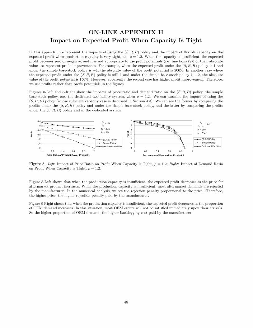
ON-LINE APPENDIX H

Impact on Expected Profit When Capacity Is Tight

In this appendix, we represent the impacts of using the (S,R,B) policy and the impact of flexible capacity on theexpected profit when production capacity is very tight, i.e., ρ = 1.2. When the capacity is insufficient, the expectedprofit becomes zero or negative, and it is not appropriate to use profit potentials (i.e. functions (9)) or their absolutevalues to represent profit improvements. For example, when the expected profit under the (S,R,B) policy is 1 andunder the simple base-stock policy is −1, the absolute value of the profit potential is 200%; In another case wherethe expected profit under the (S,R,B) policy is still 1 and under the simple base-stock policy is −2, the absolutevalue of the profit potential is 150%. However, apparently the second case has higher profit improvement. Therefore,we use profits rather than profit potentials in the figures.

Figures 8-Left and 8-Right show the impacts of price ratio and demand ratio on the (S,R,B) policy, the simplebase-stock policy, and the dedicated two-facility system, when ρ = 1.2. We can examine the impact of using the(S,R,B) policy (whose sufficient capacity case is discussed in Section 4.3). We can see the former by comparing theprofits under the (S,R,B) policy and under the simple base-stock policy, and the latter by comparing the profitsunder the (S,R,B) policy and in the dedicated system.

-2

-1.6

-1.2

-0.8

-0.4

0

0.4

1 1.2 1.4 1.6 1.8 2


Prof

it

(S,R,B) PolicySimple PolicyDedicated Facilities

%5%20

7.0

2

1

21

1

==

=+

bb

λλλ

%5%20

6.1

2

1

1

2

==

=

bbpp

-8

-6

-4

-2

0

2

4

0 0.2 0.4 0.6 0.8 1

Percentage of Demand for Product 1

Prof

it

(S,R,B) Policy

Simple Policy

Dedicated Facilities

Figure 8: Left: Impact of Price Ratio on Profit When Capacity is Tight, ρ = 1.2; Right: Impact of Demand Ratioon Profit When Capacity is Tight, ρ = 1.2.

Figure 8-Left shows that when the production capacity is insufficient, the expected profit decreases as the price foraftermarket product increases. When the production capacity is insufficient, most aftermarket demands are rejectedby the manufacturer. In the numerical analysis, we set the rejection penalty proportional to the price. Therefore,the higher price, the higher rejection penalty paid by the manufacturer.

Figure 8-Right shows that when the production capacity is insufficient, the expected profit decreases as the proportionof OEM demand increases. In this situation, most OEM orders will not be satisfied immediately upon their arrivals.So the higher proportion of OEM demand, the higher backlogging cost paid by the manufacturer.

48

ON-LINE APPENDIX I

MDP Formulations for Erlang Model

The system described in Section 5 incurs an inventory holding and backlogging cost at rate,

c(x1, x2, ·, ·, ·) = −hb x+1

m1c − b1b

x−1m1c+ b2b

x2

m2c. (14)

Let Λ = γ1 + γ2 + K1λ1 + K2λ2. The optimal profit function J∗(x1, x2, k1, k2) under the time-discount criterion(defined by replacing y(0) with x(0) in Equation (1)) satisfies the following equation:

J(x1, x2, k1, k2) =1

Λ

c(x1, x2, ·, ·) +H0J(x1, x2, k1, k2) +K1λ1H1J(x1, x2, k1, k2) +K2λ2H2J(x1, x2, k1, k2)

(15)

where H0, H1, and H2 are functions defined by,

H0J(x1, x2, k1, k2) = max

γ1J(x1, x2, k1, k2) + γ2J(x1, x2, k1, k2),γ1J(x1 + 1, x2, k1, k2) + γ2J(x1, x2, k1, k2),γ1J(x1, x2, k1, k2) + γ2J(x1, x2 + 1, k1, k2|x2 < 0).

H1J(x1, x2, k1, k2) =

J(x1, x2, k1 − 1, k2) if k1 > 1J(x1 −m1, x2,K1, k2) + p1 if k1 = 1

H2J(x1, x2, k1, k2) =

J(x1, x2, k1, k2 − 1) if k2 > 1max[J(x1, x2 −m2, k1,K2) + p2, J(x1, x2, k1,K2)− r2] if k2 = 1

H0 corresponds to the production decision: the manufacturer can idle, or choose to produce a phase for either typeof product. H1 indicates that an OEM demand arrives when the number of phases decreases from K1 to 1, and thework storage level of type 1 is decreased by m1 units as the demand is accepted. H2 indicates that an aftermarketdemand arrives when the number of phases decreases from K2 to 1. The manufacturer can either reject or accept anaftermarket demand. If the demand is accepted, the work storage level of type 2 is decreased by m2 units.

The optimal profit function J∗(x1, x2, k1, k2) under the average-profit criterion (defined by replacing y(0) with x(0)in Equation (2)) satisfies the following equation:

J(x1, x2, k1, k2)+g =1

Λ

c(x1, x2, ·, ·)+H0J(x1, x2, k1, k2)+K1λ1H1J(x1, x2, k1, k2)+K2λ2H2J(x1, x2, k1, k2)

(16)

where g is the optimal average profit.

49

Optimal Production and Admission Policies in Make-to-Stock ...

Documents

Transcript of Optimal Production and Admission Policies in Make-to-Stock ...