Ol

MS

a

ARRAA

KOPTMO

1

sc

ioba&

ptamMipadpt

N

h0

Computers and Chemical Engineering 65 (2014) 67–80

Contents lists available at ScienceDirect

Computers and Chemical Engineering

j ourna l ho me pa g e: www.elsev ier .com/ locate /compchemeng

ptimal planning of oil and gas development projects consideringong-term production and transmission

. Shakhsi-Niaei ∗, S.H. Iranmanesh, S.A. Torabichool of Industrial Engineering, College of Engineering, University of Tehran, Tehran, Iran

r t i c l e i n f o

rticle history:eceived 17 May 2013eceived in revised form 5 December 2013ccepted 6 March 2014vailable online 14 March 2014

a b s t r a c t

This paper proposes an integrated model for making a group of strategic decisions about oil and gasdevelopment projects simultaneously over a long-term planning horizon. These decisions involve: selec-tion of field and pipeline development projects, scheduling of selected projects, production planning,and upstream transmission planning. The proposed model is formulated as a linear mixed-integer-programming model. It is implemented in a case study to demonstrate its usefulness and applicability in

eywords:il and gas developmentroduction planningransmission planningathematical modeling

practice. Finally, a number of sensitivity analyses are carried out to analyze the impact of most influentialuncertainties on the solutions and the corresponding results are discussed.

© 2014 Elsevier Ltd. All rights reserved.

ptimization

. Introduction

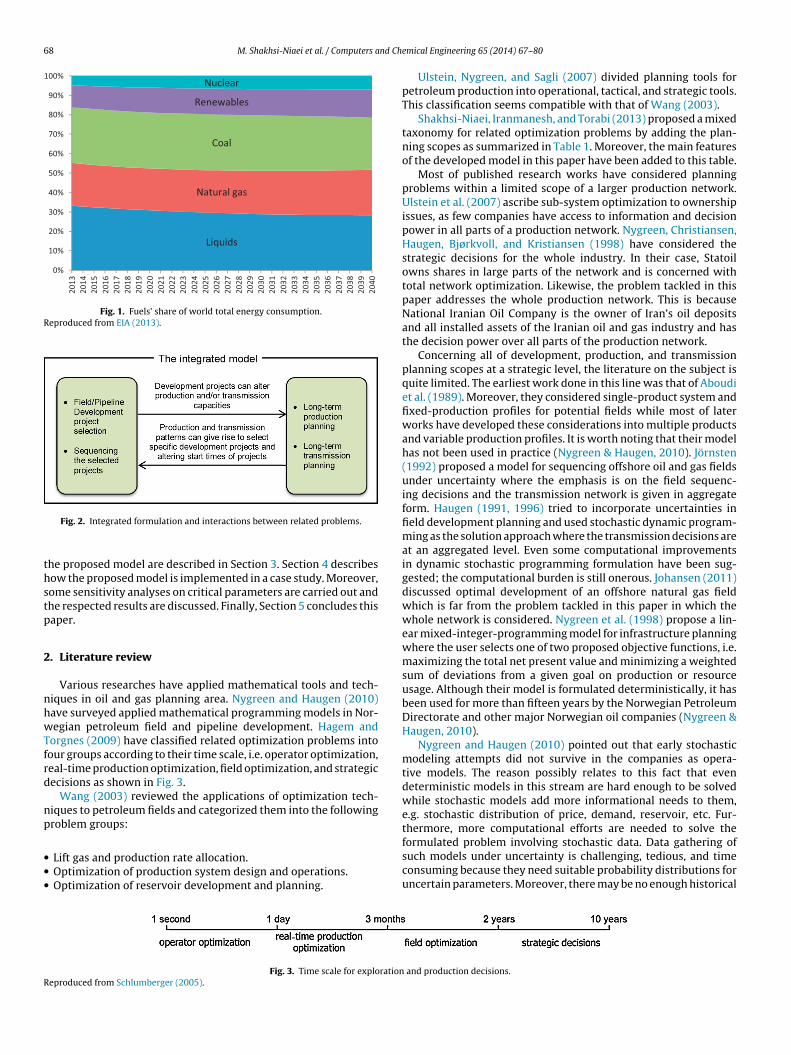
Liquid fuels and natural gas are expected to remain the majorource of energy in long-term horizon, having an estimated 50 per-ent consumption share (EIA, 2013) (Fig. 1).

As oil and gas resources have a limited availability, themportance of their planning activities rises. Optimal planningf oil and gas field development projects is an important issueecause the corresponding investment decisions are irreversiblend huge finance is committed over a long-term horizon (Huseby

Haavardsson, 2009).Among the candidate development projects, some of them

roduce oil and/or gas, while others add some capacities forransmission of the products. Basic field development decisionsre twofold: selection among the best candidate field develop-ent projects and sequencing/scheduling the selected projects.oreover, production and transmission plans have considerable

nteractions with selection and scheduling decisions. For exam-le, consider an existing production field, a demand node, andn existing pipeline which transmits the product(s) from the pro-

uction field to the demand node. After selecting and executing aipeline-development project, adding a new parallel pipeline, theransmission capacity will be increased. If the production amount

∗ Corresponding author. Tel.: +98 21 88021067; fax: +98 21 88013102.E-mail addresses: m.niaei@alumni.ut.ac.ir, msn83ie@yahoo.com (M. Shakhsi-

iaei), hiranmanesh@ut.ac.ir (S.H. Iranmanesh), satorabi@ut.ac.ir (S.A. Torabi).

ttp://dx.doi.org/10.1016/j.compchemeng.2014.03.002098-1354/© 2014 Elsevier Ltd. All rights reserved.

from the field was previously restricted to the former transmis-sion capacity, now it might be decided to increase the productionamount if it is economically feasible. In that case, both of pro-duction and transmission plans will be changed according to theproject selection decision. On the other hand, a higher level of pro-duction, as a production planning decision, may lead to selectionand execution of a new pipeline-development project if the currentpipeline is not able to transmit the increased amounts of productsand also if the benefits of the extra production amounts are higherthan pipeline development expenses.

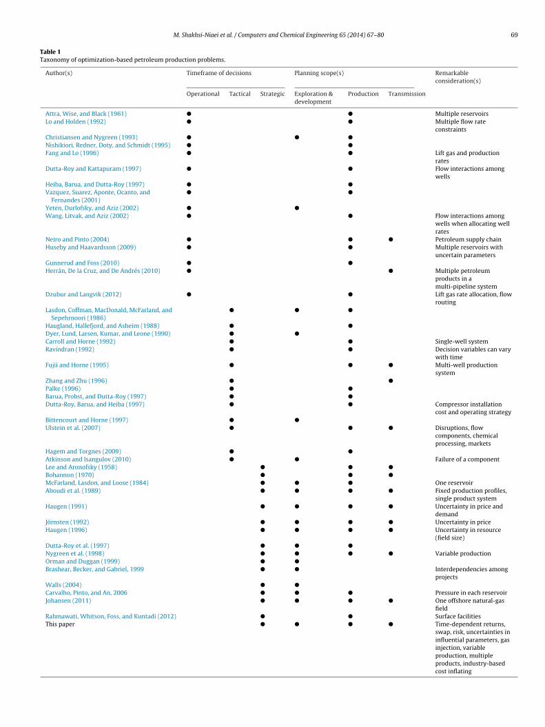
These bidirectional interactions enforce to formulate an inte-grated decision model by incorporating long-term production andtransmission decisions into a selection and scheduling optimiza-tion model. The main advantages of such integral planning are:(1) making the model more practical by accounting for some factsexisting in the reality which is neglected in many oil-and-gasproject selection models and (2) avoiding from sub-optimality aris-ing from solving these interrelated problems separately. On theother hand, the main barrier for this integrated model is that itneeds a more complex and time consuming data gathering pro-cess which is absolutely justifiable for such a long-term decisionproblem with huge financial consequences. Fig. 2 shows the com-ponents of our integrated model and their interactions. Because ofthe long-term horizon of the model and also its inherent complex-

ity, the scope of upstream network is covered and the forecasteddemand of midstream/downstream network is used as input data.

The rest of the paper is organized as follows. The relevant litera-ture is reviewed in Section 2. The details of the tackled problem and

68 M. Shakhsi-Niaei et al. / Computers and Ch

Liquid s

Natural gas

Coal

Renewables

Nuclear

0%

10%

20%

30%

40%

50%

60%

70%

80%

90%

100%20

1320

1420

1520

1620

1720

1820

1920

2020

2120

2220

2320

2420

2520

2620

2720

2820

2920

3020

3120

3220

3320

3420

3520

3620

3720

3820

3920

40

Fig. 1. Fuels’ share of world total energy consumption.Reproduced from EIA (2013).

thstp

2

nhwTfrd

np

•••

formulated problem involving stochastic data. Data gathering of

R

Fig. 2. Integrated formulation and interactions between related problems.

he proposed model are described in Section 3. Section 4 describesow the proposed model is implemented in a case study. Moreover,ome sensitivity analyses on critical parameters are carried out andhe respected results are discussed. Finally, Section 5 concludes thisaper.

. Literature review

Various researches have applied mathematical tools and tech-iques in oil and gas planning area. Nygreen and Haugen (2010)ave surveyed applied mathematical programming models in Nor-egian petroleum field and pipeline development. Hagem and

orgnes (2009) have classified related optimization problems intoour groups according to their time scale, i.e. operator optimization,eal-time production optimization, field optimization, and strategicecisions as shown in Fig. 3.

Wang (2003) reviewed the applications of optimization tech-iques to petroleum fields and categorized them into the followingroblem groups:

Lift gas and production rate allocation.Optimization of production system design and operations.Optimization of reservoir development and planning.

Fig. 3. Time scale for explorationeproduced from Schlumberger (2005).

emical Engineering 65 (2014) 67–80

Ulstein, Nygreen, and Sagli (2007) divided planning tools forpetroleum production into operational, tactical, and strategic tools.This classification seems compatible with that of Wang (2003).

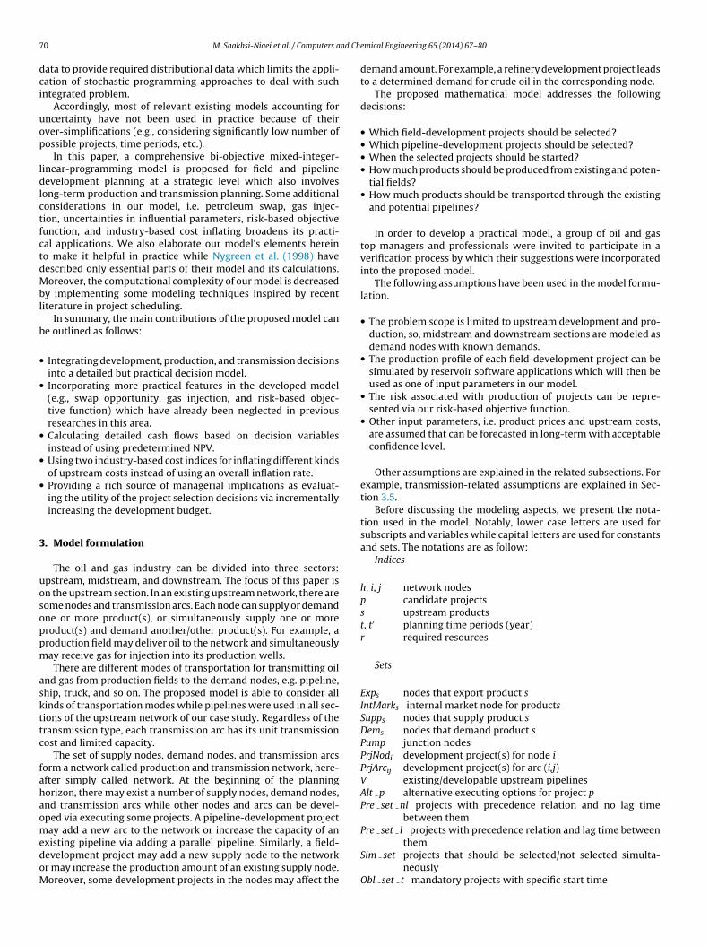
Shakhsi-Niaei, Iranmanesh, and Torabi (2013) proposed a mixedtaxonomy for related optimization problems by adding the plan-ning scopes as summarized in Table 1. Moreover, the main featuresof the developed model in this paper have been added to this table.

Most of published research works have considered planningproblems within a limited scope of a larger production network.Ulstein et al. (2007) ascribe sub-system optimization to ownershipissues, as few companies have access to information and decisionpower in all parts of a production network. Nygreen, Christiansen,Haugen, Bjørkvoll, and Kristiansen (1998) have considered thestrategic decisions for the whole industry. In their case, Statoilowns shares in large parts of the network and is concerned withtotal network optimization. Likewise, the problem tackled in thispaper addresses the whole production network. This is becauseNational Iranian Oil Company is the owner of Iran’s oil depositsand all installed assets of the Iranian oil and gas industry and hasthe decision power over all parts of the production network.

Concerning all of development, production, and transmissionplanning scopes at a strategic level, the literature on the subject isquite limited. The earliest work done in this line was that of Aboudiet al. (1989). Moreover, they considered single-product system andfixed-production profiles for potential fields while most of laterworks have developed these considerations into multiple productsand variable production profiles. It is worth noting that their modelhas not been used in practice (Nygreen & Haugen, 2010). Jörnsten(1992) proposed a model for sequencing offshore oil and gas fieldsunder uncertainty where the emphasis is on the field sequenc-ing decisions and the transmission network is given in aggregateform. Haugen (1991, 1996) tried to incorporate uncertainties infield development planning and used stochastic dynamic program-ming as the solution approach where the transmission decisions areat an aggregated level. Even some computational improvementsin dynamic stochastic programming formulation have been sug-gested; the computational burden is still onerous. Johansen (2011)discussed optimal development of an offshore natural gas fieldwhich is far from the problem tackled in this paper in which thewhole network is considered. Nygreen et al. (1998) propose a lin-ear mixed-integer-programming model for infrastructure planningwhere the user selects one of two proposed objective functions, i.e.maximizing the total net present value and minimizing a weightedsum of deviations from a given goal on production or resourceusage. Although their model is formulated deterministically, it hasbeen used for more than fifteen years by the Norwegian PetroleumDirectorate and other major Norwegian oil companies (Nygreen &Haugen, 2010).

Nygreen and Haugen (2010) pointed out that early stochasticmodeling attempts did not survive in the companies as opera-tive models. The reason possibly relates to this fact that evendeterministic models in this stream are hard enough to be solvedwhile stochastic models add more informational needs to them,e.g. stochastic distribution of price, demand, reservoir, etc. Fur-thermore, more computational efforts are needed to solve the

such models under uncertainty is challenging, tedious, and timeconsuming because they need suitable probability distributions foruncertain parameters. Moreover, there may be no enough historical

and production decisions.

M. Shakhsi-Niaei et al. / Computers and Chemical Engineering 65 (2014) 67–80 69

Table 1Taxonomy of optimization-based petroleum production problems.

Author(s) Timeframe of decisions Planning scope(s) Remarkableconsideration(s)

Operational Tactical Strategic Exploration &development

Production Transmission

Attra, Wise, and Black (1961) � � Multiple reservoirsLo and Holden (1992) � � Multiple flow rate

constraintsChristiansen and Nygreen (1993) � � �

Nishikiori, Redner, Doty, and Schmidt (1995) � �

Fang and Lo (1996) � � Lift gas and productionrates

Dutta-Roy and Kattapuram (1997) � � Flow interactions amongwells

Heiba, Barua, and Dutta-Roy (1997) � �

Vazquez, Suarez, Aponte, Ocanto, andFernandes (2001)

� �

Yeten, Durlofsky, and Aziz (2002) � �

Wang, Litvak, and Aziz (2002) � � Flow interactions amongwells when allocating wellrates

Neiro and Pinto (2004) � � � Petroleum supply chainHuseby and Haavardsson (2009) � � Multiple reservoirs with

uncertain parametersGunnerud and Foss (2010) � �

Herrán, De la Cruz, and De Andrés (2010) � � Multiple petroleumproducts in amulti-pipeline system

Dzubur and Langvik (2012) � � Lift gas rate allocation, flowrouting

Lasdon, Coffman, MacDonald, McFarland, andSepehrnoori (1986)

� � �

Haugland, Hallefjord, and Asheim (1988) � �

Dyer, Lund, Larsen, Kumar, and Leone (1990) � �

Carroll and Horne (1992) � � Single-well systemRavindran (1992) � � Decision variables can vary

with timeFujii and Horne (1995) � � � Multi-well production

systemZhang and Zhu (1996) � �

Palke (1996) � �

Barua, Probst, and Dutta-Roy (1997) � �

Dutta-Roy, Barua, and Heiba (1997) � � Compressor installationcost and operating strategy

Bittencourt and Horne (1997) � �

Ulstein et al. (2007) � � � Disruptions, flowcomponents, chemicalprocessing, markets

Hagem and Torgnes (2009) � �

Atkinson and Isangulov (2010) � � Failure of a componentLee and Aronofsky (1958) � � �

Bohannon (1970) � � �

McFarland, Lasdon, and Loose (1984) � � � One reservoirAboudi et al. (1989) � � � � Fixed production profiles,

single product systemHaugen (1991) � � � � Uncertainty in price and

demandJörnsten (1992) � � � � Uncertainty in priceHaugen (1996) � � � � Uncertainty in resource

(field size)Dutta-Roy et al. (1997) � � �

Nygreen et al. (1998) � � � � Variable productionOrman and Duggan (1999) � �

Brashear, Becker, and Gabriel, 1999 � � Interdependencies amongprojects

Walls (2004) � �

Carvalho, Pinto, and An, 2006 � � � Pressure in each reservoirJohansen (2011) � � � � One offshore natural-gas

fieldRahmawati, Whitson, Foss, and Kuntadi (2012) � � Surface facilitiesThis paper � � � � Time-dependent returns,

swap, risk, uncertainties ininfluential parameters, gasinjection, variableproduction, multipleproducts, industry-basedcost inflating

7 nd Ch

dci

uop

ldlctfctdMbl

b

•

•

•

•

•

3

uosoppm

askttc

fahaomedoM

0 M. Shakhsi-Niaei et al. / Computers a

ata to provide required distributional data which limits the appli-ation of stochastic programming approaches to deal with suchntegrated problem.

Accordingly, most of relevant existing models accounting forncertainty have not been used in practice because of theirver-simplifications (e.g., considering significantly low number ofossible projects, time periods, etc.).

In this paper, a comprehensive bi-objective mixed-integer-inear-programming model is proposed for field and pipelineevelopment planning at a strategic level which also involves

ong-term production and transmission planning. Some additionalonsiderations in our model, i.e. petroleum swap, gas injec-ion, uncertainties in influential parameters, risk-based objectiveunction, and industry-based cost inflating broadens its practi-al applications. We also elaborate our model’s elements hereino make it helpful in practice while Nygreen et al. (1998) haveescribed only essential parts of their model and its calculations.oreover, the computational complexity of our model is decreased

y implementing some modeling techniques inspired by recentiterature in project scheduling.

In summary, the main contributions of the proposed model cane outlined as follows:

Integrating development, production, and transmission decisionsinto a detailed but practical decision model.Incorporating more practical features in the developed model(e.g., swap opportunity, gas injection, and risk-based objec-tive function) which have already been neglected in previousresearches in this area.Calculating detailed cash flows based on decision variablesinstead of using predetermined NPV.Using two industry-based cost indices for inflating different kindsof upstream costs instead of using an overall inflation rate.Providing a rich source of managerial implications as evaluat-ing the utility of the project selection decisions via incrementallyincreasing the development budget.

. Model formulation

The oil and gas industry can be divided into three sectors:pstream, midstream, and downstream. The focus of this paper isn the upstream section. In an existing upstream network, there areome nodes and transmission arcs. Each node can supply or demandne or more product(s), or simultaneously supply one or moreroduct(s) and demand another/other product(s). For example, aroduction field may deliver oil to the network and simultaneouslyay receive gas for injection into its production wells.There are different modes of transportation for transmitting oil

nd gas from production fields to the demand nodes, e.g. pipeline,hip, truck, and so on. The proposed model is able to consider allinds of transportation modes while pipelines were used in all sec-ions of the upstream network of our case study. Regardless of theransmission type, each transmission arc has its unit transmissionost and limited capacity.

The set of supply nodes, demand nodes, and transmission arcsorm a network called production and transmission network, here-fter simply called network. At the beginning of the planningorizon, there may exist a number of supply nodes, demand nodes,nd transmission arcs while other nodes and arcs can be devel-ped via executing some projects. A pipeline-development projectay add a new arc to the network or increase the capacity of an

xisting pipeline via adding a parallel pipeline. Similarly, a field-evelopment project may add a new supply node to the networkr may increase the production amount of an existing supply node.oreover, some development projects in the nodes may affect the

emical Engineering 65 (2014) 67–80

demand amount. For example, a refinery development project leadsto a determined demand for crude oil in the corresponding node.

The proposed mathematical model addresses the followingdecisions:

• Which field-development projects should be selected?• Which pipeline-development projects should be selected?• When the selected projects should be started?• How much products should be produced from existing and poten-

tial fields?• How much products should be transported through the existing

and potential pipelines?

In order to develop a practical model, a group of oil and gastop managers and professionals were invited to participate in averification process by which their suggestions were incorporatedinto the proposed model.

The following assumptions have been used in the model formu-lation.

• The problem scope is limited to upstream development and pro-duction, so, midstream and downstream sections are modeled asdemand nodes with known demands.

• The production profile of each field-development project can besimulated by reservoir software applications which will then beused as one of input parameters in our model.

• The risk associated with production of projects can be repre-sented via our risk-based objective function.

• Other input parameters, i.e. product prices and upstream costs,are assumed that can be forecasted in long-term with acceptableconfidence level.

Other assumptions are explained in the related subsections. Forexample, transmission-related assumptions are explained in Sec-tion 3.5.

Before discussing the modeling aspects, we present the nota-tion used in the model. Notably, lower case letters are used forsubscripts and variables while capital letters are used for constantsand sets. The notations are as follow:

Indices

h, i, j network nodesp candidate projectss upstream productst, t′ planning time periods (year)r required resources

Sets

Exps nodes that export product sIntMarks internal market node for productsSupps nodes that supply product sDems nodes that demand product sPump junction nodesPrjNodi development project(s) for node iPrjArcij development project(s) for arc (i,j)V existing/developable upstream pipelinesAlt p alternative executing options for project pPre set nl projects with precedence relation and no lag time

between themPre set l projects with precedence relation and lag time between

themSim set projects that should be selected/not selected simulta-

neouslyObl set t mandatory projects with specific start time

nd Ch

OO

B

N

A

A

TU

P

LP

TM

UUMPR

CRV

F

A

M

y

y

ea

q

b

u

f

k

M. Shakhsi-Niaei et al. / Computers a

bl set nt mandatory projects without specific start timebl set b mandatory projects with specific bound on start time

Parameters

ist existing supply/demand of/for product s in node i inperiod t, without performing any development project inthat node where the sign ± indicates supply/demand.

Bpst′t normal production/required amount of product s inperiod t associated with project p if it starts in period t′

Ds permissible ratio for decreasing normal production ofproduct s

Is permissible ratio for increasing normal production ofproduct s

Pis total amount of recoverable product s from node i

ijs existing capacity for transporting product s from node ito node j, without performing any development projectin that arc

Upst′t additional capacity for transporting product s from node ito node j that happens via starting pipeline-developmentproject p in period t′

p,p′ lag time between the start of projects p and p′

Kprt′ t amount of resource r required in period t for project p ifit starts in period t′

Krt total available amount of resource r in period tCijs unit transmission cost from node i to node j at present

timeCCIt upstream capital cost index in period tOCIt upstream operating cost index in period tARR minimum attractive rate of return

Rst unit price of product s in period t on reference marketPRis ratio of price of product s in node i to price of product s

on reference marketPp commercial probability of project pCp risk capital associated with project pCis unit variable cost associated with variable production of

product s in node iCis annual fixed cost associated with production of product s

in node iFCis overheads associated with over-normal production of

product s in node i a suitably large positive number

Variables

pt binary variable which is equal to 1 if project p starts inperiod t; 0 otherwise

yp binary variable which is equal to 1 if project p is selectedfor execution; 0 otherwise

p starting period of project p

ist amount of over/under normal production of product s innode i in period t

ist cumulative production of product s in node i at the end ofperiod t

′ist

total amount of production/demand of/for product s innode i in period t after adding the production of theselected development project(s) in that node

′ijst

total capacity for transporting product s from node i tonode j after considering possible executed developmentproject(s) in that arc

ijst flow amount of product s transported from node i to nodej in period t

rt total amount of resource r required for all of the activeprojects in period t

emical Engineering 65 (2014) 67–80 71

zist binary variable which is assumed equal to 1 if produc-tion of product s in node i is over-normal in period t; 0otherwise

fzist binary variable which is assumed equal to 1 if the firstover-normal production of product s in node i happens inperiod t; 0 otherwise

npv net present worth of selected projectsemr expected monetary risk of selected projects

Using the aforementioned notations, the proposed mathemati-cal model is formulated by Eqs. (1)–(20) and (23)–(33), explainedin the following subsections.

3.1. Development of existing and potential fields

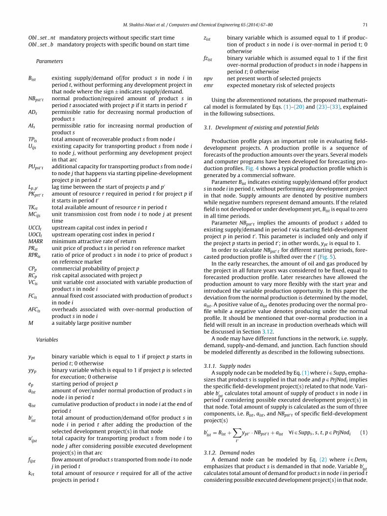
Production profile plays an important role in evaluating field-development projects. A production profile is a sequence offorecasts of the production amounts over the years. Several modelsand computer programs have been developed for forecasting pro-duction profiles. Fig. 4 shows a typical production profile which isgenerated by a commercial software.

Parameter Bist indicates existing supply/demand of/for products in node i in period t, without performing any development projectin that node. Supply amounts are denoted by positive numberswhile negative numbers represent demand amounts. If the relatedfield is not developed or under development yet, Bist is equal to zeroin all time periods.

Parameter NBpst′t implies the amounts of product s added toexisting supply/demand in period t via starting field-developmentproject p in period t′. This parameter is included only and only ifthe project p starts in period t′; in other words, ypt is equal to 1.

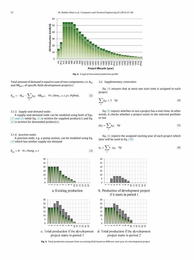
In order to calculate NBpst′ t for different starting periods, fore-casted production profile is shifted over the t′ (Fig. 5).

In the early researches, the amount of oil and gas produced bythe project in all future years was considered to be fixed, equal toforecasted production profile. Later researches have allowed theproduction amount to vary more flexibly with the start year andintroduced the variable production opportunity. In this paper thedeviation from the normal production is determined by the model,aist. A positive value of aist denotes producing over the normal pro-file while a negative value denotes producing under the normalprofile. It should be mentioned that over-normal production in afield will result in an increase in production overheads which willbe discussed in Section 3.12.

A node may have different functions in the network, i.e. supply,demand, supply-and-demand, and junction. Each function shouldbe modeled differently as described in the following subsections.

3.1.1. Supply nodesA supply node can be modeled by Eq. (1) where i ∈ Supps empha-

sizes that product s is supplied in that node and p ∈ PrjNodi impliesthe specific field-development project(s) related to that node. Vari-able b′

istcalculates total amount of supply of product s in node i in

period t considering possible executed development project(s) inthat node. Total amount of supply is calculated as the sum of threecomponents, i.e. Bist, aist, and NBpst′t of specific field-developmentproject(s)

b′ist = Bist +

∑t′

ypt′ · NBpst′t + aist ∀i ∈ Supps, s, t, p ∈ PrjNodi (1)

3.1.2. Demand nodes

A demand node can be modeled by Eq. (2) where i ∈ Dems

emphasizes that product s is demanded in that node. Variable b′ist

calculates total amount of demand for product s in node i in period tconsidering possible executed development project(s) in that node.

72 M. Shakhsi-Niaei et al. / Computers and Chemical Engineering 65 (2014) 67–80

casted

Ta

b

3

((

3

(

b

Fig. 4. A typical fore

otal amount of demand is equal to sum of two components, i.e. Bistnd NBpst′t of specific field-development project(s)

′ist = −Bist −

∑t′

ypt′ · NBpst′t ∀i ∈ Dems, s, t, p ∈ PrjNodi (2)

.1.3. Supply-and-demand nodesA supply-and-demand node can be modeled using both of Eqs.

1) and (2) while Eq. (1) is written for supplied product(s) and Eq.2) is written for demanded product(s).

.1.4. Junction nodesA junction node, e.g. a pump station, can be modeled using Eq.

3) which has neither supply nor demand

′ist = 0 ∀i ∈ Pump, s, t (3)

Fig. 5. Total production amounts from an existing field ba

production profile.

3.2. Supplementary constraints

Eq. (4) ensures that at most one start time is assigned to eachproject

∑t

ypt ≤ 1 ∀p (4)

Eq. (5) reports whether or not a project has a start time. In otherwords, it checks whether a project exists in the selected portfolioor not

yyp =∑

t

ypt ∀p (5)

Eq. (6) reports the assigned starting year of each project which

later will be used in Eq. (19)

ep =∑

t

t · ypt ∀p (6)

sed on different start year of a development project.

nd Ch

3

etet

aate

3

tdetTnpda∑

∑

rp

a

ut

q

q

r

q

3

ouDdao

fbw

M. Shakhsi-Niaei et al. / Computers a

.3. Swapping

Swap is an opportunity to decrease transmission costs. Forxample, Iran imports oil from central Asian countries in its northo be refined at Tehran and Tabriz oil refineries and then delivers anquivalent amount of oil to potential buyers in its southern exporterminals.

In order to model the swapping process, a supply node should bedded to existing network as “swap terminal” supplying the agreedmount of swapping product. Then, an equivalent total amount ofhe product should be defined as “committed export” in one or morexisting export terminal(s).

.4. Variable production

If the production amounts from all fields are forced to followheir forecasted production profiles, it is difficult to get the pro-uction to fit the capacities of the pipes and the markets (Nygreent al., 1998). In order to make these constraints less hard, produc-ion amounts have been allowed to differ from the given profiles.wo parameters Ads and AIs, allowed upper and lower variable-to-ormal ratios, control the difference between normal and variableroduction amounts. Hence, the sum of normal and variable pro-uction amounts has to be within the bounds defined in Eqs. (7)nd (8)

t′ypt′ · NBpst′t + aist ≤ AIs ·

∑t′

ypt′ .NBpst′t

∀i ∈ Supps, s, t, p ∈ PrjNodi (7)

t′ypt′ · NBpst′t + aist≥ADs ·

∑t′

ypt′ · NBpst′t

∀i ∈ Supps, t, p ∈ PrjNodi (8)

Eq. (9) ensures that if a field needs variable production, itselated development project is necessarily included in the selectedroject portfolio

ist ≤ M · yyp ∀i ∈ Supps, s, t, p ∈ PrjNodi (9)

Eqs. (10) and (11) calculate the cumulative production of prod-ct s in node i at the end of first time period and at the end of otherime periods respectively

is,1 = b′is,1 ∀i ∈ Supps, s, p ∈ PrjNodi (10)

ist = b′ist + qis,t−1 ∀i ∈ Supps, s, t≥2, p ∈ PrjNodi (11)

The cumulative production amounts cannot exceed the totalecoverable amount which is satisfied in Eq. (12)

ist ≤ TPis ∀i ∈ Supps, s, t (12)

.5. Development of existing/potential pipelines

In an upstream network each pipeline is used to transport onlyne kind of product while in a downstream network some prod-cts may be transported via a common pipeline, one after another.ue to overcapacity flows resulted by considerable increase in pro-uction amounts, an existing pipeline may need to be extended viadding a parallel line or a new pipeline may be substituted for theld one.

Variable u′ijst

denotes total capacity for transporting product srom node i to node j in year t considering existing and possi-ly developed pipelines. Parameter Uijs indicates existing capacityithout performing any development project in that arc and PUpst′t

emical Engineering 65 (2014) 67–80 73

represents additional capacity which happens via starting pipeline-development project p in period t′. If there exist no pipeline atpresent, parameter Uijs is equal to zero. Parameter PUpst′ t is astep function which includes one/some zero value(s) in the firstperiod(s) and identical positive values from delivery year of therelated pipeline-development project until the end of planninghorizon

u′ijst = Uijs +

∑t′

ypt′ · PUpst′t ∀i, j, s, t, p ∈ PrjArcij (13)

3.6. Transmission capacities

Variable fijst represents flow amount of product s transportedfrom node i to node j in period t which is bounded on total capacityusing Eq. (14)

fijst ≤ u′ijst ∀i, j, s, t (14)

3.7. Flow balance in nodes

There are two types of market nodes in an upstream network,i.e. export terminals and internal markets.

In an export node, denoted by i ∈ Exps, there may be some com-mitted amount of product to be exported which is represented bynegative values of parameter Bist. Moreover, the surplus amounts ofproducts which are supplied to the network can be exported aftermarketing activities.

The demand of internal market nodes, a subset of non-exportnodes, is forecasted for different products and represented by neg-ative values of parameter Bist.

Eqs. (15) and (16) model the balance in export and non-exportnodes, respectively∑

h: hi ∈ V

fhist + b′ist −

∑j: ij ∈ V

fijst≥0 ∀i ∈ Exps, s, t (15)

∑h: hi ∈ V

fhist + b′ist −

∑j: ij ∈ V

fijst = 0 ∀i /∈ Exps, s, t (16)

These two constraints differ in their equality/inequality sign.Hence, Eq. (15) allows surplus amounts of output flows to beexported. It should be mentioned that input flows into a node aredenoted by positive fijst while a negative fijst shows an output flow.Considering node i as the current node, predecessor nodes are rep-resented by index h if the arc hi belongs to the network, h : hi ∈ V.Similarly, successor nodes are represented by index j if the arc ijbelongs to the network, j : ij ∈ V.

In addition, the following equations ensure positive flows in allarcs of the network:

fijst≥0 ∀i, j, s, t (17)

3.8. Precedence and logical relations

Several precedence and logical relations can be defined betweenprojects. The interested readers are referred to (Demeulemeester& Herroelen, 2002) for more information about different kinds ofprecedence relations. Here we discuss three major relations usedin the strategic development-project selection literature. Eq. (18)allows project p′ to be selected if and only if project p is also selected.This constraint does not consider the time between the start ofthe successor and the predecessor projects. The term pre set nl

indicates all pairs of projects that belong to precedence set with nolag time between them

yyp′ ≤ yyp ∀p and p′ ∈ Pre set nl (18)

7 nd Ch

lid

e

saS

y

oh

y

y

3

gop

paoE

p

3

pt

y

ti

y

p

∑

s

FCi

i

∑

4 M. Shakhsi-Niaei et al. / Computers a

Eq. (19) acts similar to Eq. (18) but forces project p′ to start ateast Lp,p′ periods later than the start of project p. The term pre set lndicates all pairs of projects that belong to precedence set withetermined lag time between them

p′≥ep + Lp,p′ ∀p and p′ ∈ Pre set l (19)

Eq. (20) forces all the members of a Sim set to be selected/notelected simultaneously. Hence, a project belonging to Sim set isllowed to be selected if and only if all other projects belong toim set have been selected too

yp ≤ 1|Sim set|

∑p′ ∈ Sim set

yyp′ ∀p ∈ Sim set (20)

The term |Sim set| in Eq. (20) indicates the number of membersf Sim set. For example, if projects 3 and 5 belong to a Sim set;ence:

y3 ≤ 0.5(yy3 + yy5) (21)

y5 ≤ 0.5(yy3 + yy5) (22)

.9. Alternatives

It is possible to define several different options to develop aiven petroleum field. For example, a petroleum field can be devel-ped via drilling n1 or n2 wells which will result in two differentroduction profiles and also different drilling costs. Hence, each

ossible development pattern is defined as a separate project whilell these projects form an alternative set. It is clear that at most onef alternative projects is allowed to start. This issue is satisfied inq. (23)∑

∈ Alt set

yyp ≤ 1 ∀p′Alt set (23)

.10. Obligations

Three types of obligations have been considered in this paper. Ifroject p′ is obliged to be started in period t′, Eq. (24) is used. Theerm Obl set t denotes each time-dependent obligation set

p′t′ = 1 ∀p′ ∈ Obl set t (24)

If project p′ is obliged to be selected, regardless of its startime, Eq. (25) is used. The term Obl set nt denotes each time-ndependent obligation set

yp′ = 1 ∀p ∈ Obl set nt (25)

Eq. (26) is used where an upper bound on start time of project′ is defined that obliges it to be started no later than t′

Max npv =∑

t

⎛⎜⎜⎜⎜⎜⎜⎜⎝

(1 + MARR)−t

⎛⎜⎜⎜⎜⎜⎜⎜⎝

∑j ∈ Exps or

j ∈ IntMarks

∑s

RPRjs · PRst ·∑

i

fijst

− UOCItUOCI1

(∑

i

∑j

∑s

MCijs · fijst +∑

i

∑

− UCCItUCCI1

(∑

p

∑t′

ypt′ · PKp,devbudg,t′,t +∑

t′

t=1

yp′t = 1 ∀p′ ∈ Obl set b (26)

emical Engineering 65 (2014) 67–80

3.11. Resources

Each project needs different resources over the years, e.g.money, injection gas, and etc. Parameter PKprt′t denotes the amountof resource r required in period t if the project p starts in periodt′. After defining PKprt′ t for t′ = 1, it is shifted into other possiblestart times in order to calculate this parameter for other valuesof t′.

Eq. (27) calculates the total amounts of required resources ineach year considering selected projects. Then, the total amountsof required resources have been limited to their available amountsusing Eq. (28)

krt =∑

p

∑t′

ypt′ · PKprt′t ∀r, t (27)

krt ≤ TKrt ∀r, t (28)

3.12. NPV objective function

Net present value, NPV, has been widely used as objective func-tion of project-portfolio-selection models. The net present value(NPV) of a time series of cash flows, both benefits and costs, is thesum of the present values of the individual cash flows of a project.In the context of oil-and-gas development projects, costs includeproduction and transmission costs while benefits are achieved byselling the products in market nodes

s +∑

i

∑s

VCis · qis,1|t = 1 +∑

i

∑s

VCis · (qist − qis,t−1)|t≥2)

s

fzist · AFCis)

⎞⎟⎟⎟⎟⎟⎟⎟⎠

⎞⎟⎟⎟⎟⎟⎟⎟⎠

(29)

NPV function is calculated and maximized using Eq. (29). Ben-efits are achieved by selling the products in market nodes, i.e.internal markets j ∈ IntMarks and export nodes j ∈ Exps. A unit pricefor all products in every period is estimated as reference price, PRst.The price of product s in market node j is determined by multi-plying the reference price by the ratio of price in node j to priceon reference market, RPRjs. The term

∑i fijst calculates total input

flow to the market node j. There is no need to inflate the ben-efits because the prices are estimated for each year. After that,all benefits are transferred to the present time via multiplying by(1 + MARR)t.

On the other side of NPV, there are four cost components. Thefirst component includes all the costs of transmission in the net-work where MCijs denotes the unit transmission cost from node i tonode j at present time. It will be inflated for next periods consideringindustry-based inflation rates.

The second component calculates fixed and variable productioncosts of existing and development-related production.

The third term adds the monetary resource required for activeprojects. Parameter PKp,devbudg,t′,t represents the cost required forexecuting project p if it is started in period t′. The term devbudgemphasizes the budgetary nature of this resource.

The last term in Eq. (29) applies the fixed cost of variable produc-tion only for those fields which have variable production. Variablefzist implies the first period in which the variable production occurs.

If fzist is equal to zero for all values of t, this field does not have anyover-normal variable production and hence, AFC will not be con-sidered for this node. But, if fzist for one tis equal to one, field i willexceed the normal production of product s in period t for the first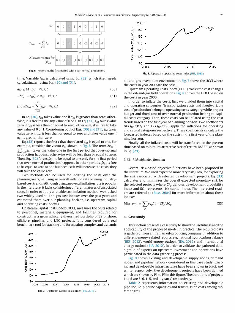

M. Shakhsi-Niaei et al. / Computers and Chemical Engineering 65 (2014) 67–80 75

0 0 1 1 0 0 1 1 0

t

tzist zist

zist

1

2 0 0 1 0 -2 -2 -1 -2 -4

Allowed values for0,1 0, 1 1 0,1 0, 1 0, 1 0, 1 0, 1 0, 1

tc

a

−

f

wzava

e∑pTttw

pbictea

tcob

zistf

Fig. 6. Reporting the first period with over-normal production.

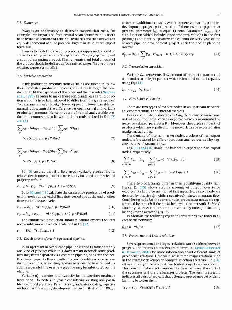
ime. Variable fzist is calculated using Eq. (32) which itself needsalculating zist using Eqs. (30) and (31).

ist ≤ M · zist ∀i, s, t (30)

M(1 − zist) < aist ∀i, s, t (31)

zist≥2zist −t∑

t′=1

zist′ ∀i, s, t (32)

In Eq. (30), zist takes value one if aist is greater than zero; other-ise, it is free to take any value of 0 or 1. In Eq. (31), zist takes value

ero if aist is less than or equal to zero; otherwise, it is free to takeny value of 0 or 1. Considering both of Eqs. (30) and (31), zist takesalue zero if aist is less than or equal to zero and takes value one ifist is greater than zero.

Eq. (32) reports the first t that the related aist is equal to one. Forxample, consider the vector zist shown in Fig. 6. The term 2zist −

tt′=1zist′ takes the value one in the first period that over-normal

roduction happens; otherwise will be less than or equal to zero.hen, Eq. (32) forces fzist to be equal to one only for the first periodhat over-normal production happens. In other periods, fzist is freeo be equal to zero or one but because it will increase the costs, theyill take the value zero.

Two methods can be used for inflating the costs over thelanning years, i.e. using an overall inflation rate or using industry-ased cost trends. Although using an overall inflation rate is popular

n the literature, it lacks considering different natures of associatedosts. In order to apply a reliable cost inflation method, we trackedwo widely-used oil-and-gas cost indexes over the past years andstimated them over our planning horizon, i.e. upstream capitalnd operating costs indexes.

Upstream Capital Costs Index (UCCI) measures the costs related

o personnel, materials, equipment, and facilities required foronstructing a geographically diversified portfolio of 28 onshore,ffshore, pipeline, and LNG projects. It is considered as a realenchmark tool for tracking and forecasting complex and dynamic

Fig. 7. Upstream capital costs index (IHS, 2013).

Fig. 8. Upstream operating costs index (IHS, 2013).

oil-and-gas investment environments. Fig. 7 shows the UCCI wherethe costs in year 2000 are the base.

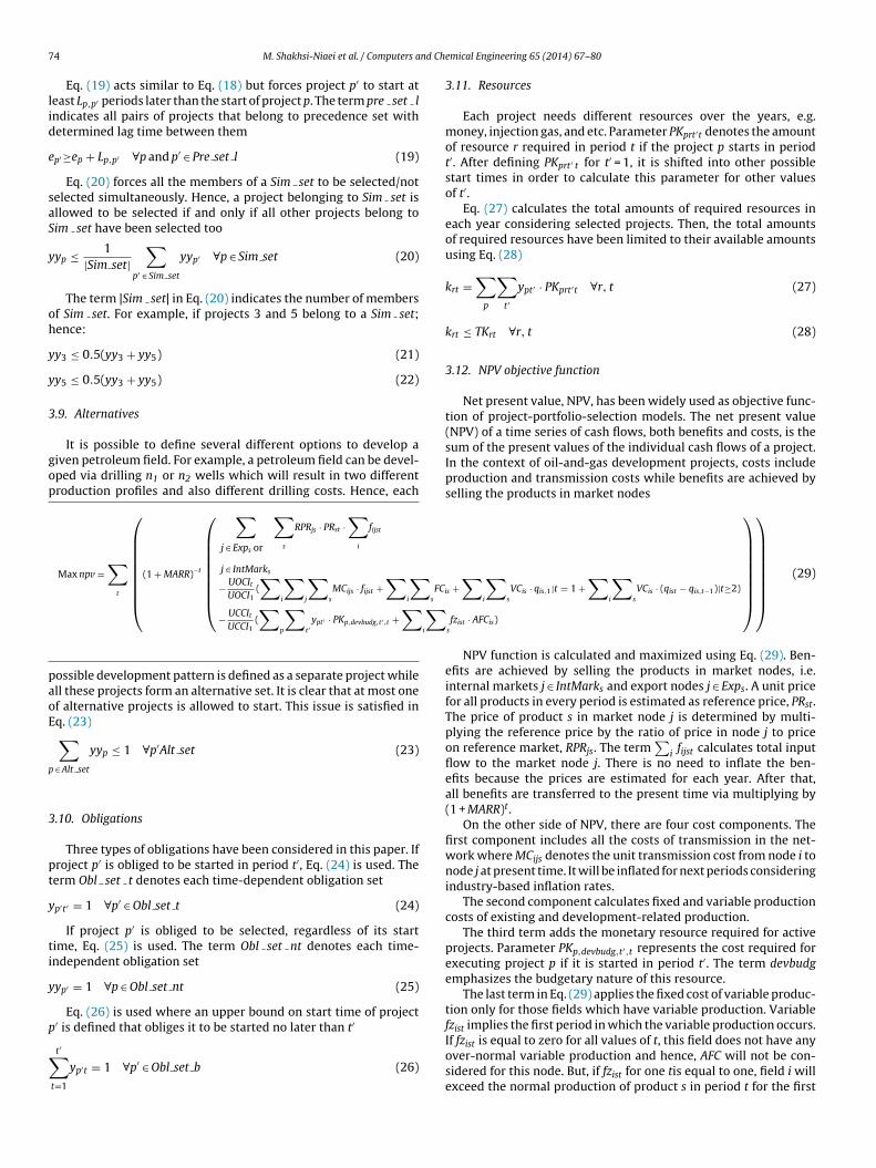
Upstream Operating Costs Index (UOCI) tracks the cost changesin the oil-and-gas field operations. Fig. 8 shows the UOCI based onthe costs in year 2000.

In order to inflate the costs, first we divided them into capitaland operating categories. Transportation costs and fixed/variablecost of production belong to operating costs category while projectbudget and fixed cost of over-normal production belong to capi-tal costs category. Then, these costs can be inflated using the costtrends based on the first year of planning horizon. Two coefficientsUOCIt/UOCI1 and UCCIt/UCCI1 apply the inflations for operatingand capital categories respectively. These coefficients calculate theforecasted indexes based on the costs in the first year of the plan-ning horizon.

Finally, all the inflated costs will be transferred to the presenttime based on minimum attractive rate of return, MARR, as shownin Eq. (29).

3.13. Risk objective function

Several risk-based objective functions have been proposed inthe literature. We used expected monetary risk, EMR, for exploringthe risk associated with selected development projects. Eq. (33)calculates and minimizes the overall expected monetary risk forthe selected projects where CPp denotes development probabilityindex and RCp represents risk capital index. The interested read-ers are referred to (Ross, 2004) for more information about theseindexes

Min emr =∑

p

yyp(1 − CPp)RCp (33)

4. Case study

This section presents a case study to show the usefulness and theapplicability of the proposed model in practice. The required datais gathered from an Iranian oil-producing company in addition todifferent energy-related reports, e.g. national hydrocarbon balance(IIES, 2012), world energy outlook (IEA, 2012), and internationalenergy outlook (EIA, 2012). In order to validate the gathered data,a group of experts on upstream investment and operations haveparticipated in the data gathering process.

Fig. 9 shows existing and developable supply nodes, demandnodes, and pipeline network considered in this case study. Exist-ing and developable infrastructures have been shown in black andwhite respectively. Five development projects have been definedwhich are shown by P1 to P5 in this figure. The durations of projects

1 to 5 are 5, 6, 1, 5, and 1 year(s) respectively.

Table 2 represents information on existing and developablepipeline, i.e. pipeline capacities and transmission costs among dif-ferent arcs.

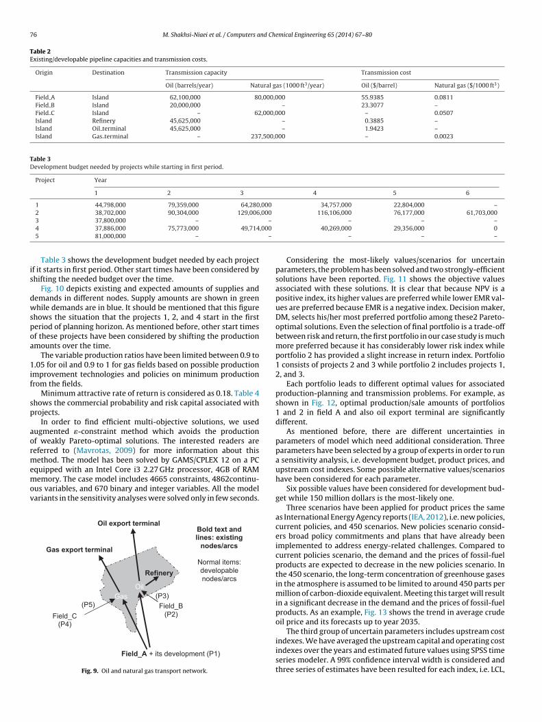
76 M. Shakhsi-Niaei et al. / Computers and Chemical Engineering 65 (2014) 67–80

Table 2Existing/developable pipeline capacities and transmission costs.

Origin Destination Transmission capacity Transmission cost

Oil (barrels/year) Natural gas (1000 ft3/year) Oil ($/barrel) Natural gas ($/1000 ft3)

Field A Island 62,100,000 80,000,000 55.9385 0.0811Field B Island 20,000,000 – 23.3077 –Field C Island – 62,000,000 – 0.0507Island Refinery 45,625,000 – 0.3885 –Island Oil terminal 45,625,000 – 1.9423 –Island Gas terminal – 237,500,000 – 0.0023

Table 3Development budget needed by projects while starting in first period.

Project Year

1 2 3 4 5 6

1 44,798,000 79,359,000 64,280,000 34,757,000 22,804,000 –2 38,702,000 90,304,000 129,006,000 116,106,000 76,177,000 61,703,000

–

,000

–

is

dwspoa

1if

sp

aormemov

3 37,800,000 –

4 37,886,000 75,773,000 49,7145 81,000,000 –

Table 3 shows the development budget needed by each projectf it starts in first period. Other start times have been considered byhifting the needed budget over the time.

Fig. 10 depicts existing and expected amounts of supplies andemands in different nodes. Supply amounts are shown in greenhile demands are in blue. It should be mentioned that this figure

hows the situation that the projects 1, 2, and 4 start in the firsteriod of planning horizon. As mentioned before, other start timesf these projects have been considered by shifting the productionmounts over the time.

The variable production ratios have been limited between 0.9 to.05 for oil and 0.9 to 1 for gas fields based on possible production

mprovement technologies and policies on minimum productionrom the fields.

Minimum attractive rate of return is considered as 0.18. Table 4hows the commercial probability and risk capital associated withrojects.

In order to find efficient multi-objective solutions, we usedugmented �-constraint method which avoids the productionf weakly Pareto-optimal solutions. The interested readers areeferred to (Mavrotas, 2009) for more information about thisethod. The model has been solved by GAMS/CPLEX 12 on a PC

quipped with an Intel Core i3 2.27 GHz processor, 4GB of RAMemory. The case model includes 4665 constraints, 4862continu-

us variables, and 670 binary and integer variables. All the modelariants in the sensitivity analyses were solved only in few seconds.

Field_A + its development (P1)

Field_C(P4)

Field_B(P2)

(P3)(P5)

Refinery

Oil export terminal

Gas export terminal

Bold text andlines: existing

nodes/arcs

Normal items:developablenodes/arcs

OilGas

Fig. 9. Oil and natural gas transport network.

– – –40,269,000 29,356,000 0

– – –

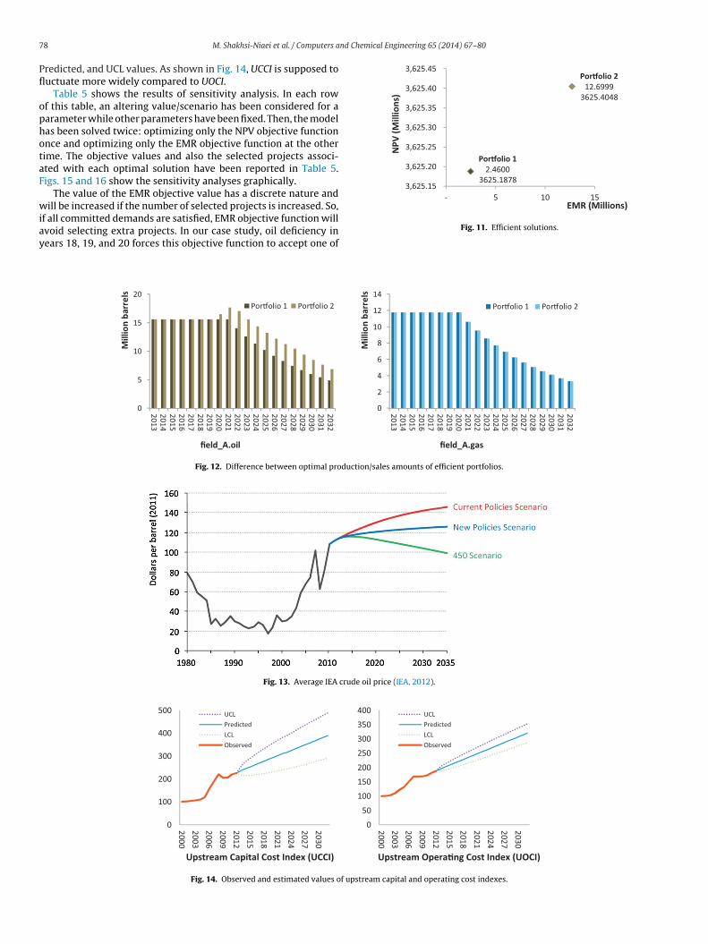
Considering the most-likely values/scenarios for uncertainparameters, the problem has been solved and two strongly-efficientsolutions have been reported. Fig. 11 shows the objective valuesassociated with these solutions. It is clear that because NPV is apositive index, its higher values are preferred while lower EMR val-ues are preferred because EMR is a negative index. Decision maker,DM, selects his/her most preferred portfolio among these2 Pareto-optimal solutions. Even the selection of final portfolio is a trade-offbetween risk and return, the first portfolio in our case study is muchmore preferred because it has considerably lower risk index whileportfolio 2 has provided a slight increase in return index. Portfolio1 consists of projects 2 and 3 while portfolio 2 includes projects 1,2, and 3.

Each portfolio leads to different optimal values for associatedproduction-planning and transmission problems. For example, asshown in Fig. 12, optimal production/sale amounts of portfolios1 and 2 in field A and also oil export terminal are significantlydifferent.

As mentioned before, there are different uncertainties inparameters of model which need additional consideration. Threeparameters have been selected by a group of experts in order to runa sensitivity analysis, i.e. development budget, product prices, andupstream cost indexes. Some possible alternative values/scenarioshave been considered for each parameter.

Six possible values have been considered for development bud-get while 150 million dollars is the most-likely one.

Three scenarios have been applied for product prices the sameas International Energy Agency reports (IEA, 2012), i.e. new policies,current policies, and 450 scenarios. New policies scenario consid-ers broad policy commitments and plans that have already beenimplemented to address energy-related challenges. Compared tocurrent policies scenario, the demand and the prices of fossil-fuelproducts are expected to decrease in the new policies scenario. Inthe 450 scenario, the long-term concentration of greenhouse gasesin the atmosphere is assumed to be limited to around 450 parts permillion of carbon-dioxide equivalent. Meeting this target will resultin a significant decrease in the demand and the prices of fossil-fuelproducts. As an example, Fig. 13 shows the trend in average crudeoil price and its forecasts up to year 2035.

The third group of uncertain parameters includes upstream cost

indexes. We have averaged the upstream capital and operating costindexes over the years and estimated future values using SPSS timeseries modeler. A 99% confidence interval width is considered andthree series of estimates have been resulted for each index, i.e. LCL,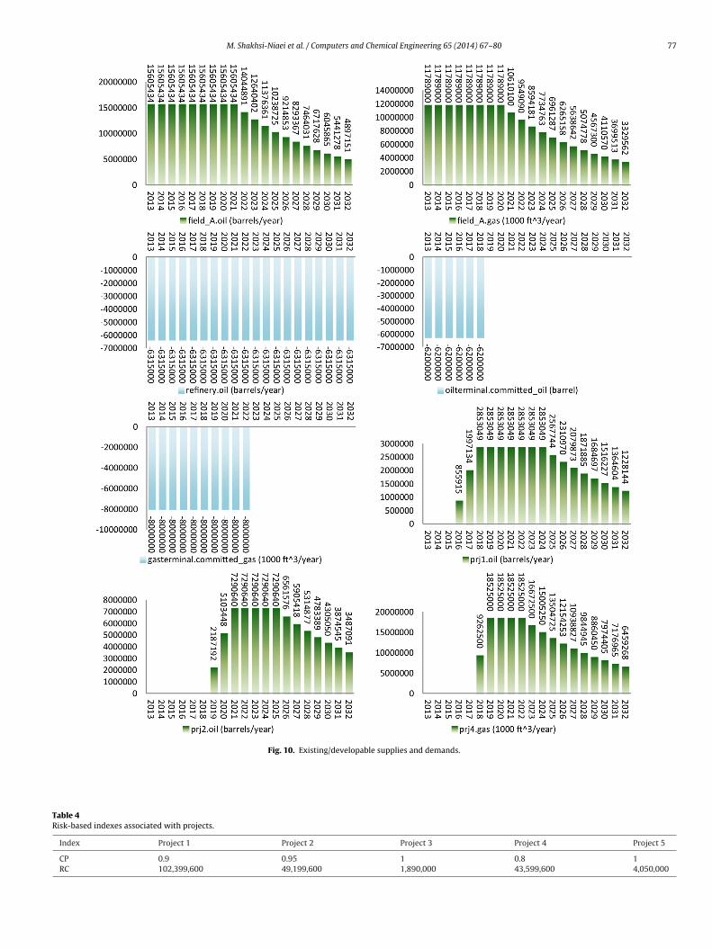

M. Shakhsi-Niaei et al. / Computers and Chemical Engineering 65 (2014) 67–80 77

Fig. 10. Existing/developable supplies and demands.

Table 4Risk-based indexes associated with projects.

Index Project 1 Project 2 Project 3 Project 4 Project 5

CP 0.9 0.95 1 0.8 1RC 102,399,600 49,199,600 1,890,000 43,599,600 4,050,000

7 nd Chemical Engineering 65 (2014) 67–80

Pfl

ophotaF

wiay

Por�olio 212.6999

3625.4048

Por�olio 12.4600

3625.1878 3,625.15

3,625.20

3,625.25

3,625.30

3,625.35

3,625.40

3,625.45

- 5 10 15

NPV

(Mill

ions

)

EMR (Millions)

8 M. Shakhsi-Niaei et al. / Computers a

redicted, and UCL values. As shown in Fig. 14, UCCI is supposed touctuate more widely compared to UOCI.

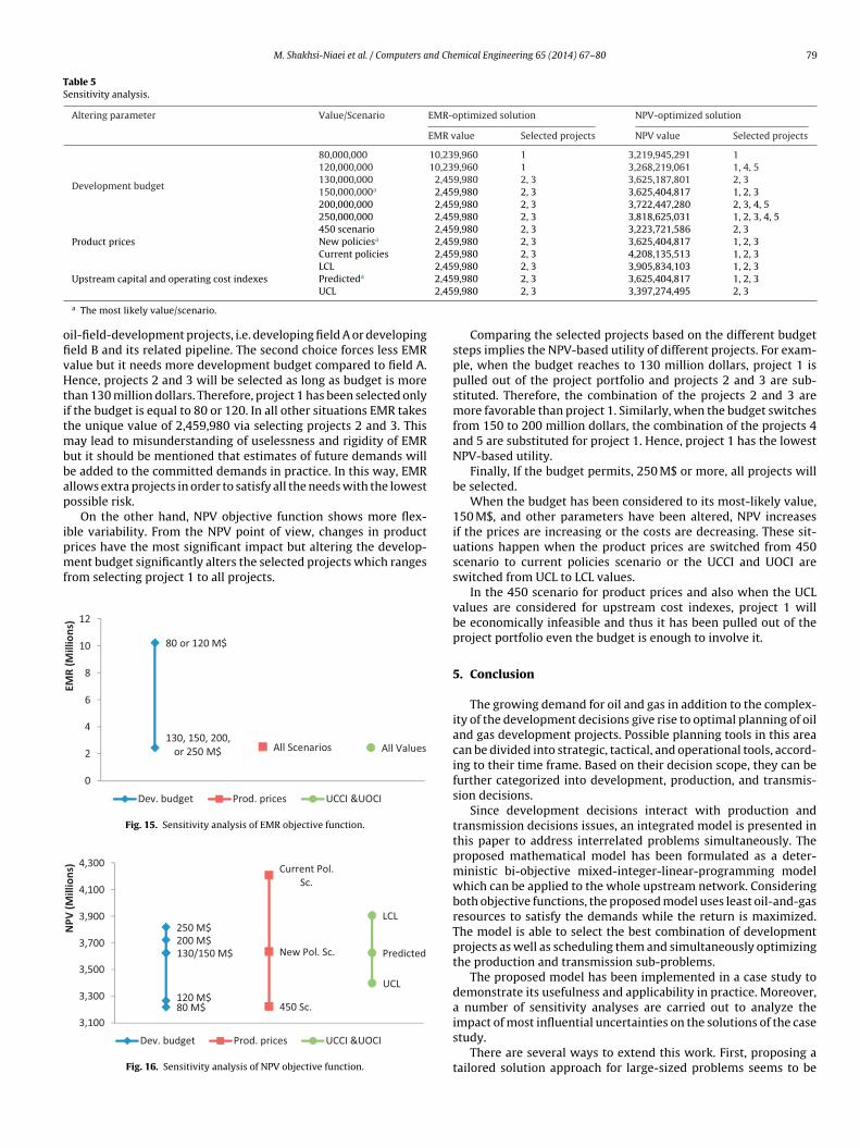
Table 5 shows the results of sensitivity analysis. In each rowf this table, an altering value/scenario has been considered for aarameter while other parameters have been fixed. Then, the modelas been solved twice: optimizing only the NPV objective functionnce and optimizing only the EMR objective function at the otherime. The objective values and also the selected projects associ-ted with each optimal solution have been reported in Table 5.igs. 15 and 16 show the sensitivity analyses graphically.

The value of the EMR objective value has a discrete nature and

ill be increased if the number of selected projects is increased. So,

f all committed demands are satisfied, EMR objective function willvoid selecting extra projects. In our case study, oil deficiency inears 18, 19, and 20 forces this objective function to accept one of

0

5

10

15

20

20132014201520162017201820192020202120222023202420252026202720282029203020312032

Mill

ion

barr

els

field _A.oi l

Por�olio 1 Por�olio 2

Fig. 12. Difference between optimal producti

Fig. 13. Average IEA crude

0

100

200

300

400

500

20002003200620092012201520182021202420272030

Upstream Capital Cost Index (UCCI)

UCLPredictedLCLObserved

1

1

2

2

3

3

4

Fig. 14. Observed and estimated values of upst

Fig. 11. Efficient solutions.

0

2

4

6

8

10

12

14

20132014201520162017201820192020202120222023202420252026202720282029203020312032

Mill

ion

barr

els

field_A.gas

Por�olio 1 Por�olio 2

on/sales amounts of efficient portfolios.

oil price (IEA, 2012).

0

50

00

50

00

50

00

50

00

20002003200620092012201520182021202420272030

Upstream Opera�ng Cost Index (UOCI)

UCLPredictedLCLObserved

ream capital and operating cost indexes.

M. Shakhsi-Niaei et al. / Computers and Chemical Engineering 65 (2014) 67–80 79

Table 5Sensitivity analysis.

Altering parameter Value/Scenario EMR-optimized solution NPV-optimized solution

EMR value Selected projects NPV value Selected projects

Development budget

80,000,000 10,239,960 1 3,219,945,291 1120,000,000 10,239,960 1 3,268,219,061 1, 4, 5130,000,000 2,459,980 2, 3 3,625,187,801 2, 3150,000,000a 2,459,980 2, 3 3,625,404,817 1, 2, 3200,000,000 2,459,980 2, 3 3,722,447,280 2, 3, 4, 5250,000,000 2,459,980 2, 3 3,818,625,031 1, 2, 3, 4, 5

Product prices450 scenario 2,459,980 2, 3 3,223,721,586 2, 3New policiesa 2,459,980 2, 3 3,625,404,817 1, 2, 3Current policies 2,459,980 2, 3 4,208,135,513 1, 2, 3LCL 2,459,980 2, 3 3,905,834,103 1, 2, 3

2,452,45

ofivHtitmbbap

ipmf

Upstream capital and operating cost indexes Predicteda

UCL

a The most likely value/scenario.

il-field-development projects, i.e. developing field A or developingeld B and its related pipeline. The second choice forces less EMRalue but it needs more development budget compared to field A.ence, projects 2 and 3 will be selected as long as budget is more

han 130 million dollars. Therefore, project 1 has been selected onlyf the budget is equal to 80 or 120. In all other situations EMR takeshe unique value of 2,459,980 via selecting projects 2 and 3. This

ay lead to misunderstanding of uselessness and rigidity of EMRut it should be mentioned that estimates of future demands wille added to the committed demands in practice. In this way, EMRllows extra projects in order to satisfy all the needs with the lowestossible risk.

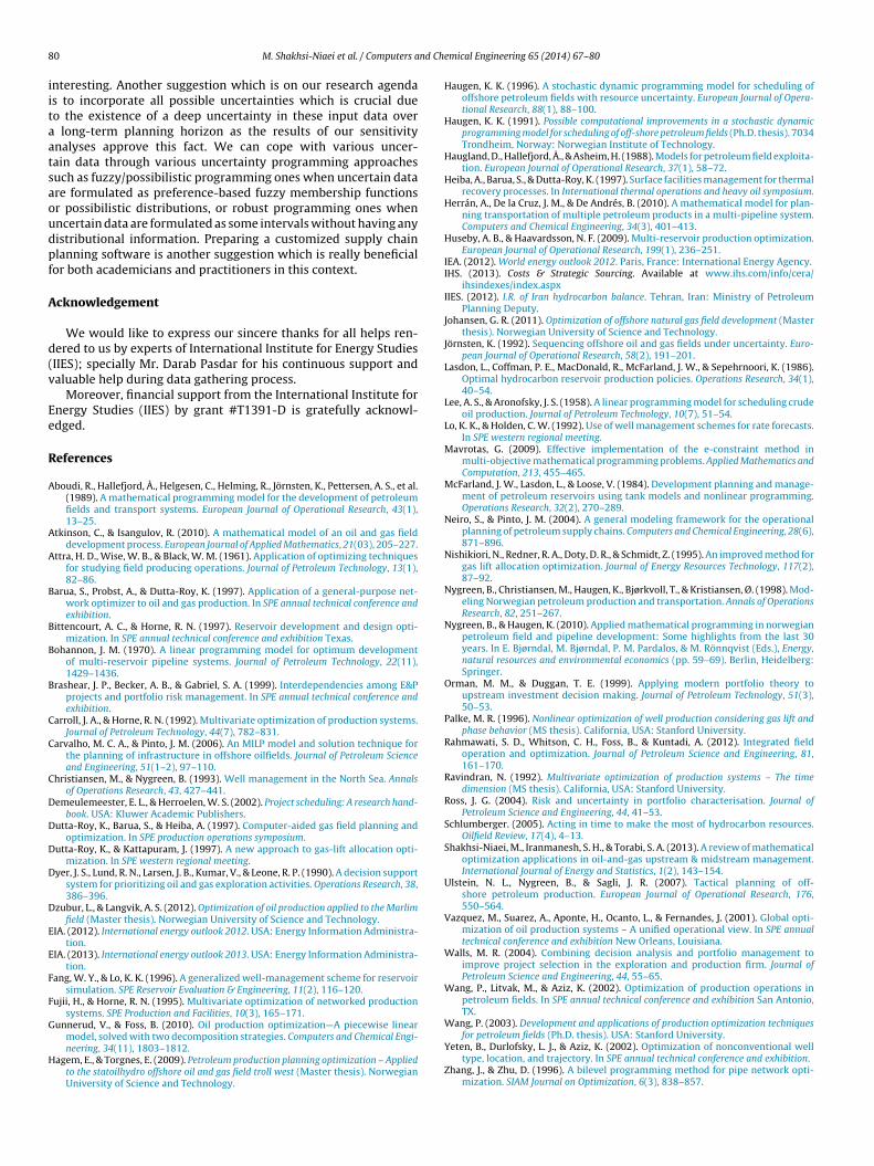
On the other hand, NPV objective function shows more flex-ble variability. From the NPV point of view, changes in product

rices have the most significant impact but altering the develop-ent budget significantly alters the selected projects which ranges

rom selecting project 1 to all projects.

80 or 120 M$

130, 150, 200 ,or 250 M$ All Sce nar ios All Valu es

0

2

4

6

8

10

12

EMR

(Mill

ions

)

Dev. budget Prod. prices UCCI &UOCI

Fig. 15. Sensitivity analysis of EMR objective function.

80 M$120 M$

130/150 M$200 M$250 M$

450 Sc.

New Pol. Sc.

Current Pol.Sc.

LCL

Predicted

UCL

3,100

3,300

3,500

3,700

3,900

4,100

4,300

NPV

(Mill

ions

)

Dev. budget Prod. prices UCCI &UOCI

Fig. 16. Sensitivity analysis of NPV objective function.

9,980 2, 3 3,625,404,817 1, 2, 39,980 2, 3 3,397,274,495 2, 3

Comparing the selected projects based on the different budgetsteps implies the NPV-based utility of different projects. For exam-ple, when the budget reaches to 130 million dollars, project 1 ispulled out of the project portfolio and projects 2 and 3 are sub-stituted. Therefore, the combination of the projects 2 and 3 aremore favorable than project 1. Similarly, when the budget switchesfrom 150 to 200 million dollars, the combination of the projects 4and 5 are substituted for project 1. Hence, project 1 has the lowestNPV-based utility.

Finally, If the budget permits, 250 M$ or more, all projects willbe selected.

When the budget has been considered to its most-likely value,150 M$, and other parameters have been altered, NPV increasesif the prices are increasing or the costs are decreasing. These sit-uations happen when the product prices are switched from 450scenario to current policies scenario or the UCCI and UOCI areswitched from UCL to LCL values.

In the 450 scenario for product prices and also when the UCLvalues are considered for upstream cost indexes, project 1 willbe economically infeasible and thus it has been pulled out of theproject portfolio even the budget is enough to involve it.

5. Conclusion

The growing demand for oil and gas in addition to the complex-ity of the development decisions give rise to optimal planning of oiland gas development projects. Possible planning tools in this areacan be divided into strategic, tactical, and operational tools, accord-ing to their time frame. Based on their decision scope, they can befurther categorized into development, production, and transmis-sion decisions.

Since development decisions interact with production andtransmission decisions issues, an integrated model is presented inthis paper to address interrelated problems simultaneously. Theproposed mathematical model has been formulated as a deter-ministic bi-objective mixed-integer-linear-programming modelwhich can be applied to the whole upstream network. Consideringboth objective functions, the proposed model uses least oil-and-gasresources to satisfy the demands while the return is maximized.The model is able to select the best combination of developmentprojects as well as scheduling them and simultaneously optimizingthe production and transmission sub-problems.

The proposed model has been implemented in a case study todemonstrate its usefulness and applicability in practice. Moreover,a number of sensitivity analyses are carried out to analyze the

impact of most influential uncertainties on the solutions of the casestudy.

There are several ways to extend this work. First, proposing atailored solution approach for large-sized problems seems to be

8 nd Ch

iitaatsaoudpf

A

d(v

Ee

R

A

A

A

B

B

B

B

C

C

C

D

D

D

D

D

E

E

F

F

G

H

0 M. Shakhsi-Niaei et al. / Computers a

nteresting. Another suggestion which is on our research agendas to incorporate all possible uncertainties which is crucial dueo the existence of a deep uncertainty in these input data over

long-term planning horizon as the results of our sensitivitynalyses approve this fact. We can cope with various uncer-ain data through various uncertainty programming approachesuch as fuzzy/possibilistic programming ones when uncertain datare formulated as preference-based fuzzy membership functionsr possibilistic distributions, or robust programming ones whenncertain data are formulated as some intervals without having anyistributional information. Preparing a customized supply chainlanning software is another suggestion which is really beneficialor both academicians and practitioners in this context.

cknowledgement

We would like to express our sincere thanks for all helps ren-ered to us by experts of International Institute for Energy StudiesIIES); specially Mr. Darab Pasdar for his continuous support andaluable help during data gathering process.

Moreover, financial support from the International Institute fornergy Studies (IIES) by grant #T1391-D is gratefully acknowl-dged.

eferences

boudi, R., Hallefjord, Å., Helgesen, C., Helming, R., Jörnsten, K., Pettersen, A. S., et al.(1989). A mathematical programming model for the development of petroleumfields and transport systems. European Journal of Operational Research, 43(1),13–25.

tkinson, C., & Isangulov, R. (2010). A mathematical model of an oil and gas fielddevelopment process. European Journal of Applied Mathematics, 21(03), 205–227.

ttra, H. D., Wise, W. B., & Black, W. M. (1961). Application of optimizing techniquesfor studying field producing operations. Journal of Petroleum Technology, 13(1),82–86.

arua, S., Probst, A., & Dutta-Roy, K. (1997). Application of a general-purpose net-work optimizer to oil and gas production. In SPE annual technical conference andexhibition.

ittencourt, A. C., & Horne, R. N. (1997). Reservoir development and design opti-mization. In SPE annual technical conference and exhibition Texas.

ohannon, J. M. (1970). A linear programming model for optimum developmentof multi-reservoir pipeline systems. Journal of Petroleum Technology, 22(11),1429–1436.

rashear, J. P., Becker, A. B., & Gabriel, S. A. (1999). Interdependencies among E&Pprojects and portfolio risk management. In SPE annual technical conference andexhibition.

arroll, J. A., & Horne, R. N. (1992). Multivariate optimization of production systems.Journal of Petroleum Technology, 44(7), 782–831.

arvalho, M. C. A., & Pinto, J. M. (2006). An MILP model and solution technique forthe planning of infrastructure in offshore oilfields. Journal of Petroleum Scienceand Engineering, 51(1–2), 97–110.

hristiansen, M., & Nygreen, B. (1993). Well management in the North Sea. Annalsof Operations Research, 43, 427–441.

emeulemeester, E. L., & Herroelen, W. S. (2002). Project scheduling: A research hand-book. USA: Kluwer Academic Publishers.

utta-Roy, K., Barua, S., & Heiba, A. (1997). Computer-aided gas field planning andoptimization. In SPE production operations symposium.

utta-Roy, K., & Kattapuram, J. (1997). A new approach to gas-lift allocation opti-mization. In SPE western regional meeting.

yer, J. S., Lund, R. N., Larsen, J. B., Kumar, V., & Leone, R. P. (1990). A decision supportsystem for prioritizing oil and gas exploration activities. Operations Research, 38,386–396.

zubur, L., & Langvik, A. S. (2012). Optimization of oil production applied to the Marlimfield (Master thesis). Norwegian University of Science and Technology.

IA. (2012). International energy outlook 2012. USA: Energy Information Administra-tion.

IA. (2013). International energy outlook 2013. USA: Energy Information Administra-tion.

ang, W. Y., & Lo, K. K. (1996). A generalized well-management scheme for reservoirsimulation. SPE Reservoir Evaluation & Engineering, 11(2), 116–120.

ujii, H., & Horne, R. N. (1995). Multivariate optimization of networked productionsystems. SPE Production and Facilities, 10(3), 165–171.

unnerud, V., & Foss, B. (2010). Oil production optimization—A piecewise linear

model, solved with two decomposition strategies. Computers and Chemical Engi-neering, 34(11), 1803–1812.

agem, E., & Torgnes, E. (2009). Petroleum production planning optimization – Appliedto the statoilhydro offshore oil and gas field troll west (Master thesis). NorwegianUniversity of Science and Technology.

emical Engineering 65 (2014) 67–80

Haugen, K. K. (1996). A stochastic dynamic programming model for scheduling ofoffshore petroleum fields with resource uncertainty. European Journal of Opera-tional Research, 88(1), 88–100.

Haugen, K. K. (1991). Possible computational improvements in a stochastic dynamicprogramming model for scheduling of off-shore petroleum fields (Ph.D. thesis). 7034Trondheim, Norway: Norwegian Institute of Technology.

Haugland, D., Hallefjord, Å., & Asheim, H. (1988). Models for petroleum field exploita-tion. European Journal of Operational Research, 37(1), 58–72.

Heiba, A., Barua, S., & Dutta-Roy, K. (1997). Surface facilities management for thermalrecovery processes. In International thermal operations and heavy oil symposium.

Herrán, A., De la Cruz, J. M., & De Andrés, B. (2010). A mathematical model for plan-ning transportation of multiple petroleum products in a multi-pipeline system.Computers and Chemical Engineering, 34(3), 401–413.

Huseby, A. B., & Haavardsson, N. F. (2009). Multi-reservoir production optimization.European Journal of Operational Research, 199(1), 236–251.

IEA. (2012). World energy outlook 2012. Paris, France: International Energy Agency.IHS. (2013). Costs & Strategic Sourcing. Available at www.ihs.com/info/cera/

ihsindexes/index.aspxIIES. (2012). I.R. of Iran hydrocarbon balance. Tehran, Iran: Ministry of Petroleum

Planning Deputy.Johansen, G. R. (2011). Optimization of offshore natural gas field development (Master

thesis). Norwegian University of Science and Technology.Jörnsten, K. (1992). Sequencing offshore oil and gas fields under uncertainty. Euro-

pean Journal of Operational Research, 58(2), 191–201.Lasdon, L., Coffman, P. E., MacDonald, R., McFarland, J. W., & Sepehrnoori, K. (1986).

Optimal hydrocarbon reservoir production policies. Operations Research, 34(1),40–54.

Lee, A. S., & Aronofsky, J. S. (1958). A linear programming model for scheduling crudeoil production. Journal of Petroleum Technology, 10(7), 51–54.

Lo, K. K., & Holden, C. W. (1992). Use of well management schemes for rate forecasts.In SPE western regional meeting.

Mavrotas, G. (2009). Effective implementation of the e-constraint method inmulti-objective mathematical programming problems. Applied Mathematics andComputation, 213, 455–465.

McFarland, J. W., Lasdon, L., & Loose, V. (1984). Development planning and manage-ment of petroleum reservoirs using tank models and nonlinear programming.Operations Research, 32(2), 270–289.

Neiro, S., & Pinto, J. M. (2004). A general modeling framework for the operationalplanning of petroleum supply chains. Computers and Chemical Engineering, 28(6),871–896.

Nishikiori, N., Redner, R. A., Doty, D. R., & Schmidt, Z. (1995). An improved method forgas lift allocation optimization. Journal of Energy Resources Technology, 117(2),87–92.

Nygreen, B., Christiansen, M., Haugen, K., Bjørkvoll, T., & Kristiansen, Ø. (1998). Mod-eling Norwegian petroleum production and transportation. Annals of OperationsResearch, 82, 251–267.

Nygreen, B., & Haugen, K. (2010). Applied mathematical programming in norwegianpetroleum field and pipeline development: Some highlights from the last 30years. In E. Bjørndal, M. Bjørndal, P. M. Pardalos, & M. Rönnqvist (Eds.), Energy,natural resources and environmental economics (pp. 59–69). Berlin, Heidelberg:Springer.

Orman, M. M., & Duggan, T. E. (1999). Applying modern portfolio theory toupstream investment decision making. Journal of Petroleum Technology, 51(3),50–53.

Palke, M. R. (1996). Nonlinear optimization of well production considering gas lift andphase behavior (MS thesis). California, USA: Stanford University.

Rahmawati, S. D., Whitson, C. H., Foss, B., & Kuntadi, A. (2012). Integrated fieldoperation and optimization. Journal of Petroleum Science and Engineering, 81,161–170.

Ravindran, N. (1992). Multivariate optimization of production systems – The timedimension (MS thesis). California, USA: Stanford University.

Ross, J. G. (2004). Risk and uncertainty in portfolio characterisation. Journal ofPetroleum Science and Engineering, 44, 41–53.

Schlumberger. (2005). Acting in time to make the most of hydrocarbon resources.Oilfield Review, 17(4), 4–13.

Shakhsi-Niaei, M., Iranmanesh, S. H., & Torabi, S. A. (2013). A review of mathematicaloptimization applications in oil-and-gas upstream & midstream management.International Journal of Energy and Statistics, 1(2), 143–154.

Ulstein, N. L., Nygreen, B., & Sagli, J. R. (2007). Tactical planning of off-shore petroleum production. European Journal of Operational Research, 176,550–564.

Vazquez, M., Suarez, A., Aponte, H., Ocanto, L., & Fernandes, J. (2001). Global opti-mization of oil production systems – A unified operational view. In SPE annualtechnical conference and exhibition New Orleans, Louisiana.

Walls, M. R. (2004). Combining decision analysis and portfolio management toimprove project selection in the exploration and production firm. Journal ofPetroleum Science and Engineering, 44, 55–65.

Wang, P., Litvak, M., & Aziz, K. (2002). Optimization of production operations inpetroleum fields. In SPE annual technical conference and exhibition San Antonio,TX.

Wang, P. (2003). Development and applications of production optimization techniques

for petroleum fields (Ph.D. thesis). USA: Stanford University.

Yeten, B., Durlofsky, L. J., & Aziz, K. (2002). Optimization of nonconventional welltype, location, and trajectory. In SPE annual technical conference and exhibition.

Zhang, J., & Zhu, D. (1996). A bilevel programming method for pipe network opti-mization. SIAM Journal on Optimization, 6(3), 838–857.