DEPARTMENT OF ECONOMICS OxCarre (Oxford Centre for the Analysis of Resource Rich Economies) Manor Road Building, Manor Road, Oxford OX1 3UQ Tel: +44(0)1865 281281 Fax: +44(0)1865 281163 reception@economics.ox.ac.uk www.economics.ox.ac.uk

Direct tel: +44(0) 1865 281281 E-mail: celia.kingham@economics.ox.ac.uk

_

OxCarre Research Paper 64

Optimal Oil Extraction as a Multiple Real Option

Nikolay Aleksandrov

Morgan Stanley, London

Raphael Espinoza International Monetary Fund, Strategy, Policy and

Review Department

1

Optimal Oil Extraction as a Multiple Real Option∗

Nikolay Aleksandrov‡ and Raphael Espinoza§

March 2011

ABSTRACT

We study optimal oil extraction strategy and the value of an oil field using a multiple real

option approach. Extracting a barrel of oil is similar to exercising a call option and optimal

strategies lead to deferring production when oil prices arelow and when volatility is high.

We show that, in theory, the net present value of a country’s oil reserves is increased

significantly (by 100 percent, in the most extreme case) if production decisions are made

conditional on oil prices. We also show that the marginal value of additional capacity is

higher for countries with bigger resources and longer production horizons. We apply the

model to Brazil and the U.A.E. in order to pin down two points of the global supply curve.

Keywords: Oil production ; Real Options ; Capacity Expansion ; Stochastic Optimization

JEL Classification: C61 ; Q30 ; Q43

∗We are grateful for comments and suggestions from ChristianBender, Ben Hambly, Vicky Henderson, SamHowison, Tahsin Saadi Sedik, Gabriel Sensenbrenner, Rick van der Ploeg, Oral Williams, and seminarparticipants at Oxford, Princeton and at the IMF. The views expressed in this paper are those of the authorsand do not reflect those of the IMF or IMF policy.

‡Morgan Stanley, London

§Corresponding author; email: respinoza@imf.orgInternational Monetary Fund, Strategy, Policy and Review Department.

2

I. I NTRODUCTION

In this paper we investigate the optimal oil extraction strategy of a small oil producer facing

uncertain oil prices. We use a multiple real option approach. Extracting a barrel of oil is

similar to exercising a call option,i.e. oil production can be modeled as the right to produce

a barrel of oil with the payoff of the strategy depending on uncertain oil prices. Production

is optimal if the payoff of extracting oil exceeds the value of leaving oil under the ground

for later extraction (the continuation value). For an oil producer, the optimal extraction path

corresponds to the optimal strategy of an investor holding amultiple real option with finite

number of exercises (finite reserves of oil). At any single point in time, the oil producer is

also limited in the number of options he can exercise, because of capacity constraints.

Our main contribution is to present the solution to the stochastic optimization problem as an

exercise rule for a multiple real option and to solve the problem numerically using the

Monte Carlo methods developed by Longstaff and Schwartz (2002), Rogers, and extended

by Aleksandrov and Hambly (2008) and Bender (2008). The Monte Carlo regression

method is flexible, it remains accurate even with increasingcapacity constraints and with

high-dimensionality problems (when there are several state variables, for instance when

extraction costs are also stochastic and independent from oil prices).

We solve the real option problem for two countries with similar capacity profiles but vastly

different reserves, Brazil and the U.A.E. and compute the threshold below which it is

optimal to defer production (US$ 73 for Brazil and US$ 39 for the U.A.E., at 2000 constant

prices). We also estimate the net present value of these countries’ oil reserves and show that

the difference with a similar calculation in a deterministic framework can exceed 20

percent. This result has important implications for oil production policy and for the design

of macroeconomic policies that depend on inter-temporal and inter-generational equity

3

considerations. The model is flexible enough to include stochastic extraction costs,

independent from oil prices, and we calibrate them for Brazil using Petrobras data.

Extraction costs have the potential to reach high levels in the medium term (US$ 18 in 2000

constant prices in one of our simulation) and to bring optimal production to a minimum. We

also investigate the value of increasing capacity and show that the marginal value of

additional capacity is higher for countries with higher resources. This is because a marginal

increase in capacity generates additional optionality to extract oil. Such optionality has

more value for countries with larger resources and longer horizons of production. The

implication of our result is that project evaluation needs to be performed in the context of

the overall oil strategy of a country.

Finally, we discuss what the world supply curve would look like if countries were fully

optimizing production by maximizing expected NPV. Brazil and the U.A.E. are two

important - and very different producers - that allow us to identify two important points of

the theoretical global supply curve. Oil supply would be very elastic, production would be

on average lower, and therefore prices would tend to be higher but much less volatile.

Section 2 provides a survey of the related literature on optimal production and real options,

while Section 3 describes briefly the oil sector in the two countries used as applications.

Sections 4, 5 and 6 cover the model formulation, solution method, and calibration of the oil

price process. Section 7 presents the main results. Section8 presents the global theoretical

supply curve and section 9 concludes.

4

II. R ELATED LITERATURE

A. Optimal Oil Production

The study of the economy of non-renewable resource extraction started with Hotelling

(1931), who showed in a deterministic general equilibrium model that the price of the

resource would grow at the rate of interest in competitive markets with constant extraction

costs. General equilibrium models later included the effect of uncertainty in technology, the

size of the resources, or the availability of substitutes. Partial equilibrium models in which

the prices are given, but the decision to extract is a function of the stochastic price process,

have a shorter history in the non-renewable resource literature, starting with Tourinho

(1979a). Tourinho (1979a, 1979b) analyzed for the first timethe valuation of resources in

the context of a real ‘call’ option to exploit a field, using the Black and Scholes formula.

Paddock, Siegel and Smith (1988) later developed a model that became a popular approach

for decisions on upstream oil investments, in which a company has the option to exploit a

field before a given date (the time to expiration) at which thefirm has to return the

concession rights back to a national authority.1 The model was able to take into

consideration resource depletion when estimating the value of the underlying asset (the oil

field). However, the issue of when to extract the resource after the field is developed is

completely absent since the only decision to take is the optimal timing to develop the field.

Cherianet al. (1998) studied optimal production of a nonrenewable resource as a control

problem in continuous time. The authors solved the Bellman nonlinear partial differential

equation (PDE) numerically using the Markov chain approximation technique of Kushner

1Real option models are surveyed in Dixit and Pindyck (1994) and, for applications to oil investments, in Dias(2004).

5

(1977) and Kushner and Dupuis (1992).2 The cost of extraction in Cherianet al. (1998) is a

function of time, the extraction rate and the total extracted amount, a model that fits well

extraction costs for ore mining. However, a limitation is that that the extraction rate is

bounded from above by a constant,i.e. extraction capacity is constant over time. Another

drawback of these numerical solutions to the Bellman PDEs isthat they are feasible only

for problems with low dimensionality, and it is therefore difficult to solve the problem with

stochastic extraction costs.

Work close to ours in terms of modeling assumptions is Caldenteyet al. (2006), who study

the optimal operation of a copper mining project when the copper spot price follows a mean

reverting stochastic process. The project is modeled as a collection of blocks (minimal

extraction units) each with its own mineral composition andextraction costs. The authors

are interested in maximizing the economic value of the project by controlling the sequence

and rate of extraction as well as investing on costly capacity expansions. Our model is more

general since we allow for multiple exercise (i.e. the company can choose to extract

different volumes every period) and because in our model thefirm is able to scale down

production.

We provide a multiple real option solution to the dynamic optimization problem. A real

option model requires that : (i) the total number of oil barrels (or the total number of real

options) is given and known;3 (ii) the oil producer is constrained by its production capacity

on the amount of oil it can extract every year (i.e. on the number of options it can exercise

every period). Production capacity does not need to be constant, but it has to be exogenous

to the decision process. It is important to allow for increasing capacity - even if it is simply

2The standard numerical methods for PDEs - e.g. finite differences - assume smoothness of of all functionsentering the problem and therefore cannot be used

3See Pindyck (1978) for an equilibrium model of price and extraction in which exploratory activities cangenerate new reserve discoveries.

6

exogenous - since most of the oil producers with sizable resources have expansion plans.

We also assume there is a minimum extraction capacity that isnon-zero. This assumption

captures the fact that some minimal extraction is often needed to finance the functioning of

the firm, the transfers to the government, or even the spending of the government in

countries where oil proceeds are the major source of revenueto the government.

B. Numerical Solutions for Real Options

Closed formulae for the price of early exercise options havenot been derived yet, even for

the simplest cases. In particular, there is no analytical method for solving multiple real

option problems. The difficulty in any option model is to compute thecontinuation value

(the expected value of delaying the extraction of a barrel).Following the analysis of Arrow,

Blackwell and Girshick (1949), the problem was recognized and discussed as an abstract

optimal stopping problem by Snell (1952), and the first application of the optimal stopping

problem to finance appeared in Bensoussan (1984).

The literature has however suggested various analytical approximations and numerical

methods. For most option pricing problems, three numericalmethods are available: lattices,

finite difference, and Monte Carlo methods. The first two approaches work best for simple

options on a single underlying (a single state variable). When there are more state variables

and the dimension of the problem increases, however, the Monte Carlo approach is

preferred as the performance of the lattice and finite difference schemes is poor (the

computational effort with these two methods grows exponentially with the number of state

variables).

The first attempt to apply Monte Carlo techniques to Americanoption pricing is due to

Tilley (1993), while Broadie and Glasserman (1997) developed the first algorithm in which

7

the suggested lower and upper bound estimates are proved to converge to the true value.

Their approach can also deal with high-dimensional American options, but the

computational effort still grows exponentially with the number of possible exercise dates.

There has been a renewal of interest in the recent years for these methods (Jaillet, Ronn and

Tompaidis, 2004; Meinshausen and Hambly, 2004; Keppo, 2004; Barrera-Esteve et al.,

2006; Bardou et al., 2007a and 2007b; Carmona and Touzi, 2008). The solution we use was

developed in Aleksandrov and Hambly (2008) and Bender (2008) as an extension to the

Monte Carlo method proposed by Longstaff and Schwartz (2002) and Tsitsiklis and van

Roy (2001).

The method relies on approximating the value function by linear regression on a suitable

space of basis functions (we will use polynomials of the oil price and of the logarithm of the

oil price) and using this to determine the optimal stopping policy (see section A for more

details). The fitted value from the regression gives an estimate for the continuation value.

By construction this optimal stopping policy gives alower bound for the option price - only

the exact decision rule would give the maximum value and an approximation can only give

a lower estimate. The method is comparatively easy to implement and for properly chosen

regression functions gives a good estimate of the value function (see Glasserman, 2003).

The method works well with two state variables (we will include stochastic extraction costs

in section F) and with increasing capacity.

Rogers (2002), Haugh and Kogan (2001), and Andersen and Broadie (2001) developed a

duality approach that provides anupperbound for the single exercise case. We use the

extension by Aleksandrov and Hambly (2008) to calculate an upper bound for the option

price in the multiple exercise case. The optimizing problemis re-written as one of a

minimization over a space of martingales and provides a goodfit to the continuation value

(see section B). We show that the two methods we use for the lower bound and the upper

8

bound provide an accurate approximation of the solution of the problem faced by a small oil

producer.

III. B RAZIL AND THE U.A.E.

We apply the model to two countries: Brazil and the U.A.E. Thetwo countries were chosen

to be representative of a non-OPEC country, with limited oilreserves and very high needs

of oil revenues, and an OPEC country, with large reserves, and an intergenerational

approach to managing its resources. Nonetheless, Brazil and the U.A.E. have roughly

similar production capacities and ambitious expansion plans. The two countries are large

producers and will allow us to pin down a rough approximate ofthe global supply curve

(see last section).

In 2008, Brazil had 12.2 billion barrels of proven oil reserves, a number that fares well

compared to that of the other non-OPEC countries, and that leaves Brazil with the second

largest oil reserves in South America after Venezuela. The major oil fields are located

offshore in the South-East, in the Rio de Janeiro state (Campos and Santos Basins). With 95

percent of crude oil produced by the state-controlled company Petroleos Brasil (Petrobras),

and production licenses issued by the Petroleum Agency (ANP), the choice of extracting oil

or leaving it under the ground in order to generate future income is an important policy

choice. Discussions on the exploitation of the oil resources gained prominence recently

after new oil reserves were discovered.

Brazil’s production of oil reached 2.3 million barrels per day (bbl/d) in 2007 (Energy

Information Administration, EIA). Brazil has been one of the fastest non-OPEC growing oil

industry in the recent years, with numerous projects brought onstream. The government

announced its intentions to exploit quickly new fields and touse the receipts as part of its

9

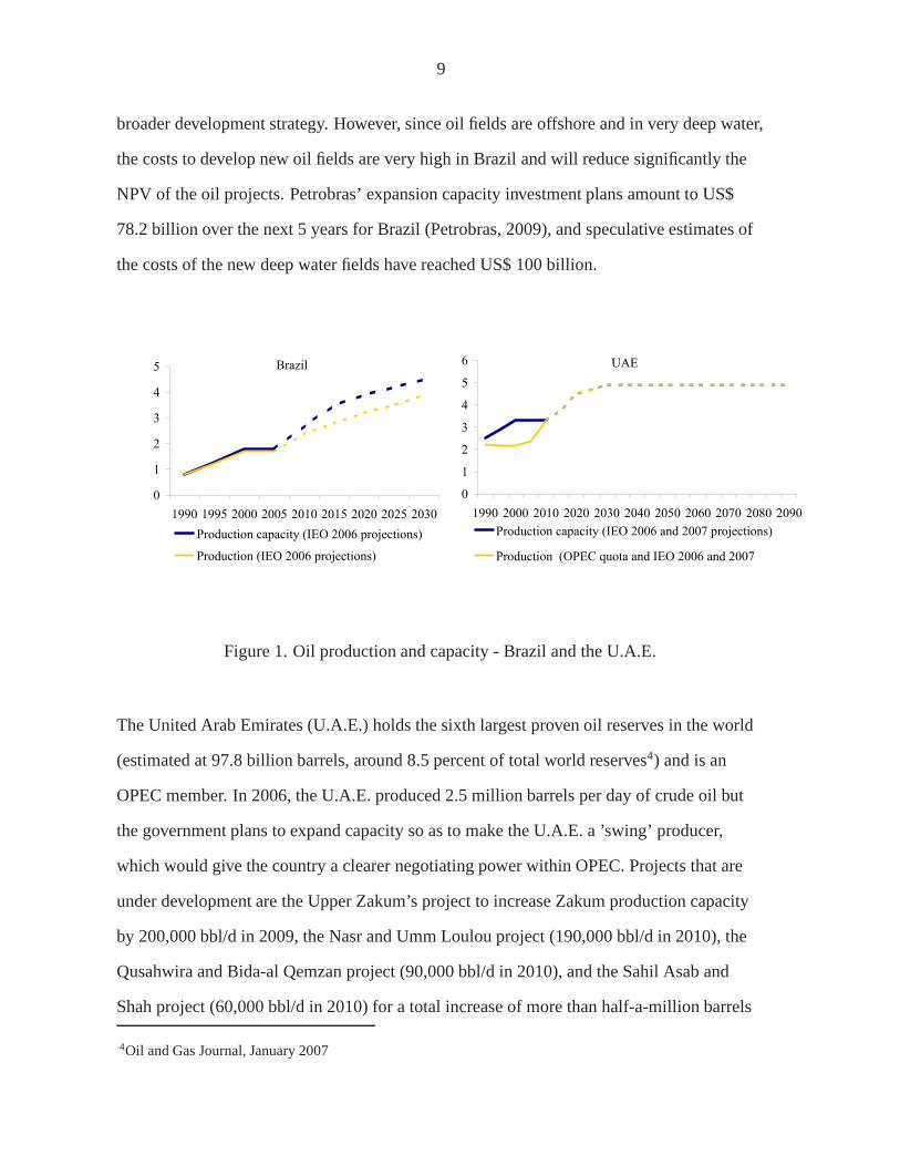
broader development strategy. However, since oil fields areoffshore and in very deep water,

the costs to develop new oil fields are very high in Brazil and will reduce significantly the

NPV of the oil projects. Petrobras’ expansion capacity investment plans amount to US$

78.2 billion over the next 5 years for Brazil (Petrobras, 2009), and speculative estimates of

the costs of the new deep water fields have reached US$ 100 billion.

Brazil

0

1

2

3

4

5

1990 1995 2000 2005 2010 2015 2020 2025 2030

Production capacity (IEO 2006 projections)

Production (IEO 2006 projections)

UAE

0

1

2

3

4

5

6

1990 2000 2010 2020 2030 2040 2050 2060 2070 2080 2090

Production capacity (IEO 2006 and 2007 projections)

Production (OPEC quota and IEO 2006 and 2007

Figure 1. Oil production and capacity - Brazil and the U.A.E.

The United Arab Emirates (U.A.E.) holds the sixth largest proven oil reserves in the world

(estimated at 97.8 billion barrels, around 8.5 percent of total world reserves4) and is an

OPEC member. In 2006, the U.A.E. produced 2.5 million barrels per day of crude oil but

the government plans to expand capacity so as to make the U.A.E. a ’swing’ producer,

which would give the country a clearer negotiating power within OPEC. Projects that are

under development are the Upper Zakum’s project to increaseZakum production capacity

by 200,000 bbl/d in 2009, the Nasr and Umm Loulou project (190,000 bbl/d in 2010), the

Qusahwira and Bida-al Qemzan project (90,000 bbl/d in 2010), and the Sahil Asab and

Shah project (60,000 bbl/d in 2010) for a total increase of more than half-a-million barrels

4Oil and Gas Journal, January 2007

10

per day by 2010 (Energy Information Administration). The plans to scale up the oil sector

in the U.A.E. will cost around US$ 20 billion in investment projects (IMF, 2007).

IV. M ODEL FORMULATION

We present here the multiple real option optimization problem. We consider an economy in

discrete time defined up to a finite time horizon ofT years at which we assume reserves

will be depleted.5 The maximum yearly capacity for extraction (the productioncapacity) is

kt (in billion barrels per year),t = 1, 2, ..., T . kt typically varies with time.6. The optimal

extraction strategy maximizes the discounted cash flows from oil salesV ∗,m,kt at timet,

subject to the capacity constraintsk = {k0, k1, k2, ..., kT} and to the total oil reserves

constraintm. If the oil producer decides to extract a barrel of oil at timet, the profit is

St − ct, whereSt is the price of oil andct the extraction cost. Profits are always positive

when the producer decides to extract oil since she is not forced to produce making losses.

We assume that oil prices follow a discrete Markov chain process(Xt)t=0,1,...,T ∈ Rd (we

come back to the discussion on oil prices in section VI). We write ht(Xt) for the payoff

from the extraction of one unit of oil at timet when the oil price isXt (the argument ofht is

kept implicit in later formulations). We assume that the payoff is non-negative:ht(x) ≥ 0

for all x ∈ Rd, t = 0, . . . , T . The decision maker has the opportunity to extract up tokt

units, that is to receivektht, at timet.

We define an extraction policyπk to be a set of ‘stopping’ times (i.e. times at which the real

options are exercised){τi}mi=1, τ1 ≤ τ2 ≤ · · · ≤ τm, such that the number of exercises (i.e.

5In several of our applications, we assume that countries extract every year a minimum amount of barrels, inwhich case extraction occurs indeed over a finite horizon.

6kt must be a multiple of the discretization unit that we use and that represents one real option to extract oil

11

annual production) is lower than production capacity each year:#{j : τj = s} ≤ ks. The

value of the policyπk at timet is then given by

V πk,mt = Et

[

m∑

i=1

hτi(Xτi)B(t, τi)

]

,

whereB(t, τi) is the discount factor used to value a payoff at timeτi in terms of cash at

time t.

Definition 1. The value function is defined as

V ∗,mt = sup

πk

V πk,mt = sup

πk

Et

[

m∑

i=1

h(Xτi)B(t, τi)

]

.

The corresponding optimal policy isπ∗ = {τ ∗1 , τ∗2 , ..., τ

∗m}.

Two alternative but equivalent formulations are needed to explain the numerical solution

used. The first formulation is used to compute the lower boundof the estimate of the oil

field (the value function) and uses dynamic programming and regression methods. The

second formulation is used to derive the dual formulation ofthe problem, and is the basis

for calculating the upper bound as a the minimum over a set of martingales. The

formulations are presented in the Appendix.

V. NUMERICAL SOLUTION

In this section we explain the solution method using a simpleexample with only one real

option (i.e. only one barrel to extract). In this case the value function can be written as

V ∗t = sup

t≤τ≤T

Et

[

Bt

hτBτ

]

, (1)

12

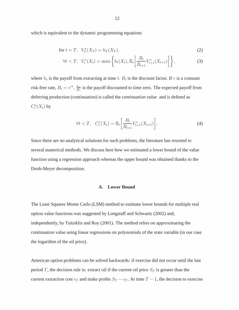
which is equivalent to the dynamic programming equations

for t = T, V ∗T (XT ) = hT (XT ), (2)

∀t < T, V ∗t (Xt) = max

{

ht(Xt),Et

[

Bt

Bt+1

V ∗t+1(Xt+1)

]}

, (3)

whereht is the payoff from extracting at timet. Bt is the discount factor. Ifr is a constant

risk-free rate,Bt = ert. hτ

Bτis the payoff discounted to time zero. The expected payoff from

deferring production (continuation) is called thecontinuation valueand is defined as

C∗t (Xt) by

∀t < T, C∗t (Xt) = Et

[

Bt

Bt+1V ∗t+1(Xt+1)

]

, (4)

Since there are no analytical solutions for such problems, the literature has resorted to

several numerical methods. We discuss here how we estimateda lower bound of the value

function using a regression approach whereas the upper bound was obtained thanks to the

Doob-Meyer decomposition.

A. Lower Bound

The Least Squares Monte Carlo (LSM) method to estimate lowerbounds for multiple real

option value functions was suggested by Longstaff and Schwartz (2002) and,

independently, by Tsitsiklis and Roy (2001). The method relies on approximating the

continuation value using linear regressions on polynomials of the state variable (in our case

the logarithm of the oil price).

American option problems can be solved backwards: if exercise did not occur until the last

periodT , the decision rule is: extract oil if the current oil priceST is greater than the

current extraction costcT and make profitsST − cT . At timeT − 1, the decision to exercise

13

will depend on whether the discounted value ofmax(ST − cT , 0) (the continuation value) is

higher than the immediate payoffmax(ST−1 − cT−1, 0). The LSM method consists in

estimating the continuation value atT − 1 using a regression of the discounted value of

max(ST − cT , 0) (which is known for each Monte Carlo path) on functions of thestate

variablesST−1 andcT−1. Each simulation corresponds to one observation in the regression.

Going backwards, we can calculate the continuation value for all periods. The coefficients

of the regression7, applied to an ‘actual’ price path provides us with an estimate of the

continuation value and the decision rule. The intuition behind this method is that the

continuation value must be a function of the state variable and therefore can be

approximated using simple functions of the oil price. The method provides a lower-bound

estimate of the value function, since only the ‘exact’ optimal policy delivers the maximum

value of the oil field, which is the value function. The estimated continuation value yields

an exercise rule: it is optimal to extract a barrel if and onlyif the current oil price is greater

than the continuation value of the barrel.

The precision of this method depends on the choice of the regressors, but we show later in

the paper that our numerical solution is accurate. The MonteCarlo simulations are used

here at two stages. During the first stage, a set of paths is simulated to determine the

optimal extraction rule using the regressions. During the second stage, having determined

the stopping rule, a second set of paths is simulated to calculate the value function given

that stopping rule.

Let ψ1, ψ2, ..., ψk,ψi : Rd → R be the basis functions (functions of the oil price in our

model) used for regression. We use backward induction and ateach step the method

approximates the continuation value with a linear combination of the basis functions.

7The coefficients are calculated for each periodt as the decision rule changes when approaching expiration.

14

Definition 2. For all timest ∈ {0, 1, 2, ..., T}, at each point of the space set define an

approximation to the continuation value by

Ct(x) =k

∑

i=1

ct,iψi(x). (5)

Let ψ = (ψ1, ψ2, ..., ψk) andct = (ct,1, ct,2, ..., ct,k). If n paths of the Markov chain are

simulated, an estimation for the regression coefficients would be

ct = argminc∈Rk

n∑

j=1

(

C(j)t −

k∑

i=1

ct,iψi(X(j)t )

)2, (6)

where

C(j)t =

Bt

Bt+1V

(j)t+1. (7)

This is a least square problem and explicit formulas exist for the coefficients.

ct = Ψ−1v (8)

Ψl,p =

n∑

j=1

ψl(X(j)t )ψp(X

(j)t ) (9)

vl =n

∑

j=1

ψl(X(j)t )C

(j)t (10)

We approximative the continuation value using the explanatory variablesX,X2, exp(X),

and a constant, whereX is the logarithm of the oil price. Once the coefficients

ct,1, ct,2, ..., ct,k are obtained the continuation value can be approximated at any point using

the current oil price. By simulating then a new set of paths, we can find a lower bound for

the value function.

15

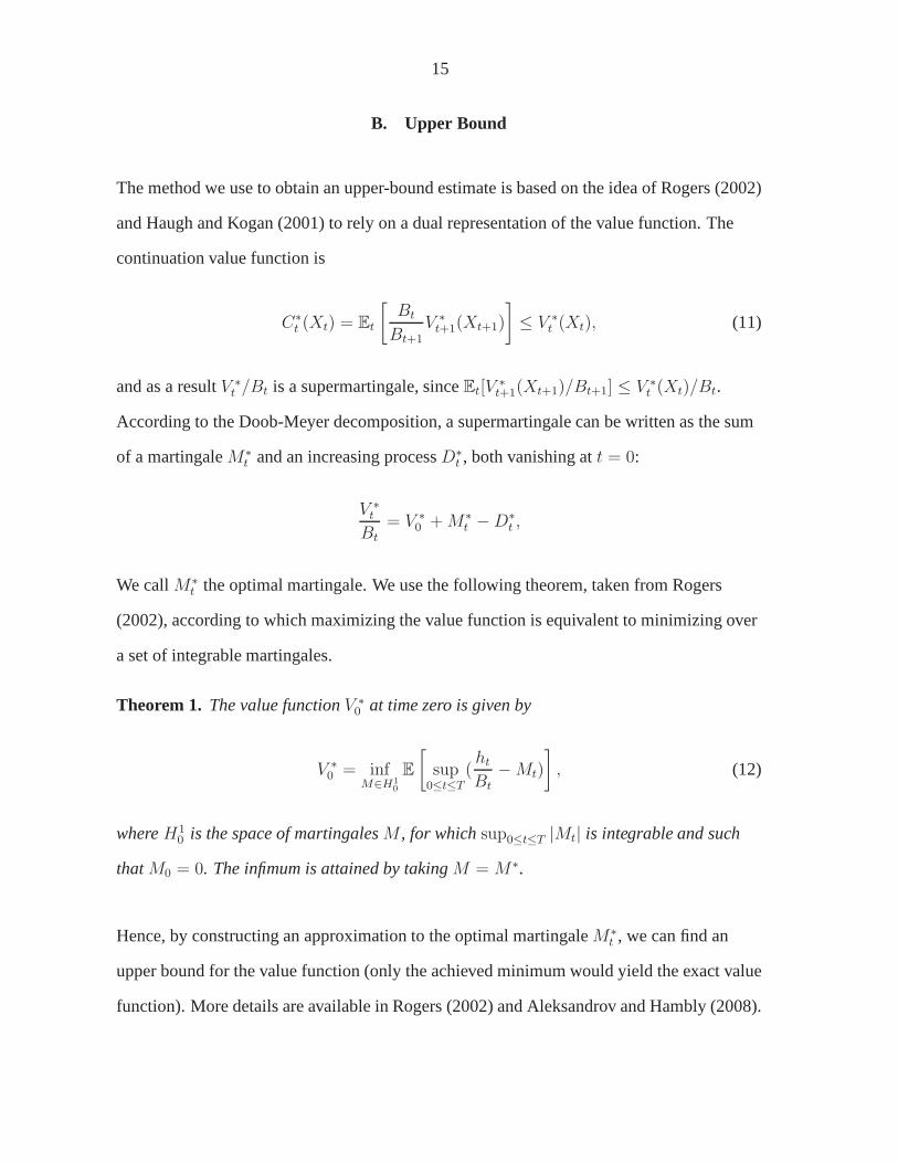
B. Upper Bound

The method we use to obtain an upper-bound estimate is based on the idea of Rogers (2002)

and Haugh and Kogan (2001) to rely on a dual representation ofthe value function. The

continuation value function is

C∗t (Xt) = Et

[

Bt

Bt+1

V ∗t+1(Xt+1)

]

≤ V ∗t (Xt), (11)

and as a resultV ∗t /Bt is a supermartingale, sinceEt[V

∗t+1(Xt+1)/Bt+1] ≤ V ∗

t (Xt)/Bt.

According to the Doob-Meyer decomposition, a supermartingale can be written as the sum

of a martingaleM∗t and an increasing processD∗

t , both vanishing att = 0:

V ∗t

Bt

= V ∗0 +M∗

t −D∗t ,

We callM∗t the optimal martingale. We use the following theorem, takenfrom Rogers

(2002), according to which maximizing the value function isequivalent to minimizing over

a set of integrable martingales.

Theorem 1. The value functionV ∗0 at time zero is given by

V ∗0 = inf

M∈H1

0

E

[

sup0≤t≤T

(htBt

−Mt)

]

, (12)

whereH10 is the space of martingalesM , for whichsup0≤t≤T |Mt| is integrable and such

thatM0 = 0. The infimum is attained by takingM =M∗.

Hence, by constructing an approximation to the optimal martingaleM∗t , we can find an

upper bound for the value function (only the achieved minimum would yield the exact value

function). More details are available in Rogers (2002) and Aleksandrov and Hambly (2008).

16

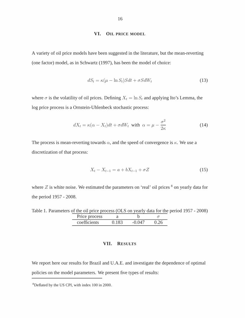
VI. O IL PRICE MODEL

A variety of oil price models have been suggested in the literature, but the mean-reverting

(one factor) model, as in Schwartz (1997), has been the modelof choice:

dSt = κ(µ− lnSt)Sdt+ σSdWt (13)

whereσ is the volatility of oil prices. DefiningXt = lnSt and applying Ito’s Lemma, the

log price process is a Ornstein-Uhlenbeck stochastic process:

dXt = κ(α−Xt)dt+ σdWt with α = µ−σ2

2κ(14)

The process is mean-reverting towardsα, and the speed of convergence isκ. We use a

discretization of that process:

Xt −Xt−1 = a+ bXt−1 + σZ (15)

whereZ is white noise. We estimated the parameters on ‘real’ oil prices8 on yearly data for

the period 1957 - 2008.

Table 1. Parameters of the oil price process (OLS on yearly data for the period 1957 - 2008)Price process a b σcoefficients 0.183 -0.047 0.26

VII. R ESULTS

We report here our results for Brazil and U.A.E. and investigate the dependence of optimal

policies on the model parameters. We present five types of results:

8Deflated by the US CPI, with index 100 in 2000.

17

1959 1965 1971 1977 1983 1989 1995 2001 20070

50

100

150

200

Oil Price

Simulated Oil Price 1

Simulated Oil Price 2

Simulated Oil Price 3

Figure 2. Oil price - historical and simulations.

1. The model parameters we used to determine the optimal policy are assumptions of

the model. We observe the changes in optimal policy when these parameters change,

for a given path of the oil price. We are interested in the dependence of optimal

policy on:

– Volatility of oil prices;

– Interest rates;

– Oil reserves;

– Long-term mean of the oil price;

2. We compare the performance, in terms of discounted cash flows, of the optimal

extraction policy with that of a policy of constant extraction rates. We find that the

value function (i.e. the discounted cash flow for the optimal policy) is around twice

higher than the discounted cash flow obtained with constant extraction policies for the

most extreme case.9

3. Brazil’s production is at par with that of the U.A.E. in spite of having much smaller

confirmed reserves. Is this optimal for Brazil? We compare the decision rule of for

9We also calculate the upper and lower bound of the value function and show that the bounds around thevalue function are tight, demonstrating the effectivenessof the numerical method.

18

Brazil with that of the U.A.E. and show that Brazil should only produce when oil

prices are high, at US$ 73, whereas the U.A.E. should produceas soon as the oil price

exceeds US$ 39.

4. We estimate the value in terms of discounted cash flows of anadditional capacity

unit, for a given volume of reserves. The result can be fed into a model of Net Present

Value of an investment project when assessing the optimality of capacity expansion.

5. We extend the model to allow for extraction costs, which assumed to follow a random

walk with drift. We use data from Petrobras to estimate the parameters of the

stochastic process and show how optimal policy is affected by these extraction costs.

We assume in all calculations that the extraction decisionsare made on a yearly basis. The

smallest unit that is used to change production is 0.2 billion barrels per year, equivalent to

0.55 million barrels per day. We also make the assumption that each country extracts at

least 0.5 billion barrels per year to finance operations and ensure a minimum of revenues.

In 2008, Brazil had 12.2 billion barrels of proven oil reserves and U.A.E. had 97.8 billion

barrels. We will use these numbers, adjusted for a recovery rate of 65 percent, for the total

extractable amounts of oil when computing the threshold at which the countries should

produce oil. Given the large difference in the proven total reserves, the production horizon

of U.A.E. is much longer: for Brazil the time horizon chosen is 15 years, which leaves us

with 25 units of 0.2 billion barrels per year (after the minimal extraction rate of 0.5 billion

barrels per year are subtracted). For the U.A.E. we considera time horizon of 100 years and

240 extractable units.

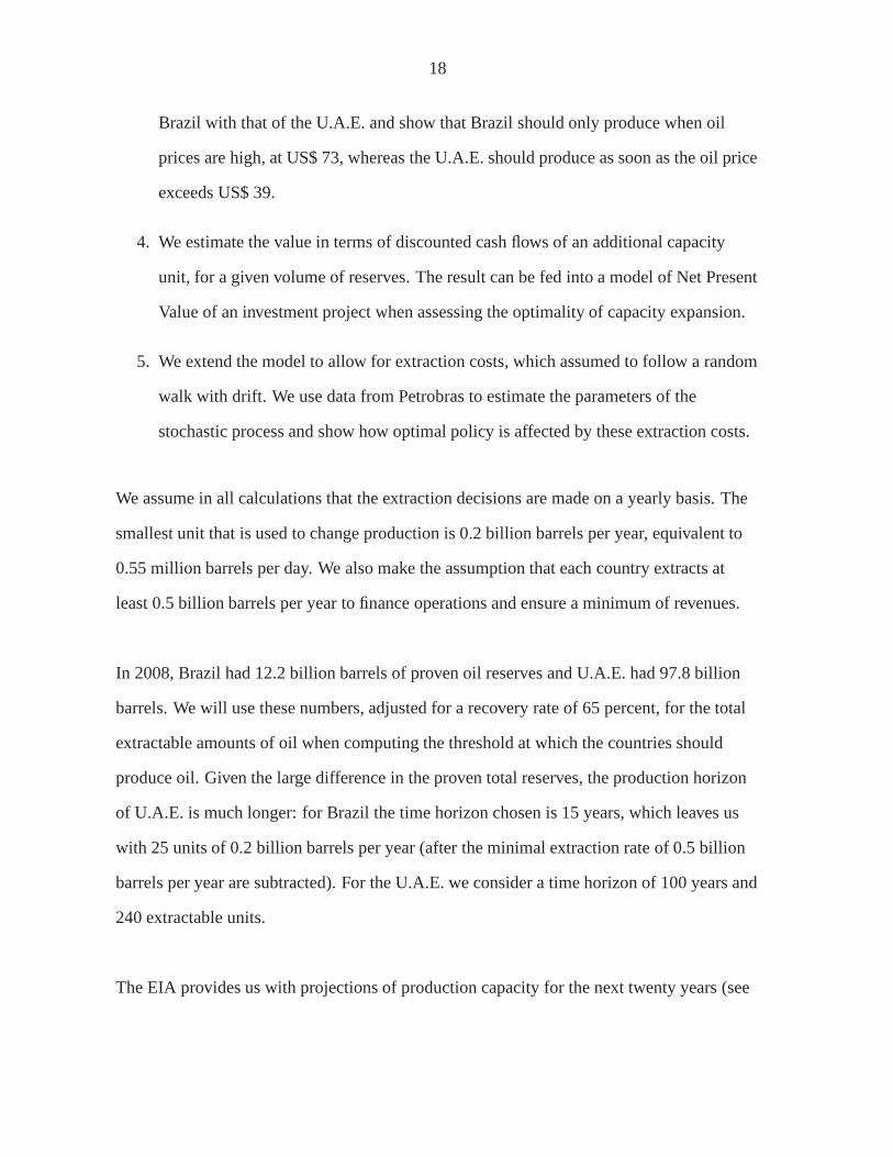
The EIA provides us with projections of production capacityfor the next twenty years (see

19

tables 2 and 3), and we assume capacity is constant after 2030. The calibration used for the

numerical results is that of table 4.

Table 2. Oil production capacity outlook 2010-2030 (Million Barrels per Day). Source: EIA,System for the Analysis of Global Energy Markets (2006);

Country 2010 2015 2020 2025 2030United Arab Emirates 3.3 3.5 3.9 4.4 4.6Brazil 2.7 3.5 3.9 4.2 4.5

Table 3. Oil production capacity outlook 2010-2030 (Billion Barrels per Year). Source: EIA,System for the Analysis of Global Energy Markets (2006);

Country 2010 2015 2020 2025 2030United Arab Emirates 1.2 1.3 1.4 1.6 1.7Brazil 1.0 1.3 1.4 1.5 1.6

Table 4. Calibration for Oil production capacity outlook 2010-2110 (One unit equals 0.2billion barrels).

Year 1-5 5 -10 10-15 15-20 20-100Extractable Units 3 4 5 6 6

A. Dependence of the Optimal Policy on the Model Parameters:the case of Brazil

We show figure 3 the optimal policy for Brazil for a particularpath of the oil price. The oil

price is relatively low at the beginning and therefore the oil producer, knowing the volatility

and trend of oil prices, decides to defer production. In 2020(the model starts in 2010),

when oil prices rise above 60 US dollars (in 2000 terms,i.e. around 75 US dollars of 2008

10), the optimal strategy is to produce at full capacity. Oil reserves are almost depleted by

2025. The model predicts very volatile production plans, since as soon as the price exceeds

a certain threshold value (see discussion later), production at full capacity is optimal. This

result could be reversed with high and increasing marginal extraction costs but we abstract

from extraction costs until section F.

10US CPI inflation between 2000 and 2008 was 25 percent

20

Optimal Extractio Policy - Brazil

0

0.2

0.4

0.6

0.8

1

1.2

1.4

1.6

1.8

1 2 3 4 5 6 7 8 9 10 11 12 13 14 15 16 Years

Oil

Pro

du

ctio

n (

in b

n

ba

rrel

s p

er y

ear)

0

20

40

60

80

100

120

140

160

180

Oil

Pri

ce

Optimal Extraction Policy Minimum Extraction

Capacity Oil Price

Figure 3. Optimal extraction policy

Sensitivity to Oil Price Volatility

0

0.2

0.4

0.6

0.8

1

1.2

1.4

1.6

1.8

0 2 4 6 8 10 12 14 16

Years

Pro

du

ctio

n (

bn

barr

els

per

yea

r)

0

20

40

60

80

100

120

140

160

180

Oil

Pri

ce

sigma = 0.13 sigma = 0.26

sigma = 0.52 Oil Price

Figure 4. Optimal extraction policy - dependence on oil price volatility

21

Sensitivity to Interest Rates

0

0.5

1

1.5

2

0 2 4 6 8 10 12 14 16

Years

Pro

du

ctio

n (

bn

barr

els

per

yea

r)

0

20

40

60

80

100

120

140

160

180

Oil

Pri

ce

r = 0.01 r = 0.02

r = 0.03 Oil Price

Figure 5. Optimal extraction policy - dependence on real interest rates

Sensitivity to Size of Reserves

0

0.5

1

1.5

2

0 2 4 6 8 10 12 14 16

Years

Pro

du

ctio

n (

bn

barr

els

per

yea

r)

0

20

40

60

80

100

120

140

160

180

Oil

Pri

ce

M = 25 M = 30

M = 40 Oil Price

Figure 6. Optimal extraction policy - dependence on oil reserves

22

Sensitivity to Long-term Mean of the Oil Price

0

0.2

0.4

0.6

0.8

1

1.2

1.4

1.6

1.8

2

0 2 4 6 8 10 12 14 16Years

Pro

du

ctio

n (

bn

ba

rrel

s p

er y

ear)

0

20

40

60

80

100

120

140

160

180

Oil

Pri

ce

a = 0.1221 a = 0.1831

a = 0.2747 Oil Price

Figure 7. Optimal extraction policy - dependence on long term mean

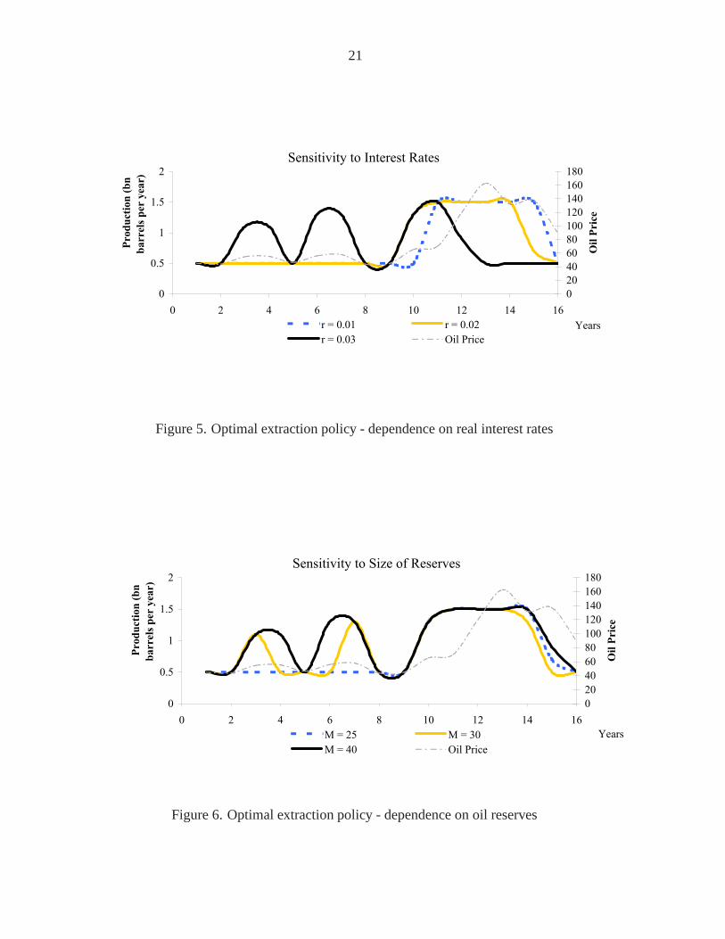
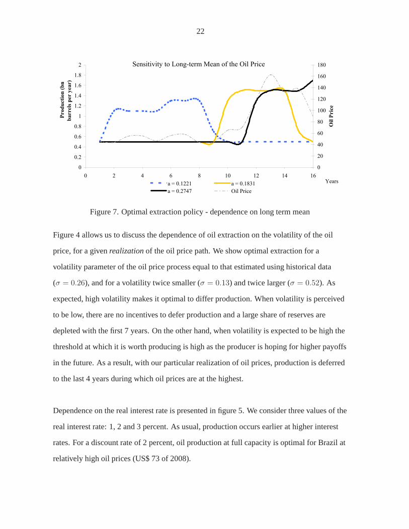
Figure 4 allows us to discuss the dependence of oil extraction on the volatility of the oil

price, for a givenrealizationof the oil price path. We show optimal extraction for a

volatility parameter of the oil price process equal to that estimated using historical data

(σ = 0.26), and for a volatility twice smaller (σ = 0.13) and twice larger (σ = 0.52). As

expected, high volatility makes it optimal to differ production. When volatility is perceived

to be low, there are no incentives to defer production and a large share of reserves are

depleted with the first 7 years. On the other hand, when volatility is expected to be high the

threshold at which it is worth producing is high as the producer is hoping for higher payoffs

in the future. As a result, with our particular realization of oil prices, production is deferred

to the last 4 years during which oil prices are at the highest.

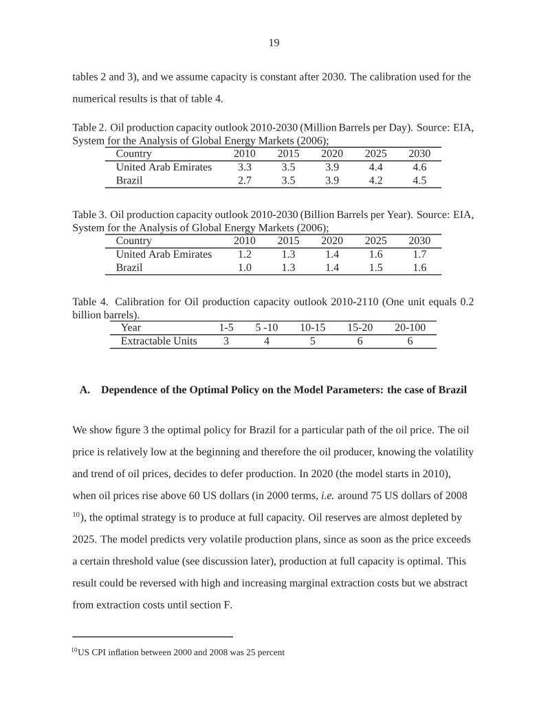
Dependence on the real interest rate is presented in figure 5.We consider three values of the

real interest rate: 1, 2 and 3 percent. As usual, production occurs earlier at higher interest

rates. For a discount rate of 2 percent, oil production at full capacity is optimal for Brazil at

relatively high oil prices (US$ 73 of 2008).

23

Finally, we show the dependence of optimal extraction on thevolume of recoverable oil

reserves. The amount of oil that is known to be in the ground or‘proven reserve’ varies as

new fields are being explored. Furthermore, recovery rates from extraction have improved

with technological advances and therefore the volume of recoverable reserves can change.

We show in figure 6, for Brazil, how production would change ifit had access to 12.5, 13.5

or 15.5 billion barrels. The profiles or production are not fundamentally changed.

B. Precision of the Solution

The numerical solution method can be affected by two types oferrors:

• Monte Carlo errors that depend on the number of paths;

• Errors coming from the approximation of the continuation values.

We can reduce the Monte Carlo error by increasing the number of paths. The size of the

Monte Carlo error, which depends on the number of paths and the standard deviation of the

estimates, can also be computed. It is more complicated however to assess the accuracy of

our approximation to the continuation value for a chosen setof basis functions. We use the

lower and the upper bounds to construct a confidence intervalfor the value function. We

compare the upper and lower bound approaches for our baseline model.11 Figure 8 shows

that the relative difference between the upper and the lowerbound does not exceed 3%,

which confirms the accuracy of the numerical approximationsused.

11The baseline model use the estimated parameters (a = 0.183126, b = −.04708 andσ = 0.26), the realinterest rater is assumed at 2 percent, and the time horizon is 100 years. Oilreserves are those provided bythe IEA, and production capacity is that of table 3 and table 4.

24

Relative difference between upper and lower bounds

0

0.005

0.01

0.015

0.02

0.025

0.03

0.035

1 3 5 7 9 11 13 15 17 19 21 23 25 27 29 31 33 35 37 39 41 43 45 47 49

Extractable units

Val

ue

Figure 8. Relative difference between the upper and lower bounds for the value functions

C. Optimal Strategy as an Improvement over Constant Extraction Policy

In this section, we compare the value of an oil field under different production policies. The

value functions are computed for different minimum extraction rates, since this is an

important determinant of the value of the oil field.A priori, minimum extraction rates

should be zero, for countries that can borrow from financial markets. However, many oil

producers crucially depend on contemporaneous oil surpluses to finance government

expenditure and current account deficits, and as a result, itmay be more realistic to assume

some minimum extraction rates. We compute the value function for three different

minimum extraction rates, of 0, 0.5 and 0.7 billion barrels per year.12

We also compute the value of the oil field under a policy of constant extraction rate (a linear

extraction model). The value of the oil field under linear extraction is calculated by

averaging the net present value of cash flows received from the sales of oil if the extraction

was done at a constant rate over time.

12To be consistent with the previous sections we use 0.2 billion barrels as a unit in all models.

25

We show in figure 9 the inter-temporal value of an oil field as a function of its size (in units

of 0.2 billion barrels) under the two extreme assumptions ofzero minimum extraction rate

and linear extraction. For instance, a 10 billion barrels oil field is worth US$ 357.9 billion

under a constant extraction policy, but is worth US$ 835.4 billion under the optimal policy

with zero minimum extraction rate. The benefits from following an optimal strategy would

therefore reach 133% in terms of net present value, a dramatic improvement. This

proportion is approximately constant for different valuesof the oil reserves.

Assuming that a minimum amount of 0.5 billion barrels per year is produced every year, the

gains from optimizing the remaining production in functionof oil prices still reach 25.6

percent (above the linear extraction value). If the minimumextraction rate is 0.7 billion

barrels per year, the gains from optimizing would be 22.5 percent.

Overall, the model predicts that the value of an oil field for which production is decided in

function of oil prices far exceeds the linear extraction value computed in a deterministic

setting. The economic and policy implications of our results for Brazil and the U.A.E. are

different. In recent years, OPEC countries tended to vary production with oil prices,

because OPEC had a policy to stabilize prices. This policy isalso in line with maximizing

expected net present value since stabilizing prices requires increasing production when

prices are high and decreasing production when prices are low. The implication of the

model for such countries is that the valuation of oil fields needs to be adjusted to take into

account the fluctuations in production that are due to oil price shocks. The current practice,

in many macroeconomic applications (such as fiscal or external sustainability assessment),

is to use a deterministic path of production (derived from production capacity) and a

deterministic price path (often deduced from future prices) to estimate the value of oil

wealth. The model shows that such valuation methods underestimate the value of oil fields

26

for countries that are able and willing to adjust productionwith oil prices.

The implications of the model for non-OPEC countries that produce at full capacity because

of their urgent need of revenues is that this policy is very costly: inter-temporal revenues

could be twice larger with an optimized strategy. We discussin the last section of the paper

how oil producers behaved in the last thirty years and the implications for world oil markets.

1 6 11 16 21 26 31 36 41 46

0

200

400

600

800

1000

Va

lue F

un

cti

on

(in

bil

lio

ns

US

$)

Net Present Value of Reserves - Lower and Upper Bounds

Linear extraction (no optimization) Optimized (Lower Bound estimate)

Optimized (Upper Bound estimate)

Extractable Units (0.2 billion barrels per unit)

Figure 9. Net present value of reserves as a function of the reserves.

D. U.A.E. - Brazil Comparison

We compare here the optimal extraction policies of Brazil and U.A.E. The two countries

have currently similar extraction rates, although their known resources are very different.

We show in figure 10 the extraction boundaries for Brazil and the U.A.E. These are

functions of the logarithm of the oil price, which we used as avariable in our approximation

to the continuation values in the optimal stopping problem.The oil price above which a

country should start producing above the minimum requirement is at the intersection of the

payoff (which is the oil price, plotted here as a function of the logarithm of the oil price)

27

and the continuation value, estimated from the regression method as a function of the

logarithm of the oil price. The calculations are made under the assumptions that the time

horizons are 15 years for Brazil and 100 years for the U.A.E. and the reserves are 12 billion

barrels for Brazil and 98 billion barrels for the U.A.E.13 If the oil price is higher than the

extraction boundary, it is optimal to extract more than the minimum amount; otherwise, the

minimum amount should be extracted. Figure 10 shows that theextraction boundary for

Brazil is significantly higher for Brazil. According to the model, in 2008, Brazil should

only start producing above the minimum when oil prices are above US$ 73 (at 2000 prices,

around 91 US$ at 2008 prices). The corresponding minimal price for the U.A.E. is US$ 39

of 2000 (49 US$ of 2008).

2.5 3 3.5 4 4.5 5 5.50

50

100

150

200

250

Log Oil Price

Pay

off/C

ontin

uatio

n V

alue

Minimum Extraction Prices − UAE and Brazil.

Payoff (Oil price)

Continuation Value − Brazil

Continuation Value − UAE

Minimum Extraction Price − UAE

Minimum Extraction Price − Brazil

Figure 10. Minimum extraction prices for 2010

13We have again assumed minimal extraction of 0.5 billion barrels per year. The oil price parameters are as intable 1 and the real interest rate is assumed to be 2 percent.

28

E. Investment Decision: Adding New Capacity

In this section, we investigate the benefits of investing in capacity expansion. More

precisely, we compute the increase in net present value of the oil fields (the value function)

that is obtained when increasing capacity, for a given amount of total reserves. The increase

in NPV is our estimate of the shadow price of the yearly production capacity constraint.

This number can be used to assess the profitability of a project for which investment costs

are known.

We consider two countries with oil reserves estimated at 5 and 10 billion barrels (25 and 50

units respectively).14 The results are presented in table 5. A capacity expansion of200

million barrels per year in 2025 (1 additional unit in Year 15) improves the value of the oil

reserves by US$ 2.1 billion, for a country whose reserves are5 billion barrels. The increase

would reach US$ 6.27 billion for a country that holds 10 billion barrels. Additional

capacity has more value for countries with larger reserves,a result that, if it already existed,

was not echoed in the oil production literature. The intuition is clear: the additional option

provided by higher capacity has more value if it is availablefor many years and if

production capacity was a tighter constraint at times of high prices. Our results therefore

suggest that project evaluation needs to be performed in thecontext of the overall oil

strategy of the country, since the viability and profitability (i.e. net present value) of

projects cannot be assessed project-by-project.

New capacity generally gives access to more reserves in addition to providing more

flexibility. We show in table 6 the value of such a project if the additional reserves are worth

1 billion barrels (5 units of 200 million barrels). 200 million barrels of increased capacity in

14The oil price process parameters are as before. We start withlog oil price of 4 (S = 54.6). The time horizonin 100 years.

29

Table 5. Added value by expanded capacity.Year (unit = 0.2 bn bbl/year) 1-5 5 -10 10-15 15- 25 units 50 unitsCurrent capacity 3 4 5 5 US$ 325.9bn US$ 622.5bnIncreased capacity 3 4 5 6 US$ 328bn US$ 628.8bnAdded value US$ 2.1bn US$ 6.27bn

2025 and 1 billion more of accessible reserves are worth US$ 65.6 billion for a country that

controls 5 billion barrels of reserves and US$ 62.7 billion for a country that owns 10 billion

barrels. The value of the project is in that case higher for the country with lower reserves

because the value of optionality is dwarfed by the value of additional oil reserves, and an

additional one billion barrels of oil reserves is worth morefor a country that has low

reserves than for a country that has high reserves. Indeed, for a similar production capacity,

a country with low reserves can ‘distribute’ the extractionof newly-found reserves more

optimally than a country that has high reserves.

Table 6. Added value by expanded capacity and increased access to reserves.Year (unit = 0.2 bn bbl/year) 1-5 5 -10 10-15 15- 25/30 50/55Current capacity 3 4 5 5 US$ 325.9bn US$ 622.5bnIncreased capacity 3 4 5 6 US$ 391.4bn US$ 685.2bnAdded value US$ 65.6bn US$ 62.7bn

F. Extraction Costs

The multiple real option approach is flexible enough to allownumerical solutions even

when the dimensionality of the problem (the number of state variables) increases. We show

briefly in this section how to extend the model to include stochastic extraction (or lifting)

costs. The extraction costs are calibrated on data reportedby Petrobras (figure 11) assuming

the process is a random walk with drift :15

ct = c+ ct−1 + σcWc1 (16)

15Since Petrobras produces 95% of Brazil’s crude oil, these numbers are accurate estimates for Brazil oil fields.

30

0

5

10

15

20

25

30

35

99/Q1

99/Q3

00/Q1

00/Q3

01/Q1

01/Q3

02/Q1

02/Q3

03/Q1

03/Q3

04/Q1

04/Q3

05/Q1

05/Q3

06/Q1

06/Q3

07/Q1

07/Q3

08/Q1

08/Q3

09/Q1

Lifting Costs without government participation, in US$ perbarrelLifting Costs with government participation, in US$ per barrel

Figure 11. Extraction costs reported by Petrobras of Brazilfor the period 1999 - 2009.Source: Petrobras reports.

whereW c1 is a standard normal random variable,c is the drift, andσc the volatility(see

estimates in Table 7).16

Table 7. Annualized parameters of the lifting cost process,estimated using quarterly data forthe period 1999 - 2009.

Extraction costs c σcCoefficients 0.416 0.602

The payoff from selling a unit of oil at timet is ht = St − ct. In order to account forct in

the regression algorithm we add it to the set of basis functionsψ. We show the impact of

extraction costs on the optimal policy in figure 12. We observe a large difference in optimal

policy in year 7: when the extraction cost is US$ 10.55 per barrel (cost path 1), maximum

production is optimal whereas when the cost is US$ 18.65 (cost path 2), production is

reduced to the minimum. For a country like Brazil, for which extraction costs are uncertain

but likely to be high, a model that includes stochastic extraction costs suggests that

16We assume extraction costs and oil prices are independent and estimate on quarterly datac = 0.104 andσc = 0.301. The numbers reported in table 7 are on a yearly basis.

31

production could be differed on account of even limited increases in extraction costs. In this

model, the two state variables are independent, but one can see from figure 12 that optimal

policy involves minimum production in year 7 because extraction costs are high, and at the

same time oil prices are low.

Sensitivity to Extraction Costs

0

0.2

0.4

0.6

0.8

1

1.2

1.4

1.6

1.8

0 2 4 6 8 10 12 14 16years

Oil

Pro

du

ctio

n (

bn

ba

rrel

s

per

yea

r)

0

20

40

60

80

100

120

140

160

180

Oil

Pri

ce/

Ex

tra

ctio

n C

ost

Cost path 1 Cost path 2

Optimal policy cost path 1 Optimal policy cost path 2

Oil Price

Figure 12. Optimal extraction policy - dependence on extraction costs

VIII. T HE GLOBAL SUPPLY CURVE

The model gives us two points in the theoretical world marketsupply curve (Brazil and the

U.A.E.), and the aim of this section is to derive a rough approximation of the rest of the

supply curve. We ranked countries with capacity higher than500 thousand bb/d by their

reserves and cumulated their production (see table 8).

Kuwait expected production profile and reserves are very similar to those of the U.A.E. and

therefore its decision rule should be the same. Algeria, Mexico and Brazil should also have

comparable policies (threshold around US$90) while Venezuela’s threshold price would lie

in between. Norway and Egypt policies should be to extract atprices higher than US$90

only. Roughly speaking, the theoretical supply curve couldbe represented as in figure 13.

32

Country Reserves Production Cumulated productionAustralia 1.5 586.4 79345.8Colombia 1.5 600.6 78759.3Argentina 2.6 792.3 78158.7

U.K. 3.6 1583.9 77366.4Egypt 3.7 630.6 75782.6

Malaysia 4.0 727.2 75152.0Indonesia 4.4 1051.0 74424.8

Ecuador 4.5 505.1 73373.8Oman 5.5 761.0 72868.7India 5.6 883.5 72107.7

Norway 6.9 2466.0 71224.2Azerbaijan 7.0 875.2 68758.3

Angola 9.0 2014.5 67883.1Mexico 11.7 3185.6 65868.6

Brazil 12.2 2422.0 62682.9Algeria 12.2 2179.8 60260.9

Qatar 15.2 1207.6 58081.1China 16.0 3973.1 56873.6

U.S. 21.3 8514.2 52900.4Kazakhstan 30.0 1429.3 44386.3

Nigeria 36.2 2168.9 42957.0Libya 41.5 1875.2 40788.1

Russia 60.0 9789.8 38912.9Venezuela 87.0 2642.9 29123.1

U.A.E. 97.8 3046.5 26480.2Kuwait 104.0 2741.4 23433.7

Iraq 115.0 2385.4 20692.4Iran 138.4 4174.4 18306.9

Canada 178.6 3350.4 14132.5Saudi Arabia 266.8 10782.1 10782.1source: IEA

Table 8. Reserves (in billion barrels) and production (in thousand bb/d) in 2008

33

In such a world, the supply elasticity would be very large andoil price volatility would

never reach the levels attained in 2008-2009. Indeed, demand would need to fall as low as

30 million bb/d to see prices declining to US$ 40. On average,production would be lower

(as several countries would find the oil price to be below their threshold price). As a result,

prices would be higher but less volatile.

World Markets

140

World Markets

d

Demand 1

Brazil Egypt

100

120

140

pri

ces)

World Markets

Demand 2

Demand 1

Brazil Egypt

Norway

60

80

100

120

140

at

20

00

pri

ces)

World Markets

Demand 2

Demand 1

Brazil Egypt

Norway

Venezuela Kuwait 40

60

80

100

120

140

pri

ce (

at

20

00

pri

ces)

World Markets

Demand 2

Demand 1

Brazil Egypt

Norway

Venezuela

UAE

Kuwait

0

20

40

60

80

100

120

140

Oil

pri

ce (

at

20

00

pri

ces)

World Markets

Demand 2

Demand 1

Brazil Egypt

Norway

Venezuela

UAE

Kuwait

0

20

40

60

80

100

120

140

0 20000 40000 60000 80000

Oil

pri

ce (

at

20

00

pri

ces)

Oil production (in thousand bb/d)

World Markets

Demand 2

Demand 1

Brazil Egypt

Norway

Venezuela

UAE

Kuwait

0

20

40

60

80

100

120

140

0 20000 40000 60000 80000

Oil

pri

ce (

at

20

00

pri

ces)

Oil production (in thousand bb/d)

World Markets

Demand 2

Demand 1

Brazil Egypt

Norway

Venezuela

UAE

Kuwait

0

20

40

60

80

100

120

140

0 20000 40000 60000 80000

Oil

pri

ce (

at

20

00

pri

ces)

Oil production (in thousand bb/d)

World Markets

Demand 2

Demand 1

Figure 13. World oil market

There are several potential explanations to why the supply curve is much less elastic in

reality than the model would predict (see for instance Krichene, 2005, who shows that

short-term supply is insensitive to price) and we discuss below the two that we think are

most relevant.

• The NPV model is not appropriate if a country’s discount rateis contingent on oil

production. This will be the case for oil producers whose budget and external

34

accounts are highly dependent on oil revenues. For such countries, cutting production

at the time prices are low will push those accounts in deficit and trigger borrowing at

increased rates, which governments and oil companies will be unwilling to do.

However, given the significant losses in NPV (100 percent in the extreme case),

strategies that lead to more volatile production should be considered, especially for

producers with larger reserves and for those who already accumulated large financial

reserves. Casual data investigation did not support the hypothesis that countries with

higher reserves produce at more volatile rates, although OPEC production is indeed

more variable than non-OPEC production. For most countries, production has been at

full capacity in the last 30 years.

• There may be technical limitations as well that reduce the benefits of choosing

variable production. For instance, there is a minimum turn-down that is necessary to

have the plant on, to avoid rusting, losing staff, etc. Similarly, if extraction costs are a

function of oil production, the solution of the model will differ somewhat and optimal

oil production will be less volatile. This is why we also computed the NPV gains for

optimizing over part of the capacity (and we found it to be in excess of 20 percent).

Depending on the specificity of these technical costs, countries could either optimize

the functioning of each extraction units over half of the capacity or take decisions

every year to shut down or run at full capacity half of the production units.

IX. C ONCLUSION

We proposed a Monte Carlo real option approach as a solution to the optimization problem

of a price-taker oil producer. This approach allows us to replicate the basic results of the

‘waiting to invest’ literature in a multiple-period setting. The Monte Carlo numerical

solution is accurate and flexible enough to solve the problemwith increasing capacity and

with several state variables. We also investigated the value of increasing capacity and

35

showed that the marginal value of additional capacity is higher for countries with higher

resources, because additional capacity generates new options to extract oil, and such options

have more value for countries with larger resources and longer horizons of production.

We showed that, in theory, the net present value of these countries’ oil reserves are grossly

underestimated (at around half of their true value, in the most extreme case) if one does not

take into account optimizing strategies. We also showed that the optimal policies imply

production profiles that are much more volatiles than the observed ones - even when one

assumes that some minimum extraction is needed to finance operations or government

budgets. As a result, the theoretical supply is much more elastic than the actual one, and the

equilibrium consequences of that result is that oil prices are lower, but much more volatile

than what would be the case if oil producers were optimizing by maximizing the NPV of oil

fields. The puzzle could be partially resolved by modeling extraction costs as a function of

oil production, but in practice, costs tend to depend on capacity rather than on production

itself. Technical costs may also limit the scope for varyingproduction, but even optimizing

over half of capacity would yield substantial benefits to oilproducers, while reducing oil

price volatility. The most convincing explanation seems tobe that countries and companies’

borrowing conditions would be worsened by such pro-cyclical extraction policies, and this

is why such extraction policies are not in place. Finding ways to reduce the pro-cyclicality

of borrowing conditions could therefore yield substantivebenefits at the individual country

level at the same time as stabilizing the oil market.

36

REFERENCES

Aleksandrov, N., and B. Hambly, 2008, “A Dual Approach to Some Multiple Exercise

Option Problems,”forthcoming, Mathematical Methods of Operations Research

Andersen, L., and M. Broadie, 2001, “A Primal-dual Simulation Algorithm for Pricing

Multidimensional American Options,” Columbia Business School Working Paper (New

York NY: Columbia Business School).

Arrow, K. J., D. Blackwell, and M.A. Girshick, 1949, “Bayes and Minimax Solutions of

Sequential Decision Problems,” Econometrica, Vol. 17, pp.213-244.

Bardou, O.A., S. Bouthemy and G. Pags, 2007a, “Optimal Quantization for the Pricing of

Swing Options,” preprint at http://arxiv.org/abs/0705.2110.

Bardou, O.A., S. Bouthemy and G. Pags, 2007b, “When Are SwingOptions Bang-bang and

How to Use It,” preprint at http://arxiv.org/abs/0705.0466.

Barrera-Esteve, C., F. Bergeret, C. Dossal, E. Gobet, A. Meziou, R. Munos and D.

Reboul-Salze, 2006, “Numerical Methods for the Pricing of Swing Options: A Stochastic

Control Approach,” Methodology and Computing in Applied Probability, Vol. 8, pp.

517-540.

Bellman, R., 1956, “A Problem in the Sequential Design of Experiments,” Sankhya, Vol.

16, pp. 221-229.

Bender, C., 2008, “Dual Pricing of Multi-exercise Options under Volume Constraints,”

37

mimeo, TU Braunschweig.

Bensoussan, A., 1984, “On the Theory of Option Pricing,” Acta Applicandae

Mathematicae, Vol. 2, pp. 139-158.

Broadie, M., and P. Glasserman, 1997, “Pricing American-style Securities by Simulation,”

Journal of Economic Dynamics and Control, Vol. 21, pp. 1323-1352.

Cairoli, R. and R. Dalang, 1996, Sequential Stochastic Optimization, Wiley Series in

Probability and Statistics, New York NY: John Wiley and Sons.

Caldentey, R., R. Epstein and D. Saure, 2006, “Optimal Exploitation of a Nonrenewable

Resource,” mimeo, New York University.

Carmona, R., and S. Dayanik, 2008, “Optimal Multiple Stopping of Linear Diffusions,”

Mathematics of Operations Research, Vol. 33, pp. 446-460.

Carmona, R., and N. Touzi, 2008, “Optimal Multiple Stoppingand Valuation of Swing

Options,” Mathematical Finance, Vol. 18, pp. 239-268.

Cherian, J., J. Patel and I. Khripko, 1998, “Optimal Extraction of Nonrenewable Resources

when Prices Are Uncertain and Costs Cumulate,” NUS BusinessSchool Working Paper

(Singapore: NUS).

Dias, M.A., 2004, “Valuation of Exploration and ProductionAssets: An Overview of Real

Option Models,” Journal of Petroleum Science and Engineering, Vol. 44, pp. 93-114.

38

Dixit, A.K., and R.S. Pindyck, 1994, Investment under Uncertainty, Princeton NJ: Princeton

University Press.

Glasserman, P., 2003, Monte Carlo Methods in Financial Engineering, New York NY:

Springer-Verlag.

Gilbert, R., 1979, “Optimal Depletion of an Uncertain Stock,” The Review of Economic

Studies, Vol. 46, pp. 47-57.

Haugh, M.B., and L. Kogan, 2001, “Pricing American Options:A Duality Approach,”

Technical Report, Operation Research Center, MIT and The Wharton School, University of

Pennsylvania.

Hotelling, H., 1931, “The Economics of Exhaustible Resources,” Journal of Political

Economy, Vol. 39, pp. 137-175.

IMF, 2007, Article IV Consultations for the U.A.E., 2007. Washington DC: International

Monetary Fund.

Jaillet, P., E.I. Ronn and S. Tompaidis, 2004, “Valuation ofCommodity-based Swing

Options,” Management Science, Vol. 50, pp. 909-921.

Keppo, J., 2004, “Pricing of Electricity Swing Options,” Journal of Derivatives, Vol. 11, pp.

26-43.

Krichene, N., 2005, “A Simultaneous Equation Model of for World Crude Oil and Natural

Gas Markets,” IMF Working Paper, N. 05/32, Washington DC: Intenrational Monetary

39

Fund.

Longstaff, F.A., and E.S. Schwartz, 2002, “Valuing American Options by Simulation: A

Least-Square Approach,” The Review of Financial Studies, Vol. 5, pp. 5-50.

Myers, S.C., 1977, “Determinants of Corporate Borrowing,”Journal of Financial

Economics, Vol. 5, pp. 147-175.

Meinshausen, N., and B.M. Hambly, 2004, “Monte Carlo Methods for the Valuation of

Multiple-Exercise Options,” Mathematical Finance, Vol. 14, pp. 557-583.

Paddock, J.L., D.R. Siegel and J.L. Smith, 1988, “Option Valuation of Claims on Real

Assets: The case of Offshore Petroleum Leases,” Quarterly Journal of Economics, Vol. 103,

pp. 479-508.

Petrobras, 2009, Petrobras Business Plan Presentation, 2009-2013.

Pindyck, R., 1978, “The Optimal Exploration and Productionof Nonrenewable Resources,”

The Journal of Political Economy, Vol. 86, pp. 841-861.

Rogers, L.C., 2002, “Monte Carlo Valuation of American Options,” Mathematical Finance,

Vol. 12, pp. 271-286.

Schwartz, E., 1997, “The Stochastic Behavior of Commodity Prices: Implications For

Valuation and Hedging,” Journal of Finance, Vol. 52, pp. 923-973.

Schwartz, E., and L. Trigeorgis, 2001, Real Options and Investment under Uncertainty:

40

Classical Readings and Recent Contributions, Cambridge MA: MIT Press.

Snell, J.L., 1952, “Applications of Martingale System Theorems,” Transactions of the

American Mathematical Society, Vol. 73, pp. 293-312.

Solow, R.M., and F.Y. Wan, 1976, “Extraction Costs in the Theory of Exhaustible

Resources,” The Bell Journal of Economics, Vol. 7, pp. 359-370.

Stiglitz, J.E., and P. Dasgupta, 1981, “Market Structure and Resource Extraction under

Uncertainty,” The Scandinavian Journal of Economics, Vol.83, pp. 319-334.

Tilley, J.A., 1993, “Valuing American Options in a Path Simulation Model,” Transaction of

Society Actuaries, Vol. 45, pp. 83-104.

Tourinho, O. A., 1979a, The Option Value of Reserves of Natural Resources, Research

Program in Finance Working Paper Series No.94, Institute ofBusiness and Economic

Research, Berkeley CA: University of California, Berkeley.

Tourinho, O. A., 1979b, The Valuation of Reserves of NaturalResources: An. Option

Pricing Approach, Ph.D. dissertation, Berkeley CA: University of California, Berkeley.

Trigeorgis, L., 1996, Real Options: Managerial Flexibility and Strategy in Resource

Allocation, Cambridge MA: The MIT Press.

Tsitsiklis, J.N., and B. van Roy, 2001, “Regression Methodsfor Pricing Complex

American-Style Options,” IEEE Transactions on Neural Networks, Vol. 12, pp. 694-703.

41

Wald, A., and J. Wolfowitz, 1948, “Optimum Character of the Sequential Probability Ratio

Test,” The Annals of Mathematical Statistics, Vol. 19, pp. 326-339.

42

APPENDIX

To simplify notations the discount factors are kept implicit in the following expressions.

The optimal payoff at timet < T is the maximum of:

1. the payoff obtained by producing at full capacitykt−1 and leaving the remaining

barrelsm− kt for later (with expected value of the remaining barrelsEt[V∗,m−kt,kt+1 ]);

1. the payoff obtained by producing one barrel less than fullcapacitykt−1 − 1 and

leaving the remaining barrelsm− (kt − 1) for later; etc.

For0 ≤ i ≤ kt the quantity

(kt − i)ht + Et[V∗,m−kt+i,kt+1 ]

is the payoff under the extracting of them-th,m− 1-th, ...,m− kt + i+ 1-th units of oil at

time t plus the expected future payoff under the remainingm− kt + i units. At timeT

(when the model ends) the only thing that can be done is to extract all barrels allowed by

production capacity and the value of the field iskThT .

The dynamic programming can therefore be formulated as:

Lemma 1. (Optimal extraction value function - Dynamic programming formulation). Thevalue functionV ∗,m,k

t at timet is given by

for t = T, V ∗,m,kT =kThT ,

∀t < T, V ∗,m,kt =max{ktht + Et[V

∗,m−kt,kt+1 ], (kt − 1)ht + Et[V

∗,m−(kt−1),kt+1 ],

..., ht + Et[V∗,m−1,kt+1 ],Et[V

∗,m,kt+1 ]}.

For m ≤ kt we have

for t = T, V ∗,m,k

T =mhT ,

∀t < T, V ∗,m,kt =max{mht, (m− 1)ht + Et[V

∗,1,kt+1 ], ...,Et[V

∗,m,kt+1 ]}.

43

The problem is also equivalent to the following optimal stopping problem formulation:

Lemma 2. (Optimal extraction value function - Optimal stopping problem formulation).The value functionV ∗,m,k

t is given by

V ∗,m,kt = max

t≤τ≤TEt

[

max{kτhτ + Eτ [V∗,m−kτ ,kτ+1 ], (kτ − 1)hτ + Eτ [V

∗,m−(kτ−1),kτ+1 ],

..., hτ + Eτ [V∗,m−1,kτ+1 ]}

]

(In themax bracket only those terms that exist are taken)