NON-CONVEXITY OF THE OPTIMAL EXERCISE BOUNDARYFOR AN AMERICAN PUT OPTION ON

A DIVIDEND-PAYING ASSET

XINFU CHEN, HUIBIN CHENG AND JOHN CHADAM

Abstract. We prove that when the dividend rate of the underlying asset following a geo-metric Brownian motion is slightly larger than the risk-free interest rate, the optimalexercise boundary of the American put option is not convex.

1. Introduction

Recently we provided a rigorous proof that the early exercise boundary for an American putoption on an asset whose price followed a geometric Brownian motion was convex when the dividendrate was zero [12]; an independent proof was obtained by Ekstrom [13]. To date the convexity ofthe early exercise boundary is an open problem when the dividend rate is non-zero. Numerical ex-periments suggest that convexity obtains for dividend rates, D 6 r, the risk-free rate, and convexitybreaks down when D becomes larger than r (D. Chakraborty [9] confirming independent privatecommunications from J. Detemple, P. Duck and G. Meyer). In this note we provide a rigorous proofthat for 0 < D − r ¿ 1 the early exercise boundary loses convexity.

The proof is based on careful estimates obtained from a pair of integro-differential equations ((4.6),(4.7) in §4) for the optimal exercise boundary. Since these equations involve the derivative of theboundary, complete rigor necessitates a proof of its regularity. To this end we provide a short, directproof that the boundary is C∞. We note that the regularity of the boundary was recently establishedfor more general underliers (Bayraktar and Xing [5] proved C∞ for jump-diffusion processes andLamberton and Mikou [21] proved continuity of the boundary for general Levy processes) but theseproofs are necessarily considerably more technical than the proof presented here.

The paper is organized as follows. In the next section we provide a direct and rigorous formulationof the American put problem as a variational inequality. We then provide mathematically precisestatements of the main results. In §3 we prove the regularity of the early exercise boundary. Anoutline of the derivation of the integro-differential equations central to our proof of the non-convexityis provided in §4. The details of the proof of the non-convexity of the optimal exercise boundarywhen 0 < D − r ¿ 1 are provided in §5. Finally, in §6 we provide a rigorous proof of the (time-to-expiry)1/2 near expiry asymptotic behavior of the early exercise boundary formally derived in[27]. Combining these results confirms the generally accepted belief that for 0 < D − r ¿ 1 theboundary begins convex at expiry and loses convexity as the time-to-expiry increases. Analyticand numerical estimates for the location of the non-convex region are provided in §2 and §5. Wealso provide numerical evidence that convexity returns when D becomes sufficiently large (e.g.,D > e0.4r ∼= 1.5r, when r = 0.05 and the volatility, σ = 0.25).

2. Background, Notation, and Main Results

We consider a financial market consisting of a bond and a stock, whose time t prices, Bt and St,are stochastic processes defined by the stochastic differential equations

dSt = µt St dt + σ StdWt, dBt = rBt dt(2.1)

Xinfu Chen acknowledges support from NSF grant DMS-0504691.Huibin Cheng and John Chadam acknowledge support from NSF grant DMS-0707953.

Department of Mathematics,University of Pittsburgh, PA, 15260, USA.

1

2 XINFU CHEN, HUIBIN CHENG AND JOHN CHADAM

where σ and r are positive constants and {Wt} is the standard Brownian motion (Wiener process).In the time interval [t, t+dt), the stock pays DStdt dividend at time t+dt. An American put optionwith strike price E and expiry T is a guaranteed right to sell a stock at price E at any time on orbefore expiry. One wants to know the value of the option and the optimal time to exercise the rightof the option.

The Black–Scholes model is widely used to value options. An important advantage of the model isthat European options (no early exercise) can be valued analytically by the Black–Scholes formula[17, 24]. The situation is quite different, however, for American put options with early exercise.While considerable progress has been made, no completely satisfactory analytic solution has beenfound. As a result, people resort routinely either to numerical methods or to analytic approximations.There is a considerable literature in these fields; see, for example, [1–13, 17, 19–23, 25–27] and thereferences therein.

2.1. The Black–Scholes Theory. We denote the Black–Scholes operator by

L∗P =∂P

∂t+

σ2

2S2 ∂2P

∂S2+ (r −D)S

∂P

∂S− rP.

Proposition 1 (Black-Scholes Theory). Consider the American put option with strike price E andexpiry T , on a stock that pays dividends at a constant rate, D > 0, in a system where the bond andstock prices obey (2.1), with positive constants σ and r. Let (B,P ) be the classical solution of

max{L∗P, (E − S)+ − P} = 0 in (0,∞)× (−∞, T ),

P (S, T ) = (E − S)+ := max{E − S, 0} on (0,∞)× {T},B(t) := inf{S > 0 | P (S, t) > (E − S)+} on (−∞, T ].

(2.2)

Then the no-arbitrage price of the option at time t is P (St, t); more precisely, the following holds:(1) For any t0 < T , there exists a self-financing portfolio starting at time t0 with a value Πt0 =

P (St0 , t0) such that at any time t ∈ (t0, T ] its value, Πt, is at least as large as P (St, t).Consequently, if the option is sold at t0 at a price, p, higher than P (St0 , t0), then the

seller can make a profit, p− P (St0 , t0), at time t0 and use P (St0 , t0) to form the above self-financing portfolio, cashing it to pay the option obligation whenever the option is exercised,making an additional profit Πτ − (E − Sτ )+ at the exercise time, τ .

(2) Define the optimal exercise time, τ∗, by

τ∗ := sup{t 6 T | Ss > B(s) ∀ s ∈ [t0, t)}.Then τ∗ 6 T and Πτ∗ = (E − Sτ∗)+.

Consequently, if at time t0 the option can be bought at a price, p, lower than P (St0 , t0),then the buyer can make the profit, P (St0 , t0) − p, at time t0 by short selling the aboveportfolio at time t0 and clearing it at the optimal exercise time at which the payment,(E − Sτ∗)+ = Πτ∗ , from the option is just enough to clear the short position.

Proof. The self-financing portfolio is maintained in each time interval (t, t + dt] with

∂P (S, t)∂S

∣∣∣S=St

shares of stock, and the remainder, Πt − StP (St, t)

∂S, in the bond.

The stochastic change, dΠt, of the value of the portfolio from t to t + dt can be calculated by

dΠt =∂P (St, t)

∂S

{dSt + DSt dt

}+

{Πt − St

∂P (St, t)∂S

}rdt.

Note that, by Ito’s Lemma,

dP (St, t) =∂P (St, t)

∂SdSt +

{∂P (St, t)∂t

+σ2S2

t

2∂P (St, t)

∂S2

}dt.

Taking the difference of dΠt and dP (St, t) we find that

d[Πt − P (St, t)] = r[Πt − P (St, t)]dt− L∗P (St, t)dt > r[Πt − P (St, t)]dt

AMERICAN PUT OPTION 3

by the variational inequality. Thus,

Πt − P (St, t) > [Πt0 − P (St0 , t0)]er[t−t0] = 0 ∀ t ∈ [t0, T ].

This completes the proof. ¤

2.2. The Change of Variables. It is mathematically convenient to use the dimensionless quanti-ties:

x := lnS

E, s :=

σ2

2(T − t), k :=

2r

σ2, ` :=

2D

σ2, α := k − `− 1,

P (S, t) = E p(x, s) = E p(

lnS

E,σ2

2(T − t)

), B(t) = Eeb(s).

In a typical financial situation we might have σ = 20% (year−1/2), T − t = 0.5 (year), with St

fluctuating in (40%E, 250%E). The resulting range of interest for the dimensionless variable (x, s)would be x ∈ (−1, 1), s ∈ [0, 0.01].

With

p0(x) := max{1− ex, 0}, Lp := pxx + α px − kp,

the variational problem for (B,P ) is transformed to

max{Lp− ps, p0 − p} = 0 in R× (0,∞), p(·, 0) = p0;

b(s) := inf{x | p(x, s) > p0(x)} ∀ s > 0.(2.3)

We shall call x = b(s) the free boundary and use the default extension b(0) := lims↘0 b(s).

2.3. The Main Results. The well-posedness, i.e., the existence of a unique solution (P, B) of (2.2)follows from the standard theory of variational inequalities; see for example, [10, 14]. Here we areconcerned with the behavior of the free boundary (the optimal exercise boundary). We will give aself-contained proof, of the C∞ regularity of the boundary, that focuses the presentation on the keyingredients in the case of the classical American put option.

Theorem 1. There exists a unique solution of (2.3). In addition, b ∈ C∞((0,∞)) ∩ C([0,∞)).

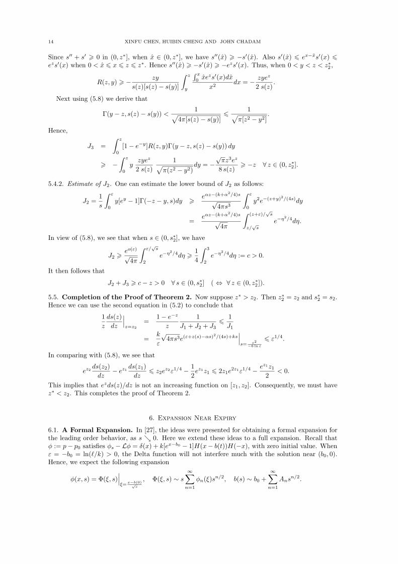
As mentioned earlier, numerical experiments suggest that there is a breakdown of the convexityof the early exercise boundary as the dividend rate, D, increases past the risk-free interest rate,r. Figure 1 shows the loss of convexity as ε := ln(D/r) = ln(`/k) crosses zero. These numericswere carried out using an integro-differential equation derived in §4. It is clear that at its onsetwhen 0 < D − r ¿ 1, the non-convex region occurs close to expiry. On the other hand, the formalexpansion of Wilmott et. al. [27, p121], for s ↘ 0,

b(s) = lnr

D− [A + o(1)]

√s, A = 0.9034...,

does not capture this behavior. More specifically,

B′′(t) =Eeb(s)σ4

4

[b(s) + (b(s))2

]

is positive for the above near-expiry asymptotics agreeing with the numerics in Figure 1 that theboundary begins convex. To observe the loss of the convexity, more precise estimates are required.In particular, we will prove

Theorem 2. When 0 < D − r ¿ 1, the optimal exercise boundary is not convex. More precisely,when ε := ln(D/r) = ln(`/k) is positive and sufficiently small, neither S = B(t) nor x = b(s) isconvex. In particular, there exist a t for which B′′(t) < 0 and hence b(s) < 0, where

0 < s 6 ε2

6| ln ε| and t = T − 2s

σ2.

4 XINFU CHEN, HUIBIN CHENG AND JOHN CHADAM

0.97 0.98 0.99 1

0.87

0.89

0.91

t

B(t

)

400 mesh pts.

800 mesh pts.

1600 mesh pts.

r=.05, d=0.055, E=1, T=1,σ=0.25

00.1

0.20.3

0.4

−0.20

0.2

0

2

4

6x 10

−3

zε=log(D/r)

s=

(T−

t)σ

2/2

Figure 1. Loss of Convexity as ε = ln(D/r) crosses zeroThe figure on the left, in the original S, t variables, shows that the optimal free boundary is notconvex. Numerical accuracy is demonstrated by the overlap of the curves produced from 400,800,and 1600 mesh points. The figure on the right shows the variation of the free boundary as εincreases. Here z = b(0)− b(t); for ε < 0, all free boundaries are convex. For ε positive and small,the free boundary loses its convexity near s = 0, i.e., near expiry.

The proof of Theorem 2 is given in §5. The intuition for the upper bound on s, the location ofthe non-convexity, comes from a formal argument giving

limε→0

s| ln ε|ε2

=18.

See Figure 2.

0 0.2 0.4 0.6 0.8 1x 10

−3

0

0.5

1

1.5

2

2.5x 10−8

ε=log(D/r)

s=(T

−t)

σ2/2

ε2/8|lnε|start timeend time

k=1.6

0 0.1 0.2 0.3 0.4 0.50

0.005

0.01

0.015

ε=log(D/r)

s=(T

−t)

σ2/2

start time

end time

ε2/8ln|ε|

Figure 2. Time interval for which the free boundary is non-convexThe solid curves in the left figure are inflection points of the free boundary curves. The dashedcurve is the analytic estimate for the location of the non-convexity. The figure on the right showsthat when ε is large enough (> 0.4), the free boundary regains convexity, the teardrop region inthe ε− s domain indicating where the free boundary is concave.

In the course of this analysis, some of the estimates can be used to provide a rigorous proof ofthe previously mentioned near-expiry expansion [27].

AMERICAN PUT OPTION 5

Theorem 3. Assume that D > r. Let A = 0.903446597884.... Then

b(s) = lnr

D− [A + o(1)]

√s, b(s) = −A + o(1)

2√

s, b(s) =

A + o(1)4s3/2

∀ s > 0

where lims↘0 o(1) = 0. Consequently, the inverse, s = s(z), of z = ln(D/r)− b(s) satisfies

s(z) =z2

A2 + o(1), s′(z) =

2z

A2 + o(1), s′′(z) =

2A2 + o(1)

∀ z > 0.

Note that the above asymptotic behavior implies that very near expiry, the optimal exerciseboundary begins convex. The location of the non-convex region occurs a little farther from expirynear t given in Theorem 2.

3. Regularity of The Free Boundary

3.1. Basic Properties of the Solution. Note that

Lp0(x) = δ(x) + (`ex − k)H(−x)

where H is the Heaviside function, H(z) = 1 for z > 0 and H(z) = 0 for z < 0, and δ(x) = H ′(x) isthe Delta function. It is critical here that Lp0 changes sign only once:

Lp0 > 0 in [b0,∞), Lp0 < 0 in (−∞, b0); b0 := min{0, ln(k/`)}.This property implies that the free boundary in (2.3b) is well-defined. Indeed, for each s > 0,

p(x, s) > p0(x) ∀x > b(s), p(x, s) = p0(x) ∀x 6 b(s).

Later we shall show that b ∈ C∞((0,∞)), from which we can derive the following: for each s > 0,

p(b(s), s) = 1− eb(s),

px(b(s), s) = −eb(s),

ps(b(s), s) = 0,

pxx(b(s)±, s) = −eb(s) + ( 12 ± 1

2 )(k − `eb(s)),

psx(b(s)±, s) = ( 12 ± 1

2 )b(s)(`eb(s) − k).

The first and second equations are a direct consequence of p(x, s) = p0(x) = 1 − ex for x 6b(s). The equation ps(b(s), s) = 0 is derived by differentiating p(b(s), s) = p0(b(s)) and usingpx(b(s), s) = p0x(b(s)). The value pxx(b(s)+, s) is obtained from the differential equation ps = Lpand ps(b(s)±, s) = 0. Similarly, differentiating px(b(s)±, s) = p0x(b(s)) we obtain the expression forpsx(b(s)±, s).

To see the monotonicity of the free boundary b, it is useful to notice that q := ps satisfies the freeboundary problem

qs(x, s) = Lq(x, s) ∀x > b(s), s > 0,

q(x, s) = 0 ∀x 6 b(s), s > 0,

q(x, 0) = max{Lp0(x), 0} ∀x ∈ R, s = 0,

Π(b(s)) =∫ s

0qx(b(t), t)dt ∀ s > 0

(3.1)

where

Π(z) =∫ z

∞min{Lp0(x), 0}dx =

{0 if z > b0,∫ z

b0(`ex − k)dx if z < b0.

Here the last equation in (3.1) is a weak formulation of the free boundary condition

b(0) = b0, b(s)[`eb(s) − k] = qx(b(s), s), b(s) 6 b0 ∀ s > 0.(3.2)

6 XINFU CHEN, HUIBIN CHENG AND JOHN CHADAM

Formally, p > p0 implies q(·, 0) = ps(·, 0) > 0. Since Lp0(x) < 0 when x < b0, one readily seesthat b(0) > b0. In the case b0 = 0, we have q(·, 0) = δ(x) so clearly b(0) 6 b0. In the case b0 < 0, wehave q(·, 0) > 0 in (b0, 0] so we also have b(0) 6 b0. Thus, we should have b(0) = b0. We denote

Qb = {(x, s) | s > 0, x > b(s)}.Note that q > 0 on the parabolic boundary of Qb, so by the maximum principle and Hopf’s Lemma,q > 0 in Qb and qx(b(s), s) > 0 for each s > 0. Thus,

b(s)[`eb(s) − k] > 0, b(s) < 0, `eb(s) − k < 0 ∀ s > 0.

We now turn to the proof of Theorem 1. Existence and uniqueness of weak solutions of (2.3)follows from the standard theory of variational inequalities (see [14] and [10] for more details). Thekey consideration here is the regularity. As remarked in [12], for the American put option, it isconvenient to carry out the analysis in terms of the function q := ps; i.e., using the free boundaryproblem (3.1), for (q, b). This is a Stefan type free boundary problem which has been well-studied(see, for example, [16, 18]). The existence of a smooth classical solution would be standard if thefree boundary condition is not degenerate; i.e., the coefficient of b at s = 0 in (3.2) is not zero. Weshall treat the degeneracy that arises here in (3.2) by using the initial value b(0) = b0− ε for positiveε and then sending ε ↘ 0. (Note that this ε is unrelated to ε := ln(`/k)).

3.2. The Bootstrap Argument. We begin with the bootstrap argument which shows that b ∈C∞((0,∞)) if b ∈ Cγ((0,∞)) for some γ > 1/2.

For this, we denote D = {(x, t) | x > b(s), s > 0}. Suppose that b ∈ Cβ/2((0,∞)) for some β > 1that is not an integer. Then by standard local regularity theory, e.g. the potential theory in [15],the solution of qs = Lq in Qb with zero boundary value on x = b(s) has the regularity q ∈ Cβ,β/2(D)and qx ∈ Cβ−1,(β−1)/2(D). Consequently, qx(b(·), ·) ∈ C(β−1)/2((0,∞)). Since `eb(s) − k < 0 for alls > 0, the last equation in (3.1) can be differentiated to give b[`eb − k] = qx(b, s), from which weconclude that b ∈ C(β+1)/2((0,∞)). Thus, by induction, b ∈ C∞((0,∞)).

3.3. An Upper Bound for q. Let q0 be the solution of

q0s = Lq0 on R× (0,∞), q0(·, 0) = max{Lp0, 0}.Then q0 > 0 on R× (0,∞) so by comparison, q 6 q0 on R× [0,∞).

For the subsequent analysis, we consider the function q0 := q0(x, t)eαx/2+(k+α2/4)t which satisfiesq0s = q0xx on R× (0,∞) with initial data δ(x) + eαx/2(`ex − k)H(−x)H(x− b0). Hence,

q0(x, s) =e−x2/(4s)

√4πs

+∫ 0

b0

e−(x−y)2/(4s)

√4πs

eαy/2(`ey − k)dy.

Note that ‖q(x, ·)‖L∞([0,∞)) is finite for every x 6= 0.

3.4. Long Time Behavior. Let (p∗(·), b∗) ∈ C1(R)× R be the solution of

p∗ = p0 on (−∞, b∗], p∗′′ + αp∗′ − kp∗ = 0 in (b∗,∞), p∗(∞) = 0.(3.3)

The solution is given by

p∗(x) := max{

1− ex,e−λ(x−b∗)

1 + λ

}, b∗ := ln

λ

1 + λ, λ :=

α +√

α2 + 4k

2.

One can use a comparison argument to show that p 6 p∗, b∗ 6 b. Since ps > 0 > b, thelimt→∞(p(·, t), b(s)) exists and must be the solution of (3.3). Hence,

p(x, s) 6 p∗(x), b(0) > b(s) > b∗, limt→∞

(p(x, t), b(t)) = (p∗(x), b∗) ∀x ∈ R, s > 0.

AMERICAN PUT OPTION 7

3.5. An Upper Bound for |b|. Let η be any positive constant such that η > −b0. We define

M0 := maxx∈[b0,0]

∣∣∣d[eαx/2(`ex − k)]dx

∣∣∣,

M(η) := max{

M0, supt>0

q0(−η/2, t)η/2

},(3.4)

bη(s) := min{−η, b(s)},q1(x, s) := M(η) (x− bη(s))e−αx/2−(k+α2/4)s.

Note that bη is a continuous decreasing function. The following is the key to our analysis:

q1s − Lq1 = −M(η)[x− bη(s)]bη(s)e−αx/2−(k+α2/4)s > 0 ∀x > bη(s), s > 0.

Now we compare q1 with q on Q where Q = {(x, t) | b(s) < x < −η/2, s > 0}. Since q 6 q0 onR × (0,∞) and q = 0 when x 6 b(s), our choice of M(η) implies that q1 > q on the parabolicboundary of Q so q < q1 in Q.

Suppose b(s) 6 −η. Then q(b(s), s) = q1(b(s), s) = 0 and q(x, s) < q1(x, s) for x ∈ (b(s),−η/2].Hence,

0 6 qx(b(s), s) 6 q1x(b(s), s) = M(η)e−αb(s)/2−(k+α2/4)s if b(s) 6 −η.

It then follows from the last equation in (3.1) or from (3.2) that

0 6 eαb(s)/2[`eb(s) − k]b(s) 6 M(η)e−[k+α2/4]s if b(s) 6 −η.(3.5)

As b∗ < b(s) < b0 for all s > 0, for any δ > 0, by taking η = −b(δ), we see that b is Lipschitzcontinuous on [δ,∞). Hence, b is locally Lipschitz on (0,∞), so by the bootstrap argument, we haveb ∈ C∞((0,∞)).

Remark 3.1. When ` > k, we have −b0 = ε := ln(`/k) > 0. Hence, we can set η = −b0 = ε in theabove analysis and use b∗ < b 6 b0 to derive that there exists a constant C > 0 such that

{0 < [b(s)− b0]b(s) 6 Ce−(k+α2/4)s ∀ s > 0,

0 6 q(x, s) 6 C[x− b(s)]e−(k+α2/4)s ∀ s > 0, x ∈ [b(s),−ε/2].(3.6)

3.6. An Approximation. Once we have the a priori estimate, the existence will be standard.There are many ways to do it. We find the following interesting. Let ε > 0 be a fixed small number.We remove the degeneracy of the free boundary condition by requiring b(0) = b0 − ε. Hence, weconsider the following problem, for (qε, bε):

qεs(x, s) = Lqε(x, s) ∀x > bε(s), s > 0,

qε(x, s) = 0 ∀x 6 bε(s), s > 0,

qε(x, 0) = max{Lp0(x), 0} ∀x ∈ R, s = 0,

Π(bε(s)) = Π(b0 − ε) +∫ s

0qx(b(t), t)dt ∀ s > 0.

(3.7)

This is a standard Stefan problem, for which the existence of a classical solution can be provenas follows. We establish the existence of a solution in a time interval [0, h] for an arbitrary large h.We define a function space

B ={

b ∈ C1([0, h])∣∣∣ b(0) = b0 − ε; 0 6 eαb/2[`eb − k]b 6 M(ε− b0) in [0, h]

}

where M(·) is defined in (3.4). Clearly, B is a closed subset of C1([0, h]).For each b ∈ B, we let q be the solution of the following initial–boundary value problem

qs(x, s) = Lq(x, s) ∀x > b(s), s ∈ (0, h],

q(b(s), s) = 0 ∀ s > 0,

q(x, 0) = max{Lp0(x), 0} ∀x > b0 − ε.

8 XINFU CHEN, HUIBIN CHENG AND JOHN CHADAM

This problem admits a unique classical solution q. As the boundary is C1, we see that q ∈∩0<β<1C

2β,β(Qb \ ([b0, 0]× {0})). This implies qx(b(·), ·) ∈ ∩0<β<1/2Cβ([0, h]).

From the solution, we define b = T[b] by solving the ode

eαb(s)/2[`eb(s) − k]db(s)ds

= qx(b(s), s)eαb(s)/2 ∀ s ∈ (0, h], b(0) = b0 − ε.

Since q > 0 in Qb, we have qx(b(s), s) > 0. Hence, b is well-defined and b(s) 6 b0− ε for all s ∈ [0, h].We want to show that T has a fixed point in B. This fixed point is a solution of (3.7).

First of all, since b 6 0, following the same line of proof as in the previous subsection, we findthat 0 6 q 6 q0 and 0 6 qx(b(s), s) 6 M(ε− b0)e−αb(s)/2−(k+α2/4)s. Hence,

0 6 eαb/2[`eb − k] ˙b 6 M(ε− b0)e−(k+α2/4)s.

Thus, T maps B to itself. In addition {T[b] | b ∈ B} is a bounded set in C1+1/4([0, h]) which is acompact subset of C1([0, h]). Hence, by the Schauder’s fixed point theorem, T admits a fixed point,bε, in B. Extend the corresponding q by zero for x < bε and denoting it by qε, we see that (qε, bε) isa classical solution of (3.7) in R× [0, h]. Since M(ε− b0) does not depend on h, we can let h →∞to obtain a solution of (3.7) on R× (0,∞).

Remark 3.2. When α > 0, we may need extra care to prevent bε from being unbounded from below.Since we know the limit b := limε↘0 bε is bounded from below by b∗, this technicality can be treatedby replacing eαb/2 by max{eαb/2, eαb∗/2}. We omit the details.

3.7. Monotonicity of the Approximation Sequence. Let 0 < ε1 < ε2. Then bε2(0) < bε1(0).We claim that bε2 < bε1 on [0,∞). Suppose this is not true. Then t∗ := sup{t > 0 | bε2 <bε1 in [0, t]} is finite and we have bε2 < bε1 in [0, t∗) and bε2(t∗) = bε1(t∗).

Now by comparison on D = {(x, t) | x > bε1(s), s ∈ [0, t∗]} we see that qε2 > qε1 on D. Sincebε1 is C1, we obtain from Hopf’s lemma that qε2

x (bε1(t∗), t∗) > qε1x (bε1(t∗), t∗). Consequently, since

bε1(t∗) = bε2(t∗), we find from the boundary condition that

−bε2(t∗) =qε2x (bε1(t∗), t∗)k − ebε1 (t∗) >

qε1x (bε1(t∗), t∗)k − ebε1 (t∗) = −bε1(t∗).

That is (bε2 − bε1)′|s=t∗ < 0. But this implies bε2(s)− bε1(s) > 0 when 0 < t∗− s ¿ 1, contradictingthe definition of t∗. Hence, we must have bε2 < bε1 on [0,∞). Consequently, by comparison, we haveqε1 < qε2 in Qbε1 .

3.8. The Limit of the Approximation Sequence. Now we define (q, b) = limε↘0(qε, bε). Weshall show that (q, b) solves (3.1) and b ∈ C∞((0,∞)) ∩ C([0,∞)).

First of all, q ∈ C∞(Qb) and qs = Lq in Qb := {(x, t) | s > 0, x > b(s)} = ∩ε>0Qbε .Next we establish the regularity of b. As the limit of a sequence of decreasing functions, b is also

decreasing. Next we claim that b(s) < b0 for every s > 0. Indeed, if this is not true, then we haveb(s) = b0 for all s ∈ [0, δ] for some δ > 0. Note that for the ε problem, integrating qε

s = Lqε overQbε we have the following identity, for t2 > t1 > 0,∫

Rqε(x, t2)dx−

∫

Rqε(x, t1)dx + k

∫ t2

t1

∫

Rqε(x, t)dxdt = −

∫ t2

t1

qεx(bε(t), t)dt = Π(bε(t1))−Π(bε(t2).

Sending ε ↘ 0 and using Lebesgue’s dominated theorem we obtain∫

Rq(x, t2)−

∫

Rq(x, t1)dx + k

∫ t2

t1

∫

Rq(x, t)dxdt = Π(b(t1)−Π(b(t2)) ∀ t2 > t1 > 0.

Now if b ≡ b0 on [0, δ], we can integrate qs = Lq over (0,∞)× (δ/2, δ) to derive∫ δ

δ/2

qx(b0, t)dt = Π(b(δ)−Π(b(δ/2)) = 0,

AMERICAN PUT OPTION 9

which is impossible since Hopf’s maximum principle implies that qx(b0, s) > 0 for each s ∈ (0, δ). Inconclusion, b(s) < b0 for every s > 0.

Now let η > −b0 be any small positive constant. Passing the estimate of bε to the limit we find that(3.5) holds. This implies that b is Lipschitz continuous on [δ,∞) where δ := inf{s > 0 | b(s) < −η}.A bootstrap argument shows that b ∈ C∞((δ,∞)). Now we can use (qε, bε) → (q, b) in the needednorm to conclude that q(b(s), s) = 0 and qx(b(s), s) = b[`eb(s) − k] for all s ∈ (δ,∞). Sendingη ↘ −b0, we must have δ → 0 since b(s) < b0 for each s > 0. Thus, b ∈ C∞((0,∞)) and (q, s) is asolution of (3.1).

Finally, let δε := inf{s > 0 | bε(s) > b0 − 2ε}. Then δε ∈ (0,∞] and b(s) > bε > b0 − 2ε for alls ∈ (0, δε). Hence, lims↘0 b(s) > b0 − 2ε. Sending ε ↘ 0 we find lims↘0 b(s) > b0. As b(s) < b0 fors > 0, we conclude that lims→0 b(s) = b0, so b ∈ C([0,∞)).

3.9. Recovering p from q. Once we have a classical solution of (q, b) of (3.1), we can define

p(x, s) := p0(x) +∫ s

0

q(x, t)dt ∀x ∈ R, t > 0.

Since q(x, t) = 0 for x 6 b(t) and since b < 0, we see that q = 0 on (−∞, b(s)] × [0, s] for eachs > 0. Hence, p(x, s) ≡ p0(x) when x 6 b(s) and px(b(s), s) = p0x(b(s)) for each s > 0. Also, ps = qon R× (0,∞). In addition, when x > b0,

Lp(x, s) = Lp0(x) +∫ s

0

Lq(x, t)dt = Lp0 +∫ s

0

qt(s, t)dt = q(x, s),

since q(·, 0) = max{Lp0, 0} = Lp0 when x > b0.When x ∈ (b(s), b0), write s = s(x) the inverse of x = b(s). Then

p(x, t) = p0(x) +∫ s

s(x)

q(x, t)dt.

Consequently,

Lp(x, s) = Lp0(x)− s′(x)qx(x, s(x)) +∫ s

s(x)

Lq(x, t)dt

= Lp0(x)− 1b(s(x))

qx(x, s(x)) + q(x, s) = q(x, s) = ps.

Thus, (p, s) is a solution of the variational inequality (2.3).Since the solution of variational inequality (2.3) is unique [10, 14], the assertion of Theorem 1

thus follows.

Remark 3.3. Let pε := p0 +∫ t

0qε(x, t)dt. Then (pε, bε) does not solve the original problem; one

finds that pεs − Lpε = −Lp0(x) in (b0 − ε, b0)× (0,∞). Indeed, as ε ↘ 0, pε ↘ p and bε ↗ b.

4. Integral Formulation

Introduce φ(x, s) = p(x, s)− p0(x). Then

φs − Lφ(x, s) = H(x− b(s))Lp0(x) on R× (0,∞), φ(·, 0) = 0 on R× {0}.Hence, we can use Green’s formula to write

φ(x, s) =∫ s

0

∫ ∞

b(s−t)

Γ(x− y, t)Lp0(y)dydt ∀ (x, s) ∈ R× [0,∞),

where Γ is the fundamental solution given by

Γ(x, s) := K(x + αs, s)e−ks, K(z, t) := (4πt)−1/2e−z2/4t.

10 XINFU CHEN, HUIBIN CHENG AND JOHN CHADAM

We therefore obtain the following, for every (x, s) ∈ R× (0,∞),

φ(x, s) =∫ s

0

Γ(x, t)dt +∫ s

0

∫ 0

b(s−t)

[`ey − k]Γ(x− y, t)dydt,

φx(x, s) =∫ s

0

Γx(x, t)dt +∫ s

0

∫ 0

b(s−t)

[`ey − k]Γx(x− y, t)dydt,

φs(x, s) = Γ(x, s) +∫ 0

b(0)

[`ey − k]Γ(x− y, s)dy −∫ s

0

b(s− t)[`eb(s−t) − k]Γ(x− b(s− t), t) dt

= Γ(x, s) +∫ 0

b0

[`ey − k]Γ(x− y, s)dy −∫ s

0

b(t)[`eb(t) − k]Γ(x− b(t), s− t) dt.

Also, for every s > 0 and x 6= b(s),

φsx(x, s) = Γx(x, s) +∫ 0

b0

[`ey − k]Γx(x− y, s)dy −∫ s

0

b(t)[`eb(t) − k]Γx(x− b(t), s− t) dt.

Evaluating these expressions at x = b(s) we then obtain the following.

Theorem 4. Let (b, p) be the solution of the variational inequality (2.3). Then b satisfies thefollowing integral identities:

0 =∫ s

0

Γ(b(s), t) dt +∫ s

0

∫ 0

b(s−t)

[`ey − k]Γ(b(s)− y, t)dydt,(4.1)

0 =∫ s

0

Γx(b(s), t)dt +∫ s

0

∫ 0

b(s−t)

[`ey − k]Γx(b(s)− y, t)dydt,(4.2)

0 = Γ(b(s), s) +∫ 0

b0

[`ey − k]Γ(b(s)− y, s)dy(4.3)

−∫ s

0

b(t)[`eb(t) − k]Γ(b(s)− b(t), s− t) dt,

b(s)[`eb(s) − k] = 2Γx(b(s), s) + 2∫ 0

b0

[`ey − k]Γx(b(s)− y, s)dy(4.4)

−2∫ t

0

b(t)[`eb(t) − k]Γx(b(s)− b(t), s− t) dt.

Also, for any θ ∈ R,

b(s)[`eb(s) − k] =(θ − b(s)

s

)Γ(b(s), s) +

∫ 0

b0

[`ey − k](θ − b(s)− y

s

)Γ(b(s)− y, s)dy(4.5)

−∫ s

0

b(t)[`eb(t) − k](θ − b(s)− b(t)

s− t

)Γ(b(s)− b(t), s− t) dt .

With the particular choice of θ = 0 and θ = [b(s)− b0]/s we have

b(s)[`eb(s) − k] =−b(s)Γ(b(s), s)

s+

1s

∫ 0

b0

[`ey − k][y − b(s)]Γ(b(s)− y, s)dy(4.6)

+∫ s

0

b(t)[eb(t)−b0 − 1]b(s)− b(t)

s− tΓ(b(s)− b(t), s− t) dt,

b(s)[`eb(s) − k] =−b0Γ(b(s), s)

s+

1s

∫ 0

b0

[`ey − k][y − b0]Γ(b(s)− y, s)dy(4.7)

−∫ s

0

b(t)[`eb(t) − k](b(s)− b0

s− b(s)− b(t)

s− t

)Γ(b(s)− b(t), s− t) dt.

AMERICAN PUT OPTION 11

Here (4.5) is obtained by adding a θ + α multiple of (4.3) to (4.4) and using

Γx(x, s) =−x− αs

2sΓ(x, s).

We shall use (4.6) and (4.7) for our analysis. For numerical simulation we use (4.5) with θ =(b(s)− b0)/(2s), since a formal asymptotic expansion suggests that for ` > k

b(s)− b0 ∝√

s, b(s) ∼ b(s)− b0

2swhen 0 < s ¿ 1.

Hence, taking θ = (b(s) − b0)/(2s) in (4.5) removes the singularity of the last integral in (4.5) in anatural way.

5. Non-Convexity

From now on we assume that ` > k. We shall prove Theorem 2.

5.1. The Idea. It is convenient to visualize graphs in the first quadrant. Hence, we introduce

z(s) = b0 − b(s) = −ε− b(s) ∀ s > 0.

Since z′(s) > 0 for all s > 0, z = z(s) admits an inverse, which we denote by s = s(z).

We can rewrite (4.6) and (4.7) as follows. Note that `ey − k = k[ey−b0 − 1]. Hence we can usethe change of variable y = y − b0 in the first integral and the change of variable y = b0 − b(t) in thesecond integral in (4.6) and (4.7) to obtain

[1− e−z]dz

ds= I1 + I2 − I3 = J1 + J2 + J3(5.1)

where

I1 :=(ε + z)Γ(−ε− z, s)

k s,

I2 :=1s

∫ ε

0

[ey − 1][z + y]Γ(−y − z, s)dy,

I3 :=∫ z

0

[1− e−y]( z − y

s(z)− s(y)

)Γ(y − z, s(z)− s(y)) dy,

J1 :=ε Γ(−ε− z, s)

k s,

J2 :=1s

∫ ε

0

y[ey − 1]Γ(−z − y, s)dy,

J3 :=∫ z

0

[1− e−y]( z

s(z)− z − y

s(z)− s(y)

)Γ(y − z, s(z)− s(y)) dy.

Since the coefficient of dz/ds at s = 0 is zero, it may be better to consider the inverse function,which is smooth on [0,∞). Hence we write (5.1) as

ds

dz=

1− e−z

I1 + I2 − I3=

1− e−z

J1 + J2 + J3.(5.2)

Recall that

B(t) = Eeb(s) = Ee−ε−z(s)∣∣∣s= σ2

2 (T−t).

12 XINFU CHEN, HUIBIN CHENG AND JOHN CHADAM

It follows that4eε

σ4E

d2B(t)d2t

=d2e−z(s)

ds2= −dz

ds

d

dz

( 1ez ds

dz

)

= e−2z(dz

ds

)3 d

dz

(ez ds

dz

)

= e−z(dz

ds

)3(d2s

dz2+

ds

dz

).

Thus, to show that B is not convex (B′′(t) > 0 not true), we need only show that ezds/dz is notan increasing function. For this, we compare the values of ezds/dz at two points:

z1 := z(s1), s1 :=ε2

[8 + ν] | ln ε| , z2 := z(s2), s2 :=ε2

[8− ν] | ln ε|(5.3)

where ν can be any constant in (0, 8). For definiteness, we fix ν = 2.For convenience, we introduce

z∗ := sup{

z > 0∣∣∣ d2s

dz2+

ds

dz> 0 in (0, z]

}, s∗ := s(z∗).(5.4)

Note that the optimal exercise boundary is convex if and only if s∗ = ∞. In the sequel, we shallshow that when ε is small, s∗ < s2; that is, the convexity changes at time before s2.

We remark that the convexity of s(·) implies the convexity of B(·) since B′′ is proportional tos′′ + s′ with s′ > 0. Hence, if B(·) is not convex, then neither is s(·).

In the sequel, ε = ln(D/r) = ln(`/k) is a small positive constant. We use the standard notationo(1) to denote a generic small quantity that approaches zero as ε ↘ 0.

5.2. The General Lower Bound of ds/dz. We shall utilize the first equation in (5.2) to estimatethe positive lower bound of ds/dz. The key here is that all terms I1, I2 and I3 are positive, so wehave the basic estimate

(1− e−z)dz

ds6 I1 + I2,

ds

dz> 1− e−z

I1 + I2.

We can estimate I2 as follows. Notice that α = k − `− 1 < −1. Hence, when 0 6 y 6 z,

Γ(−y − z, s) =e−(y+z)2/(4s)+[y+z]α/2−(k+α2/4)s

√4πs

6 e−(y+z)2/(4s)−y−(k+α2/4)s

√4πs

.

It then follows, using 0 6 ey − 1 6 yey 6 12 (y + z)ey, that

I2 :=1s

∫ ε

0

[ey − 1][z + y]Γ(−y − z, s)dy

6 e−(k+α2/4)s

4√

πs3

∫ ε

0

(y + z)2e−(y+z)2/(4s)dy =e−(k+α2/4)s

4√

π

∫ (z+ε)/√

s

z/√

s

η2e−η2/4dη

6 e−(k+α2/4)s

4√

π

∫ ∞

0

η2e−η2/4dη =e−(k+α2/4)s

26 1

2∀ s > 0.

Next, we consider

I1 :=(ε + z)Γ(−ε− z, s)

k s=

(ε + z)e−(ε+z−αs)2/(4s)−ks

√4πk2s3

.

Since α < 0, we see that

∂ I1

∂ z=

I1

ε + z

{1− (ε + z)(ε + z − αs)

2s

}< 0 when s <

ε2

2.

It then follows that when s ∈ (0, ε2/2],

I1 6 ε Γ(−ε, s)k s

6 ε e−ε2/(4s)

√4πk2s3

.

AMERICAN PUT OPTION 13

Combing these estimates, we then obtain

ds

dz=

1− e−z

I1 + I2 − I3> 1− e−z

I1 + I2> z e−z

ε e−ε2/(4s)√4πk2s3 + 1

2

∀ s ∈[0,

ε2

2

].(5.5)

5.3. The Lower Bound of ds/dz on [0, s∗2] where s∗2 = min{s2, s∗}.

(1) First we consider s ∈ [0, s1] where s1 := ε2/(10| ln ε|), 0 < ε ¿ 1. It is easy to verify thatI1 = o(1) when s ∈ (0, s1], so that

ds

dz> ze−z

o(1) + 12

, s > z2e−z

1 + o(1)∀ z ∈ [0, z1].(5.6)

This also implies that when s ∈ [0, s1], z(s) = o(ε). In particular, z1 := z(s1) = o(ε).

To extend the estimate beyond s1, we notice that s′′+s′ > 0 implies that (ezs′)′ > 0 so integratingit over [x, x + h] ⊂ (0, z∗] we obtain

s′(x + h) > e−hs′(x) ∀ 0 < x < x + h 6 z∗.(5.7)

(2) With z1 := z(s1), s∗ := s(z∗), s∗2 := min{s2, s∗}, and z∗2 := z(s∗2), we claim that z∗2 < 2z1.

Suppose not. Then we take h = z1 and integrate (5.7) over [0, z1] to obtain s(2z1) − s(z1) >e−z1s(z1), so s(2z1) > [1 + e−z1 ]s(z1) = [2 − o(ε)]s(z1). However, since s2 = 5

3s1, we obtains(2z1) > [2 − o(ε)]s1 > s2 > s(z∗2), contradicting the assumption z∗2 > 2z1. Hence, we must havez∗2 < 2z1.

(3) We now consider the lower bound of ds/dz in [s1, s∗2]. From (5.7) and (5.6) we derive, for any

z ∈ [z1, z∗2 ] ⊂ [z1, 2z1],

ds(z)dz

> e−z∗2ds(z1)

dz> e−z∗2 z1e

−z1

o(1) + 12

=e−z1−z∗2 z1

[o(1) + 12 ]z

z > z

2.

In conclusion, when ε is positive and sufficiently small,

ds(z)dz

> z

2, s(z) > z2

4, s(z)− s(y) > z2 − y2

4∀ 0 6 y 6 z 6 z∗2 .(5.8)

5.4. Upper Bounds of ds/dz. The optimal exercising boundary is convex if and only if s∗ = ∞.In what follows, we shall show that when ε is small positive, s∗ < s2. To do this, we show that thevalue ezds/dz at z2 is much smaller than at z1, so it cannot be an increasing function and thereforethe free boundary cannot be convex. In (5.8), we already have a lower bound of ezdz/ds at z1 ifs∗ > s1 (if s∗ < s1, the non-convexity is established). Here what we need is an upper bound atz = z2. The basic idea is to use the second equation in (5.2).

5.4.1. Estimate of J3. In the case s′′ > 0, it is easy to show that J3 is positive. Under the weakercondition s′′ + s′ > 0 in (0, s∗], we shall show that J3 is almost positive. For this purpose, we write

J3 =∫ z

0

[1− e−y]R(z, y)Γ(y − z, s(z)− s(y)) dy

where

R(z, y) :=z

s(z)− z − y

s(z)− s(y)=

ys(z)− zs(y)s(z)[s(z)− s(y)]

=zy

s(z)[s(z)− s(y)]

(s(z)z

− s(y)y

)

=zy

s(z)[s(z)− s(y)]

∫ z

y

s′(x)x− s(x)x2

dx

=zy

s(z)[s(z)− s(y)]

∫ z

y

∫ x

0xs′′(x)dx

x2dx.

14 XINFU CHEN, HUIBIN CHENG AND JOHN CHADAM

Since s′′ + s′ > 0 in (0, z∗], when x ∈ (0, z∗], we have s′′(x) > −s′(x). Also s′(x) 6 ex−xs′(x) 6ezs′(x) when 0 < x 6 x 6 z 6 z∗. Hence s′′(x) > −s′(x) > −ezs′(x). Thus, when 0 < y < z < z∗2 ,

R(z, y) > − zy

s(z)[s(z)− s(y)]

∫ z

y

∫ x

0xezs′(x)dx

x2dx = − zyez

2 s(z).

Next using (5.8) we derive that

Γ(y − z, s(z)− s(y)) <1√

4π[s(z)− s(y)]6 1√

π[z2 − y2].

Hence,

J3 =∫ z

0

[1− e−y]R(z, y)Γ(y − z, s(z)− s(y)) dy

> −∫ z

0

yzyez

2 s(z)1√

π(z2 − y2)dy = −

√πz3ez

8 s(z)> −z ∀ z ∈ (0, z∗2 ].

5.4.2. Estimate of J2. One can estimate the lower bound of J2 as follows:

J2 =1s

∫ ε

0

y[ey − 1]Γ(−z − y, s)dy > eαz−(k+α2/4)s

√4πs3

∫ ε

0

y2e−(z+y)2/(4s)dy

=eαz−(k+α2/4)s

√4π

∫ (z+ε)/√

s

z/√

s

e−η2/4dη.

In view of (5.8), we see that when s ∈ (0, s∗2], we have

J2 > eo(ε)

√4π

∫ ε/√

s

2

e−η2/4dη > 14

∫ 3

2

e−η2/4dη := c > 0.

It then follows that

J2 + J3 > c− z > 0 ∀ s ∈ (0, s∗2] ( ⇔ ∀ z ∈ (0, z∗2 ]).

5.5. Completion of the Proof of Theorem 2. Now suppose z∗ > z2. Then z∗2 = z2 and s∗2 = s2.Hence we can use the second equation in (5.2) to conclude that

1z

ds(z)dz

∣∣∣z=z2

=1− e−z

z

1J1 + J2 + J3

6 1J1

=k

ε

√4πs3e(ε+z(s)−αs)2/(4s)+ks

∣∣∣s= ε2

−6 ln ε

6 ε1/4.

In comparing with (5.8), we see that

ez2ds(z2)

dz− ez1

ds(z1)dz

6 z2ez2ε1/4 − 1

2ez1z1 6 2z1e

2z1ε1/4 − ez1z1

2< 0.

This implies that ezds(z)/dz is not an increasing function on [z1, z2]. Consequently, we must havez∗ < z2. This completes the proof of Theorem 2.

6. Expansion Near Expiry

6.1. A Formal Expansion. In [27], the ideas were presented for obtaining a formal expansion forthe leading order behavior, as s ↘ 0. Here we extend these ideas to a full expansion. Recall thatφ := p− p0 satisfies φs −Lφ = δ(x) + k[ex−b0 − 1]H(x− b(t))H(−x), with zero initial value. Whenε = −b0 = ln(`/k) > 0, the Delta function will not interfere much with the solution near (b0, 0).Hence, we expect the following expansion

φ(x, s) = Φ(ξ, s)∣∣∣ξ=

x−b(0)√s

, Φ(ξ, s) ∼ s∞∑

n=1

φn(ξ)sn/2, b(s) ∼ b0 +∞∑

n=1

Ansn/2.

AMERICAN PUT OPTION 15

Note that Φ satisfies

Φs − ξ

2sΦξ − 1

sΦξξ =

α√sΦξ − kΦ + k

∞∑n=1

ξnsn/2

n!∀ ξ ∈

(b(s) + ε√s

,ε√s

), s > 0.

This leads to the following

Lnφn =k ξn

n!+ αφn−1 − kφn−2 ∀ ξ ∈ (A1,∞)

where

Lnψ :=(1 +

n

2− ξ

2d

dξ− d2

dξ2

)ψ.

Here we have used the extension φ0 = φ−1 ≡ 0.The boundary conditions for φn and the unknown An will be derived from

0 = φ(b(s), s) = Φ(ξ(s), s), 0 = φx(b(s), s) = s−1/2Φξ(ξ(s), s),

ξ(s) = [b(s)− b0]s−1/2 ∼ A1 +∞∑

n=2

Ansn−1/2.

Using the asymptotic expansion, we have

0 ∼∞∑

n=1

sn/2φn

(A1 +

∞∑m=2

Ams(m−1)/2)

∼∞∑

n=1

sn/2∞∑

i=0

φ(i)n (A1)

i!

( ∞∑m=2

Ams(m−1)/2)i

∼ φ1(A1)s1/2 + [φ2(A1) + φ′1(A1)A2]s +∞∑

n=3

[φn(A1) + φ′1(A1)An + · · · ]sn/2

0 ∼∞∑

n=1

sn/2φ′n(A1 +

∞∑m=2

Ams(m−1)/2)

∼ φ′1(A1)s1/2 + [φ′2(A1) + φ′′1(A1)A2]s +∞∑

n=3

[φ′n(A1) + φ′′1(A1)An + · · · ]sn/2.

Hence, we obtain the boundary conditions and the free boundary conditions

φ1(A1) = 0, φ′1(A1) = 0, φ1(ξ) = O(ξ) as ξ →∞,

φ2(A1) = 0, φ′2(A1) + φ′′1(A1)A2 = 0, φ2(ξ) = O(ξ2) as ξ →∞,

φn(A1) = an−1, φ′n(A1) + φ′′1(A1)An = bn−1, φn(ξ) = O(ξn) as ξ →∞where am, bm are constants depending only expansions of order up to m.

For the homogeneous equation Lnψ = 0, one can verify that the following are two linear inde-pendent solutions:

ψn(ξ) =∫ ∞

ξ

(η − ξ)n+2e−η2/4dη, ψn(ξ) =∫

R(η − ξ)n+2e−η2/4dη.

Here ψn is a polynomial of degree n + 2. It is easy to verify that

φ1(ξ) = k{

ξ − A1ψ1(ξ)ψ1(A1)

}

where A1 is the solution of the transcendental equation∫ ∞

A1

(η −A1)2(η + 2A1)e−η2/4dη = 0 ⇒ A1 = −0.9034465978843...(6.1)

16 XINFU CHEN, HUIBIN CHENG AND JOHN CHADAM

6.2. An Alternative Formal Derivation. We can also use the first or second equation in (5.2) toderive the asymptotic behavior. Assume that 0 < s < ε3. Also assume that z(s) = [A + O(

√s)]√

s.Then one finds J1 = O(e−ε2/(4s)) can be neglected in the expansion for small s. Also,

J2 =1√4π

∫ ∞

A

(A− η)2e−η2/4dη + O(z).

For J3, one uses the change of variable

η =(z − y)√

s(z)− s(y)≈ A

√z − y

z + y.

Then one derives that

J3 =A2

√4π

∫ A

0

(A2 − η2

A2 + η2

)2

e−η2/4dη + O(z).

Thus the differential equation (5.2) gives the following equation for A:

A2 =1√π

∫ ∞

A

(A− η)2e−η2/4dη +A2

√π

∫ A

0

(A2 − η2

A2 + ζ2

)2

e−η2/4dη

=⇒ A = 0.9034465978843....

Numerically it is evident that A = −A1 and is precisely the value obtained in [27].

6.3. Proof of Theorem 3. The leading order expansion can be made rigorous. Instead of consid-ering the premium φ = p− p0, we consider the rate, q = ps = φs, of the premium change. We studythe blow-up family {qL, bL}L>0 defined by

qL(x, s) := L q(b0 + L−1x, L−2s), bL(s) = L [b(L−2s)− b0 ].

Information obtained from bL will be cycled back to b through the identity

b(sθ) = b0 +√

s bL(θ)∣∣∣L=1/

√s

∀ θ ∈[12, 2

], s > 0.(6.2)

We shall show that limL→∞ bL(θ) = A1

√θ in C2([δ, h]) for any h > δ > 0.

For each L > 0, (qL, bL) satisfies

qLs = qL

xx + αL−1qLx − kL−2qL ∀x > bL(s), s > 0,

qL(x, s) = 0 ∀x 6 bL(s), s > 0,

kL[eL−1bL(s) − 1]bL(s) = qLx (bL(s), s) ∀ s > 0,

qL(x, 0) = δ(x− εL) + k max{ ex/L−1L , 0} ∀x ∈ R.

From (3.6) we derive that

0 < bL(s) bL(s) 6 C, 0 > bL(s) > −√

2Cs ∀ s > 0,

0 6 qL(x, s) = Lq(b0 + xL−1, sL−2) 6 LC{b0 + xL−1 − b(L−2s)}= C[x− bL(s)] 6 C[x +

√2Cs] ∀ s > 0, x ∈ [bL(s), εL/2].

Since the bounds of the above estimates for qL and bL are independent of L, one can show that{(qL, bL)}L>1 is locally compact and we can select a subsequence along which (qL, bL) approachesa limit, (Ψ, ζ). The limit satisfies

Ψs = Ψxx ∀x > ζ(s), s > 0,

Ψ(x, s) = 0, ∀x 6 ζ(s), s > 0,

kζ(s)ζ(s) = Ψx(ζ(s), s) ∀ s > 0,

Ψ(x, 0) = k max{0, x} ∀x ∈ R,

0 6 Ψ(x, s) 6 C[x− ζ(s)] ∀x > ζ(s), s > 0.

Since the solution is unbounded, the last condition imposes a constraint on the growth of the solution.

AMERICAN PUT OPTION 17

This problem admits a unique solution and the solution is self-similar, given by

ζ(s) = A1

√s ∀ s > 0,

Ψ(x, s) = k(x−

A1√

s∫∞

x/√

s(η − x√

s)e−η2/4dη

∫∞A1

(η −A1)e−η2/4

)∀x > ζ(s), s > 0,

where A1 is the solution of the equation

1 +A1

∫∞A1

e−η2/4dη∫∞A1

(η −A1)e−η2/4dη=

A21

2.

It is easy to verify that this equation is equivalent to (6.1).Once we know the uniqueness of the limit, we then know that the whole sequence (qL, bL) con-

verges. In addition, by compactness, limL→∞ bL = ζ in C2([1/2, 2]). Using (6.2) and its differentia-tion with respective θ, we obtain the assertion of Theorem 3. This completes the proof. ¤

References

[1] F. AitSahlia & T. Lai, Exercise boundaries and efficient approximations to American optionprices and hedge parameters, J. Computational Finance, 4 (2001), 85–103.

[2] G. Barone-Adesi & R. E. Whaley, Efficient analytic approximation of American option values,Journal of Finance, 42 (1987), 301–320.

[3] G. Barone-Adesi, & R. Elliott, Approximations for the values of American options, StochasticAnalysis and Applications, 9 (1991), 115–131.

[4] G. Barles, J. Burdeau, & M. Romano, & N. Samsoen, Critical stock price near expiration,Mathematical Finance, 5 (1995), 77-95.

[5] E. Bayraktar & Hao Xing, Analysis of the optimal exercise boundary of American option forjump diffusions, preprint.

[6] M. Broadie & J. Detemple, American option valuation: New bounds, approximations and com-parison of existing methods, Review of Financial Studies, 9 (1996), 1121–1250.

[7] D.S. Bunch & H. Johnson, The American put option and its critical stock price, J. Finance,55 (2000), 2333–2356.

[8] P. Carr, R. Jarrow, & R. Myneni, Alternative characterization of American put option, Math-ematical Finance, 2 (1992), 87–105.

[9] D. Chakraborty, Numerical study of the convexity of the exercise boundary of the Americanput option on a devidend-paying asset, MS. Thesis, Department of Mathematics, University ofPittsburgh, December (2008).

[10] Xinfu Chen & J. Chadam, A mathematical analysis of the optmal boundary for American putoptions, SIAM J. Math. Anal., 38 (2006), 1613–1641.

[11] Xinfu Chen & J. Chadam Analytic and numerical approximations for the early exercise boundaryfor American put options, Dyn. Cont. Disc. and Impulsive Sys., 10 (2003), 649–657.

[12] Xinfu Chen, J. Chadam, L. Jiang, & W. Zheng, Convexity of the exercise boundary of theAmerican put option on a zero dividend asset. Math. Finance 18 (2008), 185–197.

[13] E. Ekstrom, Convexity of the optimal stopping boundary for the American put option, J. Math.Anal. Appl. 299 (2004), 147–156.

[14] A. Friedman, Variational Principles and Free Boundary Problems, John Wiley &Sons, New York, 1982.

[15] A. Friedman, Partial Diffferential Equations of Parabolic Type, Prentice-Hall, 1964.[16] A. Friedman, Analyticity of the free boundary for the Stefan problem, Arch. Rational Mech.

Anal. 61 (1976), 97–125.[17] J. Hull, Options, Futures and Other Derivative Securities, , 3rd Ed., Prentice-Hall,

New York, 1997.[18] L. Jiang, Existence and differentiability of the solution of a two phase Stefan problem for quasi-

linear parabolic equations, Chinese Math. Acta 7 (1965), 481–496.

18 XINFU CHEN, HUIBIN CHENG AND JOHN CHADAM

[19] I. J. Kim, The analytic evaluation of American Options, Review of Financial Studies, 3 (1990),547–572.

[20] R. A. Kuske & J. B. Keller, Optimal exercise boundary for an American put option, AppliedMathematical Finance 5 (1998), 107–116.

[21] D. Lamberton & M. Mikou, The critical price for the American put in an exponential Levymodel, Finance Stoch. 12 (2008), 561–581.

[22] L. W. MacMillan, Analytic approximation for the American put option, Advances in Futureand Option Research, 1 A (1986), 119–139.

[23] H. P. Jr. McKean, Appendix: a free boundary problem for the heat equation arising from aproblem in mathematical economics, Industrial Management Review, 6 ( 1965), 32–39.

[24] R. Merton, Continuous-time Finance, Blackwell, 1992.[25] P. Van Moerbeke, On optimal stopping and free boundary problems, Arch. Rational Mech.

Anal. 60 (1976), 101–148.[26] R. Stamicar, D. Sevcovic, & J. Chadam, The early exercise boundary for the American put near

expiry: numerical approximation, Canad. Appl. Math. Quart., 7 (1999), 427–444.[27] P. Wilmott, J. Dewynne, & S. Howison, The Mathematics of Financial Derivatives,

Cambridge,University Press, New York, 1995.