Author's personal copy

Optimal measurement combinations as controlled variables

Vidar Alstad 1, Sigurd Skogestad *, Eduardo S. Hori

Department of Chemical Engineering, Norwegian University of Science and Technology, Trondheim, Norway

Received 15 March 2007; received in revised form 29 November 2007; accepted 13 January 2008

Abstract

This paper deals with the optimal selection of linear measurement combinations as controlled variables, c ¼ Hy. The objective is toachieve ‘‘self-optimizing control”, which is when fixing the controlled variables c indirectly gives near-optimal steady-state operation witha small loss. The nullspace method of Alstad and Skogestad [V. Alstad, S. Skogestad, Null space method for selecting optimal measure-ment combinations as controlled variables, Ind. Eng. Chem. Res. 46 (3) (2007) 846–853] focuses on minimizing the loss caused by dis-turbances. We here provide an explicit expression for H for the case where the objective is to minimize the combined loss for disturbancesand measurement errors. In addition, we extend the nullspace method to cases with extra measurements by using the extra degrees offreedom to minimize the loss caused by measurement errors. Finally, the results are interpreted more generally as deriving linear invar-iants for quadratic optimization problems.� 2008 Elsevier Ltd. All rights reserved.

Keywords: Control structure selection; Self-optimizing control; Measurement selection; Process control; Quadratic optimization; Plantwide control

1. Introduction

Optimizing control is an old research topic, and onemethod for ensuring optimal operation in chemical pro-cesses is real-time optimization (RTO)[10]. Using RTO,the optimal values (setpoints) for the controlled variablesc are recomputed online based on online measurementsand a model of the process, see Fig. 1. In most RTO-appli-cations, a steady-state model is used for the reconciliation(parameter/disturbance estimation) and optimization steps[20,19], however dynamic versions of the RTO-frameworkhave also been reported [7]. However, the cost of installingand maintaining RTO systems can be large. In addition,the system can be sensitive to uncertainty.

A completely different approach to optimizing control isto focus on selecting the right variables c to control, whichis the idea of ‘‘self-optimizing control” [13]. The objective is

to search for combinations of measurements (y), for exam-ple, linear combinations c ¼ Hy, which when controlled,will (indirectly) keep the process close to the optimumoperating conditions despite disturbances and measure-ment errors. The need for a RTO layer to compute newoptimal setpoints cs can then be reduced, or in many caseseven eliminated. Thus, the implementation is trivial and themaintenance requirements are minimized. The idea in thispaper is extend this approach, by providing explicit formu-las for the optimal matrix H.

The issue of selecting H can also be viewed as a ‘‘squar-ing down” problem, as illustrated in Fig. 2. The number ofoutput variables that can be independently controlled (nc)is equal to the number of independent inputs (nu), but inmost cases the number of available measurements (ny) islarger, that is, ny > nu. The issue is then to select the non-square matrix H such that the map (transfer function)G ¼ HGy from u to c is square, see Fig. 2. However, select-ing H such that G is square is not the only issue. Moreimportantly, as mentioned above, control of c should(directly or indirectly) result in ‘‘acceptable operation” ofthe system.

0959-1524/$ - see front matter � 2008 Elsevier Ltd. All rights reserved.

doi:10.1016/j.jprocont.2008.01.002

* Corresponding author. Tel.: +47 73 59 41 54; fax: +47 73 59 40 80.E-mail address: skoge@chemeng.ntnu.no (S. Skogestad).

1 Present address: StatoilHydro, Oil and Energy Research Centre, N-3908 Porsgrunn, Norway.

www.elsevier.com/locate/jprocont

Available online at www.sciencedirect.com

Journal of Process Control 19 (2009) 138–148

Author's personal copy

To quantify ‘‘acceptable operation” we introduce a sca-lar cost function J which should be minimized for optimaloperation. In this paper, we assume that the (economic)cost mainly depends on the (quasi) steady-state behavior,which is a good assumption for most continuous plantsin the process industry.

Self-optimizing control [13] can now be defined. It iswhen a constant setpoint policy (cs constant) yields accept-able loss, L ¼ Jðu; dÞ � J optðdÞ, in spite of the presence ofuncertainty, which is here assumed to be represented by(1) external disturbances d and (2) implementation errors

n,cs � c, see Fig. 1.The implementation error n has two sources: (1) the

steady-state control error nc and (2) the measurement errorny ; and for linear measurement combinations n ¼ nc þHny .In Fig. 1, the control error nc is shown as an exogenous sig-nal, although in reality it is determined by the controller. Inany case, we assume here that all controllers have integralaction, so we can neglect the steady-state control error, i.e.nc ¼ 0. The implementation error n is then given by themeasurement error, i.e. n ¼ Hny .

Ideas related to self-optimizing control have been pre-sented repeatedly in the process control literature, but thefirst quantitative treatment was that of Morari et al. [11].Skogestad [13] defined the problem more carefully, linkedit to previous work, and also was the first to include theimplementation error. He mainly considered the case wheresingle measurements are used as controlled variables, thatis, H is a selection matrix where each row has a single 1

and the rest 0’s. Halvorsen at al. [3] considered the approx-imate ‘‘maximum gain method” and also proposed an‘‘exact local method” for the optimal measurement combi-nation H. They proposed to obtain H numerically by solv-ing minH�r½MðHÞ�, but did not say anything about theproperties of this optimization problem. Kariwala [8] pro-posed an iterative method involving singular value andeigenvalue decomposition. Hori et al.[5] considered indirectcontrol, which can be formulated as a subproblem of theextended null space method presented in this paper.Additional related work is presented in [15–17] onmeasurement-based optimization to enforce the necessarycondition of optimality under uncertainty, with applicationto batch processes. Bonvin et al. [2] extend these ideas andfocus on steady-state optimal systems, where a clear dis-tinction is made between enforcing active constraints andrequiring the sensitivity of the objective to be zero.

This paper is an extension of the nullspace method ofAlstad and Skogestad [1], where it was found that, inthe absence of implementation errors (i.e., n ¼ 0), it ispossible to have zero loss with respect to disturbances,provided the number of (independent) measurements(ny) is at least equal to the number of (independent)inputs (nu) and disturbances (nd), i.e., ny P nu þ nd . It isthen optimal to select H such that HF ¼ 0, whereF ¼ dyopt=ddT is the optimal sensitivity with respect todisturbances d [1]. Note that it is not possible to have zeroloss with respect to implementation errors, because eachnew measurement adds a ‘‘disturbance” through its asso-ciated measurement error, ny .

In this paper, we include the implementation error andprovide the following new results:

(1) Optimal H for combined disturbances and implemen-tation errors (Section 3).

(2) Optimal H for disturbances using possible extra mea-surements to minimize the effect of implementationerror (extended null space method, Section 4).

ControllerFeedback

Optimizer(RTO)

Process

combinationMeasurement

Fig. 1. Feedback implementation of optimal operation with separate layers for optimization (RTO) and control.

Fig. 2. Combining measurements y to get controlled variables c (linearcase).

V. Alstad et al. / Journal of Process Control 19 (2009) 138–148 139

Author's personal copy

Finally, in the discussion section, the results are inter-preted in terms of adding linear constraints to quadraticoptimization problems.

2. Background

The material in this section is based on [3], unless other-wise stated. The most important notation is given inTable 1.

The objective is to achieve optimal steady-state opera-tion, where the degrees of freedom u are selected such thatthe scalar cost function Jðu; dÞ is minimized for any givendisturbance d. Parameter variations may also be includedas disturbances. We assume that any optimally ‘‘active con-straints” have been implemented, so that u includes onlythe remaining unconstrained steady-state degrees of free-dom. The ‘‘reduced space” optimization problem thenbecomes

minu

Jðu; dÞ ð1Þ

The objective of this work is to find a set of controlled vari-ables c, or more specifically an optimal measurement com-bination c ¼ Hy, such that a constant setpoint policy(where u is adjusted to keep c constant; see Fig. 1) yieldsoptimal operation (1), at least locally.

With a given d, solving Eq. (1) for u gives J optðdÞ, uoptðdÞand yoptðdÞ. In practice, it is not possible to haveu ¼ uoptðdÞ, for example, because of implementations errorsand changing disturbances. The resulting loss (L) is definedas the difference between the cost J, when using a non-opti-mal input u, and J optðdÞ [14]:

L ¼ Jðu; dÞ � J optðdÞ ð2Þ

The local second-order accurate Taylor series expansion ofthe cost function around the nominal point (u�; d�) can bewritten as

Jðu; dÞ ¼ Jðu�; d�Þ þ ½ Ju Jd �TDu

Dd

� �þ 1

2

Du

Dd

� �T Juu Jud

JTud Jdd

� �Du

Dd

� �ð3Þ

where Du ¼ ðu� u�Þ and Dd ¼ ðd� d�Þ. For a given distur-bance (Dd ¼ 0), the second-order accurate expansion of theloss function around the optimum (Ju ¼ 0) then becomes

L ¼ 1

2ðu� uoptÞTJuuðu� uoptÞ ¼ 1

2zTz ð4Þ

where

z,J1=2uu ðu� uoptÞ ð5Þ

In this paper, we consider a constant setpoint policy wherethe controlled variables are linear combinations of themeasurements2

Dc ¼ HDy ð6Þ

We assume that nc ¼ nu, that is, the number of (indepen-dent) controlled variables c is equal to the number of (inde-pendent) steady-state degrees of freedom (‘‘inputs”) u. Theconstant setpoint policy implies that u is adjusted to givecs ¼ cþ n where n is the implementation error for c (seeFig. 1). As mentioned in Section 1, we assume that theimplementation error is caused be the measurement error,i.e. n ¼ Hny . We now want to express the loss variables z

in terms of d and ny when we use a constant setpoint policy,but first some additional notation is needed.

The linearized (local) model in terms of deviation vari-ables is written as

Dy ¼ GyDuþGydDd ¼ eGy Du

Dd

� �ð7Þ

Dc ¼ GDuþGdDd ð8Þ

whereeGy ¼ ½Gy Gyd � ð9Þ

is the augmented plant. From Eqs. (6)–(8) we get

G ¼ HGy and Gd ¼ HGyd ð10Þ

The magnitudes of the disturbances d and measurement er-rors ny are quantified by the diagonal scaling matrices Wd

and Wny , respectively. More precisely, we write

Dd ¼Wdd0 ð11Þny ¼Wny ny0 ð12Þ

where we assume that d0 and ny0 are any vectors satisfying

d0

ny0

� ����� ����2

6 1 ð13Þ

A justification for using the combined vector 2-norm in Eq.(13) is given in the discussion section of Halvorsen et al. [3].

The nonlinear functions uoptðdÞ and yoptðdÞ are also lin-earized, and it can be shown that [3]

Duopt ¼ �J�1uu JudDd ð14Þ

Dyopt ¼ �ðGyJ�1uu Jud �Gy

dÞ|fflfflfflfflfflfflfflfflfflfflfflfflfflfflffl{zfflfflfflfflfflfflfflfflfflfflfflfflfflfflffl}F

Dd ð15Þ

Table 1Notation

u Vector of nu unconstrained inputs (degrees of freedom)d Vector of nd disturbancesy Vector of ny selected measurements used in forming c

c Vector of selected controlled variables (to be identified) withdimension nc ¼ nu

ny Measurement error associated with y

nc Control error associated with c (this paper: nc ¼ 0)n Implementation error associated with c; n ¼ nc þHny

2 We use D to denote deviation variables. Often, the D is omitted and wewrite, for example, c ¼ Hy.

140 V. Alstad et al. / Journal of Process Control 19 (2009) 138–148

Author's personal copy

where we have introduced the optimal sensitivity matrix F

for the measurements. In terms of the controlled variables c

we then have

ðu� uoptÞ ¼ G�1ðc� coptÞ ¼ G�1ðDc� DcoptÞ ð16ÞDcopt ¼ HDyopt ¼ HFDd ð17ÞDc ¼ Dcs � n ¼ �n ¼ �Hny ð18Þ

where we in the last equation have assumed a constant set-point policy (Dcs ¼ 0). Upon introducing the magnitudesof Dd and ny from Eqs. (11) and (12) we then get for theloss variables z in (5) for the constant setpoint policy:

z ¼Mdd0 þMny ny0 ð19Þ

where

Md ¼ �J1=2uu ðHGyÞ�1

HFWd ð20ÞMny ¼ �J1=2

uu ðHGyÞ�1HWny ð21Þ

Introducing

M, Md Mny½ � ð22Þ

gives z ¼Md0

ny0

� �, which is the desired expression for the

loss variables. A non-zero value for z gives a lossL ¼ 1

2kzk2 (4), and the worst-case loss for the expected dis-

turbances and noise in (13) is then[3]

Lwc ¼ maxd0

ny0

���� ����2

61

L ¼ 1

2ð�r½M�Þ2

ð23Þ

where the last equality follows from the definition of thesingular value �r and the assumption about the normalizeddisturbances and measurement errors being 2-normbounded, see Eq. (13). Thus, to minimize the worst-caseloss we need to minimize �rðMÞ with respect to H. This isthe ‘‘exact local method” in Halvorsen et al.[3], and notethat we have expressed Md in (20) in terms of the easilyavailable optimal sensitivity matrix F.

3. Explicit formula for optimal H for combined disturbances

and measurement errors

From (23), the optimal measurement combination isobtained by solving the problem (‘‘exact local method”)

H ¼ arg minH

�rðMÞ ð24Þ

It may seem that this optimization problem is non-trivial asM depends nonlinearly on H, as shown in (20)–(22). Hal-vorsen et al. [3] proposed a numerical solution and Kariw-ala [8] provides an iterative solution for the optimal H

involving the singular value and eigenvalue decomposi-tions. However, (24) is in fact easy to solve, as shown inthe following. We start by introducing

Mn,J1=2uu ðHGyÞ�1 ¼ J1=2

uu G�1 ð25Þ

which may be viewed as the effect of n on the loss variablesz. We then have

M ¼ Md Mny½ � ¼ �MnH FWd Wny½ � ð26Þ

Next, we use the fact that the solution of Eq. (24) is not un-ique, so that if H is an optimal solution, then another opti-mal solution is H1 ¼ DH, where D is a non-singular matrixof dimension nu � nu. For example, this follows because Md

and Mny in (20) and (21) are unaffected by the choice of D.One implication is that G ¼ HGy may be chosen freely(which also is clear from Fig. 2 since we may add an outputblock after H which allows G to be selected freely). Alter-natively, and this is used here, it follows from (25) that Mn

may be selected freely. However, the fact that Mn may beselected freely, does not mean that one can, for example,simply set Mn ¼ I in (26) and then minimize �rðMÞ withM ¼ H FWd Wny½ �. Rather, one needs to minimize�rðMÞ subject to the constraint Mn ¼ I. IntroducingeF, FWd Wny½ � ð27Þ

the optimization problem (24) can then be stated as

H ¼ arg minH

�rðHeFÞ subject to HGy ¼ J1=2uu ð28Þ

This is fairly easy to solve numerically because of the line-arity in H in both the matrix HeF and in the equality con-straints. In fact, an explicit a solution may be found, asshown below.

Choice of norm. The optimization problems (24) and(28) involve the singular value (induced 2-norm) of M,�rðMÞ, which represents the worst-case effect of combined2-norm bounded disturbances and measurement errors onthe loss. A closely related problem is to minimize theFrobenius norm (Euclidean or 2-norm) of M, kMkF ¼ffiffiffiffiffiffiffiffiffiffiffiffiffiffiffiffiffiffiffiP

i;jjmijj2q

, which represents some ‘‘average” effect of

combined disturbances and measurement errors on theloss. Actually, which norm to use is more a matter of pref-erence or mathematical convenience than of ‘‘correctness”.First, the difference in minimizing the two norms is gener-ally minor; the main difference is that minimizing �rðMÞusually puts more focus on minimizing the largest elements.Second, as discussed below, it appears that for this partic-ular problem, we have a kind of ‘‘super-optimality”, wherethe choice of H that minimizes kMkF, also minimizes �rðMÞ[9].

Scalar case. For the scalar case (c is a scalar andnu ¼ nc ¼ 1), M and HT are (column) vectors,�rðMÞ ¼ kMkF, and an analytic solution to (28) is easilyderived. The optimization problem (28) becomes

minHTkeFTHTkF subject to GyTHT ¼ J1=2

uu ð29Þ

and from standard results for constrained quadratic opti-mization, the optimal solution is (see proof in Appendix)

HT ¼ ðeFeFTÞ�1GyðGy TðeFeFTÞ�1

Gy�1J1=2

uu ð30Þwhere it is assumed that eFeFT has full rank.

V. Alstad et al. / Journal of Process Control 19 (2009) 138–148 141

Author's personal copy

General case. The explicit expression for H in (31) holdsalso for the general case, that is, for minimizing kMkF forthe case when H is a matrix. This can be proved by rewrit-ing the general optimization problem (28) for the matrixcase, into a vector problem by stacking the columns ofHT into a long vector (see Appendix A.2). In addition,Kariwala et al. [9] have shown, as already mentioned, thatthe matrix H that minimizes the Frobenius-norm of M alsominimizes the singular value of M [9]. However, the reversedoes not necessarily hold, that is, a solution that minimizes�rðMÞ does not necessarily minimize kMkF [9], which isbecause the solution to the problem of minimizing �rðMÞis not unique. Our findings can be summarized in the fol-lowing Theorem (see Appendix A.2 for proof).

Theorem 1. For combined disturbances and measurement

errors, the optimal measurement combination problem in

terms of the Frobenius-norm, minHkMkF with M given by

(20)–(22), can be reformulated as minHkHeFkF subject to

HGy ¼ J1=2uu , where eF ¼ ½FWd Wny �. F is the optimal mea-

surement sensitivity with respect to disturbances, and Wd and

Wny are diagonal weighting matrices, giving the magnitudes

of the disturbances and measurement noise, respectively.

Assuming eFeFT is full rank, we have the following explicit

solution for the combination matrix H,

HT ¼ ðeFeFTÞ�1GyðGy TðeFeFTÞ�1

Gy�1J1=2

uu ð31ÞThis solution also minimizes the singular value of M, �rðMÞ, that

is, provides the solution to the ‘‘exact local method” in (24).

Note that eFeFT ¼ FWd Wny½ � FWd Wny½ �T in (31)needs to be full rank. This implies that (31) does not gener-ally apply to the case with no measurement error, Wny ¼ 0,but otherwise the expression for H applies generally for anynumber ny of measurements y. One special case, when theexpression for H in (31) applies also for Wy ¼ 0, is whenny 6 nd , because eFeFT then remains full rank.

4. Extended nullspace method

The solution for H in (31) minimizes the loss with respectto combined disturbances and measurements errors. Analternative approach is to first minimize the loss with respectto disturbances, and then, if there are remaining degrees offreedom, minimize the loss with respect to measurementerrors. One justification is that disturbances are the reasonfor introducing optimization and feedback in the first place.Another justification is that it may be easier later to reducemeasurements errors than to reduce disturbances.

If we neglect the implementation error (Mny ¼ 0), thenwe see from (20) that Md ¼ 0 (zero loss) is obtained byselecting H such that

HF ¼ 0 ð32ÞThis provides an alternative derivation of the nullspacemethod of [1]. It is always possible to find a non-trivial solu-tion (i.e. H–0) H satisfying HF ¼ 0 provided the number of

independent measurements (ny) is greater than the number ofindependent inputs (nu) and disturbances (nd), i.e.ny P nu þ nd [1]. One solution is to select H as the nullspaceof FT [1]:

H ¼NðFTÞ ð33Þ

The main disadvantage with the nullspace method is that wehave no control of the loss caused by measurement errors asgiven by the matrix Mny ¼ �MnHWny . In this section, westudy this in more detail, by deriving an explicit expressionfor H, see (37) and (41), that allows us to compute the result-ing Mny , see (41) and (44). The explicit expression for H al-lows us to extend the nullspace method to cases with extraor too few measurements, i.e., to cases when ny–nu þ nd .

4.1. Explicit expression for H for original null space method

From the expansion of the loss function we have, seeeqs. (5) and (14)

z ¼ ½ J1=2uu J1=2

uu J�1uu Jud �

zfflfflfflfflfflfflfflfflfflfflfflfflfflfflffl}|fflfflfflfflfflfflfflfflfflfflfflfflfflfflffl{eJDu

Dd

� �ð34Þ

We assume that H is selected to have zero disturbance loss,which is possible if ny P nu þ nd . Then from (19) and (26),z ¼ �MnHny . With the controlled variables c ¼ Hy fixed atconstant setpoints (Dc ¼ Dcs ¼ 0) we then have Dy ¼ �ny ,and get

z ¼ �MnHny ¼MnHDy ¼MnHeGy Du

Dd

� �ð35Þ

where eGy ¼ ½Gy Gyd � is the augmented plant. Comparing

Eqs. (34) and (35) yields

MnHeGy ¼ eJ ð36Þ

where eJ is defined in (34). We then have the following ex-plicit expression for H for the case where ny ¼ nu þ nd suchthat eGy is invertible

H ¼M�1neJ½eGy ��1 ð37Þ

This explicit expression gives H for a case with zero distur-bance sensitivity (Md ¼ 0), and thus gives the same resultas (33). Note that Mn can be regarded as a ‘‘free” parame-ter (e.g. we may set Mn ¼ I, see Remark 2 below).

4.2. Extended nullspace method

The explicit solution for H in (37) forms the basis forextending the nullspace method to cases where we haveextra measurements (ny > nu þ nd) or too few measure-ments (ny < nu þ nd).

Assume that we have nu independent unconstrained freevariables u, nd disturbances d, ny measurements y, and wewant to obtain nc ¼ nu independent controlled variables c

that are linear combinations of the measurements, c ¼ Hy.From the results in Section 2, the loss imposed by a constant

142 V. Alstad et al. / Journal of Process Control 19 (2009) 138–148

Author's personal copy

setpoint policy is L ¼ 12zTz where z ¼Mdd0 þMny ny0. Define

E as the error in satisfying Eq. (36):

E ¼MnHeGy � eJ ð38ÞWe want to derive a relationship between E and Md . From(15) and (9) the optimal sensitivity can be written as

F ¼ �eGy J�1uu Jud

�I

" #ð39Þ

which combined with (26) gives

Md ¼MnHeGy J�1uu Jud

�I

" #Wd ¼ ðEþ eJÞ J�1

uu Jud

�I

" #Wd

Here eJ J�1uu Jud

�I

� �¼ 0 which gives

Md ¼ EJ�1

uu Jud

�I

" #Wd ð40Þ

Note that the disturbance sensitivity is zero (Md ¼ 0) if andonly if E ¼ 0.

Let kEkF ¼ffiffiffiffiffiffiffiffiffiffiffiffiffiP

i;je2ij

qdenote the Frobenius (Euclidean)

norm of a matrix, and let y denote the pseudo-inverse ofa matrix. Then we have the following theorem:

Theorem 2 (Explicit expression for H in extended nullspacemethod). Selecting

H ¼M�1neJðW�1

nyeGyÞyW�1

ny ð41Þminimizes kEkF, and in addition minimizes the noise sensitiv-

ity kMnykF among all solutions that minimize kEkF.

Proof. Rewrite the definition (38) for E as

E ¼MnHWny|fflfflfflfflffl{zfflfflfflfflffl}�Mny

W�1nyeGy � eJ ð42Þ

From the theory of linear algebra [18], the solution for�Mny that minimizes kEkF, and in addition minimizeskMnykF among all solutions that minimize kEkF, is givenby �Mny ¼ eJðW�1

nyeGyÞy, which gives (41). To see this, note

that minimizing kEkF is equivalent to finding the least-square solution X ¼ BAy to XA ¼ B, where X ¼ �Mny ,A ¼W�1

nyeGy and B ¼ eJ. h

Remark 1. If we have ‘‘enough” measurements (ny Pnu þ nd) then the choice for H in Eq. (41) gives E ¼ 0 andthus Md ¼ 0. However, for the case with ‘‘too few” mea-surements the above choice for H minimizes kEkF, whereaswe really want to minimize kMdkF. Nevertheless, since

kMdkF 6 kEkF � kJ�1

uu Jud

�I

� �WdkF, we see that minimizing

kEkF will result in a small value of kMdkF.

Remark 2. The matrix H is non-unique and the matrix Mn

in (41) can be viewed as a parameter that can be selectedfreely. For example, one may select Mn ¼ I, or one mayselect Mn to get a decoupled response from u to c, i.e.

G ¼ HGy ¼ I . However, note that MnH, and the measure-ment noise sensitivity Mny ¼ �MnHWny , are not affected asMnH is given by (36) and (41).

Remark 3. It is appropriate at this point to make a com-ment about the pseudo-inverse Ay of a matrix. In general,we can write the least-square solution of XA ¼ B asX ¼ BAy where the following are true:

(1) Ay ¼ ðATAÞ�1AT is the left inverse for the case when

A has full column rank (we have extra measure-ments). In this case, there are an infinite number ofsolutions and we seek the solution that minimizeskXkF.

(2) Ay ¼ ATðAATÞ�1 is the right inverse for the case whenA has row column rank (we have too few measure-ments). In this case there is no solution and we seekthe solution that minimizes the Frobenius norm ofE ¼ B� XA (regular least squares).

(3) In the general case with extra measurements, butwhere some are dependent, A has neither full columnor row rank, and the singular value decompositionmay be used to compute the pseudo-inverse Ay.

4.3. Special cases of Theorem 2

We have some important special cases of Theorem 2:

4.3.1. ‘‘Just-enough” measurements (original nullspace

method)

When ny ¼ nu þ nd , the measurements and disturbancesare independent, so eGy is invertible and (41) becomes

H ¼M�1neJðeGyÞ�1 ð43Þ

as derived earlier in (37). This choice gives Md ¼ 0 (zerodisturbance loss) and from (26) the resulting effect of themeasurement noise is

Mny ¼ �eJ½eGy ��1Wny ð44Þ

Note that we in this case have no degrees of freedom leftfor affecting the matrix Mny .

4.3.2. Extra measurements: select ‘‘just-enough’’ subset

If we have extra measurements (ny > nu þ nd), then onepossibility is to select a ‘‘just-enough” subset (such thatwe get ny ¼ nu þ nd) before forming c and then obtain H

from (43) to achieve zero disturbance loss (Md ¼ 0). Thedegrees of freedom in selecting the measurement subsetcan then be used to minimize the loss with respect to themeasurement noise, that is, to minimize the norm of Mny

in (44). The worst-case loss caused by measurement noise is

Lwc ¼ maxkn0yk261

L ¼ 1

2�rðMny Þ2 ¼ 1

2�rðeJðfGy Þ�1

Wny Þ2

61

2ð�rðeJÞrðfGy Þ�rðWny ÞÞ2 ð45Þ

V. Alstad et al. / Journal of Process Control 19 (2009) 138–148 143

Author's personal copy

The selection of measurements does not affect the matrix eJ,since it from (33) depends only on the Hessian matrices Juu

and Jud . However, the selection of measurements affects thematrix eGy . Thus, in order to minimize the effect of theimplementation error, we propose the following two rules:

(1) Optimal: In order to minimize the worst-case loss,select measurements such that �rðMny Þ ¼�rðeJ½fGy ��1

Wny Þ is minimized.(2) Sub-optimal: Assume that the measurements have

been scaled with respect the measurement error suchthat Wny ¼ I. From the inequality in Eq. (45), it thenfollows that the effect of the measurement error ny

will be small when rðeGyÞ (the minimum singularvalue of eGy) is large. Thus, it is reasonable to selectmeasurements y such that rðfGy Þ is maximized.

the optimal rule requires evaluation of all possible measure-ment combination, which may be impractical. On the otherhand, for the sub-optimal selection rule of maximizing rðfGy Þthere exists efficient branch and bound algorithms [9]. Thesub-optimal rule was used successfully in [1] to select measure-ments from 60 candidates for a Petlyuk distillation case study.

4.3.3. Extra measurements: use all

For the case with extra measurements (ny > nu þ nd), wemay alternatively use all the measurements when forming c

and obtain H from (41) in Theorem 2. This gives the solu-tion that minimizes the implementation (measurementerror) loss subject to having zero disturbance loss(Md ¼ 0). More precisely, when ny > nu þ nd and the mea-surements and disturbances are independent, the choice forH in (41), where y denotes the left inverse, minimizeskMnykF (Frobenius norm) among all solutions withMd ¼ 0. Note that we need to include the noise weightbefore taking the pseudo-inverse in (41).

4.3.4. ‘‘Too few’’ measurements

If there are many disturbances, then we may have toofew measurements to get Md ¼ 0. For the case when boththe measurements and disturbances are independent, wehave ‘‘too few” measurements when ny < nu þ nd . In thiscase, the optimal H given in (41) in Theorem 2 is notaffected by the noise weight, and (41) becomes

H ¼M�1neJðeGyÞy ð46Þ

where y denotes the right inverse and Mn is, as before, freeto choose. However, this explicit expression for H mini-mizes kEkF, whereas, as noted in Remark 1, we really wantto minimize kMdkF. Minimizing kMdkF is equivalent tosolving the following optimization problem

H ¼ arg minHkHFWdk2 subject to HGy ¼ J1=2

uu ð47Þ

For this case, with few measurements and no considerationof measurement error, we have not been able to derive anexplicit expression for H, similar to (31) in Theorem 1.

However, for practical applications, Eq. (46) is most likelyacceptable, at least provided we scale the system (i.e. Gy

d)such that Wd ¼ I . There may also be cases where we dohave enough measurements, but we nevertheless want touse ‘‘too few” measurements to simplify implementation.In this case, we have that Mny ¼ eJðeGyÞyWny and to mini-mize �rðMny Þ (the effect of measurement error), we may firstselect the set of measurements that maximizes rðMny Þ, andthen select H according to (46). Also, note that if we havesufficiently few measurements, i.e. ny < nd , then (31) applieswith Wny ¼ 0 (see comment following Theorem 1).

5. Example

As a simple example, consider a scalar problem withnu ¼ 1 and nd ¼ 1 [3]. The cost function to be minimized is

J ¼ ðu� dÞ2 ð48Þwhere the nominal disturbance is d� ¼ 0. Assume that thefollowing four measurements are available:

y1 ¼ 0:1ðu� dÞ; y2 ¼ 20u; y3 ¼ 10u� 5d; y4 ¼ u

We assume that the system is scaled such that jdj 6 1 andjnij 6 1, i.e.,

Wd ¼ 1; Wny ¼ I ð49Þand we want to find the optimal measurements or combina-tions to control at constant setpoints.

Solution. From (48), it is clear that J optðdÞ ¼ 0 8d andthe optimal input is uoptðdÞ ¼ d. We find Juu ¼ 2 andJud ¼ �2 and

Gy T ¼ ½ 0:1 20 10 1 � and Gyd

T ¼ ½�0:1 0 �5 0 �ð50Þ

The optimal sensitivity matrix F is obtained from (15) or(39). This gives F ¼ 0 20 5 1½ �T.

5.1. Single measurement candidates

Let us first consider the use of individual measurementsas controlled variables (c ¼ yi, i ¼ 1; 2; 3; 4). The lossesLwc ¼ 1

2�rðMÞ2 are

L1wc ¼ 100; L2

wc ¼ 1:0025; L3wc ¼ 0:26; L4

wc ¼ 2 ð51ÞMeasurement y1 has Dyopt

1 ¼ 0, so it happens to have zerodisturbance loss (Md ¼ 0). However, this measurement issensitive to noise (as can be seen from the small gain inGy) and we see that this choice actually has the largest lossL1

wc ¼ 100. y3 is the best single measurement candidate.This illustrates the importance of taking into account theimplementation error (measurement noise).

5.2. Measurement combinations: use two of the four

measurements

Consider combining two measurements, c ¼ Hy ¼h1yi þ h2yj. Let us first consider combinations that give

144 V. Alstad et al. / Journal of Process Control 19 (2009) 138–148

Author's personal copy

zero disturbance loss Md ¼ 0, which is possible sincenu þ nd ¼ ny ¼ 2. The ‘‘null space” combination(H ¼ ðh1 h2Þ) is most easily obtained using (33). For exam-ple, for measurements (2; 3), F ¼ 20 5½ �T and

H ¼ ½h1 h2� ¼Nð½20 5�Þ ¼ ½�0:2425 0:9701� ð52Þ

The controlled variable is then c ¼ �0:2425y2 þ 0:9701y3.The same result is obtained from (41).

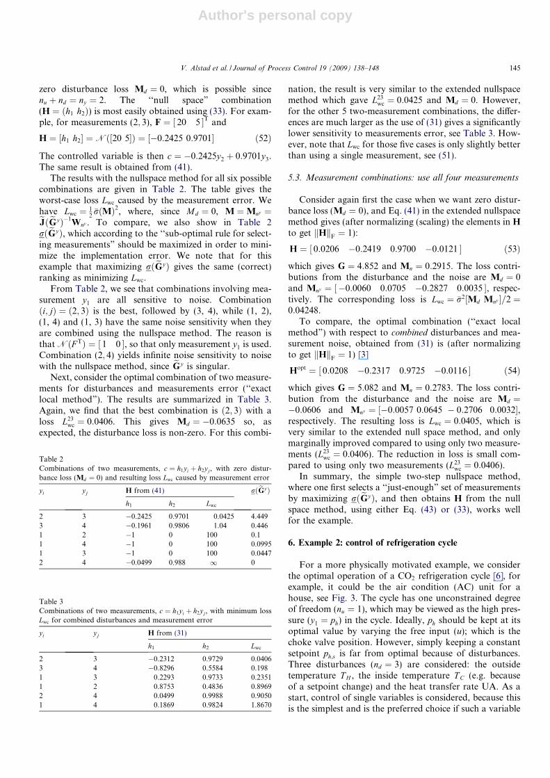
The results with the nullspace method for all six possiblecombinations are given in Table 2. The table gives theworst-case loss Lwc caused by the measurement error. Wehave Lwc ¼ 1

2�rðMÞ2, where, since Md ¼ 0, M ¼Mny ¼eJðeGyÞ�1

Wny . To compare, we also show in Table 2rðeGyÞ, which according to the ‘‘sub-optimal rule for select-ing measurements” should be maximized in order to mini-mize the implementation error. We note that for thisexample that maximizing rðeGyÞ gives the same (correct)ranking as minimizing Lwc.

From Table 2, we see that combinations involving mea-surement y1 are all sensitive to noise. Combinationði; jÞ ¼ ð2; 3Þ is the best, followed by (3, 4), while (1, 2),(1, 4) and (1, 3) have the same noise sensitivity when theyare combined using the nullspace method. The reason isthat NðF TÞ ¼ 1 0½ �, so that only measurement y1 is used.Combination (2; 4) yields infinite noise sensitivity to noisewith the nullspace method, since eGy is singular.

Next, consider the optimal combination of two measure-ments for disturbances and measurements error (‘‘exactlocal method”). The results are summarized in Table 3.Again, we find that the best combination is ð2; 3Þ with aloss L23

wc ¼ 0:0406. This gives Md ¼ �0:0635 so, asexpected, the disturbance loss is non-zero. For this combi-

nation, the result is very similar to the extended nullspacemethod which gave L23

wc ¼ 0:0425 and Md ¼ 0. However,for the other 5 two-measurement combinations, the differ-ences are much larger as the use of (31) gives a significantlylower sensitivity to measurements error, see Table 3. How-ever, note that Lwc for those five cases is only slightly betterthan using a single measurement, see (51).

5.3. Measurement combinations: use all four measurements

Consider again first the case when we want zero distur-bance loss (Md ¼ 0), and Eq. (41) in the extended nullspacemethod gives (after normalizing (scaling) the elements in H

to get kHkF ¼ 1):

H ¼ 0:0206 �0:2419 0:9700 �0:0121½ � ð53Þ

which gives G ¼ 4:852 and Mn ¼ 0:2915. The loss contri-butions from the disturbance and the noise are Md ¼ 0and Mny ¼ �0:0060 0:0705 �0:2827 0:0035½ �, respec-tively. The corresponding loss is Lwc ¼ �r2½Md Mny �=2 ¼0:04248.

To compare, the optimal combination (‘‘exact localmethod”) with respect to combined disturbances and mea-surement noise, obtained from (31) is (after normalizingto get kHkF ¼ 1) [3]

Hopt ¼ ½ 0:0208 �0:2317 0:9725 �0:0116 � ð54Þ

which gives G ¼ 5:082 and Mn ¼ 0:2783. The loss contri-bution from the disturbance and the noise are Md ¼�0:0606 and Mny ¼ ½�0:0057 0:0645 � 0:2706 0:0032�,respectively. The resulting loss is Lwc ¼ 0:0405, which isvery similar to the extended null space method, and onlymarginally improved compared to using only two measure-ments (L23

wc ¼ 0:0406). The reduction in loss is small com-pared to using only two measurements (L23

wc ¼ 0:0406).In summary, the simple two-step nullspace method,

where one first selects a ‘‘just-enough” set of measurementsby maximizing rðeGyÞ, and then obtains H from the nullspace method, using either Eq. (43) or (33), works wellfor the example.

6. Example 2: control of refrigeration cycle

For a more physically motivated example, we considerthe optimal operation of a CO2 refrigeration cycle [6], forexample, it could be the air condition (AC) unit for ahouse, see Fig. 3. The cycle has one unconstrained degreeof freedom (nu ¼ 1), which may be viewed as the high pres-sure (y1 ¼ ph) in the cycle. Ideally, ph should be kept at itsoptimal value by varying the free input (u); which is thechoke valve position. However, simply keeping a constantsetpoint ph;s is far from optimal because of disturbances.Three disturbances (nd ¼ 3) are considered: the outsidetemperature T H , the inside temperature T C (e.g. becauseof a setpoint change) and the heat transfer rate UA. As astart, control of single variables is considered, because thisis the simplest and is the preferred choice if such a variable

Table 2Combinations of two measurements, c ¼ h1yi þ h2yj, with zero distur-bance loss (Md ¼ 0) and resulting loss Lwc caused by measurement error

yi yj H from (41) rðeGyÞh1 h2 Lwc

2 3 �0.2425 0.9701 0.0425 4.4493 4 �0.1961 0.9806 1.04 0.4461 2 �1 0 100 0.11 4 �1 0 100 0.09951 3 �1 0 100 0.04472 4 �0.0499 0.988 1 0

Table 3Combinations of two measurements, c ¼ h1yi þ h2yj, with minimum lossLwc for combined disturbances and measurement error

yi yj H from (31)

h1 h2 Lwc

2 3 �0.2312 0.9729 0.04063 4 �0.8296 0.5584 0.1981 3 0.2293 0.9733 0.23511 2 0.8753 0.4836 0.89692 4 0.0499 0.9988 0.90501 4 0.1869 0.9824 1.8670

V. Alstad et al. / Journal of Process Control 19 (2009) 138–148 145

Author's personal copy

can be found. The best single controlled variable (with alarge scaled gain and a small loss) was found to be the massholdup (c ¼ M c) in the condenser [6], but it is very difficultto measure in practice. Therefore, a combination of mea-surements needs to be controlled. Theoretically, we needto combine at least four measurements (nu þ nd ¼ 4) toget zero loss, independent of the disturbances (i.e., to getMd ¼ 0). However, to simplify the implementation we pre-fer to use fewer measurements. Two measurements whichare easy to measure and have a reasonably large scaled gain[6], are the high pressure (y1 ¼ ph) and the temperaturebefore the choke valve (y2 ¼ T h). It is not possible to getMd ¼ 0 with only two measurement, so insteadH ¼ ½ h1 h2 � was obtained numerically by minimizingkMdkF; see Eq. (46) (actually, the matrix H can be obtainedexplicitly from (31) with Wny ¼ 0, since we haveny ¼ 2 < nd ¼ 3; see comment following Theorem 1). Thisgives a controlled variable c ¼ h1y1 þ h2y2 ¼ h1ph þ h2T h.To get a more physical variable, we select h1 ¼ 1, whichgives a controlled variable in the units of pressure. We find[6]

c ¼ ph;combined ¼ ph þ kðT h � 25:5 �CÞ

where k ¼ h2=h1 ¼ �8:53 bar=�C and the (constant) set-point for c ¼ ph;combined is 97.6 bar, which is the nominallyoptimal value for the high pressure. Controlling c may beviewed as controlling the high pressure, but with a temper-ature-corrected setpoint. A more detailed analysis using anonlinear model shows that this combination gives verysmall losses for all disturbances and measurement errors[6].

Other case studies. The results of this paper, and in par-ticular the use of (31) in Theorem 1 have also been applied

successfully to a distillation case study where the issue is toselect temperature combinations [4].

7. Discussion

7.1. Local method

The above derivations are local, since we assume a linearprocess and a second-order objective function in the inputsand the disturbances. Thus, the proposed controlled vari-ables are only globally optimal for the case with a linearmodel and a quadratic objective. In general, we shouldalways, for a final validation, check the losses for the pro-posed structures using a nonlinear model of the process.

7.2. Quadratic optimization problem

The following reformulations of the results in this papermay be useful for extending them to other applications andcomparing them with other results.

First, we give a reformulation of the original nullspacemethod in [1].

Theorem 3 (Linear invariants for quadratic optimizationproblem). Consider an unconstrained quadratic optimization

problem in the variables u (input vector of length nu) and d

(disturbance vector of length nd )

minu

Jðu; dÞ ¼ ½ u d �Juu Jud

JTud Jdd

� �u

d

� �ð55Þ

In addition, there are ‘‘measurement” variables y ¼ GyuþGy

dd. If there exists ny P nu þ nd independent measurements

(where ‘‘independent” means that the matrix eGy ¼ ½Gy Gyd �

has full rank), then the optimal solution to (55) has the prop-

erty that there exists nc ¼ nu linear variable combinations

(constraints) c ¼ Hy that are invariant to the disturbances

d. Here, H may be obtained from the nullspace method using

(33) (where the optimal sensitivity F may be obtained from

(15)) or from the explicit expression (37).

Next, the result on the worst-case loss [3] and the explicitexpression for the ‘‘exact local method” in Theorem 1 canbe reformulated as follows.

Theorem 4. (Loss by introducing linear constraint fornoisy quadratic optimization problem). Consider the

unconstrained quadratic optimization problem in Theorem 3,

minu

Jðu; dÞ ¼ ½ u d �Juu Jud

JTud Jdd

� �u

d

� �and a set of noisy measurements ym ¼ yþ ny , where Y ¼GyuþGy

dd. Assume that nc ¼ nu constraints c ¼ Hym ¼ cs

are added to the problem, which will result in a non-optimal

solution with a loss L ¼ Jðu; dÞ � J optðdÞ. Consider distur-

bances d and noise ny with magnitudes

d ¼Wdd0; ny ¼Wny ny0 ;d0

ny0

� ����� ����2

6 1

Qloss

TH

TC

TCTC

QCT3 T4

Pl

Ws

Ph

QH

T1T2

z

TH

PC

Ps

h,combine

T4

k

l

Vl

s

Fig. 3. Proposed control structure for the refrigeration cycle.

146 V. Alstad et al. / Journal of Process Control 19 (2009) 138–148

Author's personal copy

Then for a given H, the worst-case loss is Lwc ¼ �rðMÞ2=2,

where M is given in (20)–(22), and the optimal H that mini-

mizes �rðMÞ is given by (31) in Theorem 1. This optimal H

also minimizes kMkF.

Note from Theorem 3 that if there are a sufficient num-ber (ny P nu þ nd) of noise-free measurements, then we canobtain zero loss in Theorem 4.

7.3. Relationship to indirect control

Indirect control is when we want to find a set of con-trolled variables c ¼ Hy such that the primary variablesy1 are indirectly kept at constant setpoints. The case ofindirect control is discussed in more detail by Hori et al.[5] and their results are a special case of the results forthe nullspace method presented in this paper if we select

J ¼ 1

2ky1 � ys

1k2 ¼1

2½y1 � ys

1�T½y1 � ys

1� ð56Þ

To show this, write

Dy1 ¼ G1DuþGd1Dd ¼ fG1

Du

Dd

� �ð57Þ

and assume ny1¼ nu, so G1 is a square matrix. We find that

Juu ¼ GT1 G1 ð58Þ

Jud ¼ GT1 Gd1 ð59Þ

Consider the case with ny ¼ nu þ nd , where we can achieveperfect indirect control with respect to disturbances.Substituting (58) and (59) into the explicit expression (37)for the nullspace method gives

H ¼ P�1c;0eG1ðeGyÞ�1 ð60Þ

where we have introduced the new ‘‘free” parameterPc;0 ¼ G1J�1=2

uu Mn ¼ G1G�1. This is identical to the resultsof Hori et al. [5].

8. Conclusion

Explicit expressions have been derived for the optimallinear measurement combination c ¼ Hy.

The null space method [1] for selecting linear measure-ment combinations c ¼ Hy has been extended to the gen-eral case with extra measurements, ny > nu þ nd , see Eq.(41) in Theorem 2. The idea of the extended nullspacemethod is to first focus on minimizing the steady-state losscaused by disturbances, and then, if there are remainingdegrees of freedom, minimize the effect of measurementerrors. Alternatively, one may minimize the effect of com-bined disturbances and measurements errors, which is the‘‘exact local method” of Halvorsen et al. [3]. In this paper,we have derived an explicit solution for H for this problem,see Eq. (31) in Theorem 1. This expression applies to anynumber of measurements, including ny < nu þ nd .

To simplify, one often uses only a subset of the availablemeasurements when obtaining the combination c ¼ Hy. A

simple rule, which can aims at minimizing the effect of mea-surement errors, is to select measurements to maximizerðeGyÞ or even better, to minimize �rðeJðeGyÞ�1

Wny Þ. Here,eGy is the steady-state gain matrix from the inputs and dis-turbances to the selected measurements.

Finally, the results can be interpreted as adding linearconstraints that minimize the effect on the solution to aquadratic optimization problem; see Theorems 3 and 4.

Appendix A. Analytical solution for the exact local method

A.1. Scalar case

The minimization problem for the scalar case in (29) canbe rewritten as:

minxkeFTxk2 ¼ min

xxTeFeFTx subject to GyTx ¼ J1=2

uu ðA:1Þ

where we have introduced x,HT, which is a column-vec-tor in the scalar case.

The solution to this problem must satisfy the followingKKT-conditions (e.g. [12, p. 444]):eFeFT �Gy

GyT 0

" #x

k

� �¼

0

J1=2uu

� �ðA:2Þ

To find the optimal x, we must invert the KKT-matrix andfrom the Schur complement of the inverse of a partitionedmatrix (e.g. [14, p. 516]), we obtain that the optimal x is

x ¼ HT ¼ ðeFeFTÞ�1GyðGyTðeFeFTÞ�1

Gy�1J1=2

uu ðA:3Þ

Comment: In the scalar case, Gy is a (column) vector andJ1=2

uu is a scalar. However, the expression and proof also ap-plies if Gy were a matrix and J1=2

uu were a vector. This fact isimportant for the extension to the multivariable case.

A.2. Extension to multivariable case

To show that the solution for the scalar case also appliesto the multivariable case, we first transform the multivari-able case into a scalar problem. In this proof, we consider asystem with two controlled variables (nu ¼ 2), but it caneasily be extended to any dimension.

The optimization problem is minHTkHeFkF subject toHGy ¼ J1=2

uu , where we introduce X ¼ HT. The matrices X

and J1=2uu are split into vectors

X, ½ x1 x2 �; J1=2uu ¼ ½ J1 J2 � ðA:4Þ

We further introduce the long vectors

xn ¼x1

x2

� �; Jn ¼

J1

J2

� �ðA:5Þ

and the large matrices

GyTn ¼

GyT 0

0 GyT

" #; eFn ¼

eF 0

0 eF" #

ðA:6Þ

V. Alstad et al. / Journal of Process Control 19 (2009) 138–148 147

Author's personal copy

Then, HeF ¼ XTeF ¼ xT1

xT2

� �eF ¼ xT1eF

xT2eF

" #and for the 2-norm,

the following applies

kHeFkF ¼xT

1eF

xT2eF

" #����������

F

¼ k½ xT1eF xT

2eF �kF ¼ kxT

neFnkF

ðA:7Þwhere it is noted that k � kF ¼ k � k2 for a vector.

The constraints GyTX ¼ J1=2uu become

½GyTx1 GyTx2 � ¼ ½ J1 J2 � ðA:8Þ

or GyTx1 ¼ J1 and GyTx2 ¼ J2, which can be rewritten as

GyTx1

GyTx2

" #¼

J1

J2

� �or GyT

n xn ¼ Jn ðA:9Þ

(A.7) and (A.9) is a vector optimization problem of theform in (A.1) and from (A.3) the solution is

xn ¼ ðfFnfFn

T�1Gy

nðGyTn ðfFn

fFnT�1

Gyn�1

Jn ðA:10ÞWe now need to ‘‘unpack” this to find the optimal HT ¼ X.Substituting the values and rearranging (A.10)

x1

x2

� �¼

eF 0

0 eF" # eF 0

0 eF" #T

0@ 1A�1

Gy 0

0 Gy

� �

�Gy 0

0 Gy

� �T eF 0

0 eF" # eF 0

0 eF" #T

0@ 1A�1

Gy 0

0 Gy

� �0@ 1A�1

�J1

J2

� �we see that

x1

x2

� �¼ ðeFeFTÞ�1

GyðGyTðeFeFTÞ�1GyÞ�1

J1

ðeFeFTÞ�1GyðGyTðeFeFTÞ�1

Gy�1J2

" #ðA:11Þ

and finally,

HT ¼ X ¼ x1 x2½ �¼ ðeFeFTÞ�1

GyðGyTðeFeFTÞ�1GyÞ�1

J1 J2½ � ¼¼ ðeFeFTÞ�1

GyðGyTðeFeFTÞ�1GyÞ�1

J1=2uu ðA:12Þ

This proves that the solution for the scalar case also appliesfor the multivariable.

References

[1] V. Alstad, S. Skogestad, Null space method for selecting optimalmeasurement combinations as controlled variables, Ind. Eng. Chem.Res. 46 (3) (2007) 846–853.

[2] D. Bonvin, G. Francois, B. Srinivasan, Use of measurements forenforcing the necessary conditions of optimality in the presence ofconstraints and uncertainty, J. Proc. Control 15 (6) (2005)701–712.

[3] I.J. Halvorsen, S. Skogestad, J.C. Morud, V. Alstad, Optimalselection of controlled variables, Ind. Eng. Chem. Res. 42 (14)(2003) 3273–3284.

[4] E. Hori, S. Skogestad, Selection of controlled variables: maximumgain rule and combination of measurements, Ind. Eng. Chem. Res.,submitted for publication.

[5] E. Hori, S. Skogestad, V. Alstad, Perfect steady state indirect control,Ind. Eng. Chem. Res. 44 (4) (2005) 291–309.

[6] J.B. Jensen, S. Skogestad, Optimal operation of simple refrigerationcycles. Part II: selection of controlled variables, Comp. Chem. Eng. 31(2007) 1590–1601.

[7] J.V. Kadam, W. Marquardt, M. Schlegel, T. Backx, O.H. Bosgra, P.-J. Brouwer, G. Dunnebier, D.V. Hessem, A. Tiagounovand, S.D.Wolf, Towards integrated dynamic real-time optimization andcontrol of industrial processes, in: FOCAPO 2003, 4th InternationalConference of Computer-Aided Process Operations, Proceedings ofthe Conference held at Coral Springs, Florida, January 12–15, 2003,pp. 593–596.

[8] V. Kariwala, Optimal measurement combination for local self-optimizing control, Ind. Eng. Chem. Res. 46 (2007)3629–3634.

[9] V. Kariwala, Y. Cao, S. Janardhanan, Local self-optimizing controlwith average loss minimization, Ind. Eng. Chem. Res. (2008), in press,doi:10.1021/ie070897+.

[10] T.E. Marlin, A.N. Hrymak, Real-time optimization of continuousprocesses, in: American Institute of Chemical Engineering Sympo-sium Series – Fifth International Conference on Chemical ProcessControl, vol. 93, 1997, pp. 85–112.

[11] M. Morari, G. Stephanopoulos, Y. Arkun, Studies in the synthesis ofcontrol structures for chemical processes. Part I: formulation of theproblem, process decomposition and the classification of the control-ler task. Analysis of the optimizing control structures, AIChE J. 26 (2)(1980) 220–232.

[12] J. Nocedal, S.J. Wright, Numerical Optimization, Springer, 1999.[13] S. Skogestad, Plantwide control: the search for the self-

optimizing control structure, J. Proc. Control 10 (2000) 487–507.

[14] S. Skogestad, I. Postlethwaite, Multivariable Feedback Control,second ed., John Wiley & Sons, 2005.

[15] B. Srinivasan, CJ. Primus, D. Bonvin, N.L. Ricker, Run-to-runoptimization via control of generalized constraints, Control Eng.Pract. 9 (8) (2001) 911–919.

[16] B. Srinivasan, D. Bonvin, E. Visser, Dynamic optimization of batchprocesses – I. Characterization of the nominal solution, Comp. Chem.Eng. 27 (1) (2003) 1–26.

[17] B. Srinivasan, D. Bonvin, E. Visser, Dynamic optimization of batchprocesses – III. Role of measurements in handling uncertainty, Comp.Chem. Eng. 27 (1) (2003) 27–44.

[18] G. Strang, Linear Algebra and its Applications, third ed., HarcourtBrace & Company, 1988.

[19] Y. Zhang, D. Nader, J.F. Forbes, Results analysis for trustconstrained real-lime optimization, J. Proc. Control 11 (2001) 329–341.

[20] Y. Zhang, D. Monder, J.F. Forbes, Real-time optimization underparametric uncertainty: a probability constrained approach, J. Proc.Control 12 (3) (2002) 373–389.

148 V. Alstad et al. / Journal of Process Control 19 (2009) 138–148