Optimal design and benefits of a short turning strategyfor a bus corridor

Alejandro Tirachini • Cristian E. Cortes • Sergio R. Jara-Dıaz

Published online: 18 June 2010� Springer Science+Business Media, LLC. 2010

Abstract We develop a short turning model using demand information from station to

station within a single bus line-single period setting, aimed at increasing the service

frequency on the more loaded sections to deal with spatial concentration of demand

considering both operators’ and users’ costs. We find analytical expressions for optimal

values of the design variables, namely frequencies (inside and outside the short cycle),

capacity of vehicles and the position of the short turn limit stations. These expressions are

used to analyze the influence of different parameters in the final solution. The design

variables and the corresponding cost components for operators and users (waiting and in-

vehicle times) are compared against an optimized normal operation scheme (single fre-

quency). Applications on actual transit corridors exhibiting different demand profiles are

conducted, calculating the optimal values for the design variables and the resulting benefits

for each case. Results show the typical demand configurations that are better served using a

short turn strategy.

Keywords Public transport � Short turning � Users’ costs � Operators’ costs �Frequency

Introduction

Daily operations of urban public transport systems have to deal with both spatial and

temporal peak periods of demand that result in inefficient operation schemes when using

A. Tirachini (&)Institute of Transport and Logistics Studies, Faculty of Economics and Business,The University of Sydney, Sydney, NSW 2006, Australiae-mail: alejandro.tirachini@sydney.edu.au

C. E. Cortes � S. R. Jara-DıazCivil Engineering Department, Universidad de Chile, P.O. 228-3, Santiago, Chilee-mail: ccortes@ing.uchile.cl

S. R. Jara-Dıaze-mail: jaradiaz@ing.uchile.cl

123

Transportation (2011) 38:169–189DOI 10.1007/s11116-010-9287-8

the same vehicle supply along the entire route and over the whole day. With regard to the

spatial dimension, there are several strategies to better assign the available fleet, by

increasing the service frequency on the most demanded route sections in order to adjust the

demand with the vehicles’ supply.

Among the vehicles’ assignment strategies, the most studied in the specialized literature

are expressing, deadheading and short turning. The vehicles that perform expressing

(Jordan and Turnquist 1979; Furth 1986; Eberlein et al. 1999) serve only one section of

their route, and then they proceed without stopping until reaching either the terminal or a

pre-specified zone where the service is reestablished. The deadheading strategy (Eberlein

et al. 1998, 1999; Furth 1985, Ceder and Stern 1981; Ceder 2003a, 2004) is usually

considered for transit corridors that present high demand on one direction of operation and

low demand on the other. It consists in increasing the frequency in the peak direction by

suppressing some services in the off-peak direction, that is, vehicles not in service are

deadheaded back to the initial terminal of the peak direction.

In the present paper we focus our analysis on a very flexible and popular strategy called

short turning, expanding its scope to account for all costs involved, users’ and operators’,

considering station to station demand information. It consists in selecting part of the fleet to

serve short cycles or loops on those route segments exhibiting high demand. This strategy

has been studied in several forms by Furth (1987), Ceder (1989, 2003b), Vijayaraghavan

and Anantharmaiah (1995) and Delle Site and Filippi (1998).

Furth (1987) assumes a scheduled operation scheme, in which the frequency of

vehicles performing the short turn (hereafter, fleet B) is a multiple n of the frequency of

those vehicles serving the entire route (hereafter, fleet A); the parameter n is known as

the ‘‘scheduling mode’’. As many demand patterns can be satisfied by bus fleets

adopting either full-length or short-turn services, schedule coordination of the two

operation schemes is essential. He describes possible schedule coordination modes, and

proposes algorithms for finding the schedule offset between the schemes that will

balance loads. The optimization variables are the bus headway associated with fleet A,

and the schedule offset between the vehicles of fleet A and those of fleet B. The

process assumes as external parameters the number of cycles, the limit stations for the

short turn and the bus capacities. The author focuses on several problems. First, the

fleet size is minimized, which is equivalent to maximizing the vehicle headway. Next, a

number of solutions depending on the turn-back points are evaluated, choosing the

alternative that provides the lowest waiting time given the fleet size. Savings on fleet

size are shown to depend on the offset between vehicles A and B, on whether whole-

minute offsets are required and on the possibility of interlining vehicles between fleets

A and B.

Ceder (1989, 2003b), by means of an aggregated demand model, proposes a two-stage

optimization approach. In a first stage, the fleet size is minimized for a given demand level

while in a second stage, the number of trips using the short turn is minimized in order to

reduce the effect of the strategy on passenger trip times.

Vijayaraghavan and Anantharmaiah (1995) also pursue the reduction of fleet size

through the insertion of express services as well as short turns for the service of some trips,

where the headways and speeds of the new services are exogenously introduced and their

potential benefits calculated. The authors report savings when applying their approach in

terms of fleet and crew utilization, and an associated reduction in passenger travel times as

well.

Delle Site and Filippi (1998) develop a more complex model, in which the short turning

strategy is applied on a multi-period basis with both elastic and inelastic demand. In

170 Transportation (2011) 38:169–189

123

addition, the authors extend the work by Furth (1987) to the case of bus arrivals at stations

following a Poisson distribution. In the case of elastic demand, the social benefit is

maximized, whereas in the case of inelastic demand, the sum of user and operator costs is

minimized. The decision variables are the limit stations of the short turn (start and end), the

frequency, the capacity of vehicles (treated parametrically) and the service fare. An

application that compares the strategy with a given base situation (normal operation with

single frequency) shows that the strategy turns out to be beneficial only with demand

patterns that exhibit pronounced peaks, reducing both waiting time and fixed operator cost

(due to the operation of a smaller fleet size) and increasing the operating variable cost.

In this work we develop a short turning model taking into account that the strategy

affects not only the operation costs but also passenger in-vehicle and waiting times. This

approach is based on a microeconomic modeling of transit operations, where we clearly

establish the users and operators cost components, to investigate how the strategy affects

both parties. The analysis is restricted to a single period of operation, under the

assumption that this strategy should be useful in most cases during peak demand periods

only. The design variables in the formulated problem are frequencies, segment where the

short turn strategy should be applied, and vehicle sizes. The model is structural, as we

get optimal values of frequencies and capacities and the expected benefits from applying

short turning in different cases in order to identify and support potentially effective

public transport planning policy. We do not attempt to reach detailed results as, for

instance, the timetabling of buses A and B, which can be done once the policy has been

deemed useful.

To our knowledge, this is the first work that, under some assumptions, finds analytical

expressions for optimal frequencies both inside and outside the short cycle, which are used

to analyze the influence of the parameters of the problem in the final solution. Unlike the

existing literature that compares the short turning strategy with a given normal operation or

base case (no strategy is applied, resulting in a single frequency along the entire route), in

our model the situation with normal operation is also optimized, in order to compare both

cases on a fair basis. Once the analytical framework has been established, we conduct a

number of experiments finding that:

• The short turning strategy can yield benefits for both users and operators at the same

time.

• Cost savings are reachable not only when the demand is concentrated in the middle of a

route, but also when the most loaded section is on an extreme of the line.

• Cost savings depend largely on the imbalance between trips inside and outside the short

cycle.

• When the strategy yields benefits, vehicles may be smaller than those resulting for the

single frequency case.

• The concentration of demand plays a fundamental role: the more concentrated the trips

(the shorter the cycle is), the larger the benefits.

In Sect. 2 the short turning strategy is presented and an optimization problem is

formulated, solved and compared analytically against an also optimized normal opera-

tion. In Sect. 3 we show several applications to measure the comparative benefits of the

strategy under different situations. This section is crucial to better understand the

behavior of the key elements in the definition of the strategy, such as optimal fre-

quencies, capacity of vehicles, features of the demand and position and length of the

short turn. Finally, in Sect. 4 the main findings are summarized and extensions of this

approach are proposed.

Transportation (2011) 38:169–189 171

123

Modeling and optimization of the short-turning strategy

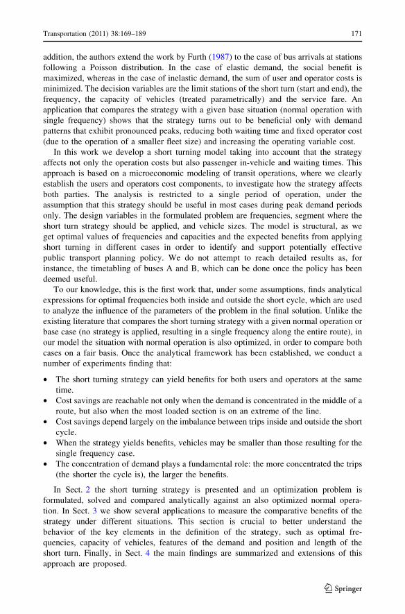
Without loss of generality, we model a single linear transit line. Fleets A and B are defined

as detailed above. The system contains N stations in one direction (N–1 segments), as

shown in Fig. 1. The operation directions are denoted direction 1 (from station 1 to N) and

direction 2 (from station N to 1). We develop a model that minimizes total cost for two

situations: normal operation, where all vehicles operate along the whole route, and oper-

ation with short turning. The model is used to measure potential benefits of short turning

under several demand configurations. Following Fig. 1, the decision variables are the start

and end stations associated with the short turn, denoted by s0 and s1, the frequency fA of

those vehicles serving the whole route (fleet A) and the frequency fB of those vehicles

serving the short cycle (fleet B). Under normal operation the decision variable is the single

frequency f.The known parameters are L, length of the corridor (km); Rk, bus running time under

normal service between stations k and k ? 1 including acceleration and deceleration at bus

stops (min); b, marginal passenger boarding time (seg/pax); and kkl, the trip rate between

stations k and l (pax/h). This disaggregated demand is assumed fixed (steady state) over the

studied period, defining a trip matrix.

Additionally, the following functions and quantities are defined:

• Passenger boarding rate at station k, whose destination is among stations l1 and l2

inclusive (pax/h): kþk ðl1; l2Þ ¼Pl2

l¼l1

kkl

• Passenger alighting rate at station k, whose origin is among stations l1 and l2 inclusive

(pax/h): k�k ðl1; l2Þ ¼Pl2

l¼l1

klk

• Passenger boarding rate at station k, direction 1:k1þk � kþk ðk þ 1;NÞ ¼

PN

l¼kþ1

kkl

• Passenger alighting rate at station k, direction 1:k1�k � k�k ð1; k � 1Þ ¼

Pk�1

l¼1

klk

• Passenger boarding rate at station k, direction 2:k2þk � kþk ð1; k � 1Þ ¼

Pk�1

l¼1

kkl

• Passenger alighting rate at station k, direction 2:k2�k ¼ k�k ðk þ 1;NÞ ¼

PN

l¼kþ1

klk

We assume that at stations boarding and alighting process are simultaneous and that

boarding dominates alighting (i.e. the boarding process is slower than the alighting pro-

cess); therefore, total dwell time at stops is considered through the boarding parameter b.

Optimal design of a bus system should include the operator cost (fuel consumption,

crew costs, lubricants, tires, maintenance, etc.) and the user costs (access, waiting and in-

vehicle times). Both are affected when a short turning strategy is applied; the former

N

1N −

1

2

0s

Bf

1sA Bf f+Af

Af

AfAf

Af

A Bf f+0s 1s

N

1N −

1

2

0s

Bf

1sA Bf f+Af

Af

AfAf

Af

A Bf f+0s 1s

Fig. 1 Short turning strategy

172 Transportation (2011) 38:169–189

123

because the fleet size can be adjusted when applying the strategy, and the latter because

users’ waiting and in-vehicle times vary due to the adjustment of frequency and changes in

dwell time at stations with respect to the normal case.

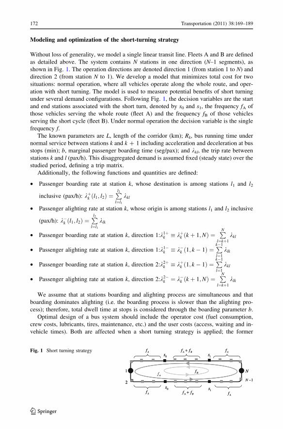
In what follows we will find the operators and users cost components as functions of the

design variables for two scenarios: normal and strategy-based operations. Then we will

find the analytical expressions for the optimal frequencies, which in the case of the strategy

will depend parametrically on the stations that define the boundaries of the short turn

service. This will be the basis for a two-stages process in order to find overall optimal

frequencies, optimal vehicle sizes and optimal short-turn segment.

The analytical expression for the waiting time depends on the vehicle and passenger

arrival processes. Regarding bus arrivals, as in Delle Site and Filippi (1998) we consider

two opposite cases: a highly controlled service where headways are kept regular along the

line, and a poorly controlled system where headways vary randomly along the line due to

traffic and demand variations. In the latter case (random arrivals), we will make the usual

assumption that vehicle arrivals are Poisson in which headways follow a negative expo-

nential distribution, noting that this is a simplification as the headways between successive

buses are likely to be correlated due to the influence of dwell times, which in turn depends

on the previous headway.

In the regular service scheme, we impose regular headways within the short turn

operation as well, although this could result in larger loads observed in buses belonging to

fleet A when compared with buses of fleet B. This differs from the work of Furth (1987),

who specifically determines the offset between fleets A and B in order to balance passenger

loads. Note that waiting times are proportional to the headway variance (Welding 1957;

Osuna and Newell 1972), which is minimized when keeping regular headways as the

possibility of vehicle bunching is reduced. Therefore, it is assumed that potential negative

effects of operating with uneven loads are outweighed by the benefits of a regular headway

scheme. Regarding passengers, we assume they arrive at stations uniformly at a fixed rate,

which is a reasonable assumption in cases of high frequency transit lines. Combining

passengers and bus arrival schemes, the average waiting time at each station would be

equal to half of the headway under regular bus arrivals, and equal to the whole expected

headway for random (Poisson) bus arrivals.

In summary, we can compute the waiting time cost (Cw) component associated with

normal service, as follows:

Cw ¼ Pw

1þ x

2

XN

k¼1

k1þk

fþXN

k¼1

k2þk

f

( )

ð1Þ

In this expression, the two bus arrival schemes discussed above are captured by the

auxiliary binary variable x, which is equal to 1 if buses arrive Poisson and 0 if they arrive

regularly spaced; Pw is the waiting time value. For the short turning strategy, we will

assume that bus arrivals at both inside (frequency fA ? fB) and outside the short turn

(frequency fA) follow a Poisson distribution. Then Cw becomes:

Cw ¼ Pw

1þ x

2

Xs0�1

k¼1

k1þk

fA

(

þXs1�1

k¼s0

kþk ðk þ 1; s1ÞfA þ fB

þ kþk ðs1 þ 1;NÞfA

� �

þXN

k¼s1

k1þk

fA

þXN

k¼s1þ1

k2þk

fA

þXs1

k¼s0þ1

kþk ð1; s0 � 1ÞfA

þ kþk ðs0; k � 1ÞfA þ fB

� �

þXs0

k¼1

k2þk

fA

)

ð2Þ

Transportation (2011) 38:169–189 173

123

Inside the key brackets in expression (2) we have split the expected waiting times of users

per direction and per origin and destination, because passengers boarding and alighting

inside and outside the short turn face different frequencies, and therefore, different waiting

times. For example, in direction 1 (first line in Eq. 2) passengers boarding before (first

term) and after (third term) the short turn are served by a frequency fA, the same as those

passengers who board inside but have destination after the short turn (second summation in

second term). Only passengers whose origin and destination are inside the short cycle

observe a frequency fA ? fB (first summation in second term). The terms in the second line

(direction 2) have an analogous interpretation. This assumes that passengers do not transfer

between vehicles A and B.

The in-vehicle time between stations corresponds to the sum of the bus running time

(Ri) and the time that passengers wait for others to board the bus (bki?/f). Under normal

operation, the cost associated with in-vehicle time (Cv) is,

Cv ¼ Pv

XN

k¼1

XN

l¼kþ1

Xl�1

i¼k

Ri þ bk1þ

i

f

� �" #

kkl þXN

k¼1

Xk�1

l¼1

Xk

i¼lþ1

Ri�1 þ bk2þ

i

f

� �" #

kkl

)(

ð3Þ

where Pv is the in-vehicle time value. When a short turning strategy is introduced, the

analytical expression for Cv becomes more complicated, as a trip can encompass areas in

which users board vehicles at rates ki?/fA or ki

?/(fA ? fB). Using the definitions of functions

gi(s0, s1) in Appendix A, the total in-vehicle time cost can be expressed as

Cv ¼ 2XN�1

k¼1

Rk þ bg5ðs0; s1ÞfA þ fB

þ bg6ðs0; s1Þ

fA

ð4Þ

where functions g5(s0, s1) and g6(s0, s1) group second order terms of the trip rates kkl, as a

function of the start and end stations s0 and s1.

Operator cost (Co) is divided into temporal and spatial components. The former includes

items as personnel costs (crew), while the latter comprises running costs, such as fuel

consumption, lubricants, tires, maintenance, etc. Following Oldfield and Bly (1988) and

Jansson (1980), the unit operator costs are expressed as a linear function of the vehicle

capacity K, where c(K) is the vehicle–hour cost (expressed in $/vh) and c0(K) corresponds

to the vehicle–kilometer cost (expressed in $/vkm). Analytically,

cðKÞ ¼ c0 þ c1K c0ðKÞ ¼ c00 þ c01K ð5Þ

Co ¼ cðKÞF þ c0ðKÞvF ð6Þ

In the previous expressions, v is the bus system commercial speed (including dwell times)

and F is the fleet size needed for a design occupancy rate (define below in Eq. 11),

obtained as the product of the frequency and the cycle time tc (which by simplicity assumes

no layover time or slack in the schedule), F = ftc. Since v = 2L/tc, Co can be rewritten as

follows for the case of normal operation as (7) and (8)

Co ¼ cðKÞftc þ 2c0ðKÞfL ð7Þ

Co ¼ f cðKÞXN�1

k¼1

Rk þ bk1þ

k

f

� �

þXN

k¼2

Rk�1 þ bk2þ

k

f

� �" #

þ 2c0ðKÞL( )

ð8Þ

On the other hand, for the short turning strategy, the operator cost must include the costs of

both fleets, A and B. Operator cost of Fleet A, which operates normally between terminals, is

174 Transportation (2011) 38:169–189

123

CoA ¼ fA

(

cðKÞ"Xs0�1

k¼1

Rk þ bk1þ

k

fA

� �

þXs1�1

k¼s0

Rk þ bkþk ðk þ 1; s1Þ

fA þ fBþ kþk ðs1 þ 1;NÞ

fA

� �� �

þXN

k¼s1

Rk þ bk1þ

k

fA

� �

þXN

k¼s1þ1

Rk�1 þ bk2þ

k

fA

� �

þXs1

k¼s0þ1

Rk�1 þ bkþk ð1; s0 � 1Þ

fA

þ kþk ðs0; k � 1ÞfA þ fB

� �� �

þXs0

k¼2

Rk�1 þ bk2þ

k

fA

� �#

þ 2c0ðKÞL)

ð9Þ

while vehicles belonging to fleet B travel a shorter distance and then their cost is:

CoB ¼ fB cðKÞXs1�1

k¼s0

Rk þ bkþk ðk þ 1; s1Þ

fA þ fB

� �

þXs1

k¼s0þ1

Rk�1 þ bkþk ðs0; k � 1Þ

fA þ fB

� �" #(

þ2c0ðKÞLs1 � s0

N � 1

) ð10Þ

Using (9) and (10), the total operator cost is Co = CoA ? CoB.

Once waiting time, in-vehicle time and operator costs have been analytically found, it is

possible to minimize total cost for both normal operation (sum of expressions 1, 3 and 8)

and for the system with short turning strategy (sum of 2, 4, 9 and 10). Moreover, for the

waiting time calculations, in Eqs. 1 and 2 passengers are assumed to board the first bus that

arrives at their station; to fulfill this condition, bus capacity is set to accommodate the

expected demand in the most loaded segment along the line, namely qmax. Under normal

operation:

K ¼ qmax

gfð11Þ

where qmax ¼ maxk

Pk

i¼1

PN

j¼kþ1

kij;PN

i¼kþ1

Pk

j¼1

kij

( )

is obtained from the OD matrix. Factor g

defines the maximum design occupancy rate (for example, g = 0.85), whose purpose is to

keep extra capacity for absorbing the intrinsic randomness of the demand. Note that if

demand is assumed to follow a random distribution, such as Poisson, this capacity and any

other finite value can be theoretically superseded, case which is not considered in this model.

After introducing (11) in (5), the optimal value of frequency f is obtained applying first

order conditions (FOC), obtaining

f � ¼

ffiffiffiffiffiffiffiffiffiffiffiffiffiffiffiffiffiffiffiffiffiffiffiffiffiffiffiffiffiffiffiffiffiffiffiffiffiffiffiffiffiffiffiffiffiffiffiffiffiffiffiffiffiffiffiffiffiffiffiffiffiffiffiffiffiffiffiffiffiffiffiffiffiffiffiffiffiffiffiffiffiffiffiffiffiffiffiffiffiffiffiffiffiffiffiffiffiffiffiffiffiffiffiffiffiffiffiffiffiffiffiffiffiffiffiffiffiffiffiffiffiffiffiffiffiffiffiffiffiffiffiffiffiffiffiffiffiffiffiffiffiffiffiffiffiffiffiffiffiffiffiffiffiffiffiffiffiffiffiffiffiffiffiffiffiffiffiffiffiffiffiffiffiffiffiffiffiffiffiffiffiffiffiffiffiffiffiffiffiffiffiffiffiffiffiffiffiffiffiffiffiffiffiffiffiffiffiffi

Pw1þx

2

PN

k¼1

k1þk þ

PN

k¼1

k2þk

� �

þ PvbPN

k¼1

PN

l¼kþ1

kkl

Pl�1

i¼k

k1þi þ

PN

k¼1

Pk�1

l¼1

kkl

Pk

i¼lþ1

k2þi

� �

þ c1qmax

g bPN

k¼1

k1þk þ

PN

k¼1

k2þk

� �

2 c0

PN�1

k¼1

Rk þ c00L

� �

vuuuuuut

ð12Þ

Expression (12) corresponds to the classical ‘‘square root formula’’, derived for a single

bus corridor with fixed demand (Mohring 1972; Jansson 1980; Jara-Dıaz and Gschwender

2003 among others), with the difference that in this formulation, (12) is expressed in terms

of the disaggregated OD demand between stations (Jara-Diaz et al. 2008).

Transportation (2011) 38:169–189 175

123

For the short turning strategy, total cost can be expressed more concisely as

CtðfA;fB;s0;s1;KÞ¼fA cðKÞ g0þbg1ðs0;s1Þ

fAþfB

þbg2ðs0;s1Þ

fA

� �

þ2c0ðKÞL� �

þfB

�

cðKÞ g3ðs0;s1Þþbg1ðs0;s1Þ

fAþfB

� �

þ2c0ðKÞs1�s0

N�1L

�

þPw

1þx

2

g1ðs0;s1ÞfAþfB

þg2ðs0;s1ÞfA

� �

þPv g4þbg5ðs0;s1Þ

fAþfB

þbg6ðs0;s1Þ

fA

� �

ð13Þ

Functions gi(s0, s1) are defined in Appendix A; g0 is the total running time, g1 is the

demand benefited by the strategy (origin and destination inside the short turn), g2 quantifies

the passengers whose origin or destination are outside the short turn, g3 is the running time

of vehicles inside the short turn, g4 is the total in-vehicle time experienced by passengers,

and g5 and g6 are quadratic factors on demand used to calculate the dwell times of

passengers whose origin and destination is inside the short turn (g5) and of all other

passengers (g6), respectively. The maximum load occurs for vehicles of fleet A, as these

enter the short turn section already with passengers on board (fleet B vehicles start service

at stations s0 or s1). Using recursively the boarding and alighting rates at stations kk? and

kk-, it is possible to obtain the load of the bus along the route for each segment and from

that, the capacity of vehicles can be set as

K ¼ 1

g#0ðs0; s1Þ

fA

þ #1ðs0; s1ÞfA þ fB

� �

ð14Þ

where #0(s0, s1) and #1(s0, s1) represent the terms that yield the maximum load, which

depends on the selection of stations s0 and s1 (see Appendix B for details). Therefore, by

introducing (14) in (13), we can see that the total cost depends only on fA, fB, s0 and s1,

namely Ct(fA, fB, s0, s1). The problem is solved in two stages. First, parametric in the value

of discrete variables s0 and s1, we apply the proper FOC to find fA* (s0, s1), fB

* (s0, s1) and

Ctðf �Aðs0; s1Þ; f �Bðs0; s1Þ; s0; s1Þ � �Ctðs0; s1Þ. Next, in a second stage, the feasible limit sta-

tions s0 and s1 are explored to select the ones that minimize �Ctðs0; s1Þ.Let us first assume that bus arrivals are distributed Poisson both for the normal operation

and for the short turning strategy, not only inside (frequency fA ? fB) but also outside the

short cycle (frequency fA). This is equivalent to set x = 1 in expressions (12) and (13).

In general, FOC do not yield analytical forms for the optimal frequencies and the

problem must be solved numerically. Nevertheless, if the unit operator costs do not depend

on capacity K, i.e. c(K) = c, c0(K) = c0 (there are no economies of vehicle size), the

optimal frequencies are derived as shown in (15) and (16), conditional on s0 and s1. A

second order analysis shows that (15) and (16) minimizes total cost.

f �Aðs0; s1Þ ¼ffiffiffiffiffiffiffiffiffiffiffiffiffiffiffiffiffiffiffiffiffiffiffiffiffiffiffiffiffiffiffiffiffiffiffiffiffiffiffiffiffiffiffiffiffiffiffiffiffiffiffiffiffiffiffiffiffiffiffiffiffiffiffiffiffiffiffiffiffi

Pwg2ðs0; s1Þ þ Pvbg6ðs0; s1Þcðg0 � g3ðs0; s1ÞÞ þ 2c0 1� s1�s0

N�1

� �L

s

ð15Þ

f �Bðs0; s1Þ ¼ffiffiffiffiffiffiffiffiffiffiffiffiffiffiffiffiffiffiffiffiffiffiffiffiffiffiffiffiffiffiffiffiffiffiffiffiffiffiffiffiffiffiffiffiffiffiffiffiffiffiffiffiffiffiffiPwg1ðs0; s1Þ þ Pvbg5ðs0; s1Þ

cg3ðs0; s1Þ þ 2c0s1�s0

N�1L

s

�ffiffiffiffiffiffiffiffiffiffiffiffiffiffiffiffiffiffiffiffiffiffiffiffiffiffiffiffiffiffiffiffiffiffiffiffiffiffiffiffiffiffiffiffiffiffiffiffiffiffiffiffiffiffiffiffiffiffiffiffiffiffiffiffiffiffiffiffiffi

Pwg2ðs0; s1Þ þ Pvbg6ðs0; s1Þcðg0 � g3ðs0; s1ÞÞ þ 2c0 1� s1�s0

N�1

� �L

s

ð16Þ

Expression (15) has the same analytical form as (12) and corresponds to the optimal

frequency for serving the stations outside the short turn (those whose demand is

176 Transportation (2011) 38:169–189

123

represented by functions g2 and g6), while (16), which is the optimal frequency of those

vehicles serving only the short turn, is computed as the difference between the optimal

frequency to serve only the short turn (first term of 16) and fA (second term of 16). Note

that in the particular case of fB = 0, expression (13) collapses to the total cost under

normal operation, and therefore if the solution (16) is positive, the strategy is beneficial

(total cost is less than that obtained under normal operation). Therefore, a condition for the

strategy to be beneficial is fB* (s0, s1) [ 0 or

Pwg1ðs0; s1Þ þ Pvbg5ðs0; s1ÞPwg2ðs0; s1Þ þ Pvbg6ðs0; s1Þ

[cg3ðs0; s1Þ þ 2c0s1�s0

N�1L

cðg0 � g3ðs0; s1ÞÞ þ 2c0 1� s1�s0

N�1

� �L

ð17Þ

where the demand benefited by the short turn is represented by functions g1 and g5, while

demand whose origin or destination is outside the short turn is represented by g2 and g6.

From (17) we conclude that the greater the demand imbalance between inside and outside

the short cycle (g1 and g5 against g2 and g6), the more likely the strategy results beneficial.

Regarding the length of the short turn, diminishing s1–s0 reduces the right side of (17) as

this implies lower operator costs; this also decreases left side of the expression, since the

shorter the short turn, less users are benefited by the strategy. Then, from the equations we

can set neither the optimal length of the short turn nor its position. For the case of a

scheduled service defined earlier (x = 0, fB = nfA), the vehicle capacity can be expressed

as:

K ¼ 1

g#0ðs0; s1Þ

fAþ #1ðs0; s1Þðnþ 1ÞfA

¼ 1

gfA

#0ðs0; s1Þ þ#1ðs0; s1Þ

nþ 1

� �

� #maxðn; s0; s1ÞgfA

ð18Þ

Thus, it is possible to obtain an analytical expression for the optimal frequency fA using the

full version of the unit operator costs shown in (5). Analytically,

f �Aðn; s0; s1Þ ¼

ffiffiffiffiffiffiffiffiffiffiffiffiffiffiffiffiffiffiffiffiffiffiffiffiffiffiffiffiffiffiffiffiffiffiffiffiffiffiffiffiffiffiffiffiffiffiffiffiffiffiffiffiffiffiffiffiffiffiffiffiffiffiffiffiffiffiffiffiffiffiffiffiffiffiffiffiffiffiffiffiffiffiffiffiffiffiffiffiffiffiffiffiffiffiffiffiffiffiffiffiffiffiffiffiffiffiffiffiffiffiffiffiffiffiffiffiffiffiffiffiffiffiffiffiffiffiffiffiffiffiffiffiffiffiffiffiffiffiffiffiffiffiffiffiffiffiffiffiffiffiffiffiffiffiffiffiffi

Pwg1ðs0;s1Þ2ðnþ1Þ þ

g2ðs0;s1Þ2

h iþ Pvb g5ðs0;s1Þ

nþ1þ g6ðs0; s1Þ

h iþ c1b#max

g ½g1ðs0; s1Þ þ g2ðs0; s1Þ�c0½g0 þ ng3ðs0; s1Þ� þ 2c00L 1þ ns1�s0

N�1

� �

vuut

ð19Þ

Once expression (19) is introduced in (13), considering x = 0 and fB = nfA, the values for

the scheduling mode n and stations s0 and s1 can be searched to minimize total cost. Note

that in practice, the search procedure of stations s0 and s1 is constrained by physical

conditions, as only in some spots along a bus route is technically possible to install a short

cycle by turning vehicles back.

Applications

Examples

In this section the objective is to quantify the potential benefits of the short turning strategy

using the analytical results obtained under the optimization scheme developed above, on a

hypothetical bus corridor comprising 10 stations. Further, we perform sensitivity analysis

regarding demand volumes and its distribution. We consider two demand scenarios that

represent two different demand distribution patterns of particular interest, as shown in the

load profiles in Fig. 2. The first case (Example 1, Fig. 2a) represents a situation with the

central business district located around one corridor terminus, and is taken from Delle Site

Transportation (2011) 38:169–189 177

123

and Filippi (1998). The second case has the same number of stops and comparable demand

level as Example 1, but represents a typical cross-town peak-demand route pattern,

illustrated by the load profile of Fig. 2b (Example 2). The values assigned to the param-

eters are: R = 2.5 min Vk, L = 8 km, Pw = 2700 ($/h), Pv = 900 ($/h), c0 = 1800 ($/vh),

c1 = 30 ($/h-pax), c00 ¼ 400 ($/vkm), c01 ¼ 1 ($/h-pax), b = 5 (s/pax) and g = 0.9 ($:

CLP-Chilean peso, USD 1&CLP 500).

With these data we searched for the optimal values of s0, s1, fA, fB, n, KA and KB for

each example under the two bus arrival schemes, i.e. regular and random (Poisson). In

Tables 1 and 2, a summary of the key results after running our model is provided for

Examples 1 and 2. Let us analyze Example 1 first.

In this case, the optimal short turn resulted between stations s0 = 7 and s1 = 10

(benefiting 49.8% of the passengers) which coincides with the most demanded section

along direction 2 in Fig. 2a. Regarding the scheduled service case (regular headways), the

optimal scheduling mode is n = 1, i.e., fA = fB and the 25 veh/h frequency is raised to

36 veh/h inside the short cycle, and reduced to 18 veh/h outside the short cycle. The

inclusion of the strategy provides savings in both in-vehicle and operator costs, and losses

in waiting time cost, with a total saving of 2.6% under random headways (Poisson arrivals)

and 3.7% considering regular headways. Therefore, in this example the waiting time

savings for passengers inside the short turn are outweighed by the increase in waiting time

for passengers whose origin or destination is outside the short turn; nevertheless, there are

savings associated with the in-vehicle time since this component depends on quadratic

terms of the demand (g5 and g6), which amplifies the demand imbalance shown in Fig. 2a.

The intuition is the following: when frequency increases for a group of stations, the waiting

time is affected only once (in the station where a passenger boards a vehicle), while the

in-vehicle time is reduced in all the downstream stations where the frequency has been

increased, which implies having less users boarding and alighting each bus.

O\D 1 2 3 4 5 6 7 8 9 101 29 14 64 4 3 3 1 1 252 14 15 70 4 4 3 1 1 273 5 5 49 3 3 2 1 0 194 8 7 4 18 15 12 4 3 1115 74 63 35 0 5 4 1 1 376 4 4 2 0 0 5 2 1 507 1 1 0 0 0 3 20 16 6368 8 6 3 0 0 26 5 7 2629 16 14 7 0 0 58 11 0 7710 13 11 6 0 0 47 9 0 10

O\D 1 2 3 4 5 6 7 8 9 101 5 8 9 13 10 17 41 4 22 7 7 8 11 8 15 35 4 23 40 35 13 17 13 23 55 6 34 20 18 22 24 19 33 77 8 45 17 15 19 34 150 265 624 67 356 15 13 16 29 348 267 630 67 367 20 18 23 40 484 131 529 56 308 21 18 23 40 494 134 130 52 289 3 3 3 6 72 19 19 5 510 1 1 1 2 23 6 6 2 3

Load profile

0

300

600

900

1200

1500

Station

Lo

ad

[p

ax

/h] Direction 1

Direction 2

Load profile

0

500

1000

1500

2000

2500

1 2 3 4 5 6 7 8 9 10 1 2 3 4 5 6 7 8 9 10

Station

Lo

ad

[p

ax

/h] Direction 1

Direction 2

Example 2Example 1

a b

Fig. 2 OD matrices (pax/h) and load profiles, examples 1 and 2

178 Transportation (2011) 38:169–189

123

Ta

ble

1O

pti

mal

val

ues

for

Ex

amp

le1

Op

erat

ion

f A(v

eh/h

)f B

(veh

/h)

F(v

eh)

K(p

ax/v

eh)

Cw

($/p

ax)

Cv

($/p

ax)

Co

($/p

ax)

Ct

($/p

ax)

DC

w(%

)D

Cv

(%)

DC

o(%

)D

Ct

(%)

Po

isso

nar

riv

als

No

rmal

31

(f)

27

45

87

14

41

43

37

50

.9-

3.9

-3

.5-

2.6

Str

ateg

y2

32

62

73

68

81

39

13

83

65

Reg

ula

rar

rival

sN

orm

al25

(f)

22

57

55

15

11

19

32

62

.1-

4.1

-5

.8-

3.7

Str

ateg

y1

81

82

24

85

61

45

11

33

14

s 0=

7,

s 1=

10

,n

=1

Ta

ble

2O

pti

mal

val

ues

for

Ex

amp

le2

Op

erat

ion

f A(v

eh/h

)f B

(veh

/h)

F(v

eh)

K(p

ax/v

eh)

Cw

($/p

ax)

Cv

($/p

ax)

Co

($/p

ax)

Ct

($/p

ax)

DC

w(%

)D

Cv

(%)

DC

o(%

)D

Ct

(%)

Po

isso

nar

riv

als

No

rmal

78

(f)

27

34

35

52

72

15

8-

3.1

-1

4.5

-1

1.1

-1

0.5

Str

ateg

y4

08

92

53

13

44

46

41

42

Reg

ula

rar

riv

als

No

rmal

65

(f)

23

39

21

56

62

13

9-

1.4

-1

4.2

-1

3.2

-1

1.9

Str

ateg

y3

46

82

13

72

04

85

41

23

s 0=

5an

ds 1

=8

,n

=2

Transportation (2011) 38:169–189 179

123

It is worth comparing results of Example 1 with those of Delle Site and Filippi (1998,

p. 32) as we used the same demand profile (AM peak in their paper), although we included

two additional optimization variables (which they treat parametrically: limit stations and

bus size) and a different set of parameters. In terms of optimal frequencies, these authors

obtain fA = 7.6 veh/h and fB = 7.4 veh/h, which in our model are fA = 23 veh/h and

fB = 26 veh/h, i.e. the latter values are roughly three times the former ones, mainly

because the assumed unit operator costs c0 and c1 are much larger than Pv and Pw in Delle

Site and Filippi’ example (representative of Rome) than in ours (representative of Santi-

ago), which increases the relative importance of operators cost in their example, reducing

frequency. However, in both cases frequencies fA and fB are similar to each other, which is

an expected qualitative result in relative terms, because both approaches attempt to min-

imize total cost for the same demand profile. Finally, cost savings obtained from both

approaches are not directly comparable as Delle Site and Filippi (1998) consider an

optimized short turning situation against a given normal operation case and not against an

optimized base situation as in our model.

In Example 2, the relative savings are more important than in Example 1, with total

benefits higher than 10%. This is because 73% of the demand occurs between stations

s0 = 5 and s1 = 8 (where the short turn is optimally established), i.e. demand within the

optimal short cycle is more concentrated than in Example 1. The demand imbalance is

enough to even produce benefits in the waiting time cost, since the waiting time loss by

users outside the short turn (frequency is reduced from 78 to 40 veh/h with random

headways) is compensated by the savings of passengers inside the short turn (frequency

goes from 78 to 129 veh/h). On the other hand, operators require a smaller fleet (two

vehicles less than under normal operation) to provide the service. The scheduling mode

n = 2 with regular headways is concordant with the results for Poisson arrival, where fB is

slightly larger than the double of fA.

Regarding optimal capacity, in both examples K is smaller when the strategy is applied,

relative to the base case. This is because a short turn increases the frequency in the segment

where the demand is the largest.

In conclusion, both examples show that a rearrangement of frequencies due to the

spatial distribution of demand, can be beneficial not only for users, whose cost is reduced

on average, but also for operators, since it may be possible to use less and smaller vehicles.

Demand sensitivity

General demand growth

We conduct additional experiments to analyze the changes in the configuration of the strategy

(location of the short turn and cost savings) due to variations in the structure of demand,

namely total demand growth or change in the trips generation from a single station.1 The

scheduled operation is studied, with emphasis on the resulting scheduling mode n.First, we study the case in which every OD pair has the same growth rate a for Example

2, amplifying the OD matrix by factors 2, 4 and 8. In the three amplified cases, the load

profile has the same shape as that of the base case (a = 1, Fig. 2b), as factor a weights

loads evenly. In this example the demand is highly concentrated inside the short turn (73%

of the trips between stations 5 and 8); therefore, an even growth rate a magnifies the

1 Results from changes in attraction of trips are analogous to those from changes in generation, as shown inTirachini (2007).

180 Transportation (2011) 38:169–189

123

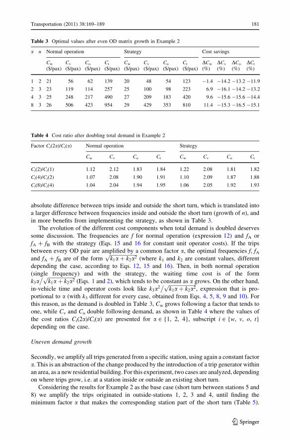
absolute difference between trips inside and outside the short turn, which is translated into

a larger difference between frequencies inside and outside the short turn (growth of n), and

in more benefits from implementing the strategy, as shown in Table 3.

The evolution of the different cost components when total demand is doubled deserves

some discussion. The frequencies are f for normal operation (expression 12) and fA or

fA ? fB with the strategy (Eqs. 15 and 16 for constant unit operator costs). If the trips

between every OD pair are amplified by a common factor a, the optimal frequencies f, fAand fA ? fB are of the form

ffiffiffiffiffiffiffiffiffiffiffiffiffiffiffiffiffiffiffiffiffik1aþ k2a2p

(where k1 and k2 are constant values, different

depending the case, according to Eqs. 12, 15 and 16). Then, in both normal operation

(single frequency) and with the strategy, the waiting time cost is of the form

k3a� ffiffiffiffiffiffiffiffiffiffiffiffiffiffiffiffiffiffiffiffiffi

k1aþ k2a2p

(Eqs. 1 and 2), which tends to be constant as a grows. On the other hand,

in-vehicle time and operator costs look like k3a2� ffiffiffiffiffiffiffiffiffiffiffiffiffiffiffiffiffiffiffiffiffi

k1aþ k2a2p

, expression that is pro-

portional to a (with k3 different for every case, obtained from Eqs. 4, 5, 8, 9 and 10). For

this reason, as the demand is doubled in Table 3, Cw grows following a factor that tends to

one, while Cv and Co double following demand, as shown in Table 4 where the values of

the cost ratios Ci(2a)/Ci(a) are presented for a [ {1, 2, 4}, subscript i [ {w, v, o, t}depending on the case.

Uneven demand growth

Secondly, we amplify all trips generated from a specific station, using again a constant factor

a. This is an abstraction of the change produced by the introduction of a trip generator within

an area, as a new residential building. For this experiment, two cases are analyzed, depending

on where trips grow, i.e. at a station inside or outside an existing short turn.

Considering the results for Example 2 as the base case (short turn between stations 5 and

8) we amplify the trips originated in outside-stations 1, 2, 3 and 4, until finding the

minimum factor a that makes the corresponding station part of the short turn (Table 5).

Table 3 Optimal values after even OD matrix growth in Example 2

a n Normal operation Strategy Cost savings

Cw

($/pax)Cv

($/pax)Co

($/pax)Ct

($/pax)Cw

($/pax)Cv

($/pax)Co

($/pax)Ct

($/pax)DCw

(%)DCv

(%)DCo

(%)DCt

(%)

1 2 21 56 62 139 20 48 54 123 -1.4 -14.2 -13.2 -11.9

2 3 23 119 114 257 25 100 98 223 6.9 -16.1 -14.2 -13.2

4 3 25 248 217 490 27 209 183 420 9.6 -15.6 -15.6 -14.4

8 3 26 506 423 954 29 429 353 810 11.4 -15.3 -16.5 -15.1

Table 4 Cost ratio after doubling total demand in Example 2

Factor Ci(2a)/Ci(a) Normal operation Strategy

Cw Cv Co Ct Cw Cv Co Ct

Ci(2)/Ci(1) 1.12 2.12 1.83 1.84 1.22 2.08 1.81 1.82

Ci(4)/Ci(2) 1.07 2.08 1.90 1.91 1.10 2.09 1.87 1.88

Ci(8)/Ci(4) 1.04 2.04 1.94 1.95 1.06 2.05 1.92 1.93

Transportation (2011) 38:169–189 181

123

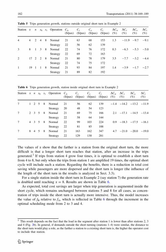
The values of a show that the farther is a station from the original short turn, the more

difficult is that a longer short turn reaches that station, after an increase in the trips

generated.2 If trips from station 4 grow four times, it is optimal to establish a short turn

from 4 to 8, but only when the trips from station 1 are amplified 19 times, the optimal short

cycle will include such a station. Regarding the benefits, there is a reduction in total cost

saving while passengers are more dispersed and the short turn is longer (the influence of

the length of the short turn in the results is analyzed in Sect. 3.3).

For a single station inside the short turn in Example 2 (say station 7) the generation rate

is doubled until reaching a = 8. Results are shown in Table 6.

As expected, total cost savings are larger when trip generation is augmented inside the

short cycle, which remains unchanged between stations 5 and 8 for all cases, as concen-

tration of trips inside the short turn is actually more intensive. Thus, the model increases

the value of fB relative to fA, which is reflected in Table 6 through the increment in the

optimal scheduling mode from 2 to 3 and 4.

Table 5 Trips generation growth, stations outside original short turn in Example 2

Station a n s0 s1 Operation Cw

($/pax)Cv

($/pax)Co

($/pax)Ct

($/pax)DCw

(%)DCv

(%)DCo

(%)DCt

(%)

4 4 2 4 8 Normal 21 63 68 153 1.3 -11.9 -9.7 -9.1

Strategy 22 56 62 139

3 8 1 3 8 Normal 22 74 76 172 0.3 -6.3 -5.3 -5.0

Strategy 22 69 72 163

2 17 2 2 8 Normal 21 80 78 179 3.5 -7.7 -3.2 -4.4

Strategy 22 74 75 172

1 19 1 1 8 Normal 21 93 84 197 1.4 -3.9 -1.7 -2.7

Strategy 21 89 82 192

Table 6 Trips generation growth, station inside original short turn in Example 2

Station a n s0 s1 Operation Cw

($/pax)Cv

($/pax)Co

($/pax)Ct

($/pax)DCw

(%)DCv

(%)DCo

(%)DCt

(%)

7 1 2 5 8 Normal 21 56 62 139 -1.4 -14.2 -13.2 -11.9

Strategy 20 48 54 123

7 2 3 5 8 Normal 21 69 75 166 2.1 -17.1 -14.5 -13.4

Strategy 22 58 64 144

7 4 3 5 8 Normal 22 99 103 224 0.9 -18.3 -17.5 -16.1

Strategy 22 81 85 188

7 8 4 5 8 Normal 21 163 162 347 4.7 -21.0 -20.0 -19.0

Strategy 22 129 130 281

2 This result depends on the fact that the load in the segment after station 1 is lower than after stations 2, 3and 4 (Fig. 2b). In general, if demands outside the short turning (stations 1–4) were similar, the distance tothe short turn would play a role, as the farther a station to a existing short turn is, the higher the operator costto include that station.

182 Transportation (2011) 38:169–189

123

Influence of the demand concentration

In real public transport systems, spatial demand peaks show different shapes, dispersion,

load level and length; for example, cases with very concentrated demand around a few

stations or more even load profiles, with demand showing peaks but over a wider section of

the route, involving more stations. Thus, it is important to understand the way the length of

the demand peak (and therefore the length of the short turn) affects the results of the

strategy in terms of cost savings. To isolate this effect, we now conduct a different

experiment in which three load profiles are considered, all of them showing a peak load of

1,000 pax/h across 2, 3 and 4 consecutive segments in the middle of the route, respectively.

In all cases, the extremes show a sharp reduction of the passenger load, to 100 pax/h,

(Fig. 3). The matrices were generated such that both the total demand (2520 pax/h) and the

trips inside the most loaded section (81% of total) are the same in the three cases.

From Table 7, we can see that the narrower the demand peak is (equivalent to say the

shorter the short turn is), the more beneficial the strategy results. This phenomenon is

observed in the three components of the total cost. When the same demand level is more

concentrated in some section of the route, it is easier for the operators to serve it (they run a

shorter distance). On the other hand, Eqs. 15 and 16 show that a shorter cycle increases fBand decreases fA, but the former effect is larger than the latter. Therefore the gain of the

users that are benefited by the strategy overcomes the loss of users outside the short turn

(whose frequency, fA, is lower if the demand is more concentrated, ceteris paribus).

Comments and conclusions

In most cities in the world, the demand for urban transit systems shows clear spatial

concentrations over certain segments of bus routes. Then, it is reasonable to offer higher

frequency in the most loaded sectors. If the demand is concentrated around a specific sector

of the route (for example the Central Business District or CBD), a short turn emerges as a

suitable strategy to better serve the resulting uneven load of passengers. This strategy aims

at reducing the cost of the operator on the one hand, and decreasing the waiting and in-

vehicle times that users spend while traveling (with respect to the standard single fre-

quency service along the entire route), on the other.

In this paper, we have introduced a model of a short turn strategy to set the optimal

values of frequencies (inside and outside the loop), capacity of vehicles and the position of

the short turn limit stations. These values and the corresponding cost components for

operators and users (waiting and in-vehicle times) are compared against an optimized

normal operation scheme (single frequency). The model was used to obtain results for

different examples, and several experiments were conducted to analyze their sensitivity.

Let us highlight the most important findings of this work.

• The short turning strategy can yield benefits for both users and operators at the same

time. Note that among passengers there are winners (origin and destination inside the

short turn) and losers (origin and/or destination outside the short turn), who observe a

lower frequency than in the single frequency case; but overall users save time.

• Cost savings are reachable not only when the demand is concentrated in the middle of a

route (a bus line crossing the CBD), but also when the most loaded section is on an

extreme of the line (radial line to the CBD).

Transportation (2011) 38:169–189 183

123

Direction 1 Direction 2

Station Load [pax/h]

1λ+

[pax/h]1λ−

[pax/h] Load

[pax/h]1λ+

[pax/h]1λ−

[pax/h]1 100 100 0 0 0 1002 100 10 10 100 10 103 100 10 10 100 10 104 100 10 10 100 10 105 1000 910 10 100 10 9106 1000 190 190 1000 190 1907 100 10 910 1000 910 108 100 10 10 100 10 109 100 10 10 100 10 1010 0 0 100 100 100 0

Total 1260 1260 1260 1260

Load profile

0

200

400

600

800

1000

1200

Station

Lo

ad [

pax

/h]

Demand load concentrated between stations 5 and 7

Direction 1 Direction 2

Station Load [pax/h]

1λ+

[pax/h]1λ−

[pax/h] Load

[pax/h]1λ+

[pax/h]1λ−

[pax/h]1 100 100 0 0 0 1002 100 10 10 100 10 103 100 10 10 100 10 104 100 10 10 100 10 105 1000 910 10 100 10 9106 1000 100 100 1000 100 1007 1000 100 100 1000 100 1008 100 10 910 1000 910 109 100 10 10 100 10 1010 0 0 100 100 100 0

Total 1260 1260 1260 1260

Load profile

0

200

400

600

800

1000

1200

Station

Lo

ad [

pax

/h]

Demand load concentrated between stations 5 and 8

Direction 1 Direction 2

Station Load [pax/h]

1λ+

[pax/h]1λ−

[pax/h] Load

[pax/h]1λ+

[pax/h]1λ−

[pax/h]1 100 100 0 0 0 1002 100 10 10 100 10 103 100 10 10 100 10 104 100 10 10 100 10 105 1000 910 10 100 10 9106 1000 100 100 1000 100 1007 1000 100 100 1000 100 1008 100 10 910 1000 910 109 100 10 10 100 10 1010 0 0 100 100 100 0

Total 1260 1260 1260 1260

Load profile

0

200

400

600

800

1000

1200

1 2 3 4 5 6 7 8 9 10

1 2 3 4 5 6 7 8 9 10

1 2 3 4 5 6 7 8 9 10

Station

Lo

ad [

pax

/h]

Demand load concentrated between stations 4 and 8

Fig. 3 Boarding and alighting rates and load profiles, different width of demand concentration

Table 7 Short turning results, different width of demand concentration

s0 s1 Normal operation Strategy Cost savings

Cw

($/pax)

Cv

($/pax)

Co

($/pax)

Ct

($/pax)

Cw

($/pax)

Cv

($/pax)

Co

($/pax)

Ct

($/pax)

DCw

(%)

DCv

(%)

DCo

(%)

DCt

(%)

5 7 58 50 93 201 49 38 73 160 -15.5 -23.3 -21.9 -20.4

5 8 58 58 94 209 52 49 80 181 -10.1 -15.2 -14.5 -13.5

4 8 58 67 94 218 55 60 86 200 -5.3 -10.1 -8.5 -8.1

184 Transportation (2011) 38:169–189

123

• Cost savings depend largely on the imbalance between trips inside and outside the short

cycle.

• When the strategy yields benefits, vehicles may be smaller than those resulting for the

single frequency case. This is because a short turn increases the frequency where the

demand is larger. The size of the vehicles is determined by those serving the whole

route (fleet A), since they circulate with more passengers when crossing the short cycle.

A corollary of this result is that a model with constant unit operator costs would

underestimate the benefits of the strategy compared with our model, where the operator

cost increases linearly with capacity K (Eq. 5).

• When facing an even growth of the OD matrix, the strategy results more beneficial.

This also happens when the trip generation or attraction from (to) a station inside a

short turn is increased. A station outside a short turn can become part of it after a raise

in the number of trips it generates or attracts, notwithstanding it produces smaller

benefits than in the original case in which the short turn comprised fewer stations.

• The concentration of demand plays a fundamental role: the more concentrated the trips

(the shorter the cycle is), the larger the benefits of a short turning strategy.

• From the modeling results, it is interesting that the analytical form for the optimal

frequencies with the strategy follows the structure of the square root formula (see

Eqs. 15, 16 and 19), even though a more complex account of the costs and benefits has

been undertaken, considering the distinct terms for users benefited by the strategy (trips

inside the short turn) and users whose situation is worse with the strategy (trips with

either origin or destination outside the short cycle), relative to the single frequency

case.

Future research can include some elements not considered here, such as:

• crowding inside vehicles (which affects waiting time, as shown by Tirachini and Cortes

2007, and in-vehicle time value); as with a short turning strategy we increase the

frequency on the most loaded part of the line and decrease it on the less demanded (less

crowded) section, and therefore occupancy rates and crowding factors would change;

• vehicle capacities according to commercial buses (and with this, to consider the case of

active capacity constraint affecting the waiting time). The capacity of available

commercial buses is highly discrete (e.g. 40, 60 and 120 pax/bus) which adds a

constraint that would limit the benefits of the approach;

• extension of the model to a network (or at least, two routes connected by a transfer

station); in which case there are more degrees of freedom as interlining may be possible

(vehicles changing lines on terminals or transfer stations)

• although this model has been conceived for a bus system application, it can be extended

to rail lines, taking into consideration some characteristic aspects of rail systems, such

as dwell time at stations (that in many cases is fixed and independent of the demand)

and the operators’ cost structure, among others.

Acknowledgements This research was partially financed by grants 1061261 and 1080140 from Fondecyt,Chile, and the Millennium Institute ‘‘Complex Engineering Systems’’ (ICM: P-05-004-F, CONICYT:FBO16).

Transportation (2011) 38:169–189 185

123

Appendix A. Definition of gi functions

• g0 is the total running time:

g0 ¼ 2XN�1

k¼1

Rk

• g1 and g2 are in the waiting and cycle times, g1 is the demand benefited by the strategy

(origin and destination inside the short turn), while g2 are the passenger whose origin or

destination are outside the short turn.

g1ðs0; s1Þ ¼Xs1�1

k¼s0

kþk ðk þ 1; s1Þ þXs1

k¼s0þ1

kþk ðs0; k � 1Þ

g2ðs0; s1Þ ¼Xs0�1

k¼1

k1þk þ

Xs1�1

k¼s0

kþk ðs1 þ 1;NÞ þXN

k¼s1

k1þk þ

XN

k¼s1þ1

k2þk

þXs1

k¼s0þ1

kþk ð1; s0 � 1Þ þXs0

k¼1

k2þk

• g3 is the running time for vehicles inside the short turn

g3ðs0; s1Þ ¼ 2Xs1�1

k¼s0

Rk

• g4 is the in-vehicle time experienced by passengers

g4 ¼XN

k¼1

XN

l¼1

kkl

Xl�1

i¼k

Ri

• g5 and g6 are the factors to calculate the total dwell time of passengers benefited by the

strategy and the others, respectively.

g5ðs0; s1Þ ¼ g15ðs0; s1Þ þ g2

5ðs0; s1Þ

g6ðs0; s1Þ ¼ g16ðs0; s1Þ þ g2

6ðs0; s1Þ

where

g15ðs0; s1Þ ¼

Xs0�1

k¼1

Xs1

l¼s0þ1

kkl

Xl�1

i¼s0

kþi ðiþ 1; s1Þ

þXs0�1

k¼1

XN

l¼s1þ1

kkl

Xs1�1

i¼s0

kþi ðiþ 1; s1Þ

þXs1�1

k¼s0

Xs1

l¼kþ1

kkl

Xl�1

i¼k

k1þi þ

Xs1�1

k¼s0

XN

l¼s1þ1

kkl

Xs1�1

i¼k

kþi ðiþ 1; s1Þ

186 Transportation (2011) 38:169–189

123

g25ðs0; s1Þ ¼

XN

k¼s1þ1

Xs1�1

l¼s0

kkl

Xs1

i¼lþ1

kþi ðs0; i� 1Þ

þXN

k¼s1þ1

Xs0�1

l¼1

kkl

Xs1

i¼s0þ1

kþi ðs0; i� 1Þ

þXs1

k¼s0þ1

Xk�1

l¼s0

kkl

Xk

i¼lþ1

k2þi þ

Xs1

k¼s0þ1

Xs0�1

l¼1

kkl

Xk

i¼s0þ1

kþi ðs0; i� 1Þ

g16ðs0; s1Þ ¼

Xs0�1

k¼1

Xs0

l¼kþ1

kkl

Xl�1

i¼k

k1þi þ

Xs0�1

k¼1

Xs1

l¼s0þ1

kkl

Xs0�1

i¼k

k1þi þ

Xl�1

i¼s0

kþi ðs1 þ 1;NÞ" #

þXs0�1

k¼1

XN

l¼s1þ1

kkl

Xs0�1

i¼k

k1þi þ

Xs1�1

i¼s0

kþi ðs1 þ 1;NÞ þXl�1

i¼s1

k1þi

" #

þXs1�1

k¼s0

XN

l¼s1þ1

kkl

Xs1�1

i¼k

kþi ðs1 þ 1;NÞ þXl�1

i¼s1

k1þi

" #

þXN

k¼s1

XN

l¼kþ1

kkl

Xl�1

i¼k

k1þi

g26ðs0; s1Þ ¼

XN

k¼s1þ1

Xk�1

l¼s1

kkl

Xk

i¼lþ1

k2þi þ

XN

k¼s1þ1

Xs1�1

l¼s0

kkl

Xk

i¼s1þ1

k2þi þ

Xs1

i¼lþ1

kþi ð1; s0 � 1Þ" #

þXN

k¼s1þ1

Xs0�1

l¼1

kkl

Xk

i¼s1þ1

k2þi þ

Xs1

i¼s0þ1

kþi ð1; s0 � 1Þ þXs0

i¼lþ1

k2þi

" #

þXs1

k¼s0þ1

Xs0�1

l¼1

kkl

Xk

i¼s0þ1

kþi ð1; s0 � 1Þ þXs0

i¼lþ1

k1þi

" #

þXs0

k¼1

Xk�1

l¼1

kkl

Xk

i¼lþ1

k2þi

Appendix B. Load of vehicles between stations

1. Load of vehicles serving the entire corridor (fleet A):

Direction 1

p1k ¼

p1k�1 þ

k1þk

fA� k1�

k

fAif 1� k� s0 � 1

p1k�1 þ

kþk ðk;s1ÞfAþfB

þ kþk ðs1þ1;NÞfA

� k�k ð1;s0�1ÞfA

� k�k ðs0;k�1ÞfAþfB

if s0� k� s1 � 1

p1k�1 þ

k1þk

fA� k1�

k

fAif s1� k�N

8>><

>>:

Direction 2

p2k ¼

p2kþ1 þ

k2þk

fA� k2�

k

fAif s1 þ 1� k�N

p2kþ1 þ

kþk ðs0;k�1ÞfAþfB

þ kþk ð1;s0�1ÞfA

� k�k ðs1þ1;NÞfA

� k�k ðkþ1;s1ÞfAþfB

if s0 þ 1� k� s1

p2kþ1 þ

k2þk

fA� k2�

k

fAif 1� k� s0

8>><

>>:

Transportation (2011) 38:169–189 187

123

2. Load of vehicles performing short turning (fleet B):

Direction 1

~p1k ¼

0 if 1� k� s0 � 1

~p1k�1 þ

kþk ðk;s1ÞfAþfB

� k�k ðs0;k�1ÞfAþfB

if s0� k� s1 � 1

0 if s1� k�N

8<

:

Direction 2

~p2k ¼

0 if s1 þ 1� k�N

p2kþ1 þ

kþk ðs0;k�1ÞfAþfB

� k�k ðkþ1;s1ÞfAþfB

if s0 þ 1� k� s1

0 if 1� k� s0

8<

:

After applying the short-turning strategy, the maximum load will correspond to some

segment, which can belong to either direction 1 or 2. However, by observing the recursive

form of the load equations above, we can establish the following:

• If the maximum load occurs along direction 1, then we can say that

gK ¼ p1max ¼

u10ðs0; s1Þ

fA

þ u11ðs0; s1ÞfA þ fB

• Otherwise, if the maximum load occur along direction 2, then we can say that

gK ¼ p2max ¼

u20ðs0; s1Þ

fA

þ u21ðs0; s1ÞfA þ fB

Thus, a generic relation between the design capacity of buses and the frequencies fA and

fB can be established in the way summarized in Eq. 14:

K ¼ 1

g#0ðs0; s1Þ

fA

þ #1ðs0; s1ÞfA þ fB

� �

where, if the maximum load happens on a segment that belongs to direction 1, then

#0(s0, s1) = u01(s0, s1) and #1(s0, s1) = u1

1(s0, s1). Otherwise, if the maximum load occurs on

a segment that belongs to direction 2, then #0(s0, s1) = u02(s0, s1) and #1(s0, s1) = u1

2(s0, s1).

References

Ceder, A., Stern, H.I.: Deficit function bus scheduling with deadheading trip insertion for fleet sizereduction. Transp. Sci. 15(4), 338–363 (1981)

Ceder, A.: Optimal design of transit short-turn trips. Transp. Res. Rec. 1221, 8–22 (1989)Ceder, A.: Public transport timetabling and vehicle scheduling. In: Lam, W., Bell, M. (eds.) Advanced

Modeling for Transit Operations and Service Planning, pp. 31–57. Pergamon Imprint, Elsevier ScienceLtd. Pub, Amsterdam (2003a)

Ceder, A.: Designing public transport network and route. In: Lam, W., Bell, M. (eds.) Advanced Modelingfor Transit Operations and Service Planning, pp. 59–91. Pergamon Imprint, Elsevier Science Ltd. Pub,Amsterdam (2003b)

Ceder, A.: Improved lower-bound fleet size for fixed and variable transit scheduling. 9th InternationalConference on Computer-Aided Scheduling of Public Transport (CASPT), August 9–11, 2004 SanDiego, California, USA (2004)

Delle Site, P.D., Filippi, F.: Service optimization for bus corridors with short-turn strategies and variablevehicle size. Transp. Res. A 32(1), 19–28 (1998)

188 Transportation (2011) 38:169–189

123

Eberlein, X.J., Wilson, N.H.M., Barnhart, C., Bernstein, D.: The real-time deadheading problem in transitoperations control. Transp. Res. B 32(2), 77–100 (1998)

Eberlein, X.J., Wilson, N.H.M., Bernstein, D.: Modeling real-time control strategies in public transitoperations. In: N.H.M. Wilson (Ed.), Computer-Aided Transit Scheduling, Lecture Notes in Eco-nomics and Mathematical Systems 471, pp. 325–346, Springer-Verlag, Heidelberg (1999)

Furth, P.: Alternating deadheading in bus route operations. Transp. Sci. 19(1), 13–28 (1985)Furth, P.: Zonal route design for transit corridors. Transp. Sci. 20(1), 1–12 (1986)Furth, P.: Short turning on transit routes. Transp. Res. Rec. 1108, 42–52 (1987)Jansson, J.O.: A simple bus line model for optimization of service frequency and bus size. J. Transp. Econ.

Policy 14, 53–80 (1980)Jara-Dıaz, S.R., Gschwender, A.: Towards a general microeconomic model for the operation of public

transport. Transp. Rev. 23(4), 453–469 (2003)Jara-Diaz, S.R., Tirachini, A., Cortes, C.E.: Modeling public transport corridors with aggregate and dis-

aggregate demand. J. Transp. Geogr. 16, 430–435 (2008)Jordan, W.C., Turnquist, M.A.: Zone scheduling of bus routes to improve service reliability. Transp. Sci.

13(3), 242–268 (1979)Mohring, H.: Optimization and scale economies in urban bus transportation. Am. Econ. Rev. 62, 591–604

(1972)Oldfield, R.H., Bly, P.H.: An analytic investigation of optimal bus size. Transp. Res. 22B, 319–337 (1988)Osuna, E.E., Newell, G.F.: Control strategies for an idealized public transportation system. Transp. Sci. 6,

52–72 (1972)Tirachini, A.: Estrategias de asignacion de flota en un corredor de transporte publico. MSc Thesis, Uni-

versidad de Chile (2007)Tirachini, A., Cortes, C.E.: Disaggregated modeling of pre-planned short-turning strategies in transit cor-

ridors. CD Proceedings, Transportation Research Board (TRB) 86th Annual Meeting, Washington DC,USA (2007)

Vijayaraghavan, T.A., Anantharmaiah, K.M.: Fleet assignment strategies in urban transportation usingexpress and partial services. Transp. Res. A 29(2), 157–171 (1995)

Welding, P.I.: The instability of a close-interval service. Oper. Res. Q. 8(3), 133–148 (1957)

Author Biographies

Alejandro Tirachini born in Chiloe, Chile, is beginning his journey in the world of transport research. He isa PhD candidate at The University of Sydney and holds a MSc in Transport Engineering from Universidadde Chile. His main research interests are public transport economics, sustainable transport and externalities.

Cristian E. Cortes is Assistant Professor at the Civil Engineering Department, Universidad de Chile. Holdsa PhD in Civil Engineering from University of California and a MSc in Transport Systems Analysis fromUniversidad de Chile. Author of more than 20 articles in ISI indexed journals, on public transportoptimization, network optimization and equilibrium, logistics, simulation, control applied to dynamictransport systems, among his topics of major interest. Dr. Cortes is currently Associate Editor ofTransportation Science, member of the Directory of the Chilean Society in Transport Engineering, andleader of applied research projects in public transport planning.

Sergio Jara-Dıaz is Professor of Transport Economics at Universidad de Chile. Holds a PhD and MSc fromMIT, where he has taught during various terms. Author of Transport Economic Theory (Elsevier, 2007) and morethan 80 articles in journals and books, on the microeconomics of transport demand, multioutput analysis intransport industries, public transport modelling and pricing, and time allocation. He teaches frequently in Spain.Resides in Nunoa, Santiago, with his only wife. http://www.cec.uchile.cl/*dicidet/sergio.html.

Transportation (2011) 38:169–189 189

123