Optimal Debt, Asset Substitution and Coupon

Rating-Trigger Covenants

Sergio SilvaPortucalense University, Portugal

e-mail: sergios@upt.pt

(corresponding author)

Jose Azevedo PereiraISEG - Technical University of Lisbon, Portugal

e-mail: jpereira@iseg.utl.pt

Abstract

The current paper analyses an optimal debt contract that incorporates a rating triggercovenant so as to impose a coupon rate increase when the credit rating of the issuing firm isdowngraded. It is shown that the presence of this particular kind of covenant albeit reducingthe value of the leveraged firm when there is no operational flexibility, may assume an im-portant role in terms of asset substitution when such flexibility is present. Such conclusioncontradicts the conclusion of Bhanot and Mello (2006) regarding this type of covenants. Theoptimal coupon increase associated to the covenant is determined and a distinction regardingthe nature of the covenant in terms of its effects (permanent or not) is also made.

JEL classification: G13, G33

1 Introduction

The widespread use of rating-based trigger covenants has been documented by some surveysconducted by rating agencies. According to Moody’s (2002a)[25], out of 711 US corporate issuersrated Ba1 or higher, 87,5%, reported a total of 2819 rating triggers. From these, 21,1% were ofthe type ”adjustment in interest or coupons”, where the initial interest rate or coupon is revised inthe event of a rating change. In Moody’s (2002b)[26], it is reported that 59% out of 345 Europeancorporate debt issuers used rating triggers, and a similar result (50% among more than 1000 USand European investment-grade debt issuers) was reported by Standard and Poor’s (2002)[27].As mentioned by Gonzalez et al (2004)[10], the main aimof such type of covenants, is: “(...) toprotect lenders against credit deterioration and asymmetric information problems (...)”. IndeedBhanot and Mello (2006)[3] showed that rating trigger covenants that dictate an early partialamortization of the principal induce equity holders to pursue low risk strategies. However, inparallel these authors concluded that coupon based triggers “(...) do not inhibit asset substitution(...)”. Our results contradict this statement and this is one of the main points of the current paper.

The purpose of the present work consists in analysing the optimal debt contract that includescoupon rating triggers. Specifically we intend to provide answers to the following questions:

• In what way the use of a coupon rating triggers covenant may have an effect on the optimalvalues of debt and equity?

• In what circumstances the use of this type of covenants may effectively prevent the substi-tution of assets?

• Is there an “optimal” coupon increase associated with the rating trigger covenant?

1

• In what circumstances is it optimal to issue debt with this kind of covenant instead of straightdebt?

• What is the relevance of the nature (permanent or not) of the coupon’s adjustment?

As in Bhanot and Mello (2006)[3], our starting point is Leland’s (1994)[17] framework. Leland’smodel is one of the so called structural credit risk models class where the default of the issuingfirm occurs whenever the value of its assets1 (modeled by a diffusion process) reaches a lowerthreshold - the default barrier. Within this class of models we can further distinguish those inwhich this default barrier is set exogenously (e.g. Black and Cox (1976)[4], Kim, Ramaswamyand Sundaresan (1993)[16], Longstaff and Schwartz (1995)[20], Briys and de Varenne (1997)[5],Ericsson and Reneby (1998)[8], Schobel (1999)[24], Hsu, Sa-Requejo and Santa-Clara (2003)[13],Hui, Lo and Tsang (2003)[14], Tauren (1999)[28], Collin-Dufresne and Goldstein (2001)[6], Juand Ou-Yang (2004)[15], Huang et al. (2003)) from the others wherein it is set endogenously.In this latter case, default occurs when equity holders find it optimal to stop financing the debtservice (e.g. Black and Cox (1976)[4], Leland (1994)[17], Leland and Toft (1996)[19], Goldstein,Ju and Leland (2001)[12], Ericsson and Reneby (2003)[9]) or to strategically default in the couponpayments (e.g. Anderson and Sundaresan (1996)[1], Anderson, Sundaresan and Tychon (1996) [2],Mella-Barral and Peraudin (1997)[22], Mella-Barral (1999)[21], Fan and Sundaresan (2000)[11]).In parallel, the structural approach literature also includes a few articles that formally addressthe asset substitution problem (e.g. Mello and Parsons (1992)[23], Leland (1998)[18], Ericsson(2000)[7]).

Assuming a endogenous default and considering a perpetuity bond, Leland (1994)[17] analysesthe optimal debt level in the presence of bankruptcy costs and tax benefits associated to the couponpayments. Since our aim is to study the inclusion in the debt contract of a covenant attacheddirectly to the firm’s credit rating, another credit event besides bankruptcy must be considered,namely the credit rating downgrade. This is achieeved, as in Bhanot and Mello (2006)[3], byestablishing a second threshold - in the sense that if the assets value decreases enough to reachthat new critical level, the firm’s credit rating is downgraded and the coupon increase embodiedin the covenant is triggered. It will be assumed that this threshold is greater than the defaultbarrier, which implies that the possible occurrence of bankruptcy is always preceded by a ratingchange.

Within this framework, we will show that, when equity holders have operational flexibility toalter the firm’s risk, the presence of a coupon type rating trigger covenant in the debt contract caneffectively prevent the substitution of assets, by forcing them to pursue low risk strategies. Theattainment of such result and the inherent benefits in terms of agency costs will, in turn, dependon the level of the minimum risk strategy available and on the spectrum of possible risk profiles.The lower the minimum risk level (which must be below some critical level) and the higher therisk spectrum, the greater are the benefits associated with the covenant.

The paper is organized as follows: in section 2 the valuation framework is established and theexpressions for the value of debt, equity, bankruptcy costs, tax benefits and the leveraged firmare derived. Section 3 addresses the optimal debt level. Section 4 focus on the prevention of thesubstitution of assets. Section 5 investigates the case of non permanent effects of the rating triggercovenant and section 6 concludes the paper.

2 The Valuation Framework

2.1 Base model

The following assumptions are assumed:

H1. The risk free interest rate, r, is constant;1Or other state variable such as the firm’s cash-flow.

2

H2. The value of the firm’s assets, Vt, is described by the following continuous diffusion process,under the risk neutral probability:

dVt/Vt = (r − α)dt + σdWt

Where r is the risk free interest rate, α is the cash payout rate, σ volatility of assets returnand dWt an increment of a standard Brownian motion.

H3. Debt comprises a bond sold at par value with infinite maturity, that promises the payment ofa continuous coupon flow of Cdt until the firm’s rating is downgraded. The bond indentureincludes a rating based covenant that dictates an increase in the coupon rate, from themoment when the credit rating of the firm is downgraded. We name this new coupon byC∆, with ∆ > 1. Thus, (∆− 1)100% corresponds to the percentage increase in the couponrate. It is also assumed that this new coupon, once effective, is permanent and irreversible2

irrespective of the future behaviour of the value of the assets, unless the firm enters inbankruptcy.

H4. Definition of the rating change: the rating downgrade is modelled through the specificationof an exogenous constant barrier. The credit event is triggered when the value of the assetsreaches this pre-specified level. Labelling this constant threshold as VB1, we define the timeof the rating change as:

τ1 = inf{t ≥ 0 : Vt ≤ VB1}

That is, the first time the value of the assets passes though the barrier level VB1.

H5. Definition of bankruptcy (liquidation of the firm): Bankruptcy occurs when the value of thecompany’s assets reaches a second threshold VB2 (the second barrier). Although this barrieris initially set exogenously, later on it will be determined endogenously in order to maximizethe equity value. Thus, the firm enters in bankruptcy and is liquidated when the equityholders are not willing to carry on with the debt service. Defining τ2 as the liquidation time,we have:

τ2 = inf{t ≥ τ1 : Vt ≤ VB2}

Note that τ2 ≥ τ1, implying that the bankruptcy event is always preceded by the firm’srating downgraded (VB1 ≥ VB2).

H6. Bondholders recovery value: When the firm is liquidated, the bondholders get a fraction ρof the value of the company’s assets, ρVB2, with 0 < ρ ≤ 1, and (1− ρ)VB2 the bankruptcycosts.

H7. We consider the existence of a corporate taxe rate defined by ι, thus, at each instant in timean amount of ιCdt (before the rating downgrade) or ι∆Cdt (after the rating downgrade) istax deductible.

Given the above description Figure 1 ilustrastes possible paths for the value of firm’s assets indifferent scenarios.

2.2 Bond value

The cash flow provided by the bond to its holder will be a function of financial health of the issuingfirm, embodied by its credit rating. Thus, while the value of the firm’s assets remains above thethreshold VB1, t < τ1, the bondholders receive a continuous coupon flow of Cdt. After the firm’srating has been downgraded - which occurs when VB1 is crossed for the first time - the coupon

2In section 5 this assumption is relaxed

3

Figure 1: Three sample path for the assets values associated to the three possible scenario. Assetsvalue remains above VB1 - I; assets value crosses VB1 but remains above VB2, - II and finally theassets value reaches VB2 - III.

flow rises to ∆Cdt and remains at this level3 until the firm enters in bankruptcy - when VB2 isreached - and is liquidated, generating a cash flow of ρVB2 to the bondholders. Notice that, interms of payoffs, debt can be understood as the sum of two assets: a straight bond (without anycovenant) paying a continuous coupon of Cdt and an asset that pays a stream of (∆−1)Cdt (whichcorresponds to the additional coupon triggered by the covenant) from the moment in which thecredit rating is downgraded until the occurrence of bankruptcy (between τ1 and τ2). Keeping thisin mind, to calculate the value of the bond it is only necessary to determine the expected value(under the risk neutral measure) of all corresponding cashflows discounted at the risk free rate.Defining the bond value before the rating downgrade (for t ≤ τ1) by BI(Vt, C,∆) and after therating downgrade (for t > τ1) by BII(Vt, C, ∆) we have:

BI(Vt, C, ∆) = E[∫ τ2

t

e−r(s−t)Cds

∣∣∣∣Ft

]+ E

[e−r(τ2−t)ρVB2

∣∣∣Ft

]+ E

[e−r(τ1−t)

∫ τ2

τ1

e−r(s−τ1)(∆− 1)Cds

∣∣∣∣Ft

](1)

BII(Vt, C,∆) = E[∫ τ2

t

e−r(s−t)∆Cds

∣∣∣∣Ft

]+ E

[e−r(τ2−t)ρVB2

∣∣∣Ft

](2)

Whose corresponding values are:

BI(Vt, C,∆) =C

r+

(ρVB2 −

C

r

)(Vt

VB2

)−X

+(∆− 1) C

r

[(Vt

VB1

)−X

−(

Vt

VB2

)−X]

(3)

BII(Vt, C,∆) =∆C

r+

(ρVB2 −

∆C

r

)(Vt

VB2

)−X

(4)

3Remember that, for the moment, we are assuming a permanent and irreversible effect of the covenant.

4

Where:

• X =

√(r − α− σ2

2

)2+ 2rσ2 +

(r − α− σ2

2

)σ2

> 0

•(

Vt

VBi

)−X

is the probability-weighted discount factor of the assets value reaching VBi from Vt.

Before the rating downgrade (expression (3)), the debt value corresponds to a perpetuity ofCdt (first term in the right hand side) corrected by the loss that will take place upon bankruptcy(second term) and adjusted by the increase in the coupon flow associated to the impact of therating trigger covenant in case of a rating downgrade (third term). Notice that the first two termsrefer to a straight bond (∆ = 1) as in Leland (1994)[17].

2.3 Equity value

The value of equity will be given by the expected present value of the continuous dividend streamreceived by equity holders - defined as the cash payout of the firm (αVtdt) minus the couponpayment to bond holders adjusted by the tax shields, ((1− ι)Cdt before the rating downgrade and(1− ι)∆Cdt after). For the valuation of the adjusted coupon payments it is possible to apply anapproach similar that used for bond valuation: the global coupon stream might be subdivided in acontinuous payment of (1−ι)Cdt until τ2 and an additional continuous payment of (1−ι)(∆−1)Cdtbetween τ1 and τ2. Thus, defining equity value by EI(Vt, C,∆), before the rating downgrade andEII(Vt, C,∆) after, we have:

EI(Vt, C,∆) = E[∫ τ2

t

e−r(s−t) [αVs − (1− ι)C] ds

∣∣∣∣Ft

]+

+ E[e−r(τ1−t)

∫ τ2

τ1

e−r(s−τ1) [− (1− ι)(∆− 1)C] ds

∣∣∣∣Ft

](5)

EII(Vt, C,∆) = E[∫ τ2

t

e−r(s−t) [αVs − (1− ι)∆C] ds

∣∣∣∣Ft

](6)

Whose corresponding value expressions are:

EI(Vt, C,∆) = Vt − (1− ι) C

r+

[(1− ι) C

r− VB2

](Vt

VB2

)−X

−

− (1− ι) (∆− 1) C

r

[(Vt

VB1

)−X

−(

Vt

VB2

)−X]

(7)

The first line represents the value of equity if straight debt is issued (∆ = 1) - in accordancewith Leland’s model results. As for the second line, the correction factor in the dividend flowassociated with the rating trigger covenant - that is, the value of the extra stream of couponpayments realized between τ1 and τ2. Notice that these accrued payments affect negatively thevalue of equity, since the expression in the vertical brackets has always a positive sign. In fact,this expression represents the diference between the probability-weighted discount factors for therating downgrade and for bankruptcy, where the former is greater than the latter since VB1 > VB2.

5

After the rating downgrade, equity value would be given by:

EII(Vt, C, ∆) = Vt − (1− ι) ∆C

r+

[(1− ι) ∆C

r− VB2

](Vt

VB2

)−X

(8)

2.4 Value of tax shield

The value of the tax shield is given by the flow of ιCdt until bankruptcy (at τ2) plus the flowassociated to the coupon increase between the rating downgrade and default (between τ1 and τ2).Thus we have:

TBI(Vt, C, ∆) = E[∫ τ2

t

e−r(s−t)ιCds

∣∣∣∣Ft

]+ E

[e−r(τ1−t)

∫ τ2

τ1

e−r(s−τ1)ι (∆− 1)Cds

∣∣∣∣Ft

](9)

TBII(Vt, C,∆) = E[∫ τ2

t

e−r(s−t)ι∆Cds

∣∣∣∣Ft

](10)

Yielding:

TBI(Vt, C,∆) =ιC

r

[1−

(Vt

VB2

)−X]

+ι(∆− 1)C

r

[(Vt

VB1

)−X

−(

Vt

VB2

)−X]

(11)

TBII(Vt, C,∆) =ι∆C

r

[1−

(Vt

VB2

)−X]

(12)

2.5 Value of bankruptcy costs

Since the bankruptcy costs considered in the present model only refer to the loss of a fraction (1−ρ)of the firm’s assets upon liquidation (at τ2) there is no need to differentiate the corresponding valuebefore and after the rating downgrade. Thus we have:

BC(Vt, C, ∆) = E[e−r(τ2−t) (1− ρ) VB2

∣∣∣Ft

](13)

Whose correspondent solution is:

BC(Vt, C,∆) = (1− ρ) VB2

(Vt

VB2

)−X

(14)

2.6 The value of the leveraged firm

The value of the leveraged firm can be calculated either from the bond ((3) or (4)) and equity ((7)or (8)) values, or using the values of the assets, tax shields ((11) or (12)) and bankruptcy costs((14)):

vi(Vt, C,∆) = Bi(Vt, C,∆) + Ei(Vt, C,∆) = Vt − BC(Vt, C,∆) + TBi(Vt, C,∆) (15)

With i = I or II, for t ≤ τ1 or t > τ1 respectively.

6

2.7 The endogenous bankruptcy trigger

As previously noted, we are assuming that VB1 is greater than VB2, so the bankruptcy event canonly occur after τ1. Thus, to obtain the barrier level that maximizes equity value, we must usethe corresponding equity formula valid for t > τ1, namely expression (8):

EII(Vt, C, ∆) = Vt − (1− ι) ∆C

r+

[(1− ι) ∆C

r− VB2

](Vt

VB2

)−X

Formally, the endogenous bankruptcy trigger is the value of VB2 that solves the following equation:

∂EII (·)∂Vt

∣∣∣∣Vt=VB2

= 0

Such value will be given by:

VB2 =∆C (1− ι)

r

X

(1 + X)(16)

Such endogenous threshold is the same as in Leland (1994), since ∆C is the coupon value afterthe rating downgrade4.

Incorporating the endogenous barrier VB2 in the expressions derived above yields:

BI(Vt, C, ∆) =C

r

[1 + (∆− 1)

(Vt

VB1

)−X

−∆k

(Vt

∆C

)−X]

(17)

EI(Vt, C, ∆) = Vt −(1− ι) C

r

[1 + (∆− 1)

(Vt

VB1

)−X

−∆m

(Vt

∆C

)−X]

(18)

vI(Vt, C, ∆) = Vt +ιC

r

[1 + (∆− 1)

(Vt

VB1

)−X

−∆h

(Vt

∆C

)−X]

(19)

TBI(Vt, C,∆) =ιC

r

[1 + (∆− 1)

(Vt

VB1

)−X

−∆(1 + X)m(

Vt

∆C

)−X]

(20)

BC(Vt, C,∆) =ιC∆ [h− (1 + X)m]

r

(Vt

∆C

)−X

(21)

4Besides the definition of X, since Leland (1994), assumes a zero cash payout ratio.

7

Where:

m =[

(1− ι) X

r (1 + X)

]X 11 + X

h =[1 + X +

(1− ρ)(1− ι) X

ι

]m

k = [1 + X − ρ (1− ι)X]m

2.8 The effect of the rating trigger covenant

The coupon increase (∆ > 1) related to the rating trigger covenant has two different direct effects.An higher ∆, will lead to:

1. An higher coupon after the rating downgrade;

2. An higher value for the endogenous bankruptcy threshold, and thus an higher probability ofbankruptcy.

Such effects will produce different impacts in the values of the bond, equity, leveraged firm, taxshields and bankruptcy costs. Starting with debt, the first effect has a positive impact on its valuewhereas the second effect influences it negatively since an higher of probability of bankruptcyunambiguously means higher bankruptcy costs. The final outcome will depend on the initialcoupon value, C. For low coupon values, the first effect dominates. The opposite occurs for highcoupon values. The same happens regarding the tax benefits, albeit in a more pronounced way.Nevertheless the effect of an higher ∆ on equity value is unambiguously negative. Finally, ingeneral, higher values of ∆ will lead to a decrease in leveraged firm values, although for lowercoupons, the positive effect on the value of the bond may slightly overcome the negative impacton equity. Figure 2 ilustrates what we have said. It depicts the debt, equity and leverage firmvalue (values taken from Bhanot and Mello (2006)[3]).

Figure 2: Bond value, equity value and leverage firm value as a function of coupon (ranging from6 to 11) and ∆ (ranging from 1 to 1,5), considering V = 150; VB1 = 120; r = 0, 07; α = 0, 01;σ = 0, 25; ι = 0, 35 and ρ = 0, 4.

8

3 The optimal debt level

3.1 The maximum coupon

As in Leland (1994)[17], each firm will face a maximum capacity to raise debt. Specifically, for agiven value of ∆, there will be a value for the initial coupon (C) that maximizes the debt value.Formally we obtain this particular value solving the following equation:

∂BI(V0, ·)∂C

= 0

Obtaining:

CM =V0

∆

1 + (∆− 1)(

V0VB1

)−X

∆k (1 + X)

1/X

Once again with ∆ = 1, Leland’s (1994) result is obtained. Notice that ∂CM

∂∆ < 0, meaningthat the use of such type of covenants reduces the firm’s indebtedness capacity. Considering thisresult, it is worthwhile to point that the approach used by Bhanot and Mello (2006)[3] is in someway restrictive. The analyses conducted by those authors consisted in calculating the optimallevel of straight debt (that is without any covenants) incurred by the firm and subsequently, for agiven ∆ - considering the existence of the covenant - in obtaining the particular coupon value thatwould generate that same amount of debt. Besides the fact that, in the firm’s perspective, thisdebt level is far from being optimal (as we will see in the next subsection), it may be unattainablefor some values of ∆, that is, higher than the correspondent maximum debt capacity. Illustratingconsidering a numerical example in which the debt level is 127,865 (value used by those authorsconsidering V = 150; VB1 = 120; r = 0, 07; α = 0, 01; σ = 0, 25; ι = 0, 35 and ρ = 0, 4), themaximum possible value for the increase in the coupon embodied in the rating triggers covenant is32% (∆ = 1, 32). For instance, for ∆ = 1, 4, the maximum coupon is 10,388 and the correspondentdebt value 124,64. For an asset value of 160, Bhanot and Mello (2006) framework would considera debt level of 136,39. This amount would only be reachable for values of ∆ lower than 1,24.Figure 3 below illustrates the influence of the coupon increase on the maximum coupon and therespective debt level considering two values for the initial assets value (V0 = 150 and V0 = 160).

3.2 The optimal coupon

In order to obtain the optimal debt level at the moment in which the securities are issued, wecalculate the coupon that maximizes the leveraged firm value, (vI(V0, C, ·)). The correspondingfirst order condition implies that the first derivative of the leveraged firm value in respect to thecoupon needs to zero:

∂vI(V0, C, ·)∂C

= 0

Resolving the above equation for C, yields:

C∗ =V0

∆

1 + (∆− 1)(

V0VB1

)−X

∆h (1 + X)

1/X

(22)

5Which corresponds to the optimal straight debt level when V = 150; r = 0, 07; α = 0, 01; σ = 0, 25; ι = 0, 35and ρ = 0, 4.

9

Figure 3: Left panel: maximum debt level at the emission date as a function of ∆; right panel:maximum coupon value as a function of ∆; considering: V0 = 150 VB1 = 120; r = 0, 07; α = 0, 01;σ = 0, 25; ι = 0, 35 and ρ = 0, 4.

From the above expression it can be verified that ∂C∗

∂∆ < 0, which means that the presence ofthis type of rating trigger covenants leads to lower optimal coupon values. Moreover, note thata decrease in the (optimal) coupon, generated by an higher ∆, more than compensates its ownincrease (∂∆C∗

∂∆ < 0)6 - even after the credit rating downgrade tackes place, the increased couponvalue triggered by the covenant (∆C∗) is less than the corresponding optimal coupon, if straightdebt were issued instead7. Given that, it is not surprising that ∆ has an unambiguously negativeeffect on the optimal debt level, as depicted in figure 4.

Figure 4: left panel: optimal debt level at the emission date as a function of ∆ ; right panel:optimal coupon at the issuance date (C∗) and coupon value after the rating downgrade (∆C∗) asa function of ∆. Both graphics considers V0 = 150; VB1 = 120; r = 0, 07; α = 0, 01; σ = 0, 25;ι = 0, 35 and ρ = 0, 4.

6Note that the relation of the endogenous bankruptcy threshold VB2 with ∆ is reversed (being now negative)since it depends on ∆C. Incorporating the optimal coupon (expression (22)) in VB2 (expression(16)) yields V ∗

B2 =

V0

nm∆h

h1 + (∆ − 1) (V0/VB1)−X

io1/X, and ∂V ∗

B2/∂∆ < 0. Thus, higher values of ∆ are associated with lower

probabilities of bankruptcy.7In fact, it can be showed that in the limit (when ∆ tends to infinity) ∆C∗ tends to the optimal coupon that

would arise in the straight debt case when the asset value is VB1.

10

The rationale of this result can be formulated as follows. Since the rating trigger (∆ > 1)imposes an increase in the coupon rate, this higher coupon can be seen as a “forced” debt levelrebalancing by the firm. But this forced rebalancing is on the opposite direction8 of what wouldbe the case if equity holders had the ability to freely restructure the capital structure, given thesmaller value of assets (VB1). In face of that, a lesser amount of debt is issued and a lower firmvalue is obtained (the decrease in the bankruptcy costs that arises from higher values of ∆ is notenough to compensate for the decrease in the tax shield).

Plugging the optimal coupon (expression (22)) into expressions (17), (18) and (19) we obtainrespectively the reduced formulas for debt, equity and leveraged firm values, at the date the debtis issued:

B∗(V0,∆) = V0

[h (1 + X)− k

r

]1 + (∆− 1)(

V0VB1

)−X

∆h (1 + X)

1+X

X

(23)

E∗(V0,∆) = V0

1− (1− ι) [h (1 + X)−m]r

1 + (∆− 1)(

V0VB1

)−X

∆h (1 + X)

1+X

X

(24)

v∗(V0,∆) = V0

1 +ιh (1 + X)

r

1 + (∆− 1)(

V0VB1

)−X

∆h (1 + X)

1+X

X

(25)

From the above expressions, it can be inferred that ∆ affects negatively debt and firm values(∂B∗/∂∆ < 0 and ∂v∗/∂∆ < 0), and positively equity value (∂E∗/∂∆ > 0)(see figure 5).

Figure 5: left panel: Leveraged firm, bond and equity values at the issuance date, consideringthe optimal coupon, as a function of ∆; right panel: Debt ratio, at the emission date, consideringthe optimal coupon (B∗/v∗), as a function of ∆. Both graphics considers V0 = 150; VB1 = 120;r = 0, 07; α = 0, 01; σ = 0, 25; ι = 0, 35 and ρ = 0, 4.

8Contrarily with what happens when the rating trigger covenant has attached a partial redemption of the debtprincipal instead of an increase in the coupon.

11

The positive relation in terms of equity value comes from the negative impact of ∆ on the op-timal coupon. Indeed, using expression (18), the total partial derivative of equity value in respectof ∆, considering the optimal coupon, is given by:

∂E∗(V0,∆)∂∆

=§EI(V0, C, ∆)

§∆

∣∣∣∣C=C∗

=∂EI(V0, C,∆)

∂∆

∣∣∣∣C=C∗

+∂EI(V0, C,∆)

∂C

∣∣∣∣C=C∗

∂C∗

∂∆

Since, either ∂EI(·)/∂C and ∂C∗/∂∆ have negative signs, their product yields a positive im-pact. Such indirect effect (trough the optimal coupon) more than compensates the negative directinfluence of ∆ on equity value (∂EI(·)/∂∆ < 0).

As a final note, it must be pointed that the approach used by Bhanot and Mello (2006) (fixingthe debt value at the optimal straight debt level (∆ = 1)), can lead to misleading results. First ofall, as previously referred (and shown in figure 5), the indebtedness of the firm would be clearlyabove the optimal level - in fact the relative excess in the coupon value regarding the correspondentoptimal level could reach 40% (see figure 6). But the most importantly, is that it would give themisleading idea that a higher ∆ negatively influences equity value, when indeed this relation isreversed at optimal levels. As we will see, this last result is central when the substitution of assetsenters in the analysis.

Figure 6: Leverage firm value (left panel) and equity value (middle panel) both as a function of ∆,considering optimal debt (dash line) and a fixed amount of debt (solid line); right panel: excessin the coupon value associated with a fixed amount of debt relative to optimal coupon value, inpercentage, as a function of ∆. The graphics consider: V0 = 150; VB1 = 120; r = 0, 07; α = 0, 01;σ = 0, 25; ι = 0, 35 and ρ = 0, 4.

4 Asset substitution

One of the conclusions of the last section regarding the use of this type of rating trigger covenants indebt contracts was that the resulting value for the leverage firm was lower than the one associatedwith the use of straight debt. Given those inefficiency costs, in the perspective of the equityholders, this kind of covenants would never be a preferable option. However, as previously stated,one reason in favour of using this kind of debt relates to the asset substitution problem. Specifically,such covenants would have the ability to prevent equity holders from changing the firm’s risk profileafter debt is in place. Regarding this issue Bhanot and Mello (2006) concluded that: “In general,an increase in coupon level decreases firm value and does not inhibit (and may even stimulate) assetsubstitution”9. Such conclusion is different from ours. Indeed, we will show that not only coupon

9Remark 6 on page 91 from Bhanot and Mello (2006).

12

type rating trigger covenants can effectively induce equity holders to pursuit low risk strategiesbut also that the gains obtained in terms of agency costs can be greater than the inefficiency costsinherent to these covenants.

4.1 Operational flexibility and coupon rating triggers covenants

In the presence of operational flexibility, the substitution of assets occurs when, after debt is inplace, equity holders have an incentive to rise the firm’s risk level (the volatility parameter ofthe asset value diffusion process: σ), transferring value to equity in detriment of bondholders. AsLeland (1994) showed and Bhanot and Mello (2006) have mentioned, this would happen if straightdebt were used, since in that case the equity value would be a positive function of σ. Could theinclusion of coupon rating trigger covenant in the bond indenture alter this positive relation? Theanswer to this question is affirmative.

Recall that we can think of a bond promising a coupon payment of C until a rating downgradeoccurs and ∆C (With ∆ > 1) thereafter, as the combination of two assets: a straight bond(without any covenant) that pays a coupon of C and an asset that generates an additional paymentof (∆−1)C after the rating change. This distinction is useful to analyze and understand the effectof the asset volatility on the equity value when the rating trigger covenant is present. Let usremember the equity value formula obtained in section 2:

EI(Vt, C,∆) = Vt − (1− ι) C

r+

[(1− ι) C

r− VB2

](Vt

VB2

)−X

−

− (1− ι) (∆− 1) C

r

[(Vt

VB1

)−X

−(

Vt

VB2

)−X]

The first line of the above expression correspond to the equity value that would result fromLeland’s (1994) model, considering the issue of straight debt with a given coupon C. Such term ispositively related to the volatility parameter. As for the second line, we have the adjustment on eq-uity value associated to the rating trigger. Specifically, (1−ι)(∆−1)C

r

[(Vt/VB1)

−X − (Vt/VB2)−X

]corresponds to the value of the additional payments (adjusted by the tax shields) made by equityholders to bondholders, as a result of a rating downgrade. This value depends on the probability-weighted discount factor of the value of assets reaching the barrier level VB1

((Vt/VB1)

−X)

and

the bankruptcy threshold VB2

((Vt/VB2)

−X). An higher volatility would increase both probabil-

ities albeit, for some range of σ, the change in the former would be greater than the change in thelatter - meaning that this adjustment value may also be a positive function of firm’s risk. However,this component enters in the value expression with a negative sign (those payments reduces thedividend flow that accrues to equity holders), thus part of equity value could be negatively affectedby an increase in σ. The higher the value of ∆ the higher will be this negative effect be. The finalimpact of an increase in asset volatility on equity value will depend on the magnitude of these twoopposing effects, which in turn will depend on the parameter values. The main point is that, for agiven ∆ > 1, it may exist a range of firm risk levels where higher values of σ leads to lower valuesof equity values, contrarily to Bhanot and Mello (2006) conclusions.

The above analysis assumed the coupon as a given. What happens, when the optimal debtlevel (the optimal coupon) alongside with the endogenous bankruptcy trigger are considered? Ifwe calculate the partial derivative of the optimal equity value (expression (24)) in respect to thevolatility parameter (∂E∗/∂σ) we would conclude that it is almost always positive10. Howeversuch result is misleading in the sense that it incorporates a positive effect of volatility that comesfrom the optimal coupon ( ∂EI

∂C

∣∣∣C=C∗

∂C∗

∂σ > 0, because those two partial derivatives have negative

10For high values of ∆ and in a range of lower values of σ, such partial derivative may turns out negative.

13

signs). Since the optimal coupon is only considered at the issuance date, we must distinguish theex-ante from ex-post firm risk. The former corresponds to a “promised” risk level to bondholders,from which the optimal coupon is determined (C∗(σex−ante)) and the optimal amount of debt isissued. After debt is in place, this coupon does not change and what we previously stated holds11

and concerns to the ex-post selection of firm’s risk (EI(C∗, σex−post).The main idea is that when coupon rating trigger covenant are present (∆ > 1), after debt is

in place, equity holders may have an incentive not to rise but to reduce the firm’s risk profile sincein doing so they are reducing the probability of the firm suffering a credit rating downgrade andconsequently reducing the value of the extra payment attached to it. Such result will depend onthe coupon increase embodied in the covenant (the specific value of ∆), on the promised firm’s risklevel (σex−ante) and on the spectrum of possible risk levels available to equity holders. Figure 7illustrates the above statement. The graph depicts the equity value as a function of σex−post and∆ assuming that optimal debt was issued with an ex-ante volatility of 0,25. As we can see, thereexist a range of ∆ values for which equity value increases with a sufficient reduction in firm’s risklevel.

Figure 7: Equity value as a function of σex−post (ranging from 0,1 to 0,4) and of ∆ (ranging from1 to 1,5), after the emission of optimal debt assuming σex−ante = 0, 25; V0 = 150; VB1 = 120;r = 0, 07; α = 0, 01; ι = 0, 35 and ρ = 0, 4.

4.2 A rational expectation framework and the equilibrium risk level

In a rational expectations setting12, bondholders at the issue date, would only be willing to“accept” a “promised” risk level and thus to pay the corresponding debt value if it were a “credible”one, that is, if after the debt is in place, it would not be advantageous for equity holders to alter it.Thus, defining σ∗ex−post as the particular risk level, within the possible values associated with theoperational flexibility, that maximizes the equity value after debt is in place, a rational expectationsequilibrium occurs when σ∗ex−post = σex−ante.

Assume for now that the operational flexibility allows equity holders to choose between onlytwo risk levels: σH and σL, where σH > σL. When straight debt is issued (∆ = 1), given thepositive relation between equity value and ex-post volatility, irrespective of σex−ante, we will always

11In reality, the results are even reinforced.12Such framework is used by Bhanot and Mello (2006) but they only applied it to partial amortization of principal

rating trigger covenants since they concluded by the uselessness of coupon increase rating trigger covenants

14

have σ∗ex−post = σH , and consequently, only the high risk level profile (σH) would constitute therational expectation equilibrium. The numerical example in table 4 illustrates the case consideringσL = 0, 10 and σH = 0, 25. When σex−ante = 0, 10, the corresponding optimal coupon value is13,343, which would generate a cash inflow of 185,18. But, after debt is in place, equity holderswould have an incentive to change the risk level to σex−post = 0, 25 since in doing so equity valuewould raise from 26,46 to 38,44 and the bond value would decrease to 143,19. Thus, anticipatingthis behaviour, bondholders wouldn’t be wiling to finance the firm at that ex-ante risk level.If, instead the promised risk level were σex−ante = 0, 25, then equity holders wouldn’t benefitfrom reducing it ex-post, since that would reduce the value of equity. Thus σH = 0, 25 is theequilibrium level, with an associated firm value of 185,51. Note however that the firm value wouldbe maximized at the low risk level (211,64). The difference between these two values derives fromagency costs.

What happens when a coupon rating trigger is used? As we saw, the existence of such covenantsalters the effect of ex-post volatility on equity values. In fact, depending on the particular valueassumed by ∆, it is possible that EI(C∗(∆, σL),∆, σL) ≥ EI(C∗(∆, σL),∆, σH) be observed, re-sulting in a low risk profile equilibrium. Let us return to the numerical example of table 4 (lowerpanel). Consider a debt contract with a rating trigger covenant that imposes a 25% increase inthe coupon value if a rating downgrade occurs (∆ = 1, 25). For a promised risk level of 0,10(σex−ante = σL), the optimal coupon would be 10,494, yielding a debt value of 148,07, an equityvalue of 51,22 and a firm value of 199,29. After debt is in place is there an incentive to pur-suit higher risk strategies? No, since a higher ex-post volatility would mean a lower equity value(48,77). Equity holders would choose to maintain the low risk level σex−post = 0, 10, thus σL

would correspond to an equilibrium. The same wouldn’t happen if instead the ex-ante volatilitywere σH (σex−ante = 0, 25), since in that case the equity value would be maximized with a σL

ex-post volatility (σex−post = 0, 10)13.

∆ = 1

σex−ante Optimal coupon σex−post Equity Debt Firm

0,25 10,609 0,25 57,65 127,86 185,510,10 51,05 151,29 202,80

0,10 13,343 0,25 38,44 143,19 181,630,10 26,46 185,18 211,64

∆ = 1, 25

σex−ante Optimal coupon σex−post Equity Debt Firm

0,25 8,177 0,25 67,50 114,23 181,730,10 72,82 118,59 191,41

0,10 10,494 0,25 48,77 128,73 177,500,10 51,22 148,07 199,29

Table 1: Equity, debt and firm value considering σex−post equal to 0,10 or 025, for different valuesof σex−ante, assuming debt without covenant, ∆ = 1 (upper panel) and, debt with a rating triggercovenant that increases the coupon value in 25% after a rating downgrade, ∆ = 1, 25 (lower panel);for V0 = 150; VB1 = 120; r = 0, 07; α = 0, 01; ι = 0, 35 and ρ = 0, 4.

What debt contract should equity holders sold? Albeit the rating trigger covenant carries aninefficiency cost, as seen in the last section, it permits to avoid the agency costs present in straightdebt. Thus the answer will depend on the magnitude of these two opposite effects. If the former is

13Note also that in that case, the reduction in ex-post volatility besides rising equity value would also rise thebond value. Despite this result, equity holders would always be better of promising a low risk ex-ante volatilitysince they obtain an higher value (199, 29 > 181, 73 + (72, 82 − 67, 50)).

15

greater then the latter, debt without covenant should be used, otherwise a rating trigger covenantis preferable. That is what happens in our numerical example. With the covenant, the equilibriumfirm value is 199,29 which is greater than the corresponding value associated with straight debtequilibrium (185,51).

In order to conduct a generalization of the above analysis we will separate two aspects: theexistence of ∆ values for which a low a risk level equilibrium occurs; and the circumstances forwhich such equilibriums are optimal compared to the straight debt case.

4.3 Coupon rating trigger covenants and the low risk level equilibrium

We begin this section formulating the following statement:

Statement 1: When equity holders have operational flexibility to choose between two risk levelprofiles, σL and σH , with σL < σH , in principle it exists a bond with a coupon rating triggercovenant with an attached ∆ = ∆∗ such that:

EI(V0, C∗(∆∗, σL),∆∗, σL) = EI(V0, C

∗(∆∗, σL),∆∗, σH)

Moreover, for ∆ > ∆∗, then:

EI(V0, C∗(∆, σL),∆, σL) > EI(V0, C

∗(∆, σL),∆, σH)

�

Implicit in the above statement is the idea that for reasonable values of potencial risk levels,we can always find a particular value of ∆ (∆∗) attached to a coupon rating trigger covenantthat has the property of inhibiting equity holders from rising the ex-post risk level after debt is inplace, an thus capable of giving credibility to an ex-ante low risk level.The argument is as follows:

As we saw in section 3, when the optimal coupon is taken into account, the influence of ∆on equity value is always positive. Putting it differently, for a given volatility, an higher value of∆ leads to an increase in the equity value (∂E∗(V0,∆, σ)/∂∆ = ∂EI(V0, C

∗(∆, σ),∆, σ)/∂∆ > 0).However, such increase is not σ-independent. Specifically, the lower the volatility , the greater theincrease in equity value (∂(E∗(V0,∆,σ)/∂∆)

∂σ < 0)14.When the distinction between the ex-ante and ex-post volatility is made, the same result is

obtained. That is, for a given σex−ante, we have15:

∂(∂EI(V0,C∗(∆,σex−ante),∆,σex−post)∂∆ )

∂σex−post< 0

What is the importance of this result? As we have seen, considering straight debt (with ∆ = 1),we always obtain16:

EI(V0, C∗(∆ = 1, σL),∆ = 1, σL) < EI(V0, C

∗(∆ = 1, σL),∆ = 1, σH)

14Note that,∂E∗(·)

∂∆=

(1−ι)r

»1 −

“V0

VB1

”−X–

C∗“

h(1+X)−m∆hX

”, and C∗, X, m and h all depend on σ.

15The partial derivative,∂EI (V0,C∗(∆,σex−ante),∆,σex−post)

∂∆, is given by:

(1−ι)C∗

r

"mp(1 + Xp)Θ − Λ +

`1

∆X

´[1 + (∆ − 1) Λ − ∆mp(1 + Xp)Θ]

"X +

1−“

V0VB1

”−X

1+(∆−1)“

V0VB1

”−X

##,

Where Θ =“

V0∆C∗

”−Xp

, Λ =“

V0VB1

”−Xp

, C∗, X depends on σ = σex−ante and finally Xp, mp are the

same as X and m, but depends on σ = σex−post.16Remember that the volatility in C∗(·) is an ex-ante volatility wether in EI(·) is an ex-post volatility.

16

What happens when the ∆ value is increased? Both terms increase, but not by the same amount.The equity value with lower ex-post volatility (left hand term) will suffer a higher increase thanthe equity value with the higher ex-post volatility (right hand term), thus shrinking the differencebetween those two values. Eventually, for a sufficiently high value of ∆ (∆∗), the inequality turnsto an equality, and for values higher than ∆∗ the inequality is reversed. Let us give a numericalexample (Table 2). For different values of ∆, considering σex−ante = σL = 0, 10, the optimalcoupon is obtained. After debt is in place, we calculate the equity value for the two possibleex-post risk levels (σL = 0, 10 and σH = 0, 25). As table 2 shows, when straight debt is used(∆ = 1), the low risk ex-post equity value is 26,46, while the high risk ex-post equity value is38,44. If instead, a rating trigger covenant entailing a 10% increase in the coupon in case of acredit rating downgrade, were used (∆ = 1, 1), this would imply an equity value increase of 11,4and 4,69 for the low and high ex-post volatility cases respectively. When the coupon increase is19,85%, the equity values are the same for the two ex-post risk scenarios (∆∗ = 1, 1985). Thus,for coupon rating trigger covenants with ∆ ≥ 1, 1985, bondholders will be willing to accept thepromised low risk level and pay the corresponding debt value since they know that after debt isin place they won’t be “hurt” because equity holders don’t have any incentive to alter the firm’srisk. For ∆ ≥ 1, 1985, σL is a risk level equilibrium.

∆ Optimal coupon Equity Equity(σex−ant = σL) (σex−post = σL) (σex−post = σH)

1 13,343 26,46 38,441,1 12,041 37,76 43,13

1,1985 10,98 46,99 46,991,25 10,494 51,22 48,77

Table 2: Optimal coupon, assuming σex−ante = σL = 0, 10, and equity value for the two risk levelscenarios (σex−post = σL = 0, 10 and σex−post = σH = 0, 25) considering different values of ∆;with V0 = 150; VB1 = 120; r = 0, 07; α = 0, 01; ι = 0, 35 and ρ = 0, 4.

Moreover, fixing the low volatility level, the higher the upper volatility, the higher ∆∗ will be.Conversely, fixing the high volatility level, the higher the lower level of volatility, the higher ∆∗

will be (Figure 8).

Figure 8: Left panel: ∆∗ as a function of σH (ranging from 0,15 to 0,40), considering σL = 0, 10;Right panel: ∆∗ as a function of σL (ranging from 0,10 to 0,25), considering σH = 0, 30; Bothpanel assume: V0 = 150; VB1 = 120; r = 0, 07; α = 0, 01; ι = 0, 35 and ρ = 0, 4.

From the above analysis one question arises:

• What happens when the operational flexibility is not restricted to only two risk profiles (σL

17

and σH) but instead refers to an interval [σL, σH ]?

There will be no change in the conclusions previously stated, since even when we were in thepresence of an interval of possible risk levels, the analysis would always be centred between thetwo extremes values of that interval, namely σL and σH . The reason for that lies in the factthat equity value is a convex function of the ex-post volatility, irrespective of the particular valueassumed by the ex-ante volatility. This means that, depending on the specific value taken by∆, the ex-post volatility that maximizes the value of equity is always either σL or σH . Figure 9illustrates this point. It depicts the equity value as a function of ex-ante and ex-post volatility,considering a ∆ value of 1,2517.

Figure 9: Equity value as a function of σex−post (ranging from 0,1 to 0,4) after the optimal debtis in place for ∆ = 1, 25 and different values of σex−ante (ranging from 0,1 to 0,4), with V0 = 150;VB1 = 120; r = 0, 07; α = 0, 01; ι = 0, 35 and ρ = 0, 4.

4.4 The optimal debt contract in the presence of operacional flexibility

After analyzing the existence of specific coupon increases (∆ ≥ ∆∗), attached to a coupon a ratingtrigger covenant, capable of making a low risk level an equilibrium one, we turn to question aboutthe optimality of such debt contracts when compared with straight debt.

Before beginning, let us state that in what concerns the coupon rating trigger covenant typeof debt, only the particular ∆∗ is relevant. Why? Because, as referred in section 3, the value ofthe leveraged firm is a decreasing function of ∆. Thus within all possible values of ∆ (greater orequal than ∆∗), ∆∗ is the one that maximizes the value of the firm.

Regarding the choice between the issuing straight debt or debt embodied with a ∆∗ ratingtrigger covenant the following statement is formulated:

Statement 2: In a rational expectation framework, when equity holders have operational flexi-bility to choose a risk level within an interval [σL, σH ], for low values of σL there exist a σ∗

such that σ∗ > σL for which:

v∗(V0,∆∗, σL) = v∗(V0,∆ = 1, σ∗)

If σH > σ∗, then:v∗(V0,∆∗, σL) > v∗(V0,∆ = 1, σH)

and it is optimal to use a coupon rating trigger covenant in the debt contract.Conversely, if σH < σ∗, then:

v∗(V0,∆∗, σL) < v∗(V0,∆ = 1, σH)17Notice that the ex-ante volatility, along with the ∆ value, only determines the optimal coupon. After the

optimal debt is in place, the equity value will depend on the ex-post volatility.

18

and it is optimal to issue straight debt.For high values of σL, σ∗ may not exist, and the optimal contract debt is always providedby straight debt.

�

Remember from section 3 that for a given volatility, the firm value that would result from theuse of straight debt is always higher than the one associated with a coupon rating trigger covenantbecause of the inefficiency cost inherent to the latter. On the other hand, the lower the firm’s riskis, the higher the corresponding firm value will be. Thus, in the presence of operational flexibility,the firm value would be maximized if straight debt were used and if the lower risk level were chosen(v∗(V0,∆ = 1, σL)). The problem arises after debt is in place, since, when straight debt is used, theequity holders would have an incentive to raise the firm’s risk level (asset substitution problem).That is why, in a rational expectations framework, the equilibrium risk level, for straight debt, isalways the higher risk profile, resulting in a firm value of v∗(V0,∆ = 1, σH). The difference betweenthose two values derives from the corresponding agency costs. The greater is the difference betweenthe higher and the lower risk profiles (that is for low values of σL and high values of σH) the greaterwould those agency costs be. Let us return to the coupon rating trigger covenant debt. Albeitthis kind of debt contract incorporates an inefficiency cost, when operational flexibility is presentand for a specific coupon increase embodied in the covenant (∆∗), it has the ability, in a rationalexpectations framework, of making the equilibrium risk level the lower risk profile (σL), resultingin a firm value of v∗(V0,∆∗, σL). Although this value is always lower than v∗(V0,∆ = 1, σL) (beingthe difference, the inefficiency cost) , it can be higher than v∗(V0,∆ = 1, σH) which constitutesthe straight debt outcome. Thus, what underlies statement 2 is the simple idea that, when theagency cots of straight debt are greater than the inefficiency cots associated with the coupon ratingtrigger covenant debt, the latter should be used, since it maximizes the firm value. Otherwise,straight debt constitutes the optimal choice. The specific value of σ∗, is no more no less thanthe value of σH for which these costs are equal, yielding a same firm value. Figure 10 depictsthe difference between the firm value when the coupon rating trigger covenant is used, and thefirm value associated with straight debt (v∗(V0,∆∗, σL)− v∗(V0,∆ = 1, σH)), as a function of σH ,considering four values of σL.

Figure 10: Difference between firm value when coupon rating trigger covenant are present andfirm value when straight debt is used, (v∗(V0,∆∗, σL) − v∗(V0,∆ = 1, σH)) as a function of σH

(ranging from σL to 0,4), for different values of σL (0,10; 0,15; 0,20 and 0,25), with V0 = 150;VB1 = 120; r = 0, 07; α = 0, 01; ι = 0, 35 and ρ = 0, 4.

19

Generally speaking, the higher the spectrum of possible risk level profiles, the higher thesuperiority of coupon rating trigger covenant type of debt relative to straight debt will be. Noticehowever that this difference does not depend solely on the gap between the two extreme risk levels,but fundamentally on the particular value assumed by the low risk level. Specifically, for a fixedgap, the lower the σL the higher will be the difference between the firm values. Put it differently, alow value of σL yields a low value of σ∗ (which is the value of σH for which the two firm values arethe same), as σL is increased, this will result also in an increase in σ∗, but in a more pronouncedway, as figure 10 illustrates (σ∗ corresponds to the intersection points of the curve lines with thehorizontal axis) and table 3 shows. In fact, for high values of the low risk level (e.g. σL = 0,25),σ∗ may even not exist.

σL σ∗ ∆∗

0,10 0,116 1,0620,15 0,174 1,1190,20 0,255 1,3590,25 - -

Table 3: σ∗ (the value of σH for which: v∗(V0,∆∗, σL) = v∗(V0,∆ = 1, σH)) and the correspondent∆∗ value for different values of σL; with V0 = 150; VB1 = 120; r = 0, 07; α = 0, 01; ι = 0, 35 andρ = 0, 4.

This outcome is explained by the fact that, for a fixed gap, the lower the low volatility levelis, the higher the agency costs of straight debt are and the lower the inefficiency cots of couponrating trigger covenant debt will be (since a lower coupon increase (∆∗) is needed), raising thedifference between both firm values. Returning to table 3, if σL = 0, 10, for values of σH greaterthan 0,116, it is optimal to use a coupon rating trigger covenant type of debt. In contrast, ifσL = 0, 25, is always optimal to use straight debt. Table ??eports firm values associated with thetwo types of debt (v∗(V0,∆∗, σL) and v∗(V0,∆ = 1, σH)) along with the agency and inefficiencycots considering different values for low and high risk levels.

Risk levels Straight Debt Coupon rating triggerDifference

σL σHFirm Agency ∆∗ Firm Inefficiencyvalue costs value costs

0,100,15 200,85 10,79 1,087 206,67 4,97 + 5,820,25 185,51 26,13 1,198 201,40 10,25 +15,880,40 173,68 37,96 1,448 192,64 19,0 +18,96

0,150,20 192,18 8,68 1,155 195,22 5,63 + 3,050,25 185,51 15,34 1,239 192,78 8,07 + 7,270,40 173,68 27,18 1,618 185,09 15,76 + 11,42

0,20 0,25 185,51 6,66 1,344 185,18 7,00 - 0,340,40 173,68 18,5 2,05 178,49 13,68 + 4,82

Table 4: Firm value associated with straight debt (v∗(V0,∆ = 1, σH)) and the correspondingagency cost(v∗(V0,∆ = 1, σL) − v∗(V0,∆ = 1, σH)); firm value associated with a coupon rat-ing trigger covenant (v∗(V0,∆∗, σL)), the corresponding coupon increase (∆∗) and the inef-ficiency costs (v∗(V0,∆ = 1, σL) − v∗(V0,∆∗, σL)); the difference between the two firm values(v∗(V0,∆∗, σL) − v∗(V0,∆ = 1, σH)), for different risk levels profiles; with V0 = 150; VB1 = 120;r = 0, 07; α = 0, 01; ι = 0, 35 and ρ = 0, 4.

20

5 Reversibility case

So far, one of the assumptions underlying the analysis was that after the rating downgrade (afterthe first threshold had been crossed) the bondholder would receive the new (increased) couponforever or until the occurrence of bankruptcy, irrespective of further movements of the value of theassets. Specifically, after the occurrence of a rating downgrade, if the value of the assets crossedVB1 from below, which could be seen as a firm’s credit rating upgrade, the coupon value would notrevert to the initial value (as before the rating downgrade), since it was assumed that the effects ofthe covenant were permanent and irreversible. Notice that such assumption leads to an hysteresisphenomena regarding the firm’s, equity and debt values. Concretely, the values of these variables,considering the same asset value (V ), are different after and before the rating downgrade.

In the present section that assumption will be relaxed. Thus, we consider that whenever thevalue of the assets crosses VB1 from above, will generate a rating downgrade which in turn leadsto an increase in the coupon payment to bondholders. However, we also consider that wheneverthe value of the assets crosses VB1 from below, the credit rating returns to the initial level andconsequently the coupon is also re-established at the initial value. In other words, the increasedcoupon is only effective as long as the value of the assets remains below the credit change threshold.Thus the effects of the covenant are now temporary instead of permanent.

5.1 Bond value

In this new framework, for valuation purposes, the relevant distinction is no more before or afterτ1, but rather above or below VB1. The diference between these two states lies on the couponreceived by the bondholder (C in the first case and ∆C in the second). We will continue to defineBI (BII) as the debt value when Vt is above (below) the credit change threshold (VB1). Thosevalue expressions will be obtained solving the following differencial equations:

• For Vt > VB1:σ2

2V 2BI

V V + (r − α) V BIV − rBI + C = 0 (26)

• For Vt ≤ VB1:σ2

2V 2BII

V V + (r − α)V BIIV − rBII + ∆C = 0 (27)

Where BiV and Bi

V V , represents the first and second partial derivative of Bi(V, ·), (i = I, II) inrelation to V respectively.

The solutions of (26) and (27) are respectively:

BI(V, ·) = A1V−X + A2V

−X+2θ +C

r(28)

BII(V, ·) = A3V−X + A4V

−X+2θ +∆C

r(29)

Where X is defined as previously, and θ =√

(r−α−σ2/2)2 + 2rσ2

σ2 . Notice that −X < 0 and−X + 2θ > 1.

The constants A1, A2, A3 and A4 are to be determined with the following boundaries condi-tions:

a1) limV→∞

BI(V, ·) < ∞

b1) BI(VB1, ·) = BII(VB1, ·)

21

c1) BIV(VB1, ·) = BII

V (VB1, ·)

d1) BII(VB2, ·) = ρVB2

Condition a1) states the nonexistence of speculative bubbles, implying that the debt value mustbe finite for high values of the firm’s assets, leading to A2 = 0. Conditions b1) and c1) relates thevalue matching and smooth pasting conditions of debt value when the state of the firm in termsof credit rating changes (downgrade vs upgrade). Finally, condition d1) corresponds to the valuematching condition that must be satisfied regarding the bankruptcy event. After some algebrathe following expressions are obtained:

BI(Vt, C, ∆) =C

r+

(ρVB2 −

C

r

)(Vt

VB2

)−X

+(∆− 1) C

r

[(Vt

VB1

)−X

−(

Vt

VB2

)−X]−

− (∆− 1) C

r

(X

2θ

) (Vt

VB1

)−X[1−

(VB1

VB2

)−2θ]

(30)

BII(Vt, C,∆) =∆C

r+

(ρVB2 −

∆C

r

)(Vt

VB2

)−X

−

− (∆− 1) C

r

(X

2θ

) (Vt

VB1

)(−X+2θ)[1−

(Vt

VB2

)−2θ]

(31)

Note that the resulting formulae are similar to those ones obtained in section 2 (expression (3)and (4)) except for the last term. Indeed, the bond value is equal to the previous one plus thisadjustment term which is related to the reversibility of the covenants. This adjustment enterswith a negative sign, lowering the debt value, since it captures the reduction on bondholders cashflow, resulting from a possible upgrade after the occurrence of downgrade.

5.2 Equity value

In terms of equity, as for the debt, the difference between the two states (above or below VB1) lieson dividends received by the equity-holder (αV − (1− ι) C in the first case and αV − (1− ι) ∆Cin the second). Defining EI and EII as the equity value for the two possible states, these aregoverned by the following differential equations:

• For Vt > VB1:

σ2

2V 2EI

V V + (r − α) V EIV − rEI + αV − (1− ι) C = 0 (32)

• For Vt ≤ VB1:

σ2

2V 2EII

V V + (r − α)V EIIV − rEII + αV − (1− ι) ∆C = 0 (33)

Whose correspondent solutions are, respectively:

EI(V, ·) = A1V−X + A2V

−X+2θ + V − (1− ι) C

r(34)

22

EII(V, ·) = A3V−X + A4V

−X+2θ + V − (1− ι) ∆C

r(35)

The constants A1, A2, A3 and A4 are to be determined with the following boundaries condi-tions:

a2) limV→∞

EIV(V, ·) ≤ 1

b2) EI(VB1, ·) = EII(VB1, ·)

c2) EIV(VB1, ·) = EII

V (VB1, ·)

d2) EII(VB2, ·) = 0

Once again, condition a2) states the nonexistence of speculative bubbles, implying that for highvalues of the firm’s assets, any additional increase in this variable is reflected in an increase, atmost in of the same magnitude, in equity value, leading to A2 = 0. Conditions b2) and c2) relatesthe value matching and smooth pasting condition of the equity value that must be verified whenthe firm’s rating is downgraded (VB1 is crossed from above) or upgraded (VB1 is crossed frombelow). Finally, condition d2) imposes that when the firm’s assets are liquidated (in the event ofbankruptcy) equity holders gets nothing.

Applying these boundary conditions yields the final expressions for equity:

EI(Vt, C, ∆) = Vt − (1− ι) C

r+

[(1− ι)C

r− VB2

](Vt

VB2

)−X

−

− (∆− 1) (1− ι) C

r

[(Vt

VB1

)−X

−(

Vt

VB2

)−X]

+

+(∆− 1) (1− ι) C

r

(X

2θ

) (Vt

VB1

)−X[1−

(VB1

VB2

)−2θ]

(36)

EII(Vt, C,∆) = Vt −(1− ι) ∆C

r+

((1− ι) ∆C

r− VB2

)(Vt

VB2

)−X

+

+(∆− 1) (1− ι)C

r

(X

2θ

) (Vt

VB1

)(−X+2θ)[1−

(Vt

VB2

)−2θ]

(37)

As for the debt, we can verify that these expressions are similar to expressions (7) and (8)obtained in section 2, except for the last term. Thus, the equity values with temporary covenanteffects are also equals to those with permanent effects plus a component associated to the reversibil-ity of the coupon increase. However, such adjustment adds value to equity since the occurrenceof an upgrade (after a downgrade had taken place), re-establishes the coupon payments to theirinitial values, (C instead of ∆C) and the continuous dividend stream rises in conformity.

23

To obtain the endogenous bankruptcy triggers we must consider the smooth pasting conditionassociated with the boundary condition d2), namely:

∂EII(·)/∂Vt

∣∣Vt=VB2

= 0

Thus, using expression (37) we get:

VB2(1 + X) r

X (1− ι)C+ (∆− 1)

(VB2

VB1

)−X+2θ

−∆ = 0 (38)

From the above equation we can see that the optimal threshold has no closed form solution soit can only be obtained numerically. Note also that for a same coupon (C) and coupon increase(∆) the endogenous VB2 obtained from equation (38) is lower than the one associated with theprevious case. Given the temporary nature of the coupon increase, the equity holders are willingto support higher negative dividends before entering in bankruptcy.

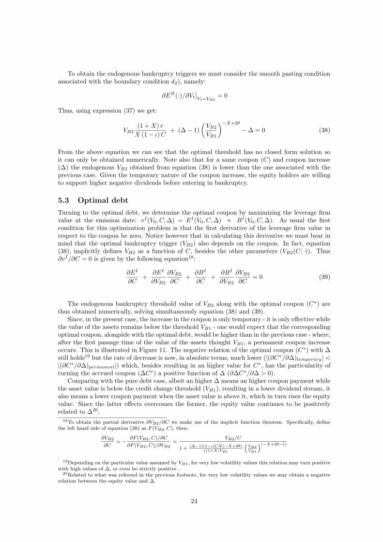
5.3 Optimal debt

Turning to the optimal debt, we determine the optimal coupon by maximizing the leverage firmvalue at the emission date: vI(V0, C, ∆) = EI(V0, C,∆) + BI(V0, C, ∆). As usual the firstcondition for this optimization problem is that the first derivative of the leverage firm value inrespect to the coupon be zero. Notice however that in calculating this derivative we must bear inmind that the optimal bankruptcy trigger (VB2) also depends on the coupon. In fact, equation(38), implicitly defines VB2 as a function of C, besides the other parameters (VB2(C; ·)). Thus∂vI/∂C = 0 is given by the following equation18:

∂EI

∂C+

∂EI

∂VB2

∂VB2

∂C+

∂BI

∂C+

∂BI

∂VB2

∂VB2

∂C= 0 (39)

The endogenous bankruptcy threshold value of VB2 along with the optimal coupon (C∗) arethus obtained numerically, solving simultaneously equation (38) and (39).

Since, in the present case, the increase in the coupon is only temporary - it is only effective whilethe value of the assets remains below the threshold VB1 - one would expect that the correspondingoptimal coupon, alongside with the optimal debt, would be higher than in the previous case - where,after the first passage time of the value of the assets thought VB1, a permanent coupon increaseoccurs. This is illustrated in Figure 11. The negative relation of the optimal coupon (C∗) with ∆still holds19 but the rate of decrease is now, in absolute terms, much lower (|(∂C∗/∂∆)temporary| <|(∂C∗/∂∆)permanent|) which, besides resulting in an higher value for C∗, has the particularity ofturning the accrued coupon (∆C∗) a positive function of ∆ (∂∆C∗/∂∆ > 0).

Comparing with the pure debt case, albeit an higher ∆ means an higher coupon payment whilethe asset value is below the credit change threshold (VB1), resulting in a lower dividend stream, italso means a lower coupon payment when the asset value is above it, which in turn rises the equityvalue. Since the latter effects overcomes the former, the equity value continues to be positivelyrelated to ∆20.

18To obtain the partial derivative ∂VB2/∂C we make use of the implicit function theorem. Specifically, definethe left hand side of equation (38) as F (VB2, C), then:

∂VB2

∂C= −

∂F (VB2, C)/∂C

∂F (VB2, C)/∂VB2=

VB2/C

1 +(∆−1)(1−ι)CX(−X+2θ)

r(1+X)VB1

“VB2VB1

”(−X+2θ−1)

.19Depending on the particular value assumed by VB1, for very low volatility values this relation may turn positive

with high values of ∆, or even be strictly positive .20Related to what was refereed in the previous footnote, for very low volatility values we may obtain a negative

relation between the equity value and ∆.

24

Figure 11: Right panel: optimal coupon as a function of ∆, when the coupon increase is tempo-rary (solide line) or permanent (dashed line); left panel: coupon value after the occurrence of adowngrade (∆C∗), when the coupon increase is temporary (solid line) or permanent (dashed line);with V0 = 150; VB1 = 120; r = 0, 07; α = 0, 01; σ = 0, 25; ι = 0, 35 and ρ = 0, 4.

5.4 Asset substitution

What happens to the ∆∗ value? Remember from the previous sections that ∆∗ was defined asthe particular value of the coupon increase for which the low volatility level (σL) would con-stitute a rational expectation equilibrium, specifically, ∆∗ would verified the following equation:EI(V0, C

∗(σL),∆∗, σex−post = σL) = EI(V0, C∗(σL),∆∗, σex−post = σH)). For the present case,

when ∆∗ exists21 it assumes a significantly much higher value than the one associated with thepermanent effects case. In other words, given the temporary nature of the coupon increase, it ismore “difficult” to force equity holders to pursuit low risk strategies. The consequence of thatis a comparatively lower firm value albeit, in some cases, it could still be higher than the oneassociated with straight debt as table 5 shows.

Risk levels Temporary coupon rating trigger DifferenceσL σH C∗ ∆∗ Firm value Permanent effects Straight debt

0,15 0,20 10,97 2,144 191,24 - 3,98 - 0,940,25 10,82 2,693 188,26 - 4,52 + 2,75

0,20 0,25 8,80 1,999 181,53 - 3,65 - 3,980,40 7,27 2,918 175,77 - 2,72 + 2,09

Table 5: Optimal coupon, ∆∗ and the correspondent firm value (vI(V0, C∗(σL),∆∗, σL)), consid-

ering a coupon rating trigger covenant with temporary effects ; the difference between that firmvalue and the ones associated with permanent effects and straight debt, for different risk levelsprofiles; with V0 = 150; VB1 = 120; r = 0, 07; α = 0, 01; ι = 0, 35 and ρ = 0, 4.

6 Conclusion

We have determined the optimal values concerning debt, equity and the leverage firm value whenthe debt contract is embedded with a covenant which establishes a permanent increase in thecoupon rate when the credit rating of the firm is downgraded. It has been shown that the use ofthese type of rating trigger covenant generates inefficiency costs reflected in a lower firm value whencompared with the use of straight debt. Nevertheless, in the presence of operational flexibility,

21When ∆ and the optimal coupon are positively related, ∆∗ doesn’t exists.

25

such covenants have the ability to “force” the equity holders to sustain a low risk level profile andthus preventing the occurrence of asset substitution. In this environment, the decision concerningwhat kind of debt should be issued will depend on the tradeoff between the agency costs of straightdebt and the inefficiency costs attached to the rating trigger covenant type of debt, which in turnwill depend on the available spectrum of risk profiles. Specifically, for low values of the lowervolatility level, the covenant should be used, otherwise, the straight debt is a preferable option.When the increase in the coupon, triggered by the credit rating downgrade, is not permanent butinstead is only effective when the assets value is above the credit rating threshold, the advantagesassociated to the covenant are reduced albeit in some cases can still generate better results thanstraight debt.

References

[1] R. Anderson and S. Sundaresan. Design and valuation of debts contracts. Review of FinancialStudies, 9(1):37–68, 1996.

[2] R. Anderson, S. Sundaresan, and P. Tychon. Strategic analysis of contingent claims. EuropeanEconomic Review, 40:871–881, 1996.

[3] K. Bhanot and A. S. Mello. Should corporate debt include a rating trigger? Journal ofFinancial Economics, 79(1):69–98, 2006.

[4] F. Black and J. C. Cox. Valuing corporate securities: some effects of bond indenture. Journalof Finance, 31(2):351–367, 1976.

[5] E. Briys and F. De Varenne. Valuing risky fixed rate debt: an extension. Journal of Financialand Quantitative Analysis, 32(2):239–248, 1997.

[6] P. Collin-Dufresne and R. Goldstein. Do credit spreads reflect stationary leverage ratios?Journal of Finance, 56(5):1929–1957, 2001.

[7] J. Ericsson. Asset substitution, debt pricing, optimal leverage and maturity. Finance,21(3):39–70, 2000.

[8] J. Ericsson and J. Reneby. A framework for valuing corporate securities. Applied MathematicalFinance, 5(3):143–163, 1998.

[9] J. Ericsson and J. Reneby. The valuation of corporate liabilities: theory and tests. SSE/EFIWorking Paper Series in Economics and Finance, 445, 2003.

[10] F. Gonzalez et al. Market dynamics associated with credit ratings. a literature review. Oc-casional Paper Series: European Central Bank, 16, 2004.

[11] H. Fan and S. Sundaresan. Debt valuation, renegotiation, and optimal dividend policy. Reviewof Financial Studies, 13(4):1057–1099, 2000.

[12] R. Goldstein, N. Ju, and H. Leland. An ebit-based model of dynamic capital structure.Journal of Business, 74(4):483–512, 2001.

[13] J. Hsu, J. Sa-Requejo, and P. Santa-Clara. Bond pricing with default risk. Working paper18/03, Anderson Graduate School of Management, UCLA, 2003.

[14] C. Hui, C. Lo, and S. Tsang. Pricing corporate bonds with dynamic default barriers. Journalof Risk, 5(3), 2003.

[15] N. Ju and H. Ou-Yang. Capital structure, debt maturity, and stochastic interest rates.Working paper, Smith Business School, University of Maryland, 2004.

26

[16] I. J. Kim, K. Ramaswamy, and S. Sundaresan. Does default risk in coupons affect thevaluation of corporate bonds? Financial Management, 22:117–131, 1993.

[17] H. Leland. Corporate debt value, bond covenants, and optimal capital stucture. Journal ofFinance, 49(4):1213–1252, 1994.

[18] H. Leland. Agency costs, risk management, and capital structure. Journal of Finance,53(4):1213–1243, 1998.

[19] H. Leland and K. Toft. Optimal capital structure, endogenous bankruptcy, and the termstructure of credit spreads. Journal of Finance, 51:987–1019, 1996.

[20] F. A. Longstaff and E. S. Schwartz. A simple approach to valuing risky fixed and floatingrate debt. Journal of Finance, 50 (3):789–819, 1995.

[21] P. Mella-Barral. The dynamics of default and debt reorganization. The Review of FinancialStudies, 12(3):535–578, 1999.

[22] P. Mella-Barral and W. Perraudin. Strategic debt service. Journal of Finance, 52(2):531–556,1997.

[23] A. S. Mello and J. Parsons. The agency costs of debt. Journal of Finance, 47:1887–1904,1992.

[24] R. Schobel. A note on the valuation of risky corporate bonds. OR Spektrum, 21:35–47, 1999.

[25] Moody’s Investors Service. Moody’s analysis of US corporate rating triggers heightens needfor increased disclosure. July 2002.

[26] Moody’s Investors Service. Rating triggers in Europe: Limited awareness but widely usedamong corporate issuers. September 2002.

[27] Standard and Poors. Survey on rating triggers, contingent calls on liquidity. 2002.

[28] M. Tauren. A model of corporate bond prices with dynamic capital structure. Working paper,Indiana University, 1999.

27