Optimal control of renewable resources with alternative use

Mathematical and Computer Modelling 50 (2009) 260–272

Contents lists available at ScienceDirect

Mathematical and Computer Modelling

journal homepage: www.elsevier.com/locate/mcm

Optimal control of renewable resources with alternative useAdriana Piazza a,∗, Alain Rapaport ba Centro de Modelamiento Matemático, Universidad de Chile, Blanco Encalada 2120, 7 Piso, Santiago, Chileb UMR Analyse des Systèmes et Biométrie. 2, place Pierre Viala. 34060, Montpellier Cedex 2, France

a r t i c l e i n f o

Article history:Received 24 September 2008Received in revised form 19 December 2008Accepted 31 December 2008

Keywords:Resource allocationOptimal controlInfinite horizonDynamic programming

a b s t r a c t

We study the optimal harvesting of a renewable resource that cannot be continuouslyexploited, i.e. after the harvest the released space cannot be immediately reallocated to theresource. In the meantime, this space can be given an alternative use of positive utility. Weconsider a discrete time model over an infinite horizon with discounting, and characterizethe optimality of two myopic policies, the greedy and the sustainable ones. We then showthat the optimal strategy consists in applying one of these policies after a finite number oftime steps. Value function and optimal feedback are explicitly determined.

© 2009 Elsevier Ltd. All rights reserved.

0. Introduction

Weconsider a discrete timemodeling of the optimal harvesting of a renewable resource (that could typically be cultivatedland, aqua-culture, forestry, . . . ) on a maximal space occupancy S > 0. We assume that the resource can be only harvestedafter reaching a ‘‘mature age’’ stage. In the general case this mature age could be arbitrary but in this work we will considerfor sake of simplicity that the mature age is equal to one time step.In this study, it is also assumed that the harvested space has to wait for at least one period before becoming available to

be reallocated again to its primary use. This particular feature can occur from practical constraints such as land refreshing,cleaning, or other resting duties that do not allow an immediate re-use of the space for the resource. From the managementpoint of view, unallocated space usually means economic loss. So we consider here that the unallocated space has a positiveutility, that could be brought by an alternative use of the space compatible with the resting duties (this could be for instancetourism, scientific investigations or experimentations, . . . ).We also assume that this alternative use can be extended tomorethan one time step without any a priori time limit. The management problem is then to determine at each time step thebest harvesting and arbitration between the resource allocation and the alternative use.In thismodelweneglect themortality of the resource in itsmature age, arguing that a rational exploitation of the resource

proceeds to spatial rotations so that no space stays occupied by the same unharvested resource for a long time.Mathematical modeling of natural resources has received great interest since the pioneer work of Clark [1]. Today,

theoretical questions in bio-economics of natural resources are commonly investigated with the help of dynamical systemsmodels and optimal control theory [2–5]. Special interest has been given to the sustainable management of naturalrenewable resources as part of an intense research around the concept of sustainable development [6–8]. The WorldCommission on Environment and Development (1987) produced the most quoted definition of sustainable development:‘‘Economic and social development thatmeets the needs of the current generationwithout undermining the ability of futuregenerations tomeet their ownneeds’’. There seems to be consensus about this definition but a lot of divergence onhow toputthe idea of sustainable development into operation. Among the different definitions of sustainability, we point out the one

∗ Corresponding author.E-mail addresses: [email protected] (A. Piazza), [email protected] (A. Rapaport).

0895-7177/$ – see front matter© 2009 Elsevier Ltd. All rights reserved.doi:10.1016/j.mcm.2008.12.009

http://www.elsevier.com/locate/mcm

http://www.elsevier.com/locate/mcm

mailto:[email protected]

mailto:[email protected]

http://dx.doi.org/10.1016/j.mcm.2008.12.009

A. Piazza, A. Rapaport / Mathematical and Computer Modelling 50 (2009) 260–272 261

by Daily and Erlich [7]: ‘‘Sustainability characterizes any process or condition that can be maintained indefinitely withoutinterruption, weakening, or loss of valued qualities’’. Influenced by it, we pay special attention to management policies thatkeep a constant resource.To the best of our knowledge, the question of alternative use of a resource have been scarcely studied within this

framework. Some authors have tackled the problem of the optimal harvesting of a resource when there exists an alternativeuse of space, but without any constraint to space allocation. In [9], Salo and Tahvonen consider a multi-aged, one-speciesforest where an alternative use of the land is possible. They characterize the state whose optimal trajectory is constant, thesustainable state, prove that it is a local saddle point and give some numerical examples that exhibit convergence to suchstate. In [10], Cominetti and Piazza study amulti-species forest and prove that two types of asymptotic behavior are possible,either there is convergence to the sustainable state for every initial condition, or the optimal trajectory converges towardsthe set of states yielding a periodic optimal trajectory. This means that the choice of the transient stage (i.e. the anticipationdecisions) is crucial before reaching amyopic strategy. Optimal periodic cycles appear aswell in [11], where a simplermodelof multi-aged, single species forest is considered. Assuming that harvest is restricted a priori to mature trees older than acertain age and that the growth aftermaturity is neglected, the authors show that every optimal trajectory becomes periodicin finite time. This implies that the problem can be reduced to a finite dimensional one and solved numerically.Inspired by these ideas, we study in this paper two particular myopic strategies – the constant policy and the greedy

periodic policy – analyzing the conditions under which they are optimal. These particular policies are the key ingredients forthe characterization of the value function and optimal trajectories in the general case.Our approach consists in determining first the subsets of initial conditions for which thosemyopic strategies are optimal.

In a second stage, we prove that an optimal trajectory has to reach one of these subsets in finite time. Our proofs are entirelybased on dynamic programming and concavity argumentations, which is not so oftenmet in the literature (most of the timeMaximum Principle or reformulation in terms of mathematical programming problems are used), apart from the analysis ofpure growth models [12]. For instance, in [13,14], dynamic pricing (or ‘‘support prices’’) are used to show the optimality ofa periodic solution over infinite horizon for problems with similar structure. Dynamic programming aims at characterizingthe value function, which is the unique solution of the Bellman equation. This is the combination of the Bellman equationwith concavity properties that plays here a determining role for obtaining short and elegant proofs. As a comparison, weprovide in an Appendix alternative proofs based on mathematical programming and duality, adapted from more generalresults [10] to the present framework.The paper is organized as follows. In Section 1we present the optimizationmodel to be solved, while in Section 2we state

and prove themain results of the paper.We first present necessary and sufficient conditions thatmake themyopic strategies(constant and greedy policies) optimal, and then give explicitly the value function and an optimal trajectory for any possibleinitial condition, solving completely the problem. Conclusions are dressed in Section 3. Finally, alternative proofs with themathematical programming approach are given in Appendix.

1. The optimization problem

With no loss of generality we assume that S = 1. For each period t ∈ Nwe denote zt ≥ 0 the fraction of space occupiedby the resource. We must decide how much resource ut to harvest

0 ≤ ut ≤ ztand the fraction vt of the space occupied by the alternative use that will be reallocated to the resource

0 ≤ vt ≤ 1− zt . (1)

The constraints on u and v can then be expressed as

(ut , vt) ∈ C(zt) where C(z) = [0, z] × [0, 1− z] (2)

and the dynamics of the system are simply written as

zt+1 = zt − ut + vt . (3)

Given an initial condition z0, the objective to be maximized is the discounted total benefit

J(z0, u, v) =∞∑t=0

bt [U(ut)+W (1− zt)]

over all admissible controls (u, v), where U(·) andW (·) are the utilities of the harvest and the use of the unallocated spacerespectively.We assume the usual hypotheses on utility functions and discount factor. Let C[0,1] be the set of C1 non-decreasing

concave functions from [0, 1] to R+.Assumption A0. The functions U(·) andW (·) belong to C[0,1]. The discount rate b belongs to the interval (0, 1).We denote z, u, v the infinite sequences of states and controls. Admissible sequences have to fulfill the dynamics (3) and

the feasibility constraints (2) at any time t ∈ N; and we refer to them as trajectories. Clearly these constraints imply that0 ≤ zt ≤ 1 for all t ∈ N so that z, u, v belong to `∞

+= `∞+(N).

262 A. Piazza, A. Rapaport / Mathematical and Computer Modelling 50 (2009) 260–272

Then, the optimization problem can be formulated as the search of optimal sequences z?, u?, v? solution of the followingmathematical program

P(z0)

V (z0) = max

∞∑t=0


s.t. (2) and (3)z, u, v ∈ `∞

+with z0 given.

The existence of solutions for P(z0) follows as a consequence of the Weierstrass theorem since the feasible set isσ(`∞, `1)-compact and the objective function is σ(`∞, `1)-upper semi continuous. For details of the proof we refer to [10]where a similar problem without constraint (1) is treated. The proof remains valid with minor changes. We cannot assurethe uniqueness of optimal solutions unless U andW are strictly concave, in which case we immediately get that u and z areunique, and uniqueness of v rightly follows from the constraints.The mathematical treatment of this problem is simpler if we state it only in terms of the state variable z . As is observed

by McKenzie [15], it is a necessary condition of any optimal trajectory that production and consumption (i.e., determinedby u and v in our model) are chosen in way so that the period’s utility is maximized given the initial and terminal states.Hence, we perform an ‘in period’ maximization to find the optimal values of ut and vt as well as the maximum benefit ofperiod t as a function of zt and zt+1. For (z, z ′) ∈ [0, 1]2 we define

f (z, z ′) =

max U(u)+W (1− z)s.t. 0 ≤ u ≤ z

0 ≤ v ≤ 1− zz ′ = z − u+ v.

Let us first denote byU(z, z ′) the set of feasible controls that induce the transition of the system from state z to z ′

U(z, z ′) = {(u, v) ∈ C(z) | z ′ = z − u+ v},and notice thatU(z, z ′) is never empty for any pair (z, z ′) ∈ [0, 1]2. Then, the function f (z, z ′) can be reformulated as

f (z, z ′) ={max U(u)+W (1− z)s.t. (u, v) ∈ U(z, z ′).

Looking carefully to the definition of the setUwe see that there is an even simpler expressionU(z, z ′) =

{(u, v) | v = z ′ − z + u, u ∈ [max(0, z − z ′),min(z, 1− z ′)]

}.

The maximum is attained when we take u equal to its upper bound. Within this approach, given a sequence of optimalstates {zt}, the optimal decisions can be calculated as

ut = min(zt , 1− zt+1),vt = min(1− zt , zt+1).

So,we get f (z, z ′) = U(min{z, 1−z ′})+W (1−z) and a dynamic optimization problem, equivalent to P(z0), can bewritten as

P(z0) =

V (z0) = max

∞∑t=0

bt f (zt , zt+1)

s.t. zt ∈ [0, 1]and z0 given.

The value function V (z0) associated with this optimal control problem can also be characterized by invoking the dynamicprogramming principle. It is a standard result (see for instance [16]) that V is the unique bounded function that satisfiesBellman equation

V (z) = maxz′∈[0,1]

U(min{z, 1− z ′})+W (1− z)+ bV (z ′). (4)

Remark 1.1. LetB[V0] be the Bellman operator defined on the set of bounded functions by

B[V0](z) = maxz′∈[0,1]

U(min{z, 1− z ′})+W (1− z)+ bV0(z ′).

The mappingB is a contraction and the value function V is the unique fixed point with

V = B[V ] = limk→∞

Bk[V0]

for any bounded function V0 (see [16] for details).

Lemma 1.2. The value function V is concave.Proof. The Bellman operator preserves concavity. Consequently, when V0 is concave the same holds for B[V0], andconsequently the value function V is a concave function. �


2. The optimal trajectory

In this section we fully describe one solution of P(z0) for every z0 ∈ [0, 1]. We emphasize that we do not attempt todescribe completely the solution set of P(z0), but only to propose one optimal trajectory. In Section 2.1 we discuss twoparticular trajectories: one constant and the other periodic. They will turn out to be the asymptotic regime of the proposedoptimal trajectory which becomes either constant or periodic after at most two time steps. In Section 2.2 we describe thetransient stages before reaching the steady state or periodic regime. Finally, in Section 2.3 we find the value function and afeedback law that yields one optimal trajectory.We will use the auxiliary C1 concave function

U(z) = U(z)+W (1− z)

which represents the maximum benefit that one can get on a single time step when the resource is z.

2.1. Asymptotic behavior

In this subsection we look closely at two particular policies for problem P(z0): the greedy periodic policy and the constantpolicy, characterizing the states for which they are optimal.

Definition 2.1 (Greedy Periodic Policy). It consists in harvesting all the resource available and reallocating to the resource allthe space that was assigned to the alternative use

ut = zt , vt = 1− zt

generating a cyclic trajectory of period two: zt+1 = 1− zt .

The benefit of the periodic trajectory generated by the greedy policy from any initial condition z ∈ [0, 1] is

JG(z) =U(z)+ bU(1− z)

1− b2.

We define p to be the largest optimal solution of

(P1) maxz∈[0,1]

JG(z).

Remark 2.2. Directly from the definition of p and the concavity of JG we know thati. JG is non-decreasing on [0, p].ii. JG is non-increasing on [p, 1].

Denote∆p ⊆ [0, 1] the set of states whose value function is V (z) = JG(z), which may be characterized as follows.

Proposition 2.3. ∆p is the set of points z ∈ [0, 1] that satisfy

U′(max(1− z, z)) ≥ bU

′(min(1− z, z)). (5)

Proof. Denote by φ(·) the function

φ(ξ, ξ ′) = U(min(ξ , 1− ξ ′))+ bJG(ξ ′).

If the greedy policy is optimal at z, then necessarily one has V (z) = JG(z) and V (1 − z) = JG(1 − z). From Eq. (4), thisimplies that the functions ξ ′ 7→ φ(z, ξ ′) and ξ ′ 7→ φ(1 − z, ξ ′) are maximized respectively at ξ ′ = 1 − z and ξ ′ = z.Functions ξ ′ 7→ φ(ξ, ξ ′) being concave (by composition of concave functions), this is also equivalent to require

0 ∈ ∂+2 φ(ξ, 1− ξ), ξ ∈ {z, 1− z}, (6)

where ∂+2 φ denotes the Fréchet super-differential of φ w.r.t. to its second argument. Simple calculations give

∂+2 φ(ξ, 1− ξ) = [−U′(ξ), 0] + bJ ′G(1− ξ)

and

J ′G(1− ξ) =U′(1− ξ)− bU

′(ξ)

1− b2.

Then, conditions (6) can be rewritten as{U′(1− ξ) ≥ bU

′(ξ)

U ′(ξ)− b2W ′(1− ξ) ≥ bU′(1− ξ)

ξ ∈ {z, 1− z}.


Noticing that U ′(ξ)− b2W ′(1− ξ) ≥ U′(ξ), these last conditions are equivalent to the simpler ones

U′(1− ξ) ≥ bU

′(ξ), ξ ∈ {z, 1− z}.

Finally, U(·) being concave, we obtain exactly the single condition (5).Conversely, assume that condition (5) holds at a given z. Denote p = min(z, 1− z) and notice that (5) is also fulfilled at

any z ∈ [p, 1− p], because U(·) is concave. Consider then the operatorMp : C[0,1] → C[0,1] defined as follows

Mp[f ](ξ) =

{f (1− p)+ f ′(1− p)(ξ − 1+ p), ξ ∈ [0, 1− p]f (ξ), ξ ∈ [1− p, p]f (p)+ f ′(p)(ξ − p), ξ ∈ [p, 1]

and notice thatMp[f ] ≥ f for any f ∈ C[0,1]. Let V be the value function for the modified utility functions U = Mp[U],

W =Mp[W ] and define the function U(z) = U(z)+ W (1− z). One has clearly V ≥ V ≥ JG. We claim that the function

JG(z) =U(z)+ bU(1− z)

1− b2

is a solution of the Bellman equation (4). To see this first observe that the definition of U implies that (5) is fulfilled for U atany z ∈ [0, 1], which in turn implies that JG is non-decreasing in [0, 1]. To see that

JG(z) = W (1− z)+ maxz′∈[0,1]

U(min(z, 1− z ′))+ bJG(z ′)

we distinguish two cases: (i) z ′ ∈ [0, 1− z], (ii) z ′ ∈ [1− z, 1].

(i) W (1− z)+ maxz′∈[0,1−z]

U(min(z, 1− z ′))+ bJG(z ′) = W (1− z)+ U(z)+ maxz′∈[0,1−z]

bJG(z ′)

= U(z)+ bJG(1− z) = JG(z)

(ii) W (1− z)+ maxz′∈[1−z,1]

U(min(z, 1− z ′))+ bJG(z ′) = W (1− z)+ maxz′∈[1−z,1]

U(1− z ′)+ bJG(z ′)

= W (1− z)+ maxz′∈[1−z,1]

−W (z ′)+ JG(1− z ′)

= JG(z).

Consequently, one has V (z) = JG. Finally, remark that JG = JG on [1 − p, p], which proves that V = JG on [1 − p, p]. Thegreedy policy is then optimal from any z ∈ [1− p, p]. �

Notice that when U′( 12 ) ≥ 0, we have p ≥

12 . As a consequence of Proposition 2.3 we deduce the following

Lemma 2.4. ∆p is nonempty exactly when U ′( 12 ) ≥ 0, and then the set ∆p is the interval [1 − p, p]. Furthermore, U is non-

decreasing on [0, p].

Proof. Condition (5) of Proposition 2.3 and concavity of the function U(·) imply the property

z ∈ ∆p ⇒ [min(z, 1− z),max(z, 1− z)] ⊂ ∆p (7)

so∆p is an interval that necessarily contains 12 whenever it is not empty. Now12 fulfills condition (5) exactlywhenU

′( 12 ) ≥ 0.

The definition of p and the concavity of U together with (7) imply∆p = [1− p, p]. The sign of U′( 12 ) and the concavity of U

imply that the function U is non-decreasing on [0, 12 ] and from (5) this also implies that U is non-decreasing on [0, p]. �

Lemma 2.5. If 12 ≤ p ≤ 1 then V (z) ≤ JG(p) for all z ∈ [0, 1].

Proof. If p = 1 then the lemma above states that V (z) = JG(z) for all z ∈ [0, 1] and the proof follows directly because JG(z)attains its maximum at z = p.Let us consider now what happens when p < 1. In this case, the differentiable function JG(z) attains its maximum at

an interior point of [0, 1], thus J ′G(p) = 0. It is a known property that the slope of any concave function f , defined as:slope f (z, z ′) = f (z)−f (z′)

z−z′ , is non-increasing w.r.t. to its second variable (see for example [17]). As V is concave we have

slope V (x, p) ≤ slope V (z, p) for all x > p, z < p.

From V (z) ≥ JG(z) for all z and V (p) = JG(p)we easily deduce

slope V (z, p) ≤ slope JG(z, p) for all z < p.


Putting the two inequalities together we get

slope V (x, p) ≤ infz<pslope JG(z, p) = 0 for all x > p

where the equality follows from the fact that J ′G(p) = 0. And we easily conclude that V (x) ≤ V (p) = JG(p) for x < p.Analogously, we get V (x) ≤ V (p) = JG(p) for x > p and the lemma follows. �

Remark 2.6. Directly from the concavity of V and the fact that V (z) ≤ V (p) for all z ∈ [0, 1]we know that

i. V is non-decreasing in [0, p]ii. V is non-increasing in [p, 1]

We will see in Section 2.3 that if U′( 12 ) < 0, the proposed optimal trajectory remains constant after at most two steps. This

motivates the definition of

Definition 2.7 (Constant Policy). It consists in always harvesting and allocating the quantity

ut = vt = min(zt , 1− zt)

so that the trajectory is constant: zt = z0.

The benefit of the constant trajectory from the initial condition z ∈ [0, 1] is given by

JS(z) =U(min(z, 1− z))+W (1− z)

1− b.

Notice that JS(z) = U(z)/(1 − b) whenever z ≤ 12 . This motivates the notion of a sustainable state, which corresponds

intuitively to a state where it is optimal to stay forever.

Definition 2.8 (Sustainable State). A state z ∈ [0, 1] is called sustainable if it is invariant under the optimal policy, i.e. theconstant trajectory is optimal and V (z) = JS(z).

Proposition 2.9. The constant policy is optimal exactly at points z solutions of problem

(P2) maxz∈[0,1/2]

JS(z).

We define z to be the largest optimal solution of (P2). If z < 1/2 then V (z) ≤ V (z) = Js(z) for all z ∈ [0, 1].

Proof. Let us first show that the constant policy cannot be optimal for z > 12 . If z > 1

2 then U(z),U(1 − z) >U(1− z)+W (1− z) and consequently

JG(z) >(U(1− z)+W (1− z))(1+ b)

1− b2= JS(z),

thus a contradiction with the optimality of the constant policy.If the constant policy is optimal at z ∈ [0, 12 ], the following inequality is obtained from the Bellman equation (4)

V (z) = JS(z) ≥ W (1− z)+ U(min(z, 1− z))+ bJS(z)= U(z)+W (1− z)+ bJS(z) = JS(z)(1− b)+ bJS(z)

which implies JS(z) ≥ JS(z) i.e. U(z) ≥ U(z). So the constant policy cannot be optimal away from z.If z = 1

2 , one has necessarily U′( 12 ) ≥ 0 and from Lemma 2.4, the constant policy that coincides with the greedy policy

at z = 12 is optimal. Otherwise, z is a maximizer of the concave function U on [0, 1]. From the Bellman equation (4), one can

write the following inequalities

V (z) = U(z)+ maxz′∈[0,1]

U(min(z, 1− z ′))− U(z)+ bV (z ′)

≤ U(z)+ b maxz′∈[0,1]

V (z ′) = JS(z)(1− b)+ b maxz′∈[0,1]

V (z ′)

from which we deduce V (z) = JS(z) = maxz′∈[0,1] V (z ′). The constant policy is then optimal from z. �

Remark 2.10. By the concavity of V and V (z) ≤ V (z) for all z ∈ [0, 1]we immediately know that

i. V is non-decreasing in [0, z]ii. V is non-increasing in [z, 1]


2.2. Transient behavior

We claim that after two time steps the proposed optimal trajectory becomes either constant or periodic with period two,depending on the sign of U

′( 12 ). Namely, if U

′( 12 ) < 0 then after at most two steps the proposed optimal trajectory reaches

z and remains there afterwards. Otherwise, if U′( 12 ) ≥ 0 it becomes 2-periodic after two time steps. More precisely, there

are two different situations depending on the initial condition. If z0 ∈ [1− p, p] the optimal trajectory is a 2-periodic cyclefrom the beginning: (z0, 1− z0, z0, . . .). If z0 6∈ [1− p, p], then the optimal trajectory reaches the (p, 1− p)-cycle in one ortwo steps.The previous subsection described the conditions under which the constant and greedy trajectories are optimal, from

the first stage. In this subsection we discuss what happens when this is not the case, i.e., we describe precisely the behaviorof the optimal trajectories during the two-step transient period before entering the periodic or steady-state regime.We claim that the optimal policy during the transient is characterized by the auxiliary problem

Q (z0)

max U(u0)+ bU(z1)s.t. u0 + z1 ≤ 1

0 ≤ u0 ≤ z00 ≤ z1 ≤ p.

This problem maximizes the two first steps benefit. The set of constraints is induced by (2) and (3) for stage t = 0 exceptfor z1 ≤ p. This last condition was introduced to assure that the two proposed asymptotic regimes are admissible after thetransient. To see this, notice that z ≤ p if and only if U

′( 12 ) ≤ 0.

For convenience we define the function

Q (z) = U(z)+ bU(1− z), z ∈ [0, 1]

and denote by q ∈ [0, 1] the point where it attains the maximum. If this point is not unique we take q as the largest optimalsolution.Problem Q (z0) can be solved explicitly: when U

′( 12 ) ≤ 0 one optimal solution is given by

(z1, u0) =

{(z, z0) when z0 ∈ [0, 1− z)(1− z0, z0) when z0 ∈ [1− z, q](1− q, q) when z0 ∈ (q, 1]

while if U′( 12 ) > 0 we have

(z1, u0) =

{(p, z0) when z0 ∈ [0, 1− p)(1− z0, z0) when z0 ∈ (1− p, q](1− q, q) when z0 ∈ (q, 1].

2.3. The optimal policy

Using the results of the previous sections we may find explicitly the value function and the feedback law that gives thevalue zt+1 as a function of zt for all t . We distinguish three different situations according to the position of the solution z of(P2) in the interval [0, 12 ]: Left, Interior, or Right.

(SL) z = 0, U′(0) ≤ 0

(SI) z ∈(0,12

), U

′(z) = 0

(SR) z =12, U

′

(12

)≥ 0

The graph of the feedback law is presented in Fig. 1. To the left, we see the feedback lawwhen (SI) holds and to the rightwhen (SR) holds. The case (SL) can be seen as a degenerate case of the former where we simply have zt ≡ 0 for all t ≥ 1. Inall situations it may happen that q = 1, in which case the last interval disappears. The graphs are very similar and could bemerged in a single diagram, but we prefer to distinguish them since they give rise to different dynamics.In Fig. 2 we present the optimal trajectory from a state z0 ∈ (p, q] when (SR) holds. Let us observe, that the trajectory

reaches the periodic cycle p, 1− p, p, . . . in two steps, the transient being z1 = 1− z0. The evolution from any other initialstate can be found similarly. We remark that for every initial state, the optimal trajectory reaches the (p, 1−p)-cycle in oneor two steps, except for the initial conditions in the interval z ∈ [1 − p, p], whose optimal trajectory is the periodic cyclez, 1− z, z, . . . from the first stage.If (SI) holds the dynamics are even simpler and it is not difficult to see that there is convergence to the state z in one or

two steps.The following theorem describes more precisely the feedback law represented in Fig. 1 and proves that it is effectively

optimal.


Fig. 1. Feedback law.

Fig. 2. Dynamics.

Theorem 2.11. If (SL) or (SI) holds there is convergence in two steps to a sustainable state and the value function is

V (z) =

{U(z)+ bJS(z), z ∈ [0, 1− z]W (1− z)+ max

z′∈[1−z,z]Q (z ′)+ b2JS(z), z ∈ [1− z, 1]

which is attained by the optimal trajectory generated by the feedback law of Fig. 1(a),{(z0, z, z, z, . . .) when z0 ∈ [0, 1− z](z0, 1− z0, z, z, . . .) when z0 ∈ (1− z, q](z0, q, z, z, . . .) when z0 ∈ (q, 1].

(8)

Otherwise, if (SR) holds then∆p is reached in at most two steps and the optimal trajectory is greedy of period two afterwards,the value function being

V (z) =

U(z)+ bJG(p), z ∈ [0, 1− p)JG(z), z ∈ [1− p, p]W (1− z)+ max

z′∈[p,z]Q (z ′)+ b2JG(p), z ∈ (p, 1]

which is attained by the optimal trajectory generated by the feedback law of Fig. 1(b),(z0, p, 1− p, p, 1− p, . . .) when z0 ∈ [0, 1− p)(z0, 1− z0, z0, 1− z0, z0, . . .) when z0 ∈ [1− p, p](z0, 1− z0, p, 1− p, p, . . .) when z0 ∈ (p, q](z0, 1− q, p, 1− p, p, . . .) when z0 ∈ (q, 1].

(9)


Proof. Denoting

∆V (z, z ′) = W (1− z)+ U(min(z, 1− z ′))+ bV (z ′)

V (·) is the value function if it is solution of the Bellman equation (4), which amounts to prove that the equality

maxz′∈[0,1]

∆V (z, z ′) = V (z) (10)

is fulfilled for any z ∈ [0, 1].Let us first study the case where (SR) holds. We distinguish three cases (i) z ∈ [1− p, p], (ii) z < 1− p and (iii) z > p(i) It follows directly from Proposition 2.3 that V (z) = JG(z).(ii)

∆V (z, z ′) = W (1− z)+ U(min(z, 1− z ′))+ bV (z ′)≤ U(z)+ bV (z ′)≤ U(z)+ bJG(p) (by Lemma 2.5).

Observing that∆V (z, p) = U(z)+ bJG(p), it follows that z ′ = p and V (z) = U(z)+ bJG(p).(iii) We start by seing two properties of argmaxz′∈[0,1]∆V (z, z ′).

1. If z ′ ≤ 1− z, then z ′ ≤ 1− p and we have∆V (z, z ′) = U(z)+W (1− z)+ bV (z ′) ≤ U(z)+ bV (1− z) for all z ′ ≤ 1− z

because V (·) is increasing in [0, p] (see Remark 2.6). Hence argmax∆V (z, z ′) ≥ 1− z.2. If z ′ ≥ 1− p, then z ′ ≥ p and we have

∆V (z, z ′) = U(1− z ′)+W (1− z)+ bV (z ′) ≤ W (1− z)+ U(1− z)+ bV (z) for all z ′ ≥ zbecause V (·) is decreasing in [p, 1] (see Remark 2.6). Hence argmax∆V (z, z ′) ≤ p.

This implies that maxz′∈[0,1]∆V (z, z ′) = maxz′∈[1−z,1−p]∆V (z, z ′). Finally

V (z) = W (1− z)+ maxz′∈[1−z,1−p]

U(1− z ′)+ bV (z ′)

= W (1− z)+ maxz′∈[1−z,1−p]

U(1− z ′)+ b[U(z ′)+ bJG(p)]

= W (1− z)+ maxz′′∈[p,z]

Q (z ′′)+ b2JG(p).

We consider now what happens if (SI) or (SL) holds.To prove that (10) is fulfilled for any z ∈ [0, 1], we distinguish two cases: (i) z ∈ [0, 1− z] and (ii) z > 1− z observing

that (i) comprises the whole interval whenever (SL) holds.(i)

∆V (z, z ′) = U(min(z, 1− z ′))+W (1− z)+ bV (z ′)≤ U(z)+W (1− z)+ bJS(z) (by Proposition 2.9).

Observing that∆V (z, z) = U(z)+ bJs(z), it follows that z ′ = z and V (z) = U(z)+ bJS(z).(ii) By a process analogous to that of (SR.iii) but using Remark 2.10 instead of Remark 2.6, it is not difficult to see that

maxz′∈[0,1]

∆V (z, z ′) = maxz′∈[1−z,z]

∆V (z, z ′)

and then

maxz′∈[1−z,z]

∆V (z, z ′) = W (1− z)+ maxz′∈[1−z,z]

U(min(z, 1− z ′))+ bV (z ′)

= W (1− z)+ maxz′∈[1−z,z]

U(1− z ′)+ b(U(z ′)+ bJs(z)) (by (SI.i))

= W (1− z)+ maxz′∈[1−z,z]

Q (z ′)+ b2Js(z). �

Remark 2.12. If the delay before reallocation of the primary use was not compulsory, that is to say if we remove constraint(1), then the reserved space can be considered as allocated to another virtual species with amaturity age equal to one. Then,the problem is easily solved and it can be shown that an optimal trajectory converges to a new sustainable state z, given byz ∈ argmaxz∈[0,1] U(z) in only one time step, the optimal trajectory being constant afterwards. In this case, the sustainablestate is the same as the one of our model when condition (SL) or (SI) holds. The qualitative behavior of both problems is thesame with convergence to the same state. However, under condition (SR), the situation is different. In this case, if reservingthe space was not mandatory then the sustainable state would change: we would have z > 1 − z. Furthermore, in theproblem without constraint (1), there might be convergence to a sustainable state with z = 1, that is to say the alternativeuse is not present at all. This represents a situation where the alternative use does not provide enough benefit to endure byitself.


3. Conclusions

We have analyzed a discrete time model for the optimal harvesting of a renewable resource, where the space occupancyis limited and reallocation after harvesting is not immediately allowed (assuming that the maturity age of the resource isreached after one time step).Techniques based on dynamic programming and concavity has led us to characterize the optimality of two myopic

strategies leading to constant or greedy periodic trajectories, and to make explicit the optimal trajectory from any possibleinitial state (along with the optimal transient decisions to be kept).This paper shows that considering an alternative use of the resource appears to be different to the abstract problem

simply adding a virtual species, because of the delay imposed before reallocating the space to its primary use. This leads toa non-trivial optimal policy, for which a different anticipation scheme might be required, before using a myopic decision.The assumption of a net benefit of the alternative use depending only on the amount cleared by the harvest, and separable

from the net revenue of the harvest could be considered to be oversimplified for real world economics. Nevertheless, this hasallowed us to provide a complete rigorous solution of the problem, and to develop amethodology based on the combinationof dynamic programming and concavity tools, that could be re-used for more complicatedmodels. This is a first step towardmore realistic modeling.

Acknowledgements

Both authors would like to thank Jean-Philippe Terreaux for several helpful comments concerning the system studied.Adriana Piazza would like also to thank Roberto Cominetti his active interest in the publication of this paper. This workwas part of the Ph.D. dissertation [18] financed by the Mathematical Engineering Department of the Universidad de Chileunder the project MECESUP. Adriana Piazza gratefully acknowledges the financial support of FONDECYT under PostdoctoralProject 3080059 while this paper was written.

Appendix. Mathematical programming proofs

A.1. Asymptotic behavior

Throughout we let z be an optimal trajectory for P(z0).To avoid working with the non-differentiable function min(·, ·) we will sometimes use the following equivalent

formulation of P(z0)V (z0) = max

∞∑t=0


s.t. 0 ≤ ut ≤ ztut + zt+1 ≤ 1and z0 given.

(11)

Proof (Proposition 2.3). To prove the necessity of condition (5) take z0 ∈ ∆p and consider the greedy trajectory issuedfrom z0: z = (z0, 1 − z0, z0, 1 − z0, . . .). Suppose that 1 − z0 > z0 and consider the perturbed trajectory zε =(z0, 1 − z0 − ε, z0 + ε, 1 − z0 − ε, . . .) where ε > 0. 1 If the original trajectory is optimal, the benefit obtained with it(V ) must be greater or equal to the one obtained with the new trajectory (Vε), this is

V − Vε =b

1− b2[U(1− z0)− U(1− z0 − ε)] +

b2

1− b2[U(z0)− U(z0 + ε)]

+b

1− b2[W (z0)−W (z0 + ε)] +

b2

1− b2[W (1− z0)−W (1− z0 − ε)] ≥ 0.

Dividing by ε > 0 and letting it to 0 yields (5). The proof in the case z0 > 1 − z0 is completely analogous, perturbing theoptimal trajectory at t = 1 instead of t = 0.To prove the sufficiency of condition (5) let us show that the greedy periodic trajectory is optimal for P(z0). We prove

the optimality using the Karush-Kuhn-Tucker (KKT) theorem. To this end we consider the Lagrangian associated with theoptimization problem stated in (11)

L =∞∑t=0

bt[U(ut)+W (1− zt)+ µtut + αt(zt − ut)+ βt(1− zt+1 − ut)

](12)

1 This feasible perturbed trajectory is obtained by allocating 1− z0 − ε at t = 0 instead of 1− z0 , keeping this extra space in the alternative use for oneperiod and allocating z0+ε at t = 1, after which we continue with a greedy periodic policy.


together with the following set of `1-multipliersµt = 0

αt =bt

1− b2[Q ′(zt)− b2W ′(1− zt)]

βt =bt+1

1− b2[U′(1− zt)− bU

′(zt)].

(13)

In fact, the multipliers belong to `1+due to condition (5). We can see that we have complementary slackness and the

feasibility constraints are fulfilled. To prove that ∇L = 0, it is left to see thatLut = Lzt = 0 for all t .

Lut = btU ′(ut)+ µt − αt − βt

= btU ′(zt)−bt

1− b2[Q ′(zt)− b2W ′(1− zt)] −

bt+1

1− b2[U′(1− zt)− bU

′(zt)]

=bt

1− b2[(1− b2)U ′(zt)− U ′(zt)+ bU

′(1− zt)+ b2W ′(1− zt)− bU

′(1− zt)+ b2U

′(zt)] = 0 (14)

Lzt = −btW ′(1− zt)+ αt − βt−1

= −btW ′(1− zt)+bt

1− b2[Q ′(zt)− b2W ′(1− zt)] −

bt

1− b2[U′(1− zt−1)− bU

′(zt−1)]

=bt

1− b2[(b2 − 1)W ′(1− zt)+ U ′(zt)− bU

′(1− zt)− b2W ′(1− zt)− U

′(zt)+ bU

′(1− zt)] = 0. (15)

Thus, the proposed trajectory is a stationary point of the Lagrangian (12) and hence a solution of P(z0). �

Proof (Proposition 2.9). Let us show that the stationary trajectory zt = z is optimal for P(z). To this end consider theLagrangian (12) with the following set of `1

+-multipliers{

µt = βt = 0αt = btU ′(z).

A routine verification shows that∇L = 0 andwehave complementary slacknesswhich implies that the proposed trajectoryis a stationary point for P(z). Hence, it is an optimal solution and z is sustainable.To prove the other implication, let z be a sustainable state. We claim that z ∈ argmaxz∈[0, 12 ] U(z). To this end, consider

the following trajectory z = z−ε ∀t ≥ 1. Given that z is a sustainable state, the benefit obtainedwith the constant trajectorymust be greater or equal to the one obtained with the alternative trajectory, which is equivalent to

U(z)− U(z − ε)+W (1− z)−W (1− z + ε) ≥ 0. (16)

If z = 12 , then the proposed alternative trajectory is feasible for 0 < ε < 1

2 . So dividing (16) by ε and letting ε → 0 yields

U ′(z)−W ′(1− z) ≥ 0 ⇐⇒ U′(z) ≥ 0

which readily implies that z = 12 ∈ argmaxz∈[0, 12 ] U(z). If z ∈ (0,

12 )we can consider ε positive and negative provided that

|ε| is small enough. So, repeating the reasoning we get

U′(z) = 0

which is equivalent to z ∈ argmaxz∈[0, 12 ] U(z). And finally, if z = 0, only the values of ε < 0 can be considered and this

yields U′(0) ≤ 0, which also gives us z ∈ argmaxz∈[0, 12 ] U(z). �

A.2. Optimal policy

Proof (Theorem 2.11). If (SL) holds we propose the primal solution zt = 0 for all t ≥ 1with the `1+-multipliersµt = βt = 0and αt = btU ′(zt). It is easy to see that the proposed trajectory is a stationary point of the Lagrangian (12) and thus anoptimal solution to P(z0).If (SI) holds, zt evolves following the feedback law showed in Fig. 1(a), reaching z in at most two steps. We recall the

proposed optimal trajectory

(8)

{(z0, z, z, z, . . .) when z0 ∈ [0, 1− z](z0, 1− z0, z, z, . . .) when z0 ∈ (1− z, q](z0, q, z, z, . . .) when z0 ∈ (q, 1].

We propose the following `1-multipliers:


µt = 0

αt =

U′(u0)− bU

′(z1) t = 0

bU ′(z1) t = 1btU ′(z) t ≥ 2

βt =

{bU′(z1) t = 0

0 t ≥ 1.

It is evident that αt ≥ 0 and βt ≥ 0 for all t ≥ 1. To see the non-negativity of α0 and β0, we calculate them as a function ofz0

α0 =

{U ′(u0) if z0 ≤ 1− zQ ′(z0) if 1− z < z0 ≤ q (Q ′(z0) ≥ Q ′(q) = 0)0 if z0 > q

β0 =

0 if z0 ≤ 1− zbU′(1− z0) if 1− z < z0 ≤ q (U

′(1− z0) ≥ U

′(z) = 0)

bU′(1− q) if z0 > q (U

′(1− q) ≥ U

′(z) = 0).

We proceed now to prove that ∇L = 0,

(14) H⇒Lu0 = U′(u0)− U ′(u0)+ bU

′(z1)− bU

′(z1) = 0

Lu1 = bU′(z1)− bU ′(z1)− 0 = 0

Lut = btU ′(z)− btU ′(z)− 0 = 0 for all t ≥ 2

(15) H⇒Lz1 = −bW′(1− z1)+ bU ′(z1)− bU

′(z1) = 0

Lzt = −btW ′(1− z)+ btU ′(z) = 0 for all t ≥ 2.

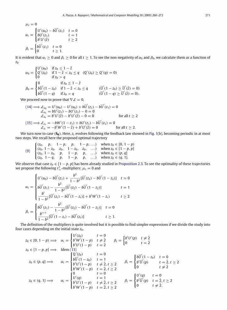
We turn now to case (SR). Here, zt evolves following the feedback law showed in Fig. 1(b), becoming periodic in at mosttwo steps. We recall here the proposed optimal trajectory

(9)

(z0, p, 1− p, p, 1− p, . . .) when z0 ∈ [0, 1− p)(z0, 1− z0, z0, 1− z0, z0, . . .) when z0 ∈ [1− p, p](z0, 1− z0, p, 1− p, p, . . .) when z0 ∈ (p, q](z0, 1− q, p, 1− p, p, . . .) when z0 ∈ (q, 1].

We observe that case z0 ∈ [1− p, p] has been already studied in Proposition 2.3. To see the optimality of these trajectorieswe propose the following `1

+-multipliers: µt = 0 and

αt =

U ′(u0)− bU

′(z1)+

b2

1− b2[U′(z2)− bU

′(1− z2)] t = 0

bU′(z1)−

b2

1− b2[U′(z2)− bU

′(1− z2)] t = 1

bt

1− b2[U′(zt)− bU

′(1− zt)] + btW ′(1− zt) t ≥ 2

βt =

bU′(z1)−

b2

1− b2[U′(z2)− bU

′(1− z2)] t = 0

bt+1

1− b2[U′(1− zt)− bU

′(zt)] t ≥ 1.

The definition of the multipliers is quite involved but it is possible to find simpler expressions if we divide the study intofour cases depending on the initial state z0.

z0 ∈ [0, 1− p) H⇒ αt =

U ′(z0) t = 0btW ′(1− p) t 6= 2btU ′(1− p) t = 2

βt =

{btU ′(p) t 6= 20 t = 2

z0 ∈ [1− p, p] H⇒ Idem (13)

z0 ∈ (p, q] H⇒ αt =

Q ′(z0) t = 0bU′(1− z0) t = 1

btU ′(1− p) t 6= 2, t ≥ 2btW ′(1− p) t = 2, t ≥ 2

βt =

bU′(1− z0) t = 0

btU′(p) t = 2, t ≥ 2

0 t 6= 2

z0 ∈ (q, 1] H⇒ αt =

0 t = 0U ′(q) t = 1btU ′(1− p) t 6= 2, t ≥ 2btW ′(1− p) t = 2, t ≥ 2

βt =

U ′(q) t = 0btU′(p) t = 2, t ≥ 2

0 t 6= 2.


Following arguments already seen in this proof and after a long but straightforward computation, we see that theproposed trajectory is a stationary point of L and hence, it is an optimal solution to P(z0). Finally, it is easy to see thatthe discounted total benefit given by the optimal trajectory is effectively the proposed value function, which proves thetheorem. �

References

[1] C. Clark, Mathematical Bioeconomics: The Optimal Management of Renewable Resources, John Wiley & Sons, New-York, 1990.[2] J.M. Conrad, Resource Economics, Cambridge University Press, New-York, 1999.[3] P. Dasgupta, The Control of Resources, Blackwell, Oxford, 1982.[4] T. Mitra, Introduction to Dynamic Optimization Theory, in: Majumdar, et al. (Eds.), Optimization and Chaos, Springer-Verlag, Berlin, 2000.[5] T. Mitra, H. Wan, Some theoretical results on the economics of forestry, Review of Economics Studies LII (1985) 263–282.[6] M. De Lara, L. Doyen, Sustainable Management of Natural Resources Mathematical Models and Methods, Springer, 2008.[7] G. Daily, P. Ehrlich, Socioeconomic equity, sustainability, and earth’s carrying capacity, Ecological Applications 6 (1996) 991–1001.[8] S. Kant, R.A. Berry, Economics, Sustainability, and Natural Resources Economics of Sustainable Forest Management, Springer, 2005.[9] S. Salo, O. Tahvonen, Renewable resources with endogenous age classes and allocation of the land, American Journal of Agricultural Economics 86 (2)(2004) 513–530.

[10] R. Cominetti, A. Piazza, Asymptotic convergence of optimal harvesting policies for a multiple species forest, Mathematics of Operations Research (inpress).

[11] A. Rapaport, S. Sraidi, J.P. Terreaux, Optimality of greedy and sustainable policies in the management of renewable resources, Optimal ControlApplication and Methods 24 (2003) 23–44.

[12] C. Le Van, R.-A. Dana, Dynamic Programming in Ecomomics, Kluwer, Dordrecht, 2003.[13] P.A. Samuelson, Optimality of profit-including prices under ideal planning, Proceedings of the National Academy of Sciences of the United States of

America 70 (1973) 2109–2111.[14] H.Y. Wan, Optimal evolution of tree-age distribution for a tree farm, in: Castillo-Chavez, et al. (Eds.), Mathematical Approaches to Ecological and

Environmental Problems, in: Lecture Notes in Biomathematics, Springer, Berlin, 1989.[15] L.W. McKenzie, Optimal economic growth, turnpike theorems and comparative dynamics, in: Handbook of Mathematical Economics III, North-

Holland, Amsterdam, 1986, pp. 1281–1355.[16] D.P. Bertsekas, Dynamic Programming: Deterministic and Stochastic Models, Prentice Hall, Englewood Cliffs, 1987.[17] J.-B. Hiriart-Urruty, C. Lemaréchal, Fundamentals of Convex Analysis, Springer Verlag, New-York, 2001.[18] A. Piazza, Modelos matemáticos para la gestión óptima de recursos naturales renovables, Ph.D. Dissertation, Universidad de Chile and Université de

Montpellier II. Chile-France, 2007.

Optimal control of renewable resources with alternative use

Documents

Transcript of Optimal control of renewable resources with alternative use