
Optik - Milivoj R. Belic
13
Contents lists available at ScienceDirect Optik journal homepage: www.elsevier.com/locate/ijleo Original research article Optical solitons and other solutions to Kudryashov’s equation with three innovative integration norms Elsayed M.E. Zayed a , Reham M.A. Shohib a , Anjan Biswas b,c,d,e , Mehmet Ekici f, *, Houria Triki g , Abdullah Kamis Alzahrani c , Milivoj R. Belic h a Mathematics Department, Faculty of Science, Zagazig University, Zagazig, Egypt b Department of Physics, Chemistry and Mathematics, Alabama A&M University, Normal, AL 35762-4900, USA c Department of Mathematics, King Abdulaziz University, Jeddah 21589, Saudi Arabia d Department of Mathematics and Statistics, Tshwane University of Technology, Pretoria 0008, South Africa e Department of Applied Mathematics, National Research Nuclear University, 31 Kashirskoe Shosse, Moscow 115409, Russian Federation f Department of Mathematics, Faculty of Science and Arts, Yozgat Bozok University, 66100 Yozgat, Turkey g Radiation Physics Laboratory, Department of Physics, Faculty of Sciences, Badji Mokhtar University, P. O. Box 12, 23000 Annaba, Algeria h Science Program, Texas A&M University at Qatar, PO Box 23874 Doha, Qatar ARTICLE INFO OCIS: 060.2310 060.4510 060.5530 190.3270.190.4370Keywords: Solitons Integrability Jacobi's elliptic functions ABSTRACT This paper applies three different integration algorithms, namely, unified auxiliary equation scheme, new mapping method and extended auxiliary equation criteria to Kudryashov's equation that studies optical solitons with four nonlinear terms. These schemes reveal Jacobi's elliptic functions, solitons and other solutions to the model. These are classified as bright, dark, singular and combo optical solitons. 1. Introduction One of the most innovative laws of refractive index that led to a new model, during 2018, for addressing the soliton pulse propagation across intercontinental distances is Kudryashov's equation (KE) [1–4]. This model comes with four nonlinear forms that are bound together. The special cases of KE is the well known and well familiar nonlinear Schrödinger's equation (NLSE) that is the most common form visible all across the literature. The two immediate special cases of KE are NLSE with power law and dual-power law nonlinearity, whose further special cases are NLSE with Kerr law and parabolic law nonlinear forms. Thus KE, is the latest and most generalized version of NLSE as it now stands. An important note in this context would be that the model is not yet experi- mentally proven. It is purely a theoretical form of refractive index as of now. KE, thus being the latest model to address soliton dynamics through optical fibers, needs to be studied from its integrability standpoint. Sure enough, it will not pass Painleve test of integrability. Thus inverse scattering transform is an epic failure based on Painleve conjecture. However, it is not the end of the road. A few integration schemes have led to the retrieval of soliton solutions to the model. These are the method of undetermined coefficients, F -expansion scheme and the method of extended trial function [1–4]. There exists a wide variety of algorithms that are applicable to nonlinear optics models. These include variational iteration scheme, mapping method, traveling waves, first integral approach and several others [5–15]. https://doi.org/10.1016/j.ijleo.2020.164431 Received 6 January 2020; Accepted 16 February 2020 ⁎ Corresponding author. E-mail address: [email protected] (M. Ekici). Optik - International Journal for Light and Electron Optics 211 (2020) 164431 0030-4026/ © 2020 Elsevier GmbH. All rights reserved. T
-
Upload
khangminh22 -
Category
Documents
-
view
0 -
download
0
Transcript of Optik - Milivoj R. Belic

Contents lists available at ScienceDirect
Optik
journal homepage: www.elsevier.com/locate/ijleo
Original research article
Optical solitons and other solutions to Kudryashov’s equation withthree innovative integration norms
Elsayed M.E. Zayeda, Reham M.A. Shohiba, Anjan Biswasb,c,d,e, Mehmet Ekicif,*,Houria Trikig, Abdullah Kamis Alzahranic, Milivoj R. Belich
aMathematics Department, Faculty of Science, Zagazig University, Zagazig, EgyptbDepartment of Physics, Chemistry and Mathematics, Alabama A&M University, Normal, AL 35762-4900, USAcDepartment of Mathematics, King Abdulaziz University, Jeddah 21589, Saudi ArabiadDepartment of Mathematics and Statistics, Tshwane University of Technology, Pretoria 0008, South AfricaeDepartment of Applied Mathematics, National Research Nuclear University, 31 Kashirskoe Shosse, Moscow 115409, Russian FederationfDepartment of Mathematics, Faculty of Science and Arts, Yozgat Bozok University, 66100 Yozgat, Turkeyg Radiation Physics Laboratory, Department of Physics, Faculty of Sciences, Badji Mokhtar University, P. O. Box 12, 23000 Annaba, Algeriah Science Program, Texas A&M University at Qatar, PO Box 23874 Doha, Qatar
A R T I C L E I N F O
OCIS:060.2310060.4510060.5530190.3270.190.4370Keywords:SolitonsIntegrabilityJacobi's elliptic functions
A B S T R A C T
This paper applies three different integration algorithms, namely, unified auxiliary equationscheme, new mapping method and extended auxiliary equation criteria to Kudryashov's equationthat studies optical solitons with four nonlinear terms. These schemes reveal Jacobi's ellipticfunctions, solitons and other solutions to the model. These are classified as bright, dark, singularand combo optical solitons.
1. Introduction
One of the most innovative laws of refractive index that led to a new model, during 2018, for addressing the soliton pulsepropagation across intercontinental distances is Kudryashov's equation (KE) [1–4]. This model comes with four nonlinear forms thatare bound together. The special cases of KE is the well known and well familiar nonlinear Schrödinger's equation (NLSE) that is themost common form visible all across the literature. The two immediate special cases of KE are NLSE with power law and dual-powerlaw nonlinearity, whose further special cases are NLSE with Kerr law and parabolic law nonlinear forms. Thus KE, is the latest andmost generalized version of NLSE as it now stands. An important note in this context would be that the model is not yet experi-mentally proven. It is purely a theoretical form of refractive index as of now.
KE, thus being the latest model to address soliton dynamics through optical fibers, needs to be studied from its integrabilitystandpoint. Sure enough, it will not pass Painleve test of integrability. Thus inverse scattering transform is an epic failure based onPainleve conjecture. However, it is not the end of the road. A few integration schemes have led to the retrieval of soliton solutions tothe model. These are the method of undetermined coefficients, F -expansion scheme and the method of extended trial function [1–4].There exists a wide variety of algorithms that are applicable to nonlinear optics models. These include variational iteration scheme,mapping method, traveling waves, first integral approach and several others [5–15].
https://doi.org/10.1016/j.ijleo.2020.164431Received 6 January 2020; Accepted 16 February 2020
⁎ Corresponding author.E-mail address: [email protected] (M. Ekici).
Optik - International Journal for Light and Electron Optics 211 (2020) 164431
0030-4026/ © 2020 Elsevier GmbH. All rights reserved.
T

It is about time to revisit the model one more time with a fresher perspective. Thus paper thus addresses the model with threeapproaches that have not been applied to KE in the past. These are unified auxiliary equation scheme, new mapping method andextended auxiliary equation criteria. These yield soliton solutions to the model along with several other solutions that emerge as abyproduct. The solutions are expressed in terms of Jacobi's elliptic function which, in the limiting case when the modulus of ellipticityapproaches zero or unity, gives soliton solutions. These are all enlisted in the rest of the paper after drawing a quick pen–picture tothese schemes.
1.1. Governing model
KE that has been proposed during 2019 reads as follows [4]:
⎜ ⎟+ + ⎛⎝
+ + + ⎞⎠
= = −bq
bq
b q b q q iiq aq| | | |
| | | | 0, 1 ,t n nn n
xx12
23 4
2
(1)
where a, b1, b2, b3 and b4 are non zero constants, while the independent variables x and t represent spatial and temporal variables,respectively. The dependent variable q x t( , ) is the complex valued describing the pulse profile. Here, a group velocity dispersion(GVD), while the coefficients b b b, ,1 2 3and b4 give self-phase modulation (SPM). The first term in Eq. (1) accounts for linear temporalevolution. When = =b b 01 2 , the model (1) transforms to the dual-power law of refractive index, while if = = =b b b 01 2 3 , it convertsto the power law. When =n 1, and = = =b b b 01 2 3 , it reduces to the well-known NLSE. When =n 2, along with =b 02 , it reduces toNLSE with anti–cubic nonlinearity.
Eq. (1) has been discussed using the traveling wave reduction, F–expansion method and undetermined coefficients where its exactsolutions have been located [1–3]. The objective of the current work is to construct the optical solitons and other solutions for Eq. (1)using three strategic integration algorithms mentioned in the abstract. To our best knowledge, Eq. (1) was not studied elsewhereemploying the unified auxiliary equation method, the new mapping method and the extended auxiliary equation method.
2. Mathematical preliminaries
In this section, we assume that Eq. (1) possesses solution in the form:
= − + + = −q x t φ ξ i ωt θ ξ x υt( , ) ( ) exp[ ( kx )], ,0 (2)
where υ, k, ω and θ0 are all non-zero constants to be determined. The parameter υ represents the soliton velocity. From the phasecomponent, k gives the frequency of the soliton, while ω is the wave number and θ0 is the phase constant. Here, φ ξ( ) is a real valuedfunction which stands for the pulse shape. Inserting (2) into (1) and distinguishing the real and imaginary parts, one has
″ − + + + + + =− − + +aφ ω φ b φ b φ b φ b φ( ak ) 0,n n n n21
1 22
13
14
1 2 (3)
and
= −υ 2ak, (4)
where (4) gives the velocity of the soliton. Setting
=φ ξ H ξ( ) ( ),n1
(5)
where H ξ( ) is a new function of ξ , we get the equation
″ + − ′ + + − + + + =a n H n b n b H n ω H n b H n b HanHH (1 ) ( ak ) 0.2 21
22
2 2 2 23
3 24
4 (6)
Balancing ″HH with H4 in (6), yields the balancenumber =N 1. The problem now is to solve Eq. (6) using the following threeintegration schemes.
3. Unified auxiliary equation method
According to this method, we assume that Eq. (6) has the formal solution:
= + +H ξ L L f ξ R g ξ( ) ( ) ( ),0 1 1 (7)
where L0, L1 and R1 are constants to be determined, such that ≠L 01 or ≠R 01 , while the functions f ξ( ) and g ξ( ) satisfy the auxiliaryODEs:
′ =f ξ f ξ g ξ( ) ( ) ( ), (8)
′ = + + −g ξ q g ξ r f ξ( ) ( ) ( ),12
12 (9)
= −⎡⎣
+ + ⎤⎦
−g ξ q r f ξ c f ξ( )2
( ) ( ) ,21
1 2 2(10)
where q1, r1and c are constants. Substituting (7) along with (8)–(10) into Eq. (6) and collecting all terms of the same order of f ξ g ξ( ) ( )
E.M.E. Zayed, et al. Optik - International Journal for Light and Electron Optics 211 (2020) 164431
2

and setting them to zero, we get the following system of algebraic equations:
+ − + − + =− − − + + =
+ + − − − −+ − + + − =− − − − + +− + =
+ + − − − + + + +
− + + + + − + =
− + =
⎡⎣
⎛⎝
− + + − ⎞⎠
+ ⎤⎦
=
+ + =
− ⎡⎣
− − + + + − − ⎤⎦
=
− + + − − + =
− ⎡⎣
− + + ⎤⎦
=
− + + − =
− ⎡⎣
+ − ⎤⎦
=
− ⎡⎣
+ + ⎤⎦
=
−
−
−
−
−
f ξ n L n b c R R Lf ξ n L R b L L R b n L L b n L bf ξ q R b R n R n R b n q L R b n L L R b
n L L b L n cωR n L L b n ωLf ξ n q L L R b L L n L L n q L R b n L L b n L L b
n ωL L n L b
f ξ n b R q R q q L b r L b q L b q ω b L b L b
n L ω n b L L L
f ξ L n r R L b b
f ξ R n b q R b L ω b L
f ξ R r n R b a n
g ξ n R b L L b L ω q b R b q R b
f ξ g ξ R n q R b ω L b L b
f ξ g ξ n L L b b
f ξ g ξ L R n R b c n n L b
f ξ g ξ L R r n R b a n
f ξ g ξ R L b b
( ): ac( 1)(cR ) ( 6cL ) 0,( ): 12 cL 2acnL 3 cn 4 0,( ): 2 cn 2acnq ack 6 cL 6 ak 3 cn
6 aq 3 0,( ): 12 anq 2ak 3 4 3
2 0,
( ): 12
[2 ( cr ) (2ak 12 6 6 2 ) 2 2 2 ]
( ak ) 12
anr ( 6cR ) 12
ar ( 2cR ) 0,
( ): 6 ( 14
) 0,
( ): nr 3 12
( ak ) 32
aq 0,
( ): 14
[ ( 1)] 0,
( ): 2 2 32
( ak 2 ) 12
( ) 0,
( ) ( ): nL [ (4 2( ak ) 12 6 ) aq ] 0,
( ) ( ): 2nR 2 (cR 3 )( 14
) acL 0,
( ) ( ): 2 [2 ac( 1) 2 ] 0,
( ) ( ): 2 ( 12
) 0,
( ) ( ): nr 2nR ( 14
) aL 0.
412
12 2
42
14
12
12
14
3 20 1 1
24 0 1
21 1
23
20 1
34
213
32 2
1 14
4 1 12 2 2
12 2
02
12
42
1 12
12
42 2
12 2
0 12
32
02
12
4 1 12 2
12 2
0 12
32
12
21 0 1 1
24 1 0 1
2 20 1
21 1 1
23
203
1 42
02
1 32
0 12
1 2
0 24 1
412
1 12 2
1 1 02
4 1 12
4 1 0 3 1 4 04
3 03
1
202 2 2
2 0 1 12
12
1 12
12
11
21 1
20 4 3
21 1
24 1 1
24 0
2 23 0 1
412
12 2
12
4
21 4 0
302
3 02
1 4 12
2 1 12
3
1 1 1 12
42
02
4 0 3 1
21 1
212
0 4 3 0
31 1
212
42
12
4
11 1 1
212
4
21 1 1
20 4 3 0 (11)
On solving the above algebraic equations (11) with the aid of Maple or Mathematica to get the following two cases:Case-1
= =+ − − +
+= − +
+= ± − + =
=− + − + − + + − +
+
=+ − + − +
+
n n ωn q n k n b n
n b nL n b
n bR a n
n bL
ba b n n q n n n b b n n b n
n n b
bn n b b n n b n
n b n
,2ab ( 2) (2 ) 3 ( 1)
2 ( 2), ( 1)
2( 2), ( 1) , 0,
16 ( 1)( 2) (2cr ) ( 1)( 1) [8aq ( 2) ( 1)]16 ( 2)
,
( 1)( 2) [4aq ( 2) ( 1)]4 ( 2)
.
42
12 2 2
32
24
2 03
41 2
41
1
242 2 4
1 12 2 2
32
1 42 2
32
4 443
23 1 4
2 232
242 3 (12)
From (2), (5), (7) and (12), then we have the solutions:
= ⎧⎨⎩
− ++
± − + ⎫⎬⎭
− + +q x t n bn b
a nn b
g ξ( , ) ( 1)2( 2)
( 1) ( ) e ,n
i ωt θ3
42
4
1
( kx )0
(13)
provided <b b 03 4 and <ab 04 .Case-2
= = −+ + + + + + +
+= − +
+
= ± + = = −− + + + + + +
+
= −+ − + + +
+
n n ωn b n b b n q k b q n
n b nL n b
n b
L nn b
R bn a b n q b b n n n n b
n n b
bn n b b n n b n
n b n
,2ak (8ak 3 ) [2ab ( 4 ) 3 ] 8ab ( 1)
2 ( 2), ( 1)
2( 2),
ac( 1) , 0,( 1)[8 cr ( 2) 4an ( 1)( 2) ( 1) ]
16 ( 2),
( 1)( 2) [2aq ( 2) ( 1)]4 ( 2)
.
2 44
3 24 3
2 24 1
232
4 12
42 0
3
4
1 24
1 1
2 21 4
2 4 21 3
24
2 4 234
4 443
23 1 4
2 232
242 3 (14)
From (2), (5), (7) and (14), then we have the solutions:
= ⎧⎨⎩
− ++
± + ⎫⎬⎭
− + +q x t n bn b
nn b
f ξ( , ) ( 1)2( 2)
ac( 1) ( ) e ,n
i ωt θ3
42
4
1
( kx )0
(15)
provided <b b 03 4 and >acb 04 .
E.M.E. Zayed, et al. Optik - International Journal for Light and Electron Optics 211 (2020) 164431
3

3.1. Solutions to Eq. (1) with case-1
For case 1, Eq. (1) has the following families of Jacobi elliptic function solutions:Family-1. If = −q m(1 2 )1
2 , =r m212, = −c m( 1)2 , then,
= =f ξ ξ m g ξξ m ξ m
ξ m( ) nc( , ), ( )
sn( , ) dn( , )cn( , )
.(16)
From (13) and (16), we have
⎜ ⎟= ⎧⎨⎩
− ++
± − + ⎛⎝
+ ++
⎞⎠
⎫⎬⎭
− + +q x t n bn b
a nn b
x m x mx m
( , ) ( 1)2( 2)
( 1) sn[ 2akt, ] dn[ 2akt, ]cn[ 2akt, ]
e .n
i ωt θ3
42
4
1
( kx )0
(17)
In particular, if → −m 1 , then we have the dark soliton solutions:
= ⎧⎨⎩
− ++
± − + + ⎫⎬⎭
− + +q x t n bn b
a nn b
x( , ) ( 1)2( 2)
( 1) tanh[ 2akt] e ,n
i ωt θ3
42
4
1
( kx )0
(18)
while if → +m 0 , then we have the periodic solutions:
= ⎧⎨⎩
− ++
± − + + ⎫⎬⎭
− + +q x t n bn b
a nn b
x( , ) ( 1)2( 2)
( 1) tan[ 2akt] e .n
i ωt θ3
42
4
1
( kx )0
(19)
Note that, the solutions (18) and (19) are equivalent to the solutions (46) and (61) in the article [1], respectively.Family-2. If = − +q m( 2 )1
2 , =r 21 , = −c m(1 )2 , then,
= =f ξ ξ m g ξm ξ m ξ m
ξ m( ) nd( , ), ( )
sn( , ) cn( , )dn( , )
.2
(20)
From (13) and (20), we have
= ⎧⎨⎩
− ++
± − + ⎡⎣⎢
+ ++
⎤⎦⎥
⎫⎬⎭
− + +q x t n bn b
a nn b
m x m x mx m
( , ) ( 1)2( 2)
( 1) sn[ 2akt, ]cn[ 2akt, ]dn[ 2akt, ]
e .n
i ωt θ3
42
4
21
( kx )0
(21)
In particular, if → −m 1 , then we have the same dark soliton solutions (18).Family-3. If = −q m(1 2 )1
2 , = − + =r m c m( 2 2 ),12 2, then,
= =−
f ξ ξ m g ξξ m ξ m
ξ m( ) cn( , ), ( )
sn( , ) dn( , )cn( , )
.(22)
From (13) and (22), we have
= ⎧⎨⎩
− ++
± − + ⎡⎣⎢
+ ++
⎤⎦⎥
⎫⎬⎭
− + +q x t n bn b
a nn b
x m x mx m
( , ) ( 1)2( 2)
( 1) sn[ 2akt, ] dn[ 2akt, ]cn[ 2akt, ]
e .n
i ωt θ3
42
4
1
( kx )0
(23)
In particular, if → −m 1 , then we have the dark soliton solutions (18), while if → +m 0 , then we have the same periodic solutions (19).Family-4. If = − +q m( 2 )1
2 , = − +r m( 2 2 )12 , = −c 1, then,
= =−
f ξ ξ m g ξξ m
ξ m ξ m( ) cs( , ), ( )
dn( , )sn( , )cn( , )
.(24)
From (13) and (24), we have
= ⎧⎨⎩
− ++
± − + ⎡⎣⎢
++ +
⎤⎦⎥
⎫⎬⎭
− + +q x t n bn b
a nn b
x mx m x m
( , ) ( 1)2( 2)
( 1) dn[ 2akt, ]sn[ 2akt, ]cn[ 2akt, ]
e .n
i ωt θ3
42
4
1
( kx )0
(25)
In particular, if → −m 1 , then we have the singular soliton solutions:
= ⎧⎨⎩
− ++
± − + + ⎫⎬⎭
− + +q x t n bn b
a nn b
x( , ) ( 1)2( 2)
( 1) coth[ 2akt] e ,n
i ωt θ3
42
4
1
( kx )0
(26)
while if → +m 0 , then we have the periodic solutions:
= ⎧⎨⎩
− ++
± − + + ⎫⎬⎭
− + +q x t n bn b
a nn b
x( , ) ( 1)2( 2)
4 ( 1) csc[2( 2akt)] e .n
i ωt θ3
42
4
1
( kx )0
(27)
Note that, the solution (26) is equivalent to the solution (48) in the article [1].
E.M.E. Zayed, et al. Optik - International Journal for Light and Electron Optics 211 (2020) 164431
4

Family-5. If = −q m(1 2 )12 , = −r m m(2 2 )1
2 4 , = −c 1, then,
= =−
f ξ ξ m g ξξ m
ξ m ξ m( ) ds( , ), ( )
cn( , )sn( , ) dn( , )
.(28)
From (13) and (28), we have
= ⎧⎨⎩
− ++
± − + ⎡⎣⎢
++ +
⎤⎦⎥
⎫⎬⎭
− + +q x t n bn b
a nn b
x mx m x m
( , ) ( 1)2( 2)
( 1) cn[ 2akt, ]sn[ 2akt, ]dn[ 2akt, ]
e .n
i ωt θ3
42
4
1
( kx )0
(29)
In particular, if → −m 1 , then we have the same singular soliton solutions (26), while if → +m 0 , then we have the periodic solutions:
= ⎧⎨⎩
− ++
± − + + ⎫⎬⎭
− + +q x t n bn b
a nn b
x( , ) ( 1)2( 2)
( 1) cot[ 2akt] e .n
i ωt θ3
42
4
1
( kx )0
(30)
Note that, the solution (30) is equivalent to the solution (62) in the article [1].Family-6. If = +q m(1 )1
2 , = −r m212, = −c 1, then,
= =−
f ξ ξ m g ξm ξ m
ξ m ξ m( ) dc( , ), ( )
(1 ) sn( , )cn( , ) dn( , )
.2
(31)
From (13) and (31), we have
= ⎧⎨⎩
− ++
± − + ⎡⎣⎢
− ++ +
⎤⎦⎥
⎫⎬⎭
− + +q x t n bn b
a nn b
m x mx m x m
( , ) ( 1)2( 2)
( 1) (1 ) sn[ 2akt, ]cn[ 2akt, ]dn[ 2akt, ]
e .n
i ωt θ3
42
4
21
( kx )0
(32)
In particular, if → +m 0 , then we have the same periodic solutions (19).Family-7. If = − + = − = −q m r c( 1 2 ), ,1
12
21
12
14 , then,
=±
= ∓f ξξ m
ξ mg ξ ξ m( )
cn( , ) 1sn( , )
( ) ds( , ).(33)
From (13) and (33), we have
= ⎧⎨⎩
− ++
± − + + ⎫⎬⎭
− + +q x t n bn b
a nn b
x m( , ) ( 1)2( 2)
( 1) ds[ 2akt, ] e .n
i ωt θ3
42
4
1
( kx )0
(34)
In particular, if → −m 1 , then we have the singular soliton solutions:
= ⎧⎨⎩
− ++
± − + + ⎫⎬⎭
− + +q x t n bn b
a nn b
x( , ) ( 1)2( 2)
( 1) csch[ 2akt] e ,n
i ωt θ3
42
4
1
( kx )0
(35)
while if → +m 0 , then we have the periodic solutions:
= ⎧⎨⎩
− ++
± − + + ⎫⎬⎭
− + +q x t n bn b
a nn b
x( , ) ( 1)2( 2)
( 1) csc[ 2akt] e .n
i ωt θ3
42
4
1
( kx )0
(36)
Note that, the solutions (35) and (36) are equivalent to the solutions (49) and (59) in the article [1], respectively.Family-8. If = − + = − = −q m r m c m( 1), (1 ), (1 )1
12
21
12
2 14
2 , then,
=±
= ∓f ξξ m
m ξ mg ξ m ξ m( )
dn( , )sn( , ) 1
, ( ) cd( , ).(37)
From (13) and (37), we have
= ⎧⎨⎩
− ++
± − + + ⎫⎬⎭
− + +q x t n bn b
a n mn b
x m( , ) ( 1)2( 2)
( 1) cd[ 2akt, ] e .n
i ωt θ3
4
2
24
1
( kx )0
(38)
Family-9. If = − +q m m( 6 1)12 , = −r 21 , =c m4 −m( 1)2, then,
=−
= − ⎡⎣⎢
+−
⎤⎦⎥
f ξξ m
m ξ mg ξ ξ m ξ m
m ξ mm ξ m
( )sn( , )
sn ( , ) 1( ) cs( , ) dn( , )
sn ( , ) 1sn ( , ) 1
.2
2
2 (39)
From (13) and (39), we have
⎜ ⎟= ⎧⎨⎩
− ++
± − + ⎡⎣⎢
+ + ⎛⎝
+ ++ −
⎞⎠
⎤⎦⎥
⎫⎬⎭
− + +q x t n bn b
a nn b
x m x m m x mm x m
( , ) ( 1)2( 2)
( 1) cs[ 2akt, ] dn[ 2akt, ] sn [ 2akt, ] 1sn [ 2akt, ] 1
e .n
i ωt θ3
42
4
2
2
1
( kx )0
(40)
E.M.E. Zayed, et al. Optik - International Journal for Light and Electron Optics 211 (2020) 164431
5

In particular, if → −m 1 , then we have dark-singular combo solitons:
= ⎧⎨⎩
− ++
± − + + + + ⎫⎬⎭
− + +q x t n bn b
a nn b
x x( , ) ( 1)2( 2)
( 1) (coth[ 2akt] tanh[ 2akt]) e ,n
i ωt θ3
42
4
1
( kx )0
(41)
while if → +m 0 , then we have the same periodic solutions (30).Family-10. If = + +q m m( 6 1)1
2 , = −r 2,1 = −c m4 +m( 1)2, then,
=+
= − ⎡⎣⎢
−+
⎤⎦⎥
f ξξ m
m ξ mg ξ ξ m ξ m
m ξ mm ξ m
( )sn( , )
sn ( , ) 1( ) cs( , ) dn( , )
sn ( , ) 1sn ( , ) 1
.2
2
2 (42)
From (13) and (42), we have
⎜ ⎟= ⎧⎨⎩
− ++
± − + ⎡⎣⎢
+ + ⎛⎝
+ −+ +
⎞⎠
⎤⎦⎥
⎫⎬⎭
− + +q x t n bn b
a nn b
x m x m m x mm x m
( , ) ( 1)2( 2)
( 1) cs[ 2akt, ] dn[ 2akt, ] sn [ 2akt, ] 1sn [ 2akt, ] 1
e .n
i ωt θ3
42
4
2
2
1
( kx )0
(43)
In particular, if → −m 1 , then we have the solitary solutions:
⎜ ⎟= ⎧⎨⎩
− ++
± − + ⎛⎝
++ + +
⎞⎠
⎫⎬⎭
− + +q x t n bn b
a nn b
xx x
( , ) ( 1)2( 2)
( 1) sech [ 2akt]tanh[ 2akt] tanh [ 2akt]
e ,n
i ωt θ3
42
4
4
3
1
( kx )0
(44)
while if → +m 0 , then we have the same periodic solutions (30).Family-11. If = −q m(2 1)1
12
2 , = −r112 , = −c 1
4 , then,
=±
= ±f ξξ m
ξ mg ξ ξ m( )
sn( , )1 cn( , )
( ) ds( , ).(45)
From (13) and (45), we have
= ⎧⎨⎩
− ++
± − + + ⎫⎬⎭
− + +q x t n bn b
a nn b
x m( , ) ( 1)2( 2)
( 1) ds[ 2akt, ] e .n
i ωt θ3
42
4
1
( kx )0
(46)
In particular, if → −m 1 , then we have the same singular soliton solutions (35), while if → +m 0 , then we have the same periodicsolutions (36).
Similarly, we can find many other solutions of Eq. (1) using (15) which are omitted here for simplicity.
4. New mapping method
According to the new mapping method, Eq. (6) has the following formal solution:
= + +H ξ α α F ξ α F ξ( ) ( ) ( ),0 1 22 (47)
where α α,0 1 and α2 are constants to be determined, such that ≠α 02 , while the function F ξ( ) satisfies the following first orderequation
′ = + + +F ξ r p F ξq
F ξ s F ξ( ) ( )2
( )3
( ),22
2 2 4 6(48)
where r p q s, , ,2 2 are constants, such that ≠s 0. Substituting (47) along with (48) into Eq. (6), collecting the coefficients of each power′ = … =F ξ F ξ e a b h j( ) ( ( )) , ( 0, , , , , 0, 1)e j ,and setting these coefficients to zero, we have the following algebraic equations as follows:
E.M.E. Zayed, et al. Optik - International Journal for Light and Electron Optics 211 (2020) 164431
6
+ + =
+ + =
+ + + + + + + =
+ + + + + =
⎛⎝
− + + ⎞⎠
+ ⎡⎣
+ + ⎤⎦
+ +
+ + =
− + + + + + + + + =
⎡⎣
+ − + + ⎤⎦
+ ⎡⎣
+ − + ⎤⎦
+ −
+ + =
− ⎡⎣
⎛⎝
− − + + − ⎞⎠
− − − ⎤⎦
=
+ − + + + + − + =
F ξ α n n b α
F ξ α α n n b α α
F ξ α n α n nα α n α α b b n α α b
F ξ α α n nα α nα b n α α α b α b
F ξ n α α b ω α b n α α α b b α b n α α α
a pα q α
F ξ n α α ω α b α b n α α b b aα n pα q α α α
F ξ n α α b α b α ω b n α α b α b ω aα n α p r α
a pα r α
F ξ α n α b α b α ω b pα r α aα r
F ξ n b α b α α ω b α b α α α α
( ): 43
as ( 1) 0,
( ): 13
as (4 7 ) 4 0,
( ): aq ( 2) 13
as( (1 2 ) 8 ) (4 ) 6 0,
( ): 2aq ( 1) (as 12 ) (4 3 ) 0,
( ): 2 13
( ak ) (4 ) 13
aq ( 16
)
16
(8 ) 0,
( ): ( 2( ak ) 12 6 ) 4 ( 14
) ( ) 4ap 0,
( ): 34
12
( ak ) 14
34
2 13
( ak ) ( 12
)
14
( 4 ) 0,
( ): 2 2 32
( ak ) 12
12
an( 2 ) 2 0,
( ): [ ( ak ) ] 2anr ( 12
) ar 0.
822 2
4 24
71 2
24 1 2
3
62 2
212
0 22
23
0 4 32
12
22
4
52 1 2 0 1 2
24
21 2 1
24 2 3
4 222
02
42
0 32
12
2 0 4 3 14
4 2 0 2 12
22
2 12
3 21 2
202
4 0 32
13
0 4 3 1 2 2 0 1 2
2 22 0
34 0
23 0
22
212
02
4 0 32
2 0 2 2
12
2 22
12
03
4 02
3 02
2 0 2 2 2 2
0 24 0
43 0
302 2
2 0 1 2 0 2 12
2 12
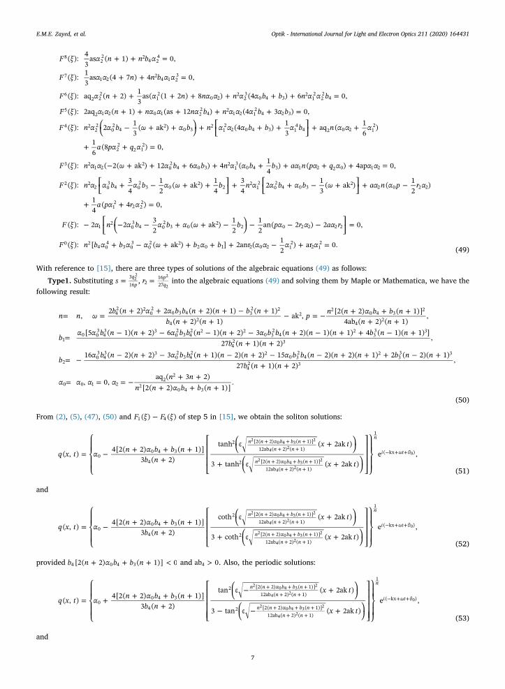
(49)
With reference to [15], there are three types of solutions of the algebraic equations (49) as follows:
Type1. Substituting =s qp
316
22, =r p
q21627
2
2into the algebraic equations (49) and solving them by Maple or Mathematica, we have the
following result:
= =+ + + + − +
+ +− = − + + +
+ +
=− + − − + − + − + + − +
+ +
= −− + − + − + − − + + + − +
+ +
= = = −+ +
+ + +
n n ωb n α α b b n n b n
b n np n n α b b n
n n
bα α b n n α b b n n α b b n n n b n n
b n n
bα b n n α b b n n n α b b n n n b n n
b n n
α α α αn n
n n α b b n
,2 ( 2) 2 ( 2)( 1) ( 1)
( 2) ( 1)ak , [2( 2) ( 1)]
4ab ( 2) ( 1),
[5 ( 1)( 2) 6 ( 1)( 2) 3 ( 2)( 1)( 1) 4 ( 1)( 1) ]27 ( 1)( 2)
,
16 ( 2)( 2) 3 ( 1)( 2)( 2) 15 ( 2)( 2)( 1) 2 ( 2)( 1)27 ( 1)( 2)
,
, 0,aq ( 3 2)
[2( 2) ( 1)].
42 2
02
0 3 4 32 2
42
22
0 4 32
42
10 0
343 3
02
3 42 2 2
0 32
42
33 3
42 3
203
43 3
02
3 42 2
0 32
42
33 3
42 3
0 0 1 22
2
20 4 3
(50)
From (2), (5), (47), (50) and −F ξ F ξ( ) ( )1 4 of step 5 in [15], we obtain the soliton solutions:
=
⎧
⎨⎪
⎩⎪
− + + ++
⎡
⎣
⎢⎢⎢
⎛⎝
+ ⎞⎠
+ ⎛⎝
+ ⎞⎠
⎤
⎦
⎥⎥⎥
⎫
⎬⎪
⎭⎪
+ + ++ +
+ + ++ +
− + +q x t α n α b b nb n
x t
x t( , ) 4[2( 2) ( 1)]
3 ( 2)
tanh ϵ ( 2ak )
3 tanh ϵ ( 2ak )e ,
n n α b b nn n
n n α b b nn n
n
i ωt θ0
0 4 3
4
2 [2( 2) ( 1)]12ab ( 2) ( 1)
2 [2( 2) ( 1)]12ab ( 2) ( 1)
1
( kx )
2 0 4 3 2
4 2
2 0 4 3 2
4 2
0
(51)
and
=
⎧
⎨⎪
⎩⎪
− + + ++
⎡
⎣
⎢⎢⎢
⎛⎝
+ ⎞⎠
+ ⎛⎝
+ ⎞⎠
⎤
⎦
⎥⎥⎥
⎫
⎬⎪
⎭⎪
+ + ++ +
+ + ++ +
− + +q x t α n α b b nb n
x t
x t( , ) 4[2( 2) ( 1)]
3 ( 2)
coth ϵ ( 2ak )
3 coth ϵ ( 2ak )e ,
n n α b b nn n
n n α b b nn n
n
i ωt θ0
0 4 3
4
2 [2( 2) ( 1)]12ab ( 2) ( 1)
2 [2( 2) ( 1)]12ab ( 2) ( 1)
1
( kx )
2 0 4 3 2
4 2
2 0 4 3 2
4 2
0
(52)
provided + + + <b n α b b n[2( 2) ( 1)] 04 0 4 3 and >ab 04 . Also, the periodic solutions:
=
⎧
⎨⎪
⎩⎪
+ + + ++
⎡
⎣
⎢⎢⎢⎢
⎛⎝
− + ⎞⎠
− ⎛⎝
− + ⎞⎠
⎤
⎦
⎥⎥⎥⎥
⎫
⎬⎪
⎭⎪
+ + ++ +
+ + ++ +
− + +q x t α n α b b nb n
x t
x t( , ) 4[2( 2) ( 1)]
3 ( 2)
tan ϵ ( 2ak )
3 tan ϵ ( 2ak )e ,
n n α b b nn n
n n α b b nn n
n
i ωt θ0
0 4 3
4
2 [2( 2) ( 1)]12ab ( 2) ( 1)
2 [2( 2) ( 1)]12ab ( 2) ( 1)
1
( kx )
2 0 4 3 2
4 2
2 0 4 3 2
4 2
0
(53)
and
E.M.E. Zayed, et al. Optik - International Journal for Light and Electron Optics 211 (2020) 164431
7

=
⎧
⎨⎪
⎩⎪
+ + + ++
⎡
⎣
⎢⎢⎢⎢
⎛⎝
− + ⎞⎠
− ⎛⎝
− + ⎞⎠
⎤
⎦
⎥⎥⎥⎥
⎫
⎬⎪
⎭⎪
+ + ++ +
+ + ++ +
− + +q x t α n α b b nb n
x t
x t( , ) 4[2( 2) ( 1)]
3 ( 2)
cot ϵ ( 2ak )
3 cot ϵ ( 2ak )e ,
n n α b b nn n
n n α b b nn n
n
i ωt θ0
0 4 3
4
2 [2( 2) ( 1)]12ab ( 2) ( 1)
2 [2( 2) ( 1)]12ab ( 2) ( 1)
1
( kx )
2 0 4 3 2
4 2
2 0 4 3 2
4 2
0
(54)
provided + + + >b n α b b n[2( 2) ( 1)] 04 0 4 3 , <ab 04 and = ±ϵ 1.
Type2. Substituting =s qp
316
22, =r 02 into the algebraic equations (49) and solving them by Maple or Mathematica, we have the
following result:
= =+ + + + − +
+ +− = − + + +
+ +
= −− + + + − + − +
+ +
= − + + −+
= = = −+ +
+ + +
n n ωα b n α b b n n b n
n n bp n n α b b n
n n
bα α b n n α b b n n b n n
n n b
b α b n α b n n bb n
α α α αn n
n n α b b n
,2 ( 2) 2 ( 2)( 1) ( 1)
( 1)( 2)ak , [2( 2) ( 1)]
4ab ( 2) ( 1),
[ ( 1)( 2) 2 ( 2)( 1) ( 1)( 1) ]( 1)( 2)
,
[( 4) ( 1)( 2) ]( 2)
, , 0,aq ( 1)( 2)
[2( 2) ( 1)].
02
42 2
0 3 4 32 2
24
22
0 4 32
42
102
02
42 2
0 3 42
32 2
24
20 3
20 4 3
42 0 0 1 2
22
0 4 3 (55)
From (2), (5), (47), (55) and F ξ F ξ( ), ( )5 6 of step 5 in [15], we obtain the dark soliton solution:
⎜ ⎟=⎧⎨⎩
− + + ++
⎡
⎣⎢ ± ⎛
⎝− + + +
+ ++ ⎞
⎠
⎤
⎦⎥
⎫⎬⎭
− + +q x t α n α b b nb n
n n α b b nn n
x t( , ) [2( 2) ( 1)]2 ( 2)
1 tanh ϵ [2( 2) ( 1)]4ab ( 2) ( 1)
( 2ak ) e ,n
i ωt θ0
0 4 3
4
20 4 3
2
42
1
( kx )0
(56)
and the singular soliton solution
⎜ ⎟=⎧⎨⎩
− + + ++
⎡
⎣⎢ ± ⎛
⎝− + + +
+ ++ ⎞
⎠
⎤
⎦⎥
⎫⎬⎭
− + +q x t α n α b b nb n
n n α b b nn n
x t( , ) [2( 2) ( 1)]2 ( 2)
1 coth ϵ [2( 2) ( 1)]4ab ( 2) ( 1)
( 2ak ) e .n
i ωt θ0
0 4 3
4
20 4 3
2
42
1
( kx )0
(57)
provided + + + <b n α b b n[2( 2) ( 1)] 04 0 4 3 and <ab 04 .Type3. Substituting =r 02 into the algebraic equations (49) and solving them by Maple or Mathematica, we have the following
result:
= =+ + − −
+− = =
= − + =− ⎡
⎣− + + − ⎤
⎦+
= −− ⎡
⎣− + + − ⎤
⎦+
=+ ⎡
⎣− − ⎤
⎦+
+
+
+
+
n n ωn α b n sα b
n s nα α α
α nn b
bα n α b n n sα b
n s n
bα n α b n n sα b
n s n
bb n q α
n
,4aps( 1) 3nq 6
( 1)ak , , 0,
4as( 1)3
,( 1) nq 4aps( 1)
( 1),
( 2) 3 nq 8aps( 1) 4
2 ( 1),
( 2) 4ns
2ns( 1),
nb
nb
nb
nb
2 0 43as( 1) 2
02
4
22
0 0 1
2 24
1
02
0 2 43as( 1) 2
02
4
2
2
0 0 2 43as( 1) 2
02
4
2
3
4 23as( 1)
0
4
4
4
4
(58)
provided <sab 04 . From (2), (5), (47), (58) and −F ξ F ξ( ) ( )7 20 of step 5 in [15], we obtain the soliton solutions:
= ⎧⎨⎩
− − + ⎡
⎣⎢
+− + +
⎤
⎦⎥
⎫⎬⎭
− + +q x t α nn b
p x tq p x t
( , ) 6pq 4as( 1)3
sech [ ( 2ak )]3 4ps(1 ϵ tanh[ ( 2ak )])
e ,n
i ωt θ0 2 2
4
2
22 2
1
( kx )0
(59)
provided > <p q0, 02 and <s 0.
= ⎧⎨⎩
+ − + ⎡
⎣⎢
+− + +
⎤
⎦⎥
⎫⎬⎭
− + +q x t α nn b
p x tq p x t
( , ) 6pq 4as( 1)3
csch [ ( 2ak )]3 4ps(1 ϵ coth[ ( 2ak )])
e ,n
i ωt θ0 2 2
4
2
22 2
1
( kx )0
(60)
provided > >p q0, 02 and <s 0.
= ⎧⎨⎩
− − + ⎡⎣⎢
++ +
⎤⎦⎥
⎫⎬⎭
− + +q x t α p nn b
p x tq p x t
( , ) 6 4as( 1)3
sech [ ( 2ak )]3 4ϵ 3ps tanh[ ( 2ak )]
e ,n
i ωt θ0 2
4
2
2
1
( kx )0
(61)
provided > <p q0, 02 and >s 0.
E.M.E. Zayed, et al. Optik - International Journal for Light and Electron Optics 211 (2020) 164431
8

= ⎧⎨⎩
+ − + ⎡⎣⎢
++ +
⎤⎦⎥
⎫⎬⎭
− + +q x t α p nn b
p x tq p x t
( , ) 6 4as( 1)3
csch [ ( 2ak )]3 4ϵ 3ps coth[ ( 2ak )]
e ,n
i ωt θ0 2
4
2
2
1
( kx )0
(62)
provided > >p q0, 02 and >s 0. We obtain the bright soliton solutions:
= ⎧⎨⎩
+ − + ⎡
⎣⎢ + − +
⎤
⎦⎥
⎫⎬⎭
− + +q x t α p nn b M p x t M q
( , ) 12 4as( 1)3
12 cosh [ϵ ( 2ak )] ( 3 )
e ,n
i ωt θ0 2
42
2
1
( kx )0
(63)
= ⎧⎨⎩
+ − + ⎡
⎣⎢ + −
⎤
⎦⎥
⎫⎬⎭
− + +q x t α p nn b M p x t q
( , ) 12 4as( 1)3
1ϵ cosh[2 ( 2ak )] 3
e ,n
i ωt θ0 2
4 2
1
( kx )0
(64)
provided > <p q0, 02 and = − >M q(9 48ps) 022 . We obtain the singular soliton solutions:
= ⎧⎨⎩
+ − + ⎡
⎣⎢ + + −
⎤
⎦⎥
⎫⎬⎭
− + +q x t α p nn b M p x t M q
( , ) 12 4as( 1)3
12 sinh [ϵ ( 2ak )] ( 3 )
e ,n
i ωt θ0 2
42
2
1
( kx )0
(65)
provided > <p q0, 02 and >M 0.
= ⎧⎨⎩
+ − + ⎡
⎣⎢ − + −
⎤
⎦⎥
⎫⎬⎭
− + +q x t α p nn b M p x t q
( , ) 12 4as( 1)3
1ϵ sinh[2 ( 2ak )] 3
e ,n
i ωt θ0 2
4 2
1
( kx )0
(66)
provided >p 0, <q 02 and <M 0. and = ±ϵ 1. Also, the periodic solutions:
= ⎧⎨⎩
− − + ⎡⎣⎢
− ++ − − +
⎤⎦⎥
⎫⎬⎭
− + +q x t α p nn b
p x tq p x t
( , ) 6 4as( 1)3
sec [ ( 2ak )]3 4ϵ 3ps tan[ ( 2ak )]
e ,n
i ωt θ0 2
4
2
2
1
( kx )0
(67)
= ⎧⎨⎩
− − + ⎡⎣⎢
− ++ − − +
⎤⎦⎥
⎫⎬⎭
− + +q x t α p nn b
p x tq p x t
( , ) 6 4as( 1)3
csc [ ( 2ak )]3 4ϵ 3ps cot[ ( 2ak )]
e ,n
i ωt θ0 2
4
2
2
1
( kx )0
(68)
provided <p 0, >q 02 and >s 0.
= ⎧⎨⎩
− − + ⎡
⎣⎢
− +− − − +
⎤
⎦⎥
⎫⎬⎭
− + +q x t α p nn b
p x tM M q p x t
( , ) 12 4as( 1)3
sec [ϵ ( 2ak )]2 ( 3 )sec [ϵ ( 2ak )]
e ,n
i ωt θ0 2
4
2
22
1
( kx )0
(69)
= ⎧⎨⎩
+ − + ⎡
⎣⎢
− +− + − +
⎤
⎦⎥
⎫⎬⎭
− + +q x t α p nn b
p x tM M q p x t
( , ) 12 4as( 1)3
csc [ϵ ( 2ak )]2 ( 3 )csc [ϵ ( 2ak )]
e ,n
i ωt θ0 2
4
2
22
1
( kx )0
(70)
provided <p 0 and >M 0.
= ⎧⎨⎩
+ − + ⎡
⎣⎢ − + −
⎤
⎦⎥
⎫⎬⎭
− + +q x t α p nn b M p x t q
( , ) 12 4as( 1)3
1ϵ cos[2 ( 2ak )] 3
e ,n
i ωt θ0 2
4 2
1
( kx )0
(71)
= ⎧⎨⎩
+ − + ⎡
⎣⎢ − + −
⎤
⎦⎥
⎫⎬⎭
− + +q x t α p nn b M p x t q
( , ) 12 4as( 1)3
1ϵ sin[2 ( 2ak )] 3
e ,n
i ωt θ0 2
4 2
1
( kx )0
(72)
provided <p 0, <q 02 and >M 0.
5. Extended auxiliary equation
According to this method, we assume that Eq. (6) has the same formal solution (47), while the function F ξ( ) satisfies the followingfirst order equation:
′ = + + +F ξ c c F ξ c F ξ c F ξ( ) ( ) ( ) ( ),20 2
24
46
6 (73)
where =c j d( 0, 2, , 6)j are constants to be determined. It is well known that Eq. (73) has the following solution:
= ⎡⎣⎢
− ± ⎤⎦⎥
F ξ cc
f ξ( ) 12
(1 ( )) ,4
6
12
(74)
where f ξ( ) could be expressed through the Jacobi elliptic functions ξ m ξ msn( , ), cn( , ), ξ mdn( , ) and so on. Here < <m0 1 is the
E.M.E. Zayed, et al. Optik - International Journal for Light and Electron Optics 211 (2020) 164431
9

modulus of the Jacobi elliptic functions. Substituting (47) along with (73) into Eq. (6), collecting the coefficients of each power′ = … =F τ F τ l j( )( ( )) , ( 0, 1, 2, ,8, 0, 1)l j , and setting these coefficients to zero, we have the following set of algebraic equations:
+ + =+ + =+ + + + + + + =
+ + + + + =
⎛⎝
− + + ⎞⎠
+ ⎡⎣
+ + ⎤⎦
+ +
+ + =
− + + + + + + + + =
⎡⎣
+ − + + ⎤⎦
+ ⎡⎣
+ − + ⎤⎦
+ −
+ + =
− ⎡⎣
⎛⎝
− − + + − ⎞⎠
− − − ⎤⎦
=
+ − + + + + − + =
F ξ α n n b αF ξ α α n n b α αF ξ α n α n nα α n α α b b n α α bF ξ α α n nα α nα b n α α α b α b
F ξ n α α b ω α b n α α α b b α b n α α α
a c α c α
F ξ n α α ω α b α b n α α b b aα n c α c α α α
F ξ n α α b α b α ω b n α α b α b ω aα n α c c α
a c α c α
F ξ α n α b α b α ω b c α c α aα c
F ξ n b α b α α ω b α b α α α α
( ): 4ac ( 1) 0,( ): ac (4 7 ) 4 0,( ): 2ac ( 2) ac ( (1 2 ) 8 ) (4 ) 6 0,( ): 4ac ( 1) (3ac 12 ) (4 3 ) 0,
( ): 2 13
( ak ) (4 ) 13
2ac ( 16
)
16
(8 2 ) 0,
( ): ( 2( ak ) 12 6 ) 4 ( 14
) ( 2 ) 4ac 0,
( ): 34
12
( ak ) 14
34
2 13
( ak ) ( 12
)
14
( 4 ) 0,
( ): 2 2 32
( ak ) 12
12
an( 2 ) 2 0,
( ): [ ( ak ) ] 2anc ( 12
) ac 0.
86 2
2 24 2
4
76 1 2
24 1 2
3
64 2
26 1
20 2
223
0 4 32
12
22
45
4 1 2 0 1 6 22
42
1 2 12
4 2 3
4 222
02
42
0 32
12
2 0 4 3 14
4 4 0 2 12
2 22
4 12
3 21 2
202
4 0 32
13
0 4 3 1 2 2 4 0 2 1 2
2 22 0
34 0
23 0
22
212
02
4 0 32
2 0 2 0 2
2 12
0 22
12
03
4 02
3 02
2 2 0 0 2 2 0
0 24 0
43 0
302 2
2 0 1 0 0 2 12
0 12
(75)
By solving the system (75), the following solution set is recovered:
= =+ + + + − + + + +
+ +
=− − + + + + + +
+ +
= −− + − + + − + −
+ +
= = = − + + ++ +
= −+
= = =
n n ωn n n α b n n n n n α b n
n n n
bα n a α c α c n n n α b n n α b n
n n n
ba n n α c α c n α b n n n α b n
n n n
c c c c c n α α b n b na n n
cn α ba n
α α α α α
,4ac ( 2)( 1) 6 ( 2) ak ( 1)( 2) 6 ( 1)
( 3 2),
( 1)[4 ( )( 1)( 2) 3 ( 2) 2 ( 1)]( 3 2)
,
2 ( 4)( 1)(2 ) 3 ( 1)( 2) 4 ( 4)( 3 2)
,
, , [2 ( 2) ( 1)]2 ( 3 2)
,4 ( 1)
, , 0, .
22
02
42 2 2
0 32 2
10 0 2 2 0
203
42
02
32 2
2
20 2 2 0
202
32
03
42
2 2
0 0 2 2 42
2 0 4 32 6
222
40 0 1 2 2
(76)
From (2), (5), (47), (74) and (76), then we have the solutions:
⎜ ⎟= ⎧⎨⎩
− ++
± ⎛⎝
+ + ++
⎞⎠
⎫⎬⎭
− + +q x t n bn b
n b α n bn b
f ξ( , ) ( 1)2( 2)
2( 2) ( 1)2( 2)
( ) e ,n
i ωt θ3
4
4 0 3
4
1
( kx )0
(77)
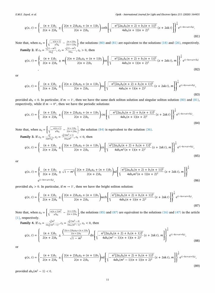
provided <b b 03 4 . We have the following families of Jacobi elliptic functions solutions of Eq. (1):
Family 1. If = −c c m
c m0( 1)
3243 2
62 2 , = −c c m
c m2(5 1)16
42 2
6 2 , >c 06 , then
⎜ ⎟= ⎧⎨⎩
− ++
± ⎛⎝
+ + ++
⎞⎠
⎡
⎣⎢ − + + +
+ ++ ⎤
⎦⎥
⎫⎬⎭
− + +q x t n bn b
n b α n bn b
n α b n b nb n n
x t m( , ) ( 1)2( 2)
2( 2) ( 1)2( 2)
sn [2 ( 2) ( 1)]4am ( 1)( 2)
( 2ak ), e ,n
i ωt θ3
4
4 0 3
4
20 4 3
2
24
2
1
( kx )0
(78)
or
⎜ ⎟= ⎧⎨⎩
− ++
± ⎛⎝
+ + ++
⎞⎠
⎡
⎣⎢ − + + +
+ ++ ⎤
⎦⎥
⎫⎬⎭
− + +q x t n bn b
n b α n bn b m
n α b n b nb n n
x t m( , ) ( 1)2( 2)
2( 2) ( 1)2( 2)
ns [2 ( 2) ( 1)]4am ( 1)( 2)
( 2ak ), e ,n
i ωt θ3
4
4 0 3
4
20 4 3
2
24
2
1
( kx )0
(79)
provided <ab 04 . In particular, if → −m 1 , then we have the dark soliton solution:
⎜ ⎟= ⎧⎨⎩
− ++
± ⎛⎝
+ + ++
⎞⎠
⎡
⎣⎢ − + + +
+ ++ ⎤
⎦⎥
⎫⎬⎭
− + +q x t n bn b
n b α n bn b
n α b n b nn n
x t( , ) ( 1)2( 2)
2( 2) ( 1)2( 2)
tanh [2 ( 2) ( 1)]4ab ( 1)( 2)
( 2ak ) e ,n
i ωt θ3
4
4 0 3
4
20 4 3
2
42
1
( kx )0
(80)
as well as the singular soliton solution:
E.M.E. Zayed, et al. Optik - International Journal for Light and Electron Optics 211 (2020) 164431
10
⎜ ⎟= ⎧⎨⎩
− ++
± ⎛⎝
+ + ++
⎞⎠
⎡
⎣⎢ − + + +
+ ++ ⎤
⎦⎥
⎫⎬⎭
− + +q x t n bn b
n b α n bn b
n α b n b nn n
x t( , ) ( 1)2( 2)
2( 2) ( 1)2( 2)
coth [2 ( 2) ( 1)]4ab ( 1)( 2)
( 2ak ) e .n
i ωt θ3
4
4 0 3
4
20 4 3
2
42
1
( kx )0
(81)
Note that, when = ⎡⎣
− − ⎤⎦
+ ++α a n
n bn bn b0
( 1) ( 1)2( 2)2 4
34, the solutions (80) and (81) are equivalent to the solutions (18) and (26), respectively.
Family 2. If = −c c mc0
(1 )32
43 2
62 , = −c c m
c2(5 )16
42 2
6, >c 06 , then
⎜ ⎟= ⎧⎨⎩
− ++
± ⎛⎝
+ + ++
⎞⎠
⎡
⎣⎢ − + + +
+ ++ ⎤
⎦⎥
⎫⎬⎭
− + +q x t n bn b
m n b α n bn b
n α b n b nn n
x t m( , ) ( 1)2( 2)
2( 2) ( 1)2( 2)
sn [2 ( 2) ( 1)]4ab ( 1)( 2)
( 2ak ), e
,
ni ωt θ3
4
4 0 3
4
20 4 3
2
42
1
( kx )0
(82)
or
⎜ ⎟= ⎧⎨⎩
− ++
± ⎛⎝
+ + ++
⎞⎠
⎡
⎣⎢ − + + +
+ ++ ⎤
⎦⎥
⎫⎬⎭
− + +q x t n bn b
n b α n bn b
n α b n b nn n
x t m( , ) ( 1)2( 2)
2( 2) ( 1)2( 2)
ns [2 ( 2) ( 1)]4ab ( 1)( 2)
( 2ak ), e ,n
i ωt θ3
4
4 0 3
4
20 4 3
2
42
1
( kx )0
(83)
provided <ab 04 . In particular, if → −m 1 , then we have the same dark soliton solution and singular soliton solution (80) and (81),respectively, while if → +m 0 , then we have the periodic solutions:
⎜ ⎟= ⎧⎨⎩
− ++
± ⎛⎝
+ + ++
⎞⎠
⎡
⎣⎢ − + + +
+ ++ ⎤
⎦⎥
⎫⎬⎭
− + +q x t n bn b
n b α n bn b
n α b n b nn n
x t( , ) ( 1)2( 2)
2( 2) ( 1)2( 2)
csc [2 ( 2) ( 1)]4ab ( 1)( 2)
( 2ak ) e .n
i ωt θ3
4
4 0 3
4
20 4 3
2
42
1
( kx )0
(84)
Note that, when = ⎡⎣
− − ⎤⎦
+ ++α a n
n bn bn b0
( 1) ( 1)2( 2)2 4
34, the solution (84) is equivalent to the solution (36).
Family 3. If =c c
m c0 3243
262 , = +c c m
c m2(4 1)16
42 2
6 2 , <c 06 , then
⎜ ⎟= ⎧⎨⎩
− ++
± ⎛⎝
+ + ++
⎞⎠
⎡
⎣⎢
+ + ++ +
+ ⎤
⎦⎥
⎫⎬⎭
− + +q x t n bn b
n b α n bn b
n α b n b nm n n
x t m( , ) ( 1)2( 2)
2( 2) ( 1)2( 2)
cn [2 ( 2) ( 1)]4ab ( 1)( 2)
( 2ak ), e ,n
i ωt θ3
4
4 0 3
4
20 4 3
2
42 2
1
( kx )0
(85)
or
⎜ ⎟= ⎧⎨⎩
− ++
± − ⎛⎝
+ + ++
⎞⎠
⎡
⎣⎢
+ + ++ +
+ ⎤
⎦⎥
⎫⎬⎭
− + +
q x t n bn b
m n b α n bn b
n α b n b nm n n
x t m( , ) ( 1)2( 2)
1 2( 2) ( 1)2( 2)
sd [2 ( 2) ( 1)]4ab ( 1)( 2)
( 2ak ),
e ,
n
i ωt θ
3
4
2 4 0 3
4
20 4 3
2
42 2
1
( kx )0 (86)
provided >ab 04 . In particular, if → −m 1 , then we have the bright soliton solution:
⎜ ⎟= ⎧⎨⎩
− ++
± ⎛⎝
+ + ++
⎞⎠
⎡
⎣⎢
+ + ++ +
+ ⎤
⎦⎥
⎫⎬⎭
− + +q x t n bn b
n b α n bn b
n α b n b nn n
x t( , ) ( 1)2( 2)
2( 2) ( 1)2( 2)
sech [2 ( 2) ( 1)]4ab ( 1)( 2)
( 2ak ) e .n
i ωt θ3
4
4 0 3
4
20 4 3
2
42
1
( kx )0
(87)
Note that, when = ⎡⎣
− ⎤⎦
+ ++α a n m
n bn bn b0
( 1) ( 1)2( 2)
22 4
34, the solutions (85) and (87) are equivalent to the solutions (16) and (47) in the article
[1], respectively.
Family 4. If =−
c c m
c m0 32 ( 1)43 2
62 2 , = −
−c c m
c m2(5 4)
16 ( 1)42 2
6 2 , <c 06 , then
=⎧
⎨⎩
− ++
±−
⎡
⎣⎢ − + + +
− + ++ ⎤
⎦⎥
⎫
⎬⎭
+ + ++ − + +
( )q x t n b
n b mn α b n b n
m n nx t m( , ) ( 1)
2( 2) 1dn [2 ( 2) ( 1)]
4ab ( 1)( 1)( 2)( 2ak ), e ,
n b α n bn b
n
i ωt θ3
4
2( 2) ( 1)2( 2)
2
20 4 3
2
42 2
1
( kx )
4 0 34 0
(88)
or
⎜ ⎟= ⎧⎨⎩
− ++
± ⎛⎝
+ + ++
⎞⎠
⎡
⎣⎢ − + + +
− + ++ ⎤
⎦⎥
⎫⎬⎭
− + +q x t n bn b
n b α n bn b
n α b n b nm n n
x t m( , ) ( 1)2( 2)
2( 2) ( 1)2( 2)
nd [2 ( 2) ( 1)]4ab ( 1)( 1)( 2)
( 2ak ), e ,n
i ωt θ3
4
4 0 3
4
20 4 3
2
42 2
1
( kx )0
(89)
provided − <mab ( 1) 042 .
E.M.E. Zayed, et al. Optik - International Journal for Light and Electron Optics 211 (2020) 164431
11

Family 5. If =−
c c
c m0 32 (1 )43
62 2 , = −
−c c m
c m2(4 5)
16 ( 1)42 2
6 2 , >c 06 , then
⎜ ⎟= ⎧⎨⎩
− ++
± ⎛⎝
+ + ++
⎞⎠
⎡
⎣⎢ − + + +
− + ++ ⎤
⎦⎥
⎫⎬⎭
− + +q x t n bn b
n b α n bn b
n α b n b nm n n
x t m( , ) ( 1)2( 2)
2( 2) ( 1)2( 2)
nc [2 ( 2) ( 1)]4ab (1 )( 1)( 2)
( 2ak ), e ,n
i ωt θ3
4
4 0 3
4
20 4 3
2
42 2
1
( kx )0
(90)
or
=⎧
⎨⎩
− ++
±−
⎡
⎣⎢ − + + +
− + ++ ⎤
⎦⎥
⎫
⎬⎭
+ + ++ − + +
( )q x t n b
n b mn α b n b n
m n nx t m( , ) ( 1)
2( 2) 1ds [2 ( 2) ( 1)]
4ab (1 )( 1)( 2)( 2ak ), e ,
n b α n bn b
n
i ωt θ3
4
2( 2) ( 1)2( 2)
2
20 4 3
2
42 2
1
( kx )
4 0 34 0
(91)
provided <ab 04 . In particular, if → +m 0 , then we have the same periodic solutions (84) and the periodic solutions:
⎜ ⎟= ⎧⎨⎩
− ++
± ⎛⎝
+ + ++
⎞⎠
⎡
⎣⎢ − + + +
+ ++ ⎤
⎦⎥
⎫⎬⎭
− + +q x t n bn b
n b α n bn b
n α b n b nn n
x t( , ) ( 1)2( 2)
2( 2) ( 1)2( 2)
sec [2 ( 2) ( 1)]4ab ( 1)( 2)
( 2ak ) e .n
i ωt θ3
4
4 0 3
4
20 4 3
2
42
1
( kx )0
(92)
Note that, when = ⎡⎣
− − ⎤⎦
+ ++α a n
n bn bn b0
( 1) ( 1)2( 2)2 4
34, the solution (92) is equivalent to the solution (60) in the article [1].
Family 6. If =−
c c
c m0 32 (1 )43
62 2 , = −
−c c m
c m2(4 5)
16 ( 1)42 2
6 2 , >c 06 , then
⎜ ⎟= ⎧⎨⎩
− ++
± ⎛⎝
+ + ++
⎞⎠
⎡
⎣⎢
+ + ++ +
+ ⎤
⎦⎥
⎫⎬⎭
− + +q x t n bn b
n b α n bn b
n α b n b nn n
x t m( , ) ( 1)2( 2)
2( 2) ( 1)2( 2)
dn [2 ( 2) ( 1)]4ab ( 1)( 2)
( 2ak ), e ,n
i ωt θ3
4
4 0 3
4
20 4 3
2
42
1
( kx )0
(93)
or
⎜ ⎟= ⎧⎨⎩
− ++
± − ⎛⎝
+ + ++
⎞⎠
⎡
⎣⎢
+ + ++ +
+ ⎤
⎦⎥
⎫⎬⎭
− + +
q x t n bn b
m n b α n bn b
n α b n b nn n
x t m( , ) ( 1)2( 2)
1 2( 2) ( 1)2( 2)
nd [2 ( 2) ( 1)]4ab ( 1)( 2)
( 2ak ),
e ,
n
i ωt θ
3
4
2 4 0 3
4
20 4 3
2
42
1
( kx )0 (94)
provided >ab 04 . In particular, if → −m 1 , then we have the same bright soliton solutions (87).
6. Conclusions
This paper implements three innovative integration schemes to the KE that serves as the latest model to address soliton dynamicsin nonlinear optical fibers. While the model is at its infancy, the soliton solutions reported in this paper as well as earlier serve as astrong footing to advance further along with KE. One of the immediate project that needs to be talked about is the formulation of themodel for birefringent fibers and with DWDM topology. The model will also be applied to additional optoelectronic devices such asoptical couplers, magneto-optic waveguides, PCF, matamaterials and such. Those studies are being currently undertaken. Theirexpected results are on the horizon and are soon to be visible.
Conflict of interest
The authors also declare that there is no conflict of interest.
Acknowledgements
The research work of the seventh author (MRB) was supported by the grant NPRP 11S-1246-170033 from QNRF and he isthankful for it.
References
[1] A. Biswas, A. Sonmezoglu, M. Ekici, A.S. Alshomrani, M.R. Belic, Optical solitons with Kudryashov's equation by F -expansion, Optik 199 (2019) 163338.[2] A. Biswas, J.V. Guzmá, M. Ekici, Q. Zhou, H. Triki, A.S. Alshomrani, M.R. Belic, Optical solitons and conservation laws of Kudryashov's equation using un-
determined coefficients, Optik 200 (2020) 163417.[3] A. Biswas, M. Ekici, A. Sonmezoglu, A.S. Alshomrani, M.R. Belic, Optical solitons with Kudryashov's equation by extended trial function, Optik 202 (2020)
163290.[4] N.A. Kudryashov, A generalized model for description of propagation pulses in optical fiber, Optik 189 (2019) 42–52.[5] N.A. Kyudryashov, First integrals and general solution of the traveling wave reduction for Schrödinger equation with anti-cubic nonlinearity, Optik 185 (2019)
665–671.[6] N.A. Kudryashov, Traveling wave solutions of the generalized nonlinear Schrödinger equation with cubic-quintic nonlinearity, Optik 188 (2019) 27–35.
E.M.E. Zayed, et al. Optik - International Journal for Light and Electron Optics 211 (2020) 164431
12

[7] N.A. Kudryashov, The Painlev approach for finding solitary wave solutions of nonlinear nonintegrable differential equations, Optik 183 (2019) 642–649.[8] N.A. Kudryashov, Solitary and periodic waves of the hierarchy for propagation pulse in optical fiber, Optik 194 (2019) 163060.[9] N.A. Kudryashov, Construction of nonlinear differential equations for description of propagation pulses in optical fiber, Optik 192 (2019) 162964.
[10] N.A. Kudryashov, D.V. Safonova, A. Biswas, Painleve Analysis and a Solution to the Traveling Wave Reduction of the Radhakrishnan–Kundu–LakshmananEquation, Regul. Chaotic Dyn. 24 (6) (2019) 607–614.
[11] A.M. Wazwaz, A variety of optical solitons for nonlinear Schrödinger equation with detuning term by the variational iteration method, Optik 196 (2019) 163169.[12] A.M. Wazwaz, Bright and dark optical solitons for (2+1)-dimensional Schrödinger (NLS) equations in the anomalous dispersion regimes and the normal
dispersive regimes, Optik 192 (2019) 162948.[13] G. Xu, Extended auxiliary equation method and its applications to three generalized NLS equations, Abstract Appl. Anal. 2014 (2014) 541370.[14] E.M.E. Zayed, R.M.A. Shohib, Solitons and other solutions to the improved perturbed nonlinear Schrodinger equation with the dual-power law nonlinearity using
different techniques, Optik 171 (2018) 27–43.[15] E.M.E. Zayed, K.A.E. Alurrfi, Solitons and other solutions for two nonlinear Schrodinger equations using the new mapping method, Optik 144 (2017) 132–148.
E.M.E. Zayed, et al. Optik - International Journal for Light and Electron Optics 211 (2020) 164431
13