Optical implementation of the fractional Hilbert transform for two-dimensional objects

$: Optical implementation of the fractional Hilbert transform for two-dimensional objects$
Optical implementation of the fractionalHilbert transform for two-dimensional objects

A. W. Lohmann, E. Tepichın, and J. G. Ramırez

The classical Hilbert transform can be implemented optically as a spatial-filtering process, whereby half theFourier spectrum is p-phase shifted. Recently the Hilbert transform was generalized. The generalized ver-sion, called the fractional Hilbert transform, is quite easy to implement optically if the input is one dimensional.Here we show how to implement the fractional Hilbert transform for two-dimensional inputs. Hence the newtransform is now suitable for image processing. © 1997 Optical Society of America

Key words: Fractional Hilbert transform, image processing.

1. Motivation and Plan

Recently several transforms with relevance to opticshave been generalized by definition of fractional ver-sions of those transforms, which are known by thenames of their inventors: Fourier, Hartley, Leg-endre, and Hilbert. If any one of those classicaltransforms is repeated m times, we call it a transformof degree m, where m obviously is an integer. Thefractional versions thereof are generalizations char-acterized by an index P, which now is real-valued andnot necessarily an integer anymore.

Here we are concerned with the Hilbert transform,1whose history related to its optical implementationand generalization procedure has been reported be-fore.2 It is quite easy to implement the fractional Hil-bert transform ~FRH! if the input is one dimensional.3However, in this project we show how to implementthe FRH for two-dimensional optical inputs as well.It is not quite as simple as implementation for one-dimensional inputs. But the extension to two-dimensional inputs is mandatory if one wants to usethe FRH for processing two-dimensional images.Digital simulations have shown that FRH image pro-cessing is fruitful.2

One of the obstacles we face when admitting two-dimensional inputs u0~x, y! to the FRH is a displayproblem, because the output up~x, y! depends on

The authors are with the National Institute of Astrophysics,Optics, and Electronics, Apdo. Postal 51 y 216, Puebla 72000,Puebla, Mexico.

Received 5 December 1996; revised manuscript received 3 April1997.

0003-6935y97y266620-07$10.00y0© 1997 Optical Society of America

6620 APPLIED OPTICS y Vol. 36, No. 26 y 10 September 1997

three continuous variables ~x, y, P!. The term P isthe fractional degree. It is zero if the output is anordinary image. And P 5 1 corresponds to the out-put of the classical Hilbert transform. The P depen-dence of the output up~x, y! is periodic in P, with acycle of DP 5 4. Because of the periodicity it isconvenient to relate P to an angle:

f 5 Pp

2. (1)

Our plan is, in Section 2, to review briefly how theFRH emerges from the classical Hilbert transform.In Section 3 we present the optical setup for perform-ing the FRH. The fractional degree P can be variedeasily by rotation of a polarizer. In Section 4, we givesome experimental results. Those results indicatethat the FRH—in contrast with the classical Hilberttransform—is able to detect the positive or negativesign of the gradient ]u0y]x. In Section 5 we suggestfour modifications of the basic setup as presented inSection 3. These modifications are appropriate if thecritical components do not exist with the correct pa-rameters or if they do not exist at all. The criticalcomponents are a pair of identical Wollaston prisms.Finally, in Section 6 we summarize and propose someother two-dimensional FRH schemes. They are rea-sonable because the step from one dimension ~x! to twodimensions ~x, y! was somewhat ambiguous.

2. Review of the Hilbert Fractionalization

The classical Hilbert transform v~x! of a one-dimensional input u~x! can be written either as aconvolution,

u~x! 3 u~x!p~21ypx! 5 v~x!, (2)

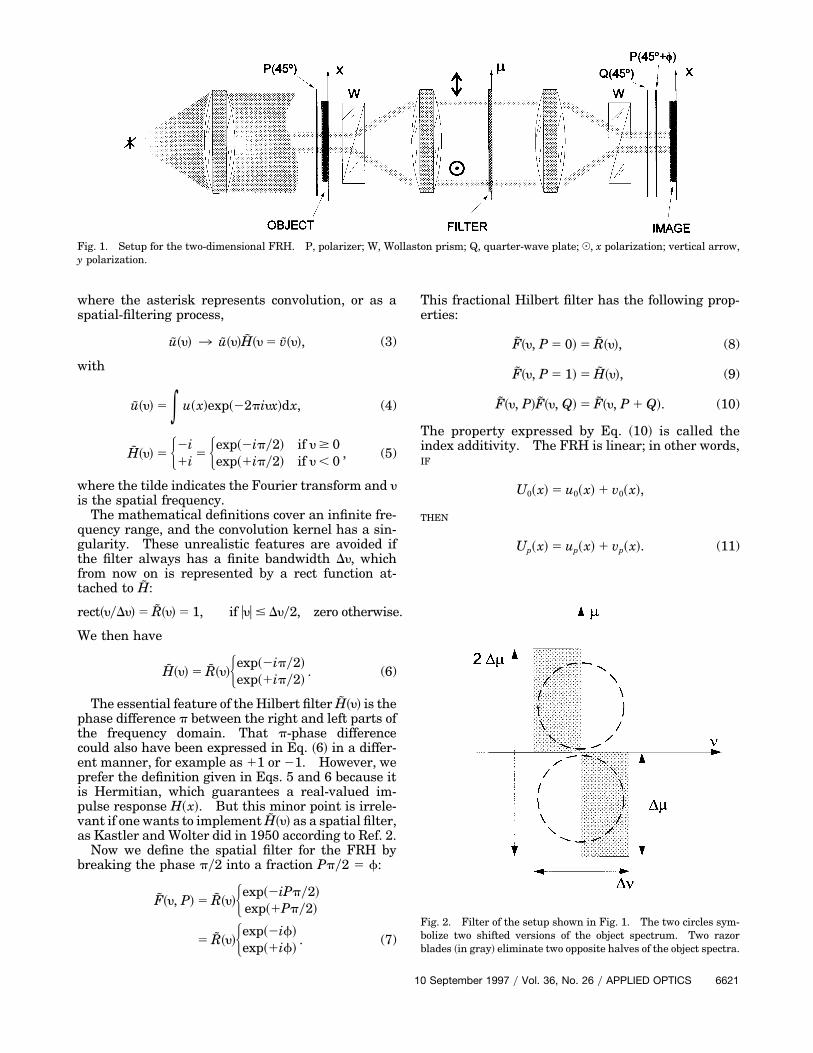
Fig. 1. Setup for the two-dimensional FRH. P, polarizer; W, Wollaston prism; Q, quarter-wave plate; J, x polarization; vertical arrow,y polarization.

where the asterisk represents convolution, or as aspatial-filtering process,

u~y! 3 u~y!H~y 5 v~y!, (3)

with

u~y! 5 * u~x!exp~22piyx!dx, (4)

H~y! 5 H2i1i 5 Hexp~2ipy2!

exp~1ipy2!if y $ 0if y , 0 , (5)

where the tilde indicates the Fourier transform and yis the spatial frequency.

The mathematical definitions cover an infinite fre-quency range, and the convolution kernel has a sin-gularity. These unrealistic features are avoided ifthe filter always has a finite bandwidth Dy, whichfrom now on is represented by a rect function at-tached to H:

rect~yyDy! 5 R~y! 5 1, if uyu # Dyy2, zero otherwise.

We then have

H~y! 5 R~y!Hexp~2ipy2!exp~1ipy2!

. (6)

The essential feature of the Hilbert filter H~y! is thephase difference p between the right and left parts ofthe frequency domain. That p-phase differencecould also have been expressed in Eq. ~6! in a differ-ent manner, for example as 11 or 21. However, weprefer the definition given in Eqs. 5 and 6 because itis Hermitian, which guarantees a real-valued im-pulse response H~x!. But this minor point is irrele-vant if one wants to implement H~y! as a spatial filter,as Kastler and Wolter did in 1950 according to Ref. 2.

Now we define the spatial filter for the FRH bybreaking the phase py2 into a fraction Ppy2 5 f:

F~y, P! 5 R~y!Hexp~2iPpy2!exp~1Ppy2!

5 R~y!Hexp~2if!exp~1if!

. (7)

This fractional Hilbert filter has the following prop-erties:

F~y, P 5 0! 5 R~y!, (8)

F~y, P 5 1! 5 H~y!, (9)

F~y, P!F~y, Q! 5 F~y, P 1 Q!. (10)

The property expressed by Eq. ~10! is called theindex additivity. The FRH is linear; in other words,IF

U0~x! 5 u0~x! 1 v0~x!,

THEN

Up~x! 5 up~x! 1 vp~x!. (11)

Fig. 2. Filter of the setup shown in Fig. 1. The two circles sym-bolize two shifted versions of the object spectrum. Two razorblades ~in gray! eliminate two opposite halves of the object spectra.

10 September 1997 y Vol. 36, No. 26 y APPLIED OPTICS 6621

Fig. 3. Fractional Hilbert images of the cross-type input object, shown in the upper left-hand corner. The corresponding fractionaldegree P appears at the top of each image. For P 5 0 the output is an ordinary image; for P 5 1, we obtain the classical Hilbert transform.

Another important property emerges if we decom-pose the exponential exp~6if! 5 cos f 6 i sin f:

F~y, f! 5 R~y!cos f 1 H~y!sin f

5 F~y, 0!cos f 1 F~y, py2!sin f. (12)

The FRH apparently is a superpositioning of ordinaryimaging and classical Hilbert filtering, with variableweights cos f and sin f, respectively.

3. Optical Implementation of the Fractional HilbertTransform

As shown in Fig. 1, the object is illuminated by amonochromatic plane wave. A polarizer at a 45° ori-entation ensures that the two polarization compo-nents ~in the x and y directions! are equally strong.A Wollaston prism W splits the two polarization com-ponents so that two spatial-frequency spectra u~y, m1 m0! and u~y, m 2 m0! will appear above each otherin the filter plane. There, one of the spectra loses itspositive frequencies ~y . 0! and the other ~u! loses itsnegative frequencies ~see Fig. 2!. This is achievedby two properly located razor blades known as knifeedges.

A second Wollaston prism W located shortly be-fore the image plane ~Fig. 1! realigns the two lin-early polarized components. A quarter-wave plateQ ~at a 45° orientation! converts the two orthogonallinear-polarization components into two circular-


polarized components, with opposite circular direc-tions. The final polarizer at an orientation of ~45°1 f! produces phase shifts 6f for the two polariza-tion components, which have traveled through theupper and lower parts of the filter ~Fig. 2!, respec-tively. In other words, that polarizer varies thephase f, as it appeared in the FRH filter @Eqs. ~7!and ~12!#. Hence the image amplitude is the out-put of the FRH:

uP~x, y! 5 u~x, y; f!

5 ** u0~y, m!F~y, m; f!

3 exp@2pi~xy 1 ym!#dydm. (13)

4. Experimental Results

Stimulated by the digital simulations in Ref. 2 weused as inputs, among others, binary pure-amplitudeand binary pure-phase objects:

u0~x, y! 5 R~xyDx!,

u0~x, y! 5 1 1 @exp~ia! 2 1#R~xyDx!. (14)

The output intensities uuP~x, y!u2 are shown in Figs.3–7 for values of P 5 0, 0.25, 0.5, 0.75, 1. As areference, we also show in each figure the correspond-ing input intensity uu0~x, y!u2.

We show first in Fig. 3 the experimental results

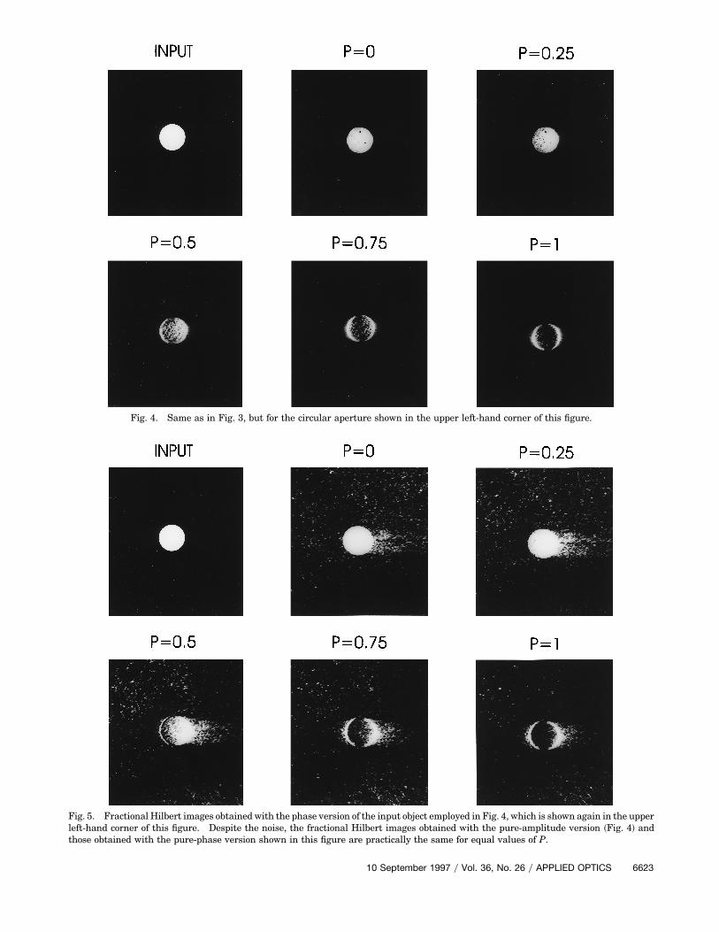
Fig. 4. Same as in Fig. 3, but for the circular aperture shown in the upper left-hand corner of this figure.

Fig. 5. Fractional Hilbert images obtained with the phase version of the input object employed in Fig. 4, which is shown again in the upperleft-hand corner of this figure. Despite the noise, the fractional Hilbert images obtained with the pure-amplitude version ~Fig. 4! andthose obtained with the pure-phase version shown in this figure are practically the same for equal values of P.


Fig. 6. Same as in Fig. 3, but for the input object shown in the upper left-hand corner, orientated at 0°.

Fig. 7. Same as in Fig. 6, but for an in-plane rotation of the input object of 90°.


obtained with a simple amplitude cross-type inputobject. As expected for P 5 0, the output is anordinary image. And, as mentioned before for P 51, the output image corresponds to the classicalHilbert transform. We next used a circular aper-ture as the input object. We show in Fig. 4 theexperimental results obtained with the pure-amplitude version; in Fig. 5 are shown the experi-mental results for the pure-phase version. Thenoise that appears in the images shown in Fig. 5 isdue to the bleaching process applied during theproduction of the pure-phase version. Despite thisnoise, the fractional Hilbert images obtained withthe phase version ~Fig. 5! are practically the sameas those obtained for the amplitude version ~Fig. 4!for equal values of P.

We finally carry out the experiment with a moregeneral object, placed at the input in different orien-tations. Figure 6 shows the experimental results ob-tained for a 0° orientation and, in Fig. 7, for an in-planerotation of 90°. As seen from these results, the asym-metries predicted in Ref. 2 are clearly visible.

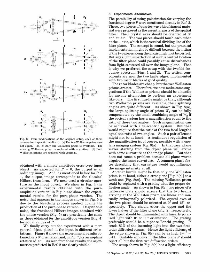
Fig. 8. Four modifications of the original setup, each of themovercoming a specific handicap: ~a! The two Wollaston prisms arenot equal. ~b!, ~c! Only one Wollaston prism is available. Themissing Wollaston prism is replaced with a grating. ~d! BothWollaston prisms are replaced with gratings.

5. Experimental Alternatives

The possibility of using polarization for varying thefractional degree P were mentioned already in Ref. 2.There, two pieces of quarter-wave birefringent mate-rial were proposed as the essential parts of the spatialfilter. Their crystal axes should be oriented at 0°and at 90°. The two pieces should touch each otherat the m axis, which is the vertical dividing line of thefilter plane. The concept is sound, but the practicalimplementation might be difficult because the fittingof the two pieces along the m axis might not be perfect.But any slight imperfection at such a central locationof the filter plane could possibly cause disturbancesfrom light scattered all over the image plane. Thatis why we preferred the setup with the twofold fre-quency spectrum ~Figs. 1 and 2!. The critical com-ponents are now the two knife edges, implementedwith two razor blades of good quality.

The razor blades are cheap, but the two Wollastonprisms are not. Therefore, we now make some sug-gestions if the Wollaston prisms should be a hurdlefor anyone attempting to perform an experimentlike ours. The first hurdle might be that, althoughtwo Wollaston prisms are available, their splittingangles are quite different. As shown in Fig. 8~a!,the large splitting angle of prism W1 can be fullycompensated by the small combining angle of W2 ifthe optical system has a magnification equal to theratio of those two angles. Such magnification canbe achieved with a telecentric system. But thatwould require that the ratio of the two focal lengthsequal the ratio of two angles. Such a pair of lensesmight not be at hand. A continuous regulation ofthe magnification is, of course, possible with a one-lens imaging system @Fig. 8~a!#. In that case, planewaves starting from the object plane will arrivewith some curvature at the image plane. But thatdoes not cause a problem because all plane wavesacquire the same curvature. A common phase fac-tor describing that curvature would not influencethe image intensity at all.

Another hurdle might be that only one Wollastonprism is at hand, either a strong one @Fig. 8~b!# or aweak one @Fig. 8~c!#. The missing Wollaston prismcould be replaced with a grating with the proper de-flection angle. As shown in Fig. 8~c!, two pieces of ahalf-wave plate should ensure that the two beamsarriving at the Wollaston prism are linear and mu-tually orthogonally polarized. The crystal axes ofthe two pieces should be oriented at 0° and 45°, re-spectively. They should cover the upper and thelower halves of the filter plane ~Fig. 2!, respectively.The object should be illuminated with linearly polar-ized light with 0° or 90° orientation. The gratingpreferably should be a p-phase Ronchi grating. Itsends 81% of the incoming light into the two first-order diffracted beams. Hence the light efficiency ofthe setup shown in Fig. 8~c! can be as high 4yp2 50.41. Suitable windows in the filter plane F shouldreject all but the first two diffraction orders.

The setup shown in Fig. 8~b! has a light efficiency


of 4yp2 5 0.41. The setup of Fig. 8~d! is the cheapestbecause now both Wollaston prisms have been re-placed with gratings. With two perfect p-phaseRonchi gratings the light efficiency could be as highas 32yp4 5 0.33 for the setup shown in Fig. 8~d!.

6. Conclusions and Possible Extensions

We have presented an optical setup for performing theFRH for two-dimensional objects and for a variable frac-tional index. Some experimental results and some pos-sible modifications of the setup were shown.

Two supplementary proposals ought to be madebefore closing: The generalization from the one-dimensional to the two-dimensional FRH was soundbut ambiguous. To divide the two-dimensional fre-quency plane into right and left sides ~y $ 0, y , 0! isonly one way of splitting the frequency domain intotwo parts. Partitioning by sectors or by rings is alsomeaningful.4,5 Finally, it should be noted that wehave considered here only one of the three definitionsof the FRH.2 That limitation is not severe becausethe two other schemes, when applied to two-dimensional objects, could benefit from the same orsimilar polarization methods. Finally, we note thatan anonymous reviewer drew our attention to an in-teresting paper by Belvax and Vareille.6 Theirsetup is somewhat similar to ours, but their motiva-tions are different.


We acknowledge fruitful discussions with D. Mend-lovic and Z. Zalevsky during the early stages of thisproject. We also acknowledge the support of theMexican Consejo Nacional de Ciencia y Tecnologia,project 211290-5-3103PE. A. W. Lohmann acknowl-edges partial support from the Mexican Consejo Na-cional de Ciencia y Tecnologia and from the DeutscheForschungsgemeinschaft.

The permanent address for A. W. Lohmann isPhysikalisches Institut, Rommel Strasse 1, 910508Erlangen, Germany.

References1. R. B. Bracewell, The Fourier Transform and Its Application

~McGraw-Hill, New York, 1995!.2. A. W. Lohmann, D. Mendlovic, and Z. Zalevsky, “Fractional

Hilbert transform,” Opt. Lett. 21, 281–283 ~1996!.3. A. W. Lohmann, J. Ojeda-Castaneda, and L. Diaz-Santana,

“Fractional Hilbert transform: optical implementation for 1-Dobjects,” Opt. Mem. Neural Networks 5, 131–135 ~1996!.

4. S. Lowenthal and Y. Belvaux, “Observation of phase objects byoptically processed Hilbert transform,” Appl. Phys. Lett. 11,49–51 ~1967!.

5. J. K. T. Eu and A. W. Lohmann, “Isotropic Hilbert spatial fil-tering,” Opt. Commun. 9, 257–262 ~1973!.

6. Y. Belvaux and J. C. Vareille, “Controle de l’etat de surface oud’homogeneıte de materiaux optiques ‘par contraste de phase’ adephasage quelconque,” Opt. Commun. 2, 101–104 ~1971!.

Optical implementation of the fractional Hilbert transform for two-dimensional objects

Documents

Transcript of Optical implementation of the fractional Hilbert transform for two-dimensional objects