Optical Flares and Quasi-Periodic Pulsations on CR Draconis ...
98
Also in this issue... • The Dwarf Nova SY Cancri and its Environs • KIC 8462852: Maria Mitchell Observatory Photographic Photometry 1922 to 1991 • Visual Times of Maxima for Short Period Pulsating Stars III • Recent Maxima of 86 Short Period Pulsating Stars J AAVSO The Journal of the American Association of Variable Star Observers Volume 46 Number 1 2018 Complete table of contents inside... The American Association of Variable Star Observers 49 Bay State Road, Cambridge, MA 02138, USA Upper panel: 2017-10-10-flare photon counts, time aligned with FFT spectrogram. Lower panel: FFT spectrogram shows time in UT seconds versus QPP periods in seconds. Flares cited by Doyle et al. (2018) are shown with (*). Optical Flares and Quasi-Periodic Pulsations on CR Draconis during Periastron Passage
-
Upload
khangminh22 -
Category
Documents
-
view
2 -
download
0
Transcript of Optical Flares and Quasi-Periodic Pulsations on CR Draconis ...

Also in this issue...• TheDwarfNovaSYCancrianditsEnvirons
• KIC8462852:MariaMitchellObservatoryPhotographicPhotometry1922to1991
• VisualTimesofMaximaforShortPeriodPulsatingStarsIII
• RecentMaximaof86ShortPeriodPulsatingStars
JAAVSOThe Journal of the American Associationof Variable Star Observers
Volume46Number1
2018
Complete table of contents inside...
TheAmericanAssociationofVariableStarObservers49BayStateRoad,Cambridge,MA02138,USA
Upperpanel:2017-10-10-flarephotoncounts,timealignedwithFFTspectrogram.
Lowerpanel:FFTspectrogramshowstimeinUTsecondsversusQPPperiodsinseconds.FlarescitedbyDoyleetal.(2018)areshownwith(*).
OpticalFlaresandQuasi-PeriodicPulsationsonCRDraconisduringPeriastronPassage

ISSN 0271-9053 (print)ISSN 2380-3606 (online)
TheJournaloftheAmericanAssociationofVariableStarObserversEditorJohnR.PercyDunlap Institute of Astronomy and Astrophysicsand University of TorontoToronto, Ontario, Canada
AssociateEditorElizabethO.Waagen
ProductionEditorMichaelSaladyga
EditorialBoardGeoffreyC.ClaytonLouisiana State UniversityBaton Rouge, Louisiana
ZhibinDaiYunnan ObservatoriesKunming City, Yunnan, China
KosmasGazeasUniversity of AthensAthens, Greece
EdwardF.GuinanVillanova UniversityVillanova, Pennsylvania
JohnB.HearnshawUniversity of CanterburyChristchurch, New Zealand
LaszloL.KissKonkoly ObservatoryBudapest, Hungary
KatrienKolenbergUniversities of Antwerp and of Leuven, Belgiumand Harvard-Smithsonian Center for AstrophysicsCambridge, Massachusetts
KristineLarsenDepartment of Geological Sciences, Central Connecticut State University, New Britain, Connecticut
VanessaMcBrideIAU Office of Astronomy for Development; South African Astronomical Observatory; and University of Cape Town, South Africa
UlisseMunariINAF/Astronomical Observatory of PaduaAsiago, Italy
NikolausVogtUniversidad de ValparaisoValparaiso, Chile
DavidB.WilliamsWhitestown, Indiana
TheCounciloftheAmericanAssociationofVariableStarObservers2017–2018
Director Stella Kafka President Kristine Larsen Past President Jennifer L. Sokoloski 1st Vice President Bill Stein 2nd Vice President Kevin B. Marvel Secretary Gary Walker Treasurer Robert Stephens
Councilors
Richard BerryTom Calderwood
Michael CookJoyce A. GuzikMichael Joner
Katrien KolenbergArlo LandoltGordon MyersGregory R. Sivakoff

JAAVSOThe Journal of
The American AssociationofVariableStarObservers
Volume46Number1
2018
AAVSO49BayStateRoad
Cambridge,MA02138USA
ISSN0271-9053(print)ISSN2380-3606(online)

Publication Schedule
The Journal of the American Association of Variable Star Observersispublishedtwiceayear,June15(Number1ofthevolume)andDecember15(Number 2ofthevolume).ThesubmissionwindowforinclusioninthenextissueofJAAVSOclosessixweeksbeforethepublicationdate.Amanuscriptwillbeaddedtothetableofcontentsforanissuewhenithasbeenfullyacceptedforpublicationuponsuccessfulcompletionoftherefereeprocess;thesearticleswillbeavailableonlinepriortothepublicationdate.AnauthormaynotspecifyinwhichissueofJAAVSOamanuscriptistobepublished;acceptedmanuscriptswillbepublishedinthenextavailableissue,exceptunderextraordinarycircumstances.
Page Charges
PagechargesarewaivedforMembersoftheAAVSO.PublicationofunsolicitedmanuscriptsinJAAVSOrequiresapagechargeofUS$100/pageforthefinalprintedmanuscript.Pagechargewaiversmaybeprovidedundercertaincircumstances.
Publication in JAAVSO
WiththeexceptionofabstractsofpaperspresentedatAAVSOmeetings,paperssubmittedtoJAAVSOarepeer-reviewedbyindividualsknowledgableaboutthetopicbeingdiscussed.WecannotguaranteethatallsubmissionstoJAAVSOwillbepublished,butweencourageauthorsofallexperiencelevelsandinallfieldsrelatedtovariablestarastronomyandtheAAVSOtosubmitmanuscripts.WeespeciallyencouragestudentsandothermenteesofresearchersaffiliatedwiththeAAVSOtosubmitresultsoftheircompletedresearch.
Subscriptions
InstitutionsandLibrariesmaysubscribetoJAAVSOaspartoftheCompletePublicationsPackageorasanindividualsubscription.IndividualsmaypurchaseprintedcopiesofrecentJAAVSOissuesviaCreatespace.PapercopiesofJAAVSOissuespriortovolume36areavailableinlimitedquantitiesdirectlyfromAAVSOHeadquarters;pleasecontacttheAAVSOforavailableissues.
Instructions for Submissions
TheJournalof the AAVSO welcomespapersfromallpersonsconcernedwiththestudyofvariablestarsandtopicsspecificallyrelatedtovariability.Allmanuscriptsshouldbewritteninastyledesignedtoprovideclearexpositionsofthetopic.Contributorsareencouragedtosubmitdigitizedtextinms word,latex+postscript,orplain-textformat.Manuscriptsmaybemailedelectronicallytojournal@aavso.orgorsubmittedbypostalmailtoJAAVSO,49BayStateRoad,Cambridge,MA02138,USA.
Manuscriptsmustbesubmittedaccordingtothefollowingguidelines,ortheywillbereturnedtotheauthorforcorrection: Manuscriptsmustbe: 1)original,unpublishedmaterial; 2)writteninEnglish; 3)accompaniedbyanabstractofnomorethan100words. 4)notmorethan2,500–3,000wordsinlength(10–12pagesdouble-spaced).
Figuresforpublicationmust: 1)becamera-readyorinahigh-contrast,high-resolution,standarddigitizedimageformat; 2)haveallcoordinateslabeledwithdivisionmarksonallfoursides; 3)beaccompaniedbyacaptionthatclearlyexplainsallsymbolsandsignificance,sothatthereadercanunderstand thefigurewithoutreferencetothetext.
Maximumpublishedfigurespaceis4.5”by7”.Whensubmittingoriginalfigures,besuretoallowforreductioninsizebymakingallsymbols,letters,anddivisionmarkssufficientlylarge.
Photographsandhalftoneimageswillbeconsideredforpublicationiftheydirectlyillustratethetext. Tablesshouldbe: 1)providedseparatefromthemainbodyofthetext; 2)numberedsequentiallyandreferredtobyArabicnumberinthetext,e.g.,Table1.
References: 1)Referencesshouldrelatedirectlytothetext. 2)Referencesshouldbekeyedintothetextwiththeauthor’slastnameandtheyearofpublication, e.g.,(Smith1974;Jones1974)orSmith(1974)andJones(1974). 3)Inthecaseofthreeormorejointauthors,thetextreferenceshouldbewrittenasfollows:(Smithetal.1976). 4)Allreferencesmustbelistedattheendofthetextinalphabeticalorderbytheauthor’slastnameandtheyear ofpublication,accordingtothefollowingformat:Brown,J.,andGreen,E.B.1974,Astrophys. J.,200,765. Thomas,K.1982,Phys. Rep.,33,96. 5)AbbreviationsusedinreferencesshouldbebasedonrecentissuesofJAAVSOorthelistingprovidedatthe beginningofAstronomy and Astrophysics Abstracts(Springer-Verlag).
Miscellaneous: 1)EquationsshouldbewrittenonaseparatelineandgivenasequentialArabicnumberinparenthesesnearthe right-handmargin.Equationsshouldbereferredtointhetextas,e.g.,equation(1). 2)Magnitudewillbeassumedtobevisualunlessotherwisespecified. 3)Manuscriptsmaybesubmittedtorefereesforreviewwithoutobligationofpublication.
Online Access
ArticlespublishedinJAAVSO,andinformationforauthorsandrefereesmaybefoundonlineat:https://www.aavso.org/apps/jaavso/
©2018TheAmericanAssociationofVariableStarObservers.Allrightsreserved.

The Journal of the American Association of Variable Star ObserversVolume 46, Number 1, 2018
Table of Contents continued on following pages
Editorial
Editorial:WhatUseIsAstronomy? John R. Percy 1
Variable Star Research
CCDPhotometryandRocheModelingoftheEclipsingDeepLowMass,OvercontactBinaryStarSystemTYC2058-753-1 Kevin B. Alton 3
APhotometricStudyoftheEclipsingBinaryNSV1000 Thomas J. Richards, Colin S. Bembrick 10
A1,574-DayPeriodicityofTransitsOrbitingKIC8462852 Gary Sacco, Linh D. Ngo, Julien Modolo 14
OpticalFlaresandQuasi-PeriodicPulsations(QPPs)onCRDraconisduringPeriastronPassage Gary Vander Haagen 21
APhotometricStudyoftheContactBinaryV737Cephei Edward J. Michaels 27
KIC8462852:MariaMitchellObservatoryPhotographicPhotometry1922to1991 Michael Castelaz, Thurburn Barker 33
Observations,RocheLobeAnalysis,andPeriodStudyoftheEclipsingContactBinarySystemGMCanumVenaticorum Kevin B. Alton, Robert H. Nelson 43
TheDwarfNovaSYCancrianditsEnvirons Arlo U. Landolt, James L. Clem 50
FirstPrecisionPhotometricObservationsandAnalysesoftheTotallyEclipsing,SolarTypeBinaryV573Pegasi Ronald G. Samec, Daniel B. Caton, Danny R. Faulkner 57
Sparsely-ObservedPulsatingRedGiantsintheAAVSOObservingProgram John R. Percy 65
Variable Star Data
RecentMaximaof86ShortPeriodPulsatingStars Gerard Samolyk 70
VisualTimesofMaximaforShortPeriodPulsatingStarsIII Gerard Samolyk 74
RecentMinimaof172EclipsingBinaryStars Gerard Samolyk 79

Table of Contents continued on next page
Review Paper
TheVariabilityofYoungStellarObjects:AnUpdate William Herbst 83
Abstracts of Papers Presented at the 106th Annual Meeting of the AAVSO, Held in Nashville, Tennessee, November 2–4, 2017
AAVSOTargetTool:AWeb-BasedServiceforTrackingVariableStarObservations Dan Burger, Keivan G. Stassun, Chandler Barnes, Sara Beck, Stella Kafka, Kenneth Li 85
PeriodVariationinBWVulpeculae David E. Cowall, Andrew P. Odell 85
FromYYBoo(eclipsingbinary)viaJ1407(ringedcompanion)toWD1145+017(whitedwarfwithdebrisdisk) Franz-Josef (Josch) Hambsch 85
Keynotepresentation:LookingforZebrasWhenThereAreOnlyHorses Dennis M. Conti 86
TheVegaProject,PartI Tom Calderwood, Jim Kay 86
TheExcitingWorldofBinaryStars:NotJustEclipsesAnymore Bert Pablo 86
BVObservationsoftheEclipsingBinaryXZAndromedaeattheEKUObservatory Marco Ciocca 86
NovaEruptionsfromRadiotoGamma-rays—withAAVSODataintheMiddle Koji Mukai, Stella Kafka, Laura Chomiuk, , Ray Li, Tom Finzell, Justin Linford, , Jeno Sokoloski, Tommy Nelson, Michael Rupen, Amy Mioduszewski, Jennifer Weston 86
Transits,Spots,andEclipses:TheSun’sRoleinPedagogyandOutreach Kristine Larsen 87
ObservationsofTransitingExoplanetCandidatesUsingBYUFacilities Michael D. Joner, Eric G. Hintz, Denise C. Stephens 87
pythonforVariableStarAstronomy Matt Craig 87
DetectingMovingSourcesinAstronomicalImages Andy Block 87
VariableStarsintheFieldofTrES-3b Erin Aadland 87
CalculatingGalacticDistancesThroughSupernovaLightCurveAnalysis Jane Glanzer 88
DiscoveryofKPS-1b,aTransitingHot-Jupiter,withanAmateurTelescopeSetup Paul Benni, Artem Burdanov, Vadim Krushinsky, Eugene Sokov 88

SearchingforVariableStarsintheSDSSCalibrationFields J. Allyn Smith, Melissa Butner, Douglas Tucker, Sahar Allam 88
SearchingforVariableStarsintheFieldofDolidze35 Jamin Welch, J. Allyn Smith 88
ASearchforVariableStarsinRuprecht134 Rachid El Hamri, Mel Blake 89
Errata
Erratum:SloanMagnitudesfortheBrightestStars Anthony Mallama 90


Percy, JAAVSO Volume 46, 2018 1
Editorial
What Use Is Astronomy?John R. PercyEditor-in-Chief, Journal of the AAVSO
Department of Astronomy and Astrophysics, and Dunlap Institute for Astronomy and Astrophysics, University of Toronto, 50 St. George Street, Toronto, ON M5S 3H4, Canada; [email protected]
Received May 8, 2018
Why do people such as AAVSOers observe or analyze variable stars? A few readers may simply say that observing is a relaxing, outdoor pastime, like fishing, and that analysis is a way to keep the mind occupied, like solitaire. But most will say “to advance the science of astronomy.” But what use is astronomy? Googling “value of astronomy” usually leads to professional astronomers’ websites which emphasize the economic value of astronomy to other sciences, and to engineering, and to society. Often, this is to counter the claim that astronomy is not relevant or useful today. In Canada, an independent study showed that government investment in astronomy repaid itself several times over. Astronomy has practical value. Almost every civilization has used the sky as a clock, calendar, and compass. Nowadays, we have other technologies for these, but we can intuitively know the time, date, and direction by glancing at the sun or stars. But knowledge of astronomy is now essential for understanding space weather, space hazards such as asteroid and comet impacts, and the nature and reality of climate change. Historically, astronomy spurred the development of mathematics. Now, it spurs the development of high-performance computing, and the analysis of “big data” with artificial intelligence and machine learning. Graduates of astronomy programs are now in demand for a wide range of careers which utilize these powerful skills. Astronomy has led to low-noise radio receivers and other communication technology, and to sensitive detectors and their application to image-processing for fields such as medicine and remote sensing. By providing the ultimate laboratory—the universe—astronomy has also advanced the physical and earth sciences which are the basis of so much of our everyday life. Over the millennia, astronomy has also occupied a deep spiritual role in society and its culture, and this has led to the relatively new field of “cultural astronomy.” Skywatching began as an attempt to understand the nature and cause of earthly and human events—what we now call astrology. The heavens were seen as the abode of the gods, and the sun, moon, and planets represented them in the sky. Buildings, and whole communities were aligned to the sky, especially to the rising and setting points of the sun. For centuries, churches and graves in some Western cultures retained these traditional alignments. The calendar was important for setting the date of religious observances, as it still is today. Eclipses and comets were “omens of disaster.”
Unfortunately, astrology is still widely accepted, even though there is no evidence for its efficacy, beyond the “placebo effect.” Among the scientific revolutions of history, astronomy and astronomers stand out. Think of Copernicus, Galileo, and Newton. Astronomy continues to resonate deeply with both philosophers and the public. I give numerous non-technical lectures to general audiences. They appreciate learning about the vastness, variety, and beauty of the sky and the universe, and are as excited about black holes as schoolchildren are. In the words of Doug Cunningham, a teacher colleague of mine, astronomy “harnesses curiosity, imagination, and a sense of shared exploration and discovery.” For a 2003 conference of the International Astronomical Union, I outlined the many reasons why astronomy should be part of the school curriculum: www.astro.utoronto.ca/~percy/useful.pdf, and I’ve been active for many decades in creating curriculum, reviewing textbooks, and providing training and resources for schoolteachers. In addition to the considerations listed earlier, astronomy can be used to illustrate otherwise-boring or difficult topics in math and physics. It requires and enables students to think about vast scales of size, distance, and time. It provides an example of the role of observation and simulation as ways of doing science. It’s the ultimate interdisciplinary subject. In my lectures and writings and other outreach activities, I love to explore astronomy’s connections to the arts and humanities, and to culture, as well as to other sciences. If properly taught, astronomy can promote rational thinking and an understanding of the nature and value and power of science—something sorely needed in this age of “fake news.” And “the stars belong to everyone.” You may have an expensive telescope and CCD camera, but one can still enjoy—and even contribute to—astronomy with binoculars and the naked eye. We need to get young people started as enthusiasts, observers, and “citizen astronomers,” to replace the graying, primarily white male observers of today. Astronomy is benign. It is environmentally friendly. It has no borders. It’s “one world, one sky.” These considerations are important to young people today. What has this got to do with you, the variable star observer or analyst? First of all: you are adding a brick or two to the wonderful edifice called “the known universe.” Astronomy, like other sciences, isn’t just big, Nobel-prize-winning discoveries. We all contribute. Your observations help to build the picture which, thanks to popularizers such as Neil deGrasse Tyson,

Percy, JAAVSO Volume 46, 20182
Stephen Hawking, and Carl Sagan, and Terence Dickinson and Helen Sawyer Hogg in my country, informs and inspires millions. That might include a young student who, attracted to science, will make the discoveries of tomorrow. And there will be such discoveries. What is the “dark matter” that makes up most of the stuff of the universe? What is the “dark energy” that pushes the universe apart at an accelerating rate? When will we first detect a spectroscopic signature of a biogenic molecule in the atmosphere of an exoplanet? And in the field of variable stars: what are fast radio bursts (FRBs)? How can we “sharpen” Cepheids and supernovae as tools for determining precise extragalactic distances? And at a more mundane level: what causes the unexplained phenomena in long-period variables—wandering periods, variable amplitudes, and “long secondary periods”—that I and my students study?
But don’t leave all the popularizing to the professionals. In addition to your variable star observing and analysis, you can help to advance astronomy through education and public outreach. I’ve outlined how you can do this, and why (Percy 2017). There are eager audiences out there in your community, from schoolchildren to seniors. Astronomy has value. Your observations and analyses have value. The AAVSO has value. JAAVSO has value—in communicating your contribution to “the known universe” to other AAVSOers and to the rest of the worldwide astronomical community.
Reference
Percy, J. R. 2017, J. Amer. Assoc. Var. Star Obs., 45, 1.

Alton, JAAVSO Volume 46, 2018 3
CCD Photometry and Roche Modeling of the Eclipsing Deep Low Mass, Overcontact Binary Star System TYC 2058-753-1Kevin B. AltonUnderOak Observatory, 70 Summit Avenue, Cedar Knolls, NJ; [email protected]
Received October 6, 2016; revised February 12, 2018; accepted March 27, 2018
Abstract TYC 2058-753-1 (NSVS 7903497; ASAS 165139+2255.7) is a W UMa binary system (P = 0.353205 d) which has not been rigorously studied since first being detected nearly 15 years ago by the ROTSE-I telescope. Other than the unfiltered ROTSE-I and monochromatic All Sky Automated Survey (ASAS) survey data, no multi-colored light curves (LC) have been published. Photometric data collected in three bandpasses (B, V, and Ic) at Desert Bloom Observatory in June 2017 produced six times-of-minimum for TYC 2058-753-1 which were used to establish a linear ephemeris from the first directly measured Min I epoch (HJD0). No published radial velocity data are available for this system, however, since this W UMa binary undergoes a very obvious total eclipse, Roche modeling produced a well-constrained photometric value for the mass ratio (qph = 0.103 ± 0.001). This low-mass ratio binary star system also exhibits a high degree of contact ( f > 56%). There is a suggestion from the ROTSE-I and ASAS survey data as well as from the new LCs reported herein that maximum light during quadrature (Max I and Max II) is often not equal. As a result, Roche modeling of the TYC 2058-753-1 LCs was investigated with and without surface spots to address this asymmetry as well as a diagonally-aligned flat bottom during Min I that was observed in 2017.
1. Introduction
The variable behavior of TYC 2058-753-1 was first observed during the ROTSE-I CCD survey (Akerlof et al. 2000; Wozniak et al. 2004; Gettel et al. 2006) and subsequently confirmed from additional photometric measurements taken by the ASAS surrvey (Pojmański et al. 2005). The system was classified as an overcontact binary by Hoffman et al. (2009). Other than the sparsely sampled photometric readings from the ROTSE-I and ASAS surveys, no other LCs from this binary system were found in the literature. TYC 2058-753-1 is also included in a survey of 606 contact binaries from which accurate colors (BVRcIc) were derived (Terrell et al. 2012). The paper herein marks the first robust determination of an orbital period and its corresponding linear ephemeris to be published. Deep, low mass ratio (DLMR) overcontact systems like TYC 2058-753-1 embody a subgroup of W UMa variables with mass ratios (m2 / m1) less than 0.25 and degrees of contact ( f ) greater than 50% (Yang and Qian 2015). Accordingly, these binary systems are approaching a final evolutionary stage before merging into single rapidly-rotating objects such as blue-straggler or FK Com-type stars. DLMR stars are considered an important astrophysical laboratory for studying the dynamical evolution of short-period binary stars in very close contact. In this regard, the Roche-type modeling of TYC 2058-753-1 contained within offers the first published study in which the physical and geometric elements of this system are derived.
2. Observations and data reduction
2.1. Photometry The equipment at Desert Bloom Observatory (DBO) located in Benson, Arizona, includes a 0.4-m catadioptic telescope mounted on an equatorial fork with an SBIG STT-1603 ME CCD camera installed at the Cassegrain focus. This f/6.7 instrument produces a 17.4 × 11.6 arcmin field-of-view with a 1.36 arcsec/pixel scale (binned 2 × 2). Automated imaging was performed
with Astrodon photometric B, V, and Ic filters manufactured to match the Bessell prescription. The computer clock was updated immediately prior to each session and exposure time for all images adjusted to 75 sec. Image acquisition (lights, darks, and flats) was performed using maximdl version 6.13 (Diffraction Limited 2016) or theskyx version 10.5.0 (Software Bisque 2013) while calibration and registration were performed with aip4win v2.4.0 (Berry and Burnell 2005). mpo canopus v10.7.1.3 (Minor Planet Observer 2015) provided the means for further photometric reduction to LCs using a fixed ensemble of four non-varying comparison stars in the same field-of-view (FOV). Error due to differential refraction and color extinction was minimized by only using data from images taken above 30° altitude (airmass < 2.0). Instrumental readings were reduced to catalog-based magnitudes using the reference MPOSC3 star fields built into mpo canopus (Warner 2007).
2.2. Light curve analyses Roche type modeling was performed with wdwint v5.6a (Nelson 2009) and phoebe 0.31a (Prša and Zwitter 2005), both of which employ the Wilson-Devinney (W-D) code (Wilson and Devinney 1971; Wilson 1990). Spatial models of TYC 2058-753-1 were rendered with binary maker 3 (bm3; Bradstreet and Steelman 2002) once W-D model fits were finalized. Times-of-minimum were calculated using the method of Kwee and van Woerden (1956) as implemented in peranso v2.5 (Vanmunster 2006).
3. Results and discussion
3.1. Photometry and ephemerides The four stars in the same FOV with TYC 2058-753-1 (Table 1) which were used to derive MPOSC3-based magnitudes showed no evidence of inherent variability over the interval of image acquisition and stayed within ± 0.007 mag for V–and Ic– and ± 0.017 for B-passbands. Photometric values in B (n = 464), V (n = 478), and Ic (n = 474) were folded by period analysis to generate three LCs that spanned 16 days between June 3 and

Alton, JAAVSO Volume 46, 20184
June 19, 2017 (Figure 1). In total, four primary (p) and two secondary (s) minima were captured during this investigation; the corresponding data (B, V, and Ic) were averaged from each session (Table 2) since no color dependency on the timings was noted. Initially a period determination was made from survey data (ROTSE-I and ASAS) collected between 1999–2009 using peranso v2.5 (Vanmunster 2006). The selected analysis method employs periodic orthogonal polynomials (Schwarzenberg-Czerny 1996) to fit observations and analysis of variance (ANOVA) to evaluate fit quality. The resulting orbital period (P = 0.353206 ± 0.000008 d) was very similar to the value cited at the International Variable Star Index website (Watson et al. 2014). The Fourier routine (FALC; Harris et al. 1989) in mpo canopus provided a comparable period solution (0.353205 ± 0.000001 d) using only the multicolor data from DBO. Finally, after converting magnitude to normalized flux, ROTSE-I, ASAS, and DBO light curve data (HJD; V mag) were then folded together; the best fit was found where the orbital period was 0.353205 ±0.000008 d (Figure 2). As expected with so few data, eclipse timing differences when plotted against period cycle number did not provide any evidence for period change (Figure 3). The first epoch (HJD0) for this eclipsing binary is therefore defined by the following linear ephemeris equation:
Min. I (hel.) = 2457909.7566 (3) + 0.353205 (8) E. (1)
There is an expectation that while DLMR systems slowly collapse into a higher degree of contact before merger, the orbital period will concomitantly decrease. Since this result is not demonstrably obvious after folding the sparsely sampled survey data (1999–2009) with high cadence LC data acquired in 2017, this hypothesis may not be proven until many more years of eclipse timing data have been collected to determine whether the orbital period of this system undergoes change(s) with time.
3.2. Light curve behavior LCs (Figure 1) exhibit minima which are separated by 0.5 phase and are consistent with synchronous rotation in a circular orbit typified by W UMa-type variable stars. The flattened bottom at Min I is diagnostic of a binary system that undergoes a total eclipse. Interestingly, LC data from the ROTSE-I and ASAS surveys (Figure 2) exhibit significant variability around Min II suggesting that the deepest minimum likely alternates from time-to-time. The 2017 LCs exhibit asymmetry during
quadrature such that Max I is fainter than Max II (Figure 1). This effect often attributed to O’Connell (1951) has been variously ascribed to the presence of cool starspot(s), hot region(s), gas stream impact on either or both of the binary stars, and/or other unknown phenomena which produce surface inhomogeneities (Yakut and Eggleton 2005). The net result can be unequal heights during maximum light and is often simulated by the introduction of starspots during Roche-type modeling of the LC data.
3.3. Spectral classification Interstellar extinction (AV) was estimated using a program (alextin) developed by Amôres and Lépine (2005) for targets within the Milky Way Galaxy (MWG). In addition to the galactic coordinates (l, b) an estimated distance (kpc) to each target is required. The dust maps generated by Schlegel et al. (1998) and later adjusted by Schlafly and Finkbeiner (2011) determine extinction based on total dust in a given direction without regard to the target distance. This often leads to an overestimation of reddening within the MWG, most commonly determined as E(B–V) = AV / 3.1. As will be described in section 3.7, the distance to overcontact binary stars can be estimated based on a number of different approaches even in the absence of a directly determined parallax. In this case the adopted
Table 1. Astrometric coordinates (J2000) and color indices (B–V) for TYC 2058-0753-1 and four comparison stars used in this photometric study.
StarIdentification R.A.(J2000) Dec.(J2000) MPOSC3a
h m s º ' " (B–V)
TYC 2058-0753-1 16 51 39.43 22 55 43.5 0.822 GSC 2058-0807 16 52 02.94 22 54 10.3 0.743 GSC 2058-0583 16 52 05.65 22 57 16.9 0.674 GSC 2058-0841 16 52 42.02 22 57 16.9 0.463 2MASS 16515918+2256394 16 51 59.06 22 56 39.0 0.387
a.MPOSC3isahybridcatalog(Warner2007)whichincludesalargesubsetoftheCarlsbergMeridianCatalog(CMC-14)aswellasfromtheSloanDigitalSkySurvey(SDSS).
Figure 1. CCD-derived light curves for TYC 2058-753-1 produced from photometric data obtained between June 3 and June 19, 2017. The top (Ic; n = 474), middle (V; n = 478), and bottom curve (B; n =464) shown above were reduced to MPOSC3-based catalog magnitudes using mpo canopus.
Table 2. New times-of-minimum for TYC 2058-753-1 acquired at Desert Bloom Observatory.
ToM UT Observation Type of HJD–2400000 ±Error Date Minimuma
57909.7566 0.0003 05 June 2017 p 57915.7595 0.0001 11 June 2017 p 57917.6978 0.0002 13 June 2017 s 57921.7631 0.0002 17 June 2017 p 57923.7032 0.0002 19 June 2017 p 57923.8823 0.0002 19 June 2017 s a. s = secondary; p = primary.

Alton, JAAVSO Volume 46, 2018 5
distance (~ 0.190 kpc) results in a reddening value (E(B–V)) of 0.0074 ± 0.0004. Color index (B–V) data collected at DBO and those acquired from an ensemble of four other sources (Table 3) were subsequently dereddened. The median result ((B-V)0 = 0.770 ± 0.042) points to a main sequence primary star with an effective temperature (5370 K) that ranges in spectral type between G8V and G9V (Pecaut and Mamajek 2013).
3.4. Roche modeling approach Perhaps the greatest obstacle to definitively characterizing the absolute dimensions, geometry, and mass of an eclipsing pair of stars is the general lack of RV data for relatively dim (Vmag > 12) binary systems. This situation is likely to continue until mitigated by the final release of spectroscopic data from the Gaia Mission in 2022. Without RV data, it is not possible to unequivocally determine the mass ratio (q = m2 / m1), total mass or whether TYC 2058-753-1 is an A- or W-type overcontact binary system. Nonetheless, a reliable photometric value for mass ratio (qph) can be determined but only for those W UMa systems where a total eclipse is observed (Terrell and Wilson 2005). Secondly, in many cases an educated guess about the W UMa subtype (A- or W-) can be made based on general characteristics of each overcontact binary system. Binnendijk (1970) defined an A-type W UMa variable as one in which the deepest minimum (Min I) results from the eclipse of the hotter more massive star by the cooler less massive cohort. By contrast W-types exhibit the deepest minimum when the hotter, but less massive star is eclipsed by its more massive but cooler companion. The published record is very clear that the majority (39 of 46) of DLMR binaries studied thus far appear to be A-type systems (Yang and Qian 2015). By and large, A-type W UMa variables can be characterized by their total mass (MT > 1.8 M
), spectral class (A-F), orbital period
(P > 0.4 d), high degree of thermal contact( f ), tendency to totally eclipse due to large size differences, mass ratio (q < 0.3), and the temperature difference (ΔT < 100 K) between the hottest and coolest star (Skelton and Smits 2009). In this case, TYC 2058-753-1 shares attributes from both A- and W-types thereby complicating a definitive assignment without having RV data. Furthermore, LC data from the ASAS (Pojmański et al. 2005) and ROTSE surveys survey (Akerlof et al. 2000; Gettel et al. 2006) suggest that Min I, the deepest minimum, alternates with Min II over time as might be expected from a heavily spotted system. This behavior has been reported for other DMLR overcontact binaries including EM Psc (Qian et al. 2008), V1191 Cyg (Ulaş et al. 2012), FG Hya (Qian and Yang 2005), and GR Vir (Qian and Yang 2004). Roche modeling of LC data from TYC 2058-753-1 was initially accomplished using the program phoebe 0.31a (Prša and Zwitter 2005). The model selected was for an overcontact binary (Mode 3); weighting for each curve was based upon observational scatter. Bolometric albedo (A1,2 = 0.5) and gravity darkening coefficients (g1,2 = 0.32) for cooler stars (< 7500 K) with convective envelopes were respectively based on the seminal work of Ruciński (1969) and Lucy (1967). The effective temperature of the more massive primary star was fixed (Teff1 = 5370 K) according to the earlier designation as spectral type G8V to G9V. Logarithmic limb darkening coefficients (x1, x2, y1, y2) were interpolated according
Figure 2. Survey data from the ROTSE-I telescope (NSVS), ASAS Survey, and photometric results (HJD; Vmag) collected at DBO were folded together using period analysis (P = 0.353205 ± 0.000008 d). Greater scatter at phase = 0.50 and 0.75 suggests the presence of an active surface for TYC 2058-753-1.
Figure 3. Linear fit of eclipse timing differences (ETD1) and period cycle number for TYC 2058-0753-1 captured at DBO over 16 days.
Table 3. Spectral classification of TYC 2058-753-1 based upon dereddened (B–V) data from four surveys and the present study.
Terrell et al. 2MASS USNO-A2 UCAC4 Present 2005 Study
(B–V)0 0.728 0.815 0.774 0.770 0.667 Teff1
a(K) 5506 5282 5353 5370 5703 Spectral Classa G7-G8V G9-K0V G8-G9V G8-G9V G3-G4V a. Teff1 interpolated and main sequence spectral class assigned from Pecaut andMamajek(2013).Medianvalue,(B–V)0=0.770±0.042,correspondstoaG8V-G9Vprimarystar(Teff1=5370K).

Alton, JAAVSO Volume 46, 20186
to Van Hamme (1993) after any adjustment in the secondary (Teff2) effective temperature. Except for Teff1, A1,2, and g1,2, all other parameters were allowed to vary during DC iterations. Roche modeling was initially seeded with q = 0.150 and i = 89° based on the similarity between orbital period, effective temperature (Teff1), and light curves for TYC 2058-753-1 and EM Psc (González-Rojas et al. 2003; Qian et al. 2008). The fit with a slightly higher (+100 K) effective temperature for the secondary was initially investigated since the smaller but potentially hotter star appeared to be occulted at Min I in 2017. This assessment included synthesis of LCs for TYC 2058-753-1 with and without the incorporation of spot(s) to address the negative O’Connell effect (Max II brighter than Max I) and the flattened but diagonally aligned bottom during Min I.
3.5. Roche modeling results The initial estimates (phoebe 0.31a) for q, i, and Teff2 converged to a Roche model solution in which the effective temperature of the less massive secondary proved to be slightly higher (> 24 K) than the primary star. Thereafter, final values and errors for Teff2, i, q, Ω1,2, and the spot parameters were determined using wdwint v5.6a (Table 4). Corresponding unspotted (Figure 4) and spotted (Figure 5) LC simulations revealed that the addition of a cool spot on the primary and a hot spot on the secondary was necessary to achieve the best fit (χ2) for these multi-color data. Pictorial models rendered (bm3) with both spots using the physical and geometric elements from the 2017 LCs (V-mag) are shown in Figure 6. In this case, these results are consistent with those expected from a W-type overcontact binary system. Nonetheless, it is very clear from the ROTSE-I and ASAS survey data that the deepest minimum for TYC 2058-753-1 can alternate; this most likely occurs due to significant changes in spot location and/or temperature. A subset of LC data (2005–2007) collected during the ASAS survey (Pojmański et al. 2005) offers further insight into the challenges faced with trying to unambiguously define this system without supporting RV data. Although the Roche model parameter estimates are more variable (Table 4) from the ASAS survey data, the results suggest that Min I (Figure 7) could arise from a transit of the secondary across the face of the primary star (Figure 8). This scenario is essentially the definition of an A-type W UMa-type system and different from the 2017 findings. Interestingly, the best solution for the 2005–2007 data suggests that the secondary is also hotter (110 K) than the primary, an outcome reported for a large fraction (8/39) of A-type DLMR overcontact binaries (Yang and Qian 2015). The fill-out parameter ( f ), which is a measure of the shared outer surface volume between each star, was calculated according to Bradstreet (2005) as:
f = (Ωinner – Ω1,2 / (Ωinner – Ωouter), (2)
where Ωouter is the outer critical Roche equipotential, Ωinner is the value for the inner critical Roche equipotential, and Ω = Ω1,2 denotes the common envelope surface potential for the binary system. Since the fill-out value (f > 0.56) for TYC 2058-753-1 lies between 0 < f < 1, the system is defined as an overcontact binary. This high degree of contact in combination with the
Figure 4. TYC 2058-753-1 Roche model fits (solid-line) of LCs (B-, V-, and Ic-mag) produced from CCD data collected at DBO during 2017. This analysis assumed a W-subtype overcontact binary with no spots; residuals from the model fits are offset at the bottom of the plot to keep the values on scale.
Figure 5. TYC 2058-753-1 Roche model fits (solid-line) of LCs (B-, V-, and Ic-mag) produced from CCD data collected at DBO during 2017. This analysis assumed a W-subtype overcontact binary with a cool spot on the primary and a hot spot on the secondary star; residuals from the model fits are offset at the bottom of the plot to keep the values on scale.
Figure 6. Spatial renderings of TYC 2058-753-1 generated from photometric data (V-mag) acquired in 2017 showing putative locations of a cool spot (blue) on the primary star and a hot spot (red) on the secondary star.

Alton, JAAVSO Volume 46, 2018 7
another (M1 = 0.93 ± 0.03 M
) from Pecaut and Mamajek (2013). Additionally, two different empirical period-mass relationships for W UMa-binaries have been published, by Qian (2003) and later by Gazeas and Stępień (2008). According to Qian (2003) the mass of the primary star (M1) can be determined from Expression 3:
log M1 = (0.761 ± 0.150) log P + (1.82 ± 0.28), (3)
where P is the orbital period in days and leads to M1 = 1.08 ± 0.08 M
for the primary. The other mass-period
relationship (Equation 4) derived by Gazeas and Stępień (2008):
log M1 = (0.755 ± 0.059) log P + (0.416 ± 0.024), (4)
corresponds to a W-type W UMa system where M1 = 1.19 ± 0.10 M
. The median of all values (M1 = 1.03 ± 0.08 M
) was used for
subsequent determinations of M2, semi-major axis (a), volume-radius (rL), bolometric magnitude (Mbol), and distance (pc) to TYC 2058-753-1. The semi-major axis, a(R
) = 2.20 ± 0.05, was
calculated according to Kepler's third law (Equation 5) where:
a3 = (G × P2 (M1 + M2)) / (4π2). (5)
According to Equation 6 derived by Eggleton (1983), the effective radius of each Roche lobe (rL) can be calculated to within an error of 1% over the entire range of mass ratios (0 < q < ∞):
rL = (0.49q2/3) / (0.6q2/3 + ln(1 + q1/3)). (6)
Volume-radius values were detemined for the primary (r1 = 0.5761 ± 0.0003) and secondary (r2 = 0.2084 ± 0.0002) stars. The absolute solar radii for both binary constituents can then be calculated where R1 = a × r1 = 1.27 ± 0.03 R
and
R2 = a × r2 = 0.46 ± 0.01 R
. The bolometric magnitude (Mbol1,2) and luminosity in solar units (L
) for the primary and secondary
stars were calculated from well-known relationships where:
Mbol1,2 = 4.75 – 5 log (R1,2 / R) – 10 log (T1,2 / T
), (7)
and
L1,2 = (R1,2 / R)2 (T1,2 / T
)4. (8)
Assuming that Teff1 = 5370 K, Teff2 = 5394 K, and T
= 5772 K, the bolometric magnitudes are Mbol1 = 4.55 ± 0.05 and Mbol1 = 6.74 ± 0.05, while the solar luminosities for the primary and secondary are L1 = 1.20 ± 0.05 L
and L2 = 0.16 ± 0.01 L
,
respectively.
3.7. Distance estimates to TYC 2058-753-1 Using the data generated at DBO, the distance to TYC 2058-753-1 was estimated (183 ± 11 pc) from the distance modulus equation (9) corrected for interstellar extinction:
d(pc) = 10(m – Mv – Av + 5) / 5), (9)
Figure 7. Roche model fit (solid-line) of ASAS survey data for TYC 2058-753-1 acquired between 2005 and 2007. The positive O’Connell effect (Max I > Max II) was simulated by the addition of a cool spot on the less massive secondary component.
Figure 8. Spatial renderings of TYC 2058-753-1 generated from ASAS photometric data (2005–2007) showing putative location of a cool spot (blue) on the secondary star.
photometrically determined mass ratio (qph = 0.103 ± 0.001) meets the criteria for what is considered a deep, low mass ratio (DLMR) overcontact binary system. With the exception of AH Cnc, which is a clear outlier, analysis of 23 other DLMR systems (Yang and Qian 2015) shows a strong correlation (r = 0.94) between spectrophotometric (qsp) and photometric (qph) mass ratios when both are reported. This is by no means a substitute for having RV data, but it does point out that the qph value reported herein will likely compare favorably with a more rigorous spectrophotometric determination in the future.
3.6. Absolute parameters Preliminary absolute parameters (Table 5) were derived for each star in this system using results from the best fit simulation (spotted model) of the 2017 LC. In the absence of RV data, total mass can not be unequivocally calculated; however, stellar mass and radii estimates from binary systems have been tabulated over a wide range of spectral types. This includes a value (M1 = 0.98 ± 0.05 M
) interpolated from Harmanec (1988) and

Alton, JAAVSO Volume 46, 20188
In this case Vavg (m = 10.96 ± 0.11) was used rather than V-mag at Min I since during this time the primary star surface facing the observer is contaminated with a cool spot. MV is the absolute magnitude derived using the bolometrically corrected magnitude (Mbol1 – BC = 4.62 ± 0.05), and the interstellar extinction (AV = 0.023 ± 0.001) was determined as described in section 3.3. Empirical relationships derived from calibrated models for overcontact binaries have also been used to approximate astronomical distances (pc). Mateo and Ruciński (2017) recently developed a relationship between orbital period (0.275 < P < 0.575 d) and distance (Tycho-Gaia Astronomic Solution parallax data) from a subset of contact binaries which
Table 4. Light curve parameters employed for Roche modeling and the geometric elements determined when assuming that TYC 2058-753-1 is an A-type overcontact (2005–2007) or a W-type overcontact binary (2017).
Parameter NoSpot(2017) Spotted(2017) Spotted(2005–2007)
Teff1 (K)a 5370 5370 5370 Teff2 (K)b 5481 ± 6 5394 ± 4 5511 ± 52 q (m2 / m1)
b 0.102 ± 0.001 0.103 ± 0.001 0.101 ± 0.002 Aa 0.5 0.5 0.5 ga 0.32 0.32 0.32 Ω1 = Ω2
b 1.928 ± 0.001 1.924 ± 0.002 1.904 ± 0.012 i°b 80.13 ± 0.22 78.07 ± 0.16 80.6 ± 3.3 AP
c = TS / T — 0.89 ± 0.01 — ΘP (spot co-latitude) — 35.4 ± 0.3 — φP
c (spot longitude) — 133.7 ± 0.5 — rP
c (angular radius) — 16.2 ± 0.1 — AS = TS / T — 1.18 ± 0.01 0.69 ± 0.21 ΘS (spot co-latitude) — 90 ± 2.5 90 ± 20 φS (spot longitude) — 58.3 ± 1.3 270 ± 42 rS (angular radius) — 15.0 ± 0.2 20.0 ± 2.1 L1 / (L1 + L2)B
b,d 0.8575 ± 0.0002 0.8679 ± 0.0001 — L1 / (L1 + L2)V 0.8639 ± 0.0001 0.8707 ± 0.0001 0.8554 ± 0.0005 L1 / (L1 + L2)Ic
0.8689 ± 0.0001 0.8726 ± 0.0001 — r1
b (pole) 0.5452 ± 0.0002 0.5440 ± 0.0001 0.5510 ± 0.0033 r1 (side) 0.6138 ± 0.0007 0.6118 ± 0.0001 0.6236 ± 0.0057 r1 (back) 0.6354 ± 0.0008 0.6329 ± 0.0002 0.6467 ± 0.0065 r2
b (pole) 0.2068 ± 0.0019 0.2045 ± 0.0008 0.2127 ± 0.0104 r2 (side) 0.2173 ± 0.0024 0.2146 ± 0.0010 0.2247 ± 0.0131 r2 (back) 0.2730 ± 0.0078 0.2657 ± 0.0031 0.3060 ± 0.0829 Filling factor 56.5% 64.0% 90% χ2 (B)e 0.03074 0.01179 — χ2 (V)e 0.05511 0.01899 0.04609 χ2 (Ic)
e 0.14611 0.07703 — a.Fixedduringdifferentialcorrections(DC).b.Errorestimatesforqph, i, Ω1 = Ω2, Teff2, L1/(L1 + L2),spotparameters,r1, and r2(pole,side,andback)fromwdwintv5.6a(Nelson2009).c.Primaryandsecondaryspottemperature(AP ; AS );location(ΘP ,φP;ΘS,φS )andsize(rP;rS )parametersindegrees.d.Bandpassdependentfractionalluminosity;L1 and L2 refer to luminosities of the primary and secondary stars, respectively.e.MonochromaticbestRochemodelfits(χ2)fromphoebe0.31a(PršaandZwitter2005).
Table 5. Preliminary absolute parameters for TYC~2058-753-1 using results from the 2017 spotted Roche model.
Parameter Primary Secondary
Mass (M
) 1.03 ± 0.08 0.11 ± 0.01 Radius (R
) 1.27 ± 0.03 0.46 ± 0.01
a (R
) 2.20 ± 0.05 — Luminosity (L
) 1.20 ± 0.05 0.16 ± 0.01
Mbol 4.55 ± 0.05 6.74 ± 0.05 Log(g) 4.25 ± 0.04 4.14 ± 0.04
showed that the absolute magnitude (MV) can be estimated using expression (10):
MV = (–8.67 ± 0.65) (log(P) + 0.4) + (3.73 ± 0.06). (10)
Accordingly the absolute magnitude was calculated to be MV = 4.181 ± 0.069. Substitution back into Equation 9 yields a distance of 224 ± 14 pc. Another value for distance (167 ± 22 pc) was calculated using Equation 11:
log (d) = 0.2 Vmax – 0.18 log(P) - 1.6 (J–H) + 0.56, (11)
derived by Gettel et al. (2006) from a ROTSE-I catalog of overcontact binary stars where d is distance in parsecs, P is the orbital period in days, Vmax = 10.81 ± 0.01, and (J–H) is the 2MASS color for TYC 2058-753-1. The combined mean distance to this system is therefore estimated to be 191 ± 9 pc.
4. Conclusions
CCD-derived light curves captured in B, V, and Ic passbands produced six new times-of-minimum for the largely ignored W UMa binary system TYC 2058-753-1. A first epoch (HJD0) linear ephemeris for TYC 2058-753-1 was established, however,

Alton, JAAVSO Volume 46, 2018 9
a rigorous assessment of any eclipse timing differences is not possible without many more years of data. There is an expectation that TYC 2058-753-1, like many other DLMR systems, will eventually show a decrease in the orbital period as the binary components collapse into a single rapidly rotating star. An ensemble of reddening corrected (B–V) values from this study and other surveys suggests that the effective temperature of the most luminous star approximates 5370 K, which corresponds to G8V-G9V spectral class. The paucity of published RV data to unambiguously determine a mass ratio (q), total mass, and subtype (A or W) continues to challenge the definitive Roche modeling of newly discovered but relatively dim W UMa binaries. Fortunately this system experiences a clearly defined total eclipse at Min I which helps to constrain a photometrically determined mass ratio result (qph = 0.103 ± 0.001). Spotted solutions were necessary to achieve the best Roche model fits for TYC 2058-753-1. LCs observed between 1999 and 2009 exhibit similar asymmetry at maximum light in addition to Min I and Min II switching relative to a reference epoch; this suggests that TYC 2058-753-1 has a very active surface. Furthermore, the highly variable nature of these LCs undermines any convincing attempt to define this system as a W-type or A-type overcontact system. Until which time RV data become available, any absolute parameters derived herein for this W UMa binary are subject to greater uncertainty. Public access to the photometric data (B, V, and Ic) acquired in 2017 can be found in the AAVSO International Database at the AAVSO website (https://www.aavso.org/data-download).
5. Acknowledgements
This research has made use of the SIMBAD database, operated at Centre de Données astronomiques de Strasbourg, France, the Northern Sky Variability Survey hosted by the Los Alamos National Laboratory, the All Sky Automated Survey hosted by Astronomical Observatory of the University of Warsaw, and the International Variable Star Index maintained by the AAVSO. The diligence and dedication shown by all associated with these organizations is much appreciated. A special thanks to the JAAVSO Editorial staff and the anonymous referee for their support and valuable input.
References
Akerlof, C., et al. 2000, Astron. J., 119, 1901.Amôres, E. B., and Lépine, J. R. D. 2005, Astron. J., 130, 650.Berry, R., and Burnell, J. 2005, The Handbook of Astronomical
Image Processing, 2nd ed., Willmann-Bell, Richmond, VA.Binnendijk, L. 1970, Vistas Astron., 12, 217.Bradstreet, D. H. 2005, in The Society for Astronomical Sciences
24th Annual Symposium on Telescope Science, Society for Astronomical Sciences, Rancho Cucamonga, CA, 23.
Bradstreet, D. H., and Steelman D. P. 2002, Bull.Amer.Astron.Soc., 34, 1224.
Diffraction Limited. 2016, maximdl version 6.13 image processing software (http://www.cyanogen.com).
Eggleton, P. P. 1983, Astrophys. J., 268, 368.Gazeas, K. and Stcępień, K. 2008, Mon. Not. Roy. Astron.
Soc., 390, 1577.
Gettel, S. J., Geske, M. T., and McKay, T. A. 2006, Astron. J., 131, 621.
González-Rojas, D. J., Castellano-Roig, J., Dueñas-Becerril, M., Lou-Felipe, M., Juan-Samso, J., and Vidal-Sainz, J. 2003, Inf.Bull.Var.Stars, No. 5437, 1.
Harmanec, P. 1988, Bull.Astron.Inst.Czechoslovakia, 39, 329.Harris, A. W., et al. 1989, Icarus, 77, 171.Hoffman, D. J., Harrison, T. E., and McNamara, B. J. 2009,
Astron. J., 138, 466.Kwee, K. K., and Woerden, H. van 1956, Bull.Astron.Inst.
Netherlands, 12, 327.Lucy, L. B. 1967, Z. Astrophys., 65, 89.Mateo, N. M., and Ruciński, S. M. 2017, Astron. J., 154, 125
(http://arxiv.org/abs/1708.01097v1).Minor Planet Observer. 2015, MPO Canopus software
(http://www.minorplanetobserver.com), BDW Publishing, Colorado Springs, CO.
Nelson, R. H. 2009, wdwint version 5.6a astronomy software (https://www.variablestarssouth.org/bob-nelson).
O'Connell, D. J. K. 1951, Publ.RiverviewColl.Obs., 2, 85.Pecaut, M. J., and Mamajek, E. E. 2013, Astrophys. J., Suppl.
Ser., 208, 9.Pojmański, G., Pilecki, B., and Szczygiel, D. 2005, Acta
Astron., 55, 275.Prša, A., and Zwitter, T. 2005, Astrophys. J., 628, 426.Qian, S-B. 2003, Mon. Not. R. Astron. Soc., 342, 1260.Qian, S.-B., He, J.-J., Soonthornthum, B., Liu, L., Zhu, L.-Y., Li,
L.-J., Liao, W. P., and Dai, Z.-B. 2008, Astron. J., 136, 1940.Qian, S.-B., and Yang, Y.-G. 2004, Astron. J., 128, 2430.Qian, S.-B., and Yang, Y.-G. 2005, Mon. Not. Roy. Astron.
Soc., 356, 765.Ruciński, S. M. 1969, Acta Astron., 19, 245.Schlafly, E. F., and Finkbeiner, D. P. 2011, Astrophys. J., 737, 103.Schlegel, D. J., Finkbeiner, D. P., and Davis, M. 1998,
Astrophys. J., 500, 525.Schwarzenberg-Czerny, A. 1996, Astrophys. J., Lett., 460,
L107.Skelton, P. L., and Smits, D. P. 2009, S. Afr. J. Sci., 105, 120.Software Bisque. 2013, theskyx version 10.5.0 software
(http://www.bisque.com).Terrell, D., and Wilson, R. E. 2005, Astrophys. Space Sci.,
296, 221.Terrell, D., Gross, J., and Cooney, W. R. 2012, Astron. J., 143, 1.Ulaş, B., Kalomeni, B. Keskin, V., Köse, O., and Yakut, K.
2012, NewAstron., 17, 46.van Hamme, W. 1993, Astrophys. J., 106, 2096.Vanmunster, T. 2006, peranso v2.5, period analysis software
(CBA Belgium Observatory http://www.peranso.com/).Warner, B. 2007, MinorPlanetBull., 34, 113.Watson, C., Henden, A. A., and Price, C. A. 2014, AAVSO
International Variable Star Index VSX (Watson+, 2006–2014; http://www.aavso.org/vsx).
Wilson, R. E. 1990, Astrophys. J., 356, 613.Wilson, R. E., and Devinney, E. J., 1971, Astrophys. J., 166, 605.Wozniak, P. R., et. al. 2004, Astron. J., 127, 2436.Yakut, K., and Eggleton, P. P. 2005, Astrophys. J., 629, 1055.Yang, Y.-G., and Qian, S.-B. 2015, Astron. J., 150, 69.

RichardsandBembrick, JAAVSOVolume46,201810
Table 1. Observations of NSV 1000.
Date Duration Filters (y-m-d) (h:m)
2014-11-11 7:18 B V Ic 2014-11-18 3:49 B V Ic 2014-12-12 2:50 B V Ic 2014-12-13 5:18 B V Ic 2014-12-17 2:22 B V Ic 2014-12-20 3:52 B V Ic 2015-11-22 1:28 B V Ic 2015-11-23 1:23 B V Ic 2015-11-24 6:39 B V Ic 2015-11-26 5:06 B V Ic 2015-12-12 4:54 B V Ic 2016-10-27 1:51 unfiltered 2016-10-28 1:47 V 2016-11-19 6:09 V
Table 2. Comparison (C) and check(K) stars for NSV 1000.
Star GSC R.A.(J2000) Dec.(J2000) B Berr V Verr Ic Ic err Ident. h m s º ' "
C 9151 0903 02 55 40.23 -74 29 27.3 13.047 0.011 12.298 0.032 11.543 0.035 K 9151 0875 02 55 08.23 -74 24 52.8 13.752 0.012 13.09 0.0 12.365 0.022
A Photometric Study of the Eclipsing Binary NSV 1000Thomas J. RichardsPretty Hill Observatory, Kangaroo Ground, Victoria, Australia; [email protected]
Colin S. BembrickMountTaranaObservatory,Bathurst,NSW,Australia
Received October 12, 2017; revised December 21, 2017, January 24, 2018; accepted January 24, 2018
Abstract NSV 1000 is an unstudied eclipsing binary in Hydrus. Our photometric research in the period 2014-2016 shows it is a W UMa system with a period of 0.336 579 6(3) d, consistent with the catalogued period. Model fitting to our B, V, and Ic light curves shows the two stars are barely in contact. The parameters derived from the fit satisfy the broadly defined characteristics of a W-type W UMa system.
as in Table 2. The APASS catalogue (Henden et al. 2016) was used to obtain magnitudes of the Table 2 stars in Johnson B, V, and Sloan g, r, i bandpasses, from which Ic magnitudes were derived using the conversions in Munari et al. (2014). The comparison star was chosen for having a B–V color index very close to NSV 1000 (0.727 from APASS), eliminating secondary extinction differences; also, being 0.8 magnitude brighter, its contribution to observational errors is reduced.
3. Results
3.1. Minima and period Eight of the Table 1 observation sets contained measurable minima—11 minima in all. These times of minima were estimated in peranso (Vanmunster 2015) using a fifth-order polynomial fit on un-transformed V data (see Table 3). These are re-measurements since the minima recorded in (Richards et al. 2016). Errors are those reported by the fitting algorithm.
1. Introduction
NSV 1000 (HV 11909, GSC 9151 0041, ASAS 025619-7431.1, 3UC 031-005816) is a V = 12.75 variable in Hydrus (J2000 02h 56m 18.81s, –74° 31' 03.9"). The GCVS simply lists it as type E (eclipsing) and magnitude 13.5–14.0 (Samus et al. 2016). The AAVSO VSX (Watson et al. 2014, hereafter VSX) lists it as an EW-type eclipsing binary with a period P = 0.336582 d. Its discovery was reported by Boyce (1943) from a study of photographic plates in the region between the two Magellanic Clouds. That report contains no period or minima timings, simply describing the variable as “Eclipsing or cluster.” Except for that one reference, the literature seems to have ignored the star. The ASAS-3 survey (Pojmański 2002) records photometric data for it, folded into a noisy but distinctively EW light curve (Ast. Obs. U. Warsaw 2016) from which S. Otero derived a period and zero epoch which is recorded in the VSX. His elements are E0 = HJD 2451869.122 (20 November 2000), P = 0.336 582 d, with no uncertainty estimates. The APASS catalogue (Henden et al. 2016) gives a color index of 0.727, corresponding to G5-G8 on the Main Sequence.
2. Methods
Richards (AAVSO obscode RIX) carried out 14 nights of time-series observations at Pretty Hill Observatory, Kangaroo Ground, Victoria, Australia (37° 40' 54.0" S, 145° 12' 12.71" E, 163m AMSL), as recorded in Table 1. Instrumentation is an RCOS 41-cm Ritchey-Chrétien reflector equipped with an Apogee U9 camera with a Kodak KAF6303e CCD sensor using Custom Scientific Johnson B, V, and Cousins Ic filters. All data were calibrated in muniwin (Motl 2007) using bias frames, dark frames and flat-field frames. Photometry was executed in muniwin using comparison and check stars

RichardsandBembrick, JAAVSOVolume46,2018 11
The computer clock was synchronised to a nearby SNTP atomic time service with a variance of < 0.3 sec. The light elements derived by linear regression from these minima are:
En = HJD 2 456 973.0472(4) + 0.336 579 6(3)n d (1)
(Parenthesised numbers are the standard errors in the regression fit, expressed relative to the last digit.) As a check, we executed a period search in peranso using its ANOVA method. This gave P = 0.336579(5) d, which differs from the regression period in equation (1) by 0.1 sigma.
3.2. Light curve Observations were made of the Southern Landolt field LSE 259 (Landolt 2007) using the same telescope/filter/camera system as for the NSV 1000 observations. From them transformation coefficients were derived to correct raw photometry to the standard system. These had uncertainties, calculated using the standard method of error propagation, of 0.08 magnitude or less. These coefficients were then used to correct the raw instrumental photometric data of NSV 1000. The 2014 observations were of sufficient quality and coverage to construct complete phased light curves in B, V, and Ic. Later observations were aimed at eclipse phases only. In particular 2015 observations (undertaken in B, V, and Ic in case later observations could be added to give sufficient phase coverage for modelling work) were taken under poor sky conditions with cloud interruptions—too poor in the end for light curve work; further observations were not possible. The 2014 light curves together with the derived color index curves are shown dotted in Figure 2, along with a model fit (solid line, discussed below).
3.3. Light curve analysis Our B, V, and Ic data were imported into binarymaker3 (hereafter bm3) for light curve analysis (Bradstreet 2005). Input parameters were set as follows. These assume the two stars are in contact. Star 1 is the cooler star.
Effective wavelengths: B 4400 Å, V 5500 Å, Ic 8070 Å.Star temperatures: T1 = 5390 K. This was chosen as the temperature of a
main-sequence star with (B–V) = 0.72 (Cox 2000:388). T2 is an adjustable parameter.
Gravity brightening: G1 = G2 = 0.32, the value for convective stars, which have Teff < 7200 K (Lucy 1967).
Limb darkening: X1 = X2 = 0.719, derived from the Van Hamme (1993) tables.Reflection coefficient: R1 = R2 = \0.5, the value for convective stars (Ruciński
1969).
The adjustable parameters are:
T2, which is adjusted with respect to T1 to obtain the correct relative depths of the two eclipses.
Inclination i of the orbital axis to the observer, which adjusts the absolute depths of the two eclipses.
Fillouts f1 and f2, which affect eclipse shapes (equal for stars in contact). There are varying definitions of f; we use that of Bradstreet (2005) in which for contact and over-contact binaries (i.e., with surfaces in contact and between the inner and outer Roche surfaces) 0 ≤ f ≤ 1 represents the fractional distance of the surfaces from the inner to the outer Roche surfaces.
Mass ratio q = m2 / m1, where star 1 is the more massive, which affects the relative sizes of the two stars.
These four parameters are not entirely independent of each other, requiring concomitant adjustments of all four to obtain the best match of a computed light curve to an observed one. Of these, T2 and i are easy to adjust to approximate fits to the light curve. We chose T2 = 5555 K and i = 72.5° as offering the best initial fits to relative and absolute eclipse depths. Note for W-type W UMa eclipsing binaries the smaller star is hotter and is (partially) occulted in the primary eclipse, so by convention it is star 2. Then we adjusted the two equal fillouts to a value that gave approximate matches to the eclipse shapes, viz. f = 0.01. To arrive at the fourth adjustable parameter, q, we then conducted a “q-search” (see e.g. Liakos and Niarchos 2012) of values of q from 0.1 to 0.9 on our V phased data in bm3 to obtain the sum-of-squares residuals for the observed minus calculated (O–C) light curves. Changes to i and T2 invariably made residuals worse—so our initial choices were left as is. These residuals are plotted against q in Figure 1. The q-search residuals minimised at q = 0.3.Successively finer-grain searches were then executed in a matrix of values of q near 0.3 and f near 0.01 to find the minimum residual in that region. The best was q = 0.268, f = 0.025. That same region was then searched in the same way with the B and Ic phased data. Small adjustments of all four adjustable parameters were then executed separately in all three bandpasses, resulting in the following best (minimum residuals) values. Table 4 lists the resulting output parameters calculated in bm3 from the assumed parameters and final adjustments of the four adjustable parameters, also listed. Its last line records the sum-of-squares of residuals in each bandpass.
Table 3. NSV 1000, minima estimates. Minima types are primary (P) and secondary (S).
HJDMin. Error Type
2456973.047 0.002 P 2456973.2154 0.0017 S 2457005.022 0.002 P 2457012.090 0.002 P 2457351.026 0.002 P 2457351.1947 0.0017 S 2457353.046 0.002 P 2457369.034 0.002 S 2457690.1305 0.0011 S 2457712.0079 0.0015 S 2457712.1742 0.0015 P
Figure 1. Sum-of-squares residuals plotted against q for V-bandpass data.

RichardsandBembrick, JAAVSOVolume46,201812
Table 4. Parameters for NSV 1000. The length unit for the radii, surface area, and volume parameters is orbital major axis = 1.
Parameter Bandpass
B V Ic Star 1 Star 2 Star 1 Star 2 Star 1 Star 2
Assumed
Effective Temperature Teff 5390 5390 5390 Gravity brightening G 0.32 Limb darkening coeff. X 0.901 0.719 0.468 Reflection coefficient R 0.5
Adjusted
Mass ratio m2/m1 0.301 0.269 0.254 Fillout f 0.024 0.025 0.030 Inclination i (°) 72.5 72.5 72.5 Effective Temperature Teff (K) 5555 5555 5485
Output
Omega 7.022 7.538 7.816 Omega inner 7.037 7.554 7.835 Omega outer 6.413 6.926 7.205 Radii: r(back) 0.516 0.307 0.527 0.298 0.532 0.294 r(side) 0.491 0.273 0.502 0.265 0.508 0.261 r(pole) 0.457 0.262 0.465 0.254 0.470 0.250 r(point) 0.620 0.380 0.631 0.369 0.637 0.363 Mean r 0.488 0.281 0.491 0.272 0.503 0.268 Surface area 3.029 1.007 3.153 0.947 3.225 0.920 Volume 0.486 0.093 0.516 0.085 0.533 0.081 Relative luminosity 0.715 0.285 0.742 0.258 0.767 0.233 Sum-of-squares residuals 0.0501 0.0206 0.0129
The adjusted parameters agree well except the B mass ratio is a little higher, as is the Ic fillout. In Figure 2 the resulting model light curves (line) are shown fitted to the observed light curves (dots) in each bandpass. The B light curve shows the presence of a slight O’Connell effect, (see e.g. Hilditch 2001:264) Since it is not present in the other light curves, we have not attempted to model it, e.g. by color-sensitive hot or cool spots – which anyway are not likely to be the explanation of the effect. Figure 3 is a diagram of the system, also showing the inner and outer Roche surfaces, and the centers of mass of each component and the system. Star 1 in the above list is the larger star, on the right in the top diagram of that figure. In accordance with the low fillout, the two stars are joined by a very narrow neck. The diagram is from the V model – the B and Ic diagrams are indistinguishable from it.
4. Conclusion
From the eleven minima estimates in our data we derived by linear regression the following light elements.
En = HJD 2 456 973.0472(4) + 0.336 579 6(3)n d (1)
Is there evidence of period change? From the VSX light elements, the (O–C) of the zero epoch E0 (VSX cycle 15164)
Figure 2. The computed model light curves (line) fitted to the observed phased light curve data points (dots). Top to bottom: B, V, and Ic bandpasses, B–V and V–Ic color indices.

RichardsandBembrick, JAAVSOVolume46,2018 13
in Equation 1 is –0.004(2) d. This is ten times the 1-sigma uncertainty on E0 in Equation 1. The precision error of the VSX E0 and P is not stated. However a 1-sigma error in the VSX P of 3 × 10⁻⁷ d, which is very likely too small since that period is only given to six decimal places, would give an (O–C) error for E0 in Equation 1 of 0.005 d, sufficient to reconcile calculation with observation. Consequently, within conservatively small error limits, no period change is detected. The light curve shape (Figure 2) is typical of an EW (W UMa) eclipsing binary. This places the spectral type of the stars as G5 or G8, and temperature ~5390 K (Cox 2000:388). EWs in that temperature range are classified as W-type (Binnendijk 1970). These are characterized by the larger and more massive star being cooler and fainter, unequal eclipse depths of up to 0.1 magnitude, the frequent presence of the O’Connell effect (unequal maxima), mass ratio q = 0.4 to 0.6, slightly over-contact, and both components on or close to the main sequence. The characteristics of W-type W UMa binaries are satisfied by NSV 1000. Star 1 in the above list is indeed larger, more massive, and cooler. It does have a higher luminosity due to its size, but the unit surface brightness b is less as it must be since it is cooler (b1 / b2 = 0.858). When star 1 is placed on the H-R diagram in the position of the (B–V) color index above, it can be seen to be intermediate between spectral classes G5 and G8, very closely similar to the Sun, and with mass 0.85 M
(Cox 2000:389). In that
case star 2 at 5555K is G5 and (from q) 0.23 M
. (Being less luminous it must be displaced downwards in the H-R diagram and hence to the left of the Main Sequence, as is common with the secondaries of W-types.) Then, from Newton’s modification of Kepler’s third law, we derive the orbital radius a = 9.72 × 10⁻³ AU. Our light curves (Figure 2) show the uneclipsed V magnitude of the system is m = 12.75. Star 1 contributes 0.74 of the luminosity of the entire system, so m1 = 13.07 in V. The
Figure 3. The NSV 1000 system, showing the centers of mass of each star as crosses, and (top) the inner and outer Roche surfaces. Top, phase 0.25 at i = 90.0°. Bottom, phases 0.0 and 0.5 at i = 72.5°.
absolute V magnitude of a main sequence star intermediate in G5-G8 spectral class is +5.3, so the distance modulus is 7.77 and distance 358 pc, not allowing for interstellar extinction.
5. Acknowledgements
This research has made use of the International Variable Star Index (VSX) database, operated at AAVSO, Cambridge, Massachusetts, USA; and the AAVSO Photometric All-Sky Survey (APASS), funded by the Robert Martin Ayers Sciences Fund. The authors thank the anonymous referee for suggesting corrections and valuable improvements.
References
Astronomical Observatory of the University of Warsaw. 2016, All-Sky Automated Survey (ASAS; http://www.ast rouw.edu.pl /cgi -asas /asas_var iable /025619-7431.1,ASAS-3,0.336582,1869.1220,500,0,0, 2016 Nov 24).
Binnendijk, L. 1970, Vistas Astron., 12, 217. Boyce, E. H. 1943, Bull.Harvard.Coll.Obs., No. 917, 1. Bradstreet, D. H. 2005, in The Society for Astronomical
Sciences 24th Annual Symposium on Telescope Science, 23 (http://www.binarymaker.co), Society for Astronomical Sciences, Rancho Cucamonga, California, 23.
Cox, A. N. 2000, Allen’s Astrophysical Quantities, 4th ed.. Springer, New York.
Henden A. A., et al. 2016, The AAVSO Photometric All-Sky Survey, Data Release 9 (http://www.aavso.org/apass).
Hilditch, R. W. 2001, IntroductiontoCloseBinaryStars. Cambridge Univ. Press, Cambridge.
Landolt, A. U. 2007, Astron. J., 133, 2502. Liakos, A., and Niarchos, P. 2012, NewAstron., 17, 634. Lucy, L. B. 1967, Z.Astrophys., 65, 89.Motl, D. 2007, c-munipack software (http://c-munipack.
sourceforge.net/).Munari, U., Henden, A., Frigo, A., and Dallaporta, S. 2014,
J. Astron. Data, 20, 4.Pojmański, G. 2002, Acta Astron., 52, 397. Richards, T. J., Blackford, M., Butterworth, N., Evans, P., and
Jenkins, R. 2016, OpenEur.J.Var.Stars, 177. Ruciński, S. M. 1969, Acta Astron., 19, 245. Samus N. N., Kazarovets, E. V., Durlevich, O. V., Kireeva,
N. N., and Pastukhova, E. N. 2016, General Catalogue of VariableStars(GCVS), version 5.1, Astron. Rep., 60, 1 (http://www.sai.msu.su/gcvs/gcvs/).
van Hamme, W. 1993, Astron. J., 106, 2096.Vanmunster, T. 2015, peranso light curve and period analysis
software (http://www.peranso.com)Watson, C., Henden, A. A., and Price, C. A. 2014, AAVSO
International Variable Star Index VSX (Watson+, 2006–2014; http://www.aavso.org/vsx).
0.0 0.5

Sacco et al., JAAVSO Volume 46, 201814
A 1,574-Day Periodicity of Transits Orbiting KIC 8462852Gary Sacco3250SW195Terrace,Miramar,FL33029;[email protected]
Linh D. Ngo13980W78thAvenue,Arvada,CO80005;[email protected]
Julien ModoloLaboratoireTraitementduSignaletdel’Image,35042Rennes,France;INSERM,Rennes1University,LTSI,Rennes,F-35000,France; [email protected]
ReceivedNovember9,2017;revisedMay8,2018;acceptedMay23,2018
Abstract Observations of the main sequence F3V star KIC 8462852 (also known as Boyajian’s star) revealed extreme aperiodic dips in flux up to 20% during the four years of the Kepler mission. Smaller dips (< 3%) were also observed with ground-based telescopes between May 2017 and May 2018. We investigated possible correlation between recent dips and the major dips in the last 100 days of the Kepler mission. We compared Kepler light curve data, 2017 data from two observatories (TFN, OGG) which are part of the Las Cumbres Observatory (LCO) network, as well as archival data from the Harvard College Observatory (HCO), Sonneberg Observatory, and Sternberg Observatory, and determined that observations appear consistent with a 1,574-day (4.31-year) periodicity of a transit (or group of transits) orbiting Boyajian’s star within the habitable zone. Comparison with future observations is required to validate this hypothesis. Furthermore, it is unknown if transits that have produced other major dips as observed during the Kepler mission (e.g. D792) share the same orbital period. Nevertheless, the proposed periodicity is a step forward in guiding future observation efforts.
1. Introduction
To identify exoplanetary transits, the Kepler mission measured the brightness of objects within a portion of the sky between Cygnus and Lyra over a period of approximately four years (2009 to 2013) with a 30-minute cadence. During this observation period, the mission targeted more than 150,000 stars, finding over 2,300 confirmed exoplanetary transits. Citizen scientists in the Planet Hunters program (2018) helped identify KIC 8462852 via its highly unusual and enigmatic light curve. Yet, additional follow-up ground-based observations reveal an ordinary main sequence F star with no apparent IR excess. The star’s light curve exhibits aperiodic irregularly shaped dips ranging from 0.2% to 22.0%. It is intriguing to note that a quasi-periodicity of 24.2 days (between a subset of dips) was identified by Boyajian et al. in 2016, and this hypothesized 1,574-day periodicity is equivalent to 24.2 × 65.0. In that respect, this Kepler and Las Cumbres Observatory (LCO) comparison adds additional support to the Boyajian et al. (2016) finding. In addition, Boyajian et al. (2016) detected a 0.88-day periodicity in the Kepler photometric timeseries. They noted that the 0.88-day signal is likely related to the rotation period of the star (84 ± 4 km/s), but a paper published by Makarov and Goldin (2016) suggests this may be due to contamination by another source in the Kepler field. It is debatable as to whether this signal originates from a distant companion star. In the present paper, we examined 2017 ground-based observations and data provided by LCO as they compare to the final set of dips observed in 2013 by the Kepler Space Telescope. In addition, we also discuss the possible historical dip detections in October 1978, April 1944, and August 1935. As we detail below, these historical findings align to a 1,574.4-day periodicity.
2. Observations and analysis
2.1. Datasets Two primary sets were adopted for analysis: The four-year long-cadence Kepler photometric time-series and observations from the LCO. First, we used normalized Kepler Space Telescope data containing all 1,471 days that the mission observed KIC 8462852 (Figure 1). This photometry is based on subrastered imaging, which are made publicly available as soon as calibration is complete. They can be downloaded from a dedicated data retrieval page at Mikulski Archive for Space Telescopes (MAST; Assoc. Univ. Res. Astron. 2015). It is important also to note that the Kepler spacecraft transmitted data once per month, and every three months the spacecraft was rotating to orient its solar cells towards the Sun.
Figure 1. A visual representation of the full Kepler light curve for KIC 8462852 (May 1, 2009, to May 11, 2013). The period of study includes a range from D1400 to D1590. Lower limit flux range is limited to 0.98 to allow for clearer illustration of all dip events. Several dips drop significantly deeper, for example, D792, D1519, and D1568 drop by 18%, 22%, and 8%, respectively.

Sacco et al., JAAVSO Volume 46, 2018 15
As a result, there are monthly gaps in the observations and a larger gap every three months when the spacecraft was repositioned. Second, we used r-band daily averages taken by the LCO 0.4-m telescope network as presented in Boyajian et al. (2018). The LCO ground-based observations alerted astronomers starting in May 2017 when a nascent dip was observed, later nicknamed Elsie. The Elsie dip was followed by additional dips observed in subsequent LCO observations. For simplicity, we will refer to Kepler dips with a “D” followed by the mission day when peak depth was recorded, and we will refer to the 2017 dips by their given names as nominated through Kickstarter contributors (Table 1; note the period (days) between each peak). A mid-July 2017 dip was never named due to its shallow depth. We refer to that dip by the calendar date of peak depth (July 14, 2017) in the remainder of the paper. A comparison of Kepler and LCO data is presented in Figure 2.
2.2. Quantifying similarity between 2013 and 2017 dips In order to quantify the similarity between the dip sequences, which occurred in 2013 (observed by Kepler) and in 2017 (observed by the LCO network), we computed different cross-correlograms aiming to identify the periodicity corresponding
to an optimal agreement between time-lagged versions of these two signals. A correlation coefficient measures the extent to which two variables tend to change together. The coefficient describes both the strength and the direction of the relationship. Minitab (2018) offers two different correlation analyses. Correlation coefficients only measure linear (Pearson) or monotonic (Spearman) relationships. We used both cross-correlograms:
• Linear correlation: The Pearson correlation evaluates the linear relationship between two variables. A relationship is linear when there is a change in one variable that is associated with a proportional change in the other.
• Monotonic correlation: The Spearman correlation evaluates the monotonic relationship between two variables. In a monotonic relationship, the variables tend to change together, but not always at a constant rate. This correlation coefficient uses ranked values for each variable.
We note that these cross-correlograms were applied to the raw data, without any detrending or normalization.
3. Results
3.1. Hypothesis We produced cross-correlograms of data from the LCO network and Kepler. Since the amount of data was not sufficiently large, it was not our intent to use correlation tests to establish statistical significance. We used such tests to support our pre-existing goodness of fit hypothesis of 1,574 days periodicity that we found by matching the Kepler and LCO light curves. After performing the correlation, we found three plausible dip matchings, but only one (1,572) worked in terms of lining up the Kepler Q4 light curve vs the LCO 2017 light curve. Therefore, these tests supported the original hypothesis. However, statistical significance has not been reached yet, which will need further observational data to reach this benchmark. In the comparison of Kepler to LCO data, it is worth pointing out the differences in observation frequency between the two. Kepler data have a higher sampling rate (one point every 29.4 minutes). While LCO used two observatories, the rates are significantly lower due to required night coverage and weather conditions. Since Kepler has data gaps that might bias results in favor or against non-dips/dips if interpolated, we skipped any comparisons falling within a Kepler gap of half a day or more. The results produced by both methods show three potential correlations suggesting a possible periodicity of either: ~1,540 days, ~1,572 days, or ~1,600 days. A cross-correlogram based on Pearson’s Product Moment is presented in Figure 3. Our three matching hypotheses are depicted in the cross-correlogram, corresponding to periods of 1,540, 1,572, and 1,600 days, respectively. Both peaks have similar correlation values; however, the peak corresponding to hypothesis 1 is brief. The peak of hypothesis 2 is broader, suggesting there is greater flexibility in terms of finding a good match and that this periodicity is more robust. A third peak
Figure 2. Kepler (bottom) light curve for KIC 8462852 (Nov 2, 2012 to May 11, 2013) compared to LCO (top) light curve (Feb 22, 2017, to Sep 19, 2017) using a 1,574-day periodicity. Note that LCO first started observations in February 2017 and recorded no dips prior to Elsie, which is visually consistent with Kepler during the same period. Also note that breaks in the Kepler line curve represent missing data due to malfunction or changing orientation of the space telescope. LCO data are displayed with an overall moving average applied.
Table 1. Comparison of Kepler (2013) and LCO (2017) peak dip dates.
Dip Observatory Peak Period (MJD) (Days)
D1487 Kepler 56319 — Elsie OGG 57893 1574 D1519 Kepler 56351 — Celeste TFN 57925 1574.6 D1541 Kepler 56373 — Mid-July OGG 57948 1575 D1568 Kepler 56400 — Skara Brae TFN 57974 1574.5

Sacco et al., JAAVSO Volume 46, 201816
corresponding to 1,600 days, while broad, is clearly shallower than the first two hypotheses. Since Pearson’s Product Moment is a normalized covariance metric, favoring matching between signals of similar phase and frequency but irrespective of amplitude, we also examined the average square differences between the time series for different period hypotheses (Figure 4). In this case, we were looking for minima. While the average of square differences is clearly a less stable metric, it also supports our view that hypothesis 2 appears more plausible than hypothesis 1. Finally, and most importantly, we found a rank-based correlation in Spearman’s decisively favored hypothesis 2, as shown in Figure 5. A rank-based correlation only considers how well the order of observations matches across both time series and does not consider flux values beyond their use in sorting observations. In summary, in two of the three correlation analyses conducted, hypothesis 2 (1,574 days) had a slightly higher plausibility. Also, the Spearman’s rank-based correlation more clearly favors hypothesis 2. In the end, all three methods point to hypothesis 2.
3.2. Hypothesis 2: visual comparison of Kepler D1487 to D1590 to LCO May–Sep 2017 The final days of Kepler (Figure 1) are an interesting and active period presenting an intriguing result for this analysis. Since there is a series of dips within its last approximately 100 days, it provided an ideal visual test to all three hypotheses. We created three overlay line graphs (1540, 1572, 1600) and found only one with clear visual alignment (1572). Both hypotheses 1 and 3 failed to align visually, and given this, we discontinued consideration of these two results. Using the favored hypothesis 2 (1,572-day periodicity), our analysis then focused to more precisely refine this by visually inspecting each light curve comparison overlay. We performed this analysis and highlighted each result in the following sections. This review included the same period of Kepler days 1,401 to 1,609 with the LCO light curve from 57807 to 58015 (Modified Julian Date). We find that overall a 1,572-day period compares well; however, a slightly refined periodicity of 1,574 provides a more precise visual fit. We examine each dip correlation (Kepler vs LCO, Figure 6) in the subsequent sections using a 1,574-day periodicity. The LCO “Elsie” observation during May of 2017 is an interesting fit because when you subtract 1,574 days, you arrive in the Kepler data during a period in which no observations were being made. It turns out that over the four years of the Kepler mission, observations were interrupted for a variety of reasons. On a regular basis the spacecraft rotated and recalibrated causing a short down-period of observations. In other cases, mechanical failures caused more extended lapses, as for example between the Kepler period 1,477 and 1,489 when no observations were made. Based on a 1,574-day periodicity, we hypothesize that a dip corresponding to Elsie started on Kepler day 1,484 and ended on day 1,489 but was not observed by Kepler (Figure 6). We compare the LCO “Celeste” dip to the Kepler D1519 dip. We note that there are only about 23 LCO observations to characterize Celeste whereas there are over 900 observations
Figure 3. Cross-correlogram between Kepler and LCO data based on Pearson’s Product Moment. Maximum values suggest a correlation between both datasets.
Figure 5. Cross-correlogram computed using Spearman’s rank-based correlation. Maximum values suggest a possible correlation between both datasets.
Figure 4. Mean squared error between the Kepler and LCO data for different values of hypothetical periodicities. Minimum values suggest a potential correlation between both datasets.

Sacco et al., JAAVSO Volume 46, 2018 17
which depict D1519. Yet, even with the limited number of observations, the depression in the light curve, and timing of both peak and overall duration, during this epoch is clear (Figure 6). Next, we compared D1540 to the LCO depression that peaked on about July 14, 2017. Both D1540 and the July 14, 2017, event were a complex set of dips and sub-dips (Figure 6). These dips were also the shallowest when compared to the other dips highlighted in the present paper. Ground-based observations in 2017 only detected a maximum depression of 1.12%. However, the timing of dips across what appears to be a complex and lengthy period is correlated. The maximum dip intensity during this period was recorded by LCO on July 14, 2017, and 1,575 days earlier, the maximum intensity of that D1540 dip was recorded. On August 9, 2017, the Skara Brae dip peaked at almost 3%. 1,574 days prior, Kepler D1568 peaked as well (Figure 6, Table 1). Again, there is good agreement in the timing of each event’s maximum dip amplitude and duration of the dip. While a clear matching of duration and peak dip timing between Kepler Q4 and LCO 2017 can be seen, the dip intensity is different. Boyajian et al. (2018) point out that dip intensity may be expected to change on subsequent orbits if what we are seeing are small dust particle concentrations. This is because such optically thin dust (with a size scale < 1 micrometer) would be quickly blown out of the system. Thus, for each subsequent orbit, the amount of new dust being blown off would likely be different, causing a changing depth of stellar dimming.
3.3. 1,574-day period and a look back at Kepler When we merge Kepler with Elsie and Angkor via a 1,574-day period, some symmetry is apparent in both overlaid light curves (Figure 6). Dip D1540, sometimes described as a triplet, might be visualized as the centroid of a group of dips. Similarly, the 2017 LCO dips might be an approximately symmetric group with a centroid around July 14, 2017.
3.4. Other observations and pre-Elsie comparison to Kepler There are no reported and/or confirmed dips detected since the end of the Kepler mission and prior to Elsie. Data sources for this period include, but are not limited to: AAVSO, LCO, SWIFT, Spitzer, ASAS (or ASAS-SN), and Bruce Gary’s observations (Gary 2017). These sources had various start times of regular observations and differing degrees of accuracy. For example, it is unlikely that AAVSO could detect dip intensities lower than 0.5%. All these other sources are consistent in that no dips were detected prior to Elsie, which is another factor supporting a 1,574-day periodicity. Consequently, it is reasonable to conclude the epoch between August 25, 2016, and May 7, 2017, as consistent with Kepler as having nominal flux.
4. Testable predictions
It should be noted that at the time of this paper, no space-borne missions are collecting daily observations of KIC 8462852. Future observations should strive to obtain measurements with night-to-night differential photometry. Consequently, upcoming predictions will need to be monitored closely since they are very small (0.2–0.5%) and might be challenging to detect. On the other hand, a major dip or an attenuated/altered variant might be expected during a hypothesized return of D792 (a 16% dip) on October 17, 2019, assuming this transit is on the same 1,574-day orbit. Table 2 provides a list of all Kepler dips with the next occult using a 1,574-day period. We raise the possibility that a 1,574-day periodicity presents opportunities for confirmation of the largest dips in observatory archival media. As such, we have calculated and identified historical dates in which one of Kepler’s deepest dip (D1519 approximately 20% and D1568 approximately 8%) might be observed on such plates (Tables 3 and 4). The Kepler mission made observations of KIC 8462852 every 29.4 minutes from May 1, 2009, up until May 11, 2013,
Figure 6. This overlay compares the final Kepler dips in 2013 to the more recent ground-based observed dips of 2017. Using the clear favored hypothesis 2 (1,574-day periodicity), we overlaid the Kepler light curve from day 1,401 to 1,609 with the LCO light curve from 57807 to 58015 (Modified Julian Date). Missing periods of blue (Kepler) light curve are due to lapses of observation from the space telescope.

Sacco et al., JAAVSO Volume 46, 201818
when it experienced a fatal mechanical failure involving a second reaction wheel. Therefore, Kepler observations covered a total of 1,471 days, a period that is approximately 102 days less than the hypothesized 1,574-day periodicity. Consequently, there is a 102-day period in which no Kepler -based predictions can be made.
5. Discussion
We have proposed a 1,574-day periodicity that explains the striking similarity between the complex sequence of dimming events of KIC8462852 observed during the last two quarters of the Kepler mission and dips observed more recently from the ground. This result is certainly subject to the poor sampling due to limited number of orbital observations. However, if this hypothesized 1,574-day periodicity is confirmed by further observations, we can calculate the transiting bodies’ orbit radius, assuming it is circular. Such a calculation reveals an interesting implication in that orbiting material, causing the complex light curve, would be located at approximately 2.983 AU. This distance is within the habitable zone confined to 2.174 and 3.132 AU, based on an absolute magnitude of 3.08 and a bolometric correction of –0.15 required for an F-star such as KIC 8462852. If this 1,574-day periodicity is verified, one major challenge will be to understand how circumstellar material located at 3 AU from the star can result in such a complex sequence of dimming events. It is however worth pointing out that astronomer Bruce Gary (2018) mentioned that he may have detected a small (~1%) dimming event on May 3, 2018. This date coincides exactly with the expected return of Kepler D260 × 2 (Table 2). While we eagerly await what future observations will bring us, we can already look back at historical results using archived observatory plates. To that end, Castelaz et al.’s (2018) examination of KIC 8462852 historical photographic plates archived at the Maria Mitchell Observatory provides evidence in support of a 1,574.4-day periodicity. In their paper, Castelaz et al. (2018) identified five possible short term dimming events / dips. As in all observatory archives, there are sporadic historical observations of KIC 8462852 (some not occurring for weeks, months, etc., between observations). However, the identification of five dips presents an excellent opportunity to compare against
Table 2. Testable Predictions. A summary of the predicted recurrence of future dips based on the approximate 1,574-day periodicity.
Dip Name Depth(%) DateofNextDip 1 D140 0.5 3 Jan 2018 2 D260 0.5 3 May 2018 3 D359 0.2 9 Aug 2018 4 D425 0.2 14 Oct 2018 5 D792 16.0 17 Oct 2019 6 D1205 0.4 3 Dec 2020 7 D1487 2.0 10 Sep 2021 8 D1519 21.0 13 Oct 2021 9 D1541 3.0 3 Nov 2021 10 D1568 8.0 1 Dec 2021 11 Angkor 3.2 22 Jan 2022
Note:OnlydipsassociatedwiththeKeplerlightcurvebetween1,500and1,590canbepredictedwithhighconfidence.Theremainingdippredictionsassumesallobjectsareonthesame1,574-dayorbit.
Table 3. Correlation of D1568 to earlier cycles.
Epoch 1,574-day 1,574.4-day (–D1568) periodicity periodicity 1 9 Aug 2017 9 Aug 2017 0 18 Apr 2013 18 Apr 2013 –1 26 Dec 2008 26 Dec 2008 –2 4 Sep 2004 3 Sep 2004 –3 14 May 2000 13 May 2000 –4 22 Jan 1996 20 Jan 1996 –5 1 Oct 1991 29 Sep 1991 –6 10 Jun 1987 8 Jun 1987 –7 17 Feb 1983 14 Feb 1983 –8 27 Oct 1978 24 Oct 1978 –9 6 Jul 1974 2 Jul 1974 –10 15 Mar 1970 11 Mar 1970 –11 22 Nov 1965 18 Nov 1965 –12 1 Aug 1961 27 Jul 1961 –13 10 Apr 1957 5 Apr 1957 –14 18 Dec 1952 12 Dec 1952 –15 27 Aug 1948 21 Aug 1948 –16 6 May 1944 30 Apr 1944 –17 14 Jan 1940 7 Jan 1940 –18 23 Sep 1935 16 Sep 1935 –19 2 Jun 1931 25 May 1931 –20 9 Feb 1927 1 Feb 1927 Note:ThecalculatedtimingofpotentialpastoccurrencesofD1568basedonanapproximate1,574-dayperiodicity.
Table 4. Correlation of D1519 to earlier cycles.
Epoch 1,574-day 1,574.4-day (–D1519) periodicity periodicity
1 21 Jun 2017 21 Jun 2017 0 28 Feb 2013 28 Feb 2013 –1 7 Nov 2008 7 Nov 2008 –2 17 Jul 2004 16 Jul 2004 –3 26 Mar 2000 25 Mar 2000 –4 4 Dec 1995 2 Dec 1995 –5 13 Aug 1991 11 Aug 1991 –6 22 Apr 1987 20 Apr 1987 –7 30 Dec 1982 27 Dec 1982 –8 8 Sep 1978 5 Sep 1978 –9 18 May 1974 14 May 1974 –10 25 Jan 1970 21 Jan 1970 –11 4 Oct 1965 30 Sep 1965 –12 13 Jun 1961 8 Jun 1961 –13 20 Feb 1957 15 Feb 1957 –14 30 Oct 1952 24 Oct 1952 –15 9 Jul 1948 3 Jul 1948 –16 18 Mar 1944 12 Mar 1944 –17 26 Nov 1939 19 Nov 1939 –18 5 Aug 1935 29 Jul 1935 –19 14 Apr 1931 6 Apr 1931 –20 22 Dec 1926 14 Dec 1926
Note:ThecalculatedtimingofpotentialpastoccurrencesofD1519basedonanapproximate1,574-dayperiodicity.
the Kepler and 2017 LCO observations using a 1,574.4-day periodicity. Out of the five historical dips identified, only two of them would have fallen within the same window of time using Kepler data from D1487 to D1568, and LCO data from May 2017 to September 2017. For these two dips that did fit our window, our question was, do they align precisely to any

Sacco et al., JAAVSO Volume 46, 2018 19
of the Kepler and LCO dips using a 1,574.4-day periodicity? We find that both of the two Castelaz et al. identified dips precisely match to the day:
Maria Mitchell Observatory Match 1: Skara Brae minus 1574 = Kepler D1568 Kepler D1568 minus (1574.4 × 9) = October 22,1978
Maria Mitchell Observatory Match 2: July 2017 dip minus 1574 = Kepler D1542 Kepler D1542 minus (1574.4 × 18) = August 21,1935
Castelaz et al.’s, other three dips (using 1,574.4) would have fallen outside of the 2017 events historically. This may lend support that other Kepler dips (beyond D1487–D1568) are on a different orbit, although this point is completely unclear at this time. That being said, the July 16, 1966, dip is 30 days of D260 and the October 1980 dip is 80 days of D792. It is worth noting that Castelaz et al. used eight comparison stars and had a mean uncertainty 0.07 magnitude and the 1978 dip dimmed by at least 10% increasing this sigma result. Furthermore, first identified by Hippke et al. (2017), there is a second observation of the October 22, 1978, dip by another observatory (Sternberg, Figure 7). Hippke et al., examined historical plate data from the DASCH digital archive, managed by the Harvard College Observatory (HCO 2016), and from Sonneberg, and Sternberg observatories. Specifically, we reviewed the brightness magnitude (as found by Hippke et al.) of KIC 8462852 on the dates as found within Tables 3 and 4, which are the dates that we would expect to find a dip using a 1,574 and 1,574.4-day periodicity and subtracting from both D1519 and D1568. Using these three observatories, there were two observations made of this star during these calculated dates: October 24, 1978 at 8% (Sternberg) and April 30, 1944 at 6% (DASCH). The Sternberg finding is an intriguing observation because it fits the same data found by Castelaz et al. (2018), using completely different plates (Maria Mitchell Observatory). The Sternberg finding was first identified by Hippke et al. (2017) and is a potential 8% dip occurring around October 24, 1978 (Table 3, epoch 8 at 1,574.4-day periodicity). Given the two separate observatories, and quality of plates, we believe the 1978 dip to be a multi-sigma detection. But what about the April 30, 1944, plate within the DASCH archive? Once again using a 1,574.4-day periodicity, we find that D1568 and Skara Brae should have been observable during this exact date in 1944. DASCH records show that indeed this star did dim by 0.07 magnitude (approximately 6%). However, while interesting in itself yet another positive result, there was only one plate and the plate quality is poor. Nonetheless, we are adding this finding within this discussion as it demonstrates our overall effort to determine historical results. In the original “Where’s the Flux” paper, Boyajian et al. (2016) noted the apparent occurrence of dip separations that are multiples of 48.4, in some cases at half phase, or 24.2 days. For example, the separation between dips D792 and D1519 is approximately 15 periods of 48.6 days. We note that the proposed period of 1,574 days is equivalent to 65 even periods of 24.2 days, even if the relevance, if any, of this ratio value
Figure 7. Graph representing depression of light for KIC 8462852 on three separate Sternberg plates from October 24, 1978. This finding of a potential dip was made by Hippke et al. (2017).
remains to be determined. Still, this is yet again another apparent result involving 24.2 (1574.0 / 24.2 = 65.0). Based on this hypothesized periodicity, we provide testable prediction (historical and future) dates of possible dimming events. Should these predictions be verified, this would not only validate this periodicity hypothesis, but it would constitute a new set of extraordinary observations relating to this peculiar star and would be a significant step forward in understanding the underlying mechanisms behind these dimming events.
6. Conclusion
On the basis of several sources of photometric data for KIC 8462852 covering the longest epoch possible, we have provided support for a 1,574-day periodicity of the complex dimming events that have been observed in the light curve by the Kepler mission and ground-based telescopes. Based on this periodicity, we formulated testable predictions regarding the exact timing of historical and future events. If confirmed, this periodicity would constrain further the mechanisms at play in this unique and fascinating solar system, notably involving circumstellar material orbiting the star in its habitable zone at approximately 3 AU.
7. Acknowledgements
The authors thank Dr. Tabetha Boyajian for her assistance in both providing access to LCO network data regarding KIC 8462852, and invaluable commentary on this manuscript. We would also like to point out that this paper would not have been possible without her Kick-Starter initiative which ultimately resulted in LCO observations. We also thank Jose Solorzano for his useful cross correlation suggestions and manuscript comments. We also thank Michael Hippke for his comments on the paper and for providing archival plate data for Sonneberg, DASCH, and Sternberg. Finally, the authors acknowledge the support of the DASCH project at Harvard by partial support from NSF grants AST-0407380, AST-0909073, and AST-1313370.

Sacco et al., JAAVSO Volume 46, 201820
References
Association of Universities for Research in Astronomy, Inc. (AURA). 2015, Mikulski Archive for Space Telescopes (MAST; https://archive.stsci.edu/).
Boyajian, T. S., et al. 2016, Mon. Not. Roy. Astron. Soc., 457, 3988.
Boyajian, T. S., et al. 2018, Astrophys. J., 853, 8.Castelaz, M., Barker, T. 2018, arXiv:1803.01943.Gary, B. L. 2017, KIC8462852 Hereford Arizona Observatory
Photometry Observations #3 (http://www.brucegary.net/ts3/).
Gary, B. L. 2018, KIC 8462852 Hereford Arizona Observatory Photometry Observations #6 (http://www.brucegary.net/ts6/).
Harvard College Observatory. 2016, Digital Access to a Sky Century @ Harvard (DASCH) data release 5 (http://dasch.rc.fas.harvard.edu/index.php).
Hippke, M., et al. 2017, Astrophys. J., 837, 85.Makarov, V. V., and Goldin, A. 2016, Astrophys. J., 833, 78.Minitab. 2018, statistical software (http://www.minitab.com/
en-US/default.aspx).Planet Hunters. 2018 Planet Hunters program (https://www.
planethunters.org/).

Vander Haagen, JAAVSO Volume 46, 2018 21
Optical Flares and Quasi-Periodic Pulsations (QPPs) on CR Draconis during Periastron PassageGary Vander HaagenStonegate Observatory, 825 Stonegate Road, Ann Arbor, MI; [email protected]
Received November 18, 2017; revised February 8, March 1, 2018; accepted March 12, 2018
Abstract The high cadence search at a primary sampling rate of 10 samples/sec of CR Dra revealed six B-band flares totaling 7,574 seconds duration at 26 to 62 mmag peak above the mean. The search for sub-second or spike flares was also conducted with negative results. The study collected 2.5 × 10⁶ photometric measurements over 69.36 hours from 6 July through 10 October 2017. This represents a flare rate of 0.086 flare/hour. The analysis confirmed detection of quasi-periodic pulsations (QPPs) at periods of 71, 51, 39.5–40.9, 32, 28.4, and 21.3–21.7 seconds in the 2017-10-10 flare data within the impulsive and decay phases. Published B-band flare data from 1970–2017 over the binary’s two-body separation of 2.96–2.1 AU and through periastron passage were tabulated and analyzed using chi square. The analysis confirmed that there is statistical significance for flaring at periastron verses the more distant separations at better than a 95% probability level. This conclusion should be confirmed with a second more homogeneous photometric study over a similar range of linear two-body separations.
high or low energy flares (Doyle et al. 2018). Recent work on magnetically active M stars, including CR Dra, have shown QPPs occurring during both the impulsive and decay phases of flare activity. These pulsations modulate the flare intensity over a widely varying range of 16.2 ± 15.9 min., with the solar counterpart less than 0.1 times the length. The periods of such amplitude pulsation range from 20 to 100 seconds intermixed within the same flare and occur during either the impulsive or decaying phase or both. Doyle et al. propose that an understanding of the QPP and MHD modes (magnetohydrodynamic modes) may be linked. The MHD modes are current sheets or tubes with high currents surrounded by a toroidal magnetic field. In solar research these MHD tubes loop into the chromosphere and may exhibit several distinct types of waves: Alfven or magnetic tension components parallel to the magnetic field, slow magneto-acoustic waves with plasma compression and parallel to the magnetic field, or fast magneto-acoustic waves with plasma and magnetic pressure and not oriented to the magnetic field. The relationship between QPP and the MHD modes is still under study with no firm conclusion. Research by Zalinian and Tovmassian (1987) and further work by Tovmassian et al. (1997) reported stellar optical spikes or sub-second flares. These flares are not necessarily associated with any long-duration events and may be single occurrences or several in a cluster ranging from mmag to high-energy events. Similar solar events are reported from x-ray to visible wavelengths, with their mechanism still debated. The most prevalent theory for the solar x-ray to radio emission types is interactions among electromagnetic fields, coronal plasma, and high energy accelerated particles in a synchrotron type process. No literature could be identified on the physical mechanism for optical solar spikes or those on young M dwarfs. A final related event is coronal mass ejection (CME), a separate but related phenomenon whereby flares and CMEs can occur with or without the other. The CME causes mass loss and a likely change in the local stellar environment. Here, a magnetic flux tube’s rapid expansion is theorized to produce shock waves that eject material and energetic particles from the inner corona outward at over 1,000 km/sec to distances as far as 1 AU, thus
1. Introduction CR Draconis is one of approximately 100 nearby flare stars within 25 pc, a short period young Me dwarf binary type M5.6V (Wenger et al. 2000); B-mag 10.9, HIP 79796. One factor making CR Dra an attractive target for research is its known orbital elements and dynamical mass, making possible correlation of periastron passage with flaring events. Tamazian et al. (2008) used speckle measurements to refine the previous work of Blazit et al. (1987) to resolve the two-body system. These data revealed a highest probability mass sum of 1.00 Ms, a dynamical parallax of 58.43 mas or 17.4 pc, an orbital period of 4.040 ± 0.005 years, and subsequent ephemeris for the system. The young Me dwarf star systems such as CR Dra have been of great interest for many years due to their energetic flaring activity. The solar analog has been used as the astrophysical starting point for understanding this star group with recent stellar research refinements. The Me dwarf represents a powerful electromagnetic dynamo with regions of very high magnetic flux interacting with other nearby areas to form magnetic bridges, loops, or tubes, and as the turbulent surface moves causing electromagnetic discontinuities thereby releasing large quantities of energy (Vlahos et al. 1995). This process is enhanced by rapid body rotation and very high magnetic fields. The understanding of how these discontinuities form and release their stored energy is under study with numerous theories in play. Vlahos describes the “statistical flare,” a sequence whereby many magnetic loops in a highly inhomogeneous region are interacting, with random discontinuities releasing energy and others reforming. This energy release shows up as flares of varying intensity covering a wide range of wavelengths from x-ray to the longer visible wavelengths. This dynamo activity decreases as a star’s temperature increases (Candelaresi et al. 2014), thereby the greater flaring activity of the young, lower temperature M-stars. There is another flaring mode that shows up in both Sun and stellar studies, a sequence of fast quasi-periodic pulsations (QPPs) or oscillations (QPOs) that are not confined to either

Vander Haagen, JAAVSO Volume 46, 201822
producing potential magnetic field interaction between the components of a binary system as distant as two AU. This phenomena and associated flaring activity will be of interest in binaries as they approach periastron (Tamazian et al. 2008). As evidenced from the previous discussion, numerous astrophysical flaring theories have evolved, many as direct extensions of the solar knowledge base, with their extension to stellar flaring still in flux with no cohesive view that unifies the physical mechanisms for flares in the Me dwarf stars.
2. Research objectives
The research objectives were to extend the knowledge of CR Dra by the following means: 1) collect high cadence photometric data for detection of any sub-second or longer flare events; 2) analyze the photometric data looking for QPPs; 3) determine any correlation between orbital phase and flaring activity during periastron passage.
3. Optical system, data collection, and analysis tools
The optical system consisted of a 43-cm corrected Dall-Kirkham scope, a high-speed silicon photomultiplier (SPM), and a data acquisition system capable of sub-millisecond data collection times. The SPM was chosen for this application because it has sensitivity comparable to a standard single channel vacuum photomultiplier yet a more robust mechanical and electrical design with the disadvantage of higher dark counts. The complete optical system and the data collection and reduction pipeline are discussed in detail in Vander Haagen and Owings (2014). The data pipeline produces an integrated file with all constituents ready for analysis, each file containing up to one million data lines containing a GPS synced UT stamp, target photon count, reference, and background data. Using a 500-nm low pass filter combined with the SPM response, the resultant band pass approximates standard B band. The B band was chosen since CR Dra emits greater flare energy at shorter wavelengths (Cristaldi and Longhitano 1979). The U band would have been the best choice for low-level flare detection but the SPM detector has very little response in that region. The large photometric files from each night’s run were analyzed using signal-processing software (SignalLab 2017). SignalLab software, sigview 3.1, is an analysis program capable of quickly handling files up to 106 lines of time-based data. Any portion of the data can be reviewed nearly instantly with a powerful suite of tools: statistical analysis, smoothing, averaging, filtering, resampling, probability distributions, FFTs including spectrograms (FFT segmented over time), and complex calculation capability for correlation and convolution, to mention a few. These data were inspected for potential flares using statistical techniques, resampled for better detection and analysis of longer flares, and viewed using digital filters and FFT for detection of possible periodic occurrences.
4. Flare search and QPP analysis
The first research objective was to collect high cadence photometric data for detection of any sub-second or longer events.
The detection of very short or spiky flares is of particular interest to this researcher and represents a potentially fruitful area for better understanding of high speed flaring mechanisms where little data have been collected or research has taken place. Sub-second photometric events have been reported on M dwarfs, MK, and RS CVn stars. Short or spike flares as short as 10 to 100 ms duration have been observed unconnected with longer flaring activity. These very short flares generally consisted of one or more points at 3σ or higher with a peak at 4–10σ. A 50 ms-duration flare was reported on EV Lac in the U–B band by Zhilyaev et al. (1990) and simultaneous U- and B-band flares on BY Dra (Zalinian and Tovmassian 1987). Vander Haagen (2013) also reported very short duration flares on AR Lac, II Peg, and UX Ari of 30 to 85 ms duration with peaks 0.29–0.51 mag above the mean. The criterion was developed to isolate short duration flares in very large sample sizes (Vander Haagen 2015). The flares must consist of a minimum of three consecutive data points, two at or above 3σ and one at or above 5σ. Normal distribution statistics were used since the number of photons always exceeded 100. Statistics were collected 600 seconds prior to the event where possible using digital signal processing software (SignalLab 2017). The probability of this sequence being a random event is 5.2 × 10⁻¹³ N, where N is the number of integrations or samples taken during the observing interval and σ is for the positive events only. With N ranging from 1 to 2 × 10⁶ samples during an observing interval the probability of the event sequence being random is appropriately small. This criterion was used for each of the data sets to isolate potential short duration flares. The search for slower or longer flares with flux change of 100 mmag or less was best served by resampling to a longer gating period, typically 1 to 5 seconds, thereby improving S/N ratios. Data collection was conducted over a period 6 July 2016 through 10 October 2017. Figure 1 shows the spans in nightly data collection times in UT seconds and the dispersion over the dates. The total data collection time was 69.4 hours or 249.8 Ksec, comprising 2.5 × 10⁶ data points. No sub-second or spike flares were detected using the statistical criteria over the full measurement data set. Published photometric studies have been conducted on CR Dra over twelve occasions from May 1968 (Cristaldi and Rodono 1970) through October 2016 (Vander Haagen 2017). The historical flare data are summarized in Table 1, which also includes the latest data from this study. The very limited historical flare data were superimposed on the calculated orbital positions (Tamazian et al. 2008), and revealed “no plausible correlation between flaring activity and linear distance between components.” However, no data had been collected any closer than 2.47 AU separation. During phase one of this study photometric data at two-body linear separations over 2.42–2.75 AU were added to the knowledge base (Vander Haagen 2017), with the full separation ranging 2.1 (periastron) to 2.95 AU. A single flare was identified on 2016-09-27 of 30 mmag, 4.1σ, and 560 seconds duration at a linear separation of 2.48 AU (corrected). Six long-duration flares were detected as previously summarized in Table 1. The two shown in Figures 2 and 3 were

Vander Haagen, JAAVSO Volume 46, 2018 23
detected on 11 September 2017, at 36 mmag peak, 7.9σ, and 1,800 sec duration. Figures 4 and 5 show the second flare series detected on 10 October 2017, separated into four interlaced flares reaching a peak of 62 mmag, 12.2σ at 9,696 sec UT and total duration of 5,774 sec. The second research objective was to analyze the photometric data looking for possible QPPs. The review of data for QPPs was problematic due to the low S/N and very turbulent atmospheric conditions present. The FFT spectrogram searches employed sigview 3.1 with the total number of samples set at 16,384 and the number of time analysis segments set to 732. The results were tested for 95% confidence. From work by Doyle et al. (2018) the QPP periods prevalent in CR Dra were 20, 43, 60, and 110 secs, with similar Me stars also exhibiting 25- to 39-sec periods. Figure 6 shows the 2017-10-10 flare sequence. During the impulsive phase of flare #1 QPPs were exhibited with a 21-sec period followed by 28.4-, 54-60-, 71-, and 110-sec periods during the decay phase. A second burst in the flare #1 decay phase occurred with a 39.5- to 40.9-sec period. Flare #2 exhibited an impulsive flare of 51-sec period followed by a decay phase event of 32-sec period. The 21-, 39.5–40.9-, 54–60-, and 110-sec QPPs range 492 ± 100 sec in duration. Those reported by Doyle et al. (2018) are shown with an (*). Reviewing the spectrogram data of Figure 6, the QPPs longer than 28.4-sec period were not separable from atmospheric noise prevalent prior to the flaring events. The noise contribution was better understood by using the second channel of photometric data, the reference/guide star measurements with a cadence of 10 sec. These data were reviewed using a Sigview FFT-spectrogram as shown in Figure 7. The data show periods from 31 to 250 seconds versus the UT time in seconds. The turbulent regions are noted by the darker blue color with light blue and whites 3 to 15 times lower power spectral density (PSD) than the dark blue. The PSD contrast can be seen in the turbulent regions pre-flare on Figure 6, e.g., at 3800 UT. With these data the periods of 71, 51, 39.5–40.9, 32, 28.4, 21.3–21.7, and 32 seconds are not affected by atmospheric turbulence. However, potential QPP periods of 54–60 and 110 seconds are not separable from the atmospheric noise. There is partial correlation with Doyle’s data at periods of 21.3–21.7
and 110 seconds unconfirmed. It is important to note that the body of knowledge of QPPs is very limited and the variability is unknown.
5. Periastron passage and flare activity
The third research objective was to determine any correlation between orbital phase and flaring activity during periastron passage. Figure 8 depicts the two-body phase diagram and data collection range for each study cited in Table 1 where sufficient data were available, e.g., flares detected if any and total time of study is known. It is hypothesized that there is a relationship between flaring and the two-body linear separation, that is, “there is greater flaring at periastron passage than at more distant separations.” Assume that alpha = 0.05, or a 5% chance or less is allowed that the hypothesis is incorrect. For normal and ordinal data chi square is used as a test for statistical significance. The observational data are parsed to accommodate use in the chi square contingency table (Table 3). Total flare data collection time will be converted to seconds and divided into 100-sec bins (divide total study monitoring time by 100). Flare durations will be similarly binned into 100-sec segment bins. Observation time or flare durations will be rounded off to the next higher bin, e.g., 2,020 sec will be 21 bins and every flare will generate at least one bin. This gives some weight to shorter flare durations. Using this methodology Table 2 tabulates all the B-band study data from Table 1 and classifies them into two groups, YES flares in bin or NO flares in bin, at two separation distances, one group within 3% or less of periastron and the second more distant than 2.42 AU. It is important to note that these studies were not all of same sensitivity depth, the cadence is not stated in at least one case, and they were conducted over nearly 50 years where equipment and practices differed widely even though they were all B band. The chi square statistic can be calculated manually or using any number of available web calculators. The data for analysis and binning are shown in Table 2. The chi square results are shown inTable 3 with the input data bins in bold and the expected frequency of occurrence as (xxx) as if there were no relationship between the two-body separation and flaring.
Table 1. Summary of the published flaring activity on CR Dra over the years 1968 through 2017.
Observation No.Flares, Linear-Distance FlareRate(fl/h), Reference Date(s) Band (AU) TotalHours(h)
1968 May 28–July 14 0, U, B 2.34–2.59 0 Cristaldi and Rodono (1970) 1970 May 11–June 18 6, U, B 2.45–2.52 1 Cristaldi and Longhitano (1979) 1971 July 1 1, U, B 2.95 2 Cristaldi and Rodono (1973) 1974 June 7 1, B 2.47 0.025, 39.4 Kareklidis et al. (1977) 1974 June 0 2.47 — Mahmoud (1991) 1975 June–August 0, B 2.93–2.96 0, 46.9 Mahmoud et al. (1980) 1978 May 10–17 1 2.41 — Anderson (1979) 1980 July 19–20 0 2.41 0 Ambruster et al. (1987) 1991 June 0 (ROSAT) 2.95 0 Tsikoudi and Kellett (1997) 2007 March–July 0 2.78–2.93 0 Tamazian et al. (2008) 2007 April–July 20, U 2.83–2.92 0.69, 29.1 Dal (2012) 2016 May–Oct 1, B 2.42–2.75 0.016, 64.2 Vander Haagen (2017) 2017 July–Oct 6, B 2.17–2.1 0.086, 69.4 this study
Notes:1.Sixflareswithestimatedtotaldurationof153seconds,nototalmonitoringtimecited. 2.One1,080-secondflare,nototalmonitoringtimecited.

Vander Haagen, JAAVSO Volume 46, 201824
Comparing the actual flaring frequency with expected frequency show very significant differences. The [xxx] values are the calculated chi square statistic for each cell. Interpretation of the statistic requires looking up the normal distribution of chi square for a contingency table of two rows and two columns (degree of freedom = 1, (#rows-1) × (#columns-1)), and an alpha of 0.05. The value from the table is 3.841. The contingency tables total (112.3) must exceed the table value for statistical significance. This indicates that there is statistical significance of flaring at periastron verses the most distant data at better than a 95% probability level. Revisiting Table 1, it is noted that a very high flare rate of 0.69 flare/hr was reported by Dal (2012) at 2.83–2.92 AU, which seems to contradict the results reported at periastron of 0.086 flare/hr. Note that these flares were detected in the U band. Data from Cristaldi and Longhitano (1979) on CR Dra in both U- and B-bands show a U/B flux ratio of 6 and on other similar stars more than 7. This places many of the flares in the Dal study below the detection threshold of this study and does not permit flare rates comparisons. However, without a reasonable astrophysical flaring model for the Me dwarf and exacerbated by a void of any supporting literature on optical flaring of another Me
dwarf of comparable orbital elements during periastron, the meaning of the statistical significance takes on uncertainty. A future study to confirm the statistical significance of flaring at periastron should include collection of homogeneous photometric data, B band with similar depth exposures, and collection system over a large portion of the orbital path. CR Dra and several other shorter-period nearby flaring binaries with resolved orbital elements would be likely candidates, such as CE Boo or EZ Aqr.
6. Conclusions
A high cadence photometric search was undertaken at 10 samples/sec. No sub-second or spike flares were observed in 2.5 × 10⁶ photometric measurements over 69.36 hours from 6 July through 10 October 2017. Six long-duration flares were observed producing a flare rate of 0.086 flares/hr: on 2017-09-11, two flares with total of 1,800-sec duration, 36 mmag, 7.9σ, and on 2017-10-10 a second sequence of four flares of 5,774 sec duration peaking at 62 mmag and 12.2σ. The photometric data were further reviewed using FFT spectrograms to determine if QPPs were present during flaring events. The analysis confirmed that components at periods of 71, 51, 21.3–21.7, 28.4,
Table 2. B-band flare data tabulation; data from four research studies with CR Dra linear separation greater than 2.42 AU and one study less than 2.12 AU, periastron passage. Binning data is placed in the contingency table (Table 3).
Researcher Dates Two-body Flares, Flare 100s FlareRate Separation(AU) TotalHours Duration(sec.) Bins (flares/hour)
Group over 2.42 AU linear separation
Christaldi et al. 1970 May–Jun 2.45–2.52 6, — 153 6 — Kareklidis 1974 Jun 2.47 1, 39.4 326 4 0.025 Mahmoud 1975 Jun–Aug 2.96–2.93 0, 46.9 0 0 0 Vander Haagen 2016 May–Oct 2.75–2.42 1, 64.16 560 6 0.016
150.5, 541.8 Ksec 1,039 16 0.013 5,418 Bins
Periastron Passage Group
Vander Haagen 2017 Jul–Oct 2.17–2.1 2, — 1,800 18 4, — 5,774 58
69.4, 249.8 Ksec 7,574 76 0.086 2,498 Bins
Figure 1. CR Dra photometry 2017 date versus data collection span in UT seconds (e.g., 3,601 sec UT = 01:00:01 UT).
Figure 2. 2017-09-11 flare, time in UT seconds versus photon count, 10 samples/sec flares resampled at 1 sample/sec; 2-flare sequence, pre-flare mean 2,207, σ 28.

Vander Haagen, JAAVSO Volume 46, 2018 25
Table 3. Chi square calculation to determine statistical significance. The contingency table provides the following information: in bold, the input data on flare binning totals from Table 2; from the chi square calculation (the expected cell totals) and [the chi square statistic for each cell].
Lessthan2.17AU Greaterthan2.42AU MarginalRowTotals
YES flare in 76 (29.03) [75.99] 16 (62.97) [35.03] 92 100 sec bin
NO flare in 100 2,422 (2,468.97) [0.89] 5,402 (5,355.03) [0.41] 7,824 sec bin
Marginal Column 2,498 5,418 7,916 (Grand Total) Totals [112.3]
Note:Thesumofthechisquare[statistic]fromaboveis112.3.Forsignificancethiscalculatedchisquarestatisticmustexceedthenormaldistributionchisquare,or3.841foranalphaof<0.05.Thisindicatestheresultissignificantwithlessthan5%probabilityoferror.Thisisapass/failcriterionanddoesnotdenotestrengthofsignificance.
Figure 3. 2017-09-11 flare, time in UT seconds versus photon counts. Figure 2’s 1 sample/sec data were smoothed; pre-flare mean 2207, σ 9.6, 1,800 sec total duration; 2-flare sequence, first peak of 2,261 at 12,733 sec, 26 mmag, 5.6σ; second peak of 2,282 at 13,473 sec, 36 mmag, 7.9σ.
Figure 4. 2017-10-10 flare, time in UT seconds versus photon count, 10 samples/sec, 4-flare sequence resampled at 1 sample/sec; total duration 5,774 sec, pre-flare mean 2,050, σ 32.7.
Figure 5. 2017-10-10 flare, time in UT seconds versus photon count. Figure 4’s 1 sample/sec, 4-segment flare, smoothed; total duration 5,774 sec, pre-flare mean 2,050, σ 9. See Table 4.
Table 4. 2017-10-10 flare. See Figure 5.
PeakUT mmag σ Duration (sec.) (sec.)
1st 4,981 55 10.8 2,372 2nd 7,331 34 6.7 1,030 3rd 8,608 42 8.2 878 4th 9,696 62 12.2 1,494
Total 5,774
39.5–40.9, and 32 sec were present in the 2017-10-10 flare data during the impulsive and decay phases. However, potential QPP periods of 54–60 and 110 seconds were not separable from the atmospheric noise. All the reported flare data for CR Dra were tabulated and entered into a chi square Contingency Table to determine the statistical significance of flaring at periastron passage. The chi square analysis confirmed to better than 95% probability that the higher flare rate at periastron was of statistical significance with the caveat previously noted.
7. Acknowledgements
The author expresses his thanks to the referee for the recommendations in linking an astrophysical discussion with research objectives, concern over the photometric variability in the studies cited, and numerous other helpful clarifications.
References
Ambruster, C. W., Sciortino, S., and Golub, L. 1987, Astrophys. J., Suppl. Ser., 65, 273.
Anderson, C. M. 1979, Publ.Astron.Soc.Pacific, 91, 202.Blazit, A., Bonneau, D., and Foy, R. 1987, Astron. Astrophys.,
Suppl. Ser., 71, 57.Candelaresi, S., Hillier, A., Maehara, H., Brandenburg, A., and
Shibata, K. 2014, Astrophys. J., 792, 67.

Vander Haagen, JAAVSO Volume 46, 201826
Figure 6. Upper panel: 2017-10-10-flare photon counts, time aligned with FFT spectrogram. Lower panel: FFT spectrogram shows time in UT seconds versus QPP periods in seconds. Flares cited by Doyle et al. (2018) are shown with (*). Periods longer than 28.4 sec were typical of the atmospheric noise spectrum just prior to the flare. No QPPs were detected in flares 3 or 4.
Figure 7. Spectrogram of reference/guiding camera data plotting atmospheric noise with periods between 31 and 250 seconds over the UT (seconds) time span where the QPP data were collected in Figure 6. The darker blue color represents an increase in power spectral density of 3 to 15 times over the background light blue or white, respectively. The periods identified in Figure 6 (71, 51, 39.5–40.9, 32, 28.4, and 21.3–21.7) are outside the atmospheric turbulence zone during this data collection period. Periods 54–60 and 110 seconds shown in Figure 6 are within the turbulence noise zone and are of questionable validity.
Figure 8. Date versus binary linear body separation in AU; the red-colored segments of the orbital phase are those covered by cited photometric studies. The previous studies by Kareklidis et al. (1977) and Mahmoud et al. (1980) were phased to fit on the current epoch phase diagram.
Cristaldi, S., and Longhitano, M. 1979, Astron. Astrophys., Suppl. Ser., 38,175.
Cristaldi, S., and Rodono, M. 1970, Astron. Astrophys., Suppl. Ser., 2, 223.
Cristaldi, S., and Rodono, M. 1973, Astron. Astrophys., Suppl. Ser., 10, 47.
Dal, H. A. 2012, Publ.Astron.Soc.Pacific, 64, 82.Doyle, J. G., et al. 2018, Mon. Not. Roy. Astron. Soc., 475,
2842.Kareklidis, G., Mavridis, L. N., and Stavridis, D. C. 1977, Inf.
Bull.Var.Stars, No. 1356, 1.Mahmoud, F. M. 1991, Astrophys. Space Sci., 186, 113.Mahmoud, F. M., Mavridis, L. N., Stavridis, D., and Varvoglis,
P. 1980, Inf.Bull.Var.Stars, No. 1799, 1.SignalLab 2017, sigview 3.1 software for DSP applications
(http://www.sigview.com/index.htm).Tamazian, V. S., Docobo, J. A., Balega, Y. Y., Melikian, N. D.,
Maximov, A. F., and Malogolovets, E. V. 2008, Astron. J., 136, 3, 974.
Tovmassian, H. M., Recillas, E., Cardona, O., and Zalinian, V. P. 1997, Rev.Mex.Astron.Astrofis., 33, 107.
Tsikoudi, V., and Kellett, B. J. 1997, Mon. Not. Roy. Astron Soc., 285, 759.
Vander Haagen, G. A. 2013, J. Amer. Assoc. Var. Star Obs., 41, 114.
Vander Haagen, G. A. 2015, J. Amer. Assoc. Var. Star Obs., 43, 219.
Vander Haagen, G. A. 2017, J. Amer. Assoc. Var. Star Obs., 45, 36.
Vander Haagen, G. A., and Owings, L. E., 2014, in The Society for Astronomical Sciences 33rd Annual Symposium on Telescope Science, Society for Astronomical Sciences, Rancho Cucamonga, CA, 191.
Vlahos, L., Georgoulis, M., Kluiving, R., and Paschos, P. 1995, Astron. Astrophys., 299, 897.
Wenger, M., et al. 2000, Astron. Astrophys., Suppl. Ser., 143, 9 (http://simbad.u-strasbg.fr/simbad/).
Zalinian, V. P., and Tovmassian, H. M. 1987, Inf.Bull.Var.Stars, No. 2992, 1.
Zhilyaev, B. E., Romanjuk, Ya., and Svyatogorov, O. A. 1990, in Flare Stars in Star Clusters, Associations, and the Solar Vicinity, eds. L. V. Mirzoyan, B. R. Pettersen, M. K. Tsvetkov, IAU Symp. 137, Kluwer Academic, Dordrecht, 35.

Michaels, JAAVSO Volume 46, 2018 27
A Photometric Study of the Contact Binary V737 CepheiEdward J. MichaelsStephenF.AustinStateUniversity,DepartmentofPhysics,EngineeringandAstronomy,P.O.Box13044,Nacogdoches,TX75962;[email protected]
Received January 8, 2018; revised January 30, 2018; accepted January 30, 2018 Abstract Presented are the first multiband CCD photometry of the eclipsing binary star V737 Cephei. The observations resulted in 22 new times of minimum. New linear and quadratic ephemerides were computed from all available minimum light timings. The orbital period was found to be rapidly decreasing. The light curves were analyzed with the Wilson-Devinney program to find the best-fit stellar model. The model required a large third-light contribution and a cool spot on the larger star to fit light curve asymmetries. A fill-out of 19% is consistent with a W-subtype contact binary.
systems with a robotic mount for automated observing runs. All images were acquired using a SBIG-STXL camera equipped with a cooled KAF-6303E CCD (–30° C). The 2015 data set was obtained in five passbands: 585 images in Johnson B, 962 in Johnson V, 971 in Sloan g', 756 in Sloan r', and 682 in Sloan i'. The 2017 data set includes 1,183 images in Sloan g', 908 in Sloan r', and 1,247 in Sloan i'. Bias, dark, and flat frames were obtained on each night. mira software (Mirametrics 2015) was used for image calibration and to perform the ensemble differential aperture photometry of the light images. The coordinates and magnitudes of the comparison and check stars are listed in Table 1 with a finder chart shown in Figure 1. The standard magnitudes of the comparison stars were taken from the AAVSO Photometric All-Sky Survey (APASS) data base (Henden et al. 2014) and were used to convert the instrumental magnitudes of V737 Cep to standard magnitudes. The Heliocentric Julian Date of each observation was converted to orbital phase (φ) using the following epoch and orbital period: To = 2455685.4877 and P = 0.298765 d. Both the 2015 and 2017 data sets provided new times of minima for V737 Cep. The 2017 observations resulted in complete light curves for each observed passband and were also of higher
1. Introduction
The variability of V737 Cephei (NSV 13695) was first reported by Kukarkin et al. (1982). Using photometric observations from the ASAS-3, NSVS, and Hipparcos databases, this star was classified as a W-subtype eclipsing binary with an orbital period of 0.298755 d (Otero et al. 2005). Gettel et al. (2006) gives a maximum visual magnitude of 11.965 and a minimum of 12.370. The parallax measured from the first data release of the Gaia mission gives a distance of 243 ± 51 pc (Gaia 2016). A total of 17 eclipsing timings were reported by Hübscher et al. (2012), Hübscher and Lehmann (2012), Hübscher et al. (2013), Hübscher (2013, 2017), Hoňková et al. (2013), Nelson (2014, 2016) and Juryšek et al. (2017). V737 Cep was included in “The 79th Name-List of Variable Stars” (Kazarovets et al. 2008). Presented in this paper is the first photometric study of V737 Cephei. The photometric observations and data reduction methods are presented in section 2, with new times of minima and ephemerides in section 3. Light curve analysis using the Wilson-Devinney model (wd; Wilson and Devinney 1971) is presented in section 4. A discussion of the results and conclusions are given in section 5.
2. Observations
Multi-band photometric observations were acquired at the Waffelow Creek Observatory (http://obs.ejmj.net/index.php) in July 2015 and July 2017. A 0.30-m telescope was used for the 2015 observations and a 0.36-m telescope in 2017. Both instruments had Ritchey-Chrétien optical
Table 1. Stars used in this study.
Star R.A.(2000) Dec.(2000) g' r' i' h m s ° ' "
V737 Cep 21 23 48.4 +63 33 28 1GSC 04252-00669 (C1) 21 24 34.5 +63 30 04 11.980 11.445 11.275 1GSC 04252-00821 (C2) 21 24 45.6 +63 32 03 12.168 11.580 11.361 1GSC 04252-00725 (C3) 21 23 39.3 +63 30 31 13.085 12.004 11.560 1GSC 04252-01534 (C4) 21 23 53.1 +63 36 10 12.724 12.044 11.835 2GSC 04252-00655 (K) 21 23 41.6 +63 40 07 11.413 11.296 11.320
APASS 1comparisonstars(C1–C4)and2checkstar(K)magnitudes. Figure 1. Finder chart for V737 Cep (V), comparison (C1-C4) stars, and check (K) stars.

Michaels, JAAVSO Volume 46, 201828
quality compared to the 2015 data set. This was the result of better seeing conditions in 2017 as well as a higher signal-to-noise ratio provided by the larger telescope. The folded light curves show that both the primary and secondary eclipses are total (Figure 2). All light curves in this paper were plotted from orbital phase –0.6 to 0.6 with negative phase defined as φ – 1. The check star magnitudes were plotted and inspected each night, but no significant variability was noted. The standard deviation of the check star magnitudes (all nights) were 6 mmag for Sloan g', 5 mmag for Sloan r', and 8 mmag for Sloan i'. The Sloan r' check star magnitudes are plotted in the bottom panel of Figure 2. The 2017 observations can be accessed from the AAVSO International Database (Kafka 2017) (https:/www.aavso.org/aavso-international-database).
3. Ephemerides
Table 2 lists 17 times of minima found in the literature along with 22 new minima times from this study. The (O–C) residuals in Table 2 were computed using the following linear ephemeris:
HJD Min I = 2455685.4877 + 0.2987551E . (1)
The epoch for this initial ephemeris uses the first primary minima time shown in Table 2 (Hübscher et al. 2012) and the orbital period taken from The International Variable Star Index (VSX; Watson 2006). A new linear ephemeris was computed by least-squares solution using the residuals from Equation 1:
HJD Min I = 2457961.7788(9) + 0.298765(5)E . (2) Figure 3 shows the residuals of Equation 1 and the best-fit line of Equation 2 (solid line). A second least-squares solution using the Equation 2 residuals yields the following quadratic ephemeris:
HJD Min I = 2457961.7767(7) + 0.298763(5)E–3.3(2) × 10–10 E2. (3)
Figure 4 shows the residuals from Equation 2 and the general trend of the quadratic ephemeris (solid line). The negative curvature indicates a decreasing orbital period, which will be discussed further in section 5.
4. Analysis
4.1. Temperature, spectral type Pickles and Depagne (2010) using all-sky spectrally matched Tycho 2 stars determined the spectral type of V737 Cep, K0V. A star of this spectral type has an effective temperature of Teff = 5280 K and a color of (B–V)0 = 0.816 (Pecaut and Mamajek 2013). To find the observed color, the phase and magnitude of the g' and r' observations were binned with a phase width of 0.01. The phases and magnitudes in each bin interval were averaged. To find the color at quadrature (φ = 0.25), the binned r' magnitudes were subtracted from the linearly interpolated g' magnitudes, giving an observed (g'– r') color of 0.704 ± 0.008. Figure 5 shows the binned r' magnitude light curve with the observed (g'–r') color shown in the bottom panel. The color changes only a small amount over an orbital cycle, which is
Table 2. Times of minima and O-C residuals from Equation 1.
Epoch Error Cycle O–C References HJD 2400000+
55685.4877 0.0006 0.0 0.00000 Hübscher and Lehmann 2012 55692.5070 0.0001 23.5 –0.00148 Hoňková et al. 2013 55693.5535 0.0007 27.0 –0.00062 Hoňková et al. 2013 55707.4450 0.0001 73.5 –0.00124 Hoňková et al. 2013 55787.3664 0.0007 341.0 0.00321 Hübscher and Lehmann 2012 55791.4002 0.0002 354.5 0.00378 Hoňková et al. 2013 56072.3892 0.0012 1295.0 0.01365 Hübscher 2013 56072.5405 0.0010 1295.5 0.01557 Hübscher 2013 56421.9450 0.0002 2465.0 0.02598 Nelson 2014 56490.5127 0.0003 2694.5 0.02938 Hübscher 2013 56508.4373 0.0004 2754.5 0.02865 Hoňková et al. 2013 56519.3425 0.0002 2791.0 0.02932 Hoňková et al. 2013 56519.4923 0.0002 2791.5 0.02973 Hoňková et al. 2013 56530.3968 0.0006 2828.0 0.02967 Hoňková et al. 2013 57182.8999 0.0001 5012.0 0.05164 Nelson 2016 57217.8561 0.0001 5129.0 0.05345 present paper 57220.8436 0.0001 5139.0 0.05342 present paper 57221.7401 0.0001 5142.0 0.05366 present paper 57222.7864 0.0002 5145.5 0.05436 present paper 57223.8311 0.0001 5149.0 0.05334 present paper 57223.6830 0.0002 5148.5 0.05468 present paper 57224.7273 0.0001 5152.0 0.05327 present paper 57224.8779 0.0002 5152.5 0.05459 present paper 57227.7147 0.0002 5162.0 0.05316 present paper 57227.8652 0.0003 5162.5 0.05428 present paper 57228.7616 0.0002 5165.5 0.05443 present paper 57335.4208 0.0002 5522.5 0.05802 Juryšek 2017 57568.4563 0.0029 6302.5 0.06458 Hübscher 2017 57946.8380 0.0004 7569.0 0.07294 present paper 57952.8131 0.0004 7589.0 0.07291 present paper 57952.6652 0.0004 7588.5 0.07442 present paper 57953.7094 0.0003 7592.0 0.07301 present paper 57953.8602 0.0004 7592.5 0.07442 present paper 57954.7563 0.0002 7595.5 0.07426 present paper 57955.8008 0.0001 7599.0 0.07307 present paper 57955.6525 0.0001 7598.5 0.07418 present paper 57960.8799 0.0001 7616.0 0.07337 present paper 57960.7314 0.0001 7615.5 0.07426 present paper 57961.7762 0.0001 7619.0 0.07343 present paper
Figure 2. Folded light curves for each observed passband. The differential magnitudes of V737 Cep were converted to standard magnitudes using the calibrated magnitudes of the comparison stars. From top to bottom the light curve passbands are Sloan i', Sloan r', Sloan g'. The bottom curve shows the Sloan r' magnitudes of the check star (offset +1.6 magnitudes). Error bars are not shown for clarity.

Michaels, JAAVSO Volume 46, 2018 29
expected for a contact binary. Using the Bilir et al. (2005) transformation equation,
(g'-r') + 0.25187 (B–V) = ——————— , (4) 1.12431
gives an observed (B–V) color of 0.850 ± 0.008. The color excess was determined by differencing the observed color and the standard color for a star of spectral type K0. The approximate color excess and interstellar extinction values are E(B–V) = 0.03 ± 0.06 and AV = 0.1 ± 0.2, respectively. The small values for these two quantities are reasonable given the proximity of V737 Cep to Earth.
4.2. Synthetic light curve modeling The Sloan g', r', and i' passband data acquired in 2017 were used for light curve modeling. The observations were binned in both phase and magnitude as described in section 4.1. The average number of observations per bin for the g', r', and i' passbands was 12, 9, and 12, respectively. The binned magnitudes were converted to relative flux for modeling. Preliminary fits to the light curves were attained using the program binary maker3.0 (bm3) (Bradstreet and Steelman 2002). Standard convective parameters were employed in the model with the limb darkening coefficients taken from Van Hamme’s (1993) tabular values. A good fit was not possible until a third light contribution was added for all three passbands. There were asymmetries in the light curve as well, but they were not modeled with bm3 in this initial solution attempt. When a good fit was obtained between the synthetic and the observed light curves, the resulting stellar parameters for each passband were averaged. These values were used as the input parameters for computation of a simultaneous three-color light curve solution with the wd program (Wilson and Devinney 1971; Van Hamme and Wilson 1998). The light curve morphology of this star indicates a contact configuration, with the stars having a common convective envelope. The wd program was configured for overcontact binaries (Mode 3). Each binned input data point was assigned a weight equal to the number of observations forming that point. The Method of Multiple Subsets (MMS) was used to minimize strong correlations of parameters (Wilson and Biermann 1976) and the Kurucz stellar atmosphere model was applied. The fixed inputs included standard convective parameters: gravity darkening, g1 = g2 = 0.32 (Lucy 1968) and albedo value A1 = A2 = 0.5 (Ruciński 1969). The temperature of the hotter primary star, T1, was fixed at a 5280 K (see section 4.1). The program calculated linear limb darkening coefficients from tabulated values using the method of Van Hamme (1993). The solution’s adjustable parameters include the inclination (i), mass ratio (q = M2 / M1), potential (Ω1 = Ω2), temperature of the secondary star (T2), the normalized flux for each wavelength (L), third light (l), and phase shift. The best-fit solution parameters with errors are shown in column 2 of Table 3 (Solution 1). The filling-factor in Table 3 was computed using the method of Lucy and Wilson (1979) given by:
Ωinner – Ω f = ———————— . (5) Ωinner – Ωouter
Figure 3. The O–C residuals from Equation 1 with the solid line as the linear ephemeris fit of Equation 2.
Figure 4. The O–C residuals from Equation 2 with the solid line as the quadratic ephemeris fit of Equation 3.
Figure 5. Light curve of all Sloan r'-band observations in standard magnitudes (top panel). The observations were binned with a phase width of 0.01. The errors for each binned point are about the size of the plotted points. The g'- r' colors were calculated by subtracting the linearly interpolated binned Sloan g' magnitudes from the linearly interpolated binned Sloan r' magnitudes.

Michaels, JAAVSO Volume 46, 201830
For solution 1, Ωinner = 5.94, Ωouter = 5.33, and Ω = 5.82, which gives a fill-out of f = 0.20. Figure 6 shows the normalized light curves overlaid by the synthetic solution curves with the residuals shown in Figure 7.
4.3. Spot model Low mass, rapidly revolving contact binaries are often magnetically active and thus spotted. The asymmetries seen in the light curves (Figure 6) and in the residuals (Figure 7) are an indication of cool spots or hot regions such as faculae on the star surfaces. The light curves also show an O’Connell effect with Max I (φ = 0.25) brighter than Max II (φ = 0.75), which is also indicative of spotting. The residual plots (Figure 7) show a light loss between orbital phase φ = 0.4 and φ = 0.8, indicating a possible under-luminous region on the larger secondary star. Using the stellar parameters from solution 1, a single cool spot was modeled with bm3. The spot’s latitude, longitude, size, and temperature were adjusted until a good fit was obtained between the synthetic and observed light curves. The spot parameters were then incorporated into a new wd solution attempt. The resulting best-fit wd spotted solution parameters are shown in column 3 of Table 3 (Solution 2). Figure 8 shows the final spotted model fit (solid line) overlaid onto the observed light curves with the residuals shown in Figure 9. Solution 2 gave an improved fit with the residuals 2.3 times smaller compared to solution 1. The single large spot on the secondary star was sufficient to model most of the asymmetries in the observed light curves. A graphical representation of solution 2 is shown in Figure 10.
5. Discussion and conclusions
V737 Cep is a W-subtype eclipsing binary with the more massive cooler secondary at a lower surface brightness than its companion. The primary minimum is an occultation. The best-fit spotted wd solution gives a fill-out of 19%, which is consistent with a contact binary. The total eclipses provide the necessary constraints for an accurate determination of the mass ratio (q) in the wd solution (Wilson 1978) (Terrell and Wilson 2005). Provisional absolute stellar parameters can now be calculated using this mass ratio and the secondary star’s mass (M2). M2 was estimated from the period-mass relation for contact binaries (Gazeas and Stępień 2008):
log M2 = (0.755 ± 0.059) log P + (0.416 ± 0.024) . (6)
The calculated stellar masses are M2 = 1.05 ± 0.09 M
and M1 = 0.42 ± 0.04 M
. Kepler’s Third Law gives the distance
between the mass centers of the two stars, 2.14 ± 0.05 R
. The wd light curve program (lc) computed the stellar radii, surface gravities, and bolometric magnitudes. The mean stellar densities were calculated from the following equations:
0.0189 0.0189q ρ̄1 = ————— and ρ̄2 = ————— , (7) r3
1 (1 + q) P2 r32 (1 + q) P2
where the stellar radius is normalized to the semi-major axis and P is in days (Mochnacki 1981). All the calculated stellar
Figure 6. The wd model fit without spots (solid curve) to the observed normalized flux curves for each passband. From top to bottom the passbands are Sloan i', Sloan r', and Sloan g'. Each curve is offset by 0.2 for this combined plot. The best-fit parameters are given in column 2 of Table 3. Error bars are omitted from the points for clarity.
Figure 7. The residuals for the best-fit wd model without spots. Error bars are omitted from the points for clarity.
parameter values are collected in Table 4. A spectroscopic study of this system would provide the radial velocity measurements required to confirm the provisional masses and orbital radii presented here. The (O–C) residuals shown in Figure 4 indicate the orbital period of V737 Cep is decreasing. The quadratic least-squares solution gives the rate of period change as dP / dt = –8.0 (4) × 10–7 d yr–1, or 6.9 seconds per century. If the decreasing orbital period is the result of a secular period change, then conservative mass exchange is occurring from the larger more massive secondary star to the primary star at a rate of dM / dt = 6.3 (2) × 10–7 M
/ yr. It is also possible that the
period change results from a light-time effect. The (O–C) curve may be a small part of longer sinusoidal ephemeris caused by a third body orbiting the contact binary on a wide orbit. The light curve solution may support the second possibility, given the considerable third-light found, reaching about 37 percent in each passband. A field star could also be responsible for the third-light contribution. Careful examination of the best images

Michaels, JAAVSO Volume 46, 2018 31
Table 3. Results derived from light curve modeling.
Parameter Solution 1 Solution 2 (nospots) (1spot)
phase shift –0.0017 ±0.0002 –0.0036 ±0.0001 filling factor 20% 19% i (°) 89.8 ± 4 88.1 ± 1 T1 (K) 1 5280 1 5280 T2 (K) 4984 ± 8 4982 ± 6 Ω1 = Ω2 5.82 ± 0.03 5.83 ± 0.02 q(M2 / M1) 2.50 ± 0.02 2.50 ± 0.01 L1 / (L1 + L2) (g') 0.3918 ± 0.0017 0.3924 ± 0.0007 L1 / (L1 + L2) (r') 0.3679 ± 0.0016 0.3683 ± 0.0007 L1 / (L1 + L2) (i') 0.3581 ± 0.0012 0.3585 ± 0.0006 l 3 (g′) 2 0.376 ± 0.005 2 0.374 ± 0.003 l 3 (r′)
2 0.373 ± 0.005 2 0.371 ± 0.003 l 3 (i′)
2 0.370 ± 0.004 2 0.369 ± 0.003 r1 side 0.301 ± 0.001 0.303 ± 0.001 r2 side 0.488 ± 0.004 0.479 ± 0.002 ∑res2 0.14 0.06 Spot Parameters Star 2—cool spot
colatitude (°) 107 ± 14 longitude (°) 318 ± 3 spot radius (°) 24 ± 6 Temp.-factor 0.95 ± 0.02
1 Assumed.2Third lights are the percent of light contributed at orbital phase 0.25.
The subscripts 1 and 2 refer to the star being eclipsed at primary and secondary minimum, respectively.
Note:Theerrorsinthestellarparametersresultfromtheleast-squaresfittothe model. The actual uncertainties of the parameters are considerably larger (T1 and T2haveuncertaintiesofabout±200K).
Table 4. Estimated absolute parameters for V737 Cep.
Parameter Symbol Value
Stellar masses M1 (M) 0.42 ± 0.04
M2 (M) 1.05 ± 0.09
Semi-major axis a (R
) 2.14 ± 0.05 Mean stellar radii R1 (R
) 0.67 ± 0.02 R2 (R
) 1.01 ± 0.02 Stellar luminosity L1 (L
) 0.32 ± 0.08 L2 (L
) 0.57 ± 0.24 Bolometric magnitude Mbol,1 6.0 ± 0.3 Mbol,2 5.4 ± 0.5 Surface gravity log g1 (cgs) 4.40 ± 0.04 log g2 (cgs) 4.45 ± 0.04 Mean density ρ̄1 (g cm–3) 1.92 ± 0.06 ρ̄2 (g cm–3) 1.42 ± 0.08
The calculated values in this table are provisional. Radial velocity observations are necessary for direct determination of M1, M2, and a.
Figure 8. The wd model fit with spots (solid curve) to the observed normalized flux curves for each passband. From top to bottom the passbands are Sloan i', Sloan r', and Sloan g'. Each curve is offset by 0.2 for this combined plot. The best-fit parameters are given in column 3 of Table 3. Error bars are omitted from the points for clarity.
Figure 9. The residuals for the spotted wd model in each passband. Error bars are omitted from the points for clarity.
Figure 10. Roche Lobe surfaces of the best-fit wd spot model with orbital phase shown below each diagram.

Michaels, JAAVSO Volume 46, 201832
acquired in this study as well as a Digitized Sky Survey (DSS) image showed no evidence of a field star. Additional precision times of minima spanning several years will be necessary to confirm whether V737 Cep is a trinary system.
6. Acknowledgements
This research was made possible through the use of the AAVSO Photometric All-Sky Survey (APASS), funded by the Robert Martin Ayers Sciences Fund. This research has made use of the SIMBAD database and the VizieR catalogue access tool, operated at CDS, Strasbourg, France. This work has made use of data from the European Space Agency (ESA) mission Gaia (https://www.cosmos.esa.int/gaia), processed by the Gaia Data Processing and Analysis Consortium (DPAC, https://www.cosmos.esa.int/web/gaia/dpac/consortium). Funding for the DPAC has been provided by national institutions, in particular the institutions participating in the Gaia Multilateral Agreement.
References
Bilir, S., Karaali, S., and Tunçel, S. 2005, Astron. Nachr., 326, 321.
Bradstreet, D. H., and Steelman, D. P. 2002, Bull.Amer.Astron. Soc., 34, 1224.
Gaia Collaboration: Prusti, T., et al. 2016, Astron. Astrophys., 595A, 1 (Gaia Data Release 1).
Gazeas, K., and Stępień, K. 2008, Mon. Not. Roy. Astron. Soc., 390, 1577.
Gettel, S. J., Geske, M. T., and McKay, T. A. 2006, Astron. J., 131, 621.
Henden, A. A., et al. 2014, AAVSO Photometric All-Sky Survey, data release 9, (http:www.aavso.org/apass).
Hoňková, K., et al. 2013, OpenEur.J.Var.Stars, No. 160, 1.Hübscher, J. 2013, Inf.Bull.Var.Stars, No. 6084, 1.Hübscher, J. 2017, Inf.Bull.Var.Stars, No. 6196, 1.Hübscher, J., and Lehmann, P. 2012, Inf.Bull.Var.Stars, No.
6026, 1.Hübscher, J., and Lehmann, P. B. 2013, Inf.Bull.Var.Stars,
No. 6070, 1.
Hübscher, J., Lehmann, P. B., and Walter, F. 2012, Inf.Bull.Var. Stars, No. 6010, 1.
Juryšek, J., et al. 2017, OpenEur.J.Var.Stars, No. 179, 1.Kafka, S. 2017, variable star observations from the AAVSO
International Database (https://www.aavso.org/aavso-international-database).
Kazarovets, E. V., Samus, N. N., Durlevich, O. V., Kireeva, N. N., and Pastukhova, E. N. 2008, Inf.Bull.Var.Stars, No. 5863, 1.
Kukarkin, B. V., and Kholopov, P. N. 1982, NewCatalogueofSuspected Variable Stars, Nauka, Moscow.
Lucy, L. B. 1968, Astrophys, J., 151, 1123.Lucy, L. B., and Wilson, R. E. 1979, Astrophys, J., 231, 502.Mirametrics. 2015, Image Processing, Visualization, Data
Analysis, (http://www.mirametrics.com).Mochnacki, S. W. 1981, Astrophys. J., 245, 650.Nelson, R. H. 2014, Inf.Bull.Var.Stars, No. 6092, 1.Nelson, R. H. 2016, Inf.Bull.Var.Stars, No. 6164, 1.Otero, S., Wils, P., and Dubovsky, P. A. 2005, Inf.Bull.Var.
Stars, No. 5586, 1.Pecaut, M. J., and Mamajek, E. E. 2013, Astrophys. J., Suppl.
Ser., 208, 9, (http://www.pas.rochester.edu/~emamajek/EEM_dwarf_UBVIJHK_colors_Teff.txt).
Pickles, A., and Depagne, E. 2010, Publ.Astron.Soc.Pacific, 122, 1437.
Ruciński, S. M. 1969, Acta Astron., 19, 245.Terrell, D., and Wilson, R. E. 2005, Astrophys. Space Sci.,
296, 221.van Hamme, W. 1993, Astron. J., 106, 2096.van Hamme, W., and Wilson, R. E. 1998, Bull.Amer.Astron.
Soc., 30, 1402.Watson, C., Henden, A. A., and Price, C. A. 2014, AAVSO
International Variable Star Index VSX (Watson+, 2006–2014; http://www.aavso.org/vsx).
Wilson, R. E. 1978, Astrophys. J., 224, 885.Wilson, R. E., and Biermann, P. 1976, Astron. Astrophys., 48, 349.Wilson, R. E., and Devinney, E. J. 1971, Astrophys. J., 166, 605.

CastelazandBarker, JAAVSOVolume46,2018 33
KIC 8462852: Maria Mitchell Observatory Photographic Photometry 1922 to 1991Michael CastelazDivisionofScienceandMathematics,BrevardCollege,Brevard,NC28712;[email protected]
Thurburn BarkerAstronomical Photographic Data Archive, Pisgah Astronomical Research Institute, Rosman, NC 28772; [email protected]
Received January 23, 2018; revised February 20, 2018; accepted February 23, 2018
Abstract A new study of the long-term photometric behavior of the the unusual star KIC 8462852 (Boyajian’s Star) has been carried out using archival photographic plates from 1922 –1991 taken at the Maria Mitchell Observatory (MMO). We find five episodes of sudden, several day, decreases in magnitude occurring in 1935, 1966, 1978, and two in 1980. Episodes of sudden increase in magnitude appear to occur in 1967 and 1977. Inspection of archival light curves of KIC 8462852 from two previous studies based on the Harvard and the Sonneberg plate collections finds apparent corresponding events to these observed episodes in the MMO light curve. Also, a general trend of 0.12 ± 0.02 magnitude per century decrease is observed in the MMO light curve, significant, but less than the trend of 0.164 ± 0.013 observed in the Harvard light curve.
Metzger et al. 2017) develop models of planetary consumption where the dips are due to obscuration by planetary debris from the disruption of a Jupiter-mass planet. This study also explains the slow long term dimming of KIC 8462852. Boyajian et al. (2018) observed 4 dips from 1% to 4% beginning in May 2017 until the end of 2017. Their observations are consistent with obscuration by ordinary dust. Internal mechanism models used to describe the variations of KIC 8462852 were originally proposed by Wright and Sigurdsson (2016). Foukal (2017) explains the long and short term variability of KIC 8462852 with a model of star spots where the stellar convective zone stores the heat flux. Dips in the magnitude of KIC 8462852 may be the star storing its radiative flux. Sheikh et al. (2016) modeled the small few tenths of a percent dips in the Kepler light curve of KIC 8462852 as intrinsic transitions, but this model does not explain the deep, sudden dips like those observed in 2011 and 2013. Clearly, continued observations are needed to constrain the external and intrinsic mechanism models developed to explain the light curve. Photometry from archival photographic plates can provide data useful for testing models by searching for long term variations and dips looking back in time many decades. Photometric studies extending back more than 100 years have been conducted from historic data archived in photographic plate collections. Schaefer (2016) presents a light curve from 1,338 Harvard College Observatory plates over the period 1890 to 1989. The digitization and photometry were provided by the Digital Access to a Sky Century @ Harvard project (DASCH; Grindlay et al. 2009). The light curve from the Harvard data suggests KIC 8462852 is dimming 0.164 ± 0.013 magnitude per century. Hippke et al. (2016) accessed the Sonneberg Observatory photographic plate collection (Bräuer and Fuhrmann 1992) to produce light curves from 861 B magnitudes (Sonnberg—pv data) and 397 V magnitudes (Sonneberg-pg data) covering the period from 1934 to 1995. The light curve shows constant magnitude to within 0.03 magnitude per century, or about a 3% decrease in brightness, consistent with the ASAS light curve and Kepler data. The same study also used some plates
1. Introduction
KIC 8462852 (Boyajian’s star; R. A. (J2000) 20h 06m 15.455s Dec. (J2000) +44° 27' 24.793") is an F3V star which underwent several aperiodic dimming events lasting several days (hereafter referred to as dips) in the Kepler bandpass by 16% in 2011 and again in 2013 by 21%, 3%, and 8%, in addition to six other dips of 0.5% and less during the Kepler mission (Boyajian et al 2016). A series of dips in 2013 were separated by a total of about 50 days. The star dipped again a few percent in May 2017 (Waagen 2017). Using 800 days of photometry from the All-Sky Automated Survey for Supernovae (ASAS-SN; Shappee et al. 2014) and 4,000 days of photometry from the All-Sky Automated Survey (ASAS; Pojmański 2002), Simon et al. (2017) find two brightening episodes lasting several hundred days and a steady decrease in magnitude of 6.3 ± 1.4 mmag yr–1. Kiefer et al. (2017) reanalyzed the Kepler data and found 22 dips, with two dip events separated by 928.25 days, each lasting ~2 days and dropping 1010 ± 40 ppm. Furthermore, Gary and Bourne (2017) observe U-shaped fading separated in time by 4.4 years. Besides dips and brightening episodes, Montet and Simon (2016) found cumulative fading of 3% over the four year Kepler mission which is similar to the dimming observed by Simon et al. (2017). Explanations for long term dimming and brightening and dips include models of obscuration that could result from the catastrophic destruction of a planet, large comet fields impacting the star, asteroids, and planetary/massive object transits (for various scenerios see Boyajian et al. 2018). One transit model includes Trojan-like asteroids and a ringed planet (Ballesteros et al. 2018) and makes the prediction that large decreases will occur again in the year 2021 based on a ≈12-year orbital period of a ringed planet. Another transit model indicates a 4.31-year period attributed to a transit or groups of transits (Sacco et al. 2017). The transit model of Neslušan and Budaj (2017) shows that the light curve can be explained with four massive objects where each massive object is surrounded by a dust cloud and all four objects are in similar eccentric orbits.

CastelazandBarker, JAAVSOVolume46,201834
from the Sternberg Observatory and Pulkovo Observatory plate collections. The Astronomical Photographic Data Archive at the Pisgah Astronomical Research Institute (Castelaz 2009; Barker 2014) contains a set of astronomical photographic plates consistently taken with the same telescope from the Maria Mitchell Observatory (MMO; Strelnitski 2009) from 1922 to 1991. The plates were taken by astronomers at Maria Mitchell Observatory for a study of DF Cygni (Belserene 1984), an RV Tau variable, and the field of view of the plates fortunately encompasses KIC 8462852. KIC 8462852 is located ~4.5° from DF Cygni. Throughout the period multiple plates were taken during single nights for several nights, providing the opportunity to search for sudden dimming (dips) and brightening (flare) events that last only several days. We have extracted the photographic magnitudes of KIC 8462852 from 835 MMO plates dating from 1922 to 1991. The light curve of KIC 8462852 is used to search for such events, as well as the reported long-term dimming.
2. Data
Figure 1 shows the number of MMO plates that contain KIC 8462852 taken per year from 1920 to 2000. Also shown are the histograms for the Harvard plates (Schaefer 2016) and Sonneberg plates (Hippke et al. 2016) that also contain KIC 8462852. The coverage of the MMO plates is more heavily weighted towards the 1930s whereas the Sonneberg collection is more heavily weighted towards the 1960s. The MMO, Harvard, and Sonneberg collections complement each other. Harvard plates before 1920 are not included in the histogram because we are interested in the comparison of the MMO plates with the other collections. Note the MMO and Sonneberg collections fill in the Harvard “Menzel gap” from 1952 to 1965.
2.1. The Maria Mitchell plate collection The Maria Mitchell Observatory (Strelnitsky 2009) photographic plate collection began in 1913 with the installation of the 7.5-inch Cooke/Clarke telescope. Plates are 8 × 10 inches with a plate scale of 240" / mm and a field size of 13.5° × 17° providing a uniform set of images. A large majority of plates are blue sensitive (Friel 1992). Exposure times for the plates in this study vary from 5 minutes to 60 minutes, with two plates (plate index numbers NA 468 and NA 487) with exposure times of 180 minutes taken in 1922 (Figure 2).
2.2. KIC 8462852 photometry A 40' × 68' area around KIC 8462852 was digitized and eight comparison stars in that area were selected. The criteria for comparison star selection was adopted from Schaefer (2016), although the stars themselves are not necessarily the same comparison stars used in the Harvard study because of the much smaller field of view used for the MMO photometry. Comparison stars are within one spectral subclass, and within 0.5 visual magnitude of KIC 8462852. The comparison stars are also selected because they are not identified as variables after a search through literature. Eight stars meet these criteria. The comparison stars are listed in Table 1. Figure 3 is the finding chart for the KIC 8462852 field of comparison stars.
In this paper, to be consistent with the Harvard photometry of KIC 8462852 (Schaefer 2016), the comparison star photometric magnitudes are taken from the AAVSO Photometric All-Sky Survey (APASS; Henden and Munari 2014). Prior to 1950,
Figure 1. Histogram showing the number of plates that contain KIC 8462852 taken per year for the MMO, Harvard, and Sonneberg collections.
Figure 2. Histogram of exposure times of the plates used in this study. The two MMO plates taken in 1922 with exposure times of 180 minutes are not plotted.

CastelazandBarker, JAAVSOVolume46,2018 35
three emulsion types were used that included Speedway, Cramer Presto, and Cramer Hispeed, and after 1950, only Eastman Kodak 103aO and IIaO emulsions were used (Davis 2004). All of these emulsions are blue sensitive, and the APASS magnitudes are closest in bandpass to the emulsions. However, because the MMO plates do have a variety of emulsion types, we refer to the MMO photometric results as photographic magnitudes (mpg). The photometry follows the method used by the Harvard DASCH project (Grindlay et al. 2009; Tang et al. 2013). Stars are extracted using the Source Extractor routine in the mira pro photometry software (Walker et al. 2007). We set the threshold to 10 sigma above the background and measure the effective area of the eight selected comparison stars. This approach is more similar to iris photometry, where stellar magnitudes are measured by a density-weighted image diameter, than today’s more common aperture photometry using total flux through a fixed measurement aperture. Every digitized image was visually inspected for defects like scratches on the emulsion. A total of 867 plates were found in the MMO collection with images of KIC 8462852. Of these, 32 were rejected because of defects or faint stellar images due to exposure times less than 5 minutes. A linear fit between the comparison star magnitudes and effective areas provides the calibration for KIC 8462852. This method deviates from the DASCH method where all stars in the field from the brightest to the faintest are used for calibration which requires a more robust fitting algorithm between magnitude and effective area. Because all of our comparison stars are within 0.5 mag of KIC 8462852, we used a linear fit. From the linear fit of magnitude versus effective area we derive the magnitude of KIC 8462852. The mean residual is a measure of the uncertainty of the magnitude of KIC 8462852. Figure 4 is a histogram of uncertainties of all measured plates. The mean uncertainty is 0.07 mag and 81% of the plates have uncertainties ≤ 0.1 mag. Figure 5 shows the resulting MMO light curve of KIC 8462852. For reproducibility and independent re-analysis, we release the data used to produce the figures (https://github.com/castelaz/kic8462852-MMO-data).
3. Results
3.1. Long term variation For perspective, Figure 6 shows the light curves of KIC 8462852 and the comparison stars. A linear fit to each
Figure 3. Finding chart. This field of view is from plate NA1143 taken 25 February 1931. The digitized image size is 10 mm × 17 mm (40' × 68'). KIC 8462852 and comparison stars are indicated in the figure and the comparison star names, coordinates, and APASS magnitudes are given in Table 1.
Figure 4. Histogram of uncertainties of the MMO Photometry.
Table 1. Comparison Stars. Figure 3 shows the field-of-view with these comparison stars.
Star TYC R.A.(2000) Dec.(2000) APASS No. 3162- h m s º ' " Magnitude
1 1320-1 20 07 09.068 44 20 17.06 12.133 2 1698-1 20 08 28.312 44 00 36.23 12.108 3 488-1 20 07 16.759 44 01 24.86 12.158 4 964-1 20 07 42.879 43 40 14.10 12.478 5 420-1 20 05 45.801 43 40 28.10 12.604 6 462-1 20 05 43.265 43 59 27.68 12.351 7 316-1 20 05 13.017 44 13 41.71 12.125 8 509-1 20 05 50.997 44 41 43.34 12.107

CastelazandBarker, JAAVSOVolume46,201836
light curve is included in Figure 6. Table 2 shows the slopes from the linear fits for KIC 8462852 and the comparison stars. The absolute values of the slopes of six of the eight comparison stars are ≤ 0.04 ± 0.03 mag/century. One comparison star has a slope of + 0.06 ± 0.03, and another has a slope of – 0.07 ± 0.03 mag/century. In contrast, the derived slope of KIC 8462852 is + 0.11 ± 0.04 mag / century, larger than any of the comparison stars. The MMO light curves (Figures 5 and 6) indicate a decrease in magnitude trend of + 0.11 ± 0.04 mag / century. Although not as steep as the 0.164 ± 0.013 mag / century slope measured by Schaefer (2016), the slope measured from the 70-year MMO light curve is consistent with the Harvard data. Schaefer (2016) had binned the Harvard data in five-year intervals, and doing the same with the MMO data, the linear fit indicates a decrease of + 0.12 ± 0.02 mag / century (Figure 7). The decrease in magnitude from 1922 to 1991 shown in Figure 7 clearly indicates that KIC 8462852 is slowly fading. These results contrast with the analysis of Hippke et al. (2016) who cite a slope of 0.046 ± 0.040 mag/century from all of the available Sternberg data and 0.09 ± 0.02 from Sternberg Astrograph data alone. However, the Astrograph data are not well-sampled, and only 17 measurements exist between 1960 and 1990. The MMO light curve supports the observation of slow fading of KIC 8462852.
3.2. Episodes of dip and flare events Several photometric data points in the light curve of KIC 8462852 appear to stand out either as much dimmer (dips) or much brighter (flares) than most data points in the light curve. These anomalous data points are designated in Figure 5 with arrows. Table 3 lists the Julian Dates, dates, and magnitudes of these apparent dip and flare events in the MMO light curve. The photographic magnitudes of these events are fainter than 12.6 and brighter than 12.2, ~15% different than the average
magnitude of 12.4, or 2- to 3-sigma difference based on the range of uncertainties of 0.06 magnitude to 0.11 magnitud of the measurements. If the MMO events listed in Table 3 are real, then we would expect light curves from other data sets (Harvard, Sonneberg, and Sternberg) to show dip and flare events during the same time periods. Because the Kepler 2013 light curve shows a number of dips over a 50-day period, we also search a time window of ± 50 days around each MMO event for dips and flares in the other data sets (Harvard and Sonneberg plate collections). Also, keeping in mind that the observations conducted in each data set were not synchronized with each other, and in most cases data may have been taken for several nights, and then gaps of days or weeks before the next set, we would not expect to find dip or flare events between data sets to match exactly. In fact, the dip and flare events may not actually be the faintest or brightest variation. Only regular, multiple observations over a long time frame, like the Kepler data, will measure the true dip or flare event magnitude. With these caveats in mind, comparison to Harvard (Schaefer 2016), Sonneberg and Sternberg (Hippke et al. 2016) light curves with dip events within ± 50 days of the corresponding MMO events are given in Table 3. The Harvard, Sonneberg, and Sternberg magnitudes are each
Figure 5. Light curve of KIC 8462852 from MMO photographic plates from 1922 to 1991. The up arrows point to dip events and the down arrows point to flare events. Two up arrows are blended for dip events which occurred between JD2444464 and 2444522 in 1980. For details see section 3.2, and Table 3.
Table 2. Slopes of light curves of KIC 8462852 and comparison stars.
Star Slope (mag/century)
KIC 8462852 +0:11 ± 0:04 TYC 3162-1320-1 –0:02 ± 0:03 TYC 3162-1698-1 –0:04 ± 0:03 TYC 3162-488-1 –0:04 ± 0:03 TYC 3162-964-1 +0:03 ± 0:03 TYC 3162-420-1 +0:06 ± 0:03 TYC 3162-462-1 +0:03 ± 0:03 TYC 3162-316-1 +0:04 ± 0:03 TYC 3162-509-1 –0:07 ± 0:03

CastelazandBarker, JAAVSOVolume46,2018 37
Figure 6. The light curve of KIC 8462852 and the comparison stars with linear fits to each light curve (solid lines). The slopes are given for each linear fit. A dotted line is drawn horizontally across each plot using the mean magnitude of each star, and a typical error bar is shown for reference on the left of each light curve.
Table 3. Dip and Flare events detected in the MMO light curve (Figure 5). Because the 2013 Kepler data show dips separated by up to 50 days, the nearest minima that appear in the Harvard, Sonneberg, and Sternberg data are given when the extrema are within 50 days of the MMO extrema. The Sonneberg data are dierential magnitudes in the two color bands pv (red) and pg (blue) (Hippke et al. 2016). Blanks are given where photographic data do not exist.
MMO Harvard Sonneberg Sonneberg Sternberg pv pg
Average Mag. 12.43 12.34 –0.01 0.00 12.26
Dips
JD 2428036 2428017 — 2428054 — Date 21 Aug 1935 02 Aug 1935 — 8 Sep 1935 — Mag. 12.61 ± 0.11 12.87 ± 0.26 — 0.39 ± 0.23 —
JD 2439323 — 2439363 — — Date 16 Jul 1966 — 25 Aug 1966 — — Mag. 12.66 ± 0.09 — 0.49 ± 0.13 — —
JD 2443803 2443792 — — 2443806 Date 21 Oct 1978 10 Oct 1978 — — 24 Oct 1978 Mag. 12.68 ± 0.11 12.69 ± 0.21 — — 12.36 ± 0.10
JD 2444464 2444467 — — — Date 12 Aug 1980 15 Aug 1980 — — — Mag. 12.69 ± 0.07 12.45 ± 0.14 — — —
JD 2444522 2444523 2444521 2444521 — Date 09 Oct 1980 10 Oct 1980 08 Oct 1980 8 Oct 1980 — Mag. 12.56 ± 0.07 12.61 ± 0.12 0.25 ± 0.19 0.42 ± 0.15 —
Flares
JD 2439764 2439733 2439735 2439735 — Date 30 Sep 1967 30 Aug 1967 01 Sep 1967 01 Sep 1967 — Mag. 12.20 ± 0.09 12.29 ± 0.11 -0.29 ± 0.16 -0.13 ± 0.11 —
JD 2443366 2443371 2443372 2443372 — Date 10 Aug 1977 15 Aug 1977 16 Aug 1977 16 Aug 1977 — Mag. 12.22 ± 0.06 12.20 ± 0.11 -0.48 ± 0.13 -0.10 ± 0.10 —

CastelazandBarker, JAAVSOVolume46,201838
0.2 magnitude fainter or brighter than their respective average magnitudes, and represent ~15% differences. Figures 8, 9, 10, and 11 show the dip events detected in 1935, 1966, 1978, and 1980, respectively. The observed dip and flare events could be due to factors related to the night sky, image quality, and exposure time, for example, and should not be dismissed. However, visual inspection of the MMO plates does not show defects or dirt near KIC 8462852 or any of the comparison stars. Also, the effects of sky conditions and image quality on the photometry are minimized because the eight comparison stars are near KIC 8462852 and would be affected in the same way. So, the dip and flare light curves shown in Figures 8–12 and given in Table 3 are taken as real. Figure 8 shows the MMO light curve for a dip event that occurs on 21 August 1935 (Table 3). Data on the Harvard light curve were taken two days before the MMO dip event and do not show a dip. However, a dip event appears to occur in the Harvard data on 2 August 1935. The Sonneberg-pg data shows three possible dip events near the MMO dip event, two occurring on 8 September 1935 with relative magnitudes of 0.39 ± 0.23 and 0.31 ± 0.16. The third possible dip event in the Sonneberg-pg data occurs at 0.19 ± 0.19. Because of the irregular spacing in time, none of these events correlate with any others, but do occur within 50 days of each other, and may be similar to events observed in the Kepler 2013 light curve that shows multiple dip events. The 16 July 1966 dip event observed in the MMO light curve (Figure 9; Table 3) is mpg = 12.66 ± 0.09 and seems to continue with mpg = 12.61 ± 0.09 on 17 July 1966. But, by 20 July 1966, the MMO light curve no longer shows a dip. The Sonneberg-pv and Sonneberg-pg light curves have data on 12 July 1966 and 19 July 1966, and neither of these data show dip events similar to the July dates in the MMO light curve where no dips occur. Note the dip in the Sonneberg-pv data on 25 August 1966, 39 days after the MMO dip. A similar dip event would be expected in the Sonneberg-pg data taken on the same date, but one is not observed. MMO data do not exist for 25 August 1966. So, the nature of the apparent Sonneberg-pv dip event on 25 August 1966 is unclear. The dip event of ~10% shown in Figure 10 and given in Table 3 on 22 October 1978 occurs in the last set of plates (plate index numbers NA6114, NA6115, and NA6116) taken at the end of the 1978 season. Photometry for the next season beginning 23 April 1979 shows the magnitude is once again like that from earlier in 1978 (see Figure 5). The fact that the Sternberg data show a drop on 24 October 1978 (Hippke et al. 2016), and the Harvard data drop on 10 October 1978 suggests the event is real. Sonneberg data do not exist during this time period. Being aware that the photographic plates were taken with a non-periodic cadence, with several plates taken one night followed by several nights of no imaging, the 1978 event may be near a minimum, but is not necessarily the minimum. We observe two dip events in 1980 separated by 57 days (Figure 11; Table 3). One occurs on 12 August 1980. Three MMO photographic plates were taken on 12 August 1980 (JD 2444464.69, JD 2444464.80, and JD 2444464.83). Photometry from the first two plates, separated by 158 minutes,
Figure 7. The light curve of KIC 8462852 binned in five-year intervals. The slope of the light curve is 0.12 ± 0.02 magnitude / century (dashed line). The x-axis error bars show the five-year span for each data point. The y-axis error bars are the average residuals to the fit.
Figure 8. MMO light curve showing a dip event in 1935. The time spans 50 days before the MMO dip to 50 days after the MMO dip. The median comparison star magnitudes (denoted by “x”), offset by mpg = –0.25, don't show a dip. The MMO dip occurs on 21 August 1935 (1935.638, JD 2428036). Harvard and Sonneberg-pg data exist and those data are also shown. A dip in the Harvard data appears to occur on 2 August 1935 (arrow), and three dips appear to occur in the Sonneberg data with the deepest on 8 September 1935 (arrow). Sonneberg-pv data do not exist in 1935. The central vertical line marks the MMO dip event in each plot. See Table 3 for dates and magnitudes.

CastelazandBarker, JAAVSOVolume46,2018 39
gives mpg = 12.45 ± 0.07 and mpg = 12.46 ± 0.10, respectively. The third in the sequence for that night of observing, 45 minutes after the second, gives mpg = 12.69 ± 0.07. The next observations were on 13 August 1980 and 17 August 1980 and these give mpg = 12.56 ± 0.08 and mpg = 12.49 ± 0.08, respectively, indicating a return to an average MMO magnitude. The nearest Harvard datum is mag = 12.45 ± 0.21 on 15 August 1980, which does not appear to be significantly different from the Harvard average magnitude of 12.34, and is consistent with the 17 August 1980 MMO magnitude returning to an average magnitude. This suggests the 12 August 1980 dip event lasted only a few days. The second MMO dip in 1980 occurred on 9 October. Note that Harvard and Sonneberg light curves have data on 10 October 1980 and 8 October 1980, respectively, so a comparison in magnitudes can be made between the data sets separated by only two days. The MMO dip is ~5% below the average, whereas the Harvard and Sonneberg magnitudes are ~10% below their averages. This dip event around 8–10 October 1980 is one of the stronger cases for a sudden decrease in brightness over a short period of just a few days. Two events where KIC 8462852 appears to have flared in the MMO light curve occur on 30 September 1967 and 10 August 1977. These events are listed in Table 3 and are shown in Figure 12. In both cases, the increase in the MMO magnitude is ~10% above the normal scatter of ± 0.07 magnitude. Three MMO photographic plates were taken on 30 September 1967 (JD 2439764.6, JD 2439764.638, and JD 2439764.694).
Figure 9. MMO light curve showing a dip event in 1966. The time spans 50 days before the MMO dip to 50 days after the MMO dip event. The median comparison star magnitudes (denoted by “x”), offset by mpg = –0.25, don't show a dip. The MMO dip occurs on 16 July 1966 (1966.512, JD 2439323). Sonneberg-pv and Sonneberg-pg data exist and those data are also shown. A dip event appears to occur in the Sonneberg-pv data on 25 August 1966 data (arrow), but the Sonneberg-pg data do not show a dip event on or around 25 August 1966. The central vertical line marks the MMO dip event in each plot. See Table 3 for dates and magnitudes.
Figure 10. MMO light curve showing a dip event in 1978. The time spans 50 days before the MMO dip to 50 days after the MMO dip event. The median comparison star magnitudes (denoted by “x”), offset by mpg = –0.25, don't show a dip. The MMO dip occurs on 21 October 1978 (1978.805, JD 2443803). Harvard and Sternberg data exist and those data are also shown. A dip appears to occur in the Harvard data a few days before on 10 October 1978 (arrow), and a few days after in the Sternberg data on 24 October 1978 (arrow). Sonneberg-pv and Sonneberg-pg data do not exist for this time period. The central vertical line marks the MMO dip event in each plot. See Table 3 for dates and magnitudes.
Figure 11. MMO light curve showing two dip events in 1980. The time spans 50 days before the first MMO dip to 50 days after the second MMO dip event. The median comparison star magnitudes (denoted by “x”), offset by mpg = –0.25, don't show a dip. The MMO dips occur on 13 August 1980 (1980.617, JD 2444465) and 9 October 1980 (1980.773, JD 2444522). Harvard, Sonneberg-pv (triangles), and Sonneberg-pg (rectangles) are also shown. An apparent dip in the Harvard data on 10 October 1980 (arrow) occurs one day after the second MMO dip event. The Sonneberg-pv and Sonneberg-pg data only exist in October and dips appear on 8 October 1980 (arrow). The central vertical lines mark the MMO dip events in each plot. See Table 3 for dates and magnitudes.

CastelazandBarker, JAAVSOVolume46,201840
Photometry from the first gives mpg = 12.20 ± 0.09 whereas the next two plates taken in sequence give mpg = 12.56 ± 0.09 and 12.60 ± 0.06, 55 minutes and 155 minutes after the first plate, respectively. The next closest MMO photographic plate recorded was three nights before on 27 September 1977, where mpg = 12.50 ± 0.07. The Sonneberg light curve does not have data taken near the MMO flare event. Harvard data taken within two days of the MMO flare do not show a flare event. Note that both the Sonneberg and Harvard light curves appear to have corresponding flare events on 30 August–1 September 1967, but MMO data do not exist for that date. On 10 August 1980, the MMO magnitude was 12.22 ± 0.06, brighter than the average MMO magnitude of 12.43, and is considered a flare event. Photometry from Harvard plates suggests the the star is gradually increasing from mag = 12.35 ± 0.11 over 20 days to a peak of 12.20 ± 0.11 on 10 August 1977, then gradually decreasing for about 15 days to mag = 12.47 ± 0.16. The Harvard peak is within two days of the MMO flare event. The gradual brightening and fading over ~35 days in the Harvard light curve is reminiscent of the brightening episodes reported by Simon et al. (2017), but which in that case lasted several hundred days. The Sonneberg light curve shows an increase in magnitude from 12 August 1977 to 16 August 1977, consistent with the MMO and Harvard data. The flare events observed from the three different photographic plate collections coincide in 1977 and present a strong case for a KIC 8462852 flare event.
4. Discussion
The Kepler dip events with dips >~10% occurred in March 2011 and about 720 days later in March 2013. Note that the 1978 MMO dip event is followed by another dip event in 1980, about 720 days later. The similarity in timing between the 2011–2013 and 1978–1980 light curve dip events is enticing. Neither the 1935 nor the 1966 dip events appears to have corresponding dip events occurring within 720 days. The lack of observed dip events separated by 720 days in the 1930s and 1960s may be due to the irregularity in observing times, resulting in gaps in data. However, these times are fairly well observed as seen in the light curve (Figure 5), so we might expect to see other dips. But, if the dips are <~10%, we may not see the dip events in the MMO photographic data where typical uncertainty is ± 0.07 mag. As such, we cannot be certain the 720 days between MMO dip events 1978–1980 is a repetition of the 2011–2013 events. In any case, five apparent dip events were observed between 1922 and 1991 in the MMO light curve. Models like those of Ballesteros et al. (2018) which are based on periodic events cannot be ruled out, and attempts to fit such models to the MMO data may find a period that works. However, at the same time, debris models like those of Metzger et al. (2017) or models of internal mechanisms (e.g. Wright and Sigurdsson 2016; Foukal 2017; Sheiky et al. 2016), may also fit the MMO dip events. The 1967 and 1977 MMO flare events occur within one year of the 1966 and 1978 dip events. The same does not occur in
Figure 12. MMO, Harvard, Sonneberg-pv (triangles), and Sonneberg-pg (rectangles) light curves of observed flares over the period 30 August–30 September 1967, and again 10–16 August 1977. The dotted vertical line marks the MMO flare events in each plot. Flares observed in the Harvard and Sonneberg light curves are indicated by arrows. Sternberg data do not exist for these dates. The median MMO comparison star magnitudes (x; top frame), with magnitudes offset by mpg = +0.7, do not show the increase seen in KIC 8462852. See Table 3 for dates and magnitudes.

CastelazandBarker, JAAVSOVolume46,2018 41
1935 or 1980. Even though 23 MMO photographic plates were taken between 9 July and 11 December 1934, a year before the 1935 MMO dip event, no flare is observed. The same is true one year after, when 36 MMO photographic plates were taken between 3 April and 18 December 1936. Also, a year before the 1980 MMO dip events, 16 MMO photographic plates were taken between 23 April and 22 October 1979, and no flares were observed. Only six MMO photographic plates were taken between 26 April and 8 July 1981, a year after the 1980 MMO dip event, and no flare event was observed. As such, the flare events cannot be confidently connected to dip events. As pointed out in Section 3.2, the 1977 MMO flare event may be more of a gradual brightening over tens of days. The 1967 MMO flare lacks data and corresponding data in the Harvard and Sonneberg light curves to say the same. Without more evidence, we cannot say for certain whether the flares are sudden events or more gradual brightening of the star over tens of days. The 1967 and 1977 data seem to support both claims.
5. Conclusions
Our data indicate KIC 8462852 gradually decreased in magnitude over 70 years from 1922 to 1991. From binned five-year intervals of the light curve, our derived rate is + 0.12 ± 0.02 magnitude / century. This is consistent with the trend of slow fading first pointed out by Schaefer (2016), who found + 0.164 ± 0.013 from Harvard plates. Five dip events and two flare events are observed, but the photographic data are too sparse to firmly establish any periodicity to the occurrence of the events. Also, the uncertainty in magnitude is large enough that perhaps other smaller dip or flare events may be lost in the noise. Constraints on either periodic transit models, debris models, and intrinsic mechanism models depend on future observations. However, observations from the past 100 years, like those from the MMO photographic plates, complement new observations and provide important tests for the models. We point out that the use of archival photographic data to explore events in the light curve of KIC 8462852 can be expanded. In this paper we started with observed dips and flares in the MMO light curve and then looked for corresponding evidence of similar events from photometry from other photographic plate collections. An interesting study might be to begin with the identification of potential dips and flares in the Harvard collection, for example, and look for corresponding evidence in the Sonneberg and MMO light curves.
6. Acknowledgements
We acknowledge Terry Jednaszewski and Sheldon Kagel for digitizing the photographic plates. We gratefully acknowledge Don Cline and his efforts to secure our astronomical heritage by storing and archiving astronomical photographic plate collections in APDA at the Pisgah Astronomical Research Institute. We also gratefully acknowledge support from those who contributed to the crowdfunding project called The Astronomy Legacy Project, who helped fund the digitizing equipment that was used in this study. We also acknowledge the
countless hours at the Maria Mitchell Observatory telescope by several generations of astronomers who took the photographic plates used in this study. We thank the anonymous referee for many helpful comments for improvements which helped clarify and focus this paper.
References
Ballesteros, F. J., Arnalte-Mur, P., Fernandez-Soto, A., and Martnez, V. J. 2018, Mon. Not. Roy. Astron. Soc., 473, L21.
Barker, T. H. 2014, in Astroplate 2014, eds. L. Mišková, S. Vitek, Institute of Chemical Technology, Prague, 4.
Belserene, E. P. 1984, J. Amer. Assoc. Var. Star Obs., 13, 62.Boyajian, T. S., et al. 2016, Mon. Not. Roy. Astron. Soc., 457, 3988.Boyajian, T. S., et al. 2018, ArXiv e-prints, arXiv:1801.00732
(https://arxiv.org/abs/1801.00732).Bräuer, H.-J., and Fuhrmann, B. 1992, Sterne, 68, 19.Castelaz, M. W. 2009, in Preserving Astronomy’s Photographic
Legacy:CurrentStateandtheFutureofNorthAmericanAstronomical Plates, eds. W. Osborn, L. Robbins, ASP Conf. Ser. 410, Astronomical Society of the Pacific, San Francisco, 70.
Davis, A. 2004, J. Amer. Assoc. Var. Star Obs., 32, 126.Foukal, P. 2017, Astrophys. J., Lett., 842, L3.Friel, E. D. 1992, J. Amer. Assoc. Var. Star Obs., 21, 99.Gary, B., and Bourne, R. 2017, Res. Notes Amer. Astron.Soc.,
1, 22.Grindlay, J., Tang, S., Simcoe, R., Laycock, S., Los, E., Mink,
D., Doane, A., and Champine, G. 2009, in Preserving Astronomy’sPhotographicLegacy:CurrentStateandtheFuture of North American Astronomical Plates, eds. W. Osborn, L. Robbins, ASP Conf. Ser. 410, Astronomical Society of the Pacific, San Francisco, 101.
Henden, A., and Munari, U. 2014, Contrib. Astron. Obs. Skalnate Pleso, 43, 518.
Hippke, M., Angerhausen, D., Lund, M. B., Pepper, J., and Stassun, K. G. 2016, Astrophys. J., 825, 73.
Kiefer, F., Lecavelier des Etangs, A., Vidal-Madjar, A., Hébrard, G., Bourrier, V., and Wilson, P.-A. 2017, ArXiv e-prints, arXiv:1709.01732 (https://arxiv.org/abs/1709.01732).
Metzger, B. D., Shen, K. J., and Stone, N. 2017, Mon. Not. Roy. Astron. Soc., 468, 4399.
Montet, B. T., and Simon, J. D. 2016, Astrophys. J., Lett., 830, L39.Neslusan, L., and Budaj, J. 2017, Astron. Astrophys., 600, A86.Pojmański, G. 2002, Acta Astron., 52, 397.Sacco, G., Ngo, L., and Modolo, J. 2017, ArXiv e-prints,
arXiv:1710.01081 (https://arxiv.org/abs/1710.01081).Schaefer, B. E. 2016, Astrophys. J., Lett., 822, L34.Shappee, B. J., et al. 2014, Astrophys. J., 788, 48.Sheikh, M. A., Weaver, R. L., and Dahmen, K. A. 2016,
Phys. Rev. Lett., 117, i.d. 261101 (https://link.aps.org/doi/ 10.1103/PhysRevLett.117.261101).
Simon, J. D., Shappee, B. J., Pojmański, G., Montet, B. T., Kochanek, C. S., van Saders, J., Holoien, T. W.-S., and Henden, A. A. 2017, ArXiv e-prints, arXiv:1708.07822 (https://arxiv.org/abs/1708.07822).
Strelnitski, V. 2009, in Preserving Astronomy’s Photographic Legacy:CurrentStateandtheFutureofNorthAmerican

CastelazandBarker, JAAVSOVolume46,201842
Astronomical Plates, eds. W. Osborn, L. Robbins, ASP Conf. Ser. 410, Astronomical Society of the Pacific, San Francisco, 96.
Tang, S., Grindlay, J., Los, E., and Servillat, M. 2013, Publ. Astron.Soc.Pacific, 125, 857.
Waagen, E. O. 2017, AAVSO Alert Not., No. 579, 1.Walker, R. G., Weaver, W. B., Shane, W. W., and Babcock, A.
2007, Icarus, 187, 285.Wright, J. T., and Sigurdsson, S. 2016, Astrophys. J., Lett.,
829, L3.

Alton and Nelson, JAAVSO Volume 46, 2018 43
Observations, Roche Lobe Analysis, and Period Study of the Eclipsing Contact Binary System GM Canum VenaticorumKevin B. AltonUnderOak Observatory, 70 Summit Avenue, Cedar Knolls, NJ; [email protected]
Robert H. NelsonMountainAshObservatory,1349GarvinStreet,PrinceGeorge,BCV2M3Z1,CanadaGuestInvestigator,DominionAstrophysicalObservatoryHerzbergInstituteofAstrophysicsNationalResearchCouncilofCanada
Received January 24, 2018; revised March 23, 2018; accepted March 28, 2018
Abstract GM CVn is an eclipsing W UMa binary system (P = 0.366984 d) which has been largely neglected since its variability was first detected during the ROTSE-I campaign (1999–2000). Other than a single unfiltered light curve (LC) no other photometric data have been published. LC data collected in three bandpasses (B, V, and Rc) at UnderOak Observatory (UO) produced three new times of minimum for GM CVn. These along with other eclipse timings from the literature were used to update the linear ephemeris. Roche modeling to produce synthetic LC fits to the observed data was accomplished using binary maker 3, wdwint56a, and phoebe v.31a. Newly acquired radial velocity data were pivotal to defining the absolute and geometric parameters for this partially eclipsing binary system. An unspotted solution achieved the best Roche model fits for the multi-color LCs collected in 2013.
varying comparison stars in the same field-of-view (FOV). Only images taken above 30° altitude (airmass < 2.0) were accepted in order to minimize the effects of differential refraction and color extinction.
2.2. Light curve analyses Roche-type modeling was initially performed using binary maker 3.03 (bm3; Bradstreet and Steelman 2002). Thereafter, wdwint56a (Nelson 2009) and phoebe v.31a (Prša and Zwitter 2005), both of which employ the Wilson-Devinney (wd) code (Wilson and Devinney 1971; Wilson 1990), were used to refine the fit and estimate parameter errors. A rendering of the Roche surface from GM CVn was produced by bm3 once model fitting was finalized. Times of minimum were calculated using the method of Kwee and van Woerden (1956) as featured in peranso v2.5 (Paunzen and Vanmunster 2016).
2.3. Spectroscopic observations A total of ten medium-resolution (mean R ~ 10,000) spectra of GM CVn were acquired at the Dominion Astrophysical Observatory (DAO) in Victoria, British Columbia, Canada, between 09 April and 18 April 2017. For this study a Cassegrain spectrograph with a grating (# 21181; 1,800 lines / mm) blazed at 5000 Å was installed on the 1.85-m “Plaskett” telescope. This provided a reciprocal first order linear dispersion of 10 Å / mm that approximately covered a wavelength region between 5000 and 5260 Å. Other specifics regarding the instrument and data processing are detailed elsewhere (Nelson 2010a).
3. Results and discussion
3.1. Photometry and ephemerides A summary of the five stars in the same FOV with GM CVn used to derive catalog-based (MPOSC3) magnitudes in mpocanopus is provided in Table 1. During each image acquisition session comparison stars typically stayed within ±0.014 mag for V and Rc filters and ±0.03 mag for B passband.
1. Introduction
The variable behavior of GM CVn (GSC 2545-0970) was first observed during the ROTSE-I CCD survey (Akerlof et al. 2000); these photometric determinations are available on the Northern Sky Variable Survey website (Wozniak et al. 2004). The same data were analyzed later in more detail by Gettel et al. (2006), while an ephemeris was reported by Blättler and Diethelm (2006) based on new unfiltered light curve (LC) results. Although times of minimum light have been sporadically published since 2005, this paper marks the first detailed period analysis, spectroscopic study, and multi-color Roche model assessment of LCs for this system in the literature.
2. Observations and data reduction
2.1. Photometry Photometric collection dates (UTC) at UnderOak Observatory (UO) included seven sessions between 05 May 2013 and 31 May 2013, with an additional imaging run captured on 05 June 2013. Equipment included a 0.2-m Schmidt-Cassegrain telescope with an SBIG ST-8XME CCD camera mounted at the Cassegrain focus. Automated imaging was performed with photometric B, V, and Rc filters sourced from SBIG and manufactured to match the Bessell prescription; the exposure time for all dark- and light-frames was 60 seconds. The computer clock was updated automatically via the U.S. Naval Observatory Time Server immediately prior to each session. Image acquisition (lights, darks, and flats) was performed using ccdsoft v5 (Software Bisque 2011) while calibration and registration were performed with aip4win v2.4.0 (Berry and Burnell 2005). Images of GM CVn were plate-solved using the standard star fields (MPOSC3) provided in mpocanopus v10.7.1.3 (Minor Planet Observer 2015) in order to obtain the magnitude (B, V, and Rc) assignments for each comparison star. Reduction to magnitudes was accomplished using aperture photometry on a fixed ensemble of five non-

Alton and Nelson, JAAVSO Volume 46, 201844
Photometric values in B (n = 332), V (n = 341), and Rc (n = 345) passbands were separately processed to produce LCs that spanned 31 days in between 05 May and 05 June 2013 (Figure 1). These determinations included three new times of minimum for each filter and since there was no obvious color dependency on the timings, all data were averaged (Table 2) from each session. The Fourier routine (FALC; Harris et al. 1989) in mpocanopus produced a slightly longer period solution (0.366996 ± 0.000001 d) after initially seeding the analysis with the orbital period (0.366986 d) from the ephemeris (Equation 1) derived by Blättler and Diethelm (2006). An independent verification of all period determinations was performed using peranso v2.5 (Paunzen and Vanmunster 2016) by applying periodic orthogonals (Schwarzenberg-Czerny 1996) to fit observations and analysis of variance (ANOVA) to assess fit quality. In this case a similar period solution (0.366995 ± 0.000012 d) was obtained. Finally, folding together (time span = 5,173 d) the sparsely sampled ROTSE-I
data with those (V-mag) acquired at UO yielded a period at 0.366984 ± 0.000012 d. New minima acquired at UO along with published values starting in 2005 (Table 2) were used to analyze eclipse timings through 2016 when the latest time of minimum was reported in the literature. The reference epoch (Blättler and Diethelm 2006) employed for calculating ET differences (ETD) was defined by the following linear ephemeris Equation 1:
Min. I (HJD) = 2453502.5478 + 0.366986 E. (1)
Variations in orbital period over time can potentially be uncovered by plotting the difference between the observed eclipse times and those predicted by the reference epoch against cycle number (Figure 2). Thus far, all of the calculated ETD values basically describe a straight line relationship and suggest that little or no change to the period has occurred since 2005. The improved ephemeris (Equation 2) based on eclipse timing data available through March 2016 is as follows:
Min. I (HJD) = 2457464.5020(5) + 0.3669835(1) E. (2)
Given that these data cover a relatively short span of time (~12 yr) there is always the possibility that significant orbital
Table 1. Astrometric coordinates (J2000) and color indices (B–V) for GM CVn and five comparison stars used in this photometric study.
Star R. A. Dec. mposc3a
Identification h m s º ' " (B–V)
GM CVn 14 02 46.63 32 08 47.9 0.618 TYC 2545-0240-1 14 02 05.69 32 08 01.8 0.521 TYC 2545-1027-1 14 02 05.69 32 11 49.1 0.598 TYC 2545-0285-1 14 01 22.44 32 17 24.9 1.131 TYC 2545-0235-1 14 01 04.29 32 16 04.8 0.502 GSC 02545-0759 14 01 58.48 32 06 24.1 0.660
a. mposc3isahybridcatalogwhichincludesalargesubsetoftheCarlsberg Meridian Catalog(CMC-14)aswellasdatafromtheSloan Digital Sky Survey (SDSS).StarswithBVRcmagnitudesderivedfrom2MASSJ–Kmagnitudeshaveaninternalconsistencyof±0.05mag.forV,±0.08mag.forB,±0.03mag.forRc,and±0.05mag.forB–V(Warner2007).
Table 2. Calculated differences (ETD)1 following linear least squares fit of observed times-of-minimum for GM CVn and cycle number between 12 Jan 2005 and 17 Mar 2016.
HJD= Cycle ETD1a Reference
2400000+ No.
53382.5390 –327 –0.004378 Diethelm 2006 53382.7261 –326.5 –0.000771 Diethelm 2006 53445.4833 –155.5 0.001823 Diethelm 2006 53463.4644 –106.5 0.000609 Diethelm 2006 53502.3652 –0.5 0.000893 Diethelm 2006 53502.5476 0 –0.000200 Diethelm 2006 53502.5478 0 0.000000 Blättler and Diethelm 2006 53515.3925 35 0.000190 Diethelm 2006 53515.5758 35.5 –0.000003 Diethelm 2006 53517.4118 40.5 0.001067 Diethelm 2006 53936.5091 1182.5 0.000355 Diethelm 2007 54174.4923 1831 –0.006866 Diethelm 2007 54856.9018 3690.5 –0.007833 Nelson 2010b 54857.0824 3691 –0.010726 Nelson 2010b 54936.7183 3908 –0.010788 Nelson 2010b 55015.4361 4122.5 –0.011485 Diethelm 2010 55560.9579 5609 –0.014374 Nelson 2011 56014.7339 6845.5 –0.016563 Nelson 2013a 56069.4179 6994.5 –0.013477 Hübscher and Lehmann 2013 56408.5114 7918.5 –0.015041 Hübscher 2013 56418.4159 7945.5 –0.019163 Hübscher 2013 56418.5992 7946 –0.019314 This study 56439.6980 8003.5 –0.022247 This study 56448.6917 8028 –0.019749 This study 57021.0020 9587.5 –0.024075 Nelson 2015 57115.4993 9845 –0.025670 Bahar et al. 2017 57119.5361 9856 –0.025716 Hübscher 2017 57352.0223 10489.5 –0.025147 Nelson 2016 57464.5003 10796 –0.028356 Hübscher 2017 a.(ETD)1=EclipseTimeDifferencebetweenobservedtime-of-minimumandthatcalculatedusingthereferenceephemeris(BlättlerandDiethelm2006).
Figure 1. Folded CCD light curves for GM CVn produced from photometric data obtained between 05 May and 05 June 2013. The top (Rc), middle (V), and bottom (B) curves shown above were reduced to mposc3-based catalog magnitudes using mpocanopus. The light curves are shallow and lack a total eclipse so the wd solution required simultaneous modeling with radial velocity data. In this case, the Roche model assumed a W-subtype contact binary with no spots; residuals from the model fits are offset at the bottom of the plot to keep the values on scale.

Alton and Nelson, JAAVSO Volume 46, 2018 45
period changes in the system had not occurred within this interval. Future times of minimum could potentially reveal residuals consistent with the gravitational influence of a third (or more) body, star-spot cycles (Applegate 1992), or periodic mass transfer between either star.
3.2. Light curve behavior The phasing of the light curves reveals that GM CVn is tidally locked as expected for a W UMa eclipsing binary (Figure 1). The primary and secondary maxima are equal; this classically indicates that there are no major spots at the present (Yakut and Eggleton 2005). In contrast to the 2013 LCs, unfiltered photometric data taken during the ROTSE-I CCD survey and later by Blätter and Dielthelm (2006) did exhibit unequal heights (Max I > Max II), which indicates that this system like most other contact binaries is photospherically active (Figure 3).
3.3. Spectral classification The interstellar extinction (AV) was estimated for GM CVn according to the approach described by Amôres and Lépine (2005). This model, which is simulated in a companion program (alextin: http://www.galextin.org/explain.html) for targets within the Milky Way Galaxy, requires the galactic coordinates (l, b) and an estimated distance in kpc. In this case the value for AV (0.024) corresponds to a target positioned at l = 55.348° and b = +73.936° which is located within 200 pc
(see section 3.8). The dust maps rendered by Schlegel et al. (1998) and later refined by Schlafly and Finkbeiner (2011) determine extinction based on total dust in a given direction and not extinction within a certain distance. Therefore, reddening values for objects like GM CVn closer than 1 kpc tend to be overestimated (AV = 0.045; E(B–V) = 0.0145) particularly as they approach the galactic plane. Color index (B–V) data collected at UO and those acquired from an ensemble of eight other sources (Table 3) were corrected using the reddening value estimated by factoring in distance. The median result ((B–V)0 = 0.588 ± 0.027) which was adopted for Roche modeling indicates a primary star with an effective temperature (5920 K) that ranges in spectral type between F9V and G0V.
3.4. Spectroscopic observations A log of all spectra captured between 09 April and 18 April 2017 is provided in Table 4, while two representative sample spectra are illustrated in Figure 4. Spectral reduction was performed using the application ravere (Nelson 2010c). This software includes the ability to manually remove trace cosmic hits, produce a median background fit for each column (or wavelength), perform aperture summation and background subtraction for each column, and normalize the continuum. Final extraction of the RV data employed broadening functions (broad; Nelson 2013b) to improve peak resolution. Further details regarding the advantage of using wavelength broadening functions for contact binary systems rather than cross-correlation
Table 3. Spectral classification of GM CVn based upon dereddened (B–V) data from eight surveys and the present study.
USNO- AllSky 2MASS USNO SDSS- Tycho UCAC4 HIP/ Present B1.0 Combined A2 DR9 Tycho Study
(B–V)0 0.515 0.611 0.610 0.500 0.621 0.588 0.542 0.609 0.561 Teff1
a (K) 6218 5863 5865 6278 5839 5921 6089 5867 6009 Spectral Classa F7-F8V G1-G2V G1-G2V F6-F7V G1-G2V F9-G0V F8-F9V G1-G2V F9-G0V a. Teff1interpolatedandspectralclassassignedfromPecautandMamajek(2013).Medianvalue,(B–V)0=0.588±0.027,correspondstoanF9V-G0Vprimarystar(Teff1=5920K).
Figure 2. Straight line fit (ETD vs. period cycle number) suggesting that little or no change to the orbital period of GM CVn had occurred between 2005 and 2016.
Figure 3. Folded (unfiltered) light curves (P = 0.366986 ± 0.000045 d) for GM CVn illustrating peak asymmetry (Max I > Max II) observed during quadrature in 1999–2000 (ROTSE-I; Akerlof et al. 2000) and in 2005 (Blättler and Diethelm 2006).

Alton and Nelson, JAAVSO Volume 46, 201846
necessary to obtain a unique solution for the mass ratio (m2 / m1), determine a value for the total mass, and unequivocally determine whether GM CVn is an A-type or W-type contact binary system. Aside from initial modeling with bm3 (Bradstreet and Steelman 2002), Roche modeling of LC data from GM CVn was primarily accomplished using the programs phoebe v.31a (Prša and Zwitter 2005) and wdwint56a (Nelson 2009), both of which feature a user-friendly interface to the Wilson-Devinney (wd) code (Wilson and Devinney 1971; Wilson 1990). wdwint56a makes use of Kurucz’s atmosphere models (Kurucz 2000) which are integrated over UBVRcIc optical passbands. In both cases, the selected model was Mode 3 for an over-contact binary. Bolometric albedo (A1,2 = 0.5) and gravity darkening coefficients (g1,2 = 0.32) for cooler stars (7500 K) with convective envelopes were respectively assigned according to Ruciński (1969) and Lucy (1967). Logarithmic limb darkening coefficients (x1, x2, y1, y2) were interpolated (van Hamme 1993) following any change in the effective temperature (Teff2) of the secondary star during model fit optimization. According to the putative classification of GM CVn as spectral type F9V to G0V the effective temperature of the more massive star was fixed (Teff1 = 5920 K). Direct least-squares sinusoidal curve fitting of the RV data was initially carried out with an excel spreadsheet designed by RHN using a custom macro and the Solver add-in. These preliminary results led to values for the radial velocities (v1r = 241.05 km / s and v2r = 82.93 km / s), q = 0.344, and the systemic velocity (Vγ = –24.41 km / s). Subsequently, RV and LC data (V-mag only) were simultaneously modeled using wdwint56a in order to obtain initial estimates for K1, K2, q, the semi-major axis (SMA), and Vγ. All but the temperature of the more massive star (Teff1), orbital period (P = 0.366984 d), A1,2, and g1,2 were allowed to vary during DC iterations. In general, the best fits for Teff2, i, and Roche potentials (Ω1 = Ω2) were collectively refined (method of multiple subsets) by DC before attempts were made to simultaneously optimize Ω1,2, i, Teff2, q, Vγ, and the SMA. Once the Roche model fit was optimized using the monochromatic LC data, the other LCs (B and Rc) were added to the model. Hereafter Teff1 remained fixed while simultaneously varying Teff2, i, q, Vγ, SMA, and the Roche potential (Ω1 = Ω2) to obtain a best fit for the multicolor data. Synthesis of light curves for GM CVn with good fits during quadrature (Max I ~ Max II) and around minimum light (Min I and Min II) were possible without the incorporation of a spot.
3.6. Roche modeling results According to the convention employed herein, the primary star (m1) is considered the more massive, thus, the best fit for the mass ratio (m2 / m1) was observed at q = 0.341 ± 0.001. In order to accommodate this definition, the LC phase had to be shifted (φ ± 0.5) to properly align the RV and LC data. Simultaneous Roche modeling of RV and LC data demonstrates that GM CVn is a W-type contact binary system (Figure 1) in which the smaller but slightly hotter star is eclipsed (in this case partially) by its cooler but larger orbital partner. These results are consistent with the general observation (Csizmadia and Klagyivik 2004; Skelton and Smits 2009) that W-type eclipsing binaries have a mass ratio m2 / m1 > 0.3, are equal to or cooler than the Sun with spectral types ranging from G to K, and orbit each other
Table 4. A log of spectral observations at the DAO in April 2017.
DAO Mid-time Exposure Phaseat V2 V1 Image# (HJD= (s) Mid-exp. (km/s) (km/s) 2400000+)
3921 57852.8978 1748 0.370 -208.6 ± 2.0 37.70 ± 1.8 3938 57854.7431 157 0.398 -172.5 ± 3.6 25.95 ± 5.3 3958 57854.8960 1800 0.815 196.2 ± 3.7 -97.5 ± 3.7 3998 57859.8229 1800 0.240 -254.7 ± 1.7 56.0 ± 0.6 4032 57861.8914 600 0.876 149.0 ± 3.2 -87.8 ± 2.5
Figure 4. Representative spectra collected at DAO to determine radial velocities for GM CVn at φ = 0.398 (Image # 3938) and φ = 0.815 (Image # 3958).
Figure 5. Best fit radial velocity curve produced following simultaneous wd modeling (wdwint56a) with LC data. RMS error (2.72 km / s) for the synthetic RV curve indicated a good fit to the observed velocity data.
is described elsewhere (Ruciński 2004). Arguably, more data might dispel concerns about the robustness of the RV model fits; however, we feel confident about the final results from these ten values given the high precision of the velocity determinations and the relatively low rms (2.72 km / s) calculated for the model fits. 3.5. Roche modeling approach The newly acquired radial velocity (RV) data reported herein (Table 4; Figures 4 and 5) for the first time were

Alton and Nelson, JAAVSO Volume 46, 2018 47
with periods varying between 0.22 to 0.4 day. A pictorial model rendered with bm3 using the physical and geometric elements from the best fit Roche model is shown in Figure 6. The LC parameters and geometric elements determined for each of these model fits are summarized in Table 5. It should be noted that the listed errors only reflect the model fit to the observations which assumed exact values for all fixed parameters. The fill-out parameter ( f ), which corresponds to a volume percent of the outer surface shared between each star, was calculated according to Equation 3 (Kallrath and Malone 1999; Bradstreet 2005) where:
f = (Ωinner – Ω1,2 / (Ωinner – Ωouter), (3)
Ωouter is the outer critical Roche equipotential, Ωinner is the value for the inner critical Roche equipotential, and Ω = Ω1,2 denotes the common envelope surface potential for the binary system. In this case the constituent stars are in shallow contact (f < 15%) as defined by He and Qian (2009). The evolutionary track for GM CVn is probably similar to that described for V608 Cas (Liu et al. 2016), another W-type shallow-contact binary system with a mass ratio (q = 0.343) similar to GM CVn. Shallow-contact W UMa variables are believed to be in an evolutionary path between deep contact and near contact binary stars. When a semi-detached binary evolves inward as a result of mass transfer and/or angular momentum loss (Bradstreet and Guinan 1994) it can evolve into a contact system. Others have argued (Liu et al. 2010) that deep-contact binaries may evolve to shallow-contact systems by thermal relaxation oscillation (TRO) and could ultimately reach a broken-contact phase. Additional photometric studies on GM CVn could prove invaluable to understanding the evolutionary status of this system.
3.7. Absolute parameters Absolute parameters (Table 6) were derived for each star in this W-type W UMa binary system using results from the unspotted model simulation. Apart from a spectroscopic mass ratio (qsp), the other critical values provided by RV data are the orbital speeds (v1r + v2r). As such, the total mass can be calculated according to Equation 4 when the orbital inclination (i) is known:
(m1 + m2) sin3 i = (P / 2π G) (v1r + v2r)3. (4)
From the simultaneous fit of LC and RV data, Vγ = –25.8 ± 0.29 km / s, v2r = 236.9 ± 5.45 km / s, v1r = 76.55 ± 6.16 km / s, and i° = 63.07 ± 0.06. The total mass of the system was determined to be 1.65 ± 0.09 M
and since q = 0.341, the primary
mass = 1.23 ± 0.06 M
and the secondary mass = 0.42 ± 0.02 M
. A stand-alone star with a mass similar to the secondary would likely be classified as an early M-type. The semi-major axis, a(R
) = 2.55 ± 0.04, was calculated from Newton’s version
(Equation 5) of Kepler's third law where:
a3 = (G × P2 (M1 + M2)) / (4π2). (5)
The effective radii of each Roche lobe (rL) can be calculated to over the entire range of mass ratios (0 < q < ∞) according to the expression (6) derived by Eggleton (1983):
Figure 6. Surface model (φ = 0.25) of GM CVn showing the Roche lobe outlines for this shallow contact W-type W UMa eclipsing binary system.
Table 5. Synthetic light curve parameters employed for Roche modeling and the geometric elements determined for GM CVn, a W-type W UMa variable.
Parameter Value
Teff1 (K)b 5920 Teff2 (K) 6004 ± 4 q (m2 / m1) 0.341 ± 0.001 Ab 0.5 gb 0.32 Ω1 = Ω2 2.528 ± 0.001 i° 63.07 ± 0.06 L1 / (L1 + L2)B
c 0.7016 ± 0.0001 L1 / (L1 + L2)V 0.7071 ± 0.0001 L1 / (L1 + L2)Rc
0.7095 ± 0.0001 r1 (pole) 0.4510 ± 0.0004 r1 (side) 0.4846 ± 0.0005 r1 (back) 0.5124 ± 0.0006 r2 (pole) 0.2764 ± 0.0011 r2 (side) 0.2888 ± 0.0014 r2 (back) 0.3259 ± 0.0025 Fill-out factor 13.1% RMS (B)d 0.00982 RMS (V)d 0.00699 RMS (Rc)
d 0.00636 a. All error estimates from wdwintv5.6a(Nelson2009).b. Fixed during DC.c. L1 and L2refertoluminositiesoftheprimary(cooler)andsecondarystars,
respectively.d.Monochromaticrootmeansquaredeviationofmodelfit fromobservedvalues(mag).
Table 6. Mean absolute parameters (±SD) for GM CVn using mass ratio (q = m2 /m1) and total mass results from the simultaneous Roche model fits of LC and RV data.
Parameter Primary Secondary
Mass (M
) 1.23 ± 0.06 0.42 ± 0.02 Radius (R
) 1.21 ± 0.02 0.74 ± 0.01
a (R
) 2.55 ± 0.04 — Luminosity (L
) 1.62 ± 0.06 0.64 ± 0.02
Mbol 4.23 ± 0.04 5.23 ± 0.04 Log (g) 4.36 ± 0.03 4.32 ± 0.03
rL = (0.49q2/3) / (0.6q2/3 + ln(1 + q1/3)), (6)
from which values for r1 (0.4739 ± 0.0003) and r2 (0.2908 ± 0.0002) were determined for the primary and secondary stars, respectively. Since the semi-major axis and the volume radii are known, the solar radii for both binary constituents can be calculated where R1 = a · r1 = (1.21 ± 0.02 R
) and R2 = a · r2
= (0.74 ± 0.01 R
).

Alton and Nelson, JAAVSO Volume 46, 201848
3.8. Distance estimates to GM CVn The bolometric magnitudes (Mbol1,2) and luminosity in solar units (L
) for the primary (L1) and secondary stars (L2) were
calculated from well-known relationships where:
Mbol1,2 = 4.75 – 5 log (R1,2 / R) – 10 log (T1,2 / T
), (7)
and
L1,2 = (R1,2 / R)2 (T1,2 / T
)4. (8)
Assuming that Teff1 = 5920 K, Teff2 = 6004 K, and T
= 5772 K, the solar luminosities for the primary and secondary are L1 = 1.62 ± 0.06 and L2 = 0.64 ± 0.02, respectively. Bolometric magnitudes were calculated to be Mbol1 = 4.23 ± 0.04 and Mbol2 = 5.23 ± 0.04. Combining the bolometric magnitudes resulted in an absolute value (MV = 3.95 ± 0.04) when adjusted with the bolometric correction (BC = –0.090) interpolated from Pecaut and Mamajek (2013). Substituting into the Equation 9, the distance modulus:
d(pc) = 10(m – Mv – Av + 5) / 5), (9)
where m = Vmax (10.18 ± 0.01) and AV = 0.024, leads to an estimated distance of 174 ± 3 pc to GM CVn. This value is about 10% lower than the distance (191 ± 9 pc) calculated directly from the first release (DR-1) of parallax data from the Gaia mission (Lindegren et al. 2016). The distance to GM CVn was also estimated using two different empirical relationships derived from calibrated models for contact binaries. Mateo and Ruciński (2017) recently developed a relationship between orbital period (0.275 < P < 0.575 d) and distance (Tycho-Gaia Astronomic Solution parallax data) from a subset of contact binaries which showed that the absolute magnitude (MV) can be estimated with the expression:
MV = (–8.67 ± 0.65) (log(P) + 0.4) + (3.73 ± 0.06). (10)
Using this relationship the absolute magnitude was calculated to be MV = 4.04 ± 0.06, which upon substitution into Equation 9 yielded a distance of 168 ± 5 pc. A third value for distance (169 ± 33 pc) was derived from a ROTSE-1 catalog of contact binary stars (Gettel et al. 2006) in accordance with the empirically derived expression:
log (d) = 0.2Vmax – 0.18 log(P) – 1.6 (J–H) + 0.56, (11)
where d is distance in parsecs, P is the orbital period in days, and (J–H) is the 2MASS color for GM CVn. Collectively, the mean distance to this system is therefore estimated to be 175 ± 9 pc.
4. Conclusions
Three new times of minimum were observed based on CCD data collected through B, V, and Rc filters; these along with other published values led to an updated linear ephemeris for GM CVn. Potential changes in orbital periodicity were assessed using eclipse timings which unfortunately only cover a 12-year time period. A straight line relationship between the
observed and predicted times of minimum suggests that since 2005 no significant change in the orbital period has occurred. The intrinsic color, (B–V)0, determined from this study and eight surveys indicates that the effective temperature for the primary is ~5920 K, which corresponds to spectral class F9V-G0V. Radial velocity findings are reported for the first time herein and resulted in a robust solution for the mass ratio (q = 0.341 ± 0.001) after simultaneously modeling with the 2013 LC data. Furthermore, these Roche model simulations revealed that GM CVn is a shallow contact W-type W UMa variable. This system is a worthy candidate for further study to advance our knowledge about the evolutionary track of shallow contact binary systems.
5. Acknowledgements
This research has made use of the SIMBAD database operated at Centre de Données astronomiques de Strasbourg, France. Time-of-minima data from the IBVS website proved invaluable to the assessment of potential period changes experienced by this variable star. In addition, the Northern Sky Variability Survey hosted by the Los Alamos National Laboratory and the International Variable Star Index maintained by the AAVSO (Watson et al. 2014) were mined for valuable information. The diligence and dedication shown by all associated with these organizations is very much appreciated. R.H.N. wishes to thank the staff members at the DAO (Dmitry Monin, David Bohlender, and the late Les Saddlmyer) for their usual splendid help and assistance. We very much appreciate the critical review and useful commentary provided by the referee assigned to this paper.
References
Akerlof, C., et al. 2000, Astron. J., 119, 1901. Amôres, E. B., and Lépine, J. R. D. 2005, Astron. J., 130, 659. Applegate, J. H. 1992, Astrophys. J., 385, 621.Bahar, E., et al. 2017, Inf.Bull.Var.Stars, No. 6209, 1.Berry, R., and Burnell, J. 2005, “Astronomical Image
Processing for Windows,” version 2.4.0, provided with The Handbook of Astronomical Image Processing, 2nd ed., Willmann-Bell, Richmond, VA.
Blättler, E., and Diethelm, R. 2006, Inf.Bull.Var.Stars, No. 5699, 1.
Bradstreet, D. H. 2005, in The Society for Astronomical Sciences 24th Annual Symposium on Telescope Science, The Society for Astronomical Sciences, Rancho Cucamonga, CA, 23.
Bradstreet, D. H., and Guinan, E. F. 1994, in InteractingBinaryStars, ed. A. W. Shafter, ASP Conf. Ser. 56, Astronomical Society of the Pacific, San Francisco, 228.
Bradstreet, D. H., and Steelman, D. P. 2002, Bull.Amer.Astron. Soc., 34, 1224.
Csizmadia, Sz., and Klagyivik, P. 2004, Astron. Astrophys., 426, 1001.
Diethelm, R. 2006, Inf.Bull.Var.Stars, No. 5713, 1.Diethelm, R. 2007, Inf.Bull.Var.Stars, No. 5781, 1.Diethelm, R. 2010, Inf.Bull.Var.Stars, No. 5920, 1.

Alton and Nelson, JAAVSO Volume 46, 2018 49
Eggleton, P. P. 1983, Astrophys. J., 268, 368.Gettel, S. J., Geske, M. T., and McKay, T. A. 2006, Astron. J.,
131, 621.Harris, A. W., et al. 1989, Icarus, 77, 171.He, J.-J., and Qian, S.-B. 2009, in TheEighthPacificRim
ConferenceonStellarAstrophysics:ATributetoKam-Ching Leung, eds. B. Soonthornthum, S. Komonjinda, K.S. Cheng, K.C. Leung, ASP Conf. Ser. 404, Astronomical Society of the Pacific, San Francisco, 194.
Hübscher, J. 2013, Inf.Bull.Var.Stars, No. 6084, 1.Hübscher, J. 2017, Inf.Bull.Var.Stars, No. 6196, 1.Hübscher, J., and Lehmann, P. B. 2013, Inf.Bull.Var.Stars,
No. 6070, 1.Kallrath, J., and Milone, E. F. 1999, EclipsingBinaryStars:
Modeling and Analysis, Springer, New York.Kurucz, R. L. 2000, Baltic Astron., 11, 101.Kwee, K. K., and van Woerden, H. 1956, Bull.Astron.Inst.
Netherlands, 12, 327.Lindegren, L., et al. 2016, Astron. Astrophys., 595A, 4.Liu, L., Qian, S.-B., He, J.-J., Li, L.-J., and Liao, W.-P. 2010,
Publ. Astron Soc. Japan, 62, 81.Liu, L., Qian, S.-B., He, J.-J., Li, L.-J., Zhao, E.-G., Jiang, L.-
Q., and Han, Z.-T. 2016, NewAstron., 43, 1.Lucy, L. B. 1967, Z.Astrophys., 65, 89.Mateo, N. M., and Ruciński, S. M. 2017, Astron. J., 154, 125.Minor Planet Observer. 2015, MPO Software Suite (http://
www.minorplanetobserver.com), BDW Publishing, Colorado Springs.
Nelson, R. H. 2009, wdwint56a: Astronomy Software by Bob Nelson (https://www.variablestarssouth.org/bob-nelson).
Nelson, R. H. 2010a, in TheAlt-AzInitiative,TelescopeMirror& Instrument Developments, eds. R. M. Genet, J. M. Johnson, V. Wallen, Collins Foundation Press, Santa Margarita, CA.
Nelson, R. H. 2010b, Inf.Bull.Var.Stars, No. 5929, 1.
Nelson, R. H. 2010c, ravere: Astronomy Software by Bob Nelson (https://www.variablestarssouth.org/bob-nelson/).
Nelson, R. H. 2011, Inf.Bull.Var.Stars, No. 5966, 1.Nelson, R. H. 2013a, Inf.Bull.Var.Stars, No. 6050, 1.Nelson, R. H. 2013b, broad: Astronomy Software by Bob
Nelson (https://www.variablestarssouth.org/bob-nelson/).Nelson, R. H. 2015, Inf.Bull.Var.Stars, No. 6131, 1.Nelson, R. H. 2016, Inf.Bull.Var.Stars, No. 6164, 1.Paunzen, E. and Vanmunster, T. 2016, Astron. Nachr., 337,
239.Pecaut, M. J., and Mamajek, E. E. 2013, Astrophys. J., Suppl.
Ser., 208, 1.Prša, A., and Zwitter, T. 2005, Astrophys. J., 628, 426.Ruciński, S. M. 1969, Acta Astron., 19, 245.Ruciński, S. M. 2004, in Stellar Rotation, Proc. IAU Symp.
215, eds. A. Maeder, P. Eenens, Astronomical Society of the Pacific, San Francisco, 17.
Schlafly, E. F., and Finkbeiner, D. P. 2011, Astrophys. J., 737, 103.Schlegel, D. J., Finkbeiner, D. P., and Davis, M. 1998,
Astrophys. J., 500, 525.Schwarzenberg-Czerny, A. 1996, Astrophys. J., Lett., 460,
L107.Skelton, P. L., and Smits, D. P. 2009, S. Afr. J. Sci., 105, 120.Software Bisque. 2011, ccdsoft CCD control software (http://
www.bisque.com).Van Hamme, W. 1993, Astrophys. J., 106, 2096.Warner, B. 2007, MinorPlanetBull., 34, 113.Watson, C., Henden, A. A., and Price, C. A. 2014, AAVSO
International Variable Star Index VSX (Watson+, 2006- 2014; http://www.aavso.org/vsx).
Wilson, R. E. 1990, Astrophys. J., 356, 613.Wilson, R. E., and Devinney, E. J., 1971, Astrophys. J., 166,
605.Wozniak, P. R., et al. 2004, Astrophys. J., 127, 2436.Yakut, K., and Eggleton, P. P. 2005, Astrophys. J., 629, 1055.

Landolt and Clem, JAAVSO Volume 46, 201850
The Dwarf Nova SY Cancri and its EnvironsArlo U. LandoltDepartmentofPhysicsandAstronomy,LouisianaStateUniversity,BatonRouge,LA70803-4001;[email protected]
Visitingastronomer,KittPeakNationalObservatory,NationalOpticalAstronomicalObservatory,whichisoperatedbytheAssociationofUniversitiesforResearchinAstronomy,Inc.,undercontractwiththeNationalScienceFoundation.
James L. ClemDepartmentofPhysicsandAstronomy,LouisianaStateUniversity,BatonRouge,LA70803-4001(Currentaddress:DepartmentofPhysics,GroveCityCollege,GroveCity,PA16127);[email protected]
Visitingastronomer,KittPeakNationalObservatory,NationalOpticalAstronomicalObservatory,whichisoperatedbytheAssociationofUniversitiesforResearchinAstronomy,Inc.,undercontractwiththeNationalScienceFoundation.
Received February 22, 2018; revised April 4, 2018; accepted April 4, 2018
Abstract Multicolor UBVRI photometry, collected intermittedly over a period of 22 years, is presented for the dwarf nova SY Cancri. Additional UBVRI photometry for a handful of sequence stars in the vicinity of SY Cancri is also presented.
archives, appeared in Szkody and Mattei (1984). BVRI photometry was published by Spogli (1993). Secondary standards in the field of SY Cnc were provided by Henden and Honeycutt (1997). Bruch and Engel (1994) reported a color excess for SY Cnc of E(B–V) = 0.0. Shafter et al. (2005) determined, from AAVSO data, a recurrence time versus orbital period relation for variable stars of the Z Cam type. SY Cnc has the longest orbital period, at 0.380 day, in the group that they considered. Smith et al. (2005) conclude that the secondary companion in the SY Cnc binary system is a non-main-sequence star which fills its Roche lobe.
2. Observations
Data were obtained for SY Cnc intermittently in the time frame 1984 November through 2005 April, a period of 22 years, as primary observing programs permitted. Consequently, a variety of telescopes, detectors, and filter sets was employed for the data acquisition. A listing of telescopes, detectors, and filter sets is given in Table 1. The first column lists the UT date during which data were taken. The observatory site and telescope utilized are given next. The KPNO 0.9-m telescope used on 1993 March 16 UT, which is the 0.9-m currently on site, resulted from a combination of the two original 0.9-m telescopes on Kitt Peak, namely the No.1 0.9-m and No.2 0.9-m. The third column indicates that photomultipliers were the detector of choice except for the night of 2002 March 12 UT. Normally a 14-arc second diaphragm was used for the photoelectric observations. A description of the different filter sets used in the data acquisition process is presented in the last column. The identification includes the filter and the filter’s identification number in the KPNO and CTIO filter databases. The UBVRI set of filters used at the Lowell Perkins 1.8-m telescope was the KPNO J filter set of UBVRI filters. The majority of the data herein was taken as part of AUL’s standard star programs. An overview of data acquisition procedures and reduction techniques may be found in Landolt
1. Introduction
The dwarf nova SY Cancri (R. A. = 09h 01m 03.23s, Dec. = +17° 53' 56.2"; J2000) was discovered to be variable by Mme. L. Ceraski as announced by S. Blažko (1929). She observed a light variation between photographic magnitude 9.5 and 12.5, based on 14 photographic plates taken in the time frame 1912–1928. The star initially designated as AN 401.1929 also is known as BD+18° 2101, GSC 01397-00817, 2MASS J09010332+1753561, PG 0858+181, SV 228, AAVSO AUID 000-BBQ-187, and UCAC4 540-048343. Selected references for SY Cnc and its variable star cousins are illustrative for readers new to this kind of variable star. The characteristics of cataclysmic variable stars (CVs), a sub-group within the CVs called dwarf novae, and a further sub-division within the dwarf novae sub-group called Z Cam stars, is described extensively in Warner (1995). Sterken and Jaschek (1996) illustrate characteristic light curves for these variable stars, essentially all interacting binary systems. Dwarf novae brightnesses may increase by as much as six magnitudes (Percy 2007). The Z Cam variable star sub-group features frequent outbursts (Warner 1995), and “have a defining characteristic of a ‘still stand’ or halt [in the decline of] their light curve on the way down from maximum [brightness] (Percy 2007).” Words added by the authors are indicated within square brackets. A recent summary of the Z Cam subset was given by Simonsen (2011) and by Simonsen et al. (2014), wherein SY Cnc was included as a bona fide Z Cam class variable star. Additional information useful in understanding these variable stars may be found in the following papers. Kraft and Luyten (1965) derived the mean absolute magnitudes of dwarf novae at minimum light to be MV = +7.5 ± 0.7, based on proper motions and radial velocities. Early AAVSO observations for this class variable star, including SY Cnc, were reported by Mayall (1968) and by Mattei (1974). An initial review of the structure of cataclysmic variables was written by Robinson (1976). A discussion of a variety of observational characteristics for dwarf novae, including SY Cnc, and taken from the AAVSO

Landolt and Clem, JAAVSO Volume 46, 2018 51
(2007). Since the data were acquired over a twenty-two year period, several different combinations of detectors, coldboxes, mountain tops, and filter sets were involved. The UBVRI photometry taken under differing circumstances was standardized through use of different editions of standard stars (Landolt 1983, 1992). There were too few data in common between the ten observing runs to tie the final magnitudes and color indices together as tightly as could be done, say in the definition of standard star lists, e.g., Landolt (1992, 2009). The resulting photometric errors for a given star therefore are somewhat larger than one might like. An indication of the errors for the measured photoelectric-based magnitudes and color indices is listed in Table 2. The errors in Table 2 are the average errors of a single observation for the recovered magnitudes and color indices of the standard stars used to calibrate the nightly photometry into the UBVRI photometric system as defined by Landolt (1983, 1992). Since, on occasion, SY Cnc was somewhat fainter than the standard stars, those fainter observations’ errors may be a percent or two larger.
3. Discussion
Two finding charts, each with a separate purpose, are provided. SY Cnc and photoelectrically observed sequence stars in its vicinity, similar to standard AAVSO charts, are identified in Figure 1. The numerous stars with CCD measurements preclude identifying each star. Identifications for several brighter stars observed with the CCD detector are shown in Figure 2. The accuracy of the coordinates in Table 3 enable the identification in Figure 2 of the remaining stars observed with the CCD. When the photoelectric observational program was begun in 1984 November, the finding chart employed was an AAVSO chart dated 17 December 1968 (revised). The selection of sequence stars that was observed photoelectrically at the telescope was based on the identification numbers on that chart. Those numbers actually were the then-adopted brightness of each AAVSO sequence star. Consequently, our identification numbers for the photoelectrically-observed stars in the SY Cnc field, presented in column one of Table 4, are cross-identified with the identification numbers from the 1968 AAVSO chart in column two. The UCAC4 catalogue identification, Zacharias et al. (2013), is in the third column, and that catalogue's right ascension and declination for J2000 are presented in the last
Table 1. Telescopes, Detectors, and Filters.
UT Observatory DetectorSet-up FilterIdentifications mmddyy Telescope
111284 KPNO #1 0.9-m 1P21; cold box 10 V, 232; B, 233; U, 974 + solid CuSO4 111484 KPNO #1 0.9-m 1P21; cold box 10 V, 232; B, 233; U, 974 + solid CuSO4 121885 KPNO #2 0.9-m 1P21; cold box 10 V, 232; B, 233; U, 974 + solid CuSO4 121985 KPNO #2 0.9-m 1P21; cold box 10 V, 232; B, 233; U, 974 + solid CuSO4 111588 KPNO 1.3-m RCA 31034A-02; coldbox 51 J filter set: I, 1114; R, 1113; V, 1112; B, 1111; U-234+CuSO4 011790 KPNO #2 0.9-m 1P21; cold box 10 V, 232; B, 233; U, 974 + solid CuSO4 032490 KPNO 1.3-m RCA 31034A-02; cold box 51 J filter set: I, 1114; R, 1113; V, 1112; B, 1111; U-234+CuSO4 031693 KPNO 0.9-m RCA 31034A-02; cold box 51 J filter set: I, 1114; R, 1113; V, 1112; B, 1111; U-234+CuSO4 030996 CTIO 1.0-m RCA 31034A-02; cold box 60 Landolt (1983), Table III 031896 CTIO 1.5-m RCA 31034A-02; cold box 60 Landolt (1983), Table III 031202 CTIO 1.5-m CCD, Tek 2K #3 CCD Tek set #3 041205 Lowell 1.8-m RCA 31034A-02 J filter set: I, 1114; R, 1113; V, 1112; B, 1111; U-234+CuSO4
Table 2. RMS Photometric Errors per Night.
UT HJD RMSErrorsRecoveredStandards mmddyy 2400000.0+ V (B–V) (U–B) (V–R) (R–I) (V–I)
111284 46016.5 0.009 0.006 0.023 — — — 111484 46018.5 0.005 0.006 0.017 — — — 121885 46417.5 0.007 0.009 0.012 — — — 121985 46418.5 0.010 0.004 0.015 — — — 111588 47480.5 0.010 0.005 0.009 0.004 0.004 0.004 011790 47908.5 0.009 0.010 0.023 — — — 032490 47974.5 0.013 0.008 0.016 0.006 0.004 0.008 031693 49062.5 0.007 0.006 0.013 0.004 0.006 0.005 030996 50151.5 0.009 0.012 0.024 — — — 031896 50160.5 0.008 0.011 0.023 0.006 0.004 0.007 031202 52345.5 — — — — — — 041205 53472.5 0.007 0.005 0.020 0.011 0.015 0.021
ave 0.009 0.007 0.018 0.006 0.007 0.009 ± 0.002 0.003 0.005 0.003 0.005 0.007
Figure 1. Finding chart for photoelectric measurements of SY Cnc and sequence stars (Tables 4 and 5). SY Cnc is star 3. The field of view is approximately 30 arc minutes on a side.

Landolt and Clem, JAAVSO Volume 46, 201852
Table 3. CCD Photometry of Nearby Stars.
Ident. UCAC4 R.A.(J2000.0) Dec.(J2000.0) V (B–V) (U–B) (V–R) (R–I) (V–I) V (B–V) (U–B) (V–R) (R–I) (V–I) h m s ° ' " ObservationErrors
1 540–048331 09 00 34.31 17 55 32.9 13.414 0.715 0.328 0.377 0.404 0.781 0.0069 0.0075 0.0047 0.0072 0.0025 0.0071 2 540–048332 09 00 35.00 17 55 19.9 13.716 1.052 0.905 0.605 0.649 1.254 0.0082 0.0096 0.0156 0.0096 0.0056 0.0086 3 540–048333 09 00 40.62 17 57 48.1 15.168 0.724 0.355 0.387 0.404 0.791 0.0046 0.0076 0.0099 0.0057 0.0086 0.0091 4 540–048334 09 00 40.92 17 54 17.3 15.333 0.766 0.299 0.408 0.433 0.841 0.0040 0.0076 0.0102 0.0079 0.0079 0.0057 5 — 09 00 41.66 17 51 00.9 18.217 0.667 0.209 0.451 0.482 0.933 0.0311 0.0880 0.1057 0.0437 0.0507 0.0509 6 541–047626 09 00 42.45 18 00 23.4 16.775 0.920 0.755 0.472 0.563 1.035 0.0097 0.0475 0.0594 0.0175 0.0175 0.0137 7 — 09 00 44.11 17 56 07.3 18.522 0.408 –0.036 0.417 0.370 0.787 0.0454 0.0672 0.0762 0.0580 0.0628 0.0686 8 — 09 00 45.57 17 53 10.6 18.816 0.524 –0.273 0.278 0.175 0.453 0.0540 0.0916 0.2125 0.0914 0.1787 0.1715 9 540–048335 09 00 46.51 17 59 29.1 16.078 1.266 1.264 0.714 0.753 1.467 0.0060 0.0169 0.1044 0.0107 0.0103 0.0080 10 540–048336 09 00 47.55 17 58 55.7 15.851 1.324 1.171 0.948 1.304 2.252 0.0113 0.1255 0.1289 0.0136 0.0079 0.0116 11 540–048337 09 00 47.65 17 55 32.1 12.612 0.903 0.667 0.494 0.494 0.988 0.0015 0.0039 0.0046 0.0021 0.0020 0.0021 12 540–048338 09 00 47.96 17 54 01.8 14.545 0.399 –0.196 0.246 0.321 0.567 0.0056 0.0067 0.0052 0.0062 0.0043 0.0065 13 540–048339 09 00 48.35 17 57 56.7 15.850 0.627 0.018 0.342 0.398 0.740 0.0058 0.0152 0.0297 0.0079 0.0083 0.0086 14 540–048341 09 00 53.30 17 59 28.0 15.541 0.760 0.385 0.396 0.413 0.809 0.0100 0.0139 0.0134 0.0108 0.0073 0.0117 15 540–048342 09 00 54.17 17 58 54.9 14.072 0.630 0.165 0.347 0.364 0.711 0.0030 0.0051 0.0054 0.0039 0.0042 0.0045 16 — 09 00 54.21 17 50 02.4 17.013 0.680 0.131 0.445 0.318 0.763 0.0116 0.0239 0.0312 0.0857 0.0880 0.0260 17 539–047119 09 00 54.56 17 47 04.2 14.486 1.005 1.221 0.560 0.546 1.106 0.0028 0.0087 0.0131 0.0037 0.0050 0.0052 18 — 09 00 58.11 17 49 59.2 17.100 0.638 0.118 0.363 0.361 0.724 0.0125 0.0228 0.0307 0.0171 0.0415 0.0417 19 — 09 00 59.02 17 55 57.9 17.575 0.433 –0.259 0.275 0.394 0.669 0.0183 0.0297 0.0320 0.0265 0.0314 0.0308 20 541–047637 09 00 59.14 18 01 36.4 12.450 0.963 0.851 0.499 0.537 1.036 0.0037 0.0044 0.0038 0.0039 0.0049 0.0060 21 — 09 00 59.79 17 49 57.2 17.237 0.642 0.103 0.364 0.399 0.763 0.0138 0.0266 0.0345 0.0191 0.0217 0.0221 22 — 09 01 01.64 18 01 37.4 16.961 1.026 1.014 0.558 0.542 1.100 0.0124 0.0615 0.1240 0.0157 0.0144 0.0164 23 540–048343 09 01 03.32 17 53 56.1 13.621 0.528 –0.474 0.380 0.474 0.854 0.0048 0.0073 0.0111 0.0053 0.0029 0.0051 24 540–048344 09 01 06.67 17 48 28.3 12.680 0.828 0.556 0.446 0.439 0.885 0.0037 0.0045 0.0042 0.0041 0.0024 0.0041 25 540–048345 09 01 06.70 17 54 07.1 14.238 0.642 0.154 0.345 0.373 0.718 0.0037 0.0077 0.0081 0.0044 0.0035 0.0045 26 — 09 01 06.91 17 51 07.3 17.896 0.664 –0.116 0.344 0.441 0.785 0.0248 0.0724 0.0801 0.0412 0.0497 0.0448 27 540–048346 09 01 07.87 17 55 44.0 16.897 1.229 1.033 0.673 0.648 1.321 0.0211 0.0418 0.0747 0.0233 0.0143 0.0235 28 540–048347 09 01 08.81 17 52 13.8 16.727 0.784 0.270 0.417 0.416 0.833 0.0094 0.0342 0.0421 0.0158 0.0173 0.0150 29 540–048348 09 01 09.07 17 53 02.9 14.996 0.637 0.071 0.355 0.404 0.759 0.0056 0.0076 0.0079 0.0066 0.0048 0.0066 30 540–048349 09 01 10.06 17 59 24.9 13.575 0.821 0.434 0.440 0.465 0.905 0.0021 0.0048 0.0060 0.0031 0.0058 0.0057 31 540–048350 09 01 11.00 17 59 57.3 16.924 0.755 0.292 0.400 0.455 0.855 0.0152 0.0327 0.0396 0.0180 0.0200 0.0232 32 540–048351 09 01 11.09 17 54 22.3 16.905 0.599 –0.024 0.321 0.373 0.694 0.0108 0.0459 0.0483 0.0161 0.0265 0.0260 33 540–048352 09 01 12.53 17 50 35.8 16.542 1.240 1.162 0.711 0.691 1.402 0.0120 0.0247 0.0566 0.0140 0.0131 0.0162 34 540–048353 09 01 15.72 17 51 55.8 16.434 1.056 0.743 0.593 0.581 1.174 0.0092 0.0214 0.0368 0.0112 0.0097 0.0117 35 540–048354 09 01 15.89 17 54 12.1 12.821 0.213 0.035 0.104 0.142 0.246 0.0037 0.0061 0.0054 0.0041 0.0025 0.0041 36 540–048355 09 01 16.86 17 51 44.9 15.236 1.358 0.983 0.796 0.836 1.632 0.0048 0.0160 0.0230 0.0056 0.0040 0.0056 37 540–048356 09 01 18.77 17 52 20.8 14.005 0.571 –0.022 0.323 0.372 0.695 0.0023 0.0041 0.0069 0.0072 0.0071 0.0032 38 — 09 01 18.99 17 58 37.7 17.690 0.910 0.218 0.444 0.523 0.967 0.0192 0.0450 0.0685 0.0257 0.0279 0.0292 39 540–048357 09 01 20.33 17 49 30.0 16.041 0.502 –0.055 0.308 0.356 0.664 0.0060 0.0102 0.0133 0.0086 0.0105 0.0104 40 540–048358 09 01 21.62 17 57 43.3 16.969 1.418 1.094 1.033 1.363 2.396 0.0108 0.0378 0.1517 0.0131 0.0107 0.0133 41 540–048360 09 01 23.63 17 58 29.0 15.795 1.186 1.140 0.661 0.649 1.310 0.0106 0.0236 0.0366 0.0119 0.0074 0.0117 42 — 09 01 24.90 17 52 40.7 17.982 0.871 0.597 0.411 0.515 0.926 0.0499 0.0735 0.1043 0.0552 0.0449 0.0629 43 540–048361 09 01 25.63 17 55 58.3 16.280 1.452 1.232 0.886 0.919 1.805 0.0067 0.0214 0.0583 0.0387 0.0384 0.0080 44 — 09 01 27.23 17 50 41.8 18.479 0.801 0.192 0.373 0.324 0.697 0.0491 0.1453 0.2365 0.0599 0.1096 0.1151 45 540–048362 09 01 29.75 17 54 58.4 16.555 0.892 0.551 0.497 0.529 1.026 0.0098 0.0381 0.0481 0.0150 0.0150 0.0139 46 540–048363 09 01 30.90 17 49 14.2 16.768 0.624 –0.086 0.402 0.458 0.860 0.0219 0.0314 0.0275 0.0244 0.0236 0.0303 47 540–048364 09 01 31.16 17 54 16.5 14.662 0.533 0.145 0.321 0.372 0.693 0.0082 0.0718 0.0715 0.0086 0.0043 0.0089 48 540–048365 09 01 31.92 17 54 23.8 16.717 0.803 0.477 0.432 0.446 0.878 0.0093 0.0280 0.0388 0.0123 0.0130 0.0138 49 — 09 01 32.59 17 49 36.7 17.081 1.028 1.020 0.552 0.577 1.129 0.0464 0.0808 0.0912 0.0479 0.0389 0.0593
two columns. The UBVRI photoelectric photometry for these comparison stars appears in Table 5. Observations were downloaded from the AAVSO photometric database in the Julian Day (JD) time interval 2445700.5 ≤ JD ≤ 2453736.5 to encompass the time frame for the new data described in this paper. These AAVSO data between 1984 January 1 and 2006 January 1 UT cover 8,036 days, or 22.0 years. Visual observations indicating “fainter than” and those taken through filters other than “Johnson V” then were eliminated from the listing. The remaining 13,349 AAVSO observations have been displayed in Figure 3 as black filled circles. The new photoelectric data herein for SY Cnc, tabulated in Table 6, are illustrated in Figures 3, 4, and 5. The photoelectric
V-magnitude data have been overlaid, as red filled circles, onto the AAVSO database points in Figure 3. Figures 4 and 5 illustrate the photoelectric data as a function of Heliocentric Julian Day (HJD) (one is reminded that the AAVSO database observations are in Julian Days (JDs), whereas the authors’ are in Heliocentric Julian Days (HJDs)). While appearing somewhat redundant, the presentation of the V photoelectric data again in Figure 4 shows the behavior of those data free of the clutter of Figure 3, as well as permitting a more clear picture of the behavior of the V photoelectric data concurrent with the photoelectric color data plotted in Figure 5. These data show a range in brightness of 11.21 ≤ V ≤ 13.62 and in color index of –0.02 ≤ (B–V) ≤ +0.53. The times of

Landolt and Clem, JAAVSO Volume 46, 2018 53
observation found SY Cnc either near its brightest, V ~ 11, or its faintest, V ~ 13 magnitude. The average of seven observations near its brightest found (U–B) = –0.80 ± 0.04 and (B–V) = +0.04 ± 0.04. The average of ten observations near SY Cnc’s faintest found (U–B) = –0.72 ± 0.11, and (B–V) = +0.40 ± 0.07. There appears to be a trend, following HJD 2452000 and shown in Figure 5, in all color indices, except perhaps (U–B), by more than a couple tenths of a magnitude toward redder colors. CCD observations of the SY Cnc field in Table 3 were obtained on the photometric night of 2002 March 12 UT at the CTIO 1.5-m telescope. The detector was CTIO’s Tek2k No.6, and the filter set was CTIO’s Tek No.3, all 3 × 3 inch filters. A 14-arc second equivalent aperture was used in the reduction of the CCD data (Clem and Landolt) 2013, thereby ensuring that both the standard and program stars were reduced with the same aperture size as was employed in the definition of the standard stars. These data were calibrated with standards defined in Landolt (1992). Similar observation and reduction procedures have been described in Clem and Landolt (2013). Two successive frames were taken of the SY Cnc field, with exposures of 180, 30, 20, 20, and 30 seconds through the U,B,V, R, and I filters, respectively. A running number for the CCD data for these 49 stars is given in the first column of Table 3. The corresponding identification in the second column, together with the coordinates in columns three and four, are from the UCAC4 catalogue (Zacharias et al. 2013). In instances where UCAC4 identifications did not exist, coordinates were derived from this CCD image material [see Clem and Landolt (2013), section 3.3 for details]. The UBVRI photometry based on the CCD data is given in columns five through ten. Since the CCD photometry came from two exposures on one telescope setting on one night, the errors indicated are a combination of instrumental errors combined with errors resulting from the calibration of the instrumental photometry to the standard system. These errors are labeled as observation errors for each star's data as presented in columns eleven through sixteen. The single CCD-based photometric data point for SY Cnc from Table 3 falls at HJD 2452345.60401 in Figures 3, 4, and 5. The errors in the CCD V magnitudes in Table 3 as a function of the CCD V magnitude are illustrated in Figure 6. They are on the order of ≤ 0.01 magnitude for stars brighter than V = 16.5, and less than two percent down to V ~ 16.8. Figure 7, using data in Table 3, shows the scale to be linear when intercomparing the APASS V magnitude with our CCD V magnitude. The difference APASS V magnitudes minus the CCD V magnitudes in Table 3
Figure 2. Finding chart for SY Cnc and CCD measured sequence stars from Table 3. The field of view is approximately 25 arc minutes on a side.
Figure 3. Visual AAVSO database V magnitudes plus V photoelectric and CCDmagnitudes from this paper for SY Cnc. Black color coding indicates AAVSO data; red color coding illustrates photoelectric data from Table 6 and CCD data from Table 3.
Figure 4. Photoelectric V magnitudes for SY Cnc from Table 6 as a function of HJD.
Table 4. Comparsion Stars for SY Cnc.
Ident. Old UCAC4 R.A.(J2000.0) Dec.(J2000.0) Ident. h m s ° ' "
1 var 541-047633 09 00 50.936 +18 03 12.58 2 124 541-047637 09 00 59.139 +18 01 36.32 3 SY 540-048343 09 01 03.314 +17 53 56.03 4 142 540-048345 09 01 06.693 +17 54 07.07 5 130 540-048354 09 01 15.888 +17 54 12.14 6 122 540-048376 09 01 50.541 +17 53 59.07 7 126 540-048382 09 01 57.892 +17 53 27.85 8 115 541-047674 09 02 25.595 +18 04 09.39

Landolt and Clem, JAAVSO Volume 46, 201854
is +0.054 ± 0.069, for the 25 stars for which there are UCAC4 data. Consideration of stars brighter than V = 15th magnitude gives a difference of +0.034 ± 0.016. The outlier star in Figure 7 is SY Cnc, which has been excluded from these comparisons. Figure 8 compares, for stars in the vicinity of SY Cnc, the difference between the UCAC4 V magnitudes, taken from APASS, and the CCD V magnitudes, with the CCD V magnitudes from Table 3. A divergence beginning about V = 15th magnitude becomes much stronger for stars fainter than V = 16.2, near the effective faint limit for both data sets. It would be of interest to determine whether SY Cnc, as an object, shows any long term overall light variation. An examination of Figure 3 by eye is not sufficient. Consequently, the AAVSO data that were plotted in Figure 3 were subdivided by year. Each year's data provided an average magnitude and associated error. The associated mid-year Julian Day was taken to be 30 June. This resulted in a table of 22 mid-year Julian Days and associated average V magnitudes and associated errors. A linear regression was performed on these twenty-two pairs of Julian Date and magnitude, providing a relation:
V̄ = 12.72 ± 0.56 – 6.142 × 10⁻⁶ ± 1.130 × 10⁻⁵ JD. (1)
Application of this relation to an interval of 10,000 days, 2445000 < JD < 2455000 encompassing the data herein, indicates an overall increase in brightness of 0.06 magnitude. While there does appear to be a slight brightening, the size of the errors associated with the coefficients indicates low significance. Table 4 contains GSC 01397-00509, also known as UCAC4 541-047633, a star in the field of SY Cnc. The star has a moderate proper motion of μα = –40.8 ± 2.7 mas yr–1 and μδ = –21.0 ± 1.5 mas yr–1. Its APASS magnitude and color index are V = 12.730 and (B–V) = +0.829. When AUL initially began observations of SY Cnc and stars in its vicinity, GSC 01397-00509 was marked “var.” on the AAVSO chart dated 17 December 1968 (revised), a possible variable star. Cook (1984) noted that the sequence for SY Cnc of that era was not in good shape. Hence, several random observations of this star also were obtained over the next years, and are presented in Table 7. While one might expect smaller errors for a star of GSC 01397-00509’s brightness and
Figure 5. Photoelectric UBVRI color indices for SY Cnc from Table 6 as a function of HJD.
Figure 6. CCD V magnitude errors as a function of the CCD V magnitude from Table 3.
Figure 7. The APASS V magnitude plotted against the CCD V magnitude in Table 3. The outlier is SY Cnc.
Figure 8. The difference between APASS V magnitude and the CCD V magnitudes in Table 3 versus the CCD V magnitudes in Table 3.

Landolt and Clem, JAAVSO Volume 46, 2018 55
Table 5. Comparison Stars’ UBVRI Photoelectric Data.
Ident. V (B–V) (U–B) (V–R) (R–I) (V–I) n V (B–V) (U–B) (V–R) (R–I) (V–I) RMSErrors
SY 115 10.813 +0.556 +0.015 +0.343 +0.340 +0.680 7 0.018 0.019 0.017 0.000 0.002 0.001 SY 122 11.704 +0.995 +0.766 +0.538 +0.508 +1.044 8 0.011 0.010 0.021 0.004 0.007 0.003 SY 124 12.491 +0.989 +0.762 — — — 1 — — — — — — SY 126 12.035 +0.499 -0.015 +0.306 +0.297 +0.602 8 0.006 0.012 0.019 0.001 0.003 — SY 130 12.841 +0.204 +0.055 +0.104 +0.142 +0.246 3 0.017 0.009 0.081 — — — SY 142 14.283 +0.604 +0.199 +0.345 +0.373 +0.718 3 0.043 0.033 0.041 — — —
Table 6. UBVRI Photoelectric Data for SY Cnc.
UT HJD V (B–V) (U–B) (V–R) (R–I) (V–I) mmddyy 2400000.0+ m m m m m m
111284 46017.03000 11.210 –0.017 –0.820 — — — 111484 46018.98586 11.384 +0.019 –0.775 — — — 111484 46019.00338 11.372 +0.016 –0.794 — — — 121885 46418.03016 13.036 +0.313 –0.817 — — — 121885 46418.04486 12.944 +0.345 –0.778 — — — 121985 46418.98997 13.221 +0.363 –0.774 — — — 121985 46419.00078 13.224 +0.325 –0.814 — — — 121985 46419.00878 13.226 +0.363 –0.792 — — — 111588 47480.98158 11.619 +0.079 –0.737 +0.119 +0.156 +0.272 011790 47908.93623 13.276 +0.394 –0.609 — — — 011790 47908.95925 13.332 +0.418 –0.635 — — — 031693 49062.66303 11.849 +0.064 –0.842 +0.133 +0.182 +0.314 031693 49062.66567 11.831 +0.075 –0.846 +0.158 +0.200 +0.356 030996 50151.60221 13.443 +0.441 –0.777 — — — 031896 50160.55609 11.767 +0.062 –0.759 +0.110 +0.152 +0.263 031202 52345.60401 13.621 +0.528 –0.474 +0.380 +0.474 +0.854 041205 53472.70440 13.307 +0.499 -0.680 +0.386 +0.406 +0.791
Table 7. Multi-color Photometry for GSC 01397-00509.
UT HJD V (B–V) (U–B) (V–R) (R–I) (V–I) mmddyy 2400000.0+ m m m m m m
121885 46418.03844 12.689 +0.900 +0.485 — — — 121985 46418.99833 12.739 +0.842 +0.630 — — — 111588 47480.99760 12.728 +0.826 +0.562 +0.474 +0.403 +0.874 011790 47908.95287 12.715 +0.875 +0.523 — — — 032490 47974.79669 12.731 +0.841 +0.575 +0.460 +0.405 +0.865 031693 49062.66892 12.721 +0.854 +0.577 +0.465 +0.388 +0.854
n = 6 (UBV) 3 (RI) 12.720 +0.856 +0.559 +0.466 +0.399 +0.864 rms error 0.018 0.027 0.050 0.007 0.009 0.010
color together with the equipment involved in acquiring those data, the errors are not large enough to indicate variability. Upon comparison with tables in Drilling and Landolt (2000), the UBV color indices of GSC 01397-00509 indicate it to be an early K dwarf, or a G5 star if a giant. The R,I colors appear too blue, by 0.2 magnitude in (V–R), though, for these spectral types. The (V–I) color together with the (J–K) color of +0.447 from Cutri et al. (2003) also indicates a star of spectral type late G dwarf, or early G giant (Bessell and Brett 1988). The star marked 115 on the 17 December 1968 (revised) chart is UCAC4 541-047674 (Table 4). Correspondence between AUL and Cook (1984) agreed that its magnitude was in error. Its magnitude and color index in Table 5 herein compares well with V = 10.798 and (B–V) = +0.547, APASS magnitudes, in the UCAC4 catalog (Zacharias et al. 2013).
4. Summary
Calibrated UBVRI photometric photoelectric and CCD data for SY Cnc were obtained by the authors over a period of 22 years. The color indices of the photoelectric sequence stars encompass the colors of SY Cnc as shown in Figure 5. Although each CCD sequence star only was observed twice, there are sufficient such stars to permit appropriate calibration of CCD images. The CCD measured sequence stars also encompass the known color variations of SY Cnc. A search for a long term trend in SY Cnc’s longterm average brightness was inconclusive.

Landolt and Clem, JAAVSO Volume 46, 201856
5. Acknowledgements
It is a pleasure to thank the staffs of the KPNO, CTIO, and Lowell Observatory for their help in making the observing runs a success. The authors recognize with gratitude the long term observation efforts of the AAVSO community. They acknowledge with thanks comments from the referee. Acquisition of these data has been funded under the aegis of AFOSR grant 82-0192, Space Telescope Science Institute (STScI) grant CW-0004-85, and NSF grants AST 91-14457, AST 95-28177, AST 00-97895, AST 05-03871, and AST-0803158.
References
Bessell, M. S., and Brett, J. M. 1988, Publ. Astron. Soc. Pacific, 100, 1134.
Blažko, S., Astron. Nachr., No. 236, 279.Bruch, A., and Engel, A. 1994, Astron. Astrophys., Suppl. Ser.,
104, 79.Clem, J. L., and Landolt, A.U. 2013, Astron. J., 146, 88. Cook, L. M. 1984, private communication.Cutri, R. M., et al. 2003, 2MASS All Sky Catalog of Point
Sources, NASA/IPAC Infrared Science Archive (http://irsa.ipac.caltech.edu/applications/Gator/), VizieR II/246/out.
Drilling, J. S., and Landolt, A. U. 2000, in Allen's Astrophysical Quantities, 4th ed., ed. A. N. Cox, AIP Press, Springer, New York, 381.
Henden, A. A., and Honeycutt, R. K. 1997, Publ. Astron. Soc. Pacific, 109, 441.
Kraft, R. P., and Luyten, W. J. 1965, Astrophys. J., 142, 1041.
Landolt, A. U. 1983, Astron. J., 88, 439.Landolt, A. U. 1992, Astron. J., 104, 340.Landolt, A. U. 2007, in The Future of Photometric,
Spectrophotometric,andPolarimetricStandardization, ed. C. Sterken, ASP Conf. Ser. 364, Astronomical Society of the Pacific, San Francisco, 27.
Landolt, A. U. 2009, Astron. J., 137, 4186.Mattei, J. A. 1974, J. Roy. Astron. Soc. Canada, 68, 169.Mayall, M. W. 1968, J. Roy. Astron. Soc. Canada, 62, 141.Percy, J. R. 2007, Understanding Variable Stars, Cambridge
University Press, Cambridge.Robinson, E. L. 1976, Annu. Rev. Astron. Astrophys., 14, 119.Shafter, A. W., Cannizzo, J. K., and Waagen, E. O. 2005, Publ.
Astron.Soc.Pacific, 117, 931.Simonsen, M. 2011, J. Amer. Assoc. Var. Star Obs., 39, 66. Simonsen, M., et al. 2014, J. Amer. Assoc. Var. Star Obs., 42,
177.Smith, R. C., Mehes, O., Vande Putte, D., and Hawkins, N. A.
2005, Mon. Not. Roy. Astron. Soc., 360, 364.Spogli, C., Fiorucci, M., and Tosti, G. 1993, Inf.Bull.Var.
Stars, No. 3949, 1.Sterken, C., and Jaschek, C. 1996, in Light Curves of Variable
Stars, eds. C. Sterken, C. Jaschek, Cambridge University Press, Cambridge, 148.
Szkody, P., and Mattei, J. A. 1984, Publ.Astron.Soc.Pacific, 96, 988.
Warner, B. 1995, in Cataclysmic Variable Stars, Cambridge University Press, Cambridge, 126, 163.
Zacharias, N., Finch, C. T., Girard, T. M., Henden, A., Bartlett, J. L., Monet, D. G., and Zacharias, M. I. 2013, Astron. J., 145, 44.

Samec et al., JAAVSO Volume 46, 2018 57
First Precision Photometric Observations and Analyses of the Totally Eclipsing, Solar Type Binary V573 PegasiRonald G. SamecFaculty Research Associate, Pisgah Astronomical Research Institute, 1 PARI Drive, Rosman, NC 28772; [email protected]
Daniel B. CatonDarkSkyObservatory,DepartmentofPhysicsandAstronomy,AppalachianStateUniversity,525RiversStreet,Boone,NC28608
Danny R. FaulknerJohnsonObservatory,1414BurOakCourt,Hebron,KY41048
Received April 26, 2018; revised May 25, 2018; accepted May 28, 2018
Abstract. CCD VRcIc light curves of V573 Peg were taken 26 and 27 September and 2, 4, and 6 October, 2017, at the Dark Sky Observatory in North Carolina with the 0.81-m reflector of Appalachian State University. Five times of minimum light were calculated, two primary and three secondary eclipses, from our present observations. The following quadratic ephemeris was determined from all available times of minimum light: JD Hel MinI = 2456876.4958 (2) d + 0.41744860 (8) × E –2.74 (12) × 10–10 × E2, where the parentheses hold the ± error in the last two digits of the preceding value. A 14-year period study (covered by 24 times of minimum light) reveals a decreasing orbital period with high confidence, possibly due to magnetic braking. The mass ratio is found to be somewhat extreme, M2 / M1 = 0.2629 ± 0.0006 (M1 / M2 = 3.8). Its Roche Lobe fill-out is ~25%. The solution had no need of spots. The component temperature difference is about 130 K, with the less massive component as the hotter one, so it is a W-type W UMa Binary. The inclination is 80.4 ± 0.1°. Our secondary eclipse shows a time of constant light with an eclipse duration of 24 minutes. More information is given in the following report.
1. Introduction
Studies of solar-type eclipsing binaries continue to yield important information on their evolution and nature of orbits. These investigations possibly link detached configurations to semidetached V1010 Oph types (Angione and Sievers 2013) and Algol types to contact binaries, to overcontact binaries, and to red novae (Tylenda and Kamiński 2016) and fast rotating A-type (Guinan and Bradstreet 1988) and FK Comae single stars. Many O–C plots of these binaries are found to be sinusoidal indicating the presence of an orbiting third body. A parabolic O–C plot indicates a continuously decreasing (decaying) or increasing orbital period. V573 Pegasi is a binary in the later case in a near extreme mass ratio configuration with a decaying orbital period.
2. History and observations
The variable was discovered by Maciejewski et al. (2004) in a list of 28 new variable stars (SAVS 231034+314253). Their light curve is shown as Figure 1. They give a V-magnitude of 12.34, an amplitude of V = 0.51 mag, and the ephemeris:
JD Hel MinI = 2452885.2469 + 0.417461 (3) d × E, (1)
was given as well as an EW designation. This variable was listed in “A Catalog of 1022 Bright Contact Binary Stars” (Gettel et al. 2006). Timings of minimum light have been given by Gürol et al. (2007), Paschke (2009), Nelson (2009), Gökay et al. (2012), Demircan et al. (2012), and Hübscher (2014).
The system was listed in “The 80th Name-List of Variable Stars” (Kazarovets et al. 2013). This system was observed as a part of our professional collaborative studies of interacting binaries at Pisgah Astronomical Research Institute from data taken from Dark Sky Observatory (DSO) observations. The observations were taken by D. Caton. Reduction and analyses were done by Ron Samec. Our 2017 VRcIc light curves were taken at Dark Sky Observatory 26 and 27 September and 2, 4, and 6 October 2017 with a thermoelectrically cooled (–35° C) 2KX2K FLI camera and VRcIc filters. Individual observations included 328 in V, 338 in Rc, and 348 in Ic. The probable error of a single observation was 7 mmag in Rc and Ic, as well as 8 mmag in V. The nightly Comparison—Check star values stayed constant throughout the observing run with a precision of 3 mmag in V and Rc, and 3.5 mmag in Ic. Exposure times varied from 25-30s in V and 25s in Rc and Ic. To produce the images, nightly images were calibrated with 25 bias frames, at least five flat frames in each filter, and ten 300-second dark frames.
Figure 1. SAVS discovery light curve of SAVS 231034+314253 (V573 Peg). From Maciejewski et al. (2004).

Samec et al., JAAVSO Volume 46, 201858
The VRcIc observations are given in Table 1 as HJD vs Magnitude. Figures 2a and b show two sample light curves taken September 27 and October 2, 2017.
3. Finding chart
The finding chart, given here for future observers, is shown as Figure 3. The coordinates and magnitudes of the variable star, comparison star, and check star are given in Table 2.
4. Period Study
Five mean times (from VRcIc data) of minimum light were calculated from our present observations, three primary and two secondary eclipses:
HJD Min I = 2456876.49380 ± 0.0006, 2458023.6420 ± 0.0011, 2458028.65221 ± 0.0021
HJD Min II = 2458022.5991 ± 0.0011, 2458023.8510 ± 0.0010, 2458028.86081 ± 0.0005.
A least squares minimization method (Mikulášek et al. 2014) was used to determine the minima for each curve. VRcIc results were averaged to determine each time of minimum light. All minima were weighted as 1.0 in the period study. In addition, nineteen times of minimum light were collected from literature and listed in Table 3. A weighted least squares program was used to determine linear and quadratic ephemerides from these data:
MinI = JD Hel 2456876.4944 (11) + 0.41745021 (25) d × E (2)
MinI = JD Hel 2456876.4958 (3) + 0.41744860 (12) d × E –[2.7 (2) × 10–10 ] × E2 (3)
The residuals from the linear term of Equation 3 is shown with the quadratic fit in Figure 4. This period study covers a time interval of over 14 years and shows an orbital period that is decreasing (at the 13-sigma level). A possible cause of this effect is magnetic braking that occurs as plasma winds leave the system on stiff, but rotating and spreading, dipole magnetic field lines. This causes a continuous angular momentum loss. This scenario is typical for overcontact binaries which eventually coalesce, albeit, in a catastrophic way, producing red novae (Tylenda and Kamiński 2016). The residuals from the linear term of Equation 3 is shown with the quadratic fit in Figure 4. Both the linear and quadratic O–C residuals are given in Table 3.
5. Light curve characteristics
The VRc and Ic curves and V–Rc, V–Ic color curves are shown in Figures 5a and b. These are phased with Equation 2. Light curve amplitudes and the differences in magnitudes at various quadratures are given in Table 4. The curves are of good precision, averaging somewhat better than 1% photometric precision. The amplitude of the light curve varies from
Figure 2b. V573 Peg. Observations taken 27 September 2017.
Figure 3. Finding chart, V573 Peg (V), Comparison (C), and Check (K).
Figure 2a. V573 Peg. Observations taken 2 October 2017.

Samec et al., JAAVSO Volume 46, 2018 59
Figure 4. The residuals from the quadratic term of Equation 3 in the period study of V573 Peg.
Figure 5b. RcIc magnitude light curves of V573 Peg phased by Equation 2.
Figure 5a. VRc magnitude light curves of V573 Peg phased by Equation 2.
Figure 6a. V573 Peg, geometrical representation at phase 0.00.
Figure 6b. V573 Peg, geometrical representation at phase 0.25.
Figure 6c. V573 Peg, geometrical representation at phase 0.50.
Figure 6d. V573 Peg, geometrical representation at phase 0.75.
Figure 7a. V573 Peg, V, Rc normalized fluxes overlaid by our solution.
Figure 7b. V573 Peg, Rc, Ic normalized fluxes overlaid by our solution.
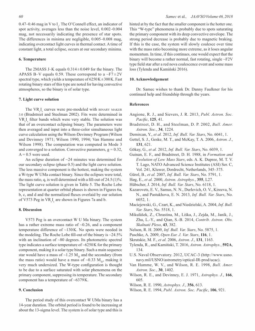
Samec et al., JAAVSO Volume 46, 201860
0.47–0.46 mag in V to Ic. The O’Connell effect, an indicator of spot activity, averages less than the noise level, 0.002–0.004 mag, not necessarily indicating the presence of star spots. The differences in minima are negligible, 0.005–0.008 mag, indicating overcontact light curves in thermal contact. A time of constant light, a total eclipse, occurs at our secondary minima.
6. Temperature
The 2MASS J–K equals 0.314 ± 0.049 for the binary. The APASS B–V equals 0.59. These correspond to a ~F7 ± 2V spectral type, which yields a temperature of 6250 K ± 300 K. Fast rotating binary stars of this type are noted for having convective atmospheres, so the binary is of solar type.
7. Light curve solution
The VRcIc curves were pre-modeled with binary maker 3.0 (Bradstreet and Steelman 2002). Fits were determined in VRcIc filter bands which were very stable. The solution was that of an overcontact eclipsing binary. The parameters were then averaged and input into a three-color simultaneous light curve calculation using the Wilson-Devinney Program (Wilson and Devinney 1971; Wilson 1990, 1994; Van Hamme and Wilson 1998). The computation was computed in Mode 3 and converged to a solution. Convective parameters, g = 0.32, A = 0.5 were used. An eclipse duration of ~24 minutes was determined for our secondary eclipse (phase 0.5) and the light curve solution. The less massive component is the hottest, making the system a W-type W UMa contact binary. Since the eclipses were total, the mass ratio, q, is well determined with a fill-out of 24.5 (1)%. The light curve solution is given in Table 5. The Roche Lobe representation at quarter orbital phases is shown in Figures 6a, b, c, and d and the normalized fluxes overlaid by our solution of V573 Peg in VRcIc are shown in Figures 7a and b.
8. Discussion
V573 Peg is an overcontact W U Ma binary. The system has a rather extreme mass ratio of ~0.26, and a component temperature difference of ~130 K. No spots were needed in the modeling. The Roche Lobe fill-out of the binary is ~24.5% with an inclination of ~80 degrees. Its photometric spectral type indicates a surface temperature of ~6250 K for the primary component, making it a solar type binary. Such a main sequence star would have a mass of ~1.25 M
and the secondary (from
the mass ratio) would have a mass of ~0.33 M
, making it very much undersized. The W-type configuration is thought to be due to a surface saturated with solar phenomena on the primary component, suppressing its temperature. The secondary component has a temperature of ~6379 K.
9. Conclusion
The period study of this overcontact W UMa binary has a 14-year duration. The orbital period is found to be increasing at about the 13-sigma level. The system is of solar type and this is
hinted at by the fact that the smaller component is the hotter one. This “W-type” phenomena is probably due to spots saturating the primary component with its deep convective envelope. The strong period decrease is probably due to magnetic braking. If this is the case, the system will slowly coalesce over time with the mass ratio becoming more extreme, as it loses angular momentum. In time, if this continues, one would expect that the binary will become a rather normal, fast rotating, single ~F2V type field star after a red nova coalescence event and some mass loss (Tylenda and Kamiński 2016).
10. Acknowledgement
Dr. Samec wishes to thank Dr. Danny Faulkner for his continued help and friendship through the years.
References
Angione, R. J., and Sievers, J. R. 2013, Publ. Astron. Soc. Pacific, 125, 41.
Bradstreet, D. H., and Steelman, D. P. 2002, Bull.Amer.Astron. Soc., 34, 1224.
Demircan, Y., et al. 2012, Inf.Bull.Var.Stars, No. 6041, 1.Gettel, S. J., Geske, M. T., and McKay, T. A. 2006, Astron. J.,
131, 621.Gökay, G., et al. 2012, Inf.Bull.Var.Stars, No. 6039, 1.Guinan, E. F., and Bradstreet, D. H. 1988, in Formation and
EvolutionofLowMassStars, eds. A. K. Dupree, M. T. V. T. Lago, NATO Advanced Science Institutes (ASI) Ser. C, Vol. 241, Kluwer, Dordrecht, Netherlands, 345–375.
Gürol, B., et al. 2007, Inf.Bull.Var.Stars, No. 5791, 1.Høg, E., et al. 2000, Astron. Astrophys., 355, L27.Hübscher, J. 2014, Inf.Bull.Var.Stars, No. 6118, 1.Kazarovets, E. V., Samus, N. N., Durlevich, O. V., Kireeva, N.
N., and Pastukhova, E. N. 2013, Inf.Bull.Var.Stars, No. 6052, 1.
Maciejewski, G., Czart, K., and Niedzielski, A. 2004, Inf.Bull.Var. Stars, No. 5518, 1.
Mikulášek, Z., Chrastina, M., Liška, J., Zejda, M., Janík, J., Zhu, L.-Y., and Qian, S.-B. 2014, Contrib. Astron. Obs. Skalnaté Pleso, 43, 382.
Nelson, R. H. 2009, Inf.Bull.Var.Stars, No. 5875, 1. Paschke, A. 2009, OpenEur.J.Var.Stars, 116, 1.Skrutskie, M. F., et al. 2006, Astron. J., 131, 1163.Tylenda, R., and Kamiński, T. 2016, Astron. Astrophys., 592A,
134.U.S. Naval Observatory. 2012, UCAC-3 (http://www.usno.
navy.mil/USNO/astrometry/optical-IR-prod/ucac).Van Hamme, W. V., and Wilson, R. E. 1998, Bull.Amer.
Astron. Soc., 30, 1402.Wilson, R. E., and Devinney, E. J. 1971, Astrophys. J., 166,
605.Wilson, R. E. 1990, Astrophys. J., 356, 613.Wilson, R. E. 1994, Publ.Astron.Soc.Pacific, 106, 921.

Samec et al., JAAVSO Volume 46, 2018 61
–0.365 22.5156 –0.350 22.5224 –0.323 22.5285 –0.316 22.5321 –0.310 22.5356 –0.280 22.5425 –0.258 22.5458 –0.239 22.5491 –0.199 22.5541 –0.175 22.5574 –0.141 22.5606 –0.108 22.5670 –0.062 22.5712 –0.012 22.5754 0.045 22.5813 0.076 22.5855 0.090 22.5897 0.073 22.5957 0.074 22.5999 0.082 22.6041 0.083 22.6095 0.055 22.6137 0.013 22.6179 –0.028 22.6229 –0.076 22.6271 –0.103 22.6313 –0.155 22.6365 –0.338 22.6766 –0.335 22.6808 –0.383 22.6850 –0.376 22.6918 –0.374 22.6922 –0.395 22.6964 –0.386 22.7022 –0.402 22.7064 –0.383 22.7148 –0.343 23.5637 –0.334 23.5676 –0.319 23.5725 –0.308 23.5765 –0.284 23.5804 –0.268 23.5854 –0.033 23.6188 0.009 23.6228 0.041 23.6267 0.074 23.6317 0.081 23.6357 0.082 23.6396 0.078 23.6448 0.081 23.6488 0.065 23.6527 –0.017 23.6620 –0.050 23.6660 –0.121 23.6732 –0.157 23.6772 –0.189 23.6811 –0.228 23.6873 –0.258 23.6913 –0.281 23.6953 –0.300 23.6993 –0.311 23.7032 –0.326 23.7072 –0.338 23.7112 –0.353 23.7152 –0.364 23.7191 –0.374 23.7231
–0.385 23.7271 –0.382 23.7311 –0.391 23.7350 –0.391 23.7390 –0.393 23.7430 –0.382 23.7470 –0.385 23.7510 –0.385 23.7549 –0.381 23.7589 –0.368 23.7629 –0.262 23.7969 –0.255 23.7985 –0.247 23.8001 –0.236 23.8028 –0.227 23.8044 –0.202 23.8060 –0.196 23.8076 –0.190 23.8092 –0.173 23.8108 –0.157 23.8124 –0.148 23.8140 –0.135 23.8156 –0.113 23.8172 –0.100 23.8188 –0.085 23.8204 –0.068 23.8220 –0.061 23.8236 –0.041 23.8252 –0.019 23.8269 –0.009 23.8285 0.010 23.8301 0.028 23.8317 0.040 23.8335 0.042 23.8351 0.069 23.8367 0.077 23.8383 0.077 23.8398 0.069 23.8414 0.078 23.8430 0.080 23.8446 0.101 23.8462 0.076 23.8478 0.074 23.8494 0.085 23.8510 0.075 23.8526 0.078 23.8542 0.073 23.8558 0.092 23.8574 0.086 23.8590 0.084 23.8606 0.086 23.8622 0.067 23.8637 0.065 23.8653 0.059 23.8669 0.037 23.8685 0.009 23.8701 –0.002 23.8733 –0.018 23.8749 –0.044 23.8765 –0.058 23.8781 –0.067 23.8797 –0.090 23.8813 –0.107 23.8829 –0.112 23.8844 –0.129 23.8860 –0.143 23.8876
–0.391 23.7350 –0.391 23.7390 –0.393 23.7430 –0.382 23.7470 –0.385 23.7510 –0.385 23.7549 –0.381 23.7589 –0.368 23.7629 –0.262 23.7969 –0.255 23.7985 –0.247 23.8001 –0.236 23.8028 –0.227 23.8044 –0.202 23.8060 –0.196 23.8076 –0.190 23.8092 –0.173 23.8108 –0.157 23.8124 –0.148 23.8140 –0.135 23.8156 –0.113 23.8172 –0.100 23.8188 –0.085 23.8204 –0.068 23.8220 –0.061 23.8236 –0.041 23.8252 –0.019 23.8269 –0.009 23.8285 0.010 23.8301 0.028 23.8317 0.040 23.8335 0.042 23.8351 0.069 23.8367 0.077 23.8383 0.077 23.8398 0.069 23.8414 0.078 23.8430 0.080 23.8446 0.101 23.8462 0.076 23.8478 0.074 23.8494 0.085 23.8510 0.075 23.8526 0.078 23.8542 0.073 23.8558 0.092 23.8574 0.086 23.8590 0.084 23.8606 0.086 23.8622 0.067 23.8637 0.065 23.8653 0.059 23.8669 0.037 23.8685 0.009 23.8701 –0.002 23.8733 –0.018 23.8749 –0.044 23.8765 –0.058 23.8781 –0.067 23.8797 –0.090 23.8813 –0.107 23.8829 –0.112 23.8844 –0.129 23.8860 –0.143 23.8876 –0.156 23.8892 –0.181 23.8908
–0.190 23.8924 –0.192 23.8940 –0.210 23.8956 –0.222 23.8972 –0.240 23.8988 –0.287 28.5012 –0.287 28.5035 –0.301 28.5058 –0.303 28.5081 –0.317 28.5104 –0.319 28.5127 –0.326 28.5150 –0.335 28.5173 –0.344 28.5196 –0.351 28.5219 –0.347 28.5242 –0.354 28.5265 –0.373 28.5287 –0.367 28.5310 –0.374 28.5333 –0.379 28.5356 –0.382 28.5379 –0.392 28.5402 –0.381 28.5425 –0.388 28.5448 –0.386 28.5471 –0.389 28.5494 –0.384 28.5517 –0.392 28.5540 –0.385 28.5563 –0.395 28.5586 –0.385 28.5609 –0.389 28.5632 –0.384 28.5655 –0.374 28.5678 –0.373 28.5700 –0.363 28.5723 –0.361 28.5746 –0.356 28.5769 –0.333 28.5792 –0.346 28.5815 –0.334 28.5838 –0.321 28.5861 –0.321 28.5884 –0.300 28.5907 –0.292 28.5930 –0.285 28.5953 –0.277 28.5976 –0.263 28.5999 –0.252 28.6022 –0.241 28.6045 –0.216 28.6068 –0.211 28.6091 –0.181 28.6114 –0.151 28.6160 –0.139 28.6183 –0.114 28.6206 –0.091 28.6229 –0.062 28.6251 –0.036 28.6274 –0.029 28.6297 0.002 28.6321 0.012 28.6345 0.039 28.6370 0.054 28.6396 0.063 28.6421
0.070 28.6446 0.077 28.6472 0.075 28.6497 0.077 28.6523 0.077 28.6548 0.072 28.6574 0.076 28.6599 0.058 28.6625 0.051 28.6650 0.026 28.6676 0.003 28.6701 –0.031 28.6727 –0.047 28.6752 –0.082 28.6778 –0.102 28.6803 –0.130 28.6829 –0.150 28.6854 –0.167 28.6880 –0.189 28.6905 –0.207 28.6931 –0.222 28.6960 –0.252 28.6985 –0.255 28.7010 –0.276 28.7036 –0.278 28.7061 –0.302 28.7087 –0.307 28.7112 –0.317 28.7138 –0.330 28.7163 –0.335 28.7189 –0.345 28.7214 –0.353 28.7240 –0.361 28.7265 –0.368 28.7291 –0.372 28.7316 –0.378 28.7341 –0.382 28.7367 –0.386 28.7392 –0.390 28.7418 –0.397 28.7443 –0.397 28.7469 –0.395 28.7494 –0.399 28.7520 –0.397 28.7545 –0.399 28.7571 –0.398 28.7596 –0.398 28.7621 –0.392 28.7647 –0.393 28.7672 –0.386 28.7698 –0.378 28.7723 –0.369 28.7749 –0.363 28.7774 –0.360 28.7800 –0.348 28.7825 –0.339 28.7851 –0.339 28.7876 –0.337 28.7902 –0.327 28.7927 –0.316 28.7952 –0.300 28.7978 –0.288 28.8003 –0.282 28.8029 –0.276 28.8054
∆V HJD 2458000+
∆V HJD 2458000+
∆V HJD 2458000+
∆V HJD 2458000+
∆V HJD 2458000+
Table 1. V573 Peg observations, ΔV, ΔRc, and ΔIc, variable star minus comparison star.
Tablecontinuedonfollowingpages

Samec et al., JAAVSO Volume 46, 201862
–0.248 22.5129 –0.222 22.5195 –0.219 22.5256 –0.210 22.5292 –0.196 22.5327 –0.173 22.5398 –0.162 22.5431 –0.143 22.5464 –0.110 22.5514 –0.096 22.5547 –0.050 22.5579 –0.021 22.5636 0.021 22.5678 0.055 22.5720 0.120 22.5779 0.145 22.5821 0.179 22.5863 0.187 22.5923 0.187 22.5965 0.189 22.6007 0.188 22.6060 0.185 22.6102 0.153 22.6144 0.111 22.6194 0.061 22.6236 0.027 22.6278 –0.015 22.6331 –0.058 22.6373 –0.116 22.6501 –0.140 22.6543 –0.205 22.6732 –0.217 22.6774 –0.243 22.6816 –0.243 22.6883 –0.261 22.6930 –0.270 22.6988 –0.276 22.7030 –0.258 22.7072 –0.260 22.7114 –0.258 22.7156 –0.250 22.7198 –0.249 23.5564 –0.240 23.5604 –0.230 23.5644 –0.218 23.5693 –0.204 23.5732 –0.189 23.5772 –0.174 23.5822 –0.153 23.5862 –0.143 23.5902 –0.119 23.5944 0.050 23.6155 0.084 23.6195 0.121 23.6235 0.165 23.6285 0.180 23.6324 0.189 23.6364 0.191 23.6416 0.187 23.6455 0.186 23.6495 0.157 23.6548 0.128 23.6588 0.092 23.6628 0.018 23.6699 –0.016 23.6739 –0.048 23.6779 –0.096 23.6841 –0.118 23.6881
∆Rc HJD 2458000+
∆Rc HJD 2458000+
∆Rc HJD 2458000+
∆Rc HJD 2458000+
∆Rc HJD 2458000+
Table 1. V573 Peg observations, ΔV, ΔRc, and ΔIc, variable star minus comparison star, cont.
Tablecontinuedonfollowingpages
–0.141 23.6921 –0.160 23.6960 –0.179 23.7000 –0.193 23.7040 –0.209 23.7080 –0.220 23.7119 –0.229 23.7159 –0.242 23.7199 –0.256 23.7239 –0.256 23.7278 –0.263 23.7318 –0.266 23.7358 –0.265 23.7438 –0.267 23.7477 –0.262 23.7517 –0.259 23.7557 –0.254 23.7597 –0.157 23.7955 –0.151 23.7972 –0.145 23.7988 –0.130 23.8015 –0.117 23.8031 –0.112 23.8047 –0.103 23.8063 –0.085 23.8079 –0.081 23.8095 –0.056 23.8111 –0.042 23.8127 –0.042 23.8143 –0.014 23.8158 –0.015 23.8174 0.004 23.8190 0.029 23.8206 0.041 23.8222 0.056 23.8238 0.075 23.8256 0.085 23.8272 0.101 23.8288 0.123 23.8304 0.130 23.8321 0.148 23.8337 0.173 23.8353 0.168 23.8369 0.185 23.8385 0.181 23.8401 0.185 23.8417 0.197 23.8433 0.180 23.8449 0.199 23.8465 0.196 23.8481 0.200 23.8497 0.193 23.8513 0.198 23.8529 0.180 23.8544 0.183 23.8560 0.194 23.8576 0.180 23.8592 0.202 23.8608 0.175 23.8624 0.183 23.8640 0.150 23.8656 0.154 23.8672 0.128 23.8688 0.127 23.8704 0.110 23.8720 0.074 23.8736 0.085 23.8752 0.048 23.8767
0.049 23.8783 0.041 23.8799 0.016 23.8815 0.007 23.8831 –0.020 23.8847 –0.020 23.8863 –0.029 23.8879 –0.045 23.8895 –0.054 23.8911 –0.173 28.4993 –0.176 28.5016 –0.184 28.5039 –0.188 28.5062 –0.196 28.5085 –0.200 28.5108 –0.214 28.5131 –0.222 28.5154 –0.228 28.5177 –0.233 28.5200 –0.238 28.5223 –0.245 28.5246 –0.253 28.5269 –0.251 28.5292 –0.257 28.5315 –0.266 28.5337 –0.266 28.5360 –0.271 28.5383 –0.269 28.5406 –0.272 28.5429 –0.276 28.5452 –0.274 28.5475 –0.275 28.5498 –0.273 28.5521 –0.278 28.5544 –0.267 28.5567 –0.258 28.5590 –0.270 28.5613 –0.259 28.5636 –0.261 28.5659 –0.257 28.5682 –0.253 28.5704 –0.242 28.5727 –0.242 28.5750 –0.232 28.5773 –0.230 28.5796 –0.220 28.5819 –0.220 28.5842 –0.209 28.5865 –0.204 28.5888 –0.183 28.5911 –0.177 28.5934 –0.169 28.5957 –0.155 28.5980 –0.148 28.6003 –0.131 28.6026 –0.118 28.6049 –0.104 28.6072 –0.081 28.6095 –0.067 28.6118 –0.059 28.6141 –0.040 28.6164 –0.018 28.6187 0.007 28.6210 0.019 28.6233 0.048 28.6256 0.070 28.6279 0.098 28.6302 0.112 28.6325
0.132 28.6349 0.157 28.6375 0.165 28.6400 0.180 28.6426 0.183 28.6451 0.180 28.6477 0.181 28.6502 0.181 28.6528 0.189 28.6553 0.184 28.6579 0.176 28.6604 0.162 28.6630 0.148 28.6655 0.121 28.6681 0.104 28.6706 0.074 28.6732 0.050 28.6757 0.028 28.6783 0.014 28.6808 –0.017 28.6834 –0.040 28.6859 –0.061 28.6885 –0.081 28.6910 –0.097 28.6939 –0.116 28.6964 –0.133 28.6990 –0.149 28.7015 –0.159 28.7041 –0.172 28.7066 –0.184 28.7092 –0.194 28.7117 –0.208 28.7143 –0.211 28.7168 –0.219 28.7194 –0.227 28.7219 –0.235 28.7244 –0.245 28.7270 –0.255 28.7295 –0.252 28.7321 –0.258 28.7346 –0.263 28.7372 –0.271 28.7397 –0.278 28.7423 –0.279 28.7448 –0.281 28.7473 –0.279 28.7499 –0.277 28.7524 –0.280 28.7550 –0.278 28.7575 –0.279 28.7601 –0.273 28.7626 –0.271 28.7652 –0.272 28.7677 –0.266 28.7703 –0.265 28.7728 –0.254 28.7753 –0.248 28.7779 –0.243 28.7804 –0.236 28.7830 –0.226 28.7855 –0.222 28.7881 –0.214 28.7906 –0.205 28.7932 –0.198 28.7957 –0.189 28.7983 –0.176 28.8008 –0.169 28.8034 –0.155 28.8059
–0.148 28.8085 –0.131 28.8110 –0.116 28.8135 –0.098 28.8161 –0.087 28.8186 –0.062 28.8212 –0.044 28.8237 –0.018 28.8263 0.009 28.8288 0.029 28.8314 0.054 28.8339 0.080 28.8365 0.108 28.8390 0.137 28.8415 0.148 28.8441 0.171 28.8466 0.176 28.8492 0.179 28.8517 0.187 28.8543 0.192 28.8568 0.179 28.8594 0.188 28.8619 0.182 28.8645 0.189 28.8670 0.187 28.8696 0.181 28.8721 0.172 28.8746 0.149 28.8772 0.121 28.8797 0.095 28.8823 0.070 28.8848 0.053 28.8874 0.023 28.8899 0.001 28.8925 –0.028 28.8950 –0.045 28.8976 –0.066 28.9001 –0.217 30.6022 –0.229 30.6048 –0.234 30.6073 –0.237 30.6099 –0.248 30.6124 –0.253 30.6149 –0.259 30.6175 –0.259 30.6200 –0.263 30.6225 –0.267 30.6251 –0.271 30.6276 –0.268 30.6302 –0.273 30.6328 –0.273 30.6353 –0.270 30.6379 –0.276 30.6404 –0.269 30.6429 –0.270 30.6455 –0.268 30.6480 –0.264 30.6506 –0.264 30.6531 –0.254 30.6556 –0.251 30.6582 –0.240 30.6607 –0.235 30.6633 –0.227 30.6658 –0.222 30.6683 –0.210 30.6709

Samec et al., JAAVSO Volume 46, 2018 63
–0.124 22.5137 –0.113 22.5204 –0.096 22.5265 –0.089 22.5300 –0.074 22.5336 –0.046 22.5406 –0.030 22.5439 –0.005 22.5472 0.018 22.5522 0.050 22.5555 0.061 22.5588 0.085 22.5646 0.135 22.5688 0.174 22.5730 0.248 22.5789 0.285 22.5831 0.315 22.5873 0.321 22.5933 0.308 22.5975 0.313 22.6017 0.314 22.6071 0.304 22.6113 0.277 22.6155 0.267 22.6205 0.190 22.6247 0.150 22.6289 0.104 22.6341 0.065 22.6383 –0.115 22.6826 –0.137 22.6894 –0.143 22.7124 –0.137 22.7166 –0.113 23.5574 –0.120 23.5614 –0.112 23.5654 –0.096 23.5702 –0.074 23.5742 –0.059 23.5782 –0.050 23.5832 –0.031 23.5871 –0.025 23.5953 0.169 23.6165 0.210 23.6205 0.243 23.6244 0.288 23.6294 0.301 23.6334 0.302 23.6374 0.307 23.6425 0.302 23.6465 0.290 23.6505 0.264 23.6557 0.233 23.6597 0.198 23.6637 0.127 23.6709 0.088 23.6749 0.056 23.6788 0.011 23.6850 –0.017 23.6890 –0.036 23.6930 –0.053 23.6970 –0.069 23.7010 –0.085 23.7049 –0.097 23.7089 –0.114 23.7129 –0.120 23.7169
–0.133 23.7208 –0.133 23.7248 –0.137 23.7288 –0.148 23.7328 –0.151 23.7367 –0.154 23.7407 –0.155 23.7447 –0.155 23.7487 –0.148 23.7527 –0.146 23.7566 –0.144 23.7606 0.011 23.8049 0.022 23.8065 0.034 23.8081 0.035 23.8097 0.055 23.8113 0.074 23.8129 0.071 23.8145 0.090 23.8161 0.097 23.8177 0.123 23.8193 0.135 23.8209 0.160 23.8225 0.163 23.8241 0.186 23.8258 0.209 23.8274 0.227 23.8290 0.225 23.8306 0.259 23.8324 0.262 23.8340 0.273 23.8356 0.280 23.8372 0.303 23.8388 0.295 23.8403 0.305 23.8419 0.319 23.8435 0.276 23.8451 0.302 23.8467 0.291 23.8483 0.286 23.8499 0.299 23.8515 0.318 23.8531 0.314 23.8547 0.295 23.8563 0.311 23.8579 0.298 23.8595 0.288 23.8611 0.284 23.8627 0.265 23.8642 0.276 23.8658 0.272 23.8674 0.261 23.8690 0.219 23.8706 0.217 23.8722 0.195 23.8738 0.193 23.8754 0.168 23.8770 0.159 23.8786 0.138 23.8802 0.124 23.8818 0.115 23.8833 0.095 23.8849 0.089 23.8865 0.079 23.8881 0.058 23.8897
0.064 23.8913 –0.048 28.4997 –0.062 28.5020 –0.058 28.5043 –0.070 28.5066 –0.079 28.5089 –0.090 28.5112 –0.095 28.5135 –0.100 28.5158 –0.107 28.5181 –0.109 28.5204 –0.116 28.5227 –0.114 28.5250 –0.125 28.5273 –0.132 28.5296 –0.132 28.5319 –0.148 28.5342 –0.129 28.5364 –0.152 28.5387 –0.152 28.5410 –0.151 28.5433 –0.149 28.5456 –0.149 28.5479 –0.152 28.5502 –0.157 28.5525 –0.148 28.5548 –0.152 28.5571 –0.156 28.5594 –0.149 28.5617 –0.147 28.5640 –0.145 28.5663 –0.136 28.5686 –0.129 28.5709 –0.134 28.5731 –0.124 28.5754 –0.116 28.5777 –0.110 28.5800 –0.099 28.5823 –0.089 28.5846 –0.097 28.5869 –0.077 28.5892 –0.065 28.5915 –0.052 28.5938 –0.050 28.5961 –0.037 28.5984 –0.034 28.6007 –0.010 28.6030 0.011 28.6076 0.026 28.6099 0.046 28.6122 0.066 28.6145 0.085 28.6168 0.104 28.6191 0.119 28.6214 0.138 28.6237 0.168 28.6260 0.181 28.6283 0.211 28.6306 0.233 28.6329 0.252 28.6354 0.267 28.6380 0.281 28.6405 0.294 28.6430 0.288 28.6456 0.294 28.6481
0.296 28.6507 0.296 28.6532 0.293 28.6558 0.289 28.6583 0.276 28.6609 0.278 28.6634 0.263 28.6660 0.239 28.6685 0.209 28.6711 0.189 28.6736 0.166 28.6762 0.138 28.6787 0.116 28.6813 0.098 28.6838 0.074 28.6864 0.052 28.6889 0.038 28.6915 0.013 28.6943 –0.004 28.6969 –0.021 28.6994 –0.030 28.7020 –0.042 28.7045 –0.052 28.7071 –0.064 28.7096 –0.077 28.7122 –0.083 28.7147 –0.091 28.7173 –0.103 28.7198 –0.111 28.7224 –0.119 28.7249 –0.122 28.7275 –0.132 28.7300 –0.133 28.7325 –0.143 28.7351 –0.145 28.7376 –0.144 28.7402 –0.150 28.7427 –0.155 28.7453 –0.153 28.7478 –0.160 28.7504 –0.160 28.7529 –0.163 28.7555 –0.157 28.7580 –0.152 28.7605 –0.152 28.7631 –0.152 28.7656 –0.150 28.7682 –0.149 28.7707 –0.146 28.7733 –0.139 28.7758 –0.131 28.7784 –0.119 28.7809 –0.120 28.7835 –0.110 28.7860 –0.099 28.7886 –0.099 28.7911 –0.089 28.7936 –0.079 28.7962 –0.070 28.7987 –0.058 28.8013 –0.050 28.8038 –0.043 28.8064 –0.012 28.8115 0.002 28.8140 0.024 28.8166
0.042 28.8191 0.053 28.8216 0.078 28.8242 0.094 28.8267 0.119 28.8293 0.146 28.8318 0.172 28.8344 0.193 28.8369 0.202 28.8369 0.230 28.8395 0.259 28.8420 0.275 28.8446 0.287 28.8471 0.304 28.8497 0.302 28.8522 0.297 28.8547 0.303 28.8573 0.304 28.8598 0.306 28.8624 0.297 28.8649 0.300 28.8675 0.304 28.8700 0.291 28.8726 0.276 28.8751 0.249 28.8777 0.227 28.8802 0.210 28.8827 0.185 28.8853 0.161 28.8878 0.137 28.8904 0.116 28.8929 0.080 28.8955 0.074 28.8980 0.034 28.9006 –0.098 30.6027 –0.110 30.6052 –0.114 30.6078 –0.121 30.6103 –0.127 30.6129 –0.129 30.6154 –0.135 30.6179 –0.139 30.6205 –0.144 30.6230 –0.144 30.6256 –0.147 30.6281 –0.151 30.6307 –0.151 30.6332 –0.148 30.6358 –0.148 30.6383 –0.150 30.6409 –0.153 30.6434 –0.141 30.6459 –0.137 30.6485 –0.140 30.6510 –0.135 30.6536 –0.128 30.6561 –0.129 30.6587 –0.115 30.6612 –0.108 30.6637 –0.100 30.6663 –0.104 30.6688 –0.092 30.6713
∆Ic HJD 2458000+
∆Ic HJD 2458000+
∆Ic HJD 2458000+
∆Ic HJD 2458000+
∆Ic HJD 2458000+
Table 1. V573 Peg observations, ΔV, ΔRc, and ΔIc, variable star minus comparison star, cont.

Samec et al., JAAVSO Volume 46, 201864
Table 2. Information on the stars used in this study.
Star Name R.A.(2000) Dec.(2000) V J–K h m s ° ' "
V V573 Peg 23 10 34.2395 31 42 53.7441 12.592 0.314 ± 0.0492
GSC 2751-1007 SAVS 231034+314253 CRTS J231034.2+314254 NSVS 9014625 3UC167-320333 C GSC 2751-01803 23 10 32.1420 31 46 54.8211 12.552 0.482
3UC244-290293
K (Check) GSC 2751-0129 23 10 34.2599 31 47 10.5003 11.2632 0.277 ± 0.0462
3UC167-320353
1 UCAC-3(USNO2012). 2 2Mass(Skrutskieet al.2006).3 TYCHO(Høg,E., et al. 2000).
Table 3. O–C Residuals for V573 Peg.
Epoch Cycles Linear Quadratic Reference 2400000+ Residuals Residuals
1 52885.2469 –9561.0 –0.0060 0.0022 VSX 2 53300.4014 –8566.5 –0.0057 –0.0008 Gürol et al. 2007 3 53301.2365 –8564.5 –0.0055 –0.0007 Gürol et al. 2007 4 53301.4443 –8564.0 –0.0064 –0.0016 Gürol et al. 2007 5 54452.3640 –5807.0 0.0030 0.0015 Paschke 2009 6 54723.7050 –5157.0 0.0014 –0.0011 Nelson 2008 7 55445.4778 –3428.0 0.0028 –0.0010 Gökay et al. 2012 8 55448.4001 –3421.0 0.0029 –0.0008 Gökay et al. 2012 9 55449.4447 –3418.5 0.0039 0.0001 Gökay et al. 2012 10 55764.4106 –2664.0 0.0036 –0.0002 Demircan et al. 2012 11 55778.3963 –2630.5 0.0047 0.0009 Demircan et al. 2012 12 55781.5255 –2623.0 0.0030 –0.0007 Demircan et al. 2012 13 55783.4059 –2618.5 0.0049 0.0011 Demircan et al. 2012 14 55790.5024 –2601.5 0.0048 0.0010 Demircan et al. 2012 15 55799.2681 –2580.5 0.0040 0.0002 Demircan et al. 2012 16 55799.4769 –2580.0 0.0041 0.0003 Demircan et al. 2012 17 56539.4090 –807.5 0.0057 0.0031 Hübscher 2014 18 56539.6127 –807.0 0.0007 –0.0019 Hübscher 2014 19 56876.4938 0.0 –0.0006 –0.0020 Hübscher 2014 20 58022.5991 2745.5 –0.0048 0.0003 This paper 21 58023.6420 2748.0 –0.0056 –0.0005 This paper 22 58023.8510 2748.5 –0.0053 –0.0002 This paper 23 58028.6522 2760.0 –0.0047 0.0004 This paper 24 58028.8608 2760.5 –0.0049 0.0002 This paper
Calculated from the light curve data given in the reference. The quadratic ephemeris yields a P·=–4.79× 10⁻⁷ d/yr.
Table 4. Averaged light curve characteristics of V573 Peg.
Filter Phase Magnitude Phase Magnitude Min. I Max. I
0.0 0.25 V 0.075 ± 0.002 –0.393 ± 0.007 Rc 0.184 ± 0.005 –0.274 ± 0.007 Ic 0.298 ± 0.006 –0.157 ± 0.004 Filter Phase Magnitude Phase Magnitude Min. II Max. II
0.5 0.75
V 0.080 ± 0.009 –0.392 ± 0.006 Rc 0.192 ± 0.007 –0.271 ± 0.006 Ic 0.303 ± 0.009 –0.153 ± 0.018 Filter Min.I–Max.I Max.I–Max.II Min.I–Min.II
V 0.468 ± 0.009 –0.002 ± 0.013 –0.005 ± 0.011 Rc 0.458 ± 0.011 –0.004 ± 0.013 –0.008 ± 0.011 Ic 0.455 ± 0.010 –0.004 ± 0.022 –0.005 ± 0.015 Filter Max.II–Max.I Filter Min.II–Max.I
V 0.002 ± 0.013 V 0.472 ± 0.016 Rc 0.004 ± 0.013 Rc 0.463 ± 0.013 Ic 0.004 ± 0.022 Ic 0.456 ± 0.013
lV, lRc, lIc (nm) 440, 550, 640, 790 xbol1,2 , ybol1,2 0.640 0 .640, 0.232, 0.232 x1Ic,2Ic , y1Ic,2Ic 0.569, 0.569, 0.271, 0.271 x1Rc,2Rc , y1Rc,2Rc 0.652, 0.652, 0. 278, 0.278 x1V,2V , y1V,2V 0.725, 0.725, 0.266, 0. 266 g1 , g2 0.320, 0.320 A1 , A2 0.5, 0.5 Inclination (°) 80.43 ± 0.06 T1, T2 (K) 6250, 6379 ± 1 Ω1= Ω2 pot 2.3421 ± 0.0005
q (m2 / m1) 0.2629 ± 0.0003 Fill–outs: F1 = F2 (%) 24.5 ± 1.0 L1 / (L1 + L2)Ic 0.7554 ± 0.0003 L1 / (L1 + L2)Rc 0.7531 ± 0.0003 L1 / (L1 + L2)V 0.7023 ± 0.0003 JDo (days) 2458028.65131 ± 0.00006 Period (days) 0.417454 ± 0.000007 r1, r2 (pole) 0.4751 ± 0.0003, 0.2613 ± 0.0006 r1, r2 (side) 0.5152 ± 0.0005, 0.2733 ± 0.0008 r1, r2 (back) 0.5426 ± 0.0006, 0.3146 ± 0.0016
Table 5. VRcIc solution parameters for V573 Peg.
Parameter Overcontact Solution Parameter Overcontact Solution

Percy, JAAVSO Volume 46, 2018 65
Sparsely-Observed Pulsating Red Giants in the AAVSO Observing ProgramJohn R. PercyDepartment of Astronomy and Astrophysics, and Dunlap Institute of Astronomy and Astrophysics, University of Toronto, Toronto ON M5S 3H4, Canada
Received May 16, 2018; revised June 14, 2018; accepted June 14, 2018
Abstract This paper reports on time-series analysis of 156 pulsating red giants (21 SRa, 52 SRb, 33 SR, 50 Lb) in the AAVSO observing program for which there are no more than 150–250 observations in total. Some results were obtained for 68 of these stars: 17 SRa, 14 SRb, 20 SR, and 17 Lb. These results generally include only an average period and amplitude. Many, if not most of the stars are undoubtedly more complex; pulsating red giants are known to have wandering periods, variable amplitudes, and often multiple periods including “long secondary periods” of unknown origin. These results (or lack thereof) raise the question of how the AAVSO should best manage the observation of these and other sparsely-observed pulsating red giants.
1. Introduction
Red giants are unstable to radial pulsation. As they expand and cool, the period and amplitude of pulsation increase. Pulsating red giants (PRGs) are classified as Mira if they have well-pronounced periodicity and visual range greater than 2.5, as SRa if they have smaller amplitudes and persistent periodicity, as SRb if the periodicity is poorly expressed, and Lb if the variability is irregular. These classes are arbitrary; there is a spectrum of behavior from strictly periodic to completely irregular, and of amplitudes from millimagnitudes up to 10 magnitudes. The AAVSO International Database contains observations of thousands of PRGs. Some are well-studied, especially the brighter Miras; see Templeton et al. (2005) for a study of the periods and period changes in 547 of them. There are many, however, which have not been studied, often because the number of observations is insufficient. A few years ago, my students and I undertook a study of some PRGs for which there were only a few hundred observations: SRa/SRb/SR stars (Percy and Tan 2013; Percy and Kojar 2013) and Lb stars (Percy and Long 2010; Percy and Terziev 2011). The present paper describes a study of several dozen more SR and Lb stars for which there were a total of 150–250 observations, and for which analysis might be possible. I thank Elizabeth Waagen, at AAVSO HQ, for compiling lists of these sparsely-observed SRa, SRb, SR, and Lb stars. Although the primary purpose of this study was to determine the basic variability parameters of as many of these stars as possible, an equally-important purpose was, more generally, to determine whether sparsely-observed PRGs can yield any meaningful results.
2. Data and analysis
Observations were taken from the AAVSO International Database (Kafka 2018). They ranged from all visual for some stars, to all Johnson V (photoelectric or CCD) for others. Periods were determined (or searched for) using the Fourier routine in the VSTAR software package (Benn 2013). Some of the stars had been studied with the All-Sky Automated Survey (ASAS: Pojmański 1997), and a period had been derived. In many cases, the ASAS light curve showed that the variability was complex,
and occurred on two or more periods or time scales. This may be true for most of our stars.
3. Results
Tables 1–4 list results for the stars classified as SRa, SRb, SR, and Lb, respectively. Columns list: the star; the period in the VSX catalog (PVSX); the mean period and semi-amplitude obtained in the present study; and notes about the star. Visual amplitudes are denoted v, Johnson V amplitudes as V. The notes are as follows: 1: new period gives a better phase curve than PVSX; 2: new period and PVSX give equally good phase curves; 3: PVSX gives a poor phase curve; 4: neither new period or PVSX gives a good phase curve; *: see note in section 3.1. Figure 1 gives one example of an SR star (EQ And) which shows a quite acceptable phase curve. Many of the Lb stars in Table 4 were observed primarily in Johnson V, and produce acceptable results with only a few dozen observations. The following are the number of stars analyzed, and the number and percent which produced results, and which appear in Tables 1–4: SRa: 21, 17, 81%; SRb: 52, 14, 27%; SR: 33, 20, 61%; Lb: 50, 17, 34%.
3.1. Notes on individual stars These notes on individual SRa, SRb, SR, and Lb stars are combined, and are listed in order of constellation. Many of the 156 stars in the input list also have observations from other sources, such as ASAS, Hipparcos, DIRBE (Smith et al. 2002), AFOEV, etc., but, unless they helped in the analysis or interpretation of the AAVSO data, they are not discussed here. KWCep the Fourier spectrum is complex; the dominant cycle lengths are about 150 days. UZCet the ASAS period is 80.9 days, but the average cycle length is about 117 days. PVSX, the new period, and the ASAS period produce equally unsatisfactory phase curves, but PVSX is probably the best. RUCrB the V observations show cycle lengths of about 60 days, but the early visual observations give a period of 436 days, which may possibly be a long secondary period. VYEri the ASAS light curve is very complex; irregular or multiperiodic star?

Percy, JAAVSO Volume 46, 201866
TZHor there is also a peak at 23.41 days, but the cycle lengths are 35 days. DV Lac the Fourier spectrum is complex, with cycle lengths in the range of 150 to 180 days. RS LMi complex; cycle lengths about 110 days; there may be a long secondary period. V360 Peg the General Catalogue of Variable Stars (Samus et al. 2017) classifies this star as possibly RV Tauri type, but we find no evidence for this. SWPic the V observations show periods of about 25 and 35 days. TWRet the General Catalogue of Variable Stars (Samus et al. 2017) classifies this star as possibly RV Tauri type, but we find no evidence for this. BNSer there are several peaks of comparable height in the Fourier spectrum. There appears to be a long secondary period.
4. Discussion
In the AAVSO observing program, there are 155 PRGs which are designated as “legacy stars,” and recommended for regular observation. Over the last decade, they have averaged about 375 observations per year (Pearce 2018). These dense, sustained observations enable astronomers to follow their wandering periods, variable amplitudes, multiperiodicity, and long secondary periods (LSPs). For the 156 stars in the present study, there are less than 250 observations in total. As a result, less than half the stars yield any meaningful result, that usually being only an estimate of the average period and amplitude. There are some stars which have only a few dozen V observations obtained on a single night (!). For others, sparse observations are spread over many decades. For others, the Fourier spectra showed many comparable peaks, with none of them prominent. Some PRGs are known to pulsate in both the fundamental and first-overtone modes. There may be some stars for which the derived period is actually an LSP, with the shorter pulsation period hidden in the noise. Some stars, especially the Lb stars, may be truly irregular. A few of the Lb stars in Table 4 had only one or two cycles of V observations, so it was not possible to say whether they showed any strict periodicity. A few others had more V observations, but not enough to say whether they were multiperiodic or irregular. A few, such as OR Cep (Figure 2), RU Leo, and Z LMi, showed good phase curves, and may be SR. Some of the stars in Tables 1–4 may, of course, have been misclassified as to variable star type because of limited observations.
5. Conclusions
Of the 156 stars that were examined, less than half yielded any useful information, that being an average period and amplitude. In many cases, that information was uncertain. It is noteworthy, however, that about a third of the Lb (irregular) variables showed some periodicity.
It is not clear that continued sparse observation of the stars in this study will yield better results. And there are many more PRGs in the AAVSO observing program with less than 150 observations in total, and which were therefore not included in the present study. AAVSO might wish to think seriously about how to manage these PRGs in its observing program. If it is decided that these stars should continue to be observed, then it might be best if observers “adopted” stars for a year or two (or three), to ensure that they were observed sufficiently regularly. Another important development is the ASAS-SN (All-Sky Automated Survey for Supernovae) project, based at Ohio State University. In the near future, it will have pre-computed light curves for all the stars in the VSX catalog at https://asas-sn.osu.edu/variables. Thus, the management of the AAVSO observing programs will have to be done in the context of ASAS-SN and other large all-sky surveys.
6. Acknowledgements
I thank the AAVSO observers who made the observations on which this project is based, the AAVSO staff who archived them and made them publicly available, and the developers of the vstar package which was used in the analysis. Special thanks to Elizabeth Waagen. I thank Professor Christopher Kochanek for helpful information about ASAS-SN. This project made use of the SIMBAD database, maintained in Strasbourg, France. The Dunlap Institute is funded through an endowment established by the David Dunlap family, and the University of Toronto.
References
Benn, D. 2013, vstar data analysis software (http://www.aavso.org/vstar-overview).
Kafka, S. 2018, variable star observations from the AAVSO International Database: (https://www.aavso.org/aavso-international-database).
Pearce, A. 2018, AAVSONewsletter, No. 75 (January), 15.Percy, J. R., and Kojar, T. 2013, J. Amer. Assoc. Var. Star Obs.,
41, 15.Percy, J. R., and Long, J. 2010, J. Amer. Assoc. Var. Star Obs.,
38, 161.Percy, J. R., and Tan, P. J. 2013, J. Amer. Assoc. Var. Star Obs.,
41, 1.Percy, J. R., and Terziev, E. 2011, J. Amer. Assoc. Var. Star
Obs., 39, 1.Pojmański, G. 1997, Acta Astron., 47, 467.Samus, N. N., et al. 2017, General Catalogue of Variable
Stars, Sternberg Astronomical Institute, Moscow (GCVS database: http://www.sai.msu.ru/gcvs/gcvs/index.htm).
Smith, B. J., Leisawitz, D., Castelaz, M. W., and Luttermoser, D. 2002, Astron. J., 123, 948.
Templeton, M. R., Mattei, J. A., and Willson, L. A. 2005, Astron. J., 130, 776.

Percy, JAAVSO Volume 46, 2018 67
Figure 1. Phase plot for EQ And, 13 Jun 2018 (database). EQ And is classified as SR. The phase diagram using mostly Johnson V observations (green), a period of 270.48 days, and epoch 2454781.925, shown here, is quite satisfactory. The period in VSX, 211: days, does not produce a good phase diagram.
Figure 2. Phase plot for OR Cep, 13 Jun 2018 (database). OR Cep is classified as Lb (irregular). The phase diagram using mostly visual (black) and a few Johnson V (green) observations, a period of 348.5 days, and an epoch of 2454651.51, shown here, is quite satisfactory.

Percy, JAAVSO Volume 46, 201868
Table 1. Variability Properties of Some SRa Stars.
Star PVSX(days) P(days) Amp(mag) Notes UV Aql 385.5 350 ± 30 0.17v many peaks LQ Ara 183.7 179.73 0.34v 1: FX Cas 289 292.4 1.44v data consistent with PVSX V533 Cas 305 303.67 1.04v 1 V864 Cas — 344 1.00V P (vis) = 368 days AL Cen 125 128.7 0.69v 1, ASAS P = 126.64 days V343 Cep 525 482.9 0.93v 1 UZ Cet 121.74 203.34 0.14V *; 1, multiperiodic? V577 Cyg 479 478.5 0.32v 1, P (V) = 460.8 days V659 Cyg 514 509.68 0.73v 1 V1059 Cyg 372 380 ± 10 0.18v poor phase curve; period spurious? AY Her 129.75 127.58 1.05v 2 IV Peg 214.0 213.8 0.95v 1, ASAS P = 210.387 days TW Ret 217.6 225.99 — *, 2, RVT according to SIMBAD VV Tel 138.8 137.6 0.70V 1 UZ Vel 354 390.6 0.16v 1:, ASAS P = 353 days NSVS J0712062+293744 106.2 106.64 0.43v 3
Table 2. Variability Properties of Some SRb Stars.
Star PVSX(days) P(days) Amp(mag) Notes
W Ara 122 119.6 0.14v 1, ASAS P = 121.8 days V505 Car 26.5 20.266 0.02V and/or 26.408 days V481 Cas 158.4 159 0.07V R Cir 222 366.3? 0.24v 1, 3, ASAS P = 220 days RU Crt 60.85 700: 0.39v broad peak in Fourier spectrum AQ Del 71.9 71.6 0.16v 1, ASAS P = 73.61 days VY Eri 102.5 189: 0.23v *; 1, ASAS P = 191 days, one cycle in V V521 Ori 221 225.17 0.36V 1 X Pav 199.19 400.3 0.33v 1 V443 Per 69.5 69.9 0.17V 3, LSP ~ 400 days RW Psc 154 154.2 0.15v 2 Z Ser 88.2 88.3 0.18v P (ASAS) = 89.379 days BN Ser 140.7 same 0.17V *; ASAS P = 144.131 days GK Vel 120: 182: 0.08v? 1, several peaks including 123.7 days
Table 3. Variability Properties of Some SR Stars.
Star PVSX(days) P(days) Amp(mag) Notes
EQ And 211: 273.6 0.82v 1; see Figure 1 KQ Aql 164.2 417 0.50v 2, PVSX gives good phase curve V925 Aql — 398.8 0.18v: poor phase curve SZ Ara 221.8 219.8 0.77v 1 UW Cam 544 523.3 0.33v variable amplitude AM Car 314 408 0.45v 1; also 50-day cycles RU CrB 436 427 0.2V *; 2, 436 days may be an LSP V1673 Cyg 115.5 116.5 0.15v AE Del 260 152.5 0.67v PVSX is an alias V529 Her 400 197.3 0.10v 2 TZ Hor ??? 35.52 0.02V *; also 23.41 days Y Mic 364: 180 ± 2 0.18v 4 V360 Peg 44.9 45.28 0.09V *; 1, RV Tau evidence weak V Pic 180 173.3 0.62v 1 SW Pic — 25.2 ± 0.1 0.026V * γ Ret 25 29.87 0.034V DR Tuc — 23.59 0.028V Hipparcos P = 23.87 days o Vir — 30.50 0.036V NSV11453 153 296.47 0.85v 1 OGLE-BLG-LPV-062772 78.09 same 0.21V 2

Percy, JAAVSO Volume 46, 2018 69
Table 4. Variability Properties of Some Lb Stars.
Star P(days) Amp(mag) Notes
KR Cep 50 0.13V one cycle in V KT Cep 77 0.16V two cycles in V KW Cep 170 ± 10 0.15v *; complex; cycles 150 days long OR Cep 348.5 0.97v good phase curve; Figure 2 DV Lac 170 ± 10 0.27V *; irregular; result uncertain PY Lac 95 0.19V one cycle in V; also short-period variability? RU Leo 161 0.38V good phase curve VX Leo 95.6 0.16V good phase curve, but complex, multiperiodic? CP Leo 190: 0.07V poor phase curve; complex, multiperiodic? GK Leo 345 ± 5 0.16V Z LMi 161: 0.31V good phase curve RS LMi 90: 0.13V *; poor phase curve; complex CX Mon 385 0.35v fair phase curve WW Psc 25 ± 0.03V FL Ser 390 ± 2 0.16v fair phase curve TT UMa 490 ± 10 0.1v fair phase curve NSV 623 74 ± 2 0.25v uncertain; ΔV = 0.50

Samolyk, JAAVSO Volume 46, 201870
Recent Maxima of 86 Short Period Pulsating StarsGerard SamolykP.O.Box20677,Greenfield,WI53220;[email protected]
Received January 16, 2018; accepted January 16, 2018
Abstract This paper contains times of maxima for 86 short period pulsating stars (primarily RR Lyrae and δ Scuti stars). This represents the CCD observations received by the AAVSO Short Period Pulsator (SPP) Section in 2017.
1. Recent observations
Table 1 contains times of maxima calculated from CCD observations made by participants in the AAVSO's Short Period Pulsator (SPP) Section. The data in this table will be web-archived and made available through the AAVSO ftp site at ftp://ftp.aavso.org/public/datasets/gsamo-461-spp86.txt. The error estimate is included. RR Lyr stars in this table, along with data from earlier AAVSO publications, are included in the GEOS database at: http://rr-lyr.irap.omp.eu/dbrr/. This database does not include δ Scuti stars. These observations were reduced by the writer using the peranso program (Vanmunster 2007). Column F indicates the filter used. A “C” indicates a clear filter. The linear elements in the General Catalogue of Variable Stars (GCVS; Kholopov et al. 1985) were used to compute the O–C values for most stars. For a few exceptions where the GCVS elements are missing or are in significant error, light elements from another source are used: VY CrB (Antipin 1996); RZ Cap and DG Hya (Samolyk 2010); AM CMi, V1124 Her, and FR Psc (GEOS Database); VY LMi (Henden and Vidal-Sainz 1997); and GW UMa (Hintz et al. 2005).
For two δ Sct stars in the table, no published light elements were found. The following light elements were calculated using a linear regression on the times of maxima listed in this paper.
V521 And Time of maximum (JD) = 2454380.625 + 0.100960755 E (1) ±0.002 0.000000056
V2416 Cyg Time of maximum (JD) = 2453612.601 + 0.055889672 E (2) ±0.001 0.000000017
References
Antipin S. V. 1996, Inf.Bull.Var.Stars, No. 4343, 1.Henden, A. A., and Vidal-Sainz, J. 1997, Inf.Bull.Var.Stars,
No. 4535, 1.Hintz , E. G., Bush , T. C., and Rose , M. B. 2005, Astron. J.,
130, 2876.Kholopov, P. N., et al. 1985, General Catalogue of Variable
Stars, 4th ed., Moscow.Samolyk, G. 2010, J. Amer. Assoc. Var. Stars, 38, 12.Vanmunster, T. 2007, peranso period analysis software (http://
www.peranso.com).
Figure 1. O–C diagram for V521 And plotted using Equation 1. Figure 2. O–C diagram for V2416 Cyg plotted using Equation 2.

Samolyk, JAAVSO Volume 46, 2018 71
Star JD(max) Cycle O–C F Observer Error Hel. 2400000 +
Table 1. Recent times of maxima of stars in the AAVSO Short Period Pulsator program.
Star JD(max) Cycle O–C F Observer Error Hel. 2400000 +
Tablecontinuedonfollowingpages
SW And 57947.6347 90023 –0.4801 V T. Arranz 0.0006 SW And 57951.6146 90032 –0.4807 V T. Arranz 0.0006 SW And 57970.6318 90075 –0.4815 V T. Arranz 0.0005 SW And 57985.6688 90109 –0.4820 V T. Arranz 0.0007 SW And 57986.5548 90111 –0.4806 V T. Arranz 0.0007 SW And 57989.6497 90118 –0.4816 V T. Arranz 0.0007 SW And 58009.5511 90163 –0.4828 V T. Arranz 0.0006 SW And 58016.6275 90179 –0.4829 V T. Arranz 0.0006 SW And 58017.5120 90181 –0.4829 V T. Arranz 0.0006 SW And 58024.5883 90197 –0.4831 V T. Arranz 0.0007 SW And 58025.4718 90199 –0.4842 V T. Arranz 0.0006 SW And 58032.5488 90215 –0.4836 V T. Arranz 0.0007 SW And 58035.6446 90222 –0.4838 V T. Arranz 0.0006 SW And 58036.5290 90224 –0.4839 V T. Arranz 0.0007 SW And 58039.6254 90231 –0.4835 V T. Arranz 0.0008 SW And 58048.4704 90251 –0.4841 V T. Arranz 0.0006 SW And 58051.5664 90258 –0.4840 V T. Arranz 0.0007 SW And 58060.8533 90279 –0.4850 V T. Polakis 0.0011 SW And 58079.4284 90321 –0.4856 V T. Arranz 0.0006 XX And 57952.8620 26102 0.2789 V G. Samolyk 0.0016 XX And 57973.8209 26131 0.2781 V G. Samolyk 0.0013 XX And 58007.7901 26178 0.2782 V K. Menzies 0.0011 XX And 58013.5727 26186 0.2788 V T. Arranz 0.0010 XX And 58031.6423 26211 0.2797 V T. Arranz 0.0010 XX And 58052.6011 26240 0.2789 V T. Arranz 0.0011 XX And 58071.3898 26266 0.2761 V T. Arranz 0.0008 XX And 58096.6942 26301 0.2844 V R. Sabo 0.0027 XX And 58115.4844 26327 0.2832 V K. Menzies 0.0014 AC And 57990.5773 13343 0.3490 V T. Arranz 0.0013 AC And 57998.4593 13354 0.4073 V T. Arranz 0.0011 AC And 58000.5791 13357 0.3934 V G. Samolyk 0.0019 AC And 58000.5822 13357 0.3965 V T. Arranz 0.0018 AC And 58003.5963 13361 0.5657 V T. Arranz 0.0021 AC And 58005.6968 13364 0.5324 V G. Samolyk 0.0021 AC And 58008.3813 13368 0.3720 V T. Arranz 0.0012 AC And 58010.5031 13371 0.3601 V T. Arranz 0.0012 AC And 58012.6183 13374 0.3415 V T. Arranz 0.0011 AC And 58022.5859 13388 0.3518 V T. Arranz 0.0011 AC And 58026.8261 13394 0.3245 V G. Samolyk 0.0015 AT And 57974.7996 25338 –0.0068 V G. Samolyk 0.0019 AT And 57989.6040 25362 –0.0084 V T. Arranz 0.0012 AT And 58031.5571 25430 –0.0055 V T. Arranz 0.0014 AT And 58034.6461 25435 –0.0011 V T. Arranz 0.0016 AT And 58039.5785 25443 –0.0040 V T. Arranz 0.0016 AT And 58070.4189 25493 –0.0093 V T. Arranz 0.0013 DY And 57917.9144 36223 –0.1720 V T. Polakis 0.0017 GM And 57981.8191 45759 0.0469 V R. Sabo 0.0011 GM And 58037.6543 45838 0.0482 V R. Sabo 0.0029 GM And 58047.5467 45852 0.0460 V K. Menzies 0.0016 V521 And 54380.6257 0 0.0007 V G. Samolyk 0.0019 V521 And 57623.7886 32123 0.0013 V G. Samolyk 0.0022 V521 And 57623.8858 32124 –0.0025 V G. Samolyk 0.0025 V521 And 57676.5896 32646 –0.0002 V G. Samolyk 0.0034 V521 And 58083.5637 36677 0.0011 V N. Simmons 0.0034 V521 And 58083.6655 36678 0.0019 V N. Simmons 0.0028 SW Aqr 57904.9420 71429 –0.0019 V T. Polakis 0.0010 SW Aqr 57951.7912 71531 –0.0017 V G. Samolyk 0.0009 SW Aqr 58024.3615 71689 –0.0013 V T. Arranz 0.0007 SW Aqr 58030.3324 71702 –0.0013 V T. Arranz 0.0008 SW Aqr 58032.6288 71707 –0.0014 V T. Polakis 0.0009 SW Aqr 58042.7334 71729 –0.0015 V T. Polakis 0.0005 SW Aqr 58064.3200 71776 –0.0021 V T. Arranz 0.0006 TZ Aqr 57998.8126 35802 0.0143 V G. Samolyk 0.0018 YZ Aqr 57978.8133 40973 0.0786 V G. Samolyk 0.0012 YZ Aqr 58077.6067 41152 0.0762 V G. Samolyk 0.0016 AA Aqr 58035.6229 61238 –0.1740 V G. Samolyk 0.0012
BO Aqr 58026.6792 23638 0.2155 V G. Samolyk 0.0015 BR Aqr 58052.7095 42369 –0.2197 V G. Samolyk 0.0009 BR Aqr 58083.5497 42433 –0.2197 V G. Samolyk 0.0009 CY Aqr 58005.7839 388237 0.0151 V G. Samolyk 0.0004 CY Aqr 58005.8449 388238 0.0152 V G. Samolyk 0.0004 CY Aqr 58005.9056 388239 0.0148 V G. Samolyk 0.0002 CY Aqr 58019.3342 388459 0.0149 V T. Arranz 0.0002 CY Aqr 58019.3952 388460 0.0149 V T. Arranz 0.0003 CY Aqr 58025.3771 388558 0.0151 V T. Arranz 0.0003 TZ Aur 57768.7653 96678 0.0145 V G. Samolyk 0.0008 TZ Aur 58029.6224 97344 0.0163 V T. Arranz 0.0006 TZ Aur 58038.6299 97367 0.0153 V T. Arranz 0.0006 TZ Aur 58040.5892 97372 0.0162 V T. Arranz 0.0007 TZ Aur 58068.7891 97444 0.0155 V K. Menzies 0.0006 TZ Aur 58102.8660 97531 0.0167 V R. Sabo 0.0007 BH Aur 57761.5641 32910 0.0068 V G. Samolyk 0.0009 BH Aur 58030.6591 33500 0.0088 V T. Arranz 0.0009 BH Aur 58042.5165 33526 0.0079 V T. Arranz 0.0009 BH Aur 58042.9719 33527 0.0072 V T. Polakis 0.0014 BH Aur 58044.7964 33531 0.0073 V G. Samolyk 0.0011 BH Aur 58052.5492 33548 0.0066 V T. Arranz 0.0009 BH Aur 58073.5312 33594 0.0085 V T. Arranz 0.0008 BH Aur 58077.6342 33603 0.0067 V T. Arranz 0.0007 RS Boo 57807.7658 42501 –0.0073 V G. Samolyk 0.0008 RS Boo 57861.7289 42644 –0.0037 V G. Samolyk 0.0013 RS Boo 57875.6893 42681 –0.0049 V T. Polakis 0.0008 RS Boo 57877.5759 42686 –0.0049 V K. Menzies 0.0007 RS Boo 57884.7415 42705 –0.0088 V T. Polakis 0.0008 RS Boo 57885.8735 42708 –0.0088 V T. Polakis 0.0009 RS Boo 57887.7598 42713 –0.0092 V T. Polakis 0.0007 RS Boo 57912.6682 42779 –0.0052 V G. Samolyk 0.0009 RS Boo 57936.8172 42843 –0.0059 V T. Polakis 0.0009 ST Boo 57797.8214 62055 0.0868 V G. Samolyk 0.0015 ST Boo 57883.6999 62193 0.0892 V R. Sabo 0.0019 ST Boo 57891.7921 62206 0.0916 V T. Polakis 0.0011 SW Boo 57798.8881 29653 0.4794 V G. Samolyk 0.0011 SW Boo 57875.9209 29803 0.4829 V T. Polakis 0.0017 SZ Boo 57803.8056 57694 0.0091 V G. Samolyk 0.0002 SZ Boo 57828.9028 57742 0.0109 V G. Samolyk 0.0013 SZ Boo 57873.8661 57828 0.0117 V T. Polakis 0.0011 TV Boo 57796.8628 106179 0.1075 V R. Sabo 0.0024 TV Boo 57877.8023 106438 0.0941 V T. Polakis 0.0014 TV Boo 57879.7084 106444 0.1249 V R. Sabo 0.0026 TW Boo 57857.7624 58178 –0.0929 V G. Samolyk 0.0011 TW Boo 57889.6978 58238 –0.0939 V T. Polakis 0.0009 UU Boo 57788.9034 47501 0.3127 V G. Samolyk 0.0013 UU Boo 57874.8073 47689 0.3156 V T. Polakis 0.0008 UU Boo 57881.6621 47704 0.3166 V N. Simmons 0.0011 UY Boo 57815.9180 24552 0.8863 V G. Samolyk 0.0009 UY Boo 57907.6819 24693 0.8822 V N. Simmons 0.0010 YZ Boo 57905.7162 151398 0.1076 V N. Simmons 0.0007 YZ Boo 57905.8203 151399 0.1076 V N. Simmons 0.0009 UY Cam 57811.6478 83307 –0.0874 V G. Samolyk 0.0039 UY Cam 58008.9899 84046 –0.0896 V T. Polakis 0.0028 UY Cam 58012.9972 84061 –0.0879 V T. Polakis 0.0024 UY Cam 58042.9035 84173 –0.0904 V T. Polakis 0.0011 UY Cam 58083.7579 84326 –0.0935 V G. Samolyk 0.0027 UY Cam 58107.7935 84416 –0.0917 V G. Samolyk 0.0033 RW Cnc 57783.7399 33310 0.2272 V G. Samolyk 0.0015 TT Cnc 57787.7912 31668 0.1086 V G. Samolyk 0.0021 VZ Cnc 57798.5654 100363 0.0244 V G. Samolyk 0.0011 VZ Cnc 57798.7318 100364 0.0124 V G. Samolyk 0.0006 AM Cnc 58108.8382 3723 0.0020 V K. Menzies 0.0021 SS CVn 57824.8045 38039 –0.3608 V K. Menzies 0.0010 SS CVn 57877.8913 38150 –0.3898 V T. Polakis 0.0013 SS CVn 57926.7242 38252 –0.3661 V T. Polakis 0.0008

Samolyk, JAAVSO Volume 46, 201872
Star JD(max) Cycle O–C F Observer Error Hel. 2400000 +
Table 1. Recent times of maxima of stars in the AAVSO Short Period Pulsator program, cont.
Star JD(max) Cycle O–C F Observer Error Hel. 2400000 +
Table continued on next page
RV Cap 57949.8732 53751 –0.0771 V G. Samolyk 0.0012 RZ Cap 57998.6419 16493 0.0024 V G. Samolyk 0.0016 YZ Cap 58006.6684 52209 0.0474 V G. Samolyk 0.0021 RR Cet 58006.8537 44890 0.0165 V G. Samolyk 0.0013 RR Cet 58030.6334 44933 0.0160 V T. Arranz 0.0011 RU Cet 58088.5851 31149 0.1384 V G. Samolyk 0.0012 RV Cet 58065.7157 30401 0.2781 V G. Samolyk 0.0027 RX Cet 58093.5888 31319 0.3363 V G. Samolyk 0.0019 RZ Cet 58043.7499 47271 –0.2224 V G. Samolyk 0.0017 UU Cet 57642.9041 27116 –0.1643 V G. Samolyk 0.0021 UU Cet 58044.7245 27779 –0.1756 V G. Samolyk 0.0019 VY CrB 57878.8188 34782 –0.1616 V T. Polakis 0.0012 VY CrB 58011.6807 35069 –0.1683 V T. Polakis 0.0008 VY CrB 58043.6258 35138 –0.1673 V T. Polakis 0.0014 XX Cyg 57881.6259 99553 0.0048 V G. Samolyk 0.0010 XX Cyg 57881.7591 99554 0.0031 V G. Samolyk 0.0005 XX Cyg 57902.6644 99709 0.0043 V G. Samolyk 0.0006 XX Cyg 57902.7988 99710 0.0039 V G. Samolyk 0.0005 XX Cyg 57928.8273 99903 0.0034 V T. Polakis 0.0005 XZ Cyg 57886.6916 29494 –2.5982 V G. Samolyk 0.0008 XZ Cyg 57905.8261 29535 –2.5984 V G. Samolyk 0.0014 XZ Cyg 57912.8201 29550 –2.6049 V H. Smith 0.0008 XZ Cyg 57928.6800 29584 –2.6128 V G. Samolyk 0.0007 XZ Cyg 57939.4160 29607 –2.6109 V T. Arranz 0.0006 XZ Cyg 57942.6774 29614 –2.6164 V G. Samolyk 0.0011 XZ Cyg 57943.6154 29616 –2.6118 V T. Arranz 0.0011 XZ Cyg 57952.4836 29635 –2.6109 V T. Arranz 0.0005 XZ Cyg 57957.6196 29646 –2.6086 V T. Arranz 0.0007 XZ Cyg 57960.4175 29652 –2.6109 V T. Arranz 0.0005 XZ Cyg 57963.6827 29659 –2.6126 V G. Samolyk 0.0007 XZ Cyg 57964.6145 29661 –2.6142 V T. Arranz 0.0006 XZ Cyg 57972.5466 29678 –2.6160 V T. Arranz 0.0004 XZ Cyg 57973.4787 29680 –2.6173 V T. Arranz 0.0004 XZ Cyg 57981.4055 29697 –2.6244 V T. Arranz 0.0007 XZ Cyg 57987.4664 29710 –2.6306 V T. Arranz 0.0007 XZ Cyg 57998.6730 29734 –2.6248 V G. Samolyk 0.0012 XZ Cyg 58011.7408 29762 –2.6246 V T. Polakis 0.0016 XZ Cyg 58022.4760 29785 –2.6235 V T. Arranz 0.0005 XZ Cyg 58031.3353 29804 –2.6315 V T. Arranz 0.0006 XZ Cyg 58037.3943 29817 –2.6396 V T. Arranz 0.0006 XZ Cyg 58038.3276 29819 –2.6397 V T. Arranz 0.0006 XZ Cyg 58052.3277 29849 –2.6406 V T. Arranz 0.0007 XZ Cyg 58074.2637 29896 –2.6395 V T. Arranz 0.0005 DM Cyg 57923.7617 36539 0.0912 V G. Samolyk 0.0009 DM Cyg 57971.6214 36653 0.0868 V T. Arranz 0.0008 DM Cyg 57977.5016 36667 0.0890 V T. Arranz 0.0007 DM Cyg 57979.6004 36672 0.0885 V T. Arranz 0.0007 DM Cyg 57983.3785 36681 0.0878 V T. Arranz 0.0008 DM Cyg 57998.4955 36717 0.0899 V T. Arranz 0.0008 DM Cyg 58001.4322 36724 0.0876 V T. Arranz 0.0008 DM Cyg 58004.3694 36731 0.0857 V T. Arranz 0.0008 DM Cyg 58009.4110 36743 0.0890 V T. Arranz 0.0009 DM Cyg 58021.5852 36772 0.0873 V K. Menzies 0.0008 DM Cyg 58028.7251 36789 0.0896 V K. Menzies 0.0011 DM Cyg 58033.3416 36800 0.0876 V T. Arranz 0.0008 V2416 Cyg 53612.6009 0 –0.0001 V G. Samolyk 0.0021 V2416 Cyg 55341.6604 30937 0.0006 V G. Samolyk 0.0019 V2416 Cyg 55341.7162 30938 0.0006 V G. Samolyk 0.0018 V2416 Cyg 55341.7687 30939 –0.0029 V G. Samolyk 0.0017 V2416 Cyg 55341.8240 30940 –0.0034 V G. Samolyk 0.0019 V2416 Cyg 56064.8193 43876 0.0031 V G. Samolyk 0.0015 V2416 Cyg 56064.8737 43877 0.0016 V G. Samolyk 0.0023 V2416 Cyg 56493.6581 51549 0.0004 V G. Samolyk 0.0021 V2416 Cyg 56493.7136 51550 0.0001 V G. Samolyk 0.0019 V2416 Cyg 56493.7681 51551 –0.0014 V G. Samolyk 0.0011 V2416 Cyg 56493.8250 51552 –0.0004 V G. Samolyk 0.0015
V2416 Cyg 56493.8797 51553 –0.0016 V G. Samolyk 0.0016 V2416 Cyg 57257.6119 65218 –0.0018 V N. Simmons 0.0024 V2416 Cyg 57531.6437 70121 0.0030 V G. Samolyk 0.0017 V2416 Cyg 57531.6989 70122 0.0023 V G. Samolyk 0.0015 V2416 Cyg 57531.8649 70125 0.0006 V G. Samolyk 0.0016 V2416 Cyg 57557.6255 70586 –0.0039 V G. Samolyk 0.0015 V2416 Cyg 57557.6823 70587 –0.0030 V G. Samolyk 0.0013 V2416 Cyg 57564.6693 70712 –0.0022 V G. Samolyk 0.0016 V2416 Cyg 57564.7303 70713 0.0029 V G. Samolyk 0.0017 V2416 Cyg 57564.7838 70714 0.0005 V G. Samolyk 0.0015 V2416 Cyg 57564.8393 70715 0.0002 V G. Samolyk 0.0021 V2416 Cyg 57579.6524 70980 0.0025 V G. Samolyk 0.0017 V2416 Cyg 57579.7052 70981 –0.0007 V G. Samolyk 0.0016 V2416 Cyg 57595.6349 71266 0.0005 V G. Samolyk 0.0015 V2416 Cyg 57595.6893 71267 –0.0010 V G. Samolyk 0.0014 V2416 Cyg 57595.7448 71268 –0.0014 V G. Samolyk 0.0017 V2416 Cyg 57595.8003 71269 –0.0017 V G. Samolyk 0.0009 V2416 Cyg 57595.8580 71270 0.0001 V G. Samolyk 0.0016 V2416 Cyg 57881.6770 76384 –0.0007 V G. Samolyk 0.0022 V2416 Cyg 57881.7330 76385 –0.0006 V G. Samolyk 0.0018 V2416 Cyg 57902.6367 76759 0.0003 V G. Samolyk 0.0021 V2416 Cyg 57902.6899 76760 –0.0023 V G. Samolyk 0.0016 V2416 Cyg 57902.7468 76761 –0.0013 V G. Samolyk 0.0014 V2416 Cyg 57902.8031 76762 –0.0009 V G. Samolyk 0.0011 V2416 Cyg 57902.8601 76763 0.0002 V G. Samolyk 0.0014 RW Dra 57811.8438 41620 0.2473 V G. Samolyk 0.0011 RW Dra 57886.7176 41789 0.2681 V T. Polakis 0.0011 RW Dra 57886.7187 41789 0.2692 V G. Samolyk 0.0008 RW Dra 57889.8125 41796 0.2626 V T. Polakis 0.0009 RW Dra 57970.4312 41978 0.2704 V T. Arranz 0.0007 RW Dra 57978.3771 41996 0.2438 V T. Arranz 0.0008 XZ Dra 57861.8290 33439 –0.1282 V G. Samolyk 0.0009 XZ Dra 57925.6771 33573 –0.1307 V G. Samolyk 0.0010 XZ Dra 57943.7924 33611 –0.1223 V N. Simmons 0.0008 SV Eri 58107.7016 31598 1.0540 V G. Samolyk 0.0021 RR Gem 57788.5870 41358 –0.5898 V G. Samolyk 0.0008 RR Gem 58037.6740 41985 –0.6165 V T. Arranz 0.0006 RR Gem 58053.5689 42025 –0.6141 V T. Arranz 0.0007 RR Gem 58074.6214 42078 –0.6190 V T. Arranz 0.0005 RR Gem 58104.8201 42154 –0.6159 V R. Sabo 0.0008 RR Gem 58108.7881 42164 –0.6210 V K. Menzies 0.0006 TW Her 57844.8896 90840 –0.0178 V G. Samolyk 0.0008 TW Her 57848.8866 90850 –0.0168 V R. Sabo 0.0009 TW Her 57926.8069 91045 –0.0186 V T. Polakis 0.0006 TW Her 57998.7346 91225 –0.0189 V R. Sabo 0.0009 TW Her 58000.3342 91229 –0.0177 V T. Arranz 0.0006 TW Her 58004.3297 91239 –0.0182 V T. Arranz 0.0005 VX Her 57877.8755 79336 –0.0652 V R. Sabo 0.0013 VX Her 57910.6624 79408 –0.0652 V G. Samolyk 0.0007 VX Her 58012.6612 79632 –0.0699 V T. Polakis 0.0010 VZ Her 57876.7265 47891 0.0855 V G. Samolyk 0.0008 VZ Her 57891.6963 47925 0.0842 V T. Polakis 0.0007 VZ Her 57923.8413 47998 0.0852 V R. Sabo 0.0007 AR Her 57824.8657 34831 –1.0266 V G. Samolyk 0.0011 AR Her 57857.7566 34901 –1.0376 V G. Samolyk 0.0018 AR Her 57866.6851 34920 –1.0397 V G. Samolyk 0.0027 AR Her 57880.8140 34950 –1.0116 V G. Samolyk 0.0010 AR Her 57906.6743 35005 –1.0028 V G. Samolyk 0.0019 AR Her 57911.8367 35016 –1.0107 V G. Samolyk 0.0009 AR Her 57928.7169 35052 –1.0516 V G. Samolyk 0.0011 AR Her 57928.7177 35052 –1.0508 V T. Polakis 0.0028 AR Her 57936.7525 35069 –1.0064 V G. Samolyk 0.0010 AR Her 57952.6955 35103 –1.0444 V G. Samolyk 0.0011 AR Her 57956.4385 35111 –1.0616 V T. Arranz 0.0008 AR Her 57965.4164 35130 –1.0142 V T. Arranz 0.0009 AR Her 57981.3771 35164 –1.0345 V T. Arranz 0.0007

Samolyk, JAAVSO Volume 46, 2018 73
Star JD(max) Cycle O–C F Observer Error Hel. 2400000 +
Table 1. Recent times of maxima of stars in the AAVSO Short Period Pulsator program, cont.
Star JD(max) Cycle O–C F Observer Error Hel. 2400000 +
AR Her 57999.7446 35203 –0.9981 V R. Sabo 0.0021 DL Her 57884.8465 33258 0.0589 V R. Sabo 0.0009 DL Her 57912.6546 33305 0.0605 V G. Samolyk 0.0015 DL Her 57969.4360 33401 0.0456 V T. Arranz 0.0014 DL Her 57985.4252 33428 0.0609 V T. Arranz 0.0008 DL Her 57993.6995 33442 0.0524 V R. Sabo 0.0013 DL Her 58001.3826 33455 0.0443 V T. Arranz 0.0015 DY Her 57881.7312 164449 –0.0327 V G. Samolyk 0.0006 DY Her 57883.8124 164463 –0.0323 V R. Sabo 0.0009 DY Her 57883.9597 164464 –0.0336 V R. Sabo 0.0010 DY Her 57886.7850 164483 –0.0323 V T. Polakis 0.0005 DY Her 57912.6469 164657 –0.0323 V G. Samolyk 0.0008 DY Her 57912.7957 164658 –0.0321 V G. Samolyk 0.0007 DY Her 57926.7663 164752 –0.0329 V R. Sabo 0.0008 DY Her 57983.3957 165133 –0.0320 V T. Arranz 0.0006 LS Her 57877.7286 129427 0.0321 V T. Polakis 0.0017 LS Her 57916.7204 129596 0.0174 V G. Samolyk 0.0016 V365 Her 57873.8253 47031 –0.1060 V T. Polakis 0.0017 V1124 Her 57875.8228 11269 0.0512 V T. Polakis 0.0012 SZ Hya 57783.8092 31838 –0.2569 V G. Samolyk 0.0009 SZ Hya 57860.6298 31981 –0.2617 V G. Samolyk 0.0013 UU Hya 57781.8625 34938 0.0053 V G. Samolyk 0.0013 DG Hya 57815.6930 7214 0.0212 V G. Samolyk 0.0013 DH Hya 57802.7900 54451 0.1050 V G. Samolyk 0.0011 XZ Lac 57878.8780 31720 0.3940 V T. Polakis 0.0015 XZ Lac 57936.9392 31812 0.4768 V T. Polakis 0.0014 RR Leo 57755.8614 31964 0.1600 V K. Menzies 0.0006 RR Leo 58101.9499 32729 0.1676 V G. Samolyk 0.0007 RR Leo 58116.8798 32762 0.1685 V K. Menzies 0.0008 SS Leo 57786.9014 25554 –0.1047 V G. Samolyk 0.0018 ST Leo 57781.8214 62468 –0.0199 V G. Samolyk 0.0009 TV Leo 57786.9103 30832 0.1289 V G. Samolyk 0.0017 WW Leo 57811.6636 38035 0.0498 V G. Samolyk 0.0013 WW Leo 58079.9342 38480 0.0542 V G. Samolyk 0.0024 AA Leo 57787.8987 30387 –0.1071 V K. Menzies 0.0009 VY LMi 57772.0176 13845 0.0193 V R. Sabo 0.0012 VY LMi 57817.7928 13932 0.0197 V K. Menzies 0.0015 VY LMi 57836.7392 13968 0.0248 V R. Sabo 0.0011 SZ Lyn 57768.8532 162977 0.0353 V G. Samolyk 0.0008 SZ Lyn 57768.9751 162978 0.0367 V G. Samolyk 0.0008 SZ Lyn 57787.7784 163134 0.0365 V K. Menzies 0.0011 SZ Lyn 57803.6864 163266 0.0339 V N. Simmons 0.0005 SZ Lyn 57844.6678 163606 0.0334 V G. Samolyk 0.0006 SZ Lyn 58011.9660 164994 0.0292 V T. Polakis 0.0008 SZ Lyn 58035.8330 165192 0.0303 V G. Samolyk 0.0008 SZ Lyn 58035.9539 165193 0.0306 V G. Samolyk 0.0008 SZ Lyn 58061.0229 165401 0.0284 V T. Polakis 0.0006 SZ Lyn 58079.7062 165556 0.0287 V N. Simmons 0.0006 SZ Lyn 58079.8272 165557 0.0292 V N. Simmons 0.0006 SZ Lyn 58079.9474 165558 0.0289 V N. Simmons 0.0005 SZ Lyn 58079.9478 165558 0.0293 V G. Samolyk 0.0006 SZ Lyn 58090.6754 165647 0.0293 V G. Samolyk 0.0007 SZ Lyn 58090.7951 165648 0.0284 V G. Samolyk 0.0011 SZ Lyn 58090.9163 165649 0.0291 V G. Samolyk 0.0009 SZ Lyn 58102.9686 165749 0.0279 V K. Menzies 0.0009 RR Lyr 57909.8036 26438 –0.4655 V G. Samolyk 0.0016
RR Lyr 57951.7430 26512 –0.4744 V N. Simmons 0.0016 RR Lyr 57959.6762 26526 –0.4773 V G. Samolyk 0.0009 RZ Lyr 57876.9569 32653 –0.0639 V T. Polakis 0.0008 RZ Lyr 57936.7800 32770 –0.0562 V N. Simmons 0.0010 RZ Lyr 58024.7158 32942 –0.0540 V R. Sabo 0.0011 CX Lyr 57921.7122 40300 1.5557 V T. Polakis 0.0038 CX Lyr 58032.7404 40480 1.5878 V T. Polakis 0.0010 CX Lyr 58068.4803 40538 1.5623 V K. Menzies 0.0020 MW Lyr 57936.7174 55035 –0.4029 V T. Polakis 0.0010 V340 Lyr 57919.8645 47931 –0.0210 V T. Polakis 0.0039 ST Oph 57882.8607 65407 –0.0270 V R. Sabo 0.0011 AV Peg 57754.5856 35771 0.1762 V R. Sabo 0.0009 AV Peg 57990.3788 36375 0.1831 V T. Arranz 0.0007 AV Peg 58056.3534 36544 0.1844 V T. Arranz 0.0007 BH Peg 57928.9370 28961 –0.1413 V T. Polakis 0.0024 BH Peg 58012.9133 29092 –0.1351 V T. Polakis 0.0016 DY Peg 58005.5959 185167 –0.0182 V G. Samolyk 0.0006 DY Peg 58005.6693 185168 –0.0177 V G. Samolyk 0.0005 DY Peg 58005.7424 185169 –0.0175 V G. Samolyk 0.0005 DY Peg 58005.8149 185170 –0.0179 V G. Samolyk 0.0006 DY Peg 58005.8881 185171 –0.0177 V G. Samolyk 0.0007 GV Peg 56183.6504 19872 0.2126 V K. Menzies 0.0011 GV Peg 56260.6466 20008 0.1072 V K. Menzies 0.0012 FR Psc 58012.7628 9439 0.0105 V T. Polakis 0.0007 FR Psc 58043.7177 9507 –0.0211 V T. Polakis 0.0013 FR Psc 58095.6649 9621 –0.0219 V R. Sabo 0.0017 DF Ser 57863.8268 64317 0.1041 V R. Sabo 0.0008 DF Ser 57877.8311 64349 0.0989 V K. Menzies 0.0009 DF Ser 57878.7102 64351 0.1024 V T. Polakis 0.0008 DF Ser 57909.7954 64422 0.1042 V G. Samolyk 0.0011 DF Ser 57938.6889 64488 0.1032 V G. Samolyk 0.0011 RV UMa 57761.9372 27104 0.1280 V G. Samolyk 0.0009 RV UMa 57858.8259 27311 0.1282 V K. Menzies 0.0008 RV UMa 57904.7015 27409 0.1340 V T. Polakis 0.0009 RV UMa 58083.9696 27792 0.1351 V G. Samolyk 0.0009 AE UMa 57754.6806 257511 0.0047 V G. Samolyk 0.0008 AE UMa 57754.7623 257512 0.0004 V G. Samolyk 0.0007 AE UMa 57754.8453 257513 –0.0026 V G. Samolyk 0.0006 AE UMa 57754.9361 257514 0.0022 V G. Samolyk 0.0009 AE UMa 57755.0237 257515 0.0038 V G. Samolyk 0.0011 AE UMa 57759.7519 257570 0.0010 V G. Samolyk 0.0006 AE UMa 57759.8336 257571 –0.0033 V G. Samolyk 0.0015 AE UMa 57759.9251 257572 0.0022 V G. Samolyk 0.0009 AE UMa 57760.0123 257573 0.0034 V G. Samolyk 0.0007 AE UMa 57760.6137 257580 0.0027 V G. Samolyk 0.0005 AE UMa 57760.6953 257581 –0.0017 V G. Samolyk 0.0005 AE UMa 57760.7835 257582 0.0004 V G. Samolyk 0.0008 AE UMa 57760.8729 257583 0.0038 V G. Samolyk 0.0007 AE UMa 57760.9544 257584 –0.0007 V G. Samolyk 0.0005 AE UMa 57761.7332 257593 0.0040 V G. Samolyk 0.0008 AE UMa 57761.8163 257594 0.0010 V G. Samolyk 0.0005 AE UMa 57761.8992 257595 –0.0021 V G. Samolyk 0.0005 AE UMa 57761.9899 257596 0.0026 V G. Samolyk 0.0007 GW UMa 57802.7358 28558 0.0020 V G. Samolyk 0.0012 GW UMa 57802.9381 28559 0.0011 V G. Samolyk 0.0009

Samolyk, JAAVSO Volume 46, 201874
Visual Times of Maxima for Short Period Pulsating Stars IIIGerard SamolykP.O.Box20677,Greenfield,WI53220;[email protected]
Received January 25, 2018; accepted January 25, 2018
Abstract This compilation contains 524 times of maxima of 9 short period pulsating stars (primarily RR Lyrae stars; RW Cnc, TT Cnc, VZ Cnc, RR Cet, XZ Cyg, DM Cyg, RW Dra, XZ Dra, RR Gem). These were reduced from a portion of the visual observations made from 1966 to 2014 that are included in the AAVSO International Database.
1. Observations
This paper is the third in a series to publish of times of maxima derived from visual observations reported to the AAVSO International Database as part of the AAVSO RR Lyr Committee legacy program. The goal of this project is to fill some historical gaps in the O–C history for these stars. This list contains times of maxima for RR Lyr stars located in the constellations Cancer, Cetus, Cygnus, Draco, and Gemini (RW Cnc, TT Cnc, VZ Cnc, RR Cet, XZ Cyg, DM Cyg, RW Dra, XZ Dra, RR Gem). This list will be web-archived and made available through the AAVSO ftp site at ftp://ftp.aavso.org/public/datasets/gsamj461vismax3.txt. These observations were reduced by the writer using the peranso program (Vanmunster 2007). The linear elements in the General Catalogue of Variable Stars (Kholopov et al. 1985) were used to compute the O–C values for all stars listed.
Figures 1, and 2 are O–C plots for two of the stars listed.
References
Kholopov, P. N., et al. 1985, General Catalogue of Variable Stars, 4th ed., Moscow.
Samolyk, G. 2010, J. Amer. Assoc. Var. Star Obs., 38, 12.Samolyk, G. 2011, J. Amer. Assoc. Var. Star Obs., 39, 23.Samolyk, G. 2012, J. Amer. Assoc. Var. Star Obs., 40, 923.Samolyk, G. 2013, J. Amer. Assoc. Var. Star Obs., 41, 85.Samolyk, G. 2014, J. Amer. Assoc. Var. Star Obs., 42, 124.Samolyk, G. 2015, J. Amer. Assoc. Var. Star Obs., 43, 74.Samolyk, G. 2016, J. Amer. Assoc. Var. Star Obs., 44, 66.Vanmunster, T. 2007, peranso period analysis software (http://
www.peranso.com).
Figure 1. O–C plot for RW Cnc. The circled times of maxima are from CCD papers published in JAAVSO (Samolyk 2010–2016).
Figure 1. O–C plot for RR Gem. The circled times of maxima are from CCD papers published in JAAVSO (Samolyk 2010–2016).

Samolyk, JAAVSO Volume 46, 2018 75
Star JD(max) Cycle O–C Observer Error Hel. (day) (day) 2400000 +
Table 1. Recent times of minima of stars in the AAVSO short period pulsator program.
Star JD(max) Cycle O–C Observer Error Hel. (day) (day) 2400000 +
Tablecontinuedonfollowingpages
RW Cnc 46527.668 12740 0.039 M. Baldwin 0.008 RW Cnc 46550.649 12782 0.037 M. Baldwin 0.007 RW Cnc 46556.665 12793 0.034 M. Baldwin 0.006 RW Cnc 46829.724 13292 0.041 M. Baldwin 0.006 RW Cnc 46845.609 13321 0.057 M. Baldwin 0.005 RW Cnc 46858.734 13345 0.049 M. Baldwin 0.006 RW Cnc 46887.727 13398 0.041 P. Atwood 0.008 RW Cnc 47617.712 14732 0.062 R. Hill 0.012 RW Cnc 47976.715 15388 0.102 M. Baldwin 0.008 RW Cnc 47999.691 15430 0.096 M. Baldwin 0.009 RW Cnc 48005.715 15441 0.101 M. Baldwin 0.005 RW Cnc 48284.767 15951 0.082 R. Hill 0.006 RW Cnc 48318.690 16013 0.078 R. Hill 0.007 RW Cnc 48335.689 16044 0.115 M. Baldwin 0.009 RW Cnc 48353.759 16077 0.127 M. Baldwin 0.008 RW Cnc 48644.836 16609 0.093 R. Hill 0.006 RW Cnc 48648.674 16616 0.102 M. Baldwin 0.003 RW Cnc 48655.812 16629 0.126 M. Baldwin 0.007 RW Cnc 48683.719 16680 0.126 M. Baldwin 0.008 RW Cnc 49095.756 17433 0.122 M. Baldwin 0.004 RW Cnc 49374.826 17943 0.120 R. Hill 0.009 RW Cnc 49397.820 17985 0.132 M. Baldwin 0.006 RW Cnc 49401.652 17992 0.133 M. Baldwin 0.006 RW Cnc 49430.673 18045 0.153 M. Baldwin 0.005 RW Cnc 49488.651 18151 0.128 M. Baldwin 0.006 RW Cnc 49749.659 18628 0.122 M. Baldwin 0.006 RW Cnc 49801.658 18723 0.137 M. Baldwin 0.003 RW Cnc 49813.700 18745 0.140 M. Baldwin 0.006 RW Cnc 49859.651 18829 0.127 M. Baldwin 0.003 RW Cnc 50138.747 19339 0.151 M. Baldwin 0.007 RW Cnc 50154.635 19368 0.170 M. Baldwin 0.008 RW Cnc 50185.775 19425 0.121 R. Hill 0.005 RW Cnc 50190.716 19434 0.137 M. Baldwin 0.003 RW Cnc 50539.840 20072 0.148 M. Baldwin 0.006 RW Cnc 50543.663 20079 0.140 G. Chaple 0.005 RW Cnc 50573.760 20134 0.141 M. Baldwin 0.006 RW Cnc 50902.642 20735 0.157 M. Baldwin 0.003 RW Cnc 51308.668 21477 0.161 M. Baldwin 0.003 RW Cnc 51633.702 22071 0.159 R. Berg 0.007 TT Cnc 39139.763 -1428 0.002 M. Baldwin 0.007 TT Cnc 39140.902 -1426 0.014 M. Baldwin 0.010 TT Cnc 39148.773 -1412 -0.003 M. Baldwin 0.006 TT Cnc 39152.707 -1405 -0.014 M. Baldwin 0.003 TT Cnc 39169.613 -1375 -0.011 M. Baldwin 0.004 TT Cnc 39178.625 -1359 -0.014 M. Baldwin 0.007 TT Cnc 39200.617 -1320 0.003 M. Baldwin 0.008 TT Cnc 39477.841 -828 0.010 M. Baldwin 0.008 TT Cnc 39530.769 -734 -0.026 M. Baldwin 0.007 TT Cnc 39533.589 -729 -0.023 M. Baldwin 0.009 TT Cnc 39556.716 -688 0.002 M. Baldwin 0.004 TT Cnc 39582.642 -642 0.010 M. Baldwin 0.006 TT Cnc 39894.746 -88 -0.037 M. Baldwin 0.005 TT Cnc 39916.758 -49 0.000 M. Baldwin 0.008 TT Cnc 39920.697 -42 -0.005 M. Baldwin 0.005 TT Cnc 40293.717 620 0.011 M. Baldwin 0.006 TT Cnc 40306.667 643 0.002 T. Cragg 0.003 TT Cnc 40333.671 691 -0.040 T. Cragg 0.008 TT Cnc 41765.384 3232 -0.051 M. Baldwin 0.008 TT Cnc 42464.647 4473 -0.029 M. Baldwin 0.008 TT Cnc 42477.618 4496 -0.018 M. Baldwin 0.008 TT Cnc 42491.720 4521 -0.002 M. Baldwin 0.007 TT Cnc 42504.698 4544 0.017 M. Baldwin 0.009 TT Cnc 42508.632 4551 0.007 M. Baldwin 0.007 TT Cnc 42832.588 5126 -0.021 M. Baldwin 0.006 TT Cnc 42845.581 5149 0.013 M. Baldwin 0.009 TT Cnc 43144.758 5680 -0.002 M. Baldwin 0.004
TT Cnc 43219.685 5813 -0.013 M. Baldwin 0.006 TT Cnc 43223.649 5820 0.006 M. Baldwin 0.009 TT Cnc 43227.590 5827 0.003 M. Baldwin 0.005 TT Cnc 43228.715 5829 0.001 M. Baldwin 0.005 TT Cnc 43241.674 5852 0.001 M. Baldwin 0.004 TT Cnc 43960.622 7128 -0.012 M. Baldwin 0.008 TT Cnc 44227.699 7602 -0.010 M. Baldwin 0.005 TT Cnc 44316.728 7760 -0.006 M. Heifner 0.004 TT Cnc 45026.680 9020 -0.001 M. Heifner 0.006 TT Cnc 45052.585 9066 -0.014 G. Chaple 0.003 TT Cnc 45079.639 9114 -0.006 G. Chaple 0.004 TT Cnc 46150.755 11015 -0.007 M. Baldwin 0.005 TT Cnc 46518.728 11668 0.033 M. Baldwin 0.006 TT Cnc 46527.740 11684 0.030 M. Baldwin 0.008 TT Cnc 46531.659 11691 0.005 M. Heifner 0.004 TT Cnc 46531.688 11691 0.034 M. Baldwin 0.005 TT Cnc 46544.616 11714 0.003 M. Baldwin 0.008 TT Cnc 46553.641 11730 0.013 M. Baldwin 0.009 TT Cnc 46793.692 12156 0.034 M. Baldwin 0.006 TT Cnc 46833.679 12227 0.016 M. Baldwin 0.006 TT Cnc 46850.566 12257 0.000 M. Baldwin 0.006 TT Cnc 46877.647 12305 0.035 M. Baldwin 0.007 TT Cnc 47232.614 12935 0.029 M. Baldwin 0.007 TT Cnc 47241.637 12951 0.037 M. Baldwin 0.004 TT Cnc 47268.654 12999 0.008 M. Baldwin 0.006 TT Cnc 47596.618 13581 0.045 M. Baldwin 0.006 TT Cnc 47921.728 14158 0.044 M. Baldwin 0.009 TT Cnc 47942.570 14195 0.039 M. Baldwin 0.005 TT Cnc 47978.613 14259 0.021 M. Baldwin 0.007 TT Cnc 48658.739 15466 0.064 M. Baldwin 0.008 TT Cnc 48675.624 15496 0.045 M. Baldwin 0.006 TT Cnc 49843.660 17569 0.050 M. Baldwin 0.006 TT Cnc 50842.637 19342 0.032 M. Baldwin 0.006 TT Cnc 50896.773 19438 0.077 R. Hill 0.006 TT Cnc 51606.723 20698 0.080 R. Hill 0.003 VZ Cnc 51212.646 63439 0.006 R. Berg 0.006 VZ Cnc 51214.596 63450 -0.006 R. Berg 0.007 VZ Cnc 51224.768 63507 0.000 R. Berg 0.005 VZ Cnc 51253.646 63669 -0.017 R. Berg 0.008 VZ Cnc 51257.604 63691 0.017 R. Berg 0.009 VZ Cnc 51261.672 63714 -0.018 R. Berg 0.009 VZ Cnc 51587.383 65540 0.001 S. Foglia 0.005 VZ Cnc 51594.356 65579 0.018 S. Foglia 0.009 VZ Cnc 51620.385 65725 0.006 S. Foglia 0.007 VZ Cnc 51627.694 65766 0.002 R. Berg 0.005 VZ Cnc 51633.581 65799 0.003 R. Berg 0.006 VZ Cnc 51634.648 65805 0.000 R. Berg 0.004 VZ Cnc 51639.643 65833 0.001 R. Berg 0.004 VZ Cnc 51943.401 67536 0.005 S. Foglia 0.004 VZ Cnc 52024.373 67990 0.000 S. Foglia 0.005 RR Cet 39169.582 10828 -0.011 M. Baldwin 0.004 RR Cet 39174.560 10837 -0.010 M. Baldwin 0.004 RR Cet 39472.650 11376 -0.002 M. Baldwin 0.005 RR Cet 39477.630 11385 0.001 M. Baldwin 0.005 RR Cet 39492.561 11412 0.000 M. Baldwin 0.006 RR Cet 40156.741 12613 -0.007 M. Baldwin 0.006 RR Cet 40186.612 12667 0.001 M. Baldwin 0.005 RR Cet 40203.758 12698 0.003 M. Baldwin 0.005 RR Cet 40208.736 12707 0.003 M. Baldwin 0.006 RR Cet 40525.614 13280 -0.004 L. Hazel 0.007 RR Cet 40562.674 13347 0.003 M. Baldwin 0.005 RR Cet 42360.558 16598 -0.007 M. Baldwin 0.006 RR Cet 42386.557 16645 0.000 M. Baldwin 0.006 RR Cet 42387.658 16647 -0.005 M. Baldwin 0.006 RR Cet 42669.700 17157 -0.008 M. Baldwin 0.006 RR Cet 42689.618 17193 0.001 M. Baldwin 0.009

Samolyk, JAAVSO Volume 46, 201876
Star JD(max) Cycle O–C Observer Error Hel. (day) (day) 2400000 +
Table 1. Recent times of minima of stars in the AAVSO short period pulsator program, cont.
Star JD(max) Cycle O–C Observer Error Hel. (day) (day) 2400000 +
Tablecontinuedonfollowingpages
RR Cet 42725.564 17258 0.000 M. Baldwin 0.007 RR Cet 43080.606 17900 -0.002 M. Baldwin 0.006 RR Cet 43096.647 17929 0.001 M. Baldwin 0.005 RR Cet 43101.624 17938 0.001 M. Baldwin 0.005 RR Cet 43420.717 18515 -0.003 M. Baldwin 0.006 RR Cet 43446.707 18562 -0.005 M. Baldwin 0.005 RR Cet 43466.621 18598 0.000 M. Baldwin 0.004 RR Cet 43755.850 19121 -0.005 M. Baldwin 0.006 RR Cet 43780.741 19166 0.000 M. Baldwin 0.007 RR Cet 43815.586 19229 0.004 M. Baldwin 0.005 RR Cet 43841.570 19276 -0.004 M. Baldwin 0.009 RR Cet 44145.734 19826 -0.006 M. Baldwin 0.004 RR Cet 44196.616 19918 -0.002 M. Baldwin 0.004 RR Cet 44222.615 19965 0.004 M. Baldwin 0.008 RR Cet 44227.593 19974 0.005 M. Baldwin 0.007 RR Cet 44253.583 20021 0.003 M. Baldwin 0.009 RR Cet 44623.552 20690 -0.004 G. Hanson 0.003 RR Cet 44875.737 21146 0.000 M. Baldwin 0.009 RR Cet 45672.638 22587 -0.013 G. Chaple 0.008 RR Cet 45677.618 22596 -0.010 G. Chaple 0.004 RR Cet 46058.666 23285 0.002 M. Baldwin 0.009 RR Cet 46078.571 23321 -0.002 M. Baldwin 0.006 RR Cet 46735.576 24509 0.005 M. Baldwin 0.004 RR Cet 46736.665 24511 -0.012 M. Baldwin 0.006 RR Cet 46787.554 24603 -0.001 M. Baldwin 0.006 RR Cet 46793.632 24614 -0.007 M. Baldwin 0.005 RR Cet 47086.742 25144 -0.002 M. Baldwin 0.005 RR Cet 47111.628 25189 -0.002 M. Baldwin 0.006 RR Cet 47121.583 25207 -0.001 M. Baldwin 0.009 RR Cet 47425.749 25757 -0.001 M. Baldwin 0.009 RR Cet 47861.540 26545 0.004 M. Baldwin 0.005 RR Cet 48211.612 27178 0.009 M. Baldwin 0.007 RR Cet 48571.623 27829 -0.001 M. Baldwin 0.005 RR Cet 51882.594 33816 -0.010 R. Berg 0.007 RR Cet 54093.618 37814 0.008 R. Harvan 0.004 RR Cet 54350.776 38279 0.008 R. Harvan 0.005 RR Cet 54387.820 38346 -0.001 R. Harvan 0.003 RR Cet 54411.614 38389 0.013 R. Harvan 0.005 XZ Cyg 52634.658 18238 -1.457 R. Huziak 0.004 XZ Cyg 52641.655 18253 -1.460 R. Huziak 0.003 XZ Cyg 52653.787 18279 -1.462 R. Huziak 0.003 XZ Cyg 52655.664 18283 -1.452 R. Huziak 0.002 XZ Cyg 52661.713 18296 -1.470 R. Huziak 0.007 XZ Cyg 52668.723 18311 -1.461 R. Huziak 0.002 XZ Cyg 52772.790 18534 -1.468 R. Huziak 0.004 XZ Cyg 52779.778 18549 -1.480 R. Hill 0.005 XZ Cyg 52779.787 18549 -1.471 R. Huziak 0.003 XZ Cyg 52806.846 18607 -1.481 R. Huziak 0.002 XZ Cyg 52820.845 18637 -1.483 R. Huziak 0.003 XZ Cyg 52848.841 18697 -1.489 R. Huziak 0.002 XZ Cyg 52877.748 18759 -1.517 R. Huziak 0.008 XZ Cyg 52883.835 18772 -1.497 R. Huziak 0.004 XZ Cyg 52884.756 18774 -1.510 R. Huziak 0.003 XZ Cyg 52885.692 18776 -1.507 R. Huziak 0.004 XZ Cyg 52886.657 18778 -1.476 R. Huziak 0.009 XZ Cyg 52988.338 18996 -1.535 S. Foglia 0.005 XZ Cyg 53573.464 20250 -1.651 B. Wilson 0.004 XZ Cyg 53620.592 20351 -1.660 G. Chaple 0.005 XZ Cyg 53630.367 20372 -1.685 B. Wilson 0.004 XZ Cyg 53637.371 20387 -1.682 B. Wilson 0.003 DM Cyg 39772.707 -6692 0.004 M. Baldwin 0.003 DM Cyg 39801.687 -6623 0.014 M. Baldwin 0.005 DM Cyg 39851.641 -6504 0.004 M. Baldwin 0.005 DM Cyg 40070.804 -5982 0.001 M. Baldwin 0.004 DM Cyg 40099.779 -5913 0.005 M. Baldwin 0.003 DM Cyg 40128.752 -5844 0.008 M. Baldwin 0.005
DM Cyg 40147.646 -5799 0.008 M. Baldwin 0.006 DM Cyg 40178.708 -5725 0.000 M. Baldwin 0.005 DM Cyg 40442.809 -5096 0.010 M. Baldwin 0.004 DM Cyg 40471.777 -5027 0.007 M. Baldwin 0.005 DM Cyg 40472.612 -5025 0.002 L. Hazel 0.005 DM Cyg 40524.670 -4901 -0.002 L. Hazel 0.009 DM Cyg 40566.664 -4801 0.006 M. Baldwin 0.003 DM Cyg 41989.578 -1412 0.014 M. Baldwin 0.009 DM Cyg 42240.635 -814 -0.005 H. Smith 0.008 DM Cyg 42271.718 -740 0.008 H. Smith 0.007 DM Cyg 42274.652 -733 0.003 H. Smith 0.003 DM Cyg 42303.635 -664 0.016 M. Baldwin 0.007 DM Cyg 42308.670 -652 0.013 M. Baldwin 0.005 DM Cyg 42569.818 -30 0.008 M. Baldwin 0.005 DM Cyg 42572.762 -23 0.013 M. Baldwin 0.007 DM Cyg 42598.784 39 0.003 M. Baldwin 0.005 DM Cyg 42632.797 120 0.008 M. Baldwin 0.003 DM Cyg 42637.840 132 0.012 M. Baldwin 0.003 DM Cyg 42658.833 182 0.012 M. Baldwin 0.003 DM Cyg 42662.607 191 0.008 M. Baldwin 0.007 DM Cyg 42669.750 208 0.013 M. Baldwin 0.004 DM Cyg 42688.639 253 0.008 M. Baldwin 0.005 DM Cyg 42725.589 341 0.011 M. Baldwin 0.007 DM Cyg 42986.736 963 0.005 M. Baldwin 0.007 DM Cyg 42994.720 982 0.011 M. Baldwin 0.007 DM Cyg 43036.705 1082 0.010 M. Baldwin 0.006 DM Cyg 43044.674 1101 0.002 M. Baldwin 0.004 DM Cyg 43337.738 1799 0.004 M. Baldwin 0.007 DM Cyg 43340.674 1806 0.001 M. Baldwin 0.007 DM Cyg 43350.755 1830 0.005 M. Baldwin 0.008 DM Cyg 43374.687 1887 0.005 M. Baldwin 0.008 DM Cyg 43395.689 1937 0.014 M. Baldwin 0.007 DM Cyg 43398.617 1944 0.003 M. Baldwin 0.005 DM Cyg 44131.705 3690 0.016 M. Heifner 0.006 DM Cyg 44165.708 3771 0.010 M. Heifner 0.006 DM Cyg 44171.585 3785 0.009 M. Heifner 0.005 DM Cyg 44192.573 3835 0.004 M. Heifner 0.006 DM Cyg 44408.808 4350 0.011 G. Hanson 0.002 DM Cyg 44435.677 4414 0.009 M. Heifner 0.005 DM Cyg 44463.806 4481 0.007 G. Samolyk 0.006 DM Cyg 44463.808 4481 0.009 G. Hanson 0.004 DM Cyg 44485.651 4533 0.020 G. Samolyk 0.005 DM Cyg 44493.622 4552 0.013 G. Samolyk 0.003 DM Cyg 44503.705 4576 0.020 M. Heifner 0.003 DM Cyg 44506.632 4583 0.008 M. Heifner 0.003 DM Cyg 44543.589 4671 0.017 G. Hanson 0.003 DM Cyg 44577.588 4752 0.007 M. Heifner 0.004 DM Cyg 44820.691 5331 0.011 M. Heifner 0.005 DM Cyg 44841.682 5381 0.009 M. Heifner 0.003 DM Cyg 44875.687 5462 0.006 M. Heifner 0.003 DM Cyg 44915.577 5557 0.009 G. Samolyk 0.004 DM Cyg 45258.620 6374 0.026 M. Heifner 0.006 DM Cyg 45593.668 7172 0.026 M. Heifner 0.005 DM Cyg 45614.664 7222 0.029 M. Heifner 0.006 DM Cyg 46311.614 8882 0.011 M. Baldwin 0.006 DM Cyg 46329.684 8925 0.027 M. Baldwin 0.004 DM Cyg 46355.703 8987 0.015 M. Baldwin 0.004 DM Cyg 46358.638 8994 0.011 M. Heifner 0.003 DM Cyg 46672.695 9742 0.013 M. Baldwin 0.006 DM Cyg 46682.786 9766 0.027 M. Baldwin 0.004 DM Cyg 46701.671 9811 0.019 M. Baldwin 0.007 DM Cyg 46712.585 9837 0.016 M. Baldwin 0.004 DM Cyg 46725.599 9868 0.015 M. Baldwin 0.005 DM Cyg 46735.685 9892 0.024 M. Baldwin 0.003 DM Cyg 46759.613 9949 0.020 G. Samolyk 0.004 DM Cyg 46983.805 10483 0.007 R. Hill 0.004

Samolyk, JAAVSO Volume 46, 2018 77
Star JD(max) Cycle O–C Observer Error Hel. (day) (day) 2400000 +
Table 1. Recent times of minima of stars in the AAVSO short period pulsator program, cont.
Star JD(max) Cycle O–C Observer Error Hel. (day) (day) 2400000 +
Tablecontinuedonfollowingpage
DM Cyg 46997.676 10516 0.022 M. Baldwin 0.005 DM Cyg 47002.709 10528 0.017 M. Baldwin 0.005 DM Cyg 47023.694 10578 0.009 M. Baldwin 0.008 DM Cyg 47039.671 10616 0.031 M. Baldwin 0.005 DM Cyg 47065.694 10678 0.023 M. Baldwin 0.003 DM Cyg 47105.569 10773 0.011 G. Samolyk 0.005 DM Cyg 47358.739 11376 0.006 M. Baldwin 0.003 DM Cyg 47382.691 11433 0.026 M. Baldwin 0.006 DM Cyg 47390.659 11452 0.016 M. Baldwin 0.005 DM Cyg 47406.630 11490 0.033 M. Baldwin 0.009 DM Cyg 47419.642 11521 0.029 M. Baldwin 0.006 DM Cyg 47477.582 11659 0.028 M. Baldwin 0.003 DM Cyg 47479.675 11664 0.022 M. Baldwin 0.007 DM Cyg 47717.723 12231 0.009 M. Baldwin 0.006 DM Cyg 47733.687 12269 0.019 M. Baldwin 0.004 DM Cyg 47749.641 12307 0.018 M. Baldwin 0.008 DM Cyg 47764.754 12343 0.016 R. Hill 0.008 DM Cyg 47767.686 12350 0.009 M. Heifner 0.004 DM Cyg 47793.728 12412 0.020 M. Baldwin 0.006 DM Cyg 47796.676 12419 0.029 M. Baldwin 0.003 DM Cyg 47862.592 12576 0.027 M. Baldwin 0.004 DM Cyg 48150.628 13262 0.039 M. Baldwin 0.007 DM Cyg 48160.692 13286 0.026 M. Baldwin 0.004 DM Cyg 48176.638 13324 0.017 G. Samolyk 0.004 DM Cyg 48208.558 13400 0.028 M. Baldwin 0.005 DM Cyg 48213.597 13412 0.029 M. Baldwin 0.005 DM Cyg 48234.588 13462 0.027 M. Baldwin 0.004 DM Cyg 48237.516 13469 0.016 G. Samolyk 0.004 DM Cyg 48237.520 13469 0.020 M. Baldwin 0.004 DM Cyg 48469.703 14022 0.020 M. Baldwin 0.005 DM Cyg 48506.643 14110 0.012 M. Baldwin 0.004 DM Cyg 48530.586 14167 0.023 M. Baldwin 0.005 DM Cyg 48535.624 14179 0.023 M. Baldwin 0.006 DM Cyg 48543.608 14198 0.030 M. Baldwin 0.004 DM Cyg 48864.802 14963 0.031 M. Baldwin 0.005 DM Cyg 48894.617 15034 0.036 M. Baldwin 0.006 DM Cyg 49160.794 15668 0.022 M. Baldwin 0.005 DM Cyg 49203.624 15770 0.026 G. Samolyk 0.005 DM Cyg 49208.661 15782 0.024 M. Baldwin 0.007 DM Cyg 49250.651 15882 0.028 M. Baldwin 0.006 DM Cyg 49625.582 16775 0.024 G. Samolyk 0.007 DM Cyg 49722.579 17006 0.034 M. Baldwin 0.005 DM Cyg 49928.721 17497 0.025 M. Baldwin 0.008 DM Cyg 49954.769 17559 0.041 M. Baldwin 0.006 DM Cyg 49957.707 17566 0.040 M. Baldwin 0.004 DM Cyg 49989.598 17642 0.022 G. Samolyk 0.003 DM Cyg 50284.771 18345 0.033 G. Samolyk 0.002 DM Cyg 50313.755 18414 0.047 G. Samolyk 0.003 DM Cyg 50337.683 18471 0.043 M. Baldwin 0.005 DM Cyg 50373.782 18557 0.034 M. Baldwin 0.003 DM Cyg 50403.590 18628 0.032 G. Chaple 0.005 DM Cyg 50928.850 19879 0.047 M. Baldwin 0.007 DM Cyg 51012.823 20079 0.048 G. Samolyk 0.003 DM Cyg 51076.645 20231 0.051 G. Samolyk 0.007 DM Cyg 51100.551 20288 0.025 R. Berg 0.003 DM Cyg 51110.638 20312 0.036 R. Berg 0.005 DM Cyg 51129.530 20357 0.034 G. Chaple 0.005 DM Cyg 51395.727 20991 0.040 R. Berg 0.006 DM Cyg 51411.678 21029 0.036 M. Baldwin 0.005 DM Cyg 51424.702 21060 0.044 M. Baldwin 0.003 DM Cyg 51429.731 21072 0.035 R. Berg 0.006 DM Cyg 51437.712 21091 0.039 M. Baldwin 0.003 DM Cyg 52165.761 22825 0.050 R. Berg 0.007 DM Cyg 52200.600 22908 0.041 R. Berg 0.007 DM Cyg 52210.675 22932 0.039 R. Berg 0.007 DM Cyg 52548.670 23737 0.047 R. Berg 0.005
RW Dra 46210.764 15428 0.050 M. Baldwin 0.007 RW Dra 46233.813 15480 0.067 M. Baldwin 0.009 RW Dra 46254.633 15527 0.070 M. Baldwin 0.003 RW Dra 46264.795 15550 0.045 M. Baldwin 0.006 RW Dra 46269.703 15561 0.081 M. Baldwin 0.009 RW Dra 46273.678 15570 0.069 M. Baldwin 0.006 RW Dra 46289.607 15606 0.053 M. Baldwin 0.004 RW Dra 46324.626 15685 0.082 M. Baldwin 0.004 RW Dra 46327.714 15692 0.069 M. Baldwin 0.005 RW Dra 46355.614 15755 0.066 M. Baldwin 0.004 RW Dra 46514.594 16114 0.038 M. Baldwin 0.008 RW Dra 46521.727 16130 0.085 M. Baldwin 0.008 RW Dra 46556.680 16209 0.047 M. Baldwin 0.007 RW Dra 46560.685 16218 0.066 M. Baldwin 0.004 RW Dra 46712.576 16561 0.037 M. Baldwin 0.003 RW Dra 46724.558 16588 0.060 M. Baldwin 0.004 RW Dra 46732.548 16606 0.077 M. Baldwin 0.004 RW Dra 46735.646 16613 0.075 M. Baldwin 0.002 RW Dra 46944.709 17085 0.081 M. Baldwin 0.005 RW Dra 46948.691 17094 0.077 M. Baldwin 0.005 RW Dra 46974.819 17153 0.073 M. Baldwin 0.003 RW Dra 46979.710 17164 0.092 M. Baldwin 0.005 RW Dra 47001.804 17214 0.040 M. Baldwin 0.003 RW Dra 47022.663 17261 0.082 M. Baldwin 0.004 RW Dra 47025.754 17268 0.072 M. Baldwin 0.003 RW Dra 47037.713 17295 0.072 M. Baldwin 0.003 RW Dra 47081.540 17394 0.051 M. Baldwin 0.002 RW Dra 47231.731 17733 0.093 M. Baldwin 0.004 RW Dra 47242.778 17758 0.067 M. Baldwin 0.004 RW Dra 47340.646 17979 0.050 M. Baldwin 0.005 RW Dra 47658.691 18697 0.081 M. Baldwin 0.005 RW Dra 47670.636 18724 0.067 M. Baldwin 0.007 RW Dra 47674.629 18733 0.074 M. Baldwin 0.004 RW Dra 47684.833 18756 0.091 M. Baldwin 0.003 RW Dra 47736.655 18873 0.091 M. Baldwin 0.005 RW Dra 47747.700 18898 0.064 M. Baldwin 0.003 RW Dra 47810.623 19040 0.092 M. Baldwin 0.002 RW Dra 47837.609 19101 0.060 M. Baldwin 0.004 RW Dra 47999.727 19467 0.071 M. Baldwin 0.008 RW Dra 48007.704 19485 0.075 M. Baldwin 0.005 RW Dra 48061.765 19607 0.100 M. Baldwin 0.004 RW Dra 48159.598 19828 0.049 M. Baldwin 0.006 RW Dra 48179.582 19873 0.101 M. Baldwin 0.005 RW Dra 48190.652 19898 0.099 M. Baldwin 0.003 RW Dra 48202.582 19925 0.070 M. Baldwin 0.005 RW Dra 48379.749 20325 0.070 M. Baldwin 0.006 RW Dra 48414.737 20404 0.068 M. Baldwin 0.005 RW Dra 48452.824 20490 0.064 M. Baldwin 0.005 RW Dra 48480.753 20553 0.089 M. Baldwin 0.004 RW Dra 48484.737 20562 0.087 M. Baldwin 0.004 RW Dra 48508.668 20616 0.100 M. Baldwin 0.004 RW Dra 48752.710 21167 0.095 M. Baldwin 0.004 RW Dra 49089.784 21928 0.109 M. Baldwin 0.005 RW Dra 49121.643 22000 0.078 M. Baldwin 0.005 RW Dra 49124.750 22007 0.085 M. Baldwin 0.004 RW Dra 49213.794 22208 0.102 M. Baldwin 0.006 RW Dra 49430.843 22698 0.122 M. Baldwin 0.005 RW Dra 49457.834 22759 0.095 M. Baldwin 0.003 RW Dra 49474.695 22797 0.125 M. Baldwin 0.004 RW Dra 49614.604 23113 0.072 M. Baldwin 0.003 RW Dra 49653.591 23201 0.083 M. Baldwin 0.006 RW Dra 49868.854 23687 0.088 M. Baldwin 0.005 RW Dra 49873.735 23698 0.097 M. Baldwin 0.003 RW Dra 49900.750 23759 0.094 M. Baldwin 0.005 RW Dra 49920.697 23804 0.110 M. Baldwin 0.005 RW Dra 49958.790 23890 0.112 M. Baldwin 0.006

Samolyk, JAAVSO Volume 46, 201878
Star JD(max) Cycle O–C Observer Error Hel. (day) (day) 2400000 +
Table 1. Recent times of minima of stars in the AAVSO short period pulsator program, cont.
Star JD(max) Cycle O–C Observer Error Hel. (day) (day) 2400000 +
RW Dra 50218.785 24477 0.115 R. Hill 0.005 RW Dra 50579.767 25292 0.119 M. Baldwin 0.003 RW Dra 50928.804 26080 0.138 M. Baldwin 0.003 RW Dra 50948.714 26125 0.116 M. Baldwin 0.005 RW Dra 50990.800 26220 0.125 R. Hill 0.006 RW Dra 51045.749 26344 0.153 M. Baldwin 0.003 RW Dra 51429.743 27211 0.138 M. Baldwin 0.003 RW Dra 52380.708 29358 0.160 M. Baldwin 0.004 RW Dra 52496.774 29620 0.181 M. Baldwin 0.005 RW Dra 52523.752 29681 0.142 M. Baldwin 0.004 RW Dra 52794.815 30293 0.139 R. Hill 0.008 XZ Dra 46017.665 8582 -0.006 M. Baldwin 0.005 XZ Dra 46018.628 8584 0.004 M. Baldwin 0.005 XZ Dra 46028.625 8605 -0.006 M. Baldwin 0.004 XZ Dra 46176.821 8916 0.000 M. Baldwin 0.005 XZ Dra 46205.874 8977 -0.014 M. Baldwin 0.009 XZ Dra 46269.735 9111 -0.003 M. Baldwin 0.007 XZ Dra 46279.742 9132 -0.003 M. Baldwin 0.006 XZ Dra 46311.681 9199 0.011 M. Baldwin 0.005 XZ Dra 46521.803 9640 -0.002 M. Baldwin 0.003 XZ Dra 46523.710 9644 -0.001 M. Baldwin 0.003 XZ Dra 46531.803 9661 -0.009 M. Baldwin 0.004 XZ Dra 46532.765 9663 0.000 M. Baldwin 0.006 XZ Dra 46534.678 9667 0.008 M. Baldwin 0.003 XZ Dra 46584.704 9772 0.001 M. Baldwin 0.003 XZ Dra 46968.762 10578 0.003 R. Hill 0.006 XZ Dra 46969.705 10580 -0.007 R. Hill 0.008 XZ Dra 46979.699 10601 -0.020 M. Baldwin 0.009 XZ Dra 47019.738 10685 -0.006 M. Baldwin 0.005 XZ Dra 47037.847 10723 -0.004 M. Baldwin 0.005 XZ Dra 47039.747 10727 -0.010 M. Baldwin 0.004 XZ Dra 47040.711 10729 0.001 M. Baldwin 0.006 XZ Dra 47081.683 10815 -0.006 M. Baldwin 0.006 XZ Dra 47082.640 10817 -0.002 M. Baldwin 0.008 XZ Dra 47083.588 10819 -0.007 M. Baldwin 0.005 XZ Dra 47678.735 12068 -0.005 R. Hill 0.009 XZ Dra 47769.738 12259 -0.013 M. Baldwin 0.005 XZ Dra 48004.670 12752 0.006 M. Baldwin 0.007 XZ Dra 48178.565 13117 -0.020 M. Baldwin 0.004 XZ Dra 48188.577 13138 -0.015 M. Baldwin 0.003 XZ Dra 48208.584 13180 -0.020 M. Baldwin 0.008 XZ Dra 48209.537 13182 -0.020 M. Baldwin 0.005 XZ Dra 48219.539 13203 -0.025 M. Baldwin 0.006 XZ Dra 48531.654 13858 -0.015 M. Baldwin 0.008 XZ Dra 49117.743 15088 -0.018 M. Baldwin 0.005 XZ Dra 49188.747 15237 -0.012 M. Baldwin 0.004 XZ Dra 49198.742 15258 -0.023 M. Baldwin 0.005 XZ Dra 49483.704 15856 -0.006 M. Baldwin 0.008 XZ Dra 49534.666 15963 -0.030 M. Baldwin 0.005 XZ Dra 49929.689 16792 -0.023 M. Baldwin 0.004 XZ Dra 50545.811 18085 -0.011 M. Baldwin 0.006 XZ Dra 50690.670 18389 -0.007 M. Baldwin 0.005 XZ Dra 50990.838 19019 -0.032 R. Hill 0.007 XZ Dra 50992.756 19023 -0.020 R. Hill 0.006 XZ Dra 51812.776 20744 -0.052 R. Hill 0.005 XZ Dra 52513.689 22215 -0.066 R. Berg 0.007 RR Gem 39494.612 -4688 -0.001 M. Baldwin 0.006 RR Gem 39500.578 -4673 0.005 M. Baldwin 0.005 RR Gem 39525.605 -4610 0.002 M. Baldwin 0.004 RR Gem 39530.765 -4597 -0.003 M. Baldwin 0.003 RR Gem 39532.751 -4592 -0.004 M. Baldwin 0.003 RR Gem 39556.593 -4532 0.000 M. Baldwin 0.003 RR Gem 39567.718 -4504 0.000 M. Baldwin 0.005 RR Gem 39598.701 -4426 -0.007 M. Baldwin 0.003
RR Gem 39612.622 -4391 0.008 M. Baldwin 0.003 RR Gem 39826.769 -3852 0.004 M. Baldwin 0.002 RR Gem 39890.727 -3691 -0.005 M. Baldwin 0.006 RR Gem 39892.721 -3686 0.003 M. Baldwin 0.006 RR Gem 39894.711 -3681 0.006 M. Baldwin 0.005 RR Gem 39915.768 -3628 0.006 M. Baldwin 0.005 RR Gem 40184.739 -2951 -0.002 M. Baldwin 0.003 RR Gem 40211.763 -2883 0.004 M. Baldwin 0.005 RR Gem 40323.805 -2601 0.005 M. Baldwin 0.004 RR Gem 40327.784 -2591 0.011 M. Baldwin 0.005 RR Gem 40657.543 -1761 0.002 J. Bortle 0.003 RR Gem 41380.669 59 0.023 G. Samolyk 0.007 RR Gem 41693.735 847 0.008 T. Cragg 0.004 RR Gem 42142.698 1977 0.010 T. Cragg 0.005 RR Gem 43520.565 5445 0.004 M. Baldwin 0.004 RR Gem 43578.575 5591 0.006 M. Baldwin 0.004 RR Gem 43599.627 5644 0.001 M. Baldwin 0.005 RR Gem 44216.665 7197 0.016 M. Heifner 0.005 RR Gem 44259.562 7305 0.003 M. Baldwin 0.004 RR Gem 44291.737 7386 -0.004 M. Heifner 0.004 RR Gem 44297.703 7401 0.002 M. Heifner 0.004 RR Gem 44340.604 7509 -0.006 M. Baldwin 0.004 RR Gem 44659.643 8312 -0.008 M. Heifner 0.004 RR Gem 44988.611 9140 -0.013 G. Chaple 0.005 RR Gem 45011.663 9198 -0.005 M. Heifner 0.004 RR Gem 45079.593 9369 -0.015 G. Chaple 0.004 RR Gem 45371.619 10104 -0.012 G. Chaple 0.003 RR Gem 45375.590 10114 -0.014 G. Chaple 0.003 RR Gem 45993.803 11670 -0.017 M. Baldwin 0.003 RR Gem 46005.723 11700 -0.016 M. Baldwin 0.004 RR Gem 46038.697 11783 -0.019 M. Baldwin 0.004 RR Gem 46112.595 11969 -0.021 M. Baldwin 0.005 RR Gem 46114.594 11974 -0.008 M. Baldwin 0.004 RR Gem 46458.645 12840 -0.028 M. Heifner 0.004 RR Gem 46493.610 12928 -0.026 M. Heifner 0.003 RR Gem 46514.661 12981 -0.033 M. Baldwin 0.004 RR Gem 46518.638 12991 -0.029 M. Baldwin 0.004 RR Gem 46520.622 12996 -0.032 M. Baldwin 0.003 RR Gem 46553.602 13079 -0.028 M. Baldwin 0.003 RR Gem 46744.704 13560 -0.033 M. Baldwin 0.002 RR Gem 46793.568 13683 -0.038 M. Baldwin 0.003 RR Gem 46831.699 13779 -0.049 M. Baldwin 0.005 RR Gem 46845.623 13814 -0.031 M. Baldwin 0.004 RR Gem 47226.639 14773 -0.035 M. Baldwin 0.005 RR Gem 47236.568 14798 -0.039 M. Baldwin 0.003 RR Gem 47807.903 16236 -0.037 G. Samolyk 0.004 RR Gem 48245.693 17338 -0.083 M. Baldwin 0.004 RR Gem 48261.579 17378 -0.090 M. Baldwin 0.005 RR Gem 48290.582 17451 -0.090 M. Baldwin 0.004 RR Gem 48636.622 18322 -0.108 R. Hill 0.004 RR Gem 48673.571 18415 -0.109 M. Baldwin 0.003 RR Gem 48719.661 18531 -0.107 R. Hill 0.006 RR Gem 48896.856 18977 -0.112 M. Baldwin 0.006 RR Gem 48898.841 18982 -0.114 M. Baldwin 0.006 RR Gem 49013.657 19271 -0.121 M. Baldwin 0.005 RR Gem 49746.668 21116 -0.148 R. Hill 0.005 RR Gem 49754.620 21136 -0.142 G. Samolyk 0.005 RR Gem 50129.671 22080 -0.152 R. Hill 0.005 RR Gem 50160.646 22158 -0.167 R. Hill 0.005 RR Gem 50516.615 23054 -0.189 G. Chaple 0.005 RR Gem 50543.627 23122 -0.194 G. Chaple 0.005 RR Gem 54142.713 32181 -0.344 R. Harvan 0.004 RR Gem 54387.837 32798 -0.361 R. Harvan 0.004

Samolyk, JAAVSO Volume 46, 2018 79
Recent Minima of 172 Eclipsing Binary StarsGerard SamolykP.O.Box20677,Greenfield,WI53220;[email protected]
Received February 6, 2017; accepted February 6, 2017
Abstract This paper continues the publication of times of minima for eclipsing binary stars from observations reported to the AAVSO Eclipsing Binary Section. Times or minima from observations received from September 2017 thru January 2018 are presented.
1. Recent observations
The accompanying list contains times of minima calculated from recent CCD observations made by participants in the AAVSO's eclipsing binary program. This list will be web-archived and made available through the AAVSO ftp site at ftp://ftp.aavso.org/public/datasets/gsamj461eb.txt. The data in this list, along with the eclipsing binary data from earlier AAVSO publications, are also included in the Lichtenknecker database (Frank and Lichtenknecker1987) administrated by the Bundesdeutsche Arbeitsgemeinschaft für Veränderliche Sterne e. V. (BAV) at: http://www.bav-astro.eu/index.php/veroeffentlichungen/service-for-scientists/lkdb-engl. These observations were reduced by the observers or the writer using the method of Kwee and van Woerden (1956). The standard error is included when available. Column F indicates the filter used. A “C” indicates a clear filter. The linear elements in the General Catalogue of Variable Stars (GCVS; Kholopov et al. 1985) were used to compute the O–C values for most stars. For a few exceptions where the GCVS elements are missing or are in significant error, light elements from another source are used: CD Cam (Baldwin and Samolyk 2007), AC CMi (Samolyk 2008), CW Cas (Samolyk 1992a), DF Hya (Samolyk 1992b), DK Hya (Samolyk 1990), EF Ori (Baldwin and Samolyk 2005), GU Ori (Samolyk 1985). The light elements used for QX And, V376 And, EK Aqr, IT Cnc, VY Cet, and V1128 Tau are from (Kreiner 2004). The light elements used for, VZ Psc, and DG Psc, are from (Paschke 2014). The light elements used for MW And, and V731 Cep are from (Nelson 2016).
The light elements used for DG CMi, V1011 Cas, EV Lyr, and V1249 Tau are from the AAVSO VSX site (Watson et al. 2014). O–C values listed in this paper can be directly compared with values published in the AAVSO EB monographs.
References
Baldwin, M. E., and Samolyk, G. 2005, Observed Minima TimingsofEclipsingBinariesNo.10, AAVSO, Cambridge, MA.
Baldwin, M. E., and Samolyk, G. 2007, Observed Minima TimingsofEclipsingBinariesNo.12, AAVSO, Cambridge, MA.
Frank, P., and Lichtenknecker, D. 1987, BAVMitt., No. 47, 1.Kreiner, J. M. 2004, “Up-to-date linear elements of eclipsing
binaries,” Acta Astron., 54, 207 (http://www.as.up.krakow.pl/ephem/).
Kholopov, P. N., et al. 1985, General Catalogue of Variable Stars, 4th ed., Moscow.
Kwee K. K., and van Worden, H. 1956, Bull.Astron.Inst.Netherlands, 12, 327.
Nelson, R. 2016, Eclipsing Binary O–C Files (https://www.aavso.org/bob-nelsons-o-c-files).
Paschke, A. 2014, “O–C Gateway” ( http://var.astro.cz/ocgate/).Samolyk, G. 1985, J. Amer. Assoc. Var. Star Obs., 14, 12.Samolyk, G. 1990, J. Amer. Assoc. Var. Star Obs. 19, 5.Samolyk, G. 1992a, J. Amer. Assoc. Var. Star Obs., 21, 34.Samolyk, G. 1992b, J. Amer. Assoc. Var. Star Obs., 21, 111.Samolyk, G. 2008, J. Amer. Assoc. Var. Star Obs., 36, 171.Watson, C., Henden, A. A., and Price, C. A. 2014, AAVSO
International Variable Star Index VSX (Watson+, 2006–2016; https://www.aavso.org/vsx).
Tablecontinuedonfollowingpages
Star JD(min) Cycle O–C F Observer Error Hel. (day) (day) 2400000 +
Table 1. Recent times of minima of stars in the AAVSO eclipsing binary program.
Star JD(min) Cycle O–C F Observer Error Hel. (day) (day) 2400000 +
RT And 58049.3893 26883 –0.0119 TG I. Megson 0.0001 RT And 58049.3894 26883 –0.0117 V T. Arranz 0.0001 RT And 58054.4214 26891 –0.0112 V T. Arranz 0.0001 RT And 58076.4329 26926 –0.0122 V T. Arranz 0.0001 RT And 58078.3197 26929 –0.0122 V T. Arranz 0.0001 RT And 58101.5904 26966 –0.0119 V S. Cook 0.0004 TW And 58063.4416 4619 –0.0619 V T. Arranz 0.0001 UU And 58075.4919 11051 0.0948 V T. Arranz 0.0001 UU And 58084.4102 11057 0.0953 V T. Arranz 0.0001 UU And 58121.5682 11082 0.0959 V K. Menzies 0.0001
WZ And 58056.5028 24702 0.0788 V T. Arranz 0.0001 WZ And 58072.5021 24725 0.0779 V T. Arranz 0.0001 WZ And 58083.6334 24741 0.0787 V N. Simmons 0.0001 XZ And 58043.6982 25099 0.1862 V G. Samolyk 0.0001 XZ And 58050.4851 25104 0.1867 V T. Arranz 0.0001 XZ And 58058.6293 25110 0.1872 V T. Arranz 0.0001 XZ And 58073.5593 25121 0.1872 V T. Arranz 0.0001 XZ And 58111.5637 25149 0.1878 V G. Samolyk 0.0001 AB And 57999.8143 65956 –0.0436 V R. Sabo 0.0005 AB And 58051.4237 66111.5 –0.0435 V T. Arranz 0.0001

Samolyk, JAAVSO Volume 46, 201880
Star JD(min) Cycle O–C F Observer Error Hel. (day) (day) 2400000 +
Table 1. Recent times of minima of stars in the AAVSO eclipsing binary program, cont.
Star JD(min) Cycle O–C F Observer Error Hel. (day) (day) 2400000 +
Tablecontinuedonfollowingpages
AB And 58051.5891 66112 –0.0440 V T. Arranz 0.0001 AB And 58058.3943 66132.5 –0.0426 V L. Corp 0.0002 AB And 58079.6336 66196.5 –0.0444 V G. Samolyk 0.0002 AB And 58137.5488 66371 –0.0444 V G. Samolyk 0.0001 AD And 58006.8987 19270.5 –0.0391 V G. Samolyk 0.0002 AD And 58070.5089 19335 –0.0385 V T. Arranz 0.0001 AD And 58071.4959 19336 –0.0377 V T. Arranz 0.0001 AD And 58074.4533 19339 –0.0389 V T. Arranz 0.0001 AD And 58077.4113 19342 –0.0395 V T. Arranz 0.0001 BD And 58044.5774 49864 0.0171 V K. Menzies 0.0001 BD And 58072.3527 49924 0.0183 V T. Arranz 0.0002 BD And 58088.5532 49959 0.0172 V G. Samolyk 0.0001 BX And 58050.5001 35275 –0.0962 V T. Arranz 0.0001 BX And 58053.5506 35280 –0.0963 V T. Arranz 0.0001 BX And 58058.4309 35288 –0.0969 V T. Arranz 0.0001 BX And 58064.5325 35298 –0.0965 V T. Arranz 0.0001 BX And 58075.5149 35316 –0.0961 V T. Arranz 0.0001 BX And 58128.5915 35403 –0.0996 V K. Menzies 0.0003 DS And 58035.8052 21665.5 0.0048 V G. Samolyk 0.0003 DS And 58079.7615 21709 0.0035 V G. Samolyk 0.0001 DS And 58111.5940 21740.5 0.0047 V G. Samolyk 0.0001 MW And 58029.8977 13561.5 –0.0084 V K. Menzies 0.0001 QX And 58002.9325 13351 0.0001 V R. Sabo 0.0003 QX And 58035.9103 13431 0.0042 V G. Samolyk 0.0002 QX And 58039.8236 13440.5 0.0018 V K. Menzies 0.0002 QX And 58079.6013 13537 0.0049 V G. Samolyk 0.0002 QX And 58079.8064 13537.5 0.0040 V G. Samolyk 0.0002 QX And 58111.5402 13614.5 0.0005 V G. Samolyk 0.0002 QX And 58111.7514 13615 0.0056 V G. Samolyk 0.0002 V376 And 58044.8954 6942 0.0035 V K. Menzies 0.0002 V376 And 58137.5414 7058 0.0033 V K. Menzies 0.0001 RY Aqr 58006.4080 8737 –0.1378 V T. Arranz 0.0001 RY Aqr 58008.3741 8738 –0.1383 V T. Arranz 0.0001 RY Aqr 58069.3379 8769 –0.1389 V T. Arranz 0.0001 CX Aqr 58043.6271 38832 0.0160 V G. Samolyk 0.0001 CX Aqr 58107.5651 38947 0.0156 V G. Samolyk 0.0001 CZ Aqr 58067.5571 17034 –0.0635 V G. Samolyk 0.0001 CZ Aqr 58111.5578 17085 –0.0633 V G. Samolyk 0.0001 EK Aqr 58052.6216 18114.5 0.0146 V G. Samolyk 0.0002 EK Aqr 58083.5729 18215.5 0.0068 V G. Samolyk 0.0003 XZ Aql 58026.6488 7537 0.1806 V N. Simmons 0.0004 KO Aql 58046.5753 5642 0.1046 V G. Samolyk 0.0001 OO Aql 57980.4642 38215.5 0.0668 V L. Corp 0.0001 V343 Aql 58045.5695 16048 –0.0364 V K. Menzies 0.0002 V346 Aql 58010.4207 14545 –0.0131 V T. Arranz 0.0001 V346 Aql 58031.4415 14564 –0.0132 V T. Arranz 0.0001 SS Ari 58019.7849 46778.5 –0.3817 V N. Simmons 0.0001 SS Ari 58064.4434 46888.5 –0.3825 V T. Arranz 0.0001 SS Ari 58066.4733 46893.5 –0.3826 V T. Arranz 0.0001 SS Ari 58074.5930 46913.5 –0.3828 V T. Arranz 0.0001 SS Ari 58079.4637 46925.5 –0.3840 V T. Arranz 0.0001 SS Ari 58124.5279 47036.5 –0.3851 V G. Samolyk 0.0002 SX Aur 58123.5755 14843 0.0196 V G. Samolyk 0.0001 TT Aur 57697.8840 27354 –0.0056 V G. Samolyk 0.0001 TT Aur 58065.7173 27630 –0.0072 V G. Samolyk 0.0001 WW Aur 58123.7688 9971.5 0.0003 V G. Samolyk 0.0002 AP Aur 58047.8474 27406 1.6600 V K. Menzies 0.0001 AP Aur 58066.6361 27439 1.6614 V T. Arranz 0.0001 AP Aur 58068.9147 27443 1.6628 V K. Menzies 0.0001 AP Aur 58084.5761 27470.5 1.6681 V T. Arranz 0.0001 AP Aur 58114.7529 27523.5 1.6713 V G. Samolyk 0.0002 AR Aur 58132.8182 4772 –0.1295 V G. Samolyk 0.0002 CL Aur 58043.8780 20152 0.1826 V G. Samolyk 0.0001 CL Aur 58083.6977 20184 0.1826 V T. Arranz 0.0001 CL Aur 58088.6750 20188 0.1825 V G. Samolyk 0.0001 EM Aur 58065.9411 14860 –1.1147 V G. Samolyk 0.0002
EP Aur 58035.8932 53682 0.0197 V G. Samolyk 0.0001 EP Aur 58063.6706 53729 0.0198 V T. Arranz 0.0001 EP Aur 58079.6281 53756 0.0201 V T. Arranz 0.0001 EP Aur 58083.7656 53763 0.0205 V N. Simmons 0.0001 EP Aur 58090.8579 53775 0.0207 V G. Samolyk 0.0001 HP Aur 58043.8308 10744.5 0.0669 V G. Samolyk 0.0002 HP Aur 58076.5570 10767.5 0.0684 V T. Arranz 0.0001 HP Aur 58132.7572 10807 0.0674 V G. Samolyk 0.0002 TU Boo 58132.9680 77298 –0.1571 V B. Harris 0.0001 TZ Boo 58144.9078 62296 0.0620 V K. Menzies 0.0001 AD Boo 58135.9287 16146 0.0357 V G. Samolyk 0.0001 Y Cam 58065.8061 4569 0.4806 V G. Samolyk 0.0001 SV Cam 58083.8837 26117 0.0606 V G. Samolyk 0.0003 SV Cam 58101.6747 26147 0.0595 V S. Cook 0.0004 CD Cam 58083.6988 6963 –0.0148 V G. Samolyk 0.0003 CD Cam 58107.7742 6994.5 –0.0112 V G. Samolyk 0.0005 WY Cnc 57849.3770 37977 –0.0433 V T. Arranz 0.0001 WY Cnc 57854.3534 37983 –0.0431 V T. Arranz 0.0001 IT Cnc 58114.8922 15439 0.0155 V K. Menzies 0.0001 SX CMa 58093.8493 18469 0.0213 V G. Samolyk 0.0001 SX CMa 58137.7050 18496 0.0220 V G. Samolyk 0.0001 UU CMa 58086.8652 6226 –0.0774 V G. Samolyk 0.0001 UU CMa 58136.6949 6249 –0.0769 V G. Samolyk 0.0005 XZ CMi 58065.8944 26989 0.0031 V G. Samolyk 0.0001 XZ CMi 58094.8349 27039 0.0031 V K. Menzies 0.0001 XZ CMi 58145.7717 27127 0.0047 V K. Menzies 0.0001 AC CMi 58070.9515 7025 0.0038 V G. Samolyk 0.0001 AK CMi 58067.9390 26447 –0.0242 V G. Samolyk 0.0001 DG CMi 58128.7750 5047 0.0516 V K. Menzies 0.0001 RZ Cas 58132.6063 12493 0.0792 V G. Samolyk 0.0001 TV Cas 58093.5730 7443 –0.0295 V G. Samolyk 0.0002 TW Cas 58005.6284 11200 0.0123 V G. Samolyk 0.0001 ZZ Cas 58020.8030 19769 0.0227 V K. Menzies 0.0001 AB Cas 57997.6161 11181 0.1374 V G. Samolyk 0.0002 CW Cas 58007.8209 51356.5 –0.1083 V K. Menzies 0.0001 CW Cas 58028.8646 51422.5 –0.1096 V K. Menzies 0.0002 CW Cas 58083.5482 51594 –0.1112 V T. Arranz 0.0001 CW Cas 58084.6653 51597.5 –0.1101 V S. Cook 0.0006 CW Cas 58136.3181 51759.5 –0.1133 V T. Arranz 0.0001 CW Cas 58139.3482 51769 –0.1124 V T. Arranz 0.0001 CW Cas 58147.3193 51794 –0.1129 V T. Arranz 0.0001 DZ Cas 58043.5993 37724 –0.2074 V G. Samolyk 0.0002 DZ Cas 58084.4152 37776 –0.2059 V T. Arranz 0.0001 IS Cas 58006.6593 15873 0.0700 V N. Simmons 0.0001 IS Cas 58052.6978 15898 0.0707 V G. Samolyk 0.0001 MM Cas 58093.7112 19588 0.1178 V G. Samolyk 0.0001 OR Cas 58052.7044 11112 –0.0319 V G. Samolyk 0.0002 OX Cas 58107.6241 6764 0.0746 V G. Samolyk 0.0003 V364 Cas 58052.5433 15371.5 –0.0245 V G. Samolyk 0.0001 V375 Cas 58023.6467 15869 0.2561 V T. Arranz 0.0001 V375 Cas 58029.5412 15873 0.2570 V T. Arranz 0.0001 V375 Cas 58032.4854 15875 0.2545 V T. Arranz 0.0002 V380 Cas 58119.5460 23926 –0.0728 V G. Samolyk 0.0003 V1011 Cas 58104.6407 3937.5 –0.0061 V K. Menzies 0.0002 V1115 Cas 57310.5838 12132.5 –0.1011 B G. Lubcke 0.0010 V1115 Cas 57310.5852 12132.5 –0.0997 V G. Lubcke 0.0001 V1115 Cas 57310.5859 12132.5 –0.0990 Ic G. Lubcke 0.0044 V1115 Cas 57311.5524 12135.5 –0.1024 V G. Lubcke 0.0005 V1115 Cas 57311.5526 12135.5 –0.1022 B G. Lubcke 0.0003 V1115 Cas 57311.5532 12135.5 –0.1016 Ic G. Lubcke 0.0038 V1115 Cas 57311.7156 12136 –0.1008 Ic G. Lubcke 0.0016 V1115 Cas 57311.7156 12136 –0.1008 V G. Lubcke 0.0000 V1115 Cas 57330.6287 12194.5 –0.1002 V G. Lubcke 0.0006 V1115 Cas 57330.6289 12194.5 –0.1000 Ic G. Lubcke 0.0010 V1115 Cas 57330.6295 12194.5 –0.0994 B G. Lubcke 0.0025 V1115 Cas 57334.6665 12207 –0.1035 B G. Lubcke 0.0015

Samolyk, JAAVSO Volume 46, 2018 81
Star JD(min) Cycle O–C F Observer Error Hel. (day) (day) 2400000 +
Table 1. Recent times of minima of stars in the AAVSO eclipsing binary program, cont.
Star JD(min) Cycle O–C F Observer Error Hel. (day) (day) 2400000 +
Tablecontinuedonfollowingpages
V1115 Cas 57334.6682 12207 –0.1018 V G. Lubcke 0.0008 V1115 Cas 57334.6683 12207 –0.1017 Ic G. Lubcke 0.0004 V1115 Cas 57335.6375 12210 –0.1024 V G. Lubcke 0.0010 V1115 Cas 57335.6376 12210 –0.1023 Ic G. Lubcke 0.0009 V1115 Cas 57335.6378 12210 –0.1021 B G. Lubcke 0.0003 V1115 Cas 57336.6063 12213 –0.1034 B G. Lubcke 0.0016 V1115 Cas 57336.6077 12213 –0.1021 V G. Lubcke 0.0003 V1115 Cas 57336.6078 12213 –0.1020 Ic G. Lubcke 0.0005 V1115 Cas 57361.6625 12290.5 –0.1022 V G. Lubcke 0.0008 V1115 Cas 57361.6632 12290.5 –0.1015 Ic G. Lubcke 0.0011 U Cep 58031.6976 5411 0.2145 V G. Samolyk 0.0001 SU Cep 58066.5088 35213 0.0069 V K. Menzies 0.0001 WZ Cep 58007.6503 71787 –0.1807 V N. Simmons 0.0001 XX Cep 58031.6934 5644 0.0199 V G. Samolyk 0.0002 ZZ Cep 58080.6939 14078 –0.0175 V S. Cook 0.0008 ZZ Cep 58093.5445 14084 –0.0177 V G. Samolyk 0.0001 DK Cep 57997.6924 24756 0.0306 V G. Samolyk 0.0001 V731 Cep 58031.6900 315.5 0.2227 V G. Samolyk 0.0002 SS Cet 58067.7448 5251 0.0678 V G. Samolyk 0.0001 TT Cet 58083.7357 52552 –0.0803 V G. Samolyk 0.0001 TW Cet 58046.7417 49466 –0.0324 V G. Samolyk 0.0001 TW Cet 58086.6642 49592 –0.0332 V G. Samolyk 0.0003 TX Cet 58035.7663 20184 0.0124 V G. Samolyk 0.0002 VY Cet 57769.4664 15461 –0.0007 V G. Silvis 0.0001 RZ Com 58132.9544 68818.5 0.0567 V G. Samolyk 0.0002 SS Com 58114.9240 80213.5 0.9309 V G. Samolyk 0.0003 SS Com 58128.9605 80247.5 0.9325 V K. Menzies 0.0002 CC Com 58120.9672 84225.5 –0.0281 V K. Menzies 0.0001 CC Com 58145.9047 84338.5 –0.0281 V K. Menzies 0.0001 TW CrB 57940.7251 34035 0.0553 V S. Cook 0.0005 V Crt 57424.8135 22830 –0.0030 V G. Samolyk 0.0001 Y Cyg 58019.6090 16208.5 0.1296 V N. Simmons 0.0001 BR Cyg 58000.6317 12353 0.0014 V G. Samolyk 0.0001 CG Cyg 58085.5142 29566 0.0773 V K. Menzies 0.0001 V704 Cyg 58079.5911 35290 0.0379 V G. Samolyk 0.0002 V836 Cyg 58005.3940 20128 0.0229 V T. Arranz 0.0001 V836 Cyg 58020.4224 20151 0.0229 V T. Arranz 0.0001 V836 Cyg 58039.3709 20180 0.0224 V T. Arranz 0.0001 V836 Cyg 58056.3597 20206 0.0225 V T. Arranz 0.0001 V836 Cyg 58073.3487 20232 0.0228 V T. Arranz 0.0001 V1034 Cyg 57970.5086 15387 0.0123 V L. Corp 0.0003 V1034 Cyg 58052.5738 15471 0.0153 V G. Samolyk 0.0002 FZ Del 58065.5329 34143 –0.0239 V G. Samolyk 0.0001 TZ Eri 58139.6045 6034 0.3435 V G. Samolyk 0.0001 YY Eri 58043.8938 51205 0.1619 V G. Samolyk 0.0001 YY Eri 58148.5422 51530.5 0.1639 V G. Samolyk 0.0001 SX Gem 58082.8912 28570 –0.0547 SG K. Menzies 0.0001 TX Gem 58135.7627 13674 –0.0407 V G. Samolyk 0.0001 WW Gem 58137.6616 25976 0.0261 V G. Samolyk 0.0001 AF Gem 58086.9272 24869 –0.0703 V G. Samolyk 0.0001 AF Gem 58136.6655 24909 –0.0722 V G. Samolyk 0.0001 AL Gem 58081.8410 22825 0.0930 V G. Samolyk 0.0001 UX Her 58001.5794 11834 0.1348 V K. Menzies 0.0001 WY Hya 58122.8393 24513.5 0.0385 V G. Samolyk 0.0001 DF Hya 58079.9279 46255 0.0069 V G. Samolyk 0.0001 DF Hya 58083.8954 46267 0.0071 V N. Simmons 0.0001 DI Hya 58101.9317 43773 –0.0402 V G. Samolyk 0.0001 DK Hya 58131.8200 29292 0.0009 V G. Samolyk 0.0001 SW Lac 58027.4548 39761 –0.0766 V T. Arranz 0.0001 SW Lac 58038.3599 39795 –0.0760 V L. Corp 0.0001 SW Lac 58045.5748 39817.5 –0.0773 V K. Menzies 0.0001 AW Lac 58066.5169 27512 0.2112 V K. Menzies 0.0001 CM Lac 58001.6743 19303 –0.0037 V K. Menzies 0.0001 CM Lac 58025.7445 19318 –0.0038 V K. Menzies 0.0001 CO Lac 58046.6570 19785 0.0088 V G. Samolyk 0.0001 CO Lac 58107.5523 19824.5 –0.0131 V G. Samolyk 0.0001
Y Leo 58093.9509 7507 –0.0678 V G. Samolyk 0.0001 UU Leo 58136.8246 7584 0.2136 V G. Samolyk 0.0001 UV Leo 58083.9457 32734 0.0442 V G. Samolyk 0.0001 VZ Leo 58107.8308 24721 –0.0514 V G. Samolyk 0.0003 XZ Leo 58132.8294 26874 0.0783 V K. Menzies 0.0002 T LMi 58101.8925 4207 –0.1317 V G. Samolyk 0.0002 RR Lep 58123.7393 30310 –0.0454 V G. Samolyk 0.0001 RY Lyn 58063.8549 10576 –0.0212 V G. Samolyk 0.0003 RY Lyn 58083.9459 10590 –0.0200 V G. Samolyk 0.0001 RY Lyn 58122.6903 10617 –0.0203 V G. Samolyk 0.0001 RY Lyn 58132.7360 10624 –0.0195 V K. Menzies 0.0001 EV Lyr 58058.3065 3380 0.0015 V T. Arranz 0.0001 β Lyr 57932.92 691 2.34 R G. Samolyk 0.02 β Lyr 57932.94 691 2.35 V G. Samolyk 0.02 β Lyr 57932.94 691 2.36 B G. Samolyk 0.02 β Lyr 57939.32 691.5 2.27 V G. Samolyk 0.03 β Lyr 57939.34 691.5 2.29 R G. Samolyk 0.02 β Lyr 57939.37 691.5 2.32 B G. Samolyk 0.02 BB Mon 58090.8907 42868 –0.0043 V G. Samolyk 0.0001 BO Mon 58093.8921 6555 –0.0174 V G. Samolyk 0.0001 V508 Oph 57986.3619 37425 –0.0265 R L. Corp 0.0001 EF Ori 58081.8253 3539 0.0090 V G. Samolyk 0.0003 EQ Ori 58081.7823 15259 –0.0445 V G. Samolyk 0.0001 ER Ori 58044.8949 38777.5 0.1368 V G. Samolyk 0.0001 ET Ori 58132.6703 33071 –0.0039 V G. Samolyk 0.0001 FH Ori 58046.8614 14944 –0.4606 V G. Samolyk 0.0002 FR Ori 58031.9021 34161 0.0402 V G. Samolyk 0.0001 FT Ori 58045.9043 5300 0.0217 V K. Menzies 0.0001 FZ Ori 58083.7548 35149.5 –0.0325 V G. Samolyk 0.0002 GU Ori 58046.9078 31820 –0.0646 V G. Samolyk 0.0002 GU Ori 58066.9111 31862.5 –0.0653 V K. Menzies 0.0001 U Peg 58039.6968 57442 –0.1668 V K. Menzies 0.0001 U Peg 58041.3844 57446.5 –0.1658 V L. Corp 0.0001 U Peg 58081.6736 57554 –0.1656 V S. Cook 0.0007 U Peg 58083.5466 57559 –0.1665 V G. Samolyk 0.0001 TY Peg 58067.7215 5697 –0.4398 V G. Samolyk 0.0002 UX Peg 58035.6516 11401 –0.0058 V G. Samolyk 0.0001 UX Peg 58083.5346 11432 –0.0059 V G. Samolyk 0.0001 BX Peg 58020.5559 49302 –0.1275 V K. Menzies 0.0001 BX Peg 58030.6519 49338 –0.1266 V K. Menzies 0.0001 DI Peg 58114.5481 18148 0.0088 V G. Samolyk 0.0001 GP Peg 58115.4866 17299 –0.0555 V K. Menzies 0.0001 Z Per 58079.7556 4064 –0.3194 V G. Samolyk 0.0001 RT Per 58030.8622 29026 0.1102 V K. Menzies 0.0001 RT Per 58077.5795 29081 0.1105 V G. Samolyk 0.0001 RT Per 58093.7186 29100 0.1110 V G. Samolyk 0.0001 RT Per 58116.6521 29127 0.1107 V S. Cook 0.0003 RV Per 58067.7315 8118 0.0057 V G. Samolyk 0.0001 RV Per 58148.6434 8159 0.0044 V G. Samolyk 0.0002 ST Per 58085.7179 5909 0.3166 V G. Samolyk 0.0002 XZ Per 58070.9673 12646 –0.0752 V G. Samolyk 0.0001 XZ Per 58106.6679 12677 –0.0753 V S. Cook 0.0005 XZ Per 58114.7297 12684 –0.0749 V G. Samolyk 0.0001 IT Per 58029.8308 18678 –0.0454 V K. Menzies 0.0002 IT Per 58054.3760 18694 –0.0398 TG I. Megson 0.0004 IU Per 58114.5823 14589 0.0071 V G. Samolyk 0.0002 KW Per 58044.8417 16795 0.0175 V K. Menzies 0.0001 KW Per 58086.7491 16840 0.0182 V G. Samolyk 0.0001 V432 Per 57997.8295 68809.5 0.0295 V G. Samolyk 0.0002 V432 Per 58028.8776 68906 0.0512 V K. Menzies 0.0001 V432 Per 58030.7946 68912 0.0391 V K. Menzies 0.0001 V432 Per 58077.5573 69057.5 0.0211 V G. Samolyk 0.0001 V432 Per 58128.5400 69216 0.0433 V K. Menzies 0.0003 β Per 58065.6732 4333 0.1302 V G. Samolyk 0.0001 Y Psc 58088.6084 3307 –0.0241 V G. Samolyk 0.0001 RV Psc 58009.8061 60702 –0.0629 V K. Menzies 0.0001

Samolyk, JAAVSO Volume 46, 201882
Star JD(min) Cycle O–C F Observer Error Hel. (day) (day) 2400000 +
Table 1. Recent times of minima of stars in the AAVSO eclipsing binary program, cont.
Star JD(min) Cycle O–C F Observer Error Hel. (day) (day) 2400000 +
RV Psc 58025.8720 60731 –0.0627 V K. Menzies 0.0001 RV Psc 58090.6891 60848 –0.0626 V G. Samolyk 0.0001 VZ Psc 58034.3645 54360.5 0.0027 V L. Corp 0.0003 VZ Psc 58034.4947 54361 0.0023 V L. Corp 0.0003 ET Psc 58054.6918 12354 –0.0057 V K. Menzies 0.0001 UZ Pup 58119.7991 16992 –0.0108 V G. Samolyk 0.0001 AV Pup 58135.7783 48455 0.2459 V G. Samolyk 0.0001 RW Tau 58107.6897 4487 –0.2796 V G. Samolyk 0.0001 RW Tau 58132.6080 4496 –0.2809 V K. Menzies 0.0001 RW Tau 58132.6081 4496 –0.2808 V G. Samolyk 0.0001 RZ Tau 58031.8282 48969 0.0868 V G. Samolyk 0.0002 RZ Tau 58135.5400 49218.5 0.0878 V G. Samolyk 0.0001 TY Tau 58046.8429 34208 0.2710 V G. Samolyk 0.0002 TY Tau 58086.7067 34245 0.2726 V G. Samolyk 0.0002 WY Tau 58043.7516 29796 0.0643 V G. Samolyk 0.0002 WY Tau 58136.5812 29930 0.0643 V G. Samolyk 0.0009 AC Tau 58119.6188 6109 0.1670 V G. Samolyk 0.0002 AQ Tau 58047.8793 23351 0.5310 V K. Menzies 0.0001 CT Tau 58066.7323 18989 –0.0673 V K. Menzies 0.0001 CT Tau 58094.7381 19031 –0.0683 V K. Menzies 0.0001 CT Tau 58114.7437 19061 –0.0676 V K. Menzies 0.0001 EQ Tau 58009.8334 52136 –0.0360 V K. Menzies 0.0001 EQ Tau 58025.8764 52183 –0.0363 V K. Menzies 0.0001 EQ Tau 58057.7918 52276.5 –0.0370 V R. Sabo 0.0002 EQ Tau 58066.8387 52303 –0.0358 V K. Menzies 0.0001 EQ Tau 58086.6360 52361 –0.0368 V G. Samolyk 0.0001 EQ Tau 58132.5461 52495.5 –0.0380 V G. Samolyk 0.0001 HU Tau 58124.6813 8194 0.0397 V G. Samolyk 0.0001 V1128 Tau 58058.5148 18202 –0.0020 V L. Corp 0.0002 V1128 Tau 58075.4634 18257.5 –0.0015 V L. Corp 0.0001 V1249 Tau 58104.6566 5466 –0.0076 V K. Menzies 0.0002
V Tri 57997.8062 57285 –0.0073 V G. Samolyk 0.0003 V Tri 58021.7999 57326 –0.0071 V K. Menzies 0.0001 X Tri 58026.7877 15979 –0.0943 V G. Samolyk 0.0001 X Tri 58034.5599 15987 –0.0943 V T. Arranz 0.0001 X Tri 58035.5314 15988 –0.0944 V T. Arranz 0.0001 X Tri 58036.5028 15989 –0.0945 V T. Arranz 0.0001 X Tri 58037.4746 15990 –0.0942 V T. Arranz 0.0001 X Tri 58072.4496 16026 –0.0945 V T. Arranz 0.0001 X Tri 58107.4246 16062 –0.0948 V T. Arranz 0.0001 X Tri 58108.3957 16063 –0.0952 V T. Arranz 0.0001 X Tri 58137.5414 16093 –0.0956 V G. Samolyk 0.0001 X Tri 58137.5415 16093 –0.0955 V K. Menzies 0.0001 RV Tri 58024.8530 15911 –0.0424 V R. Sabo 0.0001 W UMa 58104.8822 36984 –0.1052 V K. Menzies 0.0001 TX UMa 58148.8689 4293 0.2398 V G. Samolyk 0.0001 VV UMa 58102.8664 17876 –0.0750 V K. Menzies 0.0001 VV UMa 58104.9286 17879 –0.0749 V K. Menzies 0.0001 XZ UMa 58079.7886 9745 –0.1458 V G. Samolyk 0.0001 AH Vir 58114.8822 30183 0.2909 V G. Samolyk 0.0001 AH Vir 58145.8532 30259 0.2903 V K. Menzies 0.0002 Z Vul 58013.3935 6137 –0.0142 V T. Arranz 0.0001 Z Vul 58040.3980 6148 –0.0139 V T. Arranz 0.0001 AX Vul 58000.6290 6493 –0.0380 V G. Samolyk 0.0001 BE Vul 58003.4504 11528 0.1062 V T. Arranz 0.0001 BE Vul 58065.5325 11568 0.1065 V G. Samolyk 0.0001 BS Vul 58037.6075 31023 –0.0334 V R. Sabo 0.0001 BT Vul 58043.5939 19840 0.0059 V G. Samolyk 0.0002 BT Vul 58067.5595 19861 0.0063 V G. Samolyk 0.0001 BU Vul 58067.5380 43118 0.0148 V G. Samolyk 0.0001 CD Vul 58035.6707 17166 –0.0010 V G. Samolyk 0.0001

Herbst, JAAVSO Volume 46, 2018 83
The Variability of Young Stellar Objects: An UpdateWilliam HerbstAstronomyDepartment,WesleyanUniversity,Middletown,CT06419;[email protected]
Invitedreviewpaper,receivedMay30,2018
Abstract A brief update is provided on the nature of the variability of young stellar objects. The emphasis is on Type III variables, also known as UXORs or “dippers,” which undergo periodic or aperiodic occultation by circumstellar material.
1. Introduction
Stars form when cold clouds of gas and dust in the galaxy become gravitationally unstable and collapse, over hundreds of thousands to millions of years, to a dense central object with a surrounding “circumstellar” (CS) or “circumbinary” (CB) disk. Initially, a star’s main energy source is gravitational energy, released as it collapses and heats. Eventually the star is hot enough at its core to begin turning hydrogen into helium via nuclear fusion reactions. At this point the star settles into its stable “main sequence” phase and is generally constant in its light output at a level of 0.01 mag or less. Before it gets to that point it is known as a “pre-main sequence” (PMS) star. For a star like the sun this can last 30–50 million years so there are many such objects within reach of small telescopes. They have not had time to move far from their birth sites so they cluster in regions of high gas and dust density, such as the Orion nebula or the Taurus dark clouds. PMS stars are universally variables, for a variety of reasons—see the review by Herbst (2012) for more detail. Since they are still clustered within their nebulous birth-gas clouds, they were originally called “nebular variables.” As young stars, they spin 2 to 20 times faster than the Sun and have highly convective interiors. This combination of factors generates intense magnetic fields at their surfaces. They commonly have huge spots, analogous to sunspots but covering 10% or more of their photospheres. The growth and decay of these spots results in irregular variability on a timescale of months to years, while stellar rotation imprints a periodic variation of typically 2 to 10 days. This is referred to as Type I variability (Herbst et al. 1994) and can reach amplitudes of 0.5 mag or larger, although < 0.1 mag is most common. The very youngest PMS stars, those with ages under 1–10 million years or so, depending on mass, have not had time to fully dissipate their surrounding disk, either by accreting it, blowing it away with stellar winds, or condensing it into planets. In these objects, gas continues to spiral in towards the star, where it encounters an intense “magnetosphere” stretching up to 10 stellar radii from the surface. In this highly magnetized zone, gas is ionized and then levitated out of the disk to crash down onto the star’s surface within polar rings, analogous to auroral rings on Earth. The energy released by this accretion drives sporadic variability of these stars on a timescale of hours to days. This is referred to as Type II variability and can reach amplitudes of 1 or 2 mag in some cases, although it is commonly much less than that (< 0.1 mag). An extreme form of accretion variability is exhibited by a rare class of PMS stars known
as FUORs, named after the prototype FU Ori (Herbig 1977). These objects show brightness increases of many magnitudes lasting for months or years followed by a slow decline to their original levels. This is attributed to a relatively brief period of substantially enhanced accretion, the cause of which remains uncertain. A third type of PMS variability is also limited to those objects still young enough to be embedded in CS or CB disks, but in this case it is not accretion, but occultation, of the central star by matter within the disk, that causes the observed variations. Stars of this type are characterized by rather sudden fades in brightness that occur when some piece of CS material blocks all or part of their stellar photosphere from our vantage point here on Earth. In addition to being called Type III variables, these objects are also known as UXORs (after UX Ori) and “dippers,” because of their brightness dips (Stauffer et al. 2015). Normally the variations are aperiodic and unpredictable, but some, such as AA Tau and V582 Mon (also known as KH 15D), are periodic. In the author’s opinion, these are the most interesting objects to monitor and one place where AAVSO observers can continue to make important contributions to the study of PMS variables.
2. Observing Type III pre-main sequence stars
While it is generally agreed that the variations of Type III PMS stars are caused by occultation, since their spectral types do not change even as they fade by several magnitudes, the details of the process are far from understood. A basic issue is—what causes the opacity. Hydrogen and helium gas are normally transparent at optical wavelengths (unless hot and dense) so opacity is usually attributed to dust embedded within the gas. But dust cannot survive too close to a star. It should be vaporized within the magnetosphere, so if it is sheets of gas levitated by magnetic fields within the magnetosphere that are occulting the stellar surface the opacity may come from the hot, dense gas itself, not the dust. On the other hand, far from the star, only dust seems capable of blocking the starlight, but why is the dust so non-uniformly distributed? Some astronomers have suggested that the obscuring material is in the form of giant comets that occult the stars as they orbit them. Others have suggested warps in the accretion disk, which pass over the star like waves—sometimes periodically. Another possibility is that protoplanets in the disk could have large envelopes of dust around them and could periodically pass in front of the stars, causing the fades (Stauffer et al. 2018). In the case of CB disks, it can actually be the stars that are moving relative to the dust,

Herbst, JAAVSO Volume 46, 201884
that causes the brightness variations. V582 Mon is an excellent example of this (Aronow et al. 2018). There are several features of Type III PMS objects that serve to make them particularly suitable for the attention of AAVSO observers. Important representatives of the class are sufficiently bright to be readily accessible to small telescopes. These include T Ori, SU Aur, BF Ori, CO Ori, and UX Ori, to mention a few. A more exhaustive list is provided in Herbst et al. (1994). The amplitude of variation is often quite large in these stars, sometimes exceeding one or two magnitudes, and the exact cause of the behaviors is still poorly described and understood, as noted above. That said, the simple observation of brightness through a single filter versus time will not do much to advance our understanding of the objects. What is needed is either multiple filters or a coordinated campaign of spectral and photometric monitoring or, ideally, both. To address the opacity issue one needs to know the wavelength dependence of the variations. Small dust grains cause a star to redden as it fades. Gas opacity from hot H gas, for example, has a distinctive spectral signature that includes a sharp break at about 360 nm, where the Balmer continuum begins. This kind of monitoring is clearly for advanced amateurs with a variety of filters and knowledge of CCD reduction techniques. B. Staels (2018) has recently been involved with multicolor monitoring of one of these objects—SU Aur—and has discovered one of the deepest dips ever recorded. There is much fertile ground for exploration here, if one has the advanced capabilities required. A second kind of project that may interest a wider group of, still advanced, AAVSO observers is checking on PMS stars of all types that have been observed over the decades to see if they are still varying within their known ranges, or whether they have moved outside of those ranges. The actual time scales on which PMS stars change may be rather long compared to human lifetimes or to the time over which we have reasonably accurate records of their brightness. We mentioned above the FU Ori type of accretion variables and an FU Ori-type event could strike any PMS star, without warning. It is important to quantify the occurrence of large accretion outbursts on time scales much longer than has been possible so far. Simply comparing images of star forming clusters (e.g. fields in the Orion nebula and the Taurus dark clouds containing multiple PMS stars) with images taken years ago (e.g. in one of the well-known surveys such as the Palomar Sky Survey, most of which have now been digitized and are available on-line) could be a productive enterprise. Sometimes PMS stars completely change the nature of their variability and such changes may go unnoticed by professional astronomers for a long time. Famous examples include the illumination of a new nebula by a FUOR outburst in a dark cloud in Orion by an amateur astronomer (McNeil et al. 2004), long-term changes in the variability of the namesake of PMS variables, T Tau (Beck and Simon 2001), and the dramatic long-term changes exhibited by V582 Mon (Aronow et al. 2018). An interesting lesser-known example is CB 34V (Alves et al. 1997; Tackett et al. 2003) which transitioned from Type III to Type I variability.
One of the challenges for observers of PMS stars is that they are often located in young clusters, which can make it difficult to identify likely non-variable stars to serve as local flux standards. An important new resource, now available on-line to AAVSO observers and, indeed, anyone is the GAIA satellite database from the European Space Agency’s (ESA) mission. These data, available at URL: https://www.cosmos.esa.int/gaia, were processed by the Gaia Data Processing and Analysis Consortium (see URL: http://gea.esac.esa.int/archive/). This extraordinary survey of about 1 billion stars provides important basic information including distance, average brightness, and a variability index. With this information one can easily look for non-variable comparison stars that are unlikely, based on their distances, to be PMS members of a young cluster. One can also, of course, find basic information on essentially every star visible on one’s CCD image—a real gold mine.
3. Summary
PMS stars remain an attractive possibility for monitoring by advanced AAVSO observers with CCD equipment and knowledge of basic reduction techniques. The easiest thing to do is probably to compare recent images with older, digitized survey images to look for PMS stars that have dramatically changed their brightness levels, as some have been seen to do. Further monitoring of these cases may, then, reveal that they have completely changed the characteristics of their variability. In particular, it would be interesting to improve the statistics on the rare outbursts of FU Ori-type stars. If the Sun and other stars regularly went through such outbursts it could have an impact on our understanding of PMS disk evolution and potentially even relate to features of primitive meteorites that record early times in the solar system. Another area of interest is multi-color photometric campaigns, ideally coordinated with spectral monitoring, to study Type III PMS stars, with the hope of illuminating the cause of their variations.
References
Alves, J., Hartmann, L., Briceno, C., and Lada, C. J. 1997, Astron. J., 113, 1395.
Aronow, R. A., Herbst, W., Hughes, A. M., Wilner, D. J., and Winn, J. N. 2018, Astron J., 155, 47.
Beck, T. L., and Simon, M. 2001, Astron. J., 122, 413.Herbig, G. H. 1977, Astrophys. J., 217, 693.Herbst, W. 2012, J. Amer. Assoc. Var. Star Obs., 40, 448.Herbst, W., Herbst, D. K., Grossman, E. J., and Weinstein, D.
1994, Astron. J., 108, 1906.McNeil, J. W., Reipurth, B., and Meech, K. 2004, IAU Circ.,
No. 8284, 1.Staels, B. 2018, private communication.Stauffer, J., et al. 2015, Astron. J., 149, 130.Stauffer, J., et al. 2018, Astron. J., 155, 63.Tackett, S., Herbst, W., and Williams, E. 2003, Astron. J., 126,
348.

Abstracts, JAAVSO Volume 46, 2018 85
Abstracts of Papers and Posters presented at the 106th Annual Meeting of the AAVSO, Held in Nashville, Tennessee, November 2–4, 2017
was begun in December of 2015 and has yielded 66 nights of observations to date. A period analysis will be presented using the BSM data set in combination with unpublished data from the Lowell Observatory. Over almost 80 years of observations, BW Vul has closely followed a parabolic ephemeris (period increasing by 2.4 seconds/century) plus a light-travel-time effect. This parabola with excursions on either side also could be viewed as a sequence of straight lines (constant period) with abrupt period increases. The first paradigm predicted a necessary change in slope around 2004, which did not occur. Instead, the period decreased abruptly in 2009. That maximum occurred 250 minutes early compared to the first paradigm, and about 25 minutes early compared to the straight-line paradigm from 1982–2009.
From YY Boo (eclipsing binary) via J1407 (ringed companion) to WD 1145+017 (white dwarf with debris disk)
Franz-Josef (Josch) HambschOudeBleken12,Mol2400,Belgium;[email protected]
Abstract Several years ago by accident I observed YY Boo outside of an eclipse and was very surprised to see a short term periodic variation of about 0.1 mag. That was completely unexpected and it initiated an international campaign by amateurs to identify the cause of these variations. It turned out that YY Boo showed a pulsation period of about 88 min in addition to being an Algol type eclipsing binary. Hence it turned out that YY Boo has become a new member of a class of pulsating eclipsing binary systems with, at that time, the second largest amplitude after BO Her. Since August 2011, I have had a remote observatory (ROAD) under pristine skies in Chile. It has been a production facility since day one of operation. Via the AAVSO Alert Notice 462 of June 25, 2012, I came to know about the interesting star 1SWASP J140747.93-394542.6 (“J1407”; V=12.3 mag), which underwent a series of deep eclipsing events during April/May 2007. The event lasted about 52 days with changes in brightness of the star by 0.5 to 3 magnitudes according to the Alert Notice. Nightly observations were asked for, which I started on June 27 and have continued ever since. A first paper where observations from ROAD were taken up gave a possible period in the range of 3.5 to 13.8 years. Hence the coming years will be crucial to keep up observations of this interesting object. Finally, in 2015 I was asked by B. Gänsicke (U. Warwick) to observe the interesting object WD 1145+017. In this context I also got to know Bruce Gary who had observed this object already for some time and joined the pro-am team to contribute observations from Chile. WD 1145+017 was observed in the period 2015 November to 2016 July to characterize the transiting behavior of the white dwarf by dust clouds produced by an asteroid orbiting the star. The object was discovered by
AAVSO Target Tool: A Web-Based Service for Tracking Variable Star Observations
Dan BurgerKeivan G. StassunVanderbilt University, Department of Physics and Astronomy, 2301 Vanderbilt Place, Nashville, TN 37235; [email protected]
Chandler BarnesVanderbilt University, Department of Information Technology, 2301 Vanderbilt Place, Nashville, TN 37235
Sara BeckStella KafkaAAVSOHeadquarters,49BayStateRoad,Cambridge,MA02138
Kenneth LiVanderbilt University, Department of Physics and Astronomy, 2301 Vanderbilt Place, Nashville, TN 37235
Abstract The AAVSO Target Tool is a web-based interface for bringing stars in need of observation to the attention of AAVSO’s network of amateur and professional astronomers. The site currently tracks over 700 targets of interest, collecting data from them on a regular basis from AAVSO’s servers and sorting them based on priority. While the target tool does not require a login, users can obtain visibility times for each target by signing up and entering a telescope location. Other key features of the site include filtering by AAVSO observing section, sorting by different variable types, formatting the data for printing, and exporting the data to a CSV file. The AAVSO Target Tool builds upon seven years of experience developing web applications for astronomical data analysis, most notably on Filtergraph (Burger, D., et al. 2013, Astronomical Data AnalysisSoftwareandSystemsXXII, Astronomical Society of the Pacific, San Francisco, 399), and is built using the web2py web framework based on the python programming language. The target tool is available at http://filtergraph.com/aavso.
Period Variation in BW Vulpeculae
David E. Cowall20361 Nanticoke Drive, Nanticoke, MD 21840; [email protected]
Andrew P. OdellDepartmentofPhysicsandAstronomy,NorthernArizonaUniversity,Flagstaff,AZ86001
Abstract BW Vulpeculae (BW Vul) has the largest amplitude of the β Cephei stars. An observing campaign on this star using the AAVSOnet’s Bright Star Monitor (BSM) telescopes

Abstracts, JAAVSO Volume 46, 201886
Kepler and the observed activity was enhanced drastically during the observing period.
Keynote presentation: Looking for Zebras When There Are Only Horses
Dennis M. Conti141E.BayViewDrive,Annapolis,MD21403;[email protected]
Abstract How many times have each of us thought we had made a “scientific discovery” only to realize that we were the victim of our own operational, instrumentation, or processing errors? With amateur astronomers contributing more and more to pro/am collaborations, the quality and credibility of our participation is becoming even more important. This keynote presentation will review some of the common pitfalls in producing research-grade photometry results and will give examples of some “horses” that we thought were really “zebras.” In addition, it will present some procedures and new techniques for obtaining higher precision photometry. These will be especially useful in helping amateur astronomers better identify false positives in support of the upcoming TESS exoplanet mission.
The Vega Project, Part I
Tom Calderwood1184NWMt.WashingtonDrive,Bend,OR97703;[email protected]
Jim Kay26 Steeplebush Road, Shelburne, VT 05482
Abstract Vega is a key target for spectrophotometric calibration, hence confidence in its constancy is of great importance. However, decades of claims and counter-claims in professional studies have left open the possibility that Vega is, at a significant level, a variable star. We present a plan for a new photometric study and some preliminary results.
The Exciting World of Binary Stars: Not Just Eclipses Anymore
Bert PabloAAVSOHeadquarters,49BayStateRoad,Cambridge,MA02138; [email protected]
Abstract Binary stars have always been essential to astronomy. Their periodic eclipses are the most common and efficient method for determining precise masses and radii of stars. Binaries are known for their predictability and have been observed for hundreds if not thousands of years. As such, they are often ignored by observers as uninteresting, however, nothing could be farther from the truth. In the last ten years alone the importance of binary stars, as well of our knowledge of them, has changed significantly. In this talk, I will introduce
you to this new frontier of heartbeats, mergers, and evolution, while hopefully motivating a change in the collective thinking of how this unique class of objects is viewed. Most importantly, I will highlight areas in which anyone who wants can contribute to the understanding and enhancement of our astronomical knowledge base.
BV Observations of the Eclipsing Binary XZ Andromedae at the EKU Observatory
Marco CioccaDepartmentofPhysicsandAstronomy,EasternKentuckyStateUniversity,521LancasterAvenue,NewScienceBuilding3140,Richmond, KY 40475; [email protected]
Abstract XZ Andromedae is an Algol-type eclipsing binary. It has been the subject of many observing campaigns, all aiming at determining the mechanisms responsible for its period variation. Results have been inconsistent and the period changes did not seem to have a common explanation between authors. The latest of these observations (Y.-G. Yang, NewAstronomy, 25, 2013, 109) concluded that a third companion may be present and that mass transfer from the secondary to the primary companion may be occurring. We performed measurements in the Bessel band passes B and V, measured several times of minimum and developed a model, using binary maker 3, that matches well the observations and includes mass transfer by adding a hot spot on the primary (the cool, more evolved companion) and a “cold” spot on the secondary (hotter, but smaller companion). The data were collected at the EKU observatory with a Celestron C14 telescope and a SBIG STL-6303 camera.
Nova Eruptions from Radio to Gamma-rays—with AAVSO Data in the Middle
Koji MukaiStella KafkaLaura ChomiukRay LiTom FinzellJustin Linford
Jeno SokoloskiTommy NelsonMichael RupenAmy MioduszewskiJennifer Weston
Addresscorrespondenceto:GoddardSpaceFlightCenter,National Aeronautics and Space Administration, Greenbelt, MD 20771; [email protected]
Abstract Novae are among the longest-known class of optical transients. In recent years, V1369 Cen in the south reached magnitude 3.3 in late 2013, and had repeated (but not periodic) cycles of re-brightening. Earlier in 2013, V339 Del almost reached magnitude 4.0 during the northern summer. An expanding ball of gas, at about 10,000 K, expelled by a nuclear explosion on the surface of a white dwarf, can explain much of the visible light outputs of novae. But these spectacular visible light displays turn out to be just a small part of the show. Novae are also transient objects in the radio through gamma-rays—in addition to the warm, visible light-emitting gas, we need cold dust particles that emit in the infra-red, 10 million degree shock-

Abstracts, JAAVSO Volume 46, 2018 87
heated gas that emits hard X-rays, and the exposed surface of the nuclear-burning white dwarf that emits soft X-rays. Last but not least, we need an exotic process of particle acceleration to explain the gamma-rays and some radio data. In recent years, using data from satellites (such as Swift) and ground-based telescopes (including the Jansky VLA), we have made significant progress cataloging and understanding the messy process of mass ejection in novae. But we still know very little about exactly how novae produce gamma-rays. We plan to collect more gamma-ray data using the Fermi satellite over the next several years, of course continue our multi-wavelength observations from the radio to the X-rays as well. For that, we need the AAVSO community to (1) discover novae, as early as possible, and alert us; and (2) monitor novae, particularly brighter ones that are suitable for gamma-ray observations. Even in the era of ASAS-SN and other professional surveys, amateur astronomers are competitive in terms of nova discovery. Once discovered, the sheer number of small telescopes operated by the AAVSO community will provide the optical light curves and, increasingly, optical spectra that are the centerpiece of any study of novae.
Transits, Spots, and Eclipses: The Sun’s Role in Pedagogy and Outreach
Kristine LarsenCentral Connecticut State University, 1615 Stanley Street, NewBritain,CT06050;[email protected]
Abstract While most people observe variable stars at night, the observers of the AAVSO Solar Section make a single observation per day, but only if it is sunny, because our variable is the Sun itself. While the Sun can play an important role in astronomy outreach and pedagogy in general, as demonstrated by the recent 2017 eclipse, it can also serve as an ambassador for variable stars. This talk will examine how our sun can be used as a tool to explain several types of variable star behaviors, including transits, spots, and eclipses.
Observations of Transiting Exoplanet Candidates Using BYU Facilities
Michael D. JonerEric G. Hintz Denise C. StephensBrighamYoungUniversity,DepartmentofPhysicsandAstronomy,N488ESC,Provo,UT84602;[email protected]
Abstract During the past five years, faculty and student observers at Brigham Young University have actively participated in observations of candidate objects as part of the follow-up network of observers for the KELT transiting exoplanet survey. These observations have made use of several small telescopes at the main campus Orson Pratt Observatory and adjacent observing deck, as well as the more remote West Mountain Observatory. Examples will be presented in this report to illustrate the wide variety of objects that have been encountered while securing observations for the KELT Follow-
up Network. Many of these observations have contributed to publications that include both faculty and student researchers as coauthors.
python for Variable Star Astronomy
Matt Craig Minnesota State University, Moorhead, Department of Physics and Astronomy, 1104 7th Avenue South, Moorhead, MN 56563; [email protected]
Abstract Open source python packages that are useful for data reduction, photometry, and other tasks relevant to variable star astronomy have been developed over the last three to four years as part of the Astropy project. Using this software, it is relatively straightforward to reduce images, automatically detect sources, and match them to catalogs. Over the last year browser-based tools for performing some of those tasks have been developed that minimize or eliminate the need to write any of your own code. After providing an overview of the current state of the software, an application that calculates transformation coefficients on a frame-by-frame basis by matching stars in an image to the APASS catalog will be described.
Detecting Moving Sources in Astronomical Images
Andy BlockMinnesota State University, Moorhead, Department of Physics and Astronomy, 1104 7th Avenue South, Moorhead, MN 56563; [email protected]
Abstract Source detection in images is an important part of analyzing astronomical data. This project discusses an implementation of image detection in python, as well as processes for performing photometry in python. Application of these tools to looking for moving sources is also discussed.
Variable Stars in the Field of TrES-3b
Erin AadlandMinnesota State University, Moorhead, Department of Physics and Astronomy, 1104 7th Avenue South, Moorhead, MN 56563; [email protected]
Abstract The star field around the exoplanet TrES-3b has potential for finding unknown variable stars. The field was observed over several nights using Minnesota State University Moorhead’s Feder Observatory. A light curve for each star was created and are being evaluated for variability and periodicity. A python program is in development to help complete the analysis by automating some of the process. Several stars in the field appear to be variable and are being further analyzed to determine a period and to classify the type of variable.

Abstracts, JAAVSO Volume 46, 201888
Calculating Galactic Distances Through Supernova Light Curve Analysis
Jane GlanzerMinnesota State University, Moorhead, Department of Physics and Astronomy, 1104 7th Avenue South, Moorhead, MN 56563; [email protected]
Abstract The purpose of this project is to experimentally determine the distance to the galaxy M101 by using data that were taken on the type Ia supernova SN 2011fe at the Paul P. Feder Observatory. Type Ia supernovae are useful for determining distances in astronomy because they all have roughly the same luminosity at the peak of their outburst. Comparing the apparent magnitude to the absolute magnitude allows a measurement of the distance. The absolute magnitude is estimated in two ways: using an empirical relationship from the literature between the rate of decline and the absolute magnitude, and using sncosmo, a python package used for supernova light curve analysis that fits model light curves to the photometric data.
Discovery of KPS-1b, a Transiting Hot-Jupiter, with an Amateur Telescope Setup
Paul Benni3ConcettaCircle,Acton,MA01720;[email protected]
Artem BurdanovVadim KrushinskyEugene Sokov SpaceSciences,TechnologiesandAstrophysicsResearch(STAR)InstituteattheUniversityofLiege;[email protected]
Abstract Using readily available amateur equipment, a wide-field telescope (Celestron RASA, 279 mm f/2.2) coupled with a SBIG ST-8300M camera was set up at a private residence in a fairly light polluted suburban town thirty miles outside of Boston, Massachusetts. This telescope participated in the Kourovka Planet Search (KPS) prototype survey, along with a MASTER-II Ural wide field telescope near Yekaterinburg, Russia. One goal was to determine if higher resolution imaging (~2 arcsec/pixel) with much lower sky coverage can practically detect exoplanet transits compared to the successful very wide-field exoplanet surveys (KELT, XO, WASP, HATnet, TrES, Qatar, etc.) which used an array of small aperture telescopes coupled to CCDs. The RASA telescope was pointed in the direction of HIP 53535 in Ursa Major and stared at the same point in the sky every clear night from January to April 2015. The image field of view was 1.67 × 1.25 degrees, with drift corrected by autoguiding. Image exposures were 50 seconds, taken with a Rc filter. About 115 hours of data were collected and processed by k-pipe data reduction pipeline software, consisting of sequential scripts for astrometry, instrumentation + differential photometry, and Box-fitting Least Squares (BLS) periodic transit search. Rather serendipitously, a 13.0 magnitude star (GSC0414800138, 2MASS 11004017+6457504 at coordinates
R.A. 11h 00m 40.150s, Dec. +64° 57' 50.09") with periodic 10 mmag transits was detected. Follow-up with a narrow-field telescope (Celestron 1100 EdgeHD with SBIG ST-8XME camera) confirmed the transits were real and also achromatic with different filters. The Hot-Jupiter exoplanet was validated by RV measurements from the SOPHIE spectrograph. KPS-1b is similar in mass and radius to Jupiter (Mp = 1.14 ± 0.15 Mjup, Rp = 0.96 ± 0.10 Rjup) and has an orbital period of 1.70645 ± 0.00004 days. The host star is similar to our sun with mass and radius (M* = 0.93 ± 0.07 M
, R* = 0.96 ± 0.08 R
).
From this initial success, the RASA telescope was upgraded with a larger CCD size camera, and multi-field imaging capability was added to increase the survey field of view to 8.0 × 2.5 degrees. With this setup, the Galactic Plane Exoplanet Survey (GPX) was started to survey high-density star fields of the Milky Way. Over the past year, several high quality exoplanet candidates were identified and are awaiting validation.
Searching for Variable Stars in the SDSS Calibration Fields
J. Allyn SmithMelissa ButnerDouglas TuckerSahar AllamAustin Peay State University Department of Physics, Engineering,andAstronomy,P.O.Box4608,ClarksvilleTN37044; [email protected]
Abstract We are searching the Sloan Digital Sky Survey (SDSS) calibration fields for variable stars. This long neglected data set, taken with a 0.5-m telescope, contains nearly 200,000 stars in more than 100 fields which were observed over the course of 8+ years during the observing portion of the SDSS-I and SDSS-II surveys. During the course of the survey, each field was visited from ~10 to several thousand times, so our initial pass is just to identify potential variable stars. Our initial “quick-look” effort shows several thousand potential candidates and includes at least one nearby supernova. We present our plans for a follow-up observational program for further identification of variable types and period determinations.
Searching for Variable Stars in the Field of Dolidze 35
Jamin WelchJ. Allyn SmithAustin Peay State University Department of Physics, Engineering,andAstronomy,P.O.Box4608,ClarksvilleTN37044; [email protected]
Abstract We are conducting a study of the open cluster Dolidze-35. We have a data set which contains several nights and spans four years. One step of our survey is to search these data to identify candidate local standards and potential variable stars. We present early results of the variable search effort.

Abstracts, JAAVSO Volume 46, 2018 89
A Search for Variable Stars in Ruprecht 134
Rachid El HamriMel BlakeUniversityofNorthAlabama,PhysicsandEarthScienceDepartment,Box5065,Florence,AL35632;[email protected]
Abstract Contact binary stars have been found in many old open clusters. These stars are useful for obtaining the distances to these star clusters and for understanding the stellar populations and evolution of the old clusters. Ruprecht 134 is a relatively neglected, old open cluster with an age of about 1 Gyr. We have obtained observations of Ruprecht 134 using the 1-meter telescope at Cerro Tololo Interamerican Observatory for the purpose of identifying candidate contact binaries. We present the preliminary results of this search and discuss future observations.

Errata, JAAVSOVolume46,201890
Erratum: Sloan Magnitudes for the Brightest StarsAnthony Mallama14012LancasterLane,Bowie,MD20715;[email protected]
In the article “Sloan Magnitudes for the Brightest Stars” (JAAVSO, 2014, 42, 443), Equation 3 in section A.1. of the Appendix is incorrect; the coefficient of ((R–I) – C1) should be 0.935, rather than 0.953. The mean differences between the new and old results are 0.00 in all cases, and the standard deviations are all 0.00 or 0.01, which is less than the photometric uncertainties of the Johnson or Sloan values. A revised version of the catalog has been published at https://arxiv.org/abs/1805.09324. The revision is proposed as a bright star extension to the APASS database.