Optics Communications 285 (2012) 4500–4506

Contents lists available at SciVerse ScienceDirect

Optics Communications

0030-40

http://d

n Corr

Grande

fax: þ5

E-m

journal homepage: www.elsevier.com/locate/optcom

Frequency and peak discontinuities in self-pulsations of a CO2 laserwith feedback

Leandro Junges a,b, Jason A.C. Gallas a,b,c,n

a Institute for Multiscale Simulation, Friedrich-Alexander Universitat, Nagelsbachstraße 49b, 91052 Erlangen, Germanyb Instituto de Fısica, Universidade Federal do Rio Grande do Sul, 91501-970 Porto Alegre, Brazilc Departamento de Fısica, Universidade Federal da Paraıba, 58051-970 Jo~ao Pessoa, Brazil

a r t i c l e i n f o

Article history:

Received 24 May 2012

Received in revised form

12 June 2012

Accepted 14 June 2012Available online 29 June 2012

Keywords:

Self-pulsing

Laser stability diagrams

Optical instabilities

CO2 lasers with feedback

Peak-adding cascades

18/$ - see front matter & 2012 Elsevier B.V. A

x.doi.org/10.1016/j.optcom.2012.06.035

esponding author at: Instituto de Fısica, U

do Sul, 91501 970 Porto Alegre, Braz

5 51 3308 7286.

ail address: jgallas@if.ufrgs.br (J.A.C. Gallas).

a b s t r a c t

We show that self-pulsations observed in a CO2 laser with feedback display two types of recurrent

period discontinuities when control parameters are changed. Periodic self-pulsations emerge organized

in wide adjacent phases in which oscillations differ by a constant number of peaks in their period.

The number of peaks increases through characteristic pulse deformations of the signal that we describe

in detail. The passage across the boundaries delimiting adjacent phases is abrupt and not mediated by

windows of chaos. In addition, we provide an explicit criterion for locating the discontinuity boundaries

between adjacent phases.

& 2012 Elsevier B.V. All rights reserved.

1. Introduction

A standard way to stabilize and control the output frequency,wavelength and power of a laser is by using feedback loops, eitheroptical, electronic, or electrooptical [1]. The efficient design ofsuitable feedback loops requires an understanding of the impactof parameter changes. In fact, lack of such information makes itquite unclear how to optimize system operation in order tofurther develop quantum electronics and laser applications. Whilethe possible dynamical behaviors of lasers were classified in greatdetail for many situations of interest [2,3], parameters consideredwere essentially restricted to a few specific ad hoc values orintervals. Most laser systems still lack an encompassing andsystematic analysis of their control parameters classifying thenature and relative abundance of their stable pulsations.

The aim of this paper is to report stability diagrams character-izing the nature and the global distribution of self-pulsations in aclass-B laser with optical feedback when more than one para-meter is varied simultaneously. The working system consideredhere is a familiar model of a CO2 laser with a feedback loop [4–7].The control parameter space of this system was considered beforeby Yang et al. [6] with a much higher level of detail then usual forlaser systems. These authors performed the standard linearstability analysis and identified the boundaries between stable

ll rights reserved.

niversidade Federal do Rio

il. Tel.: þ55 51 3308 6522;

and unstable fixed-point (i.e. non-oscillatory) solutions of thelaser. However, they also computed numerically the period andthe number of peaks of the laser intensity as a function of twoparameters, r (feedback gain) and B (bias voltage), as definedbelow in Eqs. (1)–(3). They observed that an increase in thefeedback gain, r, results in an increase in the number of peaks ofthe laser intensity and found that an increase of the bias voltage,B, induces an increase in the period of the signal. They observed adivergence of the self-pulsing period T when increasing B afterfixing r at a particular value, viz. r¼0.21593.

The aim of this paper is to complement and extend thepioneering work of Yang et al. [6]. The reason for this is therecent upsurge of interest in studying the structure of parameterspace of laser systems due to both, the availability of morepowerful computers, and the development of automated techni-ques to record experimental data. As one specific example, wemention very recent interesting work of Toomey et al. [8]reporting automated protocols to characterize experimental timeseries data for optically injected VCSELs in terms of stability. Here,for the CO2 laser we show that, first, in addition to the perioddivergence observed by Yang et al. while tuning a single para-meter (B), the laser displays a rather distinct type of disconti-nuities when B and r are tuned simultaneously. Furthermore, wefind the laser self-pulsing to display a plethora of intricacies anddiscontinuities not only in the period (frequency) as observedbefore, but also in the intensity and in the number of peaks ofperiodic pulses. High-resolution stability diagrams in the r�B

control plane reveal that sharp discontinuities in the number ofpeaks form the boundaries of wide regions of stability, or phases.

L. Junges, J.A.C. Gallas / Optics Communications 285 (2012) 4500–4506 4501

The number of peaks increases abruptly at the phase boundariesas control parameters are changed (see Fig. 1). The location ofsuch boundaries requires tuning more than one parameter.Second, while the laser contains a relatively narrow chaotic phase,we show such phase to be about an order of magnitude largerthan previously observed by Yang et al. [6]. Further, instead of asingle islands of chaos, we find what appears to be an infinitesequence of relatively similarly looking sequence of islands.We find such chaotic phases to be riddled with large islandscharacterized by periodic self-pulsations as described below.

While studying the pattern evolution of the laser self-pulsationswe observed that their number of peaks increases systematically ina very specific way, through certain characteristic pulse deforma-

tions which we describe below in detail. Thus, bifurcation diagramsof the laser intensity are shown to contain a remarkable feature: theintensity undergoes peak-adding bifurcations mediated by pulsedeformations, not by windows of chaos, as it is usual. We establishan explicit criterion, Eq. (6), allowing one to locate pulse disconti-nuities, i.e. to determine the birth of new peaks in self-pulsations.The present work also serves an additional purpose, namely toprovide reference stability diagrams against which to comparephase diagrams obtained for much more complicated models ofthe laser, including situations involving the presence of a delayed

0.50.0 r0.0

0.35

B

1 2 3 4 5 6 7 8 9 10 11 12 13 14

Constant non-zero laser intensity

1 peak 4 5 6 72 3

0

5

10

15

20

25

0.1 0.2

1 2 3 4

Max

ima

of x

Fig. 1. (a) Stability diagram classifying self-pulsating oscillations according to the numb

denotes regions of chaotic oscillations. Black is also used in the horizontal stripe seen in

period. The narrow white stripe on the top marks zero intensity solutions (laser o

(b) Magnification of the white box in (a) showing the same mosaic pattern reported rec

(see text). The box is shown magnified in Fig. 5. (c) Bifurcation diagram showing the p

numbers. The laser intensity undergoes peak-adding cascades mediated by pulse deform

Refs. [4–6].

feedback, a classical problem in the field [9–13] that has greattechnological interest for practical applications like, e.g. securecommunications [14–19]. In a separate work we report phasediagrams for the same model studied here but taking also intoaccount the effect of a delayed feedback [20].

2. The CO2 laser with feedback

The model of the CO2 laser with feedback of interest to us isdescribed by three autonomous coupled differential equations invol-ving three variables and seven parameters. Calling x(t) the laserintensity normalized to the saturation value, y(t) the populationinversion normalized to the threshold value, and z(t) the feedbackvoltage normalized to 1=p times the voltage of the electro-opticmodulator, the governing equations can be written as [4–7]

_x ¼ kxðy�1�a sin2zÞ, ð1Þ

_y ¼ gðA�y�xyÞ, ð2Þ

_z ¼ bðB�rx�zÞ, ð3Þ

here k stands for the unmodulated cavity loss, g is the populationdecay rate, b is the damping rate of the feedback loop, r is the

0.240.2 r0.165

0.187

B

1 2 3 4 5 6 7 8 9 10 11 12 13 14

0.3 0.4

5 6 7 8

r

er of peaks of the laser intensity, x(t) in Eq. (1), as indicated by the numbers. Black

the upper part of the figure to represent periods T4400, i.e. the divergence of the

ff). The points and pair of lines are discussed in subsequent figures (see text).

ently for delay-differential equations [22] and standard accumulations of shrimps

eak-adding cascade in x(t) along the black line in (a), Eq. (4), as indicated by the

ations, not by windows of chaos, as usual. See text. B and r are in the same units of

L. Junges, J.A.C. Gallas / Optics Communications 285 (2012) 4500–45064502

feedback gain, B is the bias voltage applied to an electro-opticmodulator, A is a normalized pump parameter, and a is theamplitude of the modulation [5]. Following Yang et al. [6], we focuson the r�B control plane and fix A¼1.66, a¼ 5:8,k¼ 9:6� 10�6 s�1, g¼ 0:03� 10�6 s�1, b¼ 0:5� 10�6 s�1. Asusual, B is normalized to 1=p times the half wavelength voltage ofthe modulator [4–6].

The laser model of Eqs. (1)–(3) has already been extensivelystudied since first introduced [4,5], and forms the basis for morecomplicated situations, when delayed feedback is also included[13–20]. This is the reason of our interest in classifying itsdynamical properties over extended regions of the control para-meters. Detailed knowledge of such predictions for this paradig-matic model is of course necessary to assess the need for bettermodels and the impact of changes associated with them.

3. Peak-adding not mediated by chaos

Fig. 1(a) and (b) shows stability diagrams obtained numerically bysolving Eqs. (1)–(3) using a fixed-step h¼0.002 fourth-order Runge–Kutta algorithm on a grid of 1200� 1200¼ 1:44� 106 equallyspaced points (r,B). We started numerical integrations from the initialconditions ðxð0Þ,yð0Þ,zð0ÞÞ ¼ ð1:0,1:0,1:0Þ. However, taking them ran-domly, uniformly distributed in the interval ½0;1�, produces virtuallyindistinguishably similar diagrams. The integration is numerically aquite demanding task, performed on a cluster of 700 high-perfor-mance processors. For each solution we counted the number of peaksof x(t) and recorded whether pulses repeated or not.

Periodic pulsations were represented using 14 colors, as indi-cated by the color-bar in the figures (described in detail elsewhere[21]), to reflect the number of peaks within their period. Pulseshaving more than 14 peaks were plotted ‘‘recycling colors mod 14’’,i.e. taking as the color index the remainder of the integer division ofthe number of peaks by 14. Multiples of 14 were given the index 14.In this way all periodic pulses could be accommodated with the 14colors available. Lack of numerically detectable periodicity wasinterpreted as ‘‘chaos’’ and plotted in black. Fixed points (i.e. non-oscillatory laser intensity) were plotted using two additional colors:the color of the large domain marked ‘‘constant non-zero laserintensity’’ in Fig. 1(a), and white, to represent x¼0 no-lasingsolutions. The no-lasing solutions appear as a very narrow whitehorizontal stripe at the top of Fig. 1(a).

Fig. 1(a) and (b) shows how self-pulsations are distributed andorganized in control parameter space. Fig. 1(a) displays asequence of adjacent regions containing numbers denoting thenumber of peaks of the laser intensity. This organization agreeswell with Fig. 3 of Yang et al. [6] but considerably extends it,indicating that chaos is more abundant than originally found andthat it recurs regularly in control parameter space. In addition,Fig. 1(b) illustrates details of the inner structure of one of thechaotic windows, the one inside the white box in Fig. 1(a),showing that chaotic laser phases have a quite complex innerorganization, riddled by the familiar shrimp sequences [23–27],namely by sequences of islands where we find periodic self-pulsations which unfold in a complex and specific way, via thepulse deformations described in the next section. As may be seenfrom Fig. 1(b), the control parameter space has specific bound-aries where the shrimp sequences accumulate [28]. The peculiaradjacent arrangement of isospike regions in Fig. 1(a) shows asubtle behavior, namely, a peak-adding cascade where the num-ber of peaks grows arithmetically, not geometrically as for themore frequently observed period-doubling cascade. More impor-tantly, the several isospike windows are not separated by win-dows of chaos as it is more common for adding cascades(see Fig. 5 below) but, instead, here the number of peaks increases

abruptly from window to window, without any trace of chaosbetween them.

Fig. 1(a) contains a black line defined by the equation

B¼ 0:184756þ0:304878r, 0:05oro0:48: ð4Þ

Along this line we computed the bifurcation diagram shown inFig. 1(c), which illustrates in more detail how the number ofpeaks vary when two parameters are tuned simultaneously. As itis easy to realize from Fig. 1(a), the bifurcation diagram presentedis representative of the diagrams obtained along most lines ofconstant B, which display nothing else than a more restrictedunfolding of the bifurcation cascade.

4. Pulse deformations and isolated branches

In the previous section we saw that the bifurcation diagram ofFig. 1(c) contains several isolated branches, namely single branchesthat start quite abruptly for specific values of r and result in anatypical peak-adding cascade, not mediated by chaos. We now showthat such isolated branches arise from pulse deformations whenparameters evolve. We also provide an explicit criterion, Eq. (6),allowing one to determine the emergence of new peaks in self-pulsations.

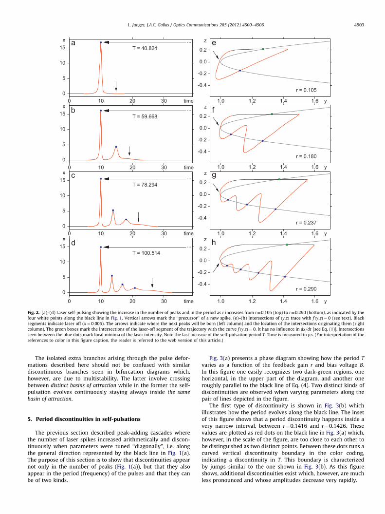
Fig. 2(a)–(d) displays examples of self-pulsations for r¼0.105,0.180, 0.237, 0.290 and B as defined by Eq. (4). These four pointsare indicated by white dots on the black line in Fig. 1(a). They arelocated immediately before the boundaries marking a change inthe number of peaks of the laser intensity. Fig. 2(a)–(d) alsocontains a vertical arrow to indicate the location of a ‘‘precursor’’of a peak, i.e. the position where a new peak will arise when r isincreased slightly. The explanation of the successive peak creationcan be given referring to Fig. 2(e)–(h), on the right column.

Fig. 2(e)–(h) shows two curves in the y� z plane. The first one,represented as a light parabolic arc, marks the solution off ðy,zÞ ¼ 0, where

f ðy,zÞ ¼ y�1�a sin2z: ð5Þ

This function is one of the two factors which appear in dx=dt

(see Eq. (1)). The other curve records the locus (y,z) obtained byintegration of Eqs. (1)–(3).

The characteristic signature of the birth of a new isolatedbranch in the bifurcation diagram is the occurrence of intersection

points between these two curves as parameters are tuned.The arrows in Fig. 2(e)–(h) show where new intersections willoccur when r is increased. Such intersections are responsible forthe several isolated branches seen at the bottom of the bifurcationdiagram in Fig. 1(c). Thus, the condition for the genesis of newisolated branches in the bifurcation diagram, i.e. for new peaks inself-pulsations, is

dx

dt¼

d2x

dt2¼ 0: ð6Þ

According to Eq. (1), this implies having

d2x

dt2¼ k

dx

dtf ðy,zÞþx

df ðy,zÞ

dt

� �¼ 0, ð7Þ

where f ðy,zÞ is given by Eq. (5). That this relation is indeed truecan be verified numerically without difficulty. As it is obvious, theexplicit conditions in Eq. (6) may be used to locate discontinuitiesin laser self-pulsations.

Summarizing, from the peak-adding cascade in Fig. 2 onerealizes the reason behind the emergence of extra peaks in thelaser intensity or, equivalently, extra branches in the bifurcationdiagrams: they arise from pulse deformations undergone by theoscillations as the parameter varies.

0

5

10

15

0 10 20 30

...T = 40.824

time

x

-0.4

-0.2

0.0

0.2

1.0 1.2 1.4 1.6

r = 0.105

y

z

0

5

10

15

0 10 20 30

...T = 59.668

time

x

-0.4

-0.2

0.0

0.2

1.0 1.2 1.4 1.6

r = 0.180

y

z

0

5

10

15

0 10 20 30

...T = 78.294

time

x

-0.4

-0.2

0.0

0.2

1.0 1.2 1.4 1.6

r = 0.237

y

z

0

5

10

15

0 10 20 30

...T = 100.514

time

x

-0.4

-0.2

0.0

0.2

1.0 1.2 1.4 1.6

r = 0.290

y

z

Fig. 2. (a)–(d) Laser self-pulsing showing the increase in the number of peaks and in the period as r increases from r¼0.105 (top) to r¼0.290 (bottom), as indicated by the

four white points along the black line in Fig. 1. Vertical arrows mark the ‘‘precursor’’ of a new spike. (e)–(h) Intersections of ðy,zÞ trace with f ðy,zÞ ¼ 0 (see text). Black

segments indicate laser off (xo0:005). The arrows indicate where the next peaks will be born (left column) and the location of the intersections originating them (right

column). The green boxes mark the intersections of the laser-off segment of the trajectory with the curve f ðy,zÞ ¼ 0. It has no influence in dx=dt [see Eq. (1)]. Intersections

seen between the blue dots mark local minima of the laser intensity. Note the fast increase of the self-pulsation period T. Time is measured in ms. (For interpretation of the

references to color in this figure caption, the reader is referred to the web version of this article.)

L. Junges, J.A.C. Gallas / Optics Communications 285 (2012) 4500–4506 4503

The isolated extra branches arising through the pulse defor-mations described here should not be confused with similardiscontinuous branches seen in bifurcation diagrams which,however, are due to multistability. The latter involve crossingbetween distinct basins of attraction while in the former the self-pulsation evolves continuously staying always inside the same

basin of attraction.

5. Period discontinuities in self-pulsations

The previous section described peak-adding cascades wherethe number of laser spikes increased arithmetically and discon-tinuously when parameters were tuned ‘‘diagonally’’, i.e. alongthe general direction represented by the black line in Fig. 1(a).The purpose of this section is to show that discontinuities appearnot only in the number of peaks (Fig. 1(a)), but that they alsoappear in the period (frequency) of the pulses and that they canbe of two kinds.

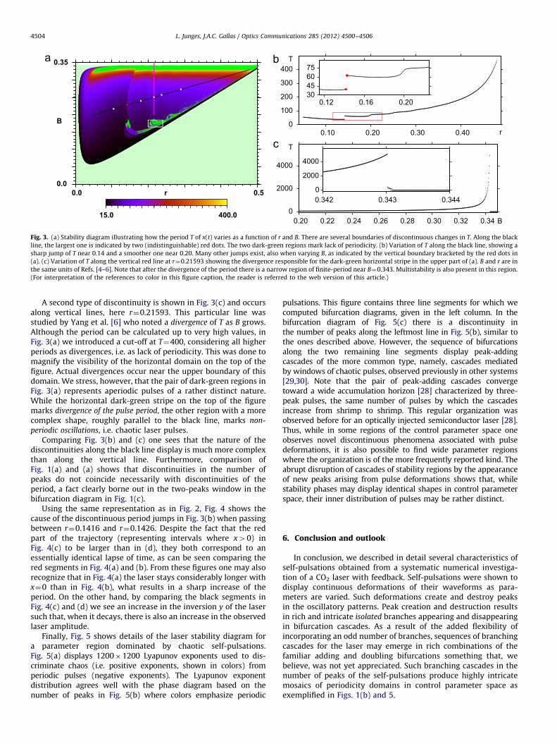
Fig. 3(a) presents a phase diagram showing how the period T

varies as a function of the feedback gain r and bias voltage B.In this figure one easily recognizes two dark-green regions, onehorizontal, in the upper part of the diagram, and another oneroughly parallel to the black line of Eq. (4). Two distinct kinds ofdiscontinuities are observed when varying parameters along thepair of lines depicted in the figure.

The first type of discontinuity is shown in Fig. 3(b) whichillustrates how the period evolves along the black line. The insetof this figure shows that a period discontinuity happens inside avery narrow interval, between r¼0.1416 and r¼0.1426. Thesevalues are plotted as red dots on the black line in Fig. 3(a) which,however, in the scale of the figure, are too close to each other tobe distinguished as two distinct points. Between these dots runs acurved vertical discontinuity boundary in the color coding,indicating a discontinuity in T. This boundary is characterizedby jumps similar to the one shown in Fig. 3(b). As this figureshows, additional discontinuities exist which, however, are muchless pronounced and whose amplitudes decrease very rapidly.

0.50.0 r0.0

0.35

B

400.015.0

0

100

200

300

400

0.10 0.20 0.30 0.40 r

T

30456075

0.12 0.16 0.20

0

2000

4000

0.20 0.22 0.24 0.26 0.28 0.30 0.32 0.34 B

T

0

2000

4000

0.342 0.343 0.344

Fig. 3. (a) Stability diagram illustrating how the period T of x(t) varies as a function of r and B. There are several boundaries of discontinuous changes in T. Along the black

line, the largest one is indicated by two (indistinguishable) red dots. The two dark-green regions mark lack of periodicity. (b) Variation of T along the black line, showing a

sharp jump of T near 0.14 and a smoother one near 0.20. Many other jumps exist, also when varying B, as indicated by the vertical boundary bracketed by the red dots in

(a). (c) Variation of T along the vertical red line at r¼0.21593 showing the divergence responsible for the dark-green horizontal stripe in the upper part of (a). B and r are in

the same units of Refs. [4–6]. Note that after the divergence of the period there is a narrow region of finite-period near B¼0.343. Multistability is also present in this region.

(For interpretation of the references to color in this figure caption, the reader is referred to the web version of this article.)

L. Junges, J.A.C. Gallas / Optics Communications 285 (2012) 4500–45064504

A second type of discontinuity is shown in Fig. 3(c) and occursalong vertical lines, here r¼0.21593. This particular line wasstudied by Yang et al. [6] who noted a divergence of T as B grows.Although the period can be calculated up to very high values, inFig. 3(a) we introduced a cut-off at T¼400, considering all higherperiods as divergences, i.e. as lack of periodicity. This was done tomagnify the visibility of the horizontal domain on the top of thefigure. Actual divergences occur near the upper boundary of thisdomain. We stress, however, that the pair of dark-green regions inFig. 3(a) represents aperiodic pulses of a rather distinct nature.While the horizontal dark-green stripe on the top of the figuremarks divergence of the pulse period, the other region with a morecomplex shape, roughly parallel to the black line, marks non-

periodic oscillations, i.e. chaotic laser pulses.Comparing Fig. 3(b) and (c) one sees that the nature of the

discontinuities along the black line display is much more complexthan along the vertical line. Furthermore, comparison ofFig. 1(a) and (a) shows that discontinuities in the number ofpeaks do not coincide necessarily with discontinuities of theperiod, a fact clearly borne out in the two-peaks window in thebifurcation diagram in Fig. 1(c).

Using the same representation as in Fig. 2, Fig. 4 shows thecause of the discontinuous period jumps in Fig. 3(b) when passingbetween r¼0.1416 and r¼0.1426. Despite the fact that the redpart of the trajectory (representing intervals where x40) inFig. 4(c) to be larger than in (d), they both correspond to anessentially identical lapse of time, as can be seen comparing thered segments in Fig. 4(a) and (b). From these figures one may alsorecognize that in Fig. 4(a) the laser stays considerably longer withx¼0 than in Fig. 4(b), what results in a sharp increase of theperiod. On the other hand, by comparing the black segments inFig. 4(c) and (d) we see an increase in the inversion y of the lasersuch that, when it decays, there is also an increase in the observedlaser amplitude.

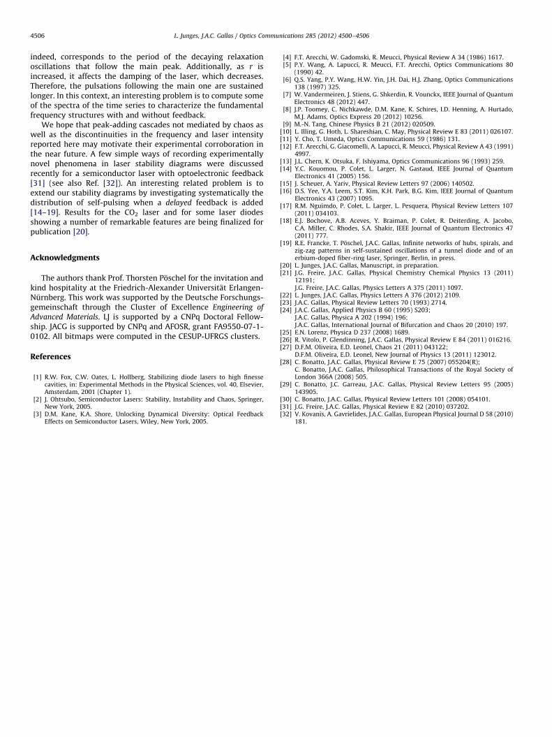
Finally, Fig. 5 shows details of the laser stability diagram fora parameter region dominated by chaotic self-pulsations.Fig. 5(a) displays 1200�1200 Lyapunov exponents used to dis-criminate chaos (i.e. positive exponents, shown in colors) fromperiodic pulses (negative exponents). The Lyapunov exponentdistribution agrees well with the phase diagram based on thenumber of peaks in Fig. 5(b) where colors emphasize periodic

pulsations. This figure contains three line segments for which wecomputed bifurcation diagrams, given in the left column. In thebifurcation diagram of Fig. 5(c) there is a discontinuity inthe number of peaks along the leftmost line in Fig. 5(b), similar tothe ones described above. However, the sequence of bifurcationsalong the two remaining line segments display peak-addingcascades of the more common type, namely, cascades mediatedby windows of chaotic pulses, observed previously in other systems[29,30]. Note that the pair of peak-adding cascades convergetoward a wide accumulation horizon [28] characterized by three-peak pulses, the same number of pulses by which the cascadesincrease from shrimp to shrimp. This regular organization wasobserved before for an optically injected semiconductor laser [28].Thus, while in some regions of the control parameter space oneobserves novel discontinuous phenomena associated with pulsedeformations, it is also possible to find wide parameter regionswhere the organization is of the more frequently reported kind. Theabrupt disruption of cascades of stability regions by the appearanceof new peaks arising from pulse deformations shows that, whilestability phases may display identical shapes in control parameterspace, their inner distribution of pulses may be rather distinct.

6. Conclusion and outlook

In conclusion, we described in detail several characteristics ofself-pulsations obtained from a systematic numerical investiga-tion of a CO2 laser with feedback. Self-pulsations were shown todisplay continuous deformations of their waveforms as para-meters are varied. Such deformations create and destroy peaksin the oscillatory patterns. Peak creation and destruction resultsin rich and intricate isolated branches appearing and disappearingin bifurcation cascades. As a result of the added flexibility ofincorporating an odd number of branches, sequences of branchingcascades for the laser may emerge in rich combinations of thefamiliar adding and doubling bifurcations something that, webelieve, was not yet appreciated. Such branching cascades in thenumber of peaks of the self-pulsations produce highly intricatemosaics of periodicity domains in control parameter space asexemplified in Figs. 1(b) and 5.

0

5

10

15

0 30 60 90

T = 39.730

time

x

-0.4

-0.2

0.0

0.2

1.0 1.2 1.4 1.6

r = 0.1416

y

z

0

5

10

15

0 30 60 90

T = 62.626

time

x

-0.4

-0.2

0.0

0.2

1.0 1.2 1.4 1.6

r = 0.1426

y

z

Fig. 4. Large jump in the self-pulsing period T and in the laser intensity observed when changing r very mildly, from r¼0.1416 to r¼0.1426. These jumps are the same ones

described in Figs. 1 and 3. In both cases, before and after the jump, the laser pulse has two peaks per period. Black segments indicate that the laser is off (xo0:005). Green

boxes mark the intersection of the laser-off segment of the trajectory with the curve f ðy,zÞ ¼ 0. Time is measured in ms. (For interpretation of the references to color in this

figure caption, the reader is referred to the web version of this article.)

0.2250.205 r

0.2250.205 r

0.179

0.187

B

0.062-0.29 0

0.179

0.187

B

1 2 3 4 5 6 7 8 9 10 11 12 13 14 15 16 17

2

7

3

5

10

811

4

0

2

4

6

8

0.206 0.207 0.208 0.209

2 5 10 ...

r

Max

ima

of x

0

2

4

6

8

0.210 0.213 0.216

8 11 14 ...

r

Max

ima

of x

0

2

4

6

8

0.216 0.218 0.220

7 10 13 ...

r

Max

ima

of x

Fig. 5. Regular organization of stable self-pulsations in control space. (a) Phase diagram of Lyapunov exponents, with colors emphasizing the extension of the chaotic

phase. (b) Phase diagram based on the number of peaks of the laser intensity, with colors emphasizing periodicity islands. Along the pair of non-horizontal lines one finds

peak-adding shrimp cascades mediated by chaos. Numbers refer to the number of spikes in the laser intensity. (c)–(e) Bifurcations diagrams along the three lines shown in

(b). Note that the pair of chaos-mediated peak-adding shrimp cascades occur along very particular ‘‘directions’’ [23] and converge towards a large three-spikes

accumulation horizon [28]. In (b) colors are recycled modulo 17. See text. B and r are in the same units of Refs. [4–6]. (For interpretation of the references to color in this

figure caption, the reader is referred to the web version of this article.)

L. Junges, J.A.C. Gallas / Optics Communications 285 (2012) 4500–4506 4505

Note that the sequence of small pulses following the funda-mental one in figures such as Fig. 2(b)–(d) decay with a decreas-ing rate as the coupling r is increased, but the separation between

the pulses has roughly the same duration. A simple calculation ofthe solitary laser equations with zero feedback shows that theperiod of the relaxation frequency is of the order of 6 ms and,

L. Junges, J.A.C. Gallas / Optics Communications 285 (2012) 4500–45064506

indeed, corresponds to the period of the decaying relaxationoscillations that follow the main peak. Additionally, as r isincreased, it affects the damping of the laser, which decreases.Therefore, the pulsations following the main one are sustainedlonger. In this context, an interesting problem is to compute someof the spectra of the time series to characterize the fundamentalfrequency structures with and without feedback.

We hope that peak-adding cascades not mediated by chaos aswell as the discontinuities in the frequency and laser intensityreported here may motivate their experimental corroboration inthe near future. A few simple ways of recording experimentallynovel phenomena in laser stability diagrams were discussedrecently for a semiconductor laser with optoelectronic feedback[31] (see also Ref. [32]). An interesting related problem is toextend our stability diagrams by investigating systematically thedistribution of self-pulsing when a delayed feedback is added[14–19]. Results for the CO2 laser and for some laser diodesshowing a number of remarkable features are being finalized forpublication [20].

Acknowledgments

The authors thank Prof. Thorsten Poschel for the invitation andkind hospitality at the Friedrich-Alexander Universitat Erlangen-Nurnberg. This work was supported by the Deutsche Forschungs-gemeinschaft through the Cluster of Excellence Engineering of

Advanced Materials. LJ is supported by a CNPq Doctoral Fellow-ship. JACG is supported by CNPq and AFOSR, grant FA9550-07-1-0102. All bitmaps were computed in the CESUP-UFRGS clusters.

References

[1] R.W. Fox, C.W. Oates, L. Hollberg, Stabilizing diode lasers to high finessecavities, in: Experimental Methods in the Physical Sciences, vol. 40, Elsevier,Amsterdam, 2001 (Chapter 1).

[2] J. Ohtsubo, Semiconductor Lasers: Stability, Instability and Chaos, Springer,New York, 2005.

[3] D.M. Kane, K.A. Shore, Unlocking Dynamical Diversity: Optical FeedbackEffects on Semiconductor Lasers, Wiley, New York, 2005.

[4] F.T. Arecchi, W. Gadomski, R. Meucci, Physical Review A 34 (1986) 1617.[5] P.Y. Wang, A. Lapucci, R. Meucci, F.T. Arecchi, Optics Communications 80

(1990) 42.[6] Q.S. Yang, P.Y. Wang, H.W. Yin, J.H. Dai, H.J. Zhang, Optics Communications

138 (1997) 325.[7] W. Vandermeiren, J. Stiens, G. Shkerdin, R. Vounckx, IEEE Journal of Quantum

Electronics 48 (2012) 447.[8] J.P. Toomey, C. Nichkawde, D.M. Kane, K. Schires, I.D. Henning, A. Hurtado,

M.J. Adams, Optics Express 20 (2012) 10256.[9] M.-N. Tang, Chinese Physics B 21 (2012) 020509.

[10] L. Illing, G. Hoth, L. Shareshian, C. May, Physical Review E 83 (2011) 026107.[11] Y. Cho, T. Umeda, Optics Communications 59 (1986) 131.[12] F.T. Arecchi, G. Giacomelli, A. Lapucci, R. Meucci, Physical Review A 43 (1991)

4997.[13] J.L. Chern, K. Otsuka, F. Ishiyama, Optics Communications 96 (1993) 259.[14] Y.C. Kouomou, P. Colet, L. Larger, N. Gastaud, IEEE Journal of Quantum

Electronics 41 (2005) 156.[15] J. Scheuer, A. Yariv, Physical Review Letters 97 (2006) 140502.[16] D.S. Yee, Y.A. Leem, S.T. Kim, K.H. Park, B.G. Kim, IEEE Journal of Quantum

Electronics 43 (2007) 1095.[17] R.M. Nguimdo, P. Colet, L. Larger, L. Pesquera, Physical Review Letters 107

(2011) 034103.[18] E.J. Bochove, A.B. Aceves, Y. Braiman, P. Colet, R. Deiterding, A. Jacobo,

C.A. Miller, C. Rhodes, S.A. Shakir, IEEE Journal of Quantum Electronics 47(2011) 777.

[19] R.E. Francke, T. Poschel, J.A.C. Gallas, Infinite networks of hubs, spirals, andzig-zag patterns in self-sustained oscillations of a tunnel diode and of anerbium-doped fiber-ring laser, Springer, Berlin, in press.

[20] L. Junges, J.A.C. Gallas, Manuscript, in preparation.[21] J.G. Freire, J.A.C. Gallas, Physical Chemistry Chemical Physics 13 (2011)

12191;J.G. Freire, J.A.C. Gallas, Physics Letters A 375 (2011) 1097.

[22] L. Junges, J.A.C. Gallas, Physics Letters A 376 (2012) 2109.[23] J.A.C. Gallas, Physical Review Letters 70 (1993) 2714.[24] J.A.C. Gallas, Applied Physics B 60 (1995) S203;

J.A.C. Gallas, Physica A 202 (1994) 196;J.A.C. Gallas, International Journal of Bifurcation and Chaos 20 (2010) 197.

[25] E.N. Lorenz, Physica D 237 (2008) 1689.[26] R. Vitolo, P. Glendinning, J.A.C. Gallas, Physical Review E 84 (2011) 016216.[27] D.F.M. Oliveira, E.D. Leonel, Chaos 21 (2011) 043122;

D.F.M. Oliveira, E.D. Leonel, New Journal of Physics 13 (2011) 123012.[28] C. Bonatto, J.A.C. Gallas, Physical Review E 75 (2007) 055204(R);

C. Bonatto, J.A.C. Gallas, Philosophical Transactions of the Royal Society ofLondon 366A (2008) 505.

[29] C. Bonatto, J.C. Garreau, J.A.C. Gallas, Physical Review Letters 95 (2005)143905.

[30] C. Bonatto, J.A.C. Gallas, Physical Review Letters 101 (2008) 054101.[31] J.G. Freire, J.A.C. Gallas, Physical Review E 82 (2010) 037202.[32] V. Kovanis, A. Gavrielides, J.A.C. Gallas, European Physical Journal D 58 (2010)

181.