1

Operational model evaluation for particulate matter in Europe and North

America in the context of the AQMEII project Efisio Solazzo1, ,Roberto Bianconi2,Guido Pirovano6,7, Volker Matthias 17, Robert Vautard3, K.

Wyat Appel9, Bertrand Bessagnet6, Jørgen Brandt16, Jesper H. Christensen16, Charles Chemel11,12,

Isabelle Coll15, Joana Ferreira8, Renate Forkel10, Xavier V. Francis12, George Grell18, Paola 5

Grossi2, Ayoe Hansen16, Ana Isabel Miranda8, Michael D. Moran14, Uarporn Nopmongcol4, Marje

Parnk19, Karine N. Sartelet5, Martijn Schaap20, Jeremy D. Silver16, Ranjeet S. Sokhi12, Julius Vira19,

Johannes Werhahn10, Ralf Wolke13, Gregg Yarwood4, Junhua Zhang14,

S.Trivikrama Rao9, Stefano Galmarini1, *

10 1Joint Research Centre, European Commission, ISPRA, Italy; 2Enviroware srl, via Dante 142, 20863 Concorezzo (MB), Italy 3IPSL/LSCE Laboratoire CEA/CNRS/UVSQ 4Environ International Corporation, Novato CA, USA 5CEREA, Joint Laboratory Ecole des Ponts ParisTech/ EDF R & D, Université Paris-Est, France 15 6Ineris, Parc Technologique Halatte, France 7 Ricerca sistema energetico (RSE), Italy 8CESAM & Department of Environment and Planning, University of Aveiro, Aveiro, Portugal 9Atmospheric Modelling and Analysis Division, Environmental Protection Agency, NC, USA 10IMK-IFU, Institute for Meteorology and Climate Research-Atmospheric Environmental Division, Germany 20 11National Centre for Atmospheric Science (NCAS), University of Hertfordshire, Hatfield, UK 12 Centre for Atmospheric & Instrumentation Research (CAIR), University of Hertfordshire, Hatfield, UK 13 Leibniz Institute for Tropospheric Research, Leipzig, Germany 14Air Quality Research Division, Science and Technology Branch, Environment Canada, Toronto, Canada 15 IPSL/LISA UMR CNRS 7583, Université Paris Est Créteil et Université Paris Diderot 25 16Department of Atmospheric Environment, National Environmental Research Institute, Aarhus University, Denmark 17 Institute of Coastal Research, Helmholtz-Zentrum Geesthacht,Geeshacht, Germany 18CIRES-NOAA/ESRL/GSD National Oceanic and Atmospheric Administration Environmental Systems 30 Research Laboratory Global Systems Division Boulder, Colorado USA 19Finnish Meteorological Institute, Helsinki, Finland 20Netherlands Organization for Applied Scientific Research (TNO), Utrecht, The Netherlands 35

* Author for correspondence: S.Galmarini. Email: Stafano.Galmarini@jrc.europa.eu

2

Abstract. More than ten state-of-the-art regional air quality models have participated in the Air

Quality Model Evaluation International Initiative (AQMEII), in which a variety of mesoscale air 40

quality modeling systems have been applied to continental-scale domains in North America and

Europe for 2006 full-year simulations. The main goal of AQMEII is model inter-comparisons and

evaluations. Standardised modelling outputs from each group have been shared on the web

distributed ENSEMBLE system, which allows statistical and ensemble analyses to be performed. In

this study, the simulations issued from the models are inter-compared and evaluated with a large set 45

of observations for ground level aerosol (PM10 and PM2.5) and its components, in both the

continents. To facilitate the discussion and interpretation of the results, three sub-regions for each

continental domain have been selected and analyses, with focus on spatially-averaged

concentration. The unprecedented scale of the exercise (two continents, one year, over twenty

groups) allows for a detailed description of model’s skill and uncertainty. 50

Analysis of PM10 yearly time series and daily cycles indicates that large positive biases exist for all

the investigated region and time of the year. We seek possible causes of PM bias in the emission

and deposition balance, and in the bias induced by meteorological factors, such as the wind speed.

PM2.5 and its major components are then analysed, and model performances highlighted. Finally,

capability of models to capture high PM concentrations is also evaluated by looking at two separate 55

PM2.5 episodes in Europe and North America.

In particular, we found a large variability among models in predicting emissions, deposition, and

PM concentration (especially PM10). Major challenges still remain to eliminate the sources of PM

bias. Although PM2.5 is, by far, better estimated than PM10, no model was found to consistently

match the observations under of variety of scenarios (sub-region and time of the year). 60

Keywords: Chemistry transport models, particulate matter, model evaluation, PM bias, emissions,

deposition

1. Introduction 65

Particulate matter (PM) is a worldwide environmental concern as it threatens human health and

ecosystems (Manders et al., 2009; Aan de Brugh et al., 2011). Human exposure to high PM

concentrations is associated with respiratory disease and shortened life expectancy (Amann et al.,

2005; Cohen et al., 2005). PM also contributes to acid rain, visibility degradation, and modification

of the Earth surface energy balance, and thus contributes to short-term climate forcings (Forster, 70

2007; Mebust et al., 2003; Appel et al., 2008; Smyth et al., 2009; Boylan et al., 2006 Wild et al.,

3

2009). Recent studies have suggested that long-term changes in aerosol concentrations, especially

due to decreasing use of coal for energy production, have significantly influenced regional warming

rates (Vautard et al., 2009; Philipona et al., 2009; Yiou et al., 2011). Although major efforts are

being made to reduce anthropogenic emissions of primary PM and aerosol precursors, PM levels 75

remain problematic and their adverse effects are foreseen to persist (Klimont et al., 2009). The

characterisation of PM sources is an area of active research, as many gaps in the knowledge of the

chemical speciation of sources, spatial and temporal distribution of airborne particles, physical and

chemical transformation, need to be filled. This is particularly true for atmospheric chemistry

transport models (CTMs), for which incorporating the wide range of PM physics and chemistry, as 80

well as dealing with the large variety of PM sources is very challenging, especially when simulating

on long temporal and large spatial scales.

PM is a conglomerate of many different types of particles (i.e. elemental and organic carbon,

ammonium, nitrates, sulphates, mineral dust, trace elements, water) with varying physical and 85

chemical properties. Particles are either emitted directly from a large number of sources and source

types or formed from a variety of chemical/physical transformation of other species, which depend,

among other factors, on their size. Furthermore, given its composite nature, high PM concentrations

might be observed at any time during the year and under a large variety of atmospheric conditions

(unlike, for example, ozone which is typically associated with hot and stagnant conditions). A 90

widely accepted classification of PM is based on the size of particles: those with diameter between

2.5 and 10 µm are referred to as coarse particles (PM10), while particles less than 2.5 µm in diameter

(PM2.5) are referred to as fine particles. PM10 and PM2.5 is a widely accepted nomenclature to define

particles with diameter less than 10 and 2.5 µm, respectively (note that PM10 includes PM2.5). This

classification is dictated by the fact that the mechanisms for the generation, transformation, removal 95

and deposition, chemical composition and optical properties of the two classes of particles are

notably different. The particles also behave differently in the human respiratory track, with the fine

fractions penetrating deeper (see, e.g., Seinfeld and Pandis (2006) for a detailed description of

particles properties). In the last decade, the fine particles have attracted much more attention than

coarse particles due to their adverse effect on public health. As a result, air quality models have 100

developed strong skills in modelling PM2.5, made possible by the availability of comprehensive

PM2.5 measurements which allows model performance to be evaluated for the individual PM

chemical components, which, in turn, allows deductions about different aspects of model

performance (e.g., the relationships between emissions, dispersion, chemistry and deposition) (refs).

105

4

Given the large impact of PM on public health and climate, accurate predictions and assessments

are required. CTMs are routinely used for assessing and forecasting PM concentrations. Reliable

global and regional modelling systems are therefore highly beneficial. The analysis presented in

this paper focuses on model cross-comparison (model to model comparison) and model evaluation

(model to observation comparison), with models sharing common emission inventories and 110

chemistry boundary conditions. Such an approach is of direct relevance for model evaluation, and is

the focus of the Air Quality Model Evaluation International Initiative (AQMEII) (Rao et al., 2011),

an international project aimed at joining the knowledge and the experiences of modelling groups in

Europe and North America. Within AQMEII, standardised modelling outputs have been shared on

the web distributed ENSEMBLE system, which allows statistical and ensemble analyses to be 115

performed (Bianconi et al., 2004). A common exercise was launched for modelling communities to

use their CTMs to retrospectively simulate the whole year 2006, for the two continents of Europe

and North America. Outputs of regional air quality models have been submitted in the form of

hourly average concentrations on a grid of points and at specific locations, allowing direct

comparison with air quality measurements collected from monitoring networks, for model 120

evaluation (details are given in Rao et al. (2011) and can be found at

http://aqmeii.jrc.ec.europa.eu/aqmeii2.htm). The primary goal of AQMEII is, in fact, to test the

ability of CTMs to reconstruct atmospheric pollutants concentrations and not to forecast air quality.

This type of evaluation, with large temporal and spatial coverage, is essential for determining model

performance and assessing model deficiencies (Rao et al., 2011; Dennis et al., 2010). 125

Although previous attempts of model harmonisation for PM have been undertaken (Smyth et al.,

2009; van Loon et al., 2007; Stern et al., 2008; Vautard et al., 2009; Hayami et al. 2008), the

unprecedented effort of the AQMEII community to provide a comprehensive set of model’s

variables for two continents and for an entire year, offers a unique opportunity for model cross-130

comparison and evaluation. In this paper we focus on the evaluation of the performance of

ensemble modelling for PM in Europe and North America, for which over ten state-of-the-art

regional air quality models, run by twenty independent groups from both continents, have submitted

their results and for which observational data are made available on the ENSEMBLE system

(described in Section 2). Emphasis of the analyses is dedicated to PM10 and PM2.5. In particular, the 135

analysis of PM10 is presented in Sections 3, and it is mostly devoted to study the possible sources

responsible for model bias. Investigation of PM2.5 focuses on the chemical compositions and

models performance, discussed in Section 4. An analysis of two episodes with elevated PM2.5

5

levels, one for each continent, is also presented (Section 5). Main conclusions are drawn in Section

6. 140

2. Monitoring data and participating models 2.1 Data used for analysis within AQMEII

In order to carry out an exhaustive evaluation of regional air quality models across seasons, models 145

are compared to observations over the full year of 2006. Modelling groups provided gridded surface

daily concentration of PM10, PM2.5 and other compounds (such as hourly SO2 and NO2), covering

the area (15°W - 35°E; 35°N - 70°N) for EU and the area (130°W – 58.5°W; 23.5°N – 59.5°N) for

NA. Additional to the gridded surface concentrations, modellers were required to provide hourly

averaged surface concentrations of the same species and at the same sites where observations at 150

receptors are available. Moreover, at several receptors positions in NA, speciated PM2.5 data are

also accessible. The analyses presented in this paper are derived by comparing the model results

with PM measurements routinely taken at receptors sites. In order to fully explore each model’s

capability, AQMEII participants also provided modelled emission and deposition data for several

species, allowing an exhaustive model cross-comparison to be carried out. 155

2.2 Participating models

Table 1 summarises the CTMs that have been used in the AQMEII activity, to provide PM

concentrations at receptor sites for the European (EU) and North American (NA) domains. These

are: 160

- CHIMERE (Bessagnet et al., 2004);

- POLYPHEMUS (Sartelet et al., 2007; Mallet et al., 2007);

- CAMx (Environ., 2010);

- COSMO-MUSCAT (Multi Scale Chemistry Aerosol Model) (Wolke et al., 2004; Renner

and Wolke, 2010); 165

- SILAM (Sofiev et al., 2006);

- DEHM (Brandt et al., 2007);

- CMAQ (Foley et al., 2010);

- LOTOS-EUROS (Long term Ozone simulation-European Operational Smog Model)

(Schaap et al., 2008); 170

- AURAMS (Gong et al., 2006; Smyth et al., 2009)

The CHIMERE, CAMx, CMAQ and DEHM models have been applied over both continents, while

the POLYPHEMUS, COSMO-MUSCAT, SILAM, and LOTOS-EUROS models were applied for

6

the EU only. AURAMS was the only model which was run exclusively over NA. Meteorological

drivers for these models are also listed in Table 1. Most of the simulations for EU (CHIMERE, 175

POLYPHEMUS, CAMx, DEHM) used meteorological fields generated by different versions of the

5th Generation Mesoscale Model (MM5; Dudhia, 1993). The SILAM and LOTOS-EUROS models

used meteorological data provided by the European Centre for Medium-range Weather Forecasting

(ECMWF), while the WRF v3.1 (Skamarock et al., 2008) meteorological model was used to

provide meteorological input data for the CMAQ model over EU and NA (run by two different 180

groups), and for the CHIMERE model over NA only. The MUSCAT model used meteorological

data provided by the German COSMO-CLM model. Finally, meteorology from the GEM model

was used for running AURAMS over NA. A more detailed description and assessment of the model

performance for the various meteorological models used can be found in Vautard et al. (this issue,

in prerparation). 185

The CTMs used in the current analysis take very different approaches in estimating PM

concentrations. The key physical and chemical mechanisms are handled in different ways by the

models. Several aspects of models settings are summarised in Table 1. The number of bins for

particle sizes varies between one (LOTOS-EUROS) and eight (CHIMERE), with the majority of 190

models having two size bins (PM10 and PM2.5). The ISORROPIA (Nenes et al., 1998) module is

predominantly used to perform the thermodynamic equilibrium within the CTMS. The dry

deposition mechanisms are modelled using the resistance analogy described by Seinfeld and Pandis

(2006), whereas the wet deposition is modelled by various modification of the scavenging

approach. Full details are given in Table 1 and references therein. Horizontal and vertical 195

resolutions were not harmonised within AQMEII, thus participants applied their own settings. Table

1 reports the number of vertical layers used for each model, ranging from 34 layers in the CMAQ

simulations to only four for LOTOS-EUROS model simulation (adjusting their position to the

height of the boundary layer). The majority of the model simulations use between nine and more

than twenty (three models each) layers, with a greater number of layers in the lower portion of the 200

troposphere.

Concerning emissions, it should be noted that AQMEII participants were given the opportunity to

use a set of “standard” emissions and boundary conditions for each continent. The EU “standard”

emissions were prepared by TNO, which provided a gridded emissions database for the year 2005 205

and 2006. The provided EU emissions dataset is widely used, for instance within the GEMS project

(http://gems.ecmwf.int). The dataset consists of European anthropogenic emissions for the 10

7

SNAP sectors and international shipping on a 0.125 by 0.0625 degree lon-lat resolution. Biomass

burning emissions were provided by the Finnish Meteorological Institute (FMI) and used by a few models. Full details on the AQMEII emissions dataset are given in AQMEII documentations, available at 210

http://aqmeii.jrc.ec.europa.eu/aqmeii2.htm. The standard emissions dataset for NA is described in

the companion paper by Pierce et al. (this issue, in preparation). It is based on the 2005 U.S.

National Emissions Inventory (NEI), the 2006 Canadian national inventory and the 1999 Mexican

BRAVO inventory. Biogenic emissions are provided by the BEISv3.14 model, fire emissions

provided by daily estimates from HMS fire detection and SMARTFIRE system (year 2006) and 215

Electric Generating Unit (EGU) point source emissions from the Continuous Emissions Monitoring

data for the year 2006. The NA emissions data set did not include any dust emissions. Both the

database (EU and NA) provided emissions of PM10 and PM2.5, which were used by all participating

groups, with the sole exception of the DEHM model, which made use of a number of different

emissions inventories (see Table 1). 220

From Section 3 onwards, the model configurations are denoted by the labels Mod1 to Mod11 for

EU, and Mod12 to Mod18 for NA. In some cases the same model, but with different configurations,

was run over both continents. Such is the case for the Mod3 and Mod18; Mod4 and Mod13; Mod10

and Mod17. No direct correspondence exists between the model labels and the model list of Table 225

1, for reason of anonymity.

2.3 Receptor observations for particulate matter

Particulate matter data for EU were prepared starting from hourly and daily data of total PM2.5 and

PM10 collected by AirBase (European Air quality database, 230

http://acm.eionet.europa.eu/databases/airbase/) and EMEP (European Monitoring and Evaluation

Programme, http://www.emep.int/) networks. A total of 863 stations with valid data were made

available in the ENSEMBLE database for Europe, which includes urban, sub-urban and rural

stations. Too few stations measuring PM2.5 speciation were available for year 2006 in AirBase in

order to be included in the Ensemble database. 235

Particulate matter data for NA were prepared from the data collected by the Aerometric Information

Retrieval Systems (AIRS: http://www.epa.gov/air/data/aqsdb.html) and Interagency Monitoring for

Protected Visual Environments, IMPROVE:

http://crocker.ucdavis.edu/Site/Research/AirQualityGroup/IMPROVEOverview.aspx) networks in 240

United States, and by the National Air Pollution Surveillance (NAPS: http://www.ec.gc.ca/rnspa-

naps/) network in Canada. A total of 1902 stations with valid data are available for US and Canada,

8

which includes urban, sub-urban and rural stations. It should be noted that not all networks

provided data with the same frequency (daily of hourly), nor are the speciation data of PM2.5 is

available at all sites for all species. More details about network measurements and data quality can 245

be found elsewhere (Appel et al., 2008; Mebust et al., 2003; Aan de Brugh 2011).

3. PM10 evaluation and models cross-comparison

250

In this section, model simulations and observations are compared for PM10. To facilitate the

discussions and synthesise the results, focus is given to three sub-regions of each continent. These

sub-regions have been selected based on different climate and air quality characteristics, availability

of measurements and previous studies (e.g., Vautard et al., this issue), and are shown in Fig 2, along

with the position of PM10 receptor sites. For EU, sub-region 1 encompasses the north Atlantic 255

region, the UK, Belgium, and northern of Spain. Sub-region 2, consisting of central Europe, has a

continental climate with marked seasonality, many large cities, and large emissions sources. Sub-

region 3, consisting of the Iberian Peninsula, was selected for the availability of measurements. For

NA, sub-region 1 consists of the southwestern part of U.S. to the west of the Rocky Mountains.

Sub-region 2 (Texas area), is located to the east of the Rocky Mountains. Sub-region 3, consisting 260

of the northeastern NA including parts of Canada, has a marked seasonal cycle, three of the North

American Great Lakes, the highest emissions sources in NA, and several large cities (e.g New York

City, Philadelphia, Toronto, Montreal).

3.1. PM10 – model skill 265

Evolution of surface PM10 is shown in Fig. 2. The monthly trend is shown, based on daily data for

the entire year. The time series for the each entire continent and for the three sub-regions of Figs. 1

have been analysed.

A pattern common to both continents and all sub-regions is a general underestimation of PM10 by 270

the models, although there are several exceptions. For NA in particular, the underestimation is

systematic across all models, though in sub-regions 2 one model slightly overestimates PM10 for the

period of October through January. For the NA sub-region 1, model bias is severe (approximately

20 µg m-3), and more marked during summer and winter. This large gap might be due to wind

blown dust, which can be an important source of PM10 in this region (Yen et al., 2005; Park et al., 275

2010), but it is not accounted for in the emission inventory. In the other NA sub-regions

9

underestimation is milder for some models but significant for others (the worst performing model,

Mod13, exhibits a bias of ~ 20 µg m-3 at both sub-regions 2 and 3).

Large biases are also observed for EU (all sub-regions), although one model (Mod1), on average, 280

predicts PM10 concentration of the same magnitude as observations, and Mod6 tends to

overestimate the observations (except at sub-region 3). It is worth noting that the low in the

observed concentrations occur during the month of August (sub-regions 1 and 2), which all models

simulated with varying degrees of success. The reduced distance between PM observations and

simulations for the summer months, which was also found in previous studies (see eg Hodzic et al., 285

2005) might be explained by considering that PM winter concentrations are often driven by strong

stable conditions that are not always well captured by meteorological models. It can also be noted

that for sub-domain 3 the highest concentrations occur in summer, probably due to the influence of

a higher rate of secondary organic aerosol formation under marked photochemical conditions and

possibly more wind-blown dust (Putaud et al., 2004). 290

Figure 3 displays the diurnal cycles for the same areas of Fig. 2. Hourly data have been used to

produce these plots, averaged over the entire year. The amplitude of the diurnal cycle is generally

underestimated by the majority of the models for EU and NA. One model for EU is closer to the

observations in terms of mean concentration and trend (Mod 6, continuous blue line in EU column 295

of Fig. 3), except for EU sub-region 3. The models underestimate observed PM10 during day-time

hours for NA. Mod 16 (dot-dot-dash light blue line of Fig 3) is able to simulate the magnitude of

PM10 concentrations during night hours reasonable well for NA sub-regions 2 and 3.

The correlation, mean, error, and spread for each model simulation (entire continent) are provided 300

in Table 2 (Table 2a for EU and Table 2b for NA) based on daily averaged data for the entire year.

The correlations for the simulations vary largely (generally lower for NA than for EU), ranging

from a minimum of 0.1 to a maximum 0.7 for EU Mod 7 and Mod 8. The maximum correlation for

NA is 0.4 (Mod 16). For the mean PM10 concentration the conclusions made from Figs. 2 and 3

hold, as the models severely underestimate PM10, with the exception of Mod 1 and Mod 6 for EU 305

(but they tend to overestimate PM2.5, as discussed later in Section 4.1). The variability, measured

by the standard deviation of the observations, is underestimated by the NA models by a factor of

two on average, indicating that the models are unable to simulate the same range in variability as

the measurements. The standard deviation for the EU observed data (ST dev of 9.8 µg m-3) is larger

than that of NA and again the models are all below the observed standard deviation (Mod 11 310

10

predicts a standard deviation six times lower). Such large differences among models depend

strongly on the composition and on the components of PM10 included in each model’s chemistry

module. For example, Mod4 lacks secondary organic aerosols and wind-blown desert dust, leading

to PM10 concentration bias among the highest.

315

We shall deepen the investigation of the model-to-model differences in the next section, with the

aid of emission and deposition patterns for each model.

3.2 Models cross-comparison. Emission and deposition of PM precursors and PM pollutants

Analysis of emissions and deposition of several species (PM precursor and pollutants) can aid 320

understanding of each model’s internal balance and chemical transformations. The stacked

distribution of quarterly accumulated emissions for five compounds is displayed in Fig. 4a (EU) and

Fig. 4b (NA). Each element of the bars is the emission over a quarter of year (three months, from

January to December), so that each full bar reflects the total over the year. The majority of

participating models (not all of them though) delivered the emission data, allowing a comprehensive 325

analysis of PM balance. Looking at emissions for EU (Fig 4a) it emerges that, with the only

exception of Mod4 which adopted a different set of emissions, and Mod6 which provided only

surface emission neglecting plume rise and volumetric sources (although they were included in the

runs) there are no large differences among the remaining models for SO2, aNOx and NH3. Larger

differences, however, can be noticed for PM. Aerosol emissions differ among models, with a high 330

variability in both the coarse (PM10) and the fine (PM2.5) components, with differences reaching

~550 and of ~200 kg km-2 between Mod1 and Mod7 for PM10 and Mod1 and Mod6 PM2.5,

respectively. Such large differences in emissions are attributable to the PM species included within

each model. For example not all models include sea salt emissions. These differences, along with

the deposition (discussed next), are among the main responsible for the wide range of performance 335

observed in Figs 2, 3 and Table 2. Such an influence can be observed considering, as an example,

European Mod1 and Mod4. Emissions of both primary PM and precursors are among the highest as

for Mod1 and among the lowest as for Mod4. This difference is clearly reflected in the computed

mean concentration (see Table 2).

340

Accumulated emissions for NA also exhibit a certain degree of variability, especially for PM10, with

Mod13 (same emission as Mod4) showing the lower emission at all quarters. This is due to the

emission inventory adopted by this model being dissimilar to the standard AQMEII emission data

11

sets for NA. Overall, with the further exception of low SO2 emission by Mod18 NA emission are

more homogeneous than for EU, with smoother PM differences among models. 345

Contributing to the final model PM concentrations is the amount of deposited substances. Playing a

pivotal role are the wet and dry deposition schemes implemented in each model. Results of

quarterly accumulated deposition (dry and wet, EU and NA) are shown in Figs. 5. Striking

differences are mostly observed for the dry deposited substances such as PM2.5 and the other PM 350

secondary components in both continents. Investigating the reasons leading to the difference in

deposition is not the scope of this study. Nonetheless, we note that although the dry deposition

module (Table 1) is similar for all model (i.e. based on the resistance analogy schemes, Seinfeld and

Pandis, 2006; Zhang et al., 2001), large deviation among models seem to indicate that the

parameterisations of such scheme are rather different. This is because dry deposition is very 355

sensitive to surface conditions (wind shear, surface roughness, temperature and radiation) and

knowledge of dry-deposition processes, as well as availability of measurements, is limited (Zhang

et al., 2001; 2002). Moreover, deposition schemes are coupled with chemistry and dispersion

components, as well as with the treatment of the atmospheric layer just above ground level, which

are treated differently by each model. Large differences in PM2.5 deposition are mostly due to the 360

sea-salt being included in the simulation of Mod 4,5 and 10 (EU) and Mod 12,13 and 17 (NA).

Spatial maps of PM2.5 deposition for these models (not reported) reveal that most of the deposition

occurs in the ocean, whilst on land it is comparable with the other models. Mod4 and Mod 3 (which

are essentially the same models as Mod13 and Mod18 for NA) exhibit PM-NO3 deposition values

higher than the other models, and Mod3 has higher values than any other participants also for PM-365

SO4 (might be associated with the inclusion of sulphate from the oceans which cannot be

distinguished from anthropogenic fine mode sulphate), and PM-TC (this latter together with

Mod10).

Concerning the wet deposition, seasonal accumulated deposition for the soluble ions SO42-, NO3

-, 370

NH4+ are reported in Fig. 5b (EU) and 5d (NA). Wet deposition depends mainly on the ability of

models to predict the amount, duration, and type of precipitation. Vautard et al. (this issue,

submitted for publication), in the context of the AQMEII activity, analysed the models performance

for precipitation over NA for the year of 2006, and concluded that there is tendency to model

overestimation seasonal precipitation (especially in areas of more frequent convection). This result 375

would lead to enhance wet removal of SO42-, NO3

-, NH4+, at least for NA. Looking at the model

results for wet deposition, it emerges a tendency of Mod4 and Mod5 to higher wet deposition

12

intensity for all species, whilst Mod17 has very low NO3- values. In particular Mod5 has the highest

wet deposition of SO4, NO3 and NH4 and the lowest dry deposition of the same specie, among all

the analysed models. This might be attributed to the internal parameterisations of the model itself. 380

The reason for the large differences between the model results may again be attributed to the way

the models internally treat the different species. Mod4, for example, calculates wet deposition of

NO3- as the sum of the wet deposition of gaseous HNO3 and NH4NO3, aerosol nitrate and organic

nitrate (H2C(ONO2)CHO). Similarly, dry deposition of PM-NO3- is calculated as the sum of 385

NH4NO3 and aerosol nitrate, based on the assumption that most of the NH4NO3 is in the aerosol

phase. Chemistry modules within other models might have different underlying assumptions,

explaining some of the spread observed in Fig 5.

3.3 Model bias 390

In this section we look at the PM10 bias and analyse possible reasons for it. We start with

investigating the gas-phase precursor SO2 and NO2, whose calculations was also part of the

AQMEII exercise. Figure 6 summarises the relationship between the mean fraction bias (MFB) and

the mean fractional error (MFE) for the three sub-regions of both continents and for rural and urban

receptors, with: 395

)(5.0)(1

obsm

obsm

CC

CC

NMFB

+

!=

" (1)

)(5.0||1

obsm

obsm

CC

CC

NMFE

+

!=

" (2)

Boylan and Russel (2006) suggested that a model performance goal (the expected level of model

accuracy) for PM is met when MFE<50% and MFB< ± 30% (internal box of Fig. 6). Additionally, 400

the model performance criteria for PM are achieved when MFE ! 75 % and MFB ! ± 60% (external

box in Fig. 6). According to these targets and the results reported in Fig 4, only three models

(Mod1, 6 and 10) satisfy the model goal criteria when compared against European receptors (urban

and rural). Model skill target for PM10 NA (Fig 6, bottom row) is not reached by any model in the

three sub-regions. This is due to the severe model underestimation of the NA sub-region 1, as a 405

probable result of missing source of anthropogenic and biogenic dust. However, Mod17 has MFE

and MFB within the goal target for sub-regions 2 and 3 (rural and urban receptors), and Mod 14, 15,

16 are also within the goal box for rural receptors and sub-regions 2 and 3. The alignment between

bias and error emerging from Fig 6, shows that most of the uncertainty is due to bias, as already

13

observed in the analysis of ozone (Solazzo et al., this issue), maybe introduced by the boundary 410

conditions or the emissions.

When looking at a similar analysis for rural receptors of SO2 and NO2 (Fig. 7), which are secondary

regarded as secondary inorganic aerosol precursors, a similar behaviour as for PM is observed

(except Mod 10, all sub-regions for SO2) in Europe, with MFB negative well aligned with MFE 415

(lower magnitude compared to PM10 for the same sub-regions). For NO2 in NA (bottom left plot of

Fig 7), the trend is again similar, with the exception of sub-region 2, where NO2 is overestimated by

all models. MFE and MFB are also aligned for SO2 (bottom right plot), although the sign of the bias

varies by model and by sub-regions. The different behaviour of NO2 and SO2 is however not

surprising, as SO2 is typically emitted by isolated point sources whose plume is not easily modelled 420

with the current resolution of chemistry transport models. NO2, on the other hand, derives from

NOx which is emitted at ground level by large area sources. The differences between NO2 and SO2

by sub-regions are thus due to the way the source distributions of the two compounds are handled in

each model. We should notice that EU models that used the emission vertical distribution from

EMEP data base, might have a too high emission spread for point sources and other elevated 425

sources. Large plume spread enhance depletion, thus deposition, reducing concentration. This is

particularly the case for SOx, largely emitted by point sources and for the chemistry related to it

(ammonium nitrate concentration is likely to increase due to reduced availability of SO4=) (e.g.,

Bieser et al., 2011)

430 3.3.1 PM10 bias and emission

We investigate here the bias induced by PM10 emission to modelled PM10 concentration. We

consider four areas characterised by PM10 emission of increasing intensity, for EU and NA. We then

analyse, for each area, the spatially averaged PM10 model bias at the receptors available in that area.

The aim is to investigate whether the PM10 bias decreases as the emission decreases, which would 435

indicate that the bias is mostly due to emissions. The reference emission scenario for the entire year

of 2006 has been taken from two models (Mod5 for EU and Mod16 for NA). The selection of areas

of different emission intensities was based on these reference scenarios (numbered 1 to 4 in Fig. 8a

for EU and 9a for NA). Receptors positioning is overlaid to the emission map of Fig. 8a and Fig. 9a.

440

The choice of the reference emission model for NA was straightforward as, among the models

which provided both PM10 emissions and concentrations at receptors (Mod12, 16 and 17 only),

emission patterns were overall quantitatively (Fig. 4b), and also geographically (in the sense of

spatial distribution of sources) similar. For EU, on the contrary, Mod5 emission map was selected

14

as it looked the most accurate and quantitatively similar to Mod1, 3, 6 and 10 (Fig 4a). As for the 445

selection of the areas with increasing emission intensity, the choice was driven, other then by the

emissions, also by the availability of measurements. In particular, it was possible to identify three

areas for each emission magnitude in NA (labelled with letters a,b,c in the figures), whilst only one

area for each intensity was identified in EU. Other area of the EU continents either lacked

measurements or differences among models were too high. Areas shown in Figs 8a and 9a have 450

been selected after numerous sensitivity tests, especially for EU.

Mean fractional bias of modelled PM10 concentration at receptors (averaged over the pool of

receptors falling in each emission area) is shown in Fig. 8b (EU) and Fig. 9b (NA). Numbers

indicate the emission area, models are classified by colour. Each model bias is plotted against its 455

own PM10 emission. Due to the differential emission among models presented in Fig 4a, some

models show higher emission for area “2” than for area “1” (EU Mod 6 and 7) and similar intensity

for area “3” and “4” (EU Mod7 and Mod8). This is, again, due to having based the analysis on a

reference emission map that is not geographically the same for all models. By contrast, for the NA

continent (Fig 9b), emission intensities are distributed in decreasing order (from”4” to “1”), 460

although some overlap between areas “3” and “4”. We shall point out that the concentration bias,

i.e. point observation vs interpolated grid cell model concentration, might also contain some error

introduced by assuming the receptor representative of an extended area. However, we are looking

here at long temporal and large spatial scales for which mutual cancellation of error is expected.

With this assumption in mind, we notice two different behaviours for EU and NA domains. For the 465

former, PM10 concentration negative bias is smaller for regions characterised by low emission

intensity (such as area “4”) than for high-emission areas. MFB values for area “4” are in fact

clustered between 0.2 and -0.7, whereas the average MFB for the other areas (“1” to “3”) are

approximately in the range 0 to -1, and show comparable, negative, values of MFB. This result

might indicate that local sources have a relevant influence on PM concentration, not always well 470

captured by regional models. It is also worth noting that differences in model performances in

different areas are very clear for region 1 in EU, and that EU sub-region 1 experiences emissions

higher than the other areas for all main pollutants (e.g. SO2 and NOX) (not shown), thus enhancing

the influence of local sources on the observed concentrations.

475

For NA (Fig 9b), if we exclude the area “3c’ of Fig 9a (characterised by high concentration bias due

to wind blown dust, see Section 3.3), MFB has comparable values for all areas, between 0.1 and -1,

with no reduced bias for low emission zones.

15

Some considerations might be formulated based on the results of Figs 8b and 9b. For EU, there are 480

low- emission regions (or at least one region) for which part of the PM10 concentration bias can be

attributed to the input emissions. The other examined areas showed a comparable MFB for all

models. NA domain allows more regions to be analysed (thanks to the extension of the domain and

of data availability) and the bias of PM10 does not depend on the PM10 emission data set. The

uniformity of MFB values for several classes of emission gives an important indication about the 485

internal processes of the CTMs involved, and demonstrates that despite the variety of algorithms

and internal parameterisations, the level of uncertainty is, overall, comparable.

It is also worth noting that differences in model performances according to the area are very clear

for region 1 in EU, but less for the corresponding sub-region 1 in NA. This can be explained 490

considering that EU sub-region 1 experiences emissions higher than the other areas for all main

pollutants (e.g. SO2 and NOX), thus enhancing the influence of local sources on the observed

concentrations.

The above analysis tends to show that different sources of uncertainty occur in the two continents. 495

Over EU biases are larger in high anthropogenic emission regions indicating a bias in emissions

themselves or in chemistry and thermodynamics of anthropogenic compounds, while over NA the

bias is rather uniform indicating a lack of background PM concentrations and therefore a possible

lack of biogenic emission precursors or secondary formation from biogenic emissions. The

uniformity of MFB values also demonstrates that despite the variety of algorithms and internal 500

parameterisations used, the level of skill is, overall, comparable.

3.3.2 PM10 and wind speed biases

Meteorological biases can also induce PM concentrations bias. In particular, Vautard et al. (this 505

issue, submitted for publication) have shown that the models participating in the AQMEII exercise

have a tendency to overestimate the 10 m wind speed (especially in EU), which should translate

into a negative bias for concentration predictions. What is the fraction of total PM10 bias that can be

attributed to wind speed overestimations? This issue is addressed by analysing the annual daily

wind speed bias against PM10 bias for the three regions of Figs. 1 (which are the same regions 510

considered by Vautard et al. for studying the wind speed). It needs to be emphasised that the

analysis presented is strictly valid in a spatially-averaged sense, as observed wind speed and PM10

concentrations are not collocated.

16

Results for all the participating models are reported in Fig 10a (EU) and Fig 10b (NA). Data have 515

been averaged over the whole year and are presented for each sub-regions. In general, PM10

negative bias is higher when the wind speed bias is higher. Over EU this trend is marked, for each

region or all regions together. Over NA, this trend is not so clear, in particular when taking each

region separately, but wind biases are of smaller amplitude.

520

4. PM2.5 and PM2.5 components 4.1 Time series Monthly time series for PM2.5, based on 24-hour data, are shown in Fig. 11. With respect to PM10 525

(Fig 2), the model bias is much lower for both continents, demonstrating an enhanced capability of

the CTMs to simulate PM2.5.

For EU, the majority of models underestimate the monthly averaged daily PM2.5 concentrations at

all sub-regions, with several exceptions. In particular, Mod1 shows an overall satisfactory 530

agreement for all sub-regions and for the majority of the year (the high concentrations in January

for sub-region 2 are not well reproduced). As was the case for PM10 (Fig. 2), some models estimate

a pronounced peak in PM2.5 concentrations in August which does not show up in the observed data,

most probably due to fire emissions that are not taken into account by all groups.

535

Similarly to EU, the majority of NA models tend to underestimate PM2.5, especially for sub-region

2, where only Mod17 overestimates PM2.5 concentrations throughout the year (Fig. 11). Mod17

shows positive bias (over prediction) also at sub-region 3 and, on average, over the entire NA

continent. Mods 16 and 18 underestimate PM2.5 in the summer, but overestimate PM2.5 throughout

much of the rest of the year, while all other models underestimate PM2.5 throughout the entire year. 540

Looking at sub-regions individually, there are models that perform satisfactorily for short periods,

closely following the observations for a season, such as for example Mod18 at sub-region 1

between October and December, Mod17 for sub-region2 for April-June, and Mods 12, 15 and14 for

sub-region3 for October-December. For sub-region 3 in particular, all models predict the July peak

and the April and October lows, although the amplitude is not well captured. Despite the enhanced 545

model performance for PM2.5 compared to PM10, results seem to indicate that further improvements

are needed to CTMs in order these to be successfully applied under a variety of conditions.

17

It is interesting to compare the monthly PM2.5 and PM10 concentrations, as it provides indications of

the proportion of the fine and coarse components of PM for each model in comparison to the 550

observations. Results of mean PM2.5/PM10 concentration ratio, standard deviation and correlation

coefficient (PCC) against the observed PM2.5/PM10 ratio for the whole continental areas are

presented in Table 3. The mean ratio is overestimated by all models for both NA and EU (with the

exception of Mod1 and Mod6 for EU), which is consistent with larger underestimation of PM10

compared to PM2.5. Other than quantifying the bias, it is also useful to compare the association 555

between the observed and modelled PM2.5 to PM10 ratio. This ratio provides an indication of

whether the models are able to reproduce the trend in the measured fine to coarse PM fraction. PCC

values in Table 3 indicate that the correlation is typically below 0.5, and that in many cases the two

trends are uncorrelated (exceptions being Mods 7, 8 and 11 for EU and Mods 14 and 16 for NA).

As it is discussed in the next section 4.2, the correlation for PM2.5 generally exceeds 0.4 for most 560

models, hence the poor correlations in Table 3 are primarily due to the low or negative correlations

for PM10.

4.2 PM2.5 - Model Skill

To deepen the investigation, the skill of the model to simulate the daily variability of daily mean 565

PM2.5 concentration is summarised in Fig. 12 (EU) and Fig. 13 (NA), for the three sub-regions

(circles, square and triangles for sub-region 1,2,3 respectively). Taylor plots representation is

adopted (Taylor, 2001). The ensemble mean of all available models is provided for comparison.

Moreover, analysis of PM2.5 components NH4, SO4, NO3 and EC, elemental carbon) is reported in

Fig. 14 for NA (PM2.5 speciated data for EU are not widely available and therefore are not included 570

in the analysis).

For EU, the amplitude of daily PM2.5 variability is generally underestimated by the majority of

models at all sub-regions, while the correlation with observations is always less than 0.8, with

slightly better results for the rural sites. The largest underestimation in the spread occurs for EU 575

sub-region2 (urban and rural), whereas for sub-region3 (urban and rural) the ensemble mean is

among the best performing in terms of correlation coefficient (exceeding 0.6) and spread. Model

correlation ranges between 0.55 and 0.75 for most models at both rural and urban stations.

Computed correlation for NA is generally higher than for EU, indicating that the daily variability of 580

PM2.5 is better reproduced for NA, most likely due to better PM emission datasets for NA than EU.

The only exception is NA Mod18 that shows correlation values lower than 0.6 for all sub-regions.

18

The observed standard deviation is rather well reproduced for sub-region 2, as proved also by the

ensemble mean score for this region, and to a lesser extent at sub-region 3. Conversely, a systematic

worsening in model performance is observed at sub-region1. 585

The Taylor diagrams for inorganic aerosols and elemental carbon (Figs. 13) confirm the systematic

underestimation of the standard deviation for sub-region1. By contrast, for sub-regions 2 and 3 the

model performance varies depending on the PM-component being considered. Sulphate is well

reproduced for both sub-regions 2 and 3, as indicated by the high correlation values (exceeding 0.7), 590

and by the model spread which is very close to that of the observations. Nitrate is overestimated for

sub-region3 and to a lesser extent for sub-region2. Conversely, ammonium is underestimated for

both regions. In most cases, model performance for sulphate and nitrate are mutually compensating,

meaning that underestimations in sulphate are related to overestimations in nitrate. The only

exception is Mod15 overestimating both sulphate and nitrate. Finally, P-EC standard deviation is 595

well reproduced for sub-region3, while underestimated for sub-region2. The latter analysis suggests

that EC emissions are probably underestimated for NA.

Overall, poorer model skill is observed for NA sub-region1. The systematic underestimation of the

computed standard deviation for all species in this region indicates there may be large emission 600

sources missing in the emissions inventory for western NA. In addition, the western U.S. is also a

challenging region to model due to its complex terrain and the close proximity of the western U.S.

to western boundary of the model makes the region particularly sensitive to errors in the prescribed

meteorological and chemical boundary conditions.

605

Finally, it is worth noting that the models showed, domain by domain, more homogenous

performance for the selected compounds than for total PM2.5 mass. This result might suggest that,

while CTMs are reliable to simulate inorganic aerosol, there is still a lack in the reconstruction of

some processes strongly influencing PM2.5 concentration other than inorganic aerosol chemistry.

610 5. Two episodes with elevated PM concentrations Two episodes with elevated PM concentrations in Europe and North America have been selected

for a more detailed investigation of the model performance. It is of special interest to investigate if

the CTMs do not only capture the average PM concentrations correctly but if they are able to 615

reproduce peak values in the same way.

19

In Europe a period of 16 days between 13 and 28 April 2006 was chosen. During this time elevated

PM2.5 concentrations were observed at several stations in Central Europe. For the evaluation of the

AQMEII model results, a region between 49° and 56° North and between 0° and 14° East was 620

selected. Daily average PM2.5 values were available at seven stations, four of which in Germany,

and one in Denmark, Belgium and Great Britain, respectively. All stations are classified as rural

stations. This type of stations typically represents the modeled concentrations, which are grid cell

average values, best.

625

Figure 15 demonstrates that the modeled PM2.5 concentrations scatter considerably around the

observations. Except Mod4 and Mod6, all models show an increase in PM2.5 concentrations from

day 103 to day 115. The observations show a first peak on day 105 and 106 that is not well

represented by the models but the high values between day 113 and day 116 are captured. The

correlation coefficients are between 0.45 and 0.62 for all models except one. The bias varies 630

between -8.8 to 12.2 µg m-3, only 5 models show mean deviations less than 3 µg m-3. The mean

observed concentration is 15.6 µg m-3.

In North America, the analysis could be done in a more detailed way. On one hand, at many stations

hourly PM2.5 measurements are available, but on the other hand the chemical composition is 635

measured on a daily average basis every three to four days. This allows additional insights in the

possible reasons for deviations between models and observations. The region that was chosen for

the investigations was in the Eastern US between 32° and 45° North and between 72° and 92° West.

Data from eighteen receptor stations, either classified as rural or suburban, was available. Six

different model results could be used for the evaluation. 640

Between 14 July (day 195) and 29 July (day 210), high PM2.5 values above 20 µg m-3 were observed

on several days (Fig. 16). On other days, the concentrations decreased to ~5 µg m-3. These abrupt

changes are mostly driven by transport phenomena and the models capture these changes quite well.

Inaccuracies are found in the simulated timing of the episodes, e.g. the peak on day 199 is seen a bit 645

later in the model results and another day of high PM values is modeled at the end of the period

(day 209), although these high values were not observed. The correlation coefficients are between

0.42 and 0.58 for all models. These values are based on hourly concentrations and can therefore not

be compared to the correlations in Europe that rely on daily averages.

650

The model biases are between -5.2 and +3.8 µg m-3, corresponding to -39% to +28% with a mean

observed value of 13.3 µg m-3. This is less than in the episode that was chosen for Europe.

20

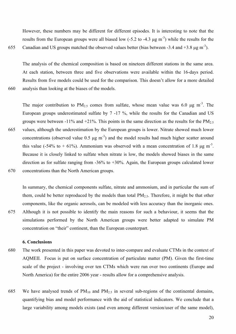
However, these numbers may be different for different episodes. It is interesting to note that the

results from the European groups were all biased low (-5.2 to -4.3 µg m-3) while the results for the

Canadian and US groups matched the observed values better (bias between -3.4 and +3.8 µg m-3). 655

The analysis of the chemical composition is based on nineteen different stations in the same area.

At each station, between three and five observations were available within the 16-days period.

Results from five models could be used for the comparison. This doesn’t allow for a more detailed

analysis than looking at the biases of the models. 660

The major contribution to PM2.5 comes from sulfate, whose mean value was 6.0 µg m-3. The

European groups underestimated sulfate by 7 -17 %, while the results for the Canadian and US

groups were between -11% and +21%. This points in the same direction as the results for the PM2.5

values, although the underestimation by the European groups is lower. Nitrate showed much lower 665

concentrations (observed value 0.5 µg m-3) and the model results had much higher scatter around

this value (-54% to + 61%). Ammonium was observed with a mean concentration of 1.8 µg m-3.

Because it is closely linked to sulfate when nitrate is low, the models showed biases in the same

direction as for sulfate ranging from -36% to +30%. Again, the European groups calculated lower

concentrations than the North American groups. 670

In summary, the chemical components sulfate, nitrate and ammonium, and in particular the sum of

them, could be better reproduced by the models than total PM2.5. Therefore, it might be that other

components, like the organic aerosols, can be modeled with less accuracy than the inorganic ones.

Although it is not possible to identify the main reasons for such a behaviour, it seems that the 675

simulations performed by the North American groups were better adapted to simulate PM

concentration on “their” continent, than the European counterpart.

6. Conclusions

The work presented in this paper was devoted to inter-compare and evaluate CTMs in the context of 680

AQMEII. Focus is put on surface concentration of particulate matter (PM). Given the first-time

scale of the project - involving over ten CTMs which were run over two continents (Europe and

North America) for the entire 2006 year - results allow for a comprehensive analysis.

We have analysed trends of PM10 and PM2.5 in several sub-regions of the continental domains, 685

quantifying bias and model performance with the aid of statistical indicators. We conclude that a

large variability among models exists (and even among different version/user of the same model),

21

especially for modelled PM10 concentration, with model estimation varying by a factor up to seven.

Because most of the models shared the emissions and the atmospheric boundary conditions, reasons

for the large prediction spread need to be seek elsewhere. We have analysed model’s outputs in 690

terms of emissions, dry and wet deposition of several species relevant to PM, concluding that the

internal parameterisations of models play a pivotal role, although the native schemes are often

similar. This is for instance the case of dry deposition, for which large difference exists, although

the majority of models adopt a resistive-analogy approach. Clearly, efforts are needed to harmonise

such fundamental modules of CTMs. Concerning the difference between modelled and observed 695

PM concentrations, we observe a severe model underestimation of PM10 over the entire year and for

all the regions, often exceeding a mean fractional error of 75%, in both continents. Additionally to

the known causes of PM10 underestimation – unmodeled and/or unaccounted sources in the

emission inventories, especially anthropogenic and natural dust – we have sought for other causes

of bias. For Europe, we found that regions with low PM emission intensity have lower PM10 700

concentration bias and that a relationship exists between wind speed and PM10 biases. Thus, we

conclude that part of bias for PM10 can be ascribed to PM emission and other meteorological

factors, such as wind speed, at least for EU.

Evaluation of PM2.5 concentrations shows, as expected, enhanced model performance with respect 705

to PM10, with correlation coefficients often exceeding 0.7 (higher, on average, for North America

than Europe). PM2.5 time series reveal that some models perform better than other in some areas and

during some short periods of the year (seasons), but we found this behaviour not uniform is time

and space. We conclude that further improvements are required in order CTMs to be successfully

applied to a variety of conditions. Concerning the model skill in estimating the PM2.5 major 710

components (North America only) we found, domain by domain, a more homogenous performance

for the selected compounds than for total PM2.5 mass. This result might suggest that, while CTMs

are reliable to simulate inorganic aerosol, there is still a lack in the reconstruction of some processes

strongly influencing PM2.5 concentration other than inorganic aerosol chemistry.

715

Finally, analysis of two high PM2.5 concentration episodes in Europe and North America has

revealed that, while there is a considerable scatter of model results about the observations with

significant biases, models seem to be able to catch the episode peaks and the sharp oscillations

around them, especially for North America. Investigation of the chemical components (North

America only) shows that the chemical components sulfate, nitrate and ammonium, and in 720

particular the sum of them, could be better reproduced by the models than total PM2.5. Therefore, it

22

might be that other components, like the organic aerosols, can be modeled with less accuracy than

the inorganic ones.

Acknowledgments 725 It is acknowledged the Centre for Energy, Environment and Health (CEEH), financed by The

Danish Strategic Research Program on Sustainable Energy under contract no 2104-06-0027.

Homepage: www.ceeh.dk.

RSE contribution to this work has been partially financed by the Research Fund for the Italian 730

Electrical System under the Contract Agreement between RSE and the Italian Ministry of Economic

Development (Decree of March 19th, 2009). References Aan de Brugh, J.M.J., Schaap, M., Vignati, E., Dentener, F., Kahnert, M., Sofiev, M., Huijnen,V., 735

Krol, M.C., 2011. The European aerosol budget in 2006. Atmos. Chem. Phys 11, 1117-1139. Amann, M., Bertok, I., Cofala, J., Gyarfas, F., Heyes, C., Klimon, Z., 2005. Baseline scenarios for

the Clean Air for Europe (CAFÉ) Programme. Final Report, International Institute for applied systems analysis, Schlossplatz 1, A-2361 Laxenburg, Austria.

Appel, K.W., Bhave, P.V., Gilliland, A.B., Sarwar, G., Roselle, S.J., 2008. Evaluation of the 740 Community Multiscale Air Quality (CMAQ) model version 4.5: Sensitivities impacting model performance; Part II - particulate matter, Atmospheric Environment 42, 6057-6066.

Berge, E., 1997. Transboundary air pollution in Europe. In: MSC-W Status Report 1997, Part 1 and 2, EMEP/MSC-W Report 1/97, The Norwegian Meteorological Institute, Oslo.

Bessagnet, B., Hodzic, A., Vautard, R., Beekmann, M., Cheinet, S., Honoré, C., Liousse, C., Rouil, L., 2004. 745 Aerosol modeling with CHIMERE: preliminary evaluation at the continental scale. Atmospheric Environment 38, 2803-2817.

Bianconi, R., Galmarini, S., Bellasio, R., 2004. Web-based system for decision support in case of emergency: ensemble modelling of long-range atmospheric dispersion of radionuclides. Environmental Modelling and Software 19, 401-411. 750

Biesier, J., Aulinger, A., Matthias, V., Quante, M., Denier van Der Gon, H.A.C., 2011. Vertical Emission profiles for Europe based on plume rise calculations. Environmental Pollution, in press.

Binkowski, F.S. and S.J. Roselle, 2003: Models-3 Community Multiscale Air Quality (CMAQ) Model Aerosol Component 1. Model Description, J. Geophys. Res., 108(D6), 4183, doi:10.1029/2001JD001409. 755

Bond, T.C., E. Bhardwaj, R. Dong, R. Jogani, S. Jung, C. Roden, D.G. Streets, S. Fernandes, and N. Trautmann (2007), Historical emissions of black and organic carbon aerosol from energy-related combustion, 1850-2000, Glob. Biogeochem. Cyc., 21, GB2018

Boylan, J.W., Russell, A.G., 2006. PM and light extinction model performance metrics, goal, and criteria for three-dimensional air quality models. Atmospheric Environment 40, 4946-4959. 760

Brandt, J., J. H. Christensen, L. M. Frohn, C. Geels, K. M. Hansen, G. B. Hedegaard, M. Hvidberg and C. A. Skjøth, 2007. THOR – an operational and integrated model system for air pollution forecasting and management from regional to local scale. Proceedings of the 2nd ACCENT Symposium, Urbino (Italy), July 23-27, 2007

Byun, D. and K.L. Schere, 2006: Review of the Governing Equations, Computational Algorithms, and Other 765 Components of the Models-3 Community Multiscale Air Quality (CMAQ) Modeling System. Appl. Mech. Rev., 59, 51-77.

Christensen, J. H., 1997: The Danish Eulerian Hemispheric Model – a three-dimensional air pollution model used for the Arctic, Atm. Env., 31, 4169–4191

Corbett J. J. and P. S. Fischbeck, 1997: Emissions from ships. Science, 278:823–824, 1997 770

23

Dennis et al., 2010. A framework for evaluating regional-scale numerical photochemical modeling systems. Environ Fluid Mech DOI 10.1007/s10652-009-9163-2

Dudhia, J. 1993 A nonhydrostatic version of the PennState/NCAR mesoscale model: Validation tests and simulation of an Atlantic cyclone and cold front. Monthly Weather Review 121, 1493-1513.

ENVIRON, 2010 . User’s Guide to the Comprehensive Air Quality Model with Extensions (CAMx). Version 775 5.2.Available at: http://www.camx.com.

Erisman, J.W., Draaijers, G.P.J., Mennen, M.G., Hogenkamp, J.E.M., van Putten, E., Uiterwijk, W., Kemkers, E., Wiese, H., Duyzer, J.H., Otjes, R. and Wyers, G.P., 1996, Towards development of a deposition monitoring network for air pollution in Europe, RIVM Report 722108014, RIVM, Bilthoven, The Netherlands. 780

Foley, K.M., S.J. Roselle, K.W. Appel, P.V. Bhave, J.E. Pleim, T.L. Otte, R. Mathur, G. Sarwar, J.O. Young, R.C. Gilliam, C.G. Nolte, J.T. Kelly, A.B. Gilliland, and J.O. Bash, 2010: Incremental testing of the Community Multiscale Air Quality (CMAQ) modeling system version 4.7. Geosci. Model Dev., 3, 205-226.

Forster, PM; Ramaswamy, V; et al. 2007. Changes in Atmospheric Constituents and in Radiative 785 Forcing , In: Solomon; S; Qin, D; Manning, M; Chen, Z; Marquis, M; Averyt, KB; Tignor, M; Miller, HL (Ed) Climate Change 2007: The Physical Science Basis. Contribution of Working Group I to the Fourth Assessment Report of the Intergovernmental Panel on Climate Change, Cambridge University Press.

Gong, S.-L., Barrie, L.A., Blanchet, J.-P., 1997. Modeling sea-salt aerosols in the atmosphere. Part 790 1: Model development. J. Geophys. Res. 102, 3805-3818.

Gong, W., A.P. Dastoor, V.S. Bouchet, S. Gong, P.A. Makar, M.D. Moran, B. Pabla, S. Ménard, L-P. Crevier, S. Cousineau, and S. Venkatesh, 2006. Cloud processing of gases and aerosols in a regional air quality model (AURAMS). Atmos. Res. 82, 248-275.

Graedel, T.E., T.S. Bates, A.F. Bouwman, D. Cunnold, J. Dignon, I. Fung, D.J. Jacob, B.K. Lamb, J. A. 795 Logan, G. Marland, P. Middleton, J.M. Pacyna, M. Placet, and C. Veldt (1993): A Compilation of Inventories of Emissions to the Atmosphere. Global Biogeochemical Cycles. 7, 1-26.

Guelle,, W., Schulz, M., Balkanski, Y., Dentener, F., 2001. Influence of the source formulation on meddling the atmospheeric global distribution of ´sea salt aerosol. Journal of Geophysical Research 106, 27509-27524. 800

Guenther, A. B., Zimmerman, P. R., Harley, P. C., Monson, R. K., Fall, R., 1993. Isoprene and monoterpene emission rate Variability: Model Evaluations and Sensitivity Analyses. Journal of Geophysical Research 98 (D7), 12609-12617.

Hayami, H., Sakurai, T., Han, Z., Ueda, H., Carmichael, G.R., Streets, D., Holloway, T., Wang, Z., Thongboonchoo, N., Engardt, M., Bennet, C., Fung, C., Chang, A., Park, S.U., Kajino, M., Sartelet, 805 K., Matsuda, K., Amann, M., 2008. MICS-Asia II: Model intercomparison and evaluation of particulate sulfate, nitrate and ammonium. Atmospheric Environment 42, 3510-3527.

Hodzic, A., Vautard, R., Bessagnet, B., Lattuati, M., and F. Moreto, 2005: On the quality of long-term urban particulate matter simulation with the CHIMERE model. Atmospheric Environment, 39, 5851-5864.

Jiang, W., 2003. Instantaneous secondary organic aerosol yields and their comparison with overall 810 aerosol yields for aromatic and biogenic hydrocarbons. Atmospheric Environment 37, 5439–5444.

Kelly, J.T., P.V. Bhave, C.G. Nolte, U. Shankar, and K.M. Foley, 2010: Simulating emission and chemical evolution of coarse sea-salt particles in the Community Multiscale Air Quality (CMAQ) model, Geosci. Model Dev., 3, 257-273. 815

Kim, Y., Couvidat, F., Sartelet, K., and Seigneur, C.: Comparison of different gas-phase mechanisms and aerosol modules for simulating particulate matter formation, J. Air Waste Manage. Assoc, in press, 2011.

Klimont, Z., et al. 2009. Projections of SO2, NOx and carbonaceous aerosols emissions in Asia. Tellus, 61B, 602-617. 820

Lamarque, J.F., Bond, T.C., Eyring, V., Granier, C., Heil, A., Klimont, Z., Lee, D., Liousse, C., Mieville, A., Owen, B., Schultz, M.G., Shindell, D., Smith, S.J., Stehfest, E., Van Aardenne, J., Cooper, O.R., Kainuma, M., Mahowald, N., McConnell, J.R., Naik, V., Riahi, K., Van Vuuren, D.P., 2010. Historical (1850-2000) gridded anthropogenic and biomass burning emissions of reactive gases and aerosols: Methodology and application. Atmospheric Chemistry and Physics Discussions 10, 4963-5019. 825

24

Loosmore, G., Cederwall, R., 2004. Precipitation scavenging of atmospheric aerosols for emergency response applications: testing an updated model with new real-time data. Atmospheric Environment 38, 993–1003.

Makar, P.A., Bouchet, V.S., Nenes, A., 2003: Inorganic chemistry calculations using HETV ! a vectorized solver for the SO4

2-!NO3-!NH4

+ system based on the ISORROPIA algorithms. 830 Atmos. Environ. 37, 2279-2294.

Mallet V., Quélo D., Sportisse B., Ahmed de Biasi M., Debry E., Korsakissok I., Wu L., Roustan Y., Sartelet K., Tombette M., and Foudhil H., 2007. Technical Note: The air quality modeling system Polyphemus. Atmos. Chem. Phys., 7, 5479-5487.

Manders, A.M.M., Schaap, M., Hoogerbrugge, R., 2009. Testing the capability of the chemistry 835 transport model LOTUS-EUROS to forecast PM10 levels in the Netherlands. Atmospheric Environment 43, 4050-4059.

Mårtensson E.M., Nilsson E.D., de Leeuw G., Cohen L.H and Hansson H-C, Laboratory simulations and parameterisation of the primary marine aerosol production, J. Geophys. Res., 108(D9), 4297, doi:10.1029/2002JD002263, 2003. 840

Mebust, M.R., Eder, B.K., Binkowski, F.S., Roselle, S.J., 2003. Models-3 Community Multiscale Air Quality (CMAQ) model aerosol component. 2. Model evaluation. Journal of Geophysical Research 108, D6, 4184, doi:10.1029/2001JD001410.

Monahan, E.C., Spiel, D.E., Davidson, K.L., 1986. In: Monahan, E.C., Mac Niocaill, G. (Eds.), Oceanic Whitecaps. Riedel, Norwell, MA, pp. 167–174. 845

Nenes, A., Pilinis, C., and Pandis, S.: ISORROPIA: A new thermodynamic equilibrium model for multicomponent inorganic aerosols, Aquat. Geochem., 4, 123-152, 1998.

Park, S. H., Gong, S. L., Gong, W., Makar, P. A., Moran, M. D., Zhang, J., Stroud, C. A., 2010. Relative impact of windblown dust versus anthropogenic fugitive dust in PM2.5 on air quality in North America, J. Geophys. Res., 115, D16210, doi:10.1029/2009JD013144. 850

Philipona R, Behrens K, Ruckstuhl C (2009) How declining aerosols and rising greenhouse gases forced rapid warming in Europe since the 1980s. Geophys. Res. Lett. 36:doi:10.1029/2008GL036350

Pierce, T., Pouliot, G., Denier van der Gone, D., Schaap, M., Moran, M., and et al. Comparing Emission Inventories and Model-Ready Emission Datasets between Europe and North 855 America for the AQMEII Project. Submitted for publication

Pun, B., C. Seigneur and K. Lohman (2006) Modeling secondary organic aerosol via multiphase partitioning with molecular data, Environ. Sci. Technol., 40, 4722-4731.

Putaud, J.-P., Raes, F., Van Dingenen, Bruggemann, E., and et al., 2004. A European aerosol phenomenology – 2 : Chemical characteristics of particulate matter at kerbside, urban, rural 860 and background sites in Europe. Atmospheric Environment 38, 2579-2595.

Rao, S.T., Galmarini, S., Puckett, K., 2011. Air quality model evaluation international initiative (AQMEII). Bulletin of the American Meteorological Society 92, 23-30. DOI:10.1175/2010BAMS3069.1

Renner, E., Wolke, R., 2010. Modelling the formation and atmospheric transport of secondary inorganic aerosols with special attention to regions with high ammonia emissions. Atmos. Environ. 41, 1904–865 1912.

Renner, E., Wolke, R., 2010. Modelling the formation and atmospheric transport of secondary inorganic aerosols with special attention to regions with high ammonia emissions. Atmospheric Environment 44(15), 1904–1912.

Sartelet K., Debry E., Fahey K., Roustan Y., Tombette M., Sportisse B., 2007. Simulation of aerosols and 870 gas-phase species over Europe with the Polyphemus system. Part I: model-to-data comparison for 2001. Atmospheric Environment, 41 (29), 6116-6131, doi:10.1016/j.atmosenv.2007.04.024.

Sartelet, K., Debry, E., Fahey, K., Roustan, Y., Tombette, M. and Sportisse, B.: Simulation of aerosols and gas-phase species over Europe with the Polyphemus system. Part I: model-to-data comparison for 2001, Atmospheric Environment, 41 (29), 6116-6131, doi:10.1016/j.atmosenv.2007.04.024, 2007. 875

Schaap, M., Timmermans, R.M.A., Roemer, M., Boersen, G.A.C., Builtjes, P.J.H. Sauter, F.J., Velders, G.J.M. and Beck, J.P. (2008) The LOTOS–EUROS model: description, validation and latest developments’, Int. J. Environment and Pollution, Vol. 32, No. 2, pp.270–290.

25

Schaap, M., Timmermans, R.M.A., Sauter, F.J., Roemer, M., Velders, G.J.M., and et al. 2008. The LOTOS-EUROS model: description, validation and latest developments. Int. J. environ. Pollut. 32, 270-290. 880

Schell B., I.J. Ackermann, H. Hass, F.S. Binkowski, and A. Ebel (2001), Modeling the formation of secondary organic aerosol within a comprehensive air quality model system, Journal of Geophysical research 106, 28275-28293.

Schultz, M. G., A. Heil, J. J. Hoelzemann, A. Spessa, K. Thonicke, J. Goldammer, A. C. Held, and J. M. Pereira, 2008. Global emissions from wildland fires from 1960 to 2000. Global Biogeochemical 885 Cycles, 22:B2002, April 2008.

Seinfeld, J., and S. Pandis, Atmospheric Chemistry and Physics, 1326 pp., Wiley, New York, 2006. Simpson, D., Fagerli, H., Jonson, J.E., Tsyro, S., Wind, P., and Tuovinen, J.-P., 2003. The EMEP Unified

Eulerian Model. Model Description. Technical Report EMEP MSC-W Report 1/2003,.The Norwegian Meteorological Institute, Oslo, Norway. 890

Simpson, D., Fagerli, H., Jonson, J. E., Tsyro, S., Wind, P., and Tuovinen J-P 1-8-2003, Transboundary Acidification, Eutrophication and Ground Level Ozone in Europe, PART I, Unified EMEP Model Description. pp. 104.

Skamarock, W.C., Klemp, J.B., Dudhia, J., Gill, D.O., Barker, D.M., Wang, W., Powers, J.G., 2008. A description of the Advanced Research WRF Version 2. NCAR technical note NCAR/TND468+STR. 895

Smith, S. J., Pitcher, H., and Wigley, T.M.L. (2001) Global and Regional Anthropogenic Sulfur Dioxide Emissions. Global and Planetary Change, 29, pp 99-119

Smyth, S.C., W. Jiang, H. Roth, M.D. Moran, P.A. Makar, F. Yang, V.S. Bouchet, and H. Landry, 2009: A comparative performance evaluation of the AURAMS and CMAQ air quality modelling systems. Atmos. Environ., 43, 1059-1070. 900

Sofiev, M., A model for the evaluation of long-term airborne pollution transport at regional and continental scales, Atmos. Env., 34(15), pp. 2481-2493, 2000. Sofiev, M., Siljamo, P., Valkama, I., Ilvonen, M., Kukkonen, J., 2006. A dispersion modeling system SILAM and its evaluation against ETEX data. Atmospheric Environment 40, 674-685

Sofiev, M., Soares, J., Prank, M., de Leeuw, G., Kukkonen, J., A regional-to-global model of emission and 905 transport of sea salt particles in the atmosphere, submitted for publication in Journal of Geophysical Research - Atmospheres, 2011

Stern, R., Builtjes, P., Schaap, M., Timmermans, R., Vautard, R., Hodzic,A., Memmesheimer, M., Feldmann, H., Renner, E., Wolke, R., Kerschbaumer,A., 2008. A model inter-comparison study focussing on episodes with elevated PM10 concentrations. Atmospheric Environment 910 42, 4567-4588

Stohl, A., Williams, E., Wotawa, G., Kromp-Kolb, H., 1996. A European inventory of soil nitric oxide emissions and the effect of these emissions on the photochemical formation of ozone, Atmospheric Environment 30, 3741-3755.

Strand, A., Hov, O., 1996. The impact of man-made and natural NOx emissions on upper tropospheric 915 ozone: A two-dimensional model study. Atmospheric Environment 8, 1291-1303.

Taylor, K.E., 2001. Summarising multiple aspects of model performance in a single diagram. J. Geophys. Res. 106, 7183-7192.

van Loon, M., Vautard, R., Schaap, M., Bergström, R., Bessagnet, B., Brandt, J., and et al. 2007. Evaluation of long-term ozone simulations from seven regional air quality models and their ensemble average. 920 Atmos. Environ. 41, 2083-2097.

Vautard, R., M. Schaap, R Bergström, B. Bessagnet, J. Brandt, P.J.H. Builtjes, J.H. Christensen, C. Cuvelier, V. Foltescu, A. Graf, A. Kerschbaumer, M. Krol, P. Roberts, L. Rouïl, R. Stern, L. Tarrason, P. Thunis, E. Vignati, P. Wind, 2009, Skill and uncertainty of a regional air quality model ensemble. Atmos. Environ., 43, 4822-4832. 925

Vautard, R., Moran, M.D., Solazzo, E., Gilliam, R.C., Matthias, V., et al. Evaluation of the meteorological forcing used for AQMEII air quality simulations. Submitted for publication to Atmospheric Environment (this issue)

Vautard, R., Yiou, P., and G. J. van Oldenborgh, 2009: Decline of fog, mist and haze in Europe over the past 30 years, Nature Geoscience, 2, 115-119. 930

Vestreng V, Støren E. Analysis of the UNECE/EMEP Emission Data. MSC-W Status Report 2000. Norwegian Meteorological Institute: Blindern, Oslo; 2000.

26

Wolke, R., Knoth, O., Hellmuth, O., Schröder, W., Renner, E. 2004. The parallel model system LM-MUSCAT for chemistry-transport simulations: Coupling scheme, parallelization and applications. Parallel Computing, 363–370 935

Wolke, R., Knoth, O., Hellmuth, O., Schröder, W., Renner, E. 2004. The Parallel Model System LM-MUSCAT for Chemistry-Transport Simulations: Coupling Scheme, Parallelization and Applications. In Parallel Computing, b363–370. Elsevier, 2004.

Yin, D., Nickovic, S., Barbaris, B., Candy, B., Sprigg, W.A., 2005. Modeling wind-blown desert dust in the southwestern United States for public health warning: A case study. Atmospheric 940 Environment 39, 6243–6254.

Yiou, P., G.-J. Van Oldenborgh and R. Vautard, 2011: Trends of fog, mist and haze over the past 30 years and regional warming, Atmospheric Environment, submitted.

Zhang, L., Gong, S., Padro, J., Barrie, L., 2001. A size-segregated particle dry deposition scheme for an atmospheric aerosol module. Atmospheric Environment 549–560. 945

Zhang, L., Moran, M.D., Makar, P.A., Brook, J.R., Gong, S., 2002. Modelling gaseous dry deposition in AURAMS: a unified regional air-quality modeling system. Atmospheric Environment 36, 537-560

950

955

960

965

27

Captions

Figures

Figure 1a. Three sub-regions for EU (daily and hourly receptors shown).

Figure 1b. Three sub-regions for NA (daily and hourly receptors shown). 970

Figure 2 PM10 24-hour monthly time series for the whole continent (top row), sub-regions 1 to 3

(second to fourth row). Left column EU and right column NA (observation is the line with

symbols)

Figure 3 PM10 daily cycle for the whole continent (top row), sub-regions 1 to 3 (second to fourth

row). Left column EU and right column NA (observation is the line with symbols) 975

Figure 4a – Quarterly accumulated emissions for EU continental domain

Figure 4b – Quarterly accumulated emissions for NA continental domain

Figure 5a - Quarterly accumulated dry deposition for EU continental domain

Figure 5b - Quarterly accumulated wet deposition for EU continental domain

Figure 5c - Quarterly accumulated dry deposition for NA continental domain 980

Figure 5d - Quarterly accumulated wet deposition for NA continental domain Figure 6- MFB vs MFE for PM10 in Europe (top row) and North America (bottom row), at urban

(left column) and rural (right column) sites.

Figure 7 - MFB vs MFE for NO2 (left column) and SO2 (right column) in Europe (top row) and 985

North America (bottom row).

Figure 8a – Annual averaged PM10 emission over Europe and areas used for analysis (see text for

details). PM10 receptors are also shown (grey symbols)

Figure 8b – Analysis of bias in the emission areas of Fig 8a as function of PM10 emission (see text

for detail). 990

Figure 9a. Annual averaged PM10 emission over North America and areas used for analysis (see

text for details). PM10 receptors are also shown (white dots)

Figure 9b. Analysis of bias in the emission areas of Fig 9a as function of PM10 emission (see text

for detail).

Figure 10. PM10 concentration MFB vs wind speed MFB, averaged over all year and over the three 995

sub-regions for Fig 1 for a) EU and b) NA (Square: Dom1; Triangle: Dom2; Circle: Dom3)..

Figure 11. PM2.5 24-hour monthly time series for the whole continent (top row), sub-regions 1 to 3

(second to fourth row). Left column EU and right column NA (legend on the right)

28

Figure 12 –Taylor plots of PM2.5 for EU sub-regions (circle, square, triangles for sub-region 1,2,3 1000

respectively) at a) urban and b) rural sites

Figure 13 - Taylor plots of PM2.5 for EU sub-regions (circle, square, triangles for sub-region 1,2,3

respectively) at a) urban and b) rural sites

Figure 14- Taylor plots of PM2.5 components for NA sub-regions (circle, square, triangles for sub-

region 1,2,3 respectively). a) P-NH4; b) P-SO4; c) P-NO3; d) P-EC. 1005

Figure 15. Temporal evolution of the average of daily PM2.5 concentration at 7 receptor stations in

Central Europe between 13 and 28 of April 2006.

Figure 16. Temporal evolution of the average of 18 hourly PM2.5 concentration from 18 receptor

stations in the Eastern US between 14 and 29 of July 2006.

1010

Tables

Table 1. Summary of model main modules, resolution and data providers

Table 2- Statistical analysis for PM10 a) EU and b) NA – whole continents

Table 3 PM2.5/PM10 statistic based on monthly averaged daily data for the whole continental domain of a) EU and b) NA. PCC is the correlation coefficient of the monthly model distribution 1015 against the observation.

29

Table 1

!"#$%& '$(")"%&)*+$&

,-"(./-*0&1"#2%$&

3(./-*0&1"#2%$&

4$/&)/%5&1"#2%$& 6$5&#$78& 9(:&

#$78& ;1*& <=& >$(5*0/%&($)"%25*"-& 35?$(&

!!"#$%&'()(#

*+#,'#-.#/+#0'#12#3&,45#

678998:6;<#

:=,#(-#>?#<++@AB#78;#&4.C)(,(#D%('&4-)E#

!.,>%>,#(-#>?#/F2@#

6,#D?.=G#>,G#4=3#D?.=G#4D>H(,I&,I#J.)#I>4(4#>,G#C>)-&D?(4#

K>4L#M'3()4.,#(-#>?A#J.)#I>4BL#)(4&4-&H(#

>CC).>D%#J.)#C>)-&D?(4#

4->,G>)G# 4->,G>)G#F#?(H(?4#1J&)4-L#

<+#'5##

!!"#:.?EC%('=4#

+A+/0'#-.#/+0'#1"#3&,45#

678998:6;/#7=C()7.)I>'#1N&'#(-#>?A#<+//5#

!.,>%>,#(-#>?#/F2@#

O>4%.=-#D.(JJ&D&(,-#1P&-%#C>)>'(-()4#J).'#Q..4'.)(#>,G#$(G()P>??B#7>)-(?(-#

(-#>?#<++/A5#

R%>,I#(-#>?A#1<++/5#

4->,G>)GS# 4->,G>)G#F#?(H(?4#J).'#4=)J>D(#-.#

/<++##

O9T1U;5#!!"#1MV5#$;!W#

:!<A"#

:!<A"X/+#678998:6;/#

78;:#4('&XH.?>-&?(#

4D%('(#P&-%#>I&,I#

M'&44&.,#&,C=-#

1M,H&).,5#

$;!W#)>&,.=-#>,G#P>4%.=-#

R%>,I#4D%('(#J.)#I>4(4#>,G#C>)-&D?(4#

4->,G>)G# 4->,G>)G#

<@#1<S5#J&)4-L#*+#1S+5#'#U;#1MV5#

#

$Y+"#$%('&D>?#

!(D%>,&4'#

$87!8#!=4D>-#

:!<A"#:!<A"X/+#

#

9(,,()#>,G#O.?Z(#1<+/+5#

789K;!#17D%(??#(-#>?A[#

<++/5#

K=(??(#(-#>?A#1<++S5#

Y()I(#1/FF\5#9(4&4-&H(#

7(&,J(?G#>,G#:>,G&4#

4->,G>)G*##

4->,G>)G#<<#?>E()4##

1J&)4-L#@+#'5#O.?Z(#(-#>?A##

1<++*5#

M$!OT#76Q;!#

:!<A"#>,G#:!/+B#

4(>#4>?-#]#"#3&,4#J).'#+A+/#-.#S+#

'Z'#

VCG>-(G#^!;_#'.G(?#17.J&(H[#<+++5[#&,D?=G(4#78*[#U8S[#U`*#

U.,(#

76Q;!#,>-&H(#4D%('(#

17.J&(H#(-#>?[#<+//5#

7D>H(,I&,I#D.(JJ&D&(,-#

C>)>'(-()&a>-&.,##

9(4&4-&H(#17(&,J(?G#>,G#:>,G&4[#/FF25#

4->,G>)G#

7->,G>)GB#.P,#

3.=,G>)&(4#J.)#4(>#4>?-#

F#?>E()4#P&-%#H>)E&,I#

-%&DZ,(44B#-.CL#/+#Z'#

#

2 Nenes et al (1998) 3 Emissions Includes: Biomass burning; Biogenic organic compounds of SOA:a-pinene, limonene, sesquiterpene, hydrophilic isoprene 4 Fire :FMI Biogenic: Guenther et al. (1993); Stohl et al. (1996)

30

!!"#^M`!#

<#4&a(#3&,4#1/X<A"[#@X/+#0'#G&>'(-()5A#U.#

C>)-&D?(#GE,>'&D4A#

!.G&J&(G#H()4&.,#.J#

7-)>,G#>,G#`.H#1/FF*5[#

4&'&?>)#-.#-%(#M!M:##'.G(?#17&'C4.,#(-#>?A[#<++S5A#

/#4&a(#3&,#'(>,##@#0'#G&>'(-()#

6,#D?.=G[#3(?.P#D?.=G#4D>H(,I&,I##

D.(JJ&D&(,-4#1$%)&4-(,4(,[#/FF\5#

9(4&4-&H(#'(-%.G#

7(H()>?#4.=)D(4"#

U(4-(G#&,#>#%('&4C%()&D#

'.G(?#

<F#?>E()4[#-.CL#/++#%:>#

_P.XP>E#,(4-&,I#3(-P((,#

%('&4C%()&D#>,G#U;bMV#

G.'>&,4#1T).%,#(-#>?A[#<++<5#

O9T#$!;c#

_)&'.G>?#4&a(#G&4-)&3=-&.,#1Y&,Z.P4Z&#>,G#9.4(??(#

<++S5#

678998:6;/## T.?(E#(-#>?#N(??E#(-#>?A#1<+/+5#

^()&H(G#J).'#-%>-#.J#9;^!#14((#YE=,#>,G#

7D%()([#<++@5#

9(4&4->,D(#?>P#D.,D(C-#14((#YE=,#>,G#7D%()([#<++@5#

4->,G>)G# 4->,G>)G#S*#?>E()4[#J&)4-L#<"#'#

#

M$!OT#Q8_87XMV987#

/#4&a(#3&,#1+X<A"='5B##>?4.#<A"X

/+='#J.)#4(>X4>?-##

6778998:6;/# U.,(#

!.,>%>,#/F2@[#

!>)-(,44.,#<++S#

7&'C4.,[#<++S#

9(4&4->,D(#>CC).>D%B#>().4.?#

)(4&4->,D(4#J.??.P&,I#M^;$#

1M)&4'>,#/FF*5#

7->,G>)G# 7->,G>)G#

*#?>E()4#14=)J>D([#3.=,G>)E#?>E()[#<#)(4&G=>?#?>E()45#

T.)(4-#J&)(#('&44&.,4#=4&,I#

G>->#J).'#T!6b7&?>'#

17.J&(H#<+//5#!.G(?#

G(4D)&C-&.,#&,#17D%>>C#<++25#

KM!#;V9;!7#

+A+/#0'#-.#*/#0'#

1G&>'(-()B#/<#3&,45#

`M_d#1!>Z>)#(-#>?A[#<++S5#3>4(G#.,#

678998:6;/#

e&>,I#1<++S5B#\#?='C(G#d8$#C)(D=)4.)#4C(D&(4#

K.,I#(-#>?A#1/FF\5#

6,XD?.=G#>,G#3(?.PXD?.=G#4D>H(,I&,I#J.)#I>4(4#>,G#C>)-&D?(4#1K.,I#(-#>?A[#<++@5#

R%>,I#(-#>?A#1<++/5#

f=>4&X4->,G>)G#14>'(#

&,H(,-.)&(4[#.P,#

C).D(44&,I5B#YM67#HSA+F#

$?&'>-.?.I&D>?#C).J&?(4#

<F#?(H(?4#1J&)4-#?>E()L#

/"#'5#

MWC?&D&-#-)(>-'(,-#.J#,=D?(>-&.,[#

D.,G(,4>-&.,[#D.>I=?>-&.,[#4P(??&,I[#>D-&H>-&.,B#

;^8!X<#I>4XC%>4(#

'(D%>,&4'#

$87!8#X$Q!##$!;c#

_)&'.G>?#4&a(#G&4-)&3=-&.,#1Y&,Z.P4Z&#>,G#9.4(??(5#

678998:6;/#789K;!#

17D%(??#(-#>?A[#<++/5#

O&,G#4C((G#G)&H(,#

1!.,>%>,#(-#>?A5#

4((#YE=,#>,G#7D%()([#<++@#

9(4&4->,D(#>CC).>D%#

4->,G>)G# 4->,G>)G#S+#?>E()4[#J&)4-#S@#'#

$Y6d#I>4#C>%4(#D%('&4-)E#J.)#M=).C([#$Y+"#D%('&4-)E#J.)#

U;#

"# K?.3>?L# 6:$$# 9:$# SX:^# Q>'>)f=(# (-# >?# 1<+/+5[# Y.,G# (-# >?# 1<++\5[# 7'&-%# (-# >?# 1<++/5B# # 7%&C4L# $.)3(--# >,G# T&4D%3(DZ# 1/FF\5B# KM6;# ,>-=)>?# ('&44&.,4# 1K)>(G(?# (-# >?A# /FFS5[#O&?GJ&)(4L#7D%=?-a#(-#>?A#M=).C(L#M!M:#1d(4-)(,I#>,G#7-g)(,[#<+++5#

31

Table 2a RMSE PCC Mean St Dev

PM10 daily averaged

hourly data

Mod1 10.4 0.3 23.7 5.5 Mod2 20.5 0.5 9.2 2.7 Mod3 15.3 0.3 13.4 3.8 Mod4 21.7 0.6 7.9 2.2 Mod5 15.3 0.4 15.6 7.5 Mod6 11.5 0.1 29.3 7.4 Mod7 15.3 0.7 14.4 4.7 Mod8 21.4 0.7 7.9 3.0 Mod9 18.7 0.4 11.4 4.0 Mod10 12.7 0.4 18.8 5.6 Mod11 19.0 0.1 9.0 1.7

Observation 27.7 9.8 Table 2b

PM10 daily averaged

hourly data

RMSE PCC Mean St Dev Mod12 20.9 0.3 10.5 2.0 Mod13 25.6 0.3 5.7 1.6 Mod14 17.2 0.2 14.5 3.0 Mod15 17.5 0.2 14.2 3.2 Mod16 19.9 0.4 11.5 2.2 Mod17 5.3 0.15 20.1 2.9

Observation 30.7 5.4

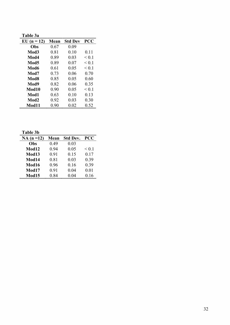
32

Table 3a EU (n = 12) Mean Std Dev PCC

Obs 0.67 0.09 Mod3 0.81 0.10 0.11 Mod4 0.89 0.03 < 0.1 Mod5 0.89 0.07 < 0.1 Mod6 0.61 0.05 < 0.1 Mod7 0.73 0.06 0.70 Mod8 0.85 0.05 0.60 Mod9 0.82 0.06 0.35 Mod10 0.90 0.05 < 0.1 Mod1 0.63 0.10 0.13 Mod2 0.92 0.03 0.30 Mod11 0.90 0.02 0.52

Table 3b NA (n =12) Mean Std Dev. PCC

Obs 0.49 0.03 Mod12 0.94 0.05 < 0.1 Mod13 0.91 0.15 0.17 Mod14 0.81 0.03 0.39 Mod16 0.96 0.16 0.39 Mod17 0.91 0.04 0.01 Mod15 0.84 0.04 0.16

33

Figures

Figure 1a.

Figure 1b.

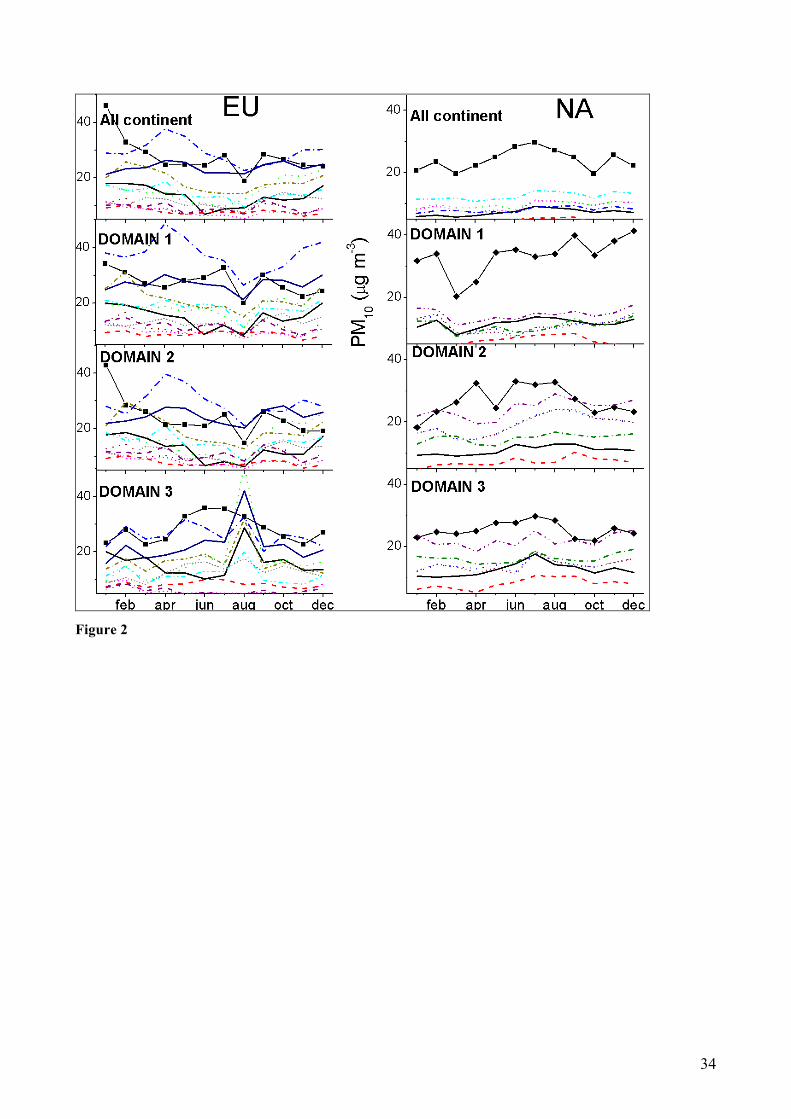
34

Figure 2

35

Figure 3

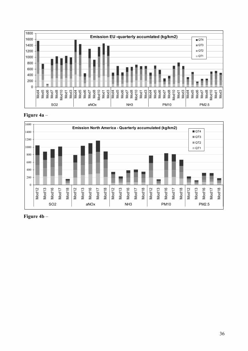
36

Emission EU -quarterly accumlated (kg/km2)

0

200

400

600

800

1000

1200

1400

1600

1800Mod4

Mod5

Mod6

Mod7

Mod8

Mod10

Mod1

Mod3

Mod4

Mod5

Mod6

Mod7

Mod8

Mod10

Mod1

Mod3

Mod4

Mod5

Mod6

Mod7

Mod8

Mod10

Mod1

Mod3

Mod4

Mod5

Mod6

Mod7

Mod8

Mod10

Mod1

Mod3

Mod4

Mod5

Mod6

Mod7

Mod8

Mod10

Mod1

Mod3

SO2 aNOx NH3 PM10 PM2.5

QT4

QT3

QT2

QT1

Figure 4a –

Emission North America - Quarterly accumulated (kg/km2)

0

200

400

600

800

1000

1200

1400

1600

Mod12

Mod13

Mod16

Mod17

Mod18

Mod12

Mod13

Mod16

Mod17

Mod18

Mod12

Mod13

Mod16

Mod17

Mod18

Mod12

Mod13

Mod16

Mod17

Mod18

Mod12

Mod13

Mod16

Mod17

Mod18

SO2 aNOx NH3 PM10 PM2.5

QT4

QT3

QT2

QT1

Figure 4b –

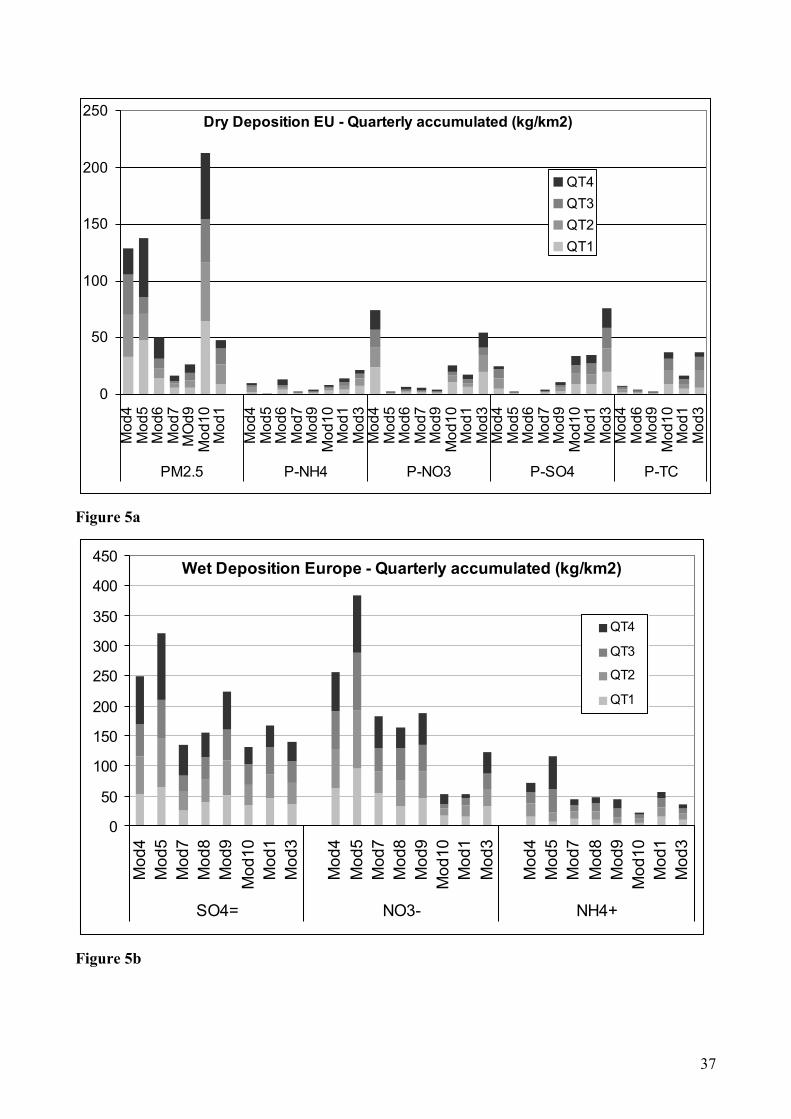
37

Dry Deposition EU - Quarterly accumulated (kg/km2)

0

50

100

150

200

250Mod4

Mod5

Mod6

Mod7

MOd9

Mod10

Mod1

Mod4

Mod5

Mod6

Mod7

Mod9

Mod10

Mod1

Mod3

Mod4

Mod5

Mod6

Mod7

Mod9

Mod10

Mod1

Mod3

Mod4

Mod5

Mod6

Mod7

Mod9

Mod10

Mod1

Mod3

Mod4

Mod6

Mod9

Mod10

Mod1

Mod3

PM2.5 P-NH4 P-NO3 P-SO4 P-TC

QT4QT3QT2QT1

Figure 5a

Wet Deposition Europe - Quarterly accumulated (kg/km2)

0

50

100

150

200

250

300

350

400

450

Mod4

Mod5

Mod7

Mod8

Mod9

Mod10

Mod1

Mod3

Mod4

Mod5

Mod7

Mod8

Mod9

Mod10

Mod1

Mod3

Mod4

Mod5

Mod7

Mod8

Mod9

Mod10

Mod1

Mod3

SO4= NO3- NH4+

QT4

QT3

QT2

QT1

Figure 5b

38

Dry Deposition North America - Quarterly accumulated (kg/km2)

0

20

40

60

80

100

120

140Mod12

Mod13

Mod16

Mod17

MOd12

Mod13

Mod16

Mod17

Mod18

MOd12

Mod13

Mod16

Mod17

Mod18

MOd12

Mod13

Mod16

Mod17

Mod18

MOd12

Mod13

Mod16

Mod17

Mod18

PM2.5 P-NH4 P-NO3 P-SO4 P-TC

QT4

QT3

QT2

QT1

Figure 5c

Wet Deposition NA - Quarterly accumulated (kg/km2)

0

50

100

150

200

250

Mod12

Mod13

Mod16

Mod17

Mod18

Mod12

Mod13

Mod16

Mod17

Mod18

Mod12

Mod13

Mod16

Mod17

Mod18

SO4= NO3- NH4+

QT4

QT3

QT2

QT1

Figure 5d

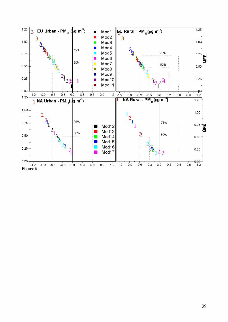
39

Figure 6

40

Figure 7.

41

Figure 8a

Figure 8b

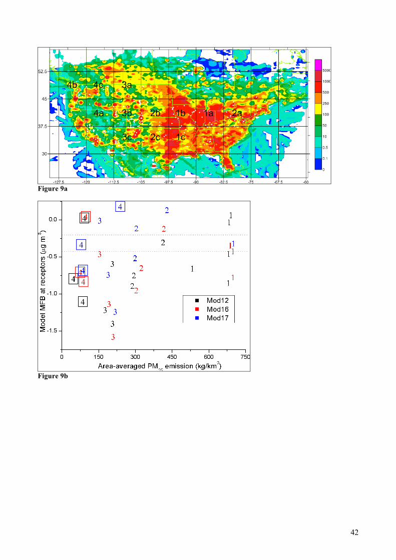
42

Figure 9a

Figure 9b

43

a)

b) Figure 10

44

Figure 11

45

Figure 12a

Figure 12b

Figure 13a

Figure 13b

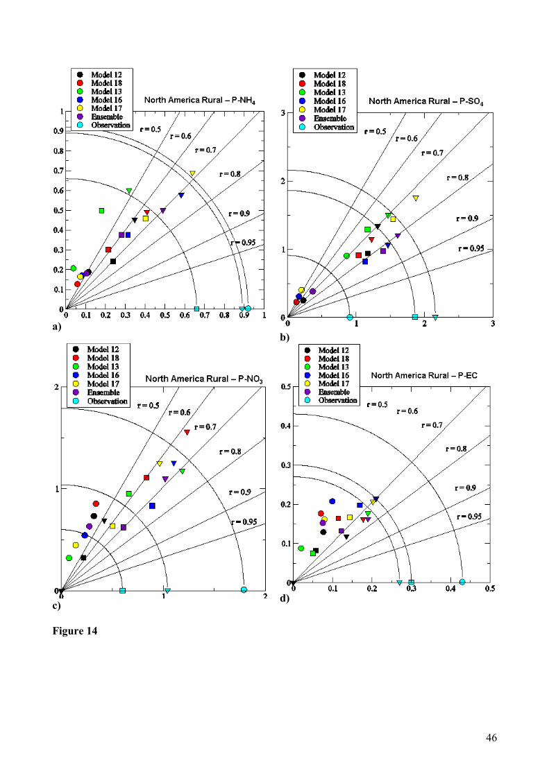
46

a)

b)

c)

d)

Figure 14

47

Figure 15

Figure 16