Onset and End of the Rainy Season in South America in Observations and the ECHAM 4.5 Atmospheric...

Onset and End of the Rainy Season in South America in Observations and theECHAM 4.5 Atmospheric General Circulation Model

BRANT LIEBMANN,* SUZANA J. CAMARGO,� ANJI SETH,# JOSÉ A. MARENGO,& LEILA M. V. CARVALHO,@

DAVE ALLURED,* RONG FU,** AND CAROLINA S. VERA��

*NOAA–CIRES Climate Diagnostics Center, Boulder, Colorado� International Research Institute for Climate and Society, Earth Institute at Columbia University, Palisades, New York

#Department of Geography, University of Connecticut, Storrs, Connecticut&CPTEC/INPE, Cachoeira Paulista, Brazil

@Department of Atmospheric Sciences, University of São Paulo, São Paulo, Brazil**Earth and Atmospheric Sciences, Georgia Institute of Technology, Atlanta, Georgia

��Department of Atmospheric and Ocean Sciences, CIMA/UBA-CONICET, Buenos Aires, Argentina

(Manuscript received 14 October 2005, in final form 20 June 2006)

ABSTRACT

Rainfall in South America as simulated by a 24-ensemble member of the ECHAM 4.5 atmosphericgeneral circulation model is compared and contrasted with observations (in areas in which data are avail-able) for the period 1976–2001. Emphasis is placed on determining the onset and end of the rainy season,from which its length and rain rate are determined.

It is shown that over large parts of the domain the onset and ending dates are well simulated by the model,with biases of less than 10 days. There is a tendency for model onset to occur early and ending to occur late,resulting in a simulated rainy season that is on average too long in many areas. The model wet season rainrate also tends to be larger than observed.

To estimate the relative importance of errors in wet season length and rain rate in determining biases inthe annual total, adjusted totals are computed by substituting both the observed climatological wet seasonlength and rate for those of the model. Problems in the rain rate generally are more important thanproblems in the length.

The wet season length and rain rate also contribute substantially to interannual variations in the annualtotal. These quantities are almost independent, and it is argued that they are each associated with differentmechanisms.

The observed onset dates almost always lie within the range of onset of the ensemble members, even inthe areas with a large model onset bias. In some areas, though, the model does not perform well. In southernBrazil the model ensemble average onset always occurs in summer, whereas the observations show thatwinter is often the wettest period. Individual members, however, do occasionally show a winter rainfallpeak. In southern Northeast Brazil the model has a more distinct rainy season than is observed. In thenorthwest Amazon the model annual cycle is shifted relative to that observed, resulting in a model bias.

No interannual relationship between model and observed onset dates is expected unless onset in themodel and observations has a mutual relationship with SST anomalies. In part of the near-equatorialAmazon, there does exist an interannual relationship between onset dates. Previous studies have shown thatin this area there is a relationship between SST anomalies and variations in seasonal total rainfall.

1. Introduction

The purpose of the work presented here is to exam-ine and compare statistics relevant to the South Ameri-can rainy season in observations and an atmospheric

general circulation model (GCM). The wet season isdescribed by three parameters: its onset, end, and rainrate. All three are important from meteorological andsocietal perspectives.

From a meteorological perspective, onset and endrepresent a sudden change in a tropical atmosphericheat source, the addition or subtraction of which isknown to alter both the large-scale (e.g., Simmons 1982;Silva Dias et al. 1983) and regional circulation (e.g.,Horel et al. 1989; Figueroa et al. 1995; Lenters and

Corresponding author address: Brant Liebmann, NOAA–CIRESClimate Diagnostics Center, R/PSD1, 325 Broadway, Boulder,CO 80305-3328.E-mail: [email protected]

15 MAY 2007 L I E B M A N N E T A L . 2037

DOI: 10.1175/JCLI4122.1

© 2007 American Meteorological Society

JCLI4122

Cook 1997). The rate determines the magnitude of thatheat source.

In other parts of the world, especially India, timing ofthe rainy season has long been a subject of extremeinterest, which is reflected in the literature (e.g., Sahaand Saha 1980). Crops are planted relative to the an-ticipated onset of the rainy season. In South America,however, although crops are certainly planted to takeadvantage of the climatological rainy season, any addedbenefit to be gained by an accurate prediction of rainyseason onset for a particular season is as yet unrealized.

Although the timing and quality of the wet season isof importance to agriculture in tropical South America,the ecosystem and forest is more sensitive to the lengthof the dry season (Sombroek 2001). Thus the endingdate is of interest as well. The 2005 drought in thesouthwestern Amazon, most severe in at least 100 yr,resulted from an extended dry season. The drought se-verely affected the population downstream along theAmazon River main channel and its tributaries, theSolimões and Madeiras Rivers, that depend on rivertransportation, even though the wet season near theequator was near average.

The spatial and temporal variability of onset and endof the rainy season in South America has been the sub-ject of some research. Kousky (1988) examined the spa-tially varying climatology of onset, using outgoing long-wave radiation (OLR) as a proxy for rainfall. A pentadaverage of 240 W m�2 or below was considered to bedeep convection. Onset was defined as occurring whendeep convection began, provided that 10 of 12 preced-ing pentads were not convective, and 10 of 12 subse-quent pentads were convective. The onset date was un-determined in extreme northwestern South Americabecause the climatological OLR is always below thethreshold for convection. From the equator to thesoutheast, however, Kousky (1988) concluded that on-set proceeds from northwest to southeast from roughlyAugust to October, with a later onset in eastern Brazil,although it is somewhat irregular in space. The end ismore regular and proceeds to the northwest.

Horel et al. (1989) examined the interannual variabil-ity of onset of the South American rainy season, againusing pentads of OLR. They defined 10° � 10° boxesand determined the fraction of grid points (on a 2° � 2°grid) with OLR less than 200 W m�2. Onset was de-fined as the first pentad on which the box with themaximum fraction of low OLR appeared in the South-ern Hemisphere, provided it remained there for 25days. A consistent definition was used for demise. Com-posites of 200-mb circulation from before and after on-set revealed the development of the Bolivian High anda downstream trough corresponding to onset.

More recently, rainfall measurements from gaugesthroughout parts of South America have become avail-able to the research community. Marengo et al. (2001)and Veiga et al. (2002) examined onset and end of theAmazon basin rainy season using pentads of observedrainfall computed from daily station records averagedonto grids. They defined onset (and end) analogous toKousky (1988) and obtained similar results: onset pro-ceeds from northwest to southeast. The rainy seasonwithdraws from southeast to northwest but is slowerthan onset. When Marengo et al. (2001) adjusted thethresholds for onset to be higher, however, the sense ofonset is reversed, although the pattern of withdrawalremains the same. Marengo et al. found an unexpect-edly weak relationship between the length of the rainyseason and total accumulation. There is also only aweak correlation between the date of onset or end andthe total rainy season accumulation. A lack of corre-spondence between onset date and subsequent accumu-lation was confirmed by Janowiak and Xie (2003).Liebmann and Marengo (2001) found statistically rel-evant correlations between onset or demise and tropi-cal sea surface temperature (SST) anomalies on someareas of the near-equatorial eastern Amazon. (Theirstudy included the Amazon basin only.)

Liebmann and Marengo (2001), using gridded dailyprecipitation data, defined onset at a given point to bewhen accumulated precipitation begins to exceed itsannual climatology. This definition is quite similar tothat used in the present study. Using this definition,they found that the Amazon wet season begins first inthe southeastern Amazon, and expands northward. Thepentad-based definition of Janowiak and Xie (2003),also defined locally, produced the earliest onset over aregion from 10° to 15°S, from which it progressed to thenortheast and southwest. (They were unable to defineonset in the northwest Amazon.) They noted that thissense of onset is quite different than the classic advanceof onset in other parts of the globe.

The work presented here is an exploratory analysis ofthe ability of an atmospheric GCM to simulate the wetseason in South America. The observed wet season iscontrasted with that of the ECHAM 4.5 GCM, whichwas forced with observed SSTs. The onset and end ofthe wet season are computed and compared. Thesequantities allow the partition of the wet season into itslength and rain rate. The relative importance of biasesin the length of, and rain rate during, the wet season isestimated. The two are distinguished because they arealmost completely independent and are associated withdifferent physics. For example, onset, which is of courserelated to rainy season length, is associated with a de-crease in convective inhibition energy (CINE), as

2038 J O U R N A L O F C L I M A T E VOLUME 20

shown by Fu et al. (1999), whereas once the rainy sea-son begins, CINE is of minor importance.

The ability of the model to accurately simulate inter-annual variability may also depend on the proper par-tition of the wet season into length and rain rate. Bothcontribute substantially to interannual variability, butLiebmann and Marengo (2001) showed that in areas ofthe Amazon where calendar season rainfall anomaliesare related to SST anomalies, the relationship seems tobe through an association with onset or end, rather thanthrough the wet season rain rate.

2. Data

Observed rainfall over South America is estimatedfrom daily station records that have been averaged ontogrids that exactly duplicate those of the model. Datafrom the 26-yr period 1976–2001 are used in this study,with the exception of 29 February, which is omittedfrom all calculations. One fewer year is used when theperiod in question spans two calendar years. Details ofthis dataset can be found in Liebmann and Allured(2005). Observed SSTs are those provided in the Na-tional Centers for Environmental Prediction–NationalCenter for Atmospheric Research (NCEP–NCAR) re-analysis archives.

The model rainfall comes from matching years for 24ensemble members of the ECHAM 4.5 (Roeckner et al.1996) atmospheric GCM with a horizontal resolution ofapproximately 2.8° � 2.8° latitude–longitude [triangu-lar truncation at wavenumber 42 (T42)] and 19 verticallevels (hybrid sigma pressure coordinates). All of theintegrations start in or before 1950 and extend until2005. These integrations were performed at the Inter-national Research Institute for Climate and Society(IRI) and this model at this resolution is one of themodels used for the IRI routine seasonal forecasts(Goddard et al. 2001, 2003). The ECHAM 4.5 wasforced with observed monthly evolving SSTs. The out-put of the model is masked before display to matchareas with rainfall observations in order to facilitatedirect comparison with the observations.

The ECHAM 4.5 model was developed at the Max-Planck-Institute for Meteorology in Hamburg, Ger-many. It evolved from the spectral weather predictionmodel of the European Centre for Medium-RangeWeather Forecasts (ECMWF; Simmons et al. 1989).The ECHAM 4.5 model parameterization of cumulusconvection is based on the bulk mass flux of Tiedtke(1989), modified according to Nordeng (1994). Detaileddescription of the ECHAM 4.5 GCM and its climatol-ogy is given in Roeckner et al. (1996). The interannualvariability of the precipitation in the model is discussedin Moron et al. (2001) and Camargo et al. (2001).

3. Results

a. Annual rainfall

Figures 1a and 1b show climatological annual totalrainfall from observations and as an average over the 24ensemble members. The maximum in the northwestAmazon of more than 3 m yr�1 and the minimum inNortheast Brazil are both evident in the model. Thesoutheastward extension of high precipitation valuesfrom the northwest Amazon maximum, known as theSouth Atlantic convergence zone (SACZ), is repro-duced by the model. The SACZ, however, appears toextend erroneously southward into southern Brazil asthe easternmost band of alternating high and low valueswhose contrast increases toward the mountains, whileobserved rainfall decreases monotonically to the west.The alternating bands of errors can be seen if the biasis plotted as a percent of the observed total (Fig. 1c),but the errors associated with this extension of theSACZ are quite small south of about 25°S becausethere is an observed maximum in southern Brazil. Thebanding is suspected to result from improper resolutionof the Andes Mountains in this relatively course-resolution model.

Another problem area is in the vicinity of northernBrazil and French Guiana. The model Atlantic inter-tropical convergence zone (ITCZ) does not extend farenough to the west, as seen in the unmasked field (notshown), and thus there is a model minimum. The ob-servations show a maximum with values about as highas those in the northwest Amazon.

b. Onset of the rainy season

A quantity “anomalous accumulation” is defined ateach grid point over time as

A�day� � �n�1

day

�R�n� � R, �1�

where R(n) is the daily precipitation and R is the cli-matological annual daily average. The calculation canbe started at any time, but in practice it is started 10days prior to the beginning of the driest month and issummed for a year.

From (1), the beginning of the rainy season is definedas the day after the start of the longest period for whichanomalous accumulation remains positive (relative tothe day before the start). Thus, for the period whosebeginning marks the start of the rainy season, the ac-cumulation is above the annual mean accumulation.The end of the rainy season is defined as the day withinthat period on which anomalous accumulation reachesa maximum. This definition is almost identical to thatproposed by Liebmann and Marengo (2001).


Figure 2 shows examples of anomalous accumulationcurves. The dashed curve is calculated from observa-tions for a single year in the southern Amazon basin,while the solid curve comes from model output at thesame point for the same year. The observed and modelannual climatologies can be seen to be quite similar, asduring the dry season (centered on about 4 July) thenegative slope of each is about the same (i.e., when it isdry the accumulation curve is reduced by the sameamount each day). In general, the comparison of

anomalous accumulation curves does not yield infor-mation about total rainfall, as the model and observa-tions have different climatologies. At this particularpoint, however, since the climatologies are almost iden-tical, it can be seen that for this particular rainy seasonmore rainfall was recorded than was simulated by thechosen realization because the observed anomalous ac-cumulation is larger.

In this particular year the observed onset occurs on17 October and the simulated onset occurs on 18 Oc-

FIG. 1. Annual total precipitation, averaged for the years 1976–2000 on model grid. Dashedlines indicate data perimeter. (a) Observed values; (b) 24-member ensemble average of theECHAM 4.5 model; and (c) model�observations expressed as percent of observed.


tober (vertical line). In the 365 days beginning on 21June (10 days before the start of the average driestmonth), these dates begin the longest period duringwhich anomalous accumulation stays above that ex-pected from the annual climatology. Although for theexample shown there is a close correspondence be-tween observed and simulated onset dates, there is noreason to expect such a correspondence unless onset atthis point is controlled by SST anomalies.

The end of the rainy season is defined to occur whenrainfall no longer exceeds its climatology, which ofcourse occurs when the curve reaches its peak. For thisexample, the model ending (denoted by vertical line) islater than observed. It should be noted that at this lo-cation the model performs quite well (in a statisticalsense) and onset and end are robustly defined becauseof the steady rainfall during the wet season and an al-most complete lack of rain during the dry season, asevidenced by the nearly straight curves during and afterthe wet season.

The average starting dates of the observations andthe ensemble are shown in Figs. 3a and 3b. Althoughthe comparison is not exact because the climatologiesof the observations and models are different, onset oc-curs with a rapid increase in rainfall, which is capturedby the methodology. Qualitatively the maps are quitesimilar, but Fig. 3c, the difference, reveals an overallearly model bias, and some areas with large discrepan-cies. South of 25°S, near the equator in western Brazil,and in southern Northeast Brazil, the model bias is so

large that model and observed onset occur in differentseasons. Even though the onset bias is large in southernBrazil, the model annual total precipitation is close tothat observed (Fig. 1c).

An interesting aspect of Figs. 3a and 3b is that theyboth indicate that, using the present definition, onset ofthe rainy season occurs first in the southern Amazonbasin or father south and progresses northward. Seth etal. (2007) showed that Climate Prediction Center(CPC) Merged Analysis of Precipitation (CMAP) pen-tad estimates of precipitation (Xie et al. 2003) for the1979/80 Amazon rainy season are consistent with thepresent climatology. That season was characterized bya rapid shift rather than a smooth transition from theNorthern to Southern Hemisphere. The rapid transi-tion observed by Seth et al. (2007) runs contrary to thebroadly held belief that the rainy season progressesfrom northwest to southeast, from the climatologicalNorthern Hemisphere summer maximum, across theequator and into the Amazon. Janowiak and Xie (2003)also found onset to progress toward the equator, andnoted that this sense of progression is different than inthe other monsoons of the world.

Figure 4 is similar to Fig. 3, except it shows the cli-matological ending dates. The direction of withdrawalin the observations and the ensemble is broadly consis-tent, progressing northward. The largest discrepanciesin ending date (Fig. 4c) occur in southeast SouthAmerica, eastern Brazil, and the northwest Amazon.These areas also have large discrepancies in onset date(Fig. 3c).

Figure 5a shows the bias in wet season length. It isusually positive, but often small. The wet season rainrate can easily be computed with knowledge of thelength. Figure 5b shows the average difference in thewet season daily rate (approximated as the rate for thefirst 45 days from each year’s onset). The pattern isquite similar to the error pattern in the annual totalprecipitation.

A distinction is made between the wet season rainrate and length. They both can contribute to the bias inannual total rainfall, but they are expected to resultfrom different processes. For example, Fu et al. (1999)showed that a moistening of the planetary boundarylayer and a lowering of the temperature at its top,thereby reducing CINE, control the conditioning of thelarge-scale thermodynamics prior to onset. Li and Fu(2004) showed in their composite analysis that the mainincrease in convective available potential energy(CAPE) and reduction in CINE occur prior to rainyseason onset, although in the tropical atmosphere,CAPE often exists in the absence of deep convection

FIG. 2. Anomalous accumulation [computed from (1)] for asingle year of observations (dashed curve) and a single modelrealization (solid curve). Vertical lines indicate the start and enddates of the model wet season.


(e.g., Williams and Renno 1993). While there must besome level of CINE to overcome for rainfall to occurduring the wet season, the rate is likely to be controlledby other aspects as well, such as the available moisture.

Biases in the wet season length and rain rate mustcontribute to biases in the annual total, unless they ex-actly cancel. The purpose of the following crude calcu-lations is to determine the relative importance of theerrors in length and rain rate in causing the model bi-ases in total annual precipitation. This is accomplishedby assuming two rainfall regimes, dry and wet. To de-

termine the effect of length biases, the model climatol-ogy is adjusted by the following equation:

A � �Lecham � Lobs� � �Rwet � Rdry�, �2�

where A is the adjustment, Lobs is the observed averagelength of the rainy season, Lecham is the model en-semble average length, Rwet is the model rainy seasonrain rate, defined as the average rate from onset until 44days after onset, and Rdry is the model dry season rate,defined as the average rate from 45 days before eachyear’s onset, until the day before onset.

FIG. 3. Climatological onset date averaged from onset date for each year for (a) observationsand (b) all ensemble members. (c) Average onset date of model�observations.


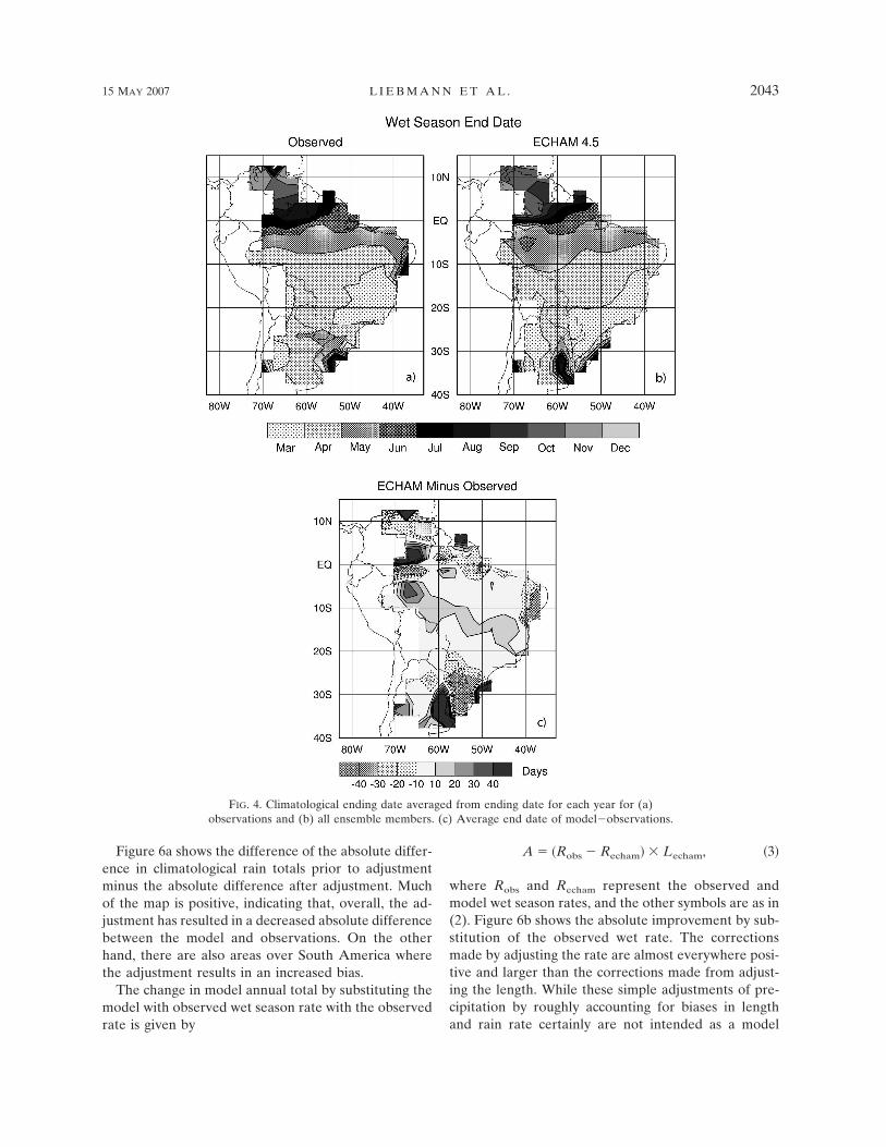
Figure 6a shows the difference of the absolute differ-ence in climatological rain totals prior to adjustmentminus the absolute difference after adjustment. Muchof the map is positive, indicating that, overall, the ad-justment has resulted in a decreased absolute differencebetween the model and observations. On the otherhand, there are also areas over South America wherethe adjustment results in an increased bias.

The change in model annual total by substituting themodel with observed wet season rate with the observedrate is given by

A � �Robs � Recham� � Lecham, �3�

where Robs and Recham represent the observed andmodel wet season rates, and the other symbols are as in(2). Figure 6b shows the absolute improvement by sub-stitution of the observed wet rate. The correctionsmade by adjusting the rate are almost everywhere posi-tive and larger than the corrections made from adjust-ing the length. While these simple adjustments of pre-cipitation by roughly accounting for biases in lengthand rain rate certainly are not intended as a model

FIG. 4. Climatological ending date averaged from ending date for each year for (a)observations and (b) all ensemble members. (c) Average end date of model�observations.


“fix,” they do suggest that gains in simulation climatol-ogy could be achieved by an improved estimation of theclimatological onset, and even more so by improvementof the wet season rate.

The wet season length and rain rate contribute notonly to biases in annual totals, but to their variations tointerannual variability. Figures 7a and 7b show the vari-ance of observed annual (July–June) precipitation ex-

plained by the length of the wet season and its rain rate.The length of the wet season and its rain rate are nearlyuncorrelated. The wet season length explains little vari-ance in the southern Amazon and northern La Platabasins, which includes the region affected by the SACZ.In this area, onset varies little from year to year, so itcan account for little variation of rainfall. From theequator to 10°S, however, upward of 40% is explained

FIG. 6. Absolute improvement of model precipitation annual climatology by substitution of(a) observed length and (b) observed rate of wet season. Positive values indicate an improve-ment.

FIG. 5. Average observed�ensemble average rainy season (a) length and (b) rain rate.


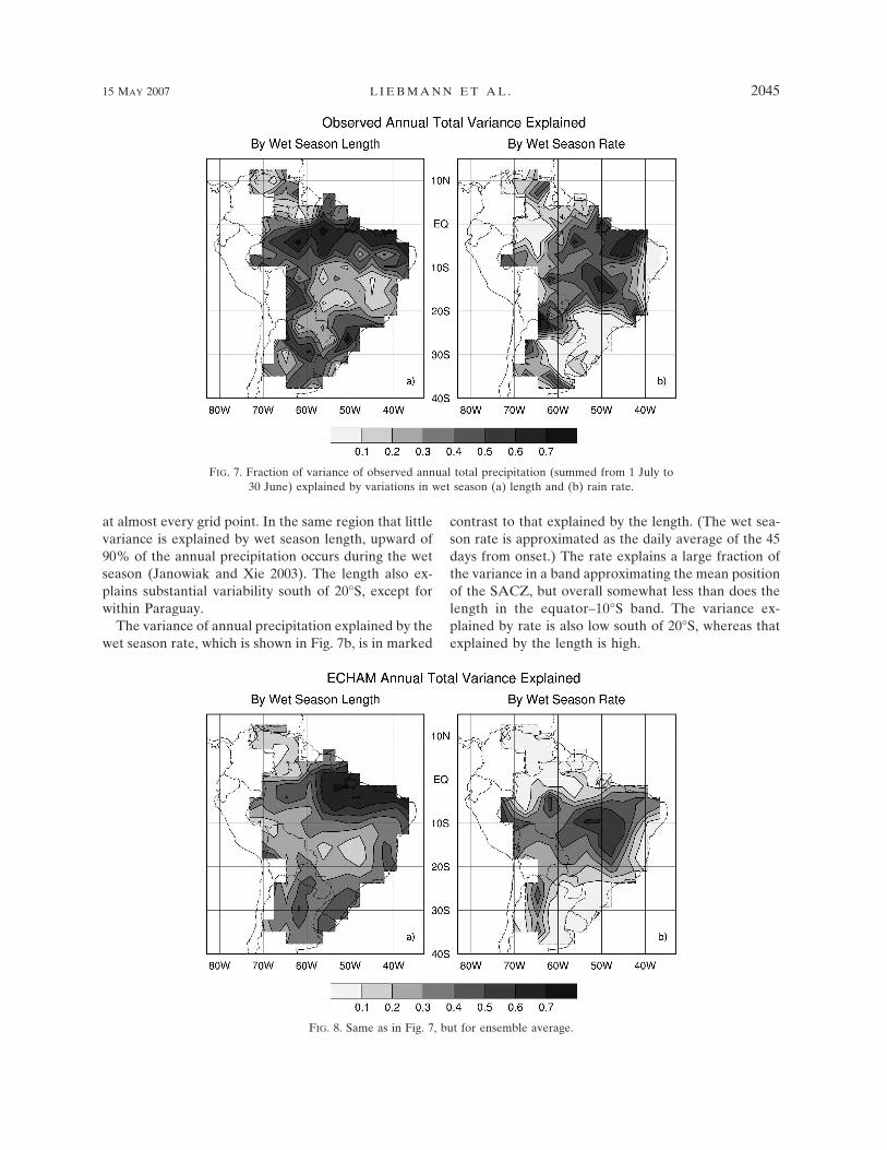
at almost every grid point. In the same region that littlevariance is explained by wet season length, upward of90% of the annual precipitation occurs during the wetseason (Janowiak and Xie 2003). The length also ex-plains substantial variability south of 20°S, except forwithin Paraguay.

The variance of annual precipitation explained by thewet season rate, which is shown in Fig. 7b, is in marked

contrast to that explained by the length. (The wet sea-son rate is approximated as the daily average of the 45days from onset.) The rate explains a large fraction ofthe variance in a band approximating the mean positionof the SACZ, but overall somewhat less than does thelength in the equator–10°S band. The variance ex-plained by rate is also low south of 20°S, whereas thatexplained by the length is high.

FIG. 7. Fraction of variance of observed annual total precipitation (summed from 1 July to30 June) explained by variations in wet season (a) length and (b) rain rate.

FIG. 8. Same as in Fig. 7, but for ensemble average.


Figure 8 is the model average equivalent to Fig. 7.The pattern quite closely resembles that of observa-tions. Variations in length are important near the equa-tor, yet play little role in the southern Amazon andSACZ. Like observations, these are the areas wherevariations in the rate assume the most importance.

Except for a region of SST influence in southeastBrazil, the only relationships between rainfall in SouthAmerica and SST occur in the near-equatorial band,supporting the contention of Fu et al. (1999) that SSTvariations should be related to variations of wet seasononset due to small variations in land surface tempera-ture. Liebmann and Marengo (2001) found that in areasthat exhibit correlations between total rainfall and SST,the connections are through the SST connection withonset or end rather than rain rate.

There is no expectation of an interannual correlationbetween observed and model onset except in those ar-eas in which SST anomalies affect onset. Figure 9 showsthe correlation between the observed and the ensembleaverage onset. In the areas with statistically relevantcorrelations (correlations greater than 0.5), there areknown relationships between SST anomalies (i.e.,Niño-3.4) and seasonal mean rainfall (e.g., Liebmannand Marengo 2001). On the other hand, there are areas,such as Northeast Brazil, that enjoy strong relationshipswith SST, and the model seasonal rainfall anomaliesthere are quite realistic (e.g., Goddard et al. 2001,2003), yet there are no strong correlations between ob-served and model onsets.

c. Regional comparisons

There are many areas in the domain used in thisstudy in which the model seems to perform quite well.For example, in the southern Amazon basin the ob-served and modeled annual totals are quite similar (Fig.1), and the difference between the observed and simu-lated average onset and end dates are both within a fewdays of each other (Fig. 3 and Fig. 4). At 12.6°S, 53.4°W(at which point examples of anomalous accumulationare shown in Fig. 2) the phasing of the annual cycle is inexcellent agreement (Fig. 10a), and the monthly clima-tologies from June to November are nearly identical.Furthermore, the intermodel spread of the monthly cli-matology is negligible. Figure 10b shows that there isalso little interannual variation in onset dates, and thatthe observed onset is almost always within the range ofthe individual member onsets.

There are, however, some areas in which there con-sistently appear large discrepancies between the obser-vations and the model. One of these areas lies in south-ern Brazil. Although the annual totals are similar (Fig.1), the observations indicate a local maximum of more

than 1700 mm, while the model shows an extension ofthe Amazon basin rainfall that does not appear in ob-servations. In this area there are large biases in theaverage rainy season starting and ending dates (Figs. 3cand 4c). As discussed below, part of the bias is theresult of a shortcoming of the analysis technique, andpart is due to a real difference between the observa-tions and the model.

Figure 11a shows the monthly climatology in south-ern Brazil of the observations and the model. The ob-servations reveal distinct summer and winter maxima inrainfall, and although the summer climatological aver-age is larger than that during winter, the largest singlemonthly total occurred during winter. The winter peakis largely absent in the model.

The reason for the difference between observationsand the model is that in 5 of the 25 yr, the observedsummertime rainy season was quite short (by thepresent definition), whereas the model rainy season ismuch more regular. In each year the ensemble averageonset date occurs in the summer (Fig. 11b). In the ob-servations, the years with a short summertime rainyseason are all followed by a wintertime rainy seasonthat exceeded that of the previous summer. Thus thealgorithm considers onset in these years to be quite late,

FIG. 9. Correlation between observed and ensemble averageonset. Ensemble average is calculated as average of onset of eachmember.


as it begins counting near the end of July (10 days be-fore the beginning of August, the driest month in theclimatology). In one year, onset occurs in mid-July,which is defined as being extremely late. Had the algo-rithm started counting earlier, the average onset wouldhave changed. If these five unusual years, in which on-

set occurs after the end of February, are removed fromthe calculation of average onset, the average becomes 7October, just 14 days later than the model average. It isinteresting that for a few of the individual members,onset occurs as late as is observed in the most extremeof years (Fig. 11b). These late model onsets (corre-sponding to a nearly absent summer rainy season) donot occur often enough to bring the average onset inline with the observed. Further complicating the statis-tics is that in some years in southern Brazil, there is nodistinct break between the summer and winter rainy

FIG. 10. Monthly daily average precipitation at 12.6°S, 53.4°Wfor observations and ensemble average. Thin curves on either sideof ensemble mean represent 1 std dev intermodel climatology. (b)Onset date for each year at same point for observations and av-erage of each ensemble member. Open circles denote observeddate, closed circles denote average over all ensemble members,and dots indicate onset for 18 ensemble members. Graphics limi-tations prevent showing each ensemble member.

FIG. 11. Same as in Fig. 10, but for grid point at 26.5°S, 53.4°W.


seasons, so the observed rainy season appears to lastmore than a year.

Another location with large differences between ob-served and model onset is along the coast of northeastBrazil. Although this area is relatively small, it is in-cluded because of the longstanding interest in northeastBrazil precipitation. The grid point of interest, locatedat 12.6°S, 39.4°W is not on the edge of the data void ofthe Atlantic. Edge points potentially are problematicalbecause often fewer stations are averaged into thesegrid points.

Figure 12a is like Fig. 10a, except it shows themonthly climatology of the southern northeast Brazil

point. The model annual total is substantially less thanobserved (Fig. 1c), owing primarily to a lack of a pro-nounced observed dry season at this location, in sharpcontrast to the model. In the northern part of northeastBrazil, where observations show distinct wet and dryseasons, the model climatology simulates the observa-tions quite well (not shown).

The interannual onset dates are shown in Fig. 12b. Inabout half of the years the observed onset is near themodel average. The observed average onset date forthose years (onset occurring before 1 February) is 19November, close to the model average of 2 December.In the other half of the years, however, the observedaverage is 27 March, which is much later than the mid-January average found in northern northeast Brazil.

Although there are many years in which observedonset occurs quite late with respect to the model aver-age, they are nonetheless almost always within therange of the individual ensemble members. Unlike theobservations, with a noticeable separation betweenearly and late starts, there is no distinct separation inthe model. The model starting dates, however, do tendto cluster toward the early end of the range; thus theaverage model starting date is earlier than that ob-served.

A third area in which there is a systematic differencein onset date is the northwest Brazilian Amazon. Here,observations reveal a maximum in May and a minimumduring August, although the low values from August toNovember suggest a strong projection onto the annualharmonic (Fig. 13a). Note that the northwest Amazonreceives more precipitation during its “driest” monththan northeast Brazil receives during its wettest month.The model, on the other hand, produces a double maxi-mum in rainfall, consisting of a distinct peak in Apriland a broad peak from October to December. Thislater model maximum nearly coincides with the ob-served annual minimum. Since the most dramatic risein model precipitation occurs from July to September,while the observed precipitation begins increasing rap-idly in November, there is a large systematic differencein onset, as reflected in Fig. 13b. The climatologies ofthe northwestern Amazon and Northeast Brazil are dis-cussed in detail by Figueroa and Nobre (1990) andMarengo and Nobre (2001).

4. Summary and discussion

Variations and model biases of the wet season lengthand rain rate on South American annual total precipi-tation have been examined. Statistics of the rainy sea-son are calculated for both observations and a 24-member ensemble of the ECHAM 4.5 model, and thetwo are compared.



Onset and end are defined as the beginning and endof the longest period during which rainfall exceeds itsannual climatology. One of the interesting aspects ofthis definition is that the rainy season progresses north-ward from the Southern Amazon, rather than fromnorthwest to southeast as has been found in previousstudies. The sense of onset seems to depend on whetherthe definition is based on a universal or local threshold.The universal threshold (e.g., Kousky 1988; Marengo etal. 2001) produces a poleward-progressing onset, whilea local threshold (e.g., Liebmann and Marengo 2001;

Janowiak and Xie 2003) produces results consistentwith the present study.

In general, the agreement between the climatologicalonset and end dates and the length of the rainy seasonbetween the observations and the ECHAM 4.5 en-semble is deemed to be quite good. Although the biasin length tends to be positive as a result of a model wetseason that tends to start early and end late, over alarge part of the domain the bias is less than 20 days.

The interannual wet season lengths and rain rates arealso calculated. These two contributors to the annualtotal are separated because each are influenced by dif-ferent processes and they are nearly independent. Tounderstand their relative contribution to the bias in an-nual total precipitation, the model climatology is recal-culated twice: once by replacing the model wet seasonlength by that observed (and adjusting the total to ac-count for changed lengths of precipitation at the dryand wet season rates), and also by replacing the averagemodel wet season rate with the observed. Although acrude approximation, the results indicate that problemsin the rain rate contribute more to the bias than dosystematic biases in length.

Variations in total rainfall are not dominantly ex-plained by variations in rate. It is shown that over mostof the zone from the equator to 10°S, variation of therainy season length accounts for upward of 40% of thevariance of the observed annual total. In the area affectedby the SACZ, however, the variation of rate explainsmuch more variance than does the variation of the length.The model partitions the explained variance quite well.

The fact that the length does not contribute much tovariance in the vicinity of the SACZ may provide a clueas to why prediction skill is low in that area. Liebmannand Marengo (2001) found that those areas with aninterannual relationship between rainfall and SST werecharacterized by a consistent relationship with onset orend (e.g., high totals and an early onset, both related toSST of the same sign). Fu et al. (1999) argued that onsetwould not be related to SST away from the equatorialzone. Since the wet season rate does not seem to berelated to SST anomalies, areas in which interannualrainfall variability is dominated by that of the rate mayenjoy increasing skill as land surface influences becomebetter understood.

More subtly, model biases of timing can also affectinterannual variability. For example, imagine a regionin which the observed onset usually occurs in Decem-ber, but the model has an early bias such that onsetoccurs in November. Thus if one is concerned with De-cember–February (DJF) totals, even if the observedand model onset track perfectly, onset variations in themodel will not contribute to variance of DJF totals.



One of the goals of future work will be to quantifythe extent that biases in the timing of the rainy seasonundermine the simulation of calendar season variabil-ity. In areas where onset or end timing is related to SSTanomalies the bias may ruin predictive skill as well.

Acknowledgments. The authors would like to thankthe NOAA Climate Program Office (Climate Predic-tion Program for the Americas) for their support. Theyalso would like to thank the Max Planck Institute forMeteorology for making the ECHAM4.5 model acces-sible to IRI. We are indebted to Dr. B. Blumenthalfor the IRI Data Library and to Dr. D. DeWitt forperforming the ECHAM4.5 model integrations withsupport from Dr. X. Gong. This paper is funded in partby a grant/cooperative agreement from NOAA,NA050AR4311004. Thanks also to IAI/CRN055/PROSUR, FAPESP 01-123165-01, and to PROBIO/MMA/BIRD/GEF/CNPq from Brazil, for partiallyfunding this research. JM was partially supported bythe Brazilian Conselho Nacional de DesenvolvimentoCientıfico e Tecnologico (CNPq). Finally, the sugges-tions of the anonymous reviewers aided in considerablyimproving the manuscript from its original form.

REFERENCES

Camargo, S. J., S. E. Zebiak, D. G. DeWitt, and L. Goddard,2001: Seasonal comparison of the response of CCM3.6,ECHAM4.5, and COLA2.0 atmospheric models to observedSSTs. IRI Tech. Rep. 01/01, Palisades, NY, 68 pp.

Figueroa, N., and C. A. Nobre, 1990: Precipitation distributionover central and western tropical South America. Climaná-lise, 5, 36–40.

——, P. Satyamurty, and P. L. Silva Dias, 1995: Simulations of thesummer circulation over the South American region with aneta coordinate model. J. Atmos. Sci., 52, 1573–1584.

Fu, R., B. Zhu, and R. E. Dickinson, 1999: How do atmosphereand land surface influence seasonal changes of convection inthe tropical Amazon? J. Climate, 12, 1306–1321.

Goddard, L., S. J. Mason, S. E. Zebiak, C. F. Ropelewski, R.Basher, and M. A. Cane, 2001: Current approaches to sea-sonal to interannual climate predictions. Int. J. Climatol., 21,1111–1152.

——, A. G. Barnston, and S. J. Mason, 2003: Evaluation of theIRI’s “net assessment” seasonal climate forecasts: 1997–2001.Bull. Amer. Meteor. Soc., 84, 1761–1781.

Horel, J. D., A. N. Hahmann, and J. E. Geisler, 1989: An investi-gation of the annual cycle of convective activity over thetropical Americas. J. Climate, 2, 1388–1403.

Janowiak, J. E., and P. Xie, 2003: A global-scale examination ofmonsoon-related precipitation. J. Climate, 16, 4121–4133.

Kousky, V. E., 1988: Pentad outgoing longwave radiation clima-tology for the South American sector. Rev. Bras. Meteor., 3,217–231.

Lenters, J. D., and K. H. Cook, 1997: On the origin of the Bolivianhigh and related circulation features of the South Americanclimate. J. Atmos. Sci., 54, 656–678.

Li, W., and R. Fu, 2004: Transition of the large-scale atmosphericand land surface conditions from the dry to the wet seasonover Amazonia as diagnosed by the ECMWF Re-Analysis. J.Climate, 17, 2637–2651.

Liebmann, B., and J. A. Marengo, 2001: Interannual variability ofthe rainy season and rainfall in the Brazilian Amazon Basin.J. Climate, 14, 4308–4318.

——, and D. Allured, 2005: Daily precipitation grids for SouthAmerica. Bull. Amer. Meteor. Soc., 86, 1567–1570.

Marengo, J. A., and C. A. Nobre, 2001: General characteristicsand variability of climate in the Amazon basin and its links tothe global climate system. The Biogeochemistry of the Ama-zon Basin, M. E. McClaine, R. L. Victoria, and J. E. Richey,Eds., Oxford University Press, 17–42.

——, B. Liebmann, V. E. Kousky, N. P. Filizola, and I. C. Wainer,2001: Onset and end of the rainy season in the BrazilianAmazon Basin. J. Climate, 14, 833–852.

Moron, V., M. N. Ward, and N. Navarra, 2001: Observed andSST-forced seasonal rainfall variability across tropicalAmerica. Int. J. Climatol., 21, 1467–1501.

Nordeng, T. E., 1994: Extended versions of the convective param-etrization scheme at the ECMWF and their impact upon themean climate and transient activity of the model in tropics.ECMWF Tech. Memo. 206, Reading, United Kingdom, 25pp.

Roeckner, E., and Coauthors, 1996: The atmospheric general cir-culation model ECHAM-4: Model description and simula-tion of present-day climate. Max-Planck Institute for Meteo-rology Tech. Rep. 218, Hamburg, Germany, 90 pp.

Saha, S., and K. Saha, 1980: A hypothesis on onset, advance andwithdrawal of the Indian summer monsoon. Pure Appl. Geo-phys., 118, 1066–1075.

Seth, A., S. A. Rauscher, S. J. Camargo, J.-H. Qian, and J. S. Pal,2007: RegCM3 regional climatologies for South America us-ing reanalysis and ECHAM global model driving fields. Cli-mate Dyn., 28, 461–480.

Silva Dias, P. L., W. H. Schubert, and M. DeMaria, 1983: Large-scale response of the tropical atmosphere to transient con-vection. J. Atmos. Sci., 40, 2689–2707.

Simmons, A. J., 1982: The forcing of stationary wave motion bytropical diabatic heating. Quart. J. Roy. Meteor. Soc., 108,503–534.

——, D. M. Burridge, M. Jarraud, C. Girard, and W. Wergen,1989: The ECMWF medium-range prediction models: Devel-opment of the numerical formulations and the impact of in-creased resolution. Meteor. Atmos. Phys., 40, 28–60.

Sombroek, W. G., 2001: Spatial and temporal patterns of Amazonrainfall. Ambio, 30, 388–396.

Tiedtke, M., 1989: A comprehensive mass flux scheme for cumu-lus parameterization in large-scale models. Mon. Wea. Rev.,117, 1779–1800.

Veiga, J. A., J. A. Marengo, and V. B. Rao, 2002: A influencia dasanomalies de TSM dos oceanos Atlantico e Pacifico nas chu-vas do moncao da America do Sul. Rev. Bras. Meteor., 17,181–194.

Williams, E., and N. Renno, 1993: An analysis of conditional in-stability of the tropical atmosphere. Mon. Wea. Rev., 121,21–36.

Xie, P., J. E. Janowiak, P. A. Arkin, R. Adler, A. Gruber, R.Ferraro, G. J. Huffman, and S. Curtis, 2003: GPCP pentadprecipitation analyses: An experimental dataset based ongauge observations and satellite estimates. J. Climate, 16,2197–2214.


Onset and End of the Rainy Season in South America in Observations and the ECHAM 4.5 Atmospheric...

Documents

Transcript of Onset and End of the Rainy Season in South America in Observations and the ECHAM 4.5 Atmospheric...