This document contains the post-print pdf-version of the refereed paper:

“Online model predictive control of industrial processes using low level control hardware: a pilot-scale distillation column case study”

by Bart Huyck, Jos De Brabanter, Bart De Moor, Jan F. Van Impe, and Filip Logist

which has been archived on the university repository Lirias (https://lirias.kuleuven.be/) of the Katholieke Universiteit Leuven. The content is identical to the content of the published paper, but without the final typesetting by the publisher. When referring to this work, please cite the full bibliographic info:

Bart Huyck, Jos De Brabanter, Bart De Moor, Jan F. Van Impe, Filip Logist, Online model predictive control of industrial processes using low level control hardware: A pilot-scale distillation column case study, Control Engineering Practice, Volume 28, 2014, Pages 34-48. The journal and the original published paper can be found at: http://www.journals.elsevier.com/control-engineering-practice/ http://dx.doi.org/10.1016/j.conengprac.2014.02.016 The corresponding author can be contacted for additional info. Conditions for open access are available at: http://www.sherpa.ac.uk/romeo/

Postprint version of paper published in Control Engineering Practice 2014, vol 28, pages 34 - 48. The content is identical to the published paper, but without the final typesetting by the publisher.

Journal homepage: http://www.journals.elsevier.com/control-engineering-practice/ Original file available at: http://dx.doi.org/10.1016/j.conengprac.2014.02.016

Online model predictive control of industrial processes

using low level control hardware:

a pilot-scale distillation column case study

Bart Huycka,b, Jos De Brabanterb, Bart De Moorb, Jan F. Van Impea, FilipLogista,∗

aDepartment of Chemical Engineering (CIT - BioTeC), KU Leuven, W. de Croylaan 46,B-3001 Leuven, Belgium

bDepartment of Electrical Engineering (ESAT - STADIUS), KU Leuven, KasteelparkArenberg 10, B-3001 Leuven, Belgium

Abstract

Throughout the years, the computing power of industrial controllers hassteadily increased. Together with the development of efficient quadratic pro-gram (QP) solvers, this raises the question whether these devices can host anonline model predictive controller (MPC). The applicability of online MPC isinvestigated using a programmable automation controller (PAC) and a pro-grammable logic controller (PLC) for the control of an industrially relevantprocess, i.e., a pilot scale distillation column. It is demonstrated that bothdevices are capable of hosting MPC, however the limitations of the PLC arereached for the investigated set-up. Finally, guidelines and pitfalls for use inpractice are highlighted.

Keywords: online MPC, linear MPC, PLC, PAC, pilot-scale distillationcolumn

∗Corresponding authorEmail addresses: bart.huyck@kuleuven.be (Bart Huyck),

jos.debrabanter@esat.kuleuven.be (Jos De Brabanter),bart.demoor@esat.kuleuven.be (Bart De Moor), jan.vanimpe@cit.kuleuven.be (JanF. Van Impe), filip.logist@cit.kuleuven.be (Filip Logist)

Postprint version of manuscript accepted for Control Engineering PracticeApril 13, 2014

Postprint version of paper published in Control Engineering Practice 2014, vol 28, pages 34 - 48. The content is identical to the published paper, but without the final typesetting by the publisher.

Journal homepage: http://www.journals.elsevier.com/control-engineering-practice/ Original file available at: http://dx.doi.org/10.1016/j.conengprac.2014.02.016

1. Introduction

One of the most successful advanced control methodologies in industry isModel Predictive Control (MPC). It has been a widely applied technique inprocess industry over forty years (Qin and Badgwell, 2003; Bauer and Craig,2008; Mathur et al., 2008). The advantages of MPC over classic controlmethodologies, e.g., PID control, are its ability (i) to steer the process in anoptimal way while taking proactively desired future behavior into account,(ii) to tackle multiple inputs and outputs simultaneously and (iii) to incor-porate constraints (Maciejowski, 2002; Darby and Nikolaou, 2012).

Although model predictive control originates from the petrochemical in-dustry (Richalet et al., 1978; Cutler and Ramaker., 1980), it has been suc-cessfully transferred to many other application areas, e.g., automotive indus-try (Hrovat et al., 2012), paper and pulp industry (VanAntwerp and Braatz,2000), power converters (Kouro et al., 2009) and traffic control (Bellemanset al., 2006).

Current research on MPC focuses on, e.g., fast(er) algorithms (Bemporadet al., 2002; Ferreau et al., 2008; Wang and Boyd, 2010; Mattingley and Boyd,2012) to encourage and simplify the use of MPC. Moreover, many of thesealgorithms were developed with embedded applications in mind. These areapplications where the control scheme runs on an autonomous platform, oftenintegrated in a machine. Typical examples are microcontrollers and field-programmable gate arrays (FPGAs). Due to the technical improvements,these devices have become readily available at relatively low prices. Nev-ertheless, as robustness, industry-proven reliability, and long-term supportare important features for the process industry, less powerful programmablelogic controllers (PLCs) are still omnipresent in process plants. These devicesare robust and typically last the lifetime of an installation which eliminatesexpensive hardware replacements. However, evolving legislation may forcecompanies to meet new standards that cannot always be reached by tradi-tional control schemes. In such cases, an upgrade to, e.g., an MPC runningon installed hardware can be considered. Consequently, it is interesting toevaluate these devices for the implementation of MPC algorithms.

Bemporad et al. (2002) suggested explicit MPC to solve the MPC prob-lem. Here, the underlying quadratic program is solved offline and piecewise

2

Postprint version of paper published in Control Engineering Practice 2014, vol 28, pages 34 - 48. The content is identical to the published paper, but without the final typesetting by the publisher.

Journal homepage: http://www.journals.elsevier.com/control-engineering-practice/ Original file available at: http://dx.doi.org/10.1016/j.conengprac.2014.02.016

linear solutions are stored in a look-up table. For the online application, theright piecewise linear solution is rapidly selected based on the measurementsof the current state of the system. This development has been successfullyexploited on PLC hardware by, e.g., Kvasnica et al. (2010); Valencia-Palomoand Rossiter (2011a,b, 2012). However, this approach is mainly feasiblefor small-scale systems and short time horizons as the storage complexitystrongly increases with the size of the MPC problem.

In contrast, results for online MPC hosted by PLCs are scarce (e.g.,Necoara and Clipici (2013)). Here, the underlying QP has to be solved on-line in each step. Also in Huyck et al. (2012) a successful illustration on asmall-scale air-heating set-up has been presented. Although the knowledgegained in this study was substantial, the employed small-scale set-up hadonly a limited relevance for (process) industry. To explore the constraintsthat will be encountered when using MPC on a PLC in such environments,an example more relevant to industry, i.e., a pilot-scale distillation column,will be used in the current paper. As a first step, a programmable automa-tion controller (PAC) is tested, while in a second step a transfer to a PLCis made. For the employed PLC hardware, not only memory and speed con-straints will be evaluated, but also ease of implementation in practice (e.g.,through the use of ready-to-use code) will be investigated.

The structure of the paper is as follows. Section 2 presents the pilot-scale distillation column. Section 3 discusses the general approach towardsan implementation of MPC on a PLC. First, a linear model is identified,which exhibits an acceptable trade-off between model complexity and modelaccuracy. Second, the MPC algorithm is implemented and tuned. Section 4describes the specific hard- and software that are employed, while Section 5focuses on practical features related to the implementations on the employedcontrol hardware. Section 6 elaborates on the memory consumption of thealgorithms on the different devices. Next, Section 7 illustrates the iden-tification results, while Section 8 provides and discusses the actual modelpredictive control results. To enable a systematic performance assessment,a more powerful PAC is first evaluated before the PLC is tested. Section 9discusses the results obtained in view of practical applications and finally,Section 10 summarizes the main conclusions.

3

Postprint version of paper published in Control Engineering Practice 2014, vol 28, pages 34 - 48. The content is identical to the published paper, but without the final typesetting by the publisher.

Journal homepage: http://www.journals.elsevier.com/control-engineering-practice/ Original file available at: http://dx.doi.org/10.1016/j.conengprac.2014.02.016

2. Pilot-scale distillation column set-up

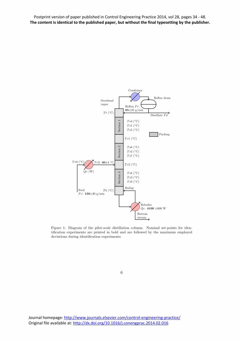
The pilot-scale experimental set-up involves a packed distillation column(see Figures 1 and 2 as well as references Logist et al. (2009); Bonilla et al.(2012)). The column is about 4.5 m high and has an internal diameter of6 cm. The column works under atmospheric conditions and contains threesections of about 0.95 m with Sulzer CY packing (Sulzer, Winterthur) respon-sible for the separation. This packing has a contact surface of 700 m2/m3

and each meter packing is equivalent to approximately 3 theoretical trays.The feed stream containing a mixture of methanol and isopropanol is fed intothe column between packed sections 2 and 3. The temperature of the feedcan be adjusted by an electric heater which can deliver power up to 250 W.At the bottom of the column a reboiler is present containing two electricheaters, each of 3000 W. These can be manipulated to deliver heat to thereboiler from 0 up to 6 kW. In the reboiler, a part of the liquid is vaporizedwhile the rest is extracted as the bottom stream. At the top of the column,a total condenser allows the condensing of the entire overhead vapor stream,which is then collected in a reflux drum. A part of the condensed liquid isfed back to the column as reflux, while the remainder leaves the column asthe distillate stream.

In this set-up the following four variables can be manipulated: the re-boiler power Qr (W), the feed rate Fv (g/min), the power of the feed heaterQv (W) and the reflux flow rate Fr (g/min). The distillate flow Fd (g/min)is adjusted to maintain a constant reflux drum level. Measurements are avail-able for the reflux flow rate Fr, the distillate flow rate Fd, the feed flow rateFv and 15 temperatures. The temperature probes are placed at the top ofthe column T t and at three places on every packing section (Ts1 to Ts9).Temperature measurements Tv1 and Tv2 are available between section 1and 2 and between section 2 and 3 respectively. Finally, the temperaturemeasurement Tb in the reboiler of the column, and the temperatures of thefeed before and after heating (Tv0 and Tv2, respectively) complete the listof measured temperatures. All temperatures are measured in degrees Celsiuswith a resolution of 0.01oC.

The pilot-scale distillation column is equipped with a Compact FieldPoint(National Instruments (NI), Austin). This device consists of a NI cFP-2020Real-Time Controller, a NI cFP-AIO-610 8-Channel Combination Analog

4

Postprint version of paper published in Control Engineering Practice 2014, vol 28, pages 34 - 48. The content is identical to the published paper, but without the final typesetting by the publisher.

Journal homepage: http://www.journals.elsevier.com/control-engineering-practice/ Original file available at: http://dx.doi.org/10.1016/j.conengprac.2014.02.016

Input/Output Module, NI cFP-RTD-124 8-Channel 4-Wire RTD Tempera-ture Module, NI cFP-AI-110 8-Channel Analog Voltage and Current InputModule and NI cFP-AIO-600 8-Channel Combination Analog Input/AnalogOutput Module. This device is only used as a service-hatch to pass the mea-sured outputs to the controller and desired inputs to the actuators of thecolumn (Chambel et al., 2011).

There is no on-line measurement of the concentrations in the distillateand bottom streams although these are very important for the chemical pro-cess. The concentrations can be measured off-line, e.g., based on a theirrefractive index using a refractometer. However, since the concentrations forthe system under study can be easily inferred from the temperatures whentemperature and pressure are known, only a controller for the temperaturesis implemented.

3. Approach

To systematically evaluate the possibilities for running MPC on PLCs, thefollowing approach has been adopted. First a model is identified. Afterwardsan MPC controller is implemented and tested experimentally. In order togradually decrease the computational and memory available in the industrialcontrol device, a PAC has been studied before moving to a PLC. In the viewof safety, the developed controllers have always been evaluated through ahardware-in-the-loop (HIL) experiment before the actual test with the pilot-scale column itself. More detailed information is provided in the followingsubsections.

3.1. Identification of a model for control

Distillation columns can be described by linear low order systems (Skoges-tad, 1997). An ideal model for control has to combine an accurate trackingof the main column behavior with a low model complexity. Different lin-ear time-invariant models exist. In this paper, identification based on loworder transfer functions, often also called process models, is employed toobtain a model for control. This model is identified around a well-knownand safe operating point. The identification of the model is performed usingthe Matlab System Identification Toolbox (Ljung, 2009). Only identificationbased on the continuous first and second order transfer functions with delayis considered. A Multiple-Input Multiple-Output (MIMO) process model is

5

Postprint version of paper published in Control Engineering Practice 2014, vol 28, pages 34 - 48. The content is identical to the published paper, but without the final typesetting by the publisher.

Journal homepage: http://www.journals.elsevier.com/control-engineering-practice/ Original file available at: http://dx.doi.org/10.1016/j.conengprac.2014.02.016

Packing

Section3

Ts3 (◦C)

Ts9 (◦C)

Ts8 (◦C)

Section2

Ts2 (◦C)

Ts7 (◦C)

Ts6 (◦C)

Section1

Ts1 (◦C)

Ts5 (◦C)

Ts4 (◦C)

Tb (◦C)

Tv2 (◦C)

Tv1 (◦C)

T t (◦C)

ReboilerQr: 4100 ±600 W

Boilup

Condensor

Reflux drumOverheadvapor

Reflux Fr:65±25 g/min

Distillate Fd

Bottomstream

Qv (W)

FeedFv: 150±30 g/min

Tv2: 40±4 ◦CTv0 (◦C)

Figure 1: Diagram of the pilot-scale distillation column. Nominal set-points for iden-tification experiments are printed in bold and are followed by the maximum employeddeviations during identification experiments.

6

Postprint version of paper published in Control Engineering Practice 2014, vol 28, pages 34 - 48. The content is identical to the published paper, but without the final typesetting by the publisher.

Journal homepage: http://www.journals.elsevier.com/control-engineering-practice/ Original file available at: http://dx.doi.org/10.1016/j.conengprac.2014.02.016

Figure 2: Pictures of the pilot-scale distillation column: condenser (left), packed sectionand feed introduction (center), and reboiler (right).

constructed based on two identified Multiple-Input Single-Output (MISO)process models. This model is converted to a state-space formulation for usein the model predictive controller.

3.2. Model predictive control formulation

In this subsection, the model predictive control formulation is described.Linear Model Predictive Control is well known in literature (Maciejowski,2002; Camacho and Bordons, 2003; Rossiter, 2003; Wang, 2009). The basicformulation for linear MPC used for the practical implementation in thiswork is summarized below.

A linear, time-invariant discrete-time model is used:

x(k + 1) = Ax(k) +Bu(k) (1)

y(k) = Cx(k),

with A ∈ Rp×p, B ∈ R

p×m and C ∈ Rq×p. Here, m, p and q are the number

of inputs u(k) ∈ Rm, states x(k) ∈ R

p and outputs y(k) ∈ Rq, respectively.

The cost function to be solved in each MPC step is given in this work:

J =

Hp∑

i=1

‖y(k + i)− yref(k + i)‖2Wy

(2)

+Hc−1∑

j=0

‖u(k + j)− uref(k + j)‖2Wu

.

7

Postprint version of paper published in Control Engineering Practice 2014, vol 28, pages 34 - 48. The content is identical to the published paper, but without the final typesetting by the publisher.

Journal homepage: http://www.journals.elsevier.com/control-engineering-practice/ Original file available at: http://dx.doi.org/10.1016/j.conengprac.2014.02.016

with yref the output reference and y the predicted output. uref relates to thecorresponding control reference profile. Hp and Hc (with Hc ≤ Hp) are theprediction and the control horizon of the controller, respectively. Wy ∈ R

q×q

and Wu ∈ Rm×m are the positive definite weighting matrices. A terminal

constraint ensuring stability can be omitted as long as the prediction horizonis long enough and the plant is stable (Maciejowski, 2002), which is the casein this work.

To remove the steady state error, an augmented model is constructed:[∆x(k + 1)y(k + 1)

]

︸ ︷︷ ︸

ξ(k+1)

=

[A 0

CA I

]

︸ ︷︷ ︸

A

[∆x(k)y(k)

]

︸ ︷︷ ︸

ξ(k)

+

[B

CB

]

︸ ︷︷ ︸

B

∆u(k) (3)

y(k) =[0 I

]

︸ ︷︷ ︸

C

[∆x(k)y(k)

]

where ∆u(k) = u(k)− u(k − 1) is the difference between two successiveinputs, ∆x(k) = x(k) − x(k − 1) is the difference between two successivestates and ξ(k) is the augmented state:

ξ(k) =

[∆x(k)y(k)

]

(4)

The calculation of the future predictions are based on Eq. (3). In a matrixformulation the future predictions can be written as:

y1...Hp= Fξ +Φ∆u1...Hc

. (5)

The matrices F and Φ can be found in Maciejowski (2002); Wang (2009).y1...Hp

∈ RHp·q and ∆u1...Hc

∈ RHc·m are the arrays into which the different

vectors y(k) and ∆u(k) haven been stacked over the prediction and controlhorizon, respectively.

In the current work only input constraints are taken into account for theMPC problem:

uMin(k + j) ≤ u(k + j) for j = 1 . . .Hc (6)

uMax(k + j) ≥ u(k + j) for j = 1 . . .Hc. (7)

8

Postprint version of paper published in Control Engineering Practice 2014, vol 28, pages 34 - 48. The content is identical to the published paper, but without the final typesetting by the publisher.

Journal homepage: http://www.journals.elsevier.com/control-engineering-practice/ Original file available at: http://dx.doi.org/10.1016/j.conengprac.2014.02.016

At present, no state constraints are included, but the methodology canbe extended.

The optimization problem can be formulated as the minimization of costfunction (2), subject to model equations (3) and input constraints (6) and (7).To solve the optimization problem, the procedure described in Wang (2009)is followed. By elimination of the states and using the following recursion forthe inputs:

u(k + j) = u(k − 1) +Hc−1∑

j=0

∆u(k + j), (8)

a Quadratic Program (QP) is obtained:

min∆u

1

2∆uT

1...HcH∆u1...Hc

+ g∆u1...Hc(9)

subject to :

[−C1

C1

]

∆u1...Hc≤

[−u

′

Min

u′

Max

]

(10)

with ∆u1...Hca vector containing the decision variables ∆u(k + j) with

j = 1 . . .Hc. To solve this QP problem, the Hildreth algorithm (Hildreth,1957; Wang, 2009) and qpOASES (Ferreau et al., 2008) will be used.

The Hessian matrix H in Eq. (9) is a constant matrix as soon as all MPCparameters have been selected. It can be calculated with:

H = ΦTWybdΦ+Wubd, (11)

with Wybd and Wubdblock diagonal matrices of Wy and Wu respectively.

The Hessian can be computed offline as no online information is required.The aim in this work is to minimize the online calculation burden. To this en,matrices that can be computed in advance, are calculated offline and storedin the memory.

The gradient vector g in Eq. (9) has to be calculated online. It containsthree parts depending on the current state ξ(k), the reference of the inputsuref and the reference of the outputs yref. The reference for the inputs uref isemployed in such a way that the calculated inputs will not deviate too muchfrom a well-known and safe nominal working point of the employed set-up.So, g has to be calculated according to

g = G1ξ −G2yref,1...Hp−G3uref,1...Hc

(12)

9

Postprint version of paper published in Control Engineering Practice 2014, vol 28, pages 34 - 48. The content is identical to the published paper, but without the final typesetting by the publisher.

Journal homepage: http://www.journals.elsevier.com/control-engineering-practice/ Original file available at: http://dx.doi.org/10.1016/j.conengprac.2014.02.016

where G1, G2 and G3 are gradient matrices to be calculated according toWang (2009); Maciejowski (2002). The gradient matrices G1, G2 and G3

are constant and are computed offline according to:

G1 = ΦTW Tybd

F (13)

G2 = ΦTW Tybd

(14)

G3 = W Tubd

. (15)

The constraints in Eq. (10), i.e., the minimum and maximum admissiblevalues u

′

Max and u′

Min require online information and, hence, are calculatedonline. u

′

Max is a column matrix with u′

Max(k+ j) = uMax(k + j)− u(k − 1),with j = 1 . . .Hc and similarly is u

′

Min a column matrix u′

Min(k+j) = uMin(k+j)− u(k − 1), with j = 1 . . .Hc. The matrix C1 is a lower triangular matrixbuild up from identity matrices.

4. Hard- and software

The current section provides details about the control hardware and soft-ware used. To gradually move towards a PLC device, a PAC has been testedin an intermediate step. The software includes different algorithms for theonline solution of the QP in each MPC step.

4.1. Programmable Automation Controller

As a PAC, a National Instruments CompactRIO has been used. This PACcontroller consists of a NI cRio–9024 Real-Time Controller (800 MHz CPU,512 MB of memory) (National Instruments Corporation, 2010), a cRIO–9114Reconfigurable Chassis, a NI 9265 Analogue Current Output module and aNI 9217 RTD 24-Bit Analogue Input Module. The real-time controller isprogrammed with LabVIEW and is able to run a software library compiledfrom C/C++ code via a call library function. The library is compiled for theVxWorks 6.3 operating system with the GCC-compiler version 3.4.4.

The LabVIEW programming environment has been used to program thePAC. The LabVIEW programming concept is based on a Virtual Instrument(VI). A graphical user interface is composed of a front panel on a block dia-gram. The employed QP solvers are programmed in C and compiled with a

10

Postprint version of paper published in Control Engineering Practice 2014, vol 28, pages 34 - 48. The content is identical to the published paper, but without the final typesetting by the publisher.

Journal homepage: http://www.journals.elsevier.com/control-engineering-practice/ Original file available at: http://dx.doi.org/10.1016/j.conengprac.2014.02.016

GNU Compiler Collection (GCC), which is a freeware compiler to a librarycompatible with the VxWorks operating system. The data between the Lab-VIEW VIs and the QP solvers, written in C, is exchanged by means of theLabVIEW call library function.

4.2. Programmable Logic Controller

A Siemens CPU319-3DP/PN PLC is used as PLC. The base memory ofthis CPU is increased to the maximum allowed 8 MB. This CPU is the fastestSiemens S7-300 CPU currently available. It takes 40 ns for one floating-pointoperation (Siemens AG, 2011). The Siemens CPU is programmed using theStep 7 Professional 2010 software. To code the problem, the Structured

Control Language (S7-SCL) is used. This programming language correspondsto Structured Text (ST) in the standard IEC 61131-3.

4.3. QP algorithms

To solve the QP problem, several algorithms have been used.

Hildreth QP algorithm. The Hildreth algorithm has been chosen for itslimited number of code lines which makes it easy to implement. It hasbeen written based on (Wang, 2009) in C for the PAC and in S7-SCL forthe PLC. This algorithm calculates the solution in two steps. First, theunconstrained solution is calculated and if no constraints are violated,this solution is adopted. If a constraint is violated, a constrained QPis solved. The solution of the QP is then passed to the inputs of theset-up. For more information about the solution, see Hildreth (1957);Luenberger (1997); Wang (2009). If a solution to the QP could not befound, the unconstrained solution is compared to the constraint. If aconstraint is violated, then that entry of the unconstrained solution islimited to the constraint.

qpOASES QP algorithm. qpOASES is an open-source C++ implemen-tation of the recently proposed online active-set strategy (Ferreau et al.,2008). It builds on the idea that the optimal sets of active constraintsdo not differ much from one QP to the next. At each sampling in-stant, it starts from the optimal solution of the previous QP and followsa homotopy path towards the solution of the current QP. Along thispath, constraints may become active or inactive as in any active-set QP

11

Postprint version of paper published in Control Engineering Practice 2014, vol 28, pages 34 - 48. The content is identical to the published paper, but without the final typesetting by the publisher.

Journal homepage: http://www.journals.elsevier.com/control-engineering-practice/ Original file available at: http://dx.doi.org/10.1016/j.conengprac.2014.02.016

solver and the internal matrices factorizations are adapted accordingly.While moving along the homotopy path, the online active-set strategydelivers sub-optimal solutions in a transparent way. Therefore, suchsub-optimal feedback can be reasonably offered to the process in casethe maximum number of iterations is reached.

A simplified version of qpOASES has been translated to S7-SCL. Notethat the simplified implementation does not allow for hot starting ofthe QP solution and is not fully optimized for speed. On the PAC, theplain ANSI C implementation of qpOASES has been used. Althoughthe full version of qpOASES is perfectly suited for hot starting, thisfeature is not used. Furthermore, the algorithm is only used with coldstarts as a solution can be found in one step when no constraints areactive. This makes it possible to start the search for a solution withoffline, previously computed matrices.

5. Controller implementation features

Every industrial control device has its own characteristics. This sectionpresents how the QP solvers have been implemented and what the conse-quences are of the typical features of the employed PAC and PLC devices.

5.1. Model predictive controller implementation

To compute a new input for the process, the sequence of actions presentedin Algorithm 1 are followed. In advance, constant matrices are precomputedand the reference trajectory for the output is selected. This sequence of stepsto solve the MPC problem has been used for both controller devices and theemployed QP algorithms.

5.2. Features of the implementation on the PAC

The practical limitations while using PAC and PLC controllers is differ-ent. Programmable automation controllers employ a Real-Time OperationsSystem (RTOS). It is an extra layer between the user code and hardware.Consequently, more resources are required to run both this RTOS and theuser code. On the other hand, the operating system handles all basic tasksin a more user-friendly way, e.g., file system operations, parallelization ofuser programs and memory management. The CompactRIO runs VxWorks

12

Postprint version of paper published in Control Engineering Practice 2014, vol 28, pages 34 - 48. The content is identical to the published paper, but without the final typesetting by the publisher.

Journal homepage: http://www.journals.elsevier.com/control-engineering-practice/ Original file available at: http://dx.doi.org/10.1016/j.conengprac.2014.02.016

Offline: Calculate H, G1, G2 and G3.Online: Start PLC or PAC.Store all precomputed matrices in working memory, together with the reference forinputs and output.while CPU is running do

if controller interval passed since last call thenScale the in- and outputs.Calculate current state.Calculate g, u

′

Minand u

′

Max.

case Hildreth algorithmCalculate the unconstrained inputs of the process.if unconstrained inputs violate constraints then

while maximum number of iterations is not reached and solutionnot found do

Solve one iteration of the QP.end

if maximum number of iterations is reached thenUse unconstrained solution, but inputs violating a constraintare limited to that constraint.

end

end

end

case qpOASESwhile maximum number of iterations is not reached and solution notfound do

Solve one iteration of the QP.end

if maximum number of iterations is reached thenUse last sub-optimal solution.

end

end

Scale and apply the calculated inputs to the systemend

end

Algorithm 1: Steps to compute the inputs on the experimental set-up forthe PAC and PLC.

13

Postprint version of paper published in Control Engineering Practice 2014, vol 28, pages 34 - 48. The content is identical to the published paper, but without the final typesetting by the publisher.

Journal homepage: http://www.journals.elsevier.com/control-engineering-practice/ Original file available at: http://dx.doi.org/10.1016/j.conengprac.2014.02.016

as its RTOS. A compiler exists to convert (existing) C/C++ code. All im-plemented QP solvers are originally written in C or C++ and are convertedinto a library, supported by the RTOS.

During run-time, two programs run in parallel to control the distillationcolumn set-up. The first LabVIEW program, further called the Human Ma-

chine Interface Virtual Instrument or HMI VI, performs the data exchangebetween the program and the in- and output cards of the Compact Field-point, the scaling of the in- and outputs, the visualization of the processvariables and logging of the data. The PI-controllers are also part of thisprogram. A second LabVIEW program, further called the Model Predictive

Control Virtual Instrument or MPC VI, performs the preparative calcula-tions for the QP, e.g., the estimation of the state and selection of the currentreference. Instead of using the built-in MPC controller (Balbis et al., 2005),the currently employed QP algorithms are programmed in C. The approachis similar to Canale et al. (2012), who implemented a QP solver on a Na-tional Instruments eXtensions for Instrumentation (PXI) system. Howeverthe employed QP solvers, the target system and the employed C-compilerare different. The QP algorithm is located in a separated library, called fromwithin the MPC VI. The HMI VI runs at a rate of 10 Hz. The MPC VI iscalled every minute.

5.3. Features of the implementation on the PLC

No compiler exists to transform C/C++ source code to a running binaryon a Siemens PLC. Therefore, the C/C++ code has to be translated intoS7-SCL (ST). For this paper, the time consuming step has been taken totranslate the qpOASES and Hildreth solvers to S7-SCL, the Siemens dialectof the ST language according to IEC 61131-3. The qpOASES solver is trans-lated without the hot starting possibilities.

To calculate the appropriate inputs of the system and solve the QP, anumber of built-in function blocks (FB) and organization blocks (OB) areprogrammed. Organization blocks are built-in functions called as hardwareinterrupts. Function blocks are user-defined functions with correspondingdata stored in a data block (DB) with the same number. Fig. 3 depicts theorder in which these blocks are called.

14

Postprint version of paper published in Control Engineering Practice 2014, vol 28, pages 34 - 48. The content is identical to the published paper, but without the final typesetting by the publisher.

Journal homepage: http://www.journals.elsevier.com/control-engineering-practice/ Original file available at: http://dx.doi.org/10.1016/j.conengprac.2014.02.016

t

Start

PLC

First

callMPC

MPC

intervalelapsed

OB100 OB35 OB1 OB1 OB35 OB1 OB1

FB2

FB6 FB3 FB4

FB28 FB29 FB30

Figure 3: Schematic overview of the different employed organization and function blocksin the PLC.

Every function block has a corresponding data block. A data block can-not exceed 64 kB on the Siemens S7-319 CPU. The editor and the compilerimpose some additional limitations. Initialization of a variable must be ona line not exceeding 255 characters. This is not a big issue, but only awk-ward when initializing matrices. More important is the limitation that anarray initialized with unique elements cannot exceed 255 elements. Strangelyenough, an array can be as large as desired as long as it fits into the 64 kB ofavailable memory. To overcome this limitation, each array containing morethan 255 elements has to be filled during runtime (e.g., in OB100 at thestart) by arrays of maximum 255 elements. As can easily be understood,this situation is very unpractical. Linked with this situation is the need forabsolute addressing if a function needs data in a data block different from itsown data block. For example, to initialize matrices containing more than 255elements, OB100 writes data to DB2. This operation requires fault-sensitiveabsolute addressing. The most important employed FBs and OBs to codethe program are presented below. A graphical representation of the order ofcalling is given in Fig. 3.

OB100 - Cold Start. This block is called once when the controller is started.It is employed to initialize matrices containing more than 255 differ-ent elements. This procedure is followed to overcome the limitation anarray cannot exceed 255 elements at compilation time. In the case a

15

Postprint version of paper published in Control Engineering Practice 2014, vol 28, pages 34 - 48. The content is identical to the published paper, but without the final typesetting by the publisher.

Journal homepage: http://www.journals.elsevier.com/control-engineering-practice/ Original file available at: http://dx.doi.org/10.1016/j.conengprac.2014.02.016

matrix of more than 255 different elements is to be initialized, severalarrays are combined in this block at runtime into a combined array.For the distillation column, the Hessian H and matrices G1, G2 andG3 are initialized in OB100.

OB1 - Main loop. This loop is started as soon as OB100 is finished. Whenthis function finishes, it restarts. This loop is used to program standardtasks of the PLC. During the experiments, it is not used. It will runduring the idle time of the CPU between two OB35 calls.

OB35 - Timed loop. This timed organization block is called every minute.It contains the necessary code to read the current inputs. This infor-mation is scaled and employed to calculate the current state (FB3).Together with the reference for the in- and outputs, the state is used toupdate vector g (FB2). Now, the QP is solved and the scaled solutionwill be passed to the outputs of the PLC.

FB2 - Main program. This function scales the in- and outputs, calls theestimator block, calls the QP solver itself and finally presents the cal-culated inputs to the system.

FB3 - State estimator. This block estimates the current state to be usedto calculate the current gradient g in Eq. (9) for the QP solver.

FB6 - Column model. For hardware-in-the-loop experiments on the PLC,the state-space model of the column is implemented in this block.

FB4 - QP solver. This block calculates the input of the system. For theHildreth algorithm, all code is written in this function block. For theqpOASES algorithm, a number of additional function blocks are called:FB28, FB29 and FB30. The block FB29 requires the most memory and,hence, determines the practical limits for using qpOASES on a PLC(see Section 6).

FB28 - Calculate relative distance. This function is only needed for theqpOASES algorithm and calculates the relative distance to the finalsolution (Ferreau et al., 2008).

FB29 - QR and Cholesky decomposition. This function is only neededfor the qpOASES algorithm and calculates the QR decomposition based

16

Postprint version of paper published in Control Engineering Practice 2014, vol 28, pages 34 - 48. The content is identical to the published paper, but without the final typesetting by the publisher.

Journal homepage: http://www.journals.elsevier.com/control-engineering-practice/ Original file available at: http://dx.doi.org/10.1016/j.conengprac.2014.02.016

on Givens rotations and the Cholesky decomposition (Golub and Van Loan,1996).

FB30 - Matrix inversion. This function is only needed for the qpOASESalgorithm. This block calculates the inverse of a lower triangular matrixby substitution.

Practical experiments on the pilot-scale column are performed in the follow-ing way. The LabVIEW Human Machine Interface Virtual Instrument runson a PC which is connected to the PLC and the column by an ethernet con-nection. The QP solver is running on the PLC. An OPC server (NI OPCserver 2012, OPC is OLE for Process Control where OLE is an acronym forObject Linking and Embedding) is responsible for the data exchange betweenthe PC and the PLC.

6. Memory use and constraints

To get insight in the memory consumption of the applied algorithms onthe PAC and PLC devices, the memory consumption is presented in thissection. For the PAC, memory sizes are obtained by the built-in performance

and memory profiler.

6.1. PAC

To get an idea of the required memory on the PAC device, two differ-ent methodologies are followed. First the built-in profiler is used to providean idea of the memory consumption of the running VIs. Second, the totalamount of used memory is verified when downloading the files to the devicewith LabVIEW. The latter is about 70 MB. According to the profiler, thememory requirements for the Virtual Instrument running the controller (i.e.,MPC VI) are 102.7 kB for qpOASES and 98.9 kB for Hildreth.

Together with the HMI VI, which requires approximately 2795 KB andsome additional general VIs, e.g. for error checking, the memory footprintis nearly 3500 kB. Compared to the total required memory on the device ofapproximately 70 MB, the memory needed for the VIs of the MPC controlleris limited. The difference with the 70 MB used is mainly related to theoverhead of the RTOS and additional general features.

17

Postprint version of paper published in Control Engineering Practice 2014, vol 28, pages 34 - 48. The content is identical to the published paper, but without the final typesetting by the publisher.

Journal homepage: http://www.journals.elsevier.com/control-engineering-practice/ Original file available at: http://dx.doi.org/10.1016/j.conengprac.2014.02.016

6.2. PLC

For the PLC, the function blocks containing the QP solvers can be re-garded as the bottlenecks for memory use. Hence, figures given are relate tothese blocks only.

6.2.1. Hildreth Algorithm

For the Hildreth algorithm, FB4 is the function block with the highestmemory consumption and is populated with the matrices to solve the QP.For a Hessian of size 40×40, the total required memory is 8 matrices of 1600real elements, plus 7 real numbers, two vectors of 40 and two vectors of 80real numbers. This results in 53124 bytes needed. Increasing to a Hessian of44×44 elements exceeds the 64 kB limit of the FB. It has to be noted thatbased on symmetry 4 matrices can be eliminated. This makes it possible toincrease the size of the Hessian to 64×64 elements which can be consideredas the maximum practical limit for using the Hildreth algorithm in a PLC.Overcoming this limit is possible by storing matrices in different functionblocks, but since absolute addressing is required, this is very fault sensitiveand has to be avoided if possible.

6.2.2. qpOASES

For qpOASES, the QR and the Cholesky decomposition calculated inFB29 require the most memory. The calculation of these decompositionsneeds 11 matrices of the size of the Hessian. For the pilot-scale distillationcolumn, a Hessian with 1600 elements is constructed. 11 matrices of 1600elements violate the 64 kB limit. However, reusing temporary matrices em-ployed in the QR decomposition for the Cholesky decomposition reduces thenumber of required matrices from 11 to 8 so that experiments can be per-formed. This limitation poses a strong practical constraint on using MPCbased on qpOASES on a PLC. The total required memory in the employedformulation for hardware-in-the-loop experiments is 8 matrices of 1600 realelements plus 1 vector of 40 real elements and 15 real numbers which makesin total 51420 required bytes. Increasing the size of the Hessian to 44×44results in 62188 bytes. This is the absolute maximum to fit the QR andthe Cholesky decomposition into one function block. Separating both QRand Cholesky decomposition is not worthwhile, as the latter needs no extramemory to be allocated in the current implementation.

18

Postprint version of paper published in Control Engineering Practice 2014, vol 28, pages 34 - 48. The content is identical to the published paper, but without the final typesetting by the publisher.

Journal homepage: http://www.journals.elsevier.com/control-engineering-practice/ Original file available at: http://dx.doi.org/10.1016/j.conengprac.2014.02.016

7. Identification results

In this section, the results are summarized to obtain a suitable model forcontrol of the column.

7.1. Excitation signals

In order to generate estimation and validation data for the system iden-tification, two experiments are performed. The excitation signal is built upwith Pseudo Random Binary (PRB) signals for the different manipulatedvariables. Before the excitation signals are applied, the column is kept at aconstant operating point for two hours to ensure that the column is in steady-state. The nominal steady-state values of the different manipulated variablesare: a reflux flow rate Fr of 65 g/min, a feed flow rate Fv of 150 g/min, afeed heater duty Qv of 152 W to maintain a feed temperature Tv2 of 40oCand a reboiler power Qr of 4100 W. These nominal values are known toyield an appropriate operating point for the column (Logist et al., 2009). Allmanipulated variables are controlled by PI controllers except for the heatingduties which are controlled directly. When the column has reached steady-state the experiment is started.

When the excitation signals are applied, all manipulated variables switchbetween two values. The reflux flow rate Fr fluctuates between 40 and90 g/min, while the feed flow rate Fv changes between 120 and 180 g/min.The feed heater duty Qv is manipulated between 0 and 250 W and thereboiler power Qr switches between 3500 and 4700 W. These values are dis-played in Fig. 1. The distillate flow rate Fd is manipulated in order to keepthe content of the reflux drum at 40% of its maximum volume. All data arerecorded with a sampling period of 100 ms.

The first PRB input signal is constructed in the following manner. Thereboiler duty Qr is a repeated periodic signal of 6000 s. The clock period,i.e., the minimum time before the signal is allowed to switch, is 300 s. Fromprevious experiments (Logist et al., 2009), it is known that the dynamics ofthe system are faster at the top of the column. Therefore, the clock periodof the other inputs is slightly smaller. For the feed flow rate Fv and feedtemperature Tv2 a clock period of 120 s is taken with a period of length3720 s and for the reflux flow rate Fr, the clock period is 20 s with a periodlength of 5100 s. These input signals are combined into one experiment with a

19

Postprint version of paper published in Control Engineering Practice 2014, vol 28, pages 34 - 48. The content is identical to the published paper, but without the final typesetting by the publisher.

Journal homepage: http://www.journals.elsevier.com/control-engineering-practice/ Original file available at: http://dx.doi.org/10.1016/j.conengprac.2014.02.016

time span of 25000 s. The second experiment is slightly slower. The periodicsignal has a length of 8000 s for all manipulated variables and the clockperiod for Qr, Fv, Tv2 and Fr is 500 s, 120 s, 120 s and 60 s, respectively.The duration of the experiment is also 25000 s in total.

7.2. Data preparation

The sampling period of the three recorded data sets is reduced to 60 s.Therefore, for every 60 s a sample is taken from the original recorded datathat is first filtered with zero-phase digital filter (-3dB frequency = 0.3 Hz).Next, an identification and a validation data set have been created. The firstPRB data set described in the former section is selected to be the estimationdata set, the second is the validation data set.

7.3. Model identification and validation

Here different quality indexes are calculated to assess the model quality,e.g., the FIT value as defined in the Matlab Identification Toolbox (Ljung,2009) and the mean Squared errors (MSE). The model selection is based onmodel selection criteria as, e.g., the Akaike Information Criterion (AIC) (Akaike,1974). However, operator experience is also taken into account.

For each output, a MISO model consisting of low order transfer functions,is fitted. After initial identifications with each of the four transfer functionsof an identical structure, an attempt has been made to create a model with alower AIC and a lower MSE/higher FIT. Therefore each of the input-outputtransfer functions pairs is exchanged with a different model structure. Ifre-identification resulted in lower AIC and MSE, and if the structure couldbe reasonably accepted based on operator expertise, then the new structure,called PMIX, will be adopted. In Table 1 the MSE, FIT and AIC are indi-cated for the final identified model.

From physical insight, one can assume that all subsystems have a timedelay. This is not the case in the PMIX models, as several second order mod-els appear without a time delay. In these cases, the second order pole masksthe time delay. Re-estimation based on a first order transfer function withtime delay resulted often in a worse AIC or FIT value. In such a case, thesecond-order subsystem has been preserved. The two selected PMIX modelshave been merged into one MIMO transfer function presented in Eq. (16)and converted to state-space.

20

Postprint version of paper published in Control Engineering Practice 2014, vol 28, pages 34 - 48. The content is identical to the published paper, but without the final typesetting by the publisher.

Journal homepage: http://www.journals.elsevier.com/control-engineering-practice/ Original file available at: http://dx.doi.org/10.1016/j.conengprac.2014.02.016

0 50 100 150 200 250 300 350 40058

59

60

61

62

63

64

Tem

pera

ture

(°C

)

Time (min)

Reduced State−Space (53.1%)Identified PMIX (56.3%)Measured Temperature

0 50 100 150 200 250 300 350 40076.5

77

77.5

78

78.5

79

79.5

80

80.5

Tem

pera

ture

(°C

)

Time (min)

Reduced State−Space (76.8%)Identified PMIX (80.5%)Measured Temperature

Figure 4: Validation of the top and reboiler temperature. Each figure depicts the simula-tion for the reduced state-space model and the identified PMIX model.

21

Postprint version of paper published in Control Engineering Practice 2014, vol 28, pages 34 - 48. The content is identical to the published paper, but without the final typesetting by the publisher.

Journal homepage: http://www.journals.elsevier.com/control-engineering-practice/ Original file available at: http://dx.doi.org/10.1016/j.conengprac.2014.02.016

Table 1: The FIT and MSE values for the reduced state-space model and identified PMIXmodels for both the reboiler and top temperature.

Models FIT MSE AIC- Top temperature -

Reduced State-Space 53.1% 0.2608PMIX transfer function 56.3% 0.2261 -3.83

- Reboiler temperature -Reduced State-Space 76.8% 0.0810PMIX transfer function 80.5% 0.0566 -1.66

[

Tt

Tb

]

=

−2.26(1+2565s)(1+135s)

0.531+735s

3.74(1+1803s)(1+78s)

−3.45(1+2698s)(1+72s)

e−53.3s

−1.87(1+890s)(1+169s)

0.621+1465s

e−307s 5.21(1+2864s)

e−43s −2.36(1+1275s)(1+525s)

FvQvQrFr

(16)

Conversion to discrete state-space is required for the model predictivecontrol formulation. The selected discretization interval is one minute. Thisinterval has been selected based on a trade-off between a sufficiently smallmodel size on the one hand and a sufficient capability to represent the dy-namics in the process on the other hand. The resulting model is of order 20.After plotting the Hankel singular values, no clear jump can be noted, butthere is a significant reduction in state energy by a factor of 500 betweenthe state with the highest energy and state 13. Therefore, the number ofstates to be left in the controller model, is selected to be 13. The reducedstate-space model has been checked to be observable and controllable by arank test following the standard procedure implemented in Matlab ControlSystem Toolbox (MathWorks, 2009). In Fig. 4 two plots are depicted. Thefirst one presents the simulation of the reduced state-space and original se-lected transfer function model for the top temperature, the second one doesthe same for the reboiler temperature. For the top temperature, both modelsfollow the trend of the measured temperature well, although some peaks arenot captured. Especially, sharp peaks and fast variations are not coveredby the models. The fast varying peaks are believed not to disturb the con-trol action of the controller due to the long time constants of the model. Forthe reboiler temperature, the measured temperatures are followed accurately.

22

Postprint version of paper published in Control Engineering Practice 2014, vol 28, pages 34 - 48. The content is identical to the published paper, but without the final typesetting by the publisher.

Journal homepage: http://www.journals.elsevier.com/control-engineering-practice/ Original file available at: http://dx.doi.org/10.1016/j.conengprac.2014.02.016

Table 1 presents the FIT and MSE values for the plotted models. Con-version to state-space and model reduction results in only a small loss ofaccuracy of the model. As a result, the reduced state-space model is selectedto be the controller model.

8. Model predictive control results

In this section, the observations when implementing and using an MPCon low level hardware to control the distillation column, are described. First,the results for the more powerful PAC are presented, while afterwards theobservations for the PLC are provided.

8.1. Model predictive control settings

The different MPC horizons are determined in trial-and-error simulationsand are set to Hc = 10 steps for the control horizon and Hp = 50 steps forthe prediction horizon. Every step takes one minute. This leads to a Hes-sian of size 40×40 in Eq. (9). The weight matrix Wy is a diagonal matrixwith elements Wy11 = 1 and Wy22 = 0.9. This punishes each deviationfrom the top temperature reference slightly more than a deviation from thereboiler temperature. The weight matrix Wu has four elements on the diag-onal Wu11 = 0.8, Wu22 = 1, Wu33 = 0.8 and Wu44 = 1 for the feed flow rate,the feed duty, the reboiler duty and the reflux flow rate, respectively. Thischoice has been made to encourage the use of the flow rates, which are thefastest varying control variables. All of the off-diagonal elements are takenequal to 0.

As a reference trajectory for both the top and reboiler temperature, asequence of steps is applied. The sizes of these steps for the top temperatureare 0.88 and 0.62oC. For the reboiler the large and small steps are 0.44 and0.31oC, respectively. The length of the steps is between 50 and 60 minutes forboth the top and the reboiler temperature. Note, the shift of approximately30 minutes between jumps in both reference values. As the outputs are highlycorrelated (Huyck et al., 2013), each change in reference trajectory for oneof the two temperatures will also affect the other temperature.

8.2. Model predictive control on a PAC

8.2.1. Hardware-in-the-loop experiments

To make sure that the controlling LabVIEW VI and corresponding C-libraries for the MPC controller are implemented correctly, hardware-in-the-

23

Postprint version of paper published in Control Engineering Practice 2014, vol 28, pages 34 - 48. The content is identical to the published paper, but without the final typesetting by the publisher.

Journal homepage: http://www.journals.elsevier.com/control-engineering-practice/ Original file available at: http://dx.doi.org/10.1016/j.conengprac.2014.02.016

loop experiments are performed. The VI running the MPC controller isconnected to a linear plant model of the pilot-scale distillation column. Theemployed linear plant model is the discrete state-space representation of theMIMO transfer function in Eq. (16) obtained before model reduction. Thenumber of states of this model is 20. The HIL simulations are plotted togetherwith the experiments on the column in Fig. 5. Both the Hildreth and theqpOASES algorithm have been employed for HIL experiments. Given theidentical result and correspondingly indistinguishable plots, only one HILexperiment is plotted. The overall shape of the reference is followed well,but it is clear that the column will never reach a steady-state situation forthis experiment. After the HIL experiments, it can now be expected that theLabVIEW VI is working properly and, hence, it is employed on the pilot-scaleset-up.

8.2.2. Experiments on the pilot-scale set-up

The top plot in Fig. 5 depicts the measured top and the reboiler tem-perature during the experiment. Both controlled variables follow the samereference trajectory as during the HIL experiment. The numerous changesyield a challenging reference path to be tracked. As mentioned earlier, thetime constants of the different subsystems are longer than half an hour, caus-ing the system to never reach steady-state. These references are selected inorder to combine the safety regulations of the column with a sufficient num-ber of set-point changes in the time slot available for experiments.

Two experiments are recorded: one experiment with the Hildreth algo-rithm and one with qpOASES. Unfortunately, the environmental conditionswere different. This is of major importance as the pilot-scale distillationset-up is not thermally insulated from its environment. As a consequenceheat loses depend largely on the environmental conditions. For the Hildrethexperiment the ambient temperature was 17oC at noon. At night the temper-ature was not lower than 14oC. For the second experiment, the temperatureat noon was 10oC and close to zero at night.

In the first two hours of the experiment, both the top and reboiler tem-peratures are followed quite accurately. The plotted temperature obtainedfrom hardware-in-the-loop experiments can be considered as the temperatureto be tracked. The differences between the HIL experiments and the experi-ments on the set-up are limited for both QP solvers. The inputs, presented

24

Postprint version of paper published in Control Engineering Practice 2014, vol 28, pages 34 - 48. The content is identical to the published paper, but without the final typesetting by the publisher.

Journal homepage: http://www.journals.elsevier.com/control-engineering-practice/ Original file available at: http://dx.doi.org/10.1016/j.conengprac.2014.02.016

0 50 100 150 200 250 30058.5

59

59.5

60

60.5

61

Top

Tem

pera

ture

(°C

)

HildrethqpOASESHIL exp.Reference

0 50 100 150 200 250 300

77.5

78

78.5

79

Time (Minutes)

Reb

oile

r T

empe

ratu

re (

°C)

0 100 200 300

100

120

140

160

180

200

Fee

d F

low

rat

e (g

/min

)

0 100 200 300

0

50

100

150

200

Fee

d D

uty

(W)

HildrethqpOASESHIL exp.Reference

0 100 200 300

3000

3500

4000

4500

5000

Reb

oile

r D

uty

(W)

Time (Minutes)0 100 200 300

40

50

60

70

80

90

100

Ref

lux

Flo

w r

ate

(g/m

in)

Time (Minutes)

Figure 5: Measured outputs (top) and inputs (bottom) for experiments on the distillationcolumn and HIL experiments tracking the desired reference temperature profile with anMPC controller running on the PAC.

25

Postprint version of paper published in Control Engineering Practice 2014, vol 28, pages 34 - 48. The content is identical to the published paper, but without the final typesetting by the publisher.

Journal homepage: http://www.journals.elsevier.com/control-engineering-practice/ Original file available at: http://dx.doi.org/10.1016/j.conengprac.2014.02.016

in the bottom plot in Fig. 5, also differ only slightly form the HIL experiment.

However, between the second and fourth hour, both temperatures have tofollow a step down in the temperature. As soon as the top temperature ref-erence starts decreasing, both the top and the reboiler temperature decrease.For the experiments with the Hildreth solver, corresponding to an ambienttemperature of 17oC at noon, the top temperature only decreases half theapplied temperature step for the top temperature. This temperature staysconstant for half an hour and increases slightly to 3h40. This is the momentwhere both the top and reboiler reference are back at the nominal temper-atures. The top temperature evolves now quickly to this temperature. Themeasured reboiler temperature is 0.25oC below the reference in the interval2h20 to 3h15. From 3h25 this temperature is close to the nominal reboilertemperature. For the experiments with the qpOASES solver, the top tem-perature hardly leaves the nominal temperature, the reboiler temperature iseven further from the reference.

It is clear from the plot in the top plot of Fig. 5 that the top and thereboiler temperature do not follow their references accurately in this interval.From the input plots presented in the bottom plot of Fig. 5, one can see thattwo constraints are reached for Hildreth and three for qpOASES. This, to-gether with an ambient temperature below the excitation experiment, causesthe inaccurate control. Nevertheless, this difficult control is interesting toinvestigate the behavior of the different QP solvers. The latter part of theexperiment from 4h on, is a repetition of the first 4 hours, but speeded upwith a factor 2.

In Table 2 the mean cost J , which is the cost J divided by the length ofan experiment, has been adopted because not all experiments have exactlythe same duration. The mean cost values corroborate the visual observationsthat the experiment with the Hildreth algorithm as QP solver is much closerto the reference than the experiment with qpOASES as solver.

Based on these two control experiments, it can be concluded that for thispilot-scale set-up the ambient temperature is of high importance. Althoughdifficult to incorporate in the model, except if a (large) sequence of exper-iments throughout the year can be set-up, the quality of control can onlybe considered good when the ambient temperature differs only at most 3oC

26

Postprint version of paper published in Control Engineering Practice 2014, vol 28, pages 34 - 48. The content is identical to the published paper, but without the final typesetting by the publisher.

Journal homepage: http://www.journals.elsevier.com/control-engineering-practice/ Original file available at: http://dx.doi.org/10.1016/j.conengprac.2014.02.016

Table 2: The mean cost J calculated for hardware-in-the-loop (HIL) experiments andexperiments (EXP) on the set-up using the PAC.

J

Hildreth (EXP) 2.7255qpOASES (EXP) 5.0153qpOASES (HIL) 0.8337

Table 3: The total run time as well as the mean, minimum and maximum run times forone MPC iteration are presented to indicate the speed of the algorithms on the PAC.

run-time (ms)total mean min. max.

Hildreth (EXP) 1655 4.58 0.28 67.59qpOASES (EXP) 333 1.33 0.84 3.11qpOASES (HIL) 314 0.89 0.83 1.69

from from the value of 20.6oC measured during the identification experiment.

The bottom plot in Fig. 5 depicts the four inputs of the distillation col-umn. The two heating powers do not reach the constraints for the Hildrethexperiment. Both flow rates touch the constraints. For the qpOASES exper-iment, all controller variables hit the constraints except the reboiler duty.

The bottom plot in Fig. 6 depicts the number of iterations required tosolve the QP problem for both the Hildreth and qpOASES experiment to-gether with the HIL experiment. All algorithms require between 10 and 15iterations to solve the MPC problem around 30 minutes after the start. Oneactive constraint on the reflux flow rate is responsible for this peak in thenumber of iterations. For the HIL experiment, no more than one iteration isrequired to present a solution, demonstrating no constraints are hit anymore.For the two experiments on the real set-up, the number of iterations increasesfast as soon as two or more constraints are hit in the interval 2h15 to 3h10.The maximum number of iterations for Hildreth is 70 and for qpOASES is30. The number of iterations for qpOASES is lower to solve the same prob-lem. For practical use, the required time is more critical. Based on the twoplots displaying the required time, the upper left plot in Fig. 6 presents therequired time for each calculation of an optimal input, the upper right is anextract of the left plot, but limited to 4 ms. As can be seen, the Hildreth

27

Postprint version of paper published in Control Engineering Practice 2014, vol 28, pages 34 - 48. The content is identical to the published paper, but without the final typesetting by the publisher.

Journal homepage: http://www.journals.elsevier.com/control-engineering-practice/ Original file available at: http://dx.doi.org/10.1016/j.conengprac.2014.02.016

0 50 100 150 200 250 3000

0.5

1

1.5

2

2.5

Cal

cula

tion

Tim

e (s

)

0 50 100 150 200 250 3000

5

10

15

20

25

30

35

Time (Minutes)

Itera

tions

HildrethqpOASES

Figure 6: Calculation time and number of iterations for the employed QP algorithms onthe PAC.

algorithm requires more time than the qpOASES algorithm if the numberof iterations is above 20. qpOASES requires maximum 3.2 ms to solve theproblem. Hildreth multiplies this value at some iterations with a factor ofnearly 10. This confirms the suggestion made by Huyck et al. (2012). Largesystems, and this column can be considered between small and average scaleson an industrial level, can benefit from this new state-of-the-art solver on in-dustrial devices.

Table 3 presents the mean time for one iteration and total runtime for theexperiment. The mean time for one iteration for Hildreth is higher than thatfor the qpOASES algorithm. This demonstrates that the increased complex-ity for qpOASES leads to a decrease in computation time, but the systemhas to be sufficiently large. The cause for the peaks seen in the calculationtime (upper left plot in Fig. 6) is not clear, but most likely a hardware inter-rupt for communication or module detection causes the algorithm to pausefor some time. This phenomenon is not seen for the qpOASES algorithmas these modules were removed from the CompactRIO device. Table 3 alsoindicates the minimum and the maximum required calculation times for theQP solvers. It is clear that the Hildreth algorithm requires significantly more

28

Postprint version of paper published in Control Engineering Practice 2014, vol 28, pages 34 - 48. The content is identical to the published paper, but without the final typesetting by the publisher.

Journal homepage: http://www.journals.elsevier.com/control-engineering-practice/ Original file available at: http://dx.doi.org/10.1016/j.conengprac.2014.02.016

time to solve the QP. Note that the maximum time required for Hildreth ismore than 20 times higher than the maximum required time for qpOASES.

The PAC has clearly sufficient computation power to run the MPC con-troller and the PI controllers together with the data logging routines on thisset-up. Whichever QP solver used, the computation time is below 5 ms. To-gether with the approximately 30 ms for the MPC VI, this is far below theone minute update interval between two MPC inputs. The employed workingmemory is around 70 MB. Be aware that this value contains the controllerprograms and the operation system memory demands. In summary, the ques-tion of whether MPC can be applied on a PAC for this pilot-scale distillationcolumn, can be answered positively.

8.3. Model predictive control on a PLC

This section presents the results of the final aim of this work, i.e., run-ning an MPC on a PLC to control the pilot-scale distillation column. First,hardware-in-the-loop experiments are carried out.

8.3.1. Hardware-in-the-loop experiments

In Fig. 7, the in- and outputs are plotted for the HIL experiments onPLC. The settings for the MPC are taken identical to those for the PACdevice. A shift of plus 0.3 and minus 0.3oC for the top and reboiler referencesrespectively is applied to make the control a little bit more challenging suchthat the input constraints are touched during the HIL experiments.

For the Hildreth algorithm, the number of iterations is presented in Fig. 8.The required time to solve the QP is plotted in the upper plot of Fig. 8. Themaximum required time is around 556 ms for 35 iterations (Table 5). Theminimum value for the run times of 14 ms is the required time to present asolution if a QP has to be solved.

Worthwhile to mention is that in trials previous to this experiment, smallmistakes caused the QP solver to reach its maximum number of iterations.For the pilot-scale distillation column HIL experiments on PLC, this max-imum is set to 250 iterations. This corresponds to a calculation time of3970 ms. With a cycle time of 4 seconds for the organization block initiat-ing the MPC solver, this is the absolute maximum allowed calculation time

29

Postprint version of paper published in Control Engineering Practice 2014, vol 28, pages 34 - 48. The content is identical to the published paper, but without the final typesetting by the publisher.

Journal homepage: http://www.journals.elsevier.com/control-engineering-practice/ Original file available at: http://dx.doi.org/10.1016/j.conengprac.2014.02.016

0 50 100 150 200 250 30058.5

59

59.5

60

60.5

61

61.5

Top

Tem

pera

ture

(°C

)

HildrethqpOASESReference

0 50 100 150 200 250 30077

77.5

78

78.5

79

Time (Minutes)

Reb

oile

r T

empe

ratu

re (

°C)

0 100 200 300

100

120

140

160

180

200

Fee

d F

low

rat

e (g

/min

)

0 100 200 300

0

50

100

150

200

Fee

d D

uty

(W)

HildrethqpOASESReference

0 100 200 300

3000

3500

4000

4500

5000

Reb

oile

r D

uty

(W)

Time (Minutes)0 100 200 300

40

50

60

70

80

90

100

Ref

lux

Flo

w r

ate

(g/m

in)

Time (Minutes)

Figure 7: Measured outputs (top) and inputs (bottom) for the top- and reboiler tem-perature for an experiment tracking a desired reference temperature profile with a MPCcontroller running on the PLC.

30

Postprint version of paper published in Control Engineering Practice 2014, vol 28, pages 34 - 48. The content is identical to the published paper, but without the final typesetting by the publisher.

Journal homepage: http://www.journals.elsevier.com/control-engineering-practice/ Original file available at: http://dx.doi.org/10.1016/j.conengprac.2014.02.016

0 50 100 150 200 250 3000

0.5

1

1.5

2

2.5

Cal

cula

tion

Tim

e (s

)

0 50 100 150 200 250 3000

5

10

15

20

25

30

35

Time (Minutes)

Itera

tions

HildrethqpOASES

Figure 8: Calculation time and number of iterations for the used QP algorithm on thePLC.

Table 4: The mean cost J calculated for hardware-in-the-loop (HIL) experiments andexperiments (EXP) on the set-up using the PLC.

J

Hildreth (HIL) 0.7668qpOASES (HIL) FailedHildreth (EXP) 1.6622

for the maximum number of iterations. On the pilot-scale set-up, an MPCupdate cycle of 1 minute is selected. The calculation times to solve the QPare far below this cycle time. The calculation time of the QP is therefore notconsidered to be a bottleneck for the implementation of MPC on a PLC forthe pilot-scale set-up.

As already mentioned in Section 5.3, the other programming issues, e.g.,maximum amount of 64 kB for each function block and the difficult initializa-tion of array larger than 255 elements are much harder to take into account.Based on the latter issues, a practical limit for a QP to be solved with theHildreth algorithm is a Hessian with 64×64 elements. It is possible to in-crease that size, but then you have to spread the matrix data in different

31

Postprint version of paper published in Control Engineering Practice 2014, vol 28, pages 34 - 48. The content is identical to the published paper, but without the final typesetting by the publisher.

Journal homepage: http://www.journals.elsevier.com/control-engineering-practice/ Original file available at: http://dx.doi.org/10.1016/j.conengprac.2014.02.016

Table 5: The total, mean, minimum and maximum run times for one MPC iteration ispresented to indicate the speed of the algorithms on the PLC.

run-time (ms)total mean min. max.

Hildreth (HIL) 70956 212.4 15 556qpOASES (HIL) 11780 1308.8 1104 2026Hildreth (EXP) 31123 91.0 14 532

data blocks which makes it even more difficult to manage as a programmer.The memory constraint is not yet reached. According to the online memorystatus information, the current implementation needs only 4% of the 8 MBavailable Random Access Memory, 16% of the 1.4 MB working memory and26% of the 0.7 MB retentive data memory. Hence, there is enough spaceto add additional control programs and to increase the QP problem size to64×64 elements as suggested.

For the qpOASES algorithm, the experiments ended abruptly after 8 timesteps with a system failure. According to the diagnostic registers, the errorwas caused by a scan cycle monitoring time violation, which means that thealgorithm needed more than 3.95 s. Increasing the cycle time to 10 seconds,or even one minute, caused the scan cycle monitoring time to be set to itsmaximum setting of 5999 ms. Unfortunately, even this is not high enoughfor the qpOASES algorithm. When taking a margin of about 10 percent, oneiteration needs between 350 and 450 ms. According to a Matlab simulation,up to 25 iterations are to be expected for the reference trajectory as employedin this HIL experiment. This is at least 8.75 s and far above the maximumallowed calculation time, the scan cycle monitoring time, of 6 s for the PLC.The additional calculations required for this algorithm, need too much timeto calculate the solution online. The presented time values in Table 5 arecalculated on the first 7 time steps. The time step causing an error is notadded. The maximum calculation time indicated in the table corresponds to5 iterations.

As already mentioned in Section 5.3, the practical upper memory limitfor this algorithm should be a Hessian of size 44. The required calculationtime, however, reduces this upper limit. An experiment with control horizonset to 5 instead of 10, corresponding to a Hessian size of 20 was successful.

32

Postprint version of paper published in Control Engineering Practice 2014, vol 28, pages 34 - 48. The content is identical to the published paper, but without the final typesetting by the publisher.

Journal homepage: http://www.journals.elsevier.com/control-engineering-practice/ Original file available at: http://dx.doi.org/10.1016/j.conengprac.2014.02.016

This successful HIL experiment for qpOASES demonstrates that the code isworking properly. The observation that a control horizon of 10 steps reachesthe computing power limits of the employed PLC, which is the most power-ful of its series, demonstrates that on a PLC does not need a sophisticatedsolver as, e.g., qpOASES. The speed constraint is the bottleneck for this algo-rithm. The Hildreth algorithm on the other hand succeeds to solve the MPCproblem with control horizon 10. For the Hildreth algorithm, the practical

memory constraint of 64 kB for one block is reached first for this experiment.

In contrast to the PAC exponents, the required time to solve the QP ishigher for qpOASES than for Hildreth. Although the number of iterations isdifferent, it is also important to repeat the S7-SCL translation which is notfully optimized for speed, which can affect the calculation time. Optimizationof the algorithm is not done as the practical memory constraint limits theuse of qpOASES on a PLC.

8.3.2. Experiments on the pilot-scale set-up

Nevertheless the unexpected failure of the qpOASES algorithm duringthe HIL experiments, experiments on the set-up are performed. Using theHildreth algorithm, the results plotted in Fig. 9 are obtained. The additionalshift for the reference of 0.3oC employed in the HIL experiments on the PLC,has been removed. The ambient temperature was 14oC at the start of theexperiment and 19oC at noon.

After a transient from the start-up temperatures above the set-point dur-ing the first 30 minutes (top plot of Fig. 9), the reference is followed clearlymore accurate than for the experiments on the PAC. The different envi-ronmental conditions during the PLC experiment mainly cause the bettercontrol, which was confirmed by the mean cost values in Tables 2 and 4. Incontrast to the PAC experiments, the reference trajectory is now also followedwhen the temperature decreased below the reference starting temperature forboth the top and the reboiler temperature.

The inputs plotted in the bottom plot of Fig. 9 are also more close to theHIL experiments. The constraints are hit only during a few minutes for theflow rates.

The calculation time to present a solution to the column and the numberof iterations required to calculate the QP are plotted in Fig. 10. Some more

33

Postprint version of paper published in Control Engineering Practice 2014, vol 28, pages 34 - 48. The content is identical to the published paper, but without the final typesetting by the publisher.

Journal homepage: http://www.journals.elsevier.com/control-engineering-practice/ Original file available at: http://dx.doi.org/10.1016/j.conengprac.2014.02.016

0 50 100 150 200 250 30058.5

59

59.5

60

60.5

61

Time (Minutes)

Top

Tem

pera

ture

(°C

)

Measured temperatureHardware−In−The−LoopReference temperature

0 50 100 150 200 250 300

77.5

78

78.5

79

Time (Minutes)

Reb

oile

r T

empe

ratu

re (

°C)

0 100 200 300

100

120

140

160

180

200

Fee

d flo

w r

ate

(g/m

in)

0 100 200 300

0

50

100

150

200

Fee

d du

ty (

W)

0 100 200 300

3000

3500

4000

4500

5000

Reb

oile

r du

ty (

W)

Time (Minutes)0 100 200 300

40

50

60

70

80

90

100

Ref

lux

flow

rat

e (g

/min

)

Time (Minutes)

Figure 9: Measured outputs (top) and inputs (bottom) for the top- and reboiler tem-perature for an experiment tracking a desired reference temperature profile with a MPCcontroller running on the PLC.

34

Postprint version of paper published in Control Engineering Practice 2014, vol 28, pages 34 - 48. The content is identical to the published paper, but without the final typesetting by the publisher.

Journal homepage: http://www.journals.elsevier.com/control-engineering-practice/ Original file available at: http://dx.doi.org/10.1016/j.conengprac.2014.02.016

0 50 100 150 200 250 300 3500

100

200

300

400

500

600

Cal

cula

tion

Tim

e (m

s)

0 50 100 150 200 250 300 3500

5

10

15

20

25

30

35

itera

tions

Time (Minutes)

Figure 10: Calculation time and number of iterations for the used QP algorithm on thePLC.

run-times are presented in Table 5. The maximum number of iterations is33 and at maximum 532 ms are required during this experiment.

9. Practical guidelines

To encourage the use of MPC in industry, the ease of implementation ofmodel predictive controllers on commonly used devices has to be investigated.In this paper two standard industrial devices have been employed, i.e. (i) aPAC device, which can be seen as a robust computer with real-time prop-erties and additional in- and outputs, and (ii) a PLC, a standard industrialautomation device. Experiments with MPC on the PAC demonstrate thatMPC can easily be implemented. Neither memory nor speed constraints areencountered in this paper and it is believed that even much larger systemscan be MPC-controlled by these types of devices. However, absolute limitswere not investigated. The practical implementation of MPC by an engineeris realizable in a limited amount of time. The software is well documented,is easy to use and has many features. In summary, MPC implemented onPAC devices is ready for industry.

35

Postprint version of paper published in Control Engineering Practice 2014, vol 28, pages 34 - 48. The content is identical to the published paper, but without the final typesetting by the publisher.

Journal homepage: http://www.journals.elsevier.com/control-engineering-practice/ Original file available at: http://dx.doi.org/10.1016/j.conengprac.2014.02.016

The second investigated device is a PLC. Historically, this device is sit-uated in the automation branch of the industry. The evolution in industryhas been to request additional features, e.g., logging and human-machine in-teraction, which go together with the increase in computation power of thePLC. The research in this work to employ MPC on a PLC demonstrated thatthese devices, although capable, are not the ideal devices to run MPC. Thelimited amount of memory and especially the limited speed of the devicesmake it difficult to implement MPC. Based on the experience from this work,one can conclude that online MPC on a PLC is only applicable for problemsresulting in a QP of limited size. For the PLC used for this study, a Hes-sian of size 64×64, or 4096 elements is the absolute maximum. Importantto notice is that the classical Hildreth algorithm is able to successfully run ahardware-in-the loop test and experiments for the pilot-scale set-up.

The state-of-the-art qpOASES algorithm, created with MPC applicationsin mind, fails in this test due to its complexity. Notice, however, that it wasnot optimized for speed. The hardware time constraint that a function can-not run longer than 5999 ms, is reached very fast for qpOASES. For theHildreth algorithm, the 560 ms required for the experiments in this paperis sufficiently removed from the previously mentioned time constraint. Al-though QP algorithms tailored for MPC exist, simple algorithms have beenfound to do the job in the current situation using the PLC as a host. More-over, the uncommon programming language is an extra barrier for the easyapplicability of MPC on PLCs, as the employed algorithms are complex andrequire thorough testing. Given the easy applicability for MPC on a PAC,PLCs are not advisable for MPC applications in industry. To make a PLCa valuable alternative for a PAC, not only speed and memory limits needto increase drastically, e.g., by a factor of 100, but also the standard pro-gramming languages employed in a PLC have to include more commonlyused languages such as C or C++. However, in that situation the differencebetween a PAC and a PLC has become rather small.

10. Conclusion

In this paper, the use of an online model predictive control algorithmhosted by a programmable automation controller and a programmable logiccontroller for a pilot-scale binary distillation column has been investigated.

36

Postprint version of paper published in Control Engineering Practice 2014, vol 28, pages 34 - 48. The content is identical to the published paper, but without the final typesetting by the publisher.

Journal homepage: http://www.journals.elsevier.com/control-engineering-practice/ Original file available at: http://dx.doi.org/10.1016/j.conengprac.2014.02.016

A linear state-space model of the pilot-scale distillation column has beenobtained via system identification. This model is employed to design a modelpredictive controller which is used in practical experiments on the set-up. Theruntimes for two online QP solvers, the Hildreth and the qpOASES algorithm,have been evaluated and compared. It has been demonstrated that it is pos-sible to run an online MPC algorithm on a PAC which is not only able to runthe supervisory algorithm, but is also responsible for data logging, human-machine interfacing and low level control. It has also been experimentallyverified that the pilot-scale set-up can be MPC controlled by a PLC usingthe Hildreth algorithm. Unfortunately, the current implementation for theqpOASES algorithm surpassed the limits of the current state-of-the-art PLCdevices such that these experiments were not successful. Possible future workis the integration of output (state) constraints.

Acknowledgements

Work supported in part by Katholieke Universiteit Leuven: OT/10/035,OPTEC Center-of-Excellence Optimization in Engineering (PFV/10/002),SCORES4CHEM (KP/09/005); by the Belgian Federal Science Policy Of-fice: Belgian Program on Interuniversity Poles of Attraction, IAP VII/19(DYSCO); by the European Commission: Interreg IVa 2 Seas 07 022 BE i-MOCCA. J.F. Van Impe holds the chair Safety Engineering sponsored bythe Belgian chemistry and life sciences federation essenscia.

References

Akaike, H., 1974. A new look at the statistical model identification. IEEETransactions on Automatic Control 19, 716 – 723.

Balbis, L., Katebi, R., Dunia, R., 2005. Graphical based predictive controldesign. In: Proceedings of the IEEE Conference on Control Applications.pp. 297 – 302.

Bauer, M., Craig, I. K., 2008. Economic assessment of advanced processcontrol - a survey and framework. Journal of Process Control, 2 – 18.

Bellemans, T., De Schutter, B., De Moor, B., 2006. Model predictive controlfor ramp metering of motorway traffic: A case study. Control EngineeringPractice 14, 757 – 767.

37

Postprint version of paper published in Control Engineering Practice 2014, vol 28, pages 34 - 48. The content is identical to the published paper, but without the final typesetting by the publisher.

Journal homepage: http://www.journals.elsevier.com/control-engineering-practice/ Original file available at: http://dx.doi.org/10.1016/j.conengprac.2014.02.016

Bemporad, A., Morari, M., Dua, V., Pistikopoulos, E. N., 2002. The explicitlinear quadratic regulator for constrained systems. Automatica 38, 3 – 20.

Bonilla, J., Logist, F., Degrve, J., De Moor, B., Van Impe, J., 2012. A re-duced order rate based model for distillation in packed columns: Dynamicsimulation and the differentiation index problem. Chemical EngineeringScience 68 (1), 401 – 412.

Camacho, E. F., Bordons, C., 2003. Model Predictive Control. Springer.

Canale, M., Cerone, V., Razza, V., Regruto, D., 2012. Rapid prototyping ofpredictive controllers through an industrial platform. In: Proceedings ofAmerican Control Conference. pp. 4715 – 4720.

Chambel, A. J., Pinheiro, C. I., Borges, J., ao M. Silva, J., 2011.Methodologies for input-output data exchange between labview and mat-lab/simulinksoftware for real time control of a pilot scale distillation pro-cess. In: 21st European Symposium on Computer Aided Process Engineer-ing. pp. 708 – 712.

Cutler, C., Ramaker., B., 1980. Dynamic matrix control - a computer controlalgorithm. In: Proceedings of the Joint American Control Conference, SanFrancisco, 1980. pp. Paper WP5–B.

Darby, M. L., Nikolaou, M., 2012. Mpc: Current practice and challenges.Control Engineering Practice 20 (4), 328 – 342.

Ferreau, H. J., Bock, H. G., Diehl, M., 2008. An online active set strategy toovercome the limitations of explicit MPC. International Journal of Robustand Nonlinear Control 18, 816 – 830.

Golub, G. H., Van Loan, C. F., 1996. Matrix Computations. Johns HopkinsUniversity Press, Baltimore, MD, USA.

Hildreth, C., 1957. A quadratic programming procedure. Naval ResearchLogistics Quarterly 4, 79 – 85.

Hrovat, D., Di Cairano, S., Tseng, H., Kolmanovsky, I., 2012. The devel-opment of model predictive control in automotive industry: A survey. In:IEEE International Conference on Control Applications (CCA). pp. 295 –302.

38

Postprint version of paper published in Control Engineering Practice 2014, vol 28, pages 34 - 48. The content is identical to the published paper, but without the final typesetting by the publisher.

Journal homepage: http://www.journals.elsevier.com/control-engineering-practice/ Original file available at: http://dx.doi.org/10.1016/j.conengprac.2014.02.016

Huyck, B., De Brabanter, J., De Moor, B., Van Impe, J., Logist, F., 2013.Model predictive control of a pilot-scale destination column using a pro-grammable automation controller. In: Proceedings of the European Con-trol Conference. pp. 1053 – 1058.

Huyck, B., Ferreau, H., Diehl, M., De Brabanter, J., Van Impe, J., De Moor,B., Logist, F., 2012. Towards online model predictive control on a pro-grammable logic controller: practical considerations. Mathematical Prob-lems in Engineering, vol. 2012, Article ID 912603, 20 pages.

Kouro, S., Cortes, P., Vargas, R., Ammann, U., Rodriguez, J., 2009. Modelpredictive control - a simple and powerful method to control power con-verters. IEEE Transactions on Industrial Electronics 56, 1826 – 1838.

Kvasnica, M., Rauova, I., Fikar, M., 2010. Automatic code generation forreal-time implementation of model predictive control. In: IEEE Interna-tional Symposium on Computer-Aided Control System Design (CACSD).pp. 993 – 998.

Ljung, L., 2009. System Identification Toolbox User’s Guide. The Math-Works, Inc, Natick.

Logist, F., Huyck, B., Fabre, M., Verwerft, M., Pluymers, B., De Brabanter,J., De Moor, B., Van Impe, J., 2009. Identification and control of a pilotscale binary distillation column. In: Proceedings of the European ControlConference. pp. 4659 – 4664.

Luenberger, D. G., 1997. Optimization by Vector Space Methods. John Wiley& Sons.

Maciejowski, J., 2002. Predictive Control with Constraints. Pearson Educa-tion Limited.

Mathur, U., Rounding, R. D., Webb, D. R., Conroy, R. J., 2008. Use model-predictive control to improve distillation operations. Chemical EngineeringProgress 104, 35 – 41.

MathWorks, T., 2009. Control System Toolbox User’s Guide. The Math-Works, Inc, Natick.

39

Postprint version of paper published in Control Engineering Practice 2014, vol 28, pages 34 - 48. The content is identical to the published paper, but without the final typesetting by the publisher.

Journal homepage: http://www.journals.elsevier.com/control-engineering-practice/ Original file available at: http://dx.doi.org/10.1016/j.conengprac.2014.02.016

Mattingley, J., Boyd, S., 2012. CVXGEN: a code generator for embeddedconvex optimization. Optimization and Engineering 13, 1 – 27.

National Instruments Corporation, June 2010. Operating instructions andspecifications CompactRIO NI cRIO-9024. 375233C-01.

Siemens AG, March 2011. CPU 31xC and CPU 31x: Technical specificationsmanual. A5E00105475-12.

Necoara, I., Clipici, D., 2013. Efficient parallel coordinate descent algorithmfor convex optimization problems with separable constraints: applicationto distributed mpc. Journal of Process Control 23 (3), 243 – 253.

Qin, S., Badgwell, T. A., 2003. A survey of industrial model predictive controltechnology. Control Engineering Practice 11, 733 – 764.

Richalet, J., Rault, A., Testud, J., Papon, J., 1978. Model predictive heuristiccontrol: Applications to industrial processes. Automatica 14, 413 – 428.

Rossiter, J., 2003. Model-based predictive control: a practical approach.CRC.

Skogestad, S., 1997. Dynamics and control of distillation columns: A tutorialintroduction. Chemical Engineering Research and Design 75, 539 – 562.

Valencia-Palomo, G., Rossiter, J., 2011a. Efficient suboptimal parametricsolutions to predictive control for PLC applications. Control EngineeringPractice 19, 732 – 743.

Valencia-Palomo, G., Rossiter, J., 2011b. Programmable logic controller im-plementation of an auto-tuned predictive control based on minimal plantinformation. ISA transactions 50 (1), 92 – 100.

Valencia-Palomo, G., Rossiter, J., 2012. Novel programmable logic controllerimplementation of a predictive controller based on laguerre functions andmultiparametric solutions. Control Theory & Applications, IET 6 (8), 1003– 1014.

VanAntwerp, J., Braatz, R., 2000. Fast model predictive control of sheet andfilm processes. Control Systems Technology, IEEE Transactions on 8, 408– 417.

40

Postprint version of paper published in Control Engineering Practice 2014, vol 28, pages 34 - 48. The content is identical to the published paper, but without the final typesetting by the publisher.

Journal homepage: http://www.journals.elsevier.com/control-engineering-practice/ Original file available at: http://dx.doi.org/10.1016/j.conengprac.2014.02.016

Wang, L., 2009. Model Predictive Control System Design and Implementa-tion Using MATLAB. Springer-Verlag London Limited.

Wang, Y., Boyd, S., 2010. Fast model predictive control using online op-timization. IEEE Transactions on Control Systems Technology 18, 267 –278.

41