one-w ay buckling analysis of pipeline liners - UCL Discovery

O n e -w a y B u c k lin g A n a ly sis OF P ipelin e L iners

Yunxiao Wang, M.Sc.

Department of Civil and Environmental Engineering University College London

Supervisors:Prof. James G. A. Croll Prof. Alastair C. Walker

Thesis submitted for the degree of Doctor of Philosophy (Ph.D.) at the University of London

March 2003

ProQuest Number: U642022

All rights reserved

INFORMATION TO ALL USERS The quality of this reproduction is dependent upon the quality of the copy submitted.

In the unlikely event that the author did not send a complete manuscript and there are missing pages, these will be noted. Also, if material had to be removed,

a note will indicate the deletion.

uest.

ProQuest U642022

Published by ProQuest LLC(2015). Copyright of the Dissertation is held by the Author.

All rights reserved.This work is protected against unauthorized copying under Title 17, United States Code.

Microform Edition © ProQuest LLC.

ProQuest LLC 789 East Eisenhower Parkway

P.O. Box 1346 Ann Arbor, Ml 48106-1346

Abstract

Sub-sea pipelines are susceptible to premature failure caused by the corrosion of the

inner wall of carbon steel pipes when conveying corrosive oils and gases. One of the

cheapest ways of preventing contact between the inner wall of the carbon steel pipes and

the corrosive oils and gases involves the insertion of corrosion-proof steel liners inside

the host pipes. The pipelines are then expanded hydraulically to the point of yielding of

the inner liners so that after removal of the hydraulic pressure a mechanical bond

between the inner liners and the outer pipes is formed. However, the buckling behaviour

of the inner liners, constrained by the outer pipes, under thermal loading is only partially

understood.

Due to the confinement from the outer pipes, the inner liners can only deflect inward. In

this thesis, an understanding of the one-way buckling phenomena is built-up through

sequential analyses of a simplified rigid-link model, a simplified beam-link model, a

continuum liner-only model, and a continuum liner-pipe model. In the process, the

fundamental differences between the one-way buckling and the classic two-way

buckling are examined, and the extremely important roles of imperfections in the one

way buckling are identified. Three categories of imperfections are proposed and the

concept of “critical imperfection” is defined. It is concluded that if imperfections are

smaller than the critical imperfections, pipeline liners will never buckle. Detailed results

for a typical pipeline liner are given and verified by finite element analyses with

ABAQUS.

In the finite element analyses, the partial-model simulates a single lobe of the buckled

shape while the full-model treats the full circumference of a pipeline liner over a length

L. The effects of nine cases having different combinations of various geometric

parameters are examined. Modal shape transitions and the effects of material plasticity

in both the partial- and full-models are illustrated by the snapshots of the modal shapes

captured during animations using a special computer programme.

Acknowledgements

I would like to thank my supervisors Professor James G. A. Croll and Professor Alastair

C. Walker for their active supervision, guidance, encouragement, support and patience

throughout this PhD. I am indebted to Professor Alastair C. Walker for originally

inspiring me to pursue the PhD degree at University College London and for helping me

in the application for the PhD scholarship and the industrial sponsorship.

I have to thank Mott MacDonald Charitable Trust for the award of the PhD scholarship

and deep appreciation goes to the Oil & Gas Division, especially Professor Alastair C.

Walker, Dr Charles Ellinas and Colin Gamblin, for their support in my use of the

ABAQUS licences and the office facilities.

I would like to thank United Pipeline Ltd for the additional funding during three

academic years, which made the present study possible.

University College London, especially the Department of Civil and Environmental

Engineering, is thanked for the opportunity for me to undertake this research. I also

have to thank my Graduate Advisor Dr Peter Domone and Departmental Secretary

Janette J Yacoub for their enthusiastic support during the course of the study.

The entire staff and friends in Shanghai Port Machinery Plant are thanked for their

understanding and support during my pursuit of the PhD degree. KW Ltd are thanked

for the permission for the use of the office colour printers.

I am grateful to my friends and colleagues for their advice and assistance. I am also

grateful to Professor Shiying Li, Weijun Shang, Dr Y. S. Hsu, Dr X. N. Niu, G. P. Xu,

Y. G. Wei, H. Y. Wang for their useful discussions. Dave Bennett, Brian Stewart and

Dr Y. S. Hsu are especially thanked for numerous suggestions to improve the technical

accuracy and readability and Dr Spencer Wilmshurst’s assistance with the ABAQUS

licences and during the frequent workstation system breakdown is highly appreciated.

I am particularly pleased to take this opportunity to thank Professor Alastair C. Walker

and Dr. Barbara Wilson for their boundless kindness, generosity, friendship, advice, and

encouragement throughout the study.

Finally, I would like to specially thank my wife for her support and my son for putting

up with my long hours at the computer and general unavailability during this PhD.

Nomenclature

Roman (Lower Case)

b width of cross section or subscript representing bending strain energy

c a constant used in the assumption that heat flow is proportional to temperature rise

k a constant used with Fourier’s Law of Conductivity

m axial wave number or subscript representing membrane strain energy

n circumferential wave number

0 subscript representing imperfection or fundamental state

p pressure

r radial coordinate or subscript representing reference position in heat flow

t thickness of circular cyclindrical shell

u in-plane displacement in x-direction

V in-plane displacement in 6-direction

w magnitude of incremental radial deflection or (with subscript o) magnitude of

imperfection

X axial coordinate or subscript representing axial direction

Roman (Upper Case)

A area of the cross section of a rigid- or beam- link or (with subscript) coefficient

B (with subscript) coefficient

C extensional stiffness parameter C = Et/(1- v^) or (with subscript) stiffness of the

moment spring

D bending stiffness parameters D = Et^/[ 12(1- v^)]

E Young’s Modulus

F subscript representing fundamental state

1 second moment of area of cross section

K (with subscript) stiffness of membrane spring

L length or subscript representing liner

M bending moment

N normal or shearing stress resultant

P end thrust or subscript representing pipe

R radius

T temperature rise

U strain energy

7

V potential energy by external force

W incremental radial deflection profile or (with subscript o) imperfection profile

Greek (Lower Case)

a thermal expansion coefficient

P constant representing temperature gradient at the reference position or (with

subscript) rotation used in strain-displacement relationship

5 axisymmetric deflection in continuum liner-pipe model

e strain

<|) angle change of the axial rigid-link

V rotational deflection

9 angle representing the length o f circumferential link

K (with subscript) curvature

|X (with subscript) coefficient

V Poisson’s ratio

0 angle change due to the movement of the end of circumferential link, or

circumferential coordinate in continuum model or subscript representing

circumferential direction

V angle change of circumferential rigid-link

Greek (Upper Case)

A length change of axial spring

n total potential energy

V differential operator

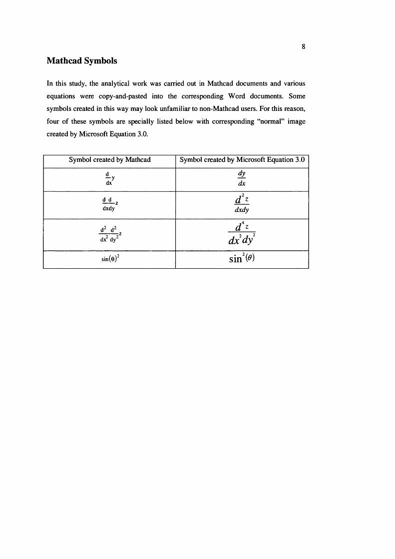
Mathcad Symbols

In this study, the analytical work was carried out in Mathcad documents and various

equations were copy-and-pasted into the corresponding Word documents. Some

symbols created in this way may look unfamiliar to non-Mathcad users. For this reason,

four of these symbols are specially listed below with corresponding “normal” image

created by Microsoft Equation 3.0.

Symbol created by Mathcad Symbol created by Microsoft Equation 3.0

l y dydx dx

/ zdxdy dxdy

d2 ddx dy dxdy

sin(e)^

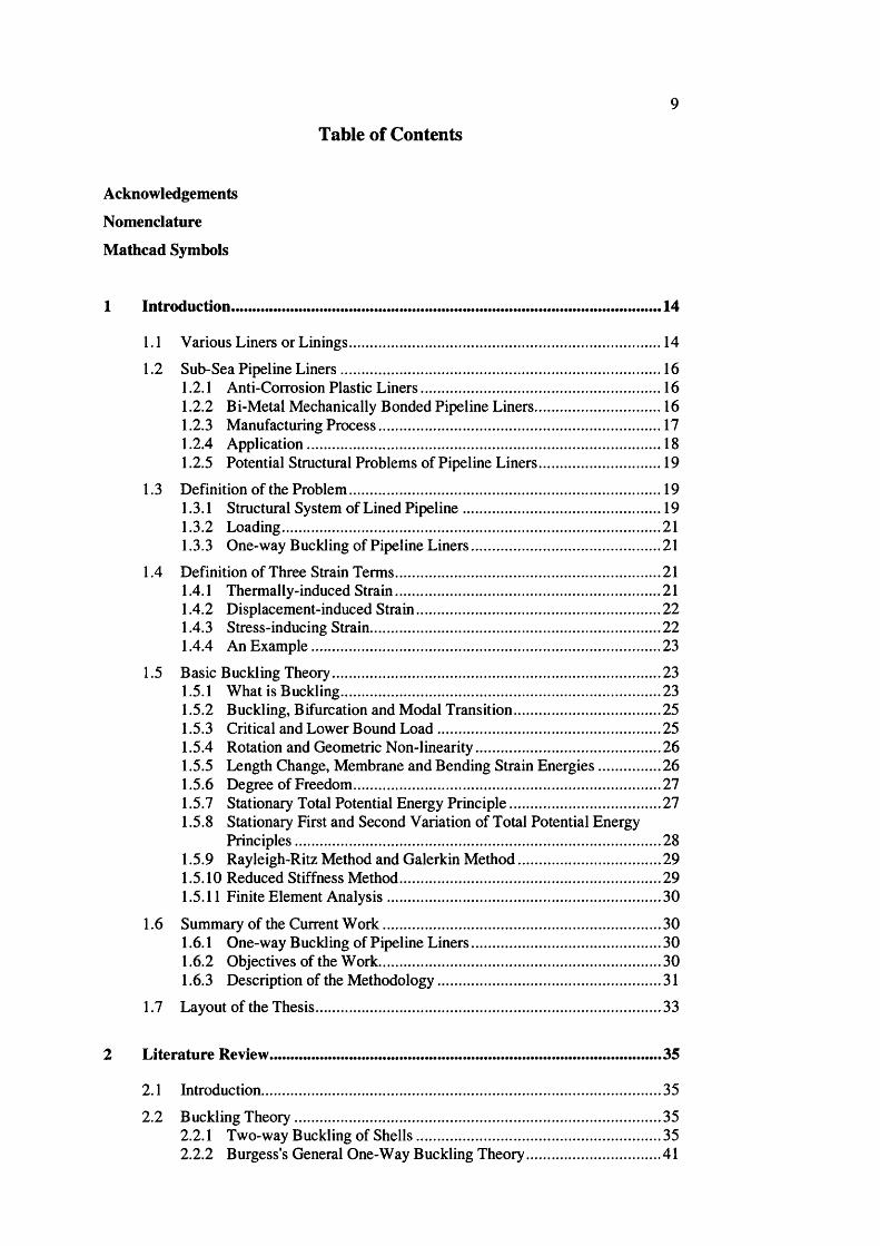
Table of Contents

Acknowledgements

Nomenclature

Mathcad Symbols

1 Introduction.......................................................................................................... 14

1.1 Various Liners or Linings...................................................................................14

1.2 Sub-Sea Pipeline Liners.....................................................................................161.2.1 Anti-Corrosion Plastic Liners..............................................................161.2.2 Bi-Metal Mechanically Bonded Pipeline Liners................................ 161.2.3 Manufacturing Process........................................................................ 171.2.4 Application........................................................................................... 181.2.5 Potential Structural Problems of Pipeline Liners...............................19

1.3 Definition of the Problem.................................................................................. 191.3.1 Structural System of Lined Pipeline...................................................191.3.2 Loading................................................................................................. 211.3.3 One-way Buckling of Pipeline Liners................................................ 21

1.4 Definition of Three Strain Terms...................................................................... 211.4.1 Thermally-induced Strain....................................................................211.4.2 Displacement-induced Strain.............................................................. 221.4.3 Stress-inducing Strain.......................................................................... 221.4.4 An Example..........................................................................................23

1.5 Basic Buckling Theory..................................................................................... 231.5.1 What is Buckling..................................................................................231.5.2 Buckling, Bifurcation and Modal Transition..................................... 251.5.3 Critical and Lower Bound Load.........................................................251.5.4 Rotation and Geometric Non-linearity............................................... 261.5.5 Length Change, Membrane and Bending Strain Energies............... 261.5.6 Degree of Freedom...............................................................................271.5.7 Stationary Total Potential Energy Principle...................................... 271.5.8 Stationary First and Second Variation of Total Potential Energy

Principles............................................................................................... 281.5.9 Rayleigh-Ritz Method and Galerkin Method.................................... 291.5.10 Reduced Stiffness Method...................................................................291.5.11 Finite Element Analysis......................................................................30

1.6 Summary of the Current W ork..........................................................................301.6.1 One-way Buckling of Pipeline Liners................................................ 301.6.2 Objectives of the Work........................................................................ 301.6.3 Description of the Methodology.........................................................31

1.7 Layout of the Thesis...........................................................................................33

2 Literature Review.................................................................................................35

2.1 Introduction.........................................................................................................35

2.2 Buckling Theory................................................................................................ 352.2.1 Two-way Buckling of Shells.............................................................. 352.2.2 Burgess's General One-Way Buckling Theory..................................41

10

2.2.3 Croll's Reduced Stiffness Method....................................................... 432.2.4 Upheaval Buckling...............................................................................46

2.3 Simplified Analysis............................................................................................472.3.1 Advantages........................................................................................... 472.3.2 Croll and Walker's Simplified Model..................................................472.3.3 Burgess's Link Model...........................................................................49

2.4 Imperfection........................................................................................................502.4.1 Knockdown Factor............................................................................... 502.4.2 Kinematic Relations............................................................................. 512.4.3 Imperfection and One-way Buckling of Rings.................................. 522.4.4 Recent Developments........................................................................... 53

2.5 Buckling of Liners.............................................................................................552.5.1 Tunnel Liners........................................................................................ 552.5.2 Liners in Pipeline Rehabilitation......................................................... 602.5.3 Liners in Nuclear Power Plant.............................................................61

2.6 Finite Element Analysis....................................................................................662.6.1 Zhu's W ork........................................................................................... 662.6.2 Others....................................................................................................67

2.7 Experimental Work........................................................................................... 682.7.1 General..................................................................................................682.7.2 Burgess' Experimental R ig .................................................................. 682.7.3 Tests on Bi-Metal Mechanically Bonded Lined Pipes....................... 74

2.8 Concluding Remarks......................................................................................... 77

Buckling Analysis with Simplified Rigid-Link Model..................................... 79

3.1 Introduction........................................................................................................ 79

3.2 Axial 2-Rigid-Link Model.................................................................................79

3.3 Bi-directional 4-Rigid-Link Model...................................................................83

3.4 Formulation.........................................................................................................853.4.1 Thermally-induced Displacements...................................................... 853.4.2 Imperfection, Incremental Displacements and Kinematic

Relationships..........................................................................................853.4.3 Force-inducing Displacements............................................................893.4.4 Total Potential Energy..........................................................................903.4.5 Application of Stationary Potential Energy Principle....................... 913.4.6 Application of Stationary Second Variation of Potential Energy

Principle................................................................................................. 943.4.7 Reduced Stiffness Method................................................................... 94

3.5 Example..............................................................................................................953.5.1 Geometry of a Typical Pipeline Liner.................................................953.5.2 Rigid-Links and Spring Stiffness........................................................ 953.5.3 Equilibrium Paths................................................................................. 963.5.4 Variation with Wave Numbers.......................................................... 1063.5.5 Variation with Wall Thickness and Radius...................................... I l l3.5.6 Comparison with Results from the Published Work........................112

3.6 One-way Buckling Mechanism...................................................................... 112

3.7 Concluding Remarks........................................................................................113

Buckling Analysis with Simplifîed Beam-Link Model....................................115

11

4.1 Introduction...................................................................................................... 115

4.2 Beam-Link Model............................................................................................116

4.3 Buckling Analysis with Beam-link Model.................................................... 1184.3.1 Thermally-induced Displacements.................................................... 1184.3.2 Imperfection and Displacements........................................................1194.3.3 Kinematic Relationships.....................................................................1234.3.4 Stress-inducing Strains.......................................................................1264.3.5 Total Potential energy........................................................................1274.3.6 First Variation of Total Potential energy.......................................... 1284.3.7 Second Variation of Total Potential energy..................................... 129

4.4 Imperfection and Deformed Shape.................................................................1324.4.1 Imperfection Functions.......................................................................1324.4.2 Displacement Functions.....................................................................1334.4.3 Coefficients......................................................................................... 133

4.5 Examples..........................................................................................................1354.5.1 Results for the Typical Pipeline Liner...............................................1354.5.2 Variation with Wave Numbers.......................................................... 1364.5.3 Variation with Wall Thickness and Radius...................................... 138

4.6 Concluding Remarks......................................................................................139

Buckling Analysis with Liner-Only Continuum M odel................................... 140

5.1 Introduction..................................................................................................... 140

5.2 Simplification of the Outer Pipe..................................................................... 141

5.3 Description of Liner-Only Continuum Model............................................... 141

5.4 Displacement and Imperfection Variables.....................................................1425.4.1 Deflection........................................................................................... 1425.4.2 Imperfection........................................................................................ 143

5.5 Formulation...................................................................................................... 1435.5.1 Thermally-induced Strains.................................................................1435.5.2 Displacement-induced Strains........................................................... 1445.5.3 Stress-inducing Strains.......................................................................1465.5.4 Total Potential Energy........................................................................1465.5.5 First Variation of Total Potential Energy......................................... 1475.5.6 Pre-condition for Bifurcation - Critical Imperfection......................1495.5.7 Second Variation of Total Potential Energy..................................... 1505.5.8 Buckling Temperature at Critical Imperfection................................1525.5.9 Equilibrium Path................................................................................ 153

5.6 Assumed Deformed and Imperfection Shape................................................ 1555.6.1 Deflection............................................................................................1555.6.2 Imperfection........................................................................................ 1565.6.3 Coefficients......................................................................................... 156

5.7 Examples..........................................................................................................1625.7.1 Results for a Typical Pipeline Liner.................................................. 1625.7.2 Variation with Wave Numbers.......................................................... 1635.7.3 Effects of the Thickness.....................................................................1655.7.4 Effects of the Radius.......................................................................... 165

5.8 Concluding Remarks....................................................................................... 166

Liner-Pipe Continuum Model...............................................................................168

12

6.1 Introduction.......................................................................................................168

6.2 Description of Liner-Pipe Contin uum Model................................................ 168

6.3 Coupling of the Inner Liner with the Outer Pipe...........................................171

6.4 Temperature Distribution................................................................................ 1736.4.1 Review of Heat Flow...........................................................................1736.4.2 Temperature Distribution in the Inner L iner................................... 1746.4.3 Temperature Distribution in the Outer Pipe.................................... 174

6.5 Pre-buckling Fundamental State - Without Imperfection.............................1756.5.1 Thermally-induced Strains in the Fundamental State...................... 1756.5.2 Displacement-induced Strains in the Fundamental State..................1766.5.3 Stress-inducing Strains in the Fundamental State............................1776.5.4 Total Potential Energy in the Fundamental State............................1786.5.5 Stationary Potential Energy Principle in the Fundamental State.... 1786.5.6 Discussion............................................................................................ 179

6.6 Pre-buckling Fundamental State - With Imperfection.................................. 1816.6.1 Review of the Effect of Imperfection.................................................1816.6.2 Fundamental State............................................................................... 182

6.7 Formulation.......................................................................................................1826.7.1 Description of Buckled Shape - Incremental Deformation............. 1826.7.2 Description of Imperfection................................................................1836.7.3 Total Incremental Displacement........................................................ 1836.7.4 Kinematic Relationships..................................................................... 1846.7.5 Displacement-induced Strains............................................................1846.7.6 Stress-inducing Strains........................................................................1866.7.7 Total Potential Energy.........................................................................1876.7.8 Stationary Potential Energy Principle................................................189

6.8 Discussion......................................................................................................... 1926.8.1 W ithout Imperfection..........................................................................1926.8.2 Critical Imperfection...........................................................................1936.8.3 Critical Temperature...........................................................................193

6.9 Assumed Deformed Shape..............................................................................1946.9.1 Deflection............................................................................................ 1946.9.2 Imperfection.........................................................................................1946.9.3 Coefficients.......................................................................................... 195

6.10 Examples......................................................................................................... 1966.10.1 Results for a Typical Pipeline Liner................................................... 1966.10.2 Variation with Wave Numbers...........................................................1976.10.3 Equilibrium Paths................................................................................ 199

6.11 Summary, Discussion and Concluding Remarks........................................... 1996.11.1 Summary.............................................................................................. 1996.11.2 Discussion............................................................................................2006.11.3 Conclusion...........................................................................................200

7 Finite Element Analysis - Elastic Buckling.....................................................202

7.1 Introduction.......................................................................................................202

7.2 Finite Element One-way Buckling Analysis................................................. 2037.2.1 Two-way Deformation Function for One-Way Buckling Analysis 2037.2.2 Eigenvalue Buckling Analysis No Longer Valid..............................2047.2.3 Adapted Post-buckling Analysis for One-way Buckling Analysis. 2047.2.4 Pseudo-two-way Approach.................................................................205

13

7.3 Description of Finite Element Model.............................................................2067.3.1 Modelling of the Outer Pipe - Application of Thermal Loading.... 2067.3.2 Modelling of the Outer Pipe - Simplification by Springs............... 2077.3.3 Full and Partial Modelling.................................................................210

7.4 Results from Various Runs with ABAQUS..................................................2157.4.1 Cases and Runs.................................................................................. 2157.4.2 Equilibrium Path................................................................................2177.4.3 Approximate Buckling Temperature................................................ 2217.4.4 Post-buckling Modal Transition - Partial-Model............................ 2247.4.5 Post-buckling Modal Transition - Full-Model.................................2297.4.6 Detailed Results................................................................................. 235

7.5 Concluding Remarks....................................................................................... 236

8 Finite Element Analysis - Elastic-Plastic Buckling..........................................237

8.1 Introduction.......................................................................................................237

8.2 Material Property of the Pipeline Liner..........................................................237

8.3 Results form Finite Element Elastic-Plastic Buckling Analysis.................. 2398.3.1 Equilibrium Path................................................................................ 2398.3.2 Buckling Temperature....................................................................... 2448.3.3 Post-buckling Modal Transition - Partial-Model............................ 2468.3.4 Post-buckling Modal Shape and Transition - Full-Model.............. 2508.3.5 Detailed Results................................................................................. 255

8.4 Comparison between Elastic and Elastic-Plastic Buckling..........................2558.4.1 Equilibrium Path................................................................................ 2558.4.2 Buckling Temperature....................................................................... 2568.4.3 Modal Shape and Transition..............................................................258

8.5 Comparison of Results................................................................................... 259

8.6 Concluding Remarks.......................................................................................260

9 Summary, Conclusions, Recommendations and Further Work.....................261

9.1 Summary........................................................................................................... 261

9.2 Conclusions and Recommendations.............................................................. 263

9.3 Further W o rk ................................................................................................... 269

Appendix A Detailed Results from Elastic FE Analysis....................................... 271

Appendix B Detailed Results from Elastic-Plastic FE Analysis............................307

List of Figures

List of Tables

References

Bibliography

14

1 Introduction

1.1 V arious L iners o r L inings

Liners or linings have been used for a variety of purposes since ancient times. During

the winter our coats need proper linings to protect us from the elements. Liners such as

sleeve linings guard products from wearing and moisture. Appropriate domestic

chimney liners help prevent fire damage to homes or carbon monoxide poisoning.

Liners offer waterproofing and impermeability in the ceilings of houses and garden

ponds. Linings offer good quality decorative finish combined with noise absorption in

theatres. They even add to the beauty of constructions and can be used to give them real

character.

Liners or linings have their obvious advantages over unlined alternatives. Only linings

can provide repeated structural protection (by replacing liners rather than components as

a whole). Liners offer physical properties that the primary materials lack. Lined

products are financially more attractive. With lining materials, which are usually of high

quality and therefore more expensive, placed in the right places only, the amount of the

expensive materials needed is greatly reduced.

After the industrial revolution, liners have inevitably been extended to engineering

applications. Indeed liners have been put into use virtually everywhere in the civil

engineering. Today's building code requires liners in all new chimneys; and old,

damaged, or worn out chimneys are required to be restored or relined by seamless flues

or metal liners. These liners allow for a smooth flow of exhaust, a more efficient

operation of chimneys, and provide thermal insulation and sealants for environmental

protection. Liners are also used in bridge deck waterproofing and structural protection

and are seen in crane brakes and clutch bands. A new tunnelling technique with liner

plates reduces the amount of soil to be handled, saves expensive pavement repairs,

requires minimum construction site space and reduces the need to detour traffic.

Geosynthetic clay liners (GCL) are products that have been used selectively in some

barrier systems for landfills, surface impoundments, and other liquid/solid waste-

retaining facilities.

Early forms of modem tunnel often made use of cast iron linings. The linings are

installed after the ground movement induced by excavation and other loads has

stabilized. The tunnel linings will then bear any subsequent loads from rock, earth and

15

water pressure etc. Although tunnel linings have been in extensive application since

they were first introduced, literature review reveals that the research for the design of

tunnel linings is far from over.

In recent years, liners have been extensively used in the rehabilitation of underground

pipelines used for water distribution, sewer and drainage networks. New pipe lining

technologies such as cure-in-place-pipe (CIPP) expedite the application of liners in

urban utility systems. With CIPP, a polymeric pipe liner is directly cast against the wall

of a deteriorating host pipe. A thermosetting resin is impregnated at ambient

temperature into a flexible (commonly polyester felt) tube with a cross sectional

perimeter equal to the inner circumference of the host pipe. The tube is then pressure-

inverted (opposite to soil/rock/water pressure from the outside) against the wall of the

host pipe from a suitable access point, and heated in-situ (using water, steam or air) to

cure the resin, thus forming a structurally sound lining. Over 13,000km of CIPP linings

have been installed worldwide since the introduction of the process in 1971.

Another example of the application of the liners for pipeline networks is the use of high-

density polyethylene liners (HDPE). The process involves the insertion of a

deformed/reformed (or folded and formed) plastic liner pipe into an existing

underground pipeline. The liner is manufactured as a standard round pipe to specifically

fit the dimension of the pipeline to be rehabilitated. Then, the cross-sectional area of the

liner is reduced in the factory by “deforming or folding” the pipe into a U-shaped

section to facilitate transportation and field installation. The liner pipe is transported to

the construction site on a reel or as a continuous coil, depending on the size of the

rehabilitation project. Then, a special process utilizing heat and pressure is used in the

field to “reform” the liner back to closely fit the interior profile of the host pipe.

Lining technologies such as “no-dig” technology in the rehabilitation of urban pipeline

networks help to install pipelines in-situ, greatly extending the useful life of unlined or

damaged underground pipes without disturbing the infrastructure on top of the pipeline

networks. Furthermore, they actually help make use of the residual life of the damaged

pipelines.

Liners are also used in nuclear power plants (NPP). The number of NPP has been

increasing rapidly as the power demand increases. In NPP, concrete cylinders or

spherical caps are used as containment vessels that are lined by thin steel liners. The

steel liners are attached to the inner surfaces of the concrete shells by stiffeners or studs.

16

The steel liners are impermeable and play an important role in the prevention of leakage

of any released products.

In the last few years, lining technologies have started to be adopted in the oil & gas

industry. To provide a welded, pressure-resistant durable system, steel pipes are

invariably used to transport raw well-head fluids over large distances. However, many

well-head fluids are extremely aggressive to normal steels. Due to the difficulties in

identifying a viable and passive alternative pipeline material, the traditional solution to

this problem has been to remove the offending wet acid gases close to the point of

recovery. Recently it has been proposed to use various forms of internal liners to protect

the oil & gas pipelines from the corrosion that would otherwise be caused by the

aggressive components.

1.2 S u b -S ea P ipeline L iners

1.2.1 Anti-Corrosion Plastic Liners

Sub-sea pipelines are widely used to transport fluids from offshore platforms to onshore

facilities. One of the major design concerns of sub-sea pipelines is the internal corrosion

of the carbon steel pipeline walls. One of the proposed anti-corrosion solutions is the

adoption of pipe lining technology. Although plastic lined pipelines have been proposed

as an option for cost-effective North Sea pipelines (Howard and Tough, 2002), their

application is limited for a variety of reasons, for example, permeation-induced

corrosion to the host pipes, creep in the plastic liners, the accumulation of fluids and

pressure within the annulus, etc. Therefore, the long-term strategy is to develop metal-

lined pipes which do not suffer from these problems.

1.2.2 Bi-Metal Mechanically Bonded Pipeline Liners

One of the extreme cases in the oil and gas industry recently is the conveyance of

corrosive fluids at high temperature under high pressure (HTHP) (Walker et a l, 2CXX)).

The initial designs of such pipelines, like those designed and manufactured by United

Pipeline Ltd (UPL), are as follows

• Corrosion Resistant Alloy (CRA) pipelines

• Metallurgically Clad Lined Pipe packages

17

The conventional design is the CRA pipelines which are made from corrosion resistant

steel such as 13% Chrome. However, a 13% Chrome pipe is up to 10 times the cost of a

carbon steel pipe. Furthermore, it has been pointed out (Walker et al, 2000) that the

application of CRA pipelines is limited to small-diameter pipelines due to high material

and manufacturing cost. Therefore, for many applications, alternative designs have

become necessary.

The first alternative to the conventional design is metallurgically lined pipelines. A

metallurgically lined pipeline is constructed from a carbon steel pipe metallurgically

lined with a thin layer of corrosion resistant material. In this case, liners are bonded to

the host pipes by weld cladding. However, for large-diameter pipelines, metallurgically

clad pipelines are operationally cost-ineffective. Again the manufacturing cost of

metallurgically lined pipelines limits their application.

Bi-metal, mechanically bonded, lined pipes are innovative products introduced as the

cost-saving alternatives to both CRA and metallurgically lined pipelines. They consist

of CRA thin liners tightly fitted to the carbon steel pipes by a mechanical process. In

this way, pipes and liners form composite pipelines. The details of the manufacturing

process are described in Section 1.2.3.

The use of bi-metal mechanically bonded pipelines has made it possible for well-head

fluids, that are extremely aggressive to normal carbon steels, to be transported onshore.

By eliminating the need for initial sub-sea processing to remove the offending

components, bi-metal mechanically bonded pipelines are proven to be cost effective

solution to engineering problems, reducing both capital and operating expenditures. Bi

metal mechanically bonded pipelines are the subject of this PhD study.

1.2.3 Manufacturing P rocess

A bi-metal mechanically bonded lined pipe is fabricated from a seamless or welded

carbon steel pipe lined with a corrosion resistant alloy liner shell at the inner surface,

mechanically bonded by a process of hydraulic expansion. The CRA liner is directly

manufactured as a standard round pipe to specifically fit the dimension of the carbon

steel pipe. The cross sectional perimeter of the liner is marginally smaller than the inner

circumference of the host pipe. This allows the CRA liner to be inserted into the inside

of the carbon steel pipe. Finally, hydraulic pressure is applied to the inside of the

pipeline liner. As the hydraulic pressure inside the liner increases, the liner is expanded

18

and pressed against the interior profile o f the host pipe. The hydraulic pressure is then

further increased until the inner liner has yielded. The residual strain that rem ains after

the hydraulic pressure is rem oved provides a m echanical interference fit o f the liner in

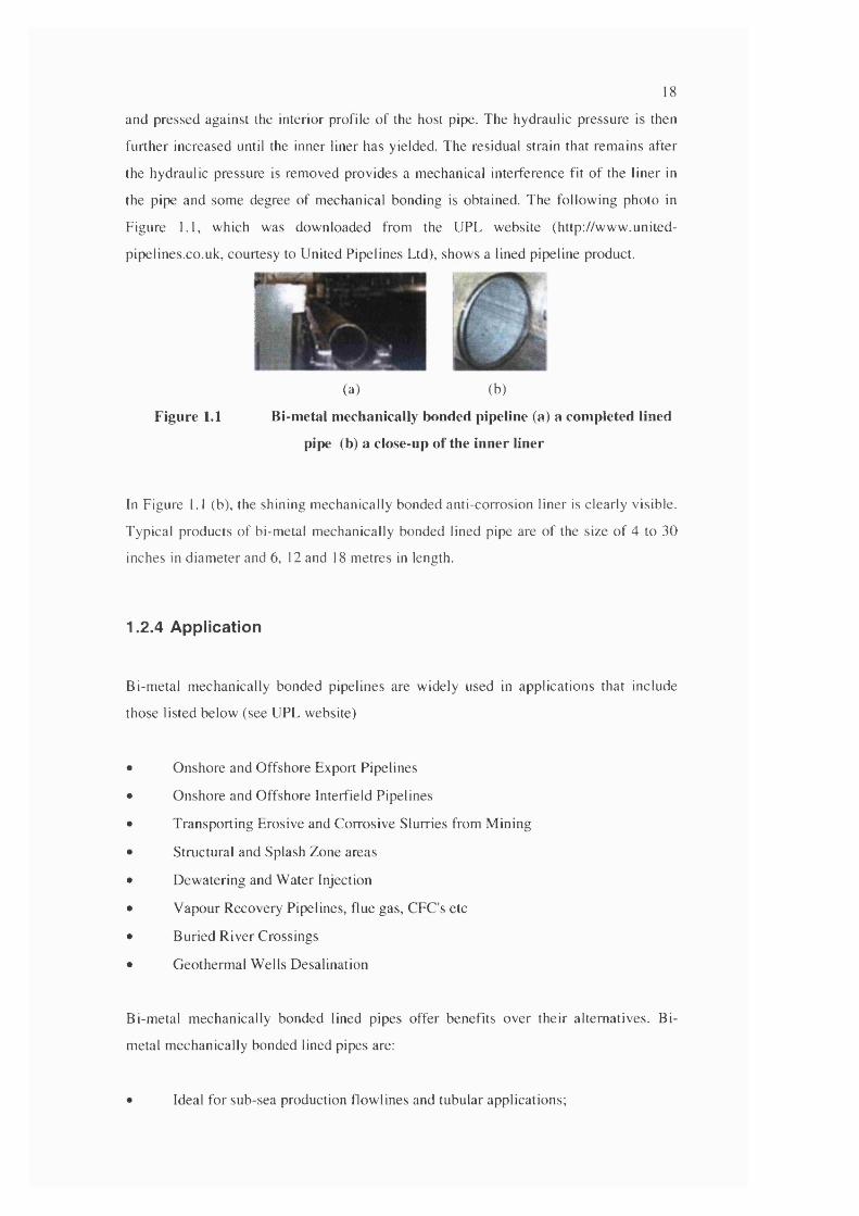
the pipe and some degree of m echanical bonding is obtained. The follow ing photo in

Figure 1.1, which was dow nloaded from the UPL website (http://w w w .united-

pipelines.co.uk, courtesy to United Pipelines Ltd), shows a lined pipeline product.

(a) (b)

Figure 1.1 Bi-metal mechanically bonded pipeline (a) a completed lined

pipe (b) a close-up of the inner liner

In Figure 1.1 (b), the shining m echanically bonded anti-corrosion liner is clearly visible.

Typical products of bi-metal m echanically bonded lined pipe are o f the size o f 4 to 30

inches in diam eter and 6, 12 and 18 m etres in length.

1.2.4 Application

Bi-m etal m echanically bonded pipelines are widely used in applications that include

those listed below (see UPL website)

Onshore and Offshore Export Pipelines

Onshore and Offshore Interfield Pipelines

Transporting Erosive and Corrosive Slurries from M ining

Structural and Splash Zone areas

De w atering and W ater Injection

V apour Recovery Pipelines, flue gas, CFC's etc

Buried R iver Crossings

Geotherm al W ells Desalination

Bi-m etal m echanically bonded lined pipes offer benefits over their alternatives. B i

metal m echanically bonded lined pipes are:

• Ideal for sub-sea production Bowlines and tubular applications;

http://www.united-

19

Especially suited where resistance to localised corrosion, chloride and sulphide

stress corrosion cracking and erosion or corrosion is paramount;

Ideal for transporting raw aggressive fluids, multiphase fluids and wet gases

directly from remote installations without process treatment;

Particularly suitable for high temperature high pressure (HTHP) process

conditions.

1.2.5 Potential Structural Problem s of Pipeline Liners

Like cure-in-place pipe liners and high density polyethylene liners that have been the

subject of extensive researches with regard to their buckling, bi-metal mechanically

bonded liners could also have potential problems associated with local buckling.

The liner wall thickness of a bi-metal pipeline is usually very thin. It is well known that

thin circular cylindrical shells are prone to buckle under compressive loadings. The

inner liner of a bi-metal, mechanically bonded, pipeline could be under compressive

loadings under various scenarios. One of the most imminent threats is the buckling of

the in-situ lining under thermally-induced loading.

The fluid inside a sub-sea pipeline can, not only be extremely aggressive to the

conveyance vehicle, but also transfer heat to it through convection. Under the

operational condition, a mechanically bonded liner is sometimes heated to more than

160°C. As the pipeline liner is heated, it tends to expand. The host pipe and the liner are

made from different metals, therefore, they have different thermal expansion

coefficients. Because of the difference in the thermal expansion coefficients in the inner

liner metal and the outer pipe metal, the inner liner could be under compression in the

circumferential direction. The inner liner could also have axial compression induced as

a result of the restraint in the axial direction. The thermal buckling of bi-metal

mechanically bonded pipelines is the main topic of this PhD research.

1.3 Definition of th e P rob lem

1.3.1 Structural System of Lined Pipeline

A sub-sea pipeline conveying fluids from oilfield is usually lying on seabed as shown in

the sketch in Figure 1.2.

20

/ / / / / / / ' / / / / / / / / / / / / / / / /

Figure 1.2 Sketch showing a pipeline on seabed

Since offshore platforms are far away from onshore facilities, say tens of kilometres

away, a pipeline may be considered as infinitely long when building an analytical

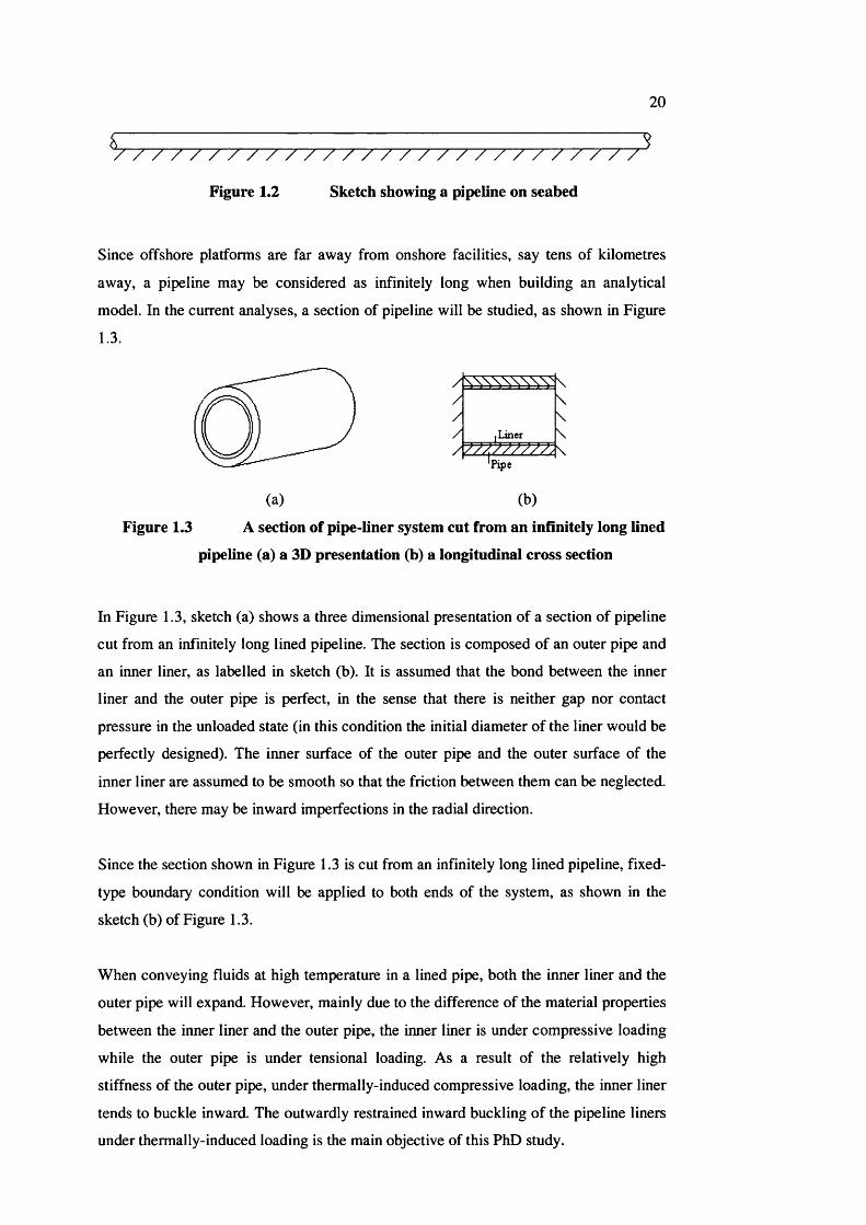
model. In the current analyses, a section of pipeline will be studied, as shown in Figure

1.3.

(a)

.Liner \

'Pipe

(b)

Figure 1.3 A section of pipe-liner system cut from an infinitely long lined

pipeline (a) a 3D presentation (b) a longitudinal cross section

In Figure 1.3, sketch (a) shows a three dimensional presentation of a section of pipeline

cut from an infinitely long lined pipeline. The section is composed of an outer pipe and

an inner liner, as labelled in sketch (b). It is assumed that the bond between the inner

liner and the outer pipe is perfect, in the sense that there is neither gap nor contact

pressure in the unloaded state (in this condition the initial diameter of the liner would be

perfectly designed). The inner surface of the outer pipe and the outer surface of the

inner liner are assumed to be smooth so that the friction between them can be neglected.

However, there may be inward imperfections in the radial direction.

Since the section shown in Figure 1.3 is cut from an infinitely long lined pipeline, fixed-

type boundary condition will be applied to both ends of the system, as shown in the

sketch (b) of Figure 1.3.

When conveying fluids at high temperature in a lined pipe, both the inner liner and the

outer pipe will expand. However, mainly due to the difference of the material properties

between the inner liner and the outer pipe, the inner liner is under compressive loading

while the outer pipe is under tensional loading. As a result of the relatively high

stiffness of the outer pipe, under thermally-induced compressive loading, the inner liner

tends to buckle inward. The outwardly restrained inward buckling of the pipeline liners

under thermally-induced loading is the main objective of this PhD study.

21

1.3.2 Loading

Under the operational condition, a lined pipe may transport fluids at high temperature.

The pipeline could be under combined thermal and mechanical loadings. In the current

first-generation research, only the thermally-induced loading will be considered, that is,

• A lined pipe is assumed to have been perfectly designed and manufactured so

that at the ambient temperature there is neither gap nor contact pressure between

the inner liner and the outer pipe;

• The hot medium that the pipeline conveys results in a temperature rise in the

lined pipe;

• No mechanical loading such as inner pressure, axial force or bending moment is

considered.

1.3.3 One-way Buckling of Pipeline Liners

A general definition for one-way buckling of any structural system has been given by

Burgess (Burgess, 1969). For the current specific one-way buckling of a pipeline liner,

one-way buckling is defined as the buckling where the liner can only deform radially

towards the centre line of the pipe. Radial displacements away from the centre line of

the pipe are not a consideration owing to the confinement offered by the host pipe

which is considered not to displace. With or without imperfection, the liner’s radial

coordinates cannot increase above their original values at the unloaded state i.e. the

incremental radial deflections must be inward. For convenience, in the current research,

both the incremental normal displacements and imperfection are taken as positive when

radially inward. In this case buckling displacements can take positive values only.

1.4 Definition of T hree S tra in T erm s

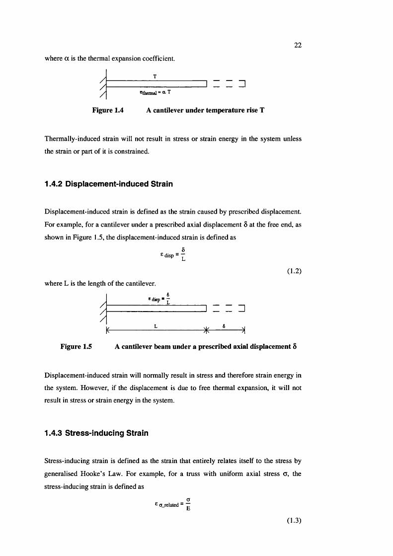
1.4.1 Thermally-induced Strain

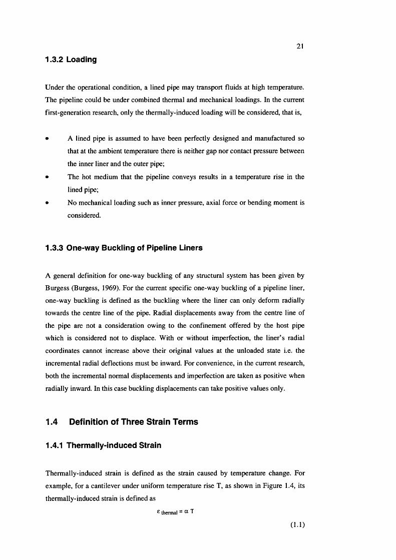
Thermally-induced strain is defined as the strain caused by temperature change. For

example, for a cantilever under uniform temperature rise T, as shown in Figure 1.4, its

thermally-induced strain is defined as

G thermal = Ct T

( 1. 1)

22

where a is the thermal expansion coefficient.

///

z z □^thennal = O' T

Figure 1.4 A cantilever under temperature rise T

Thermally-induced strain will not result in stress or strain energy in the system unless

the strain or part of it is constrained.

1.4.2 Displacement-induced Strain

Displacement-induced strain is defined as the strain caused by prescribed displacement.

For example, for a cantilever under a prescribed axial displacement 6 at the free end, as

shown in Figure 1,5, the displacement-induced strain is defined as

ÔG disp - ^

( 1.2)

where L is the length of the cantilever,s

1 z z □y ____________

//

N------------------- ---------------------^ — -------N

Figure 1.5 A cantilever beam under a prescribed axial displacement 5

Displacement-induced strain will normally result in stress and therefore strain energy in

the system. However, if the displacement is due to free thermal expansion, it will not

result in stress or strain energy in the system,

1.4.3 Stress-inducing Strain

Stress-inducing strain is defined as the strain that entirely relates itself to the stress by

generalised Hooke’s Law, For example, for a truss with uniform axial stress a, the

stress-inducing strain is defined as

aG a_related - “

(1.3)

23

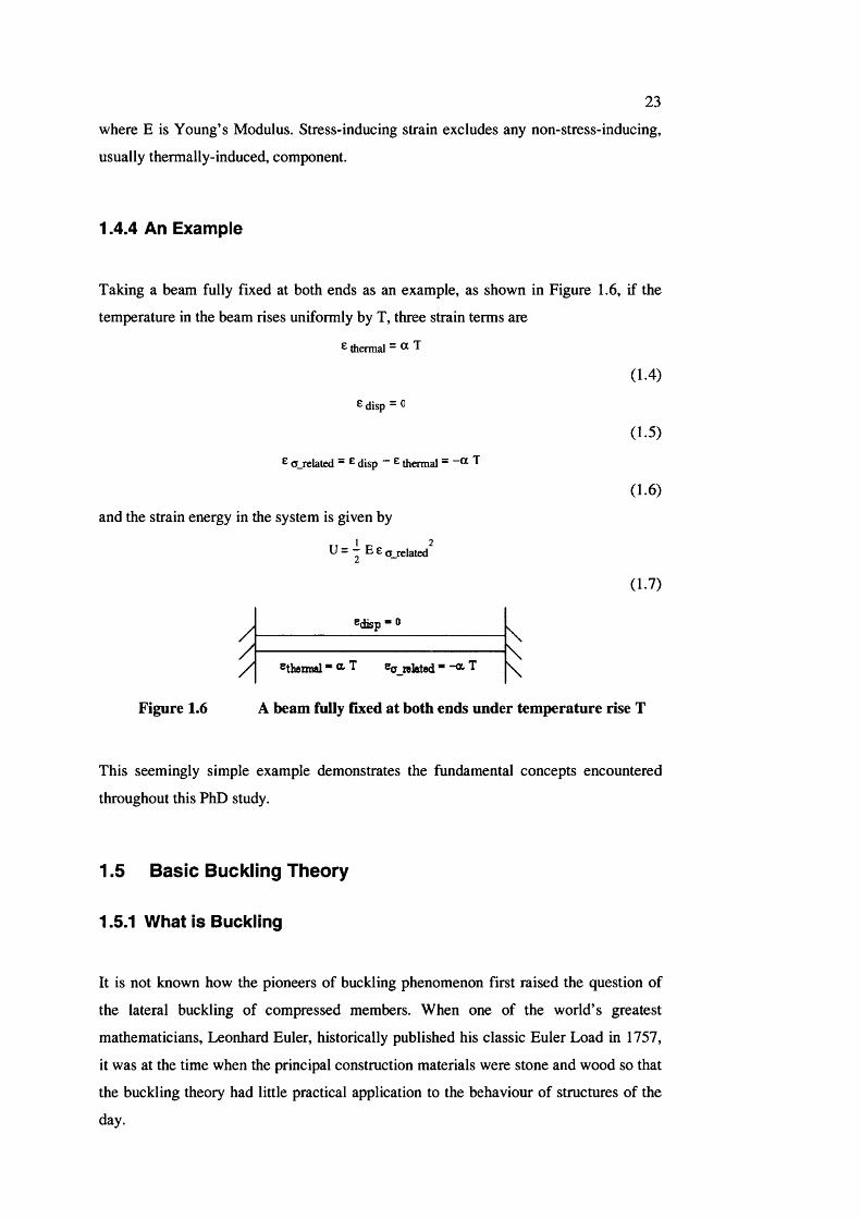
where E is Young’s Modulus. Stress-inducing strain excludes any non-stress-inducing,

usually thermally-induced, component.

1.4.4 An Example

Taking a beam fully fixed at both ends as an example, as shown in Figure 1.6, if the

temperature in the beam rises uniformly by T, three strain terms are

G thermal = ® T

(1.4)

(1.5)

( 1.6)

G disp - 0

G CT_related ~ ^ disp ^ thermal ~ ® ^

and the strain energy in the system is given by

///

U - “ E e (^related

Bdisp

\

(1.7)

Figure 1.6 A beam fully fîxed at both ends under temperature rise T

This seemingly simple example demonstrates the fundamental concepts encountered

throughout this PhD study.

1.5 B asic Buckling T heory

1.5.1 What is Buckling

It is not known how the pioneers of buckling phenomenon first raised the question of

the lateral buckling of compressed members. When one of the world’s greatest

mathematicians, Leonhard Euler, historically published his classic Euler Load in 1757,

it was at the time when the principal construction materials were stone and wood so that

the buckling theory had little practical application to the behaviour of structures of the

day.

24

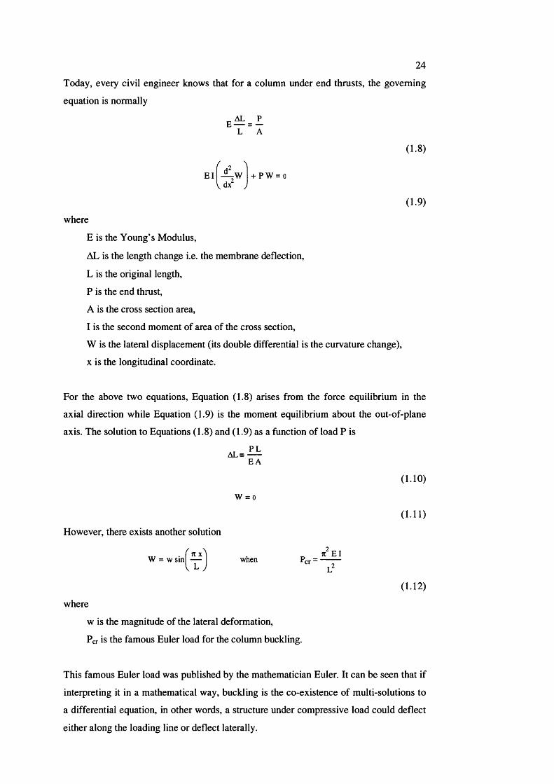
Today, every civil engineer knows that for a column under end thrusts, the governing

equation is normally

L A

E l + P W = 0

(1.8)

(1.9)

where

E is the Young’s Modulus,

AL is the length change i.e. the membrane deflection,

L is the original length,

P is the end thrust,

A is the cross section area,

I is the second moment of area of the cross section,

W is the lateral displacement (its double differential is the curvature change),

X is the longitudinal coordinate.

For the above two equations. Equation (1.8) arises from the force equilibrium in the

axial direction while Equation (1.9) is the moment equilibrium about the out-of-plane

axis. The solution to Equations (1.8) and (1.9) as a function of load P is

AL= —EA

W = 0

(1.10)

( 1. 11)

However, there exists another solution2

71 X 1 _ 71 EIW = w sin — when P r =

L ; i}

(1.12)

where

w is the magnitude of the lateral deformation.

Per is the famous Euler load for the column buckling.

This famous Euler load was published by the mathematician Euler. It can be seen that if

interpreting it in a mathematical way, buckling is the co-existence of multi-solutions to

a differential equation, in other words, a structure under compressive load could deflect

either along the loading line or deflect laterally.

25

1.5.2 Buckling, Bifurcation and Modal Transition

Buckling is a general term for the behaviour of structures undergoing transverse

deflection when under compression. Buckling events may be classified into two

categories - buckling where the developing deflection pattern is basically orthogonal to

the pre-buckling deflection pattern and snap-through where the instability is connected

with relatively large displacement amplitudes without a significant change of the

displacement pattern (Wullschleger and Meyer-Piening, 2002). In the current research,

however, the first category of buckling will happen only at ideal and special conditions

(when the amplitude of imperfection is exactly the critical value, see Chapters 3-9).

With a normal imperfection (other than critical imperfection), the pipeline liner will

have transverse deflection on top of the pre-buckling geometric shapes without apparent

displacement pattern change. For convenience, in the current research, whenever any of

the pipeline liner shell deviates significantly from its original position in the radial

direction, it is considered to have buckled, even when there is no significant deflection

pattern change.

Bifurcation however occurs only at certain stages of buckling. Consider, as an example,

a column buckling under the action of axial end loads. When the magnitude of the end

thrusts reaches Per (critical load), the column could be in an equilibrium state by either

remaining straight and with zero lateral displacement, or taking on a sinusoidal shape

with non-zero lateral displacement. Such points on an equilibrium path, at which the

equilibrium path branches with different mode shapes, are termed bifurcation points.

The associated phenomena are termed bifurcations.

In the current study it is found that during the post-buckling stage an equilibrium path

characterizes itself with discontinuity. The discontinuous points are not bifurcation

points because they are not the starting points of the branching. Rather, they are the

starting point of different modal shapes. The change of modal shapes during the post-

buckling is termed as modal transition.

1.5.3 Critical and Lower Bound Load

In the current research, the loads corresponding to the peaks in an equilibrium path, no

matter if the peaks are the bifurcation points or modal transition points or the results of

material yielding etc, are termed “peak loads” or “critical loads”.

26

Similarly, the loads corresponding to the troughs in an equilibrium path, no matter what

the cause of the troughs, are termed “lower bound loads”. In the current study, peak

loads, or critical loads or lower bound loads will be used in the comparison of results

from different methods in different chapters.

1.5.4 Rotation and Geometric Non-linearity

In Section 1.5.1, the governing equations for the column buckling have two solutions.

Equation (1.8) gives displacement in the direction of the applied load and involves no

rotation. The corresponding strain-displacement equation is

de = — u dx

(1.13)

where axial strain e is linear and equal to the first differential of the axial displacement u

with respect to the axial coordinate, x. Since both displacement u and coordinate x are

axial, there is no rotation involved so that the strain-displacement equation is

geometrically linear.

However, in Equation (1.9), apart from the usual axial displacement u in the x direction,

there is the lateral displacement w that is perpendicular to the loading line. Non-uniform

lateral displacement results in rotation in the column. The corresponding strain-

displacement equation takes the following form

(1.14)

The differential of lateral displacement w with respect to x represents the rotation

between the element of the column and the undeformed axial direction. This rotation

will affect both the element length and its curvature change and consequently membrane

and bending strain energies in the system. It is a general characteristic that buckling

always involves such out of plane rotations and should therefore be considered as a

geometrically non-linear process.

1.5.5 Length Change, Membrane and Bending Strain Energies

Equation (1.8) in Section 1.5.1 involves the axial deflection only, resulting in a decrease

of the column length and an accumulation of the membrane strain energy in the system.

27

There is no bending strain energy involved In Equation (1.9), however, the axial

displacement u in the loading direction remains but will change to ensure that the

increase of the length due to the lateral displacement w will initially cause no change in

the membrane energy. The bending of the column will inevitably generate bending

strain energy.

1.5.6 Degree of Freedom

The column buckling in Section 1.5.1 involves the axial and lateral displacement

variables u and w. However, as long as the derivation of critical eigenvalue load is the

main objective, the relatively small axial displacement u may be eliminated. Then the

strain-displacement equation becomes

(1.15)

For the column buckling in Section 1.5.1, it still leads to the same critical load.

In the analytical work of the current study, both the in-plane displacements u and v are

neglected. Ignoring u and v dramatically reduces the amount of the mathematical work.

It is believed that the results from the formulation still retain adequate degrees of

accuracy and this simplification is appropriate for the current stage of the research.

1.5.7 Stationary Total Potential Energy Principle

When a structure buckles, it must remain in equilibrium in its buckled position. In

Section 1.5.1, Equation (1.8) relates to force equilibrium in the x direction while

Equation (1.9) is based on moment equilibrium. From an energy formulation, a structure

is in equilibrium when its total potential energy is stationary.

For a one degree of freedom system, the stationary total potential energy principle may

be written as follows

— n = 0dw

(1.16)

where H is the total potential energy, w is the one degree of freedom displacement

variable.

28

1.5.8 Stationary First and Second Variation of Total Potential Energy

Principles

The change of total potential energy mentioned in Section 1.5.7 may be rewritten as

An = ôn + — 6 n + — 6 n + — n + o(n)2! 3! 4!

(1.17)

where the terms on the right side of the equation are linear, quadratic, etc, respectively

and 0(n) is the sum of the remaining terms. With infinitesimally small displacements,

each non-zero term in the above expansion is much larger than the sum of the

succeeding terms. Usually, most of the terms vanish. For normal buckling analysis, the

first term i.e. the first variation of total potential energy is among those that vanish.

However the current study is an exception. When the first variation does not vanish, the

following condition must first be satisfied.

— (6n) = 0dw

(1.18)

The author terms this condition as the stationary first variation of total potential energy

principle. When the first variation vanishes, then the second variation of the total

potential energy must be stationary. For a two degrees of freedom system, the condition

for this stationarity is

d ddW|dw2V 2!

-Î- ô^n

d d

dwjdw2V2!s^n

dw 21

= 0

(1.19)

where wi and W2 are two displacement variables. The current study simplifies a pipeline

liner as a one degree of freedom system. For a one degree of freedom system. Equation

(1.19) becomes

( 1.20)

where w is the one degree of freedom displacement variable. The author terms this

condition as stationary second variation of the total potential energy principle (the

second variation is proportional to w therefore when the second differential is zero so is

the first differential). The stationary first and second variation of the total potential

energy principles, together with Rayleigh-Ritz method, will be employed throughout the

analytical analysis in this PhD study.

29

1.5.9 Rayleigh-Ritz Method and Gaterkin Method

Rayleigh-Ritz method will be employed in the analytical development of the critical

imperfection and buckling temperature formulations in later chapters. Chapter 2 will

review the published work by Ding et al, 1996, where Galerkin method was used.

Basically, when Rayleigh-Ritz method is employed, the displacement functions are

replaced by assumed deformed shapes with a few degrees of freedom (one degree of

freedom for the current study). In the current research, the deformed shape is usually

assumed to be squared sine or cosine waves. Then stationary potential energy principle

is used to derive the temperature-displacement relationship.

When Galerkin method is employed, similar deformed shapes are also assumed, but the

governing equations rather than the total potential energies will be used in the formation

of homogeneous equations for displacement variables. The homogeneous equations are

derived by the minimization of the errors of the products of the left of the governing

equations and every admissible displacement function.

1.5.10 Reduced Stiffness Method

It is well known that there exists a discrepancy between the analytical solutions and the

experimental results for buckling loads. This problem may be largely answered by the

Reduced Stiffness Method.

The Reduced Stiffness Method provides lower bound of the buckling load for any

buckling structure. Basically the buckling process is the process losing membrane strain

energy while gaining bending strain energy. The residual membrane strain energy

(when a structure has buckled, the remaining membrane strain energy is relatively small

so that the author term it as residual membrane strain energy; this terminology will be

used again later) and the bending strain energy together with other terms of strain

energies will determine the buckling load. Due to the uncertainties of loading

conditions, the geometric and material defects, etc, the amount of residual membrane

strain energy is varying. The lower bound of the buckling load is the buckling load

derived when the stabilizing residual membrane strain energy in a system is eliminated.

The Reduced stiffness method will be further reviewed in Chapter 2 and will be

employed in the current analytical work.

30

1.5.11 Finite Eiement Analysis

Normal finite element buckling analysis refers to eigenvalue and eigenvector extraction.

When imperfection is involved, in finite element analysis, the combination of the

eigenvectors extracted from an eigenvalue analysis is usually used as the form of the

imperfection and then the corresponding geometrically non-linear analysis is carried

out. The current research deals with unconventional finite element buckling analysis in

the sense that the current buckling is the one-way buckling so that no eigenvalue and

eigenvector extraction is possible. The details of the finite element analysis will be

discussed in Chapters 7 and 8.

1.6 S um m ary of th e C urren t W ork

1.6.1 One-way Buckling of Pipeline Liners

The thermal buckling of bi-metal mechanically bonded pipeline liners is relatively new.

Almost all the available references regarding the buckling of cylindrical-type liner, of

whatever materials and under whatever loadings, treated the buckling as a normal two-

way (inward and outward) buckling by methodologies that do not address the

underlying one-way buckling characteristics (except Burgess’ one-way buckling of

contained ring, Burgess, 1969 and Fan’s nuclear power plant liner. Fan et al. from

Qinghua University, 1996, to the best of the author’s knowledge). Since a bi-metal

mechanically bonded pipeline liner is perfectly bonded to the host pipe, the no-outward-

deflection rule has to be strictly followed. The current research is One-way Buckling

Analysis of Pipeline Liners.

1.6.2 Objectives of the Work

The essential objectives of the work described in this thesis are:

• To review and collate available information on the elastic and elastic-plastic

buckling of cylindrical shells, especially the buckling analyses of different liners

in various engineering applications;

• To identify the fundamental one-way buckling mechanism of confined

cylindrical liners by simplified analysis using rigid-link modelling and beam-

link modelling. This enables answers to two basic questions: (i) does a confined

31

perfectly circular cylindrical liner without imperfection buckle and (ii) at what

conditions does it buckle;

• To identify the fundamental differences between one-way buckling and normal

two-way buckling and to derive generic equilibrium paths for different

categories of imperfection profiles;

• To carry out analytical analysis with liner-only continuum model and liner-pipe

continuum model to derive more accurate critical imperfection and the

corresponding critical temperature;

• To carry out a series of finite element numerical elastic and elastic-plastic

buckling analyses in order to verify the analytical results, perform parametric

studies on the effects of various pipeline geometrical parameters, examine the

modal shape at the on-set of the buckling and modal shape transition at the post-

buckling stage and investigate the effect of the material plasticity on both the

buckling temperature and the modal shape transition;

• To compare the results from the analytical and numerical analyses with those

from published experimental results;

• To prepare conclusions from the assessment of the analysis results, to make

recommendations for application of the results from this research.

1.6.3 Description of the Methodology

In the current one-way buckling analysis, the imperfection is included from the very

beginning to the end. The involvement of imperfection means inclusion of the coupling

terms of the imperfection and the displacements. Therefore, the detailed analysis for the

current one-way buckling analysis contains tedious mathematical work. Therefore, the

current study will be carried out step by step starting from simple approaches and

increasing in complexity:

• Firstly commencing analytical analysis and followed by finite element numerical

analysis with ABAQUS;

• Firstly analytical analysis with simplified models and then analytical analysis

with continuum models;

• Firstly analytical simplified analysis with rigid-link models and then analytical

simplified analysis with flexural beam-1 ink models;

• Firstly analytical analysis with liner-only continuum model and then analytical

analysis with liner-pipe continuum model;

32

• Firstly to examine basic one-way buckling mechanism and then to derive

detailed buckling temperature and its variation against various parameters;

• Firstly finite element analysis with partial-models and then finite element

analysis with full-models;

• Firstly finite element elastic buckling analysis and then finite element elastic-

plastic buckling analysis.

Lining techniques in pipelines are relatively new technologies and there is little

published work about the buckling of shell liners available. Among the published work

about the buckling of liners, most researches employed modified free shell buckling

methodology. However, liner buckling is fundamentally different from free shell

buckling in that it is a one-way buckling. Therefore, it will be necessary to clearly

define the one-way buckling mechanism before the detailed analysis is carried out. It

will be appropriate that the first step is carried out by a simplified model.

The simplified models are not intended to describe precisely the response of the

structure but to establish the general behaviour or phenomena. In the current study, the

methodology in the book Elements of Structural Stability (Croll and Walker, 1972) will

be adopted for the buckling analysis of pipeline liners, and, link models similar to those

in the book will be developed. The objective is to give an insight to the physics of

thermal one-way buckling of pipeline liners so that the mechanism of the thermal one

way buckling of pipeline liners can be understood.

In this simplified analysis phase, two simplified analyses with two different simplified

models are carried out. Firstly, the pipeline liner is simplified as rigid-links, as in the

book Elements of Structural Stability. The second simplified model uses beam links to

address the effect of the changes of the wave lengths.

After the simplified analyses have answered the fundamental questions i.e. the one-way

buckling mechanism, continuum models are aimed to produce more accurate results.

The deformation functions in the continuum model are two-dimensional, and the

loading and boundary conditions are also more precisely simulated. In the analytical

analysis with liner-pipe model, even the temperature distribution based on the thermal

convection is considered.

Throughout the analytical analyses, after the corresponding models are constructed, the

deformed shapes are assumed. Then the stationary total potential energy principle

33

and/or the stationary first/second variation of total potential energy principles are

employed so that the formulas for the critical imperfection and the corresponding

critical temperature are derived.

However, in the analytical work, some aspects of the analysis are still simplified in

order to reduce the complexity of mathematical work. Even in the continuum liner-pipe

model, deformed shapes are inevitably assumed in advance. After the basic buckling

behaviour of pipelines has been gradually understood, finite element analysis with less-

simplified models becomes necessary.

In the finite element elastic and elastic-plastic buckling analysis, while the modelling of

the inner liner as shell elements is straightforward, the modelling of the outer pipe is

quite difficult. In the final methodology, basically, the outer pipe is replaced by springs

so that the complicated coupling of non-linear contact and non-linear buckling is

avoided, largely solving the convergence problem. Finally, non-linear buckling analysis

is carried out with ABAQUS arc-length RIKs method.

1.7 L ayout of th e T h es is

The current thesis consists of nine chapters. Chapter 2 is a review of the past work in the

similar areas such as the buckling analysis of nuclear power plat liners or high-density

polyethylene lined pipes.

Chapter 3 will describe the work in the very first phase of the study - the simplified

analysis with rigid-link model. In this chapter, the basic one-way buckling concept will

be proposed.

In Chapter 4, the simplified analysis in Chapter 3 will be further extended to the

simplified analysis with flexural beam-1 ink simplified model.

After the basic buckling mechanism of one-way buckling is identified in the previous

Chapters 3 and 4, Chapter 5 will start to look at the analytical analysis with continuum

model. In Chapter 5, the outer pipe will be treated as rigid, the liner-only continuum

model will be described and the corresponding results will be given.

Chapter 6 will conclude the analytical work by the liner-pipe combined continuum

model. The work described here is the most detailed among the analytical work with an

34

aim to provide more accurate buckling temperatures for the typical pipeline liners.

Finite element analyses will be described in Chapters 7 and 8. Chapter 7 will deal with

the finite element elastic buckling analysis.

Chapter 8 will address the finite element elastic-plastic buckling analysis.

Finally, in Chapter 9, the work will be summarised and the detailed conclusions and

recommendations will be given. At the end of Chapter 9, the possible further work will

be identified.

35

2 Literature Review

2.1 In troduction

It has been pointed out in Chapter 1 that there are a large number of engineering

applications of liners or linings virtually in every industrial area. The current literature

review reveals that many kinds of liners, except the sub-sea pipeline liners which are

relatively new, have been under intensive investigations (for example, steel tunnel

liners, Berti et al, 1998; non-metal underground pipeline liners, El-Sawy et a l, 1998;

steel liners in nuclear power plant pressure vessels. Fan et a l, 1996).

These liners in other industrial applications have some sort of similarities with the sub

sea pipeline liners in that they all are contained circular cylindrical shells so that the

author believes it is worthwhile to know how their buckling analysis is carried out.

Space does not allow a thorough review of all these references. Although most of the

references available to the author will be listed in the References and Bibliography

sections of this thesis, only a relatively small selection of them, with important direct

relevance to the current study, will be selected for discussion in the following sections.

In this chapter. Section 2.2 reviews buckling theory. In Sections 2.3-7, various aspects

of the buckling of circular cylindrical liners will be reviewed. Finally, conclusions will

be drawn in Section 2.8.

2.2 B uckling T heory

2.2.1 Two-way Buckling of Shells

Like all the scientific activities, the buckling theories were also developed step by step.

While Leonhard Euler historically published his classic Euler Load in 1757, stability

equations for cylindrical shells were developed more than a century later. According to

Brush (Brush, 1975), Lorenz published solutions for cylinders subjected to axial

compression in 1911. Solutions for buckling under uniform lateral pressure were given

by Southwell in 1913 and by von Mises in 1914. Results for cylinders subjected to

torsional loading were given by Schwerin in 1925 and Donnell in 1933. In 1932, Flugge

presented a comprehensive treatment of cylindrical shell stability, including cylinders

under combined loading and subject to bending.

36

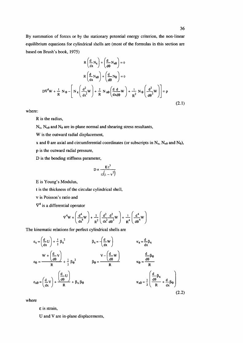
By summation of forces or by the stationary potential energy criterion, the non-linear

equilibrium equations for cylindrical shells are (most of the formulas in this section are

based on Brush’s book, 1975)

DV W + — N ft -( 0 ^d 2Nx _iî_w + —< dx , R+ T N X0 I — — w I + N 0

VdxdG R-W

d0= P

(2.1)

where:

R is the radius,

Nx, Nx0 and Ne are in-plane normal and shearing stress resultants,

W is the outward radial displacement,

X and 0 are axial and circumferential coordinates (or subscripts in Nx, Nxe and Ne),

p is the outward radial pressure,

D is the bending stiffness parameter.

D =12(1 - v )

E is Young’s Modulus,

t is the thickness of the circular cylindrical shell,

V is Poisson’s ratio and

is a differential operator

f d ^ w l 2 d % l 1 f d ^ w l+ — + —Idx^ j R' \ dx de ) R ,de^ ;

P x - H — w dx

The kinematic relations for perfect cylindrical shells are

w + 1 —V £0=------

= I “ V j + + Px Pe

*x - —Px dx

P 0 =

V-l —W d0

RK 0 =

—Pe de

R

Kx0 = - R

(2.2)where

e is strain,

U and V are in-plane displacements.

37

p is rotation.

These strain-displacement equations are subjected to change from projects to projects.

Usually, the expression for the rotation in the circumferential direction may be

simplified as

By neglecting the V term in the rotation in the circumferential direction, the number of

strain energy terms is greatly reduced.

By using the adjacent equilibrium criterion or the stationary potential energy criterion,

and neglecting the initial rotations of the pre-buckling state, the corresponding linear

stability equations are

d (vV i) + -1 Neidx

; W1 + ~ Nx0o f wi I + N0OVdxdG de'

■wi = 0

(2.3)In Equation (2.3), the variables with subscript o are the variables in the fundamental

state while those with subscript 1 are the variables contributed by incremental

displacements. Equation (2.3) may be rewritten as follows by the introduction of a

portion of the constitutive and kinematic relations/ \

,24 VDV u 1 = —

R

D V \ 1 =

v d x

r

[WI

i l ldx^ dO

dx de

•wir

R" de'[ W I

d (v * wi) + ^ cI f . , \

- Vdx

;W1dxdO

2 ;wi

R" de= 0

(2.4)

where C is the extensional stiffness parameter and V again is a differential operator

C = ^1 - v ^

w = v"* (v V)In Equation (2.4), ui and vi are the in-plane incremental displacements. Equation (2.4)

is partially uncoupled and rewritten from the Donnell stability equations in coupled

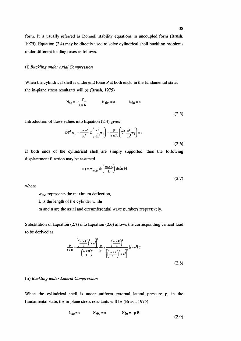
38

form. It is usually referred as Donnell stability equations in uncoupled form (Brush,

1975). Equation (2.4) may be directly used to solve cylindrical shell buckling problems

under different loading cases as follows.

(i) Buckling under Axial Compression

When the cylindrical shell is under end force P at both ends, in the fundamental state,

the in-plane stress resultants will be (Brush, 1975)

PNvn = —

2 7C RxBo — 0 N0O = 0

(2.5)

Introduction of these values into Equation (2.4) gives

DV*wi+-^-^cf-^W] ldx“ y 2 7C R I dx

= 0

(2.6)

If both ends of the cylindrical shell are simply supported, then the following

displacement function may be assumed

w 1 = w s i n‘ m,n i L sin(n 0 )

(2.7)where

Wm,n represents the maximum deflection,

L is the length of the cylinder while

m and n are the axial and circumferential wave numbers respectively.

Substitution of Equation (2.7) into Equation (2.6) allows the corresponding critical load

to be derived as

p 2 1C R

( mic R

■I Lmi c R

l - v j Cm 1C R m 1C R

(2 .8)

(ii) Buckling under Lateral Compression

When the cylindrical shell is under uniform external lateral pressure p, in the

fundamental state, the in-plane stress resultants will be (Brush, 1975)

Nvn = 0 xGo - 0 N0O = - p R(2.9)

39


d ( v ^ w i ) + -—— c ■wiV de

= 0

(2. 10)

If both ends of the cylindrical shell are simply supported, substitution of Equation (2.7)

into Equation (2.10) results in the critical load

- i 2

p R =

m jt R ) 2+ n

D (i -v^)m it R 1 2

+ n

(2 . 11)

(iii) Buckling under Combined Axial and Lateral Compression

When the cylindrical shell is under the axial compressive load P and the uniform

external lateral pressure p, the in-plane stress resultants of the fundamental state will be

(Brush, 1975)

PNvn = —

2 7t RN xGo = 0 N0O = - p R

(2. 12)


d ( v * w i ) ^W] 1 + v'* vdx

P d_ , ;wi2 Jt R dx 7 de

-W ] = 0

(2.13)

If both ends of the cylindrical shell are simply supported, substitution of Equation (2.7)

into Equation (2.13) gives the critical load as

p R =

mnR 1 2+ n (l -v^)

m J t R 1 2+ n

2 2 n R ( m T c R n + --------- '

pR(2.14)

(iv) Torsional Buckling

When the cylindrical shell is under a torque Q, in the fundamental state, the in-plane

stress resultants will be (Brush, 1975)

XO — 0 Nx0o — N0O = 02 7[R"

(2.15)

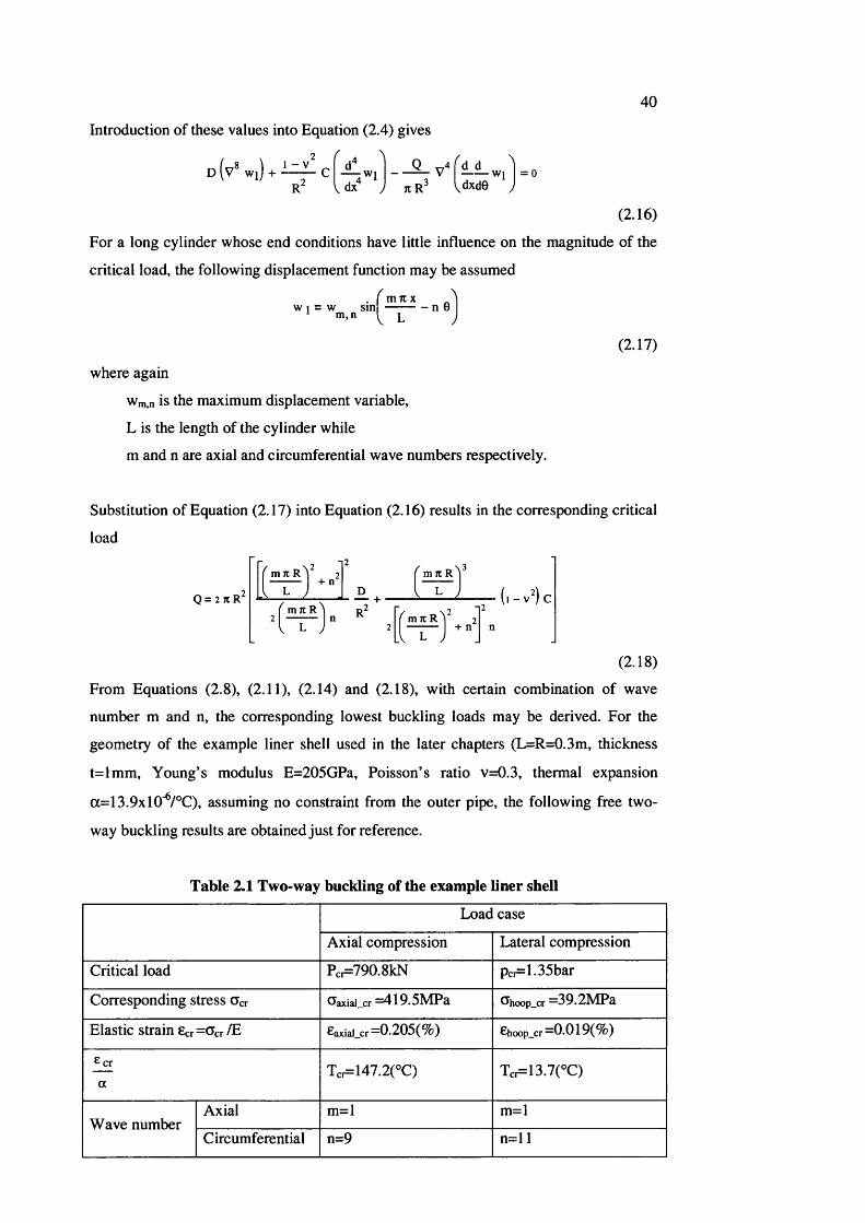
40


d ( v ® w i ) + -i— ^ C - ^ w i

R K R— v 4 ^ ^ w i 1=0

3 IdxdeV dx y

(2.16)

For a long cylinder whose end conditions have little influence on the magnitude of the

critical load, the following displacement function may be assumed

. f mTCx w 1 = w s i n n 0

(2.17)

where again

Wm.n is the maximum displacement variable,

L is the length of the cylinder while

m and n are axial and circumferential wave numbers respectively.

Substitution of Equation (2.17) into Equation (2.16) results in the corresponding critical

load2

Q = 2 TC R"

m ri R 1 2+ n

D

m 71 R

m 71 R 2 I ---------- I n

(i - v )m7cR 1 2

+ n

(2 .18)

From Equations (2.8), (2.11), (2.14) and (2.18), with certain combination of wave

number m and n, the corresponding lowest buckling loads may be derived. For the

geometry of the example liner shell used in the later chapters (L=R=0.3m, thickness

t=lmm. Young’s modulus E=205GPa, Poisson’s ratio v=0.3, thermal expansion

a=13.9xlO‘ /°C), assuming no constraint from the outer pipe, the following free two-

way buckling results are obtained just for reference.

Table 2.1 Two-way buckling of the example liner shell

Load case

Axial compression Lateral compression

Critical load Pcr=790.8kN Pcr=1.35bar

Corresponding stress Ccr Gaxial_cr =419.5MPa Ghoop_cr =39.2MPa

Elastic strain 6cr=(Tcr/E £axial_cr=0.205(%) £hoop_cr=0.019(%)

aTcr=147.2(°C) Tcr=13.7(°C)

Wave numberAxial m=l m=l

Circumferential n=9 n=l 1

41

This review so far has considered the four classic two-way shell buckling problems.

Later researchers started to apply the general cylindrical shell buckling theory to various

“actual” cylindrical shells such as stiffened cylindrical shells under more complicated

loadings (Baruch and Singer, 1963).

2.2.2 B urgess’s General One-Way Buckling Theory

To the author’s knowledge, Burgess’s work (Burgess, 1969, 1971), is the only reference

available on the research of the one-way buckling, where the general equilibrium and

stability conditions were established for general structural systems with general one

way constraints. In Burgess’s general one-way buckling theory, general free systems

were defined as ones which can deform without meeting any rigid barriers to their

generalised deflections, whatever values these generalised deflections may have (each

of the system's generalised coordinates is free to take any value so that any generalised

displacement from its original position is completely reversible). One-way systems were

defined as ones for which some or all of the system's generalised coordinates cannot

take values in certain regions because of physical boimdaries to its displacement.

Burgess’s work established one-way structural system's equilibrium characteristics and

provided a conceptual background regarding the one-way buckling phenomena.

The general one-way theory is based on the discrete generalised coordinate approach

that was applied extensively at that time in the form of arrays/vectors to avoid the great

complexity of the equations in the later stages of analysis. The theoretical background is

the Euler-Lagrange equation that gives the basic equilibrium conditions and Fourier's

revision or re-statement of the general equilibrium condition at the boundary of

displacements (Fourier's inequality).

The Euler-Lagrange equation states that we need a stationary value of the system's

potential energy for static equilibrium. This is widely used in the engineering

applications. In contrast, the application of Fourier’s inequality in the buckling analysis

is not seen very often in the literature because the majority of the research up to now has

focused on two-way buckling. According to Fourier's revision or re statement of the

general equilibrium condition, at the boundary of the displacement, for static

equilibrium, the first variation of the system's potential energy for any possible virtual

displacement of the system must be either positive or zero.

For one-way systems of n independent generalised coordinates lying upon m boundaries

42

simultaneously, and for which m<n, equilibrium is given by two conditions. The first

condition of equilibrium is for the virtual displacement that does not take the system

away from any of its m boundaries

|Q p | = 0 for all p from m+1 to n

(2.19)

where Op is a matrix of (m+1) by (m+1) whose elements for the last row are the partial

differentials of the potential energy with respect to a generalised coordinate and the

other elements are the partial differentials of the left side of the boundary condition

equations with respect to a generalised coordinate. This first condition of equilibrium

corresponds to the equilibrium condition for free two-way systems that the first

variation of its potential energy is stationary. The second condition of equilibrium is for

the virtual displacement that takes the system away from any or all of its m boundaries

iL > 0 for all j from 1 to mkl

(2.20)

where (j) is a matrix of m by m whose elements are the partial differentials of the left

side of the boundary condition equations with respect to a generalised coordinate while

({)j is the same (]) matrix but the elements of jth row are replaced by the partial

differentials of the potential energy with respect to a generalised coordinate. This

second condition of equilibrium corresponds to the Fourier’s inequality that the first

variation of its potential energy is greater than or equal to zero. It represents the

condition that the generalised reaction forces should be greater than or equal to zero

when the system is in contact with the boundaries.

The criterion of stability of equilibrium systems is that the determinants of various

principal minors of the matrix X are zero.

I x| = 0 for all the principal minors of X

(2.21)

Here X is the matrix of (n-m) by (n-m) with elements as the mathematical combinations

of the partial differentials of the potential energy with respect to a generalised

coordinate and the partial differentials of the left side of the boundary condition

equations with respect to a generalised coordinate. A principal minor of a matrix is the

same matrix having the last several rows and the same number of the last columns

removed.

Burgess’s one-way buckling theory for the first time developed the general criteria for

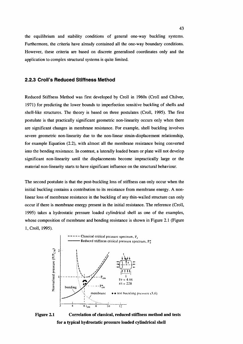
43

the equilibrium and stability conditions of general one-way buckling systems.

Furthermore, the criteria have already contained all the one-way boundary conditions.

However, these criteria are based on discrete generalised coordinates only and the

application to complex structural systems is quite limited.

2.2.3 Croll’s Reduced Stiffness Method

Reduced Stiffness Method was first developed by Croll in 1960s (Croll and Chilver,

1971) for predicting the lower bounds to imperfection sensitive buckling of shells and

shell-like structures. The theory is based on three postulates (Croll, 1995). The first

postulate is that practically significant geometric non-linearity occurs only when there

are significant changes in membrane resistance. For example, shell buckling involves

severe geometric non-linearity due to the non-linear strain-displacement relationship,

for example Equation (2.2), with almost all the membrane resistance being converted

into the bending resistance. In contrast, a laterally loaded beam or plate will not develop

significant non-linearity until the displacements become impractical ly large or the

material non-linearity starts to have significant influence on the structural behaviour.

The second postulate is that the post-buckling loss of stiffness can only occur when the

initial buckling contains a contribution to its resistance from membrane energy. A non

linear loss of membrane resistance in the buckling of any thin-walled structure can only

occur if there is membrane energy present in the initial resistance. The reference (Croll,

1995) takes a hydrostatic pressure loaded cylindrical shell as one of the examples,

whose composition of membrane and bending resistance is shown in Figure 2.1 (Figure

1, Croll, 1995).

Classical critical pressure spectrum,Reduced stiffness critical pressure spectrum, P;

l/r = 4.06 r./t = 228E

oZbending

membrane • test b u ck l in g pressure i 6 , 6 )

Figure 2.1 Correlation of classical, reduced stiffness method and tests

for a typical hydrostatic pressure loaded cylindrical shell

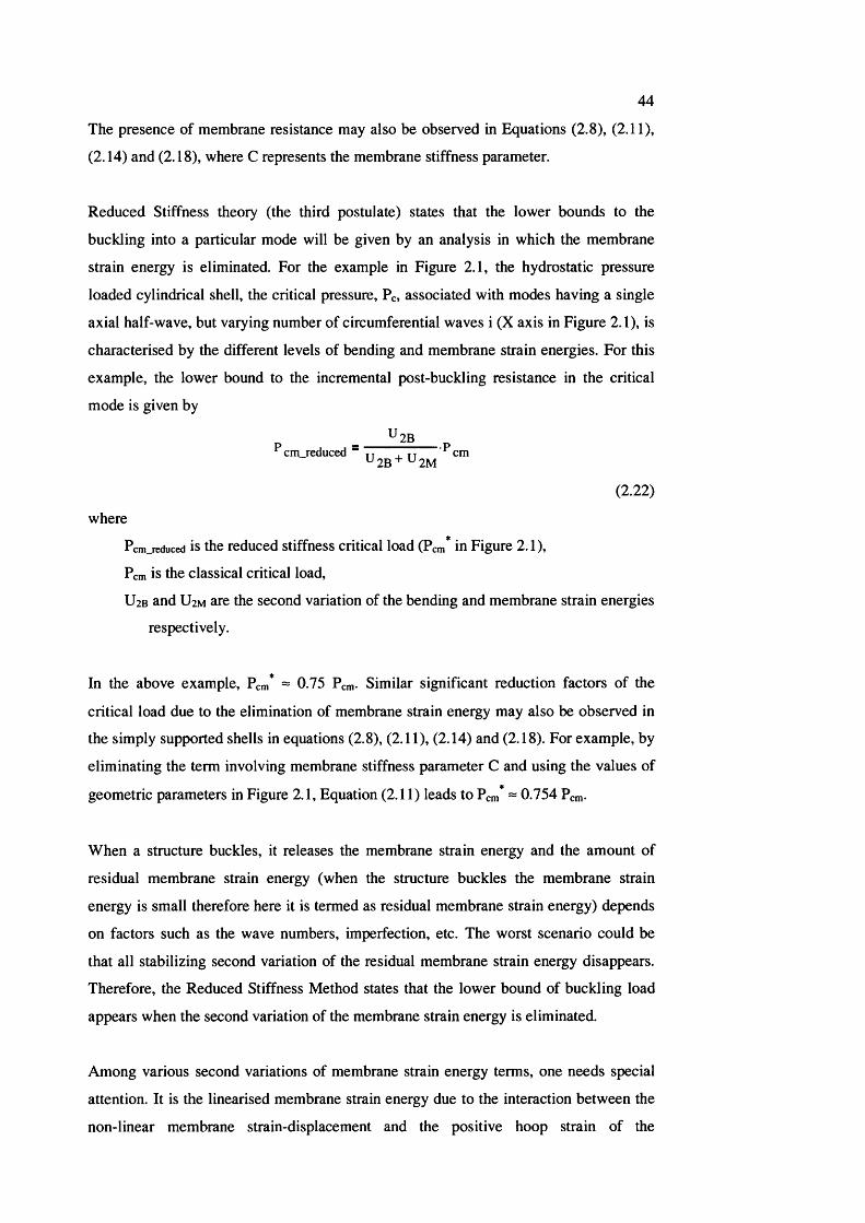
44

The presence of membrane resistance may also be observed in Equations (2.8), (2.11),

(2.14) and (2.18), where C represents the membrane stiffness parameter.

Reduced Stiffness theory (the third postulate) states that the lower bounds to the

buckling into a particular mode will be given by an analysis in which the membrane

strain energy is eliminated. For the example in Figure 2.1, the hydrostatic pressure

loaded cylindrical shell, the critical pressure, ?c, associated with modes having a single

axial half-wave, but varying number of circumferential waves i (X axis in Figure 2.1), is

characterised by the different levels of bending and membrane strain energies. For this

example, the lower bound to the incremental post-buckling resistance in the critical

mode is given by

^2BPcm_reduced= U2B+U 2M

(2.22)

where

Pcm_reduced is the reduced stiffness critical load (Pan* in Figure 2.1),

Pan is the classical critical load,

UzB and U2M are the second variation of the bending and membrane strain energies

respectively.

In the above example, Pcm* = 0.75 Pcm- Similar significant reduction factors of the

critical load due to the elimination of membrane strain energy may also be observed in

the simply supported shells in equations (2.8), (2.11), (2.14) and (2.18). For example, by

eliminating the term involving membrane stiffness parameter C and using the values of

geometric parameters in Figure 2.1, Equation (2.11) leads to Pan* = 0.754 Pan-

When a structure buckles, it releases the membrane strain energy and the amount of

residual membrane strain energy (when the structure buckles the membrane strain

energy is small therefore here it is termed as residual membrane strain energy) depends

on factors such as the wave numbers, imperfection, etc. The worst scenario could be

that all stabilizing second variation of the residual membrane strain energy disappears.

Therefore, the Reduced Stiffness Method states that the lower bound of buckling load

appears when the second variation of the membrane strain energy is eliminated.

Among various second variations of membrane strain energy terms, one needs special

attention. It is the linearised membrane strain energy due to the interaction between the

non-linear membrane strain-displacement and the positive hoop strain of the

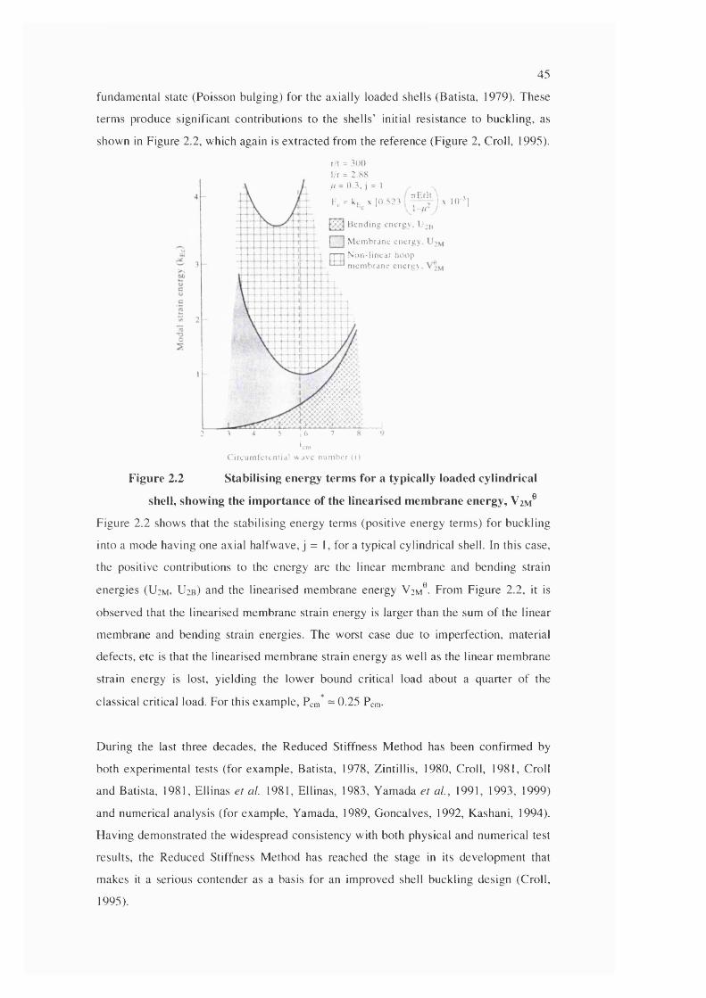
45

fundam ental state (Poisson bulging) fo r the axially loaded shells (Batista, 1979). These

term s produce significant contributions to the shells’ initial resistance to buckling, as

shown in Figure 2.2, which again is extracted from the reference (Figure 2, Croll, 1995).

r,t = 3 00 l/r = 2.SK it - 0 .3 , j = 1

K = k . X (0.5231-,/r

Hciuling energy, t'^n

I I Membrane energy,

: r— I Non-l inear hoop ■ membrane energy.

Trl-.rlt X lO -'l

2 3 4 5 , 6 7

i.rnCireiimlertnOal vva\c number (i)

Figure 2.2 Stabilising energy terms for a typically loaded cylindrical

shell, showing the importance of the linearised membrane energy, Vim®

Figure 2.2 shows that the stabilising energy terms (positive energy term s) fo r buckling

into a mode having one axial halfwave, j = 1, for a typical cylindrical shell. In this case,

the positive contributions to the energy are the linear m em brane and bending strain

energies (U 2M, U^b) and the linearised m em brane energy V2M®. From Figure 2.2, it is

observed that the linearised m em brane strain energy is larger than the sum o f the linear

m em brane and bending strain energies. The worst case due to im perfection, material

defects, etc is that the linearised m em brane strain energy as well as the linear m em brane

strain energy is lost, yielding the low er bound critical load about a quarter o f the

classical critical load. For this exam ple, Pcm* ~ 0.25 Pcm-

During the last three decades, the Reduced Stiffness M ethod has been confirm ed by

both experim ental tests (for exam ple, Batista, 1978, Zintillis, 1980, Croll, 1981, Croll

and Batista, 1981, Ellinas et al. 1981, Ellinas, 1983, Y am ada et a l , 1991, 1993, 1999)

and num erical analysis (for exam ple, Yam ada, 1989, G oncalves, 1992, Kashani, 1994).

H aving dem onstrated the w idespread consistency with both physical and num erical test

results, the R educed Stiffness M ethod has reached the stage in its developm ent that

makes it a serious contender as a basis for an im proved shell buckling design (Croll,

1995).

46

In the current study, the Reduced Stiffness Method will be employed and the

formulation for lower bound buckling temperature of one-way buckling of pipeline

liners will be developed.

2.2.4 Upheaval Buckling

One of the buckling phenomena which is analogous to the current one-way buckling of

pipeline liners is that of upheaval buckling (Croll, 1997, Mork et al 1997, Ballet and

Hobbs, 1992, Palmer et al 1990, Ju and Kyriakides, 1988, Pedersen and Jensen, 1988,

Taylor and Gan, 1986, etc.). Upheaval buckling is seen during the summer in pavement

surfaces (shown to the author by his supervisor just outside UCL), roofs or floors and

railway tracks (Kerr 1974). This section briefly reviews the upheaval buckling in the oil

and gas pipelines.

Among the vast quantity of literatures of upheaval buckling of pipelines is the work by

Hobbs (1984, 1989). Hobbs pointed out that pipelines under compressive forces induced

by the restraint of axial extensions due to temperature changes or other causes may

buckle vertically upwards as well as laterally. Hobbs pointed out the differential

equation for the upheaval buckling of pipelines is

j + I + - (4 - L I = 0

where w is the upward displacement, m=q/EI, n^=P/EI, q and P are selfweight (per unit

length) and axial force respectively, El is the flexural stiffness. The origin of the x axis

along the pipeline is located at the centre of the buckle of wavelength L. The

assumption is that the bending moment at the lift-off point is zero. Considering the

slope at the ends of the buckle is zero, the solution to the differential equation is given

by

(an f— 1 = — n L = 8.98682 (n L )^ = 80.763 P = — — !L 2 J 2 2

which has its lowest root nL=8.98682. By comparing the axial load P in the buckle with

the axial load Po well away from the buckle, which is greater than P in the buckle

because of the friction between pipe and subgrade along the two lengths of pipe Ls

sliding in towards the buckle, the following equation is derived

P q = P + - | y >/o.00001597E A n q - 0.25 (p. E l)^

where |LL is the friction coefficient, EA is the extensional stiffness.

Although the above one-dimensional one-way buckling analysis is different from the

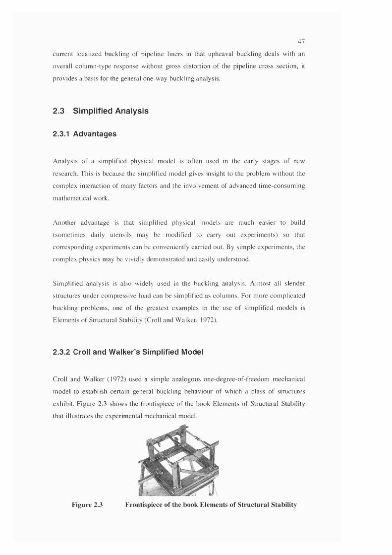
47

current localized buckling of pipeline liners in that upheaval buckling deals with an

overall colum n-type response w ithout gross distortion o f the pipeline cross section, it

provides a basis for the general one-w ay buckling analysis.

2.3 Sim plified A nalysis

2.3.1 Advantages

A nalysis o f a sim plified physical model is often used in the early stages o f new

research. This is because the sim plified model gives insight to the problem w ithout the

com plex interaction o f many factors and the involvem ent of advanced tim e-consum ing

m athem atical work.

A nother advantage is that sim plified physical m odels are m uch easier to build

(som etim es daily utensils may be m odified to carry out experim ents) so that

corresponding experim ents can be conveniently carried out. By sim ple experim ents, the

com plex physics may be vividly dem onstrated and easily understood.

S im plified analysis is also widely used in the buckling analysis. A lm ost all slender

structures under com pressive load can be sim plified as colum ns. For m ore com plicated

buckling problem s, one of the greatest exam ples in the use o f sim plified m odels is

E lem ents o f Structural Stability (Croll and W alker, 1972).

2.3.2 Croll and Walker’s Simplified Model

Croll and W alker (1972) used a sim ple analogous one-degree-of-freedom m echanical

model to establish certain general buckling behaviour o f which a class o f structures

exhibit. F igure 2.3 shows the frontispiece o f the book Elem ents of Structural Stability

that illustrates the experim ental m echanical model.

Figure 2.3 Frontispiece of the book Elements of Structural Stability

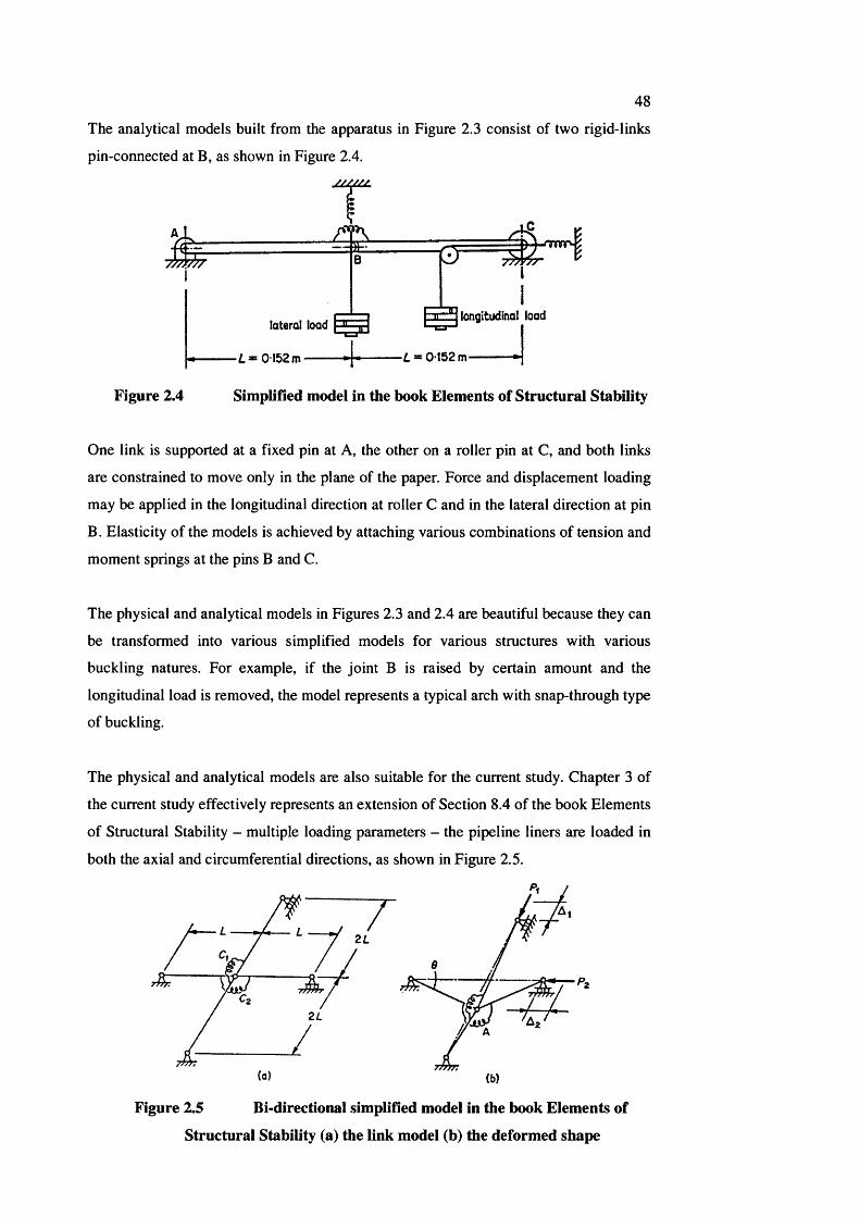
48

The analytical models built from the apparatus in Figure 2.3 consist of two rigid-links

pin-connected at B, as shown in Figure 2.4.

.//A///.

Figure 2.4

lateral load

0 1 5 2 m -------

longitudinal load

• L = 0 1 5 2 m-

Simplified model in the book Elements of Structural Stability

One link is supported at a fixed pin at A, the other on a roller pin at C, and both links

are constrained to move only in the plane of the paper. Force and displacement loading

may be applied in the longitudinal direction at roller C and in the lateral direction at pin

B. Elasticity of the models is achieved by attaching various combinations of tension and

moment springs at the pins B and C.

The physical and analytical models in Figures 2.3 and 2.4 are beautiful because they can

be transformed into various simplified models for various structures with various

buckling natures. For example, if the joint B is raised by certain amount and the

longitudinal load is removed, the model represents a typical arch with snap-through type

of buckling.

The physical and analytical models are also suitable for the current study. Chapter 3 of

the current study effectively represents an extension of Section 8.4 of the book Elements

of Structural Stability - multiple loading parameters - the pipeline liners are loaded in

both the axial and circumferential directions, as shown in Figure 2.5.

721

21

(a) (b)

Figure 2.5 Bi-directional simplified model in the book Elements of

Structural Stability (a) the link model (b) the deformed shape

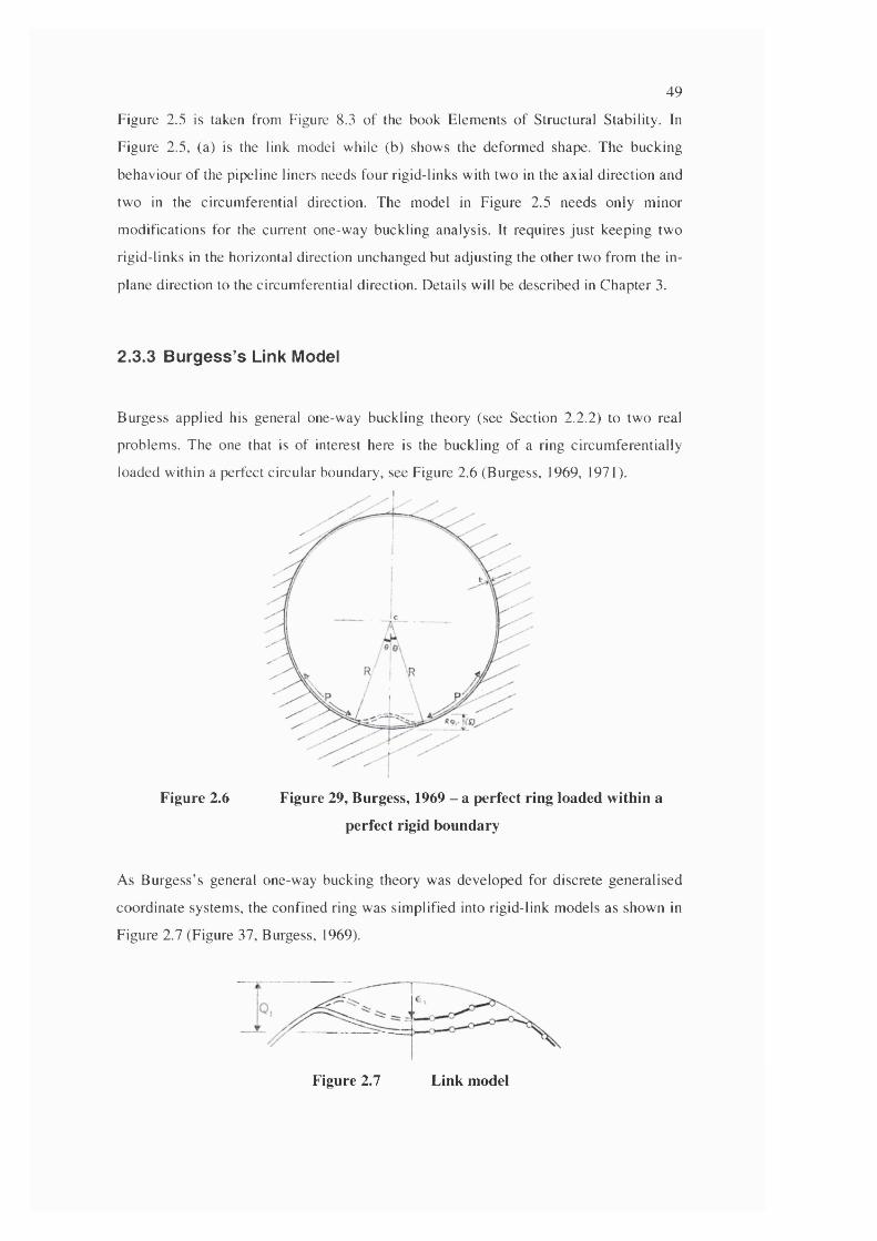
49

Figure 2.5 is taken from Figure 8.3 o f the book Elem ents o f Structural Stability. In

Figure 2.5, (a) is the link model w hile (b) shows the deform ed shape. The bucking

behaviour o f the pipeline liners needs four rigid-links with tw o in the axial direction and

two in the circum ferential direction. The model in Figure 2.5 needs only m inor

m odifications for the current one-way buckling analysis. It requires ju st keeping two

rigid-links in the horizontal direction unchanged but adjusting the o ther two from the in

plane direction to the circum ferential direction. D etails will be described in C hapter 3.

2.3.3 B urgess’s Link Model

Burgess applied his general one-way buckling theory (see Section 2.2.2) to tw o real

problem s. The one that is o f interest here is the buckling of a ring circum ferentially

loaded within a perfect circular boundary, see Figure 2.6 (Burgess, 1969, 1971).

Figure 2.6 Figure 29, Burgess, 1969 - a perfect ring loaded within a

perfect rigid boundary

As B urgess’s general one-way bucking theory was developed for discrete generalised

coordinate system s, the confined ring was sim plified into rigid-link m odels as show n in

F igure 2.7 (Figure 37, Burgess, 1969).

Figure 2.7 Link model

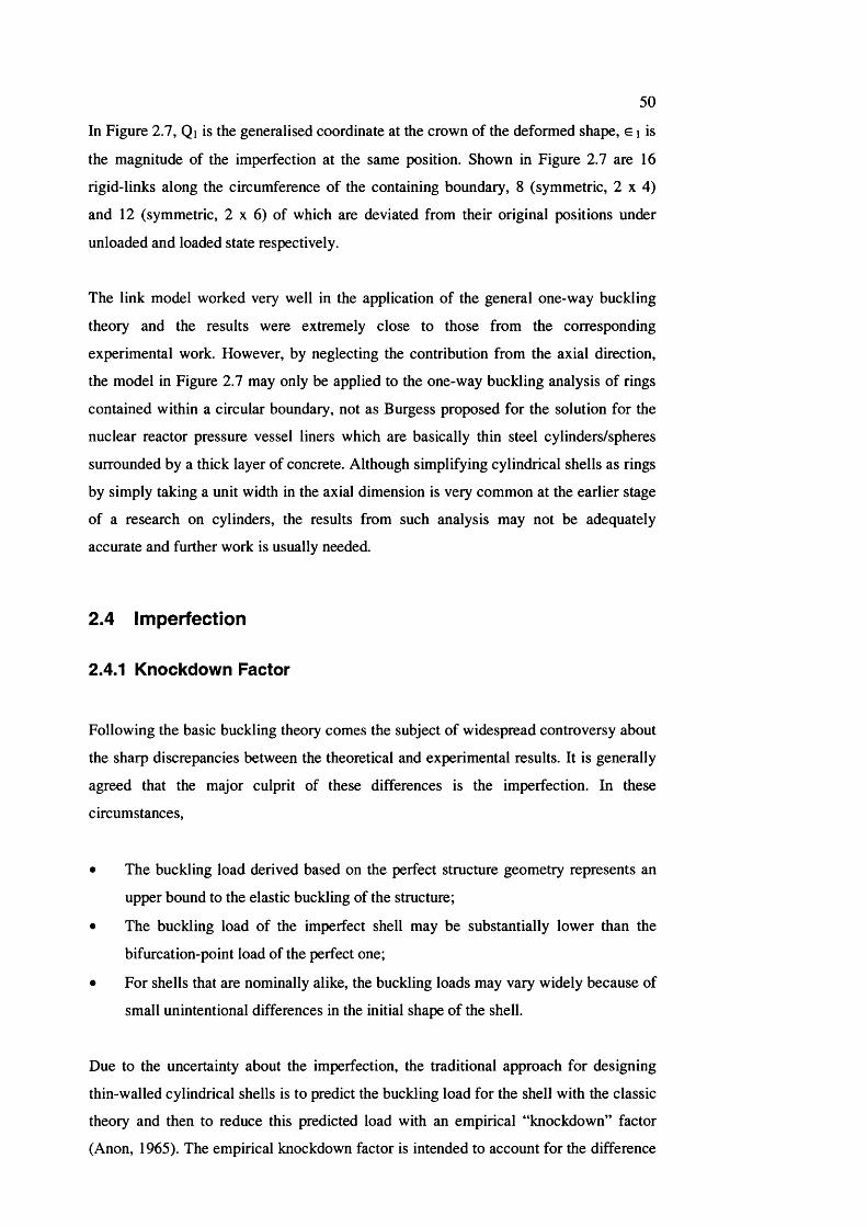
50

In Figure 2.7, Qi is the generalised coordinate at the crown of the deformed shape, g i is

the magnitude of the imperfection at the same position. Shown in Figure 2.7 are 16

rigid-links along the circumference of the containing boundary, 8 (symmetric, 2 x 4 )

and 12 (symmetric, 2 x 6) of which are deviated from their original positions under

unloaded and loaded state respectively.

The link model worked very well in the application of the general one-way buckling

theory and the results were extremely close to those from the corresponding

experimental work. However, by neglecting the contribution from the axial direction,

the model in Figure 2.7 may only be applied to the one-way buckling analysis of rings

contained within a circular boundary, not as Burgess proposed for the solution for the

nuclear reactor pressure vessel liners which are basically thin steel cylinders/spheres

surrounded by a thick layer of concrete. Although simplifying cylindrical shells as rings

by simply taking a unit width in the axial dimension is very common at the earlier stage

of a research on cylinders, the results from such analysis may not be adequately

accurate and further work is usually needed.

2.4 Im perfection

2.4.1 Knockdown Factor

Following the basic buckling theory comes the subject of widespread controversy about

the sharp discrepancies between the theoretical and experimental results. It is generally

agreed that the major culprit of these differences is the imperfection. In these

circumstances,

• The buckling load derived based on the perfect structure geometry represents an

upper bound to the elastic buckling of the structure;

• The buckling load of the imperfect shell may be substantially lower than the

bifurcation-point load of the perfect one;

• For shells that are nominally alike, the buckling loads may vary widely because of

small unintentional differences in the initial shape of the shell.

Due to the uncertainty about the imperfection, the traditional approach for designing

thin-walled cylindrical shells is to predict the buckling load for the shell with the classic

theory and then to reduce this predicted load with an empirical “knockdown” factor

(Anon, 1965). The empirical knockdown factor is intended to account for the difference

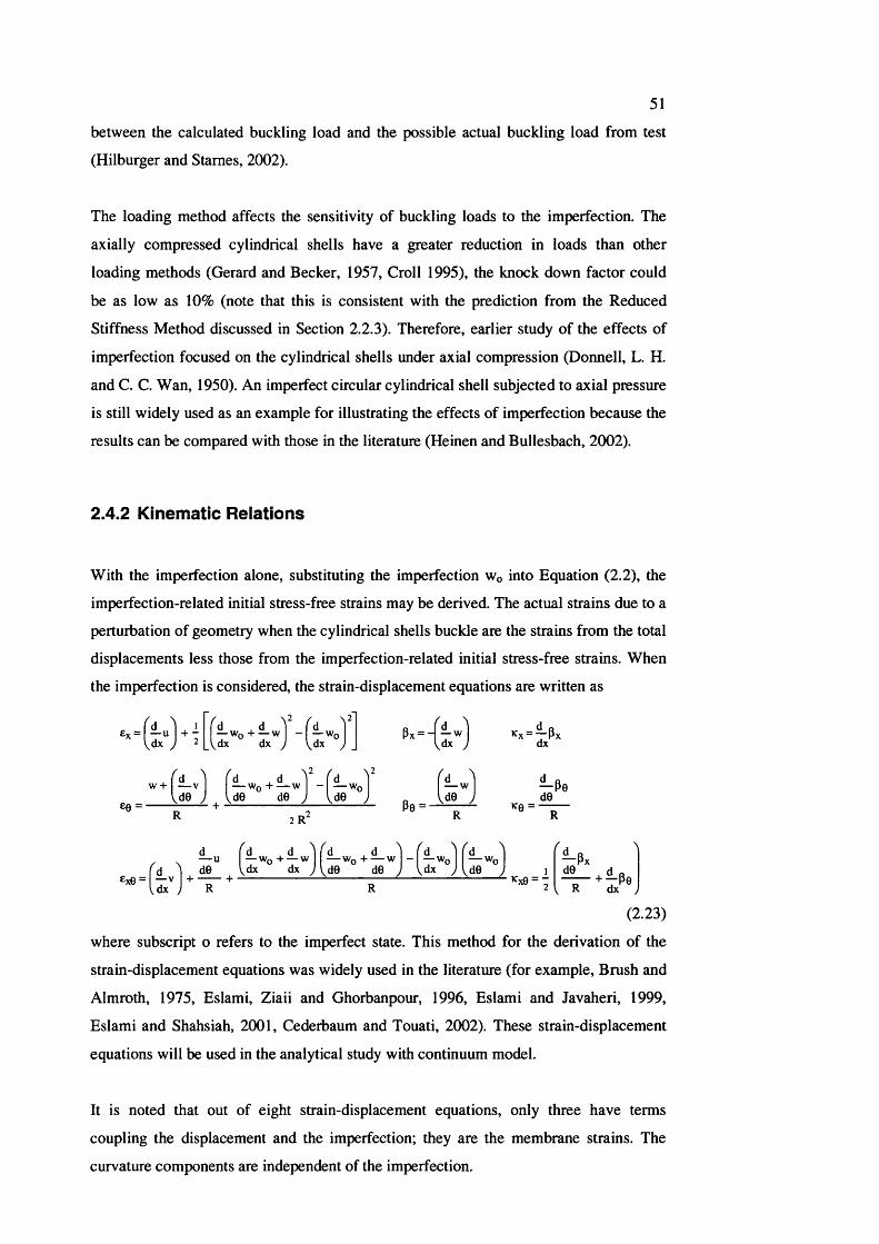
51

between the calculated buckling load and the possible actual buckling load from test

(Hilburger and Starnes, 2002).

The loading method affects the sensitivity of buckling loads to the imperfection. The

axially compressed cylindrical shells have a greater reduction in loads than other

loading methods (Gerard and Becker, 1957, Croll 1995), the knock down factor could

be as low as 10% (note that this is consistent with the prediction from the Reduced

Stiffness Method discussed in Section 2.2.3). Therefore, earlier study of the effects of

imperfection focused on the cylindrical shells under axial compression (Donnell, L. H.

and C. C. Wan, 1950). An imperfect circular cylindrical shell subjected to axial pressure

is still widely used as an example for illustrating the effects of imperfection because the

results can be compared with those in the literature (Heinen and Bullesbach, 2002).

2.4.2 Kinematic Relations

With the imperfection alone, substituting the imperfection Wo into Equation (2.2), the

imperfection-related initial stress-free strains may be derived. The actual strains due to a

perturbation of geometry when the cylindrical shells buckle are the strains from the total

displacements less those from the imperfection-related initial stress-free strains. When

the imperfection is considered, the strain-displacement equations are written as

d d Y fd Wq H w — Wqdx dx ) V dx

P x -- | I

W + f — Wo + — w l - 1 ^ — W o l w l — p 0ee= Uej ^Ue de J Ue J Ue J ,^_de

2 R R2R

------------------------- R-------------------------- "’«=2 V R dx )

(2.23)

where subscript o refers to the imperfect state. This method for the derivation of the

strain-displacement equations was widely used in the literature (for example. Brush and

Almroth, 1975, Eslami, Ziaii and Ghorbanpour, 1996, Eslami and Javaheri, 1999,

Eslami and Shahsiah, 2001, Cederbaum and Touati, 2002). These strain-displacement

equations will be used in the analytical study with continuum model.

It is noted that out of eight strain-displacement equations, only three have terms

coupling the displacement and the imperfection; they are the membrane strains. The

curvature components are independent of the imperfection.

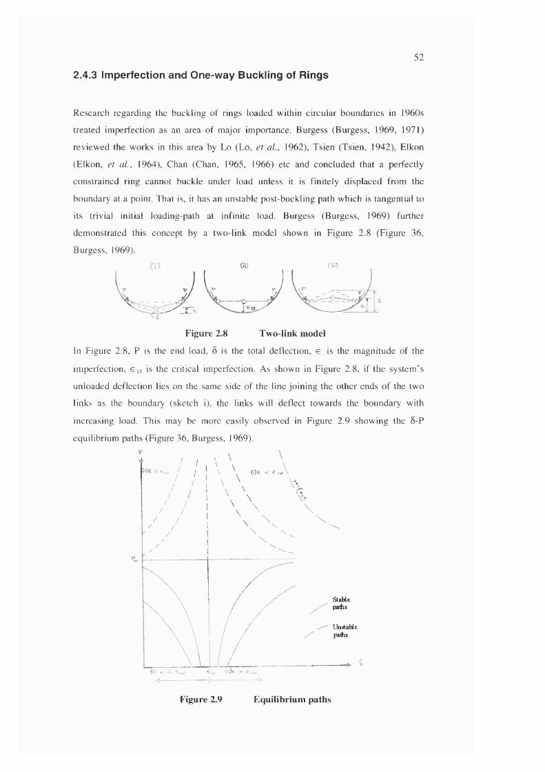
52

2.4.3 Imperfection and One-way Buckling of Rings

Research regarding the buckling of rings loaded within circular boundaries in 1960s

treated im perfection as an area of m ajor im portance. Burgess (Burgess, 1969, 1971)

review ed the works in this area by Lo (Lo, et a l , 1962), Tsien (Tsien, 1942), Elkon

(Elkon, et a l , 1964), Chan (Chan, 1965, 1966) etc and concluded that a perfectly

constrained ring cannot buckle under load unless it is finitely displaced from the

boundary at a point. That is, it has an unstable post-buckling path w hich is tangential to

its trivial initial loading-path at infinite load. Burgess (Burgess, 1969) further

dem onstrated this concept by a tw o-link model shown in Figure 2.8 (Figure 36,

Burgess, 1969).

!

------0

Figure 2.8 Two-link model

In Figure 2.8, P is the end load, 5 is the total deflection, e is the m agnitude of the

im perfection, € „ is the critical imperfection. As shown in Figure 2.8, if the system ’s

unloaded deflection lies on the same side o f the line jo in ing the o ther ends o f the two

links as the boundary (sketch i), the links will deflect tow ards the boundary with

increasing load. This may be more easily observed in Figure 2.9 show ing the Ô-P

equilibrium paths (Figure 36, Burgess, 1969).

StaUcpaths

Unstablepaths

— (>

Figure 2.9 Equilibrium paths

53

If the given imperfection is greater than the distance to the line between the opposite

ends of the two links (sketch iii in Figure 2.8) it will have a stable primary equilibrium

path as shown in the Ô-P equilibrium paths in Figure 2.9, tending to take the deflection

further away from the boundary with increasing load. If the given imperfection is equal

to the distance to the line between the opposite ends of the two links (sketch ii in Figure

2.8), it will bifurcate at a finite critical load.

While Burgess historically defined the importance of the magnitude of the imperfection

to the type of equilibrium path, he did not interpret the critical imperfection correctly

due to the limitation from the simplification of the cylindrical shells to rings. For

buckling into modes having an axial periodic form, the current research will show that

the critical imperfection does not correspond to the position when the free ends of the

two rigid-links are “flat”.

2.4.4 Recent Developments

2.4.4.1 Measurement of Imperfections

Early studies of the effects of the imperfections simply assumed an imperfection profile

based on personal intuition. Nowadays, people start to look at the imperfection in quite

a different way. Some researches have focused on actually measuring the imperfections

(for example, Wullschleger and Meyer-Piening, 2002).

The development of the techniques for measuring the geometric imperfections is traced

from the sixties to the present day (Singer and Abramovich, 1995). Now researchers are

even talking about international imperfection data banks (Abramovich, Singer and

Weller, 2002), which were established in order to facilitate the evaluation of the

imperfection measurements and correlation studies.

One of the earliest imperfection measurements is “maximum out-of-roundness” or

“ovality”. The “out-of-roundness” extracts only the magnitude of the geometric

imperfection and disregards its shape. By disregarding the shape of the imperfection,

information of prime importance is neglected.

From the late 1960s, complete and automated imperfection surveys were introduced.

Scanning devices such as reluctance-type and capacitance-type pickups with contact or

non-contact were developed. In the late 1970s, the extent of geometric imperfection

54

measurements greatly increased. A program of complete imperfection surveys of full-

scale shells was initiated by Arbocz and Babcock (Arbocz and Babcock, 1976).

The importance of measuring the imperfection was stressed by Singer and Abramovich

in their paper The Development of Shell Imperfection Measurement Techniques (Singer

and Abramovich, 1995). The argument is that if we do not know the imperfections and

the boundary conditions, we cannot improve our predictions of the buckling loads, no

matter how sophisticated our codes are and how large and fast our computers become.

Therefore, a large-scale international project was instigated to measure and test large

and small shells of different types of constructions, to record in a standard form and to

use the international imperfection data bank as an aid for the design of cylindrical

shells.

At the present stage of the current study, no appropriate data from measured

imperfection are available. However, observed imperfection profiles (see Figure 2.31)

will be considered for the selection of input for the imperfection profiles used in the

analytical and numerical analyses.

2.4.4.2 Random Imperfections

Accurate experimental measurement of imperfections, when incorporated into

theoretical analyses, allows precise prediction of the buckling loads for circular

cylindrical shells. This approach, however, is impractical for the prediction of the

buckling load of shells manufactured in normal production lines. The best one can hope

to do for these shells is to establish the characteristic initial imperfection distributions

which a given fabrication process is likely to produce, and then to combine this

information with some kind of statistical analysis of both the initial imperfections and

the corresponding critical loads, in a form of statistical imperfection-sensitivity analysis

(Arbocz and Hoi, 1995).

Arbocz pointed out that these kinds of characteristic initial imperfection distributions do

exist. For the given characteristic initial imperfection distribution, since initial

imperfections are obviously random in nature, some kind of stochastic stability analysis

is required. This is realized by reliability function. Elishakoff suggested utilizing the

Monte Carlo method to obtain the reliability function. To reduce the complexity of the

calculations, Arbocz replaced the Monte Carlo method by the first-order second-

moment method (Arbocz and Hoi, 1995).

55

The stochastic approach of buckling analysis with random imperfection requires the

following steps (Bielevicz and Gorski, 2002)

• Simulation of random variables or random fields describing the structure, its

loading and imperfections

• Solution of the structural problem for every realization of the simulation process

to create a set of results

• Statistical description of the results obtained

The stochastic approach for the random imperfection discussed here may be adopted for

the future buckling analysis for production line, lined-pipes.

2.4.4.3 Disturbance Energy and Imperfection Kinemates

Disturbance energy is an approach that, within the frame of a non-linear theory, looks

for a critical state of the stability-sensitive structure where the disturbance energy has

reached a minimum (Heinen, A. H., Bullesbach, J., 2002). Imperfection kinemates were

introduced as another unknown quantity in addition to the disturbance kinemates in

order to determine the amplitude of a type of imperfection that is most unfavourable to

the structure. In such an approach the Ljapunov criterion for stability is employed, so

that any fundamental motion state of imperfect shells can be put into them in order to

examine its kinetic stability. According to Ljapunov, the fundamental state of motion to

be examined for its stability is regarded as being kinetically stable if the value of the

vector of the disturbance-induced displacements does not exceed a specified tolerance

limit i.e. the disturbed neighbouring motion of the shell element remains near the

fundamental motion.

Disturbance energy and the imperfection kinemates approach offer a new way to

determine the worst imperfection. However, the methodology is quite new and needs

further verification, and is consequently inappropriate to adopt it for the current, first-

generation, one-way buckling analysis of pipeline liners.

2.5 B uckling of L iners

2.5.1 Tunnel Liners

This literature review reveals that many tunnel liner or similar buckling theories (for

56

example, Croll, 2001, Berti, et al, 1998, Fok, 2002) have been developed in the past. In

this section, some of the theories will be outlined.

2.5.1.1 Ring Buckling

References are found simplifying the tunnel liners as rings, an example of which was

presented by Croll (2001). Here, the lining material is concrete that was sprayed onto

the tunnel cavities as soon as practical after boring. The background of the research is

the collapse of the Heathrow Express Tunnel, where The New Austrian Tunnelling

Method was adopted to provide the necessary stiffness to prevent distortion and collapse

of tunnel cavities in soft ground tunnelling.

This ring buckling theory simplifies the tunnel liner as a ring restrained radially and

tangentially by an infinite surrounding elastic medium whose stiffness is taken into

account. An elastic analysis of critical pressures, after some simplification, is derived as

Pcr=3| ^

where y is a “soft ground tunnel buckling parameter”

24 r i

(2.24)

Y =(3 -U g) (i + gg)

(2.25)

where

Vg Eg VIUg - Kg - - M-i - Ki -

1 - Vg I - Vg -VI 1 -vi^

where:

E is Young’s Modulus,

V is Poisson’s ratio,

r is the mid-surface radius,

t is the thickness, and

subscripts g and 1 represent ground and liner respectively.

The above soft ground tunnel buckling parameter is a single composite parameter which

encapsulates all the relevant ground and liner geometric and material properties. It is

this closed-form analytical representation of elastic critical buckling that provides a

particularly convenient basis for predicting various elastic-plastic failure conditions.

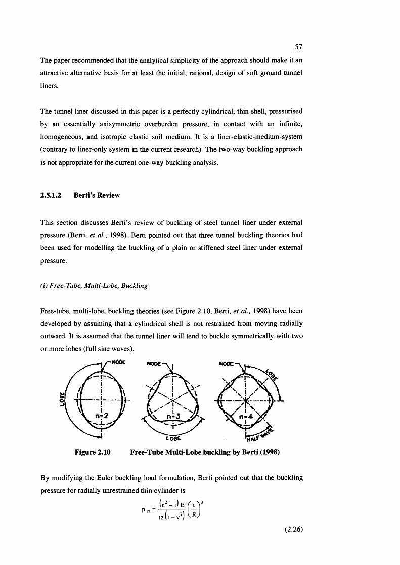
57

The paper recommended that the analytical simplicity of the approach should make it an

attractive alternative basis for at least the initial, rational, design of soft ground tunnel

liners.

The tunnel liner discussed in this paper is a perfectly cylindrical, thin shell, pressurised

by an essentially axisymmetric overburden pressure, in contact with an infinite,

homogeneous, and isotropic elastic soil medium. It is a liner-elastic-medium-system

(contrary to liner-only system in the current research). The two-way buckling approach

is not appropriate for the current one-way buckling analysis.

2.5.1.2 Berti’s Review

This section discusses Berti’s review of buckling of steel tunnel liner under external

pressure (Berti, et al, 1998). Berti pointed out that three tunnel buckling theories had

been used for modelling the buckling of a plain or stiffened steel liner under external

pressure.

(i) Free-Tube, Multi-Lobe, Buckling

Free-tube, multi-lobe, buckling theories (see Figure 2.10, Berti, et al, 1998) have been

developed by assuming that a cylindrical shell is not restrained from moving radially

outward. It is assumed that the tunnel liner will tend to buckle symmetrically with two

or more lobes (full sine waves).

HOOC

n -2

Figure 2.10 Free-Tube Multi-Lobe buckling by Berti (1998)

By modifying the Euler buckling load formulation, Berti pointed out that the buckling

pressure for radially unrestrained thin cylinder is

P cr “12 (l - V )

E I _t_

R

(2.26)

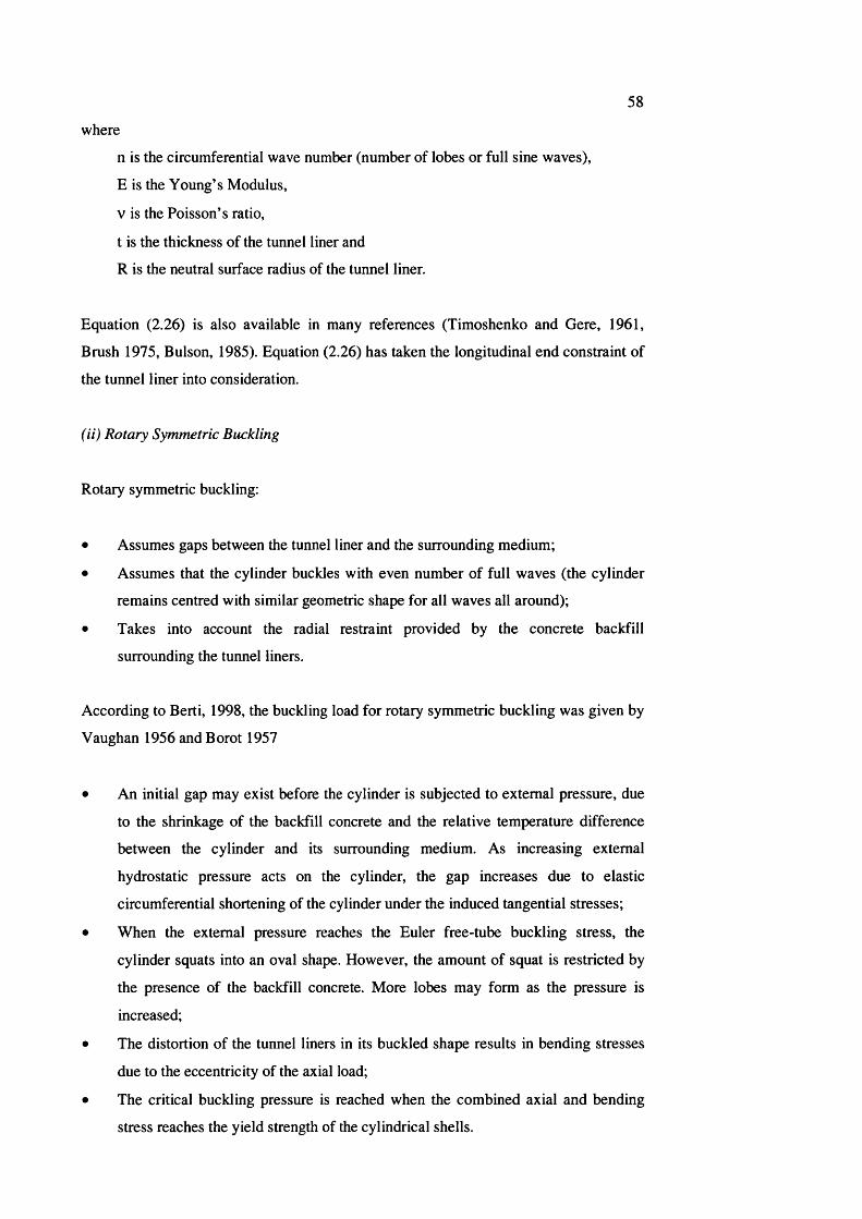
58

where

n is the circumferential wave number (number of lobes or full sine waves),

E is the Young’s Modulus,

V is the Poisson’s ratio,

t is the thickness of the tunnel liner and

R is the neutral surface radius of the tunnel liner.

Equation (2.26) is also available in many references (Timoshenko and Gere, 1961,

Brush 1975, Bulson, 1985). Equation (2.26) has taken the longitudinal end constraint of

the tunnel liner into consideration.

(ii) Rotary Symmetric Buckling

Rotary symmetric buckling:

• Assumes gaps between the tunnel liner and the surrounding medium;

• Assumes that the cylinder buckles with even number of full waves (the cylinder

remains centred with similar geometric shape for all waves all around);

• Takes into account the radial restraint provided by the concrete backfill

surrounding the tunnel liners.

According to Berti, 1998, the buckling load for rotary symmetric buckling was given by

Vaughan 1956 and Borot 1957

• An initial gap may exist before the cylinder is subjected to external pressure, due

to the shrinkage of the backfill concrete and the relative temperature difference

between the cylinder and its surrounding medium. As increasing external

hydrostatic pressure acts on the cylinder, the gap increases due to elastic

circumferential shortening of the cylinder under the induced tangential stresses;

• When the external pressure reaches the Euler free-tube buckling stress, the

cylinder squats into an oval shape. However, the amount of squat is restricted by

the presence of the backfill concrete. More lobes may form as the pressure is

increased;

• The distortion of the tunnel liners in its buckled shape results in bending stresses

due to the eccentricity of the axial load;

• The critical buckling pressure is reached when the combined axial and bending

stress reaches the yield strength of the cylindrical shells.

59

The critical buckling pressure for the rotary sym m etric buckling can be com puted by

solving a com plicated equation, which involves the gap ratio i.e. the ratio of the initial

gap to the radius o f the tunnel liner. The larger the gap ratio, the low er the buckling

tem perature.

(iii) Single-Lobe Buckling

Single-lobe buckling theory is sim ilar to the rotary sym m etric buckling theory except

that it assum es that when the liner buckles, a single buckled lobe develops with the rest

o f the liner resting on the surrounding m edium and feeding m aterial into the lobe, see

F igure 2.11 for illustration (Berti, et a i , 1998). This is actually a snap-through type

buckling. The critical buckling pressure form ulation is com plicated and the buckling

tem perature depends on the gap ratio.

Figure 2.11 Single-Lobe Buckling by Berti (1998)

All these three tunnel buckling theories reviewed by Berti (Berti et a l , 1998) either

com pletely ignores the constraint o f the surrounding m edium (w hich is apparently not

appropriate) or assum es gap betw een the liner and the medium (by exaggerating the

effect o f the gap the classical two-way buckling theory applies). This is appropriate for

the tunnel liners surrounded by elastic medium but not the case for the pipeline liners

surrounded by alm ost rigid outer pipes.

60

2.5.2 Liners in Pipeline Rehabilitation

2.5.2.1 Bonding in the Pipeline Rehabilitation

There is a large quantity of reported work on the buckling of pipeline rehabilitation

liners (B akeer et a i , 2001). Liners in pipeline rehabilitation are usually non-m etallic

and they are usually not fully bonded to the host pipes. The design o f liners in the

pipeline rehabilitation may consider the following three scenarios (B akeer et a l , 1999)

• No bond exists between the liner and the host pipe, or no structural im provem ent

is introduced by the grout between the liner and the host pipe;

• A perfect bond exists between the liner and the host pipe and the two pipes w ould

then work together as a com posite structure;

• The liner pipe has sufficient rigidity to act independently. Any additional support

provided by grouting or the host pipe would further enhance the liner’s load-

bearing capacity.

2.5.2.2 Chunduru’s Work

A ccording to Chunduru (Chunduru et a l , 1996), pipeline rehabilitation liners usually do

not adhere or bond to the host pipes and field installations are typically not continuously

grouted, see Figure 2.12 for the field installation process (Chunduru, et a l , 1996).

U-Powit -Tar

BE F O R EDEFORMING

r t r t

<b) A F T E Rd e f o r m in g

(C l FORMATION IN THE F I E L D

THICKNESS, t

OD

«D C IR C U L A R RING UNDER P L A N E S T R E S S C O N D I T I O N

Figure 2.12 Figure 1 of Chunduru s work -U liner formation

A ccordingly, a pipe rehabilitation liner should be designed to sustain the applied loads

on its own, even though a cracked host pipe would still provide additional resistance

and confinem ent. Chunduru suggested that the buckling load for such rehabilitation

pipeline liners is

61

2 E O a (3Per® / 2\ 3

i l - V J-SDR-FS

(2.27)

where

per is the critical buckling pressure or equivalent water head pressure,

E is the time-dependent modulus of elasticity,

C is the reduction factor to account for liner ovality,

a is the lining factor;

P is the stress concentration factor;

V is Poisson’s ratio,

SDR is the standard dimension ratio, and

FS is the factor of safety.

The SDR is an industry standard that defines the required minimum thickness of a pipe

wall t as a function of its nominal diameter D

S D R = ^ - ,t

(2.28)

where ODavg is the average outer diameter, t is the liner wall thickness.

Bakeer et al. (1999) verified that the buckling pressures of rehabilitation pipelines in

Equation (2.27) were within 15% of their measured value by experimental work.

The research on non-metallic pipeline rehabilitation liners focuses on not only the

initiation of the buckling but also the subsequent growth/growth rate of the buckled

lobes due to the creep of the material. For the initiation of the buckling, like the work by

Chunduru et al. (1996) discussed in this section, they tend to just adapt the classical

buckling load of free shells under external pressure to the needs of one-way buckling.

This is realized by various factors and coefficients supported by experimental work.

However, the factors and coefficients derived in this way are project-specific and

therefore not applicable to sub-sea pipeline liners.

2.5.3 Liners in Nuciear Power Plant

2.5.3.1 Fan, Fu and Fang’s Work

Researchers in Tsinghua (Qinghua) University published a series of papers regarding

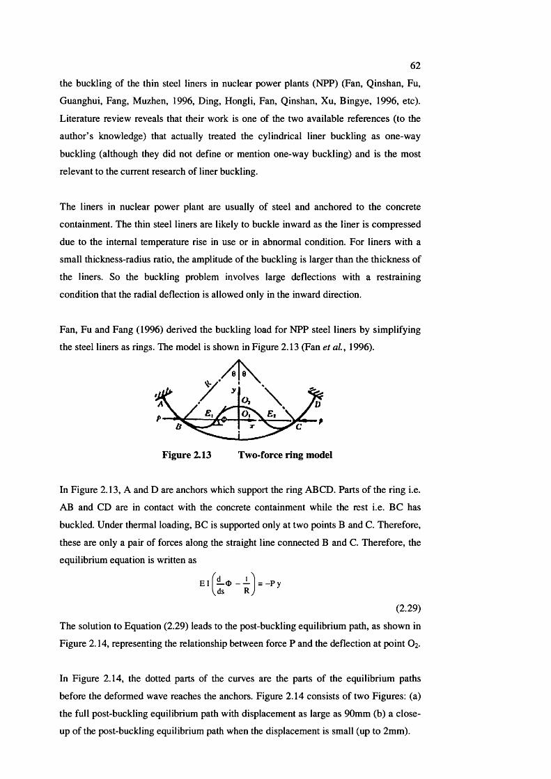
62

the buckling of the thin steel liners in nuclear power plants (NPP) (Fan, Qinshan, Fu,

Guanghui, Fang, Muzhen, 1996, Ding, Hongli, Fan, Qinshan, Xu, Bingye, 1996, etc).

Literature review reveals that their work is one of the two available references (to the

author’s knowledge) that actually treated the cylindrical liner buckling as one-way

buckling (although they did not define or mention one-way buckling) and is the most

relevant to the current research of liner buckling.

The liners in nuclear power plant are usually of steel and anchored to the concrete

containment. The thin steel liners are likely to buckle inward as the liner is compressed

due to the internal temperature rise in use or in abnormal condition. For liners with a

small thickness-radius ratio, the amplitude of the buckling is larger than the thickness of

the liners. So the buckling problem involves large deflections with a restraining

condition that the radial deflection is allowed only in the inward direction.

Fan, Fu and Fang (1996) derived the buckling load for NPP steel liners by simplifying

the steel liners as rings. The model is shown in Figure 2.13 (Fan et a l, 1996).

Figure 2.13 Two-force ring model

In Figure 2.13, A and D are anchors which support the ring ABCD. Parts of the ring i.e.

AB and CD are in contact with the concrete containment while the rest i.e. BC has

buckled. Under thermal loading, BC is supported only at two points B and C. Therefore,

these are only a pair of forces along the straight line connected B and C. Therefore, the

equilibrium equation is written as

E l l — O = —P yds R y

(2.29)

The solution to Equation (2.29) leads to the post-buckling equilibrium path, as shown in

Figure 2.14, representing the relationship between force P and the deflection at point 0%.

In Figure 2.14, the dotted parts of the curves are the parts of the equilibrium paths

before the deformed wave reaches the anchors. Figure 2.14 consists of two Figures: (a)

the full post-buckling equilibrium path with displacement as large as 90mm (b) a close-

up of the post-buckling equilibrium path when the displacement is small (up to 2mm).

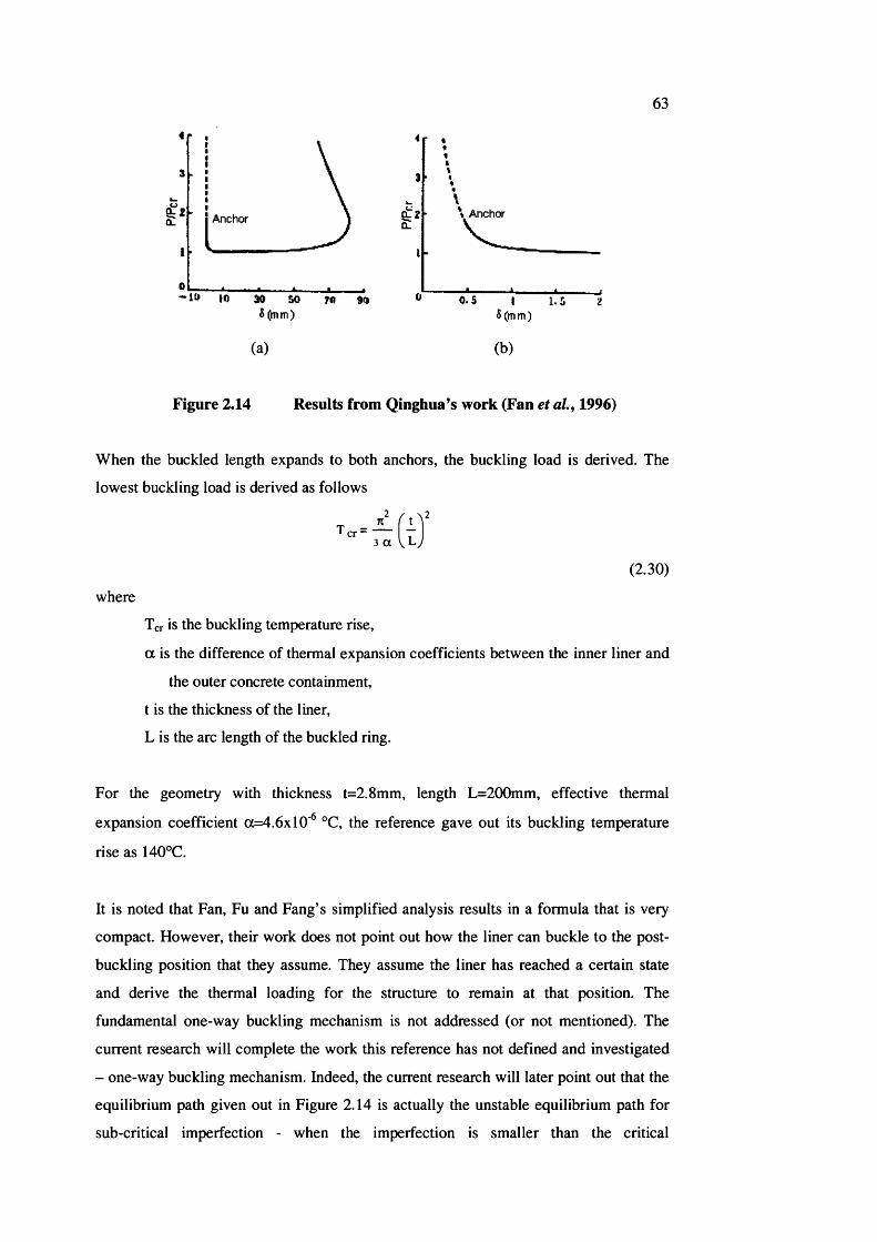
63

Anchor % Anchor0,2

1.5

(a) (b)

Figure 2.14 Results from Qinghua’s work (Fan et ah, 1996)

When the buckled length expands to both anchors, the buckling load is derived. The

lowest buckling load is derived as follows

T r r =

(2.30)

where

Ter is the buckling temperature rise,

a is the difference of thermal expansion coefficients between the inner liner and

the outer concrete containment,

t is the thickness of the liner,

L is the arc length of the buckled ring.

For the geometry with thickness t=2.8mm, length L=200mm, effective thermal

expansion coefficient 0=4.6x10^ °C, the reference gave out its buckling temperature

rise as 140°C.

It is noted that Fan, Fu and Fang’s simplified analysis results in a formula that is very

compact. However, their work does not point out how the liner can buckle to the post-

buckling position that they assume. They assume the liner has reached a certain state

and derive the thermal loading for the structure to remain at that position. The

fundamental one-way buckling mechanism is not addressed (or not mentioned). The

current research will complete the work this reference has not defined and investigated

- one-way buckling mechanism. Indeed, the current research will later point out that the

equilibrium path given out in Figure 2.14 is actually the unstable equilibrium path for

sub-critical imperfection - when the imperfection is smaller than the critical

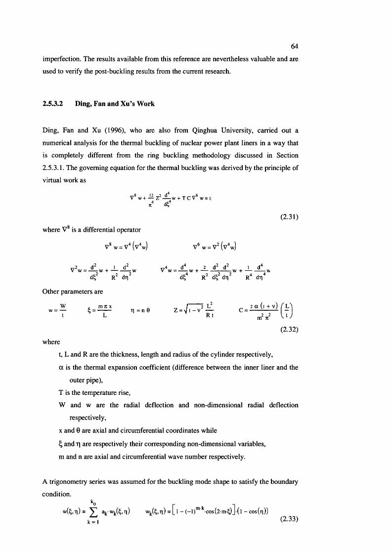
64

imperfection. The results available from this reference are nevertheless valuable and are

used to verify the post-buckling results from the current research.

2.S.3.2 Ding, Fan and Xu’s Work

Ding, Fan and Xu (1996), who are also from Qinghua University, carried out a

numerical analysis for the thermal buckling of nuclear power plant liners in a way that

is completely different from the ring buckling methodology discussed in Section

2.5.3.1. The governing equation for the thermal buckling was derived by the principle of

virtual work as

V* w + — + T C w = 0

71

(2.31)

where V* is a differential operator

(v w) V % = (v' w)

V^w = - ^ w + V " ^ w = - ^ w + — X ; - ^ w + — — w dTl d d dTl R dll'*

Other parameters are

t L Rt U

(2.32)

where

t, L and R are the thickness, length and radius of the cylinder respectively,

a is the thermal expansion coefficient (difference between the inner liner and the

outer pipe),

T is the temperature rise,

W and w are the radial deflection and non-dimensional radial deflection

respectively,

X and 0 are axial and circumferential coordinates while

^ and r\ are respectively their corresponding non-dimensional variables,

m and n are axial and circumferential wave number respectively.

A trigonometry series was assumed for the buckling mode shape to satisfy the boundary

condition.p -|

w f e h ) = V aj -Wjj( ,Ti) wj^( ,Ti) = - (-1)"* *^-cos(2-n>^J-(l-cos(ti))k t i (2.33)

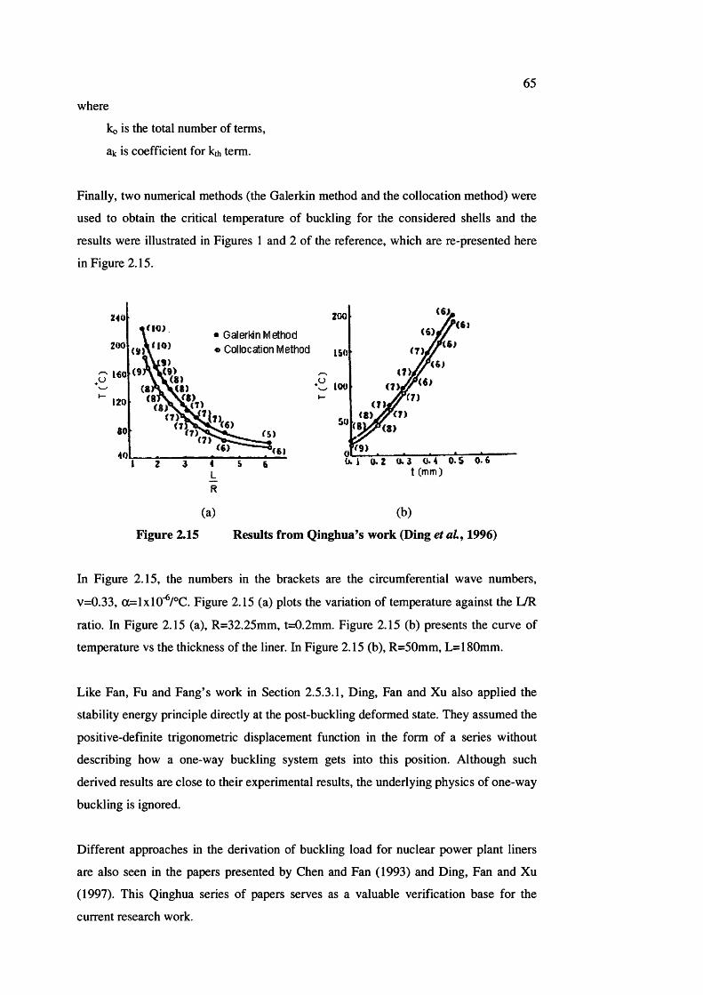
65

where

ko is the total number of terms,

aic is coefficient for ko, term.

Finally, two numerical methods (the Galerkin method and the collocation method) were

used to obtain the critical temperature of buckling for the considered shells and the

results were illustrated in Figures 1 and 2 of the reference, which are re-presented here

in Figure 2.15.

ZOO

L«0

120

<0

40

G alerhin Method

4 & 6

R

'<61

ISO

(6)w 100 ( 7 )j

(S )(8)

t (mm)

(a) (b)

Figure 2.15 Results from Qinghua’s work (Ding et a l, 1996)

In Figure 2.15, the numbers in the brackets are the circumferential wave numbers,

v=0.33, a=lxlO'^/°C. Figure 2.15 (a) plots the variation of temperature against the L/R

ratio. In Figure 2.15 (a), R=32.25mm, t=0.2mm. Figure 2.15 (b) presents the curve of

temperature vs the thickness of the liner. In Figure 2.15 (b), R=50mm, L=180mm.

Like Fan, Fu and Fang’s work in Section 2.5.3.1, Ding, Fan and Xu also applied the

stability energy principle directly at the post-buckling deformed state. They assumed the

positive-definite trigonometric displacement function in the form of a series without

describing how a one-way buckling system gets into this position. Although such

derived results are close to their experimental results, the underlying physics of one-way

buckling is ignored.

Different approaches in the derivation of buckling load for nuclear power plant liners

are also seen in the papers presented by Chen and Fan (1993) and Ding, Fan and Xu

(1997). This Qinghua series of papers serves as a valuable verification base for the

current research work.

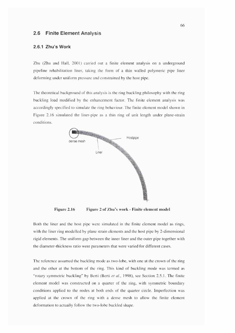
66

2.6 Finite E lem ent A nalysis

2.6.1 Zhu’s Work

Zhu (Zhu and Hall, 2001) carried out a finite elem ent analysis on a underground

pipeline rehabilitation liner, taking the form of a thin w alled polym eric pipe liner

deform ing under uniform pressure and constrained by the host pipe.

The theoretical background of this analysis is the ring buckling philosophy with the ring

buckling load m odified by the enhancem ent factor. The finite elem ent analysis was

accordingly specified to sim ulate the ring behaviour. The finite elem ent model shown in

Figure 2.16 sim ulated the liner-pipe as a thin ring o f unit length under plane-strain

conditions.

Hostpiped en se mesh

Liner

Figure 2.16 Figure 2 of Zhu’s work - Finite element model

Both the liner and the host pipe were sim ulated in the finite elem ent model as rings,

w ith the liner ring m odelled by plane strain elem ents and the host pipe by 2-dim ensional

rigid elem ents. The uniform gap between the inner liner and the outer pipe together with

the diam eter-thickness ratio were param eters that were varied for different cases.

The reference assum ed the buckling mode as two-lobe, with one at the crow n o f the ring

and the o ther at the bottom o f the ring. This kind o f buckling m ode was term ed as

“ rotary sym m etric buckling” by Berti (Berti et a i , 1998), see Section 2.5.1. The finite

elem ent model was constructed on a quarter o f the ring, with sym m etric boundary

conditions applied to the nodes at both ends of the quarter circle. Im perfection was

applied at the crow n of the ring with a dense m esh to allow the finite elem ent

deform ation to actually follow the two-lobe buckled shape.

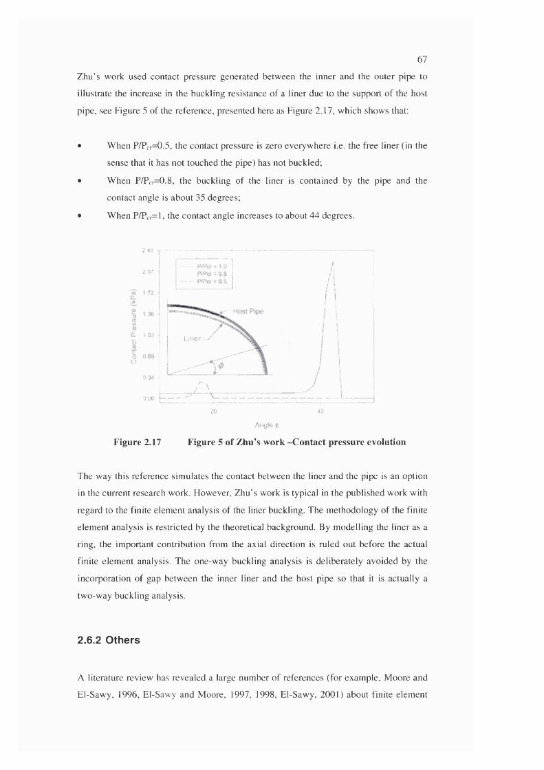
67

Z hu’s work used contact pressure generated betw een the inner and the outer pipe to

illustrate the increase in the buckling resistance o f a liner due to the support o f the host

pipe, see Figure 5 o f the reference, presented here as Figure 2.17, which shows that:

• W hen P/Pcr=0.5, the contact pressure is zero everyw here i.e. the free liner (in the

sense that it has not touched the pipe) has not buckled;

• W hen P/Pcr=0.8, the buckling o f the liner is contained by the pipe and the

contact angle is about 35 degrees;

• W hen P/Pcr=l, the contact angle increases to about 44 degrees.

o

2 0 /

t 03 Liner ^

rU.txi

20 40

.\ngie $

Figure 2.17 Figure 5 of Zhu’s work -Contact pressure evolution

The way this reference sim ulates the contact between the liner and the pipe is an option

in the current research work. However, Z hu’s work is typical in the published work with

regard to the finite elem ent analysis o f the liner buckling. The m ethodology o f the finite

elem ent analysis is restricted by the theoretical background. By m odelling the liner as a

ring, the im portant contribution from the axial direction is ruled out before the actual

finite elem ent analysis. The one-way buckling analysis is deliberately avoided by the

incorporation o f gap betw een the inner liner and the host pipe so that it is actually a

tw o-w ay buckling analysis.

2.6.2 Others

A literature review has revealed a large num ber o f references (for exam ple, M oore and

El-Saw y, 1996, El-Sawy and M oore, 1997, 1998, El-Saw y, 2001) about finite elem ent

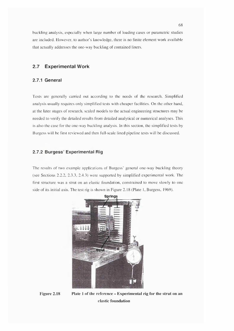
68

buckling analysis, especially when large num ber o f loading cases or param etric studies

are included. However, to author’s know ledge, there is no finite elem ent work available

that actually addresses the one-way buckling of contained liners.

2.7 E xperim ental W ork

2.7.1 General

Tests are generally carried out according to the needs o f the research. Sim plified

analysis usually requires only sim plified tests with cheaper facilities. On the other hand,

at the later stages of research, scaled m odels to the actual engineering structures may be

needed to verify the detailed results from detailed analytical or num erical analyses. This

is also the case for the one-way buckling analysis. In this section, the sim plified tests by

Burgess will be first review ed and then full-scale lined pipeline tests will be discussed.

2.7.2 B urgess’ Experimental Rig

The results o f two exam ple applications of B urgess’ general one-w ay buckling theory

(see Sections 2.2.2, 2.3.3, 2.4.3) were supported by sim plified experim ental work. The

first structure was a strut on an elastic foundation, constrained to move slowly to one

side of its initial axis. The test rig is shown in Figure 2.18 (Plate 1, Burgess, 1969).

Springs

Figure 2.18 Plate 1 of the reference - Experimental rig for the strut on an

elastic foundation

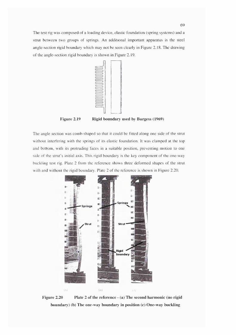
69

T he test rig was com posed of a loading device, elastic foundation (spring system s) and a

strut between two groups of springs. An additional im portant apparatus is the steel

angle-section rigid boundary which may not be seen clearly in F igure 2.18. The draw ing

o f the angle-section rigid boundary is show n in Figure 2.19.

Figure 2.19 Rigid boundary used by Burgess (1969)

The angle section was com b-shaped so that it could be fitted along one side of the strut

w ithout interfering with the springs o f its elastic foundation. It was clam ped at the top

and bottom , with its protruding faces in a suitable position, preventing m otion to one

side of the stru t’s initial axis. This rigid boundary is the key com ponent o f the one-w ay

buckling test rig. Plate 2 from the reference shows three deform ed shapes o f the strut

with and w ithout the rigid boundary. Plate 2 o f the reference is show n in Figure 2.20.

' Springs

» Strut

-J

Springs

Strut

Rigid boundary

V -;

Figure 2.20 Plate 2 of the reference - (a) The second harmonic (no rigid

boundary) (b) The one-way boundary in position (c) One-way buckling

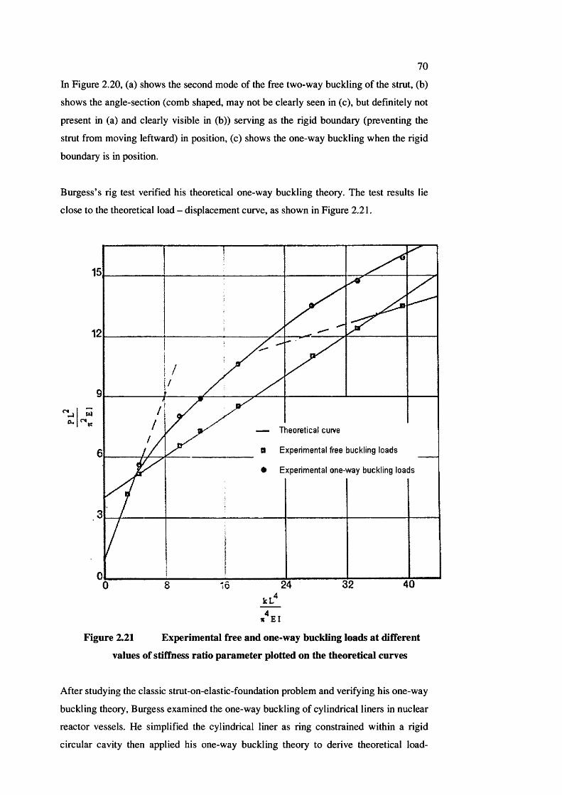
70

In Figure 2.20, (a) shows the second mode of the free two-way buckling of the strut, (b)

shows the angle-section (comb shaped, may not be clearly seen in (c), but definitely not

present in (a) and clearly visible in (b)) serving as the rigid boundary (preventing the

strut from moving leftward) in position, (c) shows the one-way buckling when the rigid

boundary is in position.

Burgess’s rig test verified his theoretical one-way buckling theory. The test results lie

close to the theoretical load - displacement curve, as shown in Figure 2.21,

CM

T h e o re t i c a l curve

E x p e r im e n ta l f ree b u ck l in g l o a d s

E x p e r im e n ta l o n e - w a y b u ck l in g l o a d s

4kL

/ e i

Figure 2.21 Experimental free and one-way buckling loads at different

values of stiffness ratio parameter plotted on the theoretical curves

After studying the classic strut-on-elastic-foundation problem and verifying his one-way

buckling theory, Burgess examined the one-way buckling of cylindrical liners in nuclear

reactor vessels. He simplified the cylindrical liner as ring constrained within a rigid

circular cavity then applied his one-way buckling theory to derive theoretical load-

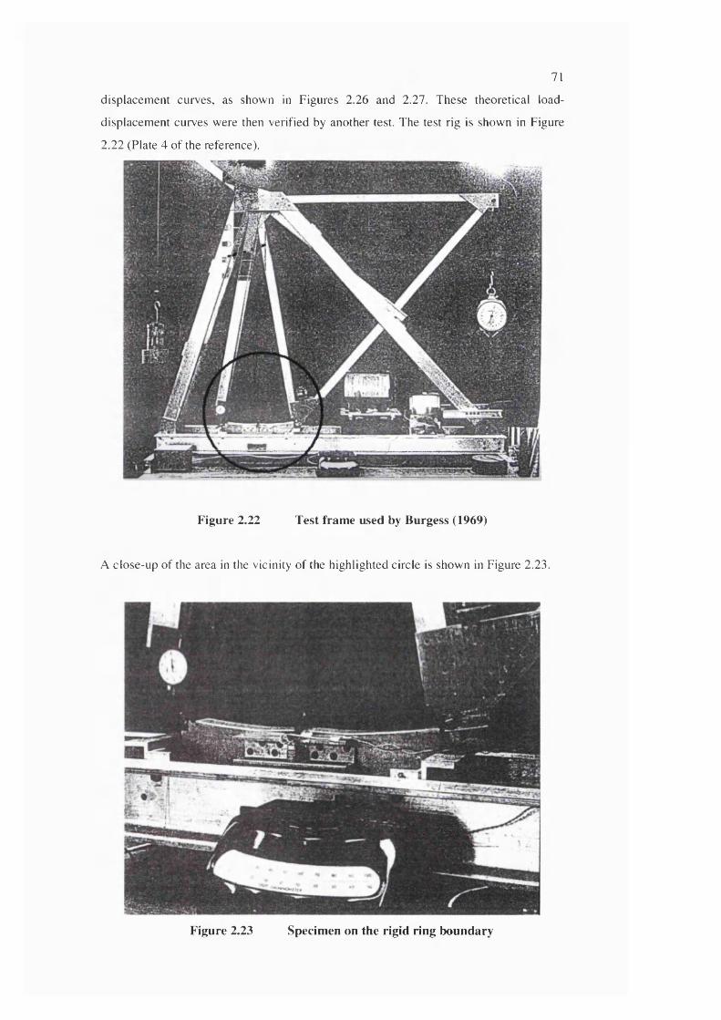
71

displacem ent curves, as shown in Figures 2.26 and 2.27. These theoretical load-

displacem ent curves were then verified by another test. The test rig is show n in Figure

2.22 (Plate 4 o f the reference).

Figure 2.22 Test frame used by Burgess (1969)

A close-up of the area in the vicinity of the highlighted circle is shown in Figure 2.23.

■ '

Figure 2.23 Specimen on the rigid ring boundary

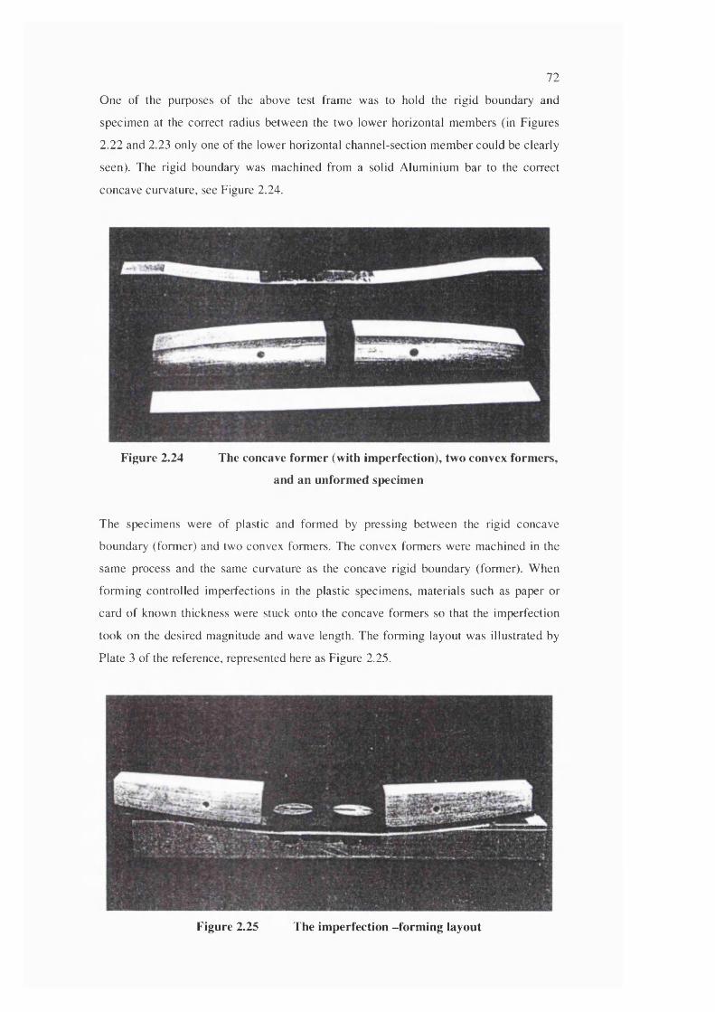
72

O ne of the purposes o f the above test fram e was to hold the rigid boundary and

specim en at the correct radius between the two low er horizontal m em bers (in Figures

2 .22 and 2.23 only one of the lower horizontal channel-section m em ber could be clearly

seen). The rigid boundary was m achined from a solid A lum inium bar to the correct

concave curvature, see Figure 2.24.

Figure 2.24 The concave former (with imperfection), two convex formers,

and an unformed specimen

T he specim ens were of plastic and form ed by pressing betw een the rigid concave

boundary (form er) and two convex formers. The convex form ers w ere m achined in the

sam e process and the same curvature as the concave rigid boundary (form er). W hen

form ing controlled im perfections in the plastic specim ens, m aterials such as paper or

card o f known thickness were stuck onto the concave form ers so that the im perfection

took on the desired m agnitude and wave length. The form ing layout was illustrated by

P late 3 of the reference, represented here as Figure 2.25.

Figure 2.25 The imperfection -forming layout

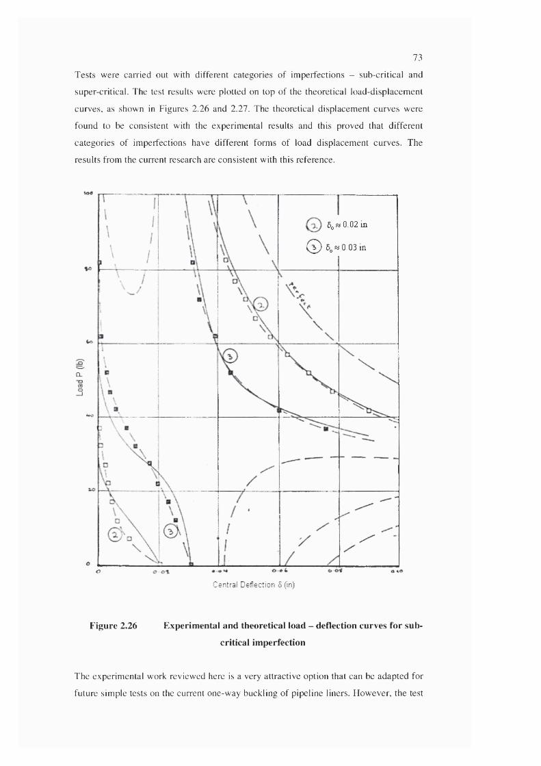
73

Tests were carried out with different categories of imperfections - sub-critical and

super critical. The test results were plotted on top of the theoretical load-displacement

curves, as shown in Figures 2.26 and 2.27. The theoretical displacement curves were

found to be consistent with the experimental results and this proved that different

categories of imperfections have different forms of load displacement curves. The

results from the current research are consistent with this reference.

ÔqW 0.02 in

@ 5^ « 0 . 0 3 in

CL

**c

OCentral Deflection 6 (in)

Figure 2.26 Experimental and theoretical load - deflection curves for sub-

critical imperfection

The experimental work reviewed here is a very attractive option that can be adapted for

future simple tests on the current one-way buckling of pipeline liners. However, the test

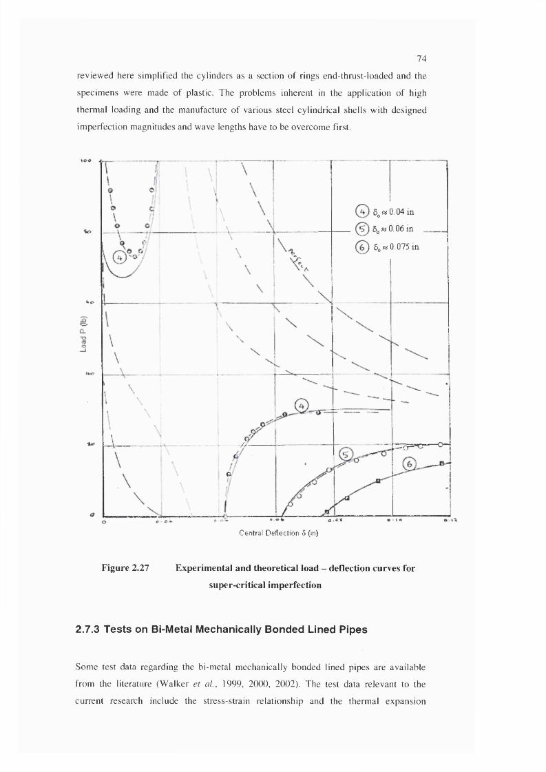
74

review ed here sim plified the cylinders as a section of rings end-thrust-loaded and the

specim ens were made o f plastic. The problem s inherent in the application of high

therm al loading and the m anufacture o f various steel cylindrical shells with designed

im perfection m agnitudes and wave lengths have to be overcom e first.

5 w 0.04 in

5<, M 0.06 in

6o K 0.075 in

// .—a —

€i

o .«YCentral D eflection 5 (in)

Figure 2.27 Experimental and theoretical load - deflection curves for

super critical imperfection

2.7.3 T ests on Bi-Metal Mechanically Bonded Lined Pipes

Som e test data regarding the bi-m etal m echanically bonded lined pipes are available

from the literature (W alker et a i , 1999, 2000, 2002). The test data relevant to the

current research include the stress-strain relationship and the therm al expansion

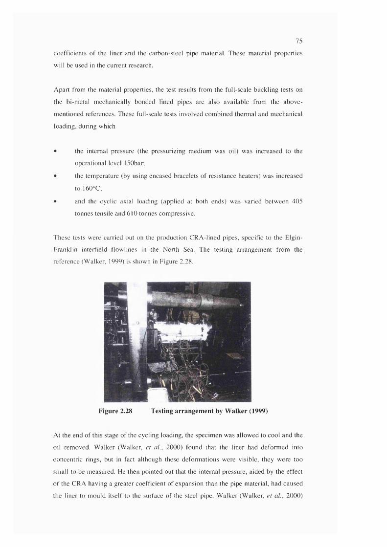
75

coefficients of the liner and the carbon-steel pipe material. These material properties

will be used in the current research.

Apart from the material properties, the test results from the full-scale buckling tests on

the bi-metal mechanically bonded lined pipes are also available from the above-

mentioned references. These full-scale tests involved combined thermal and mechanical

loading, during which

• the internal pressure (the pressurizing medium was oil) was increased to the

operational level I50bar;

• the temperature (by using encased bracelets of resistance heaters) was increased

to I60°C;

• and the cyclic axial loading (applied at both ends) was varied between 405

tonnes tensile and 610 tonnes compressive.

These tests were carried out on the production CRA-lined pipes, specific to the Elgin-

Franklin interfield flowlines in the North Sea. The testing arrangement from the

reference (Walker, 1999) is shown in Figure 2.28.

Figure 2.28 Testing arrangement by Walker (1999)

At the end of this stage of the cycling loading, the specimen was allowed to cool and the

oil removed. Walker (Walker, et ai, 2000) found that the liner had deformed into

concentric rings, but in fact although these deformations were visible, they were too

small to be measured. He then pointed out that the internal pressure, aided by the effect

of the CRA having a greater coefficient of expansion than the pipe material, had caused

the liner to mould itself to the surface of the steel pipe. Walker (Walker, et al, 2000)

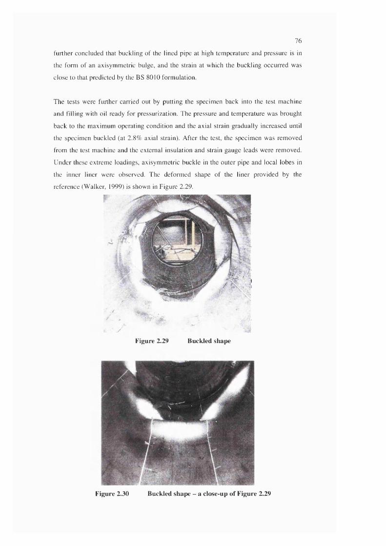
76

further concluded that buckling of the lined pipe at high temperature and pressure is in

the form of an axisymmetric bulge, and the strain at which the buckling occurred was

close to that predicted by the BS 8010 formulation.

The tests were further carried out by putting the specimen back into the test machine

and filling with oil ready for pressurization. The pressure and temperature was brought

back to the maximum operating condition and the axial strain gradually increased until

the specimen buckled (at 2.8% axial strain). After the test, the specimen was removed

from the test machine and the external insulation and strain gauge leads were removed.

Under these extreme loadings, axisymmetric buckle in the outer pipe and local lobes in

the inner liner were observed. The deformed shape of the liner provided by the

reference (Walker. 1999) is shown in Figure 2.29.

s

yFigure 2.29 Buckled shape

Figure 2.30 Buckled shape - a close-up of Figure 2.29

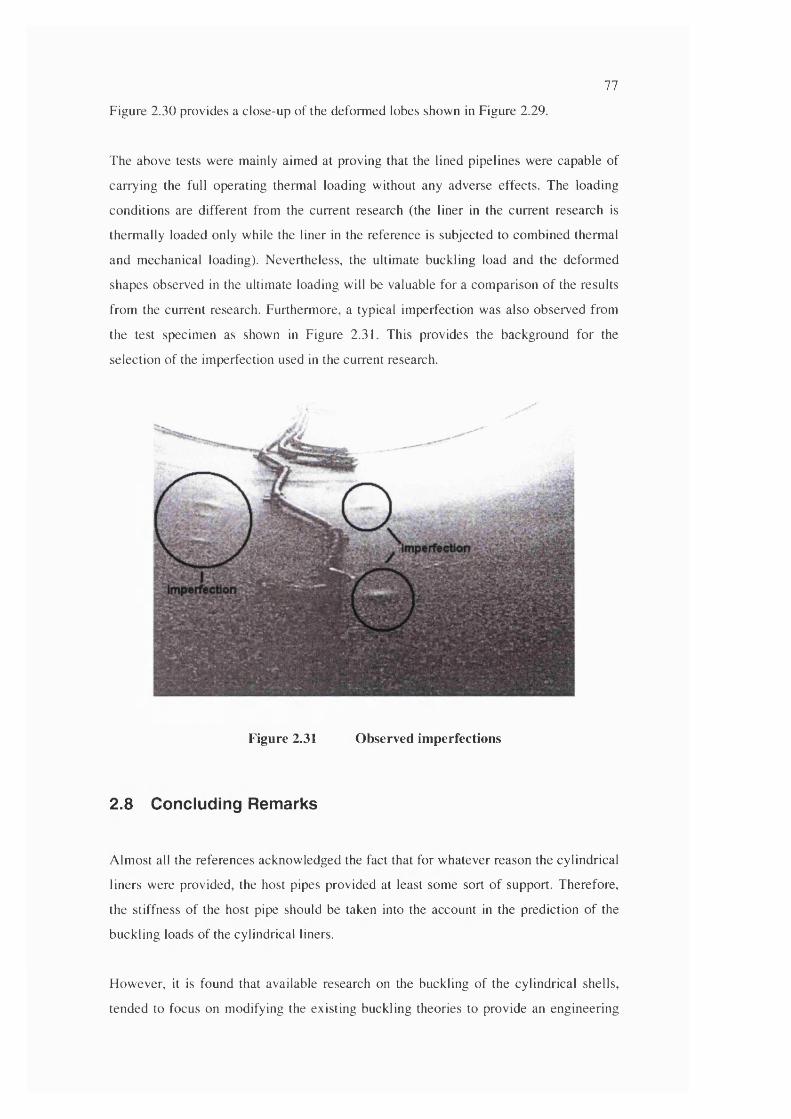
77

Figure 2.30 provides a close-up of the deform ed lobes shown in Figure 2.29.

The above tests were mainly aim ed at proving that the lined pipelines were capable of

carrying the full operating therm al loading w ithout any adverse effects. The loading

conditions are different from the current research (the liner in the current research is

therm ally loaded only while the liner in the reference is subjected to com bined therm al

and m echanical loading). N evertheless, the ultim ate buckling load and the deform ed

shapes observed in the ultim ate loading will be valuable for a com parison o f the results

from the current research. Furtherm ore, a typical im perfection was also observed from

the test specim en as shown in Figure 2.31. This provides the background for the

selection o f the im perfection used in the current research.

Figure 2.31 Observed imperfections

2.8 C oncluding R em arks

A lm ost all the references acknow ledged the fact that for w hatever reason the cylindrical

liners were provided, the host pipes provided at least som e sort o f support. Therefore,

the stiffness o f the host pipe should be taken into the account in the prediction o f the

buckling loads of the cylindrical liners.

H ow ever, it is found that available research on the buckling o f the cylindrical shells,

tended to focus on m odifying the existing buckling theories to provide an engineering

78

solution. The buckling behaviour of the cylindrical liners was considered the same as

that in free cylindrical shells except that the host pipes provided some form of restraint.

Because of the extra stiffness from the host pipes, it is generally agreed that the existing

buckling load formula should be modified to account for the increase of resistance due

to the stiffening. The most common method of accounting for the extra stiffness from

the host pipes is by adding extra coefficients such as those in Equation (2.27).

Some researchers devoted themselves to developing formulas exclusively for the

buckling of cylindrical shells. However, in the process, the basic buckling mechanism

was ignored. General buckling theories and methodologies such as stationary total

potential energy principle, stationary second variation of total potential energy principle,

virtual work principle, Rayleigh-Ritz and Galerkin methods were directly used with the

assumed deflection that actually was post-buckling displacement. The initiation of the

buckling was generally ignored.

Another available one-way buckling theory, however, has so far been applied to just

discrete generalised coordinate systems, and its application has been limited as the

number of discrete generalised coordinates increases.

It would appear that none of the available solution is able to account fully for the

observed one-way buckling of pipeline liners. To better understand the mechanism, the

buckling of restrained cylindrical liners will be the main aim of this thesis.

79

3 Buckling Analysis with Simplified Rigid-Link Model

3.1 In troduction

This chapter describes the analytical results from a simplified, rigid-link model,

designed to simulate the restrained buckling of pipeline liners. As shown in Figures 1.2

and 1.3, pipeline liners are composed of circular cylindrical inner liners and outer pipes,

with the latter providing constraint to the former. The liners are prone to deform inward

under thermally-induced compression due to the confinement from the pipes in the

longitudinal and radial directions. In this chapter, the inner liners will be simplified as

rigid-links while the outer pipe will be assumed rigid. The objective of such analysis is

to give insight to the physics of the one-way buckling of pipeline liners so that the basic

one-way buckling mechanics can be better understood.

In this chapter. Section 3.2 will introduce the ideas of the simplified rigid-link model by

reference to a simplified 2-rigid-link model. Section 3.3 will extend this and describe a

simplified 4-rigid-link model to represent the constrained buckling of pipeline liners.

Section 3.4 will establish the kinematic relationships between various displacement and

rotation variables and describe the corresponding buckling analysis. Section 3.5 will

provide applications of the formulations from Section 3.4, while Section 3.6 discusses

the one-way buckling mechanisms. Finally, Section 3.7 will draw the conclusions from

the rigid-link analysis that will assist later interpretation of the constrained buckling of

continuous pipeline liners.

3.2 Axial 2-Rigid-Link Model

A simplified rigid-link model for a pipeline liner needs at least four rigid-links i.e. two

in the axial direction and two in the circumferential direction. Obviously, this involves

the coupling of the effects from both directions. Before considering an appropriate 4-

rigid-link model in Section 3.3, the ideas will be developed using an even simpler, 2-

rigid-link, model. To achieve this, rigid-links will model behaviour in the axial direction

while ignoring its interaction with behaviour in the circumferential direction. After the

behaviour of 2-rigid-link model is fully understood, it may be simply extended to a 4-

rigid-link model in Section 3.3.

A strip of pipe liner shell of length 2L, joined as two pieces in the middle, is taken to

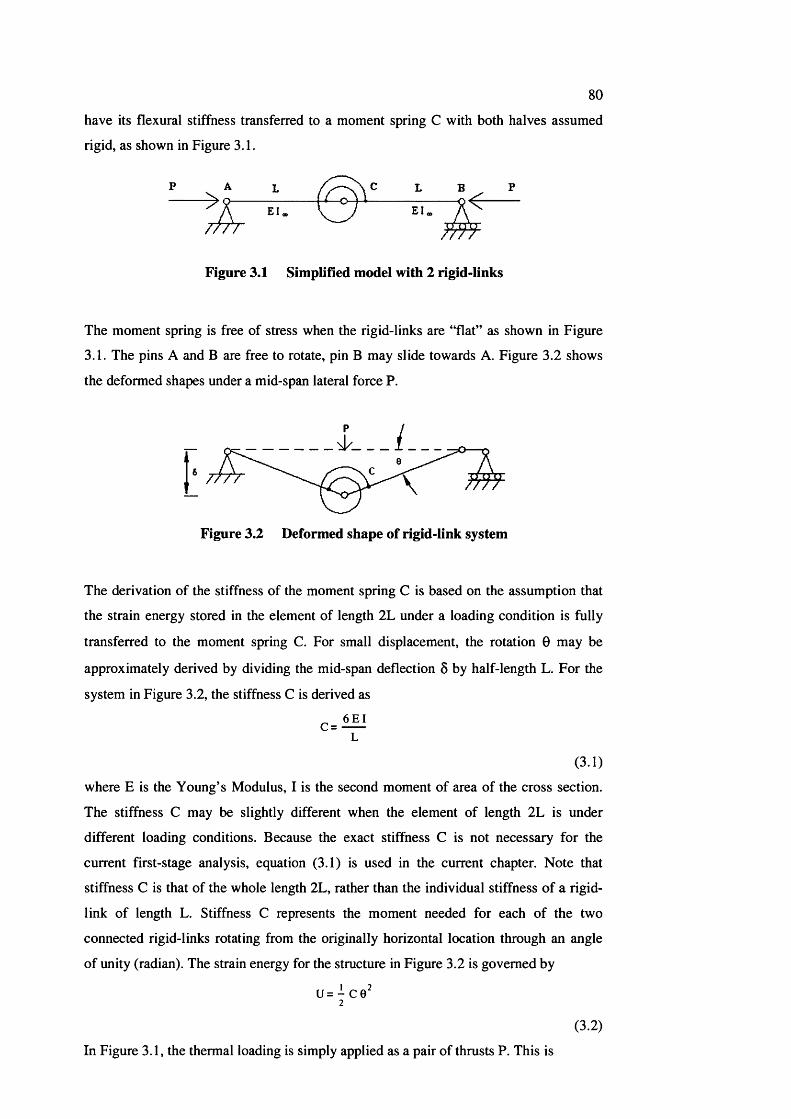
80

have its flexural stiffness transferred to a moment spring C with both halves assumed

rigid, as shown in Figure 3.1.

rrrr

Figure 3.1 Simplified model with 2 rigid-links

The moment spring is free of stress when the rigid-links are “flat” as shown in Figure

3.1. The pins A and B are free to rotate, pin B may slide towards A. Figure 3.2 shows

the deformed shapes under a mid-span lateral force P.

® T T n

Figure 3.2 Deformed shape of rigid-link system

The derivation of the stiffness of the moment spring C is based on the assumption that

the strain energy stored in the element of length 2L under a loading condition is fully

transferred to the moment spring C. For small displacement, the rotation 0 may be

approximately derived by dividing the mid-span deflection 5 by half-length L. For the

system in Figure 3.2, the stiffness C is derived as

C^ 6 E IL

(3.1)

where E is the Young’s Modulus, I is the second moment of area of the cross section.

The stiffness C may be slightly different when the element of length 2L is under

different loading conditions. Because the exact stiffness C is not necessary for the

current first-stage analysis, equation (3.1) is used in the current chapter. Note that

stiffness C is that of the whole length 2L, rather than the individual stiffness of a rigid-

link of length L. Stiffness C represents the moment needed for each of the two

connected rigid-links rotating from the originally horizontal location through an angle

of unity (radian). The strain energy for the structure in Figure 3.2 is governed by

u= - ce^2

(3.20In Figure 3.1, the thermal loading is simply applied as a pair of thrusts P. This is

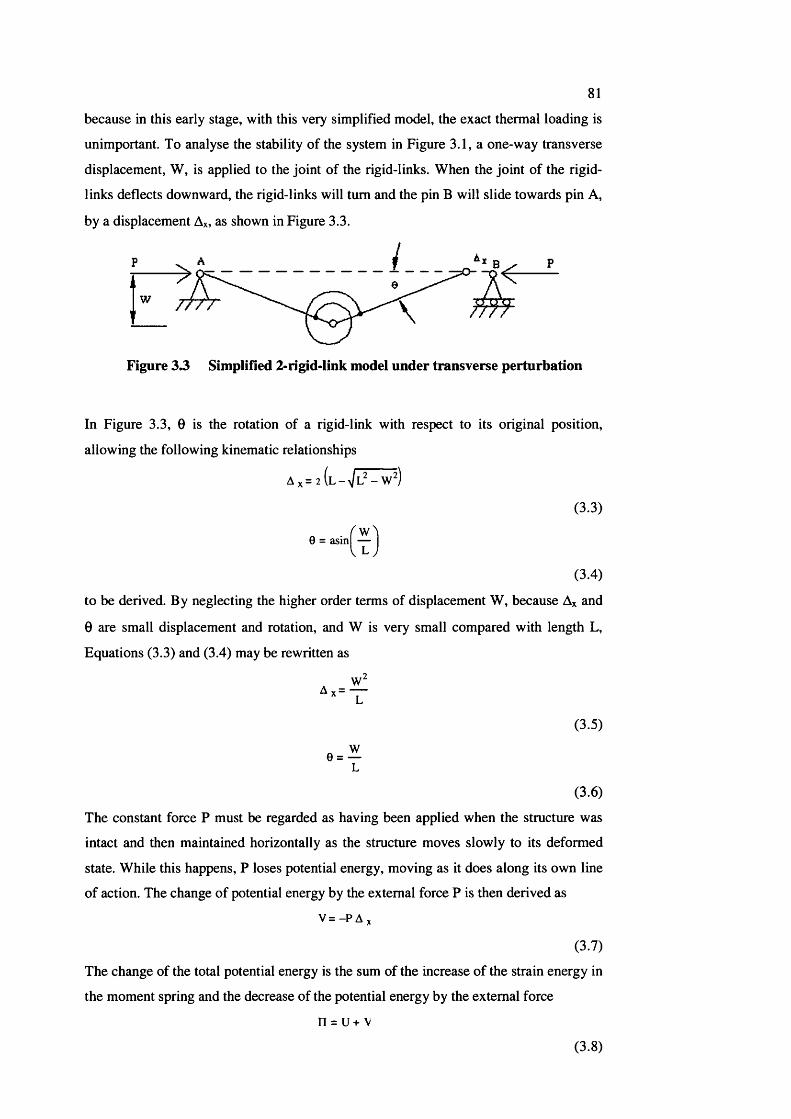
81

because in this early stage, with this very simplified model, the exact thermal loading is

unimportant. To analyse the stability of the system in Figure 3.1, a one-way transverse

displacement, W, is applied to the joint of the rigid-links. When the joint of the rigid-

links deflects downward, the rigid-links will turn and the pin B will slide towards pin A,

by a displacement Ax, as shown in Figure 3.3.

w Ttrr j m

Figure 3 3 Simplified 2-rigid-link model under transverse perturbation

In Figure 3.3, 0 is the rotation of a rigid-link with respect to its original position,

allowing the following kinematic relationships

Ax= 2(l --^L^-W^)

(3.3)

0 = asm —I L

(3.4)

to be derived. By neglecting the higher order terms of displacement W, because Ax and

0 are small displacement and rotation, and W is very small compared with length L,

Equations (3.3) and (3.4) may be rewritten as

A Y =

e = —L

(3.5)

(3.(0

The constant force P must be regarded as having been applied when the structure was

intact and then maintained horizontally as the structure moves slowly to its deformed

state. While this happens, P loses potential energy, moving as it does along its own line

of action. The change of potential energy by the external force P is then derived as

V = - P A x

(3.7)

The change of the total potential energy is the sum of the increase of the strain energy in

the moment spring and the decrease of the potential energy by the external force

n = u+ V

(3.8)

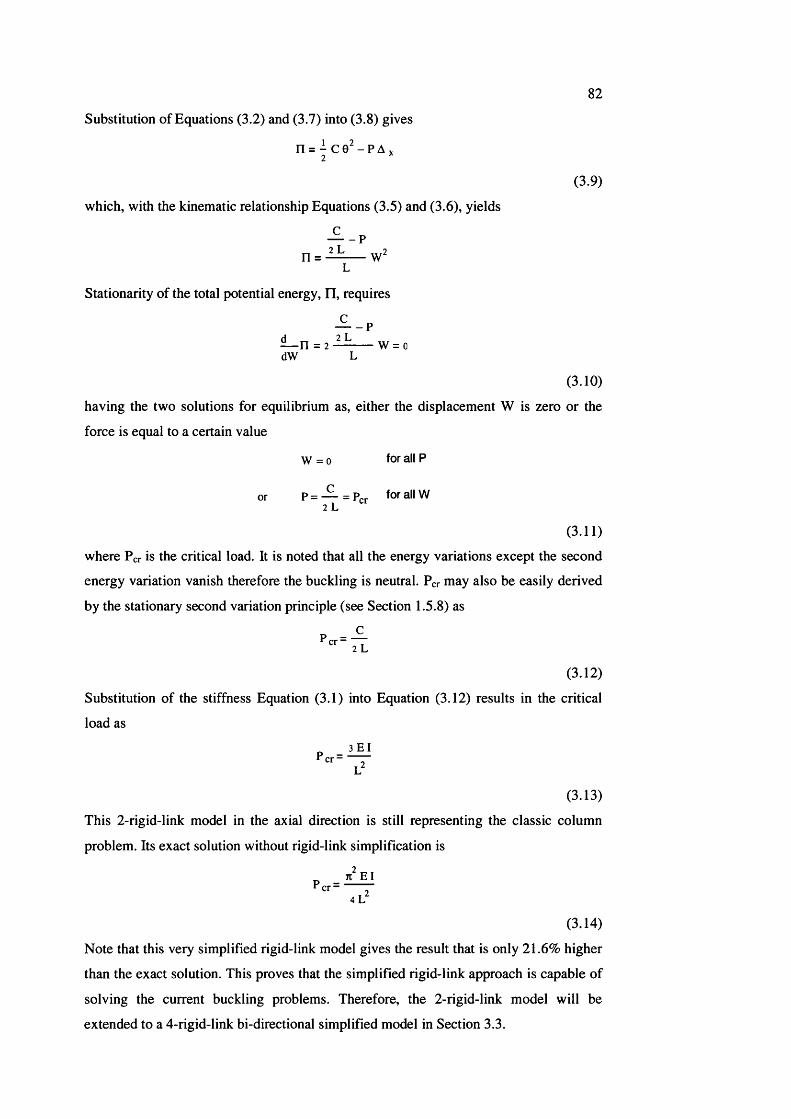
82

Substitution of Equations (3.2) and (3.7) into (3.8) gives

n = - c e ^ - P A j ,2

(3.90

which, with the kinematic relationship Equations (3.5) and (3.6), yields

^ - pn = ——

L

Stationarity of the total potential energy, fl, requires

^ - P— n = 2— — w = o dW L

(3.10)

having the two solutions for equilibrium as, either the displacement W is zero or the

force is equal to a certain value

W = 0 for all P

or P = — = Per for all W2L

(3.11)

where Per is the critical load. It is noted that all the energy variations except the second

energy variation vanish therefore the buckling is neutral. may also be easily derived

by the stationary second variation principle (see Section 1.5.8) as

(3.12)

Substitution of the stiffness Equation (3.1) into Equation (3.12) results in the critical

load as

' • ■ ■ f

(3.13)

This 2-rigid-link model in the axial direction is still representing the classic column

problem. Its exact solution without rigid-link simplification is

pcr-4 L

(3.14)

Note that this very simplified rigid-link model gives the result that is only 21.6% higher

than the exact solution. This proves that the simplified rigid-link approach is capable of

solving the current buckling problems. Therefore, the 2-rigid-link model will be

extended to a 4-rigid-link bi-directional simplified model in Section 3.3.

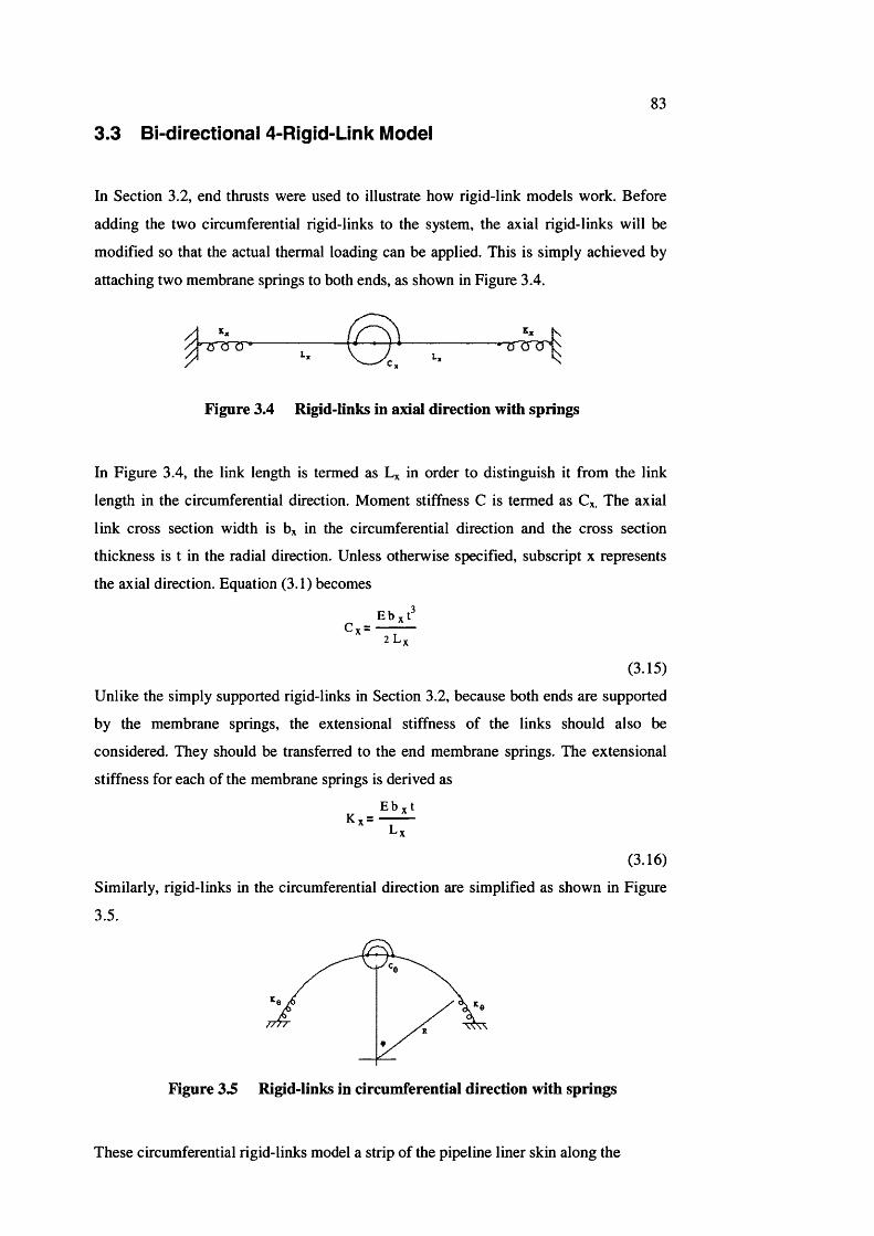
83

3.3 B i-directional 4-Rigid-Link Modei

In Section 3.2, end thrusts were used to illustrate how rigid-link models work. Before

adding the two circumferential rigid-links to the system, the axial rigid-links will be

modified so that the actual thermal loading can be applied. This is simply achieved by

attaching two membrane springs to both ends, as shown in Figure 3.4.

Figure 3.4 Rigid-links in axial direction with springs

In Figure 3.4, the link length is termed as in order to distinguish it from the link

length in the circumferential direction. Moment stiffness C is termed as C* The axial

link cross section width is b% in the circumferential direction and the cross section

thickness is t in the radial direction. Unless otherwise specified, subscript x represents

the axial direction. Equation (3.1) becomes

Cv =Ebxt"

2 L ,

(3.15)

Unlike the simply supported rigid-links in Section 3.2, because both ends are supported

by the membrane springs, the extensional stiffness of the links should also be

considered. They should be transferred to the end membrane springs. The extensional

stiffness for each of the membrane springs is derived as

E b , tK, =

(3.16)

Similarly, rigid-links in the circumferential direction are simplified as shown in Figure

3.5.

Figure 3.5 Rigid-links in circumferential direction with springs

These circumferential rigid-links model a strip of the pipeline liner skin along the

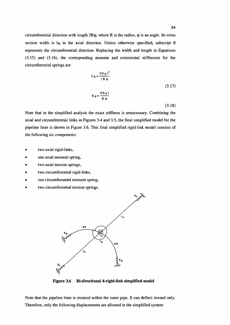
84

circumferential direction with length 2Rtp, where R is the radius, cp is an angle. Its cross

section width is be in the axial direction. Unless otherwise specified, subscript 0

represents the circumferential direction. Replacing the width and length in Equations

(3.15) and (3.16), the corresponding moment and extensional stiffnesses for the

circumferential springs are

C e =Eber 2 R (p

(3.17)

Ke =E b 0 t

R (p

(3.18)

Note that in the simplified analysis the exact stiffness is unnecessary. Combining the

axial and circumferential links in Figures 3.4 and 3.5, the final simplified model for the

pipeline liner is shown in Figure 3.6. This final simplified rigid-link model consists of

the following six components:

two axial rigid-links,

one axial moment spring,

two axial tension springs,

two circumferential rigid-links,

one circumferential moment spring,

two circumferential tension springs.

R 9

Figure 3.6 Bi-directional 4-rigid-link simplified model

Note that the pipeline liner is encased within the outer pipe. It can deflect inward only.

Therefore, only the following displacements are allowed in the simplified system:

85

• The central joint connecting the axial and circumferential rigid-links displaces

radially inward only, no axial and circumferential displacements are allowed;

• The outer ends of the axial rigid-links can displace axially only, no

circumferential and radial displacements are allowed;

• The outer ends of the circumferential links can displace along the inner surface

of the outer pipe wall only, no axial and radial displacements are allowed.

Further details of these displacements will be discussed in Section 3.4.

3.4 Form ulation

3.4.1 Thermally-Induced D isplacem ents

Under temperature rise T, a free non-rigid axial link will expand by ttxLxT, where ttx is

the thermal expansion coefficient in the axial direction. Similarly, a free axial end

membrane spring will expand. The amount the free axial end membrane spring expands

is assumed equal to that of the free non-rigid axial link. Therefore,

^ x_thermal - ® x ^ x T

(3.19)

Note that thermal loading will not result in any flexural displacement to the links.

Therefore, there is no thermal loading to the central moment springs. In the

circumferential direction, a free circumferential link will expand by OeRtpT, where Oe is

the thermal expansion coefficient in the circumferential direction. Therefore, under the

thermal loading, a free circumferential tension spring will expand by the same amount

the free circumferential link does

^ 0_thermal = Ot q R <p T

(3.20)

3.4.2 Imperfection, Incremental D isplacem ents and Kinematic

Relationships

3.4.2.1 Imperfection

It is assumed that the imperfection is radially inward only. The magnitude of the

imperfection is denoted as Wq. In the axial direction, as shown in Figure 3.7, without

imperfection, the length of the axial rigid-link is Lx. With imperfection Wo, the new

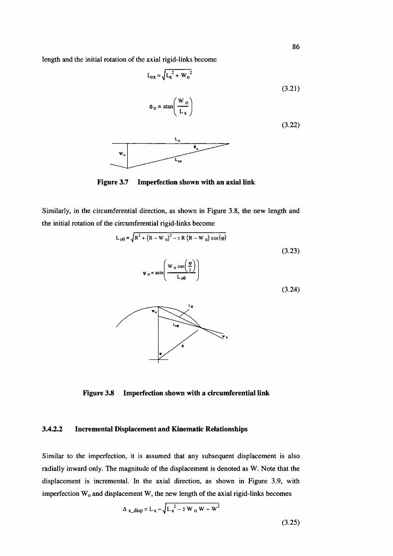
length and the initial rotation of the axial rigid-links become

1-ox ~ -I- W q

(t>o = atanW

Lx

Wo

Figure 3.7 Imperfection shown with an axial link

86

(3.21)

(3.22)

Similarly, in the circumferential direction, as shown in Figure 3.8, the new length and

the initial rotation of the circumferential rigid-links become

L oe = + (R - w o)^ - 2 R (R - W o) COS(9 )

(3.23)

y o = asmW

Log

(3.24)

Figure 3.8 Imperfection shown with a circumferential link

3.4.2.2 Incremental Displacement and Kinematic Relationships

Similar to the imperfection, it is assumed that any subsequent displacement is also

radially inward only. The magnitude of the displacement is denoted as W. Note that the

displacement is incremental. In the axial direction, as shown in Figure 3.9, with

imperfection Wo and displacement W, the new length of the axial rigid-links becomes

^ x_disp = L % - - 2 W o W -

(3.25)

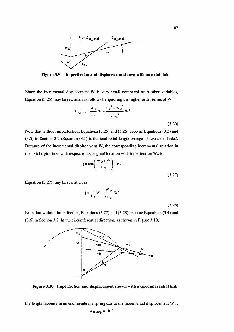
87

X totalX total

ox

ox

Figure 3.9 Imperfection and displacement shown with an axial link

Since the incremental displacement W is very small compared with other variables,

Equation (3.25) may be rewritten as follows by ignoring the higher order terms of W

Wo Lx + Wo^ nA x_disp = - — W + ----------- W

Lx 2L x^

(3.26)

Note that without imperfection, Equations (3.25) and (3.26) become Equations (3.3) and

(3.5) in Section 3.2 (Equation (3.3) is the total axial length change of two axial links).

Because of the incremental displacement W, the corresponding incremental rotation in

the axial rigid-links with respect to its original location with imperfection Wo is

(|)= asinV ^o x J

(3.27)

Equation (3.27) may be rewritten as

1= — w +Lx 2 L '

(3.28)

Note that without imperfection. Equations (3.27) and (3.28) become Equations (3.4) and

(3.6) in Section 3.2. In the circumferential direction, as shown in Figure 3.10,

Figure 3.10 Imperfection and displacement shown with a circumferential link

the length increase in an end membrane spring due to the incremental displacement W is

^ 0_disp “ 0

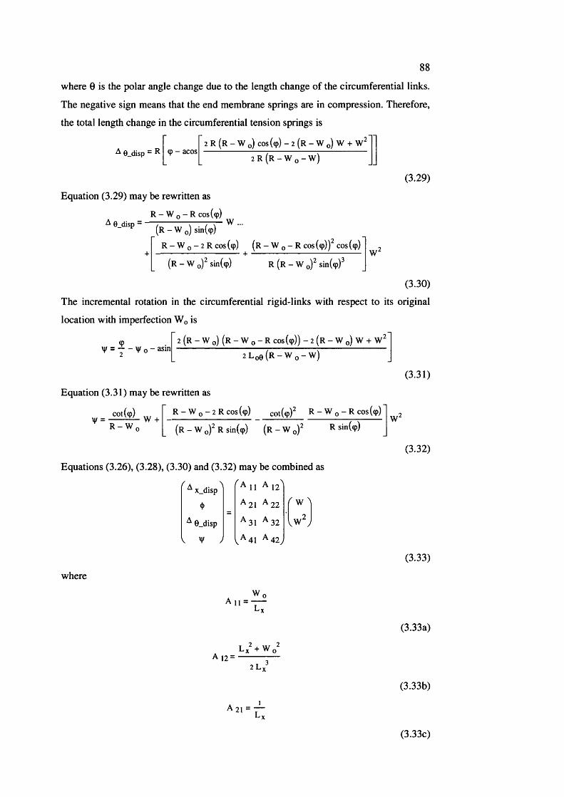
88

where 0 is the polar angle change due to the length change of the circumferential links.

The negative sign means that the end membrane springs are in compression. Therefore,

the total length change in the circumferential tension springs is

2 R (r - W o) cos((p) - 2 (r - W o ) w +6_disp = R (p - acos

2 R (R - W o - W)

(3.29)


R - W o - R cos((p)^ 0_disp - : : ~ W ...

(R -W o )s in ((p )

R - W o - 2 R cos ((p) (r - W o - R cos ((p))^ cos ((p)

(r - W o)^ Sin((p) R (r - W o)^ sin((p)^

(3.30)

The incremental rotation in the circumferential rigid-links with respect to its original

location with imperfection Wq is

2 (r - W o) (R - w o - R cos((p)) - 2 ( r - W o ) w +\p = Y - \|/ o “ asm

2 L „ e ( R - w „ - w )

(3.31)


R - W o - 2 R cos(<p) cot((p)^ R - W q - R cos(<p)

R - W n (r - W o)^ R Sin((p) (r - W o)^ ^

Equations (3.26), (3.28), (3.30) and (3.32) may be combined as

(3.32)

f A A- ^x_disp ' A l l A 1 2 '

4) A 2 I A 22

^ 0_dlsp

I V JA 3 I

^ * 4 1

A 3 2

A 4 2 ^

w ^

vW y

(3.33)

where

A 11 =W

(3.33a)

A 12 =2 L ,

(3.33b)

A 21 = —

(3.33c)

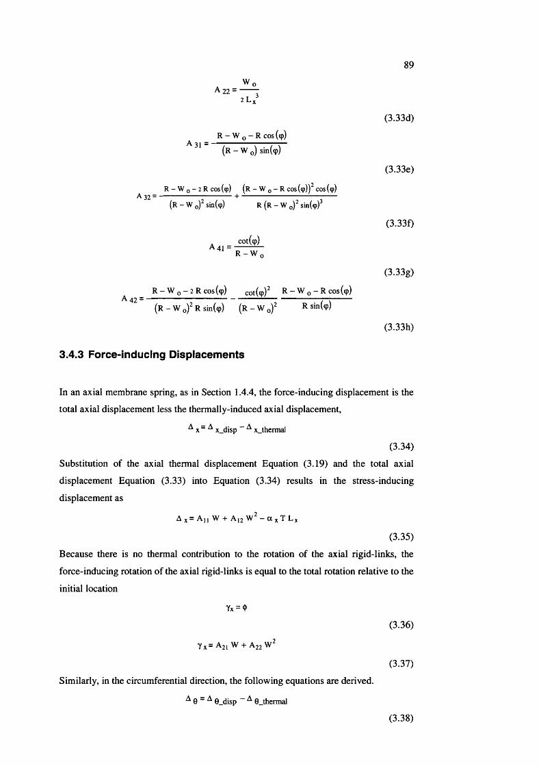
WoA 2 2 = ------:

2 L /

R - W o - R cos ((p)

(r - W o) sin((p)

R - W 0 - 2 R cos ((p) ( r - W o - R cos ((p))^ cos {(p)A 3 2 =---------------------------- + --------------------------------------

(R - W o) sin(<p) R (r - W o)^ sin(<p)^

cot((p)A41 =R - W

R - W o - 2 R cos(<p) cot(cp)^ R - W o - R cos(<p)A 42 = ------------------------------------------------------- 7~\------

( R - W o)^ R sin((p) ( R - W o) ^

89

(3.33d)

(3.33e)

(3.33f)

(3.33g)

(3.33h)

3.4.3 Force-inducing Dispiacements

In an axial membrane spring, as in Section 1.4.4, the force-inducing displacement is the

total axial displacement less the thermally-induced axial displacement,

^ X “ ^ x_disp “ ^ x_therma]

(3.34)

Substitution of the axial thermal displacement Equation (3.19) and the total axial

displacement Equation (3.33) into Equation (3.34) results in the stress-inducing

displacement as

A X = A]] W + A 12 W^ - a X T L;,

(3.35)

Because there is no thermal contribution to the rotation of the axial rigid-links, the

force-inducing rotation of the axial rigid-links is equal to the total rotation relative to the

initial location

Yx = <l>

(3.36)

Y x= A21 W + A22 W^

(3.37)

Similarly, in the circumferential direction, the following equations are derived.

^ 0 ^ 0_disp ^ 0_thermal

(3.38)

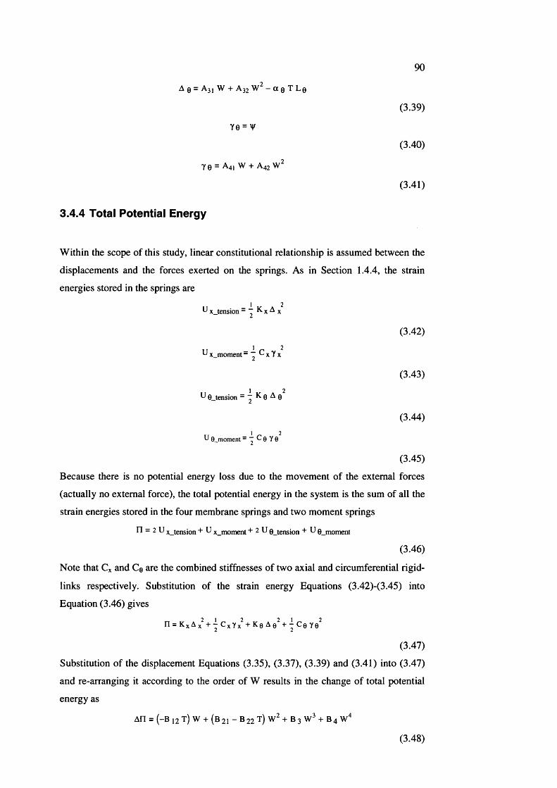
90

A 0 — A3J W + A32 W — oc 0 T L 0

(3.39)

Y0 = V

(3.40)

Y 0 = ^41 W + A 42

(3.41)

3.4.4 Total Potential Energy

Within the scope of this study, linear constitutional relationship is assumed between the

displacements and the forces exerted on the springs. As in Section 1.4.4, the strain

energies stored in the springs are

U x_tension - ^ x ^ x

^ x_moment - ^ x Y x

U 0_tension - K 0 A 0

(3.42)

(3.43)

(3.44)

(3.45)

Because there is no potential energy loss due to the movement of the external forces

(actually no external force), the total potential energy in the system is the sum of all the

strain energies stored in the four membrane springs and two moment springs

n = 2 U x_tension + U x_moment + 2 U 0 tension + U 0_moment

(3.46)

Note that Cx and Ce are the combined stiffnesses of two axial and circumferential rigid-

links respectively. Substitution of the strain energy Equations (3.42)-(3.45) into

Equation (3.46) gives

n = KxAx + -^CxYx^+K0 Ae + ^ C 0 Y0^

(3.47)

Substitution of the displacement Equations (3.35), (3.37), (3.39) and (3.41) into (3.47)

and re-arranging it according to the order of W results in the change of total potential

energy as

A n = ( - B 12 T ) W + ( b 21 - B 22 T ) + B 3 + B 4 w "

(3.48)

91

where the various combined coefficients are

Bi 2 = 2 Kx Ai i a x L x + 2 K0 A3 i a e L e

B21 = K x A 11 + - ^ A 21 + K g A 31 + A 41^

B2 2 = 2 KxAi 2 axLx + 2 Ke A32a e Le

B3 = 2 Kx Ai i A i 2 + CxA2 l A 22 + 2K0A3iA32 + CeA4iA42

B 4 = K x A \2 + A 22 + K g A 32 + A 42^

(3.49)

(3.50)

(3.51)

(3.52)

(3.53)

3.4.5 Application of Stationary Potential Energy Principle

The stationary potential energy principle is

— A n = c dW

(3.54)

Substitution of the change of the total potential energy expression Equation (3.48) into

Equation (3.54) gives

(—B 12 T ) + 2 (B 21 — B 22 T ) W + 3 B 3 + 4 B 4 = 0

(3.55)

By solving the temperature rise T, the equilibrium path is derived as

2 B21 W + 3B3\V^+4B4W^T = ----------------------------------------------

B 12 + 2 B22 W

(3.56)

It can be proved that coefficient B21 is always positive and coefficient B 12 can be

positive, zero or negative. To describe the characteristics of the equilibrium Equation

(3.56), the following coefficients are represented

B l 2 = 2 K x A i i a x L x + 2 K g A 3 i a g L g

A 11 = —^ x

R - W o - R cos ((p)

(r - W 0) sin((p)

SO that the coefficient B12 can be rewritten as

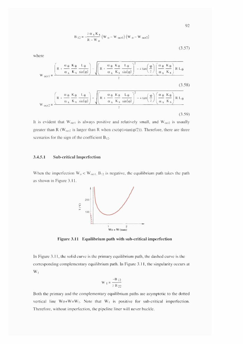
^ 1 2 - ^ ^ o ^ o c r l) o o c r l)

92

(3.57)

w here

R +«0 K g L g

Wa X K% sin((p)

- R +a g K g L g

(% X *^x sin((p)o c r l -

1 ^ q 0 K g l- 4 tan -

V2 y/ K x J

RL0

(3.58)

^ o cr2 -

Otg K g L g ]R + ------------------T-r +

t t x Kx sin((pj I

a g K g L g ] / mR + ------------------ T-- - 4 tan —

t tx Kx sin((p) I V2

qg Kg q X ^ X

RLe

(3.59)

It is evident that Wocri is always positive and relatively sm all, and Wocr2 is usually

greater than R (Wocr2 is larger than R when csc((p)>tan((p/2)). Therefore, there are three

scenarios for the sign o f the coefficient B 12.

3.4.5.1 Sub-critical Imperfection

W hen the im perfection Wq < Wocri. B 12 is negative, the equilibrium path takes the path

as shown in Figure 3.11.

200

H100

1 2W o + W {m m )

Figure 3.11 Equilibrium path with sub-critical imperfection

In Figure 3.11, the solid curve is the prim ary equilibrium path, the dashed curve is the

corresponding com plem entary equilibrium path. In Figure 3.11, the singularity occurs at

W ,

- B 12W 1 =

2 B22

Both the prim ary and the com plem entary equilibrium paths are asym ptotic to the dotted

vertical line W o+W =W ,. Note that W , is positive for sub-critical im perfection.

Therefore, w ithout im perfection, the pipeline liner will never buckle.

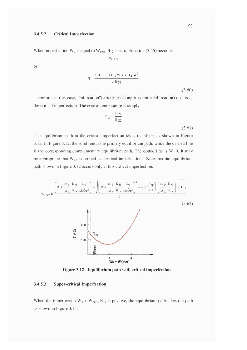
93

3.4.5.2 Critical Imperfection

W hen im perfection Wo is equal to Wocri, B ,2 is zero, Equation (3.55) becom es

W = C

or

,2

T =2 B 21 + 3 B 3 W + 4 B 4 W'

2 B22

(3.60)

Therefore, in this case, “bifurcation”(strictiy speaking it is not a bifurcation) occurs at

the critical im perfection. The critical tem perature is sim ply as

B21

(3.61)

The equilibrium path at the critical im perfection takes the shape as shown in Figure

3.12. In Figure 3.12, the solid line is the prim ary equilibrium path, w hile the dashed line

is the corresponding com plem entary equilibrium path. The dotted line is W =0. It m ay

be appropriate that Wocr is term ed as “critical im perfection” . N ote that the equilibrium

path show n in Figure 3.12 occurs only at this critical im perfection.

R +a 0 K g L g

wt t x Kx sin((p)

a g K g L g

a X Kx sin((p)- 4 tan I "Y

« g K g

« X K x

R L g

200

100

21Wo + W (mm)

Figure 3.12 Equilibrium path with critical imperfection

3.4.5.3 Super critical Imperfection

(3.62)

W hen the im perfection W q > Wocri, B |] is positive, the equilibrium path takes the path

as shown in Figure 3.13.

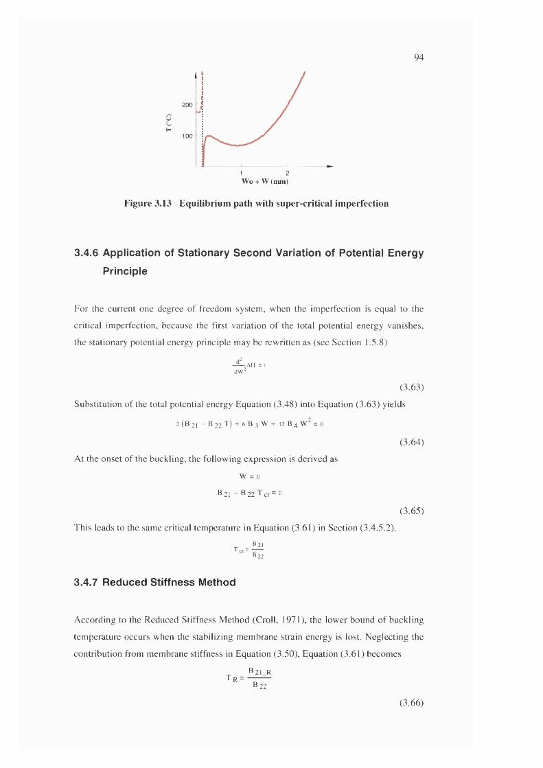
94

200

U

H100

1 2Wo + W (mm)

Figure 3.13 Equilibrium path with super-critical imperfection

3.4.6 Application of Stationary Second Variation of Potential Energy

Principle

For the current one degree o f freedom system , when the im perfection is equal to the

critical im perfection, because the first variation o f the total potential energy vanishes,

the stationary potential energy principle may be rewritten as (see Section 1.5.8)

— An = c dW-

(3.63)

Substitution o f the total potential energy Equation (3.48) into Equation (3.63) yields

2 ( B 21 - B 22 T) + 6 B 3 W + 12 B 4 = o

(3.64)

At the onset o f the buckling, the follow ing expression is derived as

w = 0

B21 - B 22 T cr = 0

(3.65)

This leads to the same critical tem perature in Equation (3.61) in Section (3.4.5.2).

B21T r r = B22

3.4.7 Reduced Stiffness Method

A ccording to the Reduced Stiffness M ethod (Croll, 1971), the lower bound o f buckling

tem perature occurs when the stabilizing m em brane strain energy is lost. N eglecting the

contribution from m em brane stiffness in Equation (3.50), Equation (3.61) becom es

B2 1 RT r =

B22

(3.66)

95

where

B21_R= “ C x A 21^+ C e A 4 i ^

(3.67)Lower bound critical temperature for a given pipeline liner will be given in Section 3.5.

3.5 E xam ple

3.5.1 Geometry of a Typical Pipeline Liner

This section applies the formulations from Section 3.4 to a typical pipeline liner as an

example: the radius of the neutral surface of the pipeline liner R = 0.3m and the

corresponding wall thickness t=lmm. This geometry will be used as an example to

illustrate results from various formulations throughout this thesis.

3.5.2 Rigid-Links and Spring Stiffness

For a section of the pipeline of length equal to the radius R, if the wave number along

the axial length is m, the length of one axial rigid-link L* is

Similarly, if the wave number along the circumference is n, the length of one

circumferential rigid-link Le is

L 0 = — n

In order not to complicate the analysis, the widths of the rigid-link cross section are not

treated as independent variables. Instead, the widths of the rigid-link cross sections are

chosen as a fraction, say 50%, of the lengths of the rigid-links in the other direction. A

half of the length of the circumferential links (Le/2) is used as the width of the cross

section of the axial links (b j. Similarly, a half of the length of the axial links (L%/2) is

used as the width of the cross section of the circumferential links (be).

hbe = “

Note that both the length and the cross section of the rigid-link will vary with the wave

numbers. The material properties based on the test results from the references (Walker,

1999, 2002) are: Young’s Modulus E=210GPa, the thermal expansion coefficients in

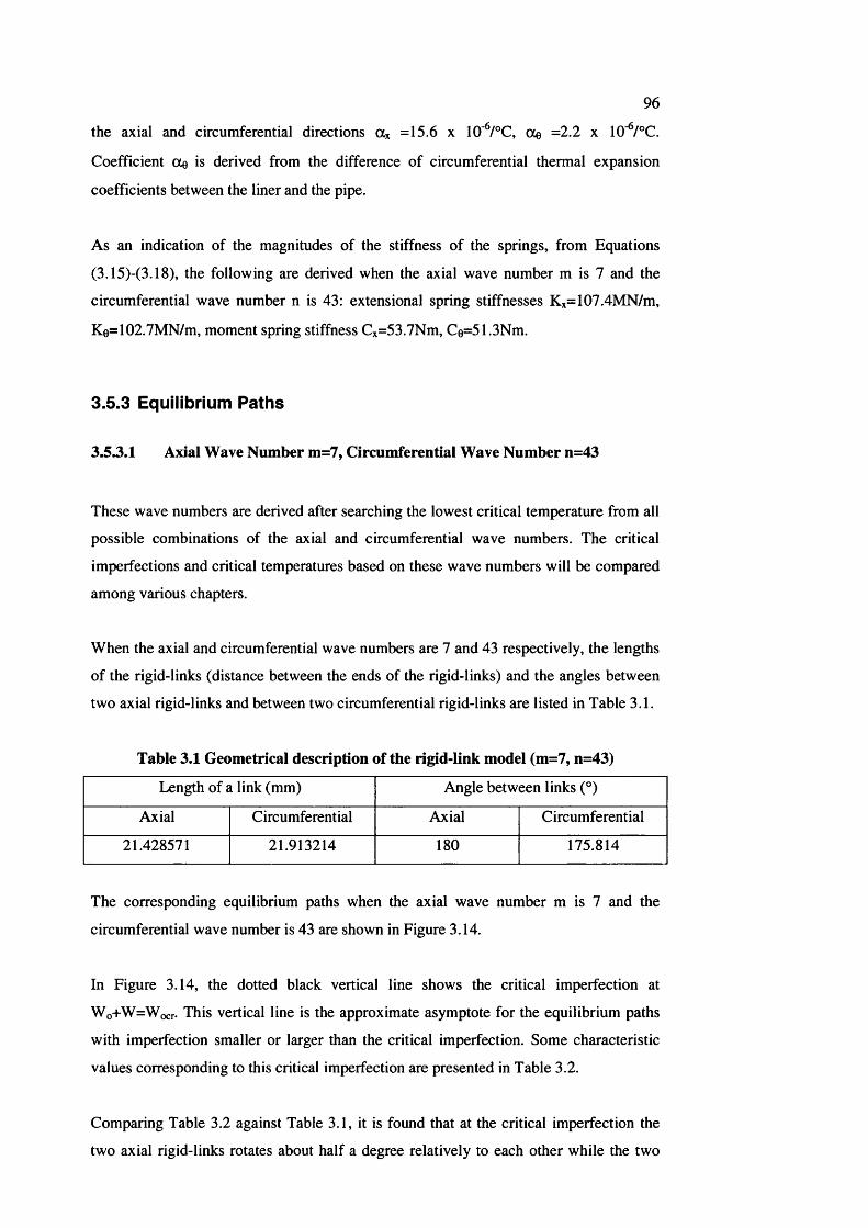
96

the axial and circumferential directions ttx =15.6 x 10'^/°C, Oe =2.2 x 10^/°C.

Coefficient Oe is derived from the difference of circumferential thermal expansion

coefficients between the liner and the pipe.

As an indication of the magnitudes of the stiffness of the springs, from Equations

(3.15)-(3.18), the following are derived when the axial wave number m is 7 and the

circumferential wave number n is 43: extensional spring stiffnesses Kx=107.4MN/m,

Ke=102.7MN/m, moment spring stiffness Cx=53.7Nm, C@=51.3Nm.

3.5.3 Equilibrium Paths

3.53.1 Axial Wave Number m=7, Circumferential Wave Number n=43

These wave numbers are derived after searching the lowest critical temperature from all

possible combinations of the axial and circumferential wave numbers. The critical

imperfections and critical temperatures based on these wave numbers will be compared

among various chapters.

When the axial and circumferential wave numbers are 7 and 43 respectively, the lengths

of the rigid-links (distance between the ends of the rigid-links) and the angles between

two axial rigid-links and between two circumferential rigid-links are listed in Table 3.1.

Table 3.1 Geometrical description of the rigid-link model (m=7, n=43)

Length of a link (mm) Angle between links (°)

Axial Circumferential Axial Circumferential

21.428571 21.913214 180 175.814

The corresponding equilibrium paths when the axial wave number m is 7 and the

circumferential wave number is 43 are shown in Figure 3.14.

In Figure 3.14, the dotted black vertical line shows the critical imperfection at

Wo+W=Wocr. This vertical line is the approximate asymptote for the equilibrium paths

with imperfection smaller or larger than the critical imperfection. Some characteristic

values corresponding to this critical imperfection are presented in Table 3.2.

Comparing Table 3.2 against Table 3.1, it is found that at the critical imperfection the

two axial rigid-links rotates about half a degree relatively to each other while the two

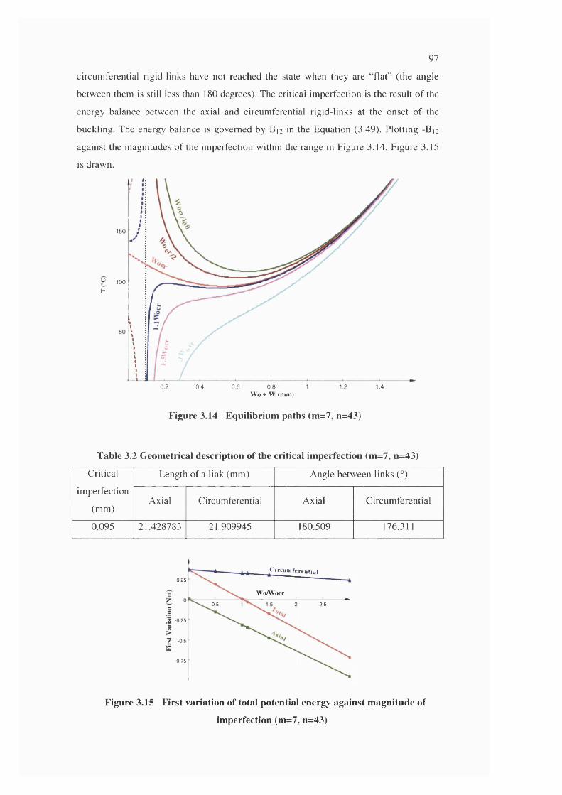
97

circum ferential rigid-links have not reached the state when they are “fla t” (the angle

betw een them is still less than 180 degrees). The critical im perfection is the result o f the

energy balance betw een the axial and circum ferential rigid-links at the onset o f the

buckling. The energy balance is governed by B 12 in the Equation (3.49). P lotting -B 12

against the m agnitudes o f the im perfection within the range in Figure 3.14, F igure 3.15

is drawn.

150

100f-

0.2 0.4 0.6 0.8 1.2 1.4W o + W (m m )

Figure 3.14 Equilibrium paths (m=7, n=43)

Table 3.2 Geometrical description of the critical imperfection (m=7, n=43)

Critical

im perfection

(m m )

Length of a link (m m ) A ngle betw een links (°)

Axial Circum ferential Axial C ircum ferential

0.095 21.428783 21.909945 180.509 176.311

Circumferentia l0.25

WoAVocr

0.5 2.5

.2 -0-25

-0.75

Figure 3.15 First variation of total potential energy against magnitude of

imperfection (m=7, n=43)

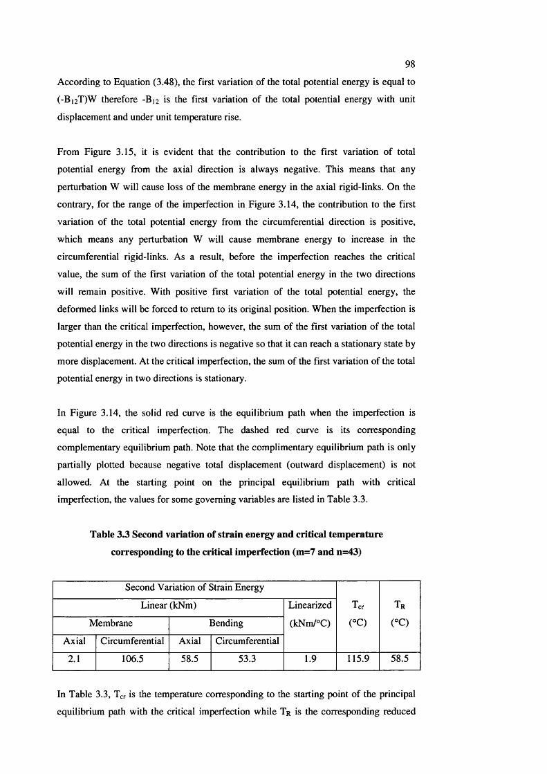
98

According to Equation (3.48), the first variation of the total potential energy is equal to

(-Bi2T)W therefore -B12 is the first variation of the total potential energy with unit

displacement and under unit temperature rise.

From Figure 3.15, it is evident that the contribution to the first variation of total

potential energy from the axial direction is always negative. This means that any

perturbation W will cause loss of the membrane energy in the axial rigid-links. On the

contrary, for the range of the imperfection in Figure 3.14, the contribution to the first

variation of the total potential energy from the circumferential direction is positive,

which means any perturbation W will cause membrane energy to increase in the

circumferential rigid-links. As a result, before the imperfection reaches the critical

value, the sum of the first variation of the total potential energy in the two directions

will remain positive. With positive first variation of the total potential energy, the

deformed links will be forced to return to its original position. When the imperfection is

larger than the critical imperfection, however, the sum of the first variation of the total

potential energy in the two directions is negative so that it can reach a stationary state by

more displacement. At the critical imperfection, the sum of the first variation of the total

potential energy in two directions is stationary.

In Figure 3.14, the solid red curve is the equilibrium path when the imperfection is

equal to the critical imperfection. The dashed red curve is its corresponding

complementary equilibrium path. Note that the complimentary equilibrium path is only

partially plotted because negative total displacement (outward displacement) is not

allowed. At the starting point on the principal equilibrium path with critical

imperfection, the values for some governing variables are listed in Table 3.3.

Table 3.3 Second variation of strain energy and critical temperature

corresponding to the critical imperfection (m=7 and n=43)

Second Variation of Strain Energy

Ter

(°C)

Tr

(°C)

Linear (kNm) Linearized

(kNm/°C)Membrane Bending


2 .1 106.5 58.5 53.3 1.9 115.9 58.5

In Table 3.3, T^ is the temperature corresponding to the starting point of the principal

equilibrium path with the critical imperfection while Tr is the corresponding reduced

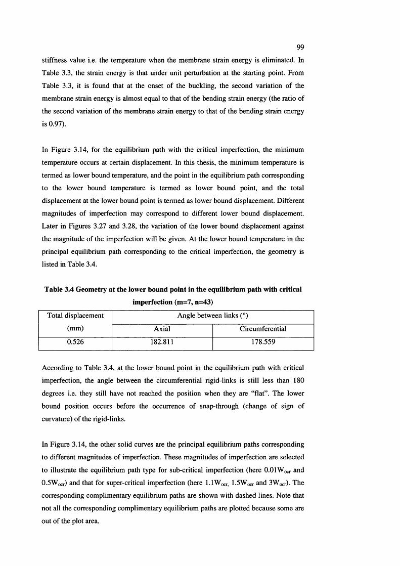
99

stiffness value i.e. the temperature when the membrane strain energy is eliminated. In

Table 3.3, the strain energy is that under unit perturbation at the starting point. From

Table 3.3, it is found that at the onset of the buckling, the second variation of the

membrane strain energy is almost equal to that of the bending strain energy (the ratio of

the second variation of the membrane strain energy to that of the bending strain energy

is 0.97).

In Figure 3.14, for the equilibrium path with the critical imperfection, the minimum

temperature occurs at certain displacement. In this thesis, the minimum temperature is

termed as lower bound temperature, and the point in the equilibrium path corresponding

to the lower bound temperature is termed as lower bound point, and the total

displacement at the lower bound point is termed as lower bound displacement. Different

magnitudes of imperfection may correspond to different lower bound displacement.

Later in Figures 3.27 and 3.28, the variation of the lower bound displacement against

the magnitude of the imperfection will be given. At the lower bound temperature in the

principal equilibrium path corresponding to the critical imperfection, the geometry is

listed in Table 3.4.

Table 3.4 Geometry at the lower bound point in the equilibrium path with critical


Total displacement

(mm)

Angle between links (°)

Axial Circumferential

0.526 182.811 178.559

According to Table 3.4, at the lower bound point in the equilibrium path with critical

imperfection, the angle between the circumferential rigid-links is still less than 180

degrees i.e. they still have not reached the position when they are “flat”. The lower

bound position occurs before the occurrence of snap-through (change of sign of

curvature) of the rigid-links.

In Figure 3.14, the other solid curves are the principal equilibrium paths corresponding

to different magnitudes of imperfection. These magnitudes of imperfection are selected

to illustrate the equilibrium path type for sub-critical imperfection (here O.OlWœr and

0.5Wocr) and that for super critical imperfection (here 1.1 Wocr. L5Wocr and 3Wocr)- The

corresponding complimentary equilibrium paths are shown with dashed lines. Note that

not all the corresponding complimentary equilibrium paths are plotted because some are

out of the plot area.

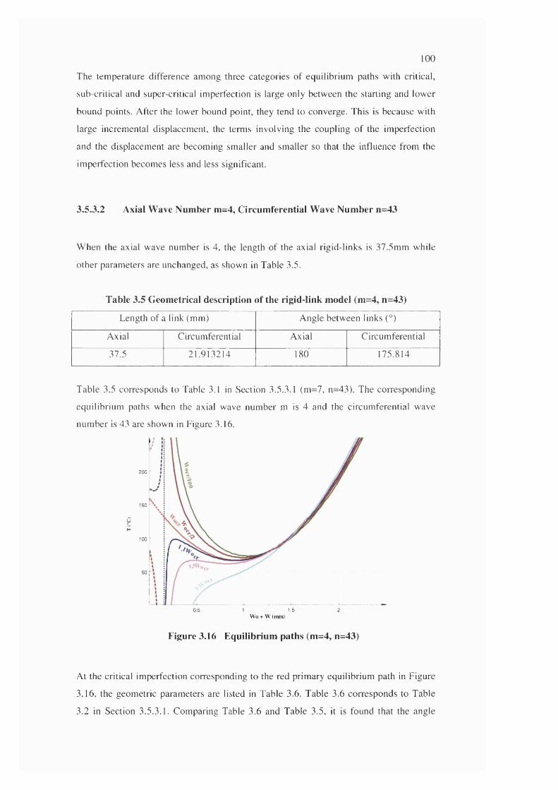
100

The tem perature difference am ong three categories of equilibrium paths with critical,

sub-critical and super-critical im perfection is large only betw een the starting and low er

bound points. A fter the lower bound point, they tend to converge. This is because with

large increm ental displacem ent, the term s involving the coupling o f the im perfection

and the displacem ent are becom ing sm aller and sm aller so that the influence from the

im perfection becom es less and less significant.

3.5.3.2 Axial Wave Number m=4, Circumferential Wave Number n=43

W hen the axial wave num ber is 4, the length o f the axial rigid-links is 37.5m m w hile

o ther param eters are unchanged, as shown in Table 3.5.


Length o f a link (mm) A ngle betw een links (°)


3T 5 21.913214 180 175.814

Table 3.5 corresponds to Table 3.1 in Section 3.5.3.1 (m =7, n=43). The corresponding

equilibrium paths when the axial wave num ber m i s 4 and the circum ferential wave

num ber is 43 are shown in Figure 3.16.

200

150

100

50

0.5 1.5 2W o + W (mm)


At the critical im perfection corresponding to the red prim ary equilibrium path in Figure

3.16, the geom etric param eters are listed in Table 3.6. Table 3.6 corresponds to Table

3.2 in Section 3.5.3.1. Com paring Table 3.6 and Table 3.5, it is found that the angle

101

betw een the circum ferential rigid-links has increased by 0.8 degrees because o f the

critical im perfection.


Critical

im perfection

(m m )

Length o f a link (m m ) Angle betw een links (°)


0.153 37.500312 21.908162 180.467 176.613

S im ilar to Section 3.5.3.1, the terms o f the first variation of the strain energies in both

the axial and circum ferential directions are plotted in Figure 3.17.

0.25

W oAVocr

0.5 2.5

.2 -0.25

-0.75



Note in Figure 3.17 that the vertical axis plots the first variation o f the strain energy

with unit displacem ent and under unit tem perature rise. F igure 3.17 is very sim ilar to

F igure 3.15, where the axial wave num ber is 7 and the am ount of energy in the axial

direction is slightly larger. Figure 3.17 again illustrates that the first variation o f the total

potential energy will not be stationary if the m agnitude of the im perfection is sm aller

than the critical im perfection. At the starting point o f the principal equilibrium path with

the critical im perfection in Figure 3.16, the term s o f the second variation o f various

strain energy term s are listed in Table 3.7.

Table 3.7 Second variation of strain energy and critical temperature

corresponding to the critical imperfection (m=4 and n=43)

Second Variation of Strain Energy

Ter

r c )

T r

r c )

L inear (kNm ) Linearized

(kN m /°C)M em brane Bending


1.02 89.8 10.9 53.3 1.2 131.1 54.3

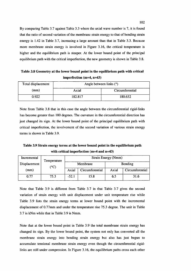
102

By comparing Table 3.7 against Table 3.3 where the axial wave number is 7, it is found

that the ratio of second variation of the membrane strain energy to that of bending strain

energy is 1.42 in Table 3.7, increasing a large amount than that in Table 3.3. Because

more membrane strain energy is involved in Figure 3.16, the critical temperature is

higher and the equilibrium path is steeper. At the lower bound point of the principal

equilibrium path with the critical imperfection, the new geometry is shown in Table 3.8.



Total displacement

(mm)

Angle between links (°)


0.922 182.817 180.632

Note from Table 3.8 that in this case the angle between the circumferential rigid-links

has become greater than 180 degrees. The curvature in the circumferential direction has

just changed its sign. At the lower bound point of the principal equilibrium path with

critical imperfection, the involvement of the second variation of various strain energy

terms is shown in Table 3.9.

Table 3.9 Strain energy terms at the lower bound point in the equilibrium path

with critical imperfection (m=4 and n=43)

Incremental

Displacement

(mm)

Temperature

CC)

Strain Energy (Nmm)

Membrane Bending


0.77 75.3 -52.1 15.8 6.5 31.6

Note that Table 3.9 is different from Table 3.7 in that Table 3.7 gives the second

variation of strain energy with unit displacement under unit temperature rise while

Table 3.9 lists the strain energy terms at lower bound point with the incremental

displacement of 0.77mm and under the temperature rise 75.3 degree. The unit in Table

3.7 is kNm while that in Table 3.9 is Nmm.

Note that at the lower bound point in Table 3.9 the total membrane strain energy has

changed its sign. By the lower bound point, the system not only has converted all the

membrane strain energy into bending strain energy but also has just begun to

accumulate tensional membrane strain energy even though the circumferential rigid-

links are still under compression. In Figure 3.16, the equilibrium paths cross each other

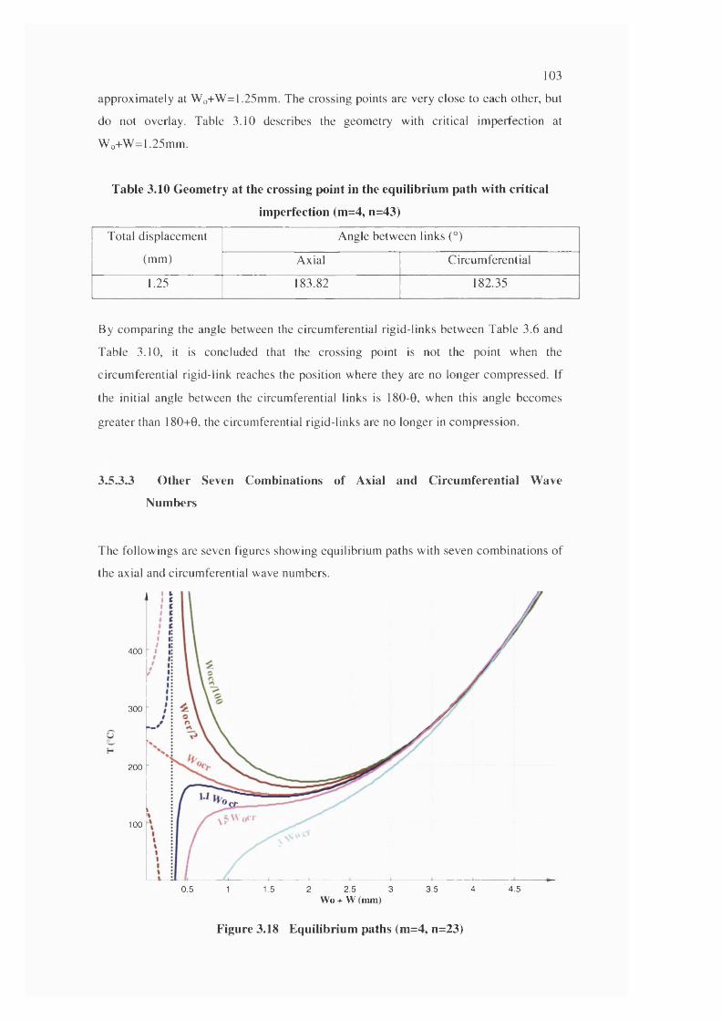
103

approxim ately at W o+W =1.25mm. The crossing points are very close to each other, but

do not overlay. Table 3.10 describes the geom etry with critical im perfection at

W o+W = 1.25mm.

Table 3.10 Geometry at the crossing point in the equilibrium path with critical


Total displacem ent

(m m )

Angle betw een links (°)

A xial Circum ferential

1.25 183.82 182.35

By com paring the angle between the circum ferential rigid-links betw een Table 3.6 and

T able 3.10, it is concluded that the crossing point is not the point when the

circum ferential rigid-link reaches the position where they are no longer com pressed. If

the initial angle between the circum ferential links is 180-0, when this angle becom es

greater than 180-1-0, the circum ferential rigid-links are no longer in com pression.

3.5.33 Other Seven Combinations of Axial and Circumferential Wave

Numbers

T he follow ings are seven figures showing equilibrium paths with seven com binations of

the axial and circum ferential wave numbers.

400

300

200

100

0.5 1.5 2 2.5 3 3.5 4 4.51Wo + W (mm)


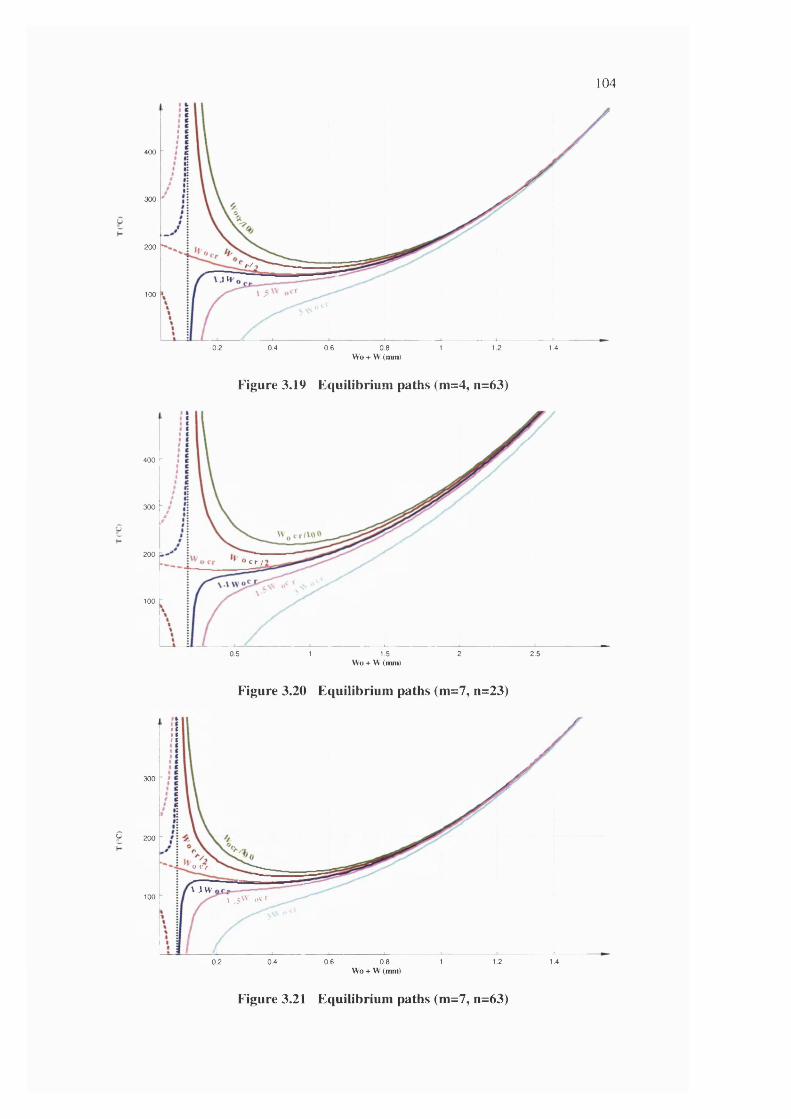
104

400

300

200

/•/IM

100

0.2 0.4 0.6 0.8 1 1.2 1.4Wo + W (mm)


400

300

200“ c r /

100

0.5 1 1.5 2 2.5Wo + W (mm)


ii

300

y 200

O C f

\ \ W100 V 5\V „cr

1.20.2 0.4 0.6 0.8 1 1.4Wo + W (mm)


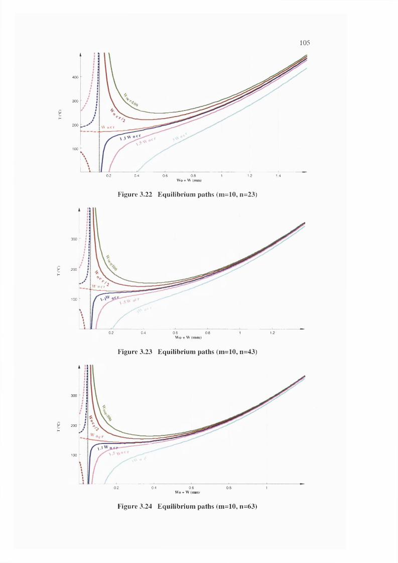
105

400

300

H200 W o c r

\\V

100

0.2 0.4 0.8 1.20.6 1 1.4Wo + W (mm)


300

u 200 -

H

M <) c r

100 -

0.2 0.4 0.6 0.8 1 1.2W o + W (mm )


200H

\ .1100

0.2 0.6Wo + W (mm)

0.4 0.8 1


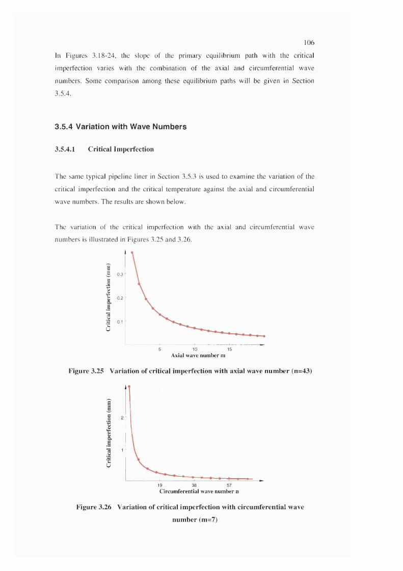
106

In Figures 3.18-24, the slope o f the prim ary equilibrium path w ith the critical

im perfection varies with the com bination o f the axial and circum ferential wave

num bers. Some com parison am ong these equilibrium paths will be given in Section

3.5.4.

3.5.4 Variation with Wave Numbers

3.5.4.1 Critical Imperfection

The same typical pipeline liner in Section 3.5.3 is used to exam ine the variation o f the

critical im perfection and the critical tem perature against the axial and circum ferential

wave num bers. The results are shown below.

The variation o f the critical im perfection with the axial and circum ferential wave

num bers is illustrated in Figures 3.25 and 3.26.

EE 0.3

§Ib 0.2

Ës

S 0.1

Ù

5 10 15Axial wave number m

Figure 3.25 Variation of critical imperfection with axial wave number (n=43)

u

i

2

1

19 38 57Circumferential wave number n

Figure 3.26 Variation of critical imperfection with circumferential wave

number (m=7)

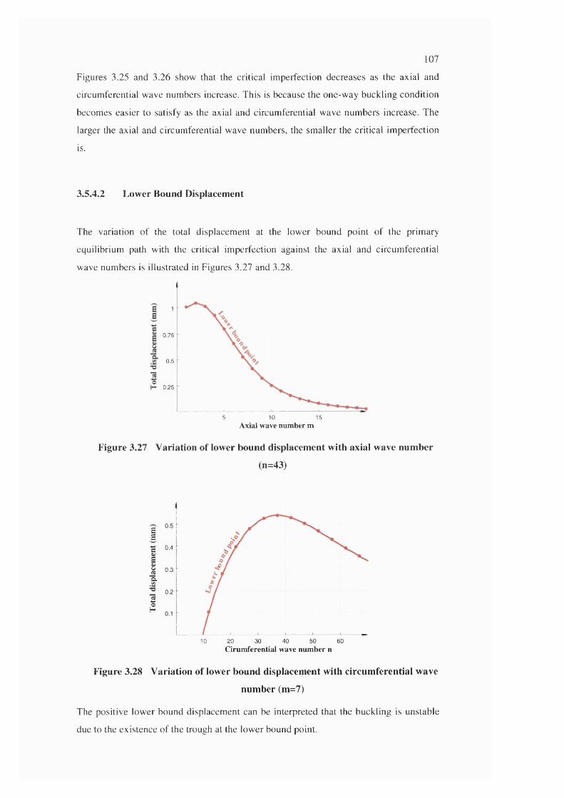
107

Figures 3.25 and 3.26 show that the critical im perfection decreases as the axial and

circum ferential wave num bers increase. This is because the one-w ay buckling condition

becom es easier to satisfy as the axial and circum ferential wave num bers increase. The

larger the axial and circum ferential wave num bers, the sm aller the critical im perfection

is.

3.S.4.2 Lower Bound Displacement

The variation o f the total displacem ent at the lower bound point o f the prim ary

equilibrium path with the critical im perfection against the axial and circum ferential

wave num bers is illustrated in Figures 3.27 and 3.28.

0.75

0.5

H 0.25


Figure 3.27 Variation of lower bound displacement with axial wave number

(n=43)

sEC 0.4E* 0-3 a..2

0.2«g

10 20 30 40 50 60Cirumferential wave number n

Figure 3.28 Variation of lower bound displacement with circumferential wave

number (m=7)

The positive low er bound displacem ent can be interpreted that the buckling is unstable

due to the existence o f the trough at the low er bound point.

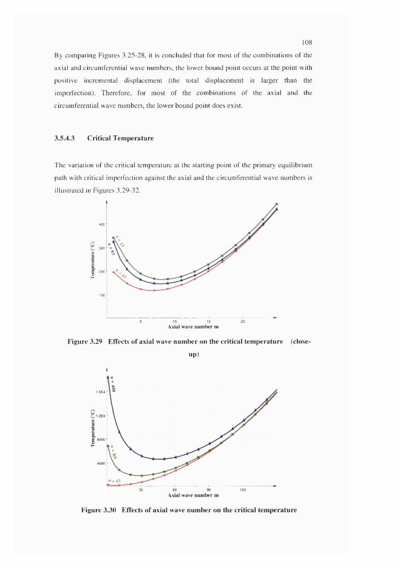
108

By com paring Figures 3.25-28, it is concluded that for most o f the com binations o f the

axial and circum ferential wave num bers, the low er bound point occurs at the point w ith

positive increm ental displacem ent (the total displacem ent is larger than the

im perfection). Therefore, for most o f the com binations o f the axial and the

circum ferential wave num bers, the low er bound point does exist.

3.5.4.3 Critical Temperature

The variation o f the critical tem perature at the starting point o f the prim ary equilibrium

path with critical im perfection against the axial and the circum ferential wave num bers is

illustrated in Figures 3.29-32.

I

400

300

200

100


Figure 3.29 Effects of axial wave number on the critical temperature (close-

up)

1.6E4

g 8000

4000


Figure 3.30 Effects of axial wave number on the critical temperature

109

135i

130

t3125

a^ 120

115

35 5040 45 55Circumferential wave number n

Figure 3.31 Effects of circumferential wave number on the critical

temperature (close-up)

2000m = 50

1500

1000

500

20 40 80 100 120 14060Circumferential wave number n

Figure 3.32 Effects of circumferential wave number on the critical

temperature

In Figures 3.29 and 3.30, it is found that the critical tem perature is very sensitive to the

axial wave num ber when the circum ferential wave num ber is not too large say around

43.

In Figures 3.31 and 3.32, it is found that the critical tem perature is sensitive to the

circum ferential wave num ber only when the circum ferential wave length is either too

long or too short. For the wave num bers around 43, the critical tem perature does not

vary much.

In Figures 3.29-32, it is found that, for the given geom etric param eters in the current

section, the lowest critical tem perature occurs with an axial wave num ber o f 7 and a

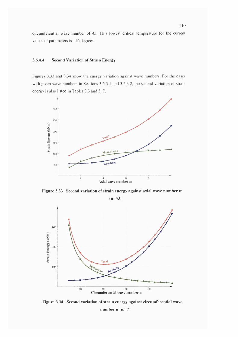
110

circum ferential wave num ber o f 43. This lowest critical tem perature for the current

values o f param eters is 116 degrees.

3.S.4.4 Second Variation of Strain Energy

Figures 3.33 and 3.34 show the energy variation against wave num bers. For the cases

with given wave num bers in Sections 3.5.3.1 and 3.5.3.2, the second variation o f strain

energy is also listed in Tables 3.3 and 3. 7.

300

250

200

150

100


Figure 3.33 Second variation of strain energy against axial wave number m

(n=43)

600

400

200

8020 40 60Circumferential wave number n

Figure 3.34 Second variation of strain energy against circumferential wave

number n (m=7)

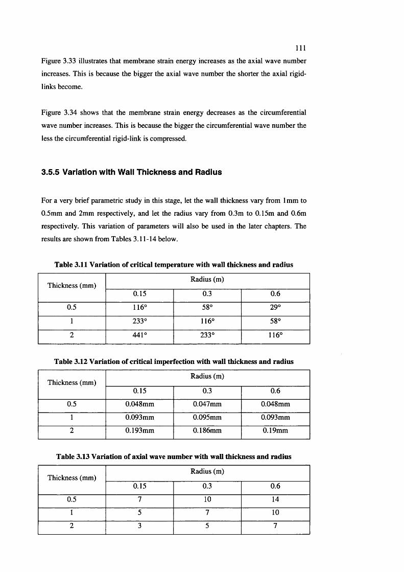
I l l

Figure 3.33 illustrates that membrane strain energy increases as the axial wave number

increases. This is because the bigger the axial wave number the shorter the axial rigid-

links become.

Figure 3.34 shows that the membrane strain energy decreases as the circumferential

wave number increases. This is because the bigger the circumferential wave number the

less the circumferential rigid-link is compressed.

3.5.5 Variation with Wall T hickness and Radius

For a very brief parametric study in this stage, let the wall thickness vary from 1 mm to

0.5mm and 2mm respectively, and let the radius vary from 0.3m to 0.15m and 0.6m

respectively. This variation of parameters will also be used in the later chapters. The

results are shown from Tables 3.11-14 below.

Table 3.11 Variation of critical temperature with wall thickness and radius

Thickness (mm)Radius (m)

0.15 0.3 0 .6

0.5 116° 58° 29°

1 233° 116° 58°

2 441° 233° 116°

Table 3.12 Variation of critical imperfection with wall thickness and radius


0.15 0.3 0 .6

0.5 0.048mm 0.047mm 0.048mm

1 0.093mm 0.095mm 0.093mm

2 0.193mm 0.186mm 0.19mm

Table 3.13 Variation of axial wave number with wall thickness and radius


0.15 0.3 0 .6

0.5 7 1 0 14

1 5 7 1 0

2 3 5 7

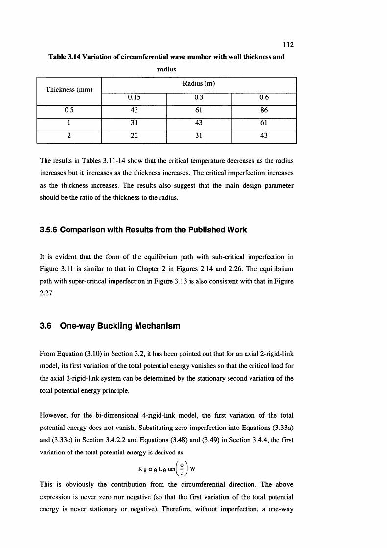
112

Table 3.14 Variation of circumferential wave number with wall thickness and

radius


0.15 0.3 0 .6

0.5 43 61 8 6

1 31 43 61

2 2 2 31 43

The results in Tables 3.11-14 show that the critical temperature decreases as the radius

increases but it increases as the thickness increases. The critical imperfection increases

as the thickness increases. The results also suggest that the main design parameter

should be the ratio of the thickness to the radius.

3.5.6 Com parison with Resuits from the Pubiished Work

It is evident that the form of the equilibrium path with sub-critical imperfection in

Figure 3.11 is similar to that in Chapter 2 in Figures 2.14 and 2.26. The equilibrium

path with super-critical imperfection in Figure 3.13 is also consistent with that in Figure

2.27.

3.6 O ne-w ay B uckling M echanism

From Equation (3.10) in Section 3.2, it has been pointed out that for an axial 2-rigid-link

model, its first variation of the total potential energy vanishes so that the critical load for

the axial 2 -rigid-link system can be determined by the stationary second variation of the

total potential energy principle.

However, for the bi-dimensional 4-rigid-link model, the first variation of the total

potential energy does not vanish. Substituting zero imperfection into Equations (3.33a)

and (3.33e) in Section 3.4.2.2 and Equations (3.48) and (3.49) in Section 3.4.4, the first

variation of the total potential energy is derived as

K e a 0 L 0 tan I — ] W

This is obviously the contribution from the circumferential direction. The above

expression is never zero nor negative (so that the first variation of the total potential

energy is never stationary or negative). Therefore, without imperfection, a one-way

113

buckling system will never buckle. Imperfection is no longer playing a part as a knock

down factor of the buckling load. Instead, imperfection is essential in one-way buckling.

With imperfection. Equation (3.49) in Section 3.4.4 is rewritten as Equation (3.57). The

first variation of the total potential energy vanishes when the magnitude of the

imperfection is equal to the critical imperfection in Equation (3.62).

With stationary first variation of the total potential energy, the critical temperature can

be obtained via the stationary second variation of total potential energy principle.

Therefore, a one-way buckling system with critical imperfection can buckle just like a

two-way buckling system does.

Review Equation (3.62)

^ a g K g L g R +

WOx Kx sin((p)

a g K g LgR +

ttx Kx sin((p)— 4 tan I "Y

«X KxR L g

It is obvious that the critical imperfection is the result of the coupling of the effects from

both the axial and circumferential directions. The critical imperfection is the results of

the balance of the work done in both directions after a disturbance of displacement W

under thermal loading. The energy release due to the extension of length in the axial

direction is equal to the energy accumulation due to the decrease of length in the

circumferential direction.

However, the increase of the length in the axial direction is not necessary equal to the

increase of the length in the circumferential direction. Nor does the critical imperfection

correspond to the position when the circumferential links are “flat” as a ring arch snap-

through does. It is the energy balance that creates the critical imperfection.

3.7 C onclud ing R em arks

From the above analysis, the following conclusions may be drawn

• The rigid-link model is capable of demonstrating the underlying basic buckling

mechanism of the one-way buckling of pipeline liners. Without imperfection,

under a virtual disturbance W in the radial direction, according to the strain-

displacement equations (3.33), the length increase in the axial rigid-links is one-

114

order smaller than the length decrease in the circumferential rigid-links,

accordingly, the possible membrane energy release in the axial rigid-links is far

smaller than the possible membrane energy accumulation in the circumferential

rigid-links. Therefore, without imperfection, a one-way buckling system will

never buckle.

With imperfection, the coupling terms of imperfection and the deflection that

occur in the formula of the length change in rigid-links make it possible the

length changes in both directions of the same order, which subsequently makes

it possible a new equilibrium state under a virtual radial disturbance. The new

equilibrium state can only be realized when the magnitude of imperfection

exceeds a certain value referred as “critical imperfection”.

The critical imperfection is the result of the energy balance due to a disturbance

in the geometric shape under thermal loading. At the critical imperfection, the

membrane energy release in the axial rigid-links is equal to the membrane

energy accumulation in the circumferential rigid-links. It is neither the balance

of the length change in both directions nor the position when a part of the shell

becomes “flat” as in a snap-through.

When the imperfection is smaller than the critical imperfection, the one-way

buckling system will never buckle. If the imperfection is equal to the critical

imperfection, the one-way buckling system “bifurcates” just as a two-way

buckling system. When the imperfection is larger than the critical imperfection,

the one-way buckling system behaves in a way similar to the post-buckling of a

two-way buckling system.

The example suggests that a pipeline liner could buckle at temperature about 116

degrees with an axial wave length of 43mm and a circumferential wave number

of 43 and a critical imperfection of 0.1mm. The example also suggests that

critical temperature is very sensitive to the slight change of axial wave length

but not so sensitive to the slight change of the circumferential wave number.

The results from the parametric study show that the critical temperature

decreases as the radius increases and the critical imperfection increases as the

thickness increases.

115

4 Buckling Analysis with Simpiified Beam-Link

Model

4.1 In troduction

This chapter describes further work on the simplified analysis presented in Chapter 3. In

Chapter 3, the liners are simplified as rigid-links, with the membrane and bending

stiffness being transferred to membrane and moment springs. The rigid-link model

works very well for the understanding of the most basic one-way buckling mechanism:

• The liner will never buckle without imperfection and

• At the critical imperfection the pipeline liner “bifurcates” just like a two-way

buckling in which either W=0 (incremental displacement is zero) or T=Tcr

(temperature is equal to critical temperature).

However, the rigid-link approach has the following drawbacks:

• The selection of stiffness of various membrane and moment springs is arbitrary.

A good guess of the buckled shape is essential;

• The transference of membrane and moment stiffness of the rigid-links to the

membrane and moment springs is simplified, especially in the circumferential

direction. This is adequate for the understanding of the one-way buckling

mechanism but the resulting values for the buckling temperature and the critical

imperfection may not be sufficiently accurate;

• The actual deformed shape may not be adequately described by the rigid-link

model.

These drawbacks may largely be overcome by replacing the rigid-links with flexural

links. By doing this, the displacement variables are now switched from point

displacement to displacement functions along the beam axial directions. In this way, the

beam-link model allows the system to pick up more realistic deformed shapes. After the

basic objectives for the one-way buckling mechanism have been achieved with the

rigid-link model in Chapter 3, it is intended that this chapter should

• develop more accurate formula for critical imperfection and its corresponding

buckling temperature;

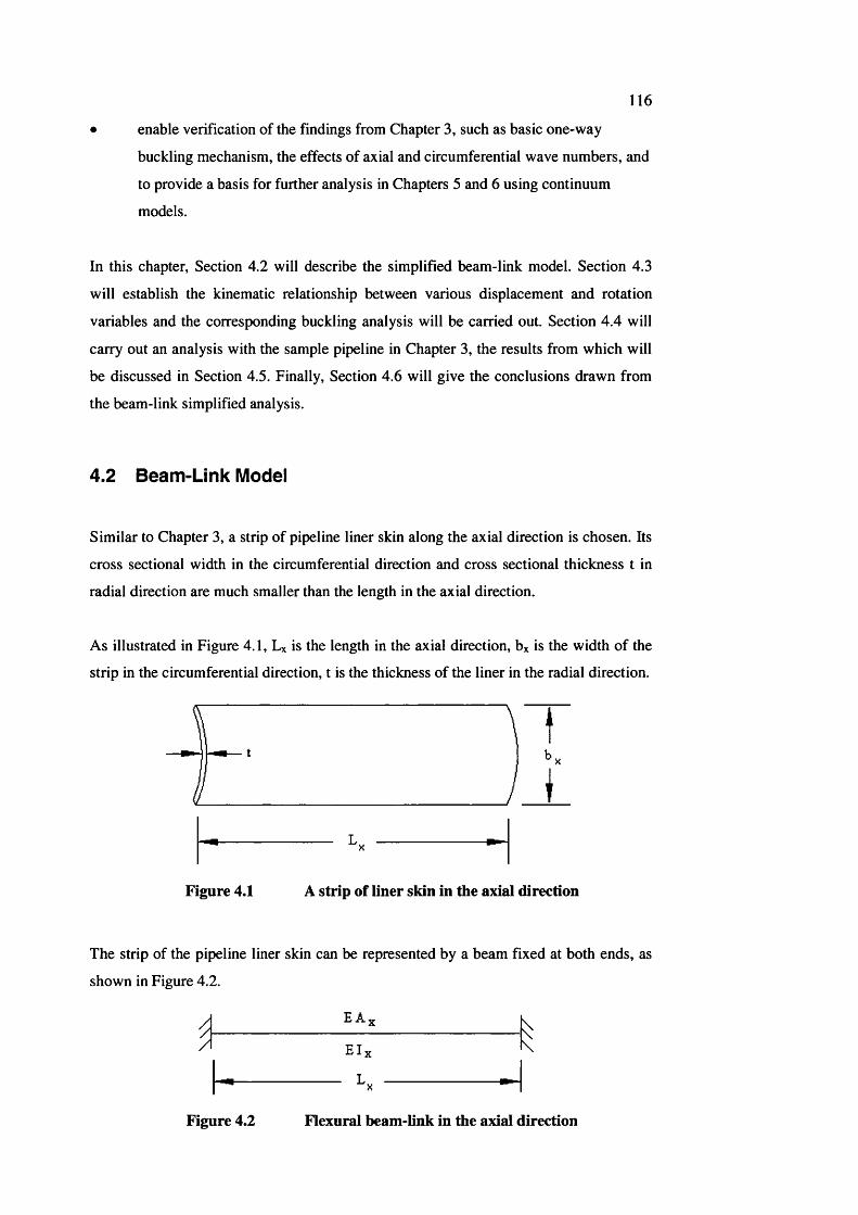
116

• enable verification of the findings from Chapter 3, such as basic one-way

buckling mechanism, the effects of axial and circumferential wave numbers, and

to provide a basis for further analysis in Chapters 5 and 6 using continuum

models.

In this chapter. Section 4.2 will describe the simplified beam-link model. Section 4.3

will establish the kinematic relationship between various displacement and rotation

variables and the corresponding buckling analysis will be carried out. Section 4.4 will

carry out an analysis with the sample pipeline in Chapter 3, the results from which will

be discussed in Section 4.5. Finally, Section 4.6 will give the conclusions drawn from

the beam-link simplified analysis.

4.2 Beam -Link Model

Similar to Chapter 3, a strip of pipeline liner skin along the axial direction is chosen. Its

cross sectional width in the circumferential direction and cross sectional thickness t in

radial direction are much smaller than the length in the axial direction.

As illustrated in Figure 4.1, Lx is the length in the axial direction, bx is the width of the

strip in the circumferential direction, t is the thickness of the liner in the radial direction.

L

Figure 4.1 A strip of liner skin in the axial direction

The strip of the pipeline liner skin can be represented by a beam fixed at both ends, as

shown in Figure 4.2.

E A,

EIx

L..

Figure 4.2 Flexural beam-link in the axial direction

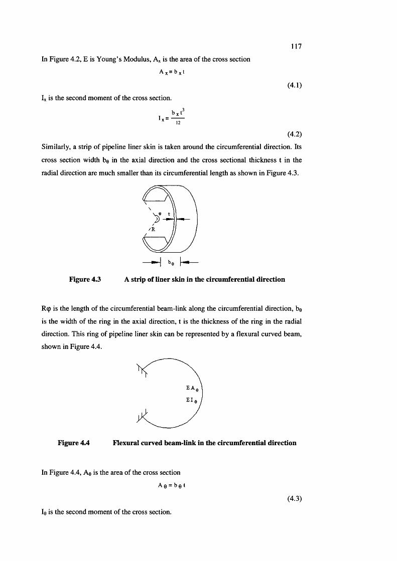
In Figure 4.2, E is Young’s Modulus, A% is the area of the cross section

117

(4.1)

Iv is the second moment of the cross section.

Iy =12

(4.2)

Similarly, a strip of pipeline liner skin is taken around the circumferential direction. Its

cross section width be in the axial direction and the cross sectional thickness t in the

radial direction are much smaller than its circumferential length as shown in Figure 4.3.

/R

b,

Figure 4.3 A strip of liner skin in the circumferential direction

Rtp is the length of the circumferential beam-link along the circumferential direction, be

is the width of the ring in the axial direction, t is the thickness of the ring in the radial

direction. This ring of pipeline liner skin can be represented by a flexural curved beam,

shown in Figure 4.4.

EA

E l

Figure 4.4 Flexural curved beam-link in the circumferential direction

In Figure 4.4, Ae is the area of the cross section

Ae = be t

le is the second moment of the cross section.

(4.3)

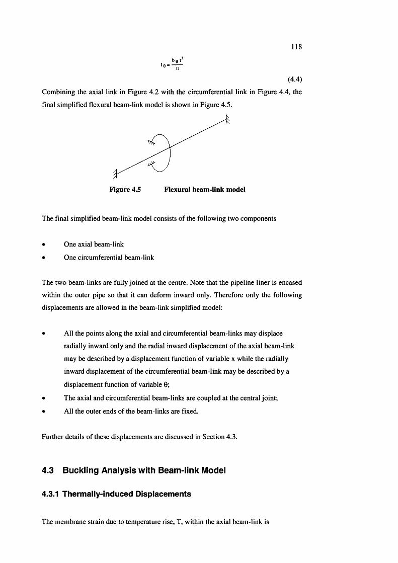
bet ‘ 0 = —

1183

(4.4)

Combining the axial link in Figure 4.2 with the circumferential link in Figure 4.4, the

final simplified flexural beam-link model is shown in Figure 4.5.

Figure 4.5 Flexural beam-link model

The final simplified beam-link model consists of the following two components

• One axial beam-link

• One circumferential beam-link

The two beam-links are fully joined at the centre. Note that the pipeline liner is encased

within the outer pipe so that it can deform inward only. Therefore only the following

displacements are allowed in the beam-link simplified model:

• All the points along the axial and circumferential beam-links may displace

radially inward only and the radial inward displacement of the axial beam-link

may be described by a displacement function of variable x while the radially

inward displacement of the circumferential beam-link may be described by a

displacement function of variable 0 ;

• The axial and circumferential beam-links are coupled at the central joint;

• All the outer ends of the beam-links are fixed.

Further details of these displacements are discussed in Section 4.3.

4.3 B uckling A nalysis w ith B eam -link Model

4.3.1 Thermally-induced Displacem ents

The membrane strain due to temperature rise, T, within the axial beam-link is

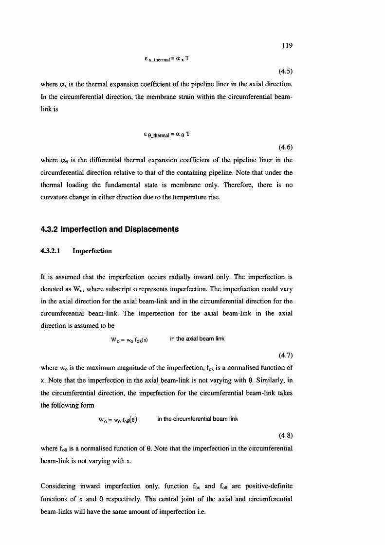
119

G x_thermal = # x T

(4.5)

where ttx is the thermal expansion coefficient of the pipeline liner in the axial direction.

In the circumferential direction, the membrane strain within the circumferential beam-

link is

G 0_thermal ~ ® 0 T

(4.6)

where ote is the differential thermal expansion coefficient of the pipeline liner in the

circumferential direction relative to that of the containing pipeline. Note that under the

thermal loading the fundamental state is membrane only. Therefore, there is no

curvature change in either direction due to the temperature rise.

4.3.2 Imperfection and Displacem ents

4.3.2.1 Imperfection

It is assumed that the imperfection occurs radially inward only. The imperfection is

denoted as Wq, where subscript o represents imperfection. The imperfection could vary

in the axial direction for the axial beam-link and in the circumferential direction for the

circumferential beam-link. The imperfection for the axial beam-link in the axial

direction is assumed to be

W q = W o fo x (x ) in the axial beam link

(4.7)

where Wq is the maximum magnitude of the imperfection, fox is a normalised function of

X . Note that the imperfection in the axial beam-link is not varying with 0. Similarly, in

the circumferential direction, the imperfection for the circumferential beam-link takes

the following form

W q = Wq foe(@) in the circumferential beam link

(4.8)

where foe is a normalised function of 0. Note that the imperfection in the circumferential

beam-link is not varying with x.

Considering inward imperfection only, function fox and foe are positive-definite

functions of x and 0 respectively. The central joint of the axial and circumferential

beam-links will have the same amount of imperfection i.e.

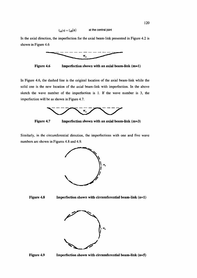
120

W x ) = W e ) at the central joint

In the axial direction, the imperfection for the axial beam-link presented in Figure 4.2 is

shown in Figure 4.6

Figure 4.6 Imperfection shown with an axial beam-link (m=l)

In Figure 4.6, the dashed line is the original location of the axial beam-link while the

solid one is the new location of the axial beam-link with imperfection. In the above

sketch the wave number of the imperfection is 1. If the wave number is 3, the

imperfection will be as shown in Figure 4.7.

Figure 4.7 Imperfection shown with an axial beam-link (m=3)

Similarly, in the circumferential direction, the imperfections with one and five wave

numbers are shown in Figures 4.8 and 4.9.

Figure 4.8 Imperfection shown with circumferential beam-link (n=l)

Figure 4.9 Imperfection shown with circumferential beam-link (n=5)

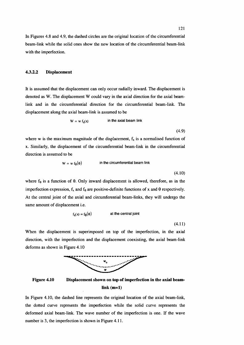
121

In Figures 4.8 and 4.9, the dashed circles are the original location of the circumferential

beam-link while the solid ones show the new location of the circumferential beam-link

with the imperfection.

4.S.2.2 Displacement

It is assumed that the displacement can only occur radially inward. The displacement is

denoted as W. The displacement W could vary in the axial direction for the axial beam-

link and in the circumferential direction for the circumferential beam-link. The

displacement along the axial beam-link is assumed to be

W = w fx(x) in the axial beam link

(4.9)

where w is the maximum magnitude of the displacement, fx is a normalised function of

X. Similarly, the displacement of the circumferential beam-link in the circumferential

direction is assumed to be

W = w feCe) in the circumferential beam link

(4.10)

where fg is a function of 0. Only inward displacement is allowed, therefore, as in the

imperfection expression, fx and fg are positive-definite functions of x and 0 respectively.

At the central joint of the axial and circumferential beam-links, they will undergo the

same amount of displacement i.e.

f x) = fe(e) at the central joint

(4.11)

When the displacement is superimposed on top of the imperfection, in the axial

direction, with the imperfection and the displacement coexisting, the axial beam-link

deforms as shown in Figure 4.10

Figure 4.10 Displacement shown on top of imperfection in the axial beam-

link (m=l)

In Figure 4,10, the dashed line represents the original location of the axial beam-link,

the dotted curve represents the imperfection while the solid curve represents the

deformed axial beam-link. The wave number of the imperfection is one. If the wave

number is 3, the imperfection is shown in Figure 4.11.

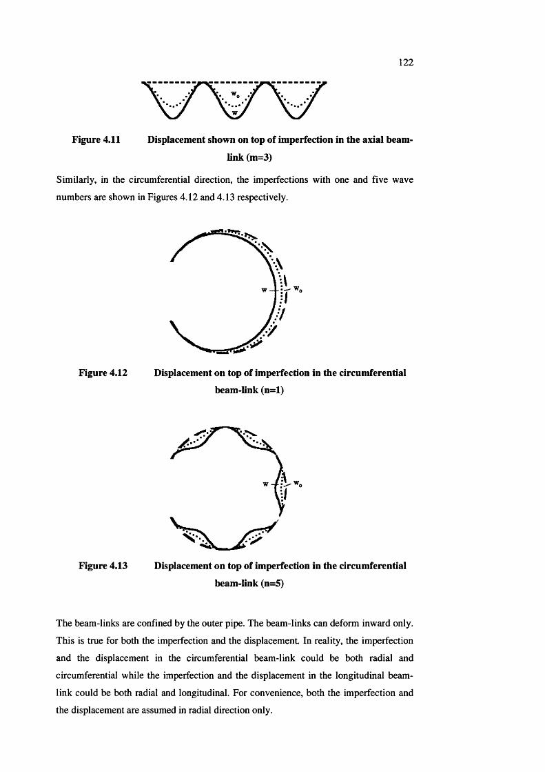
122

Figure 4.11 Displacement shown on top of imperfection in the axial beam-

link (m=3)

Similarly, in the circumferential direction, the imperfections with one and five wave

numbers are shown in Figures 4.12 and 4.13 respectively.

Figure 4.12 Displacement on top of imperfection in the circumferential

beam-link (n=l)

Figure 4.13 Displacement on top of imperfection in the circumferential

beam-link (n=5)

The beam-links are confined by the outer pipe. The beam-links can deform inward only.

This is true for both the imperfection and the displacement. In reality, the imperfection

and the displacement in the circumferential beam-link could be both radial and

circumferential while the imperfection and the displacement in the longitudinal beam-

link could be both radial and longitudinal. For convenience, both the imperfection and

the displacement are assumed in radial direction only.

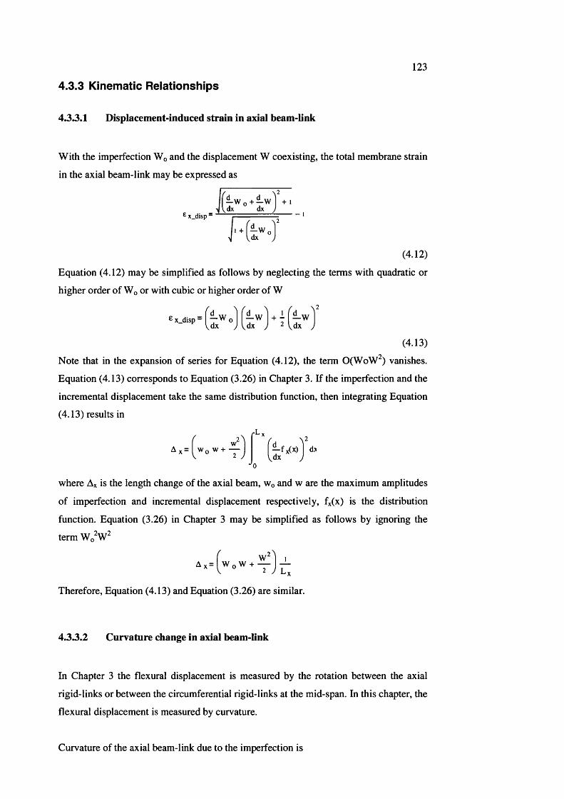
123

4.3.3 Kinematic Relationships

4.33.1 Displacement-induced strain in axial beam-link

With the imperfection Wo and the displacement W coexisting, the total membrane strain

in the axial beam-link may be expressed as

^ x_disp =

lW o + — + 1 dx dx y

1

I + 1 — W, dx

(4.12)

Equation (4.12) may be simplified as follows by neglecting the terms with quadratic or

higher order of Wq or with cubic or higher order of W

(4.13)Note that in the expansion of series for Equation (4.12), the term O(WoW^) vanishes.

Equation (4.13) corresponds to Equation (3.26) in Chapter 3. If the imperfection and the

incremental displacement take the same distribution function, then integrating Equation

(4.13) results in

.LvIA v = l W q W + — d,

where A% is the length change of the axial beam, Wo and w are the maximum amplitudes

of imperfection and incremental displacement respectively, f%(x) is the distribution

function. Equation (3.26) in Chapter 3 may be simplified as follows by ignoring the

term Wo^W^

Therefore, Equation (4.13) and Equation (3.26) are similar.

4.3.3.2 Curvature change in axial beam-link

In Chapter 3 the flexural displacement is measured by the rotation between the axial

rigid-links or between the circumferential rigid-links at the mid-span. In this chapter, the

flexural displacement is measured by curvature.

Curvature of the axial beam-link due to the imperfection is

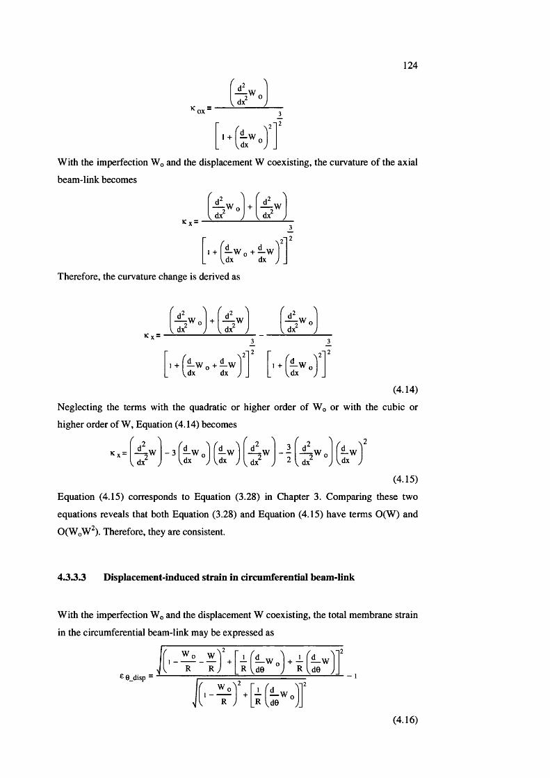
124

^ox =' S ' " ' ]

1 + — wVdx

With the imperfection Wq and the displacement W coexisting, the curvature of the axial

beam-link becomes

K Y —_ Vfd 1- ^ W o +I dx j I dx j

1 + —Wn + —Wdx dx

Therefore, the curvature change is derived as

K Y —

fd ^ 1 f d 1 fd ^ 1+V dx j I dx J I dx j

2r /"h

1 + 1 - W o + - W 1 l + [ - W o l_ Vdx dx J _ . Id x J _

(4.14)

Neglecting the terms with the quadratic or higher order of Wq or with the cubic or

higher order of W, Equation (4.14) becomes

K Y —

vdx- 3 — 1 f — W tW

dx^ W o

vdx y-W

dxvdx J \d x

(4.15)

Equation (4.15) corresponds to Equation (3.28) in Chapter 3. Comparing these two

equations reveals that both Equation (3.28) and Equation (4.15) have terms 0(W ) and

O(WqW^). Therefore, they are consistent.

4.3.3.3 Displacement-induced strain in circumferential beam-link

With the imperfection Wq and the displacement W coexisting, the total membrane strain

in the circumferential beam-link may be expressed as

^0_disp -

W o W

R R R U e— — W o 1 + - f — w

R IdO- 1

w1 I +

R-L M -wR IdG

(4.16)

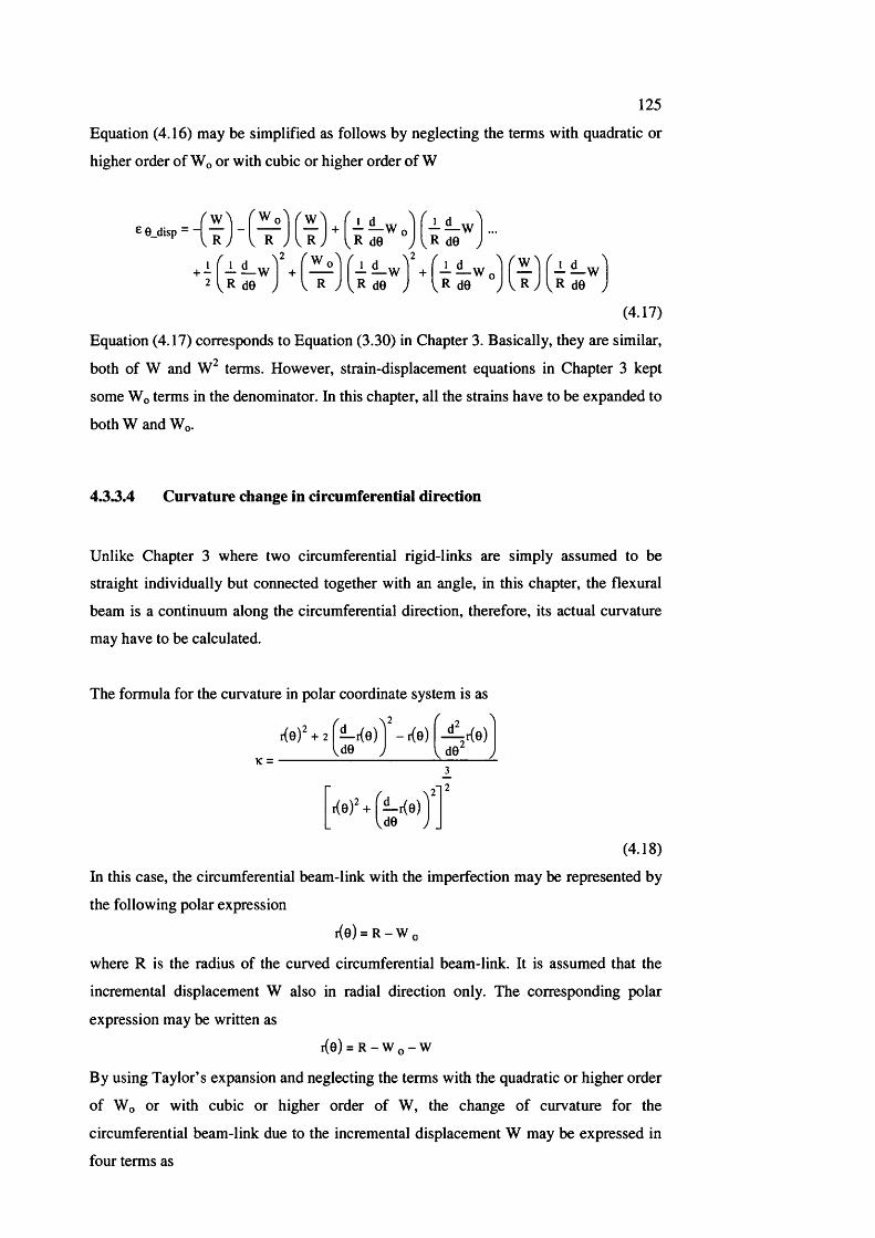
125

Equation (4.16) may be simplified as follows by neglecting the terms with quadratic or

higher order of Wq or with cubic or higher order of W

G 0_disp =w

R de

f 1 d ^--- + - — W o

^ R d 0 j

R

-L ^ w R de

- - - WR J I R deR de J V R de

(4.17)

Equation (4.17) corresponds to Equation (3.30) in Chapter 3. Basically, they are similar,

both of W and terms. However, strain-displacement equations in Chapter 3 kept

some Wo terms in the denominator. In this chapter, all the strains have to be expanded to

both W and Wq.

4.33.4 Curvature change in circumferential direction

Unlike Chapter 3 where two circumferential rigid-links are simply assumed to be

straight individually but connected together with an angle, in this chapter, the flexural

beam is a continuum along the circumferential direction, therefore, its actual curvature

may have to be calculated.

The formula for the curvature in polar coordinate system is as

K =

\ 2 f ^2 1-Ke) -Ke) - ^ r ( 0 )

ld0 J ld0: j

rief 4_Ke)Vd0

(4.18)

In this case, the circumferential beam-link with the imperfection may be represented by

the following polar expression

i{0 ) = R - W o

where R is the radius of the curved circumferential beam-link. It is assumed that the

incremental displacement W also in radial direction only. The corresponding polar

expression may be written as

r(0 ) = R - W o - W

By using Taylor’s expansion and neglecting the terms with the quadratic or higher order

of Wo or with cubic or higher order of W, the change of curvature for the

circumferential beam-link due to the incremental displacement W may be expressed in

four terms as

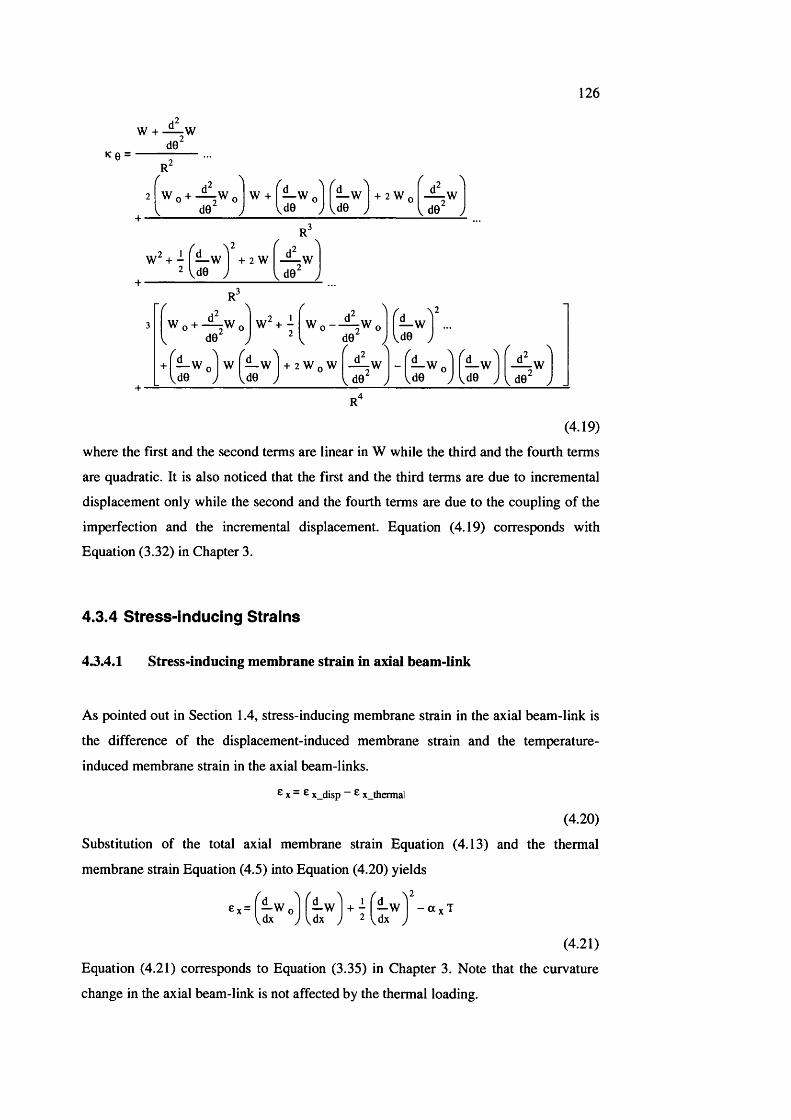
126

K 0 =

W + - i i - W de

f^ O ■' 2 ^ O

V de" yW +

de— w I + 2 w

\de' < i w 'yae" J

+ - f — w I + 2 w 2 U e

R

ï ” '

Wd Wo + -^ W ode

w^+ - W o --^ W o

de de

de/

de

:Wde

- I — w , de

— w de

:Wde

R"

(4.19)

where the first and the second terms are linear in W while the third and the fourth terms

are quadratic. It is also noticed that the first and the third terms are due to incremental

displacement only while the second and the fourth terms are due to the coupling of the

imperfection and the incremental displacement. Equation (4.19) corresponds with

Equation (3.32) in Chapter 3.

4.3.4 Stress-inducing Strains

4.3.4.1 Stress-inducing membrane strain in axial beam-link

As pointed out in Section 1.4, stress-inducing membrane strain in the axial beam-link is

the difference of the displacement-induced membrane strain and the temperature-

induced membrane strain in the axial beam-1 inks.

x_disp “ G x_therma]

(4.20)

Substitution of the total axial membrane strain Equation (4.13) and the thermal

membrane strain Equation (4.5) into Equation (4.20) yields

(4.21)

Equation (4.21) corresponds to Equation (3.35) in Chapter 3. Note that the curvature

change in the axial beam-link is not affected by the thermal loading.

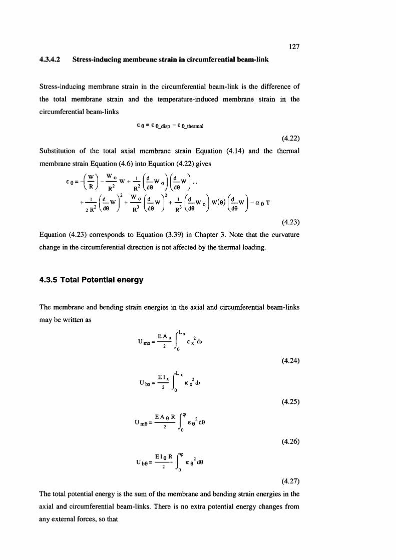
127

4.3A 2 Stress-inducing membrane strain in circumferential beam-link

Stress-inducing membrane strain in the circumferential beam-link is the difference of

the total membrane strain and the temperature-induced membrane strain in the

circumferential beam-1 inks

G 8 - G 0_disp “ E 0_thermal

(4 22)

Substitution of the total axial membrane strain Equation (4.14) and the thermal

membrane strain Equation (4.6) into Equation (4.22) gives

R ; r 2 r2 de ° A d 0

VdO+ — r l — w | + -T —Wo|w(e)

vdG y- a 0 T+ —

R I de ) r3 Vde

(4.23)

Equation (4.23) corresponds to Equation (3.39) in Chapter 3. Note that the curvature

change in the circumferential direction is not affected by the thermal loading.

4.3.5 Total Potential energy

The membrane and bending strain energies in the axial and circumferential beam-1 inks

may be written as

E A , l'-mx'“

AxJ Ex^d)

' -'0

IT 2 .u bx = K X d>• 0

(4.24)

EA 0 R r 2 Um0 = - ^ 6 0 de

• 0

(4.25)

(4.26)

E lf iR f(Pr(pUb0 = — K0‘ de

(4.27)

The total potential energy is the sum of the membrane and bending strain energies in the

axial and circumferential beam-1 inks. There is no extra potential energy changes from

any external forces, so that

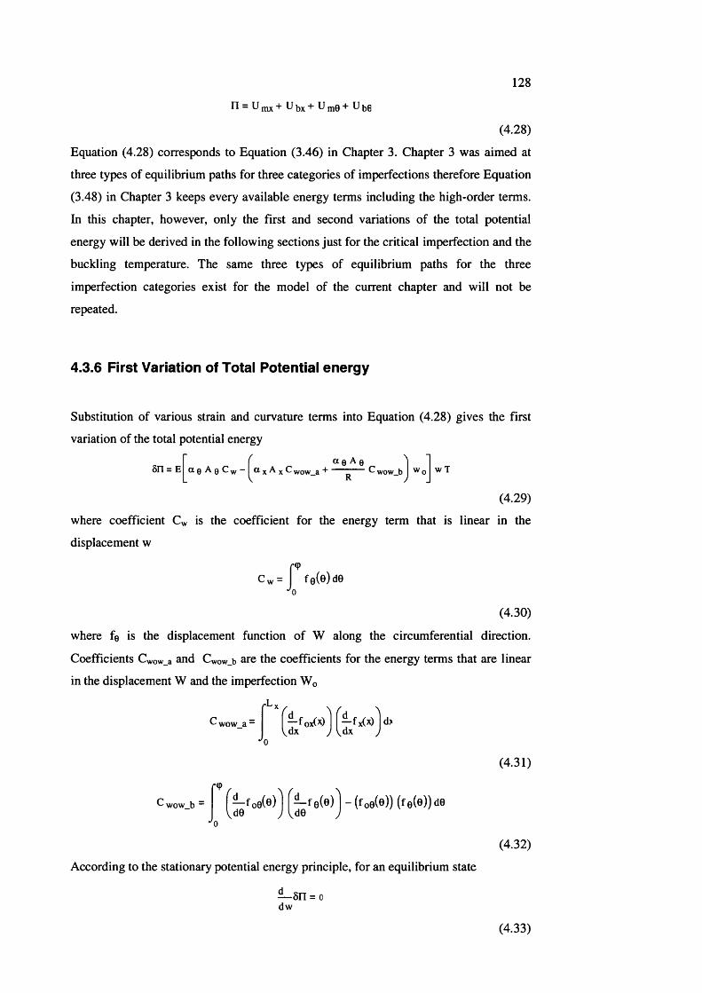
128

n = U inx + U bx + UIJ10 + U 56

(4.28)

Equation (4.28) corresponds to Equation (3.46) in Chapter 3. Chapter 3 was aimed at

three types of equilibrium paths for three categories of imperfections therefore Equation

(3.48) in Chapter 3 keeps every available energy terms including the high-order terms.

In this chapter, however, only the first and second variations of the total potential

energy will be derived in the following sections just for the critical imperfection and the

buckling temperature. The same three types of equilibrium paths for the three

imperfection categories exist for the model of the current chapter and will not be

repeated.

4.3.6 First Variation of Total Potential energy

Substitution of various strain and curvature terms into Equation (4.28) gives the first

variation of the total potential energy

ôn = Ea 8 A Q

8 A 8 C yy — I a X A X C wow_a ^ C wow_b I ^ o w T

(4.29)

where coefficient Cw is the coefficient for the energy term that is linear in the

displacement w

r<PCw= fe(e)d0

* 0

(4.30)

where f8 is the displacement function of W along the circumferential direction.

Coefficients Cwow_a and Cwow_b are the coefficients for the energy terms that are linear

in the displacement W and the imperfection Wq

-L ,

C ,

(4.31)

Cwow b -r<p

' d^ f o e ( e ) I l ^ f e ( e ) | - ( fo e (e )) ( fe(e))d e

(4.32)

According to the stationary potential energy principle, for an equilibrium state

— 5n = 0dw

(433)

129

Therefore

K3

where Wocr is the critical imperfection, )i2 and ps are as follows

M’2 ” ®0 ^ 0 ^w

(4.34)

(4.35)

. _ . “ e ^ e ^wow_a ^ wow_b

(4.36)

As in Equation (3.62) in Chapter 3, the critical imperfection in Equations (4.34), (4.35)

and (4.36) is the result of the coupling of the imperfection and displacement between

the axial and circumferential directions.

4.3.7 Second Variation of Total Potential energy

Six second variation of six strain energy terms are derived as

.Lv2 2

V dx ydx

2 ^ ^ mx_hoop - E T a X A

rL,

^ fx (x ) I dx

] 2 „ E A e R- s nm 0 = — -—

r<p

—f 00(e) —f 0(e) - (f00(e)) (f e(e))vd0 '

W n W

(4.37)

(4.38)

(4.39)

^ - ( W e ) ) ^R ^

de

(4.40)

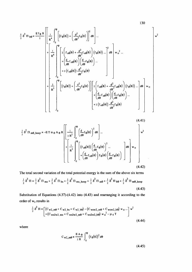
130.<p

f 2 T2

1(fe (9 )) + - ^ f e ( e ) de

r "0

- <19 J.

r 2 ^

de

— fo0(e) l f— f0(e)vd0 J \ d Q

2 (fo0(®)) - ^ 1 0 (0 )dO

de

(fe(e))^ 2 ^- ^ f e ( 0 )

vde

r( 2 1

2 f 00(e) + — 5^00(0) ( f e ( 0 ) ) ... deI de J

+ — foe(0 ) — fe ( 0 ) ...Vde J Vde

+ 2 (f 00(e)) -^fe(e)- de -

(4.41)

1 C.2S n m0_hoop “ E T (X 0 A 0 R

r<p

2—fe(e)l de de J

(f00(e)) 0 (0 )j ... de

+ 1' —fo0(0)lfe(0) f— fe(0)I de J ^de

(4.42)

The total second variation of the total potential energy is the sum of the above six terms

— 5 n = — 6 n nix + n m x_hoop ~ r i n i0 + 5 n y 0 + — 6 n m 0_ hoop

(4.43)

Substitution of Equations (4.37)-(4.42) into (4.43) and rearranging it according to the

order of Wq results in

- 5^n =2 (C w2_m0 + C w2_bx C w2_be) “ (C wow2_m0 + C wow2_be) ^ o ...

wo2w2_mx C wo2w2_m0 ^ wo2w2_be) "'0 “ 4 ^

(4.44)

where

w2 m0 -EAe

2 R(f 0 (0 ))^ de

(4.45)

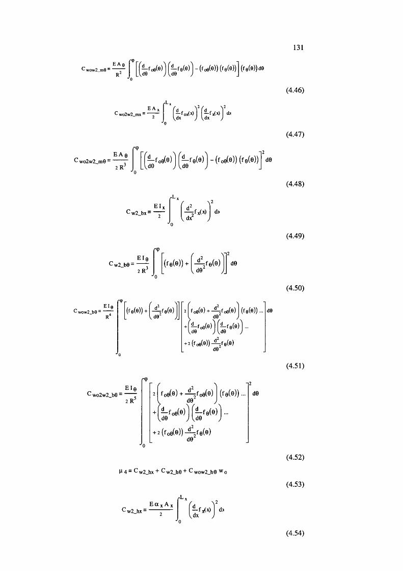
131

wow2 m0 ~E A 0 r<p

oe(e)j - (foe(e)) {fe(e)) (fe(e))d0

C wo2w2_mx ~EA

C wo2w2 m0 -EAe

2—foe(9)l f— fe(e)l - ( toM ) (fe(e)) d0 J vd0 J

d0

C w2_b0 -E l0

2 R"

' 9r r 0

(f 0 (e)) + - ^ f e ( e )- <19 J.

d0

C wow2_b0 -El0

-<P - - f 2 ] -

(f0 (e)) + 2 f 00(0 ) + -^ ^ 00(0 ) (f0(0))...I de" J . I dO J

+ —fo0(0) —f0(0) ...Vd0 J Vd0

+ 2 (f 00(0 )) 0 (0 )- d0 -

d0

C wo2w2 b0 -E l0

7 ?

2 A fo0(®) + ■■^fo0(®) (^0 (0 ))

:(foe(e))-^fe(e)d0

d0

^ w2 hx “E a V A

—fx(x) I d>

(4.46)

(4.47)

rL.E l / 2

-^fx(x)V dx y

d>

(4.48)

(4.49)

(4.50)

(4.51)

H 4 - C ^2 hx ^ (7 w2 h0 + C wow2 h0 0

(4.52)

(4.53)

(4.54)

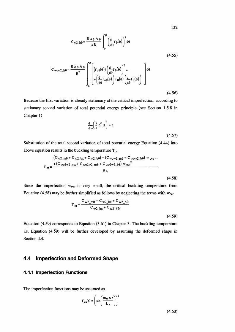
132

C w2 h 0 -Eae Ae

2R

(4.55)

E a e A er(p

Cwow2_h0” , (f 00(G)) I — f0(G) ... devde y

+ f — f o 0 ( 0 ) l f 0 ( e ) f — feCe)VdG J Vde

(4.56)

Because the first variation is already stationary at the critical imperfection, according to

stationary second variation of total potential energy principle (see Section 1.5.8 in

Chapter 1)

— ( - 0 n l = 0dwV 2

(4.57)

Substitution of the total second variation of total potential energy Equation (4.44) into

above equation results in the buckling temperature Ter

(C w2_me + ^ w2_bx + C w2_be) ~ (C wow2_me + C wow2_be) ocr •••

(C wo2w2_mx + C wo2w2_me + C wo2w2_be) ^ ocr

(4.58)

Since the imperfection Wocr is very small, the critical buckling temperature from

Equation (4.58) may be further simplified as follows by neglecting the terms with Wocr

^ w 2 m0"*’ ^ w 2 bx ^ w2 b0Tcr =

^ w2 hx ^ w2 he

(4.59)

Equation (4.59) corresponds to Equation (3.61) in Chapter 3. The buckling temperature

i.e. Equation (4.59) will be further developed by assuming the deformed shape in

Section 4.4.

4.4 Im perfection an d D eform ed S h a p e

4.4.1 Imperfection Functions

The imperfection functions may be assumed as

f ox( ) -\ \ 2

(4.60)

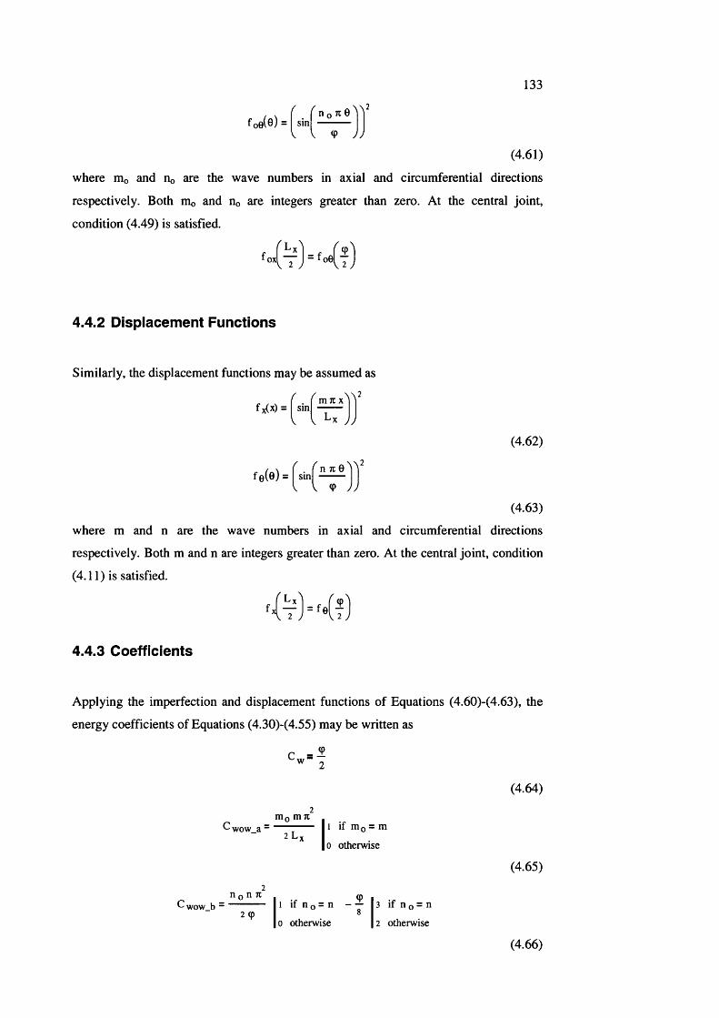
133

, n n 7t 0sin

V V 9 yy(4.61)

where nio and Hq are the wave numbers in axial and circumferential directions

respectively. Both mo and no are integers greater than zero. At the central joint,

condition (4.49) is satisfied.

f o x l f

4.4.2 Displacement Functions

Similarly, the displacement functions may be assumed as,2

f x(x) = sinm ic X

fe(@)= sinn 7C 0

(4.62)

V V 9

(4.63)

where m and n are the wave numbers in axial and circumferential directions

respectively. Both m and n are integers greater than zero. At the central joint, condition

(4.11) is satisfied.

4.4.3 Coefficients

Applying the imperfection and displacement functions of Equations (4.60)-(4.63), the

energy coefficients of Equations (4.30)-(4.55) may be written as

C w - f

mo mjc 2 L,

1 if m o = m

0 otherwise

n n n 71wow b - 29

91 if n o = n ------

80 otherwise

3 if n o = n

2 otherwise

(4.64)

(4.65)

(4.66)

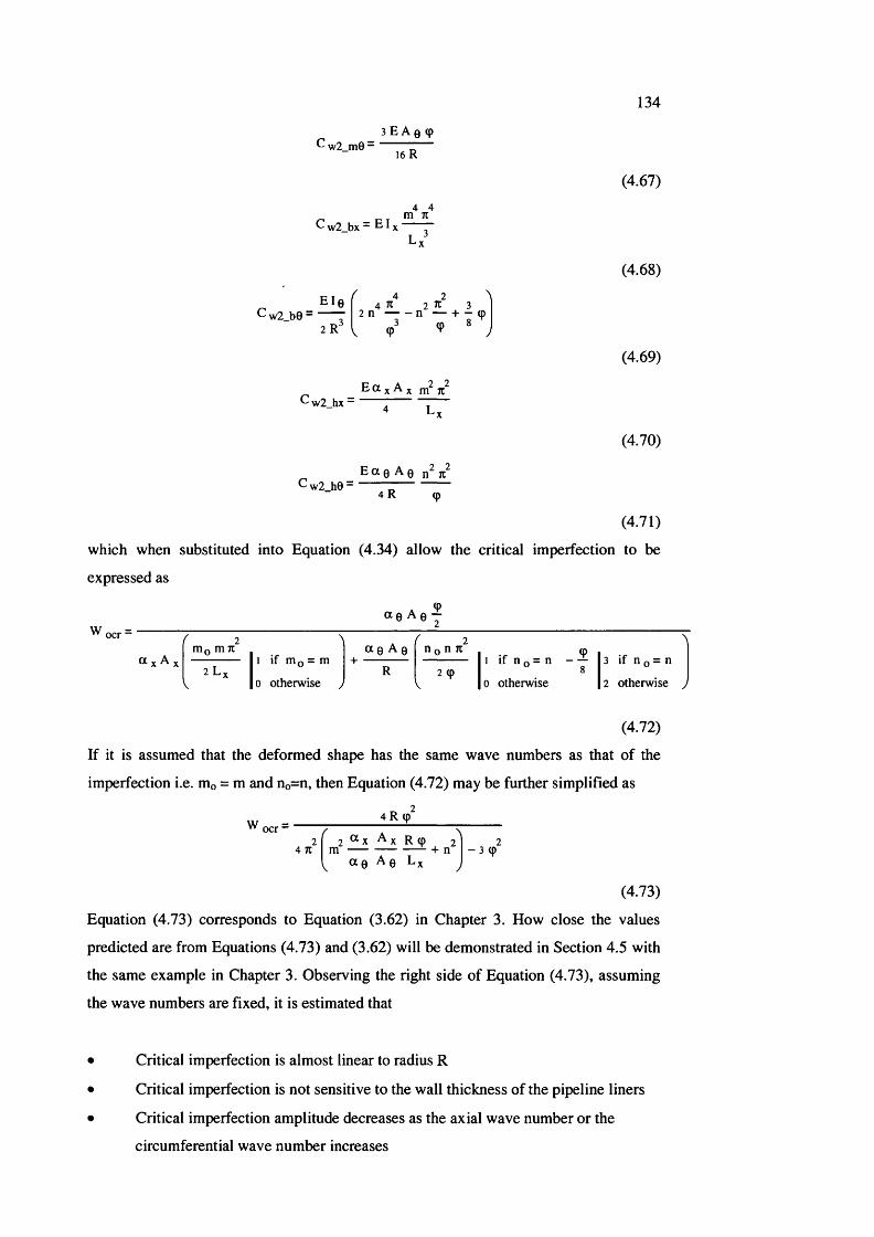
134

^ w2 m6 -3 E A e (p

16 R

C w2 bx ~ EIX4 4

tn K

(4.67)

C w2 b0 “E l0

I F

4 2 ^4 It 2 It 3 2 n n ---- 1— (D

V 9 9 * ,

• w2_hx -E O X A X

4 L v

C w2_h9 “E ot 0 A 0 71

(4.68)

(4.69)

(4.70)

4 R (p

(4.71)

which when substituted into Equation (4.34) allow the critical imperfection to be

expressed as

w

(p« 0 A 0 y

a y A

/ 2 nio m K2 L y

1 i f n io = m

0 o th erw ise

« 0 A 0

R

n n n 7t

2(P

(pI i f n o = n ------

80 O therw ise

3 i f n o = n

2 o th erw ise >

(4.72)

If it is assumed that the deformed shape has the same wave numbers as that of the

imperfection i.e. mo = m and no=n, then Equation (4.72) may be further simplified as

w 4 R (p

2 r 2 ®X^ xR<P 24 71 m ------- + n

« 0 A 0 Lx- 3 (p

(4.73)

Equation (4.73) corresponds to Equation (3.62) in Chapter 3. How close the values

predicted are from Equations (4.73) and (3.62) will be demonstrated in Section 4.5 with

the same example in Chapter 3. Observing the right side of Equation (4.73), assuming

the wave numbers are fixed, it is estimated that

Critical imperfection is almost linear to radius R

Critical imperfection is not sensitive to the wall thickness of the pipeline liners

Critical imperfection amplitude decreases as the axial wave number or the

circumferential wave number increases

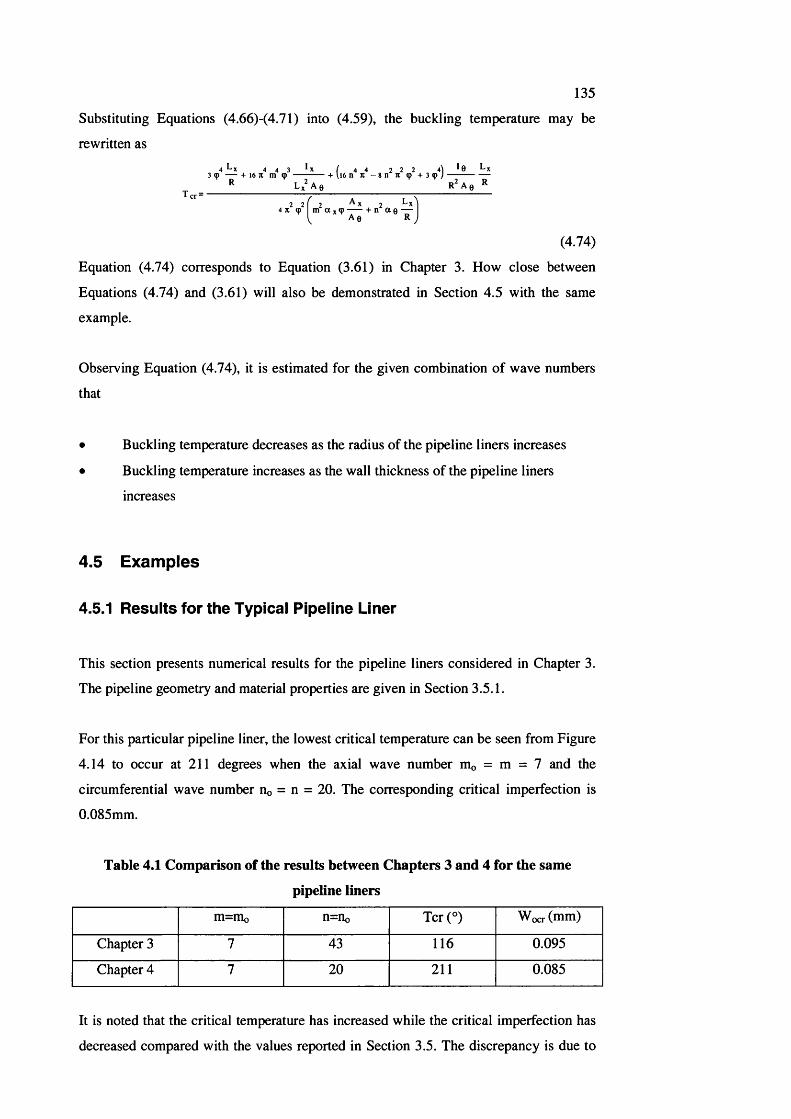
135

Substituting Equations (4.66)-(4.71) into (4.59), the buckling temperature may be

rewritten as

4 4 4 3 *X I 4 4 2 2 2 4 ^ * 03<p + 16 71 m (D + \16n 7t - 8 n It (p + 3 < p j ----------------

R I R

T „ =Lx A@ R A e

4 71 (p I m a%<p + n a e —A e R

(4.74)

Equation (4.74) corresponds to Equation (3.61) in Chapter 3. How close between

Equations (4.74) and (3.61) will also be demonstrated in Section 4.5 with the same

example.

Observing Equation (4.74), it is estimated for the given combination of wave numbers

that

• Buckling temperature decreases as the radius of the pipeline liners increases

• Buckling temperature increases as the wall thickness of the pipeline liners

increases

4.5 E xam ples

4.5.1 R esults for the Typical Pipeline Liner

This section presents numerical results for the pipeline liners considered in Chapter 3.

The pipeline geometry and material properties are given in Section 3.5.1.

For this particular pipeline liner, the lowest critical temperature can be seen from Figure

4.14 to occur at 211 degrees when the axial wave number mo = m = 7 and the

circumferential wave number no = n = 20. The corresponding critical imperfection is

0.085mm.

Table 4.1 Comparison of the results between Chapters 3 and 4 for the same

pipeline liners

m=mo n=no Tcr(°) Wocr (mm)

Chapter 3 7 43 116 0.095

Chapter 4 7 2 0 2 1 1 0.085

It is noted that the critical temperature has increased while the critical imperfection has

decreased compared with the values reported in Section 3.5. The discrepancy is due to

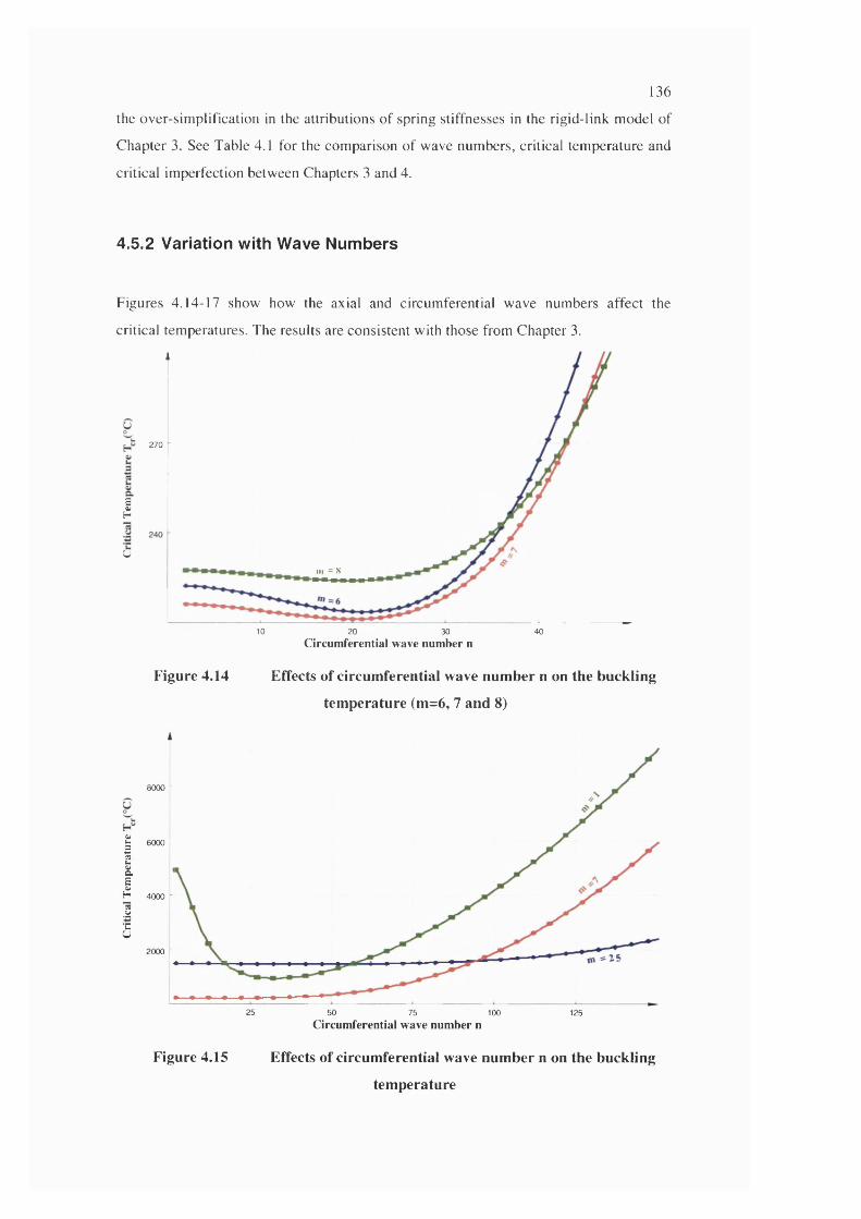
136

the over sim plification in the attributions o f spring stiffnesses in the rigid-link m odel of

C hapter 3. See Table 4.1 for the com parison o f wave num bers, critical tem perature and

critical im perfection between Chapters 3 and 4.

4.5.2 Variation with Wave Numbers

Figures 4.14-17 show how the axial and circum ferential wave num bers affect the

critical tem peratures. The results are consistent with those from C hapter 3.

Iu

270

ni = S

10 20 30 40

Figure 4.14

Circumferential wave number n

Effects of circumferential wave number n on the buckling

temperature (m=6 , 7 and 8 )

8000 -

t3

6000 -

I 'IH 4000 -

5S

2000 ^

25 50 75 100 125

Figure 4.15

Circumferential wave number n

Effects of circumferential wave number n on the buckling

temperature

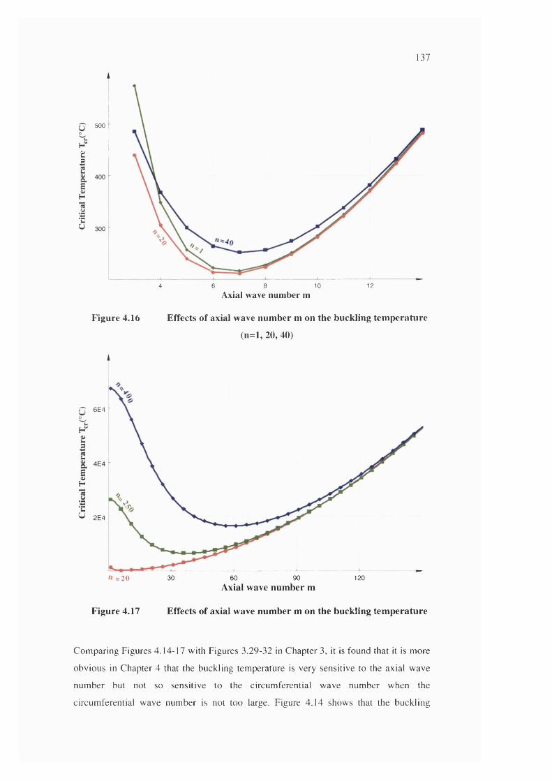
137

H''âi5

500


Figure 4.16 Effects of axial wave number m on the buckling temperature

(n=l, 20, 40)

n 6E4

U 2E4 -

=20 30 60 90

Axial wave number m120

Figure 4.17 Effects of axial wave number m on the buckling temperature

C om paring Figures 4.14-17 with Figures 3.29-32 in C hapter 3, it is found that it is m ore

obvious in C hapter 4 that the buckling tem perature is very sensitive to the axial wave

num ber but not so sensitive to the circum ferential wave num ber when the

circum ferential wave num ber is not too large. Figure 4.14 shows that the buckling

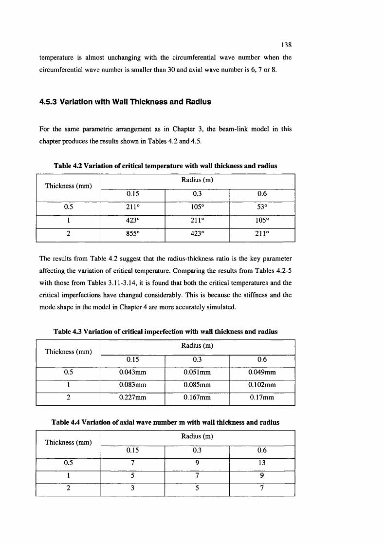
138

temperature is almost unchanging with the circumferential wave number when the

circumferential wave number is smaller than 30 and axial wave number is 6 , 7 or 8 .

4.5.3 Variation with Wall Thickness and Radius

For the same parametric arrangement as in Chapter 3, the beam-link model in this

chapter produces the results shown in Tables 4.2 and 4,5.



0.15 0.3 0 .6

0.5 2 1 1 ° 105° 53°

1 423° 2 1 1 ° 105°

2 855° 423° 2 1 1 °

The results from Table 4.2 suggest that the radius-thickness ratio is the key parameter

affecting the variation of critical temperature. Comparing the results from Tables 4.2-5

with those from Tables 3.11-3.14, it is found that both the critical temperatures and the

critical imperfections have changed considerably. This is because the stiffness and the

mode shape in the model in Chapter 4 are more accurately simulated.



0.15 0.3 0 .6

0.5 0.043mm 0.051mm 0.049mm

1 0.083mm 0.085mm 0 .1 0 2 mm

2 0.227mm 0.167mm 0.17mm

Table 4.4 Variation of axial wave number m with wall thickness and radius


0.15 0.3 0 .6

0.5 7 9 13

1 5 7 9

2 3 5 7

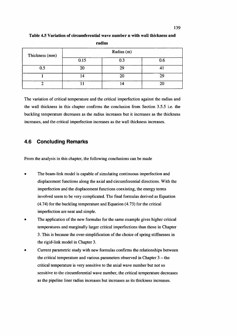
139

Table 4.5 Variation of circumferential wave number n with wall thickness and

radius


0.15 0.3 0 .6

0.5 2 0 29 41

1 14 2 0 29

2 11 14 2 0

The variation of critical temperature and the critical imperfection against the radius and

the wall thickness in this chapter confirms the conclusion from Section 3.5.5 i.e. the

buckling temperature decreases as the radius increases but it increases as the thickness

increases, and the critical imperfection increases as the wall thickness increases.

4.6 C onclud ing R em arks

From the analysis in this chapter, the following conclusions can be made

The beam-link model is capable of simulating continuous imperfection and

displacement functions along the axial and circumferential directions. With the

imperfection and the displacement functions coexisting, the energy terms

involved seem to be very complicated. The final formulas derived as Equation

(4.74) for the buckling temperature and Equation (4.73) for the critical

imperfection are neat and simple.

The application of the new formulas for the same example gives higher critical

temperatures and marginally larger critical imperfections than those in Chapter

3. This is because the over simplification of the choice of spring stiffnesses in

the rigid-link model in Chapter 3.

Current parametric study with new formulas confirms the relationships between

the critical temperature and various parameters observed in Chapter 3 - the

critical temperature is very sensitive to the axial wave number but not so

sensitive to the circumferential wave number, the critical temperature decreases

as the pipeline liner radius increases but increases as its thickness increases.

140

5 Buckling Analysis with Liner-Only Continuum

Model

5.1 In troduction

In Chapters 3 and 4, the simplified physical models adopted have only a conceptual link

with real pipeline liners. In Chapter 3, the liner shells were simplified as rigid-links in

the axial and circumferential directions, connected and constrained by the one-degree-

of-freedom membrane and moment springs. In Chapter 4 the rigid-links and springs

were replaced by the flexural beams to address the effects of different wave lengths.

This simplified analysis gave the answers to the most basic questions that were raised at

the very beginning of the study, without the involvement of overly complex

mathematical analysis. In particular it showed that the liner will not buckle without

imperfection.

However, this study is not only aimed at answering the fundamental questions such as

whether the liner could buckle without imperfection. Design engineers of bonded lined

pipelines need to know exactly with what imperfection and at what temperature they

will buckle. Neither the rigid-link simplified model nor the beam-link simplified model

is likely to produce accurate enough results to be suitable for the application in the

design of pipeline liners.

For this purpose, analysis with continuum models is necessary. In order to avoid a

sudden dramatic increase of mathematical work, this phase is again divided into two

stages. In the first stage, the buckling analysis with the liner-only continuum model will

be carried out. This will be described in this chapter. The work of the second stage will

consider a more complete modelling of the liner-and-pipe continuum interaction, this is

the topic of Chapter 6 .

In this chapter, the effect of ignoring the outer pipe is first examined and then the liner-

only continuum model will be described. The variables involved in the analysis will be

defined in Section 5.4. Section 5.5 will present the theoretical work of the buckling

analysis. Section 5.6 will describe the detailed formulation while Section 5.7 presents

the numerical results. Finally, Section 5.8 will draw conclusions.

141

5.2 Sim plification of th e O u ter P ipe

As has been pointed out, this chapter deals with the liner-only continuum model. The

title is self-explanatory - only the inner liner is included in the model. However, the

outer pipe must not be simply ignored. In other words, the outer pipe must be simplified

as an appropriate boundary constraint condition or be incorporated into loading

conditions for the inner liner-only continuum model.

Firstly, if the outer pipe is simply neglected, the liner-only model is a two-way buckling

problem that means the liner could go beyond the inner surface of the outer pipe. That is

obviously physically incorrect. Therefore, the first pre-condition is that the outer pipe

restrains the movement of the liner to just inward. This may be simply realized by

assuming an inward-only deformed shape.

Secondly, one of the basic characteristics of the problem here is that the structure is

thermally loaded. In a thermally loaded structure, the mechanical stress or strain energy

level in the structure is determined by the amount of the thermally-induced strains being

constrained. It is, therefore, very important to correctly model the amount of the thermal

expansion being resisted by the outer pipe. In the present case, the final radial thermal

expansion coefficient for the liner-only continuum model is assumed equal to the

difference of the radial thermal expansion coefficients between the inner liner and the

outer pipe.

® 0 ~ ® 0_liner ~ ® 0_pipe

(5.1)

5.3 D escrip tion of Liner-Oniy C on tinuum Model

Because the one-way buckling of this chapter considers the outer pipe to be rigid, the

current liner-only continuum model includes the liner only. As the thickness of the liner

is very small compared with its midsection radius, the liner can be represented as a thin

shell as shown in Figures 5.1 and 5.2.

Figure 5.1 Simplification of an inner liner as an empty thin shell - the

cross section of the neutral surface

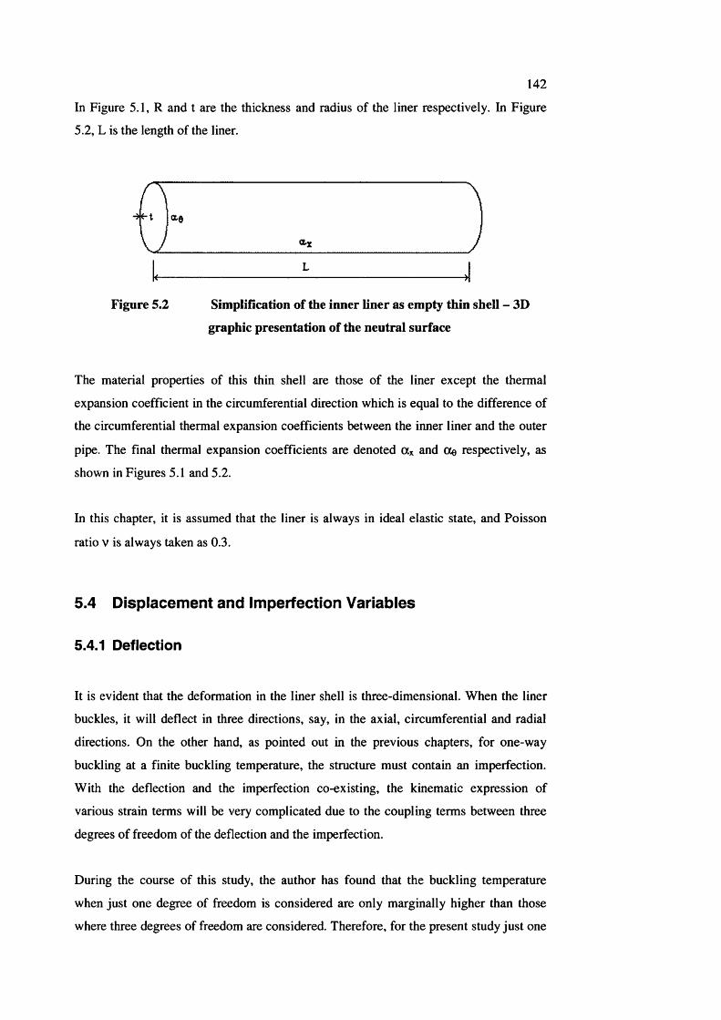
142

In Figure 5.1, R and t are the thickness and radius of the liner respectively. In Figure

5.2, L is the length of the liner.

L

Figure 5.2 Simplification of the inner liner as empty thin shell - 3D

graphic presentation of the neutral surface

The material properties of this thin shell are those of the liner except the thermal

expansion coefficient in the circumferential direction which is equal to the difference of

the circumferential thermal expansion coefficients between the inner liner and the outer

pipe. The final thermal expansion coefficients are denoted and Oe respectively, as

shown in Figures 5.1 and 5.2.

In this chapter, it is assumed that the liner is always in ideal elastic state, and Poisson

ratio V is always taken as 0.3.

5.4 D isp lacem en t an d Im perfection V ariab les

5.4.1 Deflection

It is evident that the deformation in the liner shell is three-dimensional. When the liner

buckles, it will deflect in three directions, say, in the axial, circumferential and radial

directions. On the other hand, as pointed out in the previous chapters, for one-way

buckling at a finite buckling temperature, the structure must contain an imperfection.

With the deflection and the imperfection co-existing, the kinematic expression of

various strain terms will be very complicated due to the coupling terms between three

degrees of freedom of the deflection and the imperfection.

During the course of this study, the author has found that the buckling temperature

when just one degree of freedom is considered are only marginally higher than those

where three degrees of freedom are considered. Therefore, for the present study just one

143

degree of freedom for both the deflection and the imperfection is adequate to describe

the current structure.

Among the three degrees of freedom, it is evident that the radial deflection is of prime

importance. Therefore, the deformations in the axial and circumferential directions may

be neglected. Let W be the inward radial deflection, which may be factored as a product

of a function of axial coordinate and a function of circumferential coordinate

w = w f x(x) f e(e)

(5 /0

where w is the maximum value of the radial inward deflection, f% and fe are normalized

functions of x and 0 respectively. Here subscripts x and 0 represent the axial and

circumferential directions respectively, while variables x and 0 represent the axial and

circumferential coordinates respectively. Because the radial incremental deflection is

inward only, both fx and fe should be positive-definite.

5.4.2 Imperfection

Similar to the deformation, the imperfection may also be described by a maximum

imperfection Wo, two positive-definite normalized functions, fox and foe, of x and 0

respectively

^ o “ ^ O f ox( ) f osl®)

(5.3)

Here subscript o represents imperfection.

5.5 Form ulation

5.5.1 Thermaliy-induced Strains

In thermal buckling analysis, stress-inducing strains are determined by thermally-

induced strains as well as membrane and bending strains due to deflection. Thermally-

induced strains are products of the thermal expansion coefficients and the temperature

change. Various variables concerning thermally-induced strains are listed in Table 5.1.

In the analysis, the temperature rise is denoted as T, the unit of which is degree Celsius.

Thermal expansion coefficients are ttx and Oe respectively, where x and 0 represent the

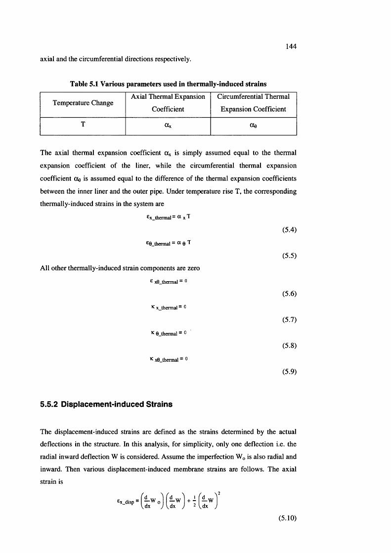
144

axial and the circumferential directions respectively.

Table 5.1 Various parameters used in thermally-induced strains

Temperature ChangeAxial Thermal Expansion

Coefficient

Circumferential Thermal

Expansion Coefficient

T « X Oe

The axial thermal expansion coefficient is simply assumed equal to the thermal

expansion coefficient of the liner, while the circumferential thermal expansion

coefficient (Xe is assumed equal to the difference of the thermal expansion coefficients

between the inner liner and the outer pipe. Under temperature rise T, the corresponding

thermally-induced strains in the system are

thermal

^0_thermai - ® 0 "T

All Other thermally-induced strain components are zero

G x0_thermal = ^

^ x_thermal “

^ 0_thermal - ^

^ x0 thermal ~ 0

(5 .4)

(5.5)

(5 .6)

(5 .7)

(5.8)

(5.9)

5.5.2 Displacement-induced Strains

The displacement-induced strains are defined as the strains determined by the actual

deflections in the structure. In this analysis, for simplicity, only one deflection i.e. the

radial inward deflection W is considered. Assume the imperfection Wq is also radial and

inward. Then various displacement-induced membrane strains are follows. The axial

strain is

(5.10)

145

Equation (5.10) corresponds to Equation (4.13) in Chapter 4. These equations are

similar in format but their physical interpretation is different. While Wq and W in

Chapter 3 are functions of x only, they are functions of both x and 0 here. The

membrane strain is

£0_disp

fd 1 fd— Wo — w — wdO d0 I d0

+ + -I R J I R 2 I R J(5.11)

Equation (5.11) corresponds to Equation (4.17) in Chapter 4. While Equation (4.17) has

six terms. Equation (5.11) has three terms. The missing terms are the coupling terms of

higher orders. In Chapter 4, the strain-displacement equations are derived directly by

Taylor expansion and more coupling terms of imperfection Wo with deflection W and

W^ are retained. In the present context this becomes difficult due to the complexity

involved in the continuum model. Therefore, the classic strain-displacement equations

that are widely used in the literature will be adopted here. The shear strain is

Ex9_disp “de de

R+ I —w

dxde

dx y V dx

(5.12)

where R is the radius of the neutral surface of the liner. The shear strain in the

continuum model has no corresponding expression in the previous chapters. The

curvature in the axial direction is

^x_disp - :Wdx

(5.13)

Again, Equation (5.13) corresponds to Equation (4.15) in Chapter 4. The displacement

function W in Chapter 4 is a function of x only but here it is a function of both x and 0

here so that

^0_disp -R

:Wde

(5.14)

For the same reason when comparing Equation (5.11) and Equation (4.17), Equation

(5.14) has removed all the coupling terms of imperfection Wq and displacement W. The

twist is

■ 'xe.disp = ( y

(5.15)

The twist in the continuum model has no corresponding equivalence in the previous

chapters.

146

5.5.3 Stress-inducing Strains

As pointed out in Section 1.4, stress-inducing strain is equal to displacement-induced

strain less thermally-induced strain. Accordingly, by subtracting Equations (5.10)-(5.15)

by Equations (5.4)-(5.9), the following six stress-inducing strain terms are derived,2

■{t )— W o f - w ld6 d6 1 dO

+ + -I R J I R J 2 I R J - a 0 T

6x8 =' i - '

R dx— W 1 + f — W

dx

f d ) ^ H A— w — Wde d6

I R J (dx J I R J

K y s :Wdx

vde' y

(5.16)

(5.17)

(5.18)

(5.19)

(5.20)

(5.21)

where R is the radius of the neutral surface of the liner. Because the right hand sides of

Equations (5.6)-(5.9) are zero. Equations (5.18)-(5.21) look the same as Equations

(5.12)-(5.15). However, their physical meanings are different. What Equations (5.16)-

(5.21) represents are the strains and curvatures which result in strain energy in the

system. In Equations (5.16)-(5.21), the notation £x_a_reiated» £ 0 _o_reiated» £x0 _<i_reiated,

Kx_o_related. K0_a_related» KxO o related denoted aS 6x, Eg, 6x0, Kx, Kg, Kx0 for C o n v e n ie n c e .


There are changes in both membrane and bending strain energies in the system when it

buckles. The membrane strain energy in the system may be expressed as

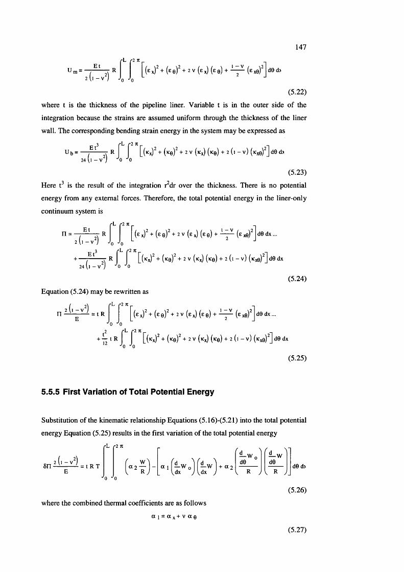
147

Um= . Rç L '2 K

Jq j 0(exf + (ee f + 2 V (e J (ee) + (e^e) d0 d>

(5.22)

where t is the thickness of the pipeline liner. Variable t is in the outer side of the

integration because the strains are assumed uniform through the thickness of the liner

wall. The corresponding bending strain energy in the system may be expressed as

"L r 2 7C

U b = j [(Kx)^+(Ke)^ + 2 v(Kx)(Ke) + 2 (i-v)(Kxef]ded>24 ( l - V^) 0 * 0

(5.23)

Here t is the result of the integration r^dr over the thickness. There is no potential

energy from any external forces. Therefore, the total potential energy in the liner-only

continuum system is

n = -T R

fL '2 K

d0 d x ...

^~~Â ^ + 2 V (k x ) (K g ) + 2 (i - v ) (k x b )^ ] d0 dx- V ) * 024 ( l - v 1

(5.24)


ç L '2 K

(e xY + (e e)" + 2 V (e %) (e e) + (e xo) d0 d x ...

4 t R12

L /*2 JI[ ( k x ) ^ + (k b )^ + 2 V ( k x ) ( k b ) + 2 ( i - v ) (k x b )^ ] d0 dx

0 "0

(5.25)

5.5.5 First Variation of Total Potential Energy

Substitution of the kinematic relationship Equations (5.16)-(5.21) into the total potential

energy Equation (5.25) results in the first variation of the total potential energy

ç L •2 n r

h r ) -/

a 1 1 •V-w „ Iw 1 + 0 2 dx M d x

-Wd0

V R yd0

d0 d>

(5.26)

where the combined thermal coefficients are as follows

a i = a x + v a g

(5.27)

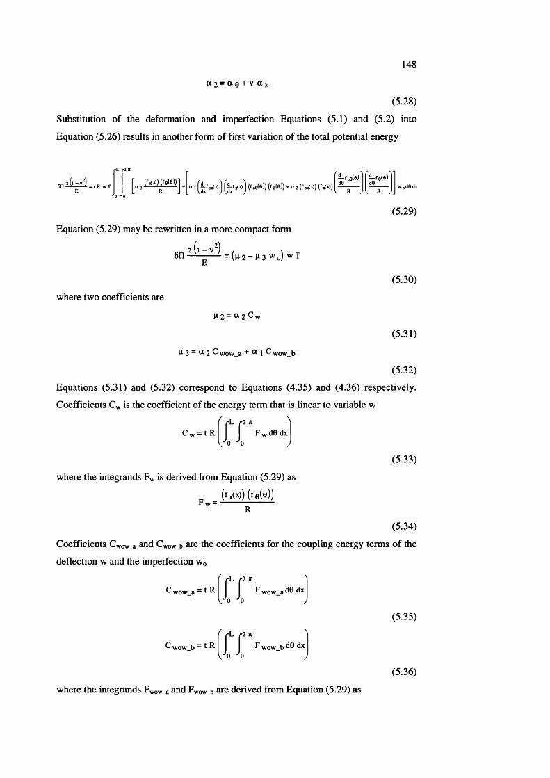
148

a 2 = a 0 + v a

(5.28)

Substitution of the deformation and imperfection Equations (5.1) and (5.2) into

Equation (5.26) results in another form of first variation of the total potential energy

6 n ------= t R w T ox(*) 1 k f x C O I ( f o e ( e ) ) ( f 0( e ) ) + «2 (foxO O )

— f o e ( e ) deW o d 0 d :

(5.29)

Equation (5.29) may be rewritten in a more compact form

2 (l - V )ôn = ( p 2 -1 1 3 Wo) w T

where two coefficients are

^ 2 = « 2 C

(5.30)

(5.31)

(5.32)

Equations (5.31) and (5.32) correspond to Equations (4.35) and (4.36) respectively.

Coefficients Cw is the coefficient of the energy term that is linear to variable w

' 'L Ç2 K ^C w = t R I I F w de dx

(5.33)

where the integrands Fw is derived from Equation (5.29) as

(fx(x)) ( f e ( e ) )

(5.34)

Coefficients Cwow_a and Cwow_b are the coefficients for the coupling energy terms of the

deflection w and the imperfection Wo

-(i:rL r2 71 ^

F wow a de dx

Vo 0

L r2 7C ^

F wow b de dx

(5.35)

(5.36)

where the integrands Fwow_a and Fwow_b are derived from Equation (5.29) as

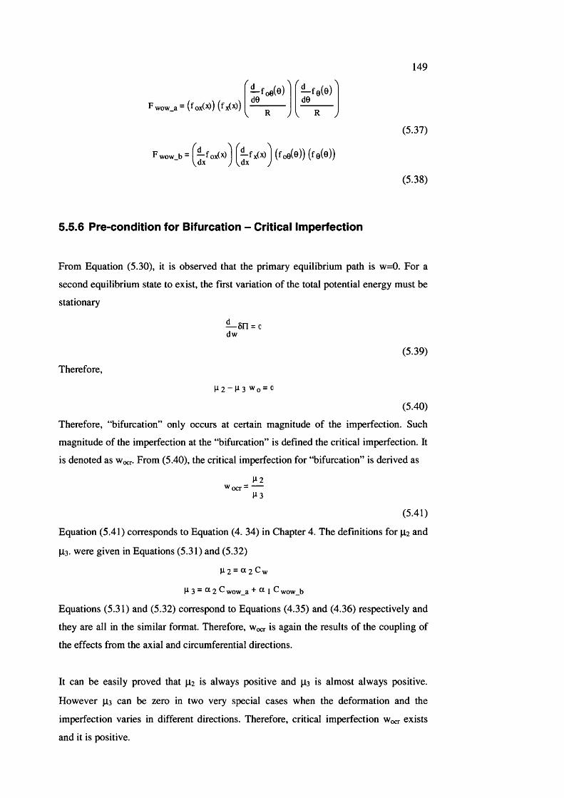
149

F wow_a - (fox(^)) (f x(X))

f o e ( e ) l f — Me)"*de de

R

F wow_b - x(^)^ (loe(® )) (fo l® ))

(5.37)

(5.38)

5.5.6 Pre-condition for Bifurcation - Critical imperfection

From Equation (5.30), it is observed that the primary equilibrium path is w=0. For a

second equilibrium state to exist, the first variation of the total potential energy must be

stationary

—sn = odw

(5.39)

Therefore,

P 2 - ^ 3 Wq = 0

(5.40)

Therefore, “bifurcation” only occurs at certain magnitude of the imperfection. Such

magnitude of the imperfection at the “bifurcation” is defined the critical imperfection. It

is denoted as Wœr. From (5.40), the critical imperfection for “bifurcation” is derived as

1^2W o c r = -----

P 3

(5.41)

Equation (5.41) corresponds to Equation (4. 34) in Chapter 4. The definitions for p2 and

P3. were given in Equations (5.31) and (5.32)

g 2 “ ® 2 ^ w

H 3 ~ ® 2 C wow_a + Ot 1 C wow_b

Equations (5.31) and (5.32) correspond to Equations (4.35) and (4.36) respectively and

they are all in the similar format. Therefore, Wocr is again the results of the coupling of

the effects from the axial and circumferential directions.

It can be easily proved that |Li2 is always positive and fi3 is almost always positive.

However |Li3 can be zero in two very special cases when the deformation and the

imperfection varies in different directions. Therefore, critical imperfection w^r exists

and it is positive.

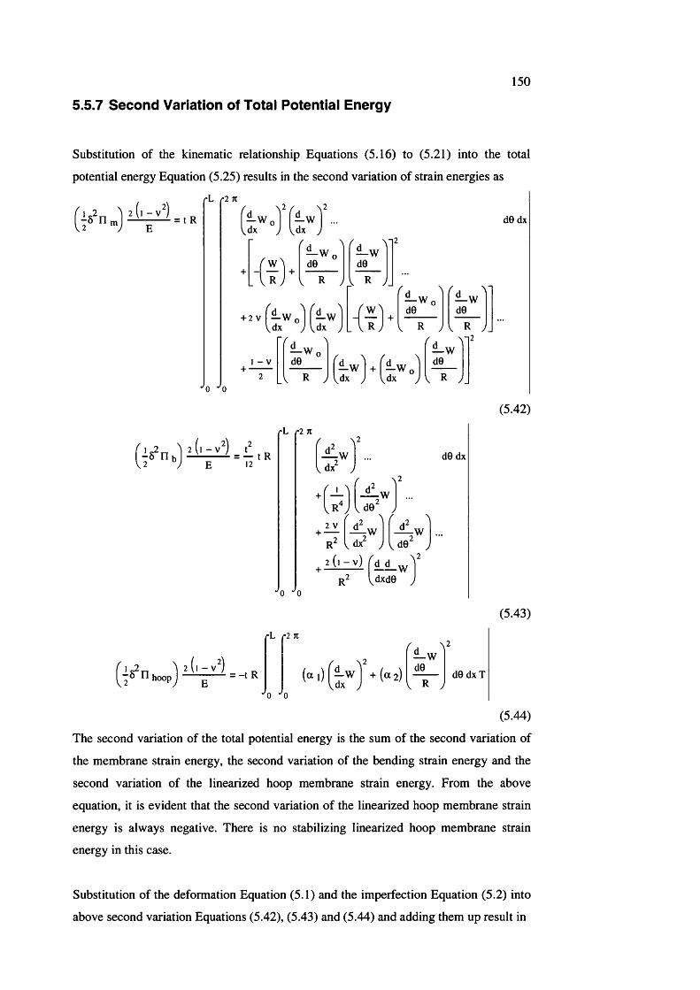
150

5.5.7 Second Variation of Total Potential Energy

Substitution of the kinematic relationship Equations (5,16) to (5.21) into the total

potential energy Equation (5.25) results in the second variation of strain energies as

■2 7t

d6 dx

w— wd0___

V R yde

+ 2V I —wdx j Vdx

1 - V d0

. ~ r" y

.V R y j

wR

— W dO de

dx— W + — W

dx

de

0 * 0

(5.42)

rL r l n

I dxdO dx

-w

2 V

der . \

:WV dx y

r 2 i dxde

r 2 A^w

\ d e " y 2

(5.43)

rh •2 It

de\ R y

d ed x T

(5.44)

The second variation of the total potential energy is the sum of the second variation of

the membrane strain energy, the second variation of the bending strain energy and the

second variation of the linearized hoop membrane strain energy. From the above

equation, it is evident that the second variation of the linearized hoop membrane strain

energy is always negative. There is no stabilizing linearized hoop membrane strain

energy in this case.

Substitution of the deformation Equation (5.1) and the imperfection Equation (5.2) into

above second variation Equations (5.42), (5.43) and (5.44) and adding them up result in

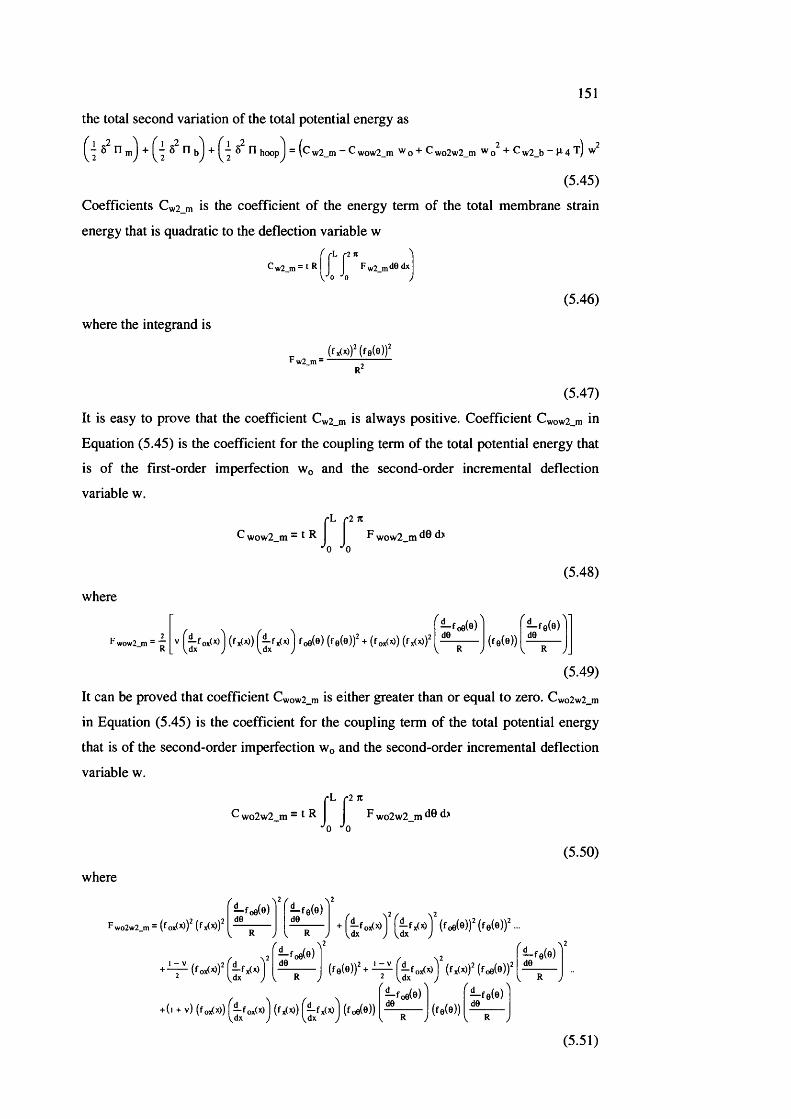
151

the total second variation of the total potential energy as

5 + n + ^ - S n hoop^ - w2_m ~ ^ wow2_m w q + C wo2w2_m ^ w2_b “ 4 f ) w

(5.45)

Coefficients Cw2_m is the coefficient of the energy term of the total membrane strain

energy that is quadratic to the deflection variable w

4 f f(5.46)

where the integrand is

Fw2 m =

(5.47)

It is easy to prove that the coefficient Cw2_m is always positive. Coefficient Cwow2_m in

Equation (5.45) is the coefficient for the coupling term of the total potential energy that

is of the first-order imperfection Wq and the second-order incremental deflection

variable w.

-L r2 KC w ow 2_m = t R I I F w ow2_m ^ 8 d>

0 * 0

(5.48)

where

r wow2_m = ^

— f oe(®)de — fe(e) dO

j foe(e) ( fe (e ) f + (foxCO) (fx(x))'

(5.49)

It can be proved that coefficient Cwow2_m is either greater than or equal to zero. Cwo2w2_m

in Equation (5.45) is the coefficient for the coupling term of the total potential energy

that is of the second-order imperfection Wq and the second-order incremental deflection

variable w.

*L r 2 K

^ w o2w2 m “ t R F wo2w2 m d 8 d>

(5.50)

where

r wo2w2_m - ( f ox(x)) ( f x(x))

—foe(0) de>2

— fe(e) dO

>2

+ (fox(x))

+(i + v) (fox(x)) [ j (fx(x)) f ^ U x ) j (foe(e))

— foe(®)2

f n2 — fe(0)dO

I R(f e(0))^ + ox(x) j (f x(x)) (f oe(0))^

d0

I R )—fooCo)d0

(fe(e))— fe(e)dO

(5.51)

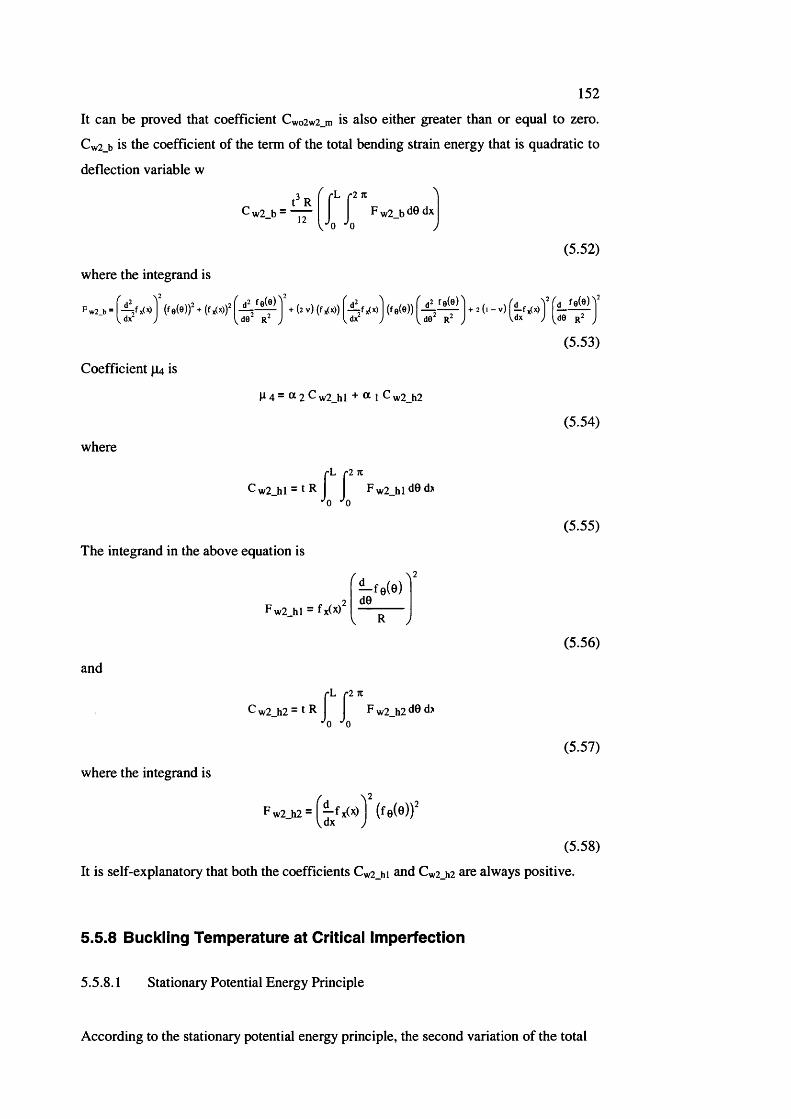
152

It can be proved that coefficient Cwo2w2_m is also either greater than or equal to zero.

Cw2_b is the coefficient of the term of the total bending strain energy that is quadratic to

deflection variable w

t^R12

L r2n

I/. Fw2 bdQdx


F w 2_b = + (2 v) (f^x)) (fe(e))Idx J l,d0 j Idx l,d0

(5.52)

fe(e)d0 r2

(5.53)

Coefficient \u is

where

4 = a 2 C w2 hi + « 1 C w2 h2

(5.54)

C w 2_hl ~ t R I I F w 2_hl d 8 d>*^0 •'o

(5.55)

The integrand in the above equation is

P w2 hi “ fx ( \ )d 0 ______

V R /(5.56)

and

fL r l K

C w 2_h2 - t R I I F w2_h2 d 8 d> • 0 * 0

(5.57)


F * 2 j t 2 = f ^ f x ( > o j ( f e ( e ) ) '

(5.58)

It is self-explanatory that both the coefficients Cw2_hi and Cw2_h2 are always positive.

5.5.8 Buckling Tem perature at Critical imperfection

5.5.8.1 Stationary Potential Energy Principle

According to the stationary potential energy principle, the second variation of the total

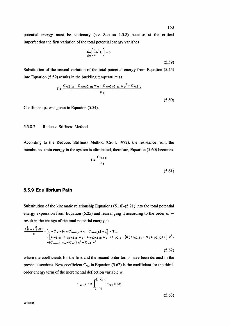
153

potential energy must be stationary (see Section 1.5.8) because at the critical

imperfection the first variation of the total potential energy vanishes

— f V n I = 0dwV 2

(5.59)

Substitution of the second variation of the total potential energy from Equation (5.45)

into Equation (5.59) results in the buckling temperature as

^ _ C w2_m ~ C wow2_m W g + C wo2w2_m ^ o + C w2_b

(5.60)

Coefficient p4 was given in Equation (5.54).

5.5.8 .2 Reduced Stiffness Method

According to the Reduced Stiffness Method (Croll, 1972), the resistance from the

membrane strain energy in the system is eliminated, therefore. Equation (5.60) becomes

C w2_bT =

(5.61)

5.5.9 Equilibrium Path

Substitution of the kinematic relationship Equations (5.16)-(5.21) into the total potential

energy expression from Equation (5.25) and rearranging it according to the order of w

result in the change of the total potential energy as

g — 2 C w ~ (® 2 C wow_a + 1 C wow_b) ^ o] ^ ^ —

~ C wow2_m Wq + C wo2w2_m " 'o ■*" ^w2_b “ (® 2 C w2_h I ® 1 C! w2_h2) 't’J •• wow3 Wq — C^ 3 ) w + Cyj, 4 w

(5.62)

where the coefficients for the first and the second order terms have been defined in the

previous sections. New coefficient Cw3 in Equation (5.62) is the coefficient for the third-

order energy term of the incremental deflection variable w.

(•L . I T .

C w3 = t R I I F yv3 d0 d>'0 "0

(5.63)

where

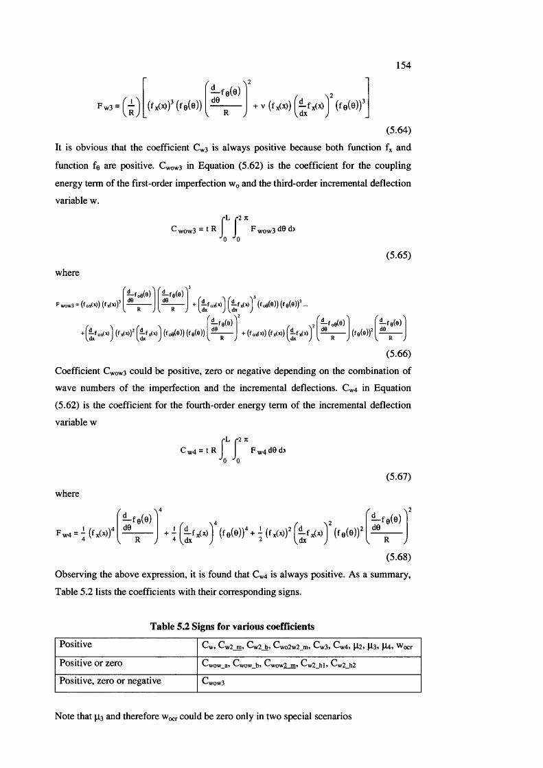
154

F w 3 = | - (f (x)f (fe(e))

f A—fe(e) de____

V R /

(5.64)

It is obvious that the coefficient Cw3 is always positive because both function f* and

function fe are positive. Cwow3 in Equation (5.62) is the coefficient for the coupling

energy term of the first-order imperfection Wq and the third-order incremental deflection

variable w.

'L r l n

wow3 F w ow 3

(5.65)

where

— f oe(®) — fe(e)r wow3 - ox(x)) x(x))

deI R J

daI R J

+ (foo(e)) ( fe (e ) ) '...

— fe(e) de — fe(e)deR

(5.66)

Coefficient Cwows could be positive, zero or negative depending on the combination of

wave numbers of the imperfection and the incremental deflections. Cw4 in Equation

(5.62) is the coefficient for the fourth-order energy term of the incremental deflection

variable w

*L r l nF w4 d0 d>

'0 "0

where

F w4 “ (f x(^))d0_____

V R y

(5.67)

/ . \2 —fe(e)de____

V R /

(5.68)

Observing the above expression, it is found that Cw4 is always positive. As a summary.

Table 5.2 lists the coefficients with their corresponding signs.

Table 5.2 Signs for various coefficients

Positive C\v» Cw2 m. C\v2 b> Cwo2w2_m» Cw3» Cw4» jd-2» 13» lt4, ^ocr

Positive or zero C\vow_a5 Cwow_b’ ^wow2_m» C\v2_hl» C\v2_h2

Positive, zero or negative C\vow3

Note that p3 and therefore Wœr could be zero only in two special scenarios

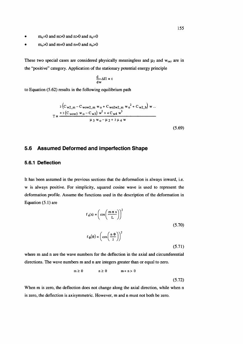
155

• nio= 0 and m> 0 and n> 0 and no= 0

• nio> 0 and m= 0 and n= 0 and no> 0

These two special cases are considered physically meaningless and p,3 and w^r are in

the “positive” category. Application of the stationary potential energy principle

— A n = 0dw

to Equation (5.62) results in the following equilibrium path

2 ( c w2_m “ C wow2_tn W g + C wo2w2_m w g + C w2_b) ^

^ + 3 (C wow3 Wg —C wg) w + 4 C w4 ^

H3 W g - g 2 + 2 g 4 w

(5.69)

5.6 A ssu m ed D eform ed a n d Im perfection S h a p e

5.6.1 Deflection

It has been assumed in the previous sections that the deformation is always inward, i.e.

w is always positive. For simplicity, squared cosine wave is used to represent the

deformation profile. Assume the functions used in the description of the deformation in

Equation (5.1) are

(5.70)

f 0 (e} =

(5.71)

where m and n are the wave numbers for the deflection in the axial and circumferential

directions. The wave numbers m and n are integers greater than or equal to zero.

m > 0 n > 0 m + n > 0

(5.72)

When m is zero, the deflection does not change along the axial direction, while when n

is zero, the deflection is axisymmetric. However, m and n must not both be zero.

156

5.6.2 Imperfection

Similar to the deformation, the imperfection has also been assumed always inward, i.e.

Wo is always positive. For simplicity, squared cosine wave is used to represent the

imperfection profile. Assume the functions used in the description of the imperfection

are

f o x ( x ) = COSITln 71 X

(5.73)

foe(0 ) = cos

(5.74)

where nio and rig are the wave numbers for the imperfection in the axial and the

circumferential directions. The wave numbers mo and % are again integers greater than

or equal to zero.

iHo > 0 Ho > 0 nio + no>0

(5.75)

When mo is zero, the imperfection does not change along the axial direction, while

when no is zero, the imperfection is axisymmetric. However, mo and no must not both be

zero.

5.6.3 Coefficients

Substitution of various integrands together with and fe into various coefficient

expressions results in

Cu/ =71 L t

1 i f m > 0 A n > 0

2 if (m = 0 A n > 0) V ( m > 0 A n = 0)

4 if m = 0 A n = 0

(5.76)

n 0 n 71 L t

32 R3 if m o = m A m > 0

4 if (m o = 0 A m > o ) V (m o > o a m = o)

8 if m o = 0 A m = 0

2 otherwise

1 i f n o = n An > o 0 otherw ise

(5.77)

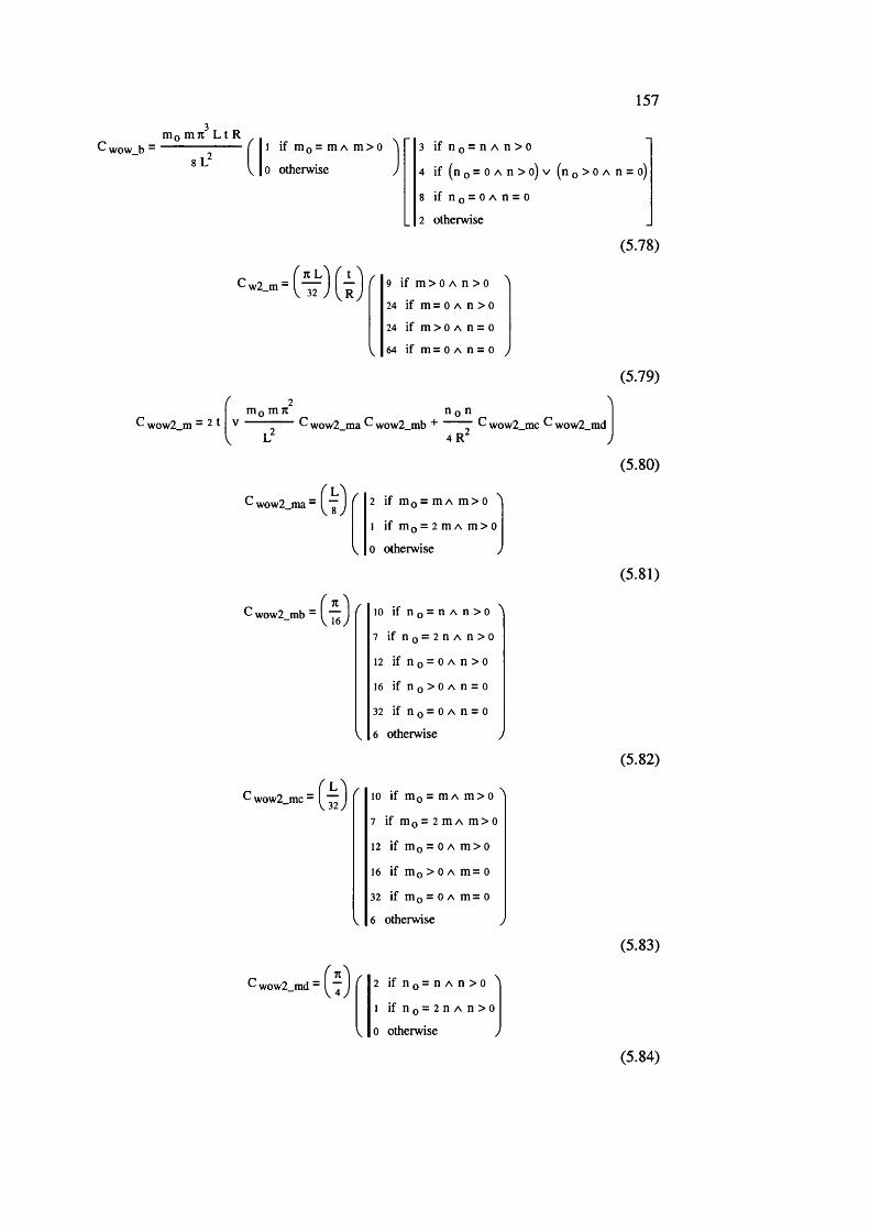
157

wow b -m o m ji L t R

s\}1 if m o = m A m > 0

0 otherwise

3 i f r i o = n A n > 0

4 i f ( n o = O A n > o ) v ( n o > O A n = o)

8 i fno = OAn = o2 otherwise

(5.78)

Cw2_ m = l ^ j ( ^ 9 if m > O A n > o ^

24 if m = 0 A n > 0

24 if m > 0 A n = 0

V 64 if m = 0 A n = 0 y

(5.79)

C wow2 m ~ 2 t

I' 2m o m 7t

V --------------

V L"C wow2 ma C wow2 mb +

4R"C wow2 me C wow2 md

C wow2_ma “ g J f 2 if m o = m A m > 0 ^

1 if m o = 2 m A m > 0

K 0 otherw ise >

C wow2 mb “ 1 , -/ 10 if n o = O A n > 0167

7 if n o = 2 n A n > 0

12 if n o = 0 A n > 0

16 if n o > O A n = o

32 if n o = O A n = o

V 6 otherwise

C wow2_mc - 1 22 10 if m o = m A m > 0 ^

7 if m o = 2 m A m > 0

12 if m o = 0 A m > 0

16 if m o > 0 A m = 0

32 if m o = 0 A m = 0

V 6 otherw ise >

(5.80)

(5.81)

(5.82)

(5.83)

C- wow2_md - 1 ^ 2 i f n o = n A n > 0 1 i f n o = 2 n A n > 0

0 otherwise

(5.84)

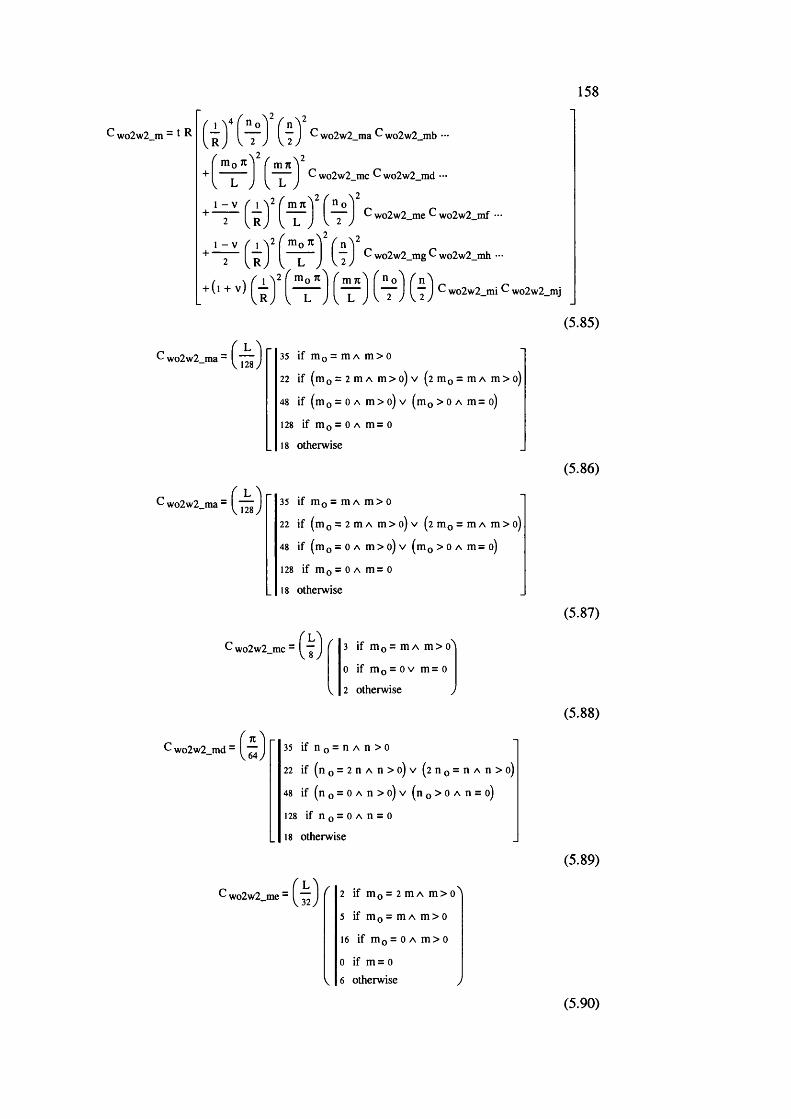
158

C wo2w2 m - ^ ± V f i L 2l f i l Y r rr J V 2 y V 2 y wo2w2_ma ^ wo2w2_mb —

( mjiVI L j ^wo2w2_md "L1 - V y 1 mn n,

2 l R j l L ] L 2 ' ^ wo2w2_me C wo2w2_mf —

+ ( ^ ~ J I f ) C wo2w2_mg C w o2w 2_m h-

+ (i + v ) f - ^2 rcïnlt ITlTt n,

L ] V 2 J V 2 ' ^ wo2w2_mi C wo2w2_mj

C w o2 w 2 _ m a= l j^g

C wo2w2_ma - t

35 if n io = m A m > 0

22 if ( m o = 2 m A m > o ) V ( 2 n i o = n i A m > o )

48 if (m o = 0 A m > 0) V (n io > 0 A m = 0)

128 if rrio = 0 A m = 0

18 otherwise

35 i f iTio = m A m > 0

22 i f ( r t i o = 2 m A m > o ) v ( 2 m g = m a m > 0 )

48 i f ( n i o = 0 A m > 0 ) V ( iT io > 0 A m = 0 )

128 if n i o = 0 A m = 0

18 otherwise

C wo2w2 me “ I „ / 3 if n io = m A m > 0^

0 if OÎQ = 0 V m = 0

V 2 otherw ise >

C wo2w2_md - 1 ^ 35 if n 0 = n A n > 0

22 if (n 0 = 2 n A n > 0 ) V ( 2 r i o = n A n > o )

48 if ( n 0 = 0 A n > 0) V ( n 0 > 0 A n = 0 )

128 if n 0 = 0 A n = 0

18 otherwise

C wo2w2_me - 1 / 2 if m o = 2 m A m > 0 ^

5 if m o = m A m > 0

16 if m o = 0 A m > 0

0 if m = 0

V 6 otherwise y

(5.85)

(5.86)

(5.87)

(5.88)

(5.89)

(5.90)

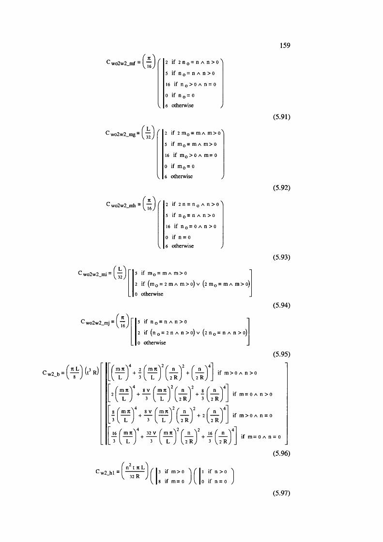
159

^ wo2w2 mf “ . ,/ 2 if 2 n o = n A n > 0 ^

5 i f r i o = n A n > 0

16 if n o > O A n = o

0 if n 0 = 0

V 6 otherwise >

wo2w2_mg - 2 if 2 m o = m A m > 0 ^

5 if m o = m A m > 0

16 if m o > 0 A m = 0

0 if m o = 0

V 6 otherwise >

C wo2w2 mh ” . , 2 if 2 n = n o A n > 0 ^

5 if n o = O A n > 0

16 if n o = O A i i > o

0 if n = 0

V 6 otherw ise y

C wo2w2_mi - 1

C wo2w2_mj -

5 if n i o = n i A m > o

2 if (m o = 2 m A m > o) V (2 n io = m A m > o)

0 otherw ise

5 if n o = n A n > 0

2 i f ( n o = 2 n A n > o ) v ( 2 n o = n A n > o )

0 otherw ise

C w2_b

(5 .91)

(5.92)

(5.93)

(5 .94)

(5.95)

4m K

if m > 0 A n > 0+ -2 R 2 R

4 2 28 Vm 71 m 71

if m = 0 A n > 0+ -2 R

28 V

if m > 0 A n = 0+ 22 R 2 R

2 232 V m 7tif m = 0 A n = 0

2 R 2 R

(5 .96)

C w 2 h i -32 R

18 if m = 0

1 if n > 0

0 if n = 0

(5.97)

^ . m T tV f 71 L t r ' \ /Cw2_h2 = I — 1 if m > 0

0 if m = 0

3 if n > 0

8 if n = 0

n t 32 L

- f I + 5 V (ti m)^ if m > 0 A n > 04 L R ,

16 V (tc m)^ if m > 0 A n = 0

4 I I i f m = 0 A n > 0I R J

0 i f m = O A n = o

C wow3 - ( R C wow3_a C wow3_b •••

Cwow3_c f'W0w3_d —

C wow3_e C wow3_f —

160

(5.98)

(5.99)

(5.100)

^ wow3 a “/ 35 if m g = m A m > 0 \

26 if m o = 2 m A m > o

21 if m g = 3 m A m > 0

64 if m g > 0 A m = 0

40 if m g = 0 A m > 0

128 if m g = 0 A m = 0

V 20 otherwise /

^ wow3_b - ( ^

C wow3 c - „ i f

C wow3_d - 1

3 i f i i o = n A n > 0

-1 ifiio = 3nAn>00 otherwise

3 i f n i o = m A m > 0 ^

-1 if m o = 3 m A m > 0

0 otherwise

/ 35 if n g = n A n > 0

26 if r i g = 2 n A n > 0

21 if n g = 3 i i A n > o

64 if n g > 0 A n = 0

40 if n g = O A n > o

128 if i ig = 0 A n = 0

V 20 otherwise y

(5.101)

(5.102)

(5.103)

(5.104)

161

c wow3_e - 1 2 2f 5 if m o = m A m > 0

4 if m o = 2 m A m > 0

1 if m o = 3 m A m > 0

\ 0 otherwise y

^ wow3 f - , 16/ 5 if n o = O A n > 0 ^

2 i f n o = 2 n A n > 0

3 i f n o = 3 n A n > 0

16 if n o = 0 ^ n > 0

0 if n = 0

V 4 otherw ise y

C wow3_g - [ 2 2f 5 if m o = m A m > 0

2 if m o = 2 m A m > 0

3 if m o = 3 m A m > 0

16 if m o = O A m > o

0 if m = 0

V 4 otherwise /

C wow3 h - , ,16/ 5 if no = n A n > 0 \

4 if no = 2 n A n > 0

1 if rio = 3 n A n > 0

V 0 otherwise y

C w4 =n L t R

32768n Y ( ï t m Y f tt21 I — + 336 + 40 ---------r J l L j l l r

I -f6144 ------ l f m > 0 A n = 0' L J

(5.105)

(5.106)

(5.107)

(5.108)

if m > 0 A n > 0

384 I — I if m = 0 A n > 0R.

o i f m = O A n = o

(5.109)

If the deformed shape has the same wave numbers as those of imperfection i.e. m*, = m

and no=n, substitution of the coefficients into Equation (5.31) for p,i, Equation (5.32) for

\i2, the critical imperfection Equation (5.41) becomes

16 a 2 R Lw,

( 4 Y a 1 R^ + a 2 L^)

(5.110)

162

Equation (5.110) corresponds Equation (4,73). Since Wo is small, neglecting Wq terms in

Equation (5.60) results in

j j î i î Y + 1 Y f j L Y ^ r JL^ _ 4 p ^ 2 ^ ^ 2 ^ 2 l 2 R t j I L ; 3 I L ; U a J { i R

^ * ^ 3 7 2 9 2 24m 7C a 1 R + n a 2 L

(5.111)

Equation (5.111) corresponds to Equation (4.74). The comparison between these

equations will be given in Section 5.7.

5.7 E xam ples

5.7.1 R esults for a Typical Pipeline Liner

For a typical pipeline liner, the values for thermal expansion coefficients in the axial

and circumferential directions are listed in Table 5.3.

Table S3 Values for thermal coefficients for the liner


CtLx ate

1.56 X 10 " 2 .2 X lO **

In Table 5.3, the thermal expansion coefficient in the circumferential direction is

actually the difference of that of the inner liner and that of the outer pipe. For the typical

pipeline in Chapters 3 and 4, the radii and the thickness for the inner liner and the outer

pipe are listed in Table 5.4.

Table 5.4 Values for geometrical parameters

Radius (m) Thickness (mm) Length (m)

Rl tL L

0.3 1 0.3

After searching the results for all combinations of the axial and circumferential wave

numbers, the lowest buckling temperature is derived when the axial wave number is 6

and the circumferential wave number is 25. Substitution of the values of the above

material and geometrical parameters into the critical imperfection Equation (5.41) and

its corresponding buckling temperature Equations (5.60) and (5.61) results in the

following results

163

Table 5.5 Critical Temperature and imperfection for typical pipeline liner

mo Ho m n Wocr

(mm)Tcr(°) T c/(°)

6 25 6 25 0.402 193 10 1

In Table 5.5, T^ is the critical temperature and Ter is its corresponding value when

reduced stiffness method is applied.

Table 5.6 is the comparison of the axial and circumferential wave numbers as well as

the buckling temperature and the critical imperfection among chapters.

Table 5.6 Comparison of the results among Chapters 2,3 and 4 for the same

pipeline liners

m=mo n=rio Tcr(°) Wocr (mm)

Chapter 3 7 43 116 0.095

Chapter 4 7 2 0 2 1 1 0.085

Chapter 5 6 25 193 0.402

5.7.2 Variation with Wave Num bers

For the given material and geometrical values of a pipeline liner, its buckling

temperature may vary with the deformed shape i.e. wave numbers. This is clearly shown

in all the expressions for various coefficients. In-house codes with Visual Basic have

been developed to address the variation of the critical temperature etc with the changing

of wave numbers.

In the program, wave numbers mo, m, no and n are varied from 0 to 100 respectively,

resulting in combinations of wave numbers. For each combination, the program will

calculate the corresponding critical magnitude of the imperfection first using Equation

(5.41). Then the value of this imperfection will be substituted into Equation (5.60) to

calculate the corresponding critical buckling temperature. Similarly from Equation

(5.61), the corresponding critical buckling temperature by the Reduced Stiffness

Method is derived.

Figure 5.3 shows the variation of buckling temperature with wave number m in the axial

direction. In Figure 5.3, the horizontal axis is the axial wave number m, the vertical axis

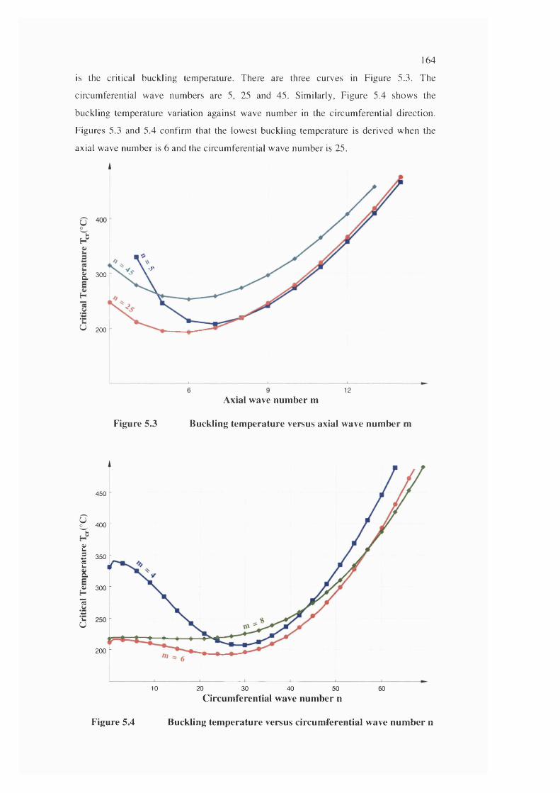
164

is the critical buckling tem perature. There are three curves in Figure 5.3. The

circum ferential wave num bers are 5, 25 and 45. Sim ilarly, Figure 5.4 show s the

buckling tem perature variation against wave num ber in the circum ferential direction.

Figures 5.3 and 5.4 confirm that the lowest buckling tem perature is derived w hen the

axial wave num ber is 6 and the circum ferential wave num ber is 25.

O'^ 300

200 ■

Figure 5.3

12Axial wave number m

Buckling temperature versus axial wave number m

450

y 400 -

£2 350 -2 ^ a

^ 300 -

1

uU

200 -

10 20 30 40 50Circumferential wave number n

60

Figure 5.4 Buckling temperature versus circumferential wave number n

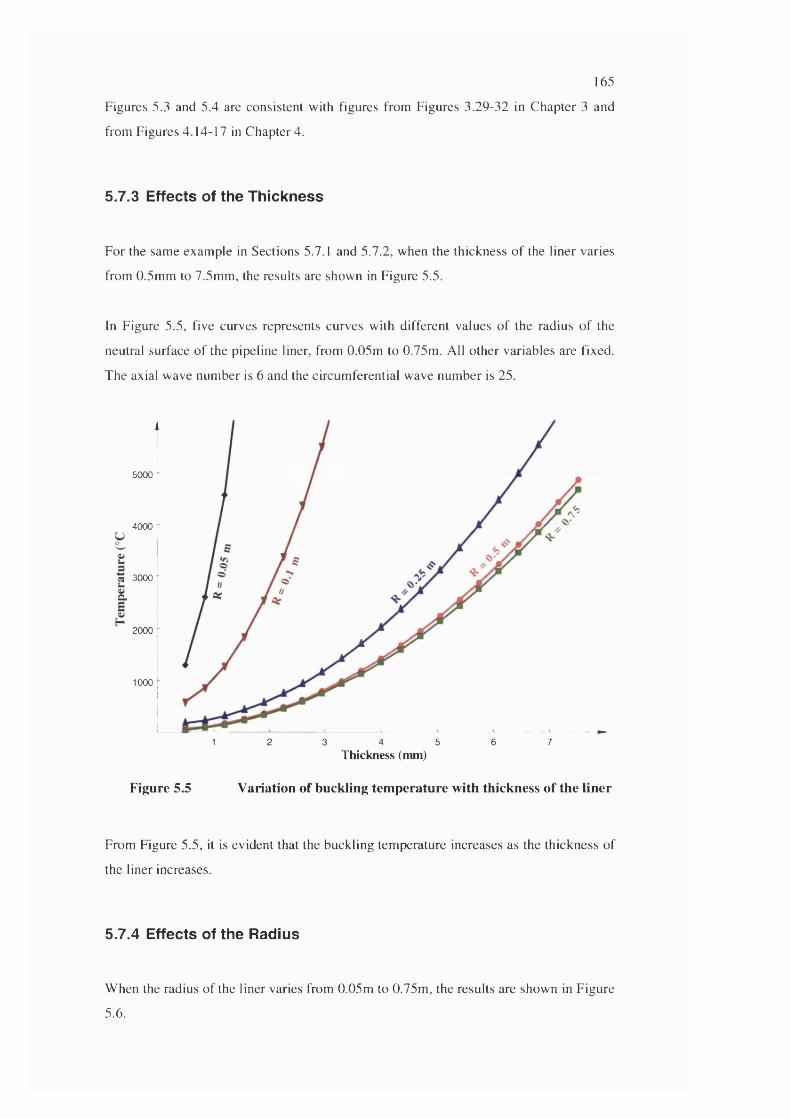
165

Figures 5.3 and 5.4 are consistent with figures from Figures 3.29-32 in C hapter 3 and

from Figures 4.14-17 in C hapter 4.

5.7.3 Effects of the Thickness

For the same exam ple in Sections 5.7.1 and 5.7.2, when the thickness o f the liner varies

from 0.5m m to 7.5m m , the results are shown in Figure 5.5.

In Figure 5.5, five curves represents curves with different values o f the radius o f the

neutral surface o f the pipeline liner, from 0.05m to 0.75m. All o ther variables are fixed.

The axial wave num ber is 6 and the circum ferential wave num ber is 25.

5000

4000

ea 3000

a.

2000

1000

1 2 3 4 5 6 7Thickness (mm)

Figure 5.5 Variation of buckling temperature with thickness of the liner

From Figure 5.5, it is evident that the buckling tem perature increases as the thickness of

the liner increases.

5.7.4 Effects of the Radius

W hen the radius o f the liner varies from 0.05m to 0.75m , the results are show n in F igure

5.6.

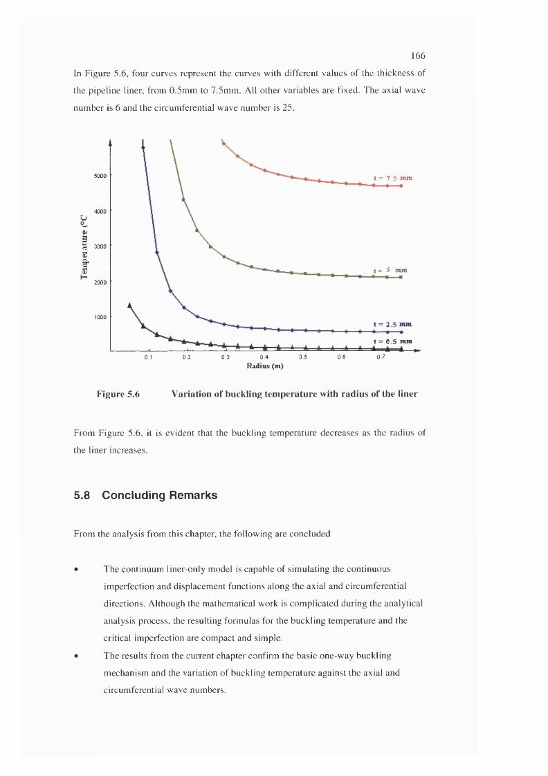
166

In Figure 5.6, four curves represent the curves with different values o f the thickness of

the pipeline liner, from 0.5m m to 7.5m m . All o ther variables are fixed. The axial wave

num ber is 6 and the circum ferential wave num ber is 25.

ict

!

5000 t = 7.5 nun

4000

3000

5 nun2000

1000

t = 0 .5 nun

0.70.2 0.3 0.4 0.5 0.60.1

Radius (m)

Figure 5.6 Variation of buckling temperature with radius of the liner

From Figure 5.6, it is evident that the buckling tem perature decreases as the radius of

the liner increases.

5.8 C oncluding R em arks

From the analysis from this chapter, the follow ing are concluded

The continuum liner-only model is capable of sim ulating the continuous

im perfection and displacem ent functions along the axial and circum ferential

directions. A lthough the m athem atical work is com plicated during the analytical

analysis process, the resulting form ulas for the buckling tem perature and the

critical im perfection are com pact and simple.

The results from the current chapter confirm the basic one-w ay buckling

m echanism and the variation o f buckling tem perature against the axial and

circum ferential wave numbers.

167

The variation of the buckling temperature against the wall thickness and the

radius of the pipeline liners is consistent with that from the previous chapters.

The formulas derived from the current chapter are capable of searching the

lowest buckling temperature among those of various combinations of wave

numbers etc. Further work is recommended for a more detailed parametric study

to further investigate the variation of the buckling temperature against the wall

thickness and the neutral surface radius of the pipeline liners. For a given

thickness or radius, searching all possible combinations of wave numbers could

result in lower buckling temperature than those given in the current parametric

study.

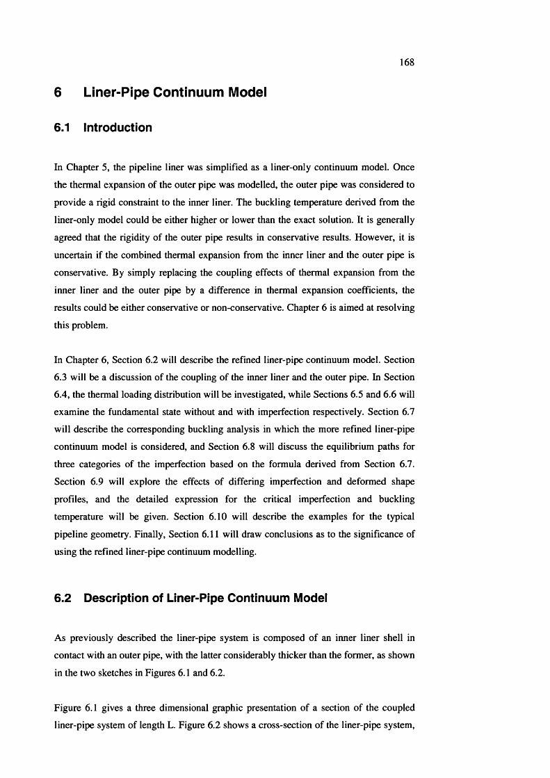
168

6 Liner-Pipe Continuum Model

6.1 In troduction

In Chapter 5, the pipeline liner was simplified as a liner-only continuum model. Once

the thermal expansion of the outer pipe was modelled, the outer pipe was considered to

provide a rigid constraint to the inner liner. The buckling temperature derived from the

liner-only model could be either higher or lower than the exact solution. It is generally

agreed that the rigidity of the outer pipe results in conservative results. However, it is

uncertain if the combined thermal expansion from the inner liner and the outer pipe is

conservative. By simply replacing the coupling effects of thermal expansion from the

inner liner and the outer pipe by a difference in thermal expansion coefficients, the

results could be either conservative or non-conservative. Chapter 6 is aimed at resolving

this problem.

In Chapter 6 , Section 6.2 will describe the refined liner-pipe continuum model. Section

6.3 will be a discussion of the coupling of the inner liner and the outer pipe. In Section

6.4, the thermal loading distribution will be investigated, while Sections 6.5 and 6 .6 will

examine the fundamental state without and with imperfection respectively. Section 6.7

will describe the corresponding buckling analysis in which the more refined liner-pipe

continuum model is considered, and Section 6 .8 will discuss the equilibrium paths for

three categories of the imperfection based on the formula derived from Section 6.7.

Section 6.9 will explore the effects of differing imperfection and deformed shape

profiles, and the detailed expression for the critical imperfection and buckling

temperature will be given. Section 6.10 will describe the examples for the typical

pipeline geometry. Finally, Section 6 .11 will draw conclusions as to the significance of

using the refined liner-pipe continuum modelling.

6.2 D escrip tion of L iner-Pipe C on tinuum Modei

As previously described the liner-pipe system is composed of an inner liner shell in

contact with an outer pipe, with the latter considerably thicker than the former, as shown

in the two sketches in Figures 6 .1 and 6.2.

Figure 6.1 gives a three dimensional graphic presentation of a section of the coupled

liner-pipe system of length L. Figure 6.2 shows a cross-section of the liner-pipe system.

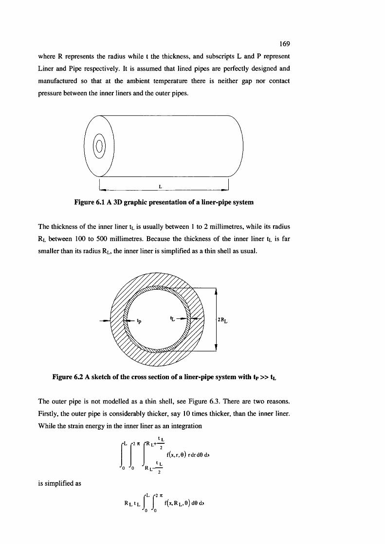
169

where R represents the radius while t the thickness, and subscripts L and P represent

Liner and Pipe respectively. It is assumed that lined pipes are perfectly designed and

manufactured so that at the ambient temperature there is neither gap nor contact

pressure between the inner liners and the outer pipes.

L

Figure 6.1 A 3D graphic presentation of a liner-pipe system

The thickness of the inner liner tt is usually between 1 to 2 millimetres, while its radius

Rl between 100 to 500 millimetres. Because the thickness of the inner liner tL is far

smaller than its radius Rl, the inner liner is simplified as a thin shell as usual.

Figure 6.2 A sketch of the cross section of a liner-pipe system with tp » tL

The outer pipe is not modelled as a thin shell, see Figure 6.3. There are two reasons.

Firstly, the outer pipe is considerably thicker, say 10 times thicker, than the inner liner.

While the strain energy in the inner liner as an integration

çL '2 71

f ( x ,r ,0 ) rd rdG d>

is simplified as

R l ^L [ [ f ( x ,R L ,0 ) d 0 d >• 0 * 0

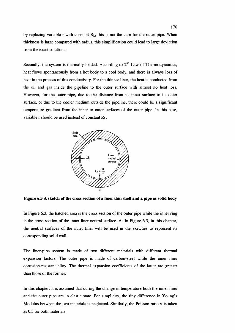
170

by replacing variable r with constant Rl, this is not the case for the outer pipe. When

thickness is large compared with radius, this simplification could lead to large deviation

from the exact solutions.

Secondly, the system is thermally loaded. According to 2" Law of Thermodynamics,

heat flows spontaneously from a hot body to a cool body, and there is always loss of

heat in the process of this conductivity. For the thinner liner, the heat is conducted from

the oil and gas inside the pipeline to the outer surface with almost no heat loss.

However, for the outer pipe, due to the distance from its inner surface to its outer

surface, or due to the cooler medium outside the pipeline, there could be a significant

temperature gradient from the inner to outer surfaces of the outer pipe. In this case,

variable r should be used instead of constant Rl.

Solidpipe

Linerneutralsurface

tp + —

Figure 6.3 A sketch of the cross section of a liner thin shell and a pipe as solid body

In Figure 6.3, the hatched area is the cross section of the outer pipe while the inner ring

is the cross section of the inner liner neutral surface. As in Figure 6.3, in this chapter,

the neutral surfaces of the inner liner will be used in the sketches to represent its

corresponding solid wall.

The liner-pipe system is made of two different materials with different thermal

expansion factors. The outer pipe is made of carbon-steel while the inner liner

corrosion-resistant alloy. The thermal expansion coefficients of the latter are greater

than those of the former.

In this chapter, it is assumed that during the change in temperature both the inner liner

and the outer pipe are in elastic state. For simplicity, the tiny difference in Young’s

Modulus between the two materials is neglected. Similarly, the Poisson ratio v is taken

as 0.3 for both materials.

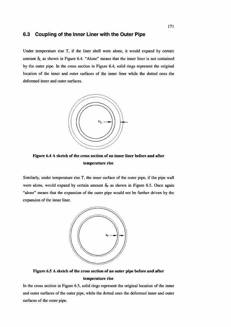
171

6.3 C oupling of th e Inner Liner w ith th e O u ter P ipe

Under temperature rise T, if the liner shell were alone, it would expand by certain

amount 5 l as shown in Figure 6.4. “Alone” means that the inner liner is not contained

by the outer pipe. In the cross section in Figure 6.4, solid rings represent the original

location of the inner and outer surfaces of the inner liner while the dotted ones the

deformed inner and outer surfaces.

Figure 6.4 A sketch of the cross section of an inner liner before and after

temperature rise

Similarly, under temperature rise T, the inner surface of the outer pipe, if the pipe wall

were alone, would expand by certain amount 5? as shown in Figure 6.5. Once again

“alone” means that the expansion of the outer pipe would not be further driven by the

expansion of the inner liner.

Figure 6.5 A sketch of the cross section of an outer pipe before and after

temperature rise

In the cross section in Figure 6.5, solid rings represent the original location of the inner

and outer surfaces of the outer pipe, while the dotted ones the deformed inner and outer

surfaces of the outer pipe.

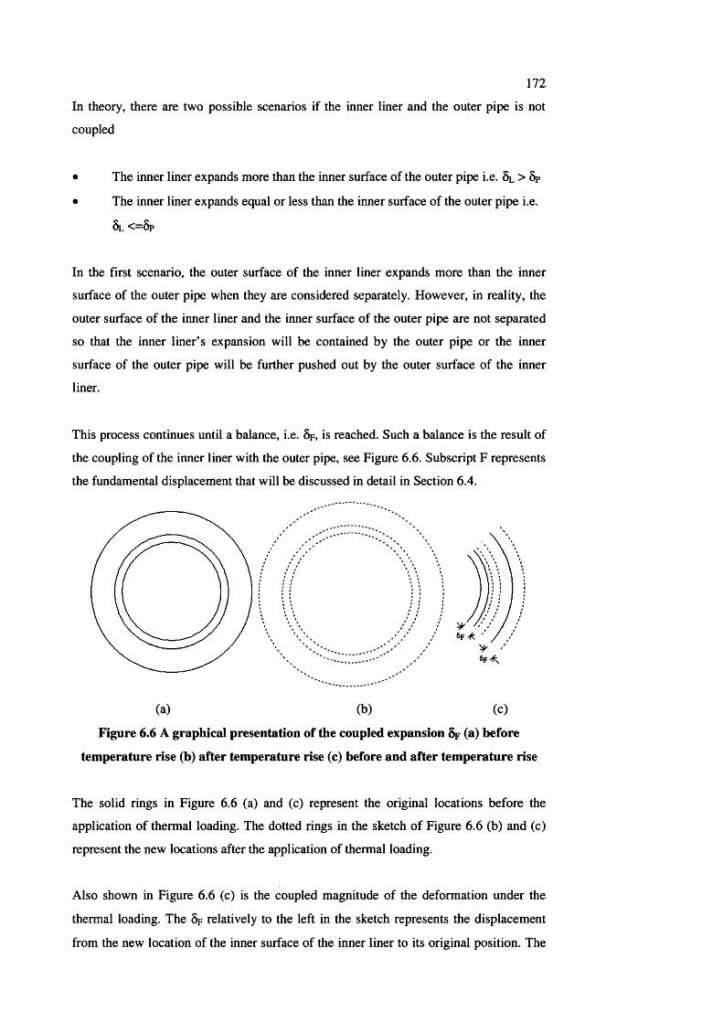
172

In theory, there are two possible scenarios if the inner liner and the outer pipe is not

coupled

• The inner liner expands more than the inner surface of the outer pipe i.e. 5l > 5?

• The inner liner expands equal or less than the inner surface of the outer pipe i.e.

5 l < = 5 p

In the first scenario, the outer surface of the inner liner expands more than the inner

surface of the outer pipe when they are considered separately. However, in reality, the

outer surface of the inner liner and the inner surface of the outer pipe are not separated

so that the inner liner’s expansion will be contained by the outer pipe or the inner

surface of the outer pipe will be further pushed out by the outer surface of the inner

liner.

This process continues until a balance, i.e. 5 f , is reached. Such a balance is the result of

the coupling of the inner liner with the outer pipe, see Figure 6 .6 . Subscript F represents

the fundamental displacement that will be discussed in detail in Section 6.4.

(a) (b) (c)

Figure 6.6 A graphical presentation of the coupled expansion 6f (a) before

temperature rise (b) after temperature rise (c) before and after temperature rise

The solid rings in Figure 6 .6 (a) and (c) represent the original locations before the

application of thermal loading. The dotted rings in the sketch of Figure 6 .6 (b) and (c)

represent the new locations after the application of thermal loading.

Also shown in Figure 6 .6 (c) is the coupled magnitude of the deformation under the

thermal loading. The 5f relatively to the left in the sketch represents the displacement

from the new location of the inner surface of the inner liner to its original position. The

173

bottom-right 5f in the sketch is the displacement from the new location of the outer

surface of the outer pipe to its original position. Due to the coupling, they undergo the

same amount of displacement 5f.

Therefore, after the coupling of the inner liner with the outer pipe, the inner liner is held

back radially inward by the outer pipe by ( 5 l - 6 f ), while the inner surface of the outer

pipe is pushed radially outward by the inner liner by ( 5 f - 5?).

It is noticed that although both the inner liner and the inner surface of the outer pipe are

globally displaced outward, the liner is held relatively inward. Here “relatively inward”

means the inner liner deflects inward from the position of its free expansion. Therefore,

the inner liner is in compression because it is “pressed” inward by the outer pipe, while

the outer pipe is in tension because its inner surface is “pushed” outward by the inner

liner.

From energy point of view, under the thermal loading, apart from the compressive

membrane strain energy in the inner liner, there is also tensional strain energy in the

outer pipe. This is the part of the energy that further destabilizes the liner-pipe system.

The condition for the inner liner alone to expand more than the outer pipe alone will be

given in Section 6 .6 .6 . In the second scenario, i.e. the free expansion of the outer pipe

alone is not less than the free expansion of the inner liner alone, there will be no

coupling. In this study, only the first scenario will be investigated. The first scenario is

the right scenario that will be considered in the current study.

6.4 T em p era tu re D istribution

6.4.1 Review of Heat Flow

It may be necessary to review what is heat and temperature and how heat transfers. Heat

is the total amount of internal kinetic energy of the atoms and molecules that make up a

substance. Temperature is a relative term refers to the average kinetic energy of the

atoms and molecules in a substance. Heat may transfer across the boundaries of a

system, either to or from another system. Heat transference occurs only when there is a

temperature difference between the systems. Heat is transferred by conduction,

convection and radiation, which may occur separately or in combination. Among three

174

ways of transferring of heat, only conduction is by contact therefore is the only way of

heat transference that is relevant to this research.

In the pipeline, the oil and gas inside is at high temperature that is in contact with the

inner surface of the pipeline liner. According to Newton’s Law of Cooling, there is

always a thin layer of fluid through which the heat is transferred by conduction. The

heat flows between the oil or gas inside the pipeline and the pipeline liner and pipe. The

temperature distribution inside the liner and pipe wall is governed by Fourier’s Law of

Conduction

—Q = -A. A f - T dt y d r

(6 .1)

where Q is heat, t is time, X is thermal conductivity of the material of the pipeline, A is

the area of the contact, T is the temperature rise, r is the radial coordinate of the

pipeline.

6.4.2 Tem perature Distribution in the inner Liner

For the pipeline liner, because its thickness is very small, it is assumed that throughout

the thickness the liner will have the same amount of temperature rise T.

6.4.3 Tem perature Distribution in the Outer Pipe

In the thick outer pipe wall of a lined pipe, assume the heat flow is proportional to the

temperature rise,

— Q p = c T p dt

(6.2)

where Qp is the heat in the outer pipe wall of a lined pipe, c is a constant, Tp is the

temperature distribution inside the outer pipe wall, then in this special case Fourier’s

Law of Conductivity Equation (6.1) may be rewritten as

- T p = - k T p dr

(6.3)

where k is a constant. Solution of the above differential equation requires use of two

boundary conditions. The first boundary condition is

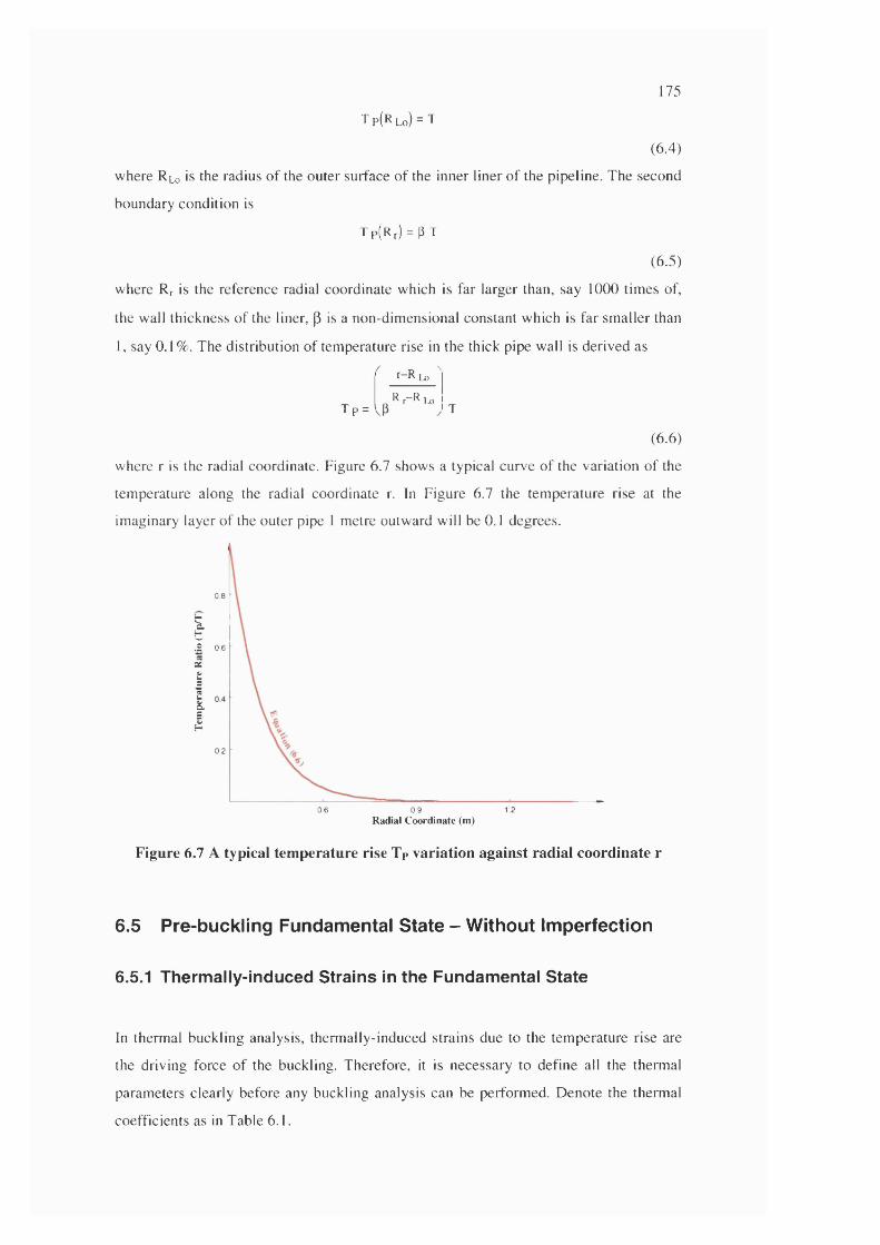
T p ( R lo) = T

175

(6.4)

where R lo is the radius o f the outer surface of the inner liner o f the pipeline. The second

boundary condition is

Tp(Rr) = |3T

(6.5)

where Rr is the reference radial coordinate which is far larger than, say 1000 tim es of,

the wall thickness o f the liner, |3 is a non-dim ensional constant which is far sm aller than

1, say 0.1% . The distribution o f tem perature rise in the thick pipe wall is derived as

r-R Lo '

Tp = Rr-R W

(6 d%

where r is the radial coordinate. Figure 6.7 shows a typical curve o f the variation o f the

tem perature along the radial coordinate r. In Figure 6.7 the tem perature rise at the

im aginary layer o f the outer pipe 1 m etre outw ard will be 0.1 degrees.

0.8

I.£ 0.6

XIII

0.2

0.6 0.9 1.2Radial Coordinate (m)

Figure 6.7 A typical temperature rise Tp variation against radial coordinate r

6.5 Pre-buckling Fundam ental S ta te - W ithout Im perfection

6.5.1 Thermally-Induced Strains in the Fundamental State

In therm al buckling analysis, therm ally-induced strains due to the tem perature rise are

the driving force o f the buckling. Therefore, it is necessary to define all the therm al

param eters clearly before any buckling analysis can be perform ed. D enote the therm al

coefficients as in Table 6.1.

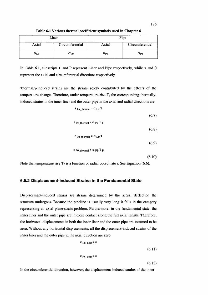
176

Table 6.1 Various thermal coefficient symbols used in Chapter 6

Liner Pipe


O tLx CtLB a p x otpe

In Table 6.1, subscripts L and P represent Liner and Pipe respectively, while x and 0

represent the axial and circumferential directions respectively.

Thermally-induced strains are the strains solely contributed by the effects of the

temperature change. Therefore, under temperature rise T, the corresponding thermally-

induced strains in the inner liner and the outer pipe in the axial and radial directions are

G Lx_thermal - Lx T

(6.7)

E Px_thermal ~ ® Px P

(6.8)

G L0_thermal - L8 T

(6.90

e P 0_ th erm al = « P 0 T p

(6. 10)

Note that temperature rise Tp is a function of radial coordinate r. See Equation (6 .6 ).

6.5.2 Displacement-induced Strains in the Fundam ental S tate

Displacement-induced strains are strains determined by the actual deflection the

structure undergoes. Because the pipeline is usually very long it falls in the category

representing an axial plane-strain problem. Furthermore, in the fundamental state, the

inner liner and the outer pipe are in close contact along the full axial length. Therefore,

the horizontal displacements in both the inner liner and the outer pipe are assumed to be

zero. Without any horizontal displacements, all the displacement-induced strains of the

inner liner and the outer pipe in the axial direction are zero.

G Lx_disp -

(6.11)

G Px_disp “ G

(6. 12)

In the circumferential direction, however, the displacement-induced strains of the inner

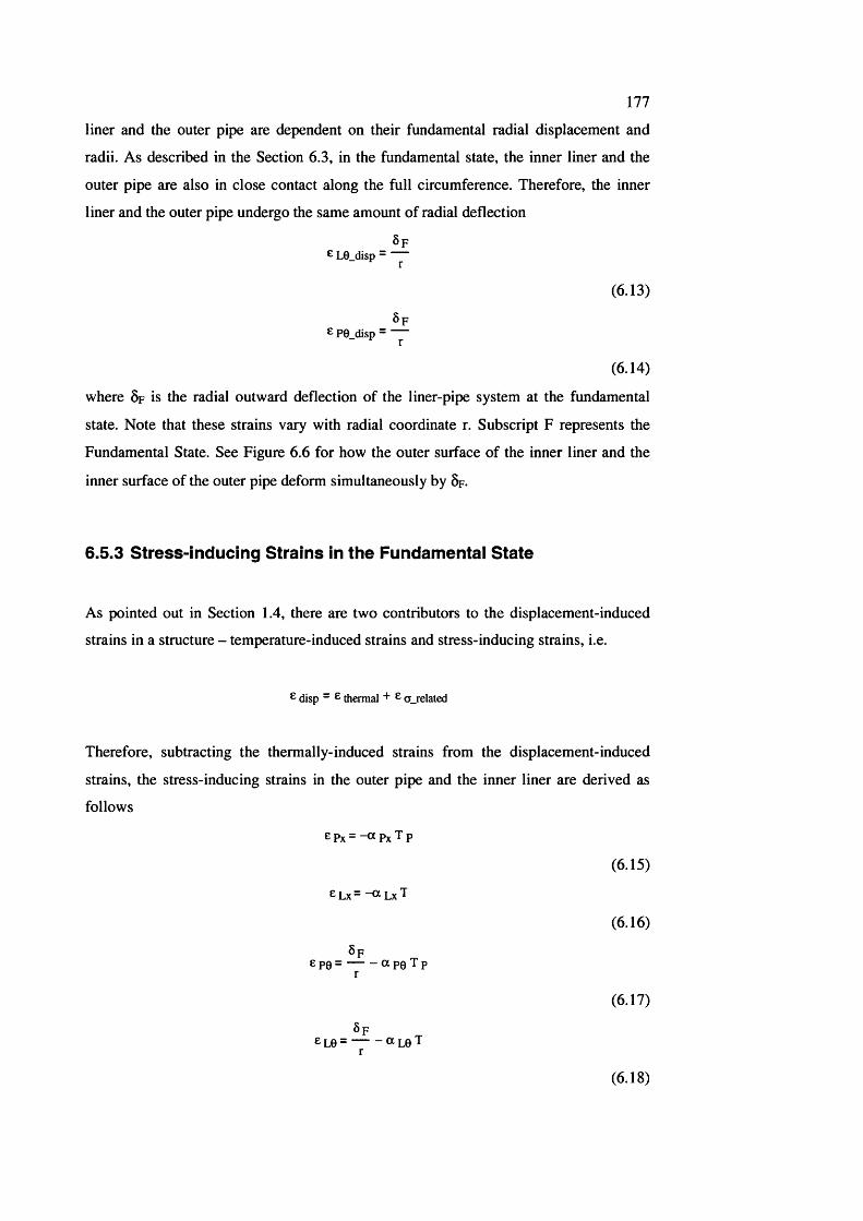
Ill

liner and the outer pipe are dependent on their fundamental radial displacement and

radii. As described in the Section 6.3, in the fundamental state, the inner liner and the

outer pipe are also in close contact along the full circumference. Therefore, the inner

liner and the outer pipe undergo the same amount of radial deflection

ÔFe L0_disp = —

(6.13)

5fe P0_disp - —

(6.14)

where Sp is the radial outward deflection of the liner-pipe system at the fundamental

state. Note that these strains vary with radial coordinate r. Subscript F represents the

Fundamental State. See Figure 6 .6 for how the outer surface of the inner liner and the

inner surface of the outer pipe deform simultaneously by 5p.

6.5.3 S tress-inducing Strains in the Fundamentai S tate

As pointed out in Section 1.4, there are two contributors to the displacement-induced

strains in a structure - temperature-induced strains and stress-inducing strains, i.e.

G disp “ G thermal + a_related

Therefore, subtracting the thermally-induced strains from the displacement-induced

strains, the stress-inducing strains in the outer pipe and the inner liner are derived as

follows

e px = - a px T p

(6.15)

£Lx= -«L xT

(6.16)

Spep0 = a P8 Tp

£L0 = «L0 T

(6.17)

(6.18)

178

6.5.4 Total Potential Energy in the Fundamental State

Apart from the above strain components, in the fundamental state, all the other strain

components are zero. Because there are no shear strains and curvatures, the total strain

energies in the outer pipe and the inner liner may be written as

U p =E

f L '2 71 R Po

2 ( l - V^) - 0 0 R lo

[(e Px) + (e pe) + 2 V (e Px) (e pe)] rdrde dx

(6.19)

ç L '2 k r

J q J 0 - 1

Lo

[(e Lx) + (e Le) + 2 V e Lx (e ls)] rdrd0 d>■ Li

(6.20)

where Rpo, R lo, R u and R lo are the radii of the inner and outer surfaces of the outer

piper and the inner liner respectively. Unlike the force-loaded structure, in the

thermally-loaded liner-pipe system, there are no external forces. There is no

corresponding potential energy contributed by the external forces. Therefore, the sum of

the strain energies in the inner liner and in the outer pipe is the total potential energy.

n = Up + U L

(6.21)

Here strain energy is denoted as U and total potential energy as H. As before, subscripts

P and L represent Pipe and Liner respectively.

6.5.5 Stationary Potential Energy Principle in the Fundam ental State

According to the stationary potential energy principle, the derivative of the total

potential energy with respect to the fundamental radial deflection is zero.

— n = 0d Sp

(6.22)

Substituting equations from Equations (6.15)-(6.18) and Equations (6.19)-(6.21) into

Equation (6.22), the fundamental radial deflection is derived.

6 p = m TtL

(6.23)

Noticed that 5f is linear to temperature rise T. In Equation (6.23), |lIi is a non-

dimensional coefficient. It is defined as the ratio of the fundamental radial deflection to

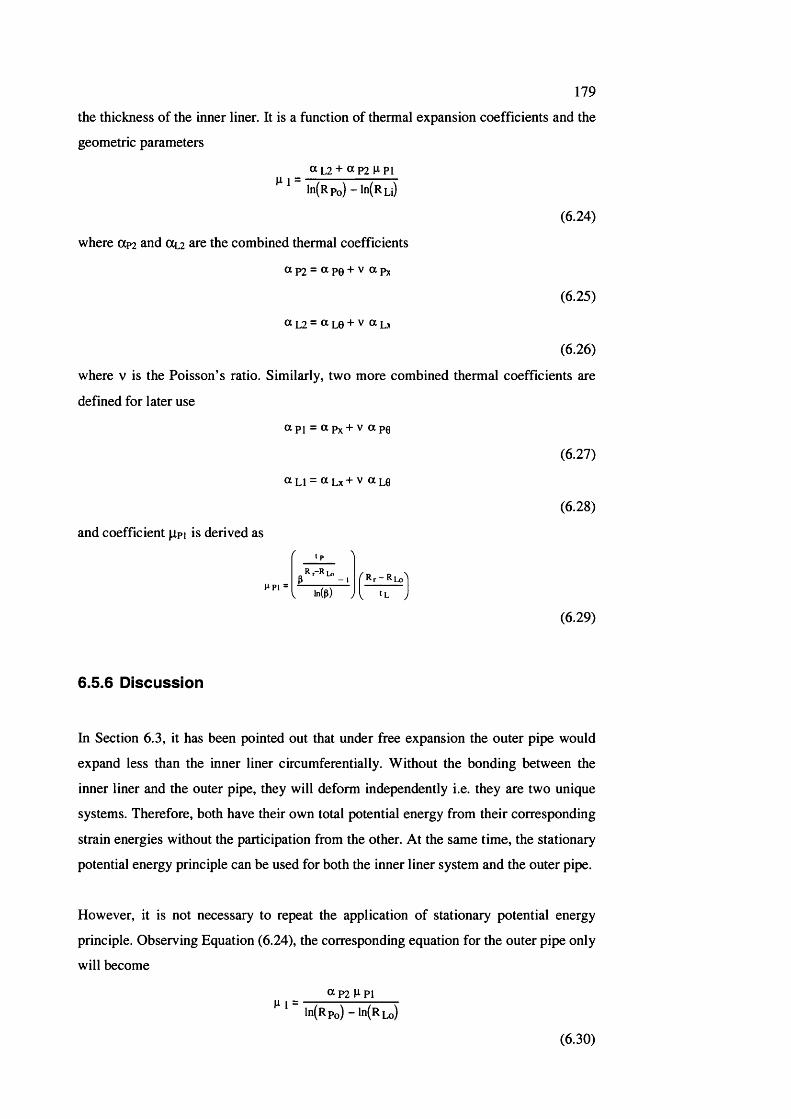
179

the thickness of the inner liner. It is a function of thermal expansion coefficients and the

geometric parameters

« L2 + « P2 PI

ln ( R p o ) - ln ( R u )

(6.24)

where a ?2 and Œl2 are the combined thermal coefficients

ap 2 = a p 0 + v apx

(6.25)

aL 2 =»Le + v a u

(6.26)

where v is the Poisson’s ratio. Similarly, two more combined thermal coefficients are

defined for later use

a PI = a Px + V a pe

aLl = «Lx+v «Le

and coefficient p,pi is derived as

t p_

Rf ~ Rlo

(6.27)

(6.28)

HPI =R r-R Lo

I - I

ln(p) «L

(6.29)

6.5.6 D iscussion

In Section 6.3, it has been pointed out that under free expansion the outer pipe would

expand less than the inner liner circumferentially. Without the bonding between the

inner liner and the outer pipe, they will deform independently i.e. they are two unique

systems. Therefore, both have their own total potential energy from their corresponding

strain energies without the participation from the other. At the same time, the stationary

potential energy principle can be used for both the inner liner system and the outer pipe.

However, it is not necessary to repeat the application of stationary potential energy

principle. Observing Equation (6.24), the corresponding equation for the outer pipe only

will become

« P 2 l^Pl1 =

In(Rpo) - ln (R L o)

(6.30)

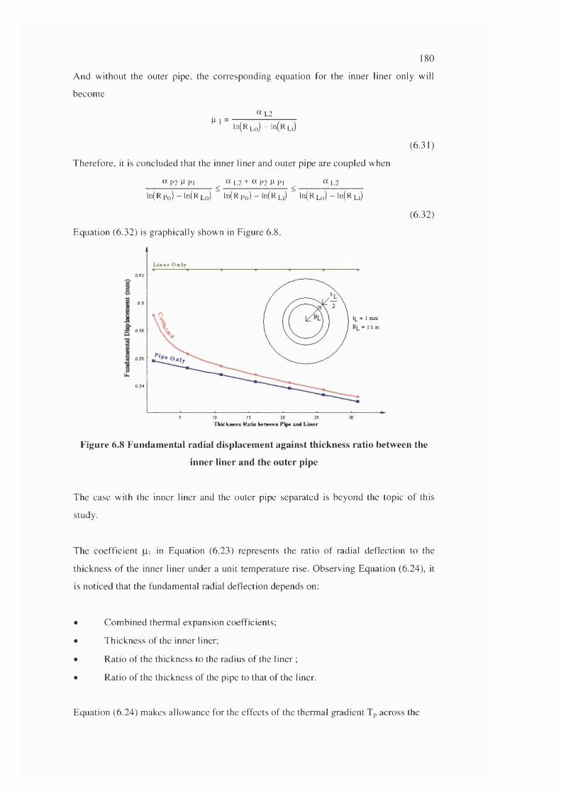
180

A nd w ithout the outer pipe, the corresponding equation for the inner liner only will

becom e

a L2

ln(R Lo)-ln(R u)

Therefore, it is concluded that the inner liner and outer pipe are coupled when

(6.31)

a P2 P PI » L 2 + « P 2 M PI « L 2< — <

ln(R Po) - ln(R l o ) ln(R Po) - ln(R Li) ln(R Lo) “ ln(R Li)

E quation (6.32) is graphically shown in Figure 6.8.

(6.32)

0.82

0 6

^ - 1 mm RL - 0 .Î m0 58

0.56

0 54

5 to 15 20 25TkickiKss Ratio between P y and Liner

30

Figure 6.8 Fundamental radial displacement against thickness ratio between the

inner liner and the outer pipe

The case with the inner liner and the outer pipe separated is beyond the topic o f this

study.

The coefficient pi in Equation (6.23) represents the ratio o f radial deflection to the

thickness o f the inner liner under a unit tem perature rise. O bserving Equation (6.24), it

is noticed that the fundam ental radial deflection depends on;

• C om bined thermal expansion coefficients;

• Thickness of the inner liner;

• R atio o f the thickness to the radius o f the liner ;

• Ratio o f the thickness o f the pipe to that o f the liner.

Equation (6.24) m akes allow ance for the effects o f the therm al gradient Tp across the

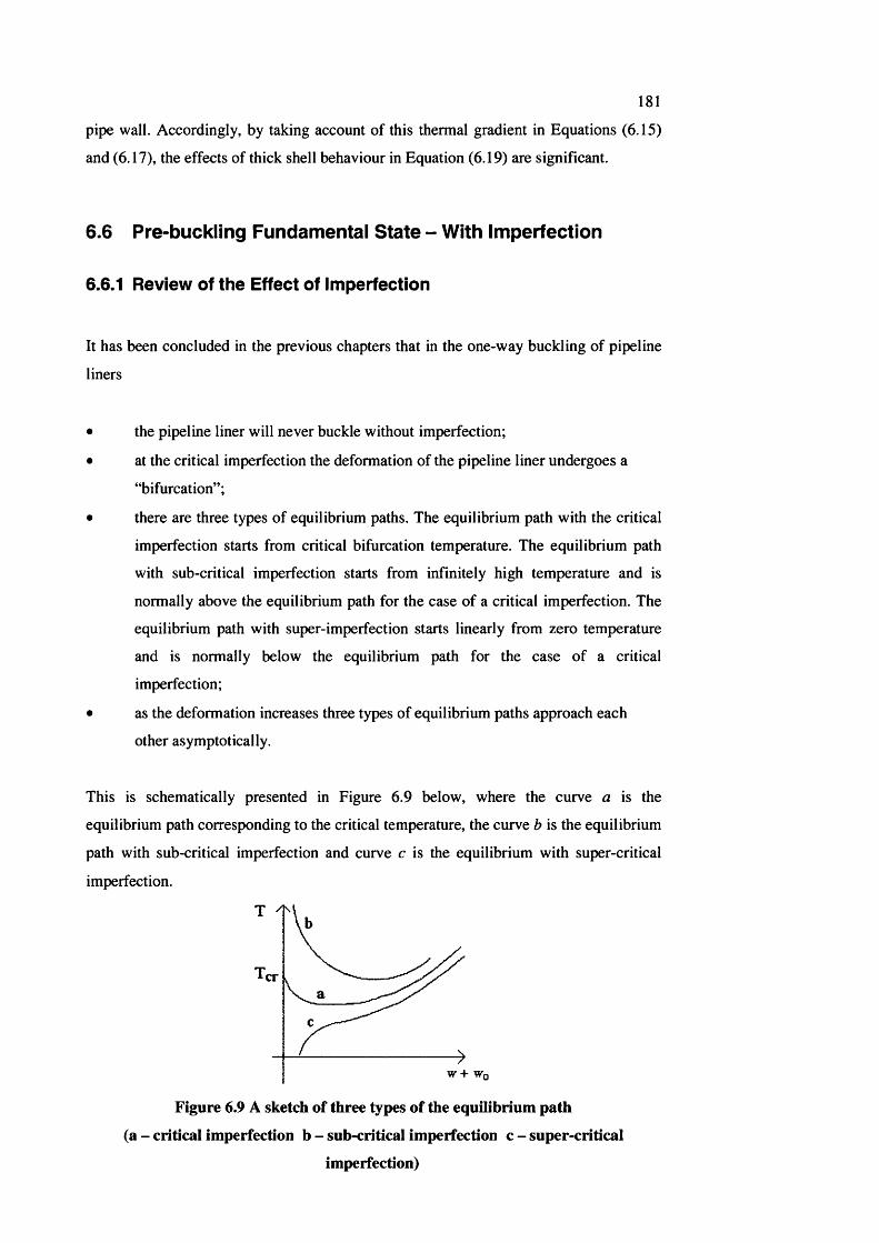
181

pipe wall. Accordingly, by taking account of this thermal gradient in Equations (6.15)

and (6.17), the effects of thick shell behaviour in Equation (6.19) are significant.

6.6 P re-buck ling F undam en ta l S ta te - W ith im perfec tion

6.6.1 Review of the Effect of imperfection

It has been concluded in the previous chapters that in the one-way buckling of pipeline

liners

• the pipeline liner will never buckle without imperfection;

• at the critical imperfection the deformation of the pipeline liner undergoes a

“bifurcation”;

• there are three types of equilibrium paths. The equilibrium path with the critical

imperfection starts from critical bifurcation temperature. The equilibrium path

with sub-critical imperfection starts from infinitely high temperature and is

normally above the equilibrium path for the case of a critical imperfection. The

equilibrium path with super-imperfection starts linearly from zero temperature

and is normally below the equilibrium path for the case of a critical

imperfection;

• as the deformation increases three types of equilibrium paths approach each

other asymptotically.

This is schematically presented in Figure 6.9 below, where the curve a is the

equilibrium path corresponding to the critical temperature, the curve b is the equilibrium

path with sub-critical imperfection and curve c is the equilibrium with super-critical

imperfection.

T

cr

W+ Wt

Figure 6.9 A sketch of three types of the equilibrium path

(a - critical imperfection b - sub-critical imperfection c - super critical

imperfection)

182

In the above sketch, w is the incremental displacement, Wq is the magnitude of the

imperfection, T the temperature rise and Ter the critical bifurcation temperature.

6.6.2 Fundam ental State

The effect of the imperfection to the liner-pipe system is very similar to that from the

liner-only continuum model i.e.

• There also exists the critical imperfection in the liner-pipe system for which the

liner-pipe system “bifurcates”.

• The fundamental displacement for the liner-pipe system with the critical

imperfection is equal to the fundamental displacement for the liner-pipe system

without imperfection.

• Similarly three types of equilibrium path exist for the liner-pipe system.

The above conclusions will be demonstrated in the Sections 6.7 and 6.8. At present we

simply use the fundamental deflection from the liner-pipe system without imperfection

as the fundamental deflection for the liner-pipe system with the critical imperfection.

6.7 F orm ulation

6.7.1 Description of Buckled Shape - Incremental Deformation

The radial incremental deformation of the liner of a liner-pipe system is composed of

two parts — an axisymmetric part and a non-axisymmetric part

w L = 8+ w fx(x) fe(e)(6.33)

where 6 is the axisymmetric radial inward deflection, w is the maximum value of the

non-axisymmetric radial inward deflection, f% and fg are normalised functions of x and 0

respectively. Here subscripts x and 0 represent axial and circumferential directions

respectively, while variables x and 0 represent axial and circumferential coordinates

respectively. Because the radial incremental deflection is inward only, both f% and fg

should be positive-definite. For simplicity, the displacements in the horizontal and

circumferential directions are ignored.

183

It is evident that due to the bonding with the inner liner, the deformation of the outer

pipe will be equal to the axisymmetric part of the deformation of the inner liner, i.e.

W p = S

(6.34)

Therefore, the whole system of the inner liner and the outer pipe could be described

with two independent variables Ô and w.

Notice that the deformations are in different directions in the fundamental and buckling

states. In Section 6.5, outward fundamental deflection is assumed as positive 5p. This is

based on the fact that the actual fundamental radial deflection is outward. However, in

this section, incremental radial deflections 5 and w due to the buckling are always

inward. Therefore, it is reasonable to assume that both 5 and w are positive when the

deflections are inward.

6.7.2 Description of Imperfection

Similar to the deformation, an imperfection may also be described by a maximum

imperfection Wq, a non-negative normalised function of x, fox(x), and a non-negative

normalised function of 0, foe(0). Assume the imperfection takes the following shape

^ O - ^ O ^ox(^) fooC®)

(6.35)

Here subscript o represent imperfection.

6.7.3 Total Incremental Displacement

The total incremental displacement is the sum of the fundamental displacement and the

incremental displacement. The outer pipe and the inner liner have the same fundamental

displacement 5f. The incremental displacement in the outer pipe is due to axisymmetric

perturbation 5 only. The incremental displacement in the inner liner is due to

axisymmetric perturbation 5 and non-axisymmetric perturbation W.

W p = —6 p + Ô

(6.36)

W l= - S f + 5 + wfx(x)f e(e)

(6.37)

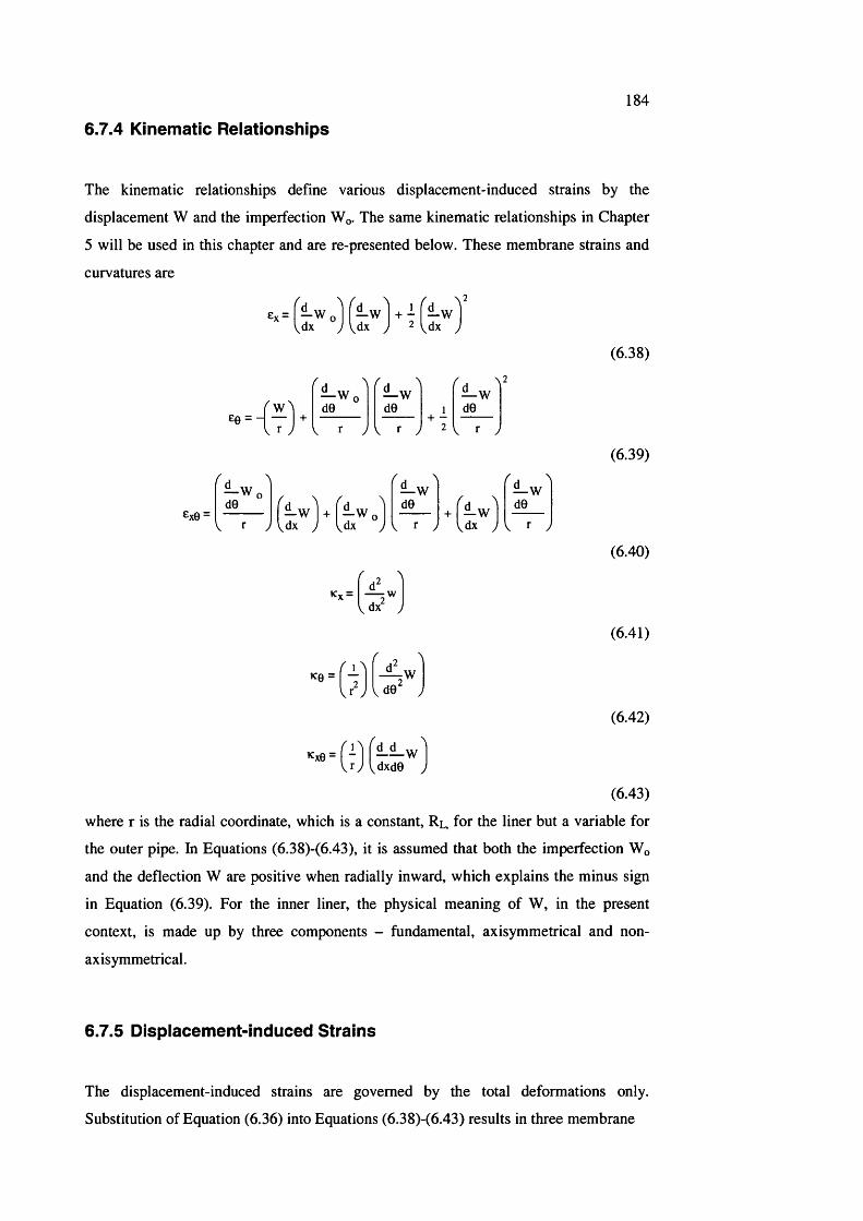
184

6.7.4 Kinematic Relationships

The kinematic relationships define various displacement-induced strains by the

displacement W and the imperfection Wq. The same kinematic relationships in Chapter

5 will be used in this chapter and are re presented below. These membrane strains and

curvatures are, 2

ee = -I y I +

— W , d0__

V r Jde de

V r y

ex0 =

— W, de__

V r y dx— W + — W

dx

de

V r y+ I — W

dx

deV r y

' 4 - 'V dx y

K 0 = | -

(6.38)

(6.39)

(6.40)

(6.41)

(6.42)

(6.43)

where r is the radial coordinate, which is a constant, Rl, for the liner but a variable for

the outer pipe. In Equations (6.38)-(6.43), it is assumed that both the imperfection Wq

and the deflection W are positive when radially inward, which explains the minus sign

in Equation (6.39). For the inner liner, the physical meaning of W, in the present

context, is made up by three components - fundamental, axisymmetrical and non-

ax isymmetrical.

6.7.5 Displacement-induced Strains

The displacement-induced strains are governed by the total deformations only.

Substitution of Equation (6.36) into Equations (6.38)-(6.43) results in three membrane

strains and three curvatures in the outer pipe as

185

epx= 0

Ô P - 5ep0 =

e px0 = 0

K Px - 0

Kp0= 0

(6.44)

(6.45)

(6.46)

(6.47)

(6.48)

Kpx0= 0

(6.49)

Substitution of Equation (6.37) into Equations (6.38)-(6.43) results in three membrane

strains and three curvatures in the inner liner as

ELx= (fo e(0 )) (feW )) Wo w + ( f 0 ( e ) f w

(6.50)

/ j— foe(0 ) d9

y

^ f e ( e )d0____

V Rl yw O w + ^ ( f x(x)}^

/'a—fe(e)d0______

V R l y

(6.51)

«Lxe— foe(e) d6

I Rl( f e ( 0) ) W o w +1 ^ f o x ( x ) I ( f o e ( e ) )

deI Rl j

R Lx“r 2 ^

— /x ( x )V dx y

I Rl

(6.52)

(6.53)

KL0 = ^ 1 (fx(x))R l

/ 2 ^- ^ f 0 ( e )

v d e y

(6.54)

— f0(e) % de

(6.55)

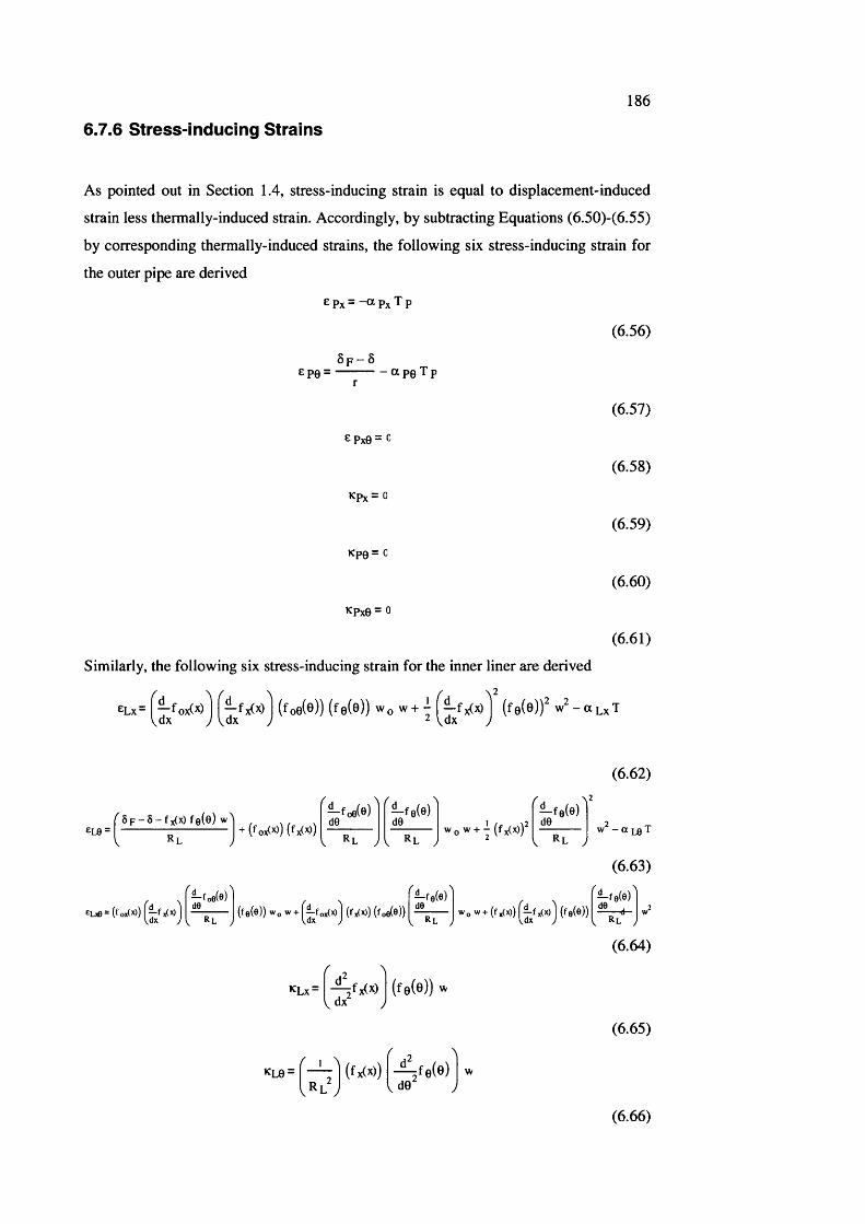
186

6.7.6 S tress-inducing Strains

As pointed out in Section 1,4, stress-inducing strain is equal to displacement-induced

strain less thermally-induced strain. Accordingly, by subtracting Equations (6.50)-(6.55)

by corresponding thermally-induced strains, the following six stress-inducing strain for

the outer pipe are derived

e Px = - a Px T p

ôp - 6e p0 = --------------a p0 T p

r

E px0 = 0

Kp>x = 0

K p 0 = 0

(6.56)

(6.57)

(6.58)

(6.59)

(6.60)

(6.61)

Similarly, the following six stress-inducing strain for the inner liner are derived

GLx= ( f o e ( 0 ) ) ( f e ( 0 ) ) Wo w + j ( f e ( 0 ) ) ^ - a L x T

(6.62)

^-foe(e)^ d9

foe(e)^d6______

V Rl yde

fe(e)

V " L . /WoW+^(fx(x)f

/ .— fe(e) de

eLje= (fox(x)) — (f0(0 )) W o w + ^ fox(x)j (fx(x)) (f00(e)) W o w+(f^x))^^f^x)j (fe(e))

W - t t L e T

(6.63)

— fe(e)

^Lx-r 2 ^— /x (x )

V dx J

Rl

(6.64)

(6.65)

KL0 =Rl

(f x(*)) — rfeCo)V y V d0 y

(6.66)

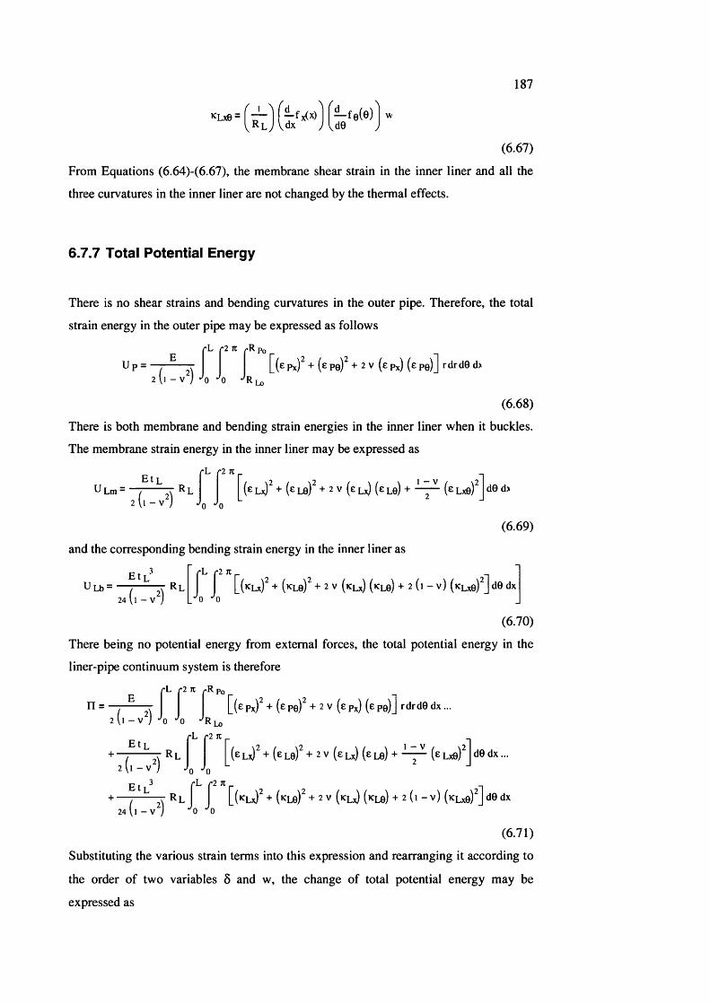
187

(6.67)

From Equations (6.64)-(6.67), the membrane shear strain in the inner liner and all the

three curvatures in the inner liner are not changed by the thermal effects.


There is no shear strains and bending curvatures in the outer pipe. Therefore, the total

strain energy in the outer pipe may be expressed as follows

U p =E

fL *2 K 'Rpo

2 (l - V^) * 0 0 R lo

[ ( e Px) + (e p g f + 2 v (e p%) (e p e)] rdrdG d>

(6.68)

There is both membrane and bending strain energies in the inner liner when it buckles.

The membrane strain energy in the inner liner may be expressed as

U Lm -E t L

fL '2 K

2 ( , _ v f ' j 0 0(eLx)^ + (eL0)^ + 2v (elx) (eLe) + (etxe) dO d>

(6.69)

and the corresponding bending strain energy in the inner liner as

EtL"U u j = — 7------ % R l

24 (l - V )[ \_ { ^ L x f + (k lg )^ + 2 V ( k l x ) ( k l g ) + 2 ( i - v ) ( k l x g ) ^ ] d 0 d x

0 *0

(6.70)

There being no potential energy from external forces, the total potential energy in the

liner-pipe continuum system is therefore

rL r2 K /-R po

n =2 (l - V ) •

E tL

[ ( e Px) + (e Pe)^ + 2 V (e p j (e pg)] rdrdG d x ...

(i - v^)R l

. ^ R l

' Lo ■2 K

0 *'0 L r2 K

(e Lx) + (e Le)' + 2 V (e Lx) (e lg ) + (e Lxg) dG d x ...

24 *'0 •'0[ ( k l x ) ' + ( k l g ) ' + 2 V (k lx ) ( k lg ) + 2 ( i - v ) ( k l x g ) '] dG dx

(6.71)

Substituting the various strain terms into this expression and rearranging it according to

the order of two variables 5 and w, the change of total potential energy may be

expressed as

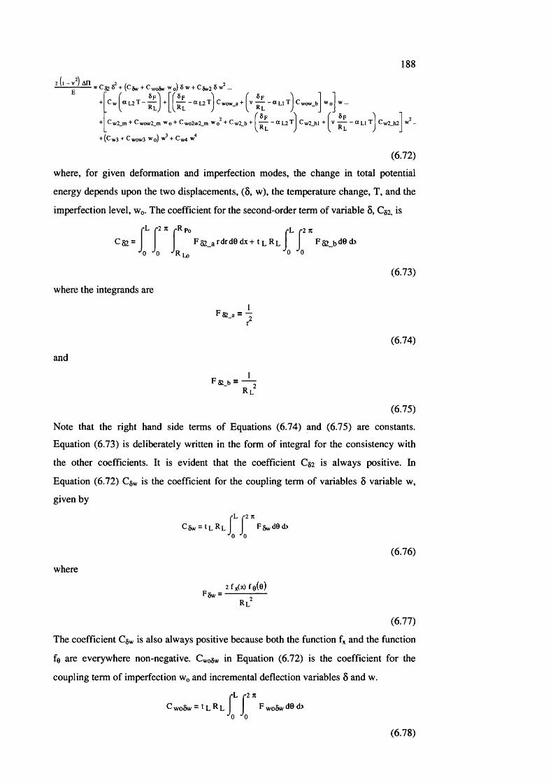
188

2 u - V j ATI= C s2 ^ +(C8w + C wo5w w o) S w + C 8w2 S

a L 2 T - |^ | + Sp ] ( 8p— - a l 2 T I C wow_a + I v — - a l i T | C wow_b

2 r 5p "1 r 8pCw2_m + Cwow2_m Wq + Cwo2w2_m w„ + Cw2_b + I — - « L2 T I Cw2_hl + I V — - a lI T | Cw2_h2

C w3 ^ wow3 ^ o) ^ + C w

(6.72)

where, for given deformation and imperfection modes, the change in total potential

energy depends upon the two displacements, (5, w), the temperature change, T, and the

imperfection level, Wq. The coefficient for the second-order term of variable 5, C§2. is

C S2 =

where the integrands are

rh '2 K

Jq j 0

Po L r2 KF 82 a rdrdG dx+ t

Lo

F 82 bd0d>

(6.73)

F 82_a = —

(6.74)

and

F a_b = — :Rl

(6.75)

Note that the right hand side terms of Equations (6.74) and (6.75) are constants.

Equation (6.73) is deliberately written in the form of integral for the consistency with

the other coefficients. It is evident that the coefficient C§2 is always positive. In

Equation (6.72) C§w is the coefficient for the coupling term of variables 6 variable w,

given by

Cgw — ^LRL f f Fgvvd0d> *0 •'o

(6.76)

where

PSw =2 fx(x) f e(e)

(6.77)

The coefficient Cgw is also always positive because both the function f% and the function

fe are everywhere non-negative. CwoSw in Equation (6.72) is the coefficient for the

coupling term of imperfection Wq and incremental deflection variables 5 and w.

'•L r2 KC woSw

*0 *0F wodw dG d>

(6.78)

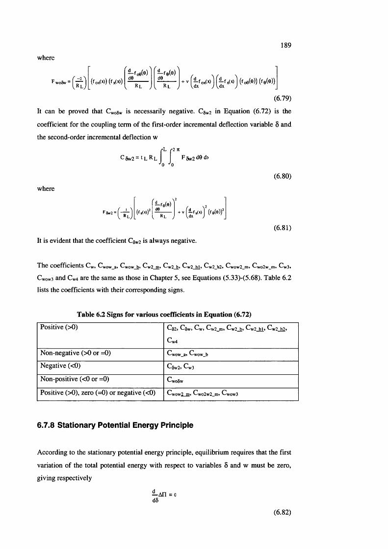
189

where

( f ox(*)) ( f x(^))

— foe(e) d0_____V Rl y

\ . \ — fe (e ) de

R l+ V I ^ fo x (x ) J (fo e(e )) ( fe (e ) )

(6.79)

It can be proved that CwoSw is necessarily negative. Cgwz in Equation (6.72) is the

coefficient for the coupling term of the first-order incremental deflection variable Ô and

the second-order incremental deflection w

c 8w2 = t L R L J J F 5w2

where

FSw2' (“t )

0 •'0

(6.80)

deR l

(6.81)

It is evident that the coefficient Cgwz is always negative.

T h e c o e f f i c i e n t s C ^ , Cwow_a» Cwow b> Cw2_mi Cw2 b» Cw2 h i» Cw2_h2» Cwow2_m» Cwo2w_m> Cw3,

Cwow3 and Cw4 are the same as those in Chapter 5, see Equations (5.33)-(5.68). Table 6.2

lists the coefficients with their corresponding signs.

Table 6.2 Signs for various coefficients in Equation (6.72)

Positive (>0) Cg2» Cgw, Cw, Cw2_m» Cw2 b> C\v2 hi» Cw2 h2>

C\v4

Non-negative (>0 or =0) C\vow_a» Cwow_b

Negative (<0) C§w2* Cw3

Non-positive (<0 or =0) CwoSw

Positive (>0), zero (=0) or negative (<0) Cwow2 m< Cwo2w2_m» Cwow3

6.7.8 Stationary Potential Energy Principle

According to the stationary potential energy principle, equilibrium requires that the first

variation of the total potential energy with respect to variables 6 and w must be zero,

giving respectively

— An = 0 dS

(6.82)

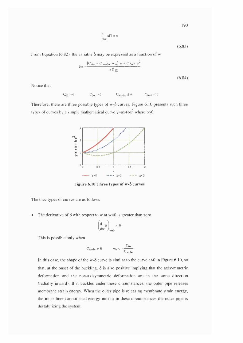
— An = c d w

190

(6.83)

From Equation (6.82), the variable 5 may be expressed as a function of w

(C§w + Cwoôw Wo) w+ C§w2 w5= —2Cgz

(6.84)

Notice that

Cg2>o C&y >0 f-woôw - 0 f'Sw2 ^ C

Therefore, there are three possible types of w-8 curves. Figure 6.10 presents such three

types of curves by a simple mathematical curve y=ax+bx^ where b>0.

2

X

+X«jII 0

1

—— a>0 »-4) - - - a<0

Figure 6.10 Three types of w-5 curves

The thee types of curves are as follows

The derivative of 5 with respect to w at w=0 is greater than zero.

> 0îL sdw

This is possible only when

CwoSw ^ 0 W o < —Cgw

Cwo&v

In this case, the shape of the w-6 curve is similar to the curve a>0 in Figure 6.10, so

that, at the onset of the buckling, 5 is also positive implying that the axisymmetric

deformation and the non-axisymmetric deformation are in the same direction

(radially inward). If it buckles under these circumstances, the outer pipe releases

membrane strain energy. When the outer pipe is releasing membrane strain energy,

the inner liner cannot shed energy into it; in these circumstances the outer pipe is

destabilizing the system.

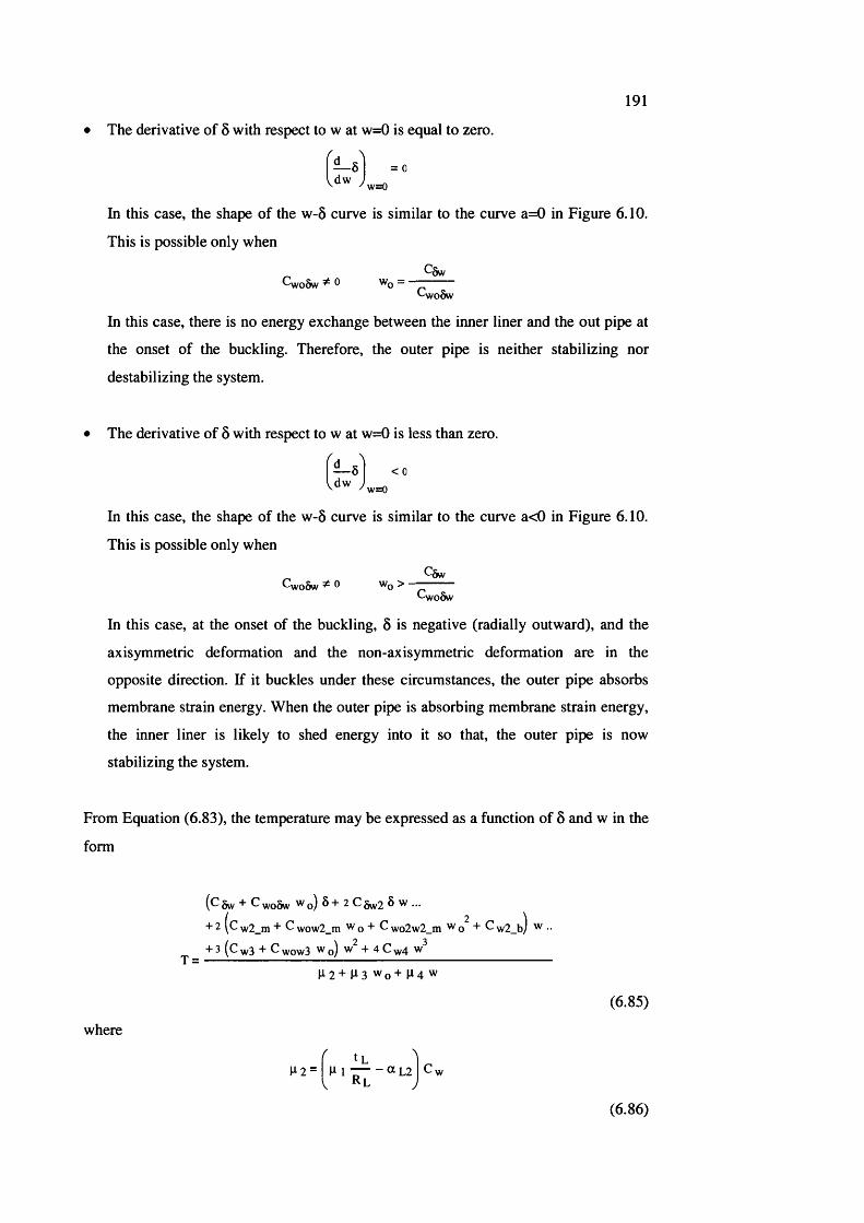
191

The derivative of 6 with respect to w at w=0 is equal to zero,

— 5 I = c

In this case, the shape of the w-5 curve is similar to the curve a=0 in Figure 6,10.


^ ^ôwQvoSw ^ ^

^voôw

In this case, there is no energy exchange between the inner liner and the out pipe at

the onset of the buckling. Therefore, the outer pipe is neither stabilizing nor

destabilizing the system.

The derivative of 5 with respect to w at w=0 is less than zero,

— 8 I <0

In this case, the shape of the w-5 curve is similar to the curve a<0 in Figure 6,10,


^5wCwoSw ^ 0 "'o ^

CwoSw

In this case, at the onset of the buckling, 5 is negative (radially outward), and the

axisymmetric deformation and the non-axisymmetric deformation are in the

opposite direction. If it buckles under these circumstances, the outer pipe absorbs

membrane strain energy. When the outer pipe is absorbing membrane strain energy,

the inner liner is likely to shed energy into it so that, the outer pipe is now

stabilizing the system.

From Equation (6,83), the temperature may be expressed as a function of 5 and w in the

form

(C 5w C wodw w o) 5 + 2 C gw2 ^ ^ •••

+ 2 ( c w2_m C wow2_m w q + C wo2w2_m ^ o C w2_b) ^ ••

+ 3 (C w3 C wow3 w q) w + 4 C w4

(6,85)

where

P 2 =V

m — - a l 2 I C w

(6,86)

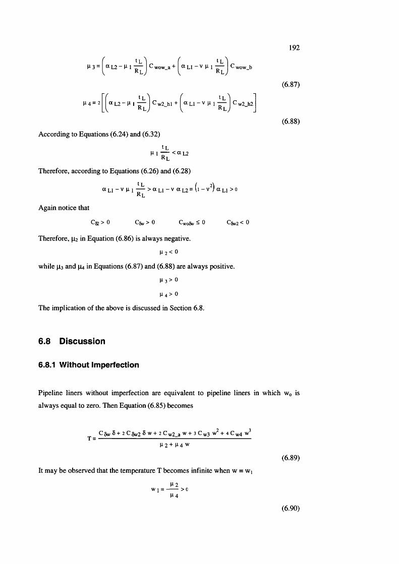
H 3 = a L2 - 1tL

R lc wow_a + I « L 1 - V m

R lc wow b

( ( 1U 4 = 2 a L2 - 11 1 — ^ w 2 _ h l + « L I - V 11 1 — C w2 h2. 1 R l ; I ■ .

192

(6.87)

(6 .88)

According to Equations (6.24) and (6.32)

tLH 1 — < a l2

R l

Therefore, according to Equations (6.26) and (6.28)

tL / 2)« L l - v u i — > a L i - v a L 2 = U - v ) a L i > c

R l

Again notice that

Cg2 0 C&v 0 tZyyoSw — t) Cg 2 t)

Therefore, |i2 in Equation (6.86) is always negative.

^2< 0

while |i3 and [U in Equations (6.87) and (6.88) are always positive.

I t 3> 0

U4> 0

The implication of the above is discussed in Section 6.8.

6.8 D isc u ss io n

6.8.1 Without Imperfection

Pipeline liners without imperfection are equivalent to pipeline liners in which Wo is

always equal to zero. Then Equation (6.85) becomes

T =C5w 5 + 2 C 5 w2 8 w + 2 C w2_a w + 3 C w3 + 4 C ^4

|I2 + ^14 w

(6.89)

It may be observed that the temperature T becomes infinite when w = w%

K2w 1 = > 0

K4

(6.90)

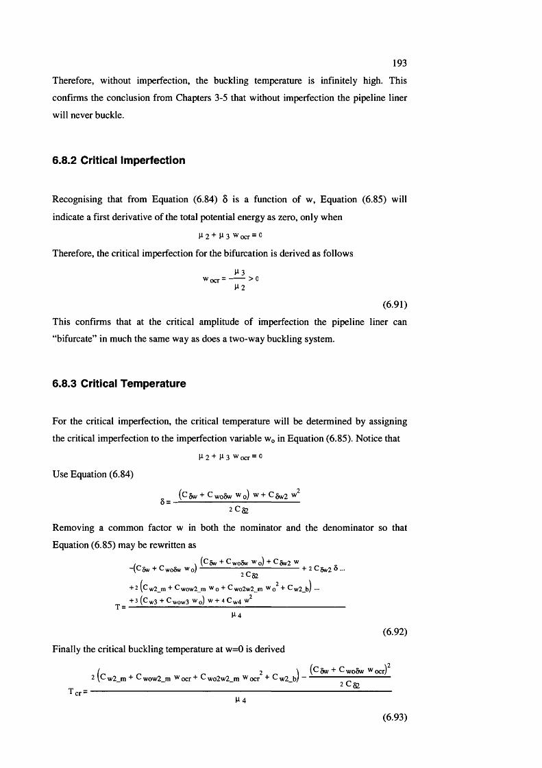
193

Therefore, without imperfection, the buckling temperature is infinitely high. This

confirms the conclusion from Chapters 3-5 that without imperfection the pipeline liner

will never buckle.

6.8.2 Critical Imperfection

Recognising that from Equation (6.84) S is a function of w. Equation (6.85) will

indicate a first derivative of the total potential energy as zero, only when

1^2+ 1^3 Wocr=0

Therefore, the critical imperfection for the bifurcation is derived as follows

1^3Wocr = ------- > 0

^2

(6.91)

This confirms that at the critical amplitude of imperfection the pipeline liner can

“bifurcate” in much the same way as does a two-way buckling system.

6.8.3 Critical Tem perature

For the critical imperfection, the critical temperature will be determined by assigning

the critical imperfection to the imperfection variable Wq in Equation (6.85). Notice that

P 2 + 1^3 Wocr = 0

Use Equation (6.84)

(C 5w ^ woSw ^ o) w + C gw2 w0 = ------------------------------------------------------------

2 C s2

Removing a common factor w in both the nominator and the denominator so that


^ _ \ (^Sw + CwoSw Wq) + C§w2 W ^ ^—\ C 5w CwoSw Wq] + 2 Cgw2 o •••

2C 52

+ 2 ( c w2_m + C wow2_m w g + C wo2w2_m o + C w2_b) —

+ 3 (C w3 C wow3 ^ o) w + 4 C w4 ^T =

K4

(6.92)

Finally the critical buckling temperature at w=0 is derived

» ^ ... 2 . ^ ) (Cgw + Cwoôw Wocr)2 \C w2_m + C wow2_m ocr + C wo2w2_m ^ ocr + C w2_bj ~

T ________________________________________________________ cr~

(6.93)

194

6.9 A ssu m ed D eform ed S h a p e

6.9.1 Deflection

Similar to Chapter 5, the same squared cosine waves are assumed

\ \ 2. . . , , triTC Xf x (x ) = COS

(6.94)

fe(e) =

(6.95)

where m and n are the wave numbers for the deflection in the axial and circumferential

directions.

m > 0 n > 0 m + n > 0

(6.96)

When m is zero, the deflection does not change along axial direction, while when n is

zero, the deflection is axisymmetric. However, m and n cannot both be zero.

6.9.2 imperfection

Similar to Chapter 5, the imperfection is assumed always radially inward, i.e. Wq is

always positive. For simplicity, squared cosine waves are used to represent the

imperfection profile

f f mo n x ^ y fox(x)= cos — -----

V V L y y

(6.97)

f 00(0) = f c o s f °V 2

(6.98)

where nio and no are the wave numbers for the imperfection in the axial and

circumferential directions.

iTio > 0 no ^ 0 mo + Ho > 0

(6.99)

When mo is zero, the imperfection does not change along the axial direction, while

when no is zero, the imperfection is axisymmetric. However, mo and no can not both be

zero.

195

6.9.3 Coefficients

Substituting of Equations (6.94)-(6.99) into various corresponding equations, the

expressions for various coefficients are derived.

C g 2 = { l - K l ) -

f fRpo] ‘ 0In + ----V

Jt-LtL1 i f m > 0 A n > 0

2 if (m = 0 A n > 0) V (m > 0 A n = 0)

4 i f m = 0 A n = 0

Cwo&v — 2'tL'Ho n v iTio m

I'Cwo8w_a‘Cwo&v_b I Cwog^v_c’^wo6w_d4 R j r

3 i f m o = n i A m > 0

4 if (iTio = 0 A m > O) V (m = 0 A m o > O)

8 i f mo = m A m = 0

2 otherwise

C wo&v b “ (ît ) ■

C wo&v_c “ I 2

1 if Ho = n A n > 0

0 otherwise

1 i f mo = m A m > 0

0 otherwise y

C woSw_d ” 1 ^ 3 if no = n A n > 0

4 i f ( n o = 0 A n > 0 ) v ( n = 0 A r i o > 0 )

8 if no = O A n = 0

2 otherwise

2 / \ 2 I m-JC+ V

2 R l J V Lif m > 0 A n > 0

2Riif m = 0 A n > 0

i f m > 0 A n = 0

0 i f m = 0 A n = 0

(6.100)

(6.101)

(6.102)

(6.103)

(6.104)

(6.105)

(6.106)

(6.107)

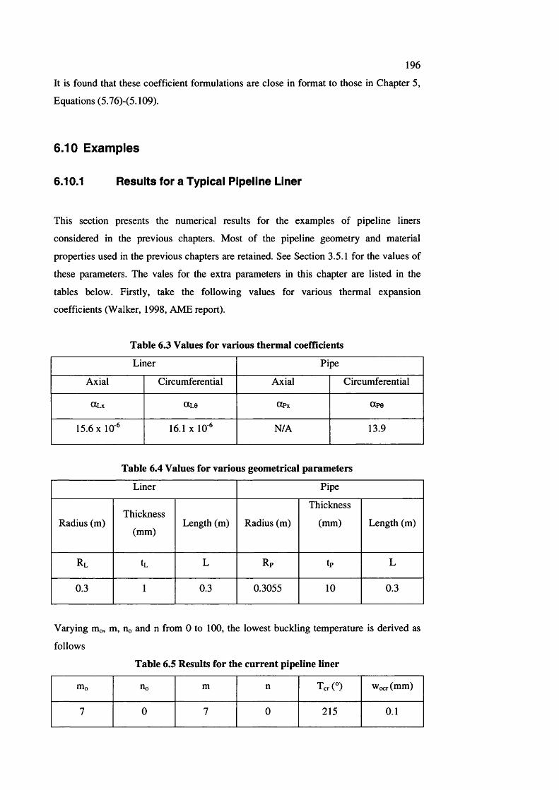
196

It is found that these coefficient formulations are close in format to those in Chapter 5,

Equations (5.76)-(5.109).

6.10 E xam ples

6.10.1 Results for a Typical Pipeline Liner

This section presents the numerical results for the examples of pipeline liners

considered in the previous chapters. Most of the pipeline geometry and material

properties used in the previous chapters are retained. See Section 3.5.1 for the values of

these parameters. The vales for the extra parameters in this chapter are listed in the

tables below. Firstly, take the following values for various thermal expansion

coefficients (Walker, 1998, AME report).

Table 6.3 Values for various thermal coefficients

Liner Pipe


ttL x CtL0 OCpx otpe

15.6 X 10' 16.1 X 10^ N/A 13.9

Table 6.4 Values for various geometrical parameters

Liner Pipe

Radius (m)Thickness

(mm)Length (m) Radius (m)

Thickness

(mm) Length (m)

Rl tL L Rp tp L

0.3 1 0.3 0.3055 10 0.3

Varying mo, m, no and n from 0 to 100, the lowest buckling temperature is derived as

follows

Table 6.5 Results for the current pipeline liner

mo Ho m n Tcr(°) Wocr(mm)

7 0 7 0 215 0.1

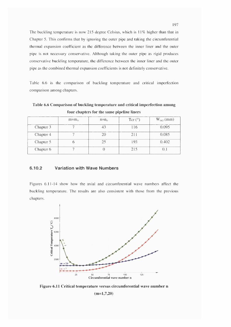
197

The buckling temperature is now 215 degree Celsius, which is 11% higher than that in

Chapter 5. This confirms that by ignoring the outer pipe and taking the circumferential

thermal expansion coefficient as the difference between the inner liner and the outer

pipe is not necessary conservative. Although taking the outer pipe as rigid produces

conservative buckling temperature, the difference between the inner liner and the outer

pipe as the combined thermal expansion coefficients is not definitely conservative.

Table 6.6 is the comparison of buckling temperature and critical imperfection

comparison among chapters.

Table 6.6 Comparison of buckling temperature and critical imperfection among

four chapters for the same pipeline liners

m=m„ n=no Tcr(°) Wocr (mm)

Chapter 3 7 43 116 0.095

Chapter 4 7 20 211 0.085

Chapter 5 6 25 193 0.402

Chapter 6 7 0 215 0.1

6 .10.2 Variation with Wave Numbers

Figures 6.11-14 show how the axial and circumferential wave numbers affect the

buckling temperature. The results are also consistent with those from the previous

chapters.

8000

u 6000

H 4000

2000

20

m = 7

100 12525 50 75Circumferential wave number n

Figure 6.11 Critical temperature versus circumferential wave number n

(m=l,73)

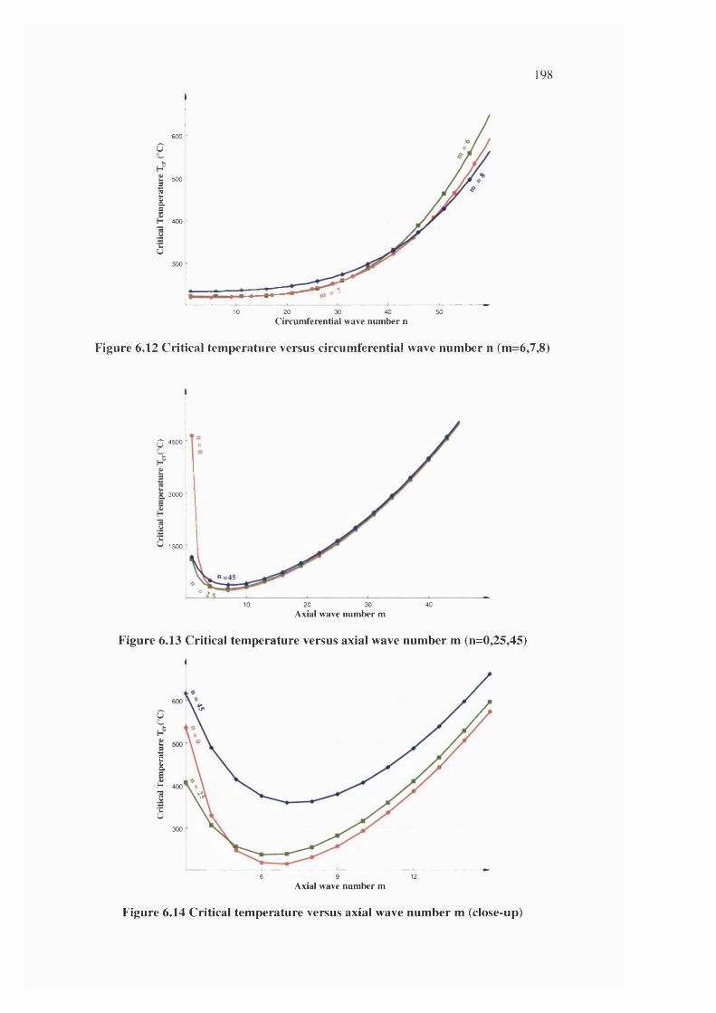
198

K

{E

600

500

400

300

10 20 30 40 50Circumferential wave number n

Figure 6.12 Critical temperature versus circumferential wave number n (m=6,7,8)

n 4500

3000

1500

10 20 30 40Axial wave number m

Figure 6.13 Critical temperature versus axial wave number m (n=0^5,45)

600

IH 400

S

5300

6 9 12

Axial wave number m

Figure 6.14 Critical temperature versus axial wave number m (close-up)

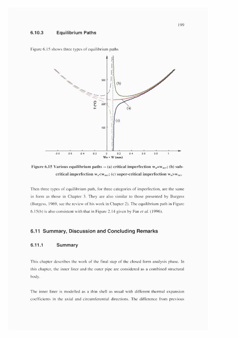
199

6.10.3 Equilibrium Paths

Figure 6.15 shows three types of equilibrium paths

X300

200

100

■0.8 •0.6 -0.4 -0.2 0 0.4 0.6 0.8 1Wo +W (m m )

Figure 6.15 Various equilibrium paths -- (a) critical imperfection Wo=Wocr; (b) sub-

critical imperfection Wo<Wocr; (c) super critical imperfection Wo>Wocr

Then three types of equilibrium path, for three categories of imperfection, are the same

in form as those in Chapter 3. They are also similar to those presented by Burgess

(Burgess, 1969, see the review of his work in Chapter 2). The equilibrium path in Figure

6.15(b) is also consistent with that in Figure 2.14 given by Fan et al. (1996).

6.11 Sum m ary, D iscussion and C oncluding R em arks

6.11.1 Summary

This chapter describes the work of the final step of the closed form analysis phase. In

this chapter, the inner liner and the outer pipe are considered as a combined structural

body.

The inner liner is modelled as a thin shell as usual with different thermal expansion

coefficients in the axial and circumferential directions. The difference from previous

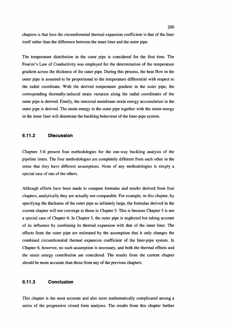
200

chapters is that here the circumferential thermal expansion coefficient is that of the liner

itself rather than the difference between the inner liner and the outer pipe.

The temperature distribution in the outer pipe is considered for the first time. The

Fourier’s Law of Conductivity was employed for the determination of the temperature

gradient across the thickness of the outer pipe. During this process, the heat flow in the

outer pipe is assumed to be proportional to the temperature differential with respect to

the radial coordinate. With the derived temperature gradient in the outer pipe, the

corresponding thermally-induced strain variation along the radial coordinates of the

outer pipe is derived. Finally, the tensional membrane strain energy accumulation in the

outer pipe is derived. The strain energy in the outer pipe together with the strain energy

in the inner liner will determine the buckling behaviour of the liner-pipe system.

6.11.2 D iscussion

Chapters 3-6 present four methodologies for the one-way buckling analysis of the

pipeline liners. The four methodologies are completely different from each other in the

sense that they have different assumptions. None of any methodologies is simply a

special case of one of the others.

Although efforts have been made to compare formulas and results derived from four

chapters, analytically they are actually not comparable. For example, in this chapter, by

specifying the thickness of the outer pipe as infinitely large, the formulas derived in the

current chapter will not converge to those in Chapter 5. This is because Chapter 5 is not

a special case of Chapter 6. In Chapter 5, the outer pipe is neglected but taking account

of its influence by combining its thermal expansion with that of the inner liner. The

effects from the outer pipe are estimated by the assumption that it only changes the

combined circumferential thermal expansion coefficient of the liner-pipe system. In

Chapter 6, however, no such assumption is necessary, and both the thermal effects and

the strain energy contribution are considered. The results from the current chapter

should be more accurate than those from any of the previous chapters.

6.11.3 Conclusion

This chapter is the most accurate and also most mathematically complicated among a

series of the progressive closed form analyses. The results from this chapter further

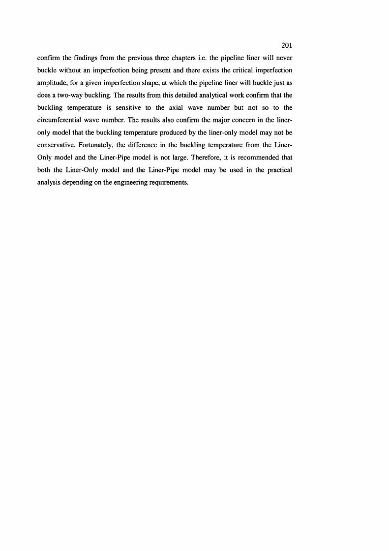
201

confirm the findings from the previous three chapters i.e. the pipeline liner will never

buckle without an imperfection being present and there exists the critical imperfection

amplitude, for a given imperfection shape, at which the pipeline liner will buckle just as

does a two-way buckling. The results from this detailed analytical work confirm that the

buckling temperature is sensitive to the axial wave number but not so to the

circumferential wave number. The results also confirm the major concern in the liner-

only model that the buckling temperature produced by the liner-only model may not be

conservative. Fortunately, the difference in the buckling temperature from the Liner-

Only model and the Liner-Pipe model is not large. Therefore, it is recommended that

both the Liner-Only model and the Liner-Pipe model may be used in the practical

analysis depending on the engineering requirements.

202

7 Finite Eiement Anaiysis - Eiastic Buckiing

7.1 In troduction

From Chapters 3 to 6 various models have been developed for the analytical analysis

task for predicting the buckling of pipeline liners - the simplified rigid-link model,

simplified beam-1 ink model, continuum liner-only shell model and continuum liner-pipe

shell model. In these models, some aspects of the analysis are always simplified in order

to reduce the complexity of the analytical work. These simplifications include reducing

the number of degrees of freedom of the system, the assumption of the deformed shape

and the liner material properties. Now that the basic one-way buckling theory of the

pipeline liners has been developed, the finite element analysis, which does not need to

assume the deformed shape, is to be used to check the main conclusions relating to

buckling behaviour.

This chapter and Chapter 8 deal with the finite element analysis with ABAQUS. The

objectives of the finite element analysis include:

• To derive the equilibrium paths and the buckling temperatures for various runs

of nine cases by the finite element numerical analysis;

• To extract generic equilibrium path types from the variety of equilibrium paths

for all nine cases and compare them with those from the analytical work;

• To carry out a brief parametric study and examine the variation of the buckling

temperatures with various geometries including the wall thickness and the radius

of the liner shell;

• To examine the deformed shapes at the on-set of the buckling and at the post-

buckling for various pipeline liner initial geometries;

• To study the mode shape transitions that are observed from the results of the

various runs of nine cases;

• To provide a basis for the study of the elastic-plastic one-way buckling to be

described in Chapter 8.

This chapter describes the first stage work of the finite element analysis - elastic

buckling. The effect of the elastic plastic stress strain relationship will be investigated in

Chapter 8.

203

7.2 F inite E lem ent O ne-w ay B uckiing A nalysis

Finite element analysis is widely used in almost all areas of engineering applications

including the finite element buckling analysis. However, the finite element one-way

buckling analysis has seldom been systematically discussed in the literatures.

Furthermore, it was found from the current study that finite element one-way buckling

analysis is in most respects different from the finite element two-way buckling analysis.

Therefore, it may be necessary to start this chapter by a brief overview of the finite

element one-way buckling analysis.

7.2.1 Two-way Deformation Function for One-Way Buckling Analysis

It is generally known that in the finite element structural analysis structures are

descretized into many small elements so that the deformation within any element could

be assumed to be simple functions of its nodal displacements. With a finite number of

elements, the infinite number of degrees of freedom problem (continuum) can be

reduced to a finite number of degrees of freedom problem. As the total number of

elements increases, the solution to the problem generally converges. This is also the

case for the finite element buckling analysis.

In the finite element buckling analysis, the assumed deformation functions have to be

able to simulate the non-linear deformation due to rotation. Deformation shape

functions vary with types of elements used in the model. For example, a four-node

quadrilateral shell element could take deformation shape functions with twenty-four

coefficients determined by the twenty-four degrees of freedom of the nodal

displacements and rotations at four nodes. Generally, by allowing large number of

degrees of freedom for one element or constructing the model with very fine mesh, it is

possible for a finite element model to capture the true buckling modal shape.

However, the deformation shape function allows both-way of deformation, i.e. positive

and negative deformation. Although the author has been tempted to write special finite

element codes with one-way deformation functions, it was finally concluded that it

might be more appropriate to use two-way deformation functions for one-way buckling

analysis. This is not to save time for writing new finite element code. Rather, it is the

only possible solution. This will be further discussed in Section 7.2.4.

204

7.2.2 Eigenvalue Buckling Analysis No Longer Valid

In most cases, the finite element buckling analysis refers to the finite element

eigenvalue buckling analysis. For eigenvalue problems, because of the non-linear

kinematic relationship between the displacements and various strain terms, at the on-set

of the buckling, the application of the stationary potential energy principle to the finite

element model leads to the following equation

{ [k]+?i[kp] } [ u ] = 0

(7.1)

where [k] is the geometric stiffness, [kp] is the load stiffness. A, is the eigenvalue, [u] is

the eigenvector. In the above equation, the geometric stiffness [k] is derived from the

energy term due to the linear components of the strains, while the load stiffness [kp] is

derived from the linearized energy term that is the product of the loads multiplied by the

quadratic components of the strains. At the on-set of the buckling, energy terms other

than the linear energy terms are trivial and may be neglected. The above equation leads

to a typical eigenvalue equation.

The eigenvalue buckling problem is an eigenvalue problem only when the first variation

of the total potential energy vanishes so that the second-order energy terms leads to

Equation (7.1). It must be pointed out here that the first variation is automatically zero

only when the displacements in the deformed lobes in one direction are equal to those in

the opposite lobes so that the total work done is zero. Obviously, this is not possible for

the one-way buckling. Therefore, the eigenvalue buckling analysis is no longer valid in

the finite element one-way buckling analysis.

7.2.3 Adapted Post-buckling Analysis for One-way Buckling

Analysis

In the post-buckling analysis of two-way buckling problems. Equation (7.1) is no longer

valid because the high order terms missing in the left side are no longer trivial. Instead,

the finite element post-buckling analysis may only be fulfilled by a geometrically non

linear finite element static analysis. Therefore, the finite element two-way post-buckling

analysis is usually carried out in the following three steps

• Step 1 - the finite element eigenvalue buckling analysis for the extraction of the

buckling loads and the buckled modal shapes at the on-set of the buckling

205

• Step 2 - generation of the typical imperfection by linearly combining the first

several mode shapes when no details of imperfections caused in a manufacturing

process is known

• Step 3 - finite element non-linear static analysis for the post-buckling behaviour

The finite element two-way post-buckling analysis may be adapted for the one-way

buckling analysis. However, in the one-way buckling, because it is impossible to know

the exact critical imperfection in the finite element analysis, the above mentioned Step 1

is only feasible in theory. Therefore, in the current finite element buckling analysis. Step

1 will have to be modified. Accordingly, the above three-step approach may have to be

changed as follows

• Step 1 - generation of the typical large imperfection based on the results from

previous trial-analyses or on engineering judgement

• Step 2 - finite element non-linear static analysis for the post-buckling behaviour

• Step 3 - repetition of Step 1 and 2 as necessary with smaller amplitude of

imperfection until the approximate critical imperfection is reached

In the current finite element buckling analysis, the typical imperfection is based on the

results from the analytical work. By carrying out various static geometrically non-linear

analyses with the amplitude of the imperfection approaching the critical value, the

virtual eigenvalue state may be simulated.

7.2.4 Pseudo-two-way Approach

It has been pointed out in Section 7.2.1 that no special one-way deformation functions

are necessary for the finite element one-way buckling analysis. Indeed, pseudo-two-way

buckling approach will be used for the whole finite element one-way buckling analysis.

The author has been tempted to construct a pure-one-way buckling finite element model

by constraining the deformation in the opposite direction completely. Unfortunately this

was proved to be a failure because the finite element analysis is unlikely to converge

when the load approaches the critical value.

For the system to converge, it needs somewhere in the opposite direction to shed some

energy. By constraining the deformation to the opposite direction completely, the

system cannot shed any energy to the surrounding medium.

206

The solution is a pseudo-two-way approach. Rather than suppressing the deformation in

the opposite direction completely, very stiff springs are used to allow tiny deformation

to the opposite direction, say in the scale of a thousandth of a millimetre. This allows

energy exchange between two opposite directions, which is more realistic. This is why

in Section 7.2.1 it is concluded that it is not necessary to use special one-way

deformation functions for one-way buckling analysis. Detailed description of pseudo-

two-way model will be given in Section 7.3.

7.3 D escrip tion of Finite E iem ent Modei

The current finite element buckling analysis is the further work for the previous

analytical analysis. Therefore, the finite element model for the buckling analysis will

also be based on the conclusions from the previous analytical work. This includes the

following considerations

• The thermal loading. As in analytical work, the thermal loading is applied in the

axial and circumferential directions.

• The modelling of the outer pipe. The finite element model will be composed of

the liner shell and the simplified outer pipe - springs.

• The wave numbers in the axial and circumferential directions of the deformation

and the imperfection and the magnitude of the imperfection. This is based on the

results from analytical work.

7.3.1 Modelling of the Outer Pipe - Application of Thermal Loading

The outer pipe will be simplified as a series of extremely stiff springs but the

circumferential thermal expansion coefficient of the inner liner is accordingly modified.

As in the analytical work, the axial thermal expansion coefficient is set to be equal to

that of the inner liner while the circumferential thermal expansion coefficient is set to be

equal to the difference of those between the inner liner and the outer pipe. The thermal

expansion coefficient in the radial direction is assumed very small so that it is taken as

zero.

— ^x_liner 0C|- = 0 Ct0 = (Xg Hner “ ®0_pipe

(7.2)

By means of these thermal expansion coefficients, the thermal loading is applied by a

207

temperature rise T. In the current study, only the thermal loading is considered while

other loadings such as internal and external pressure and self-weight are neglected.

The other consideration is that the buckling analysis of cylindrical shells needs very fine

mesh to capture accurate mode shapes. By modelling the outer pipe as rigid reduces the

number of shell elements 50% for the same mesh size.

7.3.2 Modelling of the Outer Pipe - Simplification by Springs

The immediate consideration for the modelling of the contact between the inner liner

and the outer pipe is the rigid contact surface. The rigid contact surface suppresses

completely the penetration of the inner liner into the outer pipe. Unfortunately, the

buckling analysis with such models is unlikely to converge.

The alternative to the contact rigid surface is the springs with bi-1 inear stiffness. The

springs are constructed along the radial direction all over the outer surface of the inner

liner. The spring stiffness acts along the radial direction. The springs allow the inner

liner to move radially inward freely but provide very large resistance to the radially

outward movements.

The advantages of bi linear springs over the contact surface are obvious. Springs are

able to absorb a small amount of energy even if the stiffness is very large and the

displacements are tiny. On the contrary, the contact surface involves no energy

exchange with the inner liner at all even if very large tolerance of penetration is

specified. This tiny energy absorption has been proved to be the key for the system to

converge at the limit point of the thermal loading. Furthermore, by adjusting the

stiffness of the springs, higher speed of the convergence may be possible for the initial

test run to find out the critical imperfection. Furthermore, the spring stiffness may be

fine-tuned by observing the amount of the penetration (the outward radial

displacement). As long as the penetration is tiny, the lower the spring stiffness, the

faster is the convergence of the finite element analysis.

The stiffness of the springs is bi-1 inear. Figure 7,1 shows the force displacement

relationship of the springs. It is noted from Figure 7,1 that the stiffness of the springs is

always zero when it is in compression. For free inward movement, the springs must be

tension-only or the springs can only take tensional forces. This is in contrast with the

fact that the outer pipe is compression only. Actually, the spring stiffness is deliberately

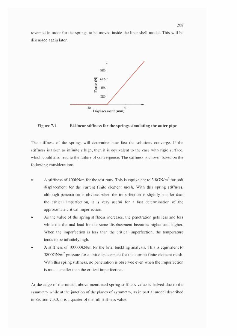
208

reversed in order for the springs to be m oved inside the liner shell m odel. This will be

d iscussed again later.

8E6

Z 6E6

?k 4E6

2E6

-50 50Displacement (mm)

Figure 7.1 Bi linear stiffness for the springs simulating the outer pipe

The stiffness o f the springs will determ ine how fast the solutions converge. If the

stiffness is taken as infinitely high, then it is equivalent to the case with rigid surface,

which could also lead to the failure o f convergence. The stiffness is chosen based on the

follow ing considerations

• A stiffness o f lOOkN/m for the test runs. This is equivalent to 3.8GN/m^ for unit

displacem ent for the current finite elem ent mesh. W ith this spring stiffness,

although penetration is obvious when the im perfection is slightly sm aller than

the critical im perfection, it is very useful for a fast determ ination o f the

approxim ate critical imperfection.

• As the value of the spring stiffness increases, the penetration gets less and less

w hile the thermal load for the same displacem ent becom es higher and higher.

W hen the imperfection is less than the critical im perfection, the tem perature

tends to be infinitely high.

• A stiffness o f lOOOOOkN/m for the final buckling analysis. This is equivalent to

3800G N /m “ pressure for a unit displacem ent for the current finite elem ent mesh.

W ith this spring stiffness, no penetration is observed even when the im perfection

is m uch sm aller than the critical im perfection.

At the edge o f the model, above m entioned spring stiffness value is halved due to the

sym m etry w hile at the junction o f the planes o f sym m etry, as in partial m odel described

in Section 7.3.3, it is a quarter o f the full stiffness value.

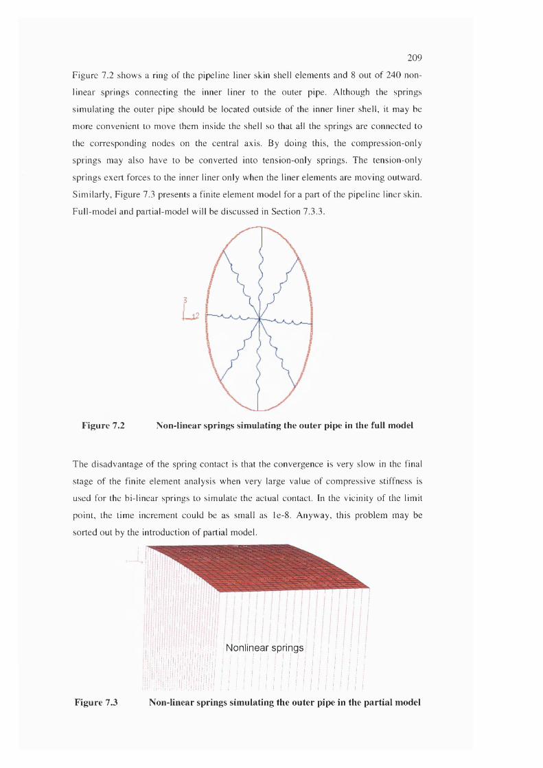
209

Figure 7.2 shows a ring of the pipeline liner skin shell elem ents and 8 out o f 240 non

linear springs connecting the inner liner to the outer pipe. A lthough the springs

sim ulating the outer pipe should be located outside o f the inner liner shell, it m ay be

m ore convenient to move them inside the shell so that all the springs are connected to

the corresponding nodes on the central axis. By doing this, the com pression-only

springs may also have to be converted into tension-only springs. The tension-only

springs exert forces to the inner liner only when the liner elem ents are m oving outward.

Sim ilarly, Figure 7.3 presents a finite elem ent model for a part o f the pipeline liner skin.

Full-m odel and partial-m odel will be discussed in Section 7.3.3.

Figure 7.2 Non-linear springs simulating the outer pipe in the full model

The disadvantage o f the spring contact is that the convergence is very slow in the final

stage o f the finite elem ent analysis when very large value o f com pressive stiffness is

used for the bi-linear springs to sim ulate the actual contact. In the vicinity o f the limit

point, the tim e increm ent could be as small as le-8 . A nyw ay, this problem m ay be

sorted out by the introduction o f partial m odel.

ililiinii

Figure 7.3a i B i i i i M i

Non-linear springs simulating the outer pipe in the partial model

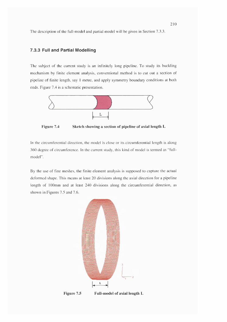
210

The description o f the full-m odel and partial m odel will be given in Section 7.3.3.

7.3.3 Full and Partial Modelling

The subject o f the current study is an infinitely long pipeline. To study its buckling

m echanism by finite elem ent analysis, conventional m ethod is to cut out a section of

pipeline o f finite length, say 1 metre, and apply sym m etry boundary conditions at both

ends. Figure 7.4 is a schem atic presentation.

Figure 7.4 Sketch showing a section of pipeline of axial length L

In the circum ferential direction, the model is close or its circum ferential length is along

360 degree of circum ference. In the current study, this kind o f model is term ed as “full-

m odel” .

By the use o f fine m eshes, the finite elem ent analysis is supposed to capture the actual

deform ed shape. This means at least 20 divisions along the axial direction for a pipeline

length o f 100mm and at least 240 divisions along the circum ferential direction, as

show n in Figures 7.5 and 7.6.

Figure 7.5 Full-model of axial length L

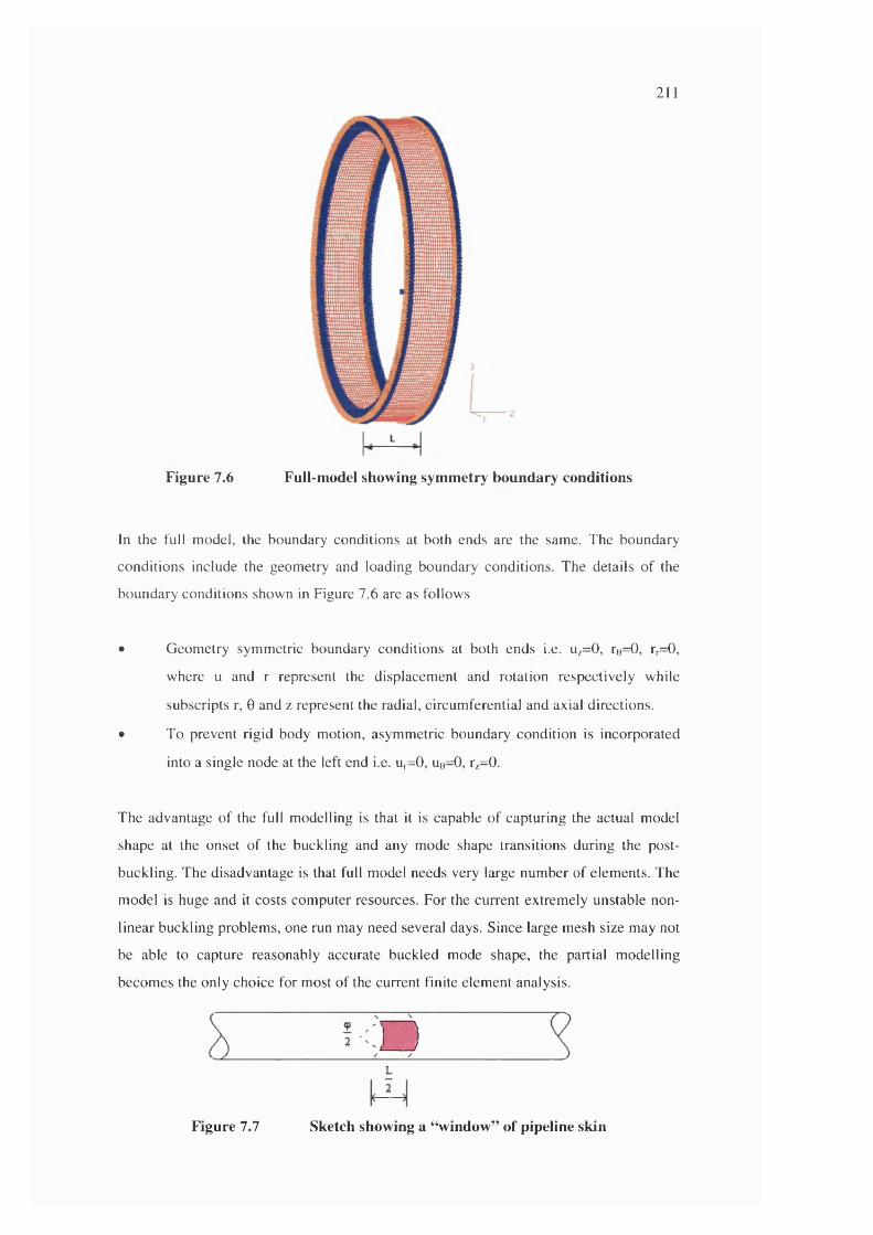
21

--------2

Figure 7.6 Full-model showing symmetry boundary conditions

In the full model, the boundary conditions at both ends are the same. The boundary

conditions include the geom etry and loading boundary conditions. The details o f the

boundary conditions shown in Figure 7.6 are as follows

• G eom etry sym m etric boundary conditions at both ends i.e. Uz=0, re=0, rr=0,

where u and r represent the displacem ent and rotation respectively while

subscripts r, 0 and z represent the radial, circum ferential and axial directions.

• To prevent rigid body m otion, asym m etric boundary condition is incorporated

into a single node at the left end i.e. U r=0, u e = 0 , rz= 0 .

The advantage o f the full m odelling is that it is capable o f capturing the actual model

shape at the onset o f the buckling and any m ode shape transitions during the post-

buckling. The disadvantage is that full model needs very large num ber of elem ents. The

m odel is huge and it costs com puter resources. For the current extrem ely unstable non

linear buckling problem s, one run may need several days. Since large mesh size m ay not

be able to capture reasonably accurate buckled mode shape, the partial m odelling

becom es the only choice for most o f the current finite elem ent analysis.

}

Figure 7.7 Sketch showing a “window” of pipeline skin

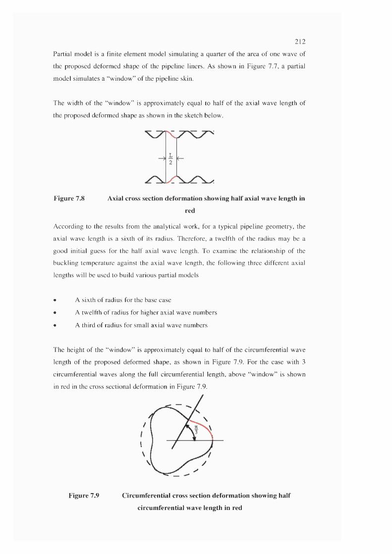
212

Partial model is a finite elem ent model sim ulating a quarter o f the area o f one wave o f

the proposed deform ed shape o f the pipeline liners. As shown in Figure 7.7, a partial

m odel sim ulates a “w indow ” o f the pipeline skin.

The w idth of the “w indow ” is approxim ately equal to half o f the axial wave length of

the proposed deform ed shape as shown in the sketch below.

Figure 7.8 Axial cross section deformation showing half axial wave length in

red

A ccording to the results from the analytical work, for a typical pipeline geom etry, the

axial wave length is a sixth o f its radius. Therefore, a tw elfth of the radius may be a

good initial guess for the half axial wave length. To exam ine the relationship of the

buckling tem perature against the axial wave length, the follow ing three different axial

lengths will be used to build various partial m odels

• A sixth o f radius for the base case

• A twelfth o f radius for higher axial wave num bers

• A third of radius for small axial wave num bers

T he height o f the “w indow ” is approxim ately equal to half o f the circum ferential wave

length o f the proposed deform ed shape, as shown in Figure 7.9. For the case with 3

circum ferential waves along the full circum ferential length, above “w indow ” is shown

in red in the cross sectional deform ation in Figure 7.9.

/

I

Figure 7.9 Circumferential cross section deformation showing half

circumferential wave length in red

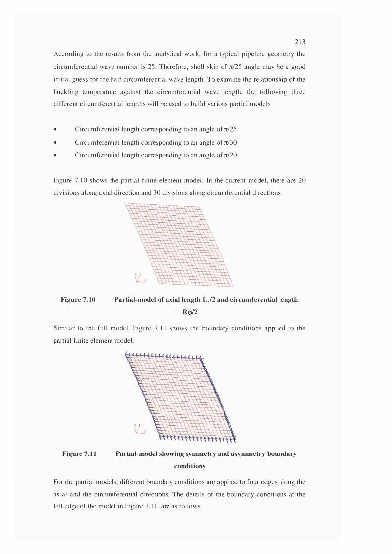
213

A ccording to the results from the analytical work, for a typical pipeline geom etry the

circum ferential wave num ber is 25. Therefore, shell skin o f 7t/25 angle may be a good

initial guess for the half circum ferential wave length. To exam ine the relationship o f the

buckling tem perature against the circum ferential wave length, the follow ing three

different circum ferential lengths will be used to build various partial m odels

• C ircum ferential length corresponding to an angle o f 7c/25

• C ircum ferential length corresponding to an angle o f n /30

• Circum ferential length corresponding to an angle o f 71/20

Figure 7.10 shows the partial finite elem ent model. In the current m odel, there are 20

d ivisions along axial direction and 30 divisions along circum ferential directions.

Figure 7.10 Partial-model of axial length L%/2 and circumferential length

R(p/2

Sim ilar to the full model. Figure 7.11 shows the boundary conditions applied to the

partial finite elem ent model.

Figure 7.11 Partial-model showing symmetry and asymmetry boundary

conditions

For the partial m odels, different boundary conditions are applied to four edges along the

axial and the circum ferential directions. The details o f the boundary conditions at the

left edge o f the model in Figure 7.11. are as follows

214

• Geometry asymmetric boundary condition i.e. Ur=0, Ue=0, rz=0, where u and r

represent displacement and rotation respectively while subscripts r, 0 and z

represent radial, circumferential and axial directions.

• Loading symmetric boundary condition i.e. Uz=0

The details of the boundary conditions at the right edge of the model in Figure 7.11 are

as follows

• Geometry symmetric boundary condition i.e. Uz=0, re=0, ri=0, where u and r



• Loading symmetric boundary condition i.e. Uz=0

The details of the boundary conditions at the lower edge of the model in Figure 7.11 are

as follows

• Geometry asymmetric boundary condition i.e. Ur=0, Uz=0, r@=0, where u and r



• Loading symmetric boundary condition at both ends i.e. u e = 0

The details of the boundary conditions at the upper edge of the model in Figure 7.11 are

as follows

• Geometry symmetric boundary condition i.e. ue=0, rr=0, rz=0, where u and r

represent displacement and rotation respectively while subscripts r 0 and z


• Loading symmetric boundary condition at both ends i.e. u e = 0

The advantage by using the partial model is that the size of the problem is greatly

reduced. The run-time needed reduced from days to hours. The disadvantage is that a

number of models have to be built to address all the possible combinations of wave

numbers in the axial and circumferential directions. This is because the partial model

simulates only a “window” from the entire pipeline liner skin. The width and height of

the “window” are equal to the axial and circumferential wave lengths respectively.

Therefore, it needs different models for different mode shapes with different wave

number combinations.

215The following strategy for the model construction is developed. Between two models,

the full model is used mainly for the following purposes

• To examine the mode shapes at the onset of the buckling

• To investigate the mode shape transition at the post-buckling

• To verify the modelling of partial models

One case (out of nine cases) of the finite element one-way buckling analysis is carried

out with the full-model. The partial model is mainly used for the following analysis

• To carry out various fast runs with relatively small stiffness value of bi linear

springs so that the critical imperfection for various cases can be determined

• To carry out various runs of nine cases of finite element analysis and compare

the results with those obtained from the analytical work

• To carry out a parametric study to address the effect of the radius, the wall

thickness of the pipeline liner

7.4 Results from Various Runs with ABAQUS

In this section, various cases and runs for the finite element analyses will first be

described. Then generic results extracted from these various finite element analysis

cases and runs will be presented. To obtain a clear picture of the FE modelling of the

one-way buckling a large quantity of data was acquired. To maintain the simplicity of

the presentation, most of the detailed results will be given in a separate Appendix A.

7.4.1 Cases and Runs

As has been pointed out in the previous section, two forms of finite element models i.e.

• Partial-model

• Full-model

are used in the finite element analyses for different purposes. Partial-model is designed

for deriving mainly the equilibrium path and therefore the buckling temperatures. Full-

model is designed mainly for observing the initial deformed shape at the on-set of the

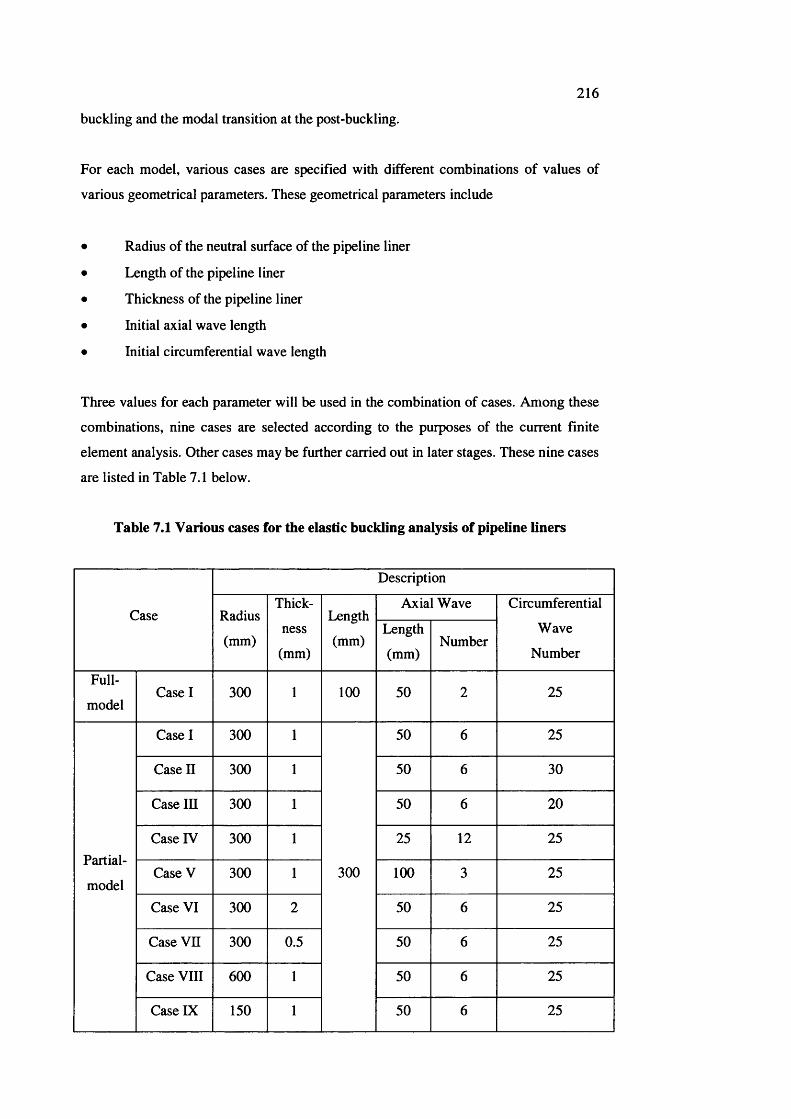
216buckling and the modal transition at the post-buckling.

For each model, various cases are specified with different combinations of values of

various geometrical parameters. These geometrical parameters include

Radius of the neutral surface of the pipeline liner

Length of the pipeline liner

Thickness of the pipeline liner

Initial axial wave length

Initial circumferential wave length

Three values for each parameter will be used in the combination of cases. Among these

combinations, nine cases are selected according to the purposes of the current finite

element analysis. Other cases may be further carried out in later stages. These nine cases

are listed in Table 7.1 below.

Table 7.1 Various cases for the elastic buckling analysis of pipeline liners

Case

Description

Radius

(mm)

Thick

ness

(mm)

Length

(mm)

Axial Wave Circumferential

Wave

Number

Length

(mm)Number

Full-

modelCase I 300 1 100 50 2 25

Partial-

model

Case I 300 1

300

50 6 25

Case II 300 1 50 6 30

Case in 300 1 50 6 20

Case IV 300 1 25 12 25

Case V 300 1 100 3 25

Case VI 300 2 50 6 25

Case Vn 300 0.5 50 6 25

Case VIII 600 1 50 6 25

Case IX 150 1 50 6 25

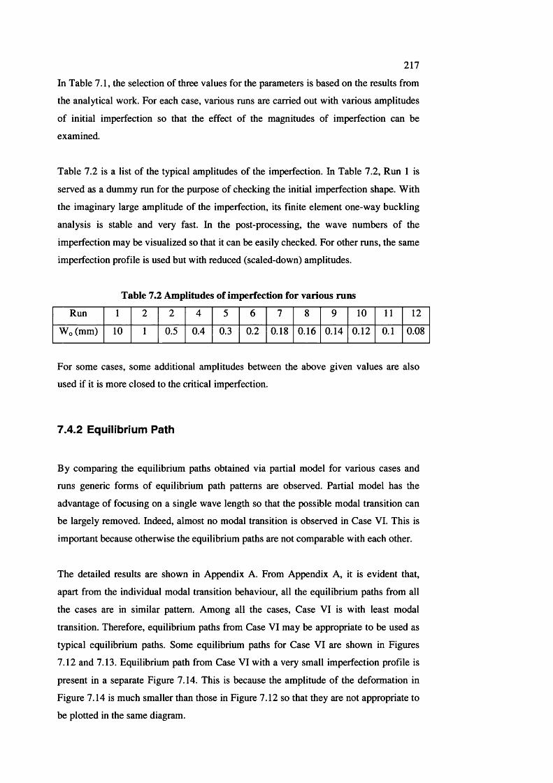
217In Table 7.1, the selection of three values for the parameters is based on the results from

the analytical work. For each case, various runs are carried out with various amplitudes

of initial imperfection so that the effect of the magnitudes of imperfection can be

examined.

Table 7.2 is a list of the typical amplitudes of the imperfection. In Table 7.2, Run 1 is

served as a dummy run for the purpose of checking the initial imperfection shape. With

the imaginary large amplitude of the imperfection, its finite element one-way buckling

analysis is stable and very fast. In the post processing, the wave numbers of the

imperfection may be visualized so that it can be easily checked. For other runs, the same

imperfection profile is used but with reduced (scaled-down) amplitudes.

Table 7.2 Amplitudes of imperfection for various runs

Run 1 2 2 4 5 6 7 8 9 10 11 12

Wo (mm) 10 1 0.5 0.4 0.3 0.2 0.18 0.16 0.14 0.12 0.1 0.08

For some cases, some additional amplitudes between the above given values are also

used if it is more closed to the critical imperfection.


By comparing the equilibrium paths obtained via partial model for various cases and

runs generic forms of equilibrium path patterns are observed. Partial model has the

advantage of focusing on a single wave length so that the possible modal transition can

be largely removed. Indeed, almost no modal transition is observed in Case VI. This is

important because otherwise the equilibrium paths are not comparable with each other.

The detailed results are shown in Appendix A. From Appendix A, it is evident that,

apart from the individual modal transition behaviour, all the equilibrium paths from all

the cases are in similar pattern. Among all the cases. Case VI is with least modal

transition. Therefore, equilibrium paths from Case VI may be appropriate to be used as

typical equilibrium paths. Some equilibrium paths for Case VI are shown in Figures

7.12 and 7.13. Equilibrium path from Case VI with a very small imperfection profile is

present in a separate Figure 7.14. This is because the amplitude of the deformation in

Figure 7.14 is much smaller than those in Figure 7.12 so that they are not appropriate to

be plotted in the same diagram.

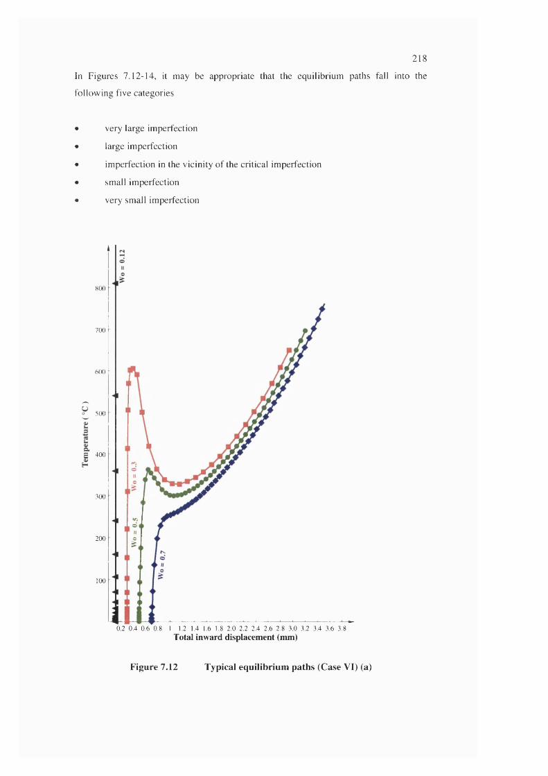
218

In Figures 7.12-14, it may be appropriate that the equilibrium paths fall into the

follow ing five categories

very large im perfection

large im perfection

im perfection in the vicinity o f the critical im perfection

small im perfection

very small im perfection

800

700

600

500

E 400

300

200

100

0.2 0.4 0.6 0.8 1 1.2 1.4 1.6 1.8 2.0 2.2 2.4 2.6 2.8 3.0 3.2 3.4 3.6 3.8Total inward displacement (mm)

Figure 7.12 Typical equilibrium paths (Case VI) (a)

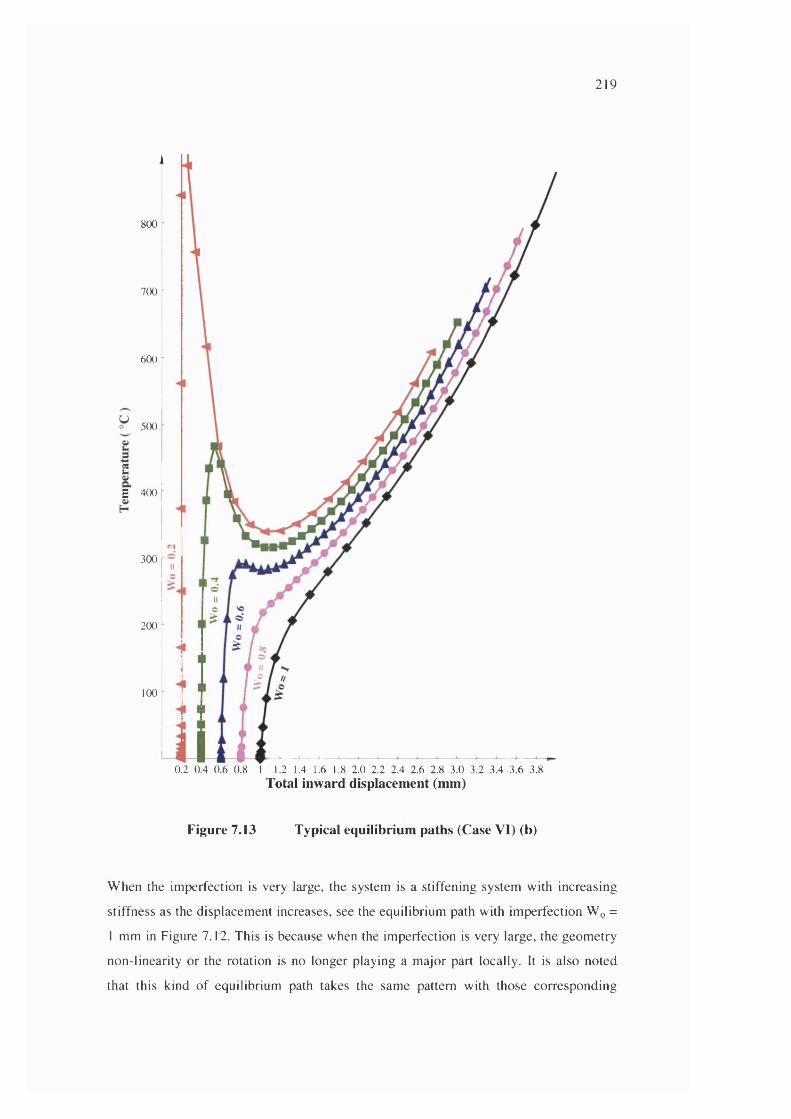
219

800

700

6 0 0 r

500

E 4 0 0

300

200

100

0.2 0 .4 0 .6 0 .8 1 1.2 1.4 1.6 1.8 2 .0 2 .2 2 .4 2 .6 2 .8 3 .0 3 .2 3 .4 3 .6 3.8

Total inward displacement (mm)

Figure 7.13 Typical equilibrium paths (Case VI) (b)

W hen the im perfection is very large, the system is a stiffening system with increasing

stiffness as the displacem ent increases, see the equilibrium path with im perfection W q =

1 mm in Figure 7.12. This is because when the im perfection is very large, the geom etry

non-linearity or the rotation is no longer playing a m ajor part locally. It is also noted

that this kind o f equilibrium path takes the sam e pattern with those corresponding

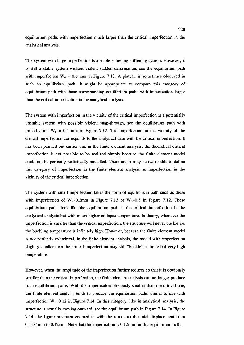
220equilibrium paths with imperfection much larger than the critical imperfection in the

analytical analysis.

The system with large imperfection is a stable-softening-stiffening system. However, it

is still a stable system without violent sudden deformation, see the equilibrium path

with imperfection Wq = 0.6 mm in Figure 7.13. A plateau is sometimes observed in

such an equilibrium path. It might be appropriate to compare this category of

equilibrium path with those corresponding equilibrium paths with imperfection larger

than the critical imperfection in the analytical analysis.

The system with imperfection in the vicinity of the critical imperfection is a potentially

unstable system with possible violent snap-through, see the equilibrium path with

imperfection Wq = 0.5 mm in Figure 7.12. The imperfection in the vicinity of the

critical imperfection corresponds to the analytical case with the critical imperfection. It

has been pointed out earlier that in the finite element analysis, the theoretical critical

imperfection is not possible to be realized simply because the finite element model

could not be perfectly realistically modelled. Therefore, it may be reasonable to define

this category of imperfection in the finite element analysis as imperfection in the

vicinity of the critical imperfection.

The system with small imperfection takes the form of equilibrium path such as those

with imperfection of W o=0.2mm in Figure 7.13 or W o=0.3 in Figure 7.12. These

equilibrium paths look like the equilibrium path at the critical imperfection in the

analytical analysis but with much higher collapse temperature. In theory, whenever the

imperfection is smaller than the critical imperfection, the structure will never buckle i.e.

the buckling temperature is infinitely high. However, because the finite element model

is not perfectly cylindrical, in the finite element analysis, the model with imperfection

slightly smaller than the critical imperfection may still “buckle” at finite but very high

temperature.

However, when the amplitude of the imperfection further reduces so that it is obviously

smaller than the critical imperfection, the finite element analysis can no longer produce

such equilibrium paths. With the imperfection obviously smaller than the critical one,

the finite element analysis tends to produce the equilibrium paths similar to one with

imperfection W o=0.12 in Figure 7.14. In this category, like in analytical analysis, the

structure is actually moving outward, see the equilibrium path in Figure 7.14. In Figure

7.14, the figure has been zoomed in with the x axis as the total displacement from

0.1184mm to 0.12mm. Note that the imperfection is 0.12mm for this equilibrium path.

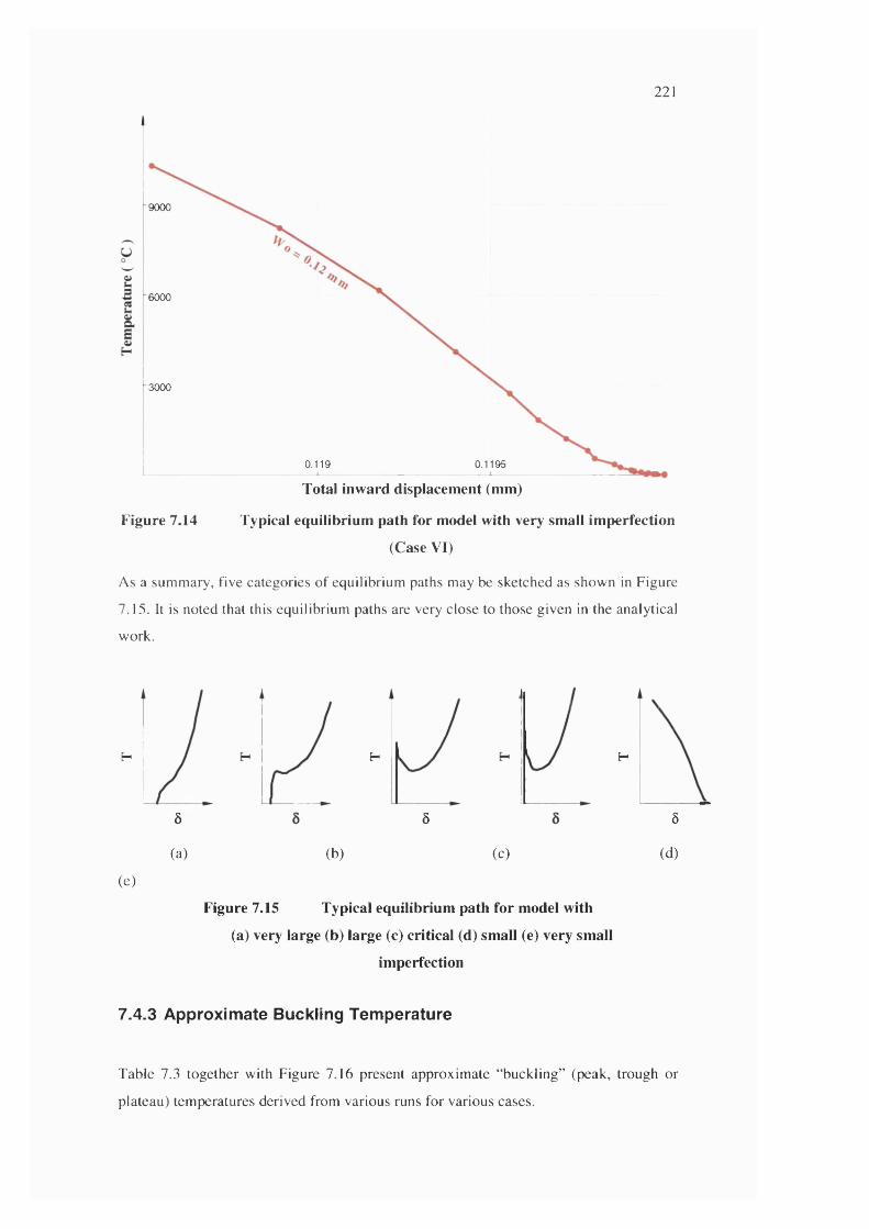
221

9000

■6000

3000

0.11950.119


Figure 7.14 Typical equilibrium path for model with very small imperfection

(Case VI)

As a sum m ary, five categories of equilibrium paths may be sketched as show n in Figure

7.15. It is noted that this equilibrium paths are very close to those given in the analytical

work.

H

Ô

H

Ô

H

Ô

(a) (b) (c) (d)

(e)

Figure 7.15 Typical equilibrium path for model with

(a) very large (b) large (c) critical (d) small (e) very small

imperfection

7.4.3 Approximate Buckling Temperature

Table 7.3 together with Figure 7.16 present approxim ate “buckling” (peak, trough or

plateau) tem peratures derived from various runs for various cases.

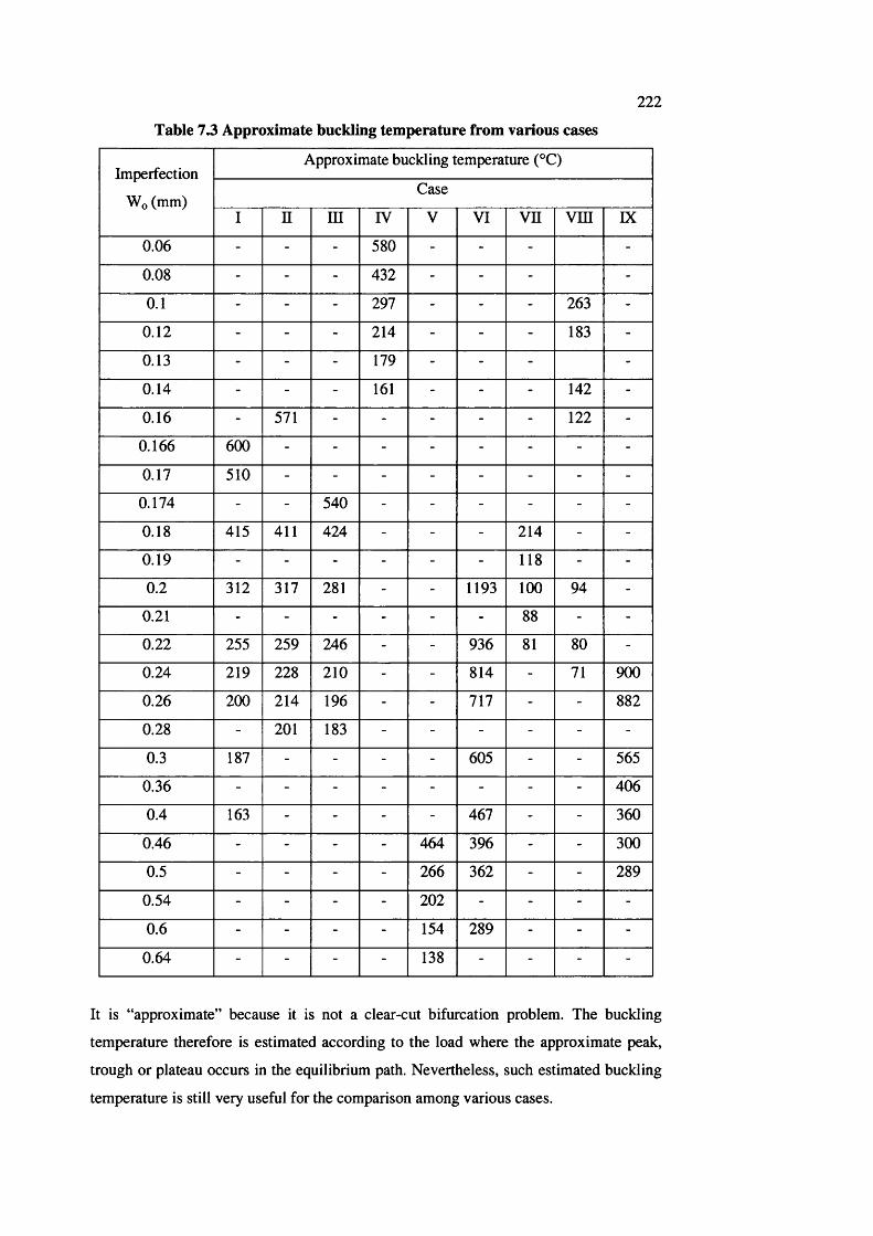
222Table 13 Approximate buckling temperature from various cases

Imperfection

Wo (mm)

Approximate buckling temperature (°C)

Case

1 n m IV V VI vn vm DC

0.06 - - - 580 - - - -

0.08 - - - 432 - - - -

0.1 - - - 297 - - - 263 -

0.12 - - - 214 - - - 183 -

0.13 - - - 179 - - - -

0.14 - - - 161 - - - 142 -

0.16 - 571 - - - - - 122 -

0.166 600 - - - - - - - -

0.17 510 - - - - - - - -

0.174 - - 540 - - - - - -

0.18 415 411 424 - - - 214 - -

0.19 - - - - - - 118 - -

0.2 312 317 281 - - 1193 100 94 -

0.21 - - - - - - 88 - -

0.22 255 259 246 - - 936 81 80 -

0.24 219 228 210 - - 814 - 71 900

0.26 200 214 196 - - 717 - - 882

0.28 - 201 183 - - - - - -

0.3 187 - - - - 605 - - 565

0.36 - - - - - - - - 406

0.4 163 - - - - 467 - - 360

0.46 - - - - 464 396 - - 300

0.5 - - - - 266 362 - - 289

0.54 - - - - 202 - - - -

0.6 - - - - 154 289 - - -

0.64 - - - - 138 - - - -

It is “approximate” because it is not a clear-cut bifurcation problem. The buckling

temperature therefore is estimated according to the load where the approximate peak,

trough or plateau occurs in the equilibrium path. Nevertheless, such estimated buckling

temperature is still very useful for the comparison among various cases.

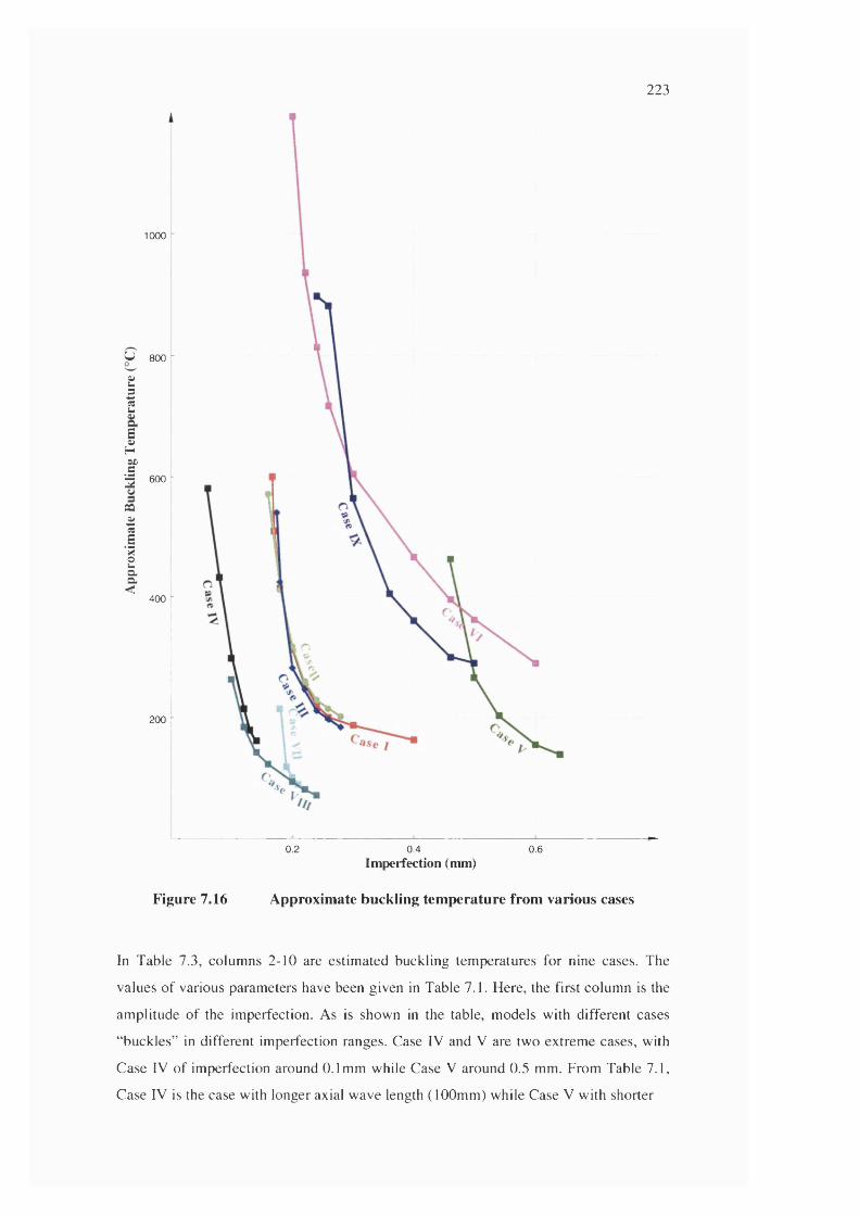
223

1000

u 800

tS

I

IOX)

'J 600

CQaIIâ<

400

200

0.2 0.4Imperfection (mm)

0.6

Figure 7.16 Approximate buckling temperature from various cases

In Table 7.3, colum ns 2-10 are estim ated buckling tem peratures for nine cases. The

values o f various param eters have been given in Table 7.1. Here, the first colum n is the

am plitude o f the im perfection. As is shown in the table, m odels with different cases

“buckles” in different im perfection ranges. Case IV and V are two extrem e cases, with

Case IV o f im perfection around 0.1m m w hile Case V around 0.5 mm. From Table 7.1,

Case IV is the case with longer axial wave length (100m m ) w hile Case V with shorter

224

axial wave length (25mm).

In Table 7.3, represents the runs from which no buckling temperature is possibly

estimated (no apparent peak, trough or plateau can be observed). This is because among

five categories of imperfection mentioned earlier in this section, only the third category

i.e. imperfection in the vicinity of the critical imperfection displays plateau in the

equilibrium path so that “buckling” temperature may be estimated.

It is noted from Figure 7.16 that the first three cases have very close imperfection-

temperature curves. According to Table 7.1, the first three cases analyse the pipeline

liners with the same values of geometric parameters except the circumferential wave

numbers. Therefore it is found that the collapse temperature is not very sensitive to the

circumferential wave number.

It is also noted from Figure 7.16 that Case I, Case IV and Case V demonstrates similar

range of buckling temperature but at very different imperfection ranges. According to

Table 7.1, Case I, Case IV and Case V analyse the pipeline liners with the same values

of geometric parameters except the axial wave lengths. Therefore it is found that the

critical imperfection is very sensitive to the axial wave number.

Case I, Case VI and Case VII are three cases with the wall thickness of 1mm, 2mm and

0.5mm respectively. From Figure 7.16, it is found that the collapse temperature is very

sensitive to the wall thickness. As the thickness decreases, the collapse temperature

decreases.

Similarly, Case I, Case VIII and Case DC are three cases with the liner neutral surface

radius of 300mm, 600mm and 150mm respectively. Comparing the corresponding

imperfection-temperature curves in Figure 7.16 reveals that the collapse temperature is

very sensitive to the radius. As the radius increases, the collapse temperature decreases.

7.4.4 Post-buckling Modal Transition - Partiai-Modei

In this section, the modal shape and transition will be demonstrated by an example from

the partial-model. The modal shape and transition will be further explained by another

example from the full-model in Section 7.4.5.

As for the partial-model, in Section 7.2, the equilibrium paths for various imperfection

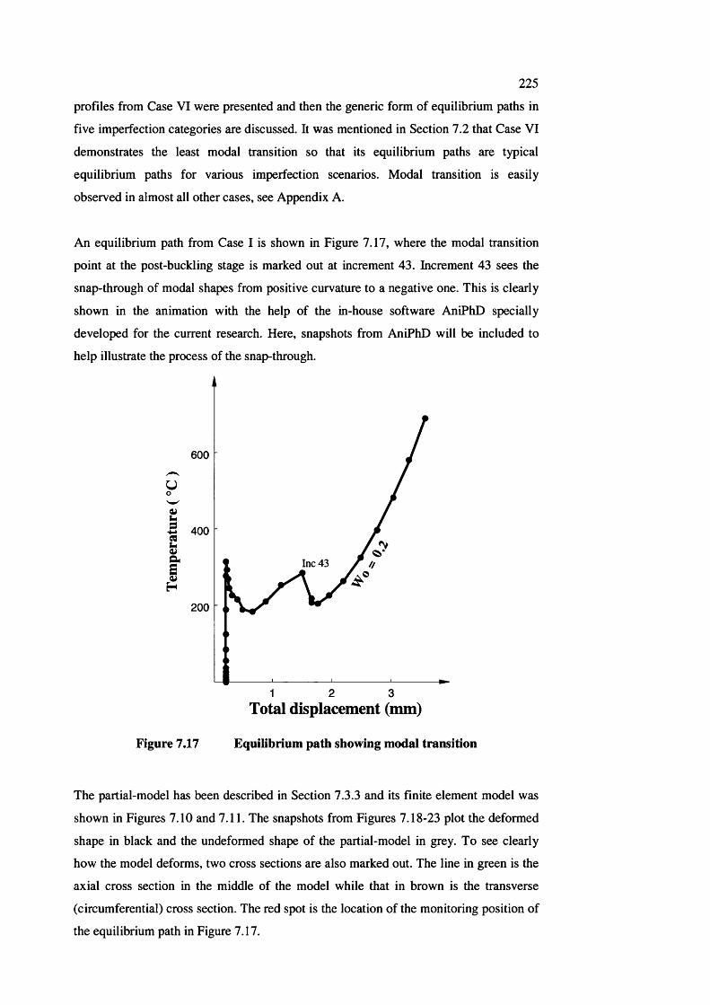
225profiles from Case VI were presented and then the generic form of equilibrium paths in

five imperfection categories are discussed. It was mentioned in Section 7.2 that Case VI

demonstrates the least modal transition so that its equilibrium paths are typical

equilibrium paths for various imperfection scenarios. Modal transition is easily

observed in almost all other cases, see Appendix A.

An equilibrium path from Case I is shown in Figure 7.17, where the modal transition

point at the post-buckling stage is marked out at increment 43. Increment 43 sees the

snap-through of modal shapes from positive curvature to a negative one. This is clearly

shown in the animation with the help of the in-house software AniPhD specially

developed for the current research. Here, snapshots from AniPhD will be included to

help illustrate the process of the snap-through.

6 0 0

Uo

I5 4 0 0

I

Inc 43

200

1 2 3

Figure 7.17

Total displacement (mm)

Equilibrium path showing modal transition

The partial-model has been described in Section 7.3.3 and its finite element model was

shown in Figures 7.10 and 7.11. The snapshots from Figures 7.18-23 plot the deformed

shape in black and the undeformed shape of the partial-model in grey. To see clearly

how the model deforms, two cross sections are also marked out. The line in green is the

axial cross section in the middle of the model while that in brown is the transverse

(circumferential) cross section. The red spot is the location of the monitoring position of

the equilibrium path in Figure 7.17.

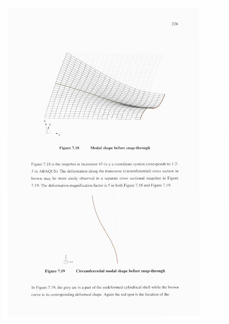
226

Figure 7.18 Modal shape before snap-through

Figure 7.18 is the snapshot at increment 43 (x-y-z coordinate system corresponds to 1-2-

3 in A BA Q U S). The deform ation along the transverse (circum ferential) cross section in

brow n may be more easily observed in a separate cross sectional snapshot in Figure

7.19. The deform ation m agnification factor is 5 in both Figure 7.18 and Figure 7.19.

Figure 7.19 Circumferential modal shape before snap-through

In Figure 7.19, the grey arc is a part o f the undeform ed cylindrical shell w hile the brown

curve is its corresponding deform ed shape. Again the red spot is the location o f the

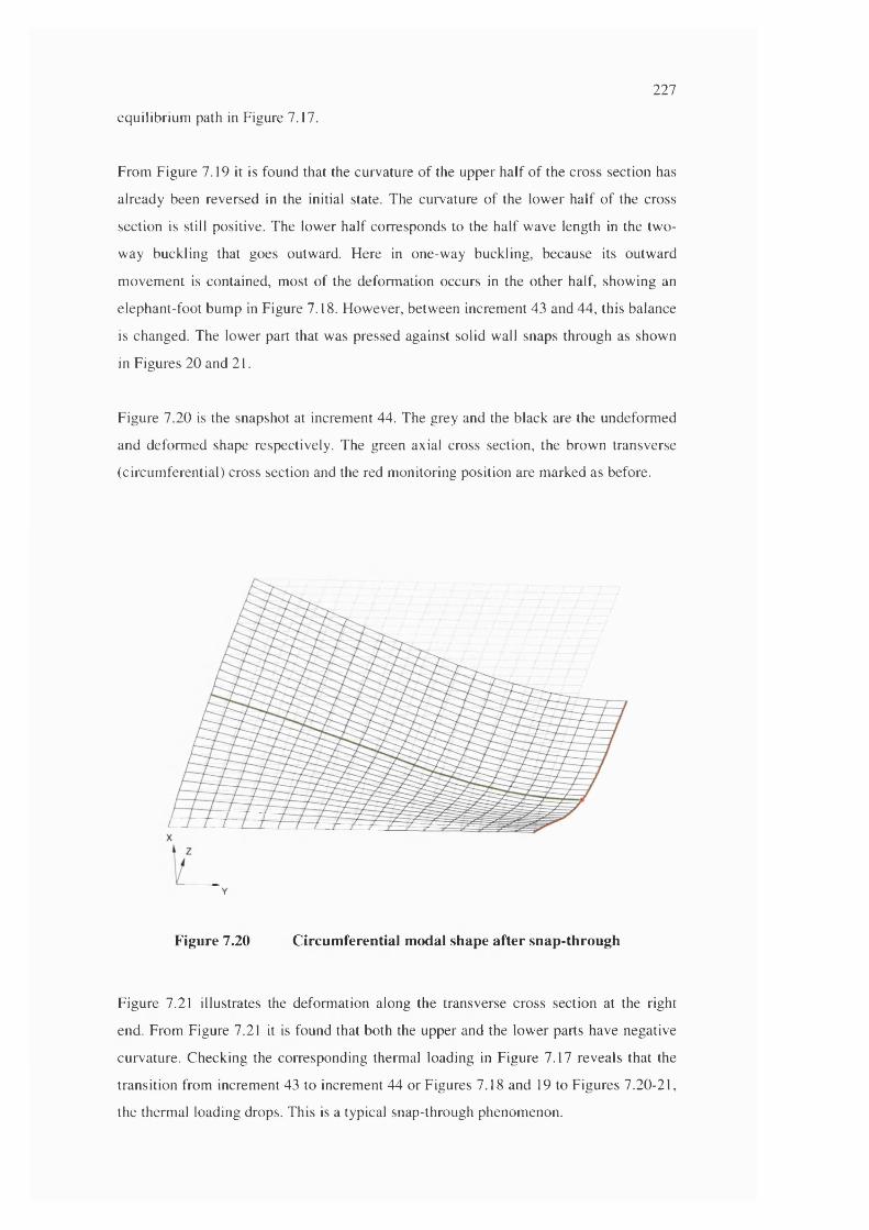
227

equilibrium path in Figure 7.17.

From Figure 7.19 it is found that the curvature o f the upper half o f the cross section has

already been reversed in the initial state. The curvature of the low er half o f the cross

section is still positive. The lower half corresponds to the half wave length in the two-

way buckling that goes outward. Here in one-w ay buckling, because its outw ard

m ovem ent is contained, most o f the deform ation occurs in the o ther half, show ing an

elephant-foot bum p in Figure 7.18. How ever, betw een increm ent 43 and 44, this balance

is changed. The lower part that was pressed against solid wall snaps through as shown

in Figures 20 and 21.

Figure 7.20 is the snapshot at increm ent 44. The grey and the black are the undeform ed

and deform ed shape respectively. The green axial cross section, the brown transverse

(circum ferential) cross section and the red m onitoring position are m arked as before.

Figure 7.20 Circumferential modal shape after snap-through

Figure 7.21 illustrates the deform ation along the transverse cross section at the right

end. From Figure 7.21 it is found that both the upper and the low er parts have negative

curvature. C hecking the corresponding thermal loading in F igure 7.17 reveals that the

transition from increm ent 43 to increm ent 44 or Figures 7.18 and 19 to F igures 7.20-21,

the thermal loading drops. This is a typical snap-through phenom enon.

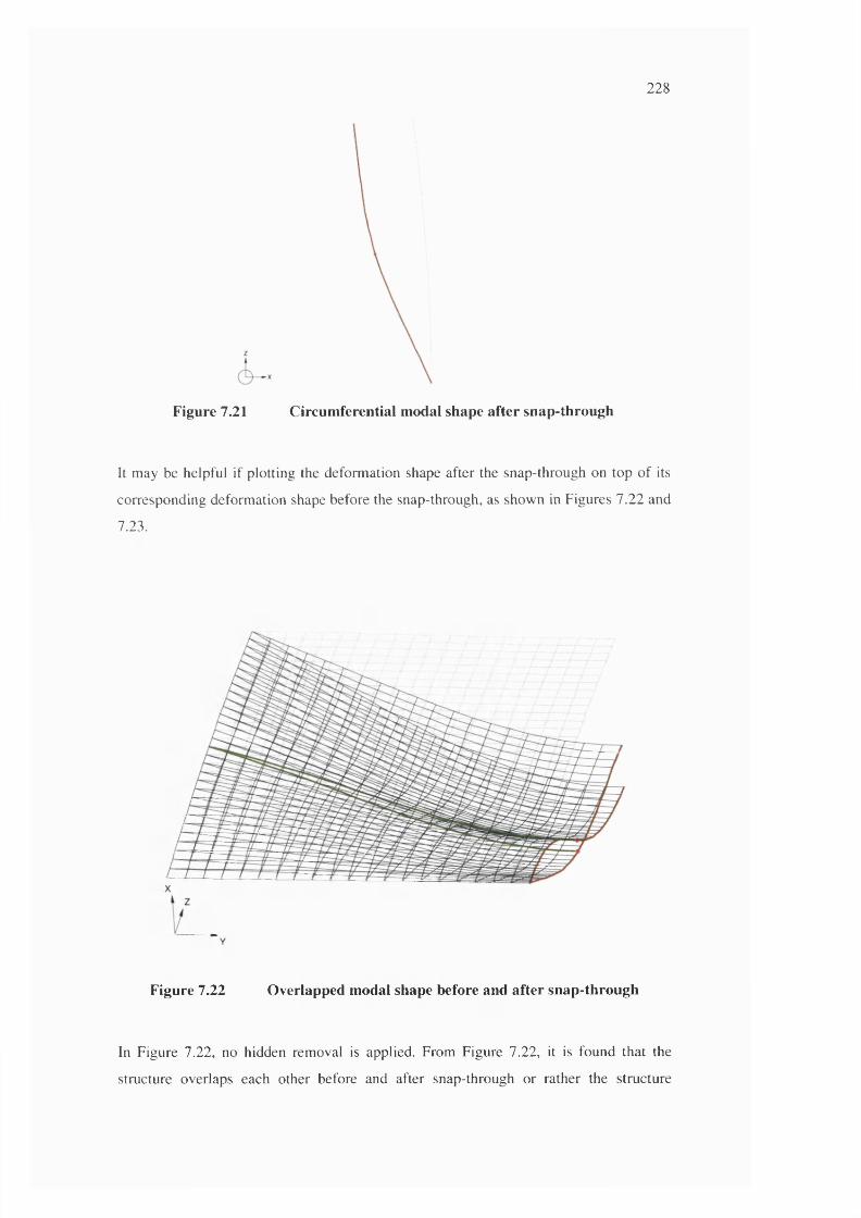
228


It may be helpful if plotting the deform ation shape after the snap-through on top o f its

corresponding deform ation shape before the snap-through, as show n in Figures 7 .22 and

7.23.

Figure 7.22 Overlapped modal shape before and after snap-through

In Figure 7.22, no hidden removal is applied. From Figure 7.22, it is found that the

structure overlaps each other before and after snap-through or rather the structure

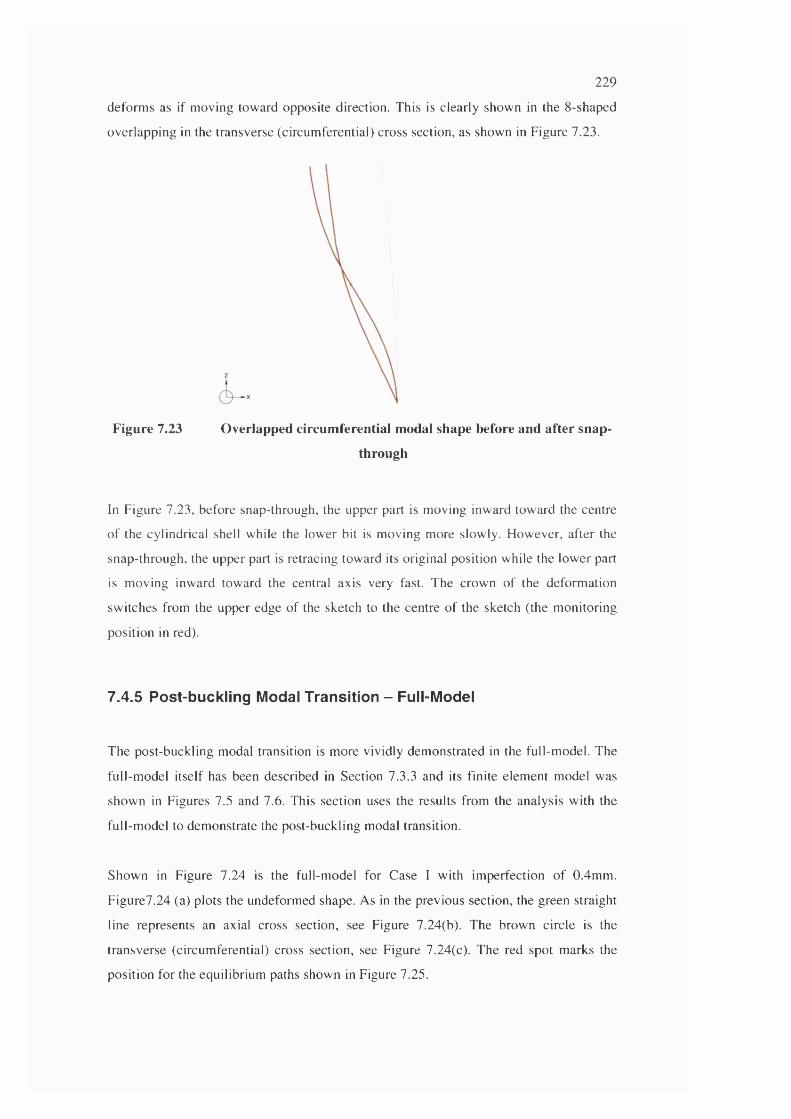
229

deform s as if m oving tow ard opposite direction. This is clearly shown in the 8-shaped

overlapping in the transverse (circum ferential) cross section, as shown in Figure 7.23.

Figure 7.23 Overlapped circumferential modal shape before and after snap-

through

In Figure 7.23, before snap-through, the upper part is m oving inw ard tow ard the centre

o f the cylindrical shell while the lower bit is m oving more slowly. H ow ever, after the

snap-through, the upper part is retracing tow ard its original position while the low er part

is m oving inward tow ard the central axis very fast. The crow n o f the deform ation

sw itches from the upper edge of the sketch to the centre o f the sketch (the m onitoring

position in red).

7.4.5 Post-buckling Modal Transition - Full-Model

The post-buckling modal transition is m ore vividly dem onstrated in the full-m odel. The

full-m odel itself has been described in Section 7.3.3 and its finite elem ent m odel was

show n in Figures 7.5 and 7.6. This section uses the results from the analysis w ith the

full-m odel to dem onstrate the post-buckling modal transition.

Show n in Figure 7.24 is the full-m odel for Case I w ith im perfection o f 0.4m m .

F igure7.24 (a) plots the undeform ed shape. As in the previous section, the green straight

line represents an axial cross section, see Figure 7.24(b). The brown circle is the

transverse (circum ferential) cross section, see Figure 7.24(c). The red spot m arks the

position for the equilibrium paths shown in Figure 7.25.

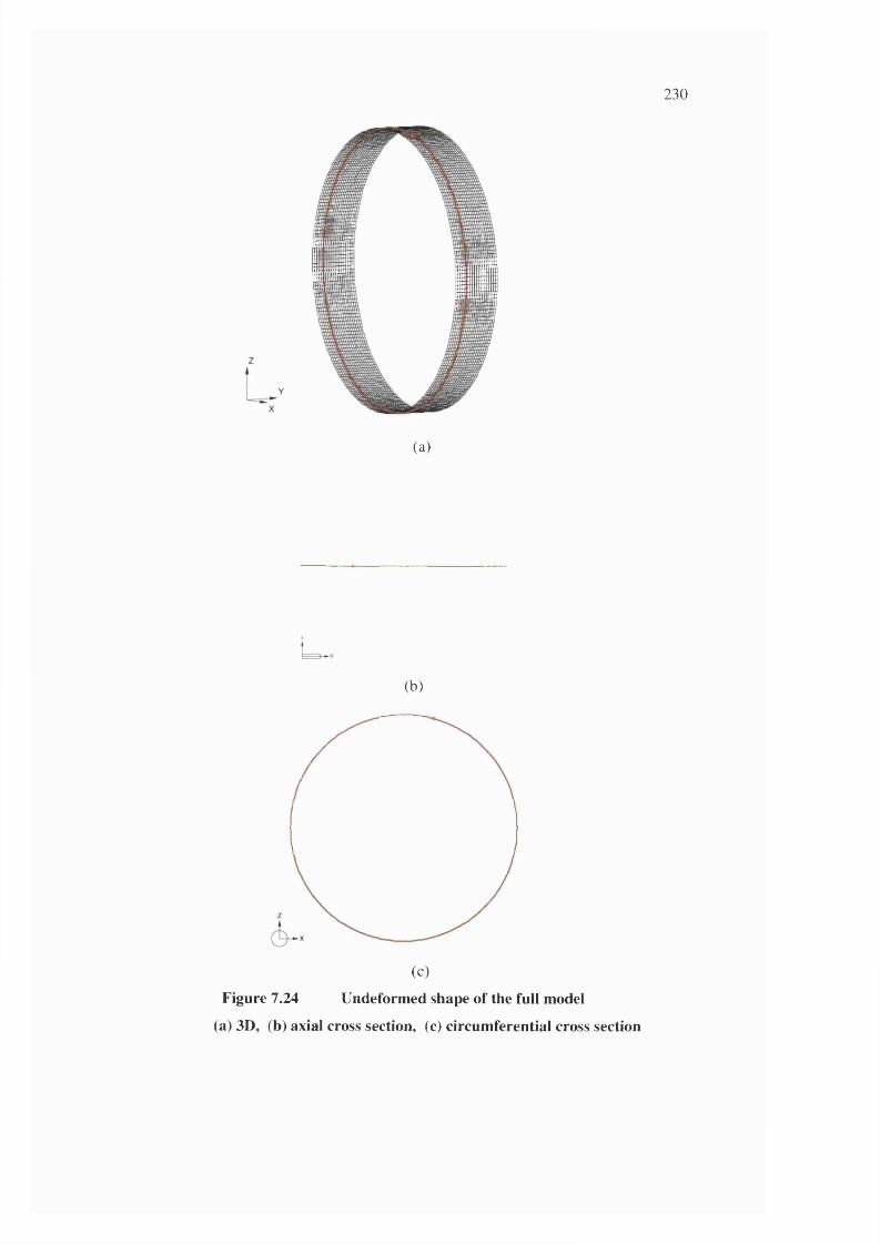
230

(a)

(b)

(c)

Figure 7.24 Undeformed shape of the full model

(a) 3D, (b) axial cross section, (c) circumferential cross section

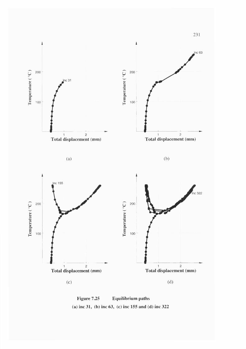
231

U

SiIa

I

200

Inc 31

100

1

Si

IË.

I

Inc 63

200

100

21

Total displacement (mm) Total displacement (mm)

(a) (b)

Inc 155

Si

I

I

200 :

100

L1 2

Total displacement (mm)

(c)

Si3

2&

I

Inc 322

200 r

100

1 2 Total displacement (mm)

(d)


(a) inc 31, (b) inc 63, (c) inc 155 and (d) inc 322

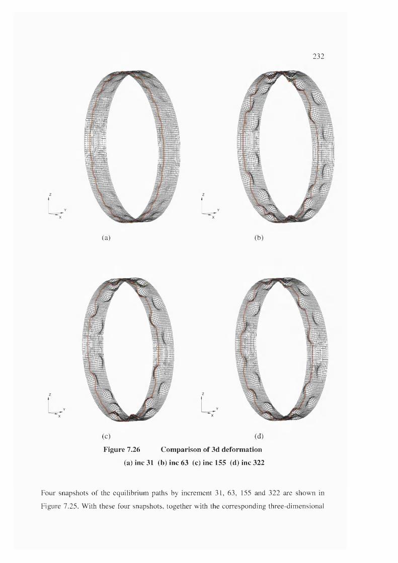
232

(a) (b)

(c) (d)Figure 7.26 Com parison of 3d deform ation

(a) inc 31 (b) inc 63 (c) inc 155 (d) inc 322

F o u r sn ap sh o ts o f the eq u ilib riu m paths by in crem en t 31, 63 , 155 and 322 are sh o w n in

F ig u re 7 .25 . W ith these fou r snapsho ts, to g e th e r w ith the c o rre sp o n d in g th ree -d im en sio n a l

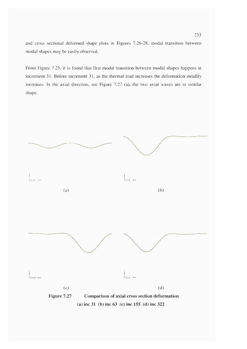
233and c ro ss sec tiona l d e fo rm ed shape p lo ts in F ig u res 7 .2 6 -2 8 , m odal tran s itio n b e tw een

m o d al shapes m ay be easily observed .

F rom F ig u re 7 .25 , it is found tha t first m o d al tran s itio n b e tw een m o d al shapes h ap p en s at

in c rem en t 31. B efo re increm en t 31, as the therm al load increases the d e fo rm a tio n stead ily

in c reases . In the ax ia l d irec tion , see F igu re 7 .27 (a), the tw o ax ia l w aves are in s im ila r

shape .

U

(a) (b)

u

(c) (d)

Figure 7.27 Com parison of axial cross section deform ation


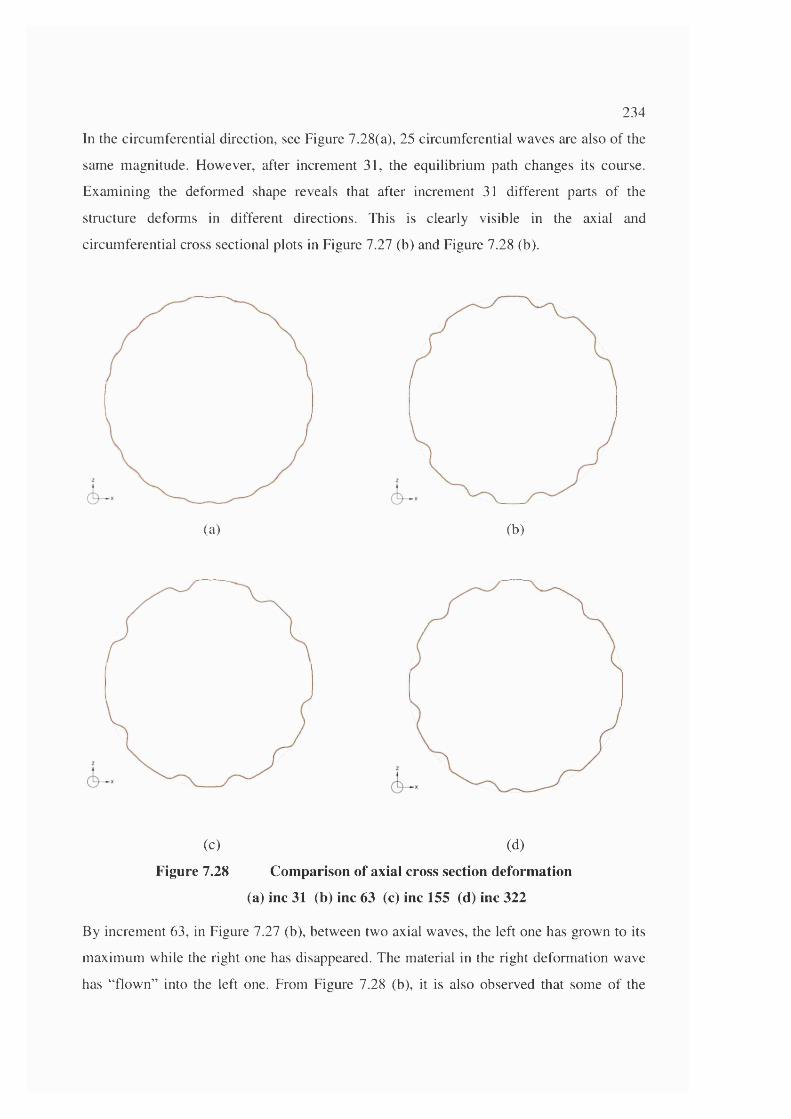
2 3 4

In the c ircu m feren tia l d irec tion , see F igu re 7 .28 (a), 25 c ircu m feren tia l w aves are a lso o f the

sam e m ag n itu d e . H o w ever, a fter in c rem en t 31, the eq u ilib riu m p a th ch an g es its co u rse .

E x am in in g the d e fo rm ed shape rev ea ls tha t a fte r in c rem en t 31 d iffe ren t p arts o f the

stru c tu re d e fo rm s in d iffe ren t d irec tio n s. T h is is c lea rly v isib le in the ax ia l and

c ircu m fe ren tia l c ro ss sec tiona l p lo ts in F igu re 7 .27 (b ) and F igu re 7 .28 (b).

(a) (b)

(c) (d)Figure 7.28 Com parison of axial cross section deform ation


B y in c rem en t 63 , in F igu re 7 .27 (b), b e tw een tw o ax ia l w aves, the left one has g ro w n to its

m ax im u m w hile the rig h t one has d isap p eared . T h e m ateria l in the rig h t d e fo rm a tio n w ave

has “ flo w n ” in to the left one. F rom F igu re 7 .28 (b), it is a lso o b se rv ed tha t som e o f the

235circumferential waves are grown while others have disappeared. The wave numbers in both

the axial and the circumferential directions has changed. This is clearly modal transition.

After increment 63, the structure starts another modal transition. From the equilibrium path

in Figure 7.25 (c), it is found that the equilibrium path is starting going backwards. This is

because the position of monitoring the equilibrium path (the red spot) stars to return to its

original position.

By increment 155, another different modal shape has taken its form. In Figure 7.26 (c),

comparing with Figure 7.26 (b), some bumps have changed its position while others do not

move. In the axial direction, the axial cross section deformation shown in Figure 7.27 (c)

reveals that the grown left bump has returned to its original position while the undeveloped

right bump has now grown to its maximum. In the circumferential direction, in Figure 7.28

(c), comparing with Figure 7.28 (b), not only the positions of the bumps have moved but

also the number of bumps has reduced.

After increment 155, further modal transitions occur again and again. This is shown in the

equilibrium path in Figure 7.25 (d) with the equilibrium paths repeat itself from time to

time. As the snap-through happens, the temperature fluctuates. It is interesting to note that

among all possible modal shapes, a lower limit in the temperature exists.

7.4.6 Detailed Results

In the above sections, the equilibrium paths from Case VI were used in the discussion of

the typical equilibrium path while Case I were referred in the examination of the modal

transition. In Section 7.4.3, some approximate collapse temperatures were extracted from

the corresponding equilibrium paths of various runs in the nine cases. The details of these

equilibrium paths for all the nine cases are given in Appendix A.

Appendix A lists the equilibrium paths case by case from Case I to Case IX. For each case,

about twelve equilibrium paths for various amplitudes of imperfection are presented in

separate figures. At the end of each case, several equilibrium paths with selected typical

236amplitude of imperfection are plotted in the same figures for comparison. Each individual

curve is labelled with the corresponding amplitude of the imperfection.

7.5 Concluding Remarks

From the above finite element elastic buckling analysis, the following are concluded

• The animation of the deformed shape from the finite element elastic buckling

analysis reveals that the one-way buckling of pipeline liners is characterized by the

modal transition. As the amplitude of the incremental displacement increases, the

system varies its deformed shapes, reducing the overall wave numbers while

growing the remaining deformed lobes.

• Finite element elastic one-way buckling analysis produces the similar generic

equilibrium paths as those derived from analytical work. The buckling temperature

from the finite element numeric analysis matches those from the analytical work.

• The buckling temperature is not very sensitive to the circumferential wave number.

However, different wave numbers correspond to different critical amplitude of

imperfection. Lowest buckling temperature occurs when the axial wave length is

about 50mm and the circumferential wave number is equal to 25.

• As the thickness decreases, the collapse temperature decreases. As the radius

increases, the collapse temperature decreases.

237

8 Finite Eiement Anaiysis - Elastic-Plastic Buckling

8.1 introduction

In the previous chapter the finite element elastic one-way buckling analysis of pipeline

liners was described. The current chapter will deal with the corresponding finite element

elastic-plastic one-way buckling analysis. All the finite element runs from nine cases

described in Chapter 7 will be re-run with the incorporation of the elastic-plastic

material property. The results from the elastic-plastic one-way buckling analysis will be

compared to those from the elastic one-way buckling analysis.

In this chapter, the material property of the pipeline liners will be described in Section

8.2. In Section 8.3, results from nine cases of finite element analysis for the elastic-

plastic buckling will be discussed. Section 8.4 will compare results between the elastic

and the elastic-plastic one-way buckling. Finally, conclusions for the current chapter

will be given in Section 8.5.

8.2 Material Property of the Pipeline Liner

Anti-corrosion pipeline liners are usually made of alloys of Nickel, or, Inconel. From a

tensile test load-displacement curve, for a typical corrosion resistant alloy (CRA)

material at 160 degree Celsius, the true stress strain relationship is derived as shown in

Figure 8.1. Some material parameters are shown in Table 8.1 (Walker, 1999).

Table 8.1 Material property used in the plastic buckling analysis

Description Young’s Modulus Poisson’s Ratio Yield Stress

CRA Tensile Test 4 @ 160°C 2.05GPa 0.3 325MPa

Converting the stress strain relationship in Ramberg-Osgood format, the following

parameters are derived.

Table 8.2 Ramberg-Osgood stress-strain relationship of CRA

Oo(Mpa) £ o Gu (Mpa) £u C n

350 0.00171 600 0.0383 0.00152 17.661

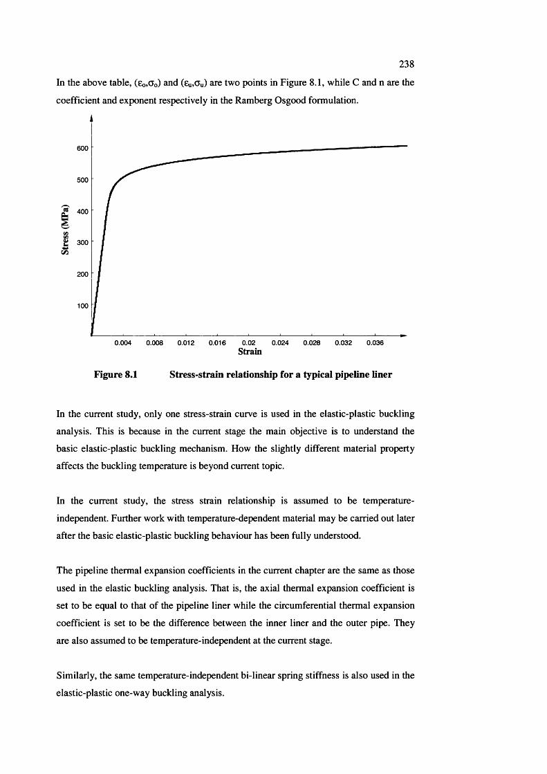
238In the above table, (£o,Oo) and (£u,au) are two points in Figure 8.1, while C and n are the

coefficient and exponent respectively in the Ramberg Osgood formulation.

600

500

5 400

%s 300

200

100

0.008 0.012 0.016 0.02 0.024 0.028 0.032 0.0360.004Strain

Figure 8.1 Stress-strain relationship for a typical pipeline liner

In the current study, only one stress-strain curve is used in the elastic-plastic buckling

analysis. This is because in the current stage the main objective is to understand the

basic elastic-plastic buckling mechanism. How the slightly different material property

affects the buckling temperature is beyond current topic.

In the current study, the stress strain relationship is assumed to be temperature-

independent. Further work with temperature-dependent material may be carried out later

after the basic elastic-plastic buckling behaviour has been fully understood.

The pipeline thermal expansion coefficients in the current chapter are the same as those

used in the elastic buckling analysis. That is, the axial thermal expansion coefficient is

set to be equal to that of the pipeline liner while the circumferential thermal expansion

coefficient is set to be the difference between the inner liner and the outer pipe. They

are also assumed to be temperature-independent at the current stage.

Similarly, the same temperature-independent bi-linear spring stiffness is also used in the

elastic-plastic one-way buckling analysis.

2398.3 Results form Finite Eiement Eiastic-Piastic Buckling

Anaiysis

The finite element elastic buckling analysis described in Chapter 7 has provided a basis

for the finite element elastic-plastic buckling analysis. The same partial-model and full-

model will be used in the same nine cases for the finite element elastic-plastic one-way

buckling analysis. Therefore, the finite element models will not be further described in

the current chapter. Furthermore, like Chapter 7, to maintain the simplicity of the

presentation, most of the detailed results from this chapter will be given in a separate

Appendix B.

As in Chapter 7, the generic results in this chapter will also be presented in two aspects.

Section 8.3.1 will give out various equilibrium path scenarios. Section 8.3.2 will present

various buckling temperatures. Finally, Section 8.3.3 will discuss about the modal

transition in the elastic-plastic one-way buckling.


As in Chapter 7, for a given imperfection profile, temperature rise against total

displacement at a specified location is plotted as an equilibrium path. As before the

monitoring position of the equilibrium path is usually located at the crown of the

imperfection profile. After a series of runs with various imperfection profiles were

carried out, a series of equilibrium paths were derived.

Observing these equilibrium paths, it is found that within certain range of imperfection

they are similar in shape such as stiffening, plateau or snap-through. Grouping the

equilibrium paths for the whole range of possible imperfections, it may be appropriate

that all the equilibrium paths fall into three types of curves for three categories of

imperfection. These three categories of imperfection are

• very large imperfection

• intermediate imperfection

• very small imperfection

Comparing with the elastic one-way buckling where five equilibrium path scenarios

were classified, two equilibrium path types have disappeared. Out of the five

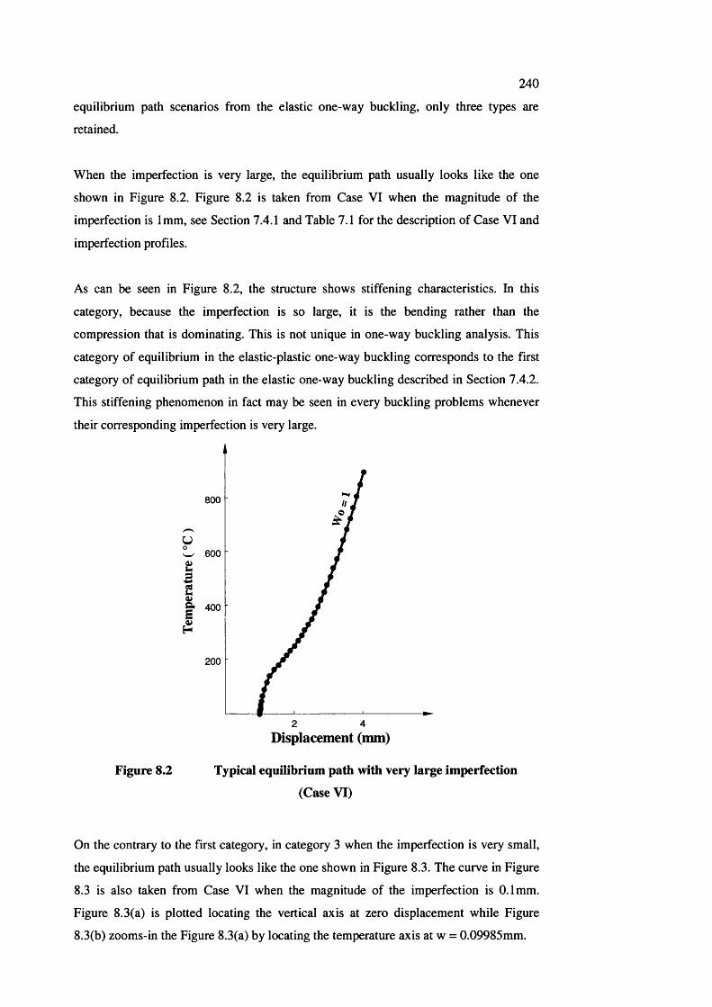
240

equilibrium path scenarios from the elastic one-way buckling, only three types are

retained.

When the imperfection is very large, the equilibrium path usually looks like the one

shown in Figure 8.2. Figure 8.2 is taken from Case VI when the magnitude of the

imperfection is 1mm, see Section 7.4.1 and Table 7.1 for the description of Case VI and

imperfection profiles.

As can be seen in Figure 8.2, the structure shows stiffening characteristics. In this

category, because the imperfection is so large, it is the bending rather than the

compression that is dominating. This is not unique in one-way buckling analysis. This

category of equilibrium in the elastic-plastic one-way buckling corresponds to the first

category of equilibrium path in the elastic one-way buckling described in Section 7.4.2.

This stiffening phenomenon in fact may be seen in every buckling problems whenever

their corresponding imperfection is very large.

y

II

800

600

400

200

2 4

Figure 8.2

Displacement (mm)

Typical equilibrium path with very large imperfection

(Case VI)

On the contrary to the first category, in category 3 when the imperfection is very small,

the equilibrium path usually looks like the one shown in Figure 8.3. The curve in Figure

8.3 is also taken from Case VI when the magnitude of the imperfection is 0.1mm.

Figure 8.3(a) is plotted locating the vertical axis at zero displacement while Figure

8.3(b) zooms-in the Figure 8.3(a) by locating the temperature axis at w = 0.09985mm.

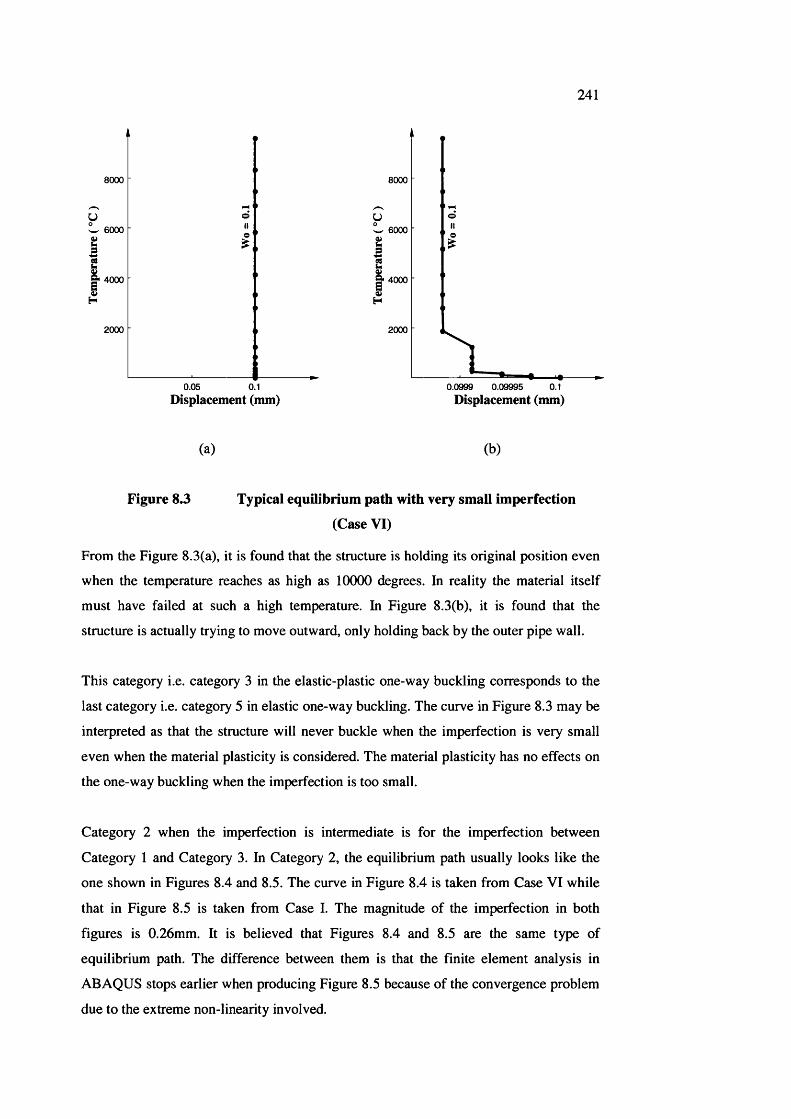
241

8000

U

I 6000

4000

2000

0.05 0.1Displacement (mm)

u

I

8000

6000

4000

2000

0.09995 0.10.0999Displacement (mm)

(a) (b)

Figure 8.3 Typical equilibrium path with very small imperfection

(Case VI)

From the Figure 8.3(a), it is found that the structure is holding its original position even

when the temperature reaches as high as 10000 degrees. In reality the material itself

must have failed at such a high temperature. In Figure 8.3(b), it is found that the

structure is actually trying to move outward, only holding back by the outer pipe wall.

This category i.e. category 3 in the elastic-plastic one-way buckling corresponds to the

last category i.e. category 5 in elastic one-way buckling. The curve in Figure 8.3 may be

interpreted as that the structure will never buckle when the imperfection is very small

even when the material plasticity is considered. The material plasticity has no effects on

the one-way buckling when the imperfection is too small.

Category 2 when the imperfection is intermediate is for the imperfection between

Category 1 and Category 3. In Category 2, the equilibrium path usually looks like the

one shown in Figures 8.4 and 8.5. The curve in Figure 8.4 is taken from Case VI while

that in Figure 8.5 is taken from Case I. The magnitude of the imperfection in both

figures is 0.26mm. It is believed that Figures 8.4 and 8.5 are the same type of

equilibrium path. The difference between them is that the finite element analysis in

ABAQUS stops earlier when producing Figure 8.5 because of the convergence problem

due to the extreme non-linearity involved.

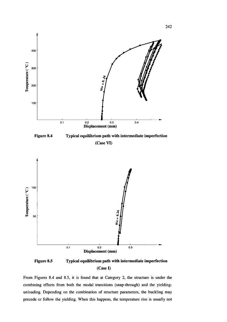
242

400

y300

I100

0.1 0.2 0.3 0.4Displacement (mm)

Figure 8.4 Typical equilibrium path with intermediate imperfection

(Case VI)

100y

i0.30.1 0.2

Displacement (mm)

Figure 8.5 Typical equilibrium path with intermediate imperfection

(Case I)

From Figures 8.4 and 8.5, it is found that at Category 2, the structure is under the

combining effects from both the modal transitions (snap-through) and the yielding-

unloading. Depending on the combination of structure parameters, the buckling may

precede or follow the yielding. When this happens, the temperature rise is usually not

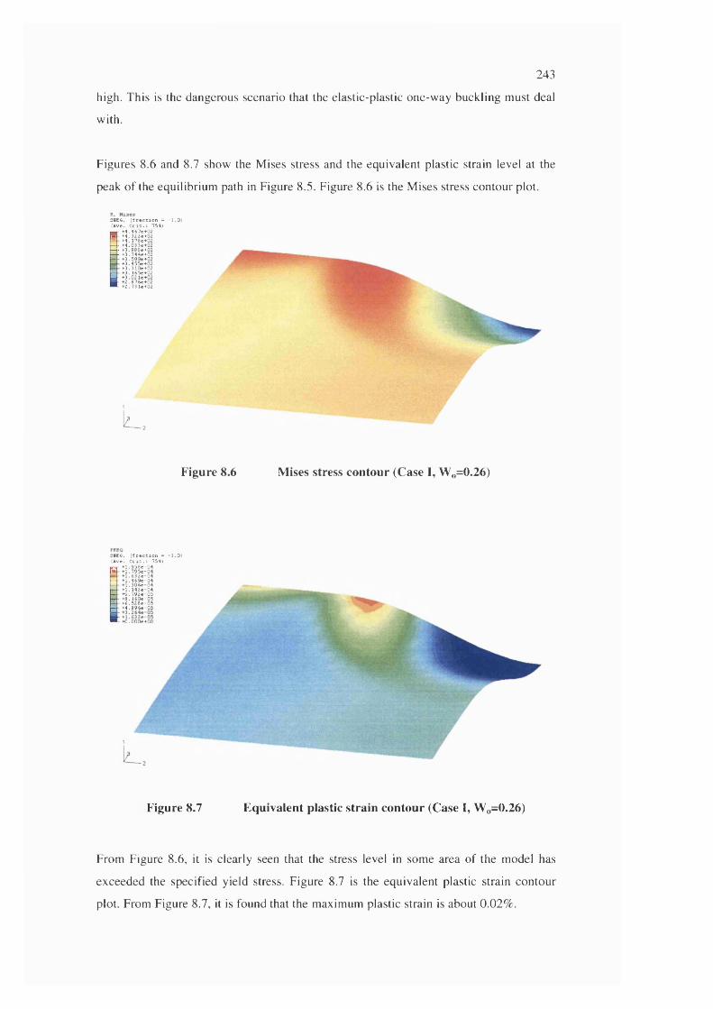
243

high. This is the dangerous scenario that the elastic-plastic one-w ay buckling m ust deal

with.

Figures 8.6 and 8.7 show the M ises stress and the equivalent plastic strain level at the

peak o f the equilibrium path in Figure 8.5. Figure 8.6 is the M ises stress contour plot.

3 MEG, ( f r a c t i o n = - 1 .0 ) (A ve . C e l t . : 751 )^ + 4 .4 6 7 e + 0 2 m ~ M .3 2 2 e + 0 2— + 4 .1 7 8 e + 0 2— - + 4 .0 3 3C+02— - + 3 .8 8 8 e + 0 2 + 3 .7 4 4 e + 0 2

♦ 3 .5 9 9 e+ Q 2 + 3 . 455e+ 02 ♦ 3 .3 1 0 e + 0 2

— + 3 .! 6 5 e + 0 2

■ + 3 .0 2 1 6 + 0 2 + 2 .8 7 6 e + 0 2 + 2 .7 3 1 e + 0 2

Figure 8.6 Mises stress contour (Case I, Wo=0.26)

3 MEG, ( f r a c t i o n = - 1 .0 ) (A ve . C e l t . : 754 )

M - + 1 .9 5 8 e -0 4 m + 1 .7 9 5 e - 0 4— - + 1 . 6 3 2 e -0 4 + 1 .4 6 9 e -0 4— + l . 3 0 6 e - 0 4— - + 1 . 1 4 2 e -0 4— - + 9 .7 9 2 e - 0 5 m - + 8 .1 6 0 6 - 0 5 K + 6 .5 2 8 e - 0 5— - + 4 .8 9 6 e - 0 5

* +O .00D e+0O

Figure 8.7 Equivalent plastic strain contour (Case I, Wo=0.26)

From Figure 8.6, it is clearly seen that the stress level in som e area of the model has

exceeded the specified yield stress. F igure 8.7 is the equivalent plastic strain contour

plot. From Figure 8.7, it is found that the maxim um plastic strain is about 0.02% .

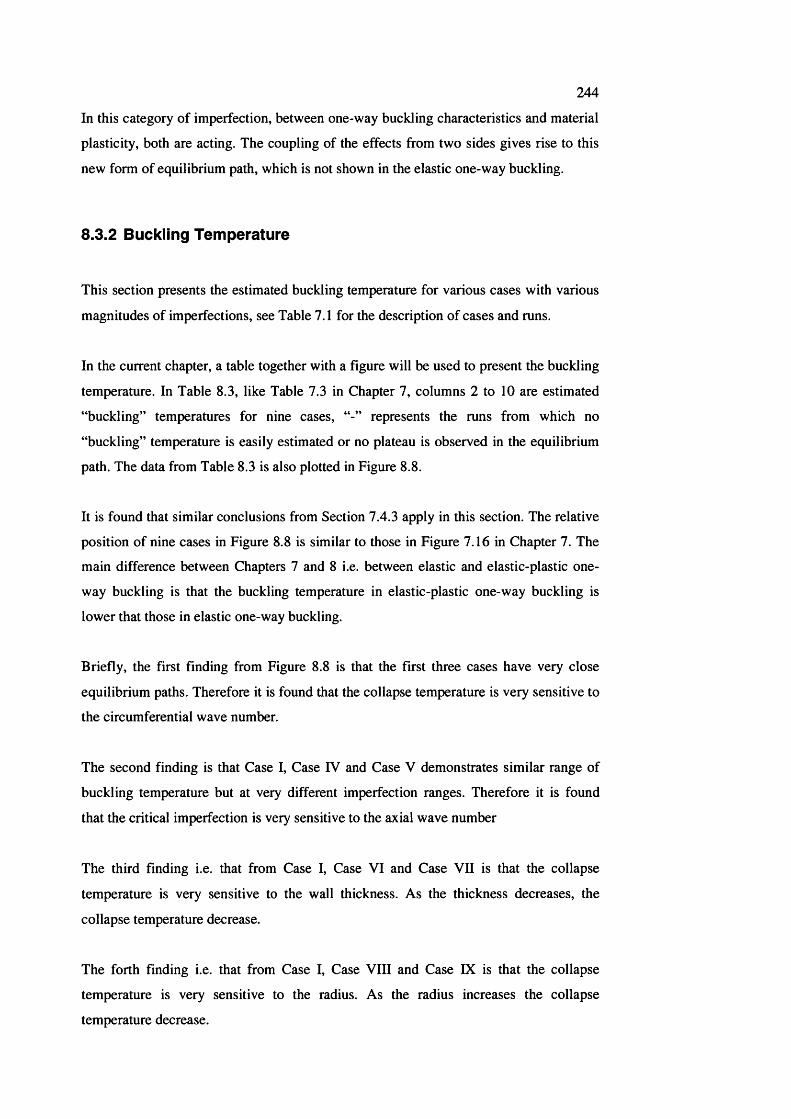
244

In this category of imperfection, between one-way buckling characteristics and material

plasticity, both are acting. The coupling of the effects from two sides gives rise to this

new form of equilibrium path, which is not shown in the elastic one-way buckling.

8.3.2 Buckling Tem perature

This section presents the estimated buckling temperature for various cases with various

magnitudes of imperfections, see Table 7.1 for the description of cases and runs.

In the current chapter, a table together with a figure will be used to present the buckling

temperature. In Table 8.3, like Table 7.3 in Chapter 7, columns 2 to 10 are estimated

“buckling” temperatures for nine cases, represents the runs from which no

“buckling” temperature is easily estimated or no plateau is observed in the equilibrium

path. The data from Table 8.3 is also plotted in Figure 8.8.

It is found that similar conclusions from Section 7.4.3 apply in this section. The relative

position of nine cases in Figure 8.8 is similar to those in Figure 7.16 in Chapter 7. The

main difference between Chapters 7 and 8 i.e. between elastic and elastic-plastic one

way buckling is that the buckling temperature in elastic-plastic one-way buckling is

lower that those in elastic one-way buckling.

Briefly, the first finding from Figure 8.8 is that the first three cases have very close

equilibrium paths. Therefore it is found that the collapse temperature is very sensitive to

the circumferential wave number.

The second finding is that Case I, Case IV and Case V demonstrates similar range of

buckling temperature but at very different imperfection ranges. Therefore it is found

that the critical imperfection is very sensitive to the axial wave number

The third finding i.e. that from Case I, Case VI and Case VII is that the collapse

temperature is very sensitive to the wall thickness. As the thickness decreases, the

collapse temperature decrease.

The forth finding i.e. that from Case I, Case VIII and Case IX is that the collapse

temperature is very sensitive to the radius. As the radius increases the collapse

temperature decrease.

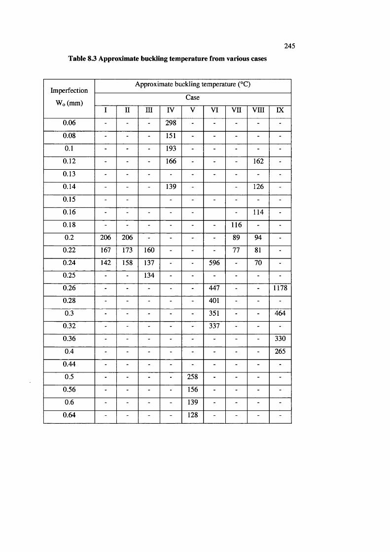
Table S3 Approximate buckling temperature from various cases

245

Imperfection

Wo (mm)

Approximate buckling temperature (°C)

Case

I II m IV V VI vn vm DC

0.06 - - - 298 - - - - -

0.08 - - - 151 - - - - -

0.1 - - - 193 - - - - -

0.12 - - - 166 - - - 162 -

0.13 - - - - - - - - -

0.14 - - - 139 - - 126 -

0.15 - - - - - - - -

0.16 - - - - - - 114 -

0.18 - - - - - - 116 - -

0.2 206 206 - - - - 89 94 -

0.22 167 173 160 - - - 77 81 -

0.24 142 158 137 - - 596 - 70 -

0.25 - - 134 - - - - - -

0.26 - - - - - 447 - - 1178

0.28 - - - - - 401 - - -

0.3 - - - - - 351 - - 464

0.32 - - - - - 337 - - -

0.36 - - - - - - - - 330

0.4 - - - - - - - - 265

0.44 - - - - - - - - -

0.5 - - - - 258 - - - -

0.56 - - - - 156 - - - -

0.6 - - - - 139 - - - -

0.64 - - - - 128 - - - -

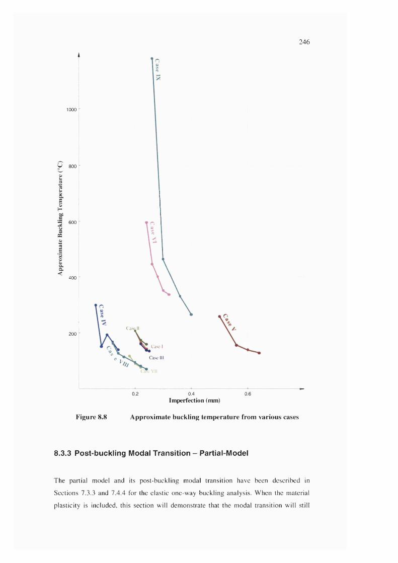
246

1000

y 800

tB2K1

H0£

3 600

nBes.12â<

400

200C ase II

Case I

Case III


0.6


8.3.3 Post-buckling Modal Transition - Partial-Model

The partial model and its post-buckling modal transition have been described in

Sections 7.3.3 and 7.4.4 for the elastic one-w ay buckling analysis. W hen the m aterial

plasticity is included, this section will dem onstrate that the modal transition will still

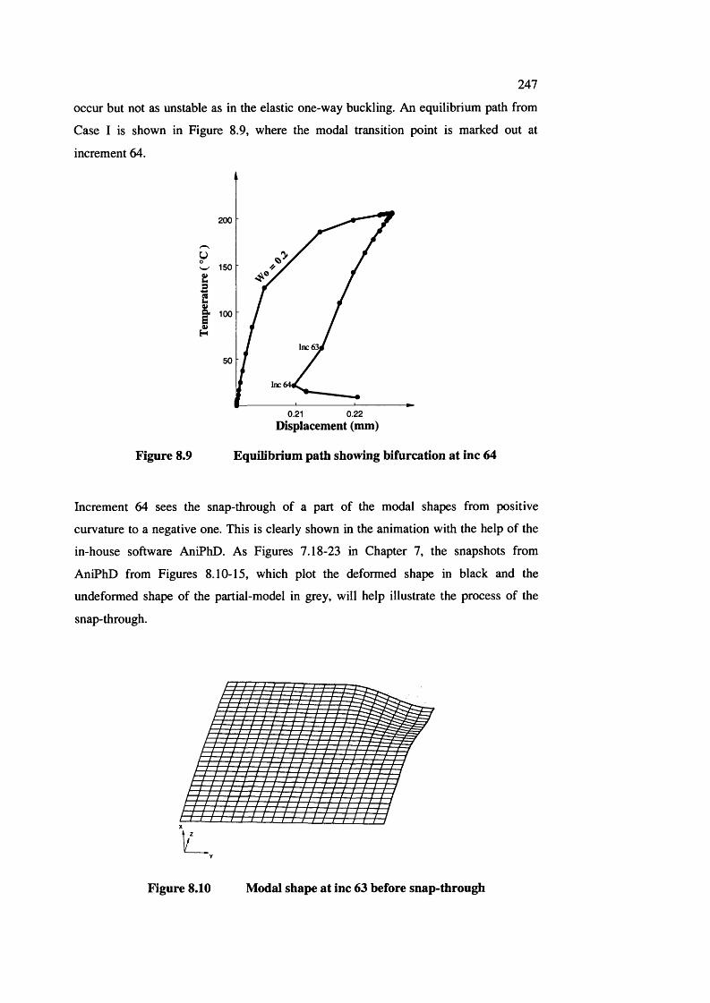
247

occur but not as unstable as in the elastic one-way buckling. An equilibrium path from

Case I is shown in Figure 8.9, where the modal transition point is marked out at

increment 64.

200

Uw 150

II 100I

Inc 63,

Inc

0.21 0.22

Figure 8.9

Displacement (mm)

Equilibrium path showing bifurcation at inc 64

Increment 64 sees the snap-through of a part of the modal shapes from positive

curvature to a negative one. This is clearly shown in the animation with the help of the

in-house software AniPhD. As Figures 7.18-23 in Chapter 7, the snapshots from

AniPhD from Figures 8.10-15, which plot the deformed shape in black and the

undeformed shape of the partial-model in grey, will help illustrate the process of the

snap-through.

Figure 8.10 Modal shape at inc 63 before snap-through

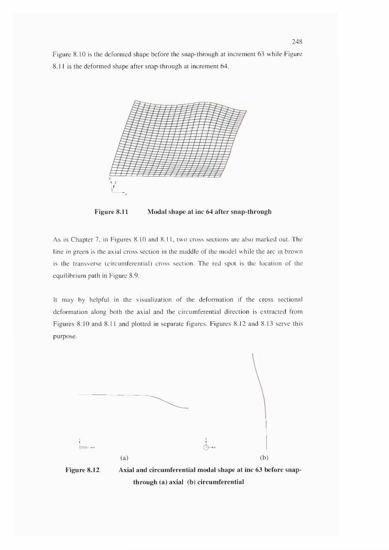
248

Figure 8.10 is the deform ed shape before the snap-through at increm ent 63 while F igure

8.11 is the deform ed shape after snap-through at increm ent 64.

Figure 8.11 Modal shape at inc 64 after snap-through

As in C hapter 7, in Figures 8.10 and 8.11, tw o cross sections are also m arked out. The

line in green is the axial cross section in the m iddle of the model w hile the arc in brown

is the transverse (circum ferential) cross section. The red spot is the location o f the

equilibrium path in Figure 8.9.

It may by helpful in the visualization o f the deform ation if the cross sectional

deform ation along both the axial and the circum ferential direction is extracted from

F igures 8.10 and 8.11 and plotted in separate figures. Figures 8.12 and 8.13 serve this

purpose.

u

Figure 8.12

(a) (b)

Axial and circumferential modal shape at inc 63 before snap-

through (a) axial (b) circumferential

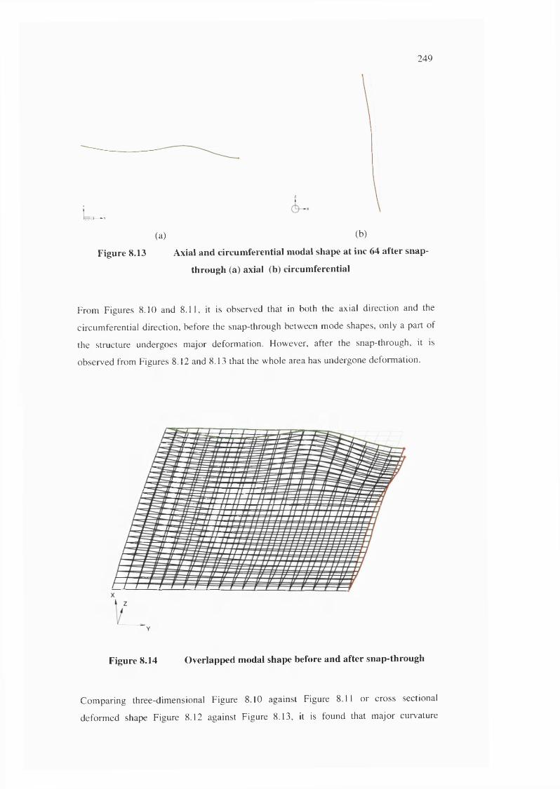
249

U ,

(a) (b)

Figure 8.13 Axial and circumferential modal shape at inc 64 after snap-

through (a) axial (b) circumferential

From Figures 8.10 and 8.11, it is observed that in both the axial direction and the

circum ferential direction, before the snap-through betw een m ode shapes, only a part of

the structure undergoes m ajor deform ation. How ever, after the snap-through, it is

observed from Figures 8.12 and 8.13 that the whole area has undergone deform ation.


C om paring three-dim ensional Figure 8.10 against Figure 8.11 or cross sectional

deform ed shape Figure 8.12 against Figure 8.13, it is found that m ajor curvature

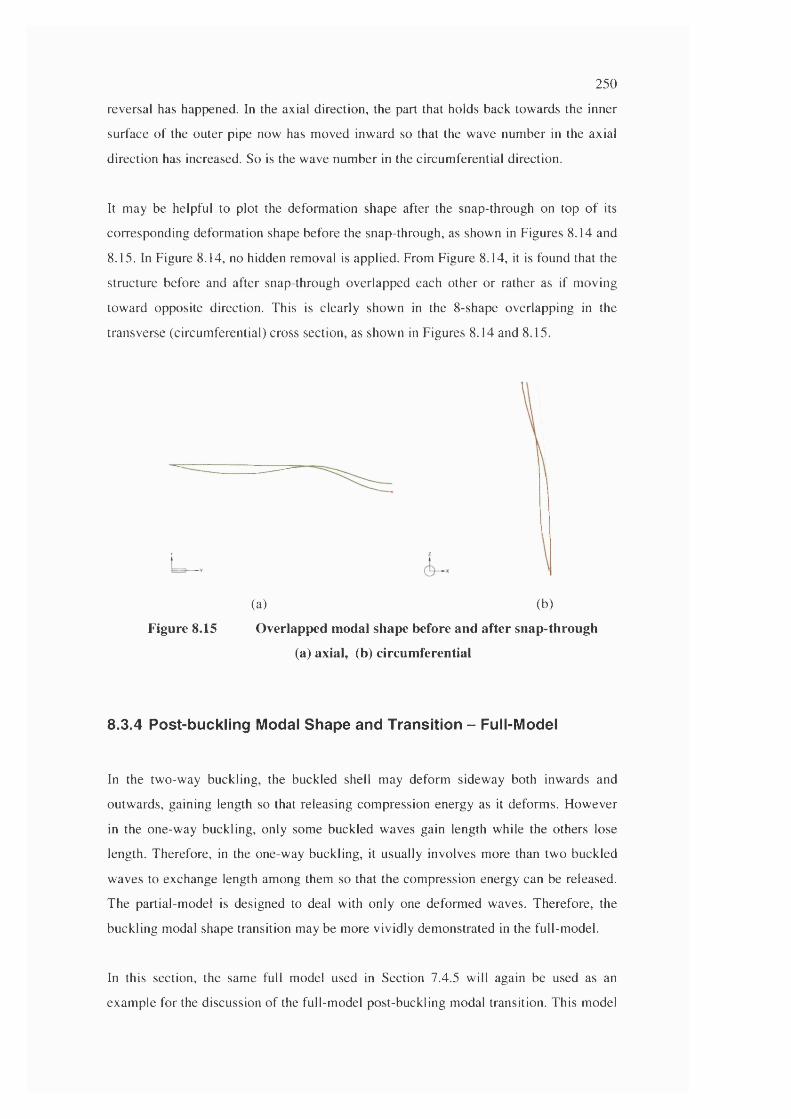
250

reversal has happened. In the axial direction, the part that holds back tow ards the inner

surface o f the outer pipe now has m oved inw ard so that the wave num ber in the axial

direction has increased. So is the wave num ber in the circum ferential direction.

It m ay be helpful to plot the deform ation shape after the snap-through on top o f its

corresponding deform ation shape before the snap-through, as show n in Figures 8.14 and

8.15. In Figure 8.14, no hidden removal is applied. From Figure 8.14, it is found that the

structure before and after snap-through overlapped each other or rather as if m oving

tow ard opposite direction. This is clearly show n in the 8-shape overlapping in the

transverse (circum ferential) cross section, as show n in Figures 8.14 and 8.15.

(a) (b)


(a) axial, (b) circumferential

8.3.4 Post-buckling Modal Shape and Transition - Full-Model

In the tw o-w ay buckling, the buckled shell may deform sidew ay both inwards and

outw ards, gaining length so that releasing com pression energy as it deform s. H ow ever

in the one-w ay buckling, only some buckled waves gain length while the others lose

length. Therefore, in the one-way buckling, it usually involves more than tw o buckled

w aves to exchange length among them so that the com pression energy can be released.

The partial-m odel is designed to deal with only one deform ed waves. Therefore, the

buckling modal shape transition may be more vividly dem onstrated in the full-m odel.

In this section, the sam e full model used in Section 7.4.5 will again be used as an

exam ple for the discussion o f the full-m odel post-buckling modal transition. This model

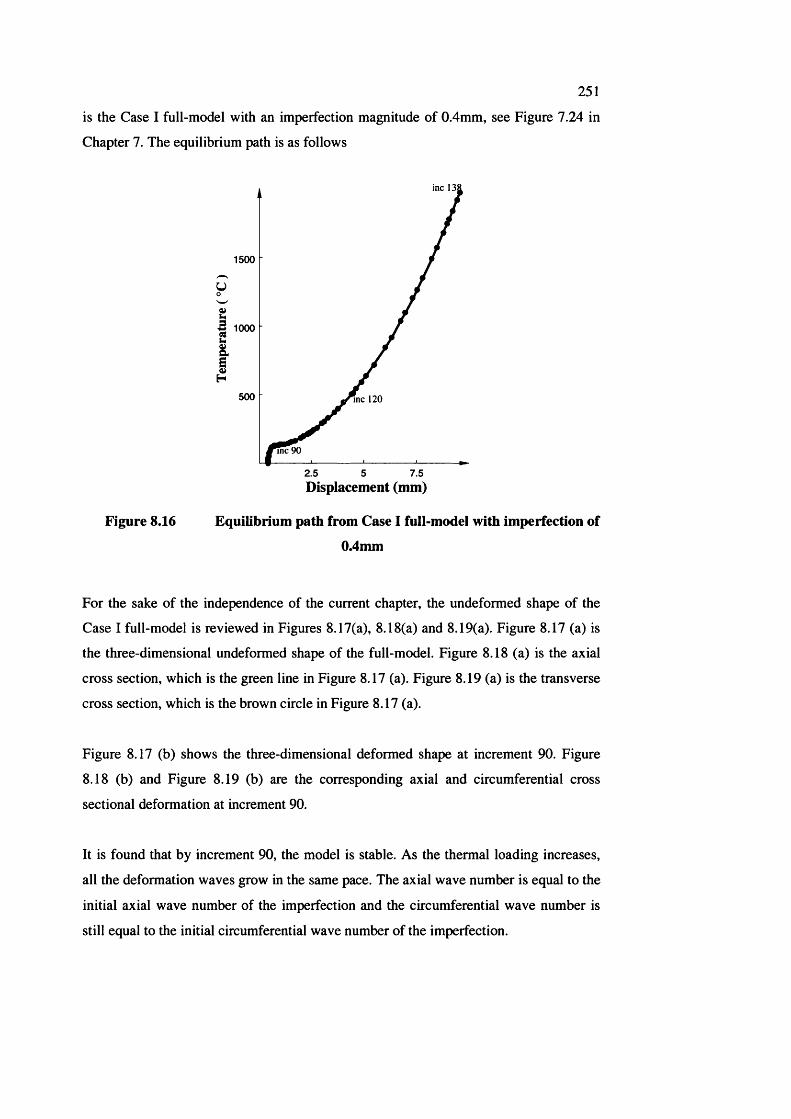
251is the Case I full-model with an imperfection magnitude of 0.4mm, see Figure 7.24 in

Chapter 7. The equilibrium path is as follows

inc 131

1500

y

500 me 120

me 90

2.5 5 7.5Displacement (mm)

Figure 8.16 Equilibrium path from Case I full-model with imperfection of

0.4mm

For the sake of the independence of the current chapter, the undeformed shape of the

Case I full-model is reviewed in Figures 8.17(a), 8.18(a) and 8.19(a). Figure 8.17 (a) is

the three-dimensional undeformed shape of the full-model. Figure 8.18 (a) is the axial

cross section, which is the green line in Figure 8.17 (a). Figure 8.19 (a) is the transverse

cross section, which is the brown circle in Figure 8.17 (a).

Figure 8.17 (b) shows the three-dimensional deformed shape at increment 90. Figure

8.18 (b) and Figure 8.19 (b) are the corresponding axial and circumferential cross

sectional deformation at increment 90.

It is found that by increment 90, the model is stable. As the thermal loading increases,

all the deformation waves grow in the same pace. The axial wave number is equal to the

initial axial wave number of the imperfection and the circumferential wave number is

still equal to the initial circumferential wave number of the imperfection.

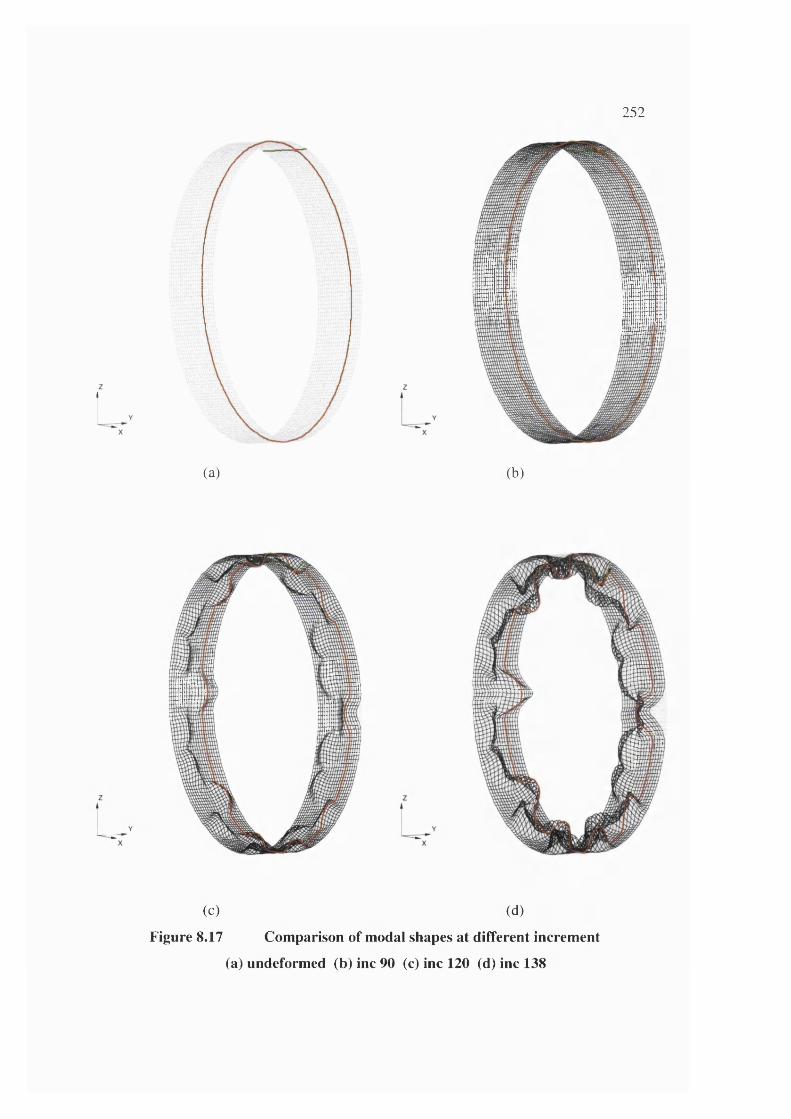
252

(a) (b)

(c) (d)

Figure 8.17 Comparison of modal shapes at different increment

(a) undeformed (b) inc 90 (c) inc 120 (d) inc 138

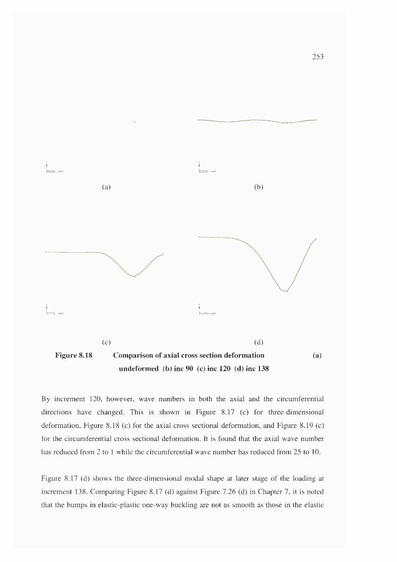
253

(a) (b)

u

(c) (d)

Figure 8.18 Comparison of axial cross section deformation

undeformed (b) inc 90 (c) inc 120 (d) inc 138

(a)

By increment 120, however, wave numbers in both the axial and the circumferential

directions have changed. This is shown in Figure 8.17 (c) for three-dimensional

deformation. Figure 8.18 (c) for the axial cross sectional deformation, and Figure 8.19 (c)

for the circumferential cross sectional deformation. It is found that the axial wave number

has reduced from 2 to 1 while the circumferential wave number has reduced from 25 to 10.

Figure 8.17 (d) shows the three-dimensional modal shape at later stage of the loading at

increment 138. Comparing Figure 8.17 (d) against Figure 7.26 (d) in Chapter 7, it is noted

that the bumps in elastic-plastic one-way buckling are not as smooth as those in the elastic

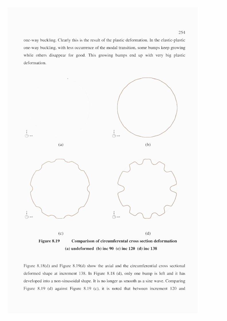
254

one-way buckling. Clearly this is the result of the plastic deformation. In the elastic-plastic

one-way buckling, with less occurrence of the modal transition, some bumps keep growing

while others disappear for good. This growing bumps end up with very big plastic

deformation.

(a) (b)

ko (d)

Figure 8.19 Comparison of circumferental cross section deformation

(a) undeformed (b) inc 90 (c) inc 120 (d) inc 138

Figure 8.18(d) and Figure 8.19(d) show the axial and the circumferential cross sectional

deformed shape at increment 138. In Figure 8.18 (d), only one bump is left and it has

developed into a non-sinusoidal shape. It is no longer as smooth as a sine wave. Comparing

Figure 8.19 (d) against Figure 8.19 (c), it is noted that between increment 120 and

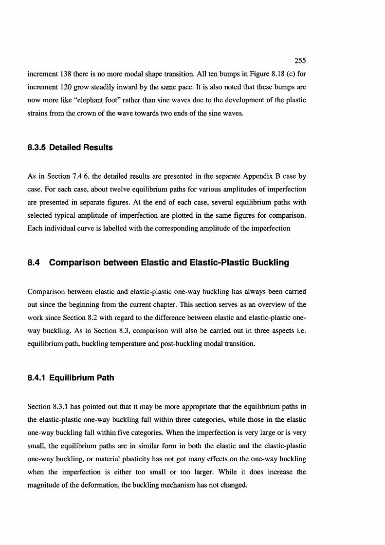
255

increment 138 there is no more modal shape transition. All ten bumps in Figure 8.18 (c) for

increment 120 grow steadily inward by the same pace. It is also noted that these bumps are

now more like “elephant foot” rather than sine waves due to the development o f the plastic

strains from the crown of the wave towards two ends o f the sine waves.

8.3.5 Detailed R esu lts

As in Section 7.4.6, the detailed results are presented in the separate Appendix B case by

case. For each case, about twelve equilibrium paths for various amplitudes o f imperfection

are presented in separate figures. At the end of each case, several equilibrium paths with

selected typical amplitude o f imperfection are plotted in the same figures for comparison.

Each individual curve is labelled with the corresponding amplitude o f the imperfection

8.4 Comparison between Elastic and Elastic-Plastic Buckling

Comparison between elastic and elastic-plastic one-way buckling has always been carried

out since the beginning from the current chapter. This section serves as an overview of the

work since Section 8.2 with regard to the difference between elastic and elastic-plastic one

way buckling. As in Section 8.3, comparison will also be carried out in three aspects i.e.

equilibrium path, buckling temperature and post-buckling modal transition.


Section 8.3.1 has pointed out that it may be more appropriate that the equilibrium paths in

the elastic-plastic one-way buckling fall within three categories, while those in the elastic

one-way buckling fall within five categories. When the imperfection is very large or is very

small, the equilibrium paths are in similar form in both the elastic and the elastic-plastic

one-way buckling, or material plasticity has not got many effects on the one-way buckling

when the imperfection is either too small or too larger. W hile it does increase the

magnitude o f the deformation, the buckling mechanism has not changed.

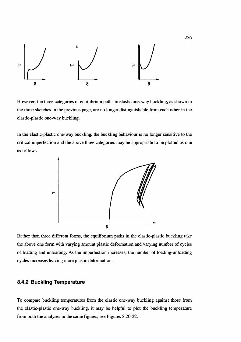
256

H

5

H

5

H

6

However, the three categories o f equilibrium paths in elastic one-way buckling, as shown in

the three sketches in the previous page, are no longer distinguishable from each other in the

elastic-plastic one-way buckling.

In the elastic-plastic one-way buckling, the buckling behaviour is no longer sensitive to the

critical imperfection and the above three categories may be appropriate to be plotted as one

as follows

H

5

Rather than three different forms, the equilibrium paths in the elastic-plastic buckling take

the above one form with varying amount plastic deformation and varying number o f cycles

o f loading and unloading. As the imperfection increases, the number of loading-unloading

cycles increases leaving more plastic deformation.

8.4.2 Buckling T em pera tu re

To compare buckling temperatures from the elastic one-way buckling against those from

the elastic-plastic one-way buckling, it may be helpful to plot the buckling temperature

from both the analyses in the same figures, see Figures 8.20-22.

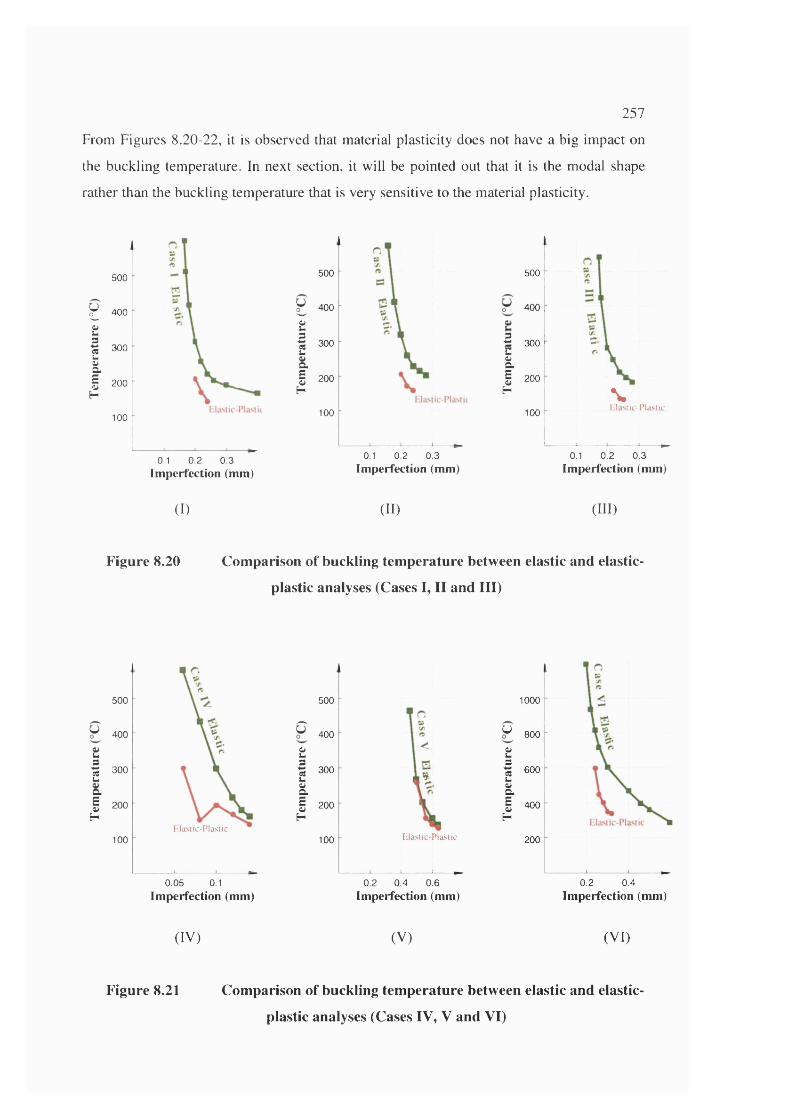
257

From Figures 8.20-22, it is observed that material plasticity does not have a big impact on

the buckling temperature. In next section, it will be pointed out that it is the modal shape

rather than the buckling temperature that is very sensitive to the material plasticity.

500

r 400

iI 300

II 200H

100

500

r 400

iI ^aI 200H

100

0.1 0.2 0.3Imperfection (mm)


B

II

500

400

300

200

100%Elastic-Pla.'.iic


(I) (II) (III)

Figure 8.20 Comparison of buckling temperature between elastic and elastic-

plastic analyses (Cases I, II and III)

k32Q.IH

500

400

300

200

100Elastic-Plastic


2322.SoH

500

400

300

200

100 Elastic-Plastic


1000

u

232

I800

600

400

200


(I)/) (V) ()/I)


plastic analyses (Cases IV, V and VI)

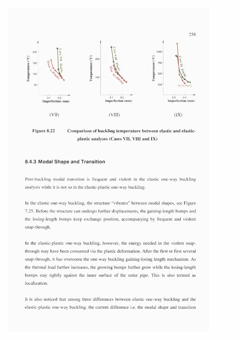
258

200

150

100

50

0.1 0.2 Imperfection (mm)

U

a

I

200

100

0.1 0.2 Im perfection (mm)

1000

gu9

II

500

250 [•lasiic-Pla'iic

0.2 0.4Im perfection (mm)

(VII) (VIII) (I)()


plastic analyses (Cases VII, VIII and IX)

8.4.3 Modal S hape and T ransition

Post-buckling modal transition is frequent and violent in the elastic one-way buckling

analysis while it is not so in the elastic-plastic one-way buckling.

In the elastic one-way buckling, the structure “vibrates” between modal shapes, see Figure

7.25. Before the structure can undergo further displacements, the gaining-length bumps and

the losing-length bumps keep exchange position, accompanying by frequent and violent

snap-through.

In the elastic-plastic one-way buckling, however, the energy needed in the violent snap-

through may have been consumed via the plastic deformation. After the first or first several

snap-through, it has overcome the one-way buckling gaining-losing length mechanism. As

the thermal load further increases, the growing bumps further grow while the losing-length

bumps stay tightly against the inner surface of the outer pipe. This is also termed as

localization.

It is also noticed that among three differences between elastic one-way buckling and the

elastic-plastic one-way buckling, the current difference i.e. the modal shape and transition

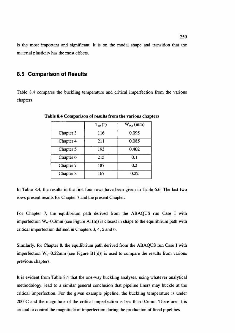
259is the most important and significant. It is on the modal shape and transition that the

material plasticity has the most effects.

8.5 Comparison of Results

Table 8.4 compares the buckling temperature and critical imperfection from the various

chapters.

Table 8.4 Comparison of results from the various chapters

T c r ( ° ) W ocr (mm)

Chapter 3 116 0.095

Chapter 4 211 0.085

Chapter 5 193 0.402

Chapter 6 215 0.1

Chapter 7 187 0.3

Chapter 8 167 0.22

In Table 8.4, the results in the fu*st four rows have been given in Table 6.6. The last two

rows present results for Chapter 7 and the present Chapter.

For Chapter 7, the equilibrium path derived from the ABAQUS run Case I with

imperfection W o=0.3mm (see Figure A 1(h)) is closest in shape to the equilibrium path with

critical imperfection defined in Chapters 3 , 4 , 5 and 6.

Similarly, for Chapter 8, the equilibrium path derived from the ABAQUS run Case I with

imperfection W o=0.22m m (see Figure B l(d )) is used to compare the results from various

previous chapters.

It is evident from Table 8.4 that the one-way buckling analyses, using whatever analytical

methodology, lead to a similar general conclusion that pipeline liners may buckle at the

critical imperfection. For the given example pipeline, the buckling temperature is under

200°C and the magnitude o f the critical imperfection is less than 0.5mm. Therefore, it is

crucial to control the magnitude o f imperfection during the production of lined pipelines.

260

8.6 Concluding Remarks

From the above analysis, the following are concluded

• The material plasticity has great affects on the post-buckling behaviour i.e. the

modal shape and the modal transition. When the material plasticity is considered,

the structure reaches stable state after one or several snap-through. After this stage,

the deformed bump will grow steadily while the other parts o f the structure hold

tightly against the inner surface o f the outer pipe.

• Collapse temperature in the elastic-plastic buckling o f pipeline liners is generally

lower than the corresponding collapse temperature in the elastic one-way buckling.

However, this effect is not as significant as those from the variation o f the

geometric parameters.

• In the elastic-plastic one-way buckling, it is no longer so sensitive to the magnitude

o f the imperfection. While it can never buckle when the imperfection is too small

and it is quite a stiffening structure when the imperfection is too large, for the most

intermediate imperfection, it “buckles” either before it yields or after it yields.

261

9 Summary, Conclusions, Recom mendations and Further Work

9.1 Summary

Sub-sea pipelines are sometimes required to convey fluids that are corrosive to the

carbon steel pipes. One cost-effective solution to this problem is the use of bi-metal

mechanically bonded pipelines. This involves inserting a thin CRA (corrosion resistant

alloy) shell of a slightly smaller radius into the host carbon steel pipe. Hydraulic

pressure is applied internally to expand both the inner liner and the host carbon steel

pipe well beyond the yielding of the CRA liner. Upon removal of the hydraulic

pressure, a mechanical bond between the inner liner and the outer pipe is formed.

When the lined pipe is in contact with fluids at high temperature, both axial and hoop

compressions are built up within the liner. Because the CRA liner is usually very thin,

from 1mm to 3mm, it tends to buckle under compressive loading. Furthermore, due to

its confinement by the outer pipe, the liner shell can only buckle inwards. This is termed

“one-way buckling” in the current thesis. The one-way buckling of the bi-metal,

mechanically bonded, pipeline liners is the topic of the current thesis.

The immediate difficulty with the one-way buckling analysis is the lack of directly

relevant past research in this subject. Firstly, bi-metal pipe lining is a relatively new

technology. The only available reference is the companion work (test work) of the

current research carried out by Walker et al. (1999,2000). In Chapters 1 and 2 of this

thesis, the author has collected and reviewed available information in many engineering

applications that are to some extent relevant to the topic, for example, municipal

underground pipeline liners and nuclear power plant pressure vessel liners. Secondly, to

the best knowledge of the author, the only available reference (Burgess, 1969) about the

one-way buckling phenomena is more than three decades old. This reference involves a

first generation theory that employed the discrete generalised coordinate approach,

which is not directly applicable to the current research on the shell, thermally-induced

one-way buckling. Previously published studies about the buckling of various liners

tend to ignore the fact that the liners can only deflect inwards. The most common

treatment of this constraint is to scale-up the free buckling load by an “enhancement

factor”, which is usually supported by experimental work. The other trend was to

262

assume a post-buckling deformed shape and derive the corresponding limit load. The

questions of whether this post-buckling state is stable and how the liner could deform

into the assumed shape were not even mentioned.

The second main part of the thesis was the development of analytical approaches. This

involved two phases. The first phase was aimed at understanding the underlying one

way buckling mechanism of the circular cylindrical shells by employing simplified

analysis. By simplified analysis using link models, the underlying physics of the

problem was identified while the mathematical work was greatly reduced. The first

phase was again divided into two steps. The first step involved the simplified rigid-link

model, which enabled answers to the fundamental question of whether a perfect pipeline

liner could buckle. The second step involved the simplified beam-link model, where the

findings from the first step were verified and the effects of the axial and circumferential

wave numbers were examined. The second phase involved the extension of analytical

work to the consideration of continuum models. This was also carried out in two steps.

The first step was the analysis with a liner-only continuum model where the one-way

buckling analysis was carried out with continuous imperfection and displacement

functions. The second step examined the effect of the sharing of the strain energy

between the outer pipe and the inner liner. In this main part of the work, the first phase

was set up to examine the basic one-way buckling physics and the second to provide

numerical results for the actual buckling temperatures. In both phases, the importance of

the imperfection to the one-way buckling was identified.

The third main part of the work was the finite element analysis. The finite element

analysis was carried out with ABAQUS. Two forms of model were established in the

process. The first is the full-model, which involves thousands of elements for the model

to develop the right number of waves in both the axial and circumferential directions.

The full-model is capable of capturing the modal transitions during the post-buckling

stage. To save the computer resources, a second type of model was developed. This is

termed the partial-model. Partial-model considers only a quarter of a single deformed

wave. Different partial-models were used for the prediction of different one-way

buckling behaviour for models with the prescribed wave numbers. The partial-model

was mainly used for the derivation of equilibrium paths for different imperfections with

various combinations of wave numbers; it was also used to perform parametric studies.

Both the full-model and partial-model used springs to simulate the constraint from the

host pipe. This third main part of the work is described in Chapters 7 and 8. Chapter 7

dealt with the numerical elastic buckling analysis while in Chapter 8 material non-

263

linearity was considered. The conclusions drawn from the above three main parts of the

work is given in Section 9.2.

9.2 C o n c lu s io n s a n d R eco m m en d a tio n s

The work undertaken in this study, and described in the preceding chapters, leads the

author to the following conclusions and recommendations:

• The analytical work reveals that the thermal buckling of the pipeline liners is

fundamentally different from normal two-way buckling in that the liners can

move only radially inwards and the available methodology of adopting the free-

shell buckling theory with enhancement factor is unable to recognize the

fundamental underlying one-way buckling mechanism. Literature review

concluded that the general one-way buckling theory (discrete generalised

coordinate approach) is not suitable for the constrained shell buckling. However,

the new one-way buckling theory proposed in the current study can now be

employed for any one-way buckling analysis of constrained circular cylindrical

shells.

• Analytical analyses from Chapters 3 to 6 have shown that the perfect pipeline

liner will never buckle. This is because the one-way buckling of the perfect liner

is not an eigenvalue problem. For any trivial transverse perturbation the first

variation of the total potential energy in the system is not automatically

stationary nor is it negative. In fact, for any trivial virtual allowable displacement

within the circular cylindrical boundary of the containment, the strain energy

increase in the perfectly circular cylindrical shell in the circumferential direction

is an order of magnitude greater than that in the axial direction. Therefore the

buckling temperature for the perfect liner is infinitely high. This conclusion

challenges the correctness of the finite buckling temperatures found for the

perfect NPP (nuclear power plant) pressure vessel liners in past work (see

Section 2.5.3).

• From the analytical analyses from Chapters 3 to 6, it is concluded that an

imperfection is of ultimate importance in the one-way buckling of circular

cylindrical shells. Indeed, an imperfection has to be considered in the one-way

buckling analysis from the very beginning to the end (in free buckling

imperfections are often only considered in the later stages to derive the

264

knockdown factor to the critical load). Actually, this is one of the main features

of the one-way buckling that is different from the free buckling. Without an

imperfection the perfect pipeline liner will never buckle. The way the

imperfection was incorporated throughout the current one-way buckling study

(three categories, wave numbers, square-sine function, etc) is recommended for

all the one-way buckling analyses in the future.

A circular cylindrical liner with the critical imperfection can buckle at the finite

buckling load even when contained within the rigid circular cylindrical

boundary. The critical imperfection corresponds to the special imperfection

profile where under allowable small virtual displacement the strain energy

increase in the circumferential direction is in balance with the strain energy

decrease in the axial direction so that the first variation of the total potential

energy is automatically zero. This critical imperfection does not correspond to an

arch type snap-through shape (where for link model the angle between two

circumferential links becomes 180° or for continuum model a part of the shell

becomes flat) nor is it the shape where the increase of the length in the axial

direction is equal to the decrease of the length in circumferential direction.

Rather, it corresponds to an imperfection profile at which the structure is

“transverse-movable” allowing the structure to be in an equilibrium state under

any small transverse disturbance. The critical imperfection is positive-definite so

that it always exists for any contained perfectly circular cylindrical shells. The

formulas for the critical imperfection are provided in Equations (3.62), (4.73),

(5.110) and (6.91) for choices among different analysis approaches.

In one-way buckling, when the imperfection is smaller than the critical

imperfection (sub-critical imperfection), including the case when the liner is a

perfectly circular cylinder, the liner will never buckle. When the imperfection is

sub-critical, the same mechanism as for the perfectly circular cylindrical liner

still applies in that it will not reach an equilibrium state under any small

transverse perturbation (the first variation of the total potential energy is still

positive). On the contrary, after the perturbation is removed, the liner shell will

return to its original position. In the design of lined pipes, it is recommended that

the imperfection be controlled strictly within the sub-critical category.

When the imperfection is larger than the critical imperfection (super-critical

imperfection), the deflection will increase from that of the imperfection.

265

Depending upon the extent to which the imperfection is greater than the critical

imperfection, the post-buckling behaviour will exhibit a peak or plateau or

trough load. In most cases, a peak load is also reached when modal transition

occurs. The lowest peak load is recommended as the design criteria for the

maximum operational load.

Based on the results from the analytical analysis for the typical pipeline liners,

the author recommends that during the conceptual design stage analytical one

way buckling analysis is carried out directly via stationary total potential energy

principle, regardless of whether the first variation of the total potential energy is

positive, zero or negative. That is to say, in the conceptual design stage, the

critical buckling load derived from the formula for the critical imperfection may

be used as the design load, regardless of whether the actual imperfection is sub-

critical or super-critical. Furthermore, because the critical imperfection is usually

small, the critical load formulation for the critical imperfection could be further

simplified by eliminating terms containing the imperfection (see the

simplification of Equations 4.58 and 6.92 with imperfection terms into Equations

4.59 and 6.93 without imperfection terms).

From the analytical approach it is concluded that there are three kinds of

equilibrium paths (temperature rise T versus total displacement w) corresponding

to the three categories of imperfection. All these three kinds of equilibrium paths

include two parts - a primary equilibrium path (with displacement offsetting

from the original position and the rigid boundary) and a complementary

equilibrium path (with displacement towards or staying within the rigid

boundary). For the critical imperfection, these two paths join continuously at the

critical bifurcation point with w=Wœr (critical imperfection) and T=Tcr (critical

load). For sub-critical imperfection, the primary equilibrium path starts from an

infinitely high temperature and thermal load drops as w increases. The primary

equilibrium path for sub-critical imperfection is unstable. The corresponding

complementary equilibrium path starts from w=Wq (the magnitude of the

imperfection) and thermal load rises as w decreases (deflect towards rigid

boundary). The complementary equilibrium path for sub-critical imperfection is

stable. For super-critical imperfection, the real equilibrium path starts from

w=Wo (the magnitude of the imperfection) and the thermal load increases as w

increases (deflects inward towards the central axis of the cylinder). This primary

equilibrium path for super-critical imperfection is stable. The corresponding

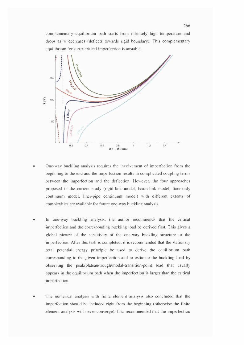
266com plem entary equilibrium path starts from infinitely high tem perature and

drops as w decreases (deflects tow ards rigid boundary). This com plem entary

equilibrium for super-critical im perfection is unstable.

150

100H

Li0.2 0.4 0.6 0.8 1.2 1.41

Wo + W (mm)

O ne-w ay buckling analysis requires the involvem ent o f im perfection from the

beginning to the end and the im perfection results in com plicated coupling term s

betw een the im perfection and the deflection. How ever, the four approaches

proposed in the current study (rigid-link m odel, beam -link m odel, liner-only

continuum model, liner-pipe continuum m odel) with different extents of

com plexities are available for future one-w ay buckling analysis.

In one-w ay buckling analysis, the author recom m ends that the critical

im perfection and the corresponding buckling load be derived first. This gives a

global picture o f the sensitivity o f the one-w ay buckling structure to the

im perfection. A fter this task is com pleted, it is recom m ended that the stationary

total potential energy principle be used to derive the equilibrium path

corresponding to the given im perfection and to estim ate the buckling load by

observing the peak/plateau/trough/m odal-transition-point load that usually

appears in the equilibrium path when the im perfection is larger than the critical

im perfection.

The num erical analysis with finite elem ent analysis also concluded that the

im perfection should be included right from the beginning (otherw ise the finite

elem ent analysis will never converge). It is recom m ended that the im perfection

267

be incorporated into the structure when the finite element model is being

developed. This is completely different from the finite element analysis of free

buckling that automatically generates the imperfection as a combination of

modal shapes. It is recommended that a simple analytical analysis with rigid-link

model be carried out to find out the approximate critical imperfection before the

actual finite element analysis so that the imperfection profile can be easily

introduced into the finite element model. Otherwise, it is recommended to run a

series of finite element analyses starting with very large imperfections and

gradually reducing their magnitudes until the approximate critical imperfection is

reached.

It is observed that the equilibrium paths from finite element numerical analysis

and those from analytical analysis are in similar forms. The only difference is in

the following three aspects. Firstly, the finite element numerical analysis is

capable of simulating the natural selection of wave numbers so that the modal

transition is usually observed in the corresponding equilibrium paths. Secondly,

springs are used in the finite element model to simulate the outer pipe, which is

capable of absorbing some of the strain energy. When the imperfection is smaller

(but not too small) than the critical imperfection, the presence of the membrane

strain energy in the springs in the pre-buckling stage changes the equilibrium

path for the sub-critical imperfection category slightly. Thirdly, the exact critical

imperfection cannot be captured in the finite element analysis simply because the

finite element model is made from discrete elements.

Based on the success of the spring model (and the non-success of the rigid

surface model) the author concludes that the best way to model one-way

buckling system in the finite element analysis is to use bi-linear springs to

simulate the confinement from the outer pipe to the inner liner. The springs are

so modelled that they exert no forces at all when in tension but huge compressive

forces when in compression. The current study found that these tiny compressive

strains in the springs are vital to the convergence of the one-way buckling system

when the thermal loading is approaching the buckling temperature.

From finite element numerical analysis, it is also concluded that that elastic one

way buckling of pipeline liners involves modal transition. The one-way buckling

could start with a combination of axial and circumferential wave numbers similar

to the initial imperfection wave numbers. As the pipeline liner deflects, the

268

developed bumps may feed materials to the neighbouring bumps so that the

wave numbers are changed and the system is picking up the best thermal load

shedding path. If no material plasticity is considered, when the thermal loading

reaches certain levels, the system will snap-through between modes very

frequently and dynamically.

• From the results of both the analytical analysis and finite element analysis in the

current study it is concluded that the one-way buckling of pipeline liners is very

sensitive to the axial wave number but not so sensitive to the circumferential

wave number. For the typical pipeline liner in the current study, while the axial

wave length is about 50mm and the variation of the circumferential wave

number is from 1 to 30, the buckling temperature varies within 10%. Therefore

circumferential wrinkles with various circumferential lengths could be developed

in the thermal buckling of pipeline liners. This is consistent with the observation

from the available test results.

• The author recommends that when the material plasticity has to be considered

finite element analysis be carried out (instead of analytical analysis). The

coupling of one-way buckling behaviour and the material plasticity involves the

complicated combination of buckling and the loading-unloading process. It is

concluded that the buckling of the pipeline liners could occur before or after the

material is in a plastic state, depending on the combination of the values of the

pipeline geometry and other material properties such as thermal expansion

coefficients. It is also concluded from the current study that the material

plasticity has not got a big impact on the buckling load but does have a

significant impact on the modal shapes and the modal transition. With material

plasticity, the snap-through between modes is less frequent. After the initial few

snap-through incidences, the pipeline liner tends to grow several bumps with

plastic deformation while the other bumps stay in their original position without

plastic deformation. As the thermal loading increases, the buckled bumps grow

with visible residual deformation as if it has been plastically formed.

• The parametric study from the current work concludes that the buckling

temperature of the pipeline liners is very sensitive to the wall thickness and the

mid-surface radius. Generally, the buckling temperatures increase as the wall

thickness increases or as the mid-surface radius decreases. However, the

parametric study needs further work which is described in Section 9.3.

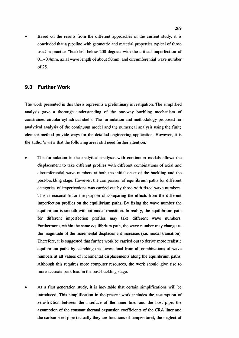
269

Based on the results from the different approaches in the current study, it is

concluded that a pipeline with geometric and material properties typical of those

used in practice “buckles” below 200 degrees with the critical imperfection of

0.1 ~0.4mm, axial wave length of about 50mm, and circumferential wave number

of 25.

9.3 F u rthe r W ork

The work presented in this thesis represents a preliminary investigation. The simplified

analysis gave a thorough understanding of the one-way buckling mechanism of

constrained circular cylindrical shells. The formulation and methodology proposed for

analytical analysis of the continuum model and the numerical analysis using the finite

element method provide ways for the detailed engineering application. However, it is

the author’s view that the following areas still need further attention:

• The formulation in the analytical analyses with continuum models allows the

displacement to take different profiles with different combinations of axial and

circumferential wave numbers at both the initial onset of the buckling and the

post-buckling stage. However, the comparison of equilibrium paths for different

categories of imperfections was carried out by those with fixed wave numbers.

This is reasonable for the purpose of comparing the effects from the different

imperfection profiles on the equilibrium paths. By fixing the wave number the

equilibrium is smooth without modal transition. In reality, the equilibrium path

for different imperfection profiles may take different wave numbers.

Furthermore, within the same equilibrium path, the wave number may change as

the magnitude of the incremental displacement increases (i.e. modal transition).

Therefore, it is suggested that further work be carried out to derive more realistic

equilibrium paths by searching the lowest load from all combinations of wave

numbers at all values of incremental displacements along the equilibrium paths.

Although this requires more computer resources, the work should give rise to

more accurate peak load in the post-buckling stage.

• As a first generation study, it is inevitable that certain simplifications will be

introduced. This simplification in the present work includes the assumption of

zero-friction between the interface of the inner liner and the host pipe, the

assumption of the constant thermal expansion coefficients of the CRA liner and

the carbon steel pipe (actually they are functions of temperature), the neglect of

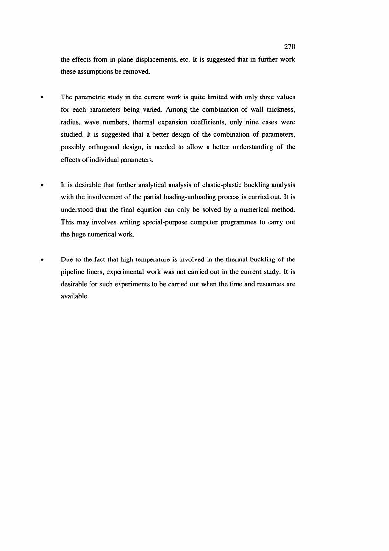
270

the effects from in-plane displacements, etc. It is suggested that in further work

these assumptions be removed.

The parametric study in the current work is quite limited with only three values

for each parameters being varied. Among the combination of wall thickness,

radius, wave numbers, thermal expansion coefficients, only nine cases were

studied. It is suggested that a better design of the combination of parameters,

possibly orthogonal design, is needed to allow a better understanding of the

effects of individual parameters.

It is desirable that further analytical analysis of elastic-plastic buckling analysis

with the involvement of the partial loading-unloading process is carried out. It is

understood that the final equation can only be solved by a numerical method.

This may involves writing special-purpose computer programmes to carry out

the huge numerical work.

Due to the fact that high temperature is involved in the thermal buckling of the

pipeline liners, experimental work was not carried out in the current study. It is

desirable for such experiments to be carried out when the time and resources are

available.

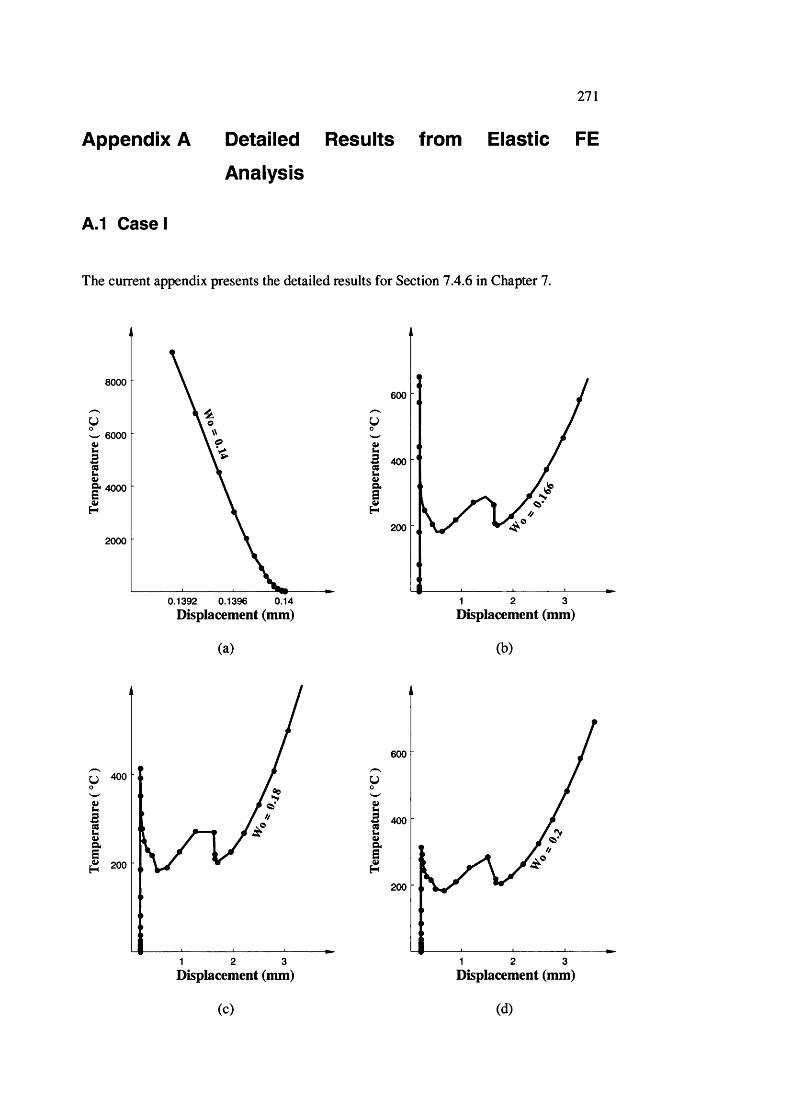
271

Appendix A Detailed Results from Elastic FE

Analysis

A.1 C a se I

The current appendix presents the detailed results for Section 7.4.6 in Chapter 7.

8000

w 6000

g- 4000

2000

0.140.1392 0.1396Displacement (mm)

(a)

600

■2 400

200

1 2 3Displacement (mm)

(b)

400

1 2 3

600

B 400

200

1 2 3Displacement (mm) Displacement (mm)

(c) (d)

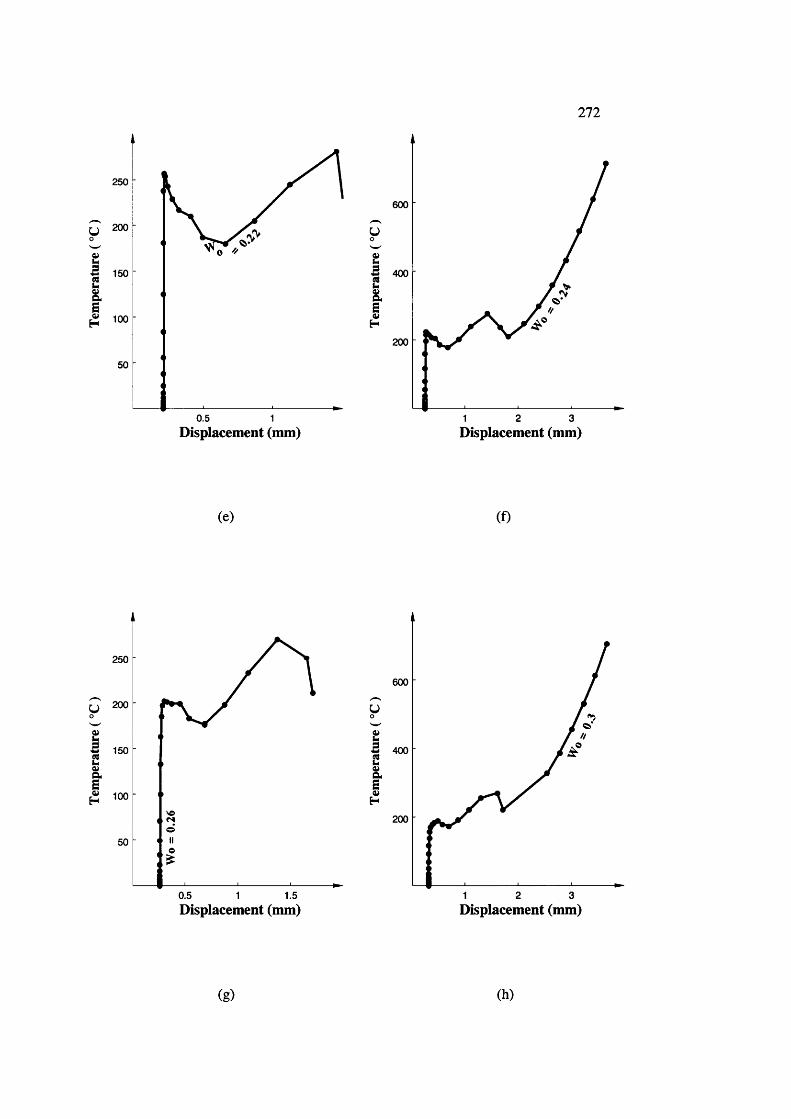
272

250

y 200

50

0.5 1

600

U

1200

2 31Displacement (mm) Displacement (mm)

(e) (f)

250

y 200

s

0.5 1 1.5

600

y

Is 400

I200


(g) (h)

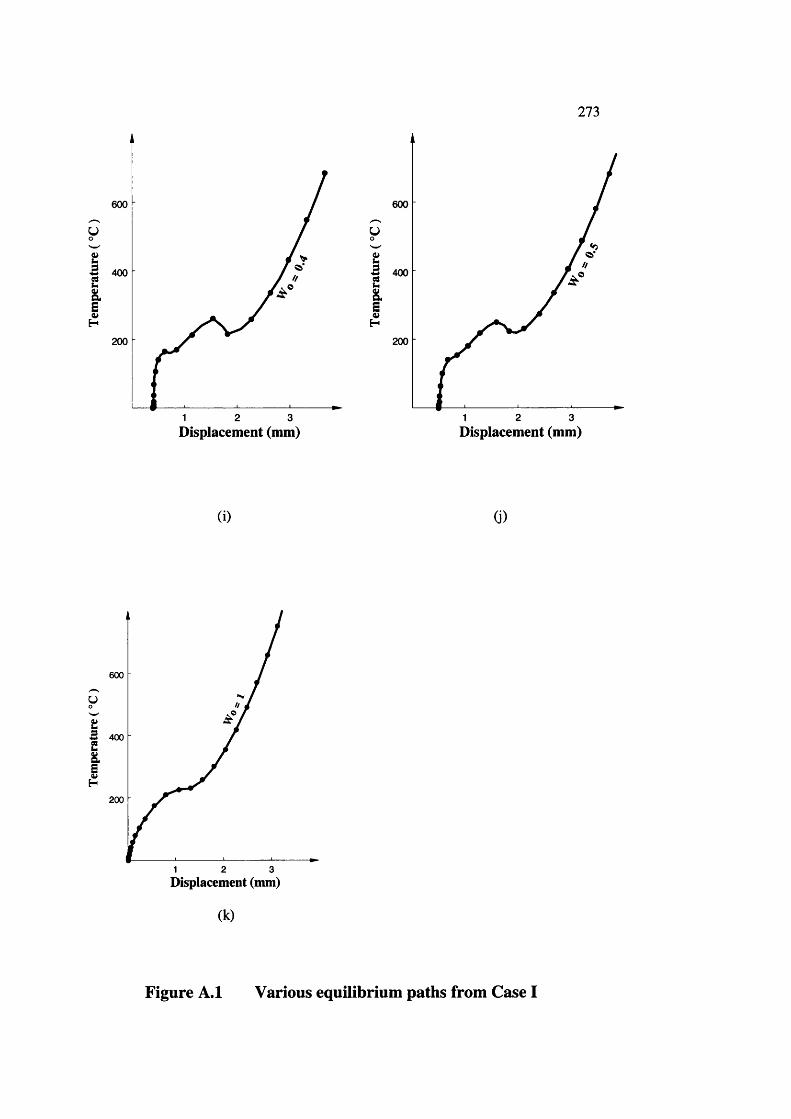
273

600

U

(200

1 2 3

600

y

1200


(i) (i)

600

200


(k)

Figure A.1 Various equilibrium paths from Case I

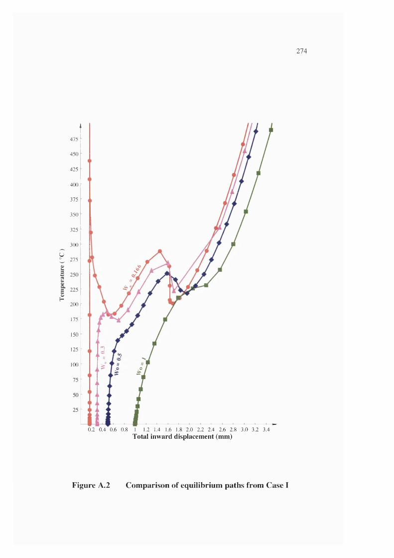
274

475

4 5 0

425

4 0 0

375

350

325

300

U275 ^

Ii

H200

175

150

125

100

0.2 0 .4 0 .6 0 .8 1 1.2 1.4 1.6 1.8 2 .0 2 .2 2 .4 2 .6 2 .8 3 .0 3 .2 3 .4


Figure A.2 Comparison of equilibrium paths from Case I

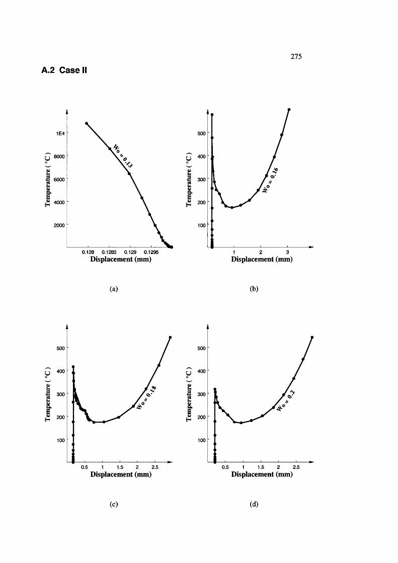
275

A.2 Case II

1E4

8000

B 6000

4000

2000

0.128 0.1285 0.129 0.1295

500

? ^

I3 300

^ 200

100


(a) (b)

500

I3 300

H 200

100

0.5 2 2.51 1.5

500

y 400

I3 300

iH 200

100

0.5 1 1.5 2 2.5

Displacement (mm) Displacement (mm)

(c) (d)

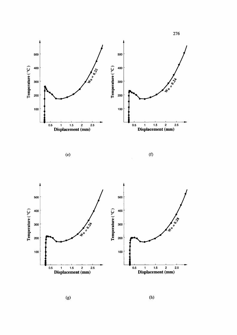
116

500

100

2.50.5 1 1.5 2

500

15 300

H 200

100

2 2.51.50.5 1Displacement (mm) Displacement (mm)

(e) (f)

500

I5 300IH 200

100

2.50.5 1.5 21

500

? ^«I_ 300I

200

100

2 2.51.50.5 1Displacement (mm) Displacement (mm)

(g) (h)

I l l

500

100

0.5 1 1.5 2 2.5

500

I5 300

^ 200

100

0.5 1 1.5 2 2.5Displacement (mm) Displacement (mm)

(i) (j)

700

600

uo 5 0 0

(200

100

0.5 1 1.5 2 2.5 3

800

600

& 400

200

1 2 3 4Displacement (mm) Displacement (mm)

(k) (1)

Figure A 3 Various equilibrium paths from Case II

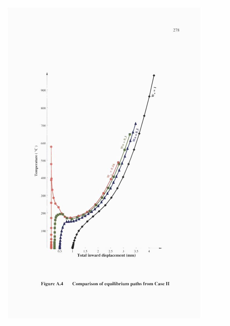
278

9 0 0

80 0 ^

700

6 0 0 ^

u

I ' 1iEH I

4 0 0

300

200

100

0.5 1.5 2 2.5 3 3.5 4Total inward displacement (mm)

Figure A 4 Comparison of equilibrium paths from Case II

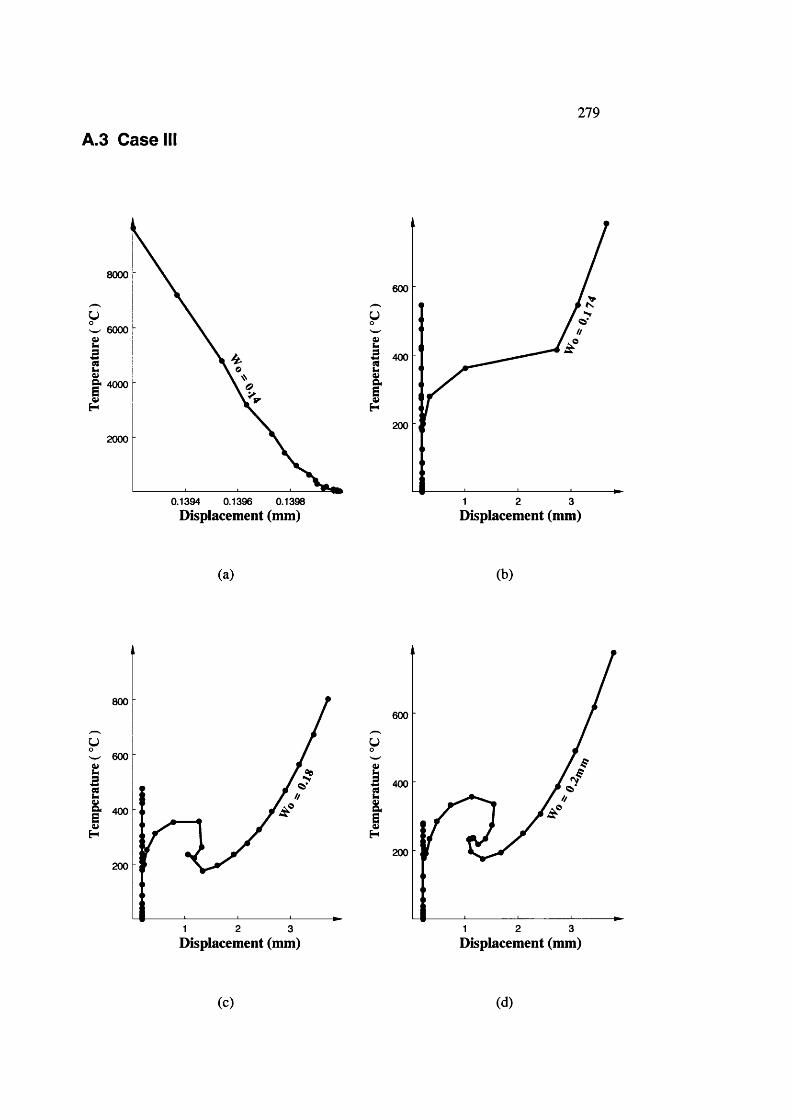
279

A 3 Case III

8000

6000

2000

0.1394 0.1396 0.1398

600

u

1200

1 2 3


(a) (b)

800

uW 600

I 400

H

200

1 2 3

600

y

IS 400

I200


(c) (d)

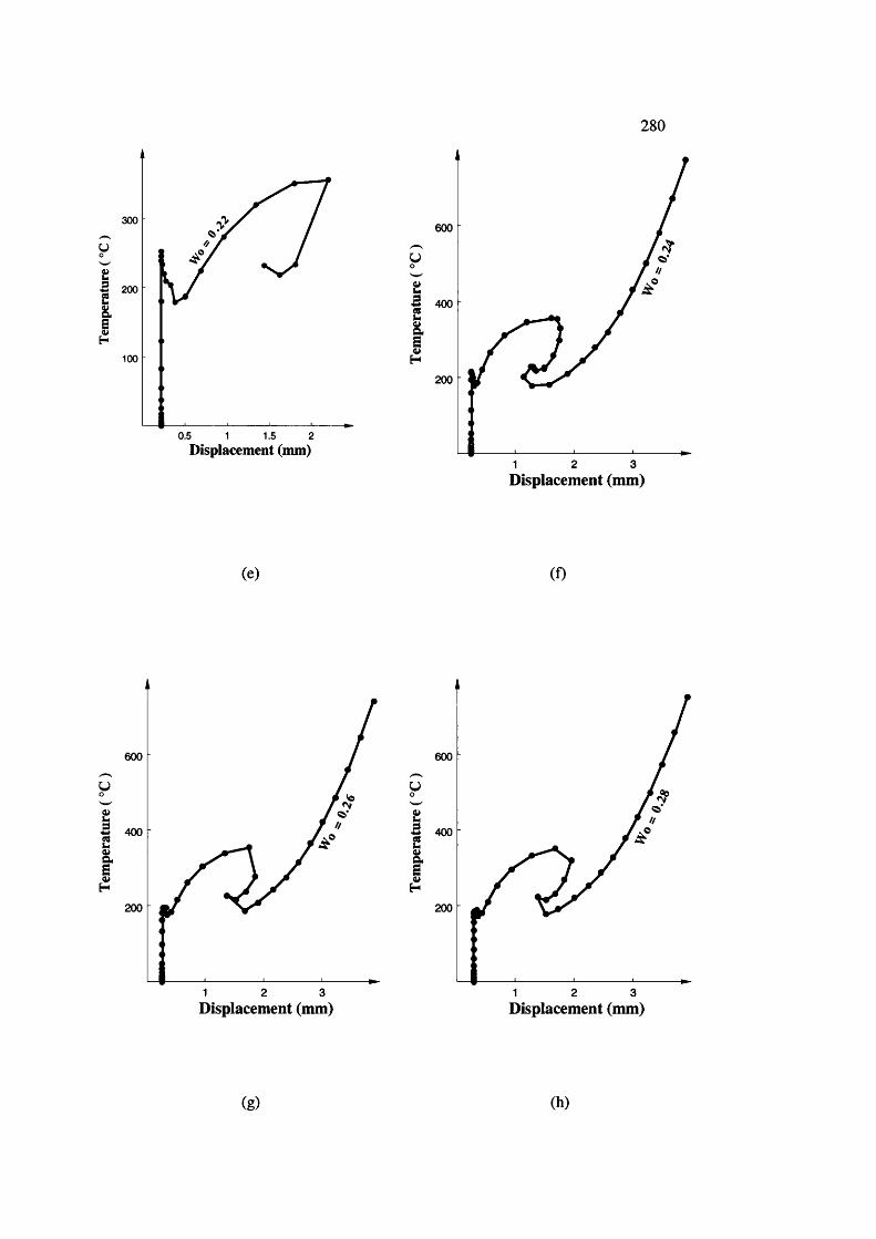
280

300

■a 200

100

0.5 1 1.5 2Displacement (mm)

600

y

IS 400

Î200

2 31Displacement (mm)

(e) (f)

600

-w 400

200

31 2

600

I 400

I200

1 2 3


(g) (h)

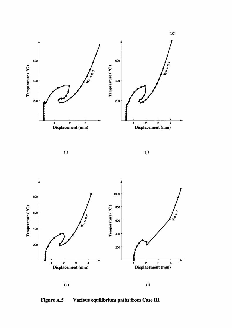
281

600

U

I200

31 2

600

U

1200


(i) (i)

800

600

& 400

200

31 2 4

I1000

800

600

400

200


(k) (1)

Figure A.5 Various equilibrium paths from Case III

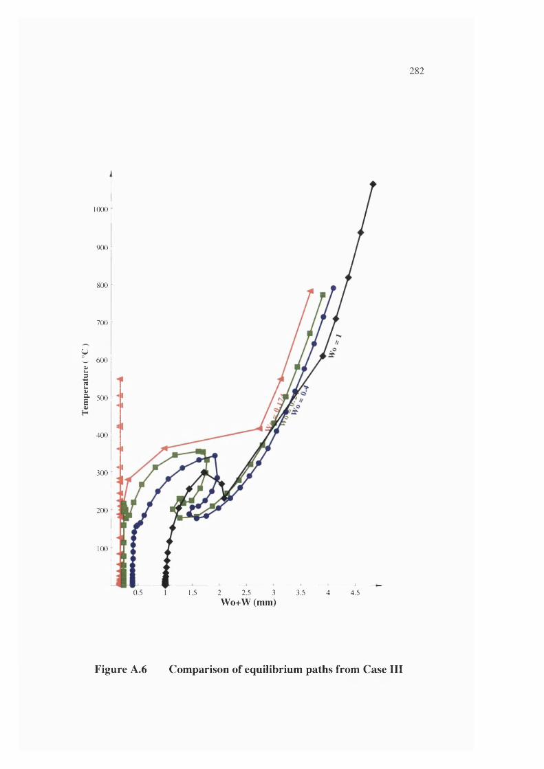
282

1000

900 r

800

700 ‘

UL 600 t3

2%g" 500:

400 ^

300

200

100

0.5 1.5 2 2.5 3 3.5 4.54Wo+W (mm)

Figure A.6 Comparison of equilibrium paths from Case III

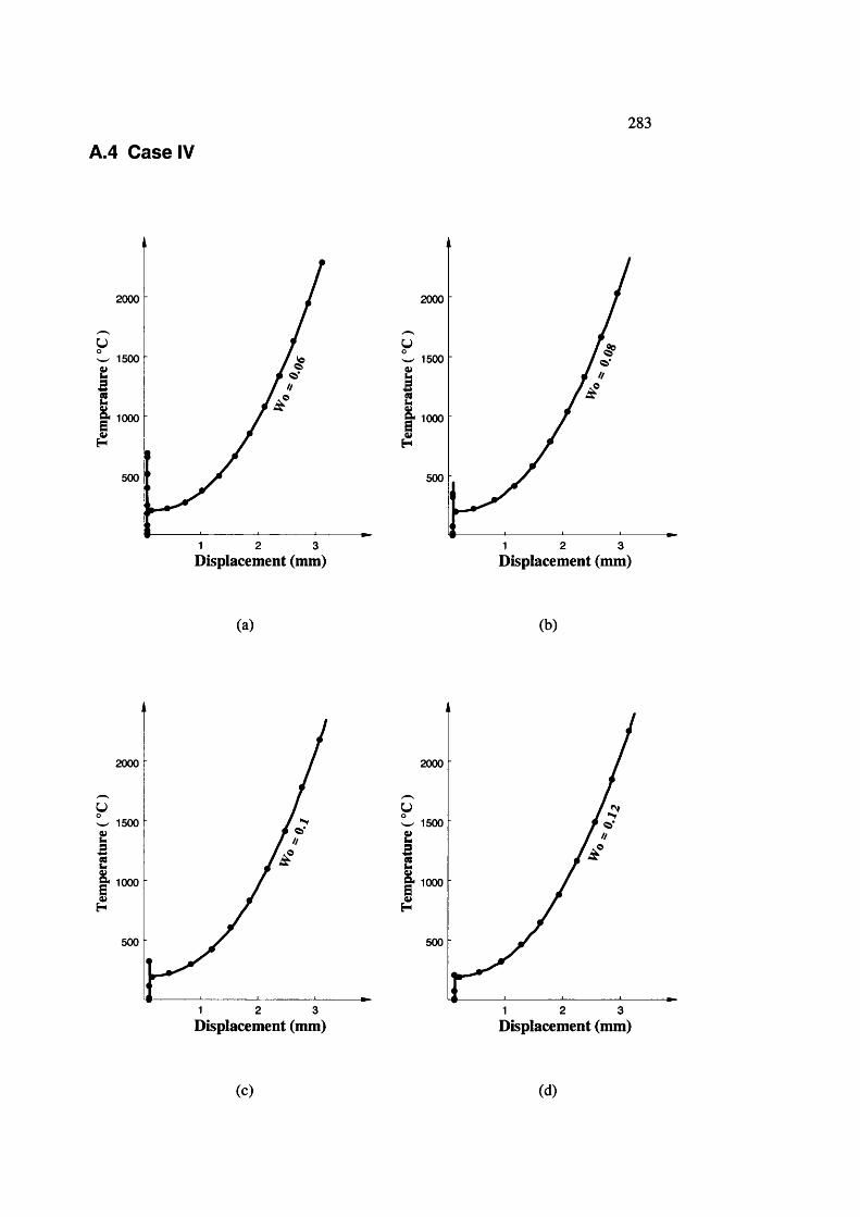
283A.4 Case IV

2000

UW 1500

Ig- 1000I

500

1 2 3

2000

1500

S- 1000

500

1 2 3


(a) (b)

2000

uW 1500

I& 1000

I500

1 2 3

2000

uW 1500

Ig- 1000

I500

2 31Displacement (nun) Displacement (mm)

(c) (d)

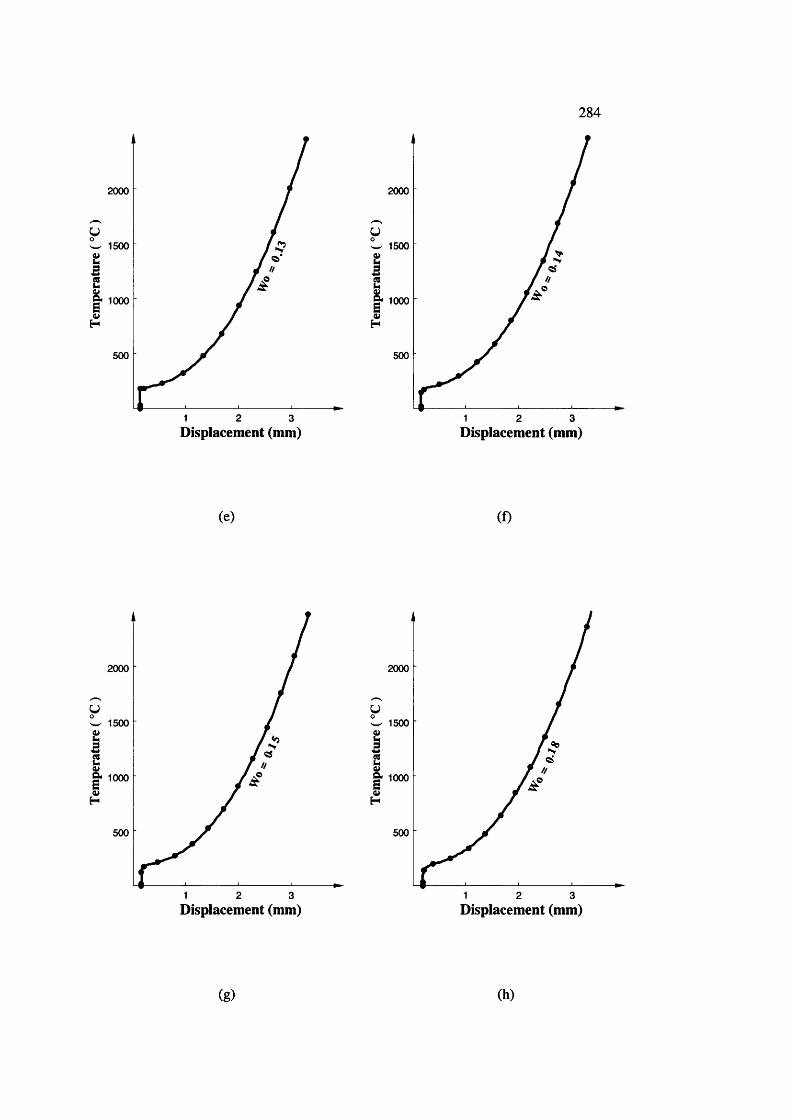
284

U

I2000

1500

1000

500

1 2 3

U

(

2000

1500

1000

500


(e) (f)

2000

1500

S- 1000

500

1 2 3

2000

1500

9 * 1000

500


(g) (h)

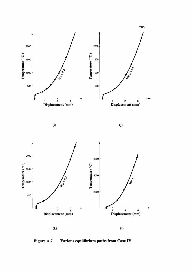
285

U

I2000

1500

1000

500

2 31

2000

UW 1500

ig- 1000I

500


(i) (j)

2000

1500

g* 1000

500

2 31

6000

B 4000

2000


(k) (1)

Figure A.7 Various equilibrium paths from Case IV

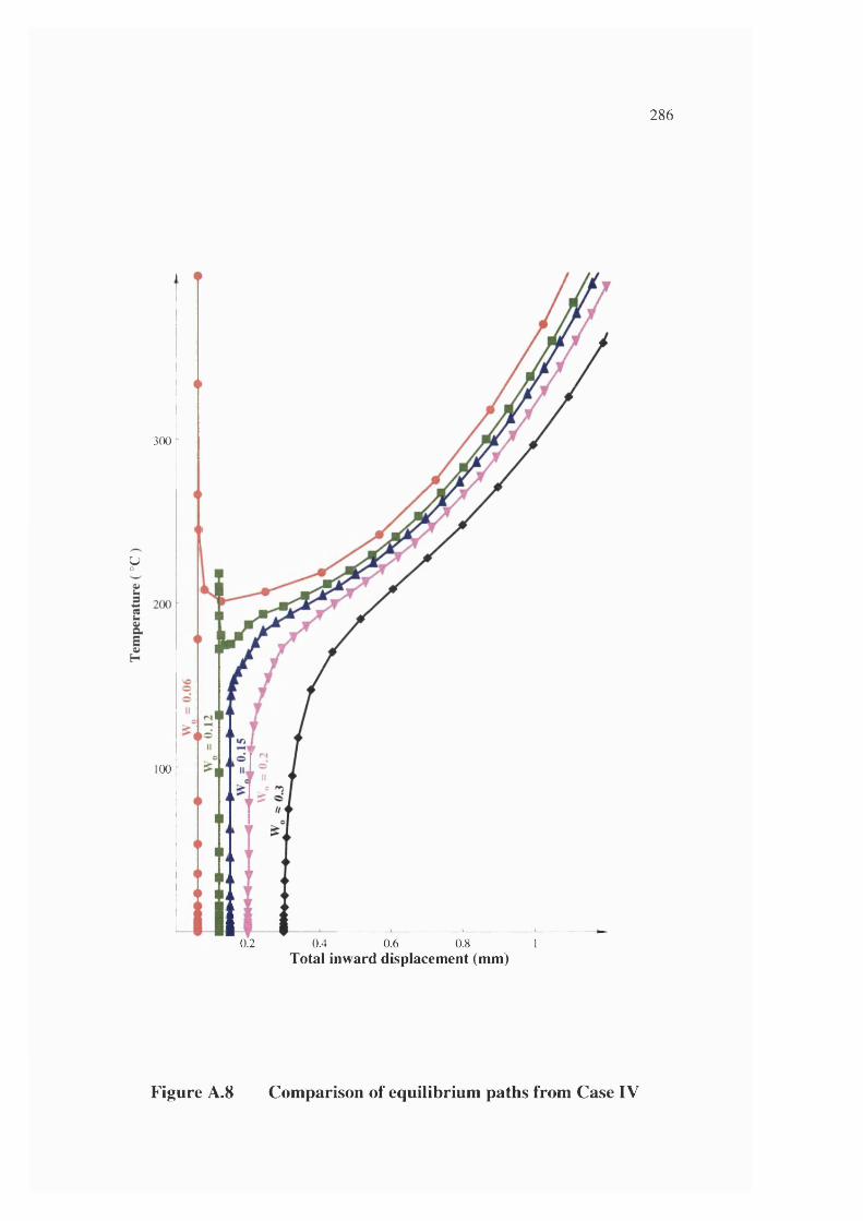
286

300

y

100

0.2 0.4Total inward displacement (mm)

0.6 0.8 1

Figure A.8 Comparison of equilibrium paths from Case IV

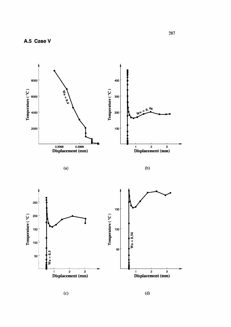
287

A.5 Case V

8000

6000

a 4000

2000

0.3998 0.3999

Displacement (mm)

400

300

_ 0.g- 200 o 1

100

1 2 3

Displacement (mm)

(a) (b)

250

y 200

1 2 3

150

u

!1 2 3


(c) (d)

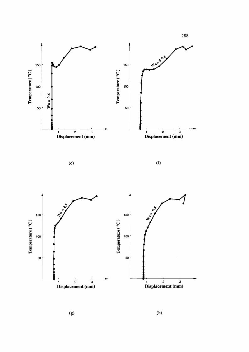
288

150

I31 2

150

U

(2 31


(e) (f)

150

y

100

31 2

150

y

II321


(g) (h)

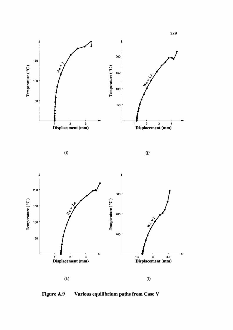
289

150

U

!50

1 2 3

I200

150

100

50

1 2 3 4Displacement (mm) Displacement (mm)

(i) (j)

200

150

^ 100

50

1 2 3

U

300

200

100

31.5 4.5Displacement (mm) Displacement (mm)

(k) (l)

Figure A.9 Various equilibrium paths from Case V

290

250

200

y

t3 1502ai

H

100

i k

0.5 1.5 2 2.5 3 3.5 4Total inward displacement (mm)

Figure A.IO Comparison of equilibrium paths from Case V

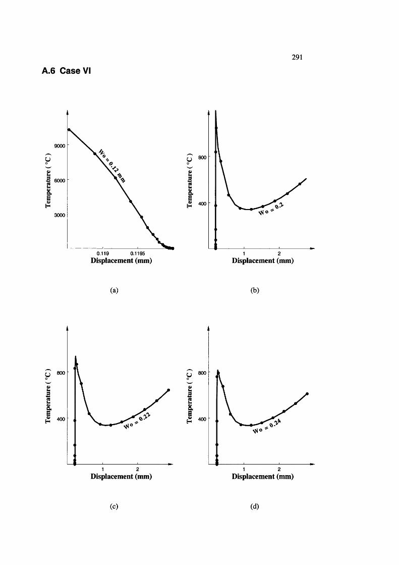
A.6 Case VI291

9000

B 6000

3000

0.119 0.1195

[ 400

21Displacement (mm) Displacement (mm)

(a) (b)

1 2

Ç 800


(c) (d)

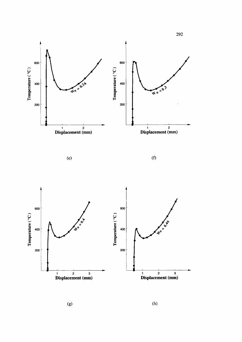
292

U

600

400

200

1 2 Displacement (mm)

U

}

600

400

200

21Displacement (mm)

(e) (f)

600

-S 400

200

31 2

600

y

Ss 400

î200


(g) (h)

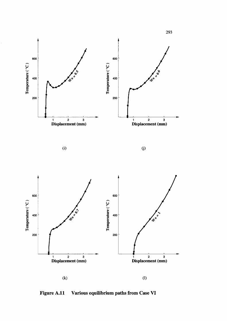
293

I

600

400

200

1 2 3

600

U

i200


(i) (i)

600

s 400

200

1 2 3

600

U

I5 400

I200


(k) (1)

Figure A .ll Various equilibrium paths from Case VI

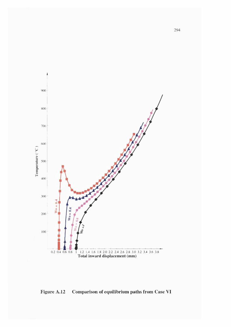
294

900

800

700

600 -

y

IIa.

! j400 i

300

200

100

0.2 0.4 0.6 0.8 1 1.2 1.4 1.6 1.8 2.0 2.2 2.4 2.6 2.8 3.0 3.2 3.4 3.6 3.8Total inward displacement (mm)

Figure A. 12 Comparison of equilibrium paths from Case VI

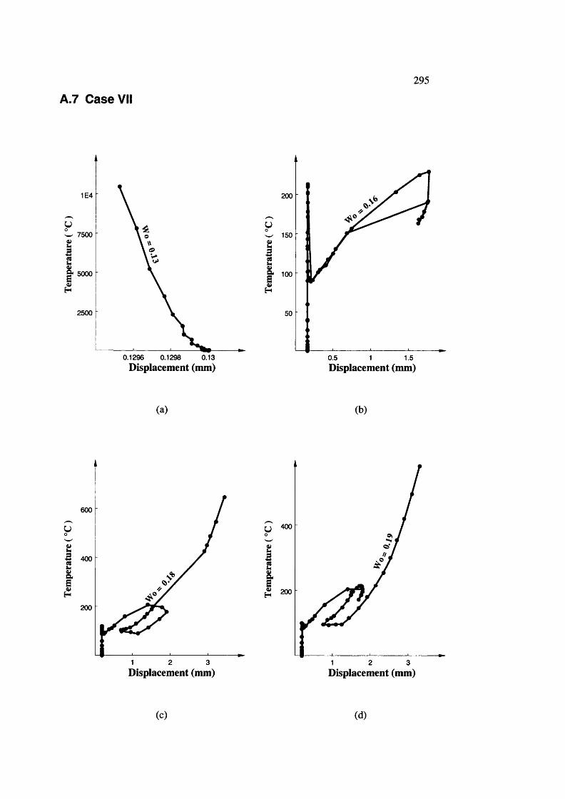
295

A.7 Case VII

1E4

7 500

5000

2 500

0.1296 0.1298 0.13

200

uW 150

tI 100

H

0.5 1 1.5


(a) (b)

600

u

!200

1 2 3 2 31Displacement (mm) Displacement (mm)

(c) (d)

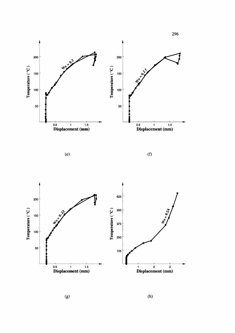
296

U

t200

150

100

50

0.5 1 1.5

î

200

150

100

50

0.5 1 1.5Displacement (mm) Displacement (mm)

(e) (f)

200

150

0.5 1 1.5

f625

500

375

250

125


(g) (h)

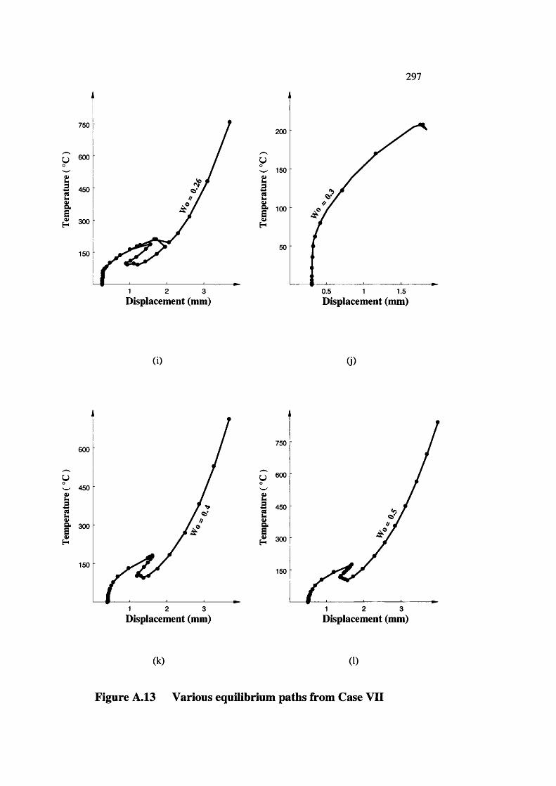
297

750

IS 450

^ 300

150

1 2 3

1

200

150

100

50


(i) (j)

600 -

450

O- 300

150

1 2 3

u

750

600

450

300

150


(k) (1)

Figure A.13 Various equilibrium paths from Case VII

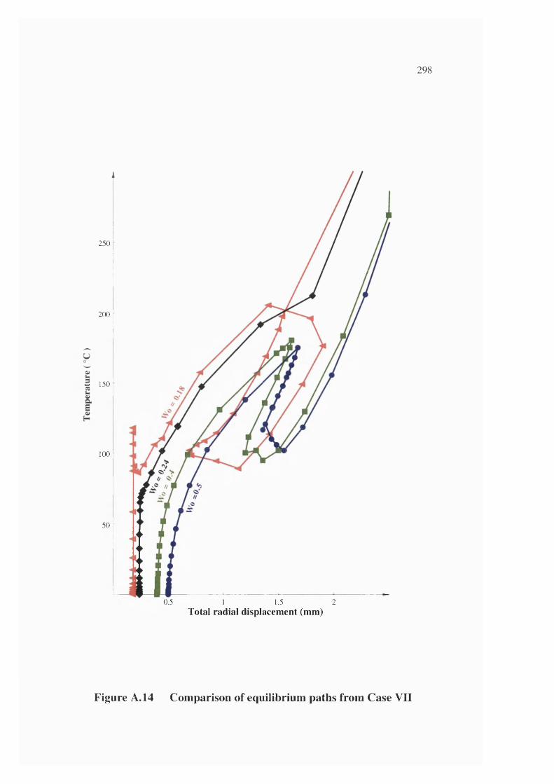
298

I

250

[200î

I

ç 150

100 r

50

L0.5 1.5 21

Total radial displacement (mm)

Figure A.14 Comparison of equilibrium paths from Case VII

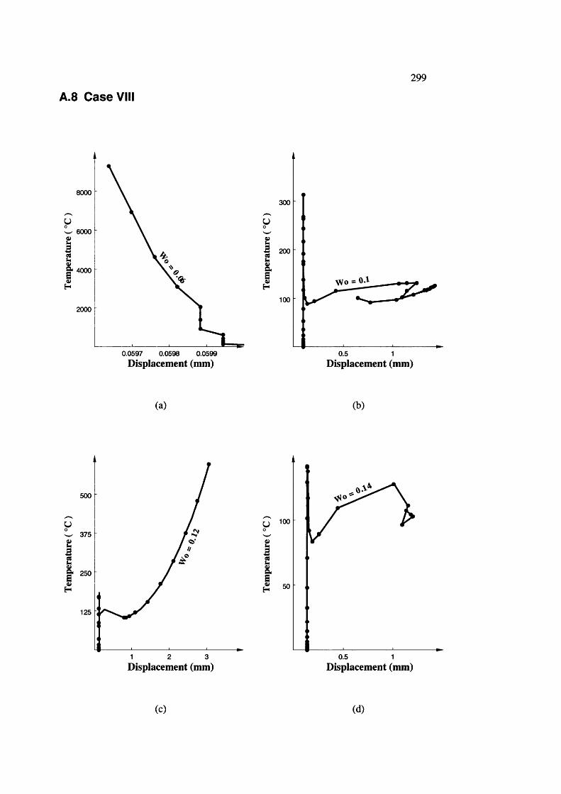
299

A.8 Case VIII

8000

6000

9- 4000

2000

0.0597 0.0598 0.0599

Displacement (mm)

300

y

I3 200

I100

0.5

Displacement (mm)1

(a) (b)

500

yW 375

I& 250

I125

1 2 3

i0.5 1


(c) (d)

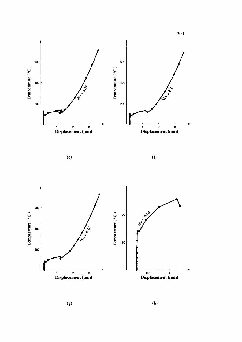
300

600

u

!200

1 2 3

600

u

I200


(e) (f)

600

u

I5 400

I200

1 2 3

ÇJ 100

I

I0.5 1


(g) (h)

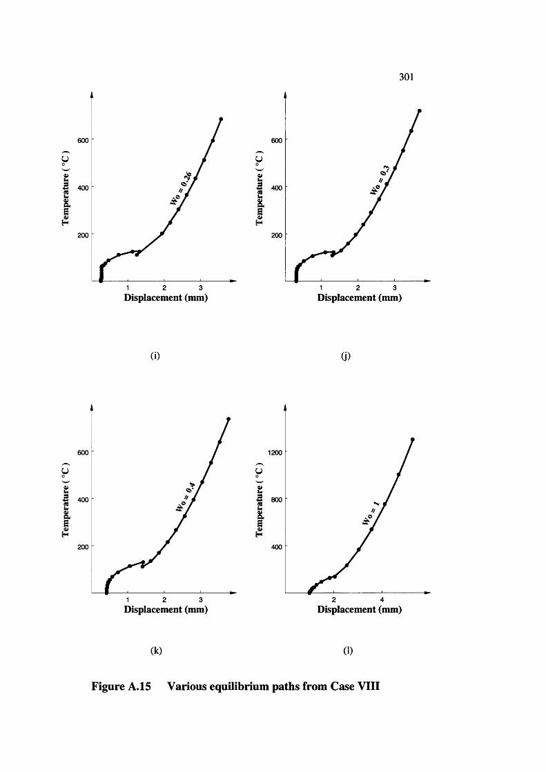
301

600

1200

2 31

600

y

1200


(i) (j)

600

y

1200

1 2 3

1200

y

}400


(k) (1)

Figure A.15 Various equilibrium paths from Case VIII

302

3 00

u

tB 2002

100

0.5 1.5 2ITotal inward displacement (mm)

Figure A. 16 Comparison of equilibrium paths from Case VIII

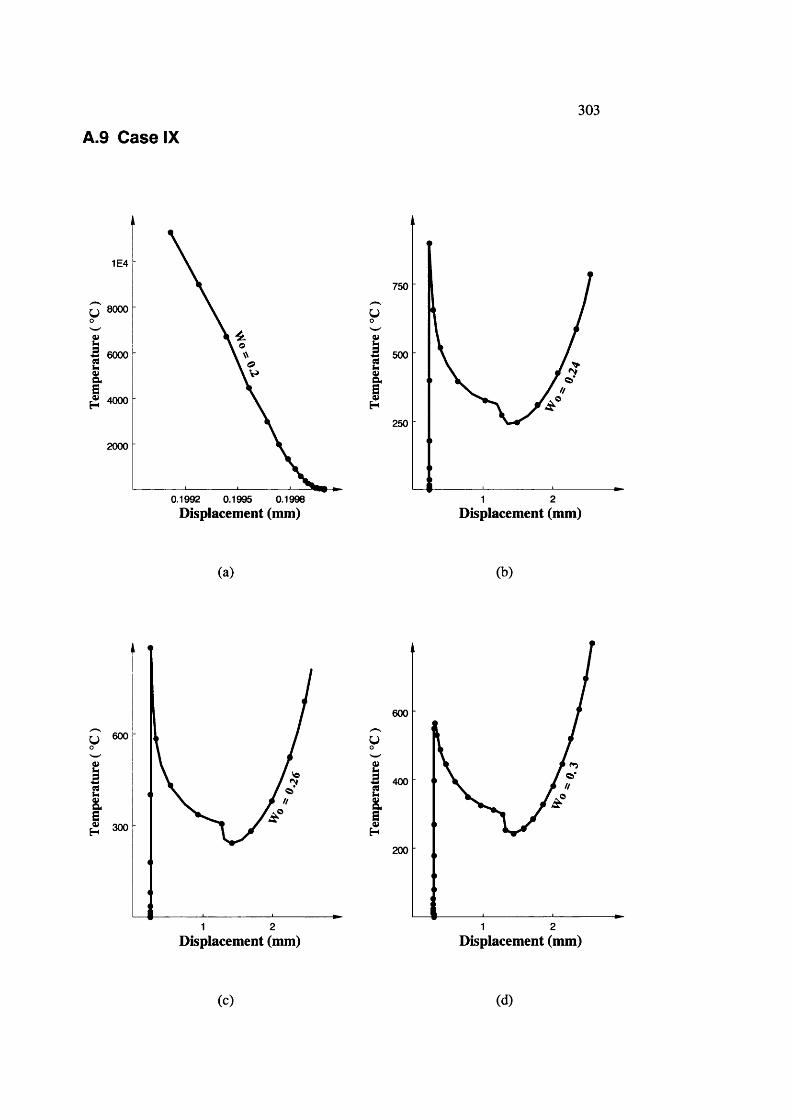
303

A.9 Case IX

1E4

8000

5 6000

4000

2000

0.19980.1992 0.1995

750

12 500

I250


(a) (b)

Ç 600

[^ 300

1 2

600

u

IS 400

I200


(c) (d)

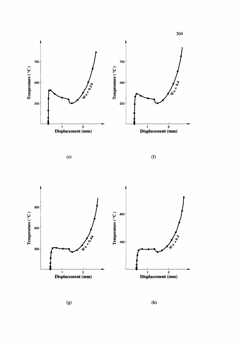
304

750

I250

1 2

750

1250


(e) i f )

900

u

I5 600

I300

1 2

iI 400


(g) (h)

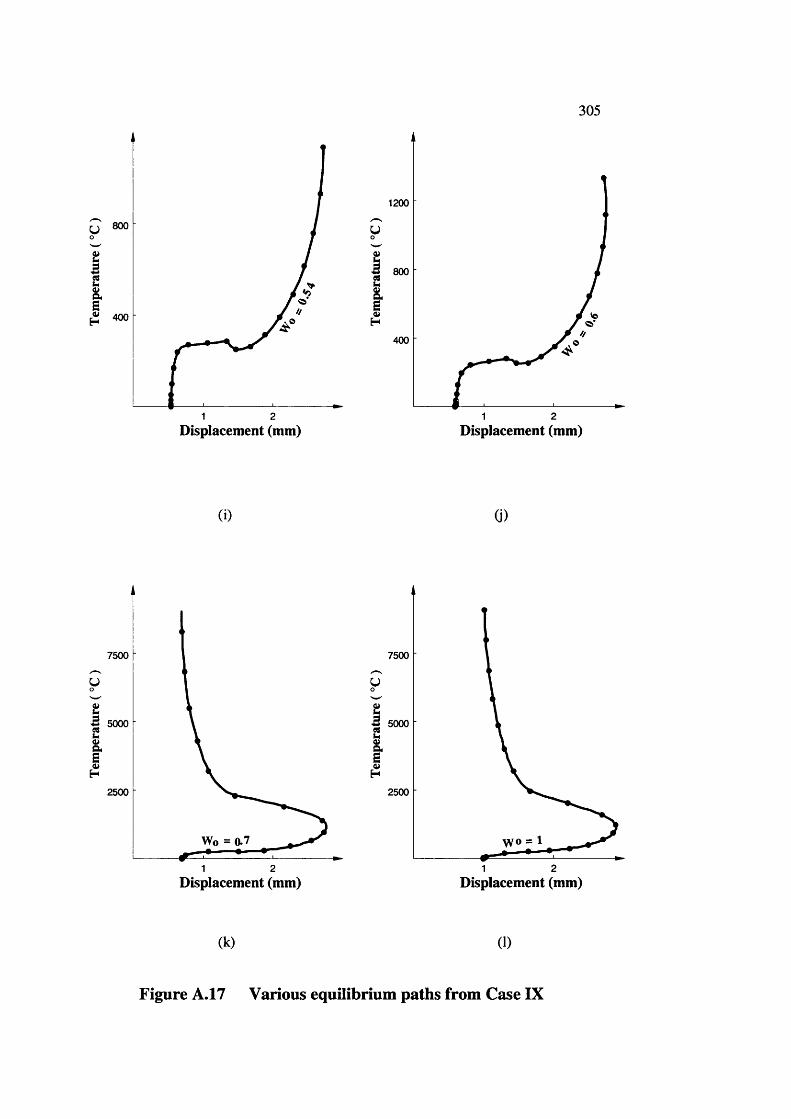
305

800

400

1 2

1200

u

I5 800

I400


(i) G)

7500

■3 5000

2500


7500

3 5000

2500

WO = 1

1 2 Displacement (mm)

(k) (1)

Figure A.17 Various equilibrium paths from Case IX

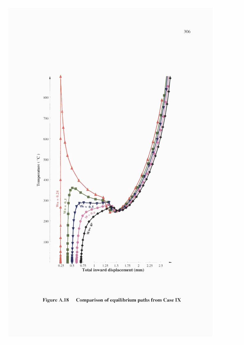
306

800

i L

700

600

?3

2Q.E 400D

H

300

200i i

100

0.25 0.5 0.75Total

1.25 1.5 1.75 2Total inward displacement (mm)

2.25 2.5

Figure A. 18 Comparison of equilibrium paths from Case IX

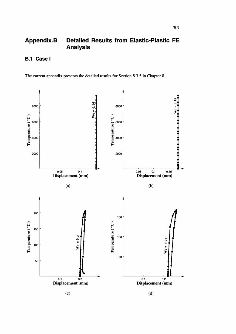
Appendix.B

B.1 C a se I

307

Detailed Results from Elastic-Plastic FE Analysis

The current appendix presents the detailed results for Section 8.3.5 in Chapter 8.

8000

6000

4000

2000


(a)

8000

w 6000g

ig- 4000

I2000

0.05 0.1 0.15Displacement (mm)

(b)

200

uw 150Ig- 100I

«Ne


(c)

150

U


(d)

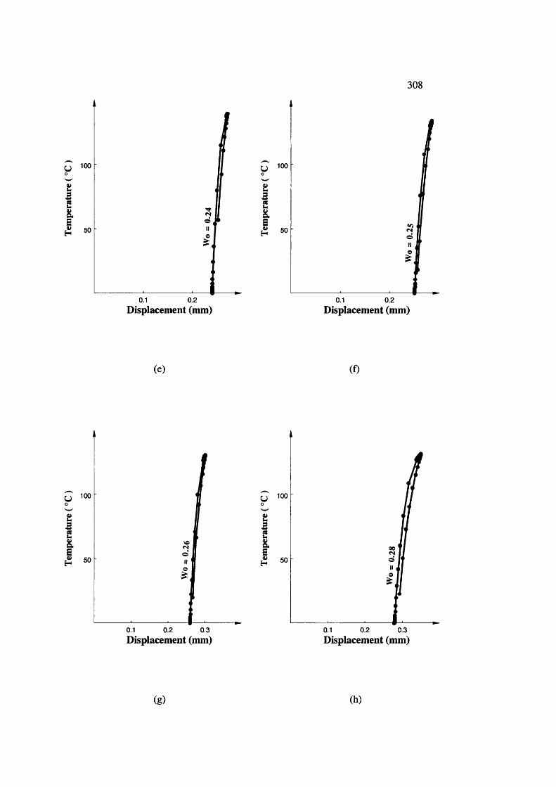
308

^ 100

I o

0.1 0.2

1«0


(e) (f)

I0.1 0.2 0.3

1

0.1 0.2 0.3Displacement (mm) Displacement (mm)

(g ) (h)

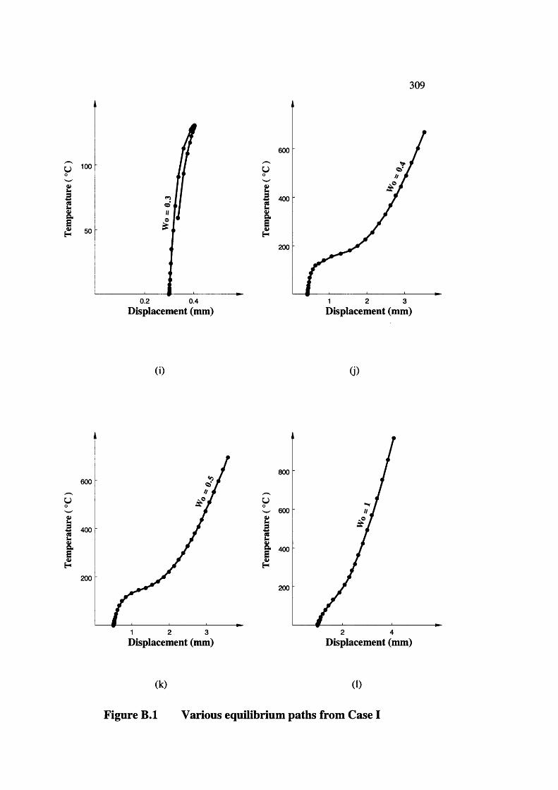
309

^ 100

i^ 50

0.2 0.4

600

y

1200


(i) (j)

600

y

Is 400

I200

1 2 3

800

600

& 400

200


(k) (1)

Figure B.l Various equilibrium paths from Case I

310

200

150 r

100

50


(a)

â:2

I.i

H

i

600 •

400

200

2Displacement (mm)

31

(b)

Figure B.2 Comparison of equilibrium paths from Case I

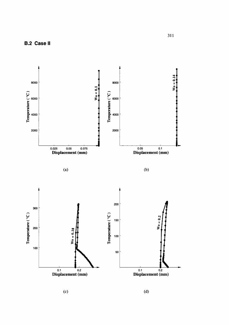
311

B.2 Case II

8000

w 6000

i| - 4000

H

2000

8000

W 6000

IS' 4000

H

2000



(a) (b)

300

y

s 200 oe

I o

100

0.1 0.2

200

yo150

I

g- 100

I


(c) (d)

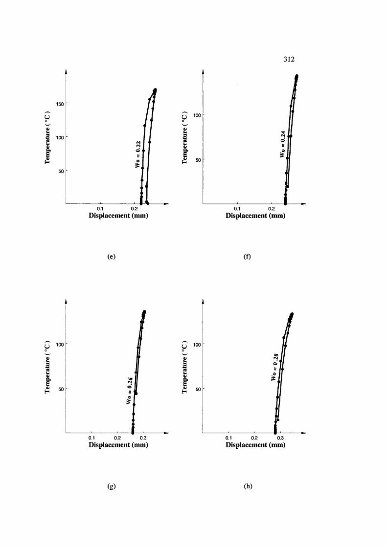
312

150

y

1

?!

0.1 0.2

1


(e) (f)

U

I100

50


y 100oe«N

1


(g ) (h)

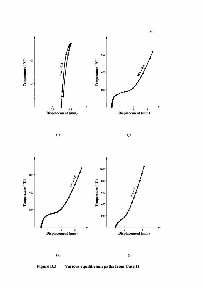
313

0.2 0.4

600

y

1200


(i) (i)

600

y

1200

1 2 3

1000

y 800

Is 600

^ 400

200


(k) (1)

Figure B.3 Various equilibrium paths from Case II

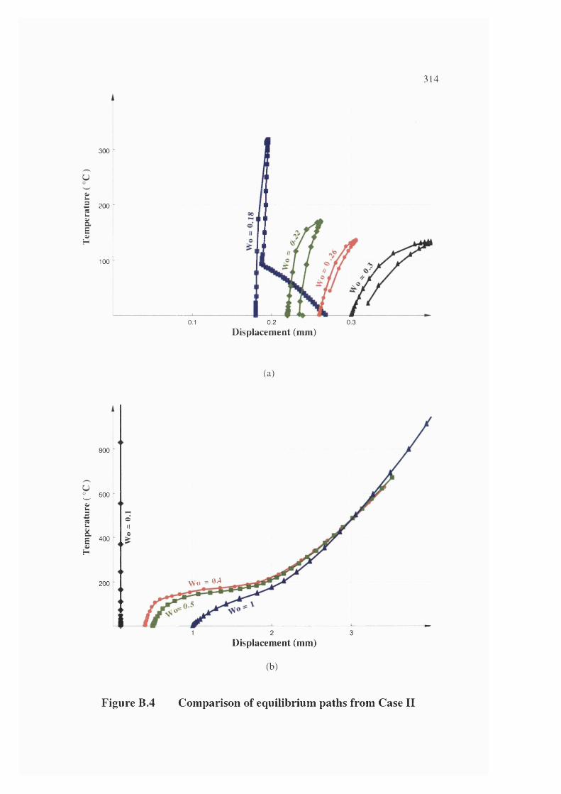
314

300

tB 200

IIH

100


(a)

800

^ 600

Î3

2I 400H

200

oII©

W’o = 0 4


(b)

Figure B.4 Comparison of equilibrium paths from Case II

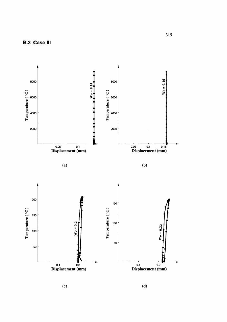
B.3 Case III315

8000

oUW 6000

Ig- 4000

I2000


8000

u6000

14000

2000


(a) (b)

200

UW 150

Ig- 100

I

0.1 0.2

150

y

II0.20.1


(c) (d)

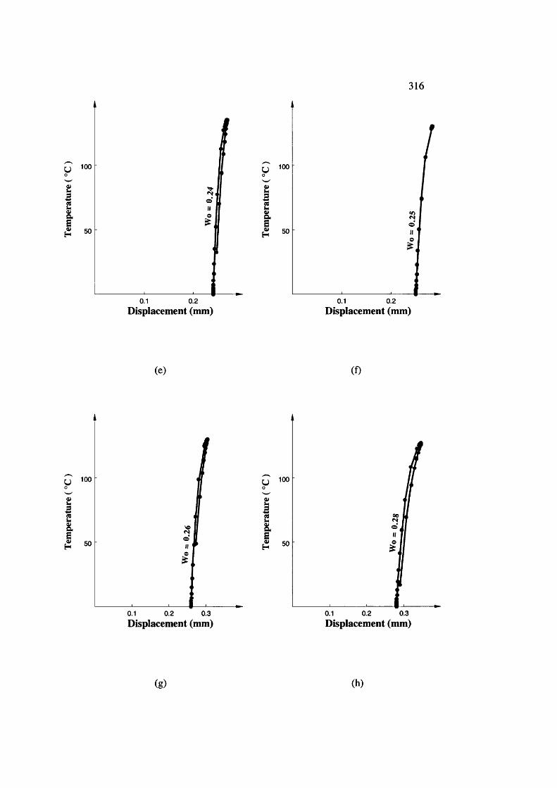
316

100

1 50

0.1 0.2 Displacement (mm)

1


(e) (f)

U

1

100

50


I0.1 0.2 0.3Displacement (mm)

(g ) (h)

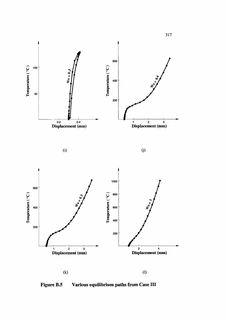
317

1

0.2 0.4

600

U

!200


(i) G)

600

U

1200

1 2 3

1000

y 800

I5 600I 400

200

2 4


(k) (1)

Figure B.5 Various equilibrium paths from Case in

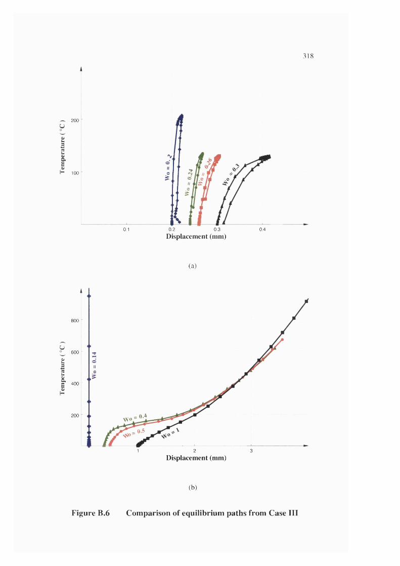
318

200

IE0»H 100

0.1(

0.2 0.3 0.4

Displacement (mm)

(a)

800 -

u600 -

t32I 400 -

H

200

_ 0.5

2Displacement (mm)

31

(b)

Figure B.6 Comparison of equilibrium paths from Case III

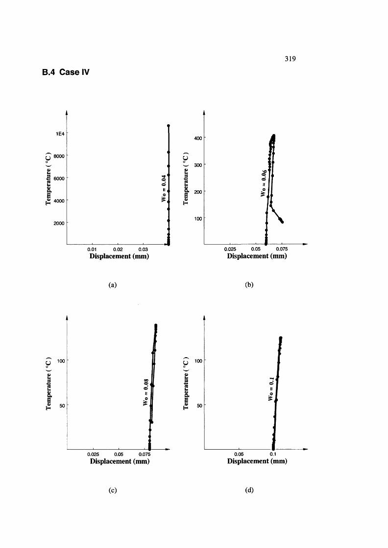
319

B.4 Case IV

u

1E4

8000

;S 6000

^ 4000

2000


400

uW 300

Ig- 200I

se

100


(a) (b)

g 00

0.025 0.05 0.075

^ 100

I

0.10.05Displacement (mm) Displacement (mm)

(c) (d)

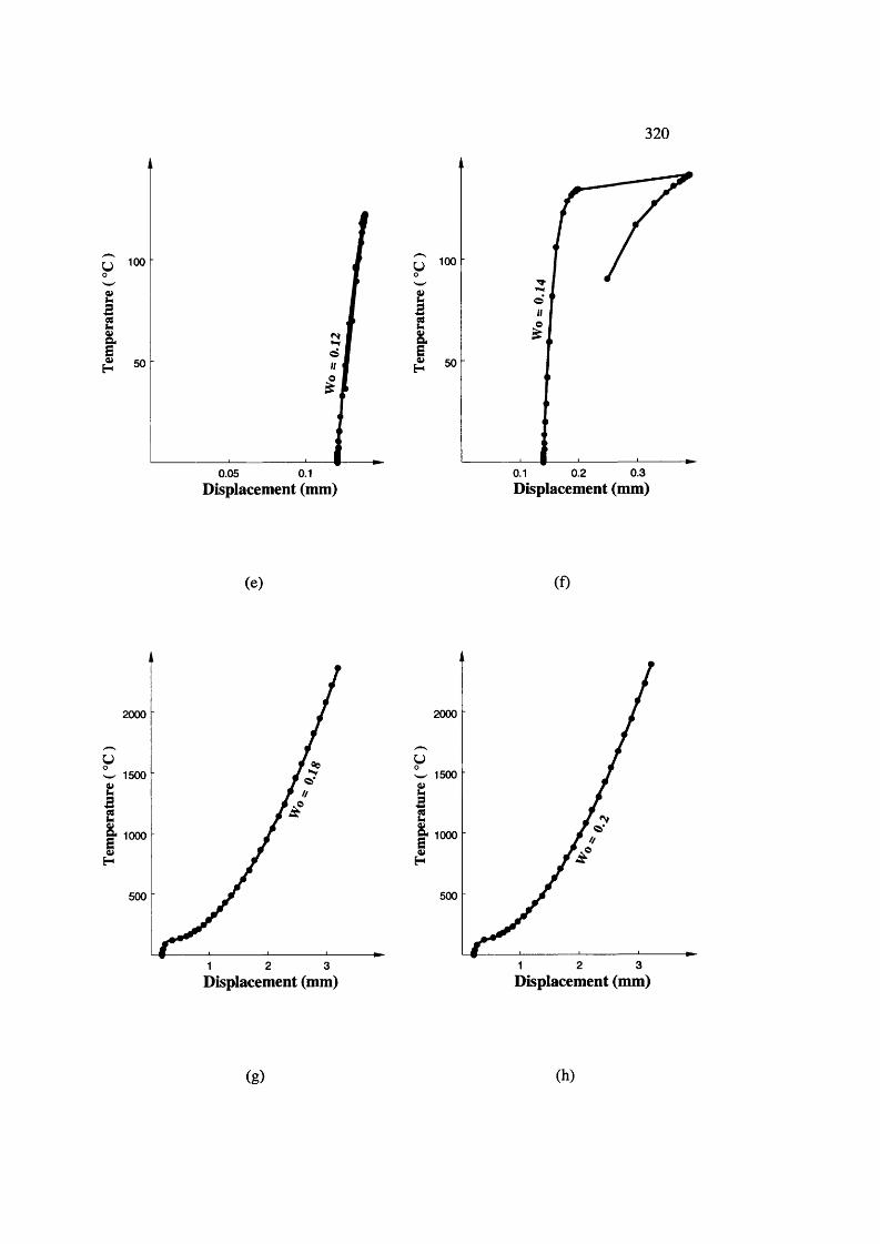
320

^ 100

I o

0.05 0.1

1

o

0.30.20.1Displacement (mm) Displacement (mm)

(e) (f)

2000

uW 1500i& 1000

H

500

21 3

2000

uW 1500I& 1000

I500


(g ) (h)

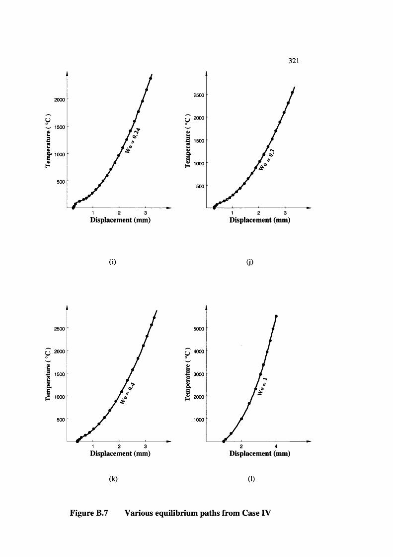
321

2000

1500

500

1 2 3

2500

2000

B 1500

1000

500


(i) (j)

2500

2000

B 1500

1000

500

1 2 3

5000

ç j 4000

SÇ 3000I 2000

1000


(k) (1)

Figure B.7 Various equilibrium paths from Case IV

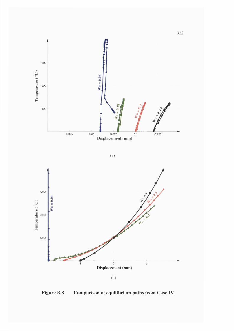
322

300

2 200

100

0.025 0.05 0.075D isplacem ent (m m )

0.1 0.125

( a )

3000 -

a 2000 -

1000 :

i1 2 3

D isplacem ent (m m )

(b)

Figure B.8 Comparison of equilibrium paths from Case IV

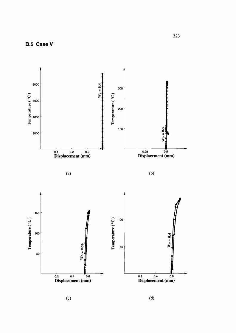
323

B.5 Case V

8000

uW 6000

iS' 4000

I2000


300

u

;■5 200

I100

0.50.25Displacement (mm)

(a) (b)

150

I ™I50


s


(c) (d)

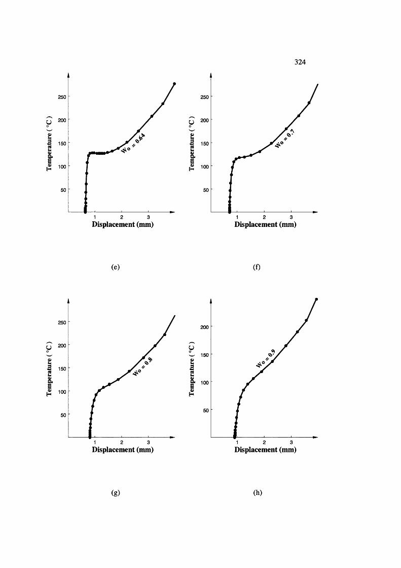
324

250

y 200

I5 150I 100

1 2 3

250

y 200


(e) (f)

250

y 200

1 2 3

200

yW 150Ig- 100

I


(g) (h)

325

250

1 2 3

300

1100


(i) (i)

300

u

I

I100

2 4

400

yW 300

I|- 200

H

100


(k) (I)

Figure B.9 Various equilibrium paths from Case V

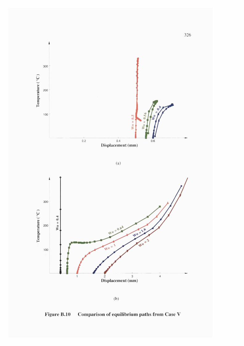
326

300 ItB 200

i

I100

i!


(a)

i

300 -

200 -

100 -


(b)

Figure B IO Comparison of equilibrium paths from Case V

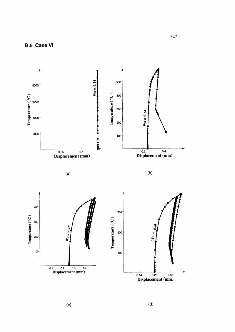
327

B.6 Case VI

8000

6000

14000

2000


500

IS 300

^ 200

100


(a) (b)

400

uW 300ig- 200

I100

0.40.30.20.1Displacement (nun)

300

a 200

100

0.420.280.14Displacement (mm)

(c) (d)

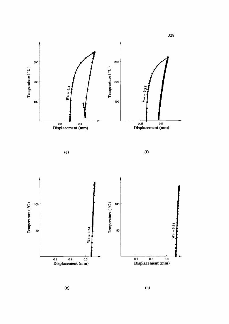
328

300

u

1100

0.40.2

300

y

1100


(e) (0

10.2 0.30.1

1o

0.2 0.30.1Displacement (mm) Displacement (mm)

(g) (h)

329

Ç 100

i ve

0.25 0.5

150

u

0.25 0.5 0.75Displacement (mm) Displacement (mm)

( i ) (j)

800

600

200

1 2 3

800

uw 600ig- 400

I200


(k ) (1)

Figure B .ll Various equilibrium paths from Case VI

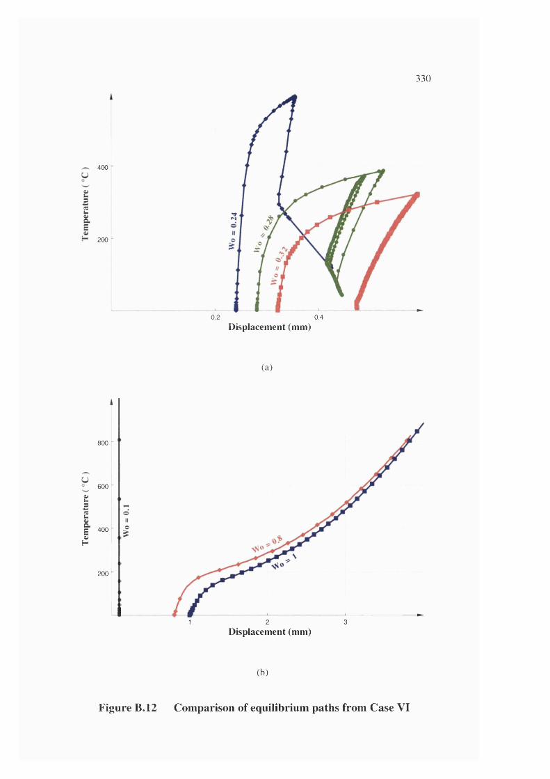
330

400

s2

EH 200

«N

0.2 0.4

Displacement (mm)

(a)

800

^ 600

ï

Ig 400O)H

200

2Displacement (mm)

31

(b)

Figure B.12 Comparison of equilibrium paths from Case VI

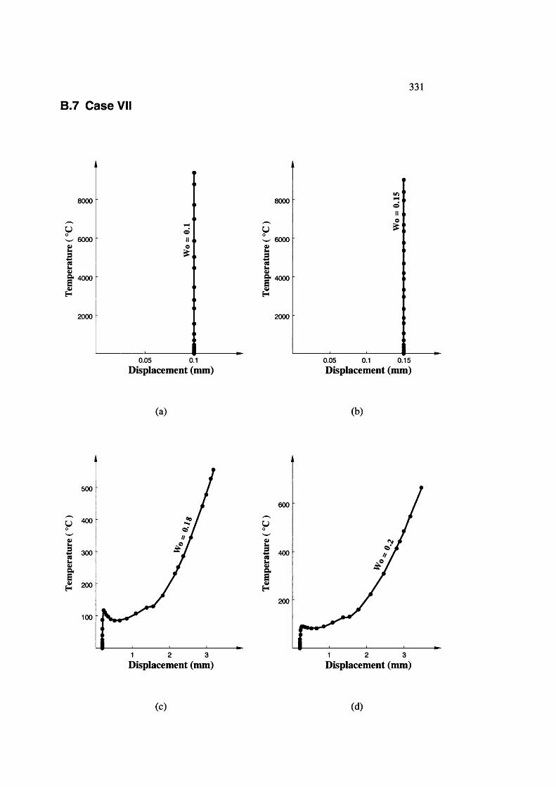
B.7 C ase VII331

U

8000

6000

Ig- 4000

I

IIe

8000

u6000

4000

2000 2000



(a) (b)

500

s

100

1 2 3

600

u

200


(c) (d)

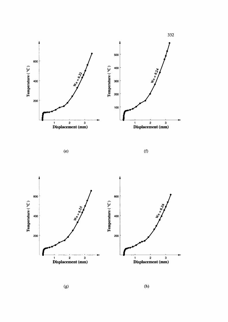
332

600

U

1200

1 2 3

500

2

I 300

i 200

100


(e) (f)

600

U

I’5 400

I200

1 2 3

600

U

Is 400

I200


(g) (h)

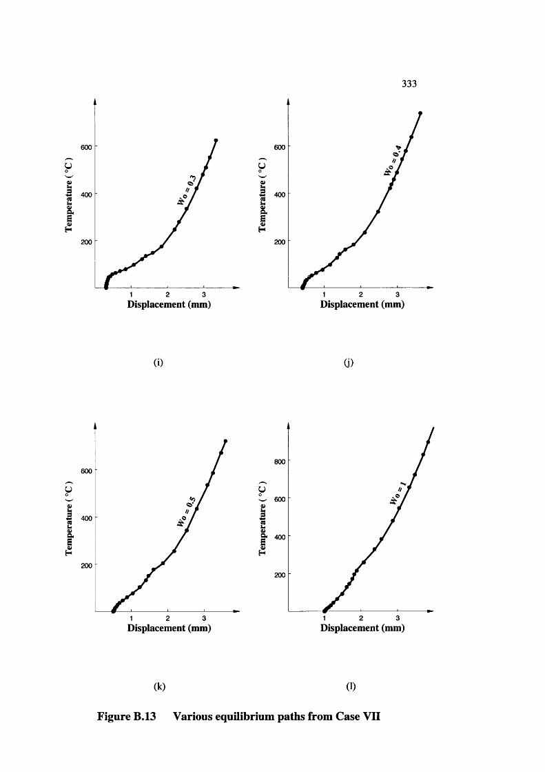
333

600

U

1200

1 2 3

600

y

1200


(i) (i)

600

y

}200

2 31

800

600

& 400

200

31 2Displacement (mm) Displacement (nun)

(k) (1)

Figure B.13 Various equilibrium paths from Case VII

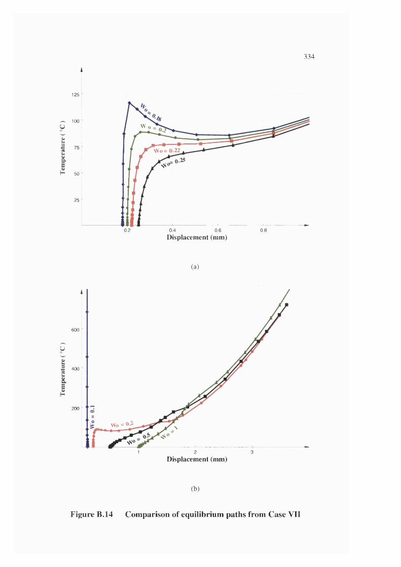
334

125 -

100

t

IaEH 50

25

0.2 0.4 0.6 0.8Displacement (mm)

(a)

600

u

5 400 2

EH

200

Wo = 0-^


(b)

Figure B.14 Comparison of equilibrium paths from Case VII

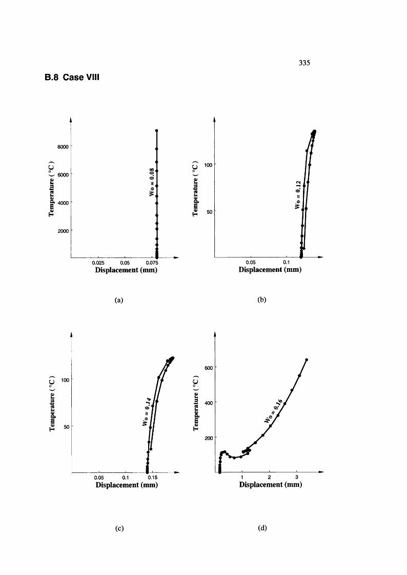
B.8 C ase VIII

335

8000

w 6000

i& 4000

I2000


i <N


(a ) (b)

0.150.05 0.1

600

!200


(c) (d)

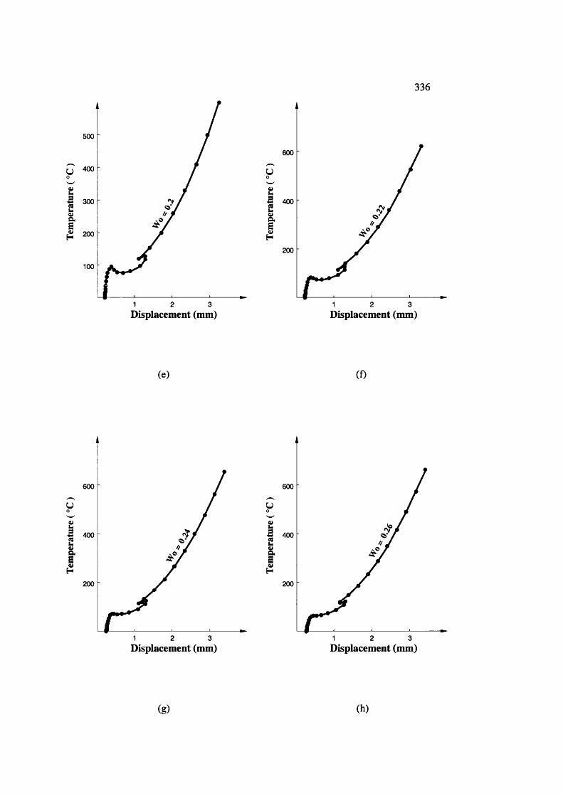
336

500

IB 300

^ 200

100

1 2 3

600

I3 400

Î200


(e) (f)

600

u

I3 400

I200

1 2 3

600

u

I■2 400

I200


(g) (h)

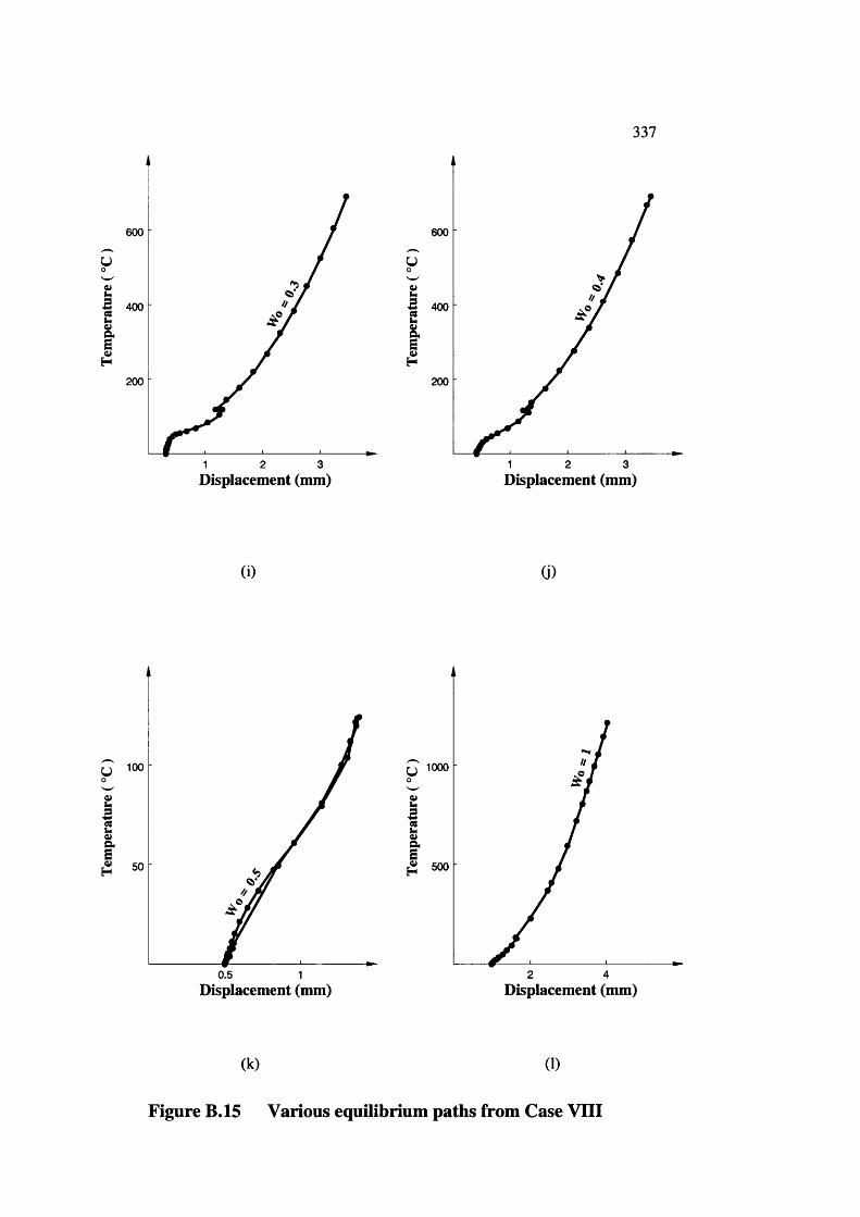
337

600

y

1200

2 31

600

y

i200


( i ) Ci)

t0.5 1

1000


(k ) (1)

Figure B.15 Various equilibrium paths from Case VIII

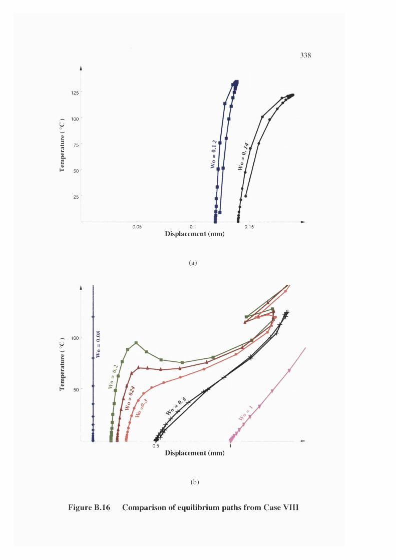
338

125

100U

t

I "aE0)

H 50

25

0.05 0.1 0.15

D isplacem ent (m m )

( a )

30

100 -u

0.5 1D isplacem ent (m m )

(b)

Figure B.16 Comparison of equilibrium paths from Case VIII

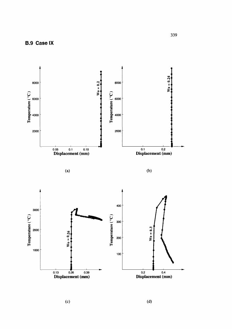
339

B.9 C ase IX

8000

w 6000I& 4000I

2000


8000

w 6000ig* 4000

I2000

0.1 0.2 Displacement (mm)

(a) (b)

3000

u

I 2000

1000

0.13 0.26 0.39

400

u300

II 200

H

100


(c) (d)

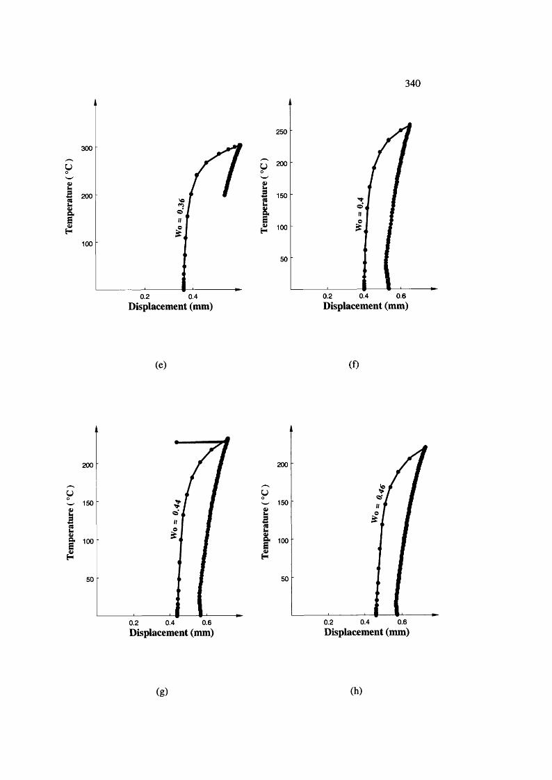
340

300

y

1100

0.40.2

250

y 200

I5 150

100


(e) (f)

200

150

g- 100

0.60.40.2

200

yw 150

l& 100I


(g) (h)

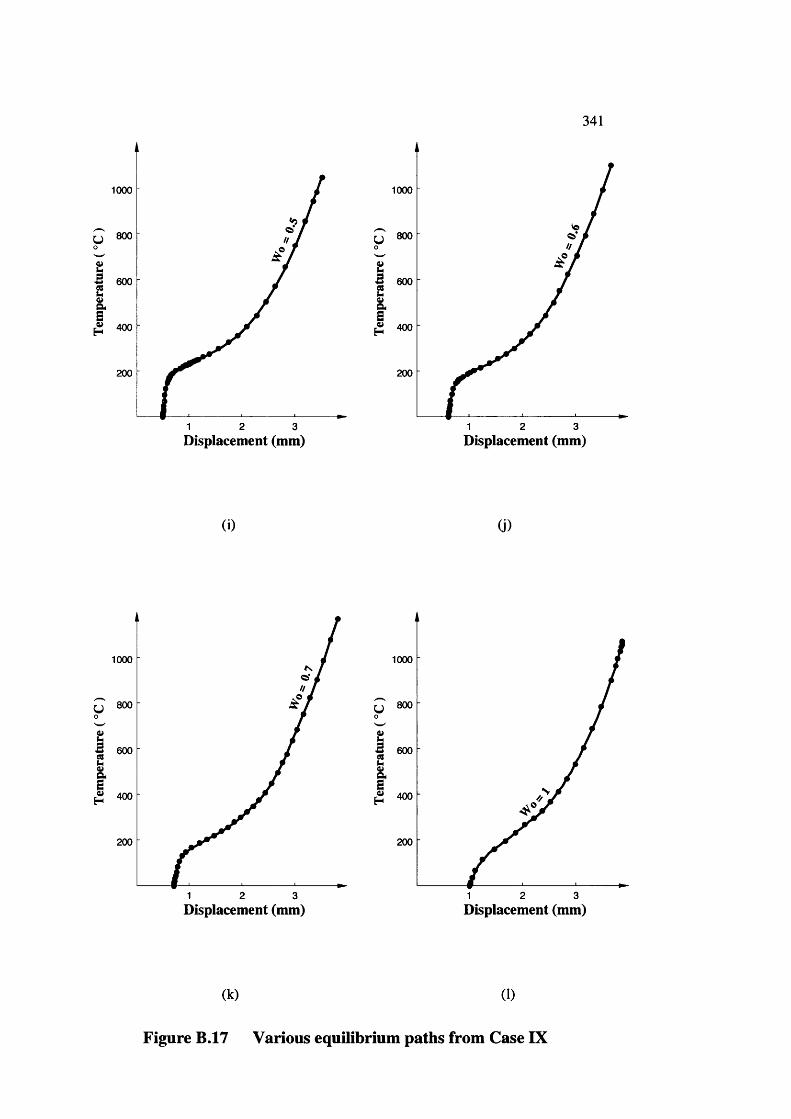
341

1000

;G 600

H 400

200

1 2 3

1000

iG 600

^ 400

200


( i ) ( i )

1000

^ 800

IS 600

^ 400

200

21 3

1000

IG 600

H 400

200


(k ) (1)

Figure B.17 Various equilibrium paths from Case IX

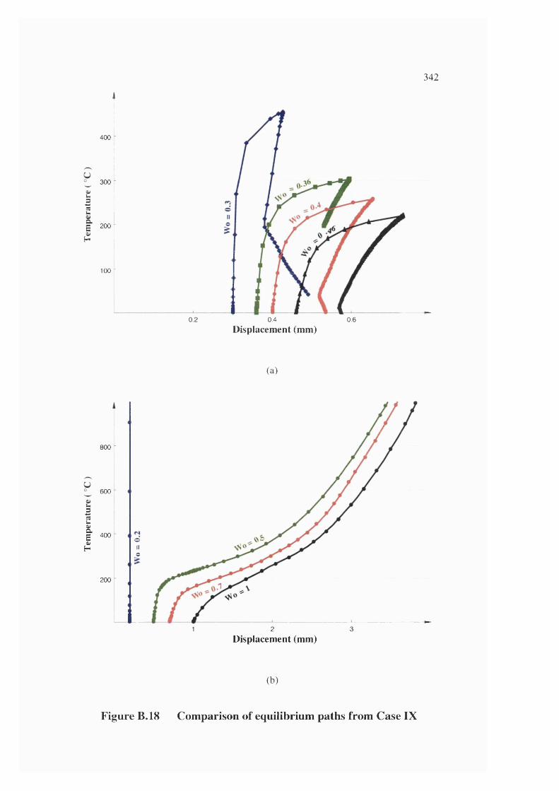
342

400

° 300

ï I2

I »»[■ ^ !

100


(a)

800

^ 600

II 400O)H

200

oIIo

L2

Displacement (mm)31

(b)

Figure B.18 Comparison of equilibrium paths from Case IX

343

List of Figures

Figure 1.1 Bi-metal mechanically bonded pipeline (a) a completed lined pipe (b) a

close-up of the inner liner

Figure 1.2 Sketch showing a pipeline on seabed

Figure 1.3 A section of pipe-liner system cut from an infinitely long lined pipeline

(a) a 3D presentation (b) a longitudinal cross section

Figure 1.4 A cantilever under temperature rise T

Figure 1.5 A cantilever beam under a prescribed axial displacement 6

Figure 1.6 A beam fully fixed at both ends under temperature rise T

Figure 2.1 Correlation of classical, reduced stiffness method and tests for a typical

hydrostatic pressure loaded cylindrical shell

Figure 2.2 Stabilising energy terms for a typically loaded cylindrical shell, showing

the importance of the linearised membrane energy, V2m

Figure 2.3 Frontispiece of the book Elements of Structural Stability

Figure 2.4 Simplified model in the book Elements of Structural Stability

Figure 2.5 Bi-directional simplified model in the book Elements of Structural

Stability (a) the link model (b) the deformed shape

Figure 2.6 Figure 29, Burgess, 1969 - a perfect ring loaded within a perfect rigid

boundary

Figure 2.7 Link model

Figure 2.8 Two-link model


Figure 2.10 Free-Tube Multi-Lobe buckling by Berti (1998)

Figure 2.11 Single-Lobe Buckling by Berti (1998)

Figure 2.12 Figure 1 of Chunduru's work -U liner formation

Figure 2.13 Two-force ring model

Figure 2.14 Results from Qinghua's work (Fan et a l , 1996)

Figure 2.15 Results from Qinghua's work (Ding et al, 1996)

Figure 2.16 Figure 2 of Zhu's work - Finite element model

Figure 2.17 Figure 5 of Zhu's work -Contact pressure evolution

Figure 2.18 Plate 1 of the reference - Experimental rig for the strut on an elastic

foundation

Figure 2.19 Rigid boundary used by B urgess ( 1969)

344

Figure 2.20 Plate 2 of the reference - (a) The second harmonic (no rigid boundary)

(b) The one-way boundary in position (c) One-way buckling

Figure 2.21 Experimental free and one-way buckling loads at different values of

stiffness ratio parameter plotted on the theoretical curves

Figure 2.22 Test frame used by Burgess (1969)

Figure 2.23 Specimen on the rigid ring boundary

Figure 2.24 The concave former (with imperfection), two convex formers, and an

unformed specimen

Figure 2.25 The imperfection -forming layout

Figure 2.26 Experimental and theoretical load - deflection curves for sub-critical

imperfection

Figure 2.27 Experimental and theoretical load - deflection curves for super-critical

imperfection

Figure 2.28 Testing arrangement by Walker ( 1999)

Figure 2.29 Buckled shape

Figure 2.30 Buckled shape - a close-up of Figure 2.29

Figure 2.31 Observed imperfections

Figure 3.1 Simplified model with 2 rigid-links

Figure 3.2 Deformed shape of rigid-link system

Figure 3.3 Simplified 2-rigid-link model under transverse perturbation

Figure 3.4 Rigid-links in axial direction with springs

Figure 3.5 Rigid-links in circumferential direction with springs

Figure 3.6 Bi-directional 4-rigid-link simplified model

Figure 3.7 Imperfection shown with an axial link

Figure 3.8 Imperfection shown with a circumferential link

Figure 3.9 Imperfection and displacement shown with an axial link

Figure 3.10 Imperfection and displacement shown with a circumferential link

Figure 3.11 Equilibrium path with sub-critical imperfection

Figure 3.12 Equilibrium path with critical imperfection

Figure 3.13 Equilibrium path with super-critical imperfection








345







Figure 3.25 Variation of critical imperfection with axial wave number (n=43)

Figure 3.26 Variation of critical imperfection with circumferential wave number

(m=7)

Figure 3.27 Variation of lower bound displacement with axial wave number (n=43)

Figure 3.28 Variation of lower bound displacement with circumferential wave

number (m=7)

Figure 3.29 Effects of axial wave number on the critical temperature (close-up)


Figure 3.31 Effects of circumferential wave number on the critical temperature

(close-up)


Figure 3.33 Second variation of strain energy against axial wave number m (n=43)

Figure 3.34 Second variation of strain energy against circumferential wave number n

(m=7)

Figure 4.1 A strip of liner skin in the axial direction

Figure 4.2 Flexural beam-1 ink in the axial direction

Figure 4.3 A strip of liner skin in the circumferential direction

Figure 4.4 Flexural curved beam-link in the circumferential direction

Figure 4.5 Flexural beam-link model

Figure 4.6 Imperfection shown with an axial beam-link (m=l)

Figure 4.7 Imperfection shown with an axial beam-link (m=3)

Figure 4.8 Imperfection shown with circumferential beam-link (n=l)

Figure 4.9 Imperfection shown with circumferential beam-link (n=5)

Figure 4.10 Deformation shown on top of imperfection in an axial beam-link (m=l)

Figure 4.11 Deformation shown on top of imperfection in an axial beam-link (m=3)

Figure 4.12 Deformation on top of imperfection in circumferential beam-link (n=l )

Figure 4.13 Deformation on top of imperfection in circumferential beam-link (n=5)

Figure 4.14 Effects of circumferential wave number on the critical temperature (m=6,

7 and 8)


Figure 4.16 Effects of axial wave number on the critical temperature (n=l, 20, 40)

346


Figure 5.1 Simplification of an inner liner as an empty thin shell - the cross section

of the neutral surface

Figure 5.2 Simplification of the inner liner as empty thin shell - 3D graphic

presentation of the neutral surface

Figure 5.3 Critical temperature versus axial wave number m

Figure 5.4 Critical temperature versus circumferential wave number n

Figure 5.5 Variation of critical temperature with thickness of the liner

Figure 5.6 Variation of critical temperature with radius of the liner

Figure 6.1 A 3D graphic presentation of a liner-pipe system

Figure 6.2 A sketch of the cross section of a liner-pipe system with t? » tL

Figure 6.3 A sketch of the cross section of a liner thin shell and a pipe as solid body

Figure 6.4 A sketch of the cross section of an inner liner before and after

temperature rise

Figure 6.5 A sketch of the cross section of an outer pipe before and after

temperature rise

Figure 6.6 A graphical presentation of the coupled expansion dF (a) before

temperature rise (b) after temperature rise (c) before and after

temperature rise

Figure 6.7 A typical temperature rise Tp variation against radial coordinate r

Figure 6.8 Fundamental radial displacement against thickness ratio between the

inner liner and the outer pipe

Figure 6.9 A sketch of three types of the equilibrium path (a - critical imperfection

b - sub-critical imperfection c - super critical imperfection)

Figure 6.10 Three types of w-5 curves

Figure 6.11 Critical temperature versus circumferential wave number (m= 1,7,20)

Figure 6.12 Critical temperature versus circumferential wave number m (m=6,7,8)

Figure 6.13 Critical temperature versus axial wave number n (n=0,25,45)

Figure 6.14 Critical temperature versus axial wave number n (close-up)

Figure 6.15 Various equilibrium paths — (a) critical imperfection; (b) sub-critical

imperfection; (c) super-critical imperfection

Figure 7.1 Bi-linear stiffness for the springs simulating the outer pipe

Figure 7.2 Non-linear springs simulating the outer pipe in the full model

Figure 7.3 Non-linear springs simulating the outer pipe in the partial model

347

Figure 7.4 Sketch showing a section of pipeline of axial length L

Figure 7.5 Full-model of axial length L

Figure 7.6 Full-model showing symmetry boundary conditions

Figure 7.7 Sketch showing a “window” of pipeline skin

Figure 7.8 Axial cross section deformation showing half axial wave length in red

Figure 7.9 Circumferential cross section deformation showing half circumferential

wave length in red

Figure 7.10 Partial-model of axial length L%/2 and circumferential length R(p/2

Figure 7.11 Partial-model showing symmetry and asymmetry boundary conditions

Figure 7.12 Typical equilibrium paths (Case VI) (a)

Figure 7.13 Typical equilibrium paths (Case VI) (b)

Figure 7.14 Typical equilibrium path for model with very small imperfection (Case

VI)

Figure 7.15 Typical equilibrium path for model with (a) very large (b) large (c)

critical (d) small (e) very small imperfection


Figure 7.17 Equilibrium path showing modal transition

Figure 7.18 Modal shape before snap-through

Figure 7.19 Circumferential modal shape before snap-through




Figure 7.23 Overlapped circumferential modal shape before and after snap-through

Figure 7.24 Undeformed shape of the full model (a) 3D, (b) axial cross section, (c)

circumferential cross section

Figure 7.25 Equilibrium paths (a) inc 31, (b) inc 63, (c) inc 155 and (d) inc 322

Figure 7.26 Comparison of 3d deformation (a) inc 31 (b) inc 63 (c) inc 155 (d) inc

322

Figure 7.27 Comparison of axial cross section deformation (a) inc 31 (b) inc 63 (c)

inc 155 (d) inc 322

Figure 7.28 Comparison of axial cross section deformation (a) inc 31 (b) inc 63 (c)

inc 155 (d) inc 322

Figure 8.1 Stress-strain relationship for a typical pipeline liner

Figure 8.2 Typical equilibrium path with very large imperfection (Case VI)

Figure 8.3 Typical equilibrium path with very small imperfection (Case VI)

Figure 8.4 Typical equilibrium path with intermediate imperfection (Case VI)

348

Figure 8.5 Typical equilibrium path with intermediate imperfection (Case I)

Figure 8.6 Mises stress contour (Case I, Wo=0.26)

Figure 8.7 Equivalent plastic strain contour (Case I, Wo=0.26)


Figure 8.9 Equilibrium path showing bifurcation at inc 64

Figure 8.10 Modal shape at inc 63 before snap-through

Figure 8.11 Modal shape at inc 64 after snap-through

Figure 8.12 Axial and circumferential modal shape at inc 63 before snap-through (a)

axial (b) circumferential

Figure 8.13 Axial and circumferential modal shape at inc 64 after snap-through (a)

axial (b) circumferential


Figure 8.15 Overlapped modal shape before and after snap-through (a) axial, (b)

circumferential

Figure 8.16 Equilibrium path from Case I full-model with imperfection of 0.4mm

Figure 8.17 Comparison of modal shapes at different increment (a) undeformed (b)

inc 90 (c) inc 120 (d) inc 138

Figure 8.18 Comparison of axial cross section deformation (a) undeformed (b) inc

90 (c) inc 120 (d) inc 138

Figure 8.19 Comparison of circumferental cross section deformation (a) undeformed

(b) inc 90 (c) inc 120 (d) inc 138

Figure 8.20 Comparison of buckling temperature between elastic and elastic-plastic

analyses (Cases I, II and HI)


analyses (Cases IV, V and VI)


analyses (Cases VII, VIII and DC)

Figure A. 1 Various equilibrium paths from Case I

Figure A.2 Comparison of equilibrium paths from Case I

Figure A.3 Various equilibrium paths from Case II

Figure A.4 Comparison of equilibrium paths from Case II

Figure A.5 Various equilibrium paths from Case III

Figure A.6 Comparison of equilibrium paths from Case III

Figure A.7 Various equilibrium paths from Case IV

Figure A.8 Comparison of equilibrium paths from Case IV

Figure A.9 Various equilibrium paths from Case V

Figure A. 10 Comparison of equilibrium paths from Case V

349

Figure A. 11 Various equilibrium paths from Case VI

Figure A. 12 Comparison of equilibrium paths from Case VI

Figure A. 13 Various equilibrium paths from Case VII

Figure A. 14 Comparison of equilibrium paths from Case VII

Figure A. 15 Various equilibrium paths from Case VIII

Figure A. 16 Comparison of equilibrium paths from Case VIII

Figure A. 17 Various equilibrium paths from Case EX

Figure A. 18 Comparison of equilibrium paths from Case EX

Figure B. 1 Various equilibrium paths from Case I

Figure B.2 Comparison of equilibrium paths from Case I

Figure B.3 Various equilibrium paths from Case II

Figure B.4 Comparison of equilibrium paths from Case II

Figure B.5 Various equilibrium paths from Case III

Figure B.6 Comparison of equilibrium paths from Case HI

Figure B.7 Various equilibrium paths from Case FV

Figure B.8 Comparison of equilibrium paths from Case EV

Figure B.9 Various equilibrium paths from Case V

Figure B. 10 Comparison of equilibrium paths from Case V

Figure B. 11 Various equilibrium paths from Case VI

Figure B.12 Comparison of equilibrium paths from Case VI

Figure B.13 Various equilibrium paths from Case VII

Figure B. 14 Comparison of equilibrium paths from Case VII

Figure B. 15 Various equilibrium paths from Case VIE

Figure B.16 Comparison of equilibrium paths from Case VIII

Figure B.17 Various equilibrium paths from Case EX

Figure B.18 Comparison of equilibrium paths from Case IX

350

List of Tables

Table 2.1 Two-way buckling of the example liner shell



Table 3.3 Second variation of strain energy and critical temperature corresponding

to the critical imperfection (m=7 and n=43)





Table 3.7 Second variation of strain energy and critical temperature corresponding

to the critical imperfection (m=4 and n=43)



Table 3.9 Strain energy terms at the lower bound point in the equilibrium path with

critical imperfection (m=4 and n=43)

Table 3.10 Geometry at the crossing point in the equilibrium path with critical





Table 3.14 Variation of circumferential wave number with wall thickness and radius

Table 4.1 Comparison of the results between Chapter 2 and Chapter 3 for the same

pipeline liners




Table 4.5 Variation of circumferential wave number with wall thickness and radius

Table 5.1 Various Parameters Used in Thermally-induced Strains

Table 5.2 Signs for various coefficients

Table 5.3 Values for thermal coefficients for the liner

Table 5.4 Values for geometrical parameters

351

Table 5.5 Critical Temperature and imperfection for typical pipeline liner

Table 5.6 Comparison of the results among Chapter 2, Chapter 3 and Chapter 4 for

the same pipeline liners

Table 6.1 Various Thermal Coefficient Symbols Used In Chapter 6

Table 6.2 Signs for various coefficients in equation (6.72)

Table 6.3 Values for Various Thermal Coefficients

Table 6.4 Values for Various Geometrical Parameters

Table 6.5 Results for the Current Pipeline Liner

Table 6.6 Comparison of critical temperature and critical imperfection among four

chapters for the same pipeline liners

Table 7.1 Various cases for the elastic buckling analysis of pipeline liners

Table 7.2 Amplitudes of imperfection for various runs

Table 7.3 Approximate buckling temperature from various cases

Table 8.1 Material property used in the plastic buckling analysis

Table 8.2 Ramberg-Osgood stress-strain relationship of CRA

Table 8.3 Approximate buckling temperature from various cases

Table 8.4 Comparison of results from the various chapters

352

References

The following is a list of sources that are referred to in the text of the thesis and have specifically been used to develop the basis o f the thesis:

Abramovich, H., Singer, J. and Weller, T,, 2002, Repeated buckling and its influence on the geometrical imperfections. International Journal of Non-Linear Mechanics, Vol 37, n 4-5, pp. 577-588

Anon, 1965, Buckling of Thin-walled Circular Cylinders, NASA Space Vehicle Design Criteria, NASA SP-8007

Arbocz, J., J. M. A. M. Hoi, 1995, Collapse of Axially Compressed Cylindrical Shells with Random Imperfections, Thin-Walled Structures, No 23, pp 131-158

Arbocz, J. and Babcock, CD., 1976, Prediction of buckling loads based on experimentally measured initial imperfections, Proc. lUTAM Symp. Buckling of Structures, Harvard University, Cambridge, (Ed. B. Budiansky), Springer Verlag, Berlin 1976, 291-311

Bakeer, R.M., Barber, M.E.,Taylor J.E and Pechon, S.E, 2001, Long-term buckling performance of HDPE liners. Journal of Materials in Civil Engineering, Volume 13, No 3, pp 176-184

Bakeer, Reda, Barber, Michael E., Pechon, Sean E., Taylor, John E. and Chunduru, Suryanarayana, 1999, Buckling of HDPE Liners under External Uniform Pressure, Journal of Materials in Civil Engineering, Vol. 11, No. 4, pp. 353-361

Ballet, J.P. and Hobbs, R.E., 1992, Asymmetric effects of prop imperfection on the upheaval buckling of pipelines, Thin-Walled Structures, No. 13, pp. 355-373

Baruch, M., and J. Singer, 1963, Effect of Eccentricity of Stiffeners on the General Instability of Stiffened Cylindrical Shells under Hydrostatic Pressure, J. Mech. Eng. Sci., vol5, pp.23-27

Batista, R., 1979, Lower bound estimates for cylindrical shell buckling loads, PhD thesis. University College London

Batista, R. and Croll, J. G. A., 1978, Design approach for axially compressed unstiffened cylinders. Stability Problems in Engng. Struct. Components, University College, Cardiff

Berti, D., Stutzman, R., Lindquist, E., and Eshghipour, M., 1998, Technical Forum, Buckling of Steel Tunnel Liner under External Pressure, Journal of Energy Engineering, vol. 124, issue 3, pg. 55-89

Bielewicz, E. and Gorski, J., 2002, Shells with random geometric imperfections simulation - based approach. International Journal of Non-Linear Mechanics, No. 37, pp. 777-784

Brush, Ron and Almroth, Bo O., 1975, Buckling of Bars, Plates, and Shells, International Student Edition, McGraw-Hill, Tokyo

Bui son, P. S., 1985, Buried structures: Static and dynamic strength. Chapman & Hall, London

353

Burgess, I. W., 1971, The Buckling of a Radially Constrained Imperfect Circular Ring, Int. J. mech. Sci., Pergamon Press, Vol. 13, pp.741-753

Burgess, I. W., 1971, On the Equilibrium and Stability of Discrete One-Way Structural Systems, Int. J. Solids. Structures, Pergamon Press, Vol. 7, pp.667-683

Burgess, I. W., 1969, Ph.D. Thesis, Department of Civil Engineering, University College London

Cederbaum, G., Touati, D., 2002, Postbuckling analysis of imperfect non-linear viscoelastic cylindrical panels. International Journal of Non-linear Mechanics, No 37, pp 757-762

Chan, H.C. and McMinn, S.J., 1966, The Stability of a uniformly compressed ring surrounded by a rigid circular surface. Int. J. Mech. Sci., Vol. 8

Chan, H.C., 1965, Stability of the elastic lining of a prestressed concrete pressure vessel, PhD thesis. Dept, of Structural Engineering, Manchester College of Science and Technology

Chen, Wen and Fan, Qinshan, 1993, The Study on the Biaxial Instability of a Point- Supported Cylindrical Liner Shell Encased in a Concrete Pressure Vessel, Journal of Tsinghua University, Vol. 33, No. 5, pp. 108-113

Chunduru, Surya, Barber, Michael E. and Bakeer, Reda, 1996, Buckling Behaviour of Polyethylene Liner System, Journal of Materials in Civil Engineering, Vol. 8, No. 4, pp. 201-206

Croll, J. G. A., 2001, Buckling of Cylindrical Tunnel Liners, Journal of Engineering Mechanics, Vol 127, No 4, pp 333-341

Croll, J.G.A., 1997, A simplified analysis of imperfect thermally buckled subsea pipelines. Proceedings of the Seventh International Offshore and Polar Engineering Conference, Honolulu, USA, pp. 666-676

Croll, J.G.A., 1995, Towards a Rationally Based Elastic-Plastic Shell Buckling Design Methodology, Thin-Walled Structures, No. 23, pp. 67-84

Croll, J. G. A., 1981, Lower Bound Elasto-plastic Buckling of Cylinders, Proc. Instn Civ. Engrs, Part 2, pp. 235-261

Croll, J. G. A. and Batista, R. C., 1981, Explicit Lower Bounds for the Buckling of Axially Loaded Cylinders, Int. J. Mech. Sci. vol. 23, No. 6, pp. 331-343

Croll, J. G. A. and Walker, A. C., 1972, Elements of Structural Stability, Macmillan, London

Croll, J.G.A. and Chilver, A. H., 1971, Approximate Estimates of the Stability of Cooling Towers under Wind Loading, LASS Colloq. on the Structural Design of Cooling Towers, Bruxelles

Ding, Hongli, Fan, Qinshan and Xu, Bingye, 1997, Nonlinear Analyses of Thermal Postbuckling Problems of Liner Shells, Journal of Tsinghua University, Vol. 37, No. 8, pp. 32-35

354Ding, Hongli, Fan, Qinshan and Xu, Bingye, 1996, Numerical Analysis of the Liners Encased in a Rigid Cavity, Journal of Tsinghua University, Vol. 36., No. 3, pp. 18-22

Donnell, L. H., and C. C. Wan, 1950, Effects of Imperfection on Buckling of Thin Cylinders and Columns under Axial Compression, J. Appl. Mech., vol 17, pp. 73-83

Elkon, Y., Pian, T.H.H. and Hsu, P.T., 1964, Note on the instability of circular rings confined to a rigid boundary, J. App. Mech., Vol. 31

Ellinas, C. P. and Croll, J. G. A., 1983, Experimental and theoretical correlation for elastic buckling of axially compressed cylinders: stringer stiffened, J. Strain Anal., 18(1), pp 41-67; Experimental and theoretical correlation for elastic buckling of axially compressed cylinders: ring stiffened, J. Strain Anal., 18(2), pp 81-93

Ellinas, C. P. and Croll, J. G. A., 1981, Overall Buckling of Ring Stiffened Cylinders, Proc. Instn Civ. Engrs, Part 2, pp. 637-661

Ellinas, C. P., Batista, R. C. and Croll, J. G. A., 1981, Overall Buckling of Stringer Stiffened Cylinders, Proc. Instn Civ Engrs, Part 2, pp. 479-512

El-Sawy, K.M., 2001, Inelastic stability of tightly fitted cylindrical liners subjected to external uniform pressure, Thin-Walled Structures, Volume 39, No 9, pp 731-744

El-Sawy, Khaled and Moore, Ian D., 1998, Stability of Loosely Fitted Liners Used to Rehabilitate Rigid Pipes, Journal of Structural Engineering, Vol. 124, No. 11, pp. 1350- 1357

El-Sawy, Khaled and Moore, Ian D., 1997, Parametric study for buckling of liners: effect of liner geometry and imperfections. Proceedings of the 1997 ASCE Conference on Trenchless Pipeline Projects, Boston, MA, USA, pp416-423

Eslami, M R. and Shahsiah, R., 2001, Thermoelastic buckling of imperfect cylindrical shells. Journal of Thermal Stresses, No 24, pp. 71-89

Eslami, M.R. and Javaheri, R., 1999, Buckling of composite cylindrical shells under mechanical and thermal loads. Journal of Thermal Stresses, No 22, pp. 527-545

Eslami, M R., Ziaii, A.R. and Ghorbanpour, A., 1996, Thermoelastic buckling of thin cylindrical shells based on improved stability equations. Journal of Thermal Stresses, No 19, pp. 299-315

Fan, Qinshan, Fu, Guanghui and Fang, Muzhen, 1996, Circumferential Buckling of Steel Liners for the Containment in NPPs, Journal of Tsinghua University, Vol. 36., No. 4, pp. 105-110

Fan, Qinshan and Chen, Wen, 1994, Post-buckling behaviour of a point-supported cylindrical liner shell of concrete pressure vessels, Acta Mechanica Solida Sinica, Volumne 7, No 2, ppl79-189

Fok, S. L., 2001, Analysis of the buckling of long cylindrical shells embedded in an elastic medium using the energy method. Journal of Strain Analysis, Vol. 37„ No. 5, pp. 375-383

Gerard, G. and Becker, H ., 1957, Handbook of Structural Stability, Part III, Buckling of Curved Plates and Shells, NACA TN 3783

355Goncalves, P. B. and Croll, J, G, A., 1992, Axisymmetric buckling of pressure-loaded spherical caps, ASCE J. Struct. Engng, 118 (4), pp. 970-985

Heinen, A. H., Bullesbach, J., 2002, On the influence of geometric imperfections on the stability and vibration of thin-walled shell structures. International Journal of Non-linear Mechanics, No 37, pp. 921-935

Hilburger, M.W. and Starnes Jr., J.H., 2002, Effects of imperfections on the buckling response of compression-loaded composite shells. International Journal of Non-linear Mechanics, No. 37, pp. 623-643

Hobbs, R. E., 1989, Two-Dimensional Upheaval Buckling of a Heavy Sheet, Thin- Walled Structures, No. 8, 235-252

Hobbs, R. E., 1984, In-Service Buckling of Heated Pipelines, Journal of Transportation Engineering, Vol. 110, No. 2, pp. 175-189

Howard, B. and Tough, G., 2002, Plastic lined pipelines for cost-effective North Sea tie- backs - 1, Pipes & Pipelines International, March-April, pp. 27-28

Howard, B. and Tough, G., 2002, Plastic lined pipelines for cost-effective North Sea tie- backs - 2, Pipes & Pipelines International, May-June, pp. 21-24

Ju, G.T. and Kyriakides, 1988, Thermal buckling of offshore pipelines. Journal of Offshore Mechanics and Arctic Engineering, Vol. 110, pp. 355-364

Kashani, M. and Croll, J. G. A., 1994, Lower bounds for overall buckling of spherical spacedomes, ASCE J. Engng Mech., 120(5), pp949-970

Kerr, A.D., 1974, On the stability of the railway track in the vertical plane. Rail International, Vol. 5, pp. 132-142

Lo, Hsu, Boddanoff, J.L., Goldberg, J.E. and Crawford, R.F., 1962, A buckling problem of a circular ring, Proc. 45th US National Congress of Applied Mechanics, Vol. 1

Moore, Ian D, El Sawy, Khaled, 1996, Buckling strength of polymer liners used in sewer rehabilitation. Transportation Research Record, No 1541, pp 127-132

Mork, K.J., Bjomsen, T., Venas, A. and Thorkildsen, P., 1997, A reliability-based calibration study for upheaval buckling of pipelines. Journal of Offshore Mechanics and Arctic Engineering, Vol. 119, pp. 203-208

Palmer, A C., Ellinas, C.P., Richards, D M., and Guijt, J., 1990, Design of submarine pipelines against upheaval buckling. Offshore Technology Conference, Texas, pp.551- 560

Pedersen P.T. and Jensen, J.J., 1988, Upheaval creep of buried heated pipelines with initial imperfections. Marine Structures, No. 1, pp. 11-22

Singer, J., Abramovich, H., 1995, The Development of Shell Imperfection Measurement Techniques, Thin-Walled Structures, No 23, pp. 379-398

Taylor, N. and Gan, A.B., 1986, Submarine pipeline buckling - imperfection studies, Thin-Walled Structures, No. 4, pp. 295-323

356Timoshenko, S. P., Gere, J. M., 1961, Theory o f elastic stability, McGraw-Hill, New York

Tsien, H.S., 1942, A theory for the buckling of thin shells, J. Aero. Sci., Vol. 9

Walker, Alastair, 2002, Testing of the Tangguh field pipeline, KW Ltd Report

Walker, Alastair, Spence, Mark and Reynolds, David, 2000, Use of CRA-lined pipe in high-temperature systems. Pipes and Pipelines International, Volume 45, No 4, pp 20- 29

Walker, Alastair, 1999, Material Tests on Elgin Franklin Flowline, AME Report, Mott MacDonald Ltd

Wullschleger, L. and Meyer-Piening, H. R., 2002, Buckling of geometrically imperfect cylindrical shells — definition of a buckling load. International Journal of Non-Linear Mechanics, Vol. 37, No 4-5, pp. 645-657

Yamada, S. and Croll, J. G. A., 1999, Contributions to understanding the behavior of axially compressed cylinders, ASME J. Appl. Mech., Vol 66, pp. 299-309

Yamada, S. and Croll, J. G. A., 1993, Buckling and post-buckling characteristics of pressure-loaded cylinders, ASME J. Appl. Mech., Vol 60, pp. 290-299

Yamada, S., 1991, Relationship between non-linear numerical experiments and a linear lower bound analysis using FE method on the overall buckling of reticulated partial cylindrical frames. Int. Conf. Comp. Civil Bldg Engng, Tokyo

Yamada, S. & Croll, J. J. A., 1989, Buckling behavior of pressure-loaded cylindrical panels, ASCE J. Engng Mech., 115, pp. 327-344.

Zhu, M. and Hall, D.E., 2001, Creep induced contact and stress evolution in thin-walled pipe liners, Thin-Walled Structures, Volume 39, No 11, pp 939-959

Zintillis, G. M., 1980, Buckling of rotationally symmetric shells, PhD thesis. University College London

357

Bibliography

The following is a list of sources that has been used by the author to develop a background of wider understanding of mechanics o f buckling:

Aalders, Alexander C., Bakeer, Reda M. and Barber, Michael E., 1997, Deformation measurement of liners during buckling tests. Proceedings of the 1997 ASCE Conference on Trenchless Pipeline Projects, Boston, MA, USA, pp 327-334

Ahlgren, Charles S., Mattson, Richard A, 1997, Buckling capacity of tunnel and penstock liners using finite element analysis techniques. Proceedings of the 1997 International Conference on Hydropower. Part 1 (of 3), Atlanta, G A, USA, pp 95-102

Alesso, Harry Peter, 1979, Elementary Catastrophe Theory Modelling of an End- Loading Ring in a Rigid Cavity, Nuclear Engineering and Design, Volume 53, No 1, pp 55-70

Anderson, W.;Adams, C., Armijo, E., Bartos, J.;Cameron, B., Garcia, F., Henneke, B., Randolph, B., Salazar, M.A., Sandoval, D., Steckle, W., Turchi, P.J. and Gale, D., 2001, A proposed atlas liner design fabricated for hydrodynamic experiments on Shiva Star, 28th IEEE International Conference on Plasma Science/ 13th IEEE International Pulsed Power Conference, Las Vegas, NV, USA, pp P3D15

Anon, 1987, Concrete Containment Tests, Phase 2, Structural Elements with Liner Plates, Electric Power Research Institute (Report) EPRINP, 592p

Bagchi, Ashutosh and Paramasivam, V., 1996, Stability Analysis of Axisymmetric Thin Shells, Journal of Engineering Mechanics, Vol. 122, No.3, pp. 278-281

Bangash, Y., 1987, Three-Dimensional Rupture Analysis of Steel Liners Anchored to Concrete Pressure and Containment Vessels, Engineering Fracture Mechanics, Volume 28, No 2, pp 157-185

Bhuyan, G.S., 1992, Effect of composite damage on the fatigue behaviour of the metal- lined hoop-wrapped cylinders. Journal of Pressure Vessel Technology, Transactions of the ASME, Volume 114, No 1, pp 120-123

Buchert, Kenneth P., 1984, Structural Performance Predictions for Liner Plates on Nuclear Facilities, Structural Engineering in Nuclear Facilities, Proceedings of the Conference, Raleigh, NC, USA, pp 887-893

Chen, W.W., Becker, D.L., 1990, Nonlinear fmite-element analysis of an exploratory shaft liner for a nuclear waste repository, 1990 Pressure Vessels and Piping Conference, Nashville, TN, USA, pp 29-34

de la Vergne, J. and Cooper, L. O., 1983, Simplified Procedure for the Design of the Full Hydrostatic Steel Mine Shaft Liner (HSL), Transactions of the American Institute of Mining, Metallurgical, and Petroleum Engineers, Society, Volume 274, pp 1841- 1847

Demi, M., Wunderlich, W., 1997, Direct Evaluation of the “Worst” Imperfection Shape in Shell Buckling, Comput. Methods Appl. Mech. Engrg. 149 201-222

Dhar, A S. and Moore, I D, 2001, Liner buckling in profiled polyethylene pipes. Geosynthetics International, Volume 8, No 4, pp 303-326

358

Durban, D. and Ore, E., 1999, Plastic Buckling of Circular Cylindrical Shells under Nonuniform Axial Loads, Journal of Applied Mechanics Vol. 66, pp374-379

Durham, Kenneth S., 1987, How to Prevent Deep-Well Liner Failure: Part 2 - A Brief Excursion into Theory Takes the Mystery out of Deep-Well Liner Failures, World Oil, Volume 205, No 5, pp 47-49

El-Bayoumy, L., 1972, Buckling of a Circular Elastic Ring Confined to a Uniformly Contracting Circular Boundary, Journal of Applied Mechanics, Transactions ASME, Volume 39, Ser E, No 3, pp 758-766

Findley, William Nichols, 1987, 26-Year Creep and Recovery of Poly(Viney Chloride) and Polyethylene, Polymer Engineering and Science, Volume 27, No 8, pp 582-585

Forrestal, Michael J. and Therrmann, George, 1965, Buckling of a Long Cylindrical Shell Surrounded by an Elastic Medium, Int. J. Solids Structures, Vol. 1, pp. 297-309

Frost, S R., Korsunsky, A.M., Wu, Y. and Gibson, A.G., 2000, Collapse of polymer and composite liners constrained within tubular conduits. Plastics, Rubber and Composites, Volume 29, No 10, pp 566-572

Frost, Phil and Pitt, John M., 1997, Proceedings of the 1997 ASCE Conference on Trenchless Pipeline Projects, Boston, MA, USA, pp 150-156

Funk, R. R., Cruikshank, K. A. and Millward, D. R., 1983, Gas Hammer Buckling in Steel Chimney Liners, Proceedings of the American Power Conference, Volume 45, pp 869-872

Goto, Yoshiaki and Zhang, Chonghou, 1999, Plastic Buckling Transition Modes in Moderately Thick Cylindrical Shells, Journal of Engineering Mechanics, Vol. 125, No. 4, pp426-434

Jamal, M., Midani, M., Damil, N., and Potier-Ferry, M., 1999, Influence of Localized Imperfections on the Buckling of Cylindrical Shells under Axial Compression, International Journal of Solids and Structures 36 441-464

Jefts, A. R., Guha-Majumdar, S. and Wanchoo, M. K., 1977, Trans of the Int Conf on Struct Mech in React Technol, 4th, Serial Title: Combustion, Volume J(a), San Francisco, CA, USA, J5/10, 11 pages

Julien, J. T., Hanson, N. W.;Schultz, D. M., 1985, Thermal Buckling Tests of Steel Plates in Concrete Secondary, Transactions of the 8th International Conference on Structural Mechanics in Reactor Technology. Vol. J. Extreme Loading and Response of Reactor Containments, Brussels, Belg, pp 167-172

Kennedy, Timothy C. and Lindberg, Herbert E., 1978, Model Tests for Plastic Response of Lined Tunnels, ASCE J Eng Mech Div, Volume 104, pp 399-420

Kicher, T. P. and Schrader, M. J., 1975, Design Selection of Patterns and Spacings for Stud Anchors Used on Liner Shells, ASCE Spec Conf on Struct Des of Nucl Plant Facil, 2nd, Proc, New Orleans, LA, USA, pp 1366-1409

Kicher, Thomas P., 1974, Buckling of a Stud-Supported Thin Cylindrical Liner Shell Encased in Concrete, Nuclear Engineering and Design, Volume 26, No 2, pp 250-262

359Kyriakides, Stelios, 1986, Propagating Buckles in Long Confined Cylindrical Shells, International Journal of Solids and Structures, Volume 22, 1986, pp 1579-1597

Leaver, Jonathan D., 1982, Failure Mode Analyses for Casing and Liners in Geothermal Production Wells, Proceedings of the New Zealand Geothermal Workshop, Auckland, NZ, pp 217-221

Liu, T. H., Loceff, F. and Moore, W. E., 1979, Analysis and Design of Containment Liner/Anchorage System, Transactions of the International Conference on Structural Mechanics in Reactor Technology, Volume L, Berlin, Germany, L9.8, 8p

Long, S.W., Dillingham, D., Northcutt, J.M., Franklin, J., Garza, A., Gibson, E, and Snapp, D., 2001, 2.8 years of field performance of high density polyethylene sleeved sinkersbars (polybars). Southwestern Petroleum Short Course: 48th Annual Meeting, Lubbock, TX, USA, pp 65-68

Matsunaga, Hiroyuki, 1999, Buckling of Homogeneous Isotropic Cylindrical Shells under Axial Stress, Journal of Engineering Mechanics, Vol. 125, No. 6, pp. 613-621

Mimaki, Toshitaro and Takada, Nobuhiro, 1990, Finite element analysis of implosion strength of C-II pipe, Nippon Steel Technical Report, No 47, pp 24-29

Mirfakhraei, P. and Redekip, D., 1998, Buckling of Circular Cylindrical Shells by the Differential Quadrature Method, International Journal of Pressure and Vessels and Piping 75 347-353

Moon, Young I., 1981, Design of a Steel Liner against Rupture, Nuclear Engineering and Design, Volume 65, No 3, pp 431-436

Moon, Young In and Kicher, Thomas P., 1977, Plastic Buckling of a Steel Liner Encased in a Concrete Cylinder, Nuclear Engineering and Design, Volume 41, No 2, pp 281-291

Motaijemi, Daryoush, 1976, Liners in the Top-Hung Scheme, American Society of Mechanical Engineers, Applied Mechanics Division, AMD, Chimney Des Symp and Exhib, 2" , Edinburgh, Engl, pp 158-170

Oberpichler, R., Schnellenbach, G. and Weber, R, 1975, Stress Analysis of Liners for Prestressed Concrete Reactor Pressure Vessels with Regard to Non-Linear Behaviour of Liner Material and of Anchor-Characteristics, Machine Design, Int Conf on Struct Mech in React Technol, 3rd, Trans, London

Olowokere, David O., Gaddy, Joel, Desai, Suresh, 1979, On the Stability of Stiffened Thin Shell Dome Liners for Prestressed Concrete Nuclear Reactor Containment Structures, Proc ASCE Eng Mech Div Spec Conf, 3" , Austin, TX, USA, pp 152-156

Omara, A. M., Guice, L. K., Straughan, W. T. and Akl, F. A., 1997, Buckling Models of Thin Circular Pipes Encased in Rigid Cavity, Journal of Engineering Mechanics, Vol. 123, No. 12, pp. 1294-1301

Pai, Shantaram S. and Chamis, Christos C., 1995, Probabilistic assessment of combustor liner design. Proceedings of the International Gas Turbine and Aeroengine Congress and Exposition, Houston, TX, USA, pages 95-GT-121, 9 pages

Sal vail, Kenneth L. and Schrock, B. Jay, 1994, Large-diameter brick sewer rehabilitation. Public Works, Volume 125, No 8, pp 36-37

360

Schmidt, W. W., 1984, Liner Buckling of Composite Overwrapped Spherical Tankage, AIAA/SAE/ASME 20th Joint Propulsion Conference, Cincinnati, AIAA-84-1421

Schmidt, Herbert, 1998, Damages at the flue gas liner of a double-skin chimney because of Thermal imperfections', Stahlbau, Volume 67, No 6, pp 452-458

Shariyat, M., and Eslami, M. R., 1999, Dynamic Buckling and Post-buckling of Imperfect Orthotropic Cylindrical Shells Under Mechanical and Thermal Loads, Based on the Three-Dimensional Theory of Elasticity, Journal of Applied Mechanics, Vol. 66, pp. 476-484

Shen, Hui-Shen, 1999, Thermomechanical postbuckling of Composite Laminated Cylindrical Shells with Local Geometric Imperfections, International Journal of Solids and Structures 36 597-617

Shen, Hui-Shen, 1998, Postbuckling Analysis of Imperfect Stiffened Laminated Cylindrical Shells under Combined External Pressure and Thermal Loading, Int. J. Mech. Sci., Vol. 40, No. 4, pp.339-355

Simitses, G. J. and Hsiung, S. S., 1999, Imperfection Sensitivity of Moderately Thick Laminated Cylindrical Shells, Journal of Aerospace Engineering, Vol. 12, No. 1, pp. 8- 14

Song, Y., Sheinman, I., and Simitses, G. J., 1995, Thermoelastoviscoplastic Buckling Behavior of Cylindrical Shells, Journal of Engineering Mechanics, Vol. 121, No. 1, pp 62-70

Straughan, W. Thomas, Guice, Leslie K. and Mal-Duraipandian, Chalcy, 1995, Longterm structural behaviour of pipeline rehabilitation systems. Journal of Infrastructure Systems, Volume 1, No 4, pp 214-220

Swansson, N.S., Trippit, B.J. and Stocks, G.J., 1995, Buckling failure and durability of Louvre type combustor liners, Proceedings of the 12th International Symposium on Air Breathing Engines. Part 2 (of 2), Melbourne, Aust, p 1216

Toyoda, Y., Matsuura, S., 1999, Dynamic buckling behavior of fluid-coupled two concentric cylindrical shells under horizontal excitations, American Society of Mechanical Engineers, Pressure Vessels and Piping Division (Publication) PVP, Structures under Extreme Loading Conditions, Fluid-Structure Interaction, and Structural Mechanics Problems in Reactor Safety - 1999 (The ASME Pressure Vessels and Piping Conference), Boston, MA, USA, pp 219-228

Tschiersch, R.T. and Huessler, W., 1988, New solution for vessel liner buckling analysis, American Society of Mechanical Engineers, Pressure Vessels and Piping Division (Publication) PVP, Design and Analysis of Piping, Pressure Vessels and Components, pp 133-138

Vangansbeke, Larry C. and Pattison, David C., 1997, Chimney liner modifications at Louisville gas & electric company's Mill Creek station units 1 and 2, Proceedings of the 1997 59th Annual American Power Conference. Part 1 (of 2), Volume 59-1, pp 315-320

Winstead, Ted L., Burdette, Edwin G. and Armentrout, Daryl R., Liner Anchorage Analysis for Nuclear Containments, ASCE J Struct Div, Volume 101, pp 2103-2116

361Zhuang, W.Z. and Swansson, N.S., 2000, Localized thermal buckling due to hot streaks in a combustor liner. Journal of Propulsion and Power, Volume 16, No 4, pp 611-665

one-w ay buckling analysis of pipeline liners - UCL Discovery

Documents

Transcript of one-w ay buckling analysis of pipeline liners - UCL Discovery