
Casing and Liners for Drilling and Completion
439
-
Upload
khangminh22 -
Category
Documents
-
view
2 -
download
0
Transcript of Casing and Liners for Drilling and Completion


Casing and Liners for Drilling and Completion

This page intentionally left blank
Casing and Liners for Drillingand CompletionDesign and Application
Second Edition
Ted G. Byrom
AMSTERDAM • BOSTON • HEIDELBERG • LONDONNEW YORK • OXFORD • PARIS • SAN DIEGO
SAN FRANCISCO • SINGAPORE • SYDNEY • TOKYO Gulf Professional Publsihing is an imprint of Elsevier

Gulf Professional Publishing is an imprint of Elsevier225 Wyman Street, Waltham, MA 02451, USAThe Boulevard, Langford Lane, Kidlington, Oxford, OX5 1GB, UK
Second Edition 2015Copyright c© 2015 Elsevier Inc. All rights reserved.
First Edition 2007Copyright c© 2007 by Gulf Publishing Company.
No part of this publication may be reproduced or transmitted in any form or by any means, electronic or mechanical, includingphotocopying, recording, or any information storage and retrieval system, without permission in writing from the publisher.Details on how to seek permission, further information about the Publisher’s permissions policies and our arrangements withorganizations such as the Copyright Clearance Center and the Copyright Licensing Agency, can be found at our website:www.elsevier.com/permissions.
This book and the individual contributions contained in it are protected under copyright by the Publisher (other than as may benoted herein).
NoticesKnowledge and best practice in this field are constantly changing. As new research and experience broaden our understanding,changes in research methods, professional practices, or medical treatment may become necessary.
Practitioners and researchers must always rely on their own experience and knowledge in evaluating and using any information,methods, compounds, or experiments described herein. In using such information or methods they should be mindful of their ownsafety and the safety of others, including parties for whom they have a professional responsibility.
To the fullest extent of the law, neither the Publisher nor the authors, contributors, or editors, assume any liability for any injuryand/or damage to persons or property as a matter of products liability, negligence or otherwise, or from any use or operation ofany methods, products, instructions, or ideas contained in the material herein.
Library of Congress Cataloging-in-Publication DataA catalog record for this book is available from the Library of Congress
British Library Cataloguing in Publication DataByrom, Ted G.
Casing and liners for drilling and completion : design and application / by Ted G. Byrom. – Second edition.pages cm
Includes bibliographical references and index.ISBN 978-0-12-800570-5
1. Oil well casing–Design and construction. I. Title.TN871.22.B97 2014622′ .3381–dc23
2014014250
For information on all Gulf Professional publicationsvisit our web site at store.elsevier.com
This book has been manufactured using Print On Demand technology. Each copy is produced to order and is limited to black ink.The online version of this book will show color figures where appropriate.
ISBN: 978-0-12-800570-5

Dedication
To Anne

This page intentionally left blank

Contents
Acknowledgments xiPreface xiiiPreface to the First Edition xvAcronyms xvii
1 Introduction to casing design 11.1 Introduction 11.2 Design basics 21.3 Conventions used here 3
1.3.1 Organization of book 41.3.2 Units and math 41.3.3 Casing used in examples 5
1.4 Oilfield casing 61.4.1 Setting the standards 61.4.2 Manufacture of oilfield casing 61.4.3 Casing dimensions 91.4.4 Casing grades 121.4.5 Connections 141.4.6 Strengths of casing 171.4.7 Expandable casing 17
1.5 Closure 17
2 Casing depth and size determination 192.1 Introduction 192.2 Casing depth determination 20
2.2.1 Depth selection parameters 202.2.2 The experience parameter 212.2.3 Pore pressure 212.2.4 Fracture pressure 212.2.5 Other setting depth parameters 242.2.6 Conductor casing depth 242.2.7 Surface casing depth 252.2.8 Intermediate casing depth 262.2.9 Setting depths using pore and fracture pressure 26
2.3 Casing size selection 282.3.1 Size selection 292.3.2 Borehole size selection 292.3.3 Bit choices 32

viii Contents
2.4 Casing string configuration 332.4.1 Alternative approaches and contingencies 34
2.5 Closure 34
3 Pressure load determination 353.1 Introduction 363.2 Pressure loads 373.3 Gas pressure loads 383.4 Collapse loading 38
3.4.1 Collapse load cases 393.5 Burst loading 41
3.5.1 Burst load cases 423.6 Specific pressure loads 46
3.6.1 Conductor casing 463.6.2 Surface casing 473.6.3 Intermediate casing 483.6.4 Production casing 493.6.5 Liners and tieback strings 503.6.6 Other pressure loads 51
3.7 Example well 523.7.1 Conductor casing example 523.7.2 Surface casing example 533.7.3 Intermediate casing example 603.7.4 Production casing example 66
3.8 Closure 74
4 Design loads and casing selection 754.1 Introduction 764.2 Design factors 76
4.2.1 Design margin factor 794.3 Design loads for collapse and burst 804.4 Preliminary casing selection 82
4.4.1 Selection considerations 824.5 Axial loads and design plot 86
4.5.1 Axial load considerations 874.5.2 Types of axial loads 884.5.3 Axial load cases 914.5.4 Axial design loads 96
4.6 Collapse with axial loads 984.6.1 Combined loads 98
4.7 Example well 1014.7.1 Conductor casing example 1014.7.2 Surface casing example 1024.7.3 Intermediate casing example 1034.7.4 Production casing example 112
4.8 Additional considerations 1234.9 Closure 125

Contents ix
5 Installing casing 1275.1 Introduction 1275.2 Transport and handling 127
5.2.1 Transport to location 1285.2.2 Handling on location 128
5.3 Pipe measurements 1285.4 Wrong casing? 1295.5 Crossover joints and subs 1305.6 Running casing 130
5.6.1 Getting the casing to the rig floor 1305.6.2 Stabbing process 1315.6.3 Filling casing 1315.6.4 Makeup torque 1315.6.5 Thread locking 1325.6.6 Casing handling tools 1335.6.7 Running casing in the hole 1345.6.8 Highly deviated wells 135
5.7 Cementing 1365.7.1 Mud removal 136
5.8 Landing practices 1385.8.1 Maximum hanging weight 139
5.9 Closure and commentary 141
6 Casing performance 1456.1 Introduction 1466.2 Structural design 146
6.2.1 Deterministic and probabilistic design 1476.2.2 Design limits 1476.2.3 Design comments 148
6.3 Mechanics of tubes 1486.3.1 Axial stress 1496.3.2 Radial and tangential stress 1506.3.3 Torsion 1526.3.4 Bending stress 153
6.4 Casing performance for design 1536.4.1 Tensile design strength 1546.4.2 Burst design strength 1556.4.3 Collapse design strength 159
6.5 Combined loading 1666.5.1 A yield-based approach 1666.5.2 A simplified method 1686.5.3 Improved simplified method 1706.5.4 Traditional API method 1726.5.5 The API traditional method with tables 1756.5.6 Improved API/ISO-based approach 176
6.6 Lateral buckling 1776.6.1 Stability 178

x Contents
6.6.2 Lateral buckling of casing 1836.6.3 Axial buckling of casing 186
6.7 Dynamic effects in casing 1876.7.1 Inertial load 1876.7.2 Shock load 188
6.8 Thermal effects 1896.8.1 Temperature and material properties 1896.8.2 Temperature changes 190
6.9 Expandable casing 1966.9.1 Expandable pipe 1976.9.2 Expansion process 1976.9.3 Well applications 1986.9.4 Collapse considerations 200
6.10 Closure 200
7 Casing in directional and horizontal wells 2037.1 Introduction 2047.2 Borehole path 2047.3 Borehole friction 205
7.3.1 The Amontons-Coulomb friction relationship 2067.3.2 Calculating borehole friction 2117.3.3 Torsion 216
7.4 Casing wear 2167.5 Borehole collapse 220
7.5.1 Predicting borehole collapse 2207.5.2 Designing for borehole collapse 221
7.6 Borehole curvature and bending 2237.6.1 Simple planar bending 2247.6.2 Effect of couplings on bending stress 2267.6.3 Effects of bending on coupling performance 235
7.7 Combined loading in curved boreholes 2357.8 Casing design for inclined wells 2387.9 Hydraulic fracturing in horizontal wells 245
7.9.1 Casing design consideration 2467.9.2 Field practices 249
7.10 Closure 250
Appendix A: Notation, symbols, and constants 251Appendix B: Units and material properties 259Appendix C: Basic mechanics 265Appendix D: Basic hydrostatics 335Appendix E: Borehole environment 361Appendix F: Summary of useful formulas 383Glossary 397References 401Index 405

Acknowledgments
I owe very special thanks to Leon Robinson who encouraged the first edition of this textbook as the firstin a series of textbooks that he envisioned as an encyclopedia of drilling technology. Simply put, hisgoal was to publish a record of current drilling technology before the “old timers” all retired and fadedaway. He recognized that a trend in more frequent personnel turnover was resulting in an industry cycleof having to continually reinvent drilling practices and technology that have been well known by earliergenerations of engineers. His encouragement was invaluable to the first edition, and he continues to bean inspiration for this second edition.
Thanks also to Marc Summers for his valuable suggestions on additional load cases and theirsystematic organization, and so too, the many helpful suggestions of others who used the first edition inteaching casing design.
Finally, and especially, I extend my grateful appreciation to my editors, Katie Hammon, KattieWashington, and Anusha Sambamoorthy whose enthusiasm and tireless efforts made this the smoothestpublishing experience of my career.

This page intentionally left blank

Preface
This second edition represents a significantly revised and improved version of the first edition,and in many respects it is a new book. I have taught various aspects of casing design over morethan twenty years, and for the past six I taught a 5-day basic casing design course from the firstedition of this book. I felt that some changes in organization and approach would greatly enhanceits value for engineers learning casing design. Hence, the present focus is on a clear and logicalprogression through the design/selection sequence and related practices followed by material onmore advanced topics of casing performance mechanics and casing in directional and horizontalwells.
I have added some new material on loading cases and some additional perspective on approaches todesign. Especially topical is the addition of a section on casing performance in hydraulic fracturing ofhorizontal wells, a relatively new application and one in which I have been consulting in the past fewyears. Along these lines, I have also added a brief overview of some aspects of rock mechanics as itrelates to fracturing and horizontal wells in a separate appendix.
While the first edition contained much foundational matter such as units of measure, hydrostatics,and so forth, it was all interspersed throughout the main body of text. That order of presentationworks well for an introduction to casing design, but once an engineer is past the fundamentals itmakes for an amount of clutter for someone wanting to refer back specifically to the design/selectionprocess. Consequently, I have moved most of the foundational material from the body of the textinto appendices for easy study and reference. One might question the necessity for including suchfoundational material in a text like this, but having taught specific industry training courses for engineersover the past eighteen years, I can assure you that most of this material is essential. Engineers whoapproach casing design for the first time typically come from various disciplines and may or maynot have any previous exposure to solid mechanics, but more importantly, it is an inescapable factthat we forget what we were taught if we are not using it on a regular basis. Those new to thetopic of casing design should devote serious study to these appendices, and I highly encourage allto at least review them. In the appendices I have gone into greater depth and detail on some ofthe peripheral issues of casing than might seem necessary for those whose only interest is in basiclevel casing design, but I did so to enhance the value of the book as a fairly complete reference onthe topic.
I have included scant material on pipe standards and specifications, especially in regard toconnections, only what is essential to understand the process of casing design. The reasons for thisare twofold, one is that standards and specifications change periodically and a book based heavily onthem is out of date as soon as a new specification or standard is published, and the other is that mostof the meager published data on oilfield tubulars is of a nominal or minimal performance nature andreadily available elsewhere. My focus in this book is on the fundamental mechanics that will not changeover time.

xiv Preface
Finally and importantly, as with the first edition, I have tried to maintain a conversational style sothat it may be easily read and understood by those seeking self education without the necessity of aninstructor. There are many precautions and opinions sprinkled throughout, sometime homiletic in tone,but all based in real case histories, most of which could never find their way into print. I hope theseadd to the content. Overall, the reader should find this edition to be a much improved and more usefultextbook.
Ted G. ByromMount Vernon, Indiana
January, 2014

Preface to the First Edition
Hardly anyone reads a Preface. Please read this one, because this book is a bit different and what iswritten here is the actual introduction to the book. I never read a textbook that I really liked when I wasa student. The main reason is that most authors seemed more interested in presenting the informationwith the goal of impressing colleagues rather than instructing the reader as a student of the subject.For a long time, I thought they were so smart that they could not relate to the ordinary student. I nowknow that is rarely true. You should know that I have reached a point in my career where no one isimportant enough that I need to impress, and certainly no money is to be made writing a textbook. Myreason for accepting the task of writing this text is that I truly wanted to attempt to explain this subjectin an understandable manner to the many petroleum engineers who need or want to understand it but atbest received a couple of classroom lectures and a homework assignment on the subject from someonewho never designed or ran a real string of casing in his life. I was in that same position some 44 yearsago. This book is also intended for those coming into the oilfield from other disciplines and needing tounderstand casing design.
This book is not written in the style of most textbooks. That is because it its main purpose isto teach you, the reader, about casing and casing design without need of an instructor to “explain”it to you. I would like you to read this as if you and I were sitting down together as I explainthe material to you. While some of the material requires a little formality, I have tried to put iton a readable level that progresses through the various processes in a logical manner. I have alsotried to anticipate, pose, and answer some of the questions you might ask in the process of ourdiscussion.
The first five chapters of this book lay a foundation in basic casing design. It is, if you will, a recipebook for basic casing design. It does go into some detail at times, but overall its purpose is to actuallyteach an understanding of basic casing design. If you are not an engineer, and many casing strings aredesigned by nonengineers, do not be discouraged by the many equations you see. The information inthis part should be sufficient to design adequate casing strings for the vast majority of the wells drilledin the world, and although the chapter on hydrostatics contains some calculus, none of it is beyondthe capabilities of a second-year engineering student. The sixth chapter is about running and landingcasing. Most of it is common sense, but there are some practical insights that are worth the time it takesto read.
Chapter 6 begins the discussion of slightly more advanced material. Some of this material is notcovered in universities, except on a graduate level, but I have tried to present it so that any under-graduate engineering student should be able to understand it. The remaining chapters continue in thesame vein.
I have not tried to cover everything about casing or casing design in this book. I have never had anyaspirations of writing the definitive text on casing or any other subject, mostly because some aspects holdno interest at all for me. I have personally run and cemented close to a couple of hundred casing stringsas a field drilling engineer, designed several hundred more, and been involved with several thousand

xvi Preface to the First Edition
casing strings over my career. These have ranged from very shallow strings to a few over 23,000 ft.Never have I designed a string for a geothermal well, and my corrosion and sour gas experience islimited. Consequently, little is said about those subjects in this book. There are much better sources forthat than what I could write on those particular topics.
Ted G. ByromMount Vernon, Indiana
September, 2006

Acronyms
AEUB Alberta Energy and Utilities BoardAPI American Petroleum InstituteIADC International Association of Drilling ContractorsISO International Organization for StandardizationSPE Society of Petroleum Engineers
See Glossary for technical acronyms.

This page intentionally left blank

1Introduction to casing design
Chapter outline head
1.1 Introduction 11.2 Design basics 21.3 Conventions used here 3
1.3.1 Organization of book 41.3.2 Units and math 4
Roundoff 51.3.3 Casing used in examples 5
1.4 Oilfield casing 61.4.1 Setting the standards 61.4.2 Manufacture of oilfield casing 6
Seamless casing 7Welded casing 7Strength treatment of casing 8
1.4.3 Casing dimensions 9Outside diameter 9Inside diameter and wall thickness 10Joint length 10Weights of casing 11
1.4.4 Casing grades 12API grades 12Non-API grades 13
1.4.5 Connections 14API 8-rd connections 15Other threaded and coupled connections 15Integral connections 16
1.4.6 Strengths of casing 171.4.7 Expandable casing 17
1.5 Closure 17
1.1 Introduction
In this textbook, we will explore the fundamentals and practices of basic casing design with someintroduction to more advanced ideas and techniques. We will use a simple process that involves manualcalculations and graphical plots. This is the historical method of learning casing design and will instilla depth of understanding. For the vast majority of casing strings run in the world this is still the method
Casing and Liners for Drilling and Completion. http://dx.doi.org/10.1016/B978-0-12-800570-5.00001-2Copyright © 2015 Elsevier Inc. All rights reserved.

2 Casing and Liners for Drilling and Completion
Conductor 150 ft
Surface 3000 ft
Intermediate 10,500 ft
Production 14,000 ft
Figure 1.1 Casing string design for a typical well.
employed. Those engineers already well founded in the process may use more advanced techniquesand specific software. While there is some excellent software on the market that does casing design,one cannot really learn the process using software. This is not by any means a harangue about casingdesign software; some of it is excellent and quite sophisticated especially compared to the crude firstattempts that hit the market. But the unwelcome fact is that many who are using it are overwhelmed bymultipage, detailed printouts, half of which they do not even pretend to understand. And truth be told,many of the “support” personnel experience the same problem. Information is not knowledge if you donot understand it.
1.2 Design basics
Casing design is a bit different from most structural design processes in engineering because the“structure” being designed is a single tubular monolith of given outside diameter primarily supportedfrom the top end. There is nothing to actually “design” in the conventional sense of structuralengineering. Geometrically speaking, our structure is already designed. The available tubular sizes andstrengths are standardized, so the design process maybe thought of as a two-step process:
1. Calculate the anticipated loads.2. Selecting from the available standard tubes those with adequate strength to safely sustain those loads.
As simple as that may sound, casing design is still not a linear process. It is not a matter of calculatingthe anticipated loads and then selecting the casing. The selected casing itself is part of the load. Hence,the process must be iterated to account for that fact. Still, it is quite an easy process in the vast majorityof cases.

Introduction to casing design 3
The basic design/selection sequence in its iterative form might be listed in steps:1. Determine depths and sizes of casing.2. Determine pressure loads.3. Apply design factors and make preliminary selection.4. Determine axial loads and apply design factors.5. Adjust preliminary selection for axial design loads.6. Adjust for combined tension/collapse loading.
Some might not consider Step 1 a part of casing design, and technically that is true. That step mightbe done by someone other than the casing designer and not in conjunction with the actual design process.However, we are going to include it in our treatment because it is essential for us to understand how itis done and how the results affect our design process.
The actual design process starts with Step 2, where we calculate the pressure loads for variousscenarios using basic hydrostatics. We do this for all the strings in the well.
In Step 3 we select the worst case pressure loading from the previous step and apply a design factorwhich gives us a margin to account for uncertainty in the loads and pipe strengths. The results of that aredesign pressure-load plots for each string of casing in the well. From these plots, we make preliminaryselections of casing, which will safely sustain those design loads.
Because the axial load (weight) of the string is a function of the casing itself, we must thencalculate it from the preliminary pressure-load selection. We then apply a design factor to the axialload and check to see if our preliminary selection has sufficient axial strength. If it does, Step 4 iscomplete and we skip Step 5. If it does not, then in Step 5, we must modify the preliminary selectionso that it also satisfies the axial design load. When we modify the preliminary selection, we mustrecalculate the axial load for the modified string and apply our axial design factor again. We mustalso check to ascertain that the modified string still meets our pressure-load design requirements. Soin this step, the process becomes iterative. It is not difficult though, because in the manual process,it is easy to visually see the values and minimize the iterations. Seldom are more than two iterationsrequired.
Finally, in Step 6, we check for the effects of combined axial tension and collapse loading, oftenreferred to as biaxial loading. This is a critical step even in basic casing design, because tension in astring reduces the collapse resistance of the casing. This step too may require several iterations becauseany change or adjustment in the casing selection always requires that all the loads be rechecked.
For your early reference, Step 1 is covered in Chapter 2, Step 2 in Chapter 3, and Steps 3-6 inChapter 4. Chapter 5 covers the casing installation process, and the remainder of the chapters coversmore advanced topics.
1.3 Conventions used here
There is in the petroleum literature a virtual plethora of odd terminology, incoherent physical units,mathematical inconsistencies, and so forth. I have tried to adhere to several principles in this book:
• A readable text• A progressive sequence for learning and self education• Sufficient background material in appendices• Adherence to ISO mathematics [1] and mechanics [2] standards• Avoidance of acronyms except for organizational names (5) and those appearing in API/ISO standards (8) that
you must necessarily understand plus only one other that is too common to not know (BOP)

4 Casing and Liners for Drilling and Completion
Readability is essential for self-education, and I think, one of the most important features I haveaimed for in this textbook. Perhaps I have oversimplified some concepts, but I prefer that to pedanticgibberish and superfluous acronyms that are more confusing than educational. And if the copy editor issuccessful at ironing out my convoluted sentence structure, you should find this book fairly readable.
1.3.1 Organization of book
The book is organized in a logical sequence that a beginner would follow to learn casing design, startingwith the basics and proceeding to the more advanced topics. Chapters 2–4 illustrate basic casing designand Chapter 5 covers installation in the well. Having learned that material, the reader will have acquiredthe skills necessary for a fundamental level of casing design. That is the level of most who actuallydesign the majority of casing strings in the world. Chapter 6 covers the details of casing strengths andperformance, and Chapter 7 covers casing in deviated and horizontal wells. That latter chapter alsocontains materials on casing for hydraulic fracturing in horizontal wells.
Most of the referential and foundational materials on mechanics, hydrostatics, rock behavior, and soforth, have been moved to separate appendices so as not to clutter the logical progression of the designprocess and casing specific topics. Most of that material has been expanded in these appendices andshould serve as handy reference or refresher for those needing it. I have also added an appendix with themost commonly used equations for easy access, rather than requiring a search through the text to locatethem. Those equations that are boxed in the text are listed in this appendix along with their respectiveequation numbers from the text to facilitate locating the qualifications and discussions.
You will notice a number of redundancies in this text, and I can already imagine the number oftimes a reader may say, “He already said this!” While partly the result of my writing process, I haveintentionally left some of these in place and added some. The reason is that it is seldom that anyonewould read a text like this from beginning to end. More commonly one reads selectively those topics ofconcern or need, thus some of the pertinent precautions and qualifications mentioned elsewhere may bemissed. I beg your patience when you encounter these.
1.3.2 Units and math
The problem with units in oilfield technology is that there are too many systems and hybrid systems inplay, none of which use consistent units in oilfield applications. Here, I adhere to a simple underlyingprinciple: all physical phenomena are independent of any units used to measure them. If we useconsistent units from a coherent system, no conversion factors are necessary in properly stated physicalformulas and equations. Importantly, none of the formulas or equations in this book require conversionfactors if you use consistent units. There are no conversion factors included in any of the formulas, andit is left to you as a properly educated engineer to know when you need them. All that said, most of theglobal drilling and completion operations use the USC system (US Customary) of oilfield units, and wewill bow to that custom here because it is the system of the vast majority of readers. The fundamentalformulas will not require conversion factors, but our calculations will, and we will show them in theexamples. Units of measure, physical constants, and material properties used in this text are covered indetail in Appendix B.
As in the first edition [3], I use specific gravity (specific density), ρ, (SG) for liquid density, wherespecific gravity is defined as ρ ≡ ρ/ρwtr, rather than the cumbersome lb/gal (ppg) of the USC system.This is done for ease of use in any unit system, where early in their education, every engineer committed

Introduction to casing design 5
to memory that water density, ρwtr, is 62.34 lb/ft3, 8.33 ppg, and 1000 kg/m3. (We avoid the niceties oftemperature variation as we seldom have that data anyway.)
Throughout the petroleum literature (SPE, API, IADC, etc.), there is a virtual hodgepodge of variablenames, symbols, multiletter computer variables, mixed mode math, and grade school arithmetic, all ofwhich are inconsistent and quite confusing. All math here will be in strict algebraic form with single-kernel, italicized letter/symbol variables. Nonitalicized subscripts will be used for further identificationand clarification. Italicized subscripts will denote variable descriptors rather than names. Further, I willuse mostly standard variable names from mechanics rather than from the petroleum literature as per ISO80000-4 [2] to make this more universal for all readers. At first encounter, this may be a bit confusingto some, but Appendix A defines all the notation and variables used, so you should not have to searchthrough the text to find a variable’s definition where first used. A glossary of petroleum related termsand acronyms is also included. There are a few instances where the same symbols are necessarily usedto represent different quantities, but those are quite local and should be obvious from the context. Whereapplicable to terms and abbreviations, I have adhered closely to the SPE Style Guide [4].
For those who have used the first edition of this text, I should call attention to two significant changesin usage. As before all of our pressure loads are defined in terms of a differential pressure across thecasing wall. But in this edition, we will define that differential pressure in a single, consistent manner:
�p ≡ pi − po
⎧⎨⎩
< 0 → collapse loading= 0 → no differential loading> 0 → burst loading
(1.1)
where pi and po are inside and outside pressure, respectively. This should avoid some confusion inherentin the previous edition. The second change is in the definition of the conversion factor, gc, that convertspounds (mass) to slugs (mass). In this edition, I use gc = 1/32.174049 slug/lb, which is the moreconventional form (though there is no standard). This is the reciprocal of the value used in the earlieredition. More discussion on this is found in Appendix B.
Roundoff
The API rounds off pressure ratings to the nearest 10 psi, and we will follow that convention in mostof our pressure load calculations. We will use the ≈ symbol to denote where we roundoff. However,there are a few places where we will not roundoff because intermediate results may have significance infurther calculations, and where we want to illustrate something more clearly.
1.3.3 Casing used in examples
All of the design process and calculations will be illustrated with examples. Most are based on realwells. For the sake of simplicity and avoidance of commercialism, I limit all of the casing used in thedesigns to API threaded and coupled pipe (ST&C, LT&C, and Buttress). This does not constitute arecommendation, but utilizes the most widely used and standardized casing in the world. This bookprimarily addresses the design process and the mechanics employed, so I have purposely limitedthe amount of API/ISO standards covered because they can and do change periodically whereasthe fundamental mechanics do not. Furthermore, I make scant mention of proprietary casing andconnections because those standards are set by the individual manufacturer, not always readily available,and subject to change for marketing and business-related reasons.

6 Casing and Liners for Drilling and Completion
1.4 Oilfield casing
Anyone reading this book is assuredlyalready familiar with the oilfield tubes (casing, tubing, drill pipe,and line pipe) referred to as Oil Country Tubular Goods or OCTG, the standardized tubes used indrilling, completion, and production applications. But for a refresher and consistency in our discussions,we include this brief and basic section on oilfield casing.
The steel tubes that become a permanent part of an oil or gas well are called casing, and the tubesthat are removable, at least in theory, are referred to collectively as tubing, which are not covered inthis book. Oilfield casing is manufactured in various diameters, wall thicknesses, lengths, strengths, andwith various connections. The purpose of this text is to examine the process of selecting the type andamount we need for specific wells. But first, a question: What purpose does casing serve in a well?There are three:
• Maintain the structural integrity of the borehole.• Keep formation fluids out of the borehole.• Keep borehole fluids out of the formations.
It is as simple as that, though we could list many subcategories under each of those. Most are self-evident. Additionally, there are some cases where the casing also serves a structural function to supportor partially support some production structure, as in water locations.
1.4.1 Setting the standards
By necessity, oilfield tubulars are standardized. Until recent times, the standards were set by the Amer-ican Petroleum Institute (API) through various committees and work groups formed from personnel inthe industry. Now, the International Organization for Standardization (ISO) is seen as taking on that role.Currently, most of the applicable ISO standards are merely the API standards, but that role may expandin the future. In this text, we refer primarily to the API standards, but it should be understood that thereare generally identical standards, and in some cases, more advanced standards, under the ISO name.
It is important that some degree of uniformity and standardization is in force and that manufacturersbe held to those standards through some type of approval or licensing procedure. In times of casingsupply shortages, a number of manufacturers have entered the oilfield tubular market with substandardproducts. Some of these have resulted in casing failures where no failure should have occurred. Anycasing purchased for use in oil or gas wells should meet or exceed the current standards as set foroilfield tubulars by the API or ISO.
Some casing on the market is not covered by API or ISO standards. Some of this non-API casingis for typical applications, some for high-pressure applications, high-temperature applications, low-temperature applications, and some for applications in corrosive environments. Many of these typesof casing meet or exceed API standards, but one must be aware that the standards and quality controlfor these types of casing are set by the manufacturer. It probably should not be mentioned in the sameparagraph with the high-quality pipe just referred to, but it should also be remembered that there aresome low-quality imitations of API products on the market as well, including some with fraudulent APImarkings.
1.4.2 Manufacture of oilfield casing
There are two types of oilfield casing manufactured today: seamless and welded. Each has specificadvantages and disadvantages.

Introduction to casing design 7
Seamless casing
Seamless casing accounts for the greatest amount of oilfield casing in use today. Each joint ismanufactured in a pipe mill from a solid cylindrical piece of steel, called a billet. The billet is sizedso that its volume is equal to that of the joint of pipe that will be made from it. The manufacturingprocess involves:
• Heating the billet to a high temperature• Penetrating the solid billet through its length with a mandrel such that it forms a hollow cylinder• Sizing the hollow billet with rollers and internal mandrels• Heat treating the resulting tube• Final sizing and straightening
The threads may be cut on the joints by the manufacturer or the plain-end tubes may be sent or sold toother companies for threading. The most difficult aspect of the manufacture of seamless casing is thatof obtaining a uniform wall thickness. For obvious reasons, it is important that the inside of the pipeis concentric with the outside. Most steel companies today are very good at this. A small few are not,and which is one reason that API and ISO standards of quality were adopted. Current standards allow a12.5% variation in wall thickness for seamless casing. The straightening process at the mill affects thestrength of the casing. In some cases, it is done with rollers when the pipe is cool and other cases whenthe pipe is still hot. Seamless casing has its advantages and also a few disadvantages.
Advantages of seamless casing• No seams to fail• No circumferential variation of physical properties
Disadvantages of seamless casing• Variations in wall thickness• More expensive and difficult manufacturing process
Welded casing
The manufacturing process for welded casing is quite different from that of seamless casing. The processalso starts with a heated steel slab that is rectangular in shape rather than cylindrical. One process usesa relatively small slab that is rolled into a flat plate and trimmed to size for a single joint of pipe. It isthen rolled into the shape of a tube, and the two edges are electrically flash welded together to form asingle tube. Another process uses electric resistance welding (ERW) as a continuous process on a longribbon of steel from a large coil. The first stage in this process is a milling line in the steel mill:
• A large heated slab is rolled into a long flat plate or ribbon of uniform thickness.• Plate is rolled into a coil at the end of the milling line.
The large coils of steel “ribbon” are then sent to the second stage of the process, called a formingline.
• Steel is rolled off the coil and the thickness is sized.• Width is sized to give the proper diameter tube.• Sized steel ribbon is formed into a tubular shape with rollers.

8 Casing and Liners for Drilling and Completion
• Seam is fused using electric induction current.• Welding flash is removed.• Weld is given an ultrasonic inspection.• Seam is heat treated to normalize.• Tube is cooled.• Tube is externally sized with rollers.• Full body of pipe is ultrasonically inspected.• Tube is cut into desired lengths.• Individual tubes are straightened with rollers.
This is the same process by which coiled tubing is manufactured, except coiled tubing is rolled ontocoils at the end of the process instead of being cut into joints. Note that, in the welding process, no fillermaterial is used; it is solely a matter of heat and fusion of the edges.
Welded casing has been available for many years, but there was an initial reluctance by many to use itbecause of the welding process. Welding has always been a matter of quality control in all applications,and a poor-quality weld can lead to serious failure. Today, it is both widely accepted and widely usedfor almost all applications except high-pressure and/or high-temperature applications. It is not used inthe higher yield strength grades of casing.
Advantages of welded casing• Uniform wall thickness• Less expensive than seamless• Easier manufacturing process• Inspected during manufacturing process (ERW) and defective sections removed
Uniform wall thickness is very important in some applications, such as the newer expandable casing.
Disadvantages of welded casing• High temperatures of welding process• Possible variation of material properties caused by welding• Possible faulty welds• Possible susceptibility to failure in weld
Welded casing has been used for many years now. Many of the so-called disadvantages are perhapsmore a matter of perception than actuality.
Strength treatment of casing
When a cast billet or slab is formed into a tube it is done at quite high temperature. The deformation thattakes place in the forming process is in a plastic or viscoplastic regime of behavior for the steel. As itcools, its crystalline structure begins to form. Once the crystalline structure forms or begins to form, anyadditional plastic deformation to which we subject the tube will change its properties. The change maybe minor or significant, depending on the constituents of the steel, the amount of deformation, and thetemperature. Heating a tube above certain temperatures and cooling slowly allow the crystals to formmore uniformly with fewer structural imperfections, called dislocations, in the lattice structure. Theproperties of the steel can be modified by the addition of certain constituents to the alloy and, to someextent, by controlling the cooling rate. One common process for enhancing the performance properties

Introduction to casing design 9
of casing is to heat the tube above a certain temperature then quickly cool it by spraying it with wateror some other cool fluid to strengthen and harden it (quenching), especially near the surface. The casingis then heated again, but to a lower temperature, and allowed to remain at that temperature for a periodof time to allow “relaxation” of the steel to some specific lower hardness and strength (tempering). Thisprocess is called quench and temper, or QT for short, and is an inexpensive alternative to adding moreexpensive alloying constituents.
Some steels are said to get “stronger” when they are deformed plastically at ambient temperatures.This is part of the manufacturing process in some steels and is called cold working. Cold workingtypically increases the steel’s yield strength; however, it does not, in general, increase the ultimatestrength. Straightening casing joints in the latter stages of the manufacturing process can also havean effect on the properties of the tube depending on whether it is done at “cool” temperatures or“warm” temperatures. It should be noted that any steel that is cold worked is no longer isotropic.Its yield strength will vary depending on the direction of the loading. For example, if a tube iscold worked by axially stretching, it may see an increase in tensile yield strength, but it willsuffer a reduction in compressive yield strength. This elastic-plastic behavior will be discussed morefully in Appendix C.
1.4.3 Casing dimensions
Casing comes in an odd assortment of diameters ranging from 4-1/2 in. to 20 in. that may seem quitepuzzling at first encounter, e.g., 5-1/2, 7, 7-5/8, 9-5/8 and 10-3/4 in. Why such odd sizes? All we canreally say about that is that they stem from historical sizes from so far back that no one knows thereasons for the particular sizes any longer. Some sizes became standard and some vanished. Within thedifferent sizes, there are also different wall thicknesses. These different diameters and wall thicknesseswere eventually standardized by the API (and now ISO). The standard sizes as well as dimensionaltolerances are set out in API Specification 5CT [5] and ISO 11960 [6].
Outside diameter
The size of casing is expressed as a nominal diameter, meaning that is the designated or theoreticaloutside diameter of the pipe. API and ISO allow for some tolerance in that measurement, and the specifictolerance differs for different size pipe. The tolerances for nonupset casing 4-1/2 in. and larger are givenas fractions of the outside diameter in Table 1.1. Note that the amount of minimum tolerance for theoutside diameter is much less than for the maximum tolerance. This is necessary to assure that standardthreads cut on the joint will be of adequate depth and height.
For upset casing, Table 1.2 shows the current API and ISO tolerances measured 5 in. or 127 mmbehind the upset.
Table 1.1 Tolerance for Non-upsetCasing Outside Diameter [5, 6]
Nominal Outside Tolerances
Diameter, do(in.) Maximum Minimum
≥ 4-1/2 +0.01do −0.005do

10 Casing and Liners for Drilling and Completion
Table 1.2 Tolerance for Upset CasingOutside Diameter [5, 6]Nominal Outside Tolerances (in.) Tolerances (mm)
Diameter, do(in.) + − + −> 3-1/2 to 5 7/64 0.0075do 2.78 0.0075do
> 5 to 8-5/8 1/8 0.0075do 3.18 0.0075do
>8-5/8 5/32 0.0075do 3.97 0.0075do
Table 1.3 Minimum Drift Mandrel Dimensions[5, 6]Nominal Outside Mandrel Length Mandrel Diameter
Diameter (in.) (in.) (mm) (in.) (mm)
< 9-5/8 6 152 di − 1/8 di − 3.189-5/8 to 13-3/8 12 305 di − 5/32 di − 3.97>13-3/8 12 305 di − 3/16 di − 4.76
Inside diameter and wall thickness
The inside diameter of the casing determines the wall thickness or vice versa. Rather than a specifictolerance for the amount at which the internal diameter might exceed a nominal value, the tolerancespecified by API and ISO is given in terms of minimum wall thickness. The minimum wall thicknessis 87.5% of the nominal wall thickness. The maximum wall thickness is given in terms of the nominalinternal diameter, however. It specifies the smallest diameter and length of a cylindrical drift mandrelthat must pass through the casing (Table 1.3).
The internal diameter of casing is a critical dimension. It determines what tools and so forth maybe run through the casing. It is not uncommon to have to select a casing for a particular applicationsuch that the drift diameter is less than the diameter of the bit normally used with that size casing, eventhough the bit diameter is less than the nominal internal diameter of the pipe. In cases like this, it is apractice to drift the casing for the actual bit diameter rather than the standard drift mandrel diameter.This may be done with existing pipe in inventory, and those joints that will not pass the bit are culledfrom the proposed string. Or it may be done at special request at the steel mill, in which case there willbe an extra cost. This procedure applies only to casing where the desired bit diameter falls between thenominal internal diameter and the drift diameter of the casing.
Joint length
The lengths of casing joints vary. In the manufacture of seamless casing, it all depends on the size ofthe billet used in the process. Usually, there is some difference in weight of the billets, and this resultsin some variation in the length of the final joints. One could cut all the joints to the same length, butthat would be a needless expense and, in fact, would not be desirable. (Wire line depth correlation forperforating and other operations in wells usually depends on an electric device to correlate the couplingswith a radioactive formation log; so if all the joints are the same length, it can cause errors in perforatingor packer setting depths.) For ERW casing, it is much easier to make all of the joints the same length,

Introduction to casing design 11
Table 1.4 Length Range of Casing [7]Range 1 Range 2 Range 3
(ft) (m) (ft) (m) (ft) (m)
16-25 4.88-7.62 25-34 7.62-10.36 34-48 10.36-14.63
but there may still be some waste if that is done. Even if the joints vary in length, they need to be sortedinto some reasonable ranges of lengths for ease of handling and running in the well. Three ranges oflength are specified by API Recommended Practices 5B1 [7], Ranges 1, 2, and 3 (Table 1.4).
Most casing used today is in either Range 2 or 3, with most of that being Range 3. Range 1 is stillseen in some areas where wells are very shallow, and the small rigs that drill those wells cannot handlelonger pipe.
Weights of casing
The term casing weight refers to the linear “weight” of casing expressed as mass per unit length, suchas kg/m or lb/ft. The use of the term weight is so common that we are going to use that term for now, butit should be understood that we are not talking about weight but linear density (mass per unit length),and we will use the symbol ρ� to so designate. One might logically assume that the published casingweight is determined by the density of the steel and the dimensions of the casing body. For instance,we may have a joint of 7 in. 26 lb/ft casing and reasonably assume from that our joint actually weighs26 lb/ft. Our assumption would be wrong. The published value is the nominal weight of the casing, notthe actual weight. For outdated reasons, the nominal weight of casing is based on a joint that is 20 ftin length (including coupling). It includes the total weight of the plain-end pipe plus the weight of acoupling, minus the weight of the metal cut away to make the threads on each end, and divided by 20 ftto give the nominal weight in terms of pounds per foot (or kg/m). And the threads used in that calculationare an obsolete thread that is no longer manufactured. In other words, casing almost never weighs thesame as its nominal weight. Fortunately, the difference is small enough that in most cases of casingdesign, it is relatively insignificant. API Spec 5CT [5] has formulas for calculating the actual weightof a joint, but it requires specification of the thread dimensions, and so forth, and we are not going toconcern ourselves with that here. One particular formula in API Spec 5CT and ISO 11960 sometimesis useful though, and that is a formula for calculating the nominal casing weight of plain pipe withoutthreads or couplings:
ρ� = ρs At (1.2)
or more in the form used by the API
ρ� = ρs π (do − tw) tw or ρ� = ρsπ
4
(d2
o − d2i
)(1.3)
where
ρ� = linear density (mass per unit length), plain-end “casing weight”ρs = density of API carbon steel, 7850 kg/m3 or 490 lb/ft3
At = cross-sectional area of the tubedo = outside diameterdi = inside diametertw = wall thickness

12 Casing and Liners for Drilling and Completion
This formula (in various forms) appears in several API/ISO publications accompanied by a statementthat martensitic chromium steels (L-80, Types 9Cr and 13Cr) have densities different from carbon steelsand a correction factor of 0.989 should be applied. Interestingly though, the density of carbon steel isnowhere to be found in those publications. The API/ISO version of the formulas contain an appropriatefactor, C, that combines the steel density, π , and a conversion factor for the dimensional units. Fromthese formulas, one can back out the values of steel density used, 490 lb/ft3 or 7850 kg/m3. I have cast theformula here as to make sense of the mechanics it is supposed to portray. Here, we must use consistentunits as already mentioned. In other words, we must use the diameters and wall thickness in feet ormeters with the appropriate density value rather than inches or millimeters. We discuss consistent unitsin more detail in Appendix B.
1.4.4 Casing grades
Casing is manufactured in several different grades. Grade is a term for classifying casing by strengthand metallurgical properties. Most of the grades are standardized and manufacture is licensed by theAPI; a few are specific to the particular manufacturer.
API grades
The API grades of casing are manufactured under a license granted by the API. These grades mustmeet the specifications listed in API Spec 5CT [5] or ISO 11960 [6]. These grades have yield strengthsranging from 40,000 to 125,000 psi. These grades are listed in Table 1.5.
The letter designations are essentially arbitrary, although there may be some historical connotation.The numbers following the letters are the minimum yield strengths of the metal in ksi (103 psi). Theminimum yield strength is the point at which the metal goes from elastic behavior to plastic behavior.And it is specified as a “minimum,” meaning that all joints designated as that particular grade shouldmeet that minimum strength requirement, although it is allowed to be higher. We use the minimum yield
Table 1.5 API Casing Properties [5]
Grade Yield Strength (ksi) Minimum Tensile Hardness
Min. Max. Strength (ksi)a HRC HBW/HBS
H-40 40 80 60J-55 55 80 75K-55 55 80 95N-80 80 110 100M-65 65 85 85 22 235L-80 80 95 95 23 241C-90 90 105 100 25.4 255C-95 95 110 105T-95 95 110 105 25.4 255P-110 110 140 125Q-125 125 150 135
aA tube property, not a material property.

Introduction to casing design 13
strength as the design limit in most casing design. The yield strength may be higher than the minimum,and a maximum allowable value is also listed in the table. The reason for the maximum value is to assurethat the casing sold in one particular grade category does not have tensile and hardness properties thatmay be undesirable in a particular application. Some years back, it was common practice to downgradepipe that did not meet the minimum specifications for which it was manufactured. In other words, ifa batch of casing did not meet the minimum specifications for the grade it was intended, it could bedowngraded and sold as the next lower grade. There also were cases where one grade was sold as thenext lower grade to move it out of inventory. Some of the consequences of this practice were disastrous.One typical example was the use of N-80 casing for tie-back strings and production strings in high-pressure gas wells in the Gulf Coast area of the United States. Many of these wells drilled in the 1960sused lignosulfonate drilling fluids and packer fluids, which over time degraded to form hydrogen sulfide(H2S). As it turned out, some wells that were thought to have N-80 grade casing, actually had P-110,and there were a number a serious casing failures caused by hydrogen embrittlement. Some of these“N-80” casing strings had P-110 grade couplings on them, and in some wells almost every couplingin the entire string cracked and leaked. It became standard practice (and continues) to add a biocide tothe weighted packer fluid to prevent bacterial formation of H2S, before the manufacture of controlledhardness casing such as L-80 grade.
You will also notice in the chart that some different grades have the same minimum yield strength.Again, this is a case where the metallurgy is different. For instance both N-80 and L-80 have a minimumyield strength of 80,000 psi, but their other properties are different. L-80 has a maximum Rockwellhardness value of 22 but N-80 does not. N-80 actually might be a down-rated P-110 but L-80 cannot be.The grades with the letter designation L and C have maximum hardness limitations and are for specificapplications where H2S is present. Those hardness limits are also shown in the table.
The ultimate strength value listed is the peak strength of the casing in a uniaxial test. In other words,the pipe body should not fail prior to that point. This value is based on tensile test samples and doesnot account for things like variations in wall thickness, pitting, and so forth. It is not really possible topredict actual failure strength, because there are too many variables, but this value essentially means thatthe casing should fail at some tensile value higher than the minimum. You should clearly understand thatultimate strength is not a material property, but is the point at which a uniaxial tensile test of a prismaticsample exhibits its highest value. You might say it is the ultimate strength of a structural member, notthe material itself.
Also shown in the table are values for minimum elongation. This is specified as the minimum percenta flat sample will stretch before ultimate failure. When you consider that K-55, for instance, yields at anelongation of 0.18%, then you can imagine that nearly 20% elongation is considerable. But one shouldnot be misled into thinking that, if we design casing with the yield strength as a design limit, thereis necessarily a considerable additional “strength” remaining before the casing actually fails. Once thematerial is loaded beyond the elastic limit (yield), the incremental stress required to stretch it to failureis often be quite small. We discuss more on plastic material behavior in Appendix C.
Non-API grades
Non-API grades of casing are not licensed by the API and consequently do not necessarily adhere toAPI or ISO specifications. This is not to imply that they are inferior, in fact, the opposite is true inmany cases. Most non-API grades are for specialized applications to meet requirements not covered inthe API or ISO specifications. Examples are high-temperature and/or high-corrosive environments andhigh-collapse and high-tensile strength requirements. In these cases, one must rely on the specifications,quality control, and reputation of the manufacturer. A particular case in point is V-150 casing with

14 Casing and Liners for Drilling and Completion
a minimum yield strength of 150 ksi. It sees frequent use by some companies in some high-pressureapplications but has never been adopted as an API standard. For extremely critical wells, many operatorselect to do a number of qualification tests and inspections on the specific casing that will be used in aparticular application. For instance, one operating company has invested a large amount of money andresearch into qualifying connections for use in high-pressure wells [8].
It should also be mentioned again that a number of manufacturers make casing that supposedly meetsAPI/ISO specifications but are not licensed as such. Typically, this casing is sold below the market priceas so-called “equivalent” to API/ISO casing. While some of this pipe has been found to be acceptable,much of it is not. This was a particular problem in the late 1970s, when the demand for casing farexceeded the supply, and similar situations have re-occurred from time to time and likely will continue.It is a case of “buyer beware.”
1.4.5 Connections
Many types of connections are used for casing. These are threaded connections, and there are three basictypes: coupling, integral, and weld-on.
The most common type is a threaded pipe with couplings. A plain joint of pipe is threaded externallyon both ends and an internally threaded coupling, or collar as it is sometimes called, joins the jointstogether. A coupling usually is installed on one of the threaded ends of each joint after the threads arecut. The end of the coupling that is installed at the threading facility (usually at the steel mill) is calledthe mill end. The other end of the coupling typically is called the field end, since it is connected in thefield as the casing is run into the well. An integral connection is one in which one end of the pipe isthreaded externally (called the pin end) and the other end is threaded internally (called the box end). Thejoints are connected by screwing the pin end of one joint into the box end of another. In most cases, anintegral connection requires that the pipe body be thicker at the ends to accommodate both internal andexternal threads and still have a tensile strength reasonably close to that of the pipe body. The increasedwall thickness in this case is called an upset, and it may be an increase of the external diameter, externalupset (EU), a reduction in the internal diameter, internal upset (IU), or a combination of both (IEU).Most integral joint casing is externally upset, so as to have a uniform internal diameter to accommodatedrilling and completion tools. Finally, the weld-on connection is one in which the threaded ends arewelded onto the pipe instead of being cut into the pipe body itself. This type of connection typicallyis used for large-diameter casing (20 in. and more), where the difficulty of cutting threads on the pipebody becomes more pronounced due to the large size and variations in uniformity of diameter androundness.
Of the three types of connections mentioned, there are also different ways in which threadedconnections bring about a seal. These primary sealing methods are interference and metal-to-metal sealsor combinations of both.
Interference sealing relies on the compression of the individual threads against one another to causea seal. Typically, this is the sealing mechanism of “V” or wedge-shaped threads that are forced tightagainst one another as the connection is made. The threaded area is tapered so that the more it is madeup the greater the contact force between the threads from the circumferential stress in the pin and box.Despite all the force though, interference alone does not cause a total seal, because there has to be sometolerance in the thread dimensions for the connections to be made up. There is always some small gapin the cross-sectional profile of a connection. In the case of wedge-shaped threads, there is a small gapbetween the crest of one thread and the valley of the other. These connections require a thread lubricantto fill this small gap and effect a true seal. For that reason, it is necessary to use a good quality thread

Introduction to casing design 15
lubricant. Another aspect of this type of seal is that the contact force must be great enough to resist anypressure force tending to press fluids into the contact area.
Metal-to-metal seals rely on the contact of metal surfaces other than the threads to effect a seal. Thismay be a tapered surface on the pin and box that contact each other in compression, a shoulder contact,or a combination of the two. These types of seals are strictly metal-to-metal contact and do not rely onthread lubricant to bring about the seal. For this reason, it is extremely important that the connectionsare protected during handling and running to avoid damaging the seal surfaces. And, since these sealsare also dependent on the compression of the metal surfaces, the type of thread lubricant is important toachieve the desired makeup torque.
There is a secondary type of sealing mechanism, called resilient seals or rings. Resilient sealstypically are polymer rings inserted into a special recess in the threaded area to provide additionalseals to keep gas or corrosive fluids out of the thread gaps. They usually are not considered a primaryseal but only an additional seal to improve the quality of an interference seal and a corrosion barrier forsome metal-to-metal seals.
API 8-rd connections
The most common type of casing connection in use is the API 8-rd connection, where 8-rd means8-round or eight threads per inch and a slightly rounded profile. The profile is a V or wedge shape butslightly rounded at the crest and valleys of the threads. There is also an API 11.5-V thread, which has11-1/2 threads per inch and a sharp V-profile. This typically is a line pipe thread and is seldom usedin down-hole applications today. The API 8-rd connection is made in either ST&C (short thread andcoupling) or LT&C (long thread and coupling). These two threads are the workhorses of the industryand sufficient for most normal applications. Like most connections, these are not as strong in tensionas the pipe body itself because of the reduced net cross-sectional area of the tube, resulting from thethreads being cut into the pipe body wall in the absence of an upset. These are interference-seal typeconnections. The threads are wedge shaped, cut on a tapered profile, and made up until a prescribedtorque is attained. At full makeup torque, the threads do not achieve a pressure seal, because the threadsdo not meet in the base of the groove, leaving two small channels at the base of the thread in both pipeand the coupling. How then do they seal and prevent pressure leaks? They form a pressure seal with theuse of thread lubricant that fills the voids between the thread roots. The gap is very small and its length isquite long because of the number of turns at a pitch of eight per inch, so the lubricant forms a good sealin most cases. However, one must always use an approved thread lubricant, because an inferior one thatages and shrinks in time and temperature eventually will leak. Although these connections often are usedin gas well applications, they generally are not recommended, because they rely on the thread lubricantfor a seal. Another precaution is, that since the threads are wedge shaped, they tend to override eachother when subjected to high tension or compression. This override mechanism is referred to as jump-out. Because of this jump-out tendency, ST&C and LT&C connections generally are not recommendedfor wells that have high bending stress caused by wellbore curvature or applications where temperaturefluctuations cause high axial tensile and compressive loads.
Other threaded and coupled connections
A number of types of threaded and coupled connections have different profiles from the API 8-rd.Instead of wedge-shaped threads, many have a more square profile or something similar to give themgreater tensile and bending strengths. Examples of this type of thread is the Buttress (now an API
16 Casing and Liners for Drilling and Completion
thread), 8-Acme, and the like. These threads typically are used where higher tensile strengths areneeded in the joints. In general, they also rely on thread lubricant to form a seal and are prone toleak in high-pressure gas applications. Most of these connections require less makeup torque thanAPI 8-rd connections. This is an advantage but also can be a disadvantage, because the maximummakeup torque usually is less than that required to rotate the casing in the hole. Where rotation isplanned for cementing or orienting precut windows for multilateral wells, these types of connectionsare to be avoided. Also, because the makeup torque is relatively low, most of these joints have a“makeup mark” on the pipe. When the pipe is made up properly, the coupling edge is aligned withthe makeup mark. If the maximum torque is attained before the coupling reaches the makeup mark, it isan indication that the thread lubricant is the wrong type, the connections have not been properly cleaned,the pipe is not round, or the connection has been damaged. If the makeup mark is reached before theoptimum torque is achieved, that is an indication the connections are either worn or the threads werenot properly cut. Although not as common, some threaded and coupled pipe also has metal-to-metalseals.
Integral connections
Another type of connection used for casing is one in which a metal-to-metal seal is achieved that isindependent of the threaded area. These usually are integral-type connections cut into both ends ofthe pipe with no separate coupling. Some have a smooth tapered seal that seats very tightly when theproper makeup torque is achieved, others have a shoulder type seal, and as mentioned previously, stillothers have a combination of both. These types of connections give both high tensile strengths (somegreater than the pipe body itself), greater bending strengths for curved wellbores, and greater pressuresealing for high-pressure gas wells. Some of these threads may be cut in nonupset pipe for use as liners,typically called flush-joint connections because both the inner and outer diameters are the same in boththe tube and connection. Most integral and metal-to-metal sealing connections often are referred to aspremium connections, but this often is a misnomer. With the exception of API X-line, these should bereferred to as proprietary threads. They are patented, and their dimensions and properties are strictlythose specified by the manufacturer, even though they usually cut are on API specific tubes.
Many of the proprietary connections are designed for special applications, where the loading exceedstypical casing design loads. High tensile loads and high pressures come to mind, but there are othertypes of loading we often do not consider. One of these is high torsion. If a casing string is to berotated (for cementing or drilling), the frictional torque often is much higher than the recommendedmaximum makeup torque of most connections. Additionally, in some wells, where temperatures cyclesignificantly between flowing and shut-in times, severe compressive loading can take place. Thata particular connection may be strong in tension does not necessarily mean that it is as strong incompression. For these applications, special connections have been designed. One proprietary thread isof an interlocking design, so that it may used in high-torque situations, curved wellbores where bendingfrom borehole curvature is a possible cause of connection failure, and situations where axial compressiveloading is significant. The interlocking-type thread is somewhat unique in that it is wider at the crestthan at the base, and its width also is tapered along its length.
One should always consult the individual manufacturer for properties such as strengths and makeuptorque. Another important point is that one should follow the manufacturer’s recommendation as tothread lubricant, as some lubricants commonly used with API 8-rd connections can result in loss ofpressure seal in some of the proprietary connections. And, on the subject of thread lubricants, it shouldbe mentioned that some connections are coated with special coatings at the mill to avoid the need for

Introduction to casing design 17
field lubrication. This is not a labor-saving process but one of avoiding possible environmental andformation damage from conventional lubricants.
1.4.6 Strengths of casing
The strengths of the many sizes, weights, and grades of casing are given in various sources. API casingstrengths and dimensions are given in API Bulletin 5C2 [9], and formulas used for calculating thosevalues are given in API Bulletin 5C3 [10] or ISO 10400 [11]. These values are also published in manyother sources. We discuss in detail the formulas used to calculate casing design strengths in Chapter 6.
1.4.7 Expandable casing
Before leaving our general discussion on casing, we should mention an alternative to traditional casingthat falls outside the API and ISO notions of standardized casing. In the last decade or so, reformablemetal technology has given rise to a number of applications in the oilfield. The most significant ofthese is the advent of expandable casing. Expandable casing is an ERW casing that is run into a well,and then the diameter is expanded by a combination mechanical/hydraulic process to a larger diameterbefore cementing. This gives rise to a number of options where multiple casing strings are required byreducing hole sizes necessary and in some cases reducing the number of strings required. Expandablecasing has also been used successfully to patch areas of damaged or corroded casing. The advantagesare clearly obvious but there are some drawbacks, specifically in strengths as compared to standard APIcasing. Expandable casing will be discussed in more detail in Chapter 6.
1.5 Closure
In this chapter, we described an outline of the basic casing design procedure and why it is not a linearprocedure. We also commented briefly on the organization of this text and on a few of the conventionsemployed, all of which will be discussed more fully later.
While we assume a basic knowledge of casing and its usages, we covered a few of the basics ofoilfield casing. This section was not intended to be a comprehensive description of the manufacturing,metallurgy, and specifications of casing. The interested reader should refer to other publications forthose types of information, such as the API and ISO publications mentioned in the references cited inthis chapter as well as the published information of several casing manufacturers and the manufacturersof proprietary connections.
In Chapter 2, we will begin our casing design process where we will learn how to choosecasing depths and sizes. Then we will determine the depths and sizes of casing for an examplewell. That example selection will be carried forward through the remainder of the design process inChapters 3 and 4.

This page intentionally left blank

2Casing depth and size determination
Chapter outline head
2.1 Introduction 192.2 Casing depth determination 20
2.2.1 Depth selection parameters 202.2.2 The experience parameter 212.2.3 Pore pressure 212.2.4 Fracture pressure 21
Sources of fracture data 222.2.5 Other setting depth parameters 242.2.6 Conductor casing depth 242.2.7 Surface casing depth 252.2.8 Intermediate casing depth 262.2.9 Setting depths using pore and fracture pressure 26
2.3 Casing size selection 282.3.1 Size selection 292.3.2 Borehole size selection 292.3.3 Bit choices 32
Bit clearance 32
2.4 Casing string configuration 332.4.1 Alternative approaches and contingencies 34
2.5 Closure 34
2.1 Introduction
Arguably the most critical step in well construction is determining the setting depths for the variouscasing strings. Selecting the casing setting depths is not a part of the actual casing design process,but setting the wrong size casing at the wrong depth can preclude the well ever reaching its objective.Although the engineer who designs the casing strings may not be the same one who selects the depthand sizes, we must cover the fundamental aspects of this critical process in order to fully appreciate theactual design process. Figure 2.1 illustrates a schematic of a typical well showing four strings of casing:conductor casing, surface casing, intermediate casing, and production casing. Why does this well requirefour strings of casing? How is that determination made? How are the setting depths determined? Howare the casing sizes determined? This chapter addresses those questions.
Casing and Liners for Drilling and Completion. http://dx.doi.org/10.1016/B978-0-12-800570-5.00002-4Copyright © 2015 Elsevier Inc. All rights reserved.

20 Casing and Liners for Drilling and Completion
Conductor 150 ft
Surface 3000 ft
Intermediate 10,500 ft
Production 14,000 ft
Figure 2.1 A typical casing installation.
2.2 Casing depth determination
While the depths to which the various casing strings are set are critical, those depths are determined bya number of parameters most of which we cannot control. What are those parameters?
2.2.1 Depth selection parameters
When we make a determination of the setting depths for the various casing strings in our well, there areseveral parameters that we must consider.
• Experience in an area• Pore pressure (formation fluid pressure)• Fracture pressure• Borehole stability problems• Corrosive zones• Environmental considerations• Regulations• Company policy
Some of these criteria may overlap in practice. For instance, many regulations for the protection offresh water sources near the surface might also be considered to be environmental parameters. Whilethis is a text primarily about casing, two of these criteria, pore pressures and fracture pressures, are soimportant that we will discuss them in a little more detail than the others in order to understand theirimportance and what they represent.

Casing depth and size determination 21
2.2.2 The experience parameter
Of all the depth selection criteria listed in the preceding text, successful experience in an area withprevious wells is unquestionably the most reliable of all. It should never be discounted out of hand inorder to try something else thought to be more “technologically advanced” or more “cost effective.”But the risk, if any, in relying heavily on such experience is often a lack of understanding as to whyit has been so successful. Too often, blind use of such experience without understanding, can result insomething going wrong when least expected. There are always exceptions, so one should understandwhy the current method has proven successful.
2.2.3 Pore pressure
All sedimentary formations contain pore spaces (voids) that are filled with fluids (gas or liquids).Since the rock is buried, that fluid is under pressure that may vary from a simple hydrostatic columnto something near the stress caused by the weight of the overlying rock. The pore pressure dictatesour minimum mud density which must be adjusted continually in the drilling process to prevent theformation fluids from entering the borehole. You should already be quite familiar with this topic, but amore detailed discussion and refresher is found in Appendix E.
There are various methods for determining or estimating the magnitude of pore pressures inboreholes, and while we cannot go into those methods, here is a brief list of some methods and sources.
• Before drilling
• Production data in area• Direct measurements in other wells• Log correlations• Paleontology correlations• Seismic correlations
• While drilling
• Shale density measurements• Drilling rate monitoring• Gas monitoring• Full mud logging• Logging while drilling (MWD)
For this text, we will assume that we already have access to reasonable pore pressure estimates forour borehole, and after reading the above we have some fundamental understanding of what it means.Further in-depth reading may be found in the book by Fertl [12].
2.2.4 Fracture pressure
The subject of fracture pressures for drilling mud programs and casing design can be complicated—alot more so than many realize. Considerable confusion as to what is actually meant by fracture pressureadds to the complexity. A true definition of fracture pressure is the pressure at which a formation matrixopens (fractures) to admit whole liquids through an actual crack in the matrix of the rock as opposed toinvasion through the natural porosity of the rock. This sounds straight forward, but some of the thingswe often hear called fracture pressures are not true fracture pressures by that definition. In order tobetter grasp the intricacies of the topic, it would serve to understand a little of the fundamentals of

22 Casing and Liners for Drilling and Completion
rock mechanics. These are covered in Appendix E, and it is advisable to review that material if you areunclear about any of the following.
Sources of fracture data
There five sources commonly used for obtaining fracture data are as follows:
• Lost circulation caused inadvertent fracture in nearby wells• Intentional fracturing during stimulation of nearby wells• Minifracture tests• Fracture gradient curves and correlations• Leakoff tests• Pressure integrity tests• Some acoustic logging correlations
The first two of these are self-explanatory. The first may be invaluable because it typically singlesout the weakest zone in an open hole section. We also refer to this type of fracture as a drilling inducedfracture and usually it is inadvertent. The second sometimes has value for correlation purposes but islimited in that it only applies to producing zones, and they are not usually the trouble zones unless theyare being depleted by production in nearby wells.
The third method, the minifracture test, is by far the most reliable of all the methods. It is a purposefuland accurate test but is time consuming and expensive. Figure 2.2 illustrates an actual test using less than5 bbl of fluid. In that test, a packer is set in the hole, usually an open hole drill stem test packer containinga pressure recorder. Circulation fluid, usually drilling fluid, is pumped slowly into the well at a constantrate. Point B on the chart is the maximum pressure and is the fracture pressure of the formation. Thepressure immediately drops a bit and levels off as pumping continues at the same rate. This is the fracturepropagation pressure. The fracture propagates at a lower pressure than the initial fracture pressurebecause the fluid entering the fracture now acts as a wedge with a distinct mechanical advantage inopening the fracture to allow growth at the tip. At point C on the chart, the pump is stopped and thepressure drops sharply at first to point D then more gradually as the pressure dissipates until it reachesthe hydrostatic pressure of the fluid column where it began (slightly above the formation pore pressure).The pressure at point D is the fracture closure pressure, and at the instant, it closes that pressure is equalto the minimum horizontal stress component (at the borehole wall), σh, which is acting perpendicularto the fracture walls and providing the closing force. Several points are important to mention here.First is that the shape of the curve, especially past point C, is dependent on the permeability of theformation and the properties of the borehole fluid. In this particular case, this test was carried out in ashale (for a stability analysis) and with a filter-cake building drilling mud. In a permeable zone with aclear fluid, the curve beyond point C would look identical to this picture because the pressure woulddissipate into the formation naturally through the pores. That was not the case in this test though,
t
Pore pressure
AB
C
Dp
Figure 2.2 A minifracture test for borehole stability analysis.

Casing depth and size determination 23
and the observed “dissipation” behavior was achieved by opening a valve at the surface to affect ableed-off. Some knowledge and experience is necessary to conduct such a test. Even a poorly done testshould give an accurate fracture pressure even if the closure pressure is botched. Fortunately the fracturecloser pressure, if missed, can be easily determined by slowly reapplying pressure. The formation, oncefractured, will always reopen and take mud at the closure pressure so this can be repeated as many timesas necessary to assure success.1 Notice that I have not yet mentioned point A in this test. That is becauseI am saving it for later, but for now we will say it is the point at which the pressure-volume relationshipbecomes nonlinear.
In consolidated rocks with significant tensile strength, a minifracture test has the disadvantage ofbeing a destructive test in that once the rock is fractured it cannot sustain that pressure again in thatborehole—only the lesser fracture closure pressure. In unconsolidated or naturally fractured formations(either macrofractures or microfractures), there are no further disadvantages because the rock had noinitial tensile strength.
The third method, fracture gradient curves and similar correlations, are most valuable and generallyreliable enough to use in casing depth determination. They are used quite successfully in many areasand are most often the most reliable source available. However, you should be aware of somethingimportant. These correlations are not to be used in borehole stability analyses because they are based ona plane-strain model that assumes transverse isotropy in the horizontal stress field. Such a condition isextremely rare in real boreholes. In other words, the foundational assumption is not correct. They oftensuffice for our purposes because a correlation is built into an “effective Poisson’s ratio” rather than anactual Poisson ratio of the rock. This is discussed in more detail in Appendix E.
Next on the list is the often used “fracture pressure” called the leakoff pressure. Generally speaking,a leakoff pressure test as practiced is not related to actual fracture pressure except in unconsolidatedformations or those already containing natural fractures, microscopic or macroscopic. In other words,the validity is limited to formations with no tensile strength. On the positive side, a formation with notensile strength is not damaged by such a test and will always open at the same pressure, so this is analmost risk-free method to determine the maximum mud density that can be used in a borehole. Thedownside is, what about a formation that does have tensile strength like that shown in Figure 2.2? Manyperform such a test and call point A the “leaf-off point” and stop the test before reaching point B. Thatis okay in most cases because it is a safe point below the actual fracture pressure. Unfortunately, anappalling amount of nonsense has been written about this point that needs debunking. Some say this isthe point at which “whole mud begins to enter the formation.” Whole mud particles cannot enter mostformations because the permeability is too low. The permeability necessary for most filter-cake buildingmuds to enter the formation is on the order of darcies and not millidarcies. The formation must actuallyfracture for whole mud to enter. Even if the permeability is very high, most filter-cake building mudswill bridge these pores in an instant. Another popular misconception is that such a point representsthe beginning of fracture growth down the borehole wall before the fracture opens enough for mud toenter. The reality is that a surface fracture propagating under constant applied pressure (as in this test)propagates at the speed of a Rayleigh wave, or about 1/4 the speed of sound in the rock. So a surfacefracture in a 60-ft long borehole (the length of the test hole below the test packer in Figure 2.2) wouldtraverse its length in about 0.02 s. So that notion too is bunk. The only thing we can truthfully say aboutpoint A is that it is the point at which the pressure-volume relationship becomes nonlinear. That can becaused by a number of things, not the least of which is the all too common error of assuming that rockbehaves in a linear elastic mode all the way to failure.
1 Fracture closure pressure, as used here, means the natural pressure at which the fracture closes. This is not the same pressureas the “fracture closure pressure” after a massive hydraulic fracture treatment in which the near borehole stress field has beensignificantly affected by the treatment itself.

24 Casing and Liners for Drilling and Completion
Our next consideration is the pressure integrity test. This is a test performed to test a casing seat forcement and formation integrity. It is performed after a casing string has been set and cemented in place.Once the cement has adequately cured, the float collar, shoe track, and float shoe plus some small amountof new formation, 30 ft±. The well then is pressured to the equivalent pressure of the maximum muddensity to be used in drilling to the next casing point. If there is a cement failure, remedial cementingis performed. If the test fails because of formation weakness at the shoe, then that is a serious problem.The casing string was set too high. The chances of cementing a fractured formation in an open boreholesuccessfully are almost nonexistent. An additional casing string will most certainly be required to reachthe objective, and unless this contingency has been planned for, then the well may have to be abandonedbecause this weak zone must be isolated before achieving the higher mud densities required. All thatsaid, the point is that a successful integrity test does not give us a fracture pressure, and we shouldnot refer to it as such. It merely tells us that the formation can support a given pressure, and often thatinformation is sufficiently adequate for well planning. One further point might be worth mentioning hereabout integrity tests. Most setting depths are adjusted to place the shoe in a stable, low-permeabilityzone where possible. This is as it should be, but it calls into question many integrity tests. A casingstring set in a shale for instance, should not be integrity tested in the shale except where the permeableformation below it is over pressured. All things being equal a permeable formation will fracture at alower pressure than an adjacent shale whose permeability is measured in nanodarcies. Typically, a shalehas higher values of horizontal stress than an adjacent sandstone because it tends to be more plastic inits deformations.
Finally, relatively new to our tool box is the use of acoustic logs in determining mechanical rockproperties. Some of these techniques have unfortunately been sold beyond their actual capabilities,but the technology is good and continues to improve. Like seismology, the technical difficulty is intranslating dynamically measured rock properties into quasistatic properties (Young’s modulus forinstance). It also requires a focused acoustic tool, rather than one that gives averaged readings. Thestatus is that with a given known measurement in close proximity, the ability to correlate using thesetechniques is very good.
2.2.5 Other setting depth parameters
The other parameters listed previously are self-explanatory and need little elaboration. However, a fewcomments may be in order.
• Experience in an area should never be casually tossed aside in favor of pore pressure and fracture pressure data.There are usually good reasons that casing setting depths have become standardized in a particular area. Beforemaking any changes one should investigate those reasons thoroughly.
• Borehole stability problems exist in many areas. Casing is not the only solution in but a few cases, so allpossibilities should be evaluated.
• Regulations should never be violated. That should not have to be said, but many would be surprised to learnhow frequently violations actually occur.
Casing setting depth is determined by the requirements to maintain the integrity of the borehole andprotect the environment. Yes, it is that simple. Or perhaps we should say it is that complicated.
2.2.6 Conductor casing depth
The conductor casing is the largest diameter casing run in the well. It often serves to support the weightof the subsequent tubes in the wellbore and also to maintain some minimal amount of borehole integritywhile drilling the surface hole for the surface casing. Individual wells may require two conductors, one a
Casing depth and size determination 25
structural conductor to support the well head and casing and another to provide borehole integrity whiledrilling the surface hole.
Conductor casing may require the drilling of a hole in the ground and cementing in place or it maybe driven into the ground with a diesel pile-driving hammer. The criteria for selecting the depth of theconductor can be very simple or very complicated. On the simple side, we want the conductor deepenough to prevent washing out under the rig or platform while drilling the surface hole. In most of thesecases, the first casing head is attached to the surface casing once it is in place and cemented so theconductor serves no further purpose. For many shallow wells with hard surface soils the conductor maybe set at depths of 50 ft or so, sometimes 100 ft. On the other hand, in areas where the surface soils (orocean bottom) are extremely soft it may be necessary to set the conductor 200-500 ft below the surface(or ocean bottom) just to drill the hole for the surface casing. There are some situations where the surfaceformations are so incompetent or problematic that two strings of conductor casing may be required. Inother cases, the conductor casing is also a support structure for the well and must additionally supporta small platform attached to the wellhead and some minimal amount of production equipment—not asuncommon as many might think, thousands of these type wells exist in shallow waters. While conductorpipe is usually considered the simplest of the casing strings we will run in our well, it is often morecomplicated in terms of both setting depth and design. The setting depth of conductor in many casesmust be determined by soil bearing tests and coring. This gets more into the realm of the civil engineerthan it does into the petroleum engineer’s domain. Most companies have their own specifications or theyrely on the standard practice in the area that has already proved successful.
There are unfortunately no handy formulas for determining the setting depth of conductor casing.There are just too many variables and complexities to consider here. That probably sounds like anavoidance of the issue, and it is. About the only guide, we can offer in the absence of soil bearing testssimilar to those performed for foundations of bridges, tall buildings, and similar structures, is to usewhat has proven successful in the area. And as much as we hate to say it that brings us to a rule ofthumb.
In the absence of soil mechanics data and analysis, the only way to reliably select the depth ofconductor casing is to use the depth already proved successful in the area. In other words do whateveryone else does. The main thing is that if you do not have data to support your choice, do not attemptto set your conductor casing at a lesser depth than is standard in an area. If it is a critical well and thereis nothing in the area, then get soil data.
2.2.7 Surface casing depth
There are a number of factors affecting the setting depth of surface casing:
• Pore pressures• Fracture pressures• Depth of fresh water bearing zones• Legal regulations and requirements
Which of those do we choose? Which are the most important? The answer is almost always the onethat requires the deepest casing string. Strictly speaking from a design point of view, the first two arethe most important—they are related and are our basis for maintaining borehole integrity. We intendthat to include well safety. The last two may also be related. Protecting surface fresh water sands isof extreme importance in populated areas and in truth it should be everywhere. Regulations requireprotecting freshwater in most areas now. However, it is sometimes possible to obtain a variance from

26 Casing and Liners for Drilling and Completion
the regulations if the fresh water sands will be protected by the next string of casing. Damaging a freshwater aquifer is not acceptable and carries stiff penalties in most parts of the world.
The question of regulations as already mentioned is usually a matter of protecting freshwateraquifers, but in many cases regulations also address safety aspects of setting sufficient surface casing.Unfortunately, regulations do not always take specific situations into account, and they may require morecasing than is really needed and sometimes less than what is needed. In those cases, it is best to consultwith regulatory agencies, as to what exceptions and variations from the regulations might be possible.
Aside from the regulations, the surface casing must allow us to drill to the next (or final) casing pointwith the mud density required to contain the formation pressures encountered and not cause fracturefailure of the exposed formations near the upper part of the hole. If more than one additional stringof casing (an intermediate casing string) is required, then the two become interdependent as to settingdepths.
2.2.8 Intermediate casing depth
The most common cause for needing intermediate casing is that the borehole below the surface stringmay require a mud density too high (or sometimes too low) for the formations between the final drillingdepth and the surface casing depth. A high mud density may fracture exposed weak zones or a muddensity too low may allow higher pressured zones to flow into the borehole. Additional reasons forrunning intermediate casing include the presence of unstable zones and corrosive zones. Instability insome zones, usually shales, may make it impossible to drill to total depth without isolating these zones.The presence of corrosive zones may require isolation to protect the production string.
2.2.9 Setting depths using pore and fracture pressure
Aside from regulations and known problem zones, casing depths are typically selected using formationpore pressure and formation fracture pressure, and that is what we will address now. The best way tounderstand how these two parameters are used is to make a plot of pore pressure and fracture pressureversus depth. Figure 2.3 is a plot of the two parameters for a simple well.
It shows a plot of the formation pore pressure versus depth on the left and the fracture pressure onthe right. Notice that the pressure is given in terms of equivalent mud density (specific gravity here)to make the plot more easily used by drilling personnel. Drillers use plots like this to determine muddensities required at various depths for drilling the well. The mud density must be slightly higher thanthe formation pressure to prevent formation fluids from entering the borehole, and at the same time thedensity must be less than the fracture pressure so that the drilling fluid does not fracture and enter theformations. These two lines shown in the chart do not include any safety margins. Drillers typicallydrill with the density slightly higher than that required to balance the formation pressures. This allowssome safety margin, especially when making trips because the action of pulling the pipe tends to causea negative pressure surge or a reduction in the hydrostatic pressure while the pipe is in motion.
Likewise drillers like to keep the maximum density slightly lower than the fracture pressure becauserunning the drill string into the hole causes positive surge pressures. We will refer to this as a fracturemargin, but in many contexts, it is referred to as a “kick margin” so that during a well-control event, theformation is not fractured in the process of killing the well. Different companies have their own specificpolicies on the values of these design margins, and it may vary with type and location of individualwells. In Figure 2.3, we arbitrarily used a margin of 0.06 specific gravity (∼ 0.5 lb/gal or 60 kg/m3) forboth the pore pressure and fracture pressure. This is not a recommendation, but just a simplification forillustration purposes, and we will use the same values in all our examples to avoid confusion.

Casing depth and size determination 27
d
d
pm
Figure 2.3 Pore and fracture pressures with margins.
We added these two safety margins to the figure, and we can see that the mud density requiredto contain the pore pressure plus the safety margin at 12,000 ft is 1.4 SG, but above 1700 ft that muddensity begins to exceed the fracture margin. In other words, we cannot drill safely to 12,000 ft in thewell unless the hole is cased down to 1700 ft or more because the mud density required to containthe pore pressure at bottom is greater than the fracture pressures at the surface (including the safetymargins). That is exactly how we determine the setting depth of the surface casing for this well.
In Figure 2.4, we start with the mud density at 12,000 ft (point a) and draw a line vertically until itintersects the fracture margin line (point b) then horizontally to the vertical axis (point c); we can readthe setting depth of the surface casing which in this case is about 1700 ft.
m
a
b
c dp
d
Figure 2.4 Selection of casing setting depths.
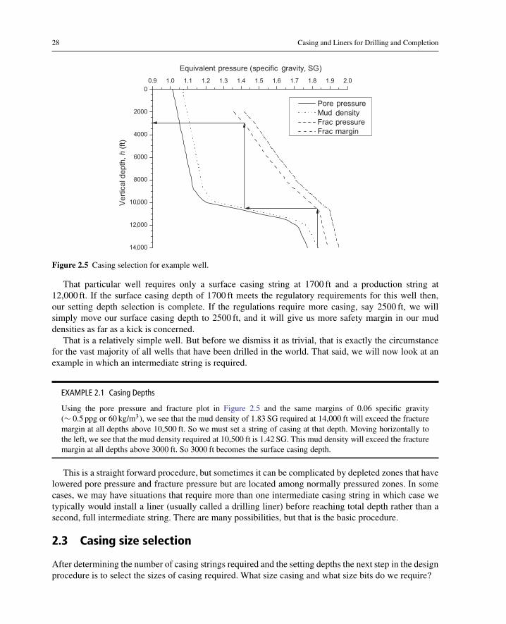
28 Casing and Liners for Drilling and Completion
d
p g
pdpm
,
,
,
Figure 2.5 Casing selection for example well.
That particular well requires only a surface casing string at 1700 ft and a production string at12,000 ft. If the surface casing depth of 1700 ft meets the regulatory requirements for this well then,our setting depth selection is complete. If the regulations require more casing, say 2500 ft, we willsimply move our surface casing depth to 2500 ft, and it will give us more safety margin in our muddensities as far as a kick is concerned.
That is a relatively simple well. But before we dismiss it as trivial, that is exactly the circumstancefor the vast majority of all wells that have been drilled in the world. That said, we will now look at anexample in which an intermediate string is required.
EXAMPLE 2.1 Casing Depths
Using the pore pressure and fracture plot in Figure 2.5 and the same margins of 0.06 specific gravity(∼ 0.5 ppg or 60 kg/m3), we see that the mud density of 1.83 SG required at 14,000 ft will exceed the fracturemargin at all depths above 10,500 ft. So we must set a string of casing at that depth. Moving horizontally tothe left, we see that the mud density required at 10,500 ft is 1.42 SG. This mud density will exceed the fracturemargin at all depths above 3000 ft. So 3000 ft becomes the surface casing depth.
This is a straight forward procedure, but sometimes it can be complicated by depleted zones that havelowered pore pressure and fracture pressure but are located among normally pressured zones. In somecases, we may have situations that require more than one intermediate casing string in which case wetypically would install a liner (usually called a drilling liner) before reaching total depth rather than asecond, full intermediate string. There are many possibilities, but that is the basic procedure.
2.3 Casing size selection
After determining the number of casing strings required and the setting depths the next step in the designprocedure is to select the sizes of casing required. What size casing and what size bits do we require?

Casing depth and size determination 29
2.3.1 Size selection
Once the setting depths have been determined, the next step is obviously to select the sizes of the casingstrings to be set. The sizes will depend on a number of criteria, but two important things to know aboutselection of casing size are as follows:
• Hole size determines casing size• Hole size at any point in the well except the surface is determined by the previous string of casing
This means that in selecting casing size, we usually start with the casing size at the bottom of the holeand work to the top.
The size of the last string of casing run in a well is generally determined by the type of completionthat will be employed. That decision is usually the function of an interdisciplinary team of reservoir,production, and drilling personnel. There are numerous criteria on which this decision is based, so wewill assume for our purposes that the size of the final string is predetermined, and we will proceed fromthat point. From the standpoint of drilling operations, our input into that process is to assess the risksand allow for alternatives. For example, if we know there are serious hole stability problems in an areaand our drilling experience in the area is limited, we may be well advised to recommend a final size thatis still large enough for us to set an extra string of casing or liner and still reach the objective with ausable size of hole for a good completion. This is a point that is unfortunately too often overlooked inthe desire to keep well costs low.
Once we know the diameter of the final string of casing or liner, the process proceeds like this:
• Determine the hole size (bit size) for the final string of casing.• Determine what diameter casing will allow that size bit to pass through it. That is the size of the next string of
casing.• Repeat the procedure until all of the hole sizes and casing sizes have been determined.
Many times in actual practice, casing sizes are often determined by what is readily available in someinventory (the company’s, partner’s, or vendor’s) and the delivery times. The cost of leaving surpluspipe in inventory or excessive delivery times often supersede any “optimum design” based strictly onengineering calculations.
Precaution: After the casing strings have been designed be sure to check the drift diameters to becertain that all the desired bit sizes can be accommodated.
2.3.2 Borehole size selection
What is the proper borehole size for various sizes of casing? What do we require of the borehole size?
• A borehole must be large enough for the casing to pass freely with little chance of getting stuck.• There should be enough clearance around the casing to allow for a good cement job.• In general, the bigger the borehole the more costly it is to drill.
There are no formulas for determining the ideal borehole size.Selecting the borehole size is primarily based on current practices in the area or areas with similar
lithology. There are a number of charts and tables in the literature, some good for some areas, but greatlylacking for other areas. The best advice we can offer is to use what is common practice in the area unless

30 Casing and Liners for Drilling and Completion
Casing/liner
Bit/hole
Casing/liner
Casing/liner
Casing/liner
Casing/liner
Bit/hole
Bit/hole
Bit/hole
4 4 1/2 5 5 1/2
5 5/8 6 1/8 6 1/2 8 1/2
6 5/8 7 7 5/8 8 5/8 9 5/8
6 3/4
8 5/8 9 5/8 10 3/4 11 3/4 13 3/8
11 3/4 13 3/8 16 20
16 20 24 30
12 1/410 5/89 7/88 3/48 1/27 7/8
10 5/8 12 1/4 14 3/4 17 1/2
14 3/4 17 1/2 20 26
7 7/8
6 5/8
Figure 2.6 Typical bit and casing sizes for hard rock environments.
there is good reason to do otherwise. No matter what specific charts we suggest here, they going to bewrong for some particular locale or application. That notwithstanding, here are two charts that showsome typical choices. One chart is for hard rock (Figure 2.6), and the other is for unconsolidated rock(Figure 2.7).
These charts start with the last string of casing or liner and work downward to the first casing stringof the well. You can see on these charts that there are many options even for those situations wherethe same size liner or casing is to be run. In general, hard rock offers us more choices, and clearancebetween the casing and borehole wall can be less than for unconsolidated formations.
You will note in the chart for unconsolidated rock that there are still some options, but not as many.A few may not be available even though shown on the chart. For instance on the fourth row from the topit shows that either an 8-1/2 in. or an 8-3/4 in. bit may be used from 9-5/8 in. casing. That may be truein some cases, but if the 9-5/8 in. casing string contains any 40 lb/ft or heavier pipe then the 8-3/4 in.bit cannot be used. What is common practice in one area may not work in another because formationpressures may require a heavier pipe.

Casing depth and size determination 31
Casing/liner
Bit/hole
Casing/liner
Casing/liner
Casing/liner
Casing/liner
Bit/hole
Bit/hole
Bit/hole
4 4 1/2 5 5 1/2
5 5/8 6 1/8 6 1/2 8 1/2
6 5/8 7 7 5/8 8 5/8 9 5/8
6 3/4
8 5/8 9 5/8 10 3/4 11 3/4 13 3/8
11 3/4 13 3/8 16 20
16 20 24 30
12 1/410 5/89 7/88 3/48 1/27 7/8
10 5/8 12 1/4 14 3/4 17 1/2
14 3/4 17 1/2 20 26
7 7/8
6 5/8
Figure 2.7 Typical bit and casing sizes for unconsolidated rock environments.
EXAMPLE 2.2 Casing Size Selection
Continuing with the same example, we looked at previously in this chapter; assume that we have determinedthe following casing depths:
• Surface casing: 3000 ft• Intermediate casing: 10,500 ft• Production casing: 14,000 ft
The production engineers tell us they will require a production casing diameter of 7 in., so the productioncasing size is determined. Assume that the well is in an area of unconsolidated formations. Use the softformation chart (Figure 2.7) to determine the intermediate casing size, the surface casing size, and theconductor casing size.
• Intermediate casing: 9-5/8 in.• Surface casing: 13-3/8 in.• Conductor casing: 20 in.

32 Casing and Liners for Drilling and Completion
Although not shown in the chart as a possible path, some operators in areas where borehole stability is aserious problem elect an alternative for 7 in. casing as follows:
• Intermediate casing: 10-3/4 in.• Surface casing: 16 in.• Conductor casing: 24 in.
That choice would be a case where experience in a particular area might influence the decision in order toallow more margin for the effects of anticipated problems.
A precautionYou may note in the two charts above that more casing-borehole clearance is specified in unconsolidatedformations than in hard rock formations. Why? Most unconsolidated formations occur in newergeological marine environments where swelling shales and high permeability zones are commonplace.These environments are known for reduced clearance caused by the swelling shales, accumulationof break-out and sloughing debris, as well as differential sticking tendencies in the more permeableformations. There is sometimes a tendency for those inexperienced in these environments to assumethat these unconsolidated zones will be washed out and actually have greater clearance instead of less.While that is definitely true through some intervals, it is not true of the entire exposed borehole. Theconsequences of such an assumption is almost always disastrous.
2.3.3 Bit choices
Obviously from the above charts, we select the hole size for our particular casing and that automaticallysets our bit size too. While that is true, there is another aspect to the bit sizes that should be mentioned.Those charts are based on the most commonly available bit sizes. There are special cases where it will benecessary to use an unusually thick wall casing, and you find that the common bit used in that casing willnot work—the bit is too large. There are other diameters of bits available for special applications that arenot shown in these charts. In general, they tend to cost more, but the biggest problem is that often thereis a limited choice of bit types when it comes to uncommon bit sizes. For instance for one common size,we may have a choice of 25 different tooth and hardness characteristics just from a single manufacturer,and maybe 50-100 choices if we include all manufacturers. However, with some odd size bit, we maybe limited to a small range of tooth and hardness choices and possibly only one manufacturer. That maybe acceptable for some special cases, but it should always be considered.
Bit clearance
To determine the bit clearance, we look at the casing tables for the internal diameter and see if it islarger than the diameter of the bit. But in the tables, we see two diameters listed. One is the nominalinternal diameter and the other is the internal drift diameter which is slightly smaller than the internaldiameter. The internal diameter is the diameter to which the tube is supposedly manufactured. Once ithas gone through the milling process, it is inspected for final diameter by passing a mandrel through itof the diameter listed as the internal drift diameter. So its internal diameter might be the same as thenominal internal diameter or it might be slightly smaller (or larger), but we know that it is at least aslarge as the drift diameter (assuming the manufacturer does its job). We normally assume that the driftdiameter is the maximum bit diameter, we can be assured will pass through the casing. But in manycases, bits greater than the drift diameter have been used. In that case, you must drift the casing with a

Casing depth and size determination 33
mandrel the size of the bit first and cull out those joints that are undersized. Some steel mills will do thisfor customers (usually at extra cost).
2.4 Casing string configuration
Once we determine the depths of the casing strings, we may still have several alternatives.Figure 2.8 shows three possible configurations for our example well. The first shows a conventional
production casing string. The second shows a production liner where the intermediate string also servesas part of the production string. The third one shows a tieback string inside the intermediate string andconnected to a liner at the bottom of the intermediate string. One can see that the second option mightsave the operator money by eliminating a full production string, but why would an operator elect tochoose the third option as opposed to the first or the second? One reason might be to reduce the weightof the final string and save money using a lower tensile strength casing. Of course that has to be moresaving than the additional cementing and equipment cost and additional rig time required. However,here is a typical situation for choosing the third option. We are drilling a high pressure, well and theintermediate casing is required to contain the high density mud while drilling the lower part of the hole.In this case, suppose it takes a few weeks to drill the hole below the intermediate casing so there maybe considerable wear from the drill string on the intermediate string. This means we have to rule outoption number two because the intermediate casing may not be able to contain the pressures required ofa production string that has loss of wall thickness from the wear. In this case the first option is usuallycheaper than the third option which requires more time, more cement, and more equipment, so we stillsee no reason for selecting the third option. Consider two more things though. Remember that we saidthat it was a high pressure well. The operator wants to be assured that the casing above the cement doesnot leak, and the best way to assure this is a hydrostatic test of the casing connections as the casing isbeing run in the hole. This cannot be done with a full string of pipe because the static time requiredto test each connection will probably allow the casing to become stuck before it gets to bottom. Thatwould then be an extremely costly situation which would require another liner of a smaller diameter
Productioncasing
Productionliner
Tiebackcasing
Conductorcasing
Surfacecasing
Intermediatecasing
150 ft
3000 ft
10,500 ft
14,000 ft
Figure 2.8 Three possible casing configurations.

34 Casing and Liners for Drilling and Completion
than the production casing. So, while the third option is not common there are often very good reasonsfor doing it. And further, there are many wells that require two liners instead of one, and the tiebackstring is always a preferred option in that case. There are many possibilities. Well conditions and costsdictate the actual choices. We will discuss those choices in more detail later.
2.4.1 Alternative approaches and contingencies
There are additional approaches to allow for more clearance for the casing. One method is to under reamthe open hole below the current casing string. This allows additional clearance and is a proven methodwhere the expense of the extra time and reaming can be justified. A similar result can be obtained witha bicentered bit for drilling below the current string of casing. Such a bit will drill a larger diameterhole than its nominal diameter. This technique can eliminate the extra expense of under reaming andaccomplish the same result.
Another option is the use of expandable casing. This is a relatively new technology and has provensuccessful in a number of applications. The hole is typically drilled with a bicenter bit or under-reamedto give more clearance. The casing itself is run just like a conventional liner and is expanded after it isin place. Expandable casing will be discussed in more detail in Chapter 6.
2.5 Closure
In this chapter we have examined the procedures for selecting casing setting depths and casing sizes.We used a plot of formation pore pressures and fracture pressures to select the setting depths. This is astraightforward method that may appear deceptively simple. The truth is that it is not the procedure thatis complex, but the data itself for use in the plot. Often, it is not readily available nor is it totally reliable.When this type of procedure first came into use many operators looked at it as a way to save moneyby reducing the number of casing strings traditionally run in some areas. It appeared that in manycases, it was possible to run surface casing a bit deeper and eliminate an intermediate casing stringaltogether. When it worked it did save costs, but when it did not work it not only added the string thatwas “eliminated” but often an additional string as well, and resulted in a very small hole size at bottomand significant additional costs. The problem in these situations was that the data proved unreliable insome cases and that the margins were too close for operating personnel to adhere to in others. So in allcases, the data used in the depth selection process must be scrutinized with care. A prudent philosophymight be stated like this:
• Exploratory wells or critical wells. Data are possibly scarce or unreliable, so allow for the unexpected withcontingencies in casing size and depths. Usually this means allowing for the possibility of running one morecasing string or liner than the plan calls for. These are not the wells where we try to save money on casing.
• Development wells. Data reliability and risks are well known. These are the wells where casing costs can beminimized and smaller margins can be used.
No matter what method you use to determine the casing setting depth, always keep in mind that it is oneof the most critical steps in assuring a well’s success. Do not be caught in the trap of compromising thechances of success by trying to save money by unnecessarily minimizing casing depths and sizes.

3Pressure load determination
Chapter outline head
3.1 Introduction 363.2 Pressure loads 373.3 Gas pressure loads 383.4 Collapse loading 38
3.4.1 Collapse load cases 39Installation stage—collapse loads 39Drilling stage—collapse loads 40Production stage—collapse loads 40
3.5 Burst loading 413.5.1 Burst load cases 42
Installation stage—burst loads 42Drilling stage—burst loads 43Production stage—burst loads 44
3.6 Specific pressure loads 463.6.1 Conductor casing 463.6.2 Surface casing 47
Surface casing collapse loads 47Surface casing burst loads 47
3.6.3 Intermediate casing 48Intermediate casing collapse loads 48Intermediate casing burst loads 49
3.6.4 Production casing 49Production casing collapse load 49Production casing burst loads 50
3.6.5 Liners and tieback strings 503.6.6 Other pressure loads 51
3.7 Example well 523.7.1 Conductor casing example 52
Conductor collapse loads 52Conductor burst load 53Additional considerations 53
3.7.2 Surface casing example 53Surface casing collapse loads 54Surface casing burst loads 56
3.7.3 Intermediate casing example 60Intermediate casing collapse loads 62Intermediate casing burst loads 63
3.7.4 Production casing example 66Production casing collapse loads 68Production casing burst loads 70
3.8 Closure 74
Casing and Liners for Drilling and Completion. http://dx.doi.org/10.1016/B978-0-12-800570-5.00003-6Copyright © 2015 Elsevier Inc. All rights reserved.

36 Casing and Liners for Drilling and Completion
3.1 Introduction
In this chapter, we discuss the pressure loads, collapse and burst, used in the design of casing strings.To illustrate the process, we continue with the example selection from the previous chapter, wherewe determined the setting depths and casing sizes. Here we will discuss the various types of pressureloads and some particulars as they apply to the different types of casing strings. The actual calculationsare merely hydrostatic calculations with various combinations of fluids inside the casing and in theannulus outside the casing. After a discussion of the pressure loads and their application to thedifferent casing strings, we present examples using the casing program we selected in the previouschapter.
To determine the strength of the casing needed, we must now consider the types and magnitudes ofthe loads the casing must safely bear. A number of different considerations and possibilities accompanyeach string of casing run in a well. Some simple load situations suffice for most casing strings, butoften special conditions may apply to a specific well or type of well. We will discuss the types of loadscommonly used as design criteria for each type of casing string. Three basic types of loads commonlyare considered:
1. Collapse loads are differential pressure loads in which the outside pressure exceeds the inside pressure, tendingto cause the casing to collapse, �p = pi − po < 0.
2. Burst loads are differential pressure loads in which the inside pressure exceeds the outside pressure, tending tocause the casing to rupture or burst, �p = pi − po > 0.
3. Axial loads are tension or compression loads mostly caused by gravitational and frictional forces on the pipe,but they can also be caused by pressure and temperature changes as well as bending in curved wellbores.
The first two of those load types are dictated by well conditions and anticipated operations in thewell. They are functions of formation pore pressures, fracture pressures, drilling fluid pressures, andcement pressures. Those are the two we cover in this chapter. For the most part, we will be workingwith differential pressure loads across the casing wall, defined as the inside pressure minus the outsidepressure, �p ≡ pi − po. The third type of load, axial load, is a function of the casing selection processitself; in other words, the axial load is a function of the weight of the casing selected. Axial loads arecovered in the next chapter.
We have used the terms, collapse and burst, rather loosely as if their meanings were obvious, but weshould clarify that now because they are somewhat misleading. Collapse is a form of radial instabilitythat results in radial buckling. The actual deformation referred to as collapse of the pipe is a postbucklingevent. From that, one would assume that the collapse rating of a casing is the minimum pressure at whichthe instability occurs and that any small perturbation in the load, could then cause buckling followed byactual postbuckling collapse. That is not quite the case, however. The API collapse rating is defined fortwo extremes: (1) elastic stability for pipe with a relatively large diameter to wall thickness ratio, do/tw,and (2) for thicker wall pipe with smaller do/tw ratios, the formula defines the collapse rating to theminimum collapse pressure that will cause yield in the pipe. The burst rating is a bit easier to define; it isthe internal pressure at which the inner wall of the pipe initially yields. It is not the pressure at which thepipe would actually rupture as one might expect from the word “burst.” We will delve into these ratingsin Chapter 6, but for now we are satisfied with knowing what the two terms mean, and that we can lookup the values in available tables.
One more clarification about pressure: We will always work in gauge pressure rather than absolutepressure since the difference is insignificant at the magnitudes and applications we are using. When wespecify 0 psi, we mean atmospheric pressure. Further, we will not use any atmospheric gradient whenworking with empty or partially empty casing.

Pressure load determination 37
3.2 Pressure loads
The magnitude of the pressure loads that a particular casing string actually experiences in service for themost part are unknown. Certainly, we can calculate the loads we are likely to encounter if all operationsare perfectly successful, but the problem is that often there are imperfections in our cementing resultsor problems in our drilling operations. We almost always are able to determine loads if all is perfect,and we can almost always determine the type of loading that would take place if things go totallyawry. But between those two situations is a great unknown. Hence, our most logical approach is toassume the worst case that can happen, within reason, and that is the one we typically use for our casingdesign. We assume that we can reasonably predict the nature of the worst case loading and calculateits values. For now, we do not concern ourselves with the probability of such loading occurring. Thething that we have to always keep in mind is that we cannot change our designed casing string onceit is in the ground and cemented. If that “unlikely” worst case should occur, it is too late to changeour design.
The process we now address consists of determining the types of pressure loads and the sources ofthose loads. These are listed below:
Types of pressure loads• Collapse loading• Minimum internal pressures• Maximum external pressures
• Burst loading• Maximum internal pressures• Minimum external pressures
Sources of pressure loads• Formation fluids• Water (fresh or salty)• Oil• Gas
• Drilling fluids• Whole mud• Mud filtrate• Un-set cement• Whole cement• Cement filtrate
• Stimulation fluids• Ocean or surface water• Atmosphere
These are the pressure sources that contribute in various combinations to the pressure loading ofcasing in wells. It is relatively easy to ascertain the internal pressures for design purposes because wealmost always know the internal fluids, at least in the design stages. The difficulty is that we seldomknow the external fluids and pressures once the casing is in the ground and cemented. It is the singlebiggest problem in the pressure loading phase of casing design. All we can do is make some reasonableassumptions, and what is reasonable to one engineer may not be reasonable to another. It can become a
38 Casing and Liners for Drilling and Completion
bit too subjective. The most common approach is to consider the worst case, not the most likely case.That may seem like a case of avoidance or oversimplification. It is both, but I will repeat time and againin this textbook: You cannot change your design once the casing is in the ground.
3.3 Gas pressure loads
Gas pressure is one of the most common loads in casing design, and we need to make a few comments. Itis often the case that we know the gas pressure at a source depth but need the value of the pressure in a gascolumn at another depth. This is not the same simple hydrostatic calculation we use for incompressibleliquids because gas is compressible, and hence, its gradient is not a constant. There are a number ofapproaches for calculating natural gas pressures using the ideal gas law and compressibility factors. Thecompressibility factor is itself a function of temperature, pressure, and gas composition. Where the dataare available, such methods are employed. However, for our basic casing design, we are going to usethe common practice of assuming any gas encountered is pure methane whose molecular mass is 16 g(or 16 lb when using a lb-mol) and whose compressibility factor, Z = 1 for a fairly large range. Sincemethane is the least dense of the natural gas components, it gives us the most conservative results incasing design. Many companies use it as a standard in casing design.
Fortunately, the assumption regarding the compressibility leads to a simple equation that we will usein our basic design work:
p = p0 expM g (h− h0)
ZRTavg(3.1)
where
p, p0 = pressures, pressure at h and pressure at h0, respectively
h, h0 = vertical depths, depth of interest and reference depth, respectively
M = molecular mass, 16 for methane
g = gravitational acceleration
Z = gas compressibility factor, Z ≈ 1 for methane
R = ideal gas constant, see Appendix B for appropriate values
Tavg = average absolute temperature, Tavg = (T + T0)/2
This equation is derived in Appendix D as Equation (D.16). In this equation, R = 1545 in USC unitsand R = 8314 in SI units.
3.4 Collapse loading
In the case of collapse loading, our task is to determine the least amount of pressure the casing will haveinside and the maximum amount of pressure the casing will have on the outside (simultaneously at anygiven stage in the operations).

Pressure load determination 39
Internal loads, collapse• Evacuated casing (fully or partially)• Gas• Oil• Freshwater• Field saltwater or stimulation fluids• Drilling or workover fluids• Combinations and partial columns of these
To these we might add some applied pressure in various situations.
External loads, collapse• Freshwater• Saltwater• Formation pressure• Drilling fluid• Cement (un-set)
3.4.1 Collapse load cases
We categorize collapse loading by operational stage such as installation, drilling, and production. Wefurther breakdown the operations into different events and possible occurrences that may take placewithin those three operational stages.
Installation stage—collapse loads
The installation stage is the running and cementing of the casing string. It also includes postcementingoperations such as pressure testing.
Installation—runningThere is only one collapse scenario in running casing and that is running an empty or partially emptycasing string. Neither is almost ever done intentionally and few designs account for it.
Installation—conventional cementingThe density of cement is almost always greater than the displacement fluid. Once the cement is inplace and the displacement and plug-bump pressure is released, this differential should not cause casingcollapse. It is imperative that this calculation be included in the design, especially when the differencein densities is significant.
Installation—inner string cementingInner string cementing is a process wherein the casing is not cemented with conventional top and bottomwiper plugs but by running a smaller diameter string (usually drill pipe) inside the casing with a sealassembly that connects to a special float shoe on the casing. The cement is then pumped through theinner string rather than the casing. This is especially effective in cementing large diameter pipe. Itreduces pumping time as well as reducing contamination of the cement slurry as it is pumped in the

40 Casing and Liners for Drilling and Completion
large diameter pipe. Inner string cementing is usually restricted to conductor and some large diametersurface strings. The collapse situation occurs because the cement is more dense than the fluid inside thecasing which may be even less dense than the displacement fluid used in the inner string.
Drilling stage—collapse loads
Collapse during drilling is almost always caused by loss of internal pressure from lost circulation. Insome cases it can be severe enough to completely evacuate the casing.
Drilling—lost circulation, evacuatedComplete evacuation occurs when a very weak zone below the casing fractures and allows the drillingmud to enter. The hydrostatic head is reduced and the mud level in the well drops. Continuedpumping only pumps more mud into the fractured zone and does nothing to keep the mud levelabove a static equilibrium with the fractured zone. In some severe cases, the casing string may becompletely evacuated. This usually happens when drilling below surface casing, but is not unknownwith depleted zones below some intermediate strings. This is the most common case used in surfacecasing design.
Drilling—lost circulation, partial evacuationIn most cases of lost circulation, the casing is not fully evacuated. With very accurate fracture data andformation pressure data, we could calculate the level to which the drilling fluid would be in equilibriumwith a fractured formation. This is mostly wishful thinking since such accurate and reliable data areseldom available during the design process. For surface casing, we usually design for a fully evacuatedstring, but for intermediate casing, we seldom see a fully evacuated string and to design for such, mightseem a bit too conservative. In most cases of lost circulation while drilling below intermediate casing,the most immediate concern is a kick caused by the loss of hydrostatic head. Allowing the well toremain static is not an option, the hole should be kept full if at all possible to avoid gas from reachingthe surface. Filling with drilling mud will not work because the level will continue to fall and the mudsupply on hand will be quickly exhausted. The common procedure is to try to keep the hole full withfresh water, or if offshore, seawater. That is what we will use in our examples.
Production stage—collapse loads
This case applies primarily to the production casing. One may not think of collapse as a possibilityduring the producing life of a well. But to the contrary, it is a very real possibility, perhaps not in theearly stages but definitely in the later life of the well.
Production—evacuationHow can a production string be evacuated? More easily than many might suspect. For example, a packerin a gas well develops a slow leak, and the packer fluid is “produced” along with the gas until it isexhausted. Or, the perforations sand up below the packer and the flowing gas well bleeds to atmosphericpressure. Or another, a well is stimulated and coiled tubing is run to jet the well with nitrogen. Thejetting removes all the fluid but the perforations are plugged. The nitrogen flow is stopped and bledto zero. The casing collapses below the packer. And there are many more. These are things that arealmost never planned, but they happen frequently. A production string should always be designed forevacuation if possible.

Pressure load determination 41
Table 3.1 Summary Collapse LoadingCases
Collapse Loading C S I P
InstallationRunning, empty S S SCementing, post plug bump A A A A
DrillingLost circulation A A ACuttings injection S S S
ProductionEvacuation S S AArtificial lift S SStimulation, squeeze S A
C, conductor; S, surface; I, intermediate; P, production; A, alwaysapplicable; S, sometimes applicable.
Production—artificial liftArtificial lift poses similar hazards as evacuation. It is not at all uncommon to bleed off the gaspressure from casing prior to a workover in a gas-lift well. Depending on the liquid level in the casinga collapse situation might arise. A submersible pump could pump a well “dry” if the perforationsshould plug.
Production—stimulation, squeezeIt is possible that production casing can collapse during a stimulation or squeeze cementing operation.When a well is stimulated or squeeze cemented through perforations using a retrievable squeeze tool orcement retainer, often times the formation must be fractured to initiate pump in. The collapse problemarises from the fact that whenever we fracture a formation through perforations we have no idea wherethe fluid is going in the annulus. We like to assume that there is good cement and the fracture takes placein the perforations, but that is not always the case. If there is a channel such that the casing above thepacker experiences the fracture pressure it is possible that the casing could collapse above the treatmentpacker or retainer. It is prudent practice to always assure that the work string annulus above the packeris full and that some amount of pressure is applied to the annulus at the surface. This helps to preventcollapse but also is needed to monitor the casing for work string and packer leaks, especially whensqueezing with cement. In all cases, the fluid density in the casing should be equivalent to the formationpressure or slightly higher, so it is a matter of the maximum differential pressure between the formationpressure and the formation fracture pressure.
A summary of collapse loading cases for the three stages of well construction is given in Table 3.1.
3.5 Burst loading
For burst loading, we seek to find the maximum internal pressure and the minimum external pressureoccurring simultaneously at any given stage of operations. In low pressure wells or wells that will notflow, burst is seldom considered. However, one should keep in mind the possibility of a future fracturejob or high-rate stimulation that might be pumped down the production casing. In burst loading, the

42 Casing and Liners for Drilling and Completion
external pressure is the resisting load, and the external loading in a burst situation normally is taken tobe the lowest possible pressure externally. At the surface of the string, that pressure is taken to be zeroor atmospheric pressure. In a subsea casing string, it would be the seawater pressure at the wellhead.The external pressures other than at the surface could be from a number of sources.
External loads, burst• Atmospheric pressure (at surface of string)• Seawater pressure (at surface of string)• Freshwater• Saltwater• Formation pressure• Drilling fluid
It is never acceptable to assume that hardened cement will give us support in burst, even thoughit will. The problem with cement is that we have to design our string before the well is cemented. Ifour cement job is near perfect, then we have additional support in those sections covered by cement.However, if there is even a small interval where the cement is poor, then we have no support at thatinterval, and there is nothing we can reasonably do to change that. Hence, we can never safely assumethat the hardened cement gives us any benefit when we are in the design stage.
Internal loads, burst• Gas• Oil• Water• Combinations of gas and liquids• Cement (liquid)• Pump pressure (plug bump, test pressure, stimulations)
3.5.1 Burst load cases
Burst loading can occur in all stages of well construction and production. The various cases are describedhere, and they will all be illustrated in the examples later in the chapter.
Installation stage—burst loads
The installation stage is the running and cementing of the casing string. It also includes postcementingoperations such as pressure testing.
Installation—plugged float or annular bridgeDuring cementing, there is always the possibility that a float could plug or the annulus could bridgewhile displacing the cement. Such an unanticipated event would likely be accompanied by a significantincrease in pump pressure before the cementer could become aware and shut off the pump. While thisis unlikely, it should be included in the burst cases. The worst case depends on a number of things likethe cement volumes and densities compared the annular fluid and displacement fluids. This is one of themore complicated hydrostatic calculations and is better understood by example; hence, we will examinethis case later in this chapter in the example cases.

Pressure load determination 43
Installation—plug bumpWhen the top wiper plug (on top of the cement) contacts the top float, it stops the displacementcirculation and an increase in pressure occurs. This is an anticipated event and the cementer appliesa predetermined additional pressure above the displacement pressure before stopping the pump. This isreferred to as the plug-bump pressure. Its purpose is to assure that the plug is indeed seated on top ofthe float. Because the cement is almost always more dense than the displacement fluid, the maximumdifferential pressure occurs when all the cement is displaced. Added to that differential then is the plug-bump pressure. The magnitude of this pressure is a matter of preference, company policy, and so forth,but it is generally on the order of 500-1500 psi depending on the casing and well conditions. And to becandid, its actual magnitude sometimes is a result of careless monitoring of the displacement progressand may exceed the predetermined amount. In any case, the differential burst pressure in the upperportion of the casing can be quite significant, and this should always be a design consideration for allconventionally cemented casing strings.
Installation—pressure testEveryone should agree that all casing should be pressure tested once it is in place. In many areas, itis required by regulations. Where the controversy arises pertains to when it is tested. Many operatorslegitimately claim that the plug-bump pressure is the best test. If the casing holds pressure then there isno reason for it to leak later. That is valid, but unfortunately, many regulations require a pressure testbe performed later before drilling out the floats and proceeding to drill deeper (or after 24 h or so forproduction strings). Most who favor the former argue that premature pressure testing after the cement hassupposedly set can damage the cement sheath around the casing, and this is a valid point. It is especiallyvalid for surface casing where lower temperatures slow the cement curing process and the curing timewhile installing and testing the BOP stack on the surface casing is relatively short. Waiting additionaltime for cement to strengthen is expensive and too often ignored. It is not so critical on intermediatestrings where temperatures are higher, more time is required to change out the BOP stack and topick up a string of smaller diameter drill pipe to drill below the intermediate string. Those argumentsnotwithstanding, most pressure tests are done after the cement has been placed and supposedly cured.Our only question is, what is the fluid in the annulus? Simply put, we do not know. About the best wecan come up with is that in the worst case, it is the same as the mud the casing was run in. Assuming thedisplacement fluid in the casing is the same density as original mud, then this case will give a uniformdifferential pressure test to the entire casing string. Since most regulations specify a surface pressure forthe test, this is the most legitimate form of the pressure test. Changing the mud in the casing before thetest is obviously not a good idea.
Drilling stage—burst loads
There are only two general cases of burst loads that occur in the drilling stage of well construction. Theyare the maximum mud density used in the casing before the next casing string is set and the pressurefrom a kick.
Drilling—maximum mud densityWe always know, or should know, the maximum mud density we will use in drilling below a casing stringto reach the next casing point. What we never know is the fluid in the annulus. So again we take a worstcase scenario that is within reason. For surface casing we generally assume something like freshwaterfor surface casing and maybe saltwater for intermediate casing. Some would assume the mud the casing

44 Casing and Liners for Drilling and Completion
was run in and others might assume formation pressure. While a formation pressure gradient mightsound most reasonable, we must also consider depletion of zones covered by the casing that are beingproduced in other wells. That applies mostly to production casing, but formation pressures as backupare seldom used in most cases. For simplicity (and lack of data), most use freshwater or saltwater inbasic design and use more detailed information for critical wells.
Drilling—well kickThere are three fluids involved in kicks, singly or in combination: gas, oil, and saltwater. Of these, gasis the most severe and dangerous. In considering kicks, we limit ourselves to surface and intermediatecasing strings, because production strings are designed as a tubing backup and that is included in theproduction stage of operations. We normally assume that the kick originates at the highest pressurezone below the casing string, and that in the worst case we have a solid column of the formation fluid(gas, oil, or saltwater) all the way to the surface. All well-control methods are designed to prevent that,but it happens, and when it does, it is too late to change the casing design. There are two approachesto determine the pressure inside the casing: (1) if the pressure of the column of fluid does not exceedthe least fracture pressure in the open hole (usually near the shoe) then the pressure of that columnis calculated from the kick source zone to the surface, or (2) if the pressure of the kick fluid columnexceeds the formation fracture anywhere in the open hole, we assume the kick fluid is flowing into thatformation, and we calculate the pressures in the casing using that fracture pressure as the source zonepressure and assume a solid column of the kick fluid from there to the surface.
As already stated, gas is the most severe of these and is usually the basis for our design. Thereare, however, some areas of the world where there is no gas present, and the design is based on anoil column. Seldom do we design for a saltwater kick, but it is a common possibility in some wellsbetween the surface and intermediate casing strings where there is no gas or oil. As usual, the questionof the annular fluid is the same, and again, freshwater, saltwater, or drilling mud are the commonoptions.
Production stage—burst loads
In the production stage of operations, the only affected string is the production string. The exceptionto that would be a well that has a production liner and utilizes the intermediate string as part of theproduction string. In that case, the intermediate string must meet the design criteria of both intermediateand production casing.
Production—pressure testIn a production casing pressure test, we almost always assume the backup pressure is the mud in whichthe casing was run because the test is carried out soon after cementing. If the displacement fluid insidethe casing is the same drilling fluid then the pressure test differential will be uniform from top to bottom.If a less dense displacement fluid is used (common with some operators to enhance cement to pipebonding) then the test should be performed when the displacement fluid is replaced by the more denseworkover/completion fluid.
Production—tubing backupThe production casing is a pressure backup for the tubing string. Tubing strings leak, and that is a given.Not always, but it is one of those unfortunate things we cannot predict nor always prevent. Because

Pressure load determination 45
Table 3.2 Summary Burst Loading Cases
Burst Loading C S I P
InstallationCementing, plugged float A A A ACementing, plug bump A A A APressure test S A A A
DrillingMax mud dens. below shoe A A A SGas kick (full gas col.) A A SOil kick (full oil col.) A A SSalt wtr. kick (full salt wtr. col.) A A S
ProductionPressure test S ATubing backup S ATubing gas leak S AStimulation, squeeze S A
C, conductor; S, surface; I, intermediate; P, production; A, alwaysapplicable; S, sometimes applicable.
the production casing does have some backup in the annulus, it does not have to have the same burstrating as the tubing, except near the surface. What the backup fluid is, is still unknown but generally wemay use freshwater or saltwater. You must remember though that the production casing absolutely mustcontain the well pressure so the worst case is mandatory here.
Production—tubing leakOne of the most severe burst loadings in a gas well results from a near-surface tubing leak. Theseleaks are not at all uncommon in gas wells. Near-surface tubing corrosion from freshwater condensationmixed with CO2 to form carbonic acid is quite common in many gas wells. Most operators monitor suchcorrosion in tubing, but occasional leaks still occur. The result is that wellhead gas pressure is appliedto the top of a full column of weighted packer fluid, and the differential pressures on the casing can bevery high near the packer. Some casing designers ignore this case altogether. Some operators providefor an emergency relief system on the annulus and/or use a reduced density packer fluid. Some elect topurchase a very expensive casing string.
Production—stimulations, squeezeA production string must be able to withstand stimulation and squeeze pressures. When such treatmentsare performed below a retrievable packer or a drillable retainer, only the portion of casing below that toolexperiences the treatment burst pressures. On the other extreme hydraulic fracture treatments performedwithout tubing in the well, subject the entire production string to the treatment pressures. The pressuresfor high-rate hydraulic fracture treatments can be quite high and are often the critical case for burstdesign. We will not consider this in our basic design process, but will discuss it in detail in Chapter 7.
A summary of burst loads for different casing strings during three stages of well construction isshown in Table 3.2.
46 Casing and Liners for Drilling and Completion
3.6 Specific pressure loads
As we saw in Tables 3.1 and 3.2, different casing strings experience some common types of pressureloads, but also some different types. We will now look at some of these loads as they apply to differentstrings.
In all our calculations, we will be using specific gravity, ρ, for density values to make it easier forthose working in different unit systems, so ρ = ρ ρwtr. We will consistently use a water density, ρwtr,of 1000 kg/m3 in SI units and 8.33 ppg in USC units or 62.43 lb/ft3 should the need arise. Most of ourpressure calculations at various depths will be done using liquid gradients:
γ = g ρ = g ρ ρwtr (3.2)
Using consistent units in a coherent system, e.g., SI, that is all we need. In USC units, we will needsome conversion factors, where γ will be in psi/ft (lbf/in.2/ft) and ρwtr will be in ppg (lb/gal). Thespecific gravity, ρ, is dimensionless and independent of our choice of system. We will use water densityof 1000 kg/m3 and 8.33 ppg in all our calculations.
γ = g ρ Cppg gc ρwtr = 32.14 ρ (0.052)
(1
32.14
)(8.33) (3.3)
This is all discussed in Appendix D including derivations of the conversion factors needed for USCunits. Since g · gc ≈ 1 in all our applications, we will not show it in our numerical calculations whenusing USC units.1
3.6.1 Conductor casing
Conductor casing design is to some extent different from all other casing in a well. Most of the conductorcasing is not regular API casing, some is API line pipe, but beyond 20 in. OD, none is API casing. Beingof a typically large outside diameter and relatively thin wall thickness, it generally has a low collapserating. When conductor is set in a drilled hole and cemented, it is usually cemented with an inner string(drill pipe), so there is little differential collapse pressure on the casing. Only rarely is conductor casingcapable of pressure control so burst is seldom a consideration. In offshore applications where a diverter(similar to an annular preventer) is installed, its purpose is to divert a shallow gas kick away fromthe rig to provide enough time for emergency evacuation before the gas breaks through the shallowzones outside the conductor and under the rig. Rarely can conductor hold pressure and prevent gas frombreaking through to the surface. As for tension, most conductor casing is set at such shallow depth thattension is not a consideration either. In many land locations, conductor is set by a small rig (“rat hole”rig) before the drilling rig arrives on location. Many offshore platforms have conductor casing installedas part of the platform installation process, though some require an additional conductor string oncethe rig is on the well. In many water locations, the conductor is driven into the earth with a diesel piledriver hammer. Additional joints are welded to the string as it is driven until it reaches a point where eachstroke of the hammer causes negligible additional penetration. The excess and damaged top portion is cutoff with a cutting torch. There are also conductor connections (even for drive pipe) that can be installedbefore the conductor joints are sent to the location, thus eliminating the time consuming welding process
1 Please note that the conversion factor, gc, does not convert g. It converts the density of water, ρwtr, from lb/gal to slug/gal. Thistraditional notation often confuses. Also please note that gc in this edition is a more conventional form and is the reciprocal ofthe form used in the first edition.

Pressure load determination 47
on the rig. There are a number of things to consider with drive pipe such as soil adhesion, elastic responseof the pipe to the hammer, hammer sizing and so forth. Where the conductor casing supports a wellheadand additional strings of casing there can be a considerable compressive load.
3.6.2 Surface casing
In this section, we examine the particular loads as they apply to surface casing. Typically, the loads insurface casing are relatively low compared to other casing strings in the well, but many casing failuresoccur because of under-designed surface casing.
Surface casing collapse loads
The collapse load for surface casing depends on the worst-case scenario anticipated, in which thepressure outside the casing exceeds the internal pressure. There are a number of possibilities, but themost commonly accepted situation assumes that the surface casing is empty inside (usually causedby lost circulation while drilling somewhere below) and has mud pressure on the outside of the samemagnitude as when the casing was run. We can modify the internal pressure, if we have some knowledgeof the worst case of lost circulation that could be encountered and how far the drilling fluid would dropin the surface casing should that occur. But, in the absence of such knowledge, we should assume the lostcirculation situation could be severe enough to empty the surface casing. On the outside of the surfacecasing, we know the pressure when the casing is run; it is the hydrostatic pressure of the mud column.If the cement is of greater density than the mud (and it usually is) we easily can calculate the pressurecontribution of the cement. The question is, what is the pressure after the cement hardens? We can befairly certain that it will not be as high as the cement pressure before it hardened, but the actual pressuredepends on the integrity of the cement job, that is, whether there are channels in the cement or someformations are not cemented properly. Typically, a safe assumption is that the highest pressure outsidethe casing after cementing is the mud pressure before cementing. It may be less, but it is unlikely to begreater.
Another possibility is a cementing related collapse or post plug-bump collapse where the internalpressure is released after the top wiper plug seats on the top float (plug bump). The liquid phase cementis almost always more dense than the displacement fluid (also a good cementing practice), and thepressure differential could cause a collapse. Such an event is rare, but should always be considered.
Typical surface casing collapse design loads• Cementing collapse• Severe lost circulation
Surface casing burst loads
The worst case burst load on the surface casing is based on the maximum anticipated internal pressureand the minimum anticipated external pressure. Let us look at the external pressure first. In collapse, wesought the maximum external pressure, now we are interested in the minimum. The minimum externalpressure is likely to occur sometime after cementing. It is believed that, when cement hardens, fluidin the spaces where the cement has channeled or is absent often is similar in density to freshwater orsaltwater. For that reason, many assume that the minimum external pressure is equivalent to a freshwatergradient. Some believe that a freshwater gradient is not really likely and they use the mud pressure onthe outside, just as we did in collapse. That is also a valid external load but not the most severe thatcould occur.

48 Casing and Liners for Drilling and Completion
The internal pressure for burst is a little more complicated. If we drill a well some distance below thesurface casing, encounter a gas kick, and get a large volume of gas in the casing, then the pressures couldget quite high. However, if the pressure is very high, the formations at the bottom of the surface casingwill fracture and gas flow will go into those formations. That being the case, it does not make senseto design a surface casing string to withstand say, 6000 psi internal pressure, if the formation belowthe surface casing fractures at 3500 psi. The typical procedure for determining burst load is to assumethat the maximum internal pressure is equivalent to the fracture pressure beneath the casing shoe andgas from that point to the surface. In cases where gas is known to not be present, we could use oil orsaltwater as the internal fluid. However, gas gives us the most critical load and should always be usedunless there is absolute certainty that no gas is present in the zones between the surface casing and thenext string of casing.
In addition, there are some other possibilities listed in Table 3.2.
Typical surface casing burst design loads• Internal pressure—equivalent of gas kick that fractures and flows into formation(s) below the casing shoe• External pressure—freshwater gradient
Again, we must emphasize there many possibilities and different companies have a variety ofapproaches. These, however, are simple and should be safe in most cases.
Surface casing load plotsOne of the easiest ways to work with casing loads is to construct a set of design load plots. Theanticipated loads, such as collapse pressures and burst pressures, are plotted graphically as pressureversus depth. This makes it very easy to visualize the loading, rather than relying on a lot offormulas. (We still need formulas and calculations to construct the load plots, but they require veryfew calculations.)
3.6.3 Intermediate casing
The intermediate casing loading often is straightforward, like the surface casing, except that themagnitude of the loads generally is greater. For many designs the procedure is exactly the same asour surface casing example.
Intermediate casing collapse loads
Collapse loading in intermediate casing is not often critical, but it can be. Many companies use a mudgradient outside the intermediate casing and no pressure on the inside. This almost always is the case ifthe intermediate casing later will become part of the production string after a production liner is set. Ifthe intermediate casing will eventually be covered by the production casing or a tieback string, then theissue of collapse load will be different.
Unlike the surface casing, total evacuation seldom occurs nor is even possible in most cases. Withvery accurate fracture data we could predict the depth to which the fluid inside the casing would fall,but we never have data that reliable. Often when lost circulation is experienced while drilling belowintermediate casing, it results in a kick event because of the loss of hydrostatic head. This can be a veryserious situation, and the normal procedure is to try to keep the casing full in order to better managethe kick. Obviously, the casing cannot be kept full using drilling mud because it has already fractured aformation and will continue to enter the fracture and the available supply on hand will exhaust quickly. It

Pressure load determination 49
is possible that no liquid will stay full to the top, but safety dictates that liquid continuously be pumpedinto the well to keep formation fluids, especially gas, from reaching the surface if at all possible. Thisusually means pumping freshwater or seawater to achieve this end. So for our lost circulation collapseload, we will assume the fluid inside the intermediate casing is all freshwater (seawater would be usedoffshore). Again we do not know what the outside pressure is, but we may conservatively assume it is amud channel (which is slightly greater than formation pressures).
However, in some cases, intermediate casing is set to allow the drilling of low-pressure formationsbelow the casing. In those cases, it is possible that the casing could be empty or nearly so.
Intermediate casing burst loads
The typical burst load for intermediate casing is similar to that for the surface casing. It assumesa freshwater, saltwater, or drilling mud gradient on the outside and gas pressure on the inside. Themaximum gas pressure is assumed to be a full column of gas with a pressure equal to the lesser of (1)that attributable to the source formation, or (2) that equivalent to the lowest fracture pressure below thecasing shoe. Those are the assumptions we will employ. In addition we also consider the plug-bumppressure and the test pressure prior to drilling out the shoe track.
In the first edition, I included a discussion of a once popular alternate approach called the “maximumload method” developed by Prentice [13]. It is based on the fracture pressure assumption above butallows for a partial mud column in the casing in addition to the gas. This method allows for a lowerworking pressure BOP stack to be utilized in many cases and consequently results in a considerablecost saving. While the method is sound in principle, it has two serious weaknesses. First, the well mustbe shut in before gas reaches a critical depth in the casing and certainly before it reaches the surface.Second, a functioning pump and adequate mud supply must be available to replace mud in the casingshould any migrate downward into the gas column and flow into the fracture. A failure of either ofthese two would result in a surface gas pressure exceeding the working pressure of the BOP stack andwellhead. While the method was once quite popular and successful, I believe that no prudent operatoris willing to assume such a risk in present times. Consequently, I have excluded it from this edition.
3.6.4 Production casing
As one might imagine, there are a number of different ways to consider the loads in the productioncasing. One purpose of the production casing is as a backup string for the production tubing, so thatit can support the same loads as a tubing string. However, there are some major differences in themaximum loads that a production string might encounter as compared to a tubing string. In some cases,the collapse load might be higher, and in other cases, the burst load might be significantly higher.
Production casing collapse load
The most common approach to collapse loading in a production string is to assume that the worstcollapse scenario is one in which the casing is empty and open to the atmosphere. This is not common,but it does happen. Another possibility is to assume that the well always has some amount of liquid orpressure inside it, equal to the formation pressure at the time (usually taken to be the depletion pressure).The situation for each well may be different and can be complex. One should always keep in mind thatwhat may actually occur in the future may be difficult to foresee. Casing often collapses during theproducing life of some wells, because later in the life of the well someone attempted some operationthat was not foreseen when the casing string was designed.

50 Casing and Liners for Drilling and Completion
Production casing burst loads
As far as burst is concerned, the most common procedure is to assume that the casing must withstandthe maximum shut-in formation pressure in the form of a gas column for a gas well (or oil for an oilwell) from the perforations all the way to the surface. In other words, the production casing is a backupfor the tubing as far as burst pressure is concerned. And, there are many ways in which a situation suchas that can occur. However, one other situation can be much worse, especially with a gas well. Supposethe tubing is set in a packer and a leak develops in the tubing near the surface. There is no problemwith casing burst at the surface, because it was designed for that pressure. But, what happens down-holebecause of the gas pressure on top of the packer fluid? The burst load is much higher in a situation likethis than with a pure gas column in the casing. Designing for a case like this can lead to a very expensivecasing string. Although this particular scenario is often ignored in production casing design, it is not atall an uncommon situation in the producing life of many gas wells. A lot of wells in the world havepressure relief valves on the tubing or casing annulus because of this very situation; the alternative is apossible down-hole rupture of the production casing and an underground blowout.
3.6.5 Liners and tieback strings
Liners and tieback strings are special situations; however, the approach is very similar to that of eitherthe intermediate or production casing. The thing that is different in the load curve for a liner or a tiebackis that the load curve is not just for the liner or tieback but for the casing in which it hangs if it is a lineror the liner and tieback combination. Sometimes, liners must meet the requirements of two functions(see Figure 3.1). In other words, a liner or a tieback is never designed by itself but as a contiguous partof another string of casing. The only thing that really differs as far as the load is concerned is the tensionload, since it is a separate part of a longer string.
In the figure, we see a well with a production liner and two possibilities for final completion. On theleft, the well could be completed as is, with the production liner and the intermediate casing forming
Productioncasing
Productionliner
Tiebackcasing
Conductorcasing
Surfacecasing
Intermediatecasing
150 ft
3000 ft
10,500 ft
14,000 ft
Figure 3.1 The example well with production liner and two completion options.

Pressure load determination 51
Conductor casing150 ft
Surface casing3000 ft
Tieback casing
Drilling liner
Intermediate casing10,500 ft
Production liner14,000 ft
Figure 3.2 The example well with a drilling liner and a production liner.
the final production string. In this case, the intermediate string is designed to function as both theintermediate string and the upper portion of the production string. In the second case, where a tieback isrun, the intermediate casing serves only as an intermediate string and the liner and the tieback togetherserve as the production casing. Figure 3.2 shows another common liner situation.
In this case, there are two liners: a drilling liner and a production liner. On the left, the intermediatecasing serves its normal purpose, but it also serves as a portion of a second intermediate string inconjunction with the liner, so both have to be designed as one string and the string has to satisfy bothfunctions. On the right, the drilling liner is tied back to the surface and a production liner run below it.In a case like this, the design depends on when the tieback is run. If the tieback is run immediately afterrunning the drilling liner, the intermediate casing serves as intermediate only until the tieback is run,then the drilling liner and tieback serve as a second intermediate string, and finally, in conjunction withthe production liner, they serve as a production string. If the tieback is run after the production lineris run, then the intermediate casing has to be designed to perform its first function as well as a secondintermediate string with the drilling liner. Finally, like before, the tieback, the drilling liner, and theproduction liner all function as the final production string. It may sounds more complex than it actuallyis, but the only thing to keep straight is to be sure all strings are designed to meet all the required loadsto which they will be subjected in their various roles during drilling and production.
3.6.6 Other pressure loads
There is another type of pressure loading that has caused problems in wells in more recent times, andthat is collapse and/or burst resulting from thermal loading of fluids trapped in annular spaces. Whilethis type of loading has been common for so many years and easily dealt with in most wells, it hasbecome problematic more recently in subsea completions. For wells that reach the surface, it is commonpractice (and should be mandatory) to install and maintain pressure gauges on all annuli at the wellhead.If trapped pressure becomes excessive, it can be released at the surface. Not so with subsea completionswhich generally have no means to monitor annular pressure nor any means of pressure release. In those

52 Casing and Liners for Drilling and Completion
types of wells, it is necessary to design the casing to withstand those pressures and to possibly tailor theannular fluids to reduce expansion (not always possible). But in order to quantitatively determine thethermal loads, it is necessary to determine the temperature which involves dynamic heat conductionand convection modeling and knowledge of the volumetric coefficients of thermal expansion, heatconductance, flow properties, compressibility, etc. of the annular fluid. Most of these material propertiesare also temperature and pressure dependent. A number of papers have addressed this topic, and Halaland Mitchell [14] is a good place to start.
3.7 Example well
The best way to understand the construction of the load plots is with an example. We use the depthselection curve, Figure 2.5 that we plotted in Chapter 2 along with a linear temperature gradientequation, T = 74+ 0.0018 h and construct a data table for our example well, Table 3.3.
3.7.1 Conductor casing example
For our example well, we will consider 20 in. conductor casing set in a drilled hole at 150 ft.
Conductor casing dataSize: 20Depth: 150 ftMud density: 9.0 ppg
Cementing dataCement to surface with 1.32 SG cement slurry, use inner string for cementing
Conductor collapse loads
Our example well is an on-shore well and the conductor will be cut off to install the casing head onthe surface casing, so it will not be subject to any significant loads. It is not uncommon to float shallowconductor into the hole when using a small conductor rig, though not a recommended practice. Thedifferential pressures at thetop and bottom are
�p0 = pi − po = 0− 0 = 0�p150 = 0− 0.052 (1.08) (8.33) (150) = −70 psi
Table 3.3 Example Well Data
Depth Fm Press Mud Dens Frac Press Frac Marg
(ft) (SG equiv) (SG) (SG equiv) (SG equiv) (◦F)
0 1.01 1.02 - - 743000 1.05 1.11 1.48 1.42 128
10,500 1.36 1.42 1.88 1.82 26314,000 1.78 1.84 1.94 1.88 328

Pressure load determination 53
We will use an inner string for cementing so assuming 1.32 SG cement outside and 1.08 SG mud on theinside, the differential pressures are�p0 = pi − po = 0− 0 = 0�p150 = 0.052 (1.08− 1.32) (8.33) (150) = −16 psi
We are considering here fairly consolidated soils. In some near wetland areas, the soils may be almostliquid and could exert higher pressures, but not likely in excess of 1.0 psi/ft gradient (2.31 SG), whichwould give us −80 psi in the cementing calculation above. Collapse in conductor casing is uncommonin most land wells, but is not uncommon in offshore operations. Large diameter line pipe has a greaterdiameter to wall thickness ratio and generally a lower yield strength than we normally are accustomedto and a collapsed conductor that renders a platform slot unusable is a very serious matter. Do not ignorethe collapse potential of conductor.
Conductor burst load
As we mentioned, conductor seldom provides any pressure containment other than possibly as a diverter.So the only pressure requirement is that it should at least be as strong as the fracture pressure at the shoewhich we have no way of determining in most cases. If we make a guess that it cannot be higher than1.0 psi/ft that gives us 150 psi for our example (it could be higher in some places).
Additional considerations
While it may appear that we just brushed through the conductor loading, we have done more than isusually done for most on-shore applications. Where the conductor will not be supporting a wellhead,we often depend on the pile driving company to recommend and even supply the conductor. In thecase of small specialty land rigs that routinely set conductor before the drilling rig moves on location,the choice is sometimes nothing more than the corrugated road culvert material or whatever pipe theycan buy cheaply from a salvage supplier. And to some it might come as a surprise but there are stilla very large number of wells drilled without conductor casing at all. Where we really have to concernourselves with conductor casing is where it may support the wellhead (and subsequent casing strings)and in offshore operations and other new areas where we may actually require soil boring samples andother data for which we can justify the higher costs. In some deep water locations, the conductor is jettedinto the seabed floor rather than driven or run into a drilled hole.
3.7.2 Surface casing example
Surface casing dataSize: 13-3/8 in.Depth: 3000 ftMud density at shoe ft: 1.11 SG at 3000 ftFracture pressure at shoe: 1.48 SG equiv. at 3000 ftTemperatures: 74 ◦F at surface, 128 ◦F at 3000 ftMax mud dens and temp before next casing string: 1.42 SG, 263 ◦F at 10,500 ft
Cementing dataConventional cementing procedure. Cement to surface (required). Lead slurry: 2700 ft, 1.37 SG; tailslurry: 300 ft, 1.85 SG. Use 50% excess on lead slurry to assure cement to surface. Displace with 1.11 SGmud and bump plug with 500 psi above final displacement pressure.

54 Casing and Liners for Drilling and Completion
Preliminary calculationsWe will be using gradients of the mud, water, and cement in a number of calculations, we will do thoseseparately here.
γwtr = 1.0 (0.052) (8.33) = 0.433 psi/ft
γmud = 1.11 (0.052) (8.33) = 0.481 psi/ft
γfrm = 1.05 (0.052) (8.33) = 0.455 psi/ft
γfrac = 1.48 (0.052) (8.33) = 0.641 psi/ft
γcmt−lead = 1.37 (0.052) (8.33) = 0.593 psi/ft
γcmt−tail = 1.85 (0.052) (8.33) = 0.801 psi/ft
γmud−max = 1.42 (0.052) (8.33) = 0.615 psi/ft
γfrm−max = 1.36 (0.052) (8.33) = 0.589 psi/ft
The two “maximum” gradients are the mud density and formation pressure at the formation at 10,500 ftwhich will be part of the borehole environment before intermediate casing is set.
Cement/fracture checkBecause cement density is almost always greater than mud density in surface holes, we should comparethe hydrostatic head of the cement with the fracture pressure before proceeding.
pcmt = γcmt−lead Lcmt−lead + γcmt−tail Lcmt−tail
= 0.593 (2700)+ 0.801 (300) = 1841 psi
pfrac = γfrac h = 0.641 (3000) = 1923 psi
∴ pcmt < pfrac
This is a rather narrow margin, and in practice we might consider modifying the cement program toavoid possible lost circulation.
Surface casing collapse loads
In Table 3.1, we see there is one collapse situation in the installation stage, one in the drilling stage, andnone in the production stage of operations.
Installation—conventional cementing (post plug bump)The only collapse situation arising from cementing is attributable to the denser cement immediatelyafter the plug has bumped and the internal pressure has been released, post plug-bump collapse loadingas shown in Figure 3.3a. The float acts as a check valve to prevent back flow of the cement, and thereis a pressure differential between the un-set cement in the annulus and the less dense displacement fluidinside the casing. To calculate the cementing collapse load, we calculate the differential pressures atthe surface and at the shoe. But here, the cement gradient is not a constant; it changes at 2700 ft—the interface between the lead slurry and the tail slurry. Consequently, a differential pressure plot willrequire three points.
�p = pi − po
�p0 = 0− 0 = 0 psi

Pressure load determination 55
(a) (b)
ChannelMud, 1.11 SG
Evacuated
3000 ft
Cmt, 1.37 SG
Cmt, 1.85 SG
Mud, 1.11 SG
3000 ft
Figure 3.3 Surface casing collapse: (a) cementing, post plug bump and (b) lost circulation, evacuated.
�p2700 = (γmud − γcmt−lead) Lcmt−lead
= (0.481− 0.593) 2700 = −302 ≈ −300 psi
�p3000 = (γmud − γcmt−tail) Lcmt−tail +�p2700
= (0.481− 0.801) 300+ (−300) = −396 ≈ −400 psi
This is an insignificant collapse load, and we need not consider it in our design. Recall fromChapter 1 that API standards roundoff pressure ratings to the nearest 10 psi, and we will generallyfollow that convention except where roundoff in intermediate results may affect subsequent calculationssignificantly.
Drilling—lost circulationThe most common cause of surface casing collapse is lost circulation. The only question is as to thedegree of severity. Will the mud level fall below the surface casing shoe or will it reach equilibriumsomewhere inside the surface casing? Most of the time it is somewhere inside the surface casing,but we seldom know where. In an area where we can establish the weakest formation pressure withreasonable certainty, we can actually calculate the mud level in the surface casing. In absence of thatdata, the safest approach is to assume it is severe enough to drop all the way below the shoe, and thisis the approach most designers use. The other question we need answered is, what kind of fluid is onthe outside? Surface casing is usually cemented to the surface, but we never rely on the cement tokeep any hydrostatic pressure off the casing. We must always assume that the cement job is a failureor at least a partial failure and we cannot know in advance at what depths it will be a failure. Theonly safe assumption we can make then is that the hydrostatic pressure on the outside of the casing isthe formation pressure or the drilling mud pressure when the casing was run. Over time it will likelybe the formation pressure, but initially there may be a long channel of drilling mud that was bypassedby the cement slurry and still maintains near original hydrostatic mud pressure. We will always assumethen that the fluid pressure in the annulus after the cement has set is equal to the hydrostatic pressureof the mud it was run in. We will calculate a collapse load for severe lost circulation with the surfacecasing empty and the 1.11 SG drilling mud on the outside (see Figure 3.3b).

56 Casing and Liners for Drilling and Completion
Post plug-bumpc
p
d
l
Figure 3.4 Example surface casing collapse loads.
�p0 = 0− 0 = 0 psi
�p3000 = pi − po = 0− γmud h
= 0− 0.481(3000) ≈ −1440 psi
The surface casing collapse load is plotted in Figure 3.4.
Surface casing burst loads
Next, we examine the burst loads for surface casing. Table 3.2 shows three burst loads in the installationstage and four in the drilling stage. It is seldom necessary to calculate all of these once you have done afew. We will do all of these in the installation stage, but will do only two in the drilling stage.
Installation—cementingBecause the cement density is usually greater than the mud density, there is a possibility, thoughremote, that the float could plug while cement is still inside the casing. We assume that should suchan unexpected event happen, some additional amount of pressure will be applied at the surface beforethe pumps can be stopped. Few actually consider this possibility in casing design, but we will includeit here for illustrating the possibility. We have specified our cement volumes in terms of column lengthin the annulus of the wellbore, so it is necessary to calculate the column length inside the casing. Thecolumn lengths are inversely proportional to the ratio of the cross-sectional areas of the inside area tothe annular area:
k i/o = d2bit − d2
o
d2i
= 17.5002 − 13.3752
12.6152 = 0.800

Pressure load determination 57
In this calculation, it was necessary to use an inside diameter, even though we have not yet made a13-3/8 in. casing selection. So we used a typical inside diameter. The difference is negligible in our loadcalculations because we never know the hole diameter precisely. One precaution however, this method isnot valid in inclined wellbore unless the inclination is constant throughout the interval. If the inclinationis not constant (and it seldom is), we must use the measured lengths of the columns along the wellborepath then convert the internal length to vertical depths.
Next we calculate the lengths of the cement columns inside the casing. We are not using a proprietaryspacer here since we are cementing to the surface, and we will assume that the lead slurry acts as ascavenger/spacer. Recall also that we are using 50% excess in our lead slurry to assure that we get cementto the surface, so while we used 2700 ft as the column length in the annulus for previous calculations,we must account for the excess when it is inside the casing. So let us calculate the lengths of the cementinternally.
Lcmt−lead = 0.800 (1.5) (2700) = 3240 ft
Lcmt−tail = 0.800 (300) = 240 ft
Lcmt−lead−actual = 3000− 240 = 2760 ft
We see that the excess lead slurry will actually fill the casing by itself so the worst case here is witheither the lead slurry in the casing and mud outside or the tail slurry and lead slurry inside and mudand part of the lead slurry outside. We do not know which so we will calculate both. With only the leadslurry inside, mud outside, and 1000 psi pump pressure, we have
�p0 = 1000− 0 = 1000 psi
�p3000 = 1000+ (0.593− 0.481) 3000 ≈ 1340 psi
If on the other hand, the tail slurry is in the casing just as we start to pump the displacement fluid wehave to determine the interface depth of the mud and lead slurry on the outside (see Figure 3.5a).
Llead−outside = [3240− (3000− 240)]/
0.800 = 600 ft
Lmud−outside = 3000− 600 = 2400 ft
1000 psi
Mud, 1.11 SG
Cmt, 1.37 SG
Cmt, 1.85 SG
Float plugged
3000 ft3000 ft
(a) (b)
Water channel, 1.00 SG
Gas injection 3000 ft
Figure 3.5 Surface casing burst: (a) cementing, float plugged and (b) gas kick.

58 Casing and Liners for Drilling and Completion
Now we calculate the pressure differentials at the various fluid interfaces, assume 1000 psi excess surfacepressure when the pumps are stopped.
�p0 = 1000− 0 = 1000 psi
�p240 = 1000+ (0.801− 0.481) (240) ≈ 1080 psi
�p2400 = 1000+ 0.801 (240)+ 0.593 (2400− 240)− 0.481 (2400)
≈ 1320 psi
�p3000 = 1000+ (0.801) (240)+ 0.593 (3000− 240)− 0.481 (2400)
− 0.593 (600) ≈ 1320 psi
Installation—plug bumpWhen the top wiper plug bumps at the float collar, the pumping pressure is increased by some amount toassure the plug has actually seated. In our example we have chosen 500 psi as the additional plug-bumppressure. At this point, all cement should be in the annulus, and the casing should be full of displacementfluid. At the surface, the differential pressure is the difference between the inside and annular hydrostaticheads plus the plug-bump pressure.
�p0 = pcmt−3000 − pdspl−3000 +�pbump
= 0.593 (2700)+ 0.801 (300)− 0.481 (3000)+ 500
≈ 900 psi
At the shoe, the differential pressure is the final surface pressure at the surface (from the previouscalculation) minus the annular hydrostatic head.
�p3000 = �p0 + pdspl−3000 − pcmt−3000
= 900+ 0.481 (3000)− 0.593 (2700)+ 0.801 (300)
≈ 500 psi
If we did this correctly, the differential pressure at the shoe is the plug-bump pressure (± some roundofferror) because that is the differential pressure we are attempting to put on the plug to be sure it is seated.Note that in these calculations, we are ignoring the length of the shoe track (distance between the floatcollar and the float shoe—usually 60-70 ft) as being insignificant to our load calculations.
Installation—pressure testIt is customary (and often required) to pressure test casing before resuming drilling. Many regard theplug bump as a pressure test and adjust the bump pressure accordingly. This has a definite advantagein that a pressure test after the cement has cured involves the risk of damaging the cement sheath byradial expansion and axial contraction of the casing if the cement has not properly cured. However, inmany areas, regulations require the test prior to resuming drilling and there is no choice. We do notknow the hydrostatic pressure outside the casing when this test is conducted. The most likely worst caseis that the cement job went badly and left a mud channel from the surface all the way to the bottom.Assuming the test fluid in the casing is also drilling mud, then any pressure applied to the surface givesus a constant differential test of the entire string equal to the applied surface pressure. We will assumethat here and that the 1500 psi test pressure required gives a �p = 1500 psi at all points in the surfacecasing string.
Pressure load determination 59
Drilling—maximum mud densityAs we drill down to the next casing point (10,500 ft), we will increase the mud density up to 1.42 SG.This does create a differential pressure on the casing though it is generally insignificant, but forillustration, we will calculate it. Again, we have no idea what the annular pressure is but a worst caseassumption might again be a freshwater channel from top to bottom.
�p0 = 0− 0 = 0 psi
�p3000 = (γmax − γwtr) h = (0.615− 0.433) 3000 ≈ 550 psi
Drilling—gas kickThe worst case drilling burst load on surface casing usually occurs during a gas kick. Table 3.2 liststwo other possibilities: an oil kick and a saltwater kick. Oil and saltwater kicks present less severeburst loading than gas, assuming the same formation pressure at the source of the kick. There are areasin the world where there are no gas bearing formations, so we will also present an oil kick example forthe intermediate casing. In a gas kick, the worst case scenario is one in which gas gets all the way tothe surface. There are two possibilities: (1) the source pressure is low enough that the pressure resultingfrom a full gas column does not exceed the fracture pressure of any formation below the casing shoe(the less common of the two), and (2) the gas pressure does exceed the fracture pressure of a formationbelow the shoe, and in this case, the surface pressure is that of a column of gas from the fractured zoneto the surface with the fracture pressure as the maximum pressure in the casing (the more common ofthe two).
A significant difficulty in this type load calculation is determining the source pressure. Normally wewould think the highest formation pressure below the casing would be the one to use, and that is true foran intermediate string or surface string that requires only a production string below it. In those two cases,we know the highest pressures we will encounter. But for surface casing followed by an intermediatecasing string to be set in a pressure transition zone the kick may come from a higher pressure zone thanwas planned to be cased off by the intermediate string. For example, suppose an intermediate string isto be set in a zone with a 1.50 SG equivalent pressure. We calculate the gas pressure to the surface andfind that it does not result in fracture of any formation below the surface casing shoe. We may use thatgas pressure in calculating the surface casing burst load, and that is typical. But suppose that as we aredrilling this well, we encounter the transition zone prematurely and inadvertently drill into a zone belowit with a 1.70 SG equivalent pressure. This is not uncommon and is how many gas (and saltwater) kicksoccur. In such a case, the gas column usually fractures a formation below the surface casing shoe. Gasflows into this zone at its fracture pressure (an underground blowout), and if the gas column does reachthe surface, its pressure is dictated by the fracture pressure of the fractured zone it is flowing into ratherthan its source zone. This is generally the worst case scenario and the one we will use in our example(see Figure 3.5b).
First we will determine if gas from the formation at 10,500 ft will fracture the formation at the casingshoe. If not, then we will look at the formation pressures a little below 10,500 ft in case we inadvertentlydrill beyond the planned casing seat because of geological uncertainty (or carelessness). Our maximumformation pressure at 10,500 ft is 1.36 SG equivalent, and our fracture pressure at the shoe at 3000 ft is1.88 SG equivalent.
pfrac = 0.641 (3000) ≈ 1920 psi

60 Casing and Liners for Drilling and Completion
That is a relatively low fracture pressure. The gas pressure at 10,500 ft is
p10500 = 0.589 (10500) ≈ 6180 psi
Using Equation (3.1), the gas pressure at the surface casing shoe is:
p3000 = 6180 exp
⎡⎣ 16 (3000− 10500)
1545(
460+ 128+2632
)⎤⎦ ≈ 5490 psi
That exceeds the fracture pressure of 1920 psi by a considerable margin, so in this case, the formationat the shoe will fracture and we will assume a gas column from there to the surface.
p3000 = pfrac ≈ 1920 psi
Knowing the gas pressure is 1920 psi at 3000 ft, we calculate the gas pressure at the surface:
p0 = 1920 exp
⎡⎣ 16 (0− 3000)
1545(
460+ 74+1282
)⎤⎦ ≈ 1820 psi
This gives us a maximum surface pressure of 1820 psi and a nasty underground blowout, but the casingand BOP are safe if we use 3000 psi rated BOP and design our surface casing accordingly. Those are thepressures inside the surface casing, what do we use outside? At the surface, we use atmospheric pressurewhich is zero for our purposes, but what fluid is in the annulus. As already discussed, the heaviest fluidin the annulus would be our drilling mud when the casing is run. We could also use a gradient equivalentto our formation pressure at the shoe or possibly salt water. The worst case we could have for surfacecasing would be freshwater. Your company may have its own policy, but for surface casing, we will usea freshwater density of 1.0 SG. (γwtr = 0.433).
�p0 = pi − po = 1820− 0 = 1820 psi
�p3000 = 1920− 0.433 (3000) ≈ 620 psi
So now we plot our burst load lines in Figure 3.6.
3.7.3 Intermediate casing example
The intermediate casing loading is often straight forward like the surface casing, except that themagnitude of the loads is generally greater. In many strings of intermediate casing, the maximumpressure from a gas kick is not sufficient to fracture any formation below the shoe, and hence, themaximum surface pressure will be from a full column of gas.
Intermediate casing dataSize: 9-5/8 in.Depth: 10,500 ftMud density at shoe ft: 1.42 SG at 10,500 ftFracture pressure at shoe: 1.88 SG equiv. at 10,500 ftTemperatures: 74 ◦F at surface, 263 ◦F at 10,500 ftMax mud dens and temp before next csg string: 1.84 SG, 326 ◦F at 10,500 ft

Pressure load determination 61
b
dk
t
lp
d
Figure 3.6 Example surface casing burst loads.
Cementing dataCement to 500 ft inside surface casing, 1000 ft tail slurry at 1.91 SG, 7000 ft lead slurry w/50% excess at1.44 SG, 1000 ft spacer at 1.44 SG, displace plug w/1.42 SG mud, bump plug with 1000 psi above finaldisplacement pressure.
Preliminary calculationsHere, we calculate the gradients we will be using for the intermediate casing.
γwtr = 1.0 (0.052) (8.33) = 0.433 psi/ft
γmud = 1.42 (0.052) (8.33) = 0.615 psi/ft
γfrm = 1.36 (0.052) (8.33) = 0.589 psi/ft
γfrac = 1.88 (0.052) (8.33) = 0.814 psi/ft
γcmt−lead = 1.44 (0.052) (8.33) = 0.624 psi/ft
γcmt−tail = 1.91 (0.052) (8.33) = 0.827 psi/ft
γmud−max = 1.84 (0.052) (8.33) = 0.797 psi/ft
γfrm−max = 1.78 (0.052) (8.33) = 0.771 psi/ft
The two “maximum” gradients are the mud density and formation pressure at the formation at 14,000 ftwhich will be part of the borehole environment before production casing is set.
Cement/fracture checkCement density is almost always greater than mud density in intermediate holes, and we should comparethe hydrostatic head of the cement with the fracture pressure before proceeding. Because the cementslurry is not designed to reach the surface, we must consider the consequences of the 50% excess in

62 Casing and Liners for Drilling and Completion
the lead slurry. Since the lead slurry is more dense than the drilling mud (1.44-1.42), we must assumethe greatest hydrostatic pressure would occur if the hole were perfectly in-gauge (exactly 12-1/4 in.diameter), and the excess cement would increase the column length of the lead slurry by 50%. So insteadof a 7000-ft column, we would have 1.5(7000) = 10, 500 ft, which would fill the annulus by itself. Soif we have a 1000 ft of tail slurry, the maximum length of the lead slurry would be 10500− 1000 =9500 ft. We now calculate the pressures.
pfrac = 0.814 (10500) ≈ 8550 psi
pmax cmt = 0.827 (1000)+ 0.624 (9500) ≈ 6760 psi
∴ pmax cmt < pfrac
Intermediate casing collapse loads
There are three collapse loads shown in Table 3.1, and they are collapse caused by the cement slurryafter the plug is bumped and the internal pressure is released, and two lost circulation scenarios. In thedrilling category, we will only need one of the lost circulation scenarios and not both.
Installation—cementingPost plug-bump collapse is the only case we need examine for this operational stage. We already sawin our preliminary calculations that the worst case for annular pressure is a gauge hole where the leadslurry reaches the surface. That will be our assumption here. The fluid inside the casing is 1.42 SGmud, and in the annulus is 1.44 SG cement from surface to 9500 ft and 1.91 SG mud from 9500 to10,500 ft.
�p0 = pi − po = 0− 0 = 0 psi
�P9500 = (0.615− 0.624)9500 ≈ −90 psi
�p10500 = −90+ (0.615− 0.827) 1000 ≈ −300 psi
As with the surface casing, the post plug-bump collapse load is insignificant.
Drilling—lost circulationAs previously discussed, lost circulation always poses a collapse possibility for intermediate casing. Wewill assume here that in the event of lost circulation, the casing will be kept full of water to avoid akick. Again we do not know what the outside pressure is, but we may conservatively assume it is a mudchannel (which is slightly greater than formation pressures).
In the case of freshwater in the pipe:
�p0 = 0
�p10500 = (0.433− 0.615)10500 ≈ −1910 psi
Should we prefer to assume an empty intermediate casing:
�p10500 = (0− 0.615) 10500 ≈ −6460 psi
We now plot the first two possibilities in Figure 3.7 as our collapse loads.

Pressure load determination 63
p l
,
d
c
Figure 3.7 Example intermediate casing collapse loads.
Intermediate casing burst loads
For the intermediate casing, we must consider three burst loads in the installation stage. In the drillingstage, we need only calculate the cementing load and one of the three kick cases. We will calculate thegas kick as it is the most severe, but for illustration, we will also calculate the oil kick as an example forthose who do not have gas to contend with.
Installation—conventional cementingAgain we mention that it is a rare occurrence that a float should plug with the cement still inside thecasing, but we will again illustrate the possibility.
In the intermediate casing, the installation burst possibilities are the same as in the surface casing.First, we look at the possibility of the float plugging or the annulus packing off while the cement is stillin the casing and the cementer pumping up to 1000 psi before shutting down, and we need the ratio ofcolumn lengths inside to outside.
ki/o = d2bit − d2
o
d2i
= 12.252 − 9.6252
8.6812 = 0.762
Next we calculate the lengths of the cement columns inside the casing. Recall also that we are using50% excess in our lead slurry to assure that we get cement to the surface. While we used 7000 ft as thecolumn length in the annulus for previous calculations, we must account for the excess when it is insidethe casing. So let us calculate the lengths of the cement internally.
Lspac = 0.762 (1000) = 762 ft
Llead = 0.762 (1.5) (7000) = 8001 ft
Ltail = 0.762 (1000) = 762 ft

64 Casing and Liners for Drilling and Completion
Ltotal = 762+ 8001+ 762 = 9525 ft
Lmud = 10500− 9525 = 975 ft
There are two ways to look at this. One case would be that the spacer has reached the shoe and thereis 975 ft of displacement fluid in the casing on top of the tail slurry. The other case of 975 ft of mudahead of the spacer just as the last of the tail slurry is pumped into the pipe gives a greater differentialburst pressure near the surface and through the string, although there is not a significant difference. Thelatter is the case we will use. With the mud ahead, spacer, lead slurry, and tail slurry just into the pipeand 1000 psi additional pressure before the pump can be stopped we have
�p0 = 1000− 0 = 1000 psi
�p762 = 1000+ (0.827− 0.615) (762) ≈ 1160 psi
�p8763 = 1160+ (0.624− 0.615) (8001) ≈ 1230 psi
�p9525 = 1230+ (0.624− 0.615) (762) ≈ 1240 psi
�p10500 = 1240+ (0.615− 0.615) (975) ≈ 1240 psi
Installation—plug bumpNext to consider is the plug bump which is identical to the placement pressure with the addition of thebump pressure.
�p0 = �pbump + pmax cmt 10500 − pdspl 10500
= 1000+ 0.827 (1000)+ 0.624 (9500)− 0.615 (10500) ≈ 1300 psi
�p9500 = 1300+ (0.615− 0.624) (9500) ≈ 1210 psi
�p10,500 = �pbump = 1000 psi
The final result in a plug-bump calculation should always be equal to the additional plug-bump pressure(within some roundoff error).
Installation—test pressurePressure testing the casing after cement has set and before drill out with the same mud used to drillthe hole will result in a differential pressure equal to the test pressure. We will use 2500 psi as the testpressure and no calculations are required.
After drilling a few feet below the shoe, it is usually the case with intermediate casing to performa shoe integrity test before weighting up the mud and drilling farther. The integrity test pressure isequivalent to the maximum mud density that will be used in drilling below the shoe. The reason thistest is performed before weighting up the mud is so that if it will not hold the pressure, then possibleremedial steps can be taken with minimum mud loss. Otherwise if the mud had already been weightedup to 1.84 SG, a fracture during the test would result in loss of more expensive mud and the mud densitywould have to be reduced back to 1.42 SG before taking remedial steps. With a column of 1.42 SG mud,the surface pressure necessary to test the casing to the equivalent of 1.84 at the shoe is
p0 test = (0.797− 0.615)10500 ≈ 1910 psi

Pressure load determination 65
Like the casing test pressure, this pressure results in the same differential pressure all the way to bottomsince we are assuming 1.42 SG mud in the annulus after cementing. This is less than the test pressure of2500 psi, so it is not considered in the burst loading.
Drilling—maximum mud densityThe maximum mud density anticipated below 10,500 ft is 1.84 SG. We will assume that the fluid outsidethe casing is a channel of 1.42 SG mud in which it was run.
�p0 = 0
�p10500 = (0.797− 0.615) 10500 ≈ 1910 psi
This is the same as the integrity test differential pressure.
Drilling—gas kickThe worst case is that of a severe kick that results in the casing being full of gas at either a pressureattributable to the zone of the kick or the weakest fracture pressure below the shoe whichever results inthe least pressure at the surface. This is exactly the situation we examined at the surface casing thoughhere we have a better fix on the maximum pressure than in the surface casing application because weplan to stop at the producing formation. (In some cases, though, there is a possibility of drilling intohigher pressures below the target zone and that must always be considered.) So for our example, we cansee that the maximum formation pressure of 1.78 SG occurs at 14,000 ft. The fracture gradient at the10,500 ft shoe is 1.88 SG equivalent. We now calculate the formation pressure at 14,000 ft and the gaspressure at the intermediate shoe from the formation pressure.
pfm−14000 = (0.770) 14000 = 10, 780 psi
pgas−10500 = 10, 780 exp
⎡⎣ 16 (10500− 14000)
1545(
460+ 263+3262
)⎤⎦ ≈ 10, 270 psi
pfrac−10500 = (0.816) 10500 ≈ 8570 psi
From these calculations, we find the formation gas pressure will exceed the fracture pressure at theshoe by about 1700 psi. We will then assume that the formation will fracture at the shoe, gas will enterthat formation and that the maximum surface pressure will be determined by the fracture pressure at theshoe. With the fracture pressure at the shoe as the gas pressure at 10,500 ft, we can now calculate thegas pressure at the surface.
pgas−0 = 8570 exp
⎡⎣ 16 (0− 10500)
1545(
460+ 74+2632
)⎤⎦ ≈ 7210 psi
We have our top and bottom internal pressures. The outside pressure at the top is zero, so it remainsto determine the outside pressure at the bottom. What is the fluid outside the casing? Earlier we used themud in which the casing was run, 1.42 SG. When our kick occurs it is now several days (or weeks?) later.Perhaps the annular space now has the pressure of the formations. Perhaps in setting the cement gave upfree water to form a freshwater channel. We cannot know with any degree of certainty what is behind

66 Casing and Liners for Drilling and Completion
the casing. Rather than debate this as many individuals and companies continue to do we will selectthe worst case which is fresh water. This is a bit inconsistent with what we did with the test pressuresand shoe tests, but this one is critical and failure always has disastrous results. So, using freshwater as abackup, the differential pressures for burst are
�p0 = 7210− 0 = 7210 psi
�p10500 = 8570− 0.433 (10500) ≈ 4020 psi
Drilling—oil kickSome producing areas in the world do not have any potential for a gas kick but do have the possibility ofan oil kick. Almost no treatment on casing design considers an oil kick, so let us use this same exampleand assume the production is oil rather than gas. Assume an oil gradient instead of gas and assumethat the oil in our well is 35 API gravity at 60 ◦F. First we will determine if the oil pressure from theformation at 14,000 ft can cause fracture at the shoe. The average temperature of the oil from bottom tosurface is (326+ 74)/2 = 200 ◦F, and that gives us an average API gravity of approximately 46. Thenusing the API formula relating specific gravity and API gravity
Specific gravity = 141.5
API Gravity+ 131.5= 141.5
46+ 131.5= 0.80
We can then convert that to a gradient as follows
γoil = 0.052 (0.80) (8.33) = 0.347 psi/ft
(Please note that this is all approximate, but close enough for casing design.) For a column of oil from14,000 to 10,500 ft, the pressure at 10,500 ft would be:
poil(10500) = 10774− 0.347 (14000− 10500) ≈ 9560 psi
The oil pressure exceeds the shoe fracture pressure so the bottom pressure with oil will also be the shoefracture pressure, and the pressure differential at the shoe will be the same as with the gas. Using thefracture pressure at the shoe, 8570 psi, we calculate the surface pressure differential with oil:
�p0oil = 8570− 0.347 (10500) ≈ 4930 psi
The intermediate casing burst loads are plotted in Figure 3.8.
3.7.4 Production casing example
Production casing requires some slightly different considerations from the previous strings. It serves asa pressure backup for the tubing string and must necessarily retain its integrity for the life of the well.Generally, no drilling will take place below it. But in cases where possible deepening at a later date maybe contemplated, then it must also be designed as an intermediate string for the deepening operations.
Production casing dataSize: 7 in.Depth: 14,000 ftFormation pressure at shoe: 1.78 SG equiv. at 14,000 ftMud density: 1.84 SG at 14,000 ft

Pressure load determination 67
p l
d
bpmk
k
Figure 3.8 Example intermediate casing burst loads.
Fracture pressure at shoe: 1.94 SG equiv. at 14,000 ftTemperature at surface and shoe: 74 ◦F, 326 ◦FProduction: gas and condensateCompletion: 2-7/8 in. tubing with wire line set packer just above perforations near bottom.
Cementing dataCement to intermediate casing with 500 ft overlap, 1000 ft tail slurry at 1.99 SG, 3000 ft lead slurryat 1.87 SG ppg, 1000 ft spacer (1.84 SG) and displace plug w/1.20 SG brine, bump plug with 1200 psiabove final displacement pressure. Use 25% excess on all cement.
Preliminary calculationsHere we calculate the gradients we will be using for the production casing.
γwtr = 1.0 (0.052) (8.33) = 0.433 psi/ft
γmud = 1.84 (0.052) (8.33) = 0.797 psi/ft
γfrm = 1.78 (0.052) (8.33) = 0.771 psi/ft
γfrac = 1.94 (0.052) (8.33) = 0.840 psi/ft
γcmt−lead = 1.87 (0.052) (8.33) = 0.810 psi/ft
γcmt−tail = 1.99 (0.052) (8.33) = 0.862 psi/ft
γspcr = 1.84 (0.052) (8.33) = 0.797 psi/ft
γdispl = 1.20 (0.052) (8.33) = 0.520 psi/ft
68 Casing and Liners for Drilling and Completion
Cement/fracture checkThis conventional cementing job is designed to reach 500 ft up into the intermediate string set at10,500 ft. It calls for 25% excess on both the lead and tail slurries. Since both are more dense thanthe drilling mud, we must assume the longest possible cement columns, i.e., a gauge hole diameter. Soinstead of a 3000 ft lead column, we would use 1.25(3000) = 3750 ft. Likewise with the tail slurry, wewould use 1.25(1000) = 1250 ft. We now calculate the worst case pressures.
pfrac = 0.840 (14000) ≈ 11, 760 psi
pmax cmt = 0.810 (3750)+ 0.862 (1250)+ 0.797 (14000− 3750− 1250)
≈ 11, 290 psi
∴ pmax cmt < pfrac
Production casing collapse loads
Production collapse loading is one of the most important considerations in casing design. It is not just amatter of determining the collapse loading during initial completion and production, but designing forthe loading throughout the life of the well. The worst case of collapse loading in production casing willseldom occur early in the life of the well but often years after the completion. A collapse of the produc-tion casing at any point in the life of the well often results in abandonment of the well at that time.
Installation—evacuatedA string may be run empty or partially empty. If it is intentional, then the design should account forthis loading. For the most part, the only occasion to run casing empty is in the case of extended reachand long horizontal sections where the intent is to reduce borehole friction by reducing the gravitationalcontact force. Even in those cases, the entire string cannot be empty. A fully empty string will not run anyfarther into a highly deviated hole than the same string fully filled because the buoyancy increase in thelower portion is negated by the buoyancy increase of the upper portion which provides the force to pushthe lower portion into the hole (see Chapter 7). If the empty string is the result of inadvertent failureto fill the casing while running, then it is a breakdown in supervision. The case of a fully evacuatedproduction string during the production stage is a definite possibility and we will address it later.
Installation—cementingThe cementing collapse situation arises at post plug bump when the cement is still in liquid formand the internal displacement pressure is from a brine displacement fluid with a lower density thanthe drilling mud. The reason many operators do something similar to this on a production stringis to help assure a good bond between the casing and the cement. Once the cement is set, andbefore perforating, the less dense brine is displaced with a normal density completion fluid. Thischange in internal pressure increases the contact force between the casing and the cement sheath fora better seal.
�p0 = 0 psi
�p9000 = (0.520− 0.797)9000 ≈ −2490 psi
�p12750 = −2490+ (0.520− 0.810) 3750 ≈ −3580 psi
�p14000 = −3580+ (0.520− 0.862) 1250 ≈ −4010 psi

Pressure load determination 69
Production—evacuationAs explained earlier in this chapter, total evacuation of a production string during the producing lifeof the well is not a rare occurrence. We are going to design for that case here. The only remainingquestion is, what are the annular loads? Initially the pressure might be that of the mud in whichthe casing was run, but later it will probably regress to the formation pressure. It may be neitherof those, but it should not be greater than that of the mud in which it was run.2 We do not knowwhen or if that regression might take place so we will elect to use the mud in which the casingwas run.
�p0 = 0 psi
�p14000 = 0− 0.797 (14000) ≈ −11, 160 psi
Production—stimulation, squeezeWe also discussed earlier the mechanism for production casing collapse during a squeeze or stimulationtreatment. We will assume that during such an event, the fluid density in the casing should be equivalentto the formation pressure or slightly higher, so it is a matter of the maximum differential pressurebetween the formation pressure and formation fracture pressure. For our example, here it is
�psqz−14000 = (0.771− 0.840)14000 ≈ −970 psi
We see that this is inconsequential compared to our conventional collapse load, and we can ignore it.But you need to be aware of these types of operations because there can be instances where they are notinsignificant. The relevant production collapse loads are plotted in Figure 3.9.
l
, ,
d
p
Figure 3.9 Example production casing collapse loads.
2 There is a possibility of trapped pressure equivalent to the cementing pressures, but these should dissipate in a relatively shorttime.

70 Casing and Liners for Drilling and Completion
Production casing burst loads
The burst loads for production casing are a bit different for production casing as compared tointermediate and surface casing. The cementing and plug-bump loads are similar, but the burst loadsare not governed by a well kick, but by the producing zone as a backup for the tubing should it fail.
Installation—conventional cementingHere too, we examine the possibility of a plugged float or annulus bridge forming to stop the pumpingof the cement. Since the displacement fluid in this case is 1.20 SG brine, the greatest differential burstpressure will occur just before the displacement fluid starts to enter the casing.
We must calculate the cement column lengths in the casing, and we begin by calculating the internalto annular ratio assuming a gauge hole diameter.
ki/o = d2bit − d2
o
d2i
= 8.52 − 7.002
6.0942 = 0.626
Using this ratio, we calculate the column lengths inside the casing (including the excess as usual).
Lspacer = 0.626 (1000) = 626 ft
Llead = 0.626 (1.25) (3000) = 2348 ft
Ltail = 0.626 (1.25) (1000) = 783 ft
Lmud = 14000− 2348− 783− 626 = 10, 243 ft
Now we will calculate the differential pressures.
�p0 = 1000− 0 = 1000 psi
�p783 = 1000+ (0.862− 0.797) 783 ≈ 1050 psi
�p3131 = 1050+ (0.810− 0.797) 2348 ≈ 1080 psi
�p14000 ≈ 1080 psi
It was not necessary to calculate additional differential pressures below 3131 ft because the spacer andmud densities inside are the same as the mud density outside so there is no change in differential pressurefrom 3131 to 14,000 ft.
Now we must pose a question: Is this actually the worst case? This is how we handled it in theprevious examples, but something is different here. We are using a less dense displacement fluid. Whenthe lead cement reaches the float, what is the pumping pressure just before the float plugs? Is it negativeas before or is it positive?
ppump = 0.797 (14, 000)− 0.810 (2348)− 0.862 (783)− 0.520 (10, 869)
≈ 2930 psi
This amount of pressure obviously calls into question our previous calculation as the worst case of floatplugging. We must now calculate this case again using the differential pump pressure, 2930 psi, plus apump increase of 1000 psi prior to shut off and using the column lengths previously calculated.

Pressure load determination 71
�p0 = 3930− 0 = 3930 psi
�p10869 = 3930+ (0.520− 0.797) (10869) ≈ 920 psi
�p11652 = 920+ (0.862− 0.797) 783 ≈ 970 psi
�p14000 = 970+ (0.810− 0.797) 2348 ≈ 1000 psi
This gives us a somewhat different burst profile than when displacing with the same drilling mud thatis in the annulus, and this should always be kept in mind.
Question—why did this last calculation show a differential pressure at the shoe equal to our excessdifferential pressure of 1000 psi when the first calculation did not, 1080 psi? It is because we did nottake into account the fluid column differential pressure when determining the effect of the additional1000 psi pump pressure in the first step. The differential fluid column pressure at the surface would havebeen −80 psi (which would not show on a gauge) because the fluid was falling and not in equilibrium,so our actual excess pump pressure to give us a 1000 psi differential at the shoe would have actuallybeen 920 psi.
Installation—plug bumpNext we calculate the plug-bump burst load. Using the maximum cement column from previously, wecalculate the surface displacement pressure when the plug reaches the top float and when the plug isbumped with 1200 psi additional. (You will notice we have already calculated the first two quantitiesbelow in the installation collapse loading, but we repeat them here for clarity.)
pmax cmt−14000 = 0.862 (1.25) (1000)+ 0.810 (1.25) (3000)
+ 0.797 (1000)+ 0.797 (8000) ≈ 11, 290 psi
p0 = 11290− 0.520 (14000) = 4010 psi
p0bump = 4010+ 1200 = 5210 psi
Next we calculate the differential burst pressures at the annulus density change depths at surface, 9000,12,750, and 14,000 ft. We have already made parts of these calculations, but we will show them in fullonce more.
�p0 = pi − po = 5210− 0 = 5210 psi
�p9000 = 5210+ (0.520− 0.797) 9000 ≈ 2720 psi
�p12750 = 2720+ (0.520− 0.810) 3750 ≈ 1630 psi
�p14000 = 1630+ (0.520− 0.862) 1250 ≈ 1200 psi
The final result in a plug-bump calculation should always be equal to the additional plug-bump pressure(within some roundoff error).
A light density displacement fluid would usually be replaced by a completion fluid before pressuretesting the casing, so the pressure test would then assume both the same fluid inside and outside thecasing (remember we discount any cement support once it has set). So whatever pressure we elect fora test pressure is uniform from top to bottom. If the well is to be stimulated through the casing the testpressure should be equivalent to the highest stimulation pressures anticipated.

72 Casing and Liners for Drilling and Completion
Production—tubing backupWe consider that the packer or seal assembly might leak or fail during production, so that the packerfluid is produced with the gas, resulting in a full column of gas in the annulus between the tubing andproduction casing. This necessitates our requirement that the production casing should be designed asa full pressure backup for the tubing. We will select our burst load line accordingly. This well will be agas well, and since the bottom hole formation pressure is equivalent to 1.78 SG, we can calculate a gaspressure at the surface using methane.
pfm−14000 = (0.771)14000 ≈ 10, 790 psi
p0 = 10790 exp
⎡⎣ 16 (0− 14000)
1545(
460+ 74+3262
)⎤⎦ = 8660 psi
What kind of fluid would we have outside the production casing? Inside the intermediate casing theinitial fluid should be drilling mud and cementing spacer. After some years, the solids may settle andthe fluid might be close to freshwater in density. What about below the intermediate casing shoe? Orwhat if the cement top did not reach the intermediate shoe because of lost circulation while cementing?We cannot know these things when designing the casing string, and we cannot change the design oncein the hole so about the worst case we can have is freshwater. With that in mind then, the differentialloading pressures are
�p0 = 8660− 0 = 8660 psi
�p14000 = 10790− 0.433 (14000) ≈ 4730 psi
That bottom pressure differential is obviously not possible at the perforations or possibly some distancefrom the perforations. But we are going to assume it is a worst case for our design. Many would use aformation pressure gradient on the outside, which is more likely in the earlier few years of the well butunlikely if we have solids settling in the upper annulus inside the intermediate casing. Your experienceand judgment must come into play here.
In this simplified approach, we calculated a net burst pressure at the shoe and at the surface. Weconnected them with a straight line. Implicit in this is the assumption that both the liquid outside thecasing and the gas or liquid inside the casing have constant densities from the shoe to the surface. Forthe most part, that is reasonable for the liquids, but we know that the gas density varies with depth, sinceit is temperature and pressure dependent. Our gas equation is exponential, so how does this affect ourtwo-point calculation? The answer, perhaps surprisingly, is not very much with methane. For a plot ofthe equation used in this example using only 2 points as here and also using 140 points see Figure 3.10.While hardly discernible on the plot, the 140-point, incremental calculation gives a value of 8637 psiat the surface versus 8660 psi for the two-point calculation we used here. So for the purposes of basiccasing design, this nonlinearity of the gas density usually is ignored.
Production—tubing leakWe must consider one additional burst scenario here and that is one of a shallow tubing leak in a gas well.If we have a weighted packer fluid behind the tubing and the tubing leaks at or near the surface (not theleast uncommon) then we must consider one additional burst case with well head pressure on top of thepacker fluid. Let us assume that this example has a weighted packer fluid (1.84 SG) in the tubing annulusand the packer is just above the perforations near the bottom of the hole . The differential pressure at the

Pressure load determination 73
p
LE
d
,, , ,
,
,
Figure 3.10 Methane gas equation plotted with 2 points and with 140 points.
top is still 8660 psi as before. But if a near-surface tubing leak results in 8660 psi gas pressure on top ofthe packer fluid, then the differential pressures at the top and bottom are now:
�p0 = 8660 psi
�p14000 = 8660+ (0.797− 0.433)14000 ≈ 13, 760 psi
Many ignore this type of event in production casing design, but it does happen and we should considerit in our example design.
We can see that this almost triples the burst load at the bottom of the casing. This might require avery expensive casing string, but the reality is that it is not uncommon to develop a tubing leak at ornear the surface. Could we expect to rely on the cement to resist such a burst load? Some operators do,but it is a really bad idea for reasons we have already mentioned. This is a point where we really maylegitimately question the use of a freshwater gradient outside the pipe. For a production string, as in ourexample, for an over-pressured interval at 14,000 ft and below the intermediate casing, it is a stretch ofthe imagination to visualize a freshwater gradient outside the production casing. In this case, it is muchmore reasonable to assume something closer to formation pressures rather than a freshwater gradient.Let us look at a gradient equivalent to the formation pressure, 1.78 SG, behind the casing, which isslightly less than the mud the casing was run in:
�p14000 = 8660+ (0.797− 0.771) (14000) ≈ 9020 psi
While this value is still quite high, it is about the minimum burst load we can reasonably expect if ourwell develops a tubing leak at or near the surface in the early life of the well, before the zone depletes(see Figure 3.11).
Another point that should be made, is that we used methane in our gas calculations, which is a worst-case scenario. In an actual design for the production casing, it would be much more useful to use theactual gas that will be produced rather than methane. That would result in lower surface pressures thanwhat we calculated. For our example well, we use the loads we calculated here, but the point is that,

74 Casing and Liners for Drilling and Completion
p l
lbb
d
Figure 3.11 Example production casing burst loads.
when designing a production casing string for a gas well, we should consider the best data we haverather than rely on the simplifications we use for designing other strings in the well.
3.8 Closure
It should be pointed out with emphasis that the loads used in this chapter are more or less typical, butstill they represent a number of simplifying assumptions. One always should evaluate the possibilitiesin each individual well rather than rely on common practice. More and more often, new wells are drilledin fields with depleted reservoirs present. This may change significantly the load curves for a particularwell, and one should always be wary of using common “recipes” for the loads in these types of wells.
Our example load plots for collapse and burst are complete. We have not mentioned load plots foraxial tension yet. That is because the well itself does not impose the axial load (discounting boreholefriction and curvature for now). The axial load is not determined until we make our preliminary selectionof pipe for the well, because it is a function of the weight of the specific pipe and the density of thedrilling fluid. We address the axial load in the next chapter, where we use these curves to arrive at basiccasing designs for all three of our example casing strings.

4Design loads and casing selection
Chapter outline head
4.1 Introduction 764.2 Design factors 76
4.2.1 Design margin factor 79
4.3 Design loads for collapse and burst 804.4 Preliminary casing selection 82
4.4.1 Selection considerations 82Weight and grade 82Connections 82Design strengths 83Simplicity—the key to success 83
4.5 Axial loads and design plot 864.5.1 Axial load considerations 87
Weight of casing 87Borehole friction 87Axial load design factors 87
4.5.2 Types of axial loads 88Calculating true axial load 90
4.5.3 Axial load cases 914.5.4 Axial design loads 96
4.6 Collapse with axial loads 984.6.1 Combined loads 98
4.7 Example well 1014.7.1 Conductor casing example 1014.7.2 Surface casing example 1024.7.3 Intermediate casing example 103
Intermediate casing example—collapse and burst design loads 103Intermediate casing example—preliminary selection 104Intermediate casing—axial load 108Intermediate casing—combined load adjustments 109Intermediate casing—design margin factors 109
4.7.4 Production casing example 112Production casing example—axial loads 114Production casing—combined loading 120Production casing—design margin factors 121
4.8 Additional considerations 1234.9 Closure 125
Casing and Liners for Drilling and Completion. http://dx.doi.org/10.1016/B978-0-12-800570-5.00004-8Copyright © 2015 Elsevier Inc. All rights reserved.

76 Casing and Liners for Drilling and Completion
4.1 Introduction
In the previous two chapters, we covered the first three steps of basic casing design:
1. Determined casing depths2. Selected casing sizes3. Developed pressure load plots for collapse and burst
And in this chapter, we continue the process to make our initial casing design, then refine it to accountfor combined loads. Our method will proceed as follows:
• Develop design loads for collapse and burst.• Select casing for collapse and burst design.• Develop axial load plots.• Develop axial design plots.• Adjust preliminary casing selection for axial loads.• Refine basic design/selection for combined loads.
As previously discussed, casing selection is primarily a two-step procedure when done manually.Just like writers make a first draft then revise it to make it better, we make a preliminary casingselection based on published strength properties of the tube then refine it, if necessary, to accountfor the effects of combined loads. It is very easy to use the published values to get a preliminarydesign; and when used with appropriate design factors, many of these preliminary designs become afinal design with no need for further refinement. However, the currently published values for collapse,burst, and tension are based on tests and formulas that assume no other loads are present in the casing.In other words, the collapse rating you see in the tables is the collapse rating with no tension in thetube; the collapse rating is lower if the tube is in tension, but such a value does not appear in anystandard tables. We begin with the initial selection process then discuss ways to refine it for combinedloading.
In this chapter, we will take a slightly different approach from the last where we first discussedthe different types of pressure load scenarios for each type of casing, conductor, surface, intermediateand production. All the calculations involved were basic hydrostatics, so we postponed those for theexamples near the end of the chapter. The stages of design covered in this chapter will be approacheddifferently. The load types and procedures will be exactly the same for all the strings except, for themagnitudes of the worst case collapse and burst loads. The calculations involved though, will be ofseveral types, all best learned from examples. Therefore, we will select one of our example casingstrings and take it through the remainder of the design process. Then near the end of the chapter, we willrepeat the process for each of the other example strings. For simplicity we will select the surface casingstring as our learning example.
4.2 Design factors
A design factor1 is a margin applied to a load or structural strength to account for uncertainty as tothe load, the structural properties, or both. The way design factors were historically applied in oilfieldcasing design was directly to the magnitude of the load. In years past this was also the norm in mostconstruction processes.
1 The old term, “safety factor,” is no longer used because of the growing malignancy of tort litigation where the connotation wasconstrued to mean something never intended.

Design loads and casing selection 77
S ≥ kD L, kD > 1
In this approach S is the strength of the structure, L is the load, and kD is the design factor which isalmost always greater than unity. In this context we might call it a load design factor.
S ≥ kDL L, kDL > 1
In this case we have labeled our design factor, kDL , as a load factor. We could also use an alternativeapproach with a strength design factor, kDS , as
kDSS ≥ L, kDS < 1
The two approaches are mathematically equivalent. For example, if we select a strength design factor,kDS = 0.80 , which is akin to common oil field practice of restricting loads so that they do not exceed80% of the yield strength of a tube, then our design criterion would look like this.
0.80 S ≥ L
This is down-rating the strength by 20%. From this we can easily see that an equivalent statement is
S ≥ 1
0.80L = 1.25L → kDL = 1.25
Notice that on one side, we reduced the strength by 20%, but the equivalent procedure increased the loadby 25%. Although they are equivalent mathematically, there is a difference in meaning. In constructionindustries and civil engineering in general, there is recognition of two distinct types of uncertainty. Oneis an uncertainty in the structural strength, and the other is an uncertainty in the loads.
kDS S ≥ kDL L, kDS < 1, and kDL > 1
Here kDS accounts for possible variations and loss of the strengths of materials used in theconstruction, and kDL accounts for possible overloading of the structure (which is not uncommon forbridges, buildings, etc.). The justification for such an approach is easy to understand because the twoare not necessarily related.
For our purposes though, we will follow oilfield tradition and use a single design factor, kD. We coulduse either a strength factor, kD = kDS , a load factor, kD = kDL, or a composite factor like kD = kDL/kDS(if applied to the right hand side of the equation or the reciprocal if applied to the left). Since our collapseand burst loads in basic casing design are usually selected to be the worst case in our simple scenarios,it would seem to make more sense to use a strength factor rather than a load factor, and this is whatsome current software does. However, for manual casing design that can lead to potential errors becauseit has to be calculated for each different type of casing considered for use in the string, and you cannotlook at a strength table to spot-check for errors since the table values are never plotted graphically. Wecan, however select a strength factor and “convert” it by taking the reciprocal. For example, if we wantto consider down rating the tubular strength by say 20%, then we can then use the reciprocal as a designfactor on the right-hand side of the equation and plot the design load alongside the load plot.
0.80 S ≥ L → S ≥ 1
0.80L = 1.25 L → kD = 1.25
While this appears to make perfect sense for collapse and burst since we are dealing with fair certaintyas to the worst case loads, what about tension? Why do we use much larger design factors in tensionthan in burst or collapse? If we use a 1.25 design factor in burst and collapse and a 1.6 design factorin tension, what does that imply? Why would we down rate the material by 20% in collapse and burst,

78 Casing and Liners for Drilling and Completion
then 37.5% in tension? That makes no sense. In tension loading, the biggest variant is the load, not thestrength of the tube. The simple buoyed axial load does not account for friction in the borehole whichcan be significant. In a highly deviated well we usually have to calculate an estimate of the friction load(with torque and drag software), but we still apply a significant design factor because of the considerableuncertainty. In plain speak, we do not know the actual or worst case friction load in a casing string beforethe well is drilled, no matter how sophisticated the friction software we have at hand.
So in the end, the only reasonable approach is to use the approach with two design factors, one forstrength of the structure (casing string), and the other for the load uncertainty. We can combine theminto a single composite factor, and it matters not a whit which side of the equation we put it on as longas we get the numerator and denominator correct for the side we plan to use. We are going to alwaysput it on the right side. We do this because it is much easier to use in a manual design procedure, and itreduces the chance for calculation error. In other words, the design line adjacent to the load line and thestrength values of the casing come directly from the tables with no adjustment or down-rating applied.We will use the following convention:
S ≥ kD L where kD = kDL
kDS≥ 1 with kDL ≥ 1 and 0 < kDS ≤ 1
Now we address the actual values of the design factor. There was a time when there were someindustry recommended standards that most oil companies seemed to accept, even though almosteveryone deviated from them from time to time. Of the companies that have specific design factorpolicies, few agree with each other as to what they should be. And almost no company will publish theirdesign factors, not because of safety issues or secrecy but because of lability issues. Here is a range ofthe commonly used design factors.
• Design factor, tension: 1.6-2.0• Design factor, collapse: 1.0-1.125• Design factor, burst: 1.0-1.25
Table 4.1 presents a range of the commonly used design factors.We reiterate: these are not industry standards nor are they recommendations. They are merely some
common industry values that have been used for well over sixty years in many, many casing designapplications. Your company will likely have its own design factors, and usually the design factorswill vary depending on the type of well and possibly its proximity to populated areas. You mayquestion the design factors of 1.0 in. the table chart which amounts to no design factor at all. Thoseare sometimes used when the possibility of a worst case scenario is so extremely remote that it isalmost nonexistent. An example might be a surface casing collapse load plot that assumes the casing iscompletely empty, yet no such lost circulation problem in that particular geologic area has ever occurred.That explanation is not to justify a 1.0 design factor, but to explain why it is sometimes used by somecompanies.
In some countries, Canada being an example, minimum design factors are specifically required byregulatory agencies and also the loading requirements to which they will be applied. In such cases you
Table 4.1 Common DesignFactors, kD
Collapse Burst Tension
1.0-1.125 1.0-1.25 1.6-2.0

Design loads and casing selection 79
Table 4.2 Minimum Design Factors for Alberta [15]
H2S pp H2S pp H2S pp CO2 pp
<0.34 kPa ≥0.34 kPa >500 kPa >2000 kPa
Collapsea 1.0 1.0 1.0 1.0Burst 1.0 1.25 1.35 1.35Tensionb 1.6 1.6 1.6 1.6
aCasing evacuated internally.bNo allowance for buoyancy.
are not limited to those loads and factors. You can use more severe loading cases and higher designfactors as long as the design meets the regulatory minimum. In Alberta, Canada, where many wellshave high H2S or CO2 concentrations in the produced fluids, specific minimum design factors arerequired by regulation. While these may be subject to change, they are listed in Table 4.2 where H2S andCO2 concentrations are listed in terms of partial pressure (pp). There are provisions for using reduceddesign factors in Alberta under some circumstances, where the casing to be used has met certain testrequirements. Table 4.2 shows some Alberta minimum design factors and loading conditions [15] andis presented here as an illustration only, and you should always seek out the most current version foractual casing design.
4.2.1 Design margin factor
When we make our final casing selection, including all adjustments and refinements, we know that someportions of the selection strength will exceed one or two of the three design criteria (collapse, burst,or axial) by a fairly significant amount, while very close to the design factor for the other load. Forexample, one section of the casing we select based on the burst design load may far exceed our tensilerequirements. What we would like to have is some measure of how much margin we have between ourdesign loads and the actual strengths of the casing in our selection. This gives us a quick reference asto which are the most critical loads in our final selection. We do this with what we will call a designmargin factor2, kM.
kM ≡ S
kD (L)≥ 1.0 (4.1)
where, as before, kD is the design factor, S is the strength rating of the casing (collapse, burst, or tension),and L is the load. The design margin should always have a value of 1.0 or greater, where a value of1.0 indicates that the strength of the casing is exactly the same as the design load. A value less than1.0 indicates the strength is less than the design load, and an error has been made in the selection. Bycomparing the design margins for the different loads, one can easily see which loads are the most criticalin the string.
The design margin factor will be calculated as the very last step in our basic design procedure.
2 Some call this design margin factor a “safety factor,” but I find this somewhat confusing terminology, especially for those of mygeneration who are still so accustomed to its original connotation.

80 Casing and Liners for Drilling and Completion
4.3 Design loads for collapse and burst
To make a preliminary selection of specific casing for a casing string, it is first necessary to apply designfactors to the collapse and burst loads. The result is called a design load, and we employ the design loadin the form of a plot or design line. The best way to illustrate the process is to use an example, andfor now we will use the example surface casing load plots we developed in the previous chapter. Theselection of design factors for this example is arbitrary, with the primary intent being that of illustratingdifferent possibilities. In practice, one would weigh the choice of design factors in light of companystandards, experience in an area, perceived risk, and so forth. Those are decisions we cannot examinehere.
EXAMPLE 4.1 Surface Casing Collapse and Burst Design Loads
Recall that it is 13-3/8 in. casing to be set at 3000 ft. We arbitrarily select design factors:
Collapse, kD = 1.125Burst: kD = 1.125
First, we refer to the surface casing collapse loadplot from the previous chapter, Figure 3.4, and see thatthe evacuated lost circulation collapse load is the worst case. And the following two points are plotted.
�p0 = 0 psi
�p3000 = −1440 psi
In the calculations we used a sign convention to differentiate between collapse, <0, and burst, >0. This helpsavoid confusion in the calculation stage, but for the load and design plots we will use absolute values sincethe casing collapse and burst ratings are all positive values in standard tables. We multiply these two valuesby our design factor to get the design collapse load.
�p0 = 1.125 |(0)| = 0 psi
�p3000 = 1.125 |(−1440)| = 1620 psi
We plot these design values on the same plot with our maximum load plot (see Figure 4.1). It is not necessaryto show both on the same plot, but it greatly aids visually in seeing the relative magnitude of the result andalso for spotting any error.
From Figure 3.6, the worst case burst load is the gas kick where the differential pressures are
�p0 = 1820 psi
�p3000 = 620 psi
We multiply these values by the burst design factor
�p0 = 1.125 (1820) ≈ 2050 psi
�p3000 = 1.125 (620) ≈ 700 psi
Likewise we plot these values with our maximum burst load (see Figure 4.2).

Design loads and casing selection 81
Figure 4.1 Collapse design load for surface casing example.
Gas kickDesign factor, 1.125
Figure 4.2 Burst design load for surface casing example.

82 Casing and Liners for Drilling and Completion
4.4 Preliminary casing selection
We are now ready to select the casing that will meet our design requirements in collapse and burst. Weconstructed design plots that show the specific collapse and burst requirements, but many choices ofcasing meet those requirements. So what are some of the things we need to consider at this point?
We have so many variables and choices that we could spend a great deal of time discussing allthe possibilities. The most prevalent consideration is cost, or perhaps we should say minimum cost.Minimum cost, however, can be misleading, because that does not necessarily translate to the marketprice of the casing. Cost also includes logistics, transportation, availability, current inventory, and soforth. Many considerations go into the selection process. In the examples used here, we stay with somerather simple choices, but keep in mind that there are additional considerations.
4.4.1 Selection considerations
There are a number of considerations that come into play in making a preliminary selection of casingto meet the calculated pressure loads. These are weight, grade, connections, design strengths, andsimplicity of the resulting string.
Weight and grade
In selecting the casing for our string, we often are presented with a choice of a particular weight andgrade of pipe versus a different weight or grade, both of which might satisfy our design. For example,we might have a choice between 7 in. 23 lb/ft N-80 and 7 in. 26 lb/ft K-55, either of which might satisfya design. The most obvious selection criterion might be cost or availability, as previously mentioned,but what else might enter into the decision? A thicker wall pipe might offer better corrosion or wearlife; hence, we might choose the thicker wall 26 lb/ft K-55. But, if it is a directional well where the pipeis below the critical inclination angle,3 then the heavier it is, the greater the force required to push itin the hole. In that case the 23 lb/ft N-80 might be a better choice. Also the preferred or available bitsize or completion equipment dimensions can enter into the selection process, so that one might favor aspecific limit on the internal diameter reduction of a thicker wall pipe. The choice of grade of pipe alsois significantly affected by the presence of corrosive fluids or hydrogen sulfide.
Connections
In the process of selecting casing to meet our load requirements, we are confronted with many differenttypes of connections. What type do we need? For most normal pressure applications, we can use standardAPI ST&C or LT&C couplings; but for higher pressures and temperatures, bending in curved wellbores,rotating torque, high-tensile loads, gas containment, and so forth, integral and proprietary connectionsmay be necessary. In those cases, one must refer to the proprietary manufacturer’s specifications andrecommendations. We can comment on a couple of things though. If there is considerable boreholefriction or problems with unconsolidated formations, then one should consider the use of beveledcouplings or integral connections to reduce sliding friction. These can significantly reduce frictionaldrag on the casing. Another consideration is clearance problems, both in the open hole section and inside
3 The critical inclination angle, denoted αcr, is the inclination angle below which nothing will move by its own weight,approximately 70◦±. See Chapter 7 for derivation and more details.

Design loads and casing selection 83
of existing casing strings. In some cases, flush-joint casing might be the choice because of clearanceproblems, and in other cases, special clearance couplings might be the choice. There are just too manyvariables to construct a decision chart for all the different possibilities.
Design strengths
In selecting casing that meets our design requirements, we rely on published values of strengths forthe various sizes and types of casing. The source of these design strengths is API Bulletin 5C2 [9],which essentially is a collection of tables listing the dimensions and strengths of the various sizesand grades of API casing. The source of the strength values for these tables is the collection offormulas published in API Bulletin 5C3 [10]. These formulas have been used for many years with goodsuccess.
It is also necessary to specify what we mean by collapse strength and burst strength as used in thistext for basic casing design. What we call the collapse strength is listed in API Bulletin 5C2 as “CollapseResistance.” It is the minimum external pressure at which the pipe collapses, as calculated from formulasin API Bulletin 5C3. It assumes no internal pressure or axial load on the pipe. The burst strength as weuse it here, is listed in API Bulletin 5C2 as “Internal Yield Pressure.” It is the internal pressure at whichthe inner wall of the pipe or coupling yields, as calculated from the formulas in API Bulletin 5C3. Itis not the pressure at which the pipe actually ruptures or bursts, but we use it as the limiting pressure.It assumes no external pressure or axial load on the pipe. These explanations will suffice for now, butmore detailed discussions are in Chapter 6.
In recent times, certain limitations have been recognized with some of the formulas of API Bulletin5C3, and an effort is well underway to revise these in light of modern manufacturing processes andcasing requirements. Currently, in ISO/TR 10400 [11], the new formulas are published, but they are notyet officially adopted into the API tables at the time of this writing. For now, we take all strength valuesfrom the current API Bulletin 5C2 and formulas from API Bulletin 5C3. When or if these documentsare revised, they will not affect this basic design procedure, other than to change the published strengthvalues slightly. We discuss the new formulas and approaches in Chapter 6, but for now, we just mentionthis to inform you that at least some of the published strength values we use are likely to change in thefuture, but those changes do not affect the basic casing design procedures we use.
Simplicity—the key to success
One thing to always keep in mind about different weights and grades of pipe, as well as connections,is that the fewer different types you have in a single string, the better. The more different types youhave, the easier it is for a mistake to occur while running it in the hole. For every point in our designwhere we change from one type connection to another, we require a crossover sub or joint. In fact, ifwe are prudent operators, we require two crossovers on location for each of those points, in case oneis damaged while running the casing. Not many things can be worse than running a string of 10-3/4 in.casing to 10,000 ft and damage a crossover joint by cross-threading it when the casing is 2000 ft frombottom. Yes, it does happen! If you do not have a spare, then you have to pull 8000 ft of 10-3/4 in. casingout of the hole, laying it down in singles as you pull it. Another thing you will learn if you ever haveto pull casing, is that often the mill end of the coupling will back out instead of the field end, so youneed backup tong jaws that fit the coupling as opposed to the pipe body, as were used when running the

84 Casing and Liners for Drilling and Completion
casing. You also will discover that casing made up to the maximum recommended makeup torque oftenhas galled threads when it is backed out and requires that a good number of the joints be replaced. Theseare things we must avoid. The casing running process with most rigs of the world is an intense andcontinuous operation. To stop or interrupt the process, even momentarily, in many areas, will cause thestring to stick off bottom. Pipe is rolled off pipe racks or off-loaded from barges as it is being run into thewellbore and usually part, if not most, of this operation occurs at night. Hence, the simpler the design,the less is the likelihood of a costly mistake. Today, in many cases, the rig costs are so high comparedto the casing costs that there is no cost benefit to having more than one type of casing in a particularstring. In those cases, we might choose just one weight, grade, and connection that meets all the loadcriteria and disregard any cost savings of multiple weights or grades as inconsequential compared to therig cost. This is common on many offshore wells and remote wells. However, that does not apply formost wells drilled in the world, and we would not learn much about casing design if we were to adoptthat philosophy here.
Another point about simplicity is that the best way to let people in the field know that you areinexperienced and have never run any casing yourself is to send a casing design and casing string tothe field that has several short sections of various weights, grades, or connections that might requirecrossover joints. Most operators seldom run a section of different type of casing that is less than 1000 ftin length and some set 2000 ft as a minimum. There is almost never any justification for running asection less than 500 ft in length, except in short strings of conductor and surface casing. A justifiableexception is sometimes made to use few thicker wall joints at the top of a string for wear, wellheadsupport, or gauge control where that same pipe is also used in the string further down hole.
EXAMPLE 4.2 Surface Casing—Preliminary Selection
For this example, we will assume that Table 4.3 lists the 13-3/8 in. casing available in our inventory for thisparticular well.
We can begin with either the burst or collapse, and it is really immaterial which we choose. For mostsurface casing strings, collapse usually is more critical than burst, and the initial selection for collapse oftensatisfies the requirements for burst, too. That said, we start with collapse using the design plot we previouslyconstructed (Figure 4.1). We typically start at the top of the design plot and the lowest collapse strength pipewe have and see where the collapse rating of that section intersects our design line. In this case, the pipe withthe lowest collapse rating, the 54.5 lb/ft K-55 which has a collapse rating of 1130 psi, can be run to a depthof 2100 ft before its collapse rating is exceeded on our design plot (see Figure 4.3). At that point, we go tothe casing with the next higher collapse rating; it is 61 lb/ft K-55 with a collapse rating of 1540 psi. We seethat rating is exceeded by our design plot at a depth of about 2850 ft. Then, we select the casing with the next
Table 4.3 Available 13-3/8 in. Casing for the SurfaceCasing Example
Wt. ID Clps Press Int Yld Jt Strength
(lb/ft) Grade Conn. (in.) (psi) (psi) (klbf)
54.5 K-55 ST&C 12.615 1130 2730 54761 K-55 ST&C 12.515 1540 3090 63368 K-55 ST&C 12.415 1950 3450 71868 N-80 ST&C 12.415 2260 5020 96372 N-80 ST&C 12.347 2670 5380 1040

Design loads and casing selection 85
Collapse pressure load, |Δp| (psi)
Ver
tical
dep
th, h
(ft)
f
Figure 4.3 Preliminary selection based on collapse for surface casing example.
higher collapse rating, which is 68 lb/ft K-55 with a collapse rating of 1950 psi, which exceeds our maximumcollapse design load of 1620 psi at bottom.
So our collapse design is satisfied by a string of 13-3/8 in. K-55 casing with 54.5 lb/ft from 0 to 2100 ft,61 lb/ft from 2100 to 2850 ft, and 68 lb/ft from 2850 to 3000 ft. This string will work and probably is the leastcostly string we could run using our available inventory. However, remember what we said about simplicity.We have a 150 ft section of casing on bottom. What should we do about this? There is nothing wrong with itas far as our design is concerned, but do we really want to send three different sections of pipe to the location,one of which is only 150 ft in length (five joints)? No, we are going to opt for simplicity.
We have some obvious choices for simplifying this casing string. One is that we could just extend the61 lb/ft section all the way to bottom and assume that the chances are slim that it would ever experience theworst-case collapse load. But there is a serious problem with that approach. Suppose a joint in that casingstring happened to be defective, and actually collapsed during the drilling of this well, not in the bottom150 ft, but somewhere above that point. It clearly is not the fault of the design, but rather, a defective joint.Such would be clear to us as engineers, but in a litigation proceeding how clear will it be to a trial judge orjury of peers who may not have even passed high school math. The hard fact is this: You selected a designcriteria, and you did not adhere to it. Whether or not it actually was a contributing factor to the failure may belost to them, along with your credibility as an engineer. This is not some remote possibility; this is the realityof today’s world. The point here is that, if you select a design factor of 1.125 in. collapse, stay with it. Neverchange your design factor for some type of convenience that is unrelated to the mechanics involved.
At this point, we elect to simplify our design by eliminating the 61 lb/ft section and using 68 lb/ft pipefrom 2100 to 3000 ft (Figure 4.3). Many operators would have just elected to run 68 lb/ft all the way fromsurface to 3000 ft. That might be the best choice if the additional cost is not a consequence. Here though, weare learning casing design, and that choice would teach us nothing.
Now that we have made our selection based on the collapse design load, we check that selection for burstand adjust it if necessary. To do this, we plot the burst ratings of our selected casing string on the burst loadchart (see Figure 4.4). We see that the burst rating of the casing string exceeds the burst design at all points.

86 Casing and Liners for Drilling and Completion
f
Figure 4.4 Preliminary collapse selection compared to burst design for surface casing example.
It is typical that a surface casing sting that meets the collapse requirement also meets or exceeds the burstrequirements without necessity of modification, but sometimes it does not. In any case, we always check it tobe sure.
This concludes the preliminary selection process. Once we conclude this step, we can determine theweight of the string and the axial loads.
4.5 Axial loads and design plot
We did not consider axial loads at the time we made our collapse and burst load plots for the simplereason that we cannot know the axial loads until we know the weight of the casing. Therefore, weselected casing that would satisfy our design parameters for both collapse and burst, and having madethat preliminary selection, we now determine the axial loads and possibly adjust our selection if theaxial loads are too great for the casing we selected for collapse and burst.
There are four sources of axial load (tension or compression) in a casing string:
• Gravitational forces (weight and buoyancy)• Borehole friction• Bending• Temperature changes
The axial load in a casing string at any point from gravity or weight is a function of the buoyancy of thedrilling fluid and the inclination of the wellbore. The borehole friction is a function of gravity, buoyancy,borehole inclination, and curvature, and also the axial load in the pipe. In the case of a curved wellbore,

Design loads and casing selection 87
the axial load is a function of the friction, but the friction itself is also a function of the axial load; inother words, they are not independent of each other. We are not going to address directional wells orborehole friction at this time but will discuss them in Chapter 7.
There are a number of considerations when it comes to determining the design criteria for axiallyloaded casing. Here are a few questions we might have:
• Weight of casing—in air or buoyed weight?• Borehole friction—how much?• Design factors—an over-pull margin or a design factor?
We discuss these in the following sections.
4.5.1 Axial load considerations
We have postponed any detailed discussion of axial load until now. As already mentioned, we cannotcalculate axial loads until we have a preliminary selection for which to make the calculations.
Weight of casing
When we work with casing in a wellbore, we must consider its weight and the amount of tension in thestring from that weight. What measure do we use for the weight? Do we use the weight of the casing inair or the buoyed weight of the casing in the drilling fluid in the hole? As hard as it may be to believe,this question has no universally accepted answer in oilfield practice today. Many use the weight in air,claiming that it gives an extra margin of safety. Others say the buoyed weight is more realistic. We preferthe buoyed weight, but will illustrate both methods.
Borehole friction
We know that there is friction in a wellbore, and as we move the pipe, the friction increases or decreasesthe axial load in the casing, depending on whether the pipe motion is up or down. In directional wells, wehave software that can predict the friction with reasonable accuracy while we are in the design process.For “vertical” wells, we know there is some amount of friction, but we have no means of calculatingit, unless we assume some wellbore path and use software as we would for a directional well. Wecan measure the pickup and slack-off weight while drilling the well, whether it is a vertical well or adirectional well. The problem with this is that we usually have to design and purchase the casing stringfar in advance of the time when we can measure the actual friction in a particular well. Also, the frictionload we measure with the drill string is not the same as the friction load the casing string experiences.For most near-vertical wells, we do not consider the friction specifically, but we allow for it with a designfactor. That is one reason the design factor for the axial load is usually larger than the design factors forcollapse or burst. We have a much better chance of predicting the worst-case loading for collapse andburst than in tension. At least, we have a better chance when we are sitting in an office several monthsbefore the well is drilled. We discuss borehole friction in much more detail in Chapter 7, but for now,we assume we can avoid estimating it if we select an appropriate design factor.
Axial load design factors
When it comes to the tensile design of casing, there are two schools of thought. One is to use a designfactor, say 1.6, and the other is to use a specified amount of over-pull, say 100,000 lbf. It is quite common

88 Casing and Liners for Drilling and Completion
to use both and say that the design should incorporate whichever one leads to the strongest design. Incases where the design factor results in the higher value, that usually is the case only near the surfaceand the over-pull is greater near the bottom.
The significance of the design factor or over-pull is especially critical in casing design, because ofthe borehole friction and the fact that its magnitude generally is not known when the casing string isdesigned. Friction force opposes the motion of the pipe, so we might think that it is of little significancein the design, since it reduces the axial tension only as the casing is run into the well. While that is true,there are two other considerations. One is that, if we intend to reciprocate the casing during cementing(as is desirable for a good primary cement job), then the friction increases the axial tensile load when thepipe is in an upward motion. The second, and extremely important, consideration is that, if a problemis encountered in running the casing, the casing string may have to be pulled out of the hole beforereaching bottom. While this is rare, it does happen. So the design factor or over-pull must account forthe fact that the casing might be subjected to the full amount of friction in an upward motion. That isone reason for the popularity of an over-pull margin rather than a typical design factor. It is easier forthe driller if he knows that he can safely pull a certain amount, say, 100,000 lbf, above the weight of thecasing string, and this margin is a constant for the entire string.
4.5.2 Types of axial loads
We consider three forms of axial load. Each has its particular use, but not necessarily in casing design.The three forms are:
• The unbuoyed axial load is simply the weight of the casing string in air. (Remember we do not consider “air” ashaving any mass or buoyancy in our design process.)
• The effective axial load is determined from Archimedes’ principle, which gives us the total buoyed weight, butdoes not give us any information about the axial load within the casing string itself.
• The true axial load is determined from the actual gravitational hydrostatic forces acting on the tube and is validfor all bodies.
The first of these was a common approach for many years because of its simplicity and additionaldesign margin, but it is a load the casing never experiences in the borehole. The second is verycommon and is probably used more when buoyancy is considered than the true axial load. It is simpleto calculate, but it is problematic in that it is a fictitious load that is only correct at the top of thecasing string. The third is the actual load in the casing, and unfortunately, a bit more tedious tocalculate.
The buoyed weight of the casing in drilling fluid is the most realistic approach for designing casingto withstand axial loads. It is the true axial load that we will use for our designs in the examples.
Unbuoyed Axial LoadThe unbuoyed weight of a casing string, or the “weight in air” as it is often called, is simply
w = g ρ� L (4.2)
If we chose to use the weight of the casing in air, the design process is quite simple. The drawbackto the approach is that it often leads to an over design of the string, since the casing is neveractually suspended in air. While the weight in air approach was quite common at one time, it isless favored by most operators today. However, it is still the method required by regulation in somelocales.

Design loads and casing selection 89
Effective Axial LoadThe effective axial load as we define it, is calculated using Archimedes’ principle, in that the buoyantforce is equal to the weight of a fluid displaced by the submerged portion of a body. For convenience weuse a buoyancy factor, kb, based on the density difference between that of the body and the fluid. Thebuoyancy factor multiplied by the weight of the casing in air gives the buoyed weight of the casing.
w = kb (g ρ� L) (4.3)
The buoyancy factor is calculated as
kb = 1− ρmud
ρsteel(4.4)
and is explained in more detail in Appendix A (Equation (D.19)) if you are not already familiar with thetopic.
We will not use the effective axial load here, but to calculate the effective axial load at any point wecould use the following procedure:
Fj = g kb
j∑i=1
ρ� i Li (4.5)
where we sum the buoyed weights of each section up to the top of some section, j, and for the totalbuoyed weight of a string with n sections we just set j = n and sum over the entire string.
As already stated, the effective axial load is a fictitious load except for a single point in a casingstring, the very top of the string. Why does anyone use it then? Most likely because it is so simple,but more disturbingly is the possibility they do not understand what it is. As to its simplicity, yes, butconsider a case where the fluid inside the casing is different from the fluid in the annulus. How doesthat affect our simple buoyancy factor equation above? Clearly stated, the effective axial load is of nouse in determining the axial load in casing design because it does not give us the axial load! That said,does the effective axial load have any use at all? The answer to that is emphatically, yes. It is used indetermining the point of neutral stability for lateral buckling in tubular strings. It has been used correctlyfor many years in calculating the length of drill collars needed to prevent lateral buckling in drill pipe.We will discuss lateral buckling in Chapter 6, and again, see Appendix A for more detailed discussionon buoyancy.
True Axial LoadThe term, true axial load, is redundant, but we use it anyway to differentiate from the effective axial loadwhich is so pervasively present in oilfield usage. The true axial load is the actual axial load in the buoyedpipe. More specifically it is the axial component of the weight of the pipe less the force from hydrostaticpressure acting on the net cross-sectional areas of the pipe that are perpendicular to the longitudinal axisof the pipe (discounting friction forces for now). It can be a tedious calculation when done manually, butis easily programmed into a spreadsheet or some such software. Two things are important to rememberwhen doing the calculations:
1. Always work with vertical depths, never measured depths. The gravitational force, mg, is vertical, so the axialload is affected only by the axial components of its weight and hydrostatic forces (neglecting friction for now,see Chapter 7).
2. Two calculations are necessary at every point where the pipe cross-sectional area changes—one just below thechange and one just above the change. The pressure at that point will cause a discontinuity shift in the axial loadplot.

90 Casing and Liners for Drilling and Completion
Calculating true axial load
Calculating the true axial load is a process of determining the buoying forces from pressure actingon cross-sectional areas of the casing where those buoying forces act upon the unbuoyed weight ofthe casing string. Those buoyancy points occur at the bottom of the casing string and at any pointin the string where the internal diameter changes (the outside diameter is a constant in all but a fewrare tapered string applications). But do not be misled into thinking that all these buoyant forces are inthe opposite direction to the gravitational forces. Whenever the internal diameter of a section is greaterthan the section below it (very common) the pressure force (“buoyant”?) is downward and adding to thegravitational force.
The formulas and procedure for calculating true axial load are developed in Appendix A and will beillustrated with an example in the next section.
F↓j = −p0A0 + p1A1 +j∑
i=2
pi (Ai − Ai−1)+j−1∑i=1
wiLi j = 1, . . . , n (4.6)
F↑j = −p0A0 + p1A1 +j∑
i=2
pi (Ai − Ai−1)+j∑
i=1
wiLi, j = 1, . . . , n (4.7)
where
j = section number where forces are being calculated in step
n = total number of sections in string
i = node number, section number (starting at bottom with node and section 1)
A0 = total cross-sectional area of casing at bottom, 0.25πd2o
Ai = internal cross-sectional area of casing in section i, 0.25πd2i
p0 = pressure outside casing at bottom of string
pi = pressure inside casing at node i
wi = unbuoyed linear weight of casing in section i (w = g ρ�)
Li = vertical length of section i
F↓j = axial force in the bottom of section j
F↑j = axial force in the top of section j
Note: Mathematically, the convention is that when a summation index, i, is initially greater thanthe summation limit, j or j− 1, then the summation is zero. And in a case where j− 1 < 0, then thesummation is zero. This is standard in mathematics, but be cautioned that this is not always consistentin some programming languages.
While those formulas lend themselves easily to programming, they are a bit confusing if doing thecalculations manually because they separate the bottom and top loads of each section and calculate themseparately. When doing the calculations manually we prefer to do them sequentially without having torepeat so many of the calculations in the summations.

Design loads and casing selection 91
Here is a simple procedure for manual calculation of the true axial load:
1. Calculate the cross-sectional areas: A0, A1, . . . , An.2. Calculate the unbuoyed weight of each section: Wi = wiLi.3. Calculate the pressure at each node: p0, p1, p2, . . . , pn , pn+1.4. Starting at the bottom, calculate the force at the bottom of section 1, F↓1 , then the top of section 1, F↑1 , bottom
of section 2, F↓2 , top of section 2, F↑2 , etc.
The procedure would then go in sequence as follows:
F↓1 = −p0A0 + p1A1
F↑1 = F↓1 +W1
F↓2 = F↑1 + p2 (A2 − A1)
F↑2 = F↓2 +W2
...
F↓j = F↑j−1 + pj(Aj − Aj−1
)(4.8)
F↑j = F↓j +Wj (4.9)
...
F↓n = F↑n−1 + pn (An − An−1)
F↑n = F↓n +Wn
Notice that we always start at the bottom of the casing string. That is because the pressure at a nodehas no effect on the forces below it.
Before we leave this section, it may or may not be obvious to you that since both the true axial loadand the effective axial load are the same at the surface, they must be somehow related. They are. Therelationship between the true axial load, F, and the effective axial load, F, is given by
F = F − (Aopo − Aipi) (4.10)
where Ao and Ai are the outside and inside cross-sectional areas of the casing, respectively, and po and piare the outside and inside pressures, respectively. You can see from this relationship that at the surface,where po = pi = 0, then F = F as we would expect. In fact, from this relationship you may see an easierway to calculate the true axial load. Calculate the effective axial load first, and then use the above toadjust it to the true axial load. There will however, be a small (but insignificant) difference in the resultsof the two methods. The difference arises from the fact that the API linear density (“weight”) of thecasing is the nominal density and not the actual density.
4.5.3 Axial load cases
Similar to the collapse and burst loads there are more than one case for axial load in the well constructionprocess. The two cases we always check occur in the installation stage of operations. There are somespecial cases that occur in the production stage that involve high pressure stimulations and thermaleffects. These last two will not be included in our basic design, but will be discussed in Chapters 6 and 7in the appropriate context. The axial load cases are shown in Table 4.4

92 Casing and Liners for Drilling and Completion
Table 4.4 Summary AxialLoading Cases
Axial Loading C S I P
InstallationRunning A A A APlug bump A A A A
ProductionStimulation S SThermal effects S S
C, conductor; S, surface; I, intermediate; P,production; A, always applicable; S, sometimesapplicable.
The axial calculation methods in the previous section are the bases of both cases. The running caseis exactly the calculation in the previous section. In the running case, p1 = p0 because the fluid insideis usually equal to the fluid in the annulus. Also in the running case, the surface pressure is zero sopn+1 = 0.
The plug-bump case differs in that p1 = p0 because of the difference between the hydrostatic head ofthe annular and internal columns, and with the addition of the additional pump pressures for displace-ment and plug bump. Likewise pn+1 = 0 because the surface pressure is the differential displacementpressure plus the additional plug-bump differential. These pressures are already determined in the burstload calculations and are then included in pressure calculations for substitution into Equations (4.6)and (4.7).
We will now show examples using the surface casing we previously selected to meet the collapse andburst designs.
EXAMPLE 4.3 Surface Casing Example—Axial Load, Running Case
Referring to Figure 4.5, we calculate the forces as before. For example
F↓1 = force at the bottom of section 1
F↑1 = force at the top of section 1
So, the force at the top of section 1 is equal to the force at the bottom of section 1 plus the weight of section 1:
F↑1 = F↓1 +W1
To make it easier we will calculate all of the cross-sectional areas first.
A0 = (π/4)(13.375)2 = 140.500 in2
A1 = (π/4)(12.415)2 = 121.055 in2
A2 = (π/4)(12.615)2 = 124.987 in2
Then the section weights:
W1 = 68(900) = 61, 200 lbf

Design loads and casing selection 93
F2
L1
L2
1w1 L1
w2 L2
3
2p1 A1
p0 A0
p2(A2 - A1)
Figure 4.5 Example surface casing schematic.
W2 = 54.5(2100) = 114, 450 lbf
And the nodal pressures:
p0 = 0.052(1.11)(8.33)(3000) = 1440 psi
p1 = 0.052(1.11)(8.33)(3000) = 1440 psi
p2 = 0.052(1.11)(8.33)(2100) = 1010 psi
Calculate the true axial load at the bottom of each section and at the top of the well using Equations (4.8)and (4.9). Since the fluid inside and outside are the same the pressure at the shoe is the same inside and outside.
F↓1 = −p0A0 + p1A1 = 1440 (−140.500 + 121.055) = −28, 000 lbf
F↑1 = F↓1 +W1 = −28000 + 61200 = 33, 200 lbf
F↓2 = F↑1 + p1 (A2 − A1) = 33200 + 1010 (124.987 − 121.055) = 37, 170 lbf
F↑2 = F↓2 +W2 = 37170 + 114450 = 151, 620 lbf
Before proceeding we will now calculate the unbuoyed axial load and the effective axial load forcomparison. We will not use those loads in our design, but it is important to see how they compare.
EXAMPLE 4.4 Surface Casing—Unbuoyed and Effective Axial Loads
There are two sections of casing in the surface string, 900 ft of 68 lb/ft on bottom and 2100 ft of 54.5 lb/ftcasing on top. The mud density is 1.11 SG.
The unbuoyed axial casing load is
F3000 = 0
F2100 = 68 (900) = 61, 200 lbf

94 Casing and Liners for Drilling and Completion
F0 = 61200 + 54.5 (2100) = 175, 650 lbf
Recall that in USC units g · gc ≈ 1. Had we been working in SI units, g would have appeared in thecalculation.
The effective axial load is calculated with a buoyancy factor:
kb = 1− ρmud
ρsteel= 1− 1.11 (62.34)
490= 0.873
The effective axial load is obtained by multiplying the unbuoyed axial load by the buoyancy factor:
F3000 = 0
F2100 = 0.873 (68) (900) = 53, 430 lbf
F0 = 53430 + 0.873 (54.5) (2100) = 153, 340 lbf
See Figure 4.6 for a comparison of the unbuoyed and effective axial loads with the true axial load.Note that the effective axial load is the same as the unbuoyed load at bottom, 0 lbf, and roughly the sameas the true axial load at the top. If our theory is correct they should give exactly the same results at thetop, but here we see they do not. There is a difference of 1690 lbf as calculated. Roundoff error? No,roundoff plays a small part, but the significant reason is that the nominal weight of the casing is not theactual weight, and it affects these calculations differently.
Note the true axial load plot on the left. It actually is in compression at the bottom, because ofthe hydrostatic pressure on the cross-sectional area of the tube at the bottom. Note also that, as youmove up the plot from bottom to 2100 ft, the plot shifts slightly. That is because of the difference in
−Axial load, F (1000 lbf)
Ver
tical
dep
th, h
(ft)
−
True axial loadUnbuoyed axial loadEffective axial load
Figure 4.6 Surface casing example: comparison of types of load calculation methods.

Design loads and casing selection 95
cross-sectional area of the 54.5 lb/ft and the 68 lb/ft casing at that point. The tension increases, meaningthat the net hydrostatic force is acting downward, because the internal diameter of the 68 lb/ft casingbelow is smaller than the internal diameter of the 54.5 lb/ft pipe above. (Had the heavier pipe been ontop, the plot would have shifted in the opposite direction.) It is important to note: The pressure acting atthe point of change in cross-sectional area has no effect on the axial load in the casing below that point,only on the casing above that point.
Another thing to note about these plots is that the unbuoyed load plot essentially parallels the trueload plot, except for the change in cross-sectional area. It is much easier to calculate manually, sincethere are no differences in cross-sectional areas and hydrostatic pressures to consider. That is why, inthe past, many used this as the basis for their design (along with an appropriate design factor). And, asstated previously, many still use it, especially when doing manual calculations for calculating the axialload. Some also justify its use by stating that, since we do not know the magnitude of borehole frictionin the well when we are designing the casing string, the axial load in air is a safer approach.
Next we will calculate the plug-bump case of axial loading, again using the surface casing as anexample.
EXAMPLE 4.5 Surface Casing Example—Axial Load, Plug-Bump Case
The casing sizes and depths will be exactly the same as the previous example. The pressures will however, bedifferent because of the different fluids in the annulus and inside the casing, the displacement pressure, andthe differential plug-bump pressure. These pressures were all calculated in the previous chapter and are:
p0 = 1840 psip1 = p0 + 500 = 2340 psip3 = 900 psi (0 psi in previous example)
The only pressure calculation we must make is
p2 = 900+ 0.052 (1.11) (8.33) (2100) = 1910 psi
Now we have all the data to make the true axial load calculations.
F↓1 = −p0A0 + p1A1 = −1840 (140.500) + 2340 (121.055) = 24, 750 lbf
F↑1 = F↓1 +W1 = 24750 + 61200 = 85, 950 lbf
F↓2 = F↑1 + p1 (A2 − A1) = 85950 + 1910 (124.987 − 121.055) = 93, 460 lbf
F↑2 = F↓2 +W2 = 93460 + 114450 = 207, 910 lbf
As you might expect, the axial load is greater during plug bump. This is often the case and points out thenecessity to calculate the tension in plug bump.
We will use only the true axial loads in our design. We now plot both the running case and the plug-bump case (see Figure 4.7). Obviously the plug-bump case is the more severe loading for this casingstring.
Before continuing we need to cover one more case, not critical to our axial design but of somesignificance when we discuss combined loading. This case might be called the post plug-bump axialload. The cement is in place and the bump pressure is released. It is identical to the running case exceptnow the external fluid contains cement.

96 Casing and Liners for Drilling and Completion
Axial load, F(1000 lbf)
Ver
tical
dep
th, h
(ft)
− −
Figure 4.7 Axial loads for surface casing example.
EXAMPLE 4.6 Surface Casing Example—Axial Load, Post Plug Bump
In this example the internal pressure has been released and the casing is buoyed on the outside by cement andmud (or in this particular example, all cement). The only variable that differs here is the outside pressure atthe shoe. Now p0 = 1840 psi as in the last example, and all the internal pressures are the same as the runningcase.
F↓1 = −p0A0 + p1A1 = −1840 (140.500) + 1440 (121.055) = −84,200 lbf
F↑1 = F↓1 +W1 = −84200 + 61200 = −23,000 lbf
F↓2 = F↑1 + p1 (A2 − A1) = −23000 + 1010 (124.987 − 121.055)
= −19,030 lbf
F↑2 = F↓2 +W2 = −19030 + 114450 = 95,420 lbf
4.5.4 Axial design loads
After calculating the axial loads, we next develop a design load plot. We previously discussed twopossibilities, a design factor and an over-pull margin. We could use either, or possibly both. For example,we might select both an axial load design factor of 1.6 and an over-pull margin of 100,000 lbf forinstance. Figure 4.8 shows those two criteria applied to the surface casing true axial load previouslycalculated.

Design loads and casing selection 97
Figure 4.8 Example surface casing design loads.
In axial loading, the design factor is a bit different from collapse and burst loading. The latter twoof these design loads assume a static environment where the worst case loads are accounted for. Is thattrue of the axial load? What if we cannot get the casing to bottom and have to pull it out of the hole?Most would say that is accounted for when we use a larger design factor. But is that correct? Notice thatan axial design factor has a decreasing margin with depth and gives no margin at all near bottom. Thatis fine for a static casing string where tension is minimal near bottom, but if we should have to pull itout of the hole before cementing, there is no tensile margin in the lower part of the design load. Butthat may not be the case if we have to move the pipe upward, even for reciprocation while cementing.Most drillers know that there is a predetermined amount above the weight of a drill string that they cansafely apply should the drill string become stuck. This is called an over-pull margin and 100,000 lbfseems to be a most common value. When it comes to reciprocating casing while cementing, almost noone on location has any idea of the safe limit above the string weight. The over-pull margin is uniformfrom bottom to top, and that is why many prefer it to the axial design factor. Most casing strings thatare adequate in severe collapse loading near bottom tend to have sufficient joint strength too, but this issomething to keep in mind. For our axial designs we are going to consider both a design factor and anover-pull margin. The axial selection will be based on the more critical of the two.
In this case, the design factor of 1.6 is less than the 100,000 lbf over-pull except near the surface,so we use both as the design lines. In Figure 4.9, we plot the casing we already selected to meet thecollapse and burst requirements, and we find that it easily exceeds the tension requirements also. This isfairly typical of many surface strings, but the tensile design should always be checked to be certain.
At this point we might consider our surface casing design complete, and for many this might be true.However, we are going to add one more step to our design process. We are going to consider the effectof tension in the string and how it reduces the collapse resistance.

98 Casing and Liners for Drilling and Completion
Figure 4.9 Burst preliminary selection compared to axial design loads for surface casing example.
4.6 Collapse with axial loads
All casing is loaded with a combination of loads, such as tension, internal pressure, and externalpressure. The significance of this is that, in the case of combined loads, the table values we used forcollapse, burst, and tension are not valid. For instance, the collapse value of the 13-3/8 in. 54.5 lb/ft K-55casing was listed as 1130 psi. But that value is valid only if there is no axial tension or compression inthe casing. In the presence of tension, the collapse value is lower, and in the presence of compression,the collapse value may be higher. So we look at combined loads as they apply to axial tension andcollapse to determine whether or not we need to refine our casing design.
The combined loads of tension and collapse in casing is often referred to as biaxial loading, usuallymeaning a combination of axial tension and collapse loads. This implies that the loading is on only twoof the principal axes of the casing which is not true. All casing in a borehole is always loaded on all threeprincipal axes: the radial, tangential, and longitudinal axes. What the term refers to is a simplification ofthree-dimensional loading into a two-dimensional case for ease of handling. The application in casingdesign is called biaxial design and it works sufficiently well for most basic applications. In fact, it worksso well that few have ever seen need to go to anything more sophisticated. We will discuss all this indetail in Chapter 6, and for now we will use a two-dimensional simplification here.
4.6.1 Combined loads
Casing designs for many wells ignore altogether the effects of combined loads, and many operators havenever suffered any consequences for having done so. There are two reasons that the deleterious effectsare rarely seen. First, a large-enough design factor in collapse has been used, so that combined loadingeffects are never seen. Second, and most prevalent, is that the actual loads on the casing strings havebeen lower than the worst-case design loads. However, casing failures from combined loading do occur.And, when they happen, the consequences are serious to the extent that the well may be lost.

Design loads and casing selection 99
The subject of combined loading is a bit complicated, and there are several approaches that work.We will delay any discussion on the topic until Chapter 6, but we need some tool now that we can usefor basic casing design. So for now, we introduce a simple and useful equation for use in calculating thereduction in collapse rating caused by axial tension. Again, we will leave any explanation and discussionfor Chapter 6.
kclps =√
1− 3
4
(F
At Y
)2
− 1
2
(F
AtY
)(4.11)
where kclps is a collapse rating reduction factor at a point in tension, F is the axial tension at that point,At is the cross-sectional area of the tube, and Y is the yield strength of the tube.
Where do we apply this formula? The answer may seem obvious: any point where a casingstrength line intercepts the collapse design line in our collapse charts. The next question is whetheror not the casing is in tension at that point. If no, then there is no need to consider that point,but if yes, then there is definitely going to be a reduction in the collapse rating. For example, oursurface casing collapse design plot with preliminary selection shows such a point at 2100 ft (seeFigure 4.3).
The next step is to determine whether or not the casing is in tension at that point, and if so, how much.And here is where a dilemma arises: which axial load curve do we use? If you have never consideredthis, you are far from alone. Combined loads are almost never a combination of the worst case designloads because these never occur at the same time. In our surface casing example, the worst case collapseload which is the one we must consider, occurs during a serious lost circulation event while drillingand after the surface casing is cemented. What is the tensile load in the pipe then? We do not know!We calculated three load cases: running, plug bump, and post plug bump. If our borehole was perfectlyvertical and the surface casing is concentric to the borehole, then the answer is easy—the post plug-bump load. But we know such a configuration is not possible in reality; the casing does contact theborehole wall, and there is friction. Realistically, all three of our axial load cases are hypothetical andmay never actually exist.
We could make legitimate arguments for a number of scenarios. In an ideal vertical well with nofriction, we could list the sequence like this:
• Prior to cementing, the casing is in the running state.• At plug bump the casing has been stretched by the pressure and is in the plug-bump state.• As soon as the pressure is released, casing contracts into the post plug-bump state.
That would suggest the post plug-bump curve as the logical choice, and referring to Figure 4.10 we seethat the critical collapse point is actually in compression and no adjustment is needed. But if we considerfriction (and we must) the sequence may be quite different:
• While cementing we reciprocate the pipe with enough movement at the surface to assure the entire string movesup and down.
• Reciprocation almost always ends on a down-stroke so that the cementing head is at its lowest position where itwas installed. Much of the lower casing is most likely in compression.
• Did reciprocation cease before or after plug bump?• If before plug bump, was the plug-bump pressure significant enough to overcome frictional resistance and
actually stretch the casing into the calculated plug-bump state?• If after plug bump, then the calculated plug-bump pressure has no significance in the later collapse loading.
• If casing was actually stretched into the plug-bump state, is the cement buoyancy and tension in the casing (fromthe plug bump) sufficient to contract the pipe into the calculated post plug-bump state?

100 Casing and Liners for Drilling and Completion
-----Axial load, F (1000 ft)
Ver
tical
dep
th, h
(ft)
Post plug-bumpba l
Figure 4.10 Three buoyed axial load cases for example surface casing.
For the most part these questions are unanswerable. For many years most casing strings weredesigned using the unbuoyed axial load and the worst case collapse case as the combined loads. Itworked well and still does, but perhaps it also results in over-design. For our examples, I will use therunning case of the true axial load (buoyed), but it is up to you or your company policy as to what youwill use in your designs.
EXAMPLE 4.7 Surface Casing Example—Combined Collapse and Tension
From Figures 4.3 and 4.10 and Table 4.3 we get our data:
h = 2100 ft
pclps = 1130 psi
F = 37,160 lbf
Y = 55,000 psi
At = 0.25π(
13.3752 − 12.6152)= 15.513 in2
Substituting into Equation (4.11)
kclps =√
1− 3
4
(F
At Y
)2
− 1
2
(F
AtY
)
=√
1− 3
4
(37160
15.513 (55000)
)2
− 1
2
(37160
15.513 (55000)
)= 0.9775

Design loads and casing selection 101
Now we calculate the reduced collapse strength of the casing:
pclps = 0.9775 (1130) = 1105 psi
Obviously now our setting depth of 2100 ft for the top section will not meet our design requirements. Whatwe require is a design margin factor of 1.00 or higher (recall kM = pclps/(kD�p). In our case, kD�p = 1130from our design line, and
kM = 1105
1130= 0.98 < 1.00
So to meet our design requirements for collapse we will have to adjust our selection by moving the bottomof the 54.5 lb/ft section to a shallower depth to reduce the collapse load on the bottom of the section. For thisexample, we will move the bottom of the section up to 2000 ft. This is just a guess, and we will examine abetter method later. At 2000 ft our collapse design load is 1080 psi. But something else occurs when we makethis adjustment; we reduced the collapse load, but we had to lengthen the bottom section and the result is anincrease in tension. This is the nature of the process. We must also recalculate the axial load for the change,and this is where a spreadsheet or some other program can be very useful. We are not going to show thecalculations, but the axial tension at 2000 ft is 43,770 lbf and
kclps =√
1− 3
4
(43770
15.513 (55000)
)2
− 1
2
(43770
15.513 (55000)
)= 0.9734
The increased tension reduces the collapse rating a bit more.
pclps = 0.9734 (1130) = 1100 psi
but
kM = 1100
1080= 1.02 > 1.00
Our adjustment was successful.
You may question why we used the collapse design load and the axial load rather than the axialdesign load. Keep in mind that we are working with the collapse design in this process. The axial designload applies only to the axial design, and is not relevant to the collapse design.
4.7 Example well
In this section, we will finalize our basic casing design for all four of our example strings. We used thesurface string as an example throughout this chapter so we will not repeat those calculations, but we willdo the conductor, intermediate, and production strings through the entire sequence.
4.7.1 Conductor casing example
From the previous chapter we determined that our maximum collapse load might be as high as 70 psiand possibly 80 psi. The worst burst load we estimated to be about 150 psi. The lowest grade of 20 in.API line pipe is Schedule 10 grade A with a 0.25 in. wall thickness. It is pressure tested to 600 psi so itis more than adequate for burst. API does not give a collapse rating for line pipe, but we can calculateit from API formulas (in Chapter 6) and it is 94 psi. This gives us a design factor of 1.18 which should

102 Casing and Liners for Drilling and Completion
be sufficient. But since there is considerable uncertainty in our loading we might opt for a Schedule 20grade A with a calculated collapse pressure of 320 psi. If we consider casing instead of line pipe, thelightest API 20 in. casing is 94 lb/ft H-40 which has a collapse rating of 520 psi. For some operators,this might be preferable to line pipe.
4.7.2 Surface casing example
We have used our surface casing as an example so far in this chapter and will not repeat thosecalculations here, but we will now calculate the design margins for this string.
Surface Casing—Design Margin FactorsRecall that we defined the design margin as the strength of the actual casing selected divided by thedesign load (kD· Load). The actual loads were not necessarily calculated at all the depths that we needto check, but we can either get the values from our load plots or we may easily calculate them from thecalculated end points using a linear interpolation since our load lines are all linear. Remember too thatwe adjusted the section depths for combined collapse and tension so the depth of the top section is notthe same as our initial selection. Here I have calculated the load values rather than try to read them fromthe load plots. We will begin with the collapse design and show the calculation results in a tabular form(Table 4.5).
The depths listed in the table are at the bottom of each section where the maximum collapse loadingoccurs. Next we calculate the design margins for burst (Table 4.6). In these calculations the largest burstload is at the top of each section so the depths in our table will be at the top of each section, rather thanat the bottom as in the collapse loading.
Finally, we calculate the axial design margin (Table 4.7). Here too, the maximum axial load is at thetop of each section and in this example the over-pull margin was greater than the design factor at bothpoints.
This completes our basic surface casing design. We have designed for collapse, burst and axialloading. Additionally we have accounted for a reduction in collapse resistance caused by tension. Thefinal design is summarized in Table 4.8.
Table 4.5 Surface Casing Collapse Design MarginFactors
Depth Strength Load Design
Section (ft) (psi) (psi) kD (psi) kM
2 2000 1130 960 1.125 1080 1.051 3000 1950 1440 1.125 1620 1.20
Table 4.6 Surface Casing Burst Design MarginFactors
Depth Strength Load Design
Section (ft) (psi) (psi) kD (psi) kM
2 0 2730 1820 1.125 2050 1.331 2000 3450 800 1.125 900 3.83

Design loads and casing selection 103
Table 4.7 Surface Casing Axial Design Margin Factors
Depth Strength Load kD or Design
Section (ft) (klbf) (klbf) Over-pull (klbf) kM
2 0 547 209 100 309 1.771 2000 718 93 100 193 3.72
Table 4.8 Example 13-3/8 in. Surface Casing Design Summary
Design Margin, kM
Depth ID Wt.
Section (ft) (in.) (lb/ft) Grade Conn. Clps Brst Axial
2 2000 12.615 54.5 K-55 ST&C 1.05 1.33 1.771 3000 12.415 68 K-55 ST&C 1.20 3.83 3.72
Mud density: 1.11 SG.Design factors, kD: 1.125 (clps and brst), 1.6 or 100,000 OP (axial).
4.7.3 Intermediate casing example
We follow exactly the same procedure here as with the surface casing. For this example, we will use thefollowing design factors:
• Collapse: 1.125• Burst: 1.20• Axial: 1.6 or 100,000 lbf over-pull (whichever is greater)
Intermediate casing example—collapse and burst design loads
From the pressure loads we calculated in Chapter 3, we will now apply the design factors for collapseand burst to give us the pressure design loads.
Intermediate Casing Example—Collapse Design LoadFrom Chapter 3 the collapse pressures for the intermediate casing are:
�p0 = 0
�p10500 = 1910 psi
Applying the design factor, kD = 1.125, we calculate the collapse design load at the shoe as
�p10500 = 1.125 (1910) = 2150 psi
We plot the collapse design in Figure 4.11.
Intermediate Casing Example—Burst Design LoadAgain referring to the pressure loads calculated in Chapter 3 the burst loads are:
�p0 = 7210 psi
�p10500 = 4020 psi

104 Casing and Liners for Drilling and Completion
Collapse pressure load, |Dp| (psi)
Ver
tical
dep
th, h
(ft)
Design factor, 1.125 Lost circ.
Figure 4.11 Collapse design load for intermediate casing example.
The design burst load is then
�p0 = 1.20 (7210) ≈ 8650 psi
�p10500 = 1.20 (4020) ≈ 4820 psi
Figure 4.12 is a plot of the intermediate casing burst design load.
Intermediate casing example—preliminary selection
We assume that we have available the 9-5/8 in. casing of Table 4.9 in our inventory for use in this well.Note that, since we elected to drill an 8-1/2 in. hole from the bottom of the intermediate casing
to total depth, we may have a problem with some of the casing in this inventory. If we use any53.5 lb/ft casing in the intermediate string, it must be specially drifted for an 8-1/2 in. bit. The 58.4 lb/ftcasing cannot be used at all unless we use a smaller bit, and we do not consider that an option forour well.
In a precursory examination of the available pipe and the loads, we can see almost immediatelythat the collapse loading is very small, and the weakest pipe in our inventory easily could sustain themaximum collapse load. We also note that the burst load is relatively high and the first three items inour inventory will not even sustain the burst load at the bottom of the string, where the burst load isthe lowest. Therefore, it looks like the best place to start the selection is with the burst design, and thatis fairly typical of intermediate strings run to protect lower-pressured formations from higher pressuresbelow. In the cases where the intermediate casing is run to protect low-pressure formations below, wewould probably start with the collapse selection first. Again, it really makes no difference whether we

Design loads and casing selection 105
Burst pressure load, Dp (psi)
Ver
tical
dep
th, h
(ft)
Design factor, 1.20 Gas kick
10,000
12,000
Figure 4.12 Burst design load for intermediate casing example.
Table 4.9 Available 9-5/8 in. Casing for the Intermediate CasingExample
Wt. ID Drift Clps Press Int Yld Jt Strength
(lb/ft) Grade Conn. (in.) (in.) (psi) (psi) (klbf)
36 K-55 ST&C 8.921 8.765 2020 3520 42340 K-55 ST&C 8.835 8.679 2570 3950 48640 K-55 LT&C 8.835 8.679 2570 3950 56140 N-80 LT&C 8.835 8.679 3090 5750 73743.5 N-80 LT&C 8.755 8.599 3810 6330 82547 N-80 LT&C 8.681 8.525 4750 6870 90553.5 N-80 LT&C 8.535a 8.379 6620 7930 106258.4 N-80 LT&C 8.435b 8.279 7890 8650 116743.5 P-110 LT&C 8.755 8.599 4420 8700 110547 P-110 LT&C 8.681 8.525 5300 9440 121353.5 P-110 LT&C 8.535a 8.379 7950 10,900 1422
aDrift ID is less than bit diameter.bNominal ID is less than bit diameter.

106 Casing and Liners for Drilling and Completion
Burst pressure load, Dp (psi)
Ver
tical
dep
th, h
(ft)
Design factor, 1.20 Gas kick
43.5 lb/ft, P-110
53.5 lb/ft, N-80
47 lb/ft, N-80
43.5 lb/ft, N-80
40 lb/ft, N-8010,000
12,000
Figure 4.13 Preliminary selection for burst for intermediate casing example.
start with the collapse or burst selection, but if we start with the most critical one first it usually resultsin less revision.
Intermediate Casing Example—Burst SelectionWe start our burst selection at the top of the string and plot the various sections as to their burst ratingsonto the design plot, see Figure 4.13.
While the selection process was done graphically in that figure, you should also understand how it isdone with calculations. Most of the depths and pressures I use in this and other examples are calculatedrather than read from the small graphs used as illustrations in this text.4 The calculations are easy todo since our design load lines are linear. The only precaution I would advise, is to be careful aboutroundoff if you do this manually. It is easy to accumulate roundoff errors such that when you calculateyour design margin later, it may be slightly less than 1.00 at some critical points. A spreadsheet doesnot roundoff internally to the same degree, but only in the displayed results, hence it may give differentanswers from manual calculations rounded off at each step.
Calculating Burst Selection DepthsThe burst pressures are:
�p0 = 8650 psi
�p10500 = 4820 psi
4 Full-size graphs on sheets such as 8.5× 11 in. or A-4 are read with sufficient accuracy, but not these small versions, so I havecalculated the values to keep the examples more accurate for our purposes.

Design loads and casing selection 107
Calculate pressure gradient:
γ = �p
�h= 4820− 8650
10500− 0= −0.36476 psi/ft
The pressure, p, at any depth, h, may be calculated from the linear equation
p = p0 + γ h (4.12)
In our application for selecting depths for particular types of casing where p is the burst pressure ratingof the pipe, pbrst, we rearrange Equation (4.12) to calculate the depth at which the design pressure isequal to the burst pressure rating of the casing:
h = 1
γ(pbrst − p0) (4.13)
For our example, we will set this up in tabular form as you can easily do with a spreadsheet to do anynumber of these calculations (see Table 4.10).
In this selection, we selected some 40 lb/ft N-80, 43.5 lb/ft N-80, 47 lb/ft N-80, and 53.5 lb/ft N-80,and 43.5 lb/ft P-110 casing in the string (refer back to Figure 4.13). This might constitute an optimumdesign from an engineering point of view, but do we really want to run something like this in our well?There is also a problem with this selection in that the drift diameter is less than the 8-1/2" bits we planto use in drilling below it. So if we stay with this selection, the 53.5 lb/ft pipe must be specially driftedto be sure that an 8-1/2 in. bit will pass through it. What if it will not pass through enough pipe in ourinventory to fill out this section? We would then extend the 43.5 lb/ft P-110 from top to 5200 ft. Andthat brings up another point. If this well is in a hard rock area, where we will be drilling for a long timebelow the intermediate casing, do we think that the 43.5 lb/ft pipe has enough wall thickness to sustainthe wear caused by the rotating tool joints and still maintain sufficient burst resistance. This is not aneasy question to answer, but is quite typical, because wear often is a problem with intermediate strings,and the worst wear often occurs nearer the surface than further down-hole. We discuss wear later inChapter 7 and bring it up at this point only because this is the kind of question that often arises withintermediate casing.
There are a number of alternatives to this selection that would simplify the string considerably andreduce the chances for errors on location in running a string with five different sections. A simplealternative is to run only 43.5 lb/ft casing giving us a single wall thickness in our string. We initially
Table 4.10 Calculated Tops of IntermediateCasing for Burst
Internal Yield, Section Top,
Casing pbrst (psi) h (ft)a
9-5/8 43.5 lb/ft P-110 8700 -9-5/8 53.5 lb/ft N-80 7930 19749-5/8 47 lb/ft N-80 6870 48809-5/8 43.5 lb/ft N-80 6330 63609-5/8 40 lb/ft N-80 5750 7950
ah = (pbrst − p0)/γ = (pbrst − 8650)/(−0.36476).

108 Casing and Liners for Drilling and Completion
Burst pressure load, Dp (psi)
V
ertic
al d
epth
, h (
ft)
Design factor, 1.20 Gas kick
43.5 lb/ft, P-110
43.5 lb/ft, N-80
10,000
12,000
Figure 4.14 Alternate preliminary burst selection for intermediate casing example.
assumed that this well is being drilled in soft formations and we will only drill 3500 ft below this casingstring. It should drill fairly rapidly, but always keep in mind the caveat about wear we mentioned abovewhen making a choice like this. The simpler selection is shown in Figure 4.14.
A quick check shows that all the casing we selected easily exceeds the collapse design requirements,so we will not plot that.
Intermediate casing—axial load
Now that we have our preliminary intermediate casing selection, we can calculate the axial loads. Thisis greatly simplified in this case because even though we have two sections, they both have the samewall thickness.
Preliminary Axial Calculations
A0 = (π/4) (9.625)2 = 72.760 in2
A1 = (π/4) (8.755)2 = 60.201 in2
W1 = w1 L1 = 43.5 (10500) = 456,750 lbf
Installation—Axial Running CaseCalculate the pressure inside and outside the shoe.

Design loads and casing selection 109
p0 = 0.052 (1.42) (8.33) (10500) = 6458 psi
p1 = p0 = 6458 psi
Calculate the sectional forces.
F↓1 = −p0A0 + p1A1 = 6458 (60.201− 72.760) = −81,110 lbf
F↑1 = F↓1 +W1 = −81110+ 456750 = 375,640 lbf
Installation—Axial Plug-Bump CaseCalculate the annular cement pressure and the internal pressure at the shoe.
p0 = 0.052 (8.33) [(1.91) (1000)+ (1.44) (9500)] = 6753 psi
p1 = 6753+ 1000 = 7753 psi
Calculate the sectional forces.
F↓1 = −p0A0 + p1A1 = −6753 (72.760)+ 7753 (60.201)
= −24,610 lbf
F↑1 = F↓1 +W1 = −24610+ 456750 = 432,140 lbf
The plug-bump load is obviously the greater, so we will plot it and use our design factor of 1.6 andan over-pull to get the axial design load, see Figure 4.15.
Next we check to see hour preliminary burst selection compares to our tension design in Figure 4.16.We can see that it easily satisfies the axial load requirements.
Intermediate casing—combined load adjustments
We now check our intermediate string to see if any adjustments are required for combined loading.Referring to Figure 4.17 we see that the collapse values are far exceeded by the casing collapse ratings,so there is no need for a tension/collapse check on the intermediate string.
Intermediate casing—design margin factors
Recall that we defined the design margin as the strength of the actual casing selected divided by thedesign load (kD· Load). The actual loads were not necessarily calculated at all depths that we need tocheck, but we can either get the values from our load plots or we may easily calculate them from thecalculated end points using a linear interpolation since our load lines are all linear. Here I have calculatedthe load values rather than try to read them from the load plots.
The depths listed in Table 4.11 are at the bottom of each section where the maximum collapse loadingoccurs. Next we calculate the design margins for burst (Table 4.12). In these calculations the largest burstload is at the top of each section so the depths in our table will be at the top of each section, rather thanat the bottom in the collapse loading.

110 Casing and Liners for Drilling and Completion
-Axial load, F (1000 lbf)
Over-pull, 100,000 lbfDesign factor, 1.6Plug-bump case
V
ertic
al d
epth
, h (
ft)
10,000
12,000
Figure 4.15 Axial design loads for intermediate casing example.
Axial load, F (1000 lbf)
V
ertic
al d
epth
, h (
ft)
10,000
12,000-
Plug-bump case
43.5 lb/ft, N-80
43.5 lb/ft, P-110
1.6 design factor100,00lbf over-pull
Figure 4.16 Preliminary selection, axial strength for intermediate casing example.

Design loads and casing selection 111
Collapse pressure load, |Dp| (psi)
V
ertic
al d
epth
, h (
ft)
10,000
12,000
Design factor, 1.125Lost circ.
43.5 lb/ft, P-110
43.5 lb/ft, N-80
Figure 4.17 Preliminary selection, collapse strength for intermediate casing example.
Table 4.11 Intermediate Casing Collapse DesignMargin Factors
Depth Strength Load Design
Section (ft) (psi) (psi) kD (psi) kM
2 6360 4420 1157 1.125 1300 3.401 10,500 3810 1910 1.125 2150 1.77
Table 4.12 Intermediate Casing Burst Design MarginFactors
Depth Strength Load Design
Section (ft) (psi) (psi) kD (psi) kM
2 0 8700 7210 1.20 8650 1.011 6360 6330 5278 1.20 6330 1.00
Finally we calculate the axial design margin (Table 4.13). Here too, the maximum axial load is at thetop of each section and in this example the over-pull margin was greater than the design factor at bothpoints.
This completes our basic intermediate casing design. We made our preliminary selection based onthe burst design load, and that selection also satisfies the collapse and axial design loads. Additionally

112 Casing and Liners for Drilling and Completion
Table 4.13 Intermediate Casing Axial Design MarginFactors
Depth Strength Load kD or Design
Section (ft) (klbf) (klbf) Over-pull (klbf) kM
2 0 1105 427 100 527 2.101 6360 825 150 100 250 3.30
Table 4.14 Example 9-5/8 in. Intermediate Casing DesignSummary
Design Margin, kM
Depth ID Wt.
Section (ft) (in.) (lb/ft) Grade Conn. Clps Brst Axial
2 6360 8.755 43.5 P-110 LT&C 3.40 1.01 2.101 10,500 8.755 43.5 N-80 LT&C 1.77 1.00 3.30
Mud density: 1.42 SG.Design factors, kD: 1.125 clps, 1.20 brst, 1.6 or 100,000 OP (axial).
we found that no correction for a reduction in collapse resistance caused by tension was necessary. Thefinal design is summarized in Table 4.14.
4.7.4 Production casing example
Finally, we come to the production casing, which is the last casing string in our example. We expectthat it should be capable of containing full well pressure throughout the producing life of the well. Itshould not collapse if the well becomes depleted significantly or during any operations conducted inthe wellbore during work overs or stimulations. For the 7 in. production casing at 14,000 ft, we use thefollowing design factors:
• Collapse: 1.125• Burst: 1.20• Axial: 1.6 or 100,000 lbf over-pull
We apply the collapse design factor to our collapse load to get the collapse design
�p14000 = 1.125 (11160) ≈ 12,560 psi
and plot the results on our load plot, Figure 4.18Then the burst design:
�p0 = 1.2 (8660) ≈ 10,390 psi
�p14000 = 1.2 (4730) ≈ 5680 psi
which is plotted in Figure 4.19:Note that we did not use the burst load plot we generated assuming a near surface tubing leak. In
practice, we might have chosen that load plot, even though it is not common practice in most designs.We should also note that the inventory of available casing will not suffice for that load case, and we

Design loads and casing selection 113
Collapse pressure load, |Dp| (psi)
V
ertic
al d
epth
, h (
ft)
EvacuationDesign factor, 1.125
12,000 14,00010,000
10,000
12,000
14,000
Figure 4.18 Collapse design load for example production casing.
Burst pressure load, Dp (psi)
V
ertic
al d
epth
, h (
ft)
10,000
12,000
14,000
10,000 11,000
Tbg Backup Dsgn Fctr, 1.20
Figure 4.19 Burst design load for example production casing.

114 Casing and Liners for Drilling and Completion
Table 4.15 Available 7 in. Casing for the Production CasingExample
Wt. ID Drift Clps Press Int Yld Jt Strength
(lb/ft) Grade Conn. (in.) (in.) (psi) (psi) (klbf)
26 N-80 LT & C 6.276 6.151 5410 7240 51929 N-80 LT & C 6.184 6.059 7030 8160 59732 N-80 LT & C 6.094 5.969 8600 9060 67235 N-80 LT & C 6.004 5.879 10,180 9240 74638 N-80 LT & C 5.920 5.795 11,390 9240 81426 P-110 LT & C 6.276 6.151 6230 9960 69329 P-110 LT & C 6.184 6.059 8530 11,220 79732 P-110 LT & C 6.094 5.969 10,780 12,460 89735 P-110 LT & C 6.004 5.879 13,030 12,700 996
would have to opt for higher strength casing with proprietary connections. Given an adequate inventoryfor selection the design is quite simple. However, we do not choose that load case here because somevery important points in this example would not be illustrated had we done so, and the purpose of thisexample is to illustrate as many points as possible.
Now that we generated the design plots for collapse and burst it is time to begin selecting specificcasing for the example well.
Table 4.15 shows the 7 in. casing available to us for this production string.We will start with the collapse load for the evacuated production string. We know that the
burst design load will require higher pressures near the surface, so we stop our collapse selectionat about the halfway point. This selection shown in Figure 4.20 will meet our collapse designrequirements.
We then continue with the burst selection by plotting the preliminary selection for collapse with theburst design curves (plotting the burst strengths now) and continuing with the upper portion to meetthe burst design requirements. Figure 4.21 shows the results. Though this might be the lowest costselection (in some cases), it is not a good design as it contains too many sections. We see that there isa section of 29 lb/ft pipe in the middle of the section that should definitely be eliminated. The modifiedselection is shown in Figure 4.22. In practice we might want to simplify this design further, but weare going to leave it as it is so that we can see how to deal with the combined collapse and tensileloads.
Production casing example—axial loads
Next we check the axial loading for the various cases (Figure 4.23).
• Installation—running• Inside: mud, 1.84 SG• Outside: mud, 1.84 SG
• Installation—plug bump• Inside: 1.20 SG + 1200 psi above differential displacement pressure• Outside: tail slurry 1.99 SG (1000 ft + 25%), lead slurry 1.91 SG (3000 ft + 35%), spacer and mud 1.84 SG

Design loads and casing selection 115
Collapse pressure load, |Dp| (psi)
V
ertic
al d
epth
, h (
ft)
Evacuation
29 lb/ft, N-80
32 lb/ft. N-80
32 lb/ft, P-110
35 lb/ft, P-110
Design factor, 1.125
Figure 4.20 Preliminary selection based on collapse design for example production casing.
Burst pressure load, Dp (psi)
V
ertic
al d
epth
, h (
ft)
Dsgn Fctr, 1.20Tbg Backup
29 lb/ft, P-110
32 lb/ft, N-80
29 lb/ft, N-80
32 lb/ft, N-80
32 lb/ft, P-110
35 lb/ft, P-110
10,000
10,000 11,000 12,000 13,000
12,000
14,000
Figure 4.21 Preliminary selection for burst and collapse designs for example production casing.

116 Casing and Liners for Drilling and Completion
Burst pressure load, Dp (psi)
V
ertic
al d
epth
, h (
ft)
Dsgn Fctr, 1.20Tbg Backup
29 lb/ft, P-110
32 lb/ft, N-80
32 lb/ft, P-110
35 lb/ft, P-110
10,000
10,000 11,000 12,000 13,000
12,000
14,000
Figure 4.22 Alternate burst and collapse preliminary selection for example production casing.
F3
L1
L2
1w1 L1
w2 L2
4
2p1 A1
p0 A0
p2(A2 - A1)
3
L3w3 L3 p3(A3 - A2)
Figure 4.23 Axial schematic for example production string.
Preliminary Calculations• Cross-sectional areas
A0 = (π/4) (7.000)2 = 38.485 in2
A1 = (π/4) (6.004)2 = 28.312 in2

Design loads and casing selection 117
A2 = (π/4) (6.094)2 = 29.167 in2
A3 = (π/4) (6.184)2 = 30.035 in2
• Section weights
W1 = w1 L1 = 35 (1979) = 69, 265 lbf
W2 = w2 L2 = 32 (8067) = 258, 144 lbf
W3 = w3 L3 = 29 (3954) = 114, 666 lbf
Running Case• Calculate pressures
p0 = p1 = 0.052 (1.84) (8.33) (14000) = 11,158 psi
p2 = 0.052 (1.84) (8.33) (12021) = 9581 psi
p3 = 0.052 (1.84) (8.33) (3954) = 3151 psi
• Calculate section forces
F↓1 = −p0A0 + p1A1 = 11158 (−38.485 + 28.312)
= −113,510 lbf
F↑1 = F↓1 +W1 = −113510 + 69265 = −44, 245 lbf
F↓2 = F↑1 + p2 (A2 − A1) = −44245+9581 (29.167 − 28.312)
= −36,053 lbf
F↑2 = F↓2 +W2 = −36053 + 258144 = 222,091 lbf
F↓3 = F↑2 + p3 (A3 − A2) = 222091+3151 (30.035 − 29.167)
= 224,826 lbf
F↑3 = F↓3 +W3 = 224826 + 114666 = 339,492 lbf
Plug-Bump Case• Calculate pressures
p0 = 0.052 (8.33) [(1.99) (1250)+ (1.87) (3750) + (1.84) (9000)]
= 11,288 psi
p1 = 11,288+ 1200 = 12,488 psi
p2 = 12488 − 0.052 (8.33) (1.20) (14000 − 12021)
= 11,459 psi
p3 = 12488 − 0.052 (8.33) (1.20) (14000 − 3954)
= 7266 psi

118 Casing and Liners for Drilling and Completion
• Calculate section forces
F↓1 = −p0A0 + p1A1 = −11288 (38.485) + 12488 (28.312)
= −80,858 lbf
F↑1 = F↓1 +W1 = −80858 + 69265 = −11,593 lbf
F↓2 = F↑1 + p2 (A2 − A1) = −11593 + 11459 (29.167 − 28.312)
= −1796 lbf
F↑2 = F↓2 +W2 = −1796 + 258144 = 256,348 lbf
F↓3 = F↑2 + p3 (A3 − A2) = 256348 + 7266 (30.035 − 29.167)
= 262,655 lbf
F↑3 = F↓3 +W3 = 262655 + 114666 = 377,321 lbf
The plug-bump load is the highest (Figure 4.24) so we will apply the design factors to it and thencheck our burst/collapse selection to see if it is adequate in axial load design.
For the production casing example, we use the true axial load in the plug-bump stage in 1.82 SG mudand a design factor of 1.6 or 100,000 lbf over-pull. Then we plot these on in Figure 4.25 for designingthe tension.
As can be seen in Figure 4.26, we are fortunate that the string we selected for collapse and burst alsomeets the design load for tension. While this is often the case with higher pressures, the general case isthat deeper wells with lower pressures require adjustment of the preliminary selection for tension. Thisselection is adequate as is. Now we will check the effect of the axial loads on collapse.
Axial load, F (100 lbf)
V
ertic
al d
epth
, h (
ft)
-
10,000
12,000
14,000
True axial loadPlug-bump axial load
Figure 4.24 Axial loads for example production casing.

Design loads and casing selection 119
Figure 4.25 Axial design load for example production casing.
Axial load, F (1000 lbf)
V
ertic
al d
epth
, h (
ft)
- -
10,000
12,000
14,000
Plug-bump axial loadDesign factor, 1.6Over-pull, 100,000 lbf
29 lb/ft, P-110
32 lb/ft, N-80
32 lb/ft, P-110
35 lb/ft, P-110
Figure 4.26 Preliminary selection axial strength and axial design for example production casing.
120 Casing and Liners for Drilling and Completion
Production casing—combined loading
Examining our collapse design plot with the casing selection (Figure 4.20), we see that there arepossibly two critical points (where the casing collapse rating intercepts the design line). These occurat 12,021 ft and 9590 ft. At 12,021 ft the casing is actually in axial compression. This will tend toincrease the collapse resistance (though we seldom make any adjustments for that since it is a benefit).At 9590 ft, however, there is a tensile load of 41,739 lbf. and the collapse design load is 8600 psi Whilewe could read an adequate value from a large size plot, this value was calculated from the slope ofthe load curve for this example, rather than read from the small plot in this text. We employ thesame simple formula used for the surface casing (Equation (4.11)) to calculate the reduced collapsevalue.
kclps =√
1− 3
4
(F
At Y
)2
− 1
2
(F
AtY
)
=√
1− 3
4
(41739
9.317 (80000)
)2
− 1
2
(41739
9.317 (80000)
)= 0.971
The reduced collapse rating of the 32 lb/ft N-80 section is
pclps = kclps pclps = 0.971 (8600) = 8351 psi
and the design margin is
kM = 8351
8600= 0.971 < 1.00
which requires that we adjust our collapse selection.We will try what we did for the surface casing and raise the section bottom to 9500 ft. The tension
value at 9500 ft will be greater than at 9590 ft, but we will not have to recalculate the axial load curvebecause both this section and the one below it have the same wall thickness so the axial load line willnot change. And furthermore, the axial load gradient is 32 lbf/ft (the linear weight of the casing) so it iseasy to calculate the tension value at any point in this section, F = 41,379+ 32(90) = 44,619 lbf. Thecollapse design load at 9500 ft is 8519 psi.
kclps =√
1− 3
4
(44619
9.317 (80000)
)2
− 1
2
(44619
9.317 (80000)
)= 0.969
The reduced collapse rating of the 32 lb/ft N-80 section is
pclps = kclps pclps = 0.969 (8600) = 8333 psi
and the design margin is
kM = 8333
8519= 0.978 < 1.00
which still does not meet our requirements.We will try a 200 ft move this time so that the bottom of the N-80 section is at 9300 ft. The tension is
50,659 lbf and the collapse design load is 8340 psi.

Design loads and casing selection 121
kclps =√
1− 3
4
(50659
9.317 (80000)
)2
− 1
2
(50659
9.317 (80000)
)= 0.964
The reduced collapse rating of the 32 lb/ft N-80 section is
pclps = kclps pclps = 0.964 (8600) = 8290 psi
and the design margin is
kM = 8290
8340= 0.994 < 1.00
We are getting closer, but we are still not there. We can keep guessing and get close in a couple of moresteps, but this is a tedious process, and we have enough data now that we can use a numerical iterativetechnique like a secant method, or we can use a graphical method.
Suppose we say our calculation process here is some function of the depth, h, that we will call f (h),where if we select the correct value of h, then our design margin factor will be equal to 1.00. So we sayf (h) = 1.00 or f (h)− 1.00 = 0. So we seek a depth, h, such that
y = f (h)− 1 = 0
We already have calculated three points (two would have sufficed) so let’s stop and plot them.
y1 = f (h1)− 1 = f (9590)− 1.000 = 0.971− 1.000 = −0.029
y2 = f (h2)− 1 = f (9500)− 1.000 = 0.978− 1.000 = −0.022
y3 = f (h3)− 1 = f (9300)− 1.000 = 0.994− 1.000 = −0.006
We plot these points and extrapolate to y = 0 and read the value of h that will satisfy our function.We can see in Figure 4.27. We see that a depth of 9220 ft should be the correct adjusted depth, so wewill check it. At 9220 ft the tension is 53,219 lbf, and the collapse design load is 8269 psi.
kclps =√
1− 3
4
(53219
9.317 (80000)
)2
− 1
2
(53219
9.317 (80000)
)= 0.962
The reduced collapse rating of the 32 lb/ft N-80 section is
pclps = kclps pclps = 0.962 (8600) = 8273 psi
and the design margin is
kM = 8273
8269= 1.00
This interpolated depth is correct.
Production casing—design margin factors
Finally we calculate the design margin factors and summarize the results. Note that we did change thedepth of the bottom of section 3 to account for the combined load effects.
The depths listed in Table 4.16 are at the bottom of each section where the maximum collapse loadingoccurs.

122 Casing and Liners for Drilling and Completion
Depth, h (ft)
9220 ft
h3
h2
h1
−
−
−
−
−
−
Figure 4.27 Collapse/tension interpolation.
Next, we calculate the design margins for burst. In these calculations the largest burst load is at thetop of each section so the depths in Table 4.17 are at the top of each section, rather than at the bottomas in the collapse loading.
Finally, we calculate the axial design margin. Here too, the maximum axial load is at the top of eachsection, and in this example the over-pull margin was greater than the design factor at both points (seeTable 4.18).
This completes our basic production casing design. We made our preliminary selection based onboth the collapse and the burst design loads, and that selection also satisfies the axial design loads.Additionally we found it necessary to apply a correction for a reduction in collapse resistance caused bytension. The final design is summarized in Table 4.19. Remember that in this table, the collapse marginis calculated at the bottom of each section (the depth shown in the table), but the burst and axial margins
Table 4.16 Production Casing Collapse Design MarginFactors
Depth Strength Load Design
Section (ft) (psi) (psi) kD (psi) kM
4 3954 8530 3152 1.125 3546 2.413 9220 8273a 7350 1.125 8269 1.002 12,021 10,780 9582 1.125 10,780 1.001 14,000 13,030 11,160 1.125 12,555 1.04
aReduced collapse for tension.

Design loads and casing selection 123
Table 4.17 Production Casing Burst Design MarginFactors
Depth Strength Load Design
Section (ft) (psi) (psi) kD (psi) kM
4 0 11220 8660 1.20 10,392 1.083 3954 9060 7550 1.20 9060 1.002 9220 12,460 6072 1.20 7286 1.711 12,021 12,700 5286 1.20 6340 2.00
Table 4.18 Production Casing Axial Design MarginFactors
Depth Strength Load kD or Design
Section (ft) (klbf) (klbf) Over-pull (klbf) kM
4 0 797 377 1.6 603 1.323 3954 672 256 1.6 410 1.642 9220 897 89 100 189 4.751 12,021 996 −12 100 88 11.32
Table 4.19 Example 7 in. Production Casing DesignSummary
Design Margin, kM
Depth ID Wt.
Section (ft) (in.) (lb/ft) Grade Conn. Clps Brst Axial
4 3954 6.184 29 P-110 LT&C 2.41 1.08 1.323 9220 6.094 32 N-80 LT&C 1.00 1.00 1.642 12,021 6.094 32 P-110 LT&C 1.00 1.71 4.751 14,000 6.004 35 P-110 LT&C 1.04 2.00 11.32
Mud density: 1.84 SG.Design factors, kD: 1.125 clps, 1.20 brst, 1.6 or 100,000 OP (axial).
are calculated at the top of each section (which is the bottom of the next higher section as shown in thedepth column).
4.8 Additional considerations
Generally, cost is the overriding factor in deciding which type of casing to select when several types ofcasing satisfy the load requirements of the design. Obviously, we could select a string of some weightof P-110 grade pipe that might meet all our design criteria easily. However, the cost of such a stringwould far exceed that of a string made up of several weights of N-80, K-55, and even some P-110, ifrequired. For the designs in this chapter, our basic premise was to try to select the lowest grade first,

124 Casing and Liners for Drilling and Completion
then the lowest weight, because that is how costs tend to run. We also tended to stay away from theheaviest weight in any grade, since that usually is a special item, not readily available and often withtoo small an internal diameter to use common bit and tool sizes. Market costs vary considerably, and wedo not attempt to put casing costs into our examples here, but in general, the lower the grade, the loweris the cost. The other thing that complicates the cost picture is the inventory status within a companyand the availability of certain weights and grades. It may be more costly to purchase some K-55 casingthan to use some N-80 already owned by the company or the company’s partners in some joint venture.These considerations may override what we tend to call an optimum design based on a common scaleof prices.
One important point that we have not discussed that should be mentioned here is the depth selectionsthat appear in our designs. Casing does not come in lengths that are readily arranged to satisfy our exactdesign depths. Each section is always going to be a little shorter or longer than our design specifications.And to add to that uncertainty, the pipe as purchased is tallied in a pipe yard “threads-on” and usuallywith the protectors on also. Further the tally process is typically somewhat sloppy.5 Once the pipe ison location, and tallied accurately, the rig supervisor is going to have to “fit” the pipe on location tothe design. In all likely hood he or she will not have any idea as to whether it is better to make aparticular section a little longer or a little shorter in length than the design. The truth is that it shouldbe inconsequential, as long as the difference is not more than the length of a joint. But sometimes themeasurement differences between what is shipped and what is on location require a bigger difference.We can alleviate this problem by adjusting our design to make it easier in the field, and here is where thedesign margin factors can help us. For example, look at our final design summary for the 7 in. productioncasing (Table 4.19) keeping in mind that the collapse design margin factor is calculated at the bottomof each section and the burst and axial design factors are calculated at the top of each section. We cansee the bottom of section 2 has a design margin factor of 1.00 at its bottom at 12,021. We could easilyraise the bottom of that section to an even 12,000 ft or even higher thus raising the margin a little andalso giving the field supervisor a round number to aim for with the casing on location. But, if we raisethe bottom of section 2 it will also raise the top of section 1. The burst and axial margins at the top ofsection 1 will then be reduced slightly, but they are 2.00 and 11.34, respectively, so a small reductionis of no consequence. There are any number of adjustments we might make, but the result is that weessentially have to do the selection process all over from the beginning to avoid confusion.
Table 4.20 shows a possible conservative revision to allow flexibility in the field for fitting the casingon hand to the design. Essentially, this was a reworking of the entire selection procedure from the start.
Table 4.20 Example 7 in. Production Casing DesignSummary—Alternate Field Design
Design Margin, kM
Depth ID Wt.
Section (ft) (in.) (lb/ft) Grade Conn. Clps Brst Axial
4 4500 6.184 29 P-110 LT&C 2.11 1.08 1.323 9100 6.094 32 N-80 LT&C 1.01 1.02 1.752 11,800 6.094 32 P-110 LT&C 1.02 1.70 4.671 14,000 6.004 35 P-110 LT&C 1.04 1.98 10.06
Mud Density: 1.84 SG.Design factors, kD: 1.125 clps, 1.20 brst, 1.6 or 100,000 OP (axial).
5 Believe me on this issue. I worked in a pipe yard one summer as a teenage truck swamper.

Design loads and casing selection 125
I added 2% to the design factors (except at the surface and bottom depths which are fixed) and roundedthe results to an even 100 ft, always favoring the conservative direction. It still required a combined loadadjustment to the bottom of section 3 which calculated exactly at 9200 ft, but I raised that to 9100 ftto allow more flexibility at the rig site. This may seem a pointless exercise if you are satisfied that anyfield variation in “fitting” the actual casing to your design is not a significant concern. This step doesgo beyond normal practice, and few would ever go to the trouble. It is not an engineering considerationexcept in a most critical well, but depending on your professional situation, it can be a liability issue. Ifyou are employed by a substantial company, it is probably a waste of time, but if you are a consultantor with a small organization, you soon learn that being right can still cost you a considerable amount inattorney fees just to prove it.
4.9 Closure
In the basic designs for surface casing, intermediate casing, and production casing that we just examined,we used a variety of design factors. Typically, a company has a set of design criteria for a specific areaor field or even one used company wide and stays with those criteria for all designs.
Another point we should make is that we selected from our inventory of pipe without explanation asto why we chose one as opposed to another. Many possible combinations would work just as well as theselections we made. In general, the choice between two different types of casing for a particular sectionis based on
• Cost• Availability• Simplicity of design• Minimum number of crossovers• Wear considerations• Weight in highly deviated or horizontal wells
The basic casing design process we considered so far in this text is adequate for the vast majority of allwells drilled in the world every year. What we presented was more or less a method for basic casingdesign. Also, we briefly covered some aspects of combined loading with little explanation. Again, thereason was to give the reader who has made it thus far through this text the ability to do basic casingdesign. We could have gone a bit further and also included some simple formulas for curved wellbores,but at some point, we have to stop and say that we have covered an adequate amount for basic casingdesign and some additional topics will require a better understanding of the underlying principles.

This page intentionally left blank

5Installing casing
Chapter outline head
5.1 Introduction 1275.2 Transport and handling 127
5.2.1 Transport to location 1285.2.2 Handling on location 128
5.3 Pipe measurements 1285.4 Wrong casing? 1295.5 Crossover joints and subs 1305.6 Running casing 130
5.6.1 Getting the casing to the rig floor 1305.6.2 Stabbing process 1315.6.3 Filling casing 1315.6.4 Makeup torque 1315.6.5 Thread locking 1325.6.6 Casing handling tools 1335.6.7 Running casing in the hole 134
Running speed 134Getting casing to bottom 134Tagging bottom 135
5.6.8 Highly deviated wells 135
5.7 Cementing 1365.7.1 Mud removal 136
5.8 Landing practices 1385.8.1 Maximum hanging weight 139
5.9 Closure and commentary 141
5.1 Introduction
Many of the problems that occur with casing are not problems with design, but problems with handlingand running practices. Some companies have specific running practices, but they vary little from thebasics. Several things must be kept in mind when transporting, handling, and running casing. Most fallin the category of common sense.
5.2 Transport and handling
Transport of casing is truly one of the most important of all casing handling processes, yet it is seldomgiven due consideration. Ordinarily, it is just assumed that this requires no attention as those who are
Casing and Liners for Drilling and Completion. http://dx.doi.org/10.1016/B978-0-12-800570-5.00005-XCopyright © 2015 Elsevier Inc. All rights reserved.

128 Casing and Liners for Drilling and Completion
doing it know what they are doing. Anyone who has ever worked in a pipe yard, boat dock, loaded atruck or boat would find such an assumption laughable. Therefore, it is essential here to suggest someguidelines.
5.2.1 Transport to location
Some casing gets damaged on the way to the location and on the location prior to running. There is nogood reason for this to happen as often as it does. It is something that almost always could be avoided,but it still happens from time to time. Whether casing is loaded on trucks, boats, or barges, it must beadequately protected. This means not only care in handling while transferring from racks to trucks, toboat, to rig, all joints should have thread protectors in place and no cables or hooks should be used thatcan cause damage to the protectors or the pipe. On racks, trucks, or boats the casing should be placedcarefully with wood stripping between layers. The casing should be secured so that it cannot moveduring transport, and strapping is preferable to steel chains.
5.2.2 Handling on location
Once the casing is on location it is off-loaded from trucks onto pipe racks or off work boats or bargesonto the rig itself. In some cases rack capacity is limited, and the casing must remain on barges andbe transferred to the rig as it is being run. Whatever the procedure, it is imperative that the casing besubjected to as little transfer as possible so as to reduce the chances for damage. All transfer must bedone using good practices to prevent damage to the casing. Another important consideration is that thefinal transfer, whether to the racks or onto a barge must be done so that the casing is in the propersequence in which it will be run into the hole. It is not acceptable to try to swap the order of pipe on theracks during the running process. Such an endeavor will most likely lead to errors. All transfers mustbe considered when the pipe is loaded at the pipe yard. For instance if the casing must be loaded ontotrucks for transport to a dock, loaded directly from the trucks onto work boats, and then off-loaded ontothe rig, all of these transfers must be taken into account so that the order of the pipe does not have to beshuffled at the rig. There is usually too little rack space on most offshore rigs to do this, and it is mucheasier to do it in a pipe yard when the pipe is loaded the first time.
Whether or not a company requires some type of electro-magnetic inspection on location is a matterof policy and the type of well that is being drilled. However, there are several things that are essential:
• Casing should be drifted on location to be sure that no damage has caused a reduction of the internal diameter,and also to be sure that nothing is lodged inside the pipe (it happens).
• The thread protectors should be removed and the threads cleaned with a solvent to remove any unknown type oflubricant on the threads.
• The cleaned threads should be visually inspected.• In offshore locations where bare metal rusts in a matter of minutes, the threads should be lubricated as soon as
they are inspected with the same lubricant that will be used when the string is run in the hole.• In most cases, the protectors on the pin end should be cleaned and reinstalled.• Do not place any type of equipment, such as casing spiders or tongs, on top of the casing that is on the pipe
racks. This is not always possible on many small offshore rigs, but it is a bad practice that should be avoided.
5.3 Pipe measurements
One of the most critical aspects of running casing is the pipe tally or pipe measurement. The importanceof this simple task cannot be overemphasized. The success of the entire well depends on it being
Installing casing 129
done correctly. So, who is responsible for the measurements, the rig crew? Absolutely not! Thefinal responsibility of the pipe measurements is with the operator’s representative on location, andwho is in charge of the well. If the operator’s representative does not personally do the physicalmeasurement, then he or she should at the very minimum witness and record a duplicate of themeasurement. There is no excuse for botching this simple procedure, yet it continues to happen alltoo often.
As to the actual measurement procedure, there are many variations on how and when to do it. Mostoften, it is done when the pipe is off-loaded at the rig onto the rig pipe racks. The best methods involveremoving the protectors (from both ends) and numbering each joint with a paint type marker (notchalk) that will remain on the pipe until it goes in the hole. After a layer of pipe is measured andbefore it is covered with another layer, the recorded measurements should be inspected to ascertainthat the joint numbers of the first and last casing joints on the layer correspond to the numbers of therecorded measurements. Then the measurements should be reviewed for any joints whose lengths varysignificantly from the others. If a short or long joint is spotted in the tally, then that joint should bephysically checked on the rack to be sure the recorded value is not a mistake. Most practical systemsinvolve recording the joint measurements in a tally book or on some form that lists the joints in groupsof 10. As the total length of each group is summed, the total length for each 10-joint group will be tentimes the average length of joint in that group. If a mistake has been made in the measurements or in theaddition, it is often easy to spot using that method.
Accuracy is essential in pipe measurements, but it is incredible as to how often so little at-tention is given to this phase of the process. Whatever system you use, it should be simple andconsistent. The final responsibility for an accurate tally lies with the company representative on thelocation—not the roughnecks or roustabouts. One more time; there is no excuse for an incorrectcasing tally!
5.4 Wrong casing?
Everyone who is involved in casing design and installation should be aware of an insidious mishap thatdoes occur. Sometimes a joint (or more) of the wrong type gets into a sting of casing. Unfortunately,it is not usually discovered until it is too late—after the casing has been run and cemented. Suchoccurrences are always attributed to human error. But what is not always understood, is that it isnot always a random error. For instance, a pipe yard loading-crew accidentally drops a joint ofcasing, damaging the threads. That is a random accident. They then “correct” this random accidentby taking a replacement joint from another rack making sure that they picked one with the samecolor coupling! Even when we think we take great care, things can mysteriously go wrong. Onesuch instance involved an intermediate string for a critical well with high H2S content. The operatorsent an engineer to the steel mill to witness the rolling, testing, and inspection of the string. Healso stayed to witness the loading of the string onto barges at the mill, and met the barges at thedestination port to witness the off-loading onto reserved pipe racks in the pipe yard, and later theloading onto trucks to the rig. On location the pipe was drifted, run, and cemented. Later during thedrilling process the operator ran a wire-line caliper to monitor any wear in the casing. And what didthey find? One joint in that string was the wrong wall thickness (one size less than all the rest)! Wheredid it come from? That was never solved, but the point here is that the most sophisticated design everdone is useless if this sort of mistake happens in the field. The casing process is always more than thedesign.

130 Casing and Liners for Drilling and Completion
5.5 Crossover joints and subs
When the pipe is measured, that is the time to check all of the crossover joints (if any are required) asto correct threads and placement in the string on the racks or in a separate location where they can beadded to the string when needed. Be sure the crossovers are included in the tally. There should be at leastone spare for each different type of crossover used—you cannot wait for a replacement if one shouldbe damaged during the running process. Crossovers for proprietary connections should be cut only bya machine shop or manufacturer licensed to cut that specific thread. The legal issue is one thing, but animproperly cut thread can cause failure of the string.
Crossover subs or couplings for API ST&C and LT&C threads need special comment. A short pinwill make up into a long coupling, so no crossover is normally required when ST&C is run aboveLT&C. The reverse is not true, because a long pin will not make up properly into a short coupling. Someoperators get around this crossover issue by purchasing an LT&C coupling and sending it to the rig as acrossover. The idea is that, when it comes time to make up the LT&C pipe into the top of the ST&C, theshort coupling will be removed and the long coupling installed on the short pin. That sounds easy, but itis a poor practice. It often comes as a surprise that the short coupling may not back off easily. We cannotpredict the torque required to remove a coupling that was installed at the mill. It may come off easily ifthe pipe is relatively new, but if the pipe has been sitting on a rack in the hot sun for two or three years itmight require so much torque that the threads are galled and ruined in the removal process. This is notuncommon. It is also not uncommon to see a rig crew use a cutting torch to heat or even cut a couplingto get it off. So it is far better to have a dedicated crossover joint or sub (and a spare) for each place oneis needed. The cost saved by purchasing an LT&C coupling for a crossover is miniscule compared tothe potential cost if something goes wrong.
5.6 Running casing
The running procedures are important, not only for the success of the well, but also for personnelsafety. Many injuries occur during the running process because of the relatively large size andweight of the casing, the length of the joints, and the unfamiliarity of regular drilling crews with theprocedures. For those fortunate enough to work on rigs that have automated pipe handling systems,it may seem hard to imagine the crude casing running procedures that are common to many drillingoperations.
The running procedure itself must be looked upon as a critical operation in the well. It should notbe hurried, but should be smooth and efficient as far as time is concerned. Typically, the worst thingthat can happen during the running procedure (aside from personnel injury) is to have to stop for somereason. In many parts of the world, it might be possible to stop the operation for several hours or even aday without sticking the casing. In other parts of the world, if the operation is stopped for half an hour,the casing will never be moved again. For that reason, all of the equipment must be in good workingorder and a certain amount of redundancy is desirable.
5.6.1 Getting the casing to the rig floor
Usually the pin protectors are removed before the pipe is picked up to the V-door of the rig, so as not toslow the make-up process on the rig floor. In this case, the pin should be protected with a quick-releasetype rubber protector during this time and until it is up on the rig floor ready to stab.

Installing casing 131
5.6.2 Stabbing process
The stabbing process (fitting the pin of a new joint into the box of the previous joint to begin the makeupprocess) is critical to prevent damage to the casing. All rigs do not have or use adjustable stabbingboards. It is still quite common to see jury-rigged stabbing boards that are nothing more than some2′′ × 8′′ boards tied to derrick cross members. Where available, there are mechanical stabbing armsthat can greatly ease the stabbing process. These aids are not available in many locales, so whatevermeans are employed, it is important that they allow for accurate stabbing of the joints to prevent threaddamage. In some cases, this means shelter from winds that can cause difficulty and misalignment. Someproprietary connections require clamp-on stabbing guides to protect sealing surfaces and threads duringthe stabbing process. Where such guides are recommended, they should always be used.
5.6.3 Filling casing
In general, the casing should be filled with mud as it is being run into the well. An adequate fill lineshould be rigged up to assure that the filling operation will not slow the running process. In any event,you should visually assure the casing is full at least every few joints, even if it means slowing the runningprocess until you see the mud at the surface inside the casing. It is especially important to be sure thatthe first joints of casing run are full because of the buoyancy effect if they are empty. If the first jointsof casing are empty they may actually begin to float or at least lag behind the elevators as they go inthe hole. This is a recipe for disaster because some casing tools with integral slips may actually openwithout a load and allow the casing to fall to bottom. It has happened.
Some companies use self-fill or differential-fill type float equipment to aid or replace the surface fillprocedure. Where it works, it is fine, but when it does fail (and it sometimes does) it can cause seriousproblems if you are not aware that it has failed and is not allowing fluid into the casing. Casing collapsecan result. Another objection that many operators have with this type of equipment is that it may allowhole debris to enter the casing at the bottom. Once on bottom and circulation is initiated, it may plugthe float equipment, and there is no way to circulate it out short of running pipe inside the casing tothe float to clean it out. If debris should remain in the casing after circulation and is pushed down tothe float collar with the bottom cement wiper plug and plugs the float, then one is left in the precariousposition of having all the cement inside the casing and no way to pump it in either direction. Self-fillor differential-fill float equipment has been most successful in hard rock areas, and it has failed mostlyin areas of unconsolidated formations. If you use such equipment, just be aware of the possibilities forfailure—it is much safer to fill from the surface.
5.6.4 Makeup torque
All connections should be made up to the proper specified torque while running. Most casing crews haveall the standard torque values, but it is good practice to check and be sure that everyone is in agreement.There are different types of thread lubricant available for environmental considerations, high pressuresand temperatures, and many have different frictional resistance. The correct type of thread lubricant andclean threads are essential for getting the correct amount of torque and seal. For critical applicationsthere are special services that measure both torque and the number of revolutions of the pipe to be surethat the maximum torque did not occur before the coupling was fully made up.
Another point about proper torque is its measurement. The torque of a typical casing tong is measuredwith a hydraulic transducer in the tong line. In other words it actually measures tension in the tong line

132 Casing and Liners for Drilling and Completion
and not torque. The torque gauge is calibrated such that it multiplies the length of the tong arm times thetension in the tong line to give the torque. That only works correctly if the tong line is perpendicular tothe tong arm when the torque measurement is made. If the angle is more or less than 90◦, then the actualtorque will be less than that shown on the gauge. A few degrees is not going to make an appreciabledifference, but it is not uncommon to see casing tongs rigged up with a considerable deviation from theproper 90◦.
One last but most important point about make-up: The best casing design with the best quality pipecan fail if the casing is not properly made up on the rig.
5.6.5 Thread locking
One of the true disasters associated with casing is the disengagement of the bottom joint (or severaljoints) after the casing has been cemented and operations have resumed to drill out the cement insidethe casing. The torque from the rotating bit drilling out the cement and float equipment in the bottom twojoints starts to turn the casing, and the bottom joint(s) back out at a connection. Once this happens, thereis usually no remedy; the hole has been junked and must be abandoned. This is slightly more prevalentwith the trend to use PDC bits rather than roller bits in drilling out the floats and cement because ofhigher torque values. The reason that this sort of thing happens is not the bit, but that the cement aroundthe bottom joints is incompetent, usually because has not yet reached a satisfactory strength. It happensmost often on surface casing, where the temperature at the shoe is relatively low, and the cement doesnot set as fast as expected, or the operator is in a hurry to start drilling and does not allow sufficient timefor the cement to set. While those are cementing issues which we will not cover here, there steps thatcan be taken in the running process of the casing to prevent such an event.
Most operators secure the connections on the bottom joints up to one joint above the float collar toprevent accidental back off of the casing while drilling out cement. There are chemical kits consistingprimarily of a thermoset polymer used to “glue” the connections. The resin and hardener are mixed andapplied in place of thread lubricant to the cleaned connections on the float equipment and bottom joints.There are a couple of problems associated with such a practice. One is that most use the compound onlyon the field make-up part of the connection. They assume that the mill end will not back off. This isa poor practice. If you are going to use the locking compound you should remove the couplings and“lock” all the threads, not just the field threads. (The mill ends might best be treated in a pipe yard priorto shipping to the rig.) The second problem is that, if something goes wrong and the casing string has tobe pulled back out of the hole before reaching bottom, those connections cannot be easily broken out.That presents something of a dilemma in that if you do it you are safe from backing off the pipe, but ifyou have to pull the pipe you cannot easily undo it. You actually can heat the pipe with a welding torchto a temperature where the polymer will break down and the pipe can be backed out. But those jointsshould be replaced and not run back in the hole. An alternate procedure to the tread locking compoundis that of tack welding the couplings on the lower joints. This was common practice for many yearsbefore the polymer compounds were available and is still common in some areas. However, welding oncasing couplings can lead to serious problems and should be avoided at least for couplings with higheryield strengths than K-55.
When is thread locking necessary? As already mentioned, the cause of casing back-off while drillingfloat equipment is almost always caused by drilling out before the cement has had sufficient timeto harden. Hence, the risk of a joint backing off is most acute on the surface casing or a cementedconductor casing because the temperatures are relatively low and the cement sets relatively slowly. Inthe case of deeper intermediate strings the issue is less critical because the temperatures are higher

Installing casing 133
and it often takes much longer to change out BOPs, drill strings, and other equipment in order toresume drilling below the intermediate casing. In the case of stage cementing equipment, there is littleneed to lock the threads of the stage tools. For a joint to back-off at a stage tool, the joints below itmust also rotate, and this is almost impossible for a stage tool that is a few thousand feet above thecasing shoe.
5.6.6 Casing handling tools
A wide variety of elevator and spider assemblies are available to run casing. Some elevators are calledsquare shouldered (see Figure 5.1a). They have no slip elements. Instead, they have an internal diameterthat will fit around the casing body but is too small for a coupling to pass through; they are hingeopening. The spider may be similar to the elevator and hinged or large enough for the coupling topass through with some type of slip assembly built in, or there may be just a simple set of manualslips.
Elevators and spiders increase in sophistication from there. We assume that anyone who runs casingknows to select an elevator and spider combination of sufficient strength to suspend the casing safely.There is one important point to make in this regard though. The elevator and spiders normally used torun heavy casing strings (see Figure 5.1b and c) are rated at 500 tons (1,000,000 lbf) or even 1000 tons(2,000,000 lbf) and have an internal slip assembly that is either manually activated with an external leveror is air or hydraulically actuated.
These are very good tools for the purpose of running heavy strings of casing. The problem is thateven a heavy string of casing is not “heavy” when it starts in the hole. The efficiency and ease withwhich the manual lever operates the slips is such that it is possible for someone on the rig floor toeasily open the slips even with a few hundred feet of casing suspended in the spider. A similar problemcan occur when the pipe is in the elevator and an obstruction is hit, causing the load on the elevator tomomentarily ease so that the slips jump open. The result in either case is a portion of a casing stringdropping in the hole and going to bottom. For this reason, it is often preferred to start a long string ofcasing in the hole with lower weight capacity rated tools, then switching over to the 500 ton tools whenthe casing is at the bottom of the surface casing or some other point where the running process can bepaused to switch the elevator and spider. The possibility of such an event may sound remote, but there
(a) (b) (c)
Stabbingguide Rotary
table
Figure 5.1 Casing tools: (a) wrap-around square-shouldered elevator, (b) slip-type casing elevator with stabbingguide, and (c) slip-type casing spider.

134 Casing and Liners for Drilling and Completion
are a number of these instances in many companies’ annals of bad events. In one case a casing crewmember slipped and fell against the release lever on a spider and dropped 400 ft of 13 3/8′′ casing tothe bottom of a 5000 ft well. In another case, the crew was not filling the 7 5/8′′ casing properly, and asthe driller lowered the casing, it was buoyed enough so that it did not descend at the same rate as theelevator. The elevator slips opened. No one realized the elevator slips were open until the driller stoppedthe elevator above the spider and the casing kept on going right through the spider before anyone hadtime to react. Approximately 1100 ft of 7 5/8′′ casing fell 12,000 ft before it stopped. The well had to besidetracked.
One additional point about casing tools: a spare elevator/spider combination should be on the rig incase there is a problem with the primary tools. There will not be time to order a replacement if one fails.
5.6.7 Running casing in the hole
There several considerations to keep in mind while actually running casing. These include the runningspeed, getting casing all the way to bottom, what to do if it does not get to bottom, and whether or notto tag the bottom of the hole with the casing or stop just above bottom.
Running speed
Running casing is an intense operation; in cases where differential sticking is likely, it is even moreso. There is often the temptation to run it too fast. But because casing is of a larger diameter than thedrill string, the annular clearance is smaller, and the displacement and surge pressures in the annulus areusually higher that when running a drill string in the hole. If a formation is fractured during the runningprocess, then the tendency to differentially stick the casing off bottom is increased, and the chances ofgetting a good cement job are usually decreased considerably depending on where the fracture occurs.There are formulas for calculating surge pressures. Almost no one ever uses them. A sure way to get intotrouble running casing is to rely on some dubious value of the fracture pressure from some unknownsource and a formula that may or may not model the actual mud rheology and hole conditions. A ruleof thumb is that casing should be run in the hole at a slower rate than the drill string. Another is toobserve the delay and rate at which the mud spills over the bell nipple, and if there is a noticeable delaybetween the rate of displacement and the mud being displaced from the borehole, then the casing isbeing run too fast for that particular mud. It is mostly a matter of experience and the known conditionsof the specific borehole. The point here is: Do not attempt to run the casing too fast; it is not a race.
Getting casing to bottom
What should we do if the casing will not go to the bottom? When this happens (and it sometimes does)there is a tough decision to make. Should we rig up to circulate and try to wash past an obstruction orshould we start out of the hole immediately? There are no firm rules on this because there are so manyvariables. In many places it is possible to install a circulating head (or top drive) and wash through anobstruction. In other situations where differential sticking is prevalent the act of turning on the pump tocirculate is the equivalent of saying, “This is where I want to stick my casing string.” You cannot rotatea casing string to free it like drill pipe.
One should always decide before starting in the hole what the risks are, and what the decision will beshould something stop the casing from going to bottom. It is much easier to make such a tough decisionbefore starting in the hole than when a problem arises during the running process.

Installing casing 135
Tagging bottom
We might also mention the issue of tagging the bottom of the hole with the casing. Some say that itshould not be done because it can possibly plug the float shoe or even stick the casing in cuttings or fillon bottom. There is legitimacy to this line of thinking. Others do routinely tag bottom to verify theirpipe measurements. I was schooled in the “do not tag bottom” discipline and never had a problem, butI have seen a couple of cases where followers of that mode of thinking set the production casing shoeabove the bottom of the pay, and that can also be problematic.
In recent years it has become common practice when setting liners in Level 4 multi-lateral wells(where the upper portion of the cemented liner is washed over and milled out flush with the junction)to tag bottom as a depth reference so as to avoid cementing the liner with a coupling in the window. Ifa liner coupling (or any liner connection) is in the window when the liner is cemented, the coupling orconnection will be partially milled in the wash-over operation. The result is a loose section of milledpipe above the connection as well as a loose, partial coupling in the wellbore. Do not make the foolishassumption that the cement will hold it in place. Lateral wellbores have been lost to re-entry in suchcases.
Another important point along these lines: We hate to admit that it happens, but sometimes we findthat the casing stops 42 ft from bottom, or maybe even 83 ft, or some such multiple of the pipe lengthrange being used. This sort of thing happens too often, and the embarrassment of having made a mistakein the tally or joint count is only secondary to the reality that it could also end your current employment.Check your records quickly and make your decision, because the result of trying to wash pipe to bottomthat is already on bottom may only compound your problems.
5.6.8 Highly deviated wells
Directional and highly deviated wells pose a special set of conditions. borehole friction may be quitehigh, and borehole stability problems may complicate the situation even further. Unlike most nearlyvertical wells, the hookload does not always increase as the casing nears bottom. It often decreases asmore casing enters the highly deviated portion and must be pushed in the hole (see Figure 5.2).
Obviously if the hookload goes to zero, we have nothing more to push the casing with, and the casingwill go no further. (A top drive rig will allow us to add additional force, but it may not be enough either.)
Hookload
MD
, Btm
of
Csg
0
0
Vertical well
Deviated well
Figure 5.2 Decreasing hook load as casing is run into highly deviated wells.

136 Casing and Liners for Drilling and Completion
If it is not on bottom, then our only hope is to be able to pull it out of the hole. Will our design allow thecasing to be pulled out of the hole with the amount of borehole friction that is in this well? It is essentialin highly deviated wells that we incorporate borehole friction into our design and running procedures.We will discuss borehole friction in Chapter 7.
5.7 Cementing
Cementing is a totally separate topic from this textbook, but it is a critical phase of well constructionand is closely related to casing design as we have already seen in our basic design process. Therefore, itis necessary that we mention a few relevant points, since a bad cement job can render the entire casingprocess utterly useless.
While cements and cementing is a complex technological discipline in itself, there are two simple,but fundamental rules that are crucial to successful cementing:
• Get the mud out.• Use ample cement.
Those may seem overly simplistic, but they summarize succinctly the requirements of a successfulcement job. Accomplishing the first is the crucial requirement of primary cementing, and we will discussthat in more detail. The second tells us that cement is cheap compared to the consequences of a badcement job, so do not skimp on the amount of cement you use, that is, more is usually better in mostcases.
5.7.1 Mud removal
Casing is run into a borehole that is filled with drilling mud which has remained more or less staticfor a number of hours. Most drilling fluids begin to gel or become more viscous in the boreholewith time. As the casing is run some of the mud is displaced by the casing. This displaced mud isusually the less viscous mud. Once the casing is in place it is mostly in contact with the wall of theborehole, that is it is eccentric to the borehole. The circulating velocity is the slowest where the casingis closest to (or touching) the borehole wall, making mud removal difficult in that area. The gelledmud must be removed in order to get a successful primary cement job. Here are some of the necessarysteps:
• High circulation rates (but below fracture pressure)• Pipe movement (rotation or reciprocation) and with scratchers where possible• Pipe centralization (minimum of 70% of concentric clearance)• Adequate precirculation prior to starting cement into casing (minimum of two hole volumes)• No delay between precirculation and starting cement into casing• Adequate preflush contact time (rule of thumb: 10 minutes minimum)
For horizontal wells where pipe movement is usually not possible we add two more.
• Remove all cuttings from horizontal lateral• 0% free water in cement slurry
Of course, there are many other considerations as to cement type and chemistry, rheology, formationlithology, cement/mud/spacer/preflush compatibility, and so forth, but this listing covers the mechanicalaspects associated with the casing string.
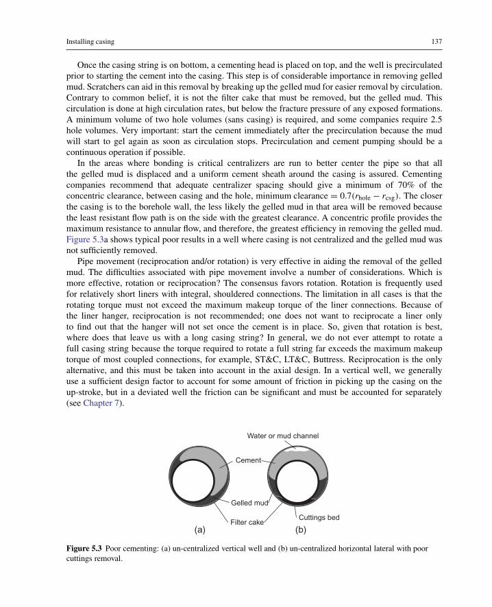
Installing casing 137
Once the casing string is on bottom, a cementing head is placed on top, and the well is precirculatedprior to starting the cement into the casing. This step is of considerable importance in removing gelledmud. Scratchers can aid in this removal by breaking up the gelled mud for easier removal by circulation.Contrary to common belief, it is not the filter cake that must be removed, but the gelled mud. Thiscirculation is done at high circulation rates, but below the fracture pressure of any exposed formations.A minimum volume of two hole volumes (sans casing) is required, and some companies require 2.5hole volumes. Very important: start the cement immediately after the precirculation because the mudwill start to gel again as soon as circulation stops. Precirculation and cement pumping should be acontinuous operation if possible.
In the areas where bonding is critical centralizers are run to better center the pipe so that allthe gelled mud is displaced and a uniform cement sheath around the casing is assured. Cementingcompanies recommend that adequate centralizer spacing should give a minimum of 70% of theconcentric clearance, between casing and the hole, minimum clearance = 0.7(rhole − rcsg). The closerthe casing is to the borehole wall, the less likely the gelled mud in that area will be removed becausethe least resistant flow path is on the side with the greatest clearance. A concentric profile provides themaximum resistance to annular flow, and therefore, the greatest efficiency in removing the gelled mud.Figure 5.3a shows typical poor results in a well where casing is not centralized and the gelled mud wasnot sufficiently removed.
Pipe movement (reciprocation and/or rotation) is very effective in aiding the removal of the gelledmud. The difficulties associated with pipe movement involve a number of considerations. Which ismore effective, rotation or reciprocation? The consensus favors rotation. Rotation is frequently usedfor relatively short liners with integral, shouldered connections. The limitation in all cases is that therotating torque must not exceed the maximum makeup torque of the liner connections. Because ofthe liner hanger, reciprocation is not recommended; one does not want to reciprocate a liner onlyto find out that the hanger will not set once the cement is in place. So, given that rotation is best,where does that leave us with a long casing string? In general, we do not ever attempt to rotate afull casing string because the torque required to rotate a full string far exceeds the maximum makeuptorque of most coupled connections, for example, ST&C, LT&C, Buttress. Reciprocation is the onlyalternative, and this must be taken into account in the axial design. In a vertical well, we generallyuse a sufficient design factor to account for some amount of friction in picking up the casing on theup-stroke, but in a deviated well the friction can be significant and must be accounted for separately(see Chapter 7).
(a) (b)Filter cake
Gelled mud
Cement
Water or mud channel
Cuttings bed
Figure 5.3 Poor cementing: (a) un-centralized vertical well and (b) un-centralized horizontal lateral with poorcuttings removal.

138 Casing and Liners for Drilling and Completion
Horizontal wells exhibit additional complications because drilled cuttings are more difficult toremove. The casing tends to lie on the bottom of the borehole in the cuttings bed, and since thepipe is even harder to move because of friction, movement is often ignored. Shown in Figure 5.3bis a typical result in a horizontal lateral where cuttings were not sufficiently removed, the casing wasnot centralized, and was not moved during cementing. It also illustrates another common problem incementing a horizontal lateral as a mud or water channel has formed along the top of borehole becauseof too much free water in the cement slurry.
5.8 Landing practices
There is no standard practice for landing casing after it has been cemented. It is assumed that the casingis now fixed at the top of the cement. (The fixed point is often referred to as the freeze point). Thecasing above the freeze point can actually buckle laterally and even into a spiral or helix because ofits weight, the weight of the fluids inside, and/or a change in temperature. Only in rare cases wouldthis buckling actually result in damage to the casing because the relatively small annular clearancelimits the severity of the postbuckling displacements, but it could cause wear problems in intermediatecasing strings where drilling will continue below. In production strings it may cause difficulty in runningproduction equipment. As already mentioned, the severity of the postbuckled deformation is limited bythe clearance between the casing and borehole wall which is normally relatively small, but it can beconsiderable in a washed out area. We will discuss lateral buckling in Chapter 6.
Four landing procedures are common and were once mentioned as recommended practices in anumber of publications (but no longer). Roughly they are as follows:
• Land the casing with the same load on the wellhead as the hook load after cementing.• Land the casing with tension at the top of the cement which is assumed to be the freeze point.• Land the casing with the neutral point (axial tension/compression) at the freeze point.• Land the casing with compression at the freeze point.
You can see that some of those are in opposition (the second and last), and none are in agreement.There are operating companies that have selected one of these (with possible variations) and are adamantthat theirs is the best method to use. One problem with all this is that, once the casing is on bottom andcemented, we are not really certain what happens down hole when we land (or hang) the casing at thesurface. Is the freeze point at the top of the cement or is the pipe stuck somewhere above the top of thecement? Do we even know where the top of the cement is? In some cases there is a limitation on whatthe wellhead equipment can support. There is also the question of the type of hanger used—a slip-typehanger gives us considerable flexibility (if we can get it down into the casing head properly) whereas amandrel-type hanger cannot be adjusted once the pipe is on bottom or cemented.
It is generally agreed by most operators though that the casing should not buckle above the freezepoint. That means that the effective axial load should be in tension if at all possible everywhere abovethe freeze point. Do not be misled into using the true axial load, the neutral point for buckling is thepoint where the effective axial load is equal to zero. Anything above that point should have an effectivetensile load. (You learned to calculate the effective load in Chapter 4 so it should be no problem foryou.) If the casing will be heated by circulating or by produced fluids you should take into account thatthe heat will expand the casing and reduce the tension, and possibly even put part of the noncementedcasing in compression. (Temperature effects are covered in Chapter 6.) If you are using a mandrel-typehanger instead of a slip type, and in many situations you have no choice, then there is no way to adjust

Installing casing 139
the axial load above the top of the cement after it has set. In that case you should, if possible, designthe cementing job such that the cement top is well above the neutral point. You may also be able torotate the pipe while cementing or before cementing. This will serve to allow the pipe to overcomeany residual frictional force from going in the hole and work the neutral point to the shoe (exceptin horizontal wells). However, before you elect to rotate the casing you must be sure that the torquerequired for rotation does not exceed that maximum recommended make-up torque of the casing con-nections. It usually does exceed the maximum for 8-rd couplings and many other non-shouldered typeconnections.
One significant problem, as far as lateral casing buckling, is concerned is hole washout and badcement or no cement in those washed out intervals. In the presence of heated circulating fluid orproduced fluids, buckling in this interval can occur. That is not a landing problem, but rather, it is acementing problem that must be addressed. Along these same lines is the presence of a stage tool in acasing string. Often a stage tool will be used some distance above the top of the lower stage of cement.This means that there is an unsupported section of casing that is fixed at both ends (at the stage tool andat the top of the lower stage cement), and a significant rise in temperature can cause lateral buckling ofthe casing in that unsupported interval.
5.8.1 Maximum hanging weight
There are limits on the amount of weight that may be hung on a casing hanger:
• Tensile strength of the casing string• Maximum support strength of wellhead and support casing• Support rating of the casing hanger• Collapse rating of the top casing joint when using slip-type hanger
The first limitation in the above list is a matter of proper casing design such that if tension abovethe string weight is to be applied (e.g., preventing thermal buckling), the additional tension must beincluded in the design loads. The second item is a matter of structural integrity of the supporting casingsor platform and is beyond the scope of our discussion. The third item applies primarily to slip-typehangers, and one need refer to the hanger manufacturer’s rating for the particular hanger to be used.There is also the case of weight and wellhead pressures exceeding the rating of the casing head suchthat the hanger actually causes the head to expand, but that is rare and most wellhead manufacturers haveeliminated those problems from their equipment. The last item concerning the collapse load of a slip-type hanger on casing can sometimes be a serious problem for heavy strings of casing (see Figure 5.4).The weight of the casing forces the slip segments downward which in turn imposes a radial, compressiveforce on the outside of the casing in the slip area. Such a force can exceed the collapse resistance of thecasing.
A simple formula can be used to estimate the collapse load imposed by a slip-type casing hanger.
phgr = kDW
Aslip tan φ(5.1)
where
phgr = external casing pressure from hanger
kD = design factor
W = hanging weight of casing

140 Casing and Liners for Drilling and Completion
W
f
Figure 5.4 Slip-type casing hanger.
Aslip = apparent gross contact area of slips
φ = taper of slips and hanger (measured from vertical)
To be as consistent as possible, the pressure load from this equation should be compared to the combinedtension-collapse pressure rating of the casing. As to the design factor it is a matter of company policy,but a commonly used design factor is 2.0.
EXAMPLE 5.1 Slip Hanger Collapse Load
From our continuing example the 7′′ production casing has the following data:
• Buoyed casing string weight at surface: 339,000 lbf• Type of 7′′ casing at surface: 29 lb/ft, P-110• Nominal collapse rating: 8530 psi• Hanger taper: 25◦• Hanger slip length: 10 in.
Using a design factor of 2.0, determine if the entire buoyed weight of the string can be hung on the hanger.The reduced collapse rating of the casing with 339,000 lbf tension is: 7271 psi1
phngr = 2.0339,000
π (7) (10) tan 25= 6612 psi
This value is well below the reduced tension-collapse rating of the casing.
In this example, case the casing may be hung safely with the full buoyed weight on the hangerwithout danger of collapse. Whenever doing this type of calculation it is important to know whether the
1 As calculated from the traditional API method in the next chapter.

Installing casing 141
angle of the slip segments is measured from the horizontal or vertical. If the angle is measured from thehorizontal it must be subtracted from 90◦ before using in this formula. It is also important to compareto the reduced collapse rating of the casing rather than the published nominal collapse rating, thoughmany assume the design factor of 2.0 is sufficient to ignore the combined collapse/tension effect.
5.9 Closure and commentary
This chapter closes out the casing design and installation portion of this textbook, and from here on thetopics become considerably more technical in nature though still sprinkled with a lot of precautions,suggestions, and opinions based on experience and case histories, most too sensitive to ever seepublication. But before moving on there are some things that need to be said, and maybe best saidin anecdotal form since written documentation will never see the light of day.
Casing strings fail, but it least they do not fail too often. By far the most common cause of casingfailure is corrosion. In fact, I can safely state that corrosion causes more casing failures than all the restcombined. That is a topic we do not cover in this textbook because there are many sources available. Sowhat are the other causes?
Over the last 55 years I have supervised on-site the running of casing strings that number into thehundreds in my earlier years. I have designed, checked, and approved designs for casing strings thatnumber well into the thousands. And having spent most of those years in drilling and completionoperations, I have been involved directly, indirectly, or peripherally with numbers into the tens ofthousands. I am not trying to impress anyone with my long experience because there are many whohave had considerably more. The reason I mention this at all is to emphasize a point: in all those casingstrings, I have seen only one that failed because of a bad casing design!2 What does this say? I willnot attempt to answer that, but offer the two most plausible reasons. Either the design process is soeasy everyone can do it correctly, or on the other hand, perhaps we are over designing all our casingstrings.
So if the design process, which is the technical emphasis of this textbook, seems to work okay, whatare the problems? They are many and varied, but most distill down to some human link in the chain ofevents that failed, inadvertently, carelessly, intentionally or out of laziness or ignorance. Even a defectivejoint of casing can in effect be attributed to someone not doing their job properly.
The most common and serious casing problem I have witnessed over the years (aside from corrosion)is the backing off of the shoe track of surface casing while drilling out. It is not a life endangering eventbut a costly one. In all but one case it resulted in abandonment of the well. This event is always aresult human error (though we like to claim otherwise, especially if we are personally responsible). Itcomes down to two things: not properly thread locking the joints in the shoe track and/or drilling outprematurely. Interestingly, all of these I have personally seen involved H-40 grade casing. That mayhave other implications because that also means they were relatively shallow casing strings and it isunlikely that the cement had properly cured before drilling took place.
This type of problem is also often exacerbated by a purely non-technical issue. Many wells in NorthAmerica for instance, are drilled under a “footage” contract, meaning the drilling contractor is paidX dollars per foot drilled down to the intermediate casing point or total depth. The contractor makes
2 It was a production string that collapsed around a tubing string as in Figure 6.5c, when the string became partially evacuated.It failed because the designer did not take into account the combined effects of tension/collapse, either through omission orignorance of the method.

142 Casing and Liners for Drilling and Completion
his money in the upper part of the hole where the drilling is fast and easy. Waiting for cement to curesufficiently is costing him money while none is being earned since no drilling is taking place. Mostdrilling contracts specify a minimum waiting time for cement to cure, but some do not. And when theydo, it is often some standard clause that has not been reevaluated in years (if ever) let alone adapted toa particular well or field area. If the operator has no representative on location (and many do not fora footage contract), the waiting time may get shaved a bit. I once had a client who contracted severalshallow wells, and typically saw no need for the expense of having a representative on location. Thewells were drilled under a footage contract and required only 500 ft of surface casing. I will not detailthe resulting problems here, but the contractor had zero hours waiting on cement. Why? Because he didnot cement the surface casing. He wrapped the bottom joints with large diameter hemp rope that swelledin the drilling fluid and held the surface casing in place for the three days it took to drill to total depth.Illegal? Yes. Was any of this on the drilling report? No, it reported a conventional cement job and 8 hwaiting on cement. A rare occurrence? Sadly, no.
Another casing problem I have seen frequently also involves shallow wells and H-40 grade surfacecasing. The number of shallow wells drilled in North America with 8-5/8 in. surface casing and 4-1/2 in.production casing is in the hundreds of thousands at minimum. Most of these use H-40 surface casingwith a threaded casing head on top. The problem? Not uncommonly, the casing head and BOP stackbreaks off the casing at the threads. It is caused by a combination of a poorly stabilized BOP stack,vibrations, settling of the soil beneath the substructure, and so on. The kinds of things that do notnormally occur with bigger rigs, but are common to these necessarily low cost operations. Almost alloccur in 28 lb/ft H-40 8-5/8 in. casing. It is the minimum weight in that grade and definitely meets thedesign requirements for these casing strings. The solution is easy and is 100% successful everywhere Ihave seen it applied—put two joints of 32 lb/ft casing in the top of the string. It works. This is one ofthose quirks in casing design that we learn from practice, and unfortunately this particular one seems tobe learned and relearned time and again. I have seen this one result in expensive forensic failure analysisand even lawsuits (to no avail), while the solution is trivial.
Though I have seen a number of tensile failures in tubing, I have seen only one tensile failure in casingin the form we would normally expect. Five others were from the cyclic pressures and temperatures ofhydraulic fracturing in horizontal wells as discussed in Chapter 7. Those resulted from coupling leaksand subsequent erosion but the fracture fluid through the leaks. Though the final failure was in axialtension, I cannot call those true axial failures in the normal sense.
The one axial casing failure I did experience (on a telephone with the on-site drilling foreman) wasalmost bizarre. A production string of 4-1/2 in. H-40 grade casing was run in a shallow well. It wasto be a pumping well, and this was the same type casing that had been run in hundreds of wells inthe same field. The cement was being displaced, and just as the top wiper plug landed on the floatcollar, circulation was lost. The drilling fluid level and cement in the annulus fell rapidly. It fell, andit continued to fall. Then suddenly, the casing parted at the first connection below the elevator. A bigsurprise. A check of its rated joint strength showed that it certainly had enough tensile strength to besuspended in air all the way to total depth without failure, but the failure occurred because it did nothave enough strength to be suspended in air and full of water. The water could not fall out the bottombecause of the seated wiper plug. At the time I thought there was nothing we could have done once theannulus fluid started to fall. But I was wrong about that, there was something we could have done hadwe anticipated such an event. And probably we should have anticipated it since the producing zone wasmostly depleted. Do you see what it was? At least we were able to secure the top of the parted casingand complete the well normally. This was an unusual case to be sure, but also it is a reminder that casingdesign should not become routine even for shallow wells. Oh yes, what could we have done to prevent

Installing casing 143
the failure? We could have immediately lowered the casing and set it on bottom to relieve the tension—acontingency we later adopted for such instances.
You may have noticed that much of what I have said here involves shallow wells. I started my careerdrilling relatively deep high pressure gas wells, where considerable effort and care was put into casingdesign and related practice. Consequently, I encountered few casing problems. It was not until much laterwhen I began working more frequently with shallow wells and older wells that I began to experiencereal casing problems. Too often it is the routine, the normal, the shallow wells that seem to bite yourprofessional ego the hardest. This is complacency, avoid it.
Running casing is as important as the casing design itself. If the casing is damaged or it does notreach bottom, the success of the entire well is jeopardized. We have looked at some practical aspects inthis chapter, and I hope that these may be of use to you. There is much that could have been discussed,but we covered the essence.
This chapter concludes what might be called the basics of casing design and practices. It has beenpresented as something of a “recipe” for casing design. Though some of the issues were discussedin detail, little was said about where the strength ratings come from, and what their limitations are.The remaining chapters of this text will examine the mechanics of casing and special conditions andapplications in more detail.

This page intentionally left blank

6Casing performance
Chapter outline head
6.1 Introduction 1466.2 Structural design 146
6.2.1 Deterministic and probabilistic design 1476.2.2 Design limits 1476.2.3 Design comments 148
6.3 Mechanics of tubes 1486.3.1 Axial stress 1496.3.2 Radial and tangential stress 150
Lamé solutions and yield 1516.3.3 Torsion 1526.3.4 Bending stress 153
6.4 Casing performance for design 1536.4.1 Tensile design strength 154
Pipe body yield 154Joint strength 155
6.4.2 Burst design strength 155Ductile rupture formula 156Coupling performance with internal pressure 159
6.4.3 Collapse design strength 159Traditional API collapse formula 161Improved collapse formula 164
6.5 Combined loading 1666.5.1 A yield-based approach 1666.5.2 A simplified method 1686.5.3 Improved simplified method 1706.5.4 Traditional API method 1726.5.5 The API traditional method with tables 1756.5.6 Improved API/ISO-based approach 176
6.6 Lateral buckling 1776.6.1 Stability 178
The Woods stability model 1796.6.2 Lateral buckling of casing 183
Buckling in a vertical wellbore 185Buckling in an inclined wellbore 185
6.6.3 Axial buckling of casing 186
6.7 Dynamic effects in casing 1876.7.1 Inertial load 1876.7.2 Shock load 188
6.8 Thermal effects 1896.8.1 Temperature and material properties 189
Casing and Liners for Drilling and Completion. http://dx.doi.org/10.1016/B978-0-12-800570-5.00006-1Copyright © 2015 Elsevier Inc. All rights reserved.

146 Casing and Liners for Drilling and Completion
6.8.2 Temperature changes 190
6.9 Expandable casing 1966.9.1 Expandable pipe 1976.9.2 Expansion process 1976.9.3 Well applications 1986.9.4 Collapse considerations 200
6.10 Closure 200
6.1 Introduction
The first four chaptersof this text were written to provide a basic foundation in casing design. Theymore or less constitute a recipe, if you will, for basic casing design. That “recipe” should be adequatefor designing casing strings for the vast majority of wells drilled in the world. One need not be anengineer to do it successfully, and it is hoped that the preceding chapters were enlightening to thosewho are not. Beginning with this chapter, we abandon the recipe. From here on, we address a numberof topics considered more advanced. The intent here is not to try to teach a method for designingcasing for critical wells but to help one understand the principles involved. More and more, we rely onsoftware to do casing design. On the one hand, that is good, because it allows us to make sophisticatedcalculations and adjustments that require an excessive amount of time if done manually, and whichfew are actually trained to do in practice. On the other hand, we have people using software todesign casing for real wells who are clue-less as to what the software is doing and what the resultsmean. This is not an exaggeration. In this chapter, we examine some of the topics that may fill afew gaps in the education of many drilling engineers in regard to casing design. The purpose hereis to impart a degree of understanding of some of the concepts and terminology for more advancedtopics concerning casing and its use. This chapter begins with a brief discussion of design methodsand then looks at some of the concepts of solid mechanics as applied to casing and oilfield tubulars ingeneral. We then address the design performance of casing for collapse loading, burst loading, axialloading, and the all important combined loading. Additionally we will briefly cover lateral buckling,dynamic loading, and thermal effects, and we will end the chapter with a brief discussion of expandablecasing.
In this chapter we will make use of the concepts of solid mechanics covered in Appendix C. If youare not familiar with that topic or need a refresher, I strongly recommend that you review it beforedelving into the material that follows. If you are not already thoroughly familiar with the von Misesyield criterion, you must definitely read that section (C.6.3) of the appendix before proceeding.
6.2 Structural design
The design of structures is almost as old as humanity itself. Whether the first “structures” were forshelter, tools, or weapons, the design process from its primitive beginnings has been around a long time.Almost everything we see each day is a structure of some sort. Casing also is a structure, though wemay not often think of it in that context. It is a containment structure for the most part, and the designprocedures we use are similar in many respects to those of more complex structures.

Casing performance 147
6.2.1 Deterministic and probabilistic design
There are two general approaches to designing casing or any type of structure. One is a deterministicdesign method, the process with which we are most familiar. We use published values for theminimum strengths and performance properties of the materials, load scenarios based on observed andhypothetical criteria, and a set of formulas to calculate structural performance with those loads. Thenwe specify the types and sizes of structural materials required to safely sustain the loads. This is themethod used for the design of most common static structures, such as bridges, skyscrapers, televisiontransmission towers, drilling rig masts, and even oilfield casing strings. The other general approach isa probability-based design method, in which we use statistical test data for the strengths and propertiesof actual materials and probabilistic loading scenarios. This approach often is used in the design ofstructures subject to dynamic and cyclic loading such as airframes, turbine blades, and so forth, wherefatigue failure is a significant or dominant factor. The probabilistic design criteria in these types ofstructures may also be weighted on the consequences of structural failure. In other words, the criticalstrengths and loads often are based on things like risk to human life, property value, the environment, andso forth. An example would be the blade of a gas turbine operating in some remote oilfield location asopposed to a jet engine turbine blade on an aircraft flying human passengers across a continent: in otherwords, a 0.1% probability of failure in 10,000 h of service may be acceptable for the remote oilfield gasturbine, but that same failure probability in an aircraft engine design would likely have aircraft fallingout of the sky almost daily, and that is not acceptable. This method can also be applied to static typestructures: we see an example of this in the oil field in the design of pipelines, where the publishedstandards for strength often are based on the human population density in the vicinity of the pipeline. Aprobability-based design must account for the consequences of failure in addition to the probability of afailure. And, to do that, one must have reliable limit data on actual materials or components to work withrather than some limit set by manufacturing standards that allow considerable tolerance. Obviously, thebetter data we have, the better both methods work, but it is especially important in probability-baseddesign if any significant savings is to be realized.
6.2.2 Design limits
One thing we must get very clear in our heads is that, when we design a casing string (or any other typeof structure for that matter), we are not attempting to predict failure. Predicting actual failure is nearimpossible, even when we have the most complete data we can imagine1: in the case of oilfield tubesand borehole conditions, predicting failure is impossible. So our goal is to select some design limits andselect our casing such that the anticipated loads do not exceed those limits. Calculating design limitsand predicting failure are separate and distinct processes.
A design limit is naturally linked to some strength property of the structural member, which is a tubein our case. Since we already stated that we cannot predict actual failure of the tube, there must be someother property of the tube that we can reliably predict or calculate. The historic design limit for casing,as well as most structures in the world, is the elastic yield point: the stress at which a material goes fromelastic behavior to plastic behavior. The elastic yield point or yield stress (sometimes referred to as theyield strength) of a metal such as steel is well defined and relatively easy to determine experimentally.What we never know, however, is the actual yield stress of a particular joint of casing. The only value
1 If you doubt this, think of the “precision” shear pins used in the oilfield tools and designed to shear at a specified load. Howmany times have you seen one shear at exactly the specified load?
148 Casing and Liners for Drilling and Completion
we have to work with is called a minimum yield stress, also which is not a material property. In otherwords, a joint of casing with a specified minimum yield stress (strength) is sold with the manufacturer’sassurance that it will not yield at a lesser value. It may yield at a higher value (also limited by an uppervalue in most cases), so the only value we have to work with is the minimum yield stress, which may ormay not be the actual yield stress.
We can (and sometimes do) design beyond the yield stress in some cases of structural design, butworking within the plastic regime is quite complex and generally avoided in all but the simplest cases.These usually are cases in which part of the material body or structure remains elastic and the designlimit might be selected as the point at which the entire body reaches the yield point (or possibly somepoint before that state is reached) assuming that no critical members of the structure actually fail beforethat point is reached. These types of design limits typically are one-time limits and do not consider theeffects of cyclical loading (which changes the yield stress value). An example is the new ISO formulaproposed for ductile rupture of casing, which we discuss later in this chapter. The only cyclical loadingin the plastic regime for oilfield tubulars is in coiled tubing, and we all know (or should know) thatcoiled tubing has a very short service lifespan because of the cyclic loading in the plastic regime.
6.2.3 Design comments
It is not likely in the near future that more than a small number of companies will be doing probability-based casing designs for more than a relatively few critical wells, as compared to the number of wellsdrilled in the world each year. Those companies doing this work have their own expertise and criteriafor risk, and those criteria cannot necessarily carry over to other companies. For instance, years agowith the advent of tubing-less completions, many looked at it as a way to save money. If you drilled alot of these wells, you could save a sizeable amount of money. To be sure, there were failures, and theinexpensive wells completed with 2-3/8 in. tubing/casing could not be effectively worked over with theequipment of the day. The larger companies accepted this risk, and the frequency of failed wells (whichwere usually plugged as expendable) was within reason. But, for a small operator that had only one wellor two, a failure sometimes was cause for bankruptcy. That is not acceptable from the small operator’sperspective. However, that said, the one benefit of the trend toward probabilistic casing design that everyoperator, big or small, has realized is a decided improvement in the design formulas and the ways inwhich certain variations in casing tolerances can be measured and accounted for, even in deterministicdesign. And even what we call a deterministic design is based on some probabilities of certain criticalloading occurrences and possible failures of casing to meet minimum standards. The difference is that,in deterministic design, we do not attempt to quantify those probabilities (see Klever and Tallin [16]).
One last comment should be made. A common mistake is to think that a deterministic design gives usa 100% safe structure at a higher cost, and a probabilistic design gives us a more cost-effective structurebut at a slightly greater risk. While that may be true in some particular cases, it is not true in general.In fact, many of the probability-based designs are safer than some deterministic designs. Both methodshave their place and applications.
6.3 Mechanics of tubes
Casing is a tube. A tube may serve as a beam, a column, a pressure vessel, or any combination of thethree from the standpoint of mechanics. A casing string, to some extent, is all of those. The stress in a

Casing performance 149
z
rθ σθ
σr σz
Figure 6.1 Cylindrical coordinate system for a tube, and stress component directions on tube body.
tube is of particular interest to us in light of the yield strength we just discussed, since that is what weneed to know to determine if the tube is in an elastic range or not. We are fortunate in many respectsthat a tube is a fairly easy structure to analyze in an elastic state. In general, we need be concerned withonly four stress components for our applications:
• Axial stress• Radial stress• Tangential stress• Torsional stress
To understand these stress components, we first need a convenient coordinate system. One that fits ourneeds quite well is a circular cylindrical coordinate system, as shown in Figure 6.1, which also showsthe first three stress components listed above.
There are three orthogonal coordinate axes, as with a Cartesian coordinate system. The axial coordi-nate, z, runs along the central axis of the tube; the radial coordinate, r, that runs from the central axisout in any direction; and the tangential coordinate, θ , which is an angular measure about the centralaxis as measured from some arbitrary reference point. The main difference between this and a Cartesiancoordinate system is that two of the coordinate measures are in standard length units and one is anangular measure. Hence, the physical meaning of θ is not the same as z or r. The measure of physicaldistance in the θ coordinate is rθ . This is a right-hand coordinate system, but it is oriented so thatthe axial coordinate, z, is in a downward direction. This is intentional so that the z-axis corresponds tothe vertical depth (in a well), and furthermore, the compass azimuth (when viewed from above) and theconventional angles of trigonometric functions rotate in the same direction.
6.3.1 Axial stress
The axial stress in a straight tube is merely the axial load divided by the cross-sectional area of the tube:
σz = Fz
At= Fz
π(r2
o − r2i
) = Fzπ4
(d2
o − d2i }) (6.1)
where
σz = axial load stress component
Fz = axial load
ro, ri = pipe radius, outside and inside walls, respectively
do, di = pipe diameter, outside and inside walls, respectively

150 Casing and Liners for Drilling and Completion
We always assume that the pipe is straight and stress free before it is run in a well. If the pipe is ina curved bore hole, there will be additional stresses in the axial direction from bending, which we willdiscuss later.
6.3.2 Radial and tangential stress
We should all be thankful to Lamé, who in 1852, worked out the elastic stress solutions in tubes becauseof internal and external pressure. His solutions for the axial stress resulting from pressure depend onwhether the tubes are open on the ends, capped on the ends, or the ends are free or fixed (plane strain).The Lamé solutions for the stress components attributable to pressure are
σr = r2i r2
o (po − pi)
r2o − r2
i
1
r2 +por2
o − pir2i
r2o − r2
i
(6.2)
σθ = − r2i r2
o (po − pi)
r2o − r2
i
1
r2 +por2
o − pir2i
r2o − r2
i
(6.3)
�σz =
⎧⎪⎪⎪⎪⎪⎨⎪⎪⎪⎪⎪⎩
pi r2i −po r2
o
r2o−r2
icapped ends, both free ends, one or both
0 open ends, one or both free ends, one or both
ν (�σθ +�σr) open or capped ends fixed ends, both
(6.4)
where the non-subscripted r is the radius at any point in the wall of the pipe. Please note that althoughthe equations for σr and σθ may appear identical, they are not; the second equation has a negative signin front of the first term. Another important point concerns the change in axial stress caused by pressure(Equation (6.4)). Casing in a well is already in a state of axial stress and is subjected to hydrostaticpressure. You must be careful with this equation because it accounts for change in axial stress causedby change in pressure from some reference state. Capped-end conditions affect casing only when oneend of the casing is free to move. When casing is run in a well, the only time the capped-end conditionnormally applies is when the top wiper plug is bumped during cementing. After that, the casing is fixedat the top by the wellhead and below by cement. If you want to consider the wellhead a cap, then youmust also consider that, for it to move enough to cause an axial stress change in the casing string, itmust move every tubular string in the well that is attached to the wellhead, some of which are cementedto the surface. (Some thermal wells allow for wellhead movement.) The second term in the numeratorof the capped-end formula is for external pressure that acts on the capped free end, pressure that mayor may not be present. Post plug bump is a case in point here. If the ends are fixed, you must knowif they were fixed before the pressure change was applied or afterward because the fixed-end axialstress equation is only valid for changes in the axial stress from pressure applied after the ends arefixed.
The general Lamé formulas are useful as they are stated above, but as it turns out we are seldominterested in the stress at various points within the wall of the cylinder, because the maximum stressalways is at one of the walls if there is pressure. Which one? It is not intuitive, but whether the greaterpressure is internal or external, yield always occurs at the inner wall first! (Work it out, if you do notbelieve it.) If we substitute ri in place of r to get the Lamé solutions at the inner wall, we find they aregreatly simplified:

Casing performance 151
σr = −pi (6.5)
σθ = pi(r2
o + r2i
)− 2por2o
r2o − r2
i
(6.6)
The axial stress change is unchanged from in Equation (6.4). The sum of the radial and tangentialstress in that equation is a stress invariant through the wall of the tube, so it does not matter if theyare calculated at the inner wall or outer wall, so long as both are calculated at the same place. Onemore caveat: often you may see the tangential stress equation without the second term in the numerator.That is typical of pressure vessels where there is no external pressure. Many use that form and use thedifference between the internal and external pressure as the internal pressure. Don’t do that! Yes, it givesclose results, but it is a sloppy practice.
There are times when we might need to calculate the radial and tangential stress at the outer wall. Inbending and torsion, the tube yields first at the outer wall, so if we are checking for yield in these caseswhere pressure is also present, we may want to check both the inner and outer walls. The radial andtangential stress components at the outer wall are
σr = −po (6.7)
σθ = −po(r2
o + r2i
)+ 2pir2i
r2o − r2
i
(6.8)
Lamé solutions and yield
Here is an important point illustrated in Figure 6.2 that concerns location of initial yield from pressure: ifwe apply pressure to casing internally until it yields, will it yield first at the inner wall or the outer wall?Similarly, if we apply pressure to casing externally until it yields, will it yield first at the inner wall orthe outer wall? These are not such simple questions as one might think, and the answers are importantto know. Despite any apparent simplicity, the answer is that it makes no difference as to whether thepressure causing yield is internal or external, the casing will always yield first at the inner wall. This isnot intuitive, and if you would like some practice with the Lamé equations you might work this out as anexercise.
The Lamé solutions are extremely useful, but we must be very careful to not use them beyond theyield point. Remember that these are elasticity solutions based on linear elastic material behavior. Theyare not valid beyond the yield point. If you use them to calculate the stress components for use in thevon Mises yield criterion, and the result is greater than the yield, then the calculated stress component
po
pi
Figure 6.2 Internal and external pressure increasing to yield stress in casing.

152 Casing and Liners for Drilling and Completion
Figure 6.3 Internal pressure causing yield in a fixed-end casing.
values are quantitatively meaningless. In that case, they will tell you only that the initial yield has beenexceeded, but not by how much. This is illustrated in Figure 6.3 where we have calculated the yieldmeasure, Ψ , using the Lamé elastic solutions at the inner and outer walls of a tube of the dimensions of7 in. 23 lb/ft casing with a yield stress of 80,000 psi. We also calculated and plotted the distortionalenergy density,
√3J2, using elastic-plastic theory.2 Two things are important in this figure. One is
that yield occurs first at the inner wall causing the distortional energy density to become nonlinearwith respect to the internal pressure, and though the outer wall does not yield until sometime later, thedistortional energy density becomes nonlinear well before it actually yields. The second thing to note isthat once the yield point is reached at the inner wall, the elastic values of the yield, Ψ , calculated withthe Lamé equations become meaningless because the material is no longer elastic. See Appendix C fora discussion on plasticity and an example of a similar analysis with different end conditions.
6.3.3 Torsion
We do not often rotate casing in a borehole. It does help in attaining a good primary cement job, but oftenthe friction in the borehole is such that the torque required to rotate the casing exceeds the maximumrecommended makeup torque of the connections such as ST&C, LT&C, buttress, and so on. However,many times, liners are rotated while cementing and casing can be rotated with some proprietaryconnections or special stop rings inserted to prevent over-makeup of non-shouldered connections, likebuttress, ST&C, or LT&C. The equation for the shear stress from torsion in a pipe body is given by
σrθ = 2 r Tq
π(r4
o − r4i
) (6.9)
2 The elastic-plastic constitutive equation used in this example is not that of an API steel, but a piecewise linear approximation ofa strain hardening steel with a yield stress of 80,000 psi.

Casing performance 153
rkro
Figure 6.4 Simple planar bending of tube.
where r = ro to calculate the shear stress at the outer wall where it is a maximum or r = ri at the innerwall. The torque (rotational moment) in the casing is Tq and it must be in consistent units. In oilfield unitsit usually is in lbf ft and it must be multiplied by 12 to change it to lbf in. to be consistent with the radiiunits. In SI units, the torque will be in Joules (N m) so the radii must be in meters so that the stress will bein Pa.
6.3.4 Bending stress
The bending of casing in curved wellbores is discussed in detail in Chapter 7 and derived in Appendix C,so all we present here is a formula for planar bending stress that refers to Figure 6.4:
σb = ±Er
rκ
(6.10)
The radius of the pipe is r = ro at the outside wall where the bending stress is a maximum, and r = ri ifit is desired to calculate the bending stress at the inner wall. The radius of the wellbore curvature is rκ .It must be in the same units as the radius of the pipe. The bending stress component has a plus sign onthe convex side of its curvature as that portion is in tension. On the concave side, it is negative becauseit is in compression.
The bending stress component is added to the axial stress for determining yield, but it should beremembered that the bending stress is a maximum only along a line running parallel to the central axisin the plane of curvature on the convex side and the concave side. The values calculated in the bendingequation are not the bending stress at other points around the circumference of the tube.
6.4 Casing performance for design
In earlier chapters, we took the published values of casing strengths at face value. In this section, weexamine some of the formulas from which those strengths are calculated. What are the bases of theseformulas? What are their limitation? Are there better formulas or methods? We will address thosequestions and then look at combined loading and its effects. We will also look at lateral instability(buckling) and the effects of temperature on casing design.
Reiterating what was previously mentioned, we cannot actually predict failure of a joint of casing,and we do not seek a to do so. What we are interested in is a value we can use as a design limit.

154 Casing and Liners for Drilling and Completion
A particular joint of casing may fail at that limit or it may not; the important consideration is that itdoes not fail before that limit point. Historically, yield strength has been used as a design limit, and thatcontinues. However, some of the formulas used in the past were based on some simplifying assumptionsand tests that did not realistically model actual loading. For example, the API collapse formulas arebased on collapse tests on short samples of casing, and it has been found that joint length plays a partin collapse, i.e., end conditions affect the collapse of short tubes. So, much of what is covered in thispart of the chapter might be characterized as design strength formulas and calculations. Most are stillbased on yield strength or test data. While it may be perfectly acceptable to use conservative formulasin the vast majority of wells drilled in the world, there are deeper, high-pressure, high-temperature wellswhere such conservative formulas might greatly increase well costs by requiring much higher strengthsthan is necessary or even available. We examine the current formulas and discuss some of the changes.
6.4.1 Tensile design strength
Casing failure in tension is not common. When it does occur it usually occurs at a connection, andthe connection is usually ST&C or LT&C. The failure in those types of connections usually is aresult of pull-out rather than fracture of the casing body. In some cases, the pull-out is the result ofa split coupling caused by hydrogen embrittlement or over-torque during makeup. As far as tensilestrength of casing is concerned, it is specified in two ways by the API and ISO, pipe body yield andjoint strength. The first is the value of the pipe body yield strength exclusive of threads, expressed asaxial tension (or compression) rather than axial stress, and the second is the value of the connectionstrength, which always refers to tension and not compression. The pipe body yield values use theminimum yield strength as the design strength limit. The joint strength is based on the minimumvalue from formulas that use the minimum ultimate strength and the yield strength separately or incombination.
Pipe body yield
Pipe body strength at yield is the yield stress of the metal multiplied by the specified cross-sectionalarea of the tube.
Fmax = Y At (6.11)
where
Fmax = pipe body strength at yield
Y = uniaxial yield strength of pipe
At = cross-sectional area of tube, π(
r2o − r2
i
)For example, the pipe body yield for 7 in. 23 lb/ft N-80 casing is
Fmax = 80000 (π/4)(
7.0002 − 6.3662)= 532, 000 lbf
which is the value shown in the published tables. This value is valid for either tension or compression.For ST&C and LT&C couplings, the strength of the connection usually is less than that of the pipe body.For instance, for the above 7 in. 23 lbf/ft N-80 casing with LT&C connections, the joint strength ratingis 442,000 lbf, or about 17% less than the pipe body yield, so one must be aware that the joint strengthis usually the lesser of the two.

Casing performance 155
Joint strength
Joint strength is usually the yield strength of a casing connection in tension; however, formulas alsoare available for the fracture strength of connections, although they are not used often in casing design.The calculation of joint strength depends on the specific type of coupling and includes things suchas the makeup length of the threads, the cross-sectional area of the tube under the last full thread,and so forth. Furthermore, the formulas have been adjusted to fit actual tests with various samples ofcasing connections. The resulting formulas for ST&C, LT&C, buttress, and extreme-line are listed inAPI 5C3 and ISO/TR 10400. Additionally, one must refer to API 5B to get some of the necessarythread dimensions for use in the formulas. Proprietary thread manufacturers, in general, do not publishtheir formulas but only the connection strength values. For those reasons, we do not include any jointstrength formulas here. Almost no one actually uses them, since the results are published in many tables.The thing we must point out as a precautionary note is that one should always check both the bodystrength and connection strength for any casing design. And remember, the strength of connections incompression is not addressed by API standards.
6.4.2 Burst design strength
The traditional API formula for what we commonly refer to as burst is not actually a formula for burstor pipe rupture but a yield formula for internal pressure. It is based on a thin-wall tube that assumesyield takes place across the entire wall thickness at a single pressure. It also includes a design factor toaccount for the 12.5% variation in wall thickness allowed by API casing specifications (API Spec 5C2or ISO 11960). The result is a formula for the internal yield pressure:
p = 0.875 Ydo − di
do(6.12)
This formula known as the Barlow formula was derived from three-dimensional shell theoryassumptions and is adequate for basic casing design, but it leaves a lot to be desired. For one thing,it assumes that yield occurs throughout the pipe wall at the same time, which it does not. What is lost bythe assumption of a thin-wall cylinder with a uniform stress throughout the wall of the cylinder? We canuse the Lamé elastic formulas along with a yield criterion to determine the yield at the inner wall for athick-wall tube and compare the results. In the absence of any axial load or axial constraints, that is, thepipe is free to move axially and the ends are not capped, the Lamé formulas give the stress componentsat the inner wall as
σr = −pi (6.13)
σθ = pi(r2o + r2
i
)− 2por2o(
r2o − r2
i
) (6.14)
In absence of axial stress, at internal yield, the following holds for the von Mises yield criterion:
Y ={
1
2
[(σθ − σr)
2 + (σr)2 + (−σr)
2]} 1
2
(6.15)
If the external pressure is zero, that is, po = 0, then we can solve this equation for the internal pressureat yield in terms of the yield strength of the pipe and the internal and external diameter of the pipe. Theresult is

156 Casing and Liners for Drilling and Completion
pi = Yd2
o − d2i√
3d4o + d4
i
(6.16)
This equation is the thick-wall equivalent of Equation (6.12), except it does not account for atolerance in the wall thickness. The wall thickness is accounted for in ISO 10400 by calculating aninternal diameter based on the tolerance in the wall thickness such that, for this equation,
di ≡ do − 0.875 (do − di) (6.17)
This definition uses the standard API tolerance; however, other values could be used for specificsituations where the actual tolerance is known as opposed to the specified maximum toleranceof 12.5%.
EXAMPLE 6.1 Comparison of Burst Equations
Using 7 in. 26 lbf/ft P-110 casing in this example, the Barlow (Equation (6.12)), gives an internal pressure atinternal yield
p = 0.875 Ydo − di
do= 0.875 (110000)
7.000 − 6.276
7.000≈ 9960 psi
whereas Equation (6.16) using Lamé’s pressure equation and von Mises yield criterion gives
di = do − 0.875 (do − di) = 7.000 − 0.875 (7− 6.276) = 6.367 in.
pi = Yd2
o − d2i√
3d4o − d4
i
= 1100007.0002 − 6.3672√
3 (7.000)4 + 6.3674≈ 9900 psi
From this example we see that there is only a slight difference in the two. The formula based on thick-wall tubes will usually be slightly conservative. The problem with the API Barlow formula, though, isthat it is valid only if the pipe has no axial stress. It also assumes that any external pressure can beaccounted for by subtracting it from the internal pressure and using the difference, �p = pi − po, as theinternal pressure (as long as �p > 0). Some do the same thing with the Lamé formula for tangentialstress, which is not good practice, because it does not give the same result as when both internal andexternal pressures are used.
Ductile rupture formula
The current ISO/TR 10400 [11] includes new formulas for ductile rupture as differentiated frominternal yield. Few, if any, oilfield tubulars actually fail in rupture when the internal wall surfacereaches the yield point, which is the basis for the conventional API/ISO formulas for “burst” or,more correctly, internal yield. If the material were perfectly plastic, it would quickly yield all theway through the wall thickness as the pressure is increased and rupture, but that is not the way mostoilfield tubulars behave (coiled tubing excepted). Unless they are very brittle, they are made of a strain-hardening material, so that once the yield stress has been exceeded, the stress still increases before

Casing performance 157
ultimate failure occurs, as discussed in Appendix C. The recent ISO formulas take that into accountby actually modeling the material behavior in the plastic regime. In addition, certain defect sizes aretaken into account, so that the pipe may more realistically model actual casing. Even fracture growth isconsidered.
To use these formulas, one must have more specific data than is conventionally published. Inparticular, one needs inspection results for the casing to be used or at least have a specific inspection inmind and know that casing not meeting those standards will be culled from this particular application.We are going to present only some basics of the formulas here, but before using these formulas,one should definitely read the discussion in ISO/TR 10400 (Appendix B) and some of the associatedreferences. The primary ductile rupture formula in ISO/TR 10400 includes a capped-end effect such thatthe internal pressure generates an axial stress from the pressure effect on the end caps. For a capped-end effect to be realized, one end of the tube must be free to move in relation to the other end, so thatthe axial stress is a function of the internal pressure. This almost never happens with casing in a wellexcept in the plug-bump case, since one end of the casing is cemented (fixed) and the other attachedto a wellhead. Unless the wellhead is free to move, the capped-end effect does not occur. One couldargue that the wellhead may move, but its movement is considerably restricted by the other strings ofpipe also attached to the wellhead, in addition to the fact that the conductor and surface casing areusually cemented at the surface. For casing, the pressure effects are almost always those of fixed endsnot capped ends. That being said then, the ISO design formula for the internal pressure at ductile rupturewith capped ends is
p = 2k1Utw − k2 δ
do − tw + k2δ(6.18)
where
p = internal pressure at ductile rupture
U = minimum tensile strength of casing
do = outside diameter of casing
tw = reduced wall thickness from the tolerance, e.g., (0.875 tw)
k1 =[(
1
2
)n+1
+(
1√3
)n+1]= correction factor
k2 = burst strength factor, 1.0 for Q&T or 13Cr steels,
default 2.0 for others not specifically measured
δ = depth of imperfection in wall thickness
n = dimensionless hardening index for true stress/strain
curve from uniaxial tensile test
This formula is called a design formula, which calculates rupture assuming certain minimum valuesfor the quantities in the formula, such as the minimum tensile strength. This is derived from a limitstate formula, which predicts rupture for a specific sample where the quantities just listed are knownexactly for that sample. Some of these quantities can be calculated from measurements or tests. Table 6.1suggests values for the hardening index, n, in the absence of actual test data. A hardening index, as usedhere, is a means of approximating a uniaxial stress-strain curve for a particular material, with a curve fit

158 Casing and Liners for Drilling and Completion
Table 6.1 ISO SuggestedHardening IndexValues [11]
API Grade Hardening Index, n
H-40 0.14J-55 0.12K-55 0.12M-65 0.12N-80 0.10L-80 0.10C-90 0.10C-95 0.09T-95 0.09P-110 0.08Q-125 0.07
to an idealized material, such as a Ramberg-Osgood material [17], or a Ludwik power-law material [18].No conversion factors are required if you use consistent units.
We use this formula to determine the ductile rupture pressure for the same casing in the previousexample.
EXAMPLE 6.2 Ductile Rupture Formula
Using the same casing as in the previous example and assuming our casing inspection rejects all defects inexcess of 5% of the wall thickness, we determine the variable quantities for use in equation (P-110 casing hasa minimum ultimate tensile strength of 125,000 psi):
tw = 0.875 tw = 0.875 (0.362) = 0.317 in.
For the hardening index, we use n = 0.08 for P-110 (Table 6.1) and calculate the correction factor:
k1 =[(
1
2
)n+1
+(
1√3
)n+1]
=[(
1
2
)0.08+1
+(
1√3
)0.08+1]= 1.026
The maximum allowable depth of the wall thickness defect in the selected casing is
δ = 0.05 (0.362) = 0.0181 in.
For the burst strength factor we use 2.0, the default value. We substitute these values into Equation (6.18):
p = 2k1Utw − k2 δ
do − tw + k2δ
= 2 (1.026) (125000)0.317− 1.0 (0.0181)
7− 0.317 + 1.0 (0.0181)≈ 11, 440 psi

Casing performance 159
We can see that this value is about 14% higher than the current API formula in the previous example.Part of this is attributable to the capped-end effect. As we will later see with the von Mises yield criterion,internal yield is higher in the presence of axial tension, which is what we have with a capped-end effect.
An additional ISO ductile rupture formula accounts for external pressure and arbitrary axial loading.It is a nonlinear limit state formula, see ISO10400/TR [11] pages 25-30. One difficulty with that formulais that for a fixed end tube such as casing cemented at the bottom and fixed to a wellhead at the top,the axial load is not a constant, but is a function of the pressure as in the Lamé formula for fixed ends,σz = σz 0ν(�σr +�σθ ), Equation (6.4). But beyond the yield point, σr and σθ are elastic-plastic stresscomponents, not proportional to the pressure, as in the capped end case. Finally though, one shouldnote that the ductile rupture formulas take into account material behavior in a plastic regime. In ourdiscussion on plastic behavior in Appendix C, we pointed out that materials become history dependentin this regime, so these formulas are valid only if the loading exceeds the yield stress and proceedsto rupture. If the loading stops once yield has been exceeded but short of the rupture value, then theformulas are valid for subsequent loading only if the loading path is exactly the same as before, once thenew yield value is exceeded. Therefore, the use of the ductile rupture formulas is a highly questionableendeavor, especially for cyclic loading in casing beyond the yield point. At least in my opinion andexperience with plasticity [19].
Coupling performance with internal pressure
In some configurations, casing couplings will yield before the pipe body or will leak at a lesser internalpressure than that which will yield the pipe body. There are formulas in ISO 10400 to calculate thesevalues for API round thread and buttress threads. It is rare that anyone ever needs to use these formulasbecause the values are listed in the tables of casing properties in API 5C2. Because of this and the needto refer to actual thread specifications, I do not include them here. The important point to rememberis that in some casing the coupling is weaker than the pipe body in internal yield and/or leak pressurerating.
6.4.3 Collapse design strength
Casing collapse is actually two phenomena (1) an instability (radial buckling), and (2) collapse (post-buckling). The collapse rating of casing usually (but not always) refers to the pressure at which thepipe becomes radially unstable and the actual collapse is the behavior after the instability is reachedand usually takes place at a lower pressure than the buckling pressure. Casing collapse possibly is themost common type of failure after corrosion and wear. There have been cases of collapse resulting fromdefective casing joints, but the cause often is one of not accounting for the actual collapse load on thecasing. This is especially true where the casing is in tension and subjected to a collapse load. Perfectlyround casing with a uniform wall thickness is quite resistant to collapse pressure. If there is a variationin the wall thickness because of eccentricity or defects, the cross section is ovalized, or the collapseloading is other than hydrostatic pressure (e.g., borehole stability problems), then failure from collapseusually occurs at lesser loads. The typical post-buckling collapse mode is shown if Figure 6.5a wherethe casing tends to flatten in cross section. Collapse also depends on outside support of the casing (seeFigure 6.5b) in that casing with little outside clearance or partially supported by cement may beginto collapse into the configuration illustrated or the partial support may prevent total collapse. Anothermode (Figure 6.5c) is common in production casing where tubing is present.

160 Casing and Liners for Drilling and Completion
(a)
(c)
(b)
Figure 6.5 Common collapse modes: (a) unsupported collapse, (b) partially supported collapse (e.g., cement orcoupling), and (c) unsupported collapse with tubing inside.
Sometimes partially collapsed casing may be restored with an internal casing roller, but fullycollapsed casing, is usually a total loss. It may be possible to mill out, and sometimes even recover, acollapsed portion of the casing. When a tube begins to buckle in collapse (collapse is a form of buckling),the buckle propagates along the tube at a much lower pressure than what caused the initial collapse. Thebuckle propagation pressure may be on the order of 60 – 65% of the initial collapse pressure if the casingis unsupported. For an undersea, welded pipeline, the entire line may collapse because of a defect in onejoint. For this reason, many undersea pipelines now include rings, called buckle arrestors, welded to thepipe at various intervals so that, if a collapse should occur, it will not propagate the full length of thesubmerged pipeline.
Fortunately, in a casing string, a hydrostatic-induced collapse typically is limited to one joint,because as the buckle propagates, it usually stops at a coupling. In the case of a threaded cou-pling, the propagation stops because the collapse of the pipe inside a coupling does not transferthe load to the other pin inside the coupling. It also opens the interior of the casing to externalpressure, so that the pressure differential is relieved. In the latter case, it becomes what is knownas a wet buckle, and it tends to stop at that point. In the case of integral joints, the propagatingbuckle usually is stopped by the increased thickness of the pipe upset. In that case, the upset servesas a “buckle arrestor.” In the case of flush joint casing, the buckle might continue to propagate untilthe pressure differential is less than the buckle propagation pressure, or it may stop if it becomesa wet buckle from an opening at one of the collapsed connections. An extreme example is coiledtubing that has no connections; if it collapses, the buckle propagates until the pressure differentialis less than the propagation pressure. There are formulas for collapse strength but not for bucklepropagation. Buckles have been observed to propagate at pressures of about 65% or so of the initialcollapse pressure (see Yeh and Kyriakides [20]; Kyriakides, Babcock, and Elyada [21]; Chater andHutchinson [22]). For an exhaustive treatment see also the excellent book on offshore pipelines byKyriakides [23].
Interestingly the case of casing collapsed around tubing is often one of the easiest to repair becausemaximum dimension of the collapsed casing is less than the ID of the un-collapsed casing. The tubing

Casing performance 161
itself is almost never collapsed and provides a passage through the collapsed casing for a chemicalcutter, can be easily cut internally itself, and provides a smooth internal surface for a spear. Since themaximum dimension of the collapsed casing is less than the un-collapsed casing it can be retrieved oncecut free.
Traditional API collapse formula
The API formula for collapse is not a single formula, but rather four:
• Yield strength collapse formula• Plastic collapse formula• Transition collapse formula• Elastic collapse formula
Each formula has a range for which it is valid, depending on the yield strength of the material and theratio of the outside diameter to the wall thickness.
Yield collapse formula
pYC = 2Y
[(do/tw)− 1
(do/tw)2
](6.19)
Valid range:
(do/tw) ≤ A− 2+√
(A− 2)2 + 8 (B+ C/Y)
2 (B+ C/Y)(6.20)
Plastic collapse formula
pPC = Y
[A
(do/tw)− B
]− C (6.21)
Valid range:
A− 2+√
(A− 2)2 + 8 (B+ C/Y)
2 (B+ C/Y)< (do/tw) ≤ Y (A− F)
C+ Y (B− G)(6.22)
Transition collapse formula
pTC = Y
[F
(do/tw)−G
](6.23)

162 Casing and Liners for Drilling and Completion
Valid range:
Y (A− F)
C + Y (B− G)< (do/tw) ≤ 2+ B/A
3B/A(6.24)
Elastic collapse formula
pEC = 46.95× 10⁶
(do/tw) [(do/tw)− 1]2 (6.25)
Valid range:
(do/tw) >2+ B/A
3B/A(6.26)
where
do = outside diameter
tw = nominal wall thickness
Y = yield stress of pipe
pYC = collapse pressure, yield pressure formula
pPC = collapse pressure, plastic formula
pTC = collapse pressure, transition formula
pEC = collapse pressure, elastic formula
As with most API formulas, the units are not consistent, so for USC units with dimensions in inchesand psi the API constants in those formulas are calculated with:
A = 2.8762+ 0.10679× 10⁻⁵Y + 0.21301× 10⁻¹⁰Y2 − 0.53132× 10⁻¹⁶Y3
B = 0.026233+ 0.50609× 10⁻⁶Y
C = −465.93+ 0.030867Y − 0.10483× 10⁻⁷Y2 + 0.36989× 10⁻¹³Y3
F =46.95× 10⁶
[3B/A
2+ (B/A)
]3
Y
[3B/A
2+ (B/A)− (B/A)
][1− 3B/A
2+ (B/A)
]2
G = FB/A
(6.27)
For SI units, where yield stress is in MPa and diameter in mm, the collapse formulas and rangeformulas are the same, but the API constants are calculated from the following formulas:
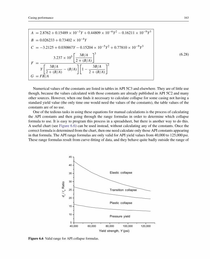
Casing performance 163
A = 2.8762+ 0.15489× 10⁻³Y + 0.44809× 10⁻⁶Y2 − 0.16211× 10⁻⁹Y3
B = 0.026233+ 0.73402× 10⁻⁴Y
C = −3.2125+ 0.030867Y − 0.15204× 10⁻⁵Y2 + 0.77810× 10⁻⁹Y3
F =3.237× 10⁵
[3B/A
2+ (B/A)
]3
Y
[3B/A
2+ (B/A)− (B/A)
][1− 3B/A
2+ (B/A)
]2
G = FB/A
(6.28)
Numerical values of the constants are listed in tables in API 5C3 and elsewhere. They are of little usethough, because the values calculated with those constants are already published in API 5C2 and manyother sources. However, when one finds it necessary to calculate collapse for some casing not having astandard yield value (the only time one would need the values of the constants), the table values of theconstants are of no use.
One of the tedious tasks in using these equations for manual calculations is the process of calculatingthe API constants and then going through the range formulas in order to determine which collapseformula to use. It is easy to program this process in a spreadsheet, but there is another way to do this.A useful chart (see Figure 6.6) can be used instead, without calculating any of the constants. Once thecorrect formula is determined from the chart, then one need calculate only those API constants appearingin that formula. The API range formulas are only valid for API yield values from 40,000 to 125,000 psi.These range formulas result from curve-fitting of data, and they behave quite badly outside the range of
Figure 6.6 Valid range for API collapse formulas.

164 Casing and Liners for Drilling and Completion
API yield values, especially in the low range below 40,000 psi. In other words, do not extrapolate thesecurves outside the yield value range shown in the figure.
The yield collapse formula is based on the external pressure that causes yield to occur at the innerwall of the casing, so that the yield strength is the design limit. Usually, the pipe will not collapse atthat pressure. The elastic collapse formula is based on elastic stability and does not depend on the yieldstrength of the casing. The plastic collapse and the transition collapse formulas are based on tests doneon casing samples, and the formulas essentially are curves fitted to the test results. The end of each rangefor the various formulas is the intersection of the curves for each formula.
Improved collapse formula
There are difficulties with the traditional API collapse formulas other than that they are not valid forcollapse in combination with tension; for instance, only the elastic collapse formula is valid in tension.Also, the collapse tests on which they were based were performed with very short sections of casing, andwork done in recent years has shown that the values in those tests were affected by the end conditions. Inthe more recent ISO/TR 10400 standard, a new approach is recommended. The new formulas are basedon work originally done by Tamano, Mimaki, and Yanagimoto [24] and recently published by Kleverand Tamano [25]. The full formula contains terms for inclusion of defects, ovality, eccentricity, and soforth. Although not yet accepted universally, it is an improvement on the traditional API formulas, plusit has the advantage of being able to include known data about the specific pipe for a casing string andcan be used in probabilistic casing design methods. The formula essentially contains a yield collapseformula and an elastic collapse formula and accounts for the transition between those two:
pclps =pelas + pyld −
[(pelas − pyld
)2 + 4pelaspyldHt
] 12
2 (1−Ht)(6.29)
where
pelas = 0.825 (2E)(1− ν2
) ( dotw
)(dotw− 1)2 (6.30)
is the elastic collapse portion, and
pyld = 2kyY
(twdo
)(1+ tw
2do
)(6.31)
is the yield collapse portion.In these formulas, ky is a bias factor for yield collapse, and Ht is a decrement factor for the transition
region between elastic and plastic collapse. These values can be determined from actual tests of thecasing to be used or one can use the default values in the tables of ISO/TR 10400, as shown inTable 6.2.
These results from this method will vary slightly from the values calculated with the traditionalformulas from API 5C3. The new method is considered to be more accurate.
The procedure for calculating reduced tension/collapse using this method is much easier than thetraditional API method. We will show examples of both methods of collapse combined with tension

Casing performance 165
Table 6.2 Collapse Yield-Bias and Transition-DecrementFactors from ISO 10400 [11]
Cold Rotary Straightened Hot Rotary Straightened
API Grade Ht kt Ht kt
H-40 0.164 0.910 n/a n/aJ-55 0.164 0.890 n/a n/aK-55 0.164 0.890 n/a n/aM-65 0.164 0.880 n/a n/aL-80 0.164 0.855 0.104 0.865L-80 9Cr 0.164 0.830 n/a n/aL80 13Cr 0.164 0.830 n/a n/aN-80 as rolled 0.164 0.870 n/a n/aN-80 Q&T 0.164 0.870 0.104 0.870C-90 n/a n/a 0.104 0.850C-95 0.164 0.840 0.104 0.855T-95 n/a n/a 0.104 0.855P-110 0.164 0.855 0.104 0.855Q-125 n/a n/a 0.104 0.850
later in this chapter, but for now, we look at an example of a collapse calculation with the new formulain the absence of tension.
EXAMPLE 6.3 Using the Improved Collapse Formulas
We apply these new formulas to determine the collapse rating of 7 in. 32 lb/ft N-80 casing. We calculate thewall thickness first:
tw = 1
2(do − di) = 1
2(7.000− 6.094) = 0.453 in
Next, we calculate the elastic collapse using Equation (6.30):
pelas = 0.825 (2E)(1− ν2
) ( dotw
) (dotw− 1)2
= 0.825 (2)(30× 106
)(1− 0.282) ( 7.000
0.453
)(7.0000.453 − 1
)2
= 16, 641 psi
then, the yield collapse, using Equation (6.31):
pyld = 2kyY
(twdo
)(1+ tw
2do
)
= 2 (0.870) (80000)
(0.453
7.000
)(1+ 0.453
2 (7.000)
)
= 9300 psi

166 Casing and Liners for Drilling and Completion
Now, we use these values in Equation (6.29) to calculate the collapse rating of the casing:
pclps =pelas + pyld −
[(pelas − pyld
)2 + 4pelaspyldHt
] 12
2 (1− Ht)
= 16641 + 9300− [(16641 − 9300)2 + 4 (16641) (9300) (0.164)] 1
2
2 (1− 0.164)
≈ 8060 psi
This is the value of collapse we would read from a table that uses the proposed new collapse formula(recall that API rounds values to the nearest 10 psi). It is a bit lower than the current published valueof 8600 psi calculated using the current API formulas. Partly, this reflects that many of the early APItests used short tube samples, which generally gave higher collapse values. Also, the new formuladistinguishes between cold and hot rotary straightened pipe. We used the cold value here, but N-80is one grade that is straightened by either method.
6.5 Combined loading
Almost always, casing is subjected to some type of combined loading. Here are the most commonindividual types:
• Tensile and compressive loads attributable to gravitational forces, borehole friction, hydrostatic forces, andbending forces
• Collapse and burst loads from hydrostatic pressures• Torsion loads from borehole friction
There are various ways to calculate a design limit for combined loading. Most of them work, but someare quite misleading and can cause serious problems if one does not understand the limitations. We aregoing to look at a simple method that has been around for more than 150 years and in publicationfor almost 100 years. It has proven effective throughout all those years in all engineering designapplications.
6.5.1 A yield-based approach
As we have already stated we generally use the yield strength (elastic limit) as our design limit. So, whatwe would like to have is some method of quantifying the combined loads into a single value to comparewith some simple strength or stress value for the material of the tube. For example, if Y is the yield stressdetermined from a uniaxial test and Ψ represents the combined load, we might compare them thus:
Y > Ψ → no yield (6.32)
Y ≤ Ψ → yield (6.33)
where Ψ is a yield measure as defined in Appendix C. This is exactly what we looked at with the vonMises yield criterion previously. The only practical difficulty we have at this point is that casing loadsgenerally are known in terms of axial force, pressure (internal and external), and possibly torque. We

Casing performance 167
need stress values for the von Mises yield criterion. We make use of the Lamé formulas for those stresscomponents. The yield-based approach is best illustrated by an example.
EXAMPLE 6.4 Combined Loads in a Yield-Based Approach
Suppose we have a point in a casing string where the internal pressure is 4000 psi, the external pressure is4000 psi, and the true tension in the pipe at this point is 160,000 lbf. Our casing is 7 in. 23 lb/ft, K-55. It hasan internal diameter of 6.366 in. We increase the pressure at the surface to 4000 psi to test it for a plannedstimulation; the internal pressure at our point of interest will be 8000 psi. Will the pipe yield under this load?
First of all, we want to determine where the pipe will yield first, at the inner wall or the outer wall. Internalor external pressure always causes yield at the inner wall first, as mentioned previously. We have no bendingor torque in the pipe, which always causes yield at the outer wall first. So, we require the yield condition atthe inner wall. Second is that the test pressure of 4000 psi is applied after the casing is cemented and hung offat the surface (i.e., the ends are fixed), so we must account for the effect of that pressure change on the axialstress.
Determine the axial stress before the pressure test:
σz0 =Fz
At= 160000
π4
(7.002 − 6.3662
) = 24, 040 psi
Determine the radial stress before the pressure test using the Lamé equation for the inner wall(Equation (6.5)):
σr0 = −pi = −4000 psi
Determine the radial stress when the test pressure is applied:
σr = −8000 psi
Determine the tangential stress before pressure test using the Lamé equation for the inner wall(Equation (6.6)):
σθ0 =pi(r2
o + r2i
)− 2por2o(
r2o − r2
i
)
= 4000[(7/2)2 + (6.366/2)2]− 2 (4000) (7/2)2
(7/2)2 − (6.366/2)2
= −4000 psi
Determine the tangential stress when the test pressure is applied:
σθ = 8000[(7/2)2 + (6.366/2)2
]− 2 (4000) (7/2)2
(7/2)2 − (6.366/2)2 = 38, 260 psi
Determine the incremental radial and tangential stress from the test pressure:
�σr = σr − σr0 = −8000 − (−4000) = −4000 psi
�σθ = σθ − σθ0 = 38260 − (−4000) = 42, 260 psi

168 Casing and Liners for Drilling and Completion
Then, using the Lamé equation for fixed end tubes (Equation (6.4)), calculate the change in axial stresscaused by the test pressure:
�σz = ν (�σθ +�σr) = 0.28 (42260 − 4000) = 10, 710 psi
The axial stress including the test pressure effects is
σz = σz0 +�σz = 24040 + 10710 = 34, 750 psi
Now, using the three stress components calculated in the presence of the test pressure, we want to determinewhether or not yield will occur. Since there is no torsion, these values are principal stress components and maybe plugged directly in to the von Mises yield formula:
Ψ ={
1
2
[(σθ − σr)
2 + (σr − σz)2 + (σz − σθ )
2]} 1
2
Ψ ={
1
2
[(38260 + 8000)2 + (−8000 − 34750)2 + (34750 − 38260)2
]} 12
Ψ = 44, 610 psi
Finally, check the yield condition:
Y = 55, 000 psi
Ψ = 44, 610 psi
Y > Ψ → no yield
In this case, there is no yield. The combined load in this example is approximately 90% of the yieldstrength of the pipe. Questions might arise: How close to the yield strength would we design if we wereaware of these calculations? What would be a reasonable limit? What are the recommended designfactors for combined loading? Those are good questions, and there are no standard answers. Someoperators would go up to 80% of the yield in a case like this, which would amount to a design factorof 1.25. That might be acceptable for a one-time occurrence, where the specifics are known in detail.If we were spot checking a conventional casing design for a well that had not been drilled, we mightwant to think again. In those cases, our confidence level might be somewhat less, so we might set a 1.6design factor as an absolute minimum. You are on your own in this area, unless your company has someparticular policy.
One other caveat about using yield stress as a limiting point in combined loading is that it does notaccount for collapse at loads lower than the yield strength of the casing. You should always check thecollapse using the combined load collapse formulas of API or ISO, which are covered in the next twosections.
6.5.2 A simplified method
There is a very simple method for adjusting casing to account for combined tension/collapse loads. Ithas been used by a number of operating companies for many years, and when combined with design

Casing performance 169
Figure 6.7 The two-dimensional von Mises yield criterion.
factors, it has proven workable for most normal vertical wells. It has its basis in a more theoreticalcontext but has been simplified for easy use. Some would say it is oversimplified and that is an accuratestatement, because it departs from theory and the results tend to be somewhat conservative. It is basedon a 2D plot of the von Mises yield criterion where it intercepts the σθ − σz principal stress plane (seeFigure 6.7).
Here is how the method works: We take the tension load of the casing at the point of interest, anddivide it by the joint tensile strength of the casing to get a decimal fraction. Then, we then locate thatpoint on the horizontal tension/compression axis. From there, we go down vertically to the point ofintersection with the ellipse. From that intersection, we go left horizontally to the vertical burst/collapseaxis and read the collapse fraction. We multiply the collapse rating of the pipe by that fraction. Thatgives us a reduced collapse rating of the casing under that amount of tensile load.
EXAMPLE 6.5 Simplified Tension/Collapse Adjustment
• Joint tensile strength = 547,000 lbf• API collapse rating = 1130 psi• Tensile load = 61,200 lbf
We determine the fraction of tensile load to the tensile strength:
61200
547000≈ 0.1
We go to the positive 0.1 point on the horizontal axis, down to the intersection with the ellipse, thenhorizontally to the vertical axis, where we read a value of 0.94. We multiply the collapse rating by this fractionto get a reduced collapse rating:
0.94 (1130) ≈ 1060 pasi
This value of 1060 psi is taken to be the reduced collapse rating at that point. If our design plot has a highervalue, then we must adjust our casing string accordingly.

170 Casing and Liners for Drilling and Completion
The chart in this method is based on a yield criterion for steel known as the von Mises yield criterion,which we discuss in detail in Appendix C. A formula can be derived from the plot for the quadrantconcerning tension and collapse:
kclps =√
1− 0.75k2tens − 0.5ktens (6.34)
where
kclps = fraction of collapse rating, i.e., pclps/pclps (reduced clps /clps rating)
ktens = fraction of tensile rating, i.e., F/Ftens (tens load/joint tens strength)
To calculate the reduced collapse pressure of casing with axial tension, the factor calculated inEquation (6.34) is multiplied by the published collapse pressure (without tension):
pclps = kclps pclps (6.35)
This method should be used with caution: perhaps I should not even include it here, but it has beenin common use for many years by many people for non-critical wells and with success. It is not theAPI method for calculating tension/collapse combined loads, nor is it the improved method of the ISO.It might be called a quick-and-dirty method that proved successful in many normal pressured wells allover the world before the days of electronic calculators and computers. While that approach is simplein its graphical form, it is not as well accepted if one is actually going to do the calculations. The reasonfor this is that the graph is based on stresses rather than loads and joint strength. The joint strength of atube in tension is based on the connection strength rather than the cross-sectional area of the tube itself.
I have intentionally presented the 2D von Mises yield criterion in Figure 6.7 in a format too small foruse because I do not want you to use this method. If you are intent on using it however, you can plot alarger one for yourself using Equation (6.38).
You may also note that the chart in this procedure shows a reduction of burst strength in axialcompression. Additionally, it shows an increase in collapse strength in axial compression and an increasein burst strength in axial tension. While this is true, almost no one uses a simple chart like this for thosecases in practice. Increases in burst or collapse resistance from axial loads are seldom considered in basiccasing design. Likewise, a case of reduced burst, which almost always results from axial compressionfrom thermal expansion, is not considered using such a simple method. These types of combined loadsare generally considered only in more-advanced designs and more-sophisticated methods are used ratherthan reading simple values from a chart like this. We discuss those issues later.
6.5.3 Improved simplified method
A more consistent way of expressing the reduced collapse fraction based on stresses is as follows:
kclps =√
1− 0.75
(F
AtY
)2
− 0.5F
AtY(6.36)
where
Y = yield strength
F = axial load
At = cross-sectional area of tube body

Casing performance 171
and the reduced collapse rating is calculated with Equation (6.35). This is the formula we used inChapter 4. A similar approach was proposed by Wescott, Dunlop, and Kimler [26] that attempts toaccount for the difference in the thickness of the tube body and the area under the threads. Theirformula is
kclps =√
1− 0.932
(F
AtY
)2
− 0.26F
AtY(6.37)
where the variables are the same as in Equation (6.36).
EXAMPLE 6.6 Simple Formulas for Reduced Collapse
Using Equation (6.34) in our previous example, we get the same conservative collapse value we got from theplot in Figure 6.7 (assuming we can read the graph accurately):
kclps =√
1− 0.75f 2tens − 0.5ftens
=√
1− 0.75
(61200
547000
)2
− 0.5
(61200
547000
)= 0.939
pcpls = kclpspclps = 0.939 (1130) ≈ 1060 psi
If, instead, we use Equation (6.36) for this example, we get a slightly higher value for the reduced collapse:
kclps =√√√√1− 0.75
(61200
π4
(13.3752 − 12.6152
)(55000)
)2
− 0.5
(61200
π4
(13.3752 − 12.6152
)(55000)
)= 0.962
pclps = kclps pclps = 0.962 (1130) ≈ 1090 psi
Using Equation (6.37) we get
kclps =√
1− 0.932
(61200
547000
)2
− 0.26
(61200
547000
)= 0.965
pclps = 0.965 (1130) ≈ 1090 psi
The difference in the last two equations in that example is that Equation (6.36) is based on the vonMises ellipse:
x2 − xy+ y2 = 1 (6.38)

172 Casing and Liners for Drilling and Completion
and Equation (6.37) is a modified version that uses the axial load and the joint strength as developed byWescott et al. [26], based on the ellipse:
x2 − 0.52xy+ y2 = 1 (6.39)
The axial stress formula (6.36) has been used for many years with success and generally is preferableto the conservative method of Equation (6.34). Recall that Equation (6.36) is the one we used in ourexample designs in Chapter 4, and it also appears in the minimum casing design requirements of theAEUB as the preferred formula [15]. The second formula (6.37) currently appears in the catalog of amajor casing manufacturer and has seen many years of use. It might appear that the differences betweenthese formulas are a bit trivial, but since they appear in various sources, usually without explanation, mypurpose here has been to explain the differences.
6.5.4 Traditional API method
Because collapse is a stability and post-buckling event, we cannot use a strictly yield based ap-proach like we considered earlier. However, since a yield value appears in three of the four APIcollapse formulas (elastic collapse is not affected by yield strength), yield certainly plays a role incollapse.
The traditional API method for calculating the effects of combined loads has a basis in the vonMises yield criterion, and the method is published in API Bulletin 5C3. The reason it is referredto here as the “traditional” API method is because it may be phased out with the adoption of thenewer ISO/TR 10400 standards. But, as of this writing, the traditional method has not been officiallyreplaced.
We will derive and show the equations for this method, but the method may be summarized asfollows: The API method uses the fractional axial stress, σz/Y, to calculate a fractional tangential stress,σθ , using an equation for the lower right-hand quadrant of the 2D plot of the von Mises yield criterion(see Figure 6.7). This method assumes the radial stress, σr, from internal pressure is negligible, sothat the tangential stress, σθ represents the yield strength in collapse. The fractional tangential stress isthen multiplied by the original uniaxial yield strength of the pipe to give us a “reduced” yield value.This reduced yield value is then substituted into one of the four API collapse formulas to calculatethe reduced collapse rating of the pipe. Although this method is not especially good engineering, it ispreferable to the previous simplified methods. It is extremely important to understand though, that thepresence of tension does not actually reduce the yield strength of the tube, but merely moves the loadingstress to a different position on the yield criterion curve so that we are using a different value from thatof the uniaxial yield. This value is referred to as a “reduced” yield because all the off-axis values on theyield curve in the lower right-hand quadrant of the Figure 6.7 are less than unity.
Earlier in this chapter, we used a 2D version of the von Mises yield surface (Equation (6.36)). Thatis where the traditional API-based approach begins. The von Mises yield surface in two dimensions is
σ1 − σ2
Y= σ3 − σ2
2Y±√
1− 3(σ3 − σ2)2
4Y2(6.40)
where σ1, σ2, and σ3 are the three principal stress components. In the absence of shear components,such as torsion, the three principal stress components are σθ , σr, σz and we may substitute them intoEquation (6.40) to get a convenient form for our use:

Casing performance 173
σθ − σr
Y= σz − σr
2Y±√
1− 3(σz − σr)2
4Y2 (6.41)
We purposely set the stress components in that order, so that the radial stress is the one we want tosubtract from the other components. The radial stress is the negative value of the internal pressure(recall that yield from internal or external pressure always occurs at the inner wall first). If it is zero, wecan leave it out, but in any event, we should know its value, so for now we rewrite it with the internalpressure:
σθ + pi
Y= σz + pi
2Y±√
1− 3(σz + pi)2
4Y2 (6.42)
Plotted it is an ellipse exactly like Figure 6.7 except−pi is substituted for σr and the terms, (σθ − σr)
and (σz − σr), become (σθ + pi) and (σz + pi), respectively.Now, here is how API uses this 2D formulation. API assumes that the tangential stress becomes an
effective yield stress for collapse. So, we define an effective yield stress in collapse as
Y ≡ −σθ (6.43)
We may rewrite Equation (6.42), adjusting the signs to account for the fact that the tangential stress iscompressive (negative) in a collapse situation:
Y = Y
√1− 3
4
(σz + pi
Y
)2
+ pi − σz
2(6.44)
This is essentially the API formula, except the API version assumes that the internal pressure isnegligible or zero and, hence, uses the following formula:
Y = Y
√1− 3
4
(σz
Y
)2 − σz
2(6.45)
This formula is used to calculate a reduced yield value, Y. That reduced yield value then is used inthe appropriate API collapse formula, from the earlier section on API collapse, to determine the reducedcollapse value caused by the tension.
EXAMPLE 6.7 Traditional API Method
Using data from the production casing example in Chapter 4: 7 in. 32 lb/ft N-80 casing (ID = 6.094 in.) andan axial load at the bottom of that section of 41,739 lbf, we want to determine the reduced collapse strengthof the casing.3 The published API collapse value with no tension is 8600 psi.
We calculate the reduced yield using Equation (6.45):
Y = 80000
√√√√1− 34
(41739
π4
(7.0002 − 6.0942) (80000)
)2
3 Normally we would roundoff such a value, but we use the same value as in the example production casing so as to compareresults of the various methods.

174 Casing and Liners for Drilling and Completion
− 1
2
[41739
π4
(7.0002 − 6.0942
)]
= 77, 666 psi
We now must determine which API collapse formula to use. To do that, we need the value of do/tw:
do
tw= do
0.5 (do − di)= 7.000
0.5 (7.000− 6.094)= 7.000
0.453= 15.453
We also need the API formula constants at the reduced yield strength. Without showing the calculations, wecalculate them from the formulas shown in the section on API collapse formulas (6.27):
A = 3.062736
B = 0.065539
C = 1885.482
F = 1.993754
G = 0.042664
We start with the range limit for yield collapse and Equation (6.20) using those constants and do/tw =15.453:
(do/tw) ≤ 3.062736 − 2
2 (0.065539 + 1885.482/77666)
+√
(3.062736 − 2)2 + 8 (0.065539 + 1885.482/77666)
2 (0.065539 + 1885.482/77664)
= 13.127
We see that our value of do/tw is greater than that, so we must then check the formula for the upper rangeformula for plastic collapse formula which is Equation (6.22):
(do/tw) ≤ 77666 (3.062736 − 1.993754)
1885.482 + 77666 (0.065539 − 0.042664)= 22.769
Our do/tw is within the range of the plastic collapse formula, so we use Equation (6.21) to calculate thereduced collapse strength of the casing:
pPC = 77666
[3.062736
15.453− 0.065539
]− 1885.482 ≈ 8420 psi
This shows a reduction of 180 psi in the collapse resistance of the casing in tension. It is not much inthis case, but it might put our design below the minimum design factor, in which case, we might have toadjust the design to compensate.
So far we have only accounted for collapse pressure in the form of a differential pressure, but themagnitude of the internal pressure does have some effect in combined loading. The traditional APImethod does account for this in the form of a correction for the presence of internal pressure.
pclps = preduced + pi
(1− 2tw
do
)(6.46)

Casing performance 175
It should be noted that the inclusion of internal pressure in our combined loading for collapse meansthat to use differential pressures as we did in our basic collapse load plots and design procedure wemust subtract the internal pressure from the results of Equation (6.46). This complicates the basic designprocedure somewhat. In the previous example, we did not add a pressure correction for internal pressureand use the actual external pressure as the collapse pressure, since our example production casing wasdesigned assuming no internal pressure. But we will now illustrate a case where there is internal pressurein the following example.
EXAMPLE 6.8 Internal Pressure in API Traditional Method
In the case of the 7 in. 32 lb/ft production casing in the previous example, we examined the reduction incollapse resistance at a point where the tension was 41,739 lbf. In Chapter 4, we compared the reduced collapsepressure to the differential collapse pressure to adjust for combined loading using Equation (6.36), and madedesign adjustments accordingly. In that case the casing was evacuated so there was no concern for any internalpressure. But for this example let us assume that there is an internal pressure from, say a brine workover fluid,and the internal pressure is 3000 psi. What is our reduced collapse pressure in this case?
Just as in the previous example we use Equation (6.45) to calculate a reduced yield and then the plasticcollapse formula to get a reduced collapse pressure of 8420 psi as compared to 8600 psi with no axial load.Then we substitute into Equation (6.46) as the preduced value:
pclps = 8420+ 3000
(1− 2 (0.453)
7.000
)≈ 11, 030 psi
This is the reduced collapse pressure with an internal pressure of 3000 psi. For comparison let us look at thedifferential load pressures with no internal pressure and with the 3000 psi internal pressure.
1) �pclps = pi − po = 0− 8420 = −8420 psi
2) �pclps = pi − po = 3000 − 11030 = −8030 psi
What this illustrates is that the presence of internal pressure actually reduces the differential collapseresistance of the casing a bit further. Most casing designs do not account for this. However, in most cases,the presence of internal pressure reduces the magnitude of the differential loading so the additionalreduction in collapse resistance may not be significant.
The necessity of determining which API collapse formula is applicable, as well as calculating the APIconstants for those formulas makes this a tedious process when done manually. In the case of standardyield strengths, like 80,000 psi, for instance, there are tables in API 5C3 and ISO/TR 10400 specifyingthe values of the five constants, but for our case of a yield of 77,664 psi, a nonstandard yield value, allthe constants must be calculated. There are five constants in all, though only two appear in the transitioncollapse formula. In this case, all five had to be calculated to determine the correct formula to use. Onecan easily program the API method into a spreadsheet and avoid the tedium and inherent errors in doingthe calculations manually.
The current API method does not account for combined loads in combination with burst. It is seldomconsidered in casing design, but when it is, the yield-based approach is used because burst is not astability type event like collapse.
6.5.5 The API traditional method with tables
One need not do the preceding calculations to use the traditional API method. Tables published in APIBulletin 5C2 allow one to look up the reduced collapse value directly. For instance, in the example, we

176 Casing and Liners for Drilling and Completion
could use Table 4 in API 5C2 [9]. It is in terms of axial stress rather than axial load, but it also givesthe cross-sectional area of the tube to make the axial stress calculation easier if you have not alreadycalculated it.
σz = 41739/9.317 = 4480 psi
The table gives the collapse pressure corresponding to axial stress in 5000 psi increments, so for zeroaxial stress, the collapse pressure is 8610 psi, and at 5000 psi axial stress, the collapse value is 8400 psi.We may do a linear interpolation for 4480 psi axial load and get a collapse value of 8420 psi (roundedto nearest 10 psi) which is the value we got with the traditional API calculation method.4 If you do nothave a spreadsheet programmed for the API method, it is much easier to use Table 4 in API Bulletin5C2.
6.5.6 Improved API/ISO-based approach
The proposed new API/ISO formula for combined tension and compression begins something like thecurrent API method as far as calculating a reduced collapse strength, in that it first uses an equation tocalculate a reduced yield value. The equation for calculating the reduced yield is
Y = 1
2
(√4Y2 − 3(σz)
2 − σz
)(6.47)
It is the same as the equation we used to calculate the reduced yield strength in the current API methodwith no internal pressure (Equation (6.45)) although in a slightly different form. The reduced yield fromthis formula then is used in Equation (6.31) to calculate a reduced yield collapse, which then is usedin Equation (6.29) along with the elastic collapse from Equation (6.30) to calculate a reduced collapsestrength without internal pressure. If there is internal pressure, then a correction using Equation (6.46)may be added. This internal pressure correction is called a simplified method in ISO/TR 10400 and givesresults to an accuracy of ±5% when 0 ≤ σz/Y ≤ 0.4. Outside that range, one should refer to ISO/TR10400 for the more rigorous internal pressure correction method (currently listed in Appendix H of ISO10400 [11]). This is an iterative solution technique.
EXAMPLE 6.9 Improved API/ISO Collapse Formula
We apply these new formulas to determine the reduced collapse rating of the 7 in. casing in the previousexamples. In Section 6.4.3 we calculated the wall thickness (0.453 in.) and the collapse value without tension,which was 8060 psi, so we do not repeat those.
Now, we use an axial tension of 41,739 lbf to determine the reduced yield using Equation (6.47):
Y = 1
2
⎛⎝√
4Y2 − 3
(Fz
At
)2
− Fz
At
⎞⎠
4 If you noticed, we used a collapse value of 8600 psi in all our design calculations which is the value listed in the main tablesof API 5C2. However, in Table 4 as mentioned above, it is listed as 8610 psi. The API formulas give a value of almost exactly8605 psi depending on the precision of your calculating device. So this apparently accounts for why it is rounded to two differentvalues in the main tables and Table 4 of API 5C2.

Casing performance 177
= 1
2
⎛⎜⎝√√√√4(80000)2 − 3
(41739
π4
(72 − 6.0942)
)2
− 41739π4
(72 − 6.0942)
⎞⎟⎠
= 77, 666 psi
Note again that this is exactly the reduced yield value we calculated using the traditional API method in theearlier example. This method differs from the traditional method in the manner in which the reduced yield isused once calculated. The reduced yield value is then used in Equation (6.29). We may use the elastic collapsevalue of 16,641 psi that we calculated in Section 6.4.3 with Equation (6.30) because it is independent of yieldstrength, but we must re-calculate a reduced yield collapse value using Equation (6.31).
pyld = 2kyY
(twdo
)(1+ tw
2do
)
= 2 (0.870) (77666)
(0.453
7
)(1+ 0.453
2 (7)
)
= 9028 psi
Now, we plug this value and the elastic collapse value into Equation (6.29):
pclps =pelas + pyld −
[(pelas − pyld
)2 + 4pelaspyldHt
] 12
2 (1− Ht)
= 16641 + 9028 − [(16641 − 9028)2 + 4 (16641) (9028) (0.164)] 1
2
2 (1− 0.164)
≈ 7870 psi
The traditional API method gives a reduction of 180 psi from the published API collapse value of8600 psi. This formula gives a reduction of 730 psi, from the published API collapse value. However,if one calculates the collapse value without tension using the improved formulas, the unloaded collapsevalue is 8060 psi, so this example is a reduction of 190 psi. The question is really whether the unloadedcollapse value is 8600 psi as per the traditional API formulas or 8060 psi as given by the improvedformulas. From the discussions in ISO/TR 10400 and the notes leading to the improved formulas, itwould appear to favor the new formulas. All indications are that the newer formulas are better, but untilthe old ones are declared obsolete they will still be used by many.
6.6 Lateral buckling
Much has been written over the years about lateral buckling of oilfield tubulars. Some of it has beengood, some a bit misinformed, and some even has been ludicrous. Lateral buckling is called columnarbuckling in most areas of structural engineering, but lateral buckling of oilfield tubulars differs fromthe common concepts of columnar buckling as it is understood by most structural engineers. In moststructural applications where gravity is considered, the load on the column is at the top of the columnas opposed to the bottom as in our case. In those cases, gravitational forces tend to contribute to thetendency of a column to buckle. In the case of oilfield tubulars, the loading is a bit different. Usually,

178 Casing and Liners for Drilling and Completion
the top of the column (casing or tubing) is fixed and the buckling load is caused by a reactive force onthe bottom. The reactive force is caused by the weight of some portion of the column resting on bottom,some pressure force on the bottom, or a combination of both. Many refer to lateral buckling of casingas simply buckling. However, collapse is a form of buckling called radial buckling. There is also axialbuckling, in which the casing is crushed in an axial direction. And, we could include torsional buckling.This section is about lateral buckling. Lateral buckling occurs when the casing becomes unstable anddisplaces laterally disproportionately to the magnitude of a very small lateral force.
6.6.1 Stability
The best way to visualize the concept of stability is with a simple and commonly used illustration.In Figure 6.8, three balls are in equilibrium on three surfaces. In case (a), a ball rests at the lowpoint on a concave surface. The ball is in static equilibrium; in other words, it will not move unlesssome force is applied to it. If we nudge the ball with some small force, it will move slightly thenreturn to its original position as soon as the small force, called a perturbation, is removed. Also notethat to move it further from its initial position requires an increasing force the farther it is moved.This ball is in a state of stable equilibrium. In case (b), the ball rests on a flat horizontal surface.It is also in a state of static equilibrium. If a small force is applied, the ball will move. It willcontinue to move with no requirement that the force be increased as in the first case. It will stopwhen the force is removed, or if its environment is frictionless, it will continue to move at constantvelocity until another force is applied to stop it or it falls off the edge of the surface. It will notreturn to its original position, however. We call this case conditionally stable equilibrium or sometimesneutrally stable equilibrium. The third case, (c), also is in static equilibrium, though, from a practicalstandpoint, we might have a bit of trouble comprehending how someone could get a ball to balanceon the high point of convex surface. Nevertheless, it is easy to understand that, if we apply even thesmallest of perturbations to this ball, it will roll off the surface. Once it starts to move, no additionalforce is required to keep it rolling away from its static equilibrium point. We call this conditionunstable equilibrium. This last condition is the type of instability that concerns us with buckling ofcasing.
How does lateral buckling occur? If you consider the type of lateral or columnar buckling shown inmost engineering texts, you will see something like Figure 6.9a.
Typically, these are weight-less columns with a vertical load applied at the top and the bottom eitherhinged or fixed. The initial buckling mode is in the form of a single curve. Other modes are possible(usually at higher loads), leading to sinusoidal-type configurations with an increasing number of nodes.These additional nodes are mostly theoretical, because once the column buckles into a single curve, theother modes are not possible unless some constraints are applied. A perfect beam with a perfectly appliedaxial load (as is the case of our mathematical models) never buckles laterally unless some perturbation
(a) (b) (c)
Figure 6.8 Equilibrium states: (a) stable, (b) neutrally stable, and (c) unstable.

Casing performance 179
(a) (b)
R = F + W R
F F = W − R
Figure 6.9 Lateral buckling: (a) typical structural column and (b) casing in borehole.
is applied. In other words, we could keep applying a load until the column yields in compression anddeforms axially in a plastic regime, until it is just a lump of metal on the ground. For instance, theequation5 for the elongation or compression of an elastic tube is
�L = 2F + w L2
2π(r2
o − r2i
)E
(6.48)
Nowhere in that equation is any allowance for lateral buckling, because there is no inherent instabilityin the formula itself. Lateral buckling has to be determined in other ways. As to casing in a wellbore,it usually is fixed on bottom with cement and has lateral constraint in the form of a borehole wall,Figure 6.9b. Buckling in this case is affected by the weight of the casing, and we see that only the lowerpart of the casing is buckled, because the buckling is caused by axial compression at the bottom from theweight of the casing. As the distance from the bottom increases, the axial compression decreases. Whencasing buckles in this manner, it initially may be in the shape of a sinusoidal curve, with decreasingfrequency as the distance from the bottom increases, until a point is reached where there is no buckling.It may be even more extreme and form a helical shape in the wellbore, with decreasing pitch as thedistance from bottom increases.
It would seem intuitive, then, that for lateral buckling to occur in casing, it would have to be causedby a compressive load and some small perturbation. For many years, it was assumed that, if casing washung in tension throughout the full string or at least the portion of the string above the top of the cement,then lateral buckling could not occur. That sounds intuitively simple, and that was the assumption upuntil papers by Lubinski [27] and by Klinkenberg [28] and several discussions of those papers.
The Woods stability model
In 1951, in a discussion of the paper by Klinkenberg [28], Henry Woods [29] presented an exampleillustrating the buckling neutral point in a simple way that became something of a classic. It essentiallyshowed that, contrary to popular intuition, lateral buckling could occur in casing in tension (under certain
5 See Appendix C for derivation.

180 Casing and Liners for Drilling and Completion
pressure conditions). Much of what had been done previously was based on intuition combined with anunfortunate lack of understanding of hydrostatics.
Woods, however, based his analysis on the theory of elastic stability, using a thought experimentwith a weight-less tube in a hypothetical test chamber. The model as Woods set it up illustrates his pointquite well, but it has been criticized because it does not model something that can occur in reality, evenunder the most ideal of conditions. I have modified his thought experiment to one that more realisticallymodels an actual wellbore situation. This modified version gives exactly the same results and is perhapsmore realistic in terms of our experience with casing in boreholes, see Figure 6.10. A weight-less tubeis installed in a pressure test chamber, fixed at the lower end, and free at the upper end. While the upperend is free to move, it is closed internally with a frictionless pressure seal that does not move. Thereis also a frictionless pressure seal on the outside of the tube, between the upper chamber and lowerchamber. The lower chamber, representing a wellbore annulus, has a pressure po, and inside the tube thepressure is pi. The top chamber is open to the atmosphere, and the tube is held in tension at the top by asuspended weight, W. The tube is long enough that its stiffness against bending is negligible. Also, thechambers are large enough that the pressures in the lower chamber remains constant. Woods then said,if one could apply a small lateral force to the tube in the large chamber such that the tube would deflectlaterally by a small amount, then the top of the tube would slide downward some small amount δL. Andthe suspended weight would rise by the same displacement, δL. The following volume changes wouldoccur:
δVo = −πr2o δL
δVi = πr2i δL
po
pi
W
Figure 6.10 A modified Woods model.

Casing performance 181
Since pressure is in each of the places where volume changes occur, a change in potential energy ineach place is equal to the change in volume times the pressure, and the total change in potential energy,δΠ is given by
δΠ = δVopo + δVipi + δL W
δΠ = πr2oδLpo − πr2
i δLpi + δL W
The last term is the force, W, acting on the tube. We may express it in terms of axial stress as
W = Atσz = π(
r2o − r2
i
)σz
We can substitute the axial stress into the equation:
δΠ = πr2oδLpo − πr2
i δLpi + π(
r2o − r2
i
)δL σz
For this system to remain stable, the change in potential energy must be zero or positive:
πr2oδLpo − πr2
i δLpi + π(
r2o − r2
i
)δL σz ≥ 0
σz ≥ πr2i pi − πr2
opo
π(r2
o − r2i
)We could then write the stability condition in a number of ways, four of which follow:
σz ≥ Aipi − Aopo
Ao − Ai(6.49)
σz ≥ ri2pi − r2opo
r2o − r2
i
(6.50)
Fz ≥ Aipi − Aopo (6.51)
σz ≥ 1
2(σθ + σr) (6.52)
The last version was derived using the Lamé formulas. Recall that the sum of the tangential stressand the radial stress is constant through the wall of the pipe, so it makes no difference whether they arecalculated at the inner or outer wall, as long as both are calculated at the same point.
What Woods’s model illustrates is the difference between the change in potential energy by a slightincrease in the internal volume of the tube and slight decrease in the annular volume in addition tomechanical work done on the weight. If the deflection results in an increase in potential energy, thenthe tube is stable, whereas if it results in a decrease in potential energy, then it is unstable. If thereis no change in potential energy, then it is conditionally stable. Obviously, if the internal pressure is

182 Casing and Liners for Drilling and Completion
sufficiently greater than the external pressure, then the system is unstable, even when the axial stress ispositive or in tension. Likewise, with a sufficiently higher external pressure, the system is stable whenthe axial stress is compressive. This particular article by Woods turned around a lot of thinking aboutlanding practices for casing. His results have been generally accepted.
One of the most important concepts to come from the Woods’ model is the concept of the neutralpoint as to lateral buckling. One interesting aspect of the equilibrium points derived from this modelis in Equation (6.51). That might look vaguely similar to something we saw in Chapter 4, where weexamined the relationship between the true and effective axial loads. If we rearrange it slightly, it showsthat, at the neutral point,
Fz + (Aopo − Aipi) = 0 (6.53)
Now, it should look familiar, because the left-hand side is exactly the effective load. So, at the neutralpoint for lateral buckling,
Fz = Fz + (Aopo − Aipi) = 0 (6.54)
stating that the effective axial load is zero at the buckling neutral point. It can be seen that the conditionof stability is exactly the same as the neutral point of an effective load curve calculated using a buoyancyfactor as opposed to a true axial load curve. The neutral point in buckling is the point at which theeffective load curve goes from compression to tension; that is, the point where the effective load is zero.If the pipe is off bottom, then the neutral point is at the bottom of the string, and no amount of hydrostaticpressure can cause the string to buckle as long as its effective density (the pipe and its contents if closedended) is greater than the fluid it is in. Such was the basis for determining the length of the drill collarsnecessary in a bottom hole assembly to prevent lateral buckling of the drill pipe while rotating—a modethat leads to early failure in drill pipe. The simple formula
LDCAt (ρsteel − ρfluid) g = Wbit
equates the buoyed weight of drill collars of length, LDC and cross-sectional area, At to the desired weighon the bit, Wbit. We can regroup the equation as
LDC (Atρsteel)
(1− ρfluid
ρsteel
)g = Wbit
where the first term in parentheses is the linear density of the drill collars and the second term inparentheses you will recognize as the buoyancy factor so
LDC ρl kb g = Wbit
and rearranging to solve for the length of the drill collar assembly
LDC = Wbit
ρl kb g(6.55)
Standard practice called for two or three additional collars so that the neutral point was always within
the drill collar string and not in the drill pipe at any time while rotating.This simple formula worked well for many years, and still does because it is correct. Unfortunately,
the consequences of this stability issue got lost for some in the 1960s, when some erroneously thoughtthe transition point from axial compression to axial tension (the true axial load as calculated in

Casing performance 183
Chapter 3) should be the criterion instead. Only in an unbuoyed system where they are identical, is thattrue. There was no change in drill string failure rate by going to the true axial load which always requiredmore drill collars, but at least it was a boon to rental tool companies. If one bought into that erroneousnotion, then one would require drill collars even for rotating drill pipe off bottom since it is always inaxial compression near the bottom of the string without drill collars. This of course, was ludicrous andfortunately most began to see that. The issue here is one of stability and not axial compression. Sadlythat fact is still lost on many who should know better, and is still found in places from which it shouldhave long since been purged.
Somewhat related to that error was also a notion that “drill pipe tool joints are not designed to drill incompression.” That was nonsense back then, and is patently obvious today as we drill horizontal wellswith drill pipe in compression all the time. Apparently this thinking arose from the fact that drillingwith drill pipe in compression caused premature failure in the connections where the failure rate indrill collars in compression was much less. But even early on, when that view was widely held, manysmall drill collars had exactly the same connections as some drill pipe. The only difference was thatsome of the drill collar connections had a small relief area between the last thread and the connectionshoulder whereas drill pipe tool joints usually did not. This allows more flexing in the connection withless fatigue failure, and that in itself is a clue to the reality of the problem. What seems to have gottenlost in all of this, both then and even now, is that all pipe (drill pipe, drill collars, tubing, and casing)that is in the unstable region will likely buckle laterally.6 With the exception of tubing, the bucklingitself is seldom a problem. It is the rotation while in the buckled configuration that causes the seriousissues, especially in drill pipe. Contrary to what was a popular opinion for so long is that drill collarsbuckle too. The difference between drill pipe and drill collar buckling is the severity of the bending inthe buckled configuration—slight for drill collars and more severe for drill pipe.
Here are some things you should understand about lateral buckling.
• Lateral buckling is a stability phenomenon.• All pipe below the neutral point as determined with Equations (6.49)–(6.52) is unstable—always assume that it
will buckle.• The severity of buckling in drill pipe is greater than that of drill collars because of the respective clearance in
the borehole.• Lateral buckling itself seldom causes pipe failure.• It is the rotation while in the buckled configuration that causes premature failure, not the buckling itself.• Considerable care is taken in proper makeup torque with drill collars, but such is seldom the case with drill pipe.
Lateral stability is important in all phases of drilling and completions and often seems to be one ofthe least well understood. Having covered possibly more than enough on stability, we now turn to howit affects casing.
6.6.2 Lateral buckling of casing
As previously stated, lateral buckling of tubulars in wells has been a considerable topic for many years.It is quite a bit different from the structural engineer’s typical columnar buckling, in that it is constrainedby the walls of a bore hole. Possibly even more significant is that the buckling load is caused by a relativedisplacement from the bottom of the suspended column, and the resultant force at the bottom of thecolumn is caused by both gravity and the elastic resistance of the column acting in the same direction.
6 We are discussing vertical boreholes for now and will address inclined wellbores later.

184 Casing and Liners for Drilling and Completion
Very little in typical columnar buckling of structures applies globally to a casing string because of thenature of the loading and the post-buckling constraints, but they are quite similar locally where weignore the effects of gravity except in the form of an axial load.
Like most buckling, lateral buckling has bifurcation points into different modes. Few slender stand-alone structural columns ever reach a second bifurcation point because post-buckling deformation doesnot allow for it. Lateral buckling of tubes in wellbores does often result in additional bifurcations intoadditional modes. The first mode of lateral buckling is something like a single curve, which may becomesinusoidal because of the borehole constraints and end conditions. In its most severe mode though, itbecomes helical in shape. Most of us have seen a permanent helix in a recovered tubing string, workstring, or tail pipe that was compressed beyond its yield strength.
For purposes of analysis we may (and do) idealize the post-buckling configuration as sinusoidalor helical locally, but because of the nature of the loading in a borehole, the configuration cannot beperfectly sinusoidal nor perfectly helical on a larger scale. The situation is even more complicated inan inclined wellbore (and all are inclined to some degree) because the constraint is not only curvedaxially, but also radially, and there is a definite gravitational force component transverse to the constraint(borehole) axis.
For the most part, buckling of casing in wellbores is not the problem it is with tubing or drill pipe.The primary reason for this is that the clearance between casing and the borehole wall is relativelysmall in most wells. So, even when it is buckled, the degree of buckling is so small in most cases thatthere are few serious consequences. If the buckling is severe enough, the casing actually could yield orfail. This is rare and almost always a consequence of some geotectonic activity, like subsidence, faultmovement, and so forth. And, severe cases do happen with large temperature fluctuations. Less severecases of buckling can have serious consequences too. One is the possibility of extensive casing wear inan intermediate string while drilling to the next casing point. Another is the difficulty of running andretrieving completion equipment in a buckled production string. So, for these reasons, we try to avoidany lateral buckling in casing. If we are using a slip-type casing hanger, we have some control overthe final axial load in the non-cemented portion of the casing string. We may even be able to take intoaccount possible thermal expansion and design our casing such that we can pull enough tension to avoidbuckling. If we are using a mandrel-type hanger, there is not much we can do other than to try to supportthe casing with cement. When the top wiper plug is bumped at the end of the cement job and internalpressure is released, we have to live with whatever axial stress is in the non-cemented portion. The finalmotion with a mandrel hanger is always downward.
One of the most insidious forms of buckling can occur in a cemented section where there isan interval of bad cement and we have no means of controlling the axial load in the casing, nomatter what type of hanger we have at the surface. Serious problems have arisen when casing inone of these sections of an intermediate string experiences increased temperatures from drilling andcirculation in higher-temperature zones below the intermediate casing, as is discussed later in thischapter.
I end this part of the discussion with a comment about helical post-buckling. Most of the papers onthe subject are based on experiments with rods under axial compression in tubes to simulate pipe insidea borehole. Mathematically, they are modeled as one-dimensional, two-point boundary value problemswith a single degree of translational freedom at each boundary, one of which is static, and the othersubjected to an axial load. There are three rotational degrees of freedom at each end as being understoodbut not constrained. In none of the early papers or experiments is torsion considered, and in fact somehave mentioned that torsion is of no significance. It is interesting that in none of those rod experimentsare any rotational degrees of freedom considered, especially rotation about the axial coordinate. So how

Casing performance 185
is torsion ruled out other than by intuition? What is the perturbation that causes the tube to bifurcateinto a helix rather than another sinusoidal mode? Here is something we should understand about a helix:a straight rod (or tube) forced axially into a helix will require a rotation (twist) of 2π radians for eachcycle of the helix if it is to be torsion free. If one end of the tube is not allowed to rotate freely withrespect to the other end then there will be torsion in the tube. Likewise, when a helical buckle is releasedby pulling tension in the pipe, a full 2π rotation of the tube is required for each cycle of the helix if itis to be torsion free.7 Logically one would assume from this that a right-hand rotation of a drill stringat the surface and drag on a bit at the bottom would enhance the tendency for pipe to buckle somewhathelically (with a left-hand pitch) as a first mode rather than sinusoidally, yet torsion is not included inour basic buckling formulas. Why not? Any helically buckled tube that makes contact with a boreholeor casing wall will have friction that will affect the freedom to rotate as helical pitch changes, andtorsion will become a factor in the pitch of the helix and the stress state of the tube. So? I am posturingintuitively here, and have no intent or desire for getting personally involved in tubular buckling analysis.I mention all this to perhaps give you pause for thought.
Buckling in a vertical wellbore
The published work on buckling of vertical structural columns could fill a small library. As interestingas all that may be to some, it is of little practical consequence in casing design for reasons alreadymentioned. That is why this is the shortest section in this book. Seldom are real wellbores vertical. Ifyou do have a near-vertical wellbore and the effective load is in compression, assume the casing willbuckle; you do not need a formula.
Buckling in an inclined wellbore
It is a bit more difficult for casing to buckle in an inclined wellbore, because gravity tends to hold it tothe low side of the bore hole. It can start to move away from the low side, but the farther it moves, themore it has to move up the side of the wellbore. In one sense, it is like the ball resting in the low pointof a concave surface in Figure 6.8, but that analogy is only for visualizing the gravitational effect; itdoes not tell us much about buckling. Here is a formula for buckling in a straight but inclined wellbore(Dawson and Paslay [30]):
Fcrit = 2
√4EI g kb ρ� sin α
�r(6.56)
where
Fcrit = critical axial buckling force
ρ� = linear density of casing
kb = buoyancy factor
�r = concentric radial clearance between pipe and hole (rh − ro)
g = local acceleration of gravity
7 Any cowboy who has ever thrown a lasso or rig hand who has pulled a coiled water hose knows this intuitively.

186 Casing and Liners for Drilling and Completion
E = Young’s elastic modulus
I = second area moment of tube cross section
α = borehole inclination angle
Commonly we see this equation with the buoyed linear weight, w, where w = g kb ρ�, but this time Ihave included all the terms for clarity. One particular reason for this is that for close to 17 years, almosteverywhere it was published in USC units, the buoyed linear weight, w, is stated in lbf/ft and all otherlength units in inches in the notation tables at the end of those papers, even in the original paper. Tobe fair, I can verify that the calculations in the original paper were definitely done correctly, and it isonly the notation table at the end that is erroneous. It appears that the calculations in most of the otherpapers were done correctly also. In practice though, that has not always been the case, because manyhave taken the formula as stated in those papers and used it without noticing the inconsistency (and Iinclude myself). While the error is a small careless error that was repeated without discernment, it is nosmall error if you do not make this correction in your calculations. The correct critical buckling load isabout 70% less than the load calculated using the wrong units as stated in those papers. So, if you useUSC units, you should ignore the units given in those papers and use consistent units.
Of particular note regarding this equation is that as the inclination angle goes to zero (verticalwellbore), the critical buckling load in this formula also goes to zero, implying that any compressionin a vertical well will cause buckling. We are using buoyed weight in this formula so the equation isreferring to the actual stability point, and as stated in the previous section on vertical wellbores, if theeffective axial load is zero or less then assume that the pipe will buckle. It is not necessary to switchto a different formula as the inclination angle approaches zero as some recommend. From a practicalviewpoint, this is the only formula needed for a straight section of borehole whether vertical or inclined.
This formula works pretty well for casing, but it does not take into account any wellbore curvature.Wellbore curvature was considered by He and Kyllingstad [31] and then later by Mitchell [32] in thecourse of resolving differing published formulations. This is Mitchell’s solution:
Fcrit = 2 E I rκ
�r
⎡⎣1+
√1+ g kbρ� �r r2
κ sin α
EI
⎤⎦ (6.57)
where α is the average inclination angle over the short interval being considered. Later, Mitchelladvanced his study to include the effects of couplings. In that paper [33], he recommended that theradial clearance be calculated with the coupling radius as opposed to the pipe body radius; that is,�r = rh − rcpl.
One should remember that all lateral buckling formulas are approximate, at the very best. Somehave sweeping assumptions that may or may not be realistic. The two just discussed have been usedextensively, and they are reasonable. They do not account for the effects of torsion, connections, andso forth. Mitchell continues to work in the area of tubular buckling in wellbores and has taken someof those things into account. For anyone interested in the subject, his papers on the subject are a goodsource.
6.6.3 Axial buckling of casing
Axial buckling of casing may be described as a crushing or collapsing effect in the longitudinal axialdirection of the tube. It is usually characterized as a composite of faceted triangular faces and folds inits configuration. It can also take the form similar to that of a bellows in some thin wall configurations.

Casing performance 187
It always involves yield of the material. True axial buckling of casing is rare. When it does occur, suchbuckling is usually in conjunction with lateral buckling or bending in the presence of high axial loads.There are structural formulas for axial buckling, but in the case of casing, it is so rare that we typicallyconsider compressive axial yield or lateral buckling criteria as limits instead.
6.7 Dynamic effects in casing
The effects of motion is not generally considered in casing design because for the most part casingis in a quasi-static mode. The exception occurs when casing is lowered into the hole where there is asequence of motion states: a static state, an acceleration state, a constant velocity state (more or less),a de-acceleration state, and then another static state. This cycle is repeated for each joint in the string.The dynamic states in this cycle are relatively benign as far as inertial forces are concerned and areusually ignored. The initial acceleration is gravitational and relatively small. The constant velocity isalso relatively small on the order of a few feet per second. The only significant inertial force comesfrom the de-acceleration at the end of each cycle. Obviously the longer the casing string, the moresignificant the force. Drillers intuitively understand this and can even feel it in the brake lever and actualrig floor motion. They can, and usually do, monitor the magnitude of the force on the weight indicator.In other words, these natural dynamic effects are almost never a problem, and hence, they are seldomever considered in design of the string except in very deep wells.
There is one dynamic event that is not routine and is sometimes considered, and that is the emergencystop. It may be intentional with the sudden application of the brake or unintentional with a prematuresetting of the slips while the pipe is still in motion. The latter of those two is obviously the most drasticand severe load generator. There is a sudden change in momentum and also a shock impulse. Bothdeserve examination.
6.7.1 Inertial load
Inertial loading of casing strings occurs when we initiate motion and cease motion. Each happensonce for each joint added to the casing string. There is also the possibility of an inadvertent changein momentum caused by hitting an obstruction in the borehole or setting the spider slips while thecasing is still in motion. It is Newton’s second law in practice:
F = p = mu+mu (6.58)
where force is equal to the time rate of change of momentum. And in our case where mass is constantand we consider only one dimension,
F = mu (6.59)
The fundamental equation of structural dynamics is an expansion of that equation which I haverearranged from the traditional form so that you might easily see that it is the same equation with moreforce terms (still in one-dimensional form).
ku+ cu+ f = mu (6.60)
Forces are on the left and acceleration on the right. The first term, is an elastic force proportionalto displacement (or deformation). The second term is called a damping term that is proportional to

188 Casing and Liners for Drilling and Completion
the velocity. The third term does not normally appear, and it is a forcing function, which I haveadded here to account for forces independent of displacement or velocity. Most structural dynamicsanalyses are based on this equation. It does have a serious flaw in that almost nowhere is dampingforce linearly proportional to the velocity, but it is part of the classical method because it lends toclosed form solutions of the equation not otherwise possible, and to some extent it is accurate enoughfor rudimentary analysis. It the case of a casing string that term would be insignificant compared tofrictional damping and friction damping which would be accounted for in the third term. But in acurved borehole it would be much more complicated as the contact force is a function of all the otherterms.
That is all fundamental and easily understood. The question is how do we apply that to casing design?And additionally, should we even consider it in casing design? Almost no one considers inertial forcesin casing design. The only way to properly do an inertial force analysis would be with an explicit typefinite element analysis, which should include borehole friction. That is beyond what we can addresshere. However, many who do choose to include dynamic effects, usually employ the rigid body shockload addressed in the next section rather than any consideration of inertial forces.
6.7.2 Shock load
There is a popular formula that has found its way into some casing design contexts that seems to be usedfrequently without much due consideration. It is
�σ = u√
E ρ (6.61)
where �σ is the impulse change in axial stress, u is the relative velocity of the pipe in relationto some stationary, rigid object impacted, E is Young’s modulus, and ρ is the density of the steel.This formula is usually presented in oilfield context complete with a value for
√E/ρ lumped in with
several conversion factors into a single numerical value I will denote as C for now. So the formula ispresented as
�σ = Cu
with little or no explanation given as to what C is. Whether or not you or your company choose to useit is immaterial here, but if we do choose to use it, we should understand it and be able to explain whywe use it. The derivation by Timoshenko [34] is as good as any and it comes from a thought experimentin which there is an impact of a rigid body on the end of a static elastic bar suspended horizontally (sothat gravity plays no role). The velocity, u, in the equation is the velocity of the rigid body. The otherassumption is that a flat face of the rigid body impacts the end face of the bar perfectly across its surface.Although Timoshenko used a solid bar, the equation is equally valid for a prismatic tube.
If we consider USC units where E = 30× 106 lbf/in2, ρ = 490 lb/ft3, and velocity, u in ft/s, thenC ≈ 1780 with �σ in psi. In consistent SI units, E = 2.068× 10¹¹ Pa and ρ = 7850 kg/m3, then C =4.029× 10⁷ and neither contains nor requires any unit conversion factors.
Now we examine this equation. Notice in particular that mass, m, of neither the tube nor the rigidbody is present, so an inertial force, p, is not included. This is a purely theoretical impulse load only, andit does not account for any inertial force. The result is a compressive elastic wave propagating down thelength of the tube. If the other end of the tube is free, the impulse will reflect and travel back through thelength of the tube as a tensile wave of equal magnitude (in theory). We could in a thought experimentimagine a negative impact on the end and generate a tensile impulse wave at impact similar to suddenly

Casing performance 189
setting slips on a moving joint of casing. Or we could assume a situation where the bottom of the casingstrikes a ledge or bridge while being run in the hole, thus generating a compressive wave. The equationwill work either way. In theory such a shock wave can propagate the length of the tube and reflect backand forth for an infinite length of time. If an end is free it reflects back as an opposite type of wave,that is, a tensile wave reflects back as a compressive wave and vice versa. If an end is fixed it reflectsback in the same mode, a tensile wave reflects back as a tensile wave and a compressive wave as acompressive wave.
The speed at which casing is lowered into a borehole is relatively slow, say on the order of 5-8 ft/s.Let us look at casing being lowered at 8 ft/s and apply the formula.
�σ = 1780 (8) = 14, 240 psi
That would likely represent a worst case scenario and is not an alarming number. It is about 18% ofthe yield of N-80 casing and would likely be compensated for in a design factor if ignored completely.In almost all cases where the spider slips are prematurely set, the casing is almost already stopped, sothe speed would be much slower. The impulse formula gives results that we can reasonably accept andpossibly that is why its use is seldom questioned.
That being understood, let us examine another case that is not so intuitively reasonable. Supposewe have a rigid plate attached to one end of a joint of casing that is suspended horizontally as inTimoshenko’s derivation. Now we have an archer with a modern compound bow who releases a rigid-tipped arrow at 300 ft/s that passes internally through the length of the joint striking the rigid plate at theother end. Bam! The impulse, �σ , is 534,000 psi! That is about 6.7 times the minimum yield strengthof N-80 casing and almost 5 times the minimum ultimate strength. Can such an event cause the casingto actually part in tension? Perhaps now, this equation does not appear so reasonable as before when itgave results we could easily accept.
In the real world, there is no such thing as a rigid body nor an instantaneous transfer of force as inthe theoretical model. It just cannot happen. Any rig floor hand can tell you that a rotary table (or rigfloor) is not a rigid body because it definitely moves any time you set the weight of pipe in the slips.Furthermore, in a borehole, an elastic wave attenuates fairly rapidly because of the viscous boreholefluids, frictional contact with the borehole wall, and the presence of non-uniformly spaced couplings.The reflection of such a wave at the end is almost nil except in very short lengths of pipe. If this werenot the case, the problem of real-time telemetry from down-hole tools would have been laid to rest overdecades ago. The shock load from premature setting of slips is an impact loading between two elasticbodies, not an elastic body and a rigid body. The choice to use or not use this formula is entirely yours.
6.8 Thermal effects
So far we have not discussed temperature and how it affects casing design, except in brief. We now lookat two aspects of temperature effects on casing, its magnitude and the change in magnitude.
6.8.1 Temperature and material properties
An engineering rule of thumb in most structural applications is that we do not consider temperatureeffects on the properties of many structural metals until the temperature exceeds 50% of the meltingtemperature of the metal; that is, T ≥ 0.5Tm. Most casing applications easily fall below that point. Steel

190 Casing and Liners for Drilling and Completion
properties do vary with temperature and naturally they are dependent on the alloy composition. There areno API standards or open source data for API tubulars, but like all steels, there is some effect. How mucheffect is open to question. Some discussion and charts were published by Holliday [35] as examples.They indicate that most grades retain about 90% of their yield up to around 700 ◦F (∼ 370 ◦C). There isno universally accepted threshold temperature at which one should start down-rating the yield strengthfrom temperature, although some companies definitely have their own standards. I am not about torecommend a threshold temperature, but certainly at some point, one might consider reducing the yieldvalue of casing to around 90% or so.
Geothermal and steam injection wells, for instance, not only have high temperature environments butalso large changes in temperature. Those high-temperature environments are not considered here.
6.8.2 Temperature changes
The thermal consideration in most casing design is not the actual temperature per se but the change intemperature. Temperature change causes casing to expand or contract. When casing is run in the hole, themud has been in a static condition for several hours before the casing reaches bottom. The temperatureof the mud may or may not be close to an equilibrium state, depending on how long circulation has beenstatic, but in most wells it is relatively close to static equilibrium (or more accurately, a steady state in theearth’s natural heat flux). Once casing is on the bottom and circulation begins, the temperature profilemoves further away from the static thermal equilibrium state again. Much depends on the differencebetween the surface and down-hole temperatures, circulation rates, circulation time, and so forth. Ascirculation continues, the lower part of the hole normally is cooled below its static temperature and theupper part of the hole is warmed above its static temperature. Once cement is in place and circulationceases, temperatures begin to return to the static thermal equilibrium state. We do not know how close tothe static profile the temperature is when the cement sets. There may be some added axial compressivestress in the lower part of the casing as it warms, and there may be added tensile stress in the upperportion of the well as it cools. This amount of stress generally is ignored in most casing design, and inmost cases, it likely is nowhere near any critical value. But when we start to produce the well, the casingis exposed to a different thermal profile than it experienced before. Now, fluids from the formation travelup the hole and warm the upper part of the casing. No cooler fluids circulate downward from the surfaceto offset the warming. More of the casing in the upper part of the hole expands, and the axial stresschange is toward compression. Whether it actually goes into compression or not depends on how muchtension was in the pipe initially and how much the temperature is increased.
We can show the effects of temperature change on uniaxial stress in casing with a 1D, thermoelasticversion of Hooke’s law:
σ = σ0 + E ε − E αT �T (6.62)
where
σ = uniaxial stress
σ0 = initial stress (before deformation or temperature change)
E = Young’s elastic modulus (material dependent)
ε = uniaxial strain (change in length/original length)
αT = coefficient of linear thermal expansion (material dependent)
�T = Tt − T0 = change in temperature from initial state to some time, t

Casing performance 191
ΔT
(a) (b)
Figure 6.11 Thermal effects: (a) suspended tube and (b) constrained tube.
In general, both the elastic modulus and the coefficient of thermal expansion are functions oftemperature, but within a limited range, they are sufficiently constant that we assume them to be sohere. With that assumption, this equation looks straightforward, and it is.
The simplicity of that equation can be misleading because temperature effects are not alwaysintuitive. For instance, we can say that a temperature change can cause a strain without causing a stress,and it can also cause a stress without a strain.
Look at the vertical tube in Figure 6.11a. A metal tube (or casing string) is suspended from the topend and free at the lower end. If we heat that tube by some amount, �T, then it will expand and getlonger; that is, we induced a thermal strain in the tube. But, have we changed the stress? No, we havenot. In this case, the total positive uniaxial strain we might measure is equal to the thermal strain; thatis, ε = αT �T, so the stress in the bar at any point has not changed, it still is equal to the initial stress,σ0, which in this example is the body force of gravity.
Now examine the tube in Figure 6.11b. This tube is constrained at both ends. If we apply the sametemperature change to this tube, it tries to expand, but it cannot (we will assume it does not bucklelaterally). The tube has not gotten longer, so we have not caused any strain; that is, ε = 0. But, have wechanged the stress in this bar? Absolutely. We changed it by the amount, −E αT �T, a negative value,since the change in stress is compressive. What we see here is that the product of the coefficient ofthermal expansion and the change in temperature, αT �T, is something like an “effective strain.” If wesubstitute values into the uniaxial thermoelastic Hooke’s law we can calculate the change in axial stressin casing with fixed ends (as in Figure 6.11b) in USC units as
�σ =(
30× 106)(
6.9× 10⁻⁶)
�T
�σ = 207 psi/◦F (6.63)
and in SI units
�σ =(
206.8× 10⁶)(
12.42× 10⁻⁶)
�T
�σ = 2568 Pa/◦C (6.64)

192 Casing and Liners for Drilling and Completion
In the uniaxial case, it was relatively simple, and we can use this simple equation to calculate changesin axial stress in casing if we know the magnitude and the end conditions. It begins to get a bit morecomplicated in three dimensions:
σij = σ0 ij + Cijkl εkl − δijE
1− 2ναT �T (6.65)
If you are familiar with index notation, this will make sense to you, if not please refer to Appendix C.We are not going to use this equation, but I show it for reference because you need to see that the 1Dform (Equation (6.62)) does not simply translate into 2D and 3D applications. The temperature termsonly apply in the three coordinate axes directions. For composite materials, this gets much more difficult,in that the thermal coefficient is not necessarily the same in all directions nor is the elastic modulus. Oneadditional thing we might mention so that you do not go through life thinking that things are too simple.In the unconstrained bar, we said no stress is caused by heating the bar. That is true only if the bar isthin and heated slowly and uniformly, so that the temperature is always uniform throughout the bar. If itis thick and we heat it rapidly and/or locally, then we induce some amount of stress within the bar untilthe temperature becomes uniform throughout.8
One of the important points that come out of thermoelasticity is that we are dealing withchanges in stress and strain. Too often undergraduate engineers are taught Hooke’s law (in onedimension) as
σ = E ε
and left at that. Most applications assume an initial stress-free state, but you should always think ofHooke’s law should as
σ = σ0 + E ε
because nothing in a wellbore is stress free.In casing design, thermal effects usually lead to a situation of compression (note the negative sign
in the Hooke’s constitutive equation). That is something we are not accustomed to seeing in basiccasing design, except in bending and borehole friction in inclined wells, which we cover in the nextchapter. To determine the thermal effects in casing, we must know a number of things that we do notconsider in most wells. The major thing we need to know, obviously, is the change in temperature.This can be measured in actual wells, but we also can use a heat transfer software model to estimateit. We must also know if the casing is free to move or not, and this we often do not know and cannotdetermine except at the wellhead and top of cement (where we assume it is not free to move). Wealready covered the effect of pressure changes on axial stress when the pipe is constrained at theends, and we might have to incorporate that into our thermal stress calculations, too. The best wayto illustrate the thermal stress is with examples, where we can see the assumptions we must make alongthe way and how we might decide the question as to what additional data we require for a particularapplication.
EXAMPLE 6.10 Thermal Effects on an Unbuoyed Casing String
Referring to Figure 6.11b, assume that, initially, the tube is at a constant temperature throughout its length.Let us also assume that it is hanging by its own unbuoyed weight before the lower end was constrained. Its
8 In some hypersonic flight vehicles, localized heating can occur so rapidly that inertial forces are generated that can cause yieldingeven in an unconstrained tube like Figure 6.11a.

Casing performance 193
cross-sectional area is 7.55 in.2, its linear density 26 lb/ft, and its total length is 10,000 ft (it is 7 in. casing).We will assume a coefficient of linear thermal expansion of 6.9× 10⁻⁶/◦F. The tensile force at the top is
F0 = g ρ� h = 26 (10000) = 260, 000 lbf
and, at the bottom, it is zero. If we set our z-coordinate axis at the top with a positive direction downward,then the axial stress at any point is
σz = F0
At−(
ρ�
At
)z
where At is the cross-sectional area of the bar (or tube). Now, if we apply a constant temperature change tothis bar, we can calculate the axial stress at any point by
σz = σ0 + E (εz − αT �T) = F0
At−(
ρ�
At
)z− E αT �T
since εz = 0 , because the bar is constrained. If we change to temperature in the bar by increasing it 100 ◦F,the axial stress at the top is
σz = Fo
At−(
w
At
)z− E αT �T
= 260000
7.55− 26
7.55(0)− 30× 106
(6.9× 10⁻⁶
)100
≈ 13, 700 psi
At the bottom, the axial stress is
σz = Fo
At−(
w
At
)z− E αT �T
= 260000
7.55− 26
7.55(10000)− 30× 106
(6.9× 10⁻⁶
)100
≈ −20, 700 psi
The bar is in compression at the bottom and in tension at the surface, although the tension at the top nowis less than before the temperature change.
Let us now look at another example, this one in a wellbore.
EXAMPLE 6.11 Thermal Effects on Hanging Weight
Suppose we have a well with a string of 7 in. 26 lb/ft L-80 casing in a vertical well. The top of the cement is at10,000 ft, and the well is perforated in a zone at 14,000 ft. After the cement sets, the hook load is 275,000 lbf,and we calculate the true axial load at the top of the cement is 13,000 lbf. We pull an additional 50,000 lbfon the casing above its hook weight and set it in a slip-type hanger. We run a shut-in temperature survey inthe well and find the temperature at the top of the cement is 220 ◦F and its gradient is linear to a surfacetemperature of 70 ◦F; that is, T = 70− 0.015h, where h is the vertical depth. Below that point, we find thatthe formations are much hotter, and the temperature at 14,000 ft is 370 ◦F. To keep this simple, let us saythat our heat transfer model predicts that, with the anticipated production rate, the heat transfer will reacha near steady state with a temperature increase of 150 ◦F uniformly along the casing string. We ignore anystresses caused by any temperature change between the time the cement set and the temperature survey was

194 Casing and Liners for Drilling and Completion
run and any effects from the possible expansion of fluids in the annulus outside the 7 in. casing, althoughexpansion of trapped fluids is not something we can ignore in many cases (see Halal and Mitchell [14]).We also assume that the pipe stays straight and does not buckle. The cross-sectional area of our casingis 7.55 in.2.
We would like to determine the following.
• The axial stress in the casing at the top of the cement• The axial stress in the casing at the surface• The amount of tension at the surface to avoid any compression in the casing from the temperature increase
during production
Since the casing is constrained at the top and the bottom (wellhead and cement), there is no axial strain fromthe change in temperature. Assuming a coefficient of linear thermal expansion of 6.9× 10⁻⁶/◦F, the axialstress at the top is
σz = σo − EαT �T
= 275000 + 50000
7.55− 30× 106
(6.9× 10⁻⁶
)150
≈ 12, 000 psi
and, at the top of the cement, it is
σz = σo − EαT �T
= 13000 + 50000
7.55− 30× 106
(6.9× 10⁻⁶
)150
≈ −23, 000 psi
The top of the casing is still in tension, but the bottom is in compression. What is the magnitude of thecompressive force at the bottom?
Fz = σz At = −23000 (7.55) ≈ −173, 600 lbf
Suppose we are concerned about buckling. What amount of tension should we pull so that the casing doesnot go into compression at the top of the cement with this amount of temperature change?
Fz + 13000
7.55− 30× 106
(6.9× 10⁻⁶
)150 = 0
Fz ≈ 221, 000 lbf (additional at the bottom)
Fz = 275000 + 221000 = 496, 000 lbf (total hanging weight at surface)
Assuming we use proprietary couplings with a higher tensile strength, the pipe body yield of thiscasing is only 604,000 lbf, leaving us with a tensile design factor of about 1.22, which is very low. If wedown-rate the yield to 90%, as mentioned earlier, then we must look at other options. Additionally, wemust consider whether our wellhead and conductor would support that amount of weight. We actuallymight have to live with some amount of buckling in the lower section of this casing string. In thatcase, we also have to determine the limit of our connections in compression near the bottom. There

Casing performance 195
are no formulas for determining the compression strength of API connections. Some manufacturers ofproprietary connections have compression strength data for their couplings, although that informationusually is not published. See Jellison and Brock [36] for a discussion of connections in compression.An alternative approach would be to bring the cement higher to a point where the casing tension isgreater, but one also must consider that cemented casing is not necessarily immune to coupling failurein compression with large temperature increases.
The preceding is a simple calculation, and you will note, we made a lot of simplifying assumptions.We did not consider any inclination and friction in the bore hole that would resist pipe motion, and weassumed that the temperature change would be constant along the entire length of the string. However,we can use simple calculations like that to spot-check thermal stresses at various points to determine ifwe need a more in-depth investigation.
One particular thermal problem has occurred in a number of cases of intermediate casing stringswhere abnormally high temperatures are encountered when drilling below the intermediate string. Itinvolves a cemented intermediate string through a washed out interval of the borehole where the casingis virtually un-cemented, but the casing on either side of that interval is securely cemented. When thehigher temperature zones below the casing are being drilled the circulating temperature in the casingincreases markedly. At some point the casing in the un-cemented interval buckles laterally. Any damagefrom the buckle is not necessarily critical or even noted, but as drilling continues a hole is worn in thecasing fairly quickly. Let us look at an example of this.
EXAMPLE 6.12 Thermal Buckling
Referring to the constrained bar in Figure 6.11b and assume it is 7-5/8 in. casing with an ID of 6.875 in. Wewill assume the un-cemented interval is 50 ft in length and for our purposes we will assume the axial load inthis section of casing is negligible for now. First of all we need a buckling formula, and we will use an Eulercolumn formula for fixed ends (cemented in our case):
Fcr = 4π2EI
L2
We calculate the axial second area moment
I = Ia = π
64
(d4
o − d4i
)= π
64
(7.6254 − 6.8754
)= 56.269 in4.
then the critical buckling force is
Fcr = 4π2EI
L2 = 4π2(30× 106
)(56.269)
[12 (50)]2 = 185, 118 lbf
This force will give us an axial stress of
σz = F
At= 4 (185118)
π(7.6252 − 6.8752
) = 21, 674 psi
Now, how much change in temperature is required to give us a compressive stress of 21,674 psi? From
Equation (6.63) we determine that the constrained thermal stress is 207 psi/◦F.
�T = 21674
207= 105 ◦F

196 Casing and Liners for Drilling and Completion
Figure 6.12 Thermal buckling as a function of free pipe length and temperature increase, 7-5/8 in. 29.7 lb/ftcasing.
We could repeat this calculation and make a chart for this particular 7-5/8 in. casing as to free length andtemperature change (Figure 6.12).
There is much more we could say about thermal effects, but in general we do not know thetemperatures very accurately unless the well has been static for some period of time. A circulatingor flowing well is a forced convection heat exchanger and, the time for the temperature to equalize tothe steady state geothermal normal is usually unknown for most wells.
6.9 Expandable casing
Two problems with casing sizes sometimes arise in the drilling of wells, both of which can increase thewell costs and possibly prevent a well from reaching its objective:
• Unanticipated conditions that require an additional casing string of casing after the well has been started.• Known conditions that require multiple casing strings for a well before it has been started.
In the first case, the sizes and depths already are selected, and one or more strings may be set before theneed for an additional string arises. Unexpected borehole stability or pressure problems may require anadditional string that was not originally planned for. Another problem of similar nature is the possibilitythat a planned casing string may stick before reaching its planned depth and thereby necessitate anadditional string. In these cases, an additional casing string or liner must be set and the final casingstring at total depth will be smaller than desired, unless some contingency was included in the originalplan to allow for such an event. The second case is becoming more common in some areas, especiallywhere depleted zones may be present. Typically, we think in terms of a surface string, an intermediatestring, and a production string, possibly with a liner somewhere in that mix, but basically three or fourstrings. Occasionally, we may even find it necessary to run five or six strings, counting liners. In recent

Casing performance 197
times, however, we are seeing wells that require 7 or even as many as 10 strings of casing to reach anobjective. A conventional approach to this problem requires some very large boreholes and large casingsizes to reach the total depth with a final casing string size that allows for adequate production. In eachof these cases, size and clearance become serious problems.
One answer to these problems is expandable casing. This is a type of casing with connections thatcan be run through conventional casing (or other expandable casing) then expanded to a larger diameterthan a conventional string run through that same size pipe. While this is a relatively new technology, ithas seen some good success in numerous applications. However, it is not necessarily a panacea, as thereare drawbacks, too.
6.9.1 Expandable pipe
Expandable casing is not your typical casing product. First of all, it must be ductile enough that it canbe expanded without rupturing and still have sufficient strength to function properly. We discuss plasticmaterial behavior in Appendix C, so we do not rehash that here, but this is exactly the type of materialbehavior involved in the expansion process. Consequently, it does not come in standard API grades,weights, and so forth. Likewise, there are no published standards of performance properties but ratherthose are set by the manufacturer. Most expandable pipe is not seamless pipe, since the wall thicknesshas to be much more uniform than most seamless pipe. It is manufactured from flat plate steel that hasbeen precisely rolled to be within close tolerances. Seamless pipe can be used and is being used in someexpandable applications, but the wall thickness must be very carefully rolled to within close tolerances.You can imagine the results of the expansion process if the wall thickness is not uniform before theexpansion begins; most of the expansion will take place in the portions where the wall thickness isthe thinnest. Additionally, the connections must be expanded, since it must be run as individual joints.When you consider the amount of expansion of the pipe body and the threaded connections, you cometo appreciate the technology of the process, in that it is not nearly as simple as it might first appear.Obviously, for the performance properties of the expanded pipe to be reasonable, the expansion processmust be uniform.
6.9.2 Expansion process
Two basic processes are used for expanding pipe, and they essentially are the same two processesthat have been around since the early 1960s when the first internal casing patches were introduced.Of course, they have seen considerable improvement since that introduction. One process involvesa swaging operation in that an internal swaging mandrel is run with the expandable casing, and itexpands the pipe from the bottom up as it is pushed or pulled through the tube. This typically is ahydraulic process. The other process employs a roller-type device that expands the casing from thetop down, using a tapered device with rollers that expand the casing as the device is rotated with awork string. One thing that must be kept in mind, though, is the elastic unloading discussed previouslyabout elastic-plastic behavior. If we expand a tube plastically, it always exhibits some amount of elasticshrinking from its plastic state when unloading. This means that it has to be expanded to a slightlylarger diameter than its final diameter to account for the elastic unloading once the expansion tool isremoved.
The swaging process uses a mandrel with a circular cross section that is in the bottom of theexpandable casing as it is run. The mandrel can be either a solid piece or of a type that allows forretraction and retrieval through a smaller diameter. In its expanded position, it is pumped and/or pulled
198 Casing and Liners for Drilling and Completion
through the casing from the bottom upward and expands the casing as it moves upward (Figure 6.13).This may be accomplished hydraulically, with a mechanical pulling force, or a combination of both, aslong as the casing is not allowed to move as it is being expanded. It is a positive type of expansion, in that,for the mandrel to pass through, the casing must expand to the diameter of the mandrel. Advantages ofthis process are that it imparts a true hoop stress (uniform tangential stress) to the casing being expanded.If the wall thickness of the casing is uniform and the material is isotropic, then the hoop stress is trulyuniform around the circumference. The expanded tube should be round. A perceived disadvantage isthat the swaging process induces an axial stress in the pipe as it is being pumped or drawn through thepipe. Whether or not this is an actual disadvantage seems to be more of a marketing argument than atechnical one. Usually a special coating is applied internally to reduce the friction. If the mandrel is aone-piece device and for some reason it cannot be pulled through the entire expandable casing, then itcannot be removed unless it can be milled up. This was always an argument against the earlier mandrel-type casing patch tool, yet it was the only truly successful one on the market. Again, marketing forcesplayed a dominant role in that discussion too. This may not be a problem with retractable-type mandrels,though they lack the simplicity of a single piece mandrel.
The roller-type process was in use long before the expandable casing patch was introduced in the1960s. It traditionally was used to try to restore partially collapsed casing. The roller process is simple, inthat the process starts from the top and expands the casing as it is rotated downward into the expandableor collapsed pipe. It has the advantage that it can be removed at any time, replaced, and then resumethe operation where it stopped. The historic problem with rollers is that they do not work very well, atleast in the fixed version. A roller device does not induce true uniform hoop stress in a tube, becauseit contacts the casing at only a finite number of points, usually three or four. The old roller-type casingpatches typically failed because they never were round in cross section once expanded, since the rollershad only three contact points. Expanders with four rollers were introduced and had better success thanthree rollers but still never were as successful as the swage-type process. The use of casing rollers torestore partially collapsed casing historically enjoyed limited success primarily because of the pointcontact with the casing wall and the elastic unloading between contact points. It is an inferior processfor longer sections of expandable casing.
6.9.3 Well applications
At the beginning, we mentioned the unanticipated well problem as a possible application for expandablecasing. For someone who has been involved in drilling operations for a period of time, this usually isthe first application that comes to mind. Expandable casing could be used in such an application asa temporary means of getting past some troublesome zone. Originally, the availability and lead timerequired for the expandable pipe to be a readily available solution for this type of problem was limited.The expandable casing had to be ordered and available as a backup for a particular well before theactual need arose. This changed in time and is not so critical a limitation now. Another drawback toexpandable casing as an unplanned contingency string is the cementing issue. If the expandable string isto be reliably cemented, then the hole in which it is to be placed must be either under-reamed to a largerdiameter than the bit that will pass through the casing above it or it must be drilled initially to a largerdiameter as with a bi-center bit. These are not necessarily amenable to unanticipated situations that mayarise and require an additional casing string. As it currently stands, expandable casing is a planned partof the casing program and for that application, it has proven quite successful.
The cementing process in regard to expandable casing is a bit different from conventional casingcementing. The usual procedure is to displace the cement prior to expanding the casing. This requires

Casing performance 199
Figure 6.13 Schematic of a mandrel-type casing expansion tool.
that the casing expansion be completed before the cement begins to harden. The expandable casing canbe reciprocated and even rotated during the displacement process prior to expansion, so in that respect, itis no less effective than a conventional liner cementing job. The biggest differences may be the cementnear the top of the liner and whether or not one wants cement in the annulus above the liner beforethe expansion process begins. As the casing is expanded, the mud and cement in the annulus mustbe displaced somewhere, and it goes into the annulus between the running string and the previouslyset casing. If cement actually is displaced into this space above the expandable liner, then there is aconsiderable discomfort factor until the expansion is complete and this cement can be circulated outof the wellbore. For the most part though, since the expandable casing is used for a temporary drillingliner, it is not critical to have cement all the way to the top of the liner. Most expandable casing is runas a liner and the final part of the expansion process is the expansion of the overlap in which some typeof elastomer seals on the outside of the expandable casing seal against the casing through which it has

200 Casing and Liners for Drilling and Completion
been run. Once that seal has been established there is no way to displace cement into the annulus shortof perforating and squeezing, so the seal itself must be considered adequate.
6.9.4 Collapse considerations
The collapse rating of expandable casing is usually less than what one is accustomed to in similar sizesof conventional casing. This is mostly because of the thinner wall of the expanded tubes as compared toAPI tubes. The thinner wall is the tradeoff we accept for the larger internal diameter which is the primaryreason we choose the expandable tube. In the discussion on plasticity, we mentioned that a material thatstrain hardens in plastic tension may gain yield strength in that direction, but in the process, it loses yieldstrength in compression. Also, if the casing wall does not expand uniformly, then the collapse strengthis less than if it had expanded uniformly. With conventional casing, we can inspect its wall thickness andeccentricity before it is run in the hole. With expandable casing, there is no way to know with certaintythe final wall thickness and any eccentricity until after it is in the hole and expanded. Since it has beencold-worked, it has different material properties and is no longer isotropic.
The most noted change is in the collapse strength. It has been suggested that one could use thetraditional API formulas with the post-expansion diameter and reduced wall thickness, both of whichcan be reliably predicted, along with the pre-expansion API grade to calculate a post-expansion collapsevalue. Such a procedure will not work, because the pre-expansion yield value is no longer valid. Thepipe has not only been expanded radially, but has undergone a bending cycle around the nose of themandrel all the while in a state of axial tension. It is no longer isotropic and the yield surface sizeand location relative to the original σ1 = σ2 = σ3 axis are not known. In short, we do not know whatthe post-expansion collapse value is and we have no formula from which to calculate it. Some recentinvestigations in this area has been done by Klever [37], but we are still far from having a reliablemethod.
Consequently, the most obvious practical application for expandable casing is as an intermediatestring or a drilling liner that eventually will be cased with conventional casing. This is no insignificantniche, and in those applications, it can be invaluable. In Chapter 3 we used a total evacuation scenariofor production casing collapse load. We would not attempt this with expandable casing. This isnot to say that it cannot be used as a production liner at all, but to do so requires considerableforethought as to the pressure environment throughout the life of the well so that severe evacuation neveroccurs.
The significant advantage of expandable casing is illustrated in Figure 6.14 which shows aconventional casing program for a particular application along with an alternative utilizing expandablecasing. The advantage of expandable casing in the well plan is readily apparent, in that the total depthnow can be reached with the same size conventional casing on bottom and smaller casing at shallowdepths. There are several possible variations. While this may not be applicable for the most commonwells drilled in the world, it represents a considerable advantage in those costly wells that do fall outsidethe common category.
6.10 Closure
We covered a lot of ground in this chapter. Some topics we covered in more detail than others. This isnot to slight any particular topic, but the material in this chapter in conjunction with Appendix C easilycould constitute a separate book. In the next chapter, we look at inclined and curved wellbores. Much of

Casing performance 201
7”
9-5/8”
11-3/4”
13-3/8”
16”
20”
26”
36”
7”
9-5/8”
Expandable9-5/8” x 11-3/4”
11-3/4”
13-3/8”
Exapandable13-3/8” x 16”
16”
20”
Expandable7” x 9-5/8”
(a) (b)
Figure 6.14 Well schematic (a) conventional and (b) expandable casing.
what was covered in this chapter and the previous one will carry over into it and will be further explainedas to how it applies in those circumstances.
We have barely scratched the surface of mechanics of tubes, but we have gone far beyondwhat most petroleum engineers and engineers coming into drilling and completion engineering fromother disciplines, such as electrical or chemical engineering, normally have been exposed to at anundergraduate level. This should help you understand much of what is written in the literature on thebehavior of casing. Some of the terminology appearing in the petroleum literature is a bit convolutedat times, but most of it represents the honest efforts of those dedicated to trying to solve the problemsof casing loading and design. I strongly encourage you to study Appendix C as a foundation and asupplement to this chapter.
The formulas and methods we have discussed in this chapter and elsewhere are sound and adequatefor design of off-the-rack API casing. Because of the fairly wide variations in manufacturing tolerancesallowed by API and the limited properties data published for such casing, these formulas necessarily leadto conservative designs in most cases. With stricter manufacturing control and an availability of morespecific property data on specific batches of casing, we can certainly do better designs for critical wells.

This page intentionally left blank

7Casing in directional and horizontal wells
Chapter outline head
7.1 Introduction 2047.2 Borehole path 2047.3 Borehole friction 205
7.3.1 The Amontons-Coulomb friction relationship 2067.3.2 Calculating borehole friction 2117.3.3 Torsion 216
7.4 Casing wear 2167.5 Borehole collapse 220
7.5.1 Predicting borehole collapse 2207.5.2 Designing for borehole collapse 221
Effect of perforations 222Salt flow and geotectonic activity 222
7.6 Borehole curvature and bending 2237.6.1 Simple planar bending 2247.6.2 Effect of couplings on bending stress 226
Mode 1. tension, no contact 228Mode 2. tension, point contact 229Mode 3. tension, wrap contact 229Mode 4. compression, no contact 229Mode 5. compression, point contact 230Mode 6. compression, wrap contact 230Comments on bending-stress magnification 231
7.6.3 Effects of bending on coupling performance 235
7.7 Combined loading in curved boreholes 2357.8 Casing design for inclined wells 2387.9 Hydraulic fracturing in horizontal wells 245
7.9.1 Casing design consideration 246High treatment pressures 246Worst case burst 247Pressure and temperature cycling 248
7.9.2 Field practices 249
7.10 Closure 250
Casing and Liners for Drilling and Completion. http://dx.doi.org/10.1016/B978-0-12-800570-5.00007-3Copyright © 2015 Elsevier Inc. All rights reserved.

204 Casing and Liners for Drilling and Completion
7.1 Introduction
Many wells drilled each year are directional wells, and an increasing number of those are horizontalwells. In one sense, all wells are inclined to some degree, and the phenomena we are about to discussaffect them too, even though we usually ignore them when it comes to casing design for “vertical” wells.We are now ready to consider wells in which these phenomena cannot be ignored. What are they? Thereare principally two: borehole friction and borehole curvature.
Simply put, borehole friction affects the axial load in casing by resisting its motion. An upwardmotion of the casing increases the tension, and a downward motion decreases the tension. If the casingis rotated, this too adds a torsion load to the casing—something we never consider in basic casingdesign. Borehole curvature causes bending stresses in casing. Historically, this stress was ignored inmost casing designs, until horizontal wells began being drilled. Even then, it is surprising how manycasing strings are still designed for horizontal wells that do not take bending into account, possiblybecause the bending-stress magnitude is not understood to be significant. For example, a string of 7in. K-55 casing run through the build section of a medium-radius well with a radius of curvature of400 ft will have a bending stress amounting to near 40% of its yield strength, and that does not accountfor additional stress from friction, gravity, or pressure. Bending stress is not insignificant in horizontalwells.
In this chapter, we look at borehole friction and curvature and their effects on casing design. We alsoconsider combined loads in directional wells with some examples of how we do the calculations.
7.2 Borehole path
Before we get into the effects of friction and curvature in boreholes, we should examine theborehole path, or more specifically, how it is quantified. The basic measurement tools for determiningthe borehole path are an inclinometer for measuring the borehole inclination (the deviation angle, α,of the borehole from vertical), a magnetic compass for measuring the borehole direction (azimuthangle, β, from magnetic north), and the drill pipe measurements for determining the length, �s, alongthe borehole path between directional survey points. The resulting data defines a spatial direction vectorat each survey point using α and β. The drill pipe measurement, �s, is the distance between two of thevectors as measured along the borehole path between them. Contrary to what is often assumed, that isnot enough information to specify the location of a second survey point even when the first of the twois known exactly.
This is not like plotting points on a Cartesian coordinate system because we do not know thecoordinates of the second vector. All we know is the distance from the first point as measured along theborehole path. Mathematically, the second point could be anywhere within a sphere of radius, r = �s.Considering an actual drilling assembly, we know that is not the case since there is a limit to how muchsuch an assembly will flex, but we also know that the greater the value of �s, the greater the uncertainty.This brings us to the crux of all directional calculation methods: we must always assume that we knowthe shape of the borehole path between survey points.
There are a number of calculation methods that have seen use, each differing by the assumptionsmade as to the shape of that path. Earlier methods assumed segmented straight-line paths averagedbetween survey points. Everyone knew straight-line segments were not as accurate as curved segments,but these were almost essential assumptions because even those methods required trig tables and amechanical or electric-mechanical calculator which were adding machines with the capability to also

Casing in directional and horizontal wells 205
multiply and divide. Slide rules had trig functions, but did not have nearly the precision required. Asdigital computers and hand-held electronic calculators came along it became possible to consider curvedborehole paths which is where we are today. Before you dismiss all the older methods out of hand, youshould realize that as �s is decreased in size (number of survey points in a given interval increased) allof the methods then and now converge to the same result.
The method used almost exclusively today is known as the minimum curvature method as proposedby Taylor and Mason [38] in 1972. They arrived at their method by minimizing a quadratic curve thatwould give the minimum path length between two survey points and having the same vector directionsas the survey vectors at the two ends. Their result is that the borehole path between two survey pointsis approximated by a segment of a circle in a plane. The details of Taylor’s and Mason’s minimumcurvature method are presented in Appendix E. Additionally a borehole path interpolation scheme basedon the minimum curvature method is presented for more accurate calculation of contact force for use inborehole friction and casing wear calculations.
Possibly the most serious limitation on mechanics of tubes in boreholes is the lack of accurate dataon borehole geometry. No one really believes that a borehole path calculated by the minimum curvaturemethod with survey points spaced 90 ft or more apart is very accurate. The single biggest problemwith this and all methods of this type is that all errors and inaccuracies are cumulative. The locationof each survey point is calculated from the location of the previous survey point and every error andinaccuracy carries over to the next survey. Hence we have what is called a cone of uncertainty thatincreases in radius with depth, see Wolff and De Wardt [39]. We do not know where the wellbore is,but we can reasonably assume that it is somewhere in that cone. With the digital instruments of todaywe can eliminate reader error, but there is still inherent inaccuracy in the measurements themselves. Wetypically assume that a gyroscopic survey instrument run on wireline is more accurate than a magneticinstrument run on drill pipe. True, the gyroscopic instruments are more precise, but the real question is,are the results more accurate? We do not know because we do not have a way to compare them—we donot have a well in which we know with certainty the location of the bottom of the hole.1 Think aboutit. I hate to dispel another common misconception, and that is that wireline depth measurements aremore accurate than drill pipe depth measurements. No. The opposite is true, if the drill pipe is measuredaccurately in tension in the elevators while tripping into the hole. Wireline takes a different path througha borehole than drill pipe; it takes all the shortcuts, the shortest route. Accelerometer tests have shownthat down-hole wireline tools do not necessarily move at the same speed as the depth counter on thesurface reel, and in fact there are times when they are not even moving in the same direction. And youwill not likely find that in print. My point here is to make you aware that to some extent, many of ouranalyses that depend on borehole geometry are only precise as academic exercises, but they are stilluseful approximations in our applications.
7.3 Borehole friction
Friction is a resistance to motion between two bodies or media. We all studied it in basic physics orengineering courses and learned a so-called friction law for rigid bodies. It is not a law of physics at all,but you might not guess that from the way it is often presented in basic physics texts. Friction is quitecomplex by its very nature, and the simple friction relationship most of us learned does not hold up well
1 Actually there was one. It was drilled near the Grand Canyon in the USA and intersected the canyon wall, so its location wasdetermined precisely. I know of no other.

206 Casing and Liners for Drilling and Completion
in many real-life situations. However, it is a simple relationship, and it works well enough for numerouspractical applications, ours included.
7.3.1 The Amontons-Coulomb friction relationship
The simple friction relationship is often referred to as the Coulomb friction law or a bit more accuratelyas the Amontons-Coulomb friction law. It was originally the outcome of two postulates by Amontonsin 1699 and has been understood in its present form since about 1790, when Coulomb added a thirdpostulate to it.
• Frictional force is proportional to the weight of the body being moved (Amontons, 1699).• Frictional force is independent of the apparent contact area (Amontons, 1699).• Frictional resistance is independent of the sliding velocity (Coulomb, 1790).
That is the simple friction relationship we all learned and is stated mathematically as
F ≤ μ N (7.1)
It says that the frictional force, F, is less than or equal to a friction factor, μ, multiplied by the normalcontact force, N, normal meaning perpendicular to the contact surface. The relationship is necessarilyan inequality, because the product of the friction factor and the normal contact force is equal to thefrictional force only when the force opposite the friction force is equal to or greater than that product.In other words, if the force applied to generate motion of a body is less than μN, then the frictionalforce is equal to the applied force and not that product. Once the body is in motion, the friction force isequal to μN and independent of the applied force, as long as the motion is sustained. In 1699, Amontonsconsidered objects sliding on a level surface, so he used weight instead of contact force in his postulate.
What are the assumptions in that relationship? There are several, and they often are not mentioned inbasic texts.
• The contact surfaces are smooth.• The contact surfaces are dry (uh, oh!).• The contact surfaces do not deform.• The friction factor is a constant, that is, not affected by the heat generated.
We could add more, but that about covers the areas of our interest. We should discuss these limitationsbriefly.
When we require that the surfaces are smooth, we are talking about a matter of scale. Ona microscopic scale, even smooth surfaces are not what we would consider smooth. There arenumerous asperities that are elastically deformed, plastically deformed, fractured, melted, fused, andso forth, as two surfaces slide relative to one another. But these microscopic asperities are smallcompared to the entire surface area, and the distribution of the asperities on the smooth surfaces isrelatively uniform. Casing sliding in a borehole is generally on a scale that allows the use of such arelationship.
What about deformation of the contact surfaces? Suppose we have a string of casing with LT&Ccouplings and a string of identical-weight casing with tapered integral connections. Which is going toslide in the hole (or out of the hole) easier? No question about it, the casing with the tapered connectionswill slide easier than the casing with the square shouldered couplings, even though both may haveidentical contact force. The friction relationship does not account for couplings gouging a boreholewall. But again, that is a matter of scale, since a long string of casing has many connections (asperities?)

Casing in directional and horizontal wells 207
of uniform size. Their gross effect might be legitimately included in a friction factor. In other words,the coupling shape can be accounted for by the friction factor if we are considering numerous joints ofcasing.
What can we say about the effects of lubrication? Can the Amontons-Coulomb dry-frictionrelationship work for lubricated surfaces? In general, the answer is no, but again it depends on scale andthe accuracy desired. If the lubrication is consistent, the dry-friction relationship can give reasonablypractical results. By consistent, we mean that the friction factor does not vary significantly with contactforce. The walls of a borehole usually are coated with a filter cake and the borehole contains some typeof liquid drilling fluid. This provides considerable lubrication as the casing slides along the boreholewall. If the casing couplings scrape the filter cake off portions of the wall as it slides, that changes thefriction factor; in other words, the friction factor may increase in those areas. Another thing that mayhappen is that, with removal of some of the filter cake, the casing in contact with permeable formationsmay tend to be forced harder against the wall from the difference in hydrostatic pressure in the boreholeand formation pore spaces. In this case, the contact force has increased. We may reasonably accountfor some of these things by lumping all we do not know into some average friction factor. The oneinconsistency we may encounter, though, is that the friction factor may vary with pipe diameter, weight,coupling shape, and so forth. This brings up a question of terminology.
Is such a composite factor as we just described, a friction coefficient in the sense of the Amontons-Coulomb relationship or is it something else that we might refer to as a friction factor? Is such adistinction really necessary? We could argue those points either way (and some do). Our use here ismore as a composite (or catch-all) factor and we are going to use the term, friction factor, and thevariable name, μ, in our borehole friction discussion. Just keep in mind that μ, as we use it, is not avalue that you can look up in some table in a handbook on friction.
The single question that most often arises about the Amontons-Coulomb relationship concerns thepostulate that the frictional force does not depend on the apparent area of contact. If that is true, thenwhy do racing cars have wide tires rather than narrow? The simple answer is that the postulate is true,but racing tires are much more complicated. Briefly, the crux of the matter is the last qualificationmentioned, the one regarding heat. For the most part, a narrow tire of the same composition gives thesame frictional resistance on a given race car as a wide one—at low speeds. At high speeds, severalthings come into play, and heat is a major one. Wide tires distribute the heat over a larger area, andthe heat is dissipated to the atmosphere more quickly. There is also the matter of wear or ablation ofthe tire. A narrow tire with a much smaller area of compound in contact with the track wears in itsradial dimension much faster than a wider tire. In fact, a narrow tire might make only a few laps beforeit would have to be replaced. On a wet track, racers have to switch to grooved tires, which actuallyreduce the contact area. This is a matter of hydrodynamics, where the narrower contact areas tend to cutthrough the lubricating layer of water, whereas the slick tires tend to “float” on top of it. That is totallyoff the subject at hand, but it comes up in almost every discussion of the Amontons-Coulomb frictionrelationship, so that is why we address it. Still on the issue of heat, a good example of a breakdownof the simple friction relationship is automobile brakes. This is a practical example of heat affectingthe friction factor significantly. Brakes are said to “fade” when they get hot, in other words the frictionfactor is reduced with heat. That is true in most cases of friction. Fortunately, we generally need notbe concerned about the heat of friction affecting the motion of casing in a bore hole. However, it cansignificantly affect casing wear from internal drill pipe rotation.
Most of the preceding discussion on the limitations of the Amontons-Coulomb friction relationshiphas to do with linearity. In other words, the assumption of the relationship is that the friction factor is aconstant. As long as the friction factor is not a function of the contact force, Equation (7.1) is simple and

208 Casing and Liners for Drilling and Completion
easy to use. Also, linearity means that if we change our mud properties to reduce the friction factor by25%, for instance, then we also reduce the frictional force by 25%. Likewise, if we reduce the contactforce by some amount, we also reduce the friction force by the same amount. Or, if we change our casingdesign by increasing the wall thickness of the casing in a horizontal section of a well, we increase thefriction force in that part of the hole proportionally.
Before we leave this friction relationship, there is one other important point to cover that relatesto casing design. When most of us learned the simple version of friction, we were taught that twofriction factors apply to a particular problem, a static friction factor, μs, being the larger, and a kinetic(or dynamic) friction factor which we label simply, μ, without subscript because it is the only one ofinterest in our applications.
That means the force to initiate motion is greater than the force required to sustain the motion onceinitiated. Which do we use for casing design? It might seem obvious that a static friction factor is morerealistic, since motion of the pipe ceases and initiates for each connection made up in the casing string.This might not seem worth the concern, if we are considering the running process, but if we are going toreciprocate the casing while cementing or if we encounter an obstruction in the bore hole before reachingbottom and have to pull the casing out of the hole, it may be a serious concern. The caveat about staticfriction factors is that they are problematic except for rigid bodies. We see an example of that on the rigweight indicator all the time. When pipe is picked up off bottom we see the weight indicator increasegradually until some maximum point is reached, then it drops back to a slightly lower value. That prettymuch seems to confirm what we have been taught about static and kinetic friction factors, but reconsiderwhat we actually observe. When the driller starts to pick up the pipe, we see it moving through the rotaryas the weight indicator reading increases. Some of the pipe already is moving before we reach the peakload. And, before the final peak is reached, a lot of the pipe is moving. The pipe is not a rigid bodylike the simple objects we encountered in basic friction applications. Once the entire string of pipe is inmotion, the situation is fairly simple, since it is moving more or less as a rigid body and an approximatekinetic friction factor pretty well predicts the resistance to motion. But, what about the initiation stage?What is going on there? Obviously, if some of the pipe is in motion, we cannot assume a single staticfriction factor and apply it to the entire string. This brings up a basic flaw in the Amontons-Coulombfriction relationship as a step-function. Suppose we have a rigid body with a total weight, W, resting ona flat surface, as in Figure 7.1. We apply a gradually increasing force, P, to the body, and the frictionforce, F, resists any motion.
As P increases so does the value of F, which is equal to P, until it reaches its maximum value,P = F = μs W. As P continues to increase, the value of the friction force decreases suddenly to itsmaximum dynamic value of F = μW. It remains at that value as long as P ≥ F = μ W. This is shownin Figure 7.2.
Once motion is initiated and P = F = μ W, the motion is quasi-static. If P > F = μ W then themotion is characterized by Newton’s second law, P− μ W = m u.
WP
F
Figure 7.1 A rigid body of weight, W, at rest on a flat surface.

Casing in directional and horizontal wells 209
F
P
Figure 7.2 Static friction force increases until motion is initiated, then changes to a kinetic friction force.
An extensible body, however, does not behave like that. Suppose now, we model the same rigid bodywith four pieces instead of one and connect them with massless springs to simulate elastic extensibility.The total weight is the same, W, but each segment now weighs one fourth the total, W/4. This isillustrated in Figure 7.3.
We stipulate that initially the segments are all static, and there is no load in the connecting springs. Inthis case, as we apply a force, P, we see that initially the only body acted on until motion is initiated is theone on the left. No force is transmitted to the next segment until the first one moves. As the static frictionin the first segment is overcome, the friction force drops back to the kinetic value. As we continue toincrease the force, P, the same thing takes place successively in each of the other segments, but whenthe final segment is set in motion the total difference between the maximum static friction force andthe maximum dynamic friction force is only one-fourth that of the previous rigid body example. Thefriction force for the segmented example is shown in Figure 7.4.
Now, suppose we divide the body into an infinite number of segments attached by massless springs.We could say that the difference between the static friction and dynamic friction disappears altogether,
P
F
W/4 W/4 W/4W/4
Figure 7.3 Extensible body model.
F
P
Figure 7.4 Friction force in a segmented body.

210 Casing and Liners for Drilling and Completion
and it does, at least in this model. However, some would argue that the weight of each segment goes tozero; and while that argument may at first seem valid, it does not affect the limit. Since the static frictionfactor is greater than the kinetic friction factor, we can show the friction force at any time as the sum ofthe segments in motion times the kinetic friction factor plus the weight of one static segment times thestatic friction factor.
μ < μs → F = μW
n(n− i)+ μs
W
n(7.2)
where n is the total number of segments, n− i is the number of segments in motion, and i is the currentnumber of static segments. We can take the limit of the friction force as the number of segments goes toinfinity:
limn→∞F = μ W lim
n→∞
(n− i
n
)+ μs lim
n→∞(w
n
)(7.3)
limn→∞F = μ W (1)+ μs (0) (7.4)
limn→∞F = μ W (7.5)
That may be a bit over simplified, but what we have shown is that, for an extensible body, a staticfriction factor does not exist in the context of the linear Amontons-Coulomb friction relationship. This isnot to say that a static friction factor does not exist even though all bodies are extensible to some degree,but that there are serious deficiencies in the linear Amontons-Coulomb friction relationship in regard toextensible bodies. It also points out that, for casing in a borehole, we cannot assume some value for astatic friction factor, as with a rigid body, and use it for predicting the initiating force with any degreeof accuracy.
So, as to calculating casing loads with friction, we are pretty comfortable with a kinetic frictionfactor. We know that it will take more force to initiate motion, but to determine a static friction factor fora particular well is not addressed because it is not possible. All we can truthfully say is that we requiresome amount of force greater than the kinetic friction force to initiate motion in a casing string thathas come to rest. Another thing that we may notice in many boreholes is that the initiating force oftenincreases with time. That usually is a sign of differential sticking, which in terms of friction translatesinto increased contact force rather than a different friction factor. In many such cases, the friction factorbecomes a catch-all for all those things we cannot quantify otherwise.
There is another important concept to understand when dealing with directional wells: There is somecritical inclination angle at which a body is at static equilibrium with movement impending. In commonengineering terms, this is known as the angle of repose, except in that case the angle of is conventionallymeasured from horizontal. Since we measure inclination from the vertical, we simply call it a criticalinclination angle, αcr, meaning that any casing in the well where the inclination is greater than this valuewill not slide under its own weight; that is, it has to be pushed into the hole.
The critical inclination angle depends on the friction factor, and it can be derived as follows(Figure 7.5):
W cos αcr − μ W sin αcr = 0
1− μW sin αcr
W cos αcr= 0
tan αcr = 1
μ

Casing in directional and horizontal wells 211
W
W cos acr
acr
W sin acr
Figure 7.5 Critical inclination angle.
then
αcr = tan−1 1
μ(7.6)
Since we know the friction factor only approximately, this formula at best gives us an idea as towhere in our borehole the casing will cease to slide from its own weight. For example, if an open holefriction factor is 0.4, then the critical inclination angle, αcr = 68◦. We know, then, that we cannot expectthe casing to slide from its own weight and must be pushed anywhere the inclination exceeds 68◦. Allof us have seen similar limiting values in relation to wire line logging tools in directional wells.
7.3.2 Calculating borehole friction
A number of commercial friction software models on the market calculate borehole friction, probablyto the point that hardly anyone cares how they work as long as they give reliable results. One doesnot really have to have software, since the calculations can be done manually, although it is a tediousprocess. In addition to the tedium, doing borehole friction calculations manually is error prone, in thatif an error is made, it carries through to all the subsequent calculations. One can fairly easily programone of the models into a spreadsheet and get results as accurate as any commercial software, althoughthe commercial software has numerous options to make life much easier.
Some assumptions are common to all the current models for borehole friction:
• The Amontons-Coulomb friction relationship is valid.• The tubular string is a rigid body in translation.• The tubular string is a rigid body in rotation.• The tube has no bending stiffness.• The tube is in contact with the bore hole everywhere.
The first assumption already has been discussed adequately. The second, third, and fourth assumptionsare referred to collectively as the soft string assumptions. None of them is true, but that needsexplanation. If the entire string is in translation or rotation, it does not matter if it is extensible ornot because we are primarily interested in the value of friction when the entire string is in translationor rotation and not some intermediate values when only a portion of the string is in motion. Thefourth assumption is that bending the pipe around a curve does not add to the contact force. In other

212 Casing and Liners for Drilling and Completion
words, the contact force required to bend the tube is ignored. This is reasonable for drill pipe in mostcases, and even for casing in most situations, so we can generally accept this assumption. Some of thecommercial software now includes contact force caused by bending stiffness.2 The fifth assumption,regarding discontinuous contact, might be questioned, however. Without better data than we currentlyget regarding the borehole path and shape, it is not possible to determine where the pipe is in contactwith the borehole wall and where it is not. This is not a serious limitation, though, because of thefirst assumption in the list. Since the Amontons-Coulomb friction relationship is independent of thearea of contact, the portion of the pipe that is not in contact is accounted for in the contact forcewhere the pipe is in contact. From a practical standpoint, the current torque-and-drag software worksquite well.
Most of the commercial software is based on the model of Johancsik, Frieson, and Dawson [40],which is a difference equation that uses the buoyed specific weight of the pipe in its calculations. Theresult is an effective axial load. Another model was formulated by Sheppard, Wick, and Burgess [41]. Itis in the form of a differential equation and it ultimately produces the true axial load, with the effectiveaxial load as an intermediate step. One might question why the commercial models use the formerinstead of the latter. It was published first, it is easy to program, and not many people use the true axialload for casing design in directional wells, because the unfortunate truth is that many do not understandthe difference. When programmed, the second model actually does the same thing in terms of buoyedspecific weight and results in an effective axial load, but it also shows how to take that result onestep further to calculate the true axial load. The issue is inconsequential from a practical standpoint, inthat both models produce the effective axial load and one goes a step further to produce the true axialload. The true axial load formulas of Sheppard et al. may also be used with the Johancsik et al. modelresults to determine the true axial load. The differential equation of Sheppard et al. is not solvable inclosed form, except in the case of a single plane, that is, constant azimuth, and the assumption that theborehole curvature is that of a segment of a circle between survey points. (A circle-segment well pathbetween surveys is the basic assumption of the minimum curvature method currently used in directionaldrilling.) Such closed-form solutions are derived in Appendix E. However, the single-plane, or 2D,closed-form solution is of little practical use, because it can be used only for idealized single-planewell paths and it results in two closed-form equations. The two solutions occur because at points wherethe contact is on the high side of the hole, the gravitational force subtracts from the contact force, andwhen the contact is on the low side of the hole, the gravitational force adds to the contact force. Anincremental calculation method must be used to determine when to switch from one solution to theother. A number of tests were done using the closed-form solution to test the accuracy of numericaltechniques for solving Johancsik et al.’s difference equation and Sheppard et al.’s differential equation.A simple incremental method was used in Johancsik et al.’s equation. An Euler method, a second-order Taylor series, and a fourth-order Runge-Kutta method were used for solving Sheppard et al.’sdifferential equation. As it turns out, the simple incremental method gave almost identical results withthe difference equation as the more sophisticated fourth-order Runge-Kutta method for the differentialequation, when the same number of increments were used. The Euler method never approached theorder of accuracy of the other methods, even with twice the number of increments. The net result is that
2 In their paper, Taylor and Mason [38] state that a quadratic borehole path should be adequate, and they could see no need fora higher order curve. Well, not quite. The minimum curvature borehole path is a quadratic spline which is a class C1 curve atthe junctions (survey points) meaning that the slope (first derivative) is continuous at the survey points, but not the curvature(the second derivative). To get an adequate well path to include bending, we really need class C2 smoothness at the junctions.Of course this requires a cubic spline and more assumptions. Where bending stiffness is added to software it is a patchwork ofsorts, but while hardly as mathematically elegant as continuous curvature at the junctions, it works well enough.

Casing in directional and horizontal wells 213
a simple incremental solution to either equation gives acceptable results, as long as one uses a sufficientnumber of subintervals between survey points. The following is the differential equation of Sheppardet al. [41]:
dF
ds= w cos α ± μ
[(F
dα
ds+ w sin α
)2
+(
wdβ
dssin α
)2] 1
2
(7.7)
where
F = effective axial load
w = buoyed linear weight of casing, w = kb g ρ�
s = coordinate along the casing central axis
μ = friction factor
α = inclination angle
β = azimuth angle
The first term on the right is the gravitational contribution to the axial load, and the second termis the frictional contribution, that is, the friction factor multiplied by the contact force. The ± sign isdetermined by whether the pipe motion is into the well (negative) or out of the well (positive). Twothings to note about this equation are that the axial load appears on both sides of the equation andthe contact force always is positive. In a straight section of bore hole, the axial load is dependenton the contact force, but the contact force is not dependent on the axial load. In that case, the axialload disappears from the contact force term. In a curved bore hole, the axial force is dependent onthe contact force as in a straight section, but also the contact force is dependent on the axial load.The differential equation may be solved numerically as an initial-value problem using a second-orderTaylor method or a fourth-order Runge-Kutta method. As previously mentioned, an Euler method doesnot give very good results, even with a significantly greater number of increments. An incrementalformulation of the Sheppard et al. equation gives equally good results as the more sophisticated Taylorand Runge-Kutta techniques with sufficient number of increments. The initial condition at the bottomof the hole is F (0) = F0 which accounts for any weight set on bottom. The incremental form ofJohancsik et al. [40] is
Fn = F0 +n∑
i=1
[(si − si−1) wi cos
(αi−1 + αi
2
)± μiNi
](7.8)
where the contact force is given by
Ni = (si−1 − si)
{[wi sin
(αi−1 + αi
2
)+ Fi−1
(αi − αi−1
si−1 − si
)]2
+[
Fi−1
(βi − βi−1
si−1 − si
)sin
(αi−1 + αi
2
)]2} 1
2
(7.9)

214 Casing and Liners for Drilling and Completion
borehole path
x
y
z
s i
Fi +1
Fi
s i +1
x-y projection
Figure 7.6 Node numbering system for borehole friction calculations.
In this last equation, the angle measurements must be in radians. (When angles appear in formulasoutside of trigonometric functions, they are almost always in radians.) The numbering of the nodes startsat the bottom of the hole with node 0 and proceeds to the top as seen in Figure 7.6.
Using these formulas one may write a simple spreadsheet program to do the calculations of boreholefriction for casing design.
To convert the values of effective load at any node to true load, one may use the formula fromChapter 4:
Fi = Fi − (poAo − piAi) (7.10)
There are times when we might consider rotating the casing while cementing. This is not often donein highly inclined or horizontal wells because of the significant amount of friction. However, if it can bedone at a torque less than the maximum recommended makeup torque of the connections, then there isa possibility of doing it. After all, getting a good cement job in a horizontal well is difficult enough asis, and everything we could do to displace the mud is worthwhile. The differential form of the torsionequation is
dTq
ds= ro μ
[(w sin α + F
dα
ds
)2
+(
Fdβ
dssin α
)2] 1
2
(7.11)
where ro is the outside radius of the casing. This is also a one-dimensional differential equation with theboundary condition, Tq (0) = Tq 0 at the bottom of the tube, although that would be zero for most casingstrings. We could solve this initial-value problem using a second-order Taylor method or a fourth-orderRunge-Kutta as previously mentioned. We could just as easily cast this equation in an incremental form,where it becomes
Tq n = Tq 0 +n∑
i=1
ri μi Ni (7.12)
and the normal contact force is calculated by Equation (7.9) as in the axial friction case. In this case,the axial load used to calculate the normal contact force is not itself a function of the contact force, so itmay be calculated separately for use in Equation (7.9) from the following.

Casing in directional and horizontal wells 215
Fi = Fo +i∑
k=1
(sk−1 − sk) wk cos
(αk−1 + αk
2
)(7.13)
An incremental approach such as this and the one for sliding friction are used in most commercialsoftware. And, as previously mentioned, numerical techniques do not give better solutions when applieddirectly to the differential form as long as a sufficient number of increments are used.
The drawbacks to using these models for casing design are the lack of actual friction factors and theidealized well plan as opposed to the actual hole as drilled.
Common Friction FactorsThere are no tables of values in which to look up friction factors for boreholes. There are some averagevalues for water-based drilling fluids:
• 3.0-4.0 for an open hole.• 2.0-2.5 for a cased hole.
If one were using an oil-based mud, those values might be reduced by 30-50%. In practice,measurements of the actual hook load are made in the field, and the values are plugged into a commercialtorque-and-drag model, which iteratively finds a friction factor that gives results matching the fieldmeasurements. This is of great benefit during drilling operations but of little use if the casing is beingdesigned before the well is drilled, unless one has data from previously drilled wells. Even if we havethe correct friction factor, the next problem facing the casing designer is the well path.
In a conventional L-shaped horizontal well plan, for instance, the vertical portion of the well planis exactly that—vertical! There is no friction in that portion of the hole according to the models. Andthe rest of the hole also is totally smooth with no tortuosity. The actual hole is quite different, there isfriction in the “vertical” section, and none of the rest of the well is quite as smooth as the planned wellpath. How do we deal with that? One possibility is to use the data from a similar well with some possibleadjustments. Some commercial software have a way to impose some tortuosity on the planned well pathin the form of a sinusoidal curve or some type of random “noise” curve. Both are good, but they requiresome experience to know how much tortuosity to use. One other method is to add an inclination of a fewdegrees to the “vertical” section of the plan and use a “high” friction factor for casing design. Figure 7.7shows the calculated true axial load for upward motion of 5-1/2 in. casing in an actual well plan and thetrue axial load in this well as it was actually drilled.
For most wells, it is not critical what method is used, as long as it is recognized that one cannot use aperfect well path plan to design a casing string for a real well. Long-reach and high-pressure wells mayrequire a lot more planning and even considerable effort to drill the well as nearly smooth and close tothe planned path as possible.
The result of the friction calculations just discussed is a load curve similar to Figure 7.7 that wewould employ for designing our casing string for tensile loads. In that particular curve, the friction iscalculated for an upward motion of the casing string once on bottom, similar to what we would expectif reciprocating the casing while cementing. We can plot these curves either in terms of effective axialload or true axial load, depending on how we intend to design our casing string. If we expect to rotatethe casing while cementing, we would also want a plot of the rotating torque from friction, so that wemight verify whether or not the connections of our string will permit rotation. Maximum recommendedmakeup torque generally is the limiting factor in rotating most casing strings. The main point here isthat, in highly deviated wells, we do not use the simple vertical well assumptions we used in Chapter 4.

216 Casing and Liners for Drilling and Completion
14,000
12,000
10,000
8000
6000
4000
2000
0
-50 0 50 100 150 200
Axial load (1000 lbf)
Me
asu
red
de
pth
(ft
)
As drilled As planned
Axial load pulling 5.5 in. casing off bottom
Figure 7.7 Drag friction distribution for 5-1/2 in. casing being pulled off bottom in a horizontal well, as plannedand as drilled.
That having been said, there is one other important point: The friction curves do not account for bendingstresses in the pipe attributable to borehole curvature. That is a later topic.
7.3.3 Torsion
All torsion in wellbores is a result of frictional resistance to rotation, hence, torsion in casing is almostnever considered. There are few occasions where casing can be rotated in horizontal wells because thetorque required to rotate casing usually exceeds the maximum makeup torque of the connections. Thereare instances however where liners can be (and are) rotated while cementing. Sometimes liners havebeen rotated to get to bottom and to help clean the hole while circulating.
One thing we must include here is that slotted liners should never be rotated. Tests have shown thatthey easily fail at less than a third the torque required to fail a solid liner and the failure occurs so easilythat there is no indication at the surface that the liner has failed. There are some slotted liners sold ascapable of being rotated liners, but tests (unpublished unfortunately) have shown that they fail just aseasily.
7.4 Casing wear
Casing wear is a serious problem in many intermediate strings and some surface strings. It often is thereason that an intermediate string cannot be used as a production string in combination with a productionliner. Reduced wall thickness or a hole in the pipe can be disastrous. There is no good way to repair badlyworn pipe so that it will contain higher internal pressures other than to run a new string inside it with theaccompanying reduction of internal diameter. Hence, it is quite important to prevent or minimize casingwear.

Casing in directional and horizontal wells 217
The primary mechanism for casing wear is the rotation of drill pipe, although the tripping of the drillpipe also contributes to the wear but to a lesser degree. Two things are necessary for the wear to occur,and these are fairly obvious: contact force and movement of the drill pipe (rotation and sliding). Therate of wear depends on a number of things, such as
• Magnitude of contact force• Rotation speed• Lubricity of the drilling fluid• Relative hardness of the drill pipe tool joints and casing• Presence of abrasives
Of course, the total amount of wear depends on all these plus the time duration during which wearoccurs. Typically, we measure the amount of wear as a percentage of reduction in the wall thickness,with 100% meaning that the wall thickness is completely worn through. Reduction of wall thickness isa linear measure and therefore somewhat misleading. The amount of metal removed under a specific setof conditions generally is a linear function of time, but the reduction of wall thickness is not. Figure 7.8illustrates why it is not.
It is easy to see that, as the tool joint wears into the wall of the casing, more volume of metalmust be removed in relation to the amount of penetration. So, while the rate of metal removed maybe linear with time or cumulative revolutions, the reduction in actual wall thickness is not. We can seethat, initially, the wall thickness reduction is quite fast, but as it progresses, it becomes much slowerbecause of the increasing volume of metal that must be removed for a corresponding reduction in wallthickness.
Prevention of casing wear is of utmost concern in most wells. Historically, most of what was knownabout preventing wear came from common sense and experience. We have long known that rough hard-banded tool joints can wear a hole in casing as quickly as a mill. Even heat galling can take place whenthe lubricity of the mud is low and the contact force is high. And, no matter what precautions are taken,if there is sand in the mud, all wear mechanisms are accelerated. Even with rubber pipe protectors,the presence of sand causes wear, since the sand grains can become embedded in the rubber itself. So,assuming we know to keep abrasives to a minimum and hard-banded tool joints out of the casing whilerotating, where do we install the pipe protectors to reduce wear? It was once thought that we could make
Figure 7.8 Increasing volume of metal with reduction in wall thickness.

218 Casing and Liners for Drilling and Completion
a plot of dog-leg severity (hole curvature) to determine where the critical wear areas were. Historically,this proved unreliable. In general, casing wear is not a function of the magnitude of the dog-leg severity.The worst wear in casing typically occurs nearer the surface rather than deeper and often where themagnitude of the dog-leg severity is typically less than 1◦ or 2◦ per 100 ft, as opposed to deeper inthe well where the dog-leg severity might exceed 4◦/100 ft, for example. Another approach that provedmore useful is a plot of the difference between successive dog-leg severity measurements. While thatis a much better indication of the areas of most severe wear, it too can be grossly misleading in someparts of the well. Until casing was studied more seriously, that remained the only tool readily availableto most operators for determining the best location for pipe protectors. Most operators just ran them onevery joint or so in the upper half of the casing as a precaution.
A lot of work has been done to try to quantify wear in casing, and software is available to predictthe amount of wear. The results of such predictions have been mixed at best and, in many cases, havebeen totally unreliable. The difficulty in quantifying wear is in quantifying all the variables that affectthe process. In other words, one has to know pretty accurately the time spent rotating, the penetrationrate, the lubricating properties of the mud, the rotation speed, the type and concentration of solids andabrasives in the drilling fluid, and so forth. However, this is not a dismissal of such software by anymeans. While it has proven relatively poor at quantifying actual casing wear, it is extremely good atpredicting where the critical wear areas in a casing string are located. For any given mud system andamount of rotating time, the areas of most severe wear are those areas that experience the greatestamount of contact force between the tool joints and casing. That contact force is quite easy to quantify,at least to the accuracy needed.
An investigation was done several years ago with this type of software run post priori on several wellsthat had experienced holes worn in the casing. Good drilling data were available, as well as caliper logsthat had been used to locate the holes, and of course, directional surveys, which are essential for useof the software. The results were a bit disappointing. In none of these particular wells did the softwarepredict a hole in the casing, even though each actually had a hole worn through the casing. In fact, theworst wall thickness loss predicted in any of the wells by the software was slightly more than 50%. But,the important point again is that where the software predicted the worst wear to occur was exactly wherethe holes were (see Figure 7.9). In addition to the wear curves, the contact force curves were plotted forcomparison in Figure 7.10, and in fact, the wear curves and contact force curves were almost identical,except of course for the scale. The conclusion of that particular study was that, while the software wasnot very good at quantifying the amount of wear, it was excellent for determining the critical wear areas.It also was found that a contact force curve by itself was adequate for predicting where pipe protectorswere needed while drilling below those strings of casing. And that, ultimately, is what we want to know,because we cannot know with certainty the exact properties of the mud system, abrasives content, androtating time prior to drilling below the casing. However, we do know the shape of the hole we justcased, and the planned well path below the casing well enough to predict the amount of contact forceon the casing string we have just installed.
The other useful indicator mentioned, differential dog-leg severity essentially is the differencebetween the dog-leg severity at one point and that at the previous point. While it often gives a similarplot to the two above, it gives misleading results near the bottom of the casing string because it cannotaccount for the reduction in contact force caused by smaller values of axial tension.
Rotating contact force can be calculated from the borehole friction formulas presented earlier inEquations (7.9) and (7.13), and they easily can be programmed into a spreadsheet. Most commercialtorque-and-drag software also generates a contact force curve. But, to use the contact force fordetermining the need for pipe protectors, one must have directional survey data, and in the case of

Casing in directional and horizontal wells 219
w
Figure 7.9 Results from casing wear software, showing the predicted amount of wear in a particular well. Thiscasing string had a hole in it at about 3000 ft.
Figure 7.10 Contact force for same well.

220 Casing and Liners for Drilling and Completion
vertical wells, this may not be available. Many companies feel that if a well requires an intermediatestring for over-pressured reservoirs below, then it should also have a gyro survey run in the intermediatecasing in the event it becomes necessary to drill a relief well to kill a blowout. In those cases, the gyrosurvey can serve both purposes. There really is no reason for not being able to determine where thecasing wear will be most severe and where pipe protectors should be placed in a drill string. Giventhat knowledge and common sense as regard to wear mechanisms, casing wear should not be a severeproblem.
7.5 Borehole collapse
One of the early concerns in horizontal drilling was a borehole stability issue related to the way inwhich the in situ stress field is oriented to a horizontal borehole. Because the largest of the in situ stresscomponents, the overburden stress, σv, acts in a vertical direction it was feared that borehole collapsewould be a potential problem. And in some cases that proved to be true. However, the dilemma was:Will it, or will it not be a problem? Lacking any quantitative data, many operators elected to run sometype of liner into the horizontal section as a sort of insurance policy just in case. But rather than run a fullstring of casing or conventional liner and cement it in place which is quite expensive, most chose to runa slotted or perforated liner instead. As insurance against borehole collapse it is probably a reasonablechoice. Unfortunately, from a completion perspective it is probably the worst choice one can make fora horizontal well. Unless you can get it out of the borehole later (and you should assume you cannot),there is nothing else you can do with that wellbore as far as monitoring production or zonal isolationfor testing or stimulation. In short, there is nothing effective you can do other than accept what thewell produces. Additionally, a slotted liner is a very poor means of sand control, its original purpose.The problem inherent with this type of completion is that most of the flow along the lateral takes placeoutside the liner and does not enter the liner until it is near the heel of the lateral. There is no way torun any kind of production profile to plan a stimulation. There is no way to spot a stimulation treatmentwhere it is most needed and one cannot even use diverting agents to perform an effective stimulation. Ifthe well starts to produce saltwater there is no way to determine where it is being produced and no wayto isolate it or shut it off. The hard fact is that once you install a slotted liner in a horizontal lateral youhave precluded all remaining options for managing the production from that lateral.
All that said, there are some better options even with slotted liners. One of the more successful isslotted (or pre-perforated) liner sections along with blank sections and external casing packers. Inflatablecasing packers have long been favored, though their reputation has often suffered somewhat over theyears, mostly from haphazard placement practices and inadequate evaluation than from actual failureof the packer itself. In recent years, swelling type packers have become quite popular in many suchapplications. And of course a conventional casing string or liner is always an option, whether cementedor with some type of zonal isolation packers. The critical point here is that whatever means one takes toinsure against borehole collapse the most important consideration in the selection process is the futuremanagement of production in the wellbore.
7.5.1 Predicting borehole collapse
There are methods for predicting borehole failure through collapse, and they are discussed briefly inAppendix E. The problem that we face in casing design is that we seldom have the data and/or expertiseto do a proper analysis. Typically, most such stability analyses are done for drilling purposes, but critical

Casing in directional and horizontal wells 221
for casing design is the issue of pressure depletion during the life of the well. A horizontal wellbore thatis stable during drilling (even under-balanced) may later become unstable later in its producing life asthe pore pressure declines. These are issues we cannot address here, except to develop an awareness forthe potential problems.
There is one somewhat related issue that we must consider, and this is probably a good place. Oftentimes in earlier horizontal drilling operations one would hear someone claim that their borehole hadcollapsed “halfway through the build section.” Mostly, such incidents have occurred while running drillpipe back in a hole after a bit trip. But the same phenomenon has also occurred when running casinginto a horizontal well where it hits an obstruction about halfway through the build section where theinclination is about 45◦ or so. Casing failures have occurred in such instances, and I have included areal-life example later in this chapter. The usual description of such an event has been that the drillpipe encountered an obstruction, the driller circulated, rotated, and washed through the obstruction,and a “bunch of cuttings came across the shale shaker.” The conclusion: “borehole collapse.” Or isit? If you examine the example borehole stability curves in Appendix E you will note that the mostcritical stability inclination is 90◦, not some intermediate value like 45◦. If the borehole collapsed at themidpoint in the build section, it would collapse from that point all the way down, yet in these instancesthe lower part of the hole was always open. There are instances where there is an unstable shale zoneon top of the pay zone and the transition from the shale to the pay zone is near the midpoint of the buildsection. In those cases such an explanation might certainly be valid, but most of these “collapses” werereported where such was not the case. The true explanation in most of these cases was (and still is) acuttings removal problem. The part of a build section between about 40◦ to 60◦ is the most difficultpart of a hole to clean of drilled cuttings. In the horizontal section, cuttings tend to settle to bottom andare removed with a combination of agitation from pipe rotation, proper mud rheology, and circulationrate. In the build section, however cuttings may settle to the low side of the hole where the circulatingvelocity is low, but they also start migrating back down the hole and form accumulations. In fact labexperiments have shown that along the low side of the hole there actually can be a flow of cuttingsin the opposite direction of the circulation. Drillers are accustomed to making a bit trip and findinga few feet of “fill” on bottom after a trip, but in a horizontal well the fill is not on bottom but in thebuild section and it is usually more severe. So, cuttings removal in these wells is critical in the casingprocess.
7.5.2 Designing for borehole collapse
What are the forces on casing during a borehole collapse? If there is any one topic in casing designthat begs a good solution this is it. The one thing we can say is that, with the possible exception of saltflow, it is not likely to be a uniform radial pressure load. The problem with a collapsing borehole is thatthe loading on the pipe is seldom uniform like a hydrostatic pressure. It can be different in every case,depending on the geometry of the borehole cross section (seldom a perfect circle), the formation stressfield, the formation material, formation heterogeneities, etc. The ultimate design process will likely besome sophisticated finite element procedure that cannot be replicated by simple manual calculations.There is one simple method that has been used, though not particularly good. That is a unidirectionaldistributed load as shown in Figure 7.11.
In the figure the distributed load f is acting in a vertical direction uniformly across the surface of thepipe. An approximate solution to this problem was derived by Nester et al. [42]. And it is stated as
Y >2 f ro
3 (ro − ri)(7.14)

222 Casing and Liners for Drilling and Completion
f
f
rori
Figure 7.11 A possible non-uniform, transverse loading on casing.
The only questions are what value to use for the distributed traction load, f and some would suggestusing the value of the overburden stress, f = σv. That might be a bit severe and can lead to selectingsome very heavy pipe in a horizontal section where friction is directly proportional the pipe weight. Amore reasoned choice might be f = σv − pdepl, where pdepl is the pore pressure at depletion. If you dochoose to use this formula, you should definitely also check the conventional radial collapse becausethis formula will sometimes give you a lesser collapse value.
Effect of perforations
Another design concern that many have is the effect of perforating on casing collapse strength inborehole collapse. Crushing tests performed by King [43] led to the following conclusions:
1. Shot densities of 4-8 shots per foot have little effect on crush resistance.2. Shot densities of 12-16 shots per foot with 60o phasing have little effect on crush resistance.3. Phasing of 0◦, 90◦, or 120◦ with 12-16 shots per foot significantly reduce crush resistance, especially when a
line of perforations is 90◦ to the load direction.
Salt flow and geotectonic activity
In some parts of the world salt beds behave as a visco-plastic liquid, though the flow rate is quiteslow. Consequently the hydrostatic pressure exerted by the salt is equal to the overburden stress,σv discussed in Appendix E. This pressure is much higher than ordinary pore pressures and caneasily collapse a conventionally designed casing string. One solution is the use of special thick-walled casing with wall thicknesses on the order of 1-1.5 in. Other solutions have been successfullyapplied, such as two concentric casing strings with cement between the two strings. If the salt flowis radially symmetric (i.e., hydrostatic) in nature the problem is similar to conventional collapseexcept with higher external pressures. The difficulty arises when the flow is not symmetric and weare back to the quandary mentioned above—how to model a non-uniform borehole collapse. Theseare not common design considerations, but for those interested, equations for collapse of concentric

Casing in directional and horizontal wells 223
casing-cement-casing strings with uniform radial loading have been proposed by Marx and El-Sayed [44], and for non-uniform loads by El-Sayed and Khalaf [45].
As to geotectonic activity such a fault movement and subsidence, the prognosis is grim. These forcesof nature can move mountains, and there is no casing string that can resist such forces. In the case offault motion the most successful approach has been to under-ream the hole across the fault and cementthe casing below and above the expanded hole section. This allows some amount of movement of thefault before it eventually collapses and shears the casing. Similarly, un-cemented casing in subsidenceintervals allow some flexibility in the casing string to postpone eventual failure. The hard fact is that allyou can do is delay the time of casing failure; you cannot prevent it.
7.6 Borehole curvature and bending
Curved boreholes add stress to casing, and often that added stress is quite significant. A general lack ofunderstanding of this has led to casing failures in the build sections of a number of horizontal wells. Wenow examine the effects of borehole curvature and the resulting bending stresses in casing.
But, before we get into particulars, we need to see a couple of formulas, because we encounter themtime and again in working with curved boreholes. Curvature is the change in angle with respect to thedistance along the path, or mathematically,
κ ≡ dθ
ds(7.15)
where
κ = curvature
θ = reference angle (inclination angle in 2D wellbore)
s = distance along curved path (wellbore length measurement)
The curvature may be expressed in two forms: as curvature, meaning a change in angle as just shown,or a radius of curvature, rκ :
rκ = 1
|κ| (7.16)
There is a mathematical quirk here, in that the curvature can be either positive or negative (as wedefined it), but the radius of curvature always is positive, since a negative radius is meaningless.
Curvature is measured in units of reciprocal length, that is, L−1. In oilfield parlance, curvature iscalled by a colorful term, dogleg severity, in reference to a crooked hole. It usually is measured indegrees per 100 ft or degrees per 10 m. To convert from curvature as used in oilfield terminology toradius of curvature and vice versa, we need a formula. In USC units this is
κ = 18000
π rκ
(7.17)
rκ = 18000
π κ(7.18)

224 Casing and Liners for Drilling and Completion
where
κ = curvature (dogleg severity), degrees/100 ft
rκ = radius of curvature, ft
In SI units, the conversion formula is
κ = 1800
π rκ
(7.19)
rκ = 1800
π κ(7.20)
where
κ = curvature (dogleg severity), degrees/10 m
rκ = radius of curvature, m
There are two other versions of curvature in metric units, degrees per 30 m and degrees per 100 m.The former is numerically approximately the same as degrees per 100 ft and was used for a number ofyears but is fading from popularity. When using degrees per 30 m, the numerator is 5400. The lattermeasure, degrees per 100 m, was common about 20 years ago but does not see much use today.
We employ two conventions in referring to curvature here:
• Although we often use radius, rκ , to quantify curvature, the descriptions small or large values of curvature referto the values of κ . Hence, a large radius refers to a small curvature and vice versa.
• Measure of curvature in boreholes always is assumed to be taken at the central axis of the bore hole.
One more comment on curvature is in order. As we defined it in Equation (7.15) we are usingcurvilinear coordinates. In Cartesian coordinates curvature takes on a more complicated form and isconventionally defined as:
κ =∣∣∣∣∣∣
d2y/dx2[1+ (dy/dx)2] 3
2
∣∣∣∣∣∣In most instances the derivative in the denominator is small when squared so the equation reducesto κ ≈ ∣∣d2y/dx2
∣∣. The absolute value is taken in the conventional form, but for our applications weallow for the negative value also because curvature has sign significance in borehole applications (buildsections and drop sections).
7.6.1 Simple planar bending
Calculating bending stresses can be a formidable undertaking in general. Even the planar bendingproblem is a two-dimensional elasticity boundary-value problem, and several assumptions usually areadopted so that a simple solution may be obtained from a one-dimensional ordinary differential equation,a derivation of which is given in Appendix C. These ad hoc assumptions are known variously as Euler-Bernoulli beam theory, planar beam theory, or simply just beam-bending theory. No theory really isinvolved, but merely a set of a priori assumptions about the way a beam deforms in bending that allowsfor an analytic solution to the more complicated boundary-value problem. For the case of tubes, such ascasing, these are the typical assumptions:
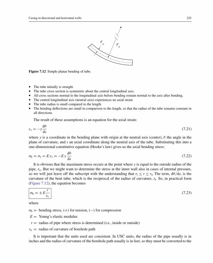
Casing in directional and horizontal wells 225
rκro
Figure 7.12 Simple planar bending of tube.
• The tube initially is straight.• The tube cross section is symmetric about the central longitudinal axis.• All cross sections normal to the longitudinal axis before bending remain normal to the axis after bending.• The central longitudinal axis (neutral axis) experiences no axial strain• The tube radius is small compared to the length.• The bending deflections are small in comparison to the length, so that the radius of the tube remains constant in
all directions.
The result of these assumptions is an equation for the axial strain:
εs = −ydθ
ds(7.21)
where y is a coordinate in the bending plane with origin at the neutral axis (center), θ the angle in theplane of curvature, and s an axial coordinate along the neutral axis of the tube. Substituting this into aone-dimensional constitutive equation (Hooke’s law) gives us the axial bending stress:
σb = σs = E εs = −E ydθ
ds(7.22)
It is obvious that the maximum stress occurs at the point where y is equal to the outside radius of thepipe, ro. But we might want to determine the stress at the inner wall also in cases of internal pressure,so we will just leave off the subscript with the understanding that ri ≤ r ≤ ro The term, dθ/ds, is thecurvature of the bent tube, which is the reciprocal of the radius of curvature, rκ So, in practical form(Figure 7.12), the equation becomes
σb = ±Er
rκ
(7.23)
where
σb = bending stress, (+) for tension, (−) for compression
E = Young’s elastic modulus
r = radius of pipe where stress is determined (i.e., inside or outside)
rκ = radius of curvature of borehole path
It is important that the units used are consistent. In USC units, the radius of the pipe usually is ininches and the radius of curvature of the borehole path usually is in feet, so they must be converted to the

226 Casing and Liners for Drilling and Completion
same unit (it does not matter which). In SI units, both measures should be in meters. Young’s modulususually is in units of psi, kPa, or MPa, and the bending stress is in the same units.
It is necessary to remember the assumptions of this formula before using it, especially with tubes. Asa tube bends, its cross section tends to ovalize rather than remain circular. The pipe radius in the bendingplane is reduced as the cross section becomes ovalized, and the formula no longer is valid. Since there isno simple way to determine the point at which the shape is too ovalized to use the formula, the tendencyis to ignore it, since it will over-predict the maximum bending stress when the pipe is slightly ovalized.That makes the formula possibly a bit conservative in casing design. For long and medium radius ofcurvature wells, it seems to work well for all but larger diameter, thin-wall pipe. For short-radius wells,it should be used with caution, and again, it would depend on the pipe diameter and wall thickness. Thatmay seem to avoid the specific, but for certain, we can say that it becomes meaningless if the yield pointis exceeded. In addition to the tendency to become oval the cross section changes in another way. Thecompressive side becomes thicker and the tensile side becomes thinner. This causes the neutral axis toshift also. These effects are negligible for small bending deflections, but do not ignore the possibilities.And since in the case of oval deformation, Equation (7.23) will over predict the stress (the effectivevalue of ro is reduced), it may still be considered as a conservative approach.
7.6.2 Effect of couplings on bending stress
One limitation of the simple bending formula, as we typically apply it, is that it assumes the casing isin contact with the borehole wall along its entire length and its curvature is the same as that of the borehole. This does not account for an amount of standoff from the couplings. The coupling standoff allowsfor local bending with a smaller radius of curvature than that of the bore hole, therefore possibly a higherbending stress from axial tension or compression loading in the pipe. In the tensile case, the couplingsare assumed tangent to the borehole wall, so that if the pipe between couplings is not in contact withthe borehole wall, then the tension tends to straighten the joint between couplings. The result is that thegreatest bending stress in the joint is in the pipe body near the couplings, until the pipe makes contactwith the borehole wall, then the maximum bending stress in the pipe may be at some other point. In thecompression case, the casing between couplings is forced toward the borehole wall in a compressivemode and the bending stress is higher near the couplings. Once pipe body contact with the boreholewall is made in compression, the point of maximum curvature and bending stress may be at some otherpoint in the tube. This is illustrated in Figure 7.13.
An equation for determining the maximum bending stress with connections was derived for thetension case by Lubinski [46] in 1961, and later derivations were done for both tension and compressionby Paslay and Cernocky [47] in 1991. Lubinski’s equation initially was developed to account for the
(a) (b)
contact
Figure 7.13 Effects of couplings in bending: (a) tension and (b) compression.

Casing in directional and horizontal wells 227
standoff of drill-pipe tool joints and the effects this had on the fatigue of drill pipe rotating in tensionin curved boreholes. His equation later began to appear in conjunction with casing design in curvedwellbores. His equation (and all that follow in this discussion) assumes that the borehole curvatureis constant and in a plane between casing couplings, the coupling length is small compared to thelength of the joint, the couplings are in contact with the borehole wall, and the couplings are tangentto the borehole curvature at the point of contact. Also assumed is that, since the coupling is relativelysmall in length, its entire length is in contact with the wall and it does not bend. These are reasonableassumptions. Although not in Lubinski’s original form, his equation from 1961 can be written as follows:
σ b = λb Ero
rκ
(7.24)
which is essentially the same as our previous bending equation (7.23), except for the factor, λb, whichhas been called a bending-stress magnification factor. Note that there is no ± in this equation, sinceLubinski’s equation is valid only in tension. Lubinski’s bending-stress magnification factor is
λb = ϕ
tanh (ϕ)(7.25)
where
ϕ ≡ �
2η (7.26)
and
η ≡√|Fs|E Ia
(7.27)
where
� = joint length between couplings
Fs = axial load along curvilinear borehole path (tension in this case)
E = Young’s modulus of elasticity
Ia = axial second area moment of tube cross section
The second area moment of the tube cross section about an axis passing through the center of thetube perpendicular to its longitudinal axis is
Ia = π
4
(r4
o − r4i
)= π
64
(d4
o − d4i
)(7.28)
A reminder, use consistent units. Note also that we used the absolute value of the axial load in thisformula. In this particular equation, we are talking about tension, but later we use the same quantitiesfor equations in which the axial load is in compression, a negative value, and the square root would bea complex number. We choose this slight modification so that we may use the same nomenclature laterin both the tension and compression states. And, in that context, we could resume use of the ± sign inEquation (7.24), once the equations for λb are derived for the compression case.
The limitation of this equation of Lubinski’s is that the casing does not contact the borehole wallbetween the couplings. Simply stated, if there is contact, the equation is not valid. That notwithstanding,

228 Casing and Liners for Drilling and Completion
his equation has appeared in various places to show that coupling standoff is important in casingdesign, but without mention of the contact limitation. One cannot just plug numbers into Lubinski’sequation without understanding its limitations. One must always determine the valid range for a specificapplication.
The maximum displacement, ymax, from a straight configuration to contact by the midpoint of thecasing between couplings, as written by Lubinski, is
ymax ≈ �2
8R+ ω (7.29)
This gives the approximate maximum displacement of the midpoint of an initially straight pipe deflectedto the point of contact with the borehole wall. The second term, ω , is the standoff from the coupling,defined as
ω ≡ rcpl − rcsg = dcpl − dcsg
2(7.30)
where
ω = standoff
rcsg = outside radius of casing
rcpl = outside radius of coupling
dcsg = outside diameter of casing
dcpl = outside diameter of coupling
As previously mentioned, Paslay and Cernocky [47] did additional work in this area. They solvedthe problem in both tension and compression and cast it in a slightly different format, which lends itselfto computer programming. The tension case results in a formula for each of the three possibilities: nocontact, point contact, and wrap contact. The first two are self-explanatory, and the wrap contact isreached when the curvature of the pipe in contact with the bore hole begins to follow the curvature ofthe bore hole. Since there are both tension and compressive axial-loading possibilities, the pipe can takesix modes of deformation:
• Mode 1. Tension, no contact• Mode 2. Tension, point contact• Mode 3. Tension, wrap contact• Mode 4. Compression, no contact• Mode 5. Compression, point contact• Mode 6. Compression, wrap contact
Paslay and Cernocky derived equations for all six modes, plus four equations necessary to define thetransition between modes (two for tension and two for compression). I present their results with verylittle explanation, and one should read their paper for a full understanding of the derivations.
Mode 1. tension, no contact
The bending-stress magnification factor for this mode is
λ = ϕcosh ϕ
sinh ϕ(7.31)

Casing in directional and horizontal wells 229
This equation is equivalent to Lubinski’s equation (7.25). The nomenclature for this equation and allthe following remain the same as previously defined.
Mode 2. tension, point contact
Point contact begins when the tension is such that
1− cosh ϕ +(
ϕ
2− 2 η ω R
�
)sinh ϕ = 0 (7.32)
This nonlinear equation in ϕ must be solved numerically for values of tension, Fs, contained in η
and ϕ, to establish the value of tension at which contact is established. The equation for the bending-stress magnification factor for point contact is
λb =ϕ[(sinh ϕ − ϕ)−
(ϕ2 + 2 η ω R
�
)(cosh ϕ − 1)
]2 (cosh ϕ − 1)− ϕ sinh ϕ
(7.33)
Mode 3. tension, wrap contact
Wrap contact begins when the curvature in the casing first begins to equal that of the bore hole wherethe two are in contact. Wrap contact begins when the magnitude of the tension is such that
ϕ
2(cosh ϕ + 1)− 2 sinh ϕ +
(2
ϕ− 2η ω R
�
)(cosh ϕ − 1) = 0 (7.34)
This nonlinear equation must be solved numerically to determine the value of the axial tension atwhich the wrap contact begins. The equation for the bending-stress magnification factor in wrap contactis
λb =ξ2
2 + η2R ω (cosh ξ − 1)− ξ (sinh ξ − ξ)
ξ sinh ξ − 2 (cosh ξ − 1)(7.35)
where we must first solve the following nonlinear equation numerically for ξ :
ξ2
2(cosh ξ + 1)− 2ξ sinh ξ +
(2− η2R ω
)(cosh ξ − 1) = 0 (7.36)
Paslay and Cernocky state that the solution of interest is in the range
ϕ ≤ ξ ≤ η R cos−1[
R
R+ ω
](7.37)
Mode 4. compression, no contact
The equation for no contact in compression is.
λb = ϕ
sin ϕ(7.38)

230 Casing and Liners for Drilling and Completion
Mode 5. compression, point contact
When the compression load in the casing reaches a magnitude at which point contact is made, thefollowing condition is satisfied:
1− cos ϕ −(
ϕ
2+ 2 η ω R
�
)sin ϕ = 0 (7.39)
It must be solved numerically to obtain the axial load at which point contact occurs.The Paslay and Cernocky bending stress magnification factor for point contact in compression is a bit
more complicated, in that there are three possibilities as to where the maximum bending-stress occurs.The maximum could occur at the coupling, the midpoint of the joint, or under some circumstances,at another location in the pipe. One must determine the first two, then determine if the third possibilityexists and, if so, its magnitude. Once those are calculated, the maximum of the three is the bending-stressmagnification factor.
At the coupling,
Λcpl =ϕ[(
2 η ω R�− ϕ
2
)(1− cos ϕ)+ ϕ − sin ϕ
]2 (1− cos ϕ)− ϕ sin ϕ
(7.40)
At the midpoint,
Λmid =ϕ[−(
2 η ω R�− ϕ
2
)(1− cos ϕ)+ ϕ cos ϕ − sin ϕ
]2 (1− cos ϕ)− ϕ sin ϕ
(7.41)
Two additional quantities are needed to determine the possible third point:
Γ =ϕ[(
2 η ω R�− ϕ
2
)sin ϕ + 1− cos ϕ
]2 (1− cos ϕ)− ϕ sin ϕ
(7.42)
Ω = tan−1(
Γ
Λcpl
)(7.43)
Then, the third possible bending-stress moment is
Λs = Λcpl cos Ω − Γ sin Ω ⇔ 0 < Ω < ϕ (7.44)
If Ω is outside the valid range, then Λ does not exist and the maximum bending-stress moment willbe either at the midpoint or the coupling. The maximum bending-stress factor is the maximum absolutevalue of the three possibilities:
λb = max(∣∣Λcpl
∣∣ , |Λmid| , |Λs|)
(7.45)
Mode 6. compression, wrap contact
When the compression load in the casing reaches a magnitude such that wrap contact begins, thefollowing condition is satisfied:
ϕ
2(1+ cos ϕ)− 2 sin ϕ +
(2
ϕ− 2 η ω R
�
)(1− cos ϕ) = 0 (7.46)

Casing in directional and horizontal wells 231
As before, this must be solved numerically to determine the axial compressive load at which wrapcontact begins.
The bending-stress magnification factor for wrap contact in compression has two possibilities: Themaximum is at the coupling or some other point between the coupling and the midpoint. Since the casingcurvature at the midpoint is the same as the borehole curvature, the bending magnification factor thereis unity.
At the coupling,
Λcpl =ξ2 − η2ω R (1− cos ξ)+ ξ (ξ − sin ξ)
ξ sin ξ − 2 (1− cos ξ)(7.47)
where we must first solve the following nonlinear equation numerically for ξ :
ξ2
2(1+ cos ξ)− 2ξ sin ξ +
(2− η2 ω R
)(1− cos ξ) = 0 (7.48)
Paslay and Cernocky do not give a range for the solution, but it appears the range given in Equation(9.32) might be at least a starting point.
We then calculate two more quantities:
Γ =(
ξ2 − η2ω R
)sin ξ + ξ (1− cos ξ)
ξ sin ξ − 2 (1− cos ξ)(7.49)
and
Ω = tan−1(−Γ
Λcpl
)(7.50)
Then, we calculate a stationary value of the bending-stress factor at some location in the pipe, if itexists:
Λs = Λcpl cos Ω − Γ sin Ω ⇔ 0 < Ω < ξ (7.51)
If Ω is outside the specified range, then Λs does not exist. Paslay and Cernocky recommend assigninga value of unity in that case, if it is used in a computer program. A value of unity is equivalent to sayingthere is no bending-stress magnification at that point. Then, the maximum bending-stress magnificationfactor for this joint of pipe is the maximum of the absolute values of Λcpl and Λs:
λb = max(∣∣Λcpl
∣∣ , |Λs|)
(7.52)
Comments on bending-stress magnification
As can be seen, calculation of the bending stress magnification factors of Paslay and Cernocky isnot exactly something that can be done manually. These formulas may be programmed for computerimplementation, but the programming is not trivial. Paslay and Cernocky were interested primarilyin drill-pipe fatigue, and they mention solving the transition equations for the standoff quantity thatwe labeled ω. In that context, the equations are linear and solved easily. That may be of some use inselecting a drill-pipe string with various options as to tool joint dimensions, but in most casing design,the standoff, ω, is a fixed quantity, and our primary interest in the transition equations is in the value ofthe axial load that determines the transition point from one mode of contact to another, so that we might

232 Casing and Liners for Drilling and Completion
Y
Figure 7.14 Typical behavior of transition equations for tension and compression. The compression equation hasadditional solutions farther to the left (solutions at Y = 0).
apply the appropriate equation for the bending-stress magnification factor, λb. In terms of the axialload, which is contained in the variables, η and ϕ, these equations are nonlinear and must be solvednumerically. All the nonlinear equations that must be solved numerically have been recast here to avoidsingularities in the numerical solutions, so they may not exactly resemble those of Paslay and Cernocky.However, some of these equations have local minima and maxima and multiple roots, so they are bestsolved with a bracketing technique, such as the bisection method. It might be of some help to see a plotof some of the nonlinear equations that determine the contact mode transition points, and an example isshown in Figure 7.14. This figure is for a specific casing size and borehole curvature so it will vary fordifferent casing sizes and borehole curvature.
The two equations that define the transition between tensile modes are relatively easy to solve witha simple bracketing method, such as a bisection method. However, for small values of curvature, κ , (orlarge radius, rκ ), there is a range for which contact is physically impossible and will result in an infiniteroot. That condition, which is not addressed by Paslay and Chernocky, can be quantified as
ω >
√r2κ +(
�
2
)2
− rκ (7.53)
Another characteristic of the tensile modes is that, when the curvature is small, the value of the tensileload at which point contact occurs is far greater than the joint strength of the casing, so there is no pointin searching for a root if it lies beyond the joint strength.
The two transition equations for compression exhibit especially bad behavior, as equations withtrigonometric functions often do over a wide range of values. As previously mentioned, the equationsof Paslay and Cernocky have been recast here to avoid numerical singularities, but they still producemultiple roots. The first roots for these two equations tend to lie close to the origin for large curvature

Casing in directional and horizontal wells 233
and further away for smaller values of curvature. From a computational standpoint, this means thata combination procedure that first brackets the root starting very near the origin, then proceeds tolocate the root within the bracket, is a good approach. The physical meaning of the additional rootsto these equations does not appear to have been explored, but Mitchell [33] has done work in lateralbuckling of drill pipe in curved boreholes and shows that the Paslay and Cernocky equations under-predict the bending-stress magnification in cases where compressive loading causes lateral buckling.The reason for the higher bending-stress magnification in those cases is that the lateral bucklingis out of the plane of the wellbore curvature to which the Paslay and Cernocky equations areconfined.
It is does not seem to have been mentioned in any of the discussions on the bending-stressmagnification factor as to the nature of the axial load used for actual calculations. Simple bending,as described by Equation (7.23), is independent of axial loading, but the bending-stress magnificationfactor, λb, is not. That raises the question as to whether we use the true axial load or the effective axialload to calculate λb. The largest factors in tension arise from use of the effective axial load, which hasno compression in the string. More accurate results should come from the true axial load, however, thecompressive axial load in the bottom portion of the string begs a few questions. First, the values ofλb in the compressive section are usually minimal except in the case of a horizontal (or other highlydeviated well), where a significant amount of casing is below the critical angle point. Secondly thecompression formula does not consider lateral buckling which generally will not be planar as requiredin the assumptions.3
When one calculates the bending-stress magnification factors for a particular casing design, one maybe alarmed at their magnitudes, which easily may range between 1 and 4, yet for some reason, thisprocess rarely is considered in actual casing design. One excuse might be that it is not somethingthat can be calculated easily, but surely if casing failures actually occur because of bending-stressmagnification, then everyone would have a computer program to calculate it. The most probablereason that we do not recognize problems caused by bending-stress magnification is likely because,in most casing strings, the highest value of tension occurs near the surface, where the curvature oftenis relatively small. It is not unusual to see bending-stress magnification factors of over 5 in suchinstances, but the bending stress attributable to borehole curvature is so small that, when multipliedby a large magnification factor, it still is only a small percentage of the yield strength of the casing,especially when we are inclined to use relatively large design factors in tension loading. This is notto say that it can be ignored, but that it does not seem to cause problems in most wells (or at leastthat we recognize as such). Bending-stress magnification should certainly be considered for casingdesign in deeper wells and any well where the combined loading may be close to the yield of thecasing.
We definitely do not attempt an example calculation here, but Figure 7.15 shows an example of thebending stress magnification factors for an actual horizontal well. And, as would be expected from ourdiscussion, they are highest near the surface.
These factors were calculated to check a previously designed casing string for the specific boreholein which it would be run. While the results might tend to be cause for apprehension because of the largemagnitudes, the overall effect in this well is negligible, as will be seen in a following section of thischapter devoted to combined loading in directional wells. The combined loading for this well is shownwith and without bending-stress magnification in that section in Figure 7.16. It can be seen there that
3 Personally, I run both along with both an upward and downward friction calculation (using software of course), and almostalways opt for the effective load for a design check as it is more conservative.

234 Casing and Liners for Drilling and Completion
Figure 7.15 Bending stress magnification factor for a horizontal well.
Figure 7.16 Combined loading in a horizontal casing string.
the only significance of the bending-stress magnification is in the build section of the well, as one wouldintuitively expect.
The transition point equations as I have formulated them here are all nonlinear because I have usedthe coupling standoff, ω, as a given, and then calculated the axial load at the mode transition points.However, as I mentioned above, Paslay and Cernocky formulated the algorithm using the axial loadas the given and calculating the standoff at the transition points using linear equations. In our case

Casing in directional and horizontal wells 235
of known actual standoff that method could be used to calculate the standoff at the transition pointsand then determine into which mode bracket the actual standoff belongs. That might be a preferableapproach for some who would rather not program as many nonlinear equations.
One last comment is in order here. Paslay and Cernocky assumed a constant curvature, κ , andcouplings tangent to the borehole wall. Those are reasonable assumptions and really the only way toobtain closed form solutions. Implicit in the assumption of tangent couplings is the assumption thatthe curvature remain constant or nearly constant at least one joint length either side of the joint inconsideration. That is not a serious restriction, given the approximate nature of assumed geometry, butthe stress magnification could be more severe (or less) if the borehole path varied from that smoothcurvature.
7.6.3 Effects of bending on coupling performance
There are no standards on coupling performance in bending other than what some companies andmanufacturers established for themselves. API Bulletin 5C3 and a 2004 draft of ISO 10400 containedtwo formulas for “joint strength of round thread casing with combined bending and internal pressure.”Oddly, there were no terms in those two formulas to quantify the bending or pressure. The first editionof this text included those two formulas (with a note of considerable skepticism). The release version ofISO/TR 10400 [11] made no such mention of bending or internal pressure. Therefore those two formulasdo not appear in this edition.
One way that combined bending and axial load was handled historically amounted to multiplyingthe maximum bending stress times the cross-sectional area of the tube, adding it to the axial load, thencomparing that sum to the joint strength of the casing. The best recommendation that could be madehere is no recommendation at all, as no particular method inspires much confidence. One thing thatshould be understood about the eighth-rd thread in a bending situation, though, is that it is considered apoor choice by most operators. V-shaped threads have a tendency to “jump out” or override one anotherbecause the shape is conducive to this, and possibly more so in the presence of a thread lubricant. Mostoperators of horizontal wells elect to use a thread with a more squared profile as opposed to a V-shapedprofile, because it lessens the possibility of jump-out. A buttress thread has a square contact in tensionbut is somewhat tapered in compression. A buttress-type thread has performed successfully in medium-radius wells for many operators. Most proprietary threads are a better choice, and in critical wells, theproprietary threads that tend to interlock are a much better, although more expensive solution. Someproprietary thread manufacturers publish bending performance data for their connections, and these canbe quite useful.
7.7 Combined loading in curved boreholes
We examined combined loading in the previous chapter. Perhaps, the most common occurrence of failurefrom combined loading is in horizontal wells or highly deviated wells. Primarily, this is caused by theaddition of the bending stress, which can be quite significant in magnitude. Our approach to casingdesign for these wells is to use conventional load curves for burst and collapse. Then, the tension designis based on a load curve that includes the effects of both gravity and friction, so it will be quite differentfrom casing hanging in a vertical well. A typical curve like this was shown earlier in Figure 7.7. John

236 Casing and Liners for Drilling and Completion
Greenip [48] illustrated a simple method for designing casing strings in highly deviated wells, usingtorque-and-drag curves like we discussed in an earlier section on borehole friction. He went a stepfurther to include bending stress, which he converted to an “equivalent axial load” by multiplying thebending stress by the cross-sectional area of the tube so that it might be considered part of the tensileload. That equivalent axial load is added to the axial load from the borehole friction curves in theappropriate places to constitute a tensile load curve for casing selection. The procedure produces anadequate design for most directional wells and has been used successfully by numerous operators. Here,we assume that we designed a casing string by that method or something similar, and we now are readyto check it for the effects of combined loading, especially in the build section.
Although none of the single loads, such as tension, bending, or burst, may exceed the yield strengthof the pipe individually, it is quite possible that the combination of the loads may exceed the yieldstrength. And there are no handy charts to adequately show the effects of the combined loads oftenencountered in highly deviated wells. It is easy to check the combined loads at critical points manuallyto determine whether we need to make adjustments to a design or not. We also could do this with aspreadsheet and check the entire string. Next is an example of a horizontal well in which there was acasing problem. The operator had drilled the vertical part of the hole and a build section to an inclinationof 90◦. The company was running 7 in. casing, and about halfway through the build section, the casinghit an obstruction, which is not unusual in a horizontal well, if the drilled cuttings are not sufficientlycleaned out of the bore hole.4 The operator took immediate action. He put a circulating head on thecasing, then tried to wash through the obstruction. At first unsuccessful, the driller slacked off the brakeeven further. As hard as it may be to understand, he set the entire string weight on the obstruction. Theshoe plugged and the internal pressure at the surface rose to 3000 psi before he was able to shut off thepumps and pick up the string off bottom to relieve the pressure. The operator pulled the casing out ofthe well and found one of the joints in the build section had buckled and crushed. Here are the data andcalculations for this actual case.
EXAMPLE 7.1 Combined Loading in Curved Wellbore
Data at 6000 ft (TVD):
• Casing OD = 7.0 in.• Casing ID = 6.366 in.• Casing grade = K-55 (Y = 55,000 psi)• Young’s modulus = 30×106 psi• Axial compression = –122,000 lbf (from torque and drag estimate)• Radius of curvature = 300 ft• External pressure = 3000 psi• Internal pressure = 6000 psi
Determine if combined loads will yield pipe.
1. Calculate the axial stress:
σ z = −122000π4 (7.02 − 6.3662)
= −18, 331 psi
4 The build section of horizontal wells is notoriously difficult to clean because cuttings tend to migrate down the low side of thehole at inclination angles between 45◦ and 60◦, even at relatively high circulating rates.

Casing in directional and horizontal wells 237
2. Calculate the bending stress:
σ b = −30× 106 (7.0/2)
12 (300)= −29, 167 psi
Note that we had to get the radius of curvature into the same units as the pipe radius.3. Calculate the pressure effect using at the outside wall using the Lamé equations:
σ r = −3000 psi
σθ = −3000(3.52 + 3.1832)+ 2(6000)(3.183)2
3.52 − 3.1832 = 25, 694 psi
4. The maximum axial stress at the external wall is the preceding axial stress plus the bending stress:
σ z = −18331 − 29167 = −47, 498 psi
5. Since there is no torque, these are principal stress components and can be plugged directly into the vonMises criterion:
Ψ =√
1
2
[(−3000 − 25694)2 + (25694 + 47498)2 + (−47498 + 3000)2]
Ψ ≈ 63, 900 psi
63, 900 > 55, 000 → yield
Clearly, this combined load value is well above the yield strength of the casing. This casing string, infact, did fail. The operator was not aware that the combined loading could be that significant. In this case,the operator was lucky to get the casing out of the hole. Others have encountered similar circumstancesand found the lower part of the casing string missing when they pulled the string out of the hole. In thiscase, we calculated the combined load at the outer wall of the casing, assuming that, since the maximumbending stress occurs at the outer wall, that would be the critical location. But, the maximum stress frompressure occurs at the inner wall, and if we calculate it at the inner wall, we find that the combined loadthere would be slightly less at 63,700 psi. In this case, it was not obvious as to whether the maximumcombined load would occur at the inner wall or outer wall, but it did appear obvious that, since the pipewas in compression, it would occur on the concave side of the curve. One should be careful about suchassumptions, however. While the maximum combined load typically occurs on the concave side whenthe pipe is in compression and on the convex side when it is in tension, that is not true in general becauseof the influence of the pressure.
It is relatively easy to program the Lamé equations and the von Mises yield criterion in a spreadsheetto calculate the combined loading for a well for use in casing design. From a directional survey, oneneeds the measured depths, true vertical depths, and radius of curvature between survey points. Froma torque-and-drag model, one needs the true axial loads for motion in both directions, so that one maycheck for the worst-case scenario. Additionally, one needs the pipe dimensions and specific weights,the fluid densities, applied pressures, and so forth. One does not actually need both directional andfriction software to get this data, as it all can be programmed into a single spreadsheet. The additionof a bending-stress magnification factor would be a bit cumbersome in a spreadsheet though, but itcan be done. One convenient way to look at combined loading in casing design is in a plot of the

238 Casing and Liners for Drilling and Completion
combined load as a percentage of pipe yield stress. Figure 7.16 shows the combined load in an actualL-shaped horizontal well as a percent of the yield of the casing. This is a rather simple case, wherethe entire string is a single weight and grade of casing, 5-1/2 in., 17 lb/ft, N-80. The operator plansto do multiple hydraulic fracture treatments in this well at high rates and pressures. The combinedload is calculated for a burst scenario, where the fracture treatment might screen out with a fullcolumn of fracture fluid and proppant such that the pressure equalizes at maximum surface treatmentpressure.
A plot like this figure provides an easy way to visualize the effects of combined loading. If necessary,a casing string can be modified to compensate for the combined loading effects. One last reminderthough, combined loading using a von Mises yield criterion does not account for connection strengthnor collapse prior to yield, as mentioned in previous chapters.
7.8 Casing design for inclined wells
The example well we used in Chapters 2–4 was for a vertical well. How would we design casing for adirectional well with the same fracture and formation pressure data? The answer is that we would followexactly the same procedure using vertical depths and pressures as before and we would reach a point asat the end of Chapter 4 with a completely designed casing program adequate for our directional well towhich we would add the following steps:
Intermediate Casing• Calculate borehole friction for intermediate string and adjust axial design if necessary.• Calculate combined loads for intermediate string in curved portion of wellbore and adjust design if necessary.• Calculate the section lengths of the casing for purchasing and running (as opposed to the vertical lengths in the
design.• Calculate contact force on intermediate string for placement of drill pipe protectors while drilling to total depth.
This can only be done after the intermediate hole is drilled and before drilling below the intermediate casing.
Production Casing• Calculate borehole friction for production string and adjust axial design if necessary.• Calculate combined loads for production string in curved portion of wellbore and adjust design if necessary.• Calculate the section lengths of the casing for purchasing and running (as opposed to the vertical lengths in the
design.
Let us illustrate these items in examples, first lets us establish the well geometry and data. Typicallywe would have this data in a well profile plan provided by a service company according to ourspecifications, in other words, they would do all the calculations. But for our example we will makethe specifications and do the calculations ourselves.
EXAMPLE 7.2 Directional Well Profile
Using data from our example well in previous chapters we will say the vertical depth is 14,000 ft as before.Our target zone at 14,000 ft is 8000 ft horizontally from the surface location and we will drill a horizontal

Casing in directional and horizontal wells 239
a
bc
l5
l1
l2
l4
l3
r1
θ1
r2 θ2
1
2
34 5
Scale:0 5000 ft
0
Figure 7.17 Example directional well profile.
lateral from that point an additional 3000 ft in length. That is the entirety of our data for this well plan, asurface location and a target at the beginning of a lateral and a target at the end of the lateral. From there on, itis up to us as to how we drill the hole. Optimizing a borehole path is not the topic of our endeavor here, so wewill just arbitrarily select a common approach. We will drill a vertical hole to 3000 ft and set surface casing.At 500 ft below the surface casing we will begin the directional drilling with an upper build section with aradius of 1000 ft. We will hold a constant inclination angle to near the top of the lateral at which point we willdrill a lower build section with a radius of 500 ft. Upon reach a horizontal inclination at our first target we willdrill the lateral for an additional 3000 ft. A profile of this plan is shown in Figure 7.17.
Datavertical depth = 14, 000 ft
hz displ. = 11, 000 ft
a = 7000 ft
b = 10, 000 ft
l1 = 3500 ft
l5 = 3000 ft
r1 = 1000 ft
r2 = 500 ft
Using the given data and Figure 7.17 we may calculate the additional quantities needed. The onlyclarification needed is to recognize that the line, c, is not parallel to l3, so the angle, θ2 requires a bit moreattention.
Calculations
c =√
a2 + b2 =√
70002 + 100002 = 12, 207 ft
l3 =√
a2 + b2 − r22 =√
70002 + 100002 − 5002 = 12, 196 ft

240 Casing and Liners for Drilling and Completion
θ2 = π
2−[sin−1
(a
c
)+ sin−1
( r2
c
)]
= π
2−[
sin−1(
7000
12207
)+ sin−1
(500
12207
)]= 0.91912 rad
θ1 = π
2− θ2 = π
2− 0.91912 = 0.65167 rad
(≈ 37◦)
l2 = r1 θ1 = 1000 (0.91912) = 919 ft
l4 = r2 θ2 = 500 (0.65167) = 326 ft
Calculate the measured depths of the nodes:
s1 = l1 = 3500 ft
s2 = s1 + l2 = 3500 + 919 = 4419 ft
s3 = s2 + l3 = 4419 + 12196 = 16, 615 ft
s4 = s3 + l4 = 16615 + 326 = 16, 941 ft
s5 = s4 + l5 = 16941 + 3000 = 19, 941 ft
Calculate the vertical depths of the nodes:
h1 = s1 = 3500 ft
h2 = h1 + r1 sin θ1 = 3500+ 1000 sin (0.65167) = 4107 ft
h3 = h2 + l3 sin θ2 = 4107 + 12207 sin (0.91912) = 13, 812 ft
h4 = h3 + r2 − r2 sin θ1 = 13812 + 500− 500 sin (0.65167) = 14, 000 ft
h5 = h4 = 14, 000 ft
It is an exercise in trigonometry, but to avoid common mistakes remember that inclination is measuredfrom vertical (θ1 is the same as the inclination angle, θ2 is not, even though they may appear otherwise), andalways work in radians and convert to degrees when finished.
Now that we have those calculations done we need to determine the measured depths of our casingsections. First, we do the 9-5/8 in intermediate casing which has two sections with the transition pointat a vertical depth of 6360 ft and the bottom at 10,500 ft.
EXAMPLE 7.3 Intermediate Casing Section Lengths
We calculate the lengths, �, of the two sections, starting with the top section, �2. The bottom section length,�1, is all in the inclined straight section.
�2 = s2 + 6360 − h2
cos θ1= 4419 + 6360 − 4107
cos (0.65167)= 7253 ft
�1 = 10500 − 6360
cos θ1= 10500 − 6360
cos (0.65167)= 5207 ft

Casing in directional and horizontal wells 241
Table 7.1 Example 9-5/8 in. Intermediate Casing
Weight Vert. Depth Meas. Depth Sect. Length
Section (lb/ft) Grade (ft) (ft) (ft)
2 43.5 P-110 6360 7253 72531 43.5 N-80 10500 12460 5207
We summarize the results in Table 7.1.
Next we will determine the borehole friction for this casing string. We do these calculations withsoftware programmed from the equations earlier in this chapter using only six survey points (at thenodes in Figure 7.17) because this is a smooth well plan. Because of the smoothness of the plannedprofile we will use higher than average friction factors to account for some amount of tortuosity in thewell as drilled. We will use a factor of 0.3 in. the cased hole and 0.5 in. the open hole. The verticalsection of the well will have zero contact no matter what friction factor we select, we will assume anincreasing inclination angle up to 4◦ in that section. We will also employ the interpolation algorithm inAppendix E to add nodal points so as to generate a usable graph that we would not get with only sixsurveys. The friction load is plotted in Figure 7.18 along with the axial strengths of the casing.
As you can see, the casing strength is well above the friction load. You may notice that the frictionload is based on the effective axial load instead of the true axial load. Both the Johancsik et al. [40] andthe Sheppard et al. [41] models calculate borehole friction using the effective stress as is this case. Thiscurve can be corrected to a true axial load with friction using Equation (7.10), but given the approximatenature of our method of using a smooth well plan profile and increased friction factors to accountfor tortuosity, it is hardly worth the effort since it usually has to be done manually. Most commercial
Figure 7.18 Example intermediate casing, axial load with friction (upward motion case).

242 Casing and Liners for Drilling and Completion
software can be “tricked” into giving a true axial load by applying a “bit weight load” equivalent tothe buoyant pressure load at the bottom, but this only works if the entire casing string is the same wallthickness.
A point regarding that friction curve is that there exists a pervasive misconception that in a directionalwell with friction, the true axial load does not exist because most of the string is “out of the shadowof the casing top.” That is pure bunk, and where such a notion came from is a mystery (I have seenthis actually taught in industry training courses). The only time the pressure effects are not distributedthroughout a string of pipe is when the pressure has changed while the pipe is static and the changein pressure is not sufficient to cause the pipe to move axially and redistribute the new pressure forces.But if you move the pipe again the changed pressure effects will be distributed in the pipe as a trueaxial load.
We should also check the combined load in the intermediate casing from the bending, axial load, andburst pressure.
EXAMPLE 7.4 Intermediate String Combined Loading
We will examine the combined loading just inside the top of the build section where the radius of curvatureis 1000 ft. The axial load at this point taken from Figure 7.18 at 3500 ft is 365 klbf. We will assume thatthe internal pressure when the casing is set is 2150 psi and the external pressure is 1520 psi. The internalpressure in burst is 7660 psi and the external pressure is still 1520 psi (these values all interpolated from datain Chapter 3). The casing is 9-5/8 in. 43.5 lb/ft P-110 (ID = 8.755 in.).
We will assume that yield will first occur at the inner wall.Determine the initial axial stress:
σz0 =Fz
At= 365000
π4
(9.6252 − 8.7552
) ≈ 29, 060 psi
Determine the bending stress
σb = 30× 106 (4.8125)
12 (1000)≈ 12, 030 psi
Determine the initial radial stress the Lamé equation for the inner wall (Equation (6.5)):
σr0 = −pi = −2150 psi
Determine the radial stress when the burst pressure is applied:
σr = −7660 psi
Determine the tangential stress before pressure test using the Lamé for the inner wall (Equation (6.6)):
σθ0 =pi(r2
o + r2i
)− 2por2o(
r2o − r2
i
)
= 2150[(9.625/2)2 + (8.755/2)2]− 2 (1520) (9.625/2)2
(9.625/2)2 − (8.755/2)2
≈ 5150 psi

Casing in directional and horizontal wells 243
Determine the tangential stress when the test pressure is applied:
σθ = 7660[(9.625/2)2 + (8.755/2)2]− 2 (1520) (9.625/2)2
(9.625/2)2 − (8.755/2)2 ≈ 63, 480 psi
Determine the incremental radial and tangential stress due to the test pressure:
�σr = σr − σr0 = −7660 − (−2150) = −5510 psi
�σθ = σθ − σθ0 = 63480 − 5150 = 58, 330 psi
Then, using the Lamé equation for fixed end tubes (Equation (6.4)), calculate the change in axial stressdue to the test pressure:
�σz = ν (�σθ +�σr) = 0.28 (58330 − 5510) = 14, 790 psi
The axial stress including the test pressure effects is
σz = σz0 + σb +�σz = 29860 + 12030 + 9700 = 55, 880 psi
Now, using the three stress components calculated in the presence of the test pressure, we want to determinewhether or not yield will occur. Since there is no torsion, these values are principal stress components and maybe plugged directly in to the von Mises yield formula:
Ψ ={
1
2
[(σθ − σr)
2 + (σr − σz)2 + (σz − σθ )
2]} 1
2
Ψ ={
1
2
[(63480 + 7660)2 + (−7660 − 55580)2 + (55580 − 62480)2
]} 12
Ψ = 67, 660 psi
Finally, check the yield condition:
Y = 110, 000 psi
Ψ = 67, 660 psi
Y > Ψ → no yield
The combined load is nowhere near the yield strength of this casing section.
At this point we could calculate the bending stress magnification factors and the contact forces fordetermining placement of drill pipe protectors to protect the intermediate casing from wear. Neither ofthese two would be of much use when run on a smooth well plan profile. In practice, we would do abending stress magnification check with actual survey data as the drilling is nearing the casing point.As to the contact force calculations we could do those once the drilling reaches the casing point andsometime before the drill string is picked up to drill out. A more accurate contact force calculationcould be made from a gyro survey made inside the casing, but this is seldom done except in a wellwhere wear might be an extremely critical element of the drilling operation.

244 Casing and Liners for Drilling and Completion
Table 7.2 Example 7 in. Production Casing (AlternateSelection)
Weight Vert. Depth Meas. Depth Sect. Length
Section (lb/ft) Grade (ft) (ft) (ft)
4 29 P-110 4500 4910 49103 32 N-80 9100 10700 57902 32 P-110 11800 14090 33901 35 P-110 14000 19940 5850
Next, let us calculate the lengths of sections for the production casing.
EXAMPLE 7.5 Production Casing Lengths
�4 = s2 + 4500 − h2
cos θ1= 4419 + 4500 − 4107
cos (0.65167)= 4910 ft
�3 = s2 + 9100 − h2
cos θ1= 4419 + 9100 − 4107
cos (0.65167)= 10, 700 ft
�2 = s2 + 11800 − h2
cos θ1= 4419+ 11800 − 4107
cos (0.65167)= 14, 090 ft
�1 = s5 = 19, 940 ft
The results of these section length calculations are shown in Table 7.2. We calculate the productioncasing axial load with borehole friction. This time the calculation is a bit more complicated by the factthat there are four sections of casing (only three different weights though) and both cased hole andopen hole friction factors.The results are shown in Figure 7.19, and as in the intermediate string there isadequate tensile strength in the original selection.
Figure 7.19 Example production casing, axial load with friction (upward motion case).

Casing in directional and horizontal wells 245
The maximum combined load might occur at the top of the upper build section if the plug bumps thefloat collar during an upward motion of the pipe while reciprocating during the cement displacement.
EXAMPLE 7.6 Combined Loads for Production Casing
Data• Pipe data (at top of upper build section 3500 ft): 7.000 in. OD, 6.184 in. ID, P-110• Radius of curvature of upper build section: 1000 ft• Tension with friction from Figure 7.19: 460,000 lbf• Pressures from plug-bump case (Chapter 3): pi = 6820 psi, po = 2790 psi• Additional tension from plug-bump case (Chapter 4): 38,000 lbf
Calculate Stress Components
σz = 460000 + 38000π4
(7.0002 − 6.1842
) ≈ 58, 940 psi
σr = −6820 psi
σθ = 6820(3.5002 + 3.0922
)− 2 (2790)(3.5002
)3.5002 − 3.0922 ≈ 29, 890 psi
σb = 30× 106 (3.5)
12 (1000)= 8750 psi
σz = 58940 + 8750 = 67, 690 psi
Check for Yield
Ψ ={
1
2
[(29890 + 6820)2 + (−6820 − 67690)2 + (67690 − 29890)2
]} 12
≈ 64, 530 psi
64, 530 psi < 110, 000 psi → no yield
There is no combined load problem with this casing string. In a well like this we always design thewell path with a long radius curve for the upper build section to avoid high friction and bending forceswhere the axial forces are high. If we were to plan a hydraulic fracture treatment through this string wewould repeat this calculation with the maximum internal treatment pressure.
7.9 Hydraulic fracturing in horizontal wells
Ironically, the initial impetus for horizontal wells was that it is a way to overcome the limitations ofhydraulic fracturing. Hydraulic fracturing was, and still is problematic in that the direction of hydraulicfractures cannot be controlled. It is a given—determined by the in situ stress field which we cannot
246 Casing and Liners for Drilling and Completion
change. Unfortunately, hydraulic fractures almost always orient in the least desirable direction formaximum productivity (see Appendix E for detailed explanation), whereas a horizontal well can bedrilled in a direction for best productivity. Few envisioned early on that hydraulic fracturing would everbe necessary in horizontal wells, but that changed quickly as it became obvious that hydraulic fracturingcould considerably enhance productivity in horizontal wells in low permeability formations. Hydraulicfracturing in horizontal wells in some areas was common for more than a decade before the shale gasboom began, and it is now almost routine in those shale formations.
Casing in horizontal wells was also rare in the beginning. For one thing, there was no point in itfor most of the formations then being drilled, because no zonal isolation was necessary. Secondly, itwas expensive compared to a vertical well. And technically it was hard to do successfully. Gettingcasing to bottom and adequately cemented posed new problems not experienced in vertical wells.But there were good reasons to run casing in some areas because zonal isolation and stimulationare not easily accomplished in open hole completions. There was also the possibility of boreholecollapse because of formation instability, but few operators understood that well enough to predictor quantify any possible problems. Many operators opted to run slotted liners as insurance againstborehole collapse, and while that sounded like an inexpensive and easy solution at the time (andunfortunately still does to many), it is possibly the worst completion choice one can make. Exceptfor possible borehole support, it virtually eliminates any further completion or production optionssuch as production monitoring (most flow is outside the liner until it nears the heel end), selectivestimulation, zonal isolation, and so forth. It is also the poorest sand control method in the industry.I have already made this point, but it is critically important and bears repeating: Once a slotted lineris in place, all further options are eliminated, unless you can get it out later, and good luck withthat.5
7.9.1 Casing design consideration
In addition to the items already covered, there are some special considerations concerning the design ofcasing strings for hydraulic fracturing stimulations in horizontal wells, especially as they apply to thehigh-pressure, high-volume treatments for shale formations.
• Relatively high treatment pressures• Pressure cycling• Temperature cycling
High treatment pressures
There is little that we need add to what we have already covered as far as internal pressure is concerned.The pressures we experience in these high-volume fracture treatments is not in itself a complicated issue.It is a source of high casing costs not normally encountered in these areas since these high pressuresare not intrinsic to the normal producing phase of the wells. That may lead to a discounting of itsimportance, and some have paid the price with a very expensive fracturing stage going through casingleaks rather than into the intended zone.
The only burst design question here is one of determining the burst pressure load for the fracturejob. The anticipated treatment pressures are dependent on depth, casing size, formation properties,
5 The exception to that caveat is the use of short slotted sections in a conventional liner with inflatable or swelling casing packersbetween to achieve true zonal isolation; many of those have been quite successful.
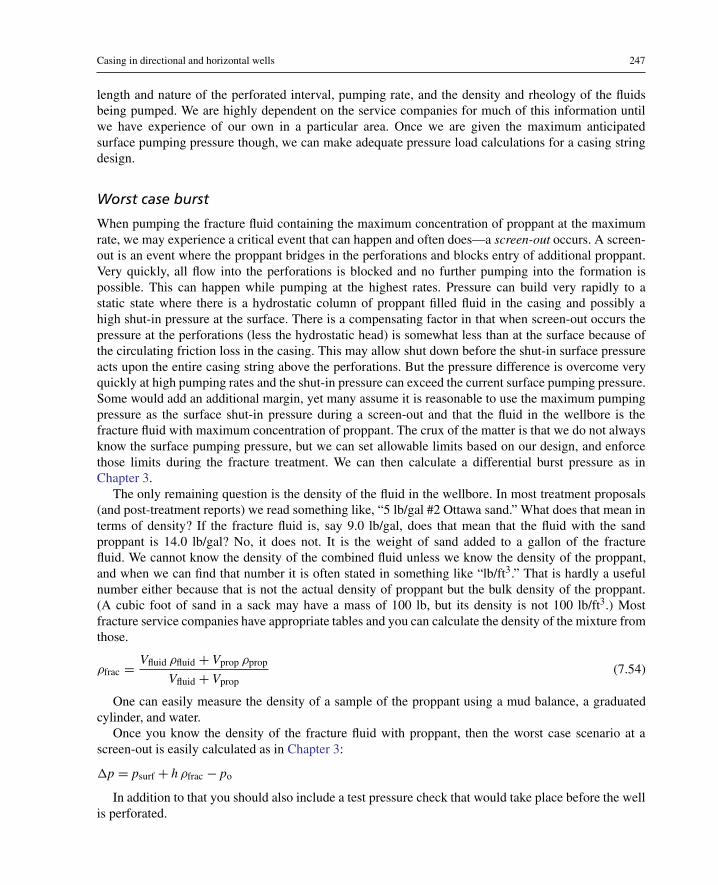
Casing in directional and horizontal wells 247
length and nature of the perforated interval, pumping rate, and the density and rheology of the fluidsbeing pumped. We are highly dependent on the service companies for much of this information untilwe have experience of our own in a particular area. Once we are given the maximum anticipatedsurface pumping pressure though, we can make adequate pressure load calculations for a casing stringdesign.
Worst case burst
When pumping the fracture fluid containing the maximum concentration of proppant at the maximumrate, we may experience a critical event that can happen and often does—a screen-out occurs. A screen-out is an event where the proppant bridges in the perforations and blocks entry of additional proppant.Very quickly, all flow into the perforations is blocked and no further pumping into the formation ispossible. This can happen while pumping at the highest rates. Pressure can build very rapidly to astatic state where there is a hydrostatic column of proppant filled fluid in the casing and possibly ahigh shut-in pressure at the surface. There is a compensating factor in that when screen-out occurs thepressure at the perforations (less the hydrostatic head) is somewhat less than at the surface because ofthe circulating friction loss in the casing. This may allow shut down before the shut-in surface pressureacts upon the entire casing string above the perforations. But the pressure difference is overcome veryquickly at high pumping rates and the shut-in pressure can exceed the current surface pumping pressure.Some would add an additional margin, yet many assume it is reasonable to use the maximum pumpingpressure as the surface shut-in pressure during a screen-out and that the fluid in the wellbore is thefracture fluid with maximum concentration of proppant. The crux of the matter is that we do not alwaysknow the surface pumping pressure, but we can set allowable limits based on our design, and enforcethose limits during the fracture treatment. We can then calculate a differential burst pressure as inChapter 3.
The only remaining question is the density of the fluid in the wellbore. In most treatment proposals(and post-treatment reports) we read something like, “5 lb/gal #2 Ottawa sand.” What does that mean interms of density? If the fracture fluid is, say 9.0 lb/gal, does that mean that the fluid with the sandproppant is 14.0 lb/gal? No, it does not. It is the weight of sand added to a gallon of the fracturefluid. We cannot know the density of the combined fluid unless we know the density of the proppant,and when we can find that number it is often stated in something like “lb/ft3.” That is hardly a usefulnumber either because that is not the actual density of proppant but the bulk density of the proppant.(A cubic foot of sand in a sack may have a mass of 100 lb, but its density is not 100 lb/ft3.) Mostfracture service companies have appropriate tables and you can calculate the density of the mixture fromthose.
ρfrac = Vfluid ρfluid + Vprop ρprop
Vfluid + Vprop(7.54)
One can easily measure the density of a sample of the proppant using a mud balance, a graduatedcylinder, and water.
Once you know the density of the fracture fluid with proppant, then the worst case scenario at ascreen-out is easily calculated as in Chapter 3:
�p = psurf + h ρfrac − po
In addition to that you should also include a test pressure check that would take place before the wellis perforated.

248 Casing and Liners for Drilling and Completion
Pressure and temperature cycling
One of the more insidious problems that has been encountered in the high pressure, high volume, multi-stage fracture treatments in recent times is that of coupling leaks. I have been involved in the forensicsof several cases and the most likely source of the majority of these leaks is the cycling of pressure andtemperature with the multiple stages. While none of the temperature or pressure cycles came near thepressure rating of the couplings, the cyclic loading appeared to have a significant effect. In several casesthe pressure cycles were on the order of 9000-10,000psi and the temperature cycles on the order of100 ◦F. Here is an example based on an actual well in the Marcellus shale in the USA.
EXAMPLE 7.7 Temperature and Pressure Cycle for a Fracture Stage
Assume that there is a section of casing between two fixed (cemented or stuck) points. We determine themagnitude of the maximum differential axial stress in a stimulation cycle during winter conditions.
• Casing: 5-1/2 in. 20 lb/ft. P-110, 4.778 in.ID• Initial down-hole pressure: pi = po = 3000 psi• Maximum surface treating pressure cycle: �p = 10, 000 psi• Maximum temperature change: �T = −100 ◦F (cold fracture fluid, near freezing point)
First we calculate the initial stress from the hydrostatic pressure:
σr = −3000 psi
σθ = 3000(2.7502 + 2.3892)− 2 (3000)
(2.7502)
2.7502 − 2.3892 = −3000 psi
We do not know the axial stress, but for this example we are calculating the change in axial stress caused bythe pressure and temperature cycle. Now we assume the maximum pressure cycle and calculate the change instress caused by the change in pressure.
�σr = −13000 − (−3000)=− 10, 000 psi
�σθ = 13000(2.7502 + 2.3892)− 2 (3000)
(2.7502)
2.7502 − 2.3892 − (−3000)
= 71, 530 psi
�σz = 0.28 (−10000 + 71530) = 17, 230 psi
Notice that there is now a change in the axial stress of the casing because of the change in internal pressure.We used the Lamé fixed end formulas here.
Next we calculate the change in axial stress from the contraction caused by the cold fracture treatmentfluid. This particular well was fractured in winter where the fracture fluid had to be warmed to slightly abovethe freezing point to prevent freezing. Normally we might not consider such a drastic reduction of bottom-holetemperature, but in the case of such large volumes of treatment at a relatively shallow depth it is easy to lowerthe casing temperature to very near the surface temperature.
�σT = −Eα �T = −30× 106(
6.9× 10⁻⁶)
(−100) = 20, 700 psi
Finally we calculate the differential stress cycle of a treatment stage.
�σz = 17230 + 20700 = 37, 930 psi

Casing in directional and horizontal wells 249
In that example we used the extreme values that could be encountered in a single fracture stage,and we see that the results are not at all critical to the axial yield strength of the casing. Even thoughwe do not know the initial axial stress, it is most likely a compressive stress since this is a horizontallateral and the casing was pushed into the hole at that point. This particular calculation was made intrying to determine why a casing string failed after the fourth stage of a multi-stage fracture treatment.Several similar failures were also reported and examined, and it hardly seemed likely that the magnitudeof pressure-temperature change was severe enough to cause a coupling failure—all the failures werein couplings. Down-hole videos of two failures verified the coupling failures. Severe erosion had takenplace and the couplings appeared to not be made up fully. In either case, once a coupling started to leak,the fracture fluid and sand proppant began to quickly erode the threads and couplings. Great care wasexercised in the running process (because a previous string had a similar failure), and it seemed unlikelythat the connection was not fully made up. Had that been the case, the failure would more likely haveoccurred during the first fracture stage, rather than the fourth. It is most plausible that the additionalseparation occurred after the failure—possibly during a cycle of increased axial tension as in theexample.
All of the failures investigated in this area and another area (where temperature was not a factor)failed in couplings. There are a number of possibilities such as improper makeup of connections,improper amount or type of thread compound, and the axial and radial cycling that caused the couplingsto leak. After the first incident, considerable care had been taken to assure the first two were not theproblem. Because the threads were interference type (API 8rd and buttress) it appeared likely that thecycling was causing a breakdown in the sealing effectiveness of the thread compound. The obvioussolution appeared to be to employ a metal-to-metal seal connection, or at least one in which thepins contact a shoulder sufficiently so that the threads themselves do not cycle between tension andcompression. Two successful and inexpensive solutions have been used, one is the use of insert stop-rings for buttress couplings as used in drilling with casing to prevent additional makeup while rotatingthe casing, and the other is a special buttress connection with an extended pin so that the two pins contacteach other and form a shoulder. In both these cases the connections can be made up to the point wherean axial tension/compression cycle does not cause movement in the threads.
7.9.2 Field practices
There is a significant paradox in designing and selecting casing for a horizontal well that will undergohigh-pressure, high-volume, multi-stage hydraulic fracturing. On the one hand, the fracture pressuresdemand a substantial casing string, and on the other, the resulting well will be low pressure and requireonly a minimal casing string design. In other words we design and install a high pressure casing stringin a well that will never need it again once it starts producing (unless additional fracturing is done laterin the well’s life). That is one reason for seeking a low cost solution to the leak problems just discussed.
There is an associated problem that has also concluded with an expensive fracture stage going througha coupling leak instead of the intended target zone. That problem involves the field practice. A lowpressure well does not need a 10,000 psi wellhead. This has been recognized from almost the beginningof hydraulic fracturing in the 1950s. The solution was then, and still is, a Christmas tree saver, a deviceinstalled on the wellhead that isolates the top of the wellhead from the casing so that the wellhead isnever subjected to the high treatment pressures. And here is where field practice comes into play—casing should be adequately tested to the maximum anticipated treatment pressure before the day of thetreatment in case there is a leak. And a small leak should never be ignored because it will definitely getmuch bigger during a large volume treatment. This test requires extra time, equipment, and expense, but

250 Casing and Liners for Drilling and Completion
the cost of pumping the first fracture stage into a casing leak well above the pay zone and the subsequenttask of repairing the resulting hole should be incentive enough. It has happened.
Finally, there is the process of running and cementing a casing string in horizontal well. Getting thecasing to bottom (or the end of the lateral) is one task. Getting an adequate cement job is the other. Theless the friction the easier the first. Here are some points on friction reduction:
• Smooth borehole with as little tortuosity as possible• Minimize contact force in the lateral (lighter weight, higher strength casing)• Minimize friction factor (friction reducers in mud—oil, plastic beads, ground walnut shells, etc.)• Beveled couplings on casing• Centralizers
Those are all self-explanatory, but recalling the friction equation from earlier in this chapter, F = μ N,you can see that it is a linear relationship and lowering either the friction factor or contact force (orboth) will also reduce the friction force proportionally. The last item, centralizers, is thought to be a bitcontroversial. If you get the hole clean, centralizers are an aid to getting casing in a horizontal section,if you do not clean the hole prior to running the casing, the centralizers can be an impediment. As faras the cementing goes, rigid centralizers are preferred and are good if the formation is competent. If theformation is soft, the bow type are better for friction reduction, especially the “double-bow” type whichprovide better rigidity and standoff. Cementing was discussed in Chapter 5.
There have been a number of problems in horizontal wells where getting to bottom has beendifficult—pinched pins from rotating, damaged connections or buckled joints from trying to push orjar casing past obstructions, and so on. A possible aid is the use of insert-stop rings or long pin buttressconnections as mentioned previously which may allow for rotation of the casing string, but do not everattempt to rotate ST&C or LT&C casing.
7.10 Closure
Directional wells and horizontal wells place additional loads on casing that are not present in verticalwells. We looked at the effects of friction and curvature in this chapter and saw the extent of these typesof loadings. We also examined the combined effects of tension or compression, pressure, and bendingin these types of wells to get a feel for the relative significance. What one should get from this chapteris an understanding of the loads in these types of wells and a certain amount of comfort in being able tocheck conventional designs for these types of wells.
Appendix A: Notation, symbols, and constants
Chapter outline head
Variables 251Subscripts and superscripts 251
A.1 Mathematical operators and symbols 252A.2 Standard ISO and traditional solid mechanics variables and symbols 253A.3 Casing and borehole application-specific variables 255
The symbols and notation used in continuum solid mechanics are not standardized. Amongdisciplines, mathematicians tend to adhere to particular notation conventions, engineers to others,physicists to yet others, and so on. Further, various authors within disciplinary groups tend have theirown particular preferences too. Adding to that is the fact that there are just too many different variables,types of variables, and types of operators for the Roman and Greek alphabets to avoid repetition.Therefore, I have tried to use some of the more common conventions within the mechanics community,and use them in as consistent a manner as possible. There are some variable and operator representationsthat are consistent through the entirety of the text. But strict consistency is not practical, so somevariables of lesser importance may be represented by the same letter or symbol as others. In thosecases such duplication should be obvious from the context and will be defined on first usage.
Please note that some of the mathematical symbols appearing in this appendix are not used in thistext. They are included for consistency and completeness in relation to some of those that are used.
Variables
A strict adherence to algebraic convention is used for representation of variables in that a variableconsists of a single kernel only, and further specification is indicated with subscripts and superscripts.1
This text also conforms to current ISO mathematical standards for slanted variables to distinguishbetween variables and operators. This is especially important for upper case Greek characters whichin past traditions were non-slanted in all occurrences and often causing confusion.
I have tried to make all equations, especially in-line equations (those appearing in a line of text),absolutely clear by including enough delimiters to avoid confusion even where their inclusion mightappear redundant.
Subscripts and superscripts
The standard convention used here is that italicized subscripts and superscripts signify a variable quan-tity, e.g., the subscript, i, in xi is a variable indicating the coordinate directions as in three-dimensional
1 The use of multi-letter variable names should only appear in computer algorithms and programs as their appearance in equationsis both sloppy and confusing.

252 Casing and Liners for Drilling and Completion
space, x1, x2, x3. Non-italicized subscripts or superscripts are descriptors, e.g., the plain text subscript,i, in di denotes the inside diameter of a tube. This practice is not standard with ISO, but is with manyscience texts. The one exception I have made is with the linear density symbol where ISO specifies,ρl but with a non-italicized subscript would appear as ρl, both of which can be easily misinterpreted, soI have opted for ρ� to avoid confusion.
A.1 Mathematical operators and symbols
These are some of the more common operators and symbols that are useful in our text, and though wemay seldom use many of them they are listed here for reference.
Mathematical Operators and Symbols
∴ therefore
∀ for all
∈ in
→ to, as in A to B, or implies, as in A implies B
⇒ if, if A then B
⇔ iff, if and only if, B if and only if A
⊕ addition operation
� scalar multiplication operation
⊗ vector multiplication operation
∅ null or empty set
V a vector space
R space of real numbers
C space of complex numbers
E3 Euclidean space (manifold) (3D)
· inner product operator
× cross product operator
grad grad or gradient
∇ grad operator
div div or divergence
∇· div or divergence operator
curl curl
∇× curl or curl operator
∞ infinity∑summation
∝ proportional to
� � row vector, 1× n

Appendix A: Notation, symbols, and constants 253
{ } column vector, n× 1
[ ] matrix, m× n
[ ]T transpose of a matrix, n× mT transpose operator (superscript T)
| | absolute value of a scalar
‖ ‖ magnitude of a vector or a norm
det[ ] determinant (the common notation | | is not used here to avoid confusion)
δ delta, a small variation
� Delta, an increment
δij Kronecker delta
C0, . . . , C∞ smoothness (C2 is continuous in its second derivative, C∞ is infinitely differentiable andsmooth)
Points, Vectors, Tensors
x, y, z typical points in a mathematical space
u, v, w typical vectors
0 zero vector
T, S typical tensors, 2-order
A.2 Standard ISO and traditional solid mechanicsvariables and symbols
Physical dimensions for mass, length, time, and force and temperature are given by the symbols M, L,t, F, and T, respectively.2
Scalar Variables
m mass, M
ρ mass density, M/L3
ρ� linear density, M/L
v specific volume (1/ρ), L3/m
p pressure (energy density), (F L)/L3 → F/L2
s distance (along a curvilinear path), L
T temperature, T
t time, t
V volume, L3
ν Poisson’s ration, dimensionless
2 Although force is not a fundamental unit, F = M L/t2, we will use F here for simplicity.

254 Casing and Liners for Drilling and Completion
Ia second area moment, axial, L4
μ dynamic friction factor, dimensionless
μs static friction factor, dimensionless
Z gas compressibility factor, dimensionless
αT coefficient of linear thermal expansion, T−1
βT coefficient of volumetric thermal expansion, T−1
I1, I2, I3 stress invariants, F/L2
J2, J3 deviatoric stress invariants (J1 = 0), F/L2
σ principal stress component (eigenvalue), F/L2
σ ′ principal deviatoric stress component (eigenvalue), F/L2
τo octahedral stress, F/L2
Some of the scalar symbols may have a subscripted 0, as h0, meaning a reference value. Whenpreceded by a � the meaning is an incremental value such as �h means h− h0.
Points
X, x coordinate points or coordinate systems (context dependent)
X1, X2, X3 coordinate points or axes in X
x1, x2, x3 coordinate points or axes in x
Vectors
Direct notation:
F force, F
M moment, F L
Tq torque, F L
p linear momentum, M L/T
h angular momentum, M L/T
r radius vector (from origin), L
Fg weight (mg), F
g local gravitational acceleration,3 L/t2
u linear displacement vector, L
u linear velocity, L/t
u linear acceleration, L/t2
Index notation:
Fi force, F
Mi moment, F L
3 Gravitational acceleration is a vector.

Appendix A: Notation, symbols, and constants 255
Tq i torque, F L
pi linear momentum, M L/T
hi angular momentum, M L/T
ri radius vector (from origin), L
Fg i weight (mgi), F
gi local gravitational acceleration,4 L/t2
ui linear displacement vector, L
ui linear velocity (v is not used), L/t
ui linear acceleration (a is not used), L/t2
Second-Order Tensors5
Direct notation:
T or S stress tensor, F/L2
S′ deviatoric stress tensor, F/L2
E strain tensor, dimensionless
Index notation:
σij stress tensor, F/L2
σ ′ij deviatoric stress tensor, F/L2
εij strain tensor, L/L
Vector/tensor subscript variables (always in italics)
i,j,k general coordinate indices: 1,2,3
l,m,n also general coordinate indices: 1,2,3
x,y,z rectangular Cartesian coordinates
r,θ ,z circular cylindrical coordinates, (−π ≤ θ ≤ π)
r,θ ,φ spherical coordinates, (−π ≤ θ ≤ π , 0 ≤ φ ≤ π)
A.3 Casing and borehole application-specific variables
At cross-sectional area of tube, At = π(r2o − r2
i ), L2
di inside tube diameter, L
do outside tube diameter, L
4 We usually omit the subscript on gi because we typically use an earth-oriented coordinate system, but this is not always the case.5 Here these symbols are for small strain and displacements, other notation is defined in the very few places where needed.

256 Casing and Liners for Drilling and Completion
gi local gravitational acceleration,6 L/s2
g0 standard gravitational acceleration, L/s2
gc USC conversion factor (see Appendix B)
h vertical depth of a point in a borehole, L
kb buoyancy factor, dimensionless
kclps collapse rating reduction factor, dimensionless
kD design factor, dimensionless
kM design margin factor, dimensionless
� length along a curvilinear path, e.g., s2 − s1, L
L a straight length or vertical length, e.g., h2 − h1, L
p pressure, F/L2
pi inside or internal pressure, F/L2
po outside or external pressure, F/L2
�p differential pressure load, �p ≡ pi − po, F/L2
ri inside tube radius, L
ro outside tube radius, L
rh radius of hole (borehole), L
rcpl radius of coupling, L
rκ radius of curvature for borehole path, L
s coordinate distance along a curvilinear path, L
�s distance along a curvilinear path between two points on that path, L
tw pipe wall thickness (ro − ri), L
T temperature, T
Tm temperature at melting point, T
Tq torque, F L
w linear weight of tube (w = g ρ�), F/L
w buoyed linear weight of tube (w = kb g ρ�), F/L
Y uniaxial yield stress, F/L2
α inclination angle, rad. or deg. depending on context
β survey azimuth, rad. or deg. depending on context
αcr critical inclination angle, rad. or deg. depending on context
γ specific weight or fluid gradient, usually with subscript identifier, (F/L2)/L
κ borehole path curvature, (κ = r−1κ ), L−1
λb bending stress magnification factor, dimensionless
6 We usually omit the coordinate subscript on g because we typically use an earth-oriented coordinate system, but this may notalways be the case.

Appendix A: Notation, symbols, and constants 257
μ composite kinetic friction factor, dimensionless
μs composite static friction factor, dimensionless
ρ� tube linear density, mass per unit length of tube (ρ� = ρ At), M/L
ρ specific density (water = 1.0), dimensionless
ρf density of fluid, M/L3
ρs density of steel (see Appendix B), M/L3
Ψ yield measure (“fictitious von Mises equivalent stress”), F L/L3 → F/L2

This page intentionally left blank

Appendix B: Units and material properties
Chapter outline head
B.1 Introduction 259B.2 Units and conversions 259B.3 Material properties 262
B.1 Introduction
In this textbook, I have written all of the equations and formulas in their physical form withoutconversion factors. Any numerical values appearing in them are physical or mathematical constants.Any consistent set of units from a coherent unit system may be used without conversion factors. Inthis appendix, we will list some conversion factors that are often required between metric and Englishsystems, as well as some commonly required within inconsistent English systems.
Additionally, a number of material property values as used in this textbook are also listed, as well assome physical constants.
B.2 Units and conversions
All physical phenomena are independent of the units used to measure them, and consequently, all unitsof measure are arbitrary. Hence, most systems developed over the centuries are based on convenience ofusage. In the latter quarter of the twentieth century most of the world adopted a standard system calledthe SI system. It too is an arbitrary system, but it is also what is called a coherent system. A coherentsystem allows use of the equations of mechanics and physics without need of conversion factors. Despitethe many advantages of such a system, there are vestiges of other systems still in use, especially inthe oilfields of the world. By far, the most prevalent oilfield usage is a mixture of units mostly in theEnglish engineering system, but hardly consistent. It is referred to in ISO standards as the USC (USCustomary) system. Almost every calculation done with this system requires conversion factors makingit cumbersome as well as confusing. We will not debate the issue of unit systems here, but we use theUSC system in this text because of its overwhelming prevalence in the world’s oilfields.
Table B.1 shows a comparison of four common systems.The SI, the English absolute, and the English gravitational systems shown in the table are coherent
systems. The English engineering system is not coherent. Almost no one uses the English absolutesystem as the poundal is almost unknown. While the English gravitational system is used frequently inengineering where Newton’s second law is applicable, commercial scales that measure mass in slugs arenon-existent. A slug is gcm where m is in lb and gc = (1/32.174049) lbf · lb−1 · ft−1 · s2. Depending on

260 Casing and Liners for Drilling and Completion
Table B.1 Common Systems of Units
Physical International English English EnglishQuantity SI Absolute Gravitational Engineering
Length m ft ft ftForce N pdl lbf lbfMass kg lb slug lbTime s s s sStress/pressure Pa (N/m2) pdl/ft2 lbf/ft2 psi (lbf/in.2)Energy/torsion J (N m) pdl ft lbf ft lbf ftDensity kg/m3 lb/ft3 slug/ft3 lb/ft3
Table B.2 Consistent Units in SI and EnglishGravitational Units with Smaller Scale Subsets
Physical International English Gravitational
Quantity SI SI (mm) (ft) (in)
Length m mm ft in.Force N N lbf lbfMass kg ton (103 kg) slug lbf s2/in.a
Time s s s sStress/pressure Pa (N/m2) MPa (N/mm2) lbf/ft2 psi (lbf/in.2)Energy/torsion J (N m) mJ (10−3J) lbf ft lbf in.Density kg/m3 ton/mm3 slug/ft3 lbf s2/in.4 b
albf s2/in. = slug/12.blbf s2/in.4 = slug/124.
the scale of interest we may choose other sets of consistent units within those two systems which alsodo not require conversion factors. Table B.2 shows both the SI and English Gravitational systems in twosets of consistent units depending on the scale being used.
Table B.3 shows some of the more common conversion factors required to convert various USCunits to consistent SI units and Table B.4 lists conversion factors to convert common USC units into theconsistent English gravitational system.
Mass and force
One of the more confusing things about the USC system is in dealing with mass, lb, and force, lbf,especially in gravitational loads. Under the force of earth’s standard gravity the two have the samenumerical value, and that was the intent of the definition of a pound-force. In our context the local gravityseldom varies enough from the standard value to make any significant difference in our calculations.1
The net result is that we often omit the acceleration of gravity from Newton’s second law when the onlyforce is that of gravity. USC units require a conversion factor which, for lack of anything better, I willcall gc. So that the weight of an object is given by
W = m g = gc m g
1 If we want to get even more technical, the centrifugal force of the earth’s rotation opposes the gravitational force so the weightof an object is a maximum at the poles and a minimum at the equator.

Appendix B: Units and material properties 261
Table B.3 Conversion of Common USC Unitsto Consistent SI
Physical Quantity USC SI
Length 1 ft = 0.3048 ma
1 in. = 0.0254 m a
Area 1 ft2 = 0.09290304 m2 a
1 in.2 = 0.64516 ×10⁻³ m2 a
Volume 1 ft3 = 0.028316846592 m3 a
1 gal (US) = 3.785411784×10⁻³ m3
1 bbl = 0.158987294928 m3
Force 1 lbf = 4.4482216152605 NMass 1 lb = 0.45359237 kga
1 slug = 14.593903 kgDensity 1 lb/ft3 = 16.018463374 kg/m3
1 lb/gal = 0.119826427317 kg/m3
Pressure/stress 1 psi = 6894.75729317 PaTorsion/energy 1 lbf ft = 1.35581794833 JPressure gradient 1 psi/ft = 22620.5947939 Pa/mLinear mass gradient 1 lb/ft = 1.48816394357 kg/mLinear weight gradient 1 lbf/ft = 14.5939029372 N/m
aConversion is exact.
Table B.4 Conversion of Common USC Unitsto Consistent English Gravitational Units
Physical Quantity USC Consistent Eng. Grav.
Length 1 in. = 1/12 fta
Area 1 in.2 = 1/144 ft2 a
Volume 1 in.3 = 1/1728 ft3 a
1 gal (US) = 231/1728 ft3 a
1 bbl = 9702/1728 ft3 a
Force 1 lbf = 1 lbfa
Mass 1 lb = 1/32.174049 slugDensity 1 lb/ft3 = 1/32.174049 slug/ft3
1 lb/gal = 0.23250165 slug/ft3
Torsion/energy 1 lbf ft = 1 lbf fta
Pressure gradient 1 psi/ft = 144 lbf/ft2/fta
Linear mass gradient 1 lb/ft = 1/32.174049 slug/ftLinear weight gradient 1 lbf/ft = 1 lbf/fta
aConversion is exact.

262 Casing and Liners for Drilling and Completion
Table B.5 Some Other Common OilfieldUnits Within the USC System
Physical Quantity USC USC
Area 1 acre = 43,560 ft2 a
Volume 1 bbl = 42 gal(US)a
1 ft3 = 1728/9702 bbla
Density 1 lb/ft3 = 231/1728 lb/gal(US)a
1 lb/gal = 1728/231 lb/ft3 a
Pressure gradient 1 lb/gal = 0.052 psi/ft1 lb/ft3 = 1/144 psi/fta
aConversion is exact.
where m is in lb and gc = (1/32.174049) lbf · lb−1 · ft−1 · s2. The net result of this is that numerically,gc · g ≈ 1 and therefore gets omitted from many equations where USC units are used. That is fairlystraight forward, but confusion often arises in the case of inertial forces when Newton’s second law is
F = m u = gc m u
In this case, gc u = 1 in general unless the acceleration, u is equal to the gravitational acceleration, g.We might make one more important point to remember. Though we seldom write it as such, g is actuallya vector and not a scalar. So properly written, the weight equation is W = m g = gc m g, and Newton’ssecond law is F = m u = gc m u when expressed in USC units. Always remember too that gc is aconversion factor in the USC system for converting engineering system mass units, lb, into consistentgravitational system mass units, slug, and has nothing to do physically with gravitational acceleration.Please note that gc as it appears in this edition is the reciprocal of that used in the first edition. Theusage here is more conventional. Other common USC units in oilfield usage are shown in Table B.5.
B.3 Material properties
Solid materials used in this text are all API steel for which there is little data published, and some isinferred from calculation examples in some of the API standards. For properties of steel in Table B.6we see that Poisson’s ratio is only 0.28 which is the value used in ISO/TR 10400 [11] rather than the
Table B.6 Steel Properties Used in This Text
Symbol Description SIa USCa
ρ Density 7850 kg/m3 490 lb/ft3
E Young’s modulus 206.8 GPa 30× 106 psiG Shear Modulus 75.8 GPa 11× 106 psiν Poisson’s ratio 0.28 0.28α Thermal exp. coef.—linearb 12.42 × 10⁻⁶ ◦C−1 6.9× 10⁻⁶ ◦F−1
β Thermal exp. coef.—volumeb 37.26 × 10⁻⁶ ◦C−1 20.7× 10⁻⁶ ◦F−1
aProperty values will vary with composition.bActual values may vary significantly with temperature range and composition.

Appendix B: Units and material properties 263
Table B.7 Other Constants and Properties Usedin This Text
Symbol Description SI USC
ρw Water density (4 ◦C) 1000 kg/m3 8.33 lb/galg0 Standard gravity 9.80665 m/s2 32.174049 ft/s2
Table B.8 Standard Constants and Values Used in GasEquations
Symbol Description SIa USCa
R Gas constant 8314.462 J/K/mol 1545.349 ft lbf/R/lb-molg0
b Std Gravity 9.80665 m/s2 32.174049 ft/s2
MC1 C1 mass 16 g/mol 16 lb/lb-mol
aIn proper units for use in gas equations of Appendix D.bCommonly used when local value of g is not known.
common value used for steel, 0.3. The coefficients of thermal expansion given here are the ones usedin the text and are average values for carbon steel in the 70-220 ◦F range. Actual values may varyconsiderably with temperature range and metal composition. Other properties and gas constants used inthis text are given in Table B.7 and Table B.8, respectively.

This page intentionally left blank

Appendix C: Basic mechanics
Chapter outline head
C.1 Introduction 266C.2 Coordinates 267C.3 Notation convention 268
C.3.1 Index notation 269Conventions of index notation 269
C.4 Scalars, vectors, and tensors 271C.4.1 Scalars 272C.4.2 Vectors 272
Base vectors 273Vector magnitude 274Unit vectors 275Polar and axial vectors 275
C.4.3 Coordinate invariance 275C.4.4 Vector operations 276
Kronecker delta and permutation symbol 276Vector addition 277Inner product 277Open product 279Cross product 279
C.4.5 2-Order tensors 282C.4.6 Tensor operations 283
Dyadic tensor product 284Tensor product 284Inner product of two tensors 285Curvilinear coordinates 285
C.4.7 Coordinate transforms 285Transforming vectors 289Transforming tensors 290
C.5 Kinematics and kinetics—strain and stress 291C.5.1 Deformation and strain—kinematics 291
Large deformations 292C.5.2 Stress—kinetics 293
Stress invariants 295Deviatoric stress 295Principal stress components 297Principal deviatoric stress components 299Principal stress directions 300Comments on stress 300

266 Casing and Liners for Drilling and Completion
C.6 Constitutive relationships 301C.6.1 Elasticity 303C.6.2 Plasticity 304C.6.3 Yield criteria 309
C.7 Natural laws 319C.7.1 Conservation of mass 319C.7.2 Conservation of momentum 320
Newton’s laws of motion 320C.7.3 Conservation of energy 321C.7.4 The second law 321
C.8 Field problems 322C.9 Solution methods 331C.10 Closure 332
C.1 Introduction
This appendix is intended as a foundation level introduction to the mechanics of solids. This material isgenerally taught on a graduate level, but I think it is important for those seriously working with oilfieldtubulars who have not studied this subject to any extent, to have a basic reference or refresher source.There are excellent references on the topic, but most are difficult for those whose interest comes aboutfrom an interest in tubulars in oilfield applications. I attempted something similar in the first editionof this textbook, but was constrained from presenting what I thought was an adequate treatment. Itfelt to me like starting a trip but stopping before getting anywhere. This appendix is more complete,but still very brief. It assumes an understanding of undergraduate calculus, linear algebra, and matrixoperations.
In our field of endeavor we are working in an environment in which we assume a three-dimensionalEuclidean spatial geometry, E3, and that time, t, is represented as a monotonically increasing realvalue. Further, we assume that Newtonian mechanics is sufficiently accurate for our applications.These are nothing more than the assumptions of classical mechanics as taught in basic physicsand engineering courses that have served us well for many years and still do so in our everydaymacroscopic world. However, classical mechanics deals with points, point masses, point loads, andrigid bodies. These are mathematical conveniences that do not physically exist in our universe, letalone in our macroscopic world. We still employ them for convenience in many applications, but inour applications, all material bodies have mass and volume (and hence, density), and all material bodiesare deformable. The only deformation phenomena taught in traditional classical mechanics coursesare modeled with springs (usually without mass). So, here we must add an additional assumptionas to the nature of material bodies, and that is that they are continuous on the scale in which weare working. In other words, we may ignore the molecular, atomic, and subatomic substructure anddiscontinuities of a material and assume a continuous material for whatever order of differentiationwe may require. This extension to classical mechanics is known as continuum mechanics and is whatengineers work with every day. It applies to both solids and fluids, though our concentration here will beon solids.

Appendix C: Basic mechanics 267
Our goal is to employ continuum mechanics to construct mathematical models of the material bodiesand events we are investigating. It is a simple task to do an experiment, record the data, plot the datato show the results. For example, we might apply several tensile loads to a bar and record the stretchin the bar for each load. A plot would give us a performance curve for that bar and might prove usefulfor some specific application. What if we want to use a different size bar or use a different materialfor the bar? Our plot is useless as a model because all it does is “output the input.” We seek to makemodels that can predict behavior for different input. This appendix is a brief introduction/refresher to thistopic.
C.2 Coordinates
Before we explain the index notation that we will be using, we need a coordinate system, because indexnotation always refers to a coordinate system. Figure C.1 illustrates a right-hand Cartesian coordinatesystem similar to the one we employ in the various chapters. Note, however, that the coordinate axes arenot labeled x, y, z, but x1, x2, x3. We just as easily could have labeled them y1, y2, y3; z1, z2, z3; x′1, x′2, x′3;or even X1, X2, X3. In this notation, the letters, x, x′, and X refer to specific coordinate systems, and wemay have as many or as few as we need for a specific use (typically, we seldom need more than two).The numbered subscripts, 1, 2, and 3, refer to the three axes of those specific coordinate systems.
Once we have the coordinate system established, we can refer to a point in that coordinate system.So, instead of referring to a point by its three coordinates, x1, x2, x3, we can simply refer to the point asxi where i = 1, 2, 3.
The letter index, i in this case, is assumed to include all three axes, so it is not necessary to write outthe range of the index, i, except in cases where other subscripts might cause confusion.
We used a Cartesian coordinate system as an example, but we are not limited to Cartesian coordinates.For instance in a circular cylindrical coordinate system we may still number the axes as 1, 2, 3, insteadof r, θ , z. The only thing we have to be careful about in other coordinate systems is the physical meaningof some of the quantities, but we do not concern ourselves with that for now.
x1
x2
x3
Right-handrotation +
Figure C.1 A right-hand Cartesian coordinate system.

268 Casing and Liners for Drilling and Completion
The greatest advantage to numbered coordinate systems is in computation. Computers do not doqx, qy, qz or qx i, qy j, qz k very well at all. The computational baggage of such notations is excessivelyinefficient.1
One important point to remember is that the physical entities which we will encounter that arerepresented by scalars, vectors, and tensors are coordinate invariant, meaning that they do not dependon our selection of coordinates. While their numerical components take on different values in differentcoordinate systems, the physical entity itself is invariant. Once a coordinate system is assigned to suchan entity, it becomes unique and its values are fixed in any other coordinate system we may later choose.This will repeated time and again in case you miss it here.
C.3 Notation convention
The notation used in continuum mechanics is relatively simple, at least it is simple after you understandit. The difficulty in understanding is for the most part a difficulty in explaining it, and that is mychallenge, not yours.
There are three general notational schemes employed in engineering mechanics: algebraic, direct,and index notations. The first is the most common and is taught from an early age on through mostundergraduate engineering curricula. It can become extremely cumbersome when dealing with the mostcommon entities of mechanical phenomena, vectors and tensors. The second finds popularity in thediscipline of mathematics where its compactness is an asset to a discipline primarily interested inqualifying mathematical and physical phenomena rather than quantifying them. The third one, oncethought the domain of mathematicians, is a shorthand version of the first and an expansion of the second.Let us look at an example in way of clarification.
Let us assume a vector, q, represents a steady-state heat flux across a material boundary at somepoint. Assume also that q = q(x, y, z). We would like to find the gradient of that vector by taking thespatial derivative of it. In one-dimensional space this is written simply as dq/dx.In three dimensions itbecomes a little more complicated because q has three components, qx i, qy j, qz k. The gradient vectoris given by:
• Algebraic notation:⎡⎢⎢⎢⎢⎢⎢⎢⎢⎢⎢⎣
∂qx i
∂x i
∂qx i
∂y j
∂qx i
∂z k
∂qy j
∂x i
∂qy j
∂y j
∂qy j
∂z k
∂qzk
∂x i
∂qzk
∂y j
∂qzk
∂z k
⎤⎥⎥⎥⎥⎥⎥⎥⎥⎥⎥⎦
• Direct notation
∇q or grad q
• Index notation
qi,j
1 We will use x, y, z in most of our discussions and derivations for clarity, but never for programmed computation.
Appendix C: Basic mechanics 269
Algebraic notation can become exceedingly verbose mathematically as in the above example. Somewould shorten that example by omitting the unit coordinate vectors, i, j, k, as being understood.The direct notation is the most compact of all in that it seldom refers to a coordinate system at all,because scalars, vectors, and tensors are independent of any coordinate system used to reference them.Index notation is similar to direct notation in its compactness, but it always refers to components(the subscripts) in some coordinate system.2 In continuum mechanics the indices (subscripts) alwaystake the values of 1, 2, 3 in three dimensions, 1, 2 in two dimensions, and in relativity 0, 1, 2, 3.You may have noticed the comma in the indices “qi,j.” It denotes partial differentiation (more onthat later).
From that example, index notation should obviously have some appeal. It is:
• Logical• Economical and compact• Easily learned
We will introduce index notation in the next section. But before leaving this section we wantto emphasize an extremely important point. A vector or tensor will have different componentvalues in different coordinate systems, but they are the same entity and do not depend on thecoordinate system you select. All vectors and tensors are independent of any reference coordinatesystem.
C.3.1 Index notation
In a previous finite element textbook I co-authored, I was told that it is forbidden to present indexnotation to undergraduates. I think this is nonsense. It takes only a few minutes to understand the basicsof index notation for small deformations in Cartesian coordinate systems, and after a little practice andfamiliarity, one would wonder why this was never taught sooner. It greatly simplifies the appearanceof the equations of mechanics and, I believe, enhances understanding. Index notation is simply this:Coordinates are numbered and noted with subscripts.3 That is it! That is the whole idea! It was moreor less formalized by Einstein to make life easier in dealing with the geometric analogy of generalrelativity where there are four dimensions in non-Euclidean space-time. We use a much more modestversion though.
Conventions of index notation
The power of the index notation is not merely the handy way to denote coordinates, but in ad-ditional conventions that greatly reduce the amount of writing we have to do. We cover some ofthose now.
2 As long as we use orthogonal coordinate systems such as Cartesian or cylindrical the indices will all appear as subscripts.In more general coordinate systems indices may appear as both subscripts and superscripts. We will not use non-orthogonalcoordinates here.
3 In some coordinate systems, the axes are not orthogonal. There, we must use both superscript and subscript indices. But we arenot going to concern ourselves with that degree of complexity here. See Simmonds [49] for a good foundation level book onvectors and tensors.

270 Casing and Liners for Drilling and Completion
Summation conventionAny index repeated in a term is automatically summed over its entire range (3). For example,
aij xj = ci →3∑
j=1
aij xj = ci i = 1, 2, 3
In the summation convention, a non-repeated index is called a free index, and the repeated index iscalled a dummy index. In the example, i is a free index, and j is a dummy index.
Range conventionAny free (not repeated) index is implied to take on all possible values of its range (3). For example,
aij xj = ci →a11 x1 + a12 x2 + a13 x3 = c1a21 x1 + a22 x2 + a23 x3 = c2a31 x1 + a32 x2 + a33 x3 = c3
NuancesThe dummy index may be changed without affecting the meaning. The following is acceptable becausechanging the dummy index does not change the meaning, since it only implies a sum over the range:
aij xj = aik xk
The free index may not be changed within an equation, unless we change all occurrences of thatparticular index. For example,
aij xj = ci ↔ akj xj = ck
The two equations are equivalent but the following is not:
aij xj = akj xj
because the free index is not consistent on both sides.A repeated index on a single variable is called a contraction:
aii = a11 + a22 + a33
A dummy index can be repeated only once in a term. The following expressions are meaningless:Ciiii , εiii , aibici
We might think of indexed quantities as matrices, although that is not necessarily the purpose. Twoexamples follow:
ai =⎧⎨⎩
a1a2a3
⎫⎬⎭ bij =
⎡⎣ b11 b12 b13
b21 b22 b23b31 b32 b33
⎤⎦

Appendix C: Basic mechanics 271
When considered in terms of matrix algebra, the first index is the row number and the second is thecolumn number. (Caution: While this is the most common practice, some use the opposite convention:)
ci = ajbij →⎧⎨⎩
c1c2c3
⎫⎬⎭ =
⎡⎣ b11 b12 b13
b21 b22 b23b31 b32 b33
⎤⎦⎧⎨⎩
a1a2a3
⎫⎬⎭
=⎧⎨⎩
a1b11 + a2b12 + a3b13a1b21 + a2b22 + a3b23a1b31 + a2b32 + a3b33
⎫⎬⎭
In index notation, it makes no difference whether we write
ci = ajbij or ci = bijaj
as long as we keep the indices in the correct order, but the order of the indices does make a difference;for instance, in general,
ajbij = ajbji
Partial derivativesPartial derivatives with respect to spatial coordinates occur frequently in solid mechanics, and indexnotation allows for a shortcut in notation by using a comma to denote partial differentiation.
fi,j ≡ ∂fi∂xj
fi,jk ≡ ∂2fi∂xj ∂xk
We also use summations in derivatives; for instance,
ui,ij =
⎧⎪⎪⎪⎪⎪⎪⎪⎨⎪⎪⎪⎪⎪⎪⎪⎩
∂2u1
∂x1∂x1+ ∂2u2
∂x2∂x1+ ∂2u3
∂x3∂x1
∂2u1
∂x1∂x2+ ∂2u2
∂x2∂x2+ ∂2u3
∂x3∂x2
∂2u1
∂x1∂x3+ ∂2u2
∂x2∂x3+ ∂2u3
∂x3∂x3
⎫⎪⎪⎪⎪⎪⎪⎪⎬⎪⎪⎪⎪⎪⎪⎪⎭
Note that the result is still a 3×1 vector.It becomes readily apparent that index notation can save a lot of space and effort in presenting
mathematical expressions. It is not necessary to write out such long expressions, and it also lends itselfwell to computer algorithms.
This is enough to get us started. We will add to this as needed in context of certain applications. Theimportant things to remember for now are the ideas of the indices and the summation convention. It is asimple concept at this level, and one only need a little practice to master it.
C.4 Scalars, vectors, and tensors
Most of you are already familiar with scalars and vectors. Tensors are perhaps not quite so familiarto many bachelor level engineers except perhaps in the form of matrices. What follows is not by any
272 Casing and Liners for Drilling and Completion
means a thorough treatment, but I hope sufficient to grasp the basic concepts and to clear up any possiblemisconceptions.
C.4.1 Scalars
Scalars are nothing more than single numbers. Here, they will always be real numbers, and they obey thesimple addition and multiplication rules of ordinary arithmetic. In our context, pressure, mass, density,and temperature are commonly encountered scalars. Obviously they are not necessarily constants, butcan be functions of space and time. They may also have the physical dimensions of some vectors andtensors, like ft/s or psi and so forth. We can often speak of them in terms of scalar fields over somevolume of space, such as a temperature field or pressure field. And since a scalar field is a functionof space we can determine its spatial gradient at different points (its rate of change within that spacein different directions). Its gradient, however, is not a scalar, but is a vector because it is assigned adirection as well as a magnitude. The dp/dx in Darcy’s one-dimensional flow rule is an example of apressure gradient in one direction—it is a vector, the gradient of a scalar pressure field in the x-direction.
C.4.2 Vectors
Now we turn to the traditional engineering concept of a vector as a special case of a general algebraicvector. A simple definition of a geometric or physical vector is a quantity with both a magnitude (orlength) and a direction in some space, e.g., displacement, velocity, momentum, and so forth in E3.Mathematically such a vector is an ordered n-tuple such as (u1, u2, u3, . . . , un) which may or maynot represent any physical phenomena. It may be expressed in a number of notations, for example, adisplacement vector, u, may be written variously as:
1. u2. (u, v, w) e3.(
u i, v j, w k)
4. u i+ v j+ w k5.(ux, uy, uz
)6. (u1, u2, u3)
The first of these is called direct notation, used primarily in mathematics where the component valuesin any particular coordinate system are seldom important. While it is quite compact, it is a bit abstractfor most engineers whose primary interest is in numerical results. Form 2 above is a slightly expandedgeneral form where e is understood as a set of base vectors of some coordinate system. These are notnecessarily unit base vectors nor is the coordinate system necessarily orthogonal. Forms 3 and 4 areexpansions commonly used in undergraduate engineering texts where i, j, and k are unit base vectors ina Cartesian coordinate system and u, v, and w are the three component magnitudes, respectively. Thesetwo examples are very easy to visualize as physical quantities, especially when numerical values areassigned to the components. But in the age of computers they are extremely cumbersome to the pointof being an impediment to computation because they involve three different variable names as well asthree different coordinate names for the same vector. Number 5 illustrates the components with a singlename but with component subscripts denoting three coordinate directions. This form is very common,but is still un-handy for machine computation and becomes even messier when we get to tensors later.The last form is more computationally efficient in that the variable has a single name and the indices aresequential numbers rather than characters. In the more efficient index notation we commonly write thatsame displacement vector simply as
Appendix C: Basic mechanics 273
ui where i = 1, 2, 3
or simply, ui, where the index, i, is assumed to take the range of some spatial coordinate systemdirections. In other words, ui represents all three of the components of u in our coordinate system.More formally we might write the vector, u as a vector sum of its components:
u =3∑
i=1
ui ei
This then brings us back to the summation convention of index notation where the above may be writtenmore simply as
u = uiei = u1 e1 + u2 e2 + u3 e3
where the expansion is understood but seldom written.I have included a set of unit base vectors, ei, similar to the familiar i, j, k, into the mix here as a
formality where
e1 = (1, 0, 0)
e2 = (0, 1, 0)
e3 = (0, 0, 1)
For clarity u might be written more fully as
u = uiei
= u1e1 + u2e2 + u3e3
= u1(1, 0, 0)+ u2(0, 1, 0)+ u3(0, 0, 1)
= (u1, 0, 0)+ (0, u2, 0)+ (0, 0, u3)
= (u1, u2, u3)
In most applications base vectors are understood, do not change, and are omitted for simplicity, soour displacement vector is usually written simply as ui with the base vectors being understood but notwritten. The written economy of index notation is becoming readily apparent and will become more soas we progress. We do, however, need to understand base vectors and basis in a little more depth beforewe proceed.
Base vectors
When we wish to work with vectors in component form, we must have some basis to which they refer.For example, u, refers to a vector in direct notation and requires no coordinate system or basis, howeverwhen we cast the same vector in component form, ui for instance, there is an implied basis to which thesubscript refers. The basis itself is comprised of a set of base vectors. In three-dimensional Euclideanspace, E3, there are three base vectors and ui means (u1, u2, u3)e where e is the basis or u1e1, u2e2, u3e3where e1, e2, e3 are the base vectors of the basis e. The three base vectors are not necessarily unit valuednor orthogonal in general. When they are orthogonal we call e an orthogonal basis. When they are bothorthogonal and unit valued, as e1, e2, e3, we call the basis e an orthonormal basis.

274 Casing and Liners for Drilling and Completion
x1
x3
x2
e3e2
e1
uu3
u1
u2
θ3 θ2
θ1
Figure C.2 Rectangular components of a vector.
Most commonly we work with orthonormal bases on which we define a Cartesian coordinate system.The components of a vector in such a basis are the projections of the vector onto the basis vectors.For example, consider the vector, u, with magnitude, u, in a Cartesian coordinate system with anorthonormal basis:
u = u1e1 + u2e2 + u3e3 (C.1)
The vector components, u1, u2, u3, are the projections of u onto their respective base vectors, e1, e2, e3with the angles θ1, θ2, θ3, as shown in Figure C.2 and given by
u1 = u cos θ1, u2 = u cos θ2, u3 = u cos θ3 (C.2)
where the length of the vector, u = ‖u‖ is defined in the next section.The bases we have described here are relatively simple, but the topic can get much more complicated
in some applications, as in curvilinear coordinate systems for example. In cases where displacementsand/or strains are of significant magnitude a basis assigned to a point in a material body that was initiallyorthonormal in an undeformed reference configuration may not be orthonormal in the resulting deformedconfiguration. That being said, we will not include basis vectors in our notation beyond this point exceptwhere necessary for clarity.
Vector magnitude
The magnitude (or “length”) of a vector representing some physical quantity is obviously an importantproperty and its coordinate components by themselves may not directly express what we need to knowabout a particular vector. For example, a displacement (vector), u, of some point in a material bodymay be represented in coordinate form as (u1, u2, u3), but that does not tell us the magnitude of thetotal distance that point has moved. There are many mathematical operations where knowledge of themagnitude of a vector is necessary. The magnitude, u, of a vector, u is defined by
u = ‖u‖ ≡√
(u1)2 + (u2)2 + (u3)2 ≥ 0 (C.3)

Appendix C: Basic mechanics 275
The magnitude of a vector is either positive or zero, and in most contexts a zero vector is a point andnot a vector. An important point: When squaring vector (and tensor) components it is wise to alwaysuse parentheses to avoid confusion, e.g., use (ui)
2 or (u2)2 instead of u2
i or u22, respectively. While we
will seldom use superscripted vector or tensor components in this text, more general vector and tensoranalyses do, and omitting the parentheses can cause confusion. The exception will be when we are usingsecond-order derivatives like ∂2u2/∂x2
2 where parentheses might cause even worse confusion.
Unit vectors
A unit vector is a vector whose magnitude is unity (1). Any non-zero vector can be unitized so that itsmagnitude is unity, and its direction is unchanged. A unit vector, u, for instance is defined as
u ≡ u‖u‖ (C.4)
In index form we might express it as
ui = ui
u= ui√
(u1)2 + (u2)2 + (u3)2(C.5)
It is quite important to note that a component, ui, of a unit vector, u, is not equal to unity (unless theother two components are equal to zero), so ui always denotes the components of a unit vector and notcomponents that are themselves unity in value.
Polar and axial vectors
So far we have assumed that vector orientation is obvious from the physical quantities they represent,but that is not always the case. Polar vectors, also called true vectors, are the vectors we are mostaccustomed to using. They have the property that when transformed by coordinate rotations theymaintain their correct orientation. For example if we consider a reflection of some event or a transformfrom a right-hand coordinate system to a left-hand system, a polar vector will still retain the properorientation for the quantity it represents. On the other hand, an axial vector, or pseudo-vector, is orientedby some established convention and when transformed into a reflection or from a right-hand to left-hand coordinate system it will generally point in the opposite direction from the quantity it represents.Examples of axial vectors are torque (moment), angular momentum, and electro-magnetic flux whichare oriented by convention rather than obvious physical entities. Typically axial vectors arise from across product such as f× u = τ which might represent force×length = torque, an axial vector. Torquedoes not have an intuitive “direction” like force, so the direction of the torque vector is assigned byconvention as it is a mathematical construct of a special operation on two vectors.
C.4.3 Coordinate invariance
What we have covered about vectors so far has been illustrated in Cartesian coordinate systems whichis where we work for the most part, and we think of a vector as an ordered 3-tuple (or orderedtriple if you prefer) whose components are dependent on the particular coordinate system chosen.But mathematically, a vector is an objective entity, and it is coordinate invariant. In other words itrepresents the same entity, independent of any coordinate system in which it is cast. Once it is quantifiedin component form in any coordinate system it is absolutely unique. It may be transformed into other

276 Casing and Liners for Drilling and Completion
coordinate systems where its components may take different numerical values, but it is still the sameunique vector. This is an extremely important point to remember.
C.4.4 Vector operations
The basic operations of vectors are addition and multiplication, and there is no operation called“division” in vector (or tensor) operations. Vector addition and multiplication take different forms fromthe arithmetic of scalar numbers. Additionally, there are several special operators that are unique tovector (and tensor) operations. We will introduce two especially useful operators immediately, andthough they are tensors, it is not essential to understand tensors at this point.
Kronecker delta and permutation symbol
Before we get into specific vector operations it is advisable to introduce two tensor operators and anidentity that relates them. They are extremely useful in applying index notation to vector (and tensor)operations. These are the Kronecker delta which is a 2-order tensor and the permutation symbol whichis a 3-order tensor in our usage. For now let us be satisfied that a 2-order tensor has two subscripts anda 3-order tensor has three.
The Kronecker delta, is written in index notation as δij, a delta with two coordinate subscripts inorthogonal coordinate systems. It is defined simply as
δij ≡{
1 if i = j0 if i = j
(C.6)
Where i and j take on the values 1, 2, 3. It might also be thought of as an identity tensor since in matrixform it is written
I = [δij] =⎡⎣ 1 0 0
0 1 00 0 1
⎤⎦
as Iv = v. Its usefulness will soon become apparent as we proceed.The permutation symbol or permutation tensor is a 3-order tensor which in Cartesian coordinate
systems is defined as
εijk ≡⎧⎨⎩
0 if any two indices are equal1 when i, j, k are an even permutation of 1, 2, 3−1 when i, j, k are an odd permutation of 1, 2, 3
(C.7)
The idea of even and odd permutations is easily visualized in Figure C.3 so that (1,2,3), (2,3,1), (3,1,2)are even permutations, and (3,2,1), (2,1,3), (1,3,2) are odd permutations. The permutation symbol is ashortcut for computing determinants and cross products which we will soon encounter. In those contextsit serves as a notational device, hence the term, permutation symbol, however, in a more general contextit is a 3-order tensor called the Levi-Civita tensor where it can take ± values other than 1 in its evenand odd permutations. We will not encounter that form in this text, but you should be aware that we areemploying a special case of the more general form.

Appendix C: Basic mechanics 277
Even permutation Odd permutation1
2
3 1
2
3
Figure C.3 Even and odd permutations.
The permutation symbol and Kronecker delta are related in Cartesian coordinates by a relationshipcalled the ε-δ identity:
εijkεipq = δjpδkq − δjqδkp (C.8)
which is used in computing a triple cross product that we will see later.
Vector addition
All engineers are familiar with vector addition in a geometric context where vectors are graphicallyarranged head to tail, and and a resultant vector (the vector sum) is drawn from the first tail to thelast head. For computational work that is a bit primitive and we use the component form instead. Forexample the sum w of two vectors, u and v is
w = u+ v
w = (u1 + v1, u2 + v2, u3 + v3)
or
wi = ui + vi
Inner product
Often we find need to multiply two vectors in a manner that produces a scalar value. This is variouslyreferred to as inner product, dot product, scalar product. The inner product between two vectors, u andv is defined as
u · v ≡ ‖u‖ ‖v‖ cos θ , 0 ≤ θ ≤ π (C.9)
where ‖u‖ and ‖v‖ are the magnitudes of u and v, respectively, and θ is the angle between the twovectors (see Equation (C.3) for vector magnitude). An inner product of a vector with itself or “square”of a single vector, is given by
u2 = u ·u = ‖u‖2 cos 0 = ‖u‖2 (C.10)
From the definition Equation (C.9) we can see that the inner product between any two different unitbase vectors, e1, e2, e3 of an orthonormal coordinate system is zero since θ = π/2 and cos π/2 = 0 andthe inner product of a unit base vector with itself as in Equation (C.10) is equal to 1. Hence,
e1 · e2 = e2 · e3 = e3 · e1 = 0
e1 · e1 = e2 · e2 = e3 · e3 = 1

278 Casing and Liners for Drilling and Completion
We could as easily express the above two equations as the Kronecker delta:
ei · ej = δij (C.11)
Typically we are working with the component form of vectors in some orthonormal coordinate systemso the inner product of u and v is
u ·v = (u1e1 + u2e2 + u3e3) · (v1e1 + v2e2 + v3e3
)= (u1v1 + u2v2 + u3v3)
= ui vi
or using the Kronecker delta as a substitute for the orthonormal base vectors,
u ·v = (uj vk)
δjk = ui vi
An inner product of a vector with itself is often encountered and is
u ·u = (ui)2 = ui ui = u1 u1 + u2 u2 + u3 u3
There are several other uses for the inner product of two vectors. From the definition of the innerproduct (Equation (C.9)), we may find the angle between two vectors u and v as
cos θ = u ·v‖u‖ ‖v‖ (C.12)
or
θ = cos−1
(ui vi√
(ui)2 (vi)
2
)(C.13)
Also considering two vectors, u = 0 and v = 0, if the inner product, u ·v = 0 then u and v areperpendicular vectors, i.e.,
u ·v = 0 ⇒ u ⊥ v (u, v = 0) (C.14)
This is sometimes useful in computational work to test whether or not two vectors areperpendicular.4
The inner product is a form of contraction which refers to any tensor operation which results in atensor (or vector) of an order less than the original. In this definition we are talking of tensors in generalof any order including scalars and vectors.
We might also mention at this point that in many engineering contexts, the “dot” is often omittedfrom the notation and is to be assumed by the context. For example a = uv might be used, and in thiscase it should be obvious that a is a scalar and a = u ·v is the implied meaning since that is the onlypossible product of two vectors, u and v, that can produce a scalar.
4 In practice, the finite arithmetic of computers will seldom compute inner products as exactly zero from roundoff and truncation,so if such a test is required one must test an absolute value of the inner product against some arbitrarily small positive constant orvariable depending on the application, for example, “If abs(Prod)<Small then Prod = 0.0e00,” where Prod is the inner productand Small = 1.0e-10 or something within reason.

Appendix C: Basic mechanics 279
Open product
An open product of two vectors produces a tensor called a dyad. We have not yet covered 2-ordertensors, but for explanation of this vector operation just consider them to be 3× 3 matrices for the timebeing. For example
T = u⊗ v (C.15)
where T is a dyad tensor produced from the open product of two vectors, u and v. In Cartesiancoordinates we could express it as
Tij = ui vj =⎡⎣ u1v1 u1v2 u1v3
u2v1 u2v2 u2v3u3v1 u3v2 u3v3
⎤⎦ (C.16)
Upon examination you will see that this dyad tensor is symmetric, i.e., T = TT or Tij = Tji because thevector components are scalars and multiplication of scalars is commutative.
The open product is also called a tensor product, but that name is a bit confusing and will not be usedhere. In fact we will not have need for the open product in this text but include it should you encounterit elsewhere.
Cross product
The cross product or vector product is another type of multiplication of two vectors, u and v, that yieldsa third vector, w that is perpendicular to the plane containing the original two vectors.
u × v = w (C.17)
The magnitude of the cross product may be defined as
‖u × v ‖ ≡ ‖u‖ ‖v‖ sin θ , (0 ≤ θ ≤ π) (C.18)
and by convention its direction is perpendicular to the plane containing the original two vectors anddirected like a right hand coordinate system as in u → v → u × v shown in Figure C.4.
u v
u x v
Right-handrotation +
Figure C.4 Cross product, right-hand convention.

280 Casing and Liners for Drilling and Completion
Because the cross product results in an axial vector it is not commutative. In other words
u × v = − (v × u) (C.19)
so that the commuted magnitude is the same but the orientation is in the opposite direction. A crossproduct is distributive over addition
u × (v+ w) = u × v+ u × w (C.20)
A cross product is not associative.
u × (v × w) = (u × v) × w (C.21)
An oftentimes useful property of the cross product is its use calculating a unit normal vector to aplane defined by two vectors. Given two vectors, u and v, then a unit normal vector, n, to those twovectors and a plane they define is
n = u × v‖u × v‖ (C.22)
Somewhat similar to the inner product, the angle between u and v is given by
sin θ = ‖u × v ‖‖u‖ ‖v‖ , (0 ≤ θ ≤ π) (C.23)
or
θ = sin−1(‖u × v ‖‖u‖ ‖v‖
)(C.24)
Computing a cross productThe defining equation for the cross product (Equation (C.18)) given previously is not particularlyuseful if one does not know the angle between the two vectors. The magnitude of the crossproduct is usually calculated from the components of the two vectors in a Cartesian coordinatesystem as
u × v = det
⎡⎣ e1 e2 e3
u1 u2 u3v1 v2 v3
⎤⎦ (C.25)
Suppose now we want to calculate a vector, w, using the above equation by cofactor expansion onthe first row for the determinate.
w = u × v = det
⎡⎢⎣
e1 e2 e3
u1 u2 u3v1 v2 v3
⎤⎥⎦
= (u2v3 − u3v2) e1 + (u3v1 − u1v3) e2 + (u1v2 − u2v1) e3
Alternatively, we may make use of the permutation symbol so that the direct notation equation for wabove may be expressed in index notation as
wi = εijk uj vk (C.26)

Appendix C: Basic mechanics 281
Let us use this equation to calculate the three components of w. First let is calculate w1 so the free indexi is 1 and w1 = ε1jkuj vk. Recall that the permutation symbol is zero if any two indices are the same,so that leaves only two possibilities, ε123 which is an even permutation, and ε132, an odd permutation.Therefore,
w1 = ε123u2v3 + ε132u3v2 = (1)u2v3 + (−1)u3v2 = u2v3 − u3v2
which is exactly what we calculated using the determinate form above. Now we calculate the remainingtwo components, w2 and w3.
w2 = ε231u3v1 + ε213u1v3 = (1)u3v1 + (−1)u3v2 = u3v1 − u1v3
w3 = ε312u1v2 + ε321u2v1 = (1)u1v2 + (−1)u2v1 = u1v2 − u2v1
There are two combination products with the cross product that are useful to know thoughthey seldom apply in our applications here. The most common is the called the scalar tripleproduct which is a triple product of three vectors as in u ·(v × w) that gives a scalar value re-sult. Geometrically it calculates the volume of a parallelepiped (Figure C.5) and as such we maywrite it as
vol (u, v, w) = |u · (v × w)| (C.27)
and it forms a right-hand system, and by symmetry it is invariant under cyclic permutation, i.e.,
u · (v × w) = w · (u × v) = v · (w × u) (C.28)
Notice that in Equation (C.27) we used absolute value notation on the result of the scalar triple productresult because in that particular context a volume is a positive scalar. The scalar triple product alwaysyields a scalar value, but it is not necessarily positive.
Another cross product is often called the triple cross product or triple vector product and isgiven by
u × (v × w) = (u ·w) v− (u ·v) w (C.29)
Similarly
(u × v) × w = (u ·w) v− (v ·w) u (C.30)
u
v
w
Figure C.5 Parallelepiped formed by scalar triple product.

282 Casing and Liners for Drilling and Completion
and is a different vector from Equation (C.29). Computing the triple vector product for t = u × (v × w)
in component form makes use of the ε-δ identity (Equation (C.8)) as
ti = εijk uj(εkpq vp wq
)= εkij εkpq
(uj vp wq
)= (δipδjq − δiqδjp
)uj vp wq
= (uj wq δjq)
vpδip −(uj vp δjp
)wqδiq
= (ur wr) vi − (ur vr) wi
This is the component form of Equation (C.29) above and also serves as a proof of the ε-δ identity.Before leaving the cross product, we should understand that it is a special case of a more general
vector operation called variously the wedge product, the outer product, or the exterior product. We willnot encounter those forms in this text because they refer to a more general case in vector spaces ofdimensions greater than three.
C.4.5 2-Order tensors
We have mentioned before that scalars and vectors may be thought of as tensors of 0-order and 1-order,respectively, because they obey similar rules. However, in common usage of continuum mechanics,“tensor” refers to a 2-order tensor. And that is the custom we will follow from here on unless we specifyotherwise. Like a vector, a tensor is an objective entity, and it is coordinate invariant. It only takes onnumerical values when it is quantified in some coordinate system at which time it becomes absolutelyunique even though its components may have different numerical values when transformed into othercoordinate systems.
The definition of a tensor is usually unsatisfying for most engineers when first encountered: A tensoris a linear operator that transforms a vector into another vector. So its definition tells us what it does, butbefore we get into tensor operations let us cover a few things about what it is in terms of representation.In our context we typically think of a tensor as being represented as a 3× 3 matrix in some coordinatesystem.
In direct notation we indicate a tensor in boldface upper case like, T for instance. In componentindex form we might represent the same tensor as Tij where i, j each take all values of 1, 2, 3, in threedimensions (or 1, 2 in two dimensions), so there are nine tensor components in three dimensions. Inmatrix form the first subscript refers to the matrix row number and the second to the matrix columnnumber.5 For example
T = Tij =⎡⎣ T11 T12 T13
T21 T22 T23T31 T32 T33
⎤⎦
Possibly the best starting point is with three examples. Simmonds [49] uses one I particularly likecalled the projection operator that projects a vector onto another vector. It is quite commonplace inmany applications (including this text) and is defined as
5 While this is common in most of mechanics, some texts use an opposite convention, especially some mathematical texts as wellas some of Truesdale’s work [50, 51].

Appendix C: Basic mechanics 283
x2
x1
u
v
Proju v
Figure C.6 Projection operator.
Projuv ≡ (v · u)
u (C.31)
which is illustrated geometrically in Figure C.6. The vector, u, is generally not a unit vector, but mustbe unitized for the projection calculation using Equation (C.4) or (C.5).
While Proju does not fit so nicely into our notion of a tensor as a 3× 3 matrix it is nevertheless alinear operator that transforms one vector, v into another with magnitude v · u in the direction of u, itdoes meet the definition of a tensor. Notice the projection tensor is equivalent to projecting a vectoronto a basis vector to calculate its component in that direction as shown previously in Equations (C.1)and (C.2) and as illustrated in Figure C.2.
An example of a tensor is the Kronecker delta which we have already used and may represent as a3× 3 matrix
I = [δij] =⎡⎣ 1 0 0
0 1 00 0 1
⎤⎦
which we earlier called an identity matrix because I v = v when used with a vector or in matrix form
Iv = δij vj =⎡⎣ 1 0 0
0 1 00 0 1
⎤⎦⎧⎨⎩
v1v2v3
⎫⎬⎭ =
⎧⎨⎩
v1v2v3
⎫⎬⎭
It “transforms” a vector into itself.Another common tensor, T, forms the Cauchy stress relationship whereby the stress tensor at a point
on a surface (a physically real surface or an imaginary interior surface) transforms a unit vector normalto that surface, n, into the equivalent traction vector (distributed load vector), t, acting on the surface atthat point as in t = n T.
Further discussion of tensors requires an understanding of tensor operations which is the next section.
C.4.6 Tensor operations
Similar to vectors, tensors have analogous operations of addition and multiplication with somewhatdifferent rules from scalars or vectors. Tensors add as we would expect, but multiplication is somewhatdifferent.

284 Casing and Liners for Drilling and Completion
Dyadic tensor product
The dyadic tensor product is a tensor operation on a vector as v = T u. Some authors use a dotnotation, v = T ·u, but more commonly it is omitted and we will not use it here. We have alreadyshown an example of a dyadic tensor product as Cauchy’s stress relationship, t = n T, as the productof a vector and a tensor. In general dyadic products are not commutative, u T = T u unless Tis symmetric, i.e., u T = T u ⇔ T = TT. In our work here, most of the tensors we use will besymmetric and that sometimes leads to carelessness. In index notation we have more flexibility, forexample
u T = ui Tij = Tij ui
and
T u = Tij uj = uj Tij
are all valid, as long as we keep the indices in the proper sequence to indicate the proper sum-mation. However, the second forms in each of the above, while correct, are considered sloppypractice and should be avoided as many common computational errors result from improper indexnotation.
A dyadic product, v = T u, written in matrix form would be⎧⎨⎩
v1v2v3
⎫⎬⎭ =
⎡⎣ T11 T12 T13
T21 T22 T23T31 T32 T33
⎤⎦⎧⎨⎩
u1u2u3
⎫⎬⎭ (C.32)
and v = u T would be written as
⌊v1 v2 v3
⌋ = ⌊ u1 u2 u3⌋⎡⎣ T11 T12 T13
T21 T22 T23T31 T32 T33
⎤⎦ (C.33)
Again, Equations (C.32) and (C.33) are equivalent if T is symmetric, T = TT or Tij = Tji.
Tensor product
The tensor product of two tensors is one that results in another tensor. Such operations occur frequentlyin continuum mechanics applications. It is commonly written as
T = U V (C.34)
Some authors use a dot as in T = U ·V, but most omit it as we will here. The best way to understandthe operation is to cast it in index notation in Cartesian coordinates as
Tij = UikVkj (C.35)
where it is seen as the simple multiplication of two 3× 3 matrices. The tensor product forms areal vector space, and as such obeys all the rules. It is not, however, commutative, in that U V =V U. But
U V =[VTUT
]T(C.36)

Appendix C: Basic mechanics 285
Inner product of two tensors
The inner product of two tensors is a product that results in a scalar value. For example
U : V = UijVij
= U11V11 +U12V12 +U13V13 + · · · + U33V33 (C.37)
There is another form where
U . . V = UijVji
= U11V11 +U12V21 +U13V31 + · · · + U33V33 (C.38)
If either tensor is symmetric (U = UT or V = VT) then they are the same form. The inner product iscommutative, is associative with addition and scalar multiplication, and U : U > 0 when U = 0.
Curvilinear coordinates
Before moving on, this is an appropriate place to bring up an important point. The previous examplesof matrix representations of dyadic products are only valid for rectangular Cartesian coordinatecomponents. Things become much more complicated in curvilinear coordinates where the componentsof a tensor in a coordinate system are not the same as the physical components they represent. Wealluded to this earlier when we talked about “distances” in a cylindrical coordinate system where θ , isnot the same type of coordinate as r and z. For example, the dyadic product, vi = Tijuj, expressed inmatrix form in Equation (C.32) is only valid in rectangular coordinates. In more general coordinatesit would be written as vi = Tijuj where vi is a covariant vector and uj is a contravariant vector (seeSimmonds [49]). This is not said to confuse the issue, but to make you aware of more general conceptsthat we are specializing in our treatment.
C.4.7 Coordinate transforms
Quite often it becomes necessary to transform the components of a vector or tensor from one coordinatesystem into another. In working with tubes in boreholes one finds it is quite often useful to employ aglobal coordinate system that is earth oriented to account for a downward vertical gravitational forceand some compass orientation of the borehole itself. However, it is more convenient when working withsome segment of a borehole or a tube within a borehole to use a local coordinate system oriented inrelation to the segment of the borehole or the tube. Were it not for the gravitational force component,our work could be greatly simplified, but that is almost never our case and we are constantly faced withworking with two coordinate systems in the same analysis.
The topic of coordinate transformation is quite easy, but as a consequence, almost no textbookon tensor analysis gives an adequate explanation for someone who actually intends to apply such atransform in actual calculations. Furthermore, the notation can cause considerable confusion to thepractitioner. I will try to remedy that here by explaining coordinate transforms as something you areactually going to apply in practice since it is essential in our applications.
A transform between Cartesian coordinates whose origins are coincident is easily accomplished bya 3× 3 orthogonal rotation matrix, [Q]. Such an orthogonal matrix has some interesting and specificproperties.

286 Casing and Liners for Drilling and Completion
[Q] [Q]T = [Q]T [Q] = [I]
[Q]T = [Q]−1
det [Q] = det [Q]T = 1
where the superscript, T, denotes the transpose of the matrix, [Q].In index notation, given that [Q] = Qij, then the above may be stated as6
Qik Qjk = Qki Qkj = δij
Qji = Q−1ij
det Qij = det Qji = 1
One must be very careful about index notation in regard to transposed matrices. The general custom is toalways use free indices in alphabetical order, and therefore free indices in reverse order would indicatea transpose matrix form, e.g., if [Q] = Qij then [Q]T = Qji. Unfortunately this is not always so clear oradhered to consistently, as we will discuss later.
To understand the orthogonal rotation matrix, we should see how it is defined. The standard derivationis correct, but can lead to misunderstanding if not followed closely. Consider two coordinate systems,x and x′, with orthogonal base vectors, ei meaning e1, e2, e3 and e′i meaning e′1, e′2, e′3, respectively,then
ei ·ej = δij and e′i ·e′j = δij (C.39)
because the base vectors are orthogonal. Note especially here that the index on ei refers to the numberof the base vector, e.g., e2, and not to its individual components.
A vector, u, may be expressed in either coordinate system as
u = ujej = u′je′j (C.40)
If we want to transform a vector, uj from the original coordinate system, x, to a new coordinatesystem, x′, we use the vector equality as expressed in the above equation and rearrange it to thefollowing:
e′j u′j = ej uj (C.41)
We multiply both sides by e′i we get
(e′i ·e′j
)u′j =
(e′i ·ej
)uj (C.42)
Since e′i ·e′j = δij then
u′i =(e′i ·ej
)u′j (C.43)
6 Strictly speaking, Qij refers to specific components of the matrix, [Q], and hence the second two equalities are not correct forindividual components of the matrix, but are meant in this context to denote the entire matrix in index notation.

Appendix C: Basic mechanics 287
At this point we define the transform matrix as
Qij ≡(e′i ·ej
) = cos θij (C.44)
From this we can see that
u′i = Qij uj (C.45)
or in direct notation
u′ = Q u (C.46)
If we wish to perform the inverse operation, recall that [Q]T = [Q]−1 so pre-multiplying both sides byQT gives
QTu′ = u (C.47)
or
Qjiu′i = uj (C.48)
Here, we must always exercise caution with indices to distinguish between the transform matrixand its transpose. We will always use Qij for the components of [Q] and Qji for the components of itstranspose, [Q]T. Be aware that some authors do differ in this notation.
In general form the transform matrix, [Q], is written as
[Q] =
⎡⎢⎢⎣
cos θ11 cos θ12 cos θ13
cos θ21 cos θ22 cos θ23
cos θ31 cos θ32 cos θ33
⎤⎥⎥⎦
In matrix form the row numbers refer to the components of the transformed vector and the columnnumbers refer to the components of the vector being transformed. For example, u′1 = Q11u1 +Q12u2 +Q13u3. In some texts you might see the components written as Qi′j as to keep the meaning clear, but wewill not do that here as it encumbers the notation considerably. Now comes the confusing part; the angleθij is the angle measured from the original ith coordinate to the new jth coordinate. For example, θ13 isthe angle from x1 to x′3 which appears contrary to the notation of row and column numbers we have juststated, but that is how it is measured.
For a simple example, assume that the x′ coordinate system is formed by a rotation of the xsystem by an angle, θ , counterclockwise about the x3 axis as in Figure C.7. This is a right-handrotation in a right-hand coordinate system so θ is a positive rotation angle. The angle betweenthe x1 axis and the x′1 axis is θ hence the Q11 component is cos θ . Next, the angle between x1and x′2 is θ + π/2, so Q12 = cos(θ + π/2)= sin θ . The angle between x1 and x′3 is π so Q13 =cosπ = 0. The second row of [Q] is done similarly. Q21 =cos(π/2− θ) =− sin θ . Then Q22 = cos θ
and Q23 = cos π = 0.This completes the first two rows of Qij, and you should be able to see the pattern now. The first
subscripts of θij, the row numbers, i, are the axes of the original coordinate system from which θ ismeasured, and the second subscripts, j, the column numbers, are the transformed axes to which θ is

288 Casing and Liners for Drilling and Completion
x3,x¢3
x¢2x2
x¢1
x1
θ13
θ12
θ11
Figure C.7 Example of positive rotation of θ about the x3 axis.
measured. For completeness, the last row is Q31 = cos π = 0, Q32 = cos π = 0, Q31 = cos 0 = 1. Wemay write it in matrix form as
[Q] = Qij =⎡⎣ cos θ sin θ 0− sin θ cos θ 0
0 0 1
⎤⎦
It may seem obvious at this point that the general case will usually be much more complicated thana simple rotation about a single axis and the values of θij will be much more tedious to calculate thanthat simple example. The good news is that any configuration can be determined by three consecutiverotations, each about a single axis. For many applications, two consecutive rotations is all that isrequired. Any orientation can be achieved by a rotation about an axis of the original system followedby second rotation about an axis of the transformed system, followed by a third rotation about an axisof the second transformed system. In other words, we only have to determine three rotation anglesat maximum. And we may combine those three rotations into a single matrix if it is one we maybe continually using for a particular application. In common practice of evaluating borehole stresscomponents, we will require only two rotations rather than three.
[Q] = [Q′] [Q]Tensor and matrix multiplication is associative but not commutative in general, so the order ofmultiplication is critical because [Q′] [Q] = [Q] [Q′]. Hence, the sequence of rotations proceeds fromright to left.
That being understood, three axial rotation forms are all we will ever require, and we will seldomneed more than two of them for most transformations in our context.
[1Q]=⎡⎣ 1 0 0
0 cos θ1 sin θ10 − sin θ1 cos θ1
⎤⎦
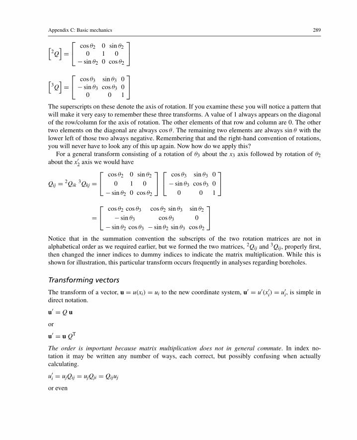
Appendix C: Basic mechanics 289
[2Q]=⎡⎣ cos θ2 0 sin θ2
0 1 0− sin θ2 0 cos θ2
⎤⎦
[3Q]=⎡⎣ cos θ3 sin θ3 0− sin θ3 cos θ3 0
0 0 1
⎤⎦
The superscripts on these denote the axis of rotation. If you examine these you will notice a pattern thatwill make it very easy to remember these three transforms. A value of 1 always appears on the diagonalof the row/column for the axis of rotation. The other elements of that row and column are 0. The othertwo elements on the diagonal are always cos θ . The remaining two elements are always sin θ with thelower left of those two always negative. Remembering that and the right-hand convention of rotations,you will never have to look any of this up again. Now how do we apply this?
For a general transform consisting of a rotation of θ3 about the x3 axis followed by rotation of θ2about the x′2 axis we would have
Qij = 2Qik3Qkj =
⎡⎣ cos θ2 0 sin θ2
0 1 0− sin θ2 0 cos θ2
⎤⎦⎡⎣ cos θ3 sin θ3 0− sin θ3 cos θ3 0
0 0 1
⎤⎦
=⎡⎣ cos θ2 cos θ3 cos θ2 sin θ3 sin θ2
− sin θ3 cos θ3 0− sin θ2 cos θ3 − sin θ2 sin θ3 cos θ2
⎤⎦
Notice that in the summation convention the subscripts of the two rotation matrices are not inalphabetical order as we required earlier, but we formed the two matrices, 2Qij and 3Qij, properly first,then changed the inner indices to dummy indices to indicate the matrix multiplication. While this isshown for illustration, this particular transform occurs frequently in analyses regarding boreholes.
Transforming vectors
The transform of a vector, u = u(xi) = ui to the new coordinate system, u′ = u′(x′i) = u′i, is simple indirect notation.
u′ = Q u
or
u′ = u QT
The order is important because matrix multiplication does not in general commute. In index no-tation it may be written any number of ways, each correct, but possibly confusing when actuallycalculating.
u′i = ujQij = ujQji = Qijuj
or even

290 Casing and Liners for Drilling and Completion
u′i = ukQik = ukQki = Qikuk = Qkiuk
Remember, we may use any indices we choose but the free index must always signify the row index ofthe original [Q]matrix as we defined it above. While this is mathematically a trivial point, it is one of themost frequent sources errors in student programming. So, whatever notation you choose, be consistentin its use.
EXAMPLE C.8 Coordinate Transform of a Vector
Suppose ui = (1, 1, 1) and our new coordinate system represents a rotation of π/2 (90◦) counterclockwiseabout the x3 axis so that our coordinate transform tensor in matrix form is
Qij =⎡⎣ 0 1 0−1 0 00 0 1
⎤⎦
then
u′i = Qijuj =⎡⎣ 0 1 0−1 0 00 0 1
⎤⎦⎧⎨⎩
111
⎫⎬⎭ =
⎧⎨⎩
1−11
⎫⎬⎭
Alternatively we could do it u as a row vector and QT as
Qji =⎡⎣ 0 −1 0
1 0 00 0 1
⎤⎦
then
u′i = ujQji =⌊
1 1 1⌋⎡⎣ 0 −1 0
1 0 00 0 1
⎤⎦ = ⌊ 1 −1 1
⌋
In the above example we assumed that a row vector and a column vector were equivalent for ourtransformation, but in non-orthogonal coordinates that is not necessarily the case.
Transforming tensors
The transformation of tensor components from one coordinate system to another is quite similar to thatof vectors in that the transformation matrix, [Q], is exactly the same. The difference is that the 2-ordertensor has nine components represented as a 3× 3 matrix, and requires two multiplications insteadof one.
T′ = Q T QT
In index notation where [Q] = Qij one possibility is
T ′ij = Qip Tpq Qjq

Appendix C: Basic mechanics 291
EXAMPLE C.9 Tensor Transform
Assume the same transform matrix, [Q] as in Section C.4.7 and a tensor
Tij =⎡⎣ 1 2 3
4 5 67 8 9
⎤⎦
then the transform is
T ′ij =⎡⎣ 0 1 0−1 0 00 0 1
⎤⎦⎡⎣ 1 2 3
4 5 67 8 9
⎤⎦⎡⎣ 0 −1 0
1 0 00 0 1
⎤⎦
=⎡⎣ 0 1 0−1 0 00 0 1
⎤⎦⎡⎣ 2 −1 3
5 −4 68 −7 9
⎤⎦
=⎡⎣ 5 −4 6−2 1 −38 −7 9
⎤⎦
where we started the matrix multiplication from the right. It makes no difference as to which matrixmultiplication is done first as long as you do not commute the matrix sequence.
As a quick error check when transforming tensors manually, recall that the sum of the diagonalelements of the transformed matrix will be the same as the sum of the diagonal elements of theoriginal matrix. Also, if the original matrix is symmetric, then the transformed matrix will also besymmetric. These checks are no guarantee against errors, but if either of these fail there is definitelyan error.
C.5 Kinematics and kinetics—strain and stress
The two fundamental tensor quantities of the mechanics of deformable bodies are strain and stress. Ingeneral, strain is a measure of kinematics, kinematics meaning movement in space as a result of forceor energy—displacement, translation, deformation. Stress on the other hand is a measure in kinetics,kinetics meaning the forces and energy that provide motion.
C.5.1 Deformation and strain—kinematics
All real materials are deformable. But it is perfectly appropriate in many cases to assume that certainobjects behave as rigid bodies and do not deform, since in many cases we are not interested indeformation or the magnitude of deformation does not affect our observations or calculations. Anexample would be picking a casing string up off bottom in a well to reciprocate the pipe while cementing.When we first begin to pull on the pipe, it is stretching. The top is moving, but the casing shoe is not.Once we pull a certain amount, the entire string is moving. If we are trying to determine the maximumload required to reciprocate the pipe, then we are not interested in the load as the pipe is stretchingbefore the entire string is moving. We are interested only in the load from gravity and friction when theentire string is moving. This is modeled as a rigid body motion and the deformation or stretch in thepipe has no significance in this context. A rigid body motion may be a translation and/or a rotation in

292 Casing and Liners for Drilling and Completion
space. A body moves from one position to another without deformation. A rotary table rotates whiledrilling, and that is a rigid body motion for most applications. Certainly, there is some amount ofdeformation in the individual parts, but that is of no interest if we are interested in penetration rateas a function of rotary speed. If we are interested in bit speed as a function of rotary speed, however,we might consider the deformation of the drill pipe in torsion as a possible fluctuating variable. If weare interested in the burst pressure of a casing string, the burst value is based on a deformation of thecasing.
Deformation by itself is not that meaningful. For instance, if a casing string is stuck, we pick up onit to try to free it, and we pull maybe 6 ft or 2 m through the rotary table. Is that significant? We cannotanswer such an important question with only the amount of information given. If it is stuck at a depthof 10,000 ft, then a 6 ft or 2 m stretch is not very much. But, if the casing is stuck near the surface thatdeformation could be quite significant. So, what we need is a measure that gives us some idea of howsignificant the stretch is.
One way to measure deformation, then, is simply the stretch divided by the original length. Thatis a simple measure of strain and satisfactory at low values for uniaxial deformations. However, if wewere to measure the wall thickness of the pipe very accurately, we also would find that, as the pipestretched and got longer, the wall thickness decreased slightly. One simple definition of strain in threedimensions is
εij = 1
2
(ui,j + uj,i
)(C.49)
where ui is the deformation in one of the three axis directions. This definition of strain, called the Cauchyinfinitesimal strain, is the measure most commonly used for small strains. Suppose, for our pipe examplefrom above (with a “strain” measure ΔL/L = 0.0006), the x3 coordinate is vertical and downward ina weight-less environment (for simplicity), so that the strain from the 6 ft stretch is uniform along theentire length of the tube down to 10,000 ft, that is, du/dx3 is a constant all along the length of the pipe,then
ε33 = 1
2
(u3,3 + u3,3
) = 1
2
(∂u3
∂x3+ ∂u3
∂x3
)= 1
2(0.0006+ 0.0006) = 0.0006
This is fairly straightforward, but note that there are a total of nine strain components instead of one,and the others may not be zero. In fact, not all will be zero. Because, as we said, when we stretch thepipe in one direction, there is a change in the other dimensions as well. Those other changes may beinsignificant or they may not. In addition to the strain definition given by Equation (C.49), the Cauchyinfinitesimal strain, there are other definitions of strain. We save those for later. The Cauchy strain tensormay be written as a matrix:
εij =⎡⎣ ε11 ε12 ε13
ε21 ε22 ε23ε31 ε32 ε33
⎤⎦ (C.50)
Large deformations
We are not going to cover large deformations in this text, but we should mention a few things that areimportant. Most all of the engineering mechanics problems we solve are based on small deformations

Appendix C: Basic mechanics 293
and infinitesimal strains. The world gets a lot more complicated when we consider finite or largedeformations and finite or large strains.
Strains within the elastic limit of metals like steel are very small, and we are quite safe in that respect.Where we get into trouble with even small strains is when the displacements become finite, so that eventhough the strains are very small, the geometry of the deformed body changes measurably.
In our area of interest this is most common in the bending of tubes in curved wellbores. Sucha problem is classified as one with nonlinear geometry. The rule of thumb is that deflection of anystructural member with a length to radius of gyration ratio of 10:1 or greater should be considered asone of nonlinear geometry. That means that most problems we address regarding lateral deflection ofcasing (or tubing or drill pipe) should be considered as geometrically nonlinear.
In the linear geometry of small deformations and infinitesimal strains we need only consider onecoordinate system—the original reference coordinate system. Once we move to the next step up incomplexity, finite deformations and infinitesimal strains, we must now include an additional coordinatesystem, the current or deformed coordinate system. This presents additional complexities as to how wedefine strain. If the reference coordinate system is designated the X-coordinate system and the deformedcoordinate system is the x-coordinate system then we have two measures of the strain:
Eij = 1
2
(ui,j + uj,i + uk,iuk,j
) = 1
2
(∂ui
∂Xj+ ∂uj
∂Xi+ ∂uk
∂Xi
∂uk
∂Xj
)
and
eij = 1
2
(ui,j + uj,i − uk,iuk,j
) = 1
2
(∂ui
∂xj+ ∂uj
∂xi− ∂uk
∂xi
∂uk
∂xj
)
Very few textbooks deal with large deformations to any extent, and it sometimes becomes a matterof self study to piece together a workable knowledge of the topic. One place to begin is the book byFung [52].
C.5.2 Stress—kinetics
Our early concept of stress was most likely that it is a “distributed load” as opposed to a “point load.”That is all right for many simple engineering calculations, but it is quite misleading when we advanceto more complicated problems. First of all, we need to recognize that, in the real world, there is nosuch thing as a point load. A point load is a mathematical convenience that exists only in theory andcalculations. All real loads are distributed loads. Think about it this way; if we could apply a true pointload of 100 lbf to the surface of a steel block, what would happen? If it is truly a point load, the contactarea shrinks to zero, the pressure exerted by the load goes to infinity, and the steel block fails at the pointof contact. Of course, this does not happen in the real world, because the contact area is not zero, so theload actually is distributed over some area, even though it may be very small. So, even though true pointloads do not exist, we use them in our calculations for convenience. Now, back to the distributed load,is a distributed load that we typically measure in psi (lbf/in.2) or Pa a stress? No, it is not. Just becauseit has the same units of stress does not make it a stress.
What is a distributed load then? Some call it a stress vector. This is an unfortunate bit of terminologythat has become entrenched in elementary mechanics. If you want to use that term, you have plenty ofcompany, but it can be confusing to call two totally different things stress. A distributed load is a vector,it has magnitude and direction, but stress is never a vector. The proper name for a distributed load isa traction or traction vector, and it is a directional load (force) distributed over some area of contact.

294 Casing and Liners for Drilling and Completion
Something else worth noting is that you cannot apply a stress. You can apply only traction; stress is aresult of the traction. But, most important, remember that stress itself is never a vector.
We have said that stress is a tensor. What is a tensor? That is a good question for which there is nota good answer. Or at least, there is no good answer that would ever satisfy an engineer. A tensor is amathematical quantity that transforms according to certain rules (which were illustrated previously, butwe lack space to explain here). Also, when we speak of a tensor, we typically are talking about a 2-ordertensor, such as stress (or strain). There are other tensors of different orders as well.
The stress tensor for small displacements and strains is called the Cauchy stress tensor. In componentform, σij, it has nine components and is typically written as a 3×3 matrix.
[σij] =⎡⎣ σ11 σ12 σ13
σ21 σ22 σ23σ31 σ32 σ33
⎤⎦
In our applications it is real-valued and symmetric, σij = σji, such that σ12 = σ21, σ13 = σ31, σ23 = σ32,thus reducing the number of different components to six.
Figure C.8 shows the sign convention of the components. All of the components shown are positive invalue. For example, σ11 to the right is on the positive x1 face of the block and is pointed in the positivex1 direction, hence it is positive in sign. On the left side there is a component of σ11 pointing in thenegative x1 direction, but it is on the negative x1 face of the block so it too is a positive component. Theoff-diagonal or shear components of the stress matrix follow a similar convention. The shear component,σ12, is on the positive x1 face and is pointed in the positive x2 direction. On the negative face (notshown) σ12 would point downward in the negative x2 direction and hence is also positive. The firstsubscript denotes the face and the second denotes the direction. Considering the diagonal components,σ11, σ22, σ33, positive is tension, and negative is compression.
A very important formula that relates the stress tensor and a traction vector is known as Cauchy’sformula7 and is
t = n T → ti = nj σij (C.51)
σ11
σ33
σ22
σ11
σ33
σ22
x1
x3
x2
σ23
σ32
σ31σ13
σ12
σ21
Figure C.8 Stress sign convention.
7 A derivation of this important formula appears in every book on continuum mechanics. We will not take space to derive it herebecause we are not going to use it.

Appendix C: Basic mechanics 295
where t (ti), n (nj), and T (σij) are a traction vector acting on a surface with a unit normal vector, andthe stress at the point of contact, respectively. The surface need not be a physical surface, but can be animaginary one drawn within a material body itself.
One final point before we move on. It is misleading to assume that we can always determine a uniaxialstress by dividing a uniaxial load by the cross-sectional area of the material body. This is true only for aprismatic bar, that is, one with a constant cross section, but it is not true near the ends of the bar, wherethe loads are applied. We cannot determine the axial stress in a tube under a thread cut into the tube bydividing the axial load by the cross-sectional area under the thread. Likewise, we cannot calculate theuniaxial stress in a coupling, connection, or upset in a tube in a similar fashion. Whenever the cross-sectional area of a tube changes, the stress field at the change and in the near vicinity of the change ismore complicated than a single uniaxial component. In the case of a connection, additional complicationcomes from the addition of tangential, radial, and shear stress components in the connection itself. Saint-Venant’s principle, however, effectively states that, at some distance away from the ends of a long tube(or point of change in diameter), the stress field becomes uniaxial, and there we are safe in dividing thecross-sectional area by the axial load to get the uniaxial stress component. For all practical purposes,that distance is relatively short in oilfield casing, but in a strict interpretation of the theory, it is validonly for tubes of infinite length.
Stress invariants
Some things about a stress tensor are invariant no matter how we may rotate our coordinate system.These are called stress invariants, and three are associated with a symmetric stress tensor:
I1 = σii (C.52)
I2 = 1
2
[(I1)
2 − σijσji
](C.53)
I3 = 1
3
[3I1I2 − (I1)
3 + σijσjkσki
](C.54)
You might well ask, of what use are those three invariants? There are a number of times when thoseare useful, but one use that is of importance is to find the three principal stress components. We canexpand the determinant in the following equation to get a cubic equation in terms of the above stressinvariants, from which we can solve for the three principal stress components:
det[σij − σδij
] = 0
where σ is a principal stress component and δij is the Kronecker delta. We will return to methods todetermine the principal stress components and their directions after the next section.
Deviatoric stress
To understand a yield stress and plastic material behavior, it is necessary to learn about one other typeof stress component and its invariants, the deviatoric stress. The stress tensor may be decomposed into aspherical (or hydrostatic) stress and a deviatoric stress. The spherical stress is that part of the stresstensor that is basically equal in all directions, that is, just like hydrostatic pressure. The deviatoric

296 Casing and Liners for Drilling and Completion
stress is what is left after the spherical stress is taken out. One way of thinking about it is that thespherical stress might be said to be the part of the stress tensor trying to compress a material body (orpull it apart) uniformly in all directions and the deviatoric part of the stress is what attempts to distortits shape.
In terms of the three principal stress components, the spherical stress is
σspherical = σ1 + σ2 + σ3
3(C.55)
We could then calculate the three principal deviatoric stress components by subtracting the sphericalstress from each principal stress component:
σ ′1 = σ1 − σ1 + σ2 + σ3
3
σ ′2 = σ2 − σ1 + σ2 + σ3
3(C.56)
σ ′3 = σ3 − σ1 + σ2 + σ3
3
If we do not have the principal stress components, we can calculate the deviatoric stress from thestress tensor components as
σ ′ij = σij − δijσkk
3(C.57)
There are several things to note here. The off-diagonal components of the deviatoric stress tensor arethe same as the regular stress tensor. The only components that are changed are the ones on the diagonal.Each of those has subtracted from it one third of the sum of the diagonal components, which is I1/3.Now, the deviatoric stress also has similar invariants:
I′1 = σ ′ii = 0
I′2 =1
2
[(I′1)2 − σ ′ijσ ′ji
]= −1
2σ ′ijσ ′ji
I′3 =1
3
[3(I′1) (
I′2)− (I′1)2 + σ ′ijσ ′jkσ ′ki
]= 1
3σ ′ijσ ′jkσ ′ki
But rather than use the same notation as the regular stress invariants, it is customary to define thesedeviatoric stress invariants as follows:
J1 ≡ I′1 = 0 (C.58)
J2 ≡ −I′2 =1
2σ ′ijσ ′ji (C.59)
J3 ≡ I′3 =1
3σ ′ijσ ′jkσ ′ki (C.60)
Note that we defined J2 as −I′2. There is a purpose to that in later applications, but use care in that someauthors do not use this convention.
We show an example of the deviatoric stress when we discuss yield stress in the section on plasticity.

Appendix C: Basic mechanics 297
Principal stress components
As already stated, the stress tensor is invariant under any coordinate system and that only the componentvalues vary. In Cartesian (and other orthogonal systems) it is possible to find a coordinate systemin which all the off-diagonal components of the stress matrix disappear leaving only the diagonalcomponents. These three diagonal values are called the principal stress components of a stress tensor.The principal stress components are the eigenvalues of the stress matrix and their direction vectorsare the eigenvectors. Recall from your linear algebra that a system of linear equations [A]{x} = {C}has a unique solution if and only if the coefficient matrix, [A], is non-singular, i.e., det[A] = 0.For a homogeneous system, [A]{x} = {0}, with a non-singular, [A], the unique solution is {x} = {0},and is called the trivial solution. If the homogeneous system is singular, det[A] = 0, then there isno unique solution, and there may be an infinite number of them which will include the trivialsolution.
In mathematical terms the eigenvalues, σ , make the matrix [σij − δijσ ] singular, such that there arenontrivial solutions to the homogeneous set of equations, [σij − δijσ ]{xj} = {0}. The nontrivial solutions,{xj} are the eigenvectors. Singular systems are of no interest to us except to solve for the eigenvaluesand eigenvectors which are the principal stress components and their direction vectors. In matrix formwe express the singular equation set as⎡⎣ σ11 − σ σ12 σ13
σ21 σ22 − σ σ23σ31 σ32 σ33 − σ
⎤⎦⎧⎨⎩
x1x2x3
⎫⎬⎭ =
⎧⎨⎩
000
⎫⎬⎭ (C.61)
Here the eigenvalues are of a value that makes the stress matrix singular. Since one characteristicof a singular square matrix is that its determinant is zero, we solve for the eigenvalues (principal stresscomponents) by setting the determinant of
[σij − σδij
]equal to zero:
det[σij − σδij
] = 0 (C.62)
or in matrix form as
det
⎡⎣ σ11 − σ σ12 σ13
σ21 σ22 − σ σ23σ31 σ32 σ33 − σ
⎤⎦ = 0 (C.63)
When we expand that determinant, we get a characteristic equation whose coefficients are the threestress invariants:
σ 3 − I1σ2 + I2σ − I3 = 0 (C.64)
When the stress tensor is symmetric (always the case in our applications), that cubic equationhas three real roots, which are the three principal stress components. Any cubic equation alwayshas a closed form solution, meaning there is a formula we can use to find the three principal stresscomponents.
General formulaThe characteristic equation may be solved for the real roots, the principal stress components, as follows:
a = 1
9
(I21 − 3 I2
)(C.65)

298 Casing and Liners for Drilling and Completion
b = 1
54
(2 I3
1 − 9 I1 I2 + 27 I3
)(C.66)
1. If a3 + b2 > 0 then there are three real and unequal roots (principal stress components) and the equation maybe solved by the trigonometric method as follows.
φ = cos−1(
a√b3
)(C.67)
σ1 = −2√
a cos (φ/3)− I1/3 (C.68)
σ2 = −2√
a cos [(φ + 2π) /3]− I1/3 (C.69)
σ3 = −2√
a cos [(φ − 2π) /3]− I1/3 (C.70)
2. If a3 + b2 = 0 then there are three real roots and at least two are equal. These roots may be solved with thefollowing which involves complex arithmetic (the results are real valued, but the intermediate arithmetic willinvolve complex numbers).
A = 3√−b+
√b2 + a3 (C.71)
B = 3√
b+√
b2 + a3 (C.72)
σ1 = − (A+ B) (C.73)
σ2 = A+ B
2− A− B
2
√−3 (C.74)
σ3 = A+ B
2+ A− B
2
√−3 (C.75)
3. If a3 + b2 < 0 then there is one real root and two conjugate complex roots, i.e., the tensor is not real valued andsymmetric. We do not consider this case since our stress tensor is symmetric.
Polar coordinatesIn tubes where σrz, σθz = 0.
σ1 = σθ + σz
2+√(
σθ − σz
2
)2
+ σ 2rθ (C.76)
σ2 = σθ + σz
2−√(
σθ − σz
2
)2
+ σ 2rθ (C.77)
σ3 = σr (C.78)
and in tubes where there is no torsion, i.e., σrθ = 0, then
σ1 = σθ (C.79)

Appendix C: Basic mechanics 299
σ2 = σz (C.80)
σ3 = σr (C.81)
Principal deviatoric stress components
The characteristic equation for the principal deviatoric stress is:(σ ′)3 + J2σ
′ + J3 = 0 (C.82)
This is similar to the characteristic equation for principal stress components except that J1 is zero anddoes not appear.
General FormulaSimilar to solving for roots of the cubic characteristic equation for principal stresses we set:
a = −J2/3 (C.83)
b = −J3/2 (C.84)
1. If (J3/2)2 − (J2/3)3 < 0 then
φ = cos−1(
B√A3
)(C.85)
σ ′1 = 2√
a cos (φ/3) (C.86)
σ ′2 = 2√
a cos [(φ + 2π) /3] (C.87)
σ ′3 = 2√
a cos [(φ − 2π) /3] (C.88)
2. If (J3/2)2 − (J2/3)3 = 0 → J2/J3 = 3/2 then
A = 3√−b+
√b2 + a3 (C.89)
B = 3√
b+√
b2 + a3 (C.90)
σ1 = A+ B (C.91)
σ2 = −A+ B
2+ A− B
2
√−3 (C.92)
σ3 = −A+ B
2− A− B
2
√−3 (C.93)
3. If (J3/2)2 − (J2/3)3 > 0 then the stress tensor is not real valued and symmetric.
And as before, step 2 above involves complex arithmetic. There are any number of softwareprograms available that will do these calculations, if you are not familiar with programming complex

300 Casing and Liners for Drilling and Completion
variables. And there are other approaches that can avoid complex arithmetic altogether (see Allen andHaisler [53]), but are too long to go into here.
Principal stress directions
After solving for the principal stress components (or deviatoric principal stress components), we mayalso need the orientation of the components, the eigenvectors. To do this we plug an individual principalstress component into Equation (C.61) and solve for its eigenvector. If there are three different roots wewill have to do this three times to solve for all three eigenvectors. While this is easy to say, it is nota simple as that, because each eigenvalue makes the coefficient matrix, [σij − δijσ ] singular, and thusrendering an infinite number of solutions. But the important characteristic of these solutions is that thevalues are always in the same proportion to each other, which is all we need to define a vector and whichwe can easily make unit vectors using Equation (C.4). One way to do this is to set one of the solutioncomponents to unity and solve the set for the other two.⎡⎣ σ11 − σ1 σ12 σ13
σ21 σ22 − σ1 σ23σ31 σ32 σ33 − σ1
⎤⎦⎧⎨⎩
1x2x3
⎫⎬⎭ =
⎧⎨⎩
000
⎫⎬⎭ (C.94)
We can then use two of those three equations to solve for the components, x2, x3. Traditionally we makethe eigenvector a unit vector with Equation (C.5). And we repeat the process for each principal stresscomponent.
Comments on stress
There are a number of ways we can use the stress invariants, I1, I2, I3 and the deviatoric stress invariants,J2, J3 in applications. For example, if we calculate the principal stress components, σ , we do not haveto solve another cubic equation for the principal deviatoric stress components because
σ ′ = σ − I1/3 (C.95)
Another way to get the principal deviatoric stress components without solving the characteristicequation is to calculate another stress quantity called the octahedral stress, τo.
τ0 =√
2
3J2 (C.96)
then
φ = cos−1(√
2J3
τ 3o
)(C.97)
Then the principal deviatoric stress components are then
σ ′1 =√
2 τo cos
(φ
3+ 4π
3
)(C.98)
σ ′2 =√
2 τo cos
(φ
3
)(C.99)

Appendix C: Basic mechanics 301
σ ′3 =√
2 τo cos
(φ
3+ 2π
3
)(C.100)
From these results we can back into the principal stress components with Equation (C.95)
σ = σ ′ + I1/3 (C.101)
This involves a few more steps, but avoids solving the cubic characteristic equation totally.One last comment. The notion of principal stress components raises an interesting question. Since
stress is independent of any coordinate system and may be represented mathematically as a symmetricalstress tensor that can always be resolved into three principal stress components in any coordinate systemsuch that the “shear” components disappear, then is shear stress a physical reality or just a mathematicalnotation? Or posing it another way, if for any stress, we can orient our coordinate system such thatthe shear components disappear, is there actually such a physical entity that we can designate as shearstress or is it just a name for the off-diagonal components of a stress matrix? What I am driving at hereis that shear components of stress are nothing more than the mathematical names for components ofstress in particular directions and are not some separate kind of physical stress as much common usagetends to imply. The unfortunate use of separate variable names, σ and τ , for diagonal and off-diagonalcomponents, respectively, of a stress matrix as if they are somehow a different type of stress, hascontributed greatly to the misunderstanding. While the orientation of stress at some point in a materialbody or structure is obviously very important, it is that orientation with regard to a material body orstructure that may be critical rather than some separate physical entity of the stress tensor. As one wisesoul once stated it, “A material cannot ‘feel’ a shear component, only the principal components.”
C.6 Constitutive relationships
Suppose we have a solid cube of some material that measures 1 meter on each edge, and it is lying ona flat surface. We know the weight of the cube. We apply a downward force of a known magnitude ontop of that object. If we are asked, What is the force on the flat surface?, we have an easy problem. It isNewtons third law, and the answer is the force on the surface is the weight of the cube plus the force weapplied to the top of the cube. If we approach it slightly differently and instead of measuring the forcewe apply on top we instead measure how much we actually compress that cube vertically, by say 0.2%of its original height (see Figure C.9). We now have a different problem in determining the resultantforce on the flat surface.
We know that it is equal to the weight of the cube plus whatever force is necessary to compress thecube by 0.2%. In order to solve this problem we need to know something about the material the cube ismade of, and more specifically how the material responds to a compressive load. Such a relationship iscalled a constitutive equation and in this case it is a simple one-dimensional version of Hookes law.
σz = Edu
dz
This simple relationship relates a load (stress), to a deformation gradient (strain), by means of aconstant, Young’s modulus, which is a property of the material. There are many constitutive relationshipsin every day use though we do not often think of them as such. Here are two one-dimensionalexamples.

302 Casing and Liners for Drilling and Completion
W1 m
0.002 m
F = unknown
R = ?
Figure C.9 Force, displacement, and reaction.
q = −kdT
dx
v = k
μ
dp
dx
The first is Fouriers law of heat conduction that relates heat flux to a temperature gradient by means of amaterial property, the conductivity. The second is Darcy flow that relates fluid flux to a pressure gradientwith two material properties, permeability and viscosity.
There are many types of material behavior, for example, elastic, plastic, viscoelastic, viscoplastic.Elastic behavior could be subdivided into linear elastic, non-linear elastic, hyper-elastic, and viscoelas-tic. If one were to apply a load to a material and plot the load curve (load versus deformation) such asa stress-strain curve, one could not really understand much about a materials behavior. It is only whenthe load is removed that we can begin to understand its behavior. For example, look at the material loadcurve in Figure C.10a. What type of behavior is this? We might be tempted to say it is elastic-plasticsince it looks like what we have often seen to illustrate how a metal behaves elastically up to a yieldpoint and then becomes plastic beyond the yield point. But in truth, all we can say for this examplewithout more information is that its behavior is non-linear.
Now let us reveal the unloading behavior on that same material, Figure C.10b. We see that it returnsto the same point that we started. So when the load is removed it has no permanent deformation. It is bydefinition elastic.
The defining criteria for elastic behavior is that if a body is subjected to a load and the load is laterremoved it will return to its original state. But we notice something else about this material load curve.
σ
ε
σ
ε(a) (b)
Figure C.10 Nonlinear behavior: (a) loading curve and (b) loading and unloading curves with a hysteresis loop.

Appendix C: Basic mechanics 303
s
e
Figure C.11 Slow loading and unloading cycle. Linear elastic material?
It did not return by the same path with which it was loaded (a hysteresis loop). What could explainthat? Time. It is a rate-dependent behavior, in other words it is viscoelastic. The shape of this load curvedepends on the loading and unloading rate. The loading and unloading curve does not tell us the rate atwhich the load was applied or removed. For example, we could load the same material very slowly andremove the load also very slowly. We might get a loading and unloading curve that would look like thestraight path in Figure C.11. If you were not aware of the time dependent curves you might assume thatit is a linear elastic material. And it is, albeit at very slow rates of loading. Many materials that we mightconsider linear elastic are actually rate dependent materials. Porous formation rock in most wells is anexample.
Appearances can be deceiving. We are not going to concern ourselves with rate dependent materialshere, but the point is important, do not jump to conclusions that are not justified.
C.6.1 Elasticity
We said that an elastic material is one in which the material returns to its original state after an appliedload is removed. A linear elastic material8 is one whose loading path and unloading path are thesame straight line. The constitutive behavior of a linear elastic material is modeled by Hooke’s law,as mentioned before. It is called a law, but it is not a law of physics or nature. It is just a convenientrelationship that models the behavior of certain materials within a very limited range of deformation.We might even say that we are very fortunate that it does, even though its range is quite small, becausealmost every structure or machine we come into contact with daily is designed using this constitutiverelationship. Hooke’s law written in three-dimensional tensor form is
σij = Cijkl εkl (C.102)
If we were to write that out in matrix form, the stress and strain tensors would each contain 9 termsand the elastic modulus would contain 81 terms. All are symmetric (except in the presence of bodymoments—usually electro-magnetic). For an isotropic material, one whose material properties are thesame in all directions, Equation (C.102) can be simplified considerably. We can use a contracted notation(called Voigt notation) and write the stress and strain in vector form and the elastic modulus as a 6 × 6matrix:
8 We should note that, when we refer to an elastic material, we are speaking to only a particular range of a particular material’sbehavior. Materials may exhibit different types of behavior in different load ranges.

304 Casing and Liners for Drilling and Completion
⎧⎪⎪⎪⎪⎪⎪⎨⎪⎪⎪⎪⎪⎪⎩
σ11σ22σ33σ23σ13σ12
⎫⎪⎪⎪⎪⎪⎪⎬⎪⎪⎪⎪⎪⎪⎭= E
(1+ ν) (1− 2ν)
⎡⎢⎢⎢⎢⎢⎢⎣
1− ν ν ν 0 0 0ν 1− ν ν 0 0 0ν ν 1− ν 0 0 00 0 0 1−2ν
2 0 00 0 0 0 1−2ν
2 00 0 0 0 0 1−2ν
2
⎤⎥⎥⎥⎥⎥⎥⎦
⎧⎪⎪⎪⎪⎪⎪⎨⎪⎪⎪⎪⎪⎪⎩
ε11ε22ε33ε23ε13ε12
⎫⎪⎪⎪⎪⎪⎪⎬⎪⎪⎪⎪⎪⎪⎭
where we have now included Poisson’s ratio, ν. This is a bit more complicated than the simple one-dimensional form, but often a number of simplifying assumptions, such as plane strain or plane stress,can be adopted to reduce it to two dimensions for a number of applications. We are not going to use thisconstitutive relationship, but merely show it so that you can see what it looks like.
C.6.2 Plasticity
We defined an elastic material as one in which, when an applied load is removed, the material goesback to its original state. A material is said to behave plastically when an applied load is removed and itdoes not go back to its original state. In other words, it has undergone some permanent deformation inthe loading process. Plasticity is a complex topic and there are exceptions to just about everything, butwe are concerned primarily with steel in casing here, so we are going to confine our discussion to thatlimited scope. Steel behaves more or less as a linear elastic material up to a point, called the yield point.When loaded beyond that point, its behavior is said to be plastic, but the elasticity has not disappeared,it is still exhibited when the loads are removed. Figure C.12a shows a load curve for elastic-plasticbehavior of a test sample in uniaxial tension.
The loading in this curve is such that the sample is linear elastic up to its yield point, Y, then deformsplastically until the load is removed, at which time, it unloads elastically. The difference between theinitial strain (zero here) and the final strain is the permanent deformation of the material in a plasticmode. It is of significance at this time to make mental note of this elastic unloading. When a metal, suchas steel, is deformed plastically to a certain size or shape, it will always display some amount of elastic“rebound” or deformation when the load is removed. When coiled tubing is bent plastically onto a reel,a lot of elastic energy is stored on that reel, and if you were to release the end of the tube, you wouldwitness an amount of elastic unloading you might not otherwise imagine.
In many cases, the behavior of the metal at the yield point is somewhat more complicated than thatin Figure C.12a. Sometimes the elastic behavior becomes nonlinear before the actual yield stress isreached, and that point is called the proportional limit. Ductile steels often exhibit this behavior and
s
e
s
e
(a) (b)
Y YFailure
Ultimate strength
Figure C.12 Uniaxial test, elastic-plastic behavior of steel: (a) loading and unloading and (b) loading to failure.

Appendix C: Basic mechanics 305
ℓ0
Δℓ
F
F
A = cross- sectional area
Figure C.13 A typical steel test sample.
materials like cast iron seldom exhibit a distinctive yield point. There are other cases where the stressactually decreases slightly after the yield stress is reached; hence, there is an upper yield stress and alower yield stress. This is typical of some steel alloys. In many cases, the yield point is indistinct ona stress-strain chart, so the yield point is defined as some arbitrary point offset from the proportionallimit by a specified amount of strain (API does this). We do not concern ourselves with those details,but rather assume that, as long as we do not exceed the published yield stress for the casing material, itsbehavior is linear and elastic up to that point.
What happens if we continue to load the test sample? Figure C.12b shows the uniaxial loading of asample all the way to failure. At this point, we need to explain a few things. First of all, in this figure,we are looking at a uniaxial load curve. It is plotted as stress versus strain, which we already discussedbut we need to understand a bit more. We must emphasize one thing about this figure, and that is inreference to the point labeled as the ultimate strength. That is not a material property, it is a propertyof the sample geometry and the test type. It is the point at which the test sample begins to experiencesignificant deformation of its initial geometry in tension. You will observe nothing comparable in acompressive test. While it is not a material property, it is a property in a tube in tension and does havesome use—it appears in the current ISO formulas for ductile rupture.
The samples of material used in these tests are relatively small compared to the massive machinein which they are tested. The samples usually look like the one shown in Figure C.13, sometimescolloquially referred to as a dog bone sample. The sample is placed in a large machine that pulls itin tension, as the load and stretch are recorded.
The ends are larger than the test portion, so the gripping effects of the machine do not affect thestress in the narrower test portion. The cross-sectional area of the test portion is measured accuratelybefore the test begins. The stretch in the sample is measured by the machine as a displacement, andthe load is measured with a pressure transducer, These are recorded on a chart similar to that shownin Figure C.12b. The machine itself is massive in relation to the size of the sample, but nevertheless ithas some amount of elastic stretch while pulling tension, as does the wider portion of the sample, sousually an electronic strain gauge is attached to the sample in the thinner area to measure the stretch.The results may be plotted as load versus stretch, which is the raw data from the machine, but that isnot of much use unless one is testing a particular structural element or part as opposed to a sampleof material like we are considering here. We use the following relationships to get the values for astress-strain plot:

306 Casing and Liners for Drilling and Completion
σ = F
A, e = �− �o
�o= Δ�
�o
where the stress is the machine-measured load divided by the cross-sectional area of the sample, and thestrain is the stretch in the sample section divided by the original length of the sample section.This strainmeasure is known as the engineering strain or the nominal strain. These are plotted as in Figure C.12b.Similar tests may be run in compression or cyclical loading.
In looking at Figure C.12b, we see that the material deforms elastically up to the yield point, thenbegins its plastic deformation, in which a lot of strain takes place with little increase in stress, yet thestress continues to increase up to a point, where it begins to decline until the sample fails. The part ofthe curve where the stress continues to increase in the plastic range is called strain hardening. But whatabout the part of the curve where it starts to decline. Is this “strain softening” then? This part of the curvecan be misleading because of the way we calculated the stress and strain. Our definition holds only forvery small deformations. If we actually measured the cross-sectional area of the sample as it stretches,we would find that the area is getting smaller. So, what we have plotted on the vertical axis is not the truestress, but rather the load divided by the original cross-sectional area of the sample, which is commonlyreferred to as the engineering stress or nominal stress. And, if we looked at the failed sample, we wouldsee that the most significant decrease in cross-sectional area occurred in only a small part of the lengthof the sample and the cross-sectional area at the point of failure is possibly less than half the originalarea. If we were to plot the true stress, we would find that, in many cases, it continues to increase rightup to the point of failure; and for some materials, the increase is rather drastic just before failure. Wemight also note that our measure of strain, e above, is no longer valid either, since the reduction in crosssection (called necking-down) is quite localized, so that the uniaxial strain in the region of failure isapparently a lot greater than elsewhere along the sample length. The true strain is not Δ�/�0 but ratherd�/� , which leads to a true strain or logarithmic strain measure:
ε = ln
(�
�0
)= ln
(1+ �− �o
�0
)(C.103)
We might also note that the appearance of the sample itself began to change just before failure, in thatvisible bands of discoloration or surface texture began to appear on the surface of the sample where thearea reduction was most pronounced, giving the appearance of some change in the metal itself. Theseare called Lüder’s bands, and that is exactly what they indicate. Two things are of importance here. Ifwe tested several samples of the same material, all would fail at different values. That is the nature ofmaterials; we cannot predict the actual load value at which the material fails. We can determine a rangeof values, but we cannot predict the exact value for any particular sample. If all of the samples werecut in precisely the same way under the same conditions and we could perform rigorous inspectionson them, we could get pretty close, but the point is we could not predict the exact failure strength. Thesecond point is this. We said that, if we used a measure of true stress and strain, then we could saythat the material never got “weaker” before it failed, and that is often true. However, the sample itselfgot weaker before it failed, and that is important. In terms of total load, it failed at a load less than themaximum load it was subjected to in the test. If it were a structural member or casing, that would beimportant. So, while the true stress is important, the load on a structure does not know to reduce itselfwhen the cross-sectional area of a structural member is reduced by plastic deformation. In casing, theapparent stress at the maximum load is called the ultimate strength. It is very important to rememberthat the ultimate strength is not a material property; it is a property of the sample in uniaxial tension.Likewise it is a property of a right, prismatic tube like casing. We never want to exceed that maximumload value, no matter how we measure stress or strain.

Appendix C: Basic mechanics 307
Now, let us go back to the issue of strain hardening mentioned earlier. Strain hardening in a metal, forthe most part, is caused by defects in its crystalline structure, called dislocations. All steels have someamount of this type of defect. But defect might be a severe term to use in an oilfield context, so perhapsa dislocation should be thought of as an imperfection in the crystalline lattice of a metal. A dislocationis a missing bond at a lattice junction. When a metal is stressed beyond its initial yield point, thesedislocations begin to move or migrate. No material physically moves (at least, on an observable scale),but where a bond is missing at a lattice junction, a bond forms, and the missing bond is transferred tothe next junction, sort of like the game of musical chairs, where there is one fewer chair than the numberof people present. When one person gets up, another takes his or her place. What causes the strain-hardening effect is that as these dislocations begin to accumulate at grain boundaries, there is no otherplace for them to go, and they begin to resist the deformation of the material. There are other contributingfactors, but that is the main one. While most structural steels are strain hardening materials to somedegree, some are not. Some brittle steels exhibit very little strain hardening, and failure strength is veryclose to the yield strength. Some soft steels behave more like what is known as an elastic-perfectly-plastic material, in that once yield stress is reached, the material continues to elongate to failure withno increase in stress required. The steel used for coiled tubing closely approximates this latter behavior.Also some strain-softening materials are such that, once yield is reached, continued elongation requiresless and less stress.
For a strain-hardening type of steel, if we stop loading a sample before we reach the maximum andremove the load, we know that it unloads elastically as shown in Figure C.12a. What happens if we applya load again? The answer is that it goes right back up the same path as the unloading path. Furthermore,it does not yield until it reaches the value at which the load was removed before. It may vary with abit of hysteresis and become slightly nonlinear before yielding again, but after yield, it continues on thesame path, as if the unloading never took place. The result, though, is that, on re-loading, it actuallyyields at a higher value than the original yield value at the start of the test. We could repeat this processany number of times, and each time, we increase the yield value until we reach the top of the curve. So,for a strain-hardening material, we can increase the yield strength by cold working it. Or can we? It alldepends on what our application is. Let us look at compression.
If we were to test an identical sample in compression, it would be a mirror image (and upside down)of the one we just showed. And we could compress it to the same point and increase its yield strengthin compression just as we did in tension. The question is, then, if we work our sample in tensionfirst then test it in compression, will the yield point in compression be increased just like the one intension? The answer is no, it would not. In fact, if we increased the yield in tension, then the yieldin compression actually would be less than the initial yield. This is called the Bauschinger effect. Inother words, we cannot have it both ways. Is the amount of reduction in compression equal to theamount of increase in tension? Again the answer is no, the reduction in the compressive yield stressgenerally is less than the increase in tensile yield stress. We can show this with an ellipse, which wecall a yield surface in two dimensions for now. We are not plotting strain now but principal stresscomponents in two directions. Up is tension, down is compression. We do not concern ourselves withthe transverse component for now. We know that, when we increase the tensile load beyond the yieldsurface, we increase the yield stress in that direction. One way to think about it would be that the yieldsurface gets larger. In other words, it expands by the amount we go beyond the initial yield stress, asshown in Figure C.14a. This is known as isotropic hardening; the yield surface grows uniformly in alldirections.
This means that we also increased the yield strength in compression by the same amount; andwe already said that does not happen. Isotropic hardening does not happen, but it is useful in a few

308 Casing and Liners for Drilling and Completion
(a) (b)
Y0
load path
Y
σ1
σ2Y0
load path
Y
σ1
σ2
Figure C.14 Strain hardening: (a) isotropic hardening and (b) kinematic hardening.
applications when repeated loading does not cause yielding in different directions. Another possibilitymight be that the yield surface actually moves as shown in Figure C.14b. Here, the yield surfacestays the same size, but it moves as the stress exceeds the yield stress. This model is called kinematichardening
For kinematic hardening in the simple uniaxial case we are discussing, the reduction in yield stress incompression is of exactly the same magnitude as the increase in the tensile yield stress. We already saidthat does not happen either. What actually takes place is something in between. The yield surface grows,but it also moves. This is called combined hardening. And what all this amounts to is this: When workingin the plastic regime, we have to keep up with the growth of the yield surface and keep track of whereit is. This usually is done with something called internal state variables, which are defined by a flowrule to account for the translation of the yield surface and a growth law that accounts for its expansionor hardening. In the simple incremental theory of plasticity, one internal state variable is a second-ordertensor that tracks the translation of the yield surface, and the other is a scalar that keeps track of the sizeof the yield surface. Take into account also that we are not talking about the three-dimensional spacewe live in, but rather a nine-dimensional stress space. Another point of complication is that, when thestress is on the yield surface (it cannot go past it), the most common plasticity theory requires that plasticstrain can take place only in a direction normal to this nine-dimensional hyper-surface. In some plasticitytheories, the yield surface is not regular and smooth, like the ellipse we illustrated, and loading pathsalso may change shape in addition to size and location. Additionally, in larger deformations such asthe necking discussed in the uniaxial test previously mentioned, localized rotations within the materialbegin to occur. These rotations must be tracked, too. At some point, we begin to kid ourselves as to whatwe know how to do in this strange space. So we are going to drop back a notch or two for now and thinkabout how to stay out of it. Obviously, if we stay inside that yield surface with our stress and do notbump into it, we should stay out of serious trouble. That is the topic of the next section, but let us lookat one more scenario first.
One of the most difficult aspects of materials that have been loaded beyond the initial yield point ispredicting their properties at a later time, because the loading beyond initial yield makes it a history-dependent material. You cannot predict its future behavior unless you know the history of its loading.For example, suppose we take two identical samples, both with an initial yield strength of 80,000 psi.We subject them both to a uniaxial load of 90,000 psi. In other words, we work hardened them intension to increase the yield strength (in tension). If we test these two samples, one in tension and onein compression. We find that the tensile sample does indeed yield at 90,000 psi as we expect. But thesample we test in compression does not yield at 90,000 psi, nor even the original 80,000 psi. We find thatin compression it yields at say 77,000 psi. This is a case of combined hardening (somewhere between

Appendix C: Basic mechanics 309
isotropic and kinematic) which is typical in many metals. By cold working this metal we have movedthe yield surface (in stress space) and we have also changed the size.
That example was for a simple uniaxial test. If we had subjected a large sheet of steel to the sameuniaxial stress then cut samples from it in various directions, the results would have been even morealarming. The point is that, when a metal is loaded beyond the initial yield point, we cannot possiblypredict its behavior, unless we know the history of the loading. And, that not only means the exactloads but also the exact sequence. One oilfield example would be a well subject to large temperaturefluctuations from a shut-in state to a flowing state, and back to shut-in. If, in compression from thermalexpansion, suppose a portion of the production casing string yields. Take into account that, during theheated stage, the packer fluid also is heated and expands, causing a high internal pressure in the casing.Assume that the casing actually yields at the inner wall with a combined axial compressive stress, aradial compressive stress, and a tangential tensile stress, but because of strain hardening, it does notactually fail in this particular case. Then, the well is shut in for a few days and cools to where thatportion of the casing is now in tension and even has a net differential pressure from the outside. Now,the state of stress at the inner wall is axial tension, radial compression, and tangential compression.What is the yield strength of the casing under that load? All we can honestly say is that it differs fromwhat it was before the yield occurred and is probably less, but without knowing the exact history of theloading, we cannot predict the yield in the current state. We may be able to get close enough for “oilfielduse” with some appropriate assumptions—or we may not.
The history dependence and the changes in yield are the primary reasons we try to stay out of theplastic regime in most engineering design. We can do fairly well with one-time loading, but whenthe loading is cyclical and even varies in magnitude and direction with the cycles, it is extremelydifficult to get any meaningful results. James F. Bell, who did significant experimental work withlarge deformation plasticity at Johns Hopkins University, once made the comment that, if you subject amaterial to varying loads beyond the initial yield point, it may become impossible to even find the yieldpoint experimentally. What that translates to is that incremental plasticity theory works much better asa mathematical concept than it does with real materials.
C.6.3 Yield criteria
A yield criterion is a hypothesis that defines the limit of elastic behavior under any possible state ofstress. We call that limit a yield surface, although it is a surface in a mathematical sense only. Therehave been a number of yield criteria over the years, but two have proven quite successful, especially formetals such as steel. The oldest of these is that of Tresca, dating back to 1864. It is a piecewise linearmodel that in cross section is a hexagon. It found a lot of use before computers became available forcomputations and still enjoys some use because it lends itself to a number of closed-form solutions thatotherwise require a computer and numerical solutions. It does not model real metals very well except insome special cases and is considered outmoded in today’s technology.
The other yield criterion that is most used and best models metals like steel is the one attributedto Richard von Mises in 1913, who developed it from theoretical concepts. The idea behind it is thatpure spherical stress (hydrostatic pressure) has no effect on the yielding of a material because it acts indirect opposition (compression or tension) to the bonding forces of the atomic structure of a materialwhich are very strong. Assuming a material body is isotropic, a spherical stress causes a materialbody to compact or expand uniformly, thus preserving its initial shape (but not size). If we subtractthe spherical stress from the stress tensor we are left with the deviatoric stress. The deviatoric portionof the stress tensor tends to distort the shape of the material body. It is this distortional or deviatoric

310 Casing and Liners for Drilling and Completion
portion of the stress state that causes the material to yield, by shearing action. This concept was firsthypothesized by James Clerc Maxwell in 1858 but never published except in his private letters. LaterM. T. Huber, in 1905, published a similar hypothesis, but it went unnoticed because it was published ina journal that was not widely read outside his home country (Poland). About 11 years after von Mises’spublication, Heinrich Hencky did some work with plasticity, especially in the range beyond the yieldpoint, and his name became associated with it too. So, variously, you will hear it referred to as the vonMises hypothesis, the Maxwell-Mises hypothesis, the Huber-Mises hypothesis, or the Hencky-Miseshypothesis, and so on. That should give fair due to all those who contributed their skills to the idea,but we call it the von Mises yield criterion for the sake of brevity. Plotted in principal stress space,the von Mises yield criterion is a circular cylinder, which makes more physical sense than the Trescacriterion. Its biggest disadvantage is that it does not lend itself to closed-form solutions of elastic-plasticproblems.
The von Mises yield criterion may be stated mathematically as
Y ≥ √3J2 (C.104)
where Y is the uniaxial yield strength of the material and J2 is the second deviatoric stress invariant,defined in Equation (C.59). The yield condition is
Y >√
3J2 → no yield (C.105)
Y = √3J2 → yield (C.106)
Y <√
3J2 → not possible (C.107)
Now, comes a bit of semantics. What is√
3J2 ? It has the units of stress, traction, pressure—is it anyof those things? No, it is not. It is a scalar quantity with the same units as stress, traction, or pressure. It isdefinitely not a stress. You might well ask, then, how can we compare a scalar to the uniaxial yield stressand get anything meaningful? The truth is we are not comparing it to the uniaxial stress component,Y, we are comparing it to the value of
√3J2 in which σ11 = Y and all other stress components are
zero. We, in fact, are comparing it to another scalar. In continuum mechanics,√
3J2 may be written inseveral different forms and it is seldom referred to by any particular name in most continuum mechanicstextbooks. Properly,
√3J2 is distortional energy density or deviatoric energy density, a scalar value. The
distortional energy density is commonly called the von Mises equivalent stress or something similar inmany contexts. And that is okay as long as you understand what it actually is.
Now we must consider another serious misconception. In the above equations we stated that thedistortion energy density cannot exceed the uniaxial yield stress value of a metal (Equation (C.107)). Inthis case the value of Y is the current yield stress and not necessarily the initial yield value. When theloading exceeds the yield stress, the yield surface expands and moves in principal stress space as in theexamples shown in Figure C.14.
In our applications we are only concerned with the initial yield value which we take as our designlimit in most cases. If we calculate
√3J2, and its value exceeds that of the initial yield stress what does
that mean? It means that the stress resulting from that particular loading exceeds the yield strength ofthe material, and that is all we can draw from our calculations. It does not tell us by how much the yieldhas been exceeded, because all of our calculations (in this textbook) are based on linear elasticity andare not valid beyond the initial yield stress. So any value of
√3J2 that we calculate with linear elasticity

Appendix C: Basic mechanics 311
and exceeds the yield stress of the material is purely fictitious. Do we then refer to it as the “fictitiousdistortional energy density” or perhaps the “fictitious von Mises equivalent stress?”
Since I do not mind being labeled an eccentric, and I refer to it as a yield measure which is about asapt a description as I can come up with.9 And I use the symbol, Ψ (Psi), to denote this yield measure.If this violates your sensitivities, then feel free to use whatever you like as long as I have made thepoint in your mind that if this value exceeds the initial yield stress value, then it is purely fictitious(unless you have calculated it with a valid elastic-plastic constitutive model). So, we define a yieldmeasure, Ψ :
Ψ ≡ √3J2 ={
1
2
[(σ1 − σ2)
2 + (σ2 − σ3)2 + (σ3 − σ1)
2]} 1
2
(C.108)
where Ψ is our yield measure and σ1, σ2, σ3 are the three principal stress components, assuming thematerial is linear elastic. We also state that Y ≡ Y0, in other words Y is the initial yield strength, andwe do not concern ourselves with changes in the yield strength caused by work hardening. The yieldcondition is
Y > Ψ → no yield (C.109)
Y ≤ Ψ → yield (C.110)
This may seem a lot like nitpicking. It is.The best way to comprehend all this is to see a picture of it. Figure C.15 shows a plot of
the von Mises yield surface plotted in principal stress space, which has only three coordinateaxes.
The von Mises yield surface is a cylinder in this space.10 The central axis of the surface is alongthe line, σ1 = σ2 = σ3. In theory, the ends do not terminate, but we can assume that it extends as far
Yσ3
σ2σ1
σ1= σ2= σ3
Figure C.15 The von Mises yield surface plotted in principal stress space.
9 My apologies to readers of the first edition and training manuals where I used a different name for this. Over time I have used atleast three different names seeking something appropriate. Mathematically it is a distance measure or metric in principal stressspace. I refuse to call it anything with “stress” in the name because it is not a stress.
10 The intercept of this cylinder with the σ1-σ2 plane is a two-dimensional ellipse as already seen in Figure C.14 and will appearlater in Figure C.18.

312 Casing and Liners for Drilling and Completion
Y
Ψa
σ1
σ 2σ3
s1 = s2 = s3
Figure C.16 Example of load that is beyond the boundaries of the von Mises yield surface.
as any load we could practically imagine. (Be careful to not confuse this cylinder with a section ofpipe.) The meaning is that any combination of principal stress components that plots on the inside ofthis cylindrical yield surface does not cause yield and anything on the surface or outside does causeyield. The radius of the cylinder is the uniaxial yield stress of the material. As discussed in the previoussection, this yield surface grows and its axis moves about as various combinations of stress exceed itsinitial boundaries. As it grows and moves, it may no longer retain its shape as a cylinder and may evendevelop corners. Most plasticity theory demands that the outside of the surface remain convex though.But, as we said, our primary interest is not what happens outside this yield surface but that we keep ourcasing stress inside it. Another thing that should be apparent with this surface is that the central axis is aspherical stress. You can see that, no matter the magnitude of the spherical stress, it always plots withinthe cylindrical yield surface, it makes no difference whether it is 1000 psi or 106 psi. Spherical stress(compression or tension) cannot cause yield in materials that can be modeled by the von Mises yieldcriterion.
Figure C.16 shows a case where we calculate a load on casing using elastic assumptions, and weplot that point in principal stress space. You can see that it is outside the yield surface (meaning that thematerial will yield), and our yield measure is the distance from the central axis to that point. This givessome physical meaning to our yield measure. So the yield measure, Ψ , or
√3J2, is actually a distance
measure in the principal stress space. A distance measure (sometimes called a metric) is not a vector buta scalar. It is always positive. You can see that Y is also a distance measure in this space, and although ithas the same value of, say, σ11 at the yield point in a uniaxial stress-strain test, it is not the same thing.Maybe that does not justify my nitpicking, but at least you can see the point.
As mentioned before, we can write the von Mises yield criterion in several forms, such asEquation (C.108), which is in terms of principal stress components. If the principal stress componentscorrespond to the cylindrical coordinate axes (and they do in absence of torsion) we can write it in termsof the coordinate axes components:
Ψ ={
1
2
[(σθ − σr)
2 + (σr − σz)2 + (σz − σθ )
2]} 1
2
(C.111)

Appendix C: Basic mechanics 313
z
r
sr sz
q sq
Figure C.17 Principal stress components in cylindrical coordinates.
If the principal stress components do not correspond with the coordinate axes, as when torsion ispresent, then we have a choice. We can resolve the stress into principal stress components and useEquation (C.108) or we use the expanded version of the von Mises criterion when the axial componentsof stress are not the principal stress components:
Ψ ={
12
[(σθ − σr)
2 + (σr − σz)2 + (σz − σθ )
2]
+ 3(σ 2
rθ + σ 2rz + σ 2
θz
) } 12
(C.112)
In this case, we normally consider only the shear stress from torsion, σrθ and the other twocomponents of shear are assumed to be zero. If we prefer to get the principal stress components anduse the principal stress formula, then
σ1 = σθ + σr
2+√(
σθ − σr
2
)+ σ 2
rθ
σ2 = σθ + σr
2−√(
σθ − σr
2
)+ σ 2
rθ
σ3 = σr
(C.113)
When we work with principal stress components, it is immaterial how they are numbered, but thecustom is that the largest value is σ1 and the smallest is σ3. There are a number of other ways toshow the von Mises criterion in equation form. Usually, it is shown in a form that makes sense as tohow it relates to deviatoric stress, octahedral stress, principal stress, and the like. One note of caution:Whenever doing manual calculations with the von Mises yield criterion, no matter which formulayou use, be careful with the signs, so that you do not run amok. Tension is positive; compression isnegative.
Now that we have seen the von Mises yield criteria in equation form and in a graph, let us examinehow it applies to casing design. First of all, we hear terms like biaxial casing design and triaxial casingdesign. Those terms refer to the coordinate axes and the state in which the principal stress components

314 Casing and Liners for Drilling and Completion
are aligned with those coordinate axes. And, in terms of casing, the coordinate axes usually are circularcylindrical coordinates as in Figure C.17. So biaxial casing design refers to two principal stresses alignedwith two coordinate axes. The two principal stresses referred to are the axial stress component and thetangential stress component. In a biaxial sense, the radial stress component is ignored. Triaxial designrefers to all three. If there is a nonzero shear stress component, as in rotational torsion, then neither ofthose terms apply as the principal stress components are not aligned with the coordinate axes. Althoughit is not technically correct, some refer to any three-dimensional stress state as triaxial, whether theprincipal stresses are aligned with the coordinate (or pipe) axes or not, and that is okay as long as weunderstand the meaning.
Earlier, we employed an ellipse in a two-dimensional chart to correct for the combination of tensionand collapse pressure. Essentially, that was a biaxial approach, and that chart is another way tovisualize the von Mises yield criterion. If the principal stress components are the tangential, radial,and axial stress components, that is, no shear components, then we can use Equation (C.111) to derivethe equation for the ellipse. On the yield surface, Ψ = Y, the yield measure is equal to the yieldstress:
Y ={
1
2
[(σθ − σr)
2 + (σr − σz)2 + (σz − σθ )
2]} 1
2
Y2 = 1
2
[(σθ − σr)
2 + (σr − σz)2 + (σz − σθ )
2]
Y2 = (σθ − σr)2 − (σθ − σr) (σz − σr)+ (σz − σr)
2
With a bit of algebra, we have gotten the von Mises yield surface into an elliptic equation of the formr2 = x2 − xy+ y2. This is a quadratic equation we can solve as
x = y
2±√
r2 − 3y4
4
which we can put in a more useful dimensionless form:
x
r= y
2r±√
1− 3y2
4r2
We can write this in terms of the principal stress components:
σz − σr
Y= σθ − σr
2Y±√
1− 3(σθ − σr)2
4Y2 (C.114)
or, equivalently,
σθ − σr
Y= σz − σr
2Y±√
1− 3(σz − σr)2
4Y2 (C.115)
We can plot either of those as in Figure C.18, which is exactly what we used in Chapter 6.

Appendix C: Basic mechanics 315
Figure C.18 The von Mises yield criterion in two dimensions.
So far we have not accomplished much. We have taken a three-dimensional surface and plotted it intwo dimensions. Since the radial stress is the negative value of the pressure on the wall of the tube, wecan substitute that into the equations. Then, if we know the pressure and one other component, we canfind the value of the third at the yield surface. However, this is no easier than calculating it, but it doesprovide a useful way of illustrating an elastic stress state in relation to the yield surface. The basis ofso-called biaxial casing design is that we ignore the radial stress, which usually is small compared tothe other two components, and we have the following equivalent equations:
σz
Y= σθ
2Y±√
1− 3(σθ )2
4Y2 (C.116)
or
σθ
Y= σz
2Y±√
1− 3(σz)2
4Y2 (C.117)
Those are the biaxial design formulas (we need only one), then we could plot them and the plot wouldbe exactly as before, except we assume the radial stress or pressure at the wall is zero. One always should

316 Casing and Liners for Drilling and Completion
remember that the underlying assumption of biaxial casing design is that the radial stress componentis relatively small compared to the tangential and axial stress components, and that assumption is notalways true.
Before leaving this section, it might be worth illustrating the von Misses yield criterion with anexample to show how the hydrostatic pressure (or spherical stress) has no effect on yield.
EXAMPLE C.10 Hydrostatic Pressure Effect on Yield
Suppose a block of steel in the shape of a cube has a yield strength of 40,000 psi. It is loaded three-dimensionally in tension such that the three principal stress components are σ1 = 80, 000 psi, σ2 = 50, 000 psi,and σ3 = 50, 000 psi.
Each of those components is greater than the yield strength of the steel. Will it yield? We calculate thedeviatoric stresses to see the hydrostatic pressure effects:
σ ′1 = 80,000− 80,000+ 50,000+ 50,000
3= 20, 000
σ ′2 = 50,000− 80,000+ 50,000+ 50,0003
= −10, 000
σ ′3 = 50,000− 80,000+ 50,000+ 50,000
3= −10, 000
Then we calculate
J2 = 1
2
[(σ ′1)2 + (σ ′2)2 + (σ ′3)2]
= 1
2
[(20,000)2 + (−10,000)2 + (−10,000)2
]
= 300× 106
Then, we substitute into the yield criterion to calculate the yield measure:
Ψ = √3J2
Ψ =√
3(300 × 106)
Ψ = 30, 000 psi
And, we check the yield condition:
Y > Ψ ?
40, 000 > 30,000 → no yield
For this particular example we did not have to even make the calculations, because we could see thattwo of the components were 50,000 psi and the third was greater than that, so the hydrostatic stress is

Appendix C: Basic mechanics 317
50,000 psi. We subtract that value from 80,000 psi and it leaves us with the equivalent of 30,000 psi inone direction.
In order to better understand the behavior of casing in the plastic regime, we might look at an exampleof the elastic-plastic behavior at the inner wall of a 7 in, 23 lb/ft tube with an 80,000 psi yield strength.This is not an example of actual API casing, but a tube of the same dimensions with a common strainhardening uniaxial behavior in tension.
EXAMPLE C.11 Elastic-Plastic Behavior of a 7 in. OD Tube
In this example analysis, we will use a 7 in. OD, 6.366 in. ID tube with a yield strength of 80,000 psi. Auniaxial tensile test for a sample of this steel is given in Figure C.19. This data is a piecewise linear plot,which is common for an analysis of this type.
,
,
,
,
,Nom
inal
uni
axia
l str
ess
(psi
)
Nominal uniaxial strain
Figure C.19 Uniaxial test data for example material.
We will assume no initial axial stress, and load the tube with increasing internal pressure with no externalpressure.
The analysis is done with a special purpose finite element program for nonlinear material behavior.Nonlinear geometry is not considered as the strains are less that 2.5%. Three cases are analyzed, (1) freeends (at least one open), (2) both ends capped (at least one end free), and (3) both ends fixed (capped or notcapped has no effect). The results are plotted in Figure C.20.
You will note from the figure that the free end model yields at an internal pressure of about 7250 psi, thefixed end model at about 7900 psi, and the capped end model at about 8050 psi. In the first case the axial stressremains at zero, hence the lower yield pressure. In the latter two cases we have an increase in axial tensioncaused by “ballooning” in the fixed end case, and end forces from pressure in the capped end case. Recallfrom the two-dimensional ellipse plot of the von Mises yield criterion that tension increases the burst (internalyield) limit whereas it decreases the collapse resistance.

318 Casing and Liners for Drilling and Completion
Figure C.20 Internal pressure loading effects on inner wall of 7 in. OD tube.
Another point that should be emphasized is this: once the distortional energy density,√
3J2, reachesthe yield point, 80,000 psi in this example, the plot becomes nonlinear. The Lamé equations are perfectlyvalid up to this point and would duplicate exactly the curves from the finite element analysis. Had weemployed them beyond that point they would have continued as straight lines with exactly the sameslope as before and would not be valid at all. This is why I am adamant about the nomenclatureregarding a “yield measure,” Ψ , when doing manual calculations using the Lamé equations, becausethe results are purely fictitious if elastic equations are used beyond the yield point, and they often arewhen we use them as a check on yielding with combined loads. Another example similar to the aboveis shown if Chapter 6, Figure 6.3, where we show the simultaneous behavior at both the inner andouter walls of a fixed end model, as well as the error of the elastic equations and Ψ beyond the yieldpoint.
At this point I add a caution. The von Mises yield criterion has no basis in physics, it is what we callphenomenological, in that it describes what is observed rather than any underlying principles of physics.The hypothesis has been tested many times for over a century and found to be valid for a number ofmetals. For many years most experiments showed variations, and the variations were almost alwaysattributed to anisotropy in the samples. Even the famous experiment of Taylor and Quinney [54] whichin the eyes of many verified the criterion once and for all, showed some small but disturbing variationsalso attributed to anisotropy. Over 40 years later Bell [55] revisited their experiment and noted thatthey had plotted their results as nominal stress versus logarithmic strain. He recalculated their results

Appendix C: Basic mechanics 319
using nominal stress versus nominal strain and found “precise agreement” of the Taylor and Quinneyexperiment with the von Mises criterion.
Before you go away overly enthralled with it, we should consider a quotation from BernardBudianski [56] of Harvard University, one of the world’s foremost solid mechanics experts, “No onereally believes Mises’ theory is really right. It might be good enough, but it is not really right.”
C.7 Natural laws
Many so-called “laws” have appeared in science and engineering over the centuries, but most are merelyrelationships that are convenient and approximate. There are some naturally occurring laws, however,that are foundational in their nature that we refer to as natural laws or sometimes as laws of physics.These are the true laws of nature and the foundation on which natural sciences are based. Man did notinvent them nor can they be derived from more fundamental axioms. They just are! And always havebeen as far as we know! Humans eventually discovered them and formulated them into mathematicalexpressions which are the foundations of science. If we cannot derive them, how do we know they aretrue? We don’t! However, throughout the history of the universe as we know it, man has never seen anyevidence that they have ever been violated. Mathematically that is not a proof, but it is overwhelminglythe nearest thing to it that we can imagine.
The natural laws we speak of are called conservation laws in that some particular quantity isconserved. The quantity may or may not be some physical quantity like mass for instance, but rather amathematical quantity like energy.11 These conservation laws are generally expressed as mathematicalequations, and they are reversible as mathematically formulated. But there is another law that issomewhat different in that it is not an equality equation but an inequality from which no quantitycan actually be calculated. Yet it constrains all events in our universe by stating that none of theseconservation laws is actually reversible in the real universe even though they are formulated as such.While there are conservation laws that apply on a sub-atomic scale we only concern ourselves with themacroscopic scale:
• Conservation of mass• Conservation of momentum• Conservation of energy• Entropy production
C.7.1 Conservation of mass
Those of my generation were taught this law from early on stated as, “Matter can neither be creatednor destroyed.” Later we learned that it is not true because energy and matter are equivalent, at least ona quantum scale. That said, however, on our macroscopic scale it is fundamental. In our applicationswhere we consider the mass of a body a constant, it is almost trivial
m = 0 → dm
dt= 0 (C.118)
11 Mass and energy are equivalent in modern physics, as in E = mc2.

320 Casing and Liners for Drilling and Completion
In fluid mechanics, conservation of mass is expressed more elaborately and called a continuityequation which we will not need in our work.
C.7.2 Conservation of momentum
There are two types of momentum, linear momentum that is concerned with straight-line motion andwill be central to our focus, and angular momentum which is concerned with rotational motion. Bothare vector quantities, the first being a polar vector and the second, an axial vector. For material bodieswith uniform density, we may express them, respectively, as
p = m u → pi = m ui (C.119)
and
h = m r × u → hi = m εijkrjuk (C.120)
Newton’s second law as expressed by Euler says that the change of rate of linear momentum is equalto the applied force (or moment in the case of angular momentum which we will not be using):
F = p = m u+ m u → Fi = m ui + mu (C.121)
As we already stated in the previous section that we will not consider cases where mass changes withtime, so m = 0, and we may express conservation of linear momentum as:
F = p = m u → Fi = m ui (C.122)
where the force, F is assumed to be the summation of forces, �F.Without going into any details of derivation, we may also express conservation of linear momentum
in terms of stress as
∇ ·T+ ρ b = ρ u → σji,j + ρ bi = ρ ui (C.123)
where the second term is the body force vector (gravity in our case). Though we skipped over angularmomentum it does have a consequence in our considerations of the stress tensor in that, in the absenceof electro-magnetic body forces, the Cauchy stress tensor is symmetric:
T = TT → σij = σji (C.124)
Newton’s laws of motion
Newton’s laws of motion are not natural laws but are a special case subset of the law of conservation ofmomentum. They are:
• First law: Objects in motion (or at rest) stay in that motion (or at rest) unless acted upon by some force.
u = 0 (C.125)
• Second law: Force on a body is equal to the rate of change of momentum (inertia).
F = p = mu+ mu (C.126)
• Third law: Every reaction has an equal and opposite reaction (equilibrium).∑F = 0 (C.127)

Appendix C: Basic mechanics 321
The first law is more or less a statement of condition in absence of forces. In statics we employ the thirdlaw for equilibrium. In dynamics where mass is constant we generally combine the second and thirdlaws as∑
F = mu (C.128)
by which D’Alembert became famous for performing a simple algebraic feat as∑
F− mu = 0.
C.7.3 Conservation of energy
We cannot know the amount of energy present in a system, but what we can know and measure is thechange of energy in a system. So the conservation of energy law that we use is one that balances thechanges in total energy, not the total energy itself. There are any number of ways to express this law, butwe quantify energy in four forms, internal energy, E, kinetic energy, K, heat energy, Q, and mechanicalenergy (work), W. The energy balance is thus stated as the change in internal energy plus the change inkinetic energy is equal to the heat added plus the work done on the system:
dE + dK = dQ+ dW (C.129)
or in terms of rate of change12
dE
dt+ dK
dt= dQ
dt+ dW
dt(C.130)
That is a global form of the law. We will not go into the long derivation of the local component form,but give the result here
ρe = σijεij + ρ r − qi,i (C.131)
where e is the rate of change of internal energy, εij is the strain rate, r is the rate of generation of internalenergy, and qi,i is the gradient of heat flux into the system.
In the above form you can see that the conservation of energy is coupled with the conservation oflinear momentum through the mechanical energy term, σijεij. This creates considerable difficulty inthermal stress analyses because the heat flow depends on the stress-strain rate, but the stress depends onthe heat changes. This is often referred to as two-way coupling. For most engineering applications thestress-strain term is considered small and negligible and can be omitted so that the changes in heat andstress can be calculated incrementally in time. This coupling is often called one-way coupling. Thesewill not concern us here, but it is an important point to understand—thermal and mechanical effects areinterrelated.
C.7.4 The second law
The second law (of thermodynamics) is not something we find much use for in mechanics since it cannotbe used to calculate anything. It is actually a constraint on what is physically possible, and does have
12 In solid mechanics we may use the simple time derivative as d/dt whereas in fluid mechanics we must use the total derivative(or co-moving derivative), D/Dt, which gives the rate of change of a fluid at a particular location as well as the rate of changein the material itself as it moves past that location.

322 Casing and Liners for Drilling and Completion
application in formulating some material constitutive equations. In its global form, the total internalentropy, Si, is defined as
ρ dSi ≡ ρ ds− dq
T≥ 0 (C.132)
where s is entropy, q is heat flux, T is temperature, and ρ is material density. Stated here in localcoordinate form with time dependence, it is
ρdS
dt= ρ
ds
dt−(qi
T
),i− ρ r ≥ 0 (C.133)
In this form the second law is often called the Claus-Duhem inequality. While the law says that therate of entropy production is either zero or positive the reality is that it is never zero. The importance isthat while all the other conservation laws are mathematically reversible the second law tells us that inthe real world they are not.
Our macroscopic version of entropy may seem unrelated to the idea of entropy as discussed byphysicists, but it is not. There seems to be a prevalent misconception about entropy production in thatit has something to do with randomness, and that is a false notion. I suspect it comes from the popularillustration in many elementary physics texts that show a two-chambered box with an opening betweenthe two chambers. Two particles are placed in one chamber and on inspection after some lengthy timeinterval it is found that there is one particle in each chamber. This has nothing to do with going fromorderliness to randomness, it is merely a matter of probabilities. You could perform the same experimentwith two dense metal billiard-sized balls in a weight-less environment, and the results would be quitedifferent—they would both be in the same chamber and touching each other. The assumption in the firstcase is that there is no physical attraction between the particles, and each has a 50% probability of beingin either chamber. The probability of each being in separate chambers is about 67%. But the metal ballshave a gravitational attraction to each other, and though small, it will eventually pull them together sothe probability in that case is 100% that they will both be in the same chamber.
C.8 Field problems
The notion of a field problem stems from the presence of a material body interior domain and itsboundary. While various entities will vary within that domain they all obey the definitions and lawswe have covered. If we consider a linear elastic mechanical field in a solid (no thermal effects), we havethe following equations:
1. Conservation of mass, m = 0, 1 equation2. Conservation of linear momentum, σji,j + ρ bi = ρ ui, 3 equations3. Conservation of angular momentum, σij = σji, 1 equation4. Definition of small strain, εij = 1/2 (ui,j + uj,i), 9 equations5. Elastic constitutive equation, σij = Cijkl εkl, 9 equations
We have 23 equations, how may unknowns?
• ui, 3• σij, 9• εij, 9• ρ, 1• bi, 3

Appendix C: Basic mechanics 323
We have 25 unknowns and 23 equations, so we have to eliminate some unknowns (or find moreequations). Number 1 does not apply here so we have only 22 equations. We can specify ρ, leavingus with 24 unknowns. We can apply number 3 to make σij symmetric so that we now have 18 unknownsand 21 equations. But when we apply number 4, we find that εij is also symmetric which reduces thenumber of equations in number 5 to 6. Now we have 12 unknowns left (ui, σij, and bi) and 9 equations.We can then specify the body forces, bi, and we are left with 9 unknowns and 9 equations.
This is an outline of the formulation of a simple linear elastic field problem. Perhaps the best way tounderstand it is with examples. There are two very important field problems in tubular mechanics thatlend themselves to frequent use: tube elongation and simple tube bending. Those we will now illustratewith examples and add a corollary to the second one.
EXAMPLE C.12 Tube Elongation
The elongation (stretch) of a tube is one of the basic field problems in mechanics of tubes. It is easily derived,and an understanding of the derivation is important, because the results may be expressed in many usefulforms for a variety of applications. We begin with a vertically suspended tube (or uniaxial bar) as shown inFigure C.21.
Figure C.21 Vertical tube (or uniaxial bar).
Kinetic Equation (Equilibrium)
dF
dz+ f (z) = 0 (C.134)
This is derived from a balance of forces in Figure C.21 above as follows:
− (F +ΔF)+ F +∫ z+Δz
zf (z) dz = 0 (C.135)

324 Casing and Liners for Drilling and Completion
Divide Equation (C.135) by Δz
−ΔF
Δz+ 1
Δz
∫ z+Δz
zf (z) dz = 0
and take the limit as Δz→ 0
limΔz→0
(−ΔF
Δz+ 1
Δz
∫ z+Δz
zf (z) dz
)= dF
dz+ f (z) = 0 (C.136)
Kinematic Equation (Strain)
ε = du
dz(C.137)
Constitutive Equation (One-Dimensional)
σ = Eε (C.138)
Field EquationThen for a uniaxial tube or bar, F = A σ and which we substitute into the kinetic equation, (C.136) to get
d
dz(Aσ)+ f (z) = 0 (C.139)
and substituting the constitutive Equation (C.138) gives
d
dz(AE ε)+ f (z) = 0 (C.140)
and finally substituting the kinematic Equation (C.137) gives the general governing differential equation fora uniaxial bar or tube:
d
dz
(AE
du
dz
)+ f (z) = 0 (C.141)
Boundary Value ProblemThe general governing differential equation has no unique solution. To obtain solutions for specificapplications we must now apply some boundary conditions. A one-dimensional equation such as this onehas two boundaries, one at each end. For most applications we assume the cross section is prismatic, i.e., thecross-sectional area, A , is constant and Young’s modulus, E , is also a constant. For a vertical bar or tubethe forcing function, f (z), is attributable solely to the gravitational force per unit length and is a constant,w = g ρ�. In this case the differential equation simplifies to:
AEd2u
dz2 + w = 0 (C.142)
Integrate once:
AE∫
d2u
dz2dz+
∫w dz = AE
du
dz+ wz+ C1 = 0

Appendix C: Basic mechanics 325
at the boundary, z = L, AE du/dz = P (the end load) and the integration constant
C1 = − (P+ wL)
Integrate once more:
AE∫
du
dzdz+
∫[w − (P+ w L)] dz = AEu+ w z2
2
− (P+ w L) z+ C2 = 0
At the boundary where z = 0 the displacement u = 0 and by inspection we can see that the integrationconstant, C2 = 0.
Displacement (Stretch)The displacement at any point, 0 ≤ z ≤ L, then is given by
u = 1
AE
[(P+ w L) z− w
z2
2
](C.143)
For the entire tube where z = L the total displacement is:
u = 1
AE
[P L+ w
2L2]
(C.144)
or for a specified displacement the required load is:
P = AE u
L− w L
2(C.145)
Incremental DisplacementAn incremental displacement from a change in load is:
Δu = ΔPL
AE(C.146)
Incremental LoadIncremental load required for a given incremental stretch:
ΔP = AE Δu
L(C.147)
Free PipeThis equation can also be rearranged to give the length of free pipe when measuring an incrementaldisplacement and incremental load:
L = AE Δu
ΔP(C.148)
326 Casing and Liners for Drilling and Completion
Note: this equation is only marginally reliable for determining the free point of stuck pipe (especially in openhole) because of borehole friction and lack of precision in a typical weight indicator.
Composite Bar or TubeIf the bar are tube is composed of more than one size (still prismatic in each size) then we can expand theprevious formulas.
Δ u = ΔP
E
n∑i=1
Li
Ai(C.149)
and
ΔP = Δu E
(n∑
i=1
Li
Ai
)−1
(C.150)
A note of caution: Be aware that uniaxial formulas are for continuous tubes and are not valid nearconnections or the ends. The stress field near connections and ends are not the same as the pipe body andthere is no formula that is valid there. As an example, the composite formula above is commonly used forlong bars of, say two different diameters, milled from a single piece of stock. There is no connection,but the local stress field near the diameter change is not a simple σ = F/A. The formula is not validnear the diameter transition (and the two ends where loads are applied). In these types of problems weappeal to Saint-Venant’s principle that says the local stress field becomes a uniform uniaxial stress fieldvery quickly as the distance from that local area increases. And in fact it does, and we seldom concernourselves, but also keep in mind that a fundamental assumption in Saint-Venant’s theory is that the baris infinitely long.
Another important field problem in tubular mechanics is that of planar bending of tubes or beams.The derivation is a bit more involved, but again it is important to understand the assumptions that gointo it so that you can also understand the limitations.
EXAMPLE C.13 Planar Beam (Tube) Bending
The so-called theory of simple beam bending in a plane is not an actual theory but a set of ad hoc assumptionsas to the nature of the beam in its deformed state. Our beam is a tube so our set of assumptions addresses thatas follows.
• Cross sections perpendicular to longitudinal axis before bending remain perpendicular after bending• Tube cross sections remain circular• Tube is initially straight and prismatic• Tube is long in relation to its diameter
The first assumption is often referred to as the classical Euler-Bernoulli assumption, and the others arequalifiers for which the first is true.
A right-hand Cartesian coordinate system is assumed. The downward positive vertical coordinate here is zand the z-displacement is uz. A horizontal y-coordinate is defined as positive “out of” the page.

Appendix C: Basic mechanics 327
Moment, Shear, and Axial Second Area Moment (Definitions)
M ≡∫A
σxx z dA (C.151)
V ≡∫A
σxz dA (C.152)
Ia ≡∫A
z2 dA (C.153)
These integrations are over a cross-sectional area, A, of the beam (tube). The second area moment, Ia, definedabove is an axial second area moment. In the case of a tube, the axis, a, in the subscript is any outside diameter.For this derivation we will take Ia = Iy so that the diameter used is on the y-axis. We will not include thederivation of Ia, but will give the formulas at the end of the example.
Kinetic Equations (Equilibrium)Referring to the above free-body diagram we set up equilibrium equations in shear
−V + (V +ΔV)+∫
f (x) dx = 0 (C.154)
and in moment
−M + (M +ΔM)+ VΔx+∫
f (x) Δx dx = 0 (C.155)
Similar to the uniaxial tube procedure, we divide these two equations by Δx and take the limit as Δx→ 0.
dV
dx+ f (x) = 0 (C.156)
dM
dx+ V = 0 (C.157)
It is important to note that these equilibrium equations are specific to the coordinate system and conventionsin the free-body diagram (Figure C.22), hence the signs are specific to that diagram. You may notice thatin other sources the convention may be different, so always use caution when working with beam bendingequations.
Figure C.22 Tube in simple planar bending, free-body diagram.

328 Casing and Liners for Drilling and Completion
Kinematic EquationsIt is in the kinematics that our bending assumptions come into play, and we will specifically point them out asthey are encountered. The axial displacement from small rotational bending about the y-axis is
ux = −z θy (C.158)
and, hence, the axial strain is
ε = dux
dx= −z
dθy
dx(C.159)
Next, we incorporate the Euler-Bernoulli small rotation assumption as in Figure C.23 and make the followingapproximation.
θ ∼= tan θ = limΔx→0
Δuz
Δx= duz
dx(C.160)
This is the important simplifying assumption that limits the simple beam bending equation to small rotations.
Figure C.23 Small rotation of simple beam (tube).
Constitutive Equation (One-Dimensional)
σ = Eε (C.161)
Field EquationNow substitute (C.160) into (C.159)
ε = −zd
dx
(duz
dx
)(C.162)
then (C.162) into (C.161)
σ = −E zd
dx
(duz
dx
)(C.163)

Appendix C: Basic mechanics 329
Now substitute (C.163) into (C.151)
M =∫A
−zEd
dx
(duz
dx
)z dA = −EIy
d2uz
dx2(C.164)
then (C.164) into (C.157)
V = − d
dx
(−EIy
d2uz
dx2
)(C.165)
Finally we substitute (C.165) into (C.156) to get the governing differential equation for small deflection planarbeam bending:
d2
dx2
(EIy
d2uz
dx2
)+ f (x) = 0 (C.166)
Boundary Value ProblemThere are many possible load conditions, so the equation will not be integrated further here for any particularsituation. For most tubes E and I are constants, and many useful formulas may be obtained by integration andspecification of the value of two or more of these boundary conditions:
uz = transverse displacement
duz
dx= slope
d2uz
dx2 = curvature (approximate)
EIyd2uz
dx2 = moment
EIyd3uz
dx3 = shear
EIyd4uz
dx4= − f (x) = the transverse load (C.167)
Second Area Moment (Axial)
Ia = π(r4
o − r4i
)4
(C.168)
or
Ia = π(d4
o − d4i
)64
(C.169)
where a is any diameter.
Another example closely related to the previous one is that of axial stress in a tube that results fromthe bending just described. This is an important part of casing design in curved wellbores and is includedhere.

330 Casing and Liners for Drilling and Completion
EXAMPLE C.14 Axial Bending Stress
Along a curvilinear borehole path, s, we may define the curvature at any point as
κ ≡ dθ
ds(C.170)
Likewise we define a radius of curvature as
rκ ≡∣∣∣∣ 1κ∣∣∣∣ (C.171)
and while the curvature, κ , can be positive or negative, a radius of curvature, rκ only has meaning when it ispositive.
Figure C.24 Simple planar bending of tube.
Similar to Equation (C.159) in the previous example the axial strain is
ε = du
ds= −z
dθ
ds
Appealing to the small rotation assumptions of the previous example,
θ ≈ du
dx
as in Equation (C.160) and ds ≈ dx, and wecan express the small strain in Cartesian coordinates as
ε = du
dx= −z
dθ
dx= −zκ = −z
rκ
In the previous example, we assumed a positive z which gave a negative strain. In this case we will assume thatz measured from the centroid of the tube can be either positive or negative depending on the direction of therotation. So that now we say ±z and substitute into Hooke’s one-dimensional constitutive Equation (C.161)
σ = ±Ez
rκ
For the small bending of casing (or any tube) the maximum value of z is the outside radius of the tube, ro,(Figure C.24), so the maximum axial bending stress is
σb = ±Ero
rκ
(C.172)

Appendix C: Basic mechanics 331
Some commentary on those examples is in order. Notice that in Section C.8, we took two differentialequations, (C.156) and (C.157), and through a substitution process we ended up with the singleEquation (C.166). Did you notice that the first two differential equations are about different entities,force and moment, respectively, and the differential forms (differentiated with respect to length) are inunits of F/L and F, respectively? We did the process correctly, but I would like to call to your attentionto something else you may encounter. Often you will see those two combined into a single equationequivalent to:
dV
dx+ V + dM
dx+ f (x) = 0
Mathematically this is legitimate since both equations equate to zero, but physically it makes no sense,and you can run amok if you are not careful.
C.9 Solution methods
To understand mechanical theory we cast entities and events in mathematical form which we callmodels. The mathematical formulation we seek is simple (and elegant if possible) and conveys theessential physical nature of the model. In continuum mechanics these models take the form of fieldproblems defined by differential equations. The ideal is to find a closed-form solution to these equationsif possible. Such solutions, referred to as exact solutions, are the pinnacle of mathematical modeling.They can be easily taught, printed in a textbook like this, and used by engineers with pencil and paper, ahand held calculator, or laptop computer. We tend to think of such solutions as the ultimate in mechanics.At least that is the prevalent notion in academia. It is not a wrong notion, except where it tends toclaim superiority over so-called “numerical approximations.” All solutions are approximate becauseall models are approximate. The false faith in so-called “exact solutions” as opposed to “numericalapproximations,” is unjustified. The truth is that an exact solution to an over-simplified model is not asaccurate as a proper numerical solution to a more exacting and complex model that better represents thephysical reality. All real problems in mechanics are solved numerically. That may sound a bit brash, butit is true. With the abundance of digital computers it has become possible to easily obtain more accuratesolutions to almost any physical problem than with reliance on closed-form solutions used in the past.This is a reality of our time.
Along these lines, the extent to which engineers have in the past avoided nonlinear equations isno longer acceptable. There is plenty of software available to perform these tasks, and plenty of freeprogramming software if you do not have access to commercial versions. Every engineer at this timehas been taught numerical methods and some basic programming skill in at least one language to solvesimple nonlinear equations and initial value problems.
Unfortunately, when it comes to solid mechanics the situation is not quite as simple because weare dealing with partial differential equations in two and three dimensions. Commercial software isalmost mandatory for all but a few who can and do write their own. It is not cheap, and the trainingand skill level required is not minimal. I am alluding to the finite element method here which wasborn in structural engineering and has evolved to multi-physics applications today. While training andskill levels are significant barriers in themselves, most commercial finite element software does not dosubsurface borehole mechanics very well. Most commercial packages are focused toward simulatedloading and behavior of manufactured parts or components and assemblies of such. For example, a ruleof thumb says that any structural member whose length to radius of gyration ratio is greater than 10:1

332 Casing and Liners for Drilling and Completion
should be analyzed as geometrically nonlinear in any deflection situation. Okay, but that means everyjoint of oilfield pipe exceeds that 10:1 ratio. What about a 14,000 ft string of 7 in. casing with a ratioof over 90,000:1. It can be done, but not always easily. Most analyses regarding casing can be confinedto a local region to evaluate rupture, collapse, buckling and so forth. But to evaluate a full casing stringon a global scale, for torque, drag, impact loads, bending stress magnification, inertial reactions tosudden decelerations, and so forth, requires analyses that most commercial software is not well suitedfor. One of the real complications with the finite element method is contact problems, and especiallywhen friction is included. As we discuss in Chapter 7, the Amontons-Coulomb friction equation isproblematic with extensible bodies (like long tubes). Another difficulty is that most calculations withcasing in the borehole must start from the bottom of the string and this is sometime difficult to do withcommercial software. Some applications are better analyzed with special-built software, as for example,Newman’s finite element model [57] as used by McSpadden et al. [58] for a casing path in a borehole.I am not denigrating the finite element method in the least; I think it is one of the most useful toolsengineers can have access to. I taught graduate courses in the subject; I co-authored two textbooks onthe subject, I have written a at least a couple of dozen specialty finite element programs including onefor dynamic aerothermal stress analysis for NASA; I am a believer! But, I find that commercial finiteelement software is not that well suited for many of the applications we want to address. (At least thatis my opinion.)
I think there is one very important point we must always keep in mind regarding casing design.The data we have both a priori for the design process and even later as the well is drilled are ofvarying accuracy and reliability. And among the least accurate is the actual geometry of the boreholepath. So even the most sophisticated analytical approaches in casing design must be taken as a fairapproximation.
There is no need to detail any of the numerical methods here as there are many excellent sources.For those interested in further reading about numerical methods, I can recommend the one by Burdenand Faires [59]. As to finite element methods the standard is Zienkiewicz [60] and his two companionvolumes. For those just wanting an introduction in terms of undergraduate level math, I cannot help butrecommend one by Huebner et al. [61] that I co-authored.
C.10 Closure
We have covered a lot of deep material in this appendix with a rather sweeping brush stroke, the pointbeing to give you a basic acquaintance with the foundational material to the mechanics of tubes as usedin subsurface borehole environments. For those whose interest go deeper there is a wealth of literatureon the subject.
For those whose interest is not so much depth but a more complete but systematic approach towhat we have covered written in the mathematical language of the undergraduate I can recommendthe introductory text to structural analysis by Allen and Haisler [53], and although its primary topic isaerospace structures it just as easily applies to casing.
For those who want to go farther, I can recommend two texts on vectors and tensors. By far, themost popular and enduring is the one by Simmonds [49] often referred to as the “little yellow book.”It is short, concise, and easy to understand. My only reservation is his use of the terms “cellar” and“roof” for subscript and superscript coordinate variables which makes for easy initial understanding,but leaves one disadvantaged when encountering the conventional terms, covariant and contravariant, inall the rest of the literature. The other text, by Lebedev et al. [62], is newer, is more complete, and has

Appendix C: Basic mechanics 333
several applications to mechanics, but unfortunately, a sparse index. Adequate treatments of vectors andtensors may also be found in the classic text on continuum mechanics by Malvern [63] and the solidmechanics text of Fung [52] and also in his book on continuum mechanics [64]. These last three textsuse only subscripted vectors and tensors (covariant) in orthogonal coordinate systems as we do here.A newer text on continuum mechanics by Irgens [65] is quite good if perhaps a bit heavy on math andlight on examples. Though intended primarily for physicists, the text by Jeevanjee [66] is excellent inmany of its explanations on vectors and tensors as covered in his first three chapters. A good look-uptype reference is the classic Bronshtein and Semendyayev Handbook of Mathematics [67] now in itsfifth English edition.
For those wanting more in-depth coverage of linear algebra there are any number of basic linearalgebra texts available. Most authors, myself included, tend to recommend the text they learned from,having never experienced any other unless they taught the subject. I used Kolman [68] which I found tobe at least adequate as an introductory text, but it was a fourth edition and it is now in the ninth editionand appears to get poor reviews at Amazon. A more advanced and rigorous book on vector and tensoranalysis is by Bowen and Wang [69] that is sufficiently rigid to satisfy most mathematicians, but it isnot for the feint of heart. It was originally published in two volumes but has since been reprinted in aDover paperback edition in one volume. Recently, the introductory linear algebra textbook by Larsonand Falvo [70] seems to get the best reviews at Amazon.

This page intentionally left blank

Appendix D: Basic hydrostatics
Chapter outline head
D.1 Introduction to subsurface hydrostatic loads 335D.2 Hydrostatic principles 336
D.2.1 Basic concepts 336D.2.2 Hydrostatic pressure 337D.2.3 Compressibility 339
D.3 Formulation of hydrostatics 339D.3.1 Gases 340
D.4 Buoyancy 343D.4.1 Buoyancy and Archimedes’ principle 343D.4.2 Fluid density 344D.4.3 Axial load in a vertical tube 345D.4.4 Axial load in a horizontal tube 346D.4.5 Axial load in an inclined tube 347D.4.6 Moment in a horizontal tube 348D.4.7 Moment in an inclined tube 350
D.5 Oilfield calculations 350D.5.1 Hydrostatic pressures in wellbores 350D.5.2 Buoyed weight of casing 354D.5.3 The ubiquitous vacuum 358
D.6 Closure 359
D.1 Introduction to subsurface hydrostatic loads
The pressure loads on tubes in wellbores are for the most part hydrostatic, meaning static or quasi-static, but there are applications where fluid dynamics also come into play during circulation whereboth pressure and friction from fluid flow also exert loads on the tubes. The biggest drawback toapplication of pressure loads is that they usually must be calculated from surface measurements withassumed conditions in the wellbore, rather than by direct measurements. Hydrostatics is a fairly simpletopic and as such receives relatively brief coverage in basic fluid mechanics courses. Because of thisbrief coverage and the fact that most such courses deal with near surface hydrostatics with liquidsonly, the frequent number of misconceptions and intuitive assumptions arising should not be surprising.Almost no one is immune to an occasional blunder (myself included). For those reasons, we will coverhydrostatics in a bit of detail beyond the simplified equation, p = g ρ h, that we are all so accustomed tousing.

336 Casing and Liners for Drilling and Completion
D.2 Hydrostatic principles
Most simply stated, hydrostatics is the effect of gravity on fluids at rest. To be more precise, weshould include temperature which is quite important in wellbore hydrostatics. A better description is:hydrostatics is the effect of gravity and temperature on fluids at rest. Before we begin discussion of thecalculations of hydrostatics, we should clarify some of the fundamental concepts involved.
D.2.1 Basic concepts
FluidA fluid is a material that cannot sustain a shear load when at rest. The definition includes both liquidsand gases. Or another way, a solid is a material that retains its shape when at rest; a fluid is a materialthat does not. While both definitions seem to clearly delineate between a fluid and a solid, the divisionis not quite as distinct as one might hope. What we left out of the definitions is time. How much timeis allowed for a shear load to dissipate? Seconds? Hours? Years? Centuries? For example, we think of asalt diapir as a solid, yet on a geologic timescale it is more like a fluid. The distinction is not as clear aswe would like, but for our purposes the simple definition will apply.
PressureWe normally think of pressure as a force per unit area. That is a useful description for most applications,but pressure is actually something else: it is energy density with physical dimensions F L/L3, that is,energy per unit volume resulting from molecular motion and resistance to compaction. We seldom writeit with those dimensions since the length units partially cancel leaving F/L2 (psi in USC units) whichis obviously force per unit area. In the ideal gas equation, pV = nRT, the term pV represents energydensity times volume which results in the macroscopic energy of that volume of gas. The right hand-side represents the same energy in terms of molecular activity as a function of temperature.
While pressure has the units of force per unit area like a traction vector (a distributed force), it isnot a distributed force vector. Pressure, as we encounter it in mechanics is a scalar value, and whenwe use it as a traction (distributed force), we are actually multiplying it with a unit normal vector tothe contact surface as t = −p n, and it is negative because the unit normal vector, n, is conventionallypositive outward from a surface. And while we are referring to a “surface,” we should be clear that it isnot necessarily a physical surface we refer to, but any surface, physical or imaginary drawn within thefluid itself as in Figure D.3 later in this appendix. Perhaps that is a bit technical, but the important thingsto remember in our applications are
• Hydrostatic pressure at a point is the same in all directions (it is a scalar not a vector).• Hydrostatic pressure can only act in a normal direction to a surface (there are no other pressure components
acting on a surface at any point).
Archimedes’ principleSimply stated, the brilliant discovery of Archimedes is that the net buoyant force on a body in a fluid isequivalent to the weight of the fluid displaced by that body. It is an extremely useful and simple concept.But the key ideas are that it is a net force and it acts only in an upward vertical direction. It has nohorizontal force component. It says nothing about the distribution of forces acting on a body nor aboutthe distribution of forces within a body. It is most easily applied to a rigid body in an incompressible

Appendix D: Basic hydrostatics 337
fluid. When that is not the case, other things must be taken into account. For instance, consider a rigidbody in a compressible fluid where the rigid body density is only slightly greater than that of the fluid atthe surface. The body will sink initially, but because of gravity, the density of the compressible fluidwill increase with depth so the body may descend only to a point where its density and that of thefluid are equal, and there it will remain suspended. Or consider a case of a compressible body and anincompressible fluid in which the density of the body is slightly less than that of fluid. If placed in aclosed tank of incompressible fluid, the body will remain at the top of the tank, but if the pressure insidethe tank is increased until the density of the compressed body becomes greater than that of the fluid thenit will start to sink. And as it sinks deeper, its density will continue to increase because the hydrostaticpressure is also increasing. It will only stop when it reaches the bottom of the tank. If the pressure onthe tank is released, the body may remain on bottom if the hydrostatic pressure is sufficient that thedensity of the body cannot recover to its initial value. High altitude weather balloons are a buoyancyscenario where both the body and the fluid are compressible. Initially, the effective density of the balloon,including its gas content and cargo, is less than that of the surface atmosphere. When released, theballoon will rise. The density of the atmosphere decreases with altitude, but the effective density of theballoon also decreases as its gas expands. Eventually, though, the effective density of the balloon willequal that of the atmosphere at some altitude and the balloon will cease to rise any farther.1
D.2.2 Hydrostatic pressure
Another clarification we make in this introduction concerns the fundamental nature of pressure in themacroscopic scale of material bodies. As already stated, pressure at a point has the same magnitude inall directions, and it only acts on a body normal to its surface at a point of contact. It has no tangentcomponent acting on any surface which it contacts. In the sense of pressure acting on the surface of amaterial body, pressure is a stress which is a scalar, −p, multiplied by the identity tensor, I. In matrixform, we would express it as
−pI = −p[I] = −p
⎡⎣ 1 0 0
0 1 00 0 1
⎤⎦ =
⎡⎣ −p 0 0
0 −p 00 0 −p
⎤⎦ (D.1)
It is what we refer to in solids as a spherical stress. Why the negative sign though? Recall Cauchy’sformula from Appendix C (Equation (C.51)), t = n T, relating stress the traction at a point on a surfaceby its action on an outward unit normal vector to that surface. For example, let us assume a flat verticalsurface some submerged object. The surface is a positive face perpendicular to a horizontal x2 Cartesiancoordinate as in Figure D.1. At some point on that surface, the magnitude of the hydrostatic pressure isp. So the traction on that surface is
tj = ni σij = �0, 1, 0�⎡⎣ −p 0 0
0 −p 00 0 −p
⎤⎦ = �0,−p, 0�
While that is straightforward, some amount of confusion occasionally tends to arise, especially inbuoyancy and subsurface applications. And even when a hydrostatic effect is correct, the explanationsometimes typically offered for the effect may be dead wrong. Take for instance an oft used sample
1 The altitude is restricted by the capacity and weight of the balloon and cargo, otherwise a weight-less balloon with aninfinitesimal elastic modulus and containing hydrogen could reach the upper edge of the atmosphere.

338 Casing and Liners for Drilling and Completion
Figure D.1 Solid with outward normal on positive 2 face.
Air
Water
Cork cylinder
Small weight
Closed chamber
Outlet
Figure D.2 Floating cork cylinder in chamber.
question from a fundamentals of engineering exam. A cylindrical cork is floating vertically in a chamberhalf filled with water as in Figure D.2 where a small weight on the bottom keeps the cork cylinderin a vertical position. Initially, the upper part of the chamber contains air at standard atmosphericpressure.
Suppose now that we attach a vacuum pump to the outlet and remove the air from the upper part ofthe chamber so that it now has a vacuum. The question is: (A) does the cork rise slightly in the water,(B) does the cork maintain the same level in the water, or (C) does the cork sink slightly in the water?The correct answer is C, but the explanation usually given appeals to Archimedes’ principle saying thatthe air has mass and is buoying the cork and hence when it is removed it no longer buoys the cork. Whilethat is true in essence it is quite misleading as stated. The air is not directly buoying the cork, it actsonly downward on the top surface of the cork and horizontally on the exposed side of the cork. So howcan it buoy the cork? It does so only indirectly by acting on the surface of the water. The only buoyingforce acting on the cork is on the bottom surface of the cork, where there is no contact with the air. Thatbuoying force is the combined hydrostatic pressure of the water plus the pressure of the air on top of thewater, acting in conjunction on the bottom of the cork in an upwards direction. While it might seem thatthe air pressure on top of the cork and on the surface of the water are the same, they are not. Becausethe air has mass, the air pressure on the water surface is slightly greater than on the top of the cork.

Appendix D: Basic hydrostatics 339
A
Figure D.3 Imaginary material boundary in a liquid.
Hence the net effect of the air is a buoying force, but only indirectly as the portion of the cork in theair experiences no direct buoying force at all, but rather a downward force from the air pressure on top.The pressure difference between the top of the cork and the surface of the water is indeed small, but stillenough to add to the buoyancy force on the bottom of the cork.
Another fiction which arises occasionally is that hydrostatic pressure can cause a free body to movein some direction other than vertically upward. It cannot. If it were true we might design a ship that couldcross the oceans without power, a violation of the natural laws. Whenever we observe any material bodymotion other than vertically upward seemingly caused by hydrostatic pressure, it is caused by a resultantforce of the buoyant force on the body and some other applied force or physical constraint, removal of aconstraint, or contact with some other body. One of the better and often used illustrations of hydrostaticequilibrium is shown in Figure D.3 where we draw an imaginary boundary in a liquid defining somearbitrary domain, A. The liquid contained within that boundary is in equilibrium with its surroundings.If A is a solid but with the same density as the liquid, it is also in equilibrium and will experience nomotion caused by hydrostatic pressure.
D.2.3 Compressibility
All materials are compressible; the only distinction is the relative degree as in a particular application.Incompressibility is an assumption we often make in particular applications where material compress-ibility is negligible or where we ignore it simply because we do not know how to account for it.Unfortunately, the later is more common than we are prone to admit. Contrary to what we have beengiven to assume in many engineering courses, water is compressible. It is significantly less compressiblethan most metals, only about 0.7% the compressibility of steel at room temperature and atmosphericpressure. It varies with temperature and pressure, for example, at down-hole conditions of 200 ◦F and6000 psi it is about 1.1% that of steel.
D.3 Formulation of hydrostatics
All matter on earth is affected by gravity, whether or not we choose to ignore it in some particularapplication. From Newton’s second law, we can derive the fundamental formulation of hydrostatics.

340 Casing and Liners for Drilling and Completion
In index notation Newton’s second law says
fi = m ui (D.2)
where the mass, m, is not a function of time.The fundamental differential equation of hydrostatics is
dp = ρ g dz (D.3)
where p is pressure, ρ is the fluid density, g is the local gravitational acceleration, and z is a verticalcoordinate measure. In integral form, the fundamental equation is
∫ ph
p0
dp =∫ h
h0
ρ g dz (D.4)
where in the limits of integration p0 is the pressure at a reference point, z = h0, and ph is the pressureat some point z = h. Although it is almost never noted formally in these equations, g and z are actuallyvectors, but since they are always vectors in the same direction (vertical), only their scalar magnitudes,g and z, are commonly used.
In general ρ and g are not constants, but for most applications at or near the earths surface we assumethat at least g is constant. The density, ρ is almost never constant, but over relatively short intervalsand isothermal conditions, it may be nearly constant for many liquids. In wellbores, we generallyassume that it is constant for most circulating fluids used in wellbore operations because we seldom haveaccurate fluid property data or accurate knowledge of the wellbore temperature which usually increaseswith depth but also varies with the forced-convection effects of circulation. For most applications, theassumption of constant density is accurate enough for the approximate nature of the calculations wemust make to determine pressure loads in a wellbore. In those cases, the assumptions of constant ρ andg simplify Equation (D.4) to
ph − p0 = ρ g (h− h0) (D.5)
While many applications of this equation occur where both h0 = 0 and p0 = 0 leading to the commonform of
p = ρ g h (D.6)
It is important to remember that such is not always the case and Equation (D.5) is always the basicequation for hydrostatics when ρ and g are constants. It is also important to remember that in manywellbore applications the known pressure, p0, is at some depth h0 > h so that p0 > p. Perhaps a lessburdensome form to remember to avoid mistakes is
�p = ρ g Δh (D.7)
D.3.1 Gases
Unlike in the previous equations, we may almost never assume a constant density for gases. Fortunately,we do have an equation of state for gases from which we can derive an equation of state for gas density,and from which we can substitute into Equations (D.3) and (D.4) and solve in closed form for someuseful approximations for many applications.

Appendix D: Basic hydrostatics 341
We are all familiar with the simple form of this state equation known as the ideal gas law, oftenwritten as
pV = nRT (D.8)
where p is the pressure of the gas, V is the gas volume, n is the number of moles, and T is the absolutetemperature. R is the “ideal gas constant” which is a conversion factor that converts mass-temperature(MT) to energy (F L) for an “ideal gas.” In terms of physical properties, this equation is an energybalance that says “macroscopic energy = microscopic energy” or in physical dimensions, F L = F L. Inthat form, common in chemistry and physics, the equation is hardly useful in engineering applicationswhere gas pressure is to be calculated. In essence, it relates a macroscopic energy scale to a microscopicone, and we seldom know (or even care) how many moles of gas are present in a particular wellboreor even the earth’s atmosphere for that matter. Before we begin to derive a more useful form of thisequation, we should examine some of its aspects for better understanding.
MoleBriefly, the definition of a mole is the amount of a substance that contains the same number of atomsor molecules as the number of atoms in 12 g of 12C (carbon-12). It is a unit of measure defined in theSI system and abbreviated as mol. It is sometimes called a gram mole (g mol), but in many engineeringapplications a more useful form is the kmol (equivalent to the old kg mol). It is often defined in USCunits as a pound-mole (lb-mol) and in some cases an ounce-mole. In any event, it always corresponds tothe Avogadro constant of 6.022141× 10²³ atoms or molecules of the substance.
Gas Constant, RThe gas constant is essentially a conversion factor that converts absolute temperature into energy permole of gas per degree absolute temperature (F L/mol/T).
In working with real gases as opposed to an “ideal gas,” we typically employ a compressibility factor,Z, to account for variations from Equation (D.8) as
pV = nZRT (D.9)
The value of Z is dependent on the composition of the gas, and in general, Z is not a constant but rather,a function of both temperature and pressure.
In order to calculate gas density (physical units, M/L3) from Equation (D.9) for use in Equation (D.3)or (D.4) we work with n, the number of moles. If we represent the mass of a mole of gas by M, therelationship of a mass of gas, m, to the number of moles, n, is given by
n = m
M(D.10)
Next we divide both sides of Equation (D.9) by V, the volume of gas, and substitute Equation (D.10)for n,
p = 1
VnZRT = 1
V
m
MZRT . (D.11)
so that both sides are in terms of energy density. The density of a gas is
ρ = m
V(D.12)

342 Casing and Liners for Drilling and Completion
and substituting this into Equation (D.11), and rearranging to get ρ gives
ρ = pM
ZRT(D.13)
which is our goal, an equation of state for the density of a gas as a function of temperature and pressure.Now, we may substitute that into the differential form of the hydrostatic equation (D.3) to get
dp = pM
ZRTg dz (D.14)
or into the integral form of the hydrostatic equation (D.3) resulting in
∫ ph
p0
dp
p=∫ h
h0
M
ZRTg dz (D.15)
In wellbore applications the temperature, T, is almost never a constant. One simple approach is touse an average temperature, Tavg as a constant in Equation (D.15). The resulting integration is
p = p0 expMg (h− h0)
ZRTavg(D.16)
A slightly different approach for most wellbores is to take the temperature as a linear function ofthe vertical coordinate, z, such as T = T0 + kT z where T0 is the temperature at h0 and kT is a lineartemperature gradient. Substituting this relationship into Equation (D.15) yields
p = p0
(T0 + kTh
T0 + kTh0
) Mg
ZRkT (D.17)
The two equations above are adequate for many wellbore hydrostatic calculations where we often usemethane as a worst case gas load. Methane has a molecular mass of M = 16 g mol and a compressibilityfactor of Z ≈ 1. But for more accurate work, we must consider the compressibility factor, Z, whichwe obviously assumed constant in the above two derivations. In general, it is not constant and is notonly material dependent, but also a function of both pressure and temperature. Gases encountered inwellbores are never a single molecular gas but consist of several hydrocarbons and oftentimes includeCO2, H2S, and even elemental He. If a greater degree of accuracy is required, one must turn to moresophisticated methods. There are a number of correlations and models for use with natural gas. Someare fairly simple requiring only the specific gravity of the gas (air = 1.0) and others more accurate whichrequire a detailed knowledge of the chemical composition of the gas. Those methods will not be coveredhere, and Equation (D.16) will suffice for our basic design process.
As to the value of the gas constant, R, standard values are readily available in many sources.Table B.8 in Appendix B gives standard values for R along with values for standard gravitationalacceleration and M for methane, C1, in SI and USC units. The confusion often encountered with gasequations in a gravitational environment as in Equations (D.14)–(D.17) is in the units of R and M. Mostreference sources give the SI value of R as 8.314462 J K mol, but most standard chemistry referencesgive molecular mass in g/mol which is inconsistent with R and requires a conversion factor in ourformulations. In this text we will apply a conversion factor to the gas constant so that R = 8314.462mJ K mol, thus allowing the use of M in standard chemistry units of g mol. This has the advantage that

Appendix D: Basic hydrostatics 343
when working in USC units M will have the same numerical value, though in units of lb/lb-mol instead.The problem in USC units though is complicated not by R or M, but by use of lb and lbf as mentionedearlier in this chapter. The inclusion of the conversion factor, gc numerically cancels g if the two arenumerically equal (and they usually are assumed equal for most applications). The result of that isthe conversion is often invisible in the calculations so that R and M appear consistent. Numericallythey are, but in terms of units, they are not—yet another reason not to use USC units in seriousengineering work.
Again, always keep in mind that the known gas pressure p0 may be at some depth h0 > h and thatp0 > p in those cases. If you substitute into the equations correctly this is automatically accounted for,but it is a common source of error in manual calculations.
D.4 Buoyancy
The effects of buoyancy from the presence of fluids in a wellbore are significant. While we may chooseto ignore it in certain calculations (unbuoyed design), it is nevertheless always present.
D.4.1 Buoyancy and Archimedes’ principle
When we mention buoyancy, Archimedes’ principle automatically comes to mind. It is an essential partof hydrostatics, which states that the buoyant force on a submerged, or partially submerged, body isequal to the weight of the volume of fluid displaced by the body. This is quite handy for calculatingthe buoyed weight of submerged objects, such as casing, without the necessity of determining thehydrostatic forces on the body, which requires details of the body geometry and depths within the fluid.For instance, a cube with dimensions b× b× b submerged in a liquid, as shown in Figure D.4, has abuoyant hydrostatic force acting on the bottom cross-sectional area, b× b. We can calculate the forceon the bottom easily:
Fbottom = −gρliquid h b2
The force on the top is
Ftop = gρliquid (h− b) b2
The net buoying force is the sum of those two (no buoying force on the sides). And the buoyedweight, W , of the cube can be calculated as
W = gρsolidb3 + gρliquid (h− b) b2 − gρliquidh b2
= g[ρsolidb3 + ρliquid
(hb2 − b3 − hb2
)]= g(ρsolid − ρliquid
)b3
We see that the depth is irrelevant (assuming the liquid is incompressible) and the buoyed weightdepends only on the difference in densities of the solid and the liquid and the volume of the solid (or thedisplaced liquid), and above equation in its final form is a statement of Archimedes’ principle, whichcan be generalized as
W = g(ρsolid − ρliquid
)Vsolid (D.18)

344 Casing and Liners for Drilling and Completion
where
W = buoyed weight of solid
Vsolid = volume of solid
ρsolid = density of solid
ρliquid = density of liquid
Now suppose that, instead of the orientation in Figure D.4, the cube had been oriented with the“bottom” face 60◦ to the vertical and a “side” face 30◦ to vertical. The calculation of the buoyed weightis somewhat more complicated but yields the same result. So, it should be obvious that Archimedes’principle is of considerable use in simplifying calculations of buoyed weight of submerged or semi-submerged objects.
A handy relationship we can derive for employing Archimedes’ principle is the formula for abuoyancy factor for a body, which is the ratio of the buoyed weight in a liquid to the weight in air. Westart with the ratio of a buoyed solid to an unbuoyed solid using the generalized Archimedes’ principleabove (Equation (D.18)):
W
W= g(ρsolid − ρliquid
)Vsolid
g ρsolid Vsolid= 1− ρliquid
ρsolid
From that we define the buoyancy factor, kb, as the ration of W/W as
kb ≡ W
W= 1− ρliquid
ρsolid(D.19)
We could also use specific gravity or specific weights in the formula instead of density.While Archimedes’ principle can be of great use, as we just demonstrated, it can also get us into
serious trouble if we are not careful. Here is an important question: Can we use Archimedes’ principleto determine a load at some point within a buoyed body? We will examine some examples of axial andmoment loads on tubes from buoyancy and gravity shortly.
D.4.2 Fluid density
Throughout this text, we continually use the density of fluids in wellbores to calculate hydrostaticpressures. The common oilfield measure of liquid density is pound per gallon (lb/gal or ppg), which
Figure D.4 Solid cube submerged in a liquid.

Appendix D: Basic hydrostatics 345
almost always requires conversion factors every time it is used. Almost anyone who uses that measurehas long since committed to memory the necessary conversion factors, but it is still an awkward measure,especially for those accustomed to SI units and in regions where the common engineering densitymeasure, pound per cubic foot, is used instead. Therefore, in the interest of making this text moreuniversal, I use specific gravity (density), ρ, in referring to the densities of wellbore liquids. This specificgravity is easily multiplied by the density of water in whatever units one may want to use to give thedensity of the liquid in those units.
That, of course, brings up the question as to what is the density of water to which our measure isspecific. Pure water at 4 ◦C has a density of 1000 kg/m3, and at 20 ◦C, it has a density of 998 kg/m3.Respectively then, those give us densities of 8.345 lb/gal and 8.33 lb/gal or 62.43 lb/ft3 and 62.32 lb/ft3.Some will immediately ask to what temperature do we refer when we have to convert the specificgravity into a value of density for a calculation. It is interesting that this question arises in this context,because it almost never arises when one reads a drilling fluid density from a drilling report and uses it inhydrostatic calculations. At what temperature was the density measurement made on the rig, and howdoes that relate to the temperature and density down hole? Do we ever even consider that? In this text, Iuse the density of water at 20 ◦C for the sake of consistency and possibly some notion that it is perhapscloser to the average temperature at which most rig density measurements are made. But I also add thatit does not make any difference, because nobody knows the density of the drilling fluid at 4 or 20 ◦C inthe first place. Furthermore, if I work in SI units, I use water at 4 ◦C just to make my life easier, sincethe density in kg/m3 is simply 1000 times the specific gravity rather than 998 times.
D.4.3 Axial load in a vertical tube
Suppose we have a smooth tube suspended vertically in a liquid to some depth, h, as in Figure D.5.We want to know the axial load, Fa, in that tube at point a, some distance, �, from the bottom.The density of the liquid (fluid) is ρf, the density of the tube (solid) is ρs, and the tube is open atboth ends.
We use Newton’s third law by saying the force at point a is equal to the buoyed weight of the portionof the tube below that point, and we can calculate that buoyed weight by calculating the displaced vol-ume times the difference in the density of the solid and the fluid, in other words Archimedes’ principle:∑
Fz = 0
g VΔρ − Fa = 0
Fa = gπ(
r2o − r2
i
)� (ρs − ρf) (D.20)
Figure D.5 A smooth open-ended tube suspended vertically in a liquid.

346 Casing and Liners for Drilling and Completion
Now, is that correct? Is that really the axial force in the tube at point a? Let us compare to Newton’sthird law and the actual forces, that is, the body force of the section of tube below point a and the forceof the fluid on the bottom of the tube. Assuming there is no pressure at the surface, then∑
Fz = 0
gρsπ(
r2o − r2
i
)�− gρfπ
(r2o − r2
i
)h− Fa = 0
Fa = gπ(
r2o − r2
i
)(�ρs − hρf) (D.21)
The two methods give different results because � = h. We know that Newton’s law with the forcesis correct, so what is wrong with using Archimedes’ principle in Newton’s law? Before we answer that,let us note one thing about the results. If � = h, then they both give the same results. In other words,the only point where Archimedes’ principle can give the correct axial load in the suspended tube isat the surface. The casing in this example is being acted on by forces (at the surface) not accountedfor in Archimedes’ principle. The problem with Archimedes’ principle is that, in general, it cannot beused on part of a body to give the loads within the body itself. This is important to remember, andit is a common mistake. Newton’s third law with actual forces gives us the true loads; Archimedes’principle gives us something often termed effective loads in the vertical direction. Actually, there arelegitimate applications for the effective loads, and we discuss those Chapter 6. For now we considerhow Archimedes’ principle can give us misleading results.
D.4.4 Axial load in a horizontal tube
Now let us attempt another application using Archimedes’ principle. Suppose we have an open-endedtube fixed to a vertical wall and extending horizontally into a liquid, and the central longitudinal axisof the tube is at some depth, h, as in Figure D.6. What is the longitudinal axial load in this horizontaltube (neglecting bending loads caused by gravity for now)? We can see that a pressure load on the endof the tube is acting on the cross-sectional area, so we know there is a compressive axial load in thetube. Can we use Archimedes’ principle to determine that load? No, we cannot, because Archimedes’principle applies to gravitational (vertical) loads only. Also we cannot simply multiply the pressure bythe cross-sectional area, as we did previously, because it is apparent from the figure that the pressure onthe cross section is not the same at all points since the pressure varies with depth. So, let us see how wecalculate the load on the end attributable to the liquid pressure, which varies with depth.
We could show this more easily if it were a solid bar with a rectangular cross section, but since ourinterest is in tubes, we may as well see the details of how it is done. Since pressure varies with depth,we can express the pressure at any point on the tube end as follows:
Figure D.6 Horizontal tube, centroid at depth, h.

Appendix D: Basic hydrostatics 347
p = po + gρf (h+ r cos θ) (D.22)
Note carefully the orientation of our coordinate system, because we have adopted the convenientsystem mentioned earlier for our use in wellbore calculations, and it appears to be upside down towhat we are accustomed to seeing; that is, the z-axis is positive downward. The angle, θ , is measuredcounterclockwise from the positive z-axis. Since the pressure varies over the area of the tube, the forceof the pressure on the end of the tube is the pressure integrated over the area of the tube:∑
Fy = 0
−F −∫∫
p dA = 0
F = −∫ ro
ri
∫ 2π
0[po + gρf (h+ r cos θ)] r dθ dr
F = −∫ 2π
0
po
2
(r2
o − r2i
)dθ − gρf
∫ 2π
0
[h
2
(r2
o − r2i
)+ r3
o − r3i
3cos θ
]dθ
F = − (po + gρf h) π(
r2o − r2
i
)(D.23)
From this result, we see that the force on the end of the tube is equal to the pressure at the centerof the tube end times the cross-sectional area of the tube. Is this a general result for any tube, or is itspecific for a horizontal tube face? This can be generalized to any inclination and is an important resultin fluid statics, in that the force of a fluid of constant density on a submerged flat surface is equal to thepressure at the centroid of the surface times the area of the surface.
D.4.5 Axial load in an inclined tube
We generalize the preceding statement with the following example of an inclined tube. The tube inFigure D.7 is inclined at some angle, α, from vertical. Note that, in oilfield applications, wellboreinclination angles are always measured from vertical not horizontal. So again the pressure at the centerof the tube end at its end is given by
p = po + g ρf (D.24)
where po is a surface pressure and h is the depth of the center of the tube end. If we use Newton’s thirdlaw, again with the subscripts denoting a coordinate direction along the longitudinal axis of the tube, theaxial force on the end of the tube is
Figure D.7 Tube at a in inclined angle in a liquid.

348 Casing and Liners for Drilling and Completion
∑Fs = 0
−F −∫∫
p dA = 0
F = −∫ ro
ri
∫ 2π
0[po + gρf (h+ r cos θ sin α)] r dθ dr
F = −∫ 2π
0
po
2
(r2o − r2
i
)dθ − gρf
∫ 2π
0
[h
2
(r2
o − r2i
)+ r3
o − r3i
3cos θ sin α
]dθ
F = − (po + gρf h)
π(
r2o − r2
i
)(D.25)
We see then that the result is the same. No matter what the inclination angle the hydrostatic force onthe end of the tube is equal to the cross-sectional area of the tube times the pressure at the centroid ofthe tube end.
Now let us look at the axial force at some point, a, some distance, �, from the end of an inclinedtube: ∑
Fs = 0gρsπ(
r2o − r2
i
)� cos α −
[po + gρfπ
(r2
o − r2i
)h]− Fa = 0
Fa = gπ(
r2o − r2
i
)(�ρs cos α − hρf)− po (D.26)
Notice that, as the inclination angle goes to 0◦ (vertical), Equation (D.26) is identical to Equa-tion (D.21) with the addition of a surface pressure, and when the inclination goes to 90◦ (horizontal), itis identical to Equation (D.23).
D.4.6 Moment in a horizontal tube
Let us now look at one more example of a horizontal tube and determine the moment in the tube at somepoint a. We determine the moment about the x-axis, in Figure D.8.
Again we might be tempted to use Archimedes’ principle as others have before. We try that using thebuoyed weight of the end segment to find the moment at point a about the x-axis:∑
Mx = 0∫ �
ya
π(
r2o − r2
i
)g (ρs − ρf) (y− ya) dy −Ma = 0
Figure D.8 A fixed horizontal tube.

Appendix D: Basic hydrostatics 349
Ma = (�− ya)2
2π(
r2o − r2
i
)g (ρs − ρf) (D.27)
That is pretty straight forward and relatively easy. Now, let us do it using the actual forces, and tosave a little bit of calculation, we use the center of gravity of the segment as the length of the momentarm:∑
Mx = 0
(�− ya)2
2g
[ρsπ(
r2o − r2
i
)+ ρf
∫ 2π
0(h+ ro cos θ) ro cos θ dθ
−ρf
∫ 2π
0(h+ ri cos θ) ri sin θ dθ
]
+ g ρf
∫ 2π
0
∫ ro
ri
(h+ r cos θ) r2 cos θ dr dθ −Ma = 0
Ma = (�− ya)2
2g[ρsπ(
r2o − r2
i
)− ρfπr2
o + ρfπri2
]+ g ρf
π
4
(r4
o − r4i
)
Ma = (�− ya)2
2g π(
r2o − r2
i
)(ρs − ρf)+ g ρf
π
4
(r4
o − r4i
)(D.28)
We can see immediately that the results are different. The first term of the result is the moment fromgravity, and we see that it is exactly the same as the moment we derived using Archimedes’ principle.But the second term is a moment at the end of the tube from the difference in the pressure from thetop of the tube to the bottom of the tube. We might call this term a pressure-end moment. Clearly, thisterm is finite and does contribute to the moment in the tube, so it is not something fictitious that we canarbitrarily disregard. But, how significant is this term in oilfield applications? Let us look at an exampleto get some idea of the magnitude of that term in an oilfield context. Say, the tube is 9-5/8 in. casingwith an inside diameter of 8.681 in., and the fluid is drilling fluid with a specific gravity of 2.0 (16.66ppg, 124.64 lb/ft3, or 1996 kg/m3):
g ρfπ
4
(r4
o − r4i
)=
32.2
(ft
s2
)
32.2
(lb ft
lbf s2
)124.64
(lb
ft3
)π
4
⎧⎪⎪⎨⎪⎪⎩
⎡⎢⎢⎣
9.625
2(in)
12
(in
ft
)⎤⎥⎥⎦
4
−
⎡⎢⎢⎣
8.681
2(in)
12
(in
ft
)⎤⎥⎥⎦
4⎫⎪⎪⎬⎪⎪⎭ = 0.86 lbf ft (D.29)
This is a relatively small value in oilfield calculations (0.86 lbf ft or 1.16 J), so we almost alwayschoose to ignore it. But if we choose to assume its value to be negligible, then we must certainlyacknowledge at least to ourselves that we are doing so.

350 Casing and Liners for Drilling and Completion
D.4.7 Moment in an inclined tube
That was for a horizontal tube, but what is generalized result for an inclined tube? In this example, theinclination angle is α, h is the depth at the center of the tube end, and s is a coordinate along the axis ofthe inclined tube. Now the pressure varies along the length of the tube.
∑Mx = 0
∫ �
sa
g ρsπ(
r2o − r2
i
)(s− sa) sin α ds
+∫ �
sa
∫ 2π
0g ρf {[h− (�− s) cos α]+ ro sin α cos θ} ro (s− sa) cos θ dθ ds
−∫ �
sa
∈2π0 g ρf {[h− (�− s) cos α]+ ri sin α cos θ} ri (s− sa) cos θ dθ ds
+g ρf
∫ 2π
0
∫ ro
ri
g ρf (h+ r cos θ sin α) r2 cos θ dr dθ −Ma = 0
Ma = (�− sa)2
2g[ρsπ(
r2o − r2
i
)− ρfπr2
o + ρfπr2i
]sin α + gρf
π
4
(r4
o − r4i
)sin α
Ma = (�− sa)2
2gπ(
r2o − r2
i
)(ρs − ρf) sin α + gρf
π
4
(r4o − r4
i
)sin α (D.30)
This was also a bit tedious to do, but most of the terms evaluate to zero and the results are identical tothe horizontal case, except for the sine of the inclination angle. Note that, as the inclination angle goesto zero (vertical wellbore), both terms, the gravitational moment and the pressure-end moment, vanish,as one would expect. Likewise, both terms are a maximum when the tube is horizontal.
D.5 Oilfield calculations
It is important that we become familiar with routine calculations involving hydrostatics in bore-holeapplications. This is particularly important, because more often than not, we do not have measuredpressures down hole, and we must rely on surface pressures and known fluid densities to calculate down-hole pressures and loads. In drilling and casing applications, we typically work with gauge pressuresas opposed to absolute pressures. Atmospheric pressure is negligible in the context of these types ofapplications, so it typically is ignored, but at least we acknowledge here that we recognize the differencebetween absolute pressures, which include atmospheric pressure, and gauge pressures, which do not.
D.5.1 Hydrostatic pressures in wellbores
Liquid ColumnsCalculating hydrostatic pressure of a liquid column in a wellbore is probably the most frequent type ofcalculation made in drilling, completion, intervention, and stimulation work. It is easy to do and one ofthe first things a field engineer learns to do. The best way to understand it is with an example. Figure D.9shows a simple but common wellbore situation. A tube is hanging freely in a vertical wellbore with an

Appendix D: Basic hydrostatics 351
Figure D.9 An open-end tube suspended in a well.
open end. The wellbore fluid has a specific gravity of 1.5 and the depth of the tube is h. What is thehydrostatic pressure at the end of the tube?
The pressure can be calculated as
p = p0 + gρfh = p0 + g (1.5ρw) h
where ρw is the density of water. This calculation is quite simple in SI units, because the density anddepth are always in consistent units. For instance, if the depth is 3000 m, then the calculation is
p = 0+(
9.81m
s2
)(1.5)
(998
kg
m3
)(3000 m) = 43.97× 10⁶ N
m2 = 43.97 MPa
SI units are consistent and all these types of calculations are straight forward; however, USC units arenot consistent and conversion factors are required. The fact that pressure is measured in psi (lbf/in.2),depth in ft, and density in lb/gal basically means that length, area, and volume are measured in threedistinct and inconsistent units. So let us derive the necessary conversion factor such that we may have itavailable for use in all our oilfield calculations of this type. One way to do this is as follows:
p = p0 + g CL gc ρf h (D.31)
where CL is a conversion factor for the length, area, and volume units and gc is a conversion factor forthe mass units as previously discussed. We can calculate the value of this factor as
CL =(
gal
231 in3
)(12 in
ft
)
CL = 0.051948
(gal
in2 ft
)
CL ≈ 0.052
(gal
in2 ft
)(D.32)
This is the factor commonly used in the oil field, and since any deviation of local gravity fromstandard gravity is usually negligible, the term g · gc is assumed to be unity and generally is ignoredin the USC system of units. However, this has also led to a certain amount of misunderstanding on the

352 Casing and Liners for Drilling and Completion
part of those using these units, since the gravitational acceleration is an essential part of any equationdealing with gravitational body forces (e.g., hydrostatic pressure) and cannot be omitted. We could usethe proper formula for pressure in a fluid of constant density as
p = p0 + gρf h (D.33)
with the understanding that, when using USC units for calculation, it actually means
p = p0 + g CL gc ρf h (D.34)
and always keeping in mind that gc is a conversion factor for ρh and not g. We take one more step tosimplify that for our use. If we use specific weight instead of density, it makes the use of conversionfactors somewhat easier. Specific weight is defined as
γ ≡ gρ (D.35)
In the English engineering system, this means
γ = g gcρ (D.36)
The SI units of specific weight are N/m3, and in USC units, they are lbf/gal. This makes the pressureformula slightly less cumbersome because the specific weight is a pressure gradient.
p = p0 + γ h (D.37)
Remember though that, in USC units, we still need the conversion factor for length, area, and volume as
p = p0 + CLγ h (D.38)
If we take the previous example, with a depth of, say 10,000 ft, and calculate the pressure at the endof the tube it goes like this:
p = p0 + CL γ h
p = 0+(
0.052gal
in2 ft
)(1.5)
(8.33
lbf
gal
)(10, 000 ft)
p = 6487lbf
in2
And in SI units
p = p0 + γ h
p = 0+ (1.5)
(9810
N
m3
)(3048 m)
p = 44.85 MPa
In the SI unit calculation, we used the specific weight of water at 4 ◦C to make life easier, so theresults are slightly different. If you prefer, you could use the density at 20 ◦C and the specific weightof water would be γ = gρ = 9.81 (998) = 9790 N/m3. That type of calculation should become routinefor the engineer or anyone doing hydrostatic calculations in wellbores. From now on, we do not showthe conversion factor in the formula, so that the formula is not unit specific, but you must remember toinclude it when using USC units.

Appendix D: Basic hydrostatics 353
(a) (b)
1.5 SG mud
1200 psi
h
1.5 SG mud
10000 ft
1200 psi? psi
1.1 SG water
Figure D.10 (a) Same well with surface pressure and (b) same well with different fluids and surface pressure.
Figure D.10a shows another example of the same well with pressure on the surface. The formula isthe same but the pressure at the surface is not zero in this case.
p = p0 + γmud h
p = p0 + (1.5 γwtr) h
If the surface pressure is 1200 psi, calculate the pressure at the bottom of the tube:
p = 1200+ 0.052 (1.5) (8.33) (10000) = 7697 psi
Figure D.10b shows different fluids in the same wellbore. In this case, the fluid in the annulus has aspecific gravity of 1.5, as before, but the fluid in the tubing has a specific gravity of 1.1.
There is a pressure of 1200 psi on the annulus, and the tubing is closed at the surface. Here, our taskis to calculate the pressure at the surface in the tubing. There are various ways to do this, but the easiestway is to set up an equality knowing the pressure in both the tubing and annulus are equal at the bottomof the tubing:
p0 tbg + γtbg h = p0 ann + γann h
p0 tbg = p0 ann +(γann − γtbg
)h
p0 tbg = 1200+ (0.052) (1.5− 1.1) (8.33) (10000)
p0 tbg = 2933 psi
For a slightly different perspective, suppose we do not know the density of the fluid in the tubing,but we measure the pressure at the surface of the tubing to be 2000 psi. All other variables are the same.What is the specific gravity of the fluid in the tubing? What is the density of the fluid in the tubing? Westart out exactly the same; that is, we know the pressure at the bottom of the tubing:
p0 tbg + γtbg h = p0 ann + γann h
ρtbg = p0 ann + γann h− p0 tbg
g h

354 Casing and Liners for Drilling and Completion
ρtbg = p0 ann − p0 tbg
g h+ ρann
ρtbg
ρwtr= p0ann − p0 tbg
γwtr h+ γann
γwtr
ρtbg = p0 ann − p0 tbg
γwtr h+ ρann
ρtbg = 1200− 2000
0.052 (8.33) 10000+ 1.5
ρtbg = 1.32
And the answer to the second question is
ρtbg = ρtbg ρwtr = 1.32 (8.33) ≈ 11.0lb
gal
The only difficulty with this particular problem is where to use the conversion factors, and that is justa matter of practice and familiarity with the units.
D.5.2 Buoyed weight of casing
To calculate the axial loads on casing, we have to find the weight of the casing in the fluid thatsurrounds it. We show the specific details of the calculations in Chapter 4, but will define some ofthe nomenclature here.
Weight of Casing in AirIn some casing designs, we use what we call the weight of the casing string in air. However, strictlyspeaking, we actually mean the weight of casing in a vacuum, since air is a gas and there is a differencein the pressure on the top and on the bottom of a casing string suspended in a borehole containing onlyair. However, this buoyant force is relatively small compared to the weight of the casing and usuallyignored in practice. So when we speak of the weight of casing in air, we actually ignore all buoyantforces on the casing string. To calculate the weight of a casing string suspended vertically in air, wemerely multiply the weight per unit length times the length to get the weight of the string and the axialload at the surface.
Weight of Casing in a LiquidWhen the casing is hanging in a liquid, we must include the buoyant forces on the tube to determinethe buoyed weight of the string and the axial loads. We already distinguished between the true axialload and something called the effective load. We saw that Archimedes’ principle gave us the correctload at the surface but did not give us the true axial load at any other point within the string, but rather,what we called the effective axial load in Chapter 4. Another factor to consider is that, in most casingstring designs, the wall thickness is not the same for the entire string, and that contributes further tothe inaccuracy of using Archimedes’ principle. To get the true axial load, we must use the actual forcesattributable to the weight of the tube and the hydrostatic pressure at the points where it acts on cross-sectional areas.
The best way to understand the calculation procedure for the true axial load is to refer to a schematicof a casing string with different inside diameters. Figure D.11 shows a schematic of a casing string with

Appendix D: Basic hydrostatics 355
Figure D.11 Schematic of hydrostatic forces on a casing string.
four sections with three internal changes of diameter. We number the tops and bottoms of these sectionsas nodes starting at node 1 at the bottom and ending with node 5 at the top.2 Wherever the cross-sectionalarea changes, we will have two calculations to make because there is a pressure step at that node. Wecalculate the axial force in the top of the joint just below the node, and then the axial load in the bottomof the joint just above the node. Please note the pressure at a cross-sectional area change has no effecton the casing below that point, it only affects the axial load above that point. There are a number ofways we could cast these equations, but this is an easy way to formulate them for programming. Thefirst equation calculates the axial force at the bottom of section j just above its bottom node, j, and thesecond equation calculates the axial force at the top of section j just below its top node, j+ 1.
F↓j = −p0A0 + p1A1 +j∑
i=2pi (Ai − Ai−1)+
j−1∑i=1
wiLi
j = 1, . . . , n(D.39)
F↑j = −p0A0 + p1A1 +j∑
i=2pi (Ai − Ai−1)+
j∑i=1
wiLi
j = 1, . . . , n(D.40)
2 This numbering scheme is different from the first edition, and is a bit easier to program with most software (the earlier schemewas set for compatibility with C++).

356 Casing and Liners for Drilling and Completion
where
j = section number
n = total number of sections in string
and the arrows denote the top or bottom of the sections (not the direction of the loads).Note: Mathematically, the convention is that when a summation index, i, is initially greater than
the summation limit, j or j− 1, then the summation is zero. And in a case where j− 1 < 0, then thesummation is zero. This is standard in mathematics, but be cautioned that this is not always consistentin some programming languages.
While those formulas lend themselves easily to programming, they are a bit confusing if doing thecalculations manually because they separate the bottom and top loads of each section and calculate themseparately. When doing the calculations manually, we prefer to do them sequentially without having torepeat so many of the calculations in the summations. Here is a way to more easily visualize the processwhen doing the calculations sequentially and manually. The subscripts on the force, Fj , will refer to a
section number. The arrow superscripts designate the bottom or top of section j. For example, F↓j is the
load at the bottom of section j, and F↑j is the load at the top of section j. From the diagram, we easily
see that the load at the bottom of section 1 is F↓1 = −p0A0 + p1A1. At the top of section 1 it is equal to
the force at the bottom of section 1 plus the weight of section 1, F↑1 = F↓1 + w1L1. In the summationequations (D.39) and (D.40), these two quantities are calculated for each summation. For n sections ofcasing, both of these forces are calculated 2n times. The forces at the top and bottom of section 2 arecalculated 2n− 1 times and so forth. If we calculate these in a sequence, F↓1 , F↑1 , F↓2 , F↑2 , F↓3 , F↓3 , andso on, we eliminate the repetitious calculations. We can further reduce the work of manual calculationby lumping similar types of calculations into groups.
Here is a simple procedure for manual calculation of the trues axial load:
1. Calculate the cross-sectional areas: A0, A1, . . . , An.2. Calculate the unbuoyed weight of each section: Wi = wiLi.3. Calculate the pressure at each node: p0, p1, p2, . . . , pn, pn+1.4. Starting at the bottom, calculate the force at the bottom of section 1, F↓1 , then the top of section 1, F↑1 , bottom
of section 2, F↓2 , top of section 2, F↑2 , etc.
The procedure would then go in sequence as follows:
F↓1 = −p0A0 + p1A1
F↑1 = F↓1 +W1
F↓2 = F↑1 + p2 (A2 − A1)
F↑2 = F↓2 +W2
...
F↓j = F↑j−1 + pj(Aj − Aj−1
)(D.41)
F↑j = F↓j +Wj (D.42)
...

Appendix D: Basic hydrostatics 357
F↓n = F↑n−1 + pn (An − An−1)
F↑n = F↓n +Wn
Notice that we always start at the bottom. That is because the pressure at a node has no effect on theforces below it.
Buoyed Weight of Casing in Inclined and Curved WellboresCasing rarely hangs vertically in an actual wellbore. Most wells are inclined to some extent, and thewellbores are also curved. The casing is partially or sometimes totally supported by the walls of theborehole. Therefore, the axial load is that component of the gravitational body force not supported bythe borehole wall. We ignore friction for now, but discuss it at length in Chapter 7. So, for our purposeshere, the only force acting on the casing are the body forces of the casing attributable to gravity and thehydrostatic forces of the fluid in the wellbore.
There are two approaches we might take: (1) a trigonometric resolution of gravitational and pressureforces (as in the first edition) which is a bit tedious unless using specific software (see Figure D.12),or (2) use only true vertical depths for section lengths and pressure forces. The second is considerablyeasier to do and gives exactly the same result. The only caveat is that the section lengths are verticalprojections and must be resolved into actual lengths for purchasing and actually running the casing. Thisis the method we use in this edition.
A Clarification on Buoyed Axial LoadsIn Chapter 4, it is stated that the true axial load based on equilibrium forces and hydrostatics and theeffective axial load based on Archimedes’ principle will both give the same axial load at the surface. Thatis a true statement, but if you actually calculate them using the equations above and the buoyancy factorsas shown in Chapter 4, you will find that the results do not agree. The difference is relatively small, butwe know the results should be exactly the same except for a little numerical roundoff. Why don’t theyagree? It comes back to the fact that we use the nominal weight in our calculations, and the nominalweight is not the actual weight. If we used the actual weight to calculate the effective load, it would giveus the exact buoyed load at the surface. But the equations above for the true load would not. The reason
Figure D.12 A segment of casing in an inclined wellbore.

358 Casing and Liners for Drilling and Completion
Figure D.13 Schematic of hydrostatic forces on a coupling.
the true load would not be accurate is because we did not take into account the couplings. There arebuoyant forces on the couplings that are not accounted for in our casing schematic (Figure D.11). Theforces acting on a coupling are shown in Figure D.13. While the difference between the pressure actingdownward on the top edge and the upward pressure on the bottom edge is small, it makes a differencewhen you consider 200, 300, or more couplings. It is still easy to calculate the true axial load by usingthe actual body weight of the pipe from the pipe body formula (Equation (1.2) in Chapter 1). Then addin the weight and buoyant force on the couplings (you need calculate the magnitude of only one). If youprogram the procedure, all you need is ID and OD of the pipe, the OD of the coupling, and the densityof the steel.
D.5.3 The ubiquitous vacuum
The foolish gaffes regarding a vacuum could be a great source of humor and professional teasing were itnot for the serious costs that have often resulted. A perfect vacuum is zero absolute pressure and does notexist. In oilfield terms, that is roughly 15 psi less than atmospheric pressure. A near perfect vacuum byitself does not cause casing to collapse. It does not suspend a significant column of fluid in an annulus.I will not mention any specific instances (and I know of several) because, to this day, those involved arestill embarrassed. If your design or operation procedure is close enough to a disaster that you have toconsider a vacuum, then you are too close to worry about it. Revise your design or pause to think aboutthe actual magnitude of a vacuum.

Appendix D: Basic hydrostatics 359
D.6 Closure
We may have spent an inordinate amount of time on basic hydrostatics, especially as the subject appliesto oilfield casing in wellbores. One reason for this is that it is an important topic: a secondary reason isthat there seems to exist a pervasive degree of confusion in the oil field about hydrostatics, especially inregard to buoyancy.

This page intentionally left blank

Appendix E: Borehole environment
Chapter outline head
E.1 Introduction to the borehole environment 361E.2 Pore pressure in rocks 361E.3 Basic rock mechanics 364E.4 Fracture pressure 366E.5 Borehole stability 367E.6 Borehole path 371
E.6.1 Minimum curvature method 371E.6.2 Interpolations on the borehole path 373
General interpolation procedure 373Specific interpolation procedure 373Programming borehole path calculations 376Interpolation algorithm 377Comments on the interpolation method 378
E.7 Closed-Form friction solutions 378E.7.1 Closed-Form drag solutions 379
Closed-Form solutions for upward motion 379Closed-Form solutions for downward motion 379Remarks on the Closed-Form solution 380
E.7.2 Closed-Form torque solution 380
E.8 Closure 381
E.1 Introduction to the borehole environment
We easily imagine a borehole as a vertical cylindrical hole drilled through a rigid medium. This is anideal for visualization and understanding. Unfortunately, that picture is an idealization that is not truein practice. Actual boreholes are not straight except possibly over small intervals nor are they verticalexcept within small intervals. The rock in which the borehole is drilled is not a rigid medium, and thoughwe may treat it as such, its mechanical behavior cannot be taken for granted in all applications. In thisappendix, we examine the characteristics and mechanical behavior of this rock medium in brief. Wethen turn to the geometry of the borehole path and some of its consequences.
E.2 Pore pressure in rocks
Before getting into the mechanics of rock behavior, let us first explore an important property ofsedimentary rocks, porosity. All sedimentary rocks contain voids called pores, the space between the

362 Casing and Liners for Drilling and Completion
(a) (b)
FF
Figure E.1 Soil compaction model. (a) Free drainage and (b) restricted drainage.
solid grains of the sedimentary deposition and any other solids formed in the process. The volumefraction of the bulk rock that constitutes the pores is called porosity, φ = Vpores/Vbulk rock. All porespaces contain some type of fluid. The connectivity of pore spaces (if any) allows those fluids to flowthrough the rock. The measure of the conductivity of rock to fluid flow through the pore spaces is calledpermeability. While porosity and permeability are physically related, there is no general correlationbetween the two and the two terms are not interchangeable.
Pore pressure (also called formation pressure) is the pressure of the fluid that fills the porespaces (or voids) in the rock. This pressure normally determines the lower limit of the drilling fluiddensity (exceptions are under-balanced drilling operations or some borehole stability problems). Allsedimentary rock contains some type of fluid in the pore spaces and this fluid may be in the form ofliquid or gas. In general, the pressure of the fluid is dependent on the depth of the rock and the densityof the fluid, and in particular it depends on the connectivity, if any, of the pore spaces to the surface. Wecan illustrate the deposition process with a simple picture used by Terzaghi and Peck [72] to illustratethe nature of soil compaction as in Figure E.1a.
The cylinder, a, in the figure contains porous rock and liquid. A downward force, F, is applied tothe piston representing the weight of subsequent layers of rock (called overburden) deposited abovethe sample. As the force (overburden weight) is increased with increasing deposition, the rock in thecylinder is compressed forcing some of the fluid into the drain tube whose length represents the depthof the rock below the earth’s surface. If the fluid can flow freely into the tube and to the surface, it canbe seen that no matter how deep the rock or the weight of the overburden the pressure of the fluid in thepore spaces will be equivalent to the hydrostatic pressure of the fluid column in the tube. This closelymodels the situation in many formations that have porosity or channels that freely connect to the surface(though the connection may be far from obvious). In this instance, the pore pressure of the formation isequal to the hydrostatic pressure of the fluid column between the formation and the surface. Typically,such a fluid contains dissolved minerals such as salt that makes the density greater than fresh water.
In general, the path through pore spaces of various formations from some depth to the surface is notquite so direct, and there may be considerable variation if the deposition, for instance, is occurring at afaster rate than the fluid can escape. This is illustrated in Figure E.1b where we have placed a valve orchoke in the drain tube.
If we restrict the rate at which the fluid is allowed to escape as the formation is compacted by theincreasing overburden, then the pressure of the fluid in the second cylinder will be higher than in thefirst cylinder because of the reduced rate at which the fluid is allowed to escape. Such a restriction couldbe caused by very low permeability formations between the sample and the surface for instance. If the

Appendix E: Borehole environment 363
deposition rate slows or stops, the pore pressure might eventually equalize to the hydrostatic head ofthe fluid column, but such a process might require several hundred thousand years or so. In that casewe might consider for all practical purposes that the escape tube is totally sealed depending upon wherein the age of the process we drill into the formation. In the case where the fluid has been trapped or itsescape severely restricted we consider the pore pressure to be abnormally high or over-pressured. It canbe considerably higher than in the first model. We call such a formation an under-compacted formation,meaning that it has not compacted to a normal density for the given amount of overburden pressurebecause some of the fluid has been trapped and is also contributing to the support of the weight of theoverburden. The fluid pressure could vary considerably from slightly above normal to an upper limitwhich would be a pressure equivalent to the weight of the overburden. We may write an expression asto the limitation of values the formation pressure can have:
∫ h
0g ρf dz ≤ p ≤
∫ h
0g ρr dz (E.1)
where p is the formation pressure, g is the local acceleration of gravity, ρf and ρr are the densities ofthe fluid and rock, respectively, and z is a vertical coordinate axis. The limits of integration are from thesurface to some depth, h. The term on the left is the hydrostatic pressure of a column of the formationfluid; the term on the right is the overburden pressure.
Since the density of the rock usually is consistent throughout a formation interval, the term on theright is generally computed incrementally as
p ≤ gn∑
i=1
ρri �zi (E.2)
where n is the number of different rock intervals and the subscript, i denotes the ith interval, and �zi isthe ith interval thickness. This type of digital integration is a routine service of most logging companiesrunning density logs.
Four obvious consequences of these two illustrations are that, (1) the density of an under-compactedformation will be less than that of a normally compacted formation since it contains a greater percentageof fluid; (2) if the fluid is salt water, the resistivity measurement from an electric log will be lower thanthe normal formation, again because it contains a greater percentage of fluid; (3) the acoustic travel timein the under-compacted formation will be less; and (4) if we are drilling through the two formations,the drilling rate will be faster through the under-compacted formation because it is less dense and thedifferential pressure between the drilling fluid and pore pressure will be less, hence the drilled cuttingswill be more easily removed from the formation face. These four mechanisms are the primary meanswe have to detect the presence of abnormally high-pressured formations. While the fluid entrapmentmechanism explains most of the abnormally high-pressured formations in the world, there are othercauses such as a long gas column in a steeply dipped reservoir, artesian flow, a reservoir that has beenpressured by a higher pressure reservoir during uncontrolled subsurface flow in a blowout, flow in anun-cemented casing annulus, and so forth. We have no means to detect these other types of situationsexcept by direct measurements or previous knowledge of the situation.
On the other extreme, there are situations where the formation pore pressures are abnormally low,that is, less than the gradient of salt water. These cases are generally caused by depletion of the normalpore pressure by production of the fluids from the formation. This type of situation is generally knownin advance of drilling (but not always).

364 Casing and Liners for Drilling and Completion
Another point that is quite important is this. Much of what we know about formation pore pressuresin a given area seems to fail miserably at shallow depths. A number of rigs have been lost because ofdrilling into shallow pockets of trapped gas. The uncertainty and unpredictability of the presence ofthese small shallow gas accumulations often require that small diameter pilot holes be drilled in someareas to ascertain their presence prior to starting a well. And in the case of low pressure there was at leastone occurrence of a rig drilling into a shallow man-made mine shaft that swallowed the entire rig andall the water from a small lake. The data that one has available for casing point selection will seldominclude data near the surface, and one should never assume that the absence of such data means thatpore pressures near the surface are of no consequence.
There are various methods for determining or estimating the magnitude of pore pressures in awellbore, and while we cannot go into those methods, here is a brief list of some methods andsources.
• Before drilling• Production data in area• Direct measurements in other wells• Log correlations• Paleontology correlations• Seismic correlations
• While drilling• Shale density measurements• Drilling rate monitoring• Gas monitoring• Full mud logging• Logging while drilling
For this text we will assume that we already have access to reasonable pore pressure estimates forour borehole, and after reading the above we have some fundamental understanding of what it means.Further in-depth reading may be found in the book by Fertl [12].
E.3 Basic rock mechanics
All rock under the surface is in a state of stress. This stress state is almost always a compressive state,in other words, subsurface rock is always under pressure. The source of the stress in most sedimentaryenvironments is a gravitational load. Tectonic activity is another, but far beyond our discussion here.Simply put, the weight of the overlying rock, called the overburden, tends to vertically compress therock beneath. The vertically compressed rock then tends to expand laterally because of the verticalcompression. However, it cannot freely expand laterally because it is constrained by more rock alsosubject to the same overburden. Figure E.2a illustrates a block of subsurface rock with its typicalprincipal in situ stress components. There is a vertical stress component, σv, a maximum horizontalcomponent, labeled σH, and a minimum horizontal component, labeled σh. This is the normal casefor most sedimentary environments, but be aware—not always. Usually, the relative magnitudes of thethree principal stress components are σv > σH > σh and the difference between the first two is usuallysignificantly greater than the difference between the last two.
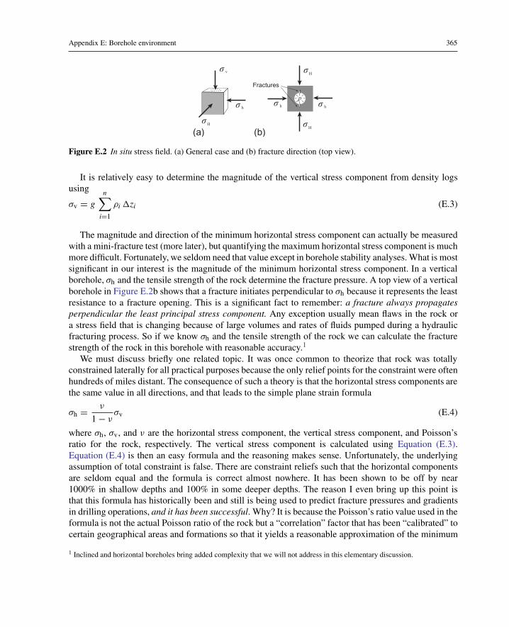
Appendix E: Borehole environment 365
(a) (b)
σ v
σ h
σ H
σ hσ h
σ H
σ H
p
Fractures
Figure E.2 In situ stress field. (a) General case and (b) fracture direction (top view).
It is relatively easy to determine the magnitude of the vertical stress component from density logsusing
σv = gn∑
i=1
ρi �zi (E.3)
The magnitude and direction of the minimum horizontal stress component can actually be measuredwith a mini-fracture test (more later), but quantifying the maximum horizontal stress component is muchmore difficult. Fortunately, we seldom need that value except in borehole stability analyses. What is mostsignificant in our interest is the magnitude of the minimum horizontal stress component. In a verticalborehole, σh and the tensile strength of the rock determine the fracture pressure. A top view of a verticalborehole in Figure E.2b shows that a fracture initiates perpendicular to σh because it represents the leastresistance to a fracture opening. This is a significant fact to remember: a fracture always propagatesperpendicular the least principal stress component. Any exception usually mean flaws in the rock ora stress field that is changing because of large volumes and rates of fluids pumped during a hydraulicfracturing process. So if we know σh and the tensile strength of the rock we can calculate the fracturestrength of the rock in this borehole with reasonable accuracy.1
We must discuss briefly one related topic. It was once common to theorize that rock was totallyconstrained laterally for all practical purposes because the only relief points for the constraint were oftenhundreds of miles distant. The consequence of such a theory is that the horizontal stress components arethe same value in all directions, and that leads to the simple plane strain formula
σh = ν
1− νσv (E.4)
where σh, σv, and ν are the horizontal stress component, the vertical stress component, and Poisson’sratio for the rock, respectively. The vertical stress component is calculated using Equation (E.3).Equation (E.4) is then an easy formula and the reasoning makes sense. Unfortunately, the underlyingassumption of total constraint is false. There are constraint reliefs such that the horizontal componentsare seldom equal and the formula is correct almost nowhere. It has been shown to be off by near1000% in shallow depths and 100% in some deeper depths. The reason I even bring up this point isthat this formula has historically been and still is being used to predict fracture pressures and gradientsin drilling operations, and it has been successful. Why? It is because the Poisson’s ratio value used in theformula is not the actual Poisson ratio of the rock but a “correlation” factor that has been “calibrated” tocertain geographical areas and formations so that it yields a reasonable approximation of the minimum
1 Inclined and horizontal boreholes bring added complexity that we will not address in this elementary discussion.

366 Casing and Liners for Drilling and Completion
horizontal stress component to which is closely related to fracture pressure in a vertical well. It does notwork in highly deviated and horizontal wells.
E.4 Fracture pressure
The pressure at which the matrix of a rock will physically fracture and admit the entrance of wholeliquids depends upon a number of things. Here is what we normally expect when we think about thatdefinition of fracture pressure:
• The wellbore liquid cannot enter the formation pore spaces prior to fracture (e.g., a filter cake building mud oran impermeable formation such as shale)
• The formation is in a state of compression from an in situ stress field (from overburden, lateral constraints,and/or tectonic activity)
• The formation matrix has some amount of cementation and hence some amount of tensile strength (may berelatively small though)
For this formation to be hydraulically fractured, the pressure of the liquid in the wellbore has toexceed both the near borehole stress field that is compressing the rock at the point of fracture andthe tensile strength of the rock matrix at that point of fracture initiation. The near borehole stress fieldis usually not the same as the in situ stress field because the rock deforms slightly when some of itis removed to form the borehole, and consequently the stress field near the borehole has changed.Once the fracture is initiated, the fluid enters the fracture and the fracture will propagate at a lowerpressure than the initial fracture pressure. The reason that the propagation pressure is lower than theoriginal fracture pressure is that once the fracture is open, the fluid pressure acts similar to a wedgein the fracture. In other words, mechanical advantage is gained as the fracture length grows (up to alimit).
That definition is widely accepted. It is normally the way we interpret “fracture pressure” and that iswhat we usually assume when we design casing. However, the “fracture pressure” we utilize at the timeof casing depth selection and casing design often comes from several different sources such as leakofftests, integrity tests, fracture gradient curves/correlations, pilot hole mini-fracture tests, and productionstimulation fracture treatments. Often the values obtained from these sources are not what we assumedfrom the above definition. Additionally, there are certain consequences of that definition of fracturepressure that we do not always anticipate, such as:
• Once fractured a formation as described above can never be pressured again to the original fracture pressure inthat wellbore because it has no tensile strength at that point once fractured. Upon repressuring, the formation willopen at the fracture closure pressure because the tensile strength, if any, is now permanently lost. The fractureclosure pressure is a function of the in situ stress field and not the rock itself. The original tensile strength atthe point of fracture is never restored. The rock is broken, and it stays broken. (Note: some mud systems mayform plugs that can sometimes effectively divert the point of fracture to a different point in the rock matrix andcement can sometimes restore some tensile strength at a point).
• The fracture pressure also depends on the orientation and inclination of the borehole in most cases. The reasonfor that is that the principal in situ stress components are generally not equal in magnitude and their orientationin relation to the wellbore can vary. That is a complicating factor in that the fracture pressure is commonlyreduced as the borehole inclination increases. The fracture pressure in an inclined wellbore will also vary withthe azimuthal direction of the inclined wellbore as well as inclination angle.
Here are some other situations to consider about fracture pressure.

Appendix E: Borehole environment 367
• Some formations have no tensile strength, e.g., unconsolidated sandstones, formations with micro fractures,faults, and so forth.
• A borehole fluid can actually enter the pore spaces under pressure prior to fracture (e.g., fracturing a porousformation with a clear fluid such as brine water).
In the case of no tensile strength, the fracture pressure depends entirely on the in situ stress field. It willopen at the same pressure each time so that fracturing it does not reduce its strength as in the previouscase. This is why in many areas it is perfectly “safe” to fracture a zone while drilling, because the“strength” of the formation has not been reduced. In actuality, the formation has no tensile strength; thecompressive in situ stress field is what holds it together.
In the case of the pressured fluid entering the pore spaces before fracture occurs, the fracturepressure will usually be lower than in the earlier definition because there is mechanical advantage tothe pressurized fluid in the pore spaces.
So we see that fracture pressure depends on orientation of the borehole to the stress field, the typeof fracturing fluid we use, the permeability of the rock, and the tensile strength of the rock, if any.Awareness of those variations enable us to better understand exactly what fracture pressure means.However, fracture pressure values come from various sources, and we must understand the nature of thesources to know what the values mean.
E.5 Borehole stability
Though seldom considered in casing design, the stability of a borehole has for the most part beenconsidered a drilling problem. With the significant increase in the number of horizontal wells beingdrilled, especially into shale formations that will be cased and fractured, it becomes a consideration incasing design too. When we consider that 90% of borehole stability problems occur in shales, we musthave at least some rudimentary understanding of the phenomenon. We will present an overview herewithout going into the details of the rock mechanics involved. First, we look at an example stabilitycurve, Figure E.3. This curve is for a specific formation at a specific depth, and shows a stable regionbetween a collapse region on the left and a fracture region on the right as functions of mud density andinclination angle. You will notice that as the borehole is inclined more and more (toward the top) thewindow of stability decreases. Why is this? It has to do with the in situ stress field not being isotropic.The three principal in situ stress components are not equal, and in general we have σv > σH > σrmh
(vertical, maximum horizontal, minimum horizontal components). In a vertical well, the stability isgoverned by the two smaller stress components, σH and σh. But as the inclination angle increases thevertical stress component, σv, which is the largest of the three, begins to take on a more dominant role.The case shown here is somewhat severe, but it is from an actual well analysis.
If that were not enough, the stability curve also depends on the direction of the borehole as well asthe inclination. Figure E.4 shows a case where it is not possible to select a mud density that will allowthe hole to remain stable when inclined at more that about 65◦. This is a curve for the same formation,same depth, and same well. The difference is that the first curve is an analysis based on drilling in thebest direction and the second is based on drilling in the worst direction for stability. What is the bestdirection? the worst direction?
To answer that we must look at what is taking place in the rock when we drill a borehole throughit. Since the rock is already in a state of compressive stress, it deforms some amount when we drill aborehole through it. In other words, we remove some of the rock and the remaining rock deforms becausesome amount supporting material has been removed. The local stress field changes. The question is: does

368 Casing and Liners for Drilling and Completion
0
15
30
45
60
75
90
1 1.1 1.2 1.3 1.4 1.5 1.6 1.7 1.8 1.9 2Mud specific gravity
Incl
inat
ion
Stable region
Collapseregion
Fractureregion
Figure E.3 A borehole stability plot in direction of σh.
0
15
30
45
60
75
90
1 1.1 1.2 1.3 1.4 1.5 1.6 1.7 1.8 1.9 2
Mud specific gravity
Incl
inat
ion
Stable region
Collapseregion
Fractureregion
Figure E.4 A borehole stability plot, in direction of σH.
this change in the near-borehole stress field cause the rock to fail? That is what a stability analysis seeksto answer, as in Figures E.3 and E.4.
Figure E.5a shows a subsurface rock element with the three principal in situ stress components,where σv > σH > σh. In Figure E.5b, we have drawn the outline of two boreholes to be drilled throughthat rock, one vertical, and the other horizontal in the direction of the maximum horizontal stresscomponent, σH.
In a thought experiment we may “drill” these two example boreholes, and if we know the original insitu stress components, we may calculate the resulting stress field around the borehole wall. In ourcase we will assume the following values: σv = 10, 000 psi, σH = 7500 psi, and σh = 7000 psi. Wecan calculate all the resulting stress components at the borehole wall, but since the tangential stresscomponent, σθ , is usually the most critical we will plot it (see Figure E.6). The plot shows the values ofσθ at the borehole wall all around its circumference. (The starting point for measuring θ is immaterialin the vertical case, but in the figure it starts on the σH-axis.)
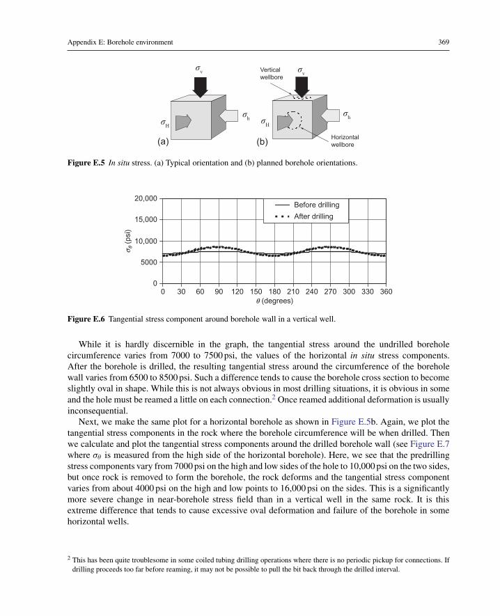
Appendix E: Borehole environment 369
σv
σH
σh
Verticalwellbore
Horizontalwellbore
σhσH
σv
(a) (b)
Figure E.5 In situ stress. (a) Typical orientation and (b) planned borehole orientations.
0
5000
10,000
15,000
20,000
0 30 60 90 120 150 180 210 240 270 300 330 360q (degrees)
s q (
psi)
Before drilling
After drilling
Figure E.6 Tangential stress component around borehole wall in a vertical well.
While it is hardly discernible in the graph, the tangential stress around the undrilled boreholecircumference varies from 7000 to 7500 psi, the values of the horizontal in situ stress components.After the borehole is drilled, the resulting tangential stress around the circumference of the boreholewall varies from 6500 to 8500 psi. Such a difference tends to cause the borehole cross section to becomeslightly oval in shape. While this is not always obvious in most drilling situations, it is obvious in someand the hole must be reamed a little on each connection.2 Once reamed additional deformation is usuallyinconsequential.
Next, we make the same plot for a horizontal borehole as shown in Figure E.5b. Again, we plot thetangential stress components in the rock where the borehole circumference will be when drilled. Thenwe calculate and plot the tangential stress components around the drilled borehole wall (see Figure E.7where σθ is measured from the high side of the horizontal borehole). Here, we see that the predrillingstress components vary from 7000 psi on the high and low sides of the hole to 10,000 psi on the two sides,but once rock is removed to form the borehole, the rock deforms and the tangential stress componentvaries from about 4000 psi on the high and low points to 16,000 psi on the sides. This is a significantlymore severe change in near-borehole stress field than in a vertical well in the same rock. It is thisextreme difference that tends to cause excessive oval deformation and failure of the borehole in somehorizontal wells.
2 This has been quite troublesome in some coiled tubing drilling operations where there is no periodic pickup for connections. Ifdrilling proceeds too far before reaming, it may not be possible to pull the bit back through the drilled interval.

370 Casing and Liners for Drilling and Completion
0
5000
10,000
15,000
20,000
0 30 60 90 120 150 180 210 240 270 300 330 360q (degrees)
s q (
psi)
Before drillingAfter drilling
Figure E.7 Tangential stress components around borehole wall in a horizontal well.
(a) (b)
σv
σh
σv
σh
(fractures)Tensile failure
σh
σv
σv
σh
Compressive failure(break-out)
Figure E.8 Borehole instability. (a) Compressive break-out failure and (b) tensile fracture failure.
We must understand one thing about this deformation: Unless the two in situ stress componentsperpendicular to the borehole axis are equal, the borehole deformation will result in an oval-shapedborehole, and there is nothing we can do to prevent it. The degree of ovality may be insignificant orit may be sufficient to cause failure in some of the rock on the borehole wall. And in the case of rockfailure, that too could be relatively insignificant or it could mean total borehole collapse. The onlymeans we have of mitigating the effects and resulting damage of the deformation is by controllingthe internal pressure (mud density), but because pressure is the same in all directions it cannot restorethe near-borehole formation to its original round shape. Too little pressure and the formation may fail incompression on the two sides tangent to the maximum stress component as in Figure E.8a, and too muchpressure and it may fracture the formation on the two sides where the wall is tangent to the minimumstress component (Figure E.8b).
Since the compressive and tensile failure points are at different locations on the borehole wall, it ispossible that they can both occur concurrently. For example, we see that the borehole stability curve inFigure E.4 shows the two curves crossing at about 65◦ inclination. Had we extended those two curvesbeyond their intercept we would have defined an area where both collapse and fracture are possible, andthat is exactly what can happen in some boreholes.
One critically important point, that must be understood when drilling horizontal wells for hydraulicfracturing, and that is that the hydraulic fractures will always propagate perpendicular to the minimumprincipal in situ stress component. Usually that is the minimum horizontal stress component, σh.Figure E.9 illustrates fracture propagation from boreholes drilled in the directions of the three principalin situ stress components. While the cylindrical borehole geometry affects the fracture orientation uponinitiation at the borehole wall, once away from the wall, the fractures will always propagate and grow

Appendix E: Borehole environment 371
Figure E.9 Fracture propagation from boreholes oriented in the three principal in situ stress component directionswhere σv > σH > σh.
in a direction perpendicular to the minimum principal in situ component as shown. Obviously then, theborehole on the left side of the figure drilled in the direction of σH will have a very poor responsea fracturing treatment except in cases where one is attempting to overcome vertical permeabilitylimitations in a thin bed or one near a gas or water contact where fracture length as measured awayfrom the wellbore is not desired.
The intent of this section is to give you a brief overview of the nature of borehole stability as it appliesto highly deviated wellbores. Space here does not allow us to go into detail about obtaining data andmaking calculations for a stability analysis, but for your information the following are required:
• In situ stress components, σv, σH, σh (magnitudes and direction)• Rock strength/failure properties• Rock failure model
More information may be obtained in the book by Fjær et al. [71] and the paper by Yew and Li [73].Also, in Chapter 2, we discussed other aspects and showed a pressure chart of a mini-frac used to obtainfracture data.
E.6 Borehole path
The basic tools for determining a borehole path are an inclinometer for measuring the boreholeinclination (the deviation angle, α, of the borehole from vertical), a magnetic compass for measuringthe borehole direction (azimuth angle, β, from magnetic north), and the drill pipe measurements fordetermining the length, �s, along the borehole path between directional survey points. The resultingdata defines a spatial direction vector at each survey point using α and β. The drill pipe measurement,�s, is the distance between two of the vectors as measured along the borehole path between them.Contrary to what is often assumed, that is not enough information to specify the location of a secondsurvey point even when the first of the two is known exactly. We must assume some shape of the boreholepath between survey points in order to specify the location of the second survey point.
E.6.1 Minimum curvature method
The method for determining a borehole path used almost exclusively today is known as the minimumcurvature method as proposed by Taylor and Mason [38] in 1972. They arrived at their method byminimizing a quadratic curve that will describe the minimum length quadratic path between two surveypoints and having the same vector directions as the survey vectors at the two ends. Their result is that theminimum quadratic borehole path between two survey points is approximated by a segment of a circle

372 Casing and Liners for Drilling and Completion
Figure E.10 Minimum curvature notation scheme.
in a plane. Their equations may be written in several forms using trigonometric identities, but here theyare in the form presented in Taylor’s and Mason’s paper:
�x = �s
ϕ
(vx sin ϕ + ux − vx cos ϕ
sin ϕ− (ux − vx cos ϕ) cos ϕ
sin ϕ
)(E.5)
�y = �s
ϕ
(vy sin ϕ + uy − vy cos ϕ
sin ϕ−(uy − vy cos ϕ
)cos ϕ
sin ϕ
)(E.6)
�z = �s
ϕ
(vz sin ϕ + uz − vz cos ϕ
sin ϕ− (uz − vz cos ϕ) cos ϕ
sin ϕ
)(E.7)
where
vx = sin α1 cos β1
vy = sin α1 sin β1
vz = cos α1
ux = sin α2 cos β2
uy = sin α2 sin β2
uz = cos α2
and
ϕ = cos−1 [uxvx + uyvy + uzvz]
(E.8)
Note: ϕ must be in radians in these equations.The numerical subscripts refer to the current survey (1) and the previous survey (2). The letter
subscripts refer to the physical directions: x is North/South, y is East/West, and z is Down/Up. Thequantities �x, �y, and �z represent the changes in North/South, East/West, Down/Up, respectively,since the previous survey with North (+), South (−), East (+), West (−), Down (+), and Up (−). Thequantity, �s, is the measured length of the well path between the two survey points.

Appendix E: Borehole environment 373
E.6.2 Interpolations on the borehole path
For a number of computations, such as contact force for friction calculations and casing wear, and forbending stress magnification, it is often necessary to determine the location of points along a boreholepath on a finer nodal mesh than is given by the directional survey results which are typically on intervalsranging from 30 to 90 ft. where the direction is being tightly controlled and significantly longer intervalselsewhere. There are various ways to do this, the most common being a simple linear interpolationof the inclination and azimuth angles separately between survey points. While that produces sufficientaccuracy for most measurements and calculations, it ignores the foundational premise of the currentsurvey method used by the industry. Such an interpolation constitutes a radius of curvature method,whereas the well path is calculated by a minimum curvature method. Here, we show a consistent methodof interpolation based on the same assumptions of the minimum curvature method.
General interpolation procedure
Given two successive survey sets, (αa, βa, sa) and (αb, βb, sb) at survey points a and b respectively, wewant to determine the survey data for any arbitrary nodal point(s) between them using the minimumcurvature method as the basis of the interpolation (refer to Figure E.10). The survey angles at points aand b describe two tangent vectors on the geodesic curve connecting the two points. That and the lengthof that geodesic, �s = sb − sa, give us enough information to determine a tangent vector at any nodeon the curve between the two points. The general procedure is as follows.
1. Translate measured angles (inclination and azimuth) for the two tangent vectors into coordinate descriptions inthe global coordinate system
2. Using the minimum curvature assumption that these two vectors are in the same plane, calculate the anglebetween them using the inner product
3. Using that angle and the arc length distance between them, determine the radius of curvature of the well pathgeodesic
4. Calculate the binormal vector to the arc using the vector product (cross product) of the two tangent vectors5. Calculate the normal vector at point a using the vector product of the binormal vector and the tangent vector at
point a6. These three orthogonal vectors (tangent, normal, and binormal) form a local coordinate system at point a from
which we can determine a tangent vector at any node between point a and point b7. Determine the incremental angle along the geodesic between point a and the interpolation node8. Calculate the tangent vector at the node in the local coordinate system9. Calculate the projection of that tangent vector back into the global coordinate system
10. Calculate the inclination and azimuth at that node
Specific interpolation procedure
Starting at the top of the borehole, the interpolation nodes will be numbered i = 1, 2, . . . , n. The nodevariables for inclination, azimuth, and measured depth will be noted as αi, βi, and si, respectively.The survey points will be numbered k = 1, 2, . . . , m and generally n > m. The survey variables forinclination, azimuth, and measured depth will be noted likewise as Ak, Bk, and Sk. In order to simplifythe notation for interpolation within each survey interval we define six scalar variables αa, βa, and sa
as the values for Ak, Bk, and Sk, respectively, at the beginning of the interval and αb, βb, and sb as thevalues for Ak+1, Bk+1, and Sk+1 at the end of the interval.
Initialize the survey index, k = 1
1. Loop through all the nodes i = 1, n incrementing the survey intervals as required:2. Initialize αa, βa, sa, αb, βb, and sb.

374 Casing and Liners for Drilling and Completion
3. Determine if the node depth, si, falls within the measured depth interval of surveys a and b, such that sa ≤ si <
sb. Note that the first survey depth is considered to be part of the interval and the second is not. We use theclosed/open interval, [sa, sb), where sb defines the end of the interval but is not included in the interval. This isan arbitrary computational convenience.
4. If si does not fall within the interval, proceed to the next survey interval by incrementing k and repeat the firststep.
5. If si = sb then assign that node the values of the survey at that same depth, αi = αa and βi = βa, return to thefirst step where the node number, i, will be incremented to i+ 1. (Usually node 1 will coincide with the firstsurvey and in that case you would assign that survey value to node 1, return to step 1 and increment to node 2.)
6. If si is within the interval and si = sa, determine the two unit vectors in global coordinates using the followingtransform.
t = (sin αa cos βa e1, sin αa sin βa e2, cos αa e3)
(E.9)
v = (sin αb cos βb e1, sin αb sin βb e2, cos αb e3)
(E.10)
In the Cartesian coordinate system that we are using, both those tangent vectors are unit vectors.7. The scalar product (inner or dot product) of these two unit vectors is the cosine of the angle between them, so
cos ϕ = t · v→ ϕ = cos−1(
t · v)
and we have
ϕ = cos−1 (t1v1 + t2v2 + t3v3) (E.11)
8. Since we assumed that the borehole path is a geodesic on a sphere we can now determine the radius of thesphere with the familiar arc formula, s = rθ , and in our nomenclature where s = �s = sb − sa the radius is
r =∣∣∣∣�s
ϕ
∣∣∣∣ (E.12)
We use the absolute value signs here as a radius is always taken to be positive. However, in our case �s willalways be positive unless we have made a mistake because sb > sa.
9. We know that the two tangent vectors are in the same plane as the two radius vectors, and that the two radiusvectors are normal to the two tangent vectors, respectively. Hence a radius vector is usually called a normalvector. A vector normal to both the tangent vectors and the radius vectors (remember they are all in the sameplane) is called a binormal vector. The binormal vector is easily found using the vector product (or crossproduct) of the two survey tangent vectors.
b = t× v = det
⎡⎣ e1 e2 e3
t1 t2 t3v1 v2 v3
⎤⎦
b = [(t2v3 − t3v2) e1, (t3v1 − t1v3) e2, (t1v2 − t2v3) e3]
(E.13)
The two vertical bars denote the determinant of the matrix given by the expansion on the right. The vectors,t and v are unit vectors, but they are not orthogonal to each other so their product b is not a unit vector, so itwill be convenient to unitize it now.
b = b‖b‖ =
(b1 e1, b2e2, b3 e3
)√
b21 + b2
2 + b23
(E.14)
10. At the first survey point we have the unit tangent vector, t, and the unit binormal vector, b, but we do not yethave the normal vector at that survey point which we will need to form a local coordinate system aligned withthe three principal direction vectors at that point. Again we use the vector product but with the unit tangentvector and binormal vectors, t and b, at survey point a to calculate the normal vector.

Appendix E: Borehole environment 375
n = b× t = det
⎡⎣ e1 e2 e3
b1 b2 b3
t1 t2 t3
⎤⎦
n = [ ( b2 t3 − b3 t2) e1, ( b3 t1 − b1 t3 ) e2, ( b1 t2 − b2 t3 ) e3]
(E.15)
In this case the unit vectors, b and t, are orthogonal to each other and their orthogonal vector product, thenormal vector, n is also a unit vector.
11. From this local coordinate system we will interpolate the tangent vectors at any point within the intervalbetween point a and point b. Note that we will no longer need the tangent vector, v, within this interval becausewe only needed it to establish the plane in which the tangents and radii reside. The triad of unit vectors wehave just calculated form a local unit basis, e:
t = e′1b = e′2n = e′3
12. Next we calculate the tangent vector at a node in the local coordinate system by first determining the distanceand angle between the node and survey point a.
�s = si − sa
�ϕ = �s
r(E.16)
13. Then we calculate the tangent vector in local coordinates
τ ′1 = cos (�ϕ) (E.17)
τ ′2 = sin (�ϕ) (E.18)
τ ′3 = 0 (E.19)
14. Then we calculate the projection of this vector into the global coordinates
τ1 = τ ′1 t1|τ ′1| +
τ ′2 n1
|τ ′2| (E.20)
τ2 = τ ′1 t2|τ ′1| +
τ ′2 n2
|τ ′2| (E.21)
τ3 = τ ′1 t2|τ ′1| +
τ ′2 n3
|τ ′2| (E.22)
15. And lastly, we convert this nodal tangent vector to an inclination angle and azimuth
αi = tan−1(
τ2
τ1
)(E.23)
βi =∣∣∣∣∣∣ tan−1
⎛⎝√
τ21 + τ2
2
τ3
⎞⎠∣∣∣∣∣∣ (E.24)
A programmable algorithm for this procedure is listed later.

376 Casing and Liners for Drilling and Completion
Programming borehole path calculations
The algorithm for doing directional survey calculations using Taylor and Masons method is fairlystraightforward and the calculations may easily be done manually using a hand-held calculator thoughalmost no one does that now. The serious drawback to manual calculations is that the errors arecumulative, so that an error in one calculation carries forward to all subsequent calculations. The taskof programming directional survey calculations for a spreadsheet or some compiled program is easy butthere are a few eccentricities involved that should be noted.
Accounting for straight sectionsIt is not uncommon that two consecutive surveys will be identical, and in fact this is often desirable invertical wells and some sections of directional wells. A program designed to employ only the minimumcurvature algorithm will likely crash when it encounters two consecutive and identical surveys becausethe radius of curvature between the two identical surveys goes to infinity, in other words, the sectionis not a curve but is straight. A simple logic test to compare successive surveys can avoid this totallyand the straight section can be handled by a straightforward trigonometric calculation. Along this line,it has been noted that some directional service companies using spreadsheets to calculate directionalsurveys have gotten around this with a procedure that adds and subtracts very small amounts to the dataduring calculations to avoid any infinities in the minimum curvature calculations. While this reeks ofprogramming laziness, the quantities used are usually on the order of 1.0× 10⁻⁸ so the accuracy maynot be affected beyond the accuracy of the measurements themselves.
Accounting for large azimuth changesWhile one might think large azimuth changes between survey points are rare, that is not the case. In nearvertical wells with small inclination it is not that unusual to see azimuth changes of up to 180◦ betweenconsecutive surveys. Though the magnitude of the change of azimuth might be large, at very smallinclination angles the change in the borehole path is minimal. Two problems arise in programmingazimuth. One is the case of the zero inclination in which azimuth is meaningless because there isno azimuth for a vertical borehole. As common practice, the azimuth may be assigned arbitrarily tothe same value as the previous survey, or especially in the case of the surface location it may be setto zero.
The other case that must be accounted for and which arises in contact force calculations where anet change in azimuth, �β = βb − βa, cannot be more than 180◦ or less than −180◦, i.e., −180◦ <
�β ≤ 180◦.3 For example, if the azimuth for one survey is βa = 12◦ and the next survey azimuth isβb = 344◦, then the net change in azimuth between the two surveys is −28◦ not 332◦. This is shownmathematically as
if
{βb − βa < −180◦ → �β = βb − βa + 360◦βb − βa ≥ 180◦ → �β = βb − βa − 360◦ .
Other considerationsIt is always good to keep in mind that a drilling assembly is a relatively large physical object that doesnot change direction rapidly or lend itself to mathematical oddities like reversing direction between
3 While one can consider a rotation of up to 360◦, the net change in direction cannot exceed ±180◦.

Appendix E: Borehole environment 377
surveys (except as previously discussed for small inclinations). Also, the mathematical possibility existsthat since the two survey vectors are assumed to be in the same plane the inner product could be zeromeaning that the two survey directions are perpendicular to each other, which should not be the case ina drilled borehole where the survey points are reasonably spaced.
Interpolation algorithm
For programming purposes the interpolation procedure is given in two algorithms below where
st = total measured depth
si = nodal measured depth
αi = nodal inclination
βi = nodal azimuth
Sk = survey measured depth
Ak = survey inclination
Bk = survey azimuth
All other variables should be self explanatory. In this general algorithm, we assume the first survey isat zero depth and that the first node is also at zero depth, otherwise the algorithms should be modifiedto take other cases into account. The procedure consists of two algorithms. The first is the main orcontrolling program that sets up the survey data and calls the interpolation subroutine.
Algorithm E.1 Main Interpolation Program
set n equal to number of nodesset m equal to number of surveyscalculate nodal depth interval; �s = st/ninitialize first depth si = 0 at i = 1for remaining node depths, i = 2,n{increment depth; si = si-1 +�s}
initialize survey counter, k = 1do while k < m{for each interpolation node, i = 1,n{
if (si = Sk){set node depth to first survey depth; si = Skset node incl. to survey incl.; αi = Akset node azimuth to survey azimuth; βi = Bk}
else if (Sk < si < Sk+1){call Minimum Curvature Interpolation subroutine}
else{increment survey counter; k = k+1}
}}

378 Casing and Liners for Drilling and Completion
The algorithm for the interpolation subroutine is:
Algorithm E.2 Minimum Curvature Interpolation Subroutine
{calculate tangent vectors; t and v, eqns.E.9 and E.10calculate included angle; ϕ, eqn. E.11calculate depth increment; �s = sb − sacalculate radius of curvature; r = �s/ϕ, eqn. E.12calculate the bi-normal vector, b, eqn. E.13unitize the bi-normal vector, b, eqn. E.14calculate the unit normal vector, n, eqn. E.15calculate the angle from survey to node, �ϕ, eqn. E.16calculate the nodal local tangent vector, τ, eqns.(E.17)-(E.19)calculate the nodal global tangent vector, τ, eqns.(E.20)-(E.22)calculate the nodal inclination, αi, eqn. E.23calculate the nodal azimuth, βi, eqn. E.24
}
We now have an interpolated survey at that node using the minimum curvature method for theinterpolation rather than a linear interpolation of inclination and azimuth separately which amountsto a radius of curvature interpolation.
Comments on the interpolation method
While this method is more refined than a linear interpolation, the difference in the results is notnecessarily that significant in many applications, and for a two-dimensional borehole profile wherethere is no change in azimuth, the results are exactly the same. The algorithm is easily programmed andinterpolations can be made for a mesh of one foot, a half meter, or one meter intervals if desired. Therun time is very short (less than a second) on most desktop and laptop PCs using Fortran or C++, buta little longer if programmed within a spreadsheet using VBA. The interpolation method can generatea uniform mesh at much shorter intervals than is common for actual directional survey data. This doesmake a difference when calculating borehole friction and especially in calculating points of maximumcontact force for determining the critical casing wear locations. Though the final results may not includethe actual survey points except where the nodes and survey points may accidentally coincide, this is notseen as a disadvantage in this type of work.
This interpolation method is quite useful in a number of borehole applications. The run time for onefoot intervals is negligible, but output for plotting purposes is excessive at those intervals. The usualprocedure is a subroutine to scan larger intervals of say, 100 ft., and pick the maximum value (contactforce, bending stress magnification, etc.) within that interval for output and plotting.
E.7 Closed-Form friction solutions
The full discussion of borehole friction is in Chapter 7, but here I add some additional information thatmay be of peripheral interest. From the three-dimensional differential equations for borehole frictionderived by Sheppard et al. [41], we may specialize these into two-dimensional form by assuming thereis no change in azimuth (β = 0). Further, we assume that the borehole path is a series of circular arcs ascalculated by the minimum curvature method which is the standard for determining the borehole path

Appendix E: Borehole environment 379
and location. With these assumptions we are able to obtain closed-form solutions for borehole frictionin both upward and downward motions as well as in pure rotation mode.
E.7.1 Closed-Form drag solutions
In two dimensions, the governing differential equation for tension may be solved exactly if we have aclosed-form expression for the curvature as a function of the axial coordinate s.
dF
ds= w cos α ± μ
∣∣∣∣ F dα
ds+ w sin α
∣∣∣∣ (E.25)
Now for sections with constant build angle the curvature, dα/ds, is given exactly by
dα
ds= α − α0
s(E.26)
This is a first-order linear ordinary differential equation and is easy to solve. There is a complicatingfacet, though, and that is the necessity of maintaining the absolute value of the contact force even thoughthese terms must be separated to get a solution. Without going into the details we will give the solutions,and the necessary criteria for their use.
Closed-Form solutions for upward motion
The two solutions for pulling casing out of the hole where the friction term is positive are
F(+) = eμ(α−α0)
{F0 + w s
(α − α0)(μ2 + 1
) [(μ2 − 1)
sin α0 + 2μ cos α0]}
− w s
(α − α0)(μ2 + 1
) [(μ2 − 1)
sin α + 2μ cos α] (E.27)
and
F(−) = e−μ(α−α0)
{F0 + w s
(α − α0)(μ2 + 1
) [(μ2 − 1)
sin α0 − 2μ cos α0]}
− w s
(α − α0)(μ2 + 1
) [(μ2 − 1)
sin α − 2μ cos α] (E.28)
The (−) solution, Equation (E.28), is used where the following conditions exist
Fdα
ds< w sin α and
∣∣∣∣ F dα
ds
∣∣∣∣ > w sin α
for all other cases the (+) solution, Equation (E.27), is used.
Closed-Form solutions for downward motion
For running casing in the hole, the sign of the friction term is negative. This leads to solution equationsidentical to Equations (E.27) and (E.28). However, in this case where
Fdα
ds< w sin α and
∣∣∣∣Pdα
ds
∣∣∣∣ > w sin α

380 Casing and Liners for Drilling and Completion
we must use Equation (E.27), the (+) solution, and for all other cases we must use Equation (E.28), the(−) solution.
Remarks on the Closed-Form solution
While the closed-form solutions may appear rather complex they are quite easily set into simplecomputer programs. The complicating factor is the problem of dealing with two solution equations andpatching them together where the magnitudes of the gravitational contact force is smaller in magnitudethan the contact force from tension. In order to patch these equations together it is necessary to get thesolution at incremental points along with the values of the contact force components to determine whichequation to use. This would seem to defeat the purpose of having an exact solution since a numericalsolution requires an incremental approach also.
E.7.2 Closed-Form torque solution
For a constant curvature in a two-dimensional wellbore, the equation for rotational torque reduces to
dTq
ds= ro μ
∣∣∣∣ w sin α + Fdα
ds
∣∣∣∣ (E.29)
and
F = F0 −s∫
0
w cos α ds (E.30)
The constant curvature in a plane means that
dα
ds= ±κ = sgn (αs − α0) κ (E.31)
where sgn is the signum operator, e.g., if (a− b) > 0 then sgn (a− b) = +1 and if (a− b) < 0 thensgn (a− b) = −1, and κ is the curvature of the borehole path (assumed constant here) and is considerednegative in a build section (remember s is measured from the bottom so that dα/ds is decreasing in abuild section), and positive in a drop-off section so that we may substitute Equations (E.30) and (E.31)into Equation (E.29) and separate variables to get
dTq = ro μ
∣∣∣∣∣∣ w sin α ds+ sgn (αs − α0)
⎛⎝F0 −
L∫0
w cos α ds0
⎞⎠ κ ds
∣∣∣∣∣∣ (E.32)
Recalling that for a constant curvature
ds = dα
κ(E.33)
and Equation (3.8.8) becomes
dTq = roμ
∣∣∣∣∣∣1
κw sin α dα + sgn (αs − α0)
⎛⎝F0 −
α∫α0
1
κw cos α dα
⎞⎠ dα
∣∣∣∣∣∣ (E.34)
Appendix E: Borehole environment 381
Assuming the weight per unit length is a constant, we now integrate this equation
Tq s∫Tq 0
dTq = ro μ
∣∣∣∣∣ 1
κw
αs∫α0
sin α dα + sgn (αs − α0)αs∫α0
(F0 − 1
κw
α∫α0
cos α dα
)dα
∣∣∣∣∣ (E.35)
we get the closed-form solution
Tq s = Tq 0 + ro μ | rκ w (cos α0 − cos αs)
+sgn (αs − α0)
{F0 (αs − α0)− 1
κw [cos α0 − cos αs − (αs − α0) sin α0]
} ∣∣∣∣ (E.36)
and as before this solution is valid only for sections where the curvature and the buoyed weight areconstants.
E.8 Closure
It is not within the scope of this text to detail the various methods for quantifying pore pressures orfracture pressures. The brief overview given in this appendix may at least cast a little insight into thesubject for those whose backgrounds do not include any study of geology or reservoir mechanics. Thereare a number of reliable sources for quantifying pore pressures and fracture pressures for well planning.Unfortunately, the majority of those are local to the Louisiana and Texas Gulf Coast. Those methodswill work anywhere, but the correlations are quite restricted geographically, and my reluctance to includeany here is strictly motivated by a desire to keep any part of this text from being restricted to a limitedgeographical area. A readable source of information on rock mechanics is the book by Fjær et al. [71].And another good source for understanding and quantifying pore pressures and fracture pressures is thebook by Fertl [12]. In any event, one should be aware that the pore pressure and fracture pressure datathat we use in casing design is only approximate at best.

This page intentionally left blank

Appendix F: Summary of useful formulas
Chapter outline head
F.1 Borehole geometry 383F.2 Directional well equations 384F.3 Hydrostatics equations 386F.4 Geometric equations for tubes 387F.5 Axial stress and displacement equations 387F.6 Tube bending equations 389F.7 Tube pressure equations 389F.8 Torsion equations 390F.9 Lateral buckling equations 390
F.10 Thermal equations 391F.11 General solid mechanics 391
F.11.1 Yield criteria 391
F.12 API/ISO performance equations 392
Listed in this appendix for convenience and quick reference are many of the formulas and equationsfrom the text. There is little or no qualification listed here and one should refer to the text if uncertain asto any formula’s assumptions and use.
PrecautionThere are no conversion factors in these formulas, so consistent units must be used.
F.1 Borehole geometry
CurvatureBorehole curvature, reference equation (7.15):
κ ≡ dθ
ds(F.1)
Radius of CurvatureReference equation (7.16):
rκ = 1
|κ| (F.2)

384 Casing and Liners for Drilling and Completion
F.2 Directional well equations
Minimum Curvature MethodSee Appendix E
�x = �s
ϕ
(vx sin ϕ + ux − vx cos ϕ
sin ϕ− (ux − vx cos ϕ) cos ϕ
sin ϕ
)(F.3)
�y = �s
ϕ
(vy sin ϕ + uy − vy cos ϕ
sin ϕ−(uy − vy cos ϕ
)cos ϕ
sin ϕ
)(F.4)
�z = �s
ϕ
(vz sin ϕ + uz − vz cos ϕ
sin ϕ− (uz − vz cos ϕ) cos ϕ
sin ϕ
)(F.5)
where
vx = sin α1 cos β1
vy = sin α1 sin β1
vz = cos α1
ux = sin α2 cos β2
uy = sin α2 sin β2
uz = cos α2
and
ϕ = cos−1 [uxvx + uyvy + uzvz]
(F.6)
Note: ϕ must be in radians in these equations.
Amontons-Coulomb FrictionReference equation (7.1):
F ≤ μ N (F.7)
Critical Inclination AngleReference equation (7.6):
αcr = tan−1 1
μ(F.8)
Differential Friction Equation, Sheppard et al. [41]Reference equation (7.7):
dF
ds= w cos α ± μ
[(F
dα
ds+ w sin α
)2
+(
wdβ
dssin α
)2] 1
2
(F.9)

Appendix F: Summary of useful formulas 385
Incremental Friction Equations, Johancsik et al. [40]Reference Equations (7.8) and (7.9):
Fn = F0 +n∑
i=1
[(si − si−1) wi cos
(αi−1 + αi
2
)± μiNi
](F.10)
and
Ni = (si−1 − si)
{[wi sin
(αi−1 + αi
2
)+ Fi−1
(αi − αi−1
si−1 − si
)]2
(F.11)
+[
Fi−1
(βi − βi−1
si−1 − si
)sin
(αi−1 + αi
2
)]2} 1
2
Torque Equation, Differential FormReference equation (7.11):
dTq
ds= ro μ
[(w sin α + F
dα
ds
)2
+(
Fdβ
dssin α
)2] 1
2
(F.12)
Torque Equations, Incremental FormReference Equations (7.12) and (7.13):
Tq n = Tq 0 +n∑
i=1
ri μi Ni (F.13)
and
Fi = Fo +i∑
k=1
(sk−1 − sk) wk cos
(αk−1 + αk
2
)(F.14)
The contact force in this set is calculated with Equation (F.11).
Axial LoadTo convert from effective axial load, F, at a point (reference equation (7.10)):
Fi = Fi − (poAo − piAi) (F.15)
Bending StressReference equation (7.23):
σb = ±Er
rκ
(F.16)
Bending Stress MagnificationThe equations for the bending stress magnification factor, λb, are quite lengthy and require considerablequalification. Refer to Section 7.6.2 for these equations.

386 Casing and Liners for Drilling and Completion
F.3 Hydrostatics equations
Basic Differential EquationReference equation (D.3):
dp = ρ g dz (F.17)
Basic Integral EquationReference equation (D.4):∫ ph
p0
dp =∫ h
h0
ρ g dz (F.18)
Basic Common FormReference equation (D.7) where ρ and g are constants:
�p = ρ g �h (F.19)
Gas Equation for DesignReference equation (D.16):
p = p0 expMg (h− h0)
ZRTavg(F.20)
or an alternate version, reference equation (D.17):
p = p0
(T0 + kTh
T0 + kTh0
) MgZRkT
(F.21)
Generalized Archimedes’ PrincipleReference equation (D.18):
W = g(ρsolid − ρliquid
)Vsolid (F.22)
Buoyancy FactorReference equation (D.19):
kb ≡ W
W= 1− ρliquid
ρsolid(F.23)
Buoyed Axial LoadBottom of a section, reference equation (39):
F↓j = −p0A0 + p1A1 +j∑
i=2
pi (Ai − Ai−1)+j−1∑i=1
wiLi (F.24)
j = 1, . . . , n

Appendix F: Summary of useful formulas 387
Top of a section, reference equation (D.40):
F↑j = −p0A0 + p1A1 +j∑
i=2
pi (Ai − Ai−1)+j∑
i=1
wiLi (F.25)
j = 1, . . . , n
or alternately as reference Equations (41) and (42):
F↓j = F↑j−1 + pj(Aj − Aj−1
)(F.26)
F↑j = F↓j +Wj
F.4 Geometric equations for tubes
Cross-sectional Area
At = π(
r2o − r2
i
)= π
4
(d2
o − di
)(F.27)
Second Area Moment, Axial
Ia = π
4
(r4
o − r4i
)= π
64
(d4
o − d4i
)(F.28)
where a is any diameter.
Radius of Gyration
rg =√
I
A= 1
2
√r2o + r2
i =1
4
√d2
o + d2i (F.29)
Polar Area Moment
Jz = π
2
(r4
o − r4i
)(F.30)
F.5 Axial stress and displacement equations
Axial Stretch at a PointReference Equations (C.143):
uz = 1
At E
[(P+ w �) z− w
2z2]
(F.31)
for 0 ≤ z ≤ �

388 Casing and Liners for Drilling and Completion
Total Axial StretchReference equation (C.144):
u = 1
AtE
[P�+ w
2�2]
for z = � (F.32)
Load for Specified DisplacementReference equation (C.145):
P = AE u
L− w L
2(F.33)
Incremental DisplacementReference equation (C.146):
�u = �PL
AE(F.34)
Incremental LoadReference equation (C.147):
�P = AE �u
L(F.35)
Free PipeReference equation (C.148):
L = AE �u
�P(F.36)
Composite Bar or TubeIf the bar or tube is composed of more than one size (still prismatic in each size), then we can expandthe previous formulas, reference Equations (C.149) and (C.150):
� u = �P
E
n∑i=1
Li
Ai(F.37)
and
�P = �u E
(n∑
i=1
Li
Ai
)−1
(F.38)
Axial StressReference equation (6.1):
σz = Fz
At= Fz
π(r2
o − r2i
) = Fzπ4
(d2
o − d2i }) (F.39)

Appendix F: Summary of useful formulas 389
F.6 Tube bending equations
Maximum Planar Bending StressReference Equations (7.23) and (C.172):
σb = ±Er
rκ
ri ≤ r ≤ ro (F.40)
Planar Bending Differential EquationReference Equation (C.166):
d2
dx2
(EIy
d2uz
dx2
)+ f (x) = 0 (F.41)
Boundary Conditions for Integrating Equation (F.41)Reference equation (C.167):
uz = transverse displacementduz
dx= slope
d2uz
dx2 = curvature (approximate) (F.42)
EIyd2uz
dx2 = moment
EIyd3uz
dx3 = shear
EIyd4uz
dx4 = − f (x) = the transverse load
F.7 Tube pressure equations
Lamé General SolutionReference Equations (6.2), (6.3) and (6.4):
σr = r2i r2
o (po − pi)
r2o − r2
i
1
r2 +por2
o − pir2i
r2o − r2
i
(F.43)
σθ = − r2i r2
o (po − pi)
r2o − r2
i
1
r2 +por2
o − pir2i
r2o − r2
i
(F.44)
�σz =
⎧⎪⎪⎪⎪⎪⎪⎨⎪⎪⎪⎪⎪⎪⎩
pi r2i − po r2
o
r2o − r2
i
capped ends, both free ends, one or both
0 open ends, one or both free ends, one or both
ν (�σθ +�σr) open or capped ends fixed ends, both
(F.45)

390 Casing and Liners for Drilling and Completion
Lamé Inner Wall Solution, r = riReference Equations (6.5) and (6.6):
σr = −pi (F.46)
σθ = pi(r2
o + r2i
)− 2por2o
r2o − r2
i
(F.47)
Lamé Outer Wall Solution, r = roReference Equations (6.7) and (6.8):
σr = −po (F.48)
σθ = −po(r2
o + r2i
)+ 2pir2i
r2o − r2
i
(F.49)
Lamé Change in Axial Stress Caused by Change in PressureInitial axial stress is calculated from Equation (F.39). The change caused by pressure is given as:
�σz =
⎧⎪⎪⎪⎪⎨⎪⎪⎪⎪⎩
pi r2i − po r2
o
r2o − r2
i
capped ends (both) free (one or both)
0 open ends (one or both) free (one or both)
ν (�σθ +�σr) open or capped ends fixed (both)
(F.50)
F.8 Torsion equations
General Torsion FormulaReference equation (6.9):
σrθ = rTq
Jz= 2 r Tq
π(r4o − r4
i
) ri ≤ r ≤ ro (F.51)
Rotational Deflection
θ = Tq L
Jz G= 2Tq L
π(r4
o − r4i
)G
(F.52)
F.9 Lateral buckling equations
Lateral BucklingReference equation (6.56):
Fcrit = 2
√4EI g kb ρ� sin α
�r(F.53)

Appendix F: Summary of useful formulas 391
Stability ConditionReference Equations (6.49), (6.50), (6.51) and (6.52):
σz ≥ Aipi − Aopo
Ao − Ai(F.54)
σz ≥ ri2pi − r2opo
r2o − r2
i
(F.55)
Fz ≥ Aipi − Aopo (F.56)
σz ≥ 1
2(σθ + σr) (F.57)
Neutral Stability PointReference equation (6.54):
Fz = Fz + (Aopo − Aipi) = 0 (F.58)
F.10 Thermal equations
Axial Stress, ThermalOne-dimensional thermoelastic Hooke’s equation, reference equation (6.62):
σ = σ0 + E ε − E α �T (F.59)
F.11 General solid mechanics
The important general equations of solid mechanics in Appendix C are too numerous to include here,and you are referred to that appendix. The equations for the von Mises yield criteria are listed. Somesolutions from that appendix for axial stretch and planar bending of tubes are listed in separate categoriesin this appendix, however.
F.11.1 Yield criteria
The von Mises Yield CriterionReference equation (C.104)
Y ≥ √3J2 (F.60)
Yield Measure, Principal StressPrincipal stress formulation, reference equation (C.108):
Ψ ≡ √3J2 ={
1
2
[(σ1 − σ2)
2 + (σ2 − σ3)2 + (σ3 − σ1)
2]} 1
2
(F.61)

392 Casing and Liners for Drilling and Completion
If torsion is the only shear stress in the tube, the principal stress components are given by referenceequation (C.113):
σ1 = σθ + σr
2+√(
σθ − σr
2
)+ σ 2
rθ
σ2 = σθ + σr
2−√(
σθ − σr
2
)+ σ 2
rθ (F.62)
σ3 = σr
Yield Measure, Cylindrical Coordinates, No TorquePrincipal stress formulation in cylindrical coordinates with not shear stress components, referenceequation (C.111):
Ψ ={
1
2
[(σθ − σr)
2 + (σr − σz)2 + (σz − σθ )
2]} 1
2
(F.63)
Yield Measure, General Stress Field, Cylindrical CoordinatesGeneral stress formulation in cylindrical coordinates, reference equation (C.112):
Ψ ={
1
2
[(σθ − σr)
2 + (σr − σz)2 + (σz − σθ )
2]+ 3(σ 2
rθ + σ 2rz + σ 2
θz
) } 12
(F.64)
F.12 API/ISO performance equations
Pipe Body YieldReference equation (6.11):
Fmax = Y At (F.65)
API Internal Yield, Barlow FormulaReference equation (6.12):
p = 0.875 Ydo − di
do(F.66)
Lamé Internal YieldReference equation (6.16):
pi = Yd2
o − d2i√
3d4o + d4
i
(F.67)

Appendix F: Summary of useful formulas 393
Reduced API Wall Thickness for Use in Equation (F.67)Reference equation (6.17):
di ≡ do − 0.875 (do − di) (F.68)
ISO Ductile RuptureReference equation (6.18):
p = 2k1Utw − k2 δ
do − tw + k2δ(F.69)
Yield Collapse FormulaReference Equations (6.19) and (6.20):
pYC = 2Y
[(do/tw)− 1
(do/tw)2
](F.70)
Valid range:
(do/tw) ≤ A− 2+√
(A− 2)2 + 8 (B+ C/Y)
2 (B+ C/Y)(F.71)
Plastic Collapse FormulaReference Equations (6.21) and (6.22):
pPC = Y
[A
(do/tw)− B
]− C (F.72)
Valid range:
A− 2+√
(A− 2)2 + 8 (B+ C/Y)
2 (B+ C/Y)< (do/tw) ≤ Y (A− F)
C+ Y (B− G)(F.73)
Transition Collapse FormulaReference Equations (6.23) and (6.24):
pTC = Y
[F
(do/tw)− G
](F.74)
Valid range:
Y (A− F)
C + Y (B−G)< (do/tw) ≤ 2+ B/A
3B/A(F.75)
Elastic Collapse FormulaReference Equations (6.25) and (6.26):
pEC = 46.95× 10⁶
(do/tw) [(do/tw)− 1]2 (F.76)

394 Casing and Liners for Drilling and Completion
Valid range:
(do/tw) >2+ B/A
3B/A(F.77)
API Constants, USCReference equation (6.27):
A = 2.8762+ 0.10679× 10⁻⁵Y + 0.21301× 10⁻¹⁰Y2
−0.53132× 10⁻¹⁶Y3
B = 0.026233+ 0.50609× 10⁻⁶Y
C = −465.93+ 0.030867Y − 0.10483× 10⁻⁷Y2
+0.36989× 10⁻¹³Y3 (F.78)
F =46.95× 10⁶
[3B/A
2+ (B/A)
]3
Y
[3B/A
2+ (B/A)− (B/A)
][1− 3B/A
2+ (B/A)
]2
G = FB/A
API Constants, SIReference equation (6.28):
A = 2.8762+ 0.15489× 10⁻³Y + 0.44809× 10⁻⁶Y2
−0.16211× 10⁻⁹Y3
B = 0.026233+ 0.73402× 10⁻⁴Y
C = −3.2125+ 0.030867Y − 0.15204× 10⁻⁵Y2 (F.79)
+0.77810× 10⁻⁹Y3
F =3.237× 10⁵
[3B/A
2+ (B/A)
]3
Y
[3B/A
2+ (B/A)− (B/A)
] [1− 3B/A
2+ (B/A)
]2
G = FB/A
ISO Collapse FormulasReference Equations (6.29), (6.30) and (6.31):
pclps =pelas + pyld −
[(pelas − pyld
)2 + 4pelaspyldHt
] 12
2 (1−Ht)(F.80)

Appendix F: Summary of useful formulas 395
where
pelas = 0.825 (2E)(1− ν2
)(do
tw
)(do
tw− 1
)2 (F.81)
is the elastic collapse portion, and
pyld = 2kyY
(twdo
)(1+ tw
2do
)(F.82)
is the yield collapse portion.
Simplified Reduced Collapse StrengthReference equation (6.36):
kclps =√
1− 0.75
(F
AtY
)2
− 0.5F
AtY(F.83)
Simplified Reduced Collapse Strength, Westcott et al. [26]Reference equation (6.37):
kclps =√
1− 0.932
(F
AtY
)2
− 0.26F
AtY(F.84)
Traditional API Reduced Yield for CollapseReference equation (6.45):
Y = Y
√1− 3
4
(σz
Y
)2 − σz
2(F.85)
API Collapse Correction for Presence of External PressureReference equation (6.46):
pclps = preduced + pi
(1− 2tw
do
)(F.86)
Collapse Pressure from Slip-Type Casing HangerNot an API/ISO formula, reference equation (5.1):
phgr = kDW
Aslip tan φ(F.87)

This page intentionally left blank

Glossary
Terms Related to Mathematics
Associative abc = (ab)c = a(bc)Commutative ab = ba
Terms Related to Borehole Applications
Azimuth The compass direction of the horizontal projection of a borehole path at a specific point onthat path. Usually measured from true north, magnetic north, or grid north, but may use any arbitraryreference.
Biaxial loading Loading on two principal tube axes, usually the axial and tangential axes.BOP Blowout preventer. A large piece of equipment on top of the casing that is essentially a valve that
can be closed (manually and/or hydraulically) to prevent uncontrolled flow of formation fluids to thesurface (blowout). Usually a set of three or more are installed, one closes on open hole, one closesaround drill pipe, and one flexible type closes around various sizes of pipe.
Borehole A hole drilled into the earth from the surface. Usually refers to the un-cased hole, but usageis not consistent in the literature (also see wellbore).
Build section The portion of a directional well where the inclination angle is increased to a specifiedpoint.
Build rate The rate at which inclination angle is increasing in a directional well.Burst A common and often misleading term referring to internal yield of a tube due to a positive
pressure differential (�p > 0) from the inside directed toward the outside. Usually does not refer toactual rupture or failure, but rather, to the internal pressure at initial yield.
Casing The relatively larger diameter pipe that is cemented in the borehole and becomes a permanentpart of the well. It provides borehole integrity (from collapse, erosion, fracture), prevents flow offormation fluids into the borehole, and prevents flow of borehole fluids into formations. Standardsizes range from 4-1/2′′ to 30′′ (114 to 762 mm) though other options are available.
Casing string Casing joints that are assembled into a continuous length in a well.Collapse Radial buckling and postbuckling collapse of a tube due to a negative pressure differential
(�p < 0) directed from the outside toward the inside. Usually, a combination of elastic instability andyielding.
Connections The means by which pipe joints are connected to each other. Typically, connections arethreaded ends with the pin (male) end run at the bottom and the box (female) end at the top. Theconnections usually fall into one of two general categories, integral, where both the box and pinthreads cut on the pipe body, and coupled where both ends of the pipe body are threaded as pins anda separate box-box coupling is installed on one end.
Coupling A threaded female-female (box-box) collar used in joining two male (pin) threaded joints ofpipe together.

398 Glossary
Directional survey A reading from a down-hole instrument consisting of an inclination angle and adirectional azimuth along with a depth measurement.
Drill collars Heavy, thick-walled pipe immediately on top of the bit. Used to give weight to the bitin order to drill. Selection is based on providing enough weight to drill efficiently yet keep the drillpipe above in a state of effective tension to prevent lateral buckling of the drill pipe and its prematurefatigue failure while rotating.
Drill pipe Relatively sturdy pipe extending from the surface to near the top of the drill collars which areconnected to the drill bit. Relatively thick-walled because of high degree of wear from many hours ofrotation in a borehole. Common diameters range from 2-7/8′′ to 6-5/8′′ (73 to 143 mm).
Drill string Refers to the entire drilling assembly: principally the drill pipe, drill collars, and bitbut also any other tools (stabilizers, cross-over subs, etc.) that are in the down hole assembly(“string”).
ERW Electric resistance welding is the process of welding metal by fusion when heated electricallyand using no filler material as with conventional welding.
EU External upset. Outside diameter of pipe is increased above nominal at joint end(s) for threading.(see also IU, IEU).
Flush-joint Pipe with both box and pin end threads cut into the tube with no upset or couplings.Inclination angle The inclination of a borehole at some point along its path, always measured from
vertical.IU Internal upset. Inside diameter of pipe is decreased below nominal at joint end(s) providing extra
thickness for threading. Uncommon in casing (see also EU, IEU).Joint A single length of pipe as it comes from the manufacturer, usually with a connection on each
end (male on one end and female on the other). Typically lengths range from 20 ft (∼ 6m) to 42 ft(∼ 13m).
LT&C API 8-rd long thread and coupling (see also ST&C).Lateral A horizontal (or near horizontal) section of a directional well.OCTG Oil Country Tubular Goods Oilfield casing, tubing, drill pipe, and line pipeOver-pull An amount of tension in casing over and above the suspended weight of the casing in a
borehole.Pipe Refers to one or more joints of pipe collectively, either assembled into a string or not. The plural,
“pipes,” is never used, but is expressed in terms of strings or joints. For example a well may be saidto have four stings of pipe (casing and/or tubing) in it, or a truckload of pipe may consist of 24 jointsof pipe.
psi units of pressure, lbf/in.2.Q&T Quenched and tempered. A hardening process in the manufacture of casing.SG Specific gravity. Density compared to water 62.43 lb/ft3, 8.33 ppg, or 1000 kg/m3.Shoe track The pipe and float equipment below the float collar that is full of cement after a primary
cement job. Typically, a float collar, two joints of casing, and a float shoe.Spherical stress A stress state in a solid (analogous to hydrostatic stress) in which all three principal
stress components are equal, σ1 = σ2 = σ3.ST&C API 8-rd short thread and coupling (see also LT&C).Stand A length of pipe (usually drill pipe) made up of two, three, or four joints (depending on the
height of the derrick) that are set aside in the derrick when a string is being pulled out of the hole forsome purpose, such as changing a bit, but with the intent that it will be run back in the hole. Ratherthan disconnect each joint, only every second, third, or fourth joint is disconnected and each stand isset aside vertically in the derrick to speed the pulling and running process.

Glossary 399
String Refers to a completely assembled length of pipe joints such as a drill string, casing string, tubingstring, etc.
Sub A short length of pipe that is typically used to change from one type of thread to another, and calleda cross-over sub. May also serve other purposes such as adjusting the length of a specific section of astring to facilitate handling the pipe.
Tubing Smaller diameter pipe through which oil or gas flows to the surface. It is intended to beremovable and replaceable should the need arise. Common sizes range from 1-1/4′′ to 5′′ (32 to127 mm).
Wellbore The hole drilled in the rock and the casing in it. This usage not consistent in the literature(also see borehole).

This page intentionally left blank

References
[1] ISO 80000-2, Quantities and Units—Mathematical Signs and Symbols to be Used in the Natural Sciencesand Technology, International Organization for Standardization, Geneva, 2009.
[2] ISO 90000-4, Quantities and Units—Mechanics, International Organization for Standardization, Geneva,2006.
[3] T.G. Byrom, Casing and Liners for Drilling and Completion, Gulf Publishing Company, Houston, TX,2007.
[4] SPE Style Guide, Society of Petroleum Engineers, Richardson, TX, 2011.[5] API Specification 5CT, Specifications for Casing and Tubing, American Petroleum Institute, Washington,
DC, 2004.[6] ISO 11960, Petroleum and Natural Gas Industries—Steel Pipes for Use as Casing or Tubing for Wells,
International Organization for Standardization, Geneva, 2004.[7] API Recommended Practice 5B1, Threading, Gauging, and Thread Inspection of Casing, Tubing, and Line
Pipe Threads, American Petroleum Institute, Washington, DC, 1999.[8] G.A. Valigura, P. Cernocky, Shell Exploration and Production Company list of connections tested for well
service pressures >8000 psi, based on standardized API/ISO qualification testing procedures, SPE 97605,2005.
[9] API Bulletin 5C2, Bulletin of Performance Properties of Casing, Tubing, and Drill Pipe, AmericanPetroleum Institute, Washington, DC, 1999.
[10] API Bulletin 5C3, Bulletin on Formulas and Calculations for Casing, Tubing, Drill Pipe, and Line PipeProperties, American Petroleum Institute, Washington, DC, 1994.
[11] ISO/TR 10400, Petroleum and Natural Gas Industries—Formulae and Calculations for the Propertiesof Casing, Tubing, Drill Pipe, and Line Pipe Used as Casing or Tubing, International Organization forStandardization, Geneva, 2007.
[12] W.H. Fertl, Abnormal Formation Pressures, Elsevier Scientific Publishing Co., Amsterdam, Oxford,New York, 1976.
[13] C.M. Prentice, Maximum load casing design, SPE 2560, 1970.[14] A.S. Halal, R.F. Mitchell, Casing design for trapped annulus pressure buildup, SPE/IADC 25694, 1993.[15] EUB Directive 010: Minimum Casing Design Requirements, Alberta Energy and Utilities Board, Alberta,
Canada, 2004.[16] F.J. Klever, A.G. Tallin, The role of idealization in understanding design margins, SPE 97574, 2005.[17] W. Ramberg, W.R. Osgood, Description of stress-strain curves by three parameters, NACA Technical Note
902, July 1943.[18] P. Ludwick, Elemente der Technologischen Mechanik, Springer-Verlag, Berlin, 1909.[19] T.G Byrom, D.H. Allen, Dynamic thermoviscoplastic response of a hypersonic leading edge, J. Therm.
Stresses 17 (1994) 419-434.[20] M.K. Yeh, S. Kyriakides, Collapse of inelastic thick-walled tubes under external pressure, J. Energ. Resour.
Technol. Trans. ASME 108 (1986) 35-47.[21] S. Kyriakides, C.D. Babcock, D. Elyada, Initiation of propagating buckles from local pipeline damages,
J. Energ. Resour. Technol. Trans. ASME 106 (1984) 79-87.[22] E. Chater, J.W. Hutchinson, On the propagation of bulges and buckles, J. Appl. Mech. Trans. ASME 51
(1984) 269-277.

402 References
[23] S. Kyriakides, E. Corona, Mechanics of Offshore Pipelines, Volume 1: Buckling and Collapse, Elsevier,Burlington, MA, 2007.
[24] T. Tamano, T. Mimaki, S. Yanagimoto, A new empirical formula for collapse resistance of commercialcasing, Proc. 2nd Int. OMAES, (1983) 489-495.
[25] F.J. Klever, T. Tamano, A new OCTG strength equation for collapse under combined loads, SPE Drill.Compl. 21(3) (2006) 164-179.
[26] B.B. Wescott, C.A. Dunlop, E.N. Kimler, Setting depths for casing, in: API Drilling and Production Practice,American Petroleum Institute, Dallas, TX (now Washington, DC), 1940.
[27] A. Lubinski, Influence of tension and compression on straightness and buckling tubular goods in oil wells,in: API Division of Production, vol. 31(4), American Petroleum Institute, New York (now Washington, DC)(1951) 31-56.
[28] A. Klinkenberg, The neutral zone in drill pipe and casing and their significance in relation to bucklingand collapse, in: API Drilling and Production Practice, American Petroleum Institute, New York (nowWashington, DC), (1951) 64-76.
[29] H.B. Woods, Discussion on paper by Klinkenberg, in: API Drilling and Production Practice, AmericanPetroleum Institute, New York (now Washington, DC), (1951) 77-79.
[30] R. Dawson, Drill pipe buckling in inclined holes, J. Petrol. Technol. 36(10) (1984) 1734-1740.[31] X. He, A. Kyllingstad, Helical buckling and lockup conditions for coiled tubing in curved wells, SPE
25370, 1993.[32] R.F. Mitchell, A buckling criterion for constant curvature wellbores, SPE J. 4(4) (1999) 349-352.[33] R.F. Mitchell, Lateral buckling of pipe with connectors in curved wellbores, SPE Drill. Compl. 18(1) (2003)
22-23.[34] S.P. Timoshenko, J.H. Goodier, Theory of Elasticity, second ed., McGraw-Hill, New York, 1970.[35] G.H. Holliday, Calculation of allowable maximum casing temperature to prevent tension failures in thermal
wells, in: ASME Petroleum Mechanical Engineering Conference, September 21-22, Tulsa, Oklahoma,1969.
[36] M.J. Jellison, J.N. Brock, The impact of compression forces on casing-string designs and connectors, SPEDrill. Compl. 15(4) (2000) 241-248.
[37] F.J. Klever, A design strength equation for collapse of expandable OCTG, SPE Drill. Compl. 25(3) (2010)391-408.
[38] H.L. Taylor, C.M. Mason, A systematic approach to well surveying calculations, Soc. Petrol. Eng. J. 12(6)(1972) 474-488.
[39] C.J.M. Wolff, J.P. De Wardt, Borehole position uncertainty, analysis of measuring methods and derivationof a systematic error model, SPE 9223, 1980.
[40] C.A. Johancsik, D.B. Friesen, R. Dawson, Torque and drag in directional wells—prediction andmeasurement, J. Petrol. Technol. 36(6) (1984) 987-982.
[41] M.C. Sheppard, C. Wick, T. Burgess, Designing well paths to reduce drag and torque, SPE Drill. Eng. 2(4)(1987) 344-350.
[42] J.H. Nestor, D.R. Jenkins, R. Simon, Resistance to failure of oil-well casing subjected to non-uniformtransverse loading, in: Drilling and Production Practices, (1955) 374-378.
[43] G.E. King, The effect of high-density perforating on the mechanical crush resistance of casing, SPE 18843,1989.
[44] C. Marx, A.H. El-Sayed, Evaluation of collapse strength of cemented pipe-in-pipe casing strings,SPE/IADC 13432, 1985.
[45] A.H. El-Sayed, F. Khalaf, Resistance of cemented concentric casing string under non-uniform loading, SPE17927, 1989.
[46] A. Lubinski, Maximum permissible dog-legs in boreholes, J. Petrol. Technol. 13(2) (1961) 175-194.[47] P.R. Paslay, E.P. Cernocky, Bending stress magnification in constant curvature dog-legs with impact on
drillstring and casing, SPE 22547, 1991.[48] J.F. Greenip Jr., How to design casing strings for horizontal wells, Petrol. Eng. Int. 62(12) (1989).

References 403
[49] J.G. Simmonds, A Brief on Tensor Analysis, Springer-Verlag, New York, 1982.[50] C. Truesdale, R.A. Toupin, The classical field theories, in: S. Flügge (Ed.), Encyclopedia of Physics, vol.
III(Part 1), Springer-Verlag, Berlin, (1960) 226-793.[51] C. Truesdale, W. Noll, The non-linear field theories, in: S. Flügge (Ed.), Encyclopedia of Physics, vol.
III(Part 3), Springer-Verlag, Berlin, (1965) 1-602.[52] Y.C. Fung, Foundations of Solid Mechanics, Prentice-Hall, Englewood Cliffs, NJ, 1965.[53] D.H. Allen, W.E. Haisler, Introduction to Aerospace Structural Analysis, John Wiley & Sons, New York,
1985.[54] G.I. Taylor, H. Quinney, The plastic deformation of metals, Philos. Trans. R. Soc. Lond. Ser. A 230 (1931)
323-362.[55] J.F. Bell, Experimental foundations of solid mechanics, in: C.F. Truesdale (Ed.), Mechanics of Solids, vol. 1,
Springer-Verlag, Berlin, Heidelberg, New York, Tokyo, (1973) 1-813 (Originally published in EncyclopediaPhys. VIa/1-4).
[56] B. Budiansky, Comments by session chairman, in: S. Nemat-Nasser, R.J. Asaro, G. Hagemier (Eds.),Theoretical Foundations for Large-Scale Computations for Nonlinear Material Behavior, Martinus NijhoffPublishers, Dordrecht, the Netherlands, (1982) 383-400.
[57] K.R. Newman, Finite element analysis of coiled tubing forces, SPE 89502, 2004.[58] A.R. McSpadden, O.D. Coker III, G.C. Ruan, Advanced casing design with finite-element model of effective
dogleg severity, radial displacements, and bending loads, SPE Drill. Compl. 27(3) (2012) 436-448.[59] R.L. Burden, J.D. Faires, Numerical Analysis, fifth ed., PWS-Kent Publishing Company, Boston, 1993.[60] O.C. Zienkiewicz, R.L. Taylor, J.Z. Zhu, The Finite Element Method: Its Basis and Fundamentals, sixth
ed., Elsevier, Burlington, MA, 2005.[61] K.H. Huebner, D.L. Dewhirst, D.E. Smith, T.G. Byrom, The Finite Element Method for Engineers, fourth
ed., John Wiley & Sons, New York, 2001.[62] L.P. Lebedev, M.J. Cloud, V.A. Eremeyev, Tensor Analysis with Applications in Mechanics, World
Scientific, Singapore, 2010.[63] L.E. Malvern, Introduction to the Mechanics of a Continuous Medium, Prentice-Hall, Englewood Cliffs,
NJ, 1969.[64] Y.C. Fung, A First Course in Continuum Mechanics, second ed., Prentice-Hall, Englewood Cliffs, NJ, 1977.[65] F. Irgens, Continuum Mechanics, Springer-Verlag, Berlin, 2010.[66] N. Jeevanjee, An Introduction to Tensors and Group Theory for Physicists, Springer Science + Business
Media, New York, 2011.[67] I.N. Bronshtein, K.A. Semendyayev, G. Musiol, H. Muehlig, Handbook of Mathematics, fifth ed.,
Springer-Verlag, Berlin, Heidelberg, 2007.[68] B. Kolman, Elementary Linear Algebra, fourth ed., MacMillan, New York, 1986.[69] R.M. Bowen, C.-C. Wang, Introduction to Vectors and Tensors, Vol. 1: Linear and Multilinear Algebra, Vol.
2: Vector and Tensor Analysis, Plenum Press, New York, 1976.[70] R. Larson, D.C. Falvo, Elementary Linear Algebra, sixth ed., Houghton Mifflin Harcourt, New York, 2009.[71] E. Fjær, R.M. Holt, P. Horsrud, A.M. Raaen, R. Risnes, Petroleum Related Rock Mechanics, Elsevier
Scientific Publishing Co., Amsterdam, Oxford, New York, 1992.[72] K. Terzaghi, R.B. Peck, Theoretical Soil Mechanics in Engineering Practice, John Wiley & Sons, New
York, 1948.[73] C.H. Yew, Y. Li, Fracturing of a deviated well, SPE Prod. Eng. 3(4) (1988) 429-437.

This page intentionally left blank

Index
Note: Page numbers followed by f indicate figures and t indicate tables.
ε−δ identity, 277, 281
AAbsolute system, 259–260Acoustic logs, 24Algebraic convention, 251Algebraic notation, 268, 269American Petroleum Institute (API), 6
Bulletin 5C3, 83, 172Bulletin 5C2, 83, 175–176collapse formula, 161–164, 163f, 174constants, 3928-rd connections, 15grades, 12–13method, for combined loads, 154Spec 5B, 155Spec 5CT, 11–12, 12t
Amontons-Coulomb friction law, 206–211,331–332, 382
Angle of repose, 210Anisotropy, 318–319Annular bridge, 42API. See American Petroleum InstituteAPI/ISO standards, 5, 14
performance equations, 390API/ISO-based approach, to combined loads, 176–177Archimedes’ principle, 88, 89, 336–337, 338f, 343
generalized, 384Artificial lift, 41Atmospheric pressure, 36Axial buckling, of casing, 186–187Axial casing failure, 142–143Axial compression, to axial tension, 182–183Axial design loads, 96–97
burst and, 97, 98ffor intermediate casing, 110ffor production casing, 119fsurface casing, 97f
Axial design margin, 102, 103t, 112t, 123tAxial loads, 3, 36, 86–97
borehole friction and, 204buoyed, 100f, 357–358, 384–385casing, 91–96, 92t
in casing string, 86–87collapse with, 98–101comparison of, 94fconsiderations, 87–88design factors, 87–88, 97in directional wells, 383ductile rupture formula for, 159effective, 89, 93–94factors affecting, 213freeze point and, 138–139in horizontal tube, 346–347in inclined tube, 347–348for intermediate casing, 108–109, 241fplug-bump case, 92, 95, 109post plug bump, 96preliminary calculations, 108production casing, 114–118, 118f,
244, 244frunning case, 108–109surface casing and, 92, 93–94, 96ftrue, 89–91, 212–213types of, 88–91unbuoyed, 88, 93–94in vertical tube, 345–346
Axial second area moment, 327Axial strength, for intermediate casing, 110fAxial stress, 149–150, 167
displacement equations and, 385formula, 172fractional, 172Lame change in, 388temperature changes and, 191–192thermal, 389
Axial tension, axial compression to, 182–183Axial vectors, 275Azimuth changes, 376
BBarlow formula, 155, 156, 390Base vectors, 273–274Bauschinger effect, 307Beam-bending theory, 224–225Bell, James F., 309

406 Index
Bendingaxial, 330borehole, 223–235couplings and, 226f, 235equations, 387internal pressure and, 235planar, 153f, 224–226, 225f, 387planar beam, 326simple planar, 224–226, 225f, 327f, 330f
Bending stress, 153, 226–235, 237, 383intermediate string, 242magnification, 373, 383–384maximum, 387
Bending-stress magnification factor, 226–227,228–229, 231
comments on, 231–235for horizontal wells, 234fLubinski’s, 226–227Paslay and Cernocky, 230
Biaxial design, 98Biaxial loading, 3, 98Bicenter bit, 34Bifurcation points, in lateral buckling, 139,
177–187, 179fBillet, 7Bisection method, 231–232Bit
bicenter, 34choices, 32–33clearance, 32–33size, for hard rock environments, 30fsize, for unconsolidated rock environments, 31f
BOP stack, 142pressure tests and, 43
Borehole clearance, 32Borehole collapse, 220–223
designing for, 221–223predicting, 220–221
Borehole friction, 205–216axial load considerations and, 87axial loads and, 204calculating, 211–216in inclined wells, 241node number system for, 214f
Borehole instability, 370fBorehole path, 204–205, 371–378
calculations, 376–377interpolations on, 373–378minimum curvature method, 371–372quadratic, 212
Borehole stability, 24, 367–371, 368fanalysis, 22f
Boreholesapplication-specific variables for, 255–259bending, 223–235curvature, 223–235curved, combined loading in, 235–238geometry, 381lateral buckling in, 179fsize selection, 29–32
Boundary conditions, for integratingequation, 387
Boundary value problem, 324–325, 329Box end, 14Buckle arrestor, 160Buckle propagation pressure, 160Buckling. See also specific buckling types
axial, 186–187of drill collars, 183in inclined wells, 185–186loads, 185–186neutral point, 179–180radial, 159thermal, 195–196, 196ftorsional, 177–178in vertical wellbores, 185
Buoyancy factor, 89, 94, 343–350, 384Archimedes’ principle and, 343
Buoyed specific weight, 212–213Buoying forces, 90Burst, 36
alternate preliminary selection, for intermediatecasing, 108f
axial design load and, 97, 98fcalculated tops of intermediate casing for, 107tcollapse compared to, 86fdesign loads, 80, 81f, 103–104, 105f, 113fdesign margin factors, 102t, 109, 111t, 123tproduction casing preliminary selection for,
115f, 116fselection, for intermediate casing, 106, 106fselection depths, 106–108worst case, 247
Burst design loadsintermediate casing, 103–104, 105fproduction casing, 113fsurface casing, 80, 81f
Burst design strength, 155–159Burst loads, 36, 37, 41–45
cases, 42, 45t

Index 407
conductor casing, 48drilling stage, 43external, 42installation stage, 42intermediate casing, 49, 67finternal, 42production casing, 50, 70, 74fproduction stage, 44surface casing, 47–48, 56, 57f, 61f
Burst strength, 83Buttress, 16
CCapped-end conditions, 150Carbonic acid, 45Cartesian coordinate system, 149, 204, 267, 267fCasing. See also specific casing types
application-specific variables for, 255–259axial buckling of, 186–187axial load, 91–96, 92tto bottom, 134clearance, 29, 34damage, 128dynamic effects in, 187–189expansion tool, 199fincorrect, 129installation, 20flateral buckling of, 183–186to rig floor, 130strength, 17, 40strength treatment of, 8–9
Casing designbasics, 2–3biaxial, 313–314friction and, 208for hydraulic fracturing in horizontal wells, 246–249for inclined wells, 238–245sequence, 3triaxial, 313–314
Casing dimensions, 9–12Casing grades, 12–14, 82
non-API, 13–14Casing handling tools, 133–134, 133fCasing hangers
collapse loads, 140mandrel-type, 138–139maximum weight on, 139–141slip-type, 139–140, 140f, 393
Casing head, 142Casing performance, for design, 153–166
Casing selection, 28f, 76based on collapse, 85fconsiderations, 82–86preliminary, 82–86simplicity, 83–86
Casing sizefor hard rock environments, 30fselection, 28–33for unconsolidated rock environments, 31f
Casing strings, 2fadditional, 196axial loads in, 86–87configuration, 33–34, 33ffailure of, 141hydrostatic forces on, 355fmultiple, 196unbuoyed, thermal effects on, 192–193
Casing wear, 216–220, 219f, 373Casing weight, 11–12
in air, 354axial load considerations and, 87buoyed, 354–358in curved wells, 357in inclined wells, 357in liquid, 354–357nominal, 94
Cauchy infinitesimal strain, 292Cauchy stress relationship, 283, 284Cauchy’s formula, 294–295Cement check
for intermediate casing, 61–62for production casing, 68for surface casing, 54
Cementing, 136–138conventional, 39with expandable casing, 198–200external burst loads and, 42head, 137inner string, 39–40installation stage, 56–58intermediate casing, 61intermediate casing burst loads and, 63–64intermediate casing collapse loads and, 62poor, 137fproduction casing, 67production casing burst loads and, 70–71production casing collapse loads and, 68–69surface casing and, 53surface casing burst loads and, 56–58surface casing collapse loads and, 47, 49

408 Index
Centralizers, 137Characteristic equation, 297Christmas tree saver, 249–250Circular cylindrical coordinate system, 148–149,
149f, 267Clausius-Duhem inequality, 322Clearance
bit, 32–33borehole, 32casing, 29, 34problems, 82–83
Coefficientfriction, 207of thermal expansion, 191
Coherent systems, 259Cold working, 9Collapse, 36. See also Borehole collapse
axial design load and, 97with axial loads, 98–101casing selection based on, 85fcharts, 99compared to burst, 86fcorrection for internal pressure, 393design, 85design loads, 80, 81f, 85–86, 103, 104f, 113fdesign margin factors, 102t, 111t, 122texpandable casing and, 158hydrostatic-induced, 160modes, 160fpartial, 160production casing preliminary selection for, 115f,
116frating, 159reduced, 120, 171reduced yield for, 393tension combined with, 100, 101tension interpolation, 122fyield-bias, 165t
Collapse design strength, 159–166Collapse formula, 392–393
API, 161–164, 163f, 174constants, 163elastic, 161–162, 177, 391improved, 164–166ISO, 392–393plastic, 161, 391transition, 391yield, 161, 391
Collapse loads, 36, 37, 38–41cases, 39, 41t
casing hangers, 140conductor casing, 48drilling stage, 40external, 39installation stage, 39intermediate casing, 48–49, 62, 63finternal, 39lost circulation and, 55–56production casing, 49, 68, 69fproduction stage, 40surface casing, 47, 54, 55f, 56f
Collapse resistance, 175Collapse strength, 83
for intermediate casing, 111fsimplified reduced, 393
Columnar buckling. See Lateral bucklingCombined hardening, 308Combined loading
in curved boreholes, 235–238in horizontal wells, 234fintermediate string, 242Lame equations and, 237–238von Mises yield criterion and, 237–238
Combined loads, 98–101, 166–177API method, 172–176API/ISO-based approach, 176–177improved simplified method for,
170–172for intermediate casing, 109for production casing, 120–121, 245simplified method for, 168–170yield-based approach, 166–168
Completion fluid, 71Composite bar, 326Composite factor, 77Compressibility, 38, 339Compressibility factor, 38Compression, 178–179
axial, 182–183no contact, 229–230point contact and, 230thermal effects on, 192–193transition equations for, 232–233, 232fwrap contact and, 230
Compressive waves, 188–189Conductor casing, 52–53
burst loads, 48collapse loads, 48depth, 24–25design factors, 101–102

Index 409
offshore platforms, 46–47pressure loads, 46–47, 52–53
Cone of uncertainty, 205Connections, 14–17, 82–83
API 8-rd, 15flush-joint, 16gluing, 132integral, 16–17premium, 16threaded, 16
Conservationof energy, 321laws, 319of mass, 319–320of momentum, 320–321
Constants, 263tAPI, 392collapse formula, 163gas, 341–343gas equation, 263t
Constitutive equation, 324, 328Constitutive relationships, 301–319Contact force, 219f
rotating, 218–220Contact surfaces, deformations on, 206–207Continuum mechanics, 266, 267, 331Contraction, 278Conventions, 3–5
algebraic, 251notation, 268–271range, 270sign, 294fsummation, 270
Conversion factors, 46Conversions, 259–262Coordinate invariance, 275–276Coordinate transforms, 285–291
of vectors, 290Coordinates, 267–268Corrosion
collapse design strength and, 159tubing, 45
Cost, 123–124minimal, 82
Coulomb friction law, 206Coupling performance, with internal pressure, 159Coupling standoff, 226, 234–235Couplings, 14, 82–83
bending and, 226f, 235bending stress and, 226–235
failures, 249hydrostatic forces on, 358f
Critical inclination angle, 210–211,211f, 382
Cross product, 279–282, 279fCrossover joints, 130Crossover subs, 130Crushing tests, 222Curvature, 381
borehole, 223–235dog-leg severity, 223–224hole, 217–218radius, 381–382wellbore, 186
Curved wells, casing weightin, 357
Curvilinear coordinates, 285Cylindrical coordinate system, 149f
DDarcy flow, 301–302Defects, 307Deformations, 8–9
on contact surfaces, 206–207large, 292–293strain and, 291–293
Depthburst selection, 106–108conductor casing, 24–25data, 34determination, 20–28from fracture pressure, 26–28intermediate casing, 26from pore pressure, 26–28selection, 27f, 124selection parameters, 20surface casing, 25–26
Depth selection curve, 52Design comments, 148Design factors, 76–79
axial loads, 87–88, 97common, 78tconductor casing, 101–102intermediate casing, 103–112minimum, 79tproduction casing, 112–123strength, 77surface casing, 102
Design formula, 157–158Design limits, 147–148

410 Index
Design loadsburst, 80, 81f, 103–104, 105f, 113fcollapse, 80, 81f, 85–86, 103, 104f, 113fplots, 96
Design margin factors, 79, 109axial, 102, 103t, 112t, 123tburst, 102t, 109, 111t, 123tcollapse, 102t, 111t, 122tintermediate casing, 109–112production casing, 121–123surface casing, 102, 102t
Design parameters, 86Design plots, 86–97Design strengths, 83Deterministic design, 147Development wells, 34Deviatoric energy density, 310Deviatoric stress, 295–296
components, 299–300Differential friction equation, 382–383Differential loading pressures, 72Differential sticking, 134Direct notation, 268, 272–273Directional wells
axial loads in, 383calculations, 239–245data, 239equations, 382minimum curvature method for, 382profile, 238–239, 239f
Dislocations, 8–9, 307Displacement, 302f, 325
equations, 385incremental, 325
Distance measure, 312Distortional energy density, 151–152, 310, 318Distributed load, 221–222, 293–294Dog bone sample, 305Dog-leg severity, 217–218
curvature, 223–224Dot product, 277Down-hole videos, 249Downward motion, closed-form solutions for, 379–380Drag
closed-form solutions for, 379–380frictional, 82–83, 216f
Drift diameters, 10, 32–33Drift mandrel, 10, 10tDrill collars, 182
buckling of, 183
Drill pipe measurements,204, 371
Drilled cuttings, 138Drilling, liners, 51, 51fDrilling fluids
gelling of, 136water based, 215
Drilling stageburst loads, 43collapse loads, 40gas kick at, 59–60maximum mud density at, 59
Drill-pipe fatigue, 231–232Ductile rupture, 148, 391Ductile rupture formula, 156–159
for axial loads, 159Ductile steels, 304–305Dummy index, 270Dyadic tensor product, 284
EEffective density, 336–337Effective loads, 346Eigenvectors, 2978-Acme, 168-rd connections, 15Elastic behavior, 302Elastic collapse formula, 177, 391Elastic modulus, 191Elastic stability, 180–181Elastic waves, 189Elastic yield point, 147–148Elasticity, 303–304Elastic-perfectly-plastic material, 307Elastic-plastic behavior, 317Elastic-plastic theory, 151–152Electric resistance welding (ERW), 7Electro-magnetic inspection, 128Elevators, 133, 133fElongation, 178–179Emergency stop, 187End conditions, 153–154, 164Energy
conservation of, 321forms, 321heat, 321internal, 321kinetic, 321mechanical, 321potential, 181–182

Index 411
Energy density, 192, 336deviatoric, 310distortional, 151–152, 310, 318
Engineering strain, 305–306Engineering stress or nominal stress, 306English engineering system, 259–260English gravitational units, 260t
USC system to, 261tEquation of state, 340Equilibrium
stable, 178states, 178fthermal, 190
ERW. See Electric resistance weldingEU. See External upsetEuclidean space, 266Euler method, 212–213Euler-Bernoulli beam theory, 224–225Exact solutions, 331Expandable casing, 17, 34, 196–200
advantages of, 200cementing with, 198–200collapse and, 158schematic, 201f
Expandable pipe, 157–158Expansion process, 197–198Experience parameter, 21Exploratory wells, 34Extensible body model, 209fExternal pressure, 151f
ductile rupture formula for, 159External upset (EU), 14
FFailures
axial casing, 142–143of casing strings, 141couplings, 249structural, 147tensile, in tubing, 142
Fatigue, drill-pipe, 231–232Field end, 14Field equation, 324, 328Field practices, 249–250Field problems, 322–331Filling operation, 131Fixed-end casing, yield stress in, 152fFloat equipment, 131Float plugging, 70Fluid, 336
completion, 71density, 344–345drilling, 136, 215formation, 37fracture, 247interfaces, 57–58statics, 347
Footage contracts, 141–142Forces, 260, 302f. See also Hydrostatic forces
buoying, 90contact, 218–220, 219ffrictional, 206gravitational, 89, 177–178, 285inertial, 188
Forcing functions, 187–188Formation fluids, 37Formation matrix, 21–22Formation pressure gradient, 43–44Forming line, 7–8Fourier’s law, 301–302Fracture check
for intermediate casing, 61–62for production casing, 68for surface casing, 54
Fracture closure pressure, 23Fracture data, 22–24Fracture fluid, 247Fracture gradient curves, 23Fracture margin, 26, 27fFracture pressure, 21–24, 366–367
depths setting using, 26–28with fracture margin, 27f
Fracture propagation, 371fFracture stage, 248Free index, 270, 289–290Freeze point, 138–139Freshwater protection, 25–26Friction, 205–206. See also
Borehole frictioncasing design and, 208closed-form solutions for, 378–381coefficient, 207combined loads and, 99–100Coulomb’s law of, 206differential, 382–383drag, 82–83, 216fincremental, 383in segmented body, 209fstatic, 209ftorsion and, 216

412 Index
Friction factors, 207–208common, 215–216temperature and, 207
Friction load, 77–78, 87, 241–242Frictional drag, 82–83, 216fFrictional force, 206
GGalled threads, 83–84Gas, 340–343
constant, 341–343equation, for methane, 73fequation constants, 263tequation for design, 384ideal, 341
Gas kick, 44intermediate casing burst loads and, 65–66surface casing burst loads and, 59–60
Gauge pressure, 36Geotectonic activity, 222–223Gravitational forces, 89, 177–178, 285
hydrostatic, 88Gravity, 177–178, 260–262
HH2S. See Hydrogen sulfideHandling, 127–128
on location, 128Hanging weight
maximum, 139–141thermal effects on, 193–194
Hard rock environments, 30fHardening
combined, 308index, 157–158, 158tisotropic, 307, 308fkinematic, 308, 308fstrain, 305–306, 307, 308f
Heat energy, 321Hencky, Heinrich, 309–310Highly deviated wells, 135–136Hole curvature, 217–218Hole size, 29Hole washout, 139Hook load, decreasing, 135fHooke’s law, 190–191, 192, 303Horizontal wells
bending-stress magnification factor for, 234fcombined loading in, 234fdrag friction in, 216f
drilled cuttings and, 138hydraulic fracturing in, 245–250tangential stress in, 370f
Huber, M. T., 309–310Hydraulic fracturing, 245–250Hydrogen sulfide (H2S), 12–13Hydrostatic calculations, oil-field, 350–358Hydrostatic equations, 384
basic common, 384basic differential, 384basic integral, 384gas equation for design, 384
Hydrostatic forceson casing string, 355fon couplings, 358fgravitational, 88
Hydrostatic loads, 335Hydrostatic pressure, 337–339
effect on yield, 316salt flow and, 222–223in wellbores, 350–354
Hydrostatic principles, 336–339Hydrostatic-induced collapse, 160Hydrostatics, formulation of, 339–343
IIdeal gas constant, 341Ideal gas law, 38, 341IEU, 14In situ stress field, 365f, 366–367, 369fInclination angle, 82Inclined wells
borehole friction in, 241buckling in, 185–186casing design for, 238–245casing weight in, 357intermediate casing in, 238production casing in, 238–239
Inclinometer, 204, 371Incremental friction equation, 383Index notation, 192, 268, 269–271Inertial force analysis, 188Inertial loads, 187–188Inner products, 277–279, 285Inside diameter, 10Installation stage
axial plug-bump case, 109axial running case, 108–109burst loads, 42casing, 20f

Index 413
cementing, 56–58collapse loads, 39plug bump, 58pressure tests, 58
Integrity tests, 24, 64–65Intermediate casing
alternate preliminary burst selection for, 108favailable, 105taxial design load for, 110faxial design margin factors, 112taxial loads for, 108–109, 241faxial strength for, 110fburst design loads, 103–104, 105fburst design margin factors, 111tburst loads, 49, 67fburst selection, 106, 106fburst selection depths, 106–108calculated tops of, for burst, 107tcement check for, 61–62cementing, 61collapse design loads, 103, 104fcollapse design margin factors, 111tcollapse loads, 48–49, 62, 63fcollapse strength for, 111fcombined loads for, 109data, 60depth, 26design factors, 103–112design margin factors, 109–112design summary, 112tevacuation of, 48–49gradients, 61in inclined wells, 238loading, 60–66preliminary selection, 104–108pressure loads, 48–49section lengths, 240–241, 241tthermal effects on, 195–196
Intermediate stringbending stress, 242combined loading, 242stress components, 243tangential stress, 242, 243
Internal diameter, 32–33Internal drift diameter, 32–33Internal energy, 321Internal pressure, 151f
collapse correction for, 393in API method, for combined loads, 174, 175bending and, 235
coupling performance with, 159loading effects, 318f
Internal state variables, 308Internal upset (IU), 14Internal yield
Barlow formula, 390Lame, 390pressure, 155
International Organization for Standardization (ISO), 611960, 11–12collapse formula, 392–393
Interpolationalgorithm, 377–378on borehole path, 373–378general, 373specific, 373–375
ISO. See International Organization for StandardizationISO/TR 10400, 83, 156–157, 164, 165t, 176Isotropic hardening, 307, 308fIterative technique, 120–121IU. See Internal upset
JJoint length, 10–11, 11tJoint strength, 155Jump-out, 15
KKick
gas, 44, 59–60, 65–66margin, 26oil, 59, 66saltwater, 59well, 44, 46–48
Kinematic equation, 328Kinematic hardening, 308, 308fKinematics, 291–301.Kinetic energy, 321Kinetic equation, 323, 324, 327Kinetics, 291–301
stress, 293–301Kronecker delta, 276–277, 283
LLame change, in axial stress, 388Lame elastic formulas, 150–151Lame equations
combined loading and, 237–238general, 387
Lame internal yield, 390

414 Index
Lame solutions, 151–152, 388Landing practices, 138–141Lateral buckling
bifurcation points in, 139, 177–187, 179fin boreholes, 179fof casing, 183–186effective axial load and, 79equations, 388neutral point, 182in oilfield casing, 177–178stability and, 178–183
Leak-off point, 23Leakoff pressure, 23Leakoff tests, 22Levi-Civita tensor, 276Linear density, 91Linear elastic material, 151–152, 302–303Liners, 50f
drilling, 51, 51fpressure loads, 50–51production, 51, 51fsetting, 135
Liquidcasing weight in, 354–357columns, 350–354
Load curves, 50, 182, 302Load factor, 77Load uncertainty, 78Loading cycle, 303fLoading effects, internal pressure, 318fLoads
anticipated, 2buckling, 185distributed, 221–222, 293–294effective, 346hydrostatic, 335incremental, 325yield strength compared to, 236–237
Long thread and coupling (LT&C), 15, 130Lost circulation
evacuated, 40intermediate casing collapse loads and, 62–63partially evacuated, 40surface casing collapse loads and, 55–56
LT&C. See Long thread and couplingLubinski’s bending-stress magnification factor,
226–227Lubrication, 207Lüder’s bands, 306Ludwik power-law material, 157–158
MMagnetic compass, 204, 371Makeup mark, 16Makeup torque, 83–84, 131–132,
215–216Mandrels
casing hangers, 138–139dimensions, 10tdrift, 10, 10tretractable-type, 197–198
Mass, 260, 266conservation of, 319–320
Material properties, 262–265temperature and, 189–190
Mathematical operators, 252–253Mathematical symbols, 252–253Matrix multiplication, 289–290Maximum load method, 49Maxwell, James Clerc, 309–310Mechanical energy, 321Mechanical rock properties, 24Metal volume, with wall thickness, 217fMethane, 38, 73–74, 342
gas equation, 73fMill end, 14Minifracture tests, 22–23, 22f, 365Minimum cost, 82Minimum curvature method, 205, 371–372,
372f, 378for directional wells, 382
Minimum yield strength, 12–13, 147–148Mole, 341Moment, 327
axial second area, 327in horizontal tube, 348–349in inclined tube, 350second area, 329–331
Momentumangular, 320conservation of, 320–321linear, 320
Motiondownward, 379–380Newton’s laws of, 320–321rigid body, 291–292upward, 379
Mudgelled, 136maximum density, 43–44, 59, 65removal, 136–138

Index 415
NNatural laws, 319–322Necking-down, 306Neutral point
buckling, 179–180lateral buckling, 182
Newtonian mechanics, 259–260Newton’s laws of motion, 320–321Node number system, for borehole friction, 214fNominal casing weight, 94Nominal diameter, 9Nominal strain, 305–306Nominal weight, 11–12Nonlinear behavior, 302fNotation
algebraic, 268, 269conventions, 268–271direct, 268, 272–273index, 192, 268, 269–271Voigt, 303–304
OOffshore platforms, 46–47Oil Country Tubular Goods (OCTG), 6Oil kick, 59, 66Oilfield calculations, 350–358Oilfield casing, 6–17
lateral buckling in, 177–178manufacture of, 6–9
Open product, 279Orthogonal axes, 285–286Orthogonal basis, 273Orthonormal basis, 273Outside diameter, 9–10, 9t, 10tOverburden, 364Over-pressure, 362–363Over-pull margin, 97
PPartial collapse, 160Partial derivatives, 271Partially collapsed casing, 160Paslay and Cernocky bending stress
magnification factor, 230Perforations, 222Permeability, 361–362Permutations, 277f
symbol, 276–277Phenomenology, 318–319Pin end, 14
Pin protectors, 130Pipe body yield, 154, 390Pipe measurements, 128–129Pipe movement, 137Pipe protectors, 218Pipe tally, 128–129Planar beam bending, 326Planar bending, 153f
simple, 224–226, 225f, 327f, 330ftheory, 224–225
Plastic collapse formula, 161, 391Plasticity, 304–309Plug bump, 43
axial loads and, 92, 95, 109installation stage, 58intermediate casing burst loads and, 64post, 96production casing and, 117–118production casing burst loads and, 71surface casing burst loads and, 58
Plugged float, 42Point contact, 229, 230Point load, 293Points, 252–255Poisson’s ratio, 303–304Polar vectors, 275Pore pressure, 21, 361–364
depths setting using, 26–28with fracture margin, 27f
Pore spaces, 21Porosity, 361–362Post-buckling, 159
helical, 184–185Potential energy, 181–182Pound-force, 260–262Pressure, 336. See also External pressure, Hydrostatic
pressure, Internal pressure, Pore pressureatmospheric, 36buckle propagation, 160cycling, 248–249differential loading, 72equations, 387formation, 43–44fracture closure, 23gauge, 36integrity test, 24internal yield, 155over, 362–363source, 59surface, 353f

416 Index
Pressure loads, 37–38conductor casing, 46–47, 52–53gas, 38intermediate casing, 48–49liners, 50–51other types, 51–52production casing, 49–50sources of, 37–38specific, 46–52surface casing, 47–48, 53–60tieback strings, 50–51types of, 37
Pressure testsBOP stack and, 43completion fluids and, 71installation stage, 43intermediate casing burst loads and, 64–65production stage, 44surface casing burst loads and, 58
Principal stress components, 297–299, 313fPrincipal stress space, 311Probabilistic design, 147Production casing, 66–74
alternate field design, 124tavailable, 114taxial design load for, 119faxial design margin factors, 123taxial loads, 114–118, 118f,
244, 244faxial schematic for, 116fburst design loads, 113fburst design margin factors, 123tburst loads, 50, 70, 74fcement check for, 68cementing, 67collapse design loads, 113fcollapse design margin factors, 122tcollapse loads, 49, 68, 69fcombined loads for, 120–121, 245cross-sectional areas, 116data, 66–67design factors, 112–123design margin factors, 121–123design summary, 123tevacuated, 68, 69gradients, 67in inclined wells, 238–239plug-bump case, 117–118preliminary calculations, 116–117preliminary selection, 115f, 116f
pressure loads, 49–50running case, 117section lengths, 244, 244tsection weights, 117
Production liners, 51, 51fProduction stage
burst loads, 44collapse loads, 40
Production stringevacuation, 40stress components, 245
Projection operator, 282–283, 283fProportional limit, 304–305Proppant, 247Proprietary threading, 16
QQuench and temper (QT), 8–9
RRack capacity, 128Radial buckling, 159Radial stress, 150–152, 167Radius curvature, 381–382Ramberg-Osgood material, 157–158Range convention, 270Rate-dependent materials, 302–303Reaction, 302fReadability, 4Real numbers, 272Reciprocation, 137Regulations, 24
freshwater protection, 25–26Resilient seals, 15Rig floor, 130Rigid body, 189
motion, 291–292of weight, 208f
Rings, 15Rock mechanics, 364–366Rockwell hardness, 13Roller process, 198Rotary tables, 189Rotational deflection, 388Roundoff, 5, 94Runge-Kutta method, 212–213Running
cases, 83–84, 108–109, 117, 143collapse loads and, 39considerations, 134–135

Index 417
procedures, 130–136speed, 134
SSafety factor, 79. See also Design margin factorSaint-Venant’s principle, 295, 326Salt flow, 222–223Saltwater
kick, 59well kicks and, 44
Scalar triple product, 281, 281fScalar variables, 253–255Scalars, 271–291Screen-out, 247Sealing
interference, 14–15metal-to-metal, 15resilient, 15
Seamless casing, 7Second area moment, 329–331Second law of thermodynamics, 321–322Section lengths
intermediate casing, 240–241, 241tproduction casing, 244, 244t
Section weight, 117Segmented body, friction in, 209fShear, 327Shear pins, 147Shear stress, 152–153Shock loads, 188–189Shoe integrity test, 64–65Short thread and coupling (ST&C), 15, 130SI. See Systeme International d’UnitesSign convention, 294fSlotted liners, 216
borehole collapse and, 220Soft string assumptions, 211Soil compaction, 362fSolid mechanics, 146
general, 389symbols, 253–255variables, 253–255
Solution methods, 331–332Source pressure, 59SPE Style Guide, 5Specific gravity, 46, 344Specific weight, 344, 351
buoyed, 212–213Spherical stress, 337Spiders, 133, 133f
Squeeze, 41, 45production casing collapse loads and, 69–70
Stabbing process, 131Stability
borehole, 22f, 24, 367–371, 368fcondition, 389elastic, 180–181lateral buckling and, 178–183neutral, 389Woods model of, 179–183, 180f
Stable equilibrium, 178Standards, setting of, 6ST&C. See Short thread and couplingSteel
densities, 12ductile, 304–305properties, 262tstrain hardening, 307test sample, 305f
Stimulations, 41, 45production casing collapse loads and, 69–70
Straight sections, 376Strain, 291–301
Cauchy infinitesimal, 292deformation and, 291–293engineering, 305–306gauge, 305–306hardening, 305–306, 307, 308fnominal, 305–306softening, 306true, 306
Strength. See also Yield strengthaxial, 110fburst, 83burst design, 155–159casing, 17, 40collapse, 83, 111f, 393collapse design, 159–166design, 83design factors, 77factor, 77joint, 155tensile design, 154–155treatment of casing, 8–9ultimate, 13, 305, 306yield, 12–13, 147–148, 236–237
Stress, 291–301. See also specific stress typesaxial bending, 330Cauchy, 283, 284deviatoric, 295–296, 299–300

418 Index
Stress (Continued)directions, 300engineering stress or nominal, 306kinetics, 293–301radial, 150–152, 167shear, 152–153sign convention, 294fspherical, 337tensors, 294von Mises equivalent, 310
Stress components, 149, 149fintermediate string, 243principal, 297–299, 313fproduction string, 245
Stress field, 326, 390. See also In situ stress fieldStress invariants, 295Structural design, 146–148Structural dynamics, 187–188Structural failure, 147Subscripts, 251–259Summation convention, 270Superscripts, 251–259Surface casing, 84t
axial design loads, 97faxial design margin factors, 103taxial load, plug-bump case, 95axial load comparison of, 94faxial loads, post plug bump, 96axial loads and, 92, 93–94, 96fburst design loads, 80, 81fburst design margin factors, 102burst loads, 47–48, 56, 57f, 61fcement check for, 54cementing and, 53collapse compared to burst in, 86fcollapse design loads, 80, 81fcollapse design margin factors, 102tcollapse loads, 47, 54, 55f, 56fcombined collapse and tension with,
100, 101cross-sectional area of, 94–95depth, 25–26design factors, 102design margin factors, 102, 102tdesign summary, 103tfracture check for, 54H-40 grade, 142load plots, 48preliminary selection, 84–85pressure loads, 47–48, 53–60
schematic, 93fshoe track of, 141
Surface pressure, 353fSwaging process, 197–198Symbols, 253–255, 276–277Systeme International d’Unites (SI), 259–260, 260t
API constants, 392
TTables, 175–176Tagging bottom, 135Tangential stress, 150–152, 167
fractional, 172in horizontal well, 370fintermediate string, 242, 243in vertical well, 369f
Taylor method, 213Taylor series, 212–213Tectonic activity, 364Temperature
changes, 190–196cycling, 248–249friction factor and, 207material properties and, 189–190
Tensile design factor, 194–195Tensile design strength, 154–155Tensile failures, in tubing, 142Tension
axial, 182–183collapse combined with, 100, 101collapse interpolation, 122fin combined loads, 99loading, 77–78no contact and, 228–229point contact and, 229transition equations for, 232fwrap contact and, 229
Tension/collapse adjustment, 169–170Tensor operations, 283–285Tensor product, 284
dyadic, 284Tensors, 252–253, 271–291, 294
definition of, 282inner products of, 285Levi-Civita, 276second-order, 253–255stress, 294transforming, 290–2912-order, 282–283
Tests. See also Pressure tests, Uniaxial test

Index 419
crushing, 222integrity, 24, 64–65leakoff, 22minifracture, 22–23, 22f, 24pressure integrity, 24shoe integrity, 64–65steel samples, 305f
Thermal buckling, 195–196, 196fThermal effects, 189–196, 191f
on axial stress, 389on compression, 192–193on hanging weight, 193–194on intermediate casing, 195–196on unbuoyed casing string, 192–193
Thermal equations, 389Thermal equilibrium, 190Thermal expansion coefficient, 191Thermodynamics, second law of, 321–322Thermoelasticity, 192Thermoset polymer, 132Thread locking, 132–133Threaded connections, 16Threading
galled, 83–84proprietary, 16V-shaped, 235
3D shell theory, 155Tieback strings, 12–13
pressure loads, 50–51Torque
closed-form solution for, 380–381equation, differential form, 383equation, incremental form, 383
Torque-and-drag software, 218–220Torsion, 152–153
equations, 388friction and, 216
Torsional buckling, 177–178Tortuosity, 215Traction, 293–294Traction vectors, 293–294, 336Transforming vectors, 289–290Transition collapse formula, 391Transition equations, 232–233, 232fTransition-decrement factors, 165tTransport, 127–128
to location, 128Transverse loading, non-uniform, 222fTreatment pressures, high, 246–247Triple cross product, 281–282
Tube elongation, 323Tube selection, 2Tubing, 6
bending equations, 387coiled, 8corrosion, 45geometric equations for, 385horizontal, 346–347, 346f, 348–349, 348finclined, 347–348, 347f, 350mechanics of, 148–153pressure equations, 387suspended, 351ftensile failures in, 142vertical, 323f, 345–346, 345f
Tubing backup, 44–45production casing burst loads and, 72
Tubing leak, 45production casing burst loads and, 72–74
UUltimate strength value, 13, 305, 306Unconsolidated rock environments, 31fUnder-compacted formation, 362–363Uniaxial test, 13, 304f, 309
data, 317fUnit vectors, 275Units, 259–262
common oilfield, 262tconversion of, 261tsystems of, 4–5, 260t
Unloading cycle, 303fUpset, 10Upward motion, closed-form solutions for, 379USC system, 4, 259
API constants, 392conversion factors, 46conversion to SI, 261tto English gravitational units, 261t
VVacuums, 339–343Variables, 251
application-specific, 255–259internal state, 308scalar, 253–255solid mechanics, 253–255
Vector space, 282Vectors, 252–255, 271–291
addition, 277axial, 275

420 Index
Vectors (Continued)base, 269coordinate transforms of, 290magnitude, 274–275operations, 276–282polar, 275rectangular components of, 274ftraction, 293–294, 336transforming, 289–290unit, 275
Vertical wellsbuckling in, 185tangential stress in, 369f
Voigt notation, 303–304Volume, 266
metal, 217fVon Mises ellipse, 171–172Von Mises equivalent stress, 310Von Mises yield criterion, 151–152, 155, 170,
309–310, 318–319, 389combined loading and, 237–2382D, 169f, 172, 315f
Von Mises yield surface, 172, 309–310, 311–312, 311f,312f
V-shaped threading, 235
WWall thickness, 10
burst design strength and, 156casing wear and, 217metal volume and, 217freduced, 391variation, 155
Wear, 159Weight, 82. See also Casing weight, Specific weight
buoyed linear, 185–186buoyed specific, 212–213hanging, maximum, 139–141
hanging, thermal effects on, 193–194nominal, 11–12rigid body of, 208fsection, 117
Welded casing, 7–8Well applications, 198–200Well kick, 44, 46–48Well schematic, 201fWellbores
curvature, 186highly deviated, 135–136, 135fhydrostatic pressures in, 350–354inclined, 185–186lateral buckling of casing in, 183–186vertical, buckling in, 185
Wet buckle, 160Woods stability model, 179–183, 180fWorst case burst, 247Wrap contact, 229
compression and, 230
YYield collapse formula, 161, 391Yield condition, 168Yield criteria, 155, 309–319, 389Yield measure, 311, 389, 390Yield point, 304
elastic, 147–148Yield strength, 147–148
joint strength and, 155loads compared to, 236–237
Yield stress, 147–148, 151fcurrent, 310in fixed-end casing, 152fas limiting point, 168
Yield surface, 307, 309. See also Von Mises yieldsurface
Young’s modulus, 188, 226–227