Journal of

Marine Science and Engineering

Article

One-Dimensional Gas Flow Analysis of the Intakeand Exhaust System of a Single CylinderDiesel Engine

Kyong-Hyon Kim 1 and Kyeong-Ju Kong 2,*1 Training Ship Management Center, Pukyong National University, Busan 48513, Korea;

bluefishkk@hanmail.net2 Department of Mechanical System Engineering, Graduate School, Pukyong National University,

Busan 48513, Korea* Correspondence: kjkong@pknu.ac.kr; Tel.: +82-51-629-6188

Received: 1 December 2020; Accepted: 18 December 2020; Published: 20 December 2020 �����������������

Abstract: In order to design a diesel engine system and to predict its performance, it is necessary toanalyze the gas flow of the intake and exhaust system. Gas flow analysis in a three-dimensional (3D)format needs a high-resolution workstation and an enormous amount of time for analysis. Calculationusing the method of characteristics (MOC), which is a gas flow analysis in a one-dimensional (1D)format, has a fast calculation time and can be analyzed with a low-resolution workstation. However,there is a problem with poor accuracy in certain areas. It was assumed that the reason was that 1Dcould not implement the shape. The error that occurs in the shape of the bent pipe used in the intakeand exhaust ports of the diesel engine was analyzed and to find a solution to the low accuracy, theresults of the experiment and 1D analysis were compared. The discharge coefficient was calculatedusing the average mass flow rate, and as a result of applying it, the accuracy was improved for themaximum negative pressure by 0.56–1.93% and the maximum pressure by 3.11–7.86% among theintake pipe pressure results. The difference in phase of the exhaust pipe pressure did not improve.It is considered as a limitation of 1D analysis that does not improve even by applying the dischargecoefficient. In the future, we intend to implement a bent pipe that cannot be realized in 1D using a 3Dformat and to prepare a method to supplement the reliability by using 1D–3D coupling.

Keywords: method of characteristics; one-dimensional numerical analysis; single cylinder dieselengine; mass flow rate; intake and exhaust system

1. Introduction

The intake and exhaust system of a diesel engine is related to the performance of the engine [1].In a four-stroke engine, the gas exchange process releases combustion gases at the end of the powerstroke, bringing more air into the next intake stroke [2]. The volumetric efficiency of an engine appearsin a form similar to torque and is affected by the mass flow rate. It may be affected by variousvariables such as engine speed, air–fuel ratio, compression ratio, intake and exhaust valve geometries,and intake and exhaust pipe length [3]. Diesel engines are designed to maximize engine performanceat the commercial speed; if the engine was operating outside of the commercial speed, the volumetricefficiency decreases and a lot of environmental pollutants are discharged. However, research is requiredto improve the performance and emission of environmental pollutants during operation, and not justat the commercial speed [4–6].

Regulations on the emission of environmental pollutants from marine diesel engines have beenstrengthened. Greenhouse gases, sulfur oxides, and nitrogen oxides are regulated and more regulation

J. Mar. Sci. Eng. 2020, 8, 1036; doi:10.3390/jmse8121036 www.mdpi.com/journal/jmse

J. Mar. Sci. Eng. 2020, 8, 1036 2 of 13

will be tightened in the future [7]. Scrubber, exhaust gas recirculation (EGR), selective catalyticreduction (SCR), etc., are used as devices to reduce the emission of environmental pollutants [8].Gas flow analysis of the intake and exhaust system is required for the design of a diesel engine, such aswhen installing environmental pollution reduction devices and calculating the kinetic energy of exhaustgas acting on a turbine for turbocharger matching [9]. If only the components of the diesel engine areseparated and the gas flow is analyzed, it is difficult to determine the effect of the components on adiesel engine [10].

Gas flow analysis of the entire diesel engine system in three-dimensional (3D) format isinefficient because it requires a high-resolution workstation and an enormous amount of time for theanalysis [11–13]. It is indicative the fact that to carry out 3D gas flow analysis of the intake and exhaustgas exchange process of a single cylinder diesel engine without a combustion reaction using AnsysFluent R15.0, a commercial flow analysis program, takes approximately 61 hours (based on a 16-corecentral processing unit) [14]. Therefore, the method of characteristics (MOC) approach has been usedfor one-dimensional (1D) format gas flow analysis with a fast calculation time and a low-resolutionworkstation [15].

The MOC is a method of calculating a pressure wave using Riemann variables called characteristiccurves. It is a method with a fast calculation time and a high accuracy in a straight pipe, nozzle, andorifice. However, there is a disadvantage of low accuracy in complex geometries such as branches andbent pipes [16].

Diesel engines are designed according to the effects of reflected waves in the flow areas of intakeand exhaust pipes, underscoring the need for numerical analysis based on reflected waves [17]. For 1Dflow analysis using the MOC, the calculation includes the influence of reflected waves [18]. In thisstudy, MOC was used to perform unsteady 1D gas flow analysis on a single cylinder diesel engine.

This 1D gas flow analysis was performed under the same boundary conditions as the experimentand the results were compared. The object of comparison was the average mass flow rate of theintake air and the intake and exhaust pipe pressure. The discharge coefficient was calculated using theaverage mass flow rate of the intake air and was applied to the 1D gas flow analysis. The results ofthe intake and exhaust pipe pressure of the gas flow analysis applying the discharge coefficient werecompared with those of the experiment.

Previous studies using 1D gas flow analysis have focused on merits and verification. The purposeof the study is to analyze the errors in the 1D gas flow analysis caused by not realizing the shape as it is.By evaluating the validity of the results, we tried to determine the cause of the low accuracy of the 1Dgas flow analysis, and to find a way to solve the problem in diesel engine intake and exhaust system.

2. Experimental Apparatus

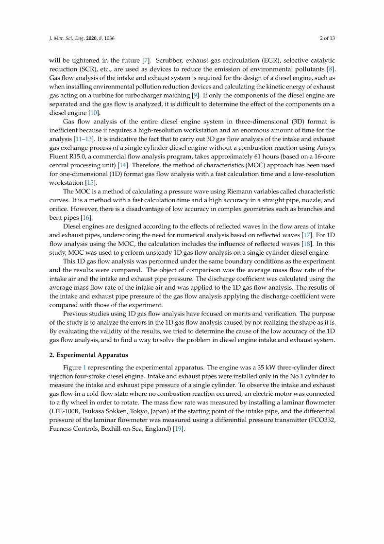
Figure 1 representing the experimental apparatus. The engine was a 35 kW three-cylinder directinjection four-stroke diesel engine. Intake and exhaust pipes were installed only in the No.1 cylinder tomeasure the intake and exhaust pipe pressure of a single cylinder. To observe the intake and exhaustgas flow in a cold flow state where no combustion reaction occurred, an electric motor was connectedto a fly wheel in order to rotate. The mass flow rate was measured by installing a laminar flowmeter(LFE-100B, Tsukasa Sokken, Tokyo, Japan) at the starting point of the intake pipe, and the differentialpressure of the laminar flowmeter was measured using a differential pressure transmitter (FCO332,Furness Controls, Bexhill-on-Sea, England) [19].

J. Mar. Sci. Eng. 2020, 8, 1036 3 of 13

J. Mar. Sci. Eng. 2020, 8, x FOR PEER REVIEW 3 of 14

through which the exhaust gas was released into the atmosphere. CA° refers to the crank angle degrees.

Figure 1. Photograph of the experimental apparatus.

Table 1. Specifications of the experimental apparatus.

Parameter Value Unit Engine speed 700, 900, 1100, 1300, 1500 rpm

Cylinder bore × stroke 0.10 × 0.11 m Compression ratio 17.6 - Intake air method Naturally aspirated -

Volume of intake port 94.25 cm³ Length of exhaust pipe 0.5 m

Diameter of exhaust pipe 0.04 m Air–intake valve opens (AVO) 342 CA° Air–intake valve closes (AVC) 580 CA°

Volume of exhaust port 32.96 cm³ Length of exhaust pipe 1.0 m

Diameter of exhaust pipe 0.04 m Exhaust valve opens (EVO) 130 CA° Exhaust valve closes (EVC) 378 CA°

Figure 2 shows a block diagram of the experimental system. The intake and exhaust pipe pressure was measured using a data acquisition (DAQ) system consisting of a piezoresistive amplifier and a rotary encoder (E6C2-CWZ3E, Omron, Kyoto, Japan) [20]. The pressure sensors were piezoresistive (4045A5, Kistler, Winterthur, Switzerland) and the measurement point was the intake and exhaust pipe 0.15 m away from the cylinder head. The data were acquired at intervals of 0.5 CA° during 100 revolutions while the engine was stable. In order to obtain an accurate measurement, the ensemble average was applied to measured data. The ensemble average was used as a method of calculating the average of remaining values excluding the top 10% and the bottom 10% of the measured data [21]. The pressure results of the intake and exhaust pipe obtained by the ensemble average were used to verify the results of the 1D gas flow analysis.

Figure 1. Photograph of the experimental apparatus.

Table 1 provides the specifications of the experimental apparatus. The intake air method was ina naturally aspirated state, and the experimental data were measured at intervals of 200 rpm in therange of 700–1500 rpm of engine speed. The intake pipe from the surge tank to the cylinder head was astraight pipe with a diameter of 0.04 m and a length of 0.5 m. The exhaust pipe was a straight pipe witha diameter of 0.04 m and a length of 1.0 m, and the end of the exhaust pipe was an open-end throughwhich the exhaust gas was released into the atmosphere. CA◦ refers to the crank angle degrees.

Table 1. Specifications of the experimental apparatus.

Parameter Value Unit

Engine speed 700, 900, 1100, 1300, 1500 rpmCylinder bore × stroke 0.10 × 0.11 m

Compression ratio 17.6 -Intake air method Naturally aspirated -

Volume of intake port 94.25 cm3

Length of exhaust pipe 0.5 mDiameter of exhaust pipe 0.04 m

Air–intake valve opens (AVO) 342 CA◦

Air–intake valve closes (AVC) 580 CA◦

Volume of exhaust port 32.96 cm3

Length of exhaust pipe 1.0 mDiameter of exhaust pipe 0.04 m

Exhaust valve opens (EVO) 130 CA◦

Exhaust valve closes (EVC) 378 CA◦

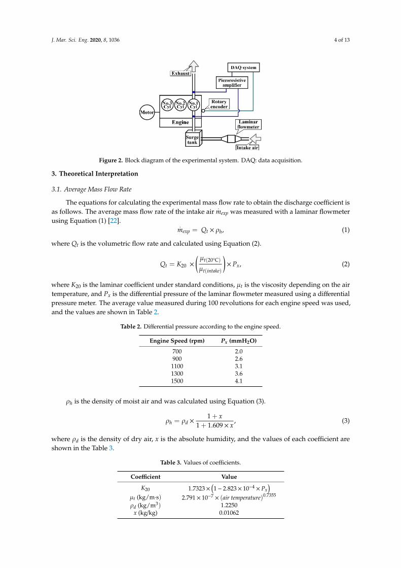
Figure 2 shows a block diagram of the experimental system. The intake and exhaust pipe pressurewas measured using a data acquisition (DAQ) system consisting of a piezoresistive amplifier and arotary encoder (E6C2-CWZ3E, Omron, Kyoto, Japan) [20]. The pressure sensors were piezoresistive(4045A5, Kistler, Winterthur, Switzerland) and the measurement point was the intake and exhaustpipe 0.15 m away from the cylinder head. The data were acquired at intervals of 0.5 CA◦ during100 revolutions while the engine was stable. In order to obtain an accurate measurement, the ensembleaverage was applied to measured data. The ensemble average was used as a method of calculating theaverage of remaining values excluding the top 10% and the bottom 10% of the measured data [21].The pressure results of the intake and exhaust pipe obtained by the ensemble average were used toverify the results of the 1D gas flow analysis.

J. Mar. Sci. Eng. 2020, 8, 1036 4 of 13J. Mar. Sci. Eng. 2020, 8, x FOR PEER REVIEW 4 of 14

Figure 2. Block diagram of the experimental system. DAQ: data acquisition.

3. Theoretical Interpretation

3.1. Average Mass Flow Rate

The equations for calculating the experimental mass flow rate to obtain the discharge coefficient is as follows. The average mass flow rate of the intake air 𝑚 was measured with a laminar flowmeter using Equation (1) [22]. 𝑚 = 𝑄 × 𝜌 , (1)

where 𝑄 is the volumetric flow rate and calculated using Equation (2). 𝑄 = 𝐾 × ( ( ℃)( )) × 𝑃 , (2)

where 𝐾 is the laminar coefficient under standard conditions, 𝜇 is the viscosity depending on the air temperature, and 𝑃 is the differential pressure of the laminar flowmeter measured using a differential pressure meter. The average value measured during 100 revolutions for each engine speed was used, and the values are shown in Table 2.

Table 2. Differential pressure according to the engine speed.

Engine speed (rpm) Px (mmH2O) 700 2.0 900 2.6

1100 3.1 1300 3.6 1500 4.1 𝜌 is the density of moist air and was calculated using Equation (3). 𝜌 = 𝜌 × . × , (3)

where 𝜌 is the density of dry air, 𝑥 is the absolute humidity, and the values of each coefficient are shown in the Table 3.

Table 3. Values of coefficients.

Coefficient Value 𝐾 1.7323 × (1 − 2.823 × 10 × 𝑃 ) 𝜇 (kg/𝑚 ∙ 𝑠) 2.791 × 10 × (𝑎𝑖𝑟 𝑡𝑒𝑚𝑝𝑒𝑟𝑎𝑡𝑢𝑟𝑒) . 𝜌 (kg/𝑚 ) 1.2250 𝑥 (kg/kg) 0.01062

3.2. Method of Charateristics

Figure 2. Block diagram of the experimental system. DAQ: data acquisition.

3. Theoretical Interpretation

3.1. Average Mass Flow Rate

The equations for calculating the experimental mass flow rate to obtain the discharge coefficient isas follows. The average mass flow rate of the intake air

.mexp was measured with a laminar flowmeter

using Equation (1) [22]..

mexp = Qt × ρh, (1)

where Qt is the volumetric flow rate and calculated using Equation (2).

Qt = K20 ×

(µt(20°C)

µt(intake)

)× Px, (2)

where K20 is the laminar coefficient under standard conditions, µt is the viscosity depending on the airtemperature, and Px is the differential pressure of the laminar flowmeter measured using a differentialpressure meter. The average value measured during 100 revolutions for each engine speed was used,and the values are shown in Table 2.

Table 2. Differential pressure according to the engine speed.

Engine Speed (rpm) Px (mmH2O)

700 2.0900 2.6

1100 3.11300 3.61500 4.1

ρh is the density of moist air and was calculated using Equation (3).

ρh = ρd ×1 + x

1 + 1.609× x, (3)

where ρd is the density of dry air, x is the absolute humidity, and the values of each coefficient areshown in the Table 3.

Table 3. Values of coefficients.

Coefficient Value

K20 1.7323×(1− 2.823× 10−4

× Px)

µt (kg/m·s) 2.791× 10−7× (air temperature)0.7355

ρd (kg/m3) 1.2250x (kg/kg) 0.01062

J. Mar. Sci. Eng. 2020, 8, 1036 5 of 13

3.2. Method of Charateristics

The equations for calculating the mass flow rate in 1D model to obtain the discharge coefficient isas follows.

The mass flow rate of the intake air.

mmoc was calculated using the MOC, as follows [18]:

.mmoc = ρ2 × u2 × F2, (4)

where the subscript 2 refers to the downstream conditions.The air density can be calculated with equation related to pressure, specific heat ratio and speed

of sound. ρ2 is the air density under downstream conditions and was calculated using Equation (5).

ρ2 =

(p2

p01

) 1κ

×κ× p01

a012 , (5)

where subscript 01 refers to the upstream stagnation conditions.The speed of sound a01

2 was calculated using the energy equation.

a012 = a2

2 +κ− 1

2× u2

2. (6)

Using Equations (5) and (6), Equation (4) can be expressed as follows:

.mmoc =

p01 × F2

a01×

(2× κ2

κ− 1

)×

(p2

p01

) 2κ

×

1−(

p2

p01

) κ−1κ

12

, (7)

to obtain the characteristics, nondimensional form is required:

ξ f =

.mmoc × a01

p01 × F2×

(2× κ2

κ− 1

)×

(p2

p01

) 2κ

×

1−(

p2

p01

) κ−1κ

12

. (8)

Equation (8) can be computed directly from the pressure ratio( p2

p01

)across the valve or port

depending on the direction of flow. When the flow is choked in the throat, Equation (8) becomes:

ξ f =

.mmoc × a0

p0 × F2= κ×

( 2κ+ 1

) κ+12(κ−1)

, (9)

where subscript 0 refers to the stagnation conditions.The actual gas flow has to take into account the discharge coefficient Cd, which can be calculated

by multiplying Equations (8) and (9) by Cd. If the value of ρh is the same, Cd can be expressed usingEquation (10) [23,24].

Cd =

.mexp.

mmoc. (10)

4. One-Dimensional Gas Flow Analysis

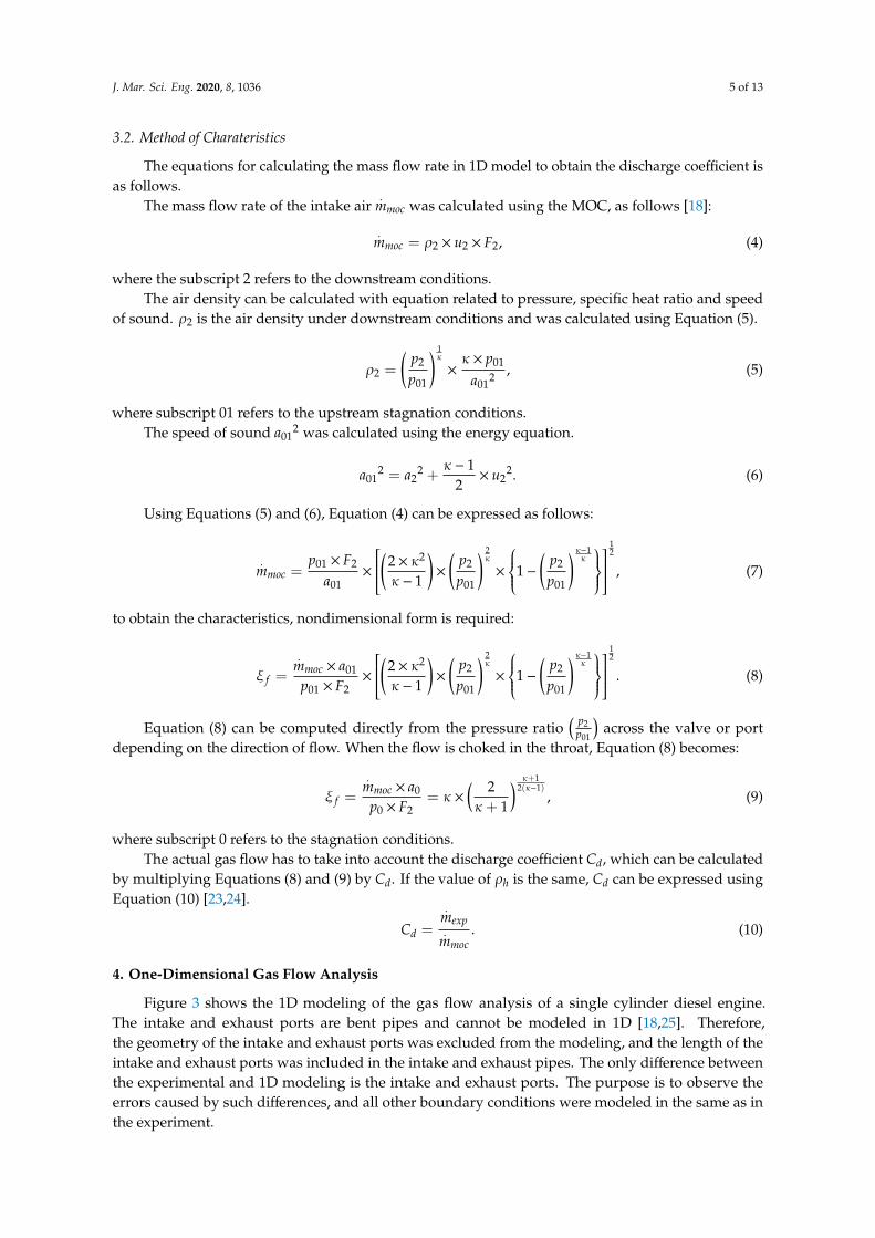
Figure 3 shows the 1D modeling of the gas flow analysis of a single cylinder diesel engine.The intake and exhaust ports are bent pipes and cannot be modeled in 1D [18,25]. Therefore,the geometry of the intake and exhaust ports was excluded from the modeling, and the length of theintake and exhaust ports was included in the intake and exhaust pipes. The only difference betweenthe experimental and 1D modeling is the intake and exhaust ports. The purpose is to observe theerrors caused by such differences, and all other boundary conditions were modeled in the same as inthe experiment.

J. Mar. Sci. Eng. 2020, 8, 1036 6 of 13

The number of meshes was 50 meshes in the intake pipe and 100 meshes in the exhaust pipe.Benson et al. verified the mesh independence in more than 12 meshes of the exhaust pipe [18], and thisstudy confirmed the mesh independence in more than 15 meshes.

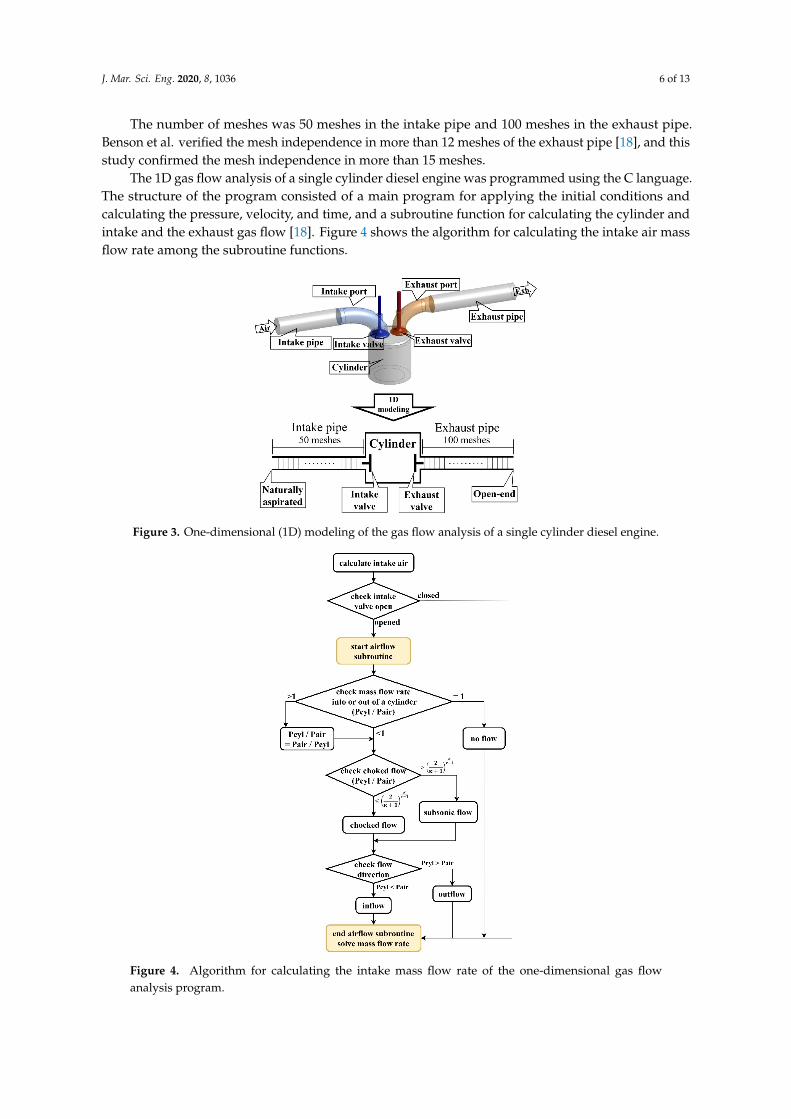
The 1D gas flow analysis of a single cylinder diesel engine was programmed using the C language.The structure of the program consisted of a main program for applying the initial conditions andcalculating the pressure, velocity, and time, and a subroutine function for calculating the cylinder andintake and the exhaust gas flow [18]. Figure 4 shows the algorithm for calculating the intake air massflow rate among the subroutine functions.J. Mar. Sci. Eng. 2020, 8, x FOR PEER REVIEW 6 of 14

Figure 3. One-dimensional (1D) modeling of the gas flow analysis of a single cylinder diesel engine.

The 1D gas flow analysis of a single cylinder diesel engine was programmed using the C language. The structure of the program consisted of a main program for applying the initial conditions and calculating the pressure, velocity, and time, and a subroutine function for calculating the cylinder and intake and the exhaust gas flow [18]. Figure 4 shows the algorithm for calculating the intake air mass flow rate among the subroutine functions.

The calculation of the intake subroutine function came after the cylinder subroutine function, which calculated the pressure and mass flow rate of the cylinder. If the intake valve was open, the intake subroutine function was started. Through the cylinder pressure and intake pressure ratio, it was possible to determine the choked flow, and to calculate whether the type of flow from the cylinder was inflow or outflow. When the characteristics of the flow are determined through the calculation algorithm, the mass flow rate can be calculated using Equation (8) or Equation (9).

Figure 3. One-dimensional (1D) modeling of the gas flow analysis of a single cylinder diesel engine.J. Mar. Sci. Eng. 2020, 8, x FOR PEER REVIEW 7 of 14

Figure 4. Algorithm for calculating the intake mass flow rate of the one-dimensional gas flow analysis program.

5. Results

5.1. Average Mass Flow Rate and Discharge Coefficient

The discharge coefficient was used to correct the difference between the 1D gas flow analysis and the measurement results. The reason is to use the gas flow analysis results to predict the performance of the experimental apparatus.

Figure 5 and Table 4 show the average mass flow rate and the discharge coefficient of the intake air according to the engine speed.

Figure 4. Algorithm for calculating the intake mass flow rate of the one-dimensional gas flowanalysis program.

J. Mar. Sci. Eng. 2020, 8, 1036 7 of 13

The calculation of the intake subroutine function came after the cylinder subroutine function,which calculated the pressure and mass flow rate of the cylinder. If the intake valve was open, the intakesubroutine function was started. Through the cylinder pressure and intake pressure ratio, it waspossible to determine the choked flow, and to calculate whether the type of flow from the cylinderwas inflow or outflow. When the characteristics of the flow are determined through the calculationalgorithm, the mass flow rate can be calculated using Equation (8) or Equation (9).

5. Results

5.1. Average Mass Flow Rate and Discharge Coefficient

The discharge coefficient was used to correct the difference between the 1D gas flow analysis andthe measurement results. The reason is to use the gas flow analysis results to predict the performanceof the experimental apparatus.

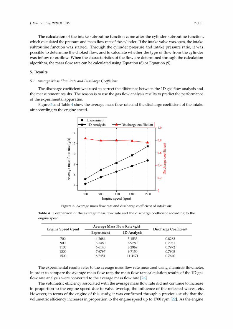
Figure 5 and Table 4 show the average mass flow rate and the discharge coefficient of the intakeair according to the engine speed.J. Mar. Sci. Eng. 2020, 8, x FOR PEER REVIEW 8 of 14

Figure 5. Average mass flow rate and discharge coefficient of intake air.

Table 4. Comparison of the average mass flow rate and the discharge coefficient according to the engine speed.

Engine Speed (rpm) Average Mass Flow Rate (g/s) Discharge Coefficient Experiment 1D Analysis 700 4.2684 5.1533 0.8283 900 5.5480 6.9780 0.7951

1100 6.6140 8.2969 0.7972 1300 7.6797 9.7150 0.7905 1500 8.7451 11.4471 0.7640

The experimental results refer to the average mass flow rate measured using a laminar flowmeter. In order to compare the average mass flow rate, the mass flow rate calculation results of the 1D gas flow rate analysis were converted to the average mass flow rate [26].

The volumetric efficiency associated with the average mass flow rate did not continue to increase in proportion to the engine speed due to valve overlap, the influence of the reflected waves, etc. However, in terms of the engine of this study, it was confirmed through a previous study that the volumetric efficiency increases in proportion to the engine speed up to 1700 rpm [22]. As the engine speed increased to 1500 rpm, the average mass flow rate increased, and the difference between the experiment and the 1D flow analysis results also increased. The reason for the difference in the average mass flow rate is the difference between the actual physical phenomena and the theoretical calculations [27,28]. The higher engine speed is the larger flow rate into the cylinder, so the difference is thought to have occurred because of this. In order to correct the differences in the results of the 1D gas flow analysis, the discharge coefficient was calculated using Equation (10). The discharge coefficient obtained in this way is a correction method for the difference between the experiment and 1D gas flow analysis. Therefore, it can be used to predict the performance of the experimental apparatus through the results of 1D gas flow analysis in the future.

5.2. Mass Flow Rate in One-dimensional Gas Flow Analysis

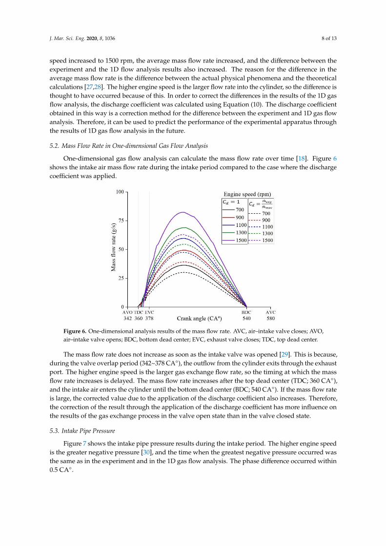
One-dimensional gas flow analysis can calculate the mass flow rate over time [18]. Figure 6 shows the intake air mass flow rate during the intake period compared to the case where the discharge coefficient was applied.

The mass flow rate does not increase as soon as the intake valve was opened [29]. This is because, during the valve overlap period (342~378 CA°), the outflow from the cylinder exits through the

700 900 1100 1300 1500

4

6

8

10

12

14

Experiment 1D Analysis

Engine speed (rpm)

Ave

rage

mas

s flo

w ra

te (g

/s)

Discharge coefficient

0

0.2

0.4

0.6

0.8

1.0

Disc

harg

e co

effic

ient

Figure 5. Average mass flow rate and discharge coefficient of intake air.

Table 4. Comparison of the average mass flow rate and the discharge coefficient according to theengine speed.

Engine Speed (rpm)Average Mass Flow Rate (g/s)

Discharge CoefficientExperiment 1D Analysis

700 4.2684 5.1533 0.8283900 5.5480 6.9780 0.7951

1100 6.6140 8.2969 0.79721300 7.6797 9.7150 0.79051500 8.7451 11.4471 0.7640

The experimental results refer to the average mass flow rate measured using a laminar flowmeter.In order to compare the average mass flow rate, the mass flow rate calculation results of the 1D gasflow rate analysis were converted to the average mass flow rate [26].

The volumetric efficiency associated with the average mass flow rate did not continue to increasein proportion to the engine speed due to valve overlap, the influence of the reflected waves, etc.However, in terms of the engine of this study, it was confirmed through a previous study that thevolumetric efficiency increases in proportion to the engine speed up to 1700 rpm [22]. As the engine

J. Mar. Sci. Eng. 2020, 8, 1036 8 of 13

speed increased to 1500 rpm, the average mass flow rate increased, and the difference between theexperiment and the 1D flow analysis results also increased. The reason for the difference in theaverage mass flow rate is the difference between the actual physical phenomena and the theoreticalcalculations [27,28]. The higher engine speed is the larger flow rate into the cylinder, so the difference isthought to have occurred because of this. In order to correct the differences in the results of the 1D gasflow analysis, the discharge coefficient was calculated using Equation (10). The discharge coefficientobtained in this way is a correction method for the difference between the experiment and 1D gas flowanalysis. Therefore, it can be used to predict the performance of the experimental apparatus throughthe results of 1D gas flow analysis in the future.

5.2. Mass Flow Rate in One-dimensional Gas Flow Analysis

One-dimensional gas flow analysis can calculate the mass flow rate over time [18]. Figure 6shows the intake air mass flow rate during the intake period compared to the case where the dischargecoefficient was applied.

J. Mar. Sci. Eng. 2020, 8, x FOR PEER REVIEW 9 of 14

exhaust port. The higher engine speed is the larger gas exchange flow rate, so the timing at which the mass flow rate increases is delayed. The mass flow rate increases after the top dead center (TDC; 360 CA°), and the intake air enters the cylinder until the bottom dead center (BDC; 540 CA°). If the mass flow rate is large, the corrected value due to the application of the discharge coefficient also increases. Therefore, the correction of the result through the application of the discharge coefficient has more influence on the results of the gas exchange process in the valve open state than in the valve closed state.

Figure 6. One-dimensional analysis results of the mass flow rate. AVC, air–intake valve closes; AVO, air–intake valve opens; BDC, bottom dead center; EVC, exhaust valve closes; TDC, top dead center.

5.3. Intake Pipe Pressure

Figure 7 shows the intake pipe pressure results during the intake period. The higher engine speed is the greater negative pressure [30], and the time when the greatest negative pressure occurred was the same as in the experiment and in the 1D gas flow analysis. The phase difference occurred within 0.5 CA°.

After the exhaust valve closes (EVC; 378 CA°), there is no flow from the cylinder to the exhaust, and the flow enters the cylinder through the intake system. The time it takes for the pressure to rise to atmospheric pressure appeared later as the engine speed increased, which is thought to be due to the large flow rate that entered the cylinder.

By applying a discharge coefficient, errors within the experimental results were reduced. Even when the discharge coefficient was applied, the negative pressure and the pressure change were larger in the 1D gas flow analysis compared to the experiment [31]. The error of the maximum negative pressure decreased by 0.56–1.93% after applying the discharge coefficient and the maximum pressure error decreased by 3.11–7.86%. This is expected to be an error caused by modeling the intake and exhaust ports as straight pipes. When the piston goes down from TDC to BDC, the amount of intake is more in a straight pipe and more gas exchanged in intake and exhaust because there is less loss compared to bent pipes due to an eddy through the pipe [32,33].

In straight pipes, reflected waves are generated at the end of the pipe. However, in bent pipes, reflected waves are generated passing through the bent area [34]. The error in the 1D gas flow analysis is thought to have been caused by not calculating the influence of the reflected wave in bent pipes, as in the experiment [35]. It is expected that errors can be reduced if the geometry of bent pipes, which cannot be modeled in 1D, such as intake ports, are analyzed in 3D and are coupled [36,37].

Figure 6. One-dimensional analysis results of the mass flow rate. AVC, air–intake valve closes; AVO,air–intake valve opens; BDC, bottom dead center; EVC, exhaust valve closes; TDC, top dead center.

The mass flow rate does not increase as soon as the intake valve was opened [29]. This is because,during the valve overlap period (342~378 CA◦), the outflow from the cylinder exits through the exhaustport. The higher engine speed is the larger gas exchange flow rate, so the timing at which the massflow rate increases is delayed. The mass flow rate increases after the top dead center (TDC; 360 CA◦),and the intake air enters the cylinder until the bottom dead center (BDC; 540 CA◦). If the mass flow rateis large, the corrected value due to the application of the discharge coefficient also increases. Therefore,the correction of the result through the application of the discharge coefficient has more influence onthe results of the gas exchange process in the valve open state than in the valve closed state.

5.3. Intake Pipe Pressure

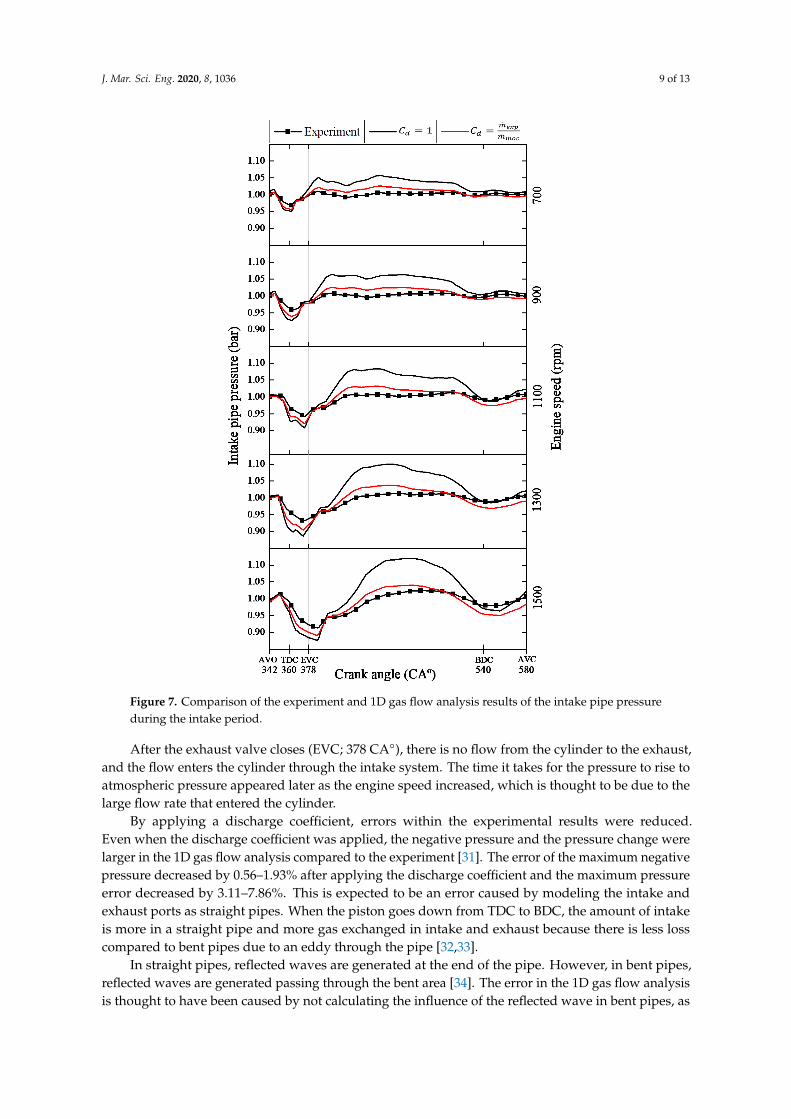
Figure 7 shows the intake pipe pressure results during the intake period. The higher engine speedis the greater negative pressure [30], and the time when the greatest negative pressure occurred wasthe same as in the experiment and in the 1D gas flow analysis. The phase difference occurred within0.5 CA◦.

J. Mar. Sci. Eng. 2020, 8, 1036 9 of 13J. Mar. Sci. Eng. 2020, 8, x FOR PEER REVIEW 10 of 14

Figure 7. Comparison of the experiment and 1D gas flow analysis results of the intake pipe pressure during the intake period.

5.4. Exhaust Pipe Pressure

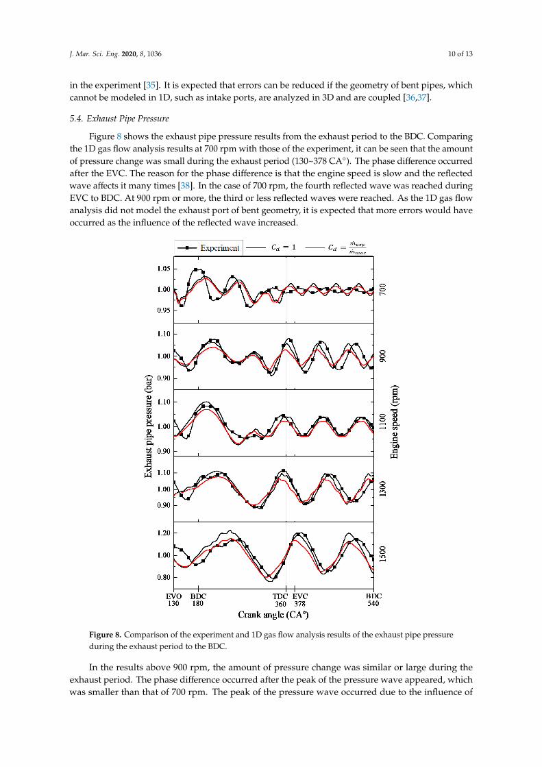
Figure 8 shows the exhaust pipe pressure results from the exhaust period to the BDC. Comparing the 1D gas flow analysis results at 700 rpm with those of the experiment, it can be seen that the amount of pressure change was small during the exhaust period (130~378 CA°). The phase difference occurred after the EVC. The reason for the phase difference is that the engine speed is slow and the reflected wave affects it many times [38]. In the case of 700 rpm, the fourth reflected wave was reached during EVC to BDC. At 900 rpm or more, the third or less reflected waves were reached. As the 1D gas flow analysis did not model the exhaust port of bent geometry, it is expected that more errors would have occurred as the influence of the reflected wave increased.

In the results above 900 rpm, the amount of pressure change was similar or large during the exhaust period. The phase difference occurred after the peak of the pressure wave appeared, which was smaller than that of 700 rpm. The peak of the pressure wave occurred due to the influence of the reflected wave [39]. In all of the results, as the influence of the reflected wave increased, a larger error occurred.

As a result of the calculation by applying the discharge coefficient, the size of the pressure change was reduced, and the phase was not affected. The reason for the phase difference likely occurred because the effect of the reflected wave generated at the open end of the exhaust pipe

Figure 7. Comparison of the experiment and 1D gas flow analysis results of the intake pipe pressureduring the intake period.

After the exhaust valve closes (EVC; 378 CA◦), there is no flow from the cylinder to the exhaust,and the flow enters the cylinder through the intake system. The time it takes for the pressure to rise toatmospheric pressure appeared later as the engine speed increased, which is thought to be due to thelarge flow rate that entered the cylinder.

By applying a discharge coefficient, errors within the experimental results were reduced.Even when the discharge coefficient was applied, the negative pressure and the pressure change werelarger in the 1D gas flow analysis compared to the experiment [31]. The error of the maximum negativepressure decreased by 0.56–1.93% after applying the discharge coefficient and the maximum pressureerror decreased by 3.11–7.86%. This is expected to be an error caused by modeling the intake andexhaust ports as straight pipes. When the piston goes down from TDC to BDC, the amount of intakeis more in a straight pipe and more gas exchanged in intake and exhaust because there is less losscompared to bent pipes due to an eddy through the pipe [32,33].

In straight pipes, reflected waves are generated at the end of the pipe. However, in bent pipes,reflected waves are generated passing through the bent area [34]. The error in the 1D gas flow analysisis thought to have been caused by not calculating the influence of the reflected wave in bent pipes, as

J. Mar. Sci. Eng. 2020, 8, 1036 10 of 13

in the experiment [35]. It is expected that errors can be reduced if the geometry of bent pipes, whichcannot be modeled in 1D, such as intake ports, are analyzed in 3D and are coupled [36,37].

5.4. Exhaust Pipe Pressure

Figure 8 shows the exhaust pipe pressure results from the exhaust period to the BDC. Comparingthe 1D gas flow analysis results at 700 rpm with those of the experiment, it can be seen that the amountof pressure change was small during the exhaust period (130~378 CA◦). The phase difference occurredafter the EVC. The reason for the phase difference is that the engine speed is slow and the reflectedwave affects it many times [38]. In the case of 700 rpm, the fourth reflected wave was reached duringEVC to BDC. At 900 rpm or more, the third or less reflected waves were reached. As the 1D gas flowanalysis did not model the exhaust port of bent geometry, it is expected that more errors would haveoccurred as the influence of the reflected wave increased.

J. Mar. Sci. Eng. 2020, 8, x FOR PEER REVIEW 11 of 14

reached the exhaust port and affected the calculation. For the same reason as the intake port, the exhaust port could not be modeled in the same geometry as in the experiment. It is necessary to reduce the error in the 1D gas flow analysis caused by bent pipes not only for the intake system, but also for the exhaust system.

When the discharge coefficient was applied, the error of the minimum pressure increased by 0.46–6.14%. In addition, the error of the maximum pressure increased by 0.53–5.03% at 900 rpm or higher. Applying the discharge coefficient was not effective in reducing the error of the exhaust pipe pressure.

Figure 8. Comparison of the experiment and 1D gas flow analysis results of the exhaust pipe pressure during the exhaust period to the BDC.

Summarizing the intake and exhaust pipe pressure results, the error of the intake pipe pressure is improved. However, since it is a result of reducing the difference in the intake mass flow rate, it is not a fundamental improvement method for the error occurring in the 1D gas flow analysis. Also, the error of the exhaust pipe pressure was not improved even when the discharge coefficient was applied. It is expected that such errors will be improved only when a method to improve errors occurring in complex shapes, which is a disadvantage of 1D, is used.

6. Conclusion

Figure 8. Comparison of the experiment and 1D gas flow analysis results of the exhaust pipe pressureduring the exhaust period to the BDC.

In the results above 900 rpm, the amount of pressure change was similar or large during theexhaust period. The phase difference occurred after the peak of the pressure wave appeared, whichwas smaller than that of 700 rpm. The peak of the pressure wave occurred due to the influence of

J. Mar. Sci. Eng. 2020, 8, 1036 11 of 13

the reflected wave [39]. In all of the results, as the influence of the reflected wave increased, a largererror occurred.

As a result of the calculation by applying the discharge coefficient, the size of the pressure changewas reduced, and the phase was not affected. The reason for the phase difference likely occurredbecause the effect of the reflected wave generated at the open end of the exhaust pipe reached theexhaust port and affected the calculation. For the same reason as the intake port, the exhaust port couldnot be modeled in the same geometry as in the experiment. It is necessary to reduce the error in the 1Dgas flow analysis caused by bent pipes not only for the intake system, but also for the exhaust system.

When the discharge coefficient was applied, the error of the minimum pressure increased by0.46–6.14%. In addition, the error of the maximum pressure increased by 0.53–5.03% at 900 rpmor higher. Applying the discharge coefficient was not effective in reducing the error of the exhaustpipe pressure.

Summarizing the intake and exhaust pipe pressure results, the error of the intake pipe pressure isimproved. However, since it is a result of reducing the difference in the intake mass flow rate, it is nota fundamental improvement method for the error occurring in the 1D gas flow analysis. Also, theerror of the exhaust pipe pressure was not improved even when the discharge coefficient was applied.It is expected that such errors will be improved only when a method to improve errors occurring incomplex shapes, which is a disadvantage of 1D, is used.

6. Conclusions

A 1D gas flow analysis was performed using the MOC for a single cylinder diesel engine, and theresults of comparing the average mass flow rate and the intake and exhaust pipe pressure with theresults of the experiment are summarized as follows:

(1) The average mass flow rate of the 1D gas flow analysis was larger than that of the experimentalresults, and the discharge coefficient was calculated using this.

(2) The 1D gas flow analysis was performed by applying the discharge coefficient, and the accuracyof the intake pipe pressure results was improved.

(3) In the exhaust pipe result of the 1D gas flow analysis, there was a difference in pressure andphase, and there was no improvement even when the discharge coefficient was applied.

(4) Applying the discharge coefficient is not a fundamental method to improve the error of 1D gasflow analysis, and the error that occurs due to the complex shape must be improved.

(5) If the shortcomings of the 1D gas flow analysis, which cannot model the bent pipe geometry ofthe intake and exhaust ports, are compensated, the error is expected to decrease.

As a result of the experiment and verification, there was a limit to increasing the accuracy, evenwhen applying the discharge coefficient obtained using the average mass flow rate. This error isthought to be due to the disadvantage of 1D gas flow analysis, which cannot calculate complexgeometries. In the future, it is expected that this problem can be solved by analyzing the complexgeometries in 3D and using 1D–3D coupling gas flow analysis.

Author Contributions: Conceptualization and methodology, K.-J.K.; experimental system configuration and datacuration, K.-H.K.; software, K.-J.K.; writing and validation, K.-J.K. and K.-H.K.; supervision, K.-J.K. and K.-H.K.All authors have read and agreed to the published version of the manuscript.

Funding: This research received no external funding.

Acknowledgments: The authors would like to acknowledgment the Turbo Engine Lab, Department ofMechanical System Engineering, Pukyong National University for purchasing and supporting the use ofthe experimental apparatus.

Conflicts of Interest: The authors declare no conflict of interest.

J. Mar. Sci. Eng. 2020, 8, 1036 12 of 13

References

1. Abdullah, N.R.; Shahruddin, N.S.; Mamat, R.; Mohd, A.; Mamat, I.; Zulkifli, A. Effects of air intake pressureon the engine performance, fuel economy and exhaust emissions of a small gasoline engine. J. Mech. Eng. Sci.2014, 6, 949–958. [CrossRef]

2. Schulten, P.J.M.; Stapersma, D. Mean value modelling of the gas exchange of a 4-stroke diesel engine for usein powertrain applications. SAE Tech. Pap. 2003. [CrossRef]

3. Kocher, L.; Koeberlein, E.; Van Alstine, D.G.; Stricker, K.; Shaver, G. Physically based volumetric efficiencymodel for diesel engines utilizing variable intake valve actuation. Int. J. Engine Res. 2012, 13, 169–184.[CrossRef]

4. Lu, X.-C.; Yang, J.-G.; Zhang, W.-G.; Huang, Z. Effect of cetane number improver on heat release rate andemissions of high speed diesel engine fueled with ethanol–diesel blend fuel. Fuel 2004, 83, 2013–2020.[CrossRef]

5. Papagiannakis, R.G.; Rakopoulos, C.D.; Hountalas, D.T.; Rakopoulos, D.C. Emission characteristics of highspeed, dual fuel, compression ignition engine operating in a wide range of natural gas/diesel fuel proportions.Fuel 2010, 89, 1397–1406. [CrossRef]

6. Kopac, M.; Kokturk, L. Determination of optimum speed of an internal combustion engine by exergy analysis.Int. J. Energy 2005, 2, 40–54. [CrossRef]

7. International Maritime Organization (IMO). Effective date of implementation of the fuel oil standard inregulation. Marpol Annex VI Resolut. MEPC 2016, 280, 1.

8. Johnson, B.T. Diesel Engine Emissions and Their Control. Platin. Met. Rev. 2008, 52, 23–37. [CrossRef]9. Davies, P.O.A.L. Piston engine intake and exhaust system design. J. Sound Vib. 1996, 190, 677–712. [CrossRef]10. Albarbar, A. Diesel engine fuel injection monitoring using acoustic measurements and independent

component analysis. Measurement 2010, 43, 1376–1386. [CrossRef]11. Onorati, A.; Montenegro, G.; D’Errico, G.; Piscaglia, F. Integrated 1d–3d fluid dynamic simulation of a

turbocharged diesel engine with complete intake and exhaust systems. SAE Tech. Pap. 2010. [CrossRef]12. Wurzenberger, J.C.; Wanker, R. Multi-Scale Scr Modeling, 1d Kinetic Analysis and 3d System Simulation; SAE

International: Warrendale, PA, USA, 2005. [CrossRef]13. Zinner, C.; Jandl, S.; Schmidt, S. Comparison of different downsizing strategies for 2- and 3-cylinder engines

by the use of 1d-cfd simulation. In Proceedings of the SAE/JSAE 2016 Small Engine Technology Conference& Exhibition, Charleston, SC, USA, 15–17 November 2016.

14. Kim, K.H.; Kong, K.J. Validation of diesel engine gas flow one-dimensional numerical analysis using themethod of characteristics. J. Korean Soc. Fish Ocean Technol. 2020, 56, 230–237. [CrossRef]

15. Brown, G.L. Determination of two-stroke engine exhaust noise by the method of characteristics. J. Sound Vib.1982, 82, 305–327.

16. Winterbone, D.E.; Pearson, R.J. Theory of Engine Manifold Design: Wave Action Methods for IC Engines;Wiley-Blackwell: Hoboken, NJ, USA, 2000; pp. 179–274.

17. Winterbone, D.E.; Pearson, R.J. Design Techniques for Engine Manifolds: Wave Action Methods for IC Engines;Wiley-Blackwell: Hoboken, NJ, USA, 1999; pp. 27–150.

18. Benson, R.S.; Horlock, J.H.; Winterbone, D.E. The Thermodynamics and Gas Dynamics of Internal-CombustionEngines; Oxford University Press: Oxford, UK, 1982; Volume 1, pp. 73–313.

19. Ohtsubo, H.; Yamauchi, K.; Nakazono, T.; Yamane, K.; Kawasaki, K. Influence of compression ratio onperformance and variations in each cylinder of multi-cylinder natural gas engine with pcci combustion.SAE Trans. 2007, 116, 396–404.

20. Han, B.; Guan, X.; Ou, J. Electrode design, measuring method and data acquisition system of carbon fibercement paste piezoresistive sensors. Sens. Actuators A 2007, 135, 360–369. [CrossRef]

21. Amann, C.A. Cylinder-pressure measurement and its use in engine research. SAE Trans. 1985, 94, 418–435.22. Lee, S.D.; Kang, H.Y.; Koh, D.K.; Ahn, S.K. The effect of intake and exhaust pulsating flow on the volumetric

efficiency in a diesel engine. J. Korean Soc. Power Syst. Eng. 2006, 9, 19–25.23. Borghei, S.M.; Jalili, M.R.; Ghodsian, M. Discharge coefficient for sharp-crested side weir in subcritical flow.

J. Hydraul. Eng. 1999, 125. [CrossRef]24. Chu, C.R.; Chiu, Y.-H.; Chen, Y.-J.; Wang, Y.-W.; Chou, C.-P. Turbulence effects on the discharge coefficient

and mean flow rate of wind-driven cross-ventilation. Build. Environ. 2009, 44, 2064–2072. [CrossRef]

J. Mar. Sci. Eng. 2020, 8, 1036 13 of 13

25. Hufnagel, L.; Canton, J.; Örlü, R.; Marin, O.; Merzari, E.; Schlatter, P. The three-dimensional structure ofswirl-switching in bent pipe flow. J. Fluid Mech. 2018, 835, 86–101. [CrossRef]

26. Tabaczynski, R.J.; Heywood, J.B.; Keck, J.C. Time-resolved measurements of hydrocarbon mass flowrate inthe exhaust of a spark-ignition engine. SAE Tech. Pap. 1972. [CrossRef]

27. Ramezanizadeh, M.; Alhuyi Nazari, M.; Ahmadi, M.H.; Chau, K. Experimental and numerical analysis of ananofluidic thermosyphon heat exchanger. Eng. Appl. Comput. Fluid Mech. 2019, 13, 40–47. [CrossRef]

28. Kim, S.J.; Jang, S.P. Experimental and numerical analysis of heat transfer phenomena in a sensor tube of amass flow controller. Int. J. Heat Mass Transf. 2001, 44, 1711–1724. [CrossRef]

29. Harrison, M.F.; Stanev, P.T. Measuring wave dynamics in ic engine intake systems. J. Sound Vib. 2004, 269,389–408. [CrossRef]

30. Ceccarani, M.; Rebottini, C.; Bettini, R. Engine misfire monitoring for a v12 engine by exhaust pressureanalysis. SAE Tech. Pap. 1998. [CrossRef]

31. Takahashi, H.; Ogino, S.; Nishimura, T.; Okuno, Y. Experimental analysis for the improvement of radiatorcooling air intake and discharge. SAE Tech. Pap. 1992. [CrossRef]

32. Lu, J.-T.; Hsueh, Y.-C.; Huang, Y.-R.; Hwang, Y.-J.; Sun, C.-K. Bending loss of terahertz pipe waveguides.Opt. Express 2010, 18, 26332–26338. [CrossRef]

33. Simizu, Y.; Sugino, K.; Kuzuhara, S. Hydraulic losses and flow patterns in bent pipes. Bull. JSME 1982, 25,24–31. [CrossRef]

34. Ohyagi, S.; Obara, T.; Nakata, F.; Hoshi, S. A numerical simulation of reflection processes of a detonationwave on a wedge. Shock Waves 2000, 10, 185–190. [CrossRef]

35. Parker, K.H.; Jones, C.J.H. Forward and Backward Running Waves in the Arteries: Analysis Using theMethod of Characteristics. J. Biomech. Eng. 1990, 112, 322–326. [CrossRef]

36. Kong, K.-J.; Jung, S.-H.; Jeong, T.-Y.; Koh, D.-K. 1d–3d coupling algorithm for unsteady gas flow analysis inpipe systems. J. Mech. Sci. Technol. 2019, 33, 4521–4528. [CrossRef]

37. Coghe, A.; Brunello, G.; Tassi, E. Effects of Intake Ports on the In-Cylinder Air Motion under Steady FlowConditions. SAE Tech. Pap. 1988. [CrossRef]

38. HeyWood, J. Internal Combustion Engine Fundamental; McGraw-Hill Book Company: New York, NY, USA,1988; pp. 748–8161.

39. Khir, A.W.; Parker, K.H. Measurements of wave speed and reflected waves in elastic tubes and bifurcations.J. Biomech. 2002, 35, 775–783. [CrossRef]

Publisher’s Note: MDPI stays neutral with regard to jurisdictional claims in published maps and institutionalaffiliations.

© 2020 by the authors. Licensee MDPI, Basel, Switzerland. This article is an open accessarticle distributed under the terms and conditions of the Creative Commons Attribution(CC BY) license (http://creativecommons.org/licenses/by/4.0/).