Three-dimensional finite element solution of gas-assisted injection moulding

INTERNATIONAL JOURNAL FOR NUMERICAL METHODS IN ENGINEERINGInt. J. Numer. Meth. Engng 2002; 53:2003–2017 (DOI: 10.1002/nme.370)

Three-dimensional *nite element solution of gas-assistedinjection moulding†

F. Ilinca∗;‡ and J.-F. H1etu

Industrial Materials Institute; National Research Council of Canada; 75 de Mortagne;Boucherville; Qu�ebec; J4B 6Y4 Canada

SUMMARY

This paper presents a *nite element algorithm for solving gas-assisted injection moulding problems. The*lling material is considered incompressible and has temperature and shear rate dependent viscosity. Thesolution of the three-dimensional (3D) equations modelling the momentum, mass and energy conserva-tion is coupled with two front-tracking equations, which are solved for the polymer=air and gas=polymerinterfaces. The performances of the proposed procedure are quanti*ed by solving the gas-assistedinjection problem on a thin plate with a ;ow channel. Solutions are shown for di<erent polymer=gasratios injected. The e<ect of the melt temperature, gas pressure and gas injection delay, on the solutionbehaviour is also investigated. The approach is then applied to a thick 3D part. Published in 2001 byJohn Wiley & Sons, Ltd.

KEY WORDS: mould-*lling; gas-assisted; *nite elements; three-dimensional

1. INTRODUCTION

Gas-assisted injection moulding is an increasingly used manufacturing process presentingimportant advantages over traditional injection moulding. The process requires lower injection-packing pressure, smaller cooling times and less moulding material than conventionalinjection moulding, allowing production of lighter parts. Gas-assisted moulded parts presentmore uniform properties, reduced shrinkage, warpage and residual stresses. Therefore, better*nal products are produced at lower costs.

The process consists of an initial phase during which the polymer is injected, followed bythe injection of the gas. In the present work, we consider that the polymer *lling is incomplete.Therefore, part of the cavity remains empty at the end of the polymer injection. Then, thegas pushes forward the polymer to complete the *lling and forms an expanding bubble insidethe part. Gas penetrates especially through wider sections, as the resistance to the ;ow is

∗Correspondence to: F. Ilinca, National Research Council of Canada, 75 de Mortagne Boulevard, Boucherville,Qu1ebec, J4B 6Y4 Canada

‡E-mail: ;[email protected]†Copyright to the Crown in the right of Canada

Received 30 March 2001Published in 2001 by John Wiley & Sons, Ltd. Revised 30 May 2001

2004 F. ILINCA AND J.-F. H 1ETU

smaller in these high temperature regions. If the ;ow leaders design is appropriate, the gaswill generate an uniform pressure distribution inside the cavity reducing warpage and residualstresses.

Temperature and pressure play very important roles in the dynamics of the gas-assistedinjection process. The gas penetration is determined by the equilibrium between the gas pres-sure and the viscous stresses inside the polymer melt. As viscosity depends on both tempera-ture and shear rate, the setting up of optimal moulding conditions is a diHcult task. Low gaspressure may result in higher than expected gas injection time, lower temperature and possiblyincomplete *lling. The same is true for too low melt temperature. On the other hand, if thegas pressure and=or melt temperature are too high, the gas penetrates into the thin sectionsof the cavity and produces *ngering defects. Another important parameter is the amount ofpolymer injected in the cavity. The volume of polymer must be small enough to allow thegas to *ll the ;ow channels. However, gas penetration must avoid formation of undesirablethin polymer skin or gas *ngering.

As for the traditional injection moulding, the numerical simulations of gas-assisted injectionare mostly based on the thin wall, Hele–Shaw approximation [1–3]. While for parts presentingthick sections such approach is clearly inappropriate, even for thin parts a mid-plane approachmay be rough, as the gas penetration is a three-dimensional (3D) phenomenon. Chen et al. [1]used a particle-tracking algorithm for computing both gas and melt front advancements. Theirmethodology is based on models describing the coating melt thickness existing between thesolidi*ed material and the gas=melt interface, as a function of processing parameters, materialproperties and ;ow geometry. Such model is generally valid for a narrow range of parameters,and has to be generated on a case by case basis. This is a major inconvenience because veryoften computations have to be done for di<erent conditions, in order to get the optimum design.In many applications, it is important to provide not only the depth of the gas penetration, butalso details on the gas core shape and polymer skin thickness. Therefore, a true 3D solutionof the injection process is needed.

Initial work on the 3D simulation of the gas-assisted injection moulding process was doneby Khayat et al. [4], which used a boundary element method. Their contribution reduces to theanalysis of isothermal, incompressible, Newtonian ;uid ;ow in simple 3D geometries. Haaghet al. [5] present a 3D model based on the *nite element method and a pseudo-concentrationtechnique for tracking the ;ow interfaces. Two-dimensional (2D) applications of the ;owaround a sharp corner and near bifurcations show the need for accurate description of thegas-polymer interface. Three-dimensional solution for the isothermal, Newtonian ;uid case ina rectangular tube is also shown.

This paper presents numerical simulations of gas-assisted injection problems based on a*nite element solution of the complete 3D equations describing the ;ow and heat transfer. Twoadditional transport equations are solved in order to track the polymer=air and gas=polymerinterfaces. The polymer melt is considered incompressible and it behaves as a generalizedNewtonian ;uid. Incompressibility determines that both the volume of polymer and gasentering the cavity can be controlled. Equations are solved using stabilized *nite elementformulations. Momentum-continuity and front tracking equations are solved by a streamlineupwind Petrov–Galerkin (SUPG) method [6]. Energy equation is solved using an operatorsplitting scheme. First, the advective problem is solved by a ;ux-corrected transport (FCT)approach [7]. Then, di<usion and source terms are solved by using a Galerkin gradient least-squares (GGLS) method [8]. Section 2 presents the governing equations of the mathematical

Published in 2001 by John Wiley & Sons, Ltd. Int. J. Numer. Meth. Engng 2002; 53:2003–2017

THREE-DIMENSIONAL FE SOLUTION OF GAS-ASSISTED INJECTION MOULDING 2005

model. The *nite element formulations and solution algorithm are summarized in Section 3.The methodology is validated in Section 4 for the isothermal *lling of a channel. Section 5shows the results for the gas-assisted injection moulding of a thin plate with a ;ow channeland of a thick part.

2. MATHEMATICAL MODEL

During the *lling of high viscosity polymer melts inertia e<ects are negligible. Therefore, thepolymer ;ow is described by the incompressible Stokes equations:

0 =−∇p+∇ · [2��(u)] (1)

−∇ · u=0 (2)

where

�(u)= (∇u+∇uT)=2 (3)

The heat transfer is modelled by the energy equation:

�cp

(@T@t

+ u · ∇T)

=∇ · (k∇T ) + 2��2 (4)

In the above equations, t; u; p; T; �; �; cp and k denote time, velocity, pressure, tem-perature, density, viscosity, speci*c heat and thermal conductivity, respectively. For the pro-cess under study, the gas is considered inviscid and perfectly compressible. Hence, pressuregradient vanishes on gas-*lled elements and continuity is not required. A pressure equal tothe gas pressure is imposed on the gas region. Moreover, because the Capillary numbers atthe polymer=air and gas=polymer interfaces are high [5], surface tension e<ects are neglected.

The position of the polymer=air and gas=polymer interfaces is modelled using a pseudo-concentration method [9]. The approach de*nes smooth functions Fi such that the critical value,Fc, represents the position of the interface. We consider i=1 and i=2 for the polymer=airand gas=polymer interfaces, respectively. The functions Fi(x; t) are de*ned as

Fi(x; t)=

Fc + di(x; t); x in *lled region

Fc; x on the interface

Fc − di(x; t); x in empty region

(5)

where di(x; t) represents the distance from the interface [10]. A front tracking value greaterthan Fc, denotes a region *lled by the polymer, while a smaller than Fc value correspondsto an empty region (*lled with air or gas, respectively). The interpretation of the variouscombinations obtained from F1 and F2 are summarized in Table I. Initial values Fi(x; t=0)are given to de*ne the initial position of the ;ow front. The pseudo-concentration functions arethen convected using the velocity *eld provided by the solution of the momentum-continuityequations:

@Fi@t

+ u · ∇Fi=0 (6)



Table I. De*nition of *lled and empty regions.

F1¿Fc F1¡Fc

F2¿Fc Polymer Empty (air)F2¡Fc Gas Gas breakthrough

Boundary conditions must complete the statement of the problem. During the polymerinjection, the velocity and temperature are imposed on the inlet section. When gas is injected,the gas pressure is imposed on the volume occupied by the gas. No-slip boundary conditionsare imposed on the cavity walls *lled by the polymer, while on the un*lled part, a freeboundary condition allows for the formation of the typical fountain ;ow. Heat transfer betweenthe cavity and the mould is given by

q= hc(T − Tmould) on Qmould (7)

where hc is a surface heat transfer coeHcient and Tmould is the mould temperature.

3. NUMERICAL APPROACH

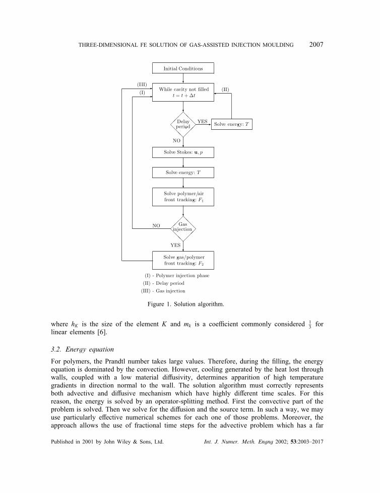
Model equations are discretized in time using a *rst-order implicit Euler scheme. At each timestep, the global system of equations is solved in a partly segregated manner. The solutionalgorithm is illustrated in Figure 1. When polymer is injected (I), only the front trackingfunction for polymer=air interface is solved, while during the gas injection (III) both fronttracking functions are computed. If gas injection is delayed, between the end of the polymerinjection and the beginning of the gas injection (II), only the energy equation is solved. The*nite element formulations of the equations are discussed in this section.

3.1. Momentum-continuity equations

The Stokes equations (1) and (2) are solved using a SUPG method [6]. This method containsan additional pressure stabilization term compared with the standard Galerkin method. In sucha way, the use of linear elements for both the velocity and pressure is permitted. The SUPGvariational formulation of the momentum-continuity equations is [6]

∫R2��(u) : �(v) dR−

∫Rp∇ · v dR +

∫R∇ · uq dR

+∑K

∫RK

{∇p−∇ · [2��(u)]} · �u∇q dRK =0 (8)

The stabilization parameter �u is de*ned as in Reference [11]

�u=mkh2K4�

(9)



Figure 1. Solution algorithm.

where hK is the size of the element K and mk is a coeHcient commonly considered 13 for

linear elements [6].

3.2. Energy equation

For polymers, the Prandtl number takes large values. Therefore, during the *lling, the energyequation is dominated by the convection. However, cooling generated by the heat lost throughwalls, coupled with a low material di<usivity, determines apparition of high temperaturegradients in direction normal to the wall. The solution algorithm must correctly representsboth advective and di<usive mechanism which have highly di<erent time scales. For thisreason, the energy is solved by an operator-splitting method. First the convective part of theproblem is solved. Then we solve for the di<usion and the source term. In such a way, we mayuse particularly e<ective numerical schemes for each one of those problems. Moreover, theapproach allows the use of fractional time steps for the advective problem which has a far



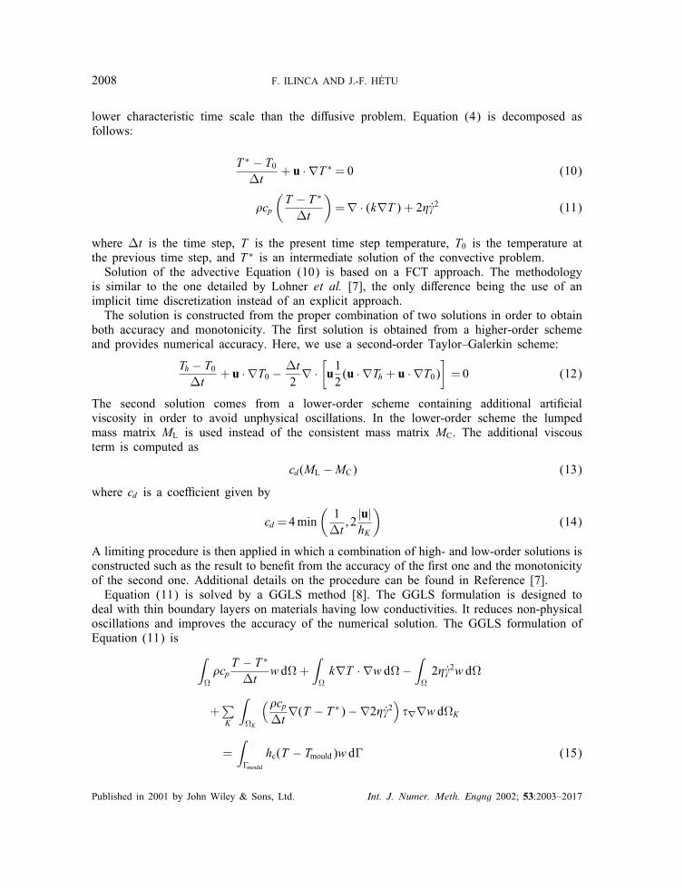
lower characteristic time scale than the di<usive problem. Equation (4) is decomposed asfollows:

T ∗ − T0St

+ u · ∇T ∗ =0 (10)

�cp

(T − T ∗

St

)=∇ · (k∇T ) + 2��2 (11)

where St is the time step, T is the present time step temperature, T0 is the temperature atthe previous time step, and T ∗ is an intermediate solution of the convective problem.

Solution of the advective Equation (10) is based on a FCT approach. The methodologyis similar to the one detailed by Lohner et al. [7], the only di<erence being the use of animplicit time discretization instead of an explicit approach.

The solution is constructed from the proper combination of two solutions in order to obtainboth accuracy and monotonicity. The *rst solution is obtained from a higher-order schemeand provides numerical accuracy. Here, we use a second-order Taylor–Galerkin scheme:

Th − T0St

+ u · ∇T0 − St2∇ ·

[u12(u · ∇Th + u · ∇T0)

]=0 (12)

The second solution comes from a lower-order scheme containing additional arti*cialviscosity in order to avoid unphysical oscillations. In the lower-order scheme the lumpedmass matrix ML is used instead of the consistent mass matrix MC. The additional viscousterm is computed as

cd(ML −MC) (13)

where cd is a coeHcient given by

cd=4min(

1St; 2

|u|hK

)(14)

A limiting procedure is then applied in which a combination of high- and low-order solutions isconstructed such as the result to bene*t from the accuracy of the *rst one and the monotonicityof the second one. Additional details on the procedure can be found in Reference [7].

Equation (11) is solved by a GGLS method [8]. The GGLS formulation is designed todeal with thin boundary layers on materials having low conductivities. It reduces non-physicaloscillations and improves the accuracy of the numerical solution. The GGLS formulation ofEquation (11) is

∫R�cpT − T ∗

Stw dR +

∫Rk∇T · ∇w dR−

∫R

2��2w dR

+∑K

∫RK

(�cpSt

∇(T − T ∗)−∇2��2)�∇∇w dRK

=∫Qmould

hc(T − Tmould)w dQ (15)



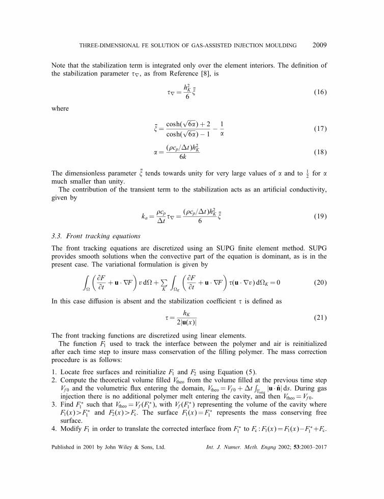
Note that the stabilization term is integrated only over the element interiors. The de*nition ofthe stabilization parameter �∇, as from Reference [8], is

�∇ =h2K6

T� (16)

where

T�=cosh(

√6�) + 2

cosh(√6�)− 1

− 1�

(17)

�=(�cp=St)h2K

6k(18)

The dimensionless parameter T� tends towards unity for very large values of � and to 12 for �

much smaller than unity.The contribution of the transient term to the stabilization acts as an arti*cial conductivity,

given by

ka=�cpSt�∇ =

(�cp=St)h2K6

T� (19)

3.3. Front tracking equations

The front tracking equations are discretized using an SUPG *nite element method. SUPGprovides smooth solutions when the convective part of the equation is dominant, as is in thepresent case. The variational formulation is given by

∫R

(@F@t

+ u · ∇F)v dR +

∑K

∫RK

(@F@t

+ u · ∇F)�(u · ∇v) dRK =0 (20)

In this case di<usion is absent and the stabilization coeHcient � is de*ned as

�=hK

2|u(x)| (21)

The front tracking functions are discretized using linear elements.The function F1 used to track the interface between the polymer and air is reinitialized

after each time step to insure mass conservation of the *lling polymer. The mass correctionprocedure is as follows:

1. Locate free surfaces and reinitialize F1 and F2 using Equation (5).2. Compute the theoretical volume *lled Vtheo from the volume *lled at the previous time stepVf0 and the volumetric ;ux entering the domain, Vtheo =Vf0 + St

∫Qinlet

|u · n| ds. During gasinjection there is no additional polymer melt entering the cavity, and then Vtheo =Vf0.

3. Find F∗1 such that Vtheo =Vf(F∗

1 ), with Vf(F∗1 ) representing the volume of the cavity where

F1(x)¿F∗1 and F2(x)¿Fc. The surface F1(x)=F∗

1 represents the mass conserving freesurface.

4. Modify F1 in order to translate the corrected interface from F∗1 to Fc :F1(x)=F1(x)−F∗

1 +Fc.



4. VALIDATION

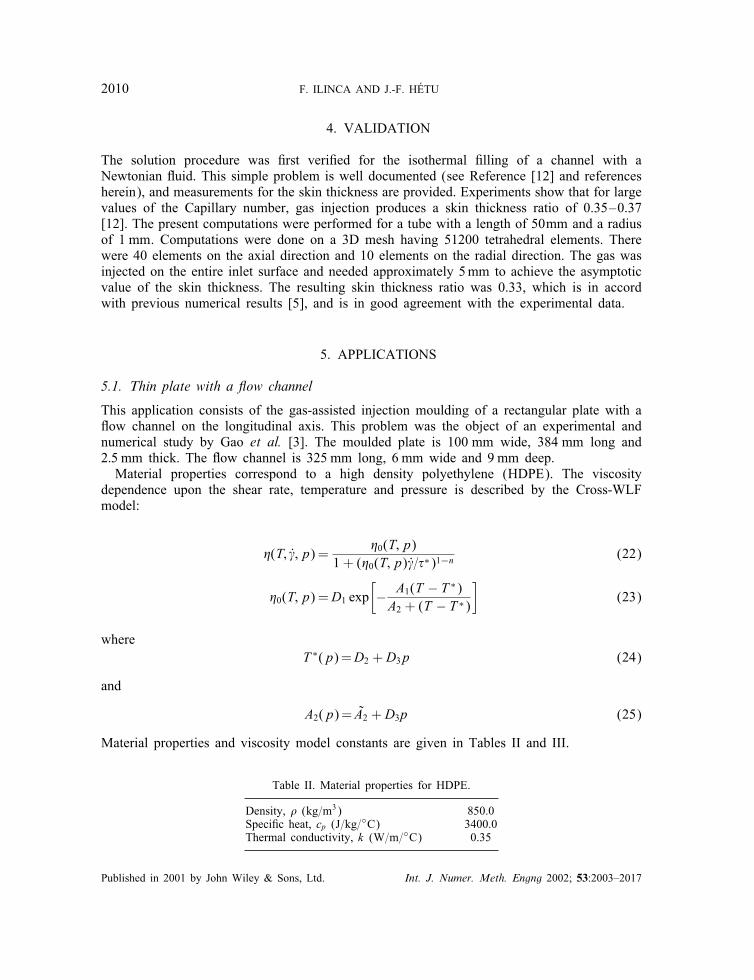
The solution procedure was *rst veri*ed for the isothermal *lling of a channel with aNewtonian ;uid. This simple problem is well documented (see Reference [12] and referencesherein), and measurements for the skin thickness are provided. Experiments show that for largevalues of the Capillary number, gas injection produces a skin thickness ratio of 0.35–0.37[12]. The present computations were performed for a tube with a length of 50mm and a radiusof 1 mm. Computations were done on a 3D mesh having 51200 tetrahedral elements. Therewere 40 elements on the axial direction and 10 elements on the radial direction. The gas wasinjected on the entire inlet surface and needed approximately 5mm to achieve the asymptoticvalue of the skin thickness. The resulting skin thickness ratio was 0.33, which is in accordwith previous numerical results [5], and is in good agreement with the experimental data.

5. APPLICATIONS

5.1. Thin plate with a /ow channel

This application consists of the gas-assisted injection moulding of a rectangular plate with a;ow channel on the longitudinal axis. This problem was the object of an experimental andnumerical study by Gao et al. [3]. The moulded plate is 100 mm wide, 384 mm long and2:5 mm thick. The ;ow channel is 325 mm long, 6 mm wide and 9 mm deep.

Material properties correspond to a high density polyethylene (HDPE). The viscositydependence upon the shear rate, temperature and pressure is described by the Cross-WLFmodel:

�(T; �; p) =�0(T;p)

1 + (�0(T;p)�=�∗)1−n(22)

�0(T;p) =D1 exp[− A1(T − T ∗)A2 + (T − T ∗)

](23)

whereT ∗(p)=D2 +D3p (24)

and

A2(p)= A2 +D3p (25)

Material properties and viscosity model constants are given in Tables II and III.

Table II. Material properties for HDPE.

Density, � (kg=m3) 850.0Speci*c heat, cp (J=kg=◦C) 3400.0Thermal conductivity, k (W=m=◦C) 0.35



Table III. Cross-WLF model constants.

n 0.52�∗ (Pa) 5:5× 104

D1 (Pa s) 1:26× 1013

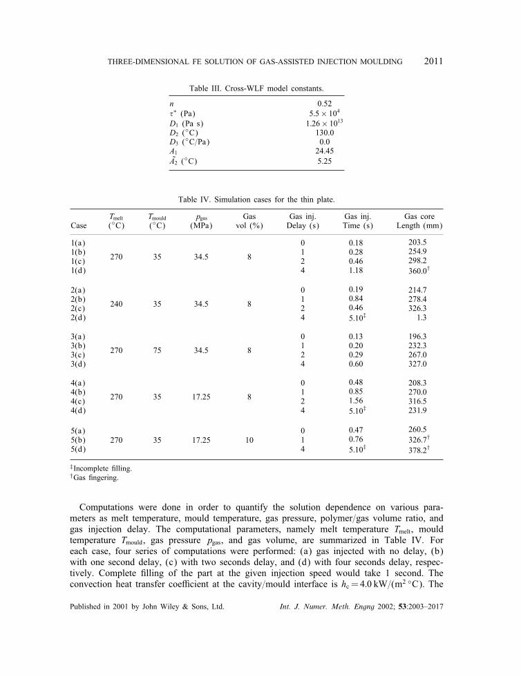
D2 (◦C) 130.0D3 (◦C=Pa) 0.0A1 24.45A2 (◦C) 5.25

Table IV. Simulation cases for the thin plate.

Tmelt Tmould pgas Gas Gas inj. Gas inj. Gas coreCase (◦C) (◦C) (MPa) vol (%) Delay (s) Time (s) Length (mm)

1(a)1(b)1(c)1(d)

270 35 34.5 8

0124

0:180:280:461:18

203:5254:9298:2360:0†

2(a)2(b)2(c)2(d)

240 35 34.5 8

0124

0:190:840:465:10‡

214:7278:4326:3

1:3

3(a)3(b)3(c)3(d)

270 75 34.5 8

0124

0:130:200:290:60

196:3232:3267:0327:0

4(a)4(b)4(c)4(d)

270 35 17.25 8

0124

0:480:851:565:10‡

208:3270:0316:5231:9

5(a)5(b)5(d)

270 35 17.25 10014

0:470:765:10‡

260:5326:7†

378:2†

‡Incomplete *lling.†Gas *ngering.

Computations were done in order to quantify the solution dependence on various para-meters as melt temperature, mould temperature, gas pressure, polymer=gas volume ratio, andgas injection delay. The computational parameters, namely melt temperature Tmelt, mouldtemperature Tmould, gas pressure pgas, and gas volume, are summarized in Table IV. Foreach case, four series of computations were performed: (a) gas injected with no delay, (b)with one second delay, (c) with two seconds delay, and (d) with four seconds delay, respec-tively. Complete *lling of the part at the given injection speed would take 1 second. Theconvection heat transfer coeHcient at the cavity=mould interface is hc = 4:0 kW=(m2 ◦C). The



mesh has 55,916 nodes and 246,050 tetrahedral elements. Results of the gas injection timeand the length of the gas core are listed in Table IV.

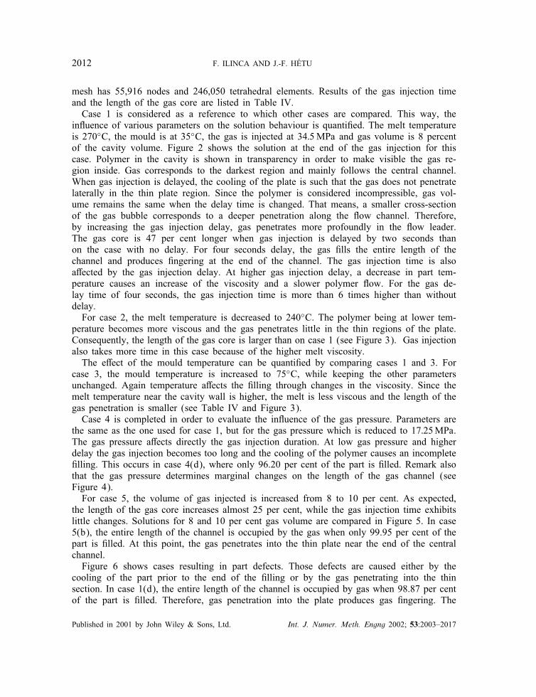
Case 1 is considered as a reference to which other cases are compared. This way, thein;uence of various parameters on the solution behaviour is quanti*ed. The melt temperatureis 270◦C, the mould is at 35◦C, the gas is injected at 34:5MPa and gas volume is 8 percentof the cavity volume. Figure 2 shows the solution at the end of the gas injection for thiscase. Polymer in the cavity is shown in transparency in order to make visible the gas re-gion inside. Gas corresponds to the darkest region and mainly follows the central channel.When gas injection is delayed, the cooling of the plate is such that the gas does not penetratelaterally in the thin plate region. Since the polymer is considered incompressible, gas vol-ume remains the same when the delay time is changed. That means, a smaller cross-sectionof the gas bubble corresponds to a deeper penetration along the ;ow channel. Therefore,by increasing the gas injection delay, gas penetrates more profoundly in the ;ow leader.The gas core is 47 per cent longer when gas injection is delayed by two seconds thanon the case with no delay. For four seconds delay, the gas *lls the entire length of thechannel and produces *ngering at the end of the channel. The gas injection time is alsoa<ected by the gas injection delay. At higher gas injection delay, a decrease in part tem-perature causes an increase of the viscosity and a slower polymer ;ow. For the gas de-lay time of four seconds, the gas injection time is more than 6 times higher than withoutdelay.

For case 2, the melt temperature is decreased to 240◦C. The polymer being at lower tem-perature becomes more viscous and the gas penetrates little in the thin regions of the plate.Consequently, the length of the gas core is larger than on case 1 (see Figure 3). Gas injectionalso takes more time in this case because of the higher melt viscosity.

The e<ect of the mould temperature can be quanti*ed by comparing cases 1 and 3. Forcase 3, the mould temperature is increased to 75◦C, while keeping the other parametersunchanged. Again temperature a<ects the *lling through changes in the viscosity. Since themelt temperature near the cavity wall is higher, the melt is less viscous and the length of thegas penetration is smaller (see Table IV and Figure 3).

Case 4 is completed in order to evaluate the in;uence of the gas pressure. Parameters arethe same as the one used for case 1, but for the gas pressure which is reduced to 17:25MPa.The gas pressure a<ects directly the gas injection duration. At low gas pressure and higherdelay the gas injection becomes too long and the cooling of the polymer causes an incomplete*lling. This occurs in case 4(d), where only 96.20 per cent of the part is *lled. Remark alsothat the gas pressure determines marginal changes on the length of the gas channel (seeFigure 4).

For case 5, the volume of gas injected is increased from 8 to 10 per cent. As expected,the length of the gas core increases almost 25 per cent, while the gas injection time exhibitslittle changes. Solutions for 8 and 10 per cent gas volume are compared in Figure 5. In case5(b), the entire length of the channel is occupied by the gas when only 99.95 per cent of thepart is *lled. At this point, the gas penetrates into the thin plate near the end of the centralchannel.

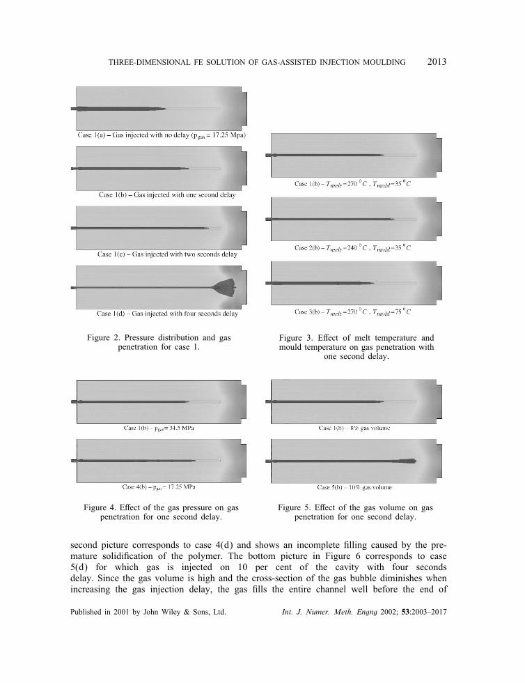
Figure 6 shows cases resulting in part defects. Those defects are caused either by thecooling of the part prior to the end of the *lling or by the gas penetrating into the thinsection. In case 1(d), the entire length of the channel is occupied by gas when 98.87 per centof the part is *lled. Therefore, gas penetration into the plate produces gas *ngering. The



Figure 2. Pressure distribution and gaspenetration for case 1.

Figure 3. E<ect of melt temperature andmould temperature on gas penetration with

one second delay.

Figure 4. E<ect of the gas pressure on gaspenetration for one second delay.

Figure 5. E<ect of the gas volume on gaspenetration for one second delay.

second picture corresponds to case 4(d) and shows an incomplete *lling caused by the pre-mature solidi*cation of the polymer. The bottom picture in Figure 6 corresponds to case5(d) for which gas is injected on 10 per cent of the cavity with four secondsdelay. Since the gas volume is high and the cross-section of the gas bubble diminishes whenincreasing the gas injection delay, the gas *lls the entire channel well before the end of



Figure 6. Moulding conditions corresponding to an incorrect *lling.

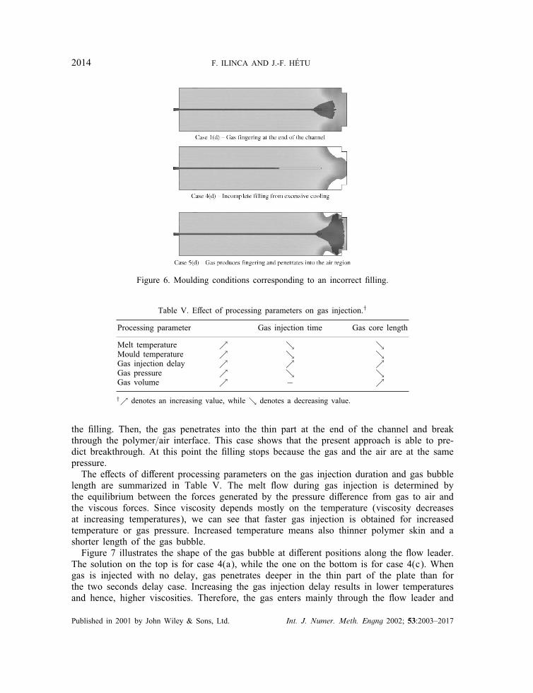
Table V. E<ect of processing parameters on gas injection.†

Processing parameter Gas injection time Gas core length

Melt temperature ↗ ↘ ↘Mould temperature ↗ ↘ ↘Gas injection delay ↗ ↗ ↗Gas pressure ↗ ↘ ↘Gas volume ↗ − ↗†↗ denotes an increasing value, while ↘ denotes a decreasing value.

the *lling. Then, the gas penetrates into the thin part at the end of the channel and breakthrough the polymer=air interface. This case shows that the present approach is able to pre-dict breakthrough. At this point the *lling stops because the gas and the air are at the samepressure.

The e<ects of di<erent processing parameters on the gas injection duration and gas bubblelength are summarized in Table V. The melt ;ow during gas injection is determined bythe equilibrium between the forces generated by the pressure di<erence from gas to air andthe viscous forces. Since viscosity depends mostly on the temperature (viscosity decreasesat increasing temperatures), we can see that faster gas injection is obtained for increasedtemperature or gas pressure. Increased temperature means also thinner polymer skin and ashorter length of the gas bubble.

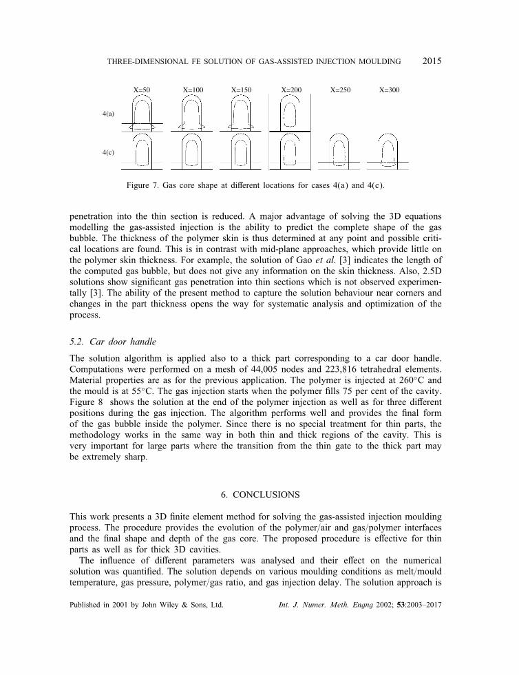
Figure 7 illustrates the shape of the gas bubble at di<erent positions along the ;ow leader.The solution on the top is for case 4(a), while the one on the bottom is for case 4(c). Whengas is injected with no delay, gas penetrates deeper in the thin part of the plate than forthe two seconds delay case. Increasing the gas injection delay results in lower temperaturesand hence, higher viscosities. Therefore, the gas enters mainly through the ;ow leader and



X=50 X=100 X=150 X=200 X=250 X=300

4(a)

4(c)

Figure 7. Gas core shape at di<erent locations for cases 4(a) and 4(c).

penetration into the thin section is reduced. A major advantage of solving the 3D equationsmodelling the gas-assisted injection is the ability to predict the complete shape of the gasbubble. The thickness of the polymer skin is thus determined at any point and possible criti-cal locations are found. This is in contrast with mid-plane approaches, which provide little onthe polymer skin thickness. For example, the solution of Gao et al. [3] indicates the length ofthe computed gas bubble, but does not give any information on the skin thickness. Also, 2.5Dsolutions show signi*cant gas penetration into thin sections which is not observed experimen-tally [3]. The ability of the present method to capture the solution behaviour near corners andchanges in the part thickness opens the way for systematic analysis and optimization of theprocess.

5.2. Car door handle

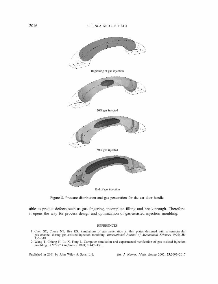
The solution algorithm is applied also to a thick part corresponding to a car door handle.Computations were performed on a mesh of 44,005 nodes and 223,816 tetrahedral elements.Material properties are as for the previous application. The polymer is injected at 260◦C andthe mould is at 55◦C. The gas injection starts when the polymer *lls 75 per cent of the cavity.Figure 8 shows the solution at the end of the polymer injection as well as for three di<erentpositions during the gas injection. The algorithm performs well and provides the *nal formof the gas bubble inside the polymer. Since there is no special treatment for thin parts, themethodology works in the same way in both thin and thick regions of the cavity. This isvery important for large parts where the transition from the thin gate to the thick part maybe extremely sharp.

6. CONCLUSIONS

This work presents a 3D *nite element method for solving the gas-assisted injection mouldingprocess. The procedure provides the evolution of the polymer=air and gas=polymer interfacesand the *nal shape and depth of the gas core. The proposed procedure is e<ective for thinparts as well as for thick 3D cavities.

The in;uence of di<erent parameters was analysed and their e<ect on the numericalsolution was quanti*ed. The solution depends on various moulding conditions as melt=mouldtemperature, gas pressure, polymer=gas ratio, and gas injection delay. The solution approach is



Beginning of gas injection

20% gas injected

50% gas injected

End of gas injection

Figure 8. Pressure distribution and gas penetration for the car door handle.

able to predict defects such as gas *ngering, incomplete *lling and breakthrough. Therefore,it opens the way for process design and optimization of gas-assisted injection moulding.

REFERENCES

1. Chen SC, Cheng NT, Hsu KS. Simulations of gas penetration in thin plates designed with a semicirculargas channel during gas-assisted injection moulding. International Journal of Mechanical Sciences 1995; 38:335–348.

2. Wang T, Chiang H, Lu X, Fong L. Computer simulation and experimental veri*cation of gas-assisted injectionmoulding. ANTEC Conference 1998; 1:447–453.



3. Gao D, Nguyen K, Garcia-Rejon A, Salloum G. Numerical modelling of the mould *lling stage in gas-assistedinjection moulding. International Polymer Processing 1997; 12:267–277.

4. Khayat RE, Derdouri A, Hebert LP. A three-dimensional boundary-element approach to gas-assisted injectionmoulding. Journal of Non-Newtonian Fluid Mechanics 1995; 57:253–270.

5. Haagh G, Zuidema H, de Vosse FV, Peters G, Meijer H. Towards a 3-D *nite element model for thegas-assisted injection moulding process. International Polymer Processing 1997; 12:207–215.

6. Franca LP, Frey SL. Stabilized *nite element methods: II. The incompressible Navier–Stokes equations.Computer Methods in Applied Mechanics and Engineering 1992; 99(2–3):209–233.

7. Lohner R, Morgan K, Peraire J, Vahdati M. Finite element ;ux-corrected transport (FEM-FCT) for the Eulerand Navier–Stokes equations. International Journal for Numerical Methods in Fluids 1987; 7:1093–1109.

8. Franca LP, Dutra Do Carmo EG. The Galerkin gradient least-squares method. Computer Methods in AppliedMechanics and Engineering 1989; 74:41–54.

9. Ilinca F, H1etu J-F. Finite element solution of three-dimensional turbulent ;ows applied to mould-*lling problems.International Journal for Numerical Methods in Fluids 2000; 34:729–750.

10. H1etu J-F, Ilinca F. 3D GLS *nite element formulation applied to mould-*lling and solidi*cation processes.Tenth International Conference on Numerical Methods for Thermal Problems, Swansea, UK, 1997.

11. Tezduyar TE, Aliabadi SK, Behr M, Mittal S. Massively parallel *nite element simulation of compressibleand incompressible ;ows. Research Report 94-013, Army High Performance Computing Research Center,Minneapolis, Minnesota, 1994.

12. Poslinski A, Oehler P, Stokes V. Isothermal gas-assisted displacement of viscoplastic liquids in tubes. PolymerEngineering and Science 1995; 35:877–892.


Three-dimensional finite element solution of gas-assisted injection moulding

Documents

Transcript of Three-dimensional finite element solution of gas-assisted injection moulding