Centrifuge modeling of one-step outflow tests for unsaturated ...
Upload
khangminh22Category
view
2download
0
ONE DIMENSIONAL COMPRESSION BEHAVIOUR OF
UNSATURATED GRANULAR SOILS AT
LOW STRESS LEVELS
BY
ANDREW KEITH GOODWIN
A THESIS SUBMITTED TO THE UNIVERSITY OF SHEFFIELD IN PARTIAL FULFILMENT FOR THE DEGREE OF DOCTOR OF PHILOSOPHY
DEPARTMENT OF CIVIL AND STRUCTURAL ENGINEERING
UNIVERSITY OF SHEFFIELD
SEPTEMBER 1991

IMAGING SERVICES NORTH Boston Spa, Wetherby
West Yorkshire, LS23 7BQ
www.bl.uk
CONTAINS
PULLOUTS

SUMMARY
Poor performance of trench reinstatements affects the quality and safety
of highways. As materials in shallow trenches are unsaturated and under
low stresses, the factors affecting their behaviour are not understood
clearly. This thesis reports on an experimental investigation into the
one dimensional compression behaviour of typical coarse granular
trenchfill materials.
Literature from the fields of rockfills and unsaturated soils are
reviewed, and some experimental difficulties faced when working with
such materials are noted. The limestone test material is classified
using standard specification tests for aggregates.
Four series of tests were performed to investigate the behaviour of
three gradings over a range of water contents. Monotonic, constant
strain and repeated load conditions were used, and investigations made
into the influence of inundation on strain development, the influence
of water content on Ko and shear strength for a given density, and the
influence of compactive effort.
A new consolidation cell was developed to perform two of the test
series. This cell allowed the measurement and control of suctions within
the test specimens, and allowed inundation under controlled conditions.
Air diffusion effects were allowed for in the design.
The experimental work shows measurable suctions exist within coarse
granular soils. Compressibility and repeated load behaviour are both
shown to be a function of water content and dry density for a given
compactive effort, and soil suction is shown to be an important
influence. Collapse settlements on inundation were recorded and were
shown to be directly influenced by soil suction. Shear behaviour was
shown to be affected by the suctions also, but the Ko tests were
inconclusive.
A qualitative model to explain the influence of suction in coarse
materials is presented, and the current test results compared with those
of previous workers. The practical implications of the research are
discussed.
- ii -

The research reported in this thesis was conducted within the Department
of Civil and Structural Engineering of the University of Sheffield under
the supervision of Dr W F Anderson and Dr I C Pyrah, and in conjunction
with the British Gas Engineering Research Station. Liaison staff at the
Research Station were Dr ROwen, Mr D Boyes and Mr G Leach. The author
wishes to express his sincere gratitude to them all for their time and
efforts, but in particular wishes to thank Dr Anderson and Dr Pyrah for
their guidance, suggestions and patience both during the experimental
work and the prolonged period over which the thesis was written. Thanks
also go to Professor T Hanna, the Head of the Department of Civil and
Structural Engineering, for the use of the departmental facilities
throughout the work.
The design and development of the apparatus was helped greatly by the
enthusiasm and competence shown by all technical staff at the
University, but the greatest endeavours were provided by Mr P L Osborne
and Mr M Foster. Their input does not go unrecognised, and neither does
the cooperation received from Mrs S Rowe and her staff when the soils
laboratory at the British Gas Engineering Research Station was
extensively used for several months.
Additional thanks go to all those who provided useful discussions
throughout the period of the research, and to my postgraduate colleagues
with whom some useful discussions were had in the local hostelries.
Those discussions and the balance in life they provided does not go
unremembered!
I am grateful to the Science and Engineering Research Council and
British Gas pIc for funding the research, and I thank also Scott Wilson
Kirkpatrick for their financial input to the production of this thesis.
In particular the secretaries who typed the text and the technicians who
prepared the figures deserve special mention - your efforts were much
appreciated. Thanks go also to British Gas for their permission to
utilise photographs of the work performed within their premises.
Finally, I wish to thank my parents and Penny for all the encouragement
and support they showed throughout this work. Without them this thesis
may never have been completed.
- iii -

ACKNOWLEDGEMENTS
The research reported in this thesis was conducted within the Department
of Civil and Structural Engineering of the University of Sheffield under
the supervision of Dr W F Anderson and Dr I C Pyrah, and in conjunction
with the British Gas Engineering Research Station. Liaison staff at the
Research Station were Dr ROwen, Mr D Boyes and Mr G Leach. The author
wishes to express his sincere gratitude to them all for their time and
efforts, but in particular wishes to thank Dr Anderson and Dr Pyrah for
their guidance, suggestions and patience both during the experimental
work and the prolonged period over which the thesis was written. Thanks
also go to Professor T Hanna, the Head of Department of Civil and
Structural Engineering, for the use of the departmental facilities
throughout the work.
The design and development of the apparatus was helped greatly by the
enthusiasm and competence shown by all technical staff at the
University, but the greatest endeavours were provided by Kr P L Osborne
and Mr K Foster. Their input does not go unrecognised, and neither does
the cooperation received from Krs S Rowe and her staff when the soils
laboratory at the British Gas Engineering Research Station was
extensively used for several months.
Additional thanks go to all those who provided useful discussions
throughout the period of the research, and to my postgraduate colleagues
with whom some useful discussions were had in the local hostelries.
Those discussions and the balance in life they provided does not go
unremembered I
I am grateful to the Science and Engineering Research Council and
British Gas plc for funding the research, and I thank also Scott Wilson
Kirkpatrick for their financial input to the production of this thesis.
In particular the secretaries who typed the text and the technicians who
prepared the figures deserve special mention - your efforts were much
appreciated. Thanks go also to British Gas for their permission to
utilise photographs of the work performed within their premises.
Finally, I wish to thank my parents and Penny for all the encouragement
and support they showed throughout this work. Without them this thesis
may never have been completed.
- iii -

TABLE OF CONTENTS (Continued)
3.4 Behavioural Characteristics of Gradings
3.4.1 Limiting Density Tests
3.4.1.1. Minimum Density
3.4.1.2 Maximum Density
3.4.2 Compaction Characteristics
Chapter 4 - Description and Development of Experimental Apparatus
4.1 Consolidation Cell
4.1.1 Cell. Plumbing and Instrumentation
4.1.1.1
4.1.1.2
4.1.1.3
4.1 1.4
4.1.1.5
Cell Dimensions
Base Platen
Top Platen
Measurement of phase volume change
Measurement and control of pore water pressures
4.1.2 Ancillary Equipment
4.1.2.1
4.1.2.2
Compaction Apparatus
Jack for Removal of the Top Platen
4.1.3 Data Acquisition System
4.1.3.1 Hardware
4.1.3.2 Software
4.1.4 Constant Temperature Apparatus
4.2 Triaxial Cell
4.2.1 Load Application and Measurement
4.2.2 Platen Details
4.2.3 Measurement of Volume Changes and Pressures
4.2.4 Data Acquisition System
- v -
PAGE
26
26
27
27
27
29
29
31
31
32
33
35
36
37
37
38
38
38
39
40
40
41
41
41
42

TABLE OF CONTENTS (Continued)
4.3 Compression Cell
Chapter 5 - Calibration of Instrumentation and Operational Checks on Apparatus
5.1 Calibration of Instrumentation
5.1.1 Temperature
5.1.1.1 University Apparatus
5.1.1.2 Research Station Apparatus
5.1.2 Volume Change Units
5.1.2.1 University Apparatus
5.1.2.2 Research Station Apparatus
5.1.3 Load Cells
5.1.3.1 University Apparatus
5.1.3.2 Research Station Apparatus
5.1.4 Pressure Transducers
5.1.5 Displacement Transducers
5.1.5.1 University Apparatus
5.1.5.2 Research Station Apparatus
5.1.6 Bourdon Gauges
5.2 Operational Checks on Apparatus
5.2.1 Operation of Air Volume Indicators and Flushing System
5.2.2 Response Tests on Ceramics
5.2.3 Permeability and Air Entry Tests on Ceramics
lapter 6 - Test Programme and Experimental Procedures
6.1 Summary of Test Programme
6.2 Test Series A
6.3 Test Series B
6.4 Test Series C
6.5 Test Series D
PAGE
43
45
45
45
45
46
46
46
48
49
49
50
50
51
51
51
52
52
52
54
56
58
58
58
61
62
65

TABLE OF CONTENTS (Continued)
4.3 Compression Cell
Chapter 5 - Calibration of Instrumentation and Operational Checks on Apparatus
5.1 Calibration of Instrumentation
5.1.1 Temperature
5.1.1.1 University Apparatus
5.1.1.2 Research Station Apparatus
5.1.2 Volume Change Units
5.1.2.1 University Apparatus
5.1.2.2 Research Station Apparatus
5.1.3 Load Cells
5.1.3.1 University Apparatus
5.1.3.2 Research Station Apparatus
5.1.4 Pressure Transducers
5.1.5 Displacement Transducers
5.1.5.1 University Apparatus
5.1.5.2 Research Station Apparatus
5.1.6 Bourdon Gauges
5.2 Operational Checks on Apparatus
5.2.1 Operation of Air Volume Indicators and Flushing System
5.2.2 Response Tests on Ceramics
5.2.3 Permeability and Air Entry Tests on Ceramics
Chapter 6 - Test Programme and Experimental Procedures
6.1 Summary of Test Programme
6.2 Test Series A
6.3 Test Series B
6.4 Test Series C
6.5 Test Series D
-v1 -
PAGE
43
45
45
45
45
46
46
46
48
49
49
50
50
51
51
51
52
52
52
54
56
58
58
58
61
62
65

TABLE OF CONTENTS (Continued) PAGE
Chapter 7 Results and Interpretation of Tests 67
Chapter
7.1 Compressibility Tests with Suction Measurements 67
7.1.1 Specimen Response to a Single Total 67 Stress Change
7.1.2 Results of Suction Measurements 68
7.1.3 Effects of Compaction Water Content and 69 Dry Density on Compressibility
7.2 Inundation Tests 69
7.3 Ko and Shear Tests 70
7.3.1 Membrane Effects 70
7.3.2 Consolidation Curves 72
7.3.3 Ko Determinations 72
7.3.4 Shear Stages 73
7.4 Strain Controlled Compression Tests 73
8 Discussion of Results and Comparison 75 with Other Work
8.1 Performance of New Consolidation Cell 75
8.1.1 Load Cell Response Characteristics 75
8.1.2 Load Cell Stability 77
8.2 Water Volume Changes Due to Total Stress Changes 77
8.3 Suction Determinations 78
8.3.1 Repeatability of Data 78
8.3.2 Comparison Between Suction Measurements 80 for Coarse and Fine Gradings
8.3.3 Vertical Suction-Water Content Profile 83
8.4 Comparison of Compressibility Results from Series A, Band D
83
8.4.1 Repeatability of Data 83
8.4.2 Effect of Compaction Water Content and Dry 84 Density on Compressibility of the Coarse Grading for Constant Compactive Effort
- vii -

TABLE OF CONTENTS (Continued) PAGE
8.4.3 Effect of Compactive Effort on the 86 Compressibility of the Coarse Grading
8.4.4 Effect of Grading on Compressibility 87
8.4.5 Comparison of Stress and Strain Controlled 88 Compression Tests
8.4.6 Magnitude of Immediate and Time Dependent 89 Strain Components
8.5 Comparison of Compressibility Results with Brady 91 and Kirk (1990)
8.6 Inundation Test Results 94
8.6.1 Relationship Between Inundation Strains 94 and Soil Suctions
8.6.2 Relationship Between Inundation Strains 95 and Other Parameters
8.6.3 Combined Effect of Total Stress Changes 96 and Inundation
8.7 Repeated Load Behaviour
8.8 Effect of Stress Level on Compressibility Behaviour
8.9 Triaxial Test Results
96
98
99
8.9.1 Consolidation Characteristics 99
8.9.2 Ko Determinations 100
8.9.3 Results of Shear Tests 101
8.9.4 Theoretical Compressibility Equation for 104 Two Phase Pore Fluid
8.10 Practical Implications of the Research
Chapter 9 Conclusions and Recommendations for Future Work
9.1 Conclusions
9.2 Recommendations for Future Work
- viii -
106
108
108
111

References
Appendix A Detailed Test Procedures
Appendix B Names and Addresses of Specialist Equipment Suppliers
Appendix C Manufacture of Load Cells
Appendix D Data Acquisition Software
Appendix E Experimental Investigations into the Properties of the High Air Entry Value Ceramics
- ix -

LIST OF TABLES
3.1 Results of petrographic analysis on quarried limestone aggregate
3.2 Compliance of test gradings with relevant Department of Transport specifications
3.3 Results of aggregate absorption value tests
3.4 Definition of soil parameters allowing for water absorption
3.5 Summary of particle shape analyses: overall fora of particles
3.6 Summary of particle shape analyses: degree of angularity of particles
5.1 Calibration constants and confidence limits for Imperial College Volume Change Units at a back pressure of 100 kPa
5.2 Influence of back pressure on calibration data of IC Volume Change Unit 28
5.3 Calibration factors and confidence limits for British Gas air water interfaces
5.4 Calibration constants and confidence limits for 2.5 kN load cells.
5.5 Calibration constants and confidence limits for commercial load cells
5.6 Calibration constants and confidence limits for commercial pressure transducers
5.7
6.1
6.2
6.3
6.4
6.5
7.1
7.2
7.3
7.4
7.5
7.6
Calibration constants and confidence limits for commercial displacement transducers used at the university
Summary of test series
Summary of tests in series A
Summary of tests in series B
Summary of tests in series C
Summary of tests in series D
Yater content distribution profiles after series A tests
Change in specimen parameters during consolidation stages of series B tests
Stress path history and variation of soil parameters for test C1
Stress path history and variation of soil parameters for test C2
Stress path history and variation of soil parameters for test C3
Stress path history and variation of soil parame~rs for test C4
- x -

LIST OF TABLES (Continued)
7.7 Results of shear tests
7.8 Virgin compression line data for test series D
7.9 Repeated load data summary for test series D
7.10 Yater content distribution profiles after series D tests
8.1 Effect of particle size on magnitude of suction for water in a lenticular state
8.2 Comparison of soil parameters for coarse and fine gradings
8.3 Immediate strain components of series A and B tests during loading
8.4 Calculation of shear strength parameters using .ethod by Fredlund et al (1978)
8.5 Calculation of theoretical air-water mixture volume changes during saturation stage of test Cl
Al Recommended batching quantities
El - Results of modulus of rupture tests
E2 - Results of ceramic deflection tests
- xi -

LIST OF FIGURES
2.1 Categories of unsaturated soil
2.2 Hysteresis of suction wate content curve
2.3 Effect of clay fraction on suction
2.4 Lenticular phase of pore water
2.5 State surface for volume change behaviour
2.6 Model of unsaturated soil
2.7 State surface for degree of saturation
2.8 Failure criterion for unsaturated soils
2.9 Effect of wetting on the suction profile in a soil
2.10 Typical pore water pressure response cuve for high air entry value ceramic
2.11 Effect of particle size on membrane penetration
3.1 Grading curves for supplied limestone aggregate
3.2 Three typical unbound trench reinstatements
3.3 Calculated nominal grading curves and specification compliance
3.4 Maximum/minimum grading envelopes for batched test gradings
3.5 Particle breakdown during batching
3.6 Method for the graphical representation of general particle shape
3.7 Chart for the visual estimation of the degree of angularity
3.8 Results of particle shape analysis
3.9 Suggested relationship between the quantitative degree of angularity and conventional qualitative visual assessment of angularity
3.10 Degree of breakdown during maximum density tests
3.11 Dry density - free water content relationship for coarse grading at standard test programme compactive effort
3.12 Comparison of the compaction of the coarse grading at standard test programme compactive effort with BS1377: 1975 Tests 12, 13 and 14 on a similar material
3.13 Comparison of grading curve for material tested using BS1377: 1975 Tests 12, 13 and 14 with main test programme coarse grading
3.14 Dry density - free water content relationship for fine and medium gradings at standard test programme compactive effort
- ~ii -

LIST OF FIGURES (Continued)
4.1 New consolidation cell and ancillary instrumentation
4.2 Top platen for consolidation cell
4.3 Base platen for consolidation cell
4.4 Diffused air volume indicator
4.5 Compaction base used during test series A and B
4.6 Compaction guide and plate used during test series A and B
4.7 Screw jack for removal of top platen from consolidation cell
4.8 Data acquisition system for test series A and B
4.9 Modified triaxial cell and instrumentation used for test series C
4.10 Data acquisition system for test series C and D
4.11 Compression cell used for test series D
5.1 Typical plot of atmospheric variations in constant temperature laboratory
5.2 Record of air and water supply temperature at the British Gas Research Station over a 29 day period
5.3 Apparatus for de-airing of volume change unit
5.4 Apparatus for calibration of volume change unit
5.5 Correlation between temperature changes and apparent water volume changes for British Gas air water interfaces
5.6 Effect of atmospheric humidity on load cell A
5.7 Medium term observations of isolated air volume indicator water level
5.8 Schematic arrangement of apparatus for response and permeability tests on high air entry ceramics
5.9 Typical response curves for high air entry ceramics
5.10 Typical response curve for 3 bar ceramic after use in 2 main series tests
5.11 Dependence of response time on period of de-airing of 5 bar ceramic
7.1 Typical load cell output variation during a loading stage
- xiii -

LIST OF FIGURES (Continued)
7.2 Typical strain development during a loading stage
7.3 Typical stress - strain curve for single loading stage
7.4 Typical pore pressure variation during a loading stage
7.5 Typical suction - stress curve for single loading stage
7.6 Suction - water content relationships for coarse and fine gradings at vertical stress of 10 kPa
7.7 Suction - water content relationship for coarse grading at vertical stress of 25 kPa
7.8 Suction-vertical stress relationship for test AS
7.9 Variation of top suction with vertical stress for fine grading
7.10 Measured water content - depth profiles after series A tests
7.11 Effect of total water content on vertical water content profile
7.12 Strain - stress curves for coarse grading from series A and B tests
7.13 Strain - stress curves for fine grading from series A tests
7.14 Effect of free water content on compressibility of coarse grading from test series A and B at usual compactive effort
7.15 Effect of free water content on compressibility of fine grading from series A tests
7.16 Typical variation of stress, strain and top pore water pressure during an inundation stage
7.17 Variation of strain during inundation stage of test B2 after correction for ceramic deflection due to inundation pressure
7.18 Effect of inundation stage on strain - stress curves for tests
7.19 Typical variation of base suction during an inundation stage
7.20 Consolidation curve for test C3
7.21 Ko stage data for test C4
7.22 Shear stress - strain curve for test C4
7.23 Volumetric strain behaviour of specimen C4
7.24 Stress - strain curve for all stages of test D2
- xiv -

LIST OF FIGURES (Continued)
7.25 Strain-stress curves for series 0 tests on coarse grading compacted with usual compactive effort
7.26 Strain-stress curves for series 0 tests on coarse grading compacted with low compactive effort
7.27 Strain-stress curves for series 0 tests on fine and medium gradings
7.28 Effect of free water content on compressibility of coarse grading from series 0 tests
7.29 Effect of grading and compactive effort on strain accumulation during repeated loading stages of series 0 tests
7.30 Effect of free water content and dry density on peak strain accumulation during repeated loading stages of series 0 tests on coarse grading compacted with usual compactive effort.
7.31 Effect of free water content and dry density on peak strain accumulation during repeated loading stages of series 0 tests on coarse grading compacted with low compactive effort.
8.1 Effect of stress level on range of measured load cell stresses
8.2 Effect of specimen tilt on range of measured load cell stresses
8.3 Effect of back pressure on volume change unit output
8.4 Conceptual model for the measurement of equilibrium suction at the base of a specimen with a low degree of saturation
8.5 , Effect of fines on equilibrium suction established between two large particles
8.6
8.7
8.8
Possible frequency distribution for particles - ceramic contacts
Field measurements of matrix suction on Glacial Till using thermal conductivity sensors
Graphical method to separate immediate strain from total strain
8.9 Immediate strain-stress curves for loading stages of series A tests
8.10 Immediate strain-stress curves for loading stages of series B tests
8.11 Effect of free water content on immediate compressibility of coarse grading from series A and B tests
8.12 Relationship between immediate strain component and stress level
8.13 TRRL compaction data for high compactive effort
8.14 TRRL compaction data for medium compactive effort
8.15 TRRL compaction data for low compactive effort
- xv -

LIST OF FIGURES (Continued)
8.16 Relationship between constrained modulus and dry density for stress range 25 - 100 kPa
8.17 Relationship between constrained modulus and dry density for stress range 25 - 250 kPa
8.18 Relationship between constrained modulus and dry density for stress range 205 - 820 kPa
8.19 Variation of constrained modulus with water content for series A tests on coarse grading
8.20 Variation of constrained modulus with water content for series D tests on coarse grading compacted with usual effort
8.21 Variation of constrained modulus with water-content for series D tests on coarse grading compacted with low effort
8.22 Variation of constrained modulus with water content for series A tests on fine grading
8.23 Variation of constrained modulus with dry density for series A tests on coarse grading
8.24 Variation of constrained modulus with dry density for series D tests on coarse grading compacted with usual effort
8.25 Variation of constrained modulus with dry density for series D tests on coarse grading compacted with low effort
8.26 Variation of constrained modulus with dry density for series A tests On fine grading
8.27 Variation of constrained modulus obtained from TRRL tests with water content for high compactive effort
8.28 Variation of constrained modulus obtained from TRRL tests with water content for medium compactive effort
8.29 Variation of constrained modulus obtained from TRRL tests with water content for low compactive effort
8.30 Variation of constrained modulus obtained from TRRL tests with dry density for high compactive effort
8.31 Variation of constrained modulus obtained from TRRL tests with dry density for medium compactive effort
8.32 Variation of constrained modulus obtained from TRRL tests with dry density for low compactive effort
8.33 Three dimensional relationship between strain at any given stress level, water content and dry density
8.34 Relationship between measured suction and inundation strain
- xvi -

LIST OF FIGURES (Continued)
8.35 Relationship between inundation strain and soil parameters void ratio, air void and free degree of saturation
8.36 Re1ationsip between suction, and air void ratio and free degree of saturation
8.37 Comparison of strain on saturation with air void ratio of backfill
8.38 Effect of total stress changes and inundation on the dry density-free water content relationship for the coarse grading
8.39 Loading and inundation stress paths for two different specimens showing uniqueness of final saturated state
8.40 First unloading curves for series A tests on coarse grading
8.41 Effect of stress level on unloading constrained modulus for coarse grading
8.42 Shear strength data from series C
8.43 Change in shear strength from saturated plane
8.44 Variation of specimen parameters during saturation stage of specimen Cl
8.45 Comparison of theory with experimental data for compressibility of air-water mixtures
A1 Bolt holes in compaction base and consolidation cell base
A2 Suction pump and manometer connection to specimen before Ko and shear tests
C1 - 2.5 kN load cell
C2 - General arrangement to set pencil level ready for burnishing axis on load cell body
C3 - Picking up and positioning a strain gauge
C4 - Position of strain gauges prior to applying adhesive
C5 - Pressure chamber for curing of strain gauge adhesive
C6 - Wiring of load cell strain gauges in full wheatstone bridge
E1 - Apparatus for the determination of the modulus of rupture
E2 - General arrangement of apparatus used to determine the elastic properties of the ceramics
£3 - Details of perspex mounting block and ceramic holders
£4 - Results of ceramic deflection tests
£5 - Bending strains developed during ceramic deflection tests
- xvii -

LIST OF PLATES
3.1 Limestone aggregate as supplied
5.1 Apparatus for calibrating displacement transducers
Al Kango hammer and compaction guide for test series A and B
A2 Component parts of top platen for consolidation cell
A3 Assembled top platen
A4 Sliding of consolidation cell and compacted specimen across compaction base using the hydraulic ram
AS Insertion of top platen into consolidation cell using the hydraulic press
A6
A7
AS
A9
AlO
All
A12
El
E2
Fully assembled consolidation cell
Removal of top platen following completion of test using the screw j~k
Compaction of triaxial test specimen
Vacuum pump and manometer used for preparation of triaxial test specimen
Triaxial test specimen ready for commencement of test
Compaction apparatus used to apply a high compactive effort to test specimens for use in test series D
Compaction apparatus used to apply a low compactive effort to test specimens used in test series D
Specimens used in modulus of rupture tests
Perspex mounting block and inserts used in ceraaic deflection tests
- xviii -

r m ,~w
S d; ,j
ep,Eu
&-
-, fT· . 1,J
x
a
aa
as
aw
a,b,c
b,d,l
e
h
m
r,t
r
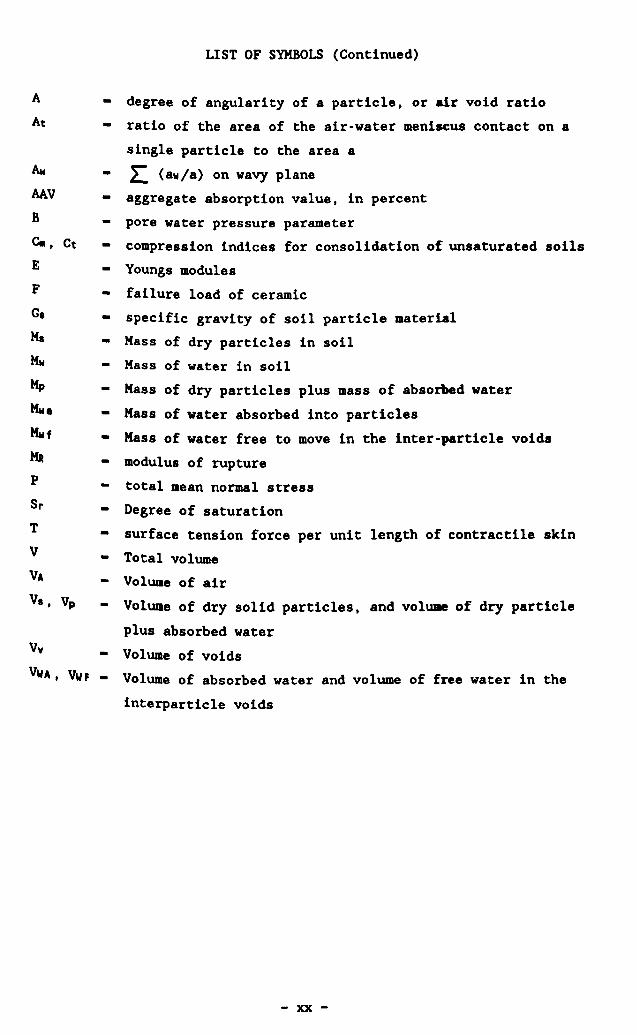
LIST OF SYMBOLS
compressibility of air water mixture and pure water
deflection
Kronecker delta
strain at peak (minimum) stress of repeated load cycle
half angle subtended at centre of a particle by water in
a lenticular state
angle of internal friction, due to effective stresses and
suction stresses
total stress
total normal (radial) stress on triaxial specimen, at failure
if subscript f attached
effective stress
equivalent intergranular stress tensor
effective deviatoric stress tensor
bulk (dry) density of soil
density of pure water
unit weight of pure water
total shear stress, at failure if subscript f attached
chi, effective stress parameter for coupled variable effective
stress equation for unsaturated soils
Poissons ratio
area of wavy plane through particle contacts above a single
particle
area of air-solid contact for a single particle on a wavy
plane
area of solid-solid contact for a single particle on a
wavy plane
area of water-solid contact for a single particle on a wavy
plane
principal dimensions of particles
breadth, depth and span of rectangular ceramic test specimens
void ratio
vertical separation of top and bottom platens
inverse of Poisson ratio
radius (thickn~ss) of circular ceramic test specimens
radius of spherical particles
- xix -

~, UW
w
WA, WF
x
A
At
Aw
MV
B
~, Ct
E
F
Gs
~
Mw
~
Mwa
Mwf
~
p
Sr
T
V
VA
Vs, Vp
Vv
VWA, VWF
LIST OF SYMBOLS (Continued)
pore air (water) pressure
force per unit area on circular ceramic test specimen
absorbed (free) water content of soil
perimeter length of contractile skin contact on a single
particle
degree of angularity of a particle, or air void ratio
ratio of the area of the air-water meniscus contact on a
single particle to the area a
~ (aw/a) on wavy plane
aggregate absorption value, in percent
pore water pressure parameter
compression indices for consolidation of unsaturated soils
Youngs modulus
failure load of ceramic
specific gravity of soil particle material
Mass of dry particles in soil
Mass of water in soil
Mass of dry particles plus mass of absorbed water
Mass of water absorbed into particles
Mass of water free to move in the inter-particle voids
modulus of rupture
total mean normal stress
Degree of saturation
surface tension force per unit length of contractile skin
Total volume
Volume of air
Volume of dry solid particles, and volume of dry particle
plus absorbed water
Volume of voids
Volume of absorbed water and volume of free water in the
interparticle voids
- xx -
A
At
~
MV
B
~, Ct
E
F
G.
~
~
~
~.
~f
~
P
Sr
T
V
VA
V" Vp
Vv
LIST OF SYMBOLS (Continued)
degree of angularity of a particle, or air void ratio
ratio of the area of the air-water meniscus contact on a
single particle to the area a
I: (aw/a) on wavy plane
aggregate absorption value, in percent
pore water pressure parameter
compression indices for consolidation of unsaturated soils
- Youngs modules
failure load of ceramic
specific gravity of soil particle material
Mass of dry particles in soil
Mass of water in soil
Mass of dry particles plus mass of absorbed water
Mass of water absorbed into particles
Mass of water free to move in the inter-particle voids
modulus of rupture
total mean normal stress
Degree of saturation
surface tension force per unit length of contractile skin
- Total volume
Volume of air
- Volume of dry solid particles, and volume of dry particle
plus absorbed water
- Volume of voids
VWA, VWF - Volume of absorbed water and volume of free water in the
interparticle voids
-~-

CHAPTER 1
INTRODUCTION
Following the onset of urban development in the late nineteenth century,
extensive networks of gas mains were installed underground. Today,
development and maintenance of these and other services require frequent
excavations to be made in the highways of the UK to the detriment of
highway quality and safety. In an effort to deal with the problem, the
utilities voluntarily established in 1974 a Model Agreement for trench
reinstatements which incorporated a method specification. However, this
non-statutory code proved ineffective on a national basis and Horne (1985)
recommended to government in his committee's report on the 1950 Public
Utilities Street Yorks Act that a national specification for
reinstatements be established in terms of materials, workmanship and
performance. York towards this goal is in progress, but the proposed
performance specification is being hampered by the lack of a fundamental
understanding of the behaviour of trenchfill materials, which are typically
unsaturated, at low stress levels and, when imported fill is used, of a
Coarse granular nature.
PreVious research relevant to understanding the behaviour of granular
reinstatements may be broadly sub-divided into the two areas of unsaturated
soils and rockfills. York on unsaturated soils has shown that soil
Suctions induced by non-saturation decrease as the coarseness of the soil
increases. Consequently, most efforts in this relatively young field of
research have concentrated on silts and clays within which high suctions
may be expected and their influence may be more clearly seen. Little work
has been reported on sands and coarser materials.
Rockfill research covers a wide area, from true rockfills used in
embankments and dams, to compaction of coarse mine and quarry wastes.
However, throughout this field it appears that most workers have
concentrated on the dry and saturated conditions, and have considered only
moderate to high stress levels. At such stresses small suctions induced by
non-saturation have been ignored.
- 1 -

The behaviour of reinstatements thus falls between tvo active areas of
work, and research is required to fill the void in current knowledge. Both
theoretical and experimental developments are required, but this first part
of an ongoing programme of research into the problem has concentrated on
the acquisition of high quality experimental data that may be used in
future theoretical work. The objectives of the research were:
i)
ii)
iii)
iv)
to review current knowledge relevant to the behaviour of trenchfill
to develop experimental apparatus suitable for high quality testing
of unsaturated coarse granular soils at low stress levels «100 kPa)
to obtain reliable data on the behaviour of typical trenchfill
materials under monotonic and repeated loads, in varying degrees of
compaction, and at a range of water contents
to assess the factors affecting the observed behaviour of the
trenchfi11 materials, make comparisons with previous work and make
recommendations for future work.
The research is principally concerned with trenchfill, but may be applied to other b
pro lems such as ground movements associated with pipe bursting at shallow 1 I
eve s, and pipe jacking through embankments.
The the i s s starts With a review of the relevant theoretical and
experimental literature in Chapter 2. Descriptions of the test materials, experim 1
enta apparatus, calibration checks on apparatus and test programme follow in chapters 3 to i bei i h 6, with particular attent on ng g ven to t e design a d
n calibration of a new one dimensional consolidation cell. The reSUlts f
o the research are presented in chapter 7, with discussion of the reSUlts
and Comparisons with previous work in chapter 8. The final chapter Contains h
t e conclusions and recommendations for future work.
- 2 -
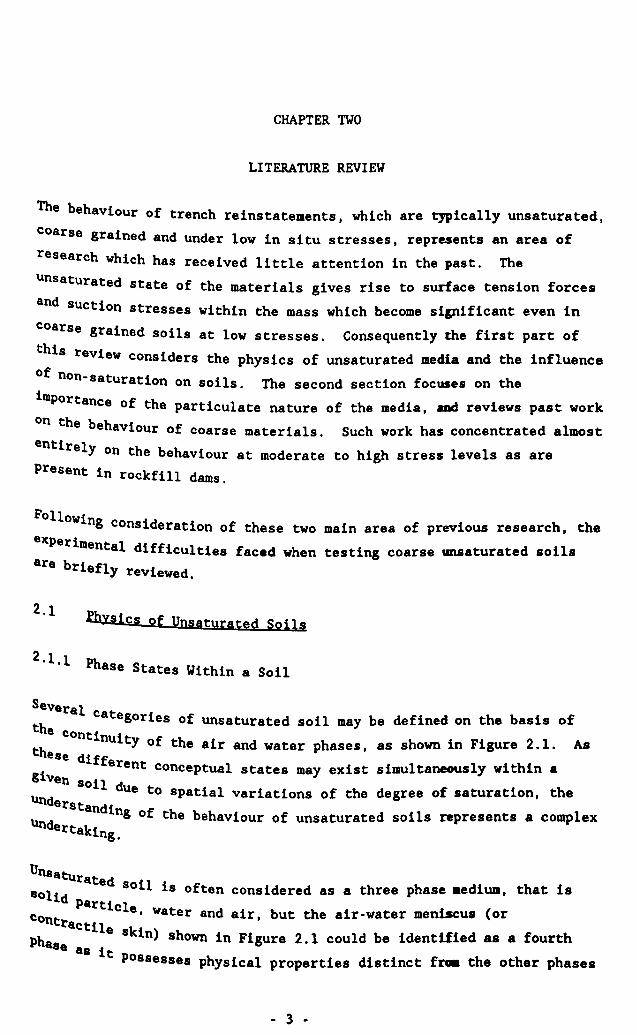
CHAPTER TWO
LITERATURE REVIEW
The behaviour of trench reinstatements, which are typically unsaturated,
coarse grained and under low in situ stresses, represents an area of
research which has received little attention in the past. The
unsaturated state of the materials gives rise to surface tension forces
and Suction stresses within the mass which become sicnificant even in
coarse grained soils at low stresses. Consequently the first part of
this reView considers the physics of unsaturated media and the influence
of non-saturation on soils. The second section focuses on the
importance of the particulate nature of the media, aDd reviews past work
on the behaviour of coarse materials. Such work has concentrated almost
entirely on the behaviour at moderate to high stress levels as are present in rockfill dams.
FOlloWing consideration of these two main area of previous research. the
experimental difficulties faced when testing coarse unsaturated soils are briefly reviewed.
2.1 lhysics of Unsaturated Soils
2.1.1 Phase States Within a Soil
Several categories of unsaturated soil may be defined on the basis of
the Conti i nu ty of the air and water phases, as shown in Figure 2.1. As
these diff erent conceptual states may exist simultaneously within a
giVen soil d ue to spatial variations of the degree of saturation, the
understanding of the behaviour of unsaturated soils represents a complex undertaking.
Unsatu rated soil is often considered as a three phase aedium, that is solid particle, water and air, but the air-water meniscus (or
Contractil ph e skin) shown in Figure 2.1 could be identified as a fourth
aSe as it possesses h h h physical properties distinct fra. t e ot er p ases
- 3 -

(Fredlund and Morgenstern, 1977). In particular, the contractile skin
Is able to sustain a tensile force and should therefore be considered
independently for stress analysis purposes. However, volumetrically
this phase is neglible and may be considered part of the water phase
(Fredlund, 1979), which may otherwise be present in a soil in three idealised states:
i)
11)
IiI)
water adsorbed by electro-chemical forces associated with the
dipolar nature of water and mineralogy of the soil, and which
properties are modified by the electro-chemical forces (and which
could thus be classed either as fifth phase or as part of the soil ~particle~);
Water absorbed within the interstices of the particles, and held
there by surface tension and/or adsorption; and
~free~ water present in the pores between particles and which is
either free to move under a gravitational potential or is retained
at a particular point by virtue of surface tension effects. As
shown in Figure 2.1, such water may be discrete and/or continuous,
dependent Upon the degree of saturation.
~ater Is lik ely to be present also as gaseous water vapour, within the
aIr pha se, which itself may be present as either small bubbles within
the adsorb d f e ilm of water around clay particles, or as absorbed air
WIthin th
AIr Withi e particle interstices, or as ~free· air between the particles.
n adsorbed water is thought to be under very high pressure (Aitchlso
n, 1956) and thus to have a low compressibility with respect to e~ternal pressures. b i
The free and absorbed air in contrast may e n eIther h a discrete or continuous form, and will both obey the normal YdrOd~amlc
J&I laws.
The free Co and absorbed water and air sub-divisions are largely only
nceptual O~t as in these states the air and water are free to move in and
of the the particle interstices under gravitational, hydrodynamic or
rmodYn 1 am c influence (Raudkivi and U'u, 1976). However, under the
- 4 -

isothermal conditions considered in this review such aovement is
Considered negligible. It is considered also that adsorbed water does
not playa significant role in coarse grained materials like limestone.
2.1.2 Stresses in an Unsaturated Soil
It is necessary to consider total stresses and pore vater pressure as in
saturated media, and also to consider the pore air pressures and surface
tension forces where these act at an interparticle contact, in order to
model realistically the various possible states of an unsaturated soil.
The difference in pore air and pore water pressures (UA - uw) is termed
the soil Suction, and is comprised of matrix (or capillary) and osmotic
components (eg Bolt and Miller, 1958; Olson and Langfelder, 1965). The fOl'Iller i h
Stat pressure difference (UA > uw) resulting from the formati f
on 0 the contractile skin or an applied pressure differential,
and the latter results from variations in spatial ionic concentration. Appropri t
a e techniques for measuring each component individually are available
, as reviewed by Krahn and Fredlund (1972), but it is the ~atrix Suction and its il b h i variations which appear to affect so e av our (Alonso et aI, 1987). Only matrix suctions are considered in this revie~ hence forward.
MOisture N Content variations directly affect the matrix suction. ~erous k
~or ers have demonstrated the hysteresis of the suction-water COntent curv h
e s own diagrammatically in Figure 2.2, and Croney and COleman (1948)
have presented data showing the influence of particle size and
clay Content on the measured suctions (see Figure 2.3). This ~ork i
~Plies that h 1 i h i as t e coarseness of a soi ncreases so t e max mum SUction h t at may exist in that soil decreases, and this may have encOUra
ged generations of subsequent workers to concentrate on measuring SUctions ~ lar ith clays and silts. Figure 2.3 also implies though that
ge suctions lllay directl 1 y gnored this
may be present even in coarse grained soils, and these
affect its behaViour. Previous researchers have apparently
potential stress or considered it to be negligible in view
- 5 -

of the large gravitational forces involved in coarse soils, and thus
quantitative data on suctions in such soils is limited. However, Jones
and Hurt (1978) measured matrix suction of up to pF3.9 (778 kPa) during
tests on a limestone aggregate at about 2% moisture content, confirming
the implication of Figure 2.3.
Other factors affecting suction include relative humidity and
temperature (Croney and Coleman, 1960), and experimental data on these
factors appears to suggest that these factors have only a small
influence generally. It is considered that although these effects are unl·k 1
1 e y to be entirely insignificant in a typical trench reinstatment,
they are probably of secondary importance under the isothermal CondO .
ltlons considered herein.
Them· Olsture Content also directly affects the magnitude of the tensile
forces d h ,an ence intergranular stresses, generated where the
Contractile skin contacts two or more particles. Haines (1925) and
FiSher (1926) showed that for water present in a lenticular state (see
Figure 2.4) in an ideal soil comprised of spherical particles of radius r, the int 1 ld b ergranular force generated between two partie es cou e eXpressed h
as s own in equation 2.1:
F _ -2TirT .......... equation 2.1
(1 + tan &/2)
~here T - surface tension force per unit length of contractile skin
2& - angle sub tended at the centre of the particle by lenticular
Water.
In a real soil h 1 f "" d • , t e wide range of possible va ues 0 r ren ers eqUation 2.1 of 1 d academic interest only. However, for idea open an ClOse pa ki
I: c ngs, the effective area of anyone contact equals 4r2 and 2r2 re
, spective1y (Aitchison and Donald, 1956), and thus a conceptual "ie~ of th
e Change in the magnitude of the intergranular stress in a
granular soil due to the combined effects of particle size and water
- 6 -

Content (implicitly incorporated through the value of~) may be derived.
Aitchison and Donald calculated this intergranu1ar stress to equal
3.8T/r in a close packing arrangement with the pore water having just
drained to the lenticular state and calculated a stress of 12.9T/r
immediately before drainage (ie the water is at its limiting moisture
tension). They presented data for sand showing the variation of
intergranu1ar stress with water content to be of the order 5 to 15 kPa.
At low applied stresses this will be a significant factor.
2.1. 3 Stress Analysis
Aitchis on and Donald expressly considered the most complicated states of
F' 19ure 2.1, namely those involving continuous air voids. The analysis
of Soil Containing small occluded air bubbles has long been appreciated
to represent an extension of the saturated state to include a
compressible pore fluid (eg Hilf, 1956; Koning, 1963; Barden et al, 1965) and . 1 d " numerous workers have considered the mathemat~ca escr~pt~on
of the compressibility of such an air water mixture (eg Schuurman, 1966; Fredlund 1
, 976; Dussea1t, 1979; Verruijt, 1982). More recently, soil
mechanics problems offshore have lead to research into soils containing
large gas bubbles (eg Wheeler, 1988). However, both these cases
represent states unlikely to form within a coarse granular trench
reinstatement and are not considered further in this review.
The modelli f' . ng 0 sOlIs containlng continuous air was initially attempted
in terms f " . o mod~fled single effectlve stress equations (eg Croney et
al, 1958' B' h • ls op, 1960; Jennings, 1960) by coupling two stress state
\7ariabl ( es ~-UA) and (UA-uw) in a single equation such as that shown in
equation 2.2. This form of equation implicitly incorporates the surface tensio
ns into the term (UA -uw) .
CT' - (r:r -UA) + X (UA -uw) .... equation 2.2
Experimental work on shear behaviour of unsaturated silts and clays (eg
Skempton, 1960' , Bishop and Donald, 1961; Bishop and Blight, 1963)
- 7 -

initially seemed to confirm the correctness of this st.ple equation, but
the parameter X was soon accepted as being a function (Blight 1965)
dependent upon numerous factors including those noted by Aitchison
(1965). Further, the function was shown to be discontinuous in nature
when applied to collapsing soils (eg Jennings and Burland, 1962; Burland
1965). The phenomenon of collapsing soils showed that the principle of
effective stress is not valid in unsaturated soils, as the reduction in
SUction which may induce collapse represents a decrease in effective
stress and would therefore be expected to induce an increase in volume, not a decrease.
As further research demonstrated the fallacy of applying a single
effective stress equation to a complex behavioural pattern induced by
the soil fabric(s), Bishop and Blight (1963) suggested plotting test
results in a three dimensional stress space (see Figure 2.5). This idea
of uncoupling the stress state variables has been adopted widely since
the mid 1960's to the present day for volume change (eg Burland, 1964;
Matyas and Radhakrishna, 1968; Barden et al 1968; Fredlund and
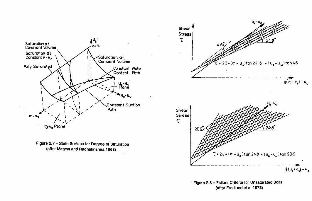
Morgenstern, 1976) and shear strength (eg Bishop and Blight, 1963; Fredlund et aI, 1978).
In 1968, Matyas and Radbakrishna abandoned the effective stress concept
and proposed analysing soil behaviour in terms of stress tensors as Shown in equation 2.3:
-crfj - [(P-\lA) + At, (\lA-uw) + ITdx] SIJ + cr'IJ ..•. equation 2.3
Where -If:f'fJ - equivalent stress transmitted by the solid contacts P - total mean normal stress (er" +C7'22 +crn)/3 \lA, UN - pore air and pore water pressures, respectively T - surface tension force per unit length of contractile skin
- perimeter of contractile skin At, -1:all/a [See Figure 2.6] IIJ - Kronecker delta t ' I J - deviatoric stress tensor
- 8 -

Theoretical models to determine the termJTdX in an idealised soil have
been attempted but its value is unobtainable in a real soil as
previously realised by Aitchison and Donald (1956). Hence Matyas and
Radhakrishna assumed this term is equivalent to At (UA-uw) as previously
suggested by M.I.T. (1963). However, and as recognised by them, this
simplification ignores the fact that "while (UA -Uw) acts uniformly over
the wetted surface of the solid particles, surface tension forces are
concentrated at small areas of solid contact. Thus a change in the air
water meniscus would not only produce a corresponding change in
intergranular stress but could also cause a redistribution in the
interparticle stresses". Where the surface tension forces playa
significant role in the behaviour of the soil, it may thus be expected
that the resultant model proposed by Matyas and Radhakrishna (1968) in
terms of the two stress state variables (~-UA) and (UA-uw) could lead to
erroneous results.
The same two stress state variables had been previously suggested by
Coleman (1962), and were later demonstrated by Fredlund (1973) and
Fredlund and Morgenstern (1977) as being suitable for the analysis of
soils using the results from a series of oedometer and triaxial
volumetric null tests. These variables have been widely adopted in
recent research (eg Lloret and Alonso, 1980; Alonso et al, 1987; Toll,
1990; Wheeler, 1991) and represent the state of the art.
2.1.4 Volume Change Behaviour
Following the suggestion by Bishop and Blight (1963), Blight (1965) and
Matyas and Radhakrishna (1968) demonstrated that a unique surface in
e-(~-UA) - (UA-uw) stress space (see Figure 2.5) was defined by the
results of isotropic compression tests on an expansive clay and loess-type
soil (Blight) and a mixture of flint powder (80%) and Kaolin (20%)
(Matyas and Radhakrishna) provided that:
i) the void ratio was always decreasing, and it) the degree of saturation was increasing.
- 9 -

If these conditions were not met then the stress path fell below the
state surface due to soil structure hysteresis. Subsequently, Alonso et
al (1990) showed from a literature review of experimental work mainly on
clays that the volumetric response of such soils is highly dependent on
the stress path (eg Maswoswe, 1985). In a clay soil susceptible to
swelling, it is apparent that the state surface defines either swelling
or collapse behaviour as suction is reduced to zero, dependent upon the
mean stress level. Blight (1965) defined the "swelling pressure" as
that stress level at which zero volume change occurs as the soil is
wetted. Burland (1965) and Barden and Sides (1970) explained this
phenomenon in terms of clay "packets" in a flocculated structure. Below
the swelling pressure, the swelling of the packets is larger than the
volume reduction induced by inter-packet slippage as the suction
decreases, and vice versa above the swelling pressure.
In granular soils, the absence of a swelling tendency should result in a
volume reduction at all ambient stress levels as the suction decreases.
If before a stress increase a large number of the particles are in or near
limiting equilibrium, either due to the existing total stress regime or
the soil suctions, large collapse settlements may occur in response to the
stress change.
A second state surface was also found by Matyas and Radhakrishna (1968),
relating the degree of saturation to (v-Ua) and (ua-uw), as shown in
Figure 2.7. Similar conditions relating its uniqueness applied, as has
been confirmed subsequently. In addition it should be noted that the
uniqueness of both the state surfaces assumes also that data from soils of
similar soil fabric are plotted only. Hence, materials compacted to
different dry densities may not be analysed in this way, as noted by
Campbell (1973).
A one dimensional mathematical model to describe the generally accepted
form of the Volume change relationships shown in Figures 2.5 and 2.7 was
- 10 -

first suggested by Fredlund and Hasan (1979) using logarithmic scales for the stresses:
e - eo - Ct log (rT-Ua) - Cm log (Ua-uw) ... equation 2.4
where Ct, Cm are constant compression indices. The model is based on
Terzaghis theory for saturated soils and assumes constant coefficients of
permeability for the air and water phases (as defined by Darcy's law).
Although subsequently extended to cover the two dimensional case
(Fredlund, 1982), the fundamental flaw in the theory is that it is not
valid for all stress ranges as it fails to fully model the variable
curvature of the state surface. Lloret and Alonso (1980, 1985)
subsequently modified equation 2.4 to overcome the latter problem and
enabled the whole warped surface to be approximately modelled.
Recent theoretical studies have largely concentrated on the development of
a general constitutive model for unsaturated soils linking volume change
and shear strength although some specific consolidation theories are still
being proposed (eg Tekinsoy and Haktanir, 1990). Before considering these
models, it will be useful to review the models of shear behaviour first.
This behaviour was first modelled independent of volume change by Fredlund
et al (1978) in terms of a modified Mohr - Coulomb type failure criterion
(see Figure 2.8). However, subsequent work showed that a simple linear
failure plane in (v-Ua),(Ua-uw) stress space did not model realistically
the observed behaviour of all soils (Escario and Saiz, 1986; Fredlund et
al 1987; Escario and Juca, 1989). Nevertheless, Toll (1990) proposed what
is essentially an extension of the work by Fredlund et al (1978) in terms of a mOdified critical state model employing 3 independent variables .
. This model was based on triaxial tests on a lateritic gravel with 9% clay
Content. Subsequently, Wheeler (1991) proposed a reduced version of Toll's
Work Using 2 independent variables. However, neither of these models is s . Ultable for the prediction of volumetric behaviour and are applicable in
their current form to shear tests on~y.
- 11 -

Turning once more to a general model for both volume change and shear
strength, the critical state model has also been used as a basis (Alonso
et a1, 1987; Karube, 1988). The most successful model to date appears to
be the e1asto-p1astic model suggested by Alonso et a1, (1990).
Quantitative predictions made using this model gave reasonable agreement
with experimental results published by a variety of authors. However, the
model is specifically aimed at predicting the behaviour of expansive
clays. No theoretical treatments have been proposed yet dealing
specifically with the volume change behaviour of unsaturated granular soils.
2.2 Compression Behaviour of Coarse Granular Soils
Early researchers in the field of granular soils typically concentrated on
testing either dry or saturated materials at moderate to high stress
levels (eg Jones, 1954; Kjaerns1i and Sande, 1963; El - Sohby, 1964;
Pellegrino, 1965; Pigeon, 1969). This led to a general appreciation of
the factors affecting the compressibility of coarse grained materials, of
which the following are noted:
i)
ii)
iii)
iv)
v)
compressibility decreases rapidly with increasing relative density
compressibility decreases as the soil grading broadens
grain size is important only for narrow graded materials,
compressibility increasing up to a limiting size beyond which an
approximately constant value is obtained.
soils comprised of angular particles are more compressible than
soils with rounded particles, for a given relative density.
compressibility generally decreases with increasing particle
strength, and a significant correlation between particle strength
and strain at any stress level apparently exists
- 12 -

vi) creep deformations may be expressed as a logarithmic function of
time, at least approximately
vii) inundation (or sluicing) may induce collapse settlements
More recent work has concentrated at the higher stress levels also (eg
Penman and Charles, 1975; Nataatmadja and Parkin, 1988; Brady and Kirk,
1990) but this current study is concerned primarily with the behaviour of
unsaturated materials at low stresses. Recent research directly relevant
in part to the current work has been recently reported by Brady and Kirk
(1990). The results of relatively simple incremental loading tests on a
limestone aggregate at low to high stresses were presented, and this data
is discussed further in section 8.5. Other work that has been reported at
lower stresses has been particularly related to the behaviour of road
materials under repeated loads. Pappin (1979) investigated the resilient
behaviour of a well graded crushed limestone at low to moderate stresses,
and also included a limited number of tests on partially saturated soil.
McVay and Taesiri (1985) also investigated the cyclic behaviour of
pavement base materials, and Thorn and Brown (1988) investigated the effect
of grading and density on the mechanical properties of a crushed dolomite.
The general applicability of the influences noted to be relevant at higher
stresses has not been questioned as a result of this work, and thus it may
be expected that granular reinstatement behaviour will follow these
general rules also.
The influence of non-saturation on the settlement of granular soils has
largely been neglected also. None of the workers noted above expressly
considered the influence of soil suctions induced by non-saturation on the
behaviour. Similarly field records of the settlement of rockfill dams (eg
Clements, 1984) and backfills (eg Leigh and Rainbow, 1979; Brandon et aI,
1990) have often been reported but suction determinations have not been
made in order to quantitatively link the variation of this parameter,
either due to sluicing, rainfall or groundwater recharge, to settlements,
although settlements are generally accepted as resulting from these
mOisture changes (eg Charles et a1, 1984).
- 13 -

More recently Houston et ~l (1988) and EI-Ehwany and Houston (1990)
reported results of a monitoring programme for a full-scale footing on a
collapsible soil subjected to water infiltration from above. This
programme included field suction measurements, and laboratory studies of
moisture infiltration rates were reported also. Their work clearly
demonstrated the influence of the reduction in soil suction from pF5.26
(17850 kPa) to pF4.4 (2460 kPa) due to the passage of a sharp wetting
front down the soil profile on the settlement records (see Figure 2.9).
The existence of the sharp wetting front was inferred from the suction
profile following 2 distinct water infiltration events, and confirmed
earlier work by Bond and Collis-George (1981) and others regarding this feature.
In the absence of suction measurements, and possibly the belief that
Suctions could affect the behaviour of coarse materials, settlements due
to inundation have variously been attributed to reduction of interparticle
friction due to wetting (Pigeon, 1969), the washing of fines into the
Voids between particles (Roberts, 1958), and reduction in particle
strength leading to crushing at the interparticle contacts (Terzaghi,
1960). However, published opinion and data are divided with respect to
each of these explanations.
Pigeon (1969) reported reduced interparticle friction for a mudstone and a
granite due to wetting, whereas Terzaghi (1960) found no such effect in
his work. It is suggested that slightly reduced frictional properties may
result provided additional water is able to get between particle contacts,
but the net effect of such ingress of water is likely to be small in terms
of settlements. In the case of an absorbent material, such additional
water could accrue even without interparticle movement as the material
Wets up from a particularly dry state, but beyond some critical water
Content, expressed possibly as a percentage of the saturated water content
of the aggregate, negligible effects could be expected as sufficient water
Would already be present at the contact for the coefficient of friction to
be at a minimum already. In a low absorbency aggregate, particle movement
WOuld be required for water to get between otherwise dry contacts and thus
for any effect on the frictional properties to be manifested.
- 14 -

With respect to the washing of fines inducing settlements, previous
workers (eg Pigeon, 1969) have found it difficult to conceptualise the
process by which the movements would occur. It is considered that
decreased stability due to the destruction of surface tension forces
between fines near a contact between several larger particles may be
involved, but in the absence of this mechanism the action of sluicing away
non-structural fines cannot affect the behaviour. Turning to the
structural fines which form part of the compaction induced soil skeleton,
such fines would surely not be washed away unless high water velocities
were involved or the fines reduced in strength and/or stiffness following
Wetting, and either crushing of elastic compression occurred. Hence
settlements resulting from this source are likely to be very small.
Thus only the crushing of particles following water softening is a likely
alternative mechanism to suction stresses. Kjaernsli and Sandes (1963)
found that the unconfined compressive strength of all the materials they
tested decreased when the rock was saturated. Similar results have been
reported by others, although some workers failed to find this effect in
all materials tested (eg Sowers et aI, 1965). If the decrease in strength
is reflected also in a reduced stiffness, movements could result from
crushing and elastic compression.
The magnitude of crushing may be quantified by measuring the particle breakdo f wn 0 a soil under load. Various methods have been proposed using
the change in particle size distributions (eg Inman, 1952; Marsal, 1965,
Pigeon, 1969), and Marsal (1967) proposed a simple relationship between his bre kd a own index, the average normal contact force between particles, and the strength of the hi 1 ti hi u d particles. However, t s re a ons p pres ppose that th
e Contact forces could be calculated reliably, and that the normal Contact f d I I orce was the major influence on crushing. Metho s to ca cu ate the fo
rmer have been attempted over the years (eg Marsal, 1963; Schlosser and Walt
er, 1986) with varying degrees of success, and conceptually it is difficult
to justify the latter assumption. In fact, Brauns and Leussink (1967) h
s Owed that for regular packings of spheres shear stresses are the major infl
uence on crushing, No other relationships have since been
- 15 -

proposed to the knowledge of the author, and it is now generally accepted
that crushing is taken to be quantified by the change in the grading
curve.
As a final note, Pigeon (1969) reported work by Hawkins that showed
compression due to wetting of a mudstone was related to the degree of
saturation, and that beyond a critical value of 7, vater content the
strains were equal to those for saturated specimens. This effect could be
related to either suction effects or degradation and loss of strength in
the mudstone, but unfortunately no strength tests vere carried out.
2.3 Experimental Difficulties of Testing Unsaturated Coarse Granular
2.3.1 Unsaturated Soils
In order to accurately measure the volume change behaviour of all the
volumetrically significant phases in an unsaturated soil, it is necessary
to measure changes of all but one of the total volu.e and air phase and
water phase volumes, if it is assumed that at low stresses the change in
volume of the soil particles is negligible. Due to the effects of
temperature and pressure on the air phase, it is this volume which is
frequently calculated rather than measured (Fredlund, 1973). In addition,
it is necessary to account for all possible losses of air and water
volume, and to measure and/or control the pore air and pore water
pressures independently. Standard techniques for saturated soils may
generally be used, with the exception of pore water pressure and air
volume measurements for specimens with continuous air voids.
The direct measurement of negative pore water pressures that result if the
continuous air voids in a specimen are open to the atmosphere has long
been appreciated (Bishop, 1960) as impractical, and impossible at water
pressures less than one atmosphere below atmospheric due to cavitation of
the water. Hilf (1956) was the first to use the axis-translation
technique, whereby a known air pressure greater than atmospheric is
applied to the specimen such that the pore water pressures become greater
- 16 -

than atmospheric, ie positive gauge pressure. The veracity of this
technique was demonstrated by Olson and Langfelder (1965) and modelled
theoretically by Bocking and Fredlund (1980), and it has subsequently
become standard practice for testing unsaturated soils.
Despite the positive pore water pressure established in the soil, it is
still necessary to separate the air and water pressures. This is
conventionally done (eg Gibbs and Coffey, 1969; Barden et aI, 1969;
Fredlund, 1973, Maswoswe, 1985) using high air entry value ceramics, which
rely on fine pores saturated with water to transmit the pore water
pressures to a transducer behind the ceramic. Air pressure is prevented
from reaching the transducer by virtue of surface tension effects,
provided the water column is maintained continuous. However, air may
still diffuse through the ceramic and gradually accumulate near the
transducer, leading to erroneous pressure measurements. As a result,
various techniques to flush the diffused air away and measure its volume
have been improvised (eg Bishop and Donald, 1961; Fredlund, 1975). It is
generally recognised that some such device is an essential for accurate
measurements, but not all early workers appreciated this (eg Matyas and
Radhakrishna, 1968; Aitchison and Woodburn 1969). All experimental data
from tests of more than about 1 day duration which do not allow for
diffused air should be treated with caution.
As an alternative to high air entry ceramics, or in addition, some workers
have made use of the filter paper approach (eg EI-Ehwany and Houston,
1990). For standard filter papers, the percentage increase in weight of
the paper by water absorbtion is directly related to the soil suction.
Such an approach has often been used in triaxial equipment.
If high air entry ceramics are used though, Fredlund and Morgenstern
(1973) noted that low permeability to water of the ceramics will cause
time lag, and thus proposed a model to predict this lag. Figure 2.10
shows a typical reponse curve obtained by Fredlund (1973) during his
doctoral research. Theoretical studies of the compliance in the pressure
measurement system were made also by Fredlund, but require the knowledge
of a compliance factor to predict the response.
- 17 -

The major problems related to testing coarse granular soils are specimen
size and membrane penetration. Head (1982) quotes a height to diameter
ratio of between '/3 and '/4 as being the optimum range for consolidation
tests, in order to minimise the effects of side friction whilst ensuring
the height is sufficiently large for accurate strain measurements. Pigeon
(1969) similarly suggests on the basis of side friction measurements and
calculations a ratio of '/2 or less for consolidation tests.
As the ratio decreases, so the frictional component of a total stress
increase will decrease proportionately, but at the risk of invalidating
the test data due to the ratio of height to maximum particle size. Penman
(1971) suggested minimum ratios of specimen dimension (ie height) to
maXimum particle size of 4 and 6 for well and narrowly graded specimens
respectively. This ratio appears to be generally accepted based upon
published details of experimental apparatus and specimens tested therein.
Kjaernsli and Sandes (1963) used particles up to 125 mm nominal diameter
in a floating ring oedometer approximately 500 mm high and 1000 mm
diameter, and a similar apparatus has been built at the Building Research
Establishment (Penman and Charles, 1915). Marsal (1973) tested 76 mm
particles in 500 mm diameter by 500 mm high specimens, and this minimum
was observed also by Boyce (1976) and Egretti and Singh (1988).
Membrane penetration into a triaxial specimen of coarse granular soil is a
phenomenon that has long been recognised (Newland and A11e1y, 1959). It
can lead to pore pressure changes in saturated media, and in unsaturated
media depending upon the degree of saturation, and can cause erroneous
phase volume changes to be measured. Numerous workers have proposed
correction formulae, based upon work with mainly sand and silt sized
particles (Frydman et a1, 1973; Romana and Raju, 1982; Vaid and Negussey,
1984) and others have suggested mitigating procedures such as the use of
liquid rubber coatings to the specimens (Kiekbusch and Schupenner. 1977)
or thicker membranes (Frydman et al, 1973).
- 18 -

2.3.2 Coarse Granular Soils
The major problems related to testing coarse granular soils are specimen
size and membrane penetration. Head (1982) quotes a height to diameter
ratio of between '/3 and '/4 as being the optimum range for consolidation
tests, in order to minimise the effects of side friction whilst ensuring
the height is sufficiently large for accurate strain measurements. Pigeon
(1969) similarly suggests on the basis of side friction measurements and
calculations a ratio of '/2 or less for consolidation tests.
As the ratio decreases, so the frictional component of a total stress
increase will decrease proportionately, but at the risk of invalidating
the test data due to the ratio of height to maximum particle size. Penman
(1971) suggested minimum ratios of specimen dimension (ie height) to
maximum particle size of 4 and 6 for well and narrowly graded specimens
respectively. This ratio appears to be generally accepted based upon
published details of experimental apparatus and specimens tested therein.
Kjaernsli and Sandes (1963) used particles up to 125 mm nominal diameter
in a floating ring oedometer approximately 500 mm high and 1000 mm
diameter, and a similar apparatus has been built at the Building Research
Establishment (Penman and Charles, 1915). Marsal (1973) tested 76 mm
particles in 500 mm diameter by 500 mm high specimens, and this minimum
was observed also by Boyce (1976) and Egretti and Singh (1988).
Membrane penetration into a triaxial specimen of coarse granular soil is a
phenomenon that has long been recognised (Newland and A11e1y, 1959). It
can lead to pore pressure changes in saturated media, and in unsaturated
media depending upon the degree of saturation, and can cause erroneous
phase volume changes to be measured. Numerous workers have proposed
correction formulae, based upon work with mainly sand and silt sized
particles (Frydman et a1, 1973; Romana and Raju, 1982; Vaid and Negussey, 1984) a d h f n ot ers have suggested mitigating procedures such as the use 0
liquid rubber Coatings to the specimens (Kiekbusch and Schupenner, 1977)
Or thicker membranes (Frydman et a1, 1973).
- 18 -

In a saturated coarse granular soil, the effects may be expected to be far
greater than in sands, as shown in Figure 2.11. Consideration of the
effects on unsaturated coarse granular materials appears to be lacking in
the literature, though Evans (1987) reported on the effect on undrained
cyclic triaxial tests on dry gravel. If a high degree of saturation
eXists, the problems will be similar to those for saturated media, but the
induced pore pressure changes would in turn lead to compression of the
occluded air. If the air is continuous and drained, pore water pressure
changes may be expected to be minimal, as penetration will be at the
expense of changes in the air volume. This artificial replacement of the
air should be treated as part of the air volume, and hence a correction
should be applied. If the air is continuous and undrained, both pore
Water and pore air pressures will be affected due to changes in the air volume.
- 19 -

Water
(a)
Disconttnuous Water. Continuous Air
Figure 2·1
Water
(b) Continuous Water. Continuous Air
Categories Of
Water
(c) Continuous Wottr. Discontinuous Air (Small Bubbles)
Unsaturated Soil
Y«Jter
Gas
(d) Continuous Water. Discontinuous Gas (Large Bubbles)
Solid Particle

LL 0.
z o ~ (,)
::J I.Il
COMPRESSIBLE
INCOMPRESSIBLE
WATER CONTENT
Figure 2·2 Hysteresis. of Suction - Water Content Curve 5~ ____ -. ______ .-____ ~ ______ ~ ____ ~ ____ ~ ______ ~
4 r---~~~~--~~~~----___ ~----+------+-------I Figures in brackets
LL are clay fractions 0.3 in "10.
:z o ..... I-
~----~~~~~~~~--~~----~----~------I
g2 I.Il ~------~----~--~~-+~~~rl-------~--~~------~
LONOON CLAY (641
o------~10~-----2~O------3+0------4+0-----5~O----~6tO----~70
MOISTURE CCNTENT (%l
Figure 2·3- Effect of Clay Fraction on Suction (after Croney and Colerran 191.8)
Figure 2· 4 Lenticular Phase Of Pore Water

Swelling
Constant Water Content Path
Saturated Path lConsolidat ion)
/u.·l.lw
SOIL GRAINS
Saturation at Constant Volume
Saturation at Constan t C7' ~ u.
Desaturation at _.--:l"<::::"""--t-Constant C1-~
J./
. "-IJ . a
Figure 2.5 - State Surface for Volume Change Behaviour (after Matyas and Radhakrishna,1968)
PORE AJR WAVY PLANE
~1\
PORE WATER
I a, I a.., ~ ~ a, I I GROSS AREA A I
T = Surface Tension
ao '= Area of Air-Solid Contact aloJc Area of Water-Solid Contact as = Area of Solid- Solid Contact
Figure 2:6 - Model of Unsaturated Soil (after Matyas and Radhakrishna.1968)
Saturation at Constant Volum~
Saturation ot Constant 0'-"'"
s· ,.
Constant Water Content A:Jth
I U -U.., " - pfane -::..~-./
,,- '-ll. - "w
.Constant Suction Path
Figure 2.7 - State Surface for Degree of Saturation (after Matyas and Radhakrishna,1968)
Shear Stress
1:
Shear Stress
l'
- (u. - u ) tan 4·6 A w
H 11, +113) - 1.1..,
t· 2·3 .. (0' - u" )tan24·8 + lUll -u.)tan 20·9
Figure 2.8 - Failure Criteria for Unsaturated Soils (after Fredlund et al,1978)
H tt, + 0,) - \.I"

!
DEGREE OF SATURATION (%1
o 25 50 75 100 0·0 -t---......L---"--~r-'------l
0·1
Sample Depth 0·6m
I 0·2 ~ UI o
0·3
0·4 +----'-___ ---,--r------1 6·0 5·0 4.1. 4-2 0·0
SUCTION (pF I
Fgse 2·9 - Effect Of Wetting On The Sue tion Profile In A Soil
(After El -Ehwany And Houston, 1990)

Vl 11.
100
80
60 UJ 0::
~ (/) UJ 0:: 11. 40 UJ
~
20 15 Bar, Thin Ceramic Disc Permeability = 8·23x10-"cm/sec ",.
-' 1---'"
.- .- , - - ..... ~..",. --I-. _---e- -- - .--
Equilization Time 6·6 minutes
~ rt I-. _-e
10--
p. .~ I
I ~
I -, I •
/ -I I
,
o 0.1 2 4 6 8 10 2 4 6 8 10
ELAPSED TIME (MIN)
• ---1--- .- - - -~.
2 4 6 8 100
Figure 2 ·10 Typical Pore Wate{ Pressure Response Curve For High Air Entry Value Ceramic (after Fredlund, 1973)
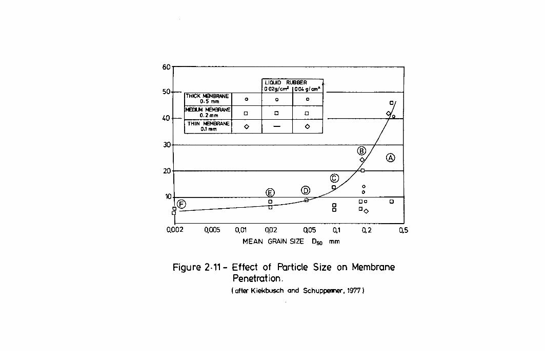
60
LIQUID RUBBER 002g/cm' 004g/a'll'&
r- THICK tEHBRANE 0 0 0
lJ 0.5 mm
MEtU4 MEM3RANE 0 0 0 0.2mm
L ,
r-THIN tEMBRAt£ 0 0 -O.lmm
~ ®
~ @ ~~ ~ DO 0 ® 0
0 .... 0 DO 0
1
50
40
30
20
10
0.002 0,005 0,01 0,02 Q05 0,1 Q2 Q5
MEAN GRAIN SIZE D50 mm
Figure 2·" - Effect of Particle Size on Membrane Penetration. ( after K iekbusch and Schuppenner, 1977 I

CHAPTER 3
TEST MATERIALS
The importance of a full and accurate description of a soil has long been
recognised as a pre-requisite to the confident interpretation of test
data. There are numerous discussions in the literature on the quantitative
description of a grading by single or multiple parameters (eg Selley,
1976), on measures of particle strength (eg Pigeon, 1969; BS8l2: 1975),
and on measures of particle shape (eg Marsal, 1963), but less information
is available on the relative merits of the various parameters suggested in
relation to the behaviour of soil under load. The classification tests
performed on the test materials used in the experimental programme have
been chosen from those available in the literature with an engineering
usage in mind. New indices have deliberately not been introduced though
some modifications have been made.
3.1 Origin and Description of Test Material
The test material was a limestone aggregate supplied by North Tyne
Roadstone Limited from the Mootlaw Quarry, near Matfen, Northumberland.
The material belongs to the Upper Limestone Series of the Upper
Carboniferous Period, is known locally as Blue Mountain Limestone, and may
be described as blue-grey in colour, fine grained, with occasional veins of calcite.
The aggregate was supplied pre-bagged in four industrially sieved nominal
size ranges of less than 5 mm, 5 mm to 10 mm, 10 mm to 20 mm, and 20 mm
to 40 rom (see Plate 3.1). The 'as supplied' particle size distributions
of the aggregates were determined using wet sieving (Test 7A of BS1377;
1975) and are shown in Figure 3.1. A petrographic analysis on a
repreSentative sample of the aggregate using X-Ray Fluorescence gave the
chemical composition listed in Table 3.1, which is typical of
Carboniferous Limestone.
- 20 -

3.2 Test Gradings
3.2.1 Specification Compliance
Unbound materials used in trenches (see Figure 3.2) usually comply with
the Department of Transport (DTp) Specification for Highway Works, 1986,
or its earlier version, the Specification for Road and Bridge Works 1975.
In order to test gradings representative of field practices, the clauses
listed in Table 3.2 were adopted as guidelines for choosing the gradings
to be Used in the research project. The gradings were chosen also to
investigate the effect of maximum particle size, and to yield data that
could be compared with published test results on fine and very coarse materials.
Calculations using the wet sieve grading curves of the supplied aggregate
Were made to determine the mix ratios required to prepare suitable
materials. The final proportions used, the calculated nominal gradings
and the DTp grading envelopes are shown in Figures 3.3a to 3.3c.
3.2.2 Preparation of Test Gradings
The gradings were batched in a 180 kg capacity concrete mixing drum in
total batch masses varying from 50 kg to 150 kg. The aggregate was added
to the drum in an air dry condition in the required proportions and mixed
for a period of 10 minutes per 100 kg. Following this the material was
tipped onto a clean dry concrete floor and quartered until specimens
SUitable for the intended tests were produced. These were double bagged
and stored ready for testing. Details of the batching procedure are
presented in Appendix A.
A preliminary test series verified that consistent results were produced
USing this method provided that at least two source bags of any size
fraction were used for each batch. As a standard laboratory precaution,
two wet sieve analyses were made on representative specimens from every
SUbsequent batch to check for deviations from the expected grading.
- 21 -

Figure 3.4 shoys that the level of repeatability obtained yas good, but
comparison of the grading curves yith the expected nominal gradings
calculated previously from the 'as supplied' gradings shoyed that
significant breakdoYn yas occurring during batching (see Figure 3.5).
Similar differences had been observed during the preliminary York. The
cause of the discrepancy yas investigated by preparing carefully by hand,
as opposed to using the concrete mixer, five specimens and comparing the
results of Yet sieve analyses on these yith the calculated nominal
gradings. Negligible differences yere found, confirming that breakdoYn yas
oCcurring as a result of using the automatic batcher.
De . Splte the breakdoYn, no changes yere made to the established procedure
as the DTp specification yas still being complied yith, and the automated m' .
lXlng procedure yas similar to that used by North Tyne Roadstone for
production of commercially used materials. The final gradings actually
tested are presented in Figure 3.Se.
3.3 Particle Classification Tests
3.3.1 Specific Gravity
Specific gravity determinations yere made using test 6A and 6B of BS1377:
1975, and during aggregate absorption value tests (see section 3.3.2). An
average of 2.71 was consistently recorded during the 16 tests on the
coarse (>5 mm) fraction of the medium and coarse test gradings, whereas 8
tests on the fine grading (minus particles greater than 2 mm) all gave a
Value of 2.75. A further 24 tests on material less than 5 mm using a
pycnometer gave results varying between 2.6 and 2.8, with an average of
2.67, but this scatter yas later attributed to equipment problems and the
reSUlts should be treated yith caution.
It is considered that the recorded higher specific gravity for the fines
represents a real difference in material properties betyeen the coarse and
fine fractions, as produced by quarrying. Nataatmadja and Parkin (1988)
also found a higher specific gravity for the fine fraction of base course
- 22 -

materials. Possible causes are the presence of calcite veins in the coarse
particles, or a tendency for fines produced by blasting to exclude the
larger particle interstices, or both. The average value of 2.71 obtained
over several months, and valid for the majority fraction of all gradings,
has been adopted in all calculations.
3.3.2 Aggregate Absorption Value Tests
A total of 8 samples per grading were tested in accordance with methods
5.4 and 5.5 of BS8l2: Part 2: 1975. Each sample was sieved to produce two
speCimens, one containing particles between 5 mm and 63 microns, and the
other containing particles greater than 5 mm. All were tested using the
appropriate method and the results are presented in Table 3.3. The data
Was used to calculate the absorption value for each test grading using the
relative fractions of the fine and coarse size ranges in the gradings and
assuming that the material passing through the 63 microns sieve had an
absorption equal to that for the material less than 5 mm. The
calculations yielded the following results which show the importance of
particle size on absorption characteristics:
Coarse grading, absorption value _ 0.8%
Medium grading, absorption value - 1.2%
Fine grading, absorption value _ 1.4%
These absorption values have been used in the analysis of the main test
series to calculate soil parameters, such as water content and degree of
saturation, by assuming the absorbed water forms part of the "solids"
component. Table 3.4 summarises the definitions of the classical soil
parameters based on this premise.
3.3.3 Grain Shape
The st 1 iIi ructural arrangement and behaviour of granu ar mater ass influ d l' enced by the grain shape. Numerous quantitative an qua ltative
parameters have been reported in the sedimentary petrology literature to
- 23 -

describe particles in terms of their overall form (eg Aschenbrenner, 1956)
and the roundness of their asperities (eg Wadell, 1932), but engineers
have preferred to use a qualitative assessment of a single parameter, the
"angularity" of a particle (Head, 1980). Angularity is largely a measure
of roundness although it takes account of the amount of curvature between
asperities as well and, as such, is a partial measure of overall form. A
quantitative measure of angularity was put forward by Lees (1963).
A quantitative approach has been adopted during this work. The average
overall partical shape of the test material has been assessed by measuring
the principal dimensions (a, b, c where a > b > c) of a representative
number of particles, and plotting the dimensional ratios bla and cfb
against each other as shown in Figure 3.6. Based upon this diagram, a
general descriptive term for the particle shape using the ratio limits
Suggested by Lees (1964) has been attributed to the particle. In
addition, the Degree of Angularity proposed by Lees (1963) has been
adopted as a quantitative measure of particle shape as it is believed this
method is correct in its recognition of the importance of the roundness of
the asperities and the relationship between the asperities.
A total of 124 particles from five size ranges, varying from 5 mm to 50 mm
in nominal diameter, were examined. The particles were placed
indiVidually on a three sided orthogonal perspex container, and the images
of the three principal planes cast onto a wall in turn using an overhead
projector. To eliminate scale effects, all particle images were made
Similar in size by moving the projector relative to the wall. The
traCings of these images, and the calculated magnification ratio, were
later Used to determine the principal dimensions and the degree of
angularity of h I t e partic es.
The results of the current work are summarised in Tables 3.5 and 3.6. The
estimation chart used is reproduced from Lees (1963) as Figure 3.7, and
the dimensional ratios for each of the size ranges are summarised in Figure 3.8.
- 24 -

Examination of the results shows that the majority of the particles,
regardless of size, are intermediate between -flaky- and
"equidimens ional " , with the overall average lying on the arbitrary
boundary between these shapes. The standard deviation of the shape
distribution for each size range is similar, confirming that the size of
particle has little effect on its shape within the limits of this work.
The degree of angularity of all the particles is generally 2100 ± 200,
although the angularity of the finest particles appears to be slightly
higher with a value of 2500. In conventional terminology, the particles
may be described as "angular" to "sub-angular-. An approximate
correlation suggested to relate this usually qualitative description to
the quantitative degree of angularity is presented in Figure 3.9.
3.3.4 Strength Tests
The compressibility of a particulate mass will be influenced by the
strength of its individual components and their susceptability to crushing
as noted in section 2.2. In dry or saturated soil, the products of
particle degradation are unlikely to affect the soil .ass other than to
effect a reduction in pore space and hence permeability. In unsaturated
Soils, the collection of finer particles in the voids between the main load c
arrying particles may cause some local re-distribution of free water
and its associated surface tension forces. This may induce further local
instabilities and small time dependent creep settlement. It is therefore considered important f tl Istre th to obtain an assessment 0 par c e ng.
The traditional method for measuring rock strength is the unconfined
compression test Which requires carefully trimmed specimens and is time consuming A fill . s a result only a small number 0 spec mens are usua y tested Fu
. rther, weak specimens may fracture during preparation and will nOt be t
ested, tending to lead to overestimated strengths. Other methods of asses i
s ng rock strength are available, such as point load tests or
irregUlar lump tests. However the applicability of the strength of the intact rock h b h b to the behaViour of its aggregate form as een s own to e
- 25 -

inconsistent (Dhir et aI, 1971), and direct measures of the performance of
the aggregate are preferred. BS8l2: 1975 details three such tests, namely
Aggregate Crushing Value (ACV) , Aggregate Impact Value (AIV) , and 10,
Fines Value. The ACV and AIV measure the resistance to pulverisation of a
uniform aggregate under static and dynamiC loading conditions
respectively. The 10% Fines test is a variation on the ACV test.
The ACV and AIV tests have been used to classify the aggregate in the
present work, and values of 22 and 18 were obtained respectively. Similar
numerical values were expected, as the AIV was intended to be aUXiliary to
the ACV by design. Further discussion of these and other strength tests
is Contained in a report edited by Collis and Fox (1985).
3.4 Behavioural Characteristics of Gradinls
3.4.1 Limiting Density Tests
The behaviour of granular soil depends amongst other things upon the initial d i ens ty and packing arrangement of the mass. However, for a given
Soil, its density will take some account of its packing arrangement
particularly if related to the limiting densities for that soil. This indicati h on as been accepted as sufficient for present purposes, even though it is appreciated 1 t th ki that, for spheres at eas •• ore an one pac ng
arrangement will give the same density (Graton and Frazer, 1935).
The Ii i i m t ng densities of a given soil are material properties, but
standard methods for their determination were not available until PUblicati
on after the research was completed of BS1377:l990. The methods of test th
at had been adopted in the absence of a British Standard were based
on those proposed by Kolbuzewski (1948) and Head (1980) for material
s ranging from clean sands to gravelly soils. BS1377:1990 appears also to b
e based upon these references, and the methods used in this research
Were largely in accordance with the new standard.
- 26 -

3.4.1.1 Minimum Density
Four specimens of each grading were tested, yielding consistent minimum
densities of 1.56 Mg/m3 and 1.63 Mg/m3 for the fine and medium gradings
respectively, or maximum void ratios of 0.74 and 0.66 respectively. For
the coarse grading, small variations in the minimum density were recorded,
the average value being 1.61 Mg/m3, or a maximum void ratio of 0.68.
3.4.1.2 Maximum Density
The maximum densities obtained were 2.30 Mg/m3 , 2.33 Kg/ml and 2.39 Kg/ml
for the fine, medium and coarse gradings, respectively, or in terms of
minimum void ratio, 0.18, 0.16 and 0.13, respectively.
The particle breakdown of each grading during the tests was investigated
also. The results of wet-sieve analyses on two spect.ens of each grading
are compared with their pre-compacted gradings in Figure 3.10 a, b, c.
3.4.2 Compaction Characteristics
The results of the compaction stages of all main series tests in which the
compactive effort was not a variable (see Chapter 4 and Appendix A), plus
extra compaction tests at the same compactive effort, are presented in
Figure 3.11 for the coarse grading. It is apparent from this figure that
the optimum free water content is 6.4%, with an associated maximum dry
density of 2.275 Mg/m3. This condition is equivalent to a void ratio of
0.20, or a relative density of 88'. In Figure 3.12, comparison of these
characteristics has been made with the results of compaction data on a
similar test material (grading curve given in Figure 3.13) provided by
British Gas Engineering Research Station using BS1377:1975 Tests 12, 13
and 14. This figure suggests that the compactive effort applied in the
majority of tests reported in this thesis probably lies between that
applied by BS1377:1975 Tests 12 and 13. However, this comparison between
compaction results is not strictly accurate as the materials involved were
undoubtedly dissimilar in some respects, as indicated by a comparison
- 27 -

between the maximum dry density achieved during the compaction of the
non-standard material to BS1377:1975 Test 14, and the maximum limiting density reported i ti 3 4 1 2 n sec on ....
Insufficient data has been collected to define the optimum water content
and maximum dry density achieved using the standard compactive effort for
the fine and medium gradings. The compaction data obtained during the
main series tests are presented in Figure 3.14 along with the dry
density-free water content relationship for the coarse grading. This
figure clearly shows that, as the coarseness of the soil increases, the
dry density achieved for the given compactive effort increases for a given
free water content. Comparison of the relative densities achieved for
each grading at the optimum compaction conditions are not possible, but at
a free water content of 3.0%, the relative densities achieved were 32"
39% and 68%, for the fine, medium and coarse gradings respectively.
- 28 -

Table 3.1 Results of Petrographic Analysis on Quarried Limestone !gBreiate
Chemical Compound Percentage of Total, by Mass
CaCOl 79.97
MgCOl 11.50
SiOz 2.80
CaS04 2.28
FezOl 2.03
A120l 1.00
K20 0.12
MnO 0.06
PZ05 0.05
Ti02 0.03
NazO <0.10
TOTAL 99.84 exc NazO
Table 3.2 Compliance of Test Gradings with Relevant Department of Transport Specifications*
Nominal Test Specification Clauses Description of Material Covered by Grading Clause
Coarse 803 (Table 8/2) Granular Sub-Base Material, Type 1 805 (Table 8/4) Wet-Mix Macadaa
Medium 804 (Table 8/3) Granular Sub-Base Material, Type 2
Fine 503 (Table 5/6) Material for Bedding, Laying and SurroundiDi of Pipes
* Department of Transport Specification for Highway WOrks. 1986

Table 3.3 Results of Aggregate Absorption Value Tests
I Number of AAV I Specific Gravity
Grading Specimens <,> I Tested I I I
lOven-Dry BasislSaturated SurfacelApparent I I Dry Basis I I I I
Fine 8 1.4;tO.2 2.57;tO.05 2.61;tO.07 2.67;tO.15
Medium
>5 ma 8 O.7;tO.1 2.65±O.Ol 2.67;tO.Ol 2.70±0.Ol <5 IDIII 8 1.4;tO.l 2. 57;tO.05 2.61;tO.05 2.67;tO.06
Coarse
>5 mm 8 O.6;tO.l 2.67;tO.Ol 2.69;tO.Ol 2.72±O.Ol <5 ma 8 l.l±O.2 2. 58;tO.10 2.62:tO.lO 2. 69:tO.07
± Limits quoted are absolute range of values measured, not standard deviations
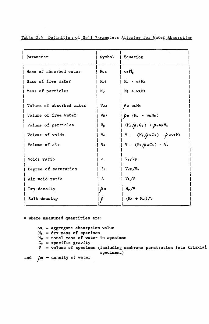
Table 3.4 Definition of Soil Parameters Allowing for Water Absorption
Parameter Symbol
Mass of absorbed water ~A
Mass of free water ~F
Mass of particles Mp
Volume of absorbed water VWA
Volume of free water VWF
Volume of particles Vp
Volume of voids Vu
Volume of air VA
Voids ratio I e I
Degree of saturation I Sr
I Air void ratio I A
I Dry density lId
I Bulk density 1/
I
* where measured quantities are:
WA aggregate absorption value Ms dry mass of specimen
Equation
wAMs
~ - wAMs
Ms + WAMs
fw wAMs
pw (Mw - wAMs)
(MslfwGs) + pWWAMs
V - (Ms1 wGs ) - f wWAMs
V (Ms1 wGs ) - Vw
Vv/VP
VWF /Vv
VA/V
Mp/V
(Ms + Mw)/V
Mw total mass of water in specimen Gs specific gravity
I I I I I I I I I I I
V volume of specimen (including membrane penetration into triaxial specimens)
and density of water

Table 3,5 Summaty of Particle $hape Analyses: Overall Fora of Particles
I I I Particle INumber ofl Average Dimensions I Average Dimensional Average
Size Particlesl± Standard Deviation Ratios ± Standard dimension Range I
I a b I I
37,S-50 4 160±5 46±3 I
28-37,5 30 I 49±10 37±5 I
20-28 30 140±8 27f!+ I
10-14 30 11814 13±2 I
5-6,3 30 I 9±2 6±1 I
Weighted Average Dimensional Ratio of all Particles
Deviation c b/8 C/b (8 + Ii! + 11)
1
36±7 O,77Q±O,0290,784±O,179 47,3
22±5 O,768±O,1410,619±O,182 36,0
17±3 O,696±O,124 O,639±O,171 28,0
9±2 O,779±O,ll4 O,665±O,186 13,3
4±1 O,745±O,160 O,622±O,219 6,3
II II 0,748 0,641 II II
Table 3,6 SUmmAty of Particle Shape Analyses: Delree of Angularity of Particles
Particle Number of Average Degree of Angularity ± Standard Deviation Size Range Particles A.b A.c Abc A
28-37,5 30 643±142 693±149 723±163 2058±351
20-28 30 596±112 696±142 660±127 1952±260
10-14 30 611±169 791±213 682±158 2084±395
5-6,3 30 735±182 845±168 732±2l4 23121424
Weighted Average of all 646 756 699 2102 Particles
NOTE: INSUFFICIENT PARTICLES IN THE SIZE RANGE 37,5 _ TO 50 mil \JERE AVAIlABLE TO ALLOW AN ACCURATE ESTIMATE OF 'nIE DEGREE OF ANGULARITY TO BE MADE

~ 2
10
'J
80
10
Vi 60 '" q: ~
UJ
~ 50 f-2 UJ u a: 40 UJ ~
30
20
10
o MICRON 2 6
Fine CLAY
c BRITISH STANDARD SIEVE SIZES 0 p= '"
In t; :;l ~ r.
~ or>
flf ;;; N .., ..,
~ .. ~ ~ ,.."
i I T N 1 III ~ i 'i'
~ Y !
"....-"" (V
/ I I
/ !I
/ / / /
[IV I V II I /
V J
/ /' / I ,/" I -- I / I ----_'-1
I / V
I-f--~ I, 1,..-1,..-I -
20 60 200 600 2 6 20 60 200m",
III
M~'()llJm Coarse Fine Medium Coarse Fine Medium Coarse g COBBLES f
SIl1 SAND GRAVH
Rgure 3-1-Grading Curves for Supplied Limestone Aggregate

2Smm
Figures in brackets refer to the clause number in the DTp specification for road and bridgeworks (1976) with which the material complies.
-....;::-""',~PPRH-~---j«(9lr01Ri8) Dense bitumen macadam wearing course.10mm size
27Smm (903) Dense bitumen macadam base course. 20mm size
TYPE 1
2Smm
--';:;::---"'"""""l~HH:r=*-=7:-S-m-m-((Q9ifi08) Dense bitumen macadam wearing course. 10mm size (903) Dense bitumen macadam base course. 20mm size
300mm (807) Dry lean concrete (18:1 aggregate cement, 6% moisture content)
c32Smm
. 100mm Smm crushed dolomite
:.0·· .. ~ 1 ' ... ,', ---L. ...... ,
SOmm
TYPE 2
2Smm
7;777:7"';RZ~Z;Z;;r::::::;;==---1c(9i70iA8) } Dense bitumen macadam wearing course.1Omm size (903) Dense bitumen mocacbm base course, 20mn size
L SOmm
TYPE 3
Smm crushed dolomite (Stabilised with 4 % cement. at 11 % moisture content)
Smm crushed dolomite
F='igure 3·2 - Three Typical Unbound Trench Reinstatements after Owen (1985)

100
90
BO I
10 )
i tjeo ~ .. ~SO ... ~ ~ 40 r
30
20
10
o
I
'00
c z
'to
Ho
II,
~ fiO C ... ~ 50 .. z ... u a: 40 r
)0 0
0 10
10 0
o
'flO
c Z
",
'Il
~'IC C
,
... ... , ~ SO .. ~ u a:: .1( I It'
.10
JO
10
11
MICIION 2
CLAY
MICRON 2
r CLAY
... lcnON 1
l ClAY
I
Fine
FIn!"
J BRITISH "A"DAIID IIIVE IIUI g I t! I': f~ . , f' , • • ¥
V ~
/
If j
j
V
v V ./
V ~
fS 20 flO 200 fSOD I • 20
Medium Co.". J Fin. Modlum I C_ Fine I MId""" e-.. SILT I SAND IlIlAyn
bl Fine Grading
Ptepcration: Fine aggregate as 5~ied by North Tyne Road.tane Limll.d OTp specification compliance: Clouse 503. Material for bedding .layir'9 en:! IUrroundr'9 piP"
& III IT 1114 ITA"D1D IIEYE IllES
I ~ 51 ,. • II: Ii ~ t ..
N l! • . " V
V /' / l/
./ I CLA t>~~ 8 ,I i/
V / ~j
GRA ~ III r /. / I
1/ 17 / /
./ / ..-/. i-" ..,-
~/
/ V ~
f---I-- ..,-l- i-' ......
i-' f- f-
1-- --6 ~ flO 200 600 I
I ',1t,'lIlm Coeup I F .ne Mf!(hum I C __ , ....
Sill I SANO ---- - --_.-
(bl Medium Grading Preparation: Rotlo of os supplied oggrw91les = 2: 1 tor fine: medilm slz. I'trIgeI
OTp specificaticln compliance: Clouse 804 Granulor sub-baw material Ty~ 2
• T
I
/)
Modlum
GIIAYfL
~ BAITISH STA"DAIID SIEYE SIZES
I II 51 ,.
i ~ ~~ ~ .. f t !
, 1/ ,
/ I I
I~ L.~ , p3 )
V I
l/ V / ....... 1 ....... 1/ ..,- V V
." / v !
...- V ,;' , / ... ~ ~ .....
--I- l---" ~/
.~
-- -- v ..... -- ~--- - --~ 6 70 eo 100 600 1 •
20 C __
.. It II :;
./ II"
~ /
II /
1/
I I
I
20
___ ~~_J __ '.h1hum COAfW I f,nf" M ... tll.nl I COOf .. F .... I MedIUm COOf"
1 -
';1[1 SAN!' GAAVfL
(e) Coarse Grading Prepara"on: Ratio of as suppllttd aggrt9Clt ... 2:1:1:1 for fine: medium: coars.:vtry coer_ Size ranges OTp specification compliance: Clouse 803. Granular sub-bole matl'l'ial Type 1
FIgure 3-3- Calculated Nominal Grading Curve and Specification Compliance
,~
flO 200mm.
I .-i_CO•BUS lJJ
T~
1/ /
flO 200mm
I C08BLES 11 J I
P 1/
/
60 l00mm
I 1 I COBBLES

co z
I()() I
i :lir., c ..
I
)
I
I
~ 50 I
~ u a: .1 .. .. I
30 l
]0 I
10 I
o
(
I 100
I
I HO
/I I
:li ~I I ~ '" ~ 50 ... Z w u 11:10 t
30 I
20 I
10 I
o
MICRO~
CLAY
MICRO~
I 100
II
10
c: z
-
in ~ c .. ~5 ~ ...
I ~ -10 .. ]0 I
]0 I
10 I
I
~~~-
MICRON 2
l CLA' 1
2
fine
2
Fo,,"
Font
11 t! ~i
I
P I
:1 i
!I!
t BAlnSH STA~DAAD SIEVE SIZES
j :I ~ ~ ~ :c: f~ ~ " ..,
~II! ... ! l! R R :;
V- V
j ~
IA fA
V
r FO 9 1,,0 ~NA YSE .
V~~
~ [;-'
k:;; ~ ~
8 20 110 200 600 2 • 20 110 200mm
P.1«hum CO"'" I font Medium Coer. , .... 1 MoII"'m
c __
COBBlES 11 J 1 Sill J SA NO J ... ~ .. ~ __ .~f.L ~--- .-
(a) Fine Grading
I BRITISH STA~OA"O III vi IIUI
I~ ~;. .
,II! j g I l: I R " s:;
~
~
~ '/
Ih ~ V OA: i I OR ~
INO ~NI ~YSI S
~V
:., 1--1.-"11-~
~ r? .,. '"/ ~ I· --I·
6 70 eo 200 600 2 • 20 10 200mm
Mt.'\hum Co. .. I fo". I MedIUm I Coer. 'iN I MoIItum Coer. I COBBLES 11J
Sil T I SA~O GRAVEL 1 (b) Medium Grading
J IIII'IIM ".,"0 IIIVIIIUI
~ II ~ II: I~ '1 t .
~tr I II " s:;
/. 1, J,V;
V V 111 ~ / 1
f?' ............ ENV L( PE I~~ ... ...v t;RAI IN!
/. f' ? ....... ~
~ / ~ £,
f1 v V-cr ~ ~ br- / 1/
~ ~ ~
~ ~
8 20 eo 200 600 2 • 20 eo 200mm
I P.1l"lhum I Co.,,, I Fin .. Mf'(hum I C __
'iN I M"",m
C __
I COBBLES I f J
Sill 1 SAND -
GRAVEL I
(e) Coarse Grading
Figure 3·4 - MaximUTl/Minimum Grading Envelopes for Botched rest Grading,

10
" It, ,.
10 ..
r : f ~' ~" '! t.
~.
c: z
10
!O
0
a
100
I
8 I
IU
~ 60
:. .. ~ SO
~ .. U II: ~o r
]0
10
10
o
MICI'IOH
I CL.AY
II,IICRDN
l CL.AY
100
'J{
~ in c .. ... ~ 50 ~ z ... u II: ,10
if
JO
20
10
Q
)
I
I
IIIICRO"
r CLA ....
2 • 20
FiN MeIIlum 1 ,IL.T
2 • 20
F,no Mellium
Sill
,
2 II 20
F",. Ml'tIlum
1 Sil T
J BRITISH STANDARD SIEVE SIZES
II • \: II: 'i ~ ..
p' .. f ! , It II ~
V 1,1 V
V
~ ~V
Lc GRA )IN /) I~ S ( ALC LnE ) ~R II AI.. ~ PLIE A 0 E~I ORAl ~N( 5
, V ;)
~ ~~
~ I---:::: V'
1·1-
'. 200 600 2 " 20 80 200mm. c __ 'I ' 'lilt Mlllium I COM. Fjne I Medium Coon.
J COBBLES J SAfoIO GRAVEL. ., -
ng
J BRITISH STANDARD SIEVE SIZES
• \: f~ ~ .. T ..
~W! r ! :! " ,. ~
V-I
~ /; 'I
V' /-:-... ~ OR [)I 0 ~ ~~~ I~ ~ S ALe ~~ TE o F
UP! ... ED GR ~c~ ~() 0 /,
.........:: ~ V
fo"" ..... f-'
I-:: r::::: --1- -~ -10 200 600 2 e 20 80 200mm
C ...... 1 , .... Mlllium C .... _ fiM I Medium Co.,. J I COBBLES
I SAfoID GRAVEl
(bl Coorse Grading
J BAITISH STANDARD SIEVE SIZES
~ ..
~ f~ ~ f ..
if lj T N ! , " II ::;
V '/ V V
~ FI ~~IIJ V / GF
V ~ V /' / I V-
/ M 01 JP
J GFIA[ N~
/ V
V II
/ r / /
.,/ /' ,/ CO ~R ;e
./ "" ./ OR II,DNI
----I-~
/ .... ~ --- i,....--f-"
eo 200 600 1 e 20 80 200rnm
C_. I fine MedIum I Coer. F,ne I Mtdlum C"", .. J I I I COBBlFS
SANfl GRAV£l
Ie) Summary of Average Grcx:tings Actually Tested
FIGURE 3-5- Particle Breakdown During Botching

* c
1'0~----------'1r------'
FLAKY
I I
EQUI-
I DIMENSIONAL
I ~ 0·66 ------ ----r----
z Q ~ o z o ...J UJ
0-0
FLAKY
AND
ELONGATED
ELONGATED
0·66
FLATNESS RATIO (c/b) * to
* Where the dimensions a:. b ~ c represent the principal dimensions of the smallest rectangular box that will just encompass the particle under consideration.
Figure JoS-Method For The Graphical Representation Of General Particle Shape (after Lees. 19S4)

0,99 100-199 200 -299 300-399 400 -499 500-599 600-699 700 -799
00 00 O(] 00 00 00 2JO Oc:::J 00 DO OD 00 00 ()O [J6 CJ~
OD Oc0. 00 00 00 Go Ol6 00 0<:) 00 DO 00 Do OD 00 Do c::>C:; cQD 00 800 -899 900 -999 1000 -1099 1100 -1199 1200-1299 1300 -1399 1400-1499 1500 -1599
DC? 0<::::> t?d tJcf eJQ 00 O?J 06 0 0 0 6 (jc:::, o~ ?70 c:::::;n ~(j OV' ot? 00 0<::::::7
Figure 3·7 - Chart For The Visual Estimation of The Degree of Angularity (after Lees,1963)

~ o ~ a: % o ~ i ... ...
o
7
06
De
05
Ge.
().]
iii
1M
00 Q.1
•• . a a . .
O.
.;
a D • ~
D a
D • I D . , .
D 0 . • D
D
1)-2 1)-3 0.., Q.§ G4Ii .- 0·7
FLATNESS RATIO (C/b I
16) Individual Test Results
!ID: • 5-6,3 mm
D
;.
.$ . .
'1:0 . DO
D
0-8
a D . D
o·q
•
Z,
-.!! .0
Q
! % Q
~ z o ..J
'"
o ,
I .......... I I I I .~~~--.--
____ l
o.e I I II I I 4. S; II I I ,.0 II
r I I 3'
It i . I I II CHi6
I I II ,. ~r------- ----"1
L -- -----j
i i
ID
-- 1- 5-6'3mm I ........... 2- 10-14mm
-- 3- 20-28mm -- 4- 28-31·5mm
~ 5- 31·5-50mm (note-insufficient da~ t ".
0 Average statistical analysi I
I'
- - ------ - --- ------
0.1 0.·2 Q.1 04 06 o.s C>l6 0·7 IU FLATNESS RATIO (c/bl
(b) Mean and Standard Deviation of Results
• 1O-14·5mm c 20-28 mm • 28-3'1'Smm
Figure 3·B-Results of Particle Shape Analysis • 315-50mm
()'I '·0

Degree of Angularity Equiva lent Descri ptive Typical Particle Angularity Term Shapes
0 t> ,&:;:J 3000 or greater Ex tremely Angular
0 CJ 0
2000 - 2999 Angular a 0 Q ~ D ~
1250 - 1999 Sub- Angular LJ a Q
~ D 0
600 - 1249 Sub - Rounded ~ 0 0 0 0 0
Less than 600 Rounded 0 () 0
0 G D
Figure 3· 9 - Suggested Relationship Between The Quantitative Degree of Angularity and Conventional Qualitative Visual Assessment of Angularity

100 I
) !II)
10 I
I
i JIG I .. ... ~ 5'
i u IE 40 r
I 3D
20 I
10 I
o
I
0
0
0
J
~ ~IG .. ~50 ~
~ li 40 r
I 3D
20 )
10 I
o I
MICRON
CLAY
MICRON 2
l CLAY I
0 100
I !II)
I 10
0
i
J 10
III
0 ~50
i u IE 4, r
)
3D )
20 I
I 10
o I MICRON 2
I CLAY I I
-
2 • 20
Fino Medium C_.
SILT
• 20
'Ino J Medium C_ ..
SILT - - - -- -
I
• 20
'Ino I Mod ...... 1 c_ liLT
J fa • ~ I S
I~ INa! S~ f4SU ~[ ~ T NO
~~
~ ~ L' L
~ ~ V ..... / .,.,
" -eo 200 lOG
I ".,. Modtum I I lAND
(a) Fine Grading
I a I 5
lORA )IN SH AFT R E
,/' .... ~
./
~~ ."
-- ~ .....
eo 200 lOG
I 'Ino I Modtum I 1 ______ MNIl_
(b) Medium Grading
~ • ~. ~
k::: 1::::=::::
.... f--- .-
.0 300 lOG
I , .... I Modtum I I __ . ___ IAN.D __
Ie) Coarse Grading
1111 IT 11M ITANOiD IIIY.tIUI
I} .. ~ , If ~
;. / /
'f
J I
~ L'
V'
~ ~~
I • 20 10 2OOInm,
C- I , ... I Mod- I ea.. I CO'ILESf Il I QIIIAYfL
11II""1T,1II0 "'YIIIIII .~ . • .. ¥ ,
~ ..
. ~~ EO ~ '"
fJ V; I'
~ t~ ~~
2 • 20 10 2OOInm,
C_ 'Ino I Mod ...... I ea.. f COIILES II I GIIIAYfL I
.IIITIIH ITANDAIID IIEYE IIZES'
I~ ~ 1 • , II .. a ,It ~ ~
) "'l !/
j ,I
~ tDS T~ ASli ~EI II
TE G
~ ~;:;:: I
~ v ~
i
~ ED IL' NG
.....
2 • 20 10 2OOInm,
c_ I 'Ino I ",..Ium 1 ea.. J I I I COIILES
(jIlAYfL
Figure 3·10 - Degree of Breakdown During Maximum Densi ty Tes ts

M
~ 01 ~
>-~
iii z ILl a >-a:: a
2300
2-2
2-200
2-100
2{)00
10900
1{)
s • ..
". 84 " B2
~o .!•
20 ~ 4G 50 FREE WATER CONTENT (".1
ISE! • ltstIat Sheffield lhversity
In 2S4nn ~. cell
• T ... at &i1ish Gas ERS in 305nm dicrMtIf' oatl ~ Specinens 82 and 84 were ~ted with a lower effort b inYts ligate this ~t.
60 64 1-0 a-o
Figure 3-11-Dry Da1Sity -Free Water Content Relationship For Coarse Grading At Standard Test Programme Compoctive Effect
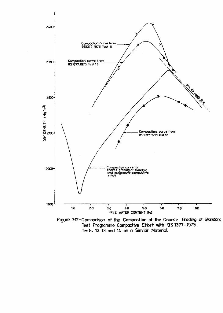
>I-
~
2-4
2-300
UJ 02->-a:: o
Compoction curve from 651377:1975 Test 14 --~
Compaction curve from~_-+o~ B51377:1975 Test 13
1--__ ComJXlC<tion curve from BSl377:197S"R!st 12
1 _____ Compaction c;:urve for coarse gradlOQ at sbndard test programme compaclive effort.
1~1~~---r---r----r---r----r----r-----or----~r-----
1-0 2-0 3-0 4-0 5-0 6-0 7-0 FREE WATER CONTENT 1'"1.)
Figure 312-Comparison of the Compaction of the Coarse Grading at Sbldard Test Programme Compocti'Je Effort with BS 1377: 1975 Tests 12 13 CI1d 14 on a Similar MateriaL

c: BRITISH STANDARD SIEVE SIZES 0
~ ~? on on II :&! S! ... l!l j '1 ..,
~ 1 ~ • R ~ ,.; 17 I
... r 'I 'i' 100
)f p
~ / :;
90
80
COAl ~SE -7 / GRAl PI!\(
7 MA E IA L 'I(~E o 11\ / TE pT ~C ~( 137'i I)
II [7
70
60
50
/ lIL,.l.--
V V
V / V
V [7
/ ~ i-o'l::'
1:;::1:: ~
1",...00 I-""" I---- --
40
30
20
10
o MICRON 2 6 20 60 200 600 2 6 20 60 200mm
'" Fine Ml'tlium Coarse Fine Medium Coarse Fine Medium Coarse 0 c
CLAY COBBLES ~ SIL T SAND GRAVH ------- - ----- - -.-------~-----.----.--- ------ ~--i--
Figure 3-13 -Comparison of Grading Curve for Material Tested Using BS 1377: 1975
Tests 12 .13 and 14 with Main Test Programme Coarse Grading

2·100
2·000
·E ~ 1·900 6 >t-iii z w o
1·800
1·700
/
Compaction curve for coarse grading _____ -/
\ \
e = 0·472 RD = 39%
'·0
?
?
2·0
e = 0·310 RD = 68%
$AS
$A1
$F2
e = 0·551 RD= 32%
40
?
5-0 FREE ~TER CONTENT (Oh)
KEY:
$ Fine grading
X Medium grading
?
6·0 7·0 8·0
Figure 314 - Dry Density- Free Water Content Relationship for Fine c;md Medium Gradings at Standard Test Programme Compoctive Effort

Pl ate 3.1 Limestone aggregate supplied
by North Tyne Roadstone Limited

CHAPTER 4
DESCRIPTION AND DEVELOPMENT OF EXPERIMENTAL APPARATUS
This chapter presents details of the experimental apparatus and
ancillary equipment used in the main test series. Details of the
calibration and operational checks made on the apparatus to ensure their
correct functioning are presented separately in Chapter 5, and the names
and addresses of the specialist equipment suppliers are presented in
Appendix B. Three major pieces of apparatus were used, namely a 254 mm
internal diameter one dimensional consolidation cell specifically
developed for testing unsaturated soils at low stresses, a conventional
triaxial cell modified to allow testing of 200 mm diameter unsaturated
specimens, and a 305 mm internal diameter strain controlled compression
cell. In the following sections an overview of each piece of apparatus
is presented initially, with a more detailed commentary on the important
aspects of each part of the apparatus in later sub-sections.
4.1 Consolidation Cell
A consolidation cell suitable for high quality testing of the proposed
materials at the low stresses envisaged was not commercially available
at the start of the project. The requirements of a suitable cell were
that it allow repeatable testing of specimens containing coarse
particles, that it allow the control and/or measurement of the pressure
and volume of the air and water phases within the specimen, and that it
allow accurate measurement of the applied vertical stress.
The general assembly of the new cell that was developed to meet these
requirements is shown in Figure 4.1 a and the associated plumbing
system in Figure 4.1 b . Two identical cells were manufactured and used
simultaneously during the test programme. Each cell essentially
consisted of a fixed base platen and a top platen through which vertical
stress was applied to a specimen radially confined by a 254 mm internal
diameter bronze alloy cylinder. Pore water pressure vas measured at

both platens using high air entry value ceramics. Specimens up to 120 mm
high with a maximum particle size of 40 mm could be accommodated, and
incremental net stresses to 165 kPa could be applied through the top
platen.
The top platen (see Figure 4.2) consisted of an upper and lower body
primarily connected at three points only using three 2.5 kN load cells
manufactured as detailed in Appendix C. The upper body used three
circumferential '0' rings to achieve a seal between the specimen and
pressurised water above that was used to apply vertical stress to the
soil. Direct measurement of the loads transmitted to the lower body
using the load cells allowed frictional losses in the applied vertical
stress due to the seals to be negated. This allowed accurate calculation
of the stress applied to the specimen. The lower body was prevented
from contacting the cell body and developing additional friction losses
by virtue of its slightly smaller diameter, and also by the height of
the upper body combining with its '0' ring seals to .inimise platen tilt
during a test.
Air pressure was regulated within the specimen at a constant raised
value via a line passing through the top platen, ensuring that the
otherwise negative pore water pressures in the spect.en were positive
(see section 2.3.1). The pore water pressures were separated from the
air pressure at both platens using large diameter saturated high air
entry value ceramics. The ceramics were supported on spiral drainage
basins and were connected to a pore water pressure transducer via a
central drainage line. An additional inlet at the outer edge of the
spiral basin was used periodically to flush away air that had
accumulated within the basin as a result of slow diffusion of air
through the ceramics.
Total specimen volume change was calculated from the cross sectional
area of the cell and the changes in specimen height as measured with an
LVDT resting on a central piston rod connected to the top platen. As
already noted, the length of the top platen and the action of its seals
- 30 -

minimised tilt and therefore allowed accurate observation of total
changes in volume.
Yater volume changes could be measured using Imperial College type
volume change units if water drained conditions were required. The
constant back pressure applied to the volume change units effectively
controlled the applied pore water pressure at the top and/or bottom of
the specimen in this mode. Alternatively, pore water pressures could be
measured using conventional pore water pressure transducers in a water
undrained mode.
The air phase in the specimens was permanently drained to the atmosphere
via a pressure regulator, and no attempt was made to aeasure directly
air phase volume changes. However. as noted in section 2.3.1, air is
able to diffuse slowly through the high air entry value ceramics,
leading to incorrect measurement of pore water pressure or water volume
change. Consequently, the volumes of diffused air re.aved during
periodic flushing of the platens were measured using new diffused air
volume indicators.
Details of the cell, its ancillary equipment, and the data acquisition
software used with the cell are presented below, together with details
of the temperature controlled laboratory within which the cell was
always used.
4.1.1 Cell, Plumbing and Instrumentation
4.1.1.1 Cell Dimensions
The cell was basically composed of two conventional 254 mm internal
diameter Rowe Cell bodies, each 127 mm high, which were rigidly bolted
together concentrically with eight bolts. To reduce any diametrical
eccentricities at the joints of the bodies. the internal faces were
smoothed locally with silicon carbide paper after asseably and never
dismantled again during the work. An approximately 4 .. thick rubber
- 31 -

gasket was sealed onto one end face of the cell using Araldite adhesive,
and holes punched for the bolts. At the other end, a small chamfer was
machined on the internal face of the cell to ease top platen insertion.
The dimensions of the fully assembled top platen reduced the maximum
specimen height to about 120 mm, although actual heights ranged from
89.0 mm to 119.1 mm. As discussed in the literature review, a minimum
specimen dimension to maximum particle size ratio of four at least is
usually considered sufficient to ensure repeatable test results are
obtained for well graded specimens. This implies a maximum particle size
of about 20 mm in the new cells. However, it was judged at the start of
the research that the coarse grading could be used in the cell despite a
maximum particle size of 37.5 mm, as only 11% by mass of material would
exceed 28mm and 20% by mass would exceed 20 mm (see Figure 3.5c).
Justification of this judgement is contained in section 8.4.1.
4.1.1.2 Base Platen
The three part base platen shown in Figure 4.3 consisted of a five high
air entry value ceramics in an aluminium locking ring which rested on an
anodised aluminium spiral grooved drainage basin which connected the
central drainage outlet and the flushing inlet. This in turn was
supported on a conventional Rowe Cell base with a pore water pressure
transducer housing block on its drainage outlet port. These components
were of the same diameter as the cell base and, when in use, were
clamped between the base and the main cylindrical body using eight
bolts. Greased '0' ring seals on the underside of the drainage basin
body around the drainage and flushing holes prevented water loss between
parts A and B, and a further '0' ring between the ceramic locking ring
and the outer rim of the drainage basin ensured a seal between these
bodies. The pressure of the soil on the ceramic ensured efficient
operation of the flushing mechanism (see Section 5.2).
The ceramic had a 450 bevelled edge and was permanently sealed into its
locking ring using Silastic RTV732 plastic sealant. When sealed in
place, the ceramic was machined flush with its locking ring using a
- 32 -

grinding belt to ensure that a sufficiently flat surface would be
exposed to the accurately machined upper surface of the drainage basin.
This was considered essential as even a small capacicy for flexing of
the ceramic across the full diameter of the cell could have lead to
cracking of the brittle ceramic and a significant reduction of its air
entry value. A series of tests aimed at quantifying the flexual
behaviour of the high air entry value ceramic and the effects on its air
entry value is reported in Appendix E. The 4 mm width of the spiral
groove was adopted on the basis of this work.
4.1.1.3 Top Platen
Details of the top platen are shown in Figure 4.2. The lower body was
essentially the same as the base platen, except that its 250 mm diameter
allowed it to move freely within the main cell body. Further, four
small air lines were bored through the metal to connect the specimen to
the void between the upper and lower bodies. This space was pressurised
with air during a test, and the bores allowed this raised pressure to be
transmitted to the specimen. The bores were capped with small diameter
porous plastic plugs to prevent any water that was te8porarily displaced
up the sides of the top platen during a test from floving into the air
void between the two main bodies of the platen and affecting the load
cells.
Stress transfer between the bodies of the top platen vas possible
through three routes:
(i) the coiled flexible plastic pipes between the drainage basin and
the drainage and flushing lines in the upper body
(ii) the maximum 3 mm wide bead of RTV732 Silastic around the
circumference of the bodies
(iii) the three load cells which were mated, bolted and sealed into the
recesses in both bodies.
- 33 -

Of these three possible stress paths, it was considered that the use of
coiled flexible pipe connections for the flushing and drainage lines
ensured negligible unmeasured stress transmission through this inter
body contact. Also, simple experimental work showed that the Youngs
Modulus of cured Silastic is about 0.2 N/mm2, and thus unrecorded stress
transmission through the circumferential bead at the small strains
required for full stress transmission to occur through the load cells
could be shown to be negligible. Consequentially, it was confidently
assumed that all significant stress transfer between the bodies would be
measured by the load cells.
The 2.5 kN capacity load cells designed and developed specifically for
the research and details of their manufacture are given in Appendix C.
The design strain of the cells at their maximum working load of 2.5 kN
was 800 micros train , which allowed for a 250, overload before the linear
elastic region of the material would be exceeded. This design strain
ensured also that the cells were stressed within their most linear
region, and minimised creep potential in the cell body. Aluminium to the
specification 2014 T6 was used as the cell body material as it shows
especially linear behaviour. The electrical circuitry employed 6mm
gauge length epoxy backed strain gauges, type Kyowa FLA-6-350-23, in a
full Wheatstone bridge for self temperature compensation, and a low 5v
energising voltage was used to minimise gauge creep. A high gauge
resistance and a long gauge length were employed to improve current and
heat dissipation characteristics, and an epoxy rather than a polyamide
backing was adopted as it exhibits a lower creep potential.
The upper body of the top platen served primarily as an efficient seal
and tilt reducing mechanism as explained in section 4.1. The central
drainage piston was rigidly screwed into the body, and the air and
flushing lines connected to it from the cell top using coiled flexible
pipe. Provision was made in the design for use of up to five '0' ring
seals but only the three shown in Figure 4.2 proved necessary in
practice. Verification of the sealing efficiency is covered in Section
5.2, but it is noted that the sizes of the '0' rings adopted for use
- 34 -

were determined from a series of trials aimed at ensuring a seal whilst
minimising side friction. The pressurised water used to apply the
specimen vertical stresses was regulated by air pressure from either a
0-100 psi (690 kPa) or 0-30 psi (207 kPa) air pressure regulator acting
on a air-deaired water bladder cell. The regulators were Nullmatic
Pressure Regulators, models 40-100 or 40-30HF, respectively.
Once the cell was assembled and the specimen compacted the top platen
was pushed into the consolidation cell using a hydraulic press until the
platen was flush with the upper flange. After full assembly of the cell
the platen would be forced slowly down into contact with the specimen
using the water pressure in the upper cell chamber.
4.1.1.4 Measurement of phase volume changes
In an unsaturated soil, measurement of two of either total specimen
volume change, or volume change of either of the fluid phases, allows
calculation of all volume changes affecting the soil if the solid phase
has a constant volume. In this work it was decided to measure total
specimen volume change and water phase volume change, and to calculate
the air volume changes.
Total volume change of a specimen in the consolidation cell was
calculated from the average specimen compression during a test and the
known constant cross sectional area of the specimen. Measurement of
axial compression to O.Olmm using Sangamo 50 mm stroke LVDT's (Type LSC
HS550) allowed calculation of total volume changes to 0.5 cm3 , as the
cell diameter was measured to be 254.0 ± 0.5 mm.
Water volume changes were measured to 0.1 cm3 using Imperial College
type volume change units connected to the cell using rigid walled
plastic piping. Water back pressure to the volume change units was
applied by 0-30 psi (207 kPa) air pressure regulators acting on an
air-deaired water bladder cell, and observed on a 0-1 bar (100 kPa) or
0-5 bar (500 kPa) Budenburg Bourdon gauge.
- 35 -

Based on the foregoing, air volume changes were calculated to an
accuracy of 1.0 c~. However, diffusion of the gas aixture that forms
air through the saturated ceramics in response to partial pressure
differences across the ceramics would result in apparent changes in
water being recorded by the Imperial College type units, and would lead
to erroneous interpretation of test data. To overcome this potential
problem, the platens were designed to allow flushing away of accumulated
air periodically. A flushing pressure about 10 kPa higher than the
current pore water pressure would be applied to the drainage basin
through the flushing inlet, and the drainage line to the volume change
unit opened. Air and water would then be displaced through the plumbing
to the volume change units in response to the pressure gradient applied.
However during the operation a bypass line would be opened to connect a
"diffused air volume indicator" between the cell and volume change units
(see Figure 4.lb).
The air volume indicator consisted of an inner sealed 0.01 cm! graduated
glass burette with a partial column of water with an inlet pipe above
the outlet pipe, as shown. When the flushed fluids entered the unit at
the slow rate of flow governed by the applied pressure gradient, the air
bubbles separated from the water and rose to be trapped in the burette.
In contrast, the water flowed without resistance through the lower
outlet pipe to the volume change units. The flushing pressure applied
was connected also to the outer chamber of the air volume indicator to
ensure the integrity of the burette during use. The sometimes large
changes in water volume used to ensure flushing were accommodated using
reversal valves to govern flow direction into the volume change units.
From the readings of the burette before and after flushing, at the known
pressure applied to the volume change units, the volu.e of air displaced
was calculated.
4.1.1.5 Measurement and Control of Pore Yater Pressures
Specimen air pressure was regulated at a constant value of typically 50
kPa using a 0-100 psi (690 kPa) air pressure regulator, and measured
using a 0-5 bar (500 kPa) Bourdon gauge. The resultant raised pore water
- 36 -

pressures in the specimen were measured using pressure transducers in
the conventional manner. Cell A utilised 0-350 kPa range transducers
(Bell and Howell model 4-366-0002-01 Mohm) , and cell B utilised 0-140
kPa range tranducers (Druck model PDCR10), the variation being chosen
originally to reflect the different gradings to be used in each cell and
their respective anticipated maximum suctions. However, measured
suctions proved to be considerably smaller than expected and lower range
transducers could have been employed for all tests.
4.1.2 Ancillary Equipment
4.1.2.1 Compaction Apparatus
The brittle nature of the high air entry value ceramics and the
requirement to apply a high compactive effort to the specimens during
preparation required that ancillary compaction apparatus be developed to
allow compaction on to a rigid unbreakable surface before assembly of
the test cell with minimal disturbance to the speciaen. The equipment
developed is shown in Figure 4.5 and consisted of a 19.05 mm (0.75-)
thick steel compaction base mounted upon four adjustable legs with a
semi-circular recess at one end and a hydraulic assembly jack at the
other. During compaction with a Kango hammer (Type 900, 60Hz, 900W) the
brass body of the consolidation cell was bolted with its greased rubber
gasket in contact with the greased compaction base using seven bolts.
Afterwards, the hydraulic ram was used to slide the specimen in the now
unbolted cell body slowly and smoothly across the base onto the base
platen of the test cell, which had been placed into and restrained in
the semi-circular recess using the guide bars shown in Figure 4.5. A
slight height difference between the ceramic and the base surface of the
compaction plate was set to minimise abrasion of the ceramic and
reorientation of compacted particles during sliding, whilst water loss
was prevented by the gasket between the plate and the base, and
plasticine plugs in the bolt holes in the base platen over which the
specimen had to slide.
- 37 -

A second piece of compaction apparatus was designed and built to ensure
that the compaction plate attached to the Kango hammer was guided near
vertically during use. Figure 4.6 shows the compaction plate and the
guide developed. The guide consisted of a 75 mm long steel collar welded
onto a 12 mm thick plate with a hole bored through it for the hexagonal
compaction base shaft to pass through. The hexagonal bar was restrained
on three faces at two separate heights using three sets of adjustable
and lockable screws orientated at 1200 in plan. The screws were
adjusted and locked onto the hexagonal bar such that tilt of the bar was
prevented and the bar was able to fall between the screws under its own
weight. The whole assembly was bolted onto the consolidation cell during
use.
4.1.2.2 Jack for Removal of Top Platen
The '0' ring seals around the circumference of the upper body of the top
platen prevented it from being inserted and removed manually from the
main cell body. Rather, insertion was facilitated using a hydraulic
press followed by water pressure above the platen after full assembly of
the cell to bring the platen into contact with the specimen.
Removal was facilitated by the screw jack arrangement shown in Figure
4.7. The jack was bolted to the top platen at three anchorage points
after removal of all pipe connections to the top platen. It was bolted
also to the consolidation cell body on its upper flange at four points,
with spacers between the cross bar supporting the jack and cell flange
to allow the top platen to be wound clear of the cell. The jack was
operated manually.
4.1.3 Data Acquisition System
4.1.3.1 Hardware
The data acquisition system was set up as shown in Figure 4.8, using a
BBC B Computer (24 k memory) with dual disk drive, an Acorn IEEE
interface, an MC Computer's analogue input unit (model 13683) and a 16
- 38 -

channel DrN plug connection box. In addition a parallel printer or a
Hewlett Packard A3/A4 plotter could be attached to the BBC for hard
copies of the data acquired.
Preliminary data analysis was completed using the BBC, but final
interpretation and manipulation of the data for more complex analysis
was made on an IBM compatible VIGLEN 48 megabyte hard disk personal
computer. Transfer of data between the BBC and the VIGLEN was aided by
the public domain software "KERMIT".
4.1.3.2 Software
The data acquisition software "LOG3" was written by the author for use
with the BBC and up to 16 data input channels. The programme allowed
for:
(i) simultaneous independent monitoring of two cells if required,
with the capacity to open and close data files for each cell
independently
(ii) allocation and in-test variation of independent linear scanning
rates for each cell
(iii) input of conversion factors and offsets for the data on each
channel for real time data output in engineering units to the
screen and disk (and printer if required)
(iv) in-test display of test details and calibration information
(v) in-test display, averaging and interpretation of output from the
load cells to allow accurate control of the applied vertical
stress.
- 39 -

An additional option for semi-automatic compensation of water volume
change measurements for flow reversal to the volume change units proved
not to be required in practice. Further details of the software and data
processing options are presented in Appendix C. Software for the BBC was
written also by the author to allow output of test data in tabulated and
graphical formats.
4.1.4 Constant Temperature Apparatus
A thermostat controlled fan driven heater was used in conjunction with a
variable speed roof mounted air circulation fan to maintain a
temperature of 20oC± l OC in the approximately 36 m2 by 4 m high square
laboratory. The thermostat was located near the windows at about the
level of the experimental apparatus, with the heater several metres
above. The roof fan was found to be necessary to assist the heater to
achieve good air circulation and a negligible temperature gradient with
height or location in the laboratory. Room temperature, atmospheric
pressure and humidity adjacent to the test equipment were continually
recorded using an Isuzu thermo-hygro-barograpb (model 3-1135) which
could be used in either 24 hour or 7 day chart mode. In addition,
temperature variations were observed at two other locations in the
laboratory using maximum/minimum thermometers. The thermometers
confirmed that temperature gradients within the room were negligible.
4.2 Triaxial Cell
Two triaxial cells of similar design (see Fi~e 4.9) and suitable for
testing specimens of 200 mm diameter and 400 .. height were used for
part of the experimental work. The cells and their ancillary equipment
were essentially conventional in nature but modified slightly to allow
the testing of both unsaturated and saturated soils. The cells were made
and commissioned by staff at the British Gas Engineering Research
Station, then calibrated by the author with the co-operation of British
Gas before the work reported in this thesis was performed. Details are
given below. The cells were not used in a constant temperature
laboratory but corrections were made for temperature effects.
- 40 -

4.2.1 Load Application and Measurement
Axial straining of specimens was applied during tests at a constant
pre-set rate using a Yykeham Farrance strain control compression
machine. Axial stresses developed within the specimen were measured
internally using a 10 kN Yykeham Farrance submersible load cell (model
YF17l09) in one version of the triaxial cell, and measured externally
using a 20 kN Sensotec load cell (mode 41) in the other.
4.2.2 Platen Details
The base platen comprised a 1 bar air entry value ceramic sealed with
Araldite into a locking ring similar to that shown in Figure 4.3 d
which was then mounted upon a grooved drainage chamber. The platen was
connected to a back pressure and volume change measurement system which
allowed either passive measurement of pore water pressure, if water
undrained conditions were enforced, or active control of the pore water
pressure if water drainage was allowed.
The upper platen was grooved similar to the base drainage chamber. When
unsaturated specimens were to be tested, the platen was placed in direct
contact with the soil and a regulated air pressure greater than
atmospheric pressure applied to the specimen through it in order to
maintain positive pore water pressures throughout (the axis translation
technique). When saturated specimens were to be tested, a porous plastic
disc was placed between the platen and the soil, and pore water pressure
at the top of the specimen was measured passively.
4.2.3 Measurement of Volume Changes and Pressures
Axial strains were measured externally. An RDP 100 mm stroke LVDT (Type
DS/2000A) accurate to about 0.2 mm was fixed to the rigid compression
machine cross beam with its armature resting on the triaxial cell, and
the vertical movement of the cell relative to the cross beam was
measured. Strains were computed assuming the total compression or
extension of the specimen corresponded to that measured by the LVDT. SH[F~-;
UNIV::; ': I \'
- 41 - U~:mA,-1Y

Volume change units doubling as air-water interfaces were used to
measure water volume change and total cell chamber volume change. The
1000 cm3 interfaces were developed and built at British Gas Engineering
Research Station to a design similar to the Imperial College type volume
change units used at the University. Displacement of the piston was
measured using either a Penny and Giles Rectilinear Potentiometer (type
HLP 1905Al/100 mm/4 kohm) or RDP 100 mm stroke LVDT (type DS/2000A).
The units were nominally accurate to about 2 cm3 at a constant
temperature. Air volume changes were not measured.
From a knowledge of the nominal cell chamber volume change, and the
effects of piston ram movements and changes in the applied cell
pressures on the nominal cell volume, the average total volume change
and the average degree of radial strain of the specimen were calculated.
Diffused air that had accumulated beneath the base ceramic was flushed
out without measurement after consolidation of the specimen, and any
diffusion that occurred during the relatively short duration main stages
of the tests was shown to be negligible. Total specimen volume changes
were nominally measured to about 0.1 cm3 •
The system employed up to 3 no 100 psi (690 kPa) capacity Sensotec
pressure transducers (TJE series, 2 gauge) to record the cell chamber
pressure, specimen air pressure, and back pressure to the base volume
change unit. The pressures were measured also on Bourdon gauges to
coarse check the output from the transducers.
4.2.4 Data Acquisition System
All data acquisition was made using a Digital Equipment Corporation DEC
PDP 11/44 mini computer, connected via a serial link to a Mowlem
Microsystems ADU 700 Datalogger which allowed 0 to 10 volt analogue
input from up to 64 channels. All transducers were used in conjunction
with either Pro tech or RDP transducer signal amplifiers, which employed
individual removable amplification cards stored in a rack unit. Each
card was calibrated for use with only one specific transducer such that
- 42 -

full scale amplified output from the transducer amplified output was
approximately 10 volts and maximum use of the input range of the data
logger could be made. The system is summarised in Figure 4.10, which
shows also that coarse checks on the recorded output were possible using
digital voltmeters connected to the amplifier output. This check system
was used during all tests, with output on the voltmeters noted
periodically by hand for subsequent correlation with the computer
recorded data.
The software for simultaneous data acquisition from several independent
concurrent tests was developed in house at British Gas Engineering
Research Station. It allowed nominated channels associated with any
given test to be scanned and their current output displayed on screen in
engineering units based upon the transducer zero values and calibration
factors stored in the computer. Data was periodically recorded on disk
on either a root time or linear time basis in millivolts, but was
usually presented in engineering units.
4.3 Compression Cells
A large number of one dimensional compression tests were made at the
Research Station in the relatively simple piece of apparatus shown in
Figure 4.11. It consisted of a 305 mm diameter metal cell into which a
specimen of maximum height 200 mm was compacted, and a conventional
strain controlled Wykeham Farrance compression machine with a rigid
plane metal top platen attached to the reaction bar of the machine via
either a 20 kN or III kN capacity model 41 Sensotec load cell. In use,
the compression cell was mounted on the compression machine and load
cycles applied to the specimen at a constant strain rate. The applied
strain was recorded using an RDP 100 mm stoke LVDT in a similar manner
to that described in section 4.2.3, and data acquisition was made using
the system noted in section 4.2.4.
- 43 -

Compaction was applied to the specimens as noted in Appendix A using
either a Kango hammer or a tamping rod. The Kango hammer was the same
used as that described above in section 4.1.2.1, but with a 300 mm
diameter compaction plate and a modified version of the compaction guide
suitable for the larger cell diameter. The tamping rod consisted of a
2 m wooden pole with a 100 mm diameter cylindrical 2 kg mass at the end.
- 44 -

_--- - P\.IIIHIMI 1""-
DUM. lID\' "",c~~u~t--=:-Ir--=-r n. ...... T£II Wft'M
UMO caLS
I'UlSHI'" ---i===~ ___ ~========t--I .... T
(al General Arrongement
'0' ..... lULl
... - ",. ........... MIA ... _1It'
TopVoIuIM j Change System
Air Pressure And Cell Chamber System
~me { Syst.m
Bock Presure 1 Su!IPIy System
0-7 Bar Gauge
AVI Back Pressur. Bypass Valve
~----------------~~ Volum. Change Unit
Reversing Volves
To
Lab Air
Supply - -----I
c.tI ""-ssur. Chamber Vent
ConsolidaliOn Cell
Connection To Vocwm Pump When Required
Vorl able Connection
Air Bteed
~~~~~~~~~~~~~~D LMII anx- VoIve
F
AVI Bock Pr..ure BrPoss Valve
To AIU ~
t GaugeS are Bourdon T}pe.
2. RigId waited jICn waIIr pre ...... ~ USId far rqJid I'tIIIIJOI'M times.
3. 16 c:hcrWIIt AIU and micro not shown. 4. ;; No .• tems total.
(bl Plumbing and Electrical Layout for Consolidation Cell
-~ AIU
)C
Figure 4·1- New Consolidation Cell and Ancillary Instrumentation
... Header Tonic
Supply Valve
Air LiMs Water l.iMs
Aush Syste
Pr ...... Transducer Pr_eRegulator Analogue q,ut ~t Volve

200mm x3JOmmx12-5mm thidc cDver ~ with 4No.12mm .bolt
I<ar'9J hammer .
holes fur assembly· ....... -...--f I--..--~ ontDconsoimtion cell body_ dunng compaction
Soil
Compactm base
(0) General Assembly
4No assembly bolts n totaC
Section A- A 24mm~ clearance hole for compaction plate shaft-
12
Collar
Pairs d 4 mm~~_ ... ~=!:=~ adjustable guide bolts with locking ruts
24
(b) Details of Guide For ~ction Plate
Figure 4- 6- Compaction Guide and Plate Used During Test Series A and B
60
230
CompaCtion shaft turned and mated into truncated cane recess in c:anpactjon I*Jte
Recess tor locking shaft into Kango HaI1VTler 3S mm long lC 4nm deep
21mm AJF hexagonal compaction shOtt
Alumilium plate
L------------------------------------_________________________ -J1C
-I
(cJ Compaction P\ate
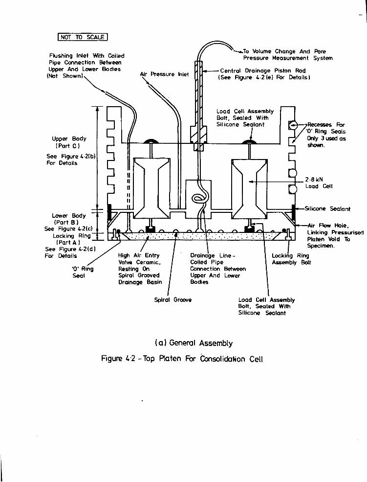
I NOT TO SCALE I
Flushing Inlet With Coiled Pipe Connection Between Upper And Lower Bodies
(Not ShOWn)~
Upper Body (Part C)
See Figure 4·2(bl For Details
Lower Body (Part B)
See Figure 4·2(c) Locking Ring
(Part A I See Figure 4·2(d) For Details High Air Entry
Valve Ceramic. Resting On Spiral Grooved Drainage Basin
_To Volume Change And Pore Pressure Measurement System
Central Drainage Piston Rod (See Figure 4·2 (el For Details)
Load Cell Assembly Bolt. Sealed With Sil icone Sealant Recesses For
'0' Ring Seals Only 3 used as shown.
--If--+----+- 2·8 kN Load Cell
~~:;:::r-Silicone Sealant
Air Flow Hole. Linking Pressurised Platen Void To Specimen.
Drainage LineCoiled Pipe Comect ion Between U~er And Lower Bodies
Spiral Groove Load Cell Assembly Bolt. Sealed With Silicone Sealant
( a) General Assembly
Figure 4·2 - Top Platen For Consol idat.ion Cell

PLAN {Hidden detail not shownl
SECTION A-A
10mn II outlet
o ...
due t for Ioadcell cable , tapped for It" BSP cable fitting.
SECTION B-B
Tapped hole for ~ H
coiled pipe fittings.
Snm II hole, tapped to aecept Jr." BSP base fUting of piston rod, and 'It H BSP col ed pipe fitting.
Direction of view tor pian
(b) Details Of Upper Body
Figure 4·2 - Top P\at~n For Consolidation Cell
3 No. 35mm fJ x S9mm deep recesses for load cells.
2 No. 40nrn x 40mm deep rec:_ for coiled pipe connec;tlons - tapped hole details as on section B-B.
5mIn deep • S- high recess for sllic:lllne _Ian!.

4mm tJ Recessed Holes For Load Cell Assembly Bolts.
10mm Deep x 35mm 0 Load Cell Seating Recess.
SECTION A-A
3mm Deep x 6mm High Recess For Silicone Sealant
(Not Shown On Plan).
8 No. 4nm ~ Hoi .. TGpped for Assembly Of Geramlc Locking Ring.
o
5mm Hole Tapped For ,.. "BSP Coiled Pipe Fitting.
4 No. 3mm £I Air Flow Holes Inclined At 45- With 6mm II x 2·5 mm Deep Cover Hole On CircllTlference For Porous Plastic Insert.
ADDrmrirl'lOtl! Centreline Of 4mm Wide x 3mm Deep SemI- Circular Spiral Groove.
o
5nm tI Hole Inclined As Shown To Join Outer Rim Of Spiral 10 Tapped ". .. BSP Coiled Pipe Fitting.
I J ~.s -I. 85 ~~1 .... "'0' Ring Groove-.. _ 220 mm Area L Plate Grooved To A SoiralfNo To Seal Locking Ring . - ----(Not Shown On Plan). 250
~I·------------~~------------~
I Direction Of View For Plan
Air Row Hoie And Recess For Porous ptastic Insert.
(c) Details Of Lower Body Figure 4·2 Top Platen For Consolidation Cell

PLAN:
~.
SECTION A-A
J.n I ,
Width Depends Upon Ptat. Thickness
8No 4.tnm " Bolt Holes. CDIXltersuric Fill' Recnsing
~ IL VAH
I_ I ~~ ~II T525~ Bar CBomic
6·3 l38ar C.ramics)
fd) C.rarnic Locking Ring
Figure 4·2 - Top Platen For Consdidation Cell
l' A.F. Hlxagoroat BrassBa ..
15
-y-~ "8' SSP TapPed Hoi.
1
1 ~
<.
C) C) N
o ,.,
Smm.801'.
:o--Flats For Spanner
'>
S.ction A-A
r--I If I ~
'/4" BSP Thr~~ Corntctiort Far Attac:hmrlt af P istOl'l To Upp~ Body
I 'o'R,f'g I I "DO I Groo~ F~ '".
eel Central Drainage Aston Rod

I 304·5 mm~ 1 .. I. 254 mmll .. I
4 mm Wide x 3 mm Deep I Semi - Circular Spiral Grooved Drainage , (Parf BJ
Inlet From Flushing System • X ::1:
Conventional Rowe Cell
I I
Main Body Of ":.I Consolidation Cell Maximum Radius Of
Spiral Groove 98·Smm
Igh Air Entry vflve Ceramic In Locking Ring (Part A) - See Figure 4·3 (bl For Details
s.9' t· . . - . ,,~~\N# J ~''',''''''. • •
(0) General As~emb(y
Figure 4 ·3 Base Platen For Consolidation Cell
I I
t::=:X: - ~To Volume
Pressure Transducer And Housing Block
Change Measurement System
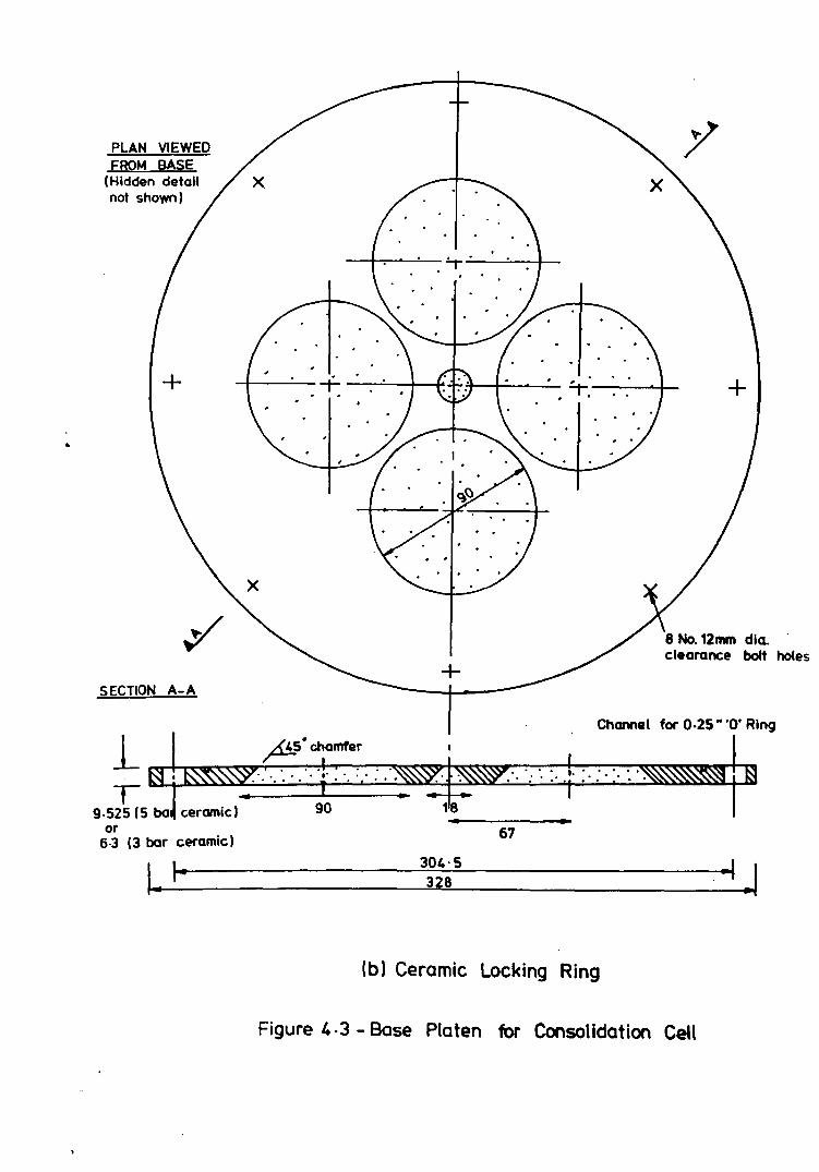
•
PLAN VIEWED FROM BASE
(Hidden detail not shown)
+
SECTION A-A
-t--"""""--- -r ---=--~ ....
+
+
8 No. 12mm dia. clearance batt holes
, Channel for 0·25" '0' Ring
~ ~ I ~~5~T::: :~t~···:··:· ·1, :.:.;.:.~ I ~ 9.525 (5 bo ceramic) 90 1~ •
or 67 6·3 (3 bar ceramic)
304·5 328
(b) Ceramic Locking Ring
Figure 4·3 - Base Platen for Consolidation Cell

Outw Chamberi _..... I Burett. BlMd Valve
jBGCk Pr Oum- enure To
Chamber • -kPa.
2Smm Thick Perspex End Block. I IImm DIameter Wall Mounting Holes Not Shown )
LJo----JIL..U....:lolI IUJUI~ ~4 No. TIe Rods With Locking Nuts.
I. I 2 Snvn Internal Oklmeter ~rspex Outer Chanbtr Wall Sealed With '0' Rings Via Force In TIe Rod •.
_10mm OIameter x 10cm" L_;""--ilt---copacity Glass Burette.
PurtloHy Filled With 'MItw Column. 10 ·1em' GracblI1ons)
• I I water Filled Outer ChamOer.
1.10 I Air Bubbles Separated • From Inflow Mixture And
Rising To Air \Iold At Top Of Burette.
blJ... I _Small Diameter Inflow ~.
25/II1II Thick Per.pex End Block (II IM\ Diameter Wall Mounting Hole. Not ShownL With 10mm ThIck Perspex Capping Plote.
"',....... ....... ~ L watw Outflow 11 Inflow To '"'- Chamber ~ C/GIge Unit I ~ur. , ... 10 kPa I I Back Pr_ur. ..,
Unit .... KPQ I
As Air Wuttt Mixturt Emtrgll From Inflow Pipe ot Low YIIoc:ity 1M Air Stparatu and RillS to bt Cdl-*<! In The Gtcd.Iattd Burette, Whilst tilt Wow Flows Downwards Due to tlw PresSIft Graditnt.
II II
II
o
o
o
) Air Water Nixtln Flows In Under to kPc:: Pres," Gradient
( a ) Left: Cross Section
(
" Inner and Outer " Chamber at Sall'lf
f>rnstft to Prwent Burett. torn 8r1a1cino During Use of the A.V.1.
Water Outflow
I bl Above: General Principles of Operation
Figure ,., - Diffused Air Volume Indicator

THRUST BlOCK F<R JACK BOL TEO ONm BASE
F 8 ,." M 12 BOLT HQ FOR RESTRAINT 0 MAIN CELL BOOY DURING E6MPA(T~
r--
HYDRAULIC
COMPACTION ~
I +
x
1+
ES
• +
t--HYDRAULIC JACK WITH ClJR VEO ENO BLOCK LL BOOY DURING FOR GUIDANCE OF MAIN CE
JACKING
1 ~
x
Jl
'-
+
e e 0 N 11\
STEEL C(J1PACTION BASE MOUNTED ON 4 ADJUSTABLE HEIGHT SU~TS
RECESS FO~~ INSERTION OF
---\
\ \ ,
PLAN
BASE PLATEN
, , "- ......
...... ..... -
EXTENT OF RECESS FOR
--
ASSEI"BLY GliDES WITH BASE PLATEN.
;' ./
I I
I /
r-- ,-
J I
ASSEf'BlY GUIDES BCLTE lJ4TO (()BCTlON BASE
CLAMPHi BAR TO
~RESTRAIN BASE PLATEN DURING JACKI~ OF THE MAIN CELL BOOY ACII)S~ THE COMPAC TlON SA S E
CONSQIDATION (ELL BQTED ONTO COMPACTION BLOCK
JACK MOUNTED ONTO THRUSt BlOCK
CLAHPII«j BAR END I 1 RESTRAINT -----~a:s:s:ss:s::5:fl~~~~~~~e~~ BASE ON
SUPPORTS
SCHEMATIC SECTIONAL ELEVATION NOT TO SCALE
Figure 4'S-Compaction Base Used During Test Series A a1d B

~ 270mm LONG x 25mm DIAMETER,1 mm THREADED BAR
JACK HANDLE
I I ~ I I I I
I I I I BALL BUSHING
4 No 40mm SQUARE SECTION r -, -,
'" RADIAL SUPPORTS -1 :I .... I ,- I I '-~ I
I I r I I 1 ~ r I I I I I I I I I I I I I I I I I I I I
I I I
I I I I I I
I I : I I I 3
I I I I 3 No M10 BOLTS FOR CONNECTING
I I I I I I J I
I~ I I
I I JACK TO PLATEN r
I I I I I I I I I I 150 I • -I I I I I I I I I I I I I I TOP PLATEN I I I (DETAILS NOT SHOWN) I I I I I I I I I I I I 4 No 170mm LONG HOLLOW SUPPORTS I I I ENCLOSING M12 THREADED RODS I I I I I --- I
I I M 12 RODS SCREWED INTO --' I CONSOLIDATION CELL FLANGE
l_J • I- CONSOLIDATION CELL l_J
Figure 4.7- Screw Jack for Removal of Top Platen from Consolidation Cell

Analogue Out Transducers As With Cell A
BBC Micro Porrollel Osc Drive - (24K Memory) Connection
j
Binary Code
Acorn IEEE 'Interface'
Digital Data
MC Computers 16 Channel
Analogue Input Unit
Analogue Data
16 Channel Dim Plug It From ~ sociated
Connection Box I-"
Figure. ,·8- Data Acquisition System For Test Series A and B
Printer
Analogue TransducE
. With Cell
Output From rs Associated B

,,~ ~ ~ ~ 'R\riC i~ ~'e~~ ~ ~ ~ ~~ v
OlsplacelMnt Transducer Clamped To Reactloh Beam. (Clamps Not Shown)
I
r- -Bleed For Cen Chamber' '"
Internal 10kN CqxJcity Whykham Forl'Ol'lC» Load
Cell
lOp Platen With ~ Annular Draina!l e { J - _ Basin.. t
~4l=:::!!!I£:L--i.~-I r
1 Bar Ceramic
InLoC~
..........
Soil Specimen
-Double Rubber Membrane WIth Double '0' Rings.als Top And Bottom.
Base Platen WlthAnrUar
Flushing Outlet (Used 1 ~OLing jr'--.......... """"-----'--'
~I-··~ ~ Basin.
==fI: : ,I r- ..... ' Specimen 0-100psl FU-e 'Abler Pressure Tr'1nsducer Pressure,WP.
I[
(0) Details Of Triaxial Celt
I
Specimen Air PresSlre, AP.
I ~ _uj I~.~ ,..,-,
. V CeCI Chamber 0-1OOpsl Pr.an,CP. Pressure Transcb:ers.
Figure 4·9 Modified Triaxial Cell And hstrunentation Used For Test Series C

~ AOU AWl R T o
AWl REO-IARGE. l LlI'£ FROM VACLUM DE-AIRED LAB WATER SUPPLY
LAB AIR I SUPPLY.
- Analogue Digital Unit -1000 em Q ir wa1er interface - Air pressure regulator -A-essure transdlx:er -Bourdon gwge
1 LAB AIR SUPPLY
Q-100 RI psi
VENT
LAB AIRl SUPPLY
(HOO psi fR
TRIAXIAL
10 ADU CELL TO ADU
FLUSHING VENT:
0-1OOpsi
10 AOU
(b) Plumbing Details
1 LAB AIR SUPFt.Y
0--20 Rl psi
Figure 4·9 - Modified Triaxial Cell and Instrumentation Used For Test Series C.
VENT
lLAB AIR SLPPLY
R
AWl RECHARGE. LINE FROM VACUUM DE-AIRED LAB WATER SUPPLY
I

Plotter -
•
Disc
iDEC PDP 11/44
Mlnl-Computer
Binary code
Mowlem Mlcrosystems
ADU 700
Data/ogger
• Amplified analogue data
Printer
Protech or RDP F-4 Digital voltmeter (sl
transducer .signal data for coarse visual check amplifiers on transducer outputs
Analogue data
Analogue output from transducers EI up to 64 channel t: Analogue output from transducers associated with COf'I1J'esslon ceUdim plug connection box associated with triaxial cell lsI
Figure I. .10 Data Acquisition System For Test Series C and 0

Rigi d Ranged Loading Plate
Reaction Beam
20kN Or 111 kN Capacity Load Cell
100mm Stroke Displacement Transducer Clamped To Reaction Beam With Armature Resting On Cell Walls
30Smm t/)x 254mm High Rigid Cell
Specimen
Istrain Controlled Loading Platen
Not to scale
Figure411- Compression Cell For Test Series 0

CHAPTER 5
CALIBRATION OF INSTRUMENTATION AND OPERATIONAL
CHECKS ON APPARATUS
This chapter presents the methods used for and results from the
calibrations and operational checks on the experimental apparatus.
Emphasis is given to non-standard calibrations, and calibrations on the
new consolidation cell. All calibrations were made using a voltage
supply of 5 volts at the University, or 10 volts at the British Gas
Engineering Research Station. Least square linear regression analyses
were applied to all calibrations to determine the best straight line fit
and confidence limits for the data.
5.1 Calibration of Instrumentation
5.1.1 Temperature
5.1.1.1 University Apparatus
As noted in section 4.1.4, a nominally constant temperature laboratory
was used for test series A and B. Temperatures recorded on the Isuzu
drum chart were compared with two independent mercury thermometers and a
second 7 day drum recorder over a period of several weeks, and no
discrepancies were revealed. Humidity and atmospheric pressure
measurements were not verified. Prior to adoption of the drum recorder,
attempts were made to utilise the temperature sensor capabilities of the
Analogue Input Unit (AIU) but the low accuracy of the instrument
precluded its use. A typical chart from the recorder is presented in
Figure 5.1, which shows that temperatures were maintained usually within
lOC of 20oC, and humidity varied between 50, and 60,. Atmospheric
pressure varied according to the weather conditions.
- 45 -
5.1.1.2 Research Station Apparatus
Temperature in the soils laboratory of the Research Station was not
controlled at the time of the experimental work reported in this thesis.
Temperature was recorded twice daily at two positions in the laboratory
on the mercury thermometers and the temperature of vater in the de-aired
water supply tank could be recorded also. As shown in Figure 5.2, large
temperature fluctuations occurred as heaters warmed the laboratory
during the day, but ceased operating at night. Variations in air
temperature of up to SOC were recorded, but corresponding water
temperature changes were limited by the containing vessel to about 20 C.
5.1.2 Volume Change Units
5.1.2.1 University Apparatus
The 100 cml capacity Imperial College volume change units (VCU's) used
with the new consolidation cell were de-aired prior to calibration in
the following manner:
a) The header tank containing de-aired water was connected through
the top and bottom of the units as shown in Figure 5.3.
b) With valves A and C open, and valves Band D closed, valve H was
opened and water flowed into chamber 1. The VCU was gently
agitated to aid flushing of air out of the vent, then valves A and
C closed when no further air was being flushed out.
c) The VCU was inverted and valves Band D opened. The VCU was
gently agitated again until chamber 2 was apparently de-aired.
Valves Band D were closed and the unit inverted again.
d) Steps 2 and 3 were repeated twice more each, then all valves
closed.
- 46 -

Once de-aired, the VCU was connected as shown in Figure 5.4 to two
Geotechnical Digital Systems digital pressure controllers (Kodel INTEL
8085), which were microprocessor based hydraulic servo mechanisms.
These units, which were previously de-aired in accordance with the
manufacturer's instructions, were capable of measuring volume changes to
an accuracy of 0.5 ~ and pressure to 0.25 kPa. Connection of the GDS
units and VCU was made underwater to ensure that no air was allowed to
enter the system, and the connection made such that a nearly full GDS
unit was connected to a nearly empty VCU chamber.
Calibration was executed semi-automatically using a specially written
computer programme "VOLCAL" (see Appendix D) together with the sse computer and AIU used for the main series test, an Electroplan
interface, one GDS unit actively computer controlled. and one GDS unit
in a passive mode. In the passive state, a GDS unit had its operational
pressure set by the four digit wheels and its stored volume varied in
response to external changes, in this case volume changes caused by the
active unit. The active unit had its stored volume controlled by the
computer, but its pressure was governed by the passive GDS unit.
The programme worked by instructing the active GDS UDit to change its
volume by a specified amount, and allowing it a variable time period
(dependent upon the volume increment specified) to achieve this change
and for the equilibrium back pressure to be set up in this system as a
whole. After equilibrium was reached, the programme recorded the output
from the displacement transducer that formed part of the VCU. The
target total volume change to be applied to a VCU cha.ber was cycled
within a specified range (usually 100 cml) for a specified number of
cycles (usually 3), for specified increments (usually 5 cml), and the
displacement transducer/volume data stored on floppy disk in a form
suitable for direct input into the least squares fit programme. Output
from the programme gave the best straight line fit and confidence limits
for the data determined for the active VCU chamber. The results of the
calibrations are presented in Table 5.1 for a back pressure of 100 kPa.
- 47 -

Investigations into the influence of back pressure on the calibrations
showed that if the back pressure varied in the range 50 kPa to 200 kPa,
negligible change in the calibration factor or confidence limits
resulted provided the VCUs were rigorously de-aired.
Investigations into the stability of the VCU output when isolated from
the rest of the plumbing were made also, and these showed that
transducer stability was not a problem.
5.1.2.2 Research Station Apparatus
Calibration of the 1000 cm3 volume change units, known as air-water
interfaces (AWl) at the Research Station, was made by the staff at the
Station using a graduated burette as the control. Water was pushed into
the water chamber of the unit in known increments and output from the
displacement transducer recorded by the computer each time. A single
half cycle was used to calibrate the units, and the results of the
calibrations are presented in Table 5.3.
Additional checks on the units were made by the writer in order to:
(a) determine the performance of the displacement transducers when
their armatures were fixed, and
(b) determine the performance of the whole unit when real volume
changes were prevented by isolating the units from the rest of the
plumbing.
The investigations into the performance of the displacement transducers
alone utilised AWlS, and showed that its sensitivity to typical
temperature fluctuations in the laboratory was negligible. A drift
equivalent to an apparent change in volume of 1.3 c~. equating to about
0.1% of full scale, was observed over the five day test period but
subsequent checks on the manufacturer's data showed that this lay within
the confidence limits for the transducer and was therefore not
significant.
- 48 -

Performance of an isolated AWl was checked also using unit AWlS. The
output from the AWl was recorded over a 1 month period and compared with
measurements of ambient laboratory air and water temperatures (see
Figure 5.5). This work revealed that a slow leak existed during the
test, but that after correction of the AWl data for this linear drift, a
clear correlation between temperature and output existed. An apparent
change in volume of 10 cml resulted from every lOC rise in temperature.
However, only a small portion of this potential error would be expected
to be manifested during a real test as the air volume change component
would be eliminated by regulation of the air pressure, and only
expansion of the water in the system and the materials of the AWl should
contribute to the problem. Allowing for the larger water volume
involved during a test, it is estimated that temperature effects during
use were less than 5 cml per degree C.
5.1.3 Load Cells
5.1.3.1 University Apparatus
Before calibration, the load cells were pre-loaded to twice their
maximum 2.5 kN working load for 15 load - unload cycles using a
compression machine and load ring. The load cells were then left under
power for at least 24 hours before detailed calibration with an oil
filled 50 kN capacity Budenburg dead weight tester (Kodel 500 used in
conjunction with Model 380L) certified to be accurate to 0.04\ of the
applied load. Calibration entailed applying five cycles of 2.8 kN
preload to the cell, followed by the main calibration run of five
further cycles of load in 0.2 kN increments up to a maximum of 2.5 kN.
A least squares analysis of the data was carried out and the calibration
data and confidence limits obtained are presented in Table 5.4 in terms
of "equivalent pressure" per millivolt change in load cell output. The
"equivalent pressure" to a force of 1 kN measured on a load cell is that
pressure which would result if 1 kN were applied over a third of the
cross sectional area of the new consolidation cell (total area - 0.1520
~), ie 19.7 kPa.
- 49 -

Following initial calibration, output from all cells at zero load was
monitored for at least 72 hours in order to assess zero drift and the
effects of atmospheric pressure and humidity variations. The results of
this work showed that zero drift, atmospheric pressure variations, and
temperature variations did not present a problem but that the load cells
were sensitive to small changes in relative humidity. A typical
variation is shown in Figure 5.6.
When in use though, the load cells would be effectively sealed into the
consolidation cell by the regulated air pressure, and the relative
humidity maintained at a sensibly constant value during any test once
equilibrium between the soil water content and atmospheric conditions
was achieved. The observed influence of relative humidity was therefore
considered to be irrelevant after the initial setting up stage of a
test.
5.1.3.2 Research Station Apparatus
The commercial load cells used in the Research Station were calibrated
using an oil-filled Budenburg dead weight tester by British Cas staff.
A preload cycle to the load cell capacity was followed by a single load
- unload calibration cycle to the maximum load in ten increments. The
results of the calibrations are given in Table 5.5. Comparison of the
calculated confidence limits with the published accuracy showed that the
load cells were generally under performing. This may be due to poor
standards of calibration, or the age of the load cells. The effects of
temperature on the performance of the load cells was not investigated
due to the relatively short period (less than 12 hours) over which
readings were taken.
5.1.4 Pressure Transducers
All transducers measured gauge pressure and were calibrated using a
Budenburg dead weight tester connected to a pressure chamber.
Transducers were subjected to at least one cycle of pre loading to
- 50 -

capacity followed by 3 load - unload cycles to capacity in ten
increments at the University, or one loading cycle to capacity in five
increments at the Research Station. Results of the calibrations are
presented in Table 5.6.
5.1.5 Displacement Transducers
5.1.5.1 University Apparatus
Displacement transducers were calibrated at the University by clamping
the transducers in a specially made calibration block (see Plate 5.1)
with the sprung captive armature of the transducer resting on the flat
movable surface, or, in the case of the submersible transducer, the free
arm was clamped to the movable surface such that any movement of the arm
in to the transducer body was along its central axis. Displacement of
the armature was effected by rotating the low geared bushing, and the
relative displacement of the arm from a pre-set zero position was
measured with a Mitutoyo digital vernier accurate to 0.001 mm.
Calibrations used three extension-compression cycles, each half cycle
comprising at least 20 increments of displacement. Initial calibration
employed the full range of the instrument to identify the most linear
region of the transducer, before a more detailed calibration was
completed over this shorter range using the increased resolution
afforded by the AIU for such a smaller range. Results of the
calibrations are presented in Table 5.7.
5.1.5.2 Research Station Apparatus
Slip gauges were used to apply known displacements to the armatures of
the transducers at the Research Station, with the transducer body
clamped in a vertical position and output recorded by the computer. The
results of only one of the calibrations made by British Gas staff was
available for checking, but it is understood that the calibrations for
this and all other transducers consisted of increasing the displacement
- 51 -

from zero (full extension of the armature) to full compression in ten
increments, but with no further cycling. The data available for the 100
mm stroke RDP LVDT (serial No D14) gave a 95% confidence limit of 0.2 mm
for the linear regression, and a calibration factor of 9.958 mm per
millivolt. This equates to a measured accuracy of 0.2% of full scale,
which compares well with the accuracy quoted by the manufacturer of 0.1%
over the middle of the range or 0.4% over the full scale. Performance
of the other transducers was assumed to follow that noted by the
manufacturer.
5.1.6 Bourdon Gauges
All Bourdon Gauges at the University and Research Station were checked
and reset if necessary in accordance with the manufacturer's
instructions using a Bourdon dead weight tester with an air-water
interface between the tester and the gauge to ensure that only water
entered the gauges. When reset, the pressure read on the gauge was the
same as that applied to within 0.5 kPa. Linear regression analyses of
the data were not made as, except in the case of the 1 bar University
gauges 12380388 and 12380389, the gauges were used only for visual
control and checking of the applied pressure. The exceptions were used
to control the air pressure in the new consolidation cell and for this
purpose reference to the calibration runs allowed the applied air
pressure to be measured to within 0.2 kPa.
5.2 Operational Checks on Apparatus
5.2.1 Operation of Air Volume Indicators and Flushing System
Following construction of the air volume indicators and spiral grooved
platen used in the consolidation cell and their connection to the
plumbing system, the following checks were made on their performance:
(a) Medium term leakage checks were made on the air volume indicators
by observing the variations of air volume indicator readings with
time at initial water pressures of atmospheric pressure and
- 52 -

100 kPa gauge. The inner glass burette used for measurement was
isolated from the external plumbing during these tests.
(b) Efficiency of air transport in the spiral flushing grooves was
checked by G-clamping at three locations a 25 .. thick perspex
block onto the platen, and applying variable flushing pressures to
dislodge any visible air.
(c) Efficiency of air bubble transport through the plumbing to the air
volume indicator was checked at variable back pressures.
The check on the performance of the isolated air volu.e indicators
showed that both at atmospheric and 100 kPa back pressure, very small
(less than 0.2 cml at 100 kPa or less than 0.3 cml at atmospheric
pressure) or zero changes in meniscus level were observed over a period
of about 10 days, as shown in Figure 5.7. The initial rise in meniscus
levels when the back pressure was at 100 kPa is attributed to solution
of air in the burette into the water, masking a very slow leak, an
effect that would be expected to be absent or reduced at atmospheric
pressure.
As further tightening of the air volume indicators to eliminate any
leaks risked damage to the glass burettes, the observed level of leakage
was accepted provided that before and after flushing the air volume
indicator reading was noted, and that the units were isolated from the
plumbing drainage system during a drained test.
The air transport efficiency checks showed that unless the perspex (or
the ceramic) was placed onto a previously saturated spiral groove and
base platen, air would be permanently trapped between the perspex (or
ceramic) and the metal even up to a flushing pressure of 200 kPa. If
the platen was saturated initially, it was found that air bubbles
entering the spiral from the flushing inlet would flov only partly
through it before adhering to the metal platen by surface tension. Once
this had occurred, the air could not be dislodged unless flushing
- 53 -

pressures exceeded 50 kPa. This problem was overcome by using a very
dilute solution of Teepol (a detergent) as the flushing medium, rather
than water alone. Addition of 5 cml of Teepol per air-water bladder cell
was sufficient to ensure that all bubbles were dislodged at a flushing
pressure of 10 kPa.
Having solved the problem of air-bubble transport through the spiral ,
it was noted also that air flowed easily through the plumbing to the air
volume indicators provided the flushing pressure exceeded 5 kPa.
However it was found that volumes of Teepol in excess of 20 cml per
bladder cell combined with high flushing pressures (ie greater than 20
kPa) caused frothing in the plumbing lines. High flushing pressures
resulted also in relatively high bubble speeds through the plumbing such
that a current set up in the inner burette of the air volume indicators
was sufficient to prevent most air bubbles entering this burette from
rising upwards to register as an air volume. Instead, bubbles were
entrained into the current and flowed straight through the inner burette
to the volume change units unhindered by the need to travel downwards.
Based on the foregoing, a flushing pressure of 10 kPa together with a
very dilute Teepol flushing medium was adopted for the tests to ensure
efficient operation of the flushing system. It was noted also that at
least 100 cml of flow was required to ensure all bubbles in the flushing
spiral reached the air volume indicator.
5.2.2 Response Tests on Ceramics
The low permeability of the high air entry value ceramics and the
compressibility of the fluid between the ceramic and the pore water
pressure transducer result in a minimum response time being required for
the system to record a change in suction conditions within a specimen
(see section 2.3.1). For confident interpretation of the pore pressure
data from the main series tests, it was necessary to ensure that the
ceramics were as completely de-aired as possible before use and to
ensure that air entry by diffusion and evaporation of water in the
- 54 -

ceramic during tests did not reduce the response time to below an
acceptable level.
De-airing was completed by assembling the consolidation (or triaxial)
cell with the ceramics sealed in their test positions, and the cell and
platen filled with de-aired water (see Figure 5.8). A cell pressure of
600 kPa was applied for 24 hours before the drainage and flushing lines
from behind the ceramic(s) were opened and water flushed through from
the cell chamber for at least 5 minutes. After closing the lines, the
600 kPa cell pressure was reapplied and the sequence repeated at least
twice more. After flushing for five minutes on the third cycle, the
cell pressure was reduced to 50 kPa (or some other nominal value) and
the drainage lines closed. Equalisation of pore pressures above and
below the cell was checked using the pore pressure transducer behind the
ceramic and comparing it with the applied cell pressure. After
equalisation the cell chamber was isolated, a cell pressure of 100 kPa
(or some other nominal value) applied to the line up to the cell, then
immediately after a data logging cycle the cell chamber line was opened
and the response of the pore pressure transducer behind the ceramic
monitored.
Typical response curves for three and five bar ceramics in the
consolidation cell and a one bar ceramic in the triaxial cell, are shown
in Figure 5.9 after three days de-airing. These are typical for both
pressure increments and decrements. All observed response curves on
de-aired ceramics in the consolidation cell showed that the top platen
ceramic always had a much faster response time than a base ceramic of
the same air entry value, such that often 99' of response would be
within 10 seconds for the three and five bar ceramics used in this
apparatus. In contrast, 95, response time for a base ceramic of three
or five bar air entry value would typically be less than 2 minutes or
less than five minutes, respectively.
The lack of a clear response curve suggested that an unknown leakage
path consistently existed in the top platen, but investigations into
the behaviour of the ceramics after two main series tests showed that a
- 55 -

response curve similar to that of the base was exhibited by the top
ceramics if the degree of de-airing was relatively low (see Figure
S.lO). After only one cycle of de-airing though, the top ceramic
exhibited its usual response pattern, implying that the top platen
ceramic design is more efficient at responding to pressure changes.
Comparison of the platen designs confirmed that more -dead" ceramic
exists in the base design, supporting the explanation given above. The
hypothesis is further supported by the relatively slow response of the
one bar high flow ceramics used in the triaxial cell, which is believed
to be related to the small drainage basin beneath the ceramic.
Based on the above, ceramics were accepted as sufficiently de-aired for
use after a minimum of three days de-airing, although checks on their
response were always made after this time to ensure DO poorly de-aired
ceramics were used. Ceramics were usually used for two tests
(equivalent to about one months's test use) before de-airing again.
The effect of the period of de-airing and applied pressure increment
were investigated also for a five bar ceramic, and typical plots are
shown in Figure 5.11. Comparison of Figures 5.11 a and 5.11 b shows
that the response time does decrease with an increase in de-airing
period, but that the increase in efficiency is gained at a progressively
slower rate as the time increases. The curves show also that a decrease
in the pressure increment applied results in higher response times, as
predicted by Fredlund (1973) and others. The shape and equalisation
times of the response tests agree also with those predicted by Fredlund.
5.2.3 Permeability and Air Entry Tests on Ceramics
Permeability and air entry tests were made to check that micro-cracking
of the ceramics had not occurred during transit from the USA, or during
machining or installation of the ceramics in their locking rings.
Permeability tests were made on ceramics immediately following
completion of de-airing by connecting the drainage 1ine(s) to a VCU and
- 56 -

applying a known pressure gradient, usually 100 kPa, across the ceramic.
The coefficient of permeability derived from the tests using Darcy's law
usually agreed reasonably well with the typical coefficients given by
the manufacturer, although some ceramics exhibited a coefficient
approximately 50% of that expected. Typical coefficients of
permeability for a one bar high flow ceramic, a three bar ceramic and a
five bar ceramic, are 0.86 x 10- 9 m/sec, 1.73 x 10- 9 m/sec and 1.21 x
10- 9 m/sec respectively.
Air entry tests were made on all new ceramics using the same apparatus
arrangement as that shown in Figure 5.8, except that the cell chamber
fluid was air rather than de-aired water. A differential pressure of up
to 250 kPa (the maximum suction expected to be measured within the test
specimens) was applied across the de-aired ceramics and the rate of flow
of air measured as an apparent water volume change by the volume change
units. The tests lasted approximately 24 hours, and the observed rates
of flow were compared with those predicted by diffusion theory and found
to be in reasonable agreement. Hence it was concluded that the air entry
value of the ceramics was sufficient for use in the tests, although the
absolute entry value of the ceramics was not determined.
- 57 -

Table 5,1 Calibration Constants and Confidence Li.its for Imperial College Volume Change Units at a Back Pressure of 100 kPa
I Unit Chamber Calibration Factor Confidence Limits (cral)
(cral ImV) 95, 99'
VCU25 Top 3.5804 0.10 0.13 Bottom 3.5656 0.13 0.17
VCU28 Top 3.1220 0.13 0.18 Bottom 3.1064 0.17 0.22
VCU5S* Top 4.1534 0.23 0.31 Bottom 4.1432 0.22 0.29
VCU145 Top 3.0961 0.12 0.16 Bottom 3.0838 0.10 0.13
*VCU55 exhibited non-linearity over the first 20c~ at each end of piston travel. Quoted data is for the range 20~ to 80cm1 of capacity.

Table S.2 Influence of Back Pressure on Calibratiop Data for I.C. Volume Chanle Unit 28
I I VCU28 I Calibration Factors I 95' Confidence Limits
I (cm3/mV) I (ca3) I I I I
Back Pressure I SOkPa 100kPa 200kPa I 50kPa 100kPa 200kPa I I I I
Top Chamber I 3.1321 3.1220 3.1221 I 0.23 0.13 0.22 I I
Bottoll Chamber I 3.1134 3.1064 3.1051 I 0.25 0.17 0.19 I I
(a) Calibration Data
Volume Changes (cal) Calculated using Calibration Factor for Output Change of 30IIV
Chamber I
Pressure - 50kPa Pressure - lOOkPa I Pressure - 200kPa I I
Top 93.96 93.66 I 93.66 I
Bottom 93.40 93.19 I 93.15 I
(b) Effect of Back Pressure on Calculated Volumes
Table S.3 Calibration Factors and Confidence Limits for British Gas Air Yater Interfaces
Unit Calibration Factor (~/aV) Confidence Limits (cal) 95' 99'
AW3 95.42 1.7 2.3
AW4 98.52 1.2 1.6
AW5 105.93 1.6 2.1
AW6 104.17 1.8 2.3

Table 5,4 Calibration Constants and Confidence Liaits for 2,5kH Load Cells
Load Cell Calibration Factor (kPa/mV) Confidence Limits (ltPa) 95, 99'
LCA -25,4032 0,10 0,14
LCB 24,5719 0,11 0.14
LCe 24.7259 0.09 0.11
LCD 25.3720 0.06 0.07 or 25.0079* 0.11* 0.15*
LCE 25.2584 0.07 0.09
LCF 26.3176 0.04 0.06 or 26.0914* 0.08* 0.11*
*Load cells D and F were damaged during Test A8. Following re-wiring and re-ca1ibration the new calibration data vere aargina11y different. as shown.
Table 5,5 Calibration Constants and Confidence Liwits for COmmercial Load Cells
1 Load Cell 1 Range Calibration Confidence
Serial Model 1 (kN) (leN/aV) Limits (leN) NUllber 1 95' 99'
1 I
LC6 Whykh811 Farrance 1 10 1.1846 0.038 0.050 Model YF 17109 1
1 LC14 Sensotec Model 411 20 0.5023 0.030 0.039
1 LC16 Sensotec Model 411 111 0.9980 0.135 0.178
1
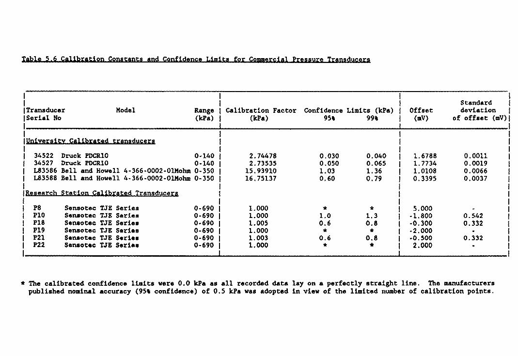
Table 5.6 Calibration Constants and Confidence Limits for Commercial Pressure Transducers
I I I I I Standard I I Transducer Model Range I Calibration Factor Confidence Limits (kPa) Offset deviation I ISeria1 No (lcPa) I (kPa) 95' 99' (mV) of offset (mV) I I I I I IYnlv!'lltx ~Alib'lt!~ t'IDI2Y~!'1 I I I I 34522 Druck PDCR10 0-140 I 2.74478 0.030 0.040 1.6788 0.0011 I 34527 Druck PDCR10 0-140 I 2.73535 0.050 0.065 1. 7734 0.0019 I 183586 Bell and Howell 4-366-0002-0lMohm 0-350 I 15.93910 1.03 1.36 1.0108 0.0066 I 183588 Bell and Howell 4-366-0002-0lMohm 0-350 I 16.75137 0.60 0.79 0.3395 0.0037 I I IRel!a[~b ~tatlQn ~Allh[!ted I[inldy~
Table 5,7 Calibration Constants and Confidence Limits for Commercial Displacement Transducers used at the Unyersity
I I I I Transducer Manufacturer RangelCalibration Constant Confidence Limits ( .. )
*
Serial Number (mm) I (mm/mV) 95, 99'
L3890 Novatech 0-50 LSC HS550 0-10*
L3900 Novatech 0-50 LSC HS550 0-10*
Submersible Sangamo 0-10+ 8-9*
Range of maximum accuracy
2,8150 2,8237
2,79806 2,79041
1.589E-3
0,046 0,009
0,048 0,014
0,003
0,061 0,012
0,063 0.019
0.004
+ Distinct non-linearity of displacement - output relationship observed fro. zero (armature fully out) to 5 mm, thus linear regression analysis not valid,

~ c: GI E f
- u U c: !...
u • f ... ~ .5 a L. " ! .! E g ~ "
a .D
.§.
e 01
UI ..-~ E f u .b
" ell -a ::l
" a L. 01
1 .5
a .D E
.5
" II ..-a ::l
" D L. 01
1. ? nF[ RR I 7:-1 J"'-L 1m I 24 J"'- 1m l.l~ Jt=I.. In, TI/.f:.A1'fJ7.t.b8'1IW t.68UTI2t.tiK ... ,D7LhK'l.1:.I'24blS ... IULIt....tU:l.'1. 7J..f\ . ~ /
I .. n
/",V I I I I I I I .....
.... -" '''--../.'' 1"""'
,,, .-
\ In
. •• ....l.....L. '\
\ 1
,~n6Rn" 7 '6. i 2'. BUlL,. 6R!,. 6 B7" b. U,. .. 6'~_2 4.
vv I
."
loV
\ , -
I l 71.681:122 6A ... ",2t.6B1:1224001L L4tiH'LI1L21.6
--'--7... I I I I I.,..,;"
I J I I
IV .....
- ..... -_l...,../
nan
\ \ 1 \ \
.\ \
Figure 5·1 - Typical Plot of Atmospheric Variatens in Constant Temperature Laboratory I based on origiool Isuzu paper chert )
I
'!

24-5
24
llS
20S
245
no
210
200
AIR TEHPERATlREl-c1
I ,
, , \ \ , , , ' , ' ,
WATER ~TURE I'CI
I " I
I , , I , I I
I
\ ' J
, , , I
I \ I \
\ \ \
I :
, \ , \ ,
I I I , I I , I
I
I ' I ' ,
la) Ambient Laboratory Air Temperature
1 b I Ambient Water Supply Temperature
I I , , I I
~
= Actual readingi2 reading; per day)
\ \
\ \
I , , I ,
, . , I , I
I
)l. = Actual reading (2 readings per day)
" ,,/" K Average curve
Figure 5·2 - Record of Air and Water Supply Temperatures at the British Gas Research Station over a 29 Day Fa'"iod

v
Header tank
\t]lve H
Valve A
Rolling bellotram seal
Valve B
Figure 5'3-Apparatus For De-Airing Of Volume Change Unit
Digital pressure and volume --r-t-'1WLU indicators
4 d igi t target pressure regulator
IIIII am
ffiII]o
Electronically controlled pump
Reset button for volume indicators
Figure 5'4-Apparatu5 For Calibration Of Volume Change Unit

Volume Chcng~ I Telllpercture ,OC) (cm',
23-5
35 t : a for application of leckcge correction
23-0
30
22·5
25
~
" " , I
, I I I I I I , I
r3;r 0 ~ " "\.,n I.r '.\ / ! ~\ .' I if \} I \', /(;'Drift corrected volume chonge
\\\./ I I \ i
caWation 'G.. of ~rent -drift corrected volIme cronges
20
15
10
5
o
21·5
21-0
20-5
2 , 6 8 10 12 14 16 Time ldays)
Appcnnl "* of IJansducer <titt 17 inRrtx:e IftJkoge
IS 20 22
x
21.
\ \\./'" I I I· 'if-water temp I'-·_t I I , I , I I I
.. I
I : lAir temp I I , I
26
I I \ I ~ ...
28
Rgu-e 5· 5 - Correlation Between Temoerature Changes and Apparent Water Volume Change for British Gas Air Water Interfaces

> E _ 0
~1: ..- I-::::) -o Q
~ ~
2·300
2·2901-42
2·280+48
2'270~54
2·260,60
2.250 ,66
72 2-240
2·230
"'- .... , ~ '-- ....
'I'
/
Load Cell Output ---...... , ?"
............... ~ "- "" ........ " ,. - Humidity
'---
2.220'
.... o 6 12 16 24 30 36 42 48 54 60 66 72
TIME(hours)
Figure 5'6-Effect of Atmospheric Humidity on Load Cell A
- -.

0·20
0·15
0·05
0·03
0·02
0.01
"VI 2 -/
;;
I
/0 /
/
l' •
1 D
0/ »
2
2
+ve A Vol = Meniscus Falling In AVI
AVI 1
3 4 5 6 7 8 9 11 12 T1_ (Days'
(a) Change in Levels of Air Volume ndicators with Atroos,:nerC hk Pn>ssure
3 4
"'e ot-~~~--~----~----L---~-----L--__ ~ ____ L-__ ~~~ __ ___
u
~ • -0·01 ~ ~ ..
-0·02
- 0'()3
-0·04
AVll
\. DC .-o1l \. --'\ //~AVI3
D \ 0 ,/
'\ / '\./
o o
-
( b) ChcJnge in lewis of Air Volume Indicators with Bad< Pressure of 100kPa
Figure 5·7 - Medium Term Observations of Isolated Air Volume Indicator Water Level "

Rigid walled flexible tubing
Flushing Line
t
£Xainage Line
f ~ Cell chamber pressure
~ J~~~~~~~~= Lower body of top platen ~ Small spacers
Flushing _,~~:;!.I line
~~~~~~_ Drainage line
(a) Consolidation Cell
Cell chamber ~:::::::[~~~~2~~~~~:: Drainage line pressure -~ - Flushing line
(b) Triaxial Cell
Figure 5·8 -Schematic Arrangement Of Apparatus For Response And Permeability Tests On High Air Entry Ceramics
'!

103
100
97
94
91
82
79
76
Response Pore Pressure Response Time Level (kPo) /seesl
90"1.
95'1.
96·59
97·89
19
26
1·60 1·87 73!=~--.__,--.-_r--r__r--r__r--r__r--~-r~~-
o 0·27 0.53 0·80 1·07 1·33 Elapsed Tim. (mini'
(a) 1 Bar Gerome in Triaxial Cell
5·6
5·2
> 4·8 .5 "5 ~ 4.4 0 ... III u 4.0 ::J
~ c ~ 3·5 I! :J 1ft
i 3·2
i 2·&
2·4
2·0
34
32
> .§ "5 30 a. "5 c: 28 ~ / i / 26 c / ,:: QI
24 / <-:J / '" '" / ... It 22
/ II
~ 20 I I
18 I
16
14 0 40
",-
'" .,..-/' ,
0 20 40
Base --------------------------Top '" '" ./
./ /
/ /
/ Response Change.n Transduc:er" ~Time Le¥eI Output !mVI (seesl
90~. 95% 90~. 95"1.
Top Cer(J'lltc 16·016 16·906 <10 <10
Base CeRmc 16·274 17·178 120 160
80 120 160 200 240 280 320 360 1.00 41.0 Tim. (secs)
bl 3 Bar Ceramic in Consolidation Cell
------------~~ -----Top
Response Change in Transducer ResponsP Time L_I Output !mVI (sees)
90% 95% 90"1. 95% -Top Ceramic 2·618 2·764 <10 <10
Base CenJmc 2·721 2·872 <55 102
SO 10 OJ 120 140 160 180 200 220 240 260 2tI) lOO 320 Time (SKS)
Ie) 5 Bar Cercvnic in Consolidation Cell
Figure 5·9 - Typical Response Curves For High Air Entry Ceromic(After 3 Days De-airil""9: Pressure Increment 50-100 kPa)

5·700
>5'500 E ;: 5·300 ~ a.. § 5100
ffi4 -gOO
~ 04 -700 (/) z g4'500
w4 -300
~ L. ·100 (/) UJ a::: 3 ·900 a... UJ a::: 3· 700 ~
3·500
3'300
3 '100
2-900
2·700
----
RE'sponse Level
Top Ceramic
Base Ceramic
------------------ Base
Top
Change in Transducer Resporse Time Out~{mV) (sees)
90% 95% 90% 95%
2·583 2·727 45 85
2·747 2·899 35 70
2,SOu, ,i" i , Iii , 'i , o 20 40 60 00 100 120 140 160 180 200 220 240 260 280 300
TIME (SECS)
Figure 5'10-Typical Response Curve For 3 Bar Ceramic After Use In 2 Main Series Tests .

500 -t
400
Vi u ., oJ!
UJ ::r i= 300
UJ Vl z 0 Q. Vl
~
20°1
100
a 20 1.0
ru • 90% response of top
J( 90% response of base
a 95 % response of lop
2195% response of base
x
E F S
0 ~ ~
!j'
60 80 100 120 140 160
500
400
Vi U
~
~ 300l B '-.,.8
~
~ ~
I 200
I
100
\I
20 40
"'-..C
0 e
~ -~
60 60
!iey. • 90 % Response ot top
"90 % Response of base
095 % Response of lop ~95 % Response (j base
-~
FG ®~
'00 120 140
TIME SINCE START OF JE·A;RING :hrs:
(b) PRESSURE If\CREt.ENT 10-SO kPo
TIME SINCE START OF DE-AIRING iHRSI
lei PRESSURE IN CREMENT 50-100 kPo
Figure 5·11- Dependence of Respa1Se Time on Period of De-airing 5 Bar Ceramic

Plate 5.1 Apparatus for calibrating displacement transducers

CHAPTER 6
TEST PROGRAMME AND EXPERIMENTAL PROCEDURES
6.1 Summary of Test Programme
Four main series of tests were performed to investigate the one
dimensional compression properties of the three granular soils prepared
with gradings as detailed in Section 3.2. Series A and B were performed
at the University in the new consolidation cell, and Series C and D
were performed at the British Gas Engineering Research Station in the
large diameter triaxial cell and the compression rig, respectively.
Details of the apparatus are given in Chapter 4, and the nature of the
series are summarised in Table 6.1. All tests had a constant air
pressure in the test specimens (ie air drained), and the reference to
drained or undrained conditions in the brief description of test type in
Table 6.1 relates to the water phase and not the air phase. The test
procedures used are summarised in this chapter and further details are
available in Appendix A.
6.2 Test Series A
The aim of Series A was to establish the compression behaviour of the
fine and coarse gradings under monotonic incremental loading compression
and to measure the changes in water content and soil suction of the
specimens due to the applied stress changes. This behaviour could be
compared with the behaviour observed in Series D under constant strain
rate compression and repeated loading conditions. A summary of the
tests reported in this thesis, and the parameters varied for each test,
are given in Table 6.2.
All specimens were batched in the concrete mixing drum as described in
Section 3.2.2 and prepared to a known water content by adding the
required mass of water and carefully mixing the soil and water together.
The material was then covered with a plastic sheet to reduce evaporation
and left for the water content to equalise for two hours. At the end of
- 58 -

this period, the material was mixed once more, weighed, and placed into
the consolidation cell to form a layer approximately 130 mm thick. Two
water content samples were taken at one-third and two-thirds uncompacted
height to check for proper mixing of the material. The cell had been
previously bolted onto the compaction base and its internal height
measured. The legs of the compaction base had been adjusted such that
level of the compaction surface and the upper surface of the base platen
were nearly flush, as noted in Appendix A.
After placement of the soil, the remaining mass in the mixing tray was
weighed and dried to provide a third check water content sample. The
specimen was compacted using a Kango hammer and compaction plate, which
was constrained to move vertically by a compaction guide. The standard
compactive effort applied was a force of 350 N to 400 N on the vibrating
Kango Hammer for a period of ten seconds, although this effort was
varied in some tests to investigate the effect of ca.pactive effort.
Following compaction, the depth to the specimen was .. asured from the
cell flange and the specimen height calculated. The consolidation cell
body was then unbolted from the compaction base, slid slowly and
smoothly across the base onto the base platen and ceramic, and bolted to
the base platen. At this stage, a damp cloth was placed across the top
of the cell to reduce evaporation whilst the top platen was retrieved
from the constant temperature laboratory. This platen would have been
fully assembled and the load cells connected to the power supply at
least 24 hours previously.
After retrieval, the top platen was placed on top of the cell using the
bevelled edge as a seating guide and inserted into the cell using a
hydraulic press. The whole cell was then transported to the constant
temperature laboratory for bolting on of the cell top and connection to
the plumbing and data acquisition systems detailed in Chapter 4.
When the cell was completely assembled and the 10ggiOl software
installed, cell pressure was applied above the top platen to push it
down slowly into contact with the soil, such that the initial contact
- 59 -

pressure (measured by the load cells) was less than 5 kPa. The specimen
air pressure and applied cell pressure were then increased alternately
in small steps in order to raise the air pressure to 100 kPa whilst
maintaining a maximum vertical stress on the specimen (v- UA) of about 5
kPa. At this stage, the displacement transducer was re-set to its most
accurate range for measurement of subsequent strains and the specimen
left under its initial contact stress for pore water pressure
equalisation to be achieved. This stage typically lasted one to three
days, and allowed the initial suction conditions of the specimen to be
measured. At the end of this period, a back pressure equal to the
equilibrium water pressure at the base was applied to the base volume
change unit and the base drain opened. The remainder of the test was
water drained at the base, and air drained, with the base suction kept
at the equilibrium value.
After equalisation, the tests were continued by increasing the cell
pressure such that an average vertical stress of 10 kPa was applied to
the specimen within approximately 5 minutes. This stress was maintained
until a new equilibrium in terms of soil suctions and axial strains had
been established, typically after one or two days. Further increments
and decrements would be similarly applied, using the nominal loading
sequence of 10 kPa to 25 kPa, 25 kPa to 50 kPa, 50 kPa to 75 kPa, 75 kPa
to 100 kPa, and nominal unloading sequence of 100 kPa to 50 kPa, 50 kPa
to 25 kPa, 25 kPa to 5 kPa, and 5kPa to zero.
Periodically during the tests, the volume of any diffused air that had
accumulated in the top and base platens was measured by flushing the air
through the plumbing to the diffused air volume indicators.
Following completion of the tests, the top platen was removed using the
special jack, and the water content - depth profile of the specimen
determined. Some specimens were used also for post-test grading
analyses to quantify the degree of particle breakdown that had occurred.
- 60 -

6.3 Test Series B
Test Series B aimed to provide data supplementary to that obtained in
Series A on the compression behaviour of the coarse grading under water
undrained loading conditions up to a nominated stress level, and
thereafter to yield data on the behaviour of the specimens during
inundation under a constant vertical stress. As such. the procedure for
Series B was identical to that for Series A until equilibrium was
reached under the vertical stress to be maintained during inundation.
except that the test was water undrained (ie the base drain was not
opened and a back pressure to control the suction was not applied). This
stress at which inundation took place was usually 75 kPa but ranged
between 59 kPa and 126 kPa. A summary of the tests performed in Series B
is presented in Table 6.3.
The inundation stage commenced with the application of a back pressure
of 50 kPa to the top volume change unit and "drainage- line as far as
the consolidation cell. After initiation of the data acquisition
software, the top "drain" was opened and water would start to inundate
the specimen at a slow rate. Gradually the inundation pressure was
increased to about 150 kPa. such that the inundation rate into the
specimen was between 1.0 cml per minute and 1.5 cml per minute.
However, as the inundation pressure increased there vas a tendency for
the top ceramic to bow away from the top platen. and the risk of ceramic
cracking increased. Consequently, in some cases when the ceramic
appeared to be less permeable than usual, a lower flow rate had to be
accepted. A rate of 0.5 cml per minute was used in one test.
The bowing action of the ceramic also tended to increase the vertical
stress on the specimen, as the friction seal around the top platen and
the applied cell pressure prevented the platen from receding from the
specimen as the inundation pressure increased. As a result. it proved
necessary to apply the inundation pressure in stages. with a reduction
in the applied cell pressure after each stage in order to maintain a
constant stress on the specimen to within 1 kPa.
- 61 -

Inundation was continued up to saturation, which took between 8 and 15
hours, during which time the specimen response was measured. When
saturation was achieved, the inundation pressure line was closed and the
applied cell pressure raised incrementally to compensate for the gradual
decrease in the top pore water pressure and ceramic bowing. This was
necessary to ensure that the vertical stress applied to the specimen was
still maintained constant. Following equalisation of the top pore water
pressure the specimen was left to equalise for a further 12 hours at
least, after which the specimen was unloaded and the test dismantled as
in Series A. However, in tests B6 and B7 this procedure was varied and a
second load-unload cycle to 125 kPa was applied after initial unloading.
6.4 Test Series C
This series aimed to measure the effect of water content, and hence soil
suction, on the Ko of the coarse grading at a constant initial compacted
dry density, and to subsequently acquire data on the shear properties of
this material. The work was carried out at the Research Station in the
modified triaxial cells.
Four specimens were tested, as summarised in Table 6.4. Each specimen
was batched as previously described in Section 3.2.2, and compacted dry
in four layers, approximately 100 mm thick, into a three-piece split
former which had been assembled around the base pedestal of the triaxial
cell with a double rubber membrane in place. Compaction was applied
through 35 light blows of a wooden tamping rod on each layer.
For all except the dry specimen, inundation to near-saturation with a
measured volume of water followed compaction, after which the top platen
was inserted, the rubber membranes sealed to it, and a 15 kPa suction
applied to the top of the specimen with a manometer and vacuum pump to
drain some of the water out. This volume was measured and the suction
locked into the material by closing the valve at the base of the
triaxial cell. The specimen former was then dismantled and a
free-standing specimen left. At this stage, the seals achieved and the
intactness of the membranes following compaction were simultaneously
- 62 -

checked by observing movement of air and water in the suction line
between its inlet to the triaxial cell base and its connection to the
top of the specimen. Any movement in the pipe would have implied a poor
seal and a non-testable specimen, but this never occurred. The average
specimen dimensions were measured after verification of the seals.
Next. the triaxial cell was assembled around the specimen. the cell
chamber filled with water. and a nominal cell pressure of 30 kPa (or 80
kPa for the dry specimen) applied. With the specimen now supported
laterally, a nominal air pressure of 20 kPa (or 70 kPa for the dry
specimen) was applied to the unsaturated and dry specimens, and the cell
pressure increased in 10 kPa increments until a cell pressure of 80 kPa
and an air pressure of 70 kPa was achieved. This ensured a maximum
applied stress (V- UA) of 10 kPa at this stage, compared to the 15 kPa
during specimen formation. For the saturated specimen, a back pressure
of 20 kPa to the base platen followed application of a cell pressure of
30 kPa. The cell pressure was then increased in steps according to the
formula below (50 kPa maximum) and the pore water pressure response
measured each time to determine the pore pressure parameter B. After
each application of the cell pressure and equalisation of the base pore
water pressure, the base pore water pressure was increased to within 10
kPa of the cell pressure before the next cell pressure increment was
applied. This process was repeated until B was greater than 0.95. when
the cell pressure was 380.9 kPa and the back pressure was 367.8 kPa.
4e1'] - 30 + u - C11
1-8
wereA~3 - change in cell pressure, u - current pore water pressure. and
all pressures are in kPa.
With the specimen set-up, the data acquisition software was started and
consolidation commenced with the pore pressures and cell pressure set to
the values shown in Table 6.4. Consolidation was continued until
volumetric strain had sensibly ceased. equivalent to less than 24 hours
- 63 -

for the dry and saturated specimens, and 4 weeks for the unsaturated
specimens. Near the end of consolidation of the unsaturated specimens,
the applied pressures were all increased by a nominal 100 kPa in steps
in order to ascertain the influence, if any, of the mean stress level on
the volumetric stain behaviour.
Ko compression under water drained conditions followed completion of
consolidation. A constant strain rate of 0.1 mm per minute was applied
and the cell pressure varied in response to the observed change in
specimen volume, as inferred from changes in triaxial cell volume. Cell
volume corrections were applied for:
(i) Increasing membrane penetration with increased cell pressure, at
about 0.5 cml per kPa (for further details of the calculation of
this value, see Chapter 7),
(ii) cell chamber deflection due to increase in the cell pressure,
(iii) volume of water displaced as the loading ram entered the triaxial
cell chamber.
At a deviator stress of 100 kPa, the loading platen was stopped and the
water drainage lines closed. The deviator stress was reduced to zero by
lowering the platen at a constant cell pressure, and then the cell
pressure was reduced to its pre Ko stage value in small steps.
Observation of the apparent change in cell volume during this stage
(after correction for the cell pressure effects) provided a method for
determining the approximate relationship between change in membrane
penetration and change in cell pressure, assuming volumetric strain of
the specimen was negligible during this unloading. This allowed back
analysis of the K. stage using the inferred membrane penetration volume
relationship for the particular specimen. The value of 0.5 cml per kPa
was based upon initial work and found to be reasonably accurate for all
specimens tested in Series C.
- 64 -

Shearing to failure at a constant cell pressure and at a strain rate of
0.1 mm per minute followed the "membrane penetration- stage. Failure was
defined as a peak in the deviator stress - axial strain curve. The
specimen was water drained during this stage, and during unloading after
shearing.
The specimen was dismantled in four layers at the end of the test and
the water content - depth profile of the specimen determined. Throughout
each test, manual readings of the digital voltmeters from each
transducer were taken to back up and verify the computer readings.
6.5 Test Series D
The aim of Series D was to establish the one dimensional compression
behaviour of all three test gradings under strain controlled undrained
conditions. The effects of water content, strain rate and repeated
loading were investigated. All specimens were batched and prepared to a
nominal water content as described previously for Series A and B, then
compacted into the compression cell in a single 200 .. thick layer using
either a high or low compactive effort. Two samples vere taken during
preparation of each specimen to verify the compaction vater content.
A high compactive effort required the application for 35 seconds of a
350 N to 400 N force to the soil using the same vibrating Kango hammer
employed in series A and B. This compactive effort bad been shown by
compaction trials to be equivalent to that used in Series A and B. The
Kango hammer was maintained vertical during compaction by a compaction
guide. A light compactive effort required the application of 35 evenly
distributed blows with a compaction rod to two successive soil layers,
each 100 mm thick before compaction.
Following compaction, the depth to the specimen was measured from the
cell flange and the initial specimen parameters deter.ined. The
specimen was transferred to the triaxial machine, and the top platen and
load cell slowly lowered into light contact with the soil. The
- 65 -

displacement transducer was then clamped to the loading frame with its
armature nearly full extended and its free end resting on the cell
flange.
After initiation of the data acquisition software, testing commenced
with between 3 and 5 cycles of applied total vertical stress, nominally
between 10 kPa and 125 kPa and at a constant strain rate of 0.5 mm per
minute. This was followed by a further 3 to 5 cycles between 10 kPa and
250 kPa at the same strain rate. The final stage of the test involved
cycling the applied stress between 10 kPa and 250 kPa at a strain rate
of 2 mm per minute for 3 to 5 cycles. Data acquisition intervals were
changed for each stage of the test to ensure that more than sufficient
data was obtained regardless of the stage duration.
The test was completed by removing the specimen in three approximately
equal layers and the water content of each determined to establish the
water content-depth profile of the specimen. Some specimens were also
used for an investigation into particle breakdown
during testing.
- 66 •

Table 6.1 Summary of Test Series
Series Number of Tests I Variables
Brief Description of Test Type I per Grading I Investigated I I Coarse Kediua Fine I ~ _______ J____ _ L __
A
B
Incremental loading compression under drained conditions
Incremental loading compression under undrained conditions followed by inundation at constant vertical stress
5 0 5 Water content
7 0 0 Water content Stress level during inundation
I C I Drained constant strain rate Ko 4 0 0 Water content I I compression followed by shearing to I I failure I I I D I Undrained constant strain rate 11 2 2 Water content I I compression with repeated loading Compactive effort I I Strain Rate I I Repeated Loading I I
Specimen Size
Height (mm)
Approx 100 to 110
Approx 100 to 110
Approx 400
Approx 150 to 180
Diameter (mm)
254.0
254.0
Approx 200
305.0
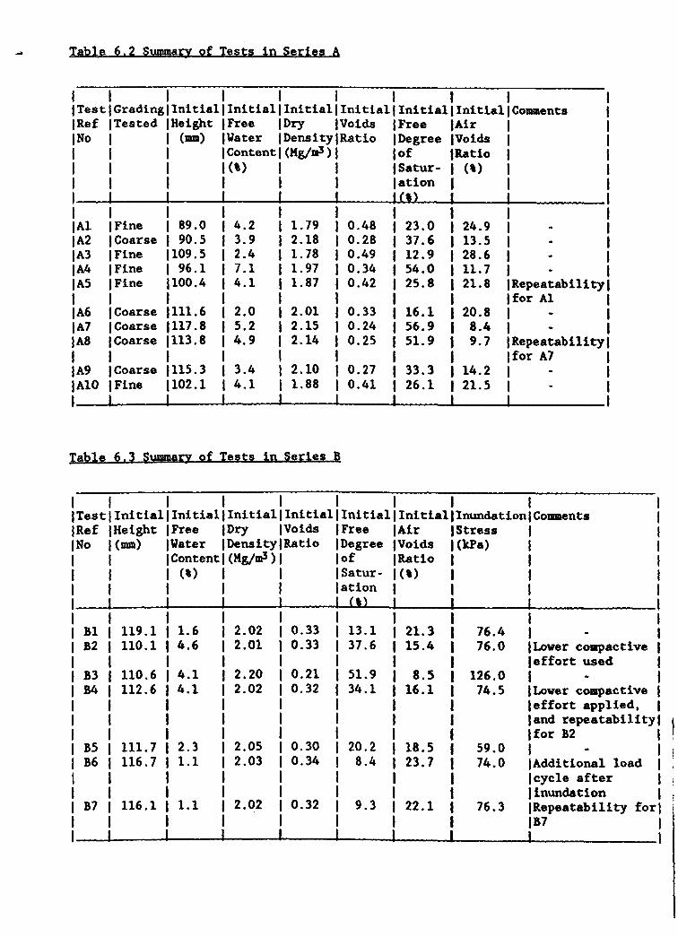
~ Table 6.2 Summaty of Tests in Series A
I I I I I I I I I ITestiGradingilnitiallInitia11Initia11lnitialilnitia11Initla1JComments IRef ITested IHeight IFree IDry I Voids I Free lAir I INo I I (am) I Vater I Density IRatio IDegree IVoids I I I I I Content I (Kglml) I lof IRatio I I I I HI} I I JSatur- I <I) I I I I I I I I ation I I I I I 1 1 1 I el) I I I I I IAl Fine I 89.0 4.2 1.79 0.48 23.0 24.9 J IA2 Coarse I 90.5 3.9 2.18 0.28 37.6 13.5 I IA3 Fine 1109.5 2.4 1.78 0.49 12.9 28.6 I IA4 Fine I 96.1 7.1 1.97 0.34 54.0 11.7 I lAS Fine 1100.4 4.1 1.81 0.42 25.8 21.8 IRepeatabi1ity I I Ifor Al IA6 Coarse 1111.6 2.0 2.01 0.33 16.1 20.8 I IAl Coarse 1111.8 5.2 2.15 0.24 56.9 8.4 I IA8 Coarse 1113.8 4.9 2.14 0.25 51.9 9.1 IRepeatability I I Ifor A7 IA9 Coarse 1115.3 3.4 2.10 0.27 33.3 14.2 I IA10 Fine 1102.1 4.1 1.88 0.41 26.1 21.5 I I I I
Table 6.3 Summaty of Tests in Sedes D
I I I I I I I I I ITestl Initial I Initial I Initial I Initial I Initial I Initla11 Inundation I Comments IRef IHeight IFree IDry IVoids I Free lAir IStress I No I(mm} IVater I DensltylRatio IDegree IVoids I (kPa) I
I I Content I (Kg/m3 ) I lof I Ratio I I I I (I) I I I Satur- I (I) I I I I I I lation I I I I I I I 1 el) I I I I I I
B1 I 119.1 1.6 I 2.02 0.33 13.1 21.3 76.4 I B2 I 110.1 4.6 2.01 0.33 37.6 15.4 76.0 ILower compactive
I I effort used B3 I 110.6 4.1 2.20 0.21 51.9 8.5 126.0 I »4 I 112.6 4.1 2.02 0.32 34.1 16.1 74.5 ILower compactive
I leffort applied, I land repeatability I Ifor 82
85 I 111.7 2.3 2.05 0.30 20.2 18.S 59.0 I 86 I 116.7 1.1 2.03 0.34 8.4 23.7 74.0 IAdditional load
I Icyc1e after I I inundation
81 I 116.1 1.1 2.02 0.32 9.3 22.1 76.3 IRepeatabi1ity for I 187 I I

Table 6.4 SummaIY of Tests in Series C
I I I IPressures During I
I Test IInitial Free IInitial Dry I Consolidation I ReferencelWater Content*1 DensitY* I I Comments
Number I <t) I (Mg/aal) I I I I I I Cell Air IWaterl I I I I I
I C1 10.5 2.02 400 368 I Saturated
I C2 0.0 2.03 102 68 I Dry • I C3 3.5 2.01 100 70 55 I Applied
199 170 156 Isuction - 15 kPa I
C4 4.2 2.09 100 71 66 I Applied 200 170 166 Isuction - 4 kPa
I
* Value at start of Ko stage.
lable ~.~ SUI!!IIIBO Qf I~§t§ in S~Ibli D
I I I I I I I I I ITestlGradingl Initial I Initia11 Initia1 I Initial I Initial I InitiallCoap- IComments IRef ITested IHeight IFree I Dry IVoids I Free lAir I action I INo I I (mil) I Water I Density I Ratio IDegree IVoids ILevel I I I I I Content I (Mg/m! ) I lof I Ratio I I I I I I (t) I I I Satur- I (t) I I I I I I I I lation I J I I I I I IDI Coarse 161.5 2.8 2.05 0.31 24.0 17 .8 I Heavy I ID2 Coarse 168.0 7.6 2.23 0.20 100.0 0.0 I Heavy I ID3 Coarse 179.0 0.0 2.18 0.21 0.0 17 .5 I Heavy I 104 Coarse 165.8 4.2 2.15 0.24 45.6 10.7 I Heavy I IDS Coarse 161.5 2.8 2.08 0.29 26.0 16.5 I Heavy I Repeatabillty I I Ifor D1 ID6 Coarse 161.1 0.0 1.96 0.38 0.0 27.6 ILight I .. \
ID6A Coarse 179.8 0.0 1.88 0.44 0.0 30.5 ILight IComputer fai1ur I I Iduring test I I IRepeat for D6 ID7 Coarse 169.8 2.7 1.79 0.50 14.4 28.4 ILight I ID8 Coarse 164.0 2.9 1. 78 0.50 15.3 28.4 ILight IRepeatability I I Ifor D7 ID9 Coarse 165.2 5.4 2.08 0.28 50.6 10.9 ILight I ID10 Coarse 171.8 4.1 1.99 0.34 31.8 17.4 ILight I ID11 I Medium 151.2 2.8 1.85 0.44 16.8 25.3 IHeavy I ID12 I MediUII 147.6 4.2 1.92 0.38 29.0 19.6 IHeavy I ID13 I Fine 146.3 3.0 1.13 0.53 14.7 29.7 IHeavy I ID14 I Fine 140.0 4.3 1.76 0.50 22.4 25.9 IHeavy I I I I I

CHAPTER 7
RESULTS OF TESTS
The results of all tests are reported in this chapter. together with
some initial interpretation of the data. Discussion of the results,
comparisons between the test series and the implications of the findings
are presented in Chapter 8.
7.1 Compressibility Tests with Suction Measurements
The results of test series A, and those for series B up to commencement
of the inundation stage, are considered under this heading. The term
"compressibility" has been used in preference to ·consolidation" even
though, by the nature of the air drained incremental load-unload tests,
pore water pressures induced by the loading changes were given time to
dissipate. Unlike conventional consolidation tests OD saturated
materials, the pore water pressure in the series B tests was not
confined to return to a back pressure but was free to attain a new
equilibrium with the induced soil fabric changes. Hence the measured
pore water pressure was not an excess pore pressure in the conventional
sense.
7.1.1 Specimen Response to a Single Total Stress Change
A typical response of the load cells to a stress increment is shown in
Figure 7.1, together with the average total stress applied. The
application of this increment resulted in the strain time curve shown in
Figure 7.2, and the incremental strain against incremental stress curve
shown in Figure 7.3. The form of these figures is typical for all
tests, whether loading or unloading, and shows that the intended
constant total vertical stress increments/decrements vere quickly
applied. The immediate and time dependent strain components may be
inferred from Figure 7.3.
- 67 -

The top and base pore water pressure response curves are plotted against
time in Figure 7.4, and show an initial surge due to system compliance
when a back pressure is not applied to the ceramic (ie the top ceramic
in Figure 7.4). The compliance influence may be seen more clearly in
Figure 7.5, which shows the suction stress path in response to total
stress changes. Figure 7.4 shows also simultaneous fluctuations in
pressure of up to 0.5 kPa from the mean pressure in response to
fluctuations in the regulated air pressure in the specimen. Small
volume changes were sometimes recorded at the base during the water
drained series A tests, but as will be discussed in Chapter 8, these
were negligible.
7.1.2 Results of Suction Measurements
The equilibrium suctions at a total stress of 10 kPa for the coarse and
fine gradings are presented in Figure 7.6 against average free water
content. The measured suctions increase as the water content decreases,
but a large degree of scatter is associated with the results for the
coarse grading. An improved relationship for the coarse grading may be
seen in Figure 7.7, which plots the suction at 25 kPa total stress
against free water content. The surprisingly similar order of magnitude
of suctions for both gradings is discussed further in section 8.3.
The warped form of the state surface for volume change shown in Figure
2.5 implies suctions should decrease as the total stress increases. The
results for both gradings confirm this expectation, as typified by
Figure 7.8. The influence of the free water content on the size of the
load-unload hysteresis loop is shown for the fine grading in Figure 7.9.
A similarly clear trend for the coarse grading was not discernible due
to the scatter in equilibrium suction values noted previously.
The variable vertical separations of the top and bottom suction-water
content curves in Figure 7.5 suggests a non-linear water content - depth
profile within the specimens. The results of the water content profile
measurements at the end of each test in series A are tabulated in Table
- 68 -
7.1 and plotted in Figure 7.10. The profiles are related to the total
water content in Figure 7.11. These figures confirm the implication of
Figure 7.5, and suggest also that, except for test A4 which has a high
average total water content, the soil water had not redistributed to
form a saturated layer at the base of the specimen.
7.1.3 Effect of Compaction Yater Content and Dry Density on
Compressibility
The strain-stress curves for the coarse and fine gradings are shown
separately in Figures 7.12 and 7.13, respectively. Inspection of these
curves shows that compressibility is a function of the compaction water
content and dry density for a given compactive effort, and this is shown
more clearly in Figures 7.14 and 7.15 which plot the strain at any given
stress level against the free water content of the soil for loading
only. Both graphs consider behaviour dry of optimum over a range in
which the dry density continually increases with increasing water
content.
7.2 Inundation Tests
The results for the inundation stage of the Series B tests are presented
in this section. Figure 7.16 shows the typical forms of the load cell
and average total stress, strain and top pore water pressure curves with
time recorded during each inundation stage. The apparent decrease in
strain as inundation commences (shown by the increase in the top pore
water pressure in Figure 7.l6c) is a function of ceramic flexure
following application of the inundation water pressure exceeding the
induced collapse strains at the constant total vertical stress.
Correction of the strain-time curve for flexure by assuming a linear
relationship between apparent strain and applied inundation pressure was
made using the apparent strain at constant vertical stress as the
inundation pressure was reduced following saturation as the benchmark.
Figure 7.17 shows the corrected curve, and Figure 7.18 shows the
influence of the inundation stage on the strain-stress curves (excluding
- 69 -

unloading stages) for the tests. As may be seen from Figure 7.17, a
large proportion of the collapse strains were manifested in the first
minutes after the start of inundation.
The pore water pressure response at the base of the specimens during
inundation is typified by figure 7.19, which shows that no change was
recorded for the first 1 to 2 hours of inundation. After this time,
there is a rapid reduction in suction to near zero followed by an
approximately linear decrease in suction during the remainder of the
infiltration stage. The finite period of time between start of
inundation and a recorded influence at the base of the specimen reflects
the rate of descent of the first wetting front through the specimen, and
the linear increase in pressure thereafter represents the gradual
increase in the height of the near saturated layer at the base of the
specimen. The equilibrium pore water pressure of typically 1.0 kPa to
1.2 kPa at the end represents the typically 100 mm to 120 mm high
saturated head of water within the specimen.
7.3 Ko and Shear Tests
7.3.1 Membrane Effects
The results of the four tests in series C on the coarse grading are
presented in the following sub-sections. However, interpretation of the
results required preliminary assessments be made of the effects of the
membrane on behaviour, as noted below.
The strength correction applied to the deviator stress measurements for
the double membrane were determined experimentally by British Gas
personnel to be 0.2226 kPa multiplied by the axial strain, the
determination being made using a dummy specimen of known properties.
Correction for membrane penetration was more difficult, and had
implications for the calculated specimen phase volumes, volumetric
strains, and the deviator stresses as noted over:
- 70 -

True total volume change of specimen Cell volume change less
correction for cell pressure
less correction for ram
penetration
True air phase volume change - True total volume change of specimen
less measured water phase volume
change
True specimen cross sectional area - original area (l-true
(l-axial strain) volumetric
strain)
True deviator stress - change in deviator load, less membrane
true specimen area strength correction
Consideration was initially given to developing a method for preventing
penetration at all, but it was decided this was not merited for such a
short series of tests. Instead, a simple and approximate method was
devised to calculate the correction for each specimen individually from
cell volume measurements. The method relied upon the assumption that,
following the Ko stage of the test, and reduction of the deviator
stress to zero, the true volumetric strain of the specimen during ~3
unloading in a water undrained state would be negligible. The near
vertical unload stress-strain curves for the radially confined tests in
series A and B suggested such an assumption would not be greatly in
error. If the assumption is correct, any recorded cell volume change
due to the reduction in V3 above (corrected for expansion/contraction
of the cell walls due to ~3) should represent the total change in
membrane penetration as the drained and pressure regulated air phase
pushes the membrane out. A linear relation between change in cell
pressure and penetration was then assumed. It was also assumed that
membrane penetration was the same during unloading and the preceding
loading stages.
- 71 -

The major drawback of this method was that it had to follow the Ko
stage, which itself relied upon a reliable estimate of the membrane
penetration factor to maintain Ko conditions. Consequently a trial test
was performed and a factor of 0.5 cm3 /kPa obtained. The actual tests
subsequently yielded values of 0.89, 0.32, 0.39 and 0.45 cm3 /kPa for
tests C1 to C4 respectively, which resulted in true Ko conditions only
being reliably maintained in test C4.
7.3.2 Consolidation Curves
The pressures on the four specimens during the isotropic consolidation
are summarised in Table 6.4. A conventional consolidation curve was
obtained for each specimen, as typified by Figure 7.20, but the times
for consolidation were noticeably different. The saturated and dry
specimens (C1 and C2) took about 16 hours and 27 hours respectively,
whereas the unsaturated specimens (C3 and C4) which were consolidated
from near saturation at a constant applied suction each took about 28
days. The changes in specimen water content, void ratio and dry
density, plus the total and free water volumetric strains during
consolidation are presented in Table 7.2. The effect of raising the
ambient consolidation pressures by a constant value was investigated
near the end of consolidation for each specimen and found to have
negligible effects.
7.3.3 Ko Determinations
As a result of testing difficulties and significant discrepancies
between the assumed and subsequently measured membrane penetration
correction factors, Ko conditions were not sufficiently maintained for a
reliable Ko value to be measured from tests C1, C2 and C3. The results
for specimen C4 are shown in Figure 7.21, and a Ko value of 0.41 was
obtained by taking Ko to equal A (rJ 3 - UA)/ A (d 1 - UA) for this
unsaturated case. A tentative value of 0.39 was obtained from the
latter stages of test C1 when Ko conditions were achieved, but initial
anisotropic stress changes render this value suspect.
- 72 -

7.3.4 Shear Stages
The complex stress paths followed by the specimens up to the start of
the shear stages are summarised in Tables 7.3 to 7.6, together with
their impact on the main specimen parameters. These stress paths will
have led to initially overconsolidated specimens and are likely to have
significantly affected the early stages of the shear tests in
particular.
The results of the shear stages are presented in Table 7.7 in the light
of the above comments. All specimens failed (ie peak shear stress)
through dilatant plastic deformations, and only exhibited shear plane
deformation movements near the ends of the tests. A typical plot of the
stress-strain curves obtained and the measured volumetric strains are
presented in Figures 7.22 and 7.23, respectively. All specimens failed
at axial strains of about 5', but as will be discussed in Chapter 8
volumetric strains differed significantly between specimens.
7.4 Strain Controlled Compression Tests
The results of the 15 tests in series D are presented in this section.
Tables 7.8 and 7.9 summarise the virgin compression line and repeated
load data for each test, respectively, and Figure 7.24 shows a typical
stress-strain curve for all stages of a test. Similar forms of curves
were obtained for all tests regardless of grading or compactive effort.
Figures 7.25 and 7.26 present the virgin compression lines only for the
usual and low compactive efforts, and Figure 7.27 presents the curves
for the fine and medium grading tests. Inspection of the curves for the
coarse grading show that in common with the series A and B tests
compressibility is a function of the dry density and vater content.
These effects are more clearly seen in Figure 7.28, which plots the
strain at a given stress level against the total water content. The
more heavily compacted specimens gave a relatively flat curve with a
slight peak over the water content range of Ot to about 5.5', but the
- 73 -

compressibility then rapidly increases as optimum water content is
approached and passed. The lightly compacted specL.ens show a similar
trend but the range of water contents tested was insufficient to show
the increase in compressibility as the optimum water content is
approached. The interactions of the dry density and water content may
not be determined from the two tests on the fine and medium gradings.
The effects of repeated loading on strain accumulation are typified by
Figure 7.29, which plots the strain at the maximum and minimum stresses
of each load cycle against cycle number. All the curves showed a
discontinuity when the peak stress was increased fro. 125 kPa to 250 kPa
after the first 4 or 5 cycles, there being also a time gap between this
cycle and the next due to the low (0.5 mm/minute) strain rate. After
the eighth to tenth cycle the strain rate was increased to 2 mm/minute.
Each of the four groups of tests (coarse grading with heavy and light
compaction, and fine and medium gradings) exhibited a different typical
response as shown by the figure, but all showed that strain rate had no
influence on the behaviour.
The effects of water content and dry density on the repeated load
behaviour have been drawn out by Figures 7.30 and 7.31, which plot the
difference in strain after one and four cycles against the free water
content (a) and dry density (b) for the heavily and lightly compacted
coarse graded specimens, respectively.
The water content - depth profile measurements at the end of each test
are summarised in Table 7.10. Except for the wettest specimen,
insufficient time «4 hours usually) had elapsed for significant
moisture redistribution to occur within the specimens.
- 74 -

Table 7,1 Water Content Distribution Profiles After Series A Tests
Test Measured Total Water Average Number Content <t> Total
Water I I Content
Top I Middle IBottom <t> I I I I
Coarse Gra~in& I I I I
A2 Not Measured 4,7 A6 2.4 I 2,7 I 3,2 2.8 A7 5.6 I 6,0 I 6.4 6.0 AS 5.1 I 5,3 I 6,7 5.7 A9 4.0 I 4.1 I 4.4 4.2
I I Ein~ Grading I I
I I A1 Not Measured 5.6 A3 3,6 I 3.S I 4.0 3,8 A4 7.4 I 8.4 I 9,7 8,9 A5 5.2 I 5,4 I 6,0 5,5 A10 5.3 I 5,4 I 5,S 5.5
I I

Table 7,2 Change in Specimen Parameters During Consolidation Stages of Series B Tests
I I Test Number Free Water Content <t> Void Ratio Final Free I Dry Density (MO/~) Volumetric Strain ('> I Initial Final I Initial Final Degree of I Initial Final Free Water Total I ~ _____ ~ __ ~~ __ ~.L ~~--L-....,Sa""t",-,u.,..r ..... a...,..t""-io",,n,""-----,(,-,',--,)--'.I~~~_~~_~~--'-I I I I C1 I 10.7* 10.5 O.ll 0.28 100.0 1,97 2.02 I 2.6 0.72 I I I I C2 I 0.0 0,0 0.l5 0.34 0.0 2.00 2.03 I N/A 0.88 I I Cl
I I I 7.9 3.5 0.31 0.31 31.0 2.01 2,01 I 60.5 0,31
I I I I C4 I 9.0 4.2 0.26 0.24 45.6 2.06 2.09 I 46.8 1.21 I I I I I ___ 1
* 9.1' before saturation stage

Table 7.3 - Stress Path History and Variation of Soil Parameters for Test C1
I I I Parameter, cr, I (1"3 I UA uw e Free water Free degree of Dry density I Sta" I (kPa) I (kPa) I (kPa) (kPa) content (,) saturation (\) (Kg/m3) I I" I After isotropic I I , I consolidation ,398, 400, 368 0.28 10.5
I 'I' IAfter air and water ,drained Ko stage , IAfter anisotropic water lundrained reduction of , (cr, - cr3) at constant cr3 I IAfter anisotropic water lundrained reduction of , 0'" 3
I I I I I I
626 515
517 515
401 401
369 0.25 9.2
369 0.25 9.2
368 0.26 9.6
100.0 2.02
100.0 2.02
100.0 2.02
100.0 2.02
I __________________ ~----~~----~------~----~--~~--------~----------~-----------
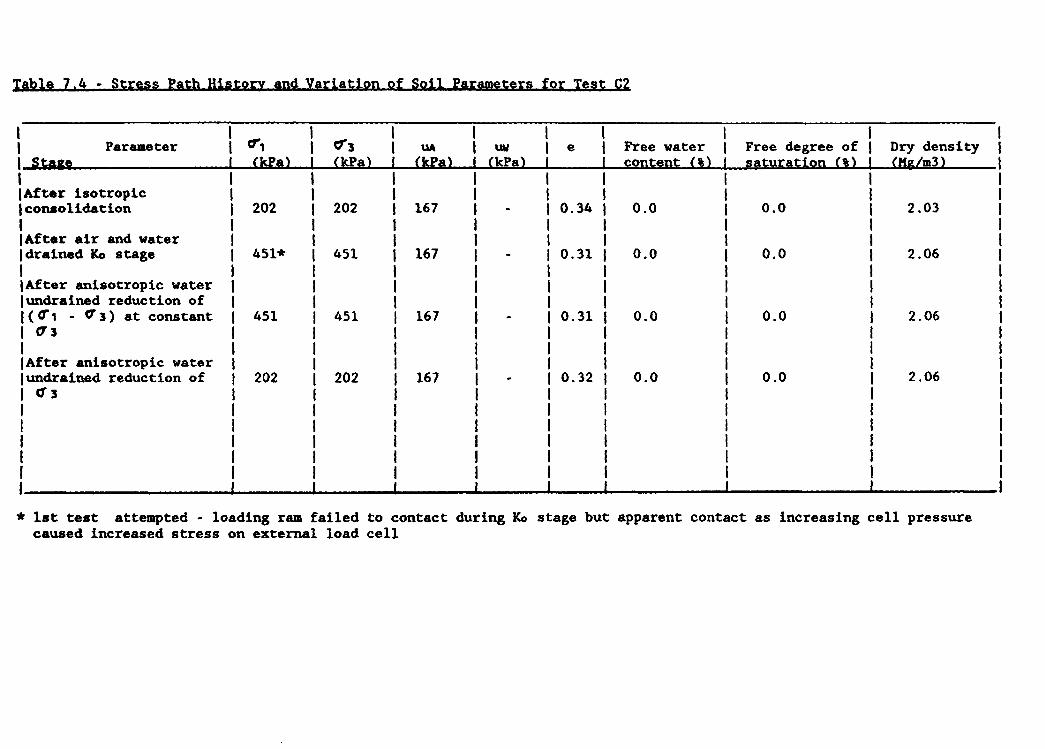
Table 7.4 - Stress Path History and Variation of Soil Parameters for Test C2
I I I Parameter I C7", C1"3 I UA I uw e Free water Free degree of Dry density I Stage I (kea) (kPa) I (kPa) I (kPa) content (%) saturation (I) (Hg/m3) I I I I IAfter isotropic I I I Iconao1idation I 202 202 I 167 I 0.34 0.0 0.0 2.03 I I I IAfter air and water I Idrained Ko stage 451* 451 I 167 0.31 0.0 0.0 2.06 I I IAfter anisotropic water I lundrained reduction of I 1(0", - cr 3) at constant 451 451 167 0.31 0.0 0.0 2.06 I CT3 I IAfter anisotropic water lundrained reduction of 202 202 167 0.32 0.0 0.0 2.06 I Cf 3 I I I I I I ________________ ~------~----~------~----~--~--------~----------~----------* 1st test attempted - loading ram failed to contact during Ko stage but apparent contact as increasing cell pressure
caused increased stress on external load cell

Table 1,5 - Stress Path Hist0tY and Variation of Soil Parameters for Test C3
I I I Parameter I cr, C7'3 UA WI I e Free water I Free degree of I Dry density I Stage I ekPal ekPa) ekPAl (kPa) I content e,) I saturation e,) I (Mg/m3) I I I I I IAfter isotropic , I' I I consolidation , 199 170 156 I 0,31 3,5 I 31,0 , 2.01 I I I I I IAfter air and water I I I , Idrained KG stage I 451 360 170 156 I 0,30 3,5 I 31,S I 2.01 I I I I I ,After anisotropic water I I I lundrained reduction of I I I I(cr, - ~3) at constant I 360 360 170 156 0,30 3,5 I 31.3 I 2.01 J C1"3 I I I I I I I J After anisotropic water I I I lundrained reduction of I 202 202 170 157 0,31 3,5 I 30.7 I 2.01 , C7'3 I I I 'I I I I I I I I I I I I I I I I I I I I I I I

Table 7.6 - Stress Path History and Variation of Soil Parameters for Test C4
I I I I I I Parameter I CT, I ~3 I UA I uw e Free water Free degree of Dry density I Stage I (kPa) I (kPa) I (kPa) I (kPa) content (,) saturation (\) (Mg/m3) I I I I I I After isotropi.c I I I I I consolidation I I 200 I 170 I 166 I I I I I IAfter air and water I I I I Idrained Ko stage I 427 I 312 I 170 I 166 I I I I I IAfter anisotropic water lundrained reduction of I (V, - fT 3) at constant I 0'3 I IAfter anisotropic water lundrained reducti.on of I cr] I I I I I
312 312 170
201 201 130
166
167
0.24 4.2 45.6 2.09
0.23 4.2 48.7 2.11
0.23 4.2 48.6 2.11
0.23 4.2 47.6 2.11
I __________________ ~----~------~----~----~----~--------~----------~-----------

Table 7.7 Results of Shear Tests
I I Pore Pressures I Failure IShear Stress Mean Stress at IVolumetric Failure ISoil Parameters at Failure ITeatl During Test IStresses+ lat Failure Failure (kPa) IStrains (') I Free Free Voids No I (kPa) I (kPa) I (kPa) '/2 (t11 f+Cr3f ·2UA) IAxia1 Total Free I Water Degree Ratio
lUAu.. (UA ·uw) I C1'1F c:f3 f P/2 (CT1f ·C13 f) I Water I Content of 1 I I I I (%) Saturation I __ ~ ~ _~_ ____ _ _ L _ _ _~ _ __ __ _ _ _ _ J _ _ I (% )
ell· 368 602 401 101 134* 15.30 ·0.91 ·0.91 110.1 100.0 1 I 1(9.6) (100.0) I I I
C2 167 710 202 254 289 14.30 ·1.28 10.0 I 1(0.0) I I
C3 170 157 13 701 202 250 282 15.15 ·2.25 +3.67113.4 I 1(3.5) I I
C4 170 167 3 420 201 110 141 15.05 ·2.20 ·0.47 14.2
+ Failure defined as peak value of shear stress * '/2 (V1f +CT3f . 2u..) for saturated soil
I 1(4.2) I I I I I I
0.0 (0.0)
25.5 (30.7)
39.9 (47.6)
0.27 (0.26)
0.33 (0.32)
0.36 (0.31)
0.28 (0.23)
(at start) Dry Density (Mg/al)
2.00 (2.02)
2.03 (2.06)
1.96 (2.01)
2.03 (2.11)

Table 7,8 Vir&in Compression Line Data for Test Series D
I Test Strains (,) and Various Stresses (kPa) on VCL
No I I 5 I 10 25 50 100 I 150 200 250
I I
01 0,00 0,24 0.31 0.37 0.40 0,42 0.45 0.47 02 0.00 0.15 0.44 0.77 1.14 1.41 1.64 1.85 03 0.00 0.05 0.13 0.23 0.35 0.44 0.50 0.57 D4 0.00 0.09 0.16 0.20 0.24 0.27 0.31 0.36 05 0.00 0.23 0.28 0.32 0.35 0.38 0.41 0.44
06A 0,00 0,33 0.93 1.47 2.10 2.52 2.85 3.14 07 0.00 0.38 0.84 1.34 2.46 3.11 3.62 4.11 08 0.00 0.40 1.31 2.24 3.40 4.18 4.77 5.34 09 0.00 0.17 0.42 0.68 1.03 1.27 1.47 1.66 010 0.00 0.20 0.53 0.86 1.30 1.62 1.85 2.08
011 0.00 0.40 0.69 0.82 0.96 l.03 1.06 l.11 D12 0.00 0.09 0.18 0.22 0.29 0.34 0.36 0.40
013 0.00 0.10 0.23 0.34 0.50 0.62 0.71 0.79 014 0.00 0.05 0.14 0.23 0.34 0.43 0.53 0.61
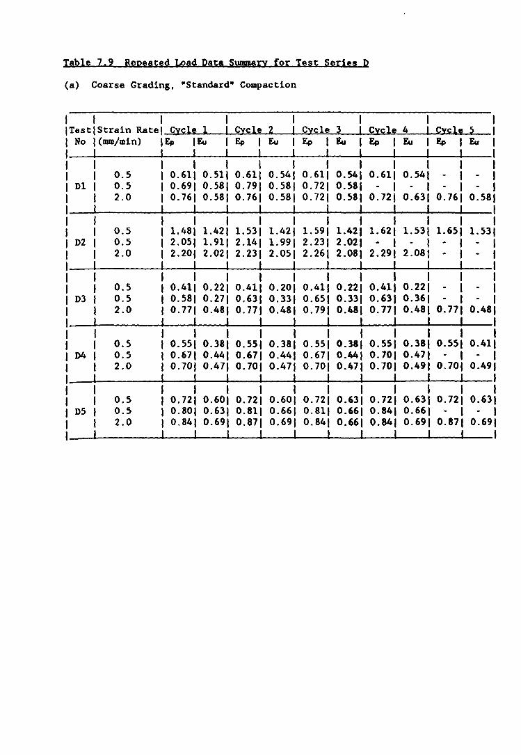
Table 7,9 Repeated Load Data Summary for Test Series D
(a) Coarse Grading. ·Standard· Compaction
I 1 I I I I I TestlStrain Ratel Cycle 1 1 Cx£h Z I Cx£le l I ~y~b 4 1 ~Y£l! ~
No I (mm/min) IEp lEu IEp 1 Eu IEp I Eu IEp I Eu IEp I Eu I 1 1 1 1 1 I I 1 1 I I I I I 1 1 I 1 1 I I 0,5 I 0,611 0.511 0.611 0,541 0.611 0,541 0,611 0.541 - 1 -
D1 1 0.5 I 0,691 0,581 0.791 0,581 0.721 0.581 - I - 1 - I -I 2.0 I 0,761 0,581 0.761 0,581 0,721 0,581 0.721 0.631 0.761 0,58 I I I I I I I I I I I I 1 I I 1 I I I 1 I I 1 0,5 1 1,481 1.421 1,531 1.421 1. 591 1.421 1,621 1.531 1,651 1.53
D2 1 0.5 1 2,051 1,911 2,14 1 1.991 2.231 2,021 - I - I - I -I 2,0 I 2,201 2,021 2,231 2,051 2,261 2,081 2,291 2,081 - I -I I I I 1 I I I 1 I I I I I I I I I I I I I I 0,5 I 0.411 0,221 0,411 0,201 0,411 0,221 0,411 0,221 - I -
D3 I 0.5 I 0.581 0,271 0.631 0,331 0,651 0,331 0.631 0.361 - I -I 2.0 I 0,771 0,481 0,771 0,481 0,791 0,481 0.771 0,481 0,771 0,48 I I I I I I I I I I I
I 1 1 I I I I I I I 0,5 I 0,551 0.381 0,551 0,381 0.551 0,381 0,551 0,381 0,551 0,41
D4 0,5 1 0.671 0,441 0,671 0.441 0,671 0,441 0.701 0.471 . I -2.0 I 0.701 0.471 0.701 0.471 0.701 0,471 0.701 0,491 0.701 0,49
1 I 1 I I I I I 1 I I I I 1 1 I 1 I I I
0.5 1 0.721 0. 60 1 0,721 0,601 0,721 0.631 0.721 0.631 0.721 0.63 D5 0.5 I 0. 80 1 0, 63 1 0.811 0.661 0.811 0,661 0,841 0,661 - I -
2,0 I 0.841 0. 69 1 0.871 0.69\ 0.841 0,661 0,841 0.691 0.871 0,69 I I I I I I I I I I

(b) Coarse Grading, Light Compaction
1 I I I I I I TestlStrain Ratel Cycle 1 I Cycle 2 I Cycle 3 I Cycle 4 I ayele 5
No I (mm/min) I Ep I Eu I Ep I Eu 1 Ep I Eta I Ep 1 Eu I Ep I Eu I 1 I 1 I I I I I 1 I I I I I I I 1 1 I I I I 0.5 I 3.321 3.161 3.351 3.191 3.371 3.191 3.401 3.191 3.431 3.24
06AI 0.5 I 4.211 3.971 4.291 4.021 4.321 4.081 4.371 4.131 4.401 4.15 1 2.0 I 4. 40 1 4.151 4.451 4.181 4. 48 1 4.181 4.481 4.241 4.511 4.26 1 I 1 I I 1 1 1 I I 1 I 1 I I I I 1 I I 1 1 I 0.5 I 2.431 2.341 2.491 2.401 2.511 2.431 2.571 2.491 2.571 2.49
D7 I 0.5 I 4.231 4.051 4.341 4.141 4.401 4.231 4.451 4.281 4.511 4.31 I 2.0 I 4.571 4.371 4.621 4.421 4.651 4.45 1 4.681 4.481 4.681 4.51 1 I I I I 1 1 1 1 1 I I 1 1 1 1 I I 1 I I 1 I 0.5 I 3.791 3.661 3.821 3.731 3.871 3.161 3.931 3.821 3.931 3.82
D8 I 0.5 1 5.851 5.651 5.951 5.771 6.061 5.851 6. 09 1 5. 91 1 - 1 -I 2.0 1 6.181 5.981 6.211 6.001 6.271 6.061 6.301 6.091 6.331 6.15 I 1 I I I I 1 I I I 1 I I 1 1 I I I I I I 1 I 0.5 1 1.301 1.121 1.351 1.171 1.441 1.231 1.441 1.301 1.501 1.32
09 I 0.5 I 2.001 1. 731 2.091 1. 791 2.141 1..51 2.171 ooS I - I -I 2.0 I 2.201 1.941 2.231 1.941 2.261 2.001 2.321 2.001 2.351 2.03 I I 1 I I 1 1 I I I I I I 1 1 1 1 I 1 1 I I I 0.5 I 1.801 1.471 1.831 1.531 1.891 1.611 1.921 1.641 1.921 1.66
D101 0.5 I 2.651 2.171 2.14 1 2.321 2.821 2.401 OOS 1(2.46) - 1 -1 2.0 1 2.991 2.491 3.021 2.461 3.051 2.571 3.0SI 2.601 3.101 2.60 I I I I 1 I 1 1 1 I 1
(c) Fine Grading:
I 1 I I I I I TestlStrain Ratel Cycle 1 I Cycle 2 1 Cycle 3 I Cycle 4 I Cycle S
No I (mm/llin) IEp lEu I Ep I Eu I Ep I Eta I Ep I Eu I Ep I Eu I 1 I I 1 I I 1 I I I I 1 1 I I 1 I I 1 I I I 1 0.5 1 0.831 0.661 0.S71 0.661 0.871 0.101 0.871 0.661 0.871 0.661
D131 0.5 I 1.071 0.731 1.101 0.771 1.131 0.101 1.131 O.SOI 1.131 0.831 I 2.0 1 1.161 0.901 1.161 0.871 1.161 0.'71 1.201 0.831 1.161 0.871 I 1 I 1 1 1 I I I I I I I I 1 I I I I I I I 1 1 I 0.5 I 0.521 0.381 0.521 0.381 0.521 0.381 0.521 0.381 0.521 0.381
0141 0.5 I 0.761 0.521 0.791 0.551 0.831 0.551 0.S61 0.591 0.861 0.591 I 2.0 I 0.861 0.5SI 0.861 0.621 0. 90 1 0.621 0.901 0.621 0.941 0.661 1 I I I I I I I I I I I

(d) Medium Grading:
\ \ \ \ \ Test\Strain Rate Cx~h 1 \ Cx~h Z Cxs;;l~ l \ Cxs;;l~ !t \ Cl~b ~
No \ (mm/min) Ep \Eu \Ep Eu Ep \ Eu \Ep Eu \ Fop Eu 1 1 1 1 1 1
\ 1 1 O.S 1. 70 1.61\ 1. 70 1.61 1.701 1.64\ 1. 30 1.64 1. 70 1.64
Dll 0.5 1. 87 1. 771 1.87 1.77 1.89\ 1.77\ 1.89 1.77 1.89 1.77 2.0 1. 87 1. 77\ 1.87 1.77 1.871 1.77\ 1.87 1.77 1.87 1.77
\ \ 1 \ \ \
0.5 0.49 0.361 0.49 0.36 0.491 0.361 0.49 0.36 0.49 0.36 012 0.5 0.59 0.431 0.62 0.43 0.661 0.43\ 0.66 0.46 0.66 0.46
2.0 0.66 0. 46 1 0.66 0.46 0.691 0.46\ 0.69 0.46 0.69 0.46 1 1 I
Note: Ep - strain at peak stress in cycle, being either 125 kPa or 250 to 275 kPa
Eu - strain at minimum stress level in cycle, 10 kPa
OOS - Out Of Scans

Table 7.10 Water Content Distribution Profiles After Series D Tests
Test Total Water Content - Pepth Profile No Top I KiddIe Base
I
Dl 3.2 4.0 3.6 D2 9.2 6.8 7.2 D3 0.0 0.0 0.0 D4 4.6 5.3 5.2 D5 3.3 3.6 3.8
D6A 0.0 0.0 0.0 D7 3.5 3.4 3.5 D8 3.3 3.8 4.1 D9 5.0 5.4 8.3 DlO 4.0 4.7 5.9
D11 3.8 4.0 4.0 D12 5.2 5.2 5.7 D13 4.4 4.4 4.3 D14 5.7 5.8 5.7
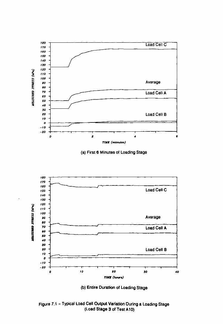
? ! CIl
~ t;;
~ :::;, CIl e
I I I
180
110 Load Cell C
180
150
140
130
120
110
100
SO Average 80
10 Load Cell A 80
50
40
30
20 Load Cell B 10
0 -./
-10
-20
o I
Till. ("''''ut .. )
(a) First 6 Minutes of Loading Stage
180
110
180 ~ 150 Load Cell C 140
130
120 -110 -100 -
SO - Average 10 '10
..... ----Load Cell A
.0 ~ 60
40 . SO 10 Load Cell B 10
0 ~
......
-10 --10
o 10 SO
(b) Entire Duration of Loading Stage
Figure 7.1 - Typical Load Cell Output Variation During a Loading Stage (Load Stage 3 of Test A10)
40

'.86
'.84
'.82
'.80
'.18
~ '.16
~ '.14
Ii) '.12
~ '.10 e t.68
'.66
'.64
'.62
'.60
10
75
70 .. ! 15
I 10
tI ~ 56
~
50
45
40
0
t.IO
to 20
TIllE (Ilovn)
Figure 7.2 - Typical Strain Development During a loading Stage (Load Stage 3 of Test A 10)
'.'4 '.11 t." t." 1.10 '.84
rorAL Sf7WN (W)
Figure 7.3 - Typical Stress-Strain Curve For Single loading Stage (Load Stage 3 of Test A10)

'03
'oz
'01
"i' ! 100
~ 99 rt)
~ 98
!!i 5'; 97 ~
~ 91
9$
94
93
6.0
4.0
3.0
Z.O
! 1.0
~ 0.0
§ -1.0 CI3
-Z.O
-3.0
-4.0
-6.0
4
0 10 ZO 30 40
TI1I8 (lwura)
Figure 7.4 - Typical Pore Pressure Variation During a Loading Stage (Load Stage 3 of Test A 10)
Top of spelclrrlen-.
'Its
AVI'RACI' STIUSS (tPa)
Figure 7.5 - Typical Suction-Stress Curve For Single Loading Stage (Load Stage 3 of Test A 10)

a-~ ~ E :;) ~
? ~ ~ Q
~ ~
50.0
40.0
30.0
20.0
10.0
0.0
-10.0
0.0
100.0
90.0
BO.O
70.0
110.0
50.0
40.0
30.0
%0.0
10.0
0.0
0.0
b.
b.
+
Base of specimen
z.o
Top of specimen
t.
Base of specimen
2.0 4.0
(a) Coarse Grading
Top of specimen
4.0 11.0
FUE rArE.R CONTENr (")
(b) Fine Grading
+
6.0
b.
B.O
Figure 7.6 - Suction-Water Content Relationships for Coarse and Fine Gradings at Vertical Stress of 10kPa
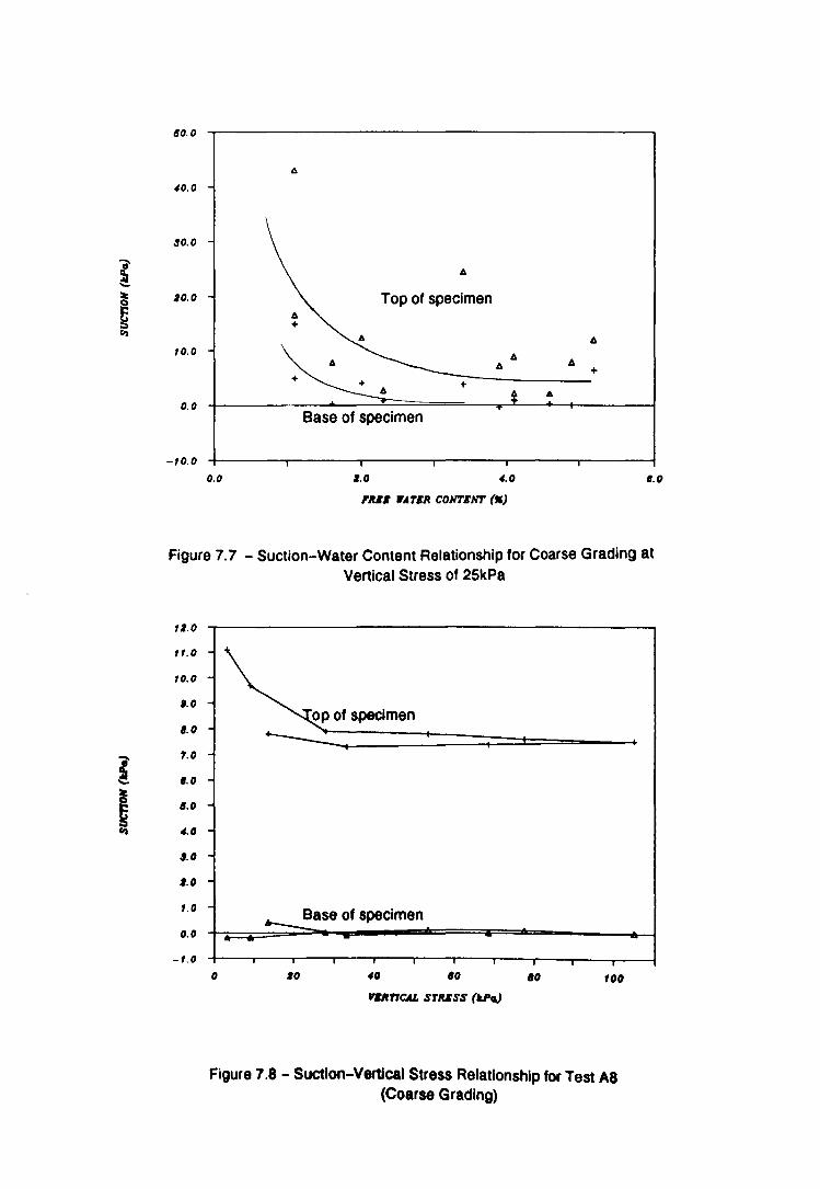
ii' ~ :.:
~ Q fII
l -.;.
I fII
60.0
40.0
30.0
6
10.0 Top of specimen
6 ,0.0 6
6 6 +
+ A
0.0 Base of specimen
-,0.0
0.0 1.0 4.0 •. 0
'IUE FATER CONTENT (_)
Figure 7.7 - Suction-Water Content Relationship for Coarse Grading at Vertical Stress of 25kPa
".0
".0
'0.0
1.0
'.0
'1.0
•. 0
6.0
4.0
3.0
1.0
t.O
0.0
-t.O
Base of specimen
0 .0 40 '0 '0 tOO ~rrCAL STUSS (th)
Figure 7.S - Suction-Vertical Stress Relationship for Test AS (Coarse Grading)

100
90
80
70
d' Q;.
60 ~
~ t; 50 ::, ~
0... e 40
30
20
fO
0
0 20 40 60 80 100
VERTICAL STRESS (kPa) a At + A3 o A4 ~ A5 x A10
Figure 7.9 - Variation of Top Suction with Vertical Stress for Fine Grading
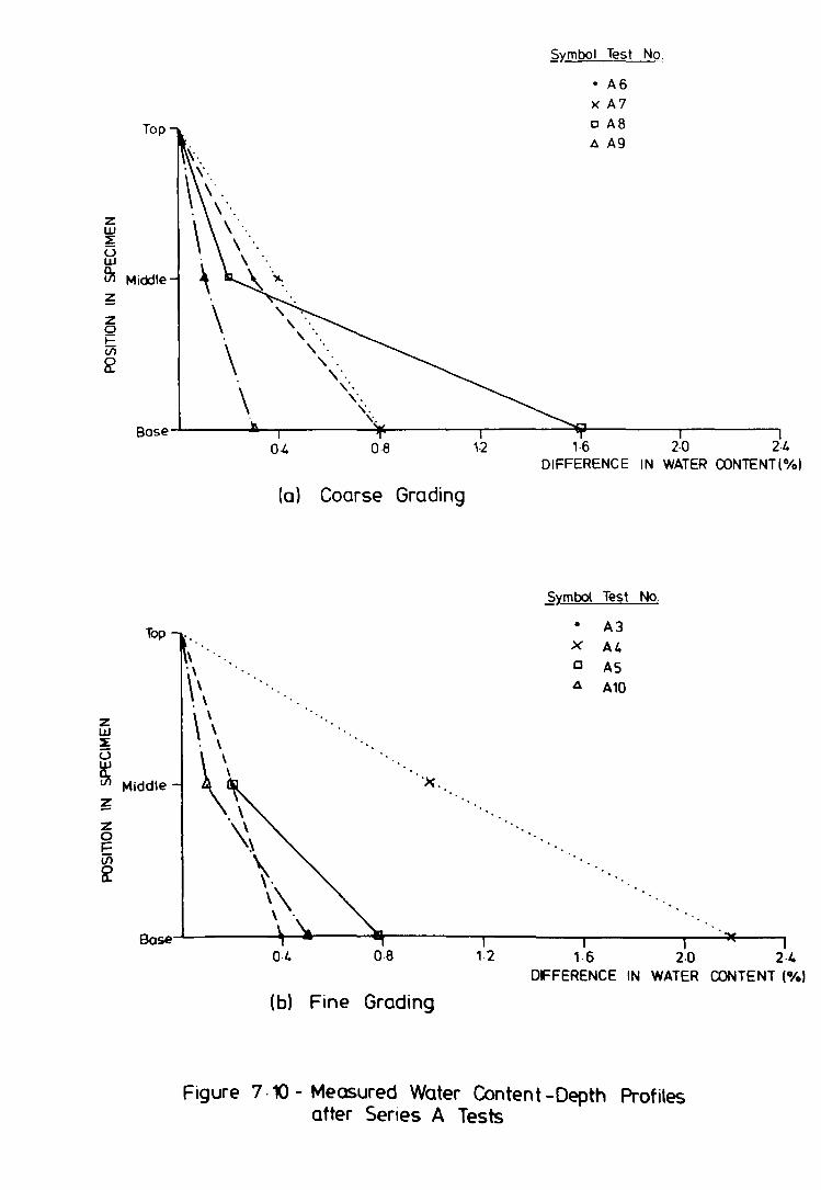
Top
z w ~ u w ~ Middle
~
z 0 E I.J')
~
, . , '. , ". , '. , '. ,'. " . , ..
?y'mbol Test No.
• A6
x A7
o AS
Il A9
"\". "\".
Bose~----~~~------~--------'-------~~-------r------~
z UJ ~ (J
~
Top
if) Middle
Bose
0-4 08 1-2 1·6 2·0 2·4 DIFFERENCE IN WATER CONTENT(%)
(a) Coarse Grading
2y'mbol Test No.
• A3 x A4 c A5 A A10
·X.
04 0·6 1-2 16 2·0 2·4 DIFFERENCE IN WATER OONTENT (Ofol
(b) Fine Grading
Figure 7·10 - Measured Water Content -Depth Profiles after Series A Tests

2-8
24
~ o - 20
I ~
15 e 16 --0 C a s: B 12 (;
i I 0·8
J ell 0·4
~ ... .! -o
o ----...---?-----10 20
)(
x = coorse grading C!) = tIne grading
,/ ~ ____ 0 x
30 40
/0 o
50
)(
/ ?
/" x
6-0
/
70
7/0
/
/
80 9·0 Total VVoter Contentt%)
FigLJ"e 7-11 - Effect of Total Water Content on Vertical Water Con tent Prof He

l.O
'.9 '.1
'.1 '.8 '.5 '.4
..... '.3 ~ '.l
~ ,. , '.0
II) 0.'
~ 0.1 e 0.1
0.' 0.5
0.4 0.3
O.l O. ,
0.0
0 lO 40 80 10 '00 'lO
~RTICAL STIUSS (kPa) o TIST Al + TIST A. 0 TIST j1
A TIST AI )( TIST A9
(a) Series A Tests
S.O
l.'
l.'
l.4
1.1
1.0
l t.I
~ t.I
t.4
fi 1.1
t.O
0.' 0.' 0.4
0.1
0.0
0 10 40 .0 .0 tOO flO
qltrlCAL STIUSS (~ o TIST.' + TIST BI • TIST B3
A TIST .4 )( TIn B' (b) Series B Tests (to B5Inc.)
Figure 7.12 - Strain-Stress Curves for Coarse Grading from Series A and B Tests (continued overleaf)

3.0
I.a I.S 1.4
1.1
1.0
!: ,.a
~ '.S '.4
~ '.1
'.0
o.a o.s 0.4
0.1
0.0
0 10 40 SO ao '00 flO
'l8Rf7CAL STIUSS (u>a,) + TIST Ba 0 TIST B7
(c) Series 8 Tests (86 and 87)
Figure 7.12 - Strain-Stress Curves for Coarse Grading from Series A and 8 Tests (continued)
I.S
1.4
1.1
1.0
,.a
~ , .. i '.4
, .. fi '.0
0.' 0.'
0.4
0.1
0.0
0 1O 40 .0 '0 '00 "0
JTRf7CAL STR8SS (u>a.) o TIST A' + ,.1$1' A3 0 ,.In M
4 TIST AI )( TIS,. AlO
Agure 7.13 - Strain-Stress Curves for Fine Grading from Series A Tests

.. ....
~ tJ f r.,
~ ... ~
~ i
C
.. .....
§
I I ... ~
I i
0
".ff
o Z.4
., . ., ".0
'.8
' .ff
'.4
' . .1
'.0
0.8
O.ff
0.4
0."
0.0
0.0 .1.0 4.0 ff.O
'1U6 FAT6R CONTENT (.) ,OItPG + Z5lcPG o 50ltPG 4 1SltPG )( 'OOIcPG
Figure 7.14 - Effeet of Free Water Content on Compressibility of Coarse Grading from Test Series A and B at Usual Compaetive Effort
.1.1
.1.4
6.6
.1.0
, .. '.1
t.4
t.6
t.O
0.1
0.1
0.4
0.6
0.0
0.0 6.0 4.0 '.0 '.0 'lUI FA r6R CONT6NT (JI)
,01tPG + U..,.. o 601&Pa 6 15lcPG )( '001cPa
Figure 1.15 - Effect ot Free Water Content on Compressibility of Fine Grading from Series A Tests

;roo '90 -'80
~ '70 180 Load Cell B 'so
d' '40
! 130 ,;ro
~ "0
~ '00
-fl i .... Start of inundation End of inundation
~ 90
80 Average
! 70
80
so Load Cell A 40
!O :ro '0
- Load Cell C
0 1
o 8 " :r4
(a) Variation of Load Cell Measurements
0.1$
o. '4 o.,! o.,:r 0."
0.'0
0.0'
~ 0.08
~ 0.01
0.08
0.05
End of inun~tion
i
is 0.04
I 0.0!
D.O'
0.0'
0.00
-0.0'
-D.O' -0.0!
-0.04 Start of inundation
-0.05
0 , " .4
(b) Strain Development During Stage
Rgure 7.18 - Typical Variation of Stress Strain and Top Pore Wat. Pressure During an Inundation Stage (Test 82) (continued overtaaf)

? ~ ~
~ ~
f II: t! i:
~ ~ e
...... ~ ~
~ ~ Ie
~ U
200
190
180
170
160
150
140
130
120
110
100
90
80
10
ISO
50
40
3D
20
10
0
0
tart of inundation
8
End of inundation t
12 11S
TIJlE (h.lJ'Urs)
20
(c) Strain Development During Stage
24
Figure 7.16 - Typical Variation of Stress Strain and Top Pore Water Pressure During an Inundation Stage (Test 82)
0.110
0.100
0.090
0.080
0.010
0.01S0
0.050 End of inundation
0.040
0.030
0.020
0.010 Start of inundation
0.000
0 8 11 11S 20 24
TIJlE (h.ours)
Figure 7.17 - Variation of Strain During Inundation Stage of Test 82 After Correction for Ceramic Deflection Due to Inundation Pressure

.......
.!.
~ r.,
~ e
g
i i
I
~.O
I.a 1.1
1.4
1.1
1.0
t.a t.I
t.4
1.1
1.0
o.a 0.1
0.4
0.1
0.0
S.O
I.' I.' 1.4
1.1
1.0
I.'
1.' f.4
f.'
f.O
0.'
0.'
0.4
0.'
0.0
0 10
Note - Inundation stage represented by last two points on curves
40 .0 .0 '00 110
VERTICAL STRESS (lcPa) o TEST Bt + TEST BI 0 T8ST B~
0
A TEST B4 x T8ST B6
<a> Tests 81 to 85
Note - Inundation stage represented by last two points on curves
.0 40 10 .0 '00 110
VERTICAL STMSS (th) + T8ST B. 0 T8ST S,
(b) Tests 86 and 87
Figure 7.18 - EHect of Inundation Stage on Strain-Stress Curve for Tests

1 .6
1.4
1.2 J rStart of inundation
1. 0
0 . 8
0 . 6 d' ~ '--
0.4
~ 0 .2 a h 0 . 0 t..> ~ en -0.2
~ -0.4 O§ -0.6
- 0 . 8
- 1. 0
-1.2
- 1.4
- 1 . 6
0 4 8 12 16 20 24 28
TIME (hours)
Figure 7.19 - Typical Variation of Base Suction During an Inundation Stage (Test B5)

ROOT TIME (mins)
o 60 80 140 160 180 200
Note: Only SlUDple data points m4Tkcd for c14rity
500
~ a ~
~ 600
c5 > ei
700 I-
~ ~ u.. ~ 800 Lll t:>
~ :r: u 900
I 11.0
Figure 7.20 - Consolidation Curve For Test C3

~ ~ ::l "l
~ ~
-.I ...J ~ u ~ ~ ~
~ :r: u
120
80
60
40
l /
30 /
o I
00
,00
80
60
1.0
~ /.
10, C).1
20 , 30
02
/
,40
0'3
/
/ e/
. / /
/ ./ /
sp 04
60, (}S
70 I 80 0'6
/
1'10 0-7
/ /
/ ./
/
h = 398mm
A = 316.7cm3
u = 170kPa
110,
09
120 VOLUME CHANGE (eru3) , 1{l AXIAL STRAIN (%)
(a) Verification of Ka Conditions
~()'7 1-0
60 70 ~o 90 100 110 120 130 140
DEVIATOR STRESS (kPa)
(b) Calculation of Ko
REQUIRED FOR
KoCONDITIONS

220
200
180
160
140
'""' ~ <Il <Il
12cl
~ <Il
~ g « ;:; 100 ILl 0
80
50
40
~o
o
L = 109'5 kPa f
c - 5-05 oro \...f -
N te : Only sample data poillts marked for clarity
'-0 5-0 &0
I L TRAIN (5/;)
Fi ur 7.22 - She r Stress-Strain Curve for SpeCimen C4
7{) 8-0

3·8
36
3·1.
32
30
2B
2-6
TOTAL VOLUME
~ 2·4
e.. z « 22 IX l-V)
u 2{)
IX f-
1-6 UJ ~ ::> -I 0 1-6 > I-z
1·1. « f-« -I
1~ 15
'0
FREE WATER VOLUME
5 6 7 8 AXIAL STRAlN(%)
Figure723-Volumetric Strain Behaviour of Specimen CL.

0
'" ~ " ~
o N ...
I-q
~
..;
o 04 N
\
\
IOd~1 SS3tilS 1'f::lllti31.
- ~ N
- ~ ~ - N
0 , -VI
~ - ~ -0
~ 01 j2
- ~ (/)
« L-
~ 0 Q)
~~ > L-:J l)
C °0
0 L-- 0 -.. (/)
~ L--0
(/)
- ~ I ...: ~ t'--
Q) L-
~~ ~ ll:

2.0
1. 9
I.B
1.7
1.6
1.5
f.4
~ f.3 "'- f.2 ~ f.f ~ f.O CI)
"'4 0.9 ~ O.B c e-.. 0.7
0.6
0.5
0.4
0.3
0.2 O. f
0.0
0 40 BO f20 f60 200 240
VERTICAL STRESS (kPa) + TEST Df <> TEST D2 ~ TEST D3
X TEST D4 V TEST D5
Figure 7.25 - Strain-Stress Curves for Series 0 Tests On Coarse Grading Compacted with Usual Compactive Effort
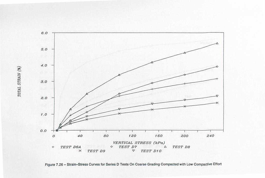
6.0
5.0
~ 4.0
'--
2S ~ 3.0 ~
~
~ c e-..
2.0
1.0
0.0
o 40 BO 120 160 200 240
VERTICAL STRESS (kPa) + TEST D6A <> TEST D7 6. TEST DB
X TEST D9 'V TEST D10
Figure 7.26 - Strain-Stress Curves for Series 0 Tests On Coarse Grading Compacted with Low Compactive Effort

1.2
1.1
1.0
0.9
~ '-
0.8
:s 0.7
~ 0.6 ~
'-4 ~ 0.5
~ 0.4
0.3
0.2
O. f
0.0
0 40 80
+ TEST D11 A TEST D13
120 160
VERTICAL STRESS (kPa) o TEST D12 x TEST D14
Medium
200 240
Figure 7.27 - Strain-Stress Curves for Series 0 Tests On Fine and Medium Gradings

~ r.'l S;
~ ~ ~ til
~ u ~ "'C
~ ~ til .... ~ e
~ ~ ~ CI)
~ ... CI)
~ u ... "'C
~ ... CI)
~ e
2. 0
1.9
1.8
1.7
1. 6
1.S
1.4 1. 3 1.2 1. 1 1.0
0. 9
0.8
0.7
0.6
O.S
0.4
0.3
0.2
0. 1
0.0
0.0 2.0 4.0 LO 8.0
FREE rATER CONTENT (") 0 10kPc. + 2SkPG 0 50kPc.
lJ. 100kPc. x 1 SOkPG V 2S0kJ'a
(a) Usual Compactive Effort
B. O
v 5.0
4.0
3. 0
2.0
1.0
0.0
0.0 2.0 4.0 1..0 B.O
FREE rATER CONTENT (,,) 0 10kPG + 2SkPG 0 SOkPc.
lJ. tOOkPc. X 1S0kPG V 2S01:Pa
(b) Low Compactive Effort
Figure 7.28 - Effect of Free Water Content on Compressiblity of Coarse Grading from Series 0 Tests
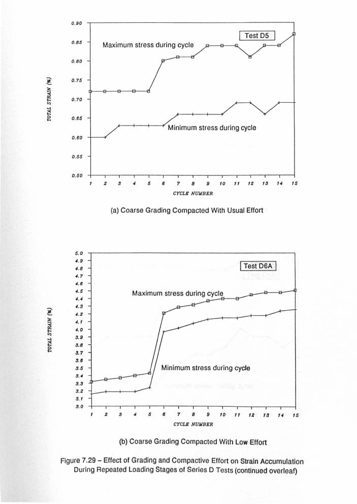
~
~ ... r.,
~ e
""' !.
~ ... r.,
~ e
0.90
0.85 Maximum stress during cycle
0.80
0.75
0.70
0.65
Minimum stress during cycle 0. 60
0.55
0.50
2 3 4 5 8 7 8 9 10 11 12 13 14 15
CYCLE NUMBER
(a) Coarse Grading Compacted With Usual Effort
5.0
4. 9
4. 8 I Test OSA I 4.7
4. 6
4.5
4.4 Maximum stress during cycle
--Ef---e-
4.3
4.2
4.1
4.0
3. 9
3.8
3.7
3. 8
3.5 Minimum stress during cycle 3.4
3.3
3.2
3. 1
3. 0
2 3 4 5 8 7 8 9 10 11 IZ 13 14 15
CYCLE NUMBER
(b) Coarse Grading Compacted With Low Effort
Figure 7.29 - Effect of Grading and Compactive Effort on Strain Accumulation During Repeated Loading Stages of Series 0 Tests (continued overleaf)
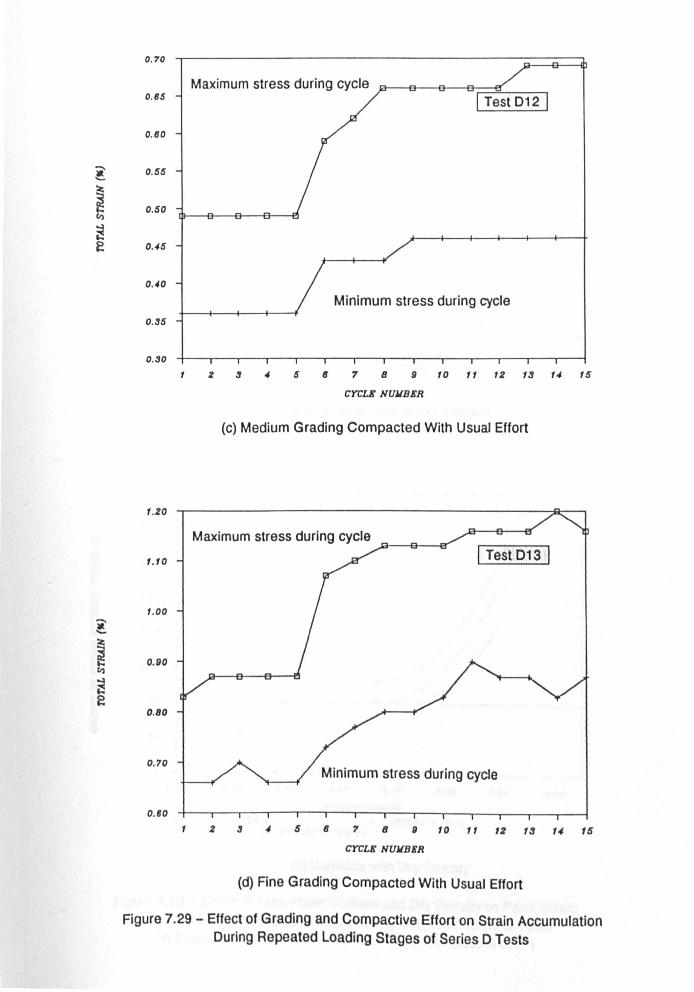
ii' '-
~ (I)
~ e
0.70
Maximum stress during cycle 0.65 I Test 012 I 0.60
0.55
0.50
0.45
0.40
Minimum stress during cycle
0.35
0.30
2 3 4 5 6 7 8 9 10 11 12 13 14 15
CYCLE NUMBER
(c) Medium Grading Compacted With Usual Effort
1.20
1.10
Maximum stress during cycle ...9-- 6-----t:r I Test 013 I
1.00
0.90
0.80
0.70 Minimum stress during cycle
0. 60
2 3 4 5 6 7 8 9 10 11 12 13 14 15
CYCLE NUMBER
(d) Fine Grading Compacted With Usual Effort
Figure 7.29 - Effect of Grading and Compactive Effort on Strain Accumulation During Repeated Loading Stages of Series 0 Tests

~
~ "I
~ ~ ~ ~ ~
~ ... "I
~
I
~ "I
~ );. t)
~ ~
~ ti is
I
0.30
0.25
0.20
0.15
0.10
0. 05
+
0.00
-0.05
- 0. 10
0.0 2.0 4.0 La 8.0
FREE !rAfER CONTENT ("J o CYCLES I fO 4 + CYr:l.ES 5 TO II
o CYCLES" 1'0 14
(a) Variation with Free Water Content
0.30
0.25
0.20
0.15
0.10
0.05
0.00
- 0.05
- 0. 10
2 .00 2 .04 2.08 L1Z Z. 1I 2.20 L24 2 .Z8
DRT WfSITT (X,/a3) o CYCLES I ro 4 + CYCLZS 5 1'0 II
o Crr:LItS 11 TO 14
(b) Variation with Dry Density
Figure 7.30 - Effect of Free Water Content and Ory Density on Peak Strain Accumulation During Repeated Loading Stages of Series D Tests
on Coarse Grading Compacted With Usual Compactive Effort

~ r"
~ >00 ~
~ t fil
~ t; ~ ~
~
---~ 9 ~ ~
~ ~ t; ~
I
0.30
0.25
0.20
0. 15
0. 10
0.05
0.00
- 0.05
- O. tO
0 .30
0.25
0.20
0. 15
0. 10
0.05
0.00
-0.05
- 0. 10
0.0
+ +
<>
2.0 4.0
FREE FATER CONTENT (,,) o CYCLES t TO -4 + CYCLES 5 TO 9
<> CYCLES t1 TO 14
(a) Variation with Free Water Content
1. '10 t .80 1.90
DRY DrNSITY (tg/""'J o CYCLES 1 TO 4 + CYCLES 5 TO 9
<> CYCLES 1 1 TO 14
+
2.00
(b) Variation with Dry Density
6.0
2. 10
Figure 7.31 - Effect of Free Water Content and Dry Density on Peak Strain Accumulation During Repeated Loading Stages of Series D Tests
on Coarse Grading Compacted With Low Compactive Effort

CHAPTER 8
DISCUSSION OF RESULTS AND COMPARISON WITH OTHER WORK
This chapter commences with a discussion of the performance of the new
consolidation cell used for Series A and B, before comparisons and
conclusions regarding the behaviour observed in all tests are drawn.
Where relevant comparisons are made with previous experimental and
theoretical work.
8.1 Performance of New Consolidation Cell
In-service performance of the new consolidation cell was good and
deviations from that anticipated only occurred with the load cells. The
two deviations are discussed below.
8 . 1 . 1 Load Cell Response Characteristics
A typical response of the load cells to a stress increment was presented
previously as Figure 7.1. This figure shows that a non-uniform stress
distribution was applied to the specimen , and Figure 8.1 shows that the
relative difference in the maximum and minimum load cell stresses
decreases as the mean total stress increases . This stress
non-uniformity may be caused by the design of the cell, and/or the
manufacture of the cells, and/or compacted stiffness non-uniformity
within the specimen.
The first could result from the load cells being constrained by the top
platen design to descend in a plane orthogonal to the cell body wall
until contact with the slightly inclined surface of the specimen.
However, the low stiffness of the specimen at low stresses, shown by the
strain-stress curves presented earlier, suggests that non-uniform
compression and particle re-orientation across the specimen should
quickly reduce any initial eccentricity. Figure 8.2 plots the ratio of
- 75 -

the peak difference in measured load cell stress to the ambient mean
stress against the initial specimen tilt measured after compaction of
the specimen. If the design is at fault one would expect the stress
variation to increase with tilt. This is clearly not the case.
The possibility of a manufacturing induced feature centres on
dimensional variations in the load cell bodies and/or recesses in the
top platens predisposing a particular load cell to contact with the soil
first. Examination of the frequency at which each load cell recorded
the maximum or minimum load revealed an apparently random variation, and
physical measurement of the load cell bodies and recesses showed no
significant variations. Taken together, these observations suggest that
the manufacturing was not at fault, although random variations in the
orientation of the cells to the soil , and random insertion of the load
cells into the recesses, could partially mask any such pre-disposition.
Hence, the third and most likely explanation is stiffness non-uniformity
present within the particulate mass despite the attempt to apply a
uniform compactive effort across the whole surface area of the soil.
Random variations in particle arrangements would be expected to cause
small stiffness variations and previous research by Brady and Kirk
(1990) has implied such non-uniformity. In their work, variations in
deflections of more than 20% of the mean deflection were measured at
circumferential quarter points on a specimen subjected to a point load
via a top platen free to tilt within limits imposed by the apparatus
dimensions. Larger variations in stresses may have been necessary to
cause these measured changes, but variations of up to 100% would be
needed to give similar results to those found in the current work.
Based on the above, it is cons idered that at least part, and probably
the majority, of the observed differ ences in load cell output are due to
stiffness non-uniformity. The r emainder must be attributed to the
apparatus and test procedures although the causes are unclear.
- 76 -

8.1.2 Load Cell Stability
Comparison of the zero outputs from each load cell were made at the
start and finish of each test. in order to verify that the bending
stress imposed on the load cells by the non-uniform stress distribution
was not having an undue effect. These comparisons showed that a small
but significant zero-drift (typically less than 0.5 kPa) sometimes
occurred. Such variations were inconsistent between tests and could not
be related to atmospheric changes or any other variable. In view of
this inconsistency. it was not possible to ascertain when the drifts
occurred. and it was decided to use the mean zero output for each test
for all stress calculations. Therefore. although the calibrated
accuracy of the load cells in pure axial compression is typically 0.1
kPa. it is considered that the average stresses recorded in service
should be taken to be accurate to 0.5 kPa only. The calibration factors
are considered to be unaffected by the non-uniformity in stress
distribution.
8.2 Water Volume Changes Due to Total Stress Changes
Test Series A employed water drained conditions in order to investigate
the magnitude of water volumetric strains induced in coarse unsaturated
soils due to an applied total stress change. Figure 8.3 shows a typical
graph of water volume change against time for one stage of a test. with
a load increment applied at time zero. It is apparent that very small
volume changes are involved. and that the direction of flow is
apparently inconsistent with what would be expected to occur as a result
of consolidation. Comparison of the results with the measured variation
of the base pore water pressure presented as Figure 8.3(b) shows that
the curves are synchronised. implying that small changes in base pore
water pressure lead to correspondingly small changes in volume.
subsequent calculations assuming the compressibility of water with 10%
air (at 100 kPa) mixed in is 0.001 m2/kN (Fredlund. 1976) and using the
approximately known volume of the base chamber of the consolidation
cell. showed that these observed changes were about 2 orders of
- 77 -

magnitude greater than expected based on the small fluctuations in water
pressure. This suggests the soil is sensitive to small changes in
suction, and that unless large water volume changes result from soil
fabric changes then the small fluctuations in regulated pressure will
mask these changes.
In addition to the above effect, it was noted that apparent water volume
changes of less than 1 cm3 occurred at a rate of between 0.01 and 0.05
cm3 fhr during many tests, and that these changes were always out of the
cell even if the total applied stress decreased during that stage. A
reasonable degree of correlation was found between these measurements
and those of the diffused air flushed out of the consolidation cell
periodically, and the rates of movement were of the same order of
magnitude as those for air diffusion recorded by Fredlund (1973). It
thus appears that air diffusion also masked any "real" water volume
changes.
As a result of the above two factors, the possibility of small leakages,
and the absence of any large (>3 cm3 ) volume changes during any test it
was concluded that water volume changes as a result of total stress
changes were not a phenomenon of any great significance in this soil
provided the soil was initially at equilibrium. Hence results for
Series A and B should be very similar. Further it was reluctantly
accepted that the current apparatus could not be used for reliable
measurement of small volume changes «3 cm3 ) despite the nominal
accuracy of the volume change units unless stringent tests were
performed to quantify diffusion and leakages.
8.3 Suction Determinations
8.3.1 Repeatability of Data
Figures 7.6 and 7.7 summarised the suction measurements made during
series A and B. The graphs showed a large degree of scatter for the
coarse grading, but gave good repeatability for the fine grading.
- 78 -

This difference in repeatability is attributed to increasingly random
variations in the soil fabric formed at the ends of the different
specimens as the coarseness of the soil increases. By the nature of the
measurement system, the equilibrium suction is that which results
uniformly at each particle-ceramic contact following redistribution of
water via the saturated ceramic. Figure 8.4(a) shows conceptually that
the initial compaction induced suctions between the ceramic and
particles 1 and 2 respectively would be different. The pore pressure
behind the ceramic would have to be different at each point of contact
for this state to be maintained and hence water flows between the
particles and ceramic until an equilibrium measured pore water pressure,
uwms is achieved and the suctions at particles 1 and 2 are the same
(Figure 8.4b). A preponderence of coarse particles in contact with the
ceramic would effectively reduce the equilibrium suction as the effect
of any small flow of water to/from them would affect the resultant
suction less than if the same small flow affected a smaller particle.
In a well graded soil the number of significantly different particle
size distributions at the ceramic interface is greater than for a more
uniform grading.
The importance of the scatter in the measured suctions must not be
overstated though. As shown in Figure 8.4b the local redistribution
of water at the ends of the specimens enforced by the measurement system
is unlikely to affect the internal suction equilibrium state unless the
suctions are continuous through the particles themselves. This is
unlikely as the free availability of water would destroy any particle
absorption suction. Given the localised nature of the internal suctions
then, and the increased probability of particular structural
arrangements of grains repeating as the soil volume increases, it may be
deduced that a scatter of suction measurements at any particular
location (in this case the ends) would not represent the scatter of the
average suction condition for the whole specimen. The true reflection
of field conditions in the laboratory thus requires an adequate soil
volume to be tested, a point which is covered in section 8.4.
- 79 -
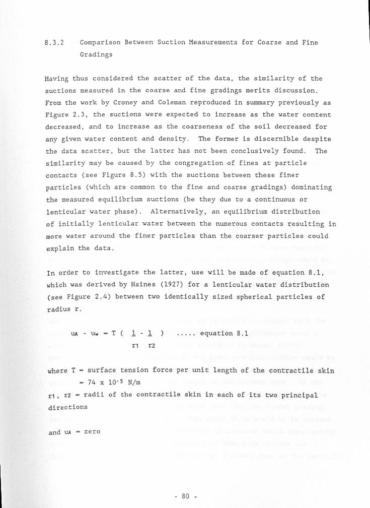
8.3.2 Comparison Between Suction Measurements for Coarse and Fine
Gradings
Having thus considered the scatter of the data, the similarity of the
suctions measured in the coarse and fine gradings merits discussion.
From the work by Croney and Coleman reproduced in summary previously as
Figure 2.3, the suctions were expected to increase as the water content
decreased, and to increase as the coarseness of the soil decreased for
any given water content and density. The former is discernible despite
the data sca tter, but the latter has not been conclusively found. The
similarity may be caused by the congregation of fines at particle
contacts (see Figure 8.5) with the suctions between these finer
particles (which are common to the fine and coarse gradings) dominating
the measured equilibrium suctions (be they due to a continuous or
lenticular water phase). Alternatively, an equilibrium distribution
of initially lenticular water between the numerous contacts resulting in
more water around the finer particles than the coarser particles could
explain the data.
In order to investigate the latter, use will be made of equation 8.1,
which was derived by Haines (1927) for a lenticular water distribution
(see Figure 2.4) between two identically sized spherical particles of
radius r.
UA - UW - T ( 1 - 1 ) r1 r2
..... equation 8.1
where T - surface tension force per unit length of the contractile skin
- 74 x 10- 5 Njm
r1, r2 - radii of the contractile skin in each of its two principal
directions
and UA - zero
- 80 -

From geometry, rl - r2 2/2 (r-r2), and hence equation 8-1 reduces to:
UA - Uw - T (2r-3r2) equation 8.2
r2 2
Table 8.1 presents the suctions calculated using the above equation for
particles ranging in size from 0.2 mm to 20 mm, with r/r2 ratios of 2
and 5. As may be seen, a water distribution resulting in lower r/r2
values for the finer particles (ie proportionately more water at the
fine particle contacts) could explain the similarity in suctions for the
fine and coarse gradings. ~ithin a low degree of saturation particulate
mass, the lenticular water distribution pattern will be a random one
initiated by the degree of mixing and compaction applied, and there
exists no reliable method to estimate the relative influence of the
coarse and fine particles at present. At the measurement points
however, a continuous water phase is enforced and the initially random
lenticular water distributions would redistribute to increase the
proportion of water at high suction points of contact, which would be
more likely to involve fine particles. Hence the conditions required
for similar measured suctions in the fine and coarse gradings would be
approached at least, to an extent dependent upon the range and frequency
of particle sizes in contact with the ceramic, and the initial water
content.
The prediction of the range of sizes of particles in contact with the
ceramic, and their relative frequencies, could be attempted using a
statistical approach similar to that advocated by Marsal (1973).
However, the standard deviations of any predicted distribution would be
expected to be relatively large, and the accuracy of such an attempt
could not be assessed within the limits of the current work. In the
absence of a reliable analytical technique but based in part upon the
work of Marsal (1973), it is considered that, for the coarse grading,
few particles of diameter greater than about 20 mm would be in contact
with the ceramic, but that the frequency of contacts would then rapidly
increase as the particle size decreases to some peak, before the
frequency would decrease once again but at a slower rate as the particle
- 81 -

size decreases further still and these finest particles "stick" on the
surface of the coarser particles . The frequency peak may correspond to
a particle size in the range 0.5 mm to 5 mm, given the flattening of the
grading curve. For the fine grading, a flatter frequency distribution
would be expected with a peak corresponding to a particle size of less
than 0.5 mm probably. Figure 8.6 idealises this largely intuitive
picture, which it must be stressed is not based upon experimental data.
The effect of the initial water content on the suctions needs to be
considered within this intuitive framework. Based on Tables 6.2 and
6.3, Table 8.2 compares the initial compacted state of the fine and
coarse gradings for the given water contents. As may be seen, the
coarse grading achieves lower void ratios and air void ratios, but
higher degrees of saturation. The latter is of primary importance, and
it states that proportionately more water is present in the total void
spaces of the coarse grading.
For the "average" r/r2 ratio to decrease between the coarse and fine
gradings, the degree of saturation should decrease at a slower rate than
the decrease in the "average" particle size. This "average" particle
size should reflect the range and frequency of particle contacts, which
intuitively may fall from maybe 2 mm (coarse grading) to 0.5 mm (fine
grading). In contrast, the degree of saturation only increased by
between 100% and 150% from the fine to coarse gradings suggesting that,
if anything, the "average" r/r2 ratio increased from the coarse to fine
gradings. The tendency for a small redistribution of water via the
ceramic would mitigate this increase as previously noted, but not
sufficiently for the similarity in suction measurements between the fine
and coarse gradings to be due wholly to the equilibrium water
distribution pattern. The coarser particles must have a significant
influence, in order to account for some of this suction scatter, but the
similarity is likely to be caused predominantly by the congregation of
fines at the ceramic face.
- 82 -

8.3.3 Vertical Suction-Water Content Profile
The suction-water content curves for the top and base of the specimens
shown in Figures 7.6 and 7.7 are not separated by a constant suction
value equal to -h ~w (where h - vertical separation) as is often assumed
in highway design based on simple capillary theory. Rather, the
difference is considerably greater, implying the water phase is not
continuous through the specimens, or the simple capillary theory is
erroneous, or the suctions measured incorporate also an element of the
aggregate suction characteristics due to its incomplete saturation.
Fredlund and Rahardjo (1987) present matrix suction values for a glacial
till at three depths up to 0 . 76 m below surface (see Figure 8.7) which
shows a similar non-linear variation of suction, which suggests the
capillary theory is incorrect as the other explanations would not hold
true for this predominantly clay soil. Consequently it is considered
that care should be taken in applying the simple capillary theory until
further research has been conducted.
8.4 Comparison of Compressibility Results from Series A, Band D
8.4 .1 Repeatability of Data
Similar forms of strain-stress curves were obtained for all tests, and
inspection of figures 7.14 , 7.15 and 7.28 allows the repeatability of
the data to be quickly assessed by examining the data for deviations
from the average.
Considering the series A and B tests on the coarse grading first (Figure
7 . 14) tests B6 and B7 at a free water content of 1.1% show excellent
agreement, and good agreement exists between tests A7 and A8 (4.9% and
5.2% free water content), The agreement between A2 and B3 (3 . 9% and
4.1%) is less good at low stresses, but improves as the applied stress
increases. The only clear exceptions to the good repeatability
otherwise obtained is test B5 ( free water content 2.3%), which exhibits
very low stiffness at low stresses. The cause of this discrepancy is
unclear, specimen BS not being unusual in any other manner.
- 83 -

The series D tests on the coarse grading (Figure 7.28) showed excellent
repeatability when subject to the "standard" compactive effort (tests Dl
and Ds), and reasonably good repeatability when lightly compacted (tests
D7 and D8) despite the large strains involved and the greater relative
influences of the soil fabric on the stiffness of such lightly compacted
specimens.
The results for the fine grading in Figure 7.15 show excellent
repeatability when similar specimens are compared (tests AS and AlO,
free water content 4.1%). Further, as shown by comparison of these two
tests with the slightly under-compacted test Al (free water content
4.2%; void ratio 0.48 compared to 0.42 and 0.41 for AS and AlO), small
changes in compactive effort do not result in highly significant changes
in compressibility of this grading.
From the above comments, it is considered good repeatability was
achieved within each piece of apparatus and for each grading. This
repeatability supports the assertion made earlier that series A and B
tests should be comparable as negligible water drainage occurred during
series A tests (section 8.2), and that the scatter of measured suctions
would not significantly affect the compressibility as the measured and
"average" internal suction conditions would have different standard
deviations (section 8.3.1). Further the judgement to use a slightly
smaller than usual height to maximum particle size ratio for the new
consolidation cell is justified.
8.4.2 Effect of Compaction Water Content and Dry Density on
Compressibility of the Coarse Grading for Constant Compactive
Effort
Having established the repeatability of the data, the measured variation
of compressibility may be confidently discussed. Figure 7.14 for the
series A and B tests shows a peak in compressibility at a free water
content of about 3.0%, with approximately symmetric decreases either
side to the limiting free water contents used of 1.1\ and 5.2%. In
contrast, the initial dry density of the specimens increased
- 84 -

approximately linearly from 1.93 Mg/m3 to 2.20 Mg/ms over the same free
water content range, implying that compressibility is a function of both
the compaction water content and dry density. The compressibility
contours shown do not close up significantly, indicating low stiffness
at very low stresses and an approximately constant and larger stiffness
at stresses above about 25 kPa.
The results for series D tests at the same compacti~ effort (Figure
7.28a) show a similar trend at equivalent stresses, ~ut with a peak at
a free water content of about 2%, a minimum at about 3.5%, and a second
much larger increase in the compressibility at water contents above this
value to a free water content of 7.6%. The low peak at a water content
of 2% disappears progressively as the stress level increases, and the
compressibility contours show only marginal closing 'Up as the stress
level increases beyond a stress of about 25 kPa.
The similar behaviour noted in both pieces of apparatus is attributed to
the suction stresses within the soil mass, and possuly an increased
intergranular friction coefficient at very low water contents. Starting
at a free water content of about 1%, the high localised suctions at
particle contacts with a congregation of fines, together with some
possibly dry surface contact points increasing the aTerage friction
coefficient between the particles, are believed to counteract the low
dry density of the mass sufficiently for the soil to have a low
compressibility. As the compaction water content increases, the
localised suction stresses decrease the internal stability of the mass
at a greater rate than the increasing dry density tends to increase this
stability. Hence the compressibility increases. As t he water content
increases further still beyond a critical value of becween 2% and 3%,
which approximately corresponds to the distinct flattening of the
suction-water content relation shown in Figures 7.6 a and 7.7, the
increasing dry density increasingly dominates and the compressibility
decreases once more.
- 85 -

However, at a free water content of about 4% to 5%, the compressibility
once more increases, but this time quite rapidly, despite the water
content being about 1.5% to 2.5% below optimum. It is believed this
increased compressibility is a function of the formation of a near
saturated layer at the base of the material, and the inducement of small
reductions in effective stress in the layer. The excess pore pressures
would be dissipated internally and upwards due to the low permeability
of the base ceramics. Evidence for the progressive formation of this
saturated layer was presented previously as Figure 7.11, which plotted
the variations of water content between the top and bottom of the
specimen, and showed an increased gradient above a free water content of
about 4%.
The above explanation would apply in particular at low vertical
stresses. As the stress level increases though, the influences of the
suctions would be expected to decrease progressively, whilst the
influence of the near saturated layer would not be greatly affected.
This behaviour pattern has been shown by the series D tests at stresses
in excess of 100 kPa, and supports the physical mechanisms suggested.
8.4.3 Effect of Compactive Effort on Compressibility of the Coarse
Grading
The results of the series D tests employing a low compactive effort were
presented in terms of compressibility in Figure 7.28 b. Yith the
exception of the reducing influence of suction stresses at higher stress
levels the same behavioural trends noted and explained above for the
higher compactive effort have been found. Although the range of water
contents used precluded the large increase in compressibility beyond a
free water content of 5.4% from being proven the similarity in trends
does appear to include a minimum at a free water content of about 5%.
The absence of the reducing influence of the suctions may be attributed
to the higher suctions likely to be present within these specimens due
to the lower degrees of saturation. Additionally, the lower number of
interparticle contacts will serve to reduce the influence of any
increased coefficient of friction at low water contents.
- 86 -

The variation of compactive effort may also be used to identify the
relative influences of the dry density and free water content
individually. Considering the series A and B tests, comparison of tests
B2 and B4 with tests A6 and Bl, which all have similar dry densities but
different water contents, it is apparent that the compressibilities of
the former (free water contents of 4.6% and 4.1%) are greater than the
latter (2.0% and 1.6%) due to the lower suctions. Similarly, specimen
B3 (free water content 4.1%) was less compressible than specimen B4
(4.1%) due to its higher dry density. Similar observations could be
made from the series D tests.
8 .4.4 Effect of Grading on Compressibility
Comparison of the series A and B test results for the coarse and fine
gradings (Figures 7.14 and 7.15) shows that the compressibility trends
of both are similar, with peak axial strains of about 1.5% and 1.7%
respectively at a stress of 50 kPa. This similarity exists despite the
higher dry density, relative density and broader grading of the coarse
grading, all of which would be expected to decrease the compressibility
of a dry material. It is suggested that the higher suction stresses
developed internally within the fine grading may explain the results by
virtue of their stiffening influence.
Similarly, evidence for the influence of the suctions on the fine and
medium gradings comes from series D tests D6A (coarse grading, dry) and
D11 (medium grading, dry) and D1l (medium grading, free water content
2.8%), and t ests 08 (coarse grading, free water content 2.9%) and 014
(fine gradings, free water water content 4.3%), which were compacted to
dry densities of about 1.86 Mg/m3 and 1.77 Mg/m3, respectively. The
compressibility of the coarse grading was greatest in each case.
Further, the higher water content specimen of each pair of tests on the
fine and medium gradings, exhibited a higher compressibility despite the
higher dry density.
- 87 -

8.4.5 Comparison of Stress and Strain Controlled Compression Tests
The similarity of the compressibility variations between the stress
controlled (series A and B) and strain controlled (series D) compression
tests has been noted above in section 8.4.3 . The correspondence of the
two types of test in terms of the magnitude of strains at any given
stress level may be verified if the "immediate" and time dependent
strain components of the series A and B tests can be separated. This
has been attempted using the incremental stress-strain curves for each
stage of every test, as typified by Figure 7.3. The incremental
immediate strain component has been taken to be equal to the strain
corresponding to the marked change in gradient of the graph, as the
stress increment was usually applied within 2 minutes. In some cases,
the change in gradient was less clear as the stress increment was
applied over a period of up to 5 minutes, and the immediate strain was
estimated by fitting two straight lines through the data as shown in
Figure 8.8
Figures 8.9 and 8.10 present the immediate strain-stress curves, Table
8.3 summarises the immediate compressibility data, and Figure 8.11
represents the compressibility data graphically. Examination of the
curves shows that repeatable compressibility results were obtained
within the same limits noted above for the total strain-stress curves.
Comparison of the series 0 data with the "immediate" compressibility
data obtained from series A and B (Figure 8.11 shows that although the
"immediate" strains from series A and B have been significantly reduced
compared with the total strains at any given stress level, they are
still approximately twice as large as the strains recorded during the
strain controlled tests of series D. This is attributed to the time
scale associated with the "immediate" strains, which was between 2 and 5
minutes. For example, points 1 to 6 on Figure 8.8 (Figure 7.3
reproduced and annotated) chart an apparently approximate linear rate of
strain development due to what is clearly a non-linear rate of stress
application when it is appreciated that each of these data points was
taken at 10 second intervals. The "immediate" strain component equals
- 88 -

0.08% (1.60% to 1.68%) when estimated in accordance with the method
noted above, but this component includes an element of time dependent
movement as shown by the strain between points 3 and 4,and 5 and 6.
A better method of estimating the "immediate" component would have been
to take the initial gradient of the incremental stress-strain curve and
extrapolate it to the intended final stress level, if constant stress
increments had been applied at a very similar rate. This not being the
case generally, it may be approximiately applied to Figure 8.8 though .
If so applied the "immediate" strain is reduced by about 30%, and data
collection at a rate in excess of every 10 seconds would probably reduce
this value further still. Hence the initial apparent discrepancy between
the two types of test is explainable and the data as a whole presents a
consistent picture.
8.4.6 Magnitude of Immediate and Time Dependent Strain Components
The above discussion centred essentially on the separation of the
"instantaneous" strains that occur as soon as a stress increment is
instantly applied, from the "immediate" strains that occur over the
several minutes when the stress increment is being applied. From the
current data, the latter is made up of about 50% of the "instantaneous"
strains that would have occurred if the full increment were applied
instantly, and 50% of short-term time dependent strains. When analysing
a physical problem , it is necessary to know the time scale over which
the material will be stressed, and hence which compressibility relation
to apply. Us ually, only two components are identified, they being the
immediate and time dependent components, but the time scale over which
the "immediate" component i s de termined is often vague. For example,
Brady and Ki r k (1990) state tha t insignificant time dependent strains
were r ecorded i n t heir tests on lime stone aggregate when compacted dry
of optimum . t h is component apparently being taken to start "a few
minutes " after t he l oad increment was applied.
- 89 -

The data obtained from this work has been investigated over three
timsescales:
(i) instant strains, determined from the strain controlled tests
(ii) immediate strains measured as detailed above, over a timescale
of 2 to 5 minutes from stress application
(iii) time dependent strains that occur after the first 2 to 5 minutes
elapsed
The relation between timescales (i) and (ii) has been dealt with above
for the coars e grading, and insufficient data has been obtained for a
similar comparison for the fine and medium gradings. The relation
between timescales (ii) and (iii) is discussed below for the coarse and
fine grading on the basis of the measured ratio of the incremental
immediate strain to the total incremental strain for each stage of the
series A and B tests.
Figure 8.12 plots this ratio against the total stress at the end of each
stage. A large degree of scatter in the data is obvious, but
nevertheless clear and similar trends in the data exist for each
grading. At low stresses, between 70% and 100% of the incremental
strain will be generated immediately, but this percentage gradually
decreases to between about 30% and 80%, as the applied stress increases
to 100 kPa. This relationship, which clearly identifies a time
dependent component when the material is tested dry of optimum, is
contrary to the findings of Brady and Kirk (1990) noted above. However,
if "immediate" were taken to include the first 30 minutes following
stress application and insignificant time dependent strains equates to
less than 10% of the total strain, then a similar conclusion could be
drawn from this data. This order of straining is not considered
insignificant by the author though.
- 90 -

8.5 Comparison of Compressibility Results with those of Brady and Kirk
(1990)
Subsequent to the completion of the test programme reported in this
thesis, Brady and Kirk (1990) reported the results of incremental
loading tests on a limestone aggregate equivalent to the coarse grading
of the current research. No suction measurements were attempted in
their relatively simple work. The effects of water content and
compactive effort were investigated, and to a lesser extent grading
influences.
Brady and Kirk used a 500 mm diameter floating ring oedometer, and
compacted the specimens into the cell in five equal layers. Three
different compactive efforts were used, and the compaction curves (not
presented by Brady and Kirk) are presented as Figures 8.13 to 8.15.
Their research did not attempt to define the optimum water content and
maximum dry density from the actual tests, as revealed by the poor
definition of the curves. Rather, optimum total water content was
determined to be 4.0% from Test 14 of BS1377:l97s, with a maximum dry
density of 2.41 Mg/m3 . This contrasts with the optimum water content of
about 6% to 9% from Figures 8.13 to 8.15, and 7.2% for the coarse·
grading used in the current research. Comparing the compaction curves
with Figure 3.11 shows Brady and Kirk's medium effort is approximately
the same as the 'standard' effort used in the current work.
Brady and Kirk refer to the term compressibility in the title of their
report, but present their conclusions with reference not to this
parameter, but to its inverse, stiffness, as quantified using the
constrained modulus . As shown by graphs 8 . 16 to 8.18, an attempt was
made to relate the measured stiffness to the dry density of the
specimens, but the apparent correlation was only achieved by plotting
the stiffness on a logarithmic scale. Had the data been presented in
terms of compressibility using a graph of the form of Figure 7.28, a
very wide scatter of strains at any given stress level and dry density
would have been apparent. For example, for the stress range 2S kPa to
- 91 -

100 kPa and a dry density of 2.27 Mg/m3, the change in strain between
these stresses for specimens 17 and 23 may be calculated to be 0.29% and
0.56% respectively. In the light of the preceding discussions in
section 8.4, this particular scatter of results becomes more
understandable when it is noted specimens 17 and 23 had total water
contents of 1.1% and 6.1% and were compacted with the same effort.
In order to compare the two sets of data the author's' data has been
reanalysed to obtain the constrained moduli for various stress ranges,
as shown in Table 8.4 . This data has been added to Figure 8.16 and
Figures 8.19 to 8.22 plot the moduli for different stress increments
derived from the various series for the coarse and fine gradings against
total water content. Figure 8.23 to 8.26 plot the same data against the
dry density. The Brady and Kirk data has also been re-analysed to plot
the moduli against total water content and dry density for each of the
three compactive efforts used (see Figures 8.27 to 8.32). Total water
content has been used as the absorption characteristics of the limestone
used by Brady and Kirk are not known.
Examination of the corresponding curves for both sets of data shows that
the few water contents used by Brady and Kirk prevents definitive
conclusions from being drawn, as the large data gaps in the curves
allows alternative "best-fits" to be drawn (eg Figure 8.27).
Additionally, the poor definition of the compaction curves may possibly
reflect poor compaction control as well, with its resultant effect on
the moduli. Despite this, similar relationships between constrained
modulus, and water content and dry density, are discernible for both
sets of corresponding data and plotting the series A data on Figure 8.16
shoWS that similar order of moduli were obtained. Further, the large
scatter in data reported by Brady and Kirk has been considerably reduced
by separating the different compactive efforts out, which reflects the
different form of curve obtained for each of the 3 different compactive
efforts. The curve form varies also with the range of stress level
considered at the higher compactive efforts .
- 92 -

The observations above are believed to be the result of the combined
influence of water content, dry density, and compactive effort on the
soil suctions, the influence of dry density alone on the total strain
potential of a soil, and the influence of the stress level and increment
on the modulus . These various influences may be expressed graphically
as shown in Figure 8.33 which plots in three dimensions the total strain
at any given stress level against total water content and dry density.
The vertical axis was chosen to be strain in order to identify the
influence of stress level more clearly, and because the constrained
modulus may be easily calculated from the graph. The reduction of A E,
to ~~~with increasing stress level results from the reduction in total
strain potential, and the reduction of the ratio of the "average"
suction stress in the soil to the applied stress. At high stresses, AEl
and !:::.'t.,. will reduce to near zero, and may reverse in sign if any
influence of decreasing interparticle friction exceeds the relative
stiffening influences of the suctions. At, and II E3 will also reduce to
near zero, and a more or less unique relation between total strain and
dry density will exist. However, the relationship would be less unique
for the constrained modulus, as it relies upon the change in strain
between two specified stresses.
The above explanation of the scatter in relationship between constrained
modulus and dry density contrasts with that offered by Brady and Kirk.
They recognised the influence of water content, but attributed it
instead to the generation of high pore water pressures during
compaction, which in turn could have caused a layer of fine material to
migrate towards the top of the layer. During loading, the coarser
particles were then conj ec tured to penetrate into the looser fines-rich
layer at the top of the underlying layer. Whilst not rejecting this
mecahnism as being responsible for a small part of the observed
influence of water content at high water contents, it is considered that
the comparable results from the research herein, which employed a single
compaction layer only, largely invalidates their suggestion. Further,
they only report evidence of such a fines-rich layer in sections of the
- 93 -

wettest specimens. This suggests that the large increase in
compressibility as the water content passes optimum could be partially
due to this mechanism, but at lower water contents when less water is
available to actually generate positive pore water pressures the
mechanism is not valid and suctions must be involved.
8.6 Inundation Test Results
8.6.1 Relationship Between Inundation Strains and Soil Suctions
The preceding discussions suggested that the soil suctions are a
significant influence on the behaviour of coarse grained soils. It is
suggested also that the destruction of suction during inundation is a
major paramete r affecting the "inundation strains" that occur at a
constant vertica l (see Figure 7 . 17) stress. The other possible factors
identifi ed in s ection 2.2, namely reduction of interparticle friction,
washing of fines and aggregate softening, are considered to be
relatively unimportant for the following reasons:
(i) friction loss: due to the absorption characteristics of the
limestone, only specimens with a very low water content and hence
relatively dry contact points between particles would be likely to
compress further after wetting.
(ii) washing of fines: as described in section 2.2, only the loss of
the fines around particle contacts would be expected to cause
straining , and this would be due to the loss of the suction
i nduced component of the interparticle forces. Evidence for the
presence of s uch fines has been discussed already in section
8.3. 2.
(iii) aggregate softeni ng and loss of stiffness: a medium to long term
mechanism such as t h is would b e unable to explain the short term
movements during the tests .
- 94 -

The possibility of a relationship between the inundation induced strains
and the measured suction has been investigated, and Figure 8.34 shows
the resultant graph. The reasonable correlation for the top and bottom
of the specimens supports the hypothesis, and the form of the curves is
consistent with the hypothesis that a maximum inundation strain exists.
The ambient stress level appears to have a negligible effect within the
limits of the current work.
The relationship between the relatively immediate straining and
destruction of suctions implies also that the suctions are between
different particles, and not in the particle interstices, as assumed
earlier.
8.6.2 Relationship Between Inundation Strains and Other Parameters
Previous workers have attempted to relate the inundation strains to the
void ratio (Egretti and Singh, 1988), the air void ratio (Charles, 1984)
or the degree of saturation (Pigeon, 1969), all of which are more
readily determined than the soil suctions. Figures 8.35 (a), (b) and
(c) plot the current data against each of these parameters. As may be
seen, the void ratio is least sensitive which is as expected given its
indirect relationship to the soil suction via the compactive effort and
compaction water content, but good correlations exist for the air void
ratio and degree of saturation. These parameters may thus be inferred
to be directly related to the soil suctions, as is confirmed by Figures
8.36 (a) and (b). It is considered the good correlation could have been
expected as each of these paramaters reflects the three parameters
identified in section 8.5 above, namely water content, dry density and
compactive effort.
From the above, it is suggested that practical relationships between
inundation strains and either the air void ratio or the degree of
saturation may be developed. Recent work by Thompson, Holden and Yilmaz
(1990 ) towards this aim is presented as Figure 8.37, with the authors
data annotated upon it. The current data is similar to that for rock
- 95 -

fragments reported by Charles (1984), but the laboratory data appears to
be several orders of magnitude smaller than observed field measurements.
Insufficient information is available at present to explain this
anomaly, but the affects of side friction and field density/water
content variations may be the dominant causes.
8 . 6.3 Combined Effect of Total Stress Changes and Inundation
Figure 8.38 summarises the changes in dry density and water content for
the specimens due to both monotonic loading and inundation . This graph
shows that for any given initial dry density, an approximately unique
final state will be reached irrespective of the stress path followed. This
implies that the discontinuity of the state surface shown in Figure 2.5
leads to a second unique state surface in the saturated e - (C1 - uA)
plane for soils which have been completely inundated (see Figure 8.39).
For this particular soil, this state surface appears to be horizontal over
the stress range tested (50 to 125 kPa) as the ambient stress during
inundation did not noticeably affect the observed strain . It would
normally be expected for the curve to be concave upwards over a large
stress range, with the highest final voids ratio at the lowest total
stress. For different soils and/or different initial fabric (dry
density), a diffe r ent final fabric would result.
Similar results for a mudstone have previously been communicated to the
author by Tanaka (1988) during discussions, but further information is
not available a t present.
8.7 Repea t ed Load Behaviour
Although not a primary aim of the r esearch, information on the first
unloadi ng characteris t ics wer e obtained from the series A and B tests,
and inf ormation on repeated loading was obtained from the series D
tests.
- 96 -

The first unloading curves for each of the series A and B tests
exhibited very similar gradients within each series, as shown by Figure
8.40 for the series A data. When the constrained moduli between each
stress decrement are plotted against the ambient stress before the next
decrement, as shown by Figures 8.41 (a) and (b) for series A and B
respectively, the curves fall in a fairly narrow linear band whose
gradient is slightly greater for the unsaturated specimens (series A)
than the near saturated specimens (series B after inundation) . This
implies the unsaturated specimens are slightly stiffer for any given
stress level, an observation which is attributed to the suction,
although a graded influence within the unsaturated specimens was not
clear. The tests on the fine grading showed a similar trend, but were
stiffer than the series A tests on the coarse grading. From 100 kPa to
25 kPa, the coarse grading strain decreased by about 0.13%, and the fine
grading decreased by about 0.10%.
The repeated load data from series D showed similar behaviour during the
first and subsequent load cycles for each of the gradings tested, but
with different moduli. The previously presented Figures 7.29 to 7.31
summarise the repeated strain data. As may be seen from Figure 7.29,
each of the 4 groups of tests (coarse grading with heavy and light
compaction, and medium and fine gradings) exhibited a different typical
response . The heavily compacted coarse graded specimens showed only
small increases of strain with cycling dependent upon the compaction
water content and density as shown in Figure 7.30. This figure plots
the difference in strain after land 4 cycles, at a peak stress of 125
kPa against the free water content (7.30a) and dry density (7.30b). The
form of the curve in Figure 7.30a is very similar to that found for
compress ibility and is attributed to the same reason, that is the
interaction between suctions and dry density. Previous workers (eg
Hicks, 1970) found also that the susceptibility to strain accumulation
increases as the degree of saturation increases. Figure 7.30b confirms
that a higher density does not necessarily mean better performance of
the material under load.
- 97 -

Figure 7.31 presents similar curves for the less highly compacted coarse
graded specimens. Strain accumulation continued to occur with cycling
for all tests, without reducing greatly in rate. No clear trends with
water content or dry density are discernible for this compacted state,
although it is possible that the susceptibility to strain accumulation
increases as the density decreases. If this is correct, it suggests the
dry density has an overriding influence if low compaction is applied
despite the suctions. This concurs with previous expectations prior to
the testing, but is contrary to the suction influence on monotonic
behaviour noted earlier. Further work is needed on this aspect before
conclusions may be drawn.
The two tests on the medium grading showed a similar behaviour to the
heavily compacted coarse graded specimens, that is little or no strain
accumulation with load cycling, and the fine grading exhibited some
increase but at a noticeably decreasing rate. No conclusions may be
drawn regarding the influence of water content or dry density, but it is
noted that both gradings were compacted with the same effort as the
heavily compacted coarse specimen.
The effect of increasing the strain rate had no apparent influence on
behaviour. This concurs with more comprehensive resilient testing
reported by Boyce (1976), who found frequency had no influence in the
range 0.1 Hz to 20 Hz.
8.8 Effect of Stress Level on Compressibility Behaviour
The preceding discussions have focussed upon the observed behaviour at
the mainly low stresses applied during the current research. As the
stress level increases, the suction effects would be expected to
progressively decrease in importance. The rate of decrease of the
suction influence with stress level would be dependent upon the
"average" suction, and hence upon the grading and the compactive effort.
- 98 -

Such a decrease was observed in the series D test results for the coarse
grading compacted with the usual effort, as remarked upon in section
8.4.2. Above a vertical stress of about 100 kPa, the peak in the
compressibility curve shown in Figure 7.28a disappears. This
corresponds to a critical vertical stress to measured top suction ratio
of between 3.3 and 10 for a free water content of between 1% and 4%.
In contrast, use of a lower compactive effort and hence lower dry
densities showed that the probable higher suctions for a given free
water content did not affect the measured compressibility at low
stresses (Figure 7.28b). However, above a stress of about 100 kPa a
peak in the compressibility relation is noticeable. This is interpreted
as meaning sufficient densification had occurred for the number of
contact points within the soil mass at which soil suctions were present
to reach a critical level, such that the local stabilising influence of
the suctions was greater than the local shear stresses induced in the
soil mass by the applied stresses. It is believed that had the tests
been continued to yet higher stresses (>250 kPa) the peak in the curve
would have again disappeared as a critical vertical stress to suction
ratio was passed. Such a critical ratio is believed to exist, but more
comprehensive testing is require to investigate its existence, and the
combined effects of compactive effort and stress level. A probabilistic
theoretical approach may allow this ratio to be predicted for a given
stress field if the suction relationships (ie to water content, stress
level and compactive effort) are known.
8.9 Triaxial Test Results
8.9.1 Consolidation Characteristics
The consolidation characteristics were largely as expected but with two
exceptions as noted below. Firstly, the dry specimen took 27 hours to
consolidate whereas a very rapid period was expected. No satisfactory
explanation for this can be offered at present, and it must be assumed
the data represents slow reorientation of particles in the dry state
under the applied stresses.
- 99 -

The second exception to the expectations concerns specimen C3, (suction
15 kPa) , which showed an unusually small total volumetric strain
compared with the other tests. Specimens Cl (saturated) and C2 (dry)
show a similar strain of 0.72% and 0.88% respectively, whilst C4
(suction 4 kPa) recorded a larger strain of 1.21% due to the large
volume of water displaced during the consolidation stage . Further
examination of the data for C3 showed that the water volumetric strain
was as expected, but only a small cell volume change was recorded. It
is unclear whether this result represents real behaviour due to unknown
causes or, more likely, a slight leak in the double membrane had
developed leading to gradual leak of air into the cell over the 28 day
consolidation period. Such a leak would be unlikely to be noticed, and
would have the effect of reducing the measured cell volume change as the
air replaced true specimen volume change. However, in view of the
uncertainty the calculation of the subsequent specimen parameters was
made on the basis of the recorded volume changes .
8.9.2 Ko Determinations
Only limited success was met with this stage of the triaxial tests, as
noted in section 7.3.3. A reliable Ko value of 0.41 and a tentative
value of 0.39 were obtained. These compare favourably with the likely
results of between 0.43 and 0.30 for a normally consolidated saturated
soil with an effective angle of friction between 350 and 400 , calculated
using the Jaky (1948) equation. It should be emphasised however that
the current data defines Ko in terms of total stresses, as no single
"effective stress" applies to an unsaturated soil.
No conclusion may be drawn with respect to the influence of soil
suction, but it is noted that the higher value of a 0.41 was obtained
from a test on a dry specimen, and the lower (0.39) from a saturated
specimen.
- 100-

8.9.3 Results of Shear Tests
Before considering the results of the shear tests, it is prudent to
consider the stress changes that have been applied to the specimens up
to the start of this stage, and the effects of these changes on the
specimen. During specimen preparation, a stress of (r:f-UA) or (O'-uw)
of up to 15 kPa was applied, and this was not exceeded until
commencement of isotropic consolidation when this pressure was increased
to about 30 kPa. During the attempted Ko stages, rf 1 and r::13 were
increased as required with the air and water phases both drained against
a constant back pressure equal to those at the end of consolidation. The
water phase was undrained and air phase drained during the anisotropic
removal of the deviator stress at constant cell pressure and then the
reduction of the cell pressure to its consolidation value. Shearing
commenced at this point with a constant cell pressure and the air and
water phases drained.
The complex stress paths followed by the specimens, which were
summarised in Tables 7.3 to 7.6 together with the impact on the main
specimen parameters, require that the shear results be treated with
caution, and direct comparison between the tests may not be strictly
valid. In particular, the early shear behaviour is likely to be
significantly affected by the oversonsolidating stress history. However,
the ultimate strength of the specimen should be largely unaffected as
the large shear strain required to reach this state will destroy to a
very large extent any soil fabric changes induced in the soil by its
stress history. The failure data were presented in Table 7.7.
As may be seen, specimens C2 to C4 were tested with a cell pressure of
about 200 kPa at the mid height of the specimen. It was decided to test
at this moderate rather than low stress level in view of the change in
cell pressure over the height of the specimen of 4 kPa, which is a
variation of 1 above or below the mid height pressure. This percentage
would have increased to an unacceptably high 4% for a cell pressure of
SO kPa. Further, a moderate stress level was used to bring the cell
- 101-

pressures for these three tests nearer to that necessarily used during
test Cl following saturation, and to thereby to give a greater degree of
confidence in comparing the results of all four tests.
Previous workers (eg Fredlund et a l, 1978) had found that the shear
behaviour could be modelled using the stress space shown in Figure 2.8
and expressed mathematically as equation 8.3, although evidence is
accumulating for a curvilinear plane at low stress levels.
t' - c' + (er - UA) tan ~' + (UA - uw) tan 0b .... equation 8.3
Attempts were made to plot the limited data obtained in this stress
space, and to calculate the values of ~' and 0b using the method
suggested by Fredlund et aI, but a more meaningful two dimensional plot
with the suctions annotated is presented in Figure 8.42. The analytical
method required the saturated s?ear strength criteria to be known first,
and given that only one saturated test was performed, it was assumed
that the data for test Cl (saturated) lay on or close to the saturated
line, and the saturated parameters were hence defined to be in the range
c' - OkPa to 15 kPa, ~' - 370 to 490 • This contrasts with parameters c'
_ 0, ¢'- 530 reported by Pappin (1979) on crushed limestone of a similar
grading. Despite this wide range of possible values, it is clear from
Figure 8.42 that shear strength rapidly increases with decreasing water
content (increasing suction). Table 8.4 presents the results of one
analytical calculation for c' - 13.8 kPa, ~' - 43.5°, and Figure 8.43
uses the graphical method for calculating the suction influence.
Several other similar analyses were made for different strength criteria
and the values for ~b were found to lie in the range 700 to 800.
The apparently very large influence of suction on behaviour, such that
they are apparently more influential than the total stress (a - UA),
cannot purely be attributed to the suctions themselves. Rather, it is
considered that interparticle friction must playa role to some extent.
Regardless of the causes though, the importance of the high value for ~b
should not be overemphasised, as given that tests C2 and C3 gave similar
- 102-

results we are in a position to quantify the maximum influence of the
suction component. If this maximum coincides with a suction of 10 kPa
say, then progressing from the saturated to dry conditions would only
give an increase in shear strength of about 40 kPa. At moderate to high
stresses, say 200 kPa to 1000 kPa, this equates to about a 25% to 5%
increase in strength, respectively. At low stresses, the influence may
be very significant if this data obtained at moderate stresses is
applicable, but further work is required in this area.
Axial strains at failure were similar for all tests despite the
different stress histories, but total volumetric strains to failure
varied, being roughly double for the unsaturated soils compared to the
saturated soil. The water volumetric strains showed a wide scatter,
varying between 0.91% increase in volume and a 3.7% decrease for
specimen C3. However, the latter is considered to be suspect in view of
the previous discussion about the possibility of a leak affecting
volumetric calculations.
Leaving the free water volumetric strain for Test C3 (suction l5kPa) out
of the considerations initially the larger free water volumetric strain
is observed in the saturated test, as would be expected due to the
greater efficiency of an incompressible pore fluid at transmitting
dilatancy induced reduced pressures in the specimen to the pressure
controlled ends of the specimens. Despite the compressible fluid in the
unsaturated soil though, the three dimensional expansion of the soil
during shear induced sufficiently large suctions within the specimen for
significant water to be drawn in. This contrasts with the negligible
free water volume changes measured during series A in which radial
movements were prevented.
The larger total volumetric strains in tests C2 (dry), C4 (suction 4
kPa) compared to Cl (saturated) may also be attributed to the
compressible pore fluid, but the strain during test C2 was not as large
as might have been expected. This may be explained by the lower axial
strain at failure, and the larger radial stiffness of the soil compared
to the saturated soil due to increased interparticle friction.
- 103-

8.9.4 Theoretical Compressibility Equation for Two Phase Pore Fluid
Reference has been made in the preceding paragraphs to the influence of
the compressible pore fluid on volumetric strain during shear. Numerous
theoretical treatments to predict pore water pressure changes due to an
applied stress increment have been proposed , and perhaps one of the
simplest and most practical equations was suggested by Fredlund (1976) .
where
PM - Sr p~ + BA~ (1 - Sr) + BA'oI Sr h .... . equation 7.1
13 M
pw Sr
UA
BA'oI
h
UA
compressibility (- change in volume/change in pressure) of
the air-water mixture
compressibility of pure water - 4.8 x 10- 7 m2/kN
degree of saturation
absolute air pressure
dUA/du'ol
Henry's coefficient of solubility
Assuming insufficient time was allowed for significant quantities of air
to enter solution, and assuming BA'oI equals unity as suggested by
Fredlund for a mixture in which the air is occluded, equation 7.1
reduces to:
P." - S r B~ + ( 1- S r )
UA
equation 7 . 2
The saturation stage of test Cl provided an opportunity to verify this
equation. Satura tion of the specimen was achieved by raising the cell
pressure to compress the pore air. The saturation process involved a
succession of two stage pressure increments until the pore pressure
parameter B equalled or exceeded 0.95. Stage 1 of each increment
involved increasing the cell pressure and measuring the water and air
undrained pore water pressure response, such that B could be calculated.
If B were less than 0.95, stage 2 entailed raising the pore
- 104-

water pressure to within 10 kPa of the cell pressure, before the
Succeeding stage 1 was performed.
The saturation stage data for volumetric changes, degree of saturation
and pore pressure parameter B are presented in Figure 8.44, and Table
8.5 summarises the calculations for change in volume, both measured and
as predicted using equation 7.2, throughout the saturation stages. It
should be noted that actual change in void volume was taken to equal the
change in cell volume, after correction for cell swell, during each
stage 2 (ie the volumetric rebound of the specimen was considered
negligible, as justified in section 7.3.1). Assuming then that all this
membrane penetration had occurred during the undrained stage 1, and
knowing the total cell volume change, the nominal specimen volume change
during stage 1 due to the change in effective stress may be calculated
(- cell volume change - membrane penetration), this being equal to the
change in void volume. The changes in air volume may also be calculated
using the measured changes in water volume, which were zero during stage
I and greater than zero during stage 2.
Figure 8.45 compares the measured and predicted volume changes during
the first saturation stages, and during each stage as a whole. As may
be seen, below about 86% free degree of saturation the theoretical
predictions do not match the experimental results. This is attributed
to the onset of continuous air voids within the specimen, as opposed to
the occluded air voids implied in the assumption that BA~ equals unity.
Between 86% and 94% saturation, good agreement is obtained despite the
simplifcations made in ' the interpretation of the test data, but beyond
94% the curves diverge increasingly again. It is suggested that this
divergence is a limit of the test data interpretation, rather than a
failure of the theory, as the assumption of zero volumetric rebound may
be expected to become less true as saturation is approached and the
reducing air volume becomes less able to accommodate the reduction in
cell pressure, thereby requiring a greater proportional effort by the
soil structure.
- 105-
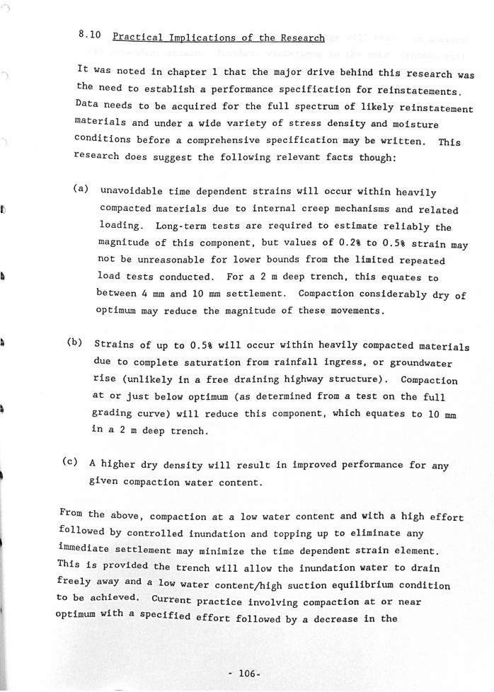
•
8.10 Practical Implications of the Research
It was noted in chapter 1 that the major drive behind this research was
the need to establish a performance specification for reinstatements.
Data needs to be acquired for the full spectrum of likely reinstatement
materials and under a wide variety of stress density and moisture
conditions before a comprehensive specification may be written. This
research does suggest the following relevant facts though:
(a) unavoidable time dependent strains will occur within heavily
compacted materials due to internal creep mechanisms and related
loading. Long-term tests are required to estimate reliably the
magnitude of this component. but values of 0.2% to 0.5% strain may
not be unreasonable for lower bounds from the limited repeated
load tests conducted. For a 2 m deep trench. this equates to
between 4 mm and 10 mm settlement. Compaction conSiderably dry of
optimum may reduce the magnitude of these movements.
(b) Strains of up to 0.5% will occur within heavily compacted materials
due to complete saturation from rainfall ingress. or groundwater
rise (unlikely in a free draining highway structure). Compaction
at or just below optimum (as determined from a test on the full
grading curve) will reduce this component. which equates to 10 mm
in a 2 m deep trench.
(c) A higher dry density will result in improved performance for any
given compaction water content.
From the above, compaction at a low water content and with a high effort
fOllowed by controlled inundation and topping up to eliminate any
immediate settlement may minimize the time dependent strain element.
This is provided the trench will allow the inundation water to drain
freely away and a low water content/high suction equilibrium condition
to be achieved. Current practice involving compaction at or near
optimum with a specified effort followed by a decrease in the
- 106-

equilibrium water content due to free drainage will result in greater
time dependent strain. Further, variations in the water content will
result in significant differential performance of the trench if the same
compactive effort were used.
1

Table 8.1 Effect of Particle Size on Magnitude of Suction for Water in a Lenticular State
I I Particle Radius, I rb I Calculated Suction
a (mm) I (rom) I (kPa) I I I I
0.1 I 0.050 I 14.8 I 0.020 I 259 .0
I I 1.0 I 0.50 I 1.48
I 0.20 I 25.9
I I 10.0 I 5.00 I 0.148
I 2.00 I 2.59
I I I I
Table 8.2 Comp ar i son of Soil Parameters for Coarse and Fine Gradings
I I I I Test I Free Void Ratio, e I Degree of I Air Void Ratio, I Number I Water I Saturation Sr I I
I Content I I I
I (%) Fine Coarse I Fine Coarse I Fine Coarse I
I I I I
I I I I A1 I 4.2 0.48 I 23.0 I 24.9 I
I I I I A5 I 4.1 0.42 I 25.8 I 21. 8 I
I I I I
A10 I 4.1 0.41 I 26.1 I 21.5 I
I I I I I
I B3 I 4.1 I 0.21 I 51. 9 I 8.8 I
I I I I I I
I I I I I I
I A3 I 2.4 I 0.49 I 12.9 I 28.6 I
I I I I I I
I A6 I 2 .0 I 0.33 I 16.1 I 20.8 I
I I I I I I
I BS I 2 .3 I 0.30 I 20.2 I 18.6 I
I- I I I I I

Table 8,3 Immediate Strain Components of Series A and B Tests During Loading
Grading Test Immediate Strain (%) at Various Stress (kPa) Levels Number 10 25 50 75 100
A2 0,42 0.75 0.99 1.12 A6 0.70 0.85 0.89 0.93 0,97
Coarse A7 0.26 0.44 0.75 A8 0.37 0.64 0.73 0.79 0.82 A9 0.81 0.94 l.09 1.19 l.24
B1 0.44 0.84 0.99 l.15 B2 0.63 l.47 l.89 2.12* B3 0.83 0.94 l.01+ 1.06+ 1.10+
Coarse B4 0.44 0.70 0.87 0.97* B5 0.54 l.30 l.82 B6 0.28 0.63 0.76 0.83* 0.87** B7 0.32 0.54 0.73 0.77 0.81**
Al 0.15 0.49 0.85 0.95 A3 0.41 0.52 0.73 0.83 0.93
Fine A4 0.33 0.47 0.63 0.72 AS l.07 1. 33 1. 75 1.86 1.95 AIO 0.78 1.02 l.23 1.32*
+ Strain components corrected for 0.07% inundation straining at 25 kPa
* Estimated by slight extrapolation of strain-stress curve
** Estimated from reload curve allowing for inundation and unloading -loading hysteresis

lable 8,4 Ca1culatiQn of ~bea, ~t,eDgth farameter~ Y~lDg Method b~ fredlYDg et a1 '12Z~)
I I I I Test I 1/2 «(1'1 +0'3 - 2UA ) 1/2 «(11 +(1'3 -2uw) 1/2 «(1'1 -CT3) (UA -uw) , I Number I I 1/2 (tT1 - (13 ) I I I I I I I 1 I (134.0) 134.0 100.5 0 I 102.1 I I I I I I I 2 I 288.9 (288.9) 254.0 I 208.6 I I I I I I I 3 I 281.5 294.7 249.5 13.2 I 212.5 I I I I I I I 4 I 140.5 143.8 109.5 3.3 I 108.8 I I I
Notes: (1) All stresses are at failure and measured in kPa
(2) Saturated shear strength - c' + (J" tan ~'- d'+[l/ztcr1+(13-2\1w)]tan'f", where d' - 10 kPa, 'fI' - 34.50
At'd
-1.6
45.4
37.0
0.7
I I t I I A't d cos 't' ' I I I
-1.3
37.4
30.5
0.6

Table 8,5 Calculation of Ib22~eti~al 6ir-Wat~r Hi~tur~ V21um2 ~hanges DurIng ~atyratloD ~t~ge 2f lest Cl
I I Absolute I ," x 10· 3 Average Final Initial Predicted Measured I Saturation Stage Sr (,) WI (kPa) I (m2 /kN) ~" WI 4W1 vv !J.Vv AVv I I I Free-formed I 80.4 85 2.306 -16 I 20 105 31 I l.874 33 2796 173 74 I I After stage I 83.0 118 1.441 17 I 9 31 38 I l. 221 20 2796 68 74 I I After stage II 86.2 138 1.000 37
18 41 43 0.821 29 2778 66 66
After stage III 89.3 167 0.641 66 28 39 40
0.511 41 2757 58 59
After stage IV 92.1 208 0.380 107 43 3' 37
0.297 50 2735 41 48
After stage V I 94.S 258 0 . 214 157 43 20 26
0.172 50 2717 23 34
After stage VI I 96.0 308 0.130 207 45 13 18
0.107 50 2710 14 23
/Continued

Table 8,5 Calculation of Theoretical Air-Water Mixture Volume Changes During Saturation Stage of Test Cl (Continued)
I I I I I I I I I I Absolute I P." x 10- 3 I Average I Final I Initial Predicted Measured I Saturation Stage I Sr(%) I ~ (kPa) I (m2 jkN) I pHI ~ A~ I Vv AVv AVv I I , I I I I I , , I , I I I After stage VII I 97.0 , 358 I 0,084 , I 257 I I I I , , I 48 , 9 17 , I I , I 0.068 I 50 I 2705 9 20 I I I I I I I , After stage VIII I 97.9 , 408 , 0.052 , I 307 I , , , , , I 30 I 4 4 , , I , I 0.046 I 30 , 2703 4 7 I I , , I I I , After stage IX , 98.3 \ 438 \ 0.039 I I 337 I , \ I , I 1 30 1 3 12 I , , , , 0,034 , 30 I 2697 3 14 , I I , 1 I 1 I After stage X I 98,7 1 468 I 1 1 367 1 I , I , 0.028 I 1 I 2701 I I I I I I I

200
190 180 Sample tests plotted only
? 170
~ 160
~ 150 140
"l
~ 130
"l 120 "-l 110 "-l
tl 100 &::l 90
S 80
~ 70
to: 60 ~ SO &::l
~ 40 30 20 10
0
0 20 40 60 80 100 120
.,4VERACE VERTICAL STRESS (kPa.) o TEST.,42 + TEST .,44 0 TEST .,45 A TEST.,47 x TEST B1 'l TEST B7
Figure 8.1 - Effect of Stress Level on Range of Measured Load Cell Stresses
10
9 -
~ 8 - Decrease of ratio with ~ : I
stress level ~ 7 ~ ~ 5i 6 -I
~ 5 '"" 0 i:: ~ 4
"-l
I i II rj 3 -lJ
&::l
~ 2 -"-l
1 -
• 0
0.0 0.2 0. 4 0.6 0.8 1. 0 1.2 1.4 1. 6 1.B 2.0
I/./iTIA'- SPEcll'1r;N T/~-r ( M", )
Figure 8.2 - Effect of Specimen Tilt on Range of Measured Load Cell Stresses

SAME TOTAL VOLUME OF WATER ON EACH SIDE OF CONTACT
FINES IN NO FINES IN
CONTACT ZONE CONTACT ZONE
' .. >:: ':':i:
Figure 8.5 - Effect of Fines on Equilibrium Suction Established Between Two Large Particles
"average " for coarse grading?
"avera <Te " for fUle grading? o f __ ~~ __
.,..
/
Fine grading psd
/ /
-:=~,/ /,,~,
~ ... " ~ possible frequency /' .- ______ ~ ~rves for
------ • ---- ,,"""" fUle grading --- , ..... , '--::::::.
63 200 600 2
LOG (PARTICLE SIZE)
Coarse grading psd
/ /
/ /
/ /
6 20
Figure 8.6 - Possible Frequency Distribution for Particle-Ceramic Contacts
100
60
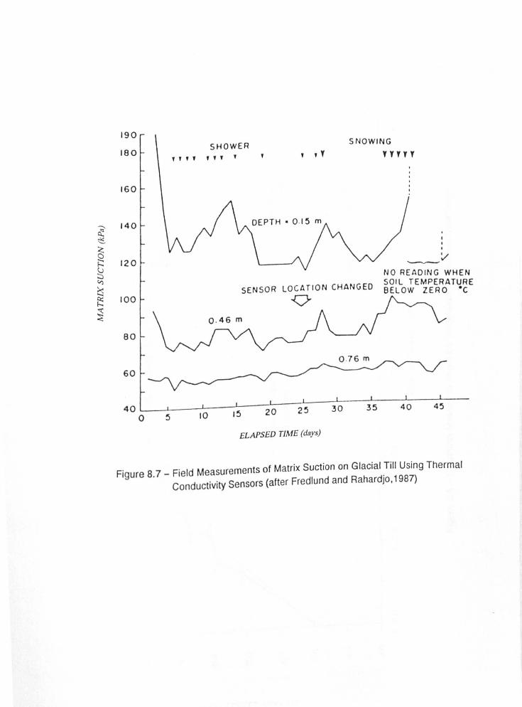
190
180
160
140
120
100
80
60
SHOWER
, , " '" , , " SNOWING
"'"
,
------~
SENSOR LOCATION CHANGED
NO READING WHEN SOIL TEMPERATURE BELOW ZERO ·C
-(/
40L-__ ~ __ --L----L----J-----~--~----~----L---~----o ~ 10 15 20 25 30 35
40 45
ELAPSED TIME (days)
Figure 8.7 _ Field Measurements of Matrix Suction on Glacial Till Using Thermal Conductivity Sensors (after Fredlund and Rahardjo,1987)
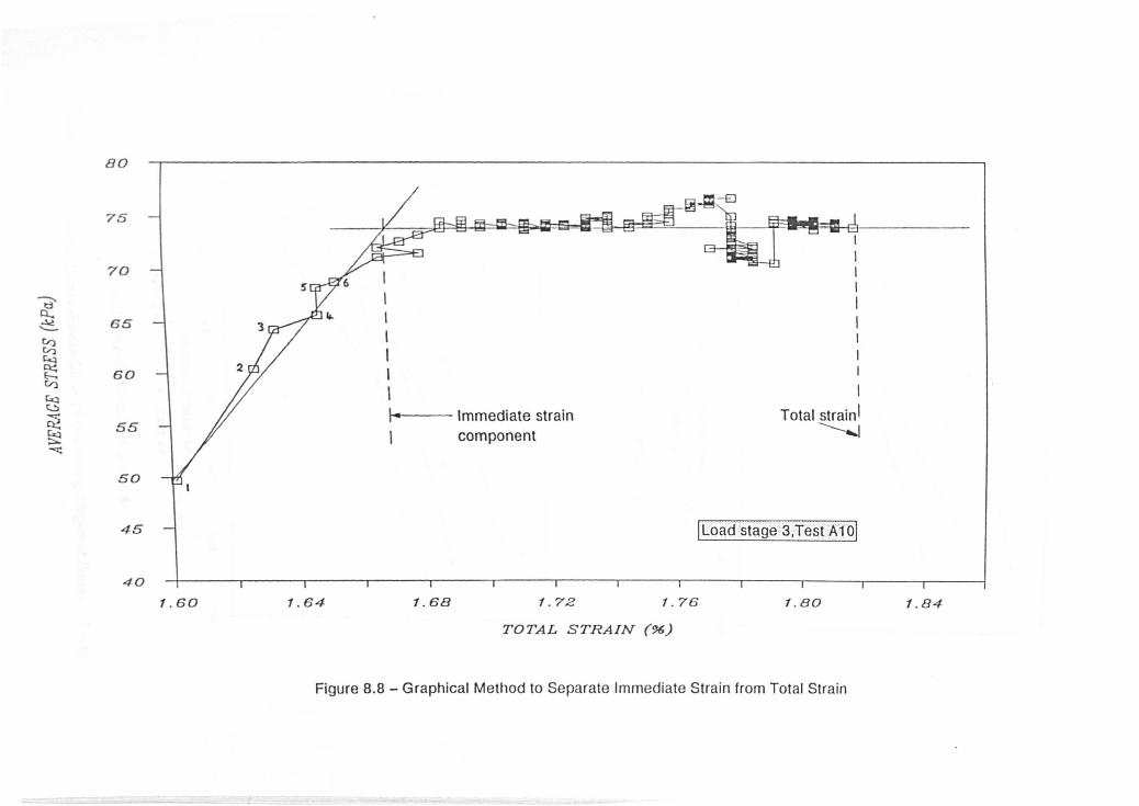
80
75
70
d-Cl.. ~ 65 ~ ~ ~
~ 60 ~
~ ~
~ 55 ~ .....:
50
45
40
1 . 60 1.64
I I , I I \- Immediate strain
component
~ - EJ
I I I I I I I I I
I
Total strain' ~
[I..oad stage 3;Test A101
1.68 1 . 72 1 . 76 I . BO
TOTAL STRAIN (96)
Figure 8.8 - Graphical Method to Separate Immediate Strain from Total Strain
I . B4

2.4
2.2
2.0
1.8
~ 1. 6
~ 1.4 &.; til 1.2 ~ ;:s 1. 0 ~ ~ 0.8 ....
0.6
0.4
0.2
0. 0
0 20 40 60 80 100 120
VERTICAL STRESS (/i:Pa.) o TEST 1.1 + TEST AS () TEST 1.4
b. TEST AS X TEST 1.10
(a) Fine Grading,Test Series A
2.0
1. 9
1. 8 1. 7 1. 6 1. 5
i' 1. 4
'- 1.S
~ 1.2
1. 1 t; 1. 0 ~ 0. 9 ;:s
0. 8 ~ ~
0. 7
O.S
0.5 0. '-0.3 0.2
0. 1
0. 0
0 2 0 40 60 80 100 120
VERTICAL STRESS (li:Po.) o TEST 1.2 + TEST AS () TEST 1.7
b. TEST AS x TEST 1.9
(b) Coarse Grading,Test Series A
Figure 8.9 - Immediate Strain-Stress Curves For Loading Stages of Series A Tests

2. tI
2. 4
2 .2
2.0
..... ~
1.8
~ 1. tI
5-; 1.4 CI)
~ 1.2 ::s ~ 1.0
~ ..... 0.8
O. tI
0. 4
0.2
0. 0
0 20 40 tlO 80 100 120
VERTICAL STRESS (kP4) c TEST BI + TEST B2 <> TEST B3
'" TEST B4 X TEST B5
(a) Coarse Grading,Tests 81 to 85
2. tI
2.4 Note - Includes inundation unloading and reloading stages
2.2
2.0
~ 1.8
~ 1. tI
5-; 1.4 CI)
~ 1.2 ::s ~ 1.0 ~ ..... 0.8
0.1
0.4
0.2
0.0
0 20 40 10 80 100 120
VERTICAL STRESS (kP4) + TEST BI <> TEST B7
(b) Coarse Grading,Tests 86 and 87
Figure 8.10 - Immediate Strain-Stress Curves For Loading Stages of Series 8 Tests

0
2 . 2
2.1
2
~ 1.9
~ 1. 8
"l 1. 7
~ 1. 6 ~ 1.5 CI)
x
~ 1. 4
{3 1.S +-------..... 1. 2 -..;
~ 1. 1
~ 0.9 CI)
~ 0.8 ;::s 0. 7 ~ ~
0.6 .... 0 .5
0.4
0 .3 0 .2
2 3 5
10kPa. + 2SkPa. FREE WATER CONTENT (1.)
o SOkPa. A 75kPa. x 1001cPa.
Figure 8.11 - Effect of Free Water Content on Immediate Compressibility of Coarse Grading From Series A and 8 Tests

1. 0 +
0 . 8 .. C
~ 0 . 8
0.'1'
~ 0 . 5
.......
~ 0.11
0 . 4 'Average' ~ .6
::s 0 . 3
~ .. 0 . 2 x
+ l ower limit 0. 1
0. 0
0 20 40 50 80 100 120
VERTICAL STRESS o:p.v AFTER EACH SDJ;E c TEST A2 + TEST A5 0 TEST A '1'
A TEST AS x TEST A8
(a) Coarse Grading, Series A Tests
1.0 c
Upper limit 0 .8
~ O. S
0.'1'
~ 0. 5 Average' ....... v
~ 0. 11 IJ.
'Ito 0.4
~
I o . S
lower limit 0 . 11
Test 87 not shown 0 . 1
0 . 0 0 tiD 40 50 so 100 HID
VERTICAL STRESS (1oP.v AFTER EACH S'rACZ c TEST B1 + TEST BJI 0 TEsr.s IJ. TEST B4 x TZST BI1 v TEsr 1111
(b) Coarse Grading, Series 8 Tests
1. 0 A
0 . 8 Upper limit
)( A A
~ o. s
c x 0 . '1'
)(
~ 0. 11 +
.......
~ 0. 11
A
0 . 4 'Average' ~
~ O. S
0 . 11 lower limit
0 . 1
0 . 0 0 110 40 110 80 '00 1110
VERTICAL STRESS (loPaJ AFTZR EACH ST.A4:Z 0 Tzsr A1 + TZSTAS 0 TEST ... 4-.. TZSTAI1 x TEST .. ,0
(c) Fine Grading I Series A Tests
Figure 8.12 - Relationship Between Immediate Strain Component and Stress Level

/1 .40
c ~?""" tI. ~1I c
/I. ~1l
I " tI.~"
/I.~tI / '\ /I.~6
/I. ~4 C
1 /I . ~~ / ~ iii /I.~/I
~ \ ? /I.~1 j ' 0
~ /I.~O "-~ /1 . /111 0,\
0
"" /I .tlll / )0.,
~ /I. tI " \ /I . tltI 0
/I .tl6 ~ / /I .tl4
tI . /I~ '--" /1 . /1/1
/1 . /11
/1 .20
0 . 0 /1. 0 4 . 0 tI. O 8.0 10.0
TOTAL WATER CONTENT (")
Figure 8.13 - TRRL Compaction Data For High Compactive Effort
/I . ~O
/1.28 -/I .2t1 - OJ 2 .24 / /1 .2/1 -
/ 1 2 .RO -iii /1 . 18 - ,,0 I ~
R.18 -~ - ? ?
R. 14 \ OJ 0 ~ R. 12
~ 2 . 10 \ 2 . 0tl ~ R. Otl '\
C
/1 . 04 "- / /I. OR ~
R.Oo
0 . 0 2 .0 4 . 0 11. 0 1l. 0 10.0
TOTAL WATER CONTENT (")
Figure 8.14 - TRRL Compaction Data For Medium Compactive Effort
1.110 / '-0
1 .86 \ /
0 / 1.80 C \ /
~ c
/ 1.7'6 \ ~ ? ~ ? / . I 1. 7'0 \ 0
"" \ / ~ 1 . tl6
1 . tlO \ /0
1 .611 '..cr/ c
1.60
0. 0 11. 0 4.0 11. 0 1l. 0 10.0
TOTAL WATER CONTENT (N)
Figure 8.15 - TRRL Compaction Data For Low Compactive Effort

100
• 60
30
• ..... . ' .'
. . .............. :........ . 3 .. -
•
o Field 2 o Field 3 o Field 1
o Field 4
• 11 ....... . •• ••••••••• • . . ..... ~.. . •••• • • ... ..
•• '+AG •••• 4-
.' B + 86 •.• 7
Key :
A9., +
83 + AS
• 23
o BRE
• 0 .5m diam oedometer test
o 1.0m diam oedometer test, BRE o In situ plate bearing test
+ 86 Current research
• •
100
60
30
3
1 ~----~----~~----~----~~--~~----~----~------L-----~1 1.5 1.6 1.7 1.8 1.9 2.0 2.1 2.3 2.4
DRY DENSITY (Mg/m3)
Figure 8.16 - Relationship Between Constrained Modulus and Dry Density for Stress Range 25-1 OOkPa (after Brady and Kirk,1990) .

100
• . ' • • •
. ' .' . . . .
•
•
.' .' .. ' .' . .' .' .' .. ' .' ....... • •
.' .'
o F~d2 o Field 4 o Field 3
o Field 1
•• • • .. ..... . • •• •••••••• •
.. . ' .' . '
Key :
• •••••• • ...... . .. . ' C BRE
• 0 .5m diam oedometer test o 1.0m diam oedometer test. BRE o In situ plate bearing test
• •
100
.. ..
1 L-____ ~ ____ -L ______ L_ ____ ~ ____ ~ ____ ~ ______ L_ ____ ~ ____ ~1
1.5 1.6 1.7 1.8 1.9 2.0 2.1 2.2 2.3 2.4
DRY DENSITY (J..Iglm3)
Figure 8.17 _ Relationship Between Constrained Modulus and Dry Density for Stress Range 25-250kPa (after Brady and Kirk,1990)

1000
100
10
• • • • •••••••••••• Second loading cycle ., ••• '"
\
! .... " .... JIt ••••••• ....... . .......... . •
• • •
•........ ............ • • Field 2
•••••• • • Fi~d 3
•
o
• Field 4 • Field 1 o
,.JJ Field 2 VO-Field4
o Field 30
.' o .... ,,,.-
.0 o ••• ~o
o (4 •• ' 0 •• -0
Field 1 0
o .. ' .' .' o
Init ial loa\din, 'Vol, •••••••••••••••
.' .' .' .'
.' o ...
BRE
.' .' o •••• . ' •• - 0
.' .' o 00" ••••• 0 0
.'
Key :
0.5m diam oedometer test 100m diam oedometer test, BRE In situ plate bearing test
1st 10id cycle 2nd load cycle o • ... o •
1000
100
10
lL-____ L-____ i-____ ~ ____ _L ____ _L ____ ~----~~--~~--~ 1 1.5 1.6 1.7 1.8 1.9 2.4
DRY DENSITY (Mglm3)
Figure 8,18 - Relation·ship Between Constrained Modulus and Dry Density for Stress Range 20S-820kPa (after Brady and Kirk,1990)

? ~ -..;.
f:5 E5 t:l §: ~
~ .,;
~ 8
? ~ -..;.
S :::; § ~
~
~ .,;
~ 8
26. 0
24. 0
22. 0
20. 0
18. 0
18.0
14. 0 .-12. 0
?/
10.0
8. 0
8.0
4. 0 0 c +
2. 0 c
0. 0
0.0 2.0 4.0 8.0 8.0
TOTAL rATER CONTENT (,,) c 10-25k.Pa. + 25 -50k.Pa. <> 5c)-75k.Pa.
b 75-100k.Pa. x 25-100k.Pa.
Figure 8.19 - Variation of Constrained Modulus With Water Content For Series A Tests on Coarse Grading
280
240
220 x
200
180
160
140
120
100
80
80
40
20
0
0. 0 2 .0 4.0 6.0 B.O
TOTAL rATER CONTENT (") c 5-10kPa. + 10-25k.Pa. <> 25-5~CPa.
b 50-100k.Pa. X 100-250kPa.
Figure 8.20 - Variation of Constrained Modulus With Water Content For Series 0 Tests on Coarse Grading Compacted With Usual Effort
I ' j
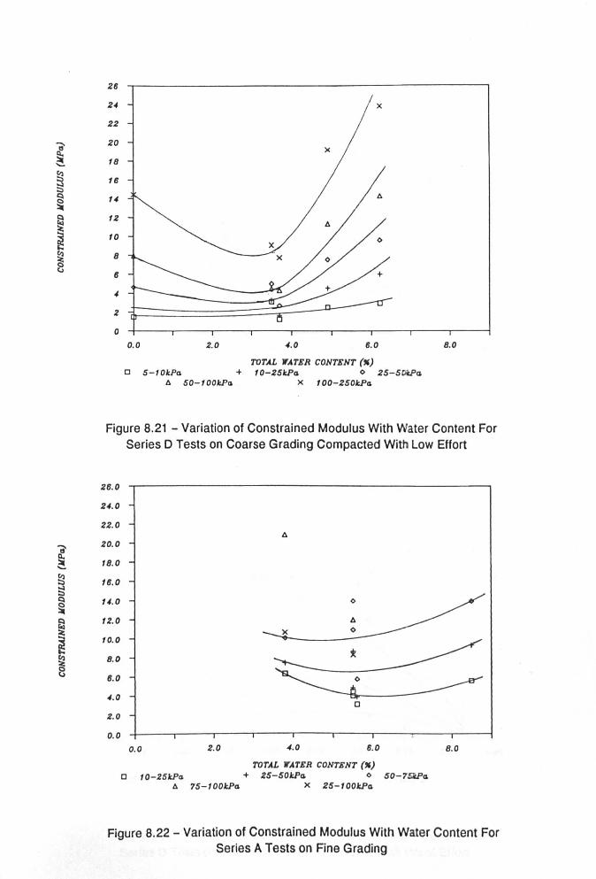
? ~ ~
~ :s ~
~ ~
~ "" ~ Q t.J
? ~ ~
~ :s ~
~ ~
~ "" ~ 8
28
24
22
20
18
18
14
12
10
8
8
4
2
0
0.0 2.0 4.0 8.0 8.0
TOTAL WATER CONTENT (,,) c 5 - 10kPa. + fO-25kPa. 0 25-5DtPa.
6 50-100kPa. X fOO-250kPa.
Figure 8.21 - Variation of Constrained Modulus With Water Content For Series 0 Tests on Coarse Grading Compacted With Low Effort
28.0
24. 0
22.0
20.0
IB.O
18.0
14.0
12.0
fO.O
B.O
8.0
4.0
2.0
0. 0
0.0 2.0
6
)(
4.0
A o
o
8.0
TOTAL WATER CONTENT (") o fO -25kPa. + 25-50kPa, 0 50-75l1Pa.
6 75- 100kPa. X 25-fOOkPa.
B.O
Figure 8.22 - Variation of Constrained Modulus With Water Content For Series A Tests on Fine Grading

? ~ '" ~ ~ ~
~ ~
~ &..;
~ <:) ~
? ~ '" ~ ~ ~
~ ~
~ &..;
~ 8
26. 0
24. 0
22. 0
20. 0
18. 0
16. 0 o
14. 0
12. 0
10.0 + 8. 0
6. 0
4. 0
2 .0
0. 0
1.94 1.98 2.02 2.06 2. 10 2.14 2.18 2.22
DRY DENSITY (M(J/m3) o 10-25k.Pa. + 25-50kPa. 0 50-75k.Pa.
A 75- 100k.Pa. X 25-100k.Pa.
Figure 8.23 - Variation of Constrained Modulus With Dry Density For Series A Tests on Coarse Grading
260
240
220
200
180
160
140
120
100
80
flO
40
20
0
2.26
1.94 1.98 2.02 2.08 2.10 2. 14 2.18 2.22 2.26
DRY DENSITY (Mg/m3) 0 5-10kPa. +
A 50-100k.P4
10-25kPa. 0 25-50kPa. X t 00-250kPa.
Figure 8.24 - Variation of Constrained Modulus With Dry Density For Series 0 Tests on Coarse Grading Compacted With Usual Effort

a-~ -..;.
~ E:l CI
~ ~
~ ... ~ 8
a-~ -..;.
S ~ CI
~ ~
~ ... ~ 8
26
24
22
20
18
16
14
12
10
8
6
4
2
0
1.70 1.80 1.90 2.00 2.10
DRY DENSITY (Jlg/m3) a S-10kPa. + 10-2SkPa. 0 2S-S0kPa.
t;. SO - 100kPa. x 100-2S0kPa.
Figure 8.25 - Variation of Constrained Modulus With Dry Density For Series D Tests on Coarse Grading Compacted With Low Effort
26. 0
24.0
22.0 "-t.
20. 0 "-18. 0 "'-
"'-18. 0 "'-14. 0
12. 0
10. 0
8.0
B.O a
4. 0 -+ a
2.0
0.0
1. 74 1.78 1.82 1.88 1.90 1.94 1.N 2.02
DRY DENSITY (Jlg/m3) a 10-2SkPa. + 2S-S0kPa. 0 SO-7SlPa.
t. 7S- 100kPa. x 2S-100kPa.
Figure 8.26 - Variation of Constrained Modulus With Dry Density For Series A Tests on Fine Grading
2.08

160
140 alternative curves for stress 130
1110
! 110
100
~ 80
~ 80
I '70
110
60
8 40
30
110
10 c
0 0 . 0 11. 0 4 . 0 8.0 8 . 0
TOTAL 'lTATllR CONTlfNT (NJ C 0-1IIU,Po. + 116- 1 00_0. 0 il6-:l06_0.
A Jl6-SJlO_0. x 100-8J10_0.
Figure 8.27 - Variation of Constrained Modulus Obtained From TRRL Tests With Water Content For High Compactive Effort
l ~
I ~
I 8
1110
110
100
80
80
'70
80
60
40
30
110
10
0 0.0
alternative curves for stress
range 0-25kPa
)(
x
A + _ ---':::---=---=-o-i::.~
- 08 --
11.0 4 . 0
--.... ~ 11.0
roTAL 'lTATllR CONTllNT (NJ C 0-Jl61c.P0. + Jl6-100_0. 0 116-:106_0.
A Jl6-8110_0. )( 100-8110_0.
8 . 0
Figure 8.28 _ Variation of Constrained Modulus Obtained From TRRL Tests With Water Content For Medium Compactive Effort
JIll
114
lIJl
~ 110 ,.
I 111
=-14
I 111
10
~ • II
4
Jl
0
0
0 . 0 11.0
alternative curves for stress range 25-1 OOkPa
)(
o .-....... +
C
4 . 0 11.0
TOTAL 'lTATllR CONTllNT (NJ
0-Jl61c.P0. + 116-100_0. 0 1I6-Z06_0.
A Z6-1I1101c.Po. )( 100-8110_0.
8 . 0
Figure 8 29 . . - Variation of Constrained Modulus Obtained From TRRL Tests With Water Content
For Low Compactive Effort

;e-~
~ ~
I
HID
140
1S0
1110
110
100
110
80
70
If 0
60
40
SO
IlO
10
0 Il. IlO Il.Il4
alternatIve curves or stress ranq.e 25-820kPa
)(
/
/" /
/ alternative curves for stress
/ \. ~e25-205kPa . b _ 'It._ ,./
. ~ ~ /
~± ;"~-~ tl.IlS Il.3:1 :I.SIf :1.40 Il.44 Il.4S
DRY DENSITY (MII/...s) c 0-tl6/I:Pa. + :l6-'00/I:Pa. 0 :l6-n6/I:Pa.
A :l6-BIlO/I:Pa. )( 100-8IlOkPa.
Figure 8.30 - Variation of Constrained Modulus Obtained From TRRL Tests With Dry Density For High Compactive Effort
'IlO
"0 alternative curves for stress 100
~ 110
SO
~ 70
~ If 0
)( .jan~8100-820kPa --- ---,/ x
~ /
~--- -
I 60
40
8 so
IlO
10
± ,,----------~+--------~+~----------____ ~ --:t.. ~----------~o--------~~~-------~
0 Il. OO :1.04 :I. OB :I. , Il 2 . '8 :I. flO Il.:l4 Il.1l1f
DRY DENSITY (MII/...s) c 0-:l6/1:Pa. + :l6-100/I:Pa. 0 Il6-~/l:Pa.
" fl6-BflOkPa. )( 'OO-S:lO/I:Pa.
Figure 8.31 _ Variation of Constrained Modulus Obtained From TRRL Tests With Dry Density For Medium Compactive Effort
:I If
R4 alternative curves for stress
:lJI range 100-820kPa
~ IlO
'B
~ 'If
~ :iii
14
I ,:1
'0
B 8
If c
4
Il
1.7:1 1.71f 0
1.80 1. lf4 '.64
'.88
DRY DENSITY (MII/...s) c 0 - 1l6/I:Pa. -+ tl6-100/I:Pa. 0 :l6-Z'tJ5/I:Pa.
Fi " 26- StlO/I:Pa. )( 'OO-B:lO/I:Pa.
gUre 8.32 _ Variation of Constrained Modulus Obtained From TRRL Tests With Dry Density For Low Compactive Effort

AE,
/
STRAIN AT GIVEN STRESS LEVEL
Conlectured form of state surface,based upon observed trends In sarles 0 tests over limited range of states
A. stress level Increases Al;to 61.decrease
Observed form for the variation of compressibility with water content and dry density for a constant compactlve effort
1,·/ r
DRY DENSITY
, ,
I I ,
I ~-. ---- ----------
I" (' ,
I I ,
\ Y \ ,,1 / ., i ) /. Ii,,"
" '.V·· ~ L,-"'" . / I~
~;' .... ..", Compaction curves for 2 different efforts
-- -- -- - ---- -----:,. -; ....----.-f Saturation line
Figure 8.33 - Three Dimensional Relationship Between Strains At Any Given Stress Level,Water Content and Dry Density

40
35
30 ~ ~ +
~ 25 --j ./ Top suction
Q., -:::.. ~ 20 0 e::: ~ ~
15 /' <>
10
5
o 0 . 00 0.20 0.40 0.60
INUNDATION STRAIN (,,)
Figure 8.34 - Relationship Between Measured Suction and Inundation Strain

\
O. tlO
0 .1I0
0 .40
O.SO
O.IlO
0 . 10
0 .00
0.80
0 .1I0
0 .40
0 .30
O.IlO
0 . 10
0 . 00
O. tlO
0 .1I0
0 . 40
O. SO
O. IlO
0 . 10
0.00
.~ ~ -.. --
upper limit of range? /
/
--
/ /
/
/
----• .-.-:-
./
lower limit of range?
0 .110 O. IlIl 0 . Il4 0 . 1It1 0 . Il8 0 . 30 0.311 0 . S4 O. StI 0 . S8 0 . 40
INITIAL YOID RATIO
(a) Void Ratio
•
•
o 111 1t1 20 114
INITIAL AIR VOID RATIO (")
(b) Air Void Ratio
+
•
+ +
+
eo IlO 40 o INITIAL FREZ DZCRZIr OF SATURATION (JO
(c) Free Degree of Saturation
Figure 8.35 _ Relationships Between Inundation Strain and Soil Parameters Void Ratio,Air Void Ratio and Free Degree of Saturation

50
40
ii' 30
~ ~ ~ g
20 c"
10
0
0
50
40
ii' 30
~ ~
~ g
20 c"
10
0
0
TOp suctions at 25kPa vertical stress +
+
+
+
+
+
20
+
+
+
++ +
8 '2 16 20
AIR VOID RATIO (,,)
(a) Air Void Ratio
Top suctions at 25kPa vertical stress '
+
+ +
40 60 80
FREE DECREE OF SATUJUTION
(b) Free Degree of Saturation
+
24
100
Figure 8.36 - Relationship Between Suction,and Air Void Ratio and Free Degree of Saturation

- I.
-3
-2
- 1 c ~
e ::l
0 V1
C 0 0
c
~ V1
~ . III -1
·2
•
d
r 21 . : 100kNI .. '
. : 'lC - 260 kH I m'
L01)-
III Mudsl_IC ... 19781
121 Clo,I~" 19841
III Sl>olt 1C>4r1ts 19841
141 Mud,t_' Sond,to,. ICharl~1 1914 I
• N~ ...... ~d V ... }
O Ed: lOO - 500 k", I III I
st l_~dV ...
% Air lIolds proor to Inundation 2
Zon, at r~s.ults tor Mor f surfae. layprs aft., 2 )'fors
. : 40 - tCC kN 1m' 11 I
M ,, : IS kHI.,' w -: 1~/. : Ofte
Figure 8.37 _ Comparison of Strain on Saturation with Air Void Ratio of Backfill (after Thompson,Holden and Yilmaz, 1990)

DRY (lNSrTY L EGEt{)
Hl
n5
no
lIS
205
(Mg/ms
) _ INITIAL COMPACTION CONDIT ION OF SPECIMEN
SPECIMEN CONDITION AF TER PRE-LOADING TO INUNDATION STRESS
o SPECIMEN CONDITION AF TE R INUNDATION
63
DRY CINSIT'f-WATER CONTENT / RELA TlONSHIP AT STANDAR D---/ TES T PROGRA MME (Cl'1PACTIVE I EFFORT /
/ /
/ /
/ /
B 4 62
5·0 6·0 7-0 s·o TOTAL WATER CONTENT (%)
9·0 1~0 11·0
Figure 8.38 _ Combined Effect of Total Stress Changes and Inundation on the Dry DensityWater Content Relationship for the Coarse Grading

1. Specimen A lower water content than specimen B but similar fabr ic.
2. After loading to inundation stress , suction in A still greater than B.
3. Following complete saturation at constant stress, both A and B converge on a unique point in the saturated e- (0" - 40.) plane by vi rtue of different collapse settlements .
state surface in satura t ed plane atter inunda t ion
e
Inundation Stress Plane
0"- u"
L State surface tor specimens A and B if (O"-u~) always increases and (u~-4. ) alway decreases, for given initial soil fabriC (dry denSity) ~ __ '7JA
Rgure 8·39- Loading and inundation stress paths tor two different specimens showing uniqueness of final saturated state.

1.B
1. 7
1.6
1.5
~ 1. 4 ~
~ 1.3 CIl ...;j
~ 1.2 ~
1.1
1.0
0 .9
O.B
0 20 40 60 BO 100 120
VERTICAL STRESS (kPa.) o TEST A2 + TEST.A6 <> TEST A7
b. TEST AB X TEST A9
Figure 8.40 - First Unloading Curves for Series A Tests on Coarse Grading

130. 0
120. 0
110. 0
100. 0
~ 90. 0
80. 0
~ ~
70. 0
I 60. 0
50. 0
8 40. 0
30.0
20.0
10.0
0.0
0 20 40 60 80 100 120
VERTICAL STRESS (kPa.) D TEST A2 + TEST AB <> TEST A 7
b. TEST 048 X TEST .A9
(a) Series A Tests
130. 0
120. 0
110. 0
100. 0
90. 0
! 80. 0
~ 70. 0 '" ~ 60.0
I 50.0
8 40.0
30.0
20. 0
10. 0
0.0
0 20 40 60
VERTICAL STRESS (kPa.) . \.
D TEST B1 b. TEST B5
+ TEST B2 <> TEST B3 x TEST B6 Q TEST B7
(b) Series 8 Tests
Figure 8.41 _ Effect of Stress Level On Unloading Constrained Modulus For Coarse Grading

300
",
250 ~"
UA - Uw = 13-2 K~"J'( DRY
/ ",/
200 / STRENGTH INCREASES AS SUCT ION INCREASESy
c a.. ",/ ~
150
ON A~'
I ,,/ t) U -U - 3-3KPa/ A W- " ~IN tj:
/' SATURATED
/
50 ",/ ESTIMATED STENGTH OF
/ SATURATED SOIL:
If'= 34 -5°, d' : 10KPa
/' ¢ ': 43'5°, c' =13-6 KPo
:0 I 0
50 100 150 200 250 300
~ (61 + 63
-2UA
) (KPo)
Figure 8-4.2 - Shear Strength ~ata From Series C
35
30 )l /
25 / IFoe: 63-4° • 'fJ" = 67 -6°
~3-40 ~ 1/ = 73 -4°
"-
3- 20 ~ "= 76-go
VI / 0 u 15
/ ~"T:J
<l 10 / 5 /
0 )( I •
I I I
5 10 15 20 UA-_Uw (KPo)
Figure 8'43 - Change in Shear Strength From Saturated Plane

w !.t Iii o w ::neo ~
~ u.1.00
w (!)
~ VI
~320
~ w
~ -21.0 "E u
w ~ ::> 6160 > ~
w (!)
~ eo I u
Sr("!. B at en
100·0 1·00
0.90
0 ·60
80.0 0.50
I
.. ' ..
--..-...---
_ - tJ.Y" ---
.. .. ' .•.. . .. ' . . , .• ... . , ..... • .. .. . . . .. • .. .. • ... ... • - 6 '\. ..... = tJ. V
1.00 0. (kPo) At End Of
(0) Volumetric Changes Due To Increase Of Cell Pressure Stage
250 200 300 350 150 50 100
I l-
./
/" Y
Sr ,,~'--B ./
/ /
/ /
/ /
/ .1 /
/
--"..--. -----/' .
50 100 150 200 250 300 3SO 4
(b) Changes In Degree Of Saturation And Pore Pressure Parameter B Due To Increase Of Cell Pressure
OjlkPa) At End Of stage
Figure 8'4.4 -Variation Of Specimen Parameters During Saturation Stage Of Specimen CI
• J \ I

B tN
cJ
180
1·0 160
0·9 140
0·8 120
0·7 10
0·6 80
0·5 60
0·4 40
0·3 2
80·0 82
B
CALCULATED AV, DURING STAGE
MEASURED AY" DURING STAGE
~
~
CALCULATEDAV. DURING PART 1 MEASUREDllVyDURtNG PART 1
"'"-
84 86 88 90 92 94 96 FREE DEGREE OF SATURATION (%) AT END OF EACH STAGE 2
Figure 8'45- Comparison of Theory With Experimental Data For Compressibility of Air-Water Mixtures
98

CHAPTER NI NE
CONCLUSIONS AND RECOMMENDATIONS FOR ....
FUTURE WORK
The one dimensional compressibility at low stresses «100 kPa
typically) of a coarse graded limestone aggregate has been investigated
under monotonic, constant strain and repeated load conditions, with
suction measurements. In addition, the effects of the inundation at a
slow rate of water from above has been investigated, and limited tests
to determine the Ko and shear properties have been performed. Tests
have also been carried out using limestone with maximum particle sizes
of 20 mm (medium grading) or 5 mm (fine grading).
The conclusions from this work are summarised below. The thesis is
completed with recommendations for future work.
9 . 1 Conclusions
The conclusions derived from this research are embodied in chapter
eight and are summarised only in brief here:
(a) Experimental Apparatus : A new consolidation cell suitable for
high quality testing of unsaturated coarse grained soils
subjected to a high degree of compaction has been developed.
The apparatus has been used to obtain repeatable
compressibility data.
(b) Suctions : Measurable suctions have been demonstrate.d to exist
within even the coarse grained material whose maximum particle
size was 37.5 mm and whose silt and clay fraction was 7%. The
suctions increased with decreasing water content, and were of
similar order of magnitude in both the fine (5 mm maximum
particle size, silt and clay fractions 12%) and the coarse
- 108-

grading . The similarity is attributable to the congregation of
fine particles around the contacts between larger particles.
Measurement of the "average" suction condition within the soil
mass does not reflect the range of suctions that will exist
locally within the mass at low degrees of saturation when the
water phase is discontinuous.
(c) Compressibility under Monotonic Load Conditions : Analysis of
the current and previous research by others shows that the
compressibility is a function of the dry density and water
content of the compacted mass, particularly at low stresses.
For a given compactive effort, compressibility increases to a
low peak before decreasing once again as the water content
increases from a dry condition to near but below optimum . As
optimum is approached and passed, the compressibility rapidly
increases. Over the same water content range, dry density
tends to increase continually except for a trough at very low
water contents and the peak at optimum.
The influence of water content is primarily attributed to the
suction stresses within the soil mass, and the compressibility
variations may be explained by reference to the measured
suction- water content and dry density-water content relations.
The increased coefficients of friction between particles at
very low contents may be influential to some degree, as _may
segregation of fines during compaction at very high water
contents .
The suction influence decreases as the applied stress
increases, although values of constrained modulus from low to
high stresses still reflect this factor. A three dimensional
plot of compressibility, expressed as strain at any given
stress level, against dry density and water content is proposed
in order to model correctly the influences identified without
introducing the complexity of stress level dependence
associated with use of the constrained modulus.
- 109-

(d) Compressibility under Strain Controlled Conditions : Similar
compressibility trends were observed from the monotonic and
stain controlled tests, but strains measured during the former
were significantly smaller than those during the latter. The
difference in stress application period between the tests
accounts for all of the apparent discrepancy. "Long-term"
strains continued to be developed after several hours during
the monotonic tests, and the "immediate" strain component was
highly dependent in magnitude upon the time period over which
it is measured. Close definition of this period must be made
whenever immediate strains are considered.
Defining "immediate" to be the first 2 to 5 minutes after
loading, the ratio of the immediate to time dependent
components was shown to be related to the total stress. The
ratio decreased from 0.7 to 1.0 at very low stresses, to 0.3 to
0.8 at a stress of 100 kPa.
(e) Inundation Effects : Small strains were observed to follow
rapidly after onset of inundation at a constant total stress
level. These strains were shown to be closely related to the
suctions within the soil before inundation, and could also be
related to the degree of saturation and air voids ratio which
reflect the suction condition of the soil. The immediacy of
the strains reflects the dominant suction influence, rather
than the longer term mechanism of particle softening.
(f) Repeated Load Effects : The strains developed during the first
4 load cycles of the heavily compacted coarse grained material
were shown to vary with the water content in a similar manner
to compressibility, that is to be a function of water content
and dry density. Use of a lower compactive effort indicated an
overriding influence of dry density. Patterns of strain
accumulation were different for each effort and for
- 110-

the other 2 gradings. The heavily compacted specimens showed
little strain accumulation after the first cycle, whereas a
near linear strain accumulation with load cycle was observed
with the lower effort. The medium grading behaved in a similar
manner to the heavily compacted coarse grained material, and
the fine grained material behaved in a manner intermediate
between the two extremes. Strain rate had no apparent
influence on behaviour within the range 0.1 rom/minute to 2
rom/minute used in the test programme.
(g) Ko Determinations: The tests produced a reliable value of 0.41
for Ko and a tentative value of 0.39.
(h) Shear Strength : The data revealed an apparently large
suction influence in terms of the Mohr-Coulomb type failure
parameters for unsaturated soils, with c' - 13.8 kPa, ~' _
43.5 0 and 0b - 700 to 800 . Some of this apparent suction
influence on ~b was attributed to interparticle friction
coefficients, but its significance was shown to be less
dramatic by consideration of the likely maximum suction within
the soil that affected shear behaviour.
9.2 Recommendations for Future Work
The establishment of a performance or even end product specification
requires a large number of different materials, conditions and stress
regimes to be investigated. Some suggestions for future work to
achieve this aim, and others of a more fundamental nature, are noted
below:
(a) further investigation of the compressibility-dry density-water
content relationship under monotonic loading conditions should
be completed over a wide range of water contents and compactive
efforts, in order to verify and define a three dimensional
relationship for the limestone;
- 111 -

(b) the relationship postulated in (a) should be investigated for a
wide range of gradings and aggregate types;
(c) the existence of a similar relationship for repeated load
conditions should be investigated, for a variety of compactive
efforts;
(d) the effect of non-Ko conditions on compressibility should be
assessed from triaxial tests;
(e) the factors affecting measured soil suctions in coarse
grained materials should be defined, such as maximum particle
size, grading, silt/clay contents, particle angularity and
particle petrography. The formulation of a theoretical model
to predict the measured suctions should be attempted. A
statistical approach based upon observed particle distributions
is likely to be the most successful technique;
(f) the validity of the capillary theory for coarse grained soils
at low degrees of saturation should be investigated using
experimental techniques, and its applicability or otherwise to
highway design assessed;
(g) the effect of grading, compaction, water content and dry
density on inundation strains should be investigated;
(h) the effects of changes in interparticle coefficients of
friction and crushing on performance should be investigated;
(i) the apparent large influence of suction (and/or interparticle
friction) on shear behaviour at low stresses should be
verified.
- 112-

REFERENCES
Aitchison, G D (1956). "The circumstances of unsaturation in soils with particular reference to the Australian environment", Proc 2nd Australia - New Zealand Conf on SMFE, Christchurch, N Z: 173-191
Aitchison, G D (1965). Contribution to conference technical session 2, Proc 6th ICSMFE, Montreal, 3: 318-321
Aitchison, G D and I B Donald (1956). "Effective stresses in unsaturated soils", Proc 2nd Australia - New Zealand Conf on SMFE, Christchurch, N Z: 192-199
Aitchison, G D and J A Woodburn (1969). "Soil suction in foundation design", Proc 7th ICSMFE, Mexico,- 2:1-8
Alonso, E E, A Gens and D W Hight (1987). "General report, Session 5: Special Problem Soils", Proc 9th ECSMFE, Dublin, 3: 1087-1146
Alonso, E E, A Gens and A Josa (1990). "A constitutive model for partially saturated soils", Geotechnique, 40: 405-430
Aschenbrenner, B C (1956). "A new method of expressing particle sphericity", J. Sed. Petrology, 26: 15 - 31
Barden, L, A 0 Madedor and G R Sides (1969). "Volume change characteristics of unsaturated clay", JSMFD, ASCE, 95 (SM1): 33-52
Barden, Land G R Sides (1970). "Engineering behaviour and structure of compacted clay", JSMFD, ASCE, 96 (SM4): 1171-1200
Bishop, A W (1960). "The principle of effective stress", NGI Pub 32: 1-5. Reprinted from Teknisk Ukeblad, 106 (No 39), 1959
Bishop, A Wand G E Blight (1963). "Some aspects of effective stress in saturated and partly saturated soil", Geotechnique, 13: 177-197
Bishop, A Wand I B Donald (1961). "The experimental study of partly saturated soil in the triaxial apparatus", Proc 5th ICSMFE, Paris, 1: 13-21
Blight, G E (1965). "Effective stress evaluation for unsaturated soils", JSMFD, ASCE, 93 (SM2): 125-148
Bocking, K A and D G Fredlund (1980). "Limitations of the axis translation technique", Proc 4th Int Conf on Expansive Soils, Colorado, USA: 117-135
Bolt, G Hand R D Miller (1958). "Calculation of total and component potentials of water in soil", Trans American Geophys Union, 39: 917-928
Bond, W J and N ColliS-George (1981). "Ponded infiltrations into simple soil systems: 1. The saturation and transition zone in the moisture Content profiles.", Soil Science, 131: 202-209
Boyce, J R (1976). "The behaviour of a granular material under repeated loading", PhD thesis, Univ of Nottingham
Brady, K C and G Kirk (1990). "The compressibility of a crushed limestone backfill", TRRL Research Report 251
Brandon, T L, M Duncan and W S Gardner (1990). "Hydrocompression settlement of deep fills", J Geotech Eng, ASCE, 116 (GT10): 1536-1548
Brauns, J and H Leussink (1967). Discussion on Marsa1 (1967), JSMFD, ASCE, 93 (SM6): 383-388
BS1377: 1975 and 1990. Purposes"
"Methods of Test for Soils for Civil Engineering
BS812: 1975. "Testing Aggregates"
Burland, J B (1964), Discussion of Bishop and Blight (1963), Geotechnique, 14: 65-68
Burland, J B (1965). "Some aspects of the mechanical behaviour of partly saturated soils". From "Moisute equilibria and moisture changes in soils beneath covered areas - a symposium in print·, Butterworths, Australia: 270-278
Campbell, J D (1973). "Pore pressures and volume changes in unsaturated soils", Doctoral thesis, Univ of Illinois, Urbana-Chamaign
Charles, J A (1984). "Some geotechnical problems assocated with the use of coal mining wastes as fill materials", Symp on the Reclamation Treatment and Utilisation of Coal Mining Wastes, Durham
Charles J A, D B Hughes and D Burford (1984). "The effect of a rise of water table on the settlement of backfill at Horsley restored opencast coal mining site, 1973 - 1983", Proc 3rd Int Conf on Ground Movements and Structures, Cardiff
Clements, R P (1984). "Post construction deformation of rockfi11 dams", J Geotech Eng, ASCE, 110 (GT7): 821-840
Coleman, J D (1962). "Stress/strain relations for partly saturated soil", Geotechnique, 12: 348-350
Collis, Land R A Fox (1985). "Aggregates: sand, gravel and crushed rock aggregate for construction purposes", Geo1 Soc, Eng Geol SP1
Croney, D and J D Coleman (1948). "Soil thermodynamics applied to the movement of moisture in road foundations", Proc 7th lot Conf for Applied Mechanics, 3: 163-177
Croney, D, J D Coleman and WPM Black (1958). "Moveaent and distribution of water in soil in relation to highway design and performance". From "Water and its Conduction in Soils·, Highway Res Board Sp Rep No 40

Croney, D and J D Coleman (1960). "Pore pressure and suction in soil" lnt Soc of SMFE, Proc Conf on Pore Pressure and Suction in Soils ' , London. Butterworths, 1961: 31-37
Dhir R K, D M Ramsay and N Balfour (1971). "A study of the aggregate impact and crushing value tests", J lnst Highway Eng, 18: 17-27
Dusseault, M B (1979). "Undrained volume and stress change behaviour of unsaturated very dense sands", Can Geotech J, 16: 627-640
Egretti, I and R N Singh (1988). "A laboratory investigation into the effects of air void and water saturation on the collapse settlement of opencast mine backfill", Mining Science and Technology, 7: 87-97
El-Ehwany, M and S L Houston (1990). "Settlement and moisture movement in collapsible soils", J Geotech Eng, ASCE, 116 (GT10): 1521-1535
El-Sohby, M A (1964). "The behaviour of particulate materials under stress", PhD thesis, Univ of Manchester
Escario, V and J F T Juca (1989). "Strength and deforaation of partly saturated soils", Proc 12th ICSMFE, Rio de Janeiro, 1: 43-46
Escario, V and J Saez (1986). "The strength of partly saturated soils", Geotechnique, 36: 453-456
Evans, M D (1987). "Undrained cyclic triaxial testing of gravels - the effect of membrane compliance", PhD thesis, Univ of California, Berkeley
Fisher, R A (1926). "On the capillary forces in an ideal soil", J Agr Sci, 16: 492-505
Fredlund, D G (1973). "Volume change behaviour of unsaturated soils", PhD thesis, Univ of Alberta, Canada
Fredlund, D G (1975). "A diffused air volume indicator for unsaturated soils", Can Geotech J, 12: 533-539
Fredlund, D G (1976). "Density and compressibility characteristics of air-water mixtures", Can Geotech J, 13 : 386-396
Fredlund, D G (1979). "Appropriate concepts and technology for unsaturated soils", Can Geotech J, 16: 121-139
Fredlund, D G (1982). "Consolidation of unsaturated porous media", Proc of the NATO Advanced Study Institute on Mechanics of Fluids in Porous Media, Newark, Delaware, USA. In "Fundamentals of Transport Phenomenon in Porous Media", Martinus Nijhoff Publishers, Dordrecht, Netherlands, 1984: 525-578
Fredlund, D G and J U Hasan (1979). "One dimensional consolidation theory: unsaturated soils", Can Geotech J, 16: 521-531
Fredlund, D G and N R Morgenstern (1976). "Constitutive relations for volume change in unsaturated soils", Can Geotech J, 13: 261-276

Fredlund, D G and N R Morgenstern (1977). "Stress state variables for unsaturated soils", J of Geotech Eng Div, ASCE, 103 (GT5): 447-466
Fredlund, D G, N R Morgenstern and R A Widger (1978). "The shear strength of unsaturated soils", Can Geotech J, 15: 313-321
Fredlund, D G, H Rahardjo and J K M Gan (1987). "Non-linearity of strength envelope for unsaturated soils", Proc 6th Ind Conf Expansive Soils, New Delhi, 49-54
Frydman, S, J G Zeit1en and I Aplan (1973). "The membrane effect in triaxial testing of granular soils", J of Testing and Evaluation, 1: 37-41
Gibbs, H J and C T Coffey (1969). "Techniques for pore pressure measurements and shear testing of soil", Proc 7th ICSMFE, Mexico, 1: 151-157
Graton, L C and H J Frazer (1935). "Systematic packing of spheres with particular relation to porosity and permeability", J Geo1, 43: 785-909
Haines, W B (1925). "A note on the cohesion developed by capillary forces in an ideal soil", J Agr Sci, 15 : 529-535
Head, K H (1980). "Manual of soil laboratory testing, volume 1 - soil classification and compaction tests", Pentech Press, London
Head, K H (1982). "Manual of soil laboratory testing, volume 2 -permeability, shear strength and compressibility tests", Pentech Press, London
Hicks, R G (1970). "Factors influencing the resilient response of granular materials", PhD Thesis, Univ of California
Hilf, J W (1956). "An investigation of pore water pressures in compacted cohesive sols", US Bureau of Rec, Tech Memo 654
Horne, M R (1985). "Review of the public utilities street works act 1950", Review panel report to the Department of Transport
Houston, S L, W N Houston and D J Spadola (1988). "Prediction of field collapse of soils due to wetting", J Geotech Eng ASCE, 114 (GT1): 40-58
Inman, D L (1952). "Measures for describing size of sediments", J
Sedimentary Petrology, 22: 125-145
Jaky, J (1948). "Pressure in silos", Proc 2nd ICSMFE, Rotterdam, 1: 103-107
Jennings, J E (1960). "A Revised effective stress law for use in the prediction of the behaviour of unsaturated soils", lnt Soc of SMFE, Proc Conf on Pore Pressure and Suction in Soils, London. Butterworths, 1961: 26-30
Jennings, J Band J B Burland (1962). "Limitations to the use of effective stresses in partly saturated soils", Geotechnique, 12: 125-144
Jones, C W (1954), "The ermeab ' , specimens of sand and sa ~ lll~y and settlement of laboratory Soils, ASTM STP 163 n -gravel m1xtures", Symp on Permeability of
Jones, R Hand K G Hurt (1978) "A and aggregate suction characte~istin os~otic method for determining rock studies", QJEG, 11: 245-252 cs w1th applications to frost heave
Karube, D (1988), "New concept of effective stress l'n u t and its proving test", In "Ad d T . nsa urated soil ASTM STP 977 vance r1axial Testing of Soil and Rock"
Kiekbusch, M and B Schuppenner (1977). "Membrane . effect on pore pressures", J Geotech Eng D' penetratlon and its 1267-1279 lV, ASCE, 103 (GT1l):
Kjaernsli, B and A Sandes (1963). "Compressibilit f . d . 1 " Y a some coarse gra1ne materla s , Proc ECSMFE, Wiesbaden, 1: 245-251
Kolbuzewski, J J (1948). "Research on packing and density f PhD thesis, Univ of London 0 sands",
Koning, H L (1963). "Some observations on the modulus of compressibility of water", Proc ECSMFE, Wiesbaden, 1: 33-36
Krahn, J and D G Fredlund (1972), "On total, matrix and osmotic suction", Soil Science, 114 (No 5): 339-348
Lees, G (1963). "A new method for determining the angularity of particles", Sedimentology, 3: 2-21
Lees, G (1964). "The measurment of particle shape and its influence in engineering materials", J of the British Granite and Whinstone Fed, 4: 1-22
Leigh, W P J and K R Rainbow (1979). "Observations of the settlement of restored backfill of opencast mine sites", Proc Symp Eng Behaviour of Industrial and Urban Fill, Univ of Birmingham, E99-E128
Lloret, A and E E Alonso (1980). "Consolidations of unsaturated soils including swelling and collapse behaviour", Geotechnique, 30: 449-477
Lloret, A and E E Alonso (1985). "State surfaces for partially saturated soils", Proc 11th ICSMFE, San Francisco, 2: 557-562
Marsal, R J (1963). "Contact forces in soils and rockfil1 materials", Proc 2nd Pan-Am. CSMFE, 2: 67-96
Marsal, R J (1965). Contribution to panel discussion, division 2, Proc 6th ICSMFE, 3: 310-316
Marsal, R J (1967). "Large scale testing of rockfill materials", JSMFD, ASCE, 93 (SM2): 27-43
,

Marsal, R J (1973) . "Mechanical properties of rockfill". From "Embankment Dam Engineering - Casagrande Volume", 1973, John Wiley and Sons, New York
Maswoswe, J (1985). "Stress paths for compacted soil during collapse due to wetting", PhD thesis, Univ of London
Matyas, ELand H S Radhakrishna (1968). "Volume change characteristics of partially saturated soils", Geotechnique, 18: 432-448
McVay, M and Y Taesiri (1985). "Cyclic behaviour of pavement base materials", J Geotech Eng, ASCE, 111 (GTl): 1-7
MIT (1963). "Engineering behaviour of partially saturated soils", MIT Phase Report No 1, Soil Stabilisation
Nataatmadja A and A K Parkin (1988). "A large cell for repeated load triaxial testing of base course materials", 14th ARRB Conf, 7: 85-93
Newland, P Land B H Allely (1950). "Volume changes during undrained triaxial tests on saturated dilatant granular materials", Geotechnique, 9: 174-182
Olson, R E and L J Langfe1der (1965). "Pore water pressures in unsaturated soils", JSMFD, ASCE, 91 (SM4): 127-150
Owen, R C (1985) "Performance of unbound aggregates in trench reinstatement", Symp Unbound Aggregates in Roads, Univ of Nottingham
Pappin, J W (1979). "Characteristics of a granular material for pavement analysis", PhD thesis, Univ of Nottingham
Pellegrino, A (1965). "Geotechnical properties of coarse grained soils", Proc 6th ICSMFE, Montreal, 1: 87-91
Penman, ADM (1971). "Rockfill", BRE CP15/71
Penman, ADM and J A Charles (191 S) . "The quality and suitability of rockfill used in dam construction", 8RE c.P €7/iS
Pigeon, Y (1969). "The compressibility of rockfill", PhD thesis, Imperial College of Science and Technology, London
Ramana, K V and V S Raju (1982). "Membrane penetration in triaxial tests", J of Geotech Eng Div, ASCE, 108 (GT2): 305-310
Raudkivi, A J and N V U' u (1976) . "Soil moisture movement by temperature gradient", J of Geotech Eng Div, ASCE, 102 (GT2): 1225-1244
Roberts, C M (1958). "The Quoich rockfill dam", Trans 6th ICOLD, 3: 101-121
Scholsser K Hand L Walter (1986). "Computer simulation of randomly pack~d spheres - a tool for investigating polydisperse materials", Part1c1e Characterisation, 3 : 129-135

Schuurman, I E (1966). "The compressibility of an air/water mixture and a theoretical relation between the air and water pressures", Geotechnique, 16: 269-281
Selley R C (1976). "An introduction to sedimentology", Academic Press, London
Skempton, A W (1960). "Effective stress in soils, concrete and rocks" Int Soc of SMFE, Proc Conf on Pore Pressure and Suction in Soils, ' London. Butterworths, 1961: 4-16
Sowers, G F, R C Williams and T S Wallace (1965). "Compressibility of broken rock and the settlement of rockfills", Proc 6th ICSMFE, Montreal, 2: 561-565
Tanaka, Y (1988). Private Communication
Tekinsoy, M A and T Haktanir (1990). "One dimensional consolidation of unsaturated fine grained soils", J Geotech Eng, ASCE, 116 (GT5): 838-850
Terzaghi, K (1960). Discussion of Steele and Cooke (1960), Trans ASCE, 125: 139-148
Thorn, N Hand S F Brown (1988). "Effect of grading and density on the mechanical properties of a crushed dolomitic limestone", 14th ARRB Conf, 7: 94-100
Thompson, J, J M W Holden and M Yilmaz (1990). "Compaction of opencast backfill beneath highways and associated developments", Syrnp on the Reclamation Treatment and Utilisation of Coal Mining Wastes, Rotterdam: 293-312
Toll, D G (1990). "A framework for unsaturated soil behaviour", Geotechnique, 40: 31-44
Vaid, Y P and D Negussey (1984). "A critical assessment of membrane penetration in the triaxial test", Geotech Testing J, ASTM, 7: 70-76
Verruijt, A (1982). "The theory of consolidation", Proc of the NATO Advanced Study Institute on Mechanics of Fluids in Porous Media, Newark, Delaware, USA. In "Fundamentals of Transport Phenomenon in Porous Media", Martinus Nijhoff Publishers, Dordrecht, Netherlands, 1984: 349-368
Wadell, H (1932). "Volume, shape and roundness of rock particles", J Geology, 40: 443-451
Wheeler, S J (1988). "A conceptual model for soils containing large gas bubbles", Geotechnique, 38: 389-397
Wheeler , S J (1991) . "An alternative framework for unsaturated soil behaviour", Geotechnique, 41: 257-261
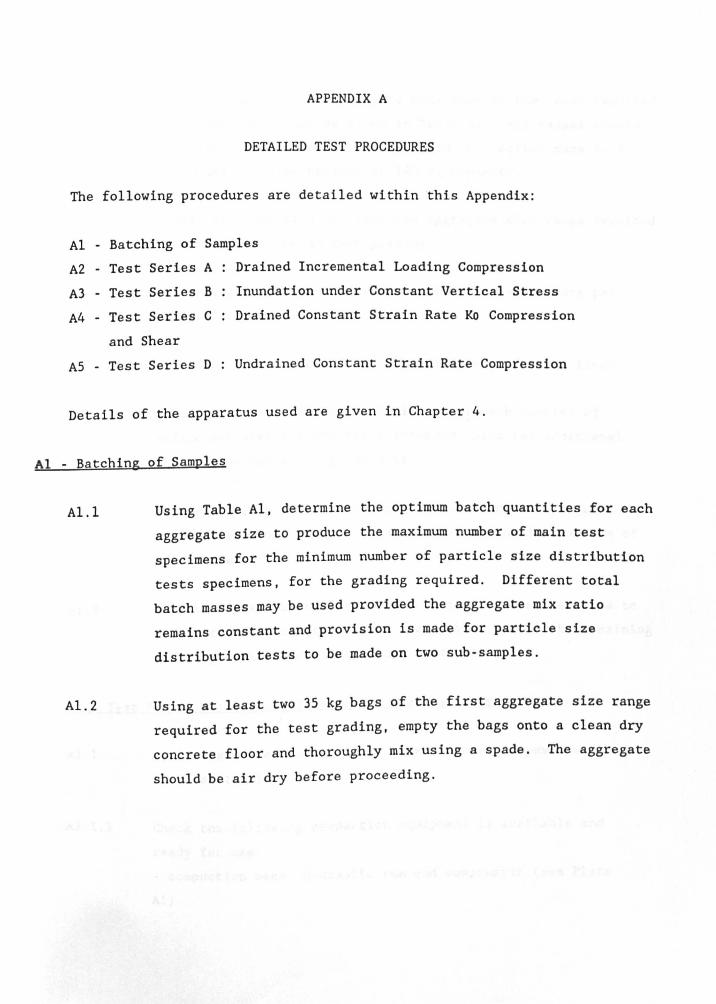
APPENDIX A
DETAILED TEST PROCEDURES
The following procedures are detailed within this Appendix:
Al - Batching of Samples
A2 Test Series A Drained Incremental Loading Compression
A3 Test Series B Inundation under Constant Vertical Stress
A4 Test Series C Drained Constant Strain Rate Ko Compression
and Shear
AS - Test Series D Undrained Constant Strain Rate Compression
Details of the apparatus used are given in Chapter 4.
Al - Batching of Samples
Al.l Using Table Al, determine the optimum batch quantities for
aggregate size to produce the maximum number of main test
each
specimens for the minimum number of particle size distribution
tests specimens, for the grading required. Different total
batch masses may be used provided the aggregate mix ratio
remains constant and provision is made for particle size
distribution tests to be made on two sub-samples.
Al.2 Using at least two 35 kg bags of the first aggregate size range
required for the test grading , empty the bags onto a clean dry
concrete floor and thoroughly mix using a spade. The aggregate
should be air dry before proceeding.

Al.3
Al.4
Al.S
Al.6
Al.7
Al.8
Al.9
Riffle or quarter the aggregate mass down to that mass required
for sample batching, as given in Table AI. All masses should
be weighed to the nearest 100 g. Add the correct mass to a
clean dry concrete batcher of 180 kg capacity.
Repeat Al.2 and Al.3 for each raw aggregate size range required
to prepare the chosen test grading.
Mix the aggregate in the concrete mixer for one minute per
every 10 kg of total batch mass.
Empty the mixed material onto the clean dry concrete floor.
Quarter the material successively to form sub-samples of
sufficient size for the tests intended, plus two additional
sub-sampled for grading analyses.
Double bag each sub-sample, and record the date, operator,
grading, specimen number, batch number, and designated use of
sub-sample.
Conduct wet sieve analyses on two of the batch sub-samples to
verify the correct grading has been formed before the remaining
sub-samples are used in the main test work.
A2 - Test Series A Drained Incremental Loading Compression
A2.l
A2.l.l
Preliminary Preparation (more than 24 hours in advance of
start of test)
Check the following compaction equipment is available and
ready for use: _ compaction base, hydrauliC ram and compressor (see Plate
AI)

A2.l.2
A2.l.3
A2.l.4
- 7 compaction base bolts for attaching cell body to
compaction base and 3 compaction base plugs for use during
sliding of cell body across compaction base
- electric Kango hammer. power transformer and compaction
plate (see Plate Al)
- compaction guide and 4 bolts to maintain Kango vertical
during compaction (see Plate Al)
- thin rigid measuring plate of diameter 200 rom to 240 rom and
constant thickness
- clock with second hand
- grease
- plasticine
_ 300 rom vernier calipers accurate to 0.01 rom
- large water content trays
- chalk
De-air the ceramics and check the ceramic response times as
detailed in Section 5.2.2 after every three tests at least.
Immerse ceramics in water when ceramics are sufficiently
de-aired.
Assemble the top platen as shown in Figure 4.2 and Plates A2
and A3 and place the platen such that the face of the top
ceramic face is in water. Connect the load cells to the power
source and leave for at least 24 hours before commencement of
step A2.2.
Select previously batched test sample (see appendix Al) and
oven dry in a dry tray of known mass for a minimum of 12
hours. or 24 hours if water had access to the bag during
storage.

A2.l.5
A2.l.6
A2.l.7
A2.1.8
A2.2
A2.2.l
A2.2.2
A2.2.3
As detailed in Section 5.2.1, check the plumbing system for
the test is de-aired, and that all transducers are
operational. Leave transducers under power for a minimum of
24 hours before the test.
Fill the de-aired water header tank with de-aired water, and
leave under vacuum.
Lock the compaction plate shaft in a lathe and if necessary
skim the plate surface until it is perpendicular to the shaft
at all points.
Place the compaction guide over the compaction plate shaft,
and adjust the guide bolts until the shaft just slides
through the guide under gravity, and no play exists between
the shaft and guide. Lock the guide bolts in position.
Specimen Preparation
Remove the aggregate to be tested from the oven and leave to
cool to room temperature.
Weigh the aggregate to the nearest gramme, and calculate the
volume of water to be added to this mass to prepare a
specimen of the desired water content (ie free water plus
absorbed water).
Add the required amount of water to the soil and mix
carefully and thoroughly by hand. Leave the mixed soil for
two hours, covered with a plastic sheet to reduce
evaporation, and prepare the compaction equipment.

A2.3
A2.3.1
A2.3.2
A2.3.3
A2.3.4
Preparation of Compaction Equipment
Lightly grease the compaction base surface and rubber gasket,
the gasket on the base of the cell body, and the inner
surface of the cell body.
Set the guides on the compaction base using the adjusting
screws such that the cell body is able to slide freely but
not deviating from a straight line along the plate to the end
guide. The body should not require more than a light push to
keep it moving, and should terminate at the end guard with
the bolt holes of the cell body and the cell base co-axial.
Note the orientation of the cellon the compaction base for
which the guides are set.
Place the cell base on the floor and completely fill the base
platen spiral with water, ensuring no air bubbles are
visible. Remove the base ceramic from its vater filled
container and place onto the cell base. Cover the ceramic
with damp absorbent paper.
With the cell base and ceramic placed loosely in the
semi-circle of the compaction base, level the compaction base
by adjusting the four base legs until the compaction base and
ceramic form a near planar surface with the compaction base
plane less than O.Smm above the ceramic. Vhen set, constrain
the ceramic and cell base in place with the end guide, and
double check the setting. Release the ceramic and base, and
make final adjustments as necessary to ensure the correct
setting.

A2.3.5
A2.3.6
A2.3.7
A1.3.B
A2.4
A2.4.1
A2.4.2
Without disturbing the base, draw chalk rings around the
compaction base legs to define their location, and fix their
adjustment using the lock nuts. Note the orientation of the
assembled cell base and ceramic and move the ceramic away
from any source of vibration.
Form smooth plugs of plasticine in the three cell base and
ceramic bolt holes that will lie nearest to the compaction
base (holes X, Y, Z in Figure A1).
Insert the ram head into the hydraulic ram and bolt the cell
body (gasket downwards) onto the compaction base in its
correct orientation using the seven bolts A to G shown in
Figure A1.
Measure and note the internal depth of the cell at six
equidistant positions around the cell circumference using the
vernier and measuring to the nearest 0.01 mID •
• Specimen Compaction and Initial Cell Assembly
Remove the plastic sheeting from the prepared specimen and
weigh the mixed soil to the nearest gramme.
Hand mix the specimen again, then carefully add material to
the cell until a pre-compacted height of about 130mm is
achieved. Ensure the material is placed such that the
apparent distribution of particles is even. and take two
water content samples (to BS1377: 1975, Clause 1.5.3) after
about a third and two thirds of the material have been added.
Use the material left in the mixing tray having third water
content test. Note all wet and dry masses.

A2.4.3
A2.4.4
A2.4.S
A2.4.6
A2.4.7
A2.4.8
A2.4.9
A2.4.10
A2.4.11
Place the compaction plate and guide on the cell, letting the
plate rest lightly on the soil surface. Bolt the compaction
guide onto the Rowe Cell body.
Lower the Kango unit over the compaction plate shaft and lock
in place.
Compact the specimen for 10 seconds, applying 3S0N to 400N
force to the Kango (see section ' 4.1.2.1).
Unbolt the guide from the cell, and slowly rotate the Kango
to break any suction before pulling the Kango and guide out
of the cell. Negligible material should be left on the
compaction plate.
Lightly place a measuring plate of known thickness onto the
compacted surface, and measure the depths to the plate at six
equidistant positions around the cell circumference using the
vernier. Note depths. If the observed specimen tilt exceeds
l.Smm over the diameter, reject the specimen.
Remove the measuring plate and cover the cell with a damp
cloth to minimise evaporation. Note time.
Re-locate the compaction base legs in their pre-compaction
positions, as indicated by the chalk rings.
Remove from the cell body the three bolts nearest the
semi-circle and replace from underneath with the metal plugs.
Ensure the plugs, stamped A, B or C, are placed in the
corresponding holes (see Figure A1).
Remove the remaining four bolts from the cell, thereby
releasing it from the compaction base.
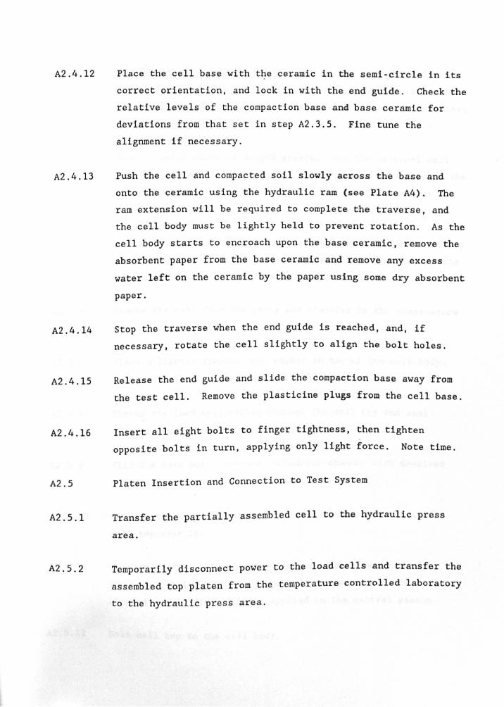
A2.4.12
A2.4.13
A2.4.14
A2.4.IS
A2.4.16
A2.5
A2.S.1
A2.S.2
Place the cell base with t~e ceramic in the semi-circle in its
correct orientation, and lock in with the end guide. Check the
relative levels of the compaction base and base ceramic for
deviations from that set in step A2.3.S. Fine tune the
alignment if necessary.
Push the cell and compacted soil slowly across the base and
onto the ceramic using the hydraulic ram (see Plate A4). The
ram extension will be required to complete the traverse, and
the cell body must be lightly held to prevent rotation. As the
cell body starts to encroach upon the base ceramic, remove the
absorbent paper from the base ceramic and remove any excess
water left on the ceramic by the paper using some dry absorbent
paper.
Stop the traverse when the end guide is reached, and, if
necessary, rotate the cell slightly to align the bolt holes.
Release the end guide and slide the compaction base away from
the test cell. Remove the plasticine plugs from the cell base.
Insert all eight bolts to finger tightness, then tighten
opposite bolts in turn, applying only light force. Note time.
Platen Insertion and Connection to Test System
Transfer the partially assembled cell to the hydraulic press
area.
Temporarily disconnect power to the load cells and transfer the
assembled top platen from the temperature controlled laboratory
to the hydraulic press area.

A2.S.3
A2.S.4
A2.S.S
A2.S.6
A2.S.7
A2.S.B
A2.S.9
A2.S.10
A2.S.11
A2.S.12
Place the top platen on the top of the cell such that all
internal plumbing and electrical connections between the cell
top and the platen will not interfere with and/or prevent final
assembly.
Place a metal plate of length greater than the external cell
diameter but width less than the cell internal diameter, on the
top platen (see Plate AS) and ensure the load cell cables are
coiled beneath it .
Place the assembly beneath the press and push the platen slowly
and evenly into the cell. Cease pressing when the metal plate
contacts the cell body flange at all points.
Remove the cell from the press and transfer to the temperature
controlled laboratory.
Place a lightly greased thin gasket on top of the cell body.
The gasket should be greased on both sides.
Thread the load cell cables through the cell top and seal
fittings, and connect to power. Note time.
Fill the base pore pressure transducer chamber with de-aired
water and connect to the cell base.
Connect the central piston to the top platen, then lower the
cell top over it.
Connect the internal plumbing lines for air pressure and
flushing, whilst supporting the cell top and preventing
excessive axial forces being applied to the central piston.
Bolt cell top to the cell body.

A2.S.13
A2.S.14
A2.S.IS
A2.S.16
A2.S.17
A2.S.IB
A2.S.19
Connect the external plumbing lines to the cell for air
pressure, cell pressure, and flushing (see Figure 4.1b).
Position the LDVT over the central piston with its armature
almost fully compressed (see Plate A6).
Remove the vacuum from the header tank and open the supply
valve (see Figure A2). With water flowing. connect the pipe to
the cell pressure bladder cell through the base water vent,
then open it.
Open the cell pressure valve at the cell top and the pressure
chamber vent. Water should now flow and slowly fill the cell
pressure chamber.
When water starts to flow out of the cell pressure chamber
vent, gently rock the cell with the vent open to remove any
trapped air. Close all the valves opened in steps A2.S.IS to
A2.S.17 except for the air vent at the top of the header tank.
Apply 10 kPa pressure to the flushing system with the flushing
and drain lines open at the top and bottom of the cell and
thereby flush de-aired water through the pl atens. Continue the
flow for several minutes to remove any trapped air then close
the drainage valves on the cell.
Isolate the air volume indicators from the rest of the plumbing
system using the AVI bypass and isolation valves. Apply 10 kPa
back pressure to the top and bottom of the de-aired volume
change units (see section S.2.1) and, when water starts to flow
slowly out of the unconnected pipes from the volume change
units and any air that was visible in the pipes is removed,
open the drainage valves on the cell. With water flowing
slowly from both pipes and both valves, connect the volume
change units to the test cell to form a closed de-aired
measurement system.

A2.S.20
A2.S.21
A2.S.22
A2.6
A2.6.1
A2.6.2
A2 . 6.3
A2 .6.4
A2.6.S
Adjust the flushing pressure and back pressures such that water
flows into or out of the volume change units until the units
are set near either end of their travel.
Close all drainage and flushing valves at the cell, leaving the
pore pressure transducers connected to the platens but isolated
from the rest of the system.
Remove the pressure from the flushing and drainage systems.
Initialising the Test System
Initiate the logging system (See section 4.1.3.3 and Appendix
C) with a scan rate of 30 seconds. Use gain 1 for the LVOT and
use the default calibration factors and offsets.
Apply a cell pressure of 2S kPa to the top platen using the low
pressure regulator.
Apply 2.5 kPa increments of cell pressure approximately every
30 seconds until the "break loose pressure- is reached, as
recorded by the onset of continuous movement of the LVOT
armature. Note this pressure, which is typically about 50 kPa.
Reduce the cell pressure in decrements of 2.5 kPa until
movement stops (typically at about 40 kPa). Note this
pressure.
Calculate the estimated LVDT output at which contact will occur
between the specimen and the descending top platen, from a
knowledge of the initial specimen clearance from the cell top,
the height of the assembled top platen, the LVOT calibration
factor, and the initial LVDT reading (see Section 6.1.1.3).

A2.6.6
A2.6.7
A2.6.B
A2.6.9
A2.6.10
A2.6.11
A2.6.l2
A2.6.13
Increase the cell pressure as described in step A2.6.3 until
movement restarts, then reduce the applied cell pressure to
about 2 . 5 kPa above that pressure when movement first stopped.
Allow the platen to slowly slide towards contact with the soil.
constantly compare the estimated LVDT output at first contact
with that recorded by the logging system, and when contact is
imminent, reduce the cell pressure such that the rate of platen
descent is less than O.lmm every 30 seconds.
When contact occurs, the load cell outputs will change and LVDT
movement will cease. Quickly reduce the cell pressure to about
25 kPa to avoid an excessive load surge being applied to the
specimen by a local reduction in friction.
Increase the cell pressure until the load cells, which will be
recording an applied specimen stress somewhere near maximum
contact stress due to side friction limiting upwards movement
of the platen, start to show a small increase in net applied
stress. Hold this first loading stress and note the cell
pressure.
Apply an air pressure of 5 kPa to the specimen using the low
pressure regulator thereby reducing the net applied stress to
the soil and decreasing the applied specimen (or load cell)
stresses.
Increase the cell pressure by about 5 kPa to re-apply an
applied specimen stress equal to the first loading stress.
Repeat steps A2.6.10 and A2.6.1l until the intended
axis-translation pressure (air pressure) is achieved. Usually
an air pressure of 100 kPa was used.
Re-set the position of the LDVT in its claap until its output
is at the top of its maximum accuracy range of output, as
determined from the calibrations.

A2.6.l4
A2.6.1S
A2.7
A2.7.l
A2.7.2
A2.7.3
A2.7.4
A2.7.S
A2.7.6
A2.7.7
Stop the data acquisition program and restart immediately as a
new file. Input the calibration constants for on screen
engineering units output (see Appendix C) and use a scan rate
of 900 seconds.
Leave the specimen for 24 hours or until sensibly constant pore
pressures top and bottom are recorded, whichever is the longer.
Check the stability of the regulating pressures and voltage
supplied periodically. Close the file when this equalisation
stage is completed.
Initialising Base Drained Conditions
Initiate a new file with the same calibration constants as used
during the equalisation stage. Use an initial scan rate of 1
minute.
Close the base drainage valve between the pressure transducer
and the cell and open the valve between the transducer and
drainage system.
Note the reading of the air volume indicator at atmospheric
pressure, with the indicator connected to the main drainage
line and the bypass valve closed.
Apply a back pressure to the drainage line equal to the
equilibrium base pore pressure, as recorded by the base
pressure transducer.
Record the new reading of the base air volume indicator.
Open the base drain between the pore pressure transducer and
the cell, thereby allowing drainage at the original equilibrium
suction.
Leave the cell for a minimum of 1 hour to check for leaks - no
Volume change should occur within the specimen.

A2.B
A2.B.1
A2.B.2
A2.B.3
A2.B.4
A2.B.S
A2.B.6
Application of First Loading Increment (usually 10 kPa)
Increase the scan rate to 10 seconds.
Close the cell pressure valve at the top of the cell.
Increment the cell pressure by 10 kPa and open the cell
pressure valve immediately after a noted scan number.
Observe the increase of average load cell stress for 30 seconds
and, if the applied vertical increment of 10 kPa has not been
fully transferred within that time, apply a smaller cell
pressure movement and observe the change in average applied
stress. Repeat every 30 seconds until the applied stress is
reached, usually within 2 minutes. Continual checks for load
surges due to sudden loss of side friction should be made, and
the cell pressure rapidly reduced if necessary. If a large
surge occurs such that the average stress applied to the soil
exceeds 12 kPa a further cell pressure increment should be
applied to achieve a revised target applied stress equal to the
surge value.
When the required average applied stress is recorded by the
load cells, leave the apparatus for 5 minutes except for finely
adjusting the cell pressure to maintain the applied stress as
the side friction decreases. Reduce the scan rate to 30
seconds at the end of this period.
Continue fine adjustments to the cell pressure as the test
proceeds and alter the scan rates approximately as follows:
after a further 10 minutes, reduce the scan rate to every minute
after a further 30 minutes, reduce the scan rate to every 5 minutes
after a further 60 minutes, reduce the scan rate to every 15 minutes
after 24 hours, reduce the scan rate to every 30 minutes

A2.8.9
A2.9
A2.9.1
A2.9.2.
A2.l0
A2.l0.l
A2.l0.2
A2.l0.3
A2.l0.4
When the pore pressures and axial strain have sensibly
stabilized stop this stage of the test.
Application of Subsequent Increments/Decrements
Application of a load increment follows the procedure detailed
in step A2.8 but the cell pressure changes used (step A2.8)
should be varied in . accordance with the required changes in the
average vertical stress. The subsequent increments usually
used were 10 kPa to 25 kPa, 25 kPa to 50 kPa, 50 kPa to 75 kPa ,
and 75 kPa to 100 kPa.
Application of a load decrement is similar to application of a
load increment but load decrement surges were not a problem.
Load decrements usually used were 100 kPa to 50 kPa, 50 kPa to
25 kPa, and 25 kPa to 5 kPa.
Final Unloading and Dismantling of the Test
Initiate the last data file and set a scan rate of 10 seconds.
Close the cell pressure line and reduce the cell pressure to
zero. Open the pressure valve immediately after a noted scan
number.
Allow the top platen to be pushed upwards by the air pressure
in the cell. and displace cell chamber water. Open the base
water vent of the cell pressure bladder cell to accommodate
this displacement. Close the vent when the platen travel limit
is reached and stop the data logging program.
Reduce the back pressure to the drainage line to zero. Close
the air volume indicator isolation valves, thereby preventing
air entering the rest of the plumbing.

A2.l0.S
A2.l0.6
A2.l0.7
A2.l0.8
A2.l0.9
A2.l0.l0
A2.l0.ll
A2.l0.l2
Disconnect the top and bottom drainage lines, open the drain
valves to atmospheric pressure, and reduce the cell air
pressure to zero.
Disconnect the load cells from the power source, and disconnect
all connections from the top of the cell.
Unbolt and raise the top of the cell. Disconnect pipes from
the top of the cell and remove it. Remove the central piston
and flange gasket.
Remove the water contained in the top platen recess using
absorbent paper, then disconnect the air and flushing
connections from the top platen.
Place three spacers on top of the top platen to prevent the
screw jack-top platen connection from squashing the load cell
cables, then bolt the screw jack to the top platen and to the
cell body.
Operate the screw jack and raise the top platen until it is
free of the consolidation cell (see Plate A7). Unbolt and
remove the jack.
Remove the top platen from the cell, invert it, and rest upon
two wooden blocks as shown in Plate A3 such that the weight of
the top platen does not rest upon the load cell cables.
Check the top ceramic for surface damage or cracks, remove the
locking ring from the top platen and check the underside of the
ceramic. Place the ceramic in water immediately to prevent any
evaporation and consequent air entry into the ceramic. Note
any observations on cracking.

A2.l0.l3
A2.l0.l4
A2.l0.lS
A2.ll
A2.ll.l
A2.ll.2
A2.ll.3
A2.ll.4
A2.ll.S
Examine the 0 ring seals of the top platen and check for
evidence of water seepage past them. Note any observations.
Remove the specimen in three approximately equal layers and
determine the water content of each layer.
Unbolt the cell body from the base and check the base ceramics
for cracking in a manner similar to that given in step
A2.l0.l2. Immerse base ceramic in water.
Operation of the Flushing System
Periodically throughout a test, it is necessary to determine
the volume of diffused air that has passed through the top and
base ceramics. Typically, this should be done at the end of
equalisation, and after every 2 loading stages thereafter. The
flushing procedure to be used is as follows:
Reduce the scan rate to 30 seconds.
With the flushing inlet to the cell closed set a flushing
pressure equal to the back pressure plus 10 kPa.
Note the air volume indicator readings at the current back
pressure.
After the 30 second scan rate has been commenced, open the top
flushing inlet and top drain, thereby flushing water and
diffused air toward the air volume indicator. Reduce the
flushing differential to 5 kPa as the bubbles approach the air
volume indicator and start to become trapped .
Continue flow until the volume change unit nears the end of its
travel, and close the flushed line. Note the new air volume
indicator reading and the back pressure.

A2.ll.6
A2.1l.7
A2.l1.8
A2.11.9
A2.1l.l0
Reverse the flow direction into the volume change unit using
the reversing valve, and re-open the flushing line.
Repeat steps A2.ll.5 and A2.ll.6 until no more air is
displaced. After the last reverse, increase the flushing
differential to 20 kPa. Repeat one more reverse sequence or
until no more air is displaced.
Note the final top air volume indicator reading at the set back
pressure, then close the top drain valve beyond the transducer
and flushing inlet valve.
Repeat steps A2 .1l.4 to A2.ll.8 for the base platen.
Continue the test stage in progress, making gradual decreases
in scan rate to that existing before the flushing procedure,
such that the pore pressure response curves are recorded.
A3 - Test Series B Inundation under Constant Vertical Stress
A3.1 Preliminary Preparation to Application of First Loading
Increment .
As for test series A, but use an air pressure of 50 kPa and
omit stage A2.7.
A3.2 Application of subsequent Increments and Flushing.
As for tests series A, tests 7 to 10, using the same increments
but terminating at either a maximum applied vertical stress of
50 kPa or 75 kPa nominally.
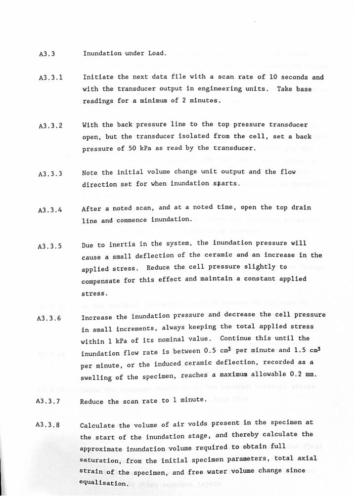
A3.3
A3.3 . l
A3.3.2
A3.3.3
A3 . 3.4
A3.3.5
A3.3.6
A3.3.7
A3.3.8
Inundation under Load.
Initiate the next data file with a scan rate of 10 seconds and
with the transducer output in engineering units. Take base
readings for a minimum of 2 minutes.
With the back pressure line to the top pressure transducer
open, but the transducer isolated from the cell, set a back
pressure of 50 kPa as read by the transducer.
Note the initial volume change unit output and the flow
direction set for when inundation s~arts.
After a noted scan, and at a noted time, open the top drain
line and commence inundation .
Due to inertia in the system, the inundation pressure will
cause a small deflection of the ceramic and an increase in the
applied stress. Reduce the cell pressure slightly to
compensate for this effect and maintain a constant applied
stress.
Increase the inundation pressure and decrease the cell pressure
in small increments, always keeping the total applied stress
within 1 kPa of its nominal value. Continue this until the
inundation flow rate is between 0.5 cm3 per minute and 1.5 em!
per minute, or the induced ceramic deflection, recorded as a
swelling of the specimen, reaches a maximum allowable 0.2 mm.
Reduce the scan rate to 1 minute.
Calculate the volume of air voids present in the specimen at
the start of the inundation stage, and thereby calculate the
approximate inundation volume required to obtain full
saturation, from the initial specimen parameters, total axial
strain of the specimen, and free water volume change since
equalisation.

A3.3.9
A3.3.10
A3.3.11
A3.3.12
A3.3.l3
A3.3.14
A3.3.15
A3.4
When the volume change unit approaches its limit of travel,
reverse the flow valves. Note the time, scan number and volume
change unit output when reversal occurred. Adjust the
inundation pressure regulator to compensate for the addition or
loss of the volume change unit piston mass.
Calculate the total volume inundated up to reversal from the
noted change in output of the volume change unit since the last
reversal, the volume change unit calibration factor for the
flow direction just completed, and inundation total prior to
commencement of the cycle just completed. Re-calculate the
total volume of inundation required for saturation as detailed
in step A3.3.B.
Continue inundation, reversing valves and adjusting pressures
as required, until full saturation is achieved.
Close the inundation line leaving the top transducer still
connected to the cell. Note the time, scan, and volume change
unit output, and calculate the final inundated volume.
As the residual inundation pressure reduces in response to
further flow, continually check and increase the cell pressure
to maintain a constant applied vertical stress.
When stable top pore pressure conditions are reached, reduce
the scan rate to 5 minutes.
Leave the specimen overnight at the constant vertical stress
during inundation, then close the data file.
Load Decrements and Dismantling of the Tests
As detailed in stage A2.l0 for test series A, except the final
water content of the test specimen is deterained ~n the basis
of a single water content test using the whole test specimen
rather than in three separate layers.

A4 - Test Series C
Shear
Drained Constant Strain Rate Ko Compression and
A4.l
A4.1.l
A4.1. 2
A4.1. 3
A4.1.4
A4.1. 5
A4.2
A4.2.l
Preliminary Preparation (more than 24 hours in advance of the
start of the test)
Fill the drainage annulus of the triaxial base pedestal with
de-aired water then cover with the high entry ceramic which
should have been sealed into its locking ring already. Bolt
the locking ring and ceramic down onto the base pedestal.
De-air the high air entry ceramic and check its response time
(see Section 5.2.2). When the ceramic is sufficiently
de-aired, place a layer of saturated absorbent paper on the
surface of the ceramic and encapsulate the base pedestal.
absorbent paper. and ceramic. with a cling film wrapping held
in place with an elastic band.
Place the previously batched specimen (see Appendix Al) in an
oven at l050 c and leave for 12 hours. or 24 hours if water
had access to the sample during storage. The minimum dry
mass required is 35 kg.
De-air the system plumbing (see Section 4.2) in a manner
similar to steps A2.5 . l5 to A2.5.l9.
Connect all transducers to the power supply.
Preparation of Equipment Immediately before Preparation
Remove the sample from the oven and leave to cool to room
temperature.

A4.2.2
A4.2.3
A4 . 3
A4.3.l
A4.3.2
A4.3.3
A4.3.4
Check the following apparatus is available and ready for use:
- three piece split former, assembled with internal joints
sealed with sellotape
- plasticine
- four '0' rings and two triaxial rubber membranes for
sealing specimen
- filter paper
- wooden tamping rod
_ de-aired water supply
_ vacuum foot pump connected to water manometer and water
collector bottle (see Figure A2)
_ thin wire more than 0.7 m in length, and metre rule
_ fork-lift truck and lifting tackle
Weigh the sample when cool and note.
Specimen Preparation Part 1 - All SpeciDens
Remove the cling film wrapping from the base pedestal ceramic
but leaving the damp absorbent paper covering the ceramic.
Stretch the membranes, one at a time, over the base pedestal
and ceramic.
,
Place a double '0' ring seal on the membrane in the
conventional arrangement, using the assembled split former as a
guide.
Lower the split former over the pedestal, taking care not to
Push the former down until it is about Smm snag the membranes.
or less from the base of the triaxial cell_ Seal this small
gap with a bead of plasticine.

A4.3.5
A4.3.6
A4.3.7
A4.3.S
A4.3.9
A4.3.10
A4.3.ll
Attach the vacuum foot pump to the former and stretch the outer
membrane over it. Apply and maintain light suction, smooth the
outer membrane to the inner surface of the former and stretch
the inner membrane into position.
Secure the membranes in position with an '0' ring.
Remove the saturated paper from the ceramic, and replace with a
damp filter paper of diameter slightly smaller than the
pedestal.
Place dry soil up to just over the quarter height of the
former, in an apparently even particle size distribution.
Compact the specimen with 35 evenly distributed blows of the
wooden tamping rod.
Repeat step A4.3.S for the second to fourth layers, but reapply
the vacuum on the membranes after the second layer. The final
layer should be about 10 mm below the top of the former before
compaction, and 20 mm after. Fine material should be added to
the top to present a smooth surface to the top platen.
Remove and reapply the vacuum again, and add some extra
material if small slumping occurs. Lightly tamp in place with
a few light blows of the tamper. The final level should be
slightly above the mating groove for the top platen (see Plate
AS).
Weigh the unused material and thereby calculate the dry mass of
the specimen.

A4.4
A4.4.1
A4.4.2
A4.4.3
A4.4.4
A4.4.S
A4.4.6
A4.5
A4.5.l
A4.5.2
A4.5.3
Specimen Preparation
Only
Part 2A - Damp and Saturated Specimens
Slowly pour a known volume of de-aired water into the top of
the specimen until the former is apparently saturated. Leave
for 5 minutes, then top up with more water of noted volume.
Cover with cling film and leave for at least 1 hour.
Remove the cling film and top up once more to the top level of
the specimen. Only a little extra water should be required.
Firmly press the top platen into the top of the former, roll
the membranes over it, and seal them in a manner similar to
that of the base pedestal .
Connect the vacuum pump via the manometer and collector bottle
to the top platen only (see Figure A2 and Plate A9).
Apply a maximum suction of 15 kPa to the specimen to suck from
the soil. This suction will need to be reapplied every minute
approximately to maintain the flow. Measure the total volume
that is removed under this vacuum.
With a suction of 15 kPa applied, close valve A (see Figure A2)
and observe the water column between the specimen and the
valve. Continuous movement implies the membranes have
punctured, and the test must be aborted.
Specimen Preparation Part 2B - Dry Specimens Only
Press the top platen into position, as in step A4.4.3.
Connect the vacuum pump and the manometer to the top platen air
line, as shown in Figure A2.
Apply a suction of 15 kPa, hold for 30 seconds, and close valve
A.

A4.6 Specimen Preparation Part 3 - All Soils
A4.6.l
A4.6.2
A4.6.3
A4.6.4
A4.7
A4.7.l
A4.7.2
A4.7.3
A4.7.4
A4.7.S
Remove the plasticine seal from the base pedestal.
Release the screw locks on the split former. Insert a
screwdriver into one of the split former joints, and carefully
prise apart. Dismantle and remove the foraer.
Using the thin wire, measure the circumference of the now
free-standing specimen at five equidistant levels over the
whole specimen height.
Using the metre rule, measure the specimen height at six
locations equidistant around the specimen circumference.
Cell Assembly
Grease the triaxial cell loading ram and secure at the top of
its travel using the clamp.
Using a fork lift and tackle, lift the cell top over the
specimen and seal the chamber. Lower the loading ram into
light contact with the specimen. Fill the cell with water.
Using the fork lift, raise the entire cell and position on the
strain controlled triaxial compression machine. Secure in place
with rope temporarily.
Attach the cross beam, level it, and secure the triaxial cell.
Remove the rope.
Taking care not to release the vacuum in the specimen, connect
all plumbing and transducers to the cell, bleeding the lines by
flushing through with water to ensure no air is trapped.

A4.7.6
A4.7.7
Apply a cell pressure of 30 kPa (or SO kPa for dry specimens)
at the specimen mid height.
Apply a pore water back pressure of 20 kPa to the base pedestal
(or a pore air pressure of 70 kPa or 20 kPa to the top platen
for dry and unsaturated specimens respectively), thereby
releasing the vacuum (see Plate A10).
A4.8 Initial Specimen Saturation (for Saturated Specimens Only)
A4.S .1
A4.S.2
A4 . S.3
A4.S.4
Initiate the computer logging system. Check all transducer
allocations and start the saturation stage of the software.
Apply a cell pressure increment of 30 kPa after preventing
water drainage from the base. Monitor the pore water pressure
response and calculate the B value. Compare the computer
calculated value with that calculated by hand from the digital
voltmeter output.
Increment the pore water back pressure by 30 kPa, then return
the specimen to a water undrained condition.
Repeat Steps A4.8.2 and A4.8.3 until B is greater than or equal
to 0.95, applying a change in cell pressure of 50 kPa, or as
calculated using the equation below, whichever is the lesser.
This will ensure a maximum difference between total and pore
water pressure of 30 kPa. Return this differential to 10 kPa
after calculating B each time. The equation used to determine
the maximum increase in cell pressure is given below:
1lf!'3 - 30 + u - tl3
l-B
where Llcr,- change in cell pressure, u - current pore water
pressure, and all pressures are in kPa.

A4.8.S
A4.9
A4.9.1
A4.9.2
A4.9.3
A4.9.4
A4.10
A4.10.1
A4 . l0.2
A4.l0.3
A4.l0.4
A4.11
A4.11.1
Terminate the saturation stage of the software.
Consolidation Stage (for saturated specimens only)
Start the consolidation stage of the soft¥are.
Increment the cell pressure to the current pore water back
pressure plus 30 kPa, and apply to the specimen when the data
acquisition unit is activated by the computer.
Computer readings are taken automatically on a root time basis ,
but take manual readings of the voltmeters on a root time basis
for a back-up.
Continue consolidation until volumetric straining has sensibly
ceased. Stop this stage of the software.
Consolidation Stage (for dry specimens only)
Initiate the computer logging system as in step A4.S.1. Omit
the saturation stage of the software.
Start the consolidation stage of the software.
Increment the cell pressure to 100 kPa, and apply to the
specimen when the data acquisition unit is activated by the
computer.
Perform steps A4.9.3 and A4.9.4, then stop the consolidation
stage of the software.
Consolidation Stage (for Unsaturated Speciuens Only)
Increment the cell pressure and pore air pressure,
respectively, by 10 kPa, until the cell pressure reaches SO kPA
and the air pressure reaches 70 kPa.

A4.1l.2
A4.12
A4.12.1
A4.12.2
A4.12.3
A4.12.4
A4.13
A4.13.l
A4.13.2
A4.13.3
A4.13 .4
A4.l3.S
Perform steps A4.10.1 to A4.10.4.
1<0 Stage
Start the shear stage of the software, specifying a scan rate
of 1 minute.
When data acquisition begins, start loading the specimen
axially at a strain rate of 0.1 mm per minute.
Using the corrections detailed in Chapter 6, adjust the cell
pressure to maintain Ko conditions, until the deviator stress
exceeds 100 kPa. Take manual readings frequently throughout
this stage.
Stop the triaxial loading platen and the software.
Stages Intermediate Between Ko Stage and Shear Stage
Start a "new" test with the software, and begin a shear stage
again. Use a scan rate of 5 seconds.
When data acquisition begins, start unloading the specimen by
reversing the triaxial machine platen direction at 0.1 mm per
minute. The specimen should be air and water undrained during
the unloading.
When the deviator stress is less than 5 kPa, stop the software
and the triaxial machine.
Start a "new" test again as in step A4.l3.l.
When data acquisition begins, start reducing the cell pressure
with the specimen air and water undrained at about 10 kPa per
minute, until the original consolidation cell pressure is
reached.

A4.13.6
A4.13.7
A4.14
A4.14.1
A4.14.2
A4.14.3
A4.14.4
A4.14.S
A4.14.6
A4.14.6
Open the drainage line to the specimen and allow the membrane
to be pushed out as the pore air pressure is raised back to
original pore pressure.
Stop the software.
Shear Stage and Dismantling
Start a "new" test, as in step A4.13.1, but specify a scan rate
of 1 minute.
When data acquisition begins, start loading the specimen to
failure at a strain rate of 0.1 mm per minute and at a constant
cell pressure. Take periodic manual readings as a back-up to
the computer readings.
Continue the test until axial straining of the specimen has
exceeded the strain at peak stress by about 1\. Reverse the
triaxial platen direction and unload the specimen to zero
deviator stress.
Stop the software and reduce the cell pressure to atmospheric
pressure.
Drain and strip the cell.
Dismantle the specimen in four layers, and determine the water
content of each layer.
Cover the base ceramic with saturated paper and cling film, as
detailed in stage A4.1 . 1.

AS - Test Series D Undrained Constant Strain Rate Compression
AS.l Preliminary Preparation (more than 24 hours in advance of start
of test).
AS.l.l
AS.l.2
AS.l.3
AS . 2
AS.3
AS.3.1
AS.3.2
A5.3.3
Place a previously batched sample (see Appendix AI) in the oven
at lOSoC and leave for a minimum of 12 hours, or 24 hours if
water had access to the sample during storage. The minimum dry
mass required for the main test specimen and two water content
tests was 30 kg for the coarse and medium grading, or 25 kg for
the fine grading.
Slide the compaction guide over the compaction plate shaft, and
adjust the guide bolts such that the shaft just slides through
under gravity and no play exists between the shaft and guide.
Connect all transducers to power supply.
Specimen Preparation
See Appendix A2.2.
Specimen Compaction and Cell Assembly
Ensure the compaction cell is clean and dry, and measure the
internal height of the cell at four equidistant locations on
the cell circumference. Place the cellon a sound concrete
floor.
Two hours after mixing the sample, uncover the prepared sample
and weigh.
Add the material and compact using compaction method (a) or (b)
b I i an apparently even particle size distribution e ow, ensur ng
results and two water content samples are taken from the mix
material during addition of the aggregate to the cell.
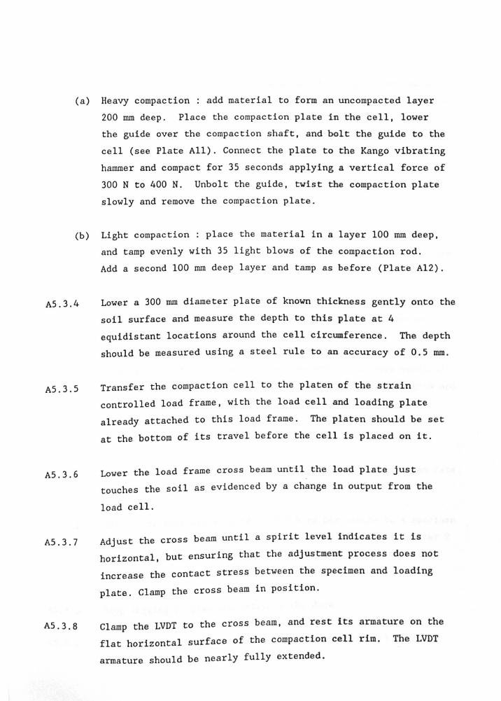
(a) Heavy compaction : add material to form an uncompacted layer
200 rom deep. Place the compaction plate in the cell, lower
the guide over the compaction shaft, and bolt the guide to the
cell (see Plate All). Connect the plate to the Kango vibrating
hammer and compact for 35 seconds applying a vertical force of
300 N to 400 N. Unbolt the guide, twist the compaction plate
slowly and remove the compaction plate.
(b) Light compaction: place the material in a layer 100 rom deep,
and tamp evenly with 35 light blows of the compaction rod.
AS.3.4
AS.3.S
AS.3.6
AS.3.7
AS.3.8
Add a second 100 mm deep layer and tamp as before (Plate A12).
Lower a 300 rom diameter plate of known thickness gently onto the
soil surface and measure the depth to this plate at 4
equidistant locations around the cell circumference. The depth
should be measured using a steel rule to an accuracy of O.S mm.
Transfer the compaction cell to the platen of the strain
controlled load frame, with the load cell and loading plate
already attached to this load frame. The platen should be set
at the bottom of its travel before the cell is placed on it.
Lower the load frame cross beam until the load plate just
touches the soil as evidenced by a change in output from the
load cell.
Adjust the cross beam until a spirit level indicates it is
horizontal, but ensuring that the adjustment process does not
increase the contact stress between the specimen and loading
plate. Clamp the cross beam in position.
Clamp the LVDT to the cross beam, and rest its armature on the
flat horizontal surface of the compaction cell rim. The LVDT
armature should be nearly fully extended.

AS.3.9
AS.3.l0
AS.4
AS.4.l
AS.4.2
AS.4.3
AS.S
AS.S.l
AS.S.2
AS.S.3
AS.S.4
Check the LVDT and load cell leads to the computerised data
acquisition system, and check the computer channel allocations.
Check the LDVT operation by inserting slip gauges between the
armature and the cell, and comparing the computer output with
the known dimensions of the slip gauges.
Initial load increment
Initialise the computer logging system with a scan rate of 5
seconds and a maximum number of scans of 500. Input the initial
specimen parameters.
After at least 30 seconds, start stressing the specimen by
raising the triaxial machine platen at a rate of 0.5 mm per
minute.
Stop the platen when the load cell records an average vertical
stress on the specimen of l2S kPa. Stop the logging program and
retrieve the data.
Subsequent load cycling
Initialise the computer as in step AS.4.1, but using a scan rate
of 2 seconds.
Unload the specimen at a rate of 0.5 mm per minute to a specimen
stress of approximately 10 kPa, then apply at least a further 2
complete load cycles between 10 kPa and 125 kPa at the strain
rate of 0.5 mm per minute.
Stop logging program and retrieve the data.
Initialise a third test stage, with a scan rate of 3 seconds.

As.s.s
As.s.6
As.s.7
As.S.B
AS.S.9
AS.6
AS.6.1
AS.6.2
A5.6 . 3
AS.6.4
Apply 3 to 5 complete load cycles between 10 kPa and 250 kPa, at
a strain rate of 0.5 mm per minute.
Stop the logging program and retrieve the data.
Initialise a fourth test stage with a scan rate of 2 seconds.
Apply 3 to S complete load cycles between 10 kPa and 250 kPa, at
a strain rate of 2.5 mm per minute.
Stop the logging program and retrieve the data.
Dismantling of the Test.
Lower the triaxial machine platen to its limit, then raise the
cross beam such that the loading plate is about 10 mm clear of
the compaction cell.
Remove the cell from the triaxial machine, but leave the
transducers connected to the power supply ready for the next
test.
Remove the specimen in three approximately equal layers and
determine the water content of each.
If required, combine the three water content specimens after
drying and use this material to perform a grading analysis on
the test material.

* AGGREGATE SIZE RANGES SUPPLIED WERE: F - less than 5 mm K - 5 .. to 10 mm C - 10 mm to 20 mm
VC - 20 !lID to 40 mm

letails Of Jack
lot Shown~_
I I I I I I 1
'-
XF'
+ G
AX
I I
//
/ Xx
;;..-
Bolt Hole ~ Not Used B+ I+Y
\ \
Cx \
"xz "
"""
Bolt Holes A To G In .comp action Base Used To Attach Consolidation Cell Body To Base During Compaction
.........
+ --/
"
Consolidation Cell Base And Base Platen Restrained In Recess By Assembly Guides During Sliding Of Cell Body After Compaction. Bolt .Hole X. Y And Z Plugged With Plasticine During Sliding To Prevent Water Loss From The Specimen.
x". \ \
+
/ /
x/ ,/
Assembly Guides
Compaction Base
Figure A1 - Bolt Holes In Compaction Base and Consolidation Cell Base

Water Manometer
Suction applied by vacuum pump
t
Collector • Bottle
Soil
Top platen with annulus for application of air pressure (or vacuum) to specimen
platten
pedestal
Low table
Rgure A2 - Suction Pump And Manometer Connection To Specimen Before Ko And Shear Tests

Plate Al Kango hamme r and compaction guide for test series A and B
Plate A2 Component par ts of top platen for consolidation cell

Plate A3 Assembled top platen
Plate A4 Sliding of consolidation cell and compacted specimen across
compaction base using the hydraulic ram

Plate A6 Fully ass emb led
consolidation cell
Plate AS Insertion of top
platen into consolidation
cell using the hydraulic
press

Plate A7 Removal of top platen following completion of
test using the screw jack
Plate A8 Compaction of triaxial test specimen

Plate A10 Triaxial test
specimen ready for
commencement of test
Plate A9 Vacuum pump
and manometer used for
preparation of triaxial
test specimen
_r __ -- ~----- -- ~ - - ..... -- -

~ compactive Plate All Compaction apparatus used to apply a h;gh
effort to test specimens for use in test series D
Plate Al2 Compaction apparatus used to apply a low compactive
effort to test specimens for use in test series D

APPENDIX B
NAMES AND ADDRESSES OF SPECIALIST EQUIPMENT SUPPLIERS
Item(sl supplied
A.Volume Change Equipment
(i) Imperial college Volume Change Units
(ii) GDS Units, Model 8085
B.Displacement transducers
(i)
(ii)
Novatech LSC H5550 (5011m stroke)
Sangamo , submersible
(iii) RDP TyPe D5/2000A
(iv ) PentaY and Giles Rectilinear potentiometer TyPe HLPI90SAl/ 100Jam/4kohm
Name of supplier
Shape Instruments Ltd
Geotechnical Digital systems Ltd
Address
Transducer Works Toutley Road Wokingh811 Berkshire RGll SSS
26 Midway Walton-on-Thames Surrey KTl2 3HZ
Novatech Measurements Ltd 83 Castleham Road St Leonards-on-Sea East Sussex TN38 9NT
Sangamo Transducers North Bersted Bognor Regis West Sussex P022 9BS
RDP Electronics Ltd
Penny and Giles Potentiometers Ltd
Grove Street Heath Town Wolverhampton Staffordshire WIO OPY
Somerford Division Christchurch Dorset BH23 3RS

Item's) suppUed
C.Equipment for manufacture and calibration of 2.5 kN load cells:
(i) General equipment
(ii) Kyowa strain gauges
(iii) Dead weight testers
D.Commercial load cells
(i)
(11)
Hodel 1lF17109 10 leN capacity
Sensotec Hodel 41 (20 kN and 110 kN capac1 ties)
E.Pressure transducers
Name of supplier Address
Welwyn Strain Measurement Armstrong Road Bas ings toke Haapshire
Graham and White Instruments
RG24 OQA
135 Hatfield Road St Albans Hertfordshire ALI 4LZ
Budenburg Grange Co Ltd Box No 5 Altrinch811 Cheshire WA14 4ER
Whykbam Farrance Engineering Ltd
RDP Electronics l%d
Weston Road Trading Estate Slough Berkshire SLl 4HW
see earlier
(1) Bell and Howell Bell and Howell l%d
Hodel 4_366-0001-0lHohD
Lennox Road Bas ings toke Hampshire RG22 4AW
(ii) Druck PDCR 10 Druck Ltd Fir Tree lane Groby Leicestershire LE6 OFH

Item(s) supplied
F.Pressure regulation system
(i) Bourdon gauges
(ii) Nullmatic Pressure Regulators, Models 40-100 and 40-30HF
G.High air entry value ceramics
H.Isuzu thermo-hygro-barograph model 3-1135
I.Data acquisition system (University):
(i) Analogue input unit Model 13683
(11) IEEE Interface
J.Data acquisition system (British Gas):
(i) DEC PDP 11/44 mini computer
(ii) ADU 700 Datalogger
Name of supplier
Budenburg Gauge Co Ltd
Moore Products Co (UK) Ltd
Soil Moisture Equipment Corporation
Isuzu Seisakusho Co Ltd
or
J S Holdings (UK Supplier)
Me Computers
Acorn Computers Ltd
Digital Equipment Corporation
Mowlem Microsysteas Ltd
Address
see earlier
5 Queensbrook Bolton Lancashire 8Ll 4AY
PO Box 30025 Santa Barbara California USA
3-8-19 Nishi-Ochiai Shinju1cu-1cu Tokyo
56 Spring Drive Stevenage Hertfordshire SG2 SAZ
Strawberry Hill House
Newbury Berkshire
Yulbourn Road Cherry Hinton Cambridge CBl 4JN
Vimgrove House Basing View Bas ings toke Hampshire
Eastman Vay Hemel Hempstead Hertfordshire HP2 7HB

Item(s) supplied
(iii) RDP Signal amplifier Rack Model 2031 Amplification Cards 2011 and 2027
(iv) Protech Signal Amplifier Rack purpose made by Pro tech Amplification Cards M17 and M65
Name of supplier Address
RDP Electronics ~d see earlier
Pro tech Instruments Ltd 241 Selbourne Road Luton LU4 8NP

APPENDIX C
MANUFACTURE OF LOAD CELLS
This Appendix details the stages and procedures leading to manufacture
of the load cells used in Test Series A and B. It does not A list of
equipment used and their suppliers is included at the end of the
Appendix.
Cl - Machining of Load Cell Bodies and Mounting Inserts
C1.1 Cut an approximately 100 mm length of 50 mm diameter Aluminium
(metallurgical specification 2014T6) bar, for the basic load cell
body.
C1.2 Drill a 12.5 mm diameter central hole and mount the cellon a
spindle in a high tolerance Meccanica Cortini H80 lathe with
ACC-RITE III digital read out (accurate to 0.001 mm on diameter
and 0.01 mm on length), or similar
1 3 Machine the bar to the dimensions shown in Figure Bl, with a C . smooth surface finish (see plate B2).
Cut two 10 mm long pieces from a 12 mm diameter Aluminium (no C1.4
special specification) bar, for the mounting inserts.
1 5 Machine the pieces to the dimensions shown in Figure Cl. Check
C . the inserts fit smoothly into the load cell.
C1.6 Tap a 4 mm screw thread through the centre of each insert.
C2 _ Initial Preparation of Load Cell Bodies Prior to Strain - Gaugin,
C2.1 Lightly scribe orthogonal axes onto an end face of the cell.
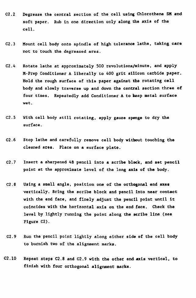
C2.2 Degrease the central section of the cell usiD& Chlorothene SK and
soft paper. Rub in one direction only along the axis of the
cell.
C2.3 Kount cell body onto spindle of high tolerance lathe, taking care
not to touch the degreased area.
C2.4 Rotate lathe at approximately 500 revolutions/minute, and apply
K-Prep Conditioner A liberally to 400 grit silicon carbide paper.
Hold the rough surface of this paper against the rotating cell
body and slowly traverse up and down the central section three of
four times. Repeatedly add Conditioner A to keep metal surface
wet.
C2.S With cell body still rotating, apply gauze sponge to dry the
surface.
C2.6 Stop lathe and carefully remove cell body without touching the
cleaned area. Place on a surface plate.
C2.7 Insert a sharpened 4B pencil into a scribe block, and set pencil
point at the approximate level of the long axis of the body.
C2.8 Using a small angle, position one of the ortholonal end axes
vertically. Bring the scribe block and pencil into near contact
with the end face, and finely adjust the pencil point until it
coincides with the horizontal axis on the end face. Check the
level by lightly running the point along the scribe line (see
Figure C2).
C2.9 Run the pencil point lightly along either side of the cell body
to burnish two of the alignment marks.
C2.10 Repeat steps C2.8 and C2.9 with the other end axis vertical, to
finish with four orthogonal alignment marks.

C2.ll Stand the load cellon one end face, and adjust the pencil in the
scribe line such that its point is 35mm above the surface plate,
ie at the mid-height of the load cell. Lightly burnish a
circumferential line around the centre of the cell body holding
the cell in place with light finger pressure on the cell flange.
C3 - Application of Axial Pair of Strain Gauges
C3.l Transfer load cell body to the constant temperature body and
leave for at least 15 minutes whilst the rest of the equipment is
prepared, to allow temperature equalisation.
C3.2 Apply Conditioner A to a clean cotton tip and scrub
longitudinally an area sufficient for one strain gauge set on one
of the four centre-hair axes of the central portion. Continue
scrubbing, replacing soiled tips every few strokes, until a clean
tip is not discoloured.
C3.3 Remove residue of Conditioner A by wiping dry. in one direction
only, with a clean dry tip. Never allow any solution to dry on
the surface, as this will leave a contaminating film and reduce
the chance of a good bond.
C3.4 Apply a liberal amount of K-Prep Neutraliser 5 to a cotton tip,
and scrub the cleaned area. Take care not to allow excess liquid
to run across the rest of the cell. Dry surface with a single
slow wipe in one direction with another clean tip.
C3.S Remove a Strain Gauge (Type FLA-6-3S0-23) fro. its acetate
envelope using tweezers and place gauge side up on gauge box.
C3.6 Lay load cell body lengthwise onto the bench, with the prepared
area uppermost.

C3.7 Lightly place a 2cm to 3cm length of Mylar tape over the gauge
face, and carefully pick up the tape with gauge attached, by its
ends. If the tape sticks to the envelope, slowly lift away at a
shallow angle to break the contact.
C3.8 Without allowing the tape to contact the cell, carefully align
the burnished axes and strain gauge markers (see Figure C3).
When correct, aligned, lightly roll the tape ends onto the cell
body, from the gauge outwards.
C3.9 Check the alignment again - if necessary, further fine adjustment
may be made by raising one end of the tape at a time and rotating
it slightly before re-laying. If several attempts fail, repeat
steps 83.2 to 83.8 with a new gauge.
C3.l0 Repeat steps 83.2 to 83.9 with the diametrically opposite axial
strain gauge.
C3.l1 With both axial gauges aligned and held with tape, slowly peel
back at a shallow angle one end of the tape for each gauge, such
that both the gauge backings are exposed and accessible (see
Figure C4). The Mylar tape will naturally curl up as
illustrated.
C3.12 APply a thin coat of M-Bond 610 (previously prepared to the
manufacturers instructions) to both gauge backings, and the
Aluminium surface onto which the gauges will lIe. Brush in one
direction only, and ensure sufficient adhesive is on the brush
for complete coverage in one stroke. Do not allow the brush to touch the tape mastic.
C3.I3 Leave adhesive to air dry by solvent evaporation for between 35
and 45 minutes. The optimum drying time was found to be 40
minutes for the laboratory conditions of 200 c and a relative
humidity of between 50, and 60, (see Figure 5.1).

C4 - Curing of Strain Gauges
C4.1 When air dry, relay gauges carefully by rolling from the tacked
end of the tape with light thumb pressure. Do not repeatedly
roll in opposite directions or apply heavy pressure.
C4.2 With both gauges and tapes attached to the metal, transfer the
body to the pressure pot (see Figure C5), check the '0' ring
seal, and bolt on the top of the pot.
3 Connect the pot to a Budenburg dead weight tester (Model 240) and
C4. apply Nitrogen at 220 kPa gauge pressure.
C4.4 Close valve on pot, wait 10 seconds and reopen. If the '0' ring
seal is working, no pressure will have been lost and the tester
will register no effect. If the seal is suspect replace quickly
and repeat test. When satisfied, re-apply nitrogen at the same
pressure and close valve.
5 Disconnect pot and place in room temperature Baby Belling
C4.
C4.6
C4.7
C4. 8
electric oven. Set thermostat to 3250 F (l620 c) and close door.
The oven will reach the set temperature in about 20 minutes, ie
at a sufficiently slow rate to preclude the formation of bubbles
snd uneven glue - lines below the gauges.
Leave pot at 3250 F for two hours, then turn oven off. Leave the
door closed whilst the oven cools.
When cool remove the pot and release the pressure. If pressure
in the pot is lost due to failure of the '0' rings reject the
gauge assembly and re-start load cell manufacture.
Remove load cell from pot. Slowly peel back the tapes at a large
angle to coarse check the bond achieved.

C5 . Application of Circumferential Strain Gaules
CS.l Repeat gauge application similar to that described above, taking
care not to damage the first pair of gauges, especially by
careless use of fluids and/or laying tape over the first gauges
and leadwires.
CS.2 Repeat curing of the new gauges exactly as before.
C6 . Post Curing of Strain Gauge Adhesive
C6.1 Place load cell alone in room temperature Baby Belling oven.
Raise temperature to just under 4000F (2050 c).
C6.2 Maintain this temperature for 2 hours, then turn oven off. Leave
oven closed during cooling.
C6.3 Remove load cell when oven is cool, and check gauges. The
backing will have changed colour from green to dark brown if the
correct temperature has been used. If temperatures in excess of
4000f have been used, the backings will be black and poorer
performance of the cell may result.
6 4 With a resistance meter, check each bonded gauge has a resistance C . of 350 ohms. If this condition is not complied with, the cell
should be rejected.
C7 . Application of Terminals and Wirin&
C7.1
C7.2
Select four copper faced terminals of three leaved clover format
(see Figure C5), and cover each with Mylar tape.
Position terminals to allow wiring as shown in Figure B6, and
secure in place with the tape. Peel back one end of the tape for
h i al to expose the terminal backings. eac term n ,

C7.3 For each terminal in turn, apply a thin coating of CN adhesive to
the terminal and aluminium, then roll terminal back into
position. Apply light thumb pressure to secure the adhesive in
seconds. Peel back tape to check bond, and proceed to next
terminal. When all terminals are attached, commence wiring.
C7.4 Cut about a 1.5m length of double pair screened cable from its
reel, and expose approximately 4 cm of each wire at both ends of
the cable.
C7.5 Tin ends of each wire, all four terminals, and the strain gauge
leadwires.
C7.6 Solder leadwires and cable wires to terminals, according to the
wiring diagram shown in Figure C6.
C7.7 With a resistance meter, check the circuit resistances between
terminals complies with that noted in Figure C6. Differences
imply a circuit fault, due to earthing or poor soldering, and
must be corrected.
~S _ Protective Coatins of Load Cell
CB.l Apply a thin coating of RTV Primer No 1 to gauges, terminals,
wires and cable near to cell. Leave to air dry for 15 minutes.
CS.2 Apply RTV 3140 silicone sealant to the primed areas, ensuring
complete coverage.
CB.3 Immediately after applying RTV 3140, clamp the cell in a pot
shaker, wrap wires carefully around the clamp, and start rotating
the shaker. The rotating action was found to form a more even
distribution of sealant than hand rotation, given the sealant
fluidity and set time.
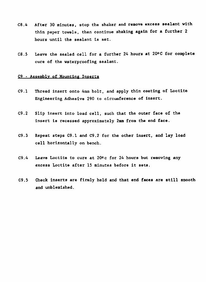
CS.4 After 30 minutes, stop the shaker and remove excess sealant with
thin paper towels, then continue shaking again for a further 2
hours until the sealant is set.
CS.S Leave the sealed cell for a further 24 hours at 200 C for complete
cure of the waterproofing sealant.
e9 - Assembly of Mountin& Inserts
C9.l Thread insert onto 4mm bolt, and apply thin coating of Loctite
Engineering Adhesive 290 to circumference of insert.
C9.2 Slip insert into load cell, such that the outer face of the
insert is recessed approximately 2mm from the end face.
C9.3 Repeat steps C9.l and C9.2 for the other insert, and lay load
cell horizontally on bench.
C9.4 Leave Loctite to cure at 200 c for 24 hours but removing any
excess Loctite after 15 minutes before it sets.
e9.S Check inserts are firmly held and that end faces are still smooth
and unblemished.

Corner to be smoothed out with 2-3 mm radius
Aluminium inserts with tapped \ hOle for 4 mm bolt, sealed in with loctite after gauges attached. Inserts 5mm deep, recessed approx 1 mm.
SECTION A-A
Scale 2:1
PLAN -
Figure C1- 2·5kN Load Cell
o o t'-

Scribe clamped in......--'· using clamp screw.
Scribe block
Screw to adjust vertical positi<:n of scribe clamp on scri be block retort
Sharp i.B pencil tap~ rigidly to scrite
Load cell body lying on surface ! plate -
" , , Small angle aligned with one of the orthogonal lines on the end face of the load cell.
Surface plate ---~----~----~--~~r-----~----~~~~-:f-~-~-;L7-----~-----;~----~~--~I:r~---I
--- 7- 7 7 7 ? > -, 7 7 7 ./ /
Figure C2-Genera! Arrangement To Set Pencil Level Ready For Burnishing Axes On Load Cell Body

I
\
Burnished lines on load cell body. --------...~--Ir-___1
Alignment marks on strain gauge.
'_-----Clear tape held between thumbs and forefingers. Tape must not cover foil gauge area.
Figure C3 - Pickif"9 Up And Positioning A Strain Gauge
Area of load cell~ ,----, body prepared ~, for gauging. 'I
I ___ I
/ /
Back of gauge outermost.
Figure CL.- Position Of Strain Gauges Prior to Applying Adhesive

")
,
, i
All dimensions in mm unless otrerwise s1ated Body rroterial EN 16 steel
-
54
~~~~~~L-Shaped end left by drilling tool
1 ... ,
1" '8 '0 Ring groove
Approx 34-5mm ~ hole drilled by 111/31' tool
Tapped hole tor ~4 asp fitting
6 No tapped holes for M8 bolts
Figure C5-Pressure Chamber for Curing of Strain Gauge Adhesive

Dim
G1
Plug Details
Point Use
1 Positive power su~ly 2 Negative output from
load cell 3 Negative power supply.
plus shield
4 Positive output from load cell
5 Not used
G1
Strain gauges and terminals mounted on load cell body
I------Double pair screened cable
2
R1_2=R2_3=~-I.=RI.-1 = 466·7 ohm
R1
_3= ~-4 = 350 ohm
Cable connections to 5 pin dim plug
Figure C6 -Wiring of Load Cell Strain Gauges Into Full Wheatstone Bridge

APPENDIX D
DATA ACQUISITION
A programme listing for the data acquisition software LOG3 written by
the author is presented in this appendix. The software was used with a
BBC B computer, disc drive, Acorn IEEE interface, He Computers analogue
input unit, and parallel printer.
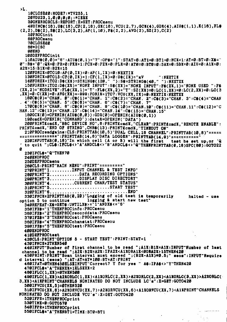
>L. 10CLOSlt0:HODI7:*TV2~~,1 20VDU23,1,e;0;0;0;:*IIII 300NIRRORCLS:RIPORT:X=GET:PROCmenu 40DIHC$(18),U$(18),CP(2,18),GX(18),VCU(2,7),GCI(4),GDX(4),AIU$(1,1),1(16),PL$
(2,2),O$(2),S$(2),LC(3,2),AP(1,10),F$(2,2),AVG(2),SZ(2),C(2) S0PROCinit 80PROCIlenu 70CLOSB£0 80*DISC 90BND
100DEFPROCinit 110AIU$(0,0)="8":AIU$(0,1)="7":OP$="1":STAT=0:AT1=0:BTl=0:NCX=1:AT=0:BT=0:X$="
0":R$="0":QX=0:PR=0:PIX=1:PCX=0:PEX=0:PLI=0:AT0=0:BTe=0:SAX=0:SBX=0:AIU=0:A1X=0: A21=15:B11=0:B21=15
120FORIX=0T010:AP(0,IX)=0:AP(l,IX)=0:NEXTIX 130FORU=0T01~ :CP(0, 11)=1 :CF(1, IX )=0: U$( II)="IlV .. :NEXTII 140FORU=1T02 :D$(XX)=STRING$(120," "): S$=STRING$(40," .. ) :NEXTXX 150FORXX=1T02:0$(XX)="NONE INPUT":S$(XI)="NONE IMPUT":F$(XX,l)="NONB USED ":F$
(XX,2)="NODRIVI":FL$(XI,1)="T":FL$(XX,2)="T":SZ(XI)=8:LC(1,XX)=0:LC(2,XX)=0:LC(3 ,XX)=0:C(XI)=0IAVG(XI)=-999:FORII=1T07:VCU(XI,IX)=I:RIXTIX:NBXTXX
180Ct(0)="CHAN. 0" :C$O )="CHAN. I" :Ct( 2)="CHAN, 2- :Ct(3)="CHAN. 3" :Ct(4)="CHAN . 4":C$(5)="CHAN. S":Ct(S)="CHAN. 6":Ct(7)="CHAN. 7-
170C$(8 )="CHAN. 8" :Ct( 9 )="CHAN. 9": C$(10 )="CHAN .10" :C$( 11)="CHAN .11" :C$(12)="C HAN .12" :C$(13)="CHAN, 13" :C$(14)="CHAN .14" :C$(1S)="CHAN . IS"
180GCX(0)=OPININ(AIU,(0,0»:GDX(0)=OPENIN(AIU$(0,l» 190clldl=OPENIN("COHHANDOO):dataX=OPENIN(OODATA") 200PRINTtOlldX, "BBC DBVICB NO", 8: PRINT£olldX, "CLBAR-: PRINTtolldl, "REHOTE ENABLE":
PRINT£OlldX, "END OF STRING" ,CHR$(13) :PRINT£clldl, "TIKIOUT ON" 210PROCread,ain.:CLS:PRINTTA8(10,5)"DUAL CBLL,lS CHANNEL":PRINTTAB(10,8)"=====
==============z":PRINTTA8(14,S)"DATA LOGGBR":PRINTTA8(14,9)"===========" 220INPUTTAB(0,18)"In whioh oell (A or B) will the tir.t teat be aet up,or 'Q to quit .. ;CL$: nCL$o" A" ANDCL$o "B" ANDCL$<> "Q"THBIPRINTTAB(I, 18)SPC(81) :OOT022
" 230IFCL$:"g"THBN70 240BNDPROC 250DIPPROCIllnu 2S0CLS:PRINT"HAIN HINU":PRINT"=========" 270PRINT"1 ......... INPUT CHANNIL • TBST INFO" 280PRINT .. 2 ............ DATA RECORDING OPTIONS" 290PRINT .. 3 ............ DISPLAy DISC DIRBCTORY" 300PRINT .. 4 ....•..... CURRBNT CHAN/TEST STATUS" 310PRINT" 5 ........................ START TIST" 320PRINT"S ............................... IND" 330nMCI=2PRINTTAB(0,20)"Lo,,1n, ot old te.t 18 te.poraril, halted - use
option 5 to continue 10,,1n, • start new teat-340RIPIAT:X$=GBT$:UNTILX$>="1"ANDX$<="Soo 350IFX$="1°OTHENPROCinto:PROCllenu 3S0IFX$="2"THENPROCreoorddata:PROCmenu 370IPX$="3"THBNPROCcat:PROCIl8nu 3S"IPX,="4"THINPROCohanatat:PROCllenu 390IFX$="~"THENPROCt .. t:PROCllenu 400ENDPROC 410DBPPROCt •• t 420CLS:PRlNT"OPTION ~ - START TEST":PRINT:STAT=l 430IlNCI=2THBN541 440npUT"Nullbl1' or tint ohannel to bl read" iAlI:811=AlI:IRPUT"ltullber ot last
channel to bl r.ad ";A21:821=A2X:IPA2X<A1IORA11<00lA21>lSTHIN421 4S0PRINTIPRIRT"Soan interval Ilust exceed ";(821-&11)*",6;" .eoa":INPUT"Require
d interval (.eo.) ";AT:&T=AT*100:BT=AT:PRINT 480IFAT=0THIN450BLSBINPUT"Correot? Y tor yel .. A$:lPA$o"Y"THIN420 470IrCL,="A"THINXI=1ILSIXX=2 480IFLC(l,XI)=0THIN500 490IFLC( l,XI-»A210RLO( 1, XX) <AUORLC(2, XI) >A210RLC(2,XI)<AlI0RLC(3,XI »A210RLC(·
3,XI)<AlIPRINT"CHANNILS NOHINATBD DO NOT INCLUDE LC·.":X=GIT:OOT0420 500IlVCU(XI,~)=0THEN520 510IFVCU(XI, e »A210RVCU(XX, 7) >A2XORVCU( XI, S) <AUORVCU(XX, 7) <AUPRINT"CHAMNELS
NOHINATED DO NOT INCLUDE VCU·.":X=GET:GOT0420 . 520IFPR=lTHBRPROCprint S30TIHI=0:GOT0670 540IlPR=lTHBNPROCprint 550IFCL'z"~"1HBNBT1=TIHB:BT0=BTl

580UCLt="B"THINAT1=TIHE:AT0=ATl 570YOU23.1.0;0;Ij0; 580PROClab.l:AIU=0:IH~=0 590FORIX=AIXTOB2X 600C'="'C"+8TR'(IX-IHX)+"I" 610PROCooDmand:PROC,etdata 820X=IN8TRCA',"I")-1:CHX=VAL(HID$(At.3.X»:V=VAL(KIO,(At,X+2»:'X=03 630IFOP'="1"THENK(IX)=V*CF(0,I~)+CF(1,I%)ELSEK(II)=(V+CF(1,11»*CF(0,I~) 640IF(NCI=2ANOCL$=" A" ANDU>=AUANDU< =A2" )ORNCI= 1THENPRINTTAB(0, U-AU+7)U, TA
B( 5. II-AU+7 )C$( I"): .1=&20309: PRINTTAB( 1 Z, 1:1: -A U+ 7 ;.y. TAB( 22. IX-AU+7 )K( IX), TAB( 3 2,I"-AIX+7)U$(II):'''=10:GOT0660
650IFCL$="B" ANOU> =B1%ANDI %<=B2XTHENPIUNTTAB(0. U-BU+7)U, TAB(5. U-BU+7 )Ct( I X):@X=&20309:PRINTTAB(12.IX-BIX+7)V.TAB(22.IX-B1I+7)1(II).TAB(32,II-B11+7)UtCII) :.1=10
660NBXTII:K$=INKBY$(10) 670IFlt$="0"PROCrunops 680IFXt="B"THENX,="NONE":GOT0860 690IFX$="S"THENX,="NONE":GOT0940 700IFK$="0"PROClabel 710IF(TIHB>=AT1)OR(TIHB>=BT1)THBN720ELSE590 720IFNCX=lANOCL,="A"THENPCX=1:T=(TIHB-AT0)/100 730UNCX=1ANOCL$="B"THBNPCI=2:T=(TIHB-BT0)/100 740IFNCX=2ANO(AT1<BT1)THBNPC~=1:T=(TIHI-AT0)/10" 750IrNC~=2ANDCAT1)=BT1)THBNPCX=2:T=(TIHI-BT0)/100 780IFPR=lPROCprint 770IFPCX=lTHBN180ELSI810 780AT1=AT1+AT: SAX=SAX+ 1: IrCL,=" A"PRINTTAB( 28,3)" SCAN NO. "j SAX-1 790IFSZ(1) o0THENR,=" A" : PROCdatad i80
800OOT0830 810BT1=BT1+BT:SBX=SBX+l:IFCL$="B"PRINTTAB(28,3)"SCAN NO. ";5BI-1 820IFSZ(2 )o0THINR,="B" : PROCdatad i80
830UNCX=lANOCL,="A"THINBT1=AT1:SBX=SAX 840UNCX=1ANOCL,="B"THENAT1=BT1:SAX=SBX 850ooT0590 880nCL,="A"AN05Z(1)O"THBNR,="A":PROCwindup 87"nCL,="B"ANOSZ(2)<>"THINR,="B":PROCwindup 880IFCLt=" A" THINA U=B UILSEB21=A2X 89"lrPR=lTHINPIX=1:PROCprint 9"0IFNCX=lTHIN93"ILSENCX=1 910UCL,="A"THENCL,="B":AT=BT:AT1=BT1:SAI=SBX:A21=B21:SZ(1)=0:0$(1)="NONI INPU
T" : S$( 1 )="NONI INPUT": F'( 1.1 )="NONE USEO": Ft( 1.2 )="IOORIVI" : VCU( 1,5 )=0: AVG( 1 )=-9 99:C(1)=C(2):PORIX=0T010:AP(0,IX)=0:NEXTII:GOT0700
920IFCL$="B"THENCL,="A":BT=AT:BT1=AT1:SBI=SAI:81X=A11:SZ(2)=0:0'(2)="NONI INPU T":5$(2)="NONI INPUT":P$(2.1)="NONE USEO":F$(2,2)="1I00RIVI":VCU(2.5)=0:AVG(2)=-9 99:C(2):C(1):FORIX=0T010:AP(1,IX)=0:NEXTIX:GOT070"
930CLS:PRINT"LOGGING COHPLETID - ALL VARIABLES RI-SETTO DIFAULT YALUIS":!=GIT: PROC1n1t
9401NOPROC 950DIFPROCr.ad.ain. geeAIU=eIIHI=I:FORIX=0T015 910C'=",C".STR,(U-IHX)+"?":PROCcoDlland:PROC,etdata 980X=INSTR(A .... ? .. )-1:V.=HID.(A.,X+2):GI(II)=VAL(HID$(V •• 2,2»:NIXTIX:INOPROC 990DBFPROC •• t.a1n8
1000UU=0:IHI=0:CLS:PRINT"CHAN GAIN" 1e10FORII=IT01~:II='00004:PRINTIX; :11=&00008:PRINTGI(IX}:NIXTII:PRINT:II=10 1020INPUT"CHANNIL TO CHANGI OR Q TO QUIT "G$ 10301FGt=";"THIN1090 ... 10.0IF(ASC(Gt»=48ANDASC(G')<=57)AND(VAL(G'»=0ANDVAL(Gt)<=l~)THBNII=VAL(Gt)BLS
Bl001 1050IF(NCI=2ANDCLt="A"ANDU<=A21)OR(NCI=2ANDCL$="8"dDII>=Bll)PRINT"TB5T CURRIN
TLY RUNNING IN THIS CILL - NOAHHENDHENTS ALLOWEO":X=GIT:GOT010"0 10S0IMPUTTA8(1.19) "NEW GAIN : "G,: IFVAL(G,) <00RVAL(Gt» 110R(VAL(Gt)-INT(VAL(G$)
»>0THINPRINTTA8(0.19)SPC(40):GOT01080 1070C'= "'C"+STR$( U-IHI)+" G" +G' 10S0PROCoomaand:PROC,etdata:PROCreadlain8:GOT01000 1090BMDPltOC 11000BPPROCooamand -
: i~~:~~MT~Oadl. "LISTEN" .GCI(AIU), "BXICUTE" : PRINT£datd,Ct:PRIN~~0~;~~£1~!~~~' . ,.~ ~. '. ~:.i ~~~~:f. ~~' .. ' ~.
. , --: -,' ._"l~f(:.",

1120DBFPROC •• tdata 1130PRINT£OlldX, "TALl" , GDX(AIU) : INPUT£dataX, A$: PRIJT£Clldl, "UNTALl" : BNDPROC 11400BFPROCdatad180 1150*DISC 1160IFR$="8"THBN1200 11700SCLI(F'(1,Z» 1180PRINTtAXX,T 1180FORIX=AIITOAZI:PRINT£AXI,K(II):NBXTIX:GOT01238 12000SCLI(F'(Z,2» 1210PRINT£8XI,T 1220FORII=81ITOB21:PRINT£BXX,K(II):NBXTII 1230*IEBB 1240BNDPROC 1250DEFPROCoat 1260CLS:PRINT"OPTION 3 - DISC DIRBCTORYH:PRINT 1270*DISC 1280INPUT"DISC DRIVE NO. "jD$:D$="*DRIVB H+D$:OSCLI(D$):*CAT 1290*IBEB 1300X=GBT:BNDPROC 1310DEFPROCwindup 1320CLS:*DISC 1330IFR'="A"THBNOSCLI(F$(l,2»:A0:rT~£AXX:X~=1 1340IFR'="B"THENOSCLI(F'(2,2»:Ae=fT~£BXX:XX=2 1350PRINT"TEST COMPLETED - CLOSH i'ILH RUU1'lNE" :PR1I1T:INPUT"ENTBR DURATION OF TE
S1 (TIMB AND/OR DATB"iS$(XX):INPUT"ENTER REMARKS/TIST DBSCRIPTION";Dt{XI) 1360IFXX=2THBN1400 1370PTRtAXI=0:PRINTtAXI,SAI:PTRtAXI=A0 1380FORIX=AlITOA2X:PRINT£AXI,C,(II),CF(0,II),CP(1.II),U,(II),GI(II):NBXTII 1390PRINT£AXX,OP$,S'(1),D$Cl):PORII=0T010:PRINT£AlI,AP(I,II):NBXTII:CLOSB£AXI:S
Z(1)=0:GOT01430 1400PTRtBXI=0:PRINTtBXI,SBI:PTR£BXI=A0 1410PORII=BlITOB21:PRINTtBXI,C'CII),CF(0,II),CP(1.II),U,(IX),GXCIX):NBXTIX 1420PRINTtBXI,OP"S,(2),D'C2):PORI1=0T010:PRINT£BII,AP(l,II):NBXTII:CLOSBtBXI:S
Z(2)=0 1430*IBBB 1440BNDPROC 14S0DBFPROCinfo 1460CLS:el=10:PRINT"OPTION 1 - INPUT CHANNBL • TEST INPO":PRINT 1470PRINT"HENU":PRINT"====" 1480PRINT"l ........................ NAMB CHANNBLS· 1490PRINT"2 ..... SIT CONVBRSION FACTORS. OFFSBTS" 1500PRINT"S ........................ ADD TEST INPO" 15lIPRINT"4 ............................ ADD UNITS" 1520PRINT"S ..................... RBAD • SBT GAINS" 1530PRINT .. S .......... ADD VOLUME CHANGE UNIT INFO" 1540PRINT"7 .... ADD LOAD CELL. AIR PRESSURE INFO· 155IPRINT"S .................. RETURN TO MAIN MENU" lS60RIPIAT:X,=GETt:UNTILX,>="l"ANDX,<="S" 1570IFX,="l"PROCnall. 15S0nX,="2"PROCfao. 1590IFXt="3"PROCteatinto 160IIFX,="4"PROCunit lS10IFX,="S"PROC •• t.dn. 162IIFX,="S"PROCvou.tart 183IIFX'=~~7."PROClo.tar_t . 1640IPX,<> "S"THIN148IBLSBBNOPROC 18510BPPROCnall. 1660CLS:PRINT"NAHI CHANNELS - HAX OF 7 CHARACTERSIIAH!" 1670PRIMT"CHAM NAHI" 1880FORIX=0T015:eX=.00004:PRINTII;:.X=&00007:PRIMTtAB(S)Ct(IX):NBXTII 1690PRINT:INPUT"CHANNIL TO CHANGB OR g TO QUIT "At 1710IFAt="g"THB1U 740 171IIF(ASC(A.)<4S0RASC(A$»57)OR(VAL(A,)<00RVAL(At»15)THIN1S8I 172IINPUTTABC0,21)"NBW NAHE "Ct(INT(VAL(A$»): I1LD(Ct(IRT(VAL(At) »»7PRINT"TO
o LONG" :OOT01721 1730G0T018S0 1740CLS:BNDPROC . ----.~----
.:"'; I

175"DBFPROCfao. 178"CLS:PRIRT:PRINT"SBT CONVBRSION FACTORS AND OFlSBTS":PRINT 177"IPRCX(>2GOT018BB 178"PRINT"PACTOR OPTION" lOP$;" HAS ALREADY 8EEN SBLBCTID POR CBLL ";CLt;" • TH
IS HAY NOT 81 ALTEREO.":PRINT:IFOP$="l"PRINT"OPTION 1. .... (OUTPUT*CON.PACTOR)+OF FSET"BLSBPRINT"OPTION 2 ..... (OUTPUT+OFFSET)*CUN.FACTOR"
1790X=GET:GOT01820 1800PRINT"AN OPTION EXISTS FOR APPLYINd THB FACTORS :":PRINT" 1 ......... (OUTPU
T*CON.FACTOR)+OFFSET":PRINT" 2 ......... (OUTPUT+OFFSIT)*CON.FACTOR" 181"RBPEAT:OPt=GBTt:UNTILOP$::"1"OROP$="2" 182"CLS:PRINT"CHAN CON.FACTOR" 1830FORI%=0T015:IX=.00004:PRINTI%; :'%=&20308:PRINTCF(0,I~):NEXTI% 1840PRINT:INPUT"CHANNEL TO CHANGE OR Q TO QUIT "At 18S"IFA$="Q"THIN 1910 1860IP(ASC(At)<480RASC(A$»57)OR(VAL(A$)<00RVAL(A$»15)THINI820 18701F(NCX=2ANOCL$="A"ANOVAL(A$)<=A2X)OR(NCX=2ANOCL$="B"ANDVAL(A$»:BU)PRINT"T
EST CURRINTLY RUNNING IN THIS CILL - NOAHHENOHBNTS ALLOWIO":X=GIT:GOT01820 18801FVAL(At)=0THIN1900 1890IFVAL(A$)=VCU(l,8)ORVAL(A$)=VCU(l,7)ORVAL(A$)=VCU(2,8)ORVAL(A$)=VCU(2,7)THE
NINPUT"FACTOR FOR THIS CHANNIL SET BY veu OPTION - SURE YOU WANT TO CHANGE ? Y FOR YIS "B$:IPB$<>"Y"THBNI820
1900INPUTTAB(0, 19) "NBW VALUI "CF(0, VAL( A$»: GOT01820 1910CLS:PRINT"CHAN OFFSET" 1920FORIX=0T015:IX='0""04:PRINTII; :8X='20308:PRINTCF(1,II):NBXTIX 1930PRINT:INPUT"CHANNIL TO CHANGE OR Q TO QUIT "A$ 1940IFA$="Q"THB1U981 1950IF(ASC(A$)<480RASC(A$»57)OR(VAL(A')<00RVAL(A$»1~)THBN1910 1980IP(NCh2ANDCLt=" A" ANOVAL( A$) < =A2~ )OR( NC~=2ANOCLt="B" ANOVAL(At) >=BU)PRINT~'T
EST CURRBNTLY RUNNING IN THIS CELL - NOAHHENDHENTS ALLOWEO":X=GET:GOT01910 1970INPUTTAB(0,19)"NB" VALUB "CF( 1, VAL(A.,) :GOTOI910 1980.X=1.:BNDPROC 19900IPPROCt •• tinfo 2000CLS:IPNCX=2ANOCL$z"A"PRINT"TBST CURRENTLY RUNNING IN CILL A • THI TIST INF
o HAY NOT BI ALTERI0":PRINT:GOT02040 2010IFNCX=1ANOCLt< >" A"00T02040 2020PRINT"CELL A":INPUT"BNTBR TEST DESCRIPTION TO BE SHOWN ON SCRBEN OURIMG TES
T: "0$0): !PLEN (Ot(1» > 120PRINT"TOO LONG": GOT02020 2031PRINT: INPUT" START or TIST: "S$O): IFLIN(St( 1) »41PRINT"TOO LONG" :OOT02838 2040IFNCI=2ANOCLt="B"PRINT"TIST CURRENTLY RUNNING IIf CILL B • THI TBST INPO Hi
Y NOT BI ALTBREO":GOT02181 2050IFNCI=1ANOCLt< >"8 "GOT02081 208"PRINT"CBLL 8":INPUT"ENTER TIST DESCRIPTION TO BI SHOWN OM SCRIEN DURING TBS
T: "D$(2):IrLIN(O$(2»>120PRIMT"TOO LONG":GOT02080 2070PlUNT:INPUT"START or TBST: "S$(2):IFLBN(S$(2»>40PRINT"TOO LOMG":GOT02070 2080CLS:IMOPROC 20g00lrPROCunit 2100CLS:PRINT"AOO UNITS paR NAHBD CHANNELS - HAX OF 8 CHARACTBRS/UMlT":PRIlfT 2118PRINT"CHAN NAHI" 2120FORIX=0T01~:IX='00104:PRINTI~;:.X='0800e:PRINTTA8(8)iU$(IX):NEXTIX 2130PRINT:INPUT"CHANMIL TO CHANGI OR Q TO QUIT "A$ 2148lPA.="Q"THBN2191 21~8Ir(ASC(A.)<480RASC(At»S7)OR(VAL(A$)<00RVAL(A$»lS)THIN2101 2180Ir(NCX=2AMOCLt="A"ANOVAL(A$)<=A2~)OR(NCI=2ANDCLt="B"ANOVAL(At»=B1I)PRIRT"T
EST CUltRlMTLY RUNNING IN THIS CILL - NOAHHENOHBNTS ALLO"IO" 2178INPUTTAB(0,22)"NI" UNITS "U$(VAL(A$»: IFLEN(U$(VAL(A$) »>8PRINT"TOO LONG":G
OT0217" 218"GOT0210' 2190CLS:INOPROC 22000lPPROCloatart 221"CLS:rORXX=lT02 2220lPXI: lPRINT"CURRBNT STATUS OF CELL A:": YI=A1I: JX=A2X 223"rrXI=2PRIMT"CURRENT STATUS OF CELL B:": YX=BU: JX=B2X 224"rr(XX=lANONCI=lANOCLt="B")OR(XX=2ANOMCX=1ANDCL$="A")PRINT"CILL IDLB":X=OBT:
ooT02371 225fJIP(XX=lANDNCI=2ANOCLt="A")OR(XI=2ANDNCX=2ANDCLt="8")PRlNT"TBST RUNNING 1M T
HIS CBLL ALRIADY - NO AHHENDHEHTS ALLOWED": X=GET : OOT02371 .' . 22e0UAVG(XI)s-988PRIHT"OPTION OFP":00T02280 227IPltUlT"OPTION ON":PRIMT"LOAO CELL CHANNELS = "iLC(1 XI);","iLC(2,XX)i",";LC(
3,XI):PRIltT"AIR PRBSSURI IN SPECIHEN (kPa) = ";AP«XI-l) 0):PRINT 2280UPUT"CHANGB STATUS? YIM "A$:IFA$O"Y"ANOA$<>"N"THiN2280 2298IFA$="N"THEN2370

23011'AVO(XI)=0THINAVO(XI)=-999:00T02370 2310AVG(XI)=I:CLS:PRINTTA8(0,20)"Note - load oell ••• y not OOOUPY ohan.8":INPUT
TA8(0,1)"INTIR LOAD CILL CHANNILS - lBt "LC(1,XX):IrLC(1,XX)<YXORLC(l,XI»JIORLC (1,XI)=0PRINTTA8(0,0)SPC(40):GOT02310 2320INPUTTA8(27,1)"2nd "LC(2,XX):IFLC(2,XI)<YXORLC(2,XI»JIORLC(2,XI)=0PRINTTA8
(0.1)SPC(40):GOT02320 2330INPUTTA8(27,2)"3rd "LC(3.XX):IFLC(3,XX)<UORLC(3.XX»JIORLC(3.XX);0PRIMTTAB
(0,2)SPC(40):GOT02330 2340PRINTTA8(0,22)"Note - air pressure must exce.d zero" 2350INPUTTA8(0,3)"AIR PRESSURE IN SPECIMEN (kPa) -AP«XI-l),0):IFAP«XX-l),0)<=
0PRINTTAB(0,3)SPC(40):GOT02350 2360INPUT"OK? N FOR NO "A$:IFA,="N"GOT02310 2370CLS:NIXTXX 2380CLS: UDPROC 2390DIFPROCvou.tart 2400CLS:FORXI=lT02 2410IFXX=lPRINT"CILL A:":YI=A1X:JX=A2X 2420IFXX=2PRINT"CELL B:":YX=8U:JX=B2X 2430IF(XX=lANDNCX=lANDCL$="8")OR(XX=2ANDNCX=lANDCLt="A")PRINT"CELL IDLB":X=GET:
GOT02660 2440IF(XX=lANDNCX=2ANDCL$="A")OR(XX=2ANDNCX=2ANOCLt="8")PRINT"TEST RUNNING IN T
HIS CILL ALREADY - NO AHMENOHENTS ALLOWEO":X=GIT:GOT02660 2450IFVCU(XX,~)=0PRINT"OPTION OFF":GOT02500 2480PRINTTA8(27)"FLOW":PRINT"CHAN NAHI CONJ'AC INTO":PRINT"-----------
--------------------" 2470FORII=lTOVCU(XX.5) 2480'1=0""04:PRINTVCU(XX.II+5);:'X='00007:PRINTTA8(S)Ct(VCU(XI,II+S»;:.1=12030
A:PRINTCr(8. VCU(XI. U+S»; : IFFLtcXI, II )="T"PRINTTA8(27)"TOP"ILSIPRINTTAB(27)"BAS I" : PRINT 2490NIXTII:PRINT 250'UNPUT"CHANGI STATUS? YIN "A':IFA$<>"Y"ANOA$o-."THEN25ee 25 U!JIFAt="N"THIN2880 2520IFVCU(XX,~»0THINVCU(XX.~)=0:GOT02660 2531VCU(XI,7)=I:PRINT"TO USE THIS OPTION RBQUIRES ftl FOLLOIIRG IRFO" 2541INPUT"INTER RO. OF UNITS - "AX OF 2 "VCU(XI,5):llVCU(XI,5)<>2ARDVCU(XI,S)<>
1THIN2540 255eFORII:1TOVCU(XX, 5) 2580CLS:PRINTTA8(I,20)"Note - VCU may not oocupy channel 0" 2571PRINTTA8(0.0)"UNIT "iU:PRINT"------":PRINT:IRPUT"VCU CHANNIL
= '"VCU(XI,IX+5):IFVCU(XI,IX+5)<YJORVCU(XI,II+5»JIORVCU(XI,II+5)=0PRINTT A8(I,3)SPC(40):GOT02570
inore.... as volume 2581PRINTTAB(",22)"Note - cal. factor +v. if vcu olp expelled tro. soil"
= "VCU(XI,IX):IFVCU(XX,II)=0 2591INPUTTAB(0,4)"CAL. FACTOR FOR FLOW INTO TOP PRINTTA8(0,4)SPC(41):GOT02591
2610INPUTTAB(0,5)"CAL. FACTOR FOR FLOW INTO 8ASI = "VCU(XX,II+2):IPVCU(XI,IX+ 2)=IPRIMTTA8(I,5)SPC(40):GOT02800
2811IF(VCU(XI,II»0ANDVCU(XI,II+2»I)OR(VCU(XI,II)<IANOVCU(XX,IX+2)<I)PRIMTTA8( 0,8)"FACTOI5 MUST BI or OPPOSITE SIGHS !":PRINTTA8(1,4)SPC(120):GOT02591
2821IMPUTTA8(0,8)"INITIAL FLOW TO TOP OR 8ASI (T/B)= "FLtcXI t II) :-lPPL.(~li 11-)<> "T"ANOrLt(XI,II)<>"8"PRINTTA8(I.8)SPC(40):GOT02620 2831IrPLt(XI, 1I)="T"THINCF(I, (VCU(XI, 11+5» )=VCU(XI, II )ILSICF(". (VCU(II, 11+&»)
=VCU(XI.II+2) .' .".~ 2641PRINT:PRINT"THI INITIAL CON.FACTOR IS NOW SIT.TR1 OFF SIT MUST STILL 81 SI
T USING OPTION 2":X=GET 2651"IITII 2661CL5:MIXTXI 2671CLS:BMDPROC 26800BPPROCrioorddata 2890'ORXI=lT02 2711CLS:PRINT"OPTION 2 - DATA RICORDING OP'1'IONS":PRlMT 2710IFXX=lPRIMT"CBLL A:"ILSBPRINT"CBLL 8:" 2721n(MCI=2ANOCL.="A"ANDXlII=1)OR(RCI=2AHDCL,="8"AMDU=2)PRINT"OPTIONS FOR THIS
CBLL ALRBADY SIT a "AY HOT 81 CHANGIO":X=GIT:GOT03081 273IIP(NCI=1ANOCL,="B"ANDXI=1)OR(NCI=1ANDCL.="A"ARDU=2)PRINT"CBLL IDLB":I=GIT:
GOT03188 2741PlIMT""IMU":PRIMT"====" 27~IPRINT"Data to di.o durin, test - on 2780PRIMT" - oft 2771PRIMT"Oata to printer - on 278ePRIIT" - ott 2791PRIMT"lnd ot options tor this oell
type 1" type 2" type 3" type 4'" type 6'":Q=GITt
'.... . ~. .
':·;4.~1~:~--. •. 'r" .~ ."~:'" ~, <

2eeelFX$=lr 1 "THIN287e 2810IFX$="2"THINSZ(XX)=e:GOT027e0 282elFNCI:2AND(X.="3"ORX.="4")PRINTTAB(e,12)"THI PRINTIR OPTION HAS ALRIADY BIE
N SIT BY THI PIRST TIST • HAY NOT BI CHANGID":X=GBT:GOT02100 2830IFX.="3"THIN3030 28401FX.="4"THENPR=0:GOT02700 28501FX$="5"THIN3e80 28S0CLS:GOT02700 2870IF(NCI=lANDCL$="A OI )OR(NCI=2ANDCL$="B")THINJX=A2X-AUILSIJI=B21-BlI 28S0CLS:PRINT"RESERVATION OF SPACI POR TEST DATA :":PRtNT:INPUT" NO. OP CHANNE
LS TO 81 USED ";CNX:INPUT" APPROX. NO. OF SCANS EXPICTID "jANX:IF(CNX>(JX+l»OR ANX<lTHBN288e
2S90INPUT" ENTER FILENAME FOR DATA ";F$(XI,1):IFLEN(F$(XI,l»>10PRtNT"TOO LONG ":GOT02890 2900PRINT:PRINT"DISC DRIVE NO. FOR "jF$(XX,l)j:IHPUTJX:IFJX<"ORJI>3THEN2870ELSE
F$(XI,2)="*DRIVB "+STR$(JI) 2910PRINT"INSERT DISC AND HIT RETURN TO CONTINUI":X=GBT:*DISC 292"OSCLI(F$( XI, 2»: SZ( XX )=( (CNI+ 1 )*ANX*6 )+734: EF.=STR$~SZ(XI): FS$=" SAVE"+CHR$3
4+F.(XX,l )+CHR$34+" ee"0" "+EF$: 08(,L1 (FS~:) 2930PRINT"RESERVED DISC SPACE FJF 'jF:t<.X.t,l)j" = "iSZ(XX)j" BYTES" 2940IFXX=2THEN2980 29seAXX=OPENUP(F$(XX,1» 296ePRINT£AXX,ANX,CNX <:S70GOT030"0 2ge0BXI=OPINUP(F.(XI,l» 2990PRINT£BXI,AHI,CNI 3000PRINT"LIAVI DISC IN DRIVI FOR RIST OP TIST ":I=GIT 3010*1111 3020CLS:GOT02700 3030CLS:PRINT:PRINT"DATA PRINTOUT DURING TIST":PRINT"THI OUTPUT PROM THI CHANNE
LS WILL BI PRINTED OUT DURING THI TEST,AFTIR THI RAW OUTPUT IN .V HAS BBBN INTIRPRITID USING THI CONVIRSION FACTORS a oppsns," 3040PRINT"VALUIS rOR THISI CALIBRATION CONSTANTS WILL BI O/P AT THI START OP T
HI TIST, ":PRINT:PRINT"CHEClt SUPFICIBNT PAPBR IS AVAILABLI1" 305ePR=1:X=GIT:CLS:GOT02100 3080CLS:NIXTXI 30101HOPROC 308eOlPPROClabel 3090CLS:PRINTTAB(8,0)"OATA OUTPUT FROH CELL ";CL$:PRINTTAB(8,l)"===============
========" 310eIFCL.="A"THBNXX=1:SX=SAX 3110IFCL$="8"THBNXX=2:SX=S8X 3120PRINTTAB(0.3)"OATA PILB=";F$(X~,l):IFS~=0PRINTTAB(28,3)"SCAN NO. 0"ILSIPRIN
TTAB(28,3)"SCAN HO. ";SI-1 3130PRINT:PRINT"CHAN NAHI O/P(mV) BNG"G DIP UHITS .. :PRINT .. ------------------
" -------------------3140PRIHTTAB(S,2.)"O : OISPLAY RUNNING OPTIONS"; 3150.J=10:IHOPROC 31800HPPROCrunop8 3170CLS:PRINT"RUNNING OPTIONS DURING LOGGING:":PRINT"--------------------------
" 3180PRINTTAB(a,3)"CILL "jCL.;" - C=DISPLAY TIST • CHANNIL INFO" 3190PRINTTA8(9,S)"A=OISPLAY AVG STRESSIS":PRINTTAB(9,7)"R=CHANGI SCAMNING RATI"
:PRINTTA8(9,9)"V=RlVERSB FLOW OIR'N INTO VCU":PRINTTA8(9,l1)"I=IND CURRINT THST" 3200IPCL.= ..... PRINTTA8(0.14) .. CELL 8 - S=START NIW TIST"ILSIPRINTTAB(0.14)"CILL • - S=START NIW TIST" 3210PRINTTAB(9,18)"D=OISPLAY CURRBNT DIP I ACCISS-:PRINTTA8(11.11)"RUNNING OPTI I
ONS":PRINTTAB(0,20)"RITURN TO SltIP":X,=GET. 322eIPX,="V"PROCrevvou 3230IPX.="C"PROCohanatat 324eIPX,="R"PROCaltert1.e 32~0IrX'="A"PROCav.lo 328aIPX,="D"ANONCI=2PROCohanifecell 3270IFX,="S"ANONCI=2THBNX,="0" 3280IFX,="S"ANONCI=lPROCnewte8t 3290'1=10:INOPROC
3300DIPPROCprint 3310*PX5,1 3320*PX8 3330*PX3,10 3340IPP11=0ANDPII=0ANDPLI=0THBN3540 33S0IFPKI=1PRINTSPC(Z0)"***OATA OUTPUT FRO" AIU LOGGING PROGRA"***":PRINT 3360IFPII=0THIN33S0ILSIPRINT"END OF TEST 1M CBLL -;CLt:PRINT"------------------
" -----------------------------------------------------3370IFMCI=lTHIN3620ILSIPRINT:PRINT"ONLY SINGLI TlST CONTINUING" 3380IFPLI=lPRINT:PRINT"--------------------------------------------------------
---------------":PRINT"NIW TIST STARTID !":PRINT-CHANNIL ALOCATIONS ARI : CILL A = ";A1:Ii" TO ";A21:PRINTSPC(25)"CELL B = "iBUi- TO ";B21:PLI=0 3390IF(NCI=1ANDCL$="8")OR(PBI=lANDCL$="A")THEN3428 3400PRINT"CBLL A:" :PRINT"TBST STARTBD : .. iSt(1) :PRINT"SCAN INTBRVAL · ". , ,
AT/100i" SICS" 3410PRINT"DATA FILl : "; F$( 1,1): PRINT"DISC ORIVI : "iF,(1,2):PRINT
"TBST DBSCRIPTION : ";D.O):PRINT:IFNCI=10RPBI=lTR1N3440 3420PRINT"CILL B:":PRINT"TIST STARTIO : ";S'(2):PRINT"SCAN INTIRVAL · ". · ,
BT/100;" SICS" 3430PRINT"DATA FILB : "; F$( 2,1) : PRINT"OISC DRIVE
"TBST DBSCRIPtION : ";O$(2):PRINT " ;F$(2,2):PRINT
3440PRINT"CHAN TRANSOUCIR CON.FACTOR OPFSBT GAIN" 3450PORII=A1ITOB21 3460.1=03:PRINTlli:tl=10:PRINTTAB(6)C$(11);:tX=l20410:PRINTTAB(16)CF(0,1X),CF(1
,U),GI(U) 347014IXTU 3480.1=10: PRINT: IFP11= 1P~INT"TE::·T DATA' : t' R1Nl''' =========" : PKX=0: GOT03500 3490PRINT"TEST DATA CONT'O":PRINT"================" ~500FRINT:FOR1I=AlITOB21 :35101FU=B2XOR(U-AU)=7THENPRINT" CHAN" i1%:001'03530 3520PRINT" CHAN ";II,i 3530NIXTIX:PII=0:GOT03620 3540IPPCI=1PRINT"CILL A ILAPSBD TI"E = ";T;" SICS-ILSBPRIMT"CILL B BLAPSED TI"E = "iT;" SICS" 3550FOR11=A11TOB21 3580.I=t02030A 3570IP«PCI=1ANDIX>A2X)OR(PCI=2ANDll<Bll»ANO(II=B210R(II-All)=7)THIMPRINT"
:GOT03610 3580IP«PCI=1ANOII>A21)OR(PCI=2ANDII<B11»THBNPRlIT" ",;:GOT03810 3590IPIX=B210R(IX-AIX)=7PRINT1(IX):GOT03610 3600PRIMT1( IX) , ; 3810NBXTU 3620.1=10 3830*FX3,0 .-3640BNDPROC 3650DIPPROCaltertime 36S0UCL,=" A"THBNT=AT ILSET=BT 3670CLS:PRINT"CURRINT TI"I INTBRVAL = ";T/l"0;" SICS":PRINT"HUlIHUH TI"I INTBRV
AL = "i(82X-AU)*0.~;" SICS":PRINT 38S"PRINT"NIW TI"B INTERVAL FRO" AFTER":INPUT"NIlT SCAN (SICS) = ";T:IFCL$="A"T
HBNAT=T*100BLSEBT=T*100 38901lT=0THIN3870 3700BNDPROC 3710DBFPROCav,lo 3720CLS:IP(CL,="A"ANDAVG(1)=-999)OR(CL$="8"ANOAVG(2)=-999)THIN3880 3730IFCLt="A"THINXX=1:T0=AT0 37.0IFCL,="8"THINXX=2:T0=BT0 3750AVG=(I(LC(l,XI»+I(LC(2,XI»+1(LC(3,XX»)/3 I 3780CLS:tl=ll:PRIMTTA8(8,0)"LOAD CELL DATA ANALYSlS":PRINTTAB(8,1)"============:
==========2":PIIMT 3770PRIMT"LOAD IMG'Q O/P DIV OP O/P FROH AVG" :PllNT"CILL (kPa) (kPa)
(X)":PRINT"------------------------------------" 3780l0RJla lT03:tX='00004:PRINTLC(JX,XX)i:tX='2031B:PRINT1(JI)::tl=t2030B:PRINTA
VG-K(JI)::tX:'2130A:PRtNT(AVG-l(JX»*100/AVG:NIXTJI 3790PRIMTTAB(I.12)·'AVG. PRISSURI TRANSMITTBD" :PRIITTAB(I.13)"8T LOAD CBLLS
a";:tX:&20308:PRtNTAVG,TAB(38,13)"kPa" -3800PRIMTTA8(0. 14)" Al R PRBSSURI IN SPICI"IN =" j :1'='20309 :PRINT(AP«XX-1) ,C(II
»).TAB(38,14)"kPa" 3810PRIMTTAB(0,1&)"NORHAL STRBSS ON SPECIMEN =" i :IX=.2"3"S:PRINT(AVG-AP«XI-1),
C(XX»),TAB(S8,15)"kPa"

382"PRINTTA8(1. 21) ~ .. ------------------------------------" : PRHlTTAB(j-.21) "C:CHAN GE AIR R=RITURN TO HAIN":PRINTTAB(0,22)" PRESSURE SHOWN OISPLAY":X, =GET$
3830IFX$="C"THBNC(XX)=C(XX)+2 3840IFX$="C"INPUT"NIN PRBSSUR~ ";AP«X%-1),C(XI»:AP«XI-1),(C(XI)-1»=(TIMI-T0
)/100:IPAP«XI-1),C(XI»<=0PRINTTAB(0.23)SPC(40):GOT03840 3850IPX$="R"GOT038S0ILSIGOT03750 38SeIX=1":INDPROC 38700lPPftOCrevvou 388eIrCL$="A"THINXI=1IL5EXI=2 3890CLS: IPVCU(XI. &)=0GO'r04050BLSBPRINTTAB( 9 ,0)"REVERSAL or VCU .... :PftINTTAB(9, 1)
"=================":PRINT 3900PRINTTAB(34)"PLOW" :PRINT"CHAN NAHE CONJAC OFFSIT INTO" :PRINT .. ----
" ----------------------------------3910FORIX=lTOVCU(XI,5) a920.X=00004:PRINTVCU(XX,IX+5)j:IX=.00007:PRINTTAB(5)C$(VCU(XI,II+5»i:ll=l2030
A:PRINTCF(0,VCU(XI,IX+S»j:.x=a2030A:PRINTCF(1,VCU(XX,IX+S»i:IFFL$(XX,II)="T"PR INTTA8(34)"TOP"ILSEPRINTTAB(34)"BASE"
3930NBXTU 3940PRINTTA8(e, 11)" RTN TO SKIP OR R TO REVBRSI" :A$=GBT$: IFA$="R"THBN3950ELSI405
o 3950INPUTTA8(0,11)"CHANNEL OF VCU TO REVERSE "RC:IF(RCoVCU(XX,S)ANORC<>VCU(XX
,7»ORRC=0PRINTTAB(0,ll)SPC(40):GOT03950 39S0PRINT"HIT ANY IIY IHHEDIATELY PLOW REVBRSEO":X=GIT 3970C$="$C"+STR$( ftC )+" I" : PROCcolllland: PROClletdata 3980X=INSTR(A$, .. I" )-1: I( RC)=VAL(MID$(A$, X+2» 3990IFRC=VCU(XI,S)THINJJ=lELSBJX=2 4000IPrLf(XI.JI)="8"THBN4030 4010FL$(XI,JI)="8":IPOP$="2"THENCF(l,RC)=(I(RC)+CF(l,RC))*CF(0,RC)/VCU(D,JI+2)
-1(RC)ILSICP(1,RC)=I(RC)*(VCU(XX,JX+2)-VCU(XX,JI»+CF(l,RC) 4e20CF(I,RC)=VCU(XI,JI+2):GOT03890 403IlL$(XI,JI):"T":IPOP$="2"THBNCP(l,RC)=(K(RC)+cr(1,RC))*CP(I,RC)/VCU(XI,JI)-K
(RC)ILSICl(1,RC):1t(RC)*(VCU(XI,JI)-VCU(XI,JI+2»+cr(1,RC) . 4140CF(I,RC)=VCU(XI,JI):GOT03890 4051IXz11:BNDPROC 40SIOIFPROCohan.tat 4070CLS:IPSTAT=lTHBR4ee0ILSIPRINT"OPTION 4 - CURUNT CHARNIL/TIST STATUS":PRINT 4080IrNCI=2PRIlIIT"CHANNILALLOCATIONS ARE:":PRINT" CILL A = "iAni" TO "iA2X:PRIN
T" CILL 8 = ";811:" TO ";821 4090IFNCI=lANDCL$="A"PRINT"CHANNILS FOR CILL A = -;All;" TO ":A21 41e0IFNCI=1ANDCLf="8"PRINT"CHANNELS FOR CELL B = "i8n;" TO "iB21 41leX=GIT:CLS:PRINT"CHAN NAHI UNITS" :PRINT"------------------" :FOR1I=8T015:.
1=100004:PRINTII: :11='00007:PRINTTA8(5)C$(IX)i :11=600008:PRINTTA8(13)U$(II):NBXT II 412"X=GIT:CLS:PRINT:PRINT"CHANNEL CONJAC OFrSBTS":PRIRT"-----------------
" -----------4130FORII=0T015:IX=100e07:PRINTIX: :IX=l2030A:PRIMTCF(0,IX)::II=a203"A:PRINTCF(1 .II):MIXTIX:PRINT:PRINT 4140IPOP.="1"THINPRINT"FACTOR OPTION 1 SBLBCTBD ie (O/P*CON .FACT
OR) +OPFSBT "ILSIP RINT" FACTO R OPT I ON 2 SELECTED 1e (O/P+OFFSIT )*CON . FACTOR" 4150X=GIT:CLS:PRINT"CHAN GAIN .. :PRINT"----------" 41S0rORII=0T015:IX='''''004:PRINTlli:IX='000''S:PRIMTGX(II):NEXTII:X=GIT 4170CLI: rORXlalT02 ·::.;t;·ii·.'1c>J 41SIzrXI=lPRIMT"CBLL A:" :T=AT: IFNCI=1ANOCL,="8"PIUNT"CBLL IDLI" :OOTO'211 4181I1II-ZPRUT"CBLL 8:": T=8T: IFNCI: lANDCL$:" A"PIlINT"CILL lOLl" :OOTO'218~,~~ .. ;,,1' 4200PIUMT"TBST STARTID : "iS$(XI):PRINT"DATA rILl ; ":F,(XI,l)sPfttNT
"DISC DUVI : "iF$(XX,2):PRINT"SCAN INTIRVAL : ":T/1H:" SICS":PIINT"TI 5T DISCRIPTION : ":O$(XI) 4211PRINT:NIXTXI:X=GIT 4220CLS:PRIMT:PRIMT"DOUBLB LOGGING - "; : InCI=2PRINT"0,,"ILSIPRINT"OrF" 423erOOI=lT02 :" 424eIrXI=lPRINT:PRIMT"CILL A:": IFNCI=1ANDCL$="B"PllRT"CILL IDLI" :GOT.Q.3.11 4251zrXI22PRIMT"CILL 8:": UNCI= lANDCL$=" A" PRINT"ClLL lOLl" :Q()1'()4318 ",~~,~-, 42SIPRlRT"DATA TO DISC - ";:IFSZ(XI)=ePllIT"OrF"ILSIPRI"T~·.Oll~·' . 427"PRIMT"DATA TO PRINTSR - ":: IFPR=0PlIMT"OF1"ILSIPRIHT"O'''~'~-{~·~·, . 42SIPIUMT"'CU RIVIRSAL - "i: IFVCU(XI, 5)=8PRIMT"OFP"ILSIPRIIT"O'" . 4290PRIIT"L01O CILL ANALYSIS -" i : IFAVG(XI)=-889PRlltT"Opr~ILSIPIW;.p.~ " 43eePRlRT"DATA ANALYSIS FACTORS - OPTION "iOPf .. ~.' :~ : ;:c~/:':; .~ . 431"PRIMT: MIXTXI: X=GIT: BNDPROC·'~:'i;;i):. ~~~.~ .~.,
,.~~:.~~ill~J',~.·:.·.
4320DEPPROCnewteet 4330CLS:INPUT"THE OPTION TO START A NEW TEST HAS 81EN SBLECTED.ARI YOU SURE (YI
N) "j At: IlAt<> "Y"ANDAt<> "M"THEN433" 4340IPU="N"THENX'=""" : GOT04470 4350PRINT:PRINT"THE OPTION TO SIMULTANEOUSLY LOG 2 CELLSHAS 8EEM SELECTED.AS A
RESULT THE DATA MONITORING OF THB EXISTING TIST HAS BEENTEMPORARILY HALTID," 43S0PRllfT:PRINT"THE PRINTED OUTPUT OPTION CAN NOT 8E CHANGED PROM THAT SET F
OR THI IXISTING TIST.IF THI PRINTER IS ON,OUTPUT IILL BEIXTENDID TO INCLUDI THE NIW CHANNILS.":X=GIT:CLS 4370PRIMT"FOR THI SIMULTANIOUS LOGGING OP 2 CILLS THI CHANNILS USED MUST BI CON
TIMUOUS, WITH CHANMBLS POR CBLL A PRBCBDING THOSI'OR CBLL B":PRINT 43S0PRINT"CHANNBLS CURRINTLY IN USB ARB:":IFCL'=-A"PRINT" START CHAM = ";A1%:
PRINT" RNO CHAN = ";A21 4390IPCL,="8"PRINT" START CHAN = ";8U :PRINT" IND CHAM =" ;821 4400PRINT:PRINT"INFO POR NEW TEST:" 441"INPUTTA8(0,10)" START CHAN = "YI:INPUTTA8(0,11)" IND CHAN = "JI:IFYX<
00RYX> 150RJI<00RJI> 150RYJ>JITHBN4410 4420PRlMTTA8(e,13)"SCAN INTERVAL POR NEW TEST MUST 81 GRIATIR THAN ";(821-
AU )*0.5 j : INPUT" SECS : "T: IPT=0PRINTTAB(0, 13 )SPC( S0): GOT04420 443"IFCL,="A"THBN811=YI:B21=JX:BT=T*100:S8X=0:C(2)=0 4440IPCL,="8"THBNA11=YI:A21=JX:AT=T*100:SAX=e:C(1)=0 44S0IPB2X<A210R811<AlITHINCLS:GOT04370 44S0STAT=0:PLJ=1:NCX=2 447eCLS:INDPROC 44S00BPPROCQhan,ecell 4490UCL,="A"THBNCL,="B"BLSBCL,="A" 4500BNDPROC
----- -
. " ~ .

APPENDIX E
EXPERIMENTAL INVESTIGATIONS INTO THE PROPERTIES OF THE
HIGH AIR ENTRY VALUE CERAMICS
Experimental investigations were made into the properties of the high
air entry value ceramics used in the main test programme in order to aid
the design of the top and base platens for the new consolidation cell.
The following tests were carried out on 3 bar ceramics:
(a) determination of the modulus of rupture of the ceramic using a
three-point loading test
(b) determination of the elastic properties from load - deflection
measurements with circular plates of various diameters
(c) determination of the effect of bending strain on the air entry
value of the ceramic
F1 - Determination of the Modulus of Rupture
A total of 13 specimens of the dimensions noted in Table El were set up
as shown in Figure El then loaded to failure in a 2 kN range Amsler
force control loading machine (accurate to ± IN) at a rate of loading
between 0.01 N/~ and 0.1 N/mm2. The results of the work are
summarised in Table El and the failed specimens are shown in Plate El.
In Table El, the modulus of rupture (or the maximum stress in the
section at failure) was calculated using equation El, which was derived
from small strain bending theory by assuming a linear strain
distribution within the specimens at failure.
where Mr
F
1
b
d
HI - ill 2bd2
- modulus of rupture
- failure load
- span of specimen
- width of specimen
- depth of specimen
..•.. equation El

Within the limits of the experimental work, neither the strain rate nor
the specimen dimensions appeared to have a significant effect on the
results, and the average modulus of rupture measured was 35.4 N/~,
with a standard deviation of 2.3 N/mm2. This value was used to
calculate the factor of safety against failure of the ceramic in bending
when supported on a smooth metal plate with 4 mm wide recesses machined
into its surface. Assuming values of b - 1 cm, d - 0.635 cm, an applied
uniformly distributed load of 200 kPa and a two span continuous beam
analogy, the maximum stress acting on the beam may be calculated to be
5.95 N/~, giving a factor of safety of 5.9.
E2 - Determination of the Elastic Properties
The elastic properties were measured using the apparatus shown in
Figures E2 and E3, end Plate E2. The equipment consisted of 6.3 mm
thick de-aired ceramic plates of either 25 mm or 30 .. diameter sealed
using RTV732 sealant into a perspex body, which was itself resting on
the base pedestal of a triaxial cell. Pressurised air in the triaxial
cell was used to apply a uniformly distributed load to the upper surface
of the ceramic, with the underside maintained with water at a constant
20 kPa back pressure. Pressures were measured using Bourdon gauges, and
deflections were measured at the centre of the plate with the 10 mm
range Sangamo submersible LVDT referred to in Table S.7.
The zero reading of the LVDT was taken with the cell pressure and back
pressure each at 20 kPa. Thereafter the cell pressure was increased in
40 kPa increments to a maximum of 320 kPa and the equilibrium deflection
of the ceramic recorded after 30 minutes. Before each load increment
was applied, the drainage basin beneath the ceramic vas flushed using a
small pressure differential and the volume of any air that had passed
through the ceramic was measured.
The results of the four tests performed are shown in Figure E4 as a
graph of net applied pressure against ceramic deflection. From plate
bending theory, the central deflection of a simply supported circular
plate subjected to a uniformly distributed load across its space is
given by equation E2:

& - In!, (m-I)(5m+1)
16Em2 t3
where t - plate deflection
... equation £2
w - uniformly distributed load expressed as force per unit area
r - radius of plate
t - thickness of plate
m - inverse of poissons ratio for the ceramic
£ - Youngs Modulus of elasticity for the ceramic
The values oft/wr4 derived from Figure E2 are presented in Table E2.
The results clearly show that test Ll gives an anomalously low value of
l/wr4, suggesting that the plate is either stiffer than the others tested
or an element of fixity was induced around the edge support by use of a
slightly oversized ceramic. Ignoring this test, the average value of
&/wr4 calculated was 1.20 x 10⁻⁶/Nm, implying E values of between 2877
N/~ if - 0.1, and 2325N/mm2 if "-0.3. Due to the relatively simple
nature of the tests and the range of results obtained, it was concluded
that £ approximately equals 2500 N/mm2 ± 500 N/~.
E3 - Determination of the Effect of Bending Strains on the Air Entty
The series of tests reported in the previous section were designed to
allow both the elastic properties to be determined and the effects of
bending strain on the air entry value to be assessed. The measurement
of the volume of air that had accumulated beneath the ceramic during
each loading stage was intended to identify the critical pressure at
which bending induced micro-cracking of the ceramic allowed air to pass
freely through. The short duration of the loading stages was intended
to prevent air accumulation due to slow diffusion fro. being mistaken
for micro-cracking.

Air flow was recorded at a net applied pressure of 250 kPa through
ceramic Ll, which as shown in Figure E5 corresponds to a bending strain
(expressed as plate deflection divided by free span) of 4.9 microstrain.
Air flow was not recorded in the other tests, although small bubbles of
air were noticed to be gradually forming across the whole area of
ceramic L2 at a net pressure of 280 kPa. The lack of a distinct line of
air bubbles and the proximity of the applied pressure to the nominal air
entry value of 300 kPa suggests that the air entry value of this
particular ceramic was about 280 kPa. In contrast, the air entry value
of ceramic H2 must be greater than 320 kPa, and that of ceramic Hl in
excess of 240 kPa.
Based on the foregoing, it was assessed that the risk of ceramic
micro-cracking by flexure across the 4 mm wide drainage prove was
negligible even if a large point load was applied by a soil particle at
mid span.

Table £1 Re.ulcs of Modulus of Rupture Tests
I I I I I I I ISpeciaenl Section Sizes ISection Span IFailure Rate Al.ed Fori Failure Failure IFallure Rate Achieved \ Modulus of 1 No I b x d x 1 (~) I Area (aa) (N/~ Sec) (N/Sec) Time Load \ (N/~ Sec) (N/Sec) \ Rupture \ 1 I <.-2) (Secs) (N) I I (N/.) I I I I I I I I \ 1 I 6.26 x 6.35 x 24.511 39.75 19.0 0.05 1.99 >200 >22 I 1 I I 2 / 5.98 x 6.28 x 24.581 31.55 19.0 0.05 1.88 160 304 1.90 0.051 36.7 I I 1 , 3 ,6.34 x 6.30 x 24.711 39.94 19.0 0.05 2.00 175 340 1.94 0.049 38.5 1 I I I 4 1 6.11 x 6.30 x 24.381 38.87 I 19.0 I 0.05 1.94 152 298 1.96 0.050 34.7 I 1 1
5 I 6.22 x 6.26 x 24.381 38.94 19.0 0.05 1.95 164 316 1.93 0.049 36.9 I 1
6 1 6.52 x 6.29 x 24.271 41.01 19.0 0.05 2.05 151 300 1.99 0.048 33.1 / 1
7 / 6.44 x 6.30 x 24.631 40.51 19.0 0.05 2.03 152 304 2.00 0.049 33.9 I 1
8 I 6.23 x 6.32 x 24.641 39.37 19.0 0.10 3.94 81 330 4.07 0.103 37.9 I 1
9 I 5.78 x 6.24 x 24.401 36.07 19.0 0.10 3.61 85 292 3.44 0.095 35.0 I I
10 I 6.43 x 6.25 x 24.211 40.19 19.0 0.01 0.40 867 344 0.40 0.010 37.0 1 I
A 112.48 x 6.27 x 25.591 78.25 19.0 0.05 3.91 143 572 4.00 0.051 33.2 I I
B 112.17 x 6.30 x 25.471 76.67 19.0 0.05 3.83 139 532 3.83 0.050 31.4 I I
c I 6.47 x 6.38 x 48.271 41.28 38.0 0.05 2.06 78 156 2.00 0.048 33.8 I I
D I 6.78 x 6.38 x 48.69/ 43.26 38.0 0.05 I 2.16 I 90 ,186 2.07 1 0.048 I 38.4 J _ L _ J ________ J__ _ _I _ _ _______ 1 _ __.1

Table E2 Results of Ceramic Deflection Tests
I Specimen I Average value of Number I S/wr4 (xIO- 6/Nm)
I I I
LI I 0.66 I
L2 I 1.15 I
MI I 1.42 I
M2 I 1.02 I I
Average I 1.20* I
* excludes results froll specimen L1

Steel loading ram
~ Specimen
r- Span of specimen ..,
2·9mm t> steel rods
Figure E1- Apparatus For The Determination of The ModJlus of Rupture
KEY [BJ Air pressure regulator
attached to laboratory air sUPPY
g Air water interface
o Water fluid bourdon gauge
Be Air-deaired water bladder cell
VCU VolJme change unit
RV Row reversal valve
AVI Air volume i1dicator
CELL PRESSURE SUPPLY
DRAINAGE SYSTEM
FLUSHING PRESSURE SYSTEM
Ceramic mounted in perspex body (see tigure E3l
AVI
Figure E2 - Gereral Arrangement of Apparatus Used to Determine The Elastic Properties of The Ceramics
0-1 Bar

27
tl-===:jL~ I c:::=1 J. ====---
---1'8 '0' Ring Groove
/'
3f1YT1 t>Bore Tapped to Accepf \8P1osticon t= - -~ - - - - -, -
Frtting
100nvn9.2mm \ ~ Deep Mot ing Recess
'-.......
150mm HiQhK 9mm t> AlunIII1iun Rod
I-~I , " Fastened to Main Body -With 2 No CaUl1eISLIlk -(: I: Brass Bolts, Not ShoNn I ,
on Section
-.........
----
" Tapped HoIl!s For 4No Stanless Steel BoIs
RIstemg Specimen Blocks Into Recess
/ /
/
65mm t> Rl!cess For Insert ion ~ Specimen I3Iod<s
( a) Plan And SecfionOf Mounting Block
_30
-j
SPECIMEN BLDCI< A V J: V /I V /I II' J:b~
I_ ;- 32 .j I I \.65
Recess For Insertion Tapped Holes For Of Ceranic Plates t>25 4 No Stainless Steel Bolts.
, / SPECIMEN BLOCK B
t>50
(bl Sections of Ceramic Holders
Figure E3 - Details of Perspex Mounting Block
And Ceramic Holders

~ ~
W 0:: :::> VI
300
til 200 R: o w
~ oCt IL.LJ Z
100
w • SPECIMEN M1
o SPECIMEN M2 ® SPECIMEN L 1 • SPECIMEN L2
(S)
®
®
(i)
®
®
o If ob, (}b2 0'03 OO/' obs 006 rim ooe doo 0'10 0'" 0'12 .. PLATE DEFLECTION,' (mm)
Figure E4- Results at Ceramic Deflection Tests

o a.. oX
300
~ 200 ::)
~ w R: ~ w z
100
m (1)
&
"
SPECIMEN M1 SPECIMEN M2 SPECIMEN L 1 SPECIMEN L2
1-0
at
at
e
2-0 3-0
BENDING STRAIN,' I FREE SPAN IC 103
Figure E5 - Bending Strains Developed During Ceramic Deflection Tests
IC
IC
IC
4-0 5-0

MODES OF FAILURE OF CERAMIC IN 3 POINT STRENGTH TESTS
SPEC'MEN FA'LURE MODE FA'LURE MODE SPEC'MEN
1
2
3
4
5
6
7
SCALE
.. -~ --------••• --o 25 50
mm
--m_ ~. -... 1Ir • --... --
8
9
10
A
B
C
D
DI RECTI ON O,F LOADING !
Plate El - Specimens Used in Modulus of Rupture Tests
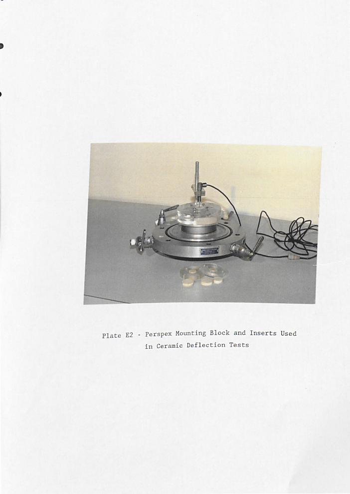
•
Plate E2 - Pe rspex Mounting Block and Inserts Used
in Ceramic Deflection Tests

CIO - Equipment Used During the Manufacture of the Load Cells
No I tell
1 High tolerance lathe
2 Local cell body material
3 Degreasing agent
4 Acidic cleaning agent
5 Cleaning agent neutraliser
6 Surface finishing for AlUllliniUII
7 Strain gauges
8 Strain gauge Dounting tape
9 Strain gauge adhesive
10 Electrical terminals
11 Protective coating
12 Protective coating
13 Glue for mounting inserts
14 Electrical cable
15 Terminal adhesive
16 Dead Weight tester
Details of item
Mechanica Cortini HaO, with ACC-RITE III digital read out
50 mm diameter bar of extruded Aluminium of specification 2014T6
Chlorothene NV
K-Prep Conditioner A
K-Prep Neutraliser 5
400 grit silicon carbide paper
FlA-6-350-23
Mylar JG Tape
M-Bond 610
CTF-60D
RTV Primer No 1
RTV 3140 Silicone Sealant
Locite Engineering Adhesive 290
2 pair, screened
CN CC-3A cyanoacrylate
Budenburg Model 240
I I Specialist I Suppl1er* I I I Inon specialist I I I I I I I
I I
non specialist
WSK+
WSM
WSK
WSK
CNI+
\iSM
\iSM
\iSK
WSM
\iSM
non specialist
Inon specialist I I I I GWI I I I I BGC+ I I I
* Full names and addresses of the spcia1ist suppliers are presented in
Appendix B.
+ Key to abbreviations used in table:
WSK - We1wyn Strain Measurement GYI _ Graham and White Instruments BeC _ Budenburg Gauge Company Limited
Copyright © 2022 FDOKUMEN