arX

iv:c

ond-

mat

/070

1035

v2 [

cond

-mat

.sta

t-m

ech]

20

Apr

200

7

On the validity of entropy production principlesfor linear electrical circuits

Stijn Bruers, Christian Maes1

Instituut voor Theoretische Fysica, K.U.Leuven

and

Karel Netocny2

Institute of Physics AS CR, Prague

Keywords: entropy production, variational principles, nonequilibrium fluctua-tions.

Abstract: We discuss the validity of close-to-equilibrium entropy productionprinciples in the context of linear electrical circuits. Both the minimum and themaximum entropy production principle are understood within dynamical fluctu-ation theory. The starting point are Langevin equations obtained by combiningKirchoff’s laws with a Johnson-Nyquist noise at each dissipative element in thecircuit. The main observation is that the fluctuation functional for time averages,that can be read off from the path-space action, is in first order around equilibriumgiven by an entropy production rate.That allows to understand beyond the schemes of irreversible thermodynamics (1)the validity of the least dissipation, the minimum entropy production, and themaximum entropy production principles close to equilibrium; (2) the role of theobservables’ parity under time-reversal and, in particular, the origin of Landauer’scounterexample (1975) from the fact that the fluctuating observable there is odd un-der time-reversal; (3) the critical remark of Jaynes (1980) concerning the apparentinappropriateness of entropy production principles in temperature-inhomogeneouscircuits.

1. Introduction

Fluctuation theory is a standard topic in equilibrium thermostatis-tics, and its relation to thermodynamic variational principles is verywell understood. In nonequilibrium these studies stem from the funda-mental work of Onsager and Machlup, and its various generalizationsare nowadays a hot topic, [1, 4, 9]. The existence of a link betweenvariational principles like that of least dissipation and the Onsager-Machlup Langrangians has been known for a long time. However, re-cent progress in better understanding the role of time-reversal symme-try and its breaking (cf. fluctuation theorems, Jarzynski identity etc.,see e.g. Refs. [4, 13]) allows to analyze this in a fresh and more system-atic way, and to clean up some old ambiguities and to reinterpret some

1http://itf.fys.kuleuven.be/~christ/2email: netocny@fzu.cz

1

2

of the existing formulations. That is the motivation of the present pa-per.

A traditional way of illustrating how entropy production principlescharacterize the behavior of (non)equilibrium systems goes via thestudy of linear electrical circuits. The reason is that they providephysically clear and mathematically simple testing grounds for thesehypotheses. The minimum and maximum entropy production princi-ples have a reputation of being vague or of being at best only sometimesvalid. In fact a well known counter example was discussed by Landauerin 1975 showing that the minimum entropy production (MinEP) prin-ciple may not be satisfied even close to equilibrium, [10, 11]. A moregeneral criticism was exposed by Jaynes, starting with the remark thatthe MinEP does not even work when in a network the resistors are keptat different temperatures, [8]. Surprisingly, it has not stopped peoplefrom applying MinEP in a variety of contexts and from inventing newproofs for it, see e.g. [17] for a critical review.

In the present paper we illustrate our new understanding of theseprinciples via dynamical fluctuation theory. No longer is it solely amatter of verifying these entropy principles but of explaining their ori-gin and their approximate nature. More mathematical details are in[16]. There are two particular steps in our analysis. First we con-nect the discussion with more recent work in nonequilibrium statisticalmechanics, in particular as described in [14, 13]. We construct a La-grangian governing the distribution of system trajectories; the entropyproduction is identified with the source term of time-reversal breakingin that Lagrangian. Secondly, we explain how the entropy productionprinciples can be derived from the fluctuation theory constructed fromthe Lagrangian. The basic input is the observation that the rate func-tion for certain stationary dynamical fluctuations is in a direct relationwith the entropy production rate, when close to equilibrium and un-der specific conditions. This yields an extension of the classical workby Onsager and Machlup [18] which enables to systematically generatevarious variational characterizations of the stationary state. Amongthese we discuss the validity of both the MinEP and of its counterpartin the maximum entropy production principle (MaxEP). In particularwe revisit Landauer’s counter example and we show why the conditionsfor the validity of the MinEP are not verified.

The plan of the paper is as follows. In the next section we introducethe general framework and formulate the main questions for whichwe give general answers. Afterwards we discuss some generic linearelectrical circuits to illustrate the main points of the theory.

The paper is part of a series of papers in which the entropy produc-tion principles are revisited and extended, also in the light of recentadvances in nonequilibrium statistical mechanics, [15, 16, 2].

3

The number of references on entropy production principles is enormous,mostly however within the formalism of irreversible thermodynamics.We mention some but only a tiny fraction of them in the course of thepaper. As is well known, much of the pioneering work was of coursedone by Ilya Prigogine, see Refs. [19, 6]. As a discussion of some con-ceptual points, we mention Refs. [8, 12].

2. Set-up and general strategy

In the present paper we explain when entropy production principlescan be expected to yield correct physical information. That will beillustrated in the context of linear electrical circuits. Given such a net-work there is often an immediate phenomenological expression of theentropy production rate S(X, X) as a function of the relevant vari-ables X = (Xα) (potentials, currents), their time-derivatives X, andin terms of the network parameters (values of the electrical elements).From S(X, X) we can still construct other entropy production vari-

ables, e.g. by substituting a dynamical law for X one obtains a typical

entropy production rate at state X. The question is now when and whythe correct physical values for the potentials and/or the currents mini-mize or perhaps maximize these entropy production rates, in whateverform. The question and part of the answer will become more clear be-low. We will then give examples of networks, write down the relevantentropy production and show how it can serve, if at all, as a variationalfunctional.

Our treatment of electrical circuits relies on the use of Kirchoff equa-tions that themselves assume a quasi-stationary regime of the Maxwellequations, thus forgetting about the dynamics of the electromagneticfield. The resulting differential equations are well known and their sta-tionary solutions are in the standard textbooks. Obviously our goalis not to study linear electrical networks; in the present paper we usethem merely as an example to illustrate why and how nonequilibriumbehavior can or cannot be obtained from variational principles for theentropy production. We refer to e.g. [7] for other and further illus-trations of the use of electrical networks in studies of nonequilibriumphysics, also using stochastic methods.

For that purpose, Kirchoff’s differential equations will be embeddedin stochastic equations whose averaged behavior reproduces the de-terministic equation. Not only does that enable the use of stochasticmethods but there is also a good physical reason to include extra noise.In accord with the fluctuation-dissipation theorem, the thermal agita-tions in a resistor are related to the distribution of the random electricfield acting upon the electrons. As a consequence, a random voltage

4

emerges and can be measured at the ends of the resistor (Johnson ef-

fect). That voltage can be described as a random process Uft given by

the Nyquist formula:

Uft dt =

√

2R

βdWt, or Uf

t =

√

2R

βξt (2.1)

with R the resistance, Wt a standard Wiener process and more for-mally, ξt a standard white noise; the prefactor is of course very smallby the presence of Boltzmann’s constant in β−1 = kBT , at least whencompared to macroscopic voltage values. Hence, every ‘real’ resistorcan be equivalently represented as an ideal resistor in series with therandom voltage source Uf

t . Using such a representation for all resis-tors present, we can study fluctuations in an arbitrary electrical circuit.The resistors in the network are the only source of fluctuations and ofsteady dissipation. Apart from the transient contributions coming fromcapacitances or inductances, each resistor R through which a current Iflows and which is kept in thermal contact with a reservoir at temper-ature β−1, contributes a steady term βRI2 to the entropy production.Having thus determined the entropy production rate S(X, X) for theelectrical circuit, we must understand how it gives rise to a variationalprinciple for the variables in the network.The following can be skipped at first reading and one can choose to godirectly to the examples in Section 3.

The line of reasoning will be as follows. For a given electrical circuitwe write down (first law) the conservation of charge, that the sum ofall currents equals zero at every node, and (second law) the conserva-tion of energy, that the sum of all potential(differences) over any loopequals zero. In those we take care to add with every resistor the ran-dom process Uf

t for an additional fluctuating potential difference. Thebasic variables are then the potentials and the currents satisfying linearstochastic differential equations of the generic form

Xα(t) = fα +∑

γ

cα,γ Xγ(t) +

√

2

vα

ξα(t) (2.2)

where the ξα(t) are mutually independent standard white noises; theXα represent the fluctuating variables (currents and potentials that canbe chosen freely); the constants vα, cα,γ are determined from Kirchoff’slaws and from the Nyquist formula (2.1) and the fα is the external“force” (such as from an external source or battery). We will see equa-tion (2.2) specified in (3.2), (3.8), (3.16), and (3.24).That stochastic dynamics induces a probability distribution P on his-tories ω, where for each time t, ωt = (Xα(t))α states the values of thepotentials and of the currents. The action in P is readily computed

5

from Ito-stochastic analysis:

P(ω) ∝ exp[

−

∫

dtL(ωt, ωt)]

with Onsager-Machlup Lagrangian, formally,

L(X, X) =1

4

∑

α

vα

(

Xα − fα −∑

γ

cα,γXγ

)2(2.3)

From a mathematical point of view, such expressions are justified withinthe Freidlin-Wentzell theory of stochastic perturbations of determinis-tic evolutions [3]. Observe that vα = O(β) in the electrical circuits andvα f 2

α is a very high frequency for not too high temperatures; thereforethe typical trajectories are Xα = fα +

∑

γ cα,γXγ and β−1 can be takenas a perturbation parameter in the theory.Each time in the examples below, we will explicitly write down thatLagrangian, see (3.4), (3.9), (3.17), and (3.25).

When applying the general model (2.2) to a particular physical prob-lem, we always have to satisfy a consistency condition: that the an-tisymmetric term under time-reversal in L is the physically correctentropy production S(X, X), usually a priori known from the context.It means the entropy production must satisfy

L(εX,−εX) −L(X, X) = S(X, X) (2.4)

with (εX)α = εαXα for parities εα = ±1, labelling the (anti)symmetryunder kinematical time-reversal. E.g., εα = 1 (or − 1) if Xα is a volt-age (or current). In our linear electrical circuits, that is ensured bysatisfying the fluctuation-dissipation relation by taking (2.1) as noiseterms, in combination with a suitable choice of variables or of the levelof description. The latter point is subtle: using a too coarse grainedlevel of description one can easily ‘become blind’ to some contributionsto the total entropy production. Relation (2.4) will be checked in eachexample below, see (3.7), (3.13), (3.18), and (3.25).When there is no driving (no external force nor battery nor differencesin temperature,...) the dynamics certainly reduces to that of an equi-librium system in which case the entropy production rate (2.4) mustbe a total time derivative:

∫ t1

t0

dt S(X(t), X(t)) = β [ H(X(t1)) − H(X(t0)) ] (2.5)

for some energy function H(X) and some inverse temperature β. Theequation (2.5) formulates the condition of detailed balance.

2.1. Transient entropy production principles. For the purpose ofobtaining variational principles, we must look back at the Lagrangian(2.3). We can for example fix a history (Xα(s)) for times s ≤ t beforesome fixed t and ask what is the most probable immediate future.

6

Clearly, it amounts to finding the (Xα(t)) that minimize L(X(t), X(t)),i.e., to minimize

D1(X, X) =1

4

∑

α

vα

[

X2

α − 2Xα

(

fα +∑

γ

cα,γXγ

)]

(2.6)

That is traditionally called the least dissipation principle because whenall variables are even, εα = 1, it is easily checked that

2D1(X, X) =1

2

∑

α

vαX2

α − S(X, X) (2.7)

which can be traced back to mechanical and equilibrium analoguesgiven by Rayleigh and Onsager, see [18]; the expression

D(X) =∑

α

vαX2

α (2.8)

is sometimes called the dissipation function. The typical behaviorXα = fα +

∑

γ cα,γ Xγ as expected from (2.2), can thus be charac-

terized as the one minimizing (2.7) (still under the condition that allεα = 1). We can rewrite that as a (transient) maximum entropy pro-duction principle (discussed in e.g. Ref. [20]). Indeed, minimizing

(2.7) over the X (for given X) is equivalent with maximizing S(X, X)under the additional constraint that D(X) = S(X, X).

Alternatively, we can fix the Xα’s in (2.3) and we collect the freevariable part of (2.3) in what we call D2; we must then find the Xα’sminimizing

D2(X, X) =1

4

∑

α

vα

[(

∑

γ

cα,γXγ

)2

−2(Xα − fα)∑

γ

cα,γXγ

]

(2.9)

The solution will give us the typical Xα’s. When now all the variablesare odd, εα = −1, that reduces to minimizing

2D2(X, X) =1

2

∑

α

vα

(

∑

γ

cα,γXγ

)2− S(X, X) (2.10)

With the definition of typical (or expected) entropy production

σ(X) = S(X, X = f +∑

γ

c·,γ Xγ) (2.11)

the expression (2.10) can be rewritten as

2D2(X, X) =1

2σ(X) − S(X, X) (2.12)

7

which we have to minimize over the Xα’s or, alternatively, S(X, X) has

to be maximized under the constraint S(X, X) = σ(X).

Remark that if either a) all variables are even and driving forcesarbitrary, or b) all variables are odd and the forces absent, fα ≡ 0,

then both the variational principles D(X)/2− S(·, X) = min (2.7) andσ(X)/2−S(X, ·) = min (2.12) are valid and in a sense dual. The reasonis that they are both corresponding to a relaxation to equilibrium withLagrangian taking the symmetric form

2L(X, X) =1

2D(X) − S(X, X) +

1

2σ(X) (2.13)

a scenario originally considered by Onsager and Machlup [18]. How-ever, that structure needs a modification when a true nonequilibriumdriving is present and/or when even and odd variables mix with eachother. (There was already an example above when all variables wereodd and a driving force was switched on.)

In applications, most interesting is the stationary regime for whichX = 0. We discuss that at large in the next section.

2.2. Stationary entropy production principles. For the station-ary regime, we obtain a variational functional by simply putting Xα = 0in the Lagrangian (2.3) to get

J (X) =1

4

∑

α

vα

(

fα +∑

γ

cα,γXγ

)2(2.14)

A more fundamental point is that J is the large deviation rate function

for empirical averages∫ T

0X(t) dx/T when T ↑ ∞, i.e.,

P[ 1

T

∫ T

0

X(t) dt = x]

≃ exp[−TJ (x)] (2.15)

The mathematical theory of such large deviations was initiated byDonsker and Varadhan, see [5, 3]. Equation (2.15) resembles Ein-stein’s formula for equilibrium fluctuations from which various vari-ational characterizations of equilibrium follow, in terms of entropy andrelated potentials, see also Ref. [15]. Our line of thinking is similarhere: a systematic way to obtain meaningful nonequilibrium varia-tional principles is to consider dynamical large deviations. That pointof view gets of course more interesting when the stationary state is lessexplicit, like for mesoscopic systems or for more general Markov pro-cesses [16] far from equilibrium, possibly with time-dependent drivingetc.

8

2.2.1. Even variables. When all fluctuating variables are even undertime-reversal (all ε = +1), then it is easy to verify that

J (X) =1

4σ(X) (2.16)

see e.g. (2.13). Thus, in that case, we get the typical (equilibrium)values for the X by minimizing the entropy production σ(X), whichbecomes zero in equilibrium. The most basic example is in Section 3.1.

2.2.2. Odd variables. Including variables that are odd under time-reversalis necessary in order to obtain a truly nonequilibrium stationary statein the present framework. We first investigate what happens when wehave only odd variables.The basic idea is always that we must minimize J (X) but now it dif-fers from the physical entropy production. That is in accord with ageneral observation that for odd variables the minimum entropy pro-duction principle does not apply. Instead, minimizing J (X) can nowbe understood as a certain maximum entropy production principle.The reason is that for odd variables

2J (X) =1

2σ(X) − S(X, 0) +

1

2

∑

α

vαf 2

α (2.17)

Hence, we need to minimize

1

2σ(X) − S(X, 0) (2.18)

In the stationary case, we have σ(X) = S(X, 0). Thence, minimiz-ing J (X) amounts to maximizing the entropy production σ(X) under

the constraint that σ(X) = S(X, 0). That repeats the discussion af-ter (2.12), but this time for the stationary case X = 0.The required modification of the MinEP (to minimizing (2.18)) whendealing with odd variables is also how Landauer’s counter example [10,11] should be understood. The details are in Section 3.2.

2.2.3. Even and odd. The above equations (2.16, 2.17) have been ob-tained for dynamical variables that are either all even or all odd un-der time-reversal. We can make that more general. Suppose our La-grangian includes both time-reversal even and odd variables: {Xα} ={X+

i , X−i }, where it is understood that the X+

i are even and that theX−

i are odd under time-reversal. The Lagrangian (2.3) now takes theform (in obvious notation):

L(X, X) =1

4

∑

i+

v+

i

(

X+

i − f+

i −∑

j+

c++

ij X+

j −∑

j−

c+−ij X−

j

)2

+1

4

∑

i−

v−i

(

X−i − f−

i −∑

j+

c−+

ij X+

j −∑

j−

c−−ij X−

j

)2

(2.19)

9

Remember that from the beginning we restrict ourselves to externaldriving forces which are even under time-reversal; for odd driving forcesalready (2.4) needs a modification but an analogous reasoning applies.

Let us first consider the entropy production rates. After some cal-culation, we find for the expected entropy production (2.11):

σ(X+, X−) =∑

i+

v+

i

(

f+

i +∑

j+

c++

ij X+

j

)2

+∑

i−

v−i

(

∑

j−

c−−ij X−

j

)2(2.20)

From this we can further construct a function of the even and a func-tion of the odd variables. We thus get two additional, even and odd,expected entropy production rates σ+(X+) and σ−(X−) given as

σ+(X+) = σ(X+, X−(X+))

σ−(X−) = σ(X+(X−), X−)(2.21)

where for the first (even) case we insert X− = X−(X+) from solvingthe stationary condition

f−i +

∑

j+

c−+

ij X+

j +∑

j−

c−−ij X−

j = 0

and likewise, for the second (odd) case we substitute X+ = X+(X−)as found from

f+

i +∑

j+

c++

ij X+

j +∑

j−

c+−ij X−

j = 0

That will be explicitly visible and done in (3.22).

The large deviation rate function (2.14) can also be calculated:

4J (X+, X−) =∑

i+

v+

i

[(

f+

i +∑

j+

c++

ij X+

j

)2+

(

∑

j−

c+−ij X−

j

)2

+ 2(

f+

i +∑

j+

c++

ij X+

j

)(

∑

j−

c+−ij X−

j

)]

+∑

i−

v−i

[(

f−i +

∑

j+

c−+

ij X+

j

)2+

(

∑

j−

c−−ij X−

j

)2

+ 2(

f−i +

∑

j+

c−+

ij X+

j

)(

∑

j−

c−−ij X−

j

)]

To simplify the structure, we make here the (nontrivial) assumptionthat the even and the odd variables do not mix in J . Hence, werequire that

J (X+, X−) = J +(X+) + J −(X−) (2.22)

10

(i.e., the cross terms are zero), with

4J +(X+) =∑

i+

v+

i (f+

i +∑

j+

c++

ij X+

j )2

+∑

i−

v−i (f−

i +∑

j+

c−+

ij X+

j )2(2.23)

and analogously for J −(X−), see below in (2.25). That decoupling ofthe even from the odd variables in the rate function J , implies therelation

4J +(X+) = σ+(X+) (2.24)

which is a generalization of (2.16).Remember now that we must minimize J (here of the form (2.22))to obtain the typical stationary values. Hence, if indeed the time-symmetric and time-antisymmetric variables in J decouple, then (2.24)tells that we should minimize the expected entropy production σ+. Wewill see an example below in Section 3.3.

There is also a MaxEP principle in the above setting. Write J − as

4J − =∑

i+

v+

i

(

∑

j−

c+−ij X−

j

)2+

∑

i−

v−i

(

∑

j−

c−−ij X−

j

)2

+ 2∑

i+

v+

i f+

i

∑

j−

c+−ij X−

j + 2∑

i−

v−i f−

i

∑

j−

c−−ij X−

j

= σ−(X−) − 2P(f, X−)

(2.25)

where P can be interpreted as the power input from the external forcesf . Suppose we take the constraint σ− = P meaning that the deliveredwork is completely dissipated and there is no accumulation of internalenergy (true indeed in the stationary state when X = 0). MinimizingJ −(X−) under the constraint σ− = P is equivalent to maximizing σ−

under the same constraint. That MaxEP principle was used similarlyin Ref. [21].

3. Examples

We demonstrate the above general theory on a few simple examplesof linear circuits. In particular we will see that close to equilibriumthe rate function J can indeed be split in the even and odd parts,and hence, depending on the choice of variables, we obtain MinEP orMaxEP principle.

3.1. RC in series. Consider a resistance R in series with a capacityC and with a steady voltage source E. Write U = Ut for the variablepotential difference over the capacitor. Kirchhoff’s second law reads

RCU = E − U + Uf (3.1)

11

By inserting the white noise ξt following (2.1), we are to study theLangevin equation

Ut =E − Ut

RC+

√

2

βRC2ξt (3.2)

There is no other free variable apart from U ; in particular, the currentI = CU . A standard reasoning proves the consistency of this model:with the battery removed, E = 0, the dynamics is reversible withrespect to the Gibbs distribution at inverse temperature β and withenergy function H(U) = CU2/2. In particular, limt↑∞〈U2

t 〉 = (βC)−1,in accordance with the equipartition theorem.

Heuristically, the entropy production rate σ(U) as a function of thevoltage U on the capacitor is simply the Joule heating in the resistorR:

σ(U) = β(E − U)2

R(3.3)

Apparently, its minimizer U∗ = E coincides with the correct value forthe stationary voltage, verifying the MinEP principle.We can understand that within our general framework. The Onsager-Machlup Lagrangian L(U, U) of the process Ut is

L(U, U) =βRC2

4

(

U −E − U

RC

)2

(3.4)

From L we can derive the fluctuations of the empirical voltage UT =∫ T

0Ut dt /T . The stationary (T ↑ +∞) fluctuations of UT are given by

(2.14)-(2.15):P[UT ≃ u] ∝ exp[−TJ (u)] (3.5)

with rate function

J (U) = L(U, 0) =1

4σ(U) (3.6)

The fluctuation law (3.5) thus gives a variational principle for the sta-tionary voltage just coinciding with the MinEP principle: the mostprobable value for the time-averaged voltage is obtained by minimiz-ing J (U) = σ(U)/4.In fact, this is just a particular example of the relation (2.16). Tosee that we still have to check that our model is consistent with rela-tion (2.4). Indeed,

S(U, U) = L(U,−U) − L(U, U) = βCU(E − U) (3.7)

is the physical entropy production rate, and its typical value (2.11)equals

S(

U, U =E − U

RC

)

= σ(U)

verifying (3.3) above. Hence, from the fluctuation point of view, themanifest validity of the MinEP principle for this RC-circuit is nothing

12

but a consequence of the invariance of the voltage (or charge) withrespect to time-reversal.

3.2. RL in series. If the capacity in the previous section is replacedwith an inductance L, the situation remarkably changes. In that case,Kirchhoff’s second law for the current I becomes

RI − Uf + LdI

dt= E

(where the minus sign is chosen for convenience only), or, inserting thewhite noise ξt from (2.1),

It =E − RIt

L+

√

2R

βL2ξt (3.8)

That is again a linear Langevin equation, but now the fluctuations con-cern the current It which is odd under time-reversal.

We can try to repeat the same as in the previous section. The La-grangian now equals

L(I, I) =βL2

4R

(

I −E − RI

L

)2

(3.9)

The construction of the fluctuation rate J (I) for the empirical current∫ T

0It dt /T can again be done following (2.14)-(2.15) with the result

J (I) = L(I, I = 0) =βR

4

(

I −E

R

)2

(3.10)

As generally true, the minimum of J over I is given by the correctstationary value. However, that J clearly differs from the physicalentropy production the expected rate of which is now

σ(I) = βRI2 (3.11)

So while we can find the most probable current I∗ = E/R by mini-mizing J (I), it does not correspond to a minimization of the entropyproduction. Indeed, our RL-circuit is the classical example first givenby Landauer through which we see that the MinEP principle is notgenerally valid and ‘not reliable’ when applied to macroscopic systems,even in the linear irreversible regime. We can now however understandwhat is the real cause of that effect.

Similarly to (3.6)-(3.7), the variational functional J (I) of (3.10) forthe stationary current satisfies

J (I) =1

4

[

L(I,−I) − L(I, I)]∣

∣

I=E−RI

L

(3.12)

13

but L(I,−I)−L(I, I) does not longer coincide with the variable entropy

production S. Since the current is odd under time reversal, the latteris rather, see (2.4),

S(I, I) = L(−I, I) −L(I, I) = βI(E − LI) (3.13)

in accordance with the phenomenology; note that the equilibrium dy-namics (i.e. (3.8) with E = 0) satisfies detailed balance with energyfunction H(I) = LI2/2.Via our fluctuation approach we thus understand the origin of theproblem: the MinEP principle is generally valid only for Markoviandynamical systems described via a collection of observables that aresymmetric under time-reversal. The Markovian property refers to thefirst order (in time) of the dynamical equation and indicates that thevariable in question thus satisfies an autonomous equation.Observe that we now see appear the ‘true’ variational principle forthe stationary current as was explained under (2.17)-(2.18): for oddobservables the above argument proposes a different functional thatreplaces the entropy production σ(I) and that can here be chosen as

1

2σ(I) − S(I, 0)

as follows from (3.10) written in the form

J (I) =1

4σ(I) −

1

2S(I, 0) +

βE2

4R

As the stationary value I∗ satisfies σ(I∗) = S(I∗, 0), we can alsostate the above variational principle as a maximum entropy produc-tion principle: we must maximize σ(I) subject to the condition that

S(I, 0) = σ(I).

3.3. RR in series. Consider an electrical circuit consisting of a bat-tery E coupled to resistors in series. Appending an independent Nyquistrandom voltage source Uf

k to all resistances Rk, we get that the currentI fluctuates according to

I∑

k

Rk = E +∑

k

Ufk (3.14)

Here, the current follows a singular Markov process of the form of awhite noise. We can however modify that singular dynamics so that itbecomes a regular Markov process and so that the (averaged) stationarycurrent remains unchanged. An important addition to the discussion isto see the effect of assigning different temperatures βk to the individualresistors, as it was claimed that such an extension would again yield acounter example to the MinEP, [8].For regularization we choose to add an inductance in series with the re-sistors so that a non-trivial transient regime can arise. However, addingonly an inductance gives a too coarse grained description, because as

14

E

R1

R2 L

C

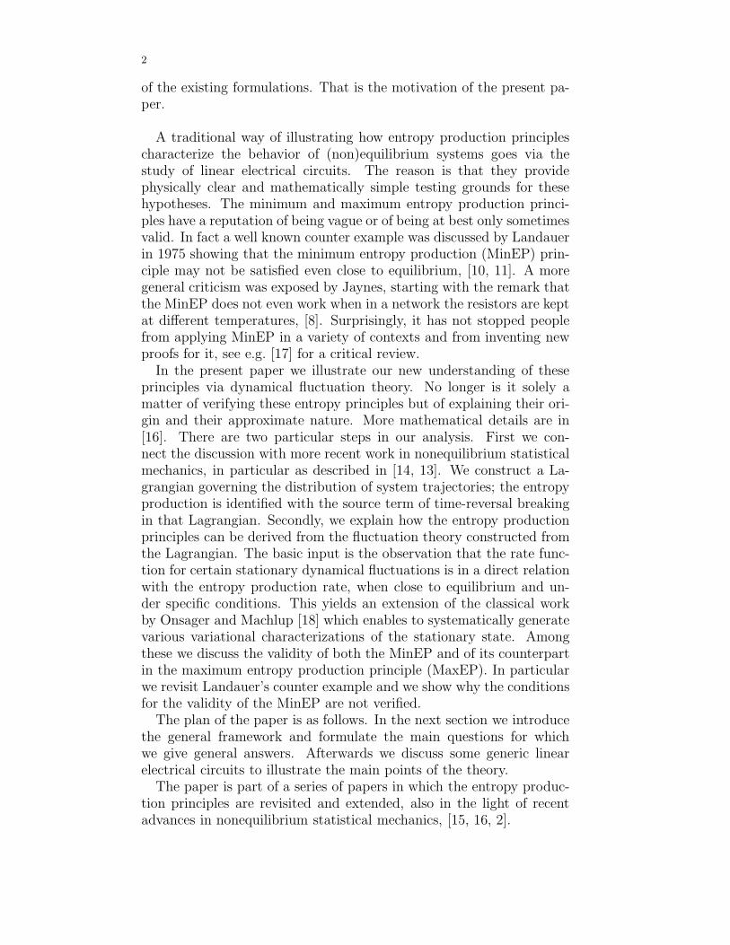
Figure 1. The regularized RR-circuit.

one can check, then (2.4) would not be satisfied with the correct ex-pression for the entropy production. That can be solved by adding acapacitance in parallel with one of the resistors, see Fig. 1. We thushave an effective RLC-circuit with two resistors in series and one ex-ternal voltage. The two independent free variables are the potentialU over the first resistor and the current I through the second resistor.The variational functional (2.14) or the expected entropy production(2.11) will not depend on the auxiliary inductance L or on the capaci-tance C.

The dynamical equations are given by Kirchoff’s laws:

U =I

C−

U

R1C+

Uf1

R1C

I =E − R2I − U

L+

Uf2

L

(3.15)

where always from (2.1), Uf1,2 dt =

√

2R1,2β−1

1,2 dWt. The equilibrium

dynamics (E = 0, β1 = β2 = β in (3.15)) can be written as

U =1

LC

∂H

∂I− γ1

∂H

∂U+

√

2γ1

βξ1

I = −1

LC

∂H

∂U− γ2

∂H

∂I+

√

2γ2

βξ2

(3.16)

for energy function H(U, I) = (CU2 + LI2)/2 and friction coefficientsγ1 = 1/(R1C

2), γ2 = R2/L2; the ξ1 and ξ2 are independent standard

white noises. The first terms on the right hand-side of (3.16) specify aHamiltonian dynamics for the pair (U, I), while the other terms balancethe dissipation and the random forcing.

15

The (nonequilibrium) Lagrangian is obtained from (3.15) as

L(U, I; U , I) =β1R1C

2

4

(

U −I

C+

U

R1C

)2

+β2L

2

4R2

(

I +R2I

L−

E − U

L

)2

(3.17)

and the variable entropy production (2.4) is

S(U, I; U , I) = L(U,−I;−U , I) −L(U, I; U , I)

= β1U(I − CU) + β2I(E − U − LI)(3.18)

as it should. One recognizes indeed the dissipation in each resistor;I −CU is the current through resistor 1 and E −U −LI is the voltageat resistor 2. Thus, the expected entropy production (2.11) is

σ(U, I) = β1

U2

R1

+ β2R2I2 (3.19)

On the other hand, the true variational functional (2.14)-(2.15) is di-rectly obtained from (3.17):

4J (U, I) = σ(U, I) + β1R1I2 + β2

(E − U)2

R2

− 2[β1UI + β2(E − U)I]

(3.20)

and differs from the entropy production because we have both an even(the potential U) and an odd (the current I) degree of freedom; com-pare with (2.16) and (2.17) valid in the case of only even respectivelyonly odd variables. So now we have to go to the formalism with mixedvariables as in (2.19)–(2.25). Although J does not exactly split intoeven and odd parts as in (2.22), it does approximately close to equilib-rium: if β = β1 = β2 + ǫ, we have

4J(U, I) = β[U2

R1

+(E − U)2

R2

]

+ β(R1 + R2)I2

− 2βEI + O(ǫ)

(3.21)

which is of the form (2.22). Since the even and the odd versions (2.21)of the entropy production rate are

σ+(U) = β1

U2

R1

+ β2

(E − U)2

R2

= β[U2

R1

+(E − U)2

R2

]

+ O(ǫ) (3.22)

and

σ−(I) = β1R1I2 + β2R2I

2 = β(R1 + R2)I2 + O(ǫ) (3.23)

the minimization of J provides us with the next two variational prin-ciples:First, the stationary voltage U∗ is obtained from minimizing J +(U) =

16

σ+(U)/4, which is a (generalized) MinEP principle (2.24).Second, minimizing J −(I) = σ−(I)− 2βEI or, equivalently, maximiz-ing σ− under the constraint σ−(I) = βEI yields the stationary currentI∗; this is an example on the MaxEP principle (2.25).

An important remark is that the above derivation of the MinEP andthe MaxEP principles was based not only on the assumption that thetemperature is approximately homogenous but also on the linearity ofthe stochastic model(s) under consideration. They should be reallytaken as a (linear) approximation around detailed balance. In partic-ular, also the current I and the forces U and E should be consideredof order O(ǫ), together with the assumed β2 = β1 + O(ǫ). The abovethen means that the MinEP and MaxEP principles are only valid up toorder O(ǫ2), i.e. within the linear irreversible regime; see [16] for somemore details.In view of this remark we understand better why these principles do notcarry over to temperature-inhomogeneous circuits: in our simple cir-cuits the temperature gradients are redundant thermodynamic forces inthe sense that they do not generate electric currents by themselves; theyonly modify the dynamics of fluctuations. Hence, these gradients yieldcorrections of order o(ǫ2), beyond the resolution of the MinEP/MaxEPprinciples. This solves the remarks by Jaynes [8]. Apparently, the pic-ture would get completely changed by adding e.g. a thermocouple intothe network.

3.4. RR in parallel. For the sake of completeness, we finally considertwo resistors in parallel and coupled with an external voltage sourceE. The independent variables are the currents I1 and I2 through thetwo resistors. To have a dynamics consistent with our condition (2.4)we again need a regularization and for that we add two inductances inseries with the resistances. The resulting stochastic dynamics is

L1I1 = E − R1I1 + Uf1

L2I2 = E − R2I2 + Uf2

(3.24)

The Lagrangian, the entropy production rate, its expectation, and thestationary variational functional are subsequently as follows:

4L =β1

R1

(L1I1 + R1I1 − E)2 +β2

R2

(L2I2 + R2I2 − E)2

S(I1, I2; I1; I2) = β1I1(E − L1I1) + β2I2(E − L2I2)

σ(I1, I2) = β1R1I2

1 + β2R2I2

2

4J (I1, I2) = σ(I1, I2) − 2S(I1, I2, 0, 0) + β1

E2

R1

+ β2

E2

R2

(3.25)

17

If β1 = β2 + ǫ, minimizing the rate function J results in minimizingσ(I1, I2) − 2βE(I1 + I2) up to order ǫ. Note that this splits into twoindependent variational problems for I1 respectively I2 which comes asno surprise: the two currents are entirely dynamically decoupled. Yet,one can again formulate a single MaxEP principle in this case: thestationary currents are obtained by maximizing the expected entropyproduction rate σ under the constraint σ(I1, I2) = βE(I1 + I2), theright hand side being just the total power input. This formulation isequivalent with the MaxEP principle in [21]. Analogous remarks as inSection 3.2 apply here.

4. Conclusions

Fluctuation theory naturally identifies the specific structure of dy-namical fluctuations as the underlying reason for the (variational) en-tropy production principles as well as their validity conditions and lim-itations; just as the equilibrium fluctuation theory explains the maxi-mum entropy principle and its derivations. It also provides a naturaland systematic way how to search for new variational principles beyondtrial-and-error methods, not available within pure thermodynamics.

We summarize our findings within that more general perspective:

• Both MinEP and MaxEP principles have various forms (for hy-drodynamic models in local equilibrium, for discrete networks,for various types of Markov processes,...), but there is no es-sential difference between them up to the crucial restriction tothe close-to-equilibrium regime. All attempts for their exactjustification beyond the linear regime are highly doubtful. Inparticular, thermodynamics itself has little to say here aboutpossible generalizations except via some trial-and-error meth-ods. We expect that dynamical fluctuation theory will present amore systematic avenue for evaluating nonequilibrium behaviorvia variational methods.

• There is no fundamental difference between the nature and va-lidity of the MinEP and the MaxEP principles. Which one isto be used depends on the choice of thermodynamic variables,whether they are symmetric or antisymmetric with respect totime-reversal. That clear observation is a first concrete resultthat the fluctuation/statistical approach provides.

• The set-up in the pioneering works of Prigogine [19] concern-ing MinEP typically refers to some canonical thermodynamicstructure. Yet, it is useful to broaden the view on these vari-ational principles; the MinEP principle is valid for mesoscopicsystems (Markovian, both with discrete and with continuous

18

state space) where one does not a priori recognize some canon-ical structure as is usually written in terms of forces and cur-rents.

Acknowledgment

K. N. is grateful to the Instituut voor Theoretische Fysica, K. U. Leu-ven for kind hospitality. He also acknowledges the support from theGrant Agency of the Czech Republic (Grant no. 202/07/0404). C. M.benefits from the Belgian Interuniversity Attraction Poles ProgrammeP6/02.

References

[1] L. Bertini, A. De Sole, D. Gabrielli, G. Jona-Lasinio and C. Landim, Minimumdissipation principle in stationary non equilibrium states, J. Stat. Phys. 116:831 (2004).

[2] S. Bruers, Classification and discussion of macroscopic entropy productionprinciples. arXiv:cond-mat/0604482.

[3] A. Dembo and O. Zeitouni. Large Deviation Techniques and Applications.Jones and Barlett Publishers, Boston (1993).

[4] B. Derrida, Non equilibrium steady states: fluctuations and large deviationsof the density and of the current, arXiv:cond-mat/0703762v1.

[5] M. D. Donsker, S. R. Varadhan, Asymptotic evaluation of certain Markovprocess expectations for large time, I. Comm. Pure Appl. Math., 28:1 (1975).

[6] S. R. de Groot, P. Mazur. Non-equilibrium Thermodynamics. North HollandPublishing Company (1969).

[7] A. Hjelmfelt and J. Ross, Thermodynamic and stochastic theory of electricalcircuits, Phys. Rev. A, 45:2201 (1992).

[8] E. T. Jaynes, The minimum entropy production principle, Ann. Rev. Phys.

Chem., 31:579–601 (1980).[9] A. N. Jordan, E. V. Suhorukov and S. Pilgram, Fluctuation statistics in net-

works: a stochastic path integral approach, J. Math. Phys., 45:4386 (2004).[10] R. Landauer, Inadequacy of entropy and entropy derivatives in characterizing

the steady state, Phys. Rev. A, 12:636–638 (1975).[11] R. Landauer, Stability and entropy production in electrical circuits,

J. Stat. Phys., 13:1–16 (1975).[12] R. Landauer, Statistical physics of machinery: forgotten middle-ground, Phys-

ica A, 194:551–562 (1993).[13] C. Maes, On the origin and the use of fluctuation relations for the entropy.

Seminaire Poincare, 2:29–62, Eds. J. Dalibard, B. Duplantier and V. Ri-vasseau, Birkhauser, Basel (2003).

[14] C. Maes and K. Netocny, Time-reversal and entropy. J. Stat. Phys., 110:269–310 (2003).

[15] C. Maes and K. Netocny, Static and Dynamical Nonequilibrium Fluctuations,arXiv:cond-mat/0612525.

[16] C. Maes and K. Netocny, Minimum entropy production principle from a dy-namical fluctuation law, arXiv:math-ph/0612063.

[17] L. M. Martyushev, A. S. Nazarova, and V. D Seleznev, On the problem of theminimum entropy production in the nonequilibrium stationary state, J. Phys.A: Math. Theor., 40: 371-380 (2007).

19

[18] L. Onsager and S. Machlup, Fluctuations and irreversible processes.Phys. Rev., 91:1505–1512 (1951).

[19] I. Prigogine, Introduction to Non-Equilibrium Thermodynamics, Wiley-Interscience, New York (1962).

[20] H. Ziegler, An Introduction to Thermomechanics, North-Holland, Amsterdam(1983).

[21] P. Zupanovic, D. Juretic and S. Botric, Kirchhoff’s loop law and the maximumentropy production principle, Phys. Rev. E, 70:056108 (2004).