Appl Math Optim (2007) 56: 364–378DOI 10.1007/s00245-007-9017-6

On the Stochastic Maximum Principlein Optimal Control of Degenerate Diffusionswith Lipschitz Coefficients

Khaled Bahlali · Boualem Djehiche ·Brahim Mezerdi

Published online: 6 September 2007© Springer Science+Business Media, LLC 2007

Abstract We establish a stochastic maximum principle in optimal control of a gen-eral class of degenerate diffusion processes with global Lipschitz coefficients, gen-eralizing the existing results on stochastic control of diffusion processes. We usedistributional derivatives of the coefficients and the Bouleau Hirsh flow property, inorder to define the adjoint process on an extension of the initial probability space.

Keywords Stochastic differential equation · Optimal control · Stochastic maximumprinciple · Degenerate diffusion

1 Introduction

The systems under consideration in this paper are governed by stochastic differentialequations (SDEs) of the form:{

dxt = b(t, xt , ut ) dt + σ(t, xt ) dBt ,

x0 = α,

This work is partially supported by MENA Swedish Algerian Research Partnership Program(348-2002-6874) and by French Algerian Cooperation, Accord Programme Tassili, 07 MDU0705.

K. BahlaliUFR Sciences, UTV, B.P 132, 83957 La Garde, Cedex, Francee-mail: bahlali@univ-tln.fr

K. BahlaliCPT, CNRS Luminy, Case 907, 13288 Marseille Cedex 9, France

B. DjehicheDivision of Mathematical Statistics, Department of Mathematics, Royal Institute of Technology,100 44 Stockholm, Swedene-mail: boualem@math.kth.se

B. Mezerdi (�)Laboratory of Applied Mathematics, University of Biskra, P.B. 145 07000 Biskra, Algeriae-mail: bmezerdi@yahoo.fr

Appl Math Optim (2007) 56: 364–378 365

where (Bt ) is a Brownian motion defined on some probability space (�,F , (Ft )t , P ),u is a suitable control process adapted to the filtration (Ft ), and (xt ) denotes the stateof the system controlled by (ut ). The control problem we are interested in, consiststo find an admissible control u that minimizes a finite horizon cost functional of theform

J (u) = E

[∫ T

0h(t, xt , ut ) dt + g(xT )

].

A control process that solves this problem is called optimal and (u, x) is called anoptimal pair, where x denotes the solution of the driving SDE corresponding to u. Ifu is some optimal control, we may ask how we can characterize it, in other words,what conditions must u necessarily satisfy? These conditions are called the Pontrya-gin necessary conditions for optimality, or the stochastic maximum principle (SMP).Roughly speaking, this principle can be formulated as follows: we assume that (u, x)

is an optimal pair, and define the Hamiltonian

H(t, x,u,p) = p . b(t, x,u) − h(t, x,u).

Consider the adapted solution (pt , qt ) of the linear backward stochastic differentialequation

{dpt = −Hx(t, xt , ut , pt ) dt + qt dBt ,

p(T ) = −gx(xT ).

Under some differentiability assumptions on the data, the stochastic maximum prin-ciple states that

maxu∈U

H(t, xt , u,pt ) = H(t, xt , ut , pt ), a.e. t ∈ [0, T ], P -a.s.

In stochastic control, the measurability assumptions made on the control variablesand the nature of solutions of the underlying SDE, play an essential role in the state-ment of the maximum principle. The first version of the stochastic maximum prin-ciple was established by Kushner [15] for the class of controls, adapted to a fixedfiltration. Haussmann [13] developed a powerful form of the stochastic maximumprinciple for the important class of feed-back controls, and applied it to solve someimportant problems in stochastic control. Versions of the SMP in which the diffu-sion coefficient is allowed to depend explicitly on the control variable were derivedby Arkin and Saksonov [1], Bensoussan [5], Peng [18]. Other extensions includingrandom coefficients, singular controls or forward-backward equations can be foundin [3, 4, 6, 8, 9, 21].

In deterministic control, some efforts have been made to derive optimality nec-essary conditions with differentiability assumptions on the data weakened or elimi-nated. The motivation being provided by a number of control problems of both prac-tical and theoretical interest. Many authors have developed optimality necessary con-ditions, including [10, 12, 17, 19, 20]. The most powerful of these results remains themaximum principle developed by Clarke, based on a differential calculus for locallyLipschitz functions.

366 Appl Math Optim (2007) 56: 364–378

In the stochastic case, the first result has been derived by Mezerdi [16] in the caseof a SDE with a non-smooth drift, by using Clarke generalized gradients. The secondresult is performed by Bahlali et al. [2] for SDEs with Lipschitz coefficients and anon degenerate diffusion matrix. The approach used in [2] applies arguments of morefunctional analytic nature and is totally different from known deterministic methods.It does not use Clarke’s generalized gradients. This approach is based on Krylov’sinequality [14] which requires the uniform ellipticity of the diffusion matrix.

The main result in this paper is a stochastic maximum principle for SDEs withglobally Lipschitz coefficients. We do not assume the uniform ellipticity of the diffu-sion coefficient, so that our result covers the deterministic case. We use distributionalderivatives of the coefficients to define the adjoint process as the solution of a linearbackward SDE defined on an extension of the initial probability space. The proofis based on a result by Bouleau and Hirsch [7] on the differentiability of the solu-tion of an SDE with Lipschitz coefficients with respect to initial data, in the sense ofdistributions.

2 Assumptions and Statement of the Main Result

2.1 Assumptions

Let � = C0(R+,Rd) be the space, of continuous functions ω such that ω(0) = 0,

endowed with the topology of uniform convergence on compact subsets of R+. LetF be the Borel σ -field over �, P be the Wiener measure on (�,F) and (Ft )t≥0the filtration of coordinate process augmented with P -null sets of F . We define thecanonical process Bt(ω) = ω(t), t ≥ 0. Thus, (�,F , (Ft )t≥0,P ,Bt ) is a Brownianmotion. Let T be a fixed strictly positive real number and A a compact subset of R

n.

Definition 2.1 By an admissible control we mean an Ft -progressively measurable,A-valued process. The set of all admissible controls is denoted by U .

For each admissible control u, let (xt ) be the solution of the controlled stochasticdifferential equation:

{dxt = b(t, xt , ut ) dt + σ(t, xt ) dBt ,

x0 = α.(2.1)

The solution (xt ) of the above equation is called the response of the control u and(u, x) is called an admissible pair. These controls are often called strong controls,because the underlying probability space and Brownian motion do not change with u.

Assume that the drift b : R+ × Rd×A → R

d and the diffusion matrix σ :R+×R

d→ Rd⊗R

d are Borel measurable functions and there exist M > 0, suchthat for all (t, x, y, a) in R+ × R

d × Rd × A

|σ(t, x) − σ(t, y)| + |b(t, x, a) − b(t, y, a)| ≤ M|x − y|, (2.2)

|σ(t, x)| + |b(t, x, a)| ≤ M(1 + |x|), (2.3)

b(t, x, .) : A −→ Rd is continuous, uniformly in (t, x). (2.4)

Appl Math Optim (2007) 56: 364–378 367

Assumptions (2.2) and (2.3) guarantee the existence and uniqueness of a strong solu-tion for (2.1), such that for any p > 0, E[supt≤T |xt |p] < +∞.

Since the functions b,σ j (the j th column of the matrix σ ) are Lipschitz con-tinuous in the state variable then, according to the Rademacher Theorem, they aredifferentiable almost everywhere in the sense of Lebesgue measure (see [10]). Letbx , σ

jx be any Borel measurable functions such that

∂b

∂x= bx(t, x, a) dx-a.e.,

∂σ j

∂x= σ

jx (t, x) dx-a.e.

Clearly, these almost everywhere derivatives are bounded by the Lipschitz con-stant M .

Finally, assume that

bx(t, x, a) is continuous in a uniformly in (t, x). (2.5)

The finite horizon cost function to be minimized over admissible controls is given by

J (u) = E

[∫ T

0h(t, xt , ut ) dt + g(xT )

], (2.6)

where h : R+ × Rd×A −→ R , g : R

d−→ R are bounded, Borel measurable func-tions and there exist M > 0, such that for all (t, x, y, a) in R+ × R

d × Rd × A

|g(x) − g(y)| + |h(t, x, a) − h(t, y, a)| ≤ M|x − y|, (2.7)

h(t, . , a) and g(.) are continuously differentiable, (2.8)

h(t, x, a) and hx(t, x, a) are continuous in a uniformly in (t, x). (2.9)

We assume throughout this paper that an optimal pair (u, x) of the control problemassociated with (2.1) and (2.6) exists. That is

J (u) = infu∈U

J (u).

Let h be a continuous positive function on Rd satisfying

∫h(x)dx = 1 and∫ |x|2h(x)dx < +∞. Define the space of functions

D :={f ∈ L2(hdx); such that

∂f

∂xj

∈ L2(hdx), j = 1, . . . , d

},

where ∂f∂xj

denotes the derivative of f in the sense of distributions. Endowed with thenorm,

‖f ‖D :=[∫

f 2hdx +∑

1≤j≤d

∫ (∂f

∂xj

)2

hdx

]1/2

,

D is a Hilbert space. Note also that D is a subset of H 1loc(R

d).

368 Appl Math Optim (2007) 56: 364–378

Let � := Rd × �, F the Borel σ -field over � and P := hdx ⊗ P, Bt (x,ω) :=

Bt(ω), (F)t≥0 be the natural filtration of Bt augmented with P -negligible sets.

Clearly, on (�, F, (Ft )t≥0, P ), (Bt )t≥0 is a Brownian motion.Let xt solve the following SDE

{dxt = b(t, xt , ut ) dt + σ(t, xt ) dBt ,

x0 = α(2.10)

associated to the control ut (x,ω) = ut (ω) on the enlarged space (�, F , (Ft )t≥0,

P , Bt ).Since the coefficients b and σ are Lipschitz continuous and grow at most linearly,

(2.10) has a unique Ft -adapted continuous solution. Note that (2.1) and (2.10) are al-most identical, but the fact that the uniqueness of the solution of (2.10) is slightlyweaker, will allow s to perform operations for (x)t≥0 which are not defined for(xt )t≥0. In fact the uniqueness of the solution of (2.10) implies that for each t ≥ 0,xt = xt , P -a.s.

The main result of the paper is stated in the following theorem.

Theorem 2.1 (Stochastic maximum principle) Let (u, x) be an optimal pair for thecontrolled system (2.1) and (2.6), then there exist an Ft -adapted process pt (theadjoint process) satisfying

pt := −E

[∫ T

t

�∗(s, t) . hx(s, xs , us) ds + �∗(T , t) . gx(xT )|Ft

](2.11)

for which the following stochastic maximum principle holds:

H(t, xt , ut , pt ) = maxa∈A

H(t, xt , a,pt ) dt-a.e., P -a.s.,

where �(s, t) (s ≥ t) is the fundamental solution of the linear equation

{d�t = bx(t, xt , ut ) . �t dt + ∑

j≤d σjx (t, xt ) . �t dB

jt ,

�(t, t) = Id .(2.12)

Here �∗ denotes the transpose of the matrix �.

3 Proof of the Main Result

The proof of Theorem (2.1) is based on a result by Bouleau and Hirsch [7] on thedifferentiability of the solution of an SDE with Lipschitz coefficients with respect toinitial data, in the sense of distributions and Ekeland’s variational principle. We firstrecall these results and then proceed to the proof of the theorem.

Lemma 3.1 (The Bouleau-Hirsch flow property) Let x be a solution of the SDE(2.10) on (�, F , (Ft )t≥0, P , Bt ). Then for P a.e. ω

Appl Math Optim (2007) 56: 364–378 369

1. For all t ≥ 0, α → xt (ω)is in Dd .2. There exists a Ft -adapted GLd(R)-valued continuous process (�t )t≥0 such that

for P -almost every ω and every t ≥ 0,

∂

∂α(xα

t (ω)) = �t (α,ω)dx-a.e.,

where the differentiation is in the sense of distributions.3. For every t ≥ 0, the image measure of P through the map Xt is absolutely contin-

uous with respect to the Lebesgue measure.4. The distributional derivative �t is the fundamental solution of the linear stochas-

tic differential equation

{d�(s, t) = bx(s, xs , us)�(s, t) ds + ∑

1≤j≤d σjx (s, xs)�(s, t) dB

js , s ≥ t,

�(t, t) = Id,(3.1)

where bx and σjx are versions of the almost everywhere derivatives of b and σ j .

Lemma 3.2 (Ekeland’s variational principle [11]) Let (V ,ρ) be a complete metricspace and F : V → R ∪ {+∞} be lower-semicontinuous and bounded from below.Given ε > 0, and let uε ∈ V satisfies F(uε) ≤ inf{F(v);v ∈ V } + ε. Then for anyλ > 0, there exists v ∈ V such that:

(i) F(v) ≤ F(uε);(ii) ρ(uε, v) ≤ λ;

(iii) ∀w �= v; F(v) < F(w) + ε/λ . ρ(w,v).

To apply the Lemma 3.2 to our control setting, let us introduce the metric d on thespace U of admissible controls

d(u, v) := P ⊗ dt{(ω, t) ∈ � × [0, T ];u(ω, t) �= v(ω, t)},

where P ⊗ dt is the product measure of P and the Lebesgue measure dt .

Lemma 3.3 (i) (U, d) is a complete metric space.(ii) For any p ≥ 1 , there exists M > 0 such that for any u,v ∈ U the following

estimate holds:

E[

sup0≤t≤T

|xut − xv

t |2p]

≤ M . (d(u, v))1/2,

where xut , xv

t are the solutions of (2.1) corresponding to u and v.(iii) The cost functional J : (U, d) → R is continuous. More precisely, for u and

v in U ,

|J (u) − J (v)| ≤ C . (d(u, v))1/2.

See [16, 22] for the detailed proof.

370 Appl Math Optim (2007) 56: 364–378

3.1 A Maximum Principle for a Family of Perturbed Control Problems

Let ϕ be a mollifier i.e. C∞, non negative function defined on Rd , with support in the

unit ball such that∫

ϕ(y)dy = 1. For n ∈ N∗ define the following smooth functions

bn(t, x, a) = nd

∫b(t, x − y, a)ϕ(ny)dy,

σ j,n(t, x) = nd

∫σ j (t, x − y)ϕ(ny)dy,

In the next lemma we list some properties satisfied by these functions.

Lemma 3.4 (a) bn(t, x, a), σ j,n(t, x) are Borel measurable functions andM-Lipschitz continuous.

(b) There exists a constant C > 0 such that for every t in [0, T ],|bn(t, x) − b(t, x)| + |σ j,n(t, x) − σ j (t, x)| ≤ C/n = εn.

(c) σ j,n(t, x), bn(t, x, a) are C1 functions in x. Moreover, for every t in [0, T ],lim

n→+∞σj,nx (t, x) = σ

jx (t, x) and lim

n→+∞bnx(t, x, a) = bx(t, x, a) dx-a.e.

(d) For every p ≥ 1 and r > 0,

limn→∞

∫ ∫[0,T ]×B(0,R)

supa∈A

|bnx(t, x, a) − bx(t, x, a)|p dt dx = 0,

where B(0, r) denotes a ball in Rd of radius r .

Proof Statements (a), (b) and (c) are classical facts (see [12] for the proof). Weprove (d). Since bn

x(t, x, a) and bx(t, x, a) are bounded by the Lipschitz constant M,

then, using the Lebesgue Dominated Convergence Theorem, it sufficies to prove thatfor every t in [0, T ]:

supa∈A

|bnx(t, x, a) − bx(t, x, a)| −→

n→+∞ 0 dx-a.e.

Using (c), for every t ∈ [0, T ] and every a ∈ A, there exists a dx-negligible subsetN(a) in R

d such that for all x /∈ N(a):

|bnx(t, x, a) − bx(t, x, a)| −→

n→+∞ 0.

Set N = ⋃a∈A N(a), where A = {a ∈ A, a has rational components}. Pick a ∈ N

and a sequence (ap)p≥0 in A such that limp→+∞ ap = a.We have

|bnx(t, x, a) − bx(t, x, a)| ≤ |bn

x(t, x, a) − bnx(t, x, ap)| + |bn

x(t, x, ap) − bx(t, x, ap)|+ |bx(t, x, ap) − bx(t, x, a)|.

Appl Math Optim (2007) 56: 364–378 371

The first and third terms in the right hand side tend to 0 as p tends to +∞ uniformlyin (t, x) and n, and the second term tends to 0 for each x /∈ N , which achieves theproof. �

Now, consider the family (Pn) of perturbed control problems, obtained by replac-ing the coefficients b, σ respectively by bn, σn in the driving controlled (2.10) onthe enlarged probability space (�, F , (Ft )t≥0, P , Bt ). Let yn be the solution of thecontrolled SDE {

dynt = bn(t, yn

t , ut ) dt + σn(t, ynt ) dBt ,

yn0 = α,

(3.2)

and define the cost functional Jn by,

Jn(u) := E

[∫ T

0h(t, yn

t , ut ) dt + g(ynT )

]. (3.3)

Using Lemma 3.4 and standard arguments from stochastic calculus, it is easy toderive the following estimates which relate the original control problem with theperturbed ones.

Lemma 3.5 Let (xt ) and (ynt ) the solutions of (2.1) and (3.2) respectively, corre-

sponding to an admissible control u. Then, there exists positive constants M1 and M2

such that:

(a) E[sup0≤t≤T |xt − ynt |2] ≤ M1 . (εn)

2,

(b) |Jn(u) − J (u)| ≤ M2εn, where εn = C/n.

Let (u, x) be an optimal pair for our control problem (2.1) and (2.6). Note that u isnot necessarily optimal for the perturbed control problem (Pn). However, accordingto Lemma 3.5, there exists a positive constant δn = 2M2εn, such that

Jn(u) ≤ inf{Jn(u),u ∈ U} + δn.

That is u is δn-optimal for the problem Pn. The cost functional Jn(u) being con-tinuous with respect to the topology induced by the metric d (Lemma 3.3), then byapplying Ekeland’s variational principle for u with λn = δ

1/2n , there exists an admis-

sible control un such that

(i) d(un, u) ≤ δ1/2n ,

(ii) Jn(un) ≤ Jn(u),(iii) un is optimal for the cost Jn(u) + δ

1/2n d(u,un).

Denote by xn the unique solution of (3.2) corresponding to un and let �n(s, t) (s ≥ t)

be the fundamental solution of the linear equation

{d�n

t = bnx(t, xn

t , unt ) . �n

t . dt + ∑j≤d σ

j,nx (t, xn

t ) . �nt . dB

jt ,

�n(t, t) = Id .(3.4)

372 Appl Math Optim (2007) 56: 364–378

The adjoint process pnt and the Hamiltonian associated with (un, xn) are then

defined by

qnt = −E

[∫ T

t

�n,∗(s, t) . hx(s, xns , un

s ) ds + �n,∗(T , t) . gx(xnT )|Ft

](3.5)

and

Hn(t, x,u,p) = p · bn(t, x,u) − h(t, x,u), (3.6)

where �n,∗ denotes the transpose of the matrix �n.

Proposition 3.1 For each εn > 0, there exists an admissible control un and a (Ft )-adapted process qn

t given by (3.5) and a Lebesgue null set N such that for t /∈ N

E[Hn(t, xnt , un

t , qnt )] ≥ E[Hn(t, xn

t , v, qnt )] − δ

1/2n (3.7)

for every A-valued Ft -measurable random variable v.

Proof un being optimal for the cost Jnδ (u) := Jn(u) + δ

1/2n d(u,un) we proceed as

in [3] to derive a maximum principle for un. Let t0 in (0, T ) and v a A-valued Ft -measurable random variable, we define the spike variation

unθ =

{v on (t0, t0 + θ),un(t) otherwise.

The optimality of un for Jnδ implies that

Jn(unθ ) − Jn(un) ≥ −δ

1/2n θ.

According to Lemma 3.4, the data defining the control problem Pn are differen-tiable, therefore the map θ → Jn(un

θ ) is differentiable at θ = 0 and that

dJ n(unθ )

dθ

∣∣∣∣θ=0

= E[H(t, xnt , un

t , qnt )] − E[H(t, xn

t , v, qnt )] ≥ −δ

1/2n

for every A-valued Ft -measurable random variable v, where qnt is the adjoint process

defined by (3.5). �

This inequality can be proved for every δn-optimal control u, using the stabil-ity of the state equation and the adjoint process with respect to the control variable(see [22]).

Let (xnt ) denote the unique solution of (3.2) corresponding to u:

{dxn

t = bn(t, xnt , ut ) dt + σn(t, xn

t ) dBt ,

xn0 = α

(3.8)

and �n(s, t) (s ≥ t) be the fundamental solution of the linear equation{

d�nt = bn

x(t, xnt , ut ) · �n

t dt + ∑j≤d σ

j,nx (t, xn

t ) · �nt dB

jt ,

�n(t, t) = Id .(3.9)

Appl Math Optim (2007) 56: 364–378 373

The associated adjoint process pnt is then defined by,

pnt = −E

[∫ T

t

�n,∗(s, t) · hx(s, xns , us) ds + �n,∗(T , t) · gx(x

nT )|Ft

]. (3.10)

Corollary 3.1 There exists a (Ft )-adapted process pnt given by (3.10) and a

Lebesgue null set N such that, for t /∈ N ,

E[Hn(t, xnt , ut , p

nt )] ≥ E[Hn(t, xn

t , v,pnt )] − δ

1/3n (3.11)

for every A-valued Ft -measurable random variable v.

Recall the adjoint process pt and the fundamental solution �t given by (2.12) and(2.11) associated to the optimal pair (u, x) of our control problem.

The following lemma relates the adjoint process pt , the fundamental solution �t

and the associated Hamiltonian given in Theorem 2.1 and pnt , �n(s, t) given by

(3.10) and (3.9) and the corresponding Hamiltonian associated to the approximatingsequence (xn

t )t≥0, given by (3.8).

Lemma 3.6 We have

limn→+∞ E

[sup

s≤t≤T

|�n(s, t) − �(s, t)|2]

= 0, (3.12)

limn→+∞ E

[sup

0≤t≤T

|pnt − pt |2

]= 0, (3.13)

limn→+∞ E[|Hn(t, xn

t , ut , pnt ) − H(t, xt , ut , pt )|] = 0. (3.14)

Proof We only prove the first assertion. The two remaining ones follow from this firstassertion, Lemma 3.4 and the continuity of the coefficients w.r.t. the correspondingarguments. Applying standard arguments from the theory of stochastic differentialequations, it holds that

E

[sup

s≤t≤T

|�n(s, t) − �(s, t)|2]

≤ ME

[sup

s≤t≤T

|�n(s, t)|4]1/2{

E

[∫ T

0|bn

x(t, xnt , ut ) − bx(t, xt , ut )|4 dt

]1/2

+∑

1≤j≤d

E

[∫ T

0|σ j,n

x (t, xnt ) − σ

jx (t, xt )|4 dt

]1/2},

where M is a positive constant.Using the Gronwall lemma and the Burkhölder-Davis-Gundy inequality, it is easy

to see that E[sups≤t≤T |�(s, t)|4] < +∞. To obtain the desired result, it is enough toprove the following two assertions (a) and (b),

374 Appl Math Optim (2007) 56: 364–378

(a) E[∫ T

0 |bnx(t, xn

t , ut ) − bx(t, xt , ut )|4 dt] → 0 as n → +∞,

(b) For every 1 ≤ j ≤ d , E[∫ T

0 |σ j,nx (t, xn

t ) − σjx (t, xt )|4 dt] → 0 as n → +∞.

We first prove (a). We have

E

∫ T

0|bn

x(t, xnt , ut ) − bx(t, xt , ut )|4 dt

≤ ME

∫ T

0supa∈A

|bnx(t, xn

t , a) − bx(t, xnt , a)|4 dt

+ ME

∫ T

0supa∈A

|bx(t, xnt , a) − bx(t, xt , a)|4 dt = M(In

1 + In2 ),

where

In1 := E

∫ T

0supa∈A

|bnx(t, xn

t , a) − bx(t, xnt , a)|4 dt

and

In2 := E

∫ T

0supa∈A

|bx(t, xnt , a) − bx(t, xt , a)|4 dt.

Indeed, we have,

In1 =

∫ T

0

∫Rd

supa∈A

|bnx(t, y, a) − bx(t, y, a)|4ρn

t (y) dy dt,

where ρnt (y) denotes the density of xn

t with respect to Lebesgue measure. Let us showthat for each t ∈ [0, T ],

limn

∫Rd

supa∈A

|bnx(t, y, a) − bx(t, y, a)|4ρn

t (y) dy = 0.

Since xnt is bounded in probability i.e. P (|xn

t | ≥ R) → 0 as R → +∞, then it isenough to show that for every R > 0,

limn

∫B(0,R)

supa∈A

|bnx(t, y, a) − bx(t, y, a)|4ρn

t (y) dy = 0.

According to Lemma 3.4(d), supa∈A|bnx(t, y, a) − bx(t, y, a)| converges to 0 dy-a.e,

at least for a subsequence. Then by Egorov’s Theorem, for every δ > 0, there exists ameasurable set F with λ(F ) < δ such that supa∈A|bn

x(t, y, a)−bx(t, y, a)| convergesuniformly to 0 on the set Fc. Note that, since the Lebesgue measure is regular, F maybe chosen closed. This implies that,

lim∫

Fc

supa∈A

|bnx(t, y, a) − bx(t, y, a)|4ρn

t (y) dy

≤ lim(

supy∈Fc

supa∈A

|bnx(t, y, a) − bx(t, y, a)|4

)= 0

Appl Math Optim (2007) 56: 364–378 375

on the other hand, since bnx, bx are bounded by the Lipschitz constant M , it holds that

∫F

supa∈A

|bnx(t, y, a) − bx(t, y, a)|4ρn

t (y)dy

= E

[supa∈A

|bnx(t, xn

t , a) − bx(t, xnt , a)|41{xn

t∈F }]

≤ 2M4P (xnt ∈ F).

Since (xnt ) converges to xt in probability, then in distribution. Applying the

Portmanteau-Alexandrov Theorem it holds that,

lim∫

F

supa∈A

|bnx(t, y, a) − bx(t, y, a)|4ρn

t (y) dy

≤ 2M4 lim sup P (xnt ∈ F)

≤ 2M4P (xt ∈ F) = 2M4∫

F

ρt (y) dy < ε,

where ρt (y) denotes the density of xt with respect to Lebesgue measure.Now, since

∫B(0,R)

supa∈A

|bnx(t, y, a) − bx(t, y, a)|4ρn

t (y) dy

=∫

F

supa∈A

|bnx(t, y, a) − bx(t, y, a)|4ρn

t (y) dy

+∫

Fc

supa∈A

|bnx(t, y, a) − bx(t, y, a)|4ρn

t (y) dy,

we get limn→∞ In1 = 0.

To prove that limn→∞ In2 = 0, let k be an integer and note that

In2 ≤ CE

∫ T

0supa∈A

|bx(t, xnt , a) − bk

x(t, xnt , a)|4 dt

+ CE

∫ T

0supa∈A

|bkx(t, x

nt , a) − bk

x(t, xt , a)|4 dt

+ CE

∫ T

0supa∈A

|bkx(t, xt , a) − bx(t, xt , a)|4 dt

= C(Jn1 + Jn

2 + Jn3 ),

where C is a constant.Using Lemma 3.4(d) and the Lebesgue Dominated Convergence Theorem to con-

clude that Jn3 converges to 0 as n → ∞ . Moreover, since bk

x being continuous andbounded, xn

t converges uniformly in probability to xt , we conclude by the Lebesgue

376 Appl Math Optim (2007) 56: 364–378

Dominated Convergence Theorem that limn→∞ Jn2 = 0. Applying the same argu-

ments used in (a) (Egorov’s theorem and the weak convergence) to conclude thatlimn→∞ Jn

1 = 0. �

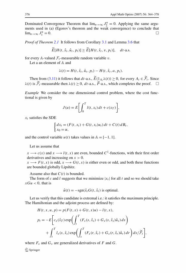
Proof of Theorem 2.1 It follows from Corollary 3.1 and Lemma 3.6 that

E[H(t, xt , ut , pt )] ≥ E[H(t, xt , v,pt )], dt-a.s.

for every A-valued Ft -measurable random variable v.

Let a an element of A and

λ(t) = H(t, xt , ut , pt ) − H(t, xt , a,pt ).

Then from (3.11) it follows that dt-a.s., E(1At λ(t)) ≥ 0, for every At ∈ Ft . Sinceλ(t) is Ft -measurable then λ(t) ≥ 0, dt-a.s., P -a.s., which completes the proof. �

Example We consider the one dimensional control problem, where the cost func-tional is given by

J (u) = E

[∫ T

0l(t, xt ) dt + c(xT )

],

xt satisfies the SDE{dxt = (F (t, xt ) + G(t, xt )ut ) dt + C(t) dBt ,

x0 = α,

and the control variable u(t) takes values in A = [−1,1].Let us assume that

x −→ c(x) and x −→ l(t, x) are even, bounded C1-functions, with their first orderderivatives and increasing on x > 0.

x −→ F(t, x) is odd, x −→ G(t, x) is either even or odd, and both these functionsare bounded globally Lipshitz.

Assume also that C(t) is bounded.The form of c and l suggests that we minimize |xt | for all t and so we should take

xGu < 0, that is

u(t) = −sgn(xtG(t, xt ) is optimal.

Let us verify that this candidate is extremal i.e.: it satisfies the maximum principle.The Hamiltonian and the adjoint process are defined by:

H(t, x,u,p) = p(F(t, x) + G(t, x)u) − l(t, x),

pt = −E

[cx(xT ) exp

(∫ T

t

(Fx(s, xs) + Gx(s, xs)us) ds

)

+∫ T

t

lx(s, xs) exp

(∫ T

s

(Fx(r, xr ) + Gx(r, xr )ur ) dr

)ds/Ft

],

where Fx and Gx are generalized derivatives of F and G.

Appl Math Optim (2007) 56: 364–378 377

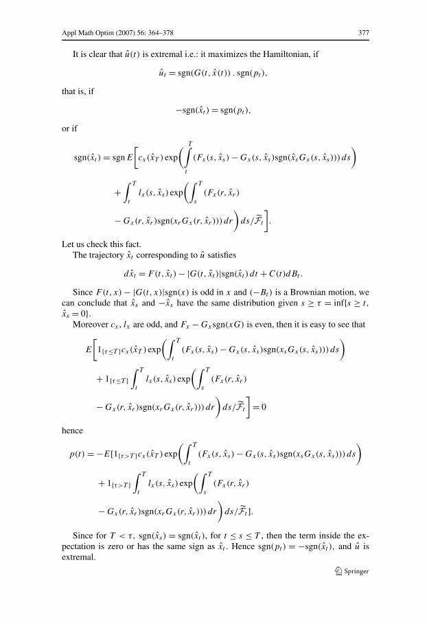
It is clear that u(t) is extremal i.e.: it maximizes the Hamiltonian, if

ut = sgn(G(t, x(t)) . sgn(pt ),

that is, if

−sgn(xt ) = sgn(pt ),

or if

sgn(xt ) = sgnE

[cx(xT ) exp

( T∫t

(Fx(s, xs) − Gx(s, xs)sgn(xsGx(s, xs))) ds

)

+∫ T

t

lx(s, xs) exp

(∫ T

s

(Fx(r, xr )

− Gx(r, xr )sgn(xrGx(r, xr ))) dr

)ds/Ft

].

Let us check this fact.The trajectory xt corresponding to u satisfies

dxt = F(t, xt ) − |G(t, xt )|sgn(xt ) dt + C(t)dBt .

Since F(t, x) − |G(t, x)|sgn(x) is odd in x and (−Bt) is a Brownian motion, wecan conclude that xs and −xs have the same distribution given s ≥ τ = inf{s ≥ t,

xs = 0}.Moreover cx , lx are odd, and Fx − Gxsgn(xG) is even, then it is easy to see that

E

[1{τ≤T }cx(xT ) exp

(∫ T

t

(Fx(s, xs) − Gx(s, xs)sgn(xsGx(s, xs))) ds

)

+ 1{τ≤T }∫ T

t

lx(s, xs) exp

(∫ T

s

(Fx(r, xr )

− Gx(r, xr )sgn(xrGx(r, xr ))) dr

)ds/Ft

]= 0

hence

p(t) = −E[1{τ>T }cx(xT ) exp

(∫ T

t

(Fx(s, xs) − Gx(s, xs)sgn(xsGx(s, xs))) ds

)

+ 1{τ>T }∫ T

t

lx(s, xs) exp

(∫ T

s

(Fx(r, xr )

− Gx(r, xr )sgn(xrGx(r, xr ))) dr

)ds/Ft ].

Since for T < τ, sgn(xs) = sgn(xt ), for t ≤ s ≤ T , then the term inside the ex-pectation is zero or has the same sign as xt . Hence sgn(pt ) = −sgn(xt ), and u isextremal.

378 Appl Math Optim (2007) 56: 364–378

The case of smooth coefficients is solved in Haussmann [13]. Note that when thediffusion coefficient C(t) is non degenerate, then the adjoint process is obtained asthe conditional expectation with respect to Ft (see [2]).

Acknowledgements The authors would like to thank the referees and the associate editor for severalsuggestions, that lead to a substantial improvement of the main result of the paper.

References

1. Arkin, V.I., Saksonov, M.T.: Necessary optimality conditions for stochastic differential equations.Sov. Math. Dokl. 20, 1–5 (1979)

2. Bahlali, K., Mezerdi, B., Ouknine, Y.: The maximum principle in optimal control of a diffusion withnonsmooth coefficients. Stoch. Stoch. Rep. 57, 303–316 (1996)

3. Bahlali, S., Chala, A.: The stochastic maximum principle in optimal control of singular diffusionswith non linear coefficients. Rand. Oper. Stoch. Equ. 13(1), 1–10 (2005)

4. Bahlali, S., Mezerdi, B.: A general stochastic maximum principle for singular control problems. Elect.J. Probab. 10(30), 988–1004 (2005)

5. Bensoussan, A.: Lectures on stochastic control. In: Lect. Notes in Math., vol. 972, pp. 1–62. Springer,Berlin (1983)

6. Bismut, J.M.: An introductory approach to duality in optimal stochastic control. SIAM Rev. 20(1),62–78 (1978)

7. Bouleau, N., Hirsch, F.: Sur la propriété du flot d’une équation différentielle stochsatique. C.R. Acad.Sci. Paris 306, 421–424 (1988)

8. Cadenillas, A., Haussmann, U.G.: The stochastic maximum principle for a singular control problem.Stoch. Stoch. Rep. 49, 211–237 (1994)

9. Cadenillas, A., Karatzas, I.: The stochastic maximum principle for linear convex optimal control withrandom coefficients. SIAM J. Control Optim. 33(2), 590–624 (1995)

10. Clarke, F.H.: Optimization and Nonsmooth Analysis. Wiley, New York (1983)11. Ekeland, I.: Non convex minimization problems. Bull. Am. Math. Soc. (N. S.) 1, 443–474 (1979)12. Frankowska, H.: The first order necessary conditions for nonsmooth variational and control problems.

SIAM J. Control Optim. 22(1), 1–12 (1984)13. Haussmann, U.G.: A stochastic maximum principle for optimal control of diffusions. In: Longman

Scientific & Technical, Harlow. Pitman Research Notes in Mathematics Series, vol. 151. Wiley, NewYork (1986)

14. Krylov, N.V.: Controlled Diffusion Processes. Springer, Berlin (1980)15. Kushner, H.J.: Necessary conditions for continuous parameter stochastic optimization problems.

SIAM J. Control Optim. 10, 550–565 (1972)16. Mezerdi, B.: Necessary conditions for optimality for a diffusion with a non smooth drift. Stochastics

24, 305–326 (1988)17. Neustadt, L.W.: A general theory of extremals. J. Comput. Syst. Sci. 3, 57–92 (1972)18. Peng, S.: A general stochastic maximum principle for optimal control problems. SIAM J. Control

Optim. 28, 966–979 (1990)19. Rockafellar, R.T.: Conjugate convex functions in optimal control and the calculus of variations. J.

Math. Anal. Appl. 32, 174–222 (1970)20. Warga, J.: Necessary conditions without differentiability assumptions in optimal control. J. Differ.

Equ. 18, 41–62 (1975)21. Yang, B.: Necessary conditions for optimal controls of forward_backward stochastic systems with

non smooth cost functionals. J. Fudan Univ. Nat. Sci. 39(1), 61–67 (2000)22. Zhou, X.Y.: Stochastic near optimal controls: necessary and sufficient conditions for near optimality.

SIAM J. Control Optim. 36(3), 929–947 (1998)