Weak variations of Lipschitz graphs and stability of phase boundaries
Upload
independentCategory
view
3download
0
ON THE BEST LIPSCHITZ EXTENSION PROBLEM FOR A DISCRETEDISTANCE AND THE DISCRETE ∞-LAPLACIAN
J. M. MAZON, J. D. ROSSI AND J. TOLEDO
Abstract. This paper is concerned with the best Lipschitz extension problem for a discretedistance that counts the number of steps. We relate this absolutely minimizing Lipschitz extensionwith a discrete ∞-Laplacian problem, which arise as the dynamic programming formula for thevalue function of some ε-tug-of-war games. As in the classical case, we obtain the absolutelyminimizing Lipschitz extension of a datum f by taking the limit as p → ∞ in a nonlocal p–Laplacian problem.
1. Introduction
Since the classical work of Arosson [6], in which he introduced the concept of absolutely min-imizing Lipschitz extension and showed its relation with the infinity Laplace equation, a largeamount of literature has appeared in this direction. For a systematic treatment of the theory ofabsolute minimizers see the recent survey [7] by Aronson, Cradall and Juutinen, and the refer-ences therein. A new insight has come in with the work of Peres, Schramm, Sheffield and Wilson[20] where it has been shown an interesting connection between absolutely minimizing Lipschitzextension and Game Theory. More precisely, the authors of [20] proved that if uε is the valuefunction for a certain ε-tug-of-war game with final payoff function f , then the uniform limit u ofuε, as ε goes to zero, is the absolutely minimizing Lipschitz extension of f .
In this work our aim is twofold, first we characterize the value function uε as the absolutelyminimizing Lipschitz extension with respect to a discrete distance in a proper way, and next weshow that uε can be obtained by taking the limit as p → ∞ in a nonlocal p–Laplacian Dirichletproblem with boundary data f .
Let (X, d) be an arbitrary metric space and let f : A ⊂ X → R. We denote by Ld(f,A) thesmallest Lipschitz constant of f in A, i.e.,
Ld(f, A) := supx,y∈A
|f(x)− f(y)|d(x, y)
.
If we are given a Lipschitz function f : A ⊂ X → R, i.e., Ld(f, A) < +∞, then it is well-knownthat there exists a minimal Lipschitz extension (MLE for short) of f to X, that is, a functionh : X → R such that h|A = f and Ld(h, X) = Ld(f,A). We will denote the space of suchextensions as MLE(f,X).
Extremal extensions were explicitly constructed by McShane [17] and Whitney [21],
Ψ(f)(x) := infy∈A
(f(y) + Ld(f, A)d(x, y)) , x ∈ X,
Key words and phrases. Lipschitz extension, Nonlocal p–Laplacian problem, Infinity Laplacian, Tug-of-wargames.
2000 Mathematics Subject Classification. 49J20, 49J45, 45G10.1
2 J. M. MAZON, J. D. ROSSI AND J. TOLEDO
andΛ(f)(x) := sup
y∈A(f(y)− Ld(f, A)d(x, y)) , x ∈ X,
belong to MLE(f,X), and if u ∈ MLE(f, X) then Λ(f) ≤ u ≤ Ψ(f).The notion of minimal Lipschitz extension is not completely satisfactory since it involves only
the global Lipschitz constant of the extension and ignore what may happen locally. To solve thisproblem, in the particular case of the euclidean space RN , Arosson [6] introduced the concept ofabsolutely minimizing Lipschitz extension (AMLE for short) and proved the existence of AMLEby means of a variant of the Perron’s method. An extension of this concept to the case of ageneral metric space is due to Juutinen [11] (see also [18]). In [11], Juutinen gave the followingdefinition.
Definition 1.1. Let A be any nonempty subset of the metric spaces (X, d) and let f : A ⊂ X → Rbe a Lipschitz function. A function h : X → R is an absolutely minimizing Lipschitz extension off to X if
(i) h ∈ MLE(f, X),(ii) whenever B ⊂ X and g ∈ MLE(f, X) such that g = h in X \B, then Ld(h, B) ≤ Ld(g,B).
Also in [11] it is proved the existence of an AMLE under the assumption that the metric space(X, d) is a separable length space.
Aronsson’s original definition in RN was formulated in a slightly different way. He assumedthat A is a compact set and required that Ld(h,D) = Ld(h, ∂D) for every bounded open set Din RN . As remarked by Juutinen in [11], for a general metric space “this kind of definition wouldbe somewhat ambiguous because the boundary of an open subset of a metric space may very wellbe empty”, and the issue of [11] was to find a right way to interpret the “boundary condition”.
Moreover, in [6], Aronsson proposed an approach to obtain the AMLE extension of a datum fby taking the limit as p →∞ in the p–Laplacian problem
(1.1)
−∆pup = 0 in Ω,
up = f on ∂Ω.
This approach was made completely rigorous by Jensen in [10] (see also [9]). In [7] you can findthe following result: the limit as p →∞ of up, u∞, is the best Lipschitz extension (AMLE) of fin Ω and moreover it is characterized as the unique viscosity solution to
(1.2)
−∆∞u∞ = 0, Ω,
u∞ = f, ∂Ω,
where ∆∞ is the infinity Laplace operator, that is, the degenerate elliptic operator given by
∆∞u :=N∑
i,j=1
uxiuxjuxixj .
Recently, Peres, Schramm, Sheffield and Wilson [20] have shown that the infinity Laplaceequation (1.2) is solved by the continuous value function for a random turn tug-of-war game, inwhich the players, at each step, flip a fair coin to determine which player plays.
THE BEST LIPSCHITZ EXTENSION PROBLEM 3
Given a bounded domain Ω in RN and a function defined outside Ω (this will be properlystated afterward), our aim is to study the Lipschitz extension problem to Ω respect to the discretedistance that counts the number of steps,
(1.3) dε(x, y) =
0 if x = y,
ε([[ |x−y|
ε
]]+ 1
)if x 6= y,
where |.| is the Euclidean norm and [[r]] is defined for r > 0 by [[r]] := n, if n < r ≤ n + 1, n =0, 1, 2, . . . , that is,
dε(x, y) =
0 if x = y,ε if 0 < |x− y| ≤ ε,2ε if ε < |x− y| ≤ 2ε,...
The distance dε was used in [20] in relation with ε-tug-of-war games. It was also used in [2] togive a mass transport interpretation of a nonlocal model of sandpiles.
1.1. Description of the main results. Since (RN , dε) is not a separable length space, thegeneral concept of AMLE due to Juutinen does not work on it. We give a concept of AMLErespect to the distance dε, which we name as AMLEε(f, Ω), in an slight different way that finds theright manner to interpret the “boundary condition” (observe that for the metric dε the boundaryof Ω is empty).
In addition, we relate this absolutely minimizing Lipschitz extension problem with a discrete∞-Laplacian problem, which arise as the dynamic programming formula for the value function ofsome ε-tug-of-war game. More precisely, we characterize the value function for the ε-tug-of-wargame with payoff function f as the AMLEε(f, Ω). Therefore, as consequence of the results in [20]we have existence and uniqueness of AMLEε(f, Ω).
Finally, we also obtain the nonlocal version of the approximation by the p–Laplacian, that is,we get the AMLEε(f, Ω) by taking the limit as p →∞ in a nonlocal p–Laplacian problem.
2. Definition and characterization of AMLEε
Given a set A ⊂ RN and ε > 0, we denote
Aε :=
x ∈ RN : dist(x,A) := infy∈A
|x− y| < ε
.
The euclidean open ball centred at x with radius r will be denoted by Br(x), and with Br(x) itsclosure. Throughout the paper, we assume that Ω is a bounded domain of RN .
Given u : Ωε → R and D ⊂ Ω, we define
Lε(u,D) := supx ∈ D, y ∈ Dε
|x− y| ≤ ε
|u(x)− u(y)|ε
.
Observe that
Lε(u,D) = supx ∈ D, y ∈ Dε
|x− y| ≤ ε
|u(x)− u(y)|dε(x, y)
≤ supx∈D, y∈Dε
|u(x)− u(y)|dε(x, y)
.
4 J. M. MAZON, J. D. ROSSI AND J. TOLEDO
And that, if D is convex, the above inequality is an equality. Indeed, for x0 = x ∈ D, xn = y ∈ Dε
and x1, x2, ..., xn−1 in the segment between x and y such that |xi − xi−1| = ε for i = 1, ..., n− 1,and |xn − xn−1| ≤ ε, we have that
|u(x)− u(y)| ≤n∑
i=1
|u(xi)− u(xi−1)| ≤ εn∑
i=1
Lε(u,D) = εnLε(u, D) = dε(x, y)Lε(u, D).
Also, for any convex D,
Ldε(u,D) = supx,y∈D,|x−y|≤ε
|u(x)− u(y)|ε
.
Therefore, the constant Lε(u,D) is not genuinely the Lipschitz constant Ldε(u,D), even if Dis convex, but, as we will see, it is the right one to treat the absolutely minimizing Lipschitzextensions when dε is considered.
Definition 2.1. Let f : Ωε \ Ω → R be bounded. We say that a function u : Ωε → R is anAbsolutely Minimizing Lipschitz Extension for Lε of f into Ω (u is AMLEε(f, Ω) for shortness) if
(i) u = f in Ωε \ Ω,(ii) for every D ⊂ Ω and v : Ωε → R with v = u in Ωε \D, then Lε(u,D) ≤ Lε(v, D).
Lemma 2.2. When Ω is convex the above definition is equivalent to the following two conditions,that match better the idea of Definition 1.1,
(i’) u ∈ MLE(f, Ωε),(ii’) for every D ⊂ Ω and v ∈ MLE(f, Ωε) with v = u in Ωε \D, then Lε(u, D) ≤ Lε(v, D).
Proof. Let us first see that (i), (ii) implies (i’) ((ii’) is immediate): take v ∈ MLE(f,Ωε), then
Lε(u,Ω) ≤ Lε(v, Ω) ≤ Ldε(v, Ωε) = Ldε(f, Ωε \ Ω).
Therefore, since Ω is convex,
(2.1) supx∈Ω, y∈Ωε
|u(x)− u(y)|dε(x, y)
= Lε(u,Ω) ≤ Ldε(f, Ωε \ Ω).
On the other hand, since u = f in Ωε \ Ω,
(2.2) Ldε(f, Ωε \ Ω) ≤ Ldε(u,Ωε) = supx∈Ωε, y∈Ωε
|u(x)− u(y)|dε(x, y)
.
Consequently, from (2.1) and (2.2), Ldε(u,Ωε) = Ldε(f, Ωε \ Ω).Let us now see that (i’), (ii’) implies (ii) ((i’) is immediate). Let us argue by contradiction and
suppose that there exist D and v such that v = u in Ωε \D and Lε(v, D) < Lε(u,D). Then, by(ii’), v can not be in MLE(f, Ωε). But also, the above strict inequality implies that, on accountthat Ωε is convex,
Ldε(f, Ωε \ Ω) ≤ Ldε(v, Ωε) = supx /∈ D, y /∈ D|x− y| ≤ ε
|v(x)− v(y)|ε
= supx /∈ D, y /∈ D|x− y| ≤ ε
|u(x)− u(y)|ε
≤ Ldε(u,Ωε) = Ldε(f, Ωε \ Ω)
and consequently v ∈ MLE(f, Ωε), which is a contradiction. ¤
THE BEST LIPSCHITZ EXTENSION PROBLEM 5
Remark that independently of the convexity of Ω, if u is AMLEε(f, Ω), it always holds that
Lε(u,Ω) ≤ Ldε(f, Ωε \ Ω).
In the next result we obtain the characterization of the AMLEε(f, Ω) by means of a discrete∞-Laplacian problem.
Theorem 2.3. Let f : Ωε \Ω → R be bounded. Then, u : Ωε → R is AMLEε(f, Ω) if and only ifu is a solution of
(2.3)
−∆ε∞u = 0 in Ω,
u = f on Ωε \ Ω,
where
(2.4) ∆ε∞u(x) := sup
y∈Bε(x)
u(y) + infy∈Bε(x)
u(y)− 2u(x)
is the discrete infinity Laplace operator.
Proof. Without loss of generality we will take ε = 1 along the proof. Let us first take u a solutionof (2.3) and suppose that u is not AMLE1(f, Ω). Then, there exists D ⊂ Ω and v : Ω1 → R,v = u in Ω1 \D, such that L1(v,D) < L1(u,D). Set δ := L1(u, D)−L1(v, D) > 0, and let n ∈ N,n > 3, such that
(2.5) supD
u− infD
u ≤ (n− 1)L1(u,D).
Take (x0, y0) ∈ D × Ω1, |x0 − y0| ≤ 1, such that
L1(u,D)− δ
n≤ |u(x0)− u(y0)| ≤ L1(u, D).
We have that ∆1∞u(x0) = 0 and ∆1∞u(y0) = 0 if y0 ∈ Ω. Let us suppose that u(y0) ≥ u(x0) (theother case being similar), which implies
(2.6) L1(u, D)− δ
n≤ u(y0)− u(x0) ≤ L1(u,D).
If y0 /∈ D, set y1 = y0. If y0 ∈ D, since ∆1∞u(y0) = 0 and x0 ∈ B1(y0), we have
supy∈B1(y0)
u(y)− u(y0) = u(y0)− infy∈B1(y0)
u(y) ≥ u(y0)− u(x0) ≥ L1(u,D)− δ
n.
Hence, there exists y1 ∈ B1(y0) such that
u(y1)− u(y0) ≥ L1(u,D)− 2δ
n.
Also, since ∆1∞u(x0) = 0, we have
u(x0)− infx∈B1(x0)
u(x) = supx∈B1(x0)
u(x)− u(x0) ≥ u(y0)− u(x0) ≥ L1(u, D)− δ
n,
and consequently, there exists x1 ∈ B1(x0) such that
u(x0)− u(x1) ≥ L1(u,D)− 2δ
n.
6 J. M. MAZON, J. D. ROSSI AND J. TOLEDO
Following this construction, and with the rule that in the case xj /∈ D or yj /∈ D, then xi = xj
or yi = yj for all i ≥ j, we claim that there exists m ≤ n for which xm /∈ D and ym /∈ D. Infact, if not, then either xii=1,...,n ⊂ D, either yii=1,...,n ⊂ D, with xii=1,...,n and yii=1,...,n
satisfying
(2.7) u(yi)− u(yi−1) ≥ L1(u,D)− 2δ
n, yi ∈ B1(yi−1), i = 1, . . . , n,
and
(2.8) u(xi)− u(xi−1) ≥ L1(u,D)− 2δ
n, xi ∈ B1(xi−1), i = 1, . . . , n.
Let us suppose the first of these two possibilities, that is, xii=1,...,n ⊂ D. Then, having in mind(2.5), (2.6) and (2.8), we get
(n− 1)L1(u,D) ≥ u(y0)− u(xn)
= u(y0)− u(x0) + u(x0)− u(x1) + · · ·+ u(xn−1)− u(xn)
≥ L1(u,D)− δn + (n + 1)(L1(u,D)− 2δ
n ),
from where it follows that2n + 3
nδ ≥ 3L1(u,D) ≥ 3δ,
which is a contradiction since n > 3. Now, for xi, yii=1,...,m, we have
v(ym)− v(xm) = u(ym)− u(xm) ≥ 2m
(L1(u,D)− 2δ
n
)+ L1(u,D)− δ
n,
v(ym)− v(xm) ≤ (2m + 1)L1(v,D),
and therefore,
(2m + 1)L1(u,D)− (4m + 1)δ
n≤ (2m + 1)L1(v, D),
that is
δ = L1(u,D)− L1(v, D) ≤ 4m + 12m + 1
δ
n,
which implies n ≤ 4m+12m+1 ≤ 2, which is a contradiction since n > 3.
Let us now consider u an AMLE1(f, Ω) and suppose that u is not a solution of (2.3). Then,x ∈ Ω : ∆1∞u(x) 6= 0 6= ∅. Let us suppose without loss of generality, that,
x ∈ Ω : sup
y∈B1(x)
u(y)− u(x) > u(x)− infy∈B1(x)
u(y)6= ∅.
Then, there exists δ > 0 and a nonempty set D ⊂ Ω such that
(2.9) supy∈B1(x)
u(y)− u(x) > u(x)− infy∈B1(x)
u(y) + δ for all x ∈ D.
Consider the function v : Ω1 → R defined by
v(x) =
u(x) if x ∈ Ω1 \D,
u(x) + δ2 if x ∈ D.
THE BEST LIPSCHITZ EXTENSION PROBLEM 7
Then, since u is an AMLE1(f, Ω), we have L1(u,D) ≤ L1(v,D). Now, there exists x0 ∈ D andy0 ∈ B1(x0) such that
L1(v, D) ≤ δ
4+ |v(x0)− v(y0)|.
Therefore, if v(x0) ≥ v(y0), by (2.9),
L1(v,D) ≤ δ
4+ v(x0)− v(y0) ≤ 3δ
4+ u(x0)− u(y0)
≤ 3δ
4+ u(x0)− inf
x∈B1(x0)u(x) < −δ
4+ sup
x∈B1(x0)
u(x)− u(x0) < L1(u,D),
which is a contradiction, and, if v(x0) < v(y0),
L1(v,D) ≤ δ
4+ v(y0)− v(x0) = −δ
4+ v(y0)− u(x0),
so, if y0 /∈ D,
L1(v,D) ≤ −δ
4+ u(y0)− u(x0) < L1(u,D),
also a contradiction, and if y0 ∈ D, since also x0 ∈ B1(y0), by (2.9),
L1(v,D) ≤ δ
4+ u(y0)− u(x0) ≤ δ
4+ u(y0)− inf
y∈B1(y0)u(y)
< −3δ
4+ sup
y∈B1(y0)
u(y)− u(y0) < L1(u,D),
again a contradiction. Then, in any case we arrive to a contradiction and consequently u is asolution of (2.3). ¤
The first analysis of the interesting functional equation −∆ε∞u = 0 appeared in the article byLe Gruyer and Archer [13], but also arise as the dynamic programming formula for the valuefunction of some tug-of-war games (see for instance [8, 15, 16, 20]). Let us briefly review theε-tug-of-war game introduced by Peres, Schramm, Sheffield and Wilson in [20]. Fix a numberε > 0. The dynamic of the game is as follows. There are two players moving a token inside a setEΩ containing Ω, a bounded domain in RN . The token is placed at an initial position x0 ∈ Ω.At the kth stage of the game, player I and player II select points xI
k and xIIk , respectively, both
belonging to Bε(xk−1) ∩ EΩ. The token is then moved to xk, where xk is chosen randomly sothat xk = xI
k or xk = xIIk , depending who was the winner of a flip of a fair coin. After the kth
stage of the game, if xk ∈ Ω then the game continues to stage k + 1. Otherwise, if xk ∈ EΩ \ Ω,the game ends and player II pays player I the amount f(xk), where f : EΩ \ Ω → R is a finalpayoff function of the game. Of course, player I attempts to maximize the payoff, while player IIattempts to minimize it.
Given a strategy for player I, that is a mapping SI from the set of all possible partially playedgames (x0, x1, . . . , xk−1) to possible positions xk ∈ Bε(xk−1), and a strategy SII for player II,we denote by Ex0
I (SI , SII) and Ex0II (SI , SII) the expected value of f(xk) (Ex0
SI ,SII[f(xk)]), if the
game terminates a.s., −∞ and +∞, respectively, otherwise (there is a severe penalization forboth players if the game never ends). The value of the game for player I is the quantity
infSII
supSI
Ex0I (SI , SII),
8 J. M. MAZON, J. D. ROSSI AND J. TOLEDO
where the supremum is taken over all possible strategies for player I and the infimum over allstrategies of player II. Similarly, the value of the game for player II is
supSI
infSII
Ex0II (SI , SII).
We denote the value for player I as a function of the starting point x0 ∈ Ω by uεI(x0), and similarly
the value for player II by uεII(x0). The game is said to have a value if uε
I = uεII =: uε. According
with the Dynamic Programming Principle, see [20], there is a value function for the ε-tug-of-wargame, uε, that satisfies the functional equation
uε(x) =12
(sup
y∈Bε(x)∩EΩ
uε(y) + infy∈Bε(x)∩EΩ
uε(y)
)in Ω,
with uε = f in EΩ \ Ω. Observe that this is (2.3) when EΩ = Ωε (see [15, 16] for this problem).In [20], using martingale methods, it is proved that problem (2.3) has a unique solution; then, byTheorem 2.3, we get the following existence and uniqueness result.
Theorem 2.4. Let f : Ωε \ Ω → R be bounded. Then, there is a unique AMLEε(f, Ω).
Some of the difficulties in the analysis of the ε-tug-of-war game are due to the fact that the valuefunction uε can be discontinuous. When the limit u := limε→0 uε exists pointwise, the function uis called the continuum value of the game. In [20], Peres, Schramm, Sheffield and Wilson provedthat if EΩ = Ω and the terminal payoff function of the game f is Lipschitz continuous on ∂Ω thenthe continuum value u exists and uε → u uniformly in Ω as ε → 0. Moreover, u is the uniqueAMLE extension of f to Ω and the unique viscosity solution of the boundary value problem
−∆∞u = 0 in Ω,
u = f on ∂Ω.
Our Theorem 2.3 gives this characterization in the case of the discrete distance. We will see inthe next section that we can also obtain the AMLEε extension by taking the limit as p → ∞ ina nonlocal p–Laplacian problem, which represents the nonlocal version of the approximation ofthe local problem with the p–Laplacian.
3. Existence of AMLEε by a nonlocal Lp-variational approach
First, let us introduce some notation. Given f : Ωε \ Ω → R and u : Ω → R, we will denote
uf (x) :=
u(x) if x ∈ Ω,
f(x) if x ∈ Ωε \ Ω.
Given a convex set K ⊂ L2(Ω), we denote by IK to the indicator function of K, that is, thefunction defined as
IK(u) :=
0 if u ∈ K,
+∞ if u 6∈ K.
Let J : RN → R be a nonnegative, radial, continuous function, strictly positive in B1(0),vanishing in RN \B1(0) and such that
∫RN J(z) dz = 1. For 1 < p < +∞ and f : Ω1 \ Ω → R
THE BEST LIPSCHITZ EXTENSION PROBLEM 9
such that |f |p−1 ∈ L1(Ω1 \ Ω), we define in L1(Ω) the operator BJp,f by
BJp,f (u)(x) := −
∫
ΩJ(x− y)|u(y)− u(x)|p−2(u(y)− u(x)) dy
−∫
Ω1\ΩJ(x− y)|f(y)− u(x)|p−2(f(y)− u(x)) dy, x ∈ Ω,
that is,
BJp,f (u)(x) = −
∫
Ω1
J(x− y)|uf (y)− u(x)|p−2(uf (y)− u(x)) dy, x ∈ Ω.
In [1] (see also [3]) we have seen that the nonlocal version of the Dirichlet problem (1.1), withboundary value f , can be written as
(3.1) BJp,f (u) = 0.
We have also established the following Poincare’s type inequality for such kind of integral opera-tors.
Proposition 3.1 ([1]). Given J : RN → R as above, p ≥ 1 and f ∈ Lp(Ω1 \ Ω), there existsλ = λ(J,Ω, p) > 0 such that
(3.2) λ
∫
Ω|u(x)|p dx ≤
∫
Ω
∫
Ω1
J(x− y)|uf (y)− u(x)|p dy dx +∫
Ω1\Ω|f(y)|p dy
for all u ∈ Lp(Ω).
We say that u is a supersolution (resp. subsolution) of the nonlocal Dirichlet problem (3.1)with boundary value f if BJ
p,f (u) ≥ 0 (resp. BJp,f (u) ≤ 0). We have the following comparison
principle.
Lemma 3.2. Let J : RN → R as above, p > 1 and f, f ∈ Lp(Ω1 \ Ω), with f ≥ f . If u is asupersolution of the Dirichlet problem (3.1) with boundary value f and u is a subsolution of theDirichlet problem (3.1) with boundary value f then u ≥ u.
Proof. By assumption we have
0 ≥ −∫
Ω1
J(x− y)|uf (y)− u(x)|p−2(uf (y)− u(x)) dy, ∀x ∈ Ω
and0 ≤ −
∫
Ω1
J(x− y)|uf (y)− u(x)|p−2(uf (y)− u(x)) dy, ∀x ∈ Ω.
Then, multiplying by (u− u)+(x), integrating and having in mind that
(uf (x)− uf (x))+ = (f(x)− f(x))+ = 0
if x ∈ Ω1 \ Ω, we get
0 ≥ −∫
Ω1×Ω1
J(x− y)|uf (y)− uf (x)|p−2(uf (y)− uf (x))(uf (x)− uf (x))+ dydx
=12
∫
Ω1×Ω1
J(x−y)|uf (y)−uf (x)|p−2(uf (y)−uf (x))[(uf (y)− uf (y))+ − (uf (x)− uf (x))+
]dydx
10 J. M. MAZON, J. D. ROSSI AND J. TOLEDO
and
0 ≥∫
Ω1×Ω1
J(x− y)|uf (y)− uf (x)|p−2(uf (y)− uf (x))(uf (x)− uf (x))+ dydx
= −∫
Ω1×Ω1
J(x− y)2
|uf (y)− uf (x)|p−2(uf (y)− uf (x))
×[(uf (y)− uf (y))+ − (uf (x)− uf (x))+
]dydx.
Then, adding the last two inequalities we obtain that∫
Ω1×Ω1
J(x− y)(|uf (y)− uf (x)|p−2(uf (y)− uf (x))− |uf (y)− uf (x)|p−2(uf (y)− uf (x))
)
×((uf (y)− uf (y))+ − (uf (x)− uf (x))+
)dydx ≤ 0.
Therefore, since (|r|p−2r − |s|p−2s)(r+ − s+) ≥ 0, we get that
(3.3)J(x− y)
(|uf (y)− uf (x)|p−2(uf (y)− uf (x))− |uf (y)− uf (x)|p−2(uf (y)− uf (x))
)
×((uf (y)− uf (y))+ − (uf (x)− uf (x))+
)= 0
for a.e. (x, y) ∈ Ω1 × Ω1.
Let Ω := x ∈ Ω : u(x) > u(x). Since (|r|p−2r − |s|p−2s)(r − s) ≥ C|r − s|p, from (3.3) weobtain that, for a.e. (x, y) ∈ Ω× Ω,
0 = J(x− y)(|u(y)− u(x)|p−2(u(y)− u(x))− |u(y)− u(x)|p−2(u(y)− u(x))
)
× (u(y)− u(x)− (u(y)− u(x)))
≥ CJ(x− y)|u(y)− u(x)− (u(y)− u(x))|pthat is,
(3.4) J(x− y)|u(y)− u(y)− (u(x)− u(x))|p = 0 for a.e. (x, y) ∈ Ω× Ω.
Therefore, if
(3.5) |Ω| > 0,
from (3.4), we getu(x)− u(x) = λ > 0 a.e. in Ω.
Then, taking the above conclusion in (3.3) we have that, for a.e. (x, y) ∈ (Ω1 \ Ω)× Ω,
0 = J(x− y)(|u(y)− uf (x)|p−2(u(y)− uf (x))− |u(y)− uf (x)|p−2(u(y)− uf (x))
)(u(y)− u(y))
= J(x− y)(|u(y)− (uf (x)− λ)|p−2(u(y)− (uf (x)− λ))− |u(y)− uf (x)|p−2(u(y)− uf (x))
)λ .
Now, since |r|p−2r − |s|p−2s = 0 if and only if r = s we conclude that
uf (x)− λ = uf (x) a.e. in Ω1 \ Ω,
which contradicts that Ω1 \ Ω contains the non-null set Ω1 \ Ω (since f ≥ f). Therefore (3.5) isfalse, and then u ≤ u a.e. in Ω. ¤
THE BEST LIPSCHITZ EXTENSION PROBLEM 11
For the energy functional
GJp,f (u) =
12p
∫
Ω
∫
ΩJ(x− y)|u(y)− u(x)|p dy dx +
1p
∫
Ω
∫
Ω1\ΩJ(x− y)|f(y)− u(x)|p dy dx,
we have the following result:
Theorem 3.3. Assume that p ≥ 2. Then, there exists a unique up ∈ Lp(Ω) such that
(3.6) GJp,f (up) = minGJ
p,f (u) : u ∈ Lp(Ω).Moreover, up is the solution of the nonlocal Euler–Lagrange equation BJ
p,f (up) = 0, and it has acontinuous representative in Ω.
Proof. Let vn ∈ Lp(Ω) a minimizing sequence, that is,
m := infGJp,f (u) : u ∈ Lp(Ω) = lim
n→+∞GJp,f (vn).
Then, by the Poincare inequality (3.2), we have
‖vn‖p ≤(
1λ
(m + 1 +
∫
Ω1\Ω|f(y)|p dy
)) 1p
.
Therefore, we can assume that vn up weakly in L2(Ω). Hence, since the functional GJp,f is
weakly lower semi-continuous in L2(Ω), we get
GJp,f (up) ≤ lim inf
n→∞ GJp,f (vn) = m,
consequently, m = GJp,f (up) and (3.6) holds.
By results in [1], we know that the operator BJp,f is completely accretive and verifies the range
condition Lp(Ω) ⊂ Ran(I + BJp,f ). Let us see that
(3.7) ∂GJp,f = BJ
p,f
L2(Ω).
Since GJp,f is convex an lower semi-continuous in L2(Ω), to prove (3.7) it is enough to show that
(3.8) BJp,f ⊂ ∂GJ
p,f .
Let us see that (3.8) holds. Set v = BJp,f (u) and let w ∈ D(GJ
p,f ). Then∫
Ωv(x)(w(x)− u(x)) dx = −
∫
Ω
∫
Ω1
J(x− y)|uf (y)− u(x)|p−2(uf (y)− u(x)) dy(w(x)− u(x)) dx
= −∫
Ω1
∫
Ω1
J(x− y)|uf (y)− uf (x)|p−2(uf (y)− uf (x)) dy(wf (x)− uf (x)) dx
=12
∫
Ω1
∫
Ω1
J(x− y)|uf (y)− uf (x)|p−2(uf (y)− uf (x)) (wf (y)− wf (x)− (uf (x)− uf (y))) dydx.
From here, using the numerical inequality12|r|p−2r(s− r) ≤ 1
2p(|s|p − |r|p) ,
12 J. M. MAZON, J. D. ROSSI AND J. TOLEDO
we obtain that
GJp,f (w)−GJ
p,f (u) =12p
∫
Ω1
∫
Ω1
J(x− y)|wf (y)− wf (x)|p dy dx
− 12p
∫
Ω1
∫
Ω1
J(x− y)|uf (y)− uf (x)|p dy dx ≥∫
Ωv(x)(w(x)− u(x)) dx,
from where it follows (3.8). The second part of the theorem is a consequence of (3.7).Now, BJ
p,f (up) = 0 can be written as∫
Ω1
J(x− y)ϕp((up)f (y)− up(x))dy = 0 ∀x ∈ Ω \N, meas(N) = 0,
for ϕp(r) := |r|p−2r. Then, the continuity of up in Ω follows by the above conclusion and theImplicit Function Theorem ([12]): since J is continuous and ϕp is continuous and increasing,
F (x, α) :=∫
Ω1
J(x− y)ϕp((up)f (y)− α)dy
is continuous in Ω× R and for fixed x ∈ Ω it is increasing in α. Therefore, by [12, Theorem 1.1]F (x, α) = 0 has a unique solution α(x) continuous in Ω. In fact, this can be proved in a directway as follows. Since limα→−∞ F (x, α) = +∞, limα→+∞ F (x, α) = −∞ and F (x, ·) is continuousand increasing, there exists a unique α(x) such that F (x, α(x)) = 0. Now α(x) is l.s.c. at x0 ∈ Ω;indeed, take α < α(x0), therefore
∫
Ω1
J(x− y)ϕp((up)f (y)− α)dy > 0.
Since J is continuous, there exists r > 0 such that∫
Ω1
J(x− y)ϕp((up)f (y)− α)dy > 0 ∀x ∈ Br(x0).
Thereforeα < α(x) ∀x ∈ Br(x0).
Similarly α(x) is u.s.c. Finally, since α(x) = up(x) in Ω\N we conclude that up has a continuousrepresentative. ¤
From now on, we will suppose that minimizers up of GJp,f are continuous and satisfy the Euler–
Lagrange equation BJp,f (up) = 0 everywhere.
At this step we also rescale de kernel J in order to deal with dε instead of with d1. So, let
Jε(z) =1
εNJ
(z
ε
).
We want to study the limit as p → ∞ of the minimizers uεp of GJε
p,f . From now on, we assumethat f ∈ L∞(Ωε \ Ω).
In [1], we have proved that
(3.9) limp→+∞GJε
p,f = Gε∞,f in the sense of Mosco,
THE BEST LIPSCHITZ EXTENSION PROBLEM 13
where
Gε∞,f (u) =
0 if |u(x)− u(y)| ≤ ε, for x, y ∈ Ω, |x− y| ≤ ε, and|f(y)− u(x)| ≤ ε, for x ∈ Ω, y ∈ Ωε \ Ω, |x− y| ≤ ε,
+∞ in other case.
Now, by Holder’s and Poincare’s inequality (3.2), we have ‖uεp‖2 ≤ C‖f‖∞ for every p ≥ 2.
Therefore, we can assume that
(3.10) uεp v∞ weakly in L2(Ω) as p → +∞.
Then, by (3.9), we have
(3.11) Gε∞,f (v∞) ≤ lim inf
p→∞ GJεp,f (uε
p).
Given v ∈ D(Gε∞,f ), by the definition of Mosco convergence, there exists vp ∈ D(GJ
p,f ), suchthat vp → v in L2(Ω), and such that
(3.12) Gε∞,f (v) ≥ lim sup
p→∞GJε
p,f (vp).
Now, by (3.6), GJεp,f (uε
p) ≤ GJεp,f (vp) for all p ≥ 2, and therefore, by (3.11) and (3.12), we obtain
that Gε∞,f (v∞) ≤ Gε
∞,f (v), and consequently
Gε∞,f (v∞) = minGε
∞,f (u) : u ∈ D(Gε∞,f ).
Therefore,
(3.13) 0 ∈ ∂Gε∞,f (v∞).
If we define
Kε∞,f :=
u ∈ L2(Ω) :
|u(x)− u(y)| ≤ ε for x, y ∈ Ω, |x− y| ≤ ε, and
|f(y)− u(x)| ≤ ε for x ∈ Ω, y ∈ Ωε \ Ω, |x− y| ≤ ε
,
we have that the functional Gε∞,f is given by the indicator function of Kε
∞,f , that is, Gε∞,f = IKε
∞,f.
Therefore, the Euler-Lagrange equation (3.13) can be written as
(3.14) 0 ∈ ∂IKε∞,f
(v∞).
Observe that Kε∞,f is not empty if we assume that Ldε(f, Ωε \ Ω) ≤ 1. In this case it is not
difficult to see that
(3.15) Ψ(f), Λ(f) ∈ u ∈ L2(Ω) : |uf (x)− uf (y)| ≤ dε(x, y), x, y ∈ Ωε
⊂ Kε∞,f ,
being Ψ(f) and Λ(f) the McShane-Whitney extensions.Now, to study the Lipschitz extension problem we can always assume that f satisfies
(3.16) Ldε(f,Ωε \ Ω) = 1.
In fact: given f : Ωε\Ω → R Lipschitz continuous respect to the distance dε, consider f(x) := f(x)k ,
k := Ldε(f, Ωε \ Ω). Now, if v : Ωε → R is AMLEε(f , Ω), then, u(x) := kv(x) is AMLEε(f, Ω).Consequently, if f satisfies (3.16), on account of (3.14) and (3.15), (v∞)f ∈ Kε
∞,f .Remark that for Ω convex, if f satisfies (3.16) then MLE(f, Ωε) = Kε
∞,f , and we conclude,directly, that (v∞)f ∈ MLE(f, Ωε).
14 J. M. MAZON, J. D. ROSSI AND J. TOLEDO
Our aim is to see that (v∞)f is AMLEε(f, Ω). To this aim we need the following result.
Lemma 3.4. Let δ > 0. There exists a unique solution u∞,δ of
(3.17)
−∆ε∞u = δ in Ω,
u = f + δ in Ωε \ Ω,
where
(3.18) ∆ε∞u(x) := sup
y∈Bε(x)
u(y) + infy∈Bε(x)
u(y)− 2u(x),
and we have a bound of the form
u∞,δ(x)− C(Ω, ε)δ ≤ u∞(x) ≤ u∞,δ(x),
where u∞ is the solution of Problem (2.3).Analogously, there is a unique solution u∞,−δ of
(3.19)
−∆ε∞u = −δ in Ω,
u = f − δ in Ωε \ Ω,
and we have a bound of the form
u∞,−δ(x) + C(Ω, ε)δ ≥ u∞(x) ≥ u∞,−δ(x).
Proof. We use probabilistic arguments. The existence and uniqueness of u∞,δ comes from the factthat it can be obtained as the value of the tug-of-war game with running payoff δ and final payofff(x) + δ, see [20], [16]. In fact, the equation verified by u∞,δ is just the dynamic programmingprinciple that holds for the value function of this game, see [15].
Hence we are left with the proof of the bounds. The fact that u∞(x) ≤ u∞,δ(x) is almostimmediate since both functions can be seen as values of the same tug-of-war game in which therunning payoff and the final payoff for u∞ are strictly below than those for u∞,δ. See [16] for adetailed proof of a comparison principle. To see the other bound,
u∞,δ(x)− C(Ω, ε)δ ≤ u∞(x),
we argue as follows. Fix η > 0. Player II follows any strategy and Player I follows a strategy S0I
such that at xk−1 ∈ Ω he chooses to step to a point that almost maximizes u∞,δ, that is, to apoint xk ∈ Bε(xk−1) such that
u∞,δ(xk) ≥ supBε(xk−1)
u∞,δ − η2−k.
We start from the point x0. The following inequality for the expectation holds:
Ex0
S0I ,SII
[u∞,δ(xk) + kδ − η2−k |x0, . . . , xk−1]
≥ 12
inf
Bε(xk−1)u∞,δ + kδ − η2−k + sup
Bε(xk−1)
u∞,δ − η2−k + kδ − η2−k
≥ u∞,δ(xk−1) + (k − 1)δ − η2−(k−1),
THE BEST LIPSCHITZ EXTENSION PROBLEM 15
where we have estimated the strategy of Player II by inf and used the fact that u∞,δ verifies(3.17). Thus Mk = u∞,δ(xk)+kδ−η2−k is a submartingale and consequently, if τ is the stoppingtime of the game, and S0
II is a quasioptimal strategy for Player II, that is a strategy such that
infSII
Ex0
S0I ,SII
[f(xτ )] ≥ Ex0
S0I ,S0
II[f(xτ )]− η,
we deduce that
u∞(x0) = infSII
supSI
Ex0SI ,SII
[f(xτ )]
≥ Ex0
S0I ,S0
II[f(xτ )]− η
≥ Ex0
S0I ,S0
II[f(xτ ) + δ + δτ − η2−τ − δ(τ + 1)]− η
= Ex0
S0I ,S0
II[Mτ − δ(τ + 1)]− η
≥ lim supk→∞
Ex0
S0I ,S0
II[Mτ∧k]− Ex0
S0I ,S0
II[δ(τ + 1)]− η
≥ Ex0
S0I ,S0
II[M0]− δEx0
S0I ,S0
II[τ + 1]− η
= u∞,δ(x0)− 2η − δEx0
S0I ,S0
II[τ + 1],
where we have used Fatou’s Lemma and the Optional Stopping Theorem for the submartingaleMk. Now, we just observe that, under strategies S0
I , S0II , the game finishes if, in some moment,
Player II obtains n = n(Ω, ε) consecutive victories. Now, the expected number of tosses to get nconsecutive victories of Player II is a finite number N = N(n). Therefore
Ex0
S0I ,S0
II[τ ] ≤ N = c(Ω, ε).
Consequently, we have
u∞(x0) ≥ u∞,δ(x0)− 2η − δC(Ω, ε),
and, since η was arbitrary, this implies the desired estimate. ¤
Remark 3.5. From [19, Proposition 7.1] and [14, Theorem 1.9] (see also [5]), the expected valuefor the stopping time for a standard ε-tug-of-war game, is O(ε−2) (see also [16]). Since we arelooking at this problem with a fixed ε > 0 we don’t need this more precise estimate.
Lemma 3.6. Let u ∈ L∞(Ω). Then,
(3.20) limp→+∞
(GJε
p,f (u)) 1
p = Lε(uf ,Ω).
16 J. M. MAZON, J. D. ROSSI AND J. TOLEDO
Proof. We have(GJε
p,f (u)) 1
p
=
(12p
∫
Ω
∫
ΩJε(x− y)|u(y)− u(x)|p dy dx +
1p
∫
Ω
∫
Ωε\ΩJε(x− y)|uf (y)− u(x)|p dy dx
) 1p
≤(
(Lε(uf ,Ω))p 12p
∫
Ω
∫
ΩJε(x− y) dy dx + (Lε(uf , Ω))p 1
p
∫
Ω
∫
Ωε\ΩJε(x− y) dy dx
) 1p
= Lε(uf , Ω)
(12p
∫
Ω
∫
ΩJε(x− y) dy dx +
1p
∫
Ω
∫
Ωε\ΩJ(x− y) dy dx
) 1p
.
Hence,
lim supp→+∞
(GJε
p,f (u)) 1
p ≤ Lε(uf , Ω).
On the other hand, suppose that
α := lim infp→+∞
(GJε
p,f (u)) 1
p< Lε(uf ,Ω).
Let α be such that α < α < Lε(uf ,Ω). Then, there exists a set A ⊂ (x, y) ∈ Ω×Ωε : |x−y| ≤ ε,with positive measure, such that |uf (x)− uf (y)| > α if (x, y) ∈ A. Consequently,
(GJε
p,f (u)) 1
p ≥(
12p
∫
AJε(x− y)|uf (y)− uf (x)|p dy dx
) 1p
> α
(12p
∫
AJε(x− y) dy dx
) 1p
,
from where it follows the contradiction
α = lim infp→+∞
(GJε
p,f (u)) 1
p ≥ α > α.
Therefore,
Lε(uf , Ω) ≤ lim infp→+∞
(GJε
p,f (u)) 1
p,
and we have concluded the proof. ¤
In the next result we denote M εp := GJε
p,f (uεp) = minGJε
p,f (u) : u ∈ Lp(Ω).
Theorem 3.7. Let f ∈ L∞(Ωε \ Ω), Ldε(f, Ωε \ Ω) = 1, and let uεp a minimizer of GJε
p,f . Then,there exists a sequence pi → +∞, as i → +∞, such that
(3.21) uεpi
v∞ ∈ L∞(Ω) in Lq(Ω) as i → +∞,
(3.22) (M εp )1/p → inf
u∈L∞(Ω)Lε(uf , Ω) as p → +∞,
(3.23) infu∈L∞(Ω)
Lε(uf ,Ω) = Lε((v∞)f , Ω),
and (v∞)f is AMLEε(f, Ω). Moreover, uεp → v∞ pointwise and hence strongly in any Lq(Ω).
THE BEST LIPSCHITZ EXTENSION PROBLEM 17
Proof. Set M ε∞ := infu∈L∞(Ω) Lε(uf ,Ω). Let v ∈ L∞(Ω) such that Lε(vf , Ω) ≤ M ε∞ + δ. Then,for p large enough,
(M εp )1/p ≤ GJε
p,f (v)1/p ≤ Lε(vf ,Ω)
(12p
∫
Ω
∫
ΩJε(x− y) dy dx +
1p
∫
Ω
∫
Ωε\ΩJε(x− y) dy dx
) 1p
≤ (M ε∞ + δ)
(1p
∫
Ωε×Ωε
J(x− y)dxdy
)1/p
≤ M ε∞ + 2δ,
and consequently
lim supp
M1/pp ≤ M∞.
Fix now q ≥ 2. For p > q, by Holder inequality,
q1/qGJεq,f (uε
p)1/q ≤ (2p)1/p(M ε
p )1/p
(∫
Ωε×Ωε
Jε(x− y)dxdy
)1/q−1/p
.
Therefore, by Poincare’s inequality (3.2), there exist a subsequence pi such that, for any q ≥ 2,
(3.24) uεpi
v∞ in Lq(Ω) as i → +∞,
v∞ ∈ L∞(Ω). Moreover, by the lower semicontinuity of GJεq,f ,
GJεq,f (v∞)1/q ≤ lim sup
p(M ε
p )1/p
(1q
∫
Ωε×Ωε
Jε(x− y)dxdy
)1/q
.
Letting now q to +∞, and having in mind Lemma 3.6, we get
Lε((v∞)f ,Ω) ≤ lim supp
(M εp )1/p ≤ M ε
∞,
and we have proved (3.21), (3.22) and (3.23).Let us prove now that (v∞)f is AMLEε(f, Ω). By Theorem 2.3 we need to prove that v∞
coincide with the unique solution u∞ of Problem (2.3). To this end we want to use comparisonarguments. Take u∞,δ as in Lemma 3.4 and regularize it as follows:
uθ∞,δ(x) = u∞,δ ∗ ρθ(x),
where ρθ is a usual mollifier. Here the convolution is taken in the whole Ωε. As u∞,δ is a solutionof (3.17), we get that uθ
∞,δ is a continuous function that, for θ small, verifies pointwise
(3.25)
−∆ε∞u ≥ δ
2 in Ω,
u ≥ f + δ2 in Ωε \ Ω.
Now, we claim that there exists pδ,θ, pδ,θ → +∞ as δ, θ → 0, such that for every p ≥ pδ,θ thefollowing inequality holds:
∫
Ωε
Jε(x− y)ϕp((uθ∞,δ)f (y)− uθ
∞,δ(x))dy ≤ 0 ∀x ∈ Ω,
18 J. M. MAZON, J. D. ROSSI AND J. TOLEDO
being ϕp(r) := |r|p−2r. To see this fact we argue by contradiction. Assume that there existspn →∞ and xn ∈ Ω such that
∫
Ωε
Jε(xn − y)ϕpn((uθ∞,δ)f (y)− uθ
∞,δ(xn))dy > 0.
We rewrite this as∫
Ωε∩(uθ∞,δ)f (y)>(uθ
∞,δ)f (xn)Jε(xn − y)ϕpn((uθ
∞,δ)f (y)− uθ∞,δ(xn))dy
>
∫
Ωε∩(uθ∞,δ)f (y)<(uθ
∞,δ)f (xn)Jε(xn − y)ϕpn((uθ
∞,δ)f (xn)− uθ∞,δ(y))dy.
Thus,(∫
Ωε∩(uθ∞,δ)f (y)>(uθ
∞,δ)f (xn)Jε(xn − y)ϕpn((uθ
∞,δ)f (y)− (uθ∞,δ(xn))dy
) 1pn−1
>
(∫
Ωε∩(uθ∞,δ)f (y)<(uθ
∞,δ)f (xn)Jε(xn − y)ϕpn(uθ
∞,δ(xn)− (uθ∞,δ)f (y))dy
) 1pn−1
.
Then, passing to the limit, using that Ω is compact (hence we can assume that xn → x0) andthat uθ
∞,δ is a uniformly continuous function that does not depend on n, we obtain
supy∈Bε(x0)
uθ∞,δ(y) + inf
y∈Bε(x0)uθ∞,δ(y)− 2uθ
∞,δ(x0) ≥ 0,
a contradiction with the fact that uθ∞,δ verifies (3.25).
Therefore uθ∞,δ is a supersolution of the problem for every p ≥ pδ,θ and, using the comparison
principle given in Lemma 3.2, we have uεp ≤ uθ
∞,δ for every p ≥ pδ,θ. Therefore, letting p → ∞,we get v∞ ≤ uθ
∞,δ. Now, we let θ → 0 and use the bounds in Lemma 3.4 to obtain
v∞ ≤ u∞(x) + Cδ.
Finally, we take δ → 0 and conclude that
v∞ ≤ u∞.
A symmetric argument using a regularization of u∞,−δ as subsolution proves the reverse in-equality. Hence we have that
v∞ = u∞.
In addition, sinceuθ∞,−δ ≤ uε
p ≤ uθ∞,δ ∀p ≥ pδ,θ,
and uθ∞,−δ, uθ
∞,δ → u∞ pointwise as θ, δ → 0, we have
uεp → v∞ pointwise as p → +∞.
¤
THE BEST LIPSCHITZ EXTENSION PROBLEM 19
4. Viscosity solutions
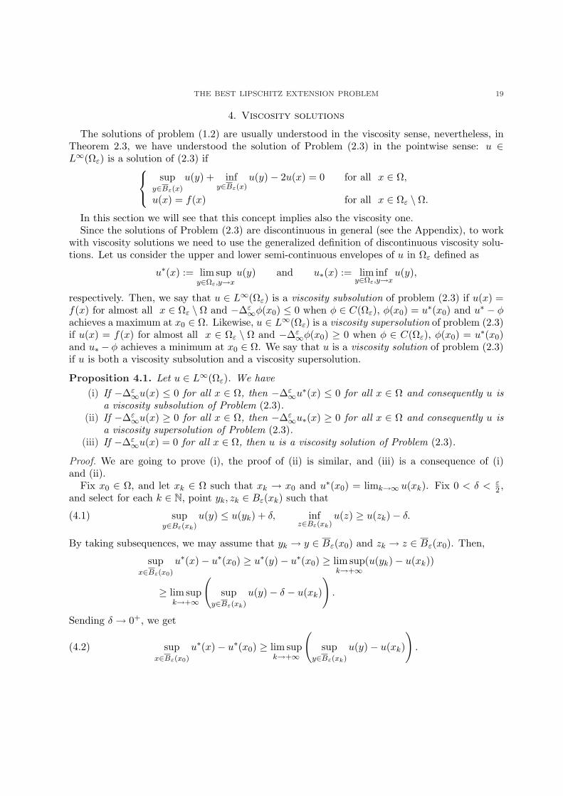
The solutions of problem (1.2) are usually understood in the viscosity sense, nevertheless, inTheorem 2.3, we have understood the solution of Problem (2.3) in the pointwise sense: u ∈L∞(Ωε) is a solution of (2.3) if
supy∈Bε(x)
u(y) + infy∈Bε(x)
u(y)− 2u(x) = 0 for all x ∈ Ω,
u(x) = f(x) for all x ∈ Ωε \ Ω.
In this section we will see that this concept implies also the viscosity one.Since the solutions of Problem (2.3) are discontinuous in general (see the Appendix), to work
with viscosity solutions we need to use the generalized definition of discontinuous viscosity solu-tions. Let us consider the upper and lower semi-continuous envelopes of u in Ωε defined as
u∗(x) := lim supy∈Ωε,y→x
u(y) and u∗(x) := lim infy∈Ωε,y→x
u(y),
respectively. Then, we say that u ∈ L∞(Ωε) is a viscosity subsolution of problem (2.3) if u(x) =f(x) for almost all x ∈ Ωε \ Ω and −∆ε∞φ(x0) ≤ 0 when φ ∈ C(Ωε), φ(x0) = u∗(x0) and u∗ − φachieves a maximum at x0 ∈ Ω. Likewise, u ∈ L∞(Ωε) is a viscosity supersolution of problem (2.3)if u(x) = f(x) for almost all x ∈ Ωε \ Ω and −∆ε∞φ(x0) ≥ 0 when φ ∈ C(Ωε), φ(x0) = u∗(x0)and u∗ − φ achieves a minimum at x0 ∈ Ω. We say that u is a viscosity solution of problem (2.3)if u is both a viscosity subsolution and a viscosity supersolution.
Proposition 4.1. Let u ∈ L∞(Ωε). We have(i) If −∆ε∞u(x) ≤ 0 for all x ∈ Ω, then −∆ε∞u∗(x) ≤ 0 for all x ∈ Ω and consequently u is
a viscosity subsolution of Problem (2.3).(ii) If −∆ε∞u(x) ≥ 0 for all x ∈ Ω, then −∆ε∞u∗(x) ≥ 0 for all x ∈ Ω and consequently u is
a viscosity supersolution of Problem (2.3).(iii) If −∆ε∞u(x) = 0 for all x ∈ Ω, then u is a viscosity solution of Problem (2.3).
Proof. We are going to prove (i), the proof of (ii) is similar, and (iii) is a consequence of (i)and (ii).
Fix x0 ∈ Ω, and let xk ∈ Ω such that xk → x0 and u∗(x0) = limk→∞ u(xk). Fix 0 < δ < ε2 ,
and select for each k ∈ N, point yk, zk ∈ Bε(xk) such that
(4.1) supy∈Bε(xk)
u(y) ≤ u(yk) + δ, infz∈Bε(xk)
u(z) ≥ u(zk)− δ.
By taking subsequences, we may assume that yk → y ∈ Bε(x0) and zk → z ∈ Bε(x0). Then,
supx∈Bε(x0)
u∗(x)− u∗(x0) ≥ u∗(y)− u∗(x0) ≥ lim supk→+∞
(u(yk)− u(xk))
≥ lim supk→+∞
(sup
y∈Bε(xk)
u(y)− δ − u(xk)
).
Sending δ → 0+, we get
(4.2) supx∈Bε(x0)
u∗(x)− u∗(x0) ≥ lim supk→+∞
(sup
y∈Bε(xk)
u(y)− u(xk)
).
20 J. M. MAZON, J. D. ROSSI AND J. TOLEDO
On the other hand,
u∗(x0)− infx∈Bε(x0)
u∗(x) ≤ u∗(x0)− u∗(z) ≤ lim infk→+∞
(u(xk)− u(zk))
≤ lim infk→+∞
(u(xk)− inf
z∈Bε(xk)u(z) + δ
).
Sending δ → 0+, we get
(4.3) u∗(x0)− infx∈Bε(x0)
u∗(x) ≤ lim infk→+∞
(u(xk)− inf
z∈Bε(xk)u(z)
).
From (4.2) and (4.3), and having in ind that by hypothesis we have −∆ε∞u ≤ 0, we obtain that
−∆ε∞u∗(x0) = −
(sup
x∈Bε(x0)
u∗(x)− u∗(x0)
)−
(inf
x∈Bε(x0)u∗(x)− u∗(x0)
)
≤ lim infk→+∞
(u(xk)− sup
y∈Bε(xk)
u(y) + u(xk)− infz∈Bε(xk)
u(z)
)= lim inf
k→+∞(−∆ε
∞u(xk)) ≤ 0.
This ends the proof. ¤
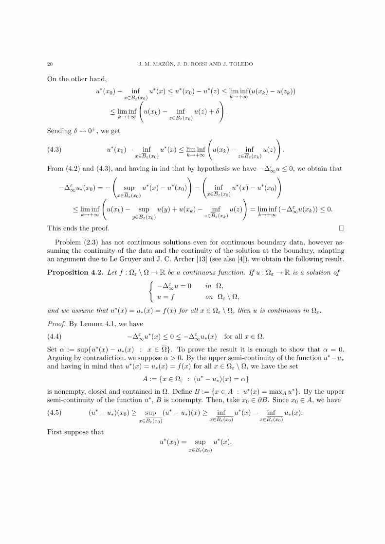
Problem (2.3) has not continuous solutions even for continuous boundary data, however as-suming the continuity of the data and the continuity of the solution at the boundary, adaptingan argument due to Le Gruyer and J. C. Archer [13] (see also [4]), we obtain the following result.
Proposition 4.2. Let f : Ωε \ Ω → R be a continuous function. If u : Ωε → R is a solution of−∆ε∞u = 0 in Ω,
u = f on Ωε \ Ω,
and we assume that u∗(x) = u∗(x) = f(x) for all x ∈ Ωε \ Ω, then u is continuous in Ωε.
Proof. By Lemma 4.1, we have
(4.4) −∆ε∞u∗(x) ≤ 0 ≤ −∆ε
∞u∗(x) for all x ∈ Ω.
Set α := supu∗(x) − u∗(x) : x ∈ Ω. To prove the result it is enough to show that α = 0.Arguing by contradiction, we suppose α > 0. By the upper semi-continuity of the function u∗−u∗and having in mind that u∗(x) = u∗(x) = f(x) for all x ∈ Ωε \ Ω, we have the set
A := x ∈ Ωε : (u∗ − u∗)(x) = αis nonempty, closed and contained in Ω. Define B := x ∈ A : u∗(x) = maxA u∗. By the uppersemi-continuity of the function u∗, B is nonempty. Then, take x0 ∈ ∂B. Since x0 ∈ A, we have
(4.5) (u∗ − u∗)(x0) ≥ supx∈Bε(x0)
(u∗ − u∗)(x) ≥ infx∈Bε(x0)
u∗(x)− infx∈Bε(x0)
u∗(x).
First suppose thatu∗(x0) = sup
x∈Bε(x0)
u∗(x).

THE BEST LIPSCHITZ EXTENSION PROBLEM 21
Then, since −∆ε∞u∗(x0) ≤ 0, we have
u∗(x0) = infx∈Bε(x0)
u∗(x),
and by (4.5) we deduce thatu∗(x0) = inf
x∈Bε(x0)u∗(x).
Then, since −∆ε∞u∗(x0) ≥ 0, we obtain that
u∗(x0) = supx∈Bε(x0)
u∗(x).
Therefore, u∗ and u∗ are constant in Bε(x0), contradicting our assumption that x0 ∈ ∂B.It remains to arrive to a contradiction in the case
u∗(x0) < supx∈Bε(x0)
u∗(x).
By the upper semi-continuity of the function u∗ there is y0 ∈ Bε(x0) such that
u∗(y0) = supx∈Bε(x0)
u∗(x).
Since u∗(y0) > u∗(x0) and x0 ∈ B, we see that y0 6∈ A. Then,
u∗(y0)− u∗(y0) < α = u∗(x0)− u∗(x0).
Hence,
(4.6) supx∈Bε(x0)
u∗(x)− u∗(x0) ≥ u∗(y0)− u∗(x0) > u∗(y0)− u∗(x0) = supx∈Bε(x0)
u∗(x)− u∗(x0).
Combining (4.5) and (4.6), we obtain −∆ε∞u∗(x0) < −∆ε∞u∗(x0), which contradicts (4.4), andthe proposition follows. ¤
5. Appendix: Examples
In this appendix we collect some concrete examples that are illustrative of the difficulties ofthe problem. In the first example we see that there exists f for which the AMLE1 of f is notAMLE of f in the sense of Definition 1.1 (in fact, there is no AMLE of f in that sense).
Example 5.1. For ε = 1, Ω = (0, 12) and f = 0χ
(−1,0] + 1χ[ 12, 32), for any z defined in (0, 1
2)
such that z(x) ∈ [0, 1], f + zχ(0, 1
2) ∈ MLE(f, Ω1). Between all of them, u = f + 1
2χ
(0, 12) is
the unique AMLE1(f, Ω) (it is very easy to prove that it is solution of (2.3)). On the otherhand, there is not AMLE of f in the sense of Definition 1.1. In fact, if u is AMLE of f , then ifB = (−1
2 , 12), the function g = 0χ
(−1, 12) + 1χ
( 12, 32) ∈ MLE(f, Ω1) and g = u in Ω1 \ B, therefore
Ld1(u,B) ≤ Ld1(g, B) = 0, and, hence, u is constant in B, that is, u = 0 in (0, 12). Similarly,
we can prove that u = 1 in (0, 12) by taking B = (0, 1) and g = 0χ
(−1,0) + 1χ(0, 3
2), which gives a
contradiction.

22 J. M. MAZON, J. D. ROSSI AND J. TOLEDO
Example 5.2. For ε = 1, Ω = (0, 2) and f = xχ(−1,0] + 2χ
[2,3), the unique solution u of (2.3)can be explicitly found as follows. First, we observe that u is increasing in x. Indeed, SinceLd1(f, Ω1 \ Ω) = 1, it is easy to see that the McShane-Whitney extensions are given in Ω by
Ψ(f)(x) = x, Λ(f)(x) = 0χ(0,1)(x) + 1χ[1,2)(x).
Then, if u is the solution of (2.3), since Ω is convex, by Theorem 2.3, u ∈ MLE(f,Ω1) andtherefore
(5.1) 0χ(0,1)(x) + 1χ[1,2)(x) ≤ u(x) ≤ x ∀x ∈ (0, 2).
By (5.1), for any x ∈ (0, 1) we have
u(x) =12x +
12
supy∈[1,x+1]
u(y),
so it is nondecreasing in this interval. For any x ∈ (1, 2) we have
u(x) =12
infy∈[x−1,1]
u(y) + 1,
so it also is nondecreasing in this interval. So, taking into account again (5.1), u is nondecreasingin all Ω = (0, 2). Therefore, for any x ∈ (0, 1) we have
u(x + 1) = 2u(x) + 1− x
and for any z ∈ (1, 2) we have
2 = u(z + 1) = 2u(z)− u(z − 1)
but taking z − 1 = x we get,
2 = 2u(x + 1)− u(x) = 3u(x) + 2− 2x
and we conclude thatu(x) =
23x, x ∈ (0, 1).
This implies
u(x) = 1 +13(x− 1), x ∈ (1, 2).
Finally, u(1) = 1.Note that u∗(2) = 4
3 < 2 = u∗(2) = f(2) and u is discontinuous at x = 1, therefore, theassumption u∗(x) = u∗(x) = f(x) for all x ∈ Ωε \ Ω in Proposition 4.2 is necessary for thecontinuity of u on Ω.
Example 5.3. For ε = 3/2, Ω = (0, 2) and f = xχ(− 3
2,0] + 2χ
[2, 72), the unique solution u of
(2.3) can also be explicitly found as follows. Since Ld 32
(f, Ω 32\ Ω) = 1, it is easy to see that the
McShane-Whitney extensions are given in Ω by
Ψ(f)(x) = x, Λ(f)(x) = −1χ(0, 1
2)(x) +
12χ
[ 12,2)(x).
Then, if u is the solution of (2.3), since Ω is convex, by Theorem 2.3, u ∈ MLE(f, Ω 32) and
therefore
(5.2) −1χ(0, 1
2)(x) +
12χ
( 12,2)(x) ≤ u(x) ≤ x ∀x ∈ (0, 2).
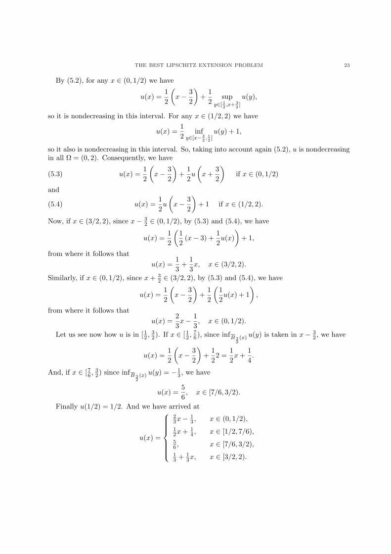
THE BEST LIPSCHITZ EXTENSION PROBLEM 23
By (5.2), for any x ∈ (0, 1/2) we have
u(x) =12
(x− 3
2
)+
12
supy∈[ 1
2,x+ 3
2]
u(y),
so it is nondecreasing in this interval. For any x ∈ (1/2, 2) we have
u(x) =12
infy∈[x− 3
2, 12]u(y) + 1,
so it also is nondecreasing in this interval. So, taking into account again (5.2), u is nondecreasingin all Ω = (0, 2). Consequently, we have
(5.3) u(x) =12
(x− 3
2
)+
12u
(x +
32
)if x ∈ (0, 1/2)
and
(5.4) u(x) =12u
(x− 3
2
)+ 1 if x ∈ (1/2, 2).
Now, if x ∈ (3/2, 2), since x− 32 ∈ (0, 1/2), by (5.3) and (5.4), we have
u(x) =12
(12
(x− 3) +12u(x)
)+ 1,
from where it follows thatu(x) =
13
+13x, x ∈ (3/2, 2).
Similarly, if x ∈ (0, 1/2), since x + 32 ∈ (3/2, 2), by (5.3) and (5.4), we have
u(x) =12
(x− 3
2
)+
12
(12u(x) + 1
),
from where it follows thatu(x) =
23x− 1
3, x ∈ (0, 1/2).
Let us see now how u is in [12 , 32). If x ∈ [12 , 7
6), since infB 32(x) u(y) is taken in x− 3
2 , we have
u(x) =12
(x− 3
2
)+
122 =
12x +
14.
And, if x ∈ [76 , 32) since infB 3
2(x) u(y) = −1
3 , we have
u(x) =56, x ∈ [7/6, 3/2).
Finally u(1/2) = 1/2. And we have arrived at
u(x) =
23x− 1
3 , x ∈ (0, 1/2),12x + 1
4 , x ∈ [1/2, 7/6),56 , x ∈ [7/6, 3/2),13 + 1
3x, x ∈ [3/2, 2).
24 J. M. MAZON, J. D. ROSSI AND J. TOLEDO
Observe that u(x) < 0 for 0 < x < 12 ; u is increasing in Ω but not in the whole Ωε.
Acknowledgments: J.M.M and J.T. has been partially supported by the MICINN projectMTM2008-03176. J.D.R. has been partially supported by MICINN project MTM2008-05824 andCONICET, Argentina.
References
1. F. Andreu, J. M. Mazon, J. D. Rossi and J. Toledo. A nonlocal p–Laplacian evolution equation with nonhomo-geneous Dirichlet boundary conditions. SIAM J. Math. Anal. 40 (2008/09), 1815–1851.
2. F. Andreu, J. M. Mazon, J. D. Rossi and J. Toledo. The limit as p → ∞ in a nonlocal p–Laplacian evolutionequation. A nonlocal approximation of a model for sandpiles. Calc. Var. Partial Differential Equations 35 (2009),279–316.
3. F. Andreu, J. M. Mazon, J. D. Rossi and J. Toledo. Nonlocal Diffusion Problems. AMS Mathematical Surveysand Monographs, vol. 165, 2010.
4. S. N. Armstrong and Ch. K. Smart. An easy proof of Jensen’s theorem on the uniqueness of infinity harmonicfunctions. Calc. Var. 37 (2010), 381–384.
5. S. N. Armstrong and Ch. K. Smart. A finite difference approach to the infinity Laplace equation and Tug-of-Wargames. To appear in Trans. Amer. Math. Soc.
6. G. Aronsson, Extension of functions satisfying Lipschitz conditions. Ark. Mat. 6 (1967), 551–561.7. G. Aronsson, M. G. Crandall and P. Juutinen, A tour of the theory of absolutely minimizing functions. Bull.
Amer. Math. Soc. 41 (2004), 439–505.8. E. N. Barron, L.C. Evans and R. Jensen, The infinity Laplacian, Aronsson equation and theier generalizations.
Trans. Amer. Math. Soc. 360 (2007), 77–101.9. T. Bhattacharya, E. DiBenedetto and J. Manfredi. Limit as p →∞ of ∆pup = f and related extremal problems.
Rend. Sem. mat. Univ. Politec. Torino 1989, special Issue (1991), 15–68.10. R. Jensen, Uniqueness of Lipschitz extensions: minimizing the sup-norm of the gradient. Arch. Rational Mech.
Anal. 123, (1993), 51–74.11. P. Juutinen, Absolutely minimizing Lipschitz extension on a metric space. Ann. Acad. Sci. Fenn.. Math. 27
(2002), 57–67.12. S. Kumagai, An implicit function theorem: Comment. Journal of Optimization Theory and Applications 31
(1980), 285–288.13. E. Le Gruyer and J. C. Archer, Harmonious extension. SIAM J. Math. Anal. 29 (1998), 279–292.14. G. Lu and P. Wang, A PDE perspective of the normalized infinity Laplacian. Comm. Partial Differential
Equations 33 (2008), 1788-181715. J. J. Manfredi, M. Parviainen and J. D. Rossi, Dynamic Programing principle for Tug-of-war games with noise,
To appear in C.O.C.V.16. J. J. Manfredi, M. Parviainen and J. D. Rossi, On the definition and properties of p–harmonious functions,
Preprint.17. E. J. McShane, Extension of range of functions. Bull. Amer. Math. Soc. 40 (1934), 837–842.18. V. A. Milman, Absolutely minimal extension of functions on metric spaces. math. Sbornik 190 (1999), 83–109.19. Y. Peres, G. Pete and S. Somersille, Biased tug-of-war, the biased infinity Laplacian, and comparison with
exponential cones. Calc. Var. Partial Differential Equations 38 (2010), 541-564.20. Y. Peres, O. Schramm, S. Sheffield and D. Wilson, Tug-of-war and the infinity Laplacian, J. Amer. Math. Soc.
22 (2009), 167–210.21. H. Whitney, Analytic extension of fiferentiable functions defined in a closed sets. Trans. Amer. Math. Soc. 36
(1934), 63–89.
Jose M. Mazon, Julian ToledoDepartament d’Analisi Matematica, Universitat de ValenciaValencia, SPAIN.E-mail address: [email protected], [email protected]

THE BEST LIPSCHITZ EXTENSION PROBLEM 25
Julio D. RossiDepartamento de Analisis Matematico, Universidad de Alicante,Ap. correos 99, 03080, Alicante, SPAIN.On leave fromDepartamento de Matematica, FCEyN UBA,Ciudad Universitaria, Pab 1 (1428),Buenos Aires, ARGENTINA.E-mail address: [email protected]
Copyright © 2022 FDOKUMEN