1

On the Steady-State Distribution in theHomogeneous Ribosome Flow Model

Michael Margaliot and Tamir Tuller

Abstract—A central biological process in all living organisms is gene translation. Developing a deeper understanding of this complexprocess may have ramifications to almost every biomedical discipline. Reuveni et al. recently proposed a new computational modelof gene translation called the Ribosome Flow Model (RFM). In this paper, we consider a particular case of this model, called theHomogeneous Ribosome Flow Model (HRFM). From a biological viewpoint, this corresponds to the case where the transition rates ofall the coding sequence codons are identical. This regime has been suggested recently based on experiments in mouse embryoniccells.We consider the steady-state distribution of the HRFM. We provide formulas that relate the different parameters of the model in steady-state. We prove the following properties: 1) the ribosomal density profile is monotonically decreasing along the coding sequence; 2) theribosomal density at each codon monotonically increases with the initiation rate; and 3) for a constant initiation rate, the translationrate monotonically decreases with the length of the coding sequence. In addition, we analyze the translation rate of the HRFM at thelimit of very high and very low initiation rate, and provide explicit formulas for the translation rate in these two cases. We discuss therelationship between these theoretical results and biological findings on the translation process.

Index Terms—Gene translation, systems biology, continued fractions, tridiagonal matrices, equilibrium point, monotone systems,translation elongation, constant elongation speed.

F

1 INTRODUCTION

Proteins are encoded in the DNA. In all living cellsthey are synthesized via several biophysical processes:the transcription of the DNA to mRNA molecules, thetranslation of each mRNA molecule to copies of theprotein, and the turnover of mRNA molecules and pro-teins. Gene translation takes place in all living organismsalmost in all the tissues and all the time. Thus, it isclearly a central intra-cellular process which is relatedto every biomedical discipline. For example, mutationsthat affect that translation rate may cause diseases, andviruses tend to exhibit adaptation to the tRNA pool oftheir host; thus, gene translation is strongly related tohuman health [1], [2], [3], [4], [5], [6], [7]. In addition, ma-nipulating the translation efficiency of genes may haveimportant biotechnological applications [8], [9], [10], [11],[12]. Finally, it is impossible to understand evolution [3],[13], [14], [15], [16], [17], [18], [19], functional genomics[20], [21], [22], [23], [24], [25], [26], and systems biology[27], [28], [29], [30], [31], [23], [5] without consideringtranslation.

Several comprehensive reviews related to translationhave recently appeared in the leading scientific literature[32], [14], [10].

The biophysical nature of translation is still at leastpartially unknown with contradicting results from dif-

• M. Margaliot is with the School of Electrical Engineering-Systems and theSagol School of Neuroscience, Tel-Aviv University, Tel-Aviv 69978, Israel.E-mail: michaelm@eng.tau.ac.il

• T. Tuller is with the Department of Biomedical Engineering, Tel-AvivUniversity, Tel-Aviv 69978, Israel.E-mail: tamirtul@post.tau.ac.il

ferent studies. One open question in the field is relatedto the rate limiting step of this process. It was suggestedthat the rate of translation initiation is very low in com-parison to elongation; thus, initiation, which is affectedamong other by the folding of the mRNA sequencenear the beginning of the ORF, is the rate limiting step[9], [33]. However, different studies have demonstratedthat adaptation of the codons to the tRNA pools alsocorrelates with protein levels, suggesting that elongationis also an important determinant of translation rate [34],[12].

Another open question is related to the features ofthe coding sequence that determine the translation elon-gation rate. It was suggested that the adaptation ofcodons to the cellular tRNA pool has significant effecton translation elongation rate [35], [8]. However, recentstudies have suggested that the translation speed ofdifferent codons is effectively constant [36] and notcorrelated with tRNA levels [37]. One of the suggestedexplanations for lack of correlation between tRNA levelsand translation speed is the fact that in many cases thecompetition for ribosomes, rather than tRNAs, limitsglobal translation [38]. It was also suggested that thislack of correlation is due to the fact that the codon usageis proportional to cognate tRNA concentrations, as thisoptimizes translational efficiency under tRNA shortage.Thus, the increased frequency of codons in highly ex-pressed genes is a byproduct of natural selection for anoverall cellular level efficient translation, and not theresult of stronger selection for translation efficiency inmore highly expressed genes [37].

When considering the factors that determine transla-tion rate it is important to remember that the relevant

2

biophysical parameters (e.g. the relative concentrationof tRNA molecules and elongation factors, the num-ber of available ribosomes and the number of mRNAmolecules) may vary significantly among different tis-sues, conditions, and organisms [10], [39], [40], [41].Thus, it is possible that each of the apparently contra-dicting theories is indeed dominant in a specific regime.

In the recent years, computational models of transla-tion have been developed (see, for example, [42], [43],[44], [45], [35], [46], [38], [47]). These models are basedon the features of transcripts and information aboutcellular concentrations of relevant molecules related tothe process of translation (e.g. tRNA molecules, elon-gation factors, and ribosomes), and may be used topredict various properties of the translation process (e.g.translation rate and ribosomal densities). Thus, thesemodels have been employed to address questions in allthe disciplines mentioned above (see, for example, [42],[43], [44], [45], [35], [46]).

Mathematical analysis of these computational modelsis important for several reasons. It can deepen our un-derstanding of the translation process, lead to algorithmsfor optimizing gene translation, and assist in improvingthe fidelity of the computational models. For example,based on such an analysis it is possible to show that therelative location of slow codons has an important effect onthe translation rate [47], or that improving the translationefficiency of a codon in one gene may decrease thetranslation rate of a second gene [43].

A conventional model of translation elongation is theTotally Asymmetric Simple Exclusion Process (TASEP) [48],[45], [44], [49]. The TASEP is a stochastic model fortraffic-like movement, that is, movement that takes placeon some kind of “tracks” or “trails”. The tracks aremodeled by a lattice of sites and the moving objects byparticles that can hop, with some probability, from onesite to a neighboring one. Simple exclusion refers to thefact that hops may take place only to a target site that isnot already occupied by another particle. The motion isassumed to be asymmetric in the sense that there is somepreferred direction of motion. The term totally asymmetricimplies that the motion is unidirectional. The TASEPhas been used to model and study a large number ofbiological systems, ranging from extracellular transportto pedestrian dynamics [50].

TASEP models for translation are based on the follow-ing assumptions [51], [50], [47], [49]. Initiation time aswell as the time a ribosome spends on translating eachcodon are random variables (e.g. with an exponentialdistribution) and are codon dependent. In addition, ribo-somes span over several codons and if two ribosomes areadjacent, the trailing one is delayed until the ribosome infront of it has proceeded onwards (see Fig. 1). Despite itsrather simple description, rigorous analysis of the TASEPis non-trivial.

Reuveni et al. [51] recently introduced a simpler anddeterministic model called the ribosome flow model (RFM).In the RFM, mRNA molecules are coarse-grained into n

x 1 x 2 x 3 x 4

Codon

Transition rate/co-adaptation to the tRNA pool

Ribosome density

Initiation rate

Protein Production rate

1 2 3

TA

SE

P

RF

M

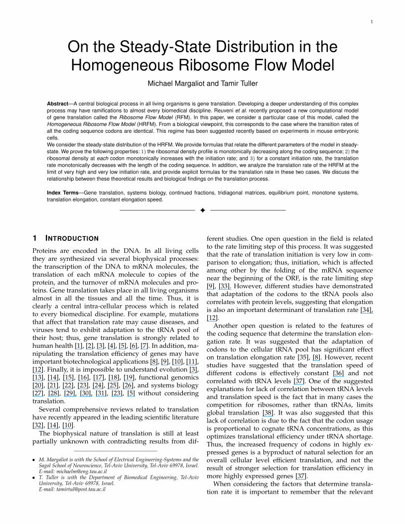
Fig. 1. The TASEP and the RFM. Upper-part: The TASEPmodel: each codon has an exponentially distributed trans-lation time; ribosomes have volume and can block eachother. Lower-part: The RFM is a coarse grained meanfield approximation of the TASEP.

sites of codons. Ribosomes reach the first site withinitiation rate λ, but are only able to bind if this siteis not already occupied by another ribosome. Thus, theinitiation rate and translation rate are not necessarilyequal even in steady state.

In practice, the initiation rate is a function of physi-cal features such as the number of available free ribo-somes and the nucleotide context surrounding initiationcodons [51], [10], [33], [35], [43]. A ribosome that occu-pies site i moves, with transition rate λi > 0, to theconsecutive site provided that the latter is not alreadyoccupied by another ribosome (see Fig. 1).

As demonstrated in [51], simulations of the full TASEPand the simpler RFM yield similar predictions. For ex-ample, the correlation between their predictions over theset of endogenous genes of S. cerevisiae is 0.96.

Denoting the probability that site i is occupied attime t by xi(t), it follows that the rate of ribosome flowinto/out of the system is given by λ(1 − x1(t)) andλnxn(t), respectively. The rate of ribosome flow fromsite i to site i + 1 is λixi(t)(1 − xi+1(t)), so the RFMis given by a set of n first-order differential equations

x1 = λ(1− x1)− λ1x1(1− x2),x2 = λ1x1(1− x2)− λ2x2(1− x3),x3 = λ2x2(1− x3)− λ3x3(1− x4),

...xn−1 = λn−2xn−2(1− xn−1)− λn−1xn−1(1− xn),

xn = λn−1xn−1(1− xn)− λnxn. (1)

The transition rates λ, λ1, . . . , λn are positive numbers.Their values can be estimated based on the codon com-

3

position of each site and the tRNA pool of the organism(see the Methods section in [51]). However, the speed oftranslation elongation may depend on other rate limitingfeatures including miRNAs, concentration of elongationfactors, ribosomal densities, and mRNA folding.

The state-variables correspond to occupation probabil-ities, so the initial condition x(0) = (x1(0), . . . , xn(0))′ isalways assumed to be in the closed unit cube

C = {x ∈ Rn : xi ∈ [0, 1], i = 1, . . . , n}.

Suppose that e = (e1, . . . , en)′ is an equilibrium pointof the RFM, i.e. for x = e the right-hand side of all theequations in (1) is zero. This yields

λ(1− e1) = λ1e1(1− e2)= λ2e2(1− e3)

...= λn−1en−1(1− en)= λnen. (2)

LetR = λnen (3)

denote the translation rate. At steady state, the transla-tion rate R is the flow out of each of the sites. Then (2)yields

en = R/λn,

en−1 = R/(λn−1(1− en)),... (4)

e2 = R/(λ2(1− e3)),e1 = R/(λ1(1− e2)),

ande1 = 1−R/λ. (5)

Combining (4) and (5) provides a finite continuedfraction expression for R:

1−R/λ =R/λ1

1− R/λ2

1− R/λ3

1− R/λ4

1− R/λ5

. . . 1−R/λn

(6)

Note that if ei ∈ [0, 1] for any i, then (2) implies that

R ≤ min{λ, λ1, . . . , λn}. (7)

Reuveni et al. [51] considered two extreme cases. Whenthe ribosome input flux is low, i.e. λ ¿ min{λ1, . . . , λn},Eq. (7) yields R ¿ λi for any i, and (6) impliesthat 1 − R/λ ≈ 0, so R ≈ λ. On the other hand,when λ À max{λ1, . . . , λn} Eq. (7) yields λ À R, so

we may approximate (6) by

1 ≈ R/λ1

1− R/λ2

1− R/λ3

1− R/λ4

1− R/λ5

. . . 1−R/λn

(8)

A solution of this equation has the form R =R(λ1, . . . , λn), i.e. R (and, therefore, e) will not dependon λ.

It was shown in [52] that the dynamical behavior of theRFM is relatively simple. Let Int(C) denote the interiorof C, i.e.

Int(C) = {x ∈ Rn : xi ∈ (0, 1), i = 1, . . . , n}.Recall that the L1 norm of a vector x ∈ Rn is |x|1 =∑n

i=1 |xi|. Let x(t; a) denote the solution of (1) at time tfor the initial condition x(0) = a.

Theorem 1 [52] Consider the RFM (1) with λ, λi > 0. Thereexists a single equilibrium point e ∈ Int(C). For any a ∈C, x(t; a) ∈ C for any t ≥ 0, and

limt→∞

x(t; a) = e. (9)

Furthermore, for any a, b ∈ C,

|x(t; a)− x(t; b)|1 ≤ |a− b|1, (10)

for any t ≥ 0.

From the biophysical point of view, (9) means that per-turbations in the distribution of ribosomes on a mRNAwill not change the asymptotic behavior of the dynamics.It will still converge to the same unique steady state e,that is, to the same distribution of ribosomes and thesame translation rates. In particular, a simulation of theRFM from any initial condition in C will converge to thesame final state. This agrees with the simulation resultsreported in [51].

Eq. (10) implies that the L1 distance between trajec-tories is always bounded by the L1 distance betweentheir initial conditions. In particular, two trajectoriesthat emanate from close initial conditions will remainclose for any t ≥ 0. From the biological point of view,this implies that the difference between two ribosomaldensity profiles can never increase.

Since e ∈ Int(C), we have in particular that e1 ∈ (0, 1),so (5) yields

R < λ,

i.e., the translation rate is always strictly smaller thanthe initiation rate.

Taking b = e in (10) yields

|x(t; a)− e|1 ≤ |a− e|1, for all t ≥ 0.

4

00.2

0.40.6

0.81

0

0.5

10

0.2

0.4

0.6

0.8

1

x1

x2

x 3

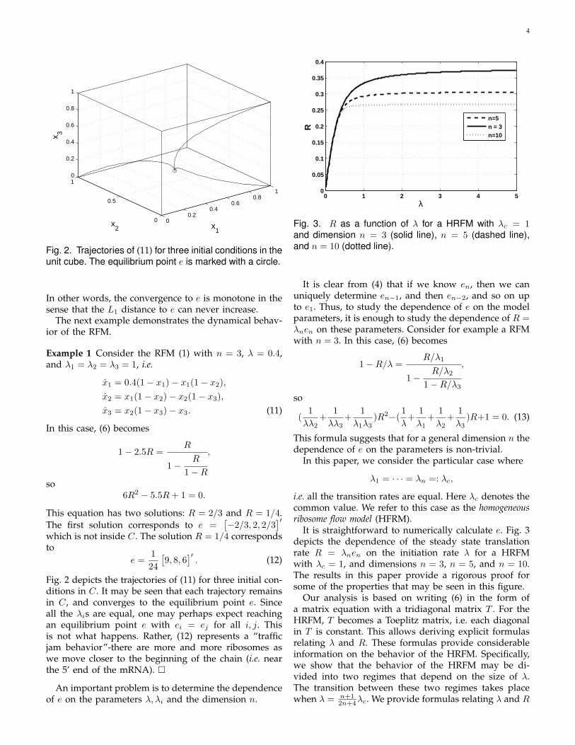
Fig. 2. Trajectories of (11) for three initial conditions in theunit cube. The equilibrium point e is marked with a circle.

In other words, the convergence to e is monotone in thesense that the L1 distance to e can never increase.

The next example demonstrates the dynamical behav-ior of the RFM.

Example 1 Consider the RFM (1) with n = 3, λ = 0.4,and λ1 = λ2 = λ3 = 1, i.e.

x1 = 0.4(1− x1)− x1(1− x2),x2 = x1(1− x2)− x2(1− x3),x3 = x2(1− x3)− x3. (11)

In this case, (6) becomes

1− 2.5R =R

1− R

1−R

,

so6R2 − 5.5R + 1 = 0.

This equation has two solutions: R = 2/3 and R = 1/4.The first solution corresponds to e =

[−2/3, 2, 2/3]′

which is not inside C. The solution R = 1/4 correspondsto

e =124

[9, 8, 6

]′. (12)

Fig. 2 depicts the trajectories of (11) for three initial con-ditions in C. It may be seen that each trajectory remainsin C, and converges to the equilibrium point e. Sinceall the λis are equal, one may perhaps expect reachingan equilibrium point e with ei = ej for all i, j. Thisis not what happens. Rather, (12) represents a “trafficjam behavior”-there are more and more ribosomes aswe move closer to the beginning of the chain (i.e. nearthe 5’ end of the mRNA). ¤

An important problem is to determine the dependenceof e on the parameters λ, λi and the dimension n.

0 1 2 3 4 50

0.05

0.1

0.15

0.2

0.25

0.3

0.35

0.4

λ

R

n=5n = 3n=10

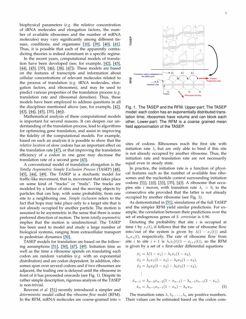
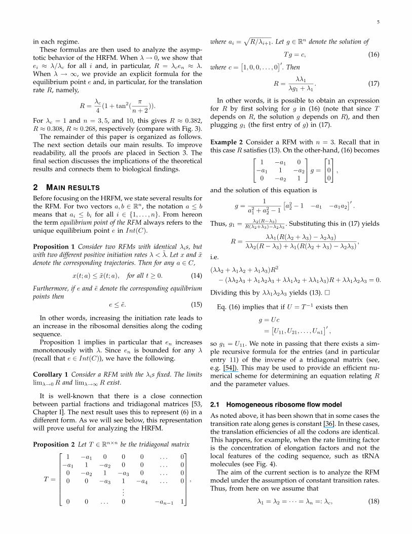
Fig. 3. R as a function of λ for a HRFM with λc = 1and dimension n = 3 (solid line), n = 5 (dashed line),and n = 10 (dotted line).

It is clear from (4) that if we know en, then we canuniquely determine en−1, and then en−2, and so on upto e1. Thus, to study the dependence of e on the modelparameters, it is enough to study the dependence of R =λnen on these parameters. Consider for example a RFMwith n = 3. In this case, (6) becomes

1−R/λ =R/λ1

1− R/λ2

1−R/λ3

,

so

(1

λλ2+

1λλ3

+1

λ1λ3)R2−(

1λ

+1λ1

+1λ2

+1λ3

)R+1 = 0. (13)

This formula suggests that for a general dimension n thedependence of e on the parameters is non-trivial.

In this paper, we consider the particular case where

λ1 = · · · = λn =: λc,

i.e. all the transition rates are equal. Here λc denotes thecommon value. We refer to this case as the homogeneousribosome flow model (HFRM).

It is straightforward to numerically calculate e. Fig. 3depicts the dependence of the steady state translationrate R = λnen on the initiation rate λ for a HRFMwith λc = 1, and dimensions n = 3, n = 5, and n = 10.The results in this paper provide a rigorous proof forsome of the properties that may be seen in this figure.

Our analysis is based on writing (6) in the form ofa matrix equation with a tridiagonal matrix T . For theHRFM, T becomes a Toeplitz matrix, i.e. each diagonalin T is constant. This allows deriving explicit formulasrelating λ and R. These formulas provide considerableinformation on the behavior of the HRFM. Specifically,we show that the behavior of the HRFM may be di-vided into two regimes that depend on the size of λ.The transition between these two regimes takes placewhen λ = n+1

2n+4λc. We provide formulas relating λ and R

5

in each regime.These formulas are then used to analyze the asymp-

totic behavior of the HRFM. When λ → 0, we show thatei ≈ λ/λc for all i and, in particular, R = λcen ≈ λ.When λ → ∞, we provide an explicit formula for theequilibrium point e and, in particular, for the translationrate R, namely,

R =λc

4(1 + tan2(

π

n + 2)).

For λc = 1 and n = 3, 5, and 10, this gives R ≈ 0.382,R ≈ 0.308, R ≈ 0.268, respectively (compare with Fig. 3).

The remainder of this paper is organized as follows.The next section details our main results. To improvereadability, all the proofs are placed in Section 3. Thefinal section discusses the implications of the theoreticalresults and connects them to biological findings.

2 MAIN RESULTS

Before focusing on the HRFM, we state several results forthe RFM. For two vectors a, b ∈ Rn, the notation a ≤ bmeans that ai ≤ bi for all i ∈ {1, . . . , n}. From hereonthe term equilibrium point of the RFM always refers to theunique equilibrium point e in Int(C).

Proposition 1 Consider two RFMs with identical λis, butwith two different positive initiation rates λ < λ. Let x and xdenote the corresponding trajectories. Then for any a ∈ C,

x(t; a) ≤ x(t; a), for all t ≥ 0. (14)

Furthermore, if e and e denote the corresponding equilibriumpoints then

e ≤ e. (15)

In other words, increasing the initiation rate leads toan increase in the ribosomal densities along the codingsequence.

Proposition 1 implies in particular that en increasesmonotonously with λ. Since en is bounded for any λ(recall that e ∈ Int(C)), we have the following.

Corollary 1 Consider a RFM with the λis fixed. The limitslimλ→0 R and limλ→∞R exist.

It is well-known that there is a close connectionbetween partial fractions and tridiagonal matrices [53,Chapter I]. The next result uses this to represent (6) in adifferent form. As we will see below, this representationwill prove useful for analyzing the HRFM.

Proposition 2 Let T ∈ Rn×n be the tridiagonal matrix

T =

1 −a1 0 0 0 . . . 0−a1 1 −a2 0 0 . . . 00 −a2 1 −a3 0 . . . 00 0 −a3 1 −a4 . . . 0

...0 0 . . . 0 −an−1 1

,

where ai =√

R/λi+1. Let g ∈ Rn denote the solution of

Tg = c, (16)

where c =[1, 0, 0, . . . , 0

]′. Then

R =λλ1

λg1 + λ1. (17)

In other words, it is possible to obtain an expressionfor R by first solving for g in (16) (note that since Tdepends on R, the solution g depends on R), and thenplugging g1 (the first entry of g) in (17).

Example 2 Consider a RFM with n = 3. Recall that inthis case R satisfies (13). On the other-hand, (16) becomes

1 −a1 0−a1 1 −a2

0 −a2 1

g =

100

,

and the solution of this equation is

g =1

a21 + a2

2 − 1[a22 − 1 −a1 −a1a2

]′.

Thus, g1 = λ2(R−λ3)R(λ2+λ3)−λ2λ3

. Substituting this in (17) yields

R =λλ1(R(λ2 + λ3)− λ2λ3)

λλ2(R− λ3) + λ1(R(λ2 + λ3)− λ2λ3),

i.e.

(λλ2 + λ1λ2 + λ1λ3)R2

− (λλ2λ3 + λ1λ2λ3 + λλ1λ2 + λλ1λ3)R + λλ1λ2λ3 = 0.

Dividing this by λλ1λ2λ3 yields (13). ¤

Eq. (16) implies that if U = T−1 exists then

g = Uc

=[U11, U21, . . . , Un1

]′,

so g1 = U11. We note in passing that there exists a sim-ple recursive formula for the entries (and in particularentry 11) of the inverse of a tridiagonal matrix (see,e.g. [54]). This may be used to provide an efficient nu-merical scheme for determining an equation relating Rand the parameter values.

2.1 Homogeneous ribosome flow model

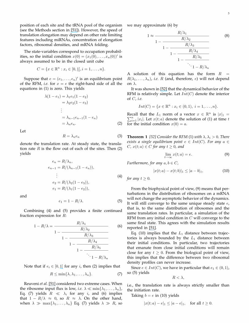
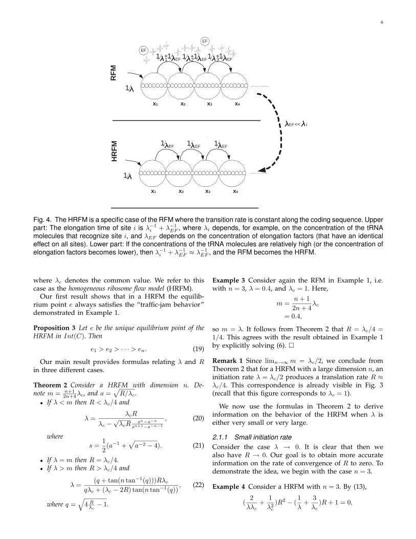
As noted above, it has been shown that in some cases thetransition rate along genes is constant [36]. In these cases,the translation efficiencies of all the codons are identical.This happens, for example, when the rate limiting factoris the concentration of elongation factors and not thelocal features of the coding sequence, such as tRNAmolecules (see Fig. 4).

The aim of the current section is to analyze the RFMmodel under the assumption of constant transition rates.Thus, from here on we assume that

λ1 = λ2 = · · · = λn =: λc, (18)

6

HR

FM

EF i <<

x 1 x 2 x 3 x 4

RF

M

EF

EF

EF 1 1 1 + EF 2 1 1 +

EF 3 1 1 +

x 1 x 2 x 3 x 4

1

1

EF 1 EF 1 EF 1

Fig. 4. The HRFM is a specific case of the RFM where the transition rate is constant along the coding sequence. Upperpart: The elongation time of site i is λ−1

i + λ−1EF , where λi depends, for example, on the concentration of the tRNA

molecules that recognize site i, and λEF depends on the concentration of elongation factors (that have an identicaleffect on all sites). Lower part: If the concentrations of the tRNA molecules are relatively high (or the concentration ofelongation factors becomes lower), then λ−1

i + λ−1EF ≈ λ−1

EF , and the RFM becomes the HRFM.

where λc denotes the common value. We refer to thiscase as the homogeneous ribosome flow model (HRFM).

Our first result shows that in a HRFM the equilib-rium point e always satisfies the “traffic-jam behavior”demonstrated in Example 1.

Proposition 3 Let e be the unique equilibrium point of theHRFM in Int(C). Then

e1 > e2 > · · · > en. (19)

Our main result provides formulas relating λ and Rin three different cases.

Theorem 2 Consider a HRFM with dimension n. De-note m = n+1

2n+4λc, and a =√

R/λc.• If λ < m then R < λc/4 and

λ =λcR

λc −√

λcRsn−s−n

sn+1−s−n−1

, (20)

wheres =

12(a−1 +

√a−2 − 4). (21)

• If λ = m then R = λc/4.• If λ > m then R > λc/4 and

λ =(q + tan(n tan−1(q)))Rλc

qλc + (λc − 2R) tan(n tan−1(q)), (22)

where q =√

4 Rλc− 1.

Example 3 Consider again the RFM in Example 1, i.e.with n = 3, λ = 0.4, and λc = 1. Here,

m =n + 12n + 4

λc

= 0.4,

so m = λ. It follows from Theorem 2 that R = λc/4 =1/4. This agrees with the result obtained in Example 1by explicitly solving (6). ¤

Remark 1 Since limn→∞m = λc/2, we conclude fromTheorem 2 that for a HRFM with a large dimension n, aninitiation rate λ = λc/2 produces a translation rate R ≈λc/4. This correspondence is already visible in Fig. 3(recall that this figure corresponds to λc = 1).

We now use the formulas in Theorem 2 to deriveinformation on the behavior of the HRFM when λ iseither very small or very large.

2.1.1 Small initiation rateConsider the case λ → 0. It is clear that then wealso have R → 0. Our goal is to obtain more accurateinformation on the rate of convergence of R to zero. Todemonstrate the idea, we begin with the case n = 3.

Example 4 Consider a HRFM with n = 3. By (13),

(2

λλc+

1λ2

c

)R2 − (1λ

+3λc

)R + 1 = 0,

7

and solving this equation yields

R =3λλc + λ2

c ± λc

√5λ2 − 2λλc + λ2

c

2(λ + 2λc). (23)

The solution with the plus sign gives R = λc/2 for λ = 0.This is clearly impossible, so the feasible solution is

R =3λλc + λ2

c − λc

√5λ2 − 2λλc + λ2

c

2(λ + 2λc)= λ + O(λ2).

This shows that for the case n = 3, when the initiationrate is very small, we have R ≈ λ. ¤

The next result describes the behavior of the HRFMfor a general dimension n.

Proposition 4 For λ ≈ 0, we have

λ =R

1−R/λc + O(R3/2)(24)

= R + O(R2).

This means that for sufficiently small values of λ, thegraph R vs. λ looks linear, and does not depend on thedimension n (see Fig. 3) nor the value λc.

Remark 2 It follows from (4) that for the HRFM

en−1 =λnen

λn−1(1− en)

=en

1− en.

Hence, if R ¿ λc (i.e. en = R/λc ¿ 1) then en−1 ≈ en.Using (4) inductively (as in the proof of Prop. 3 below)yields that in this case ei ≈ en for all i. Thus, (19) holdsyet the difference between the eis is small. Summarizing,when λ is sufficiently small (and thus becomes the lim-iting factor), we have R ≈ λ and ei ≈ en = R/λc ≈ λ/λc.

2.1.2 High initiation rate

Consider the case λ →∞. Clearly, the transition rate λc

becomes the limiting factor, and a natural question is:how does the translation rate R depend on λc? Togain some intuition, we begin by considering a simpleexample.

Example 5 Consider a HRFM with n = 3. Taking λ toinfinity in (23) yields

R ≈ 3λλc ± λc

√5λ2

2λ

=3±√5

2λc.

The solution with the plus sign is not feasible, as en =R/λc must be smaller than one. Thus, for n = 3 and a

very high initiation rate

R

λc≈ 3−√5

2≈ 0.382. ¤

The next results describes the behavior of a HRFMwith a general dimension n as λ goes to infinity. Denote

L(n) = limλ→∞

R(n)λc

(this limit exists by Corollary 1).

Proposition 5 Consider a HRFM with dimension n. Then

L(n) =14(1 + tan2(

π

n + 2)). (25)

For Example, for n = 3 this yields

L(3) =14(1 + tan2(

π

5))

≈ 0.382,

and this agrees with the result obtained in Example 5.Note that (25) implies that L(n) is a monotonically

decreasing function of n with

limn→∞

L(n) = 1/4. (26)

Thus, for a very large initiation rate, the translationrate R(n) = λcL(n) decays monotonically with thelength of the coding sequence n, and for n →∞, R(n) →λc/4 (see Fig. 3).

Recall that en uniquely determines e. Thus, Prop. 5allows us to derive an expression for ei, i = 1, . . . , n, inthe limit of infinite initiation rate.

Proposition 6 Consider a HRFM with dimension n.When λ →∞,

ei(n) =12

√(1 + tan2(

π

n + 2))

sin(π(n−i+1)n+2 )

sin(π(n−i+2)n+2 )

, (27)

for i = 1, . . . , n.

Note that for i = 1 this yields

e1(n) =12

√(1 + tan2(

π

n + 2))

sin( πnn+2 )

sin(π(n+1)n+2 )

=12

√(1 + tan2(

π

n + 2))

sin(π − 2πn+2 )

sin(π − πn+2 )

=12

1cos( π

n+2 )sin( 2π

n+2 )sin( π

n+2 )

= 1,

and this agrees of course with (5).

Example 6 Consider a HRFM with n = 3, λc = 2,and λ = 106. Solving (6) yields two solutions for R and

8

the feasible one is R ≈ 0.763932. Substituting this in (4)yields

e1 ≈ 0.999999,

e2 ≈ 0.618034,

e3 ≈ 0.381966.

On the other-hand, Eq. (27) (that corresponds to thecase λ →∞) yields

e1 = 1,

e2 ≈ 0.618034,

e3 ≈ 0.381966. ¤

3 PROOFS

Proof of Proposition 1. It can be shown that the RFM,with λ considered as an input signal, is a monotone controlsystem [55] on C. The proof then follows from the resultsin [55]. However, for the sake of completeness, we give asketch of a proof. Clearly, (14) holds for t = 0. Seeking acontradiction, assume that the proposition is false. Thisimplies that there exists a minimal time T > 0 and anindex i such that

x(t; a) ≤ x(t; a), for all t ≤ T,

xi(T ; a) = xi(T ; a), (28)xi(T+; a) > xi(T+; a).

We consider three cases.Case 1. Suppose that i = 1. It follows from (1) that

x1 − ˙x1 = λ(1− x1)− λ1x1(1− x2)

− λ(1− x1) + λ1x1(1− x2),

and using (28) yields

x1(T )− ˙x1(T ) = (λ− λ)(1− x1(T ))+ λ1x1(T )(x2(T )− x2(T )).

Since λ > λ, x2(T ) ≤ x2(T ), and x(t) ∈ C for any t ≥ 0,this yields

x1(T )− ˙x1(T ) ≤ 0.

Case 2. Suppose that 1 < 1 < n. It follows from (1) that

xi − ˙xi = λi−1xi−1(1− xi)− λixi(1− xi+1)− λi−1xi−1(1− xi) + λixi(1− xi+1),

and using (28) yields

xi(T )− ˙xi(T ) = λi−1(xi−1(T )− xi−1(T ))(1− xi(T ))+ λixi(T )(xi+1(T )− xi+1(T )).

Since the λks are positive and x(T ) ∈ C, using (28) againyields

xi(T )− ˙xi(T ) ≤ 0.

Case 3. Suppose that i = n. By (1),

xn − ˙xn = λn−1xn−1(1− xn)− λnxn

− λn−1xn−1(1− xn) + λnxn,

and using (28) yields

xn(T )− ˙xn(T ) = λn−1(xn−1(T )− xn−1(T ))(1− xn(T ))≤ 0.

Summarizing, in all three cases we have xi(T )− ˙xi(T ) ≤0. Using the same approach as in the proof of Propo-sition 1.1 in [56] (that is based on slightly perturbingthe vector field of the dynamical system) it may beshown that this implies that xi(T+) ≤ xi(T+). Thiscontradicts (28). This contradiction proves (14). The proofof (15) follows from taking t to infinity in (14) and usingTheorem 1. ¤

Proof of Proposition 2. The first equation of (16) is g1 −a1g2 = 1. Dividing by g1 yields 1− a1g2/g1 = 1/g1, or

g1 =1

1− a1g2/g1. (29)

The second equation of (16) is −a1g1 + g2 − a2g3 = 0.Dividing by g2 yields −a1g1/g2 + 1− a2g3/g2 = 0, or

a1g2/g1 =a21

1− a2g3/g2.

Substituting this in (29) yields

g1 =1

1− a21

1− a2g3/g2

. (30)

The third equation of (16) is −a2g2 + g3 − a3g4 = 0.Dividing by g3 yields −a2g2/g3 + 1− a3g4/g3 = 0, or

a2g3/g2 =a22

1− a3g4/g3.

Substituting this in (30) yields

g1 =1

1− a21

1− a22

1− a3g4/g3

.

Proceeding in this fashion and using the fact that ai =√R/λi+1, we get

g1 =1

1− R/λ2

1− R/λ3

1− R/λ4

1− R/λ5

. . . 1−R/λn

Comparing this with (6) shows that g1 = 1−R/λR/λ1

, and thisproves (17). ¤

9

Proof of Proposition 3. By (4),

en−1 =λnen

λn−1(1− en)

=en

1− en.

Since e ∈ Int(C), 0 < 1− en < 1, so

en−1 > en. (31)

Combining (4) and (18) yields

ek

ek+1=

R/(1− ek+1)R/(1− ek+2)

=1− ek+2

1− ek+1.

In particular, for k = n− 2 this yields

en−2

en−1=

1− en

1− en−1,

and (31) implies that en−2 > en−1. Proceeding in thisway shows that ei > ei+1 for all i. ¤

Proof of Theorem 2. For the HRFM, the matrix T definedin Prop. 2 becomes

T =

1 −a 0 0 . . . 0−a 1 −a 0 . . . 00 −a 1 −a . . . 0

...0 0 . . . 0 −a 1

.

Note that this matrix has constant diagonals. Thus, if wedefine g0 = 0 and gn+1 = 0, then the equation Tg = cbecomes

−ag0 + g1 − ag2 = 1,

−ag1 + g2 − ag3 = 0,

−ag2 + g3 − ag4 = 0,

...−agn−1 + gn − agn+1 = 0.

Write this set of equations as

−agi + gi+1 − agi+2 = fi, i = 0, 1, . . . , (32)

with f0 = 1, and fi = 0 for any i > 0.Let X(z) =

∑∞k=0 xkz−k denote the Z-transform of

the series {x0, x1, . . . } (see e.g. [57]). Applying the Z-transform to (32) yields

−aG(z) + z(G(z)− g0)− az2(G(z)− g0 − g1z−1) = F (z).

Since F (z) =∑∞

i=0 fkz−k = 1 and g0 = 0, this simplifiesto

−aG(z) + zG(z)− az2(G(z)− g1z−1) = 1.

orG(z) =

g1z − 1/a

z2 − z/a + 1.

The roots of the polynomial z2 − z/a + 1 are s and 1/s,

with s defined in (21). We consider two cases.Case 1. Suppose that s = 1/s. Eq. (21) implies that a =1/2, and s = 1. Thus,

G(z) =g1z − 2(z − 1)2

.

This may be written as

G(z) =2

z − 1+ (g1 − 2)

z

(z − 1)2,

and applying an inverse Z-transform yields g0 = 0, and

gk = 2 + (g1 − 2)k, k ≥ 1.

Recalling that gn+1 = 0 yields g1 = 2nn+1 , and using this

in (17) yields

R =(n + 1)λλc

2nλ + (n + 1)λc.

Since a = 1/2, R = λc/4, so

λc

4=

(n + 1)λλc

2nλ + (n + 1)λc,

and this is equivalent to λ = m. Summarizing, when λ =m, R = λc/4.Case 2. Suppose that s 6= 1/s. Then a partial fractiondecomposition yields

G(z) =g1z − 1/a

(z − s)(z − 1/s)

=α

z − s+

g1 − α

z − 1/s,

with

α =g1s− 1/a

s− 1/s. (33)

An inverse Z-transform yields g0 = 0, and

gk = αsk−1 + (g1 − α)(1/s)k−1, k ≥ 1.

Recalling that gn+1 = 0 gives αsn + (g1 − α)(1/s)n = 0,so

α =g1

1− s2n

Substituting this in (33) and simplifying yields

g1 =s2n+1 − s

a(s2n+2 − 1)

=sn − s−n

a(sn+1 − s−n−1). (34)

Substituting this in (17) yields (20).

Consider the case a > 1/2. In this case s = 12 (a−1 +

j√

4− a−2), where j =√−1. The polar representation of

this complex number is s = |s|ej∠s, with |s| = 1 and ∠s =tan−1(q), with q =

√4a2 − 1. Substituting this in (34)

yields

g1 =sin(n tan−1(q))

a sin((n + 1) tan−1(q)). (35)

10

Using the identity sin(x+y) = sin(x) cos(y)+cos(x) sin(y)implies that the denominator in (35) is

a sin(n tan−1(q)) cos(tan−1(q))+ a cos(n tan−1(q)) sin(tan−1(q)). (36)

Using the identities

sin(tan−1(x)) =x√

1 + x2,

cos(tan−1(x)) =1√

1 + x2, (37)

and the definition of q yields

sin(tan−1(q)) =q

2a,

cos(tan−1(q)) =12a

,

and combining this with (35) and (36) yields

g1 =2 sin(n tan−1(q))

sin(n tan−1(q)) + q cos(n tan−1(q))

=2

1 + q/ tan(n tan−1(q)).

Substituting this in (17) yields (22).Summarizing, in Case 1 we have λ = m and R = λc/4,

so a = 1/2. It follows from Proposition 1 that for λ < m[λ > m], a < 1/2 [a > 1/2] and this corresponds to thecase where s is a real [complex] number. This completesthe proof of Theorem 2. ¤

Remark 3 Note that using the identity

sin(nx) =n∑

k=0

sin((n− k)π

2) cosk(x) sinn−k(x),

and (37) it is possible to write the right-hand side of (35)as a rational function of q.

Proof of Proposition 4. It is clear that when λ → 0, a =√R/λc → 0. Using the definition of s in (21) yields the

expansion

1s

= a + O(a2). (38)

Consider the expression

sn − s−n

sn+1 − s−n−1=

s2n+1 − s

s2n+2 − 1= p + O(p2n+1),

where p = s−1, and the last equation follows from a longdivision. Substituting (38) yields

sn − s−n

sn+1 − s−n−1= a + O(a2) + (a + O(a2))2n+1

= a + O(a2),

and substituting this in (20) yields

λ =R

1− a2 + O(a3).

This proves (24). ¤Proof of Proposition 5. Since R/λc = en ∈ (0, 1), the

denominator in (22) must go to zero as λ → ∞. Thisyields

tan(n tan−1(√

4L(n)− 1)) =

√4L(n)− 1

2L(n)− 1. (39)

Denote P (n) =√

4L(n)− 1. Then

tan(n tan−1(P (n))) = − 2P (n)1− P 2(n)

.

Using the identity

tan(x + y) =tan(x) + tan(y)

1− tan(x) tan(y),

yields

tan(n tan−1(P (n))) = − tan(2 tan−1(P (n))),

son tan−1(P (n)) = kπ − 2 tan−1(P (n)),

for some integer k. Thus,

tan−1(P (n)) =kπ

n + 2. (40)

Since we are considering the case λ → ∞, it is clearthat λ > m and By Theorem 2, R > λc/4, i.e. L(n) > 1/4.Also, by (7), R ≤ λc, so L(n) ≤ 1. Thus, 0 < P (n) ≤√

3 for any n. Combining this with (40) yields P (n) =tan( π

n+2 ), and using the definition of P (n) proves (25). ¤Proof of Proposition 6. It follows from (4) that en(n) =

R(n)/λc = L(n). Applying (4) again yields

en−1(n) =en(n)

1− en(n)

=L(n)

1− L(n),

and

en−2(n) =en(n)

1− en−1(n)

=L(n)

1− L(n)1−L(n)

.

Proceeding in this fashion yields

1− en−i(n) = 1− L(n)

1− L(n)

1− L(n). . . 1− L(n)

, (41)

where L(n) appears in total i + 1 times. The continuedfraction in the right hand-side of this equation is aperiodic continued fraction [53]. The formula in [53, p. 23,Exercise 1.4] provides a closed-form expression for thevalue of such a continued fraction. For our case, thisformula yields the following result. Let u(n), v(n) be the

11

roots of the quadratic equation

x2 − x + L(n) = 0, (42)

with |u(n)| ≥ |v(n)|. Then the term on the right-handside of (41) is equal to

u(n) + v(n)− v(n)v(n)u(n) + 1∑i

p=0(v(n)/u(n))p

. (43)

Using (42) and (25) yields u(n) = (1 + j tan(

πn+2

))/2,

v(n) = (1 − j tan(

πn+2

))/2, where j =

√−1. The polarrepresentation of these complex numbers is

u(n) =√

L(n) exp(jπ/(n + 2)),

v(n) =√

L(n) exp(−jπ/(n + 2)).

Combining this with (43) and (41) yields

en−i(n) =

√L(n) exp(−jπ/(n + 2))

exp(−2jπ/(n + 2)) + 1∑ip=0(exp(−2jπ/(n+2)))p

=

√L(n) exp(−jπ/(n + 2))

exp(−2jπ/(n + 2)) + 1−exp(−2jπ/(n+2))1−exp(−2jπ(i+1)/(n+2))

=√

L(n)sin(π(i+1)

n+2 )

sin(π(i+2)n+2 )

,

and using (25) completes the proof. ¤

4 DISCUSSION

The RFM is a new deterministic model for translationelongation. It was already shown that this model admitsa unique equilibrium point e ∈ Int(C), and that anytrajectory emanating from a feasible initial conditionconverges to e [52].

An important problem is to analyze the dependenceof e on the various parameters of the model. Here, weconsider this problem for the particular case where allthe transition rates are identical. This corresponds to thecase where the elongation rates of the different codonsare all equal [36].

Analysis of the HRFM may also be used to derivebounds on the behavior of the more general RFM. In-deed, consider a RFM with parameters λi. Let λmin =min{λi} and λmax = max{λi}. It is straightforward toshow that the steady state translation rates in the RFMwill be bounded below [above] by the steady state trans-lation rates in the HRFM with λc = λmin [λc = λmax].

Our analysis reveals several nice properties relatedto translation elongation. First, even though the elon-gation speed is constant, the ribosomal density profileis monotonically decreasing along the coding sequence.Indeed, a decreasing ribosomal density profile has beenobserved in various organisms based on experimentalmeasurement of ribosomal densities (see, for example,[36], [58]). However, in some of these cases, riboso-mal speed along the coding sequences is probably notconstant, and slower codons at the beginning of the

transcript should strengthen this phenomenon resultingin a wider region of high ribosomal density at the 5’end of the mRNA [35]. The analysis performed here isrelevant to the cases when the elongation speed is closeto constant [36].

Second, we show that for a fixed initiation rate, in-creasing the length of the transcript decreases the trans-lation rate. This result is in accordance with the resultsreported in [43], showing that adding a codon to themRNA cannot increase its translation rate. Thus, evenif the translation efficiency of different codons is effec-tively constant, shorter transcripts should have highertranslation rate at steady state. Indeed, it is known thatin some organisms highly expressed genes tend to beshorter [43], [59], [60] suggesting that in these cases thisproperty is shaped by evolution partially due to reasonsrelated to optimization of translation rate.

Third, we provide formulas relating the translationrate of a gene and the parameters of a HRFM. Weuse these formulas to study the asymptotic behavior ofthe HRFM. When the initiation rate λ is very low, thetranslation rate is practically identical to the initiationrate. Recently, it was suggested that this is indeed theregime in some mammalian genes [36]. When the ini-tiation rate is rate limiting, improving the translationrate can be achieved by increasing the initiation rate. Inmany cases, this can be done by manipulating the 5’UTRand the beginning of the ORF which are the regions ofthe transcript related to the efficiency of its translationinitiation.

When the initiation rate is very high, the translationrate in the HRFM depends on the coding sequencelength n and the translation rate λc via the formula

R =λc

4(1 + tan2(

π

n + 2)).

As n goes to infinity, R → λc/4. One may define thecapacity of a gene as the maximal translation rate thatcan be obtained for this gene [51]. Thus, in the caseof the HRFM we have a closed-form formula for thecapacity. For example, this formula can be used whenanalyzing translation rates in mouse embryonic stemcells where in many cases translation rates are constant[36]. Our theoretical results seem to agree with somebiological data. For example, in yeast the ORF lengthrange is between 51 (1 − 2 sites) and 14, 733 (446 sites)corresponding to a maximal translation rate betweenλc/2 and λc/4.

It is interesting to compare our results with thoseobtained for the TASEP. The prototype TASEP is com-posed of a chain of L sites and is characterized bythree parameters α, β, and γ [48]. A particle entersfrom a reservoir and occupies site 1 (when this siteis empty), with probability α. A particle that occupiessite L (the rightmost site) can exit with probability β.The probability of hopping from site i to site i+1 (wherethe latter site is empty) is γ. Without loss of generality,it is possible to take γ = 1. The behavior of this model

12

includes three major phases:• a low-density (LD) phase when α is low and β

is high. In this phase the initiation rate α is ratelimiting and dominates the behavior of the system.

• a high-density (HD) phase when α is high and βis low. In this phase the translation rate β is ratelimiting.

• a maximal-current (MC) phase when both α and βare high. In this phase, input and output are moreefficient than the transport in the bulk of the system,and the particle current reaches the largest possiblevalue.

When L →∞, the average current J in the LD, HD, andMC phases is α(1− α), β(1− β), and 1/4, respectively.

As we showed here, the HRFM has two phases (seealso Fig. 3):• When λ ¿ λc the translation rate is R ≈ λ. This

roughly corresponds to the LD phase in the TASEP.• When λ À λc the translation rate is R ≈ λc

4 (1 +tan2( π

n+2 )). This corresponds to the MC phase. Inparticular, for n →∞, R ≈ λc

4 .An important question is how to determine the pa-

rameter values in the RFM/HRFM so that the modelwill capture the behavior of a real biological system.There are only a few relevant experimental measurementof translation rates and ribosomal densities, but theycan give an initial answer to this question. Based on alarge scale analysis of ribosomal densities in S. cerevisiae,Arava et al. [61] concluded that the mean number ofribosome per 100 nt is 0.64 ± 0.31. The size of theribosomal footprint is 11−13 codons [58], [36], i.e. 33−39nt. This means that 23%±11% of the mRNA is occupiedby a ribosome. Reuveni et al. [51] have shown that for aRFM for S. cerevisiae with an extremely high initiationrate λ the mean genomic probability that a site ei isoccupied by a ribosome approaches 0.5. These studiessuggest that the regime of very large λ, analyzed in thisstudy, occurs in practice.

The translation rates of codons were estimated in threeprevious studies. Ingolia et al. [36] have showen that inmouse embryonic cells 5.6 ± 0.5 codons (correspondingto 0.156± 0.014 sites in the RFM) are translated per sec-ond; a similar estimation has been obtained in [62]: themedian translation rate in mouse is about 40 proteins permRNA per hour (2/3 proteins per mRNA per minute);in mouse the mean mRNA length is about 465 codons.This suggests a translation rate of about 5.1 codons persecond which is consistent with [36]. von der Haar [63]estimated that in S. cerevisiae 32.6 codons (correspondingto 0.906 sites in the RFM) are translated per second.

It is important to remember that the data above corre-sponds to average values. In practice, it is not clear yethow many genes are translated in the elongation limitedregime and how many in the initiation limiting regime.However, we believe that both regimes occur in naturedepending on the organism and, more importantly, onvarious biological conditions (see, for example, [10], [39],

[40], [41]).There are many interesting open questions related to

the RFM and the HRFM. First, there is evidence that insome cases the rates λ, λi are time-varying and that theychange in a periodic fashion [64]. It may be interesting toanalyze the behavior of the RFM or HRFM in this case.Second, the RFM is a relatively simple mathematicalmodel, and it may be useful to modify it to incorporatemore sophisticated aspects of the translation process.For example, finiteness of the ribosomal pool, ribosomalabortion, initiation and elongation. It is also importantto remember that the final expression levels of a genedepend not only on its translation rate, but also on otherfactors including its mRNA levels; degradation rates ofthe transcripted mRNA molecules; and the degradationrates of the translated proteins. Another important re-search direction is the design of efficient algorithms forsynthesizing artificial coding sequences based on theRFM [43].

Finally, the HRFM, or suitable generalizations of theHRFM, can be used for studying additional cellularbiological processes and not only translation. For exam-ple, transcription can be modeled in a similar way totranslation; however, in this case, the model should in-clude backwards flow to simulate the possible retrogrademovement of the polymerase on the DNA [65]. Anotherpossibility is the modeling of cellular trafficking over themicrotubules network [66].

ACKNOWLEDGEMENTS

The research of MM is partly supported by the ISF. Theauthors are grateful to the anonymous reviewers and theeditor for their detailed and helpful comments.

REFERENCES[1] C. Kimchi-Sarfaty, J. Oh, I. Kim, Z. Sauna, A. Calcagno, S. Ambud-

kar, and M. Gottesman, “A ”silent” polymorphism in the mdr1gene changes substrate specificity.” Science, vol. 315, pp. 525–528,2007.

[2] J. Coleman, D. Papamichail, S. Skiena, B. Futcher, E. Wimmer, andS. Mueller, “Virus attenuation by genome-scale changes in codonpair bias,” Science, vol. 320, pp. 1784–1787, 2008.

[3] I. Bahir, M. Fromer, Y. Prat, and M. Linial, “Viral adaptation tohost: a proteome-based analysis of codon usage and amino acidpreferences,” Mol. Syst. Biol., vol. 5, pp. 1–14, 2009.

[4] A. van Weringh, M. Ragonnet-Cronin, E. Pranckeviciene,M. Pavon-Eternod, L. Kleiman, and X. Xia, “Hiv-1 modulates thetrna pool to improve translation efficiency,” Mol Biol Evol, vol. 28,no. 6, pp. 1827–34, 2011.

[5] C. Vogel, S. A. Rde, D. Ko, S. Le, B. Shapiro, S. Burns, D. Sandhu,D. Boutz, E. Marcotte, and L. Penalva, “Sequence signatures andmrna concentration can explain two-thirds of protein abundancevariation in a human cell line,” Mol. Syst. Biol., vol. 6, pp. 1–9,2010.

[6] C. Pearson, “Repeat associated non-atg translation initiation: onedna, two transcripts, seven reading frames, potentially nine toxicentities,” PLoS Genet., vol. 7, p. e1002018, 2011.

[7] J. Comeron, “Weak selection and recent mutational changes influ-ence polymorphic synonymous mutations in humans,” Proceed-ings of the National Academy of Sciences, vol. 103, pp. 6940–6945,2006.

[8] C. Gustafsson, S. Govindarajan, and J. Minshull, “Codon bias andheterologous protein expression,” Trends Biotechnol., vol. 22, pp.346–353, 2004.

13

[9] G. Kudla, A. Murray, D. Tollervey, and J. Plotkin, “Coding-sequence determinants of gene expression in escherichia coli,”Science, vol. 324, pp. 255–258, 2009.

[10] J. Plotkin and G. Kudla, “Synonymous but not the same: thecauses and consequences of codon bias,” Nat. Rev. Genet., vol. 12,pp. 32–42, 2010.

[11] N. Burgess-Brown, S. Sharma, F. Sobott, C. Loenarz, U. Opper-mann, and O. Gileadi, “Codon optimization can improve expres-sion of human genes in escherichia coli: A multi-gene study,”Protein Expr. Purif., vol. 59, pp. 94–102, 2008.

[12] F. Supek and T. Smuc, “On relevance of codon usage to expressionof synthetic and natural genes in escherichia coli,” Genetics, vol.185, pp. 1129–1134, 2010.

[13] D. A. Drummond and C. O. Wilke, “Mistranslation-inducedprotein misfolding as a dominant constraint on coding-sequenceevolution,” Cell, vol. 134, pp. 341–352, 2008.

[14] D. A. Drummond and C. O. Wilke, “The evolutionary conse-quences of erroneous protein synthesis,” Nat. Rev. Genet., vol. 10,pp. 715–724, 2009.

[15] P. Shah and M. A. Gilchrist, “Explaining complex codon usagepatterns with selection for translational efficiency, mutation bias,and genetic drift,” Proceedings of the National Academy of Sciences,vol. 108, pp. 10 231–10 236, 2010.

[16] P. Shah and M. A. Gilchrist, “Effect of correlated trna abundanceson translation errors and evolution of codon usage bias,” PLoSGenet., vol. 6, p. e1001128, 2010.

[17] G. Plata, M. E. Gottesman, and D. Vitkup, “The rate of themolecular clock and the cost of gratuitous protein synthesis,”Genome. Biol., vol. 11, p. R98, 2010.

[18] M. Bulmer, “The selection-mutation-drift theory of synonymouscodon usage,” Genetics, vol. 129, pp. 897–907, 1991.

[19] P. Sharp and W. Li, “The rate of synonymous substitution inenterobacterial genes is inversely related to codon usage bias,”Mol. Biol. Evol., vol. 4, pp. 222–230, 1987.

[20] C. Danpure, “How can the products of a single gene be localizedto more than one intracellular compartment,” Trends Cell Biol.,vol. 5, pp. 230–238, 1995.

[21] A. Kochetov, “Alternative translation start sites and their signif-icance for eukaryotic proteomes,” Molecular Biology, vol. 40, pp.705–712, 2006.

[22] T. Schmeing, R. Voorhees, A. Kelley, and V. Ramakrishnan, “Howmutations in trna distant from the anticodon affect the fidelity ofdecoding,” Nat. Struct. Mol. Biol., vol. 18, pp. 432–436, 2011.

[23] T. Warnecke and L. Hurst, “Groel dependency affects codonusage–support for a critical role of misfolding in gene evolution,”Mol. Syst. Biol., vol. 6, pp. 1–11, 2010.

[24] T. Zhou, M. Weems, and C. Wilke, “Translationally optimalcodons associate with structurally sensitive sites in proteins,” Mol.Biol. Evol., vol. 26, pp. 1571–1580, 2009.

[25] F. Zhang, S. Saha, S. Shabalina, and A. Kashina, “Differentialarginylation of actin isoforms is regulated by coding sequence-dependent degradation,” Science, vol. 329, pp. 1534–1537, 2010.

[26] K. Fredrick and M. Ibba, “How the sequence of a gene can tuneits translation,” Cell, vol. 141, pp. 227–229, 2010.

[27] J. Elf, D. Nilsson, T. Tenson, and M. Ehrenberg, “Selective chargingof trna isoacceptors explains patterns of codon usage,” Science,vol. 300, pp. 1718–1722, 2003.

[28] M. Schmidt, A. Houseman, A. Ivanov, and D. Wolf, “Compara-tive proteomic and transcriptomic profiling of the fission yeastschizosaccharomyces pombe,” Mol. Syst. Biol., vol. 3, p. 79, 2007.

[29] G. Cannarozzi, N. Schraudolph, M. Faty, P. von Rohr, M. Friberg,A. Roth, P. Gonnet, G. Gonnet, and Y. Barral, “A role for codonorder in translation dynamics,” Cell, vol. 141, pp. 355–367, 2010.

[30] O. Man and Y. Pilpel, “Differential translation efficiency of or-thologous genes is involved in phenotypic divergence of yeastspecies,” Nat. Genet., vol. 39, pp. 415–421, 2007.

[31] Z. Zhang, L. Zhou, L. Hu, Y. Zhu, H. Xu, Y. Liu, X. Chen, X. Yi,X. Kong, and L. Hurst, “Nonsense-mediated decay targets havemultiple sequence-related features that can inhibit translation,”Mol. Syst. Biol., vol. 6, pp. 1–9, 2010.

[32] J. Chamary and J. P. L. Hurst, “Hearing silence: non-neutralevolution at synonymous sites in mammals,” Nat. Rev. Genet.,vol. 7, pp. 98–108, 2006.

[33] M. Kozak, “Point mutations define a sequence flanking the auginitiator codon that modulates translation by eukaryotic ribo-somes,” Cell, vol. 44, no. 2, pp. 283–92, 1986.

[34] T. Tuller, Y. Waldman, M. Kupiec, and E. Ruppin, “Translationefficiency is determined by both codon bias and folding energy,”Proceedings of the National Academy of Sciences, vol. 107, no. 8, pp.3645–50, 2010.

[35] T. Tuller, I. Veksler, N. Gazit, M. Kupiec, E. Ruppin, and M. Ziv,“Composite effects of the coding sequences determinants on thespeed and density of ribosomes,” Genome Biol., vol. 12, no. 11, p.R110, 2011.

[36] N. Ingolia, L. Lareau, and J. Weissman, “Ribosome profiling ofmouse embryonic stem cells reveals the complexity and dynamicsof mammalian proteomes,” Cell, vol. 147, no. 4, pp. 789–802, 2011.

[37] W. Qian, J. Yang, N. Pearson, C. Maclean, and J. Zhang, “Balancedcodon usage optimizes eukaryotic translational efficiency,” PLoSGenet., vol. 8, no. 3, p. e1002603, 2012.

[38] D. Chu, D. J. Barnes, and T. von der Haar, “The role of trnaand ribosome competition in coupling the expression of differentmrnas in saccharomyces cerevisiae,” Nucleic Acids Res., vol. 39,no. 15, pp. 6705–6714, 2011.

[39] M. Welch, S. Govindarajan, J. Ness, A. Villalobos, A. Gurney,J. Minshull, and G. C., “Design parameters to control syntheticgene expression in escherichia coli,” PLoS One., vol. 4, no. 9, 2009.

[40] K. Dittmar, J. Goodenbour, and P. T., “Tissue-specific differencesin human transfer rna expression,” PLoS Genet., vol. 2, no. 12,2006.

[41] M. Frenkel-Morgenstern, T. Danon, T. Christian, T. Igarashi, L. Co-hen, Y. Hou, and J. LJ., “Genes adopt non-optimal codon usage togenerate cell cycle-dependent oscillations in protein levels,” MolSyst Biol., vol. 8, p. 572, 2012.

[42] S. Zhang, E. Goldman, and G. Zubay, “Clustering of low usagecodons and ribosome movement,” J. Theor. Biol., vol. 170, pp. 339–54, 1994.

[43] A. Dana and T. Tuller, “Efficient manipulations of synonymousmutations for controlling translation rate–an analytical approach.”J. Comput. Biol., vol. 19, pp. 200–231, 2012.

[44] R. Heinrich and T. Rapoport, “Mathematical modelling of transla-tion of mrna in eucaryotes; steady state, time-dependent processesand application to reticulocytes,” J. Theor. Biol., vol. 86, pp. 279–313, 1980.

[45] C. T. MacDonald, J. H. Gibbs, and A. C. Pipkin, “Kinetics ofbiopolymerization on nucleic acid templates,” Biopolymers, vol. 6,pp. 1–25, 1968.

[46] T. Tuller, M. Kupiec, and E. Ruppin, “Determinants of proteinabundance and translation efficiency in s. cerevisiae.” PLoS Com-putational Biology, vol. 3, pp. 2510–2519, 2007.

[47] M. C. Romano, M. Thiel, I. Stansfield, and C. Grebogi, “Queueingphase transition: Theory of translation,” Phys. Rev. Lett., vol. 102,p. 198104, 2009.

[48] R. Zia, J. Dong, and B. Schmittmann, “Modeling translation inprotein synthesis with TASEP: A tutorial and recent develop-ments,” Journal of Statistical Physics, vol. 144, pp. 405–428, 2011.

[49] L. Shaw, R. Zia, and K. Lee, “Totally asymmetric exclusion processwith extended objects: a model for protein synthesis,” Phys Rev EStat Nonlin Soft Matter Phys, vol. 68, p. 021910, 2003.

[50] D. Chowdhury, A. Schadschneider, and K. Nishinari, “Physicsof transport and traffic phenomena in biology: from molecularmotors and cells to organisms,” Physics of Life Reviews, pp. 318–352, 2005.

[51] S. Reuveni, I. Meilijson, M. Kupiec, E. Ruppin, and T. Tuller,“Genome-scale analysis of translation elongation with a ribosomeflow model,” PLoS Computational Biology, vol. 7, p. e1002127, 2011.

[52] M. Margaliot and T. Tuller, “Stability analysis of the ribosome flowmodel,” IEEE/ACM Trans. Computational Biology and Bioinformatics,2012, to appear.

[53] H. S. Wall, Analytic Theory of Continued Fractions. Bronx, NY:Chelsea Publishing Company, 1973.

[54] M. E. El-Mikkawy, “On the inverse of a general tridiagonalmatrix,” Applied Mathematics and Computation, vol. 150, pp. 669–679, 2004.

[55] D. Angeli and E. D. Sontag, “Monotone control systems,” IEEETrans. Automat. Control, vol. 48, pp. 1684–1698, 2003.

[56] H. L. Smith, Monotone Dynamical Systems: An Introduction to theTheory of Competitive and Cooperative Systems, ser. MathematicalSurveys and Monographs. Providence, RI: Amer. Math. Soc.,1995, vol. 41.

[57] K. Ogata, Discrete-Time Control Systems. Pearson Education, 1994.

14

[58] N. T. Ingolia, S. Ghaemmaghami, J. R. Newman, and J. S.Weissman, “Genome-wide analysis in vivo of translation withnucleotide resolution using ribosome profiling,” Science, vol. 324,no. 5924, pp. 218–23, 2009.

[59] E. Eisenberg and E. Levanon, “Human housekeeping genes arecompact,” Trends Genet., vol. 19, no. 7, pp. 362–5, 2003.

[60] S. Li, L. Feng, and D. Niu, “Selection for the miniaturization ofhighly expressed genes,” Biochem Biophys Res Commun., vol. 360,no. 3, pp. 586–92, 2007.

[61] Y. Arava, Y. Wang, J. D. Storey, C. L. Liu, P. O. Brown, andD. Herschlag, “Genome-wide analysis of mrna translation profilesin saccharomyces cerevisiae,” Proceedings of the National Academyof Sciences, vol. 100, no. 7, pp. 3889–3894, 2003.

[62] B. Schwanha”usser, D. Busse, N. Li, G. Dittmar, J. Schuchhardt,J. Wolf, W. Chen, and M. Selbach, “Global quantification ofmammalian gene expression control,” Nature, vol. 473, no. 7347,pp. 337–42, 2011.

[63] T. von der Haar, “A quantitative estimation of the global transla-tional activity in logarithmically growing yeast cells,” BMC SystBiol., vol. 2, p. 87, 2008.

[64] M. Frenkel-Morgenstern, T. Danon, T. Christian, T. Igarashi, L. Co-hen, Y. Hou, and L. Jensen, “Genes adopt non-optimal codonusage to generate cell cycle-dependent oscillations in proteinlevels,” Mol Syst Biol., vol. 8, p. 572, 2012.

[65] P. Cramer, D. Bushnell, and R. Kornberg, “Structural basis oftranscription: Rna polymerase ii at 2.8 angstrom resolution,”Science, vol. 292, no. 5523, pp. 1863–76, 2001.

[66] G. Cooper, The Cell – A Molecular Approach, 2nd ed., BostonUniversity Sunderland (MA): Sinauer Associates, 2000.

Michael Margaliot received the BSc (cum laude) and MSc degrees inElectrical Engineering from the Technion-Israel Institute of Technology-in 1992 and 1995, respectively, and the PhD degree (summa cumlaude) from Tel Aviv University in 1999. He was a post-doctoral fellow inthe Department of Theoretical Mathematics at the Weizmann Instituteof Science. In 2000, he joined the faculty of the School of ElectricalEngineering-Systems, Tel Aviv University, where he is currently an as-sociate professor. Dr. Margaliot’s research interests include the stabilityanalysis of differential inclusions and switched systems, optimal control,fuzzy control, computation with words, and modeling of biological phe-nomena. He is the co-author of New Approaches to Fuzzy Modeling andControl: Design and Analysis, World Scientific, 2000 and of Knowledge-Based Neurocomputing: A Fuzzy Logic Approach, Springer, 2009.

Tamir Tuller received, among others, the BSc degrees in electricalengineering, mechanical engineering and computer science from Tel-Aviv University, the MSc in electrical engineering from the Technion-Israel Institute of Technology, respectively, and the PhD degree incomputer science from Tel-Aviv University in 2006. He was a Safrapostdoctoral fellow in the School of Computer Science and the Depart-ment of Molecular Microbiology and Biotechnology at Tel-Aviv Universityand a Koshland postdoctoral fellow at the Faculty of Mathematics andComputer Science and the Department of Molecular Genetics at theWeizmann Institute of science. In 2011, he joined the department ofBiomedical-Engineering, at Tel Aviv University, where he is currently anAssistant Professor. His research interests fall in the general areas ofcomputational biology, systems biology, and bioinformatics; in particular,he works on computational modeling and engineering of gene expres-sion, evolutionary systems biology, and bioinformatics of diseases.