On the Scalability of Reliable Data Transfer in High Speed ...
28
arXiv:1307.7164v1 [cs.NI] 26 Jul 2013 On the Scalability of Reliable Data Transfer in High Speed Networks Majid Ghaderi † and Don Towsley ‡ Abstract This paper considers reliable data transfer in a high-speed network (HSN) in which the per- connection capacity is very large. We focus on sliding window protocols employing selective repeat for reliable data transfer and study two reliability mechanisms based on ARQ and FEC. The question we ask is which mechanism is more suitable for an HSN in which the scalability of reliable data transfer in terms of receiver’s buffer requirement and achievable delay and throughput is a concern. To efficiently utilize the large bandwidth available to a connection in an HSN, sliding window protocols require a large transmission window. In this regime of large transmission windows, we show that while both mechanisms achieve the same asymptotic throughput in the presence of packet losses, their delay and buffer requirements are different. Specifically, an FEC-based mechanism has delay and receiver’s buffer requirement that are asymptotically smaller than that of an ARQ-based selective repeat mechanism by a factor of log W , where W is the window size of the selective repeat mechanism. This result is then used to investigate the implications of each reliability mechanism on protocol design in an HSN in terms of throughput, delay, buffer requirement, and control overhead. Index Terms Reliable data transfer, scalability, high-speed networks, selective repeat. † Department of Computer Science, University of Calgary, Email: [email protected] ‡ Department of Computer Science, University of Massachusetts Amherst, Email: [email protected]
-
Upload
khangminh22 -
Category
Documents
-
view
0 -
download
0
Transcript of On the Scalability of Reliable Data Transfer in High Speed ...
arX
iv:1
307.
7164
v1 [
cs.N
I] 2
6 Ju
l 201
3
On the Scalability of Reliable Data Transfer in
High Speed Networks
Majid Ghaderi† and Don Towsley‡
Abstract
This paper considers reliable data transfer in a high-speednetwork (HSN) in which the per-
connection capacity is very large. We focus on sliding window protocols employingselective repeatfor
reliable data transfer and study two reliability mechanisms based on ARQ and FEC. The question we
ask is which mechanism is more suitable for an HSN in which thescalability of reliable data transfer in
terms of receiver’s buffer requirement and achievable delay and throughput is a concern. To efficiently
utilize the large bandwidth available to a connection in an HSN, sliding window protocols require a
large transmission window. In this regime of large transmission windows, we show that while both
mechanisms achieve the same asymptotic throughput in the presence of packet losses, their delay and
buffer requirements are different. Specifically, an FEC-based mechanism has delay and receiver’s buffer
requirement that are asymptotically smaller than that of anARQ-based selective repeat mechanism by
a factor oflogW , whereW is the window size of the selective repeat mechanism. This result is then
used to investigate the implications of each reliability mechanism on protocol design in an HSN in
terms of throughput, delay, buffer requirement, and control overhead.
Index Terms
Reliable data transfer, scalability, high-speed networks, selective repeat.
†Department of Computer Science, University of Calgary, Email: [email protected]‡Department of Computer Science, University of Massachusetts Amherst, Email:[email protected]
1
On the Scalability of Reliable Data Transfer in
High Speed Networks
I. INTRODUCTION
The role of a reliable data transfer protocol is to deliver data from a traffic source to a receiver
such that no data packet is lost or duplicated, and all packets are delivered to the receiving
application in the order in which they were sent1. Currently, TCP is the dominant protocol for
reliable transmission of data in the Internet. The reliability mechanism in TCP is based on a
sliding windowprotocol in which the set of packets that can be transmitted by the sender at any
time instant is determined by a logical window over the stream of incoming packets. The size
of the window is governed by the TCP congestion control algorithm known as additive increase
multiplicative decrease (AIMD). The poor performance of AIMD in a high-speed network (HSN)
has been subject to numerous studies, and consequently, several modifications have been proposed
to remedy its shortcomings [1].
In this work, we argue that another fundamental problem of TCP in an HSN is its reliability
mechanism. This problem is particularly manifested in an HSN where there is a non-zero
probability of packet loss, for example, due to small routerbuffers [2]. It has been shown
that high-speed TCP variants achieve poor bandwidth utilization due to small buffers unless the
loss probability at routers is maintained at non-negligible levels,e.g., 1% (see [3]). This results
in a large number of lost packets that need to be retransmitted by TCP, causing out-of-order
packets, and consequently long delays and a large buffer requirement at the receiver.
We consider two sliding window reliable data transfer protocols based on Automatic Repeat
Request (ARQ) and Forward Error Correction (FEC). A slidingwindow protocol allows the
sender to have multiple on-the-fly packets, which have been transmitted but not acknowledged
yet. Typically, the channel between the sender and receiveris lossy, and hence some packets may
not reach the receiver. To implement reliability, the receiver sends feedback to the sender over a
feedback channel. In this work, we assume that the sender andreceiver implement theselective
1In this paper, we only consider unicast protocols.
2
repeat protocol (SR) for reliable transmission of packets. In the selective repeat protocol, the
sender can transmit multiple packets before waiting for feedback from the receiver, while the
receiver accepts every packet that arrives at the receiver [4].
There are several important performance measures associated with the selective repeat proto-
col: throughput, buffer occupancy at the sender and receiver, packet delay, and protocol overhead.
For reliable data transfer, at the receiver, packets have tobe delivered to the applicationin-order.
Packets can arrive at the receiver out-of-order, for example, some packets may be lost causing
gaps in the sequence of received packets. Thus, the receivermay need to buffer the arriving
packets for some time until they can be delivered in-order. An important metric in analyzing
the selective repeat protocol is the so-calledre-sequencing delayat the receiver’s buffer. The
re-sequencing delay is the delay between the time when a packet is received at the receiver and
the time it is being delivered to the application. The set of packets in the receiver’s buffer is
called the re-sequencing buffer occupancy. The goal of thispaper is to analyze the receiver’s
buffer occupancy, packet delay and protocol overhead of theselective repeat protocol based on
ARQ and FEC reliability mechanisms in a setting where both protocols achieve their respective
maximum throughput.
Traditionally, SR is coupled with ARQ to recover from packetlosses. In this paper, in addition
to the traditional SR, we consider another variation of the protocol in which ARQ is augmented
with FEC at the sender to enable the receiver to recover from packet losses more efficiently.
The intuition is that, with FEC, packets do not have individual identities, and hence as long
as a sufficient number of them arrive at the receiver, the receiver is able to decode and deliver
packets in-order to the application. In contrast, with pureARQ, transmitted packets have unique
identities, and hence the receiver has to receive at least one copy of every packet before it can
deliver the packets in-order to the application. As shown inthis paper, it takes a longer time
and requires a larger buffer space for the receiver to collect a copy of every packet as opposed
to just collecting a given number of packets.
Throughout the paper, we use the term “high-speed network” to refer to a network where
the per-connection capacity approaches infinity regardless of the number of connections in the
network. We show that in an HSN, reliability mechanisms based on FEC are more suitable as
their buffer and delay performance is superior to that of ARQbased reliability mechanisms,
while asymptotically achieving the same throughput. Specifically, we show that the ARQ and
3
FEC based mechanisms, respectively, requireΘ(W logW ) andΘ(W ) buffer space, and achieve
Θ(logW ) andΘ(1) delay, whereW denotes the window size in the selective repeat protocol.
We note that employing FEC based reliability mechanisms in TCP has been proposed in the
literature. LT-TCP was proposed in [5] to augment TCP with adaptive FEC to cope with high
packet loss rates in wireless networks. TCP/NC proposed in [6] incorporates network coding as
a middleware below TCP to deal with packet losses. Our focus in this paper is to characterize
the asymptotic performance of ARQ and FEC based mechanisms in HSNs to determine which
mechanism is more scalable when per-connection capacity isvery large.
Our contributions can be summarized as:
• We derive closed-form expressions for the performance of ARQ and FEC based reliability
mechanisms in terms of throughout, receiver’s buffer and delay for an arbitrary window
sizeW .
• We characterize the asymptotic performance of the ARQ and FEC based reliability mech-
anisms as the per-connection capacity, and consequently the window sizeW , grows to
infinity.
• The asymptotic results are used to compare the performancesof the two mechanisms in
terms of throughput, delay, buffer requirement and protocol overhead.
The rest of this paper is organized as follows. In Section II,we describe the reliability
mechanisms considered in the paper. Sections III and IV are dedicated, respectively, to the exact
and asymptotic analysis of ARQ and FEC based reliability mechanisms. Several extensions and
implications of our results on protocol design are discussed in Section V. Section VI reviews
some related work, while our concluding remarks are presented in Section VII.
II. RELIABLE DATA TRANSFER PROTOCOLS
In the following subsections, we describe the operation of two selective repeat protocols based
on ARQ and FEC for reliable data transfer in lossy networks. Our objective is to study the
asymptotic performance of these protocols, and hence we focus on the basic operation of each
protocol and ignore complications that arise due to variable round-trip-times, channel reordering
and imperfect feedback.
In traditional SR, the window sizeW is used to limit the buffer space required at the sender
and receiver by limiting the difference between the greatest and smallest sequence numbers of
4
outstanding packets (packets that have been transmitted but not acknowledged yet) toW . Such
a mechanism requires exactlyW buffer space at the sender and receiver but has a throughput
penalty, and thus is unable to fully utilize the available network capacity. For instance, if every
packet in a window is acknowledged except the first packet, the sender is not allowed to transmit
any new packets since the window is exhausted. In contrast, we allow our protocols to have up
to W outstanding packets regardless of the range of the sequencenumbers of the transmitted
packets. Clearly, this approach allows SR to fully utilize the available capacity, which is desirable
in a HSN, but requires larger buffer space at the sender and receiver. Our objective in this paper
is to characterize the increased buffer requirement and corresponding packet delay at the receiver.
A. ARQ Based Selective Repeat Protocol
The ARQ-based protocol, referred to asSR-ARQ, employs ARQ for reliable data transmission.
The sender continuously transmits new packets in increasing order of sequence numbers as long
as ACKs are received for the transmitted packets. For every packet arriving at the receiver, the
receiver sends an ACK to the sender over the feedback channel. The ACK packet contains the
sequence number of the packet for which the ACK is being transmitted. After transmitting a
packet, the sender transmits up toW − 1 subsequent packets (new or retransmitted). If an ACK
arrives at the sender during this period, the correspondingpacket is removed from the sender
buffer and a new packet is subsequently transmitted. If time-out occurs,i.e., no ACK arrives
during this time, then the same packet is subsequently transmitted again. The receiver buffers
out-of-order packets for later in-order delivery to the application. A packet is delivered to the
application and removed from the receiver’s buffer only when all packets with smaller sequence
numbers have been released from the buffer.
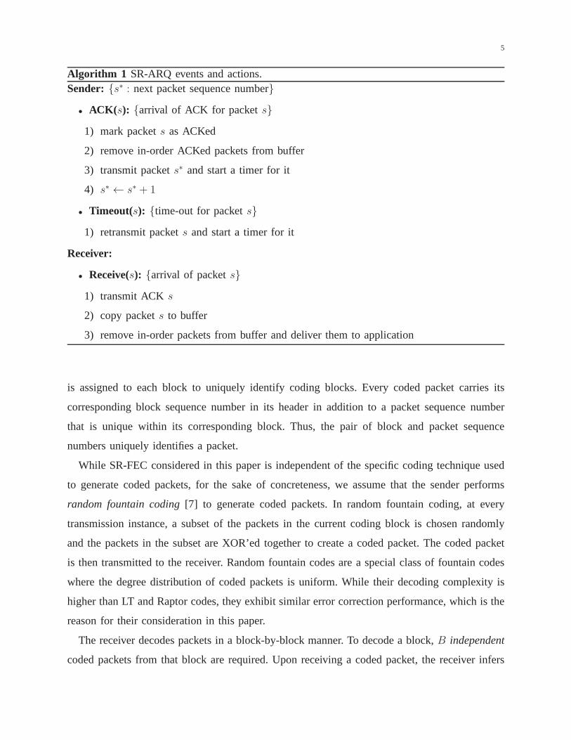
Algorithm 1 summarizes the main events and their corresponding actions at the sender and
receiver under SR-ARQ.
B. FEC Based Selective Repeat Protocol
The FEC-based protocol, referred to asSR-FEC, is a selective repeat protocol that implements
a rateless[7] coding algorithm for packet transmission. At the sender, packets are divided into
consecutivecoding blocksfor transmission to the receiver. Each coding block contains B >
1 packets, which are coded together to form coded packets. A consecutive sequence number
5
Algorithm 1 SR-ARQ events and actions.Sender: s∗ : next packet sequence number
• ACK( s): arrival of ACK for packets
1) mark packets as ACKed
2) remove in-order ACKed packets from buffer
3) transmit packets∗ and start a timer for it
4) s∗ ← s∗ + 1
• Timeout(s): time-out for packets
1) retransmit packets and start a timer for it
Receiver:
• Receive(s): arrival of packets
1) transmit ACKs
2) copy packets to buffer
3) remove in-order packets from buffer and deliver them to application
is assigned to each block to uniquely identify coding blocks. Every coded packet carries its
corresponding block sequence number in its header in addition to a packet sequence number
that is unique within its corresponding block. Thus, the pair of block and packet sequence
numbers uniquely identifies a packet.
While SR-FEC considered in this paper is independent of the specific coding technique used
to generate coded packets, for the sake of concreteness, we assume that the sender performs
random fountain coding[7] to generate coded packets. In random fountain coding, atevery
transmission instance, a subset of the packets in the current coding block is chosen randomly
and the packets in the subset are XOR’ed together to create a coded packet. The coded packet
is then transmitted to the receiver. Random fountain codes are a special class of fountain codes
where the degree distribution of coded packets is uniform. While their decoding complexity is
higher than LT and Raptor codes, they exhibit similar error correction performance, which is the
reason for their consideration in this paper.
The receiver decodes packets in a block-by-block manner. Todecode a block,B independent
coded packets from that block are required. Upon receiving acoded packet, the receiver infers
6
which original packets were XOR’ed to create the newly received coded packet. When the
block+packet sequence numbers are unique, the coding and decoding algorithms at the sender
and receiver can be synchronized, hence avoiding the need toinclude any extra information in
packet headers to help infer the identity of the XOR’ed packets. This can be implemented, for
example, by synchronizing a random number generator at the receiver with the random number
generator used at the sender for choosing the set of XOR’ed packets.
Similar to SR-ARQ, the sender continuously transmits codedpackets in increasing order of
coding block sequence number as long as ACKs are received. For everyinnovativecoded packet
(i.e., a packet that is independent of the previously received coded packets for the corresponding
block) arriving at the receiver, the receiver sends an ACK tothe sender over the feedback
channel. The ACK only contains the sequence number of the coding block for which the ACK
is being transmitted. After transmitting a packet, the sender transmits up toW − 1 subsequent
coded packets. The arrival of an ACK arrives at the sender during this period triggers a new
coded packet. The new packet is constructed from the coding block that contains the packet. If
a time-out occurs,i.e., no ACK arrives, then a coded packet from the coding block that caused
the time-out is subsequently transmitted. WhenB ACKs are received for a coding block then it
is released from the sender window.
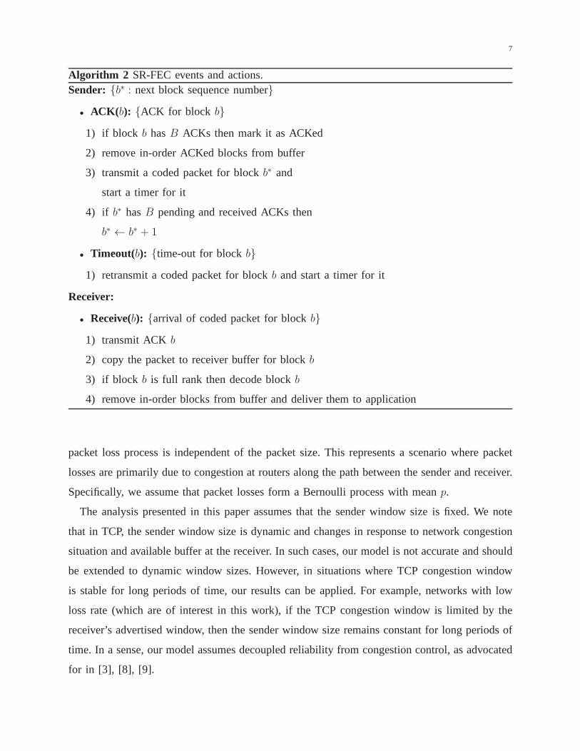
Algorithm 2 summarizes the main events and their corresponding actions at the sender and
receiver under SR-FEC.
III. EXACT PERFORMANCE ANALYSIS
An important metric in characterizing the performance of ARQ protocols is theexpected
number of retransmissionsrequired at the sender until a packet arrives successfully at the receiver.
Our focus in this section is on deriving exact expressions for this metric. Using this metric, we
show how it can be used to compute the receiver’s buffer occupancy and packet delay for
SR-ARQ and SR-FEC.
A. Assumptions
We consider a heavy traffic situation, in which packets arrive at the sender from an infinite
source. For any arrival process, this model provides upper bounds on the receiver buffer re-
quirements and packet delay. It is assumed that all packets are of the same size, and that the
7
Algorithm 2 SR-FEC events and actions.Sender: b∗ : next block sequence number
• ACK( b): ACK for block b
1) if block b hasB ACKs then mark it as ACKed
2) remove in-order ACKed blocks from buffer
3) transmit a coded packet for blockb∗ and
start a timer for it
4) if b∗ hasB pending and received ACKs then
b∗ ← b∗ + 1
• Timeout(b): time-out for blockb
1) retransmit a coded packet for blockb and start a timer for it
Receiver:
• Receive(b): arrival of coded packet for blockb
1) transmit ACKb
2) copy the packet to receiver buffer for blockb
3) if block b is full rank then decode blockb
4) remove in-order blocks from buffer and deliver them to application
packet loss process is independent of the packet size. This represents a scenario where packet
losses are primarily due to congestion at routers along the path between the sender and receiver.
Specifically, we assume that packet losses form a Bernoulli process with meanp.
The analysis presented in this paper assumes that the senderwindow size is fixed. We note
that in TCP, the sender window size is dynamic and changes in response to network congestion
situation and available buffer at the receiver. In such cases, our model is not accurate and should
be extended to dynamic window sizes. However, in situationswhere TCP congestion window
is stable for long periods of time, our results can be applied. For example, networks with low
loss rate (which are of interest in this work), if the TCP congestion window is limited by the
receiver’s advertised window, then the sender window size remains constant for long periods of
time. In a sense, our model assumes decoupled reliability from congestion control, as advocated
for in [3], [8], [9].
8
To simplify the analysis, as commonly assumed in the literature [10]–[13], we assume that a
reliable feedback channel exists between the sender and receiver. The receiver sends feedback in
the form of acknowledgement packets (ACKs) to the sender, which are assumed to be delivered
over the feedback channel reliably. We also assume that the round-trip-time between the sender
and receiver is fixed and equal toR.
B. Performance Metrics
In high-speed networks, to efficiently utilize network bandwidth, the window sizeW should
grow proportional to the per-connection capacity. This is simply stated asW = R · C, where
C is the per-connection capacity. Thus, as per-connection capacity increases, the window size
should increase as well resulting in increased buffer occupancy at the sender and receiver. We
assume that the sender and receiver have sufficient buffer space to allow each protocol, namely
SR-ARQ and SR-FEC, to operate efficiently.
With SR-ARQ, every packet received at the receiver is a useful packet, and hence the through-
put of SR-ARQ is given byρ = (1 − p)C. However, with SR-FEC, only independent coded
packets are useful for the receiver to decode and recover theoriginal packets. To avoid transmit-
ting coded packets that are not independent from the previously transmitted packets, and hence
wasting bandwidth, for every active coding block, the sender memorizes the coded packets
transmitted so far for that coding block, for example, by keeping track of the indices of the
packet subsets used to construct the coded packets. For a given coding block, the sender only
sends packets that are independent of the coded packets transmitted previously. In this case, the
throughput of SR-FEC is also given byρ = (1 − p)C. The analysis presented in Sections III
and IV considers this case. Later, in Section V, we address the case when coded packets may
be dependent.
Let Q andD denote the re-sequencing buffer occupancy and delay at the receiver, respectively.
Using the Little’s law, it follows that
E [D] =E [Q]
(1− p)C=
R
(1− p)WE [Q] . (1)
In the rest of the paper, we focus on computingE [Q] for both protocols.
9
C. SR-ARQ Analysis
Consider a window ofW packets. LetNi denote the number of times that the packet at
position i, for 1 ≤ i ≤ W , is transmitted until it is received successfully at the receiver. It
follows thatNi has a geometric distribution. In other words, the probability that the packet at
position i is received successfully inn-th transmission is given by
P Ni = n = (1− p)pn−1, n ≥ 1 . (2)
Among theW packets in the window, letℓ denote the last packet that is successfully received
at the receiver,i.e., the packet that takes the most number of retransmissions. Let NARQ denote
the number of transmissions required untilℓ is received at the receiver. It follows that
NARQ = max1≤i≤W
Ni . (3)
Since packet losses are assumed to be independent, the following relation holds for the probability
distribution of the random variableNARQ,
P NARQ ≤ n = (1− pn)W , n ≥ 1 . (4)
Using the above expression, it follows that,
E [NARQ] =∞∑
n=1
P N ≥ n =∞∑
n=1
1− (1− pn−1)W . (5)
Definef(K) for k ≥ 1 as,
f(K) =K∑
n=1
1− (1− pn−1)W , (6)
which, then yields,
E [NARQ] = limK→∞
f(K) . (7)
Next, we focus on computing a closed-form expression forf(K) that can be used to compute
E [NARQ]:
f(K) = K −
K∑
n=1
(1− pn−1)W
= K −
K∑
n=1
W∑
i=0
(
W
i
)
(−pn−1)i
= −
W∑
i=1
(
W
i
)
(−1)i1− (pi)K
1− pi.
(8)
10
Taking the limit off(K) asK →∞ yields the following result forE [NARQ]:
E [NARQ] = limK→∞
f(K)
= −W∑
i=1
(
W
i
)
(−1)i
1− pi.
(9)
The above expressions are valid when0 ≤ p < 1. If p = 1, then no packet is received at the
receiver and hence the receiver’s buffer will be empty. Overthe range0 ≤ p < 1, asp increases
so does the number of lost packets. As the number of lost packets increases, the number of
out-of-order packets in the receiver’s buffer increases aswell.
D. SR-FEC Analysis
With coding, packets are delivered to the application in a block-by-block manner. For every
coding block, the receiver needs to receiveB independent coded packets in order to decode and
recover the original coding block. LetNi denote the number of transmitted coded packets until
the receiver decodes coding blocki. The probability that the receiver receives exactlyB coded
packets after then-th packet transmission by the sender for coding blocki is given by a negative
binomial distribution,i.e.,
P Ni = n =(
n−1B−1
)
(1− p)Bpn−B, n ≥ B (10)
which is the probability thatB − 1 packets out of the firstn − 1 transmissions are received
successfully and the last transmission is a success too. Recall that, for the moment, we are as-
suming all coded packets are independent following the mechanism described earlier. Therefore,
we obtain that,
P Ni ≤ n =n
∑
i=B
(
i−1B−1
)
(1− p)Bpi−B,
= (1− p)Bn−B∑
i=0
(
B+i−1B−1
)
pi .
(11)
Consider a typical window ofW packets consisting ofM = W/B coding blocks. Without
loss of generality, we assume thatW is an integer multiple ofB. Among theM coding blocks,
let ℓ denote the last block that is decoded by the receiver,i.e., the block that takes the most
11
number of transmissions until its correspondingB coded packets are received. LetNFEC denote
the number of transmissions required until blockℓ is decoded by the receiver. It is obtained that
NFEC = max1≤i≤W
Ni . (12)
Since packet losses are assumed to be independent, the following relation holds for the probability
distribution of the random variableNFEC,
P NFEC ≤ n = (1− p)W(
n−B∑
i=0
(
B+i−1B−1
)
pi)M
. (13)
However, it seems unlikely that this would result in any simple expression forE [NFEC]. Note
thatNFEC is the number of transmissions per coding bock of sizeB. Thus, the expected number
of transmissions per packet is given by1BE [NFEC].
IV. A SYMPTOTIC PERFORMANCE ANALYSIS
The exact expressions derived in the previous section do notprovide insight about the scaling
behavior of the number of transmissions with respect toW . In this section, we derive asymptotic
expressions for the expected number of transmissions for both SR-ARQ and SR-FEC. Then, using
our asymptotic results, we compute the expected receiver’sbuffer occupancy. In particular, we
are interested in the asymptotic performance of the protocols as the window size becomes very
large, i.e., W →∞. For SR-FEC, we consider two scaling regimes: (1) the codingblock length
remains constant,i.e., B ∈ Θ(1), and (2) the coding block length scales at the same rate as the
window size,i.e., B ∈ Θ(W ).
The asymptotic analysis presented in this section utilizestechniques from the extreme value
theory [14], which is briefly described next.
A. Extreme Value Theory
Consider a sequence of IID random variablesX1, X2, . . . , Xn with a common cumulative
distribution functionF , i.e., F (x) = P Xi ≤ x. Let theXi’s be arranged in increasing order
of magnitude and denoted byX(1), X(2), . . . , X(n). These ordered values ofXi’s are calledorder
statistics, X(k) being thekth order statistics. Note thatX(1) and X(n) are the minimum and
maximum and are called theextremeorder statistics.
12
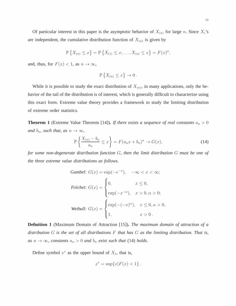
Of particular interest in this paper is the asymptotic behavior of X(n) for largen. SinceXi’s
are independent, the cumulative distribution function ofX(n) is given by
P
X(n) ≤ x
= P
X(1) ≤ x, . . . , X(n) ≤ x
= F (x)n,
and, thus, forF (x) < 1, asn→∞,
P
X(n) ≤ x
→ 0 .
While it is possible to study the exact distribution ofX(n), in many applications, only the be-
havior of the tail of the distribution is of interest, which is generally difficult to characterize using
this exact form. Extreme value theory provides a framework to study the limiting distribution
of extreme order statistics.
Theorem 1 (Extreme Value Theorem [14]). If there exists a sequence of real constantsan > 0
and bn, such that, asn→∞,
P
X(n) − bnan
≤ x
= F (anx+ bn)n → G(x), (14)
for some non-degenerate distribution functionG, then the limit distributionG must be one of
the three extreme value distributions as follows.
Gumbel:G(x) = exp(−e−x), −∞ < x <∞;
Frechet:G(x) =
0, x ≤ 0,
exp(−x−α), x > 0, α > 0;
Weibull: G(x) =
exp(−(−x)α), x ≤ 0, α > 0,
1, x > 0 .
Definition 1 (Maximum Domain of Attraction [15]). The maximum domain of attraction of a
distributionG is the set of all distributionsF that hasG as the limiting distribution. That is,
as n→∞, constantsan > 0 and bn exist such that(14) holds.
Define symbolx∗ as the upper bound ofX1, that is,
x∗ = supx|F (x) < 1 .
13
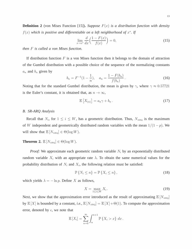
Definition 2 (von Mises Function [15]). SupposeF (x) is a distribution function with density
f(x) which is positive and differentiable on a left neighborhoodof x∗. If
limx→x∗
d
dx
(1− F (x)
f(x)
)
= 0, (15)
thenF is called a von Mises function.
If distribution functionF is a von Mises function then it belongs to the domain of attraction
of the Gumbel distribution with a possible choice of the sequence of the normalizing constants
an and bn given by
bn = F−1(1−1
n), an =
1− F (bn)
f(bn). (16)
Noting that for the standard Gumbel distribution, the mean is given byγ, whereγ ≈ 0.57721
is the Euler’s constant, it is obtained that, asn→∞,
E[
X(n)
]
= anγ + bn . (17)
B. SR-ARQ Analysis
Recall thatNi, for 1 ≤ i ≤ W , has a geometric distribution. Thus,NARQ is the maximum
of W independent and geometrically distributed random variables with the mean1/(1− p). We
will show thatE [NARQ] ∈ Θ(logW ).
Theorem 2. E [NARQ] ∈ Θ(logW ).
Proof: We approximate each geometric random variableNi by an exponentially distributed
random variableXi with an appropriate rateλ. To obtain the same numerical values for the
probability distribution ofNi andXi, the following relation must be satisfied:
P Ni ≤ n = P Xi ≤ n , (18)
which yieldsλ = − ln p. DefineX as follows,
X = max1≤i≤W
Xi . (19)
Next, we show that the approximation error introduced as theresult of approximatingE [NARQ]
by E [X ] is bounded by a constant,i.e., E [NARQ] = E [X ]+Θ(1). To compute the approximation
error, denoted byǫ, we note that
E [Xi] =
∞∑
n=0
∫ n+1
n
P Xi > x dx .
14
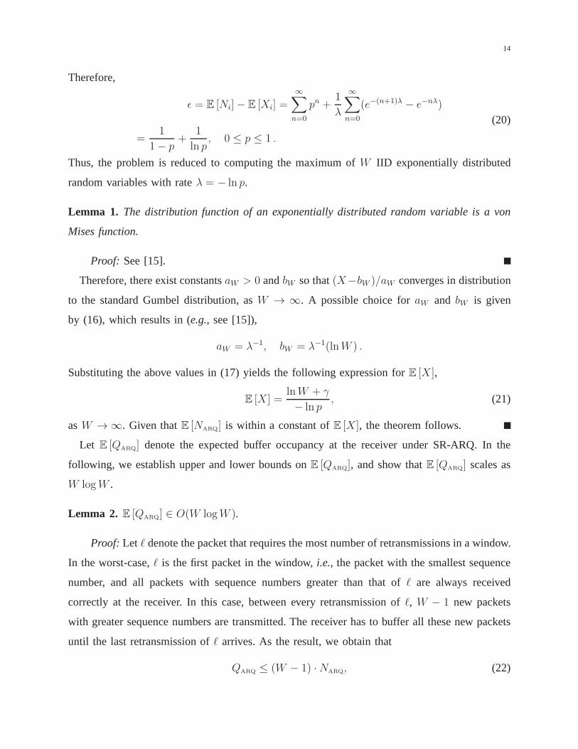
Therefore,
ǫ = E [Ni]− E [Xi] =
∞∑
n=0
pn +1
λ
∞∑
n=0
(e−(n+1)λ − e−nλ)
=1
1− p+
1
ln p, 0 ≤ p ≤ 1 .
(20)
Thus, the problem is reduced to computing the maximum ofW IID exponentially distributed
random variables with rateλ = − ln p.
Lemma 1. The distribution function of an exponentially distributedrandom variable is a von
Mises function.
Proof: See [15].
Therefore, there exist constantsaW > 0 andbW so that(X−bW )/aW converges in distribution
to the standard Gumbel distribution, asW → ∞. A possible choice foraW and bW is given
by (16), which results in (e.g., see [15]),
aW = λ−1, bW = λ−1(lnW ) .
Substituting the above values in (17) yields the following expression forE [X ],
E [X ] =lnW + γ
− ln p, (21)
asW →∞. Given thatE [NARQ] is within a constant ofE [X ], the theorem follows.
Let E [QARQ] denote the expected buffer occupancy at the receiver under SR-ARQ. In the
following, we establish upper and lower bounds onE [QARQ], and show thatE [QARQ] scales as
W logW .
Lemma 2. E [QARQ] ∈ O(W logW ).
Proof: Let ℓ denote the packet that requires the most number of retransmissions in a window.
In the worst-case,ℓ is the first packet in the window,i.e., the packet with the smallest sequence
number, and all packets with sequence numbers greater than that of ℓ are always received
correctly at the receiver. In this case, between every retransmission ofℓ, W − 1 new packets
with greater sequence numbers are transmitted. The receiver has to buffer all these new packets
until the last retransmission ofℓ arrives. As the result, we obtain that
QARQ ≤ (W − 1) ·NARQ, (22)
15
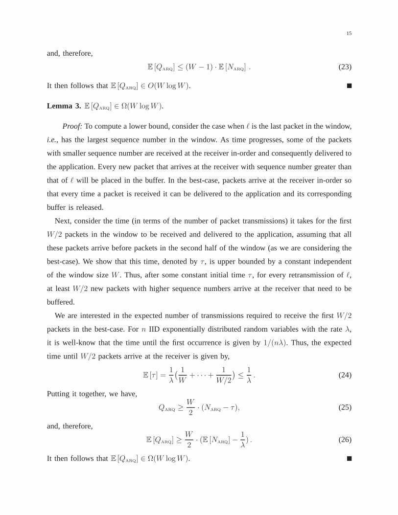
and, therefore,
E [QARQ] ≤ (W − 1) · E [NARQ] . (23)
It then follows thatE [QARQ] ∈ O(W logW ).
Lemma 3. E [QARQ] ∈ Ω(W logW ).
Proof: To compute a lower bound, consider the case whenℓ is the last packet in the window,
i.e., has the largest sequence number in the window. As time progresses, some of the packets
with smaller sequence number are received at the receiver in-order and consequently delivered to
the application. Every new packet that arrives at the receiver with sequence number greater than
that of ℓ will be placed in the buffer. In the best-case, packets arrive at the receiver in-order so
that every time a packet is received it can be delivered to theapplication and its corresponding
buffer is released.
Next, consider the time (in terms of the number of packet transmissions) it takes for the first
W/2 packets in the window to be received and delivered to the application, assuming that all
these packets arrive before packets in the second half of thewindow (as we are considering the
best-case). We show that this time, denoted byτ , is upper bounded by a constant independent
of the window sizeW . Thus, after some constant initial timeτ , for every retransmission ofℓ,
at leastW/2 new packets with higher sequence numbers arrive at the receiver that need to be
buffered.
We are interested in the expected number of transmissions required to receive the firstW/2
packets in the best-case. Forn IID exponentially distributed random variables with the rate λ,
it is well-know that the time until the first occurrence is given by 1/(nλ). Thus, the expected
time until W/2 packets arrive at the receiver is given by,
E [τ ] =1
λ
( 1
W+ · · ·+
1
W/2
)
≤1
λ. (24)
Putting it together, we have,
QARQ ≥W
2· (NARQ − τ), (25)
and, therefore,
E [QARQ] ≥W
2· (E [NARQ]−
1
λ) . (26)
It then follows thatE [QARQ] ∈ Ω(W logW ).
16
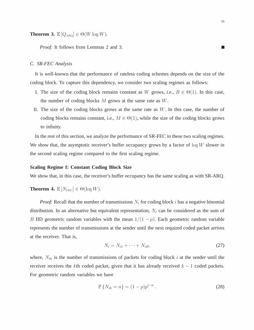
Theorem 3. E [QARQ] ∈ Θ(W logW ).
Proof: It follows from Lemmas 2 and 3.
C. SR-FEC Analysis
It is well-known that the performance of rateless coding schemes depends on the size of the
coding block. To capture this dependency, we consider two scaling regimes as follows:
I. The size of the coding block remains constant asW grows, i.e., B ∈ Θ(1). In this case,
the number of coding blocksM grows at the same rate asW .
II. The size of the coding blocks grows at the same rate asW . In this case, the number of
coding blocks remains constant,i.e., M ∈ Θ(1), while the size of the coding blocks grows
to infinity.
In the rest of this section, we analyze the performance of SR-FEC in these two scaling regimes.
We show that, the asymptotic receiver’s buffer occupancy grows by a factor oflogW slower in
the second scaling regime compared to the first scaling regime.
Scaling Regime I: Constant Coding Block Size
We show that, in this case, the receiver’s buffer occupancy has the same scaling as with SR-ARQ.
Theorem 4. E [NFEC] ∈ Θ(logW ).
Proof: Recall that the number of transmissionsNi for coding blocki has a negative binomial
distribution. In an alternative but equivalent representation, Ni can be considered as the sum of
B IID geometric random variables with the mean1/(1 − p). Each geometric random variable
represents the number of transmissions at the sender until the next required coded packet arrives
at the receiver. That is,
Ni = Ni1 + · · ·+NiB, (27)
where,Nik is the number of transmissions of packets for coding blocki at the sender until the
receiver receives thekth coded packet, given that it has already receivedk − 1 coded packets.
For geometric random variables we have
P Nik = n = (1− p)pi−n . (28)
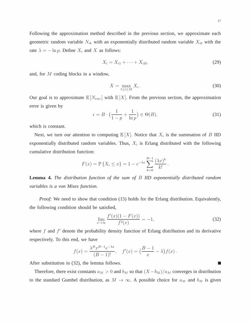
17
Following the approximation method described in the previous section, we approximate each
geometric random variableNik with an exponentially distributed random variableXik with the
rateλ = − ln p. DefineXi andX as follows:
Xi = Xi1 + · · ·+XiB, (29)
and, forM coding blocks in a window,
X = max1≤i≤M
Xi . (30)
Our goal is to approximateE [NFEC] with E [X ]. From the previous section, the approximation
error is given by
ǫ = B ·( 1
1− p+
1
ln p
)
∈ Θ(B), (31)
which is constant.
Next, we turn our attention to computingE [X ]. Notice thatXi is the summation ofB IID
exponentially distributed random variables. Thus,Xi is Erlang distributed with the following
cumulative distribution function:
F (x) = P Xi ≤ x = 1− e−λx
B−1∑
k=0
(λx)k
k!.
Lemma 4. The distribution function of the sum ofB IID exponentially distributed random
variables is a von Mises function.
Proof: We need to show that condition (15) holds for the Erlang distribution. Equivalently,
the following condition should be satisfied,
limx→∞
f ′(x)(1− F (x))
f 2(x)= −1, (32)
wheref andf ′ denote the probability density function of Erlang distribution and its derivative
respectively. To this end, we have
f(x) =λBxB−1e−λx
(B − 1)!, f ′(x) =
(B − 1
x− λ
)
f(x) .
After substitution in (32), the lemma follows.
Therefore, there exist constantsaM > 0 andbM so that(X−bM)/aM converges in distribution
to the standard Gumbel distribution, asM → ∞. A possible choice foraM and bM is given
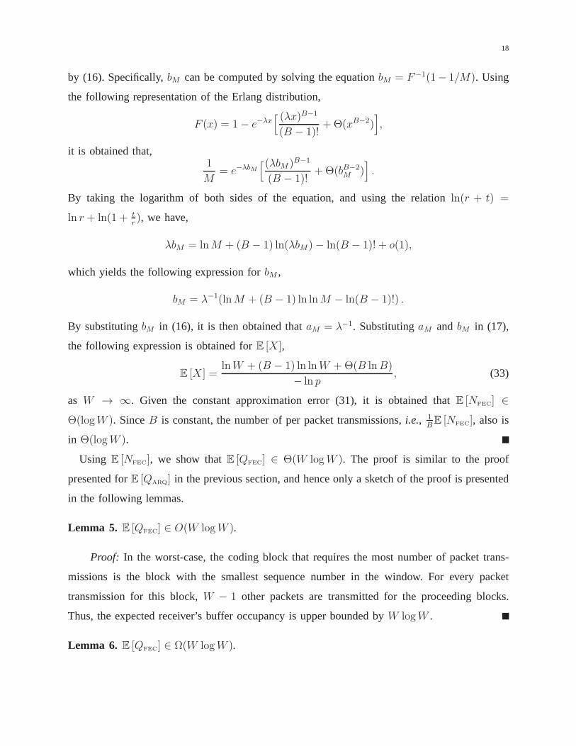
18
by (16). Specifically,bM can be computed by solving the equationbM = F−1(1− 1/M). Using
the following representation of the Erlang distribution,
F (x) = 1− e−λx[ (λx)B−1
(B − 1)!+ Θ(xB−2)
]
,
it is obtained that,1
M= e−λbM
[(λbM )B−1
(B − 1)!+ Θ(bB−2
M )]
.
By taking the logarithm of both sides of the equation, and using the relationln(r + t) =
ln r + ln(1 + tr), we have,
λbM = lnM + (B − 1) ln(λbM)− ln(B − 1)! + o(1),
which yields the following expression forbM ,
bM = λ−1(lnM + (B − 1) ln lnM − ln(B − 1)!) .
By substitutingbM in (16), it is then obtained thataM = λ−1. SubstitutingaM and bM in (17),
the following expression is obtained forE [X ],
E [X ] =lnW + (B − 1) ln lnW +Θ(B lnB)
− ln p, (33)
as W → ∞. Given the constant approximation error (31), it is obtained that E [NFEC] ∈
Θ(logW ). SinceB is constant, the number of per packet transmissions,i.e., 1BE [NFEC], also is
in Θ(logW ).
Using E [NFEC], we show thatE [QFEC] ∈ Θ(W logW ). The proof is similar to the proof
presented forE [QARQ] in the previous section, and hence only a sketch of the proof is presented
in the following lemmas.
Lemma 5. E [QFEC] ∈ O(W logW ).
Proof: In the worst-case, the coding block that requires the most number of packet trans-
missions is the block with the smallest sequence number in the window. For every packet
transmission for this block,W − 1 other packets are transmitted for the proceeding blocks.
Thus, the expected receiver’s buffer occupancy is upper bounded byW logW .
Lemma 6. E [QFEC] ∈ Ω(W logW ).
19
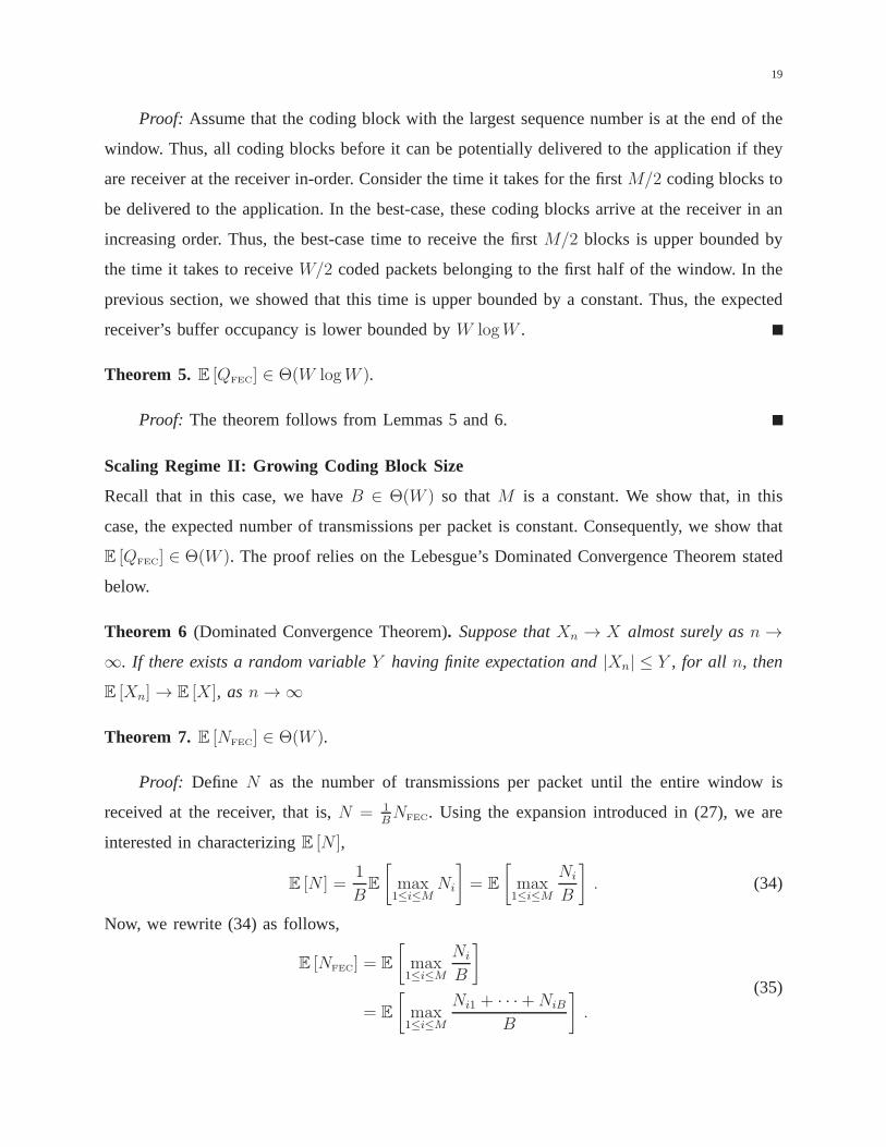
Proof: Assume that the coding block with the largest sequence number is at the end of the
window. Thus, all coding blocks before it can be potentiallydelivered to the application if they
are receiver at the receiver in-order. Consider the time it takes for the firstM/2 coding blocks to
be delivered to the application. In the best-case, these coding blocks arrive at the receiver in an
increasing order. Thus, the best-case time to receive the first M/2 blocks is upper bounded by
the time it takes to receiveW/2 coded packets belonging to the first half of the window. In the
previous section, we showed that this time is upper bounded by a constant. Thus, the expected
receiver’s buffer occupancy is lower bounded byW logW .
Theorem 5. E [QFEC] ∈ Θ(W logW ).
Proof: The theorem follows from Lemmas 5 and 6.
Scaling Regime II: Growing Coding Block Size
Recall that in this case, we haveB ∈ Θ(W ) so thatM is a constant. We show that, in this
case, the expected number of transmissions per packet is constant. Consequently, we show that
E [QFEC] ∈ Θ(W ). The proof relies on the Lebesgue’s Dominated Convergence Theorem stated
below.
Theorem 6 (Dominated Convergence Theorem). Suppose thatXn → X almost surely asn→
∞. If there exists a random variableY having finite expectation and|Xn| ≤ Y , for all n, then
E [Xn]→ E [X ], asn→∞
Theorem 7. E [NFEC] ∈ Θ(W ).
Proof: Define N as the number of transmissions per packet until the entire window is
received at the receiver, that is,N = 1BNFEC. Using the expansion introduced in (27), we are
interested in characterizingE [N ],
E [N ] =1
BE
[
max1≤i≤M
Ni
]
= E
[
max1≤i≤M
Ni
B
]
. (34)
Now, we rewrite (34) as follows,
E [NFEC] = E
[
max1≤i≤M
Ni
B
]
= E
[
max1≤i≤M
Ni1 + · · ·+NiB
B
]
.
(35)
20
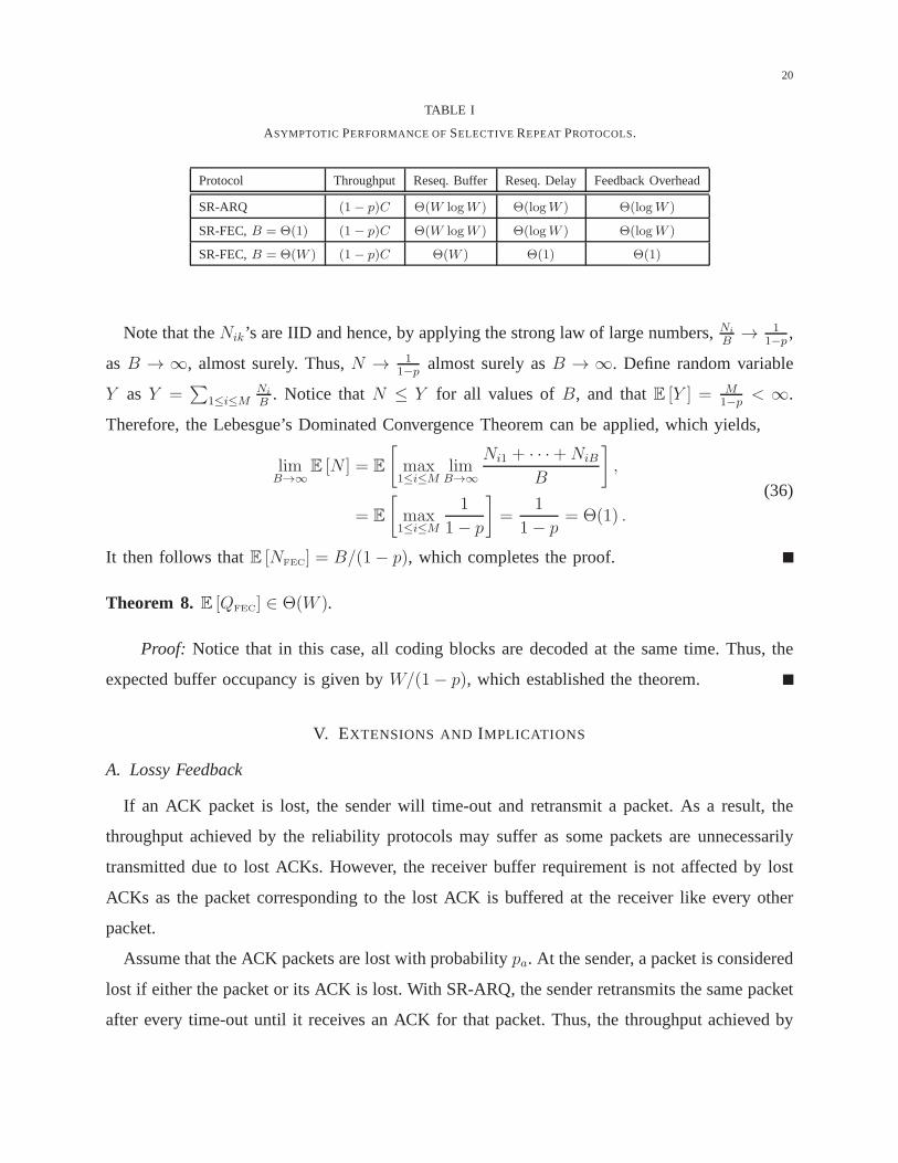
TABLE I
ASYMPTOTICPERFORMANCE OFSELECTIVE REPEAT PROTOCOLS.
Protocol Throughput Reseq. Buffer Reseq. Delay Feedback Overhead
SR-ARQ (1− p)C Θ(W logW ) Θ(logW ) Θ(logW )
SR-FEC,B = Θ(1) (1− p)C Θ(W logW ) Θ(logW ) Θ(logW )
SR-FEC,B = Θ(W ) (1− p)C Θ(W ) Θ(1) Θ(1)
Note that theNik’s are IID and hence, by applying the strong law of large numbers, Ni
B→ 1
1−p,
asB → ∞, almost surely. Thus,N → 11−p
almost surely asB → ∞. Define random variable
Y as Y =∑
1≤i≤MNi
B. Notice thatN ≤ Y for all values ofB, and thatE [Y ] = M
1−p< ∞.
Therefore, the Lebesgue’s Dominated Convergence Theorem can be applied, which yields,
limB→∞
E [N ] = E
[
max1≤i≤M
limB→∞
Ni1 + · · ·+NiB
B
]
,
= E
[
max1≤i≤M
1
1− p
]
=1
1− p= Θ(1) .
(36)
It then follows thatE [NFEC] = B/(1− p), which completes the proof.
Theorem 8. E [QFEC] ∈ Θ(W ).
Proof: Notice that in this case, all coding blocks are decoded at thesame time. Thus, the
expected buffer occupancy is given byW/(1− p), which established the theorem.
V. EXTENSIONS AND IMPLICATIONS
A. Lossy Feedback
If an ACK packet is lost, the sender will time-out and retransmit a packet. As a result, the
throughput achieved by the reliability protocols may suffer as some packets are unnecessarily
transmitted due to lost ACKs. However, the receiver buffer requirement is not affected by lost
ACKs as the packet corresponding to the lost ACK is buffered at the receiver like every other
packet.
Assume that the ACK packets are lost with probabilitypa. At the sender, a packet is considered
lost if either the packet or its ACK is lost. With SR-ARQ, the sender retransmits the same packet
after every time-out until it receives an ACK for that packet. Thus, the throughput achieved by
21
SR-ARQ isρ = (1 − p)(1 − pa)C. With SR-FEC, however, after every time-out a new coded
packet is transmitted that could potentially be useful for decoding the corresponding block at the
receiver. Only when the corresponding block is (or will be) full rank then time-outs are wasteful.
Thus, SR-FEC potentially achieves higher throughput compared to SR-ARQ.
By using more sophisticated feedback mechanisms, however,one could improve the throughput
of both protocols toρ = (1− p)C, without affecting the receiver buffer requirement. One such
mechanism is described next. Our current protocols incur feedback overhead ofΘ(logW ) per-
packet (see subsection V-C). As long as the packet length grows faster than the per-packet
feedback overhead, there will not be any loss in throughput asymptotically. To this end, we
show that the receiver can send(1 + ǫ) logW ACKs per each received packet, for anyǫ > 0,
and still maintain negligible feedback overhead if the packet size scales asω(log2W ).
Suppose that the receiver sendsn ACKs back-to-back for every received packet. The achieved
throughput isρ = (1− p)(1− pna)C. To achieve full throughput, the throughput losspnaC should
converge to0 asW grows to infinity. That is,Wpna → 0, asW →∞, or equivalently,pna = o( 1W),
which yields,
n = logpa o(1W) = Ω(logpa
1W 1+ǫ ), (37)
for any ǫ > 0.
Specifically, transmitting(1+ǫ) logW redundant ACKs ensures asymptotically full throughput
for pa < 2−1
1+ǫ . For instance, forpa < 0.5, which is the case of interest in this work (TCP does
not work for loss probabilities higher than10%), transmittinglogW redundant ACKs suffices
to achieve throughputρ = (1− p)C, asW →∞.
B. Dependent Coded Packets
In the preceding sections, we assumed that the sender keeps track of the coded packets
transmitted to the receiver in order to avoid transmitting dependent coded packets. Alternatively,
the sender might simply generate and transmit coded packetsregardless of their dependency.
This approach, while having the same buffer requirement, comes with a throughput penalty, as
there is a non-zero probability that the received packets atthe receiver are not independent.
In this subsection, using results from the theory of random matrices [16], we characterize the
throughput loss incurred due to dependent packets.
22
Let N∗i denote the number of transmitted coded packets until the receiver receivesB inde-
pendentcoded packets for coding blocki. Let N∗ik denote the number of transmissions until
the receiver receives thek-th independent coded packet given that it has already received k− 1
independent coded packets for the coding block. We have,
N∗i = N∗
i1 +N∗i2 + · · ·+N∗
iB . (38)
There areB packets in a coding block, and hence, there are2B subsets of packets that can be
XORed to create coded packets. While waiting to receive thek-th independent coded packet,
the receiver has already receivedk − 1 independent coded packets. Therefore,2k−1 packets out
of the 2B possible coded packets will not be independent of the already receivedk− 1 packets.
Let αk denote the probability that a received packet is independent of the existingk−1 packets.
The following relation holds,
αk =2B − 2k−1
2B= 1− 2k−B−1 . (39)
A packet (dependent or independent) is received with probability 1−p at the receiver. Therefore,
N∗ik is geometrically distributed with success probabilityqk = αk(1− p). It then follows that,
E [N∗i ] =
∑B
k=11qk
= 11−p
(
B +∑B
k=11
2k−1
)
, (40)
where the summation term quickly converges to a constant (≈ 1.606695) even for small values
of B. This means that, on average, the receiver needs only two extra packets in order to be able
to decode a block of packets. Specifically, letδ denote the number ofextra packets (dependent
or independent) that will be delivered to the receiver. Using our earlier argument, the probability
that a newly arrived packet is independent of the previouslyreceivedk− 1 independent packets
is given by,
βk =2B − 2k−1
2B+δ= 1− 2k−B−δ−1 . (41)
Thus, the probability of receivingB independent packets out of theB + δ received packets,
denoted byπ(δ), is given by,
π(δ) =∏B
k=1 βk =∏B
k=1(1− 2−k−δ), (42)
where, we haveπ(δ) ≥ 1−∑B
k=1 2−k−δ ≥ 1−2−δ. By takingδ = Θ(logB), we haveπ(δ)→ 1,
asB →∞. Next, we compute the throughput loss because of dependent packets. Let∆ρ denote
23
the throughput loss, we have:
∆ρ = M ·δ(1−p)C
= R1−p
M ·δW
. (43)
Therefore, the throughput loss is given by,
∆ρ =
R1−p
logBB
= Θ(1), if B = Θ(1),
R1−p
logWW
= o(1), if B = Θ(W ) .(44)
C. Protocol Overhead
Our results for the re-sequencing buffer occupancy can be used as guidelines for dimensioning
the sender and receiver buffer space. Specifically, for SR-ARQ and SR-FEC withB = Θ(1),
the proper amount of buffer space at the sender and receiver isΘ(W logW ). On the other hand,
whenB = Θ(W ) under SR-FEC, the buffer space at the sender and receiver should be scaled
asΘ(W ).
1) Data Channel Overhead:Both protocols require data packets in the sender and receiver
buffers to have unique sequence numbers. Thus, they both incur thesameoverhead in the forward
direction from the sender to the receiver. Moreover, the packet header overhead due to sequence
numbers is given byΘ(logW ).
2) Feedback Channel Overhead:Every packet has to be individually ACKed in SR-ARQ.
Thus, each ACK packet carries the sequence number of the packet it is acknowledging. In
SR-FEC, however, each ACK carries the sequence number of thecorresponding coding block
only. Thus, while both protocols send one ACK per every packet received at the receiver, the
header overhead can be different for each protocol. Specifically, for SR-ARQ and SR-FEC with
B = Θ(1), the per ACK overhead is inΘ(logW ). On the other hand, withB = Θ(W ), SR-FEC
incurs onlyΘ(1) header overhead per ACK.
D. Scaling Packet Length
To amortize the header overhead ofΘ(logW ), the packet length should also scale with
the window size asω(logW ). This has implications for both the packet loss probabilityand
throughput, as discussed below.
24
1) Effect on Packet Loss Probability:Let L denote the packet length andpe denote the bit
error rate (BER) at the physical layer. For the ease of exposition, we ignore the intermediate
protocol layers and assume that application packets are passed directly to the physical layer for
transmission. The packet loss probabilityp is then given by,
p = 1− (1− pe)L = 1− eL ln(1−pe) ≈ 1− e−Lpe . (45)
Thus, as the packet length increases, the packet error probability approaches1 exponentially
fast. To compensate for the increased packet length in orderto keep the packet error probability
constant, one can decrease the coding rate at the physical layer by adding more error control
data to each packet. The side effect of the decreased coding rate at the physical layer is a lower
per-flow capacity at the application layer. Nevertheless, the asymptotic performance of SR-ARQ
and SR-FEC in terms of buffer requirement remainsunchanged.
2) Effect on Throughput:Consider a block coding scheme at the physical layer. Define the
coding rater as r = k/n, wheren and k (n ≥ k) denote the length of coding blocks and
information messages respectively. Since packets are directly passed to the physical layer, each
message corresponds to a packet,i.e., k = L. For general classes of codes, it has been shown
that [?] the maximal coding rate achievable at block lengthn with error probabilityp is closely
approximated by,
r = Ln≈ C −
√
VnQ−1(p), (46)
whereC is the capacity of the underlying channel,V is a characteristics of the channel referred
to as channel dispersion, andQ is the complementary CDF of the standard normal distribution.
Notice that, asn → ∞, the maximal achievable rate approaches the channel capacity. Thus, a
physical layer that is designed optimally, not only does notpenalize throughput as the packet
length grows but also exhibits even a better performance.
Let assume that our objective is to keep the loss probabilityconstant atp regardless of the
packet length. Then, using the above approximation, it is obtained thatn = Θ(L), which means
that a constant throughput can be achieved for any packet length. Specifically, for any fixed
packet lengthL, let assume that our objective is to achieve the throughputρ = (1 − p)C. It
is obtained thatn = V ·(
Q−1(p)pC
)2, indicating that a fixed packet loss probability at a constant
throughput can be achieved by appropriately controlling the coding block length at the physical
layer.
25
E. Implications for Protocol Design
The scaling results for various performance metrics are summarized in Table I. The conclusion
is that SR-FEC withB = Θ(W ) asymptotically outperforms SR-ARQ in terms of buffer
requirement, delay and protocol overhead.
VI. RELATED WORK
The analysis of selective repeat protocols has received significant attention in the literature.
Our primary goal in this paper is to characterize theasymptoticperformance of selective repeat
with ARQ and FEC, which has not been considered in the literature. A summary of some related
works follows.
Selective Repeat ARQ:Some of the early work on the analysis of the selective repeatprotocol
with ARQ can be found in [10]–[13]. These classic works have been extended in several
recent papers to consider more general systems (e.g., Markovian error models and packet ar-
rival rates) [17]–[19], specifically in cellular networks in which selective repeat is typically
implemented between base stations and user devices. All these works have considered exact or
approximate analysis of selective repeat with ARQ.
Selective Repeat Hybrid ARQ: Hybrid ARQ schemes combine ARQ and FEC mechanisms
similar to SR-FEC considered in this paper. The difference is that in hybrid ARQ, the coding rate
is pre-determined based on the transmission environment. For instance, a block coding scheme
such as Reed-Solomon codes is used to generate a fixed number of coded packets in order to
cope with packet losses. In SR-FEC, however, coded packets are generated on-demand until the
receiver successfully decodes the original packets (i.e., rateless coding). Several examples of
analytical work on selective repeat with hybrid ARQ can be found in [20], [21] and references
therein. Note that none of these works has considered the asymptotic behavior of hybrid ARQ
schemes.
Packet Reordering Delay:The analysis of [22] considers reliable data transmission but assumes
that variable network delay is the cause of packet re-ordering while the network is perfectly
reliable in the sense that no packets are lost. Along the sameline, in [23], it is assumed that
the cause of variable delay is multi-path routing in the network. Their focus is on capturing the
effect of packet reordering on receiver buffer, which is quite different from the lossy scenario
considered in this paper.
26
Asymptotic Analysis: A large-deviation analysis of receiver buffer behavior under selective
repeat was presented in [24]. Additionally, using standardresults on coupon collector problem,
the authors provide an asymptotic analysis of the receiver buffer behavior for ARQ mechanism,
which is valid only when the loss rate isvery high, as opposed to our results that characterize
receiver buffer behavior under arbitrary loss rates for both ARQ and FEC mechanisms.
VII. CONCLUSION
In this paper, we studied reliable data transfer in high-speed networks, where a large number
of flows can be accommodated at high transmission speeds. We focused on two sliding window
mechanisms called SR-ARQ and SR-FEC based on ARQ and FEC, andcharacterized their
performance in the asymptotic regime of large window sizes.Specifically, we showed that, while
asymptotically achieving equal throughput, SR-FEC with a large coding block size achieves
logW improvement in buffer requirement and delay compared to SR-ARQ. However, SR-FEC
with a small coding block size is no advantageous compared toSR-ARQ. It would be interesting
to study the performance of these protocols when the available buffer space is limited.
REFERENCES
[1] Y.-T. Li, D. Leith, and R. N. Shorten, “Experimental evaluation of TCP protocols for high-speed networks,”IEEE/ACM
Trans. Netw., vol. 15, no. 5, Oct. 2007.
[2] G. Appenzeller, I. Keslassy, and N. McKeown, “Sizing router buffers,” inProc. ACM SIGCOMM, Portland, USA, Aug.
2004.
[3] Y. Gu, D. Towsley, C. Hollot, and H. Zhang, “Congestion control for small buffer high bandwidth networks,” inProc.
IEEE Infocom, Anchorage, USA, May 2007.
[4] J. Kurose and K. Ross,Computer Networking: A Top-Down Approach. New Jersey, USA: Addision-Wesley, 2012.
[5] O. Tickoo et al., “LT-TCP: End-to-end framework to improve TCP performanceover networks with lossy channels,” in
Proc. IEEE IWQoS, Passau, Germany, Jun. 2005.
[6] J. K. Sundararajanet al., “Network coding meets TCP,” inProc. IEEE Infocom, Rio de Janeiro, Brazil, Apr. 2009.
[7] D. MacKay, Information Theory, Inference, and Learning Algorithms. Cambridge, UK: Cambridge University Press,
2003.
[8] K. Sundaresan, V. Anantharaman, H.-Y. Hsieh, and R. Sivakumar, “ATP: A reliable transport protocol for ad-hoc networks,”
in Proc. ACM Mobihoc, Annapolis, USA, Jun. 2003.
[9] E. Kohler, M. Handley, and S. Floyd, “Designing DCCP: Congestion control without reliability,”ACM SIGCOMM Comput.
Communin. Rev., vol. 36, no. 4, pp. 27–38, Oct. 2006.
[10] D. Towsley and J. K. Wolf, “On the statistical analysis of queue lengths and waiting times for statistical multiplexers with
ARQ retransmission schemes,”IEEE Trans. Commun., vol. 27, no. 4, pp. 693–702, Apr. 1979.
27
[11] A. Konheim, “A queueing analysis of two ARQ protocols,”IEEE Trans. Commun., vol. 28, no. 7, 1980.
[12] M. E. Anagnostou and E. N. Protonotarios, “Performanceanalysis of the selective repeat ARQ protocol,”IEEE Trans.
Commun., vol. 34, no. 2, pp. 127–135, Feb. 1986.
[13] Z. Rosberg and N. Shacham, “Resequencing delay and buffer occupancy under the selective-repeat ARQ,”IEEE Trans.
Inf. Theory, vol. 35, no. 1, pp. 166–173, Jan. 1989.
[14] J. Galambos,The Asymptotic Theory of Extreme Order Statistics. New Jersey, USA: Wiley, 1978.
[15] L. de Haan and A. Ferreira,Extreme Value Theory: An Introduction. New Yprk, USA: Springer, 2006.
[16] C. Studholme and I. F. Blake, “Random matrices and codesfor the erasure channel,”Algorithmica, vol. 56, no. 4, 2010.
[17] D.-L. Lu and J.-F. Chang, “Performance of ARQ protocolsin nonindependent channel errors,”IEEE Trans. Commun.,
vol. 41, no. 5, pp. 721–730, May 1993.
[18] R. Fantacci, “Queueing analysis of the selective repeat automatic repeat request protocol wireless packet networks,” IEEE
Trans. Veh. Technol., vol. 45, no. 2, 1996.
[19] J. G. Kim and M. Krunz, “Delay analysis of selective repeat ARQ for a Markovian source over a wireless channel,”IEEE
Trans. Veh. Technol., vol. 49, no. 5, 2000.
[20] S. Kallel, “Analysis of a type II hybrid ARQ scheme with code combining,”IEEE Trans. Commun., vol. 38, no. 8, 1990.
[21] L. Badia, M. Levorato, and M. Zorzi, “Markov analysis ofselective repeat type II hybrid ARQ using block codes,”IEEE
Trans. Commun., vol. 56, no. 9, 2008.
[22] R. Fantacci, “Analysis on packet resequencing for reliable network protocols,”Performance Evaluation, vol. 61, no. 4,
2005.
[23] K. Zheng, X. Jiao, M. Liu, and Z. Li, “An analysis of resequencing delay of reliable transmission protocols over multipath,”
in Proc. IEEE ICC, Cape Town, South Africa, May 2010.
[24] K. D. Turck and S. Wittevrongel, “Receiver buffer behavior for the selective repeat protocol over a wireless channel: an
exact and large-deviations analysis,”Industrial and Management Optimization, vol. 6, no. 3, 2010.