On the pathways and timescales of intercontinental air pollution transport

On the pathways and timescales of intercontinental air pollution

transport

Andreas Stohl, Sabine Eckhardt, Caroline Forster, Paul James, and Nicole SpichtingerLehrstuhl fur Bioklimatologie und Immissionsforschung, Technical University of Munich, Freising, Germany

Received 15 October 2001; revised 5 April 2002; accepted 8 April 2002; published 4 December 2002.

[1] This paper presents results of a 1-year simulation of the transport of six passivetracers, released over the continents according to an emission inventory for carbonmonoxide (CO). Lagrangian concepts are introduced to derive age spectra of the tracerconcentrations on a global grid in order to determine the timescales and pathways ofpollution export from the continents. Calculating these age spectra is equivalent tosimulating many (quasi continuous) plumes, each starting at a different time, which aresubsequently merged. Movies of the tracer dispersion have been made available on anInternet website. It is found that emissions from Asia experience the fastest verticaltransport, whereas European emissions have the strongest tendency to remain in the lowertroposphere. European emissions are transported primarily into the Arctic and appear to bethe major contributor to the Arctic haze problem. Tracers from an upwind continentfirst arrive over a receptor continent in the upper troposphere, typically after some 4 days.Only later foreign tracers also arrive in the lower troposphere. Assuming a 2-day lifetime,the domestic tracers dominate total tracer columns over all continents except overAustralia where foreign tracers account for 20% of the tracer mass. In contrast, for a 20-day lifetime even continents with high domestic emissions receive more than half of theirtracer burden from foreign continents. Three special regions were identified where tracersare transported to, and tracer dilution is slow. Future field studies therefore should bedeployed in the following regions: (1) In the winter, the Asia tracer accumulates overIndonesia and the Indian Ocean, a region speculated to be a stratospheric fountain. (2) Inthe summer, the highest concentrations of the Asia tracer are found in the Middle East. (3)In the summer, the highest concentrations of the North America tracer are found in theMediterranean. INDEX TERMS: 0322 Atmospheric Composition and Structure: Constituent sources and

sinks; 0368 Atmospheric Composition and Structure: Troposphere—constituent transport and chemistry; 3309

Meteorology and Atmospheric Dynamics: Climatology (1620); 3364 Meteorology and Atmospheric

Dynamics: Synoptic-scale meteorology

Citation: Stohl, A., S. Eckhardt, C. Forster, P. James, and N. Spichtinger, On the pathways and timescales of intercontinental air

pollution transport, J. Geophys. Res., 107(D23), 4684, doi:10.1029/2001JD001396, 2002.

1. Introduction

[2] Atmospheric transport of trace substances involvesmany space- and timescales. Intercontinental transport(ICT) occurs on timescales on the order of 3–30 days and isthus most relevant for substances having a lifetime within thisrange. This involves such different species as ozone (O3) andits precursors, aerosols, mercury, and persistent organic pol-lutants. ICTalso influences shorter- (e.g., radicals) and longer-lived species (e.g., most of the greenhouse gases) throughchemical reactions with the intermediate-lived compounds.[3] With measurement techniques, particularly remote

sensing, becoming suitable for the purpose of studyingICT during the past few years, evidence of its occurrencehas accumulated. Furthermore, atmospheric transport mod-els are now capable of establishing source-receptor relation-

ships over such long distances. However, many studies stillfail to link observations unambiguously to ICT, and indi-vidual reports have not yet been distilled into a coherentpicture. This study aims at characterizing the timescales andthe pathways of ICT, both to put past observations intoperspective, and to provide guidance on where and whenfuture field campaigns should be deployed to study ICTmost effectively. The paper is organized such that wepresent a review of ICT observations in section 2, describeour methods in section 3, discuss general transport charac-teristics in section 4, quantify ICT in section 5, and finallydraw conclusions in section 6.

2. Review

2.1. Africa

[4] Sometimes Saharan dust can be transported both tonortheastern South America (during winter) and into theCaribbean (during summer) with the trade winds [Swap et

JOURNAL OF GEOPHYSICAL RESEARCH, VOL. 107, NO. D23, 4684, doi:10.1029/2001JD001396, 2002

Copyright 2002 by the American Geophysical Union.0148-0227/02/2001JD001396

ACH 6 - 1

Figure 1. Anthropogenic CO emissions in kilotons CO per year according to the EDGAR inventory.The rectangles mark the continental boxes used for evaluating ICT in section 4.

Figure 2. Total columns (a, c) and zonally averaged mixing ratios (b, d), both divided by the respectivetime interval, of the Asia tracer for ages of 6–8 days (a, b) and 25–30 days (c, d) during DJF.

ACH 6 - 2 STOHL ET AL.: INTERCONTINENTAL AIR POLLUTION TRANSPORT

al., 1996; Prospero, 1999]. Dust transports into the Medi-terranean are also very common, and sometimes the dust caneven reach northwestern Europe [Reiff et al., 1986]. O3

formed in African biomass burning plumes can be exportedboth to the tropical Atlantic [Fishman et al., 1991] and to thePacific, depending on the fire location and season. Nitrogenoxides and sulfur dioxide emitted by power plants in SouthAfrica can travel all the way to Australia if they get entrainedinto the midlatitude stormtrack after a period of localaccumulation in the subtropical high [Wenig et al., 2002].South African emissions can also be transported offshoreand then back to the continent in the flow around thesubtropical high [Garstang et al., 1996; Tyson and D’Abre-ton, 1998]. Such recirculations also occur at other places,particularly in the subtropics, and can easily be confusedwith ICT because trace gas signatures in the recirculating airmass may be indistinguishable from those of ICT.

2.2. Asia

[5] Export pathways from Asia fluctuate strongly withseason, as the location and strength of the Japan jet varieswith the position of the subtropical Pacific high. Dust fromAsia is observed quite frequently at the Mauna Loa observ-atory on Hawaii. During April 1998 an exceptional trans-Pacific transport event of dust from the Gobi desert caused

increases in particulate matter concentrations in NorthAmerica, even at the surface [Wilkening et al., 2000; Husaret al., 2001]. Observations of elevated concentrations ofmany different species over North America were traced toan Asian source, including organochlorine pesticides [Bai-ley et al., 2000], sulfate [Andreae et al., 1988], CO andperoxyacetyl nitrate in northwestern North America [Jaffe etal., 1999], and photochemical air pollution over California[Parrish et al., 1992]. Model studies suggest that Asianemissions could be important for pollutant concentrationsover North America in the future if they continue to grow[Berntsen et al., 1999; Jacob et al., 1999]. Transport at highaltitudes is an important element of ICT. In a model studyYienger et al. [2000] found that Asian emissions had themaximum impact on CO over North America in the uppertroposphere. Wild and Akimoto [2001], in another modelstudy, found that Asian emissions are more efficient inproducing O3 than European and North American sources,and thus have the greatest influence on O3 over othercontinents. Again the largest influence was found in theupper troposphere.

2.3. Australia

[6] There is little evidence of pollution export fromAustralia, but Sturman et al. [1997] reviewed papers on

Figure 3. Same as Figure 2, but for JJA.

STOHL ET AL.: INTERCONTINENTAL AIR POLLUTION TRANSPORT ACH 6 - 3

insect and dust transport from Australia to New Zealand.They found that transport of air from Southern Australia toNew Zealand occurs both in summer and in winter.

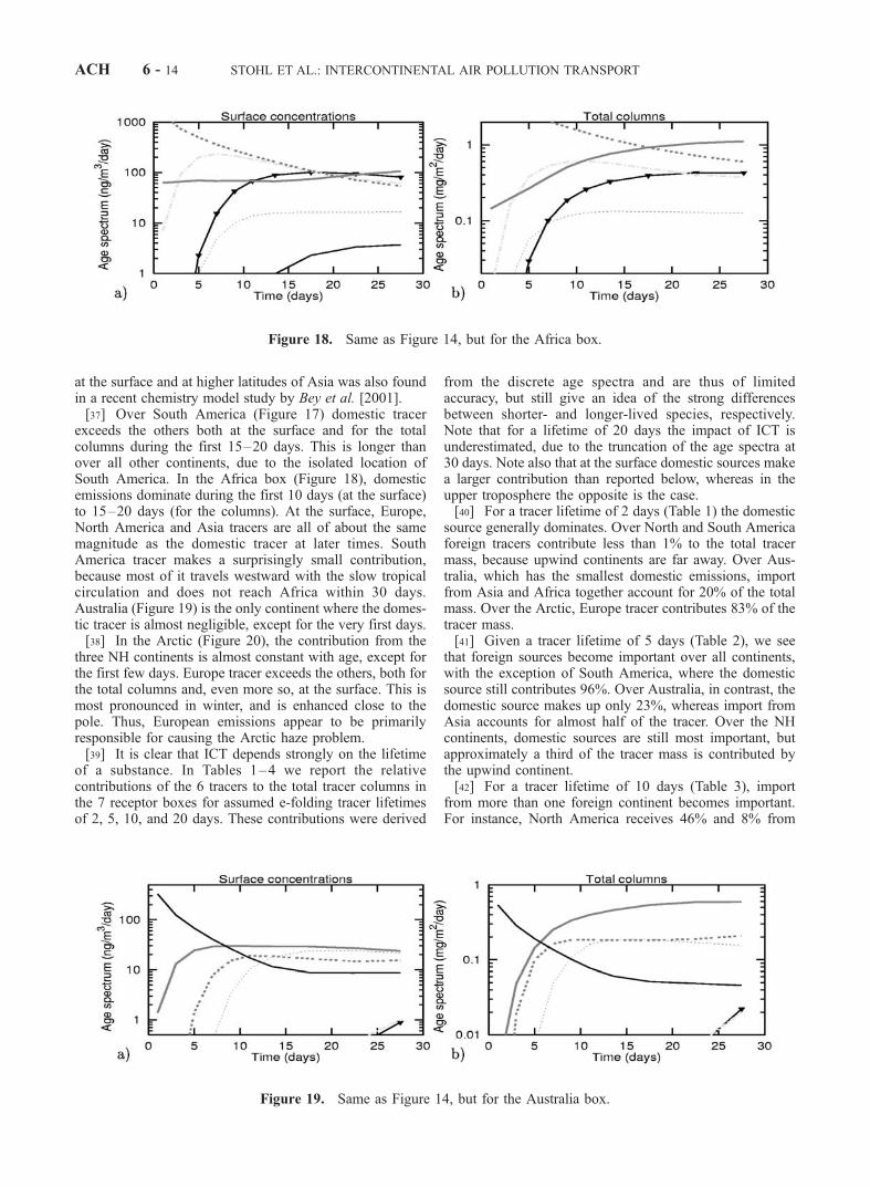
2.4. Europe

[7] Newell and Evans [2000] estimated that some 25% ofthe air parcels arriving over Central Asia have crossed overEurope before and some 4% have originated in the Euro-pean boundary layer. But because of a lack of measurementdata, there is little experimental evidence of European

pollution export to Asia. Measurements of lead isotopes atBarbados during the 1970s and 1980s suggest that a majorfraction of the lead originated from Europe, was transportedsouthwards to Africa and then westward with the tradewinds [Hamelin et al., 1989]. A model study suggests thatunder special meteorological conditions, O3 produced fromEuropean emissions can also be transported westward toNorth America within the midlatitudes [Li et al., 2001a].However, due to Europe’s location at high latitudes itspollution can be transported toward the Arctic, contributingto what has become known as the Arctic haze [Barrie,1986]. Due to high static stability, low temperatures andlack of solar radiation in winter, residence times of manycompounds are longer there than anywhere else, leading toaccumulation of pollutants north of the arctic front. It hasbeen suggested that the major pathways delivering thispollution to the Arctic are from Eurasia [Barrie, 1986;Jaeschke et al., 1999]. This is also important for the highconcentrations of mercury [Lu et al., 2001] and persistentorganic pollutants in arctic snow.

2.5. North America

[8] Parrish et al. [1998] reported a clear influence ofNorth American sources on O3 and CO at 1 km above sealevel at the Azores in the central North Atlantic. Hints onpollution transport from North America were found at Izanaon Tenerife [Schmitt, 1994] and at Mace Head, Ireland[Jennings et al., 1996], but these episodes are infrequentand corresponding O3 enhancements are marginal [Derwentet al., 1998]. Transport of emissions from boreal forest firesin Canada caused a dense haze layer over Germany inAugust 1998 [Forster et al., 2001]. O3 concentrations wereenhanced, too, and CO variations at Mace Head weredominated by this source over a one-month period. NOx

was also emitted and transported across the Atlantic [Spich-tinger et al., 2001]. Model studies by Wild et al. [1996] andSchultz et al. [1998] showed that the key factor favoring O3

transport from North America to Europe is lifting of thepolluted air to higher altitudes, as transport is faster thereand chemical lifetimes of O3 and its precursors are longer.Stohl and Trickl [1999] presented a case study of high O3

concentrations produced over North America that weretransported within a warm conveyor belt (WCB), a warmmoist airstream ahead of a cold front, to the upper tropo-sphere over Europe. Stohl [2001] showed that WCBs oftendraw their inflow from the Asian and North Americanseaboards and can thus subject boundary layer air pollutionfrom these continents to transport with the jet stream.Observations of trans-Atlantic transport have been reviewedby Stohl and Trickl [2001].

2.6. South America

[9] There is little evidence for export of South Americanpollution to other continents. Thompson et al. [1996]suggested that a significant fraction of the O3 observedover Africa was produced in biomass burning plumes fromSouth America.

3. Methods

[10] This study presents a 1-year simulation of the trans-port of anthropogenic emission tracers in order to identify

Figure 4. Annually averaged transport characteristics ofthe Asia tracer: a) vertical distribution of the horizontallyaveraged tracer mixing ratio, b) meridional distribution ofthe zonally and vertically averaged tracer concentration, andc) zonal distribution of the meridionally and verticallyaveraged tracer concentrations. Results for six age classesare drawn. The legend is placed in the top panel only.


the pathways of pollution originating from the differentcontinents over timescales up to 30 days after emission.Tracer transport was simulated with the Lagrangian particledispersion model FLEXPART (version 4.0) [Stohl et al.,1998; Stohl and Thomson, 1999] for the period January2000 to February 2001. Only passive tracers are considered,which do not undergo chemical reactions or depositionprocesses. Documentation and the source code of FLEX-PART can be obtained via the Internet from the addresshttp://www.forst.tu-muenchen.de/EXT/LST/METEO/stohl/.FLEXPART was validated with data from three large-scaletracer experiments in North America and Europe [Stohl etal., 1998]. FLEXPART was also used previously in severalcase studies of ICT [Stohl and Trickl, 1999; Forster et al.,2001; Spichtinger et al., 2001; Wenig et al., 2002] andcaptured these events, and also intrusions of stratosphericair filaments into the lower troposphere [Stohl et al., 2000],with high accuracy. Therefore, model validation is not asubject of this paper. We want to point out, though, that dueto its Lagrangian nature, FLEXPART can preserve veryfine-scale structures, as they are typically generated duringICT events. This puts it at an advantage over Euleriantransport models which suffer from numerical diffusion thattends to disperse these filaments.

[11] FLEXPART is driven with model-level data from theEuropean Centre for Medium-Range Weather Forecasts[ECMWF, 1995] with a horizontal resolution of 1�, 60vertical levels and a time resolution of 3 h (analyses at 0,6, 12, 18 UTC; 3-h forecasts at 3, 9, 15, 21 UTC).FLEXPART treats advection and turbulent diffusion bycalculating the trajectories of a multitude of particles.Stochastic fluctuations, obtained by solving Langevin equa-tions [Stohl and Thomson, 1999], are superimposed on thegrid-scale winds to represent transport by turbulent eddies.[12] ECMWF data reproduce the large-scale effects of

convection (e.g., strong ascent at the intertropical conver-gence zone (ITCZ) or within WCBs), but smaller-scaleconvective cells are not resolved. FLEXPART thereforewas recently equipped with the convection scheme ofEmanuel and Zivkovic-Rothman [1999]. This scheme isbased on the grid-scale temperature and humidity data andprovides a uniform treatment of all types (i.e., shallow todeep) of moist convection. A displacement matrix is calcu-lated for every model column from which displacementprobabilities for individual particles are derived. Thescheme was tuned such that it best reproduces the con-vective precipitation fields that are generated on-line by theECMWF model, in order to be as consistent as possible with

Figure 5. Same as Figure 2, but for the European tracer.


the driving meteorological model. A description of theimplementation and some validation was presented bySeibert et al. [2001]. The overall effect of convection onthe FLEXPART results is moderate, except for the tropicswhere it is important. Transport in the tropics is generallythought to be much less accurate than in the middlelatitudes, both because of the strong convective activityand because fewer observations are available for the dataassimilation at ECMWF than in the extratropics. We havemade FLEXPART simulations with convection both turnedon and turned off. Although there were some differencesnotable between these two model runs in the tropics (with-out convection the lifting into the upper troposphere wasless pronounced), generally differences between these twosimulations were very small (virtually everywhere concen-

tration differences were less than 20%). This confirms ourexperience that much of the convection (especially slant-wise convection in extratropical frontal systems, and con-vection in mesoscale convective complexes) is actuallyresolved in recent ECMWF analyses.[13] Tracer mixing ratios and concentrations are deter-

mined on a three-dimensional grid (2� latitude � 3�longitude resolution and 15 layers up to 15 km) applyinga kernel method. The transport of six continental pollutiontracers was simulated, representing anthropogenic emis-sions taken from the EDGAR inventory [Olivier et al.,1996] for CO for the base year 1990 (Figure 1). Africa,Asia, Australia, Europe, North America, and South Amer-

Figure 6. Same as Figure 4, but for the Europe tracer.

Figure 7. Same as Figure 4, but for the North Americatracer.


ica contribute approximately 11%, 43%, 1%, 20%, 21%and 5%, respectively, to the global anthropogenic COemissions. Emissions are highest at the east coasts of Asiaand North America, in India and Java, and in central andwestern Europe. In the southern hemisphere (SH), thehighest emissions are found in South Africa. Since theemission patterns of many other compounds are similar tothose of CO, and the focus here is on transport and not onchemistry, the CO tracer serves as a proxy for anthropo-genic emissions. 2 million particles are released betweenthe surface and 200 m over Asia, Europe and NorthAmerica together, and 1 million particles over Africa,Australia and South America together every month. Foreach hemisphere all particles carry an equal amount of

mass, and release locations are chosen randomly withineach 1� � 1� grid cell of the inventory. Time intervalsbetween particle releases are shorter for high-emission gridcells than for low-emission cells to account for the differentsource strengths. Biomass burning emissions are also veryimportant, but they are highly episodic, occur duringspecific meteorological situations, and their effectiverelease height depends on many factors. Lacking thisdetailed information, we do not consider them in this study.Other reasons for not including them are that biomassburning emissions are much less important for other speciessuch as nitrogen oxides and emission ratios between differ-ent species are highly variable both in time and space.

Figure 8. Same as Figure 4, but for the Africa tracer.

Figure 9. Same as Figure 4, but for the South Americatracer.


[14] Particles are tagged with their release time and aretransported for 30 days. At every time step they are binnedinto 1 of 10 age classes (0–2, 2–4, 4–6, 6–8, 8–10, 10–12, 12–15, 15–20, 20–25, and 25–30 days, respectively),for each of which mixing ratios are calculated independ-ently. Chemical or deposition processes are not considered.Note that deriving these age spectra is equivalent to simu-lating many individual (quasi continuous) plumes, eachstarting at a different time, which are subsequently merged.Seasonally averaged age spectra, as used in this study, thusare a superposition of all plumes occurring during thatparticular season. Because a spin-up time of 30 days isrequired, results are presented for a 1-year period beginningin February 2000, 1 month after the start of the simulation.

In the following we present seasonal averages for March,April and May (MAM), June, July and August (JJA),September, October and November (SON), and December,January and February (DJF).[15] The concept of the present study is different from the

Stohl [2001] study, which identified where on Earth WCBsoccur most frequently. These airstreams draw boundarylayer air from the warm sector of low pressure systemsand can transport this air into the upper troposphere ontimescales of 1–2 days. The chemical characteristics ofWCBs are discussed by Cooper et al. [2001], their mostremarkable feature being washout of soluble species such asHNO3 [Stohl et al., 2002]. The main WCB inflow regionswere found at the Asian and North American east coasts,relatively close to regions with high emissions. Stohl [2001]therefore speculated that emissions from Asia and NorthAmerica, in contrast to those from Europe, are transportedinto the upper troposphere. However, no explicit link toemission transport could be made.

4. General Transport Characteristics

[16] As the largest differences occur between the path-ways of the Asia tracer and the Europe tracer, we take thesetwo as our first examples. Movies showing the dispersion ofall six tracers, from which the following snapshots weretaken, can be watched via the Internet at http://www.forst.tu-muenchen.de/EXT/LST/METEO/itct/itct.html.[17] Figure 2 presents the distribution of the Asia tracer

for age classes 4 (6–8 days) and 10 (25–30 days) in DJF.Horizontal distributions are shown as maps of the total COtracer mass columns, divided by the time interval of therespective age class. Vertical distributions are shown aslatitudinally averaged cross-sections of tracer mixing ratio(mixing ratios rather than concentrations are shown becausein a well mixed state the mixing ratio is constant withheight), divided by the time interval. Figure 2a shows that at6–8 days, most of the tracer still remains relatively close toits source regions, an exception being tracer transported intothe Pacific stormtrack at about 30� N. In fact, this portion ofthe emissions has spread almost throughout the entire NorthPacific and some of it has already traveled to North Americaand beyond. The vertical cross-section (Figure 2b) showsthat north of 30�N the height of the maximum mixing ratiois tilted toward higher latitudes, confirming that WCBs aremainly responsible [Stohl, 2001]. The small maximum atthe surface close to the pole stems from emissions at highlatitudes and has experienced transport similar to Europeanemissions (see below). Tracer emitted south of about 30�N,and particularly in India, is on its way toward the ITCZ withthe trade winds at 6–8 days. Note the important role of thewinter monsoon circulation, recently explored by theINDOEX campaign [Lelieveld et al., 2001]. Maximummixing ratios are still found beneath the trade wind inver-sion, except for some of the tracer emitted in the southern-most parts of India that has arrived in the ITCZ and hasreached high altitudes.[18] At 25–30 days, tracer patterns in the midlatitude

stormtrack differ considerably from those further south.North of 30�N, the tracer is mixed throughout the tropo-sphere, both horizontally (Figure 2c) (the minima overmountain ranges are due to a lower depth of the atmosphere)

Figure 10. Same as Figure 4, but for the Australia tracer.


and vertically (Figure 2d), bounded only by the tropopauseat altitudes between approximately 9–12 km. In contrast,tracer south of 30�N still forms a compact plume within thetropical jet region over Indonesia and the equatorial IndianOcean. Little mixing into the extratropical SH has occurred.Tracer in the equatorial maximum is found mostly in themiddle and upper troposphere. Although our output (but notthe computational) domain ends at 15 km, it is obvious thatsome of it is found at even higher altitudes and may havealready entered the stratosphere. In fact, the Indonesia regionis speculated to act as a stratospheric fountain [Newell andGould-Stewart, 1981], where tropospheric air preferablyenters the stratosphere. The fact that Asian emissions accu-mulate just in this region could have important implications,since substances that are long-lived enough and are notwashed out finally reach the stratosphere.[19] The situation is different in JJA (Figure 3). As the

North Pacific stormtrack shifts southward, more tracertravels with the midlatitude westerlies, and less is trans-ported toward the ITCZ (compare Figures 2a and 3a, butnote the differences in the color scales). However, becauseof the weaker zonal circulation in summer, little tracer hasreached the North American west coast at 6–8 days. Tracerfrom India, instead of tracking toward the equator as in DJF,now travels with the summer monsoon flow. Also thevertical tracer distribution is very different from the DJFsituation (Figure 3b). The tracer mixing ratio maximizes atan altitude of about 12 km, a result of strong ascent in the

monsoon flow. At midlatitudes, tracer is transported tohigher altitudes, too.[20] Differences to the DJF situation are even larger at

25–30 days. There are two strong maxima in the total tracercolumns (Figure 3c), one over the subtropical Pacific, theother over the Middle East. The latter is due to a closedcirculation over Southern Asia at 200 hPa in JJA [Peixotoand Oort, 1992], which transports tracer from South Asiawestward after its ascent with the monsoon flow. The tracerthen gets trapped in the subtropical anticyclone and slowlydescends to lower levels. In a model simulation, Li et al.[2001b] have identified this region as the one with thehighest O3 concentrations worldwide in JJA, but this awaitsconfirmation from observations. The vertical tracer distri-bution (Figure 3d) shows maximum mixing ratios at thehighest layer of our output grid, but less than 10% of thetracer mass resides above 15 km.[21] Figure 4 summarizes the annual mean vertical (a),

meridional (b) and zonal (c) distribution of the Asia tracer.Similar panels are shown below for the other tracers tofacilitate comparisons. The mixing ratio maximizes atapproximately 10 km for the age classes from 6 to 20 days,especially for summer conditions (not shown). This impliesthat Asia tracer is being pumped selectively into the uppertroposphere, opposed to a diffusion-like dispersion processthat would require counter-gradient fluxes to obtain highermixing ratios in the upper than in the lower troposphere.Mixing and transport into the subtropical high-pressure

Figure 11. Average height in the atmosphere of the CO tracer mass in dependence of the tracer age, andfor the four seasons, MAM (a), JJA (b), SON (c), and DJF (d), respectively. Shown are North Americatracer (solid black line with triangles), Europe tracer (dash-dotted grey line), Asia tracer (thick dark greyline), South America tracer (dashed black line), Africa tracer (thick dotted grey line), and Australia tracer(solid black line), respectively.


regions leads to a slow downward propagation of the tracerat later times.[22] The Asia tracer experiences both the strongest verti-

cal and meridional transport of all northern hemisphere(NH) continents. Transport into the SH is most pronouncedin MAM and JJA, whereas transport toward the north polepeaks in DJF, giving an almost uniform tracer distributionbetween the equator and the north pole at 25–30 days.Zonal transport of the Asia tracer is the slowest of all NHtracers, because of its large portion traveling with therelatively slow tropical circulation.[23] Europe tracer is emitted into an entirely different

wind regime as the Asia tracer. Westerly winds prevail overEurope throughout the year as it is located at the highestlatitudes of all continents. Cyclogenesis is less frequent thanat the eastern seaboards of Asia and North America, becauseof Europe’s location at the end (rather than the beginning) ofthe North Atlantic stormtrack. WCBs are thus also lessfrequent [Stohl, 2001], and those that do develop areshallower than their Asian and North American counterparts.Convection is also less vigorous over Europe, and thereforeemissions from Europe tend to remain in the lower tropo-sphere. This is most obvious in DJF when almost all of theEurope tracer tracks northeastward. At 6–8 days (Figure 5a),the plume center is located over northwestern Asia. Asignificant fraction has crossed the polar circle, and someof it has already reached Canada with easterly winds at polarlatitudes. The vertical cross-section (Figure 5b) reveals thatmost of the tracer remains below 3 km, contrary to what wasfound for the Asia tracer (Figure 2b).[24] At 25–30 days, the Europe tracer has accumulated

north of the polar circle (Figure 5c). Due to subsidence inthe polar high the Europe tracer descends in the Arctic, andthus the highest mixing ratios at the pole occur at the verylowest levels (Figure 5d). This highlights the severe impactEuropean emissions appear to have for the Arctic hazeproblem. Despite its emissions being only half of the Asianones, the Europe tracer at the lowest level at the pole is 3times more abundant than the Asia tracer at 25–30 days. Atearlier times the difference is even stronger.[25] In summer (not shown), most of the Europe tracer is

still advected toward the pole. However, it spreads more inthe vertical and over a larger latitude range. At 25–30 days,a secondary plume exists over the Atlantic at about 15�N,clearly separated from the high tracer concentrations atlatitudes north of about 50�N. This plume is due to someof the emissions, mostly from southern Europe, initiallytracking across the Mediterranean and into Africa. Figure 6shows the summary panel for the Europe tracer. Figure 6aconfirms that vertical mixing is very slow (compare with theAsia tracer, Figure 4). Even at 25–30 days there is a strongvertical gradient during all seasons. Concentrations at thepole after 25–30 days are almost as high as over Europe forthe first age class, indicating rather undiluted transport.Zonal transport is much faster than for the Asia tracer andmostly toward the east.

Figure 12. (opposite) Altitude-latitude sections of theAsia tracer at 125�W for ages of a) 4–6 days, b) 8–10 days,and c) 20–25 days, during MAM. The hatched areaindicates the height of the topography.


[26] Due to space limitations, an equally detaileddescription is impossible for the other tracers. We recom-mend viewing the image loops available on our Internetwebsite and show only the summary panels in the follow-ing. In terms of vertical transport the North America tracer(Figure 7) behaves intermediately between the Asia andEurope tracers. Zonal transport is fast in the extratropicalNH, but little tracer reaches the SH. Meridional transport ischaracterized by the fastest eastward movement of all NHtracers. Only a minor fraction of North America tracer,mostly from Mexico, is exported to the Pacific. However,this tracer can loop around the subtropical anticyclonelocated over the eastern Pacific and return to NorthAmerica at higher latitudes. In measurement data suchrecirculated pollution may be confused easily with ICTfrom Asia.[27] Africa tracer (Figure 8) experiences strong vertical

transport. For Africa as a whole there are small seasonaldifferences as the ITCZ moves back and forth across Africa.Differences become apparent only if emissions for northernand southern Africa are viewed separately. Because Africais bounded on both sides by the subtropical transportbarriers, Africa tracer is largely confined to the tropics.Most of it tracks slowly across the Atlantic Ocean, reachingthe Americas after 25–30 days. But, depending on theseason, emissions from the northernmost and southernmosttips of Africa can be injected into the midlatitude storm-tracks. Emissions from South Africa can at times cross theIndian Ocean and reach Australia after only a few days.[28] South America tracer (Figure 9) experiences rapid

lifting during the first few days and is equally distributedthroughout the entire depth of the troposphere after only 6–8 days. Like for Africa tracer meridional transport is quiteslow, but more South America tracer is transported to thesouth pole, especially in JJA, when the stormtrack shiftsequatorward. Zonal transport is faster than for the Africatracer. Most of the tracer initially tracks toward the Pacific,but emissions from the southern end of the continent canalso be advected into the Atlantic and can reach southernAfrica after only 4 days.[29] Compared with NH continents, Australia is located at

rather low latitudes. NeverthelessAustralia tracer (Figure 10),like Europe tracer, spreads relatively slow into the vertical.Much of it is transported relatively fast toward the south pole,where at 15–20 days its concentrations are comparable to orexceeding those of the Africa and South America tracers,even though Australia’s emissions are much lower. Zonaltransport is fast and mostly toward the east.[30] Figure 11 compares the average height in the atmos-

phere of the six tracers in dependence of their age. Typicallythe tracers spread vertically relatively fast during the first5–10 days, after which additional vertical expansion isslow. Factors determining the initially rapid lifting areboundary layer turbulence, deep convection, transport overmountain ranges, and transport with WCBs. After about 5–10 days, these processes become inefficient, because at this

Figure 13. (opposite) Altitude-latitude sections of theNorth America tracer at 5�E for ages of a) 4–6 days, b) 10–12 days, and c) 20–25 days, during MAM. The hatchedarea indicates the height of the topography.


stage the tracer is locally uniformly distributed throughoutthe entire depth of the troposphere. Further vertical expan-sion requires transport toward regions with higher tropo-pause, particularly at low latitudes. However, meridionaltransport through the subtropics is inefficient [Yang andPierrehumbert, 1994]. Most striking is the contrast betweenthe rapid transport to high altitudes of the Asia tracer andthe tendency of the Europe tracer to stay at relatively lowlevels, particularly in DJF.

5. Quantification of ICT

[31] It is a general feature of ICT that tracer signals froman upwind continent first arrive in the upper troposphere,because transport is fastest there. This is seen in Figure 12,which shows cross-sections of the Asia tracer at the NorthAmerican west coast (125�W) during spring for differentage classes. Little tracer arrives during the first four days,but for age class 3 (4–6 days) a clear signal is found atabout 10 km altitude (Figure 12a). This is tracer that waslifted by convection or WCBs soon after its release, andsubsequently traveled with the jet stream. At 8–10 days(Figure 12b), the maximum signal has descended to 6–8

km, and tracer is seen at the surface, too. For age class 9(20–25 days) (Figure 12c), the tracer maximum has sub-sided to the surface and is found further south than thefresher tracer. While, at this age, Asia tracer could havecrossed the Pacific with the slow surface winds, it is moreconsistent with previous findings (e.g., Figure 11) that mostof it was transported at higher altitudes and got trapped inthe quasi-permanent subtropical anticyclone west of NorthAmerica, where it subsided.[32] It has been noted that pollutants from North America

are hardly ever seen at the surface in Europe [e.g., Derwentet al., 1998]. Figure 13, cross-sections of the North Americatracer at 5�E for different age classes, explains why. Forfresh tracer (e.g., 4–6 days), the concentrations are highestat 5–8 km, and north of 60�N (Figure 13a). At the surfacetracer mixing ratios are about an order of magnitude lowerand thus a North American signal is difficult to detect. Forage class 6 (10–12 days) (Figure 13b), the North Americanplume is centered at a few kilometers altitude. The tracerextends down to the surface, but only south of the Pyreneesand Alps, where few measurement stations are located. At20–25 days (Figure 13c), the tracer maximum is locatedright over the Mediterranean at about 40� latitude. Some

Figure 14. Annual average age spectra of the surface concentrations (a) and the total columns (d) of thesix tracers in the North America box in dependence of the tracer age. The linestyles are as in Figure 11:North America tracer (solid black line with triangles), Europe tracer (dash-dotted grey line), Asia tracer(thick dark grey line), South America tracer (dashed black line), Africa tracer (thick dotted grey line),Australia (solid black line).

Figure 15. Same as Figure 14, but for the Europe box.


tracer is also found further north but at this age attributing ameasured substance to a North American source is tricky,because of mixing with fresher European emissions andbecause it is difficult to describe the transport over suchlong time intervals accurately enough on a case-study basis.Southward and downward transport of the North Americatracer into the Mediterranean is found during the whole yearand throughout the Mediterranean. Downward mixing overthe mountain ranges of the Alps and Pyrenees is importantfor this, with processes similar to those reported for NorthAmerica [Hacker et al., 2001], but trapping and descent inthe Azores’ high certainly also is key. Aged Asia tracer hasa surface maximum at the same location, too. Note that theMediterranean is the region in Europe with the highest O3

concentrations, where often multiple pollution layers arefound aloft [Millan et al., 1997].[33] Next we quantify the contribution of each tracer to

the total tracer burden over every continent and over theArctic. For this, we defined 7 receptor boxes, as shown inFigure 1. We determined both surface concentrations andtotal columns. Generally the domestic source dominates thesurface concentrations during the first few days afteremission. Later on, the concentrations of foreign tracersand thus ICT, can exceed the domestic source. The decom-position of the tracers into age spectra may appear some-what artificial in this respect, as aged foreign tracers can bemixed with fresh domestic tracer, and, depending on thelifetime of a species, the domestic source may therefore

dominate the total burden most of the time, but it supportsour understanding.[34] Over North America the domestic tracer domi-

nates surface concentrations during the first 10–15 days(Figure 14a), depending on the season. Later the Asiatracer makes the largest contribution, and for tracer olderthan 20 days, Europe becomes equally important. For thetotal tracer columns (Figure 14b), the domestic tracer isless important, and Asia tracer starts to exceed it already at6–10 days.[35] At the European surface (Figure 15a), the domestic

tracer exceeds the others for all age classes throughout theyear, with the exception of JJA when vertical transport isstronger. Asia tracer ranks second for young ages, due tosporadic westward transport events. However, as theseevents normally do not penetrate deep into Europe, Asiatracer concentrations decrease with age, and after about 6days the North America tracer is more important. For thetotal columns (Figure 15b), the North America tracerexceeds the European contribution after about 8–10 days.[36] In the Asia box (Figure 16) the domestic source

clearly dominates the total columns for all age classes, butat the surface it is exceeded by the Europe tracer after about10–15 days. This is just the opposite of the Europe box,where the domestic tracer dominates at the surface but notfor the total columns. It demonstrates how differences invertical transport between the Asia and the Europe traceraffect ICT budgets. The strong contribution of European CO

Figure 16. Same as Figure 14, but for the Asia box.

Figure 17. Same as Figure 14, but for the South America box.


at the surface and at higher latitudes of Asia was also foundin a recent chemistry model study by Bey et al. [2001].[37] Over South America (Figure 17) domestic tracer

exceeds the others both at the surface and for the totalcolumns during the first 15–20 days. This is longer thanover all other continents, due to the isolated location ofSouth America. In the Africa box (Figure 18), domesticemissions dominate during the first 10 days (at the surface)to 15–20 days (for the columns). At the surface, Europe,North America and Asia tracers are all of about the samemagnitude as the domestic tracer at later times. SouthAmerica tracer makes a surprisingly small contribution,because most of it travels westward with the slow tropicalcirculation and does not reach Africa within 30 days.Australia (Figure 19) is the only continent where the domes-tic tracer is almost negligible, except for the very first days.[38] In the Arctic (Figure 20), the contribution from the

three NH continents is almost constant with age, except forthe first few days. Europe tracer exceeds the others, both forthe total columns and, even more so, at the surface. This ismost pronounced in winter, and is enhanced close to thepole. Thus, European emissions appear to be primarilyresponsible for causing the Arctic haze problem.[39] It is clear that ICT depends strongly on the lifetime

of a substance. In Tables 1–4 we report the relativecontributions of the 6 tracers to the total tracer columns inthe 7 receptor boxes for assumed e-folding tracer lifetimesof 2, 5, 10, and 20 days. These contributions were derived

from the discrete age spectra and are thus of limitedaccuracy, but still give an idea of the strong differencesbetween shorter- and longer-lived species, respectively.Note that for a lifetime of 20 days the impact of ICT isunderestimated, due to the truncation of the age spectra at30 days. Note also that at the surface domestic sources makea larger contribution than reported below, whereas in theupper troposphere the opposite is the case.[40] For a tracer lifetime of 2 days (Table 1) the domestic

source generally dominates. Over North and South Americaforeign tracers contribute less than 1% to the total tracermass, because upwind continents are far away. Over Aus-tralia, which has the smallest domestic emissions, importfrom Asia and Africa together account for 20% of the totalmass. Over the Arctic, Europe tracer contributes 83% of thetracer mass.[41] Given a tracer lifetime of 5 days (Table 2), we see

that foreign sources become important over all continents,with the exception of South America, where the domesticsource still contributes 96%. Over Australia, in contrast, thedomestic source makes up only 23%, whereas import fromAsia accounts for almost half of the tracer. Over the NHcontinents, domestic sources are still most important, butapproximately a third of the tracer mass is contributed bythe upwind continent.[42] For a tracer lifetime of 10 days (Table 3), import

from more than one foreign continent becomes important.For instance, North America receives 46% and 8% from

Figure 18. Same as Figure 14, but for the Africa box.

Figure 19. Same as Figure 14, but for the Australia box.


Asia and Europe, respectively. Africa receives significantimport from all other continents, except for Australia.[43] For a tracer lifetime of 20 days (Table 4), foreign

sources can become more important than the domesticsource. North America receives 57% of the tracer massfrom Asia, Europe receives 47% from North America, andAsia receives 34% from Europe. Europe tracer stilldominates over the Arctic, but Asia and North Americatracers are more important than for shorter-lived species.Because old tracer is mixed rather well within a hemi-sphere, the relative contributions of the different tracerstend to approach the relative source strengths of thedifferent continents. For long-lived species, e.g., most ofthe greenhouse gases, the details of ICT therefore becomeunimportant.

6. Conclusions

[44] This paper presented results of a simulation of tracertransport during the year 2000. Six tracers were releasedover the continents according to an emission inventory forCO, and Lagrangian concepts were used to derive agespectra of the tracer concentrations on a global grid in orderto establish the timescales and pathways of pollution exportfrom the continents. An Internet webpage was createdwhere movies of both the horizontal and vertical transportof the tracers can be viewed. The following conclusions canbe drawn:1. Asia tracer experiences the fastest vertical transport of

all tracers. On timescales of a few days it is distributed

throughout the entire depth of the troposphere. This is validboth for emissions into the midlatitude stormtrack, whereWCBs are responsible for the upward transport, andemissions injected into the summer monsoon flow. Emis-sions into the winter monsoon flow are at first confinedbeneath the trade wind inversion, but are also rapidly liftedonce they reach the ITCZ.2. Europe tracer has a strong tendency to remain in the

lower troposphere, because Europe is located at higherlatitudes than the other continents and at the end rather thanat the beginning of a stormtrack. Europe tracer accumulatesin the Arctic, especially in DJF. European emissions thusseem to be the main cause of the Arctic haze problem.3. All other tracers behave intermediately between Asia

and Europe tracer in terms of vertical transport. NorthAmerica tracer features the fastest meridional export of alltracers, with the plume center being located over theAtlantic Ocean at 6–8 days. Africa tracer is the one withthe weakest meridional mixing, because Africa is confinedon both sides by subtropical transport barriers. A largefraction of Australia’s emissions is transported toward theAntarctic.4. It is a general feature of ICT that tracer signals from

an upwind continent first arrive in the upper troposphere,typically after some 4 days. After travel times of about 10days, tracer also arrives in the lower troposphere, but not atthe same location as the upper tropospheric signal. In theextratropics the maximum impact at the surface is shiftedtoward lower latitudes relative to the upper troposphericsignal.

Figure 20. Same as Figure 14, but for the Arctic box.

Table 1. Relative Contributiona of the Six Emission Tracers to the

Total Tracer Columns in the Seven Receptor Boxes for a Tracer

Lifetime of 2 Days

ReceptorsNorth

America Europe AsiaSouth

America Africa Australia

North America 99.6 0.1 0.3 0.0 0.0 0.0Europe 2.6 91.2 5.6 0.0 0.5 0.0Asia 0.0 6.5 93.4 0.0 0.1 0.0South America 0.0 0.0 0.0 100.0 0.0 0.0Africa 0.1 4.9 6.0 0.5 88.6 0.0Australia 0.0 0.0 13.7 0.0 5.4 80.9Arctic 7.0 82.6 10.4 0.0 0.0 0.0

aRelative contribution is expressed in %.



Lifetime of 5 Days

ReceptorsNorth






5. Foreign tracers contribute a larger fraction to the totaltracer burden in the upper than in the lower troposphere,whereas domestic tracers are relatively more important atthe surface.6. Assuming a 2-day lifetime of the tracers, the domestic

tracers dominate total tracer columns over all continents.Only over Australia foreign tracers account for 20% of thetracer mass. This changes for longer tracer lifetimes. Forinstance, for a 20-day lifetime North America receives 57%of the tracer burden from Asia and 11% from Europe,Europe receives 47% from North America and 9% fromAsia, and Asia receives 34% from Europe and 11% fromNorth America. Over Australia, the domestic traceraccounts for less than 10%.[45] Three regions of special interest have been identified,

which are recommended for further exploration by deploy-ing future field campaigns:1. In DJF Asia tracer accumulates over Indonesia and the

Indian Ocean. This region and time of year is speculated tobe a stratospheric fountain [Newell and Gould-Stewart,1981], where most of the tropospheric air enters thestratosphere. It is thus probable that pollutants emitted inAsia can be transferred directly into the stratosphere withonly moderate previous dilution in the troposphere.2. In JJA the highest concentrations of the Asia tracer are

found in the Middle East. After ascending in the monsoonflow and traveling westward at about 200 hPa, the tracergets trapped in the subtropical high over the Middle Eastand descends there, presumably mixing with domesticemissions. Li et al. [2001b] have identified this region as theone with the highest simulated O3 concentrations worldwidein their model.

3. In JJA North America tracer arrives over northwesternEurope in the middle and upper troposphere, but descends(also partly because of downward mixing over mountainranges) as it travels southwards into the subtropical high.The highest surface concentrations of the North Americatracer over Europe are therefore found in the Mediterranean,the region with the highest O3 concentrations in Europe anda strong layering of the O3 [Millan et al., 1997]. Attributionof plumes to a North American origin may be difficult there,though, because of the high tracer age.[46] The year 2000 was in the cold El Nino/Southern

Oscillation phase and had positive values of the NorthAtlantic Oscillation (NAO) index at the beginning andnegative ones at the end. WCBs in the North Atlantic shifttoward the north for positive NAO (Eckhardt, unpublishedresults), and thus more than normal North American emis-sions may have been transported to the upper troposphereand to Europe at the beginning of the simulation, but less atthe end. Global circulation patterns were at least notparticularly unusual and the main transport patterns foundin this study should be representative also for other years.Interannual variations of ICT are likely to occur withcirculation anomalies, but their quantification remains atask for future studies.

[47] Acknowledgments. This study was part of the projects CAR-LOTTA, ATMOFAST and CONTRACE, funded by the German FederalMinistry for Education and Research within the Atmospheric ResearchProgram 2000. K. Emanuel is acknowledged for providing the source codeof his convection scheme, and P. Seibert for implementing it into FLEX-PART. ECMWF and the German Weather Service are acknowledged forpermitting access to the ECMWF archives. Part of this study was donewhile AS was guest at the NOAA Aeronomy Laboratory (AL). AS thanksthe AL staff for their hospitality, and particularly O. Cooper and M. Trainerfor enlightening discussions.

ReferencesAndreae, M. O., et al., Vertical distribution of dimethylsulfide, sulfur diox-ide, aerosol ions, and radon over the North-East Pacific Ocean, J. Atmos.Chem., 6, 149–173, 1988.

Bailey, R., L. A. Barrie, C. J. Halsall, P. Fellin, and D. C. G. Muir, Atmo-spheric organochlorine pesticides in the western Canadian arctic: Evi-dence of transpacific transport, J. Geophys. Res., 105, 11,805–11,811,2000.

Barrie, L. A., Arctic air pollution: An overview of current knowledge,Atmos. Environ., 20, 643–663, 1986.

Berntsen, T. K., S. Karlsdottir, and D. A. Jaffe, Influence of Asian emis-sions on the composition of air reaching the North Western United States,Geophys. Res. Lett., 26, 22,171–22,174, 1999.

Bey, I., D. J. Jacob, J. A. Logan, and R. M. Yantosca, Asian chemicaloutflow to the Pacific in spring: Origins, pathways, and budgets, J. Geo-phys. Res., 106, 23,097–23,113, 2001.

Cooper, O. R., et al., Trace gas signatures of the airstreams within NorthAtlantic cyclones: Case studies from the North Atlantic Regional Experi-ment (NARE ’97) aircraft intensive, J. Geophys. Res., 106, 5437–5456,2001.

Derwent, R. G., P. G. Simmonds, S. Seuring, and C. Dimmer, Observationand interpretation of the seasonal cycles in the surface concentrations ofozone and carbon monoxide at Mace Head, Ireland from 1990 to 1994,Atmos. Environ., 32, 145–157, 1998.

ECMWF, User Guide to ECMWF Products 2.1, Meteorol. Bull. M3.2,ECMWF, Reading, UK, 1995.

Emanuel, K. A., and M. Zivkovic-Rothman, Development and evaluationof a convection scheme for use in climate models, J. Atmos. Sci., 56,1766–1782, 1999.

Fishman, J., K. Fakhruzzaman, B. Croes, and D. Ngana, Identification ofwidespread pollution in the Southern Hemisphere deduced from satelliteanalyses, Science, 252, 1693–1696, 1991.

Forster, C., et al., Transport of forest fire emissions from Canada to Europe,J. Geophys. Res., 106, 22,887–22,906, 2001.

Garstang, M., et al., Horizontal and vertical transport of air over southernAfrica, J. Geophys. Res., 101, 23,721–23,736, 1996.



Lifetime of 10 Days

ReceptorsNorth







Lifetime of 20 Days

ReceptorsNorth






Hacker, J. P., I. G. McKendry, and R. B. Stull, Modeled downwardtransport of a passive tracer over western North America during anAsian dust event in April 1998, J. Appl. Meteorol., 40, 1617–1628,2001.

Hamelin, B., F. E. Grousset, P. E. Biscaye, A. Zindler, and J. M. Prospero,Lead isotopes in trade wind aerosols at Barbados: The influence of Eur-opean emissions over the North Atlantic, J. Geophys. Res., 94, 16,243–16,250, 1989.

Husar, R. B., et al., Asian dust events of April 1998, J. Geophys. Res., 106,18,317–18,330, 2001.

Jacob, D. J., J. A. Logan, and P. P. Murti, Effect of rising Asian emissionson surface ozone in the United States, Geophys. Res. Lett., 26, 2175–2178, 1999.

Jaeschke, W., et al., Measurements of trace substances in the Arctic tropo-sphere as potential precursors and constituents of Arctic haze, J. Atmos.Chem., 34, 291–319, 1999.

Jaffe, D., et al., Transport of Asian air pollution to North America, Geo-phys. Res. Lett., 26, 711–714, 1999.

Jennings, S. G., T. G. Spain, B. G. Doddridge, H. Maring, B. P. Kelly, andA. D. A. Hansen, Concurrent measurements of black carbon aerosol andcarbon monoxide at Mace Head, J. Geophys. Res., 101, 19,447–19,454,1996.

Lelieveld, J., et al., The Indian Ocean Experiment: Widespread air pollutionfrom South and Southeast Asia, Science, 291, 1031–1036, 2001.

Li, Q., et al., Sources of ozone over the North Atlantic and trans-Atlantictransport of pollution: A global model perspective, IGACt. Newsl., 24,12–17, 2001a.

Li, Q., et al., A tropospheric ozone maximum over the Middle East, Geo-phys. Res. Lett., 28, 3235–3238, 2001b.

Lu, J. Y., et al., Magnification of atmospheric mercury deposition to polarregions in springtime: The link to tropospheric ozone depletion chemis-try, Geophys. Res. Lett., 28, 3219–3222, 2001.

Millan, M., R. Salvador, E. Mantilla, and G. Kallos, Photo-oxidant dy-namics in the Mediterranean basin in summer: Results from Europeanresearch projects, J. Geophys. Res., 102, 8811–8823, 1997.

Newell, R. E., and M. J. Evans, Seasonal changes in pollutant transport tothe North Pacific: The relative importance of Asian and Europeansources, Geophys. Res. Lett., 27, 2509–2512, 2000.

Newell, R. E., and S. Gould-Stewart, A stratospheric fountain?, J. Atmos.Sci., 51, 2789–2796, 1981.

Olivier, J. G. J., et al., Description of EDGAR Version 2.0. A set of globalemission inventories of greenhouse gases and ozone depleting substancesfor all anthropogenic and most natural sources per country basis and on1 � 1 grid, RIVM Rep. No. 771060 002 [TNO MEP Rep. No. R96/119],December 1996, RIVM Bilthoven, 1996.

Parrish, D. D., et al., Indications of photochemical histories of Pacific airmasses from measurements of atmospheric trace species at Pt. Arena,California, J. Geophys. Res., 97, 15,883–15,901, 1992.

Parrish, D. D., M. Trainer, J. S. Holloway, J. E. Yee, M. S. Warshawsky,F. C. Fehsenfeld, G. L. Forbes, and J. L. Moody, Relationships betweenozone and carbon monoxide at surface sites in the North Atlantic region,J. Geophys. Res., 103, 13,357–13,376, 1998.

Peixoto, J. P., and A. H. Oort, Physics of Climate, American Institute ofPhysics, New York, 1992.

Prospero, J. M., Long-term measurements of the transport of African miner-al dust to the southeastern United States: Implications for regional airquality, J. Geophys. Res., 104, 15,917–15,927, 1999.

Reiff, J., G. S. Forbes, F. T. M. Spieksma, and J. J. Reynders, African dustreaching northwestern Europe: A case study to verify trajectory calcula-tions, J. Clim. Appl. Meteorol., 25, 1543–1567, 1986.

Schmitt, R., Simultaneous measurements of carbon monoxide, ozone, PAN,NMHC and aerosols in the free troposphere at Izana, Canary Islands, inProceedings of the EUROTRAC Symposium ’94, edited by P. M. Borrell,pp. 313–316, SPB Academic, The Hague, Netherlands, 1994.

Schultz, M., R. Schmitt, K. Thomas, and A. Volz-Thomas, Photochemicalbox modeling of long-range transport from North America to Tenerifeduring the North Atlantic Regional Experiment (NARE) 1993, J. Geo-phys. Res., 103, 13,477–13,488, 1998.

Seibert, P., B. Kruger, and A. Frank, Parametrisation of convective mixingin a Lagrangian particle dispersion model, in Proceedings of the 5thGLOREAM Workshop, Wengen, Switzerland, 24–26 September, 2001.

Spichtinger, N., M. Wenig, P. James, T. Wagner, U. Platt, and A. Stohl,Satellite detection of a continental-scale plume of nitrogen oxides fromboreal forest fires, Geophys. Res. Lett., 28, 4579–4582, 2001.

Stohl, A., A one-year Lagrangian ‘‘climatology’’ of airstreams in the north-ern hemisphere troposphere and lowermost stratosphere, J. Geophys.Res., 106, 7263–7279, 2001.

Stohl, A., and D. J. Thomson, A density correction for Lagrangian particledispersion models, Boundary Layer Meteorol., 90, 155–167, 1999.

Stohl, A., and T. Trickl, A textbook example of long-range transport: Si-multaneous observation of ozone maxima of stratospheric and NorthAmerican origin in the free troposphere over Europe, J. Geophys. Res.,104, 30,445–30,462, 1999.

Stohl, A., and T. Trickl, Experimental evidence for trans-Atlantic transportof air pollution, IGACt. Newsl., 24, 10–12, 2001.

Stohl, A., M. Hittenberger, and G. Wotawa, Validation of the Lagrangianparticle dispersion model FLEXPART against large scale tracer experi-ment data, Atmos. Environ., 24, 4245–4264, 1998.

Stohl, A., et al., The influence of stratospheric intrusions on alpine ozoneconcentrations, Atmos. Environ., 34, 1323–1354, 2000.

Stohl, A., M. Trainer, T. Ryerson, J. Holloway, and D. Parrish, Export ofNOy from the North American boundary layer during 1996 and 1997North Atlantic Regional Experiments, J. Geophys. Res., 107, 4131,doi:10.1029/2001JD000519, 2002.

Sturman, A. P., P. D. Tyson, and P. C. D’Abreton, A preliminary study ofthe transport of air from Africa and Australia to New Zealand, J. R. Soc.N. Z., 27, 485–498, 1997.

Swap, R., S. Ulanski, M. Cobbett, and M. Garstang, Temporal and spatialcharacteristics of Saharan dust outbreaks, J. Geophys. Res., 101, 4205–4220, 1996.

Thompson, A. M., et al., Where did tropospheric ozone over southernAfrica and the tropical Atlantic come from in October 1992? Insightsfrom TOMS, GTE TRACE A, and SAFARI 1992, J. Geophys. Res., 101,24,251–24,278, 1996.

Tyson, P. D., and P. C. D’Abreton, Transport and recirculation of aerosolsoff Southern Africa—macroscale plume structure, Atmos. Environ., 32,1511–1524, 1998.

Wenig, , et al., Transport of power plant emissions from South Africa toAustralia, Nature, manuscript in preparation, 2002.

Wild, O., and H. Akimoto, Intercontinental transport of ozone and its pre-cursors in a three-dimensional global CTM, J. Geophys. Res., 106,27,729–27,744, 2001.

Wild, O., K. S. Law, K. S. McKenna, B. J. Bandy, S. A. Penkett, and J.Pyle, Photochemical trajectory modeling studies of the North Atlanticregion during August 1993, J. Geophys. Res., 101, 29,269–29,288, 1996.

Wilkening, K. E., L. A. Barrie, and M. Engle, Trans-Pacific air pollution,Science, 290, 65–67, 2000.

Yang, H., and R. T. Pierrehumbert, Production of dry air by isentropicmixing, J. Atmos. Sci., 51, 3437–3454, 1994.

Yienger, J. J., et al., The episodic nature of air pollution transport from Asiato North America, J. Geophys. Res., 105, 26,931–26,945, 2000.

��S. Eckhardt, C. Forster, P. James, N. Spichtinger, and A. Stohl, Lehrstuhl

fur Bioklimatologie und Immissionsforschung, Technische UniversitatMunchen, Am Hochanger 13, D-85354 Freising-Weihenstephan, Germany.([email protected])


On the pathways and timescales of intercontinental air pollution transport

Documents

Transcript of On the pathways and timescales of intercontinental air pollution transport