Delft University of Technology

On the measurement of VIV lift force coefficients at high Reynolds numbers

de Wilde, Jaap

DOI10.4233/uuid:39f85c8e-042f-4db4-978e-4077daeda2ddPublication date2020Document VersionFinal published versionCitation (APA)de Wilde, J. (2020). On the measurement of VIV lift force coefficients at high Reynolds numbers.https://doi.org/10.4233/uuid:39f85c8e-042f-4db4-978e-4077daeda2dd

Important noteTo cite this publication, please use the final published version (if applicable).Please check the document version above.

CopyrightOther than for strictly personal use, it is not permitted to download, forward or distribute the text or part of it, without the consentof the author(s) and/or copyright holder(s), unless the work is under an open content license such as Creative Commons.

Takedown policyPlease contact us and provide details if you believe this document breaches copyrights.We will remove access to the work immediately and investigate your claim.

This work is downloaded from Delft University of Technology.For technical reasons the number of authors shown on this cover page is limited to a maximum of 10.

On the measurement of VIV lift forcecoeffi cients at high Reynolds numbers

On the m

easurement of V

IV lift force

coeffi cients at high Reynolds numbers

J.J. de Wilde

J.J. de Wilde J.J. de WildeJ.J. de Wilde

On the m

easurement of V

IV lift force coeffi cients at high Reynolds num

bers

This PhD thesis concerns the measurement of the VIV lift force coeffi cient Clv and Cla for a pipe section with large length over diameter ratio of L/D ~18 at high Reynolds numbers of Re > 1E4. The measured coeffi cients can be directly used as input parameter for pragmatic riser VIV prediction models.

Jaap de Wilde holds a MSc. in Applied Physics at University Twente in the Netherlands (1991). In 1998, he joined MARIN research centre in Wageningen, the Netherlands, where he presently has the position of Senior Project Manager and Team Leader at the Offshore Department. Prior to this position, he has worked for seven years at Delft Hydraulics in Delft, the Netherlands. Subjects of Jaap’s special interest are offshore engineering, model testing, time domain simulation, risers VIV, fl oater VIM and wind loads.

Uitnodiging

Graag wil ik u uitnodigen om aanwezig te zijn bij de openbare verdediging van mijn proefschrift op vrijdag

31 januari 2020 om 10:00 uur in de Aula van

de Technische Universiteit Delft.

Om 9:30 uur zal ik een korte presentatie geven over mijn

onderzoek.

Na afl oop bent u van harte welkom op de receptie.

Jaap de Wildej.dewilde@marin.nl

Aula en receptie:Mekelweg 5, 2628 CC Delft

cover-rug17mm_CMYK_Dec2019_DEF_3de cover optie.indd 1cover-rug17mm_CMYK_Dec2019_DEF_3de cover optie.indd 1 12/16/2019 9:54:03 AM12/16/2019 9:54:03 AM

On the measurement of VIV lift force coefficients

at high Reynolds numbers

Dissertation

for the purpose of obtaining the degree of doctor at Delft University of Technology

by the authority of the Rector Magnificus Prof. dr. ir. T.H.J.J. van der Hagen chair of the Board for Doctorates

to be defended publicly on Friday 31 January 2020 at 10:00 o’clock

by

Jacobus Jan DE WILDE Master of Science in Applied Physics

at University of Twente, the Netherlands born in Willemstad, Curaçao, the Netherlands

Propositions Accompanying the thesis

On the measurement of VIV lift force coefficients at high Reynolds numbers

by J.J. de Wilde

1. The familiar Reynolds number scale effects for the flow around a non-oscillating smooth pipe can to certain extent also be found for an oscillating smooth pipe at VIV conditions. The Reynolds scale effects for the VIV in the turbulent regime are most apparent for 1E4 < Re < 1E7.

2. The Reynolds number scale effects for the VIV for 1E4 < Re < 1E6, show an increase of the maximum A/D values, as well as a widening of the range of Ur values with positive VIV lift coefficient Clv.

3. After 20 years of work, 8 different test campaigns, several hundreds of tests, several thousand’s lines of MATLAB code and several TB’s of raw PIV data, the preliminary conclusion of the present work is that there are indeed significant Reynolds number scale effects for the VIV of risers in deep water, but that the overall impact on the fatigue damage prediction seems manageable.

4. The cost of model testing increases with at least the third power of the model scale.

5. It is well-known that research requires roughly 80% transpiration and roughly 20% inspiration. When cycling to work, like I do, it is likely that the part of 20% inspiration happens during the cycling.

6. A country that is unable to protect its migrating wading birds has a serious problem.

7. Comic books are a great way of learning a language.

8. The nineteenth century whaling industry can be considered as a forerunner of today’s offshore oil and gas industry. (Inspired by the book Moby-Dick of Herman Melville, 1851).

9. Watching the endeavors of the soccer team of my son has taught me more about management skills than what I have learned from several expensive management training courses.

10. The upcoming singularity of artificial intelligence should be considered as a serious threat. (Personal opinion, based on the book Life 3.0 of Max Tegmark, 2017).

11. Sometimes it is easier to drink a beer with your own colleagues on the other end of the globe, than in your own country.

These propositions are regarded as opposable and defendable, and have been approved by Prof. dr. ir. R.H.M Huijsmans.

This dissertation has been approved by the promotors. Composition of the doctoral committee:

Rector Magnificus chairperson Prof. dr. ir. R.H.M Huijsmans Delft University of Technology, promotor Dr. ir. J.H. den Besten Delft University of Technology, copromotor

Independent members:

Prof. dr. J. Chaplin University of Southampton Prof. dr. M.S. Triantafyllou Massachusetts Institute of Technology Prof. dr. R.M. van der Meer University of Twente Prof.dr. ir. W. van de Water Delft University of Technology Prof. dr. A. Metrikine Delft University of Technology Prof. ir. J.J. Hopman Delft University of Technology

This research was supported by MARIN and the VIVA Joint Industry Project. Cover design Liselotte van Zaanen Print GVO drukkers & vormgevers B.V., Ede the Netherlands Copyright © 2020 by J.J. de Wilde, Wageningen, the Netherlands All rights reserved. ISBN 978-90-9032696-2

3

SUMMARY The objective of the research was the measurement of the VIV lift force coefficient in-phase with velocity Clv and in-phase with acceleration Cla for a pipe section with large length over diameter ratio of L/D ~18 at high Reynolds numbers of Re > 1E4. The coefficients are measured for a forced oscillation pipe in a steady flow and can be directly used as input parameter for pragmatic riser VIV prediction models. Risers are vertical pipelines that transport fluids from the oil well on the seabed to the production facility in the free water surface. The risers in deep water are extremely slender structures, having length over diameter ratio of more than L/D = 1E3. The risers in deep water behave as a flexible string-like structure with low structural damping, which makes them susceptible for resonant vibrations. The vibrations caused by the vortex shedding in the downstream wake of the riser are known as Vortex Induced vibration (VIV) and occur when the frequency of the vortex shedding coincides with one or more of the natural frequencies of the riser. The VIV of the riser poses large challenges for the design of the risers, in particular related to metal fatigue. As shown in Chapter 3, the Reynolds scale effects of the VIV lift force coefficient Clv and Cla for Re > 1E4 are not well understood. However, the Reynolds scale effects for the drag force coefficient Cd and the Strouhal number St have been extensively studied for a non-oscillating pipe in a steady flow, for all Reynolds numbers up to about 1E7. For turbulent flow with Reynolds numbers between Re 1E3 and 6E6, the flow around a non-oscillating pipe shows several interesting transitions in the boundary layer and the wake. Govardhan & Williamson (2006) show, based on a compilation of experimental results, that the VIV of a freely vibrating circular cylinder strongly depends on the Reynolds number and proposed the following empirical relation for 1E3 < Re <

3.3E4: 0.36AD = log 0.41Re . It is, however, not clear if this empirical relation can be

used for extrapolation to Reynolds numbers beyond 3.3E4. Moreover, the result of Govardhan & Williamson does not provide much information on the underlying VIV lift force coefficients Clv and Cla. For a better understanding of the VIV of a risers, it would be desirable to fully understand the dependence of the coefficients Clv and Cla on Re, A/D and Ur, which basically means the determination of the functions

Re, ,Clv AD Ur and Re, ,Cla AD Ur . The well-known lift force coefficients Clv and Cla of

Gopalkrishnan (1993) and Sarpkaya (2004) have been established for a Re ~1E4. Real risers in deep water operate at much higher Reynolds numbers up to ~1E6.

4

The experiments were done with a new test setup in the towing tank of MARIN of 210 x 4.0 x 4.0 m. Emphasis was placed on checking the reliability of the new test setup, because the new measurements at Re > 1E4 are in a poorly charted regime, with insufficient data in open literature to compare with. In particular, it was considered important to rule out the possibility that the unexpected results were caused by setup related aspects. For this, results are also presented of the tow tests in water with the non-oscillating pipe in Chapter 5 and results of the forced oscillation tests with the pipe in calm water in Chapter 7. The main focus of the present work was on the forced oscillation tow tests in Chapter 6. The new results in Appendix 36 through Appendix 41 show the functions ,Clv AD Ur and ,Cla AD Ur and can be used directly as input parameter in the

VIV prediction model of Hartlen & Currie (1970) or the standard industry VIV prediction program of Vandiver (2003). The new results confirm the trend of increasing maximum VIV amplitudes and widening of the range of reduced velocities, as expected based on the literature study in Chapter 3. The new results at Re 2.7E5 are in the TrBL0 regime for a non-oscillating pipe, according to the Zdravkovich (1997) classification in Table 5-2. The new results at Re 3.96E4 and Re 2.7E5 deviate significantly from the established results of Gopalkrishnan (1993) and Sarpkaya (2004) for Re ~1E4. The observed differences are attributed to Reynolds scale effects. The estimated uncertainty for the new results is about 5%. New PIV measurements for the flow in the near wake of a forced oscillating pipe while being towed at constant speed in the basin are presented in Chapter 8. The PIV measurements are relevant for the present work, because the flow in the near wake of the cylinder provides better insight in the flow physics than just the overall forces. Of particular interest is the timing of the vortex shedding relative to the phase angle ϕ of the motion signal of the forced oscillation. Particle Image Velocimetry (PIV) is a relatively new optical measuring technique for non-intrusive measurement of the instantaneous 2D or 3D velocity field in a 2D plane. The PIV measurements for the present work are sampled at a frequency of 10 Hz, yielding time resolved velocity maps. The velocity maps were measured for the OD 200 mm smooth pipe at Re 9E3. The results of the new PIV measurements are compared with 2D URANS CFD calculations at the same A/D, Ur and Re. The PIV measurements and the CFD show very similar timing of the vortex shedding, which is considered as encouraging for the future use of CFD for the application towards riser VIV.

5

In Chapter 9, the effects of the new lift force coefficients Clv and Cla of Chapter 6 is evaluated for a test case of an OD 610 mm riser in deep water. The VIV predictions in Chapter 9 are obtained with a reproduced and somewhat simplified version of the Vandiver (2003) industry VIV prediction model. The dedicated version in Chapter 9 allows for a distinguishment between lock-in VIV at critical Reynolds numbers and lock-in VIV at non-critical Reynolds number. The standard industry version of the Vandiver prediction model does not have this distinguishment and uses only one set for Clv. Figure 9-1 shows the differences between using the traditional calculation and the new calculation with the new lift force coefficients Clv of Chapter 6. A new area with large VIV amplitudes appears for the participating modes for peaki < i , which is a result of the widening of the range of reduced

velocities for lock-in VIV in the critical Re regime. In spite of this new area, the overall fatigue damage is lower for the new calculation, which is explained by the larger number of participating modes for the new calculation, which reduces the fraction of the time sharing for the higher modes.

6

7

SAMENVATTING Het onderzoek had tot doel om de VIV liftkrachtcoëfficiënt in-fase met de snelheid Clv en de VIV liftkrachtcoëfficiënt in-fase met de versnelling Cla te meten voor een pijpsectie met lengte-diameter verhouding van L/D ~18 bij grote Reynoldsgetallen van Re > 1E4. De metingen zijn uitgevoerd voor een gecontroleerde opgelegde beweging in een uniforme constante stroming. De VIV liftkrachtcoëfficiënten Clv en Cla worden gebruikt in pragmatische VIV voorspellingsmodellen voor risers in diep water. Risers zijn verticale pijpleidingen in de offshore olie- en gasindustrie die gebruikt worden voor het verticale transport van vloeistoffen vanaf de zeebodem naar het drijvende productieplatform in het wateroppervlakte. De risers in diep water onderscheiden zich als extreem slanke structuren met een lengte-diameter verhouding van soms wel meer dan L/D = 1E3. Een vrij opgehangen riser in diep water gedraagt zich als een dunne snaar met geringe interne mechanische demping en is daarmee gevoelig voor resonante trillingen. De trillingen ten gevolge van de wervelafschudding achter de buis worden aangeduid met VIV, ofwel Vortex Induced Vibration. In hoge stroomsnelheden vormt de VIV van de riser een belangrijk ontwerpaspect, met name gerelateerd aan de vermoeiingsschade. Zoals gepresenteerd in Hoofdstuk 3, zijn de Reynolds schaaleffecten van de VIV liftkrachtcoëfficiënten Clv en Cla momenteel niet goed onderzocht voor Re > 1E4. Daarentegen zijn de Reynolds schaaleffecten van de weerstandskrachtcoëfficiënt Cd en het Strouhal getal St van een niet-oscillerende pijp in een uniforme constante stroming wel goed onderzocht voor alle Reynolds getallen tot ~1E7. Voor turbulente stroming met Reynolds getallen tussen 1E3 en 6E6 wordt de omstroming van een ronde buis gekenmerkt door een aantal interessante transities in de grenslaag en het zog. Govardhan & Williamson (2006) laten op basis van een compilatie van experimentele resultaten zien, dat de VIV van een vrij oscillerende cilinder sterk afhankelijk is van het Reynolds getal, en geven voor 1E3 < Re < 3.3E4 de

volgende empirische relatie: 0.36AD = log 0.41Re . Het is echter niet duidelijk of deze

relatie gebruikt mag worden voor extrapolatie voor Re > 3.3E4. Bovendien zegt de relatie weinig over de achterliggende liftkrachtcoëfficiënten Clv en Cla. Voor het verbeteren van de VIV voorspellingsmodellen zou het wenselijk zijn om de volledige afhankelijkheid van de functies Re, ,Clv AD Ur and Re, ,Cla AD Ur te kennen. De

meest gebruikte relaties hiervoor zijn momenteel afkomstig van Gopalkrishnan (1993) en van Sarpkaya (2004) voor Re ~1E4. Dit terwijl de VIV van echte risers vaak optreedt bij veel hogere Reynolds getallen tot ~1E6.

8

De experimenten zijn uitgevoerd met een nieuwe testopstelling in de sleeptank van MARIN van 210 x 4.0 x 4.0 m. Omdat voor Re > 1E4, nauwelijks publiek beschikbare meetgegevens voorhanden zijn, was het meer dan gebruikelijk van belang om de betrouwbaarheid en nauwkeurigheid van de testopstelling goed in kaart te brengen. Deze extra aandacht was met name relevant, omdat de nieuwe meetresultaten voor Re > 1E4 sterk afwijken van de algemeen geaccepteerde meetgegevens. Met dit doel worden in Hoofdstuk 5 ook resultaten gepresenteerd van de niet-oscillerende pijp in een uniforme stroming en in Hoofdstuk 7 resultaten van de oscillerende pijp in stil water, die wel rechtstreeks vergeleken kunnen worden met algemeen bekende meetgegevens. De nadruk van het huidige onderzoek lag op de meting van de VIV liftkrachtcoëfficiënten Clv en Cla in Hoofdstuk 6. De nieuwe meetresultaten in Appendix 36 t/m Appendix 41 laten de functies ,Clv AD Ur en ,Cla AD Ur zien die

rechtstreeks kunnen worden toegepast in het VIV voorspellingsmodel van Hartlen & Currie (1970) en ook in het veelgebruikte VIV voorspellingsmodel van Vandiver (2003). De nieuwe meetresultaten bevestigen de trend van toenemende maximale VIV amplitudes A/D en een verbreding van het gebied van gereduceerde snelheden Ur, zoals verwacht op basis van het vooronderzoek in Hoofdstuk 3. De nieuwe meetresultaten voor Re 2.7E5 zijn in het TrBL0 regime voor een niet-oscillerende pijp, op basis van de classificering van Zdravkovich (1997) in Tabel 5-2. De nieuwe meetresultaten voor Re 3.96E4 en Re 2.7E5 wijken sterk af van de algemeen bekende meetgegevens van Gopalkrishnan (1993) en Sarpkaya (2004) voor Re ~1E4. De gevonden verschillen worden toegeschreven aan Reynolds schaaleffecten. De nauwkeurigheid van de nieuwe meetgegevens is ongeveer 5%. In Hoofdstuk 8 worden nieuwe PIV metingen gepresenteerd voor het nabije zog van de gesleepte pijp onder opgelegde beweging. De PIV metingen zijn relevant voor het huidige onderzoek, omdat de stromingsfysica in het zog meer inzicht geeft over de Reynolds schaaleffecten dan alleen de meting van de integrale krachten op een sectie van de pijp. Met name interessant is de timing van de wervelafschudding ten opzichte van de beweging van de pijp, uitgedrukt in de fasehoek ϕ. Particle Image Velocimetry (PIV) is een relatief nieuwe meettechniek voor ongestoorde instantane meting van het volledige 2D of 3D snelheidsveld in een 2D meetvlak. Voor de gepresenteerde PIV metingen in Hoofdstuk 8 is een bemonsteringsfrequentie van 10 Hz toegepast. De PIV metingen zijn uitgevoerd voor een opgelegde beweging van een gladde OD 200 mm pijp bij Re 9E3. De nieuwe PIV metingen worden vergeleken met nieuwe 2D URANS CFD berekeningen voor dezelfde waarde van A/D, Ur en Re. De PIV metingen en de CFD berekeningen laten een overeenkomstige timing van de wervelafschudding zien, hetgeen als bemoedigend wordt beschouwd voor de CFD.

9

In Hoofdstuk 9, wordt het effect van de nieuwe meetresultaten voor Clv and Cla bekeken voor de voorspelling van de VIV voor een testgeval van een OD 610 mm riser in diep water. De VIV voorspellingen in Hoofdstuk 9 zijn uitgevoerd met een vergelijkbare, maar enigszins vereenvoudigde versie van het riser VIV voorspellingsmodel van Vandiver (2003). Het gebruikte model maakt onderscheid tussen lock-in VIV voor kritische Re getallen en lock-in VIV voor niet-kritische Re getallen. De standaard versie van Vandiver (2003) kent dit onderscheid niet en maakt alleen gebruik van een vaste set voor Clv. Het resultaat in Figuur 9-1 toont het verschil aan tussen de traditionele aanpak en de nieuwe aanpak. Opvallend is het nieuwe gebied met grote VIV amplitudes A/D voor peaki < i , ten gevolge van de

verbreding van het gebied van gereduceerde snelheden Ur. De resulterende vermoeiingsschade in Figuur 9-3 en Figuur 9-4 neemt echter niet toe, hetgeen verklaard kan worden uit de toename van het aantal participerende modes voor de nieuwe berekening, waarbij met name het verschuiven naar de participerende modes met een lager index nummer van peaki < i een gunstig effect heeft op de

uiteindelijke vermoeiingsschade.

10

11

Contents page

1  Introduction 17 1.1  Objective 17 1.2  Background 17 1.3  Lift force coefficients 19 1.4  Thesis outline 21 

2  Riser VIV 23 2.1  Risers in deep water 23 2.2  Design of offshore risers 25 2.3  Vortex induced vibrations 29 2.4  Riser VIV prediction models 31 

2.4.1  Mass-spring-damper systems 33 2.4.2  Skop-Griffin mass damping parameter 35 2.4.3  Hartlen-Currie two-parameter model 38 2.4.4  Sheared current 40 2.4.5  Wake oscillator models 42 2.4.6  Industry riser VIV prediction programs 43 

2.5  VIV suppression 44 

3  Reynolds number sensitivity of riser VIV 47 3.1  Reynolds numbers for offshore risers 47 3.2  Classification of Reynolds number regimes for riser VIV 48 3.3  Modified Griffin plot of Govardhan & Williamson 49 3.4  Literature survey of VIV experiments at high Reynolds numbers 50 3.5  Experiments with long flexible pipes 52 3.6  Drop of VIV for smooth cylinder in critical Re regime 55 3.7  Reynolds sensitivity for freely vibrating cylinder 57 3.8  Reynolds sensitivity for forced oscillation 58 3.9  Compilation of high Re VIV experiments 59 3.10  Trend of Reynolds sensitivity for maximum AD 61 3.11  Trend of Reynolds sensitivity for Clv and Cla 62 

4  Test setup and test program 67 4.1  High Reynolds VIV test setup 67 4.2  Types of tests 69 

4.2.1  Steady tow tests with non-oscillating pipe 69 4.2.2  Steady tow tests with forced oscillating pipe 70 4.2.3  Tests with forced oscillating pipe in calm water 70 

12

5  Steady tow tests with non-oscillating pipe 73 5.1  Flow around circular cylinder 73 5.2  Test matrix 78 5.3  Mean drag of OD 200 mm smooth pipe 79 5.4  Mean drag of OD 200 mm rough pipe 82 5.5  Mean lift of OD 200 mm smooth and rough pipe 83 5.6  Drag force rms of OD 200 mm smooth and rough pipe 84 5.7  Lift force rms of OD 200 mm smooth and rough pipe 86 5.8  Vortex shedding frequency of OD 200 mm smooth and rough pipe 89 5.9  Blockage effect 92 5.10  Uncertainty analysis 93 5.11  Schewe parameters 94 

6  Steady tow tests with forced oscillating pipe 95 6.1  Introduction 95 6.2  Presentation of lift force coefficients Clv and Cla 96 6.3  Comparison of contour plots for Clv, Cla and Cd 97 

6.3.1  Results for OD 200 mm smooth cylinder at Re 3.96E4 99 6.3.2  Results for OD 200 mm smooth cylinder at Re 2.7E5 100 

6.4  Relation between forced oscillation and free vibration 102 6.5  Effect of small in-line motions 104 6.6  Free vibration on long spring blades (2001/2002) 105 6.7  Higher harmonics in the lift forces 105 6.8  Uncertainty analysis 107 

7  Tests with forced oscillating pipe in calm water 109 7.1  Introduction 109 7.2  Classification of vortex shedding regimes 110 7.3  Review of KC and beta numbers 112 7.4  Discussion of results 113 7.5  Uncertainty analysis 115 

8  Investigation of the flow in the near wake 117 8.1  Timing of the vortex shedding 117 8.2  PIV measurements for the flow around a pipe 120 8.3  CFD analysis for cylinder flow and riser VIV 122 8.4  PIV test at Re 9E3 123 

8.4.1  PIV measurement campaign in 2005 and 2007 124 8.4.2  Selection of PIV test at Re 9E3 124 8.4.3  Test setup and settings of PIV test at Re 9E3 125 8.4.4  Results from camera A only (2D2C) 125 

13

8.4.5  Camera calibration 126 8.4.6  Seeding 126 8.4.7  Interrogation 127 8.4.8  Enhancing PIV accuracy with SVD analysis 127 8.4.9  Estimated accuracy of PIV results 127 

8.5  CFD run at Re 9E3 128 8.6  Comparing PIV test 103005 with CFD run 103001 129 

8.6.1  Results of time averaged velocity field 129 8.6.2  Results of time resolved vorticity fields 129 8.6.3  Results of lift and drag forces Clv, Cla and Cd 130 

9  VIV induced fatigue of offshore riser 131 9.1  Test case of OD 610 mm riser in deep water 131 9.2  Riser VIV prediction model 132 9.3  Lift force coefficient Clv selection 135 9.4  Fatigue damage calculation 136 9.5  Sensitivity of fatigue damage calculation 141 

10  Conclusions and recommendations 145 10.1  Conclusions 145 10.2  Recommendations for further research 148 

Bibliography 151 

Acronyms 165 

Acknowledgement 167 

Curriculum vitae 169 

Appendices 171 

14

Appendices page

Appendix 1 Non-dimensional parameters for steady tow tests ................ 173 Appendix 2 Non-dimensional parameters for forced oscillation VIV ......... 174 Appendix 3 Non-dimensional parameters for freely vibrating VIV ............ 175 Appendix 4 Non-dimensional parameters for forced oscillation in still

water ...................................................................................... 177 Appendix 5 Classification of deep water oil and gas risers ...................... 178 Appendix 6 Schematic solution procedure of SHEAR7 ............................ 180 Appendix 7 Hydrodynamic damping of Venugopal (1996) ....................... 182 Appendix 8 MARIN High Speed Basin (1998 – 2015) .............................. 186 Appendix 9 High Reynolds VIV test device (side view) ............................ 188 Appendix 10 High Reynolds VIV test device (front view) ........................... 189 Appendix 11 Test setup with linear bearings .............................................. 190 Appendix 12 Test setup with spring beams (1998 – 2004) ........................ 191 Appendix 13 Symmetric setup for 2D3C PIV measurements ..................... 192 Appendix 14 Instrumentation, data acquisition and test procedure ............ 193 Appendix 15 Analysis of lift force coefficients Clv and Cla ......................... 197 Appendix 16 Uncertainty analysis for non-oscillating tow test .................... 206 Appendix 17 Uncertainty analysis for forced oscillation tow tests .............. 212 Appendix 18 Uncertainty analysis for forced oscillation in still water .......... 216 Appendix 19 Review of tests with non-oscillating cylinder in air

(selection) .............................................................................. 218 Appendix 20 Review of tow tests with non-oscillating cylinder in water ..... 219 Appendix 21 Review of forced oscillating test with pipe section in calm

water ...................................................................................... 220 Appendix 22 Review of freely vibrating VIV tests with pipe section in

water ...................................................................................... 221 Appendix 23 Review of forced oscillation VIV tests with pipe section in

water ...................................................................................... 222 Appendix 24 Review of VIV experiments with flexible pipe in water .......... 224 Appendix 25 Review of full-scale riser monitoring campaigns ................... 225 Appendix 26 Review of flow visualization tests and PIV tests for riser

VIV ......................................................................................... 226 Appendix 27 Review of CFD analysis towards riser VIV prediction ........... 227 Appendix 28 Review of new tow tests with non-oscillating pipe ................. 228 Appendix 29 Review of new VIV tests with freely vibrating pipe ................ 229 Appendix 30 Review of new VIV tow tests with forced oscillation pipe ...... 230 Appendix 31 Review of new forced oscillation tests with pipe in calm

water ...................................................................................... 232

15

Appendix 32 2D graphical representation of data points for Re sensitivity ............................................................................... 233

Appendix 33 Triangulation settings for contour plots Clv and Cla. ............. 234 Appendix 34 Contour plots Gopalkrishnan (1993) at Re 1.08E4 ................ 235 Appendix 35 Contour plots Blevins (2009) for Re 1E4 to 8E4 .................... 237 Appendix 36 Contour plots rough cylinder at Re 3.96E4 ............................ 239 Appendix 37 Contour plots smooth cylinder at Re 3.96E4 ......................... 241 Appendix 38 Contour plots for intermediate rough cylinder at Re

8.79E4 .................................................................................... 243 Appendix 39 Contour plots smooth cylinder at Re 2.7E5 ........................... 245 Appendix 40 Contour plots for intermediate rough cylinder at Re

2.91E5 .................................................................................... 247 Appendix 41 Contour plots rough cylinder at Re 3.6E5 .............................. 249 Appendix 42 Comparison between Gopalkrishnan (1993), Blevins

(2009) and present................................................................. 251 Appendix 43 Uncertainty FO tests smooth cylinder at Re 3.96E4 .............. 253 Appendix 44 Uncertainty FO tests smooth cylinder at Re 2.7E5 ................ 255 Appendix 45 Sensitivity for small in-line motions in 2001 and 2002 ........... 257 Appendix 46 Higher harmonic lift forces ..................................................... 259 Appendix 47 Classification of vortex shedding regimes for FO tests in

still water ................................................................................ 262 Appendix 48 Contour plots of Morison coefficients for OD 200 mm

smooth pipe ........................................................................... 264 Appendix 49 Uncertainty of forced oscillation experiments in calm

water ...................................................................................... 265 Appendix 50 Analysis of PIV test No.103005 ............................................. 266 Appendix 51 Post processing of PIV test No. 103005 ................................ 271 Appendix 52 SVD analysis of PIV test No. 103005 .................................... 274 Appendix 53 Example of raw PIV image .................................................... 277 Appendix 54 Reconstruction of SVD velocity field for PIV test No.

103005 ................................................................................... 278 Appendix 55 Time averaged stream wise flow field u0 for PIV test No.

103005 ................................................................................... 279 Appendix 56 Vorticity field of PIV test No. 103005 for Φ = 90 deg ............. 280 Appendix 57 Vorticity field of PIV test No. 103005 for Φ = 135 deg ........... 281 Appendix 58 Vorticity field of PIV test No. 103005 for Φ = 180 deg ........... 282 Appendix 59 Vorticity field of PIV test No. 103005 for Φ = 225 deg ........... 283 Appendix 60 Carberry (2002) PIV measurement for ‘2P’ and ‘2S’

vortex shedding ...................................................................... 284 Appendix 61 Calculated forces for CFD at Ur 5.0, AD 0.3 and Re 9E3 ..... 285 Appendix 62 Pragmatic VIV prediction based on energy balance .............. 287

16

Appendix 63 Sensitivity of pragmatic VIV prediction for OD 610 mm riser ........................................................................................ 288

Appendix 64 Photographs of High Reynolds VIV test device ..................... 289 Appendix 65 Photographs of High Reynolds VIV test device ..................... 290 Appendix 66 Photographs of OD 200 mm smooth pipe ............................. 291 Appendix 67 Photographs of OD 200 mm rough pipe ................................ 292 Appendix 68 Photographs of OD 200 mm pipe with 500 micron sand

roughness .............................................................................. 293 Appendix 69 Photographs of OD 200 mm smooth pipe for PIV test No.

103005 ................................................................................... 294 Appendix 70 Photographs of PIV setup ...................................................... 295

17

1 Introduction

1.1 Objective The VIV lift force coefficient in phase with velocity Clv and in phase with acceleration Cla are important parameters for the VIV (Vortex Induced Vibrations) of risers. The lift force coefficients Clv and Cla can be obtained from measurements on a forced oscillation circular cylinder in a steady flow and can accordingly be used as input parameter for pragmatic industry riser VIV prediction models. The lift force coefficient Clv and Cla depend in general on the Reynolds number Re, the amplitude ratio A/D and the reduced velocity Ur. Risers in deep water operate at high Reynolds numbers up to ~1E7. However, the established coefficients Clv and Cla of Gopalkrishnan (1993) and Sarpkaya (2004) have been measured for Re up to ~1E4 and the Reynolds scale effects for Re > 1E4 are poorly understood. The main objective of the research was the measurement of VIV lift force coefficients Clv and Cla at Reynolds numbers above Re 1E4 and to explore the Reynolds scale effects for the VIV lift force coefficients Clv and Cla in the upper subcritical Re regime (1E4 < Re < 2.5E5) and the critical Re regime (2.5E5 < Re < 5E5). The experiments were done with a new test setup in MARIN’s 210 x 4.0 x 4.0 m towing tank. Emphasis was put on checking the reliability of the new setup, because the new measurements at Re > 1E4 are in a poorly charted regime with a lack of open literature data to compare with. It was deemed important to rule out the possibility that unexpected results were caused by setup related aspects. Therefore, results are also presented for tow tests with the non-oscillating pipe in Chapter 5, as well as for forced oscillation tests with the pipe in calm water in Chapter 7. In addition to the measurements of the lift force coefficients Clv and Cla, it was desired to study the flow in the near wake of the oscillating cylinder with PIV and CFD. In particular the timing of the vortex shedding relative to the cylinder motion is relevant to understand the VIV. A final objective was the assessment of the effect of the new Clv and Cla coefficients on the predicted fatigue damage of a deepwater riser.

1.2 Background Today, oil and gas play a dominant role in the world energy mix, with present annual oil and gas production of about 1.7E8 barrels per day, being about 55% of the world’s total primary energy demand. Roughly 20% of the oil and gas is

18

produced offshore. Drilling for offshore oil and gas started shortly after second world war, initially from fixed platforms in relatively shallow waters up to about 30 m water depth (Maari, 1985). With the use of jack-up rigs, activities were expanded into deeper waters up to about 120 m water depth. In 1961, deep water offshore drilling started using floating structures, which opened up the way for further expansion into much deeper waters. Today’s deep water oil and gas activities are widespread around the globe. Various remarkable different solutions have been developed and are in operation. By now, some of the early platforms have reached their design life and are already being abandoned and/or decommissioned, whereas new concepts are still on the drawing board. Risers are vertical pipelines that transport fluids from the oil well on the seabed to the production facility in the free water surface. The step of the oil and gas industry from relatively shallow water of less than 100 m to real deep water of up to WD = 4E3 m created large challenges for the risers. Risers are long pipelines hanging in a free catenary under the floater. They have an extremely large length over diameter ratio of L/D > 1E3, which makes them behave as flexible string-like structures in the ocean current. The structural damping of a steel riser is typically below 1%, which makes the riser susceptible to any type of resonant vibration, including the vibrations caused by the vortex shedding in the downstream wake of the riser. Vortex induced vibration occurs when the frequency of the vortex shedding coincides with one or more of the natural frequencies of the riser. The VIV poses large challenges for the design of the riser, in particular related to metal fatigue. Expensive VIV suppressing devices, such as helical strakes or streamlined fairings, are often needed to keep the VIV under control. The step from relatively shallow water to real deep water at the turn of the century gave rise to renewed interest in the research on the VIV of risers. At MARIN research institute in the Netherlands, it kicked-off the idea of developing a large test device for testing the VIV of large diameter pipe sections in a towing tank facility with the objective of investigating the Reynolds scale effects for the VIV with application towards full-scale risers. Most of the experimental VIV research up to that point had been performed in relatively small test facilities at Reynolds numbers in the intermediate sub-critical regime up to Re ~1E4. In the same period of time, stakeholders in the industry started testing the VIV for large pipe sections at high Reynolds numbers as well, but most of this industry research has not been made available into public domain. Experiments by Shell (Allen & Henning, 1997) and (Allen & Henning, 2001A) showed significant Reynolds scale effects for the VIV towards full-scale riser application. Also Exxon (Ding et al. (2004) observed significant Reynolds scale effects for the VIV.

19

In 2001/2003, the VIVARRAY JIP research project (Triantafyllou, 1999) and the Deepstar 5402 research project (Oakley & Spencer, 2004) investigated the VIV of large diameter circular cylinder sections at high Reynolds numbers. The Deepstar experiments were performed by Oceanic Consulting Corporation at NRC in St John’s, Canada (2004). The experiments of VIVARRAY JIP were partly performed at NRC in Canada and partly at MARIN research institute in the Netherlands (Wilde & Huijsmans, 2001).

1.3 Lift force coefficients Figure 1-1 provides a schematic overview of the role of the forced oscillation experiments in VIV research for risers. The VIV of a riser can be studied in many different ways, as evidenced by the referenced experiments in Appendix 19 through Appendix 27. The most common ways of testing in a laboratory are:

a) To study the flow around a section of a non-oscillating circular cylinder. This work is traditionally done in a wind tunnel. The mean drag coefficient Cd and the Strouhal vortex shedding frequency St of a non-oscillating circular cylinder have been widely explored for Reynolds numbers between Re 1E2 and 1E7.

b) To study the free vibrations of a circular test pipe in a mass-spring-damper system in a uniform flow.

c) To study the VIV by means of forced oscillation experiments with a pipe section in a steady flow.

d) To study the free vibrating VIV of a long flexible pipe section with large length over diameter ratio of L/D 100 to 1000.

The latter is presumably the closest one can get to a real riser. However, the tests with a long flexible pipe are difficult to perform, especially at the more interesting Reynolds numbers above Re 1E4. Full-scale monitoring provides an alternative method for the verification of the VIV prediction models, but full-scale monitoring is costly and most results of industry full-scale monitoring campaigns are kept proprietary. Industry VIV prediction models, such as SHEAR7 (Vandiver & Li, 2003), use a pragmatic approach, which means that they rely on heuristic VIV flow models, combined with standard structural analysis models. The models in the frequency domain adopt a modal superposition approach, in which the VIV is calculated ‘mode-by-mode’, so for each mode i = 0, 1, 2,.. separately. The frequency domain approach assumes a steady state standing wave type response, for which there should be a balance between ‘energy in’ (lift forces) and ‘energy out’ (damping).

20

The heuristic fluid flow models rely on empirical lift force coefficients, which are proportional to respectively the velocity of the oscillating riser Clv and the acceleration of the oscillating riser Cla. Today’s standard input coefficients for Clv and Cla in VIV prediction programs are primarily based on experiments performed in relatively small or medium size laboratory setting. Many researchers have contributed to the standard lift force coefficients for Clv and Cla, including Bishop and Hassan (1963), Protos et al. (1968), Toebes (1969), Jones et al. (1969), Mercier (1973), Stansby (1976), Sarpkaya (1978), Sarpkaya (1979), Chen and Jendrzejczyk (1979), Staubli (1983), Moe and Wu (1990), Cheng and Moretti (1991), Gopalkrishnan (1993), Moe et al. (1994), Sarpkaya (1995), Hover et al. (1998), Vikestad (1998), Govardhan et al. (2000), Carberry (2002), Carberry et al. (2005), Triantafyllou et al. (2003) and Sarpkaya (2004). Interesting reviews can be found in Sarpkaya (2004) and Williamson and Govardhan (2008). The initial experiments, until about the year 2000, were mostly conducted in the sub-critical Reynolds number regime, with Reynolds numbers ranging between 2.3E3 and 6E4. Recent work of Raghavan and Bernitsas (2010) and Dahl et al. (2010) present new results for higher Reynolds numbers up to 7.1E5. Appendix 22 and Appendix 23 give a review of VIV experiments for the determination of the lift force coefficients Clv and Cla. A review of the experiments of the present work is presented in Appendix 28 through Appendix 31. Initial experiments in Appendix 29 were conducted with the pipe freely vibrating on long spring blades. In 2004, the setup was modified for the specific purpose of measuring the lift force coefficients Clv and Cla, with forced oscillation tests. For the initial experiments in 2001, large Reynolds scale effects were found in the upper sub-critical Reynolds number regime. The initial freely vibrating experiments were done with the OD 200 mm pipe mounted on long spring blades (Wilde & Huijsmans, 2001). The new test setup of 2004 for the forced oscillation experiments was described in conference papers by Bridge et al. (2005), Sergent et al. (2008) and Boubenider et al. (2008). The new results in Appendix 37 and Appendix 39 show the functional relations ,Clv AD Ur and ,Cla AD Ur for two

selected Reynolds numbers of Re 3.96E4 and Re 2.7E5. The new results deviate significantly from the established results of Gopalkrishnan (1993) and Sarpkaya (2004) for Re ~1E4, but seem to confirm the trend of increasing maximum VIV amplitudes and widening of the range of reduced velocities, as discussed in Chapter 3. The observed differences are attributed to Reynolds scale effects. The new results at Re 2.7E5 are in the TrBL0 regime for a non-oscillating pipe, according to the Zdravkovich (1997) classification in Table 5-2. The estimated uncertainty for the new results at Re 2.7E5 is about 5%.

21

Figure 1-1 Role of forced oscillation experiments in research on the VIV of risers.

The VIV of a riser can be studied in many different ways. The most common ways of testing in a laboratory are: a) study the flow around a non-oscillating circular cylinder, b) study the free vibrations of a circular test pipe in a mass-spring-damper system, c) study the VIV by means of forced oscillation experiments and d) study the VIV of a long flexible pipe section.

1.4 Thesis outline Chapter 2 introduces the topic of riser VIV and briefly explains the pragmatic riser models as presently used in the industry. A literature review about Reynolds scale effects for riser VIV is provided in Chapter 3. The test setup and test program are explained in Chapter 4. Results for steady tow tests with a non-oscillating pipe are presented in Chapter 5. Although the focus of the present research was on the tests with an oscillating pipe, the tests with a non-oscillating pipe are also relevant for the present work. Chapter 6 presents the results for the steady tow tests with a forced oscillating pipe, which is the main focus of the present work. The new results as shown in Appendix 37 and Appendix 39 deviate significantly from the established results of Gopalkrishnan (1993) and Sarpkaya (2004) for Re ~ 1E4. New measurement results for the forced oscillating pipe in calm water are presented in Chapter 7 and include new results for high Sarpkaya frequency parameters between β = 1E4 and β = 1E5. Chapter 8 presents new PIV results and new CFD results for the forced oscillating pipe at Re 9E3. In particular the timing of the vortex shedding relative to the cylinder motion is relevant for better understanding the flow physics of the VIV. Last but not least, Chapter 9 shows an example for using the new lift coefficients Clv and Cla of Chapter 6 for the prediction of VIV for a riser in deep water. Chapter 10 provides the conclusions and recommendations of the present work, as well as an outline for further research.

22

23

2 Riser VIV This chapter introduces the topic of riser VIV and briefly discusses the pragmatic riser VIV models that are presently used in industry. First, it is explained what a riser is and how it is designed. A brief introduction is given about the phenomenon of vortex induced vibration. It is shown that the VIV is essentially a resonant type phenomenon, driven by the oscillating lift forces of the vortex shedding in the downstream wake of the riser. The available models for the prediction of the VIV are discussed, including the most widely used industry VIV prediction model of Vandiver (1985). It is shown how the VIV lift force coefficients Clv and Cla are used as input parameters in pragmatic industry VIV prediction models.

2.1 Risers in deep water Risers are vertical pipelines, connecting the oil wells on the seabed with a production facility in the free water surface, as shown in Figure 2-1 and Figure 2-2. The use of floating structures in the second half of the 20th century opened up the way for offshore oil and gas exploration and production into real deep water. In 2009, Shell Perdido Spar broke the world record for the deepest floating production unit in 2400 m water depth (Yiu, Stanton, & Burke, 2010). The risers for deep water offshore oil and gas production have typical bore sizes between about ID 100 and ID 1000 mm and typically hang in a free catenary configuration under the floating production unit. Hence, almost the full weight of the riser, which can be more than 6E3 kN for heavy steel riser in deep water, hangs at the top end of the riser. Risers in deep water have an extremely large length over diameter ratio L/D of more than 1E3. For instance, a 3700 m long riser of OD 406 mm outer diameter has a length over diameter ratio of L/D = 9.11E3. The long riser behaves much like a string-like structure when freely hanging in the ocean current. The natural frequency of the first bending mode i = 1 of a long catenary riser may be as low as 0.05 Hz.

Failure of a riser is highly undesirable or even unacceptable from perspective of economics, safety and spillage. Strict regulations are normally in place for activities in the vicinity of an oil and gas platform, such as an exclusion zone of up to 2 to 3 nautical miles. The Mocando accident in 2010 serves as a good reminder of the large consequences of a spillage event for the offshore oil and gas industry (CSB, 2014). Although the Mocando accident was not caused by VIV, it nonetheless illustrates the potential risks when performing this kind of complex operations in deep water.

24

Production risers for the oil and gas industry are typically designed for several decades of service life. Risers for oil and gas industry are designed according to strict industry standards, requiring a probability of failure below 1E-4. Typically, a high factor of safety up to 10 or 20 is used, which can be understood in the light of the large uncertainties associated with today’s VIV predictions. When operating in high current conditions of more than 1 m/s, it is often required to fit the riser with VIV suppressing devices over a large portion of their length.

Figure 2-1 Artist impression of deepwater riser systems.

This artist impression shows the typical layout of a deep water turret moored FPSO with a 3x3 taut mooring system (the white lines) and steel catenary risers (SCR’s) hanging under the floater. The SCR’s are depicted here by two green lines, 2 yellow lines and one red line. Source: (Offshore Technology, 2014).

25

Figure 2-2 Typical field layout for deep water oil and gas production.

Schematic drawing of a deepwater field layout with a spar type floating production unit. The floater is moored with a 3x3 catenary mooring system (dashed lines) and supports 5 SCR production risers, 2 SCR infield flow lines and 1 SCR export line. The figure is copied from Wolbers & Hovinga (2003).

2.2 Design of offshore risers Different types of risers can be distinguished, such as PR, WIR or ER, with the following functions: a production riser (PR) transports hydrocarbons from the oil well to the floater, a water injection riser (WIR) is used for pumping fluids from the floater to the well and an export risers (ER) transports the final product from the floater to an export pipeline on the seabed. Risers for deep water oil and gas industry are usually made of thick-walled steel pipe. The pipes may be seamless pipes or longitudinal welded pipes. The pipes may for instance be manufactured as UOE pipe with LSAW welding as presented in Figure 2-6. The pipes are typically made from higher grades carbon steel, such as API5L X65 with a yield stress of ~450 MPa. The risers for deep water oil and gas industry have a high wall thickness of 15 to 30 mm to cope with the high internal pressures of several hundreds of bar. The large wall thickness may also be needed to avoid external buckling due to outside pressures resulting from the large water column when operating in deep water. The risers are often built in sections, called ‘joints’. The joints have connectors on both ends, allowing the assembly of longer pipes. The typical length of a joint is between 9 and 15 m as shown in Figure 2-4. Threaded, bolted or clamped connections can be used for connecting the joints. Most risers for deep water have welded connections, as shown in Figure 2-6.

26

Flexible risers are of entirely different construction than steel risers, with complex multi-layered arrangements, providing resistance to high pressures, together with low bending stiffness. Flexible risers have the advantage that they can be manufactured, transported and installed in long length. Both flexible and steel risers have a good track record in oil and gas industry, although failures have been reported. Drilling risers are used for offshore drilling operations and are not permanently installed in the field. Drilling risers with buoyancy modules, as shown in Figure 2-5, have a large outer diameter up to OD ~1100 mm. The large diameter outer pipe of a drilling riser operates at relatively low pressure and has a relatively small wall thickness. Smaller diameter choke and kill lines, operating at high pressure are often attached to the main outer pipe. The central drill string runs through the main outer pipe and is driven from the top end by a rotary assembly in the drill tower. Risers can also be categorized according to their geometrical shape. The two most common types are: the steel catenary riser (SCR), which hang as the name suggests in a catenary shape and the top tension riser (TTR). Top tension risers are almost completely vertical risers with a large tensioning system at the top. SCRs are attractive for their low cost, conceptual simplicity and high structural capacity. SCRs are easy to fabricate and easy to install. Practical limitations for the tensioning system of a TTR imply that TTRs cannot be used on all types of floaters. In the Gulf of Mexico (GoM), TTRs are used on spar type floaters and TLP type floaters, but not on FPSO or semi-submersible type floaters. TTRs have the benefits of dry completion, which means that the riser can be easily accessed at its top end above water. Shells Auger TLP (1994) was one of the first floating production units using SCRs in deep water. In 2009, Shell Perdido Spar broke the record of the deepest SCR in 2400 m water depth (Yiu, Stanton, & Burke, 2010). The risers of the Perdido floating production unit are OD 16” (406 mm) and 3700 m in length. Holstein dry tree Spar has TTR’s of OD 15” (380 mm and 1300 m length (Yu, Allen, & Leung, 2004). Figure 2-3 shows a basic flowchart for the design of a riser system. A global finite element analysis for the static configuration is usually performed after the initial configuration, the material properties and the wall thickness have been selected. The dynamic analysis in the next step, includes analysis of the maximum offset, analysis of the wave induced fatigue damage and analysis of the VIV induced fatigue damage. The analysis of the VIV induced fatigue requires detailed knowledge of the long term as well as the short term current conditions at the offshore site.

27

Currents in deep water may originate from various sources, such as wind driven currents, eddy currents, background current, bottom currents and submerged currents. Eddy currents or loop currents in the Gulf of Mexico can reach speeds up to 2.3 m/s in the upper 600 m of the water column, with return periods of several months per year. Risers for offshore oil and gas industry are designed according to strict industry standards, often involving an iterative design loop. Obviously, the free hanging length is an important design parameter. The design of SCRs and TTRs should allow for sufficient flexibility for maximum horizontal floater excursions up to about 10% of the water depth. A too long SCR with a too low hang off angle increases the risk of over bending near its tough down point. Bai (2005) provides a comprehensive review of the main design aspects of subsea pipelines and deep water risers. API-RP-2RD (API, 1998), DNV-OS-F101 (DNV, 2000), DNV-OS-F201 (DNV, 2001) and DNV-RP-C203 (DNVGL, 2016) are industry standards/guidelines for riser design. ASME B31.1 (ASME, 1951), ASME B31.4 (ASME, 1992), ASME B31.8 (ASME, 1992), and API RP1111 (API, 1999) are industry codes for subsea pipeline design, providing guidance for the selection of the wall thickness and the material grade of the steel pipe. Fabrication tolerances can be demanding for risers with high fatigue loading. Tolerances for ‘hi-lo’ mismatch of the internal diameter at the ends of the pipe sections (joints) may be as small as 0.5 mm. Typical tolerance requirements for the variations in wall thickness are about 2 mm (Jesudasen, McShane, McDonald, Vandenbossche, & Souza, 2004). Material properties, welding quality and fabrication tolerances of the riser determine the stress concentration factors (SCR’s) and fatigue class.

Figure 2-3 Basic flowchart for riser design.

28

Figure 2-4 Riser pipes (double joints).

These riser pipes are hoisted in crates on the installation vessels. The double joints in the picture have a length of 24.4 m. The pipes are OD 711 mm with 30.8 mm wall thickness. Picture in Wolbers & Hovinga (2003).

Figure 2-5 Offshore drilling riser with buoyancy modules.

These joints of an offshore drilling riser are stacked in a yard. Drilling risers have large diameter, up to about OD 1100 mm. Smaller diameter choke and kill lines are attached to the main pipe. It can be noticed that the large diameter buoyancy modules enclose the main pipe as well as the smaller pipes, making the total outer geometry essentially circular. Source: (Wikipedia, 2002).

29

b)

a) c)

Figure 2-6 Welding of a SCR pipe.

Mechanized Pulsed Gas Metal Arc Welding (PGMAW) of a SCR pipe. The welding in the picture is for OD 10” to 16” (254 to 406 mm) clad pipe with 16 to 25 mm wall thickness. Fatigue class C2 can be achieved according to DNV-RP-C203 (DNVGL, 2016). The quality of the welds are inspected by an internal laser/camera inspection system. Shown are a) CMT/PGMAW welding and b) and c) examples of girth welds. Pictures are copied from Karunakaran et al. (2013).

2.3 Vortex induced vibrations At Reynolds number of about Re > 50, most bluff bodies generate some sort of vortex shedding in their near wake. For circular pipes, a series of alternately signed vortices can be observed as shown in Figure 2-7. The regular vortex shedding from a circular pipe is commonly known as ‘von Karman type vortex shedding’. The vortex shedding yields periodic forces on the body, which for a flexible riser may result in vortex induced vibrations or VIV. The subject of VIV has been widely studied by experiments, heuristic models and CFD computations. Comprehensive reviews can be found in Bearman (1969), Sarpkaya (1979), Williamson & Govardhan (2004) and Sarpkaya (2004). Naudascher & Rockwell (1994), Blevins (2001) and Sumer & Fredsoe (2006) have written books on the subject of VIV.

30

The vortex shedding phenomenon in the wake of a bluff body has been reported over a wide range of the Reynolds numbers:

ReUD

(2-1)

For a circular cylinder, the regular vortex shedding starts for Reynolds numbers above about 50. At Reynolds numbers between about 50 and 200, a laminar vortex street of periodic staggered vortices of opposite sign is formed in the downstream wake, as first described in detail by Von Karman (1912). Current understanding is that the regular vortex shedding process extends to very large Reynolds numbers of at least Re 1E7. Roshko (1961) observed clear peak frequency above the turbulence level for 3.5E6 < Re 9E6 with St ~0.27.

Figure 2-7 Von Karman type vortex street.

Von Karman type vortex street behind circular cylinder at Re 140. The Reynolds number of Re 140 is in the L3 regime of the Zdravkovich (1997) classification in Table 5-2. The L3 regime means laminar flow and periodic wake. Source: Dyke (1982).

31

Figure 2-8 NASA image of ocean currents.

This image of the swirling flows of the ocean current was made by NASA's Goddard Space Flight Center in Greenbelt. The image is based on a synthesis of a numerical model with observational data. The image shows the warm water entering the Gulf of Mexico (GoM) between Yucatan peninsula and Cuba island, which is known as ‘loop current’. The loop current exits the GoM by the Florida straight. During a loop current events in the GoM, the current in the top layers can reach speeds up to typically 2.3 m/s. Source NASA (2011).

2.4 Riser VIV prediction models Lock-in VIV occurs when the vortex shedding frequency synchronizes with one or more of the natural frequencies of a flexible structure. Lock-in VIV for a slender pipe may occur for one natural frequency at a time (single mode response) or several frequencies simultaneously (multi mode response). At lock-in VIV conditions, the otherwise uncorrelated vortex shedding synchronizes over a wider span wise length than for a non-oscillating pipe under the same conditions. The synchronization enhances the energy transfer from the vortex shedding to the structural vibrations. Lock-in VIV is marked by a wider range of synchronized frequencies than normally seen for resonance. VIV is self-limiting at amplitudes of about the size of the pipe diameter (A/D ~ 1). VIV at high amplitudes and associated high cyclic stresses in the pipe can lead to severe metal fatigue. For deepwater risers, the problems with lock-in VIV occur at high frequencies of 0.1 to 5 Hz, high current speeds of more than 1 m/s and high structural mode numbers of i > 10.

32

Particularly troublesome is the VIV at higher structural mode numbers for which the half wave length is shorter than about 200 pipe diameters ( λ D < 400 ). The fatigue

damage develops by accumulation of a large number of stress cycles at distinct positions along the riser, where the cyclic stresses concentrate near the anti-nodes of the participating mode shapes. In addition, for large amplitude lock-in VIV of A/D ~ 1, the mean drag on the pipe may increase by 80%, leading to increased tension in the pipe and increased global deformations. In the last half century, large amount of work has been devoted to the development of pragmatic models for the prediction of the VIV of risers. In spite of these efforts, the VIV problems remain largely unresolved today. A selection of a few pragmatic VIV prediction models are mainly used in industry, relying more or less on the same assumptions as the initial models from the eighties of the previous century. The pragmatic VIV prediction models combine a structural model of the riser with a heuristic model for the VIV fluid flow, in which the structural model provides the natural modes of the long slender pipe. Analytical solutions, finite difference (FD), finite element (FE) and lumped mass (LM) models can be used for modal analysis. The lumped mass method of Walton & Polacheck (1959) adopts a discretization by lumping the forces to a finite number of nodes, in which the nodes are connected by mass-less springs, accounting for axial stiffness, bending stiffness and torsional stiffness. The LM model of van den Boom (Boom, 1985) was inspired on the work of Nakajima et al. (1982). The fluid part of the VIV prediction can be grouped into models that actually solve the Navier-Stokes equation and models that rely on empirical methods. URANS CFD is a numerical method that solves the Reynolds Averaged NS equations in the time domain with the aid of turbulence models. CFD can be done in 2D slices (Huang, Chen, & Chen, 2008) or for full 3D flow. The latter requires much greater computing force and is still in development phase today (Holmes, Oakley, & Constantinides, 2006) and (Kamble & Chen, 2016). Pragmatic riser VIV prediction models assume a heuristic modeling of the vortex shedding process. Pragmatic VIV models are computationally inexpensive and can provide fairly robust predictions when properly used. Pragmatic VIV models can, however, only be used within the range of applications that the model was originally designed for. Pragmatic VIV models can be grouped into models that actually solves the differential equations for the dynamic response of the slender pipe in the time-domain (e.g. wake-oscillator models, WO) and models that adopt a frequency domain approach. Chaplin et al. (2005A) reviewed several pragmatic riser VIV prediction models and compared the results of the (blind) predictions with the results of a small-scale experiment with a small diameter tensioned pipe of OD 28 mm by Chaplin et al. (2005B).

33

In Section 9.5 it is shown that the fatigue damage calculation for riser VIV can be rather sensitive for the input parameters. This sensitivity is also discussed by Roveri & Vandiver (2001), Yang et al. (2008), Tognarelli et al. (2009), Jhigran and Vogiatzis (2010), Resvanis et al. (2012) and Fontaine et al. (2013). Results of Tognarelli et al. (2009) in Figure 9-5 show predicted VIV fatigue damage with new SHEAR7 version V4.5 and compare this with actually measured VIV fatigue damage for five deepwater drilling risers. Over prediction as well as under prediction by several orders of magnitude can be expected, by say a factor 10 to 100. 2.4.1 Mass-spring-damper systems

The VIV prediction models can be best understood by considering the resonance of a simple one degree of freedom mass-spring-damper system in a uniform flow. The derivation of the linear response of the simple mass-spring-damper system can be found in many textbooks, such as Goldstein (1980), Meirovitch (1986), Maltbeck (1988) or Rao (2004).

Figure 2-9 Simplified model for riser VIV.

The VIV of a riser can be understood in a simplified way by considering the resonance of simple one degree of freedom mass-spring-damper system in a uniform flow. The oscillating lift forces of the vortex shedding process excite the pipe in cross-flow direction. For steady state VIV, the energy transfer from the VIV lift forces should balance the energy dissipation of the dampers.

The dynamics of a one degree of freedom (1 dof) system can be described with a second-order differential equation:

my By Cy F t (2-2)

34

Dividing by the mass m , substituting the natural frequency by 2n C m and

substituting the relative damping by 2 nB m , yields the normalized form:

22 n nF t

y y ym

(2-3)

In which the oscillating lift force F t can, within reasonable approximation, be

represented by the simple harmonic function of Eq. (2-5). The simple harmonic function has constant frequency and constant amplitude 0F . The general solution

of Eq. (2-3) consists of a homogeneous part and particular part. The particular part is of main interest for the VIV prediction models, because the VIV manifests predominantly in (quasi) steady state conditions. Complex notation can be introduced, with the notion that the real part of the solution should be considered.

0i ty t y e

(2-4)

0i tF t F e

(2-5)

The transfer function in complex form can be obtained by introducing Eq. (2-4) and Eq. (2-5) into Eq. (2-3) and considering the particular solution:

2

1

1 2m

n n

y t C

F t i

(2-6)

The amplitude and the phase angle of the transfer function can now be obtained by the modulus and the argument of the complex number:

020 2 2

1

1 2

m

n n

y

FC

(2-7)

atan m

(2-8)

35

Figure 2-10 shows a graphically presentation of the harmonic response and the

harmonic excitation in the complex plane, in which the complex function i te is presented by a rotating unit vector. The harmonic excitation F and the harmonic response y are presented by a rotating vector with the same rotational speed. The length of the vector represents the amplitude (modulus) and the (relative) phase angle between the force and the response. The constant harmonic frequency is presented by a constant rotational speed. The figure shows the situation where the excitation leads the response by a phase angle . The graphically representation of Figure 2-10 helps to better understand the role of the lift force coefficients Clv and Cla in VIV prediction models. As later shown in Section 2.4.3, the coefficients Clv and Cla relate respectively to the velocity y and the acceleration y of the cross

flow motion of the oscillating pipe.

Figure 2-10 Graphical representation of steady state solution in the complex plane.

The graph represents the steady state solution of Eq. (2-2) for harmonic excitation and harmonic response in the complex plane. The force vector in this example leads the motion response by phase angle . The spring term and the damping term are represented respectively by Cy and By .

2.4.2 Skop-Griffin mass damping parameter

The VIV response of a one degree of freedom mass-spring-damper system can be studied experimentally by gradually varying the ratio between the natural vortex shedding frequency of the non-oscillating pipe and the natural frequency n of the

mass-spring-damper system. The frequency ratio Stf f f fn n can be varied by

gradually changing the flow velocity U or by gradually changing the natural frequency nf . Increasing the velocity results in an increase of the vortex shedding

frequency Stf , but at the same time also in an increase of the Reynolds number.

36

The result of a freely vibrating VIV experiments can be presented in a plot of the non-dimensional response amplitude A/D versus the reduced velocity Ur, using the definitions in Appendix 3. The lock-in VIV appears as a ‘bell-shaped’ with a peak of the VIV response at a reduced velocity of Ur ~5, as shown in Figure 3-5. The reduced velocity of Ur 5 coincides more or less with the resonance regime of the mass-spring-damper system, but it can be noted that the lock-in range is much wider than would be expected for normal resonance. Moreover, the response amplitude is markedly truncated at a (maximum) amplitude of A/D ~1. The latter is known as to the ‘self-limiting nature’ of lock-in VIV. The self-limiting nature distinguishes VIV from other types of fluid-structure instabilities, such as galloping. The equilibrium amplitude of steady state VIV can be found by considering the energy balance in Appendix15. The energy balance considers the work done by the external fluid forcing and compare this with the work done by the internal structural dissipation for an integer number of cycles:

, ,F y By y (2-9)

For the harmonic functions of Eq. (2-4) and (2-5) this yields:

0sinF B y (2-10) Following Khalak & Williamson (1999) this leads to:

2

31 sin *

* ** *4 A

Cy UA f

m C f

(2-11)

In which, U* is the reduced velocity, f* the frequency ratio, m* the mass ratio and ζ the damping ratio, as defined in Appendix 3. The frequency ratio f* is:

**

*A

EA

m Cf

m C

(2-12)

In which CA is the conventional potential flow added mass coefficient, which has a value of CA = 1.0 for a circular cylinder.

37

CEA is an ‘effective’ added mass coefficient that follows from the transverse fluid force in-phase with the body acceleration:

2

31 *

cos*2 *

EAU

C CyfA

(2-13)

Assuming that both U*/f* and f* are constant, it can be shown that the maximum VIV response in Eq. (2-11) expresses the following proportionality:

maxsin

* A

CyA

m C

(2-14)

Equation (2-14) shows that the maximum VIV response depends essentially on the

ratio between the external fluid force sinCy in the numerator and the product of

the mass ratio and the damping * Am C in the denominator. The latter is known

as the ‘mass-damping parameter’ and is used on the horizontal axis of a ‘Skop-Griffin’ plot (Griffin, Skop, & Ramberg, 1975), as shown in Figure 2-11. The original Skop-Griffin mass-damping parameter GS is defined as:

3 22 m

Gf

S St

(2-15)

It should be noted that there is no compelling reason for combining m* with in the Skop-Griffin representation. Several researchers have proposed different types of semi-empirical relations or least-square fit type relations for the (maximum) VIV amplitude in the Skop-Griffin representation. Govardhan & Williamson (2006) proposed:

2 0.36* 1 1.12 0.30 log 0.41 ReA

(2-16)

with:

* Am C (2-17)

38

Sarpkaya (2004) proposed:

1.05* 1.12 GSA e (2-18)

Figure 2-11 shows experimental results of the VIV response of a mass-spring-damper system for low mass-damping values of SG < 4. The experiments are performed in air as well as in water. The results are plotted on a log-log scale. The left part of the curve for SG < 0.1 shows the self-limiting nature of VIV with maximum amplitudes of A/D ~1.0. A rapid decrease of the VIV response can be observed for increasing mass-damping values for 0.1 < SG < 4.

Figure 2-11 Classical Skop-Griffin plot.

The Skop-Griffin mass-damping parameter SG of Eq. (2-15) is presented on the horizontal axis. The figure is reproduced from Govardhan & Williamson (2006). The fit of Sarpkaya (2004) is added to the plot. Results are presented on a log-log scale.

2.4.3 Hartlen-Currie two-parameter model

For single mode quasi-steady VIV, the energy transfer from the fluid flow to the motion of the cylinder should, by definition, be in perfect balance with the energy loss of the mass-spring-damper system. This concept is further discussed in Appendix 15. The work done by the excitation as well as by the damping should be considered for an integer number of cycles of the oscillation: in outE E (2-19)

39

In general, the work done can be obtained by the path integral of the inner product of the external force and the motion (Meirovitch, 1986):

in outF ds F ds (2-20)

The Hartlen & Currie (1970) model decomposes the VIV lift force in an in-phase and out-of-phase component. The model is also known as the Sarpkaya (1978) two-parameter model. The Hartlen & Currie model has been adopted by many researchers, although sometimes with different definitions and different sign conventions. For the present work, the convention of Gopalkrishnan (1993) is adopted, with the in-phase and out-of-phase components as defined in Appendix 2. The (relative) phase angle of the lift force is defined with a phase lead

convention, as shown in Figure 2-10. This yields:

0 02 2

2 sin 2 coslv la

F FC and C

DL U DL U

(2-21)

In general, the lift force coefficients Clv and Cla depend on the Reynolds number Re, the amplitude ratio A/D and the reduced velocity Ur:

Re, , Re, ,lv laC AD Ur and C AD Ur (2-22)

Birkhoff and Zarantanello (1957) modeled the oscillating lift forces of the vortex shedding process by a simple harmonic oscillator in the time domain. Bishop and Hassan (1963) confirmed the application of this time domain model by comparing the predictions with experiments. Hartlen and Currie (1970) proposed a model based on a Van der Pol type oscillator (Van der Pol, 1927) for representing the oscillating lift forces of the vortex shedding process. Skop and Griffin (1973) refined the Hartlen & Currie model with an improved method for the selection of the empirical input parameters. Iwan and Blevins (1974) further refined the model by introducing a ‘hidden’ flow parameter. Apart from the time domain model, Hartlen & Currie (1970) also introduced a frequency domain model for steady state VIV. The frequency domain model adopts a decomposition of the lift force in an in-phase and out-of-phase component. The Hartlen & Currie frequency domain model was further developed by others, such as Sarpkaya (1978) and Gopalkrishnan (1993). The Hartlen & Currie frequency domain model forms the basis for most of the pragmatic VIV prediction models for industry today and are discussed in Section 2.4.6.

40

Gopalkrishnan (1993) introduced an opposite definition of the signs for the lift force coefficients Clv and Cla, compared to the original coefficients Cmv and Cdv in the Hartlen & Currie model. In the Gopalkrishnan model, a positive lift force coefficient Clv means positive energy transfer from the fluid flow to the mechanical vibration. In the original Hartlen & Currie model, a positive coefficient Cdv means positive energy dissipation (damping) of the mechanical vibration. 2.4.4 Sheared current

In a sheared current, the vortex shedding excites the riser at different frequencies simultaneously. The regions of the excitation depend on the mode number i and the velocity profile in the water column. In first approximation, the vortex shedding frequency obeys the normal Strouhal relation for a section of a non-oscillating pipe. The sheared current velocity profile can be represented by the function U(z), with z taken as the vertical position in the water column. In most cases, the current velocities in the upper layers are higher than in the lower layers. The higher current velocities in the upper layers are therefore the dominant ones for the VIV, as can be understood from the higher energy content of the vortex shedding process in the higher layers, which roughly scales with the square of the local current speed in the numerator of Eq. (9-10). Pragmatic industry VIV programs predicts the participation of the dominant modes based on the power ratio of Eq. (9-11). The concept of ‘energy in’ and ‘energy out’ for a long riser in a sheared current is schematically depicted in Figure 2-12. The prediction of the VIV for a riser in sheared current involves at least two important steps. The first step provides the predicted equilibrium response amplitude of each of the possibly participating modes. The second step is used for the selection of the most dominant modes.

41

Figure 2-12 Excitation and damping zones.

One mode iΨ is considered in the graph. The linear current profile U z has

the highest current speed at the top. Lock-in VIV can be expected when the vortex shedding frequency matches the natural frequency of one of the participating modes. This is indicated by the blue oblique line for 4 < U r z < 8 .

In the example, a quasi-sinusoidal mode iΨ z is assumed with stretching of

the half-sine spatial wave shapes towards the top. The stretching is a result of the varying tension T z of the riser.

Figure 2-13 gives a schematic representation for the situation with possible participation of several modes. Each mode has its own lock-in and lock-out regions as shown in Figure 2-12. The lock-in regions for each mode are roughly bounded by reduced velocities Ur between 4 and 8. For the lower modes in the lower part of the graph, it can be observed that the lock-in regions are nicely separated from each other, whereas overlap can be observed for the higher modes. A major difficulty of pragmatic riser VIV analysis is the time-sharing of the possibly participating modes. Current understanding is that various types of VIV response are possible for deep water risers, including multi-mode, mode switching or travelling wave type response (Vandiver & Li, 2003) and (Baarholm, Larsen, & Lie, 2006), but the details are poorly understood at the moment. For the example of Figure 2-13, mode 4 and 5 have the longest excitation length and could therefore be marked as the most likely candidates for the VIV. Mode 4 and 5 are also the modes with their lock-in region in the higher layers of the current with higher current speed. For this reason too, mode 4 and 5 can be expected as the most likely candidates for the VIV. The time sharing probability based on power ratio Π in the prediction model of Vandiver (2003) is briefly discussed in Chapter 9.

42

Figure 2-13 Selection of the participating modes.

VIV excitation of several modes in a sheared current. In a linear velocity profile

U z , the reduced velocity Ur z increases linearly for each of the presented

modes i = 1 to i = 7. Lock-in VIV can be expected for reduced velocities between about Ur 4 and 8. The associated excitations zones are represented by the vertical bars in the middle of the graph. Although all seven modes in the example have a region with positive excitation, it is most likely that the higher modes will dominate. Mode 4 and 5 can be expected as the most likely candidates for the VIV In the example.

2.4.5 Wake oscillator models

Birkhoff & Zarantanello (1957), Bishop & Hassan (1963), Hartlen & Currie (1970), Skop & Griffin (1973) and Iwan & Blevins (1974) proposed pragmatic VIV prediction models using a wake-oscillator model in the time domain. The idea inspired others, including Facchinetti et al. (2004), Furnes & Sorensen (2007), Rosetti et al. (2009), Ogink & Metrikine (2010) and Qu & Metrikine (2016). The main difference between the different models is the different strategy for the coupling between the fluid oscillator model and the structural model. Displacement coupling, velocity coupling and acceleration coupling have been proposed. The VIV wake oscillator models in time domain use a heuristic mathematical oscillator that is self-exciting as well as self-limiting. The Van der Pol oscillator is an example of a mathematical model with this behavior. Van der Pol (1927) proposed the following partial differential equation:

2

22

1 0x x

x xtt

(2-23)

43

Rosetti (2009) used the following version of the wake oscillator model adopting acceleration coupling on the right hand side:

2 2

2 22 2

1s s yq q y

q q Att t

(2-24)

In which, is a tuning parameter, s the Strouhal frequency of the fluid oscillator

and yA is tuning a parameter that controls the acceleration coupling. The negative

term s q t describes the self-excitation of the mathematical oscillator and

positive term 2sq q t the self-limiting behavior. The variable q serves as a

coupling parameter between the wake oscillator model and the equation of motion:

22

021

( )4a L

y ym m B Cy V D C q

tt

(2-25)

The VIV lift force coefficient Cl appears on the right hand side of Eq. (2-25) as:

0 2L Lq

C C

(2-26)

The empirical input value of L 0C can be obtained from measured lift force

coefficient Clv from a forced oscillation VIV experiment, or alternatively by ‘tuning’ the L 0C value for the best fit of a measured A/D versus Ur bell curve. Facchinetti et

al. (2004), Furnes & Sorensen (2007), Rosetti et al. (2009) proposed a wake-oscillator model with a value of L 0C = 0.3.

2.4.6 Industry riser VIV prediction programs

SHEAR7 is the most widely used VIV prediction program in industry today. The calculation approach is explained in the more than a dozen papers which are referenced in the back of the SHEAR7 user manual (SHEAR7, 2015). Additional information can be found on the website of the program (www.shear7.com). In Chapter 9, a reproduced and somewhat simplified version of the full Vandiver (2003) industry VIV prediction model is presented. The reproduced and simplified version is used for testing the effects of the new lift force coefficients Clv and Cla of Chapter 6 for the prediction of the VIV for the case of an OD 610 mm riser in deep water.

44

SHEAR7 uses a nested iterative solution method as presented in Appendix 6. The calculation of the equilibrium amplitude in step 12 uses the result of energy balance formulation in Eq. (9-10). SHEAR7 assumes a smooth curve for the representation of the lift force coefficient Clv as function of A/D. A constant value is assumed for the lift force coefficient Cla. The smooth curve for the lift force coefficient Clv for input in the program is constructed by fitting two parabolas to three points, as shown in Figure 2-14, leading to the following four input parameters:

Cl0 Starting Clv value for A/D =0 Clm Maximum Clv value Am A/D value for maximum Clv A0 A/D value for Clv zero crossing

Figure 2-14 Representation of smooth lift force coefficient Clv curve in SHEAR7.

The smooth curve for the Clv lift force coefficient is constructed by fitting two parabolas to three points. The curves show Clv versus A/D. Source: SHEAR7 (2015).

2.5 VIV suppression When operating in high current conditions, VIV suppressing devices such as strakes or fairings, can be placed on a riser to control the VIV. Helical strakes for VIV suppression were originally proposed by Scruton and Walshe (1957). The standard VIV suppressing strakes for riser in deep water riser have 3 starts, a vane height of H/D = 0.1 to 0.3 and a pitch ratio of L/D = 5 to 20, as shown in Figure 2-16. The standard strakes are highly effective and can reduce the maximum amplitude of the VIV vibration by a factor 10 or more. Although the exact working mechanism of helical strakes is still subject of discussion, common understanding is that the strakes disorganize the flow around the pipe and suppress the formation of coherent vortex shedding.

45

A drawback of helical strakes is the increase of the effective frontal area of the pipe in the flow, which results in an increase of the mean drag load on the pipe. Strakes have a robust reputation, have no moving parts and work equally well for all directions of the current. Experimentally determined performance characteristics of helical strakes have been reported by Ding et al. (2004), Allen et al. (2006), Spencer et al. (2007) and Boubenider et al. (2008). Measured performance characteristics of fairings have been reported by Allen et al. (2008) and Taggart & Tognarelli (2008). Zhou et al. (2011) measured the velocity spectra in the wake of a cylinder with helical strakes for better understanding of the weakening of the vortex shedding process. Fairings are streamlined bodies, placed around the pipe to prevent the vortex shedding altogether. Fairings have low drag and can be very effective for VIV suppression when properly designed and installed. However, since the current in the ocean can be an omni-directional, it is important that the fairing is always able to freely rotate around the pipe. When a fairing gets stuck, its performance is lost or can be even counter-productive. It is also possible that a fairing becomes dynamically unstable in current, depending on its length, mass distribution and design. Short fairings are preferred in industry for ease of installation, material cost and storage space during transportation. Figure 2-15 presents examples of measured lift force coefficient Clv for use in pragmatic industry VIV prediction tools. It can be observed that the curves for the pipe with strakes have lower value of the Clv zero-crossing 0A and lower maximum

Clv value mC l .

46

Figure 2-15 Examples of lift force coefficient Clv in pragmatic industry VIV prediction tools.

Presented are the standard database SHEAR7 Clv lift curve for a bare pipe, the standard database SHEAR7 Clv lift curve for a straked pipe and a curve of Gopalkrishnan (1993) for a smooth cylinder at Re ~1E4. New results in Boubenider et al. (2008) are for an OD 200 mm rough pipe at Re 3.6E5 and an OD 324 mm straked pipe at Re 3.23E5.

Figure 2-16 Installation of deep water riser with VIV suppressing strakes.

Installation of an OD 456 mm SCR with S-lay method on a dynamically positioned pipe-lay vessel in approximately 1300 m water depth. The VIV suppressing strakes are clamped on the pipe with stainless steel straps before the pipe enters the water. Source: Allseas (2019).

47

3 Reynolds number sensitivity of riser VIV

In Chapter 2 it was explained that the semi-empirical VIV prediction models use the non-dimensional VIV lift force coefficients Clv and Cla as input. For this it is required that the non-dimensional coefficients are not too much dependent on the Reynolds number, which may be the case for turbulent flow. This chapter discusses the known Reynolds number sensitivities for riser VIV. The established VIV lift force coefficients Clv and Cla of Gopalkrishnan (1993) and Sarpkaya (2004) have been measured for a Reynolds number of ~1E4. Real risers in deep water operate at much higher Reynolds numbers of up to ~1E7. Ideally, one would like to know the full dependence of the coefficient Clv and Cla on the Reynolds number, the amplitude ratio and the reduced velocity. However, the tests at high Reynolds numbers are expensive, as can be understood from the drastic increase of the forces on the test pipe by roughly the second power of the Reynolds number.

3.1 Reynolds numbers for offshore risers Table 3-1 gives an overview of Reynolds numbers for offshore risers under typical operating conditions. The range of Reynolds numbers between Re 3E3 and 7.5E6 encompasses the upper sub-critical regime, the critical regime and the lower super-critical regime of Table 5-1. For example, an OD 250 mm production risers in 1.0 m/s current operates at a Reynolds number of Re 2.3E5, which is in the middle of the critical regime or at the start of the rapid drop of the Cd coefficient for a smooth cylinder, as shown in Figure 5-5.

48

Table 3-1 Reynolds number for offshore risers.

Riser

OD [inch]

OD [mm]

U [m/s]

T [°C]

ν [m2/s]

Re [-]

Re Regime

Umbilical 2 6

50 150

0.1 2.5

5 30

0.8e-6 1.6e-6

3E3 4.7E5

sub-critical super critical

Production riser 5 10 20

125 250 500

0.1 1.0 2.5

5 15 30

0.8e-6 1.1E-6 1.6e-6

8E3 2.3E5 1.6E6

sub-critical critical

super critical

Export riser 10 35

250 900

0.1 2.5

5 30

0.8e-6 1.6e-6

1.6E4 2.8E6

sub-critical super critical

Flexible riser 10 20

250 500

0.1 2.5

5 30

0.8e-6 1.6e-6

1.6E4 1.6E6

sub-critical super critical

Riser tower (central pipe)

20 40

500 1000

0.1 2.0

5 30

0.8e-6 1.6e-6

3E4 2.5E6

sub-critical super critical

Riser tower (overall)

80 120

2000 3000

0.1 2.0

5 30

0.8e-6 1.6e-6

1.3E5 7.5E6

sub-critical super critical

Drilling riser (bare)

20 22

500 550

0.1 2.5

5 30

0.8e-6 1.6e-6

3E4 1.7E6

sub-critical super critical

Drilling riser (with buoyancy)

40 60

1000 1500

0.1 2.5

5 30

0.8e-6 1.6e-6

6E4 4.7E6

sub-critical super critical

3.2 Classification of Reynolds number regimes for riser VIV

The Reynolds number sensitivity for the flow around a non-oscillating smooth circular pipe section is fairly well understood. However, the Reynolds number sensitivities for an oscillating pipe section under VIV conditions, are not understood very well at the moment. The classification of the Reynolds number regimes of Zdravkovich (1997) in Table 5-2 provides an overview for non-oscillating pipe sections. Unfortunately, a similar classification does not yet exist for oscillating pipes under VIV conditions. The importance of Reynolds number sensitivity for the VIV of deepwater risers is subject of debate. Some experts are particularly concerned with the unknown scale effects, whereas others believe that current design methods are essentially good enough and that the uncertainties of the Reynolds scale effects are adequately covered by the overall safety margins up to factor 10 to 20. A central question regarding the use of the lift force coefficients Clv and Cla is: in how far the results of a VIV experiment in the sub-critical Re regime can be used for the prediction of the VIV of a real riser at full-scale Reynolds numbers in the critical and super-critical regime?

49

The present approach is to directly use the lift force coefficients Clv and Cla from an experiment in the sub-critical Re regime as input for the pragmatic prediction models for the VIV of full-scale risers and accept the unknown Reynolds scale effects.

3.3 Modified Griffin plot of Govardhan & Williamson Govardhan & Williamson (2006) identified the Reynolds number sensitivity as a factor of high importance for VIV research. Govardhan & Williamson observed a gradual increase of peak VIV response for Reynolds numbers between Re 5E2 and 3.3E4 and proposed a modified version of the Griffin plot, identifying the ‘mass-damping’ ratio and the Reynolds number as the two main independent parameters for presenting the peak of the VIV response. This is for the VIV of a simple one degree of freedom mass-spring-damper system. Khalak & Williamson (1996) experimented with freely vibrating rigid pipes in a low turbulence circulating open water channel at Cornell ONR in New York, USA. The Reynolds numbers of the experiments of Khalak & Williamson ranged between Re 1E3 and 1.2E4. In 2006, Govardhan & Williamson revisited the experiments of Khalak & Williamson and compared the results with results of Vikestad (1998), Hover (1998), Khalak & Williamson (1999), Govardhan & Williamson (2000), Smogeli (2003), Dahl (2006) and Klamo (2005). Govardhan & Williamson (2006) proposed a ‘modified’ Griffin

plot of the form log ReCA B for the prediction of the peak amplitude VIV at low

mass–damping values of Am*+C ζ < 0.1 , or low Skop-Griffin values of < 0.1SG

* 0.3610log 0.41 ReA A D (3-1)

Figure 3-1 shows the fit of Govardhan & Williamson (2006) together with the measured values of the peak amplitude A/D for Reynolds numbers between Re 5E2 and 3.3E4. The fit suggests a maximum transverse VIV response of A/D ~1.25 for the highest Reynolds number of 3.3E4. It is not clear if the fit can be used for extrapolation for Reynolds numbers beyond 3.3E4. Experimental evidence so far suggests that VIV is always self-limiting and that A/D amplitudes above 2.0 are highly unlikely. This means that the fitted curve can at best only be valid up to a certain Reynolds number above Re 3.3E4. In the next section we will see that higher maximum VIV amplitudes up to A/D 2.0 have been observed in the higher sub-critical Re regime and lower critical Re regime for Reynolds numbers between Re 1.4E5 and 2E5. These cases may be exceptions and further research is needed to better understand the unexpected results.

50

Figure 3-1 Increase of maximum cross-flow VIV response with Reynolds number.

This compilation by Govardhan & Williamson (2006) shows the sensitivity for the Reynolds number for freely vibrating VIV of a circular cylinder. Maximum transverse VIV response is about A/D 1.3 at Re 3.3E4. It is not clear if the fit can be used for extrapolation for Reynolds numbers above 3.3E4.

3.4 Literature survey of VIV experiments at high Reynolds numbers

Allen & Henning (1997) tested a flexible pipe of OD 89 mm and another flexible pipe of OD 141 mm in the 900 m long towing tank of David Taylor Model Basin (DTMB) in Carderock, Maryland, USA. Allen & Henning (1997) observed a strong Reynolds number sensitivity for the smooth pipe, with for instance an almost disappearing of the VIV in the critical Re regime. In 2001, Allen & Henning repeated the experiments with the long flexible pipes, but this time using the large rotating rig of DTMB. Allen & Henning published a selection of their findings in a OTC conference paper (Allen & Henning, 2001A) and some other findings in another OTC conference paper (Allen & Henning, 2001B). The new experiments of Allen & Henning in 2001 confirmed their earlier observation of almost disappearing VIV in the critical Re regime in 1997. The new experiments of Allen & Henning in 2001 also provided evidence that the VIV can still occur in the upper critical Re regime and in the lower super critical Re regime. Ding et al. (2004) tested an OD 220 mm pipe section with a new test setup in the same towing tank at DTMB as was previously used by Allen & Henning in 1997. However, the new test setup of Ding et al. allowed for forced oscillation experiments in addition to freely vibrating experiments. The experiments of Ding et al. provided evidence that the Reynolds number sensitivity and the sensitivity for surface roughness can already occur in the higher sub-critical Reynolds number regime, which was not known before.

51

Ding et al. also reported some cases with exceptionally large VIV amplitudes for the smooth cylinder in the higher sub-critical Re regime and the lower critical Re regime. For certain test conditions, the freely vibrating smooth cylinder of Ding et al. showed VIV amplitudes of almost A/D 2.0 for Reynolds numbers between Re 1.4E5 and 2E5. When using an extrapolation of the fitted curve of Eq. (3-1), the predicted maximum transverse VIV response at a Reynolds numbers of Re 1.8E5 would be only about A/D 1.5. The higher VIV amplitude of Ding et al. seem to contradict with the earlier observation of Allen & Henning (1997) of almost disappearing VIV in the critical Re regime. Possibly the Reynolds numbers between 1.4E5 and 2E5 of Ding et al. are not yet in the same critical Re regime where Allen & Henning observed the almost disappearing VIV. Otherwise, the surface roughness and/or the free turbulence of the experiments of Ding et al. might have been slightly different from the values in the experiment of Allen & Henning, knowing that the flow around a smooth pipe depends quite strongly on these parameters in the critical Re regime. Blevins & Coughran (2009) performed free vibration experiments with test cylinders allowed to move freely in two-degrees of freedom. The diameters of the test pipes ranged between OD 3 mm and OD 127 mm and the Reynolds numbers ranged between Re 1.7E2 and 1.5E5. Blevins & Coughran reported an increase of the VIV amplitudes for increasing Reynolds numbers, with a maximum VIV response of about A/D 1.75 at a Reynolds number of Re 1.39E5. It is interesting to note that Blevins & Coughran reported a drop of the VIV amplitude by a factor 2 when the cylinder surface was roughened. ‘Strange’ VIV results were measured in 2001/2002 for an early version of the setup for present work (Wilde, Huijsmans, & Triantafyllou, 2003), as discussed in Section 6.6. The strange results were measured for the OD 200 mm smooth cylinder at Re 7.8E4 in the higher part of the sub critical Re regime. In 2003/2004, forced oscillation VIV experiments were performed for the VIVARRAY JIP. The tests for VIVARRAY JIP were done with an OD 200 mm pipe section, using the new version of the test setup for the present work, with the linear bearings, as discussed in Chapter 4. In 2003/2004, tests were also done with the new test setup for the present work for Deepstar consortium, using the same OD 200 mm pipe section. The Deepstar consortium also tested with an OD 325 mm pipe in the large towing tank of NRC in Canada (2004). These tests were done at Reynolds numbers between Re 3.2E5 and 7.1E5. Oakley & Spencer (2004) present some results of the Deepstar tests in Canada. Some other results of the Deepstar tests in Canada can be found in a paper by Dahl et al. (2010).

52

Dahl et al. (2010) presented some of the high Re results of the Deepstar tests in Canada and compared these results with his own tests results at much lower Reynolds numbers in the towing tank of MIT in Boston. The tests of Dahl et al. at MIT were in the sub-critical regime, at Reynolds numbers between 1.5E4 and 6E4. Dahl et al. observed a fairly good comparison between the low Reynolds number results for the smooth pipe at MIT and the high Reynolds number results of the Deepstar tests with the slightly roughened pipe. The surface roughness of the OD 325 mm pipe for the Deepstar tests in Canada was k/D 0.0025. Raghavan & Bernitsas (2010) tested an OD 126 mm freely vibrating pipe section in the low turbulence open water channel (LTFSW) of the University of Michigan in Michigan, USA. The objective of the experiments was to investigate measures that could promote the VIV, with the idea of using the VIV for harvesting of energy from river currents or tidal currents. The experiments of Raghavan & Bernitsas showed that the VIV could be enhanced by strategically placing roughness strips on the pipe. Raghavan & Bernitsas found maximum VIV amplitudes of about A/D 2.0, for 8E4 < Re < 1.32E5. Raghavan (2007) postulates that the increase of the VIV can be explained by the increase of the turbulence in the near wake of the cylinder at the higher Reynolds numbers. Raghavan remarks that the shear layers are thinner at the higher Re numbers and that the formation length shortens at the higher Re numbers. Raghavan further postulates that the higher velocity fluctuations and the higher Reynolds stresses increase the entrainment, which should then explain the higher lift forces. Lo & Ko (2001) provide a similar explanation, postulating that the secondary vortices in the near wake are more energetic and that the higher energy of the secondary vortices enhance the pairing of the secondary vortices, which should then explain the more energetic interaction between the small scale secondary vortices and the large scale primary vortex sheet.

3.5 Experiments with long flexible pipes Appendix 24 provides a review of VIV experiments with long flexible pipes. Experiments with really long pipes of L/D > 1000 were done by Huse et al. (1998), Halse et al. (1999), Trim et al. (2005), Vandiver et al. (2005), Vandiver et al. (2006) and Lie et al. (2012). A frequently cited experiment with a long flexible pipe is the experiment of Chaplin et al. (2005B). This experiment involves an OD 28 mm tensioned cable in a stepped current in the 230 m long Delta Flume of Delft Hydraulics in the Netherlands. It can be noted that the highest length over diameter ratio of the experiments in Appendix 24 is L/D 4.14E3. The relevant mode numbers of the experiments in Appendix 24 are up to i = 30.

53

Most of the experiments with the really long pipes are performed as part of a large industry research program, for which the results are proprietary. However, the available industry publications provide a general description of the test setup and a selection of test results. The Reynolds numbers of the experiments with the really long flexible pipes in Appendix 24 are between Re 1.6E3 and 2.2E5. Swithenbank et al. (2008) compared results of long flexible pipe experiments, including the contributions of Vandiver et al. (1983), Vandiver et al. (1993), Lie et al (1998), Halse et al. (1999), Trim et al. (2005), Vandiver et al. (2005), Vandiver et al. (2006) and Braaten et al (2008). The initial objective of Swithenbank et al. was to investigate the validity of the fitted curve of Eq. (3-1) of Govardhan & Williamson (2006) for the case of the VIV of long flexible pipes. The compilation of results by Swithenbank et al. shows that the trend of increasing VIV with increasing Reynolds number occurs also for experiments with long flexible pipes. However, the presented amplitudes for the long flexible pipes are significantly lower than the values of the fitted curve of Govardhan & Williamson (2006). The original fitted curve of Govardhan & Williamson was established for 2D pipe segments with length over diameter ratios of L/D 5 to 20. The compilation of Swithenbank is for Reynolds numbers between 1.6E3 and 2.4E5. Figure 3-2 shows a reproduction of the compilation of Swithenbank with contributions of Vandiver et al. (1993), Lie et al (1998), Trim et al. (2005) and Vandiver et al. (2005). Results of Allen & Henning (2001B) are added to the figure, to highlight the danger of extrapolation to too high Re numbers above the highest value in the compilation of Swithenbank. Results of Allen & Henning are for Reynolds numbers between 1.8E5 and 6.56E5, which is for Reynolds numbers extending into the lower super critical Re regime. The fitted curve of Swithenbank et al. (2008) in Figure 3-2 suggests an increase of the VIV response for Reynolds numbers up to about 2E5, whereas the results of Allen & Henning (2001B) show a steep drop of the VIV response in the critical Re regime. The results of Allen & Henning are discussed in the next section.

54

Figure 3-2 VIV response of long flexible pipes versus Reynolds number.

Reproduction of the compilation by Swithenbank et al. (2008) of measured A/D values of VIV experiments with a long flexible pipe. Selected cases in this graph include results of Vandiver et al. (1993), Lie et al (1998), Trim et al. (2005) and Vandiver et al. (2005) are presented. The trend lines are by Govardhan & Williamson (2006) and Swithenbank et al. (2008). Results by

Allen & Henning (2001B) are in super critical regime .

Swithenbank et al. (2008) also investigated the (peak) response frequency of the VIV in the experiments with the long flexible pipes. Results in Figure 3-3 show (peak) reduced frequency versus Reynolds numbers. A decreasing trend can be observed for the (peak) reduced frequency for increasing Re number. The fit of Swithenbank et al. (2008) in Figure 3-3 shows lock-in VIV at Ur 5.3 for Re 2E3 with a gradual increase to lock-in VIV at Ur 7.1 for Re 6E4. The increase of Ur can be interpreted as an increase of the wavelength of the vortex shedding formation, or as a reduction of the ‘effective’ Strouhal frequency St. It should be noted that low values of the Strouhal frequency below St 0.16 are not observed for the test results of the non-oscillating cylinder in Figure 5-14. The trend of increasing reduced velocity for increasing Reynolds numbers seems therefore characteristic for oscillating cylinders at lock-in VIV conditions. It is not clear if low values of St can also occur for a pipe section under forced oscillating VIV conditions.

55

Figure 3-3 Decrease of true reduced frequency fr for increasing Re number.

This plot is a reproduction of the compilation by Swithenbank (2008) for VIV experiments with long flexible pipes. The plot shows a decrease of the (peak) reduced frequency fr for increasing Re number. Results of Lie et al (1998), Trim et al. (2005) and Vandiver et al. (2005) are presented. The trend line of Swithenbank et al. (2008) is presented as well (--). A decrease of the true reduced frequency fr means an increase of the true reduced velocity Ur, or an increase of the vortex shedding formation wavelength .

3.6 Drop of VIV for smooth cylinder in critical Re regime Figure 3-4 presents a compilation of measured A/D values versus Reynolds number for freely vibrating VIV experiments. The compilation includes contributions of Allen & Henning (1997), Allen & Henning (2001B), Ding et al. (2004) and Lie et al. (2013). The results are valid for a smooth cylinder in a low turbulence flow in the critical Re regime. Results of the present work in 2001 for the freely vibrating OD 200 mm smooth pipe on spring blades are included as tests series FV 15935, whereas results of Allen & Henning (1997) are for tow tests with a relatively short length of a flexible pipe of L/D 14 to 22. Results of Allen & Henning (2001B) are for tow tests with intermediate length of flexible pipe of L/D 85. The results of Allen & Henning (2001B) suggest a strong dip of the VIV for Reynolds numbers between 2E5 and 7E5, but this interpretation may require some substantiation, noting that the reduced velocity changes as well for the tow tests with increasing tow speed and increasing Reynolds number.

56

The dip can also be attributed to a shift of the reduced velocity outside the lock-in regime. Results of the present work in 2001 were done with the OD 200 mm smooth pipe mounted on spring blades, as shown in Appendix 12. For this experiment, the OD 200 mm pipe was carefully polished and painted, to obtain an as low as possible value for the surface roughness of k/D 2E-6. The exceptionally low surface roughness of k/D 2E-6 is evidenced by the exceptionally low drag coefficient for the Re dip in Figure 5-5, which is even lower than the lowest values in the standard ESDU (1986) curve for a smooth pipe. It is interesting to note that Oakley & Spencer (2004) reported cases with almost vanishing VIV in the lower super critical Re regime for the Deepstar OD 325 mm smooth pipe for the tests at Reynolds numbers between 4E5 and 8E5. It is also interesting to note that Oakley & Spencer observed that incoming turbulence plays an important role for the VIV when testing with smooth cylinder in the critical Re regime. Oakley & Spencer tested with different values of the incoming turbulence by placing a fine grid in front of the test pipe. Oakley & Spencer (2004) reported that a value of 4% incoming turbulence, generated by the fine grid, was sufficient to let the smooth cylinder start vibrating again, for the cases where the VIV had vanished otherwise.

Figure 3-4 Drop of the VIV response for a smooth cylinder in the critical Re regime.

Open symbols (○, □ and Δ) represent results of the present work for the OD 200 mm smooth pipe freely vibrating on spring blades (Wilde & Huijsmans, 2001). Other results are by Allen & Henning (1997) and Allen & Henning (2001B), Ding et al. (2004) and Lie et al. (2013).

57

3.7 Reynolds sensitivity for freely vibrating cylinder Figure 3-5 shows a compilation of the response curves for the VIV of freely vibrating cylinders in the sub-critical Re regime, including contributions of Vikestad (1998), Oakley & Spencer (2004), Klamo (2007), Dahl et al. (2010) and Lee & Bernitsas (2011). The Reynolds numbers are between 2.6E3 and 4E5. Although all curves show more or less the familiar ‘bell shape’, with a peak at the lock-in VIV regime for reduced velocities between 4 and 8, large discrepancies can be observed between the different contribution as well. The width of the peak for the lock-in VIV is much wider for the curve of Lee & Bernitsas (2011) at the highest Reynolds number of Re 6E4. The curve of Vikestad (1998) at Re 4E4 is also much wider. The location of the peak the curve of Lee & Bernitsas is shifted to a higher value of the reduced velocities between about 8 and 12. None of the curves in show appreciable VIV for Ur < 4. Finally, the large range for the height of the peak of the bell curves should be noted. For Klamo (2007) at Re 2.6E3 the peak is A/D ~0.7, whereas for Lee & Bernitsas (2011) at Re 6E4 the peak is almost twice this value. For the higher Reynolds numbers of Re > 1E4 in Figure 3-5, it can be observed that the tail of the curves for Ur > 12 show an even more gradual decline, typically converging to a lower bound minimum value of A/D ~0.1 for the highest Ur value of Ur 16.

Figure 3-5 Typical VIV response of freely vibrating pipe section.

Contributions by Klamo (2007) for Re 2.6E3, Lee & Bernitsas (2011) for Re 6E4, Vikestad (1998) for Re 4E4, Oakley & Spencer (2004) for Re 4E5 and Dahl et al. (2010) for Re 3E4.

58

3.8 Reynolds sensitivity for forced oscillation Figure 3-6 shows VIV response plots for forced oscillation experiments. The plots can be compared with the results of freely vibrating experiments in Figure 3-5. However, for the experiments with forced oscillation, the ‘zero crossing amplitude’ of the lift force coefficient Clv is considered, which can be derived from a series of forced oscillation experiments with different amplitudes. Figure 3-6 shows the results of forced oscillation experiments by Morse (2009) at Re 4E3 and by Gopalkrishnan (1993) at Re 1.08E4. Results of the present work for forced oscillation experiments with the OD 200 mm smooth cylinder at Re 3.96E4 and Re 2.7E5 are presented as well. It can be observed that the peak of A/D 1.4 of the present work at Re 3.96E4 is higher than the peak of A/D 0.85 of Morse (2009) or the peak of A/D 0.85 of Gopalkrishnan (1993). The peak of A/D 1.4 is also significantly higher than the maximum value of A/D ~1.25 according to Eq. (3-1). The results of the present work for the OD 200 mm smooth cylinder at Re 2.7E5 differ even much more from the other results. The most remarkable observation is the much larger range of reduced velocities with positive lift, with values up to Ur ~14. This result is further discussed in Chapter 6.

Figure 3-6 Maximum VIV amplitude response for forced oscillation experiments.

The maximum VIV amplitude for forced oscillation experiments with a pipe section are obtained by considering the Clv zero crossing values. The contributions are by Morse (2009) for Re 4E3 and Gopalkrishnan (1993) for Re

1.08E4. Present results are for Re 3.96E4 and Re 2.7E5 .

59

3.9 Compilation of high Re VIV experiments Construction of a complete picture of the Reynolds number sensitivity for the VIV lift force coefficients Clv and Cla requires a large number of tests, preferably comprising a complete matrix of reduced velocities, amplitudes and Reynolds numbers. For a simple 1 dof forced oscillation motions of one selected pipe, such a test campaign can be done within a ‘normal’ duration of say a couple of weeks. The measured lift force coefficients Clv and Cla can then be conveniently presented in diagrams of VIV lift force coefficients in the form of Re, ,lvC AD Ur and Re, ,laC AD Ur

. For the construction of one such diagram a full tests matrix of say 10 reduced velocities, 10 amplitudes and 10 Reynolds numbers is needed, so, a total of about 1000 tests. Assuming that about 100 tests can be performed in one day, the total test duration of the test campaign would take about 2 weeks of time. Unfortunately, we have not yet been able to allocate the required test time of 2 weeks for testing the full matrix. Instead, the tests for the present work were done for two selected cases in the upper subcritical Re regime and the lower critical Re regime. For the present work, the tests at high Reynolds numbers of Re > 5E5 are considerably more difficult to perform than the tests for lower Reynolds numbers up to Re 5E5. For the OD 200 mm test pipe the more difficult test regime starts for tow speeds of U > 4 m/s. For U > 4 m/s, the wave making in the towing tank becomes problematic, in particular related to the increased waiting time after each test for decay of the waves. Another practical limitation is related to the forces on the test pipe for U > 4 m/s. The forces on the test pipe increases roughly with the square of the tow speed. Consequently, the maximum possible Re number scales approximately with the square root the design load of the test setup, as expressed by Eq. (3-2). Assuming a minimum ratio of the length over diameter of L/D 18 and a maximum allowable value for the drag force of 10 kN, this yields a maximum Reynolds number for the tests of about Re 9.5E5, which is achieved at a U = 5.3 m/s for the OD 200 mm cylinder. In practice, most tests for the present work were done for tow speeds up to about U = 2.8 m/s, or Re 5E5.

22

2Re dF

Cd L D (3-2)

Appendix 22 gives a review of VIV experiments with a freely vibrating pipe section, with contributions by Hover et al. (1998), Vikestad (1998), Smogeli & Hover (2003), Ding et al. (2004), Spencer & Oakley (2004), Hover et al. (2004), Jauvtis & Williamson (2004), Klamo (2007), Raghavan (2007), Dahl (2008), Morse and Williamson (2009), Blevins & Coughran (2009), Chang (2010) and Lee (2011).

60

Appendix 23 gives a review of VIV experiments with forced oscillation of a pipe section, with contributions of Mercier (1973), Sarpkaya (1978), Staubli (1983), Gopalkrishnan (1993), Moe et al. (1994), Khalak and Williamson (1996), Vikestad (1998), Hover et al. (1998), Carberry (2002), Ding et al. (2004), Spencer & Oakley (2004), Hover et al. (2004), Sarpkaya (2004), Govardhan & Williamson (2006), Aronsen (2007), Dahl (2008), Morse & Williamson (2009), Raghavan & Bernitsas (2010) and Zheng (2014). The new contributions of the present work are also included in Appendix 22. Figure 3-7 shows a compilation of results in a three-dimensional representation of A/D, Ur and Re for VIV experiments available to the author for which the three test parameters are known, as well as the associated lift load coefficient Clv. For the VIV experiments with a freely vibrating pipe section it is assumed that Clv ~ 0.0. Appendix 32 shows the same tests in a 2D graphical representation. The data points in open literature are presented by a blue dot (o) and the new contributions of the present work by a green dot (o). The 3D representation in Figure 3-7 clearly show the scarcity of data points for high Reynolds numbers above 1E5.

Figure 3-7 Compilation of VIV experiments in a three-dimensional representation.

This three-dimensional plot has log(Re) and Ur on the horizontal axes and A/D on the vertical axis. Data points that can be found in open literature in blue (o) and new data points of the present work in green (o). A total of 1307 data points in open literature and a total of 449 data points of the present work are presented.

61

3.10 Trend of Reynolds sensitivity for maximum AD

Figure 3-8 and Figure 3-9 show contour plots of maximum VIV response *maxA as a

function of log(Re) and Ur, for respectively the data points in open literature and the new contribution of the present work. The A/D values for the experiments with forced oscillation are based on the Clv zero crossing. Both Figure 3-8 and Figure 3-9 show an increase of the maximum VIV in the critical Re regime for increasing Reynolds numbers between Re 3E4 and Re 3E5, including a widening of the range of reduced velocities for the lock-in VIV in the critical Re regime. The widening seems to be more pronounced for the new contribution than for the results in open literature. The difference may be attributed to the fact that the new contribution of the present work include tests that are performed under better controlled test conditions than (some of) the other tests in open literature. It should, however, also be noted that the result in Figure 3-9 for Re > 2.7E5 is based on a relatively small number of data points and that additional tests would be required to obtain a better resolution and a higher statistical reliability.

Figure 3-8 Compilation of Reynolds sensitivity in open literature.

Contour lines of maximum AD values versus log(Re) and Ur.

62

Figure 3-9 Compilation of Reynolds sensitivity in present work.

Contour lines of maximum AD values versus log(Re) and Ur. Dotted lines indicate Re numbers of present work for Re 3.96E4 and 2.7E5.

3.11 Trend of Reynolds sensitivity for Clv and Cla Figure 3-10 shows the lift force coefficient Clv in a contour plot with log(Re) on the horizontal axis and Ur on the vertical axis. The result is for a forced oscillation amplitude of A/D 0.5. The plot is based on a compilation of results by Gopalkrishnan (1993), Carberry (2002), Zheng (2014) and new results of the present work. All cases are for a smooth pipe in a low turbulence flow. A similar widening for the range of Ur is observed for the contour line for Clv 0, as discussed in the previous section. The widening occurs for Reynolds numbers between 1E5 and 3E5.

63

Figure 3-10 Compilation of lift force coefficient Clv versus Re and Ur for A/D 0.5.

Contour plot is based on a compilation with contribution by Gopalkrishnan (1993) for Re 1.08E4, Carberry (2002) for Re 9.1E3, Zheng (2014) for Re 7.6E3 and present work for Re 3.96E4 and Re 2.7E5.

Figure 3-11 and Figure 3-12 show a selection of curves of measured Clv values and Cla values as a function of Ur. The selected curves are again for A/D 0.5. The results of Gopalkrishnan (1993) and Sarpkaya (2004) are in good agreement with each other. The lift force coefficient Clv peaks at a reduced velocity of Ur slightly below 6.0, with a height of the peak value of about Clv 0.7. Results of Gopalkrishnan and Sarpkaya show a small area with positive lift force coefficient Clv for Ur ~4. The new contribution of the present work for Re 3.96E4 and the result of Carberry at Re 2.3E3 do not show this area. The highest lift force coefficient Clv in Figure 3-11 appears for the new contribution at Re 3.96E4, with a peak value of about Clv 1.0. The new contribution for Re 2.7E5 is largely different from all the other results. The most remarkable difference for the case of Re 2.7E5 is the large range of Ur values with small but positive lift force coefficient Clv. The area with positive Clv starts at Ur 4 and extends to at least Ur 10. The ‘normal’ peak for the Clv values seems to have disappeared for the case of Re 2.7E5. The maximum value of Clv 0.4 for the case of Re 2.7E5 is much smaller than the peak Clv value of 0.7 for the ‘normal’ sub-critical Re regime.

64

Figure 3-11 Example of Clv versus Ur for A/D 0.5.

Contribution of Carberry (2002) for Re 2.3E3 (□), Gopalkrishnan (1993) for Re 1.08E4 (○) and Sarpkaya (2004) for Re 4.5E4 (◊). Present results for Re

3.96E4 and Re 2.7E5 × . Results are for smooth cylinder in low turbulence

flow and for pure cross-flow oscillation.

Although significant sensitivity can also be observed for the lift coefficient Cla for the case of Re 2.7E5 in Figure 3-12, this sensitivity is considered to be of less importance for the VIV of a deepwater riser. Results in Chapter 9 show that the VIV of a deepwater riser is indeed not very sensitive for the ‘added’ mass coefficient Ca. The low sensitivity can be understood from the energy balance Eq. (9-10), which does not specifically include the ‘added’ mass coefficient Ca or the lift coefficient Cla. The main effect of the ‘added’ mass coefficient Ca is to slightly shift the frequency if of the natural vibration modes.

65

Figure 3-12 Example of Cla versus Ur for A/D 0.5.

Contribution of Carberry (2002) for Re 2.3E3 (□), Gopalkrishnan (1993) for Re 1.08E4 (○) and Sarpkaya (2004) for Re 4.5E4 (◊). Present results for Re

3.96E4 and Re 2.7E5 × .

66

67

4 Test setup and test program This chapter discusses the test setup and the test program. The experiment were done with a new large size VIV test setup in MARIN’s 210 m long towing tank. Most tests were done with a smooth circular pipe section with an outer diameter of OD 200 mm. Four different types of tests were performed:

1) steady tow tests with a non-oscillating pipe; 2) tow tests with a forced oscillating pipe; 3) tests with a forced oscillating pipe in calm water; 4) steady tow test with a free oscillating pipe.

4.1 High Reynolds VIV test setup The experiment were done in MARIN’s 210 4.0 4.0 m (l b h) towing tank, which is shown in Appendix 8. The towing tank has a stiff overhead carriage with a rated tow speed of ~10 m/s. The carriage is equipped with four electric engines of 40 kW for driving the four steel wheels. The carriage has a block shaped design and weighs about 20 tonnes when empty. The weight of the carriage including the test frame, the gear box, the electric engine, the power pack and other necessary equipment is about 30 tonnes. The test up is designed for mean lift and drag loads on the OD 200 mm test pipe of about 10 kN at a tow speed of ~4 m/s. The maximum measured peak loads can, however, be significantly higher due to dynamic amplification, up to about 20 kN. The carriage has stabilized speed control. For the test with the digital ruler, the stability of the tow speed could be verified by considering the first derivative of the measured position signal of the carriage. Maximum variations in tow speed were below 1% for the tow speeds between 1 and 4 m/s. The variations for tow speeds below 1 m/s were even lower. The measured accuracy of the mean tow speed for the steady part of the test run was within about 1% of the target value. The first version of the new High Reynolds VIV test device in 1998 had long spring blades for testing with a freely oscillating pipe section, as shown in Appendix 12. In 2004, the spring blades were replaced by a set of linear bearings and a crank-shaft forced oscillation driving mechanism for the forced oscillation tests. The linear bearings constrain the test pipe in a pure 1 dof cross-flow motion, thereby eliminating the effect of the small in-line motions that occurred for the tests with the long spring blades. The new test setup with the linear bearings and the crank-shaft driving mechanism is shown in Appendix 9 through Appendix 11.

68

The streamlined struts support the test pipe in a horizontal position under water. The test pipe is placed at about 1.7 m below the free water surface in the 3.8 m water depth of the towing tank. The entire test setup, including the support structures and the test pipe, is mounted under the carriage as one stiff assembly, with first natural frequency of ~8 Hz in pendulum mode. The lowest internal natural frequency of the carriage itself is much higher at ~30 Hz. The 8 Hz frequency of the suspended part is well above the highest forced oscillation frequency in the test program of ~3 Hz. Large circular end plates of OD 1000 mm were used for enhancing two-dimensional flow around the OD 200 mm test pipe, as shown in Appendix 10. The test pipe itself was mounted between cardan joints at both end to improve the accuracy of the measurement of the integral the forces on the test pipe. The force transducers inside the pivoting point of the cardan joints are effectively only loaded in pure FX and FZ direction, thereby eliminating the unwanted interaction effects for the load cells, which would otherwise have been induced by the large bending moments on the clamping supports of the pipe. The cardan joints with force transducers inside are placed in the vertically moving assembly that slides along the vertical linear bearings, as shown in Figure A 9 and Figure A 10 of Appendix 11. The linear bearings were mounted on forward extending structures on the two streamlines struts, as shown in Appendix 9. The two force transducers in the two cardan joints measure the overall forces on the 3.53 m long test pipe without measuring the forces on OD 1000 mm end plates. The design has a small gap of about 4 mm between the end plates and the test pipe as shown in Figure A 10 of Appendix 11. The test program includes tests in forward as well as in backward towing direction, which means that the pipe is either pushed or pulled through the tank. The incoming flow conditions can be considered as uniform for both directions, with a low level of incoming turbulence. For tow speeds above about 1 m/s, a noticeable wave making effect was observed at the location where the streamlined struts protrude through the free water surface, but since the test pipe itself is 1.7 m under water, the effect of the wave making is considered to be small for the purpose of the tests. It should be noted that although the streamlined struts are positioned inside the large OD 1000 mm end plates, the attached structures, such as the linear bearings are placed outside the large OD 1000 mm end plates, as shown in Appendix 10, Appendix 11 and Appendix 66. Based on the results of the tests with the non-oscillating pipe in Chapter 5, the effective turbulence intensity of the incoming flow is estimated to be below 0.1%. The blockage effects for the tow tests with the OD 200 mm pipe in the 3.8 m water depth of the towing tank are discussed in Chapter 5.

69

4.2 Types of tests Four different types of tests were performed, as schematically shown in Figure 4-1. Each type of test serves a specific purpose in the test program.

(a) (b)

(c) (d)

Figure 4-1 Four types of tests were performed in the test program.

(a) steady tow test with non-oscillating pipe, (b) tow test with forced oscillating pipe, (c) test with forced oscillating pipe in calm water and (d) steady tow test with free oscillating pipe.

4.2.1 Steady tow tests with non-oscillating pipe

The steady tow tests with the non-oscillating pipe are conducted for measuring the mean drag load coefficient Cd and the Strouhal vortex shedding frequency St of the pipe. The main objective of these tests for the present work was to verify the test setup, following the discussion in Chapter 5. The steady tow tests with the non-oscillating pipe are done at tow speeds between 0.1 and 4.0 m/s and Reynolds numbers between 3.6E4 and 7.15E5. The result of the tow tests with the non-oscillating pipe can be directly compared with results of stationary cylinder flow experiments in literature, such as shown in Appendix 19 and Appendix 20.

70

The OD 200 mm circular pipe is towed at constant speed in the 200 m long towing tank. The mean drag force and the oscillating lift force are measured and analyzed for the steady part of the run, which is for about 100 m of basin length. The vortex shedding frequency is derived from the spectrum of the oscillating lift forces. The steady part of the test run of 100 m length corresponds to about 500 diameters for a cylinder of OD 200 mm. For a Strouhal frequency of 0.2 this corresponds to about 100 cycles of the vortex shedding process. The 100 cycles provide a reasonable convergence for the mean value of the drag force coefficient Cd and the vortex shedding frequency St. A higher statistical reliability can be obtained by repeating the test. Table 5-4 presents the main particulars of the OD 200 mm smooth pipe. The surface roughness of the smooth pipe is estimated to be about k/D 2E6. The length over diameter ratio of the pipe is L/D 17.7. Chapter 5 discusses the results of the steady tow tests with the non-oscillating pipe. The uncertainty of the steady tow tests with the non-oscillating pipe is estimated to be about 10% as discussed in Appendix 16. 4.2.2 Steady tow tests with forced oscillating pipe

The steady tow tests with forced oscillation of the pipe are conducted for measuring the VIV lift force coefficients Clv and Cla, which was the main objective of the present work. Results are discussed in Chapter 6. The submerged horizontal pipe is forced in regular sinusoidal motion in cross-flow direction, while being towed at constant speed. The steady part of the test run of about 100 m is used for the data analysis and the derivation of the VIV lift force coefficients Clv and Cla. The VIV lift force coefficients Clv and Cla are derived by standard Fourier analysis for a minimum of 20 to 50 steady cycles, as discussed in Appendix 15. The uncertainty for the steady tow tests with forced oscillation of the pipe is estimated to be about 5%, as discussed in Appendix 17. 4.2.3 Tests with forced oscillating pipe in calm water

The tests with forced oscillation of the test pipe in calm water are performed for measuring the added mass and damping coefficient in the Morison equation (1950). The Morison coefficients Cd and Ca depend in general on the amplitude of the forced oscillation and the frequency of the forced oscillation, which are respectively the KC number and the Sarpkaya frequency parameter β, as defined in Appendix 4. In Chapter 7 the new results for 1E4 < β < 1E5 are compared with existing results in literature. The new results for 1E4 < β < 1E5 can also be used for reconsidering the standard input values for the hydrodynamic damping models as presently used in pragmatic riser VIV prediction tools, such as the damping model of Venugopal (1996) in Appendix 7.

71

The tests with forced oscillation of the test pipe in calm water were done with the carriage positioned at a suitable location in the middle of the towing tank. The submerged horizontal pipe is forced in regular sinusoidal motion in vertical direction. The amplitude of the forced oscillation (KC number) and the frequency of the forced oscillation ( value) are accurately adjusted for each test. The forces FX and FZ on the pipe are measured for about 100 regular oscillations. The Morison coefficients Cd and Ca are derived from the measurements by standard Fourier analysis for about 20 to 50 regular cycles, as discussed in Appendix 15. The uncertainty of the tests with forced oscillation in calm water is estimated to be about 10% as discussed in Appendix 18.

72

73

5 Steady tow tests with non-oscillating pipe

This chapter discusses the results of the steady tow tests with the non-oscillating pipe. Although the focus of the present work was more on the tests with the forced oscillating pipe, the results for the non-oscillating pipe are relevant as well, because these result allow for better comparison with results in literature. The flow around a circular cylinder is a canonical case in fluid mechanics, which has been studied extensively for more than a century. It was deemed necessary to first fully understand the results of the new test setup for the simpler case of the non-oscillating pipe, before presenting new results for the oscillating pipe in Chapter 6 and Chapter 7. The tests with the non-oscillating pipe are further interesting, because they were done in water, whereas traditionally most tests with non-oscillating circular cylinders are done in a wind tunnel. Although the new tests in water essentially confirm the established results in literature, a couple of interesting new observations are presented for the measured forces in the critical Re regime.

5.1 Flow around circular cylinder At sufficiently high Reynolds numbers of Re > 40, the flow around a circular cylinder depends essentially on the position of the separation points at which the boundary layers leave the cylinder surface. Von Karman (1912) discovered, for Reynolds numbers of Re 30 to 40 that the wake becomes instable and develops into a vortex street. The vortex street consists of a regular pattern of vortices, alternatively rotating in clockwise and counter-clockwise direction. The vortex street of a circular cylinder exists over a wide range of Reynolds numbers, starting at about Re 30 and extending, as far as we know today, up to infinity. Until Roshko (1961), the common understanding was that after the boundary layer transition in the critical Reynolds number regime, the regular vortex shedding disappears and becomes chaotic. Roshko discovered, however, a re-appearing of the regular vortex shedding for Re above 5E6 and named this the ‘trans-critical’ regime. The frequency of the regular vortex shedding in the stable Re regimes increases more or less linearly with the incoming flow speed. This is based on the kinematics of the vortex street, which has stable conditions for a row of alternating clockwise and counter-clockwise vortices, with a distance between the vortices in a full cycle of approximately five times the diameter of the cylinder. This results in a stable Strouhal number for a 2D circular cylinder of about St 0.2.

74

In general, the location of the separation points on the cylinder surface depends on the Reynolds number Re, the surface roughness k/D and the turbulence intensity Tu, as defined in Appendix 1:

Re, ,d uk

C f TD

(5-1)

Figure 5-1 gives a conceptual graph of the main regions of the flow around a circular cylinder for a two-dimensional flow. More or less the same regions can be observed for the flow around most cylindrical blunt bodies in a two-dimensional flow, such as for instance for the flow around a square cylinder. For the later discussion of the result of the PIV measurements in Chapter 8 it is convenient to adopt a clear definition of the different flow regions.

Figure 5-1 Schematic depiction of flow regions for circular cylinder.

a) upstream retarded flow, b) boundary layer along the cylinder surface, c) curvilinear accelerated flow, d) downstream wake, e) shear layer and sp) separation point. The position angle for the location on the cylinder surface is measured from the forward stagnation point.

In general, the flow around a blunt body in the turbulent flow regime with Re > 1E3 is weakly dependent on the Reynolds numbers. However, for blunt bodies with a rounded shape, significant Reynolds number sensitivity can be observed in the sub-critical, the critical and the super critical regime. Figure 5-2, Figure 5-3 and Figure 5-4 show examples of Reynolds number sensitivity for the flow around a circular cylinder. Figure 5-2 shows a curve of the mean drag force coefficient Cd versus Re for 1E-2 < Re < 1E8. The curve is based on a compilation of results from several individual experiments, including the well-known results of Wieselsberger (1921). For the sub-critical regime with Reynolds numbers between Re 1E3 and 1.5E5, a more or less constant drag force coefficient of approximately Cd 1.2 can be observed. For Re numbers between 1.5E5 and 4E5, a steep drop of the Cd coefficient can be observed, which is known as the ‘drag crisis’ and constitutes a transition from laminar to turbulent flow in the boundary layer (Tani, 1964).

75

The ‘critical Re number’ can be somewhat arbitrarily defined as the Reynolds number at which the mean drag force coefficient has a value of Cd 0.8 in the region of the rapid fall of the Cd versus Re curve. Figure 5-3, by Williamson (1966a), shows the suction base pressure for the flow around a 2D circular cylinder for Re between 1E1 and 1E7. The suction base pressure defines the average pressure in the near wake of the cylinder. In Figure 5-3, the suction base pressure coefficient varies between approximately Cpb -0.2 and -1.4. In the sub-critical Re regime for 3E2 < Re < 1E5, three different sub-regimes can be distinguished, related to the transitions (Tr) in the shear layer (SL), being respectively the TrSl1, the TrSl2 and the TrSl3 regime. A steep drop of the negative Cpb coefficient can be observed for Reynolds numbers between 1E5 and 4E5. This steep drop is directly related to the aforementioned drag crisis in the critical Re regime. The critical and super critical Reynolds number regime for 1E5 < Re < 1E7 can be divided into four sub-regimes, related to the transitions (Tr) in the state of the boundary layer (BL), being respectively the TrBL1, the TrBL2, the TrBL3 and the TrBL4 regime. In the TrBL2 regime, the negative base pressure reaches its minimum value of -Cpb ~ 0.2. In the TrBL3 regime, the negative base pressure gradually increases towards a stable end value of about -Cpb = 0.6 to 0.8. Figure 5-4, by Zdravkovich (1997), shows the mean pressure distribution around a circular cylinder, with contributions of Fage & Falkner (1931) at Re 1.1E5 in the TrSL3 regime, of Flachsbart in Wiem & Harms (1932) at Re 6.7E5 in the TrBL3 regime and of Roshko at Re 8.4E6 in the TrBL4 regime.

Figure 5-2 Mean drag force coefficient Cd versus Reynolds number.

Result for smooth circular cylinder in low turbulence flow. Graph is reproduced from Schlichting & Gersten (2000). Measurement (o) by Wieselsberger (1921). Also presented are a fit through the measurements (─), an asymptotic formula for Re 0 (─ •) and a numerical result for steady flow (─ ─).

76

Figure 5-3 Suction base pressure coefficient –Cpb versus Reynolds number.

Results for smooth circular cylinder in uniform flow. Graph copied from Williamson (1966a).

Figure 5-4 Mean pressure distribution around circular cylinder.

Graph copied from Zdravkovich (1997). Results are presented of Fage & Falkner (1931) at Re 1.1E5 in the TrSL3 regime, Flachsbart in Wiem & Harms (1932) at Re 6.7E5 in the TrBL3 regime and of Roshko at Re 8.4E6 in the TrBL4 regime. Potential flow solution is shown for reference.

The standard works of Lienhard (1966), Sarpkaya & Isaacson (1981), Zdravkovich (1997) and Schlichting & Gersten (2000) summarize the present understanding of the flow around a non-oscillating circular cylinders in a steady uniform flow. The common approach is to divide the different transition regimes into three main regimes, being: the sub-critical regime (150 < Re < 2.5E5), the critical regime (2.5E5 < Re < 5E5) and the super critical regime (5E5 < Re < 3.5E6). Table 5-1 summarizes the three main regimes, following ESDU (1986).

77

A more detailed classification by Zdravkovich (1997) in distinguishes five main regimes (L, TrW, TrSL, TrBL and T) and 15 sub-regimes (subscript number). Table 5-1 Sub-critical, critical and supercritical Reynolds number regime (ESDU, 1986).

Reynolds number regime

Reynolds number range

Description

Sub-critical 2E3 to

2.5E5

Turbulent vortex street. The vortex formation zone has maximum extension for Re 2E3 and is decreasing until it disappears at Re 1E4. The fully turbulent vortex street has an almost constant Strouhal number of St 0.20. The boundary layer is laminar up to the separation point at s 80.

Critical 2.5E5

to 5.0E5

Critical regime. Unstable boundary layer, but with separation before turbulence. The width of the wake decreases and the drag force coefficient drops to a minimum value of Cd ~0.3. The Strouhal number is very variable.

Super critical 5.0E5

to 3.5E6

Supercritical regime. There is first a laminar separation at s 100. The flow becomes turbulent and then re-attaches, forming a separation bubble before finally separating from the body at s 140. The regime is recognized with a drag force coefficient increasing from Cd = 0.5 to 0.7. The wake is disorganized and the Strouhal number is very variable.

Table 5-2 Detailed classification of Re regimes by Zdravkovich (1997).

Zdravkovich State

Zdravkovich flow regime

Zdravkovich Reynolds number Range

Reynolds number regime (ESDU, 1986)

L Laminar

1 No separation 0 to 4-5 -

2 Closed wake 4-5 to 30-48 -

3 Periodic wake 30-48 to 180-200 -

Tr W

Transition in Wake

1 Far wake 180-200 to 220-250 -

2 Near wake 220-250 to 350-400 -

Tr SL

Transition in Shear

Layer

1 Lower 3.5E2-4E2 to 1E3-2E3 sub-critical

2 Intermediate 1E3-2E3 to 2E4-4E4 sub-critical

3 Upper 2E4-4E4 to 1E5-2E5 sub-critical

Tr BL

Transition in Boundary

Layer

0 Pre-critical 1E5-2E5 to 3E5-3.4E5 critical

1 Single bubble 3E5-3.4E5 to 3.8E5-4E5 critical

2 Two bubbles 3.8E5-4E5 to 5E5-1E6 critical

3 Super critical 5E5-1E6 to 3.5E6-6E6 super critical

4 Post critical 3.5E6-6E6 to (?) -

T Fully

Turbulent 1 Invariable

(?) to ∞ -

2 Ultimate -

78

As shown in Table 5-1, the laminar boundary layer on a smooth circular cylinder separates at a position angle of about = 75 to 95 degrees, depending on the Reynolds number. The thickness of the laminar boundary layer on the surface of a circular cylinder can be roughly estimated with the solution of Blasius (1908) for a flat plate. A higher order approximation by Schonauer (1963) includes the effect of the accelerated flow due to the presence of the cylinder. Table 5-3 gives typical values of the boundary layer thickness for an OD 200 mm smooth cylinder for Re 1E4, 1E5, 2.7E5 and 3.5E6. Table 5-3 Estimated values of boundary layer thickness for OD 200 mm smooth cylinder.

ReD

[-] Zdravkovich

regime

[deg] Rex

[-] OD

[mm] lam

[mm] turb

[mm] sub

[mm]

1.0E4 1.0E5 2.7E5 3.5E6

TrSL2 TrSL3 TrBL0 TrBL4

75 80 95 90

6.5E3 7.0E4 2.2E5 2.8E6

200 200 200 200

3.74 1.18 0.72

-

- - -

3.0

- - -

0.01

5.2 Test matrix The main objective of the non-oscillating tow tests with the circular pipe in water was to measure the mean drag force coefficient Cd for Re between 3.6E4 and 7.15E5. Also of interest are the lift force rms and the frequency fst of the vortex shedding process. The tests are done by towing the pipe at constant speed in a long basin. The result of the non-oscillating tow tests can be directly compared with other experiments for the flow around a circular cylinder in literature. Most tests for a non-oscillating circular cylinder in literature have been performed in a wind tunnel. The results of the present work can be compared with the tests in literature for relatively long pipes of L/D > 10 as well. The tow tank that was used for the present work has a length of 200 m. The measured forces are analyzed for the steady part of the tow, which is for about 100 m of basin length. This corresponds to about 500 diameters of the OD 200 mm cylinder, for which about 100 cycles of the vortex shedding process are recorded. The 100 cycles provide a reasonable statistical convergence for the mean drag force coefficient Cd, the lift force rms coefficient rm sC l and the vortex shedding frequency St. The reliability of the

measurements can be improved by repeating the test. The main particulars of the OD 200 mm smooth pipe are presented in Table 5-4. The OD 200 mm smooth pipe has a length over diameter ratio of L/D 17.7. Large circular end plates of OD 1000 mm were used to obtain better quality two-dimensional flow (see Appendix 66).

79

Table 5-4 Main particulars of the smooth OD 200 mm circular test pipe.

Designation Symbol Unit Value

Length L mm 3531

Diameter D mm 200

Roughness k/D - 2E-6

Weight in air m kg 114

Appendix 28a provides a review of the non-oscillating tow tests with the OD 200 mm smooth pipe. Six test campaigns were carried out throughout the years 2001 to 2015. The tow speed varied between 0.2 and 4.0 m/s, corresponding to Reynolds number between Re 3.6E4 and 7.15E5. Appendix 19 gives a review of frequently cited experiments for a circular cylinder in a wind tunnel, including the well-known contributions of Wieselsberger (1921), Achenbach (1971), Roshko (1961), Bearman (1969), Güven et al. (1975), Miller (1976), Achenbach & Heinecke (1981), Cantwell & Coles (1983), Schewe (1983) and Norberg (2003). Appendix 20 provides a review of non-oscillating tow tests with a circular cylinder in water, with contributions at the highest Reynolds numbers between Re 1E5 and 1E6 by Ding et al. (2004) and Oakley & Spencer (2004).

5.3 Mean drag of OD 200 mm smooth pipe Figure 5-5 shows the measured mean drag force coefficients Cd of the OD 200 mm smooth pipe. The Reynolds number is presented on a logarithmic scale. The solid black line in the background is the ESDU 80025 reference curve for a smooth cylinder (ESDU, 1986). The ESDU 80025 reference curve is based on a compilation of 43 reliable sources, including the well-known results of Wieselsberger (1921), Achenbach (1971) and Güven et al. (1975). The compiled ESDU curve is valid for cylinders with a relatively large aspect ratio of L/D > 10 and for 2D pipes for which end effects can be ignored. The flow conditions are assumed to be incompressible, which is for low Mach number of Ma < 0.25. The ESDU reference curve is valid for uniform flow and low incoming turbulent intensity. The ESDU 80025 report specifies the following uncertainty for the presented Cd values: +10% of Cd

3E5 < Re < 5E5-30% of Cd

for

+0.06 in Cdall other Re

-0.06 in Cdfor

80

Figure 5-5 shows the results of the measured drag crisis of the present work for Re between 2E5 and 4E5. The drag crisis of the ESDU reference curve in the background resembles the drag crisis of the curve of Cd versus Re of Wieselsberger (1921) in Figure 5-2. For test series S 15935, it can be noted that the lowest measured Cd value at the end of the rapid fall of the Reynolds dip has a value of about Cd 0.3. This exceptionally low value serves as a good indication for the low level of the surface roughness of the OD 200 mm smooth pipe for test series S 15935. A Cd value below 0.3 can only occur for a very smooth pipe in a flow with low incoming turbulence intensity. The OD 200 mm smooth pipe for the present work was manufactured from a standard commercially available 200 x 10 mm aluminum pipe. The pipe was carefully polished before it was painted and several layers of paint were used. It should be noted that the results of test series S 21536 and test series S 25059 show slightly higher Cd coefficients for the highest measured Re numbers between 3.5E5 and 7.5E5 than for test series S 15935. The test of series S 21536 and series S 25059 were done with the same OD 200 mm smooth pipe as the test of series S 15935, but in different test campaigns, with several years in between, as shown in Appendix 28. Apparently, the surface roughness of the pipe had been slightly altered over the years for test series S 21536 and S 25059, most likely due to gathering of dust and/or aging of the paint. For test series S 26893 in 2015, the pipe was polished again and finished with a new layer of paint and the low Cd value of ~0.3 were measured again. The tow tests with the non-oscillating pipe were performed with the carriage moving in forward direction (F) as well as in backward direction (B). No systematic difference was observed between the two towing directions. This confirms that the wake of the vertical struts has small or negligible effect on the test results, as also discussed in Chapter 4. The absence of differences between towing in forward and backward direction also serves as a good indication of the roundness of the OD 200 aluminum pipe. The roundness of the aluminum pipe was also checked by measuring the diameter of the pipe at several points on the two ends of the pipe. Moreover, the circumference of the pipe was measured at several locations along the length of the pipe. It can be observed that the measured Cd values in Figure 5-5 show somewhat increased scatter for the lowest Re numbers between 4E4 and 1E5. This higher scatter is attributed to the lower measuring accuracy at the lower end of the measuring range of the force transducers, as discussed in Appendix 16. The lift and drag forces on the pipe were measured with Armco 10 kN strain gauge sensors with lower end measuring accuracy of about 1 N. The measured drag force on the OD 200 mm pipe at Re 4E4 is approximately 20 N, which is only a factor 20 above the lower end measuring range of 1 N. For higher Re numbers of Re > 8E4, the signal-to-noise ratio rapidly improves with roughly the second power of the Reynolds numbers.

81

The critical Reynolds number for the OD 200 mm smooth pipe in Figure 5-5 is found at a value of Re 2.85E5. The critical Reynolds number is defined here as the Re number at which the curve of Cd versus Re crosses a value of Cd = 0.8, in the region of the rapid fall in the critical Re regime. The critical Reynolds number of Re 2.85E5 for the OD 200 mm smooth pipe corresponds reasonably well with the critical Reynolds number of the ESDU reference curve for a smooth pipe. It can, however, be observed that the gradient of the rapid fall of the Cd values in the critical Re regime is steeper in Figure 5-5 for the results of the present work than for the ESDU reference curve in the background. In particular, the negative gradient for test series S 26893 of Cd/Re -1.0E-5 is almost a factor two higher than the negative gradient of the ESDU reference curve of Cd/Re -0.5E-5. It is assumed that the gradient in the compiled ESDU reference curve is somewhat smoothed out by the averaging process when considering the results of a large number of individual contributions.

Figure 5-5 Results of mean drag load measurements with OD 200 mm smooth pipe.

The small open symbols (○, ◊) are new results for the OD 200 mm smooth pipe, obtained from different measuring campaigns in the period 2001-2015. The different test series are listed in Appendix 28. Results for forward and backward towing direction are labeled ‘F’ and ‘B’. Solid black line in the background is ESDU 80025 reference curve for a smooth cylinder (ESDU, 1986). The large open symbols (○, ◊) are results by Ding et al. (2004) and Oakley & Spencer (2004). The solid red square (■) shows the frequently cited result of Cantwell & Coles (1983). The blue vertical dotted line is the critical Reynolds number of Re 2.85E5 for the Cd = 0.8 crossing at the rapid fall of the ESDU reference curve.

82

5.4 Mean drag of OD 200 mm rough pipe Appendix 28b provides a review of the non-oscillating tow tests with an OD 200 mm rough pipe. Test series R 18996 was done with 500 micron sand particles glued on the OD 200 mm aluminum pipe. The grain distribution is uniform and has an intermediate grain density, as shown in Appendix 68. Test series R 15935 and test series R 21536 were performed with P24 water proof sandpaper glued on the OD 200 mm aluminum pipe, as shown in Appendix 67. P24 sand paper has densely distributed silicon carbide grains of about 750 μm. It was found that the effective hydraulic roughness of the OD 200 mm rough pipe is about the same for test series R 18996, test series R 15935 and test series R 21536, all having an estimated effective hydraulic roughness value of k/D ~ 0.005. This value is based on a comparison of the measured Cd versus Re curve with the ESDU (1986) reference data. It should be noted that due to the 2 mm thickness of the sandpaper, the effective outer diameter of OD 204 mm is slightly higher for test series R 15935 and test series R 21536. A general description of the most common parameters for describing the effective hydraulic roughness of a body in a fluid flow can be found in text books by Lienhard (1966), Sarpkaya & Isaacson (1981), Zdravkovich (1997) and Schlichting & Gersten (2000). Miller (1976) and Achenbach & Heinecke (1981) presents results of wind tunnel experiments with a circular cylinder with different values of the surface roughness. Figure 5-6 shows the measured drag force coefficients for the OD 200 mm rough pipe. The solid black line and the dashed black line in the background are the ESDU 80025 reference curves for a roughness value of respectively k/D 0.003 and k/D 0.01. The ESDU curve for k/D 0.003 has better agreement for the new measurements with the OD 200 mm rough pipe, when considering the lowest Cd value in the dip, whereas the ESDU curve for k/D 0.01 has a better agreement for the location of the dip. The overall interpretation is that the OD 200 mm rough pipe has an effective roughness value between k/D 0.003 and k/D 0.01. The critical Reynolds number for the OD 200 mm rough cylinder is found at Re 6E4, considering a crossing of the coefficient Cd at a value of 0.9 in the ESDU reference curve for k/D 0.005. The trend of decreasing Cd values for the highest Reynolds numbers of test series R 15935 for Re > 4E5 is interesting. Results of Shih et al. (1993) show a similar trend of decreasing Cd values for the highest Reynolds numbers in the super critical regime at Reynolds numbers between Re 3E5 and 8E6 and surface roughness of k/D 0.01. The decreasing trend of the Cd values can be observed for the results of Shih et al. for 1E6 < Re < 3E6, which is roughly the same area as where the decrease can be observed in Figure 5-6.

83

It is interesting to note that the measurements of Shih et al. show a gradual increase again of the Cd values to a value of Cd ~1.1 after the ‘second dip’, for 3E6 < Re < 8E6.

Figure 5-6 Results of mean drag load measurements with OD 200 mm rough pipe.

The effective hydraulic roughness is between k/D 0.003 and k/D 0.01, based on a comparison with the benchmark results of ESDU (1986). In general, the Reynolds dip is less deep and shifts to lower Reynolds numbers for larger values of the surface roughness.

5.5 Mean lift of OD 200 mm smooth and rough pipe Figure 5-7 shows new results of the present work for the mean value lift force of the OD 200 mm smooth and the OD 200 m rough pipe. Intuitively, there should be no mean lift force for a symmetric body in a uniform flow. However, some tests with the smooth cylinder showed unexpected large mean lift force of almost Cl = 1.0. The large mean lift was observed in the vicinity of the critical Re number of 2.85E5 and were repeatedly found for the steady tow tests with the smooth cylinder in different years. The explanation for the large mean lift force can be found by the single separation bubble in the TrBL1 sub regime of Table 5-2. Bearman (1969), Schewe (1983) and Shih et al. (1993) observed large mean lift force for flow with a single separation bubble. However, Bearman (1969), Schewe (1983) and Shih et al. (1993) observed the asymmetric flow at respectively Re 3.7E5, Re 3E5 and Re 3.7E5, which is at slightly higher Reynolds numbers than Re 2.85E5 where the large positive and negative lift forces can be observed in Figure 5-7.

84

Figure 5-7 Results of mean lift forces for OD 200 mm smooth and rough pipe.

Open symbols (○, ◊) are for smooth pipe and stars , for the rough pipe.

The different test series are listed in Appendix 28. The blue vertical dashed line presents the critical Reynolds number of Re 2.85E5. For Re < 2E5, the measured mean lift is close to zero, as expected. The ‘strange’ large positive and negative mean lift forces for the smooth cylinder at Re 2.85E5 are explained by the single separation bubble in the TrBL1 sub regime, as discussed by Bearman (1969), Schewe (1983) and Shih et al. (1993).

5.6 Drag force rms of OD 200 mm smooth and rough pipe Figure 5-8 shows the measured values of the standard deviation (rms) of the in-line drag force coefficient Cdrms for the OD 200 mm smooth and the OD 200 mm rough pipe. For the OD 200 mm smooth pipe, a gradual decrease of the drag rms coefficient Cdrms can be observed for increasing Reynolds numbers. This is explained by the decreasing correlation length of the vortex shedding process along the span wise length of the test pipe. Another, presumably somewhat less important effect, is the decrease of the strength of the vortex shedding itself for increasing Reynolds numbers. In the sub-critical, critical and super critical Re regime, the vortices shed in general in span wise cells as schematically shown in Figure 5-12 by Mattingly (1962). When integrating the forces over a longer length of the pipe, the span wise cells give rise to a spatial averaging effect for the rms values. A compilation by King (1977) provides an indication of measured values for span wise correlation length for the lift forces.

85

Results of Baroudi (1960) in Figure 5-13 show span wise correlation coefficient as function of the ratio X/D for a circular pipe at Re 1E4 to 4E4. The correlation length of the span wise cells for a smooth pipe in the critical Reynolds regime can be as small as about one cylinder diameter, or X/D = 1. In Figure 5-8 for 2E5 < Re < 8E5 it can be observed that the values of the in-line drag force rms are significantly higher for the OD 200 mm rough pipe than for the OD 200 mm smooth pipe. For this range of Re numbers it is assumed that the transition from laminar to turbulent boundary layer flow is stabilized by the effect of the surface roughness. King (1977) discusses the possibility of dependence of the correlation length on Reynolds number, turbulence intensity and surface roughness. It should be noted that the values in Figure 5-8 and Figure 5-9 are unfiltered rms values, which means that the time traces may contain some low frequency and high frequency contributions in addition to the actual rms values due to the vortex shedding process. Better results can be obtained for Figure 5-8 and Figure 5-9 by using a band filter for the range of interest for the vortex shedding process only, but this has not yet been done. An example of the high and low frequency noise can be seen in the spectral density plot of Figure 5-11 for test 103011 with the OD 200 mm smooth pipe in the critical Re regime at Re 5.37E5.

Figure 5-8 Drag rms loads for OD 200 mm smooth and OD 200 mm rough pipe.

Open symbols (○, ◊) are for the OD 200 smooth pipe and stars , for the

OD 200 mm rough pipe with designation as shown in Appendix 28. Some tests of series S 21536 were repeated with PIV measurements (x). Results are presented as unfiltered rms values. The blue vertical dotted line presents the critical Reynolds number for the smooth pipe at Re 2.85E5.

86

5.7 Lift force rms of OD 200 mm smooth and rough pipe Figure 5-9 shows measured values of the standard deviation (rms) of the lift force for the OD 200 mm smooth and the OD 200 mm rough cylinder. A decrease of the lift force rms values can be observed for the OD 200 mm smooth cylinder for increasing Re numbers. Unexpected low values of Clrms < 0.1 can be observed for 3E5 < Re < 8E5. The decrease of the lift force rms in Figure 5-9 is again explained by the decreasing size of the span wise cells as discussed in Section 5.6. A large difference can be observed between the smooth and the rough pipe for Re > 2.85E5. Where the lift force rms of the OD 200 mm smooth pipe almost disappears in the critical Reynolds number regime, a gradual increase of the lift force rms can be observed for the OD 200 mm rough pipe for Re > 2.85E5. Figure 5-10 shows the power spectrum of the lift forces on a dB scale for test 103007 for the OD 200 mm smooth cylinder at Re 3.6E5 and for test 102006 with the OD 200 mm rough cylinder at Re 3.6E5. The peak for the Strouhal number for the OD 200 mm smooth cylinder at a frequency of 5 Hz is about 58 dB lower than the peak for the Strouhal number for the OD 200 mm rough cylinder at a frequency of 2 Hz. The 58 dB difference means a factor of 6.3E5 for the power spectral density. Bearman (1969) reported a factor of 33 dB difference in power spectral density for the ‘two bubble regime’ at Reynolds numbers between Re 4E5 and Re 7E5. Figure 5-11 shows the power spectrum of the measured lift force of test 103011 for the OD 200 mm smooth cylinder at Re 5.37E5. The power spectrum shows small low frequency signal for St < 0.1 and two small peaks for 0.1 < St < 0.2.

87

Figure 5-9 Lift rms loads for OD 200 mm pipe.

Open symbols (○, ◊) are for the OD 200 mm smooth pipe and stars , for

the OD 200 mm rough pipe with designation as shown in Appendix 28. Unfiltered rms values are presented. The blue vertical dotted line presents the critical Reynolds number for the smooth pipe at Re 2.85E5.

Figure 5-10 Power spectrum of lift force for non-oscillating test at Re 3.6E5.

Results for the OD 200 mm smooth pipe (test No. 103007, ─) and the OD 200 mm rough pipe (test No. 102006, ─). Both tests are for Re 3.6E5. The measurements for the OD 200 mm rough pipe show significant lift force rms, whereas there is hardly any lift force rms for the OD 200 mm smooth pipe. The peak of the Strouhal number for the OD 200 mm smooth pipe at 5 Hz is about 58 dB lower than the peak of the Strouhal number for the OD 200 mm rough pipe at 2 Hz.

S [s

]

88

Figure 5-11 Power spectrum of the lift force of OD 200 mm smooth pipe.

Result of non-oscillating tow test No. 103011 with the OD 200 mm smooth pipe in the critical Re regime at Re 5.37E5. The power spectrum shows small low frequency signal for St < 0.1 and two small peaks for 0.1 < St < 0.2. A single peak is not observed at St 0.2. The low values of the power spectra density of S < 2E-4 mean very low lift force rms. The total standard deviation, based on the area under the curve of the power spectrum, is Clrms 0.03.

Figure 5-12 Formation of span wise cells by Mattingly (1962).

At sufficiently high Re numbers in the sub-critical, critical and super critical Re regime the vortices shedding process on a circular pipe section takes place in the form of span wise cells. The span wise cells give rise to a spatial averaging effects for the measured drag rms and lift rms values when integrating the forces over a longer length of the pipe section. This schematic picture of Mattingly (1962) shows an oscillating and wavy pattern for the line of the separation. Experiments of Mattingly are for a circular cylinder of X/D = 5 at Re 2E4.

S [-

]

89

Figure 5-13 Measured span wise correlation coefficient of Baroudi (1960).

This experimental result of Baroudi (1960) shows span wise correlation coefficient as a function of the aspect ratio X/D for a circular cylinder at Re 1E4 to 4E4. The aspect ratio of the OD 200 mm pipe in the present work of X/D = 17.7 is higher than the highest value in the results of Baroudi.

5.8 Vortex shedding frequency of OD 200 mm smooth and rough pipe

Figure 5-14 and Figure 5-15 show measured values of the (peak) Strouhal number for the OD 200 mm smooth pipe and the OD 200 mm rough pipe. The results are obtained by standard FFT analysis of the total measured lift forces for L/D 17.7. A manual detection method was adopted for finding the location of the (highest) peak. In Figure 5-14, the measured Strouhal number for the OD 200 mm smooth pipe as obtained by the PIV measurements in Chapter 8 is presented by the green crosses (x). The presented values of the present work are in good agreement with results of Achenbach & Heinecke (1981). The agreement is good for the OD 200 mm smooth pipe as well as for the OD 200 mm rough pipe. For Re < 2.85E5, the measured Strouhal numbers for the OD 200 mm smooth cylinder of the present work are in good agreement with the standard value for a circular cylinder of St 0.2. A jump of the Strouhal number to a value of about St 0.45 can be observed for the OD 200 mm smooth cylinder at the critical Reynolds number of Re 2.85E5. The jump at Re 2.85E5 does not appear for the OD 200 mm rough pipe. In Figure 5-15, an unexpected area with higher Strouhal numbers of St ~0.3 can be observed for the OD 200 mm rough pipe, at 7E4 < Re < 1.5E5. This seems a new finding. The unexpected result seems to be related to the shift of the Reynolds dip to lower Reynolds numbers for a rough cylinder as discussed in Section 5.4 for the results in Figure 5-6.

90

Figure 5-14 Measured Strouhal frequency St for a smooth pipe.

The open symbols (○, ◊) are results of the present work for the non-oscillating OD 200 mm smooth pipe The different test series are listed Appendix 28a. The red and the green crosses (x, x) are measured Strouhal numbers for the OD 200 mm smooth pipe as obtained in the present work by respectively the force measurements and by the PIV measurements in Chapter 8. The black dash-dot line (─ •) is a reference curve for a smooth cylinder, based on a compilation by Achenbach & Heinecke (1981). The blue vertical broken line (─ ─) indicates the critical Reynolds number for the smooth cylinder at Re 2.85E5. Results of Achenbach & Heinecke (1981) and Cantwell & Coles (1983) are presented by closed symbols (■, ♦).

91

Figure 5-15 Measured Strouhal frequency St for roughened pipe.

The star symbols , , , presents the measured values of the present work

for the non-oscillating OD 200 mm rough pipe. The different test series are listed in Appendix 28b. The black solid line (─) is a reference curve for a rough cylinder, based on a compilation by Achenbach & Heinecke (1981). The blue vertical solid line (─) indicates the critical Reynolds number for a rough cylinder at Re 6E4. An unexpected area with higher Strouhal numbers of St ~0.3 can be observed for 7E4 < Re < 1.5E5. This seems a new finding. Measurements of Achenbach & Heinecke (1981) for a rough cylinder are presented with a black triangle (▲).

92

5.9 Blockage effect The OD 200 mm pipe is towed at mid water depth in a 3.8 m deep towing tank. The presence of the free surface and the presence of the concrete floor of the towing tank, may result in an over prediction of the measured forces, compared to the situation of a truly two-dimensional flow in infinite water depth. In general, the blockage effect for a 2D circular cylinder becomes appreciable when the blockage ratio is higher than about D/B 0.01. In practice, however, correction for blockage effect is often omitted for blockage ratios up to about D/B 0.1. For example, Zdravkovich (2002) suggests that blockage correction may be omitted for blockage ratios up to about D/B 0.1. The blockage ratio for the OD 200 mm pipe in the present work is about D/B 0.05, which falls in the category for which it is questionable if blockage correction is needed or not. For the present work, it was decided to present uncorrected values. The effect of the blockage for a 2D circular cylinder can be easily estimated by the simple empirical correction formulas of Allen and Vincenti (1944):

11

4c

dV D

CV B

(5-2)

221

12 4

dcd

d

C D DC

C B B

(5-3)

For the OD 200 mm pipe in 3.8 m water depth, the above formulas predict an increase of cV V = 1.016 for the effective incoming flow velocity and an increase of

d dcC C = 1.038 for the drag force coefficient. This is when assuming an uncorrected

drag force coefficient of dC = 1.2. Although the increase of d dcC C = 1.038 (about

4%) may be considered as significant, it was decided to present uncorrected values for the present work. The main reason for this is that the uncorrected results in Figure 5-5 and Figure 5-6 do not give a clear indication for an over prediction of the mean drag force coefficient Cd. Also, the uncorrected results of the Strouhal frequency in Figure 5-14 do not give a clear indication for over prediction for the Strouhal frequency. A study by Klaij (2008), using 2D RANS CFD calculations for the OD 200 mm smooth cylinder in 3800 mm water depth, confirmed the blockage effect when using the empirical relations of Allen and Vincenti.

93

5.10 Uncertainty analysis Appendix 16 discusses the uncertainty analysis for the measurement of the mean drag force coefficients Cd for the tow tests with the non-oscillating pipe in the present work. The forces at the two outer ends of the test pipe were measured with Armco three-component strain gauge force transducers, with a random uncertainty of about 0.5%. In addition to the random uncertainty, a systematic uncertainty of about 1 N should be considered for the measurement of the forces at the lower end of the measuring range of the force transducers. The uncertainty of the effective incoming flow velocity is a next important contribution for the overall uncertainty of the measured mean drag load Cd in the present work. Although the accuracy of the measurement of the speed of the carriage is in itself better than 1%, the actual accuracy is somewhat lower due to the effect of the ‘residual’ current in the towing tank. For the tests between 1998 and 2014, the carriage speed was measured by means of a pulse counter on the fifth wheel. In 2014 the basin was refurbished and the position of the carriage during the test could be measured accurately with a digital ruler. It should be noted that the error bars for the Cd values in Figure 5-16 are presented as a large U expanded uncertainty with a confidence level of 95%:

Figure 5-16 Uncertainty of measured Cd values for OD 200 mm smooth pipe.

The large U expanded uncertainty for a confidence level of 95% is about 10%. The solid black line (─) in the background is the ESDU 80025 reference curve for a smooth cylinder (ESDU, 1986). ESDU specifies an uncertainty of about +/-0.06 for the reference curve in the sub-critical, critical and super critical Reynolds number regime (─ ─).

94

5.11 Schewe parameters It is important to note that often a much higher scatter is observed when comparing the measured values of the mean drag force coefficient Cd of different experiments with a 2D circular pipe section from various sources, than would be expected beforehand. This can be understood from the high sensitivity of the flow for small perturbations of difficult to quantify or even completely unknown parameters. The high sensitivity appears in particular for tests at higher Reynolds numbers in the sub-critical, critical and super critical regime. The small perturbations may include unknown or difficult to quality details of the experiment, such as the uniformity of the flow, the turbulence intensity, the turbulence spectrum and the turbulence length scale. Other unknown or difficult to quality parameters include the vibrations of the test setup and specific details of the surface roughness on the test pipe. For the tests at high Reynolds numbers in the sub-critical, critical and super critical regime, a small local unevenness of the surface of the test pipe may already have a large effect on the measured forced. The unknown or difficult to quantify test parameters for experiments involving the flow around a 2D cylinder can be collectively classified as ‘Schewe parameters’, after Schewe (1983). Table 5-5 summarizes some of Schewe’s original parameters together with some other difficult to quantify test parameters that might be relevant as well. Table 5-5 Schewe parameters

Schewe (1983) noted an unexpected large sensitivity for the flow around a 2D cylinder. The table summarizes some of Schewe’s original parameters together with some other difficult to quantify test parameters. The unknown or difficult to quantify test parameters can be collectively classified as ‘Schewe parameters’.

Schewe parameters

- surface roughness of the cylinder

- non-uniformity of the surface roughness

- parameters controlling the mobility of the separation points on curved surfaces

- three-dimensional behavior of flow over two-dimensional bodies

- non-uniformity of incoming flow

- mean shear of incoming flow

- characteristic turbulence intensity of incoming flow

- turbulence length scales of incoming flow

- small time variations of incoming flow speed

- unpredictable (or difficult to predict/control) span wise correlation and its possible dependence on the forced or free nature of the vibrations

- blockage ratio

- effect of the free surface

- size and shape of the end plates

- non-perfect circular shape of pipe

- yaw of the pipe

- deformation of the pipe during the test

- vibrations of the pipe and its support system

- temperature gradients

95

6 Steady tow tests with forced oscillating pipe

This chapter discusses the steady tow tests with the forced oscillating pipe. These tests are the main focus of the present work. The submerged horizontal pipe is forced by the crank-shaft driving mechanism in a regular sinusoidal motion in cross-flow direction, while being towed at constant speed in the towing tank. The lift force coefficients Clv and Cla are derived from the measured lift forces and have the same meaning as the coefficients in the original Hartlen & Currie (1970) VIV prediction model and can be directly used as input parameter for pragmatic industry VIV prediction models. The new results of the present work in Appendix 37 and Appendix 39 show the lift force coefficients Clv and Cla as function of A/D and Ur for two selected Reynolds numbers of respectively Re 3.96E4 and Re 2.7E5. It was found that the new lift force coefficients Clv and Cla in Appendix 37 and Appendix 39 deviate significantly from the established coefficients of Gopalkrishnan (1993) and Sarpkaya (2004) for Re ~1E4. The differences are attributed to Reynolds scale effects. The new results of the present work confirm the trend of the increasing maximum VIV amplitudes and a widening of the range of reduced velocities for 3E4 < Re < 3E5, as discussed in Chapter 3. The estimated uncertainty for the new lift force coefficients Clv and Cla at Re 2.7E5 is about 5%. The 5% uncertainty is acceptable at this stage for studying the Reynolds number scale effects of the lift force coefficients Clv and Cla and also when using the lift force coefficients Clv and Cla in pragmatic VIV prediction tools as discussed in Chapter 9. However, for fundamental academic research and for instance for validation purpose of modern CFD calculations, a higher accuracy would be desirable. A higher accuracy can be obtained by even more careful execution of the tests, by adopting a longer waiting time in between the tests and by repeating the tests multiple times to reduce the random uncertainty, but this endeavor is left for future work.

6.1 Introduction The Hartlen & Currie (1970) two-parameter VIV model was introduced in Chapter 2. The lift force coefficients Clv and Cla, which are defined in Appendix 2, can be derived by standard Fourier analysis from the measured lift force signal of a forced oscillation VIV experiment. In a forced oscillation experiment, the tow speed, the oscillation amplitude and the oscillation frequency can be independently adjusted and accurately maintained during the experiment.

96

For a VIV test with a pipe section in a freely vibrating mass-spring-damper system, however, there is inevitably always some degree of randomness in the response motion of the oscillating pipe. Even when the response motion of the freely vibrating pipe is more or less harmonic, it is still possible that the signal is somewhat modulated in amplitude and/or frequency. Another inherent difficulty of a test with a freely vibrating pipe section is the accuracy at which the (mechanical) damping value of the mass-spring-damper system can be controlled and quantified. In practice, the equivalent damping is often used as an approximate parameter, but the equivalent damping constitutes by definition a time averaged value. In practice the equivalent mechanical damping is often derived from a free decay experiment of the mass-spring-damper system in air or from the energy balance in an experiment showing (approximately) regular sinusoidal VIV response. Even if the equivalent damping value can be determined accurately, there may still be a certain degree of uncertainty related to the actual time history of the signal of the damping within a cycle. An example of this is given in Appendix 15. Small but possibly not entirely irrelevant differences may appear from a freely vibrating VIV experiment with a normal ‘structural’ type damping or with for instance a ‘hysteric’ type of damping. Another drawback of the tests with a freely vibrating pipe section is that it is by definition not possible, to perform these tests at VIV conditions with negative values of the lift force coefficient Clv. Forced oscillation experiments on the other hand provide a straightforward possibility of measuring the complete range of Ur and AD values for positive as well as negative values of the lift force coefficient Clv. A review of frequently cited forced oscillation VIV experiments in literature is presented in Appendix 23. The forced oscillation experiments of the present work are conducted in the upper sub-critical Re regime and in the critical Re regime.

6.2 Presentation of lift force coefficients Clv and Cla A convenient way of presenting the lift force coefficients Clv and Cla is in the form of a contour plot. The contour plots in Appendix 34 through Appendix 41 show isolines of the lift force coefficients Clv and Cla for reduced velocities between Ur 2 and 14 and amplitude ratios between A/D 0.1 and 1.4. An associated contour plots for the mean in-line drag force coefficient Cd is presented as well in the appendices. Delaunay triangulation with ‘Quickhull’ algorithm of Barber et al. (1996) was used for the calculation of the contour lines. The interpolation settings are summarized in Appendix 33. It should be noted that the plotting routine automatically leaves out the areas for which insufficient data points are available. For the present work it was found that a minimum of 30 to 70 strategically selected data points are needed for making a reasonably accurate contour plot.

97

The contour plots of the present work are presented in Appendix 36 through Appendix 41. Appendix 34 and Appendix 35 show similar contour plots based on results of respectively Gopalkrishnan (1993) for Re 1.08E4 and Blevins (2009) for Re between 1E4 and 8E4. The new results of the present work were obtained from three different test campaigns in the period 2004 to 2007. The results of Gopalkrishnan (1993) and Blevins (2009) were measured for a 2D circular cylinder with long L/D ratio in a uniform flow with low incoming turbulence, which is comparable with the measurements of the present work.

6.3 Comparison of contour plots for Clv, Cla and Cd For easy comparison, the same settings for the triangulation, the same settings for the plotting routine and the same settings for the color coding has been used for the contour plots in Appendix 34 through Appendix 41. In general, the different contributions show similar tends and similar values in qualitative sense, but significant differences can be observed as well when examining the results in more detail. The largest differences appear for the lift force coefficient Clv, which is also the most important lift load coefficients for the pragmatic riser VIV prediction models. Table 6-1 provides a rough qualification of the degree of comparison for the coefficients Clv, Cla and Cd, when comparing the new results of the present work with the established results of Gopalkrishnan (1993) at Re 1.08E4. The new results of test series S 18996 for the OD 200 mm rough cylinder at Re 3.96E4 compare reasonably well with the established results of Gopalkrishnan for a smooth cylinder at Re 1.08E4. This is re-assuring for the application of the lift load coefficients Clv and Cla in pragmatic VIV prediction models, because it means that the Reynolds sensitivity may be not too important when there is a certain degree of surface roughness on the riser pipe. It should, however, be noted that this is not always the case, since the surface roughness of a real riser pipe may in fact be pretty small, especially in the deeper water layers with small marine growth. Much larger differences can be observed when comparing the new results of test series S 21536 for the OD 200 mm smooth cylinder at Re 2.7E5 with the established results of Gopalkrishnan at Re 1.08E4. The new result of test series B 22022 for the OD 324 mm bare pipe at Re 2.91E5 also deviate significantly from established results of Gopalkrishnan at Re 1.08E4. Results in Appendix 42 show a detailed comparison for selected isolines in the contour plots for Gopalkrishnan (1993), Blevins (2009) and new results of test series S 18996 for the OD 200 mm rough cylinder at Re 3.96E4.

98

The selected isolines in Appendix 42a are for Clv zero crossing values, the selected isolines in Appendix 42b are for Cla zero crossings values and the selected isolines in Appendix 42c are for the mean drag force coefficients at a value of Cd 1.6. The results of Gopalkrishnan (1993) and Blevins (2009) compare reasonably well with each other, but significant differences can be observed. The peak amplitude of Blevins (2009) is for instance much higher than the peak amplitude of Gopalkrishnan (1993). The new results of the present work for the OD 200 mm rough cylinder at Re 3.96E4 are closer to the result of Blevins (2009). The maximum A/D value for the Clv zero crossing value of Gopalkrishnan, Blevins and the new contribution are respectively A/D 0.8, A/D 1.2 and A/D 1.1. Figure 6-1 below is a reproduction of the result in Appendix 42a for the isolines of the Clv zero crossing. The result in Figure 6-1 is shown here for easier comparison with the results in Figure 3-5 and Figure 3-6, where it should be noted that latter two are respectively for the VIV of a freely vibrating pipe section and for the VIV derived from a VIV experiment with a section of a forced oscillating pipe. All of the results in Figure 3-5, Figure 3-6 and Figure 6-1 show the same characteristic bell-shape curve with a peak at Ur ~6, but it can be observed that the A/D value of the peak increases for increasing Re numbers above Re 1E4, as discussed before in Chapter 3. Table 6-1 Qualitative comparison of the contour plots for Clv, Cla and Cd.

Comparison between the new results of the present work and established results of Gopalkrishnan (1993) at Re 1.08E4.

Case

Re

Appendix

Comparison Clv

Comparison Cla

Comparison Cd

Gopalkrishnan (1993) 1.08E4 Appendix 34 - - -

S 18996 OD 200 mm rough pipe

3.96E4 Appendix 36 reasonable good good

S 18996 OD 200 mm smooth pipe

3.86E4 Appendix 37 poor reasonable reasonable

B 22022 OD 324 mm bare pipe

8.79E4 Appendix 38 reasonable good good

S 21536 OD 200 mm smooth pipe

2.70E5 Appendix 39 poor poor poor

B 22022 OD 324 mm bare pipe

2.91E5 Appendix 40 poor poor poor

S 21536 OD 200 mm rough pipe

3.60E5 Appendix 41 good reasonable good

99

Figure 6-1 Comparison of ‘VIV bell curves’.

The graph shows the characteristic bell-shape curve for the VIV of a mass-spring-damper system. The graph has Ur on the horizontal axis and A/D on the vertical axis. A clear peak can be observed at Ur ~6. The new results of test series S 18996 of the present work for the OD 200 mm rough cylinder are for Re 3.96E4 (─). The result of Gopalkrishnan (1993) is obtained by forced oscillation experiments at Re 1.08E4 (─). The result of Blevins (2009) is obtained by experiments with a freely vibrating mass-spring-damper system at Re 1E4 to 8E4 (─). The associated values for the lift force coefficient Cla and the mean drag force coefficient Cd are presented in Appendix 42b and Appendix 42c. The A/D versus Ur curve for the VIV experiments with a freely vibrating pipe section in a mass-spring-damper system is obtained in a straightforward manner from the measured steady state response. For a forced oscillation VIV experiment, the equivalent A/D values are obtained by deriving the values for the Clv zero crossing.

6.3.1 Results for OD 200 mm smooth cylinder at Re 3.96E4

Appendix 37 shows the results for the OD 200 mm smooth cylinder at Re 3.96E4. The results are in reasonable agreement with the results of Gopalkrishnan (1993) in Appendix 34. An important difference is, however, the height of the peak of the lift force coefficient in Appendix 37a of Clv ~1.2, compared to Clv ~0.7 of Gopalkrishnan (1993) in Appendix 34a. The location of the peak is also somewhat shifted. The peak in Appendix 34a is at Ur 6 and A/D 0.5, whereas the peak in Appendix 37a is at Ur 7 and A/D 1.1. The isoline for the Clv zero crossings in Appendix 37a differs from the isoline for the Clv zero crossings in Appendix 34a. The most important difference is the A/D value for the Clv zero crossing, which is higher for the isoline in Appendix 37a than for the isoline in Appendix 34a.

100

The new result in Appendix 37a for the OD 200 mm smooth cylinder at Re 3.96E4 suggests that VIV can occur at a much higher amplitude of A/D 1.4 than according to the established results. Although some Reynolds scale effect can be expected when considering the step from Re 1.08E4 to Re 3.96E4, the large differences between the result in Appendix 34a and Appendix 37a, was not expected beforehand, in particular when noting that Re 1.08E4 and Re 3.96E4 are both in the ‘normal’ sub-critical Re regime for a non-oscillating cylinder. The results for the lift force coefficient Cla in Appendix 37b and Appendix 34b are in reasonable agreement with each other. The largest difference can be observed for the area where the lift force coefficient Clv peaks in Appendix 37a and Appendix 34a. A new area with negative Cla lift force coefficients seems to appear for the results in Appendix 37b for Ur ~7 and A/D ~0.8. The results for mean drag force coefficient Cd in Appendix 37c and Appendix 34c are also in reasonable good agreement with each other. The results in Appendix 37c and Appendix 34c agree on the increase of the mean drag force coefficient Cd for increasing values of A/D. The increase can be clearly observed for all tests with reduced velocities between Ur 4 and 14. It is interesting to note that the results in Appendix 37c and Appendix 34c both show a small local dip of the mean drag force coefficient in the ‘lock-in’ regime for reduced velocities between Ur 4.5 and Ur 7. 6.3.2 Results for OD 200 mm smooth cylinder at Re 2.7E5

Appendix 39 shows the new results for the OD 200 mm smooth cylinder at Re 2.7E5. Such detailed forced oscillation VIV measurements at this Reynolds number, or a similarly high Re numbers, is an important new contribution in our view. It can be observed that the results in Appendix 39 differs significantly from all other results. The most striking difference is the much larger area with small but positive lift force coefficients Clv for the higher reduced velocities between Ur 8 and 12. Normally, the area with positive lift force coefficient Clv occurs only for reduced velocities between Ur 4 and 8. Another important discovery for the new results in Appendix 39a is the presence of small but positive lift force coefficient Clv for high amplitude ratios up to A/D ~1.2, with values of the small but positive lift force coefficient Clv ranging between Clv 0.0 and 0.4. The lift force coefficients Clv in Appendix 39a seems to gradually drop for the higher values of the reduced velocity of Ur > 10. The results in Appendix 39a suggest a clear widening of the range of reduced velocities with positive Clv coefficients, as discussed before in Chapter 3 and as also shown in Figure 3-10.

101

As will be shown in Chapter 9, the wider range of reduced velocities has a significant effect on the VIV of a riser in deep water, because the wider range of Ur results in an increase of the length of the region with ‘energy in’ along the riser and an associated decrease of the length of ‘energy out’. Together this shifts the energy balance of Eq. (9-10) towards larger response amplitudes, for some of the modes. The results for the coefficients Cla in Appendix 39b show the ‘normal’ trend of gradually increasing values for increasing reduced velocity. However, the switch from negative to positive Cla coefficients at a reduced velocity of about Ur 6 does not appear in Appendix 39b. Instead it seems that the measured values of the coefficients Cla in Appendix 39b gradually approach to a limiting value of Cla ~0 for the highest measured reduced velocity of Ur 12. All measured values of the coefficients Cla are negative, even for the highest measured Ur values. The highest measured Cla value for the results in Appendix 39b is about Cla -0.1. The Cd coefficients in Appendix 39c show the normal trend of increasing values for increasing amplitudes. Also normal is the gradual decrease of the Cd values for increasing reduced velocities. However, the Cd coefficients in Appendix 39c are at least a factor two lower than the familiar ones for Re 1E4. The lower Cd values suggest that the delay of the separation point on the cylinder surface in the critical Re regime can also occurs for an oscillating cylinder under VIV conditions. The results for the OD 200 mm smooth pipe at Re 2.7E5 in Appendix 39 are in the lower part of the critical Reynolds number regime. According to the subdivision of Zdravkovich for the non-oscillating cylinder in Table 5-2, the Reynolds number of Re 2.7E5 would be in the TrBL0 regime. The Reynolds number of 2.7E5 marks the start of the rapid fall of the Cd coefficient in the critical Re regime in Figure 5-5. It should be noted that the Reynolds number of 2.7E5 is based on the undisturbed incoming flow velocity of the steady tow, whereas for the case of an oscillating pipe under VIV condition, the effective incoming flow velocity changes significantly during the motion cycle. A more relevant value for the effective incoming flow velocity can then be obtained by considering the vector summation of the incoming flow velocity and the oscillating velocity in cross-flow direction, resulting in up to 40% higher Re than the original Re for non-oscillating conditions. For the results in Appendix 39 this leads to an increase of the effective maximum Reynolds number from Re 2.7E5 to about Re 3.8E5, meaning a shift from the TrBL0 regime (pre critical) to the TrBl1 regime (single bubble) for the Zdravkovich subdivision.

102

6.4 Relation between forced oscillation and free vibration The underlying idea behind a forced oscillation VIV experiments is that the measured lift force coefficients Clv and Cla can be used in a straightforward manner as input parameters for the pragmatic VIV prediction models. The assumption may be valid when the time averaged energy transfer in a freely vibrating VIV system is not too much different from the time averaged energy transfer in an equivalent forced oscillation experiment. Obviously, the two cases should be identical when the response of the freely vibrating VIV experiment attains exactly the same pure regular harmonic motion as in the forced oscillation experiment. For large values of the mass ratio m* it can indeed be expected that VIV of a freely vibrating mass-spring-damper system approaches a pure regular sinusoidal motion, especially in the lock-in regime for 4 < Ur < 8. As shown in Appendix 15, the energy transfer during a VIV cycle can be derived in a graphical way from the area of the ‘ellipse’ of the force-displacement diagram. The advantage of the graphical method is that small deviations from a pure sinusoidal signal can be more easily detected from the distorted shape of the ellipse. An example of such a distorted ellipse is presented in Figure A 16 of Appendix 15 and in Figure A 33 of Appendix 46. For most practical applications the details of the time dependent energy transfer during the motion cycle are not too relevant, because the mass-spring-damper system acts as a low-pass filter. For most practical applications, the lift force coefficient Clv, derived by the first Fourier term, provides a sufficiently good approximation when using the measured lift force coefficient Clv as input parameter in the Hartlen & Currie (1970) model. There is ongoing debate on the question to what extent the results from a forced oscillation experiment can be used as input for the prediction of the VIV of a freely vibrating mass-spring damper system. When comparing the VIV of a freely vibrating mass-spring-damper system with the VIV of an equivalent forced oscillating system, it can indeed be concluded that the two cases will not always yield exactly the same result. In a forced oscillation experiment, the vortex shedding always appears as a result of the flow past the body and exhibits therefore a one-way coupling, whereas for a freely vibrating system it is possible that the vortex shedding and the response motion interact with each other in a two-way fashion. Most VIV experiments with a freely vibrating pipe show always some degree of irregularity for the motion response. The irregularity may appear as a modulation in amplitude as well as in frequency. The small irregularities of the response motions and the lift force initially appear in a spectral density plot as side bands of the dominant frequency. Typically, for a properly executed forced oscillation VIV experiment, the amplitude and the frequency of the imposed motion can be maintained within about 1% accuracy during the stationary part of the test.

103

Apart from the side bands, there is often also a certain degree of high frequency noise in the signals of the measured forces. The high frequency noise may originate from mechanical vibrations of the test setup, rather than actually being generated by the flow around the test pipe and it is difficult to distinguish the sources. For the present work, some degree of high frequency noise was inevitable for the experiments, in particular resulting from the stiff driving shafts connecting the submerged test pipe almost directly to the overhead carriage. This means that the small mechanical vibrations of the overhead carriage are directly transmitted through the drive shaft to the submerged test pipe, the underwater accelerometers and the underwater force transducers. The test setup for the present work was, however, stiff to allow straightforward low-pass filtering of the signals in the post processing. Carberry (2002) presents results of measured values of the lift force coefficient Clv, derived from a forced oscillation experiment that are in good agreement with the measured values of the lift force coefficient Clv derived from an equivalent experiment for the VIV of a freely vibrating mass-spring-damper system. The comparison of Carberry is for low mass ratio m* 1.19 and low mass-damping ratio Sg 0.004. The good agreement occurs for the initial and lower VIV branches as defined in Figure 8-1a. Carberry (2002) also presents results with a good comparison for higher values of the mass ratio m* 8.63 and still relatively low values of the mass-damping Sg 0.03. Carberry observed similar modes for the wake and similar ‘jumps’ in the forces and phase angles, when comparing the experiments with forced oscillation and the experiments with free vibration for the above cases. It should be noted that the results of Carberry are for relatively low Reynolds numbers between Re 2E3 and 9E3. Apart from the encouraging results, Carberry (2002) also mentions some results that require further investigation. Carberry presents certain contradicting cases where free oscillation is known to exist, but where the lift force coefficient Clv from the equivalent forced oscillation experiment gives a negative value. Morse (2009) performed a large number of forced oscillation experiments with an OD 38 mm pipe section in a low turbulence water channel at Cornell ONR in New York, USA. The tests of Morse are for a wide range of reduced velocities Ur and a wide range of amplitude ratios A/D and for a fine resolution of Ur and A/D. Morse compared the predicted amplitudes from the forced oscillation experiments with freely vibrating experiments of Govardhan & Williamson (2006) and found a good agreement for low mass-damping value of Sg 0.15 and for low Reynolds number of Re 4E3.

104

6.5 Effect of small in-line motions In general, the VIV response of a freely vibrating mass-spring-damper system with a pipe section involves response motions in two degree of freedom. The cross-flow (CF) and the in-line (IF) response are not independent from each other, but are coupled via the vortex shedding process. In case of two-way coupling, the vortex shedding may be affected by the 2D response orbit of the cylinder in a truly two-way fashion. The coupling may be particularly significant when the inertia forces of the pipe segment and the fluid forces of the vortex shedding process are of the same order of magnitude, which is the case for a freely vibrating pipe at low mass ratio m* ~1. In general it can be assumed that for high Reynolds flow of Re > 1E3, any small detail of the 2D response orbit may in principle affect the flow around the cylinder. In theory, the delicate interactions may appear for all kinds of flow details, including the separation point, the correlation length and the pressure distribution around the cylinder. Experimental results show that the 2D response of a 2D freely vibrating mass-spring damper system often takes the shape of a C-type orbit or a figure-of-eight type orbit. The C-type orbit or the figure-of-eight type orbits appear when the regular in-line motion (IL) has twice the frequency of the regular cross-flow motion (CL). The relative phase angle between the in-line and cross-flow motions determines if the 2D response takes the shape of a C-type orbit or a figure-of-eight type orbit. Dahl (2006) performed systematic series of experiments with an OD 76 mm freely vibrating pipe section, allowed to move freely in a 2D orbit. The test were performed at Re 1E4 to 6E4. Dahl tested with different ratios of the stiffness in IL and CL direction, by manipulating the stiffness in IL and CL direction of the spring bank, such as to attain frequency ratios between fIL/fCF 1.2 and 2.0. In another test setup, Dahl (2008) experimented with an OD 12 mm flexible pipe at Re 1E4. The L = 0.46 m long flexible pipe of Dahl (2008) consisted of a 12 mm molded rubber cylinder with a 6 x 3 mm rectangular beam inside. The 6 x 3 mm rectangular beam inside provided a different value for the stiffness in IL and CL direction of the flexible pipe. For the experiments with the OD 12 mm flexible pipe, Dahl observed that the third harmonic force increase for increasing in-line motions of the flexible pipe. Dahl further observed that the wake of the cylinder is affected by the relative phase angle between the in-line motions and the cross-flow motions. Zheng (2014) followed up on the work of Dahl (2008) and produced an impressively large database of forced oscillation VIV experiments for IL-CL coupling. Zheng (2014) conducted a total of 3402 tests, covering a range of 5 cross-flow amplitudes, 6 in-line amplitudes, 8 relative phase angles and 9 reduced velocities. The experiments of Zheng (2014) are for Re 7.6E3.

105

6.6 Free vibration on long spring blades (2001/2002) An unexpected large sensitivity was observed for the lift force coefficient Clv when comparing the results of forward and backward towing of the present experiments in 2001 and 2002 (Wilde, Huijsmans, & Triantafyllou, 2003). The unexpected result was found for Re 7.8E4, which is in the upper part of the sub-critical Re regime. Even before, in 1999, similar unexpected results were found for the free VIV vibration of an OD 206 mm pipe section on long spring blades (Wilde & Huijsmans, 2001). The evidence for the unexpected result is, however, much more convincing for the forced oscillation tests in 2001 and 2002. For a VIV experiment with a freely vibrating pipe it is always difficult to understand the exact role of the (per definition small) mechanical damping of the mass-spring-damper system. For the VIV experiment with the freely vibrating pipe in 1999, it can for instance be argued that the fluid forces acting on the long spring blades are not exactly the same when testing in forward and backward direction. This is to certain extent also the case, because of the different angle of the spring blades in the flow. The effective damping of the mass-spring-damper system may therefore be slightly different for the two cases with respectively forward and backward towing direction. This uncertainty is eliminated for the experiments with the forced oscillation test setup in 2001 and 2002. The only remaining difference for the forward and backward towing direction is the slight difference (approx. 3%) of the 2D orbit of the oscillating cylinder in the flow, as discussed in Appendix 45.

6.7 Higher harmonics in the lift forces Appendix 46 shows an example of the measured higher harmonics in the lift forces for test No. 704803 of test series S 15035 in 2001. This test in 2001 was performed with the OD 200 mm smooth pipe freely vibrating on the long spring blades at a Reynolds number of 2E5. A regular VIV response with cross flow amplitude of A/D 1.0 was measured at a true reduced velocity of Ur 6.5. The damping ratio was β 0.05. The result in Figure A 32 shows the measured lift force after inertia removal (─). Also shown are the first harmonic of the lift force (─) and the remaining higher harmonics after removal of the first harmonic (─). The measured motions are highly regular with only a small contribution of the third harmonic side band as presented in the spectral density plot of the motion signal in Figure A 35. The amplitude of the third harmonic is below 1% of the amplitude of the first harmonic. The result in Figure A 33 shows the signal of the lift force versus the signal of the motion in a force-displacement diagram. As explained in Appendix 15, the work done during each cycle can be derived from the area of the enclosed ‘ellipse’.

106

A clock-wise rotation means that the vortex shedding adds energy to the mass-spring-damper system. Based on energy conservation, the exact same amount of energy should be dissipated by the mechanical damping of the mass-spring-damper system. The results in Figure A 33 shows a small distortion of the measured lift forces near the extremities of the ellipse. The small distortion mainly appears as a third harmonic, as shown by the spectral density plot in Figure A 34. Table A 4 summarizes the relative contribution of the 1st, 2nd, 3rd, 4th and 5th harmonic of the measured lift force signal Fl after inertia removal, where the amplitude of the latter is used for scaling. Dahl (2008) studied the higher harmonics of the signal of the measured lift forces for a systematic series of freely vibrating and forced oscillation VIV experiments. Dahl observed a condition which he designated as ‘dual resonance’, which is a condition in which the vortex shedding frequency locks-in on the effective natural frequency of the mass-spring-damper system in in-line direction as well as in cross-flow direction. Dahl observed large amplitudes for the VIV for the cases with dual resonance, which were associated with large magnitudes of the third harmonic lift force. Dahl (2008) also studied the presence of the third harmonics in the wake of the OD 9 mm flexible pipe at Re 9.6E3 with flow visualization techniques and PIV measurements. For this experiment, Dahl (2008) observed that the third harmonic lift forces are caused by the relative motion of the cylinder with respect to a '2P' (two pairs of vortices) or '2T' (two triplets of vortices) type of vortex shedding pattern. Dahl observed that the periodic orbit is closely related to the appearance of the large third harmonic forces when the cylinder moves in a figure-of-eight-type orbit. Dahl (2008) provided the following theoretical explanation for the appearance of the third harmonic lift forces: Dahl assumes a potential flow approximation for the wake with two strong vortices in the near wake of the cylinder. The cylinder is then assumed to propagate through this wake in time. According to Dahl (2008), this shows that the third harmonic lift forces can indeed exist, resulting from the additional changes in the relative velocity of vortices with respect to the cylinder. Another explanation of Dahl (2008) suggests that the third harmonic lift forces can exist as a result of a vortex triplet in the near wake.

107

6.8 Uncertainty analysis Appendix 17 presents the uncertainty analysis for the measured lift and drag force coefficients Clv, Cla and Cd of the forced oscillation experiments with the OD 200 mm pipe. Appendix 43 and Appendix 44 show the estimated uncertainty for the OD 200 mm smooth pipe for the two selected Reynolds numbers of Re 3.96E4 and Re 2.7E5. It should be noted that the errors are presented as dimensionless coefficients and not as percentage value. Percentage values can be obtained by dividing the error values in Appendix 43 and Appendix 44 by the associated values of the dimensionless coefficients Clv, Cla and Cd in Appendix 37 and Appendix 39, but the percentage error values for the lift force coefficients Clv and Cla can be misleading when dividing by a small value of the dimensionless lift force coefficients Clv or Cla. The estimated uncertainties for Re 2.7E5 are about 5%. Figure 6-2 and Figure 6-3 show the error bars for the forced oscillation VIV tests with the OD 200 mm smooth cylinder at Re 3.96E4 and A/D 0.5. The 95% confidence level for the presented values of the lift force coefficient Clv is about dClv = 0.05. Table 6-2 shows the repeatability of the tests. The repeated tests were taken from three different test campaigns in the year 2004, 2007 and 2011. The repeat tests in Table 6-2 with towing in forward and backward direction are respectively indicated with (F) and (B).

Figure 6-2 Error bars for lift force coefficient Clv for OD 200 smooth pipe.

The error bars for Clv are presented for the forced oscillation VIV tests with the OD 200 mm smooth cylinder at Re 3.96E4 and A/D 0.5. The 95% confidence level for Clv measurements is about dClv = 0.05 It can be observed that the uncertainty increases for lower values of the reduced velocity of Ur < 7. This is for the tests at low tow speed of 0.22 m/s and associated low Re of 3.96E4.

108

Figure 6-3 Error bars for lift force coefficient Cla for OD 200 smooth pipe.

The error bars for Cla are presented for the forced oscillation VIV tests with the OD 200 mm smooth cylinder at Re 3.96E4 and A/D 0.5. The 95% confidence level for the Cla measurements is about dCla = 0.1. It can be observed that the uncertainty increases for lower values of the reduced velocity of Ur < 7. This is for the tests at low tow speed of 0.22 m/s and associated low Re of 3.96E4.

Table 6-2 Repeat tests for forced oscillation VIV experiment with OD 200 mm smooth

pipe.

Repeat tests with OD 200 mm smooth cylinder in the years 2004, 2007 and 2011. Test Nos 105010, 103058 and 102042 were measured with the cylinder towed in forward direction (F), whereas test Nos 105020 and 102044 were measured with the cylinder towed in backward direction (B).

Test No.

Year

F/B

Re

Ur

A/D

Cd

Clv

Cla

105010 2004 F 3.96E4 6.0 0.50 1.76 0.79 -1.72

105020 2004 B 3.96E4 6.1 0.50 2.51 0.88 -0.95

103058 2007 F 4.05E4 5.9 0.50 2.40 0.99 -1.89

102042 2011 F 4.05E4 6.0 0.50 1.94 1.00 -1.33

102044 2011 B 4.05E4 6.0 0.50 2.20 0.94 -1.43

109

7 Tests with forced oscillating pipe in calm water

This chapter discusses the results of the forced oscillating tests with the test pipe in calm water. The tests with the forced oscillating pipe in calm water provide another possibility for checking the test setup, in particular related to the driving mechanism for the forced oscillation. For Sarpkaya frequency parameters up to β 5.26E3, the results of the present work can be directly compared with the established results of Sarpkaya (1976a). New results are obtained for high values of the frequency parameters β between 1E4 and 1E5 which can be compared with results of Chaplin (1988) and Otter (1992).

7.1 Introduction This chapter discusses the result of the present work for the forced oscillation experiments with the OD 200 mm smooth pipe in still water. The carriage is placed at rest at a suitable location in the middle of the towing tank. The submerged horizontal OD 200 mm test pipe is forced in regular sinusoidal motion in pure vertical direction The main test parameters are the amplitude of the forced oscillation KC and the Sarpkaya frequency parameter β, as defined in Appendix 4. In general, the hydrodynamic force per unit length of the pipe can be approximated with the Morison equation (Morison, O'Brien, Johnson, & Schaaf, 1950). The hydrodynamic force in the Morison equation is assumed to consist of a linear combination of a term for the drag force and a term for the inertia force, in which the term for the drag force describes the part that is in-phase with the velocity of the fluid and the term for the inertia force the part that is in-phase with the acceleration of the fluid:

2_

1( ) ( ) ( ) ( )

4 2a d MorF t C D u t C Du t u t

(7-1)

The coefficients Ca and Cd in the Morison equation can be derived by standard Fourier analysis from the measured forces of the forced oscillation experiment, as introduced by Keulegan & Carpenter (1958). The derivation follows the same approach as for the forced oscillation tow tests in Appendix 15.

110

The general approximation for not too high KC numbers of KC < 25 is:

2

_ 200

3 cos

4

n

d MorF d

Cn U D

(7-2)

2

2 200

2 sinn

aF d

C KCn U D

(7-3)

In which U0 is the maximum velocity of the cylinder at the zero crossing of the regular motion, n the integer number of cycles and t the integration parameter. For the first harmonic, as defined in Appendix 4, this leads to:

0_ 2 2

3 sin

4d Mor

FC

DL A

(7-4)

0

2 2

4 cosa

FC

D L A

(7-5)

It should be noted that the flow around an oscillating body in still water is fully equivalent to flow around a stationary body in a moving fluid (Lighthill, 1954). For a stationary body in an accelerating flow, the Froude-Krylov pressure force should be added, which is proportional to the displaced fluid volume of the body for inviscid flow (Lighthill, 1954). This leads to 1m aC C , as defined in Appendix 4.

7.2 Classification of vortex shedding regimes In general, the coefficients Cd and Ca in the Morison equation (7-1) are a function of the KC number and the Sarpkaya frequency parameter β, as defined in Appendix 4:

_ , ,d Mor aC KC and C KC

(7-6)

Appendix 47 shows a general classification of the different vortex shedding regimes for low beta values of β < 1E3.

111

The Morison equation Eq. (7-1) provides a reasonably good approximation for high Reynolds numbers of maxRe > 1E4 and 5 < KC < 8. For KC > 25, the Morison

equation may also provide a reasonably good approximation, although outside the range stated earlier. For intermediate values of 8< KC < 25, the interaction between the vortex shedding process and the motion of the cylinder is large and deviations can be expected. In the limit of very small KC numbers of KC < 0.4, the boundary layer does not separate from the cylinder surface and the drag force approaches the Stokes solution (Stokes, 1851). The higher order solution of Stokes-Wang (Wang, 1968) in Eq. (7-7) and (7-8) can be used for KC < 2. The first term of the solution in Eq. (7-8) appears in the first term of Eq. (A-3) of the still water damping model of Venugopal (1996). However, for the prediction of the VIV of a deepwater riser, the drag term of the Stokes-Wang solution is small and can be ignored in most cases.

0.5 1.5_ 1 4a MorC

(7-7)

3

0.5 1.0 3.5_

3 1

2 4d MorCKC

(7-8)

Hall (1984) studied the stability of the unsteady boundary layer for a harmonically oscillating cylinder in still water. For the cases studied by Hall, the boundary layer is still attached to the cylinder surface, which is for small KC numbers of KC < 2 and not too small β numbers of β > 100. Hall proposed the following empirical relation for the critical KC number for the onset of the instability:

0.25 0.255.78 1 0.21critKC

(7-9)

In which critK C is the critical number, which should be understood as the lower limit

of the motion amplitude at which the first large scale instabilities emerge in the boundary layer. Honji (1981) visualized the emerging flow instabilities for these cases and observed more or less regular rows of mushroom-like structures along the lines of maximum local velocity, as shown in Figure A 36 of Appendix 47.

112

7.3 Review of KC and beta numbers Appendix 21 gives a review of experiments in open literature for oscillatory flow around a circular cylinder at rest. Sarpkaya (1976a) and (1976b) measured the forces on a circular test section in a U-shaped water tunnel. Details of the test setup can be found in Sarpkaya & Isaacson (1981) and Sarpkaya & Storm (1985). The idea of the U-shaped tunnel is to obtain a regular oscillating flow for the water around cylinder at rest. The length over diameter ratio of the test pipe in the experiments of Sarpkaya ranged between L/D 6 and 14. Sarpkaya tested for KC numbers between 1 and 140 and for a range of selected β values of 497, 1107, 1985, 3123 and 5260. Bearman et al. (1985) tested the wave forces on a horizontal captive OD 500 mm circular cylinder in the 5 x 5 m Delta flume of Delft Hydraulics in the Netherlands. The captive cylinder was placed at 1.5 m below the free water surface and the forces were measured in periodic waves as well as in random waves. The Reynolds numbers in the experiments of Bearman were in the post critical regime at β ~1E5. It should be noted that the length over diameter ratio of L/D = 0.5 of the instrumented section in the experiments of Bearman was short. Otter (1992) tested with an OD 315 mm and an OD 400 mm circular cylinder in a large rectangular water tank at the Research Laboratory of Royal Dutch Shell in Rijswijk in the Netherlands. The cylinder was kept in a vertical position and was oscillated in a sideway direction in water at rest, using a large electro-mechanical oscillator. The length over diameter ratio of the instrumented section in the experiments of Otter was respectively L/D 1.90 and L/D 1.50. The KC values ranged between 2 and 18 and the β values ranged between 3E4 and 1.5E5. The β values of Otter are roughly one order of magnitude higher than the highest β value in the test series of Sarpkaya (1976a). For the present work, three different cylinders were tested for the forced oscillation experiments in calm water, being the OD 200 mm smooth pipe, the OD 200 mm rough pipe and the OD 324 mm intermediate rough pipe. The tests of the present work are for KC values between 0.5 and 7.5 and for β values between 1E4 and 1E5. The new test results of the present work partly overlap with the results of Otter (1992). Figure 7-1 shows a graphical representation of the range of tested values of the KC numbers and β numbers. The new results of the present work are interesting because they were measured for a relatively long pipe section with length over diameter ratio of L/D 18.

113

Figure 7-1 Review of KC numbers and beta numbers.

The contributions found in open literature are by Sarpkaya (1976a), Chaplin (1988) and Otter (1992). The open square symbol (□) presents the new contribution of the present work. The Hall (1984) instability line of Eq. (7-9) is presented with a dashed line (─ ─). The approximate start for the validity of the Morison equation (7-1) at KC = 2π is presented with dash-dot line (─ •). The crosses (x) represents the area for the validity of the Stokes-Wang solution (Wang, 1968) in Eq. (7-7) and (7-8).

7.4 Discussion of results Figure 7-2 and Figure 7-3 show results of Sarpkaya (1976a), Chaplin (1988), Otter (1992) and the new results of the present work. The contributions are respectively for β values of 3.12E3, 5.26E3, 2E4, 3E4 and 2E4, where it should be noted that β 5.26E3 is the highest β value in the dataset of Sarpkaya. The result in Figure 7-2 shows a fairly good correlation for the Morison inertia coefficient Ca when comparing the results of Chaplin (1988) and Otter (1992) with the results of the present work. The Morison inertia coefficient Ca gradually increases from right to left and finally approaches the familiar value for inviscid flow of Ca 1.0 for KC < 4. It can be noted that for intermediate KC values between 8 and 25, the Ca values of Sarpkaya (1976a) for β 3.12E3 are significantly lower. The trend of lower values for Ca for lower values of β fits within the trend in the overall dataset of Sarpkaya for β values of 497, 1107, 1985, 3123 and 5260 and for KC values between 8 and 25. It is interesting to note that for low beta values of β < 3E3, Sarpkaya reports a negative Ca coefficients. This is after subtraction of the added mass of 1. This result of Sarpkaya (1976a) is not well understood and seems incorrect.

114

Figure 7-2 Comparison of Ca coefficients in Morison equation.

Results of Sarpkaya (1976a) for β 3.12E3 and β 5.26E3, Chaplin (1988) for β 2E4, Otter (1992) for β 3E4 and results of present work for β 2E4.

Figure 7-3 shows the Morison drag coefficient Cd of Sarpkaya (1976a), Chaplin (1988), Otter (1992) and the new results of the present work. It can be observed that the Morison drag coefficient Cd of Otter for β 3E4 and the Morison drag coefficient Cd of the present work for β 2E4 are considerably lower than the Morison drag coefficient Cd of Sarpkaya (1976a) for β 3.12E3 and β 5.26E3. The Cd coefficients of Otter and the present work are in reasonable good agreement with each other. The results of Sarpkaya (1976a), Otter (1992) and the new results of the present work seem to agree on the convergence of the Cd values for the highest KC values of KC > 20. A limiting value of Cd ~0.6 can be observed by extrapolation to higher values of KC > 20. The trend of lower Cd values for higher beta values for intermediate KC values between 2 and 20 fits the trend in the dataset of Sarpkaya for β values of 497, 1107, 1985, 3123 and 5260 and for KC values between 5 and 150. It is interesting to note that the highest Morison drag coefficient Cd in the dataset of Sarpkaya (1976a) is above Cd 2.0, which is for the lowest beta values in the dataset of Sarpkaya (1976a) of β = 497.

115

Figure 7-3 Comparison of Cd coefficients in Morison equation.

Results of Sarpkaya (1976a) for β 3.12E3 and β 5.26E3, Chaplin (1988) for β 2E4, Otter (1992) for β 3E4 and results of present work for β 2E4. The dash-dot line (─ •) is the Stokes-Wang solution (Wang, 1968) of Eq. (7-8) for β 1E4.

7.5 Uncertainty analysis Appendix 18 discusses the uncertainty analysis for the measured values of the Morison coefficients Cd and Ca for the present work. Results in Appendix 49 show the propagated error for the OD 200 mm smooth pipe in a graphical representation. The associated values of the coefficients Cd and Ca can be found in Appendix 48. The estimated uncertainty is about 10%.

116

117

8 Investigation of the flow in the near wake

This chapter presents new PIV measurements of the present work for the flow in the near wake of a forced oscillating pipe while being towed at constant speed in the basin. The PIV measurements are relevant for the present work because the flow in the near wake of the cylinder provides better insight in the flow physics than just the measured global forces on a section of the pipe in Chapter 6. Of particular interest is the timing of the vortex shedding relative to the phase angle ϕ of the motion of the forced oscillating pipe. Particle Image Velocimetry (PIV) is a relatively new optical measuring technique for non-intrusive measurement of the instantaneous velocity field in a 2D plane. The PIV measurements for the present work are sampled at a frequency of 10 Hz, yielding time resolved velocity maps. The presented results of the PIV measurements are for the OD 200 mm smooth pipe at Re 9E3. The results are compared with 2D URANS CFD calculations of the present work for the same value of A/D, Ur and Re. The results are also compared with existing results of similar PIV measurements by Carberry (2002) at Re 2.3E3.

8.1 Timing of the vortex shedding The jump in the lift forces was first observed by Bishop & Hassan (1963) observed at Re 6E3 and has subsequently been investigated by many researchers, including Mercier (1973) and Staubli (1983), Moe & Wu (1990), Gopalkrishnan (1993), Sarpkaya (1995), Vikestad (1998), Govardhan et al. (2000) and Carberry (2002). The jump occurs for a wide range of Reynolds numbers and amplitude ratios. The jump can also be observed in the present results of the forced oscillation VIV experiments in Appendix 36 through Appendix 41 by a change of the sign of the lift force coefficient Cla when the reduced velocity passes through the lock-in regime at Ur ~6. Ongoren & Rockwell (1988), Gu et al. (1994), Khalak & Williamson (1996) (1999) and Govardhan & Williamson (2000) investigated the flow physics of the vortex shedding of an oscillating cylinder, revealing a decrease of the vortex formation length when the reduced velocity passes through the lock-in regime from high to low. Blackburn & Henderson (2000) were able to reproduce this experimental observation by means of numerical calculations at Re 5E2. More precisely, the results show a rapid jump of the lift force as well as the phase angle, when the frequency ratio fe/fo passes through unity.

118

The frequency ratio fe/fo is defined as the ratio between the (forced) oscillation frequency and the normal Strouhal vortex shedding frequency of the non-oscillating cylinder, as shown in Appendix 2:

0

e e

St

f f

f f

(8-1)

Figure 8-1a shows the common response branches for the VIV of a freely vibrating cylinder, which have been observed for low mass-damping values of SG < 0.1 and low Reynolds numbers of Re < 1E4. Brika & Laneville (1993) observed 2S type vortex shedding for the initial branch and 2P type vortex shedding for the upper and lower branches. The 2S type vortex shedding has two single vortices of opposite sign per cycle. The 2P type vortex shedding has two pairs of counter rotating vortices per cycle. An upper branch can sometimes be observed in between the initial branch and the lower branch, in particular for VIV experiments with a low mass-damping value. The upper branch has high amplitude response and is known to be hysteretic for higher values of the mass-damping. Carberry (2002) was one of the earlier pioneers using modern PIV measuring techniques for studying the structures of the flow in the near wake of an oscillating cylinder. Carberry used a laser scanning version of the PIV setup of Rockwell et al (1993) and recorded the PIV images on high resolution Kodak TMAX 400 35 mm film. The films were later digitized at a resolution of 125 pixels/mm. Carberry tested for a uniform flow at Reynolds numbers between Re 2.3E3 and 9.1E3. Figure 8-2 shows a compilation by Carberry of results of several sources, showing the total lift force coefficient Cl and the lift angle ϕlift. The jump of the lift forces and the phase angle can be clearly observed for all presented cases. Carberry was able to confirm the existence of two different states for the vortex shedding process in the near wake of the cylinder for either side of the jump with the PIV measurements. In particular, the PIV measurements of Carberry revealed that the shear layer has a longer vortex structure for fe/fo < 1 than for fe/fo > 1 and that the longer structure for fe/fo < 1 extends all the way across the base of the cylinder. The PIV measurements of Carberry show that the longer shear layer eventually develops into a 2P type vortex pattern in the downstream wake for the low frequency state of fe/fo < 1. For the high frequency state of fe/fo > 1, the shear layer tends to have a more pronounced angle in the vicinity of the cylinder. In particular, it can be observed that the shorter shear layer rolls up in close proximity of the cylinder and sheds the vortex just after the cylinder has reached its maximum excursion in the motion cycle. For fe/fo > 1, the vortex shedding exhibits classical von Karman 2S-type pattern in the downstream wake. The differences between the low and high frequency state can be seen in the vorticity maps of Carberry in Appendix 60.

119

2S

2P

a) b)

Figure 8-1 Common VIV response branches.

Common VIV response branches for the VIV of a freely vibrating cylinder at low mass-damping values of SG < 0.1 and low Reynolds numbers of Re < 1E4. Diagram on the left is taken from Govardhan & Williamson (2000) sketches on the right show 2S and 2P type vortex shedding, as described by Williamson & Roshko (1988).

120

Figure 8-2 Lift angle ϕlift and total lift force coefficient Cl.

Compilation of experimental results by Carberry (2002), with contributions of Sarpkaya (1995), Gopalkrishnan (1993), Mercier (1973) and Staubli (1983). Figure (a) presents the lift angle ϕlift and Figure (b) the lift force coefficient Cl. Results are for Reynolds numbers between 2.3E3 and 6E4 and for a forced oscillation amplitude of A/D 0.5. For the low frequency state of fe/fo < 1, the lift force has small amplitude and is approximately out-of-phase with the displacement of the cylinder. When fe/fo passes through unity, the lift angle ϕlift as well as the lift force coefficient Cl change abruptly. Increasing fe/fo up to 2.0 leads to a gradual increase of the total lift force coefficient up to a value of Cl ~5.0. The low and high frequency state on either side of the jump exhibit respectively 2P and 2S type vortex shedding pattern in the downstream wake. Carberry (2002) was able to confirm the existence of two different states for the vortex shedding in the near wake of the cylinder with PIV measurements, as shown in Appendix 60.

8.2 PIV measurements for the flow around a pipe Appendix 26 provides a review of relevant experiments in open literature for flow visualization and/or PIV measurements in the near wake of an oscillating cylinder under VIV conditions. Some related experiments for flow visualization and/or PIV measurements for a non-oscillating cylinder are included as well. PIV measurements for an oscillating cylinder at high Reynolds numbers of Re > 1E4 are very scarce, or not existing. The frequently cited hot wire flow measurements of Cantwell & Coles (1983) at Re 1.4E5 are only for a non-oscillating cylinder. The flow visualization of Chang (2010) for a freely vibrating cylinder at Re 1E4 to 1E5 is more phenomenological than actually measured.

121

An early attempt for measurement of the flow around a non-oscillating circular pipe in water at Re 2.1E4 was presented by van der Vegt (1988). Van der Vegt used small hydrogen bubbles to visualize the flow, as shown in Figure 8-3.

a) b)

Figure 8-3 Example of early attempt for flow visualization around a circular pipe.

Van der Vegt (1988) used small hydrogen bubbles to visualize the flow around a submerged horizontal pipe in the High Speed towing tank at MARIN. This is the same towing tank as was used for the present work. Van der Vegt tested with a non-oscillating OD 150 mm smooth cylinder at Re 2.1E4. a) underwater photograph of the flow around the pipe, b) schematic drawing of the setup for the non-oscillating pipe.

a) b)

Figure 8-4 PIV test for the present work with the OD 200 mm smooth cylinder.

The PIV system for the present work is shown in Appendix 70. The two PIV cameras in the underwater housing of OD 114 mm looks down with an angle of 49.2 degrees with respect to horizontal. The light sheet of the laser illuminates the area of interest in the near wake of the pipe. a) underwater photograph showing the test pipe, the laser sheet and the seeding material, b) schematic drawing of the test setup for the PIV measurements.

122

8.3 CFD analysis for cylinder flow and riser VIV Numerical calculations for the flow around fixed cylinders in uniform flow started in the late sixties of the previous century. The initial attempts were for low Reynolds numbers of Re < 1E3. Different techniques, such as finite difference, finite element or finite volume methods were used. Of foremost difficulty for the numerical calculations of the flow around a circular cylinder at higher Reynolds numbers of Re > 1E3 are the turbulence modeling and the resolution of the numerical grid for the boundary layer. Direct numerical simulation (DNS) can today be considered as the only numerical method that actually solves the flow past the cylinder in all of its scales. DNS is, however, extremely expensive, even for moderate Reynolds numbers up to Re ~1E3, as discussed by Blackburn, Govardhan & Williamson (2000). Dong & Karniadakis (2005) pioneered with full DNS calculations for a captive cylinder at an impressively high Reynolds number of Re 1E4. Large eddy simulation (LES) is the next step after DNS, but even with LES the turbulence in the near wake is still modeled and not faithfully calculated, which may have serious consequences. Today, unsteady Reynolds averaged Navier Stokes (URANS) is the most common engineering approach. RANS means that the turbulence spatial and time scales are averaged and that turbulence is modeled instead of actually solved. URANS means that the equations are solved in a time resolved manner. Appendix 27 provides a review of recent CFD studies for the flow around a circular cylinder. Also included are some specific CFD studies towards the VIV of risers. In the last decades, the CFD research for cylinder flow has seen an impressive development, which can amongst other reasons, be understood by the vast increase of available computational power at low cost in this period of time. The computational power increased roughly by a factor of thousand, as evidenced by the number of transistors on a Pentium processor in 1995 and the number of transistors on a Quad core processor in 2015. The number of cells in the calculation domain typically increased from tens of thousands at the start of the century to tens of millions today. The initial struggle of CFD calculations with only tens of thousands of cells should be seen in the light of the notorious difficulty of the numerical calculation of the flow around a circular cylinder at high Reynolds numbers in the turbulent regime of Re > 1E3. The most difficult part is to let the calculation find the correct separation points at which the boundary layers leave the surface of the cylinder. Small errors in the predicted separation angle θ of say a few degrees, can already have a significant effect on the forces.

123

Discussions on this intriguing subject can be found in van der Vegt (1988), Lu & Dalton (1996), Schulz & Kallinderis (1997), Schlichting & Gersten (2000), Blackburn et al. (2000), Huijsmans, Wilde, & Buist (2000), Al-Jamal & Dalton (2004), Dong & Karniadakis (2005), Singh & Mittal (2005), Polner (2005), Vaz et al. (2007), Klaij (2008), Parnaudeau et al. (2008), Rosetti et al. (2012) Nguyen & Temarel (2014), Bandringa et al. (2014), Lloyd & James (2014), Rosetti (2015) and Pereira (2018). Although the present CFD computations for cylinder flow with tens of millions of cells are much more useful than the initial attempts of say twenty years ago, end users in the industry are still reluctant to accept CFD as a main tool for the prediction of vortex induced forces at Reynolds numbers consistent with riser scale VIV (Williamson & Govardhan, 2004). The coupling between the numerical solver for the flow and the numerical solver for the structural response presents its own challenges for a truly two-way coupled system. The coupling can be done in a weak manner at every time step, or in a strong manner inside the solution loop of the flow solver. The latter is considered more stable, but is computationally more expensive. Absolute (inertial) or relative (non-inertial) formulations can be adopted. The majority of the CFD research for application of VIV today is for elastically mounted cylinders with high mass ratio in one degree-of-freedom. In most cases, the Reynolds numbers are relatively low, typically for Re < 1E4. Al-Jamal & Dalton (2004) present results of two-dimensional as well as three-dimensional LES for a freely vibrating cylinder at Re 8E3. Rosetti (2015) presents recent URANS CFD results for a forced oscillating cylinder at a Reynolds number of Re 4.5E4. Rosetti (2015) also presents recent URANS CFD results for a freely vibrating cylinder at a Reynolds number of Re 1.9E4. Pereira (2018) presents interesting new results with scale resolved methods (PANS and LCTM) for a non-oscillating cylinder in the critical regime at Re 1.4E5.

8.4 PIV test at Re 9E3 Particle Image Velocimetry (PIV) is an optical measuring technique for non-intrusive measurement of the instantaneous velocity field in a 2D plane. Time resolved PIV results can be obtained by capturing the PIV images at sufficiently high sample rate. Discussion of modern PIV measuring technique can be found in books of Adrian (1991), Westerweel (1993) and Raffel et al. (1998).

124

8.4.1 PIV measurement campaign in 2005 and 2007

The objective of the PIV measurements for the present work was to study the time resolved flow in the near wake of a forced oscillating pipe, while being towed at constant speed. A first attempts of the PIV measurements was conducted in 2005, to be followed by a second attempt in 2007. The PIV measurements in 2005 and 2007 were done with the OD 200 mm smooth pipe with the test setup as discussed in Chapter 4. Although interesting new PIV results were obtained, but it was also found that the PIV measurement at high Re number in a large towing test facility are not easy to perform. Appendix 50 summarizes the main findings and the challenges of the present PIV measurements. 8.4.2 Selection of PIV test at Re 9E3

PIV test No. 103005 of test series S 21536 at a Re number of 9E3 is selected for discussion. Other PIV measurements at higher Re numbers up to 2E5 were conducted in test series S 18996 and S 21536 as well, but these results have not yet been fully processed and are not presented here. PIV test No. 103005 at Re 9E3 was selected because this test at an intermediate Reynolds number in the turbulent regime was considered a suitable test case for the present URANS CFD. Moreover, the PIV test at Re 9E3 could be compared with existing PIV results of Carberry (2002) at Re 2.3E3. It should be noted that URANS CFD for cylinder flow and VIV for Re > 1E4 is still in experimental stage. The Reynolds number of Re 9E3 of PIV test No. 103005 is in the TrSL2 regime of the Zdravkovich classification in Table 5-2. The reduced velocity of Ur 5.0 of PIV test No. 103005 is just after the jump of fe/fo in the plots of Figure 8-2, which means that 2S type vortex shedding mode was expected for PIV test No. 103005. The time resolved vorticity maps of the PIV measurements in Appendix 56 through Appendix 59 confirm the 2S type vortex shedding. The time resolved vorticity maps show a small length for the shear layer, followed by a rolling up of the shear layer in close proximity of the cylinder and by subsequent shedding of the vortex just after the cylinder has reached its maximum excursion in the motion cycle. All of this corresponds with the observations of Carberry (2002) for the high frequency state of fe/fo > 1. For the time resolved vorticity maps in Appendix 56 through Appendix 59, the 2S type vortex shedding can perhaps be most clearly distinguished by the angle of the upper and lower shear layer, which is too pronounced for 2P type vortex shedding. Table 8-1 Test parameters for forced oscillation of PIV test No. 103005 in 2007.

Test No. Cylinder PIV A/D Ur Re

103005 OD 200 mm 2D2C 0.3 5.0 9E3

- smooth cylinder - - - -

125

8.4.3 Test setup and settings of PIV test at Re 9E3

The PIV system for the present work is shown in Appendix 13. The actual PIV system can be assembled in different configurations, of which the standard configuration is for two-dimensional three-component PIV (2D3C). The symmetrical configuration was selected for the present work, with the laser sheet placed in between camera A and B. The whole PIV assembly was mounted as one stiff unit under the towing carriage, as presented in Appendix 70. The PIV system was placed at a downstream location and was placed under a downward looking angle of 49.2 degrees towards to the area of interest in the near wake of the OD 200 mm test pipe, as shown in Figure 8-4. The PIV system has two 2MB CCD cameras (A and B) of 1600 x 1200 pixel resolution each. The Nd:Yag laser has maximum light intensity of 120 mJ/flash. The PIV system has two lasers for making the double pulse, allowing for a short adjustable time between the pulses. For PIV test No. 103005 at 0.05 m/s tow speed, an image capturing rate of 10 Hz was used and a time lapse between pulses of 30 ms. Table 8-2 PIV recording parameters for PIV test No. 103005 in 2007.

Type of PIV 2D2C (Cam A only)

Recording method dual frame / single exposure

Cameras 2 mega pixel CCD (1600 x 1200) with 8 bit resolution

Tow speed 0.05 m/s

Field of view 500 x 1000 mm

Interrogation size 32 x 32 pixels

Interrogation size 10 x 10 mm

Thickness of laser sheet 4 mm

Illumination two Nd:Yag lasers with 532 nm wavelength and 120 mJ/flash

Sample frequency 10 Hz

Time between pulses 30 ms

Seeding 60 m Rilsan polyamide

PIV accuracy ~1% maximum possible accuracy for instantaneous velocities u and v

PIV accuracy after SVD ~5% effective accuracy of presented results after SVD analysis

8.4.4 Results from camera A only (2D2C)

Due to a small misalignment problem between Camera A and Camera B, that was discovered after the tests, only the 2D2C results from camera A are analyzed and presented at this stage. Although it is expected that this misalignment problem can be resolved in future with more advanced PIV post processing software, this has not been tried yet.

126

For the 2D2C images, a somewhat larger perspective error may be expected than for 2D3C images, especially for the areas of the flow with a large out-of-plane velocity component. This is because the 2D2C PIV with one camera can only detect the projected velocity components in the 2D plane of the laser sheet. Perspective errors can always be expected when the viewing direction deviates from orthogonal, even if the images are properly dewarped. For the final results after the SVD analysis, the effect of the perspective error for the 2D2C measurements is, however, expected to be acceptable, because of the phase averaging over a total of 1199 individual images. For a large number of randomly distributed out-of-plane velocity components, it may be expected that the perspective errors cancel out to certain extent. 8.4.5 Camera calibration

Ideally, the cameras for the PIV measurement are placed perpendicular to the laser sheet. However, even for a pure perpendicular arrangement, there will still be some amount of unavoidable optical deformations at the edges of the captured images. For the present PIV measurement, the cameras were placed under an angle of 36 degrees with respect to the laser sheet, as shown in Appendix 13. This means an angle of 54 degrees with respect to normal. In general, the optical deformations can be corrected by proper calibration of the PIV cameras, using a digital deformation map. For the present PIV measurements, an accurate calibration plate was used, with clearly visible dots on a regular grid with a known spacing between the gridlines. 8.4.6 Seeding

In general, the PIV measurements require appropriate seeding of the flow with a large number of uniformly distributed seeding particles in the PIV interrogation area. For PIV measurements in a large towing tank, the seeding particles are normally injected at a suitable upstream location of the test object. Once injected, the seeding particles mix in the flow and spread homogeneously in three-dimensional space. Ideally one would like to keep the seeding particles as much as possible in the 2D plane of the laser sheet, but there is of course no way to avoid mixing in the third dimension. The seeding particles need to be small enough to faithfully follow the flow and need to have a density close to the ambient fluid. Compared to other PIV measurements, the Rilsan 60 m polyamide particles that were used for present PIV measurements have a relatively large particle size, but this somewhat larger size particles was considered more suitable because of the higher detectability, especially for the areas with low concentration of the seeding.

127

8.4.7 Interrogation

The seeding particles are illuminated by the laser light and the light scattering from the seeding particles in the PIV interrogation area is detected by the CCD cameras. The velocities in the flow are derived from the measured displacements and the known 30 ms time delay between the laser pulses. It should be noted that the interrogation method for the PIV analysis does not actually track the individual particles from one image to another, but rather uses a correlation technique for tracking the patterns in the randomly distributed concentration of the seeding particles. As mentioned by Adrian (1991), Westerweel (1993) and Raffel et al. (1998), the correlation technique may find multiple correlation peaks of which the highest peak is not always the correct one. Modern PIV analysis software was used for the analysis of the PIV test No. 103005, including peak validation techniques and removal of outliers. 8.4.8 Enhancing PIV accuracy with SVD analysis

Appendix 50 explains the basic steps that were used for the post processing after capturing of the raw PIV images. In particular, the single value decomposition (SVD) analysis in Appendix 52 should be mentioned as a particularly useful step in the overall analysis to enhance the accuracy of the PIV results. The results after SVD analysis yields velocity maps of phase synchronized values for the velocities u and v. Vorticity maps were then derived from the velocity maps. The vorticity maps were derived for 16 incremental steps in one cycle of the forced oscillation of the test pipe. The result in Appendix 56 through Appendix 59 present selected vorticity maps for a phase angle of the cylinder motion of Φ = 90, 135, 180 and 225 degrees. 8.4.9 Estimated accuracy of PIV results

The maximum possible measuring accuracy that can be achieved with the present PIV system is about 1% for the derived velocities u and v in the 2D velocity maps. This maximum possible value basically follows from the pixel resolution of the CCD cameras. Also important are the accuracy of the PIV interrogation and various other steps of the PIV post processing. As explained in Appendix 50, the maximum possible measuring accuracy of 1% was, however, not obtained for the present work, mainly due to the difficulties of maintaining a large enough uniformly distributed concentration of seeding particles in the PIV interrogation area. The estimated accuracy of the presented velocities in the time resolved velocity maps is about 5%, which is a value that is obtained after enhancing the quality of the PIV measurements with the SVD analysis in Appendix 52.

128

8.5 CFD run at Re 9E3 CFD run No. 103001 of the present work is a like-for-like reproduction of PIV test No. 103005 with 2D URANS CFD. The same value for A/D, Ur and Re was used for CFD run No. 103001 as for PIV test No. 103005. The settings of the CFD calculation in Table 8-4 are based on recent work of Rosetti (2015). A two-dimensional rectangular domain was used, consisting of a total of 7.77E5 cells and a total of 608 cells along the circumference of the 2D cylinder. Figure 8-5 shows the computational domain with the inlet boundary located at 10D upstream of the center of the cylinder and the outlet boundary at 40D downstream of the center of the cylinder The computational domain has a height of 24D. The calculations were done with low values of y+ on the surface of the cylinder below 0.3, meaning that wall functions were not needed. The standard SST k-ω 2003 model was used as turbulence model. A higher-order unstructured Quick scheme was used for the discretization of the momentum equation and the turbulence equation. The iterative convergence was set to 10-5 in Linf norm. The time step was set to 200 outer loops per forced oscillation cycle, corresponding to a non-dimensional time step of ∆t U / D0.025. A total of 42 cycles of the forced oscillation was calculated, of which the last 34 cycles were used for the post processing. The CPU time for the calculation was about 1 week on a computer cluster with 256 processors.

Table 8-3 Test parameters for forced oscillation of for CFD run No. 103001.

Run No. Cylinder CFD A/D Ur Re

103001 Smooth cylinder URANS 0.3 5.0 9E3

Table 8-4 CFD settings for CFD run No. 103001.

Type of CFD URANS

CFD code ReFRESCO version 2015 (MARIN)

Turbulence model standard SST k-ω 2003

Number of freedom 2D calculation

Number of cells 777 446

Number of cells on cylinder surface 608

Size of domain 24D x 50D

Mesh type unstructured grid

y+ on cylinder surface y+ below 0.3

Wall functions wall functions were not used

Time step ∆t U / D0.025

Number of cycles total of 42 cycle, of which 34 for analysis

Iterative convergence 1E-5 in Linf norm

Grid coupling both moving grid and deforming grid were tested

129

Figure 8-5 2D computational grid for CFD run No. 103001.

The computational domain of 24D x 50D has a total of 7.77E5 cells.

8.6 Comparing PIV test 103005 with CFD run 103001 Appendix 55 through Appendix 59 show the results of PIV test No. 103005 together with the results of CFD calculation 103001. The calculated hydrodynamic lift and drag force of CFD run No. 103001 in Appendix 56b through Appendix 59b is presented by a blue arrow, starting at the center of the cylinder. The presented lift force is the first harmonic, as calculated with the Fourier method in Appendix 15. 8.6.1 Results of time averaged velocity field

Appendix 55 shows the contour plots of the time averaged stream wise flow velocities u0. PIV test No. 103005 and CFD calculation No. 103001 are in good agreement with each other. It is actually quite difficult to interpret the differences. There seems to be a small difference in the length of the reverse flow between PIV test No. 103005 and CFD run No. 103001, but such as small difference may not be conclusive at this stage. Additional PIV measurements and/or additional CFD calculations are needed to reduce the uncertainty of both the PIV and the CFD, to better understand the origin of such small differences. 8.6.2 Results of time resolved vorticity fields

Results in Appendix 56 through Appendix 59 show two-dimensional vorticity

in the plane of the laser sheet. In Appendix 57, the red anti-clockwise rotating

vortex at a distance of X/D = 2 is about to shed. The vorticity map in Appendix 57 is for a phase angle of Φ = 135 degrees for the motion of the cylinder, meaning that the cylinder is at the beginning of its downward movement from its maximum excursion.

130

The timing of the vortex shedding in Appendix 57 is in accordance with the timing of the vortex shedding of Carberry (2002) for the high frequency state of fe/fo > 1. In particular, the result of PIV test No. 103005 in Appendix 57a can be compared with the PIV result of Carberry in second row (b) of the right column of Appendix 60, both showing the same pronounced angle for the upper shear layer (blue clock-wise rotating structure near the base of the cylinder), which is characteristic for the high frequency state of fe/fo > 1. Also, the evolution in time corresponds fairly well between PIV 103005 of the present work and the PIV result of Carberry in the right column of Appendix 60. 8.6.3 Results of lift and drag forces Clv, Cla and Cd

The calculated lift and drag force coefficients Clv, Cla and Cd of CFD run No. 103001 are presented in the plots of Appendix 61. The CFD results can be compared with experimental results of Gopalkrishnan (1993) and Carberry (2002). The CFD results can also be compared with the measured results of the present work for the OD 200 mm smooth cylinder at Re 3.96E4. Table 8-5 provides a summary of the results of the different contributions. The first observation is the large scatter in the results. As such, all that can really be concluded from Table 8-5 is that the CFD more or less correctly predicts the forces within the range of the scatter of the experiments. This conclusion may be considered as somewhat disappointing, but should in fact be considered as encouraging at this stage. As discussed in Chapter 5, a relatively large scatter is normal for the measurement of the drag force coefficient Cd for a non-oscillating circular cylinders at high Reynolds numbers in the turbulent regime of Re > 1E3. A similarly large scatter may therefore also be expected for the lift force coefficient Clv, Cla for, and oscillating cylinder under lock-in VIV conditions. Table 8-5 Comparison of lift and drag force coefficients Clv, Cla and Cd.

Case Re Ur A/D Cd Clv Cla Cl

Gopalkrishnan (1993) 1.08E4 5.0 0.30 1.33 -0.44 -1.54 1.60

Carberry (2002) 4.41E3 4.5 0.25 1.7 +0.4 -1.5 1.6

Carberry (2002) 9.1E3 5.0 0.50 2.0 -0.6 -1.1 1.3

Present work Re 3.96E4 mean 3.96E4 5.0 0.50 1.6 -0.9 -2.7 2.8

Present work Re 3.96E4 range 3.96E4 5.0 0.50 1.3 1.9

-0.7 -1.0

-2.5 -2.9

2.5 2.9

PIV test No. 103005 (2007) 9.0E3 5.0 0.30 - - - -

CFD run No. 103001 (2015) 9.0E3 5.0 0.30 1.63 -0.18 -2.04 2.05

131

9 VIV induced fatigue of offshore riser The main objective of the present work was the measurement of the lift force coefficients Clv and Cla as input for pragmatic VIV prediction models for full-scale risers in deep water. In particular the work aimed at better understanding of the Reynolds number scale effects of the lift force coefficients Clv and Cla. In Chapter 6 it was shown that the results of the new measurements of the present work deviate significantly from the established ones of Gopalkrishnan (1993) and Sarpkaya (2004) at Re ~1E4. The differences were mainly found for the smooth cylinder in the upper sub-critical Re regime, the critical Re regime and the lower sup critical Re regime. In this chapter a test case is presented for studying the relevance of the new lift force coefficients Clv for the VIV predictions of an OD 610 mm riser in deep water. The VIV response of a test case riser is calculated when using the standard coefficients Clv and when using the new coefficients Clv of Chapter 6.

9.1 Test case of OD 610 mm riser in deep water A deep water riser with a free spanning length of L = 1463 m is considered for the test case. The length is measured from the hang-off point at the floater to the touchdown point on the seabed. Pinned-pinned end conditions are assumed for simplification, meaning that the two end points are restrained for displacements, but are free in rotation. For mode i = 13, a natural frequency of 13f = 0.25 Hz is

calculated, where mode i = 13 represents the peak of the power ratio in Figure 9-2. Table 9-1 Main particulars of OD 610 mm steel riser.

Parameter Symbol Unit Value

Riser length L m 1463

Outer diameter OD mm 610

Inner diameter ID mm 550

Mass ratio m+ -- 2.15

Top tension T top kN 6.00E3

Bottom tension T bottom kN 1.04E3

Natural frequency mode 13 f13 Hz 0.25

132

9.2 Riser VIV prediction model The VIV of the riser is analyzed with a reproduced version of the standard industry VIV prediction model of Vandiver (1985). The Vandiver VIV prediction model was briefly introduced in Chapter 2. The Vandiver VIV prediction model under the brand name Shear7 is the most widely used VIV prediction model for deep water risers in industry today. For the test case in this Chapter, a reproduced and somewhat simplified version of the original full Vandiver model was used, which was considered to be more suitable for assessing the effect of the new lift force coefficients Clv and Cla of Chapter 6 for the VIV predictions of a full-scale riser in deep water. The calculation starts with an analysis of the natural modes of the free hanging riser in calm water. This step can be done outside the program with any suitable method, such as FE, lumped mass or analytical. For relatively simple risers configuration, analytical methods may be used for calculation of the mode shapes and the modal frequencies, as discussed in standard works of Timoshenko, Young, & Weaver (1974) and Meirovitch (1986). The modal approach reduces the partial differential equation to a set of ordinary differential equations, which greatly simplifies the calculation. The modal approach is assumed to provide a suitable approximation for pragmatic VIV prediction of a real riser, although the assumption of prevailing single mode standing-wave type response for discrete periods of time is subject to debate. The resulting set of ordinary differential equations is:

i i i i i i iM q R q K q N t (9-1)

In which M, R, K and N are respectively the modal mass, the modal damping, the modal stiffness and the modal excitation force. The subscript ‘i’ denotes the mode number. The modal values of M, R, K and N are obtained by considering the mode shape iΨ and integrating the values over the applicable length along the riser. The

modal mass and the modal stiffness are integrated over the full length L of the riser, whereas the modal damping and the modal excitation are integrated over their appropriate lengths Lout and Lin for respectively ‘energy out’ and ‘energy in’.

133

The modal values are (Meirovitch, 1986):

2

0

L

i iM m x x dx

(9-2)

2

out

i iL

R r x x dx

(9-3)

0

L

i i iK T x x x dx

(9-4)

,

in

i iL

N t F x t x dx

(9-5)

In which m is the mass in air, r the structural damping, T the tension, F the excitation force, iΨ , the modal shape, L the length of the riser, Lin the length for

energy in and Lout the length for energy out The lift force from the vortex shedding process is assumed to be harmonic:

, i ti iF x t F x e

(9-6)

The time-averaged modal input and output power can then be calculated as:

2,

1

4in

in i i i f i i lv iL

N q DA C U x x dx

(9-7)

2 2 2 2,

1

2out

out i i i i i s i h iL L

R q A r x dx r x dx

(9-8)

In which Clv is the familiar lift force coefficient in phase with velocity, in accordance with the model of Hartlen & Currie (1970). The two damping terms in Eq. (9-8) for respectively the structural damping and the viscous damping are evaluated over the appropriate length of respectively L and Lout along the riser. The Venugopal (1996) model in Appendix 7 is used for the viscous part, with h CFr B in Eq. (9-3).

134

The steady state amplitude for each mode can then be derived from the energy balance:

, ,in i out i energy in energy out

(9-9)

Yielding (Vandiver & Li, 2003):

2

2 22

iin

out

f lv Li

i s i h iL L

C U xA

D r x r x

(9-10)

Evaluation of Eq. (9-10) requires the natural frequency iω , the mode shape iΨ , the

position of the lock-in region Lin and the position of the lock-out region Lout as input. More or less the same calculation approach is used for the simplified model for the present test case, as is used in the standard Vandiver model in Appendix 6. The simplified model for the present test case loops in straightforward manner over the relevant mode numbers from i = 4 to 24. However, instead of the full iteration in Step 10 of Appendix 6, the Clv value is looked up from the Clv versus A/D input curve in one single step. To be more precise, the calculation first starts with an initial value of Clv = 0.24 and based on the outcome of the zeroth iteration the next and final value of Clv is looked up from the Clv versus A/D input curve. Examples of Clv versus A/D curves are presented in Figure 2-14 and Figure 2-15. In the simplified version of the model, the term for the still water damping in Eq. (A-3) is not updated, but an average value of A/D 0.8 is used instead. The end result of the calculation is a plot of the calculated equilibrium response amplitude values A/D versus the mode number ‘i’, as shown in Figure 9-1. The analysis then proceeds with a selection of the ‘participating modes’ and a selection for the ‘time sharing’ of the participating modes. Time sharing means that the participating modes are contributing according to their ‘time sharing probability’. The participating modes are the modes for which the power ratio ra tio of Eq. (9-

11) has a value above a certain threshold value threshold .

135

The time sharing probability is based on the power ratio ra tio as well, as

proposed by Vandiver & Li (2003). Figure 9-2 shows the calculated power ratios for the test case of the OD 610 mm riser, with a threshold value of 10%.

2,

,,2

in iratio i

ou i

(9-11)

9.3 Lift force coefficient Clv selection The reproduced and simpler version of the model for the present work distinguishes between ‘lock-in for critical Reynolds numbers’ and ‘lock-in for non-critical Reynolds numbers’. Two different curves of Clv versus A/D are used in the model for the present work: one for ‘lock-in for critical Reynolds numbers’ and another for ‘lock-in for non-critical Reynolds numbers’. The distinction between critical and non-critical Reynolds numbers was added to the calculation for the assessment of the Reynolds number dependency for assessing the effect of the new lift force coefficient Clv of Chapter 6. The dedicated model also incorporates an extension of the range of reduced velocities for the lock-in condition in the critical Re regime from Ur = 4 to 8 to Ur = 4 to 12, reflecting the observed widening of the range of Ur values with positive Clv as discussed in Chapter 3 and Chapter 6. Table 9-2 summarizes the applied input values of the present model and compares them with the standard values in the original Vandiver model. Appendix 62 shows the modal functions and the energy values for mode i = 13. The two upper rows in Appendix 62 show respectively the mode shape and the vertical velocity profile for the velocity square. Also presented are the applied tapers for Ur, the excitation regions for non-critical Re, the excitation regions for critical Re, the modal shape function for the structural damping and the modal shape function for the region with low Ur damping. Four different regions can be observed along the length of the riser with boundaries as summarized in Table 9-3. The region with high Ur damping does not occur for mode i = 13.

136

Table 9-2 Clv lift model for critical Reynolds number regime.

Values are presented for the traditional model (○) and the new model (□) for the critical Re regime.

Parameter Symbol Traditional Critical regime

Maximum lift force coefficient Clv 0.8 0.4

AD zero crossing AD 0.9 1.0

Start lock-in Ur low 4.0 4.0

End lock-in Ur high 8.0 12.0

Start critical regime Re low - 2E5

Start critical regime Re high - 6E5

Table 9-3 Boundaries for ‘energy in’ and ‘energy out’ regions.

Region Reduced velocity Reynolds number

Low Ur damping Ur < Ur low -

Lock-in region for critical Re Ur low ≤ Ur ≤ Ur high Re low ≤ Re ≤ Re high

Lock-in region for non critical Re Ur low ≤ Ur ≤ Ur high Re < Re low Re high < Re

High Ur damping Ur high < Ur -

9.4 Fatigue damage calculation Mode i = 13 represents the peak of the power ratio in Figure 9-2. Although the effect of the bending stiffness is not completely negligible for the tension dominated mode i = 13, the effect of the bending stiffness is left out in the approximate solution of Eq. (9-12). The effect of the bending stiffness can be easily checked by comparing the natural frequencies with and without bending stiffness. Including the bending stiffness will slightly shift the natural frequencies upwards. The effect of the bending stiffness on the mode shape is small. The effect of the varying tension in the risers, resulting from the underwater weight of the riser, is, however, considerable for the fatigue damage calculation. The varying tension leads to shorter wavelength for the natural modes at the bottom part of the riser than at the top part of the riser, which has a significant effect on the curvature and the stresses. The varying wavelength along the length of the riser is shown for mode shape 1 3Ψ in the first row of Appendix 62. For 1 3Ψ the half wavelength of the

sinusoidals more than doubles from L = 69.7 m at the bottom to L = 155.4 m at the top.

137

The effect of the varying tension can be easily included in the analytical solution by stretching the sinusoidal mode shapes as shown in Eq. (9-12):

0.5

0

sins

i i as m m T s ds

(9-12)

Equation (9-13) gives the associated natural frequencies, ignoring the effect of the bending stiffness:

0.5

0

L

i am m T s ds i

(9-13)

A linear sheared current profile is assumed for the test case with a flow speed of 1.2 m/s near the sea surface and a flow speed of 0.2 m/s near the seabed. For this linear sheared current profile, the vortex shedding frequencies for the OD 610 mm riser vary from 0.4 Hz at the top to 0.07 Hz near the bottom. For mode i = 13 with

13f = 0.25 Hz, the region with lock-in VIV in the critical Reynolds number regime

occurs for span wise positions between s = 602 and 1305 m along riser (─), whereas the region with lock-in VIV outside the critical Reynolds number regime occurs for span wise positions between s = 1305 and 1463 m along the riser (─). The regions are schematically presented in the third row of Appendix 62. Figure 9-1 shows the predicted VIV amplitudes when using the traditional Clv values (○) and when using the new values (□) in Table 9-2. The 10% thresholds in Figure 9-1 for the participating modes for the traditional and the new calculation are respectively indicated by the blue and green vertical dashed lines (─.─ and ─.─). For the traditional calculation, mode 9 to 20 are the participating modes, whereas this range is increased to mode 7 to 20 for the new calculation. The amplitudes of mode 11 to 24 for the new calculation are slightly lower than for the traditional calculation, resulting from the lower maximum Clv lift value of Clv 0.4 in the new calculation, compared to standard value of Clv 0.8 in the traditional calculation. The range of possible participating modes for the lower mode numbers between 4 and 10 is increased considerably for the new calculation, which is a result of the extension of the range of lock-in reduced velocities from Ur = 4 to 8 to Ur = 4 to 12. The larger range of reduced velocities for lock-in increases the length for ‘energy in’ and reduces the length for ‘energy out’ for the riser, which shift the energy balance of Eq. (9-10).

138

For the new mode numbers between 4 and 10, the effect of the lower length for ‘energy out’ apparently outweighs the effects of the lower value for the VIV lift force coefficient of Clv 0.4.

Figure 9-1 Calculated VIV response of OD 610 mm deepwater riser.

Results for traditional lift force coefficient Clv (○) and result when using the new lift force coefficient Clv in the critical Reynolds number regime (□). Vertical dashed lines (─.─ and ─.─) indicate the 10% threshold for the power ratio of Eq. (9-11).

Figure 9-2 shows the power ratio of Eq. (9-11) for the participating modes and the non participating modes from i = 4 to 24. For the higher modes of i = 12 to 24, the old and the new calculations agree on the value of the power ratio. The peak of the power ratio for the traditional calculation at i = 13 is used for normalization. For the new calculation (□), a new area with high values of the power ratio can be observed for the lower mode numbers of i = 5 to 11, with a new peak at i = 8. Using the time sharing concept, this leads to a bias for the VIV towards the lower mode numbers, which leads to a reduction of the fatigue damage for the present test case.

139

Figure 9-2 Power ratio Пi for test case of OD 610 mm steel riser.

Results for traditional lift force coefficient Clv (○) and result when using the new lift force coefficient Clv in the critical Reynolds number regime (□). Vertical dashed lines (─.─ and ─.─) indicate the 10% threshold for the power ratio of Eq. (9-11).

The number of stress cycles for the fatigue analysis can be obtained in the familiar way by rain-flow counting (Anzai & Endo, 1979). For a random process, the stress cycles can be divided into ‘bins’, allowing for the calculation of the accumulated fatigue damage by Miner summation (Miner, 1945):

1

binNi

ii

nD

N

(9-14)

In which Ni is the number of cycles to failure and ni the number of stress cycles at a given stress range i. The SN-curve of a steel riser can be expressed in the familiar logarithmic form

log log logi iN a m (9-15) In which a is the scale parameter and m the slope parameter. For a narrow-banded process with Rayleigh-distributed stress ranges, the fatigue damage can then be more easily obtained with an approximation than actually counting the stress cycles, such as (Bai & Bai, 2005):

0 002 2 1

2

mf T mD m

a

(9-16)

140

In which T0 is the total time of the VIV loading in seconds, f0 is the zero-up crossing frequency, m0 is the zeroth spectral moment of the narrow-banded stress process and is the complete gamma function. Figure 9-3 compares the predicted fatigue damage for the traditional calculation with the new calculation. The total fatigue damage can be obtained by the time sharing probability, using the ‘power ratio’ of Eq. (9-11). The total fatigue damage for the traditional calculation is D = 58.4 year-1, which means that the riser can survive for about 1/58.4 of a year in the 1.2 m/s sheared current condition of the present test case. Assuming a safety factor of 20, this means that the riser would qualify for 1168-1 of a year in the 1.2 m/s sheared current condition of the present test case, which equates to 365x24/1168 = 7.5 hours. For the new calculation the damage reduces to D = 23.9 year-1, resulting in an increase of the time that the riser would qualify from 7.5 to 18 hours. It should be noted that the above times for qualification are calculated for one particular velocity profile and one particular current speed. In reality the current in the ocean is continuously changing, with changing velocity profile, current speed and direction. The general approach for this is to consider discrete ‘bins’ for quasi static current conditions, with a typical duration of the bins of one hour. The bins for the current should then be used with their associated long term probability of occurrence for the say 20 to 50 year design life of the riser. Apart from this, the overall fatigue assessment of deepwater risers involves several other specific factors which are not discussed here.

Figure 9-3 Fatigue damage for test case of OD 610 mm steel riser.

Results for traditional lift force coefficient Clv (○) and result when using the new lift force coefficient Clv in the critical Reynolds number regime (□). Fatigue damage per mode is scaled by power ratio ra tio of Eq. (9-11).

141

Figure 9-4 SN curve for OD 610 mm steel riser.

Graphical interpretation of the SN fatigue curve on log-log scale. Solid blue line is E-class fatigue damage curve for a steel riser. Presented are the calculated values of the stress range versus the number of fatigue cycles for different participating modes for the VIV fatigue damage analysis. Results are presented for the traditional calculation (○) and for the new calculation (□).

9.5 Sensitivity of fatigue damage calculation The fatigue damage calculation for riser VIV can be remarkably sensitive for the input parameters in the model. This important topic is discussed by Roveri & Vandiver (2001), Yang et al. (2008), Tognarelli et al. (2009), Jhigran and Vogiatzis (2010), Resvanis et al. (2012) and Fontaine et al. (2013). It can be shown that relatively small variations in predicted VIV amplitudes can have a remarkably large effect on the predicted fatigue damage values. To a large extent, this can be understood from the steep slope of the SN fatigue damage curve, with a typical value of m = 3 in Eq. (9-16). Also, the time sharing probability of the participating modes has a considerable effect on the calculated fatigue damage. For instance, a shift of the peak can have a larger effect on the calculated fatigue damage than for instance the calculated equilibrium amplitudes for the different modes. In general, a shift to lower mode numbers reduces the overall fatigue damage value, whereas a shift to higher mode numbers increases the overall fatigue damage value. The choice of the threshold value for the power ratios can also have a significant effect on the calculated fatigue damages values. Results by Tognarelli et al. (2009) in Figure 9-5 compare results of the new SHEAR7 version V4.5 with actually measured VIV fatigue damage for five deepwater drilling risers DR1 to DR5.

142

Although the values on the axes are left out in this figure, the example clearly shows the large scatter that can be expected for VIV fatigue damage predictions. Over prediction as well as under prediction by several orders of magnitude can easily occur.

Figure 9-5 Example of predicted versus measured VIV fatigue damage.

Tognarelli et al. (2009) compared predicted results of new SHEAR7 version V4.5 with actually measured VIV fatigue damage for the five deepwater drilling risers DR1 to DR5. Results are presented on log-log scale. The data points above the equality line (─) show results where SHEAR7 predicts above the measurements. Although the values on the axes are left out, the example clearly shows the large scatter that can be expected for VIV fatigue damage predictions. Over prediction as well as under prediction by several orders of magnitude can be expected.

Figure 9-6 shows an assessment of the sensitivity for the calculated VIV fatigue damage for the present calculations for the OD 610 mm steel riser. The results in Figure 9-6 are for 18 different sensitivity cases, which are listed in Appendix 63. The sensitivity cases include sensitivity for the new lift force coefficient Clv in Chapter 6, the traditional Ur regime for lock-in, the linear sheared profile of the current speed U(z), the structural damping rs, the parameters in the Venugopal damping model Crl, Crh and ksw, the added mass coefficient Ca, the top tension of the riser T, the threshold value for the power ratio threshold , for the lift force

coefficient in phase with velocity Clv and the fatigue class of the steel riser (D, E and F). The calculated values of the overall VIV fatigue damage range between D 15.4 year-1 and D 169.4 year-1, which can be compared with the calculated value for the base case of D 58.4 year-1.

143

Figure 9-6 Sensitivity of VIV fatigue damage calculation for OD 610 mm steel riser.

The results of the 18 sensitivity cases in Appendix 63 are presented on a log-log scale. The range of the calculated values are within the factor +/-10 uncertainty band.

144

145

10 Conclusions and recommendations

10.1 Conclusions Chapter 5: Steady tow tests with non-oscillating pipe

o The new test results of the tow tests with the non-oscillating pipe in water confirm the established results for a non-oscillating pipe in a wind tunnel, which is considered as a positive verification of the new test setup for tests at high Re numbers.

o Figure 5-7 shows the results of the measurements of the mean lift force for the OD 200 mm smooth and rough pipe. Intuitively, there should be no mean lift force for a symmetric circular pipe in a uniform flow. However, some tests with the smooth cylinder show remarkably large mean lift force of almost Cl 1.0. The large lift force is observed in the neighborhood of the critical Reynolds number of Re 2.85E5. The large mean lift force was repeatedly found for the steady tow tests with the smooth cylinder in different test campaigns and in different years.

o The mean lift force can be explained by the single separation bubble in the TrBL1 sub-regime, according to the Zdravkovich (1997) classification in Table 5-2. Experiments by Bearman (1969), Schewe (1983) and Shih et al. (1993) provide evidence of the existence of a single separation bubble with asymmetric flow and resulting large mean lift force. It should, however, be noted that these researchers observed the asymmetric flow for a smooth cylinder at a slightly higher Reynolds number of respectively Re 3.7E5, Re 3E5 and Re 3.7E5 than the Reynolds number of Re 2.85E5 where the large mean lift force was observed in Figure 5-7.

o In Figure 5-9, the lift force rms almost disappears for the smooth pipe in the critical Reynolds number regime for Re > 2.85E5. This is explained by the decreasing correlation length of the vortex shedding process along the span wise length. Another, presumably somewhat less important effect, is the decrease of the vortex shedding strength itself.

o The jump for the Strouhal number that was observed at Re 2.85E5 for the smooth cylinder in Figure 5-14, is not observed for the rough cylinder in Figure 5-15. However, a new unexpected area with high Strouhal numbers around St 0.3 is observed for the k/D ~5E-3 rough cylinder at Reynolds numbers between 7E4 and 1.5E5. This seems a new finding.

146

Chapter 6: Steady tow tests with forced oscillating pipe

o The main focus of the present work was on the forced oscillation tow tests in Chapter 6. The new results in Appendix 36 through Appendix 41 show the functions ,Clv AD Ur and ,Cla AD Ur and can be used directly as input parameter in

the VIV prediction model of Hartlen & Currie (1970) or the standard industry VIV prediction program of Vandiver (2003).

o The new results in Appendix 37 and Appendix 39 for the smooth cylinder at two selected Reynolds number of respectively Re 3.96E4 and Re 2.7E5 deviate significantly from the established coefficients of Gopalkrishnan (1993) and Sarpkaya (2004) for Re ~1E4. The new test results at Re 2.7E5 are in the TrBL0 regime for a non-oscillating pipe, according to the Zdravkovich (1997) classification in Table 5-2. The deviations are attributed to Reynolds number sensitivity.

o The new results for the smooth cylinder at Re 3.96E4 and Re 2.7E5 confirm the trend of increasing maximum VIV amplitudes and a widening of the range of reduced velocities, as discussed in Chapter 3. In Chapter 9 the effect of the new lift force coefficients is evaluated for the VIV of a test case riser of OD 610 mm riser in deep water.

o The estimated uncertainty for the measured lift force coefficients Clv and Cla is about 5%. The uncertainty can be improved by even more careful execution of the tests and by repeating the test to reduce the random uncertainty.

Chapter 7: Tests with forced oscillating pipe in calm water

o The Morison drag coefficient d_MorC is an important parameter for the prediction

of the hydrodynamic damping, because the equilibrium amplitude of the VIV response in and Eq. (9-10) depends as much on the ‘output power’ as on the ‘input power’.

o For relatively low values of the Sarpkaya frequency parameters β, the new test results for the forced oscillating tests in calm water compare reasonably well with the established results of Sarpkaya (1976a) at β = 5.26E3.

o For higher values of the Sarpkaya frequency parameters of 1E4 < β < 1E5, the new results deviate significantly from the established results of Sarpkaya (1976a) for 5E2 < β < 5.26E3. A much better comparison is obtained when comparing the results of the present work with Chaplin (1988) at β = 2E4 and Otter (1992) at β = 3E4. The differences are attributed to Reynolds scale effects.

147

o The good correlation with Chaplin (1988) and Otter (1992) is considered as a positive verification of the new test setup for forced oscillation tests at high Re numbers.

Chapter 8: Investigation of the flow in the near wake

o Chapter 8 presents new PIV measurements for the flow in the near wake of a forced oscillating pipe while being towed at constant speed in the basin. The PIV measurements are relevant for the present research, because the images of the flow in the near wake of the cylinder provides better insight in the flow physics than can be obtained by only considering the global forces on a L/D ~18 section of the pipe, as discussed in Chapter 6. Of particular interest is the timing of the vortex shedding process, relative to the phase angle ϕ of the motion of the forced oscillating pipe.

o The new PIV measurements in Chapter 8 show the feasibility of the PIV measuring technique for obtaining useful validation material for new numerical flow calculations (CFD). The PIV measurements have been performed at Reynolds numbers of 9E3 < Re < 9E4. Results of PIV test No. 103005 at Re 9E3 are presented.

o PIV test No. 103005 at Re 9E3 is compared with a two-dimensional URANS CFD calculation for the same A/D, Ur and Re. The new results of the PIV measurements and the CFD calculation of the present work are in good agreement.

o PIV test No. 103005 at Re 9E3 can also be compared with the PIV measurements of Carberry (2002) at Re 2.3E3, for which also a good agreement is found.

o The PIV measurements are of particular interest for understanding the timing of the vortex shedding process with respect to the oscillating cylinder. Results in Appendix 56a through Appendix 59a confirm 2S-type vortex shedding for PIV test No. 103005. The 2S-type vortex shedding for this case is most clearly evidenced by the angle of the shear layers, which is too pronounced for 2P vortex shedding.

148

Chapter 9: VIV induced fatigue damage of an offshore riser

o Results in Figure 9-1 present the predicted VIV amplitudes when using the traditional Clv values and when using the new Clv values of Chapter 6. A new area with large VIV amplitudes appears for the participating modes for peaki < i ,

which is a result of the widening of the range of reduced velocities for lock-in VIV in the critical Re regime. In spite of this new area, the overall fatigue damage is lower for the new calculation, which is explained by the larger number of participating modes for the new calculation, which reduces the fraction of the time sharing for the higher modes.

o Results in Appendix 63 and Figure 9-6 show the sensitivity for the calculated VIV fatigue damage for the test case with the OD 610 mm riser. The results shows that the fatigue damage calculation for riser VIV can be remarkably sensitive for the input parameters, as also discussed by Roveri & Vandiver (2001), Yang et al. (2008), Tognarelli et al. (2009), Jhigran and Vogiatzis (2010), Resvanis et al. (2012) and Fontaine et al. (2013).

10.2 Recommendations for further research

o Although the compilation of available data point in Figure 3-7 contains already 1307 results from open literature and 449 new results of the present work, much more work is needed to fully understand the Reynolds number scale effects for the VIV lift force coefficients Clv and Cla.

o To begin with, it would be desirable to conduct an independent confirmation of the new measurement results in Appendix 37 and Appendix 39.

o Next, it would be desirable to extend the measurements to other Reynolds numbers, including intermediate Reynolds numbers of 1E4 < RE < 2.7E5 and even more desirable for higher Reynolds numbers of 2.7E5 < Re < 2E6.

o Next, it would also be desirable to extend the measurements for pipes with other values of the surface roughness. The majority of the measurements of the present work were conducted with the OD 200 mm smooth pipe with k/D ~2E-6, and some other measurements for k/D ~1E-3 and k/D ~5E-3.

149

o Apart from the actual physical measurements of the VIV lift force coefficient Clv and Cla, it seems possible today to calculate the coefficients with new numerical flow calculation methods, such as URANS CFD. However, before relying too much on this new calculation methods, more validation and verification work is needed to obtain sufficient confidence to actually use the numerical flow calculations for the prediction of the VIV of deepwater risers. It should be kept in mind that the flow around a circular cylinder remains a particularly difficult case for numerical flow calculations.

o Although the new PIV measurements in Chapter 8 show the feasibility of the PIV measuring technique for obtaining useful validation material for new numerical flow calculations (CFD), there is still considerable room for improvement. Appendix 50 provides suggestions for improvements for the present test setup and the present PIV equipment. The most important improvements seem: introducing a better quality of the seeding in the PIV domain, even more careful execution of the tests, longer duration of the tests and execution of many more repeats of the tests.

o For future PIV measurements, it is recommended to use the full capability of the PIV equipment, using both camera A and B.

150

151

BIBLIOGRAPHY Achenbach, E. (1971). Influence of surface roughness on the cross-flow around a

circular cylinder. Journal of Fluid Mechanics 46, 321-335. Achenbach, E., & Heinecke, E. (1981). On vortex shedding from smooth and rough

cylinders in the range of Reynolds numbers 6 000 to 5 000 000. Journal of Fluid Mechanics 109, 239-251.

Adrian, R. (1991). Particle imaging techniques for experimental fluids mechanics. Annu. Rev. Fluid Mech. 23, 261-304.

Al-Jamal, H., & Dalton, C. (2005). Vortex induced vibrations using large eddy simulations at a moderate Reynolds number. Journal of Fluids and Structures 19, 73-92.

Allen, D., & Henning, D. (1997). Vortex-induced vibration tests of flexible smooth cylinder at supercritical Reynolds numbers. Vol. III, pp. 680-685. Honolulu, USA: ISOPE.

Allen, D., & Henning, D. (2001A). Prototype vortex-induced vibration tests for production risers. OTC 13114. Houston, Texas: OTC.

Allen, D., & Henning, D. (2001B). Surface roughness effects on vortex induced vibration of cylindrical structures at critical and supercritical Reynolds numbers. OTC 13302. Houston, Texas: OTC.

Allen, D., & Henning, D. (2008). Fairings versus helical strakes for suppression of vortex induced vibration: technical comparison. OTC 19373. Houston, Texas, USA: OTC.

Allen, D., Henning, D., & Lee, L. (2006). High Reynolds number flow tests of flexible cylinder with helical strakes. OMAE2006-92332. Hamburg, Germany: OMAE.

Allen, H., & Vincenti, W. (1944). Wall interference in a two-dimensional flow wind tunnel, with consideration of the effect of compressibility. Washington: Nat. Adv. Comm. Aero. .

Allseas. (2019). Allseas Project Stampede. Retrieved from https://allseas.com/wp-content/uploads/2016/04/Fitting-of-vortex-induced-vibration-VIV-strakes-1600x902.jpg

Anzai, H., & Endo, T. (1979). On-site fatigue damage under complex loading. International Journal of Fatigue.

API. (1998). API RP 2RD - Design of risers for floating production systems (FPSOs) and tension leg platforms (TLPs). Washington: American Petroleum Institute (API).

API. (1999). API RP 1111 Design, construction and maintenance of offshore hydrocarbon pipelines. Washington, USA: American Petroleum Institute (API).

152

Aronsen, K. (2007). An experimental investigation of in-line and combined in-line and cross-flow vortex induced vibrations. Trondheim, Norway: PhD thesis NTNU.

ASME. (1951). ASME B31.1 - Code for pressure piping. American Society of Mechanical Engineers (ASME).

ASME. (1992). ASME 31.4 - Code for liquid transportation systems for hydrocarbons, liquid petroleum gas, anhydrous ammonia and alcohols. American Society of Mechanical Engineers (ASME).

ASME. (1992). ASME B31.8 - Gas transmission and distribution piping systems. American Society of Mechanical Engineers (ASME).

Baarholm, G., Larsen, C., & Lie, H. (2006). On fatigue damage accumulation from in-line and cross-flow vortex induced vibration on risers. Journal of Fluids and Structures, 109-127.

Bai, Y., & Bai, Q. (2005). Subsea pipelines and risers. Elsevier. Bandringa, H., Verstappen, R., Wubs, F., Klaij, C., & Ploeg, A. v. (2014). Towards

large eddy simulations of complex flows in maritime applications. 11th WCCM.

Barber, C., Dobkin, D., & Huhdanpaa, H. (1996). The Quickhull algorithm for convex hulls. ACM Transactions on Mathematical Software, Vol. 22, No. 4, 469-483.

Baroudi, M. e. (1960). Measurement of two-point correlation of velocity near a circular cylinder shedding a Karman vortex street. Technical note University of Toronto.

Batchelor, G. (1967). An introduction to fluid dynamics. Cambridge, UK: Cambridge University Press.

Bearman, P. (1969). On vortex shedding from circular cylinder in the critical Reynolds number regime. Journal of Fluid Mechanics 34, 577-585.

Bearman, P., Chaplin, J., Graham, J., Kostense, J., Hall, P., & Klopman, G. (1985). The loading on a cylinder in post critical flow beneath periodic and random waves. BOSS conference (pp. 213-225). Delft: BOSS.

Birkhoff, G., & Zarantanello, E. (1957). Jets, wakes and cavities. Academic Press, 291-292.

Bishop, R., & Hassan, A. (1963). The lift and drag forces on a circular cylinder oscillating in a flowing field. Proceedings of Royal Society of London, 51-75.

Bishop, R., & Hassan, A. (1964). The lift and drag forces of a circular cylinder in a flowing field. Proceedings of the Royal Society of London Volume 277 Series A, 51-75.

Blackburn, H., Govardhan, R., & Williamson, C. (2000). A complementary numerical and physical investigation of vortex induced vibration . Journal of Fluids and Structures, 481-488.

153

Blasius, H. (1908). Grenzschichten in Flussigkeiten mit kleiner Reibung. Z. Math. Physik Bd. 56, 1-37.

Blevins, R. (1999). On vortex induced fluid forces on oscillating cylinders. ASME PVP Vol 389, 103-111.

Blevins, R. (2001). Flow induced vibrations. Florida: Krieger. Blevins, R. (2009). Models for vortex induced vibration of cylinders, based on

measured forces. ASME Journal of Fluid Engineering 131, 1012031-1012039.

Blevins, R., & Coughran, C. (2009). Experimental investigation of vortex induced vibration in one and two dimensions with variable mass, damping and Reynolds number. JFE131, 10120201-1012027 .

Boom, H. (1985). Dynamic behaviour of mooring lines. Boss. Boubenider, R., Alptunaer, K., Fourchy, P., Wilde, J. d., & Esselbrugge, M. (2008).

Effectiveness of polyethylene helical strakes in suppressing VIV response after sustaining high roller load damage during S-lay installation. Houston: OTC 19289.

Braaten, H., Lie, H., & Skaugset, K. (2008). Higher order modal instability of riser fairings. OMAE2008-57971. Lisbon, Portugal: OMAE.

Bridge, C., Willis, N., Sworn, A., & Wilde, J. d. (2005). Development of SHEAR7 lift curves for VIV analysis and application to single pipe and bundle Risers. OTC conference. Houston, TX, USA: OTC.

Brika, D., & Laneville, A. (1993). Vortex induced vibrations of a long flexible circular cylinder. Journal of Fluid Mechanics 250, 481-508.

Cantwell, B., & Coles, D. (1983). An experimental study of entrainment and transport in the turbulent near wake of a circular cylinder. Journal of Fluid Mechanics 136, 321-374.

Carberry, J. (2002). Wake states of a submerged oscillating cylinder and of a cylinder beneath a free surface. PhD thesis Monash University.

Carberry, J., Sheridan, J., & Rockwell, D. (2005). Controlled oscillations of a cylinder: forces and wake modes. Journal of Fluid Mechanics Vol. 538, 31-69.

Chang, C. (2010). Hydrokinetic energy harnessing by enhancement of flow induced motion using passive turbulence control. Michigan, USA: PhD thesis University of Michigan.

Chaplin, J. (1988). Loading on a cylinder in uniform oscillatory flow. Applied Ocean Research 10, 120-128.

Chaplin, J., Bearman, P., Cheng, Y., Fontaine, E., Graham, J., Herfjord, K., . . . Willden, R. (2005A). Blind prediction of laboratory measurements of vortex induced vibrations of a tension riser. Journal of Fluid and Structures, pp. 25-40.

154

Chaplin, J., Bearman, P., Huera Huarte, F., & Pattenden, R. (2005B). Laboratory measurements of vortex induced vibrations of a vertical tension riser in a stepped current. JFS 21, 3-24.

Chen, S., & Jendrzejczyk, J. (1979). Dynamic response of a circular cylinder subjected to liquid cross flow. Journal of Pressure Vessel Technology 101, 106-112.

Cheng, M., & Moretti, P. (1991). Lock in phenomena on a single cylinder with forced transverse oscillation. ASME Flow induced vibration and wear, PVP Vol 206, 129-133.

Coleman, H., & Steele, W. (2009). Experimentation, validation, and uncertainty analysis for engineers. New Jersey: John Wiley & sons.

CSB. (2014). Investigation report executive summary: drilling rig explosion and fire at the Macondo well. Washington, DC, USA: US Chemical Safety and Hazard Investigation Board (CSB).

Dahl, J. (2008). Vortex induced vibration of a circular cylinder with combined in-line and cross-flow motion. Boston, Massachusetts, USA: PhD thesis MIT.

Dahl, J., Hover, F., & Triantafyllou, M. (2006). Two degree of freedom vortex induced vibrations using a force assisted apparatus. JFS, 807-818.

Dahl, J., Hover, F., Triantafyllou, M., & Oakley, O. (2010). Dual resonance in vortex induced vibrations at subcritical and supercritical Reynolds numbers. JFM, 395-424.

Ding et al. (2004). Lift and damping characteristics of bare and straked cylinders at riser scale Reynolds numbers. Houston: Proceedings of OTC 16341.

DNV. (2000). DNV-OS-F101: Offshore standard submarine pipeline systems. Det Norske Veritas (DNV).

DNV. (2001). DNV-OS-F201: Dynamic risers offshore standard. Det Norske Veritas (DNV).

DNVGL. (2016). DNVGL-RP-C203: Recommended Practice, Fatigue design of offshore steel structures. DNVGL.

Dong, S., & Karniadakis, G. (2005). DNS of flow past a stationary and oscillating cylinder at Re 10000. JFS 20, 519-531.

Dyke, M. v. (1982). An album of fluid motion. Stanford, CA, USA: The Parabolic Press.

ESDU. (1986). ESDU data sheet 80025: Mean forces, pressures and flow field velocities for circular cylindrical structures: single cylinder with two-dimensional flow. ESDU Engineering Scientific Data Units.

Facchinetti, M., Langre, E., & Biolley, F. (2004). Coupling of structures and wake oscillators in vortex induced vibrations. Journal of Fluids and Structures, 123-149.

Fage, A., & Falkner, V. (1931). Further experiments on the flow around circular cylinder. (British) Aeronautical Research Council.

155

Fontaine, E., Rosen, J., Marcollo, H., Vandiver, J., Triantafyllou, M., Resvanis, T., . . . Johnstone, D. (2013). Using model test data to assess VIV factor of safety for SCR and TTR in GoM. OMAE2013-10984. Nantes, France: OMAE.

Furnes, G., & Sorensen, K. (2007). Flow induced vibrations modeled by coupled non-linear oscillators. ISOPE (pp. 2781-2787). ISOPE.

Gaydon, M., & Rockwell, D. (1999). Vortices incident upon an oscillating cylinder: flow structure and loading. Journal of Fluids and Structures 13, 709-722.

Goldstein, H. (1980). Classical mechanics. Addison Wesley publishing company Inc.

Golup, & Loan, v. (1989). Matrix computations. The Johns Hopkins University Press.

Gopalkrishnan, R. (1993). Vortex induced forces on oscillating bluff body. Cambridge, MA: PhD Thesis, Department of Ocean Engineering, MIT.

Govardhan, R., & Williamson, C. (2000). Modes of vortex formation and frequency response of a freely vibrating cylinder. Journal of Fluid Mechanics 420, 85-130.

Govardhan, R., & Williamson, C. (2006). Defining the modified Griffin plot in vortex induced vibration: revealing the effect of Reynolds numbers using controlled damping. JFM 561, 147-180.

Griffin, O., Skop, R., & Ramberg, S. (1975). The resonant vortex excited vibrations of structures and cable systems. OTC paper 2319. Houston: OTC.

Gu, W., Chyu, C., & Rockwell, D. (1994). Timing of vortex formation from an oscillating cylinder. Physics of Fluids 6, 3677-36-82.

Guven, O., Patel, V., & Farell, C. (1975). Report No. 175: Surface roughness effects on the mean flow past circular cylinder. Iowa City: Iowa Institute of Hydraulic Research.

Hall, P. (1984). On the stability of unsteady boundary layer on a cylinder oscillating transversely in a viscous fluid. JFM 146, 337-367.

Halse, K., Knut, M., & Lie, H. (1999). Vortex induced vibrations of a catenary riser. Third International Symposium on Cable Dynamics. Trondheim, Norway.

Hartlen, R., & Currie, I. (1970). Lift oscillation model for vortex induced vibration. Proceedings of American Society of Civil Engineers, Journal of Engineering Mechanics, Volume 96, 577-591.

Hinsberg, N., Schewe, G., & Jacobs, M. (2017). Experiments on aerodynamic behaviour of square cylinders with rounded corners at Reynolds numbers up to 12 million. JFS 74, 214-233.

Holmes, S., Oakley, O., & Constantinides, Y. (2006). Simulation of riser VIV using fully three-dimensional CFD simulations. OMAE2006-92124. OMAE.

Honji, H. (1981). Streaked flow around an oscillating cylinder. JFM 107, 507-520.

156

Hover, F., Davis, J., & Triantafyllou, M. (2004). Three-dimensionality of mode transition in vortex induced vibration of a circular cylinder. European Journal of Mechanics B/Fluids, 29-40.

Hover, F., Techet, A., & Triantafyllou, M. (1998). Forces on oscillating uniform and tapered cylinders in cross flow. JFM Vol. 3636, 97-114.

Huang, K., Chen, H.-C., & Chen, C.-R. (2008). Riser VIV induced fatigue assessment by a CFD approach. ISOPE.

Huijsmans, R., Wilde, J. d., & Buist, J. (2000). Experimental and numerical investigation into the effect of vortex induced vibration on the motions and loads on circular cylinders in tandem. Parallel Computational Fluid Dynamics 2000, 483-490.

Huse, E., Kleiven, G., & Nielsen, F. (1998). Large scale model testing of deep sea risers. OTC-8701. Houston, Texas: OTC.

Iwan, W., & Blevins, R. (1974). A model for vortex induced oscillation of structures. Journal of Applied Mechanics, 581-586.

Jauvtis, N., & Williamson, C. (2003). Vortex induced vibration of a cylinder with two degrees of freedom. JFS 17, 1035-1042.

Jauvtis, N., & Williamson, C. (2004). The effect of two degrees of freedom on vortex induced vibrations at low mass and damping. JFM509, 23-62.

Jesudasen, A., McShane, B., McDonald, W., Vandenbossche, M., & Souza, L. (2004). Design considerations particular to SCRs supported by Spar buoy platform structures. OTC 16634. Houston, Texas: OTC.

Jhingran, V., & Vogiatzis, J. (2010). Lift coefficient curves for predicting response using Shear7. OMAE2010-20597. Shanghai, China: OMAE.

Jones, G., Cincotta, J., & Walker, R. (1969). Aerodynamic forces on a stationary and oscillating circular cylinder at high Reynolds numbers. Washington, DC, USA: NASA report R-300 N69-17304.

Kamble, C., & Chen, H.-C. (2016). 3D VIV fatigue analysis using CFD simulation for long marine risers. ISOPE.

Karunakaran, D., Legras, J.-L., & Jones, R. (2013). Fatigue enhancement of SCRs: design applying weight distribution and optimized fabrication. OTC 23945. Houston: Offshore Technology Conference.

Keulegan, G., & Carpenter, L. (1958). Forces on cylinders and plates in an oscillating fluid. Journal of Research of the National Bureau of Standards 60, 423-440.

Khalak, A., & Williamson, C. (1996). Dynamics of hydroelastic cylinder with very low mass and damping. JFS10, 455-472.

Khalak, A., & Williamson, C. (1999). Motions, forces and mode transitions in vortex induced vibrations at low mass-damping. JFS 13, 813-851.

King, R. (1977). A review of vortex shedding research and its application. Ocean Engineering Volume 4, 141-171.

157

Klaij, C. (2008). CFX for cylinders. Wageningen, the Netherlands: MARIN in-house research report No. 22437-153-RD.

Klamo, J. (2007). Effects of damping and Reynolds number on vortex induced vibrations. Pasadena, CA, USA: PhD thesis Caltech.

Klamo, J., Leonard, A., & Roshko, A. (2005). On the maximum amplitude for a freely vibrating cylinder in cross flow. JFS21, 429-434.

Lam, K., Liu, P., & Hu, J. (2010). Combined action of transverse oscillations and uniform cross-flow on vortex formation and pattern of a circular cylinder. Journal of Fluid and Structures 26, 703-721.

Lee, J., & Bernitsas, M. (2011). High damping, high Reynolds VIV tests for energy harnessing using VIVACE converter. Ocean Engineering 38, 1697-1712.

Lie, H., Braaten, H., Jhingran, V., Sequeiros, O., & Vandiver, J. (2012). Comprehensive riser VIV model tests in uniform and sheared flow. OMAE2012-84055. Rio de Janeiro, Brazil: OMAE.

Lie, H., Braaten, H., Szwalek, J., Russo, M., & Baarholm, R. (2013). Drilling riser VIV tests with prototype Reynolds numbers. OMAE paper 11643. Nantes, France: OMAE.

Lie, H., Mo, K., & Vandiver, J. (1998). VIV model test of a bare and a staggered buoyancy riser in a rotating rig. OTC-8700. Houston, Texas: OTC.

Lienhard, J. (1966). Synopsis of lift, drag and vortex frequency data for rigid cylinders. Washington: Washington State University College of Engineering.

Lighthill, M. (1954). The response of laminar skin friction and heat transfer to fluctuations in the stream velocity. Proceedings of Royal Society of London, Series A Mathematical and Physical Sciences 224 No 1156, 1-23.

Lin, J., Towfighi, J., & Rockwell, D. (1995). Instantaneous structure of the near wake of circular cylinder: on the effect of Reynolds number. Journal of Fluids and Structures 9, 409-418.

Lloyd, T., & James, M. (2014). Large eddy simulations of a circular cylinder at Reynolds numbers surrounding the drag crisis. Applied Ocean Research, Applied Ocean Research.

Lo, K., & Ko, N. (2001). At the upper transition of subcritical regime of a circular cylinder. JFE 123, 422-434.

Lu, X., & Dalton, C. (1996). Calculation of timing of vortex formation from an oscillating cylinder. Journal of Fluids and Structures 10, 527-541.

Maari, R. (1985). Single point moorings. Monaco: SBM Inc. Publication. Maltbaeck, J. (1988). Dynamics in engineering. New York: John Wiley and sons. Mattingly, G. (1962). An experimental study of the three-dimensionality of the flow

around a circular cylinder. Technical note University of Maryland. Meirovitch, L. (1986). Elements of vibration analysis. McGraw-Hill book company.

158

Mercier, J. (1973). Large amplitude oscillations of a circular cylinder in a low speed stream. Hoboken, USA: PhD Thesis, Stevens Institute of Technology.

Miller, B. (1976). The hydrodynamic drag of roughened circular cylinders. Royal Institution of Naval Architects.

Miner, M. (1945). Cumulative damage in fatigue. Journal of Applied Mechanics 12, 159-164.

Moe, G., & Wu, Z.-J. (1990). The lift forces on a cylinder vibrating in a current. ASME Journal of OMAE Vol. 112, 297-303.

Moe, G., Holden, K., & Yttervoll, P. (1994). Motion of spring supported cylinders in subcritical and critical water flows. Proc. of 4th ISOPE conference (pp. 468-475). Osaka, Japan: ISOPE.

Morison, J., O'Brien, M., Johnson, J., & Schaaf, S. (1950). The forces exerted by surface waves on piles. Petroleum Transactions; AIME 189, 149-154.

Morse, T. (2009). Investigating phenomena in vortex induced vibration of a cylinder using controlled vibration. Ithaca, NY, USA: PhD thesis Cornell University.

Morse, T., & Williamson, C. (2009). Fluid forcing, wake modes and transitions for a cylinder undergoing controlled oscillations. JFS25, 697-712.

Nakajima, T., Motora, S., & Fujino, M. (1982). On the dynamic analysis of multi-component mooring lines. OTC paper 4309. Houston: OTC.

NASA. (2011, August 15). Perpetual Ocean. Retrieved from http://svs.gsfc.nasa.gov/3827

Naudascher, E., & Rockwell, D. (1994). Flow induced vibrations. Dover publication Inc.

Nguyen, L., & Temarel, P. (2014). Numerical simulation of an oscillating cylinder in cross flow at a Reynolds number of 10 000: forced and free oscillations. OMAE2014-23394. San Francisco: ASME.

Norberg, C. (2003). Fluctuating lift on a circular cylinder: review and new measurements. Journal of Fluid and Structures 17, 57-96.

Oakley, O., & Spencer, D. (2004). Deepstar high Reynolds number cylinder test program. Proceedings of DOT conference. New Orleans: DOT.

Oceanic Consulting Corporation. (2004). An experimental study into vortex induced vibration of a cylinder at high Reynolds number. St. John's, Newfoundland, Canada: Prepared for Deepstar panel 5402.

Offshore Technology. (2014, May 26). Stones field – Installing the world’s deepest FPSO and gas pipeline. Retrieved from Offshore Technology: https://www.offshore-technology.com/features/featureinstalling-the-worlds-deepest-fpso-and-gas-pipeline-4275698/

Ogink, R., & Metrikine, A. (2010). A wake oscillator with frequency dependent coupling of vortex induced vibration. Journal of Sound and Vibration 329, 5452-5473.

159

Ongoren, A., & Rockwell, D. (1988). Flow structure from an oscillating cylinder Part 1 mechanisms of phase shift and recovery in the near wake. Journal of Fluid Mechanics 191, 197-223.

Otter, A. (1992). Forces on an oscillating cylinder and related fluid phenomena. University Twente, Enschede, the Netherlands: PhD thesis .

Parnaudeau, P., Carlier, J., Heitz, D., & Lamballais, E. (2008). Experimental and numerical studies of the flow over a circular cylinder at Reynolds number 3900. Physics of Fluids 20, 085101 1-14.

Pereira, F. (2018). Towards predictive scale-resolving simulations of turbulent external flows. PhD thesis University of Lisbon.

Polner, M. (2005). Galerkin least squares stabilization operators for the Navier-Stokes equations . Enschede, Netherlands: PhD thesis.

Protos, A., Goldschmidt, V., & Toebes, G. (1968). Hydroelastic forces on bluff cylinders. ASME Journal of Basic Engineering Vol. 90, 378-386.

Qu, Y., & Metrikine, A. (2016). A wake oscillator model with nonlinear coupling for VIV of rigid cylinder contrained to vibrate in the cross flow direction. OMAE. Busan, South Korea: OMAE2016-54511.

Raffel, M., Willert, E., & Kompenhans, J. (1998). Particle image velocimetry. Springer.

Raghavan, K. (2007). Energy extraction from a steady flow using vortex induced vibration. Michigan, USA: PhD thesis University of Michigan.

Raghavan, K., & Bernitsas, M. (2010). Experimental investigation of Reynolds number effect on vortex induced vibration of rigid circular cylinder on elastic supports. Ocean Engineering.

Rao, S. (2004). Mechanical Vibrations. Upper Saddle River, New Jersey, USA: Pearson Education Inc.

Resvanis, T. (2014). Vortex induced vibration of flexible cylinders in time varying flows. Boston, Massachusetts, USA: PhD thesis MIT.

Resvanis, T., Jhingran, V., Vandiver, J., & Liapis, S. (2012). Reynolds number effects on the vortex induced vibration of flexible marine risers. OMAE2012-83565. Rio de Janeiro, Brazil: OMAE.

Rockwell, D., Magness, C., Towfighi, J., Akin, O., & Corcoran, T. (1993). High image density particle image velocimetry using scanning techniques. Experiments in Fluids 14, 181-192.

Rosetti, G. (2015). Improvements in the numerical modeling of turbulence and fluid-structure interaction for vortex induced vibrations of a rigid cylinder. PhD thesis University Sao Paulo, Brazil.

Rosetti, G., Nishimoto, K., & de Wilde, J. (2009). Vortex induced vibrations on flexible cylindrical structures coupled with non-linear oscillators. OMAE2009-79022. OMAE.

160

Rosetti, G., Vaz, G., & Fujarra, A. (2012). URANS calculations for smooth circular cylinder flow in a wide range of Reynolds numbers: solution verification and validation. Journal of Fluids Engineering Vol. 134 , 121103-1.

Roshko, A. (1961). Experiments on the flow past a circular cylinder at very high Reynolds numbers. Journal of Fluid Mechanics Vol. 10, 345-356.

Roveri, F., & Vandiver, J. (2001). SlenderEx: Using Shear7 for assessment of fatigue damage caused by current induced vibration. OMAE2001-1163. Rio de Janeiro, Brazil: OMAE.

Sarpkaya, T. (1976a). Vortex shedding and resistance in harmonic flow about smooth and rough circular cylinder at high Reynolds numbers. Monterey, CA, USA: Report No. NPS-59SL76021 of Naval Postgraduate School.

Sarpkaya, T. (1976b). In-line and transverse forces on smooth and sand-roughened cylinders in oscillatory flow at high Reynolds numbers. Monterey, CA, USA: Report No. NPS-69SL76062 of Naval Postgraduate School.

Sarpkaya, T. (1978). Fluid forces on oscillating cylinders. Journal of Waterway Ports Coastal and Ocean Division ASCE, WW4, 104, 275-290.

Sarpkaya, T. (1979). Vortex induced oscillations, a selective review. Journal of Applied Mechanics 46, 241-258.

Sarpkaya, T. (1995). Hydrodynamic damping, flow induced oscillations and bi-harmonic response. ASME Journal of OMAE Vol. 117, 232-238.

Sarpkaya, T. (2001). Hydrodynamic damping and quasi-coherent structures at large Stokes numbers. Journal of Fluids and Structures 15, 909-928.

Sarpkaya, T. (2004). A critical review of the intrinsic nature of vortex induced vibrations. Journal of Fluids and Structures.

Sarpkaya, T., & Isaacson, M. (1981). Mechanics of wave forces on offshore structures. New York: Van Nostrand Reinhold Company Inc.

Sarpkaya, T., & Storm, M. (1985). In-line force on a cylinder translating in oscillatory flow. Applied Ocean Research, Vol. 7, No. 4, 188-196.

Schewe, G. (1983). On the force fluctuations acting on a circular cylinder in cross flow from subcritical up to transcritical Reynolds numbers. Journal of Fluid Mechanics 133, 265-285.

Schlichting, H., & Gersten, K. (2000). Boundary layer theory. Spring-Verlag, 8th edition, 2000, corrected printing 2003.

Schonauer, W. (1963). Die Losung der Croccoschen Grenzschichtdifferentialgleichung mit Differenzenverfahren fur stationare laminare imkompressible Stromung. Karlsruhe: Dissertation der TH Karlsruhe.

Schulz, K., & Kallinderis, Y. (1997). Numerical flow structure interaction for cylinders undergoing vortex induced vibrations. OTC 8699. Houston: OTC.

161

Scruton, C., & Walshe, D. (1957). A means of avoiding wind excited oscillations of structures with circular or nearly circular section. Technical Report Aero Rep 335: National Physics Laboratory.

Sergent, E., Wilde, J. d., Harrisson, R., & Helle, Y. (2008). Vortex induced vibration of the GAP bundle from selection of flow lines arrangement to VIV fatigue analysis. Proceedings of OMAE.

SHEAR7. (2015). User guide for SHEAR7 version 4.9a. Australia: AMOG consulting.

SHEAR7 website. (2018). www.shear7.com. Shih, W., Coles, D., & Roshko, A. (1993). Experiments on flow past rough circular

cylinders at large Reynolds numbers. Journal of Wind Engineering and Industrial Aerodynamics Volume 49, 351-368.

Singh, S., & Mittal, S. (2005). Flow past a cylinder: shear layer instability and drag crisis. International Journal of Numerical Methods in Fluids v 47, 75-98.

Skop, R., & Griffin, O. (1973). A model for vortex excited resonant response of cylinders. Houston: OTC.

Skop, R., Ramberg, S., & Ferrer, K. (1976). Added mass and damping forces on circular cylinders. Washington, D.C., USA.: Naval Research Laboratory Report 7970.

Smogeli, O., Hover, F., & Triantafyllou, M. (2003). Force feedback control in VIV experiments. OMAE2003-37340. Cancun, Mexico: OMAE.

Spencer, D., Leverette, S., Masters, R., Quinn, R., & Schaudt, K. (2007). Enabling enhancement of riser VIV design techniques through detailed interpretation of test results for VIV suppression devices. OTC 18973. Houston: OTC.

Stansby, P. (1976). The locking on of vortex shedding due to the cross stream vibration of circular cylinders in uniform and shear flows. JFM 74, 641-665.

Staubli, T. (1983). Calculation of the vibration of an elastically mounted cylinder using experimental data from forced oscillation. ASME JFE 105, 225-229.

Stokes, G. (1851). On the effect of the internal friction of fluids on the motion of pendulums. Transaction of the Cambridge Philosophical Society 9, 8-106.

Sumer, B., & Fredsoe, J. (2006). Hydrodynamics around cylindrical structures. New Jersey: World Scientific.

Swithenbank, S., Vandiver, J., Larsen, C., & Lie, H. (2008). Reynolds number dependence of flexible cylinder VIV response data. Estoril, Portugal: Proceedings of OMAE.

Taggart, S., & Tognarelli, M. (2008). Offshore drilling riser VIV suppression devices - what's available to operators? OMAE2008-57047. Estoril, Portugal: OMAE.

Tani, J. (1964). Low speed flows involving bubble separations . Progress Aerodynamic Science Volume 5, 70.

162

Timoshenko, S., Young, D., & Weaver, W. (1974). Vibration problems in engineering. New York: Wiley.

Toebes, G. (1969). The unsteady flow and wake near an oscillating cylinder. Journal of Basic Engineering 91, 493-502.

Tognarelli, M., Yin, F., Campbell, M., & Achanta, V. (2009). Benchmarking of Shear7 V4.5: Comparison to full-scale drilling riser VIV data and legacy analyses. OMAE2009-79442. Honolulu, Hawaii, USA: OMAE.

Triantafyllou. (1999). Pragmatic riser VIV analysis. Proceedings of OTC conference.

Triantafyllou, M., Techet, A., Hover, F., & Yue, D. (2003). VIV structures in shear flow. IUTAM symposium on flow induced interactions. Rutgers State University, USA.

Trim, A., Braaten, H., Lie, H., & Tognarelli, M. (2005). Experimental investigation of vortex induced vibration of long marine risers. JFS, 335-361.

Van der Pol, B. (1927). Forced oscillation in a system with non-linear resistance. Philosophical Magazine.

Vandiver, J. (1983). Drag coefficients of long flexible cylinders. OTC-4490. Houston, Texas: OTC.

Vandiver, J. (1985). The prediction of lock-in vibrations on flexible cylinders in a sheared flow. OTC 5006. Houston, Texas: OTC.

Vandiver, J. (1993). Dimensionless parameters important to the prediction of vortex induced vibration of long flexible cylinders in ocean currents. JFS 7, 423-455.

Vandiver, J., & Li, L. (2003). Shear7 V4.3 Program Theoretical Manual. Massachusetts Institute of Technology.

Vandiver, J., Marcollo, H., Swithenbank, S., & Jhingran, V. (2005). High mode number vortex induced vibration field experiments. OTC-17383. Houston, Texas: OTC.

Vandiver, J., Swithenbank, S., Jaiswel, V., & Jhingran, V. (2006). Fatigue damage from high mode number vortex induced vibration. OMAE2006-9240. Hamburg, Germany: OMAE.

Vaz, G., Mabilat, C., Wal, R., & Gallagher, P. (2007). Viscous flow computational on smooth cylinders - a detailed numerical study with validation. OMAE paper 29275. San Diego: OMAE.

Vegt, J. v. (1988). A variationally optimized vortex tracing algorithm for three-dimensional flows around solid bodies. Delft: PhD thesis.

Venugopal, M. (1996). Damping and response prediction of a flexible cylinder in a current. Boston, USA: PhD thesis MIT.

Vikestad, K. (1998). Multi frequency response of a cylinder subjected to vortex shedding and support motion. Trondhein, Norway: PhD thesis NTNU .

163

Vikestad, K., Larsen, C., & Vandiver, J. (2000). Norwegian Deepwater Program: Damping of vortex induced vibration. OTC-11998. Houston, Texas: Proceedings of OTC.

Von Karman, T. (1912). Uber den Mechanismus des Widerstandes den ein bewegter Korper in einen Flussigkeit erfahrt. Nachrichten der K. Gesellschaft der Wissenschaften, pp. 547-566.

Walton, T., & Polacheck, H. (1959). Calculation of non-linear transient motion of cables. D.T.M.B. report 1279.

Wang, C. (1968). On the high frequency oscillating viscous flows. JFM 32, 55-68. Wiem, W., & Harms, F. (1932). Handbuch der Experimental Physik, part 1. Leipzig:

Akademische Verlag. Wieselsberger, C. (1921). Neuere feststelllungen uber die gesetze des flussigkeits

unter luftwiderstands. Phys. Z. 22, 321-328. Wikipedia. (2002, January 1). Marine drilling riser joints (with buoyancy modules)

stacked in a yard. Retrieved from https://upload.wikimedia.org/wikipedia/commons/9/91/Drilling_Riser.jpg

Wilde, J. d., & Huijsmans, R. (2001). Experiments for high Reynolds numbers VIV on risers. Proceedings of ISOPE conference.

Wilde, J. d., & Huijsmans, R. (2004). Laboratory investigation of long riser VIV. ISOPE conference. Toulon, France: ISOPE.

Wilde, J. d., Huijsmans, R., & Triantafyllou, M. (2003). Experimental investigation of the sensitivity for in-line motions and Magnus-like lift production on vortex induced vibrations. Vol. 3, pp. 593-598. Proceedings of ISOPE.

Williamson, C. (1966a). Vortex dynamics in the cylinder wake. Annu. Rev. Fluid Mech. 328, 345-407.

Williamson, C., & Govardhan, R. (2004). Vortex induced vibrations. Annual Review of Fluid Mechanics 36, 413-455.

Williamson, C., & Govardhan, R. (2008). Journal of wind engineering and industrial aerodynamics 96.

Wolbers, D., & Hovinga, R. (2003). Installation of deepwater pipelines with sled assemblies using the new J-lay system of the DCV Balder. OTC 15336. Houston, Texas: OTC.

Yang, G., Frank, W., Campbell, R., & Slocum, S. (2008). VIV model test data comparison with Shear7 V4.5. OMAE2008-57108. Estoril, Portugal: OMAE.

Yiu, F., Stanton, P., & Burke, R. (2010). Overview of deepwater and ultra deepwater Spar risers. Shanghai, China: Proc. of OMAE conference.

Yu, A., Allen, T., & Leung, M. (2004). An alternative dry tree system for deepwater Spar applications. New Orleans: DOT conference.

Zdravkovich, M. (1997). Flow around circular cylinders, Vol. 1: Fundamentals. Oxford: Oxford University Press.

164

Zheng, H. (2014). The influence of high harmonic force on fatigue life and its prediction via coupled inline crossflow VIV modelling. Cambridge, MA, USA: PhD thesis MIT.

Zheng, H., Dahl, J., Modarres-Sadeghi, Y., & Triantafyllou, M. (2014). Coupled inline crossflow VIV hydrodynamic coefficients database. OMAE2014-24659. San Francisco: OMAE.

Zhou, T., Razali, S., Hao, Z., & Cheng, L. (2011). On the study of vortex induced vibration of a cylinder with helical strakes. Journal of Fluids and Structures No. 27, 903-917.

165

ACRONYMS D Fatigue damage 2D Two-dimensional 3D Three-dimensional B Backward BL Boundary layer CFD Computational Fluid Dynamics CF Cross Flow dB decibel F Forward FD Finite Difference FE Finite Element FO Forced Oscillation FV Freely vibrating GoM Gulf of Mexico GB Giga-byte ID Inner Diameter IL In-Line JIP Joint Industry Project L Length LM Lumped Mass MARIN Maritime Research Institute Netherlands NO Non-oscillating NS Navier-Stokes OD Outer Diameter PIV Particle Image Velocimetry Re Reynolds number S Stationary, non-oscillating SCR Steel Catenary Riser SL Shear layer TDP Touch Down Point Tr Transition TTR Top Tension Riser UOE Pipe manufacturing process by U-ing, O-ing and Expansion Ur Reduced velocity URANS Unsteady Reynolds Averaged Navier Stokes VIV Vortex Induced Vibrations WD Water depth WO Wake Oscillator

166

crit critical (for Re regime) dof degree of freedom f frequency in Hz i mode number k roughness height m mass n.a. not available nc non-critical (outside critical Re regime) rms root mean square rpm revolutions per minute sp separation point std standard deviation ρ density ζ damping θ position angle on cylinder surface ϕ phase angle ν kinematic viscosity ω frequency in rad/s ψ mode shape Π power ratio

167

ACKNOWLEDGEMENT Directly in the first year of my career at MARIN research institute in the Netherlands, I got already interested in the phenomenon of the Vortex Induced Vibrations of deepwater risers. My interest was raised because the offshore oil and gas industry had embarked around that time on the challenging path towards exploration and production in increasingly deep waters. This placed the design of the risers high on the research agenda, since in fact, nobody at that time was really sure how the risers would behave in real deep water and if this critical component could be a ‘show stopper’ for the planned projects in real deep water. Since that time, although frequently interrupted, I have been working on the subject for almost 20 years. This work could not have been accomplished without the support of many people, to whom I am deeply grateful. First of all, I would like to thank my supervisor and promotor Prof. Dr. ir R.H.M Huijsmans. Rene, thank you for putting me on this challenging research topic in the beginning and for keeping me motivated throughout the years. From my colleagues at MARIN, I would like to thank in particular Dr. ir Johan Wichers (who introduced me at MARIN, † 2012), Dr. ir Bas Buchner (my former manager) and Ir. Olaf Waals (my present manager). From outside MARIN, I would like to thank in particular Prof. Michael Triantafyllou, Dr. Christopher Bridge, Mr. Neil Willis and Mr. Andy Sworn. From my colleagues at MARIN I would like to thank all colleagues who helped me, supported me or inspired me throughout the years. I would like to thank in particular those who helped me with the test setup, the instrumentation and those who worked with me in the basin, specifically Wim van den Born (technician), Wim Krechting (instrumentation), Helmut Bruder (engineer) and Gert van Ballegoyen (data analyst). For the two PIV test campaigns in 2005 and 2007, I am indebted to Dr. Jan Tukker, Mr. Rink Hallmann and Dr. Joris van den Berg. For the CFD calculations, I am indebted to Dr. Guilherme Rosetti, Dr. Arjan Koop, Dr. G. Vaz, Mr. Antonio Maximiano and Dr. Filipe Pereira. For the final phase of writing the thesis, I would like to thank my co-promotor Dr. Henk den Besten. For the final preparation of the manuscript, I would like to thank Ms. Liselotte van Zaanen (text editing) and Mr. Maarten Jongejan (Acad drawings).

168

At this place I would like to thank my parents Peter and Mies, my sister Saskia and my best friend Hein. My parents are biologists and have brought me up with a deep love for nature, for which I am grateful. I particularly remember the field trips in Spain, France, Norway, Bulgaria, Dutch Antilles and many other places. Towards my family of the ‘Cheret group’, I am grateful for more than 30 unforgettable field trips in the rural area of the North of France. Last but not least, I am most grateful to my wife Kitty, my daughter Tessa and my son Maarten. They showed incredible patience during the last years of writing the thesis and often provided me with healthy skepticism during the work, such as: “Enjoy the research! If it takes longer, you just can enjoy it longer”. Wageningen, Jaap de Wilde, December 2019

169

CURRICULUM VITAE Jaap de Wilde was born on April 5, 1966 in Willemstad, Curacao, the Netherlands. He studied Applied Physics at University of Twente in the Netherlands and completed a master thesis on air volume fraction waves in bubbly flow in 1991. From 1991 through 1998, he was employed as Project Manager at Delft Hydraulics (now Deltares) in Delft in the group of Industrial Flow Technology. In 1998, he started as a Project Manager at MARIN research center in Wageningen, the Netherlands. He presently holds the position of Senior Project Manager and Team Leader at the Offshore Department. In the more than 20 years at MARIN, he has worked on several industry and research projects, with a focus on model testing and experimental research. In particular he has worked on risers VIV, floater VIM, deepwater mooring, dynamics of large floaters in close proximity and on the prediction of wind loads on large offshore structures. From 2006 to 2008 he has presented MARIN in the Ocean Engineering Committee of the 25th ITTC.

April 5, 1966 Born in Willemstad, Curacao, the Netherlands

1978 - 1984 VWO, RSG, Den Burg, Texel, the Netherlands

1984 - 1985 Stevenson College Edinburgh, Scotland, UK

1985 - 1991 MSc Applied Physics at University of Twente, the Netherlands

1991 - 1998 Project Manager at Delft Hydraulics, Delft, the Netherlands

1998 - 2005 Project Manager at MARIN, Wageningen, the Netherlands

2005 - present Senior Project Manager at MARIN, Wageningen, the Netherlands

170

171

APPENDICES

172

173

Appendix 1 Non-dimensional parameters for steady tow tests

Mean drag force coefficient 22 d

DF

CDL U

Mean lift force coefficient 22 L

LF

CDL U

Strouhal number stf DStU

Reynolds number ReUD

Turbulence parameter uuT U

Roughness parameter k

D

174

Appendix 2 Non-dimensional parameters for forced oscillation VIV

Cross-flow amplitude ratio * AA AD

D

Forced oscillation frequency [Hz] ef

Nominal reduced velocity e

UUr

f D

Nominal reduced frequency 1e

Rf D

fU Ur

Strouhal number (for non-oscillating cylinder) 0stf D f DSt

U U

Ratio between excitation frequency and Strouhal frequency1 0

1e e R

St

f f f

f f Ur St St

Drag force coefficient 22 d

dF

CDL U

Lift force coefficient in-phase with velocity2 02

2 sinlv

FC

DL U

Lift force coefficient in-phase with acceleration 02

2 cosla

FC

DL U

Added mass coefficient related to laC 0

2 2

4 cosm

FC

D L A

Relation between mC and laC 2

3 *2

lam

C UrC

A

Reynolds number ReUD

1 In Chapter 8, the parameter is defined as fe/fo, following Carberry (2002). 2 In which is defined as the phase angle of the lift force in a phase lead convention:

0i ty t y e

0i tF t F e

175

Appendix 3 Non-dimensional parameters for freely vibrating VIV

Mass ratio *

24m

f

mm

D L

Damping ratio 4 a N

B B

Bc m m f

Natural frequency in still water [Hz] 1

2 2N

Na

Cf

m m

Strouhal number (for non-oscillating cylinder) stf DStU

Mass-damping ratio *m

Skop-Griffin parameter 3 22 m

Gf

S St

Nominal reduced velocity *

NN

UU Ur

f D

Cross-flow amplitude ratio * AA AD

D

Response frequency [Hz] of

Frequency ratio * o

N

ff

f

Frequency ratio in Eq. (2-11)

**

*

A

EA

m Cf

m C

True reduced velocity o

UUr

f D

True reduced frequency 1o

Rf D

fU Ur

Wavelength ratio Ro

UUr

D f D

Drag force coefficient 22 d

dF

CDL U

Lift force coefficient in-phase with velocity 02

2 sinlv

FC

DL U

Lift force coefficient in-phase with acceleration 02

2 cosla

FC

DL U

176

Added mass coefficient related to Cla 0

2 2

4 cosm

FC

D L A

Reynolds number ReUD

177

Appendix 4 Non-dimensional parameters for forced oscillation in still water

Amplitude ratio * AA AD

D

KC number 2au T AKC

D D

Forced oscillation frequency [Hz] 1

2fT

Sarpkaya frequency parameter 2

maxReD

T KC

Reynolds number Remax max2

ReA D

T

Reynolds number Reω 2

Re 2D

Morison drag force coefficient 0

_ 2 2

3 sin

4d Morison

FC

DL A

Morison inertia coefficient 0

2 2

4 cosa

FC

D L A

Morison added mass coefficient 1m aC C

Equivalent fluid damping in Eq. (2-2) 2equivalent _

4

3 d MorisonA

B D L CD

178

Appendix 5 Classification of deep water oil and gas risers

Classification of riser type according to:

Designation

OD (typical)

[mm]

Description

Function

Drilling riser 500 1500

Drilling risers are used in offshore industry for drilling for oil and gas. For the drilling, a smaller size drill string runs through the large diameter outer pipe.

Production Riser (PR)

100 500

Production Risers transport hydrocarbons from the subsea well to the production unit in the free surface.

Water Injection Riser (WIR)

100 500

Water Injection Risers transport injection water from the production unit to the subsea wells.

Export Riser (ER)

200 900

Export Risers transport produced hydrocarbons from the production unit to an export pipeline on the seabed.

Umbilical 50 150

Umbilicals are smaller diameter pipes/hoses/cables that are used for controlling and monitoring the energy supply to the subsea well. Umbilicals are also used for supply of chemicals to the subsea wells. The energy supply can be either electric or hydraulic.

Construction

Steel riser - Standard steel risers are made of thick-walled steel pipe, as shown in Figure 2-4 and Figure 2-6.

Flexible riser -

Flexible risers have low bending stiffness compared to steel risers. Flexible risers are assembled with a multi-layered construction. The layers are able to slip past each other, providing low bending stiffness.

179

Configuration

Steel Catenary Riser (SCR)

-

Steel Catenary Risers hang in a catenary shape from the hang off point on the production unit to the touchdown point on the seabed.

Top Tension Riser (TTR)

-

Top Tension Risers are vertical risers, which are kept under tension with a large tensioning device at the top. For Top Tension Risers, the top end is above water, allowing for dry completion.

Free Standing Hybrid Riser

(FSHR) -

Free Standing Hybrid Risers are also vertical risers but are placed at an offset position from the production unit in the free surface. Free Standing Hybrid Risers use a large submerged buoyancy tank at the top to keep the riser under tension. A flexible risers is often used to connect the off-setted top end with the production unit in the free surface.

Riser Tower 2000 3000

Riser Towers are a form of Free Standing Hybrid Risers, but with several vertical risers clustered into one large diameter tower. The tower usually has a central structural pipe in the middle, on which the individual risers are connected. The assembly of the central tower and the surrounding vertical risers is often enclosed by buoyancy modules, resulting in a more or less continuous cylindrical shape for the overall riser tower.

180

Appendix 6 Schematic solution procedure of SHEAR7 SHEAR7 uses a nested iterative solution procedure (Vandiver & Li, 2003). A reproduced and somewhat simplified version of the Vandiver pragmatic VIV prediction model is discussed in Chapter 9. The main steps of the iterative solution procedure of SHEAR7 are:

1. Read input data 2. Determine natural frequencies and mode shapes 3. Select potentially excited modes 4. Initial calculation of input power for each mode (zeroth iteration) 5. Discard modes above cut-off 6. Determine the energy in length Lin and the energy out length Lout 7. Check for multi-mode and eliminate mode overlapping 8. Calculate initial lift and drag force coefficients 9. Calculate modal input power (based on lift force coefficient Clv):

o Use initial values for first iteration o Otherwise, use updated lift and damping coefficients from step 10

10. Adjust the value of the lift force coefficient Clv and damping coefficient R(x) 11. Calculate modal output power (based on the damping model) 12. Calculate modal response amplitude based on energy balance of Eq. (9-10) 13. Check for convergence:

o If not, update lift and damping coefficients in step 10 o Proceed otherwise

14. Calculate RMS displacements and accelerations 15. Calculate RMS stresses and fatigue damage 16. Calculate (final) modal power 17. Write output

181

Figure A 1 SHEAR7 iterative solution procedure.

The above nested iterative solution procedure is outlined in the SHEAR7 theoretical manual of Vandiver & Li (2003).

182

Appendix 7 Hydrodynamic damping of Venugopal (1996) The damping model is important for the VIV prediction of a riser in sheared current because the equilibrium amplitude in Eq. (9-10) depends as much on the value of the ‘input power’ as on the value of the ‘output power’. In general, the damping consists of the sum of the mechanical damping of (the steel of) the pipe and the hydrodynamic damping of the water surrounding the pipe. Various models have been proposed for the viscous damping for the flow around the riser, including Stokes (1851), Morison et al. (1950), Wang (1968), Skop et al. (1976), Sarpkaya (1978), Chen & Jendrzejczyk (1979), Blevins (2001) and Sarpkaya (2001). Venugopal (1996) proposed a model that distinguishes between high and low reduced velocity. For high reduced velocities of Ur > 8.0, the lift force coefficient is assumed to become more negative with increasing amplitude and is assumed to be independent of the reduced velocity. For at low reduced velocities of Ur < 5.0, the lift force coefficient becomes more negative with increasing amplitude and decreasing reduced velocity. The intermediate region of 5.0 < Ur < 8.0, is the VIV lock-in region and is not considered in the damping model. Still water damping is included in the model to obtain a lower limit value for the regions where the fluid velocities are very small. The full model of Venugopal (1996) distinguishes between damping for cross-flow (CF) and damping for in-line (IL) motions. Only the model for the cross-flow motions is considered here: The cross-flow damping for low reduced velocity of Ur < 5 is:

, ,1

2CF low sw CF lowB B C DV

(A-1)

The cross-flow damping for high reduced velocity of Ur > 8 is:

2

, ,1

2CF high CF highCF

VB C

(A-2)

The still water damping model is:

2202 2

2 Resw sw

yDB k

D

(A-3)

183

In which 0y is the amplitude of the cross flow motion and in which ωR e is a local

Reynolds number:

2Re

D

(A-4)

Vikestad et al. (2000) shows that an equivalent negative lift force coefficients Clv can be derived from the Venugopal damping model, allowing for unification of the damping model with the empirical determined values for the lift force coefficient Clv for the lock-in VIV excitation regions for 5.0 < Ur < 8.0. Vikestad et al. (2000) derived the following expressions:

32 2330 0 0

, ,8 2

4 2Re

lv low sw CF lowy y yfD fD fD

C k CU D U D U D

(A-5)

0, ,lv high CF high

yC C

D

(A-6)

It should be noted that the Venugopal damping model may not be conservative for high Reynolds numbers when used in pragmatic riser VIV prediction models, especially when the model overestimates the actual damping. This can be seen in Figure A 2 and Figure A 4. The following relation is used for deriving the equivalent Morison drag coefficient from the Venugopal (1996) damping model for low reduced velocity of Ur << 1:

1

0.52 2_

6 2 32

8 8d Morison swA A

C kD D

(A-7)

184

Figure A 2 Comparison of Venugopal low Ur damping model with experimental results.

The low Ur damping model of Venugopal (1996) in Eq. (A-1) and (A-3) is based on experiments by Skop et al. (1976). The contribution of the still water fluid damping dominates for low reduced velocity of Ur << 1. Equation (A-7) with ksw = 0.25 can be used for calculating the equivalent Morison drag coefficient from the damping values of the Venugopal low Ur model. The graph shows equivalent Morison drag force coefficients Cd for β 1E3 and β 1E4. The results are compared with experimental results of Sarpkaya (1985) for β 3123 and β 5260, Chaplin (1988) for β 2E4, Otter (1992) for β 3E4 and present work for β 2E4. Significant differences can be observed between the various contributions. These differences can be important for the prediction of the VIV of deepwater risers, as shown in Chapter 9.

Figure A 3 Clv values of Gopalkrishnan in Venugopal damping model.

The Clv values of Gopalkrishnan (1993) for 4 < Ur < 9 and Re 1.08E4 are introduced in the Venugopal (1996) damping model. Equation (A-5) and (A-6) of Vikestad et al. (2000) are used for calculating the equivalent lift force coefficients Clv for the Venugopal damping model.

185

Figure A 4 New Clv values for Re 2.7E5 in Venugopal damping model.

The new lift force coefficients Clv in Appendix 39 for the OD 200 mm smooth cylinder at Re 2.7E5 are introduced in the Venugopal (1996) damping model. It can be observed that the Venugopal damping model over predicts the viscous damping for both the low and the high Ur regimes. The over prediction can for instance be observed for the transition at Ur 10. The new measurements for Re 2.7E5 show small positive values of Cl ~0.3, whereas the Venugopal damping model shows small negative values of -0.4 < Cl < -0.1. Using the Venugopal damping model for the prediction of the VIV of a deepwater riser may therefore be not conservative for this case.

186

Appendix 8 MARIN High Speed Basin (1998 – 2015)

(a) Legend:

1 workshop 2 working pond and sluice gate 3 beach 4 main carriage 5 sub carriage 6 auxiliary carriage 7 wave generator 8 wire mesh package 9 rails

The experiments of the present work were done in the MARIN High Speed Basin in the period 1998 – 2015. In 2014, the MARIN High Speed Basin was refurbished and fitted with a new wave maker and a new beach. The tank itself and its towing carriage were basically kept unaltered. However, new electro motors for driving the carriage and a new system for speed control were installed. A digital ruler was added along the side of the basin for direct measurement of the instantaneous position of the carriage along the length of the basin. The tow speed can then be derived by taking the first derivative of the position measurement. The accuracy of the new speed measurement is within 1%, which is equal to or better than the original speed measurement with the pulse counter on the fifth wheel. All tests of the present work between 2001 and 2011 were performed in the ‘old’ basin, except for the last test series S 26893 in 2015.

187

b)

Figure A 5 Water depth of MARIN High Speed Basin.

The MARIN High Speed Basin has a nominal water depth between 3.6 and 3.8 m. The carriage runs over steel rails which are placed on either side of basin. The carriage has a block shaped construction and has a nominal weight of about 20 tonnes.

c)

Figure A 6 Cross section of MARIN High Speed Basin.

The MARIN High Speed Basin has a cross sectional area of 4 x 4 m. The basin has a flat concrete floor over its full length from the wave maker to the parabolic beach. For the present work, the water depth in the basin was adjusted to 3.8 m.

188

Appendix 9 High Reynolds VIV test device (side view)

Legend:

1 two vertical struts 2 linear bearings on both ends 3 test pipe 4 two large circular end plates 5 two vertical drive shafts 6 oscillator with gearing and two crank wheels 7 30 kW electric motor

Figure A 7 Side view of test setup in 4 m deep towing tank.

The OD 200 mm test cylinder (item No. 3) is suspended at a depth of 1700 mm below the free water surface.

189

Appendix 10 High Reynolds VIV test device (front view)

Figure A 8 Front view of test setup in 4 m wide towing tank.

The effective length of the test pipe is L 3531 mm. This length constitutes 3523 mm for the pipe itself plus a 2 x 4 mm gap for the distance up to the large circular end plates.

190

Appendix 11 Test setup with linear bearings

Figure A 9 Test setup with linear bearings.

Side view of the underwater support of the OD 200 mm pipe with OD 1000 mm end plate. Also shown are the 2 vertical linear bearing shafts, the 4 linear bearings and the drive shaft of the crank-shaft driving mechanism.

Figure A 10 Details of linear bearing and cardan joint.

Detail of the underwater mounting of the OD 200 mm, showing the OD 1000 mm end plate, the vertical linear bearings and the cardan joint. The drawing shows one end of the pipe, e.g. the PS end of the pipe when looking in forward towing direction. The effective length of the test pipe is 3531 mm.

L = 3531 mm

191

Appendix 12 Test setup with spring beams (1998 – 2004)

192

Appendix 13 Symmetric setup for 2D3C PIV measurements

193

Appendix 14 Instrumentation, data acquisition and test procedure The following signals were measured for the forced oscillation tests:

Tow speed (1x) FX and FZ load on SB end of test pipe (2x) FX and FZ load on PS end of test pipe (2x) MY loads on SB and PS end of test pipe (2x) X and Z accelerations on SB and PS end of test pipe (4x) Z motions on SB and PS end of test pipe (2x) motor rpm (1x) The following measuring devices were used:

carriage speed : pulse counter on fifth wheel (1998 – 2011) carriage speed : digital ruler (2015) test pipe loads : strain gauge force transducer accelerations : accelerometers vertical motions : wire potentiometer motor rpm : pulse counter The measuring range of the strain gauge load cells on each end of the pipe was:

Maximum FX load : 14 kN Maximum FZ load : 14 kN Maximum MY torque : 0.2 kNm The lower measuring range of the load cells is about 1:1000 of the nominal value. The best measuring range for the load cells is between 1:100 and 1:1, as shown in Table A 1. Table A 1 Measuring range of load cells.

Presented values are for the sum of 2 loads cells.

Load Range

1:1000 1:100 1:1 +25%

2x FX 28 N 280 N 28 kN -

2x FZ 28 N 280 N 28 kN -

2x MY 0.4 Nm 4 Nm 0.4 kNm 0.5 kNm

194

The measured signals were digitally stored on a data acquisition system at a sample rate of 100 Hz. Before sampling, the electronic signals were Nyquist filtered at a cut-off frequency of 33.3 Hz. Identical pre-conditioner units and identical analogue filters were used for all measured signals to avoid phase synchronization errors. The estimated accuracy for the phase angle as a result of the electronics is better than ϕ = 0.1 degrees. The 33.3 Hz higher order Nyquist filters were linear up to 10 Hz. The force transducers and accelerometers are calibrated in a separate calibration setup prior to use in the test facility:

Transducers are cleaned and checked before use. Relationship between the measurement quantity and the output voltage of the

transducer was determined for a number of steps within the measurement range of the transducer. The measurement quantities that are applied during the calibration are known quantities, such as calibration weights for the forces and moments.

A linearity check is carried out using the measured relationship between the output voltage and the measured quantity.

The linear calibration factor between voltage and measurement is determined and stored.

The electronic equipment in the test facility is regularly checked by giving a certain input voltage and checking the output at the end of the data acquisition system. The following sign convention was used:

Horizontal motion (X) : pipe forward Vertical motion (Z) : pipe upwards Horizontal load (FX) : pipe forward Vertical load (FZ) : pipe upwards Torque load (MY) : top pipe forward

195

Figure A 11 Sign convention.

A right handed coordinate system is used, with the positive X-axis aligned with the forward driving direction of the carriage. The positive Z-axis is upwards. A negative FX load is measured when the pipe is towed in forward direction.

The forward (F) and backward (B) towing direction are respectively for the carriage moving towards the wave maker and away from the wave maker in Appendix 8. Equation (A-8) is used for subtraction of the own inertia (dry mass) from the measured lift force FZ for the tests with the forced oscillating pipe. The inertia correction uses the measured vertical accelerations of the pipe as seen by the accelerometers mounted on the submerged test pipe. L zF F m z (A-8)

The following test procedure was adopted for the present work:

1. Adjustment of the stroke of the crank shaft mechanism. 2. Setting the output of the force transducers and accelerometers in still water to

zero (zeroing procedure). 3. Starting of the oscillator to required frequency. 4. Accelerating the carriage to required speed. 5. Performing the actual test (measure cylinder loads and accelerations over

approximately 20 to 40 cycles). 6. Decelerating the carriage and stop the oscillator. 7. End of test. For low tow speeds (up to 1 m/s) it was possible to perform 2 or 3 tests in each run of the carriage, using the total effective length of the basin of approximately 180 m.

196

Testing of 40 cycles requires about 40 m of tank length, assuming a Strouhal wave length for the OD 200 mm test pipe of about λ = 1 m. The remaining tank length of approximately 60 m was used for acceleration and deceleration of the carriage. The following sequence was used for the waiting time in between tests: 5 minutes waiting time, 2 tests in forward direction, 5 minutes waiting time, 2 tests in backward direction, 5 minutes waiting time, etc. A sufficient waiting time should be used in between tests for decay of wave systems. Often the long (standing) waves die out the slowest in the basin, because of their long travelling time, their low damping and because the wave absorbing beaches are typically designed for the shorter waves (typically around 1 s model scale) and not for the long standing waves (typically around 10 to 100 s model scale). On average about 10 tests were conducted per hour. Figure A 12 presents the setup for the data acquisition. The MARIN Measurement System (MMS) was used for the data acquisition of the analogue signals, including the analogue signals from strain gauge load cells and the accelerometers. The MARIN digital measurement system MSES was used for the logging the digital signals, such as the digital signal from the digital ruler (from year 2014). The digital signals are logged without online electronic filtering.

Figure A 12 Data acquisition.

The measured signals were digitally stored on a data acquisition system at a sample rate of 100 Hz. The electronic signals are Nyquist filtered at 33.3 Hz before sampling. Identical pre-conditioner units and identical analogue filters were used for all measured signals to avoid phase synchronization errors. Electronic calibration tables were used to convert the measured signals from voltage units to physical units.

197

Appendix 15 Analysis of lift force coefficients Clv and Cla Method A, B and C can be used for the derivation of the in-phase part and out-of-phase part of the lift force signal. The in-phase part is defined as in-phase with the velocity of the oscillating pipe and the out-of-phase part as 90 degrees out-of-phase with the velocity of the oscillating test pipe. The in-phase and out-of-phase part are defined for the first Fourier component of the Fourier analysis. The dimensionless lift force coefficients Clv and Cla are presented in Appendix 2.

A) Fourier analysis method

In general, a smooth random signal f(t) can be represented by its Fourier series:

0

cos sink

k kk

f t a kt b kt

(A-9)

In which the first term k = 0 represents the mean value of the signal and the higher order terms k = 1, 2, … the expansion of the signal into harmonic components. The in-phase and the out-of-phase Fourier coefficients ak and bk can be obtained by multiplying the measured signal with respectively the functions cos(kt) and with sin(kt) and then take the integral. For discrete signals the integral takes the form of a simple summation:

1 1

2 2cos sin

N N

k n k nn n

a f kt and b f ktN N

(A-10)

The amplitude and the phase angle are:

2 2 2k k kc a b

(A-11)

atan kk

k

b

a

(A-12)

198

The phase angle for the present work is defined with the phase lead convention

for the force signal in Appendix 2. The in-phase and out-of-phase part of the lift force Flv and Fla in the Hartlen & Currie (1970) model are obtained from the first Fourier component:

1 1 1 1sin sinlvF c F (A-13)

1 1 1 1cos coslaF c F (A-14)

B) Inner product method

The inner product method is the second method than can be used for deriving the in-phase and the out-of-phase component. In general, the work done can be expressed by the path integral of the inner product of the signal of the external force and the signal of the motion (Meirovitch, 1986):

FW F dy (A-15)

The path integral can be converted into a time integral, by replacing the displacement y with the product of velocity and time:

0 0

T T

Fdy

W F dy F dt F y dtdt

(A-16)

A graphical representation of the work can be obtained by plotting the signal of the force versus the signal of the displacement in a force-displacement diagram. The work done during a full cycle can be derived from the area of the enclosed ellipse. The direction of the rotation in the force-displacement diagram indicates whether the external forcing is adding energy to the mechanical system (clock-wise) or extracting energy from the mechanical system (anti clock-wise).

199

Figure A 13 External excitation in a force-displacement diagram.

The clock-wise rotation in the force-displacement diagram indicates that the external force adds energy to the mechanical system.

For regular oscillation of a mass-spring-damper system, the exact same amount of energy is dissipated per cycle by the damping:

0

T

D DW F dy B y y dt

(A-17)

The damping term on the left can be represented in the form of an ellipse as well. The ellipses in Figure A 14 and Figure A 13 must have the same area for energy conservation:

20Area for damping B y

(A-18)

Figure A 14 Damping in force-displacement diagram.

The anti clock-wise direction indicates that the damping extracts energy from the mechanical vibration.

200

For energy conservation, the work done per cycle of the in-phase part of the lift force

lvF must be the same as the the work done by the total lift force F :

0 0

T T

F Flv lvW W or F y dt F y dt

(A-19)

Figure A 15 shows the work done by the excitation force in a force-displacement diagram. The area of the ellipses in Figure A 13, Figure A 14 and Figure A 15 must be all the same.

0 lvArea for excitation y F (A10-20)

Figure A 15 Work done by Flv in the force-displacement diagram.

The area of the ellipses in Figure A 13, Figure A 14 and Figure A 15 must be all the same. Flv is the in-phase part of the total lift force F.

Time-averaged inner products can be used for calculating the energy transfer instead of actually measuring the area of the ellipses. The inner product f , g and

the modulus f are defined as:

0

1,

Tf g f t g t dt

T

(A-21)

,f f f

(A-22)

201

The phase angle can be obtained by:

,cos

F y

F y

(A-23)

,sin

F y

F y

(A-24)

,cos

F y

F y

(A-25)

From which the in-phase and out-of-phase lift force can be obtained as follows:

,2lvF y

Fy

(A-26)

,

2laF y

Fy

(A-27)

The factor 2 appears for normalization. The amplitude of the velocity and the acceleration of the oscillating test pipe can be found by the inner product method as well. This approach may be used when the amplitude and or the frequency of the (regular) oscillation is not well defined.

0 2 2 ,y y y y

(A-28)

0 2 2 ,y y y y

(A-29)

202

The validity of Eq. (A-26) and (A-27) can be easily checked for pure harmonic signals, for which the inner product method yields:

2

2 1 1

2

( )

t

lv lo t

F F t y t tt t y

(A-30)

2

2 1 1

2

( )

t

la lo t

F F t y t tt t y

(A-31)

With:

2

2 2

2 1 1

2

( )

t

ot

y y t tt t

(A-32)

2

2 2

2 1 1

2

( )

t

ot

y y t tt t

(A-33)

C) Graphical method

The graphical method is the third method that can be used for deriving the in-phase and the out-of-phase components, considering that the inner products of Eq. (A-26) through (A-29) can also be ‘measured’ directly from the area of the ellipses. The ellipses are obtained by plotting two signals with respect to each other, with the notion that the second signal in the inner product brackets is taken one order higher, meaning that the time integrated signal should be used for the second signal. Figure A 13 shows the ellipse for the inner product F,y , by plotting the lift force signal F

versus the motion signal y. For a full cycle, the inner product value F,y equals T

times the area of the ellipse.

203

The other inner products are obtained in a similar way:

1 0, y sinlArea T F y F area of ellipse when plotting F versus y

2 0, y coslArea T F y F area of ellipse when plotting F versus y

2

3 0, yArea T y y area of ellipse when plotting y versus y

3 2

4 0, yArea T y y area of ellipse when plotting y versus y

The in-phase and out-of-phase lift force can now be obtained by:

1

3

2lv

AreaF

T Area

(A-34)

2

4

2la

AreaF

T Area

(A-35)

Figure A 16 shows an example of the graphical method for the analysis of steady state VIV for a freely vibrating pipe section in a mass-spring-damper system. The results are explained in Table A 2. The ellipses show respectively the excitation term by the vortex shedding process and the damping term of the mass-spring-damper system. It should be noted that even if the total energy (excitation minus damping) is conserved in each cycle, there may still be small amounts of positive/negative energy transfer during a cycle. The higher order distorting force is the remaining part after subtraction of the first harmonic from the signal of excitation minus damping. This higher order distortions yield small higher order accelerations of the cylinder during the motion cycle, which are normally ignored in the analysis of the VIV signals.

204

Figure A 16 Example of graphical method for steady state VIV.

The figure shows the work done in a ‘force-displacement’ diagram. a) excitation (lift force), b) spring + damping, c) excitation minus damping and d) perfect sinusoidal motion. The results are explained in Table A 2.

205

Table A 2 Discussion of results in Figure A 16.

a) Lift force

The blue curve (─) in Figure A 16a presents a realistic example of the VIV lift force with a locked-in third harmonic component. The third harmonic slightly deforms the ellipse. The first harmonic of the Fourier analysis only yields the ‘equivalent’ lift force Flv. In this subplot, the first harmonic lift takes the form of a perfect ellipse (─). The area of the blue and the red ellipse are equal.

b) Damping force

The blue curve (─) in Figure A 16b presents familiar case for structural damping of the type Bx . The sum of the spring term and the damping term Cx + Bx is shown. The red curve (─) is an example of more realistic damping including some hysteresis in the spring term. The area of the blue and the red ellipse in this subplot are equal.

c) Signals of lift force minus damping force

The effective energy transfer during the cycle is presented by considering the signal of the lift force minus the damping force. The green curve (─) shows the idealized situation of perfect first harmonic excitation and the standard structural damping model. The ellipse reduces to a straight line because the damping and the excitation are constantly in equilibrium with each other. The blue, red and black curves (─,─,─) present more realistic cases with small positive and negative energy within the cycle. The area of the four ellipses in Figure A 16c are all equal to zero when considering the summation of positive and negative contributions.

d) Pure harmonic oscillation

The ‘artificial case’ in Figure A 16d considers a perfect harmonic motion for which the velocity signal is perfectly 90 degrees out-of-phase with the motion signal. This idealized situation is obtained by a forced oscillation experiment with a perfect harmonic driving mechanism. In reality the motion and velocity signal show always some slightly distorted signals, resulting from noise, drift, low frequency modulation and/or higher harmonics. For a freely vibrating VIV experiments with low mass ratio there is always a certain degree of modulation for the amplitude and/or the frequency. The modulations by be within the motion cycle or may occur from cycle to cycle.

206

Appendix 16 Uncertainty analysis for non-oscillating tow test The data reduction equation for the mean drag force coefficient Cd is:

22 x

dF

CDL U

(A-36)

The independent variables in the equation are F, D, L, ρ and U. Standard Taylor series expansion can be used for the analysis of the error propagation (Coleman & Steele, 2009):

22 2 2 22 2 2 2 22

22 2 2 22 2 2 2 2

( )

d d d d dFX D L UCd

d d d d dFX D L U

C C C C Cb b b b bu Fx D L U

C C C C Cs s s s s

Fx D L U

correlation effects

(A-37)

In which the b’s are the systematic errors and the s’s the random errors. It is assumed that the tow speed U and the forces F have random error and that the length of the pipe L, the diameter of the pipe D and the water density ρ have systematic error. The systematic errors of the tow speed U and the measured force F are assumed to be included in the random error. The errors for the fluid density ρ and the pipe diameter D are negligible and can be ignored. The correlation effects are ignored as well. The simplified error equation becomes:

2 2 22 2 2 2d d dCd FX L U

C C Cu s b s

Fx L U

(A-38)

The following zeroth order uncertainties are estimated:

sFX = 1 + 0.005 Fx [N] ISO type B bρ = nil [kg/m3] ISO type A bD = nil [m] ISO type A bL = 0.1 [m] ISO type B sU = 0.002 + 0.01 U [m/s] ISO type B

207

The forces are measured with in-house manufactured Armco three-component strain gauge force transducers. The force transducers are placed inside the cardan joints, as shown in Appendix 11. The force transducers in the cardan joints are loaded in pure FX and FZ direction, so without cross talk resulting from the moments MX and MY. It should be noted that the force transducers in the cardan joints measure the nett force on the test pipe without the forces on the end plates or other structures. The Armco force transducers have the following measuring range:

FX PS sensor 308K-101 +/- 10,000 N FZ PS sensor 308K-201 +/- 10,000 N MY PS sensor 308K-601 +/- 157 Nm FX SB sensor 308K-102 +/- 10,000 N FZ SB sensor 308K-202 +/- 10,000 N MY SB sensor 308K-602 +/- 157 Nm The nominal accuracy of the Armco force transducers is about 0.1% of full range. This gives an uncertainty of ~10 N for our application. A slightly better accuracy of ~1 N is obtained for the present work, because of the following reasons:

a) The force transducers are used under water in a large test facility with a large volume of water. The large volume of water ensures constant temperature for the load cells within ~1 OC variation in a full day of testing.

b) The force transducers are mounted inside the cardan joints which eliminates cross talk effects.

c) The force transducers are regularly zeroed in still water. d) The forces are measured relative to the zeroed value. Therefore, the effective accuracy of the Armco strain gauge sensors is ~0.5% of the measured value for the present work. In addition, an absolute uncertainty of ~1 N is included to account for the lower end of the measuring range of the force transducers. So:

95% 1 0.005 [ ] FU t F N

Figure A 17 shows an example of the zero stability of the force measurement in still water. The quantification noise of the data acquisition system is ~0.5 N. The measurement has almost no drift and shows every now and then a random jump of +/- ~1 N.

208

It should be noted that the underwater weight of the OD 200 mm test pipe has been removed by the zeroing procedure at the start of each test series. The measured mean value of the FZ force has an accuracy of better than ~0.1 N.

Figure A 17 Example of zero stability of force measurement in still water.

The quantification noise of the data acquisition system is ~0.5 N.

The tow speed was measured with a pulse counter on the fifth wheel of the carriage (years 1998 – 2014), with an accuracy of ~1%. In 2014, the basin was refurbished and a digital ruler was placed along the length of the basin to obtain direct measurement of the position of the carriage along the length of the basin, as discussed in Appendix 8. The tow speed can then be derived by taking the first derivative of the position measurement, within 1% accuracy. The accuracy of the speed measurement based on the digital ruler is equal to or better than the original speed measurement with the pulse counter on the fifth wheel. For the present work, the ‘residual’ current is an important source of uncertainty for the effective incoming flow speed. In general, the residual current in a large test facilities with low blockage is small. For the present work with the OD 200 mm test

pipe in the 4 x 4 x 20 95% 1 0.005 [ ]FU t F N 0 m towing tank, the residual current

directly after the test is estimated to be about 10% of the tow speed. The initial residual current decays quickly, but a small residual current (or standing wave?) with a speed of about 1% of the tow speed remains for a long time in the basin, up to several hours after the test. Waiting for the smallest residual current to die out was considered impractical and instead a minimum waiting time of 5 to 10 minutes was adopted between tests.

209

The sensitivity for the waiting time was verified by repeat tests. It should be noted that the tests with 5 minutes waiting time did not show a systematic difference in the tests results, compared to tests with a much longer waiting time of more than half an hour. A safe estimate for the residual current speed can be taken as 2 mm/s for the tests with the OD 200 mm test pipe at tow speed up to 1.0 m/s. This residual current can be considered as a random value, for which the effect reduces for repeat tests or for tests over a longer length in the basin. The overall accuracy of the effective incoming flow velocity is estimated as follows:

95% 0.002 0.01 [ / ]UU t U m s

The temperature of the water in the basin was measured regularly during the test campaigns. In the large basin with a large volume of water of about 3E3 m3, the temperature variations are below 1 OC in a full day of testing. The temperature differences for different test campaign in different years was within ~5 OC.

01TU C

The temperature dependence of the density of fresh water can be estimated with (Batchelor, 1967):

2 3 31000.1 0.0552 0.0077 0.00004 [ ]T T T kg m

The density of the water in the basin was ρ = 1000 kg/m3 with error below 0.1%. This error can be safely ignored. The temperature dependence for the viscosity of fresh water is (Batchelor, 1967):

2 21.72256 0.04765 0.000585 6T T E m s

The linearized temperature gradient of the viscosity at 15 °C is:

0

2

150.0301 6 o

CE m s C

T

210

The error propagation of the kinematic viscosity into the Reynolds number is:

2 2 2 2Re

Re

U D

U D

(A-39)

The overall uncertainty of the Reynolds number was ~3%, which can be safely ignored for the purpose of the tests. It should be noted that the Reynolds number is presented on logarithmic scale.

R e 3 %U

The expanded large U uncertainty for the propagated error for the drag force coefficient Cd can be obtained by including a ‘coverage factor’ 95%t . For a system

with a large degree of freedom, the coverage factor can be taken from the t-distribution with a standard engineering value of 95%t 2.0 . The expanded large U

uncertainty 95%U becomes:

0.52 22

2 2 295%

d dCd FX L U

C CCdU t s b s

Fx L U

(A-40)

The partial derivatives can be replaced by their first order Taylor series expansion:

22d d

x x

C C

F FDLU

(A-41)

d dC C

L L

(A-42)

34 2d x dC F C

U UDLU

(A-43)

211

The final result for 95%t 2.0 is:

0.52 2 2

2 2 222.0Cd Fx L U

x

Cd Cd CdU s b s

F L U

(A-44)

Figure 5-16 shows an example of the error bars for the non-oscillating tow test with the OD 200 mm smooth pipe. The expanded large U uncertainty for the Cd coefficients is about:

0.1CdU

This roughly corresponds to a 95% confidence level for the measured Cd values of about 10%. The 10% value for the present work can be compared with the specified accuracy of the ESDU (1986) 80025 reference curve for a smooth cylinder of about +/-0.06. The uncertainty of the ESDU (1986) 80025 reference curve is for the sub-critical, critical and super critical Reynolds number regime.

212

Appendix 17 Uncertainty analysis for forced oscillation tow tests The data reduction equation for the lift force coefficients Clv and Cla are:

22 sinl

lvF

CDL U

(A-45)

2

2 2

2 cos2 cos Zlla

F mAFC

DL U DL U

(A-46)

The independent variables are Fl, ϕ, D, L, ρ, U, Fz, m, A and ω. The zeroth order uncertainties are estimated as follows: sFx = 1 + 0.005 Fx [N] ISO type B sFz = 0.5 + 0.005 Fz [N] ISO type B bρ = nil [kg/m3] ISO type A bD = nil [m] ISO type A bL = 0.1 [m] ISO type B sU = 0.002 + 0.01 U [m/s] ISO type B sϕ = 0.5 [deg] ISO type B bm = 2 [kg] ISO type B bA = 0.001 + 0.0001 ω2A [m] ISO type B sω = 0.001 ω [1/s] ISO type B The forced oscillation tests use a crank-shaft driving mechanism to drive the test pipe in a regular sinusoidal motion. The amplitude of the forced oscillation is manually adjusted on the crank wheel with an adjustment screw within 1 mm accuracy. The drive shafts have a length of 2.68 m, which means that the regular sinusoidal motion contains a small third order contributions. The small third order contribution increases with amplitude and is proportional to the ratio between shaft length and crank radius (Maltbaeck, 1988). The magnitude of the small third order contribution is less than 3% for the largest amplitude of A/D 1.0 and is ignored. However, for test with high speed and high forces an additional uncertainty is considered for the amplitude of the forced oscillation, which is taken proportional to

the vertical acceleration 2ω A of the test pipe:

295% 0.001 0.0001 [ ]AU t A m

213

The crank-shaft driving mechanism has a 30 kW electromotor and has a two-step belt and gear transmission to reduce the motor rpm to the required forced oscillation frequency for the test. The tested frequencies range between 0.1 and 3.0 Hz. The electromotor has a stable speed control. The uncertainty for the frequency of the forced oscillation is small:

95% 0.001 [ / ]U t rad s

As discussed in Appendix 16, the effective accuracy of the Armco strain gauge force transducers for the FZ signal is estimated to be within ~0.5% of the measured value. In addition an absolute uncertainty of 0.5 N is used for the lower end of the measuring range. The slow drift effect of the Armco strain gauge sensors in the forced oscillation experiments is small because we are only interested in the dynamic lift amplitude and not in the mean lift force. The small slow drift during the steady part of the test run is essentially filtered off in the Fourier analysis.

95% 0.5 0.005 [ ]FU t F N

The analogue channels of the forces and acceleration of the OD 200 mm test pipe were measured at 100 Hz sample rate. Identical electronic pre-conditioners and electronic filters were used to avoid errors with the relative phase angle, as discussed in Appendix 14. The error for the phase angle as a result of the electronics is estimated to be below 0.1 degrees. The effective error for the phase angle was confirmed by analyzing the variations in the phase angle over say the first 20 cycles and the last 20 cycles of tests with a total of 40 regular cycles, for tests with regular lift force due the vortex shedding process such as test No. 2030251 in Table A 3. It can be observed that the difference between analyzing the phase angle with the Fourier method or with the inner product method in Appendix 15 is small. Table A 3 shows the convergence of the lift angle for increasing number of forced oscillation cycles. It can be concluded that a minimum of about 20 to 40 regular forced oscillation cycle is needed to obtain the required uncertainty for the phase angle below ~0.5 degrees:

95% 0.5 [deg]U t

214

Table A 3 Accuracy of determination of phase angle ϕ.

Test No. 1030251 of series S 21536 in 2007 is considered at Re 2.7E5. The phase angle ϕ1 for Fourier method and the phase angle ϕ2 for the inner product method are compared. The phase angles are calculated for respectively 24, 37, 49, 61, 74 and 81 regular force oscillation cycles.

Designation Unit - - - - - -

number of cycles [-] 24 37 49 62 74 81

ϕ1 (Fourier method) [deg] 9.64 9.74 9.75 9.78 9.81 9.84

ϕ2 (inner product method) [deg] 9.62 9.72 9.73 9.76 9.79 9.82

difference (ϕ1 - ϕ2) [deg] 0.02 0.02 0.02 0.02 0.02 0.02

convergence error ϕ1 [deg] 0.20 0.10 0.09 0.06 0.03 0.00

convergence error ϕ2 [deg] 0.20 0.10 0.09 0.05 0.03 0.00

The large U expanded uncertainty for the coefficients Clv, Cla and Cd are estimated for standard engineering ‘coverage factor’ of 95%t 2.0 . The partial

derivatives for the phase angle can be approximated by their first order Taylor series expansion: Clv

Cla

(A-47)

Cla

Clv

(A-48)

2

2 28

R

Cla A

m LD U

(A-49)

The final equations for the overall large U expanded uncertainty for 95%t 2.0

becomes:

0.52 2 22 2 2 2 22

2.0Clv Fl L Ul

Clv Clv ClvU s b s Cla s

F L U

(A-50)

215

0.52 2 2 22 2 2 2

22 22 2 2 2

2 2

2

2.02 8

Fl L U Al

Cla

mR

Cla Cla Cla Clas b s b

F L U AU

Cla As Clv s b

D LU

(A-51)

0.52 2 2

2 2 222.0Cd Fx L U

x

Cd Cd CdU s b s

F L U

(A-52)

Appendix 43 and Appendix 44 show examples of the calculated error for the forced oscillation tow tests with the OD 200 mm smooth pipe. Estimated uncertainties for Re 2.7E5 are:

0.05ClvU

0.1C laU

0.05CdU

216

Appendix 18 Uncertainty analysis for forced oscillation in still water The data reduction equation for the coefficients Cd and Cm in the Morison equation are:

_ 2 23 sin

4d Morison

FC

DL A

(A-53)

2

_ 2 2 2 2

4 cos4 cos ZLa Morison

F mAFC

D L A D L A

(A-54)

The independent variables are Fl, ϕ, D, L, ρ and m. The zeroth order uncertainty estimates are:

sF = 0.5 + 0.005 F [N] ISO type B bD = nil [m] ISO type A bL = 0.1 [m] ISO type B sω = 0.001 ω [1/s] ISO type B sϕ = 0.5 [deg] ISO type B bm = 2 [kg] ISO type B bA = 0.001 + 0.0001ω2A [m] ISO type B The large U expanded uncertainty for the coefficients Cd and Ca are estimated for standard engineering ‘coverage factor’ of 95%t 2.0 . Only the relevant error

contributions are kept and the partial derivatives are replaced by their first order Taylor series expansion:

0.522 2 2 2 22 2 2 2 22 2 3

2.016Cd F L A

Cd Cd Cd Cd DCaU s b s b s

F L A A

(A-55)

0.52 2 2

2 2 2

2 222 2 2

2 2

2

2.04 16

3

F L

Ca

m A

Ca Ca Cas b s

F LU

Ca ACdb b s

AD L D

(A-56)

217

Appendix 49 shows an examples of the calculated error for the forced oscillation test in calm water. The expanded uncertainties are approximately:

_ 0.1Cd MorisonU

_ 0.1Ca MorisonU

218

Appendix 19 Review of tests with non-oscillating cylinder in air (selection)

Author

Year

D [mm]

L/D [-]

D/B [-]

Ti [%]

Re [-]

Test facility

(Wieselsberger) 1921 Ø0.05 Ø300

7.0 0.14 0.2 1E2 8E5

-

(Roshko) 1961 Ø457 5.7 0.14 - 1.5E5 9E6

Wind tunnel

(Jones, Cincotta, & Walker)

1969 Ø914 5.33 0.19 0.2 3.6E5 1.87E7

Wind tunnel

(Bearman) 1969 Ø178 12 0.06 0.2 1E5

7.5E5 Wind tunnel

(Achenbach) 1971 Ø150 3.33 0.17 0.7 4E4 3E6

High pressure wind tunnel

(Guven, Patel, & Farell)

1975 Ø271 3.08 0.18 0.2 7E4

5.5E5 Wind tunnel

(Miller) 1976 Ø100 10 0.1 - 4E5 6E6

High pressure wind tunnel (smooth and

rough pipes)

(Achenbach & Heinecke)

1981 Ø148 6.75 0.17 0.7 1.5E4 6E6

High pressure wind tunnel (smooth and

rough pipes)

(Cantwell & Coles) 1983 Ø101 25 0.04 0.6 6.9E4 3.4E5

Wind tunnel

(Schewe) 1983 Ø60 10 0.1 0.4 2.3E4 7.1E6

High pressure wind tunnel

(Shih, Coles, & Roshko)

1993 Ø316 8.23 0.11 low 3E5 8E6

High pressure wind tunnel (smooth and

rough pipes)

(Norberg) 2003 Ø120 8.8 0.1 0.1 2E4 2E5

Wind tunnel

(Hinsberg, Schewe, & Jacobs)

217 □60 10 0.1 - 8E4

1.2E7

High pressure wind tunnel (square

cylinder)

219

Appendix 20 Review of tow tests with non-oscillating cylinder in water

Author

Year

D [mm]

L/D [-]

D/B [-]

Ti [%]

Re [-]

Test facility

(Wilde & Huijsmans, 2001)

1999 Ø206 18.6 0.05 low 1.87E4 5.52E5

MARIN Netherlands

(Ding et al.) 2004 Ø220 18.0 0.05 low 1.12E5 7.8E5

DTMB Carderock

(smooth and rough pipes)

(Oakley & Spencer) 2004 Ø325 19.1 0.05 low 1.3E5 1.04E6

NRC Canada

(smooth and rough pipes)

Wilde 2019 Ø200 Ø204

17.7 0.05 low 3.5E4 7.6E5

MARIN Netherlands

(smooth and rough pipes)

220

Appendix 21 Review of forced oscillating test with pipe section in calm water

Author

Year

D [mm]

L/D [-]

k/D [-]

KC [-]

Beta [-]

Test setup

Keulegan & Carpenter

1958 Ø32 Ø76

7 16

smooth 3

120 800

2.96E4

Standing wave Office of Naval

Research USA

(Sarpkaya) 1976 n.a. n.a. smooth 4

100 497

5.26E3 In: (Sarpkaya & Isaacson, 1981)

Sarpkaya & Storm 1985 Ø64

Ø152 6

14 smooth

1 140

500 5.5E3

Oscillating U-tube

(Bearman, et al.) 1985 Ø500 10 smooth 0.1 10

~1E5 Delta Flume

Delft Hydraulics Netherlands

(Chaplin) 1988 n.a. n.a. smooth 10 20

500 2E4

In: (Blevins, 1999)

Otter 1992 Ø315 Ø400

3 smooth 2

18 3E4

1.5E5

Forced oscillation Shell Research Laboratory, the

Netherlands

Najafian et al. 2000 Ø480 27 smooth 8

40 1.5E4

Flexible pipe in irregular wave

Christchurch bay United Kingdom

Wilde 2019 Ø200 17.7 smooth 0.5 7.5

1E4 9E4

Forced oscillation High Speed Basin

MARIN, Netherlands

Wilde 2019 Ø200 17.7 rough 1.0 7.5

1E4 9E4

Forced oscillation High Speed Basin

MARIN, Netherlands

Wilde 2019 Ø324 10.9 inter-

mediate rough

0.5 6.5

1E4 1E5

Forced oscillation High Speed Basin

MARIN, Netherlands

221

Appendix 22 Review of freely vibrating VIV tests with pipe section in water

Author

Year D [mm]

L/D [-]

D/B [-]

Ti [%]

Re [-]

Test facility

Hover Triantafyllou

1998 Ø32 19.2 0.03 low 3.8E3 MIT

Cambridge

Vikestad Larsen

1998 Ø100 20 0.08 low 1.4E4 6.5E4

NTNU Norway

Wilde Huijsmans

1999 Ø206 18.6 0.05 low 1.9E4 3.7E5

MARIN Netherlands

Wilde Huijsmans

2001 Ø200 17.7 0.05 low 7E3 6E5

MARIN Netherlands

Smogeli Hover

2003 Ø76 26.2 0.05 low 1.9E4

3.05E4 MIT

Cambridge

Jauvtis Williamson

2003 Ø38 10 0.10 low 1E3 6E3

Cornell ONR New York

Ding et al.

2004 Ø220 18.0 0.05 low 7E4 7E5

DTMB Carderock

Deepstar 2004 Ø325 19.4 0.05 low 4E5 8E5

NRC Canada

Spencer Oakley

2004 Ø325 19.1 0.05 low 3E5 9E5

NRC Canada

Dahl et al.

2006 Ø76 26.2 0.05 low 1.1E4 6E4

MIT Cambridge

Govardhan Williamson

2006 Ø38 10 0.10 low 1.25E3 1.2E4

Cornell ONR New York

Klamo Roshko

2007 Ø6

Ø38 78 12

0.01 0.08

low 2E2

5.05E3 Caltech

Pasadena

Raghavan Bernitsas

2007 Ø126 7.3 0.14 low 8E3

1.5E5 LTFSW

Michigan

Blevins Coughran

2009 Ø63.5 17.8 0.06 low 1E4 8E4

Scripps Institution California

Morse Williamson

2009 Ø38 10 0.10 low 4E3 Cornell ONR

New York

(Chang) 2010 Ø89 10.3 0.11 low 4E4

1.2E5 LTFSW

Michigan

Lee Bernitsas

2011 Ø89 10.3 0.11 low 4E4

1.4E5 LTFSW

Michigan

Lie et al.

2013 Ø533 6.1 0.05 low 7.5E4

5.53E5 NTNU

Norway

222

Appendix 23 Review of forced oscillation VIV tests with pipe section in water

Author

Year

D [mm]

L/D [-]

D/B [-]

Ti [%]

Re [-]

Test facility

(Bishop & Hassan) 1964 Ø25.4 3.0 0.08 - 6E3 University College

London

Mercier 1973 Ø25.4 7.1 0.08 - 8E3 Stevens Institute

Hoboken

Sarpkaya 1978 Ø38.1 - - - 1.43E4 -

Staubli 1983 Ø - - - 6E4 -

Gopalkrishnan Triantafyllou

1993 Ø25.4 23.6 0.02 - 1.08E4 MIT

Cambridge

Khalak Williamson

1996 Ø19 Ø51

6.0 22.0

0.05 0.13

low 2.4E3 6.8E3

Cornell ONR New York

Hover Triantafyllou

1998 Ø32 19.2 0.03 low 3.8E3 MIT

Cambridge

Wu Moe

1998 Ø50 - - - 2.05E4 NTNU

Norway

Vikestad Larsen

1998 Ø100 20.0 0.1 low 1.3E4 5.9E4

NTNU Norway

Carberry Rockwell

2002 Ø25.4 Ø50.8

12.5 7.6

0.04 0.08

- 2.3E3 9.1E3

Lehigh University Pennsylvania

Hover Triantafyllou

2003 Ø76 26.2 0.05 low 3.05E4 MIT

Cambridge

Wilde Huijsmans

2003 Ø200 17.7 0.05 low - MARIN

Netherlands

Deepstar 2004 Ø325 19.4 0.05 low 4E5 8E5

NRC Canada

Spencer Oakley

2004 Ø325 19.1 0.05 low 4E5 8E5

NRC Canada

Ding et al.

2004 Ø220 18.0 - - 8E4

2.5E5 DTMB

Carderock

Sarpkaya 2004 Ø50 7.2 - - 2.5E3 4.5E4

Open water

Wilde Huijsmans

2004 Ø200 17.7 0.05 low - MARIN

Netherlands

Govardhan Williamson

2006 Ø19 Ø51

6.0 22.0

- - 1E3

1.2E4 Cornell ONR

New York

Dahl et al.

2008 Ø76 26.2 0.05 low 1.6E4 6E4

MIT Cambridge

223

Author

Year

D [mm]

L/D [-]

D/B [-]

Ti [%]

Re [-]

Test facility

Aronsen 2007 Ø100 Ø150

20 0.07 0.10

low 2.4E4 NTNU

Norway Wilde Boubenider

2007 Ø324 10.9 0.09 low 8.76E4 2.92E5

MARIN Netherlands

Morse Williamson

2009 Ø38 10.0 0.10 low 4E3 Cornell ONR

New York

Szwalek 2007 Ø100 20 0.07 low 9E3

3.6E4 NTNU

Norway Raghavan & Bernitsas

2010 Ø 6.0

14.4 - -

8E3 1.5E5

Michigan

(Zheng) 2013 Ø38 16.8 0.04 low 7.6E3 MIT

Cambridge

Wilde 2019 Ø200 17.7 0.05 low 3.96E4 3.6E5

MARIN Netherlands

224

Appendix 24 Review of VIV experiments with flexible pipe in water

Author

Year

D [mm]

L/D [-]

N

Ti [%]

Re [-]

Test facility

Exxon- Mobil

1981 Ø120 83 1 - 1.1E4 2.4E5

Skibteknisk Lab Denmark

Vandiver & Griffin

1982 Ø31 737 1 8

high 3.9E4 Castine

Maine, USA Vandiver et al.

1983 Ø41 558 1 3

high 2.6E4 Castine

Maine, USA Allen & Henning

1997 Ø89

Ø141 14 22

1 - 2E4

1.5E6 DTMB Carderock,

Maryland, USA Huse et al.

1998 Ø30 3 000 1

16 -

3.7E3 2.6E4

Hangoytangen Norway

Lie et al.

1998 Ø20 567 1 5

- 3.5E3 2.8E4

Rotating rig Marintek, Norway

Halse et al.

1999 Ø23 1232 1 9

- 1.6E3 2.9E4

Tow tank Marintek, Norway

Allen & Henning

2001 Ø38 Ø64

763 458

1 25

- 9E4

3.4E5 Rotating arm Carde-rock, Maryland, USA

Allen & Henning

2001 Ø64 85 1 4

- 1.84E5 6.56E5

Rotating arm Carde-rock, Maryland, USA

Lee et al.

2004 Ø115 32 1 4

- 7.6E4

2.65E5 Shell

Westhollow, USA (Wilde & Huijsmans)

2004 Ø16 788 1

10 low

7E3 4.3E4

Shallow Water Basin, MARIN, Netherlands

(Chaplin, Bearman, Huera Huarte, & Pattenden)

2005 Ø28 469 1

10 low

2.5E3 2.5E4

Delta Flume Delft Hydraulics,

Netherlands

Trim et al.

2005 Ø27 1 407 1

16

7.1E3 5.7E4

Ocean Basin Marintek, Norway

Vandiver et al.

2005 Ø33 1 840 3 670

10 25

- 7.6E3 2.5E4

Lake Seneca, 2004 NSWC, USA

Vandiver et al.

2006 Ø36 4 138 10 25

- 3.6E3 3.4E4

Gulf stream, 2004 Miami, USA

Braaten et al.

2008 Ø20 457 1 6

- 1.8E3 5.3E4

Tow tank Marintek, Norway

(Lie, Braaten, Jhingran, Sequeiros, & Vandiver)

2012 Ø12 Ø30 Ø80

3 167 1 267 4 75

2 30

- 5E3

2.2E5 Ocean Basin

Marintek, Norway

(Resvanis) 2014 Ø24 167 3 4

- 3E3 5E3

State Key SJTU, China

Frickel et al.

2016 Ø20 380 1 8

- 3.6E3 6.1E3

DWB MARIN, Netherlands

225

Appendix 25 Review of full-scale riser monitoring campaigns

Author

Year

D [mm]

L/D [-]

N

Ti [%]

Re [-]

Test facility

Pettersen & Saudland

1998 Ø1130 604 1 5

Sea 2E5 Helland-Hansen

Cornut & Vandiver

2000 Ø1124 316 1 4

Sea 7.6E5 Scheihallion North Sea

Shilling et al.

2005 - - - - - Svinoy Faroes

Shilling et al.

2005 - - - - - Assynt Faroes

Shilling et al.

2005 - - - - - Reki

Amazon Basin

Shilling et al.

2005 - - - - - Rebecca

Amazon Basin

Karayaka et al.

2009 Ø203 5300 1

15 Sea 5E5

Tahiti SCR GoM

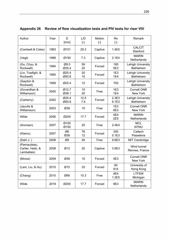
226

Appendix 26 Review of flow visualization tests and PIV tests for riser VIV

Author

Year

D [mm]

L/D [-]

Motion [-]

Re [-]

Remark

(Cantwell & Coles) 1983 Ø101 29.3 Captive 1.4E5 CALCIT Stanford

(Vegt) 1988 Ø150 7.3 Captive 2.1E4 MARIN

Netherlands

(Gu, Chyu, & Rockwell)

1994 Ø9.5

Ø25.4 59 20

Forced 185 5E3

Lehigh University Bethlehem

(Lin, Towfighi, & Rockwell)

1995 Ø25.4 Ø50.8

20 10

Forced 1E3 1E4

Lehigh University Bethlehem

(Gaydon & Rockwell)

1999 Ø25.4 12 Forced 700 Lehigh University

Bethlehem

(Govardhan & Williamson)

2000 Ø12.7 Ø38.1

10 20

Free 1E3 1E4

Cornell ONR New York

(Carberry) 2002 Ø25.4 Ø50.8

12.5 7.6

Forced 2.3E3 9.1E3

Lehigh University Bethlehem

(Jauvtis & Williamson)

2003 Ø38 10 Free 1E3 6E3

Cornell ONR New York

Wilde 2006 Ø200 17.7 Forced 4E4 2E5

MARIN Netherlands

(Aronsen) 2007 Ø100 Ø150

20 Free 2.4E4 MCL

NTNU

(Klamo) 2007 Ø6

Ø38 78 12

Forced 200

5.1E3 Caltech

Pasadena

(Dahl J. ) 2008 Ø9 48 Free 9.6E3 MIT Cambridge

(Parnaudeau, Carlier, Heitz, & Lamballais)

2008 Ø12 20 Captive 3.9E3 Wind tunnel

Rennes, France

(Morse) 2009 Ø38 10 Forced 4E3 Cornell ONR

New York

(Lam, Liu, & Hu) 2010 Ø15 33 Forced 90 814

University of Hong Kong

(Chang) 2010 Ø89 10.3 Free 4E4

1.2E5 LTFSW

Michigan

Wilde 2019 Ø200 17.7 Forced 9E3 MARIN

Netherlands

227

Appendix 27 Review of CFD analysis towards riser VIV prediction

Author

Year

CFD

[-]

Grid cells [-]

Cylinder motion

[-]

L/D

[%]

Re

[-]

Remark

(Vegt) 1988 Vortex - Captive 8.0 2.1E4 MARIN Vortex Blob

(Lu & Dalton) 1996 NS 3.3E4 Forced 2D 185 1E3

University of Houston

(Schulz & Kallinderis) 1997 - - Free 2D 6.83E3 1.85E4

Texas A&M

(Huijsmans, Wilde, & Buist)

2000 RANS 1.7E4 Captive 2D 3.75E4 4.68E5

CFX

(Al-Jamal & Dalton) 2004 LES 7.6E4 Free 2D 8E3 University of

Houston

(Dong & Karniadakis) 2005 DNS 1.2E6 Forced 3.14 1E4 Brown

University

(Singh & Mittal) 2005 FE 1.2E5 Captive 2D 2E3 1E5 1E6

India IIT

(Polner) 2005 FE

Galerkin 4.3E4 Captive 2D 200

University of Twente

(Vaz, Mabilat, Wal, & Gallagher)

2007 URANS 1.2E6 Captive 2.0 9.3E4 5.5E5

ANSYS CFX

(Klaij) 2008 URANS 6.9E5 Captive 2.0 9.3E4 ANSYS CFX

(Parnaudeau, Carlier, Heitz, & Lamballais)

2008 LES 4.4E7 Captive 3.14 3.9E3 France University

Bretagne

(Rosetti, Vaz, & Fujarra) 2012 URANS 7.0E3 5.4E5

Captive 2D 10

5E5 ReFRESCO

(Nguyen & Temarel) 2014 URANS 7.8E4 Fee

Captive 2D 1E4

University of Southampton

(Bandringa, Verstappen, Wubs, Klaij, & Ploeg)

2014 LES 8.4E5 Captive 3.14 3.9E3 RUG

ReFRESCO

(Lloyd & James) 2014 URANS 6.0E6 Captive 1.7 6.3E4

5.06E5 OpenFOAM

(Rosetti G. ) 2015 URANS 1.9E7 Captive 4.0 1E3

7.57E5 ReFRESCO

(Rosetti G. ) 2015 URANS 4.1E6 Forced 13.0 1E4

4.5E4 ReFRESCO

(Rosetti G. ) 2015 URANS 4.1E6 Free 13.0 4E3

1.9E4 ReFRESCO

(Pereira) 2018 PANS 4.6E6 2.0E7

Captive 3.0 2.0

3.9E3 1.4E5

ReFRESCO

Wilde & Maximiano 2019 URANS 5E5 Forced 2D 9E3 ReFRESCO

228

Appendix 28 Review of new tow tests with non-oscillating pipe a) Review of non-oscillating tow tests with OD 200 mm smooth pipe.

Test series

Year

Forward backward

D [mm]

k/D [-]

Re [-]

S 15306 1999 F 206 2E-6 1.87E4 – 5.52E5

S 15935 2001 F 200 2E-6 6.3E4 – 7.57E5

S 17708 2002 F/B 200 2E-6 3.6E4 – 2.7E5

S 18996 2004 F 200 2E-6 3.6E4 – 3.59E5

S 19906 PIV 2005 F 200 2E-6 3.6E3 – 1.8E5

S 21536 2007 F/B 200 2E-6 4.4E4 – 7.15E5

S 21536 PIV 2007 F 200 2E-6 3.6E3 – 2.7E5

S 25059 2011 F/B 200 2E-6 5.4E4 – 7.15E5

S 26893 2015 F/B 200 2E-6 5.0E4 – 5.0E5

b) Review of non-oscillating tow tests with OD 200 mm rough pipe.

Test series

Year

Forward Backward

D [mm]

k/D [-]

Re [-]

R 15935 2001 F 204 5E-3 3.6E4 – 7.23E5

R 18996 2004 F 200 5E-3 3.5E4 – 3.32E5

R 21536 2007 F/B 204 5E-3 3.7E4 – 3.65E5

229

Appendix 29 Review of new VIV tests with freely vibrating pipe a) Review of freely vibrating tow tests with OD 200 mm smooth pipe.

Test series

Year

Speed [m/s]

OD [mm]

k/D [-]

Remark

S 15935 2001 0.4 – 2.6 Ø 200 2E-6 1 Hz spring blades

S 15935 2001 0.6 – 2.0 Ø 200 2E-6 1 Hz spring blades + damping

S 15935 2001 1.2 – 3.2 Ø 200 2E-6 2 Hz spring blades

S 15935 2001 1.6 – 3.2 Ø 200 2E-6 2 Hz spring blades + damping

S 15935 2001 1.6 – 3.3 Ø 200 2E-6 3 Hz spring blades

S 15935 2001 2.4 – 3.3 Ø 200 2E-6 3 Hz spring blades + damping

b) Review of freely vibrating tow tests with OD 200 mm rough pipe.

Test series

Year

Speed [m/s]

OD [mm]

k/D [-]

Remark

R 15935 2001 0.6 – 2.6 Ø 204 5E-3 1 Hz spring blades

R 15935 2001 0.9 – 2.6 Ø 204 5E-3 1 Hz spring blades + damping

R 15935 2001 1.6 – 3.0 Ø 204 5E-3 3 Hz spring blades

R 15935 2001 1.6 – 3.0 Ø 204 5E-3 3 Hz spring blades + damping

230

Appendix 30 Review of new VIV tow tests with forced oscillation pipe a) Review of forced oscillation tow tests with OD 200 mm smooth pipe.

Test series

Year

Speed [m/s]

OD [mm]

k/D [-]

Remark

S 15935 2001 - Ø 200 2E-6 1 Hz spring blades

S 15935 2001 - Ø 200 2E-6 2 Hz spring blades

S 15935 2001 - Ø 200 2E-6 3 Hz spring blades

S 17708 2002 - Ø 200 2E-6 with anti- Magnus device

S 17708 2002 - Ø 200 2E-6 free vibration

S 17708 2002 - Ø 200 2E-6 free vibration

S 17708 2002 - Ø 200 2E-6 w/o anti-Magnus device

S 17708 2002 - Ø 200 2E-6 -

S 18996 2004 0.22 Ø 200 2E-6 -

S 18996 2004 0.44 Ø 200 2E-6 -

S 18996 2004 2.00 Ø 200 2E-6 -

S 18996 2004 - Ø 200 2E-6 gradual increasing tow speed

S 19906

2005

-

Ø 200

2E-6

PIV measurements Re 3.6E4 – 9.0E4

S 21536 2007 0.23 Ø 200 2E-6 -

S 21536 2007 1.50 Ø 200 2E-6 -

S 21536 2007 - Ø 200 2E-6 PIV measurements Re 9E3

S 25059 2011 0.23 Ø 200 2E-6 -

S 26893 2015 1.50 Ø 200 2E-6 -

b) Review of forced oscillation tow tests with OD 200 mm rough pipe.

Test series

Year

Speed [m/s]

OD [mm]

k/D [-]

Remark

R 15935 2001 - Ø 204 5E-3 1 Hz spring blades

R 15935 2001 - Ø 204 5E-3 3 Hz spring blades

R 18996 2004 0.22 Ø 200 5E-3 -

R 18996 2004 0.44 Ø 200 5E-3 -

R 18996 2004 - Ø 200 5E-3 gradual increasing tow speed

R 18996 2004 - Ø 200 5E-3 pipe 180 deg rotated

R 21536 2007 2.00 Ø 204 5E-3 -

231

c) Review of forced oscillation tow tests with OD 324 mm intermediate rough pipe.

Test series

Year

Speed [m/s]

OD [mm]

k/D [-]

Remark

B 22022 2007 0.30 Ø 324 1E-3 -

B 22022 2007 1.00 Ø 324 1E-3 -

232

Appendix 31 Review of new forced oscillation tests with pipe in calm water a) Review of forced oscillation tests with OD 200 mm smooth pipe in calm water.

Test series

Year

OD [mm]

k/D [-]

KC [-]

Beta [-]

Remark

S 21536 2007 Ø 200 2E-6 0.5 7.5

1E4 9E4

-

S 25059 2011 Ø 200 2E-6 0.5 7.5

1E4 9E4

-

S 26893 2015 Ø 200 2E-6 0.5 7.5

1E4 9E4

-

b) Review of forced oscillation tests with OD 200 mm rough pipe in calm water.

Test series

Year

OD [mm]

k/D [-]

KC [-]

Beta [-]

Remark

R 21536 2007 Ø 204 5E-3 1.0 7.5

1E4 9E4

-

c) Review of forced oscillation tests with OD 324 mm intermediate rough pipe in calm water.

Test series

Year

OD [mm]

k/D [-]

KC [-]

Beta [-]

Remark

B 22022 2007 Ø 324 1E-3 0.5 6.5

1E4 1E5

-

233

Appendix 32 2D graphical representation of data points for Re sensitivity

a)

b)

Figure A 18 Graphical representation of available data points for Re sensitivity.

Result in Figure 3-7 shows a three-dimensional representation of the available data points of VIV experiments. The same data point of the 3D representation in Figure 3-7 are depicted here in a 2D representation. Only the cases for which the three main test parameters Re, Ur and A/D are available are considered. a) AD versus Re and b) Ur versus Re. Data points that can be found in open literature in blue (o) and new data points of the present work in green (o). A total of 1307 data points in open literature and a total of 449 data points of the present work are presented.

234

Appendix 33 Triangulation settings for contour plots Clv and Cla.

Test series

Appendix

Number of data points

Interpolation method

Step size Ur

Step size AD

S 18996 rough Re 3.96E4

Appendix 36 69 cubic 0.2 0.01

S 18996 smooth Re 3.96E4

Appendix 37 45 cubic 0.2 0.01

B 22022 bare Re 8.79E4

Appendix 38 46 cubic 0.2 0.01

S 21536 smooth Re 2.7E5

Appendix 39 61 cubic 0.2 0.05

B 22022 bare Re 2.91E5

Appendix 40 31 cubic 0.2 0.01

S 21536 rough Re 3.6E5

Appendix 41 46 cubic 0.2 0.01

235

Appendix 34 Contour plots Gopalkrishnan (1993) at Re 1.08E4

a)

b)

236

c)

Figure A 19 Contour plots derived from Gopalkrishnan (1993) at Re = 1.08E4.

a) lift force coefficient in-phase with velocity Clv, b) lift force coefficient in-phase with acceleration Cla and c) mean drag force coefficient Cd.

237

Appendix 35 Contour plots Blevins (2009) for Re 1E4 to 8E4

a)

b)

238

c)

Figure A 20 Contour plots of compilation by Blevins (2009) for Re 1E4 to 8E4.

a) lift force coefficient in-phase with velocity Clv, b) lift force coefficient in-phase with acceleration Cla and c) mean drag force coefficient Cd.

239

Appendix 36 Contour plots rough cylinder at Re 3.96E4

a)

b)

240

c)

Figure A 21 Contour plots of forced oscillation lift force coefficients at Re 3.96E4.

Forced oscillation tests while towing of test series R 18996 with OD 200 mm rough cylinder with k/D = 5E-3. a) lift force coefficient in-phase with velocity Clv, b) lift force coefficient in-phase with acceleration Cla and c) mean drag force coefficient Cd.

241

Appendix 37 Contour plots smooth cylinder at Re 3.96E4

a)

b)

242

c)

Figure A 22 Contour plots of forced oscillation lift force coefficients at Re 3.96E4.

Forced oscillation tests while towing of test series S 18996 with OD 200 mm smooth cylinder. a) lift force coefficient in-phase with velocity Clv, b) lift force coefficient in-phase with acceleration Cla and c) mean drag force coefficient Cd.

243

Appendix 38 Contour plots for intermediate rough cylinder at Re 8.79E4

a)

b)

244

c)

Figure A 23 Contour plots of forced oscillation lift force coefficients at Re 8.79E4.

Forced oscillation tests while towing of test series B 22022 with OD 324 mm intermediate rough cylinder with k/D = 1E-3. a) lift force coefficient in-phase with velocity Clv, b) lift force coefficient in-phase with acceleration Cla and c) mean drag force coefficient Cd.

245

Appendix 39 Contour plots smooth cylinder at Re 2.7E5

a)

b)

246

c)

Figure A 24 Contour plots of forced oscillation lift force coefficients at Re 2.7E5.

Forced oscillation tests while towing of test series S 21536 with OD 200 mm smooth cylinder. a) lift force coefficient in-phase with velocity Clv, b) lift force coefficient in-phase with acceleration Cla and c) mean drag force coefficient Cd.

247

Appendix 40 Contour plots for intermediate rough cylinder at Re 2.91E5

a)

b)

248

c)

Figure A 25 Contour plots of forced oscillation lift force coefficients at Re 2.91E5.

Forced oscillation tests while towing of test series B 22022 with OD 324 mm intermediate rough cylinder with k/D = 1E-3. a) lift force coefficient in-phase with velocity Clv, b) lift force coefficient in-phase with acceleration Cla and c) mean drag force coefficient Cd.

249

Appendix 41 Contour plots rough cylinder at Re 3.6E5

a)

b)

250

c)

Figure A 26 Contour plots of forced oscillation lift force coefficients at Re 3.6E5.

Forced oscillation tests while towing of test series R 21536 with OD 204 mm rough cylinder with k/D = 5E-3. a) lift force coefficient in-phase with velocity Clv, b) lift force coefficient in-phase with acceleration Cla and c) mean drag force coefficient Cd.

251

Appendix 42 Comparison between Gopalkrishnan (1993), Blevins (2009) and present

a)

b)

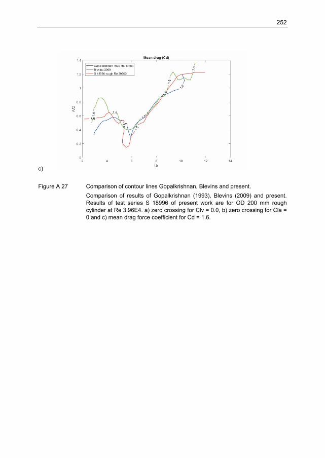
252

c)

Figure A 27 Comparison of contour lines Gopalkrishnan, Blevins and present.

Comparison of results of Gopalkrishnan (1993), Blevins (2009) and present. Results of test series S 18996 of present work are for OD 200 mm rough cylinder at Re 3.96E4. a) zero crossing for Clv = 0.0, b) zero crossing for Cla = 0 and c) mean drag force coefficient for Cd = 1.6.

253

Appendix 43 Uncertainty FO tests smooth cylinder at Re 3.96E4

a)

b)

254

c)

Figure A 28 Uncertainty of measured coefficients at Re 3.96E4.

Uncertainty analysis of test series S 18996 with OD 200 mm smooth cylinder as discussed in Appendix 17. a) uncertainty of lift force coefficient in-phase with velocity Clv, b) uncertainty of lift force coefficient in-phase with acceleration Cla and c) uncertainty of mean drag force coefficient Cd.

255

Appendix 44 Uncertainty FO tests smooth cylinder at Re 2.7E5

a)

b)

256

c)

Figure A 29 Uncertainty of measured coefficients at Re 2.7E5.

Uncertainty analysis of test series S 21536 with OD 200 mm smooth cylinder as discussed in Appendix 17. a) uncertainty of lift force coefficient in-phase with velocity Clv, b) uncertainty of lift force coefficient in-phase with acceleration Cla and c) uncertainty of mean drag force coefficient Cd.

257

Appendix 45 Sensitivity for small in-line motions in 2001 and 2002 In 2001 and 2002, an unexpected large sensitivity was observed for the measured lift force coefficient Clv for test series S 15935 and test series S 17708 (Wilde, Huijsmans, & Triantafyllou, 2003). The tests involved forward and backward towing with the OD 200 mm smooth pipe mounted on long spring blades, shown in Appendix 12. In 2004, the test setup with the long spring blades was replaced by a new test setup with linear bearings, as shown in Appendix 9. The new test setup with linear bearings ensures pure single degree of freedom cross-flow motion for the test pipe. The unexpected large sensitivity for the tests in 2001/2002 was found for the VIV lock-in regime at a Reynolds number of Re 7.8E4. In 1999, a large sensitivity was also observed for test series S 15306 with an OD 206 mm freely vibrating cylinder on long spring blades (Wilde & Huijsmans, 2001). The evidence for the large sensitivity is, however, much more convincing for the forced oscillation tests in 2001/2002, than for the previous tests with the freely vibrating pipe in 1999. The oscillating cylinder on the long spring blades is effectively constrained to an orbit along the arc of a circle with rotation point near the clamping point of the long spring blades. The effective rotation point is somewhat forward (to the left) of the clamping point of the spring blades, as shown in Appendix 12. The 2D orbit can be considered as slightly convex when towing in forward direction (F) and as slightly concave when towing in backward direction (B). For long spring blades of 2.5 length, the contribution of the in-line motions is small compared to the cross-flow motions. The in-line motions are approximately 3% of the cross-flow motions for the motions of an OD 200 mm cylinder at a forced oscillation amplitude of A/D 1.0.

Figure A 30 Motion trajectory of test pipe mounted on long spring blades.

The in-line motions are approximately 3% of the cross-flow motions for 2.5 m long spring blades.

Figure A 31 shows the measured Clv lift forces from the forced oscillation experiments with the test cylinder mounted on the spring blades together with those using the linear bearings.

258

Both configurations were tested for forward as well as backward towing direction. The Clv zero crossing for the pure cross-flow motion at Re 7.8E4 is well above one cylinder diameter, which is more than double the value expected from the Gopalkrishnan (1993) results at Re 1.08E4. The Clv zero crossing for the convex case is even higher. Results for pure cross-flow are almost symmetric for forward (○) and backward (◊) towing direction, except for the region 0.7 < AD < 1.3, where a large scatter can be observed. The reason for the large scatter is not well understood, but it is well-known that the results of VIV experiments can sometimes be remarkably sensitive for minor unknown perturbations, such as small imperfection on the surface of the cylinder.

Figure A 31 Large sensitivity for small in-line motions.

An unexpected large sensitivity was observed for the Clv lift force coefficient for test series 17708 in 2002 for forced oscillation with OD 200 mm smooth cylinder mounted on 2.5 m long spring blades. The motions are slightly convex when the carriage moves in forward direction and slightly concave when the carriage moves in backward direction. For the forced oscillation tests with the linear bearings there are no in-line motions. Results are for Re 7.8E4 and Ur 7.0. Large sensitivity can be observed for: small convex motion (○), small concave motion (◊) and pure cross-flow motion (○ , ◊). Results of Gopalkrishnan (1993) at Re 1.08E4 and Ur 7.0 are presented for reference (○). Results for pure cross-flow are almost symmetric for forward (○) and backward (◊) towing direction, except for the region 0.7 < AD < 1.3, where a large scatter can be observed. The reason for the large scatter is not well understood, but it is well-known that the results of VIV experiments can sometimes be remarkably sensitive for minor unknown perturbations, such as small imperfection on the surface of the cylinder.

259

Appendix 46 Higher harmonic lift forces The Hartlen & Currie (1970) two-parameter VIV model assumes steady VIV at constant frequency and constant amplitude. This means that the signal of the motion Z as well as the signal of the lift force FZ are assumed to be perfectly sinusoidal, or similarly that only the first harmonic of the signal is considered. In reality, the signal of the motions and the lift forces are, however, not perfectly sinusoidal and higher or lower order harmonics may be present. The higher harmonics of test No. 704803 of test series S 15935 in 2001 are considered as an example. Test No. 704803 is a freely vibrating test with the OD 200 mm smooth pipe at Re 2E5 on the long spring blades. Stable VIV response of A/D 1.0 was measured at a true reduced velocity of Ur 6.5. The damping ratio was β 0.05. The result in Figure A 32 shows the measured lift force after inertia removal (─). Also shown are the first harmonic of the lift force (─) and the higher harmonics after removal of the first harmonic (─). Figure A 33 shows the lift force signal versus the displacement signal. The motion signal was derived by double integration of the measured acceleration directly on the pipe. It can be observed that the measured motions is highly regular for this case of freely vibrating VIV. It can also be noted that the measured amplitude of the third harmonic of the motion signal is below 1% of the measured first harmonic, as shown in Figure A 35. As explained in Appendix 15, the work done during a full cycle of the oscillation can be derived from the area of the enclosed ‘ellipse’. A clock-wise rotation in Figure A 33 means that the vortex shedding adds energy to the mass-spring-damper system. For energy balance, the exact same amount of energy should be dissipated by the damping term of the mass-spring-damper system. A perfect ellipse should be expected for a perfect sinusoidal signal of the motions and the lift force. The measurement shows, however, a small distortion of the measured lift forces, in particular near the turning points. The small distortion appears predominantly in the third harmonic, as shown by the results in Table A 4 and Figure A 34. Table A 4 Higher harmonics of test No. 704803.

Test No.

Fl/Fl [-]

Flv/Fl [-]

Fla/Fl [-]

2nd

[-] 3rd

[-] 4th

[-] 5th

[-]

740803 1.000 0.185 0.983 0.007 0.086 0.013 0.002

260

Figure A 32 Total lift force coefficient Cl of freely vibrating VIV test No. 704803.

Test No. 704803 of tests series S 15935 in 2001 was carried out with the OD 200 mm smooth pipe freely vibrating on long spring blades at a tow speed of 1.1 m/s. The Reynolds number was Re 2E5 and the true reduced velocity was Ur 6.5. A stable VIV response of A/D ~1.0 was measured. Presented are the signal of the total measured lift force after inertia removal (─), the signal of the first harmonic of the lift force (─) and the signal of the higher harmonics after removal of the first harmonic (─).

Figure A 33 Force versus displacement diagram of test No. 704803.

The work done can be derived from the area of the enclosed ellipse. The clock-wise rotation corresponds to a positive lift force coefficient of Clv 0.61. The small distortion of the force signal near the turning points is third harmonic. Presented are the signal for the total measured lift force FZ after inertia removal (─) and the signal of the first harmonic of the lift force (─).The response motion is highly regular with third harmonic below 1%, as shown in Figure A 35.

261

Figure A 34 Power spectrum of measured lift force FZ of test No. 704803.

Presented are the power spectrum of the signal of the measured first harmonic of the lift force FZ (─) and the power spectrum of the remaining higher harmonics after removal of the first harmonic (─). The vertical axis is truncated at a value of S = 2E4, to better show the peak of the third harmonic of S ~0.6E4. The amplitude of third harmonic is about 8.6% of the amplitude of the first harmonic, as shown in Table A 4.

Figure A 35 Power spectrum of measured motion signal Z of test No. 704803.

The vertical axis is truncated at a value of S = 1E-5, to better show the peak of the third harmonic of S ~0.3E-5. The amplitude of the third harmonic is below 1% of the amplitude of the first harmonic.

262

Appendix 47 Classification of vortex shedding regimes for FO tests in still water

In general, the Morison coefficients Cd and Ca depend on the KC number and the Sarpkaya frequency parameter β, as defined in Appendix 4:

, ,D aC KC and C KC (A-57)

A general classification of the vortex shedding regimes for low beta values of β < 1E3 is: KC < 0.4 The flow does not separate and there are no transverse forces.

0.4 < KC < 4 A symmetric pair of vortices is formed in the wake. These vortices reverse during the flow oscillation cycle. Lift forces are small.

4 < KC < 8 One of the vortices in the pair becomes stronger and the vortex pair becomes asymmetric. The dominant frequency of lift oscillation is twice the frequency of the flow oscillation.

8 < KC < 15 Vortex pairs are shed alternately into the wake during each half-cycle of the flow oscillation. The vortex pairs convect alternately asymmetrically at approximately 45 degrees to the direction of the flow oscillation. The dominant frequency of lift oscillation and vortex shedding is twice the flow oscillation frequency.

15 < KC < 22 Multiple pairs of vortices are shed in each flow oscillation cycle and the pairs convect at 45 degrees to the direction of the flow oscillation. The dominant frequency of vortex shedding and lift oscillation is three times the flow oscillation frequency.

22 < KC < 30 Multiple pairs of vortices are shed per cycle. The dominant frequency of vortex shedding and lift oscillation is four times the frequency of flow oscillation.

KC > 30 Quasi steady vortex shedding. The frequency of vortex shedding is roughly the nearest multiple of the flow oscillation frequency, corresponding to the normal Strouhal frequency of a stationary pipe.

Honji (1981) visualized the flow around a harmonically oscillating cylinder and observed fairly regular rows of mushroom-like structures along the lines of maximum local velocity, as shown in Figure A 36.

263

Figure A 36 Honji type instability in Otter (1992).

Picture was taken for β 5.75E4 and KC 0.463

264

Appendix 48 Contour plots of Morison coefficients for OD 200 mm smooth pipe

a)

b)

Figure A 37 Contour plots of Morison coefficients for FO tests in calm water.

Combination of results of test series S 21526 and S 26893 with OD 200 mm smooth pipe. a) Morison drag force coefficient in-phase with velocity D_MorC

and b) Morison added mass coefficient in-phase with acceleration Ca .

265

Appendix 49 Uncertainty of forced oscillation experiments in calm water

a)

b)

Figure A 38 Uncertainty of measured Morison coefficients for FO in calm water.

Uncertainty analysis of Appendix 18 for forced oscillation tests in calm water. Results of combination of test series S 21526 and S 26893 with OD 200 mm smooth pipe is considered. a) uncertainty of Morison drag force coefficient in-phase with velocity D_MorC and b) uncertainty of Morison added mass

coefficient in-phase with acceleration C a .

266

Appendix 50 Analysis of PIV test No.103005 This appendix discusses the post processing of PIV test No. 103005 of test series S 21536 in 2007. PIV test No. 103005 was a forced oscillation VIV test with the OD 200 mm smooth pipe at a constant tow speed of 0.05 m/s. The main test parameters are shown in Table A 5. The amplitude of the forced oscillation was 60 mm and the period of the regular forced oscillation was 19.2 s. The FX and FZ forces on the pipe were not measured for PIV test No. 103005, because the forces of about 10 N at 0.05 m/s tow speed were much too small for the 10 kN force transducers. Table A 5 Test parameters for forced oscillation of PIV test No. 103005 in 2007

Test No. Cylinder PIV A/D Ur Re

103005 OD 200 mm smooth 2D2C 0.3 5.0 9E3

The PIV system in Appendix 13 can be assembled in different configurations. The standard configuration is for two-dimensional three-component PIV measurements (2D3C). A symmetrical configuration was used with the laser sheet placed in the between Camera A and B. At this stage only the 2D2C results from Camera A are analyzed and presented, because it was found out after the tests that Camera B suffered from a small misalignment problem. Although it is expected that the small misalignment problem can be resolved later on with more advanced PIV post processing software, this has not been tried yet. For the 2D2C images, a somewhat larger perspective error may be expected than for 2D3C images, especially for those areas of the flow with a large out-of-plane component. It should be noted that the 2D2C PIV with only one camera can only detect the projected velocity components in the 2D plane of the laser sheet. Perspective errors can occur when the viewing direction deviates from orthogonal, even if the images are properly dewarped. The effect of the perspective error for the final SVD results is expected to be small, because of the phase averaging over 1199 individual PIV images. A total of 1199 pairs of PIV images was recorded for PIV test No. 103005 in 2007. The PIV images were recorded at an image capturing rate of 10 Hz. Each pair of images was evaluated in the PIV post processing for 6887 spatial interrogation units, using 32 x 32 pixel interrogation. The 120 s duration of PIV test No. 103005 means that the cylinder has progressed forward over a length of about 6 m in the basin, meaning that about 6.2 forced oscillating cycles are recorded. PIV test Nos 103001 and 103002 are repeat tests of PIV test No. 103005.

267

The three PIV tests together were combined in one final phase synchronized result using the SVD analysis:

Test No. 103001 599 images ~3.1 cycles Test No. 103002 1199 images ~6.2 cycles Test No. 103005 1199 images ~6.2 cycles The file size for storing of one pair of raw PIV images for Camera A only is about 3.6 MB. This means that about 10 GB of raw PIV data was captured for PIV test Nos 103001, 103002 and 103005 together. It was experienced that the data processing of more than 10 GB of raw PIV images can be time consuming. Some important remarks on the quality of PIV test No. 103005 are:

1. The raw PIV images in Appendix 53 shows some direct illumination of the mid part of the OD 200 mm smooth pipe by the laser sheet. It was found out that any direct or indirect illumination of the test setup in the vicinity of the measuring area should be avoided to obtain the best possible quality for the raw PIV images. The final quality of the PIV measurements strongly depends on clean PIV images at the beginning, including high contrast, high resolution, homogenous seeding distribution and no contamination by direct or indirect reflections.

2. Appendix 69 shows the OD 200 mm smooth pipe for PIV test No. 103005 in 2007. It can be observed that the pipe was painted black with an approximately 200 mm long section of Rhodamine laser absorbing paint in the middle. The 200 mm long section in the middle is the section where the laser sheets shines on the pipe. It was found out that, in spite of the Rhodamine laser absorbing paint, there is still too much light reflection from the pipe into the measuring area. For future PIV measurements it is recommended to paint the complete pipe with Rhodamine and/or to avoid any direct illumination of the pipe by the laser sheet.

3. In general, the PIV measurements require appropriate seeding of the flow with a uniform distribution of seeding particles in the PIV interrogation area. For PIV measurements in a large towing tank, the seeding particles are normally injected at a suitable upstream location of the test object. For turbulent flow at higher Reynolds numbers of Re > 1E3, the upstream injected seeding particles tend to mix and distribute in three-dimensional space, which also means mixing out of the 2D plane of the laser sheet.

268

4. In 2007, an improved seeding method was used for PIV test No. 103005. The improved seeding method involved pre-laying of the seeding in still water prior to the actual test with the moving pipe. For PIV test No. 103005 in 2007 there was no upstream injection of the seeding during the tow test. The seeding was laid in a more or less uniform band of roughly 0.5 x 1.0 x 30.0 m (W x H x L) at the centerline of the basin and at ~1.7 m below the free surface. A short waiting time was adopted before starting the PIV tests and before moving the carriage, to allow mixing of the seeding material due to the ambient background turbulence. Although the new seeding method in 2007 in much better quality PIV measurements than the previous seeding method in 2005, there is still considerable room for improvement, as summarized below:

o Obtaining the optimum seeding concentration was difficult and required a trial and error approach.

o Even with nicely uniform seeding in the pre-laid upstream volume, there still appeared local areas (blobs) with low seeding concentration in the downstream PIV interrogation area.

o It was noted that when waiting too long after the pre-laying of the seeding material, the Rilsan 60 m seeding particles could disappear from the pre-laid volume due to dispersion or slow rising or sinking of the particles, resulting from their nett positive or negative buoyancy.

o The 20 to 30 m length of the pre-laid volume of seeding material was only just long enough for the steady state tow length for a 120 s PIV measurement.

o It was found out that when doing too many tests per day, that the concentration of seeding material in the basin was ‘pumping up’. It was experienced that a too high concentration of dispersed seeding material in the water of the basin reduced the quality of the view of the CCD cameras.

5. The Rilsan 60 m seeding particles seemed adequate for the purpose of the tests. It is not expected that significant improvement can be obtained by using another seeding material, unless opting for instance for drastically more expensive seeding material, such as fluorescent seeding material.

6. For the PIV tests in 2007, the entire PIV system was pre-calibrated as one pre-installed assembly in a separate calibration setup outside the towing tank. The calibration in a separate calibration setup was considered more time effective and presumably more accurate than in-situ calibration in the test facility itself.

269

7. At this stage only the 2D2C results from Camera A are analyzed and presented. The results of Camera B are not used because of a small misalignment problem that was detected after the tests. Although it is expected that the small misalignment problem can be resolved later on with more advanced PIV post processing software, this has not been tried yet. For the 2D2C images, a somewhat larger perspective error may be expected than for 2D3C images, especially for those areas of the flow with a large out-of-plane component. It should be noted that the 2D2C PIV results with only one camera can only detect the projected velocity components in the 2D plane of the laser sheet. Therefore, perspective errors can occur when the viewing direction deviates from orthogonal, even if the images are properly dewarped. However, the effect of the perspective error for the final SVD results is expected to be small, because of the phase averaging over 1199 individual PIV images. It is expected that the perspective error should roughly go down with the square root of the number of images.

8. It is expected that the misalignment of Camera B occurred during transport and/or installation of the pre-calibrated PIV unit under the carriage. It is also possible that the central OD 114 mm under water housing of the two cameras has experienced a small structural deformation due to its own submerged weight, when hanging under the carriage.

9. The camera settings, the camera alignment, the calibration procedure, the laser power, the sample rate and the time between dual pulses seemed more or less adequate for PIV test No. 103005. It is of course always possible to further optimize the settings.

10. It was found out that a somewhat too small laser sheet aperture was used, leading to a reduction of the effective measuring area for the cameras. This was due to limitations of the optics. This problem was resolved in the post processing by masking the edges and by only using the useful area of the raw images in the middle.

11. Single value decomposition (SVD) analysis of Appendix 52 was used as a final step in the post processing. The results after SVD analysis yields phase synchronized values for the velocities u and v in velocity maps for 16 equidistant time steps in one forced oscillation cycle of the test pipe. Consequently, vorticity maps were derived from the velocity maps. Results in Appendix 56 through Appendix 59 present the final vorticity maps for four selected phase angles of the cylinder motion of respectively Φ = 90, 135, 180 and 225 degrees.

270

12. The SVD analysis of Appendix 52 clearly demonstrates the advantage of the phase synchronization for PIV measurements when testing in a complex three-dimensional separated flow at high Re numbers of Re > 1E3 in the turbulent regime. The quality of the final PIV results significantly improves with the SVD analysis, because the random errors caused by the local areas with poor seeding quality are averaged out. The vortex shedding process at high Reynolds numbers of Re > 1E3 is a stochastic process for which the phase averaged PIV results are more useful when comparing with URANS CFD.

13. Longer duration PIV measurements and/or additional repeat tests are recommended to improve the statistical reliability of the SVD analysis. The SVD analysis allows for ‘temporal stitching’ of repeat tests into one combined set of SVD phase synchronized result. It can be expected the statistical reliability of the SVD analysis will roughly improve with the square root of the number of available PIV images. The SVD analysis also allows for combination of the results of PIV measurements at other positions by ‘spatial stitching’.

271

Appendix 51 Post processing of PIV test No. 103005 The post processing of PIV test No. 103005 with cross correlation technique starts with a subdivision of the captured images into spatial interrogation windows. The typical size of the windows range between 16 x 16 and 128 x 128 pixels. The interrogation windows of the first image of the first laser pulse are cross correlated with the windows of the second image of the second laser pulse. A range of displacements of the interrogation window on the second image is tried in order to find the maximum value for the correlation. The end result is a correlation map for pixel displacements. A low pass 3rd order Gaussian filter was used for the cross correlation. The Gaussian filter reduces the errors induced by the truncation at the size of the interrogation area. Outliers are removed by peak validation. Outliers are incorrect vectors resulting from noise in the peak detection of the cross correlation. A peak-height validation function was used for comparing the highest peak (signal) with the second highest peak (noise). The ratio is known as ‘detectability criterion’. A detectability criterion of 1.1 was used, meaning that the signal (valid vectors) can also be detected in areas with low seeding quality. After the cross correlation, a moving average filter was used, in order to reduce the velocity noise over the whole measurement area and to replace invalid vectors by interpolated vectors. The filter parameters were 3 x 3, which means that a vector in an interrogation area is replaced by the average of its 8 immediate neighbors. The acceptance factor was 0.15. The final settings for the PIV interrogation values have been defined experimentally, searching for the best compromise between the number of interpolated vectors and the number of outliers. Appendix 53 shows an example of a raw PIV image of Camera A (starboard) and of Camera B (port side). The quality of the seeding is in accordance with normal standards for this kind of PIV measurements. About 10 detectable seeding particle (or clusters) are present in a 32 x 32 pixel interrogation window. The in-plane and out-of-plane loss of particles is low when using a short time between the laser pulses of 30 ms. In general, the best possible PIV result can be obtained when the following settings are satisfied:

1. Image density Ni (minimum number of particles in an interrogation area):

10iN

2. The number of exposures Np:

2pN

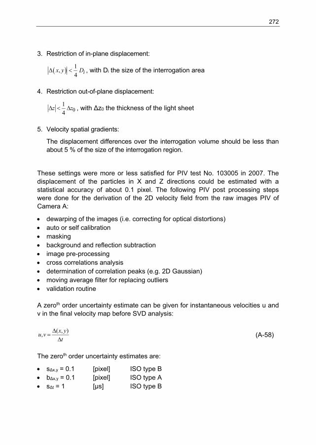
272

3. Restriction of in-plane displacement:

1,

4 ix y D , with Di the size of the interrogation area

4. Restriction out-of-plane displacement:

01

4z z , with Δz0 the thickness of the light sheet

5. Velocity spatial gradients:

The displacement differences over the interrogation volume should be less than about 5 % of the size of the interrogation region.

These settings were more or less satisfied for PIV test No. 103005 in 2007. The displacement of the particles in X and Z directions could be estimated with a statistical accuracy of about 0.1 pixel. The following PIV post processing steps were done for the derivation of the 2D velocity field from the raw images PIV of Camera A:

dewarping of the images (i.e. correcting for optical distortions) auto or self calibration masking background and reflection subtraction image pre-processing cross correlations analysis determination of correlation peaks (e.g. 2D Gaussian) moving average filter for replacing outliers validation routine A zeroth order uncertainty estimate can be given for instantaneous velocities u and v in the final velocity map before SVD analysis:

( , ),

x yu v

t

(A-58)

The zeroth order uncertainty estimates are:

sΔx,y = 0.1 [pixel] ISO type B bΔx,y = 0.1 [pixel] ISO type A sΔt = 1 [μs] ISO type B

273

The average peak displacement for the tests at 0.05 m/s tow speed is about 6 pixels, corresponding to about 1.5% accuracy for the peak displacement. The uncertainty of ~1 μs for the time between pulses is very small and can be safely be ignored. The large U expanded uncertainty for 95% confidence level is:

0.5 0.52 2 2, , ,2 2u v x y t x yU s s b

(A-59)

Overall, this leads to a zeroth order accuracy for the instantaneous velocities u and v in the final velocity map of about 3%. However, due to the practical difficulties as discussed in Appendix 50, the effective accuracy is estimated to be about 5 to 10% for the instantaneous velocities u and v in the final velocity map. It should further be noted that with SVD analysis, the accuracy of the phase synchronized results improve roughly with the square root of the 1199 PIV images.

ss

n

(A-60)

First order accuracy estimate for the PIV measurements was obtained by means of PIV tests without the pipe in the water. The uniform flow field of the PIV measurement can then be compared with the accurately measured speed of the carriage. The open water tests were done for a tow speed of 0.5 m/s (e.g. PIV test No. 60100009). The following accuracies were estimated from the open water test:

in-plane systematic error of 5% in-plane random error of 5% out-of-plane systematic error of 2% of in-plane component (not used for test No.

103005) out-of-plane random error of 5% of in-plane component (not used for test No.

103005)

274

Appendix 52 SVD analysis of PIV test No. 103005 Single value decomposition (SVD) of Golup & Loan (1989) proved to be an effective means for improving the accuracy of the PIV results. The SVD analysis was done as a final step in the post processing. The results after SVD analysis yields phase synchronized values for the velocities u and v in velocity maps for 16 equidistant time steps in one forced oscillation cycle. Finally, the vorticity maps were derived from the velocity maps. Results in Appendix 56 through Appendix 59 present the final vorticity maps for a phase angle of the cylinder motion of Φ = 90, 135, 180 and 225 degrees. SVD analysis is commonly used in structural vibration analysis and in turbulent flow analysis. The SVD analysis helps to distinguish the dominant coherent structures in a data set. Another option would have been to decompose the harmonic components in space. While this latter option is typically suitable for wave type problems, it does not seem the best approach for the flow in the near wake of a oscillating cylinder. The instantaneous velocities u and v are combined into a complex vector w:

( , ) ( , ) ( , )w t x u t x iv t x

(A-61) The SVD analysis of Golup & Loan (1989) searches for mode decomposition of the following type:

( , ) ( ) ( )k kk

w t x a t x

(A-62)

The time traces ak describe the amplitude evolution of mode shape k. The original vector field w can be reconstructed by summation of all modes. The discrete dataset of w is stored in a matrix W, where each row corresponds to a time step and each column to a position in space. The SVD method decomposes the complex matrix W as follows:

*W T D S (A-63)

This yields a Nt x Nt complex orthogonal matrix for the amplitude evolution T and a complex Nx x Nx orthogonal matrix for the base functions S in space. The real Nt x Nx diagonal matrix D yields the sorted amplitudes of each mode.

275

The results of the SVD analysis can be interpreted as follows:

The columns of S contain orthogonal basis functions in space of the data W. These are the spatial structures that evolve coherently in time.

The columns of T contain the amplitude evolution in time of each spatial mode shape, normalized to 1.

The diagonal entries iσ of D are the sorted amplitudes of each mode.

The first spatial mode (first column of S), when evolved in time according to the first column of T and using magnitude 1σ , produces a dataset that closest

resembles the original data in the L2 norm. Multiplying the kth diagonal entry with the kth column of T produces the time signal ak. The transpose complex conjugate of the kth column of S corresponds to spatial modes k:

'w D T S (A-64) For the present work it was noted that the quality of the SVD analysis improved considerably by first removing the mean from the velocity maps. This yields the complex vector w – w0 as input for the SVD analysis. It was also found that the quality of the SVD analysis improves by first using a band filter for the time evolution T. In summary, the SVD analysis involved the following steps:

Reading of the processed PIV velocity fields from file. Rotating the PIV image by 48.2 degrees. Combining the velocities u and v into a complex number w = u+i*v. The time average of each spatial data point should be subtracted, yielding w-

w0. Performing SVD analysis of Golup & Loan (1989) on the discrete dataset w-w0. Fourier analysis on the SVD time signals iT .

Zero crossing analysis of the SVD time signals iT .

Reconstruction of the PIV images based on the dominant SVD modes: W = w0 + w1 + w2.

Resampling of the result into 16 equidistant phases per cycle. Combining the interpolated velocities ui and vi into a new complex number

wi = ui+i*vi. Combining the original velocity field with its mirror image for time sample t+T/2. This last steps yields the final time synchronized velocity maps for u and v. Deriving the vorticity field from the velocity map.

276

Appendix 54 shows an example of the reconstructed velocity field for PIV test No. 103005 before and after the SVD analysis. PIV image 172/1199 of PIV test No. 103005 is considered. Appendix 55a shows the final time averaged stream wise velocity u0 for PIV test No. 103005 after the SVD analysis. The result can be compared with the result of 2D URANS CFD run No. 103001 in Appendix 55b.

277

Appendix 53 Example of raw PIV image

Cam A

Cam B

Figure A 39 Example of raw PIV images.

Camera A (starboard) and Camera B (port side)

278

Appendix 54 Reconstruction of SVD velocity field for PIV test No. 103005

a)

b)

Figure A 40 Example of PIV reconstructed velocity field after SVD analysis.

PIV image 172/1199 of PIV test No. 103005 is considered. a) initial result after standard PIV analysis and b) reconstructed result after SVD analysis. The SVD analysis greatly improves the quality of the PIV images and effectively removes the outliers.

279

Appendix 55 Time averaged stream wise flow field u0 for PIV test No. 103005

a)

b)

Figure A 41 Time averaged flow velocity uo at Re 9E3.

The plots show the time averaged streamwise velocity uo for forced oscillation PIV test No. 103005 with the OD 200 mm smooth cylinder at Ur 5.0, AD 0.3 and Re 9E3. a) PIV test No. 103005 and b) CFD run No. 103001

280

Appendix 56 Vorticity field of PIV test No. 103005 for Φ = 90 deg

a) PIV

b) CFD

Figure A 42 Vorticity field w for phase angle Φ = 90 deg.

Forced oscillation PIV test No. 103005 with OD 200 mm cylinder for Re 9E3, Ur 5.0 and AD 0.3. Presented is the phase averaged result for Φ = 90 deg with the cylinder in its uppermost position. a) PIV frame 12/16 for test No. 103005 and b) CFD frame 5/16 for run No. 103001. The vector of the hydrodynamic lift and drag force of CFD run No. 103001 is presented with a blue arrow.

281

Appendix 57 Vorticity field of PIV test No. 103005 for Φ = 135 deg

a) PIV

b) CFD

Figure A 43 Vorticity field w for phase angle Φ = 135 deg.

Forced oscillation PIV test No. 103005 with OD 200 mm cylinder for Re 9E3, Ur 5.0 and AD 0.3. Presented is the phase averaged result for Φ = 135 deg with the cylinder moving downwards. a) PIV frame 14/16 for test No. 103005 and b) CFD frame 7/16 for run No. 103001. The red anti-clockwise rotating vortex at a distance of X/D = 2 is about to shed.

282

Appendix 58 Vorticity field of PIV test No. 103005 for Φ = 180 deg

a) PIV

b) CFD

Figure A 44 Vorticity field w for phase angle Φ = 180 deg.

Forced oscillation PIV test No. 103005 with OD 200 mm cylinder for Re 9E3, Ur 5.0 and AD 0.3. Presented is the phase averaged result for Φ = 180 deg with the cylinder at the downward zero crossing position. a) PIV frame 16/16 for test 103005 and b) CFD frame 9/16 for run No. 103001.

283

Appendix 59 Vorticity field of PIV test No. 103005 for Φ = 225 deg

a) PIV

b) CFD

Figure A 45 Vorticity field w for phase angle Φ = 225 deg.

Forced oscillation PIV test No. 103005 with OD 200 mm cylinder for Re 9E3, Ur 5.0 and AD 0.3. Presented is the phase averaged result for Φ = 225 deg with the cylinder moving towards its lower position. a) PIV frame 2/16 for test No. 103005 and b) CFD frame 11/16 for run No. 103001.

284

Appendix 60 Carberry (2002) PIV measurement for ‘2P’ and ‘2S’ vortex shedding

a) Φ = 90 deg

b) Φ = 135 deg

c) Φ = 180 deg

d) Φ = 225 deg

Figure A 46 PIV images of Carberry (2002) showing ‘2P’ and ‘2S’ vortex shedding.

Result of Carberry (2002) for A/D 0.5 and Re 2.3E3. Left column shows the low frequency state for fe/fo = 0.806. Right column shows the high frequency state for fe/fo = 0.869. The rows show the time evolution of cylinder motion, with (a) cylinder in its uppermost position and (c) cylinder at its downward zero crossing position.

285

Appendix 61 Calculated forces for CFD at Ur 5.0, AD 0.3 and Re 9E3

a) Clv

b) Cla

286

c) Cd

Figure A 47 Calculated forces of CFD run No. 103001 at Re 9E3.

Lift and drag forces for CFD run No. 103001 at Ur 5.0, AD 0.3 and Re 9E3 (■). CFD results are compared with measured result of present work for test series S 18996 with the OD 200 mm smooth cylinder at Re 3.96E4 and AD 0.5 (∗). Results are also compared with result of Gopalkrishnan (1993) at Re 1.08E4 and AD 0.3 (○), Carberry (2002) at Re 9.1E3 and AD 0.5 (∇) and Carberry (2002) at Re 4.41E3 and AD 0.25 ( ). Results are presented for: a) lift force coefficient in-phase with velocity Clv, b) lift force coefficient in-phase with acceleration Cla and c) mean drag force coefficient Cd.

287

Appendix 62 Pragmatic VIV prediction based on energy balance

Figure A 48 Results of pragmatic VIV prediction based on energy balance.

The VIV of an OD 610 mm steel riser in deep water in sheared current is considered. The test case is discussed in Chapter 9. Presented result is for mode i = 13, with natural frequency of 13f 0.25 Hz. The plot shows the power

input (excitation) and power output (damping) along the length of the riser. The dedicated model of Chapter 9 distinguishes between lock-in in the critical Re regime (─) and lock-in outside the critical Re regime (─). The three lower rows show the structural damping (─), the low Ur damping (─) and the high Ur damping (─).

288

Appendix 63 Sensitivity of pragmatic VIV prediction for OD 610 mm riser Table A 6 Sensitivity of pragmatic VIV prediction.

The VIV of an OD 610 mm steel riser in deep water in sheared current is considered, as discussed in Chapter 9. For the base case #0, the standard settings of the standard industry VIV prediction model of Vandiver (1985) are used. The first sensitivity case (#1) is for the new calculation with the new lift force coefficients Clv of Chapter 6. The remaining cases #2 through #18 are sensitivity cases with respect to the base case #0.

#

Description

Symbol

Default value

[-]

Sensitivity value

[-]

Mode peak

[-]

Peak A/D [-]

Fatigue damage [1/year]

0 Base case - - - 13 0.75 58.4

1 New Clv for critical Re - nc nc + crit 13 0.73 23.9

2 Traditional lock-in regime Ur [4,8] [4,6] 17 0.53 61.3

3 Traditional lock-in regime Ur [4,8] [4,10] 10 0.83 38.5

4 Current profile U(z) [1.2;0.2] [1.4;0.2] 15 0.75 169.4

5 Current profile U(z) [1.2;0.2] [1.2;0.3] 13 0.78 71.3

6 Venugopal low damping Crl 0.36 0.18 13 0.76 66.9

7 Venugopal high damping Crh 0.40 0.20 13 0.75 56.5

8 Added mass Ca 1.0 1.2 13 0.76 70.8

9 Top tension T 6.0E6 6.6E6 12 0.74 15.4

10 Structural damping rs 0.003 0.03 13 0.64 26.1

11 Still water damping ksw ksw 0.25 0.50 13 0.66 26.2

12 Power ratio threshold Πthres 0.10 0.20 13 0.75 62.8

13 Max. lift force coefficient1 CL_m 0.80 0.40 13 0.63 20.1

14 A/D zero crossing2 A0 0.90 0.72 13 0.61 36.8

15 A/D zero crossing A0 0.90 1.08 13 0.90 86.4

16 Fatigue class D log(C) 11.610 11.764 13 0.75 41.0

17 Fatigue class E log(C) 11.610 11.610 13 0.75 58.4

18 Fatigue class F log(C) 11.610 11.455 13 0.75 83.5

1 See definition in Figure 2-14 of Chapter 2. 2 See definition in Figure 2-14 of Chapter 2.

289

Appendix 64 Photographs of High Reynolds VIV test device

290

Appendix 65 Photographs of High Reynolds VIV test device

291

Appendix 66 Photographs of OD 200 mm smooth pipe

292

Appendix 67 Photographs of OD 200 mm rough pipe

293

Appendix 68 Photographs of OD 200 mm pipe with 500 micron sand roughness

294

Appendix 69 Photographs of OD 200 mm smooth pipe for PIV test No. 103005

295

Appendix 70 Photographs of PIV setup

296

297

298

On the measurement of VIV lift forcecoeffi cients at high Reynolds numbers

On the m

easurement of V

IV lift force

coeffi cients at high Reynolds numbers

J.J. de Wilde

J.J. de Wilde J.J. de WildeJ.J. de Wilde

On the m

easurement of V

IV lift force coeffi cients at high Reynolds num

bers

This PhD thesis concerns the measurement of the VIV lift force coeffi cient Clv and Cla for a pipe section with large length over diameter ratio of L/D ~18 at high Reynolds numbers of Re > 1E4. The measured coeffi cients can be directly used as input parameter for pragmatic riser VIV prediction models.

Jaap de Wilde holds a MSc. in Applied Physics at University Twente in the Netherlands (1991). In 1998, he joined MARIN research centre in Wageningen, the Netherlands, where he presently has the position of Senior Project Manager and Team Leader at the Offshore Department. Prior to this position, he has worked for seven years at Delft Hydraulics in Delft, the Netherlands. Subjects of Jaap’s special interest are offshore engineering, model testing, time domain simulation, risers VIV, fl oater VIM and wind loads.

Uitnodiging

Graag wil ik u uitnodigen om aanwezig te zijn bij de openbare verdediging van mijn proefschrift op vrijdag

31 januari 2020 om 10:00 uur in de Aula van

de Technische Universiteit Delft.

Om 9:30 uur zal ik een korte presentatie geven over mijn

onderzoek.

Na afl oop bent u van harte welkom op de receptie.

Jaap de Wildej.dewilde@marin.nl

Aula en receptie:Mekelweg 5, 2628 CC Delft

cover-rug17mm_CMYK_Dec2019_DEF_3de cover optie.indd 1cover-rug17mm_CMYK_Dec2019_DEF_3de cover optie.indd 1 12/16/2019 9:54:03 AM12/16/2019 9:54:03 AM