IGC-11/2-2

Measure problem in slow roll inflation and loop quantumcosmology

Alejandro Corichi1, 2, ∗ and Asieh Karami3, 1, †

1Instituto de Matematicas, Unidad Morelia,Universidad Nacional Autonoma de Mexico, UNAM-Campus Morelia,

A. Postal 61-3, Morelia, Michoacan 58090, Mexico2Center for Fundamental Theory, Institute for Gravitation and the Cosmos,

Pennsylvania State University, University Park PA 16802, USA3Instituto de Fısica y Matematicas,

Universidad Michoacana de San Nicolas de Hidalgo, Morelia, Michoacan, Mexico

AbstractWe consider the measure problem in standard slow-roll inflationary models from the perspective

of loop quantum cosmology (LQC). Following recent results by Ashtekar and Sloan, we study

the probability of having enough e-foldings and focus on its dependence on the quantum gravity

scale, including the transition of the theory to the limit where general relativity (GR) is recovered.

Contrary to the standard expectation, the probability of having enough inflation, that is close to

one in LQC, grows and tends to 1 as one approaches the GR limit. We study the origin of the

tension between these results with those by Gibbons and Turok, and offer an explanation that

brings these apparent contradictory results into a coherent picture. As we show, the conflicting

results stem from different choices of initial conditions for the computation of probability. The

singularity free scenario of loop quantum cosmology offers a natural choice of initial conditions,

and suggests that enough inflation is generic.

PACS numbers: 04.60.Pp, 98.80.Cq, 98.80.Qc

∗Electronic address: corichi@matmor.unam.mx†Electronic address: karami@matmor.unam.mx

1

arX

iv:1

011.

4249

v2 [

gr-q

c] 1

Apr

201

1

I. INTRODUCTION

The measure problem in cosmology has received some attention since it was suggestedthat one should weight, over the space of classical solutions to the equations of generalrelativity, those solutions that exhibit enough inflation to account for present observations[1]. An early observation was that there exists a natural measure on the phase space ofthe theory with respect to which one should compute probabilities. Recently, Gibbons andTurok overcame some early difficulties in the total normalization and concluded that, for thesimplest inflationary potentials in a FRW universe, the probability of inflation was greatlysuppressed [2]. One potential difficulty with such calculations pertains to the choice ofinitial conditions. Since all solutions to the equations of motion are singular in the past(for expanding universes), one needs a prescription for selecting initial conditions for thosesolutions. In [2] such a prescription was put forward in terms of a ‘constant density surface’,roughly speaking, at the end of inflation. Another possibility is given by defining a ‘cut-off’,in the form of a constant density surface at, say, the Planck scale, as was early suggested in[3].

Yet another possibility is that a quantum theory of gravity might be able to providesuch Planck surface in a natural way. Such is indeed the case of loop quantum cosmology[4], a quantum framework closely related to loop quantum gravity [5] that has been able toachieve robust results regarding avoidance of big bang singularities [6, 7] (See, for instance,[8] for a recent survey). In LQC, all trajectories undergo a bounce that replaces the initialsingularity, attain a maximum critical density [7], and preserve semiclassicality across thebounce [9], thanks to uniqueness results that warranty the consistency of the theory [10].Two key results in the measure problem have been obtained in LQC. First, it has beenshown that one could account for the dynamics of the quantum universe by means of effectiveequations that capture the main quantum gravity effects and that reduce to the classicalequations in the appropriate regime [11, 12]. This was used in [11] to show that, for severalinflationary potentials, the characteristic ‘attractor behavior’ of inflationary dynamics [3, 13,14] is recovered in the low energy regime. Furthermore, Ashtekar and Sloan showed recentlythat the natural measure of [2] can be finitely implemented in LQC, and proposed a naturalPlanck scale surface on which to compute probabilities [15]. Surprisingly, the probability forhaving enough e-foldings was shown to be close to one, in contrast to the result of Gibbonsand Turok that was done for classical GR1.

In loop quantum cosmology, the underlying discreetness of the quantum geometry man-ifests itself via a dimension-full parameter λ. In the LQC literature it is standard to choosethe value of λ such that the minimum quantum of area corresponds to that found in LQG[5, 6]. But, if one considers this as a free phenomenological parameter of the theory, it isnatural to ask whether in the limit λ → 0, where the loop quantum geometric effects dis-appear, one can recover the standard Wheeler-DeWitt quantum cosmology. This has beenanswered with different levels of sophistication [6, 7, 18]. The authors of [6] showed that thedifference equation governing the LQC dynamics reduces to the differential WDW equationin the large volume limit. Later, in [7] and [18], the limit λ → 0 was studied and it wasshown that one does recover the standard WDW and the GR limit in some regime. In

1 There have been several previous attempts to study the issue of inflation within LQC. In [16] the natural

measure of [2] was considered but the effects of the bounce and superinflation were ignored. In [17] the

issue of the measure was not considered and only a small part of the parameter space was explored.

2

the case of effective classical equations, in this limit one recovers the equations of generalrelativity.

The purpose of this article is to explore the relation between loop quantum cosmologyand general relativity, as we take the limit λ → 0, regarding the measure problem in slowroll inflation. More precisely, we would like to understand the apparent tension betweenthe results of Gibbons and Turok, with those of Ashtekar and Sloan. If one starts with theanalysis of [15], that was done for a fixed value of λ (of the order of the Planck scale), andone takes the limit λ→ 0, one might expect to recover the results of Gibbons and Turok. Aswe shall show in detail this expectation is not realized. Indeed, quite the opposite occurs.As the value of the discreetness parameter is decreased, the probability of having enoughinflation increases and approaches one in the limit. One would then be forced to concludethat in the general relativity limit of loop quantum cosmology, the probability of havingenough inflation is (almost) one, in stark contrast with the analysis of Gibbons and Turok.

What is then the source of this apparent tension? As we shall argue, the tension isresolved once one analyzes in detail the assumptions underlying both calculations. Thedifference turns out to be due to the initial conditions one imposes on the corresponding‘constant density surface’. In the Gibbons and Turok analysis this is taken near the endof inflation, well below the Planck scale, whereas in the LQC calculation one is taking itat the scale set by the parameter λ (which in the Ashtekar and Sloan analysis is close tothe Planck scale). In the limit λ→ 0 the energy density at which the initial conditions aredefined in LQC diverges, so one comes closer to the big bang singularity as one approachesthe GR limit. It is this difference what accounts for the conflicting conclusions.

The structure of the paper is as follows. In Sec. II we give a brief review of the effectivedescription for loop quantum cosmology of a k=0 FRW cosmology with a scalar field. InSec. III we present the calculation of the probability for having N e-foldings or more inLQC. We put special attention to the discreetness parameter of LQC and the limit when itvanishes. Next, we give an argument based on global properties of the dynamics and theLiouville measure to understand the results of both [15] and [2]. We end in Sec. IV witha discussion. Throughout the paper we use Planck units, where G=h=c=1, (rather than8πG =1, a convention sometimes used in cosmology).

II. EFFECTIVE DYNAMICS IN LOOP QUANTUM COSMOLOGY

Let us now give a brief review of the effective formalism in LQC. The effective Hamiltonianthat one obtained from loop quantum cosmology for a k=0 FRW model is [12]

Heff = − 3

8πγ2λ2v sin2 λβ + ρv (1)

where v is the volume and, on equations of motion, β = γH, where H is the Hubbleparameter. From the previous Hamiltonian the effective Friedman equation becomes,

sin2 λβ

γ2λ2=

8π

3ρ (2)

or, equivalently

H2 =8π

3ρ

(1− ρ

ρcrit

)(3)

3

FIG. 1: Three sets of trajectories are plotted for different values of the critical density. Note that

near the origin, all trajectories approach the attractor.

where the density is given by ρ = φ2/2 +V (φ). Here ρcrit = 3/(8πγ2λ2), the critical density,is the density of the scalar field at the bounce. All trajectories undergo a bounce for whichthe density becomes exactly ρcrit. In the low density regime, namely when λβ � 1 orρ� ρcrit we approach classical general relativity. Note that the quantum geometry scale λsets the scale for the critical density. With the standard value taken in the LQC literature

λ =√

4√

3πγ `Pl and the Barbero-Immirzi parameter γ ≈ 0.237 chosen to be compatiblewith the Hawking-Bekenstein entropy [19], the critical density is ρcrit ≈ 0.41ρPl [7]. (Recallthat is the Planck units we are using `2

Pl=Gh=1, and ρPl = 1.) As we decrease the parameterλ, the critical density increases, so the ‘classical limit’ is attained in the limit when the criticaldensity diverges.

The equation of motion for the scalar field φ yield the standard Klein Gordon equationis,

φ+ 3Hφ+ V,φ = 0 (4)

For the simplest potential, namely V = m2φ2/2, we have solved the equations of motionfor various values of the critical density and for convenience, plotted them in Fig. 1. In the(φ, φ) plane, the surfaces of constant density are ellipsoids defined by ρ = φ2/2+m2φ2/2. Alltrajectories approach the ‘critical density surface’, the ellipse bounding the phase diagramwhere the bounce occurs and touch it tangentially. Something that one might expect andthat was checked in [11], is that near the origin of the plane, where the density is smallcompared to the critical one, the LQC trajectories and the classical one should coincide.This can be seen in Fig. 1. As one decreases λ the critical density increases and the maximumellipse defined by φ2

B/2 + m2φ2B/2 = ρcrit becomes larger. The classical limit (GR) can be

approached as λ → 0. One has to note however, that this limit is somewhat discontinuous

4

[7, 18], since all LQC trajectories bounce, for all values of λ, while there is no bounce inGR. In this particular sense, the GR ‘limit’, and correspondingly the big bang, correspondsto an ‘infinitely large ellipsoid’, or the point at infinity in the (φ, φ) plane (See Fig. 2).

III. PROBABILITY FOR SLOW ROLL INFLATION IN LQC

This section has two parts. In the first one, we calculate the probability for slow rollinflation in LQC and consider the limit when the discreetness parameter tends to zero. Inthe second part, we use qualitative aspects of the dynamics to gain a deeper understandingof the results.

A. Probability

Let us now evaluate the probability for inflation as done in [15], keeping track of thedependence on λ. Without loosing generality, for the remainder of the article we shall focuson the sector of the solution space for which φ is nonnegative. Then, the Liouville measuredµ when pulled back to the surface with constant β or equivalently with constant ρ, has thefrom [15],

dµ =√

8πγ v(ρ− V (φ)) dφ dv (5)

We we further choose, as in [15], the surface of constant β (and ρ) at the bounce, we get

dµ =

√3π

λvB√

1− FB dφBdvB (6)

where φB is the value of scalar field at the bounce, vB is the volume of the universe at thebounce and FB = V (φB)/ρcrit. This is the measure that will be used for computing theprobability of having N or more e-foldings.

The number of e-foldings during inflation, N , can be written as

N =

∫ tend

to

H dt =

∫ φend

φo

H

φdφ (7)

where to, φo, tend, and φend are the time and value of the scalar field at the onset and at theend of inflation, respectively. We can use the slow roll conditions, V (φ)� φ/2 and V,φ � φ,together with Eq.(4) to approximate N ,

N ≈ −∫ φend

φo

3H2

V,φdφ = 2π

(1− φ2

o + φ2end

2φ2max

)(φ2

o − φ2end) (8)

where φmax is the maximum value the scalar field can attain and is given by φmax =√2ρcrit/m. For large values of N , the value of the scalar field at the end of inflation is

much smaller than its value at the onset of inflation. Thus, for large (but finite) N we canneglect some terms and get,

N ≈ 2π

(1− φ2

o

2φ2max

)φ2o (9)

5

It should be noted that this is a slight overestimation of the value of N but this does notconstitute a problem for our analysis. From this last equation, we can find the value φNo ofthe scalar field at the onset of inflation, for a given value of N as

φNo± = ±

√3(1−

√1− 8Nγ2λ2m2/3)√

8πγλm(10)

In the GR limit, that is, in the λ 7→ 0 limit, we expect that φNo± be equal to ±√N /2π.

Let us now see how we can find φoB which is the value of the scalar field at the bouncethat evolves under the dynamics to φo± as the starting point of inflation. According toEq.(4), if at the bounce φoB > 0 then φB < 0 (and φ > 0). Similarly, if φoB < 0 then φB > 0

(and φB > 0). In the second case, after some time, φ becomes zero and after that it will benegative, but near the onset of inflation it becomes zero again. Near the start of inflationat the time for which φ = 0, the value of the scalar field is larger than φoB. After that,

φ becomes negative and the value of the scalar field starts to decrease but very soon afterφ = 0, the inflationary era starts and the scalar field at the onset of inflation remains largerthan the value of the scalar field at the bounce (φoB < φo±).

Furthermore, because of the uniqueness of the solutions, φo is a monotonic function ofφB and since φo is always greater than φB, then it is an increasing function of φB.

Given this, we can write the probability of having inflation with N e-folding or more asthe quotient of the volume on the space of solutions occupied by solutions with N or moree-foldings divided by the total volume. Since the measure does not depend on volume vand the range of this coordinate is infinite, both terms are unbounded. However, we canvery easily get rid of these spurious infinities by an appropriate renormalization (or gaugefixing [20]). One possibility is to restrict the domain of the volume integral to the intervalv ∈ (1, 2) (in Planck units). With this choice, the volume integrals in the quotient canceleach other and we get,

PN =

∫ φNa−φmax

√1− FB dφB +

∫ φmax

φNb

√1− FB dφB∫ φmax

−φmax

√1− FB dφB

= 1−

∫ φNbφNa

√1− FB dφB∫ φmax

−φmax

√1− FB dφB

, (11)

where φNa and φNb are the minimum and maximum value of φ at the bounce that causeinflation with N e-folding respectively and φmax is the maximum value of φB and is equalto 3/2γλm

√π. Then

PN = 1− arcsin(2γλmφNb√π/3)− arcsin(2γλmφNa

√π/3)− 2γλm

√π/3(φNb − φNa )

2(π/2− 1)(12)

We have plotted in Fig. 1 the dynamical trajectories for three values of λ. As one cansee, when λ becomes small, the trajectories (for finite values) are almost parallel. Then, inthe limit λ→ 0 we can approximate φNb −φNa by φNo+−φNo− and since φNo± are finite, then thedifference between φNb and φNa is finite. From the above discussion and Eq.(12), for a finiteNwe see that the probability is a decreasing function of λ (2γλm

√πφb/3 and 2γλm

√πφa/3 <

1) and when λ goes to zero we have that arcsin(2γλmφNb√π/3) ≈ 2γλmφNb

√π/3 (and

6

equivalently for φNa ) and therefore the probability in Eq.(12) goes to 1. This is the firstresult of this paper.

Let us now understand qualitatively why the probability increases as the LQC parameterdecreases. As the analysis here presented and that of [15] shows, for a given value of ρcrit,there is an interval (φNa , φ

Nb ), in the ‘kinematically dominated regime’ (where the energy

density at the bounce is mainly due to the kinetic energy), where there are not enoughe-foldings. This interval, as we have estimated before, depends on λ. In Fig. 2 we haveplotted, for three values of ρcrit, the ‘critical trajectories’ for which the transition occurs.That is, these trajectories have an almost identical behavior at small densities, so theyinflate in the same fashion, and touch the bounce surface at the points φNa and φNb . If wenow follow them to higher densities ‘back in time’, what one sees from the graph is thatas λ decreases, and ρcrit increases, the intersection points tend to the φ axis. The relativesize of the interval (φNa , φ

Nb ) in the total allowed interval (−φmax, φmax) also goes to zero as

ρcrit → ∞2. Since the integrand does not diverge, this already implies that the quotientvanishes and the probability goes to 1.

Note also that this result is independent of the precise value of N (as long as it is largeenough for our approximation to be valid). Does this mean that we can take the limitN → ∞ and also have probability one? In order to answer this one should exercise somecare. For any finite value of N , the probability will tend to one as we make l smaller fortwo reasons. The first one is that the dynamics of the effective equations is such that thosetrajectories that do not have enough inflation get ‘funneled’, for large enough values of thecritical density, into the interval (φNa , φ

Nb ) that remains bounded, while the total interval

for φ grows with ρcrit. This only happens because we are taking the bounce surface as thereference surface where the probability is computed. Furthermore, the measure is such thatrelative volume we associate to those trajectories is very small and becomes zero in the l→ 0limit. This does not mean that we can fix l and, say, take the limit N →∞.

A final remark is in order. In our analysis, as plotted in Fig. 2, the criteria for how muchinflation there is coincides with that of [15]. That is, we start with the critical density ofLQC (of the order of the Planck density), which gives an initial condition from which tomeasure e-foldings, and find those trajectories –in theories with a different l– for which thedynamics at low densities coincide, where inflation actually occurs. This is also in the spiritof [3], which suggested to take initial conditions at the Planck scale. Our strategy has tobe contrasted with a possible alternative that involves going closer to the big bang, as wedecrease l, and use that as initial condition in the e-folding counting. The problem with thischoice is that, as one approaches the big bang that has zero volume, the number of e-foldingsdiverges for all trajectories, so even the question of which trajectories have enough inflationbecomes meaningless, since every trajectory would have an infinite number of e-foldings.

B. Comparison

Let us now come to the question of how we can reconcile the results of Gibbons andTurok [2] on the one side and those of Ashtekar and Sloan [15] on the other. The firstpossible objection is: How can we compare two results that are taken on two different

2 Recall that φmax is obtained from the value of the potential at the bounce ρcrit = V (φmax). In our case

φmax =√

2 ρcrit/m, so the interval in which the scalar field can take values also diverges as ρcrit →∞.

7

FIG. 2: Here we are plotting trajectories for three different values of the critical density ρcrit. In

each case, we have a boundary of the trajectories in the (φ, φ) plane, corresponding to the bounce,

that are depicted as ellipsoids. The smallest ellipsoid can be taken as the LQC one, and the larger

ones are closer to the GR limit. The ‘critical’ curves that separate the region of enough e-foldings,

as determined by the LQC scale, are then plotted for the three different values of the critical

density ρcrit. One can see that, as the critical density increases, the intersection with the ellipsoid

of critical density comes closer to the φ axis.

theories, GR on one side and LQC on the other? As we have seen before, one can infact approximate very well the low density GR trajectories by (low density) LQC effectivetrajectories. Thus, the region of interest in the Gibbons and Turok analysis, ρGT/ρcrit � 1,which is for trajectories near the end of inflation (and therefore, around the constant densitysurface in our Figure 2), one can take the LQC effective trajectories without any problems asa very good approximation to the GR dynamics. This allows us to ‘embed’ the low densityGR dynamics in the effective LQC description with very good accuracy.

With this assumption, we can now compare the two result within the effective LQCdescription. We have two constant density surfaces, as depicted in Fig. 3. The externalellipsoid corresponds of course to the critical density ρcrit at scale λ, while the small onecorresponds to the density ρGT as chosen by Gibbons and Turok3. One puzzling fact aboutthe huge discrepancy in results is that both analysis use the natural Liouville measure (prop-erly normalized) to compute the probability on constant density surfaces. One importantproperty of the Liouville measure is that it is invariant under the dynamical evolution. So,how come we arrive to two very different conclusions?

3 The figure is not to scale, since we are asking that ρGT � ρcrit. The relative densities in the figure were

taken to illustrate our point.

8

There are two key observations to understand this apparent tension. The first one pertainsto the question of whether the time evolution invariance of the Liouville measure implies thatthe probability is also invariant. On a first view, one might imagine that the probabilityhas to be invariant since one is just measuring the relative phase space volume of thosetrajectories with N e-foldings or more, relative to the total volume in phase space. Now,the technical step that allowed to normalize the phase space volume (the total phase spacevolume is infinite) in [2] and [15] was to realize that there is an invariance in the space ofclassical solutions by rescaling the physical volume. This invariance has its origin in thefact that, instead of describing the whole universe, one has to restrict attention to a fiducialregion R in space (the spatial volume of the whole universe in k=0 FRW is infinite, so oneneeds to consider a region with a finite volume). Since this choice is arbitrary, one can inprinciple chose a smaller/larger region for which we assign a smaller/larger volume, but thephysics should be unchanged. When one takes care of this ambiguity, either by taking anappropriately chosen ‘interval in v’ as we done in the previous part, or by an appropriategauge fixing [15, 20], one still has to be careful about the possible change in physical volumeduring the dynamical evolution that would also induce a change in relative volume in phasespace.

Let us see how this comes about. Invariance of the Liouville measure means that thevolume in phase space is preserved. Let focus our attention in the quadrant in the spaceof solutions, with coordinates (vB, φB), defined by 1 ≤ vB ≤ 2 and −φmax ≤ φB ≤ φmax,and follow it through its dynamical evolution. If we now take another ‘gauge fixing’ at alower energy density, say ρ1 (See Fig. 3), we immediately notice that the range in φ is muchsmaller. Since the total volume of the quadrant we are following has to be the same (dueto the dynamical invariance of the Liouville measure), the range in v has to increase, as itindeed does, since most solutions inflate. The crucial point here is to realize that the changein volume ∆v = v1− vB from the bounce to the ρ1 surface depends on the value of φ. Thus,the lines, say, vB(φB) = 1 at the bounce gets mapped, in general to a curve v1(φ1) that is nolonger constant as a function of φ1. That is, each solution has a different change in physicalvolume depending on the value of the scalar field at the bounce. But, if one is only keepingtrack of the change in the ‘phase space coordinate’ φ when computing the probability, thenthe relative volume in phase space, as measured by only φ, can indeed change. Since thisis precisely what one means by probability in the analysis of [2, 15] and here, we are led toconclude that the probability indeed depends on the surface on which it is computed. Sincethis argument did not use any particular detail of the LQC dynamics, this ambiguity in theprobability depending on the choice of constant density surface is also present in generalrelativity. Let us now see what further assumption are made in both calculations.

The second observation is the following. When computing the probability of having Ne-foldings, one has to assume an a-priory probability distribution P(φ, v) of the classical tra-jectories, and then integrate this probability distribution with respect to the correspondingmeasure. In [15], the authors consider the most natural choices, namely, the probability iscomputed on the critical density surface (i.e., the bounce) using, as the integration measure,the Liouville measure. By invoking Laplace’s ‘principle of indifference’ as in [2], they con-sider a uniform distribution on the space of trajectories (labeled by (φ, v)) and performedan appropriate gauge fixing with respect to the volume rescaling freedom available, in thesame spirit we have done here. We have illustrated this scenario in Fig. 3, where we plottedtrajectories uniformly distributed in φ along the critical density surface. If we now followthese trajectories along the dynamical evolution we notice that, when they intersect the

9

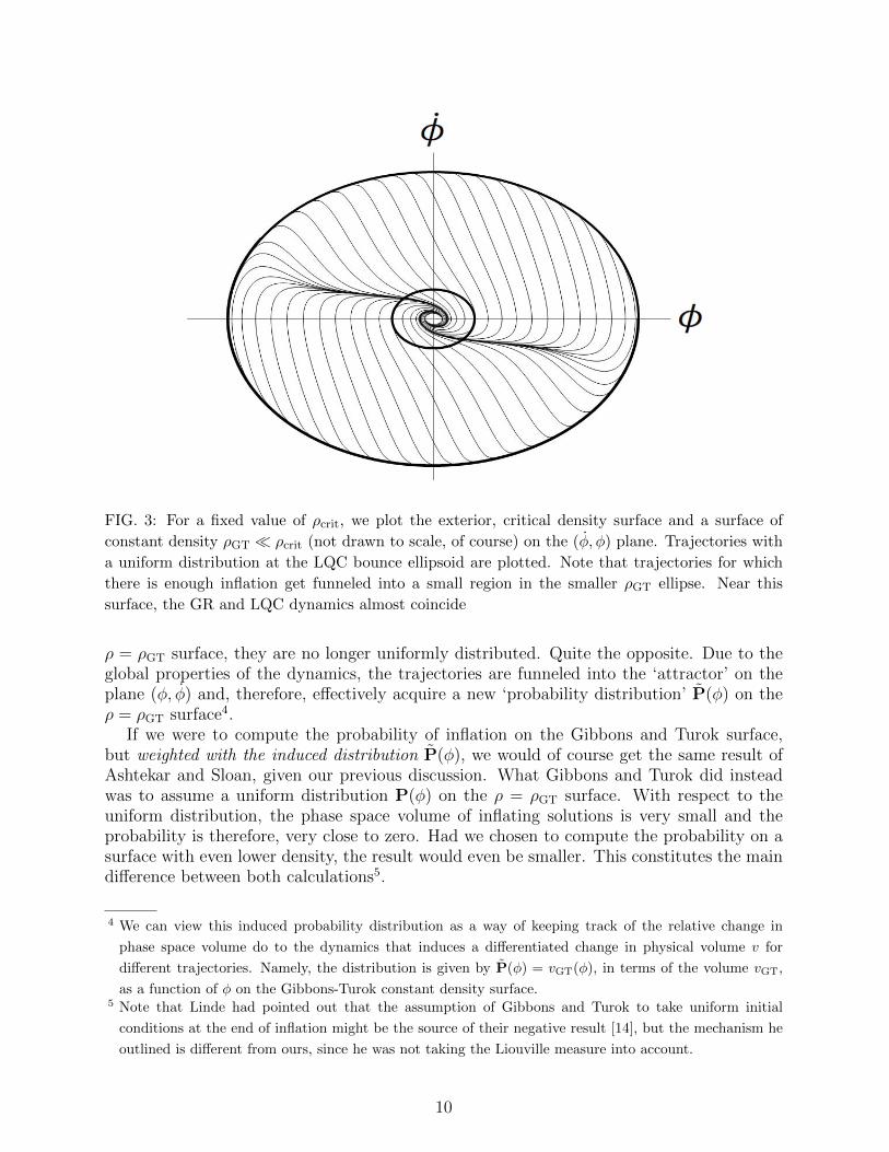
FIG. 3: For a fixed value of ρcrit, we plot the exterior, critical density surface and a surface of

constant density ρGT � ρcrit (not drawn to scale, of course) on the (φ, φ) plane. Trajectories with

a uniform distribution at the LQC bounce ellipsoid are plotted. Note that trajectories for which

there is enough inflation get funneled into a small region in the smaller ρGT ellipse. Near this

surface, the GR and LQC dynamics almost coincide

ρ = ρGT surface, they are no longer uniformly distributed. Quite the opposite. Due to theglobal properties of the dynamics, the trajectories are funneled into the ‘attractor’ on theplane (φ, φ) and, therefore, effectively acquire a new ‘probability distribution’ P(φ) on theρ = ρGT surface4.

If we were to compute the probability of inflation on the Gibbons and Turok surface,but weighted with the induced distribution P(φ), we would of course get the same result ofAshtekar and Sloan, given our previous discussion. What Gibbons and Turok did insteadwas to assume a uniform distribution P(φ) on the ρ = ρGT surface. With respect to theuniform distribution, the phase space volume of inflating solutions is very small and theprobability is therefore, very close to zero. Had we chosen to compute the probability on asurface with even lower density, the result would even be smaller. This constitutes the maindifference between both calculations5.

4 We can view this induced probability distribution as a way of keeping track of the relative change in

phase space volume do to the dynamics that induces a differentiated change in physical volume v for

different trajectories. Namely, the distribution is given by P(φ) = vGT(φ), in terms of the volume vGT,

as a function of φ on the Gibbons-Turok constant density surface.5 Note that Linde had pointed out that the assumption of Gibbons and Turok to take uniform initial

conditions at the end of inflation might be the source of their negative result [14], but the mechanism he

outlined is different from ours, since he was not taking the Liouville measure into account.

10

Furthermore, we can now understand why the probability found by Gibbons and Turokis so small. If we look at the region of Fig. 2 for which there is not enough inflation (inbetween the critical curves) on the LQC critical density surface, and follow those trajectoriesas in Fig. 3, we see that those trajectories occupy now a much larger region on the ρ = ρGT

ellipsoid. In other words, the trajectories for which there is enough inflation get funneledinto a small region in the ρ = ρGT surface that, when integrated with respect to the uniformdistribution P(φ) of [2], give a very small contribution to the probability. One could alsoconsider the opposite situation in which one starts with an uniform distribution on the GTsurface and ‘evolve back’ in time to the bounce surface. In that case, the dynamics will‘expel’ the trajectories in such a way that the probability distribution P′(φ) induced on thebounce surface is concentrated on the region where there is not enough inflation. If oneintegrates that probability distribution with respect to the Liouville measure the resultingprobability is very close to zero, as found by Gibbons and Turok in [2].6

IV. DISCUSSION

Let us summarize our results. We have reanalyzed the treatment of the simplest infla-tionary model from the perspective of loop quantum cosmology. By using effective equationwe studied the structure of the space of classical solutions with the aim of answering thequestion: How probable is it to achieve enough e-foldings? In particular we have consid-ered this question keeping the discreetness parameter of loop quantum cosmology as a freeparameter. When the parameter vanishes, one expects the dynamics to reduce to the stan-dard, general relativity behavior. The first result is that, as previously shown in [15], theprobability for enough inflation is very close to one when the discreetness parameter l is ofthe order of the Planck scale. We then considered the dependence of the probability as onedecreases the parameter and it approaches the general relativity limit. As we have shown,the probability increases and approaches one as one reaches the limit. Next, we studied theglobal properties of the system to understand the underlying reason for the discrepancy ofthese results and those of [2] in which the probability of enough inflation was computed tobe close to zero, within general relativity. What we found is that this discrepancy is dueto the differences in the underlying assumptions in both calculations. As it turns out theprobability as computed in both [2] and [15] depends very strongly on the constant densitysurface where it is calculated. While Ashtekar and Sloan assume a uniform distribution ofclassical trajectories at the naturally defined surface available due to the universal existenceof the bounce, Gibbons and Turok take it at an arbitrarily defined surface at the end ofinflation. Given the large difference in scales involved and due to the global properties ofthe dynamics and the probability measure, these two assumptions have strikingly differentconsequences. During the evolution from the bounce to the Gibbons-Turok scale, most of thetrajectories that undergo enough inflation –contributing significantly to the probability– getfunneled into a small region at the later scale, that has a correspondingly small contributionto the probability. This is the origin of the apparent tension.

We have thus found two very different results even for GR. On the one hand the Gibbons-

6 One should note that, as previously discussed, in order to make the distinction of which trajectories have

enough e-foldings, one has to introduce a cut-off for the initial condition. Here we have adopted the LQC

scale as a natural unambiguous choice.

11

Turok result involves several, somewhat ad-hoc, assumptions given that there is no preferredchoice of scale on GR. On the other hand, there is the limit of LQC when the discreetnessparameter vanishes. In this later case we have, for each scale, calculations based on unam-biguous and natural choices that provide a well defined result, even when the GR limit ofLQC is non-smooth. Thus even when in the l→ 0 limit one is approaching arbitrarily closeto the singularity, the probability of having N e-foldings –as measured from the Planck scaledown– can be given some meaning. As we have seen, the result that in the GR, l→ 0 limit,the probability goes to one for any finite value of N , seems to be generic. Whether thisresult is physically meaningful is, however, a completely different issue. In the situation inwhich λ is taken well below the Planck scale, we are implicitly assuming that the classicalequations are still valid. This is perhaps, too strong an assumption. One generically expectsquantum effects to dominate near and below the Planck scale. This is precisely what LQCprovides for us via its effective equations.

Let us end with a series of remarks.

1. Given that these two results are based on assumptions that yield completely oppo-site predictions, one might then ask what is the physically reasonable assumption tomake? How can we justify one choice over the other? Is there a ‘canonical’ choice ofinitial condition? In loop quantum cosmology we know that the bounce is generic forinflationary potentials [21], and the effective equations are a very good approximationto the dynamics of semiclassical states [12]. Since every such effective trajectory goesthrough a bounce, selecting the surface of constant density, at the bounce, seems arather natural choice. One should emphasize then that there does not exist a similarsurface that is preferred in the classical GR case. As we have seen, the probabilitydoes depend in a rather dramatic way on the choice of such surface. Without anyextra input, the LQC choice seems to be the most natural.

2. Even if one does not regard loop quantum cosmology as a fundamental theory, onecan still view its effective dynamics and choice of surface as in [15] as a procedureto regulate the classical calculation. The bounce provides then the preferred ‘cut-off’surface envisioned by the authors of [3], but in an unambiguous fashion. From thisperspective, what is amazing is that one can remove the regulator and obtain a finiteanswer. Furthermore, this ‘canonical answer’ indicates that inflation with enoughe-foldings is generic even in this particular way of approaching the GR limit.

3. As we have seen from our analysis here, the reason for the LQC result stems from thechoice of surface where to compute the probability and not directly from any effectfrom the quantum geometry underlying LQC. In fact, as we remove the parameterencoding the quantum geometric effects, the probability of inflation increases7.

4. In our analysis we have used qualitative aspects of the global dynamics of the sys-tem. Therefore, our arguments and conclusions are insensitive to changes in the freeparameters of the model. That is, our result are rather robust.

5. One should keep in mind that these results are purely classical. It is to be expected thatquantum effects might provide a more realistic distribution on the space of classical

7 This is consistent with early calculations on LQC where the integration was performed at low densities

[16].

12

trajectories. Some proposals have been put forward, but in the context of particularstates and only for those trajectories satisfying WKB conditions [22]. One couldimagine that semiclassical states in LQC might provide an improved distribution fromwhich one might get a ‘quantum corrected’ estimation of the probability for enoughinflation. This matter should certainly be studied in detail.

Acknowledgments

We would like to thank I. Agullo, A. Ashtekar, D. Sloan and P. Singh for discussions andcomments. This work was in part supported by DGAPA-UNAM IN103610 grant, by NSFPHY0854743 and by the Eberly Research Funds of Penn State.

[1] G. W. Gibbons, S. W. Hawking and J. M. Stewart, “A natural measure on the set of all

universes,” Nucl. Phys. B 281, 736 (1987); S. W. Hawking and D. N. Page, “How probable is

inflation?,” Nucl. Phys. B 298, 789 (1988).

[2] G. W. Gibbons and N. Turok, “The measure problem in cosmology,” Phys. Rev. D 77, 063516

(2008) arXiv:hep-th/0609095.

[3] V. A. Belinsky, I. M. Khalatnikov, L. P. Grishchuk and Y. B. Zeldovich, “Inflationary Stages

In Cosmological Models With A Scalar Field,” Phys. Lett. B 155, 232 (1985).

[4] A. Ashtekar, M. Bojowald and L. Lewandowski, “Mathematical structure of loop quantum cos-

mology” Adv. Theor. Math. Phys. 7 233 (2003) arXiv:gr-qc/0304074. M. Bojowald, “Loop

quantum cosmology”, Living Rev. Rel. 8, 11 (2005) arXiv:gr-qc/0601085.

[5] A. Ashtekar and J. Lewandowski “Background independent quantum gravity: A status re-

port,” Class. Quant. Grav. 21 (2004) R53 arXiv:gr-qc/0404018; C. Rovelli, “Quantum

Gravity”, (Cambridge U. Press, 2004); T. Thiemann, “Modern canonical quantum general

relativity,” (Cambridge U. Press, 2007).

[6] A. Ashtekar, T. Pawlowski and P. Singh, “Quantum Nature of the Big Bang,” Phys. Rev.

Lett 96 (2006) 141301 arXiv:gr-qc/0602086; “Quantum nature of the big bang: Improved

dynamics,” Phys. Rev. D 74, 084003 (2006) arXiv:gr-qc/0607039.

[7] A. Ashtekar, A. Corichi and P. Singh, “Robustness of key features of loop quantum cosmology,”

Phys. Rev. D 77, 024046 (2008). arXiv:0710.3565 [gr-qc].

[8] A. Ashtekar, “Loop Quantum Cosmology: An Overview,” Gen. Rel. Grav. 41, 707 (2009)

arXiv:0812.0177 [gr-qc].

[9] A. Corichi and P. Singh, “Quantum bounce and cosmic recall,” Phys. Rev. Lett. 100,

161302 (2008) arXiv:0710.4543 [gr-qc]; W. Kaminski and T. Pawlowski, “Cosmic recall

and the scattering picture of Loop Quantum Cosmology,” Phys. Rev. D 81, 084027 (2010)

arXiv:1001.2663 [gr-qc].

[10] A. Corichi and P. Singh, “Is loop quantization in cosmology unique?,” Phys. Rev. D 78, 024034

(2008) arXiv:0805.0136 [gr-qc]; “A geometric perspective on singularity resolution and

uniqueness in loop quantum cosmology,” Phys. Rev. D 80, 044024 (2009) arXiv:0905.4949

[gr-qc].

[11] P. Singh, K. Vandersloot and G. V. Vereshchagin, “Non-singular bouncing universes in loop

quantum cosmology,” Phys. Rev. D 74, 043510 (2006) arXiv:gr-qc/0606032.

13

[12] V. Taveras, “Corrections to the Friedman equations from LQG for a Universe with a free

scalar field”, Phys. Rev. D 78, 064072 (2008) arXiv:0807.3325 [gr-qc].

[13] L. Kofman, A. D. Linde and V. F. Mukhanov, “Inflationary theory and alternative cosmology,”

JHEP 0210, 057 (2002) arXiv:hep-th/0206088.

[14] A. D. Linde, “Inflationary Cosmology,” Lect. Notes Phys. 738, 1 (2008) arXiv:0705.0164

[hep-th].

[15] A. Ashtekar and D. Sloan, “Loop quantum cosmology and slow roll inflation,” Phys. Lett. B

694, 108 (2010) arXiv:0912.4093 [gr-qc].

[16] C. Germani, W. Nelson and M. Sakellariadou, “On the onset of inflation in loop quantum

cosmology,” Phys. Rev. D 76, 043529 (2007) arXiv:gr-qc/0701172.

[17] J. Mielczarek, “Possible observational effects of loop quantum cosmology,” Phys. Rev. D 81,

063503 (2010) arXiv:0908.4329 [gr-qc].

[18] A. Corichi, T. Vukasinac and J.A. Zapata, “Polymer quantum mechanics and its continuum

limit”, Phys Rev D76, 044016 (2007). arXiv:0704.0007v1 (gr-qc); “On a Continuum Limit

for Loop Quantum Cosmology,” AIP Conf. Proc. 977, 64 (2008) arXiv:0711.0788 [gr-qc].

[19] For a recent summary of results see: A. Corichi, “Black holes and entropy in loop quantum

gravity: An overview,” arXiv:0901.1302 [gr-qc].

[20] A. Ashtekar and D. Sloan, “Probability of Inflation in Loop Quantum Cosmology”,

arXiv:1103.2475 [gr-qc]; D. Sloan, “Loop Quantum Cosmology and the Early Universe”,

PhD Thesis, The Pennsylvania State University (2010).

[21] A. Ashtekar, T. Pawlowski, P. Singh, (In preparation).

[22] J. B. Hartle, S. W. Hawking and T. Hertog, “The No-Boundary Measure of the Universe,”

Phys. Rev. Lett. 100, 201301 (2008) arXiv:0711.4630 [hep-th]; J. Hartle and T. Hertog,

“Replication Regulates Volume Weighting in Quantum Cosmology,” Phys. Rev. D 80, 063531

(2009) arXiv:0905.3877 [hep-th].

14