On the lateral vibrations of an elastic rod with varying compressive force

On the lateral vibrations of anelastic rod with varying

compressive force

Bogoljub Stankovic ∗ Teodor M. Atanackovic †

Theoret. Appl. Mech., Vol.31, No.2, pp.135–151, Belgrade 2004

Abstract

We study lateral vibration of a simply supported axially com-pressed elastic rod with rotary inertia. The axial force is assumedto be a function of time. Stability of the solution is examined.The conditions are examined under which the temporal evolu-tion of the system is a slowly varying and regularly slowly vary-ing function. Also some properties of the generalized solutionto the problem are examined. Our results on stability boundaryobtained by dynamic, method agree with the results obtained bystatic (Euler) method.

Keywords: elastic rod, lateral vibration

1 Formulation of the problem

Consider a rod BC of length l simply supported at both ends. Thesupport at the end B is unmovable while at the end C the rod hasmovable joint. The axis of the rod is initially straight. At the end C therod is loaded by a compressive force F that is a function of time t andwhose action line coincides with the rod axis in the undeformed (initial

∗Institute of Mathematics, University of Novi Sad, 21000 Novi Sad, Serbia†Faculty of Technical Sciences, University of Novi Sad, 21000 Novi Sad, Serbia,

e-mail: [email protected]

135

136 B.Stankovic, T.M.Atanackovic

state). Let x−B− y be a rectangular Cartesian coordinate system withaxis x oriented along the rod axis in the initial state (see figure 1).

In what follows we consider only the plane motion (in the planex−B− y) so that (see [1]) the use D’Alembert’s principle for an elementof length dS leads to

∂H

∂S= −qx,

∂V

∂S= −qy,

∂M

∂S= −V

∂x

∂S+ H

∂y

∂S−m, (1.1)

where S ∈ [0, l] is the arc–length of the rod axis, x and y are coordinatesof an arbitrary point on the rod axis in the deformed state along the xand y axis, respectively, H and V are components of the contact force(representing the influence of the part of the rod [0, S) on the part [S, l])along the x and y axis respectively, and qx, qy and m are the intensitiesof the distributed forces per unit length of the rod axis along the x andy axis and the intensity of the distributed couple, respectively.

Figure 1: Coordinate system and load configuration

In figure 1 we showed positive directions of cross–sectional quantities.Also in our case the only distributed loads are inertial loads, so that

qx = −ρ∂2x

∂t2; qy = −ρ

∂2y

∂t2; m = −J

∂2θ

∂t2, (1.2)

where ρ is the (line) density of the rod, J is its moment of inertia of apart of the rod of unith length and t is the time. In what follows we

shall retain the term J∂2θ

∂t2representing the rotary inertia of the rod

On the lateral vibrations of an elastic... 137

cross–section. By using (1.1) and (1.2) we obtain

∂H

∂S= ρ

∂2x

∂t2,

∂V

∂S= ρ

∂2y

∂t2,

∂M

∂S= −V cos θ + H sin θ + J

∂2θ

∂t2,

∂x

∂S= cos θ,

∂y

∂S= sin θ,

1

r=

dθ

dS, (1.3)

where θ is the angle between the tangent to the rod axis and x axis andr is the radius of curvature of the rod axis.

To the system (1.3) we adjoin the constitutive equation connectingthe curvature of the rod axis (1/r) with the bending moment M . Wetake the classical Bernoulli–Euler rod theory for which

M = EI1

r, (1.4)

where EI = const. is the bending rigidity of the rod. The boundaryconditions corresponding to the rod shown in figure 1, are

H(l, t) = −F (t), M(0, t) = 0, M(l, t) = 0,

x(0, t) = 0; y(0, t) = 0; y(l, t) = 0. (1.5)

The trivial solution to system (1.3), (1.5) in which the axis of the rodremains straight, reads

H0 = −F, V 0 = 0, M0 = 0,

x0(S, t) = S, y0(S, t) = 0, θ0(S, t) = 0. (1.6)

Let H = H0 + ∆H, ...θ = θ0 + ∆θ. By substituting this in (1.3),(1.5) neglecting the higher order terms in the perturbations ∆H, ...∆θ,we obtain

EI∂4∆y

∂S4= −ρ

∂2∆y

∂t2− F (t)

∂2∆y

∂S2+ J

∂4∆y

∂2t∂2S. (1.7)


where we used∂2∆θ

∂t2=

∂2

∂t2

(∂∆y

∂S

)and

1

∆r=

∂2∆y

∂S2(see (1.3)5).

The boundary conditions corresponding to (1.7) are

∂2∆y

∂S2(0, t) = 0,

∂2∆y

∂S2(l, t) = 0,

∆y(0, t) = 0, ∆y(l, t) = 0. (1.8)

To system (1.7), (1.8) certain initial conditions must be prescribed andwe shall do it later. By introducing the dimensionless quantities

u =∆y

l, m =

Ml

E0I, τ = t

√EI

ρl4,

λ =Fl2

EI, ξ =

S

l, α =

J

ρl2,

(1.9)

from (1.7), (1.8) we obtain

∂4u

∂ξ4+ λ

∂2u

∂ξ2− α

∂4u

∂ξ2∂τ 2+

∂2u

∂τ 2= 0, 0 < ξ < 1, τ > 0, (1.10)

and

∂2u

∂ξ2(0, t) = 0,

∂2u

∂ξ2(1, t) = 0, u(0, t) = 0, u(1, t) = 0. (1.11)

2 Solutions to equations (1.10) & (1.11)

2.1 Some mathematical tools

2.1.1 Karamata’s class of functions

In studying equation (1) we use Karamata’s class (cf. [5], [7]) of regularlyvarying functions and a natural extension of them, the class of rapidlyvarying functions (cf. [6]). We cite theirs definitions.


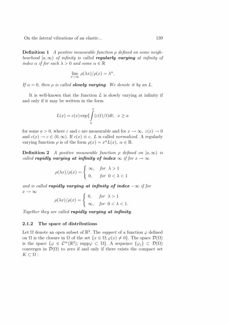
Definition 1 A positive measurable function ρ defined on some neigh-bourhood [a,∞) of infinity is called regularly varying at infinity ofindex α if for each λ > 0 and some α ∈ R

limx→∞

ρ(λx)/ρ(x) = λα.

If α = 0, then ρ is called slowly varying. We denote it by an L.

It is well-known that the function L is slowly varying at infinity ifand only if it may be written in the form

L(x) = c(x) expx∫

a

(ε(t)/t)dt, x ≥ a

for some a > 0, where ε and c are measurable and for x →∞, ε(x) → 0and c(x) → c ∈ (0,∞). If c(x) ≡ c, L is called normalized. A regularlyvarying function ρ is of the form ρ(x) = xαL(x), α ∈ R.

Definition 2 A positive measurable function ρ defined on [a,∞) iscalled rapidly varying at infinity of index ∞ if for x →∞

ρ(λx)/ρ(x) =

∞, for λ > 1

0, for 0 < λ < 1

and is called rapidly varying at infinity of index −∞ if forx →∞

ρ(λx)/ρ(x) =

0, for λ > 1

∞, for 0 < λ < 1.

Together they are called rapidly varying at infinity.

2.1.2 The space of distributions

Let Ω denote an open subset of R2. The support of a function ϕ definedon Ω is the closure in Ω of the set x ∈ Ω; ϕ(x) 6= 0. The space D(Ω)is the space ϕ ∈ C∞(R2); suppϕ ⊂ Ω. A sequence ϕj ⊂ D(Ω)converges in D(Ω) to zero if and only if there exists the compact setK ⊂ Ω :


1. suppϕj ⊂ K, j ∈ N;

2. for every α ∈ (N ∪ 0)2 ≡ N20, ϕα

j → 0 uniformly on K.

D′(Ω) is the space of all continuous linear functionals on D(Ω). It iscalled the space of distributions on Ω. Every locally integrable functionf on Ω defines the regular distribution denoted by [f ].

Every distribution has all derivatives and DαDβ = DβDα. If a func-tion f has f (α) ∈ Lloc(Ω), then Dα[f ] = [f (α)]. A locally integrablefunction on Ω has g ∈ D′(Ω) as α-derivative in the sense of distri-butions means that the regular distribution [f ] has derivative equalg, Dα[f ] = g.

The differentiation of distributions is a linear and continuous map-ping D′(Ω) → D′(Ω). If fj ⊂ D′(Ω) is a sequence of solutions toa partial differential equation and if this sequence converges in D′(Ω),then the limit of this sequence is also a solution to this equation.

If Fj is a sequence of continuous functions on Ω and if it convergesuniform on every compact set K ⊂ Ω to zero, then [Fj] converges tozero in D′(Ω), as well.

2.2 The existence and the character of found solu-tions

We consider the equation

( ∂4

∂ξ4+ λ(t)

∂2

∂ξ2− α

∂4

∂ξ2∂t2+

∂2

∂t2

)u(ξ, t) = 0, 0 < ξ < 1, t > 0, (2.1)

with the boundary conditions:

u(0, t) = u(1, t) = u(2)ξ (0, t) = u

(2)ξ (1, t) = 0, t > 0, (2.2)

and with α > 0.

Let us suppose that uk(ξ, t) = Ak sin kπξ · Tk(t), k ∈ N, where Ak

are arbitrary constants, Ak 6= 0, k ∈ N. Then uk(ξ, y) satisfies boundaryconditions (2.2) for any Tk and every k ∈ N. Moreover, in order thatu (ξ, t) satisfies (2.1) Tk, k ∈ N, has to satisfy the equation:

T(2)k (t)(α(kπ)2 + 1) + (kπ)2((kπ)2 − λ(t))Tk(t) = 0, t > 0. (2.3)


Since α > 0, equation (2.3) can be written in the form

T(2)k (t)− qk(t)Tk(t) = 0, t > 0, (2.4)

where

qk(t) =(kπ)2

α(kπ)2 + 1(λ(t)− (kπ)2), t > 0. (2.5)

Equation (2.4) is of particular importance for applied mathematicsand this accounts for the vast amount of research connected with it. Wecite only three books, we use in this paper. These are [2], [3] and [4].

Definition 3 A nontrivial solution T to (2.4) is said to be oscillatoryif there exists a sequence tn , tn → ∞, such that T (tn) = 0 for eachn ∈ N.

Theorem 1. Suppose that λ ∈ C((0,∞)) and moreover for a k =k0 ∈ N

λ(t) ≥ (k0π)2, t ≥ t1 > 0,

λ(t)− (k0π)2 6= 0 t ≥ t2 > 0.(2.6)

Then equation (2.3) has for all 1 ≤ k ≤ k0 a positive, convex anddecreasing solution T1k(t) on (t0,∞) for some t0 ≥ t1 (which dependson k). This solution is:

1) Slowly varying at ∞, T1k = L1k(t), if and only if for each µ > 1

x

µx∫

x

qk (t) dt → 0, x →∞.

2) Regularly varying at ∞ of index αk, T1k = tα1kL1k (t) if and onlyif for each µ > 1

x

µx∫

x

qk (t) dt → ck (µ− 1)

µ> 0, x →∞.

where α1k = 12

(1−√1 + 4ck

).


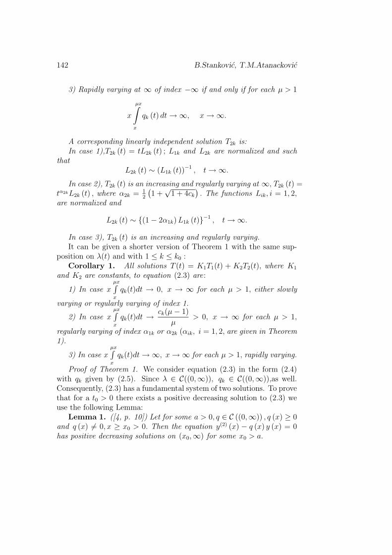
3) Rapidly varying at ∞ of index −∞ if and only if for each µ > 1

x

µx∫

x

qk (t) dt →∞, x →∞.

A corresponding linearly independent solution T2k is:In case 1),T2k (t) = tL2k (t) ; L1k and L2k are normalized and such

thatL2k (t) ∼ (L1k (t))−1 , t →∞.

In case 2), T2k (t) is an increasing and regularly varying at ∞, T2k (t) =tα2kL2k (t) , where α2k = 1

2

(1 +

√1 + 4ck

). The functions Lik, i = 1, 2,

are normalized and

L2k (t) ∼ (1− 2α1k) L1k (t)−1 , t →∞.

In case 3), T2k (t) is an increasing and regularly varying.It can be given a shorter version of Theorem 1 with the same sup-

position on λ(t) and with 1 ≤ k ≤ k0 :Corollary 1. All solutions T (t) = K1T1(t) + K2T2(t), where K1

and K2 are constants, to equation (2.3) are:

1) In case xµx∫x

qk(t)dt → 0, x → ∞ for each µ > 1, either slowly

varying or regularly varying of index 1.

2) In case xµx∫x

qk(t)dt → ck(µ− 1)

µ> 0, x → ∞ for each µ > 1,

regularly varying of index α1k or α2k (αik, i = 1, 2, are given in Theorem1).

3) In case xµx∫x

qk(t)dt →∞, x →∞ for each µ > 1, rapidly varying.

Proof of Theorem 1. We consider equation (2.3) in the form (2.4)with qk given by (2.5). Since λ ∈ C((0,∞)), qk ∈ C((0,∞)),as well.Consequently, (2.3) has a fundamental system of two solutions. To provethat for a t0 > 0 there exists a positive decreasing solution to (2.3) weuse the following Lemma:

Lemma 1. ([4, p. 10]) Let for some a > 0, q ∈ C ((0,∞)) , q (x) ≥ 0and q (x) 6= 0, x ≥ x0 > 0. Then the equation y(2) (x) − q (x) y (x) = 0has positive decreasing solutions on (x0,∞) for some x0 > a.


Suppose that λ(t) satisfies condition (2.6) for a k = k0,then qk(t)given by (2.5) satisfies conditions for q in Lemma 1 for every 1 ≤ k ≤ k0.Therefore (2.4) has a positive decreasing solution on (t0,∞) for somet0 > 0 and 1 ≤ k ≤ k0.

The assertions of Theorem 1 denoted by 1), 2) and 3) follow fromTheorem 1, Theorem 2 and Theorem 3 in [4], respectively.

In the next theorem the conditions are easier to verify than in The-orem 1. Consequently such theorem is more suitable for use.

Theorem 2. ([4]) Let the suppositions on λ (t) be the same as inTheorem 1. If τ 2qk (t) → ck, t → ∞, 1 ≤ k ≤ k0, then all decreasingsolutions of (2.4) are slowly or rapidly or regularly varying functionswith index αk =

(1−√1 + 4ck

)in the later case, according as ck =

0, ck = ∞, ck ∈ (0,∞).

The proof is obvious and follows from the proof of Theorem 1.

If we omit condition (2.6), then the following theorem is valid:

Theorem 3. Let λ ∈ C ([t0,∞)) for some t0 > 0. If Lik, i = 1, 2,denote two normalized slowly varying functions for k = k0 ∈ N, thenthere exist two linearly independent solutions T1k0 , T2k0 to (2.3):

1) Of the form T1k0 (t) = L1k0 (t) , T2k0 = tL2k0 (t) if and only ifx

∫ x

0qk0 (t) dt → 0, x →∞ for a k0 ∈ N. Moreover one has

L2k0 (t) ∼ (L1k0 (t))−1 , t →∞.

2) Of the form T1k0 (t) = tαik0L1k0 (t) , i = 1, 2, if and only if x∫ x

0(−qk0 (t)) dt

→ Ck0 , x → ∞,−∞ < Ck0 < 14, Ck0 6= 0, where αik0 , i = 1, 2, are two

roots of the equation α2 − α + Ck0 = 0, α1k0 < α2k0 . Moreover

L2k0 (t) ∼ (1− 2α1k0) L1k0 (t)−1 , t →∞.

Proof. It follows from Theorem 1.10 and Theorem 1.11 in [4].

Remark. In case 2), when 0 < Ck0 < 14,the both solutions are

always unbounded. If −∞ < Ck0 < 0, then α1k0 < 0 and α2k0 > 0.Consequently T1k0(t) → 0, t →∞ and T2k0(t)is unbounded.

In case 1) at least one of the solutions is unbounded.

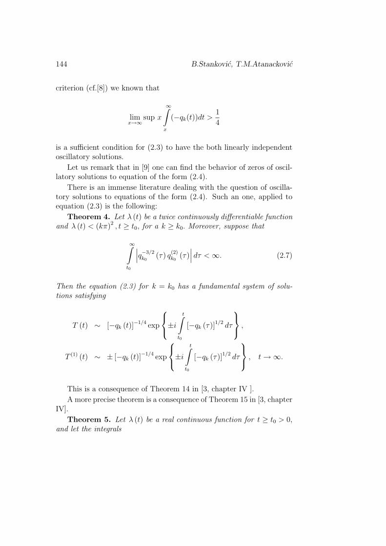
A natural question arises: What we can assert about the solutions to(2.3) if in Theorem 3 the number Ck ∈ (1/4,∞). By Hille’s oscillation


criterion (cf.[8]) we known that

limx→∞

sup x

∞∫

x

(−qk(t))dt >1

4

is a sufficient condition for (2.3) to have the both linearly independentoscillatory solutions.

Let us remark that in [9] one can find the behavior of zeros of oscil-latory solutions to equation of the form (2.4).

There is an immense literature dealing with the question of oscilla-tory solutions to equations of the form (2.4). Such an one, applied toequation (2.3) is the following:

Theorem 4. Let λ (t) be a twice continuously differentiable functionand λ (t) < (kπ)2 , t ≥ t0, for a k ≥ k0. Moreover, suppose that

∞∫

t0

∣∣∣q−3/2k0

(τ) q(2)k0

(τ)∣∣∣ dτ < ∞. (2.7)

Then the equation (2.3) for k = k0 has a fundamental system of solu-tions satisfying

T (t) ∼ [−qk (t)]−1/4 exp

±i

t∫

t0

[−qk (τ)]1/2 dτ

,

T (1) (t) ∼ ± [−qk (t)]−1/4 exp

±i

t∫

t0

[−qk (τ)]1/2 dτ

, t →∞.

This is a consequence of Theorem 14 in [3, chapter IV ].

A more precise theorem is a consequence of Theorem 15 in [3, chapterIV].

Theorem 5. Let λ (t) be a real continuous function for t ≥ t0 > 0,and let the integrals


∞∫t

(1 + qk (τ)) dτ,

g1 (t) =∞∫t

(1 + qk (τ)) cos 2τdτ,

g2 (t) =∞∫t

(1 + qk (τ)) sin 2τdτ, for a k = k0 ∈ N,

exist and suppose

∞∫

t0

|1 + qk (τ)| |gj (τ)| dτ < ∞, j = 1, 2, k = k0.

Then equation (2.3) has a fundamental system of solutions T1, T2 satis-fying:

T1 (t) = cos t + o (1) , T2 (t) = sin t + o (1) ,

T(1)1 (t) = − sin t + o (1) , T

(1)2 (t) = cot s + o (1) ,

for t →∞.Comments. It is an interesting question: How much the number

α > 0 influences on the asymptotic behavior of solutions to (2.3). It iseasily seen that the number α does not figure in (2.6) which is the basicsupposition on λ(t) of Theorem 1. The asymptotic behavior of solutionsdepends in Theorem 1 only on

limx→∞

x

µx∫

x

qk(t)dt for each µ > 1.

The number α can have an influence on this limit only in the case 2)when Ck 6= 0. This influence reflects on α1 and α2 but only on theirsnumerical values and can not change the sign.

The same conclusion is with Theorem 2 and Theorem 3 case 1). Butin Theorem 3 case 2) if for an α = α0, Ck0 is less than 1

4, then the

both solutions are unbounded. If we can find 0 < α < α0 such thatα0(kπ)2 + 1

α(kπ)2 + 1Ck >

1

4, then the solutions to (2.3) with this value of α are


oscillatory solutions. Similarly changing α we can obtain non–oscillatoryunbounded solutions instead of oscillatory solutions.

In theorems 4 and 5 the existence of the given solutions does notdepend on α > 0.

If in equation (2.3) λ is a constant, then it is easily to find solutionsof this equation.

An example for λ(t) which satisfies conditions of Theorem 4 is λ(t) =t + 1

t + 2= 1− 1

t + 2. This function is twice continuously differentiable:

λ(1)(t) =1

(t + 2)2> λ(2)(t) = − 2

(t + 2)3,

for t ≥ 0 it is monotone increasing because of λ(1)(t) > 0, t ≥ 0, andlimt→∞

λ(t) = 1. Consequently λ(t) < π2, t ≥ 0. Now,

−q1(t) =π2

απ2 + 1(π2 − λ(t)) = A(π2 − λ (t))).

Thus |q(2)1 (t)| = A

2

(t + 2)3and integral (2.7) exists. The assertion of

Theorem 4 for λ(t) =t + 1

t + 2is valid.

2.3 Generalized solutions

In Subsection 2.3 we found a sequence of solutions uk(ξ, y) = Ak sin kπξTk(t), k ∈ N, to (2.1), (2.2), which are of a special form. The char-acteristic of such solution is that the initial condition is uk(ξ, 0) =AkTk(0) sin kπξ, which is a very narrow class of functions. It is eas-ily seen that any finite sum Σuk(ξ, t) produce a new solution to (2.1),(2.2). In the following we will construct generalized solutions to (2.1),(2.2) by using some series, but preserving the basic properties of classicalsolutions, natural for the mechanical applications.

Naturally, the interesting solutions to (2.1), (2.2) are those which arebounded. Therefore we chose to prove the following theorem:

Theorem 6. Let1) λ (t) ∈ C∞ ((0,∞)) ,2) lim

t→0+λ (t) = 0,


3) λ(1) ∈ L1 ([0,∞)) ,4) there exists k0 ∈ N such that sup

t≥0|λ (t)| = Λ < (k0π)2 .

Then for every k ≥ k0, k ∈ N, equation (2.4) has a unique solu-tion Tk (t) satisfying the same initial conditions Tk (0) = T0, T

(1) (0) =T 1

0 , k ≥ k0. The elements of the sequence Tk (t)k≥k0are bounded on

[0,∞), uniformly in k ≥ k0. Moreover

u (ξ, t) =∞∑

k=k0

Ak (sin kπξ) Tk (t) , (3.1)

where |Ak| ≤ Nkβ+γ , γ > 0, 1 ≤ β ≤ 5 represents function in ξ with values

in D′((0,∞)) which is a generalized solution to (2.1),(2.2).Remark. We have first to explain the meaning of the sentence “...

which is a generalized solution to (2.1), (2.2).”For every ξ ∈ (0, 1), u(ξ, t) defines a regular distribution; u(ξ, t) is

a function in ξ with values in D′((0,∞)) which has the β − 1 contin-uous partial derivatives in ξ and other derivatives are in the sense ofdistributions (cf. 2.1.2).

Proof. Because of suppositions 1) and 2) we can continuously extendλ(t) to (−ε,∞), ε > 0 such that λ(t) = 0, t ∈ (−ε, 0]. Then forevery k ∈ N there exists a solution Tk to (2.4) with the initial condition

Tk(0) = T0 and T(1)k (0) = T 1

0 .If in (2.4) we introduce qk given by (2.5) and multiply so obtained

equation by T(1)k (t), after integrtion between 0 and t, we obtain for every

k ∈ N, k ≥ k0, t ≥ 0 :

1

2(T

(1)k (t))2 +

(kπ)4

α(kπ)2 + 1

1

2T 2

k (t)−

− (kπ)2

α(kπ)2 + 1

t∫

0

λ(τ)T(1)k (τ)Tk(τ)dτ = B,

(3.2)

where B is a constant.From (3.2) it follows that

B =1

2

(T 1

0

)2

+(kπ)4

α(kπ)2 + 1

1

2

(T0

)2

. (3.3)


Integrating by parts the integral in (3.2), this gives

1

2

(T

(1)k (t)

)2

+(kπ)2

α(kπ)2 + 1

(kπ)2 − λ(t)

2T 2

k (t)+

+1

2

(kπ)2

α(kπ)2 + 1

t∫

0

λ(1)(τ)T 2k (τ)dτ = B.

Whence

(kπ)2

α(kπ)2 + 1((kπ)2 − Λ)

(Tk(t))2

2≤

≤ B +

t∫

0

|λ′(τ)|(kπ)2 − Λ

(kπ)2

α(kπ)2 + 1

(kπ)2 − Λ

2(Tk(τ))2dτ.

(3.4)

Now we can useLemma 2. (cf. Lemma 1 in [2, p. 107]). Let u, v ≥ 0, c1 > 0 and

u satisfy the inequality

u(t) ≤ c1

t∫

0

u (τ) v (τ) dτ, t ≥ 0.

Then

u (t) ≤ c1 exp

t∫

0

v (τ) dτ

, t ≥ 0.

Applying this Lemma to (3.4) we have the inequality

1

2

(kπ)2

α(kπ)2 + 1((kπ)2 − Λ)(Tk(t))

2 ≤ B exp( 1

(k0π)2 − Λ

∞∫

0

|λ(1)(τ)|dτ).

Now it is easily seen that there exists a constant M such that |Tk(t)| ≤M, t ≥ 0, k ≥ k0.


It remains only to prove that u(ξ, t), given by (3.1) is a generalizedsolution to (2.1), (2.2). The finite sum

uK(ξ, t) =K∑

k=k0

Ak sin kπξTk(t)

is also a solution to (2.1), (2.2), we have only to prove that uK(ξ, t)converges in C((0, 1)× (0,∞)), when k →∞.

Since

|Ak sin kπξTk(t)| ≤ |Ak|M ≤ NM

kβ+γ, (ξ, t) ∈ (0, 1)× (0,∞)), 1 ≤ β ≤ 5,

for every k ≥ k0, the sequence uK(ξ, t)K≥k0 converges in C((0,∞) ×(0, 1)) and consequently in D′((0, 1)×(0,∞)). Thus [u(ξ, t)] is a solutionto ((2.1), (2.2) (cf. 2.1.2).

It is also

|(Ak sin kπξTk(t))(i)ξ | ≤ M |Ak|(kπ)i ≤ MN

kβ+γ−i,

for i = 0, ..., β − 1. Thus u(i)ξ (ξ, t) exists and

u(i)ξ (ξ, t) =

∞∑

k=k0

Ak(sin kπξ)(i)Tk(t), i = 1, ..., β − 1,

and is a continuous function on [0, 1]×[0,∞). It is easily seen that u(ξ, t)satisfy boundary condition (2.2).

This completes the proof.

Remark. The function u(ξ, t) satisfies also the initial condition

u(ξ, 0) = T0

∞∑

k=k0

Ak sin kπξ.

This is more extensive class of functions then the class uk(ξ, 0) = AkT (0) sin kπξ.


3 Concluding remarks

In applications, the most important case corresponds to the first modevibration of the rod. Thus, we choose k = 1 in (2.3) and we comparethe results obtained here, with the results about stability of the samerod, obtained by static (Euler) method.

1. Suppose that the dimensionless force λ (t) (see (1.9) is largerthan the Euler buckling force [1, p. 111], that is, λ (t) > π2. Theorem1 in Section 2.2 specifies the properties of the solution, indicting theinstability of the rod, since T2k is an increasing function. The staticmethod (the method of adjacent equilibrium configuration) also predictsinstability for λ (t) = const. > π2, independently of α since rotary inertiadoes not play any role in the static method.

2. If the axial force λ (t) is smaller than the Euler buckling forceλ (t) < π2 (assumption 4) in Theorem 1, Section 3) than the Theorem1 in Section 2.3 predicts stability if the value of the axial force is in-creased from zero (assumption 2) in Theorem 1, Section 2.3). This is inagreement with the predictions of static method. We note that aboveconclusion is independent of the value of the rotary inertia parameterα. Thus this result is in agreement with the static method where thereis no influence of rotary inertia on stability boundary.

Our results show equivalence in prediction of stability boundary bydynamic and static methods. Also our results show some of the prop-erties of the dynamic solutions and their relation to regular varyingfunctions.

References

[1] T. M. Atanackovic, Stability Theory of Elastic Rods, World ScientificCompany, Singapore, 1997.

[2] R. Bellman, Stability theory of differential equations, Mc Graw-HillBook Company, New York, 1953.

[3] W. A. Coppel, Stability and Asymptotic Behavior of DifferentialEquations, D.C. Heath and Company, Boston, 1965.


[4] V. Maric, Regular variation and Differential Equations, LectureNotes in Mathematics 1726, Springer, Berlin, 2000.

[5] J. Karamata, Sur une mode de croissance reguliere des functions,Math. (Cluj) 4 (1930), 38-53.

[6] A. Bekessy, Eine verallgemeinerung der Laplaceschen Methode, Publ.Math. Hungar. Acad. Sci. 2 (1957), 105-120.

[7] N. H. Bingham, C. M. Goldie, J. L. Teugels, Regular variation, Cam-bridge Univ. Press, Cambridge, 1987.

[8] C. A. Swanson, Comparison and oscillation theory of linear differ-ential equations, Academic Press, New York, 1968.

[9] M. Hacik, E. Omey, On the zeros of oscillatory solutions of linearsecond order differential equations, Publ. Inst. Math. (Beograd), 49,(63), (1991), 189-200.

Submitted on July 2004

O poprecnim oscilacijama elasticnog stapa sapromenljivom pritiskujucom silom

UDK 531.01

U radu se proucavaju poprecne oscilacije slobodno oslonjene, aksi-jalno pritisnute elasticne grede, bez zanemarivanje efekta rotacione in-ercije. Usvojeno je da je aksijalna sila poznata funkcija vremena. Ispi-tana je stabilnost grede u linearnoj aproksimaciji i odredjeni su uslovipod kojima je vremenska evolucija sistema opisana sporo promenljivimi regularno sporo promenljivim funkcijama. Osim toga, analizirana sui neka svojstva uopstenih resenja problema. Dobijeni rezultati ovdeiznete dinamicke analize, u saglasnosti su sa rezultatima koji se dobi-jaju statickim (Ojlerovim) metodom.

On the lateral vibrations of an elastic rod with varying compressive force

Documents

Transcript of On the lateral vibrations of an elastic rod with varying compressive force